Tidal stream device reliability comparison models Tidal stream device reliability comparison models
Upload
khangminh22Category
view
0download
0
Introduction to stream: A Framework for Data
Stream Mining Research
John ForrestMicrosoft
Matthew BolanosSouthern Methodist University
Michael HahslerSouthern Methodist University
Abstract
In recent years, data streams have become an increasingly important area of researchfor the computer science, database and data mining communities. Data streams areordered and potentially unbounded sequences of data points created by a typically non-stationary generation process. Common data mining tasks associated with data streamsinclude clustering, classification and frequent pattern mining. New algorithms are pro-posed regularity and it is important to evaluate them thoroughly under standardizedconditions.
In this paper we introduce stream, an R package that provides an intuitive interface forexperimenting with data streams and data stream mining algorithms. stream is a generalpurpose tool that includes modeling and simulating data streams as well an extensibleframework for implementing, interfacing and experimenting with algorithms for variousdata stream mining tasks.
Keywords: data stream, data mining, clustering.
Acknowledgments
This work is supported in part by the U.S. National Science Foundation as a research ex-perience for undergraduates (REU) under contract number IIS-0948893 and by the NationalHuman Genome Research Institute under contract number R21HG005912.
1. Introduction
Typical statistical and data mining methods (e.g., parameter estimation, statistical tests,clustering, classification and frequent pattern mining) work with “static” data sets, meaningthat the complete data set is available as a whole to perform all necessary computations. Wellknown methods like k-means clustering, decision tree induction and the APRIORI algorithmto find frequent itemsets scan the complete data set repeatedly to produce their results (Hastie,Tibshirani, and Friedman 2001). However, in recent years more and more applications needto work with data which are not static, but the result of a continuous data generation processwhich even might evolve over time. Some examples are web click-stream data, computer
2 Introduction to stream
network monitoring data, telecommunication connection data, readings from sensor nets andstock quotes. This type of data is called a data stream and dealing with data streams hasbecome an increasingly important area of research (Babcock, Babu, Datar, Motwani, andWidom 2002; Gaber, Zaslavsky, and Krishnaswamy 2005; Aggarwal 2007). Early on, thestatistical community also started to see the emerging field of statistical analysis of massivedata streams (see Keller-McNulty (2004)).
A data stream can be formalized as an ordered sequence of data points
Y = 〈y1,y2,y3, . . .〉,
where the index reflects the order (either by explicit time stamps or just by an integer reflectingorder). The data points themselves can be simple vectors in multidimensional space, but canalso contains nominal/ordinal variables, complex information (e.g., graphs) or unstructuredinformation (e.g., text). The characteristic of continually arriving data points introduces animportant property of data streams which also poses the greatest challenge: the size of a datastream is unbounded. This leads to the following requirements for data stream processingalgorithms:
• Bounded storage: The algorithm can only store a very limited amount of data tosummarize the data stream.
• Single pass: The incoming data points cannot be permanently stored and need to beprocessed at once in the arriving order.
• Real-time: The algorithm has to process data points on average at least as fast as thearriving data.
• Concept drift: The algorithm has be able to deal with a data generation process whichevolves over time (e.g., distributions change or new structure in the data appears).
Obviously, most existing algorithms designed for static data are not able to satisfy theserequirements and thus are only usable if techniques like sampling or time windows are usedto extract small, quasi-static subsets. While these approaches are important, new algorithmsare needed and have been introduced over the last decade to deal with the special challengesposed by data streams.
Even though R is an ideal platform to develop and test prototypes for data stream algorithms,currently R does not have an infrastructure to support data streams.
1. Data sets are typically represented by data.frames or matrices which is suitable for staticdata but not to represent streams.
2. Algorithms for data streams are not available in R.
In this paper we introduce the package stream which provides a framework to represent andprocess data streams and use them to develop, test and compare data stream algorithms inR. We include an initial set of data stream generators and data stream algorithms (focusingon clustering) in this package with the hope that other researchers will use stream to develop,study and improve their own algorithms.
John Forrest, Matthew Bolanos, Michael Hahsler 3
The paper is organized as follows. We briefly review data stream mining in Section 2. InSection 3 we cover the stream framework including the design of the class hierarchy to rep-resent different data streams and data stream clustering algorithms, evaluation of algorithmsand how to extend the framework with new data stream sources and algorithms. We providecomprehensive examples in Section 5 and conclude with Section 6.
2. Data Stream Mining
Due to advances in data gathering techniques, it is often the case that data is no longer viewedas a static collection, but rather as a dynamic set, or stream, of incoming data points. Themost common data stream mining tasks are clustering, classification and frequent patternmining (Aggarwal 2007; Gama 2010). The rest of this section will give a brief introduce thesedata stream mining tasks. We will focus on clustering, since this is also the current focus ofstream.
2.1. Clustering
Clustering, the assignment of data points to groups (typically k) such that point within eachgroup are more similar than points in different groups is a very basic unsupervised data min-ing task. For static data sets methods like k-means, k-medians, hierarchical clustering anddensity-based methods have been developed among others(Jain, Murty, and Flynn 1999).However, the standard algorithms for these methods need access to all data points and typi-cally iterate over the data multiple times. This requirement makes these algorithms unsuitablefor data streams and led to the development of data stream clustering algorithms.
In the last 10 years many algorithms for clustering data streams have been proposed Guha,Meyerson, Mishra, Motwani, and O’Callaghan (2003); Aggarwal, Han, Wang, and Yu (2003a,2004a); Cao, Ester, Qian, and Zhou (2006a); Tasoulis, Adams, and Hand (2006); Tasoulis,Ross, and Adams (2007); Udommanetanakit, Rakthanmanon, and Waiyamai (2007); Tu andChen (2009); Wan, Ng, Dang, Yu, and Zhang (2009); Kranen, Assent, Baldauf, and Seidl(2011). Most data stream clustering algorithms use a two-stage online/offline approach:
1. Online: Summarize the data using a set of k′ micro-clusters organized in a space effi-cient data structure which also enables fast look-up. Micro-clusters are representativesfor sets of similar data points and are created using a single pass over the data (typicallyin real time when the data stream arrives). Micro-clusters are typically represented bycluster centers and additional statistics as weight (density) and dispersion (variance).Each new data point is assigned to its closest (in terms of a similarity function) micro-cluster. Some algorithms use a grid instead and micro-clusters represent non-emptygrid cells (e.g., Tu and Chen (2009); Wan et al. (2009)). If a new data point cannotbe assigned to an existing micro-cluster, a new micro-cluster is created. The algorithmmight also perform some housekeeping (merging or deleting micro-clusters) to keep thenumber of micro-clusters at a manageable size or to remove information outdated dueto a change in the stream’s data generating process.
2. Offline: When the user or the application requires a clustering, the k′ micro-clustersare reclustered into k (k ≪ k′) final clusters sometimes referred to as macro-clusters.Since the offline part is usually not regarded time critical, most researchers only state
4 Introduction to stream
that they use a conventional clustering algorithm (typically k-means or DBSCAN Ester,Kriegel, Sander, and Xu (1996)) by regarding the micro-cluster centers as pseudo-points.The algorithms are often modified to take also the weight of micro-clusters into account.
2.2. Classification
Classification, learning a model in order to assign labels to new, unlabeled data points is a wellstudied supervised machine learning task. Methods include naive Bayes, k-nearest neighbors,classification trees, support vector machines, rule-based classifiers and many more (Hastieet al. 2001). However, as with clustering these algorithms need access to all the training dataseveral times and thus are not suitable for data streams with constantly arriving new trainingdata.
Several classification methods suitable for data streams have been developed recently. Exam-ples are Very Fast Decision Trees (VFDT) (Domingos and Hulten 2000) using Hoeffding trees,the time window-based Online Information Network (OLIN) (Last 2002) and on-demandclassification (Aggarwal, Han, Wang, and Yu 2004b) based on micro-clusters found with thedata-stream clustering algorithm CluStream. For a detailed description of these and othermethods we refer the reader to the survey by Gaber, Zaslavsky, and Krishnaswamy (2007).
2.3. Frequent Pattern Mining
The aim of frequent pattern mining is to discover frequently occurring patterns (e.g., itemsets,subsequences, subtrees, subgraphs) in large datasets. Patterns are then used to summarizethe dataset and can provide insights into the data. Although finding all frequent pattern isa computationally expensive task, many efficient algorithms have been developed for staticdata sets. Most notably the APRIORI algorithm (Agrawal, Imielinski, and Swami 1993) forfrequent itemsets. However, these algorithms use breath-first or depth-first search strategieswhich results in the need to pass over the data several times and thus makes them unusable forthe streaming case. We refer the interested reader to the survey of frequent pattern mining indata streams by Jin and Agrawal (2007) which describe several algorithms for mining frequentitemsets.
2.4. Existing Solution: The MOA Framework
MOA (short for Massive Online Analysis) is a framework implemented in Java for bothstream classification and stream clustering (Bifet, Holmes, Kirkby, and Pfahringer 2010).It is the first experimental framework to provide easy access to multiple data stream miningalgorithms, as well as tools to generate data streams that can be used to measure and comparethe performance of different algorithms. Like WEKA (Witten and Frank 2005), a popularcollection of machine learning algorithms, MOA is also developed by the University of Waikatoand its interface and workflow are similar to those of WEKA.
The workflow in MOA consists of three main steps:
1. Selection of the data stream model (also called data feeds or data generators).
2. Selection of the learning algorithm.
John Forrest, Matthew Bolanos, Michael Hahsler 5
3. Apply selected evaluation methods on the results of the algorithm on the generated datastream.
MOA uses a graphical user interface. As the output MOA generates a report which containsthe results from the data mining task as well as the performance evaluation. The learn-ing algorithm and the evaluation differs depending in the data mining task (classification orclustering). Classification results are shown as text, while clustering results have a visualiza-tion component that shows both the clustering (for two-dimensional data) and the change inperformance metrics over time.
The MOA framework is an important pioneer in experimenting with data stream algorithms.MOA’s advantages are that it interfaces with WEKA, provides already a set of data streamclassification and clustering algorithms and it provides a clear Java interface to add newalgorithms or use the existing algorithms in other applications.
3. The stream Framework
A drawback of MOA for R users is that for all but very simple experiments Java code has tobe developed. Also, using MOA’s data stream mining algorithms together with the advancedcapabilities of R to create artificial data and to analyze and visualize the results is currentlyonly partially possible or very difficult.
The stream framework provides a R-based alternative to the MOA framework. It is basedon several packages including proxy (Meyer and Buchta 2010), MASS (Venables and Ripley2002), clusterGeneration (Qiu and Joe. 2009), and several others. stream also interfacesthe data stream clustering algorithms already available in MOA using the rJava package byUrbanek (2010). Furthermore, stream can incorporate any algorithm which is written in alanguage interfaceable by R.
The stream framework consists of two main components:
1. Data Stream Data (DSD) which manages or creates a data stream, and
2. Data Stream Task (DST) which performs a data stream mining task.
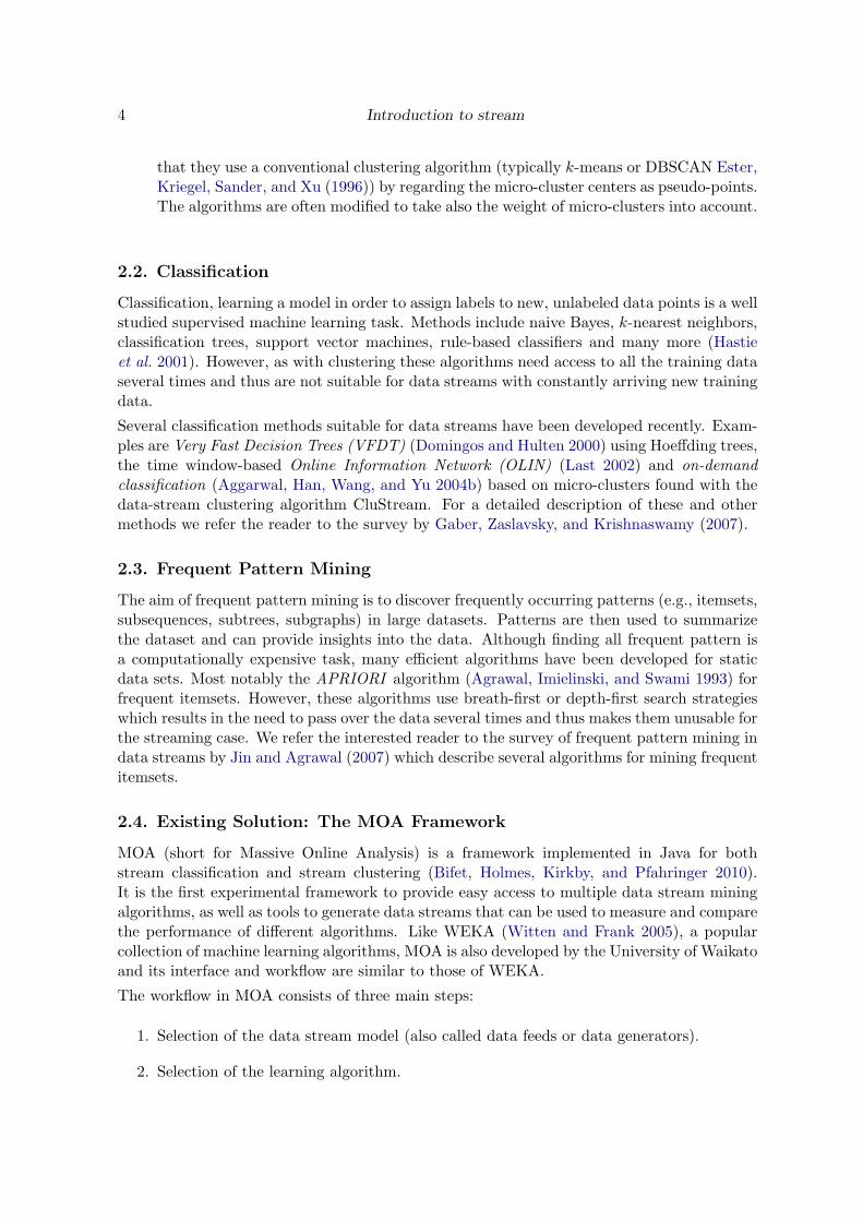
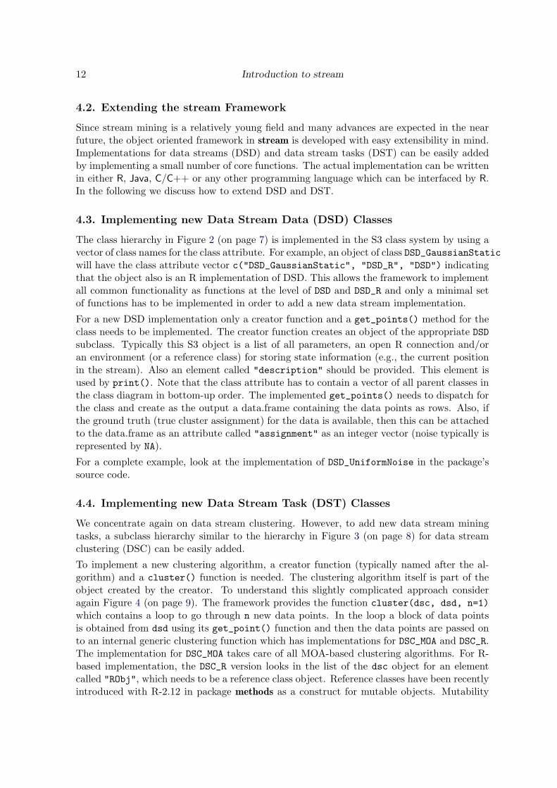
Figure 1 shows a high level view of the interaction of the components. We start by creatinga DSD object and a DST object. Then the DST object starts receiving data form the DSDobject. At any time, we can obtain the current results from the DST object. DSTs canimplement any type of data streaming mining task (e.g., classification or clustering). In thefollowing we will concentrate on clustering since stream currently focuses on this type of task,but the framework is implemented such that classification, frequent pattern mining or anyother task can easily be added.
For stream rely on object-oriented design using the S3 class system (Chambers and Hastie1992) to provide for each of the two core components a lightweight interface (i.e., an abstractclass) which can be easily implemented to create new data stream types or data stream miningalgorithms. The detailed design of the DSD and DSC classes will be discussed in the followingsubsections.
3.1. Data Stream Data (DSD)
6 Introduction to stream
Data Stream Data(DSD)
Data Stream Task(DST)
Result
Figure 1: A high level view of the stream architecture.
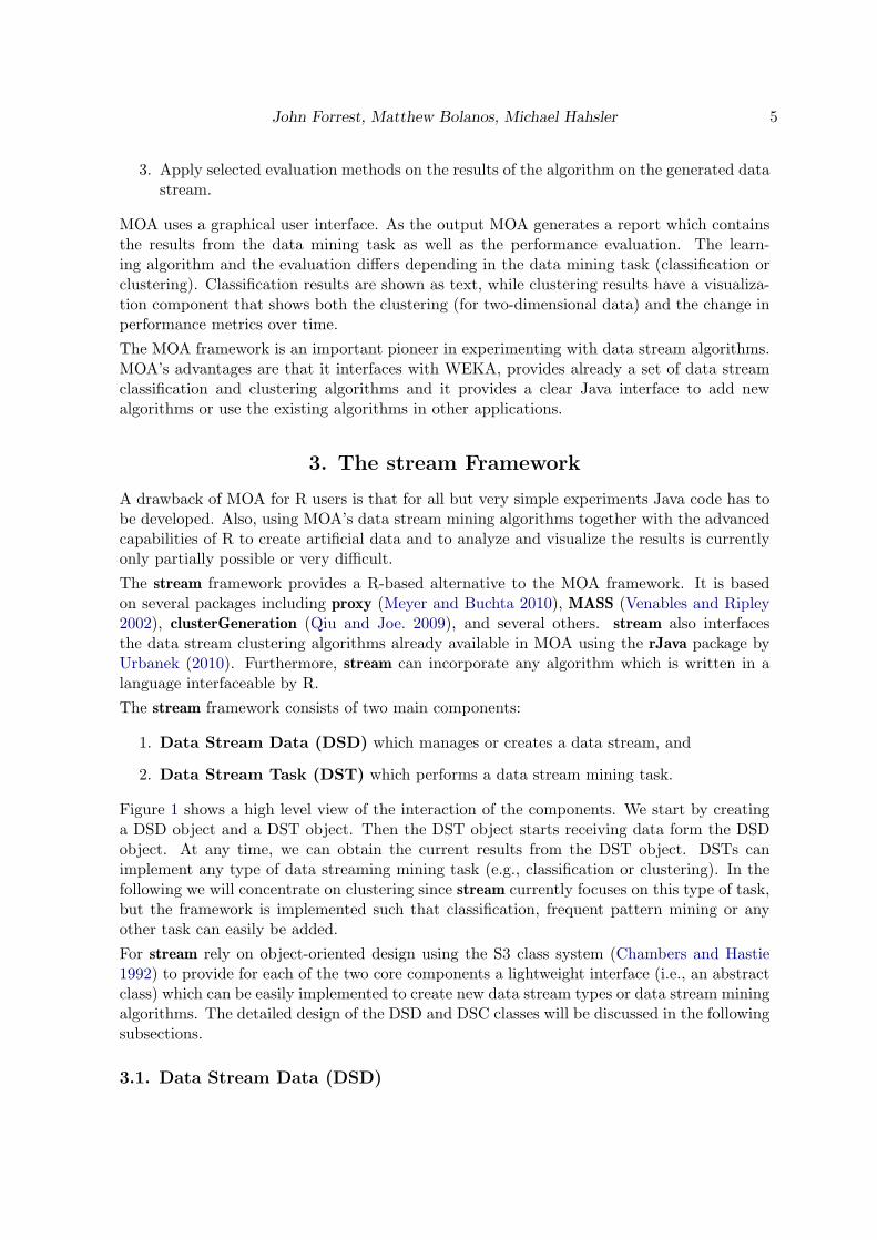
The first step in the stream workflow is to select a data stream implemented as a DataStream Data (DSD) object. This object can be a management layer on top of a real datastream, a wrapper for data stored on disk or a generator which simulates a data streamwith know properties for controlled experiments. Figure 2 shows relationship of the DSDclasses as a UML class diagram (Fowler 2003). All DSD classes extend the base class DSD.There are currently two types of DSD implementations, classes which implement R-based datastreams (DSD_R) and MOA-based stream generators (DSD_MOA). stream currently provides thefollowing generators:
• DSD_GaussianStatic, a DSD that generates static cluster data with a random Gaussiandistribution.
• DSD_GaussianMoving, a DSD that generates moving cluster data with a Gaussian dis-tribution.
• DSD_UniformNoise, generates uniform noise in a d-dimensional (hyper) cube.
• DSD_mlbenchGenerator, a class uses the generators for artificial datasets defined in themlbench package.
• DSD_mlbenchData, a DSD that wraps datasets found within the mlbench package.
• DSD_Target, a DSD that generates a ball in circle data set.
• DSD_BarsAndGaussians, a DSD that generates two bars and two Gaussians clusterswith different density.
• DSD_RandomRBFGeneratorEvents (from MOA), a data generator for moving Gaussianclusters which noise which can merge and split.
For reading a saved data stream from a file (in csv format) or to connection to a real streamusing a R connection stream provides:
• DSD_ReadStream, a class designed to read data from files or open connections. Thisobject also provides support to scale the data points using scale().
A non-streaming data set (in a data.frame) can also be wrapped in stream class and to bereplayed as a stream over and over again using:
• DSD_Wrapper, a DSD class that wraps static data (e.g., a data.frame, a matrix or a fixedportion of another data stream) as a data stream.
John Forrest, Matthew Bolanos, Michael Hahsler 7
DSD_R
DSD_GaussianStatic
DSD
DSD_MOA
DSD_Wrapper DSD_ReadStream DSD_RandomRBF. . . . . .
Ab
str
act
cla
sse
sIm
ple
me
nta
tio
n
Figure 2: Overview of the DSD class structure.
As depicted in the class diagram, other data steam implementations can be easily added inthe future.
All DSD implementations share a simple interface consisting of the following two functions:
1. A creator function. This function typically has the same name as the class. The listof parameters depends on the type of data stream it creates. The most common inputparameters for the creation of DSD classes are k, number of clusters (i.e. areas withhigh densities), and d, number of dimensions. A full list of parameters can be obtainedfrom the help page of each class. The result of this creator function is not a data setbut an object representing the streams properties and its current state.
2. The data generation function get_points(x, n=1, ...). This function is used toobtain the next data point (or next n data points) from the stream represented byobject x. The data point(s) are returned as a data.frame with each row representing asingle data point.
Next to these core functions several utility functions like print(), plot() and write_stream()to save a part of a data stream to disk are provided automatically by stream. Differentdata stream implementations might have additional functions implemented. For example,DSD_Wrapper and DSD_ReadStream have reset_stream() implemented to reset the streamto its beginning.
3.2. Data Stream Task (DST)
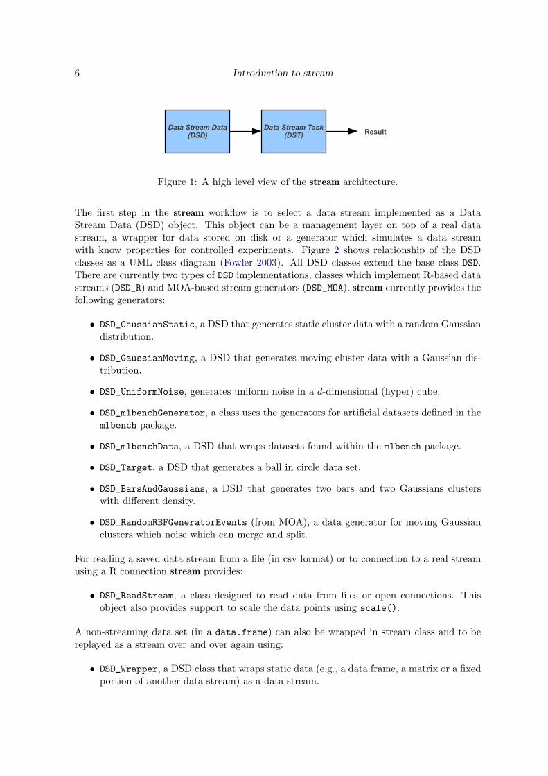
After choosing a DSD class to use as the data stream source, the next step in the workflow isto define a Data Stream Task (DST). In stream, a DST refers to any data mining task thatcan be applied to data streams. The design is flexible to allow for future extensions with evencurrently unknown tasks. Figure 3 shows the class hierarchy for DST. It is important to notethat the concept of the DST class is merely for conceptual purposes, the actual implementationof clustering, classification or frequent pattern mining are typically quite different and shareonly basic management functionality. We will restrict the following discussion on data streamclustering (DSC) since stream currently focus on this task.
3.3. Data Stream Clustering (DSC)
8 Introduction to stream
DSC_R
DST
DSC_MOA
DSC_tNN DSC_CluStream
DSC
. . .
. . .DSClassify
Ab
str
act
cla
sse
sIm
ple
me
nta
tio
n
DSC_Micro DSC_Macro DSC_Micro
DSC_tNN . . . DSC_Kmeans . . .
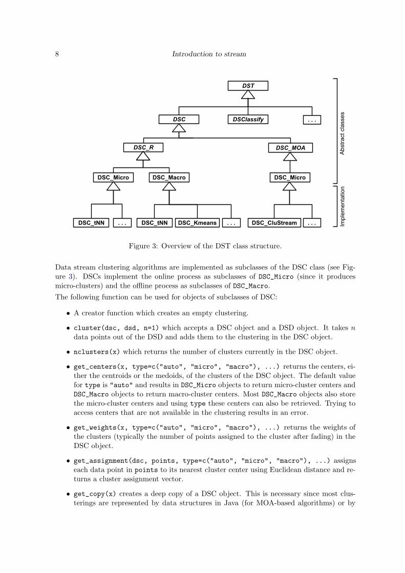
Figure 3: Overview of the DST class structure.
Data stream clustering algorithms are implemented as subclasses of the DSC class (see Fig-ure 3). DSCs implement the online process as subclasses of DSC_Micro (since it producesmicro-clusters) and the offline process as subclasses of DSC_Macro.
The following function can be used for objects of subclasses of DSC:
• A creator function which creates an empty clustering.
• cluster(dsc, dsd, n=1) which accepts a DSC object and a DSD object. It takes n
data points out of the DSD and adds them to the clustering in the DSC object.
• nclusters(x) which returns the number of clusters currently in the DSC object.
• get_centers(x, type=c("auto", "micro", "macro"), ...) returns the centers, ei-ther the centroids or the medoids, of the clusters of the DSC object. The default valuefor type is "auto" and results in DSC_Micro objects to return micro-cluster centers andDSC_Macro objects to return macro-cluster centers. Most DSC_Macro objects also storethe micro-cluster centers and using type these centers can also be retrieved. Trying toaccess centers that are not available in the clustering results in an error.
• get_weights(x, type=c("auto", "micro", "macro"), ...) returns the weights ofthe clusters (typically the number of points assigned to the cluster after fading) in theDSC object.
• get_assignment(dsc, points, type=c("auto", "micro", "macro"), ...) assignseach data point in points to its nearest cluster center using Euclidean distance and re-turns a cluster assignment vector.
• get_copy(x) creates a deep copy of a DSC object. This is necessary since most clus-terings are represented by data structures in Java (for MOA-based algorithms) or by
John Forrest, Matthew Bolanos, Michael Hahsler 9
Data Stream Data(DSD)
Data Stream Clustering
(DSC)
get_centers()get_weights()evaluate()plot()
cluster()
Data Stream Clustering
(DSC_Macro)
recluster()
get_centers()get_weights()evaluate()plot()
get_assignment()
New datapoints
(data.frame)
Cluster assignments
microToMacro()Micro-clusterassignments
Figure 4: Interaction between the DSD and DSC classes
R-based reference classes. This function is currently not available for all DSC imple-mentations.
• plot(x, dsd=NULL, ..., method="pairs", type = c("auto", "micro", "macro")
(see manual page for more available parameters) plots the centers of the clusters. Thereare 3 available plot methods: "pairs", "plot", "pc". Method "pairs" is the defaultmethod that produces a matrix of scatter plots that plots the attributes against oneanother (this method is only available when d > 2). Method "plot" simply takes thefirst two attributes of the matrix and plots it as x and y on a scatter plot. Lastly,method "pc" performs Principle Component Analysis (PCA) on the data and projectsthe data to a 2 dimensional plane and then plots the results. Parameter type controlsif micro- or macro-clusters are plotted.
• print(x, ...) prints common attributes of the DSC object (a small description of theunderlying algorithm and the number of clusters that have been calculated).
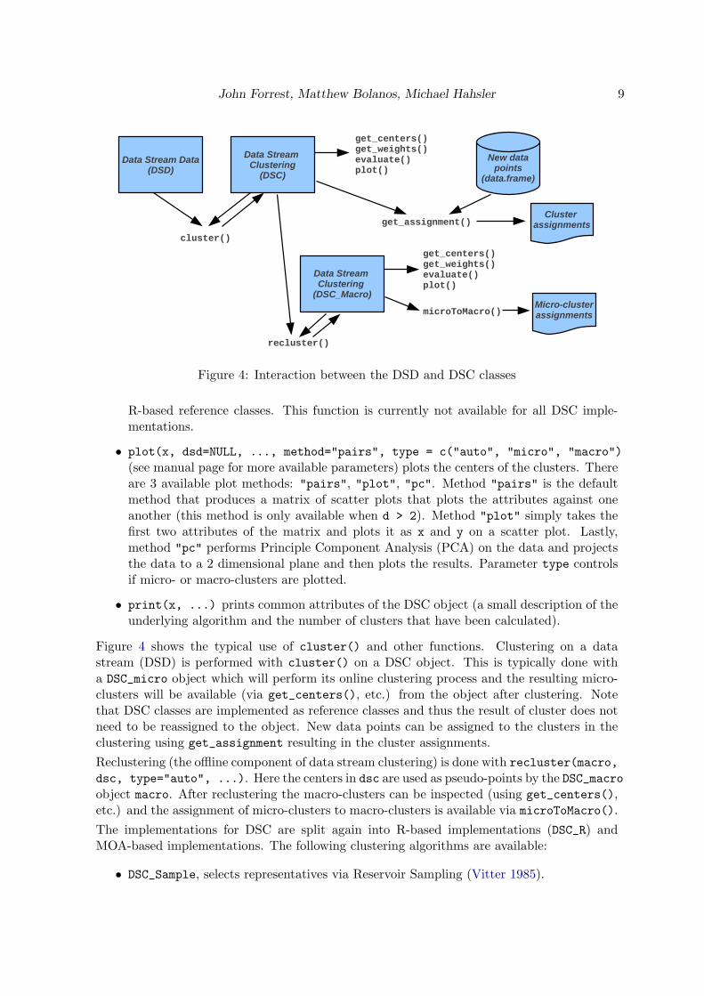
Figure 4 shows the typical use of cluster() and other functions. Clustering on a datastream (DSD) is performed with cluster() on a DSC object. This is typically done witha DSC_micro object which will perform its online clustering process and the resulting micro-clusters will be available (via get_centers(), etc.) from the object after clustering. Notethat DSC classes are implemented as reference classes and thus the result of cluster does notneed to be reassigned to the object. New data points can be assigned to the clusters in theclustering using get_assignment resulting in the cluster assignments.
Reclustering (the offline component of data stream clustering) is done with recluster(macro,
dsc, type="auto", ...). Here the centers in dsc are used as pseudo-points by the DSC_macroobject macro. After reclustering the macro-clusters can be inspected (using get_centers(),etc.) and the assignment of micro-clusters to macro-clusters is available via microToMacro().
The implementations for DSC are split again into R-based implementations (DSC_R) andMOA-based implementations. The following clustering algorithms are available:
• DSC_Sample, selects representatives via Reservoir Sampling (Vitter 1985).
10 Introduction to stream
• DSC_BIRCH, the first pass of the BIRCH (balanced iterative reducing and clusteringusing hierarchies) algorithm (Zhang, Ramakrishnan, and Livny 1996). used to generatea CF tree where the leave notes are used as micro-clusters.
• DSC_CluStream, the CluStream algorithm from MOA (Aggarwal, Han, Wang, and Yu2003b).
• DSC_DenStream, the DenStream algorithm from MOA (Cao, Ester, Qian, and Zhou2006b).
• DSC_ClusTree, the ClusTree algorithm from MOA (Kranen, Assent, Baldauf, and Seidl2009).
• DSC_tNN, a simple data stream clustering algorithm called threshold nearest-neighbors(Hahsler and Dunham 2010a,b) extended by a new shared-density graph reclusteringmethod which makes DSC_tNN a combined micro- and macro-clustering algorithm.
For reclustering, the following traditional clustering algorithms are available as objects ofclass DSC_Macro:
• DSC_Kmeans, interface to R’s k-means implementation.
• DSC_KmeansW, a version of k-means where the data points (micro-clusters) are weightedby the micro-cluster weights, i.e., a micro-cluster representing more data points hasmore weight.
• DSC_DBSCAN, DBSCAN (Ester et al. 1996).
• DSC_Hierarchical, interface to R’s hclust function.
Finally, clustering sometimes creates small clusters for noise or outliers in the data. stream
provides prune_clusters(dsc, threshold=.05, weight=TRUE) to remove a given percent-age (given by threshold) of the clusters with the least weight. The percentage is eithercomputed with the number of clusters or with the sum of the weight of all clusters (weight).The resulting clustering is a static copy (DSC_Static). Further clustering cannot be per-formed by it, but it can be used as input for reclustering.
4. Evaluating Data Stream Mining
Evaluation of data stream mining is an important issue. We will only briefly introduce theevaluation of data stream clustering here and refer the interested reader to the books byAggarwal (2007) and Gama (2010).
4.1. Evaluating Data Stream Clustering
Evaluation of clustering and in particular data stream clustering is discussed in the literatureextensively and there are many evaluation criteria available. For the evaluation of conventionalclustering we refer the reader to the popular books by Jain and Dubes (1988) and Kaufman
John Forrest, Matthew Bolanos, Michael Hahsler 11
and Rousseeuw (1990). Evaluation of data stream clustering is treated in the book by Gama(2010).
Evaluation of data stream clustering is performed in stream via
evaluate(dsc, dsd, method, n = 1000, type=c("auto", "micro", "macro"),
assign="micro"),
where n data points are taken from dsd and assigned to their closest cluster in the clustering indsc using Euclidean distance. By default the points are assigned to micro-clusters (assign),but it is also possible to direct assign them to macro-cluster centers. Then initial assignmentsare aggregated to the level specified in type. For example, for a macro-clustering, the ini-tial assignments will be made by default to micro-clusters and then these assignments willbe translated into macro-cluster assignments using the micro- to macro-cluster relationshipsstored in the clustering. Then the evaluation measure specified in method is calculated.
A simple measure is to evaluate the compactness of the data points assigned to each clusterusing the sum of squared distances between each data point and the center of its cluster(method "SSQ"). This is measure of internal cluster validity which does not require anyinformation about the ground truth (i.e., true partitioning of the data into classes).
Most evaluation measures perform external evaluation and require the ground truth (classlabel) for the data (dsd). Then based on cluster membership of each new data point and theclass label different measures can be computed. We will not describe each measure here sincemost of them are standard measures which can be found in many text books (e.g., Jain andDubes 1988; Kaufman and Rousseeuw 1990). We only list the measures currently availablefor evaluate() (method name are under quotation marks):
• "precision", "recall", F1 measure ("F1"),
• "purity", false positive rate ("fpr")
• Rand index ("Rand"), adjusted Rand index ("cRand"),
• Jaccard index ("Jaccard"),
• Euclidean dissimilarity of the memberships ("Euclidean")
• Manhattan dissimilarity of the memberships ("Manhattan"),
• Normalized Mutual Information ("NMI")
• Katz-Powell index ("KP")
• Fowlkes and Mallows’s index ("FM")
• Maximal cosine of the angle between the agreements ("angle"),
• Maximal co-classification rate ("diag"),
• Prediction Strength ("PS").
12 Introduction to stream
4.2. Extending the stream Framework
Since stream mining is a relatively young field and many advances are expected in the nearfuture, the object oriented framework in stream is developed with easy extensibility in mind.Implementations for data streams (DSD) and data stream tasks (DST) can be easily addedby implementing a small number of core functions. The actual implementation can be writtenin either R, Java, C/C++ or any other programming language which can be interfaced by R.In the following we discuss how to extend DSD and DST.
4.3. Implementing new Data Stream Data (DSD) Classes
The class hierarchy in Figure 2 (on page 7) is implemented in the S3 class system by using avector of class names for the class attribute. For example, an object of class DSD_GaussianStaticwill have the class attribute vector c("DSD_GaussianStatic", "DSD_R", "DSD") indicatingthat the object also is an R implementation of DSD. This allows the framework to implementall common functionality as functions at the level of DSD and DSD_R and only a minimal setof functions has to be implemented in order to add a new data stream implementation.
For a new DSD implementation only a creator function and a get_points() method for theclass needs to be implemented. The creator function creates an object of the appropriate DSDsubclass. Typically this S3 object is a list of all parameters, an open R connection and/oran environment (or a reference class) for storing state information (e.g., the current positionin the stream). Also an element called "description" should be provided. This element isused by print(). Note that the class attribute has to contain a vector of all parent classes inthe class diagram in bottom-up order. The implemented get_points() needs to dispatch forthe class and create as the output a data.frame containing the data points as rows. Also, ifthe ground truth (true cluster assignment) for the data is available, then this can be attachedto the data.frame as an attribute called "assignment" as an integer vector (noise typically isrepresented by NA).
For a complete example, look at the implementation of DSD_UniformNoise in the package’ssource code.
4.4. Implementing new Data Stream Task (DST) Classes
We concentrate again on data stream clustering. However, to add new data stream miningtasks, a subclass hierarchy similar to the hierarchy in Figure 3 (on page 8) for data streamclustering (DSC) can be easily added.
To implement a new clustering algorithm, a creator function (typically named after the al-gorithm) and a cluster() function is needed. The clustering algorithm itself is part of theobject created by the creator. To understand this slightly complicated approach consideragain Figure 4 (on page 9). The framework provides the function cluster(dsc, dsd, n=1)
which contains a loop to go through n new data points. In the loop a block of data pointsis obtained from dsd using its get_point() function and then the data points are passed onto an internal generic clustering function which has implementations for DSC_MOA and DSC_R.The implementation for DSC_MOA takes care of all MOA-based clustering algorithms. For R-based implementation, the DSC_R version looks in the list of the dsc object for an elementcalled "RObj", which needs to be a reference class object. Reference classes have been recentlyintroduced with R-2.12 in package methods as a construct for mutable objects. Mutability
John Forrest, Matthew Bolanos, Michael Hahsler 13
means that the object can be changed without creating a copy and assigning it back to itselfas would be necessary in a purely functional programming language. The RObj in DSC isexpected to be a reference class with a cluster method. Note at this point that methods ofreference classes are called in a very different way from normal R function calls. For example,the cluster method of Robj is invoked by RObj$cluster(). However, this is not importantfor the end user since the cluster method is only used internally and never called directly bythe user.
To obtain the clustering result, a methods called get_microclusters and get_microweights
which dispatched for the new class need to be implemented. These methods extract thecenters/weights of the clusters from the reference class object in dsc and return them as adata.frame (centers) or a vector (weights). These methods are also not exposed to the userand are called internally from get_centers and get_weights.
For a macro clustering algorithm, the clustermethod performs reclustering and get_macroclustersand get_macroweights need to be implemented. In addition microToMacro, a method whichdoes micro- to macro-cluster matching, has to be provided.
For a complete example, look at the implementation of DSC_tNN in the package’s source code.
5. Examples
Developing new data stream mining algorithms and comparing them experimentally is themain purpose of stream. In this section we give several increasingly complex examples of howto use stream. First, we start with creating a data stream using different implementations ofthe DSD class. The second example shows how to save and read stream data to and fromdisk. We then give examples in how to reuse the same data from a stream in order to performcomparison experiments with multiple data stream mining algorithms on exactly the samedata. Finally, the last example introduces the use of data stream clustering algorithms witha detailed comparison of two algorithms from start to finish by first running the online com-ponents, then using a weighted k-means algorithm to re-cluster the micro-clusters generatedby each algorithm into final clusters.
5.1. Creating a data stream
In this example, we focus on the DSD class to model data streams.
> library("stream")
> set.seed(1000)
> dsd <- DSD_GaussianStatic(k=3, d=2, noise=0.05)
> dsd
Static Mixture of Gaussians Data Stream (DSD_GaussianStatic, DSD_R, DSD)
With 3 clusters in 2 dimensions
After loading the stream package (and setting a seed for the random number generator to makethe experiments reproducible), we call the creator function for the class DSD_GaussianStaticspecifying the number of clusters as k = 4, the data dimensionality to d = 2 and a noise of
14 Introduction to stream
5%. This data stream generator chooses for each cluster randomly a mean and a covariancematrix.
New data points are requested from the stream using get_points(x, n=1, ...). When anew data point is requested from this generator, a cluster is chosen randomly and then pointis drawn from a multivariate normal distribution given by the mean and covariance matrix ofthe cluster. The following instruction requests n = 5 new data points.
> p <- get_points(dsd, n=5)
> p
V1 V2
1 0.7254021 0.44002678
2 0.2642523 0.25574463
3 0.3684851 0.13816977
4 0.6470814 0.52239215
5 0.4239730 0.08627291
The result is a data.frame containing the data points as rows. For evaluation it is oftenimportant to know the ground truth, in this case from which cluster each point was created.The generator also returns the ground truth if it is called with assignment=TRUE. The groundtruth is returned as an attribute with the name "assignment" and can easily be accessed inthe following way:
> p <- get_points(dsd, n=100, assignment=TRUE)
> attr(p, "assignment")
[1] NA 1 3 2 3 1 1 2 3 3 1 1 3 1 3 3 2 1 1 2 1 2 1 2 1
[26] 3 1 3 3 1 NA 2 2 2 NA 2 NA 1 2 3 2 NA 2 3 3 1 1 3 2 3
[51] 3 2 1 2 3 3 3 2 1 3 NA 2 1 3 2 1 1 NA 3 3 2 1 2 2 2
[76] 1 2 3 3 NA 1 1 1 2 2 3 3 2 2 1 2 2 1 3 NA 2 3 1 3 3
Note that we created a generator with 5% noise. Noise points do not belong to any clusterand thus have an assignment value of NA.
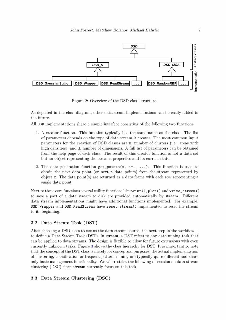
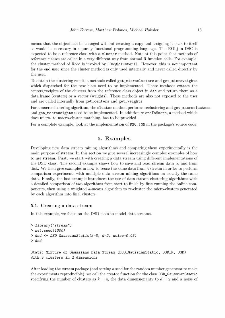
Next, we plot 500 points from the data stream to get an idea about its structure.
> plot(dsd, n=500)
Figure 5 shows the resulting plot. The assignment value is used to change the color in theplot. Noise points are plotted as gray crosses.
DSD_RandomRBFGeneratorEvents creates dynamic data streams where clusters move overtime which is called in the data mining community concept drift.
> set.seed(1000)
> dsd <- DSD_RandomRBFGeneratorEvents(k=3, d=2)
> dsd
John Forrest, Matthew Bolanos, Michael Hahsler 15
●
●
●●
●
● ●●●●
●
●
●
●
●
●
●
●●●
●
●
●
●
●
●●
●
●
●
●
●
●
●
●
●
●
●
●
●
●●
●
●
●
●
●
●
●
●
●
●
●
●
●
●
●
●
●
●
●
●
●
●
●
●
●
●●
●
●
●
●
●●
●
●
●
●
●
●
●●
●
●
●
●
●
●
●
●
●
●
●
●
●
●
●
●
●
●
●
●
●
●
●
●
●
●
●
●
●
●
●
●
●
●
●
●●
●
●
●
●
●
●
●
●
●
●
● ●●
●
●
●
●
●
●
●
●
●
● ●
●
●
●
●
●
●
●
●
●
●
●
●
●
●
●
●
●
●
●
●
●
●
●
●
●
●
●
●
●
●
●●
●
●
●
●
●
●
●
●
●
●
●
●
●
●
●
●
●
●
●
●
●
● ●
●
●
●
●
●
●
●
●
●
●
●
●
●
●
●●
●
●
●
●
●
●
●
●
●
●
●
●
●
● ●
●
●
● ●
●
●
●
●
●
●
●
●
●●
●
●●
●
●
●●
●
●
●●
●
●
●
●
●●
●
●
●
●
●
●
●
●
●
●
●
●
●
●●
●
●●
●
●
●
●
●
●
●
●
●
●
●
●
●
●
●
●
● ●
●
●
●
●
●
●
●
●
●
●
●
●
●
●
●
●
●
●
●
●
●
●
●
●
●
●
●
●
●●●
●
●
●
●●
●
●
●
●
●
●
●
●●
●●
●●
●
●
●
●
●
●●
●
●
●
●
● ●●
●
●
●●●
●
●
●
●
● ●
●
●
●
●
●
●
●
●● ●
●
●
●
●
●
●
●
●
●
●
●
●
●
●
●
●●
●
●
●●
●
●
●
●
●
●
●●
●●
●
●
●
●
●
●
●
● ●
●●
●
●
●
●
●
●
●
●
●
●●
●
●
●
●
●
●
●
●●
●
●
●
●
●
●
● ●
●
●
●
●
●
●
●
●●
●
●
●
●
●
●
●
●
●
●
●
●
●
●
●
●
0.2 0.4 0.6 0.8
0.0
0.2
0.4
0.6
0.8
1.0
V1
V2
Figure 5: Plotting 1000 data points from the data stream
Random RBF Generator Events (MOA) (DSD_RandomRBFGeneratorEvents, DSD_MOA, DSD)
With 3 clusters in 2 dimensions
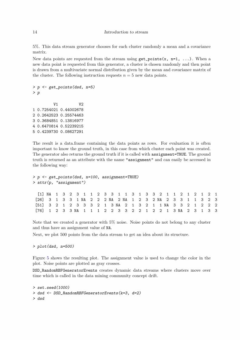
k and d again represent the number of clusters and the dimensionality of the data, respectively.In the following we request 4 times 500 data points from the stream and create a plot.
> plot(dsd, 500)
> plot(dsd, 500)
> plot(dsd, 500)
> plot(dsd, 500)
Figure 6 shows the results of the four plot instructions. It shows that the 3 clusters moveover time (the ).
An animation of the plot can also be generated using data_animation().
> data_animation(dsd, 5000)
5.2. Reading and writing data streams
Although data streams by definition are unbounded and thus storing them long term istypically infeasible, it is often useful to store parts of a stream to disk. For example, a smallpart of a stream with an interesting feature can be used to test how a new algorithm handlesthis specific case. stream has support for reading and writing parts of data streams through anR connection which provide a set of functions to interface file-like objects like files, compressedfiles, pipes, URLs or sockets (R Foundation 2011).
We start by creating a DSD object.

16 Introduction to stream
●
●
●
●
●●
●
●
●
●
●
●
●
●
●
●●
●
●
●●
●
● ●
●
●
●
●
●
●
●
●
●
●
●
●
●
●
●
●
●
●
●
●
●
●
● ●
●
●
●
●
●
● ●
●
●● ●
●●
●
●
●
●
●●
●●
●●
●
●
●
●●
●
●
●
●
●●
●
●
●
●
●
●●●
●
●●
●●
●
●
●
●●●
●
●●
●
●
●
●
●
●●
●
●
●●
●
●
●●
●
●
●
●●
●
●
● ●
●
●
●
●
●
●
●
● ●●
●
●
●
●
●
●
●
●●●
●
●
●
●
●
●
●
●
●
●
●
● ●
●
●●●●
●
●●
●
●
●●
●
●
●
● ●●
●
●
●
●
●
●●
●
●
●
●
●●
●
●
●●
●
●
●
●
●
●●
●
●
●●
●●
●
●
●
●
●
●
●
●
●●● ●● ●
●
●
●● ●
●
●●
●●
●
●
●●
●
●
●
●●
●●
●
●
●
●
● ●
●
●
●
●
● ●
●
●●●●
●
●
●
●
●
●●
●
●
●
●
●
●●
●
●
●
●
● ●●
●
●
●
●
●●
●
● ●●
●
●
●
●
● ●●
●●
●●
●●
●●
●
●●
●
●
●
●●
●
●
●●
●
●
●
●●
●
● ●
●
●
● ●●
●
●●
●
●
●●
●
●
●
●●
●
●●
●
●●
●●
●
●
●●
●
●
●
● ●
● ●
●
●
● ●●
●
●
●
●
●●
●
●
●
●
●●
●
●
●
●
● ●
●●
●
●
●●
●
●
●
●
●
●●●
●
●●
●●
●
● ●
●
●
●
●
●
●
●
●
●
●
●
●
●●
●
●
●
●●
●
●
●
●
●
●
●●
●
●
●
●
●
●
●
●●
●
●●
●●
●
●
●
●
●
●
●
●●
●●
●●
●
●●
●
●
●
●
●
●●
●
●
●
●
●●
● ●● ●
●
●
●
●● ●
●
●
●
●
● ●
●●
●
●
●
●
0.0 0.2 0.4 0.6 0.8 1.0
0.0
0.2
0.4
0.6
0.8
1.0
X1
X2
(a)
●
●
●●
●
●
●
●
●
●
●
●
●●●
●●
●
●●
●
●
●
●
●
●
●
● ●
●
●
●
●
●●
●
●
●●
●
● ●
●
●
●
●
●
●
●
●
●●
●
●
●
●
●
●●●
●
●● ●
●
●
●●
●
●
●
●
●●
●
●
●
●
● ●
●
●●
●●
●
●●
●
●
●
●
●●
●
●
●
●●
●
●
●
● ●
●
●
●
●
●●
●●
●
●
●
●
●
●
●
●
●
●
●
● ●
●
●
●
●
●●
●
●
●
●
●
●
● ●
●
●
●
●
●● ●
●●
●
●
● ●
●●
●
●●●
●
●
●●
●
●●
●
●●
●●
●
●
●
●●
●●
●
●
●
●
●
●●
●
●●
●●
●
●
●
●
● ●
●
● ●
●
●
●
●●
●●
●
●
●
●
●
●●
●
●
●
●
●
●
●
●
●
●●●
●
●
●
●●
●
●
●
●●●
●
●
●
●
●
●●
●● ●
●●
●
●
●
●
●
● ●●
●
●●
●
● ●
●
●
●
●
●
●
●
●
●●●
●
●
●
●
●
●
●
●●● ●
●
●
●
●●
●
●
●
●
●
●●
●
●
●
●●
●●
●
●
●
●●
●●
●
●●
● ●●●
●
●
●
●
●
●●
●
●●
●
●
●
●●●
●
●
●●
● ●
●●
●
●
●●
●
●
●
●
●●
●
●
●
●
●●
●
●
●
●
●●
●
●
●
●
●
●
●
●
●
●●
● ●
●
●
●
●
●●
●
●
●
●
●
●
●
●
●
●●
●
●
●
●
●
●
●
●
●●
●
●
●●
●
●
●
●●
●
●●
●
●
●
●
●
●●
● ●
●●●
●
●●●
●
●●●
●●
●
●
●
●●
●●
●
●
●
●
●●
●
●
●●
●
●● ●
●
●
●●
●
●
●
●
●
●●
●
●
●●
●● ●
●●
●
●
●
●
●
●●
●
●
●
●
●
●
●● ●
●
●●
●●
●
●
0.2 0.4 0.6 0.8 1.0
0.0
0.2
0.4
0.6
0.8
1.0
X1
X2
(b)
●
●
●
●●
●
●
●●
●
●
●
● ●●
●
●
●●
●
●
●
●
●●
●● ●
●
●
●●
●
●●
●
●
●
●●
●●
●
●●
●
●
●
●●
●
●
●
●●
●
●
●
●
●
●
●●●●● ●
●
●
●
●
●●
●
●
●
●
●
●
●●
●
●
●
●
●
●
●
●
●
●
●
●
●
●
●
●
●
●●
●
●
●
●
●● ●
●
●
●
●
●
●
●
● ●
●●
●
●
●●
●
●
●
●
●
●
●● ●
●
●
●
●
●
●● ●
●●
●
●
●
●
●
●
●
●●●
●
●
●
●
●
●
●
●
●
●
●●●
●
●●●
●
● ●
●
●
●●
●
●
●
●
●
●
●
●
●●
●●
●●
●
●
●
●●
●
●
●
●
●
●
●
●
●
●
●
●
●
●●
●
●
●
●
●
●
●
●
●
●
●
●
●
●
●
●
●
●
●
●
● ●
●
●
●●
●●●
●
●
●●●
●
●
●
●
●●
●
●
●
●●
●
●
●●●
●
● ●
●
●
●●
●
●
●
●
●
●
●
●●
●
●
●●
●
●
●
●
●
●
●
●
●
●
●●
●
●
●
●●
●
●
●
●●
●●
●
●
●
● ●
●●
●●
●●
●
●
●
●
●
●
●
●
●
●
●
●
●●
●
●
●
●
●
●●
●
●
●
●
● ●●
●●
●●
●
●
● ●
●●
●
●
●●
●●
●
●
●
●
●●
●
●
●
●
●
●
●●
●
●
●
●
●
●
●
●
●
●●●
●
●
●
●
●
●
●
● ●●
●
●
●
●
●
●●
●
● ●
●
●
●
●
●
●
●
●
●
●
●
●
●
●●
●
●
●
● ●●
●
●●
●
●
●
●
●
●
●
●
●
●●
●
●●●
●●
●●●
●
●
●
●
●
●
●
●
●
●
●
●●
●
●
●
●
●●
●
●
●
●
●●●
●
●
●
●
●
●●
●
●
●
●●
●
●
●
●
●
●●
●
●
●
●
●
●
●
0.0 0.2 0.4 0.6 0.8 1.0
0.0
0.2
0.4
0.6
0.8
1.0
X1
X2
(c)
●
●
●
●
●
●●
●
●●
●
●
●
●
●●
●
●
●
●●
●
●
●
●
●
●
●
●
●
●
●
●
●
●
●
●
●●
● ●●
●
●
●
●
●●
●
●
●
●
●
●
●
●
●
●
●
●
●
●
●
●
● ●
●●
●
●
●●
●
●
●
●●
●
●●
●
●●
●
●
●
●
●
●
● ●
●
●
● ●
●
●
●
●
●
●●●
●●
●
●
●
●
●●
●
●
● ●
●
●
●
●
●●
●
●
●
●
●
●●
●●●
●
●●●
●●
●
●
●
●
●
●
●●●
●
●
●
●
●
●
●
●
●
●●
●
●
●
●
●●
●
●
●
●
●
●
●●●
●●
●
●
●
●
●
●
●
●
●
●
●
●
●●
● ●● ●
●
●
●
●
●
●
●
●
●●
●
●
●
●
●
● ●
●
●●
●●
●●
●
●
●●
●●
●
●
●
●
●
●
●●
●●● ●
●
●
●
●
●
● ●
●●●●
●
●
●●●
●
●
●●
●● ●
●
●
●
●
●
●
●
●
●
●
●
●
●●
●
●
●
●
●
●
●
●
●●●
●
●
●
●
●
●
●
●
●
●
●
●
●
●
●
●●
●
●
●
●
●
●
●
●
●●
●●
●
●
●
●●
● ●
●
●●●
●
●
●
●
●
●●●
● ●● ●●
●
●
●
●
●
●
●
●●
●
●
●
●●
●
●
●●
●
●●
●
●
●●
●
●
●
●
●
●
●
●
●
●●
●
●
●
●
●
●
●
●
●
●
●
●
●●
● ●
●
●
●●●
●●
●
●
●
●
●
●
●●●
●
●
●
●
●
●
●
●
● ●
●●
●
●●
● ●
●
●●
●
●●
●
●
●
●
●
●
●
●●
●
●
●
●●
●
●
●
●
●●
●
●
●
●
●●●
●●
●●
●●
●
●
●
●
●●
●
●
●
●
●
●●
●
●
●
●
●
●
● ●
●
●
●
●
●
●
●●●
●
●
●●
●
●
●
●●●
●
0.0 0.2 0.4 0.6 0.8 1.0
0.2
0.4
0.6
0.8
1.0
X1
X2
(d)
Figure 6: The concept drift of DSD MOA
John Forrest, Matthew Bolanos, Michael Hahsler 17
Static Mixture of Gaussians Data Stream (DSD_GaussianStatic, DSD_R, DSD)
With 3 clusters in 5 dimensions
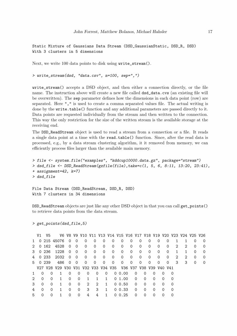
Next, we write 100 data points to disk using write_stream().
> write_stream(dsd, "data.csv", n=100, sep=",")
write_stream() accepts a DSD object, and then either a connection directly, or the filename. The instruction above will create a new file called dsd_data.cvs (an existing file willbe overwritten). The sep parameter defines how the dimensions in each data point (row) areseparated. Here "," is used to create a comma separated values file. The actual writing isdone by the write.table() function and any additional parameters are passed directly to it.Data points are requested individually from the stream and then written to the connection.This way the only restriction for the size of the written stream is the available storage at thereceiving end.
The DSD_ReadStream object is used to read a stream from a connection or a file. It readsa single data point at a time with the read.table() function. Since, after the read data isprocessed, e.g., by a data stream clustering algorithm, it it removed from memory, we canefficiently process files larger than the available main memory.
> file <- system.file("examples", "kddcup10000.data.gz", package="stream")
> dsd_file <- DSD_ReadStream(gzfile(file),take=c(1, 5, 6, 8:11, 13:20, 23:41),
+ assignment=42, k=7)
> dsd_file
File Data Stream (DSD_ReadStream, DSD_R, DSD)
With 7 clusters in 34 dimensions
DSD_ReadStream objects are just like any other DSD object in that you can call get_points()to retrieve data points from the data stream.
> get_points(dsd_file,5)
V1 V5 V6 V8 V9 V10 V11 V13 V14 V15 V16 V17 V18 V19 V20 V23 V24 V25 V26
1 0 215 45076 0 0 0 0 0 0 0 0 0 0 0 0 1 1 0 0
2 0 162 4528 0 0 0 0 0 0 0 0 0 0 0 0 2 2 0 0
3 0 236 1228 0 0 0 0 0 0 0 0 0 0 0 0 1 1 0 0
4 0 233 2032 0 0 0 0 0 0 0 0 0 0 0 0 2 2 0 0
5 0 239 486 0 0 0 0 0 0 0 0 0 0 0 0 3 3 0 0
V27 V28 V29 V30 V31 V32 V33 V34 V35 V36 V37 V38 V39 V40 V41
1 0 0 1 0 0 0 0 0 0 0.00 0 0 0 0 0
2 0 0 1 0 0 1 1 1 0 1.00 0 0 0 0 0
3 0 0 1 0 0 2 2 1 0 0.50 0 0 0 0 0
4 0 0 1 0 0 3 3 1 0 0.33 0 0 0 0 0
5 0 0 1 0 0 4 4 1 0 0.25 0 0 0 0 0
18 Introduction to stream
Looping over the data several times and resetting the position in the DSD_ReadStream to thefile’s beginning is possible and will described in the next example.
5.3. Replaying a data stream
An important feature of stream is the ability to replay portions of a data stream. Withthis feature we can capture a special feature of the data (e.g., an anomaly) and then adaptour algorithm and test if the change improved the behavior on exactly that data. Also, thisfeature can be used to conduct experiments where different algorithms need to see exactlythe same data.
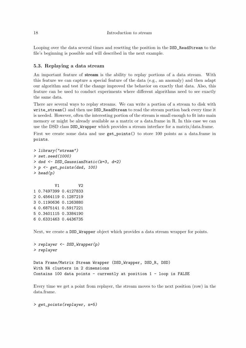
There are several ways to replay streams. We can write a portion of a stream to disk withwrite_stream() and then use DSD_ReadStream to read the stream portion back every time itis needed. However, often the interesting portion of the stream is small enough to fit into mainmemory or might be already available as a matrix or a data.frame in R. In this case we canuse the DSD class DSD_Wrapper which provides a stream interface for a matrix/data.frame.
First we create some data and use get_points() to store 100 points as a data.frame inpoints.
> library("stream")
> set.seed(1000)
> dsd <- DSD_GaussianStatic(k=3, d=2)
> p <- get_points(dsd, 100)
> head(p)
V1 V2
1 0.7497399 0.4127833
2 0.4564119 0.1287219
3 0.1190636 0.1263880
4 0.6875141 0.5917221
5 0.3401115 0.3384190
6 0.6331463 0.4436735
Next, we create a DSD_Wrapper object which provides a data stream wrapper for points.
> replayer <- DSD_Wrapper(p)
> replayer
Data Frame/Matrix Stream Wrapper (DSD_Wrapper, DSD_R, DSD)
With NA clusters in 2 dimensions
Contains 100 data points - currently at position 1 - loop is FALSE
Every time we get a point from replayer, the stream moves to the next position (row) in thedata.frame.
> get_points(replayer, n=5)
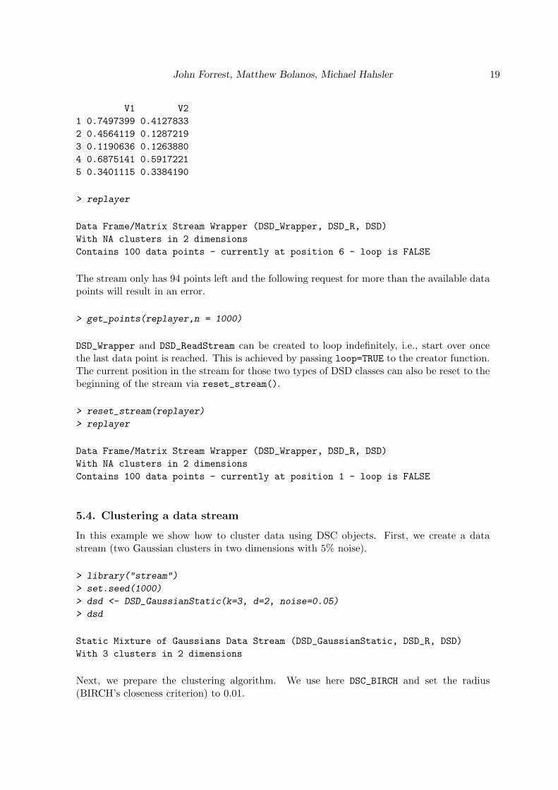
John Forrest, Matthew Bolanos, Michael Hahsler 19
V1 V2
1 0.7497399 0.4127833
2 0.4564119 0.1287219
3 0.1190636 0.1263880
4 0.6875141 0.5917221
5 0.3401115 0.3384190
> replayer
Data Frame/Matrix Stream Wrapper (DSD_Wrapper, DSD_R, DSD)
With NA clusters in 2 dimensions
Contains 100 data points - currently at position 6 - loop is FALSE
The stream only has 94 points left and the following request for more than the available datapoints will result in an error.
> get_points(replayer,n = 1000)
DSD_Wrapper and DSD_ReadStream can be created to loop indefinitely, i.e., start over oncethe last data point is reached. This is achieved by passing loop=TRUE to the creator function.The current position in the stream for those two types of DSD classes can also be reset to thebeginning of the stream via reset_stream().
> reset_stream(replayer)
> replayer
Data Frame/Matrix Stream Wrapper (DSD_Wrapper, DSD_R, DSD)
With NA clusters in 2 dimensions
Contains 100 data points - currently at position 1 - loop is FALSE
5.4. Clustering a data stream
In this example we show how to cluster data using DSC objects. First, we create a datastream (two Gaussian clusters in two dimensions with 5% noise).
> library("stream")
> set.seed(1000)
> dsd <- DSD_GaussianStatic(k=3, d=2, noise=0.05)
> dsd
Static Mixture of Gaussians Data Stream (DSD_GaussianStatic, DSD_R, DSD)
With 3 clusters in 2 dimensions
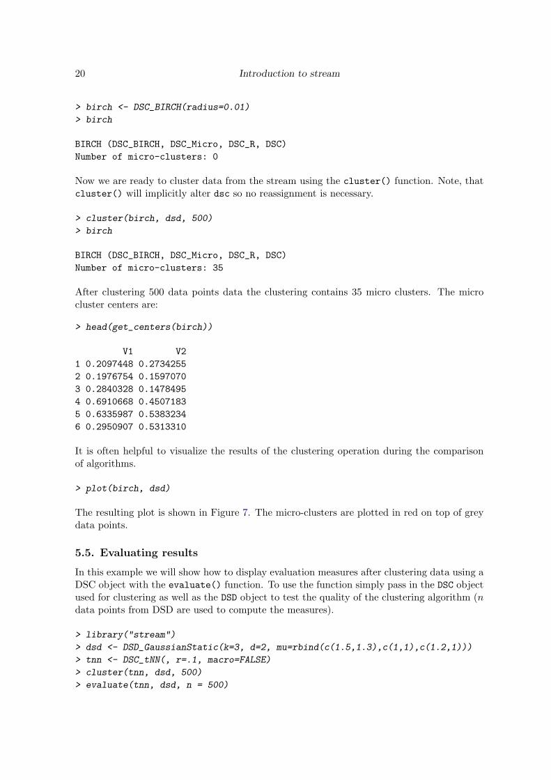
Next, we prepare the clustering algorithm. We use here DSC_BIRCH and set the radius(BIRCH’s closeness criterion) to 0.01.
20 Introduction to stream
> birch <- DSC_BIRCH(radius=0.01)
> birch
BIRCH (DSC_BIRCH, DSC_Micro, DSC_R, DSC)
Number of micro-clusters: 0
Now we are ready to cluster data from the stream using the cluster() function. Note, thatcluster() will implicitly alter dsc so no reassignment is necessary.
> cluster(birch, dsd, 500)
> birch
BIRCH (DSC_BIRCH, DSC_Micro, DSC_R, DSC)
Number of micro-clusters: 35
After clustering 500 data points data the clustering contains 35 micro clusters. The microcluster centers are:
> head(get_centers(birch))
V1 V2
1 0.2097448 0.2734255
2 0.1976754 0.1597070
3 0.2840328 0.1478495
4 0.6910668 0.4507183
5 0.6335987 0.5383234
6 0.2950907 0.5313310
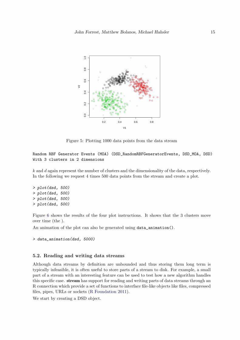
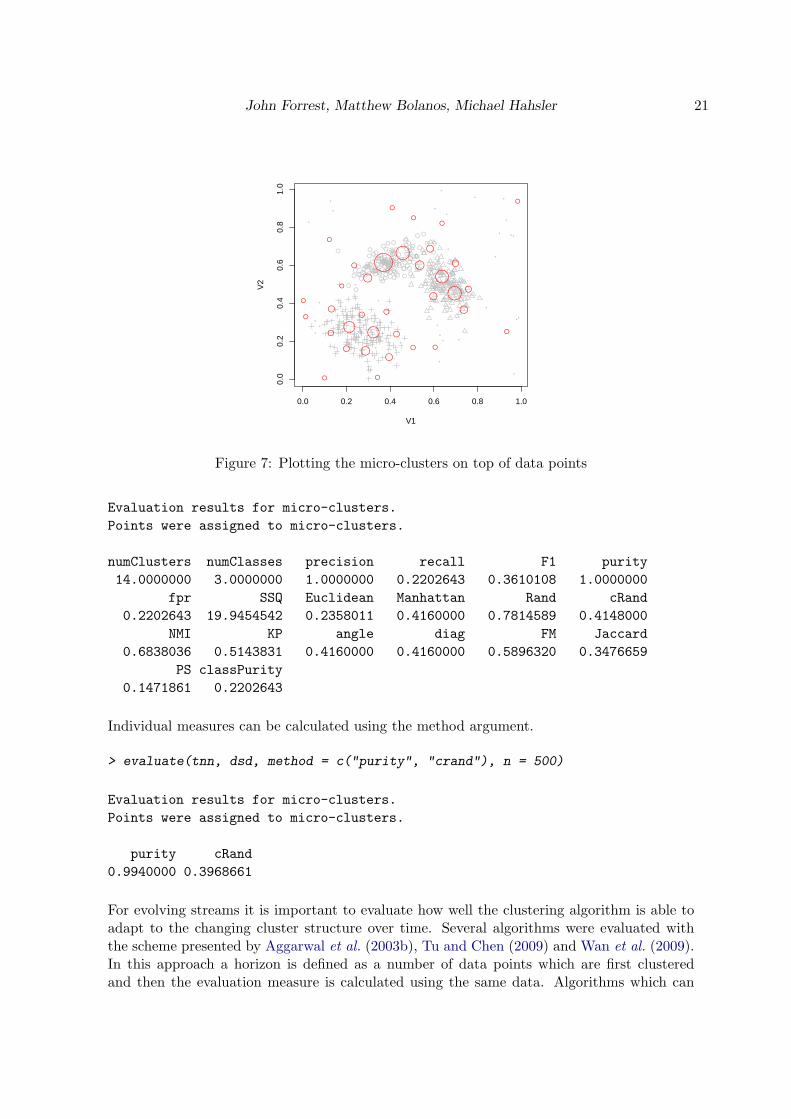
It is often helpful to visualize the results of the clustering operation during the comparisonof algorithms.
> plot(birch, dsd)
The resulting plot is shown in Figure 7. The micro-clusters are plotted in red on top of greydata points.
5.5. Evaluating results
In this example we will show how to display evaluation measures after clustering data using aDSC object with the evaluate() function. To use the function simply pass in the DSC objectused for clustering as well as the DSD object to test the quality of the clustering algorithm (ndata points from DSD are used to compute the measures).
> library("stream")
> dsd <- DSD_GaussianStatic(k=3, d=2, mu=rbind(c(1.5,1.3),c(1,1),c(1.2,1)))
> tnn <- DSC_tNN(, r=.1, macro=FALSE)
> cluster(tnn, dsd, 500)
> evaluate(tnn, dsd, n = 500)
John Forrest, Matthew Bolanos, Michael Hahsler 21
●
●
●
●
●
●●
●
●
●
●
●
●
●
●
●
● ●
●
●
●●
●
●
●●
●
●●
●
●
●
●
●
●
● ●●
●
●
●
● ●
●
●
●
●●
●
● ●
●
●
● ●
●
● ●
●
●
●
●
●
●
●
●
●
●
●●
●
●
●
●
●
●●
●●
●
●
●
●
●
●
●
●
●
● ●
●
●
●
●●
●
●
●
●
●
●
●● ●
●
●
●
●
●
●
●
●
●
●
●
●
●
●●
●●
●
●●
●
●●
●
●
●●
●●
●
●
●
●●
●
●
●●
●
●
●
● ●
●
●
●
●
●●●
●
●
●
●
● ●
●
●
●
● ●
●
●
●
●
●
●●
●
●
●
●
●
●
●
●
●
● ●
●●●
●
●
●
●
●
●
●
●
●
●
● ●
●
●
●
●
●
●
●
●
●
●
●●
●
●
●
●
0.0 0.2 0.4 0.6 0.8 1.0
0.0
0.2
0.4
0.6
0.8
1.0
V1
V2
Figure 7: Plotting the micro-clusters on top of data points
Evaluation results for micro-clusters.
Points were assigned to micro-clusters.
numClusters numClasses precision recall F1 purity
14.0000000 3.0000000 1.0000000 0.2202643 0.3610108 1.0000000
fpr SSQ Euclidean Manhattan Rand cRand
0.2202643 19.9454542 0.2358011 0.4160000 0.7814589 0.4148000
NMI KP angle diag FM Jaccard
0.6838036 0.5143831 0.4160000 0.4160000 0.5896320 0.3476659
PS classPurity
0.1471861 0.2202643
Individual measures can be calculated using the method argument.
> evaluate(tnn, dsd, method = c("purity", "crand"), n = 500)
Evaluation results for micro-clusters.
Points were assigned to micro-clusters.
purity cRand
0.9940000 0.3968661
For evolving streams it is important to evaluate how well the clustering algorithm is able toadapt to the changing cluster structure over time. Several algorithms were evaluated withthe scheme presented by Aggarwal et al. (2003b), Tu and Chen (2009) and Wan et al. (2009).In this approach a horizon is defined as a number of data points which are first clusteredand then the evaluation measure is calculated using the same data. Algorithms which can
22 Introduction to stream
better adapt to the changing stream will achieve a better value. This evaluation strategyis implemented in stream as function evaluate_cluster. The following examples evaluateDenStream and DenStream plus weighted k-means reclustering on an evolving stream.
> dsd <- DSD_GaussianMoving()
> micro <- DSC_DenStream(initPoints=100)
> evaluate_cluster(micro, dsd, method=c("purity","crand"), n=600, horizon= 100,
+ assign="micro")
purity cRand
100 0.67 0.5628322
200 0.67 0.5628322
300 0.67 0.4708696
400 0.67 0.5737903
500 0.94 0.6132992
600 0.80 0.4424282
> reset_stream(dsd)
> micro <- DSC_DenStream(initPoints=100)
> macro <- DSC_KmeansW(3)
> evaluate_cluster(micro, dsd, macro, method=c("purity","crand"), n=600,
+ horizon=100, assign="micro")
purity cRand
100 0.67 0.5628322
200 0.67 0.5628322
300 0.67 0.4708696
400 0.67 0.5737903
500 0.94 0.8319220
600 0.80 0.5862409
5.6. Reclustering DSC objects with another DSC
This examples show how to recluster a DSC object after creating it. To begin, first create aDSC object and run the clustering algorithm.
> library("stream")
> dsd <- DSD_GaussianStatic(k=3, d=2, mu=rbind(c(1.5,1.3),c(1,1),c(1.2,1)))
> tnn <- DSC_tNN(r=.04, macro=FALSE)
> cluster(tnn, dsd, 1000)
> tnn
tNN (DSC_tNN, DSC_Micro, DSC_R, DSC)
Number of micro-clusters: 62
John Forrest, Matthew Bolanos, Michael Hahsler 23
●●
●
●
●
●●
●
●
●
●
●
●
●
●
●●
●
●
●
●
●●
●
●
●
●
●
●●
●
●●
●
●●
● ●
●
●
●●
●
●
●
●●
●
●●
●
●
●●
●
●
●●●
●
●●●● ● ●
●
●
●
●●
●●
●●
●
●
●
●
●●
●
●
●
●
●
●
●
●
●
●
●
●
●
●
●
●
●
●
●
●
●●
●
●
●
●
●
●
●
●
●●
●
●
●
●
●●●●
●
●
●●
●
●
●●
●
● ●●
●
●
●
●
●
●
●
●
●
●
●
●●
●
●
●
●
●
●
●
●
●
●
●
●●
●
●
●
●
●
●
●
●
●
●
●
●
●
●
●
●
●
●
0.8 1.0 1.2 1.4 1.6
0.8
0.9
1.0
1.1
1.2
1.3
1.4
V1
V2
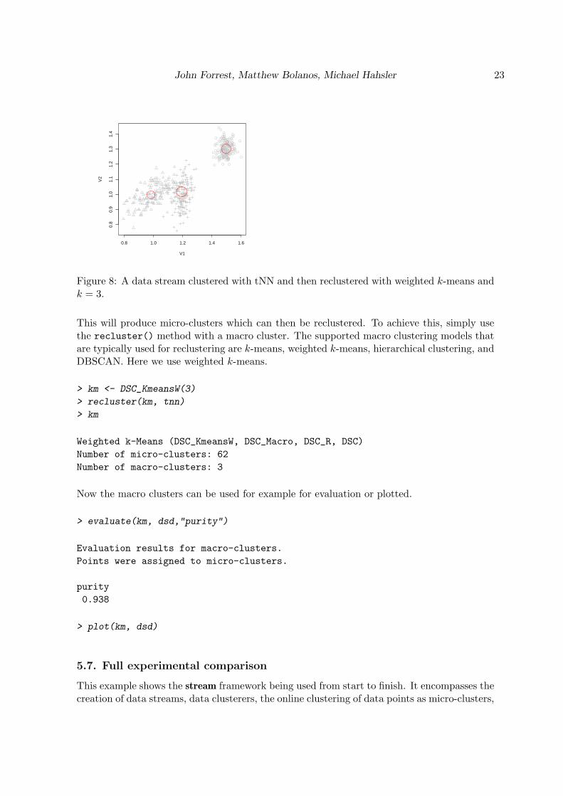
Figure 8: A data stream clustered with tNN and then reclustered with weighted k-means andk = 3.
This will produce micro-clusters which can then be reclustered. To achieve this, simply usethe recluster() method with a macro cluster. The supported macro clustering models thatare typically used for reclustering are k-means, weighted k-means, hierarchical clustering, andDBSCAN. Here we use weighted k-means.
> km <- DSC_KmeansW(3)
> recluster(km, tnn)
> km
Weighted k-Means (DSC_KmeansW, DSC_Macro, DSC_R, DSC)
Number of micro-clusters: 62
Number of macro-clusters: 3
Now the macro clusters can be used for example for evaluation or plotted.
> evaluate(km, dsd,"purity")
Evaluation results for macro-clusters.
Points were assigned to micro-clusters.
purity
0.938
> plot(km, dsd)
5.7. Full experimental comparison
This example shows the stream framework being used from start to finish. It encompasses thecreation of data streams, data clusterers, the online clustering of data points as micro-clusters,
24 Introduction to stream
and then the comparison of the offline clustering of 2 data stream clustering algorithms byapplying the weighted k-means algorithm. As such, less detail will be given in the topicsalready covered in the previous examples and more detail will be given on the comparison ofthe 2 data stream clustering algorithms.
First, we set up the data. We extract 1000 data points and put them in a DSD_Wrapper tomake sure that we provide both algorithms with exactly the same data.
> library("stream")
> set.seed(1000)
> d <- get_points(DSD_GaussianStatic(k=3, d=2, noise=0.01), n=1000,
+ assignment=TRUE)
> head(d)
V1 V2
1 0.64111587 0.4704272
2 0.17924327 0.2921518
3 0.08830749 0.2186050
4 0.81291725 0.5317657
5 0.31715474 0.2536838
6 0.62280912 0.6041445
> dsd <- DSD_Wrapper(d, k=3)
> dsd
Data Frame/Matrix Stream Wrapper (DSD_Wrapper, DSD_R, DSD)
With 3 clusters in 2 dimensions
Contains 1000 data points - currently at position 1 - loop is FALSE
Next, we create the two clustering algorithms and cluster the same 1000 data points withboth. Note that we have to reset the stream before we cluster the data points for the secondclustering algorithm.
> denstream <- DSC_DenStream()
> clustream <- DSC_CluStream()
> cluster(denstream, dsd, 1000)
> reset_stream(dsd)
> cluster(clustream, dsd, 1000)
> denstream
DenStream (DSC_DenStream, DSC_Micro, DSC_MOA, DSC)
Number of micro-clusters: 33
> clustream
John Forrest, Matthew Bolanos, Michael Hahsler 25
●
●
●
●
●
● ●
●
●
●●
● ●
●●
●
●
●
●
●
●●
●
●
●
●
●
●
●
●
●
●
●
●
●●●●
●
●
●
●
●
●
●
●●
●
●
●
●
●
●
●
●
●●
●
●
●
●●
●●
●
●
●
●
●● ●
●
●
●
●
●
●●
●●
●
●
●
●
●
●●
●
●
●
●
●
●
●
●
●
●
●
●
●
●
●
●
●
●●
●
● ●●●
●●
●
●●
●
●
●
●●
●
●●
●
●
●
●
●
●
●
●●
●
●
●
●
●
●
●
●●
●● ●
●
●
●
●
●
●
●●
●● ●
●
●●
●
●
●
●
●
●
●●●
●
● ●●
●
●●
●
●
●
●
●
●
●
●
●
●
●
●
●
●
●
●
●
●
●
●
●
●
●
●●
●
● ●
● ●●
●
●
0.0 0.2 0.4 0.6 0.8
0.0
0.2
0.4
0.6
0.8
X1
X2
(a) DenStream
●
●
●
●
●
● ●
●
●
●●
● ●
●●
●
●●
●
●
●●
●
●
●
●
●
●
●
●
●
●
●
●
●●● ●
●
●
●●
●
●
●
●●
●
●
●
●
●
●
●
●
●●
●
●
●●
●
●●
●
●
●
●
●● ●
●
●
●
●
●
●●
●●
●
●
●●
●
●●●
●
●
●
●
●
●
●
●
●
●
●
●
●
●
●
●
●●
●
● ●●●
●●
●
●●
●
●
●
●●
●
●●
●
●
●
●
●
●
●
●●
●
●
●
●
●
●
●
●●
●● ●
●
●
●
●
●
●
●●
●● ●
●
●●
●
●
●
●
●
●
●●●
●
● ●●
●
●●
●
●
●
●
●
●
●●
●
●●
●
●
●
●
●
●
●
●
●
●
●
●
●
●
●●
●
●● ●
●●
●
●
●
●
●
●
●
●
●
●
●
●
●
●
●
●
●
●
●
●
●
●●●
●
●
●
●
●
●
●
●
●
●
●
●
●
●
●
●
● ●
●
●
●
●
●
●
●
●
●●
●
●
●
●
●
●
●
●
0.0 0.2 0.4 0.6 0.8
0.0
0.2
0.4
0.6
0.8
X1
X2
(b) CluStream
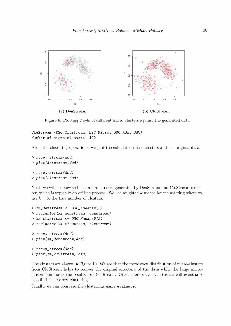
Figure 9: Plotting 2 sets of different micro-clusters against the generated data
CluStream (DSC_CluStream, DSC_Micro, DSC_MOA, DSC)
Number of micro-clusters: 100
After the clustering operations, we plot the calculated micro-clusters and the original data.
> reset_stream(dsd)
> plot(denstream,dsd)
> reset_stream(dsd)
> plot(clustream,dsd)
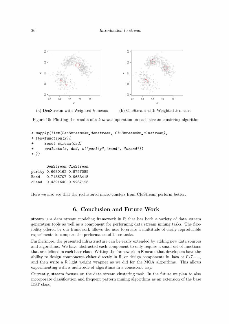
Next, we will see how well the micro-clusters generated by DenStream and CluStream reclus-ter, which is typically an off-line process. We use weighted k-means for reclustering where weuse k = 3, the true number of clusters.
> km_denstream <- DSC_KmeansW(3)
> recluster(km_denstream, denstream)
> km_clustream <- DSC_KmeansW(3)
> recluster(km_clustream, clustream)
> reset_stream(dsd)
> plot(km_denstream,dsd)
> reset_stream(dsd)
> plot(km_clustream, dsd)
The clusters are shown in Figure 10. We see that the move even distribution of micro-clustersfrom CluStream helps to recover the original structure of the data while the large micro-cluster dominates the results for DenStream. Given more data, DenStream will eventuallyalso find the correct clustering.
Finally, we can compare the clusterings using evaluate.
26 Introduction to stream
●
●
●
●
●
● ●
●
●
●●
● ●
●●
●
●
●
●
●
●●
●
●
●
●
●
●
●
●
●
●
●
●
●●●●
●
●
●
●
●
●
●
●●
●
●
●
●
●
●
●
●
●●
●
●
●
●●
●●
●
●
●
●
●● ●
●
●
●
●
●
●●
●●
●
●
●
●
●
●●
●
●
●
●
●
●
●
●
●
●
●
●
●
●
●
●
●
●●
●
● ●●●
●●
●
●●
●
●
●
●●
●
●●
●
●
●
●
●
●
●
●●
●
●
●
●
●
●
●
●●
●● ●
●
●
●
●
●
●
●●
●● ●
●
●●
●
●
●
●
●
●
●●●
●
● ●●
●
●●
●
●
●
0.0 0.2 0.4 0.6 0.8
0.0
0.2
0.4
0.6
0.8
X1
X2
(a) DenStream with Weighted k-means
●
●
●
●
●
● ●
●
●
●●
● ●
●●
●
●
●
●
●
●●
●
●
●
●
●
●
●
●
●
●
●
●
●●●●
●
●
●
●
●
●
●
●●
●
●
●
●
●
●
●
●
●●
●
●
●
●●
●●
●
●
●
●
●● ●
●
●
●
●
●
●●
●●
●
●
●
●
●
●●
●
●
●
●
●
●
●
●
●
●
●
●
●
●
●
●
●
●●
●
● ●●●
●●
●
●●
●
●
●
●●
●
●●
●
●
●
●
●
●
●
●●
●
●
●
●
●
●
●
●●
●● ●
●
●
●
●
●
●
●●
●● ●
●
●●
●
●
●
●
●
●
●●●
●
● ●●
●
●●
●
0.0 0.2 0.4 0.6 0.8
0.0
0.2
0.4
0.6
0.8
X1
X2
(b) CluStream with Weighted k-means
Figure 10: Plotting the results of a k-means operation on each stream clustering algorithm
> sapply(list(DenStream=km_denstream, CluStream=km_clustream),
+ FUN=function(x){
+ reset_stream(dsd)
+ evaluate(x, dsd, c("purity","rand", "crand"))
+ })
DenStream CluStream
purity 0.6680162 0.9757085
Rand 0.7186707 0.9683415
cRand 0.4391640 0.9287125
Here we also see that the reclustered micro-clusters from CluStream perform better.
6. Conclusion and Future Work
stream is a data stream modeling framework in R that has both a variety of data streamgeneration tools as well as a component for performing data stream mining tasks. The flex-ibility offered by our framework allows the user to create a multitude of easily reproducibleexperiments to compare the performance of these tasks.
Furthermore, the presented infrastructure can be easily extended by adding new data sourcesand algorithms. We have abstracted each component to only require a small set of functionsthat are defined in each base class. Writing the framework in Rmeans that developers have theability to design components either directly in R, or design components in Java or C/C++,and then write a R light weight wrapper as we did for the MOA algorithms. This allowsexperimenting with a multitude of algorithms in a consistent way.
Currently, stream focuses on the data stream clustering task. In the future we plan to alsoincorporate classification and frequent pattern mining algorithms as an extension of the baseDST class.
John Forrest, Matthew Bolanos, Michael Hahsler 27
References
Aggarwal C (ed.) (2007). Data Streams – Models and Algorithms. Springer.
Aggarwal CC, Han J, Wang J, Yu PS (2003a). “A Framework for Clustering Evolving DataStreams.” In Proceedings of the International Conference on Very Large Data Bases (VLDB’03), pp. 81–92.
Aggarwal CC, Han J, Wang J, Yu PS (2003b). “A framework for clustering evolving datastreams.” In Proceedings of the 29th international conference on Very large data bases -Volume 29, VLDB ’2003, pp. 81–92. VLDB Endowment. ISBN 0-12-722442-4.
Aggarwal CC, Han J, Wang J, Yu PS (2004a). “A Framework for Projected Clustering ofHigh Dimensional Data Streams.” In Proceedings of the International Conference on VeryLarge Data Bases (VLDB ’04), pp. 852–863. ISBN 0-12-088469-0.
Aggarwal CC, Han J, Wang J, Yu PS (2004b). “On demand classification of data streams.” InProceedings of the tenth ACM SIGKDD international conference on Knowledge discoveryand data mining, KDD ’04, pp. 503–508. ACM, New York, NY, USA.
Agrawal R, Imielinski T, Swami A (1993). “Mining Association Rules between Sets of Itemsin Large Databases.” In Proceedings of the ACM SIGMOD International Conference onManagement of Data, pp. 207–216. Washington D.C.
Babcock B, Babu S, Datar M, Motwani R, Widom J (2002). “Models and issues in data streamsystems.” In Proceedings of the twenty-first ACM SIGMOD-SIGACT-SIGART symposiumon Principles of database systems, PODS ’02, pp. 1–16. ACM, New York, NY, USA.
Bifet A, Holmes G, Kirkby R, Pfahringer B (2010). “MOA: Massive Online Analysis.” Journalof Machine Learning Research, 99, 1601–1604. ISSN 1532-4435.
Cao F, Ester M, Qian W, Zhou A (2006a). “Density-Based Clustering over an Evolving DataStream with Noise.” In Proceedings of the 2006 SIAM International Conference on DataMining, pp. 328–339. SIAM.
Cao F, Ester M, Qian W, Zhou A (2006b). “Density-based clustering over an evolving datastream with noise.” In In 2006 SIAM Conference on Data Mining, pp. 328–339.
Chambers JM, Hastie TJ (1992). Statistical Models in S. Chapman & Hall. ISBN9780412830402.
Domingos P, Hulten G (2000). “Mining high-speed data streams.” In Proceedings of the sixthACM SIGKDD international conference on Knowledge discovery and data mining, KDD’00, pp. 71–80. ACM, New York, NY, USA.
Ester M, Kriegel HP, Sander J, Xu X (1996). “A density-based algorithm for discoveringclusters in large spatial databases with noise.” In Proceedings of the ACM SIGKDD Inter-national Conference on Knowledge Discovery and Data Mining (KDD’1996), pp. 226–231.
Fowler M (2003). UML Distilled: A Brief Guide to the Standard Object Modeling Lan-guage. 3 edition. Addison-Wesley Longman Publishing Co., Inc., Boston, MA, USA. ISBN0321193687.
28 Introduction to stream
Gaber M, Zaslavsky A, Krishnaswamy S (2007). “A Survey of Classification Methods in DataStreams.” In C Aggarwal (ed.), Data Streams – Models and Algorithms. Springer.
Gaber MM, Zaslavsky A, Krishnaswamy S (2005). “Mining data streams: a review.” SIGMODRec., 34, 18–26.
Gama J (2010). Knowledge Discovery from Data Streams. 1st edition. Chapman & Hall/CRC,Boca Raton, FL. ISBN 1439826110, 9781439826119.
Guha S, Meyerson A, Mishra N, Motwani R, O’Callaghan L (2003). “Clustering data Streams:Theory and Practice.” IEEE Transactions on Knowledge and Data Engineering, 15(3),515–528.
Hahsler M, Dunham MH (2010a). rEMM: Extensible Markov Model for Data Stream Clus-tering in R. R package version 1.0-0., URL http://CRAN.R-project.org/.
Hahsler M, Dunham MH (2010b). “rEMM: Extensible Markov Model for Data Stream Clus-tering in R.” Journal of Statistical Software, 35(5), 1–31. URL http://www.jstatsoft.
org/v35/i05/.
Hastie T, Tibshirani R, Friedman J (2001). The Elements of Statistical Learning (DataMining, Inference and Prediction). Springer Verlag.
Jain AK, Dubes RC (1988). Algorithms for clustering data. Prentice-Hall, Inc., Upper SaddleRiver, NJ, USA. ISBN 0-13-022278-X.
Jain AK, Murty MN, Flynn PJ (1999). “Data clustering: a review.” ACM CompututerSurveys, 31(3), 264–323.
Jin R, Agrawal G (2007). “Frequent Pattern Mining in Data Streams.” In C Aggarwal (ed.),Data Streams – Models and Algorithms. Springer.
Kaufman L, Rousseeuw PJ (1990). Finding groups in data: an introduction to cluster analysis.John Wiley and Sons, New York.
Keller-McNulty S (ed.) (2004). Statistical analysis of massive data streams: Proceedings ofa workshop. Committee on Applied and Theoretical Statistics, National Research Council,National Academies Press, Washington, DC.
Kranen P, Assent I, Baldauf C, Seidl T (2009). “Self-Adaptive Anytime Stream Clustering.” InProceedings of the 2009 Ninth IEEE International Conference on Data Mining, ICDM ’09,pp. 249–258. IEEE Computer Society, Washington, DC, USA. ISBN 978-0-7695-3895-2.
Kranen P, Assent I, Baldauf C, Seidl T (2011). “The ClusTree: indexing micro-clusters foranytime stream mining.” Knowledge and Information Systems, 29(2), 249–272.
Last M (2002). “Online classification of nonstationary data streams.” Intelligent Data Anal-ysis, 6, 129–147. ISSN 1088-467X.
Meyer D, Buchta C (2010). proxy: Distance and Similarity Measures. R package version0.4-6, URL http://CRAN.R-project.org/package=proxy.
John Forrest, Matthew Bolanos, Michael Hahsler 29
Qiu W, Joe H (2009). clusterGeneration: random cluster generation (with specified degree ofseparation). R package version 1.2.7.
R Foundation (2011). R Data Import/Export. Version 2.13.1 (2011-07-08), URL http://
cran.r-project.org/doc/manuals/R-data.html.
Tasoulis D, Adams N, Hand D (2006). “Unsupervised Clustering in Streaming Data.” In IEEEInternational Workshop on Mining Evolving and Streaming Data. Sixth IEEE InternationalConference on Data Mining (ICDM 2006), pp. 638–642.
Tasoulis DK, Ross G, Adams NM (2007). “Visualising the Cluster Structure of Data Streams.”In Advances in Intelligent Data Analysis VII, Lecture Notes in Computer Science, pp. 81–92. Springer.
Tu L, Chen Y (2009). “Stream data clustering based on grid density and attraction.” ACMTransactions on Knowledge Discovery from Data, 3(3), 12:1–12:27. ISSN 1556-4681.
Udommanetanakit K, Rakthanmanon T, Waiyamai K (2007). “E-Stream: Evolution-BasedTechnique for Stream Clustering.” In ADMA ’07: Proceedings of the 3rd international con-ference on Advanced Data Mining and Applications, pp. 605–615. Springer-Verlag, Berlin,Heidelberg. ISBN 978-3-540-73870-1.
Urbanek S (2010). rJava: Low-level R to Java interface. R package version 0.8-8, URLhttp://CRAN.R-project.org/package=rJava.
Venables WN, Ripley BD (2002). Modern Applied Statistics with S. Fourth edition. Springer,New York. ISBN 0-387-95457-0, URL http://www.stats.ox.ac.uk/pub/MASS4.
Vitter JS (1985). “Random sampling with a reservoir.” ACM Transactions on MathematicalSoftware, 11(1), 37–57. ISSN 0098-3500. doi:10.1145/3147.3165. URL http://doi.
acm.org/10.1145/3147.3165.
Wan L, Ng WK, Dang XH, Yu PS, Zhang K (2009). “Density-based clustering of data streamsat multiple resolutions.” ACM Transactions on Knowledge Discovery from Data, 3, 14:1–14:28. ISSN 1556-4681.
Witten IH, Frank E (2005). Data Mining: Practical Machine Learning Tools and Techniques.The Morgan Kaufmann Series in Data Management Systems, 2nd edition. Morgan Kauf-mann Publishers. ISBN 0-12-088407-0.
Zhang T, Ramakrishnan R, Livny M (1996). “BIRCH: An Efficient Data Clustering Methodfor Very Large Databases.” In Proceedings of the 1996 ACM SIGMOD International Con-ference on Management of Data, pp. 103–114. ACM.
30 Introduction to stream
Affiliation:
Michael HahslerEngineering Management, Information, and SystemsLyle School of EngineeringSouthern Methodist UniversityP.O. Box 750122Dallas, TX 75275-0122E-mail: [email protected]: http://lyle.smu.edu/~mhahsler
John ForrestMicrosoft CorporationE-mail: [email protected]
Matthew BolanosComputer Science and EngineeringLyle School of EngineeringSouthern Methodist UniversityE-mail: [email protected]
Copyright © 2022 FDOKUMEN