A FINITE ELEMENT METHOD FOR STEADY-STATE NATURAL CONVECTION IN A SQUARE TILT OPEN CAVITY

VOL. 2, NO. 2, APRIL 2007 ISSN 1819-6608

ARPN Journal of Engineering and Applied Sciences

©2006-2007 Asian Research Publishing Network (ARPN). All rights reserved.

www.arpnjournals.com

A FINITE ELEMENT METHOD FOR STEADY-STATE NATURAL

CONVECTION IN A SQUARE TILT OPEN CAVITY

Goutam Saha1, Sumon Saha2 and Md. Arif Hasan Mamun 2

1Department of Mathematics, University of Dhaka, Dhaka-1000, Bangladesh2Department of Mechanical Engineering, Bangladesh University of Engineering and Technology, Dhaka, Bangladesh

Email: [email protected] ABSTRACT

A numerical simulation of two-dimensional laminar steady-state natural convection in a square tilt open cavity has been numerically studied. The opposite wall to the aperture is placed at either isothermal heat source or isoflux heat source, while the surrounding fluid interacting with the aperture is maintained at an ambient temperature. The two remaining walls are assumed to be adiabatic. The fluid concerned is air with Prandtl number fixed at 0.71. The governing mass, momentum and energy equations are expressed in a normalized primitive variables formulation. In this paper, a finite element method for steady-state incompressible natural convection flows has been developed. The streamlines and isotherms are produced, heat transfer characteristics is obtained for Rayleigh numbers from 103 to 106 and for an inclination angles of the cavity ranges from 0º to 60º. The results show that the Nusselt numbers increases with the Rayleigh numbers. Also the average Nusselt number changes substantially with the inclination angle of the cavity while better thermal performance is also sensitive to the boundary condition of the heated wall. Keywords: Natural convection, finite element method, Rayleigh number, square cavity, surface temperature, heat flux. INTRODUCTION

Natural convection in open cavities has received considerable attention because of its importance in several thermal engineering problems, for example, in the design of electronic devices, solar thermal receivers, uncovered flat plate solar collectors having rows of vertical strips, geothermal reservoirs, etc. During the past two decades, several experiments and numerical calculations have been presented for describing the phenomenon of natural convection in open cavities. Those studies have been focused in the present work to study the effect on flow and heat transfer for different Rayleigh numbers, aspect ratios, and tilt angles.

Le Quere et al. (1981) investigated thermally driven laminar natural convection in enclosures with isothermal sides, one of which facing the opening. They used primitive variables and finite difference expressions suitable for treating problems with large temperature and density variations. The computational domain was an enlarged domain comprising a square open cavity and a far field surrounding it. Penot (1982) studied a similar problem using stream function-vorticity formulation. He also used an enlarged computational domain similar to that of Le Quere et al. (1981) with approximately same boundary conditions. Chan and Tien (1985a) studied numerically a square open cavity, which had an isothermal vertical heated side facing the opening and two adjoining adiabatic horizontal sides. The boundary conditions at far field were approximated to obtain satisfactory solutions in the open cavity. Despite the difficulties due to unknown boundary conditions at the opening plane, few studies have also been undertaken using a computational domain restricted to the cavity. Chan and Tien (1985b) studied numerically shallow open cavities and also made a comparison study using a square cavity in an enlarged computational domain. They found that for a square open

cavity having an isothermal vertical side facing the opening and two adjoining adiabatic horizontal sides, the results obtained at high Rayleigh numbers would satisfy the previous works. In a similar way, Mohamad (1995) studied inclined open square cavities, by considering a restricted computational domain. Different from those by Chan and Tien (1985b), gradients of both velocity components were set to zero at the opening plane. It was found that heat transfer was not sensitive to inclination angle and the flow was unstable at high Rayleigh numbers and small inclinations angles. Polat and Bilgen (2002) studied numerically inclined open shallow cavities in which the side facing the opening was heated by constant heat flux, two adjoining walls were insulated and the opening was in contact with a reservoir at constant temperature and pressure. The computational domain was restricted to the cavity. Angirasa (1992) showed that the inclusion of the outside domain into the computations has a minimal effect on the heat transfer results for those cavities where one wall is isothermal and other two walls are adiabatic.

The finite element method is one of the numerical methods that have received popularity due to its capability for solving complex structural problems (Cook, 1989, Zienkiewicz, 1991). The method has been extended to solve problems in several other fields such as in the field of heat transfer (Lewis et al., 1996, Dechaumphai, 1999), electromagnetics (Jini, 1993), biomechanics (Gallagher et al., 1982), etc. In spite of the great success of the method in these fields, its application to fluid mechanics is still under intensive research. This is due to the fact that the governing differential equations for general flow problems consist of several coupled equations which are inherently nonlinear. Accurate numerical solutions thus require a vast amount of computer time and data storage. One way to

41

VOL. 2, NO. 2, APRIL 2007 ISSN 1819-6608




minimize the amount of computer time and data storage is to employ an adaptive meshing technique (Dechaumphai, 1995, Peraire et al., 1987). The technique places small elements in the regions of large change in the solution gradients to increase solution accuracy, and at the same time, uses large elements in the other regions to reduce the computational time and computer memory.

As the first step toward accurate flow solutions using the adaptive meshing technique, this paper develops a finite element formulation suitable for analysis of steady-state natural convection flow problems. The paper starts from the Navier-Stokes equations together with the energy equation to derive the corresponding finite element equations. The computational procedure used in the development of the computer program is described. The finite element equations derived and then the computer

program developed are then evaluated by example of natural convection in a square open cavity. PHYSICAL MODEL AND ASSUMPTIONS

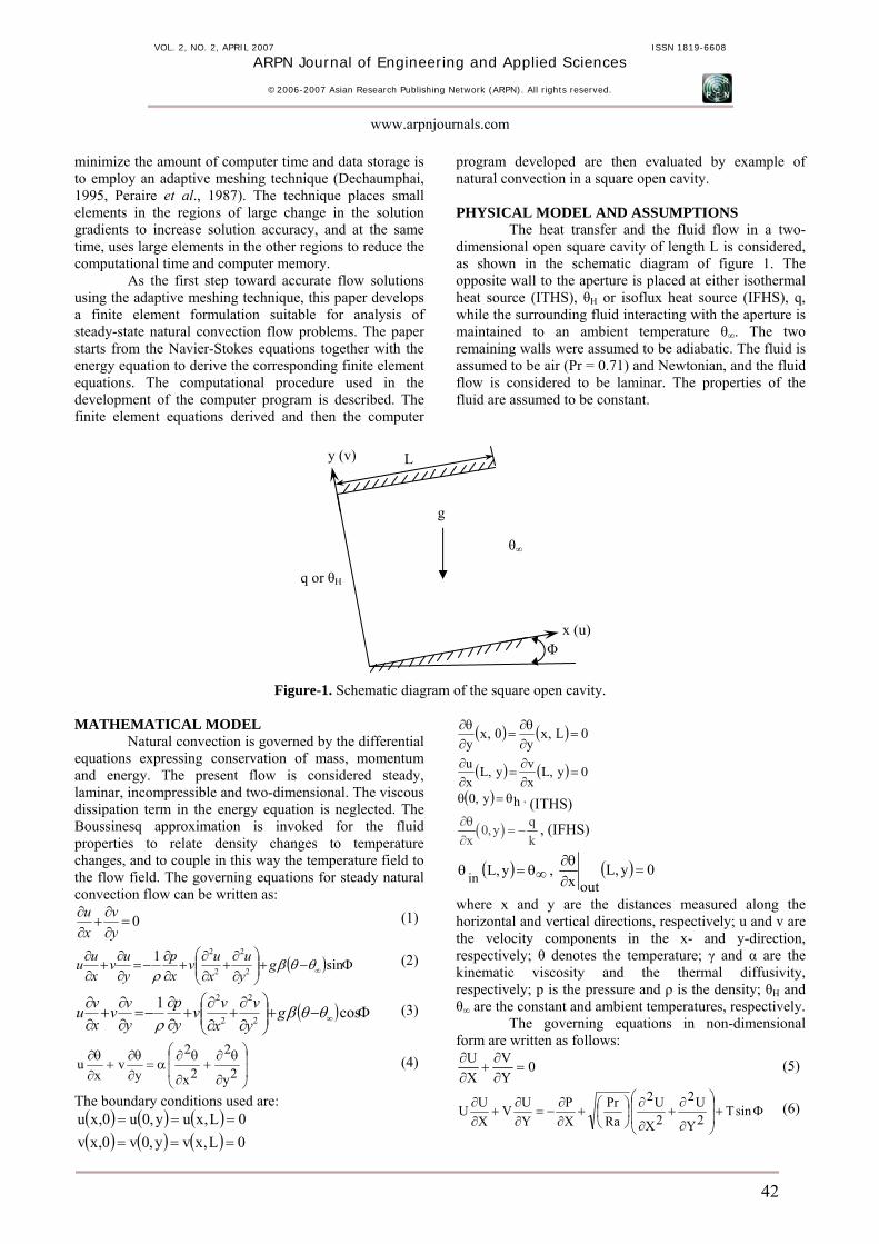
The heat transfer and the fluid flow in a two-dimensional open square cavity of length L is considered, as shown in the schematic diagram of figure 1. The opposite wall to the aperture is placed at either isothermal heat source (ITHS), θH or isoflux heat source (IFHS), q, while the surrounding fluid interacting with the aperture is maintained to an ambient temperature θ∞. The two remaining walls were assumed to be adiabatic. The fluid is assumed to be air (Pr = 0.71) and Newtonian, and the fluid flow is considered to be laminar. The properties of the fluid are assumed to be constant.

y (v) L

g

Figure-1. Schematic diagram of the square open cavity. MATHEMATICAL MODEL

Natural convection is governed by the differential equations expressing conservation of mass, momentum and energy. The present flow is considered steady, laminar, incompressible and two-dimensional. The viscous dissipation term in the energy equation is neglected. The Boussinesq approximation is invoked for the fluid properties to relate density changes to temperature changes, and to couple in this way the temperature field to the flow field. The governing equations for steady natural convection flow can be written as:

0=∂∂

+∂∂

yv

xu (1)

( ) Φ−+⎟⎟⎠

⎞⎜⎜⎝

⎛∂∂

+∂∂

+∂∂

−=∂∂

+∂∂

∞ sin12

2

2

2

θθβρ

gyu

xuv

xp

yuv

xuu (2)

( ) Φ−+⎟⎟⎠

⎞⎜⎜⎝

⎛

∂∂

+∂∂

+∂∂

−=∂∂

+∂∂

∞ cos12

2

2

2

θθβρ

gyv

xvv

yp

yvv

xvu (3)

⎟⎟

⎠

⎞

⎜⎜

⎝

⎛

∂

θ∂+

∂

θ∂α=

∂θ∂

+∂θ∂

2y

2

2x

2

yv

xu (4)

The boundary conditions used are: ( ) ( ) ( )( ) ( ) ( ) 0L,xvy,0v0,xv

0L,xuy,0u0,xu======

( ) ( ) 0L,xy

0,xy

=∂θ∂

=∂θ∂

( ) ( ) 0y,L

xvy,L

xu

=∂∂

=∂∂

( ) hy,0 θ=θ , (ITHS)

( ) q0, yx k∂θ

= −∂

, (IFHS)

( ) ∞θ=θ y,Lin , ( ) 0y,Loutx

=∂θ∂

where x and y are the distances measured along the horizontal and vertical directions, respectively; u and v are the velocity components in the x- and y-direction, respectively; θ denotes the temperature; γ and α are the kinematic viscosity and the thermal diffusivity, respectively; p is the pressure and ρ is the density; θH and θ∞ are the constant and ambient temperatures, respectively.

The governing equations in non-dimensional form are written as follows:

0YV

XU

=∂∂

+∂∂ (5)

Φ+⎟⎟

⎠

⎞

⎜⎜

⎝

⎛

∂

∂+

∂

∂⎟⎠⎞

⎜⎝⎛+

∂∂

−=∂∂

+∂∂ sinT

2Y

U2

2X

U2

RaPr

XP

YUV

XUU (6)

q or θH

x (u) Φ

θ∞

42

VOL. 2, NO. 2, APRIL 2007 ISSN 1819-6608




Φ+⎟⎟

⎠

⎞

⎜⎜

⎝

⎛

∂

∂+

∂

∂⎟⎠⎞

⎜⎝⎛+

∂∂

−=∂∂

+∂∂ cosT

2Y

V2

2X

V2

RaPr

YP

YVV

XVU (7)

⎟⎟

⎠

⎞

⎜⎜

⎝

⎛

∂

∂+

∂

∂⎟⎠⎞

⎜⎝⎛=

∂∂

+∂∂

2Y

T2

2X

T2

Ra.Pr1

YTV

XTU (8)

with the boundary conditions ( ) ( ) ( ) 0Y,0U1,XU0,XU === , ( ) ( ) ( ) 0Y,0V1,XV0,XV === ,

( ) ( ) 01,XYT0,X

YT

=∂∂

=∂∂

( ) ( ) 0Y,1XVY,1

XU

=∂∂

=∂∂

( ) 1Y,0T = (ITHS)

( ) 1Y,0XT

−=∂∂ (IFHS)

( ) 0Y,1T = if U < 0 and ( ) 0Y,1XT

=∂∂

if U > 0.

Equations (5)-(8) were normalized using the following dimensionless scales:

,LxX = ,

LyY = ,

oUuU = ,

oUvV =

,2oU

ppPρ

∞−=

tT

∆∞θ−θ= ,

αν

=Pr , αν∆β

=3LtgRa ,

( ∞θ−θ=∆ ht ) (ITHS)

kLqt =∆ (IFHS)

Here Ra and Pr are Rayleigh and Prandtl numbers, respectively. The reference velocity Uo is related to the buoyancy force term and is defined as

( )∞θ−θβ= hLgoU .

The Nusselt number (Nu) is one of the important dimensionless parameters to be computed for heat transfer analysis in natural convection flow. The local Nusselt number can be obtained from the temperature field by applying

⎟⎠⎞

⎜⎝⎛∂∂

−=XT

xNu (ITHS)

( )Y,0T1

xNu −= (IFHS)

and the average or overall Nusselt number was calculated by integrating the temperature gradient over the heated wall as

∫ ⎟⎠⎞

⎜⎝⎛∂∂

−=1

0

dYXTNu (ITHS)

( )∫−=1

0 ,01 dY

YTNu (IFHS)

FINITE ELEMENT FORMULATION The velocity and thermal energy equations (5)-(8)

result in a set of non-linear coupled equations for which an iterative scheme is adopted. To ensure convergence of the numerical algorithm the following criteria is applied to all dependent variables over the solution domain

∑ −≤−φ−φ 5101mij

mij

where φ represents a dependent variable U, V, P, and T; the indexes i, j indicate a grid point; and the index m is the current iteration at the grid level. The six node triangular element is used in this work for the development of the finite element equations. All six nodes are associated with velocities as well as temperature; only the corner nodes are associated with pressure. This means that a lower order polynomial is chosen for pressure and which is satisfied through continuity equation. The velocity component and the temperature distributions and linear interpolation for the pressure distribution according to their highest derivative orders in the differential Eqs (5)-(8) as

( ) αα= UNY,XU (9) ( ) αα= VNY,XV (10) ( ) αα= TNY,XT (11) ( ) λλ= PHY,XP (12)

where α = 1, 2, … …, 6; λ= 1, 2, 3; Nα are the element interpolation functions for the velocity components and the temperature, and Hλ are the element interpolation functions for the pressure.

To derive the finite element equations, the method of weighted residuals (Zienkiewicz, 1991) is applied to the continuity Eq. (5), the momentum Eqs (6)-(7), and the energy Eq. (8), we get

0dAA YV

XUN =⎟

⎠⎞

⎜⎝⎛

∂∂

+∂∂

α∫ (13)

dATsinA NdA2Y

U2

2X

U2

A NRaPr

dAXP

A HdAYUV

XUUA N

Φα+⎟⎟

⎠

⎞

⎜⎜

⎝

⎛

∂

∂+

∂

∂α⎟

⎠⎞

⎜⎝⎛

+⎟⎠⎞

⎜⎝⎛∂∂

λ−=⎟⎠⎞

⎜⎝⎛

∂∂

+∂∂

α

∫∫

∫∫ (14)

dATcosA NdA2Y

V2

2X

V2

A NRaPr

dAYP

AHdAYVV

XVUA N

Φα+⎟⎟

⎠

⎞

⎜⎜

⎝

⎛

∂

∂+

∂

∂α⎟

⎠⎞

⎜⎝⎛

+⎟⎠⎞

⎜⎝⎛∂∂

λ−=⎟⎠⎞

⎜⎝⎛

∂∂

+∂∂

α

∫∫

∫∫

(15)

dAA 2Y

T2

2X

T2N

Ra.Pr1dAA Y

TVXTUN ∫∫ ⎟

⎟

⎠

⎞

⎜⎜

⎝

⎛

∂

∂+

∂

∂α⎟

⎠⎞

⎜⎝⎛=⎟

⎠⎞

⎜⎝⎛

∂∂

+∂∂

α

(16) where A is the element area. Gauss’s theorem is then applied to Eqs (14)-(16) to generate the boundary integral terms associated with the surface tractions and heat flux. Then Eqs (14)-(16) become,

43

VOL. 2, NO. 2, APRIL 2007 ISSN 1819-6608




∫

∫∫

∫∫

α=

αΦ−⎟⎠

⎞⎜⎝

⎛∂∂

∂α∂

+∂∂

∂α∂

⎟⎠⎞

⎜⎝⎛+⎟

⎠⎞

⎜⎝⎛∂∂

λ+⎟⎠⎞

⎜⎝⎛

∂∂

+∂∂

α

0S 0dSxSN

A dATNsindAA YU

YN

XU

XN

RaPrdA

XP

A HdAYUV

XUUA N

(17)

∫∫

∫

∫∫

α=αΦ−

⎟⎠

⎞⎜⎝

⎛∂∂

∂α∂

+∂∂

∂α∂

⎟⎠⎞

⎜⎝⎛

+⎟⎠⎞

⎜⎝⎛∂∂

λ+⎟⎠⎞

⎜⎝⎛

∂∂

+∂∂

α

0S 0dSySNA dATNcos

dAA YV

YN

XV

XN

RaPr

dAYP

A HdAYVV

XVUA N

(18)

∫∫

∫

α=⎟⎠

⎞⎜⎝

⎛∂∂

∂α∂

+∂∂

∂α∂

⎟⎠⎞

⎜⎝⎛+⎟

⎠⎞

⎜⎝⎛

∂∂

+∂∂

α

wS wdSwqNdAA YT

YN

XT

XN

Ra.Pr1dA

YTV

XTUA N

(19)

Here (14)-(15) specifying surface tractions (Sx, Sy) along outflow boundary S0 and (16) specifying velocity components and fluid temperature or heat flux that flows into or out from domain along wall boundary Sw. Substituting the element velocity component distributions, the temperature distribution, and the pressure distribution from Eqs (9)-(12), the finite element equations can be written in the form,

0VKUK yx =βαβ+βαβ (20)

( ) uyyxx

xyx

QTKUSSRa

PMUVKUUK

αβαββαβαβ

µαµγαβγγβαβγβ

=Φ−+⎟⎠⎞

⎜⎝⎛

+++

sinPr (21)

( ) vyyxx

yyx

QTKVSSRa

PMVVKVUK

αβαββαβαβ

µαµγαβγγβαβγβ

=Φ−+⎟⎠⎞

⎜⎝⎛

+++

cosPr (22)

Tyyxx

yx

QTSSRa.Pr

1

TVKTUK

α=β⎟

⎠⎞

⎜⎝⎛

αβ+

αβ⎟⎠⎞

⎜⎝⎛

+γβαβγ+γβαβγ

(23)

where the coefficients in element matrices are in the form of the integrals over the element area and along the element edges S0 and Sw as,

dAx,NA NK x βα=αβ ∫ , (24a)

dAy,NA NK y βα=αβ ∫ , (24b)

dAx,NNA NK x γβα=αβγ ∫ , (24c)

dAy,NNA NK y γβα=αβγ ∫ , (24d)

dANA NK βα=αβ ∫ , (24e)

dAx,NA x,NS xx βα=αβ ∫ , (24f)

dAy,NA y,NS yy βα=αβ ∫ , (24g)

dAx,HA HM x µα=αµ ∫ , (24h)

dAy,HA HM y µα=αµ ∫ , (24i)

∫ α=α 0

u S 0dSxSNQ , (24j)

∫ α=α 0

v S 0dSySNQ , (24k)

∫ α=α w

T S wdSwqNQ . (24l)

These element matrices are evaluated in closed-form ready for numerical simulation. Details of the derivation for these element matrices are omitted herein for brevity. COMPUTATIONAL PROCEDURE

The derived finite element equations, Eqs (20)-(23), are nonlinear. These nonlinear algebraic equations are solved by applying the Newton-Raphson iteration technique (Dechaumphai, 1999) by first writing the unbalanced values from the set of the finite element Eqs (20)-(23) as,

βαβ+βαβ

=α

VKUKF yxp (25a)

u x y x

xx yy u

F K U U K V U M P

Pr (S S ) U sin K T QRa

β γ γ µα αβγ αβγ αµ

β αβ βαβ αβ α

β= + +

⎛ ⎞ + − Φ −⎜ ⎟⎝ ⎠

+

(25b)

vyyxx

yyxv

QTKVSSRa

PMVVKVUKF

αβαββαβαβ

µαµγαβγγβαβγαβ

−Φ−+⎟⎠⎞

⎜⎝⎛+

++=

cos)(Pr (25c)

Tyyxx

yxT

QTSSRa.Pr

1

TVKTUKF

α−β⎟

⎠⎞

⎜⎝⎛

αβ+

αβ⎟⎠⎞

⎜⎝⎛

+γβαβγ+γβαβγ

=α

(25d)

This leads to a set of algebraic equations with the incremental unknowns of the element nodal velocity components, temperatures, and pressures in the form,

⎪⎪

⎭

⎪⎪

⎬

⎫

⎪⎪

⎩

⎪⎪

⎨

⎧

β

α

α

α

−=

⎪⎪⎭

⎪⎪⎬

⎫

⎪⎪⎩

⎪⎪⎨

⎧

∆∆∆∆

⎥⎥⎥⎥⎥

⎦

⎤

⎢⎢⎢⎢⎢

⎣

⎡

p

T

v

u

pvpu

TTTvTu

vpvTvvvu

upuTuvuu

FFFF

pTvu

00KK0KKK

KKKKKKKK

(26)

where

⎟⎠⎞

⎜⎝⎛

αβ+

αβ⎟⎠⎞

⎜⎝⎛

+βαβγ+γαγβ

+γαβγ=

yyxx

yxx

SSRaPr

VKUKUKuuK

γαβγ

= UKuvK y ,

αβΦ−= KsinuTK ,

xMupKαµ

= ,

44

VOL. 2, NO. 2, APRIL 2007 ISSN 1819-6608




γ

αβγ= VKvuK x ,

⎟⎠⎞

⎜⎝⎛

αβ+

αβ⎟⎠⎞

⎜⎝⎛

+γαβγ+γαγβ

+βαβγ=

yyxx

yyx

SSRaPr

VKVKUKvvK

αβΦ−= KcosvTK ,

yMvpKαµ

= ,

γαβγ

= TKTuK x ,

γαβγ

= TKTvK y

⎟⎠⎞

⎜⎝⎛

αβ+

αβ⎟⎠⎞

⎜⎝⎛

+βαβγ+βαβγ

=

yyxx

yx

SSRa.Pr

1

VKUKTTK

0TpK = ,

xKpuKαβ

= ,

yKpvKαβ

= and

ppK0pTK == .

The iteration process is terminated if the percentage of the overall change compared to the previous iteration is less than the specified value. RESULTS AND DISCUSSION

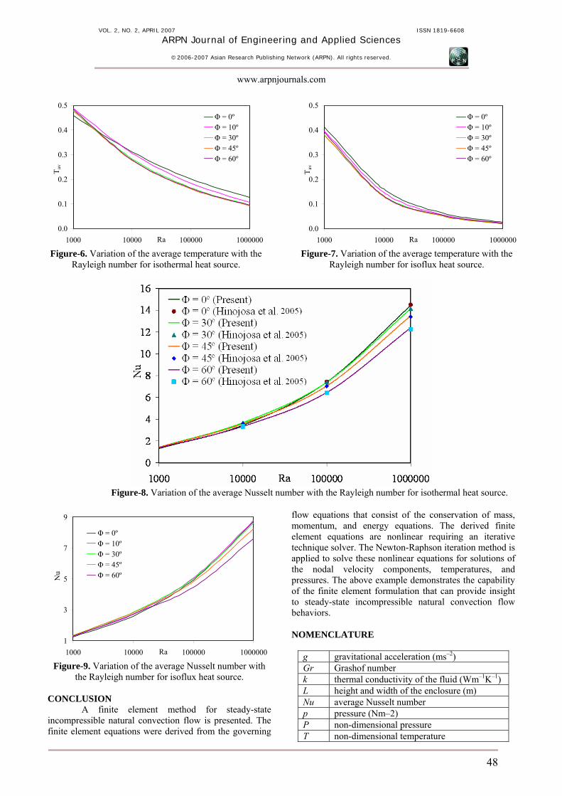
The proposed problem is an open cavity with the left vertical wall maintaining at isothermal heat source and then isoflux heat source, while the top and bottom walls are adiabatic. Obviously for high values of Rayleigh number the errors encountered are appreciable and hence it is necessary to perform some grid size testing in order to establish a suitable grid size. Grid independent solution is ensured by comparing the results of different grid meshes for Ra = 106, which was the highest Rayleigh number. The total domain is discretized into 4806 elements that results in 32643 nodes. In order to validate the numerical code, pure natural convection with Pr = 0.71 in a square open cavity was solved, and the results were compared with those reported by Hinojosa et al. (2005), obtained with an extended computational domain. In Table 1, a comparison between the average Nusselt numbers is presented.

Table-1. Comparison of the results for isothermal heat source with Pr = 0.71.

Nu Ra Present work

Hinojosa et al. [16]

Error (%)

103 1.32 1.30 1.54 104 3.45 3.44 0.29 105 7.41 7.44 0.40 106 14.44 14.51 0.48

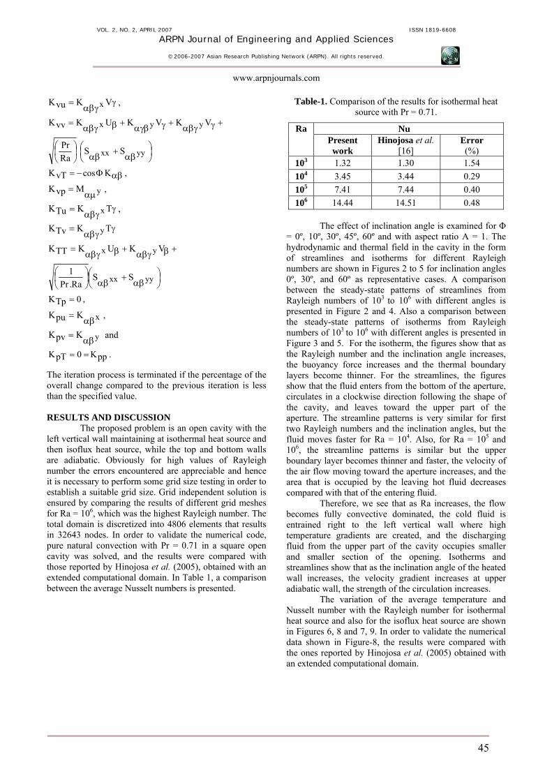
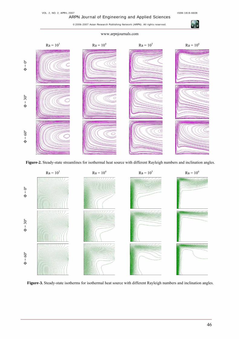
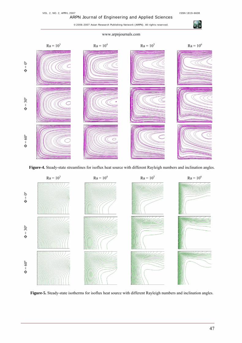
The effect of inclination angle is examined for Φ

= 0º, 10º, 30º, 45º, 60º and with aspect ratio A = 1. The hydrodynamic and thermal field in the cavity in the form of streamlines and isotherms for different Rayleigh numbers are shown in Figures 2 to 5 for inclination angles 0º, 30º, and 60º as representative cases. A comparison between the steady-state patterns of streamlines from Rayleigh numbers of 103 to 106 with different angles is presented in Figure 2 and 4. Also a comparison between the steady-state patterns of isotherms from Rayleigh numbers of 103 to 106 with different angles is presented in Figure 3 and 5. For the isotherm, the figures show that as the Rayleigh number and the inclination angle increases, the buoyancy force increases and the thermal boundary layers become thinner. For the streamlines, the figures show that the fluid enters from the bottom of the aperture, circulates in a clockwise direction following the shape of the cavity, and leaves toward the upper part of the aperture. The streamline patterns is very similar for first two Rayleigh numbers and the inclination angles, but the fluid moves faster for Ra = 104. Also, for Ra = 105 and 106, the streamline patterns is similar but the upper boundary layer becomes thinner and faster, the velocity of the air flow moving toward the aperture increases, and the area that is occupied by the leaving hot fluid decreases compared with that of the entering fluid.

Therefore, we see that as Ra increases, the flow becomes fully convective dominated, the cold fluid is entrained right to the left vertical wall where high temperature gradients are created, and the discharging fluid from the upper part of the cavity occupies smaller and smaller section of the opening. Isotherms and streamlines show that as the inclination angle of the heated wall increases, the velocity gradient increases at upper adiabatic wall, the strength of the circulation increases.

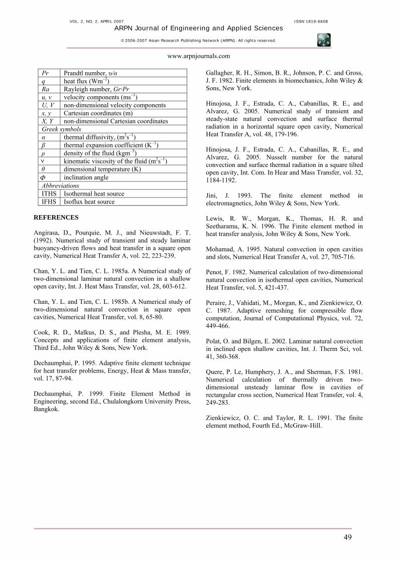
The variation of the average temperature and Nusselt number with the Rayleigh number for isothermal heat source and also for the isoflux heat source are shown in Figures 6, 8 and 7, 9. In order to validate the numerical data shown in Figure-8, the results were compared with the ones reported by Hinojosa et al. (2005) obtained with an extended computational domain.

45

VOL. 2, NO. 2, APRIL 2007 ISSN 1819-6608




Ra = 103 Ra = 104 Ra = 105 Ra = 106

Φ =

0º

Φ =

30º

Φ =

60º

Figure-2. Steady-state streamlines for isothermal heat source with different Rayleigh numbers and inclination angles.

Ra = 103 Ra = 104 Ra = 105 Ra = 106

Φ =

0º

Φ =

30º

Φ =

60º

Figure-3. Steady-state isotherms for isothermal heat source with different Rayleigh numbers and inclination angles.

46

VOL. 2, NO. 2, APRIL 2007 ISSN 1819-6608




Figure-4. Steady-state streamlines for isoflux heat source with different Rayleigh numbers and inclination angles.

Ra = 103 Ra = 104 Ra = 105 Ra = 106

0º

Φ =

Φ =

30º

Φ =

60º

Figure-5. Steady-state is herms for isoflux heat source with different Rayleigh numbers and inclination angles.

Ra = 103 Ra = 104 Ra = 105 Ra = 106

0º

ot

Φ =

Φ =

30º

Φ =

60º

47

VOL. 2, NO. 2, APRIL 2007 ISSN 1819-6608




0.0

0.1

0.2

0.3

0.4

0.5

1000 10000 100000 1000000Ra

T av

Φ = 0ºΦ = 10ºΦ = 30ºΦ = 45ºΦ = 60º

Figure-6. Variation of the average temperature with the

Rayleigh number for isothermal heat source.

0.0

0.1

0.2

0.3

0.4

0.5

1000 10000 100000 1000000Ra

T av

Φ = 0ºΦ = 10ºΦ = 30ºΦ = 45ºΦ = 60º

Figure-7. Variation of the average temperature with the

Rayleigh number for isoflux heat source.

Figure-8. Variation of the average Nusselt number with the Rayleigh number for isothermal heat source.

1

3

5

7

9

1000 10000 100000 1000000Ra

Nu

Φ = 0ºΦ = 10ºΦ = 30ºΦ = 45ºΦ = 60º

Figure-9. Variation of the average Nusselt number with

the Rayleigh number for isoflux heat source. CONCLUSION

A finite element method for steady-state incompressible natural convection flow is presented. The finite element equations were derived from the governing

flow equations that consist of the conservation of mass, momentum, and energy equations. The derived finite element equations are nonlinear requiring an iterative technique solver. The Newton-Raphson iteration method is applied to solve these nonlinear equations for solutions of the nodal velocity components, temperatures, and pressures. The above example demonstrates the capability of the finite element formulation that can provide insight to steady-state incompressible natural convection flow behaviors. NOMENCLATURE

g gravitational acceleration (ms–2) Gr Grashof number

k thermal conductivity of the fluid (Wm–1K–1) L height and width of the enclosure (m) Nu average Nusselt number p pressure (Nm–2) P non-dimensional pressure T non-dimensional temperature

48

VOL. 2, NO. 2, APRIL 2007 ISSN 1819-6608




Pr Prandtl number, υ/α

q heat flux (Wm–2) Ra Rayleigh number, Gr·Pr u, v velocity components (ms–1) U, V non-dimensional velocity components x, y Cartesian coordinates (m) X, Y non-dimensional Cartesian coordinates Greek symbols α thermal diffusivity, (m2s–1) β thermal expansion coefficient (K–1) ρ density of the fluid (kgm–3) ν kinematic viscosity of the fluid (m2s–1) θ dimensional temperature (K) Φ inclination angle Abbreviations ITHS Isothermal heat source IFHS Isoflux heat source

REFERENCES Angirasa, D., Pourquie, M. J., and Nieuwstadt, F. T. (1992). Numerical study of transient and steady laminar buoyancy-driven flows and heat transfer in a square open cavity, Numerical Heat Transfer A, vol. 22, 223-239. Chan, Y. L. and Tien, C. L. 1985a. A Numerical study of two-dimensional laminar natural convection in a shallow open cavity, Int. J. Heat Mass Transfer, vol. 28, 603-612. Chan, Y. L. and Tien, C. L. 1985b. A Numerical study of two-dimensional natural convection in square open cavities, Numerical Heat Transfer, vol. 8, 65-80. Cook, R. D., Malkus, D. S., and Plesha, M. E. 1989. Concepts and applications of finite element analysis, Third Ed., John Wiley & Sons, New York. Dechaumphai, P. 1995. Adaptive finite element technique for heat transfer problems, Energy, Heat & Mass transfer, vol. 17, 87-94. Dechaumphai, P. 1999. Finite Element Method in Engineering, second Ed., Chulalongkorn University Press, Bangkok.

Gallagher, R. H., Simon, B. R., Johnson, P. C. and Gross, J. F. 1982. Finite elements in biomechanics, John Wiley & Sons, New York. Hinojosa, J. F., Estrada, C. A., Cabanillas, R. E., and Alvarez, G. 2005. Numerical study of transient and steady-state natural convection and surface thermal radiation in a horizontal square open cavity, Numerical Heat Transfer A, vol. 48, 179-196. Hinojosa, J. F., Estrada, C. A., Cabanillas, R. E., and Alvarez, G. 2005. Nusselt number for the natural convection and surface thermal radiation in a square tilted open cavity, Int. Com. In Hear and Mass Transfer, vol. 32, 1184-1192. Jini, J. 1993. The finite element method in electromagnetics, John Wiley & Sons, New York. Lewis, R. W., Morgan, K., Thomas, H. R. and Seetharamu, K. N. 1996. The Finite element method in heat transfer analysis, John Wiley & Sons, New York. Mohamad, A. 1995. Natural convection in open cavities and slots, Numerical Heat Transfer A, vol. 27, 705-716. Penot, F. 1982. Numerical calculation of two-dimensional natural convection in isothermal open cavities, Numerical Heat Transfer, vol. 5, 421-437. Peraire, J., Vahidati, M., Morgan, K., and Zienkiewicz, O. C. 1987. Adaptive remeshing for compressible flow computation, Journal of Computational Physics, vol. 72, 449-466. Polat, O. and Bilgen, E. 2002. Laminar natural convection in inclined open shallow cavities, Int. J. Therm Sci, vol. 41, 360-368. Quere, P. Le, Humphery, J. A., and Sherman, F.S. 1981. Numerical calculation of thermally driven two-dimensional unsteady laminar flow in cavities of rectangular cross section, Numerical Heat Transfer, vol. 4, 249-283. Zienkiewicz, O. C. and Taylor, R. L. 1991. The finite element method, Fourth Ed., McGraw-Hill.

49

A FINITE ELEMENT METHOD FOR STEADY-STATE NATURAL CONVECTION IN A SQUARE TILT OPEN CAVITY

Documents

Transcript of A FINITE ELEMENT METHOD FOR STEADY-STATE NATURAL CONVECTION IN A SQUARE TILT OPEN CAVITY