SOME EVIDENCE OF SMOOTH TRANSITION NONLINEARITY IN COLOMBIAN INFLATION
Upload
independentCategory
view
3download
0
- Bogotá - Colombia - Bogotá - Colombia - Bogotá - Colombia - Bogotá - Colombia - Bogotá - Colombia - Bogotá - Colombia - Bogotá - Colombia - Bogotá - Colombia - Bogotá -

A DYNAMIC FACTOR MODEL FOR THE COLOMBIAN INFLATION ?
ELIANA GONZALEZ † LUIS F. MELO †
([email protected]) ([email protected])
VIVIANA MONROY †† BRAYAN ROJAS ††
([email protected]) ([email protected])
BANCO DE LA REPUBLICA
ABSTRACT. We use a dynamic factor model proposed by Stock and Watson [1998, 1999,2002a,b] to forecast Colombian inflation. The model includes 92 monthly series observedover the period 1999:01-2008:06. The results show that for short-run horizons, factor modelforecasts significantly outperformed the auto-regressive benchmark model in terms of theroot mean squared forecast error statistic.
Key words and phrases. Dynamic factor models, static factor models, forecast accuracy.
JEL clasification. C13, C33, C53.
Date: February 2009.? The opinions expressed here are those of the authors and do not necessarily represent neither those
of the Banco de la Repblica nor of its Board of Directors. The authors gratefully acknowledge the helpfrom Jorge Hurtado. The authors also appreciate the valuable comments and suggestions of Luis E. Arango,Andres Gonzalez and Munir Jalil. As usual, all errors and omissions in this work are our responsibility.† Members of the Macroeconomic Models Unit and Econometric Unit, respectively.†† Students of Economics at Universidad Nacional de Colombia acting as research assistants.

A DYNAMIC FACTOR MODEL FOR THE COLOMBIAN INFLATION 2
1. INTRODUCTION
Colombia has adopted an inflation targeting regime to guide monetary policy decisionssince 2001. Therefore, the Colombian central bank has been developing several modelsin order to count with reliable inflation forecasts. However, none of the existing modelsconsider a large number of predictors which might help to improve forecast performance.One of the methodologies that is useful to obtain forecasts with large data sets is dynamicfactor models.
Factor models state that variation of a large number of variables can be explained bya small number of common factors. This idea dates back to Burns and Mitchell [1946],who showed that economies are driven by a few factors. Factor models exploit the co-movement of variables and efficiently reduce the dimension of the data set to just a fewunderlying factors that can be used to construct forecasting models of smaller dimension.
Commonly used estimation procedures for these models are principal components meth-ods (Stock and Watson [1999]), state space models (Harvey [1989], Stock and Watson[1998]), cointegration frameworks (Gonzalo and Granger [1995], Pena and Poncela [2006])and frequency domain analysis (Forni and Reichlin [1998] and Forni, Hallin, Lippi, andReichlin [2000]). During the last years there has been a growing number of applicationsof dynamic factor models to forecast macroeconomic variables (see Gosselin and Tkacz[2001], Artis, Banerjee, and Marcellino [2005], Boivin and Ng [2005], Matheson [2006],Eickmeier and Ziegler [2006], De Bandt, Michaux, Bruneau, and Flageollet [2007], Zaher[2007] and Kapetanios, Labhard, and Price [2008] among others).
Recently, these dynamic factor models have been improved through advances in esti-mation techniques proposed by Stock and Watson [2002a,b], Kapetanios and Marcellino[2006] and Forni, Hallin, Lippi, and Reichlin [2005].
Given that the Stock and Watson model, hereafter SW, has several advantages over otherfactor analysis methodologies, as is explained in Sections 2 and 3, a SW dynamic fac-tor model is estimated for obtaining forecasts of Colombian inflation using 92 monthlyvariables observed for the sample period 1999:01-2008:06.
The paper is organized as follows. Section 2 introduces the SW dynamic factor model andother estimation techniques; Section 3 reviews some results of studies that use dynamicfactor models for forecasting and presents advantages of SW model over other similarmodels, Section 4 shows an empirical application of this methodology to the Colombianinflation. Finally, some concluding remarks are presented in Section 5.
2. SOME METHODOLOGIES FOR ESTIMATING DYNAMIC FACTOR MODELS
2.1. Stock and Watson model. Stock and Watson [1998, 1999, 2002a,b] use a dynamicfactor model that is based in two equations. The first equation describes a factor modelwhile the second one corresponds to a forecasting equation.
E. GONZALEZ, L. F. MELO, V. MONROY y B. ROJAS 3
Let yt be the variable to be forecasted and Xt a N−dimensional vector of covariancestationary processes with t = 1, 2, . . . , T . Then,
Xit = χit + ξit = λi(L)ft + ξit, i = 1, . . . , N (2.1)
yt+h = β(L)ft + γ(L)yt + εt+h (2.2)
where χit is the common component which is obtained as a product of factor loadings(λi(L)) and an m−dimensional factor vector (ft), with m << N , ξit are the idiosyncraticcomponents, β(L), γ(L) and λi(L) are finite lag polynomials of order q 1, εt is a whitenoise error with E(εt|Xi,t−1, ft−1, yt−1, Xi,t−2, ft−2, yt−2 . . .) = 0 and h is the forecast hori-zon.
Equation (2.1) expresses the time series as the sum of two unobserved orthogonal compo-nents, a common component driven by a small number of factors, ft, and an idiosyncraticcomponent, ξit, which is specific to each variable. The relevance of this method is that isable to extract few factors that explain the comovement of all series.
An static representation of (2.1) and (2.2) can be obtained in the following way,
Xt = ΛFt + ξt (2.3)
yt+h = β′Ft + γ(L)yt + εt+h (2.4)
whereFt = (f ′t , f′t−1, . . . , f
′t−q)
′, the i-th row of matrix Λ is (λi0, λi1, . . . , λiq), i = 1, 2, . . . , N ,β = (β0, β1, . . . , βq)
′, Xt = (X1t, . . . , XNt)′ and ξt = (ξ1t, . . . , ξNt)′.
SW uses the static principal component approach on Xt. The factor estimates are there-fore the first principal components of Xt. Then, ft is the eigenvector correspondingto the m largest eigenvalues of the T × T matrix XX ′ 2 and Λ′ = (F ′F )−1F ′X is thecorresponding loading matrix, with X = (X1, . . . , XT )′, Ft = (f ′t , f
′t−1, . . . , f
′t−q)
′ and
F =(F1, . . . , FT
)′.
The method proposed by SW has several advantages over other factor methodologiessince is very simple to implement and has some appealing statistical properties. In par-ticular, Stock and Watson [2002a] show that this methodology provides a consistent es-timator of the true latent factors and the resulting forecasts are asymptotically efficient.They also show that these results continue to hold when there is small temporal instabil-ity. 3
2.2. Other methodologies for estimating dynamic factor models. Besides the SW meth-odology there are other commonly used procedures for estimating dynamic factor mod-els described in equation (2.1). Forni, Hallin, Lippi, and Reichlin [2005] use frequency do-main analysis, Kapetanios and Marcellino [2006] employ subspace analysis algorithms,
1The orders of the three polynomials can be different, though.2In this case, it is assumed the variables in vector Xt are standardized such that they are zero mean.3They analyze specifically the case when there is a small and idiosyncratic shift in the factor loadings.
A DYNAMIC FACTOR MODEL FOR THE COLOMBIAN INFLATION 4
Otrok and Whiteman [1998] employ a Bayesian dynamic latent factor model, Gonzaloand Granger [1995] and Pena and Poncela [2006] propose a cointegration framework.What follows is a briefly explanation of these methodologies.
2.2.1. Forni, Hallin, Lippi and Reichlin model. Forni, Hallin, Lippi, and Reichlin [2005],hereafter FHLR, have proposed a weighted version of Stock and Watson estimator, wherethe time series weights are determined according to their signal to noise ratio. This pro-cedure is estimated in the frequency domain in two steps. In the first step the covariancematrices of common and idiosyncratic components of Xt, χt and ξt respectively, are esti-mated by a dynamic principal components analysis. In the second step, r linear combi-nations of Xt are found such that maximize the contemporary covariance explained bycommon factors.
In the first step, the k−lag covariance matrices of χt and ξt are estimated as:
Γχk =∫ π
−πeikθΣχ(θ)dθ (2.5)
Γξk =∫ π
−πeikθΣξ(θ)dθ (2.6)
where Σχ(θ) and Σξ(θ) are the respective spectral density matrices for frequency θ.
The general idea of FHLR is that the factor space can be consistently estimated by linearcombinations of Xt, as N → ∞. Using the contemporaneous covariance matrices ofequations (2.5) and (2.6), the linear combinations of the second step are obtained fromthe solution of the following generalized eigenvalue problem:
Γχ0 Zj = µjΓξ0Zj
where µj denotes the j−th generalized eigenvalue and Zj its N × 1 corresponding eigen-vector, j = 1, . . . , r, r = m× (q + 1). Then, the common factors are given by
Ft = Z ′Xt
with Z = [Z1, . . . , Zr].
The implementation of FHLR method depends on the specification of several parameters(number of factors, number of factors lags, number of frequencies and lags for whichthe spectral density is calculated). This increases uncertainty, generating more sources oferror in the factors estimation.
2.2.2. Kapetianos and Marcellino model. Kapetanios and Marcellino [2006], hereafter KM,use the following state-space representation model,

E. GONZALEZ, L. F. MELO, V. MONROY y B. ROJAS 5
Xt = Cft +Dεt (2.7)ft = Aft−1 +Bνt−1 (2.8)
where εt and νt are multivariate, mutually uncorrelated standard orthogonal white noisesequences of dimension, N and m. C, D, A and B are matrices of orders N ×m, N ×N ,m×m and m×m, respectively. D is assumed to be nonsingular.
However, a subspace algorithm is implemented for estimating the factors without need-ing to estimate the full state-space representation. The estimation of the factors is givenby,
ft = KXpt (2.9)
where K = S1/2k V ′kΓp
−1/2, Γf and Γp are the sample covariance matrices of Xf
t and Xpt ,
respectively, with Xpt = (X ′t−1, X
′t−2, . . . , X
′t−p)
′ and Xft = (X ′t, X
′t+1, . . . , X
′t+s−1)′. Sk
denotes the heading k × k sub-matrix of S, U SV ′ corresponds to the singular value de-composition of Γf
−1/2F Γp1/2
, F is obtained by regressingXft onXp
t and Vk represents thematrix containing the first k columns of V .
2.2.3. Otrok and Whiteman model. Otrok and Whiteman [1998] use a Bayesian approachto estimate a coincident index of economic conditions, defined as a single common factorthat accounts for all comovement among the variables considered in the data set. Usingthe notation of the previous sections, the factor model is given by:
Xit = χit + ξit = αi + λift + ξit (2.10)
where the common component, χit, is explained by one dynamic factor, ft, which is rep-resented as an autoregressive model of order p′. The idiosyncratic component, ξit, followsan autoregressive model of order q.
ft = φ01ft−1 + φ02ft−2 + · · ·+ φ0p′ft−p′ + υt (2.11)ξit = φi1ξi,t−1 + φi2ξi,t−2 + · · ·+ φiqξi,t−q + νit (2.12)
where,
E (υtυt−s) =
{σ2
0 if s = t
0 otherwise
E (νitνj,t−s) =
{σ2i if i = j, s = 0
0 otherwise

A DYNAMIC FACTOR MODEL FOR THE COLOMBIAN INFLATION 6
E (υsνit) = 0 ∀ i, s, t
However, there are some identification problems in this model. First, the sign of thedynamic factor and the factor loading are not separately identified. This is solved byrequiring one of the factors loading to be positive. Second, the scale of the factor and thefactor loadings are not separately identified. To solve this, it is assumed that σ2
0 is equalto a constant.
The estimation of the model and the unknown factor is made using a Bayesian approachbased on missing data setup, known as data augmentation. The idea is to determineposterior distributions for the unknown parameters conditional on the latent factor, thenknowing the conditional distribution of the latent factor given the observed data and theother parameters, the join posterior distribution for the parameters and the factor can besampled by using Markov Chain Monte Carlo procedure.
Let ϕ =(αi, λi, φij , φ0j , σ
2i , σ
20
)be the vector of parameters, suppose the conditional pos-
terior distributions are given by p (f/ϕ) and p (ϕ/f). Thus, starting from an initial latentfactor f (0), a drawing of ϕ can be obtained by sampling from p (ϕ/f), then f (1) is ob-tained by sampling from p (f/ϕ) and so on. The conditional distribution p (ϕ/f) can beanalyzed using the methodology proposed by Chib and Greenberg [1994], which makesuse of the Metropolis – Hasting algorithm. The conditional posterior p (f/ϕ) can be seenas a signal extraction problem, but in this case the entire distribution must be extracted.
2.2.4. Pena and Poncela model. Pena and Poncela [2006] assume that the common structuredynamics of a time series vector is explained by factors which may be nonstationary. Thefactor identification is based on common eigenstructure of the generalized covariancematrices.
The observed series are assumed to follow a two equation model. The first one indi-cates that the variables can be written as a linear combination of common factors plus anoise. The second equation assumes that the vector of common factors follows a vectorautoregressive moving average VARMA(p,q) process.
Xt = λft + ξt (2.13)
Φ(L)ft = µ+ Θ(L)at (2.14)
where Φ(L) = I − φ1L − . . . − φpLp and Θ(L) = I − θ1L − . . . − θqLq are polynomialmatrices m × m. Since the factors may be nonstationary, the roots of the determinantalequation |Φ(Z)| = 0 can be in or outside the unit circle, µ is a m × 1 vector of constants
and ati.i.d.∼ Nr(0,Σa) with Σa a full rank covariance matrix.4
4Gonzalo and Granger [1995] method also uses a cointegration framework to estimate the common fac-tors. They assume that the factors are linear combinations of the observed variables and propose an estimatorof the matrix that defines the linear combinations based on the results of Johansen and Juselius [1990].

E. GONZALEZ, L. F. MELO, V. MONROY y B. ROJAS 7
The model is written in state space form and the estimation is carried out by maximumlikelihood. The estimates are obtained by the implementation of EM algorithm.
The assumptions for this model imposes two strong restrictions in the dynamic behaviorof the variables: i) When written in state space form, Pena and Poncela [2006] assume thatthe error of equation (2.13) is serially uncorrelated. Then, the model dynamics is assumedto be completely captured by the VARMA model of the common factors, meanwhile theidiosyncratic component should behave as white noise and ii) the model assumes thatthe common factors do not have drifts.
3. FORECASTING USING FACTOR MODELS
There have been several empirical works of factor models, hereafter FM, to forecast in-flation, output and other macroeconomic variables. Their forecasting performance com-pared with other models is promising but in some extent mixed. Table 3.1 presents somerecent FM papers with empirical applications that obtain output and inflation forecastsfor different countries.
TABLE 3.1. Empirical Evidence of Factor Models Forecast Performance
PAPER METHODOLOGIES EXERCISES RESULTSFactor Models: • Simulation for different • SW forecasts systematicallySW and FHLR number of observations. outperform the other factor
Boivin and Ng [2005] • Empirical exercises for models forecasts.real activity and inflationin U.S.
•Different specifications ofthe forecasting equation.
Factor Models: • Review of 46 empirical • FM forecasts are slightlyFHLR, KM and SW studies for real activity better than other models
and inflation of several • The best performance ofNon Factor Models: countries. the forecasts are obtained
Eickmeier and Ziegler [2006] ARIMA, Random Walk, VAR, for output, in U.S. usingsingle equation models with FM, quarterly data andindicators and forecast combi- rolling forecasts.nation models. • FHLR and KM forecasts
tend to outperform SWapproach.
Factor Models: • Exercise for output and • SW, Markov - Switching,SW inflation in the U.K. STAR, and forecasts
combination models haveKapetanios, Labhard, and Price [2008] Non Factor Models: good performance.
Unconditional mean, RandomWalk, AR, VAR, BVAR, STAR,Markov - switching, forecastcombination and other models.
These studies show that factor models forecasts outperform other methodologies andthat there are some differences in factors estimates obtained from the static (SW) and thedynamic (FHLR and KM) methodologies.5 However, both, the static and the dynamic
5SW model is often mentioned as a static factor model because of the static representations given in (2.3)despite the fact that this expression comes from a dynamic relationship (2.1). Meanwhile, dynamic factormodels often refer to factor models that include an equation that states that the factor vector follows adynamic model, for example a VAR model.

A DYNAMIC FACTOR MODEL FOR THE COLOMBIAN INFLATION 8
factors are consistent estimates of the common component of the data set when bothN,T −→ ∞. 6 Furthermore, there are no clear differences in forecasting errors whenusing static or dynamic factors. Some results favor SW model while others favor FHLRand KM.
Another important difference between FHLR and SW methods is the forecasting equa-tion. As mentioned by Boivin and Ng [2005], FHLR methodology assumes a non para-metric forecast that imposes a factor structure while SW method works with an unre-stricted direct forecasts. The use of direct forecasts is convenient since the forecastinguncertainty is reduced (as the horizon increases) given that the forecasting equation onlydepends on observed values.
Hence, in terms of factor models, SW model is a convenient methodology for forecastingsince is much easier to implement than other methods, future values of the factors arenot required, still provides consistent estimators for the common component 7 and itsresulting forecasts are asymptotically efficient.
4. EMPIRICAL APPLICATION
The aim of this study is to forecast Colombian inflation using a large set of economicindicators following SW dynamic factor methodology. In this models, a large data setis summarized in a small number of common factors that enter as explanatory variablesin the forecasting equation. The dependent variable is inflation, πt, measured as theannualized monthly variation of the total Colombian consumer price index, CPI, thenπt = 12 ∗ ln(CPIt/CPIt−1).
We use data on 92 monthly macroeconomics Colombian time series from 1999:01 to2008:06. This sample was chosen given the availability of all series and to avoid a struc-tural change observed in several macroeconomic variables during 1998 as shown in Meloand Nunez [2004] among others. The data are grouped into 4 categories: Real Activity(19 series), Prices (25 series), Credit, Money and Exchange Rate (26 series) and NationalAccounts (22 series).
First, the series are seasonally adjusted using Tramo-Seats methodology proposed byCaporello and Maravall [2004], then some transformations are applied according to theorder of integration of the variables. The corresponding transformations are: (1) no trans-formation, (2) first differences, (3) second differences, (4) logarithm, (5) first differencesof logarithm and (6) second differences of logarithm. 8 Finally, an outlier correction isperformed when observations exceed six interquartile deviations from the mean, those
6This was proved by Stock and Watson [2002a,b] without imposing any restriction in the relation betweenN and T. On the other hand, Forni, Hallin, Lippi, and Reichlin [2005] showed that the dynamic factorsestimate is consistent when N,T −→∞ but requires N/T −→ 0. This result favors SW methodology.
7However, special attention must be paid when the interest is just in the estimation of the common com-ponent and not in forecasting.
8Logarithm was applied for all variables, except for series in growth rates.

E. GONZALEZ, L. F. MELO, V. MONROY y B. ROJAS 9
observations are interpolated using EM algorithm proposed by Dempster, Laird, and Ru-bin [1977]. The same algorithm is applied for interpolating missing data when the panelis unbalanced. 9 In this procedure missing values are estimated from model (2.3), wherefactors are initially extracted from the balanced panel (variables with non missing val-ues).
Five forecasting models are estimated and recursive and rolling out of sample forecastsare obtained for horizons h = 1, 2, . . . , 12 months ahead for the sample 2005:01-2008:06.10
(1) AR model. πt+h = φ0 +∑p
i=1 φiπt−i + εt+h, where the lag order, p, is chosen byBIC criterion.
(2) FAR model. πt+h = φ0 +∑m
j=1 βjfjt +∑p
i=1 φiπt−i + εt+h, where the number offactors is pre-defined, m = 1.11
(3) FAR BIC model. πt+h = φ0 +∑m
j=1 βjfjt +∑p
i=1 φiπt−i + εt+h, where the numberof factors is determined by BIC criterion.12
(4) DFAR model. πt+h = φ0 +∑m
j=1
∑pj
k=0 βjkfjt−k +∑p
i=1 φiπt−i + εt+h, where thenumber of factors is determined by BIC criterion. The number of lags of eachfactor is fixed as pj = 2, j = 1, . . . ,m.
(5) DFAR BIC model. πt+h = φ0 +∑m
j=1
∑pj
k=0 βjkfjt−k +∑p
i=1 φiπt−i + εt+h, wherethe number of factors, the lag order of the factors, and the lags of the dependentvariable are defined by BIC criterion.
Factors are re-estimated following SW methodology for the sample t = 2000:01, . . . , t′,with t′ = 2005:01, . . . , 2008:06 for each forecast horizon. The forecasts are direct in thesense of Marcellino, Stock, and Watson [2006]. Moreover, forecasts are unrestricted, sinceno restrictions on the factors structure are imposed in the forecasting equation.
Five different groups of variables are used in the models estimation: 1) real activity (ra);2) prices (pr); 3) credit, money and exchange rate (m); 4) national accounts indicators (na)and 5) all variables.
Following Otrok and Whiteman [1998] an additional forecasting model considered in thisstudy includes one factor of each of the four groups of variables 13,
(6) FAR Gr. πt+h = φo + β1f1t ra + β2f1t pr + β3f1t m + β4f1t na +∑p
i=1 φiπt−i + εt+h.
4.1. Empirical results.
9The data used in this paper is balanced. However, the interpolation of missing data is useful whenworking with real time data, since several series are available with some delay.
10For recursive forecasts the estimation sample is 2000:1-t′ while for rolling forecast is sixty-month mov-ing window up to time t′, where t′ = 2005:01, . . . , 2008:06.
11Similar results were obtained when more factors (m > 1) were included in the model.12The maximum number of factors considered for these exercises was six.13Factors of different groups were estimated separately.

A DYNAMIC FACTOR MODEL FOR THE COLOMBIAN INFLATION 10
4.1.1. Recursive forecasts. Table A.2 exhibits Bai and Ng and BIC criteria to determine thenumber of factors to be included in the forecasting equation. This table shows the resultsfor each horizon and different forecasting samples. 14
The results show that most of the times, both criteria lead to the same number of factors,except for two sets of variables: real activity and national accounts, for which Bai andNg systematically select one factor and BIC zero factors. On the other hand, for eachcriterion the results hold through the sample period and for different forecast horizons.This suggest, in terms of this analysis, that the relationship among these variables doesnot significantly change over time.
Table A.3 shows the proportion of variance explained by each factor for different samplesand set of variables. For the group of real activity indicators, the first factor explainsin average 18% of the variance. For the set of prices, 25%; for the credit, money andexchange rate group, 31%, for national accounts variables, 15%, and for the overall set ofvariables, 12%. Although, the first factor does not explain a large proportion of overallvariation of the corresponding set of variables, neither BIC nor Bai and Ng criterion selectmore than one factor for most of the cases. If we were interested in a specific proportion ofexplained variance, for instance 60%, then, at least five or six factors should be included.15
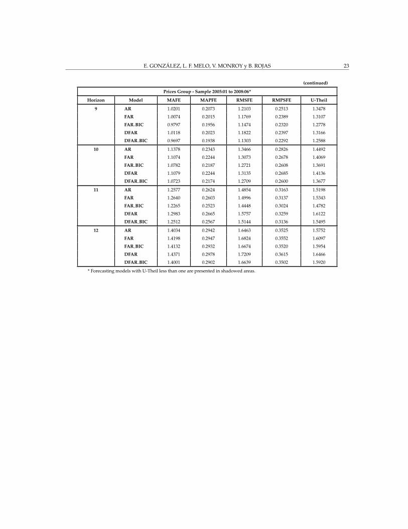
Forecasts evaluation for models (1) − (5) using different set of variables are exhibitedin Tables A.4 to A.8. Five evaluation statistics were used: mean absolute forecast error(MAFE), mean absolute percentage forecast error (MAPFE), root mean squared forecasterror (RMSFE), root mean squared percentage forecast error (RMSPFE) and U-Theil. 16
For horizons from one to five months ahead, all considered models outperform the ran-dom walk model according to the U-Theil statistic, which is less than one, in these casesthe results are presented in shadowed areas. For all horizons, except for one and twelvemonths ahead, there is at least one of the forecasting models which includes factors thathas smaller RMSFE than the autoregressive model (AR). For horizons from two to fourmonths, the model which includes one factor of each group of variables, FAR Gr, has thesmallest RMSFE.
When considering the set of price indicators, Table A.6, the results are quite similar. Fromone to six months ahead all factor models outperform random walk forecasts since U-Theil statistic is less than one. None of the factor models outperform the AR model forone month forecast horizon. For this set of variables, DFAR BIC and FAR models havethe smallest RMSFE for most horizons. Similar results are observed for other sets ofvariables.
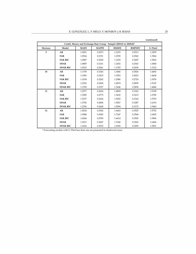
When comparing the forecast ability for different sets of variables, the set of prices indica-tors, in general, produces more accurate forecasts in terms of smaller RMSFE. However,
14BIC (BIC) and Bai and Ng (ICp2) criteria for m factors are defined as follows: BIC(m) = ln[V (m)] +
m ln(T )T
, ICp2(m) = ln[V (m)] +m(
N+TNT
)ln[min (N,T )], where V (m) = (NT )−1∑T
t=1 ξ′t(m)ξt(m).
15For all variables group more than six factors are required.16Table A.4 additionally shows the evaluation results for model (6).
E. GONZALEZ, L. F. MELO, V. MONROY y B. ROJAS 11
for the long run (10-12 months) this is not the case. Each set of variables has some fore-casting power to predict inflation, thus, estimating the factors considering the overall setof variables, as well as, models that include factors of each set of variables, seem to begood choices.
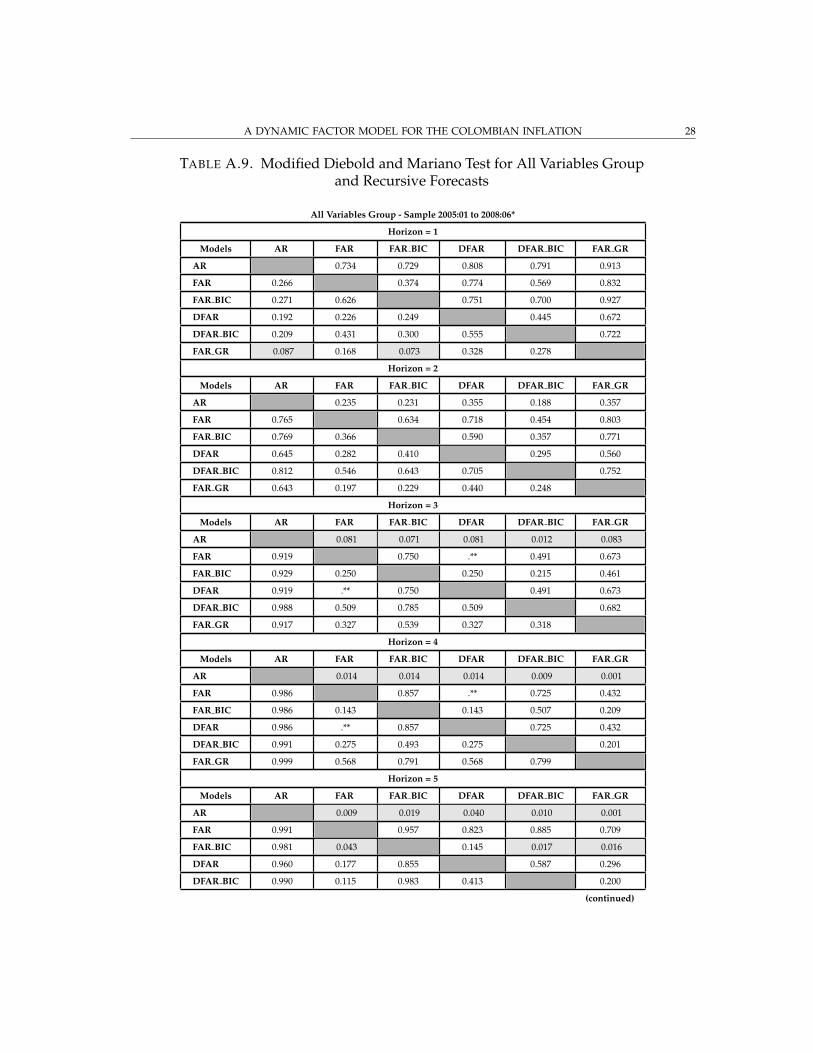
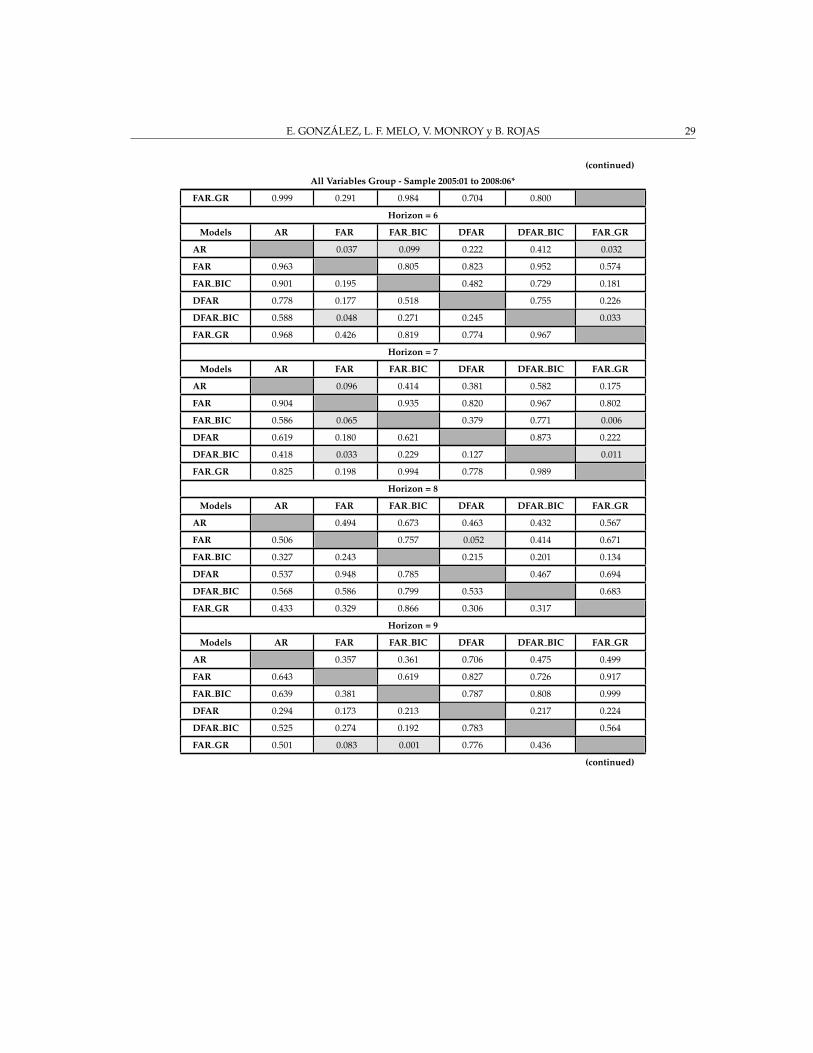
Tables A.9 to A.13 present p-values associated with the modified Diebold and Marianotest (Diebold and Mariano [1995]) for equal forecast ability of a pair of forecasting models.The shadowed cells correspond to cases when the null hypothesis is rejected at 10% sig-nificance level, which means that RMSFE of model in the column is significantly smallerthan RMSFE of model in the row. For models that consider the overall set of variables,only for horizons from 3 to 6 months there is a significant reduction in RMSFE of thefactor models forecasts, in comparison to the AR model. For the set of prices indicatorssimilar results are obtained (Table A.11). For the others sets of variables, none of the fac-tor models produce RMSFE significantly smaller than that of the AR model. Even thoughdynamic factor forecasts significantly outperform AR forecasts for some horizons, thereis no conclusive evidence to claim which of the factor models produce more accurateforecasts for inflation. Including more factors or more factor lags in the forecasting equa-tion does not necessarily reduce the forecast error, and is not always significant when areduction is observed (FAR, FAR BIC vs. DFAR, DFAR BIC).
An additional forecasting exercise was performed following Bai and Ng [2002] method-ology. These authors propose two forecast exercises. One based on all available data andother using a data set that contains only relevant or highly correlated series with the de-pendent variable. Thus, a pre-selection of variables was done, such that variables havinga contemporaneous correlation higher than 10% with the CPI inflation are included in thedata set used to estimate the factors. The evaluation of the forecasts obtained with theestimated factors from the pre-selected data set is shown in Table A.14. However, thereis no improvement in the forecasts when comparing to those of the complete data.
4.1.2. Rolling forecasts. The results of Bai and Ng and BIC criteria for determining thenumber of factors for rolling forecasts are almost identical, in more than 90% of the cases,to the ones obtained in recursive exercises. 17 From the forecasts evaluation results in Ta-bles A.15 to A.19 there are some aspects that are worth mentioning. First, comparing torandom walk forecasts, factor models produce more accurate forecasts for the short run(from one to five months) for the complete data set and prices indicators. However, forthe other data sets (credit, money and exchange rate; real activity; and national accounts)the gain in RMSFE of factor models is observed only until four months horizon. Sec-ond, for the complete data set (Table A.15), some factor models produce smaller RMSFEthan AR benchmark model for horizons from two to eleven months ahead. In particular,FAR Gr model performs well compared to the other models. Other model with goodperformance is FAR BIC.
17These results are not presented in the paper but are available upon request.
A DYNAMIC FACTOR MODEL FOR THE COLOMBIAN INFLATION 12
For the price indicators group (Table A.17), factor models are more accurate than ARmodel for horizons from one to eleven months. The models that produce the best fore-casts for most horizons are DFAR BIC and FAR BIC.
For the money and exchange rate indicators data set (Table A.18), comparing to ARmodel, there is some reduction in RMSFE of the forecasts obtained from factor modelsfrom one to ten months horizon. However, for further horizons AR produces smallerRMSFE.
For the real activity and national accounts groups (Table A.16 and Table A.19), whencomparing with the benchmark model there is not a reduction in RMSFE by factor modelsfor most of the considered horizons.
When recursive and rolling forecasts are compared (Tables A.4 to A.8 and A.15 to A.19),the former forecasts produce smaller RMSFE than the latter ones for some horizons andsome forecasting models. This result holds for the four groups of indicators that wereconsidered. However, as presented in Tables A.25 to A.29, the reduction in RMSFE is notalways significant according to the modified Diebold and Mariano tests.
In general, these results lead to the conclusion that factor models are good at forecastinginflation for short term horizons (two to six months) and some longer horizons. In mostof the cases factor models forecasts significantly outperform the benchmark AR modelforecasts. Even though, there is no conclusive evidence to establish which factor modelproduces the best forecasts, for short run horizons the best results are obtained for themodel that includes factors from each set of variables.
5. FINAL REMARKS
In this work, factor models were used as alternative methods for forecasting inflation inColombia for horizons from one to twelve months. In particular, we used a dynamic ap-proach proposed by Stock and Watson [1998, 1999, 2002a,b] and an autoregressive modelas a forecasting benchmark.
Factor models state that variation of a large number of variables can be explained bya small number of common factors. The idea of these models is based on the assump-tion that the dynamics of macroeconomic variables is determined by a few unobservablecommon factors that can be estimated using broad panel data. Then, information of largenumber of variables can be used in constructing forecasting models of smaller dimension.
When working with large number of variables an important issue is the availability ofdata since some variables are released with delay. In this regard, the implemented meth-odology uses EM algorithm to interpolate missing values. Then, a balanced panel can beused in the forecasting procedure.
Our forecasting analysis includes several exercises for different groups of variables (Allvariables, Real Activity, Prices, National Accounts and Credit, Money and ExchangeRate), recursive and rolling forecasts, and five different factor models. The five models

E. GONZALEZ, L. F. MELO, V. MONROY y B. ROJAS 13
are variations of the SW model and consider different criteria to select both, the numberof factors and the number of lags of those factors. Additionally, a model that includesfactors from each group of variables was analyzed.
The results show that, in average, one factor is appropriate to capture the commonal-ity of the economic variables considered in this study and help to explain the behaviorof Colombian inflation. On the other hand, models based on price indicators producesmaller RMSFE for most horizons. However, other groups of variables have some pre-dictive power since there is a good forecasting performance for the all-variables group aswell as the model that includes factors from each set of variables.
In terms of rolling and recursive factor forecasts, even though the latter forecasts havesmaller RMSFE than the former ones in more than 70% of the considered cases, the re-duction is not always significant.
In general, factor models outperformed the autoregressive benchmark model in termsof RMSFE for horizons between two and six months, for most of these cases there is asignificant improvement. Additionally, factor models outperformed random walk fore-casts. For these short-run horizons, the best results are obtained for recursive forecast,all-variables and prices groups as well as the model that includes factors from each set ofvariables.
A DYNAMIC FACTOR MODEL FOR THE COLOMBIAN INFLATION 14
REFERENCES
ARTIS, M., A. BANERJEE, AND M. MARCELLINO (2005): “Factor Forecast for the UK,”Journal of forecasting, 24(4), 279–298.
BAI, J., AND S. NG (2002): “Determining the number of factors in approximate factormodels,” Econometrica, 70(1), 191–221.
BOIVIN, J., AND S. NG (2005): “Understanding and comparing factor-based forecast,”International Journal of Central Banking, 1(3), 117–151.
BURNS, F., AND W. MITCHELL (1946): Measuring Business Cycles. National Bureau of Eco-nomic Research.
CAPORELLO, G., AND A. MARAVALL (2004): Program TSW, Reference Manual,Banco deEspana.
CHIB, S., AND E. GREENBERG (1994): “Markov Chain Monte Carlo Simulation Methodsin Econometrics,” Econometrics 9408001, EconWPA.
DE BANDT, O., E. MICHAUX, C. BRUNEAU, AND A. FLAGEOLLET (2007): “Forecastinginflation using economic indicators: the case of France,” Journal of Forecasting, 26(1),1–22.
DEMPSTER, A., N. LAIRD, AND D. RUBIN (1977): “Maximum likelihood from incompletedata via the EM algorithm,” Journal of the Royal Statistical Society: Series B, 39(1), 1–38.
DIEBOLD, F., AND R. MARIANO (1995): “Comparing Predictive Accuracy,” Journal of Busi-ness and Economic Statistics, 13(3), 253–263.
EICKMEIER, S., AND C. ZIEGLER (2006): “How good are dynamic factor models at fore-casting output and inflation? A meta-analytic approach,” Discussion Paper Series 42,Deutsche Bundesbank, Research Centre.
FORNI, M., M. HALLIN, M. LIPPI, AND L. REICHLIN (2000): “The generalized dynamic- factor model: Identification and estimation,” The Review of Economics and Statistics,82(4), 540–554.
(2005): “The generalized dynamic - factor model: One-sided estimation and fore-casting,” Journal of the American Statistical Association, (471), 830 – 840.
FORNI, M., AND L. REICHLIN (1998): “Let’s get real: A factor analytical approach todisaggregated business cycle dynamics,” Review of Economic Studies, 65(3), 453–73.
GONZALO, J., AND C. GRANGER (1995): “Estimation of common long-memory compo-nents in cointegrated systems,” Journal of Business and Economic Statistics, 13(1), 27–36.
GOSSELIN, M., AND G. TKACZ (2001): “Evaluating factor models: An application to fore-casting inflation in Canada,” Working Paper Series 18, Bank of Canada.
HARVEY, A. (1989): Forecasting structural time series models and the Kalman filter. Cam-bridge University Press.
JOHANSEN, S., AND K. JUSELIUS (1990): “Maximum Likelihood Estimation and Inferenceon Cointegration – With Applications to the Demand for Money,” Oxford Bulletin ofEconomics and Statistics, 52(2), 169–210.
KAPETANIOS, G., V. LABHARD, AND S. PRICE (2008): “Forecast combination and theBank of England suite of statistical forecasting models,” Economic Modelling, 25(4), 772–792.

E. GONZALEZ, L. F. MELO, V. MONROY y B. ROJAS 15
KAPETANIOS, G., AND M. MARCELLINO (2006): “A parametric estimation method fordynamic factor models of large dimensions,” Discussion Paper Series 5620, Centre forEconomic Policy Research.
MARCELLINO, M., J. STOCK, AND M. WATSON (2006): “A comparison of direct and it-erated multistep AR methods for forecasting macroeconomic time series,” Journal ofEconometrics, 135(1-2), 499–526.
MATHESON, T. D. (2006): “Factor Model Forecasts for New Zealand,” International Jour-nal of Central Banking, 2(2), 169–237.
MELO, L., AND H. NUNEZ (2004): “Combinacion de pronosticos de la inflacion en pres-encia de cambios estructurales,” Borradores de Economıa 286, Banco de la Republica.
OTROK, C., AND C. WHITEMAN (1998): “Bayesian leading indicators: Measuring andpredicting economic conditions in Iowa,” International Economic Review, 39(4), 997–1014.
PENA, D., AND P. PONCELA (2006): “Nonstationary dynamic factor analysis,” Journal ofStatistical Planning and Inference, 136(4), 1237–1257.
STOCK, J., AND M. WATSON (1998): “Difusion indexes,” Working Paper Series 6702, Na-tional Bureau of Economic Research, Inc.
(1999): “Forecasting inflation,” Journal of Monetary Economics, 44(2), 293–335.(2002a): “Forecasting Using Principal Components From a Large Number of Pre-
dictors,” Journal of the American Statistical Association, 97(460), 1167–1179.(2002b): “Macroeconomic forecasting using diffusion indexes,” Journal of Business
and Economic Statistics, 20(2), 147–62.ZAHER, F. (2007): “Evaluating factor forecasts for the UK: The role of asset prices,” Inter-
national Journal of Forecasting, 23(4), 679–693.

A DYNAMIC FACTOR MODEL FOR THE COLOMBIAN INFLATION 16
APPENDIX A. TABLES
TABLE A.2. Criteria for Determining the Number of Factors
All Variables Group
Horizon Horizon Horizon Horizon
Criteria (1999:01 to 2005:06) (1999:01 to 2006:06) (1999:01 to 2007:06) (1999:01 to 2008:06)
1 3 6 12 1 3 6 12 1 3 6 12 1 3 6 12
Bai and Ng 1 1 1 1 1 2 1 1 1 2 1 1 1 1 1 1
BIC 1 1 1 0 1 2 1 0 1 2 3 1 1 2 1 1
Real Activity Group
Horizon Horizon Horizon Horizon
Criteria (1999:01 to 2005:06) (1999:01 to 2006:06) (1999:01 to 2007:06) (1999:01 to 2008:06)
1 3 6 12 1 3 6 12 1 3 6 12 1 3 6 12
Bai and Ng 1 1 1 1 1 1 1 1 1 1 1 1 1 1 1 1
BIC 0 0 0 0 0 0 0 0 0 0 0 0 0 0 0 0
Prices Group
Horizon Horizon Horizon Horizon
Criteria (1999:01 to 2005:06) (1999:01 to 2006:06) (1999:01 to 2007:06) (1999:01 to 2008:06)
1 3 6 12 1 3 6 12 1 3 6 12 1 3 6 12
Bai and Ng 1 1 1 1 1 1 1 1 1 1 1 1 1 1 1 1
BIC 1 1 1 0 1 1 1 0 1 1 1 1 1 1 1 1
Credit, Money and Exchange Rate Group
Horizon Horizon Horizon Horizon
Criteria (1999:01 to 2005:06) (1999:01 to 2006:06) (1999:01 to 2007:06) (1999:01 to 2008:06)
1 3 6 12 1 3 6 12 1 3 6 12 1 3 6 12
Bai and Ng 2 2 1 1 1 2 2 1 1 2 1 1 1 2 1 1
BIC 3 1 1 0 1 5 1 1 1 1 1 1 0 1 1 1
National Accounts Group
Horizon Horizon Horizon Horizon
Criteria (1999:01 to 2005:06) (1999:01 to 2006:06) (1999:01 to 2007:06) (1999:01 to 2008:06)
1 3 6 12 1 3 6 12 1 3 6 12 1 3 6 12
Bai and Ng 1 1 1 1 1 1 1 1 1 1 1 1 1 1 1 1
BIC 0 0 0 0 0 0 0 0 0 0 0 0 0 0 0 0

E. GONZALEZ, L. F. MELO, V. MONROY y B. ROJAS 17
TABLE A.3. Explained Variance by the Factors
All Variables Group1999:01 to 2005:06 1999:01 to 2006:06 1999:01 to 2007:06 1999:01 to 2008:06
Number Explained Accumulated Explained Accumulated Explained Accumulated Explained AccumulatedOf Variance Explained Variance Explained Variance Explained Variance Explained
Factors Variance Variance Variance Variance1 0.1166 0.1166 0.1178 0.1178 0.1210 0.1210 0.1133 0.11332 0.0700 0.1866 0.0691 0.1869 0.0658 0.1868 0.0628 0.17613 0.0663 0.2529 0.0625 0.2494 0.0578 0.2446 0.0593 0.23544 0.0527 0.3056 0.0499 0.2993 0.0471 0.2917 0.0461 0.28155 0.0461 0.3517 0.0446 0.3439 0.0438 0.3355 0.0420 0.32356 0.0430 0.3947 0.0397 0.3836 0.0405 0.3760 0.0383 0.3618
Real Activity Group1999:01 to 2005:06 1999:01 to 2006:06 1999:01 to 2007:06 1999:01 to 2008:06
Number Explained Accumulated Explained Accumulated Explained Accumulated Explained AccumulatedOf Variance Explained Variance Explained Variance Explained Variance Explained
Factors Variance Variance Variance Variance1 0.1760 0.1760 0.1900 0.1900 0.1751 0.1751 0.1631 0.16312 0.1607 0.3367 0.1525 0.3425 0.1427 0.3178 0.1468 0.30993 0.1159 0.4525 0.1120 0.4545 0.1306 0.4484 0.1238 0.43374 0.0776 0.5301 0.0810 0.5355 0.0809 0.5293 0.0789 0.51275 0.0711 0.6012 0.0686 0.6041 0.0679 0.5972 0.0681 0.58086 0.0605 0.6618 0.0591 0.6632 0.0592 0.6564 0.0577 0.6385
Prices Group1999:01 to 2005:06 1999:01 to 2006:06 1999:01 to 2007:06 1999:01 to 2008:06
Number Explained Accumulated Explained Accumulated Explained Accumulated Explained AccumulatedOf Variance Explained Variance Explained Variance Explained Variance Explained
Factors Variance Variance Variance Variance1 0.2442 0.2442 0.2483 0.2483 0.2535 0.2535 0.2402 0.24022 0.1552 0.3995 0.1546 0.4029 0.1445 0.3979 0.1438 0.38413 0.0897 0.4891 0.0889 0.4919 0.0880 0.4859 0.0932 0.47734 0.0731 0.5622 0.0713 0.5632 0.0690 0.5549 0.0688 0.54615 0.0619 0.6241 0.0605 0.6237 0.0577 0.6126 0.0618 0.60796 0.0552 0.6793 0.0540 0.6777 0.0528 0.6654 0.0550 0.6630
Credit, Money and Exchange Rate Group1999:01 to 2005:06 1999:01 to 2006:06 1999:01 to 2007:06 1999:01 to 2008:06
Number Explained Accumulated Explained Accumulated Explained Accumulated Explained AccumulatedOf Variance Explained Variance Explained Variance Explained Variance Explained
Factors Variance Variance Variance Variance1 0.2198 0.2198 0.3790 0.3790 0.3289 0.3289 0.3023 0.30232 0.1656 0.3855 0.1390 0.5180 0.1409 0.4698 0.1465 0.44883 0.1330 0.5184 0.0822 0.6002 0.1093 0.5791 0.1134 0.56224 0.0850 0.6035 0.0652 0.6653 0.0844 0.6635 0.0837 0.64595 0.0661 0.6695 0.0506 0.7159 0.0553 0.7188 0.0623 0.70826 0.0479 0.7174 0.0412 0.7571 0.0408 0.7596 0.0416 0.7498
National Accounts Group1999:01 to 2005:06 1999:01 to 2006:06 1999:01 to 2007:06 1999:01 to 2008:06
Number Explained Accumulated Explained Accumulated Explained Accumulated Explained AccumulatedOf Variance Explained Variance Explained Variance Explained Variance Explained
Factors Variance Variance Variance Variance1 0.1564 0.1564 0.1546 0.1546 0.1546 0.1546 0.1442 0.14422 0.0998 0.2562 0.1032 0.2578 0.0977 0.2523 0.1126 0.25683 0.0856 0.3418 0.0810 0.3388 0.0806 0.3329 0.0766 0.33344 0.0769 0.4186 0.0745 0.4132 0.0709 0.4038 0.0719 0.40545 0.0701 0.4888 0.0680 0.4813 0.0667 0.4705 0.0667 0.47216 0.0612 0.5500 0.0604 0.5416 0.0622 0.5327 0.0569 0.5290

A DYNAMIC FACTOR MODEL FOR THE COLOMBIAN INFLATION 18
TABLE A.4. Recursive Forecasts Evaluation for All Variables Group
All Variables Group - Sample 2005:01 to 2008:06*
Horizon Model MAFE MAPFE RMSFE RMPSFE U-Theil
1 AR 0.1599 0.0301 0.1964 0.0370 0.6227
FAR 0.1681 0.0320 0.2043 0.0393 0.6478
FAR BIC 0.1669 0.0317 0.2013 0.0385 0.6385
DFAR 0.1723 0.0330 0.2082 0.0406 0.6603
DFAR BIC 0.1615 0.0308 0.2064 0.0398 0.6547
FAR GR 0.1749 0.0335 0.2127 0.0413 0.6744
2 AR 0.3285 0.0635 0.3925 0.0772 0.7595
FAR 0.2962 0.0565 0.3717 0.0706 0.7192
FAR BIC 0.2979 0.0571 0.3758 0.0727 0.7273
DFAR 0.3015 0.0573 0.3805 0.0718 0.7363
DFAR BIC 0.2751 0.0523 0.3696 0.0701 0.7153
FAR GR 0.3027 0.0579 0.3838 0.0739 0.7426
3 AR 0.4500 0.0886 0.5253 0.1074 0.8590
FAR 0.3585 0.0696 0.4646 0.0904 0.7598
FAR BIC 0.3809 0.0742 0.4765 0.0945 0.7793
DFAR 0.3585 0.0696 0.4646 0.0904 0.7598
DFAR BIC 0.3704 0.0719 0.4641 0.0931 0.7589
FAR GR 0.3737 0.0722 0.4744 0.0931 0.7758
4 AR 0.5934 0.1165 0.6916 0.1407 0.9995
FAR 0.4273 0.0837 0.5424 0.1093 0.7839
FAR BIC 0.4451 0.0874 0.5577 0.1135 0.8060
DFAR 0.4273 0.0837 0.5424 0.1093 0.7839
DFAR BIC 0.4358 0.0860 0.5580 0.1147 0.8064
FAR GR 0.4232 0.0831 0.5370 0.1106 0.7760
5 AR 0.7115 0.1396 0.8268 0.1681 1.0721
FAR 0.5350 0.1039 0.6865 0.1369 0.8902
FAR BIC 0.6249 0.1214 0.7666 0.1534 0.9939
DFAR 0.5842 0.1121 0.7310 0.1433 0.9479
DFAR BIC 0.5855 0.1132 0.7351 0.1457 0.9532
FAR GR 0.5728 0.1110 0.7164 0.1437 0.9289
6 AR 0.7521 0.1478 0.9007 0.1827 1.0997
FAR 0.6793 0.1321 0.8153 0.1616 0.9954
FAR BIC 0.7021 0.1385 0.8543 0.1741 1.0431
DFAR 0.7077 0.1369 0.8514 0.1669 1.0395
DFAR BIC 0.7533 0.1478 0.8842 0.1774 1.0796
FAR GR 0.6819 0.1334 0.8221 0.1651 1.0038
7 AR 0.8204 0.1631 0.9906 0.2047 1.1800
FAR 0.7596 0.1491 0.8963 0.1793 1.0677
FAR BIC 0.8338 0.1647 0.9784 0.1981 1.1654
DFAR 0.8077 0.1576 0.9601 0.1892 1.1437
DFAR BIC 0.8834 0.1729 1.0116 0.2017 1.2050
(continued)

E. GONZALEZ, L. F. MELO, V. MONROY y B. ROJAS 19
(continued)
All Variables Group - Sample 2005:01 to 2008:06*
Horizon Model MAFE MAPFE RMSFE RMPSFE U-Theil
FAR GR 0.7936 0.1555 0.9199 0.1847 1.0958
8 AR 0.8991 0.1811 1.0852 0.2248 1.2583
FAR 0.9205 0.1798 1.0835 0.2124 1.2563
FAR BIC 0.9381 0.1856 1.1229 0.2238 1.3020
DFAR 0.9219 0.1805 1.0748 0.2119 1.2462
DFAR BIC 0.9333 0.1843 1.0701 0.2152 1.2408
FAR GR 0.9397 0.1845 1.1032 0.2196 1.2792
9 AR 1.0201 0.2073 1.2103 0.2513 1.3478
FAR 1.0211 0.2028 1.1713 0.2360 1.3045
FAR BIC 1.0115 0.2033 1.1871 0.2427 1.3220
DFAR 1.1029 0.2187 1.2881 0.2581 1.4345
DFAR BIC 1.0234 0.2054 1.2064 0.2459 1.3435
FAR GR 1.0418 0.2080 1.2100 0.2451 1.3476
10 AR 1.1378 0.2343 1.3466 0.2826 1.4492
FAR 1.1324 0.2292 1.3127 0.2695 1.4127
FAR BIC 1.0864 0.2217 1.2714 0.2644 1.3682
DFAR 1.2282 0.2478 1.4574 0.2965 1.5685
DFAR BIC 1.1468 0.2331 1.3599 0.2794 1.4635
FAR GR 1.1587 0.2347 1.3546 0.2773 1.4578
11 AR 1.2577 0.2624 1.4854 0.3163 1.5198
FAR 1.2776 0.2620 1.4926 0.3107 1.5271
FAR BIC 1.2508 0.2582 1.4729 0.3099 1.5070
DFAR 1.3125 0.2685 1.5398 0.3187 1.5754
DFAR BIC 1.2720 0.2621 1.5030 0.3148 1.5378
FAR GR 1.2944 0.2652 1.5140 0.3151 1.5490
12 AR 1.4034 0.2942 1.6463 0.3525 1.5752
FAR 1.4428 0.2976 1.6757 0.3518 1.6034
FAR BIC 1.4427 0.2984 1.6986 0.3573 1.6253
DFAR 1.4689 0.3027 1.7165 0.3593 1.6423
DFAR BIC 1.4533 0.3005 1.7155 0.3604 1.6414
FAR GR 1.4409 0.2962 1.6774 0.3513 1.6050
* Forecasting models with U-Theil less than one are presented in shadowed areas.

A DYNAMIC FACTOR MODEL FOR THE COLOMBIAN INFLATION 20
TABLE A.5. Recursive Forecasts Evaluation for Real Activity Group
Real Activity Group - Sample 2005:01 to 2008:06*
Horizon Model MAFE MAPFE RMSFE RMPSFE U-Theil
1 AR 0.1599 0.0301 0.1964 0.0370 0.6227
FAR 0.1688 0.0320 0.2064 0.0394 0.6545
FAR BIC 0.1599 0.0301 0.1964 0.0370 0.6227
DFAR 0.1688 0.0320 0.2064 0.0394 0.6545
DFAR BIC 0.1599 0.0301 0.1964 0.0370 0.6227
2 AR 0.3285 0.0635 0.3925 0.0772 0.7595
FAR 0.3414 0.0661 0.3955 0.0777 0.7654
FAR BIC 0.3285 0.0635 0.3925 0.0772 0.7595
DFAR 0.3414 0.0661 0.3955 0.0777 0.7654
DFAR BIC 0.3285 0.0635 0.3925 0.0772 0.7595
3 AR 0.4500 0.0886 0.5253 0.1074 0.8590
FAR 0.4474 0.0875 0.5298 0.1070 0.8665
FAR BIC 0.4468 0.0880 0.5218 0.1069 0.8534
DFAR 0.4474 0.0875 0.5298 0.1070 0.8665
DFAR BIC 0.4535 0.0892 0.5308 0.1084 0.8682
4 AR 0.5934 0.1165 0.6916 0.1407 0.9995
FAR 0.5905 0.1154 0.6967 0.1408 1.0068
FAR BIC 0.5906 0.1158 0.6849 0.1395 0.9898
DFAR 0.5790 0.1133 0.6919 0.1400 0.9998
DFAR BIC 0.5912 0.1158 0.6916 0.1403 0.9994
5 AR 0.7115 0.1396 0.8268 0.1681 1.0721
FAR 0.7043 0.1380 0.8167 0.1657 1.0589
FAR BIC 0.7096 0.1393 0.8235 0.1676 1.0678
DFAR 0.7043 0.1380 0.8167 0.1657 1.0589
DFAR BIC 0.7040 0.1384 0.8140 0.1664 1.0555
6 AR 0.7521 0.1478 0.9007 0.1827 1.0997
FAR 0.7583 0.1494 0.9032 0.1844 1.1028
FAR BIC 0.7521 0.1478 0.9007 0.1827 1.0997
DFAR 0.7336 0.1454 0.8848 0.1820 1.0804
DFAR BIC 0.7412 0.1460 0.8832 0.1804 1.0783
7 AR 0.8204 0.1631 0.9906 0.2047 1.1800
FAR 0.8251 0.1646 0.9962 0.2060 1.1866
FAR BIC 0.8204 0.1631 0.9906 0.2047 1.1800
DFAR 0.7872 0.1582 0.9652 0.2018 1.1497
DFAR BIC 0.7979 0.1594 0.9751 0.2026 1.1615
8 AR 0.8991 0.1811 1.0852 0.2248 1.2583
FAR 0.9538 0.1915 1.1329 0.2341 1.3136
FAR BIC 0.8859 0.1793 1.0883 0.2262 1.2619
DFAR 0.9300 0.1875 1.1179 0.2320 1.2962
DFAR BIC 0.8930 0.1806 1.1003 0.2281 1.2758
(continued)

E. GONZALEZ, L. F. MELO, V. MONROY y B. ROJAS 21
(continued)
Real Activity Group - Sample 2005:01 to 2008:06*
Horizon Model MAFE MAPFE RMSFE RMPSFE U-Theil
9 AR 1.0201 0.2073 1.2103 0.2513 1.3478
FAR 1.0678 0.2165 1.2549 0.2594 1.3975
FAR BIC 1.0247 0.2085 1.2215 0.2539 1.3603
DFAR 1.0706 0.2172 1.2646 0.2613 1.4084
DFAR BIC 1.0368 0.2109 1.2459 0.2583 1.3875
10 AR 1.1378 0.2343 1.3466 0.2826 1.4492
FAR 1.1658 1.1658 1.1658 1.1658 1.1658
FAR BIC 1.1318 0.2334 1.3388 0.2818 1.4408
DFAR 1.1524 0.2376 1.3561 0.2861 1.4594
DFAR BIC 1.1304 0.2334 1.3452 0.2834 1.4477
11 AR 1.2577 0.2624 1.4854 0.3163 1.5198
FAR 1.2756 0.2659 1.5202 0.3232 1.5554
FAR BIC 1.2678 0.2645 1.5015 0.3195 1.5362
DFAR 1.2749 0.2658 1.5262 0.3242 1.5615
DFAR BIC 1.2685 0.2646 1.5096 0.3209 1.5446
12 AR 1.4034 0.2942 1.6463 0.3525 1.5752
FAR 1.3713 0.2894 1.6437 0.3540 1.5727
FAR BIC 1.3942 0.2924 1.6356 0.3508 1.5650
DFAR 1.4015 0.2952 1.6857 0.3613 1.6128
DFAR BIC 1.4246 0.2983 1.6788 0.3584 1.6063
* Forecasting models with U-Theil less than one are presented in shadowed areas.

A DYNAMIC FACTOR MODEL FOR THE COLOMBIAN INFLATION 22
TABLE A.6. Recursive Forecasts Evaluation for Prices Group
Prices Group - Sample 2005:01 to 2008:06*
Horizon Model MAFE MAPFE RMSFE RMPSFE U-Theil
1 AR 0.1599 0.0301 0.1964 0.0370 0.6227
FAR 0.1711 0.0329 0.2068 0.0403 0.6557
FAR BIC 0.1682 0.0323 0.2041 0.0399 0.6471
DFAR 0.1711 0.0329 0.2068 0.0403 0.6557
DFAR BIC 0.1682 0.0323 0.2041 0.0399 0.6471
2 AR 0.3285 0.0635 0.3925 0.0772 0.7595
FAR 0.3093 0.0595 0.3775 0.0728 0.7306
FAR BIC 0.3006 0.0577 0.3739 0.0726 0.7235
DFAR 0.3093 0.0595 0.3775 0.0728 0.7306
DFAR BIC 0.3034 0.0582 0.3717 0.0714 0.7193
3 AR 0.4500 0.0886 0.5253 0.1074 0.8590
FAR 0.3727 0.0723 0.4673 0.0928 0.7642
FAR BIC 0.3610 0.0700 0.4725 0.0924 0.7727
DFAR 0.3727 0.0723 0.4673 0.0928 0.7642
DFAR BIC 0.3549 0.0690 0.4588 0.0909 0.7504
4 AR 0.5934 0.1165 0.6916 0.1407 0.9995
FAR 0.4336 0.0846 0.5453 0.1112 0.7880
FAR BIC 0.4131 0.0808 0.5291 0.1086 0.7647
DFAR 0.4336 0.0846 0.5453 0.1112 0.7880
DFAR BIC 0.4131 0.0808 0.5291 0.1086 0.7647
5 AR 0.7115 0.1396 0.8268 0.1681 1.0721
FAR 0.5387 0.1058 0.6615 0.1364 0.8577
FAR BIC 0.5424 0.1057 0.6709 0.1362 0.8699
DFAR 0.5414 0.1062 0.6651 0.1369 0.8623
DFAR BIC 0.5755 0.1122 0.6932 0.1401 0.8989
6 AR 0.7521 0.1478 0.9007 0.1827 1.0997
FAR 0.6867 0.1341 0.8118 0.1631 0.9912
FAR BIC 0.6662 0.1303 0.7918 0.1591 0.9667
DFAR 0.7031 0.1368 0.8386 0.1669 1.0239
DFAR BIC 0.7209 0.1400 0.8451 0.1671 1.0318
7 AR 0.8204 0.1631 0.9906 0.2047 1.1800
FAR 0.7820 0.1530 0.9009 0.1800 1.0731
FAR BIC 0.7611 0.1492 0.8746 0.1756 1.0418
DFAR 0.8085 0.1579 0.9246 0.1839 1.1014
DFAR BIC 0.8085 0.1578 0.9203 0.1830 1.0962
8 AR 0.8991 0.1811 1.0852 0.2248 1.2583
FAR 0.8984 0.1766 1.0441 0.2078 1.2106
FAR BIC 0.8582 0.1688 1.0035 0.2006 1.1636
DFAR 0.9161 0.1798 1.0648 0.2112 1.2347
DFAR BIC 0.8812 0.1731 1.0328 0.2056 1.1975
(continued)
E. GONZALEZ, L. F. MELO, V. MONROY y B. ROJAS 23
(continued)
Prices Group - Sample 2005:01 to 2008:06*
Horizon Model MAFE MAPFE RMSFE RMPSFE U-Theil
9 AR 1.0201 0.2073 1.2103 0.2513 1.3478
FAR 1.0074 0.2015 1.1769 0.2389 1.3107
FAR BIC 0.9797 0.1956 1.1474 0.2320 1.2778
DFAR 1.0118 0.2023 1.1822 0.2397 1.3166
DFAR BIC 0.9697 0.1938 1.1303 0.2292 1.2588
10 AR 1.1378 0.2343 1.3466 0.2826 1.4492
FAR 1.1074 0.2244 1.3073 0.2678 1.4069
FAR BIC 1.0782 0.2187 1.2721 0.2608 1.3691
DFAR 1.1079 0.2244 1.3135 0.2685 1.4136
DFAR BIC 1.0723 0.2174 1.2709 0.2600 1.3677
11 AR 1.2577 0.2624 1.4854 0.3163 1.5198
FAR 1.2640 0.2603 1.4996 0.3137 1.5343
FAR BIC 1.2265 0.2523 1.4448 0.3024 1.4782
DFAR 1.2983 0.2665 1.5757 0.3259 1.6122
DFAR BIC 1.2512 0.2567 1.5144 0.3136 1.5495
12 AR 1.4034 0.2942 1.6463 0.3525 1.5752
FAR 1.4198 0.2947 1.6824 0.3552 1.6097
FAR BIC 1.4132 0.2932 1.6674 0.3520 1.5954
DFAR 1.4371 0.2978 1.7209 0.3615 1.6466
DFAR BIC 1.4001 0.2902 1.6639 0.3502 1.5920
* Forecasting models with U-Theil less than one are presented in shadowed areas.

A DYNAMIC FACTOR MODEL FOR THE COLOMBIAN INFLATION 24
TABLE A.7. Recursive Forecasts Evaluation for Credit, Money andExchange Rate Group
Credit, Money and Exchange Rate Group - Sample 2005:01 to 2008:06*
Horizon Model MAFE MAPFE RMSFE RMPSFE U-Theil
1 AR 0.1599 0.0301 0.1964 0.0370 0.6227
FAR 0.1807 0.0343 0.2252 0.0435 0.7141
FAR BIC 0.1736 0.0328 0.2249 0.0429 0.7131
DFAR 0.1807 0.0343 0.2252 0.0435 0.7141
DFAR BIC 0.1752 0.0333 0.2147 0.0410 0.6809
2 AR 0.3285 0.0635 0.3925 0.0772 0.7595
FAR 0.3391 0.0653 0.4262 0.0831 0.8248
FAR BIC 0.3161 0.0609 0.4059 0.0798 0.7854
DFAR 0.3322 0.0640 0.4210 0.0822 0.8147
DFAR BIC 0.2975 0.0568 0.3935 0.0749 0.7614
3 AR 0.4500 0.0886 0.5253 0.1074 0.8590
FAR 0.4237 0.0824 0.5364 0.1064 0.8773
FAR BIC 0.4064 0.0789 0.5109 0.1016 0.8355
DFAR 0.4244 0.0825 0.5367 0.1064 0.8778
DFAR BIC 0.3951 0.0761 0.5071 0.1001 0.8294
4 AR 0.5934 0.1165 0.6916 0.1407 0.9995
FAR 0.5249 0.1021 0.6557 0.1288 0.9475
FAR BIC 0.4843 0.0947 0.6307 0.1280 0.9114
DFAR 0.5249 0.1021 0.6557 0.1288 0.9475
DFAR BIC 0.4594 0.0900 0.6190 0.1254 0.8946
5 AR 0.7115 0.1396 0.8268 0.1681 1.0721
FAR 0.6262 0.1209 0.7710 0.1525 0.9997
FAR BIC 0.6324 0.1229 0.7836 0.1568 1.0160
DFAR 0.6262 0.1209 0.7710 0.1525 0.9997
DFAR BIC 0.6284 0.1224 0.7816 0.1575 1.0135
6 AR 0.7521 0.1478 0.9007 0.1827 1.0997
FAR 0.7096 0.1385 0.8665 0.1732 1.0580
FAR BIC 0.7137 0.1407 0.8645 0.1756 1.0555
DFAR 0.7096 0.1385 0.8665 0.1732 1.0580
DFAR BIC 0.7151 0.1415 0.8737 0.1788 1.0667
7 AR 0.8204 0.1631 0.9906 0.2047 1.1800
FAR 0.8044 0.1599 0.9455 0.1940 1.1263
FAR BIC 0.8074 0.1614 0.9430 0.1953 1.1232
DFAR 0.7917 0.1570 0.9407 0.1927 1.1205
DFAR BIC 0.8167 0.1631 0.9477 0.1965 1.1289
8 AR 0.8991 0.1811 1.0852 0.2248 1.2583
FAR 0.9833 0.1943 1.1483 0.2302 1.3314
FAR BIC 0.9626 0.1917 1.1222 0.2274 1.3012
DFAR 0.9705 0.1914 1.1408 0.2283 1.3227
DFAR BIC 0.9472 0.1877 1.0979 0.2214 1.2730
(continued)
E. GONZALEZ, L. F. MELO, V. MONROY y B. ROJAS 25
(continued)
Credit, Money and Exchange Rate Group - Sample 2005:01 to 2008:06*
Horizon Model MAFE MAPFE RMSFE RMPSFE U-Theil
9 AR 1.0201 0.2073 1.2103 0.2513 1.3478
FAR 1.0944 0.2191 1.2539 0.2562 1.3964
FAR BIC 1.0087 0.2030 1.1639 0.2407 1.2962
DFAR 1.0805 0.2161 1.2452 0.2543 1.3868
DFAR BIC 1.0233 0.2061 1.1783 0.2438 1.3122
10 AR 1.1378 0.2343 1.3466 0.2826 1.4492
FAR 1.1983 0.2433 1.3593 0.2823 1.4628
FAR BIC 1.1034 0.2262 1.2986 0.2724 1.3976
DFAR 1.2322 0.2494 1.4074 0.2899 1.5147
DFAR BIC 1.1530 0.2357 1.3646 0.2838 1.4686
11 AR 1.2577 0.2624 1.4854 0.3163 1.5198
FAR 1.3585 0.2773 1.5432 0.3215 1.5789
FAR BIC 1.2727 0.2636 1.5022 0.3164 1.5370
DFAR 1.3756 0.2806 1.5827 0.3287 1.6193
DFAR BIC 1.2706 0.2628 1.5094 0.3172 1.5443
12 AR 1.4034 0.2942 1.6463 0.3525 1.5752
FAR 1.5088 0.3083 1.7247 0.3568 1.6502
FAR BIC 1.4244 0.2950 1.6614 0.3503 1.5896
DFAR 1.5013 0.3067 1.7240 0.3565 1.6496
DFAR BIC 1.4166 0.2932 1.6545 0.3490 1.5831
* Forecasting models with U-Theil less than one are presented in shadowed areas.

A DYNAMIC FACTOR MODEL FOR THE COLOMBIAN INFLATION 26
TABLE A.8. Recursive Gorecasts Evaluation for National Accounts Group
National Accounts Group - Sample 2005:01 to 2008:06*
Horizon Model MAFE MAPFE RMSFE RMPSFE U-Theil
1 AR 0.1599 0.0301 0.1964 0.0370 0.6227
FAR 0.1620 0.0305 0.2079 0.0389 0.6592
FAR BIC 0.1599 0.0301 0.1964 0.0370 0.6227
DFAR 0.1620 0.0305 0.2079 0.0389 0.6592
DFAR BIC 0.1635 0.0309 0.2107 0.0407 0.6681
2 AR 0.3285 0.0635 0.3925 0.0772 0.7595
FAR 0.3312 0.0639 0.4028 0.0790 0.7795
FAR BIC 0.3285 0.0635 0.3925 0.0772 0.7595
DFAR 0.3312 0.0639 0.4028 0.0790 0.7795
DFAR BIC 0.3285 0.0637 0.4082 0.0815 0.7899
3 AR 0.4500 0.0886 0.5253 0.1074 0.8590
FAR 0.4478 0.0880 0.5256 0.1077 0.8596
FAR BIC 0.4481 0.0881 0.5217 0.1064 0.8532
DFAR 0.4478 0.0880 0.5256 0.1077 0.8596
DFAR BIC 0.4535 0.0892 0.5301 0.1085 0.8669
4 AR 0.5934 0.1165 0.6916 0.1407 0.9995
FAR 0.5946 0.1165 0.6973 0.1414 1.0077
FAR BIC 0.5934 0.1165 0.6916 0.1407 0.9995
DFAR 0.6173 0.1211 0.7116 0.1443 1.0284
DFAR BIC 0.5992 0.1175 0.6941 0.1410 1.0031
5 AR 0.7115 0.1396 0.8268 0.1681 1.0721
FAR 0.7031 0.1375 0.8268 0.1673 1.0721
FAR BIC 0.7115 0.1396 0.8268 0.1681 1.0721
DFAR 0.6910 0.1355 0.8440 0.1720 1.0943
DFAR BIC 0.7377 0.1448 0.8615 0.1751 1.1170
6 AR 0.7521 0.1478 0.9007 0.1827 1.0997
FAR 0.7649 0.1502 0.9252 0.1888 1.1297
FAR BIC 0.7521 0.1478 0.9007 0.1827 1.0997
DFAR 0.7546 0.1511 0.9774 0.2083 1.1933
DFAR BIC 0.7750 0.1549 0.9538 0.2011 1.1646
7 AR 0.8204 0.1631 0.9906 0.2047 1.1800
FAR 0.8238 0.1645 0.9956 0.2071 1.1859
FAR BIC 0.8204 0.1631 0.9906 0.2047 1.1800
DFAR 0.8286 0.1675 1.0855 0.2331 1.2931
DFAR BIC 0.8394 0.1688 1.0546 0.2240 1.2562
8 AR 0.8991 0.1811 1.0852 0.2248 1.2583
FAR 0.9053 0.1834 1.1048 0.2310 1.2810
FAR BIC 0.8991 0.1811 1.0852 0.2248 1.2583
DFAR 0.9077 0.1850 1.1886 0.2555 1.3781
DFAR BIC 0.9182 0.1872 1.1563 0.2465 1.3407
(continued)

E. GONZALEZ, L. F. MELO, V. MONROY y B. ROJAS 27
(continued)
National Accounts Group - Sample 2005:01 to 2008:06*
Horizon Model MAFE MAPFE RMSFE RMPSFE U-Theil
9 AR 1.0201 0.2073 1.2103 0.2513 1.3478
FAR 1.0544 0.2146 1.2521 0.2612 1.3944
FAR BIC 1.0210 0.2075 1.2116 0.2515 1.3494
DFAR 1.0373 0.2129 1.2884 0.2751 1.4349
DFAR BIC 0.9941 0.2022 1.1999 0.2494 1.3363
10 AR 1.1378 0.2343 1.3466 0.2826 1.4492
FAR 1.1345 0.2348 1.3583 0.2876 1.4618
FAR BIC 1.1334 0.2335 1.3430 0.2820 1.4454
DFAR 1.1036 0.2289 1.3702 0.2901 1.4746
DFAR BIC 1.1300 0.2329 1.3656 0.2865 1.4696
11 AR 1.2577 0.2624 1.4854 0.3163 1.5198
FAR 1.2835 0.2684 1.5175 0.3250 1.5526
FAR BIC 1.2577 0.2624 1.4854 0.3163 1.5198
DFAR 1.2888 0.2695 1.5385 0.3290 1.5741
DFAR BIC 1.2354 0.2581 1.4812 0.3158 1.5154
12 AR 1.4034 0.2942 1.6463 0.3525 1.5752
FAR 1.4000 0.2943 1.6496 0.3557 1.5784
FAR BIC 1.4034 0.2942 1.6463 0.3525 1.5752
DFAR 1.3584 0.2863 1.6225 0.3512 1.5524
DFAR BIC 1.3690 0.2875 1.6089 0.3459 1.5394
* Forecasting models with U-Theil less than one are presented in shadowed areas.
A DYNAMIC FACTOR MODEL FOR THE COLOMBIAN INFLATION 28
TABLE A.9. Modified Diebold and Mariano Test for All Variables Groupand Recursive Forecasts
All Variables Group - Sample 2005:01 to 2008:06*
Horizon = 1
Models AR FAR FAR BIC DFAR DFAR BIC FAR GR
AR 0.734 0.729 0.808 0.791 0.913
FAR 0.266 0.374 0.774 0.569 0.832
FAR BIC 0.271 0.626 0.751 0.700 0.927
DFAR 0.192 0.226 0.249 0.445 0.672
DFAR BIC 0.209 0.431 0.300 0.555 0.722
FAR GR 0.087 0.168 0.073 0.328 0.278
Horizon = 2
Models AR FAR FAR BIC DFAR DFAR BIC FAR GR
AR 0.235 0.231 0.355 0.188 0.357
FAR 0.765 0.634 0.718 0.454 0.803
FAR BIC 0.769 0.366 0.590 0.357 0.771
DFAR 0.645 0.282 0.410 0.295 0.560
DFAR BIC 0.812 0.546 0.643 0.705 0.752
FAR GR 0.643 0.197 0.229 0.440 0.248
Horizon = 3
Models AR FAR FAR BIC DFAR DFAR BIC FAR GR
AR 0.081 0.071 0.081 0.012 0.083
FAR 0.919 0.750 .** 0.491 0.673
FAR BIC 0.929 0.250 0.250 0.215 0.461
DFAR 0.919 .** 0.750 0.491 0.673
DFAR BIC 0.988 0.509 0.785 0.509 0.682
FAR GR 0.917 0.327 0.539 0.327 0.318
Horizon = 4
Models AR FAR FAR BIC DFAR DFAR BIC FAR GR
AR 0.014 0.014 0.014 0.009 0.001
FAR 0.986 0.857 .** 0.725 0.432
FAR BIC 0.986 0.143 0.143 0.507 0.209
DFAR 0.986 .** 0.857 0.725 0.432
DFAR BIC 0.991 0.275 0.493 0.275 0.201
FAR GR 0.999 0.568 0.791 0.568 0.799
Horizon = 5
Models AR FAR FAR BIC DFAR DFAR BIC FAR GR
AR 0.009 0.019 0.040 0.010 0.001
FAR 0.991 0.957 0.823 0.885 0.709
FAR BIC 0.981 0.043 0.145 0.017 0.016
DFAR 0.960 0.177 0.855 0.587 0.296
DFAR BIC 0.990 0.115 0.983 0.413 0.200
(continued)
E. GONZALEZ, L. F. MELO, V. MONROY y B. ROJAS 29
(continued)
All Variables Group - Sample 2005:01 to 2008:06*
FAR GR 0.999 0.291 0.984 0.704 0.800
Horizon = 6
Models AR FAR FAR BIC DFAR DFAR BIC FAR GR
AR 0.037 0.099 0.222 0.412 0.032
FAR 0.963 0.805 0.823 0.952 0.574
FAR BIC 0.901 0.195 0.482 0.729 0.181
DFAR 0.778 0.177 0.518 0.755 0.226
DFAR BIC 0.588 0.048 0.271 0.245 0.033
FAR GR 0.968 0.426 0.819 0.774 0.967
Horizon = 7
Models AR FAR FAR BIC DFAR DFAR BIC FAR GR
AR 0.096 0.414 0.381 0.582 0.175
FAR 0.904 0.935 0.820 0.967 0.802
FAR BIC 0.586 0.065 0.379 0.771 0.006
DFAR 0.619 0.180 0.621 0.873 0.222
DFAR BIC 0.418 0.033 0.229 0.127 0.011
FAR GR 0.825 0.198 0.994 0.778 0.989
Horizon = 8
Models AR FAR FAR BIC DFAR DFAR BIC FAR GR
AR 0.494 0.673 0.463 0.432 0.567
FAR 0.506 0.757 0.052 0.414 0.671
FAR BIC 0.327 0.243 0.215 0.201 0.134
DFAR 0.537 0.948 0.785 0.467 0.694
DFAR BIC 0.568 0.586 0.799 0.533 0.683
FAR GR 0.433 0.329 0.866 0.306 0.317
Horizon = 9
Models AR FAR FAR BIC DFAR DFAR BIC FAR GR
AR 0.357 0.361 0.706 0.475 0.499
FAR 0.643 0.619 0.827 0.726 0.917
FAR BIC 0.639 0.381 0.787 0.808 0.999
DFAR 0.294 0.173 0.213 0.217 0.224
DFAR BIC 0.525 0.274 0.192 0.783 0.564
FAR GR 0.501 0.083 0.001 0.776 0.436
(continued)

A DYNAMIC FACTOR MODEL FOR THE COLOMBIAN INFLATION 30
(continued)
All Variables Group - Sample 2005:01 to 2008:06*
Horizon = 10
Models AR FAR FAR BIC DFAR DFAR BIC FAR GR
AR 0.357 0.222 0.746 0.560 0.546
FAR 0.643 0.249 0.811 0.755 0.903
FAR BIC 0.778 0.751 0.806 0.797 0.853
DFAR 0.254 0.189 0.194 0.184 0.226
DFAR BIC 0.440 0.245 0.203 0.816 0.445
FAR GR 0.454 0.097 0.147 0.774 0.555
Horizon = 11
Models AR FAR FAR BIC DFAR DFAR BIC FAR GR
AR 0.528 0.419 0.679 0.592 0.628
FAR 0.472 0.278 0.790 0.579 0.801
FAR BIC 0.581 0.722 0.831 0.786 0.906
DFAR 0.321 0.210 0.169 0.206 0.278
DFAR BIC 0.408 0.421 0.214 0.794 0.629
FAR GR 0.372 0.199 0.094 0.722 0.371
Horizon = 12
Models AR FAR FAR BIC DFAR DFAR BIC FAR GR
AR 0.626 0.764 0.757 0.797 0.626
FAR 0.374 0.677 0.795 0.727 0.523
FAR BIC 0.236 0.323 0.686 0.797 0.370
DFAR 0.243 0.205 0.314 0.488 0.269
DFAR BIC 0.203 0.273 0.203 0.512 0.324
FAR GR 0.374 0.477 0.630 0.731 0.676
* P-values associated with the null hypothesis Ho : RMSFE of model of row i = RMSFE of model of
column j. Vs. Ha : RMSFE of model of row i > RMSFE of model of column j. Shadowed cells in
light gray indicate that the null hyphotesis is rejected at 10% significance level.

E. GONZALEZ, L. F. MELO, V. MONROY y B. ROJAS 31
TABLE A.10. Modified Diebold and Mariano Test for Real ActivityGroup and Recursive Forecasts
Real Activity Group - Sample 2005:01 to 2008:06*
Horizon = 1
Models AR FAR FAR BIC DFAR DFAR BIC
AR 0.882 .** 0.882 .**
FAR 0.118 0.118 .** 0.118
FAR BIC .** 0.882 0.882 .**
DFAR 0.118 .** 0.118 0.118
DFAR BIC .** 0.882 .** 0.882
Horizon = 2
Models AR FAR FAR BIC DFAR DFAR BIC
AR 0.606 .** 0.606 .**
FAR 0.394 0.394 .** 0.394
FAR BIC .** 0.606 0.606 .**
DFAR 0.394 .** 0.394 0.394
DFAR BIC .** 0.606 .** 0.606
Horizon = 3
Models AR FAR FAR BIC DFAR DFAR BIC
AR 0.577 0.160 0.577 0.709
FAR 0.423 0.375 .** 0.521
FAR BIC 0.840 0.625 0.625 0.835
DFAR 0.423 .** 0.375 0.521
DFAR BIC 0.291 0.479 0.165 0.479
Horizon = 4
Models AR FAR FAR BIC DFAR DFAR BIC
AR 0.596 0.296 0.504 0.497
FAR 0.404 0.303 0.175 0.398
FAR BIC 0.704 0.697 0.635 0.840
DFAR 0.496 0.825 0.365 0.494
DFAR BIC 0.503 0.602 0.160 0.506
Horizon = 5
Models AR FAR FAR BIC DFAR DFAR BIC
AR 0.196 0.175 0.196 0.179
FAR 0.804 0.735 .** 0.421
FAR BIC 0.825 0.265 0.265 0.180
DFAR 0.804 .** 0.735 0.421
DFAR BIC 0.821 0.579 0.820 0.579
(continued)

A DYNAMIC FACTOR MODEL FOR THE COLOMBIAN INFLATION 32
(continued)
Real Activity Group - Sample 2005:01 to 2008:06*
Horizon = 6
Models AR FAR FAR BIC DFAR DFAR BIC
AR 0.584 .** 0.302 0.186
FAR 0.416 0.416 0.185 0.075
FAR BIC .** 0.584 0.302 0.186
DFAR 0.698 0.815 0.698 0.448
DFAR BIC 0.814 0.925 0.814 0.552
Horizon = 7
Models AR FAR FAR BIC DFAR DFAR BIC
AR 0.572 .** 0.236 0.177
FAR 0.428 0.428 0.189 0.309
FAR BIC .** 0.572 0.236 0.177
DFAR 0.764 0.811 0.764 0.637
DFAR BIC 0.823 0.691 0.823 0.363
Horizon = 8
Models AR FAR FAR BIC DFAR DFAR BIC
AR 0.892 0.574 0.843 0.861
FAR 0.108 0.025 0.196 0.008
FAR BIC 0.426 0.975 0.987 0.820
DFAR 0.157 0.804 0.013 0.000
DFAR BIC 0.139 0.992 0.180 1.000
Horizon = 9
Models AR FAR FAR BIC DFAR DFAR BIC
AR 0.987 0.956 0.972 0.872
FAR 0.013 0.002 0.881 0.321
FAR BIC 0.044 0.998 0.983 0.836
DFAR 0.028 0.119 0.017 0.209
DFAR BIC 0.128 0.679 0.164 0.791
Horizon = 10
Models AR FAR FAR BIC DFAR DFAR BIC
AR 0.835 0.182 0.646 0.454
FAR 0.165 0.004 0.204 0.019
FAR BIC 0.818 0.996 0.926 0.980
DFAR 0.354 0.796 0.074 0.285
DFAR BIC 0.546 0.981 0.020 0.715
(continued)

E. GONZALEZ, L. F. MELO, V. MONROY y B. ROJAS 33
(continued)
Real Activity Group - Sample 2005:01 to 2008:06*
Horizon = 11
Models AR FAR FAR BIC DFAR DFAR BIC
AR 0.875 0.875 0.930 0.852
FAR 0.125 0.206 0.921 0.366
FAR BIC 0.125 0.794 0.974 0.861
DFAR 0.070 0.079 0.026 0.235
DFAR BIC 0.148 0.634 0.139 0.765
Horizon = 12
Models AR FAR FAR BIC DFAR DFAR BIC
AR 0.466 0.221 0.893 0.793
FAR 0.534 0.246 0.787 0.705
FAR BIC 0.779 0.754 0.888 0.788
DFAR 0.107 0.213 0.112 0.270
DFAR BIC 0.207 0.295 0.212 0.730
* P-values associated with the null hypothesis Ho : RMSFE of model of row i = RMSFE of model of
column j. Vs. Ha : RMSFE of model of row i > RMSFE of model of column j. Shadowed cells in
light gray indicate that the null hyphotesis is rejected at 10% significance level.

A DYNAMIC FACTOR MODEL FOR THE COLOMBIAN INFLATION 34
TABLE A.11. Modified Diebold and Mariano Test for Prices Group andRecursive Forecasts
Prices Group - Sample 2005:01 to 2008:06*
Horizon = 1
Models AR FAR FAR BIC DFAR DFAR BIC
AR 0.780 0.747 0.780 0.747
FAR 0.220 0.340 .** 0.340
FAR BIC 0.253 0.660 0.660 .**
DFAR 0.220 .** 0.340 0.340
DFAR BIC 0.253 0.660 .** 0.660
Horizon = 2
Models AR FAR FAR BIC DFAR DFAR BIC
AR 0.275 0.226 0.275 0.198
FAR 0.725 0.241 .** 0.199
FAR BIC 0.774 0.759 0.759 0.378
DFAR 0.725 .** 0.241 0.199
DFAR BIC 0.802 0.801 0.622 0.801
Horizon = 3
Models AR FAR FAR BIC DFAR DFAR BIC
AR 0.046 0.097 0.046 0.041
FAR 0.954 0.621 .** 0.194
FAR BIC 0.903 0.379 0.379 0.220
DFAR 0.954 .** 0.621 0.194
DFAR BIC 0.959 0.806 0.780 0.806
Horizon = 4
Models AR FAR FAR BIC DFAR DFAR BIC
AR 0.002 0.001 0.002 0.001
FAR 0.998 0.165 .** 0.165
FAR BIC 0.999 0.835 0.835 .**
DFAR 0.998 .** 0.165 0.165
DFAR BIC 0.999 0.835 .** 0.835
Horizon = 5
Models AR FAR FAR BIC DFAR DFAR BIC
AR 0.004 0.001 0.003 0.010
FAR 0.996 0.612 0.843 0.812
FAR BIC 0.999 0.388 0.420 0.881
DFAR 0.997 0.157 0.580 0.804
DFAR BIC 0.990 0.188 0.119 0.196
(continued)

E. GONZALEZ, L. F. MELO, V. MONROY y B. ROJAS 35
(continued)
Prices Group - Sample 2005:01 to 2008:06*
Horizon = 6
Models AR FAR FAR BIC DFAR DFAR BIC
AR 0.006 0.003 0.053 0.181
FAR 0.994 0.154 0.825 0.726
FAR BIC 0.997 0.846 0.978 0.907
DFAR 0.947 0.175 0.022 0.580
DFAR BIC 0.819 0.274 0.093 0.420
Horizon = 7
Models AR FAR FAR BIC DFAR DFAR BIC
AR 0.105 0.057 0.186 0.195
FAR 0.895 0.105 0.831 0.662
FAR BIC 0.943 0.895 0.933 0.866
DFAR 0.814 0.169 0.067 0.438
DFAR BIC 0.805 0.338 0.134 0.562
Horizon = 8
Models AR FAR FAR BIC DFAR DFAR BIC
AR 0.351 0.234 0.423 0.309
FAR 0.649 0.014 0.825 0.360
FAR BIC 0.766 0.986 0.966 0.821
DFAR 0.577 0.175 0.034 0.035
DFAR BIC 0.691 0.640 0.179 0.965
Horizon = 9
Models AR FAR FAR BIC DFAR DFAR BIC
AR 0.359 0.259 0.378 0.209
FAR 0.641 0.243 0.798 0.097
FAR BIC 0.741 0.757 0.821 0.171
DFAR 0.622 0.202 0.179 0.058
DFAR BIC 0.791 0.903 0.829 0.942
Horizon = 10
Models AR FAR FAR BIC DFAR DFAR BIC
AR 0.335 0.219 0.356 0.215
FAR 0.665 0.032 0.877 0.071
FAR BIC 0.781 0.968 1.000 0.451
DFAR 0.644 0.123 0.000 0.027
DFAR BIC 0.785 0.929 0.549 0.973
(continued)

A DYNAMIC FACTOR MODEL FOR THE COLOMBIAN INFLATION 36
(continued)
Prices Group - Sample 2005:01 to 2008:06*
Horizon = 11
Models AR FAR FAR BIC DFAR DFAR BIC
AR 0.581 0.318 0.800 0.621
FAR 0.419 0.033 0.785 0.587
FAR BIC 0.682 0.967 0.862 0.785
DFAR 0.200 0.215 0.138 0.036
DFAR BIC 0.379 0.413 0.215 0.964
Horizon = 12
Models AR FAR FAR BIC DFAR DFAR BIC
AR 0.705 0.628 0.998 0.613
FAR 0.295 0.310 0.786 0.360
FAR BIC 0.372 0.690 0.832 0.436
DFAR 0.002 0.214 0.168 0.036
DFAR BIC 0.387 0.640 0.564 0.964
* P-values associated with the null hypothesis Ho : RMSFE of model of row i = RMSFE of model of
column j. Vs. Ha : RMSFE of model of row i > RMSFE of model of column j. Shadowed cells in
light gray indicate that the null hyphotesis is rejected at 10% significance level.

E. GONZALEZ, L. F. MELO, V. MONROY y B. ROJAS 37
TABLE A.12. Modified Diebold and Mariano Test for Credit, Money andExchange Rate Group and Recursive Forecasts
Credit, Money and Exchange Rate Group - Sample 2005:01 to 2008:06*
Horizon = 1
Models AR FAR FAR BIC DFAR DFAR BIC
AR 0.968 0.903 0.968 0.932
FAR 0.032 0.491 .** 0.193
FAR BIC 0.097 0.509 0.509 0.306
DFAR 0.032 .** 0.491 0.193
DFAR BIC 0.068 0.807 0.694 0.807
Horizon = 2
Models AR FAR FAR BIC DFAR DFAR BIC
AR 0.892 0.728 0.843 0.513
FAR 0.108 0.080 0.012 0.152
FAR BIC 0.272 0.920 0.847 0.312
DFAR 0.157 0.988 0.153 0.202
DFAR BIC 0.487 0.848 0.688 0.798
Horizon = 3
Models AR FAR FAR BIC DFAR DFAR BIC
AR 0.632 0.294 0.636 0.328
FAR 0.368 0.039 0.840 0.157
FAR BIC 0.706 0.961 0.964 0.448
DFAR 0.364 0.160 0.036 0.155
DFAR BIC 0.672 0.843 0.552 0.845
Horizon = 4
Models AR FAR FAR BIC DFAR DFAR BIC
AR 0.267 0.102 0.267 0.109
FAR 0.733 0.252 .** 0.163
FAR BIC 0.898 0.748 0.748 0.193
DFAR 0.733 .** 0.252 0.163
DFAR BIC 0.891 0.837 0.807 0.837
Horizon = 5
Models AR FAR FAR BIC DFAR DFAR BIC
AR 0.119 0.040 0.119 0.046
FAR 0.881 0.640 .** 0.611
FAR BIC 0.960 0.360 0.360 0.420
DFAR 0.881 .** 0.640 0.611
DFAR BIC 0.954 0.389 0.580 0.389
(continued)

A DYNAMIC FACTOR MODEL FOR THE COLOMBIAN INFLATION 38
(continued)
Credit, Money and Exchange Rate Group - Sample 2005:01 to 2008:06*
Horizon = 6
Models AR FAR FAR BIC DFAR DFAR BIC
AR 0.153 0.038 0.153 0.217
FAR 0.847 0.470 .** 0.577
FAR BIC 0.962 0.530 0.530 0.712
DFAR 0.847 .** 0.470 0.577
DFAR BIC 0.783 0.423 0.288 0.423
Horizon = 7
Models AR FAR FAR BIC DFAR DFAR BIC
AR 0.141 0.076 0.119 0.253
FAR 0.859 0.451 0.151 0.521
FAR BIC 0.924 0.549 0.464 0.563
DFAR 0.881 0.849 0.536 0.558
DFAR BIC 0.747 0.479 0.437 0.442
Horizon = 8
Models AR FAR FAR BIC DFAR DFAR BIC
AR 0.804 0.705 0.782 0.550
FAR 0.196 0.017 0.146 0.001
FAR BIC 0.295 0.983 0.930 0.188
DFAR 0.218 0.854 0.070 0.047
DFAR BIC 0.450 0.999 0.812 0.953
Horizon = 9
Models AR FAR FAR BIC DFAR DFAR BIC
AR 0.742 0.266 0.707 0.332
FAR 0.258 0.000 0.138 0.004
FAR BIC 0.734 1.000 0.997 0.952
DFAR 0.293 0.862 0.003 0.027
DFAR BIC 0.668 0.996 0.048 0.973
Horizon = 10
Models AR FAR FAR BIC DFAR DFAR BIC
AR 0.548 0.155 0.792 0.633
FAR 0.452 0.108 0.793 0.520
FAR BIC 0.845 0.892 1.000 0.848
DFAR 0.208 0.207 0.000 0.191
DFAR BIC 0.367 0.480 0.152 0.809
(continued)

E. GONZALEZ, L. F. MELO, V. MONROY y B. ROJAS 39
(continued)
Credit, Money and Exchange Rate Group - Sample 2005:01 to 2008:06*
Horizon = 11
Models AR FAR FAR BIC DFAR DFAR BIC
AR 0.672 0.616 0.796 0.636
FAR 0.328 0.313 0.799 0.355
FAR BIC 0.384 0.687 0.900 0.736
DFAR 0.204 0.201 0.100 0.117
DFAR BIC 0.364 0.645 0.264 0.883
Horizon = 12
Models AR FAR FAR BIC DFAR DFAR BIC
AR 0.660 0.601 0.658 0.554
FAR 0.340 0.310 0.463 0.283
FAR BIC 0.399 0.690 0.687 0.165
DFAR 0.342 0.537 0.313 0.287
DFAR BIC 0.446 0.717 0.835 0.713
* P-values associated with the null hypothesis Ho : RMSFE of model of row i = RMSFE of model of
column j. Vs. Ha : RMSFE of model of row i > RMSFE of model of column j. Shadowed cells in
light gray indicate that the null hyphotesis is rejected at 10% significance level.

A DYNAMIC FACTOR MODEL FOR THE COLOMBIAN INFLATION 40
TABLE A.13. Modified Diebold and Mariano Test for National AccountsGroup and Recursive Forecasts
National Accounts Group - Sample 2005:01 to 2008:06*
Horizon = 1
Models AR FAR FAR BIC DFAR DFAR BIC
AR 0.909 .** 0.909 0.834
FAR 0.091 0.091 .** 0.566
FAR BIC .** 0.909 0.909 0.834
DFAR 0.091 .** 0.091 0.566
DFAR BIC 0.166 0.434 0.166 0.434
Horizon = 2
Models AR FAR FAR BIC DFAR DFAR BIC
AR 0.832 .** 0.832 0.769
FAR 0.168 0.168 .** 0.586
FAR BIC .** 0.832 0.832 0.769
DFAR 0.168 .** 0.168 0.586
DFAR BIC 0.231 0.414 0.231 0.414
Horizon = 3
Models AR FAR FAR BIC DFAR DFAR BIC
AR 0.521 0.160 0.521 0.616
FAR 0.479 0.318 .** 0.648
FAR BIC 0.840 0.682 0.682 0.676
DFAR 0.479 .** 0.318 0.648
DFAR BIC 0.384 0.352 0.324 0.352
Horizon = 4
Models AR FAR FAR BIC DFAR DFAR BIC
AR 0.679 .** 0.863 0.841
FAR 0.321 0.321 0.840 0.399
FAR BIC .** 0.679 0.863 0.841
DFAR 0.137 0.160 0.137 0.174
DFAR BIC 0.159 0.601 0.159 0.826
Horizon = 5
Models AR FAR FAR BIC DFAR DFAR BIC
AR 0.501 .** 0.650 0.924
FAR 0.499 0.499 0.658 0.958
FAR BIC .** 0.501 0.650 0.924
DFAR 0.350 0.342 0.350 0.802
DFAR BIC 0.076 0.042 0.076 0.198
(continued)

E. GONZALEZ, L. F. MELO, V. MONROY y B. ROJAS 41
(continued)
National Accounts Group - Sample 2005:01 to 2008:06*
Horizon = 6
Models AR FAR FAR BIC DFAR DFAR BIC
AR 0.988 .** 0.706 0.710
FAR 0.012 0.012 0.657 0.635
FAR BIC .** 0.988 0.706 0.710
DFAR 0.294 0.343 0.294 0.286
DFAR BIC 0.290 0.365 0.290 0.714
Horizon = 7
Models AR FAR FAR BIC DFAR DFAR BIC
AR 0.590 .** 0.706 0.716
FAR 0.410 0.410 0.716 0.739
FAR BIC .** 0.590 0.706 0.716
DFAR 0.294 0.284 0.294 0.314
DFAR BIC 0.284 0.261 0.284 0.686
Horizon = 8
Models AR FAR FAR BIC DFAR DFAR BIC
AR 0.628 .** 0.792 0.741
FAR 0.372 0.372 0.820 0.762
FAR BIC .** 0.628 0.792 0.741
DFAR 0.208 0.180 0.208 0.231
DFAR BIC 0.259 0.238 0.259 0.769
Horizon = 9
Models AR FAR FAR BIC DFAR DFAR BIC
AR 0.871 0.823 0.815 0.369
FAR 0.129 0.143 0.761 0.021
FAR BIC 0.177 0.857 0.807 0.348
DFAR 0.185 0.239 0.193 0.162
DFAR BIC 0.631 0.979 0.652 0.838
Horizon = 10
Models AR FAR FAR BIC DFAR DFAR BIC
AR 0.587 0.146 0.683 0.743
FAR 0.413 0.378 0.648 0.540
FAR BIC 0.854 0.622 0.689 0.778
DFAR 0.317 0.352 0.311 0.462
DFAR BIC 0.257 0.460 0.222 0.538
(continued)

A DYNAMIC FACTOR MODEL FOR THE COLOMBIAN INFLATION 42
(continued)
National Accounts Group - Sample 2005:01 to 2008:06*
Horizon = 11
Models AR FAR FAR BIC DFAR DFAR BIC
AR 0.837 .** 0.973 0.412
FAR 0.163 0.163 0.898 0.247
FAR BIC .** 0.837 0.973 0.412
DFAR 0.027 0.102 0.027 0.073
DFAR BIC 0.588 0.753 0.588 0.927
Horizon = 12
Models AR FAR FAR BIC DFAR DFAR BIC
AR 0.530 .** 0.387 0.214
FAR 0.470 0.470 0.203 0.166
FAR BIC .** 0.530 0.387 0.214
DFAR 0.613 0.797 0.613 0.026
DFAR BIC 0.786 0.834 0.786 0.974
* P-values associated with the null hypothesis Ho : RMSFE of model of row i = RMSFE of model of
column j. Vs. Ha : RMSFE of model of row i > RMSFE of model of column j. Shadowed cells in
light gray indicate that the null hyphotesis is rejected at 10% significance level.

E. GONZALEZ, L. F. MELO, V. MONROY y B. ROJAS 43
TABLE A.14. Recursive Forecasts Evaluation for Pre-Selected Variables
Pre-Selected Variables - Sample 2005:01 to 2008:06*
Horizon Model MAFE MAPFE RMSFE RMSPFE U-Theil
1 AR 0.160 0.030 0.196 0.037 0.623
FAR 0.165 0.031 0.203 0.039 0.645
FAR BIC 0.175 0.033 0.216 0.042 0.686
DFAR 0.165 0.031 0.203 0.039 0.645
DFAR BIC 0.163 0.031 0.204 0.039 0.646
2 AR 0.329 0.063 0.392 0.077 0.760
FAR 0.302 0.057 0.382 0.072 0.739
FAR BIC 0.329 0.063 0.410 0.079 0.793
DFAR 0.302 0.057 0.382 0.072 0.739
DFAR BIC 0.304 0.058 0.393 0.074 0.760
3 AR 0.450 0.089 0.525 0.107 0.859
FAR 0.361 0.069 0.469 0.091 0.767
FAR BIC 0.369 0.071 0.485 0.094 0.793
DFAR 0.361 0.069 0.469 0.091 0.767
DFAR BIC 0.370 0.071 0.469 0.091 0.766
4 AR 0.593 0.116 0.692 0.141 1.000
FAR 0.411 0.080 0.531 0.107 0.768
FAR BIC 0.419 0.082 0.551 0.111 0.796
DFAR 0.462 0.089 0.622 0.120 0.899
DFAR BIC 0.424 0.082 0.560 0.112 0.809
5 AR 0.711 0.140 0.827 0.168 1.072
FAR 0.581 0.111 0.746 0.145 0.968
FAR BIC 0.555 0.109 0.695 0.141 0.901
DFAR 0.639 0.121 0.832 0.158 1.079
DFAR BIC 0.635 0.121 0.796 0.154 1.031
6 AR 0.752 0.148 0.901 0.183 1.100
FAR 0.704 0.136 0.859 0.168 1.049
FAR BIC 0.779 0.150 0.910 0.178 1.111
DFAR 0.755 0.145 0.929 0.179 1.134
DFAR BIC 0.755 0.145 0.907 0.175 1.108
7 AR 0.820 0.163 0.991 0.205 1.180
FAR 0.818 0.158 0.960 0.188 1.143
FAR BIC 0.872 0.168 1.006 0.196 1.199
DFAR 0.888 0.171 1.058 0.204 1.261
DFAR BIC 0.847 0.164 0.982 0.193 1.170
8 AR 0.899 0.181 1.085 0.225 1.258
FAR 0.962 0.187 1.133 0.221 1.314
FAR BIC 1.090 0.210 1.233 0.236 1.430
DFAR 0.998 0.194 1.187 0.229 1.376
DFAR BIC 0.989 0.192 1.165 0.226 1.350
(continued)

A DYNAMIC FACTOR MODEL FOR THE COLOMBIAN INFLATION 44
(continued)
Pre-Selected Variables - Sample 2005:01 to 2008:06*
Horizon Model MAFE MAPFE RMSFE RMPSFE U-Theil
9 AR 1.020 0.207 1.210 0.251 1.348
FAR 1.065 0.211 1.241 0.247 1.382
FAR BIC 1.231 0.240 1.343 0.262 1.496
DFAR 1.065 0.211 1.241 0.247 1.382
DFAR BIC 1.058 0.209 1.219 0.243 1.358
10 AR 1.138 0.234 1.347 0.283 1.449
FAR 1.168 0.235 1.358 0.276 1.461
FAR BIC 1.388 0.273 1.487 0.294 1.600
DFAR 1.180 0.237 1.375 0.279 1.480
DFAR BIC 1.162 0.233 1.353 0.274 1.456
11 AR 1.258 0.262 1.485 0.316 1.520
FAR 1.329 0.271 1.554 0.319 1.590
FAR BIC 1.629 0.323 1.777 0.352 1.818
DFAR 1.305 0.266 1.545 0.317 1.580
DFAR BIC 1.286 0.262 1.510 0.311 1.545
12 AR 1.403 0.294 1.646 0.353 1.575
FAR 1.481 0.303 1.720 0.355 1.646
FAR BIC 1.803 0.359 2.007 0.397 1.920
DFAR 1.470 0.301 1.711 0.354 1.637
DFAR BIC 1.444 0.297 1.691 0.352 1.618
* Forecasting model with U-Theil less than one are presented in shadowed areas.
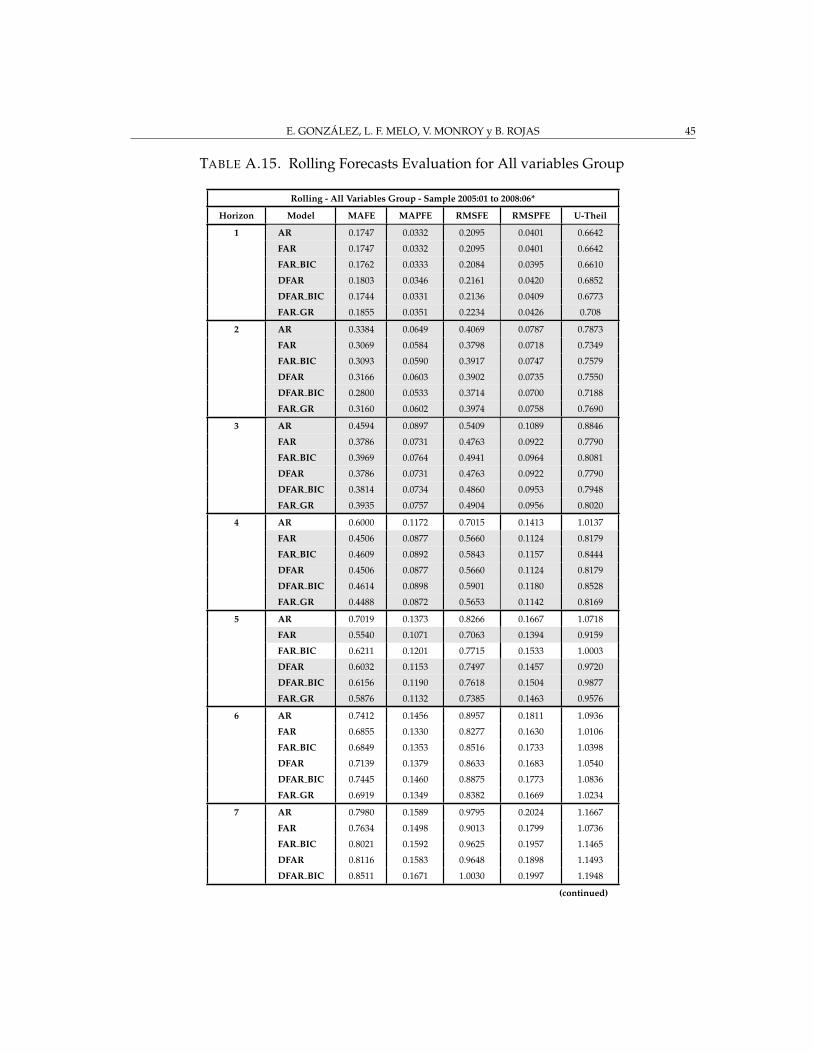
E. GONZALEZ, L. F. MELO, V. MONROY y B. ROJAS 45
TABLE A.15. Rolling Forecasts Evaluation for All variables Group
Rolling - All Variables Group - Sample 2005:01 to 2008:06*
Horizon Model MAFE MAPFE RMSFE RMSPFE U-Theil
1 AR 0.1747 0.0332 0.2095 0.0401 0.6642
FAR 0.1747 0.0332 0.2095 0.0401 0.6642
FAR BIC 0.1762 0.0333 0.2084 0.0395 0.6610
DFAR 0.1803 0.0346 0.2161 0.0420 0.6852
DFAR BIC 0.1744 0.0331 0.2136 0.0409 0.6773
FAR GR 0.1855 0.0351 0.2234 0.0426 0.708
2 AR 0.3384 0.0649 0.4069 0.0787 0.7873
FAR 0.3069 0.0584 0.3798 0.0718 0.7349
FAR BIC 0.3093 0.0590 0.3917 0.0747 0.7579
DFAR 0.3166 0.0603 0.3902 0.0735 0.7550
DFAR BIC 0.2800 0.0533 0.3714 0.0700 0.7188
FAR GR 0.3160 0.0602 0.3974 0.0758 0.7690
3 AR 0.4594 0.0897 0.5409 0.1089 0.8846
FAR 0.3786 0.0731 0.4763 0.0922 0.7790
FAR BIC 0.3969 0.0764 0.4941 0.0964 0.8081
DFAR 0.3786 0.0731 0.4763 0.0922 0.7790
DFAR BIC 0.3814 0.0734 0.4860 0.0953 0.7948
FAR GR 0.3935 0.0757 0.4904 0.0956 0.8020
4 AR 0.6000 0.1172 0.7015 0.1413 1.0137
FAR 0.4506 0.0877 0.5660 0.1124 0.8179
FAR BIC 0.4609 0.0892 0.5843 0.1157 0.8444
DFAR 0.4506 0.0877 0.5660 0.1124 0.8179
DFAR BIC 0.4614 0.0898 0.5901 0.1180 0.8528
FAR GR 0.4488 0.0872 0.5653 0.1142 0.8169
5 AR 0.7019 0.1373 0.8266 0.1667 1.0718
FAR 0.5540 0.1071 0.7063 0.1394 0.9159
FAR BIC 0.6211 0.1201 0.7715 0.1533 1.0003
DFAR 0.6032 0.1153 0.7497 0.1457 0.9720
DFAR BIC 0.6156 0.1190 0.7618 0.1504 0.9877
FAR GR 0.5876 0.1132 0.7385 0.1463 0.9576
6 AR 0.7412 0.1456 0.8957 0.1811 1.0936
FAR 0.6855 0.1330 0.8277 0.1630 1.0106
FAR BIC 0.6849 0.1353 0.8516 0.1733 1.0398
DFAR 0.7139 0.1379 0.8633 0.1683 1.0540
DFAR BIC 0.7445 0.1460 0.8875 0.1773 1.0836
FAR GR 0.6919 0.1349 0.8382 0.1669 1.0234
7 AR 0.7980 0.1589 0.9795 0.2024 1.1667
FAR 0.7634 0.1498 0.9013 0.1799 1.0736
FAR BIC 0.8021 0.1592 0.9625 0.1957 1.1465
DFAR 0.8116 0.1583 0.9648 0.1898 1.1493
DFAR BIC 0.8511 0.1671 1.0030 0.1997 1.1948
(continued)
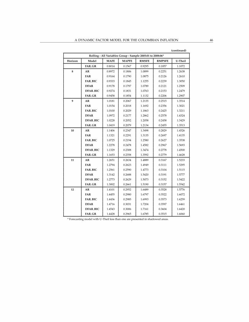
A DYNAMIC FACTOR MODEL FOR THE COLOMBIAN INFLATION 46
(continued)
Rolling - All Variables Group - Sample 2005:01 to 2008:06*
Horizon Model MAFE MAPFE RMSFE RMPSFE U-Theil
FAR GR 0.8014 0.1567 0.9295 0.1857 1.1072
8 AR 0.8972 0.1806 1.0899 0.2251 1.2638
FAR 0.9164 0.1790 1.0875 0.2126 1.2610
FAR BIC 0.9333 0.1845 1.1255 0.2239 1.3050
DFAR 0.9178 0.1797 1.0789 0.2121 1.2509
DFAR BIC 0.9274 0.1831 1.0763 0.2153 1.2479
FAR GR 0.9458 0.1854 1.1132 0.2206 1.2907
9 AR 1.0181 0.2067 1.2135 0.2515 1.3514
FAR 1.0154 0.2018 1.1692 0.2356 1.3021
FAR BIC 1.0100 0.2029 1.1863 0.2425 1.3211
DFAR 1.0972 0.2177 1.2862 0.2578 1.4324
DFAR BIC 1.0228 0.2052 1.2058 0.2458 1.3429
FAR GR 1.0419 0.2079 1.2134 0.2455 1.3513
10 AR 1.1406 0.2347 1.3498 0.2829 1.4526
FAR 1.1321 0.2291 1.3135 0.2697 1.4135
FAR BIC 1.0725 0.2194 1.2580 0.2627 1.3538
DFAR 1.2278 0.2478 1.4582 0.2967 1.5693
DFAR BIC 1.1329 0.2308 1.3474 0.2778 1.4500
FAR GR 1.1653 0.2358 1.3592 0.2779 1.4628
11 AR 1.2651 0.2634 1.4889 0.3167 1.5233
FAR 1.2794 0.2623 1.4949 0.3111 1.5295
FAR BIC 1.2561 0.2590 1.4773 0.3104 1.5115
DFAR 1.3142 0.2688 1.5420 0.3191 1.5777
DFAR BIC 1.2773 0.2629 1.5073 0.3152 1.5422
FAR GR 1.3002 0.2661 1.5190 0.3157 1.5542
12 AR 1.4101 0.2952 1.6489 0.3528 1.5776
FAR 1.4455 0.2980 1.6797 0.3522 1.6072
FAR BIC 1.4436 0.2985 1.6993 0.3573 1.6259
DFAR 1.4716 0.3031 1.7204 0.3597 1.6461
DFAR BIC 1.4543 0.3006 1.7161 0.3604 1.6420
FAR GR 1.4428 0.2965 1.6785 0.3515 1.6060
* Forecasting model with U-Theil less than one are presented in shadowed areas.

E. GONZALEZ, L. F. MELO, V. MONROY y B. ROJAS 47
TABLE A.16. Rolling Forecasts Evaluation for Real Activity Group
Rolling - Real Activity Group - Sample 2005:01 to 2008:06*
Horizon Model MAFE MAPFE RMSFE RMSPFE U-Theil
1 AR 0.1675 0.0313 0.2041 0.0381 0.6471
FAR 0.1777 0.0334 0.2141 0.0404 0.6791
FAR BIC 0.1675 0.0313 0.2041 0.0381 0.6471
DFAR 0.1777 0.0334 0.2141 0.0404 0.6791
DFAR BIC 0.1675 0.0313 0.2041 0.0381 0.6471
2 AR 0.3384 0.0649 0.4069 0.0787 0.7873
FAR 0.3434 0.0661 0.4046 0.0782 0.7830
FAR BIC 0.3384 0.0649 0.4069 0.0787 0.7873
DFAR 0.3434 0.0661 0.4046 0.0782 0.7830
DFAR BIC 0.3384 0.0649 0.4069 0.0787 0.7873
3 AR 0.4594 0.0897 0.5409 0.1089 0.8846
FAR 0.4562 0.0887 0.5419 0.1079 0.8863
FAR BIC 0.4594 0.0897 0.5409 0.1089 0.8846
DFAR 0.4562 0.0887 0.5419 0.1079 0.8863
DFAR BIC 0.4661 0.0910 0.5496 0.1104 0.8989
4 AR 0.6000 0.1172 0.7015 0.1413 1.0137
FAR 0.6038 0.1173 0.7144 0.1429 1.0324
FAR BIC 0.5973 0.1165 0.6948 0.1401 1.0041
DFAR 0.5923 0.1152 0.7097 0.1421 1.0257
DFAR BIC 0.5979 0.1165 0.7014 0.1409 1.0136
5 AR 0.7019 0.1373 0.8266 0.1667 1.0718
FAR 0.7030 0.1375 0.8199 0.1655 1.0631
FAR BIC 0.7000 0.1369 0.8233 0.1663 1.0675
DFAR 0.7030 0.1375 0.8199 0.1655 1.0631
DFAR BIC 0.6944 0.1360 0.8137 0.1650 1.0551
6 AR 0.7412 0.1456 0.8957 0.1811 1.0936
FAR 0.7472 0.1471 0.9013 0.1833 1.1005
FAR BIC 0.7412 0.1456 0.8957 0.1811 1.0936
DFAR 0.7225 0.1431 0.8829 0.1810 1.0780
DFAR BIC 0.7303 0.1438 0.8781 0.1788 1.0721
7 AR 0.7980 0.1589 0.9795 0.2024 1.1667
FAR 0.8175 0.1631 0.9994 0.2060 1.1904
FAR BIC 0.7980 0.1589 0.9795 0.2024 1.1667
DFAR 0.7796 0.1567 0.9685 0.2017 1.1537
DFAR BIC 0.7756 0.1552 0.9637 0.2003 1.1479
8 AR 0.8972 0.1806 1.0899 0.2251 1.2638
FAR 0.9308 0.1871 1.1319 0.2334 1.3124
FAR BIC 0.8840 0.1787 1.0931 0.2265 1.2674
DFAR 0.9070 0.1831 1.1168 0.2313 1.2949
DFAR BIC 0.8911 0.1800 1.1050 0.2285 1.2812
(continued)

A DYNAMIC FACTOR MODEL FOR THE COLOMBIAN INFLATION 48
(continued)
Rolling - Real Activity Group - Sample 2005:01 to 2008:06*
Horizon Model MAFE MAPFE RMSFE RMPSFE U-Theil
9 AR 1.0181 0.2067 1.2135 0.2515 1.3514
FAR 1.0566 0.2141 1.2507 0.2584 1.3929
FAR BIC 1.0227 0.2079 1.2247 0.2541 1.3639
DFAR 1.0593 0.2148 1.2605 0.2604 1.4038
DFAR BIC 1.0348 0.2104 1.2490 0.2586 1.3910
10 AR 1.1406 0.2347 1.3498 0.2829 1.4526
FAR 1.1490 0.2365 1.3656 0.2868 1.4697
FAR BIC 1.1346 0.2338 1.3420 0.2822 1.4443
DFAR 1.1355 0.2342 1.3561 0.2856 1.4594
DFAR BIC 1.1332 0.2338 1.3484 0.2837 1.4511
11 AR 1.2651 0.2634 1.4889 0.3167 1.5233
FAR 1.2766 0.2660 1.5228 0.3234 1.5580
FAR BIC 1.2752 0.2655 1.5049 0.3198 1.5397
DFAR 1.2759 0.2659 1.5287 0.3244 1.5641
DFAR BIC 1.2759 0.2656 1.5131 0.3212 1.5481
12 AR 1.4101 0.2952 1.6489 0.3528 1.5776
FAR 1.4045 0.2948 1.6565 0.3554 1.5850
FAR BIC 1.4008 0.2935 1.6382 0.3510 1.5675
DFAR 1.4348 0.3006 1.6982 0.3627 1.6248
DFAR BIC 1.4313 0.2994 1.6814 0.3586 1.6087
* Forecasting model with U-Theil less than one are presented in shadowed areas.

E. GONZALEZ, L. F. MELO, V. MONROY y B. ROJAS 49
TABLE A.17. Rolling Forecasts Evaluation for Prices Group
Rolling - Prices Group - Sample 2005:01 to 2008:06*
Horizon Model MAFE MAPFE RMSFE RMSPFE U-Theil
1 AR 0.1675 0.0313 0.2041 0.0381 0.6471
FAR 0.1742 0.0334 0.2098 0.0410 0.6654
FAR BIC 0.1718 0.0327 0.2099 0.0406 0.6658
DFAR 0.1742 0.0334 0.2098 0.0410 0.6654
DFAR BIC 0.1769 0.0338 0.2140 0.0415 0.6787
2 AR 0.3384 0.0649 0.4069 0.0787 0.7873
FAR 0.3092 0.0593 0.3800 0.0728 0.7354
FAR BIC 0.3064 0.0585 0.3818 0.0731 0.7389
DFAR 0.3136 0.0604 0.3798 0.0732 0.7349
DFAR BIC 0.2965 0.0564 0.3679 0.0699 0.7119
3 AR 0.4594 0.0897 0.5409 0.1089 0.8846
FAR 0.3924 0.0756 0.4844 0.0954 0.7922
FAR BIC 0.3761 0.0725 0.4833 0.0939 0.7904
DFAR 0.3979 0.0767 0.4871 0.0958 0.7966
DFAR BIC 0.3679 0.0712 0.4646 0.0921 0.7599
4 AR 0.6000 0.1172 0.7015 0.1413 1.0137
FAR 0.4603 0.0886 0.5888 0.1160 0.8509
FAR BIC 0.4333 0.0840 0.5513 0.1113 0.7967
DFAR 0.4603 0.0886 0.5888 0.1160 0.8509
DFAR BIC 0.4386 0.0851 0.5535 0.1118 0.7999
5 AR 0.7019 0.1373 0.8266 0.1667 1.0718
FAR 0.5540 0.1080 0.6839 0.1388 0.8867
FAR BIC 0.5585 0.1082 0.6911 0.1385 0.8961
DFAR 0.5567 0.1085 0.6874 0.1393 0.8913
DFAR BIC 0.5822 0.1132 0.7047 0.1413 0.9137
6 AR 0.7412 0.1456 0.8957 0.1811 1.0936
FAR 0.6951 0.1353 0.8263 0.1648 1.0090
FAR BIC 0.6767 0.1319 0.8059 0.1607 0.9840
DFAR 0.7115 0.1381 0.8527 0.1686 1.0411
DFAR BIC 0.7348 0.1423 0.8661 0.1698 1.0575
7 AR 0.7980 0.1589 0.9795 0.2024 1.1667
FAR 0.7847 0.1533 0.9094 0.1810 1.0832
FAR BIC 0.7660 0.1499 0.8840 0.1766 1.0530
DFAR 0.8112 0.1582 0.9329 0.1849 1.1113
DFAR BIC 0.8139 0.1584 0.9376 0.1847 1.1168
8 AR 0.8972 0.1806 1.0899 0.2251 1.2638
FAR 0.9032 0.1772 1.0589 0.2093 1.2277
FAR BIC 0.8592 0.1689 1.0083 0.2010 1.1691
DFAR 0.9209 0.1804 1.0793 0.2127 1.2515
DFAR BIC 0.8822 0.1732 1.0375 0.2061 1.2029
(continued)
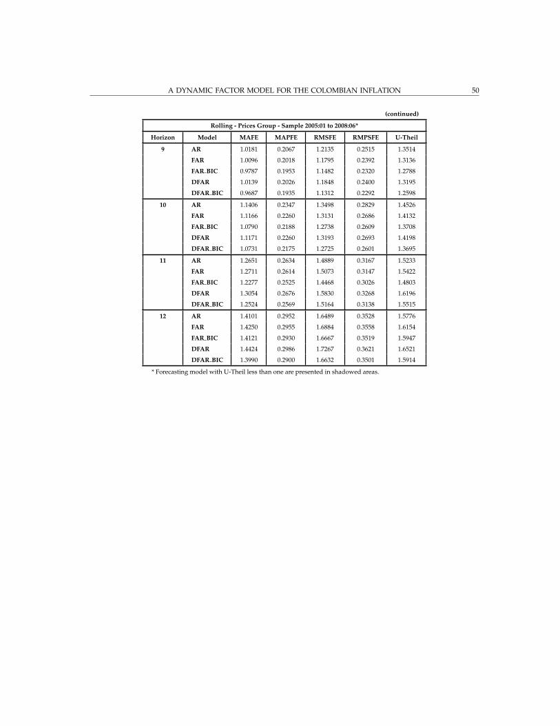
A DYNAMIC FACTOR MODEL FOR THE COLOMBIAN INFLATION 50
(continued)
Rolling - Prices Group - Sample 2005:01 to 2008:06*
Horizon Model MAFE MAPFE RMSFE RMPSFE U-Theil
9 AR 1.0181 0.2067 1.2135 0.2515 1.3514
FAR 1.0096 0.2018 1.1795 0.2392 1.3136
FAR BIC 0.9787 0.1953 1.1482 0.2320 1.2788
DFAR 1.0139 0.2026 1.1848 0.2400 1.3195
DFAR BIC 0.9687 0.1935 1.1312 0.2292 1.2598
10 AR 1.1406 0.2347 1.3498 0.2829 1.4526
FAR 1.1166 0.2260 1.3131 0.2686 1.4132
FAR BIC 1.0790 0.2188 1.2738 0.2609 1.3708
DFAR 1.1171 0.2260 1.3193 0.2693 1.4198
DFAR BIC 1.0731 0.2175 1.2725 0.2601 1.3695
11 AR 1.2651 0.2634 1.4889 0.3167 1.5233
FAR 1.2711 0.2614 1.5073 0.3147 1.5422
FAR BIC 1.2277 0.2525 1.4468 0.3026 1.4803
DFAR 1.3054 0.2676 1.5830 0.3268 1.6196
DFAR BIC 1.2524 0.2569 1.5164 0.3138 1.5515
12 AR 1.4101 0.2952 1.6489 0.3528 1.5776
FAR 1.4250 0.2955 1.6884 0.3558 1.6154
FAR BIC 1.4121 0.2930 1.6667 0.3519 1.5947
DFAR 1.4424 0.2986 1.7267 0.3621 1.6521
DFAR BIC 1.3990 0.2900 1.6632 0.3501 1.5914
* Forecasting model with U-Theil less than one are presented in shadowed areas.
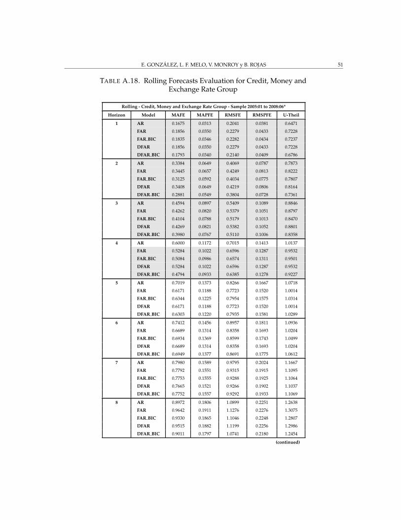
E. GONZALEZ, L. F. MELO, V. MONROY y B. ROJAS 51
TABLE A.18. Rolling Forecasts Evaluation for Credit, Money andExchange Rate Group
Rolling - Credit, Money and Exchange Rate Group - Sample 2005:01 to 2008:06*
Horizon Model MAFE MAPFE RMSFE RMSPFE U-Theil
1 AR 0.1675 0.0313 0.2041 0.0381 0.6471
FAR 0.1856 0.0350 0.2279 0.0433 0.7228
FAR BIC 0.1835 0.0346 0.2282 0.0434 0.7237
DFAR 0.1856 0.0350 0.2279 0.0433 0.7228
DFAR BIC 0.1793 0.0340 0.2140 0.0409 0.6786
2 AR 0.3384 0.0649 0.4069 0.0787 0.7873
FAR 0.3445 0.0657 0.4249 0.0813 0.8222
FAR BIC 0.3125 0.0592 0.4034 0.0775 0.7807
DFAR 0.3408 0.0649 0.4219 0.0806 0.8164
DFAR BIC 0.2881 0.0549 0.3804 0.0728 0.7361
3 AR 0.4594 0.0897 0.5409 0.1089 0.8846
FAR 0.4262 0.0820 0.5379 0.1051 0.8797
FAR BIC 0.4104 0.0788 0.5179 0.1013 0.8470
DFAR 0.4269 0.0821 0.5382 0.1052 0.8801
DFAR BIC 0.3980 0.0767 0.5110 0.1006 0.8358
4 AR 0.6000 0.1172 0.7015 0.1413 1.0137
FAR 0.5284 0.1022 0.6596 0.1287 0.9532
FAR BIC 0.5084 0.0986 0.6574 0.1311 0.9501
DFAR 0.5284 0.1022 0.6596 0.1287 0.9532
DFAR BIC 0.4794 0.0933 0.6385 0.1278 0.9227
5 AR 0.7019 0.1373 0.8266 0.1667 1.0718
FAR 0.6171 0.1188 0.7723 0.1520 1.0014
FAR BIC 0.6344 0.1225 0.7954 0.1575 1.0314
DFAR 0.6171 0.1188 0.7723 0.1520 1.0014
DFAR BIC 0.6303 0.1220 0.7935 0.1581 1.0289
6 AR 0.7412 0.1456 0.8957 0.1811 1.0936
FAR 0.6689 0.1314 0.8358 0.1693 1.0204
FAR BIC 0.6934 0.1369 0.8599 0.1743 1.0499
DFAR 0.6689 0.1314 0.8358 0.1693 1.0204
DFAR BIC 0.6949 0.1377 0.8691 0.1775 1.0612
7 AR 0.7980 0.1589 0.9795 0.2024 1.1667
FAR 0.7792 0.1551 0.9315 0.1915 1.1095
FAR BIC 0.7753 0.1555 0.9288 0.1925 1.1064
DFAR 0.7665 0.1521 0.9266 0.1902 1.1037
DFAR BIC 0.7752 0.1557 0.9292 0.1933 1.1069
8 AR 0.8972 0.1806 1.0899 0.2251 1.2638
FAR 0.9642 0.1911 1.1276 0.2276 1.3075
FAR BIC 0.9330 0.1865 1.1046 0.2248 1.2807
DFAR 0.9515 0.1882 1.1199 0.2256 1.2986
DFAR BIC 0.9011 0.1797 1.0741 0.2180 1.2454
(continued)
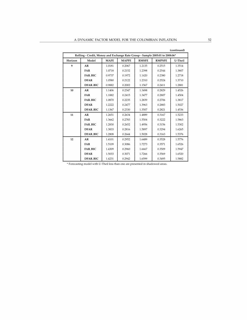
A DYNAMIC FACTOR MODEL FOR THE COLOMBIAN INFLATION 52
(continued)
Rolling - Credit, Money and Exchange Rate Group - Sample 2005:01 to 2008:06*
Horizon Model MAFE MAPFE RMSFE RMPSFE U-Theil
9 AR 1.0181 0.2067 1.2135 0.2515 1.3514
FAR 1.0718 0.2152 1.2398 0.2544 1.3807
FAR BIC 0.9737 0.1972 1.1420 0.2380 1.2718
DFAR 1.0580 0.2122 1.2310 0.2524 1.3710
DFAR BIC 0.9882 0.2002 1.1567 0.2411 1.2881
10 AR 1.1406 0.2347 1.3498 0.2829 1.4526
FAR 1.1882 0.2415 1.3477 0.2807 1.4504
FAR BIC 1.0870 0.2235 1.2839 0.2706 1.3817
DFAR 1.2222 0.2477 1.3963 0.2883 1.5027
DFAR BIC 1.1367 0.2330 1.3507 0.2821 1.4536
11 AR 1.2651 0.2634 1.4889 0.3167 1.5233
FAR 1.3662 0.2783 1.5504 0.3222 1.5863
FAR BIC 1.2830 0.2652 1.4956 0.3156 1.5302
DFAR 1.3833 0.2816 1.5897 0.3294 1.6265
DFAR BIC 1.2808 0.2644 1.5028 0.3163 1.5376
12 AR 1.4101 0.2952 1.6489 0.3528 1.5776
FAR 1.5109 0.3086 1.7273 0.3571 1.6526
FAR BIC 1.4309 0.2960 1.6667 0.3509 1.5947
DFAR 1.5033 0.3071 1.7266 0.3569 1.6520
DFAR BIC 1.4231 0.2942 1.6599 0.3495 1.5882
* Forecasting model with U-Theil less than one are presented in shadowed areas.

E. GONZALEZ, L. F. MELO, V. MONROY y B. ROJAS 53
TABLE A.19. Rolling Forecasts for Evaluation National Accounts Group
Rolling - National Accounts Group - Sample 2005:01 to 2008:06*
Horizon Model MAFE MAPFE RMSFE RMSPFE U-Theil
1 AR 0.1675 0.0313 0.2041 0.0381 0.6471
FAR 0.1673 0.0314 0.2120 0.0395 0.6722
FAR BIC 0.1675 0.0313 0.2041 0.0381 0.6471
DFAR 0.1673 0.0314 0.2120 0.0395 0.6722
DFAR BIC 0.1710 0.0322 0.2179 0.0417 0.6909
2 AR 0.3384 0.0649 0.4069 0.0787 0.7873
FAR 0.3324 0.0638 0.4147 0.0801 0.8024
FAR BIC 0.3384 0.0649 0.4069 0.0787 0.7873
DFAR 0.3324 0.0638 0.4147 0.0801 0.8024
DFAR BIC 0.3384 0.0651 0.4221 0.0829 0.8167
3 AR 0.4594 0.0897 0.5409 0.1089 0.8846
FAR 0.4546 0.0886 0.5370 0.1088 0.8783
FAR BIC 0.4575 0.0893 0.5374 0.1079 0.8789
DFAR 0.4546 0.0886 0.5370 0.1088 0.8783
DFAR BIC 0.4629 0.0904 0.5456 0.1100 0.8923
4 AR 0.6000 0.1172 0.7015 0.1413 1.0137
FAR 0.5886 0.1152 0.6973 0.1409 1.0077
FAR BIC 0.6000 0.1172 0.7015 0.1413 1.0137
DFAR 0.6113 0.1197 0.7116 0.1438 1.0284
DFAR BIC 0.6059 0.1181 0.7039 0.1416 1.0173
5 AR 0.7019 0.1373 0.8266 0.1667 1.0718
FAR 0.6955 0.1356 0.8243 0.1658 1.0689
FAR BIC 0.7019 0.1373 0.8266 0.1667 1.0718
DFAR 0.6834 0.1335 0.8415 0.1705 1.0912
DFAR BIC 0.7281 0.1424 0.8612 0.1739 1.1167
6 AR 0.7412 0.1456 0.8957 0.1811 1.0936
FAR 0.7632 0.1499 0.9267 0.1888 1.1315
FAR BIC 0.7412 0.1456 0.8957 0.1811 1.0936
DFAR 0.7529 0.1508 0.9788 0.2083 1.1951
DFAR BIC 0.7641 0.1526 0.9491 0.1997 1.1588
7 AR 0.7980 0.1589 0.9795 0.2024 1.1667
FAR 0.7898 0.1584 0.9706 0.2029 1.1562
FAR BIC 0.7980 0.1589 0.9795 0.2024 1.1667
DFAR 0.7946 0.1613 1.0627 0.2294 1.2659
DFAR BIC 0.8170 0.1645 1.0441 0.2219 1.2437
8 AR 0.8972 0.1806 1.0899 0.2251 1.2638
FAR 0.8886 0.1806 1.0934 0.2295 1.2678
FAR BIC 0.8972 0.1806 1.0899 0.2251 1.2638
DFAR 0.8910 0.1822 1.1780 0.2542 1.3659
DFAR BIC 0.9163 0.1866 1.1607 0.2468 1.3459
(continued)

A DYNAMIC FACTOR MODEL FOR THE COLOMBIAN INFLATION 54
(continued)
Rolling - National Accounts Group - Sample 2005:01 to 2008:06*
Horizon Model MAFE MAPFE RMSFE RMPSFE U-Theil
9 AR 1.0181 0.2067 1.2135 0.2515 1.3514
FAR 1.0533 0.2143 1.2486 0.2609 1.3905
FAR BIC 1.0191 0.2069 1.2149 0.2517 1.3530
DFAR 1.0363 0.2127 1.2851 0.2748 1.4311
DFAR BIC 0.9922 0.2016 1.2031 0.2496 1.3399
10 AR 1.1406 0.2347 1.3498 0.2829 1.4526
FAR 1.1331 0.2346 1.3546 0.2873 1.4579
FAR BIC 1.1362 0.2338 1.3463 0.2823 1.4488
DFAR 1.1023 0.2287 1.3666 0.2898 1.4707
DFAR BIC 1.1328 0.2333 1.3687 0.2868 1.4730
11 AR 1.2651 0.2634 1.4889 0.3167 1.5233
FAR 1.2883 0.2692 1.5187 0.3252 1.5539
FAR BIC 1.2651 0.2634 1.4889 0.3167 1.5233
DFAR 1.2935 0.2703 1.5397 0.3292 1.5754
DFAR BIC 1.2428 0.2591 1.4846 0.3162 1.5190
12 AR 1.4101 0.2952 1.6489 0.3528 1.5776
FAR 1.4071 0.2954 1.6526 0.3561 1.5812
FAR BIC 1.4101 0.2952 1.6489 0.3528 1.5776
DFAR 1.3654 0.2874 1.6255 0.3515 1.5552
DFAR BIC 1.3756 0.2886 1.6115 0.3462 1.5419
* Forecasting model with U-Theil less than one are presented in shadowed areas.

E. GONZALEZ, L. F. MELO, V. MONROY y B. ROJAS 55
TABLE A.20. Modified Diebold and Mariano Test for All VariablesGroup and Rolling Forecasts
Rolling All Variables Group - Sample 2005:01 to 2008:06*
Horizon = 1
Models AR FAR FAR BIC DFAR DFAR BIC FAR GR
AR 0.671 0.723 0.805 0.811 0.949
FAR 0.329 0.450 0.839 0.660 0.929
FAR BIC 0.277 0.550 0.774 0.740 0.975
DFAR 0.195 0.161 0.227 0.412 0.743
DFAR BIC 0.189 0.340 0.260 0.588 0.855
FAR GR 0.051 0.071 0.025 0.257 0.145
Horizon = 2
Models AR FAR FAR BIC DFAR DFAR BIC FAR GR
AR 0.139 0.220 0.282 0.083 0.321
FAR 0.861 0.866 0.753 0.311 0.923
FAR BIC 0.780 0.134 0.470 0.146 0.742
DFAR 0.718 0.247 0.530 0.175 0.638
DFAR BIC 0.917 0.689 0.854 0.825 0.906
FAR GR 0.679 0.077 0.258 0.362 0.095
Horizon = 3
Models AR FAR FAR BIC DFAR DFAR BIC FAR GR
AR 0.049 0.065 0.049 0.042 0.066
FAR 0.951 0.880 .** 0.676 0.771
FAR BIC 0.935 0.120 0.120 0.296 0.422
DFAR 0.951 .** 0.880 0.676 0.771
DFAR BIC 0.958 0.324 0.704 0.324 0.578
FAR GR 0.934 0.229 0.578 0.229 0.422
Horizon = 4
Models AR FAR FAR BIC DFAR DFAR BIC FAR GR
AR 0.024 0.018 0.024 0.017 0.005
FAR 0.976 0.736 .** 0.754 0.490
FAR BIC 0.982 0.264 0.264 0.677 0.294
DFAR 0.976 .** 0.736 0.754 0.490
DFAR BIC 0.983 0.246 0.323 0.246 0.246
FAR GR 0.995 0.510 0.706 0.510 0.754
Horizon = 5
Models AR FAR FAR BIC DFAR DFAR BIC FAR GR
AR 0.034 0.026 0.098 0.105 0.019
FAR 0.966 0.901 0.823 0.929 0.736
FAR BIC 0.975 0.099 0.278 0.356 0.070
DFAR 0.902 0.177 0.722 0.744 0.324
DFAR BIC 0.895 0.071 0.644 0.256 0.155
(continued)

A DYNAMIC FACTOR MODEL FOR THE COLOMBIAN INFLATION 56
(continued)
Rolling All Variables Group - Sample 2005:01 to 2008:06*
FAR GR 0.981 0.265 0.930 0.676 0.845
Horizon = 6
Models AR FAR FAR BIC DFAR DFAR BIC FAR GR
AR 0.107 0.094 0.315 0.457 0.108
FAR 0.893 0.679 0.823 0.923 0.622
FAR BIC 0.906 0.321 0.568 0.752 0.359
DFAR 0.685 0.177 0.432 0.700 0.245
DFAR BIC 0.544 0.077 0.248 0.300 0.055
FAR GR 0.892 0.378 0.641 0.755 0.945
Horizon = 7
Models AR FAR FAR BIC DFAR DFAR BIC FAR GR
AR 0.180 0.386 0.445 0.594 0.278
FAR 0.820 0.813 0.820 0.935 0.868
FAR BIC 0.614 0.188 0.514 0.828 0.218
DFAR 0.555 0.180 0.486 0.820 0.249
DFAR BIC 0.406 0.065 0.173 0.180 0.037
FAR GR 0.722 0.133 0.782 0.751 0.963
Horizon = 8
Models AR FAR FAR BIC DFAR DFAR BIC FAR GR
AR 0.492 0.666 0.460 0.438 0.585
FAR 0.508 0.739 0.052 0.425 0.737
FAR BIC 0.334 0.261 0.232 0.210 0.316
DFAR 0.540 0.948 0.769 0.481 0.742
DFAR BIC 0.562 0.575 0.790 0.519 0.707
FAR GR 0.416 0.264 0.685 0.258 0.293
Horizon = 9
Models AR FAR FAR BIC DFAR DFAR BIC FAR GR
AR 0.334 0.336 0.695 0.451 0.500
FAR 0.666 0.629 0.827 0.737 0.980
FAR BIC 0.664 0.371 0.784 0.812 0.982
DFAR 0.305 0.173 0.216 0.220 0.242
DFAR BIC 0.549 0.263 0.188 0.780 0.606
FAR GR 0.500 0.020 0.018 0.758 0.394
(continued)
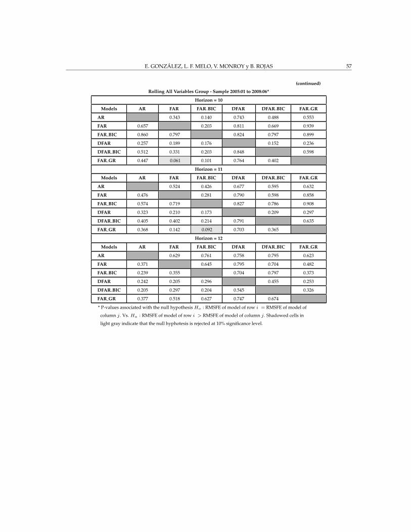
E. GONZALEZ, L. F. MELO, V. MONROY y B. ROJAS 57
(continued)
Rolling All Variables Group - Sample 2005:01 to 2008:06*
Horizon = 10
Models AR FAR FAR BIC DFAR DFAR BIC FAR GR
AR 0.343 0.140 0.743 0.488 0.553
FAR 0.657 0.203 0.811 0.669 0.939
FAR BIC 0.860 0.797 0.824 0.797 0.899
DFAR 0.257 0.189 0.176 0.152 0.236
DFAR BIC 0.512 0.331 0.203 0.848 0.598
FAR GR 0.447 0.061 0.101 0.764 0.402
Horizon = 11
Models AR FAR FAR BIC DFAR DFAR BIC FAR GR
AR 0.524 0.426 0.677 0.595 0.632
FAR 0.476 0.281 0.790 0.598 0.858
FAR BIC 0.574 0.719 0.827 0.786 0.908
DFAR 0.323 0.210 0.173 0.209 0.297
DFAR BIC 0.405 0.402 0.214 0.791 0.635
FAR GR 0.368 0.142 0.092 0.703 0.365
Horizon = 12
Models AR FAR FAR BIC DFAR DFAR BIC FAR GR
AR 0.629 0.761 0.758 0.795 0.623
FAR 0.371 0.645 0.795 0.704 0.482
FAR BIC 0.239 0.355 0.704 0.797 0.373
DFAR 0.242 0.205 0.296 0.455 0.253
DFAR BIC 0.205 0.297 0.204 0.545 0.326
FAR GR 0.377 0.518 0.627 0.747 0.674
* P-values associated with the null hypothesis Ho : RMSFE of model of row i = RMSFE of model of
column j. Vs. Ha : RMSFE of model of row i > RMSFE of model of column j. Shadowed cells in
light gray indicate that the null hyphotesis is rejected at 10% significance level.
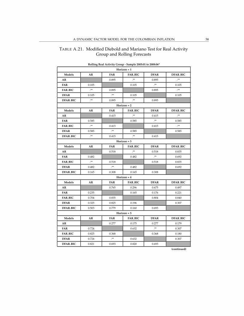
A DYNAMIC FACTOR MODEL FOR THE COLOMBIAN INFLATION 58
TABLE A.21. Modified Diebold and Mariano Test for Real ActivityGroup and Rolling Forecasts
Rolling Real Activity Group - Sample 2005:01 to 2008:06*
Horizon = 1
Models AR FAR FAR BIC DFAR DFAR BIC
AR 0.895 .** 0.895 .**
FAR 0.105 0.105 .** 0.105
FAR BIC .** 0.895 0.895 .**
DFAR 0.105 .** 0.105 0.105
DFAR BIC .** 0.895 .** 0.895
Horizon = 2
Models AR FAR FAR BIC DFAR DFAR BIC
AR 0.415 .** 0.415 .**
FAR 0.585 0.585 .** 0.585
FAR BIC .** 0.415 0.415 .**
DFAR 0.585 .** 0.585 0.585
DFAR BIC .** 0.415 .** 0.415
Horizon = 3
Models AR FAR FAR BIC DFAR DFAR BIC
AR 0.518 .** 0.518 0.835
FAR 0.482 0.482 .** 0.692
FAR BIC .** 0.518 0.518 0.835
DFAR 0.482 .** 0.482 0.692
DFAR BIC 0.165 0.308 0.165 0.308
Horizon = 4
Models AR FAR FAR BIC DFAR DFAR BIC
AR 0.765 0.296 0.675 0.497
FAR 0.235 0.165 0.176 0.221
FAR BIC 0.704 0.835 0.804 0.840
DFAR 0.325 0.825 0.196 0.307
DFAR BIC 0.503 0.779 0.160 0.693
Horizon = 5
Models AR FAR FAR BIC DFAR DFAR BIC
AR 0.277 0.175 0.277 0.179
FAR 0.724 0.632 .** 0.307
FAR BIC 0.825 0.368 0.368 0.180
DFAR 0.724 .** 0.632 0.307
DFAR BIC 0.821 0.693 0.820 0.693
(continued)

E. GONZALEZ, L. F. MELO, V. MONROY y B. ROJAS 59
(continued)
Rolling Real Activity Group - Sample 2005:01 to 2008:06*
Horizon = 6
Models AR FAR FAR BIC DFAR DFAR BIC
AR 0.857 .** 0.328 0.186
FAR 0.144 0.144 0.185 0.002
FAR BIC .** 0.857 0.328 0.186
DFAR 0.672 0.815 0.672 0.231
DFAR BIC 0.814 0.998 0.814 0.769
Horizon = 7
Models AR FAR FAR BIC DFAR DFAR BIC
AR 0.832 .** 0.355 0.177
FAR 0.168 0.168 0.189 0.157
FAR BIC .** 0.832 0.355 0.177
DFAR 0.645 0.811 0.645 0.401
DFAR BIC 0.823 0.843 0.823 0.599
Horizon = 8
Models AR FAR FAR BIC DFAR DFAR BIC
AR 0.847 0.574 0.784 0.861
FAR 0.153 0.062 0.196 0.008
FAR BIC 0.426 0.938 0.945 0.820
DFAR 0.216 0.804 0.055 0.041
DFAR BIC 0.139 0.992 0.180 0.959
Horizon = 9
Models AR FAR FAR BIC DFAR DFAR BIC
AR 0.927 0.956 0.918 0.872
FAR 0.073 0.050 0.881 0.468
FAR BIC 0.044 0.950 0.926 0.836
DFAR 0.083 0.119 0.074 0.308
DFAR BIC 0.128 0.532 0.164 0.692
Horizon = 10
Models AR FAR FAR BIC DFAR DFAR BIC
AR 0.752 0.182 0.591 0.454
FAR 0.248 0.082 0.204 0.132
FAR BIC 0.818 0.918 0.798 0.980
DFAR 0.409 0.797 0.202 0.360
DFAR BIC 0.546 0.868 0.020 0.640
(continued)

A DYNAMIC FACTOR MODEL FOR THE COLOMBIAN INFLATION 60
(continued)
Rolling Real Activity Group - Sample 2005:01 to 2008:06*
Horizon = 11
Models AR FAR FAR BIC DFAR DFAR BIC
AR 0.867 0.875 0.923 0.852
FAR 0.133 0.216 0.921 0.376
FAR BIC 0.125 0.784 0.969 0.862
DFAR 0.077 0.079 0.031 0.245
DFAR BIC 0.148 0.625 0.139 0.755
Horizon = 12
Models AR FAR FAR BIC DFAR DFAR BIC
AR 0.606 0.221 0.985 0.793
FAR 0.394 0.023 0.787 0.646
FAR BIC 0.779 0.977 0.964 0.788
DFAR 0.015 0.213 0.036 0.024
DFAR BIC 0.207 0.354 0.212 0.976
* P-values associated with the null hypothesis Ho : RMSFE of model of row i = RMSFE of model of
column j. Vs. Ha : RMSFE of model of row i > RMSFE of model of column j. Shadowed cells in
light gray indicate that the null hyphotesis is rejected at 10% significance level.
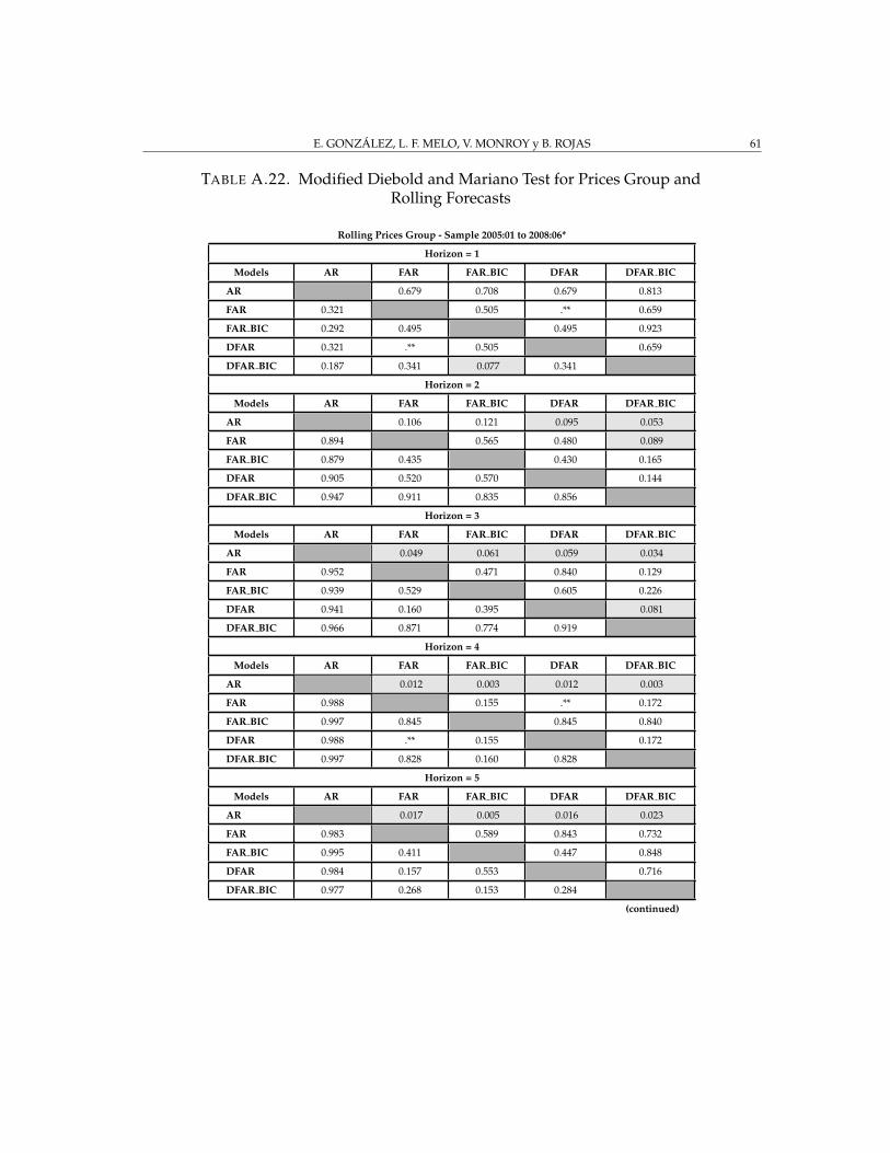
E. GONZALEZ, L. F. MELO, V. MONROY y B. ROJAS 61
TABLE A.22. Modified Diebold and Mariano Test for Prices Group andRolling Forecasts
Rolling Prices Group - Sample 2005:01 to 2008:06*
Horizon = 1
Models AR FAR FAR BIC DFAR DFAR BIC
AR 0.679 0.708 0.679 0.813
FAR 0.321 0.505 .** 0.659
FAR BIC 0.292 0.495 0.495 0.923
DFAR 0.321 .** 0.505 0.659
DFAR BIC 0.187 0.341 0.077 0.341
Horizon = 2
Models AR FAR FAR BIC DFAR DFAR BIC
AR 0.106 0.121 0.095 0.053
FAR 0.894 0.565 0.480 0.089
FAR BIC 0.879 0.435 0.430 0.165
DFAR 0.905 0.520 0.570 0.144
DFAR BIC 0.947 0.911 0.835 0.856
Horizon = 3
Models AR FAR FAR BIC DFAR DFAR BIC
AR 0.049 0.061 0.059 0.034
FAR 0.952 0.471 0.840 0.129
FAR BIC 0.939 0.529 0.605 0.226
DFAR 0.941 0.160 0.395 0.081
DFAR BIC 0.966 0.871 0.774 0.919
Horizon = 4
Models AR FAR FAR BIC DFAR DFAR BIC
AR 0.012 0.003 0.012 0.003
FAR 0.988 0.155 .** 0.172
FAR BIC 0.997 0.845 0.845 0.840
DFAR 0.988 .** 0.155 0.172
DFAR BIC 0.997 0.828 0.160 0.828
Horizon = 5
Models AR FAR FAR BIC DFAR DFAR BIC
AR 0.017 0.005 0.016 0.023
FAR 0.983 0.589 0.843 0.732
FAR BIC 0.995 0.411 0.447 0.848
DFAR 0.984 0.157 0.553 0.716
DFAR BIC 0.977 0.268 0.153 0.284
(continued)
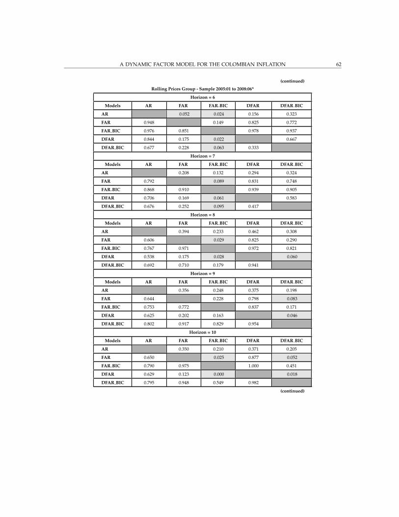
A DYNAMIC FACTOR MODEL FOR THE COLOMBIAN INFLATION 62
(continued)
Rolling Prices Group - Sample 2005:01 to 2008:06*
Horizon = 6
Models AR FAR FAR BIC DFAR DFAR BIC
AR 0.052 0.024 0.156 0.323
FAR 0.948 0.149 0.825 0.772
FAR BIC 0.976 0.851 0.978 0.937
DFAR 0.844 0.175 0.022 0.667
DFAR BIC 0.677 0.228 0.063 0.333
Horizon = 7
Models AR FAR FAR BIC DFAR DFAR BIC
AR 0.208 0.132 0.294 0.324
FAR 0.792 0.089 0.831 0.748
FAR BIC 0.868 0.910 0.939 0.905
DFAR 0.706 0.169 0.061 0.583
DFAR BIC 0.676 0.252 0.095 0.417
Horizon = 8
Models AR FAR FAR BIC DFAR DFAR BIC
AR 0.394 0.233 0.462 0.308
FAR 0.606 0.029 0.825 0.290
FAR BIC 0.767 0.971 0.972 0.821
DFAR 0.538 0.175 0.028 0.060
DFAR BIC 0.692 0.710 0.179 0.941
Horizon = 9
Models AR FAR FAR BIC DFAR DFAR BIC
AR 0.356 0.248 0.375 0.198
FAR 0.644 0.228 0.798 0.083
FAR BIC 0.753 0.772 0.837 0.171
DFAR 0.625 0.202 0.163 0.046
DFAR BIC 0.802 0.917 0.829 0.954
Horizon = 10
Models AR FAR FAR BIC DFAR DFAR BIC
AR 0.350 0.210 0.371 0.205
FAR 0.650 0.025 0.877 0.052
FAR BIC 0.790 0.975 1.000 0.451
DFAR 0.629 0.123 0.000 0.018
DFAR BIC 0.795 0.948 0.549 0.982
(continued)

E. GONZALEZ, L. F. MELO, V. MONROY y B. ROJAS 63
(continued)
Rolling Prices Group - Sample 2005:01 to 2008:06*
Horizon = 11
Models AR FAR FAR BIC DFAR DFAR BIC
AR 0.597 0.308 0.804 0.617
FAR 0.403 0.009 0.785 0.554
FAR BIC 0.693 0.990 0.875 0.785
DFAR 0.196 0.215 0.125 0.0146
DFAR BIC 0.383 0.446 0.215 0.985
Horizon = 12
Models AR FAR FAR BIC DFAR DFAR BIC
AR 0.709 0.617 0.987 0.602
FAR 0.291 0.217 0.786 0.316
FAR BIC 0.383 0.783 0.858 0.436
DFAR 0.013 0.214 0.142 0.016
DFAR BIC 0.399 0.684 0.564 0.984
* P-values associated with the null hypothesis Ho : RMSFE of model of row i = RMSFE of model of
column j. Vs. Ha : RMSFE of model of row i > RMSFE of model of column j. Shadowed cells in
light gray indicate that the null hyphotesis is rejected at 10% significance level.
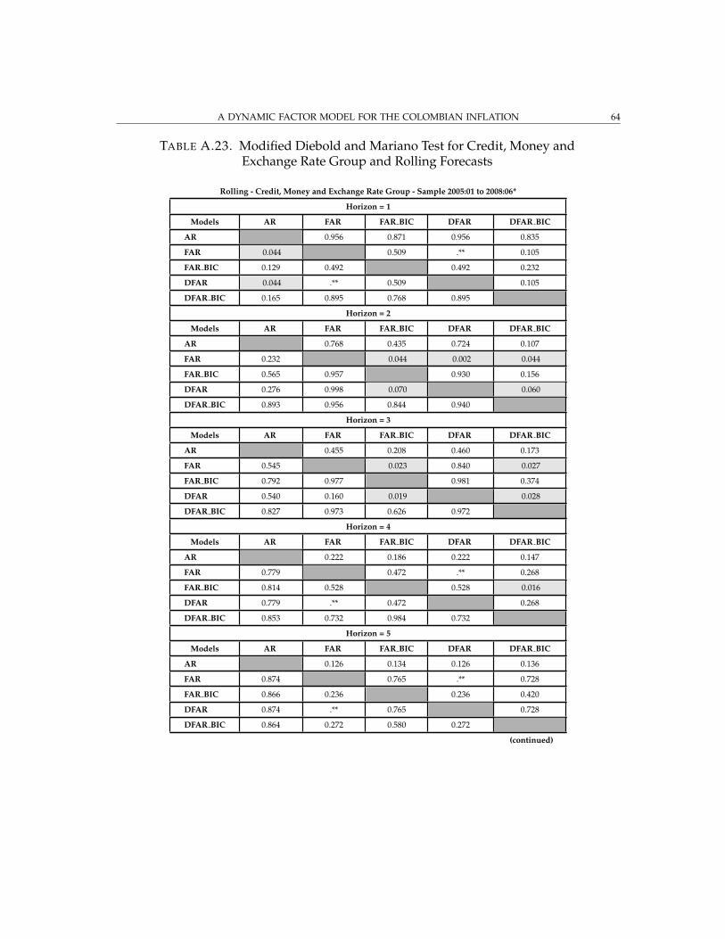
A DYNAMIC FACTOR MODEL FOR THE COLOMBIAN INFLATION 64
TABLE A.23. Modified Diebold and Mariano Test for Credit, Money andExchange Rate Group and Rolling Forecasts
Rolling - Credit, Money and Exchange Rate Group - Sample 2005:01 to 2008:06*
Horizon = 1
Models AR FAR FAR BIC DFAR DFAR BIC
AR 0.956 0.871 0.956 0.835
FAR 0.044 0.509 .** 0.105
FAR BIC 0.129 0.492 0.492 0.232
DFAR 0.044 .** 0.509 0.105
DFAR BIC 0.165 0.895 0.768 0.895
Horizon = 2
Models AR FAR FAR BIC DFAR DFAR BIC
AR 0.768 0.435 0.724 0.107
FAR 0.232 0.044 0.002 0.044
FAR BIC 0.565 0.957 0.930 0.156
DFAR 0.276 0.998 0.070 0.060
DFAR BIC 0.893 0.956 0.844 0.940
Horizon = 3
Models AR FAR FAR BIC DFAR DFAR BIC
AR 0.455 0.208 0.460 0.173
FAR 0.545 0.023 0.840 0.027
FAR BIC 0.792 0.977 0.981 0.374
DFAR 0.540 0.160 0.019 0.028
DFAR BIC 0.827 0.973 0.626 0.972
Horizon = 4
Models AR FAR FAR BIC DFAR DFAR BIC
AR 0.222 0.186 0.222 0.147
FAR 0.779 0.472 .** 0.268
FAR BIC 0.814 0.528 0.528 0.016
DFAR 0.779 .** 0.472 0.268
DFAR BIC 0.853 0.732 0.984 0.732
Horizon = 5
Models AR FAR FAR BIC DFAR DFAR BIC
AR 0.126 0.134 0.126 0.136
FAR 0.874 0.765 .** 0.728
FAR BIC 0.866 0.236 0.236 0.420
DFAR 0.874 .** 0.765 0.728
DFAR BIC 0.864 0.272 0.580 0.272
(continued)

E. GONZALEZ, L. F. MELO, V. MONROY y B. ROJAS 65
(continued)
Rolling - Credit, Money and Exchange Rate Group - Sample 2005:01 to 2008:06*
Horizon = 6
Models AR FAR FAR BIC DFAR DFAR BIC
AR 0.011 0.042 0.011 0.221
FAR 0.989 0.890 .** 0.863
FAR BIC 0.958 0.110 0.110 0.713
DFAR 0.989 .** 0.890 0.863
DFAR BIC 0.779 0.138 0.288 0.138
Horizon = 7
Models AR FAR FAR BIC DFAR DFAR BIC
AR 0.127 0.052 0.107 0.195
FAR 0.874 0.441 0.151 0.477
FAR BIC 0.948 0.559 0.462 0.506
DFAR 0.893 0.849 0.538 0.524
DFAR BIC 0.805 0.523 0.494 0.476
Horizon = 8
Models AR FAR FAR BIC DFAR DFAR BIC
AR 0.749 0.609 0.719 0.426
FAR 0.251 0.037 0.146 0.000
FAR BIC 0.391 0.964 0.847 0.089
DFAR 0.281 0.854 0.153 0.026
DFAR BIC 0.574 1.000 0.911 0.973
Horizon = 9
Models AR FAR FAR BIC DFAR DFAR BIC
AR 0.674 0.142 0.628 0.203
FAR 0.326 0.002 0.138 0.015
FAR BIC 0.858 0.998 0.989 0.952
DFAR 0.372 0.862 0.011 0.046
DFAR BIC 0.797 0.985 0.048 0.954
Horizon = 10
Models AR FAR FAR BIC DFAR DFAR BIC
AR 0.491 0.024 0.771 0.507
FAR 0.509 0.112 0.793 0.511
FAR BIC 0.976 0.888 1.000 0.848
DFAR 0.229 0.207 0.000 0.192
DFAR BIC 0.493 0.490 0.152 0.808
(continued)

A DYNAMIC FACTOR MODEL FOR THE COLOMBIAN INFLATION 66
(continued)
Rolling - Credit, Money and Exchange Rate Group - Sample 2005:01 to 2008:06*
Horizon = 11
Models AR FAR FAR BIC DFAR DFAR BIC
AR 0.677 0.558 0.796 0.591
FAR 0.323 0.291 0.799 0.325
FAR BIC 0.442 0.709 0.882 0.736
DFAR 0.204 0.201 0.118 0.134
DFAR BIC 0.409 0.675 0.264 0.867
Horizon = 12
Models AR FAR FAR BIC DFAR DFAR BIC
AR 0.660 0.613 0.658 0.569
FAR 0.340 0.312 0.463 0.283
FAR BIC 0.387 0.688 0.685 0.165
DFAR 0.342 0.537 0.315 0.288
DFAR BIC 0.431 0.717 0.835 0.712
* P-values associated with the null hypothesis Ho : RMSFE of model of row i = RMSFE of model of
column j. Vs. Ha : RMSFE of model of row i > RMSFE of model of column j. Shadowed cells in
light gray indicate that the null hyphotesis is rejected at 10% significance level.

E. GONZALEZ, L. F. MELO, V. MONROY y B. ROJAS 67
TABLE A.24. Modified Diebold and Mariano Test for National AccountsGroup and Rolling Forecasts
Rolling - National Accounts Group - Sample 2005:01 to 2008:06*
Horizon = 1
Models AR FAR FAR BIC DFAR DFAR BIC
AR 0.844 .** 0.844 0.834
FAR 0.156 0.156 .** 0.644
FAR BIC .** 0.844 0.844 0.834
DFAR 0.156 .** 0.156 0.644
DFAR BIC 0.166 0.356 0.166 0.356
Horizon = 2
Models AR FAR FAR BIC DFAR DFAR BIC
AR 0.778 .** 0.778 0.769
FAR 0.222 0.222 .** 0.622
FAR BIC .** 0.778 0.778 0.769
DFAR 0.222 .** 0.222 0.622
DFAR BIC 0.231 0.378 0.231 0.378
Horizon = 3
Models AR FAR FAR BIC DFAR DFAR BIC
AR 0.077 0.160 0.077 0.617
FAR 0.923 0.516 .** 0.752
FAR BIC 0.840 0.484 0.484 0.676
DFAR 0.923 .** 0.516 0.752
DFAR BIC 0.384 0.248 0.324 0.248
Horizon = 4
Models AR FAR FAR BIC DFAR DFAR BIC
AR 0.391 .** 0.684 0.841
FAR 0.609 0.609 0.840 0.672
FAR BIC .** 0.391 0.684 0.841
DFAR 0.316 0.160 0.316 0.359
DFAR BIC 0.159 0.328 0.159 0.641
Horizon = 5
Models AR FAR FAR BIC DFAR DFAR BIC
AR 0.433 .** 0.629 0.924
FAR 0.567 0.567 0.658 0.963
FAR BIC .** 0.433 0.629 0.924
DFAR 0.371 0.342 0.371 0.819
DFAR BIC 0.076 0.037 0.076 0.181
(continued)

A DYNAMIC FACTOR MODEL FOR THE COLOMBIAN INFLATION 68
(continued)
Rolling - National Accounts Group - Sample 2005:01 to 2008:06*
Horizon = 6
Models AR FAR FAR BIC DFAR DFAR BIC
AR 0.947 .** 0.722 0.710
FAR 0.053 0.053 0.657 0.603
FAR BIC .** 0.947 0.722 0.710
DFAR 0.278 0.343 0.278 0.252
DFAR BIC 0.290 0.398 0.290 0.748
Horizon = 7
Models AR FAR FAR BIC DFAR DFAR BIC
AR 0.366 .** 0.677 0.716
FAR 0.634 0.634 0.716 0.791
FAR BIC .** 0.366 0.677 0.716
DFAR 0.323 0.284 0.323 0.391
DFAR BIC 0.284 0.209 0.284 0.609
Horizon = 8
Models AR FAR FAR BIC DFAR DFAR BIC
AR 0.523 .** 0.750 0.741
FAR 0.477 0.477 0.820 0.842
FAR BIC .** 0.523 0.750 0.741
DFAR 0.250 0.180 0.250 0.348
DFAR BIC 0.259 0.158 0.259 0.652
Horizon = 9
Models AR FAR FAR BIC DFAR DFAR BIC
AR 0.819 0.823 0.789 0.369
FAR 0.182 0.196 0.761 0.058
FAR BIC 0.177 0.804 0.781 0.348
DFAR 0.211 0.239 0.219 0.187
DFAR BIC 0.631 0.942 0.652 0.813
Horizon = 10
Models AR FAR FAR BIC DFAR DFAR BIC
AR 0.536 0.146 0.635 0.743
FAR 0.464 0.434 0.648 0.577
FAR BIC 0.854 0.567 0.646 0.778
DFAR 0.365 0.352 0.354 0.518
DFAR BIC 0.257 0.423 0.222 0.482
(continued)

E. GONZALEZ, L. F. MELO, V. MONROY y B. ROJAS 69
(continued)
Rolling - National Accounts Group - Sample 2005:01 to 2008:06*
Horizon = 11
Models AR FAR FAR BIC DFAR DFAR BIC
AR 0.812 .** 0.978 0.412
FAR 0.188 0.188 0.898 0.264
FAR BIC .** 0.812 0.978 0.412
DFAR 0.022 0.102 0.022 0.090
DFAR BIC 0.588 0.736 0.588 0.910
Horizon = 12
Models AR FAR FAR BIC DFAR DFAR BIC
AR 0.533 .** 0.389 0.214
FAR 0.467 0.467 0.203 0.164
FAR BIC .** 0.533 0.389 0.214
DFAR 0.611 0.797 0.611 0.026
DFAR BIC 0.786 0.836 0.786 0.974
(continued)
* P-values associated with the null hypothesis Ho : RMSFE of model of row i = RMSFE of model of
column j. Vs. Ha : RMSFE of model of row i > RMSFE of model of column j. Shadowed cells in
light gray indicate that the null hyphotesis is rejected at 10% significance level.

A DYNAMIC FACTOR MODEL FOR THE COLOMBIAN INFLATION 70
TABLE A.25. Modified Diebold and Mariano Tests for Recursive andRolling Forecasts - All Variables Group
All Variables Group - Sample 2005:01 to 2008:06*
Horizon = 1hhhhhhhhhhRolling
Recursive AR FAR FAR BIC DFAR DFAR BIC FAR GR
AR 0.0610 0.5066 0.3780 0.6193 0.5726 0.7476
FAR 0.1531 0.1321 0.1728 0.4243 0.4037 0.6344
FAR BIC 0.0950 0.3295 0.0544 0.4916 0.4288 0.6800
DFAR 0.0868 0.0758 0.0833 0.0400 0.2309 0.3821
DFAR BIC 0.0775 0.1984 0.0925 0.3172 0.1964 0.4624
FAR GR 0.0122 0.0209 0.0021 0.0747 0.0599 0.0104
Horizon = 2hhhhhhhhhhRolling
Recursive AR FAR FAR BIC DFAR DFAR BIC FAR GR
AR 0.1338 0.1029 0.0917 0.2016 0.0568 0.1757
FAR 0.6753 0.1545 0.3757 0.5162 0.2319 0.5919
FAR BIC 0.5135 0.0982 0.0692 0.3103 0.0795 0.3131
DFAR 0.5296 0.1367 0.2437 0.1117 0.1182 0.3919
DFAR BIC 0.7588 0.5052 0.5819 0.6642 0.4467 0.6943
FAR GR 0.4167 0.0373 0.0172 0.2176 0.0420 0.0858
Horizon = 3hhhhhhhhhhRolling
Recursive AR FAR FAR BIC DFAR DFAR BIC FAR GR
AR 0.2011 0.0279 0.0175 0.0279 0.0017 0.0321
FAR 0.8586 0.0812 0.5034 0.0812 0.3107 0.4705
FAR BIC 0.7723 0.0658 0.1871 0.0658 0.0789 0.2323
DFAR 0.8586 0.0812 0.5034 0.0812 0.3107 0.4705
DFAR BIC 0.8338 0.1737 0.3574 0.1737 0.1246 0.3407
FAR GR 0.8175 0.0680 0.2180 0.0680 0.0925 0.0623
Horizon = 4hhhhhhhhhhRolling
Recursive AR FAR FAR BIC DFAR DFAR BIC FAR GR
AR 0.2948 0.0114 0.0119 0.0114 0.0083 0.0015
FAR 0.9644 0.0810 0.3585 0.0810 0.4014 0.2521
FAR BIC 0.9560 0.1543 0.2389 0.1543 0.2552 0.1830
DFAR 0.9644 0.0810 0.3585 0.0810 0.4014 0.2521
DFAR BIC 0.9549 0.1462 0.2034 0.1462 0.1930 0.1558
FAR GR 0.9934 0.1637 0.3309 0.1637 0.3584 0.0750
Horizon = 5hhhhhhhhhhRolling
Recursive AR FAR FAR BIC DFAR DFAR BIC FAR GR
AR 0.5047 0.0148 0.0380 0.0526 0.0171 0.0108
FAR 0.9659 0.1292 0.8777 0.6824 0.7391 0.5627
FAR BIC 0.9421 0.0473 0.3840 0.1498 0.0414 0.0682
DFAR 0.8990 0.0971 0.6694 0.1292 0.2719 0.2075
(continued)

E. GONZALEZ, L. F. MELO, V. MONROY y B. ROJAS 71
(continued)
All Variables Group - Sample 2005:01 to 2008:06*
DFAR BIC 0.8875 0.0279 0.5697 0.1025 0.1074 0.1243
FAR GR 0.9855 0.1352 0.9454 0.3439 0.3205 0.1385
Horizon = 6hhhhhhhhhhRolling
Recursive AR FAR FAR BIC DFAR DFAR BIC FAR GR
AR 0.5928 0.0660 0.1765 0.2548 0.4441 0.0775
FAR 0.9135 0.1809 0.6912 0.7133 0.8609 0.4538
FAR BIC 0.9091 0.2244 0.5534 0.4988 0.7056 0.2444
DFAR 0.7094 0.1126 0.4495 0.1809 0.6460 0.1946
DFAR BIC 0.5717 0.0204 0.2463 0.1932 0.4336 0.0333
FAR GR 0.9297 0.1867 0.6713 0.6635 0.8925 0.1629
Horizon = 7hhhhhhhhhhRolling
Recursive AR FAR FAR BIC DFAR DFAR BIC FAR GR
AR 0.7170 0.1614 0.4930 0.4278 0.6184 0.2383
FAR 0.8863 0.2324 0.9104 0.7978 0.9521 0.7188
FAR BIC 0.6908 0.1574 0.8578 0.4854 0.8324 0.1217
DFAR 0.6011 0.1606 0.5875 0.2324 0.8321 0.2019
DFAR BIC 0.4498 0.0504 0.2751 0.1409 0.6374 0.0187
FAR GR 0.7854 0.0752 0.9490 0.7211 0.9680 0.1911
Horizon = 8hhhhhhhhhhRolling
Recursive AR FAR FAR BIC DFAR DFAR BIC FAR GR
AR 0.2420 0.4778 0.6560 0.4440 0.4102 0.5506
FAR 0.4924 0.2528 0.7197 0.0136 0.3965 0.6265
FAR BIC 0.3174 0.2247 0.2141 0.2000 0.1939 0.1173
DFAR 0.5221 0.9046 0.7516 0.2528 0.4431 0.6597
DFAR BIC 0.5397 0.5513 0.7804 0.4881 0.1052 0.6565
FAR GR 0.4008 0.2134 0.6443 0.2244 0.2738 0.1673
Horizon = 9hhhhhhhhhhRolling
Recursive AR FAR FAR BIC DFAR DFAR BIC FAR GR
AR 0.2387 0.3436 0.3424 0.6991 0.4547 0.4837
FAR 0.6523 0.8512 0.6393 0.8327 0.7448 0.9446
FAR BIC 0.6452 0.3903 0.7558 0.7889 0.8269 1.0000
DFAR 0.2982 0.1788 0.2181 0.8512 0.2224 0.2308
DFAR BIC 0.5283 0.2818 0.2062 0.7851 0.8364 0.5680
FAR GR 0.4857 0.0396 0.0059 0.7650 0.3955 0.1737
(continued)
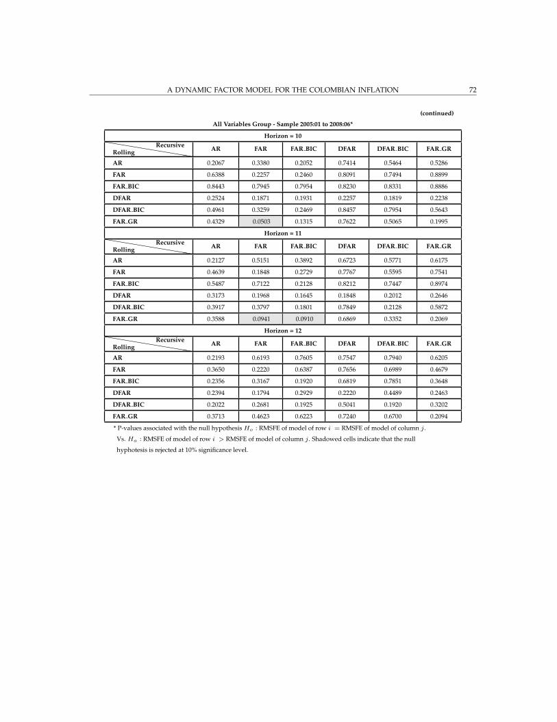
A DYNAMIC FACTOR MODEL FOR THE COLOMBIAN INFLATION 72
(continued)
All Variables Group - Sample 2005:01 to 2008:06*
Horizon = 10hhhhhhhhhhRolling
Recursive AR FAR FAR BIC DFAR DFAR BIC FAR GR
AR 0.2067 0.3380 0.2052 0.7414 0.5464 0.5286
FAR 0.6388 0.2257 0.2460 0.8091 0.7494 0.8899
FAR BIC 0.8443 0.7945 0.7954 0.8230 0.8331 0.8886
DFAR 0.2524 0.1871 0.1931 0.2257 0.1819 0.2238
DFAR BIC 0.4961 0.3259 0.2469 0.8457 0.7954 0.5643
FAR GR 0.4329 0.0503 0.1315 0.7622 0.5065 0.1995
Horizon = 11hhhhhhhhhhRolling
Recursive AR FAR FAR BIC DFAR DFAR BIC FAR GR
AR 0.2127 0.5151 0.3892 0.6723 0.5771 0.6175
FAR 0.4639 0.1848 0.2729 0.7767 0.5595 0.7541
FAR BIC 0.5487 0.7122 0.2128 0.8212 0.7447 0.8974
DFAR 0.3173 0.1968 0.1645 0.1848 0.2012 0.2646
DFAR BIC 0.3917 0.3797 0.1801 0.7849 0.2128 0.5872
FAR GR 0.3588 0.0941 0.0910 0.6869 0.3352 0.2069
Horizon = 12hhhhhhhhhhRolling
Recursive AR FAR FAR BIC DFAR DFAR BIC FAR GR
AR 0.2193 0.6193 0.7605 0.7547 0.7940 0.6205
FAR 0.3650 0.2220 0.6387 0.7656 0.6989 0.4679
FAR BIC 0.2356 0.3167 0.1920 0.6819 0.7851 0.3648
DFAR 0.2394 0.1794 0.2929 0.2220 0.4489 0.2463
DFAR BIC 0.2022 0.2681 0.1925 0.5041 0.1920 0.3202
FAR GR 0.3713 0.4623 0.6223 0.7240 0.6700 0.2094
* P-values associated with the null hypothesis Ho : RMSFE of model of row i = RMSFE of model of column j.
Vs. Ha : RMSFE of model of row i > RMSFE of model of column j. Shadowed cells indicate that the null
hyphotesis is rejected at 10% significance level.

E. GONZALEZ, L. F. MELO, V. MONROY y B. ROJAS 73
TABLE A.26. Modified Diebold and Mariano Tests for Recursive andRolling Forecasts - Real Activity Group
Real Activity Group - Sample 2005:01 to 2008:06*
Horizon = 1hhhhhhhhhhRolling
Recursive AR FAR FAR BIC DFAR DFAR BIC
AR 0.0610 0.5797 0.0610 0.5797 0.0610
FAR 0.0324 0.0667 0.0324 0.0667 0.0324
FAR BIC 0.0610 0.5979 0.0610 0.5979 0.0610
DFAR 0.0324 0.0667 0.0324 0.0667 0.0324
DFAR BIC 0.0610 0.5979 0.0610 0.5979 0.0610
Horizon = 2hhhhhhhhhhRolling
Recursive AR FAR FAR BIC DFAR DFAR BIC
AR 0.1338 0.2507 0.1338 0.2507 0.1338
FAR 0.2193 0.2140 0.2193 0.2140 0.2193
FAR BIC 0.1338 0.2507 0.1338 0.2507 0.1338
DFAR 0.2193 0.2140 0.2193 0.2140 0.2193
DFAR BIC 0.1338 0.2507 0.1338 0.2507 0.1338
Horizon = 3hhhhhhhhhhRolling
Recursive AR FAR FAR BIC DFAR DFAR BIC
AR 0.2011 0.3565 0.1502 0.3565 0.3157
FAR 0.2635 0.2097 0.2292 0.2097 0.3055
FAR BIC 0.2011 0.3565 0.1502 0.3565 0.3157
DFAR 0.2635 0.2097 0.2292 0.2097 0.3055
DFAR BIC 0.1138 0.2113 0.0807 0.2113 0.1502
Horizon = 4hhhhhhhhhhRolling
Recursive AR FAR FAR BIC DFAR DFAR BIC
AR 0.2948 0.4372 0.2294 0.3763 0.3107
FAR 0.1477 0.1702 0.1082 0.1189 0.1410
FAR BIC 0.4425 0.5234 0.2948 0.4607 0.4344
DFAR 0.2069 0.2527 0.1258 0.1702 0.1935
DFAR BIC 0.3073 0.4359 0.1973 0.3712 0.2948
Horizon = 5hhhhhhhhhhRolling
Recursive AR FAR FAR BIC DFAR DFAR BIC
AR 0.5047 0.3449 0.4488 0.3449 0.3251
FAR 0.6238 0.4304 0.5666 0.4304 0.3996
FAR BIC 0.5612 0.3929 0.5047 0.3929 0.3608
DFAR 0.6238 0.4304 0.5666 0.4304 0.3996
DFAR BIC 0.6890 0.5470 0.6520 0.5470 0.5047
(continued)

A DYNAMIC FACTOR MODEL FOR THE COLOMBIAN INFLATION 74
(continued)
Real Activity Group - Sample 2005:01 to 2008:06*
Horizon = 6hhhhhhhhhhRolling
Recursive AR FAR FAR BIC DFAR DFAR BIC
AR 0.5928 0.6057 0.5928 0.3957 0.3406
FAR 0.4870 0.5298 0.4870 0.3144 0.2167
FAR BIC 0.5928 0.6057 0.5928 0.3957 0.3406
DFAR 0.7022 0.7390 0.7022 0.5298 0.5050
DFAR BIC 0.7936 0.8177 0.7936 0.5921 0.5928
Horizon = 7hhhhhhhhhhRolling
Recursive AR FAR FAR BIC DFAR DFAR BIC
AR 0.7170 0.7100 0.7170 0.3545 0.4361
FAR 0.3854 0.4340 0.3854 0.2037 0.2834
FAR BIC 0.7170 0.7100 0.7170 0.3545 0.4361
DFAR 0.7462 0.7609 0.7462 0.4340 0.5970
DFAR BIC 0.8668 0.7852 0.8668 0.5199 0.7170
Horizon = 8hhhhhhhhhhRolling
Recursive AR FAR FAR BIC DFAR DFAR BIC
AR 0.2420 0.8532 0.4549 0.7858 0.8621
FAR 0.1256 0.5341 0.0441 0.2759 0.0012
FAR BIC 0.3211 0.9394 0.2420 0.9152 0.6843
DFAR 0.1749 0.7901 0.0317 0.5341 0.0007
DFAR BIC 0.0846 1.0000 0.1222 0.8789 0.2420
Horizon = 9hhhhhhhhhhRolling
Recursive AR FAR FAR BIC DFAR DFAR BIC
AR 0.2387 0.9716 0.9968 0.9567 0.8411
FAR 0.0473 0.8279 0.0218 0.9997 0.4122
FAR BIC 0.0235 0.9886 0.2387 0.9678 0.7954
DFAR 0.0623 0.3273 0.0504 0.8279 0.2684
DFAR BIC 0.1051 0.6229 0.1346 0.7574 0.2387
Horizon = 10hhhhhhhhhhRolling
Recursive AR FAR FAR BIC DFAR DFAR BIC
AR 0.2067 0.7792 0.1286 0.5951 0.3292
FAR 0.1962 0.4977 0.0448 0.2113 0.0826
FAR BIC 0.6912 0.9791 0.2067 0.8562 0.7367
DFAR 0.3606 0.9041 0.1360 0.4977 0.3023
DFAR BIC 0.4422 0.9470 0.0049 0.6526 0.2067
(continued)

E. GONZALEZ, L. F. MELO, V. MONROY y B. ROJAS 75
(continued)
Real Activity Group - Sample 2005:01 to 2008:06*
Horizon = 11hhhhhhhhhhRolling
Recursive AR FAR FAR BIC DFAR DFAR BIC
AR 0.2127 0.8489 0.7760 0.9088 0.7942
FAR 0.1132 0.2045 0.1921 0.7157 0.3419
FAR BIC 0.0564 0.7606 0.2127 0.9727 0.6860
DFAR 0.0616 0.0237 0.0362 0.2045 0.2184
DFAR BIC 0.1023 0.5956 0.0589 0.7291 0.2127
Horizon = 12hhhhhhhhhhRolling
Recursive AR FAR FAR BIC DFAR DFAR BIC
AR 0.2193 0.4363 0.1659 0.8586 0.7696
FAR 0.3606 0.2146 0.0135 0.6900 0.6306
FAR BIC 0.7069 0.6353 0.2193 0.8632 0.7707
DFAR 0.0077 0.1423 0.0262 0.2146 0.0126
DFAR BIC 0.1850 0.2827 0.1957 0.6121 0.2193
* P-values associated with the null hypothesis Ho : RMSFE of model of row i = RMSFE of model of column j.
Vs. Ha : RMSFE of model of row i > RMSFE of model of column j. Shadowed cells indicate that the null
hyphotesis is rejected at 10% significance level.
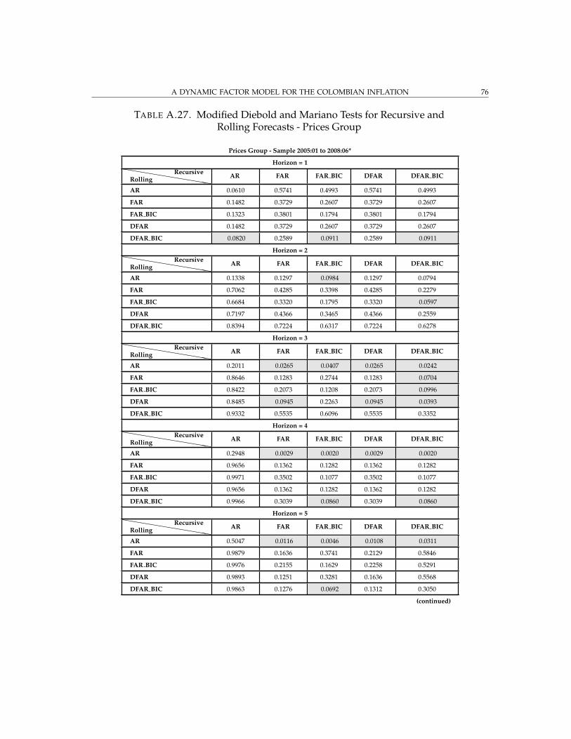
A DYNAMIC FACTOR MODEL FOR THE COLOMBIAN INFLATION 76
TABLE A.27. Modified Diebold and Mariano Tests for Recursive andRolling Forecasts - Prices Group
Prices Group - Sample 2005:01 to 2008:06*
Horizon = 1hhhhhhhhhhRolling
Recursive AR FAR FAR BIC DFAR DFAR BIC
AR 0.0610 0.5741 0.4993 0.5741 0.4993
FAR 0.1482 0.3729 0.2607 0.3729 0.2607
FAR BIC 0.1323 0.3801 0.1794 0.3801 0.1794
DFAR 0.1482 0.3729 0.2607 0.3729 0.2607
DFAR BIC 0.0820 0.2589 0.0911 0.2589 0.0911
Horizon = 2hhhhhhhhhhRolling
Recursive AR FAR FAR BIC DFAR DFAR BIC
AR 0.1338 0.1297 0.0984 0.1297 0.0794
FAR 0.7062 0.4285 0.3398 0.4285 0.2279
FAR BIC 0.6684 0.3320 0.1795 0.3320 0.0597
DFAR 0.7197 0.4366 0.3465 0.4366 0.2559
DFAR BIC 0.8394 0.7224 0.6317 0.7224 0.6278
Horizon = 3hhhhhhhhhhRolling
Recursive AR FAR FAR BIC DFAR DFAR BIC
AR 0.2011 0.0265 0.0407 0.0265 0.0242
FAR 0.8646 0.1283 0.2744 0.1283 0.0704
FAR BIC 0.8422 0.2073 0.1208 0.2073 0.0996
DFAR 0.8485 0.0945 0.2263 0.0945 0.0393
DFAR BIC 0.9332 0.5535 0.6096 0.5535 0.3352
Horizon = 4hhhhhhhhhhRolling
Recursive AR FAR FAR BIC DFAR DFAR BIC
AR 0.2948 0.0029 0.0020 0.0029 0.0020
FAR 0.9656 0.1362 0.1282 0.1362 0.1282
FAR BIC 0.9971 0.3502 0.1077 0.3502 0.1077
DFAR 0.9656 0.1362 0.1282 0.1362 0.1282
DFAR BIC 0.9966 0.3039 0.0860 0.3039 0.0860
Horizon = 5hhhhhhhhhhRolling
Recursive AR FAR FAR BIC DFAR DFAR BIC
AR 0.5047 0.0116 0.0046 0.0108 0.0311
FAR 0.9879 0.1636 0.3741 0.2129 0.5846
FAR BIC 0.9976 0.2155 0.1629 0.2258 0.5291
DFAR 0.9893 0.1251 0.3281 0.1636 0.5568
DFAR BIC 0.9863 0.1276 0.0692 0.1312 0.3050
(continued)
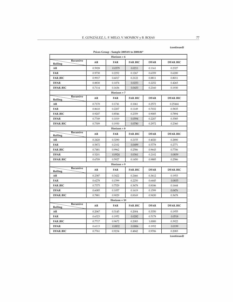
E. GONZALEZ, L. F. MELO, V. MONROY y B. ROJAS 77
(continued)
Prices Group - Sample 2005:01 to 2008:06*
Horizon = 6hhhhhhhhhhRolling
Recursive AR FAR FAR BIC DFAR DFAR BIC
AR 0.5928 0.0379 0.0211 0.1161 0.2327
FAR 0.9730 0.2252 0.1267 0.6359 0.6200
FAR BIC 0.9917 0.6017 0.2122 0.8811 0.8011
DFAR 0.8830 0.1074 0.0253 0.2252 0.4265
DFAR BIC 0.7114 0.1636 0.0433 0.2160 0.1930
Horizon = 7hhhhhhhhhhRolling
Recursive AR FAR FAR BIC DFAR DFAR BIC
AR 0.7170 0.1741 0.1061 0.2572 0.25444
FAR 0.8610 0.2207 0.1149 0.7032 0.5835
FAR BIC 0.9207 0.8546 0.2359 0.9005 0.7894
DFAR 0.7749 0.1019 0.0594 0.2207 0.3585
DFAR BIC 0.7309 0.1930 0.0780 0.2972 0.2360
Horizon = 8hhhhhhhhhhRolling
Recursive AR FAR FAR BIC DFAR DFAR BIC
AR 0.2420 0.3290 0.2155 0.4020 0.2890
FAR 0.5872 0.2102 0.0499 0.5778 0.2771
FAR BIC 0.7481 0.9962 0.2586 0.9643 0.7706
DFAR 0.5201 0.0924 0.0361 0.2102 0.0839
DFAR BIC 0.6709 0.5927 0.1450 0.9885 0.2586
Horizon = 9hhhhhhhhhhRolling
Recursive AR FAR FAR BIC DFAR DFAR BIC
AR 0.2387 0.3422 0.2466 0.3612 0.1953
FAR 0.6278 0.1599 0.2250 0.6445 0.0835
FAR BIC 0.7375 0.7529 0.3678 0.8186 0.1644
DFAR 0.6085 0.1057 0.1619 0.1599 0.0476
DFAR BIC 0.7881 0.9029 0.8169 0.9430 0.3678
Horizon = 10hhhhhhhhhhRolling
Recursive AR FAR FAR BIC DFAR DFAR BIC
AR 0.2067 0.3145 0.2004 0.3350 0.1955
FAR 0.6323 0.1952 0.0282 0.5178 0.0518
FAR BIC 0.7717 0.9672 0.2083 1.0000 0.3922
DFAR 0.6113 0.0832 0.0006 0.1952 0.0199
DFAR BIC 0.7761 0.9234 0.4842 0.9706 0.2083
(continued)

A DYNAMIC FACTOR MODEL FOR THE COLOMBIAN INFLATION 78
(continued)
Prices Group - Sample 2005:01 to 2008:06*
Horizon = 11hhhhhhhhhhRolling
Recursive AR FAR FAR BIC DFAR DFAR BIC
AR 0.2127 0.5655 0.2932 0.7964 0.6114
FAR 0.3921 0.2092 0.0068 0.7576 0.5424
FAR BIC 0.6687 0.9553 0.2145 0.8570 0.7777
DFAR 0.1929 0.1915 0.1211 0.2092 0.0112
DFAR BIC 0.3737 0.4027 0.2081 0.9544 0.2145
Horizon = 12hhhhhhhhhhRolling
Recursive AR FAR FAR BIC DFAR DFAR BIC
AR 0.2193 0.7013 0.6194 1.000 0.6041
FAR 0.2887 0.2210 0.2268 0.7394 0.3197
FAR BIC 0.3742 0.6986 0.8214 0.8345 0.4475
DFAR 0.0245 0.1743 0.1446 0.2210 0.0172
DFAR BIC 0.3889 0.6445 0.5752 0.9674 0.8214
* P-values associated with the null hypothesis Ho : RMSFE of model of row i = RMSFE of model of column j.
Vs. Ha : RMSFE of model of row i > RMSFE of model of column j. Shadowed cells indicate that the null
hyphotesis is rejected at 10% significance level.
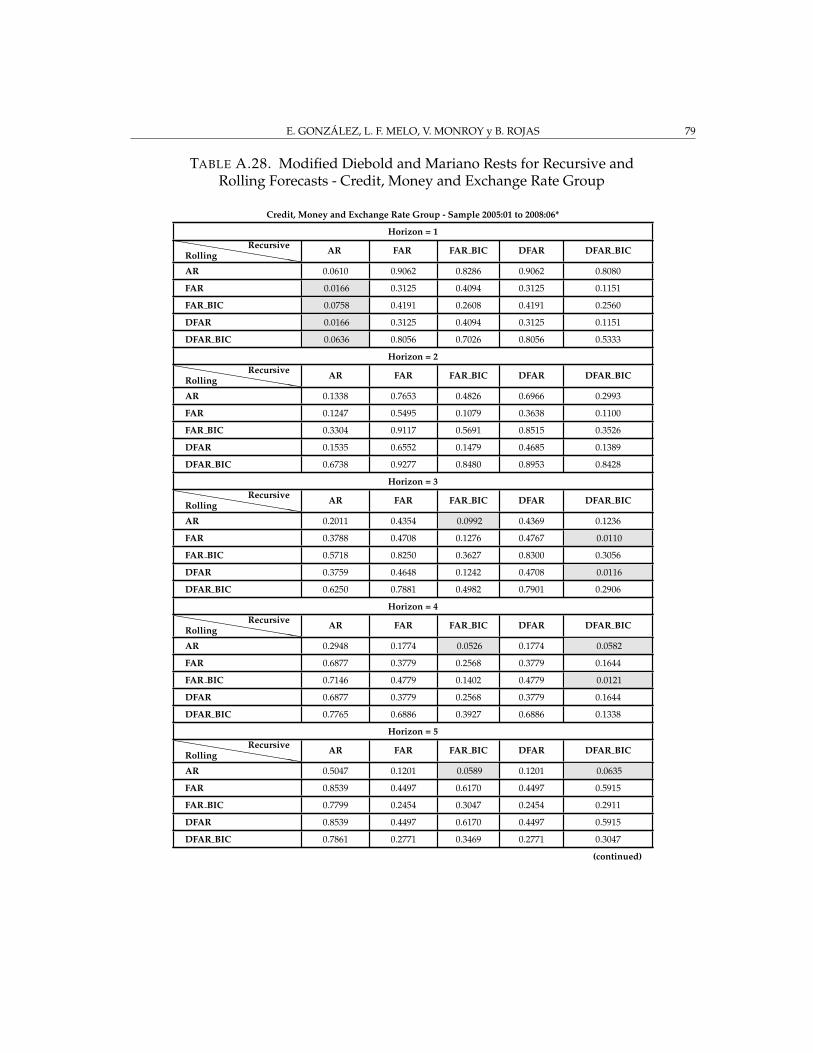
E. GONZALEZ, L. F. MELO, V. MONROY y B. ROJAS 79
TABLE A.28. Modified Diebold and Mariano Rests for Recursive andRolling Forecasts - Credit, Money and Exchange Rate Group
Credit, Money and Exchange Rate Group - Sample 2005:01 to 2008:06*
Horizon = 1hhhhhhhhhhRolling
Recursive AR FAR FAR BIC DFAR DFAR BIC
AR 0.0610 0.9062 0.8286 0.9062 0.8080
FAR 0.0166 0.3125 0.4094 0.3125 0.1151
FAR BIC 0.0758 0.4191 0.2608 0.4191 0.2560
DFAR 0.0166 0.3125 0.4094 0.3125 0.1151
DFAR BIC 0.0636 0.8056 0.7026 0.8056 0.5333
Horizon = 2hhhhhhhhhhRolling
Recursive AR FAR FAR BIC DFAR DFAR BIC
AR 0.1338 0.7653 0.4826 0.6966 0.2993
FAR 0.1247 0.5495 0.1079 0.3638 0.1100
FAR BIC 0.3304 0.9117 0.5691 0.8515 0.3526
DFAR 0.1535 0.6552 0.1479 0.4685 0.1389
DFAR BIC 0.6738 0.9277 0.8480 0.8953 0.8428
Horizon = 3hhhhhhhhhhRolling
Recursive AR FAR FAR BIC DFAR DFAR BIC
AR 0.2011 0.4354 0.0992 0.4369 0.1236
FAR 0.3788 0.4708 0.1276 0.4767 0.0110
FAR BIC 0.5718 0.8250 0.3627 0.8300 0.3056
DFAR 0.3759 0.4648 0.1242 0.4708 0.0116
DFAR BIC 0.6250 0.7881 0.4982 0.7901 0.2906
Horizon = 4hhhhhhhhhhRolling
Recursive AR FAR FAR BIC DFAR DFAR BIC
AR 0.2948 0.1774 0.0526 0.1774 0.0582
FAR 0.6877 0.3779 0.2568 0.3779 0.1644
FAR BIC 0.7146 0.4779 0.1402 0.4779 0.0121
DFAR 0.6877 0.3779 0.2568 0.3779 0.1644
DFAR BIC 0.7765 0.6886 0.3927 0.6886 0.1338
Horizon = 5hhhhhhhhhhRolling
Recursive AR FAR FAR BIC DFAR DFAR BIC
AR 0.5047 0.1201 0.0589 0.1201 0.0635
FAR 0.8539 0.4497 0.6170 0.4497 0.5915
FAR BIC 0.7799 0.2454 0.3047 0.2454 0.2911
DFAR 0.8539 0.4497 0.6170 0.4497 0.5915
DFAR BIC 0.7861 0.2771 0.3469 0.2771 0.3047
(continued)
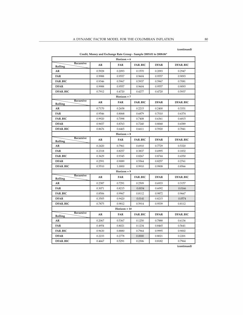
A DYNAMIC FACTOR MODEL FOR THE COLOMBIAN INFLATION 80
(continued)
Credit, Money and Exchange Rate Group - Sample 2005:01 to 2008:06*
Horizon = 6hhhhhhhhhhRolling
Recursive AR FAR FAR BIC DFAR DFAR BIC
AR 0.5928 0.2093 0.1570 0.2093 0.2947
FAR 0.9988 0.9557 0.9604 0.9557 0.9093
FAR BIC 0.9346 0.5967 0.5937 0.5967 0.7081
DFAR 0.9988 0.9557 0.9604 0.9557 0.9093
DFAR BIC 0.7912 0.4720 0.4277 0.4720 0.5937
Horizon = 7hhhhhhhhhhRolling
Recursive AR FAR FAR BIC DFAR DFAR BIC
AR 0.7170 0.2658 0.2215 0.2400 0.3331
FAR 0.9546 0.8068 0.6879 0.7010 0.6374
FAR BIC 0.9920 0.7098 0.7408 0.6361 0.6815
DFAR 0.9657 0.8763 0.7240 0.8068 0.6589
DFAR BIC 0.8676 0.6465 0.6611 0.5920 0.7841
Horizon = 8hhhhhhhhhhRolling
Recursive AR FAR FAR BIC DFAR DFAR BIC
AR 0.2420 0.7961 0.6910 0.7729 0.5320
FAR 0.2318 0.8257 0.3837 0.6995 0.1832
FAR BIC 0.3629 0.9345 0.8267 0.8744 0.4350
DFAR 0.2591 0.9089 0.5564 0.8257 0.2761
DFAR BIC 0.5510 1.0000 0.9910 0.9908 0.8566
Horizon = 9hhhhhhhhhhRolling
Recursive AR FAR FAR BIC DFAR DFAR BIC
AR 0.2387 0.7291 0.2509 0.6933 0.3157
FAR 0.3071 0.8215 0.0034 0.6092 0.0166
FAR BIC 0.8506 0.9967 0.8112 0.9872 0.9667
DFAR 0.3505 0.9420 0.0141 0.8215 0.0574
DFAR BIC 0.7875 0.9812 0.5914 0.9539 0.8112
Horizon = 10hhhhhhhhhhRolling
Recursive AR FAR FAR BIC DFAR DFAR BIC
AR 0.2067 0.5367 0.1250 0.7888 0.6136
FAR 0.4954 0.8021 0.1234 0.8465 0.5641
FAR BIC 0.9630 0.8880 0.7964 0.9995 0.9002
DFAR 0.2233 0.2778 0.0000 0.8021 0.2201
DFAR BIC 0.4667 0.5291 0.2306 0.8182 0.7964
(continued)
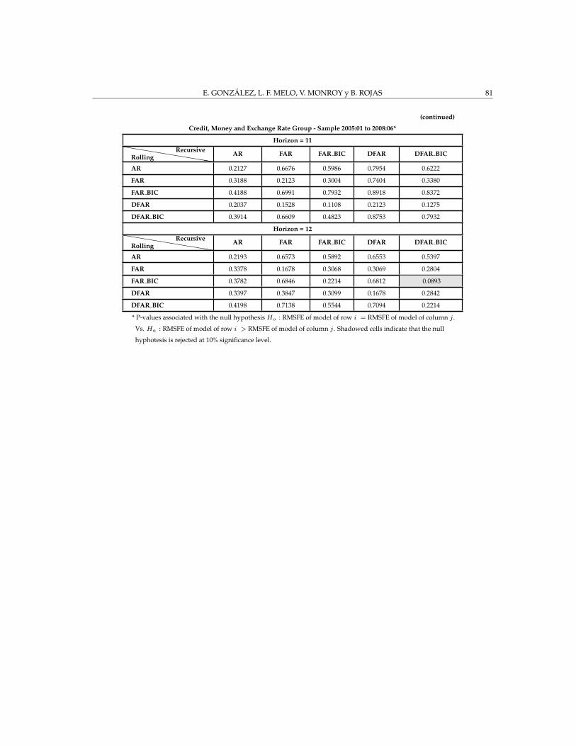
E. GONZALEZ, L. F. MELO, V. MONROY y B. ROJAS 81
(continued)
Credit, Money and Exchange Rate Group - Sample 2005:01 to 2008:06*
Horizon = 11hhhhhhhhhhRolling
Recursive AR FAR FAR BIC DFAR DFAR BIC
AR 0.2127 0.6676 0.5986 0.7954 0.6222
FAR 0.3188 0.2123 0.3004 0.7404 0.3380
FAR BIC 0.4188 0.6991 0.7932 0.8918 0.8372
DFAR 0.2037 0.1528 0.1108 0.2123 0.1275
DFAR BIC 0.3914 0.6609 0.4823 0.8753 0.7932
Horizon = 12hhhhhhhhhhRolling
Recursive AR FAR FAR BIC DFAR DFAR BIC
AR 0.2193 0.6573 0.5892 0.6553 0.5397
FAR 0.3378 0.1678 0.3068 0.3069 0.2804
FAR BIC 0.3782 0.6846 0.2214 0.6812 0.0893
DFAR 0.3397 0.3847 0.3099 0.1678 0.2842
DFAR BIC 0.4198 0.7138 0.5544 0.7094 0.2214
* P-values associated with the null hypothesis Ho : RMSFE of model of row i = RMSFE of model of column j.
Vs. Ha : RMSFE of model of row i > RMSFE of model of column j. Shadowed cells indicate that the null
hyphotesis is rejected at 10% significance level.

A DYNAMIC FACTOR MODEL FOR THE COLOMBIAN INFLATION 82
TABLE A.29. Modified Diebold and Mariano Tests for Recursive andRolling Forecasts - National Accounts Group
National Accounts Group - Sample 2005:01 to 2008:06*
Horizon = 1hhhhhhhhhhRolling
Recursive AR FAR FAR BIC DFAR DFAR BIC
AR 0.0610 0.6763 0.0610 0.6367 0.6667
FAR 0.0673 0.2112 0.0673 0.2112 0.4707
FAR BIC 0.0610 0.6763 0.0610 0.6763 0.6667
DFAR 0.0673 0.2112 0.0673 0.2112 0.4707
DFAR BIC 0.0785 0.2710 0.0785 0.2710 0.0610
Horizon = 2hhhhhhhhhhRolling
Recursive AR FAR FAR BIC DFAR DFAR BIC
AR 0.1338 0.3992 0.1338 0.3992 0.5214
FAR 0.0943 0.1880 0.0943 0.1880 0.4089
FAR BIC 0.1338 0.3992 0.1338 0.3992 0.5214
DFAR 0.0943 0.1880 0.0943 0.1880 0.4089
DFAR BIC 0.1101 0.2352 0.1101 0.2352 0.1338
Horizon = 3hhhhhhhhhhRolling
Recursive AR FAR FAR BIC DFAR DFAR BIC
AR 0.2011 0.1551 0.1533 0.1551 0.3308
FAR 0.2503 0.2408 0.2221 0.2408 0.3761
FAR BIC 0.2648 0.2613 0.2011 0.2613 0.3907
DFAR 0.2503 0.2408 0.2221 0.2408 0.3761
DFAR BIC 0.2014 0.1543 0.1754 0.1543 0.2011
Horizon = 4hhhhhhhhhhRolling
Recursive AR FAR FAR BIC DFAR DFAR BIC
AR 0.2948 0.4235 0.2948 0.6520 0.3458
FAR 0.3550 0.4994 0.3550 0.7886 0.4177
FAR BIC 0.2948 0.4235 0.2948 0.6520 0.3458
DFAR 0.1668 0.2199 0.1668 0.4994 0.2017
DFAR BIC 0.2499 0.3792 0.2499 0.6159 0.2948
Horizon = 5hhhhhhhhhhRolling
Recursive AR FAR FAR BIC DFAR DFAR BIC
AR 0.5047 0.5047 0.5047 0.6385 0.8631
FAR 0.5467 0.5620 0.5467 0.6710 0.9333
FAR BIC 0.5047 0.5047 0.5047 0.6385 0.8631
DFAR 0.3814 0.3738 0.3814 0.5620 0.7769
DFAR BIC 0.1584 0.1323 0.1584 0.2852 0.5047
(continued)

E. GONZALEZ, L. F. MELO, V. MONROY y B. ROJAS 83
(continued)
National Accounts Group - Sample 2005:01 to 2008:06*
Horizon = 6hhhhhhhhhhRolling
Recursive AR FAR FAR BIC DFAR DFAR BIC
AR 0.5928 0.8972 0.5928 0.7175 0.7265
FAR 0.0196 0.3775 0.0196 0.6529 0.6284
FAR BIC 0.5928 0.8972 0.5928 0.7175 0.7265
DFAR 0.2905 0.3389 0.2905 0.3775 0.2764
DFAR BIC 0.3144 0.3922 0.3144 0.7302 0.5928
Horizon = 7hhhhhhhhhhRolling
Recursive AR FAR FAR BIC DFAR DFAR BIC
AR 0.7170 0.6845 0.7170 0.7278 0.7515
FAR 0.7357 0.8219 0.7357 0.7701 0.8305
FAR BIC 0.7170 0.6845 0.7170 0.7278 0.7515
DFAR 0.3476 0.3440 0.3476 0.8219 0.4547
DFAR BIC 0.3244 0.3134 0.3244 0.7339 0.7170
Horizon = 8hhhhhhhhhhRolling
Recursive AR FAR FAR BIC DFAR DFAR BIC
AR 0.2420 0.5988 0.2420 0.7815 0.7257
FAR 0.4458 0.8232 0.4458 0.8571 0.8228
FAR BIC 0.2420 0.5988 0.2420 0.7815 0.7257
DFAR 0.2376 0.2226 0.2376 0.8232 0.3099
DFAR BIC 0.2442 0.2143 0.2442 0.7419 0.2420
Horizon = 9hhhhhhhhhhRolling
Recursive AR FAR FAR BIC DFAR DFAR BIC
AR 0.2387 0.8503 0.3523 0.8033 0.3298
FAR 0.1553 0.8194 0.1699 0.7863 0.0382
FAR BIC 0.1623 0.8354 0.2387 0.7957 0.3090
DFAR 0.1991 0.2660 0.2067 0.8194 0.1754
DFAR BIC 0.5928 0.9678 0.6137 0.8271 0.2387
Horizon = 10hhhhhhhhhhRolling
Recursive AR FAR FAR BIC DFAR DFAR BIC
AR 0.2067 0.5631 0.0716 0.6601 0.7106
FAR 0.4403 0.7940 0.4073 0.6925 0.5597
FAR BIC 0.5230 0.5965 0.2067 0.6691 0.7504
DFAR 0.3424 0.3949 0.3332 0.7940 0.4915
DFAR BIC 0.2242 0.4425 0.1926 0.5121 0.2067
(continued)

A DYNAMIC FACTOR MODEL FOR THE COLOMBIAN INFLATION 84
(continued)
National Accounts Group - Sample 2005:01 to 2008:06*
Horizon = 11hhhhhhhhhhRolling
Recursive AR FAR FAR BIC DFAR DFAR BIC
AR 0.2127 0.7970 0.2127 0.9813 0.3480
FAR 0.1495 0.2007 0.1495 0.8730 0.2372
FAR BIC 0.2127 0.7970 0.2127 0.9813 0.3480
DFAR 0.0290 0.0807 0.0290 0.2007 0.0638
DFAR BIC 0.5172 0.7263 0.5172 0.8989 0.2127
Horizon = 12hhhhhhhhhhRolling
Recursive AR FAR FAR BIC DFAR DFAR BIC
AR 0.2193 0.5067 0.2193 0.3748 0.1949
FAR 0.4442 0.2200 0.4442 0.1700 0.1550
FAR BIC 0.2193 0.5067 0.2193 0.3748 0.1949
DFAR 0.5985 0.7608 0.5985 0.2200 0.0124
DFAR BIC 0.7648 0.8258 0.7648 0.9930 0.2193
* P-values associated with the null hypothesis Ho : RMSFE of model of row i = RMSFE of model of column j.
Vs. Ha : RMSFE of model of row i > RMSFE of model of column j. Shadowed cells indicate that the null
hyphotesis is rejected at 10% significance level.
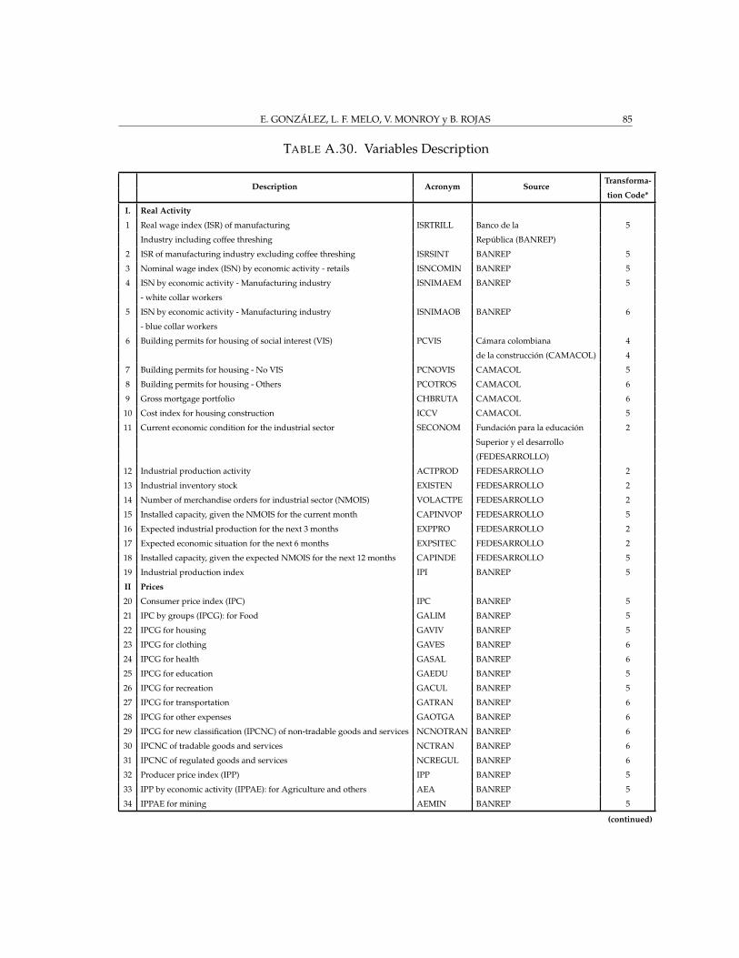
E. GONZALEZ, L. F. MELO, V. MONROY y B. ROJAS 85
TABLE A.30. Variables Description
Description Acronym SourceTransforma-
tion Code*
I. Real Activity
1 Real wage index (ISR) of manufacturing ISRTRILL Banco de la 5
Industry including coffee threshing Republica (BANREP)
2 ISR of manufacturing industry excluding coffee threshing ISRSINT BANREP 5
3 Nominal wage index (ISN) by economic activity - retails ISNCOMIN BANREP 5
4 ISN by economic activity - Manufacturing industry ISNIMAEM BANREP 5
- white collar workers
5 ISN by economic activity - Manufacturing industry ISNIMAOB BANREP 6
- blue collar workers
6 Building permits for housing of social interest (VIS) PCVIS Camara colombiana 4
de la construccion (CAMACOL) 4
7 Building permits for housing - No VIS PCNOVIS CAMACOL 5
8 Building permits for housing - Others PCOTROS CAMACOL 6
9 Gross mortgage portfolio CHBRUTA CAMACOL 6
10 Cost index for housing construction ICCV CAMACOL 5
11 Current economic condition for the industrial sector SECONOM Fundacion para la educacion 2
Superior y el desarrollo
(FEDESARROLLO)
12 Industrial production activity ACTPROD FEDESARROLLO 2
13 Industrial inventory stock EXISTEN FEDESARROLLO 2
14 Number of merchandise orders for industrial sector (NMOIS) VOLACTPE FEDESARROLLO 2
15 Installed capacity, given the NMOIS for the current month CAPINVOP FEDESARROLLO 5
16 Expected industrial production for the next 3 months EXPPRO FEDESARROLLO 2
17 Expected economic situation for the next 6 months EXPSITEC FEDESARROLLO 2
18 Installed capacity, given the expected NMOIS for the next 12 months CAPINDE FEDESARROLLO 5
19 Industrial production index IPI BANREP 5
II Prices
20 Consumer price index (IPC) IPC BANREP 5
21 IPC by groups (IPCG): for Food GALIM BANREP 5
22 IPCG for housing GAVIV BANREP 5
23 IPCG for clothing GAVES BANREP 6
24 IPCG for health GASAL BANREP 6
25 IPCG for education GAEDU BANREP 5
26 IPCG for recreation GACUL BANREP 5
27 IPCG for transportation GATRAN BANREP 6
28 IPCG for other expenses GAOTGA BANREP 6
29 IPCG for new classification (IPCNC) of non-tradable goods and services NCNOTRAN BANREP 6
30 IPCNC of tradable goods and services NCTRAN BANREP 6
31 IPCNC of regulated goods and services NCREGUL BANREP 6
32 Producer price index (IPP) IPP BANREP 5
33 IPP by economic activity (IPPAE): for Agriculture and others AEA BANREP 5
34 IPPAE for mining AEMIN BANREP 5
(continued)

A DYNAMIC FACTOR MODEL FOR THE COLOMBIAN INFLATION 86
(continued)
Description Acronym SourceTransforma-
tion Code*
35 IPPAE for manufacturing industries AEIMAN BANREP 5
36 IPP by origin of goods (IPPPB): Produced and consumed PBPRODCO BANREP 5
37 IPPPB for imports PBM BANREP 5
38 IPPPB for exports PBX BANREP 5
39 IPPPB for exports excluding coffee PBXSINCA BANREP 5
40 IPP by use or economic destiny (IPPUE): for intermediate consumption UECINTER BANREP 5
41 IPPUE for final consumption UECFINAL BANREP 5
42 IPPUE for capital formation UEFORK BANREP 6
43 IPPUE for building materials UEMATCO BANREP 5
44 Price expectations for the next 3 months EXPAUMPR FEDESARROLLO 1
III Credit, Money and Exchange Rate
45 Monetary base BASEMON BANREP 5
46 Net international reserves RESNETAS BANREP 5
47 M1 M1 BANREP 5
48 M2 M2 BANREP 5
49 M3 M3 BANREP 6
50 Total gross credit CREDBR BANREP 5
51 Currency in circulation EFECTIV BANREP 5
52 Total deposits TOTALDEP BANREP 5
53 Deposits in saving accounts DEPCTAHO BANREP 5
54 Deposits in current accounts DEPCTCOR BANREP 5
55 Interest rate of 90-day certificate CDT90DBA BANREP 3
of deposits for banks and financial corporations
56 Interbank interest rate - monthly average TIBPROME BANREP 3
57 Nominal interest rate of 90-day fixed term deposit (DTF) DTFNO90D BANREP 2
58 Active interest rate TASACTIV BANREP 3
59 Real interest rate of 90-day DTF DTFR90 BANREP 2
60 Gross domestic credit to treasury CRBTES BANREP 5
61 Gross domestic credit to commercial banks CRBBAN BANREP 5
62 Gross domestic credit to financial corporations CRBCORP BANREP 4
63 Gross domestic credit to financial sector CRDOBPRI BANREP 6
64 Net domestic credit to private sector CRDONEPR BANREP 2
65 Nominal exchange rate - average TCNMPROM BANREP 5
66 Terms of trade TERMINTE BANREP 5
67 Real exchange rate index for non-traditional commerce deflated by IPP ITCRIPPN BANREP 5
68 Real exchange rate index for non-traditional commerce deflated by IPC ITCRIPCN BANREP 5
69 Real exchange rate index for total commerce deflated by IPP ITCRIPPT BANREP
70 Real exchange rate index for total commerce deflated by IPC ITCRIPCT BANREP 5
IV National Accounts
71 Consumption goods imports - non-durables MBCNODU Departamento Administrativo 5
Nacional de Estadstica (DANE)
72 Consumption goods imports - durables MBCDUR DANE 5
73 Intermediate and raw goods imports - Fuel and others MBICOMLU DANE 5
(continued)

E. GONZALEZ, L. F. MELO, V. MONROY y B. ROJAS 87
(continued)
Description Acronym SourceTransforma-
tion Code*
74 Intermediate and raw goods imports - Agriculture sector MBISA DANE 5
75 Intermediate and raw goods imports - Industrial sector MBISI DANE 5
76 Capital goods imports - Building materials MBKMATCO DANE 5
77 Capital goods imports - Agriculture sector MBKSA DANE 5
78 Capital goods imports - Industrial sector MBKSI DANE 5
79 Capital goods imports - Apparel materials MBKEQTRA DANE 5
80 Traditional goods exports - Coffee XBTCAFE DANE 5
81 Traditional goods exports - Coal XBTCARBO DANE 5
82 Traditional goods exports - Oil XBTPETR DANE 5
83 Traditional goods exports - Iron-nickel XBTFERR DANE 5
84 Non traditional goods exports - Agriculture sector XBNTSA DANE 5
85 Non traditional goods exports - Mining sector XBNTSMIN DANE 5
86 Non traditional goods exports - Industrial sector XBNTSI DANE 5
87 Income INGRES Consejo Superior de Polıtica 5
Central national government Fiscal (CONFIS), Min. Hacienda
y Credito Publico.
88 Expenses (with interest payments) GAST CONFIS, Min. Hacienda 5
Central national government Credito Publico.
89 Interest payments INTERGC CONFIS, Min. Hacienda 2
Central national government Credito Publico.
90 Deficit or surplus SUPERAVI CONFIS, Min. Hacienda 1
Central national government Credito Publico.
91 Internal financing FININTER CONFIS, Min. Hacienda 1
Central national government Credito Publico.
92 External financing FINEXTER CONFIS, Min. Hacienda 1
Central national government Credito Publico.
*(1) no transformation, (2) first difference, (3) second difference, (4) logarithm, (5) first difference of logarithm, (6) second difference of
logarithm.
Copyright © 2022 FDOKUMEN