Department of Agricultural and Resource EconomicsUniversity of California, Davis

A Dual Least-Squares Estimator of the Errors-In-Variables Model

Using Only First And Second Moments

by

Quirino Paris

Working Paper No. 14-003

June 2014

Copyright @ 2014 by Quirino Paris All Rights Reserved.

Readers may make verbatim copies of this document for non-commercial purposes by any means, provided that this copyright notice appears on all such copies.

Giannini Foundation of Agricultural Economics

1

A Dual Least-Squares Estimator of the Errors-In-Variables Model Using Only First And Second Moments

Quirino Paris

June 2014

Abstract The paper presents an estimator of the errors-in-variables in multiple regressions using only first and second-order moments. The consistency property of the estimator is explored by Monte Carlo experiments. Based on these results, we conjecture that the estimator is consistent. The proof of consistency, to be dealt in another paper, is based upon the assumptions of Kiefer and Wolfowitz (1956). The novel treatment of the errors-in-variables model relies crucially upon a neutral parameterization of the error terms of the dependent and the explanatory variables. The estimator does not have a closed form solution. It requires the maximization of a dual least-squares objective function that guarantees a global optimum. This estimator, therefore, includes the naïve least-squares method (when only the dependent variable is measured with error) as a special case. Keywords: errors-in-variables, measurement errors, dual least squares, first moments, second moments, Monte Carlo JEL: C30 Quirino Paris is a professor in the Department of Agricultural and Resource Economics, University of California, Davis.

2

A Dual Least-Squares Estimator of the Errors-In-Variables Model Using Only First And Second Moments

Quirino Paris

June 2014

1. Introduction

For more than a century, statisticians have attempted to solve the problem of obtaining

consistent parameter estimates (intercept, slope, error variances) in a linear regression

where both dependent and independent (explanatory) variables are subject to

measurement errors. Traditionally, this problem has gone by the name of the errors-in-

variables (EIV) model. A varying degree of success was attained during a century of

efforts. One desirable objective, however, has escaped so far: the goal of obtaining an

easy method for consistent parameter estimates under general and plausible assumptions

using only first and second-order moments of the sample information. This goal is

desirable for a number of reasons: simplicity, relation to maximum likelihood estimates

under normality assumptions, global optimum, and avoidance of the difficulties

associated with obtaining valid measures of the fourths and higher moments in empirical

analyses.

Adcock (1878) appears to have pioneered the discussion of the EIV model by

recognizing that the naïve least-squares method has “a problem.” His suggestion was to

compute orthogonal (to the estimated regression line) errors for which he had to assume

equal variances of the errors in both dependent and independent variables. This means

that he had to augment the usual sample information with additional out-of-sample

knowledge about errors variances. Over time, researchers have suggested a variety of

approaches that recognize the prevailing consensus about the need of additional (user

3

supplied) information in order to obtain the desired properties of the parameter estimates.

Gillard (2010) presents an overview of various approaches covering instrumental

variables, maximum likelihood, the moment method and others. Several important papers

by Reiersøl (1950), Neyman (1951), Wolfowitz (1954) and Kiefer and Wolfowitz (1956),

however, are omitted. All these papers establish the strong consistency of maximum

likelihood estimates of a rather general EIV structural regression subject only to the

exclusion condition of Reiersøl (1950). His remarkable theorem states that – to achieve

identification of the parameter estimates – the latent variable(s) of the EIV model cannot

be distributed as normal random variables. It appears that Kiefer and Wolfowitz (1956)

results have been neglected, especially in recent years. Kendall and Stuart (1979), for

example, in their fourth edition of volume 2, dealing with maximum likelihood and the

EIV structural model, mention neither Reiersøl (1950) nor Kiefer and Wolfowitz (1956).

Another example of omitted important literature is associated with the works of

Pal (1980), Van Monfort et al. (1987), Cragg (1997) and Dagenais and Dagenais (1997)

who discuss the method of moments in the context of the EIV model estimation but do

not mention Neyman (1951), Wolfowitz (1954) and Kiefer and Wolfowitz (1956). Their

idea is to use sample moments of order higher than the first and second one to obtain

estimates of the slope coefficient and then derive the other parameters from relations

based upon first and second moments. There are some warnings. If the latent random

variable is distributed according to a symmetric distribution (normal, uniform), the third

moment vanishes and it is necessary to use forth moments to estimate the slope. The

variance of the estimated coefficient, then, involves eighth-order moments. The higher

the moments, the more demanding the information requirement for their valid measure.

4

In recent years, nonparametric methods have been applied to the EIV problem

(see Delaigle and Meister, 2007). But, often, the importance of knowing the structure of

the regression function explicitly and the dimension of the individual parameters

(elasticities) works in the direction of parametric estimation.

Also, we are not interested in sample moments of higher order. As the paper’s

title states, we discuss a rather simple procedure that achieves consistent parameter

estimates using only first and second-order moments of the sample information. In

section 2 we define the simplest EIV structural model along the lines of many

predecessors and in particular of Lindley (1947), Wolfowitz (1954), Kiefer and

Wolfowitz (1956) and Kendall and Stuart (1979). We consider the second-order moment

relations derived by these authors who noted that for the simplest EIV structural model

there are three second-order moment relations but four parameters to estimate. Hence, by

considering only these second-order moments, the EIV model is not identified.

In this paper, we introduce a neutral transformation of the random errors and set

up a mathematical programming model that, in principle, exhibits a global maximum and

achieves consistent estimates of all parameters involved. Our estimator does not have a

closed form solution. It requires a numerical optimization software like GAMS. We do

not use a maximum likelihood approach. Instead, we use a dual least-squares

methodology along the lines discussed by Paris (2011). In section 3, we give a brief and

simple introduction to the dual of the least-squares method and note that the dual least-

squares specification possesses a global maximum over the parameter space. In section 4,

we extend the estimator to three latent random variables (one dependent and two

“explanatory”). In section 5, we present a Monte Carlo experiment dealing with an EIV

5

regression with two latent variables (one dependent and one “explanatory”) and involving

6 parameters. In section 6, we present a Monte Carlo experiment dealing with an EIV

regression with three latent variables (one dependent and two “explanatory”) and

involving 10 parameters. The results of both Monte Carlo experiments do not negate the

conjecture that the dual LS estimator produces consistent estimates of the EIV model’s

parameters. In section 7, we generalize the specification of the EIV dual LS estimator to

K latent “explanatory” variables in vector and matrix notation. Conclusions come in

section 8.

2. The Simplest EIV Case

Following Kendall and Stuart (1979, p. 400), we state a linear relation between two latent

random variables in the form of

Y * =! + "X* (1)

with the objective of estimating parameters ! and ". As Y * and X* are latent variables

they are not observed directly. In their place, we measure repeatedly two random

variables Y and X that bear the following relations with the latent variables

yi = yi

* + ui* (2)

xi = xi* + vi

* (3)

i = 1,...,N , where ui* and vi

* are i.d.d. measurement errors (deviations) from the true

value of the latent variables Y * and X* .

In this simplest case, we assume that

Y * and X*

6

E(ui*) = E(vi

*) = 0, var(ui*) =!

u*2 , var(vi

*) =!v*2 all i,

cov(ui*,uj

*) = cov(vi*,vj

*) = 0, i " j,

cov(ui*,vj

*) = 0, all i, j.

(4)

The EIV model, therefore, can be restated as

yi =! + "xi

* + ui* (5)

xi = xi* + vi

*. (6)

The use of assumptions (4) allows the conclusion that

E(x) = E(x*) = µE(y) =! + "µ

(7)

Lindley (1947) and Kendall and Stuart (1979) stated the second-order moment relations:

var(y) = ! 2"x*2 +"

u*2 (8)

var(x) ="x*2 +"

v*2 (9)

cov(y, x) = !"x*2 . (10)

By using first- and second-order sample moments to approximate the left-hand-side

population moments of relations (7)-(10), the list of EIV conditions can be restated as

x = µ (11)y =! + "µ (12)myy = " 2#

x*2 +#

u*2 (13)

mxx =# x*2 +#

v*2 (14)

myx = "#x*2 . (15)

Several authors, including Lindley (1947) and Kendall and Stuart (1979) acknowledge

the non-identification of system (11)-(15) because it admits six parameters

(µ,! ,",#u*2 ,#

v*2#

x*2 ) but only five equations. These authors emphasized the need for

additional (user supplied) sample information.

7

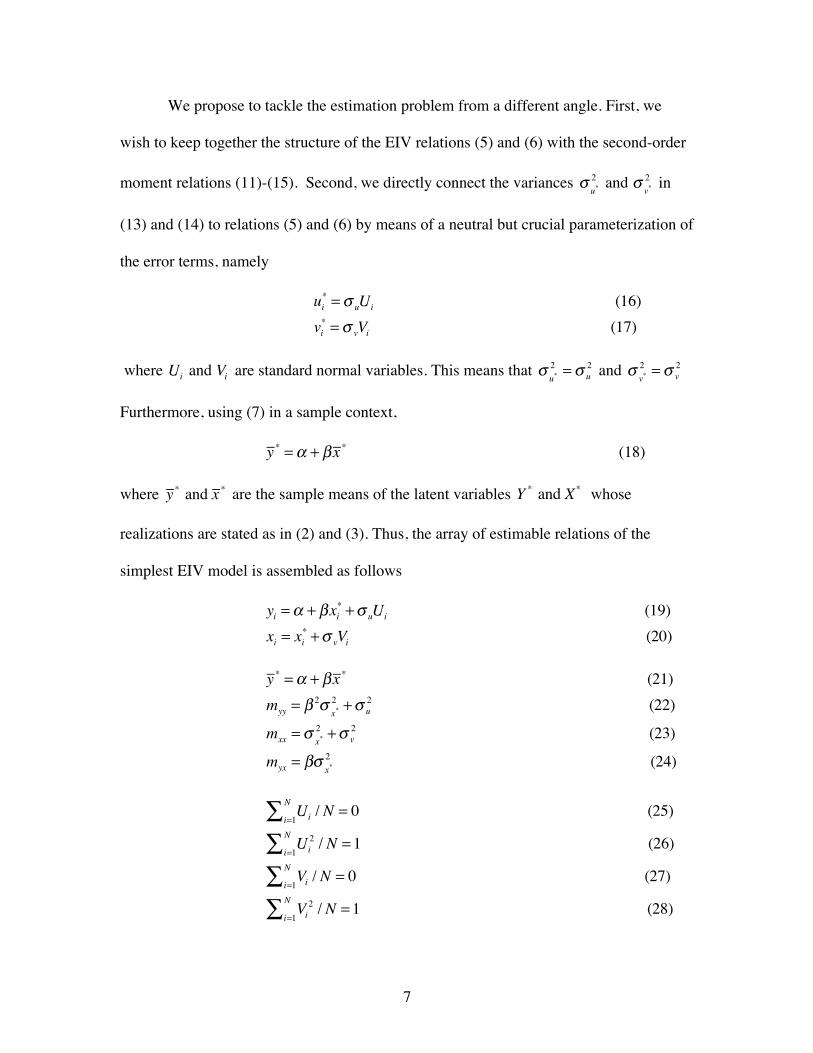
We propose to tackle the estimation problem from a different angle. First, we

wish to keep together the structure of the EIV relations (5) and (6) with the second-order

moment relations (11)-(15). Second, we directly connect the variances !u*2 and !

v*2 in

(13) and (14) to relations (5) and (6) by means of a neutral but crucial parameterization of

the error terms, namely

ui

* =! uUi (16)vi

* =! vVi (17)

where Ui and Vi are standard normal variables. This means that !u*2 =! u

2 and !v*2 =! v

2

Furthermore, using (7) in a sample context,

y * =! + "x * (18)

where y * and x * are the sample means of the latent variables Y * and X* whose

realizations are stated as in (2) and (3). Thus, the array of estimable relations of the

simplest EIV model is assembled as follows

yi =! + "xi

* +# uUi (19)xi = xi

* +# vVi (20)

y * =! + "x * (21)myy = " 2#

x*2 +# u

2 (22)

mxx =# x*2 +# v

2 (23)

myx = "#x*2 (24)

Uii=1

N! / N = 0 (25)

Ui2

i=1

N! / N = 1 (26)

Vii=1

N! / N = 0 (27)

Vi2

i=1

N! / N = 1 (28)

8

with ! u > 0,! v > 0,! x*> 0 .

This specification of the EIV model is akin to the specification of Kiefer and

Wolfowitz (1956) who derived consistent ML estimates “in the presence of infinitely

many incidental parameters (latent variables).”

We, however, will not maximize a likelihood function. The system of relations

(19)-(28) does not have a closed form solution. In principle, it can have a solution where

all the parameters have admissible values, with ! u > 0,! v > 0,! x*> 0 . In other words, it

is necessary to find an interior solution of the parameter space. Any boundary solution is

not admissible. It is desirable, therefore, to find an interior solution that optimizes some

robust statistical function. For this task, we choose the dual objective function of the

least-squares (LS) method described by Paris (2011, p. 70). The reason for this choice

resides in the global maximum of the dual LS specification, the numerical stability of the

optimization problem and the intuitive meaning of the dual LS approach.

Using the terminology of information theory, the dual of the least-squares method

corresponds to the maximization of the net value of sample information (NVSI). By

applying this criterion to the EIV model described above, the structure of the objective

function to be maximized subject to relations (19)-(28) turns out as

maxNVSI =! u yi

i=1

N

" Ui / N +! v xii=1

N

" Vi / N (29)

# [yii=1

N

" #$ # %xi*]2 / 2N #! v

2 Vi2

i=1

N

" / 2N .

It must be emphasized that the estimator developed in this section provides

estimates not only of parameters ! and " defining the linear regression but also of the

error variances ! u2 and ! v

2 . And, finally, it provides estimates of the mean and variance

9

of the latent variable X* , µx* and !

x*2 . Actually, with the estimate of the N values x̂i

* of

the latent variable it is possible to approximate rather well its entire distribution. This

result is a remarkable byproduct of the original goal that was defined simply as the

estimation of ! and " . This general result depends crucially upon the use of all the

sample information, including the sample latent variable (estimated) realizations that

were overlooked in previous works of the EIV problem.

Consistency of the dual LS estimator. At present, consistency of the dual LS estimator

specified by the maximization of (29) subject to relations (19)-(28) is formulated as a

conjecture. Consistency of the EIV parameter estimates could be proved by using the

assumptions of Kiefer and Wolfowitz (1956), but their implementation is left for another

day. In this paper, we claim that if it is possible to obtain a global maximum of (29) and

all the parameter estimates have admissible values (in particular, if all the variances have

positive values) the estimator is consistent. In a least-squares context, if there is an

interior feasible solution, that solution is a global optimal solution. For the time being,

Monte Carlo experiments may either support or negate the conjecture.

3. The Dual of the Least-Squares Estimator

Given the novelty of the dual LS estimator, we give a brief outline of its structure and

meaning using the familiar setup of a multiple regression model in vector and matrix

notation. In this section, the mathematical symbols are completely unrelated to the EIV

model discussed above. The traditional (primal) LS approach consists of minimizing the

squared deviations from an average relation of, say, a linear model that consists of three

parts:

10

y = X! + u (30)

where y is an (n x 1) vector of sample observations, X is an (n x k) matrix of

predetermined values, ! is a (k x 1) vector of unknown parameters to be estimated by the

LS method, and u is an (n x 1) vector of deviations from the quantity X! . In the

terminology of information theory, relation (30) may be regarded as representing the

decomposition of a message into signal and noise, that is, message = signal + noise, with

obvious correspondences with the three components of (30). Symbolically, then, the LS

methodology minimizes the squared deviations (noise) subject to the model’s

specification

Primal min

u,!LS = "u u / 2 (31)

subject to y = X! + u. (32)

The dual of the LS method is derived using the Lagrangian function and the

corresponding first order necessary conditions

L(u,!,") = #u u / 2 + #" (y $X! $ u) (33)

!L!u

= u" # = 0 (34)

!L!"

= # $X % = 0. (35)

Using ! = u, "u ! = "u u and (35) into the Lagrangian function, the dual specification of

the least-squares method results in

Dual maxuNVSI = !y u" !u u / 2 (36)

subject to !X u = 0 . (37)

11

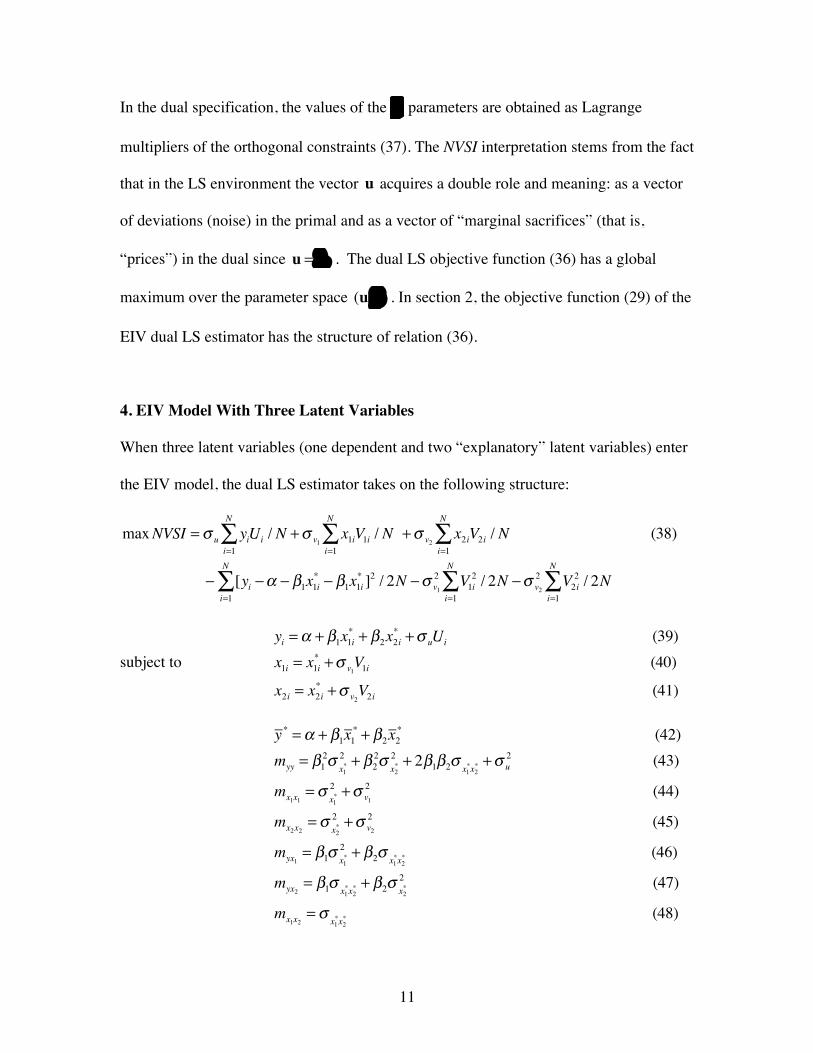
In the dual specification, the values of the ! parameters are obtained as Lagrange

multipliers of the orthogonal constraints (37). The NVSI interpretation stems from the fact

that in the LS environment the vector u acquires a double role and meaning: as a vector

of deviations (noise) in the primal and as a vector of “marginal sacrifices” (that is,

“prices”) in the dual since u = ! . The dual LS objective function (36) has a global

maximum over the parameter space (u,!) . In section 2, the objective function (29) of the

EIV dual LS estimator has the structure of relation (36).

4. EIV Model With Three Latent Variables

When three latent variables (one dependent and two “explanatory” latent variables) enter

the EIV model, the dual LS estimator takes on the following structure:

maxNVSI =! u yii=1

N

" Ui / N +! v1x1i

i=1

N

" V1i / N +! v2x2i

i=1

N

" V2i / N (38)

# [yii=1

N

" #$ # %1x1i* # %1x1i

* ]2 / 2N #! v12 V1i

2

i=1

N

" / 2N #! v2

2 V2i2

i=1

N

" / 2N

subject to yi =! + "1x1i

* + "2x2i* +# uUi (39)

x1i = x1i* +# v1

V1i (40)

x2i = x2i* +# v2

V2i (41)

y * =! + "1x1* + "2x2

* (42)myy = "1

2#x1

*2 + "2

2#x2

*2 + 2"1"2# x1

*x2* +# u

2 (43)

mx1x1=#

x1*

2 +# v12 (44)

mx2x2=#

x2*

2 +# v2

2 (45)

myx1= "1# x1

*2 + "2# x1

*x2* (46)

myx2= "1# x1

*x2* + "2# x2

*2 (47)

mx1x2=#

x1*x2

* (48)

12

Uii=1

N! / N = 0 (49)

Ui2

i=1

N! / N = 1 (50)

V1ii=1

N! / N = 0 (51)

V1i2

i=1

N! / N = 1 (52)

V2ii=1

N! / N = 0 (53)

V2i2

i=1

N! / N = 1 (54)

where !x1*x2* = cov(x1

*, x2* ) . The same assumptions stated in (4) are extended to this case.

The extension to four or more latent variables is straightforward and is given in section 7.

The EIV model of this section exhibits ten parameters that must be estimated,

(! ,"1,"2,# u2,# v1

2 ,# v22 ,µ

x1* ,µx2

* ,# x1*2 ,#

x2*2 ) .

5. Monte Carlo Experiment With Two Latent Variables

The software GAMS (1988) was used to implement the dual least-squares estimator of

section 2. The following true values of the parameters and random variables were chosen

for this example:

! = "2.0# = 0.85$ u = 1.2$ v = 1.4U ! Normal(0,1.2)V ! Normal(0,1.4)xi* !Uniform(3,9)

The “explanatory” latent variable, therefore, is distributed with mean µx*= 6.0 and

variance !x*2 = 3.0 .

13

The example has six parameters to be estimated. The implementation of a Monte

Carlo experiment depends crucially upon the seed of the GAMS program to start the

pseudo random-number generator. For this reason, we repeated 20 times the estimation

with different seeds and computed the average values of the parameters at each level of

the number of observations. The results are reported in Table 1.

Table 1. Monte Carlo Results of the EIV Estimator with Two Latent Variables

N ! = "2.0 ! = 0.85 ! u = 1.2 ! v = 1.4 µx*= 6.0 !

x*2 = 3.0

50 -1.8295 0.8242 1.1580 1.4097 5.9790 3.0967 100 -2.0384 0.8632 1.1743 1.3650 5.9730 3.0345 200 -2.0294 0.8541 1.1978 1.4021 6.0119 2.9156 500 -2.0138 0.8512 1.1839 1.3937 5.9993 3.0632 1,000 -2.0616 0.8600 1.2001 1.3960 5.9958 2.9594 2,000 -2.0368 0.8555 1.1903 1.3926 5.9911 2.9850 5,000 -1.9851 0.8463 1.1947 1.4117 6.0013 2.9887 10,000 -2.0168 0.8541 1.1998 1.4050 5.9970 2.9748

The results of Table 1 were obtained using the solver Conopt3. It is important to explore

the parameter space around the possible optimal solution by repeating the computations

with different initial points. It seems safe to say that the results of Table 1 do not negate

the conjecture that the dual LS estimator presented here produces consistent estimates of

the EIV model’s parameters.

6. Monte Carlo Experiment With Three Latent Variables

The following true values of the parameters and random variables were chosen for this

example:

14

! = 2.5"1 = 0.85"2 = #0.5$ u = 1.2$ v1 = 0.8$ v2 = 1.4U ! Normal(0,1.2)V1 ! Normal(0,0.8)V2 ! Normal(0,1.4)x1i* !Uniform(3,9)x2i* !Uniform(5,15)

The “explanatory” latent variables, therefore, are distributed with mean

µx1

* = 6.0, µx2

* = 10.0 and variance !x1

*2 = 3.0, !

x2*

2 = 8.3333 , respectively. The results are

presented in Table 2.

Table 2. Monte Carlo results of EIV model with three latent variables

N ! =2.5

!1 =0.85

!2 ="0.5

! u =1.2

! v1 =0.8

! v2 =1.4

µx1* =

6.0 !

x1*2 =

3.0

µx2* =

10.0

!x2*2 =

8.333

50 2.6104 0.8101 -0.4910 1.1210 0.7590 1.3673 6.0813 2.9495 10.1299 8.4228 100 2.3884 0.8602 -0.4975 1.1987 0.7654 1.3906 6.0493 2.8519 10.0097 8.3299 200 2.4736 0.8390 -0.4910 1.1935 0.7864 1.4167 6.0261 2.9370 9.9816 8.3605 500 2.5869 0.8446 -0.5063 1.1929 0.7856 1.3836 6.0325 3.0194 10.0663 8.1560 1,000 2.5450 0.8468 -0.5002 1.1997 0.7863 1.4092 6.0108 3.0013 10.0212 8.3982 2,000 2.5560 0.8438 -0.5026 1.1977 0.7875 1.3991 6.0192 3.0282 10.0039 8.3164 5,000 2.5937 0.8419 -0.5047 1.2061 0.7917 1.3996 6.0082 3.0099 10.0081 8.2647 10,000 2.5356 0.8447 -0.5005 1.2034 0.7899 1.4053 6.0092 3.0118 9.9987 8.3048

Also in this case, all the estimates tend toward the true values of their respective

parameters rather quickly. It is interesting to note that also at the smaller sample sizes the

“precision” of the estimated coefficients is rather surprising and, overall, satisfactory. A

guideline has emerged to evaluate the numerical results of any empirical run: First, check

15

whether all the estimated variances (standard deviations) are positive. If not, change the

initial point. Second, record the value of the objective function. Third, rerun the program

with different initial points and compare the results to the previous runs. Choose the

solution (with positive values of the variances) that corresponds to the maximum value of

the objective function. The GAMS software contains a solver (Baron) that computes a

global optimum, if it exists, and can be used to verify whether such an optimum is

associated with positive values of the variances and corresponds to the dual LS solution.

7. Generalized EIV Dual Least-Squares Estimator In Matrix Notation

There are N sample observations and K “explanatory” latent variables and all the

assumptions stated in (4) apply. Define the following vectors and matrices:

!y = [y1, y2,...yN ]" vector of sample observations of dependent variable

y*! = [y1*, y2

*,...yN* ]" vector of sample dependent latent variables

!s = [1,1,...,1]" sum vector!# = [#1,#2,...,#K ]" vector of slope coefficientsX* = [x1

*,x2* ,...,xK

* ]" matrix of latent variablesX = [x1,x2,...,xK ]" matrix of sample observations of latent variables!u = [u1,u2,...uN ]" vector of errors of dependent variableV = [v1,v2,...,vK ]" matrix of error of latent variables

!V =

v1

v2

vK

!

"

###

$

%

&&&= diagonal error matrix

!X* =

x1*

x2*

xK*

!

"

####

$

%

&&&&

' diagonal matrix of latent variables

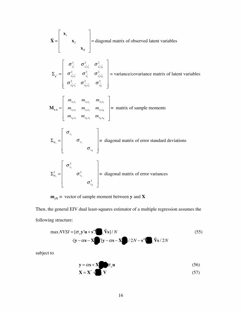
16

!X =

x1

x2

xK

!

"

###

$

%

&&&= diagonal matrix of observed latent variables

!x* =

"x1*2 "

x1*x2*

2 "x1*xK*

2

"x2*x1*

2 "x2*2 "

x2*xK*

2

"xK* x1

*2 "

xK* x2

*2 "

xK*2

#

$

%%%%%

&

'

(((((

= variance/covariance matrix of latent variables

Mx,x =

mx1x1mx1x2

mx1x3

mx2x1mx2x2

mx2xK

mxKx1mxKx2

mxKxK

!

"

####

$

%

&&&&

' matrix of sample moments

!" v=

" v1

" v2

" vK

#

$

%%%%

&

'

((((

) diagonal matrix of error standard deviations

!" v

2 =

" v12

" v2

2

" vK2

#

$

%%%%

&

'

((((

) diagonal matrix of error variances

myX ! vector of sample moment between y and X

Then, the general EIV dual least-squares estimator of a multiple regression assumes the

following structure:

maxNVSI = [! u "y u+ "s!X#! v

!Vs] / N (55)

-[y $%s $X*& "] [y $%s $X*&] / 2N $ "s!V#! v

2!Vs / 2N

subject to

y =!s +X*" +# uu (56)X = X* + $# v

V (57)

17

y * =! + x*" (58)myy = #" $x*" +% u

2 (59)

Mxx = $x* + $% v

2 (60)myx = $x*" (61)

!u s / N = 0 (62)!u u / N = 1 (63)!!V s / N = 0K (64)!!V!V / N = IK . (65)

8. Conclusion

This paper presents an estimator of the EIV structural model using only first and second-

order sample moments. The specification of the EIV model follows the lines discussed by

Kiefer and Wolfowitz (1956) who derived a consistent estimator of the EIV parameters in

the presence of infinitely many “incidental parameters” (latent variables). In order to

avoid the difficulties of the ML method in this context (identifiability and estimation

problems) we have chosen to optimize a dual least-squares objective function subject to a

list of general relations that has been associated for a long time with the EIV problem.

This specification – in general – has an interior global maximum. A crucial but neutral

novelty of this treatment concerns the parameterization of the error terms of the

dependent and “explanatory” latent variables. This “change of variable” allows the

introduction of standard deviations of the error terms in all the observations. A direct

link is thus established between the second-order moments involving error variances, the

detailed EIV observation relations involving the error standard deviations, and the

objective function. This intertwining of the moments and variance parameters, without

requiring additional (user supplied) information about them, is a fundamental

18

breakthrough in order to achieve the desired goal. In the Monte Carlo experiments, which

strictly reflect the structure of the EIV problem presented in sections 2 and 4, it is known

that a region of the parameter space exists where all the variances (standard deviations)

are positive. If the chosen objective function achieves a global maximum in this region,

the EIV parameter estimates are consistent.

We believe that the goal set out at the beginning of this paper – finding an easy

method for consistent parameter estimates of the EIV model – has been attained. This

method requires only a working knowledge of the least-squares methodology, including

its dual specification, and the knowledge of the variance/covariance law for random

variables. The estimation procedure presented here includes the naïve least-squares

method as a special case, that is, when the “explanatory” variables are measured without

error.

References

Adcock, R.J. (1878). A Problem in Least Squares. The Analyst, 5, 53-54.

Brooke, A., Kendrick, D. Meeraus, A. (1988). GAMS, User Guide, Boyd and Fraser

Publishing Company. Danvers, MA.

Cragg, J.G. (1997). Using Higher Moments to Estimate the Simple Errors-In-Variables

Model, The RAND Journal of Economics, 28, S71-S91.

Dagenais, M.G. and Dagenais, D.L. (1997). Higher Moment Estimators for the Linear

Regression Models With Errors in the Variables, Journal of Econometrics, 76,

193-221.

19

Delaigle, A. and A. Meister (2007). Nonparametric Regression Estimation in the

Heteroscedastic Errors-In-Variables Problem, Journal of the American

Statistical Association, 102, 1416-1426.

Gillard, J. (2010). An Overview of Linear Structural Models in Errors In Variables

Regressions, REVSTAT – Statistical Journal, 8, 57-80.

Kendall, M. and A. Stuart (1979). The Advanced Theory of Statistics. Vol. 2, Fourth

Edition. Charles Griffin & Company Limited, London & High Wycombe.

Kiefer, J. and J. Wolfowitz (1956). Consistency of the Maximum Likelihood Estimator

in the Presence of Infinitely Many Incidental Parameters. The Annals of

Mathematical Statistics, 27, 887-906.

Lindley, D.V. (1947). Regression Lines and the Linear Functional Relationship, Suppl.

Journal of the Royal Statistical Society, 9, 218-244.

Neyman, J. (1951). Existence of Consistent Estimates of the Directional Parameters in a

Linear Structural Relation Between Two Variables, Ann. Math. Stat., 22, 497-

512.

Pal, M. (1980). Consistent Moment Estimators of Regression Coefficients in the Presence

of Errors in Variables, Journal of Econometrics, 14, 349-364.

Paris, Q. (2011). Economic Foundations of Symmetric Programming, Cambridge

University Press, New York.

Reiersøl, O., 1950. Identifiability of a Linear Relation Between Variables Which Are

Subject to Error. Econometrica, 18, 375-389.

Van Monfort, K., Mooijaart, A. and De Leeuw, J. (1987). Regression with Errors In

20

Variables: Estimators Based on Third Order Moments, Statistica Neerlandica, 41,

223-237.

Wolfowitz, J. (1954). Estimation of the Components of Stochastic Structures, Proc. Nat.

Acad. Sci., U.S.A. 40, 602-606.