A dissertation Submitted In Partial Fulfillment Of The - SUST ...

بسم اهلل الرمحن الرحيم

Sudan University Of Science And Technology

College Of Postgraduate Studies

A dissertation Submitted In Partial Fulfillment Of The

Requirement Of M. Sc. In Agricultural Engineering

By

Esraa Salah Osman

B.Sc. Agricultural Mechanization Sudan University Of

Science And Technology (2009)

Supervisor

Prof. Dr. Hassan Ibrahim Mohammed

Sudan University Of Science And Technology

August 2015

i

DEDICATION

To my parents, to my husband, to my daughter

to my family, sisters,

brothers and friends

ii

ACKNOWLEDGEMENT

First of all thanks to Allah who enabled me to complete this study.

This study has been conducted under supervision of Prf. Dr. Hassan Ibrahim

Mohammed, to whom I have great pleasure to express my deep gratitude and

everlasting thanks for his inspiring guidance, keen interest and most valuable

assistance, advice and criticism to build up this work. I have thanked him for his

great efforts, helpful thoughts and guidance during the construction and

building of this work. Sincere thanks are due to Dr. Omran Musa Abbas for

his help in data analysis. Thanks also extended to the staff of Ministry of

Electricity and Water Resources – Wad Medani for provision of canal data.

Thanks to my colleague and staff at Department of Agricultural Engineering of

SUST.

iii

LIST OF CONTENTS

Content Page

DEDICATION…………………………………………………… i

ACKNOWLEDGEMENT……………………………..………… ii

TABLE OF CONTENTS……………………………………........ iii

LIST OF TABLES………………………………………………… v

LIST OF FIGURES………………………………………………. vii

LIST OF SYMBOLS ……………………………………………… Viii

LIST OF ABBREVIATIONS ……………………………………. ix

ENGLISH ABSTRACT…………………………………….......... x

ARABIC ABSTRACT……………………………………............ xii

CHAPTER ONE: INTRODUCTION

1.1 Background and justification…………………………………. 1

1.2 Problem definition………………………………………............ 3

1.3 Study objectives………………………………………………… 4

1.4 Study scope……………………………………………………... 5

CHAPTR TWO: LITERATURE REVIEW

2.1 Description of irrigation channels…………………………….. 7

2.2 Classification of conveyance channels…………………………. 9

2.3Factors to be considered for design of non-erodible channels…. 11

2.4 Methods of design of canal cross-section…………………… 14

2.4.1 Shapes of cross-section of canals…………………………… 15

2.4.2 Profile method (morphological method)…………………….. 16

2.4.3 Permissible velocity approach……………………………… 19

2.4.4 Design of lined channels………………………………….. 20

2.4.5 Design of unlined channel…………………………………… 24

2.5 Past Studies……………………………………………………. 30

2.5.1The optimal design of channels……………………………… 30

2.6 Canalization of Gezira Scheme………………………………. 33

2.6.1 Gezira scheme irrigation system…………………………….. 33

2.6.2 Water storages……………………………………………….. 35

2.6.3 Conveyance system…………………………………………. 35

iv

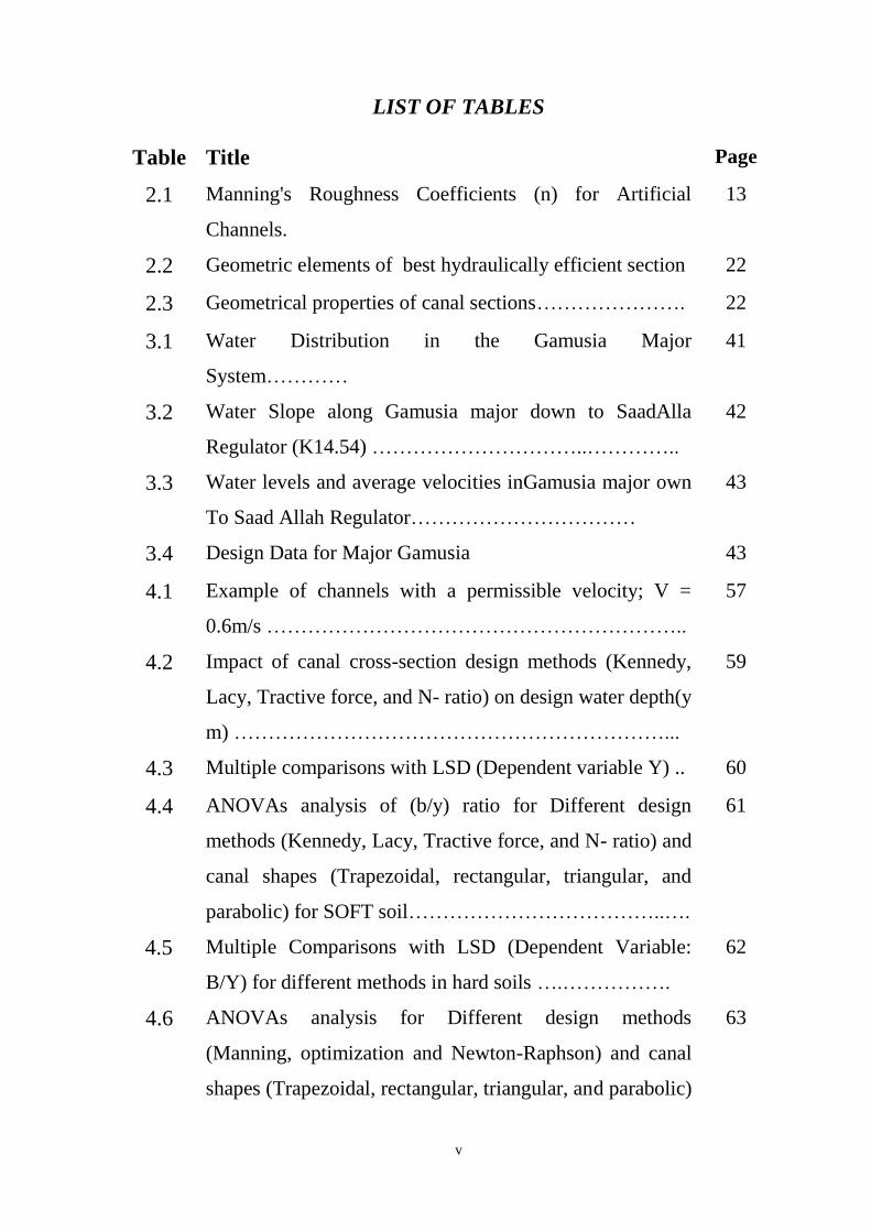
2.6.4 Water distribution system…………………………………... 35

2.7 Current Water Management of Gezira Scheme………………… 37

CHAPTER THREE: MATERIALS AND METHODS

3.1Data collection…………………………………………………. 39

3.1.1 Study area…………………………………………………… 39

3.1.2 Major canal design input data………………………………. 41

3.2 Data analysis………………………………………………….. 44

3.3 Model development……………………………………..…….. 44

3.3.1 General……………………………………………………….. 44

3.3.2 Programming technique and style………………………….. 44

3.3.3Program structure……………………………………………. 45

3.3.4Program limitations…………………………………………… 46

3.3.5 Program iterative logic……………………………………….. 46

3.3.6 Calculation procedure…………………………………………. 47

3.3.7 Model evaluation criteria……………………………………. 56

CHAPTER FOUR: RESULTS AND DISCUSSIONS

4.1 Canal cross-section design procedure using alternative

mathematical algorithms……………………………………..

57

4.1.1 Permissible velocity design approach………………………. 57

4.1.2 Cross-section design for the case of soft soils……………… 59

4.1.3 Cross-section design for the case of hard soils……………… 63

4.2 Selection of the most efficient design alternative mathematical

algorithms. …………………………………………………..

70

4.2.1 Gezira scheme major canals comparison with profile

algorithm…………………………………………………..

70

4.2.2 Comparison of design methods with design of Gezira scheme

major canals……………………………………………………

73

CHAPTER FIVE: CONCLUSIONS AND

RECOMMENDATIONS………………………………………….

REFERENCES…………………………………………………...... 79

APPENDIX 82

v

LIST OF TABLES

Table Title Page

2.1 Manning's Roughness Coefficients (n) for Artificial

Channels.

13

2.2 Geometric elements of best hydraulically efficient section 22

2.3 Geometrical properties of canal sections…………………. 22

3.1 Water Distribution in the Gamusia Major

System…………

41

3.2 Water Slope along Gamusia major down to SaadAlla

Regulator (K14.54) …………………………..…………..

42

3.3 Water levels and average velocities inGamusia major own

To Saad Allah Regulator……………………………

43

3.4 Design Data for Major Gamusia 43

4.1 Example of channels with a permissible velocity; V =

0.6m/s ……………………………………………………..

57

4.2 Impact of canal cross-section design methods (Kennedy,

Lacy, Tractive force, and N- ratio) on design water depth(y

m) ………………………………………………………...

59

4.3 Multiple comparisons with LSD (Dependent variable Y) .. 60

4.4 ANOVAs analysis of (b/y) ratio for Different design

methods (Kennedy, Lacy, Tractive force, and N- ratio) and

canal shapes (Trapezoidal, rectangular, triangular, and

parabolic) for SOFT soil………………………………..….

61

4.5 Multiple Comparisons with LSD (Dependent Variable:

B/Y) for different methods in hard soils ….…………….

62

4.6 ANOVAs analysis for Different design methods

(Manning, optimization and Newton-Raphson) and canal

shapes (Trapezoidal, rectangular, triangular, and parabolic)

63

vi

for hard soil dependent variable(y) …………………….

4.7 Multiple comparisons with LSD (Dependent variable Y.. 64

4.8 ANOVAs analysis of (b/y) ratio for Different design

methods (Manning, optimization and Newton-Raphson)

and canal shapes (Trapezoidal, rectangular, triangular, and

parabolic) for hard soil……………………………….….

65

4.9 Multiple Comparisons with LSD (Dependent Variable:

B/Y) for different methods in hard soils…………………

66

4.10 Variation of N-ratio with inflow rate and canal shape for

opt imal canal cross-section……………………………….

70

4.11 Analysis of various canal design methods of Gezira

scheme Major canals (Soft Soil) in Comparison with

Profile Algorithm dependent variable(y)

71


scheme Major canals (Soft Soil) in Comparison with

Profile Algorithm dependent variable(b / y)

72


scheme Major canals (Soft Soil) by least squire difference

(LSD)………………..……………………………………

74

vii

LIST OF FIGURES

Fig Title Page

2.1 Newton-Raphson using iterative solution 24

2.2 Gazira scheme location and water resource 34

3.1 Study location (Gamusia Major) 40

3.2 Different reaches of Gamusia Major System(source:

Proceedings of conference on Irrigation Management in

Gezira Scheme, (1989)………………………………..

50

4.1 Silt accumulating in a Gezira minor canal, Sudan. As the

silt is dug out, the banks grow higher each year………

69

4.2 Comparison of canal design methods of Gezira scheme

Major canals (Soft Soil) with Profile Algorithm.………

73

4.3 Comparison of design methods with Design of Gezira

scheme Major canals (Soft Soil)……………………….

74

viii

LIST OF SYMBOLS

A flow area [m2]

B bed width of canal [m]

P wetted perimeter [m]

k coefficient of permeability [m/s]

z side slope [dimensionless]

n Manning’s roughness coefficient [dimensionless]

Q discharge [m3/s]

R hydraulic radius [m]

So bed slope [dimensionless]

T width of free surface [m]

V average velocity [m/s]

yn normal depth [m]

f Lacy factor [mm]

α the side slop angle with the horizontal axis.

ix

LIST OF ABBREVIATIONS

EPANET Environmental Protection Agency Net .

SHARC Sediment and Hydraulic Analysis for Rehabilitation of Canals.

SIC Simulation of Irrigation Canals.

GA Genetic Algorithm.

NLOP Nonlinear Optimization Program.

ANN Artificial Neural Network.

GS Gezira Scheme .

WUAs Water Users Association.

USBR United States Bureau of Reclamation.

ASCE American Society of Civil Engineer.

x

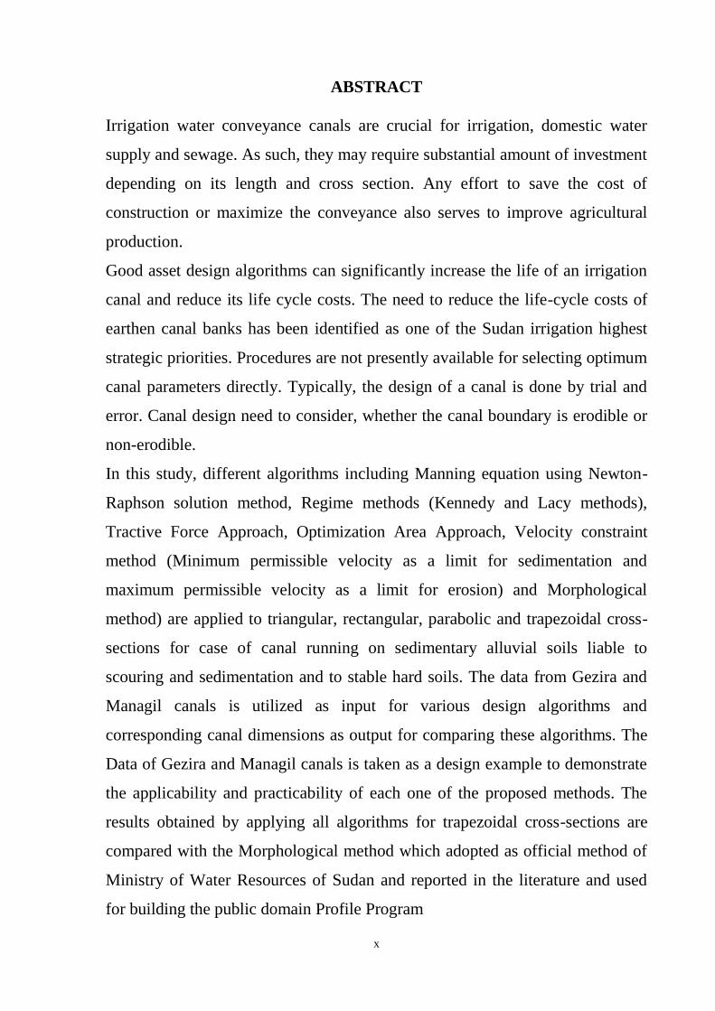
ABSTRACT

Irrigation water conveyance canals are crucial for irrigation, domestic water

supply and sewage. As such, they may require substantial amount of investment

depending on its length and cross section. Any effort to save the cost of

construction or maximize the conveyance also serves to improve agricultural

production.

Good asset design algorithms can significantly increase the life of an irrigation

canal and reduce its life cycle costs. The need to reduce the life-cycle costs of

earthen canal banks has been identified as one of the Sudan irrigation highest

strategic priorities. Procedures are not presently available for selecting optimum

canal parameters directly. Typically, the design of a canal is done by trial and

error. Canal design need to consider, whether the canal boundary is erodible or

non-erodible.

In this study, different algorithms including Manning equation using Newton-

Raphson solution method, Regime methods (Kennedy and Lacy methods),

Tractive Force Approach, Optimization Area Approach, Velocity constraint

method (Minimum permissible velocity as a limit for sedimentation and

maximum permissible velocity as a limit for erosion) and Morphological

method) are applied to triangular, rectangular, parabolic and trapezoidal cross-

sections for case of canal running on sedimentary alluvial soils liable to

scouring and sedimentation and to stable hard soils. The data from Gezira and

Managil canals is utilized as input for various design algorithms and

corresponding canal dimensions as output for comparing these algorithms. The

Data of Gezira and Managil canals is taken as a design example to demonstrate

the applicability and practicability of each one of the proposed methods. The

results obtained by applying all algorithms for trapezoidal cross-sections are

compared with the Morphological method which adopted as official method of

Ministry of Water Resources of Sudan and reported in the literature and used

for building the public domain Profile Program

xi

The result obtained indicate that: Manning equation using Newton-Raphson

solution method, Regime methods (Kennedy and Lacy methods), Tractive Force

Approach, Optimization Area Approach, Velocity constraint method (Minimum

permissible velocity as a limit for sedimentation and maximum permissible

velocity as a limit for erosion) and Morphological method in different values of

water depths are recommend not to use the Velocity constraint approach for it is

not in line with tractive force. Likewise it is not recommended to use Regime

methods for Gezira Scheme due to silt build up with time.

The design guidelines in this study have been prepared using the accumulated

knowledge and practical experience and the study analysis. The research

.

xii

المستخلص

المجاري كما زلي ومياه المنتخدام قنوات الري مهمة في الري السطحي والتزيد بمياه االس

تتطلب الدعم المالي اعتمادًا على طول وعرض مقطع القناة، أي جهود لتقليل التكلفة

االنشائية وزيادة المياه المنقولة تؤدي الي تطوير اإلنتاج الزراعي. ان الممارسات

قنوات اآلن التصميمية الجيدة تزيد من مدى فعالية قنوات الري وتقليل التكلفة، يتم تصميم ال

عن طريق المحاولة والخطأ كما يحتاج تصميم القناة لفهم مناخ محيط القناة قابل للتعرية او

غير قابل للتعرية. في هذه الدراسة معادالت رياضية مختلفة تشمل: معادلة ماننج وطريقة

نيوتن رابسون وطريقة رجيم )كندي وليسي( وطريقة المرفلوجية وطريقة أفضل مقطع

أعلى سرعة مسموح بها كحد للتعرية وأقل سرعة مسموح السرعة مقيدة بين حدين وطريقة

بها كحد لترسيب الطمي، تم تطبيقها على عدة أشكال هندسية هي المثلث المستطيل شبه

والقطع المكافئ في حالة قناة نها أحماء عالقة ومترسبة وكذلك على قناة ذات تربة المنحرف

صلبة.

ستخدمت كمدخالت أخذت من مشروع الجزيرة طبقت على معدالت ان النباتات التي ا

كذلك تم تقسيمية مختلفة ابعاد هذه القنوات كانت مخرجات للمقارنة بين المعدالت التصميمية

أخذ هذه البيانات كنموذج لإلشراف على مدى تطبيق عمل كل هذه الطرق الرياضية، الناتج

يم شبه المنحرف تم مقارنتها بالطرق المرفلوجية من تطبيق هذه المعادالت فيما يتعلق بتصم

والتي تم اعتمادها في قبل وزارة الري السودانية كطريقة فعالة وتم ادراجها لالستخدام ممثلة

في برنامج بروفايل.

النتائج التي تم الحصول عليها مباشرة باستخدام هذه النظريات التصميمية هي قيم مختلفة

لمياه، توصي هذه الدراسة بعدم استخدام طريقة السرعة المسموح بها لعدم توافقها العمق

طرق الرجيم لمشروع الجزيرة ألنها تزيد من ترسيب الطمي.وكذلك عدم استخدام

تستند الخطوات التصميمية لهذه الدراسة على مراجع معرفية ذات نطاق واسع وتجربة

عملية وتحليل الدراسة.

CHAPTER ONE

INTRODUCTION

1

CHAPTER ONE

INTRODUCTION

1.1 Background and Justification

Sudan’s irrigation assets, especially in old irrigated schemes such as Gezira,

White and Blue Nile, are ageing and improved management of this ageing

infrastructure is a major challenge facing food production at national level. The

most significant component of these assets is earthen channels. Moreover, the

country is embarking on constructing new schemes, Upper Atbara, Marawi and

Rahad, to fully utilize its share of the Nile water. Canals in all of these schemes

shall be earth canals.

There are some of earthen irrigation channels in Gezira, Rahad and New Halfa.

However, the need to reduce the life cycle costs of earthen channel banks was

identified as one of the irrigation highest strategic priorities for implementing

the program of management transfer from public administration to hands of user

associations and producer committees.

Over the next 20 years ever increasing levels of expenditure on earthen channel

bank reibresment will be required in the existing gravity fed irrigated schemes,

and the seepage from inadequately constructed earthen channels can lead to

water losses, rising groundwater levels, salinization and degrading of the

environment.

Many procedures have been developed over the years for the hydraulic design

of open channel sections. The complexity of these procedures varies according

to flow conditions as well as the level of assumption implied while developing

the given equation. The Chezy equation is one of the procedures that were

developed by a French engineer in 1768. The development of this equation was

based on the dimensional analysis of the friction equation under the assumption

that the condition of flow is uniform. A more practical procedure was presented

2

in 1889 by the Irish engineer Robert Manning (Chow, 1959). The Manning

equation has proved to be very reliable in practice.

The Manning equation invokes the determination of flow velocity based on the

slope of channel bed, surface roughness of the channel, cross-sectional area of

flow, and wetted perimeter of flow. Using this equation, the solution procedures

are direct for determination of flow velocity, slope of channel bed, and surface

roughness. However, the solution for any unknown related to the cross-sectional

area of flow and wetted perimeter involves the implementation of an implicit

recursive solution procedure which cannot be achieved analytically. Many

implicit solution procedures such as the Newton- Raphson, Regula-Falsi,

secant, and the Dekker-Brent Methods (Press et al., 1992).

One of the important topics in the area of free surface flows is the design of

channels capable of transporting water between two locations in a safe, cost -

effective manner. Even though economics, safety, and aesthetics must always

be considered, in this unit thrust is given only to the hydraulic aspects of

channel design. For that discussion is confined to the design of channels for

uniform flow. The two types of channels considered are:

1- Lined or non-erodible;

2- Unlined, earthen, or erodible.

There are some basic issues common to both the types and are presented in the

following paragraphs.

1- Shape of the cross section of the canal.

2- Side slope of the canal.

3- Longitudinal bed slope.

4- Permissible velocities - Maximum and Minimum.

5- Roughness coefficient. 6. Free board.

3

1.2 Problem definition

Open canals are used in water resources systems to transfer large quantity of

water from a river or another source to where it is used. They are essential

elements of irrigation and waterpower systems. They are free surface structures,

which carry water by gravity. An open canal may require substantial amount of

investment depending on its length and cross section, making the optimal sizing

essential. Optimal sizing is to find the optimal cross section dimensions at

minimum construction cost.

An optimal open channel cross section has channel dimensions for which the

construction cost is minimized and the conveyance is maximized. In order to

save costs, simple channels can be constructed with distinctly different

materials for the bed and side slopes. To prevent seepage losses, for example

the bed of a channel can be lined with concrete and the side slopes can be lined

with rough rubble masonry and boulder pitching. The roughness along the

wetted perimeter in such channels may be distinctly different from part to part

of the perimeter. For channels having composite roughness, an equivalent

uniform roughness coefficient is required to be used in the uniform flow

formula. The equivalent roughness equation again incorporates the flow

geometric elements and corresponding roughness coefficient values (Chow,

1959).

The channel design may be divided into two categories, depending upon

whether the channel boundary is erodible or non-erodible. For erodible

channels, flow velocities are kept low so that the channel bottom and sides are

not eroded. The minimum flow velocity in flows carrying a large amount of

sediment should be such that the material being transported is not deposited in

the channel.

The GS is the largest irrigated scheme under single management in the Sudan as

well as in the world. It was designed for a cropping intensity of 0.75, however,

4

the achieved cropping intensity is usually not more than 0.50 which is very low

by any standard.

The GS has a total area of 890,000 ha (2.12 million feddan) and uses 35% of

Sudan’s current allocation of Nile waters. This represents 6.0-7.0 billion

m3/year. The GS has a long history of satisfactory performance to the extent

that it has been used as model for design and development of all other major

irrigation systems in Sudan.

In the last years, there was tremendous reduction in the productivity of the

scheme. In addition, in recent years, the scheme has been run down in

extremely serious water management problems. The reasons are many but, the

most important ones are the water management related problems such as: (1)

sedimentation (siltation rates & de-silting practices); (2) rainfall drainage; (3)

irrigation scheduling (sowing dates, crop rotations, on farm application

method); (4) indenting system cancelling (to identify the amount of water

required to irrigate crops); (5) maintenance priorities and timing (canals and

drains); and (6) hydraulic structures damage (Ishraga et al., 2011).

1.3 Study objectives

The general and overall aim of this study is to minimize cost of crop production

by providing the country irrigated agriculture with design procedure needed to

improve the understanding of lined and unlined irrigation channel cross-section

design.

The specific objectives of this study are:

(i) To develop canal cross-section design procedure using alternative

mathematical algorithms for soft and hard soils.

(ii) To select the most efficient design alternative in comparison with

Profile Algorithm and design of Gezira scheme Major canals.

(iii) To apply the selected efficient Algorithms to Optimal Design of Canal

Cross Sections of lined and unlined Major Canals.

5

1.4 Study scope

The thesis is expanded in five chapters.

The first chapter provides the background information regarding the problem

faced when designing new canals of irrigation schemes or when re-

modeling old ones. On the basis of the problem in formulating the

design and management aspects of irrigation schemes that run in soft

or hard soil, the objectives of the research were formulated.

Chapter 2: provides an overview of history of irrigation, status, issues and

future plans of irrigation development in Sudan. The review covers

theories of design of canal of various shapes with sediment laden water

and without. A brief introduction of the Gezira Irrigation Scheme that

is selected for data collection is also given.

Chapter 3: provides canal input data collected, data analysis, and model

development. The chapter gives programming techniques and style,

structure, limitation, iterative logic and calculation procedures.

Derivation of design steps and the rationale of the proposed design

approach and the management aspect of the canal design are detailed

aided by conceptual flow chart and

Chapter 4: focuses on the explanation of the results and discussions. The

chapter covers: Canal cross-section design procedure using alternative

mathematical algorithms for soft and hard soils. In particular it details

the limitations of Permissible Velocity design approach. The chapter

considers the selection of the most efficient design alternative

mathematical algorithms for Gezira scheme Major canals in

comparison with Profile Algorithm. The chapter is about the

application of mathematical model to evaluate the proposed design

approach and comparison results with the existing canal.

6

Chapter 5: Gives the evaluation of conclusions drawn from the inferences of

previous chapters and some outlook for the future in this field.

CHAPTER TWO

LITERATURE REVIEW

7

CHAPTER TWO

LITERATURE REVIEW

2.1 Description of irrigation channels

The optimal design of channels has been of importance among researchers and

hydraulic engineers (Guo and Hughes, 1984; Froehlich, 1994; Monadjemi,

1994; Das 2000, Jain 2004 et al.; Bhattacharjya, 2004). Guo and Hughes (1984)

designed optimal channel cross sections from the first principles of calculus.

Presented optimality conditions for a parabolic channel cross section. Froehlich

(1994) used the Langrage multiplier method to determine optimal channel cross

sections incorporating limited flow top width and depth as additional constraints

in his optimization formulation. Used Langrage’s method of undetermined

multipliers to find the best hydraulic cross sections for different channel shapes

(triangular, trapezoidal, rectangular, round bottom triangular, etc.). Swamee

(2000) et al;. have proposed optimal open channel design considering seepage

losses in the analysis. Bhattacharjya (2004) presents the findings of an

investigation for optimal design of composite channels using genetic algorithm

(GA). Some of the recent advances are available in Das (2007) and

Bhattacharjya (2008). Most of the researchers used nonlinear optimization

program (NLOP) to achieve the minimum cost design for a specified discharge.

Present work incorporates variability in discharge using artificial neural

network (ANN). The necessary data for training and testing is generated using

solution of optimization formulation embedded with uniform flow

considerations.

Ideally irrigation schemes should be able to provide water in time, amount and

with desirable head to the agricultural field. The irrigation water demand

keeps on hanging throughout the irrigation season as it depends upon the

climatic conditions, type and stage of crops and soil moisture conditions. So a

8

canal network has to carry the variable amounts of flow, mostly less than the

discharge that it was designed for.

The design discharge can be defined as the maximum amount of flow that can

be handled in a proper way. Various factors like crop water requirement,

irrigation methods, water distribution plans, flow control mechanism and socio-

economic settings are considered in determining the design discharge.

Various methods are available for the design of canals. Some use basic

principles of hydraulics and soil stability to determine the geometry of the

canal. Tractive force methods, rational methods are some of the methods in this

category. Some methods have been evolved from the study of relatively stable

canals around the world. These methods are known as regime methods and the

works of Lacey (1930) is few examples in this field. Suitable design

approaches can be used depending upon whether the canal has a rigid boundary

or has an erodible boundary and is carrying clear water or has an erodible

boundary and is carrying water with sediment.

Canals are generally designed assuming steady and uniform flow. However, this

situation is seldom found in a modern irrigation scheme. Modern irrigation

schemes are increasingly demand oriented and require frequent operation of

control gates that leads to unsteady and non-uniform flow. The design becomes

more complicated incase the canal has an erodible boundary and carries water

with sediment. Most schemes in this category require a large amount of

maintenance due to unwanted deposition on or erosion of the canal bed and

banks. Efficient hydrodynamic models are available to simulate the flow for

different gate operation and inflow rates.

The remodels are being extensively used to verify the hydrodynamic

performance of the canal network for design and modernization purposes.

Although, certain similarities exist between irrigation canals and rivers, these

diment transport models for rivers are not applicable for canals due to the

9

specific differences between rivers and canals, among others the appropriate use

of sediment transport formulae and friction factor predictors, the effect of the

canal sides on the velocity distribution and sediment transport, and the

operation rules. The sediment transport concepts should be related to the flow

conditions and sediment characteristics prevailing in irrigation canals. Few

models exist that are meant for canal networks like Environmental Protection

Agency Net (EPANET) (2004), Sediment and Hydraulic Analysis for

Rehabilitation of Canals (SHARC)(HR Wallingford,2002), Simulation of

Irrigation Canals (SIC)(Malaterre and Baume,1997), but these models do not

include explicitly the effect of canal side slopes on the velocity distribution and

of maintenance on the sediment movement.

2.2 Classification of conveyance channels

Irrigation channels are crucial for surface irrigation. Any effort to save the cost

of construction or maximize the conveyance also serves to improve agricultural

production. Apart from irrigation, these channels are the major conveyance

systems for delivering water for various other purposes such as water supply,

flood control, etc. The primary concern in the design of channels is to determine

the optimum channel dimensions to carry the required discharge with the

minimum costs of construction. Water conveyance channels can be: (1) natural

channels (example, rivers, and natural streams), and (2) artificial or man-made

channels. The natural channels enjoy freedom in their plan form and geometry.

(Amlan Das,2013)

The freedom of landform is however arrested in man-made channels. The man-

made channels are constructed either as open drains or open channels, and

closed drains/pipes with either natural air in contact or without contact with the

water. The open drains are generally made as unlined and lined channels. These

channels are generally constructed in manageable regular shapes. These

channels can flow in several state of flow. Some channels run at very high

speed, while others at moderate to slow speed. Some channels run with varying

10

flow depths as the flow progresses, while in others the flow depth remains

constant throughout the journey, the latter is called uniform flow in engineering

language. The man-made channels are commonly designed and constructed to

carry uniform flows. We call the man-made channels as open channels for our

following discussion. In real life fabrication, a canal may be (i) fully in cutting,

(ii) fully in filling, and (iii) partly in cutting and partly in filling and a practical

cross-section in average conditions may have (i) Side slopes, (ii) Berms, (iii)

Freeboard, (iv) Banks, (v) Service Roads, (vi) Dowlas, (vii) Back Berm or

Counter Berms, (viii) Spoil Banks, and (ix) Borrow Pits.(Amlan Das,2013)

(i) The side slopes of the channels must be stable and must with stand forces

of water-soil interaction. In Sudan channels, relatively flatter side slopes

are provided which get steeper in the course of flow because of silting

actions.

(ii) Berm is the extra horizontal gap kept between the top edge of cutting and

toe of the bank. The berms are believed to help deposition of fine

sediments on the banks. The fine sediments are expected to serve as good

lining for reducing losses, leakage and consequent breaches. They help the

channel to attain regime conditions.

(iii) Freeboard is the margin between full supply level and bank level. In fact

freeboard can be depth dependent and discharge dependent. The freeboards

are provided to protect the channel from breaches due to wave actions, and

uncertain flow fluctuations.

(iv) Banks are provided to retain the water. They are used as means of

communication and inspection paths.

(v) Service roads on canal banks are used for inspection purpose can

potentially provide easy communication for villages.

(vi) Dowlas are provided as safety measure for driving vehicles on the roads.

(vii) Back Berm or Counter Berms are provided to give additional protection

to the banks.

11

(viii) Spoil Banks are used to deposit the additional soil close to the channel.

(ix) Borrow Pits provide the soil for channel cross-section formation.

2.3 Factors to be considered for design of non-erodible channels

Most lined channels can withstand erosion satisfactorily and are considered as

Non-erodible. Unlined channels are erodible except those excavated in firm

foundations, such as rock bed. To design non-erodible channels, the designers

computes the dimensions of the channel by a uniform-flow equation and then

decides the final dimensions on the basis of hydraulic efficiency, empirical rule

of best section, practicability, and economy.

The factors to be considered in the design are: the kind of material forming the

channel body, which determines the roughness coefficient; the minimum

permissible velocity to avoid deposition if the water carries silt or debris; the

channel bottom slope and side slopes; the freeboard; and the most efficient

section, either hydraulically or empirically determined. (Amlan Das,2013)

i- Non-erodible material and lining: The selection of the material depends

mainly on the availability and cost of the material, the method of

construction, and the purpose for which the channel is to be used. The lining

is used to prevent erosion and check seepage losses. Note that for lined

channels maximum permissible velocity can be ignored provided that the

water does not carry sand, gravel, or stones. Here, one should remember that

very high velocity flows exhibit tendency for the flow to pick up the lining

blocks and push them out of position. Therefore, lining should be designed

against such possibilities.

ii- Minimum permissible velocity: The minimum permissible velocity or then

on-silting velocity is the lowest velocity that will not start sedimentation and

induce the growth of aquatic plant and mosses. 0.6 to 0.9 m/sec velocity

generally suffices, and 0.75 m/sec velocity prevent weed and moss growth

when the percentage of silt present in water is small.

iii- Longitudinal slopes: The longitudinal slope of a channel is governed by:-

12

1- The topography,

2- The energy head requirements for the flow of water, and

3- The purpose of the channel.

iv- Side slopes: The side slopes of a channel depend on the kind of material,

maximum permissible velocity for unlined channels, method of

construction, condition of seepage loss, climatic changes, channel size …

etc.

v- Freeboard: The freeboard of a channel is the vertical distance from the top

of the channel to the water surface to prevent waves or fluctuations in water

surface from overflowing the sides. There is no universally accepted rule for

the determination of freeboard, since wave action or water-surface

fluctuation in a channel may be created by many uncontrollable causes.

Freeboard for an unlined canal or lateral is commonly governed by

considerations of canal size and location, storm-water inflow, and water-

table fluctuations caused by checks, wind action, soil characteristics,

percolation gradients, operating road requirements, and availability of

excavated material. For lined canals or laterals, the height of lining above

the water surface depends upon many factors such as: size of canal, velocity

of water, curvature of alignment, condition of storm- and drain-water

inflow, fluctuations in water level due to operation of flow-regulating

structures and wind action. The height of bank above the water surface will

vary with size and location of canal, type of soil, amount of intercepted

storm or drain water … etc. A common practice is to use

either depth of flow or design flow as the governing criteria to decide the

amount of freeboard.(Amlan Das,2013)

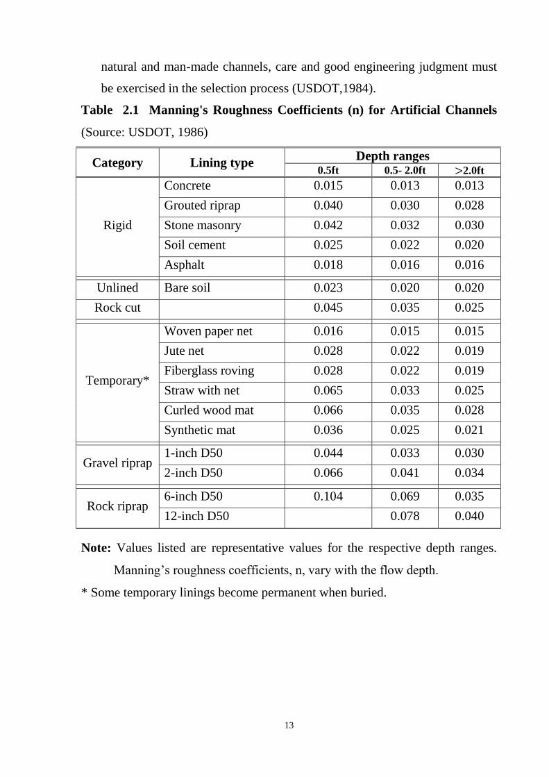
vi- Manning’s “n” Values: The Manning’s “n” value is an important variable

in open channel flow computations. Variation in this variable can

significantly affect discharge, depth, and velocity estimates. Since

Manning’s “n” values depend on many different physical characteristics of

13

natural and man-made channels, care and good engineering judgment must

be exercised in the selection process (USDOT,1984).

Table 2.1 Manning's Roughness Coefficients (n) for Artificial Channels

(Source: USDOT, 1986)

Category Lining type Depth ranges

0.5ft 0.5- 2.0ft >2.0ft

Rigid

Concrete 0.015 0.013 0.013

Grouted riprap 0.040 0.030 0.028

Stone masonry 0.042 0.032 0.030

Soil cement 0.025 0.022 0.020

Asphalt 0.018 0.016 0.016

Unlined Bare soil 0.023 0.020 0.020

Rock cut 0.045 0.035 0.025

Temporary*

Woven paper net 0.016 0.015 0.015

Jute net 0.028 0.022 0.019

Fiberglass roving 0.028 0.022 0.019

Straw with net 0.065 0.033 0.025

Curled wood mat 0.066 0.035 0.028

Synthetic mat 0.036 0.025 0.021

Gravel riprap 1-inch D50 0.044 0.033 0.030

2-inch D50 0.066 0.041 0.034

Rock riprap 6-inch D50 0.104 0.069 0.035

12-inch D50 0.078 0.040

Note: Values listed are representative values for the respective depth ranges.

Manning’s roughness coefficients, n, vary with the flow depth.

* Some temporary linings become permanent when buried.

14

2.4 Methods of design of canal cross-section

This includes: the profile method, the permissible velocity approach (maximum

or minimum velocity limits), methods for lined canals, and methods for unlined

canals.

Present design: The present design procedure of flood channels, drainage

channels and irrigation canals is still rather empirical. The design can be divided

into:

The determination of the alignment and the location of structures. This is

not discussed here;

The preparation of the design criteria. Such the side slopes, the freeboard,

the dimensions of the embankments;

The hydraulic design such as the morphological method and the regime

method.

Irrigation canals have a well- defined design discharge, which is the

maximum canal discharge. Normally, the head works of the system prevents

inflow of bed load into the canals. Also the transport of wash load through

the canals can be controlled by constructing sand trap.

Flood and drainage channels have fluctuating discharges and the bed-

forming discharge is normally lower e. g. Q1- year than the maximum

design discharge, e. g. Q20- years. The inflow of bed load and wash load

cannot be controlled. Moreover, the sediment transport becomes quite

difficult for decreasing channel gradients.(Ankum,2002)

15

2.4.1 Shapes of cross-section of canals

Canal types of cross-sections are: Triangular, rectangular, trapezoidal, and

parabolic sections.

In general Triangular sections are generally constructed for carrying small

discharges. Rectangular sections are constructed fo1r moderate discharges. For

carrying large discharges rectangular sections are not preferred. This is on

account of stability of side slopes. Vertical side walls require large thickness to

resist the earth pressure.

Trapezoidal section is better for such cases since sloping side walls require less

thickness.

Triangular open channel sections are generally used for the drainage facilities of

roadways. They collect the surface-water and water coming from the side slopes

(cut areas) and convey them to safe places where the hazardous effects of water

on roadway structure are minimized.

Rectangular open channel sections are one of the most widely used channel

types in hydraulic engineering. There are so many examples of rectangular

channel applications like conveyance lines for irrigation and municipal

purposes, stilling basins of spillways, flood protection structures, etc.

Compared to other channel types, rectangular channels have the advantage of

being constructed by smaller top width usage. This property of rectangular

channels makes them preferable for the works where the land usage is limited

by some means. These restrictions generally occur in urban areas where existing

or planned structures do not permit the usage of sloped side channels.

Trapezoidal channel sections are the most widely used open channel sections in

engineering. Most of the main water conveying lines has the trapezoidal

geometry. The most important advantage of trapezoidal sections are their ease

16

of construction. Besides their constructional advantages, they have also the

advantageous of high hydraulic efficiency. Therefore, it is not surprising that

most of the water carrying and discharging lines have been made of trapezoidal

geometry.(Lycock , 1996)

In order to define a trapezoidal section, two section variables are not sufficient.

It requires three section variables i.e., bottom width, side slope and flow depth.

Parabolic sections: Riverbeds, unlined canals and irrigation furrows all tend to

approximate a stable parabolic shape. Therefore, unlined canals can be made

more hydraulically stable by initially constructing them in a parabolic shape.

Since the channel side slopes along the cross section are always less than the

maximum allowable side slope at the water surface, parabolic channels are

physically more stable. A lined parabolic channel has no sharp angles of stress

concentration where cracks may occur. A parabolic canal is described by:

Y = a x2 (1-1)

Where:

y = the value of parabolic dimension on vertical axis,

x = the value of parabolic dimension on horizontal axis and

a = angles between (y & x) ≠0

2.4.2 Profile method (morphological method)

The profile method as described by Ankum (2002) is based on solving three

equations for three unknown. The morphological method uses hydraulic

theories to define a stable channel, such as the uniform flow formula for the

flow of water, the tractive force formula to prevent scouring, the sediment

transportation formulae for the flow of sediment. The morphological method is

recommended for further use.

Three unknown: The morphological design methods acknowledges that three

parameters has to be determined:

17

(1) the bed depth b, (2) water depth y, and (3) the gradient s of the channel.

Thus, three equations are required.

Two discharges; furthermore, the morphological design methods acknowledges

that there are two discharges relevant in the design (Ankum 1996, Ankum

2002).

- The dominant discharge also called the bed- forming discharge for the

stability of the channel in order to avoid scouring and sediment on an

annual basis.

- The design discharge also called the maximum discharge or the capacity

for the water transport capacity of the channel in order to avoid over

topping of the banks.

Equation 1: The morphological design method uses the Strickler formula as its

first equation to describe the flow of water:

Q =KA R2/3

S1/2

(2-2)

Q = V A (2-3)

With the wet cross- sectional area A:

A= (b + z y)y (2-4)

And the hydraulic radius R:

R = 𝐀

𝐛+𝟐𝐲√𝟏+𝐙^𝟐 (2-5)

Where:

Q = the discharge in m3/s, v is the velocity in m/s,

A = the wet cross sectional area in m2.

R = the hydraulic radius in m.

S = the water level energy gradient.

b = the bed depth in m, y is water depth in m.

m = the side slope (1vert: Z Hor)

K = the Strickler coefficient in m1/3

/s.

18

The value of Strickler coefficient K and the side slope z of the channel should

be considered as assumption in the design criteria.

Equation 2: The second equation is related to the flow of sediment. It is

assumed that there are two different situations.

- The channel is subjected to scouring during the dominant discharge. It

means that the channel has to be checked on the criterion of the critical

tractive force Tcr to prevent scouring. Scouring can be prevented e. g. by

reducing the gradient S.

- The channel is subject to sedimentation during the dominant charge. It

means that the channel should be checked on the sediment transport

capacity Qs/Q. Sedimentation can be prevented e. g. by increasing the

gradient S.

These two different situations cannot occur at the same time, as a channel

cannot scour the bed and deposits its sediments at the same time. This would be

reflected in the values of the allowable tractive force Tcr and of the sediment

transporting capacity E min.

Therefore, only one equation can be used in the design. Furthermore, it is

acknowledged here that there are several gradients S without scouring or

sedimentation, because the process of scouring (T = p g y s) is described by

other parameters than the process of sedimentation (E = p g v s).(Ankum 2002)

The method is coded in a computer program called Profile.

Programme profile: The computation with the Strickler formula is somewhat

cumbersome; the discharge Q can be calculated directly when other parameters

are known. But, the water depth y or the bed depth b can only be calculated by

iteration. The formula is easily programmable. The PC- program “profile” can

be downloaded from the internet site of the Section Water Management

(htt:/www.landwater.tudelft.nl). The programme is public domain and can be

19

copied freely. The output of the programme profile should be printed as a file.

This file has to be entered as an “ASCII- text file” into e. g. Word.

2.4.3 Permissible velocity approach

The maximum permissible velocity or the non-erodible velocity is the greatest

mean velocity that will not cause erosion of the channel body. This velocity is

very uncertain and variable, and can be estimated only with experience and

judgment. Generally, old and well-seasoned channels will stand much higher

velocities than new ones, because the old channels are better stabilized,

particularly with the deposition of colloidal matter. When other conditions are

the same, a deeper channel will convey water at a higher mean velocity without

erosion than a shallower one. This is probably because primarily the bottom

velocities cause the souring and for the same mean velocity; the bottom

velocities are greater in the shallower channel. Attempts were made earlier to

define a mean velocity that would cause neither silting nor scouring. It is

doubtful whether such a velocity actually exists.(Ankum,2002)

Permissible Velocities (Minimum and Maximum): It may be noted that canals

carrying water with higher velocities may scour the bed and the sides of the

channel leading to the collapse of the canal. On the other hand the weeds and

plants grow in the channel when the nutrients are available in the water.

Therefore, the minimum permissible velocity should not allow the growth of

vegetation such as weed, hyacinth as well you should not be permitting the

settlement of suspended material (non - silting velocity). The designer should

look into these aspects before finalizing the minimum permissible velocity.

"Minimum permissible velocity" refers to the smallest velocity which will

prevent both sedimentation and vegetative growth in general an average

velocity of (0.60 to 0.90 m/s) will prevent sedimentation when the silt load of

the flow is low.

20

A velocity of 0.75 m /s is usually sufficient to prevent the growth of vegetation,

which significantly affects the conveyance of the channel. It should be noted

that these values are only general guidelines.

Maximum permissible velocities entirely depend on the material that is used

and the bed slope of the channel. For example: in case of chutes, spillways the

velocity may reach as high as 25 m/s. As the dam heights are increasing the

expected velocities of the flows are also increasing and it can reach as high as

70 m/s in exceptional cases. Thus, when one refers to maximum permissible

velocity, it is for the normal canals built for irrigation purposes and Power

canals in which the energy loss must be minimized (Ankum 2002) .

2.4.4 Design of lined channels

The behavior of flow in non-erodible channel is influenced by many physical

factors and many field conditions, and is very complex and uncertain. The

stability of non-erodible channels depends mainly on the properties of materials

forming the channel body. Some channels exhibit erosion while others with

similar channel geometry, hydraulics, and soil physical properties exhibit no

erosion. In fact, one must investigate the chemical properties of the material

forming the channel body. Scientists believe that an ion exchange takes place

between the water and soil or hydration of material. These ion exchanges

provide a binder in some places and thus affecting the erosion. It is important to

mention that such phenomenon is not a rare in many open channels of West

Bengal.

The uniform flow equations for design of non-erodible channels provide

insufficient condition for design of erodible channels. The uniform flow

formula can be used for erodible channels only after a stable section of the

erodible channel is obtained. The design of erodible channels requires

experience and application of sound engineering judgment. As a guideline one

21

can design the erodible channels by using the method of permissible velocity,

and method of tractive force.(Das ,2013)

i- Optimum hydraulic section:

The channel section having least wetted perimeter for a given area is known as

the best hydraulic section. Also, a channel section that gives the minimum area

for a given discharge but not necessarily the minimum excavation is a best

hydraulic section. A channel section should be designed as a best hydraulic

section and then modified for practicability. Note that the principle of best

hydraulic section applies only to the design of non-erodible channels.

The classical optimal section is the best hydraulic section which has the

maximum flow velocity or the minimum flow area and wetted perimeter for a

specified discharge and canal bed slope. Mathematically, it could be stated as:

Minimize A = A(y ,b, z) (2-6)

Subject to: φ= Q – (1/n)* (A5/3

/ P2/3

)* SO1/2

=φ(A,P)= φ(y. b. z) = 0 (2-7)

This is a nonlinear optimization problem with nonlinear equality constraint.

Using Lagrange’s method of undetermined multipliers it can be converted into

an unconstrained optimization problem in terms of an auxiliary function

Table (2.2) depicts geometrical properties of commonly used canal sections.

Triangular sections are generally constructed for carrying small discharges.

Rectangular sections are constructed for moderate discharges. For carrying

large discharges rectangular sections are not preferred. This is on account of

stability of side slopes. Vertical side walls require large thickness to resist the

earth pressure. Trapezoidal section is better for such cases since sloping side

walls require less thickness, and Table (2.3 )geometrical elements of best

hydraulically efficient section.(Indian Institute of Technology Madras

Hydraulic ).

22

Table 2.2 Geometrical properties of commonly canal sections:

Section shape Flow perimeter p Area of flow A

Triangular 2yn√1 + z2 zyn2

Rectangular b +2yn b yn

Trapezoidal b +2yn√1 + z2 (b +z yn) yn

Circular Rϑ 0.5r2(ϑ − sinϑ)

Parabolic 2ynz2{

1

z√1 +

1

z2 + In {√1 +

1

z2}

8

3 zyn

2

Rounded bottom triangular 2y (ϑ + cotϑ) y2(ϑ + cotϑ)

Rounded corner trapezoidal b + 2y (ϑ + cotϑ) by + y2ϑ + cotϑ)

Table 2.3 Geometric elements of best hydraulically efficient section

Cross-

section A P R T D Z=A√𝐃

Trapezoidal √3y2

(1.732y2) 2√3y (3.464y) 0.5y

4√3

3y

(2.3094y)

3

4y(.75)

3

2y2.5(1.5y)

Rectangular 2y2 4y 0.5y 2y y 2Y2.5

Triangular zy2 2√2y (2.828y) √2

4y (0.3535) 2y

y

2(.5y)

√2

2y2.5

(0.707y2.5)

Parabola

4

3√2y2

(1.89y^2)

8

3√2y(3.77y) y/20.5y 2√2y(2.83y)

2

3y(.667)

8

9√3y2.5

(1.539y2.5)

Semi

Circular

π

2y2 π y 0.5y 2y

π

4y

π

4y2.5

Hydrostatic

Catenary 1.40y2 2.98y 0.468y 1.917y 0.728y 1.91y2.5

23

ii- Manning Equation Trial and Error Method:

A trial and error procedure for solving Manning's Equation is used to compute

the normal depth of flow in a uniform channel when the channel shape, slope,

roughness, and design discharge are known. For purposes of the trial and error

process, Manning's Equation can be arranged as shown in equation:

AR2/3 = (Q*n)/(1*S0.5) ( 2-8)

Where:

A = cross-sectional area (m2)

R = hydraulic radius (m)

Q = discharge rate for design conditions (m3/s)

n = Manning's roughness coefficient

S = slope of the energy grade line (cm/km)

To determine the normal depth of flow in a channel by the trial and error

process, trial values of depth are used to determine A, P, and R for the given

channel cross section. Trial values of (AR2/3

) are computed until the equality of

equation (2-20) is satisfied such that the design flow is conveyed for the slope

and selected channel cross section.(Ankum,2002)

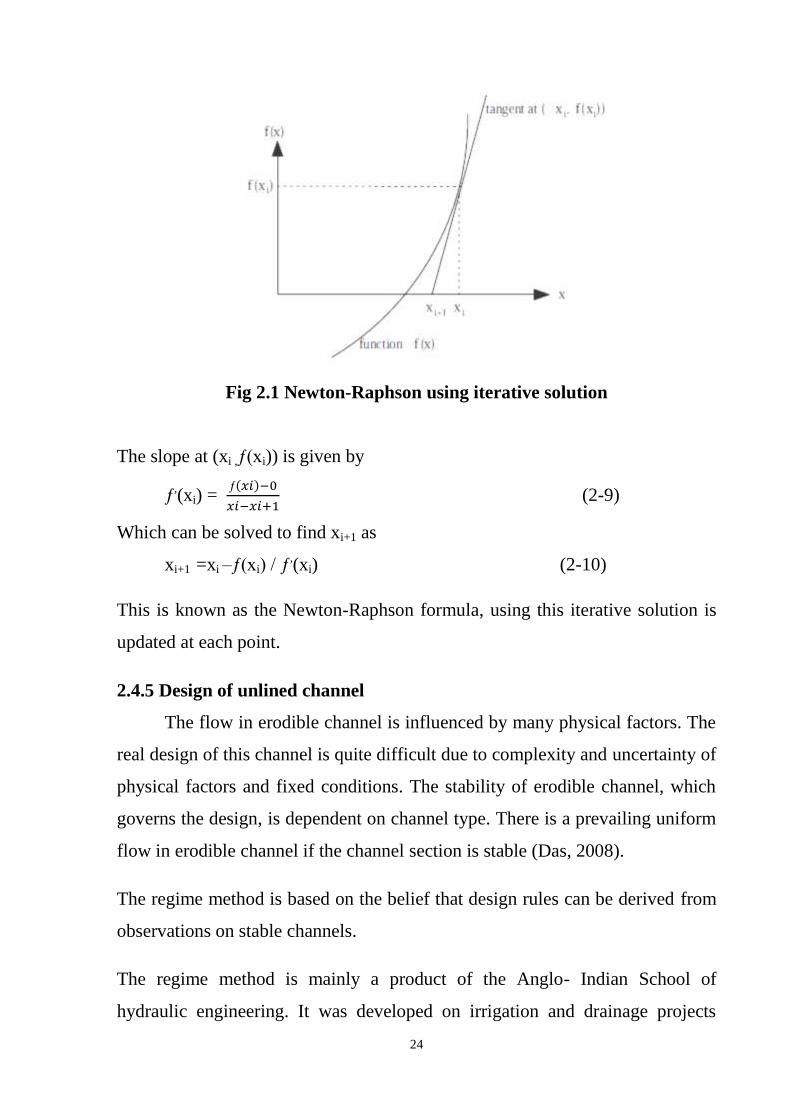
iii- Newton – Raphson Method:

The Newton-Raphson method uses the slope (tangent) of the function ƒ(x) at

the current iterative solution (xi) in the next iteration (see Figure 2-1) This is

different from the Bi section method which uses the sign change to locate the

root .

24

Fig 2.1 Newton-Raphson using iterative solution

The slope at (xi ,ƒ(xi)) is given by

ƒ,(xi) =

ƒ(𝑥𝑖)−0

𝑥𝑖−𝑥𝑖+1 (2-9)

Which can be solved to find xi+1 as

xi+1 =xi –ƒ(xi) / ƒ,(xi) (2-10)

This is known as the Newton-Raphson formula, using this iterative solution is

updated at each point.

2.4.5 Design of unlined channel

The flow in erodible channel is influenced by many physical factors. The

real design of this channel is quite difficult due to complexity and uncertainty of

physical factors and fixed conditions. The stability of erodible channel, which

governs the design, is dependent on channel type. There is a prevailing uniform

flow in erodible channel if the channel section is stable (Das, 2008).

The regime method is based on the belief that design rules can be derived from

observations on stable channels.

The regime method is mainly a product of the Anglo- Indian School of

hydraulic engineering. It was developed on irrigation and drainage projects

25

throughout the Middle East, India and Egypt with canals in fine- grained soils,

of less than 1mm particle size and for capacities up to 400m3/s. The regime

method is discussed here because of its widely used.

1- Kennedy’s method:

A channel in which neither silting nor scouring takes places is called Regime

Channel or Stable Channel. If a channel is in a stable state, the flow is such that

silting and scouring are not considered. The fundamental of designing such an

ideal channel is that whatever silt has entered the channel at its canal head is

always kept in suspension and not allowed to settle anywhere along its course.

More so, velocity of water does not produce local silt by erosion of channel

beds or sides. According to Kennedy (1895) data collected on stable channel

presented the following non-silting and non-scouring velocity this method

defines critical velocity as a velocity that is just sufficient to keep the channel

free from silting or scouring. Kennedy related the critical velocity V (m/s) with

flow depth Y(m) as:

V =0.55 Y 0.64

(2-11)

2- Lacey’s method:

Lacey equation In the 1930s Lacey performed a systematic analysis of the

available stable channel data in an attempt to improve the Kennedy equation .

He established three equations for regime channels which are presented in

literature in different forms. For design purpose it is advantageous to write them

as:

Wetted perimeter : p =4.83* Q1/2

. (2-12)

Wet cross sectional area : A 2.28*ƒ1/3

*Q5/6

. (2-13)

Channel gradient : S = 0.315 *ƒ5/3

*Q-1/6

*10-3

. (2-14)

Where Q is the dominant discharge in m3/s, and ƒ is the lacey silt factor. note

that the numerical coefficient are not dimensionless.

26

Note that Lacey’s method exhibit a tendency of resulting to a steeper bed slope

than that is permissible in the actual topography in many occasions.

3-Width to depth ratio (N) with manning equation:

Considerations: The following can be used in selecting the proper width- to

depth ration n = b/y, between the bed width b and the water depth y:

- Minimum wet cross- sectional area will lead to lower earthwork. It will

be calculated below that the minimum wet cross- sectional area will lead

to a small values of n, thus to narrow channels.

- Minimum construction costs will be obtained, for instance, when the

channel can be cleaned by machine in a single run. This is better possible

for a small values of n, thus for narrow channels.

- The type of earthwork: earthwork on deep channel will involve higher

unit rate because of the deeper layers are harder and the deeper layers will

require more vertical lift. Thus, the lower unit rates will obtained by a

large value of n, thus by wider channels.

- Minimum water level variations in the channel are attractive for several

reasons: (i) the stability of the embankments is better, (ii) the maximum

water level, and so embankments are lower, (iii) navigation is possible

during many discharges etc.

Minimum water level variations are obtained by a large value of n, thus by

wider channels.

The determination of the width- to depth ration n = b/y for the minimum cross-

sectional is usually transformed into question: What width to depth ratio n = b/y

gives the maximum Q for a fixed cross sectional area A?

This is solved in the following way (Chow, 1959):

- The Strickler formula reads:

Q = kAR2/3

S1/2

= k A5/3

p-2/3

S1/2

.

- The hydraulic radius

27

R = A/P.

- So that discharge is Q = K A5/3

p-2/3

S1/2

.

- The bed width is: b = (A/y-z y) because of the equation

A =(b+ z y)y.

- The wet perimeter p = b + 2y √(z2 + 1), so p = A/y – z y + 2y√(z

2 + 1).

Considering that the parameters Q and A are fixed, the criterion becomes one of

minimizing the term P. Thus, dp/dy = A/y2 –z+ 2√(z

2 + 1) = 0

As A = (b + z y)y, this equation becomes (- b/y -z -z + 2√ (z2 + 1) = 0) and

finally b/y = 2 √(z2 + 1) – 2z.

Are the bed and the slopes the tangents to semi- circle?

The side slope 1ver: zhor has an angle ∝ with the horizontal. Thus, to ∝ = 1/z, or

∝ = arctg z, sin ∝ =1/√z2 + 1, and sin ∝ =.1/√z2 + 1

The width- depth ratio n = b/y for the minimum cross- section reads:

b/y = 2(√z2 + 1 − z) = 2 (1

sin∝−

cos∝

sin∝) = 2 (

1−cos∝

sin∝).

Basic goniometry learns that tg ½ ∝ = (1- cos ∝)/ sin ∝, so that: tg ½ ∝ = ½

b/y.

This condition means that the point M in the middle of the water line is also the

center of a circle, which tangents are the bed and the side slopes of the cross

section.

What side slope m gives the most optimum cross- section?

The above width to depth ratio b/y = 2√ (z2 + 1) – 2z leads to an expression for

the width b:

b = 2y√ (z2 + 1) – 2zy

The cross- sectional area: A = by + zy2 =2 y

2 √ (z2 + 1) – 2zy

2, so that:

28

y2 = A/2√ (z

2 + 1) –z

The wet perimeter p = b + 2y√ (z2 + 1) = 2y {2√ (z

2 + 1) –z}, so that

P2 = 4

A

2√z2+1−z (√z2 + 1 − z)2 = 4A( √𝑧2 + 1 − z)

And finally:

p = 2√A(√z2 + 1 − z)

The minimum value is found for dp/dz = 0, so:

dp

dz =

A1/2

(√z2+1−z)1/2 (

2z

√z2+1) -1 = 0 for z =

1

√3 and so ∝ = 60°.

Width- to- depth ratio b/y: The width- to depth ratio n = b/y, between the bed

width b and the design water depth y, is often assessed on basis of practical

considerations. Considerations may include wider channels have less water

level variation, deep channels may cut through impervious horizontal layers,

deep channels require less expropriation, as well on economic considerations.

Different relations have been developed for irrigation and drainage channels in

different countries:

- In USA, the USBR- formula is used: b/y = 1.65 Q0.28

.

- The Indonesian design standards are based on the Kennedy equation, but

applied together with the tractive force concept.

Width – to – depth ratio b/y in the design, it is obvious that the width- to depth

ratio n = b/y cannot be defined on strict objective grounds. Therefore, it is

advisable to set a range of the width- to depth ratio n = b/y in the design criteria,

instead of just one value. Some guidance can be obtained from the USBR-

formula: b/y = 1.65 Q0.28

. For instance: Qdom = 30 m3/s needs a range in the

width- to depth ratio n = b/y of 3< n< 5.

29

4-Tractive force approach:

The idea of tractive force was given by du Boys in 1879. However, Brahms

stated the principle of balancing this force with the channel resistance in a

uniform flow in 1754. When water flows in a channel, a force is developed that

acts in the direction of flow on the channel bed. This force, which is simply the

pull of water on the wetted area, is known as the tractive force. This is also

known as the shear force or drag force. In a uniform flow the tractive force is

apparently equal to the effective component of the gravity force acting on the

body of water parallel to channel bottom. It is a very difficult work to account

the tractive force of channel. Engineers commonly employed membrane

analogy, analytical and finite difference methods for its quantification.

According to the tractive force concept, two forces act on a soil particle resting

on the sloping side of a channel section in which water is flowing. They are the

tractive force and the gravity-force component that tends to cause the particle to

roll down the side slope. When the resultant of these two forces is large enough

the particle will move. It is assumed that when the motion is impending, the

resistance to motion of the particle is equal to the force tending to cause the

motion. The resistance to motion is equal to the product of the normal force and

the inter particle friction i.e., the angle of repose.

The permissible tractive force is the maximum unit tractive force that will not

cause serious erosion of the material forming the channel bed on a level surface.

The permissible tractive force is generally determined in the laboratory and the

values thus obtained are called the critical tractive force. The experience has

shown that actual canals in coarse non-cohesive material can withstand

substantially higher values than the critical tractive forces measured in the

laboratory.

This is probably because the water and soil in actual canals contain slight

amounts of colloidal and organic matter, which provide a binding power, and

30

also because slight movement of soil particles can be tolerated in practical

designs without endangering channel stability. In design the permissible tractive

force is taken less than the critical value. The determination of permissible

tractive force is based upon particle size for non-cohesive material and upon

compactness or voids ration for cohesive materials.

Method of tractive force for design of channels with unprotected side

slopes:

- Select an approximate channel section by experience or from design

tables, collecting samples of the material forming the channel bed and

determining the required properties of the samples

- With these data, investigate the section by applying the tractive-force

analysis to ascertain probable stability by reaches and determine the

minimum section that appears stable.

- For channels in non-cohesive materials the rolling-down effect should be

considered in addition to the effect of the distribution of tractive forces;

for channels in cohesive material the rolling-down effect is negligible,

and the effect of the distribution of tractive force alone is a criterion

sufficient or design.

- The final proportioning of the channel section depends on other non-

hydraulic practical considerations.

2.5 Past studies

2.5.1The optimal design of channels

The design of a channel involves the selection of channel alignment, shape,

size, and bottom slope and whether the channel should be lined to reduce

seepage and/or to prevent the erosion of channel sides and bottom. Since a lined

channel offers less resistance to flow than an unlined channel, the channel size

required to convey a specified flow rate at a selected slope is smaller for a lined

channel than that if no lining were provided. Therefore, in some cases, a lined

channel may be more economical than an unlined channel.

31

Procedures are not presently available for selecting optimum channel

parameters directly. Each site has unique features that require special

considerations. Typically, the design of a channel is done by trial and error.

Channel parameters are selected and an analysis is done to verify that the

operational requirements are met with these parameters. A number of

alternatives are considered, and their costs are compared. Then, the most

economical alternative that gives satisfactory performance is selected. In this

process, it is necessary to include the maintenance costs while comparing

different alternatives. Similarly, the costs of energy required if pumping is

involved and, for power canals, the amount of revenues produced by

hydropower generation must be included in the overall economic analysis.

The channel design may be divided into two categories, depending upon

whether the channel boundary is erodible or non-erodible. For erodible

channels, flow velocities are kept low so that the channel bottom and sides are

not eroded. The minimum flow velocity in flows carrying a large amount of

sediment should be such that the material being transported is not deposited in

the channel.

The optimal design of channels has been of importance among researchers and

hydraulic engineers (Guo and Hughes, 1984; Froehlich, 1994; Monadjemi,

1994; Das, 2000 Jain et; al., 2004; Bhattacharjya, 2004). Guo and Hughes

(1984) designed optimal channel cross sections from the first principles of

calculus. Loganthan (1991) presented optimality conditions for a parabolic

channel cross section. Froehlich (1994) used the Langrange’s multiplier method

to determine optimal channel cross sections incorporating limited flow top

width and depth as additional constraints in his optimization formulation.

Monadjemi (1994) used Langrange’s method of undetermined multipliers to

find the best hydraulic cross sections for different channel shapes (triangular,

trapezoidal, rectangular, round bottom triangular, etc.). Swamee et;al. (2000)

have proposed optimal open channel design considering seepage losses in the

32

analysis. Bhattacharjya (2004) presents the findings of an investigation for

optimal design of composite channels using genetic algorithm (GA). Some of

the recent advances are available in Das (2007) and Bhattacharjya (2008). Most

of the researchers used nonlinear optimization program (NLOP) to achieve the

minimum cost design for a specified discharge. Present work incorporates

variability in discharge using artificial neural network (ANN). The necessary

data for training and testing is generated using solution of optimization

formulation embedded with uniform flow considerations.

1. Minimizing cross section area has already been studied by a few researchers

Das, A (2008). Different cross section types are concerned: Triangular du

Boys, P (1879), Rectangular du Boys, P (1879), Trapezoidal Monadjemi

(1994) , Parabolic Swamee, P.K, Mishra ,G.C, and Chahar, B.R (2000),

Curvilinear Bottomed Channel Ankum (2000) and Circular Guo and

Hughes, (1984). In this study only triangular, rectangular and trapezoidal

cross-sections are concerned due they are much widely used as benchmark

problems. Different set of conditions are considered. Guo and Hughes

accounted freeboard as input parameter. Kayos- and Altan- Sakarya(2006)

used Manning’s formula in calculating flow velocity.

2. Bhattacharjya (2004)combined the critical flow condition with other

conditions. Jain et;al (2004), followed Lotter’s approach in defining

composite canal section. Easa et ;al (2011). considered the criterion for the

side slope stability (soil conditions).

Different optimization methodologies are applied(Direct algebraic technique,

Complex variables and series expansions, Lagrange’s method, Nonlinear

optimization techniques, Sequential quadratic programming, Lagrange’s

undetermined multiplier approach, a hybrid model of genetic algorithm and

sequential quadratic programming hybrid model, genetic algorithm, and colony

optimization to design open channels. Adarsh (2012) modeled uncertainty. Also

different topics are taken as objectives. Trout(1982) considered lining material

33

cost. Das (2008) minimized the flooding probabilities. However, studies

concerning the minimum seepage loss are limited in literature. Swamee (2000)

et al. merged earth work and lining cost. Chahar (2000) also, considered the

seepage loss in the objective functions.

2.6 Canalization of Gezira Scheme:

2.6.1 Gezira Scheme irrigation system

The Gezira Scheme (800,000 ha), is located in central Sudan was famous of

growing cotton in the old days. It used to be the backbone of the Sudan

economy until 1960's and partly 1970's. The scheme consumes annually around

6 to 7 billion m3 of water, which is about 35% of the Sudan's total share from

the Nile water. The performance of the scheme is claimed to be deteriorated

during recent decades, though very few studies on water management appeared

in the literature and even these show.(Adeeb,2006)

No consensus in performance and productivity values. They mostly agree on the

declining performance of the system. Lack of appropriate operation and

maintenance, limited financial Resources, canal siltation, and changing policies

and institutional setups are among the reasons of the downfall. Accurate

information on the performance of the Gezira system is pre-requisite for

planning and management, in particular with dwindling water availability and

rising population and food demand in the region.(Adeeb 2006, Worldbank, 2000,

Eldaw 2004).

34

Fig 2.3 The GS canalization layout (Ishragaet al., 2011)

35

2.6.2 Water storages

Irrigation water is supplied from the Blue Nile reservoirs at Roseries and

Sennar. The Blue Nile has an average annual flow of 50-billion cubic meters at

Roseires, with large seasonal and annual variations. The flow of the Blue Nile

rises steeply from the end of June to an end-of-August peak, followed by a

sharp decline, to a minimum flow of about two percent of the peak, at the end of

April. The Blue Nile carries large quantities of silt as a result of its steep

gradient and heavy seasonal rainfall in its upper catchment area. The silt load in

the Nile is heaviest during July and August and as a result of an increase in

irrigation during these months, significant volumes of the reservoirs are lost to

siltation, annually.(Worldbank,2000)

2.6.3 Conveyance system

The irrigation system comprises twin main canals running from the head-works

at Sennar to a common pool at the cross-regulator at km 57. The Managil main

canal of 186 m3/sec design n capacity was constructed in parallel to the old

Gezira main canal of 168 m3/sec capacity, to serve the Managil extension.

.(Worldbank,2000)

2.6.4 Water distribution system

Water is diverted from the Sennar reservoir by means of twin main canals with

a combined maximum daily discharge capacity of 354m3/s, running north to the

first group of canal regulators 57 kilometers from the dam.

36

From kilometers 57, four branch canals convey water to the Managil extension,

while the Gezira main canal runs north for another 137 kilometers. Major canals

take off from main and branch canals and supply water to minor canals. These

canals flow continuously throughout the growing season. The network consists

of 2,300 kilometers of branch and major canals, and over 8,000 kilometers of

minor canals. Minor canals supply water via gated outlet pipes to field channels

(Abu Ishreen) each irrigating 90 feddans, called "Numbers".

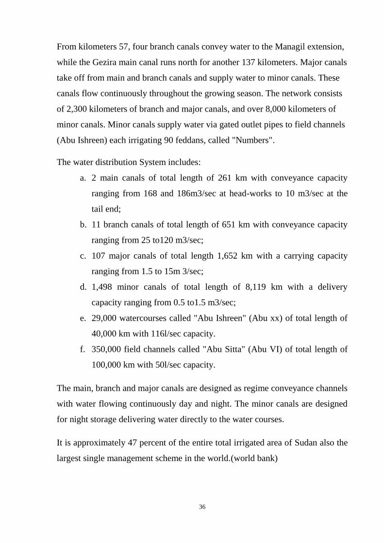
The water distribution System includes:

a. 2 main canals of total length of 261 km with conveyance capacity

ranging from 168 and 186m3/sec at head-works to 10 m3/sec at the

tail end;

b. 11 branch canals of total length of 651 km with conveyance capacity

ranging from 25 to120 m3/sec;

c. 107 major canals of total length 1,652 km with a carrying capacity

ranging from 1.5 to 15m 3/sec;

d. 1,498 minor canals of total length of 8,119 km with a delivery

capacity ranging from 0.5 to1.5 m3/sec;

e. 29,000 watercourses called "Abu Ishreen" (Abu xx) of total length of

40,000 km with 116l/sec capacity.

f. 350,000 field channels called "Abu Sitta" (Abu VI) of total length of

100,000 km with 50l/sec capacity.

The main, branch and major canals are designed as regime conveyance channels

with water flowing continuously day and night. The minor canals are designed

for night storage delivering water directly to the water courses.

It is approximately 47 percent of the entire total irrigated area of Sudan also the

largest single management scheme in the world.(world bank)

37

It has been the backbone of the Sudanese economy. Its share to total agricultural

GDP is estimated to be 35 percent (plusquellec 1990)

The Gezira irrigation scheme (0.882million ha) is mainly gravity fed and lies

between the blue and White Niles south of Khartoum (Levine and Baily 1987).

All canals have cross- regulators which serve as control points (CPs) for off-

taking canals. The stretch of canal between two regulators is called a reach. A

segment of a canal comprising two or more reaches is defined as a section.

The above conveyance and distribution system is the one which is targeted here

for assessing and quantifying the hydraulic performance in comparison with its

design objectives. This research deals with a selected portion of the physical

system of Gezira Scheme. By making use of reliable existing secondary data, an

effort is made to evaluate the system.

2.7 Current water management of Gezira Scheme

Current water management in the Gezira Scheme is substantially different from

the original design, which was used satisfactorily prior to the 1960's. The two-

fold expansion of the irrigation area and successive crop intensification in mid-

1960's following completion of Managil extension required additional quantities

of water to be diverted and distributed. Accordingly, the volume of water

released to the system at Sennar increased by more than three-fold from 2,000

million cubic meters in (1957-1958) to 7,100 million cubic meters in (1997-

1998).

In order to distribute the increased quantity of water required for intensification,

most of the branch and major canals are being operated with higher than the

original design water levels, and the minor canals that operated as night storage

canals are now flowing continuously. The present practice of canal operation

does not pose a major problem when the canal networks are adequately

maintained. However, it becomes problematic and causes breaches of the canal

38

banks and excessive loss of water when the canals are silted up, because the

water levels need to be raised even higher to deliver the.-same quantity of

water. At higher water levels the control structures in the canals cannot function

efficiently.

Moreover, the 2005 Law of the GS which was aiming to improve the

deteriorating conditions of the scheme, on the contrary, turned the GS into

kayos and now, it is losing its compass totally. Because, the GS 2005 Law

implemented what is called Water Users Associations (WUAs) which were

created without considering the nature of the scheme and the water ordering

system - the essential part of the water management system - has been

cancelled. Consequently, today, the Ministry of Irrigation is supplying the

scheme water demand by estimating not by calculating the actual demand.

CHAPTER THREE

MATERIALS AND METHODS

39

CHAPTER THREE

MATERIALS AND METHODS

3.1 Data collection

3.1.1 Study area

The Gamusia major has a length of about 21 Kilometers.It takes off from the

Main Canal of the Gezira Scheme at (Kilo 114). It has five cross regulators to

control the water along its length. There are: El. Kolab Regulator at (Kilo8.63),

Saadab Regulator at(Kilo 11.53), SaadAlla Regulator at (Kilo 14.54), Shaadin

Regulator at (Kilo 17), and Wad Kirai Regulator at (Kilo18.5). All together

there are 27 minors to irrigate a net area of about 22500 feddans. The Gamusia

major system is given in Figure (3.1). The design water slope varies between (7-

10) cm/km. from Gamusia off take to SaadAlla Regulator. Downstream

SaadAlla Regulator the design water slope is 20 cm/km. The cross regulators

are sluice type regulators, while the structures taking from the major are

movable weirs or pipe regulators. According to the design criteria for water

management in the major, water levels should be maintained at each cross

regulator in order to insure adequate flows to each minor.(Ahmed Adam 1988)

40

Fig 3.1 Different reaches of Gamusia Major System

Source: Proceedings of conference on Irrigation Management in Gezira

Scheme, ( Ahmed Adam,1988)

41

3.1.2 Major canal design input data

Data Table (3-1) gives the water distribution in the Gamusia major by

reaches. As can be seen the reach El Sadab to Saad Alla has the highest ratio

of seepage to utilization. This is due to low slope available at Saad Alla, and

confirms what the Field engineers advocate that not enough water reaches

Saad Alla regulator.

Table 3.1 Water distribution in the Gamusia major system (Ahmed

Adam,1988)

Reach Inflow

m3/d

Outflow

m3/d

Differen

ce m3/d

Flow into

minors

m3/d

Seepage

loss in

major

m3/d

Ratio of

seepage/u

tilization

%

Offtake to Khalab 451.87 389.83 62.041 60.75 1.293 2

El Khalab to

ElSadab 417.62 349.91 68.512 54.338 14.174 26.1

El Sadab to SaadAlla 388.50 276.65 111.809 82.612 29.197 35.3

SaadAlla to Shaadia 252.15 190.55 61.794 54.77 7.024 12.8

Shaadia to Wad

Kirai 166.72 - - 30.77 - -

Wad Kirai to Tail 124.50 0 124.50 110.50 14.012 12.9

Table (3.2) gives the measured water slope in Gamusia major down to

SaadAlla Regulator. In the first kilometer the slope is negative. This is due to

over digging. The consequence is that the empirical formula used to

determine the discharge is no longer valid, because the control will be

upstream instead of downstream. For the same opening (4.20 m) and same

head difference (3 cm), the discharge on (date 20/12 )was different from that

measured on(date 21/12), because the upstream water levels were different.

42

Fortunately over digging results in low velocities and this in turn will lead to

siltation, so it is expected that very soon the water slope will become

positive. The water slope in the upper reaches is within the range of the

design value (7-10 cm/km.). Near the railway bridge we can notice that the

water slope decreases upstream and increases downstream. Apparently the

railway bridge has a heading-up effect.

Table (3.2) Water Slope along Gamusia major down to SaadAlla

Regulator (K14.54) (Ahmed Adam,1988)

Distance along

Gamusia M. (km)

Water slope

(cm/km) Remarks

0 - -

1.0 -1.6 -

2.0 2.7 -

3.0 4.1 -

4.0 7.4 -

5.0 7.3 Railway crossing

5.56 13.9 -

8.63 - El Kholab Regulator

- 11.1 -

- 10.6 -

14.54 - SaadAlla Regulator

Table (3.3) compares between the design and actual water levels and average

velocities in the upper reaches of Gamusia major. A rise of about 45 cm in

the reduced levels can be noticed. This rise most likely was caused by silt

being deposited through years of operation . The undergoing bathymetric

survey will clarify this assumption. Also the rise in water levels is

necessitated by a comparative rise in the minors ‘beds as concluded in a

study by Hydraulics Research, Wallingford (July 1987).

43

Table (3.3) Water levels and average velocities in Gamusia major down

to SaadAllah regulator (Ahmed Adam,1988)

Location Reduced water level Average velocity

m/s

Design

m3/s

Actual

m3/s

Design Actual

off take 404.83 405.20 0.39 0.28

D/S EL Kholab regulator 403.98 404.49 0.32 0.24

D/S Sadab regulator 403.70 404.12 0.35 0.24

D/S SaadAllah regulator 403.33 403.80 0.32 0.27

Design data for Gamusia major is collected from reports of irrigation

department of ministry of electricity and water resources see in Table( 3.4)

Table (3.4) Design data for major Gamusia( Ministry of Electricity and

Water Resources ,Wad Medani)

Major Area

(F)

Dischargem3/s

(F = 20)

Velocity

m/s

Bed

width

(m)

Depth

(m)

Water

slope

(cm/km)

1 30130 6.975 0.496 6 1.55 11

2 25611 5.928 0.408 6 1.6 7

3 21618 5.004 0.542 6 1.12 18

4 10417 2.411 0.435 4 0.94 16

5 5317 1.231 0.288 3 0.90 8

6 2520 0.583 0.4294 3 0.50 16

F = feddan

44

3.2 Data Analysis

Descriptive statistical measures employing mean, standard deviation,

probability analysis and T-test was used as a tool for data analysis. M-stat

statistical package on PC-computer was used to generate the parameters of

central tendency of the descriptive statistics. In addition, MS Excel-6.0

spreadsheet was used to numerically check the program output for various

scenarios.

3.3 Model development

3.3.1General

The main functions of the developed model are:

1- To develop mathematical algorithms design procedure for canal cross-

section in soft and hard soils.

2- On basis of Profile Algorithm and design of Gezira scheme Major

canals select the most efficient canal cross-section design method.

3- To facilitate model application for real case study.

As given in the program general flow chart and logic the program main body

consists of a master program (opening introductory and control sheet),

General input entry format, selection of one of four major subsidiary shape

Units, and selection from two soil bed material and specific input data files .

Most of these parts are dedicated to carry specific function.

3.3.2 Programming technique and style

Adhering to the logic of the modular programming, each unit of the program

was broken down into small procedures and functions. Modular

programming was made easier to write and maintain by coding and testing

each procedure or function independently of the main program and its units

using Excel coding system.. Moreover, the programming modularity was

increased by passing value parameters and variable (global and local ones)

into the functions. However, by limiting the scope of the variables unwanted

45

side effects were eliminated. In addition, modularity was improved by

making both procedures and functions self-contained blocks to accept data

through parameters.

The program style was based on the principle of “making a place for

everything and everything in its place”. To achieve this order, defined

sections each to serve specific purpose was adopted. The major sections are

program heading, data section and process section.

3.3.3 Program structure

The mathematical procedure falls within “menu driven” program where a

menu based menu-interface is used to control the whole sequence of

program’s operations (vide: Fig. 4.5 for program main flowchart). The

program begins with some notes concerning the usage of the program and

then systematically takes the user through the rest of its facilities beginning

with the main menu which direct the user to enter the general input data (side

slope, roughness, slope, and inflow rate). From this general input data sheet

the user is requested to select canal shape from four alternative shapes

(Trapezoidal, parabolic, triangular and rectangular shapes). Once the shape is

determined the user need to specify type of canal soil material either soft or

hard soil, which logically divides the program into two models. Each

module is composed of specific mathematical calculation procedure that

requires specific input data. These procedure are: for soft soils: Tractive

force, N-ratio, Regime methods of Lacy and Kennedy procedures. For hard

soils: the optimum section, Newton- Raphson, and Manning trial procedure.

All of the above mentioned models supply the user with some common

utilities including the basic operational techniques (e.g. skipping, reentering,

editing, data restoring and saving). The program-detailed flow chart and its

coding for each mathematical procedure are given with their respective

46

functional relation in the section named and directed for calculation

procedure.

The program runs simply on a single traditional executive file built in Excel

format and made for the purposes of error handling, menus displaying and

data print out. Although each program unit is strictly directed to play a

specific segment in program hierarchy, each of these units has its own

variables and user type definitions being scattered all over the other units due

to their inter-variables dependability. Thus, program listing may impose

some difficulties when skimming its source code line . All units are compiled

first separately and later joined together to make a single big entity that runs

on a common Window programming environment.

3.3.4 Program limitations

The program limitation may be summarized as follows:

1- The program is capable to handle only canal main cross section.

2- Free board , embankments and setting out sheet are left to user

determination

3- The program does not calculate canal longitudinal section.

3.3.5 Program Iterative logic

The program is designed to prompt the user to interactively enter relevant

data for the sub-model via a sequence of driven menus. However, the user is

free to execute each sub-model separately or the whole model as one unit.

The general data entry was a guided step by step process with explanatory

notes to direct the user. Before data entry the dimensions of each input

parameter will be specified. Consequently, defined spaces in the form of

table or blank areas appear to facilitate data entry. After entry of data the

user has the facility to correct the data if there is a mistake or missing values.

The setup of data was made to allow maximum freedom for the user to enter

47

his data. To help the user in case of lacking of data or its estimation build in

files for current state of the art was made available to him. The required

input data will be detailed in the calculation procedure of each calculation

procedure (sub-model).

3.3.6 Calculation procedure

Calculation procedure is given in the flow chart shown in Fig 3.5 and design

steps are break down as follows:

48

Flow chart

START

Type of section shape

Trapezoidal

Rectangular

Triangular

Parabolic

A=(b +z y)y

P= b+2y (1+z2)0.5

A=b*y

P=b + 2y

A=Z*Y2

P=2*Y(1+z2)0.5

A =8/3*Z*Y2

P=2*Y*(z2)(1/z(1+1/(z2))0.5+ln(1/z

+(1+1/z2)0.5)

Channel section /Type

Un

Lined

A B

General input Q

,n, s, z

Lined

49

Y=Qn/(0.5√𝑠)2/9

A=Y2

P=2.82Y

T=2y

Y=Qn/(1.19√𝑠)3/8

A=1.89Y2

P=3.77 Y

T=2.83y

Find R= A/P

A

N-

Raphson

Manning Optimal

x- section

Determined b constant

Assume y

Find V= 1

𝑛 R2/3

√𝑠

Assume y

Find A5/3/P2/3

Find Q*n/√𝑠 Find A P R

Find yn+1= f yn / f ʹyn

Find f ʹyn=(5/3A2/3)/p2/3-

(4/3A5/3)/P5/3

Find f yn=((A5/3)/(P2/3))-

(Qn)/√𝑠=0 Find Vact=Q/A

Determined b

constant

IF

V=VACT

IF Y=Yn+1

Trapezoidal

Rectangula

r

Triangular

Parabolic

Y=Qn/(1.08√𝑠)0.37

A=1.73Y2

P=3.46Y

b=2.309y

Y=Qn/(1.26√𝑠)2/3

A=2Y2

P=4Y

b=A/y

C

NO

yes

yes

NO

50

Calculate A, P, R

Find n2 =1.65 Q0.28

Assume y

Determined b

constant

IF

n1=n2

Find n1 = b/y

END

C

Specific input tc ,wc

Determined b

constant

Find R =tc /w s

Find V = 1

𝑛 R2/3√𝑆

Find Aact= Q/V

Find P =A/R

Assume y

Calculate A, P, R

IF A= Aact

IF A=A

OR P=P

OR R=R

Calculate A,P ,R ,b

Find R=5/2(V2/f)

Specific input d

Find f =1.76√𝑑

Find V =(Q

f2/140)1/6

Find A=Q/V

Find P =4.75√𝑄

Assume y

B

N-ratio Tractive

force

Lacey

Calculate A,P ,R

Specific input k ,m

Assume y

Find VKeendy=0.55 y0.64

Find V = 1

𝑛 R2/3√𝑆

Kennedy

IF

VKeendy=V

NO NO

NO

NO

yes

yes

yes

yes

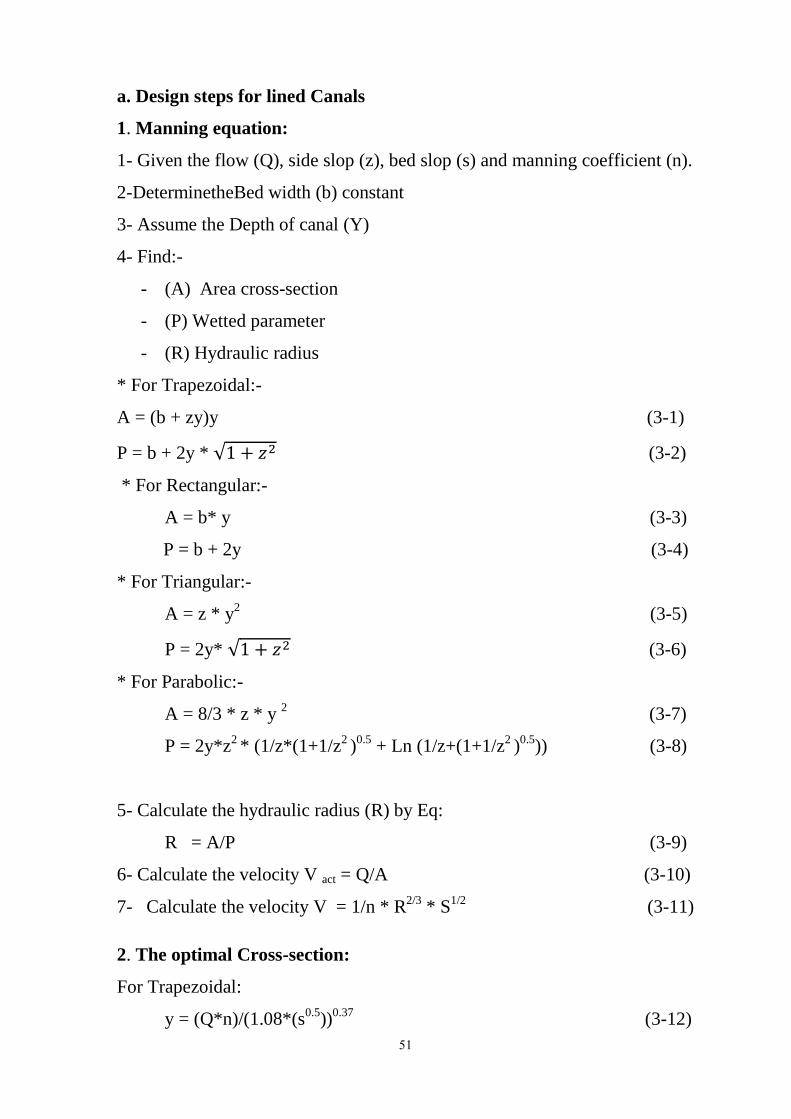
51

a. Design steps for lined Canals

1. Manning equation:

1- Given the flow (Q), side slop (z), bed slop (s) and manning coefficient (n).

2-DeterminetheBed width (b) constant

3- Assume the Depth of canal (Y)

4- Find:-

- (A) Area cross-section

- (P) Wetted parameter

- (R) Hydraulic radius

* For Trapezoidal:-

A = (b + zy)y (3-1)

P = b + 2y * √1 + 𝑧2 (3-2)

* For Rectangular:-

A = b* y (3-3)

P = b + 2y (3-4)

* For Triangular:-

A = z * y2 (3-5)

P = 2y* √1 + 𝑧2 (3-6)

* For Parabolic:-

A = 8/3 * z * y 2 (3-7)

P = 2y*z2 * (1/z*(1+1/z

2 )

0.5 + Ln (1/z+(1+1/z

2 )

0.5)) (3-8)

5- Calculate the hydraulic radius (R) by Eq:

R = A/P (3-9)

6- Calculate the velocity V act = Q/A (3-10)

7- Calculate the velocity V = 1/n * R2/3

* S1/2

(3-11)

2. The optimal Cross-section:

For Trapezoidal:

y = (Q*n)/(1.08*(s0.5

))0.37

(3-12)

52

A =1.73*y2 (3-13)

P=3.46*y (3-14)

For Triangular:

Y=((Q*n)/(0.5*(s0.5

)))2/9

(3-15)

A= y2 (3-16)

P= 2.82y (3-17)

T= 2y (3-18)

R = A/P (3-19)

For Rectangular:

Y =((Q*n)/0.5*(s0.5

))2/9

y=((Q*n)/1.26*(s0.5

))2/3

(3-20)

A=Y2 (3-21)

P=2.82y ,T =2y (3-22)

For Parabolic:

Y=((Q*n)/1.19*(s0.5

))3/8

(3-23)

A=1.89y2 (3-24)

P=3.77*y (3-25)

T=2.83*y (3-26)

T=2.83*y (3-27)

3. Neuten - Raphson:

1- Given: the flow, side slop, bed slop and manning coefficient.

2- Q= 1/n*A*R2/3

*S1/2

(Q*n/√𝑠) = (A5/3

) / (p2/3

) (3-28)

3- F(y) =(A5/3

) / (P2/3

) – (Q*n/√𝑠)) = 0 (3-29)

4- F(y)* =d(y) (3-30)

5- Assume the depth (y)

- FOR Trapezoidal:=

(Q*n/√𝑠)) = ((b+ z y )y)5/3

/(b+2y √1 + 𝑧2)2/3

(3-31)

F*y = ((5/3)*((b+2*z*y)*((b*y)+(z*y2)))

2/3/(B+(2*Y*(1+(z

2))

0.5))

2/3) -

((4/3)*((b*Y)+(z*y2))

5/3)*((1+(z

2))

0.5)/(B+(2*Y*(1+(z

2))

.5)

5/3) (3-32)

53

- For Rectangular:=

(Q*n/√𝑠)= (b*y)5/3

/ (b+2y)2/3

(3-33)

F*y = (((5/3)*y2/3

)/(B+(2*y))2/3

)) - (((4/3)*(y)^(5/3))/(b+(2*y))^(5/3)) (3-34)

- FOR Triangular: =

(Q*n/√𝑠)= (z*y2)

5/3/(2y√1 + 𝑧2)

2/3 (3-35)

f*(yn) = ((10/3)*(y*z)*(z*(y2))/(2*y*(1+z

2)

0.5))

2/3) –

((4/3)*(z*y2)

5/3*(1+z

2)

0.5)/(2*y*(1+z

2)

0.5)) (3-36)

- FOR Parabolic: =

(Q*n/√s)=(8/3*z*y2)

5/3/(2y*z

2*(

1

𝑧√1 +

1

𝑧2 + Ln(

1

𝑧+√1 +

1

𝑧2))

2/3 (3-37)

F*y = (((80/9)*(z*y)*((8/3)*z*(y2))

2/3)/(((2*y*(z

2)(X))

2/3) –

(2*((8/3)*z*(y2))

5/3*((z

2)*(X)))/(2*Y*(z

2)*(X))

5/3 (3-38)

6- Yn+1 = y - f(y)/f*(y) (3-39)

7- Determine bed width (b) constant

8- Calculate (A, P, R)

4.Minimum Velocity V = (0.6) m/s :

1- Q=A*V (3-40)

A=Q/V

2- Q = 1/n *R2/3

*S1/2

(3-41)

(Q*n/√s)=(A5/3

)/(P2/3

)

3- Determine Bed width (b) constant


5- Find: P, R

6- Calculate: (A5/3

)/ (P2/3

)

b. Design steps for unlined Canals:

1. Width to depth - N ratio (b/y):

1- Calculate N ratio from Eq:

(b/y) = 1.65*(Q^0.28) (3-42)

2- Determine bed width (b) constant

54

3- Assume the depth of canal (y)

4- Calculate N= b/y

5- Find: A, P, R

2. Tractive force:

1- Given :

The flow (Q), side slope (z),bed slop(s), manning coefficient(n), Permissible

tractive stress (t)and Specific weight of water(w)

2- Calculate hydraulic radius (R) from Eq:

R = t/w*s (3-43)

3- Calculate the Velocity (V) fromEq:

V =1/n*R2/3

*s1/2

(3-45)

4- Find area of flow by Eq:

A = Q/V (3-46)

5- Find the wetted Parameter (P) by Eq:

P = A/R

6- Determine the bed width (b) constant


8- Find A, P, R dependent from shape of canal

3. Kennedys theory:

1- Given the design flow, channels roughness coefficient, longitudinal

bed slope, critical velocity ration, and a stable side slope value.

2- Assume a trial depth of flow

3- Obtain the critical velocity V

V = 0.55 y0.64

(3-47)

4- Obtain the required flow area from

5- Determine the channel dimension

6- Determine the mean velocity by using any one of Kutter’s formula, or

Manning’s formula, or, Chezy’s formula, or Bazin’s formula

7- Compare the two velocities for convergence

55

For no convergence, repeat the procedure with a new trial flow depth.

4. Lacey theory:

Given design flow, sediment diameter size d in mm, and allowable side

slope.

1- Calculate silt factor by using f = 1.76√d mm (3-48)

2- Calculate flow velocity by using Eq:

V =(Q ƒ /140)1/6

(3-49)

3- Calculate the area of flow cross section from Eq:

A= Q/V

4- Calculate the flow-wetted perimeter from

P = 4.75√Q (3-50)

5- Knowing the area of flow (A) and the wetted perimeter (P), determine

the depth Y and width B from the geometrical relations given below:

A = by + 0.5y2

P = b+ y√5

6- Calculate the required longitudinal bed slope from Eq:

S =ƒ5/3

3340Q1/6 (3-51)

7- Check: Compute R from B and D, using the relation,

R = by+0.5y^2

B+D√5 (3-52)

8- Compare it with the value obtained from Equation:

R = 5

2

𝑣2

ƒ (3-53)

Both values of R should be approximately equal.

56

3.3.7 Model Evaluation Criteria

The performance of the developed model is evaluated based on some

performance indices in both training and testing set. Varieties of

performance evaluation criteria are available which could be used for

evaluation and inter comparison of different models. Following performance

indices are selected in this study to evaluation process.

CHAPTER FOUR

RESULTS AND DISCUSSIONS

57

CHAPTER FOUR

RESULTS AND DISCUSSIONS

4.1 Canal cross-section design procedure using alternative mathematical

algorithms

4.1.1 Permissible Velocity design approach

In the past, it was believed that the permissible velocity V can be used as a

design condition. It was thought that such a permissible velocity V would

prevent the scouring of the bed, as the sedimentation of wash load.

Since 1930, the tractive force concept (T = p g y s) is widely accepted as a

tool to describe the physical process of scouring, while it is more and more

accepted that the energy concept (E = p g v s) describes the process of

sedimentation.

As an example, different channels with a permissible velocity V = 0.6 m/s

are presented in Table 4.1. Apparently, the design discharges (Q = 100 m3/s,

10 m3/s, 1.00 m

3/s and 0.10 m

3/s) have an effect on the tractive force T and

on the sediment transport capacity E.

It can be concluded that the permissible velocity concept is not in line with

the modern judgment on the tractive force T and the sediment transport

capacity E. Thus, the permissible velocity method should not be considered

anymore as better methods are available.

Table 4.1 Example of channels with a permissible velocity; V = 0.6m/s

Q

(m3/s)

H

(m)

KS =

(1/n) b(m) z(v: h) s 10^-3 n (b/)

V

(m/s)

T

(N/m^2) E (W/m^3)

100.00 1.93 40.00 82.5 2.00 0.10 42.6 0.60 1.90 0.59

10.00 1.45 40.00 8.50 2.00 0.20 5.86 0.60 2.85 1.19

1.00 0.58 40.00 1.75 2.00 0.80 3.03 0.60 4.54 4.67

0.10 0.24 40.00 0.25 2.00 3.50 1.06 0.60 8.10 20.15

58

Permissible velocity method: The survey of Forter and Scobey in 1926 on

permissible velocity V because the basis for the permissible velocity method

(e. g. Chow 1959). It was thought that such a permissible velocity would

prevent scouring of the bed as well as deposition of sediment. The

permissible method uses only two equations: (i) the permissible velocity V

for that soil type and (ii) the Strickler formula. The channel gradient S has to

be assumed.

The limitation of the permissible velocity method is shown by the following

example for which a permissible velocity V = 1 m/s is applied. A flood

channel with a capacity of 100m3/s. Side slope 1vert: 2hor, a Strickler

coefficient K = 40 m1/3

/s and an assumed gradient S = 0.3 × 10-3

, leads to a

bed width b = 50 m and a water depth y = 1.87m.

Another channel with capacity of 10m3/s would have a bed width b = 5m and

a water depth y = 1.31m for an assumed gradient s = 0.7 × 10-3

. Evaluation

of these designs by the physics of scouring shows that the larger channel has

a tractive force T = 5.5N/m2 at the bed and the smaller channel T = 9.0 N/m

2

while e. g. a permissible tractive force Tcritical = 6 N/m2. It means the larger

channel is stable at this velocity, but the smaller channel will scour at the

permissible velocity V = 1m/s.

Thus, the permissible velocity method ignores the physical process of

scouring which is well described by bed tractive force. Furthermore, the

method provides only two equations instead of three. Therefore, the

permissible velocity method should not be used anymore, although it is still

recommended in recent literature (Jensen, 1983; James, 1988; Chaudhry,

1993, ASCE, 1995).

59

4.1.2 Impact Of Soil Type On Canal Cross-section:

Table 4.2 shows Anova analysis of design water depth for Different design

methods (Kennedy, Lacy, Tractive force, and N- ratio), and canal shapes

(Trapezoidal, rectangular, triangular, and parabolic) for soft soil. Table 4.2

indicates that there is no significant (at 0.05%) difference between the

employed design methods in soft soils.

Table 4.2 Impact of canal cross-section design methods (Kennedy, Lacy,

Tractive force, and N- ratio) on design water depth (yn)

Test between – subjects effects (Anova)

Source

Dependent variable Y Sig or not

Sum of

squares Df

Mean

square F Sig Not sig

Corrected model 58.270 15 3.885 30.639 0.000 Not sig

Intercept 169.275 1 169.275 1335.124 0.000 Not sig

Method 21.517 3 7.172 56.570 0.000 Not sig

Shape 18.144 3 6.048 47.702 0.000 Not sig

Method * Shape 18.609 9 2.068 16.308 0.000 Not sig

Error 10.143 80 0.127

Total 237.688 96

Corrected total 68.413 95

From Table 4.3 it is clear that there is significant difference between

trapezoidal and parabolic canal shapes. Analysis by least squire difference

(LSD) as depicted in Table 4.3 shows that there is significant difference

(0.05 %) in design water depth when using rectangular shape or trapezoidal

or parabolic shape while there is no significant difference for other shapes.

60

Table 4.3 Multiple comparisons with LSD (Dependent variable Y)

(I)

Shape

(J)

Shape

Mean

difference

(I-J)

Std.

Error Sig

95% confidence

interval Sig or not

Lower

bound

Upper

bound

Trapezoidal

2 0.450 0.103 0.000 0.246 0.655 NOT SIG

3 -0.812 0.103 0.000 -1.017 -0.608 NOT SIG

4 0.202 0.103 0.053 -0.002 0.407 SIG

Rectangular

1 -0.450 0.103 0.000 -0.655 -0.246 NOT SIG

3 -1.262 0.103 0.000 -1.467 -1.058 NOT SIG

4 -0.248 0.103 0.018 -0.453 -0.043 NOT SIG

Triangular

1 0.812 0.103 0.000 0.608 1.017 NOT SIG

2 1.262 0.103 0.000 1.058 1.467 NOT SIG

4 1.014 0.103 0.000 0.810 1.219 NOT SIG

Parabolic

1 -0.202 0.103 0.053 -0.407 0.002 Sig

2 0.248 0.103 0.018 0.043 0.453 NOT SIG

3 -1.014 0.103 0.000 -1.219 -0.810 NOT SIG

(I) Method (J)

Method

Mean

difference

(I-J)

Std.

Error Sig

95% confidence

interval Sig or not

Lower

bound

Upper

bound

Lacy

2 -0.16 0.103 0.878 -0.220 0.189 SIG

3 -1.053 0.103 0.000 -1.257 -0.848 NOT SIG

4 -0.163 0.103 0.117 -0.367 0.042 SIG

Tractive

Force

1 -0.16 0.103 0.878 0.189 -0.220 SIG

3 -1.037 0.103 0.000 -1.242 -0.832 NOT SIG

4 -0.147 0.103 0.156 -0.352 -0.057 SIG

N-ratio

1 1.053 0.103 0.000 0.848 1.242 NOT SIG

2 1.037 0.103 0.000 0.832 1.242 NOT SIG

4 0.890 0.103 0.000 0.685 1.094 NOT SIG

Kenndy 1 0.163 0.103 0.117 -0.042 0.367 SIG

2 0.147 0.103 0.156 -0.057 0.352 SIG

3 -0.890 0.103 0.000 -1.094 -0.685 NOT SIG

1= trapezoidal, 2= rectangular. 3= triangular, 4= parabolic

61

Table 4.4 shows Anova analysis of bed width over design water depth (N-

ratio B/Y) for Different design methods (Kennedy, Lacy, Tractive force, and

N- ratio) and canal shapes (Trapezoidal, rectangular, triangular, and

parabolic) for soft soil. The table indicates that there is no significant

difference between the employed design methods in soft soils.

As given in Table 4.5 for analysis by least squire difference (LSD) it is

evident that there is clear significant differences between canals various

shapes.

Table 4.4 Anova analysis of (b/y) ratio for Different design methods (Kennedy,

Lacy, Tractive force, and N- ratio) and canal shapes (Trapezoidal,

rectangular, triangular, and parabolic) for soft soil


Source

Dependent variable B/Y Sig or not

Sum of

squares Df

Mean


Corrected model 5383093 15 358873 3.220 0.000 NOT SIG

Intercept 663858 1 663858 5.956 0.017 NOT SIG

Method 902784 3 300928 2.700 0.051 SIG

Shape 1793371 3 597790 5.363 0.002 NOT SIG

Method * Shape 2686938 9 298549 2.678 0.009 NOT SIG

Error 8917263 80 111466

Total 14964213 96

Corrected total 14300355 95

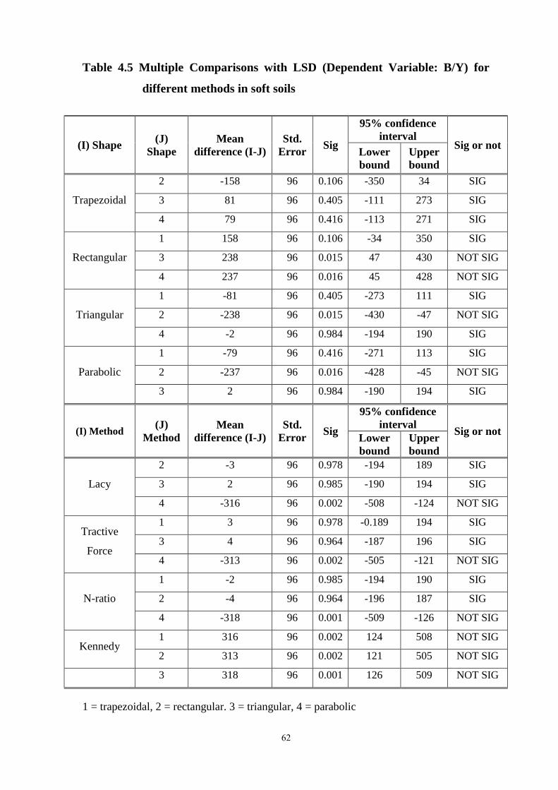
62

Table 4.5 Multiple Comparisons with LSD (Dependent Variable: B/Y) for

different methods in soft soils

(I) Shape (J)

Shape

Mean

difference (I-J)

Std.

Error Sig

95% confidence

interval Sig or not

Lower

bound

Upper

bound

Trapezoidal

2 -158 96 0.106 -350 34 SIG

3 81 96 0.405 -111 273 SIG

4 79 96 0.416 -113 271 SIG

Rectangular

1 158 96 0.106 -34 350 SIG

3 238 96 0.015 47 430 NOT SIG

4 237 96 0.016 45 428 NOT SIG

Triangular

1 -81 96 0.405 -273 111 SIG

2 -238 96 0.015 -430 -47 NOT SIG

4 -2 96 0.984 -194 190 SIG

Parabolic

1 -79 96 0.416 -271 113 SIG

2 -237 96 0.016 -428 -45 NOT SIG

3 2 96 0.984 -190 194 SIG

(I) Method (J)

Method

Mean

difference (I-J)

Std.

Error Sig

95% confidence

interval Sig or not

Lower

bound

Upper

bound

Lacy

2 -3 96 0.978 -194 189 SIG

3 2 96 0.985 -190 194 SIG

4 -316 96 0.002 -508 -124 NOT SIG

Tractive

Force

1 3 96 0.978 -0.189 194 SIG

3 4 96 0.964 -187 196 SIG

4 -313 96 0.002 -505 -121 NOT SIG

N-ratio

1 -2 96 0.985 -194 190 SIG

2 -4 96 0.964 -196 187 SIG

4 -318 96 0.001 -509 -126 NOT SIG

Kennedy 1 316 96 0.002 124 508 NOT SIG

2 313 96 0.002 121 505 NOT SIG

3 318 96 0.001 126 509 NOT SIG

1 = trapezoidal, 2 = rectangular. 3 = triangular, 4 = parabolic

63

4.1.3 Cross-section Design for the case of hard soils

Table 4.6 shows Anova analysis of design water depth for Different design

methods (Manning, optimization and Newton-Raphson) and canal shapes

(Trapezoidal, rectangular, triangular, and parabolic) for hard soil. The table

indicates that there is no significant difference between the employed design

methods in hard soils except for Manning and Newton-Raphson where a

significant is obtained in design depth. From the table it is clear that there is

significant difference between canal shapes. Analysis by least squire

difference (LSD) as depicted in Table 4.7 shows that there is no significant

difference design water depth when using rectangular shape or trapezoidal

one while there is a significant difference for other shapes .

Table 4.6 Anova analysis for Different design methods (Manning, optimization and

Newton-Raphson) and canal shapes (Trapezoidal, rectangular,

triangular, and parabolic) for hard soil


Source

Dependent variable Y Sig or not

Sum of

squares Df

Mean


Corrected model 46.38947549 11 4.23 3.05 0.0027 NOT SIG

Intercept 290.136 1 290.14 2.04 3.1E-21 NOT SIG

Shape 8.36 3 2.79 2.01 0.122 SIG

Method 11.93 3 5.96 4.31 0.018 NOT SIG

Shape *Method 26.10 6 4.35 3.14 0.0096 NOT SIG

Error 83.05 60 1.38

Total 419.57 72

Corrected total 129.44 71

64

Table 4.7 Multiple comparisons with LSD (Dependent variable Y)

(I) Shape (J)

Shape

Mean

difference

(I-J)

Std.

Error Sig

95% confidence

interval Sig or not

Lower

bound

Upper

bound

Trapezoidal

2 -0.932 0.392 0.020 -1.716 -0.147 NOT SIG

3 -0.576 0.392 0.147 -1.359 0.209 SIG

4 -0.673 0.392 0.091 -0.457 0.111 SIG

Rectangular

1 0.932 0.392 0.020 0.147 1.761 NOT SIG

3 0.356 0.392 0.366 -0.427 1.141 SIG

4 0.258 0.392 0.511 -0.525 1.043 SIG

Triangular

1 0.575 0.392 0.147 -0.209 1.359 SIG

2 -0.356 0.392 0.366 -1.141 0.427 SIG

4 -0.098 0.392 0.803 -0.882 0.686 SIG

Parabolic

1 0.673 0.392 0.091 -0.111 1.457 SIG

2 -0.258 0.392 0.511 -1.043 0.525 SIG

3 0.098 0.392 0.803 -0.686 0.882 SIG

(I) Method (J)

Method

Mean

difference

(I-J)

Std.

Error Sig

95% confidence

interval Sig or not

Lower

bound

Upper

bound

Manning 2 -0.852 0.339 0.014 -1.531 -0.172 NOTSIG

3 0.022 0.339 0.947 -0.657 0.701 SIG

Optimal

Cross-

Section

1 0.852 0.339 0.014 0.172 1.531 NOTSIG

3 0.874 0.339 0.012 0.195 1.0553 NOT SIG

Newton-

Raphson

1 -0.022 0.339 0.947 -0.701 0.656 SIG

2 -0.847 0.339 0.012 -1.55 -0.195 NOT SIG


65

Table 4.8 shows Anova analysis of bed width over design water depth for

Different design methods (Manning, optimization and Newton-Raphson) and

canal shapes (Trapezoidal, rectangular, triangular, and parabolic) for hard

soil. The table indicates that there is no significant difference between the

employed design methods in hard soils except for Manning and optimization

where a significant is obtained in design depth. From the table it is clear that

there is significant difference between canal shapes. Analysis by least squire

difference (LSD) as depicted in Table 4.9 shows that there is no significant

difference design bed width to water depth when using trapezoidal compared

to other shapes; where a clear differences are obtained for other shapes

(rectangular or triangular or parabolic),

Table 4.8 ANOVAs analysis of (b/y) ratio for Different design methods (Manning,

optimization and Newton-Raphson) and canal shapes (Trapezoidal,

rectangular, triangular, and parabolic) for hard soil

1- Tests Between-Subjects Effects (Anova)

sig or not Dependent Variable: B/Y

Source Sum of

Squares df

Mean

Square F Sig.

Corrected Model 1932.09 11 175.644 2.80302 0.00519 NOT SIG

Intercept 1278.83 1 1278.83 20.4082 3E-05 NOT SIG

Shape 391.447 2 195.724 3.12346 0.05124 SIG

Method 560.206 3 186.735 2.98002 0.0384 NOT SIG

Shape * Method 980.436 6 163.406 2.60772 0.02593 NOT SIG

Error 3759.75 60 62.6625

Total 6970.67 72

Corrected Total 129.436 71

66

Table 4.9 Multiple Comparisons with LSD (Dependent Variable: B/Y)

for different methods in hard soils

(I) Shape (J) Shape

Mean

difference

(I-J)

Std. Error Sig

95% confidence

interval Sig or

not Lower

bound

Upper

bound

Trapezoidal

2 6.17 2.64 0.02 0.89 11.45 NOT SIG

3 6.92 2.64 0.01 1.64 12.19 NOT SIG

4 6.12 2.64 0.02 0.84 11.39 NOT SIG

Rectangular

1 -6.17 2.64 0.02 -11.45 -0.89 NOT SIG

3 0.75 2.64 0.78 -4.53 6.03 SIG

4 -0.05 2.64 0.99 -5.33 5.23 SIG

Triangular

1 -6.92 2.64 0.01 -12.19 -1.64 NOT SIG

2 -0.75 2.64 0.78 -6.03 4.53 SIG

4 -0.80 2.64 0.76 -6.08 4.48 SIG

Parabolic

1 -6.12 2.64 0.02 -11.39 -0.84 NOT SIG

2 0.05 2.64 0.98 -5.23 5.33 SIG

3 0.80 2.64 0.76 -4.48 6.08 SIG

(I) Method (J)

Method

Mean

difference

(I-J)

Std. Error Sig

95% confidence

interval Sig or

not Lower

bound

Upper

bound

Manning 2 0.58 2.29 0.80 -3.99 5.15 SIG

3 -4.63 2.29 0.05 -9.20 -0.06 NOT SIG

Optimal

Cross-

Section

1 -0.58 2.29 0.80 -5.15 3.99 SIG

3 -5.21 2.29 0.23 -9.78 0.64 NOT SIG

Newton-

Raphson

1 4.63 2.29 0.05 0.06 9.20 NOT SIG

2 5.21 2.29 0.03 0.64 9.78 NOT SIG


67

Tractive force method:

The tractive force method uses two equations: (i) the tractive force formula

and (ii) the strickler formula. Also here the channel gradient s has to be

assumed.

For instance, a flood channel with a capacity of 100m3/s will be constructed

with side slopes 1ver : 2hor and a Strickler coefficient k = 40 m1/3

/s. The soil

has a permissible tractive force of Tcritical = 6 N/m2. When a channel gradient

S = 0.2 × 10-3

is assumed, a bed width b = 25 m and a water depth y = 3.00

m can be calculated. The assumption of another gradient s = 0.4 × 10-3

would

lead to other dimensions: a bed width b = 6 m and a water depth y = 1.50 m.

The tractive force method is not practical for the design as it uses two

equations to solve the three degrees of freedom. Moreover, it ignores the

process of sedimentation.

The regime method:

Many attempts have been made to develop the regime method to the channel

method to the channel design. Many authors have developed their own

regime formulae, such as Inglis in 1946, Lane in 1953, Simons and Alberson

in 1963, Blench in 1966… etc.

General, validity: It is still questionable whether the regime equations are

of a general validity (geldigheid). Obvious, there are the following

disadvantages:

- There are large discrepancies between the results from various equations

when applied under similar conditions

- The channels designed with the regime method have flatter gradients

than the tractive force theory would allow. This will lead to the

construction of several drop structures in the channel that could have

been avoided by using the tractive force method.

68

- The regime method provides normally for more equations than required

for solving the three design parameters i. e. the bed width b, the water

depth y and the gradient s. It means that the Strickler coefficient k can be

calculated from the Strickler formula. This is contradictious to common

understanding as the Strickler coefficient depends on physical parameters

such as soil type and maintenance.

- Conclusion: There seems to be no agreement in the various regime

equations. It seems obvious that the regime method can only use for very

special conditions for which the equations and its coefficients have been

developed.

Criticism of the Lacey’s method centers on the limited range of validity:

- The Lacey equations have been derived from regional data and for

velocities between 0.3 m/s and 1.2 m/s.

- The Lacey equations are based on sediment observations in Punjab-

India, for canals with suspended load and where the concentration ranges

between 1000 – 2000 ppm.

- The size of sediment has an effect on the wetted perimeter i.e. finer

sediments give more narrow channels with steeper side slopes.

- Basically the Lacey equations determine the gradient s of the channel for

a known discharge (Q) and a known silt factor (f ). In river work all three

parameters the gradient (s), the bed width (b) and the water depth (y) for

an assumed side slope (z). The Strickler formula is not yet used so that

also the Strickler coefficient (k)can be calculated. This is not logic, as the

Strickler coefficient k is related e. g. to the maintenance of the channel.

Canals of Gezira scheme are designed using Regime method. This Gezira

design approach is taken as a model for design of other irrigated schemes in

Sudan (Halfa, Rahad, and Suki). As given in Fig 4.1 the Gezira canals are

69

filled with deposited sediment. The removal of such sediment is of high cost

value and indicate that the regime design method need to be replaced by

alternative ones.

Fig 4.1 Silt accumulating in a gezira minor canal, Sudan. As the silt is dug out, the

banks grow higher each year variation of n-ratio for optimal cross –

section:-

According to USBR the N – ratio (b/y) varies with inflow rate and follows

(Q) the formulae:

Nratio(b/y) = 1.65(Q) 0.28

Nratio =ratio between the bed width(b) and the design water depth(y)

Q = design discharge m3/s

Constant of USBR (1.65, 0.28) and also it do not change with shape of canal

cross-section. As given in Table 4.10 N-value for optimal cross-section

varies with canal shape rather than the inflow rate and it is constant for each

canal shape.

70

Table 4.10 Variation of n-ratio with inflow rate and canal shape for

optimal canal cross-section

inflow

rate

Optimum canal cross-section

USBR Trapezoidal

shape

Rectangular

Shape

Triangular

shape

Parabolic

Shape

6.975 2.30 2 2 2.83 2.84

5.928 2.30 2 2 2.83 2.72

5 2.30 2 2 2.83 2.59

2.41 2.30 2 2 2.83 2.11

1.32 2.30 2 2 2.83 1.75

0 .58 2.30 2 2 2.83 1.42

4.2 Application of the efficient depth method foe gezira scheme

4.2.1 Gezira scheme major canals comparison with profile algorithm

Table 4.11 shows results of chi-squire tests for design of soft soil dependent

(y).The table indicate that there is no significant difference between all the

method (tractive forces, Lacy, N-ratio and Kennedy in comparison with

profile method.

71

Table 4.11 Analysis of various canal design methods of Gezira scheme major

canals (soft Soil) in comparison with profile algorithm.(dependent

variable (y)

Observed

(O) lacey

Expected (E)

profile O-E (O-E)^2 (O-E)^2/E Chi Clc

Chi

Test

1.53 1.89 0.36 0.1296 0.068571 0.068571 Not Sig

1.4 1.87 0.47 0.2209 0.118128 0.118128 Not Sig

1.25 1.76 0.51 0.2601 0.147784 0.147784 Not Sig

0.95 1.41 0.46 0.2116 0.150071 0.150071 Not Sig

0.75 1.15 0.4 0.16 0.13913 0.13913 Not Sig

0.46 0.9 0.45 0.2025 0.222527 0.222527 Not Sig

Observed

(O) TRF

Expected (E)


Chi

Test

0.94 1.97 1.03 1.0609 0.538528 0.538528 Not Sig

0.82 1.87 1.05 1.1025 0.589572 0.589572 Not Sig

0.71 1.76 1.05 1.1025 0.62642 0.62642 Not Sig

0.5 1.41 0.91 0.8281 0.587305 0.587305 Not Sig

0.36 1.15 0.79 0.6241 0.542696 0.542696 Not Sig

0.18 0.9 0.73 0.5329 0.585604 0.585604 Not Sig

Observed

(O) N-RA

Expected (E)


Chi

Test

2.2 1.97 0.23 0.0529 0.026853 0.026853 Not Sig

2.2 1.87 0.33 0.1089 0.058235 0.058235 Not Sig

2.3 1.76 0.54 0.2916 0.165682 0.165682 Not Sig

1.9 1.41 0.49 0.2401 0.170284 0.170284 Not Sig

1.8 1.15 0.65 0.4225 0.367391 0.367391 Not Sig

2.2 0.9 1.29 1.6641 1.828681 1.828681 Not Sig

Observed

(O) Kenndy

Expected (E)


Chi

Test

0.14 1.97 1.83 3.3489 1.699949 1.699949 Not Sig

0.48 1.87 1.39 1.9321 1.033209 1.033209 Not Sig

0.4 1.76 1.36 1.8496 1.050909 1.050909 Not Sig

0.4 1.41 1.01 1.0201 0.723475 0.723475 Not Sig

0.33 1.15 0.82 0.6724 0.584696 0.584696 Not Sig

0.28 0.9 0.63 0.3969 0.436154 0.436154 Not Sig

Table 4.12 shows results of chi-squire tests for design of soft soil bed to

depth ratio (b/y). The table indicate that there is a significant difference

between the tractive forces, Lacy and kennedy methods in comparison to

72

profile method, while there is no significant differences for the N-ratio

method in comparison with the profile method.

Table 4.12 Analysis of various canal design methods of Gezira scheme major canals

(soft soil) in comparison with profile algorithm. (dependent variable

(b/y)

Observed

(O) LACEY

Expected

(E)

PROFILE

O-E (O-E)^2 (O-E)^2/E Chi Clc Chi Test

4.22 1.89 2.33 5.4289 2.872434 2.872434 Not Sig

4.49 1.87 2.62 6.8644 3.670802 3.670802 Sig

5.1 1.76 3.34 11.1556 6.338409 6.338409 Sig

4.66 1.41 3.25 10.5625 7.491135 7.491135 Sig

4.1 1.15 2.95 8.7025 7.567391 7.567391 Sig

6.71 0.9 5.8 33.64 36.96703 36.96703 Sig

Observed

(O) TRF

Expected

(E)

PROFILE


6.38 1.97 4.41 19.4481 9.872132 9.872132 Sig

7.32 1.87 5.45 29.7025 15.88369 15.88369 Sig

8.45 1.76 6.69 44.7561 25.4296 25.4296 Sig

8 1.41 6.59 43.4281 30.80007 30.80007 Sig

8.3 1.15 7.15 51.1225 44.45435 44.45435 Sig

16.07 0.9 15.16 229.8256 252.5556 252.5556 Sig

Observed

(O) N-RA

Expected

(E)

PROFILE


2.7 1.97 0.73 0.5329 0.270508 0.270508 Not Sig

2.7 1.87 0.83 0.6889 0.368396 0.368396 Not Sig

2.6 1.76 0.84 0.7056 0.400909 0.400909 Not Sig

2.1 1.41 0.69 0.4761 0.33766 0.33766 Not Sig

1.7 1.15 0.55 0.3025 0.263043 0.263043 Not Sig

1.4 0.9 0.49 0.2401 0.263846 0.263846 Not Sig

Observed

(O)

KENNDY

Expected

(E)

PROFILE


1119.2 1.97 1117.23 1248203 633605.5 633605.5 Sig

73.4 1.87 71.53 5116.541 2736.118 2736.118 Sig

101.1 1.76 99.34 9868.436 5607.066 5607.066 Sig

47.6 1.41 46.19 2133.516 1513.132 1513.132 Sig

540.1 1.15 538.95 290467.1 252580.1 252580.1 Sig

28.8 0.9 27.89 777.8521 854.7825 854.7825 Sig

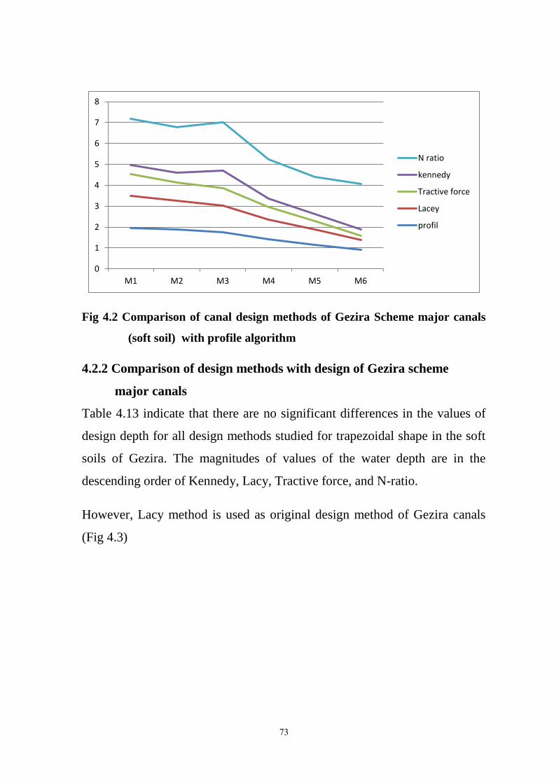
73

Fig 4.2 Comparison of canal design methods of Gezira Scheme major canals

(soft soil) with profile algorithm

4.2.2 Comparison of design methods with design of Gezira scheme

major canals

Table 4.13 indicate that there are no significant differences in the values of

design depth for all design methods studied for trapezoidal shape in the soft

soils of Gezira. The magnitudes of values of the water depth are in the

descending order of Kennedy, Lacy, Tractive force, and N-ratio.

However, Lacy method is used as original design method of Gezira canals

(Fig 4.3)

0

1

2

3

4

5

6

7

8

M1 M2 M3 M4 M5 M6

N ratio

kennedy

Tractive force

Lacey

profil

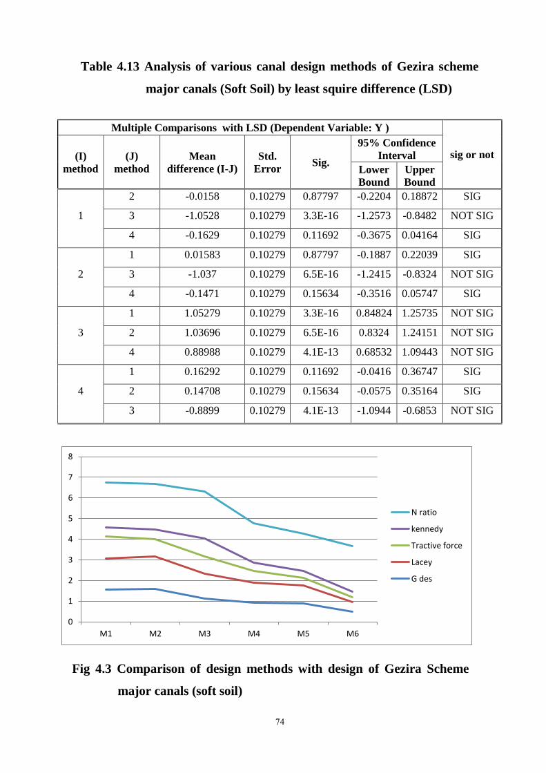
74

Table 4.13 Analysis of various canal design methods of Gezira scheme

major canals (Soft Soil) by least squire difference (LSD)

Multiple Comparisons with LSD (Dependent Variable: Y )

sig or not (I)

method

(J)

method

Mean

difference (I-J)

Std.

Error Sig.

95% Confidence

Interval

Lower

Bound

Upper

Bound

1

2 -0.0158 0.10279 0.87797 -0.2204 0.18872 SIG

3 -1.0528 0.10279 3.3E-16 -1.2573 -0.8482 NOT SIG

4 -0.1629 0.10279 0.11692 -0.3675 0.04164 SIG

2

1 0.01583 0.10279 0.87797 -0.1887 0.22039 SIG

3 -1.037 0.10279 6.5E-16 -1.2415 -0.8324 NOT SIG

4 -0.1471 0.10279 0.15634 -0.3516 0.05747 SIG

3

1 1.05279 0.10279 3.3E-16 0.84824 1.25735 NOT SIG

2 1.03696 0.10279 6.5E-16 0.8324 1.24151 NOT SIG

4 0.88988 0.10279 4.1E-13 0.68532 1.09443 NOT SIG

4

1 0.16292 0.10279 0.11692 -0.0416 0.36747 SIG

2 0.14708 0.10279 0.15634 -0.0575 0.35164 SIG

3 -0.8899 0.10279 4.1E-13 -1.0944 -0.6853 NOT SIG

0

1

2

3

4

5

6

7

8

M1 M2 M3 M4 M5 M6

N ratio

kennedy

Tractive force

Lacey

G des

Fig 4.3 Comparison of design methods with design of Gezira Scheme

major canals (soft soil)

75

Actual design:

The hydraulic design may provide different cross- sections that are valid.It is

even not justified to aim the most optimum design as so many assumptions

have been made. The design can be done in the following steps

- Step 1: Determine the elevation above the reference level at the tail

end of the channel.

- Step 2: Draw from this reference level the straight water line during

Qdom into upstream direction. The uniform flow during the dominant

discharge avoids back water effects that may influence locally

sedimentation and scouring.

- Step 3: Design the water depth y and the bed width b of the channel

by incorporating the width – to – depth ratio n = b/y. Check the

sediment transporting capacity Emin and the critical tractive force Tmax,

and return to step 2 if necessary.

- Step 4: Calculate the water level y max during Qmax with the Strickler

formula. Also here, a straight line may be taken by ignoring the back

water effects in the tail- reach of the channel. Check at the head- end,

whether;

The calculated water elevation is not higher than the available

water elevation (water cannot flow into the new channel).

The calculated flow water elevation is lower than the available

water elevation, because a drop structure is required

CHAPTER FIVE

CONCLUSIONS AND RECOMMENDATIONS

76

CHAPTER FIVE

CONCLUSIONS AND RECOMMENDATIONS

The developed computer design software system for design an open channel

cross-section has been made simple to ease and lessen time consumed as

compared to laborious manual computation of the parameters of an open

hydraulic channel section. The software is an interactive program which

integrates computation, visualization and programming language

environment that has sophisticated data structures, in-built editing and

debugging tools and supports elemental-oriented programming which makes

it an excellent tool for design works.

Water conveyance channels form a very vital component of the

infrastructure for desired canal irrigated agriculture.

The water conveyance channels are either natural, or, artificial.

The artificial open channels are constructed as either unlined (on hard

soils) or lined channels (on soft soils).

Amongst many quantifications, the Manning’s’ formula is widely used

in open channel hydraulics. In actual applications there are various

methods factors to be considered for design of non-erodible channels

Non-erodible material and lining, Minimum permissible velocity,

Longitudinal slopes, Side slopes, Freeboard, and last but not the least

the Best Hydraulic Section

Use of the maximum permissible velocity approaches not in line with

modern judgment using tractive force method (Profile methods).

However, it results in negative water depths in canals with smaller

cross-section. Therefore, it is not recommended of routine design of

canal cross-section.

Kennedy’s method and Lacey methods are mainly used for design of

stable cross sections which are free from both silting and scouring.

77

The validity of these regime methods is questionable due to large

discrepancies between the results from various equations, the channels

designed with the regime method have flatter gradients than the

tractive force, and the regime method provides normally for more

equations than required for solving the three design parameters i. e. the

bed width b, the water depth y and the gradient s.

Amongst many quantifications, the Manning’s’ formula is widely used

in open channel hydraulics.

The researchers throughout the world contributed mainly to

incorporate more and more practical conditions of fabrication in the

consideration of optimal design of open channels.

Meanwhile, the researchers advocated to use trapezoidal cross

sections, as the case of Gezira scheme, for channel design and

fabrication.

These channels are generally designed and constructed in manageable

regular shapes trapezoidal, triangular, rectangular, and parabolic to

carry uniform flows. Every geometric shape has its own advantages as

well as disadvantages. For soft soils there are significant differences

between these shapes and for construction reasons designer prefer to

use trapezoidal ones.

For hard soils there is no significant difference in design water depths

or N- ration for the studied design equations. The differences are

between Manning trial iteration procedure and Newton-Raphsontrial

procedure. It is generally recommended to employ tractive force

approaches (profile methods) are used to design the erodible channels

which scour but do not silt.

Due to the limitations of the Regime methods it is recommended for

the case of Gezira Major Canals to employ Profile methods which

results in lower water levels.

78

The developed computer model may be used as an effective

educational tool for the hydraulic analysis of open channel flow. It

allows for demonstrating the effect of varying geometric parameters of

an open channel on the hydraulics of flow. The model can be applied

to the design of trapezoidal, rectangular, triangular and parabolic.

Also, it is useful when designing or analyzing open channel

distribution systems.

79

REFERENCES

Ankum (2002) Design of open channels and hydraulic structure.

Ahmed Adam,(1988) proceedings of the Conference on Irrigation

Management in the Gezira Scheme .

Askoy B. and Altan-Sakarya A.B.(2006) Optimal lined channel design,

canadin journal of civil Engineering vol.33,no.5,pp.535-545.

ASCE.1995. Minimum design loads for buildings and other structure. ASCE

7-95,Reston,VA.

Bhattacharjya, R.K. and Satish, M.G. (2008). “Discussion of ‘Flooding

probability constrained optimal design of trapezoidal channels’ by

Amlan Das.” J. Irrig .Drain. Eng.,

Brahms, A. Elements of open canal and hydraulic engineers, Zurich,

Germany, 1754 and 1757,vol;1,105

Chow, V.T. (1959). "Open Channel Hydraulics", McGraw-Hill Int. Book.

Co., Singapore.

Chahar B.R, (2000) optimal design of channel section considering seepage

and evaporation losses. PhD. thesis submitted to Dept. of Civil

Engineering Uvin . of Rookee, India.

Chaudhry, H.1993 Open channel Flow, prentice Hall, Inc. Englewood Cliffs

,New Jersey.

Das, A. (2008). "Chance constrained optimal design of trapezoidal

channels", Jl. of Water Resources Planning and Management,

ASCE,134(3), 310-313.

80

Das, A (2013). Design of open canal.

du Boys P. (1879): Etudes du regime du Rhone et l’actionexercee par

leseauxsur un lit a fond de graviers indefin imentaffouillable (The

Rhoneand streams with moveable beds), Annales des ponts et

Chausses, Ser., 5(18): 141-195.

Dahmen E.,(1994).Lecture notes on canal design .IHE. Delft .The Nether

land.

Easa S.M. et.al;(2011) A simplified direct method for finding optimal stable

trapezoidal channels. International joumal of River Basin

Management,vol.g,no.2,pp.85-92.

Froehlich, D.C. (1994). “Width and depth constrained best trapezoidal

section.” J. Irrig. Drain. Eng., 120(4): 828-835.

Guo, C.Y. and Hughes, W. C. (1984). ‘‘Optimal channel cross section with

freeboard”. J. Irrig. Drain. Eng., 110(3): 304-314.

http://www.landwater.tudelft.nl

Ishraga S. Osman ; et al., (2011). Improving the Operation and Maintenance

for Better Sediment and Water Management in Gezira Scheme,

Sudan , ICID 21st International Congress on Irrigation and

Drainage, Tehran, Iran.

Jain, A.; Bhattacharjya, R. K. and Srinivasulu, S. (2004). “Optimal design of

composite channel using genetic algorithm.” J. Irrig. Drain. Eng., 130(4):

286-295.

James, L.G 1988. Principles of farm irrigation system design. Wiley, New

York, etc.

http://www.landwater.tudelft.nl/

81

Jensen, M.E.1983 Design and Operation of farm irrigation system. The

American Society of Agricultural Engineers.

Kennedy Robert G. (1895): The prevention of silting in irrigation canals,

Proceedings, Institution of Civil Engineers, London, 119: 281-290.

Lacey Gerald, (1930). Stable channels in alluvium, Proceedings, Institution

of Civil Engineers, London, 229: 259-384.

Logan than, (1991). Presented optimality conditions for a parabolic channel

`cross-section.

Literature of (Adeeb 2006, Worldbank, 2000, Eldaw 2004).

.Levine and Baily (1987). Performance of Gezira canals .

Lycock, (1996). Irrigation system design ,planning and construction drain.

Monadjemi, P. (1994). “General Formation of Best Hydraulic Channel

Section. ”J. Irrig. Drain. Eng., 120(1): 27-35.

Plusquellec, H., C. Burt and H. Wolter. 1994. Water Control in Irrigation system: Concepts, Issues and Applications. World Bank Technical Paper No 242.

242. Washington. DC. USA.

Ranga Raju K.G. ,(1981).Flow through open channel. Tata McGraw-Hill.

New Delhi, India.

Swamee, P.K.; Mishra, G.C. and Chahar, B. R. (2000). “Design of minimum

seepage loss canal sections.” J. Irrig. Drain. Eng., 126(1): 28-32.

Trout T.J ,(1982) Channel design to minimize lining material cost, J. irrig.

Drain. Engine .,ASCE 108(4) ,242-249.

APPENDIX

3-Paired Samples (T Test) (y) HARD CANAL (BETWEEN METHOD - Trapozoidol)

Paired Differences

df Sig. (2-tailed)

sig or not Mean

Std. Deviation

Std. Error Mean

Confidence Interval T

Lower Upper

Pair 1

MAN - OPT 0.88 0.28 0.12 -1.18 -0.58 -7.63 5 0.0006

NOT SIG

Pair 2

MAN - NRAP 0.5685 0.87 0.36 -0.34 1.48 1.60 5 0.1704 SIG

Pair 3

OPT - NRAP 1.4485 1.10 0.45 0.30 2.60 3.24 5 0.0230

NOT SIG

HARD CANAL (BETWEEN METHOD - Rectangular)

Paired Differences

df Sig. (2-tailed)

sig or not Mean

Std. Deviation

Std. Error Mean


Lower Upper

Pair 1

MAN - OPT 2.02 1.45 0.59 -3.54 -0.50 -3.43 5 0.019

NOT SIG

Pair 2

MAN - NRAP 0.90 0.64 0.26 0.23 1.58 3.46 5 0.018

NOT SIG

Pair 3

OPT - NRAP 2.93 2.04 0.83 0.78 5.07 3.51 5 0.017

NOT SIG

HARD CANAL (BETWEEN METHOD - Triangular)

Paired Differences

df Sig. (2-tailed)

sig or not Mean

Std. Deviation

Std. Error Mean


Lower Upper

Pair 1

MAN - OPT

0.14 0.43 0.17 -0.31 0.59 0.80 5 0.458 SIG

Pair 2

MAN - NRAP

0.1675 0.43 0.17 -0.62 0.28 -0.96 5 0.381 SIG

Pair 3

OPT - NRAP

0.3075 0.34 0.14 -0.67 0.05 -2.19 5 0.080 SIG

HARD CANAL (BETWEEN METHOD - Parabolic)

Paired Differences

df Sig. (2-tailed)

sig or not Mean

Std. Deviation

Std. Error Mean


Lower Upper

Pair 1

MAN - OPT

-0.647 0.294 0.120 -

0.955 -

0.338 -

5.387 5 0.003

NOT SIG

Pair 2

MAN - NRAP

-1.215 2.753 1.124 -

4.104 1.674

-1.081

5 0.329 SIG

Pair 3

OPT - NRAP

-0.568 2.612 1.066 -

3.309 2.172

-0.533

5 0.617 SIG

3-Paired Samples (T Test)(B/Y) HARD CANAL (BETWEEN METHOD - Trapezoidal)

Paired Differences

df Sig. (2-tailed)

sig or not Mean

Std. Deviation

Std. Error Mean


Lower Upper

Pair 1

MAN - OPT 1.16 0.53 0.22 0.60 1.71 5.36 5 0.003 NOT SIG

Pair 2

MAN - NRAP

-17.80 27.53 11.24

-46.69 11.10 -1.58 5 0.174 SIG

Pair 3

OPT - NRAP

-18.96 27.38 11.18

-47.68 9.77 -1.70 5 0.151 SIG

HARD CANAL (BETWEEN METHOD - Rectangular)

Paired Differences

df Sig. (2-tailed)

sig or not Mean

Std. Deviation

Std. Error Mean

Confidence Interval t

Lower Upper

Pair 1

MAN - OPT 0.45 0.53 0.22 -0.11 1.01 2.06 5 0.094 SIG

Pair 2

MAN - NRAP -1.64 1.16 0.47 -2.86 -0.43 -3.47 5 0.018 NOT SIG

Pair 3

OPT - NRAP -2.09 0.94 0.38 -3.08 -1.11 -5.46 5 0.003 NOT SIG

HARD CANAL (BETWEEN METHOD - Triangular)

Paired Differences

df Sig. (2-tailed)

sig or not Mean

Std. Deviation

Std. Error Mean


Lower Upper

Pair 1

MAN - OPT 0.148 0.235 0.096

-0.099 0.395 1.543 5 0.18 SIG

Pair 2

MAN - NRAP 0.005 0.015 0.006

-0.011 0.021 0.808 5 0.46 SIG

Pair 3

OPT - NRAP

-0.143 0.230 0.094

-0.385 0.098

-1.526 5 0.19 SIG

HARD CANAL (BETWEEN METHOD - Parabolic)

Paired Differences

df Sig. (2-tailed)

sig or not Mean

Std. Deviation

Std. Error Mean


Lower Upper

Pair 1

MAN - OPT -1.24 0.16 0.06 -1.41 -1.08

-19.39 5 6.7E-06 NOT SIG

Pair 2

MAN - NRAP -0.69 0.23 0.09 -0.93 -0.45 -7.31 5 7.5E-04 NOT SIG

Pair 3

OPT - NRAP 0.56 0.39 0.16 0.15 0.96 3.53 5 1.7E-02 NOT SIG

3-Paired Samples (T Test)(y) SOFT CANAL (BETWEEN METHOD - Trapozoidol)

Paired Differences

df Sig. (2-tailed)

sig or not Mean

Std. Deviation

Std. Error Mean


Lower Upper

Pair 1 MAN -

OPT 0.47 0.12 0.05 0.34 0.60 9.48 5 0.0002 NOT SIG

Pair 2 MAN - NRAP -1.04 0.37 0.15 -1.43 -0.65

-6.87 5 0.0010

NOT SIG

Pair 3 OPT - NRAP 0.72 0.43 0.17 0.27 1.17 4.11 5 0.0093

NOT SIG

SOFT CANAL (BETWEEN METHOD - Rectangular)

Paired Differences

df Sig. (2-tailed)

sig or not Mean

Std. Deviation

Std. Error Mean


Lower Upper

Pair 1 MAN -

OPT 0.38 0.14 0.06 0.24 0.52 6.83 5 0.001 NOT SIG

Pair 2 MAN - NRAP -0.98 0.39 0.16 -1.38 -0.57

-6.21 5 0.002

NOT SIG

Pair 3 OPT - NRAP 0.94 0.39 0.16 0.53 1.35 5.90 5 0.002

NOT SIG

SOFT CANAL (BETWEEN METHOD - Triangular)

Paired Differences

df Sig. (2-tailed)

sig or not Mean

Std. Deviation

Std. Error Mean


Lower Upper

Pair 1 MAN -

OPT 0.72 0.33 0.14 0.37 1.07 5.31 5 0.003 NOT SIG

Pair 2 MAN - NRAP -0.17 0.63 0.26 -0.83 0.49

-0.67 5 0.534 SIG

Pair 3 OPT - NRAP -1.13 0.98 0.40 -2.16 -0.10

-2.81 5 0.038

NOT SIG

SOFT CANAL (BETWEEN METHOD - Parabolic)

Paired Differences

df Sig. (2-tailed)

sig or not Mean

Std. Deviation

Std. Error Mean


Lower Upper

Pair 1 MAN -

OPT 0.23 0.13 0.05 0.09 0.36 4.38 5 0.007 NOT SIG

Pair 2 MAN - NRAP -1.06 0.39 0.16 -1.47 -0.64

-6.58 5 0.001

NOT SIG

Pair 3 OPT - NRAP 0.28 0.19 0.08 0.07 0.48 3.53 5 0.017

NOT SIG

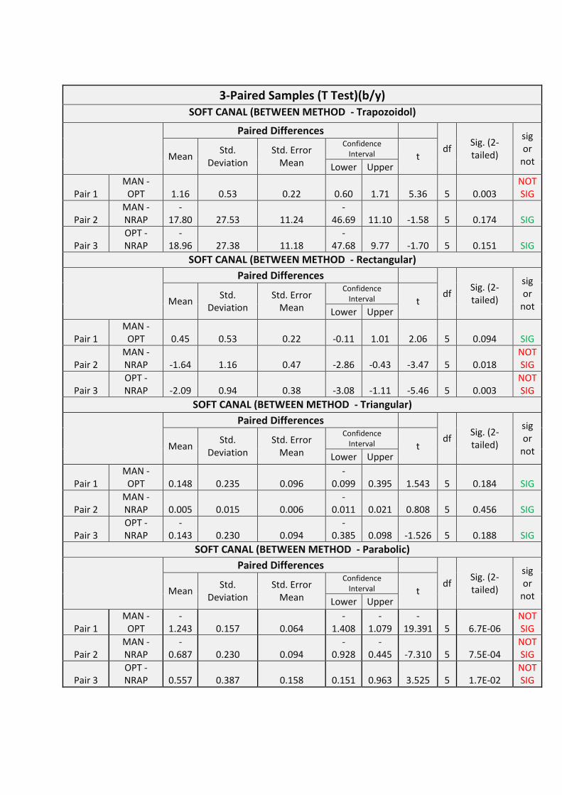
3-Paired Samples (T Test)(b/y) SOFT CANAL (BETWEEN METHOD - Trapozoidol)

Paired Differences

df Sig. (2-tailed)

sig or

not Mean Std.

Deviation Std. Error

Mean


Lower Upper

Pair 1 MAN -

OPT 1.16 0.53 0.22 0.60 1.71 5.36 5 0.003 NOT SIG

Pair 2 MAN - NRAP

-17.80 27.53 11.24

-46.69 11.10 -1.58 5 0.174 SIG

Pair 3 OPT - NRAP

-18.96 27.38 11.18

-47.68 9.77 -1.70 5 0.151 SIG

SOFT CANAL (BETWEEN METHOD - Rectangular)

Paired Differences

df Sig. (2-tailed)

sig or

not Mean Std.


Mean


Lower Upper

Pair 1 MAN -

OPT 0.45 0.53 0.22 -0.11 1.01 2.06 5 0.094 SIG

Pair 2 MAN - NRAP -1.64 1.16 0.47 -2.86 -0.43 -3.47 5 0.018

NOT SIG

Pair 3 OPT - NRAP -2.09 0.94 0.38 -3.08 -1.11 -5.46 5 0.003

NOT SIG

SOFT CANAL (BETWEEN METHOD - Triangular)

Paired Differences

df Sig. (2-tailed)

sig or

not Mean Std.


Mean


Lower Upper

Pair 1 MAN -

OPT 0.148 0.235 0.096 -

0.099 0.395 1.543 5 0.184 SIG

Pair 2 MAN - NRAP 0.005 0.015 0.006

-0.011 0.021 0.808 5 0.456 SIG

Pair 3 OPT - NRAP

-0.143 0.230 0.094

-0.385 0.098 -1.526 5 0.188 SIG

SOFT CANAL (BETWEEN METHOD - Parabolic)

Paired Differences

df Sig. (2-tailed)

sig or

not Mean Std.


Mean


Lower Upper

Pair 1 MAN -

OPT -

1.243 0.157 0.064 -

1.408 -

1.079 -

19.391 5 6.7E-06 NOT SIG

Pair 2 MAN - NRAP

-0.687 0.230 0.094

-0.928

-0.445 -7.310 5 7.5E-04

NOT SIG

Pair 3 OPT - NRAP 0.557 0.387 0.158 0.151 0.963 3.525 5 1.7E-02

NOT SIG

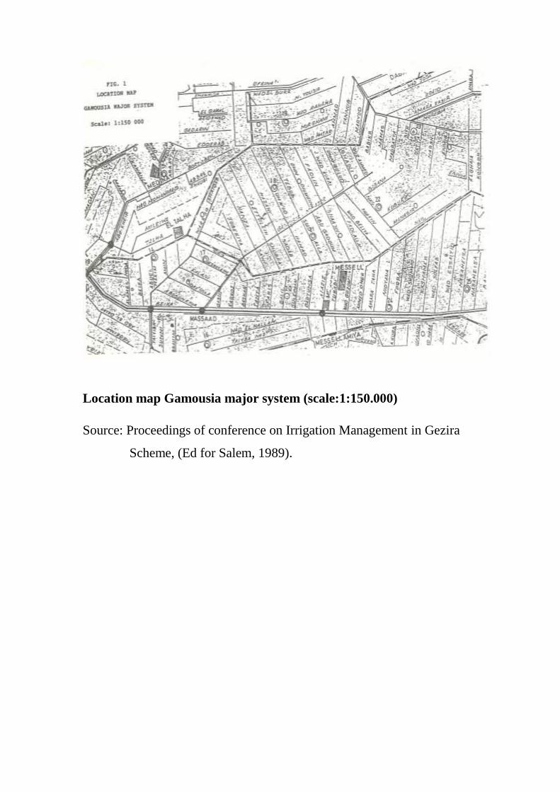
Location map Gamousia major system (scale:1:150.000)

Source: Proceedings of conference on Irrigation Management in Gezira

Scheme, (Ed for Salem, 1989).

The longitudinal section of Guamusia major

A dissertation Submitted In Partial Fulfillment Of The - SUST ...

Documents

Transcript of A dissertation Submitted In Partial Fulfillment Of The - SUST ...