A Decomposition of Austria's General Government Budget into Structural and Cyclical Components

Serguei Kaniovski, Hans Pitlik, Sandra Steindl, Thomas Url

316/2008

WORKING PAPERS

ÖSTERREICHISCHES INSTITUT

FÜR WIRTSCHAFTSFORSCHUNG

A Decomposition of Austria's General Government Budget into Structural and Cyclical Components

Serguei Kaniovski, Hans Pitlik, Sandra Steindl, Thomas Url

WIFO Working Papers, No. 316 April 2008

E-mail address: Serguei.Kaniovski@wifo.ac.at, Hans.Pitlik@wifo.ac.at, Sandra.Steindl@wifo.ac.at, Thomas.Url@wifo.ac.at 2008/079/W/0

A decomposition of Austria's general government budget into structural and cyclical components

April 2008

Serguei Kaniovski, Hans Pitlik, Sandra Steindl, Thomas Url

Research Assistance: Ursula Glauninger, Christine Kaufmann, Dietmar Klose

Abstract

The paper describes a model for the computation of trend output and the structural budget deficit in Austria. The calculation of trend output is based on a production function approach within a small macroeconomic model of the Austrian economy. A decomposition of public budgets into cyclical and structural components shows responsiveness to business cycle variations, and allows a better assessment of the sustainability of the budget balance. The model will be used in future forecasting rounds and links macroeconomic and budgetary variables of the WIFO-forecast to estimates for trend output and the structural budget deficit. Until now, such decomposition has not been part of the regular WIFO-forecast.

Keywords

Austria, WIFO-forecast, trend output, structual budget balance

1. Introduction1)

This paper describes a model for the computation of trend output and the structural budget

deficit in Austria. A decomposition of public budgets into cyclical and structural components

shows their responsiveness to business cycle variations, and allows a better assessment of the

sustainability of the budget balance. The model will be used in future forecasting rounds.

Until now, such decomposition has not been part of the regular WIFO-forecast. The model

therefore needs to draw on those macroeconomic and budgetary variables, which are part of

the WIFO-forecast. Model equations are estimated using annual data according to the

European System of National Accounts (ESA 95) published by Statistik Austria. These data

are currently available for the period 1976 to 2006 and are supplemented by the sector

accounts from 1995 onwards. Table A1 in the appendix gives a list of variables used in the

model. Figure 1 shows how these variables are fed into the macroeconomic and into the

budgetary blocs of the model.

In the case of Austria several attempts to decompose public budgets have been made in the

past. For example, the OECD (Girouard – Andre, 2005), the European Commission (Denis, et

al. 2006), and the European Central Bank (Url, 2001; Grossmann – Prammer, 2005) regularly

compute cyclically adjusted budget balances using an indirect approach, i. e. they relate

cyclically sensitive budget categories first to specific macroeconomic bases and subsequently

link the respective base to the overall output gap. Jäger (1990) and Url (1997) use structural

time series models to estimate a direct response between cyclical budget components and the

output gap.

The model presented in this paper also applies the indirect method but we do not relate the

macroeconomic base to the general output gap, rather we set up a small scale macroeconomic

model that comprises a set of behavioural equations and identities in order to compute the

cyclical variation for each of the macroeconomic bases directly. The model can be solved

recursively and delivers trend components for each macroeconomic base from which we

1) We are grateful to Fritz Breuss for valuable comments and suggestions. The usual disclaimer applies.

– 2 –

derive the cyclical component. Most of the trend and cyclical components of macroeconomic

and budgetary variables are modelled in this way; however, we use the Hodrick-Prescott filter

for some of the exogenous variables, and to initialize the values of all endogenous trend

variables by Hodrick-Prescott-trends.

The macroeconomic bloc of the model is based on a production function of the Cobb-Douglas

type, with a factor specific-technical progress. Labor-specific technical progress depends on

the share of high skilled workers in the labor force, while capital-specific technical progress is

proxied by the ratio of investment in information and communication technology (ICT) to

fixed capital formation. Thus, we include an element of an endogenous growth model, in

which the accumulations of skills and ICT equipment unfold economies of scale. Both

explanatory variables have been identified in the EU-KLEMS project as the driving forces of

total factor productivity (Peneder et al., 2007). They can be interpreted as an outcome of

household and firm decisions that are not explicitly modelled.

Potential output can be seen either as maximum sustainable output of an economy or as the

level of output produced at normal rates of capacity utilization. Here sustainability usually

implies a constant inflation rate. Thus defined, an estimate of potential output is usually

obtained using filter, or structural methods2). We follow the definition of potential output as

the output level corresponding to the normal utilization rates of capital and labor. We focus on

the normal rather the maximum utilisation of the economy because we want to estimate

cyclically adjusted budget deficits, i.e. those deficits, which prevail if there is neither a

cyclical upturn nor a downturn. In the following we will refer to this concept of output as the

trend output and label the variables accordingly.

Employment is cyclically adjusted using a detrended employment rate as a share of the

working-age population. Following Bock – Schappelwein (2005) and Steindl (2006), we use

the share of the unemployed not eligible to regular unemployment benefits as an indicator of

2) Different estimation procedures yield different results. For a survey of the most frequently used methods see, for example, European Central Bank (2000).

– 3 –

the long-term or structural unemployment. These long-term unemployed are excluded from

the trend labor input, while the detrended number of unemployed receiving unemployment

benefits is added to the cyclically adjusted employment level. Trend employment is

transformed into labor volume using the average number of hours worked. The capital stock

corresponds to the actual capital stock and thus is not adjusted for cyclical variation in

utilization rates.

The decomposition of budgetary items into cyclical and structural (trend) components uses

elasticities estimated using cointegrating equations (Url, 2001). These equations relate

cyclically dependent budgetary items to their macroeconomic bases. To extract the structural

component of a budget item, we use the long-run equation from a cointegrating system, and

replace actual values of the macroeconomic variables by their trend values. This approach

delivers a set of structural and cyclical components for each cyclically responsive tax and

expenditure item. Cyclically responsive items include social security contributions, wage

taxes, other direct taxes, indirect taxes, unemployment benefits and pension payments. In

addition to the cyclical and structural components, we try to account for past one-off revenue

or expenditure measures.

The following section describes the macroeconomic bloc. Section 3 presents the budgetary

bloc and motivates our choice of cyclically responsive budget items. In this section we also

describe the estimation methodology and the results. The accounting framework is described

in Section 4, which also includes results of the decomposition. In the final section we draw

some conclusions.

– 4 –

2. Estimation of trend output

This section defines the factor inputs and determinants of the total factor productivity used in

the production function, and presents estimates of the production function3).

The production function

We estimate trend output using a constant returns to scale Cobb-Douglas production function:

)1()()( ββ −= tLHtKCt LHaKRaaYR , (2.1)

where β is the factor share of capital in total income. The level of output, YRt is determined by

two factor inputs, the capital stock, KRt, and hours worked, LHt. The parameters ak and aLH

are, respectively, the capital and labour embodied contributions to total factor productivity,

and ac is the Hicks-neutral component. The above production function implies a unit elasticity

of substitution between factors of production.

The capital stock includes buildings, infrastructure, transport equipment, machinery and other

equipment, and intangible assets. We use the standard perpetual inventory method described

in Statistik Austria (2002) and Peneder et al. (2007), in which the cumulative flow of fixed

capital formation is adjusted for depreciation to calculate the net capital stock. To account for

variable capital utilization, we derive a capital utilization measure based on the WIFO

Business Cycle and Investment Survey data. The data on capacity utilization are available for

the manufacturing sector only. The share of manufacturing in the capital stock is about 10

percent, whereas 60 percent of the capital stock is not assigned to a particular industry. We

therefore apply our utilization measure to half of the net capital stock, and assume that the

other half is always fully utilized. For the estimation we adjust the capital stock in production

function (2.1) for fluctuations in capacity utilization:

** 5.0)1)((5.0 tttt KRKUKUKRKR ++−= . (2.2)

3) Previous work on the decomposition of output into trend or potential output and cyclical output for Austria includes Breuss (1984), Brandner – Neusser (1992), Hahn – Walterskirchen (1992), Giorno et al. (1995), Hahn – Rünstler (1996), Denis et al. (2006), Steindl (2006), and Breuss et al. (2007).

– 5 –

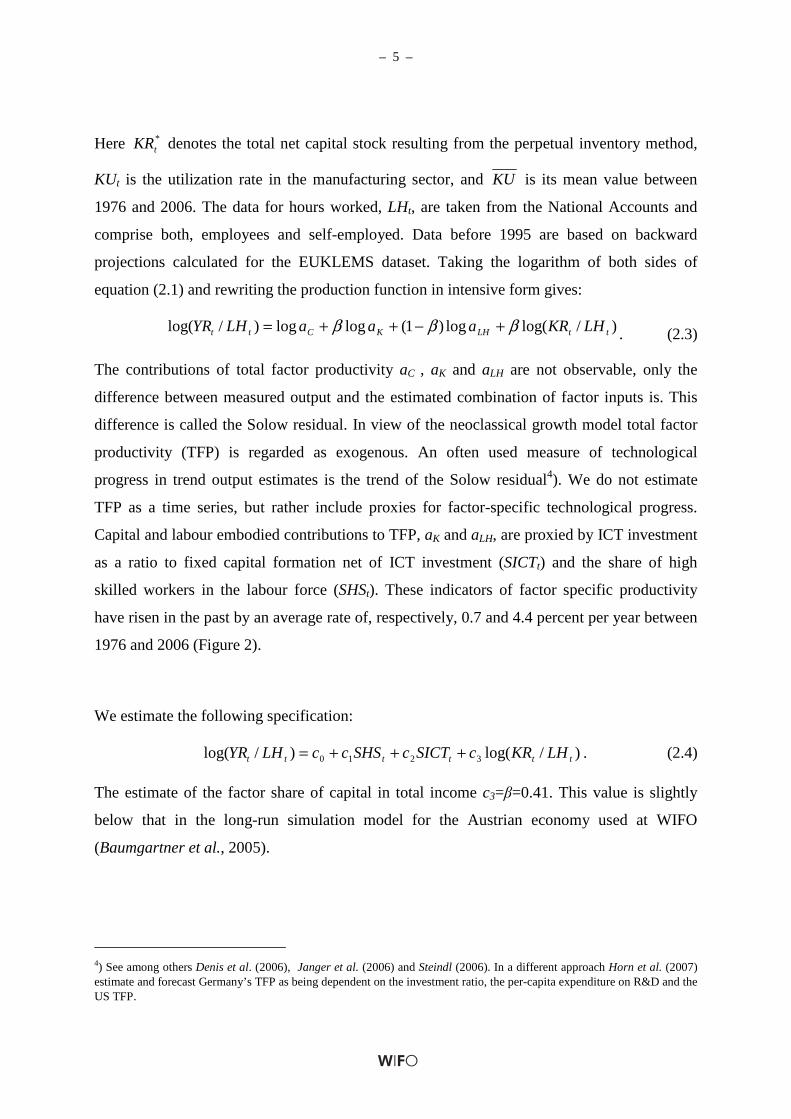
Here *tKR denotes the total net capital stock resulting from the perpetual inventory method,

KUt is the utilization rate in the manufacturing sector, and KU is its mean value between

1976 and 2006. The data for hours worked, LHt, are taken from the National Accounts and

comprise both, employees and self-employed. Data before 1995 are based on backward

projections calculated for the EUKLEMS dataset. Taking the logarithm of both sides of

equation (2.1) and rewriting the production function in intensive form gives:

)/log(log)1(loglog)/log( ttLHKCtt LHKRaaaLHYR βββ +−++= . (2.3)

The contributions of total factor productivity aC , aK and aLH are not observable, only the

difference between measured output and the estimated combination of factor inputs is. This

difference is called the Solow residual. In view of the neoclassical growth model total factor

productivity (TFP) is regarded as exogenous. An often used measure of technological

progress in trend output estimates is the trend of the Solow residual4). We do not estimate

TFP as a time series, but rather include proxies for factor-specific technological progress.

Capital and labour embodied contributions to TFP, aK and aLH, are proxied by ICT investment

as a ratio to fixed capital formation net of ICT investment (SICTt) and the share of high

skilled workers in the labour force (SHSt). These indicators of factor specific productivity

have risen in the past by an average rate of, respectively, 0.7 and 4.4 percent per year between

1976 and 2006 (Figure 2).

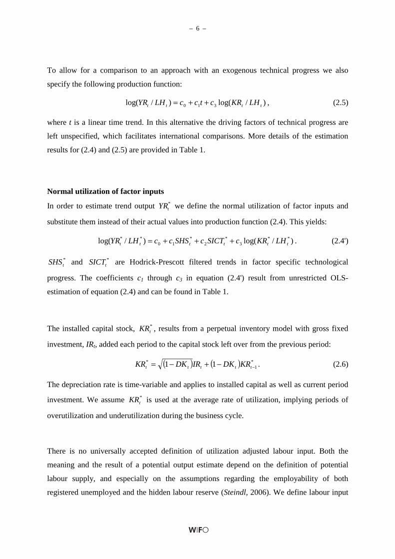
We estimate the following specification:

)/log()/log( 3210 tttttt LHKRcSICTcSHSccLHYR +++= . (2.4)

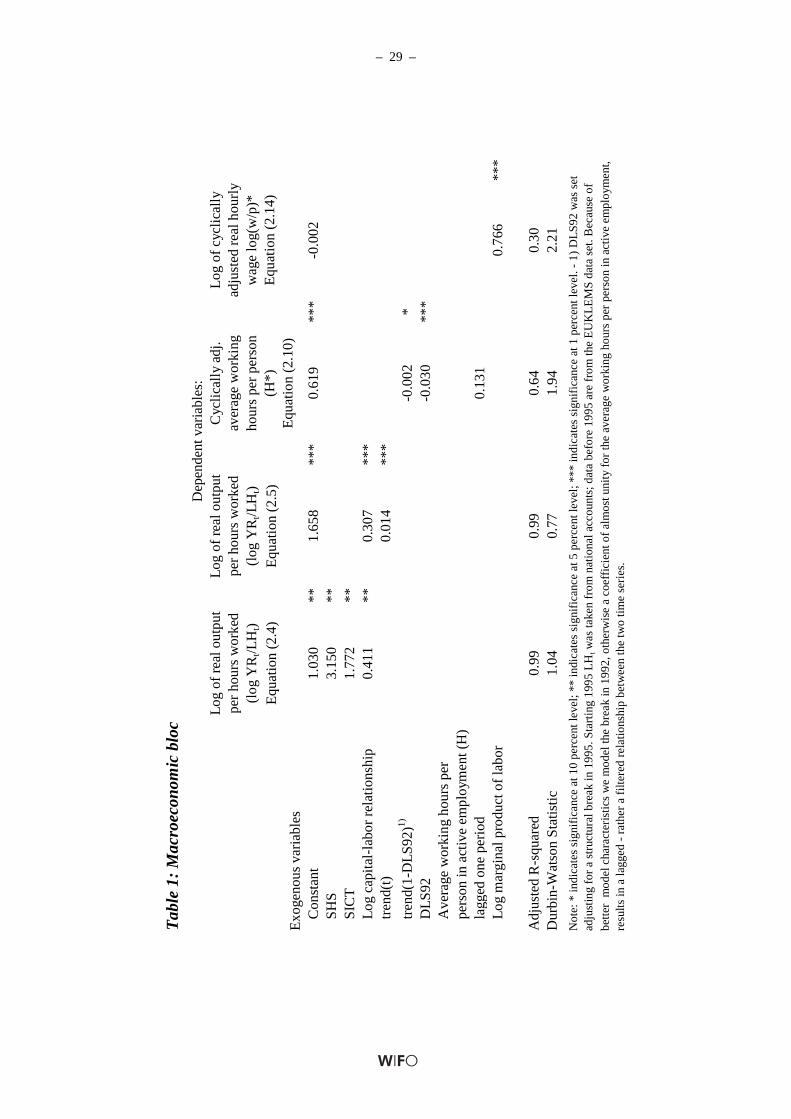
The estimate of the factor share of capital in total income c3=β=0.41. This value is slightly

below that in the long-run simulation model for the Austrian economy used at WIFO

(Baumgartner et al., 2005).

4) See among others Denis et al. (2006), Janger et al. (2006) and Steindl (2006). In a different approach Horn et al. (2007) estimate and forecast Germany’s TFP as being dependent on the investment ratio, the per-capita expenditure on R&D and the US TFP.

– 6 –

To allow for a comparison to an approach with an exogenous technical progress we also

specify the following production function:

)/log()/log( 310 tttt LHKRctccLHYR ++= , (2.5)

where t is a linear time trend. In this alternative the driving factors of technical progress are

left unspecified, which facilitates international comparisons. More details of the estimation

results for (2.4) and (2.5) are provided in Table 1.

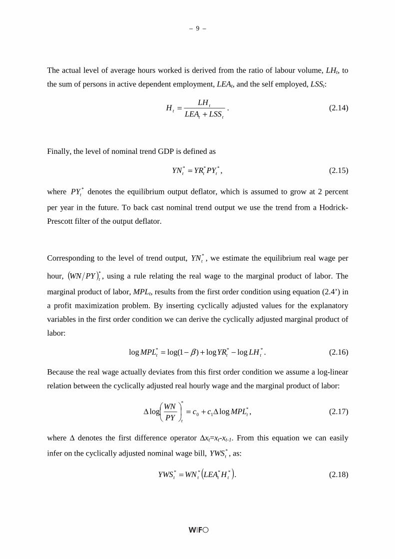
Normal utilization of factor inputs

In order to estimate trend output *tYR we define the normal utilization of factor inputs and

substitute them instead of their actual values into production function (2.4). This yields:

)/log()/log( **3

*2

*10

**tttttt LHKRcSICTcSHSccLHYR +++= . (2.4')

*tSHS and *

tSICT are Hodrick-Prescott filtered trends in factor specific technological

progress. The coefficients c1 through c3 in equation (2.4') result from unrestricted OLS-

estimation of equation (2.4) and can be found in Table 1.

The installed capital stock, *tKR , results from a perpetual inventory model with gross fixed

investment, IRt, added each period to the capital stock left over from the previous period:

( ) ( ) *1

* 11 −−+−= ttttt KRDKIRDKKR . (2.6)

The depreciation rate is time-variable and applies to installed capital as well as current period

investment. We assume *tKR is used at the average rate of utilization, implying periods of

overutilization and underutilization during the business cycle.

There is no universally accepted definition of utilization adjusted labour input. Both the

meaning and the result of a potential output estimate depend on the definition of potential

labour supply, and especially on the assumptions regarding the employability of both

registered unemployed and the hidden labour reserve (Steindl, 2006). We define labour input

– 7 –

at normal rates of utilization as the labour force that is available to fill vacancies in the job

market if actual output is at its long-term average. In addition to the trend level in employed

and self employed persons it also contains part of the registered unemployed.

We obtain the normal level of persons in dependent active employment over the business

cycle, *tLEA , by multiplying the working age population (aged between 15 and 64), POPt,

with the HP-filtered employment rate *tRE :

ttt POPRELEA ** = . (2.7)

To this cyclically adjusted dependent employment we add the Hodrick-Prescott filtered self

employed persons and an estimate of cyclically adjusted unemployment based on

administrative classifications of registered unemployment by type of benefits. Following Bock

– Schappelwein (2005) and Steindl (2006) we use the number of unemployed persons eligible

to regular unemployment benefits as an indicator for short-term employability. The reasoning

behind this choice is that hazard rates for unemployment are declining in the length of

unemployment spells (Boheim, 2006), and regular unemployment benefits are paid only

during the first months of an unemployment spell. The payment of unemployment benefits

extends, depending on the duration of past employment, to a maximum of one year5).

Following the above idea, we assume that the unemployed, LUt, comprise two groups: (1) the

unemployed receiving unemployment benefits, LUGt, and (2) the unemployed receiving no

unemployment benefits, LUSt:

ttt LUSLUGLU += . (2.8)

Both groups can be decomposed further into cyclical and trend components:

**t

Ctt

Ctt LUSLUSLUGLUGLU +++= , (2.9)

5) In most studies registered unemployment is broken down into a cyclical and a non-cyclical component using estimates of the non-accelerating inflation rate of unemployment (NAIRU), or the non-accelerating wage inflation rate of unemployment (NAWRU). Both concepts refer to the unemployment rate which is consistent with a stable rate of inflation, or wage inflation, respectively (Giorno et al., 1995; Denis et al., 2006).

– 8 –

where superscripts C and * refer to cyclical and trend components. The cyclical part of the

non-recipients, CtLUS , is small. We assume that only the recipients, LUGt, respond to the

business cycle, whereas the non-recipients belong to the structural unemployment. This

assumption is consistent with the hypothesis of long-term unemployment causing a loss in

human capital, so that even in a cyclical upturn it is difficult for this group to find

employment (Pissarides, 1992). Figure 3 gives an overview of decomposed unemployment.

The trend part of the unemployed (non-recipients) amounts to half of the registered

unemployed and increased over time6).

It follows from decomposition (2.9) that the cyclically adjusted version of total

unemployment, *tLU , can be approximated as

Cttttt LUGLULUSLUGLU −≈+= *** . (2.10)

We will use equation (2.10) to substitute for trend unemployment in the cointegrating

equation of the model. Similarly, we can use this concept to redefine the share of long-term

unemployed in total unemployed persons in structural terms as:

( ) ( )

( )Ctt

tt

t

t

t

tt

LUGLU

LUGLU

LU

LUS

LU

LUGLU

−−

≈=−

*

*

*

**

, (2.11)

which holds approximately for small CtLUS .

We estimate the labour volume at normal rates of utilization as

***** )( ttttt HLUGLSSLEALH ++= , (2.12)

where LSSt represents self employed persons. Cyclically adjusted average hours worked per

person in active employment, *tH , are estimated using the following autoregressive relation:

13210* 92)921( −++−+= tt HcDLScDLStrendccH . (2.13)

6) This phenomenon is referred to as hysteresis (Blanchard – Summers, 1986).

– 9 –

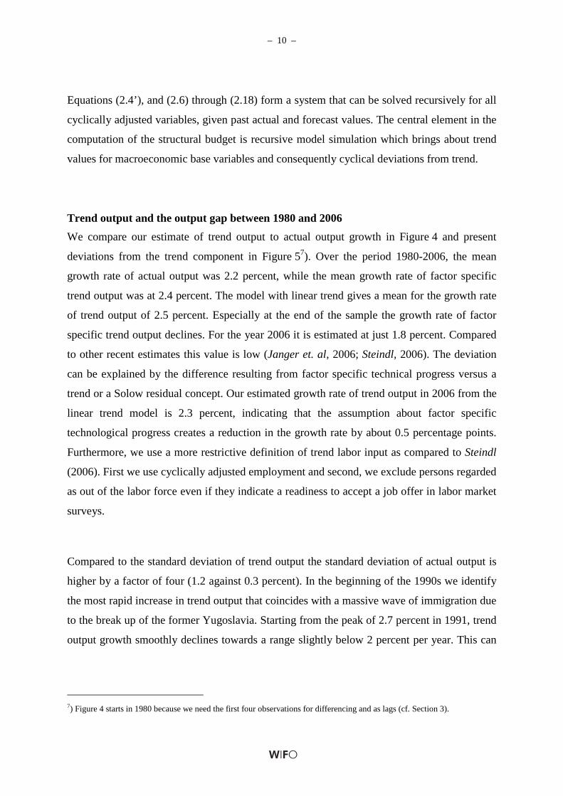
The actual level of average hours worked is derived from the ratio of labour volume, LHt, to

the sum of persons in active dependent employment, LEAt, and the self employed, LSSt:

tt

tt LSSLEA

LHH

+= . (2.14)

Finally, the level of nominal trend GDP is defined as

***ttt PYYRYN = , (2.15)

where *tPY denotes the equilibrium output deflator, which is assumed to grow at 2 percent

per year in the future. To back cast nominal trend output we use the trend from a Hodrick-

Prescott filter of the output deflator.

Corresponding to the level of trend output, *tYN , we estimate the equilibrium real wage per

hour, ( )*tPYWN , using a rule relating the real wage to the marginal product of labor. The

marginal product of labor, MPLt, results from the first order condition using equation (2.4’) in

a profit maximization problem. By inserting cyclically adjusted values for the explanatory

variables in the first order condition we can derive the cyclically adjusted marginal product of

labor:

*** loglog)1log(log ttt LHYRMPL −+−= β . (2.16)

Because the real wage actually deviates from this first order condition we assume a log-linear

relation between the cyclically adjusted real hourly wage and the marginal product of labor:

*10

*

loglog tt

MPLccPY

WN ∆+=

∆ , (2.17)

where ∆ denotes the first difference operator ∆xt=xt-xt-1. From this equation we can easily

infer on the cyclically adjusted nominal wage bill, *tYWS , as:

( )****tttt HLEAWNYWS = . (2.18)

– 10 –

Equations (2.4’), and (2.6) through (2.18) form a system that can be solved recursively for all

cyclically adjusted variables, given past actual and forecast values. The central element in the

computation of the structural budget is recursive model simulation which brings about trend

values for macroeconomic base variables and consequently cyclical deviations from trend.

Trend output and the output gap between 1980 and 2006

We compare our estimate of trend output to actual output growth in Figure 4 and present

deviations from the trend component in Figure 57). Over the period 1980-2006, the mean

growth rate of actual output was 2.2 percent, while the mean growth rate of factor specific

trend output was at 2.4 percent. The model with linear trend gives a mean for the growth rate

of trend output of 2.5 percent. Especially at the end of the sample the growth rate of factor

specific trend output declines. For the year 2006 it is estimated at just 1.8 percent. Compared

to other recent estimates this value is low (Janger et. al, 2006; Steindl, 2006). The deviation

can be explained by the difference resulting from factor specific technical progress versus a

trend or a Solow residual concept. Our estimated growth rate of trend output in 2006 from the

linear trend model is 2.3 percent, indicating that the assumption about factor specific

technological progress creates a reduction in the growth rate by about 0.5 percentage points.

Furthermore, we use a more restrictive definition of trend labor input as compared to Steindl

(2006). First we use cyclically adjusted employment and second, we exclude persons regarded

as out of the labor force even if they indicate a readiness to accept a job offer in labor market

surveys.

Compared to the standard deviation of trend output the standard deviation of actual output is

higher by a factor of four (1.2 against 0.3 percent). In the beginning of the 1990s we identify

the most rapid increase in trend output that coincides with a massive wave of immigration due

to the break up of the former Yugoslavia. Starting from the peak of 2.7 percent in 1991, trend

output growth smoothly declines towards a range slightly below 2 percent per year. This can

7) Figure 4 starts in 1980 because we need the first four observations for differencing and as lags (cf. Section 3).

– 11 –

mainly be attributed to a decline in the increase of the total capital stock as of well as capital

specific technological progress tSICT (Figure 2).

Figure 5 shows the output gap measured as percentage deviation from trend, defined as

100)( ** ⋅− ttt YRYRYR . In Figure 5 we can clearly identify three business cycle peaks in 1979,

1992, and 2000. The troughs are less clearly seen because during the downturn 1993-1998 the

gap is small and during the recession in the mid-1980s the graph indicates a double-dip

recession. Our peak dates are very similar to those derived by Scheiblecker (2007), which are

based on quarterly detrended data. Due to higher data frequency Scheiblecker identifies

additional peaks in 1985-1986, 1994-1995 and 2004, which in our case are either part of

double-dip recessions or of the more protracted downturn in the mid-1990s. Our troughs, on

the other hand, coincide in the years 1987, 1997, and 2003 precisely with Scheiblecker’s

dating. Again, Scheiblecker (2007) detects several additional troughs due to higher data

frequency. These appear on our measure as small dents on a more general business cycle

development.

3. The estimation of short-run and long-run tax and expenditure elasticities

In this section we identify cyclically dependent budget components and their related

macroeconomic bases. We then proceed with an estimation of tax and expenditure elasticities.

Elasticities show the ratio between the relative change of a budget component and the relative

change of its macroeconomic base, and as such allow us to compute the response of budget

components to changes in their macroeconomic base. By combining all tax and expenditure

responses to changes in their macroeconomic bases, we obtain indirectly the elasticity of the

public budget to the business cycle. This approach has the advantage to account for the fact

that different macroeconomic bases respond differently to business cycle variations8).

8) As an alternative one may consider directly the elasticity of a budget component D with respect to nominal output as done by Jäger (1990) or Url (1997), for example.

– 12 –

The elasticity, εDX, of a budget component, D, with respect to its macroeconomic tax base, X,

is defined as:

XdX

DdD

DX ≡ε . (3.1)

By estimating tax and spending elasticities over the period 1979-2006, we have to take into

consideration policy changes with substantial impact on the sensitivity of revenues or

expenditures to the respective macroeconomic base, e.g. major reforms of tax codes.

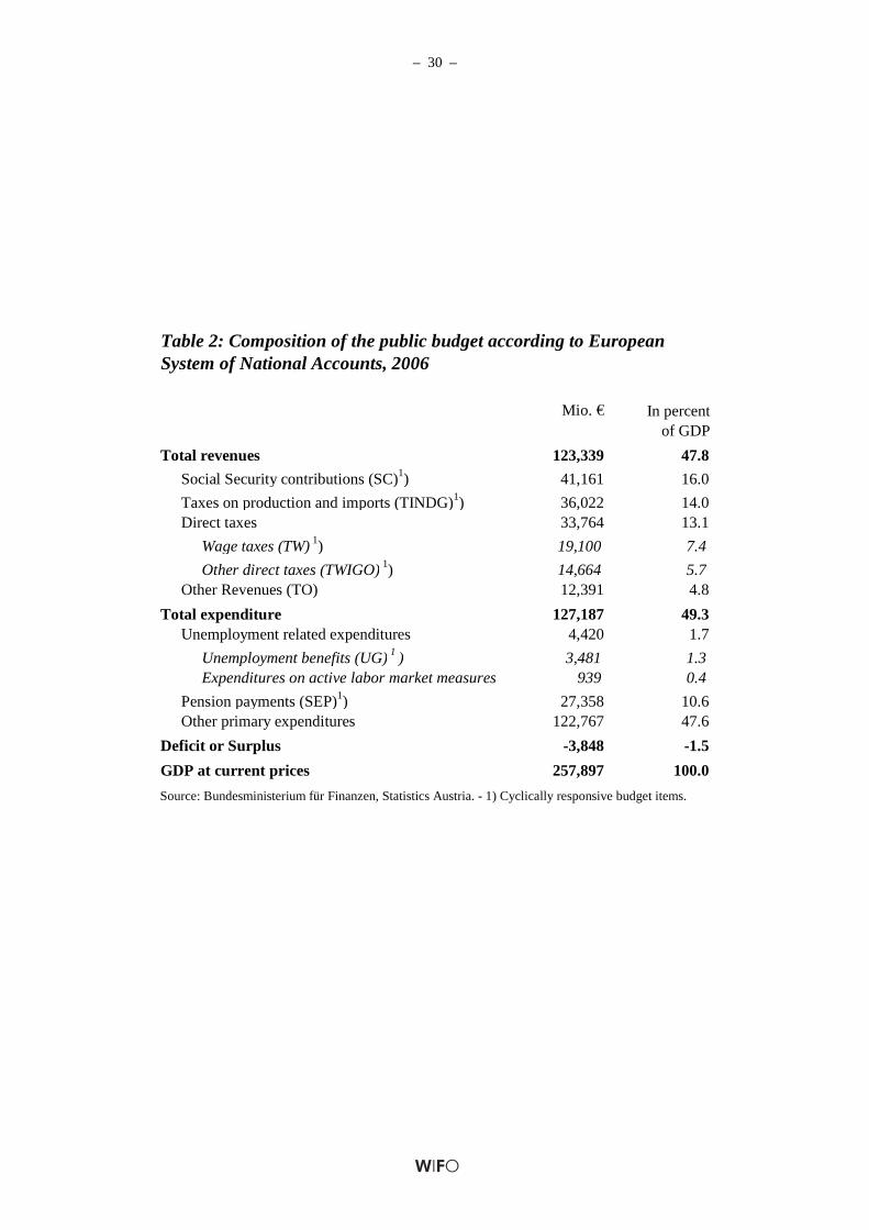
In decomposing government revenue we follow the classifications of ESA 95 and apply a

narrow concept of cyclical dependence: only budget categories that respond automatically to

business cycle variations are decomposed. In particular, on the revenue side of the general

government budget we consider wage taxes, other direct taxes except wage taxes, social

security contributions, and taxes on production and imports (indirect taxes) to be cyclically

responsive. The composition of our cyclically dependent revenue components is summarized

in Table 2. We assume 90 percent of government revenue in Austria to depend on the

business cycle. On the other hand, there are comparatively few automatic stabilizers on the

expenditures side of the Austrian budget. Consequently expenditures are mostly independent

from the business cycle, i. e. roughly a quarter of spendings will be regarded as cyclically

dependent. In a broader perspective, almost all budgetary components are related to the

business cycle, at least to a degree. During economic downswings, for example, the

government may decide to raise public investment spending in order to pursue anti-cyclical

fiscal policy. We are, however, interested only in budgetary changes related automatically to

the business cycle, i. e. without discretionary measures. This approach avoids identifying

assumptions necessary to pin down discretionary responses of economic policy to business

cycle fluctuations as in Brandner et al. (2007).

Unemployment benefits are an obvious automatic expenditure scheme which accounts for

about 3 percent of total expenditures. Monetary transfers to long-term unemployed are only

weakly related to the cycle and active labor market measures are mostly discretionary.

– 13 –

Previous computations of cyclically adjusted budget deficits by Url (2001) and Grossmann –

Prammer (2005) also considered expenditures on pensions as cyclically dependent because

until 2003 the pension adjustment was based on the per capita wage development. This

relation exposes another 21.5 percent of expenditures to cyclical variation. Since 2004 the

pension adjustment formula is based on changes in the consumer price index but discretionary

adjustments to this formula have been implemented since its introduction. We include pension

payments into our definition of the cyclical expenditure component because both per-capita

wages and the consumer price index respond to the business cycle. The change in the pension

adjustment formula will bring about a significant change in the pattern of the cyclical budget

component. Whereas per-capita wages vary procyclically, the inflation rate in Austria is anti-

cyclical (Baumgartner, 2003). We model the break in the legal framework by changing from

wage- to inflation-based pension equations.

Wage taxes

Wage taxes, TW, consist of the total proceeds of the wage income tax only. The

corresponding macroeconomic base is the total sum of wages (YWS). We take into account

wage income taxes of private and public sector employees. The relevant macroeconomic base

thus comprises both the private and the public sector wage bill. This approach is not entirely

unproblematic, as public employment is set by the government. Changes in public

employment are hence not automatically related to the business cycle. In their computations

of elasticities of direct taxes on households, Grossmann – Prammer (2005) exclude wage tax

proceedings of public sector employees, and consequently take into account only private

sector employment as an explanatory variable. Nevertheless, we include public sector wage

payments and the corresponding wage tax revenues in our calculations because wage

negotiations in the public sector are cyclically dependent at least to a degree. Level shift

dummy variables reflect major income tax reforms in 1989, 1994, 2000 and 2005.

In this context, an additional error in the ESA 95 classification affects some taxes related to

the payroll (municipal tax (Kommunalsteuer) and employers' contributions to family based

monetary transfers (Familienlastenausgleichsfonds)) with total revenues of € 5.6 bn. in 2005.

– 14 –

These two revenue streams are classified as indirect taxes rather than wage taxes. Since those

revenue categories are based on proportional rates we do not expect them to significantly

reduce the estimated elasticity for wage taxes.

Social security contributions

Cyclical variations of revenues from social security contributions, SC, are also related to the

development of wages and employment. Additional statutory factors that affect receipts are

the maximum assessment ceiling (Höchstbeitragsgrundlage), which limits individual

contributions, and the sum of risk specific contributions rates (accident, health, and pension

insurance). Discretionary adjustments of the threshold value and the contribution rates are

thereby taken into account. Trend revenues from social security contributions shift upward as

a result of an increase in the maximum assessment ceiling or the contribution rate.

Other direct taxes

The category 'other direct taxes except wage taxes', TIWGO, includes revenues from assessed

personal income taxes, the corporate income tax, taxes on interest and dividends, as well as

wealth taxes. Revenues from wealth taxes have a comparatively low share in Austria,

however. This class of taxes also includes receipts from the motor vehicle tax and the car

insurance taxes paid by households9).

'Other direct taxes' is a heterogeneous category of tax revenues and proceeds are not always

directly related to the business cycle. Most importantly, it is often claimed that interest rates

and thus also interest income depends only weakly on the business cycle (e. g. Grossmann –

Prammer, 2005: 70). Hence, receipts from capital income taxes (KeST) on private

households' and firms' earnings might better be subtracted from our base. While this

procedure is feasible for a calculation of past structural budget positions, it is currently

9) The private firms' share of these taxes falls under the heading of taxes on production and imports.

– 15 –

impractical for forecasts as it requires a prediction of future capital income tax revenues –

these are currently not included in the WIFO quarterly forecast. We leave this to future work.

Other direct taxes are probably best related to nominal GDP less total wage income, which is

approximately equivalent to gross operating surplus. Since a major fraction of receipts in this

category comes from assessed taxes on non-wage income and corporate income, we use

values of the macroeconomic base lagged one and two years as explanatory variables. To

assess the impact of major tax code revisions we also employ a shift dummy variable for 1994

and a step dummy for 2001 in our estimates.

Taxes on production and imports

According to ESA 95, taxes on production and imports include, inter alia, the value added tax

(VAT), mineral oil tax, tobacco tax, insurance tax, energy duties and the motor vehicle tax

paid by firms. By far the single most important revenue source in this class of taxes is the

VAT, which accounted for 54 percent of total taxes on production and imports in 2005.

Private consumption expenditures are usually used as the macroeconomic base for indirect

taxes but several components of private consumption are exempt from taxes or are taxed at

reduced rates. Shifts in the structure of consumption will thus affect the elasticity.

Furthermore, the mineral oil tax, energy duties and tobacco tax are, in contrast to VAT, not

(exclusively) related to value-added but are based primarily on the quantities consumed.

About 20 percent of receipts of taxes on production and imports come from quantity-related

taxes.

Additionally, public consumption net of public sector wage payments is usually subject to

indirect taxes. If we include indirect tax revenues from public consumption, we consequently

would have to include public consumption expenditure into the relevant macroeconomic base.

Doing so enables us to side-step an open discussion on whether or not public consumption

spending is cyclically dependent.

– 16 –

Private investment and exports are also not free from indirect taxes, as energy duties, and the

exporting firms' share of motor vehicle taxes fall under the heading of taxes on production

and imports. Finally, as mentioned above, the ESA 95 definition of taxes on production and

imports also includes wage-related taxes like the municipal tax and employers' family fund

contributions (FLAF).

Summing up, it seems appropriate to link revenues from taxes on production and imports

directly to nominal GDP instead of the narrower measure of private consumption expenditure.

Alternative regressions not shown in the following suggest that especially during recent years

private consumption is only weakly associated with indirect tax revenues, and that the

relationship is becoming more and more unstable. While private consumption may be a good

proxy for the tax base of VAT and other goods taxes, it is too narrow a macroeconomic base

to estimate revenue elasticities for the broader ESA 95 category of taxes on production and

imports. In our regressions we also include level shift dummy variables for the VAT reform in

1984 and changes in tax codes due to Austria's accession to the EU in 1995.

Transfers to the unemployed

On the expenditure side of the budget we take into consideration monetary transfers to the

unemployed, including related social security contributions. The typical macroeconomic base

is the number of unemployed and the per capita wage from the previous year, as

unemployment benefits depend on earnings in the previous year. We take into account that

transfers to the long-term unemployed (receivers of welfare aid (Notstandshilfe)) are smaller

than regular payments to the short-term unemployed. Although transfers of social security

contributions from the unemployment insurance to the social security system are deficit-

neutral, we include these transfer payments into our expenditure measures because the

estimated elasticity will be affected by these discretionary transactions. We account for those

transfers by considering the share of social security contributions in total unemployment

expenditures as an explanatory variable.

– 17 –

Expenditures on pensions

We consider expenditures on pensions as cyclically dependent. Until 2003 the pension

adjustment formula related the increase of pensions paid out by the social security system to

the change in per-capita wages in the previous year. Consequently, the increase in the average

pension was directly linked to the wage development. In 1993 the adjustment formula has

been changed such that the development in net per-capita wages formed the base for pension

adjustments, i. e. after 1993 increasing social security contributions were subtracted before

computing rates of change. With the pension reforms of the years 2003-2005 a link to the

inflation rate of the Consumer Price Index has been established although discretionary

adjustments to this basic formula have been inacted in every year. Given this inexact nature of

the adjustment formula, we will base the cyclical adjustment between 1979 and 2003 on the

wage base and afterwards on CPI-inflation. In the simulation model both formulas will be

included into one single equation with time varying coefficients. Instead of the CPI we use the

GDP-deflator to ensure consistency with ESA 95. The coefficient vector resulting from the

per-capita wage equation gives the parameters for the first period and is set to zero after 2003.

The parameters of the GDP-deflator equation will be zero for the period until 2003 and

feature the respective estimates from 2004 onwards.

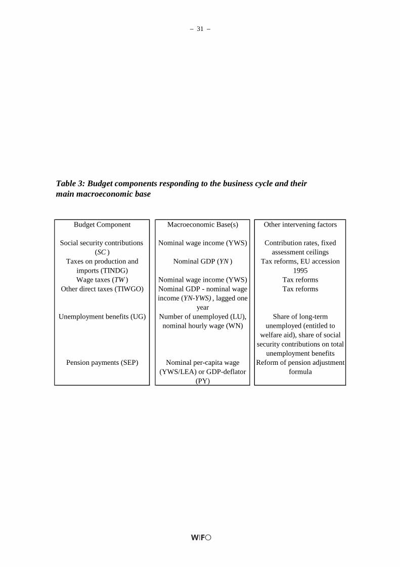
Table 3 gives an overview of cyclically variable budget items, their respective

macroeconomic bases, and of conditional variables capturing structural changes not mirrored

in the development of the macroeconomic base.

Estimation method

In order to estimate elasticities of budget components we follow Url (2001) and Grossmann –

Prammer (2005) by employing a two-step error correction technique, using data for the

period 1976 to 2006. First, we estimate the long-run relationship between (log) levels of a

certain budget component, Di,t, and the (log) level of its respective macroeconomic base Xi,t.

We also include several control variables Zt for discretionary changes of tax and expenditure

policies and other events (e. g. Austria's accession to the EU in 1995). Note that Zi,t may not

be identical for all tax and expenditure components. Lagged residuals from the long-run

– 18 –

equation of the cointegrating model are then included as an additional explanatory variable

(lagged co-integration term) into the short-run regressions. Denote the first difference

operator as ∆Di,t=Di,t-Di,t-1, then the short-run equation of the cointegrated variables is

( ) ( ) titiRtititi DcXcZccD ,1,3,2,10, loglog η++∆+∆+=∆ − , (3.2)

where c2 is an estimate of the short-run elasticity of a budget component with respect to its

macroeconomic base, and c3 is the adjustment parameter in the cointegration model, which

determines the speed at which equilibrium errors 1, −tiRD diminish. For an error correction to

occur this parameter must be negative. A higher absolute value of c3 indicates faster

adjustment towards a long-run equilibrium. The equilibrium error arises from the residual of

the long-run linear relationship10):

( ) ( ) tiRtititi DXcZccD ,,2,10, loglog +++= . (3.3)

With respect to tax variables the long-run elasticity c2 in equation (3.3) should not exceed

unity, because in a steady state tax receipts cannot exceed their respective macroeconomic tax

base. We therefore restrict c2=1 in our estimates in general, and conduct F-tests to check for

the validity of this restriction.

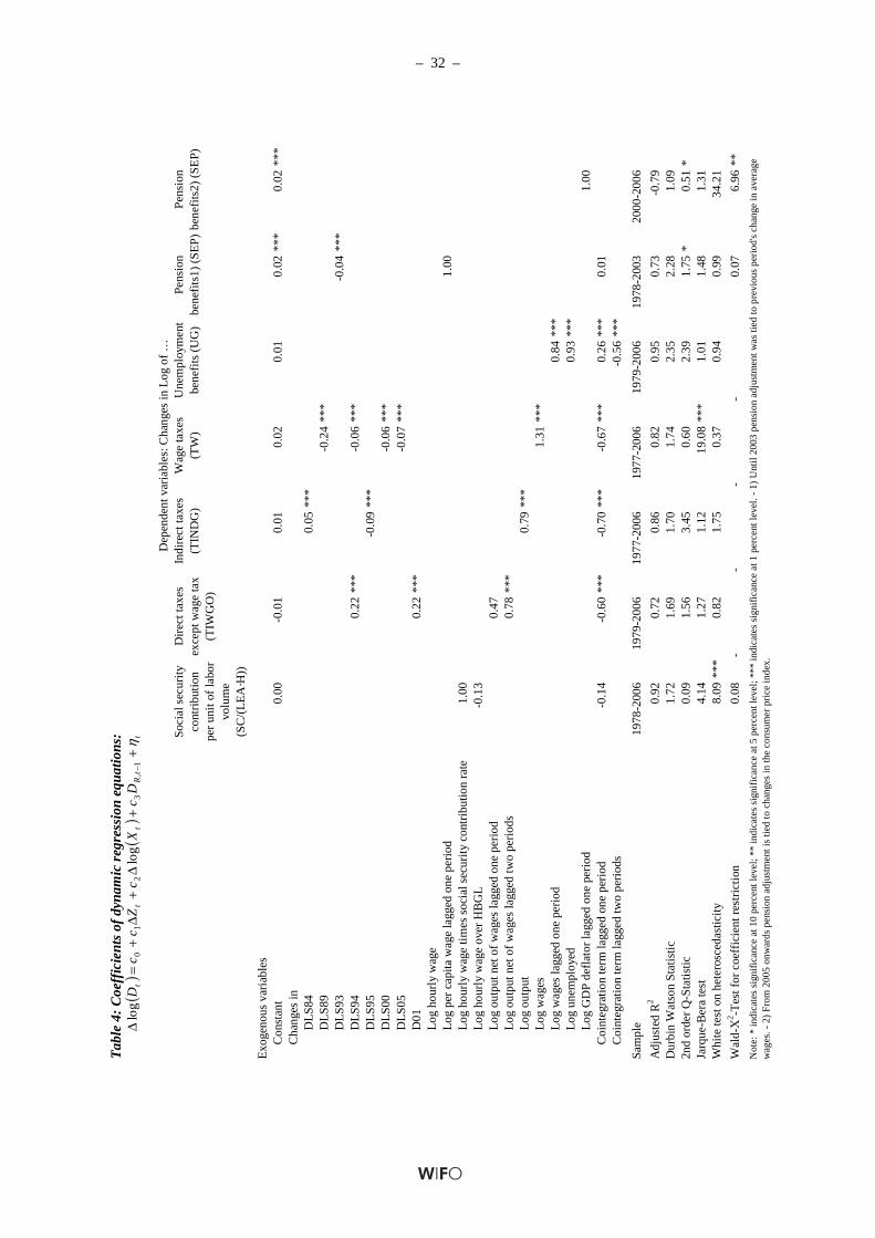
Table 4 summarizes the regression results for six short-run budget elasticities. Each column

refers to one of the cyclically adjusted budget items. The first set of variables are the constant

and either step or level shift dummies. The dummy variables indicate changes in the legal

code and coincide with dates of major tax reforms. We include dummy variables if they are

significant in either the short- or the long-run equation. Interestingly, the regression equations

for social security contributions and transfers to the unemployment do not require dummy

variables to correct for legal interventions. Instead corrective factors, such as the social

security contribution rate and the maximum assessment limit provide enough information to

reflect discretionary institutional changes.

10) As noted above, revenues from other direct taxes except wage taxes are not related to the contemporary macroeconomic base but to one-year and two years lagged values instead.

– 19 –

The short-run elasticities vary between 0.79 for indirect taxes and 1.31 for wage taxes

(Table 4). Overall, the regression fit is good and residual-based tests indicate only minor

problems with outliers in the wage tax equation and heteroscedasticity in the social security

equation. Due to a low number of observations, the regression for pension payments after the

reform of the pension adjustment formula serves only to fix the constant after 2003.

We restrict our estimate for the elasticity of social security contributions with respect to the

macroeconomic base to unity because we directly manipulate hourly wages by multiplying it

with the social security contribution rate. We also restrict the response of pension outlays to

the change in per-capita wage to unity. Both restrictions are not rejected by the data. As

expected from our discussion of taxes on production and imports, indirect taxes respond less

than proportional to variations in nominal output. Finally, the elasticities of unemployment

transfers are slightly below unity in both the number of unemployed and the per capita wage

of the previous year. The adjustment speed to disequilibrium in the tax revenues is

surprisingly fast. All error correction terms enter significantly the short-run equation.

Estimates for the adjustment parameter for taxes, are around one half, i. e. half of the

equilibrium error is corrected within the next period implying a half life of one year.

Essentially, this implies a full correction after four years. In the case of unemployment

benefits we include two lags of the error term to reduce autocorrelation in the residual of the

short-run equation. Alternatively, we could use the lagged change in unemployment benefits.

The net effect of both lagged adjustment coefficients is negative and thus allows for an

appropriate error correction mechanism.

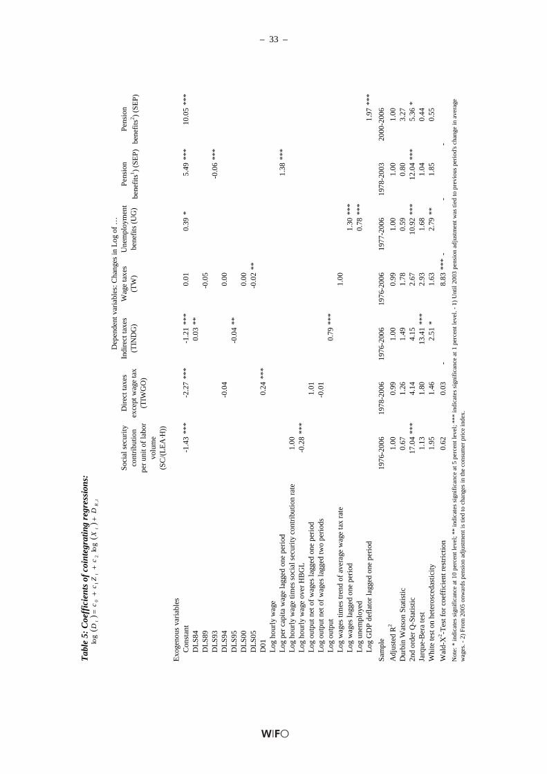
The long-run equations are presented in Table 5. We impose more structure on the estimation

of long-run elasticities because in most cases values different from unity are implausible in a

steady state equilibrium. Thus long-run elasticities of wage and other direct taxes as well as

social security contributions are restricted to unity. All of these restrictions cannot be rejected

at the 5 percent level of significance. For both direct tax variables this holds even at the 1

percent level. Although the long-run elasticity of product and import taxes is just below unity,

– 20 –

we do not restrict this coefficient; similarly, we leave coefficients in the unemployment

benefits regression unadjusted.

Our choice of cyclical budget components is largely determined by outputs from the WIFO

quarterly forecast and fails to coincide exactly with definitions used by the European

Commission, the European Central Bank, or the OECD. For this reason and because of

different sample periods we cannot provide fully comparable estimates for short-run

elasticities. Nevertheless, we summarize recent estimates for short-run elasticities of Austrian

budget components with respect to their macroeconomic base in Table 6. The estimates by the

ECB and the OeNB are based on a cointegrating approach similar to ours. The OECD

estimates are based on tax codes and data on the income distribution. Previous estimates by

WIFO (Url, 1997) and by Jäger (1990) are direct estimates of elasticities with respect to the

output gap and result from fitting structural time series models.

Direct taxes on households consist mainly of wage taxes and our concept of other direct taxes

corresponds very closely to direct taxes on firms. Our estimate for the elasticity of household

taxes is within the range of previous estimates. We do not find a higher short-run elasticity of

the wage tax with respect to wages as a result of the higher tax progression introduced by

recent tax reforms. On the other hand, the short-run elasticity of other direct taxes is above

previously estimated values. This may be a consequence of higher tax progression for self-

employed or our loose definition of gross operating surplus as the difference between output

and the total wage bill (YNt-YWSt). The smaller coefficient for indirect taxes reflects the break

down in the relation between indirect taxes and private consumption mentioned above. The

elasticity with respect to nominal output is considerably below unity. The elasticities for

social security contributions, unemployment benefits and pension payments closely match

previous estimates.

– 21 –

4. Decomposition of budget components

We decompose each budget item, iD , into a structural, *iD , a cyclical, C

iD , a discretionary,

DiD , and an irregular component, I

iD , as follows:

Iti

Dti

Ctititi DDDDD ,,,

*,, +++= . (4.1)

The identification of structural and cyclical budget components is based on the combination

of trend components of macroeconomic base variables with information from the

cointegrating equations for each budget item. The discretionary component is given

exogenously by narrowly defined one-off revenues and expenditures and the irregular

component will result as a residual from equation (4.1).

We define the structural budget component as the level of revenues or expenditures that

would occur if the output gap of the economy were zero, i. e. if there is neither a positive nor

a negative deviation from trend output. The structural components can be computed by using

the long-run revenue and expenditure equations for each of the budget items evaluated at the

respective macroeconomic base derived from solving the system (2.4’), and (2.6)-(2.18).

For example the revenue from indirect taxes follows an error correction model relating

indirect taxes to nominal output, YNt, the error correction term, TINDGR,t, and deterministic

variables related to a major tax reform and Austria's accession to the EU:

( ) ( )

ttindgtRtindg

ttindgttindgttindgtindgt

TINDG

YNDLSbDLSbcTINDG

,1,

2,1, log9584log

ηαε

+

+∆+∆+∆+=∆

−

. (4.2)

The error correction term follows from the inverted long-run equation in levels:

( ) ( )[ ]ttindgttindgttindgtindgttR YNDLSgDLSgdTINDGTINDG log9584log 2,1,, β+++−= . (4.3)

This pair of regression equations shows the average response of indirect taxes to changes in

the tax base, YNt, i.e. the coefficients show the average response of the budget component

over all stages of the business cycle. We use the long-run equation for the computation of the

– 22 –

structural budget component by substituting trend output at current prices, *tYN , for the actual

output, YNt, in (4.3) and solve for the conditional expectation of *tTINDG :

( )[ ] ( )*2,1,

* log9584log ttindgttindgttindgtindgtt YNDLSgDLSgdTINDGETINDG β+++== . (4.4)

In several cases we restrict the long-run elasticity as βi=1. Consequently, during periods

without corrective interventions the structural component of indirect taxes may deviate from

actual data even if the output gap is zero. Such deviations arise from anticipated discretionary

action.

In the following, we will rely on equations similar to (4.4) for the computation of the

structural component of the other budget items. The only exception is expenditures on

unemployment benefits, which are conceptually inversely related to their macroeconomic

bases. We compute the cyclical component of each budget category indirectly by combining

the percentage gap between the actual and the trend level of the macroeconomic base with the

short-run tax elasticity:

( ) *

,*,

*,,

, titi

titiiX

Cti D

XXX

D

−= ε . (4.5)

The gap and the short-run response are evaluated at the level of the respective structural

budget component. Overall, most of the revenue side of the public sector is subject to cyclical

variation, whereas on the expenditure side only unemployment benefits and pension outlays

vary with the business cycle.

We introduce only one discretionary component on the revenue side, DtGR , reflecting one-off

government receipts from the auction of UMTS-licences in 2000. Revenues from UMTS-

licenses are defined as negative expenditures according to ESA 95. We deviate from this

classification because these receipts are booked as revenues in the regular public budget. A

small part of revenues is not related to the business cycle, we call this part other tax revenues,

TOt, and subsume it into the structural component of revenues.

– 23 –

The discretionary component on the expenditure side, DtGE , is confined to expenses on

military aircraft. This is in contrast to the classification of the European Commission, which

treats expenses on military aircraft as regular outlays.

Given the exogeneity of the discretionary component, the irregular component follows

directly from definition (4.1):

Dti

Ctititi

Iti DDDDD ,,

*,,, −−−= . (4.6)

We compute the structural component of government expenditures, *tGE , by first subtracting

total expenditures on unemployment and pensions from total government expenditures, GEt,

and then adding their structural components again:

***tttttt SEPUGSEPUGGEGE ++−−= . (4.7)

After computing structural components for each of the four cyclically dependent revenue

items, we add the category other tax revenues, TOt, to arrive at an estimate of the structural

revenue component, *tGR :

tttttt TOTINDGSCTIWGOTWGR ++++= ***** . (4.8)

The structural deficit, *tGB , results from the difference between structural revenues and

expenditures:

***ttt GEGRGB −= . (4.9)

Similarly, the cyclical component of the budget deficit, CtGB , is the sum over all individual

cyclical revenue components minus cyclical expenditure components:

( ) ( )Ct

Ct

Ct

Ct

Ct

Ct

Ct SEPUGTINDGSCTIWGOTWGB +−+++= . (4.10)

The discretionary part of the deficit, DtGB , results from combining exogenous one-off

revenues or expenditures:

Dt

Dt

Dt GEGRGB −= . (4.11)

– 24 –

Similarly, we can construct the irregular part of the deficit, ItGB , as:

( ) ( )Itsep

Itug

Ittindg

Itsc

Ittiwgo

Ittw

It DDDDDDGB ,,,,,, +−+++= . (4.12)

The structural deficit between 1976 and 2006

The computation of the structural budget deficit over the period 1979-2006 relies on the long-

run cointegrating regressions for each cyclically responsive budget item. Most of the

macroeconomic bases result from the simulation of the macroeconomic core of the model, but

several trend variables are derived from applying the Hodrick-Prescott filter to exogenous

variables. The exogenous HP-trends are the indicators of factor specific technological

progress, i. e. the smooth components of investments in communication and telecom

equipment, *tSICT , and education, *

tSHS . Furthermore, we use the Hodrick-Prescott filter to

decompose the number of persons receiving unemployment benefits, LUGt, and the GDP

deflator, PYt, into trend, *tLUG and *

tPY , and cyclical components, CtLUG and C

tPY . To

estimate the normal utilization of employment, we use the Hodrick-Prescott filter to find the

trend component of the employment rate, *tRE and the self employed persons, .*

tLSS

In the following, we discuss the decomposition of government revenues, expenditures, and

the budget balance into structural, cyclical, and discretionary components. Figure 6 shows the

cyclical component of government revenues in relation to total revenues. The strongest

cyclical position, with +2¼. percent of government revenues, occurred during 1992-1996.

This period coincides with the pronounced upswing of the economy at the beginning of the

1990s. Several lags in the short-run tax equations cause a lengthening of the budget cycle as

compared to the business cycle. A similar, less pronounced positive cycle occurred at the

beginning of the 1980s. The smallest upturn around the year 2000 left almost no visible trace

in the cyclical revenue component. The years 1987 and 2004 mark the troughs in terms of the

cyclical budget component. Interestingly, periods of depressed government revenues do not

seem especially long compared to recessions. Business cycle upturns tend to be stronger than

recessions in Austria. This pattern is also reflected in a distinctly asymmetric cyclical revenue

– 25 –

component. The biggest positive deviation is measured at 2.3 percent of total revenues in

1992, whereas the most negative deviation was 1.8 percent in 1988. Discretionary revenues

from UMTS licenses made up for 0.8 percent of total revenues in 2000.

Figure 7 shows the cyclical component of government expenditures. Figure 7 illustrates that

by and large expenditures seem to follow a delayed procyclical pattern. This is the outcome of

the comparatively high elasticity of pension outlays with respect to lagged per-capita wages

which themselves lag behind the business cycle. These lags create considerable cyclical

variation in pension payments. Accordingly, between -0.6 and +1.2 percent of government

expenditures are due to business cycle fluctuations with the biggest cyclical outlay occurring

in 1994, two years after the business cycle peak in 1992. Recently, the cyclical variation in

government expenditures declined considerably, with the downturn in 2003 causing almost no

cyclical response. This is a direct consequence of the shift towards flexible CPI-based pension

adjustments after 2003.

Subtracting cyclical government expenditures from cyclical revenues yields the cyclical

budget deficit. We relate this measure to output at current prices, as a reasonable benchmark

to compare public deficits over time. Figure 8 shows the actual budget deficit along with the

cyclical component. The cyclical deficit component varies in the range between -1 and +1

percent of GDP and is small in comparison to the actual deficit. Peaks and troughs roughly

coincide with the cyclical development of government revenues.

The structural budget deficit is not directly the mirror image of the cyclical deficit because of

sizable discretionary and irregular components. Nevertheless, Figure 9 shows that the

structural deficit in Austria is close to the actual deficit during most of the sample period.

Until the beginning of the 1990s the structural deficit fluctuated around -3 percent of GDP. In

the first half of the 1990s a sharp deterioration of the structural deficit occurred with a lower

turning point of -5.7 percent happening in the boom year 1993. After 1995, fiscal

consolidation set in, mounting in a balanced structural budget in 2001. Since then the

– 26 –

structural budget surplus went back into the negative and reached -1.8 percent of GDP in

2006.

Figure 10 compares our results with European Commission figures of structural deficits over

the period 1976 to 2006, based on potential output estimation and on Hodrick-Prescott-

filtered series, respectively. Overall, our estimates show a similar pattern and closely match

EU estimates after 1995. Before 1995, however, our estimates mostly show higher structural

budget deficits.

5. Summary and Conclusions

The computation of trend output is based on a production function approach within a small

macroeconomic model of the Austrian economy. We estimate trend components of

macroeconomic variables by solving this model recursively for the past. For a few variables

we rely on Hodrick-Prescott filtered trend components. Future forecasts of trend output and

the decomposition of public budgets into cyclical and structural components will be based on

the regular WIFO-forecasts of macroeconomic variables. This approach will allow us to

extent the period for a recursive simulation towards the end of the forecast horizon of the

regular WIFO forecast.

Our estimate of trend output reacts strongly to changes in factor specific technical progress. In

the current model a stagnation of either human capital or ICT investment will cause a

surprisingly large reduction in the growth rate of trend output. Given that those shares

eventually converge to their steady state values, total factor productivity would eventually

stagnate in our model.

Some of our variables such as revenues or revenue bases are only indicators of the respective

variable in the theoretical sense and therefore may include components that do not vary with

the business cycle. For example, wages in the public sector are included in total wages but

– 27 –

show only minor cyclical variation. The definition of other direct taxes, on the other hand,

certainly includes non-cyclical revenues components such as taxes on interest income.

Broadening the definition of endogenous or exogenous variables reduces the size of the

estimated elasticities. Nevertheless, in terms of budget components, this will, on average,

compensate for the broader definition of the variable and leave the estimate of the cyclical and

structural component unaffected.

The model-based approach suggested here cannot link the cyclical deficit directly to output

growth rates, moreover, we can only indirectly infer on the responsiveness towards

fluctuations in the overall output gap. Given that the standard deviation of the nominal output

gap is 1.74 percent of trend nominal output and the standard deviation of the cyclical deficit

in relation to trend nominal output is 0.56 percent, we conclude from the ratio between these

standard deviations that the elasticity of the cyclical deficit with respect to variation in

nominal output is 0.25. This value is similar to the coefficient of a regression of the cyclical

deficit ratio on the nominal output gap (0.24). Both values are low compared to the elasticity

of 0.38 presented by the OeNB (Grossmann – Prammer, 2005), the value of 0.47 published

by the European Commission (European Commission, 2005), and the OECD-figure of 0.44

(Girouard – Andre, 2005). Part of the difference between the current WIFO estimate and the

European Commission and the OECD values is due to the inclusion of pro-cyclical pension

expenditures into our cyclical budget balance. The smaller difference with respect to the

OeNB-value is also explained by the same approach towards pension expenditures. The

change in the pension adjustment formula will increase the responsiveness of the Austrian

budget balance to the business cycle from 2004 onwards. Another explanation for the limited

cyclical response is our explicit modelling of lags in macroeconomic base variables. Several

budget categories are linked to lagged macroeconomic base variables. Moreover,

macroeconomic base variables themselves show lags with respect to the overall business

cycle. These features blur the relation between the output gap and the cyclical budget balance.

In an international comparison, our estimate of the sensitivity of the Austrian budget balance

with respect to the business cycle ranges among the lowest.

– 28 –

References

Baumgartner, J., "Konjunktur- und Preiszyklen im Euro-Raum", WIFO-study, Vienna, 2003.

Blanchard, O., Summers, L., "Hysteresis and the European Unemployment Problem", in Fischer, S. (ed.), NBER Macroeconomic Annual 1986, M.I.T. Press, Cambridge Mass., 1986.

Bock-Schappelwein, J., "Entwicklung und Formen der Arbeitslosigkeit in Österreich seit 1990", WIFO-Monatsberichte, 2005, 78(7), 499-510.

Boheim, R., "I'll be Back, Austrian Recalls", Empirica, 2006, 33(1), 1-18.

Brandner, P., Diebalek, L., Köhler-Töglhofer, W., "Budget Balances Decomposed: Tracking Fiscal Policy in Austria", in Larch., M., Martins, J., N., "Fiscal Indicators", European Economy Economic Papers, 2007, No. 297, European Commission, Brussels, 99-118.

Brandner, P., Neusser, K., "Business Cycles in Open Economies, Stylized Facts for Austria and Germany", Weltwirtschaftliches Archiv, 1992, 128(1), 67-87.

Breuss, F., "Konjunkturindikatoren für die österreichische Wirtschaft", WIFO Monatsberichte, 1984, 57(8), 464-492.

Breuss, F., Kaniovski, S., Url, T., "WIFO-Weißbuch: Modellsimulationen wirtschaftspolitischer Maßnahmen zur Förderung von Wachstum und Beschäftigung", WIFO-Monatsberichte, 2007, 80(3), 263-274.

European Commission, "New and Updated Budgetary Sensitivities for the EU Budgetary Surveillance", mimeo Directorate General Economic and Finance, Brussels, 2005.

European Central Bank, "Potential output growth and output gaps: Concepts, uses and estimates", ECB Monthly Bulletin, October 2000.

Denis, C., Grenouilleau, D., Mc Morrow, K., Röger, W., "Calculating potential growth rates and output gaps – A revised production function approach", European Commission, Brussels, Economic Papers, 2006, (247).

Giorno, C., Richardson, D., van den Noord, P., "Estimating potential output, output gaps and structural budget balance", OECD Economic Department, Paris, Working Papers, 1995, (157), Paris.

Girouard, N., Andre, C., "Measuring Cyclically-adjusted Budget Balances for OECD Countries", OECD Economic Department, Paris, Working Papers, 2005, (434).

Grossmann, B., Prammer, D., "Ein disaggregierter Ansatz zur Analyse öffentlicher Finanzen in Österreich", Geldpolitik und Wirtschaft, 2005, (4), 67-83.

Hahn, F. R., Rünstler, G., "Potential Output Messung für Österreich", WIFO-Monatsberichte, 1996, 69, 223-234.

Hahn, F. R., Walterskirchen, E., "Stylized Facts der Konjunkturschwankungen in Österreich, Deutschland und den USA", WIFO-Working Paper, 1992, (58).

Horn, G., Logeay, C., Tober, S., "Methodological Issues of Medium-Term Macroeconomic Projections – The Case of Potential Output", IMK Studies, 2007, 4.

Janger, J., Scharler, J., Stiglbauer, A., "Aussichten für das Potentialwachstum der österreichischen Volkswirtschaft – Methoden und Determinanten", Geldpolitik und Wirtschaft, 2006, (1), 26-57.

Jäger; A., "The Measurement and Interpretation of Structural Budget Balances", Empirica, 1990, 17, 155-170.

Noord, P. van den, "The Size and the Role of Automatic Stabiliziers in the 1990's and Beyond", OECD, Economics Dept. Working Papers, 2000, (230), Paris.

Peneder, M., Falk, M., Hölzl, W., Kratena, K., Kaniovski, S., "WIFO-Weißbuch: Technologischer Wandel und Produktivität", WIFO-Monatsberichte, 2007, 79(1), 33-46.

Pissarides C.A., "Loss of Skill During Unemployment and the Persistence of Employment Shocks", Quarterly Journal of Economics, 1992, 1371-1391.

Scheiblecker, M., "Datierung von Konjunkturwendepunkten in Österreich", WIFO-Monatsberichte, 2007, 80(9), 715-730.

Statistik Austria, "Kapitalstockschätzung in der VGR", Statistische Nachrichten, 2002, 57(2), 124-127.

Steindl, S., "Potentialwachstum in Österreich: Schätzung und Diskussion der angebotsseitigen Wachstumschancen", WIFO-Monatsberichte, 2006, 79(12), 881-891.

Url, T., "How Serious is the Pact on Stability and Growth", WIFO-Working Papers, 1997, (92), Vienna.

Url, T., "The Cyclical Adjustment of the Austrian Budget Balance by the European Central Bank", Austrian Economic Quarterly, 2001, 1(1), 36-45.

– 29 –

Tab

le 1

: M

acro

econ

omic

blo

c

Exo

geno

us v

aria

bles

Log

of

real

out

put

per

hour

s w

orke

d

(log

YR

t/LH

t)

E

quat

ion

(2.4

)

Log

of

real

out

put

per

hour

s w

orke

d

(log

YR

t/LH

t)

E

quat

ion

(2.5

)

Cyc

lica

lly

adj.

aver

age

wor

king

ho

urs

per

pers

on

(H*)

E

quat

ion

(2.1

0)

Log

of

cycl

ical

ly

adju

sted

rea

l hou

rly

wag

e lo

g(w

/p)*

Equ

atio

n (2

.14)

Con

stan

t1.

030

**1.

658

***

0.61

9**

*-0

.002

SH

S3.

150

**S

ICT

1.77

2**

Log

cap

ital

-lab

or r

elat

ions

hip

0.41

1**

0.30

7**

*tr

end(

t)0.

014

***

tren

d(1-

DL

S92

)1)-0

.002

*D

LS

92-0

.030

***

Ave

rage

wor

king

hou

rs p

er

pers

on in

act

ive

empl

oym

ent (

H)

lagg

ed o

ne p

erio

d0.

131

Log

mar

gina

l pro

duct

of

labo

r0.

766

***

Adj

uste

d R

-squ

ared

0.99

0.99

0.64

0.30

Dur

bin-

Wat

son

Sta

tisti

c1.

040.

771.

942.

21

Dep

ende

nt v

aria

bles

:

Not

e: *

indi

cate

s si

gnif

ican

ce a

t 10

perc

ent l

evel

; **

indi

cate

s si

gnif

ican

ce a

t 5 p

erce

nt le

vel;

***

indi

cate

s si

gnif

ican

ce a

t 1 p

erce

nt le

vel.

- 1)

DL

S92

was

set

ad

just

ing

for

a st

ruct

ural

bre

ak in

199

5. S

tart

ing

1995

LH

t was

take

n fr

om n

atio

nal a

ccou

nts;

dat

a be

fore

199

5 ar

e fr

om th

e E

UK

LE

MS

dat

a se

t. B

ecau

se o

f be

tter

mod

el c

hara

cter

isti

cs w

e m

odel

the

brea

k in

199

2, o

ther

wis

e a

coef

fici

ent o

f al

mos

t uni

ty f

or th

e av

erag

e w

orki

ng h

ours

per

per

son

in a

ctiv

e em

ploy

men

t, re

sults

in a

lagg

ed -

rat

her

a fi

ltere

d re

latio

nshi

p be

twee

n th

e tw

o ti

me

seri

es.

– 30 –

Mio. € In percentof GDP

Total revenues 123,339 47.8

Social Security contributions (SC)1) 41,161 16.0

Taxes on production and imports (TINDG)1) 36,022 14.0Direct taxes 33,764 13.1

Wage taxes (TW) 1) 19,100 7.4

Other direct taxes (TWIGO) 1) 14,664 5.7Other Revenues (TO) 12,391 4.8

Total expenditure 127,187 49.3Unemployment related expenditures 4,420 1.7

Unemployment benefits (UG) 1 ) 3,481 1.3Expenditures on active labor market measures 939 0.4

Pension payments (SEP)1) 27,358 10.6Other primary expenditures 122,767 47.6

Deficit or Surplus -3,848 -1.5

GDP at current prices 257,897 100.0

Source: Bundesministerium für Finanzen, Statistics Austria. - 1) Cyclically responsive budget items.

Table 2: Composition of the public budget according to European System of National Accounts, 2006

– 31 –

Budget Component Macroeconomic Base(s) Other intervening factors

Social security contributions (SC )

Nominal wage income (YWS) Contribution rates, fixed assessment ceilings

Taxes on production and imports (TINDG)

Nominal GDP (YN ) Tax reforms, EU accession 1995

Wage taxes (TW ) Nominal wage income (YWS) Tax reformsOther direct taxes (TIWGO) Nominal GDP - nominal wage

income (YN-YWS) , lagged one year

Tax reforms

Unemployment benefits (UG) Number of unemployed (LU), nominal hourly wage (WN)

Share of long-term unemployed (entitled to

welfare aid), share of social security contributions on total

unemployment benefitsPension payments (SEP) Nominal per-capita wage

(YWS/LEA) or GDP-deflator (PY)

Reform of pension adjustment formula

Table 3: Budget components responding to the business cycle and theirmain macroeconomic base

– 32 –

Tab

le 4

: C

oeff

icie

nts

of d

ynam

ic r

egre

ssio

n eq

uatio

ns:

Exo

geno

us v

aria

bles

Con

stan

t0.

00

-0.0

1

0.01

0.

02

0.01

0.

02**

*0.

02**

*C

hang

es in

D

LS

840.

05**

*D

LS

89-0

.24

***

DL

S93

-0.0

4**

*D

LS

940.

22**

*-0

.06

***

DL

S95

-0.0

9**

*D

LS

00-0

.06

***

DL

S05

-0.0

7**

*D

010.

22**

*L

og h

ourl

y w

age

Log

per

cap

ita w

age

lagg

ed o

ne p

erio

d1.

00L

og h

ourl

y w

age

tim

es s

ocia

l sec

urit

y co

ntri

butio

n ra

te1.

00L

og h

ourl

y w

age

over

HB

GL

-0.1

3

Log

out

put n

et o

f w

ages

lagg

ed o

ne p

erio

d0.

47

Log

out

put n

et o

f w

ages

lagg

ed tw

o pe

riod

s0.

78**

*L

og o

utpu

t0.

79**

*L

og w

ages

1.31

***

Log

wag

es la

gged

one

per

iod

0.84

***

Log

une

mpl

oyed

0.93

***

Log

GD

P d

efla

tor

lagg

ed o

ne p

erio

d1.

00C

oint

egra

tion

term

lagg

ed o

ne p

erio

d-0

.14

-0

.60

***

-0.7

0**

*-0

.67

***

0.26

***

0.01

C

oint

egra

tion

term

lagg

ed tw

o pe

riod

s-0

.56

***

Sam

ple

1978

-200

619

79-2

006

1977

-200

619

77-2

006

1979

-200

619

78-2

003

2000

-200

6

Adj

uste

d R

20.

920.

720.

860.

820.

950.

73-0

.79

Dur

bin

Wat

son

Sta

tist

ic1.

721.

691.

701.

742.

352.

281.

092n

d or

der

Q-S

tati

stic

0.09

1.

56

3.45

0.

60

2.39

1.

75*

0.51

*Ja

rque

-Ber

a te

st4.

141.

271.

1219

.08

***

1.01

1.48

1.31

Whi

te te

st o

n he

tero

sced

astic

ity

8.09

***

0.82

1.

75

0.37

0.

94

0.99

34

.21

Wal

d-Χ

2 -Tes

t for

coe

ffic

ient

res

tric

tion

0.08

-

--

-0.

07

6.96

**

Dep

ende

nt v

aria

bles

: Cha

nges

in L

og o

f …

Soc

ial s

ecur

ity

cont

ribu

tion

per

unit

of

labo

r vo

lum

e (S

C/(

LE

A·H

))

Dir

ect t

axes

ex

cept

wag

e ta

x (T

IWG

O)

Indi

rect

taxe

s (T

IND

G)

Wag

e ta

xes

(TW

)

Not

e: *

indi

cate

s si

gnif

ican

ce a

t 10

perc

ent l

evel

; **

indi

cate

s si

gnif

ican

ce a

t 5 p

erce

nt le

vel;

***

indi

cate

s si

gnif

ican

ce a

t 1 p

erce

nt le

vel.

- 1)

Unt

il 2

003

pens

ion

adju

stm

ent w

as ti

ed to

pre

viou

s pe

riod

's ch

ange

in a

vera

ge

wag

es. -

2)

Fro

m 2

005

onw

ards

pen

sion

adj

ustm

ent i

s ti

ed to

cha

nges

in th

e co

nsum

er p

rice

inde

x.

Une

mpl

oym

ent

bene

fits

(U

G)

Pens

ion

bene

fits

1) (

SE

P)

Pen

sion

be

nefi

ts2)

(S

EP)

()

()

tt

Rt

tt

Dc

Xc

Zc

cD

η+

+∆

+∆

+=

∆−1

,3

21

0lo

glo

g

– 33 –

Tab

le 5

: C

oeff

icie

nts

of c

oint

egra

ting

regr

essi

ons:

Exo

geno

us v

aria

bles

Con

stan

t-1

.43

***

-2.2

7**

*-1

.21

***

0.01

0.

39*

5.49

***

10.0

5**

*D

LS

840.

03**

DL

S89

-0.0

5

DL

S93

-0.0

6**

*D

LS

94-0

.04

0.

00

DL

S95

-0.0

4**

DL

S00

0.00

D

LS

05-0

.02

**D

010.

24**

*L

og h

ourl

y w

age

Log

per

cap

ita

wag

e la

gged

one

per

iod

1.38

***

Log

hou

rly

wag

e ti

mes

soc

ial s

ecur

ity

cont

ribu

tion

rat

e1.

00L

og h

ourl

y w

age

over

HB

GL

-0.2

8**

*L

og o

utpu

t net

of

wag

es la

gged

one

per

iod

1.01

Log

out

put n

et o

f w

ages

lagg

ed tw

o pe

riod

s-0

.01

Log

out

put

0.79

***

Log

wag

es ti

mes

tren

d of

ave

rage

wag

e ta

x ra

te1.

00L

og w

ages

lagg

ed o

ne p

erio

d1.

30**

*L

og u

nem

ploy

ed0.

78**

*L

og G

DP

def

lato

r la

gged

one

per

iod

1.97

***

Sam

ple

1976

-200

619

78-2

006

1976

-200

619

76-2

006

1977

-200

619

78-2

003

2000

-200

6

Adj

uste

d R

21.

000.

991.

000.

991.

001.

001.

00D

urbi

n W

atso

n S

tati

stic

0.67

1.26

1.49

1.78

0.59

0.80

3.27

2nd

orde

r Q

-Sta

tist

ic17

.04

***

4.14

4.

15

2.67

10

.92

***

12.0

4**

*5.

36*

Jarq

ue-B

era

test

1.13

1.80

13.4

1**

*2.

931.

681.

040.

44W

hite

test

on

hete

rosc

edas

tici

ty1.

95

1.46

2.

51*

1.63

2.

79**

1.85

0.

55

Wal

d-Χ

2 -Tes

t for

coe

ffic

ient

res

tric

tion

0.62

0.

03

-8.

83**

*-

--

Not

e: *

indi

cate

s si

gnif

ican

ce a

t 10

perc

ent l

evel

; **

indi

cate

s si

gnif

ican

ce a

t 5 p

erce

nt le

vel;

***

indi

cate

s si

gnif

ican

ce a

t 1 p

erce

nt le

vel.

- 1)

Unt

il 2

003

pens

ion

adju

stm

ent w

as ti

ed to

pre

viou

s pe

riod

's ch

ange

in a

vera

ge

wag

es. -

2)

Fro

m 2

005

onw

ards

pen

sion

adj

ustm

ent i

s ti

ed to

cha

nges

in th

e co

nsum

er p

rice

inde

x.

Dep

ende

nt v

aria

bles

: Cha

nges

in L

og o

f …

Soc

ial s

ecur

ity

cont

ribu

tion

per

unit

of la

bor

volu

me

(SC

/(L

EA

·H))

Dir

ect t

axes

ex

cept

wag

e ta

x (T

IWG

O)

Indi

rect

taxe

s (T

IND

G)

Wag

e ta

xes

(TW

)U

nem

ploy

men

t be

nefi

ts (

UG

)P

ensi

on

bene

fits

1 ) (S

EP

)

Pen

sion

bene

fits

2 ) (S

EP

)

()

()

tR

tt

tD

Xc

Zc

cD

,2

10

log

log

++

+=

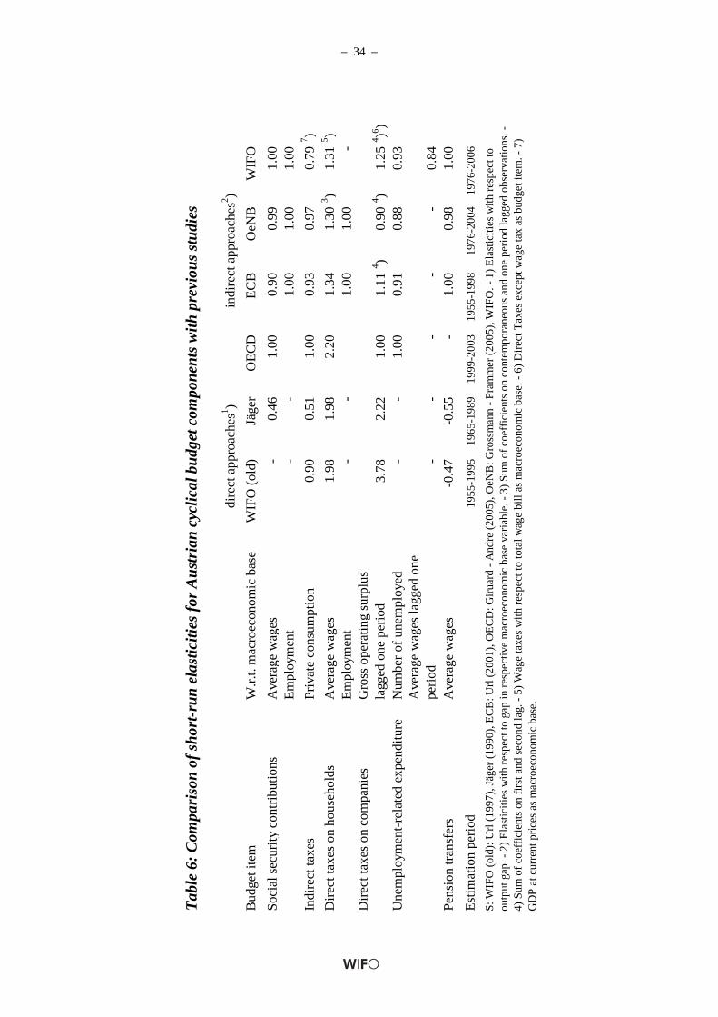
– 34 –

Tab

le 6

: C

ompa

riso

n of

sho

rt-r

un e

last

iciti

es f

or A

ustr

ian

cycl

ical

bud

get c

ompo

nent

s w

ith p

revi

ous

stud

ies

Bud

get i

tem

W.r

.t. m

acro

econ

omic

bas

eW

IFO

(ol

d)Jä

ger

OE

CD

EC

BO

eNB

WIF

O

Soc

ial s

ecur

ity

cont

ribu

tions

A

vera

ge w

ages

-0.

461.

000.

900.

991.

00E

mpl

oym

ent

--

1.00

1.00

1.00

Indi

rect

taxe

sP

riva

te c

onsu

mpt

ion

0.90

0.51

1.00

0.93

0.97

0.79

7 )

Dir

ect t

axes

on

hous

ehol

dsA

vera

ge w

ages

1.98

1.98

2.20

1.34

1.30

3 )1.

315 )

Em

ploy

men

t-

-1.

001.

00-

Dir

ect t

axes

on

com

pani

esG

ross

ope

ratin

g su

rplu

s la

gged

one

per

iod

3.78

2.22

1.00

1.11

4 )0.

904 )

1.25

4 )6 )U

nem

ploy

men

t-re

late

d ex

pend

itur

eN

umbe

r of

une

mpl

oyed

--

1.00

0.91

0.88

0.93

Ave

rage

wag

es la

gged

one

pe

riod

--

--

-0.

84P

ensi

on tr

ansf

ers

Ave

rage

wag

es-0

.47

-0.5

5-

1.00

0.98

1.00

Est

imat

ion

peri

od19

55-1

995

1965

-198

919

99-2

003

1955

-199

819

76-2

004

1976

-200

6

dire

ct a

ppro

ache

s1 )

S: W

IFO

(ol

d): U

rl (

1997

), J

äger

(19

90),

EC

B: U

rl (

2001

), O

EC

D: G

irua

rd -

And

re (

2005

), O

eNB

: Gro

ssm

ann

- P

ram

mer

(20

05),

WIF

O. -

1)

Ela

stic

itie

s w

ith

resp

ect t

o ou

tput

gap

. - 2

) E

last

icit

ies

wit

h re

spec

t to

gap

in r

espe

ctiv

e m

acro

econ

omic

bas

e va

riab

le. -

3)

Sum

of

coef

fici

ents

on

cont

empo

rane

ous

and

one

peri

od la

gged

obs

erva

tions

. -

4) S

um o

f co

effi

cien

ts o

n fi

rst a

nd s

econ

d la

g. -

5)

Wag

e ta

xes

with

res

pect

to to

tal w

age

bill

as m

acro

econ

omic

bas

e. -

6)

Dir

ect T

axes

exc

ept w

age

tax

as b

udge

t ite

m. -

7)

GD

P a

t cur

rent

pri

ces

as m

acro

econ

omic

bas

e.

indi

rect

app

roac

hes2 )

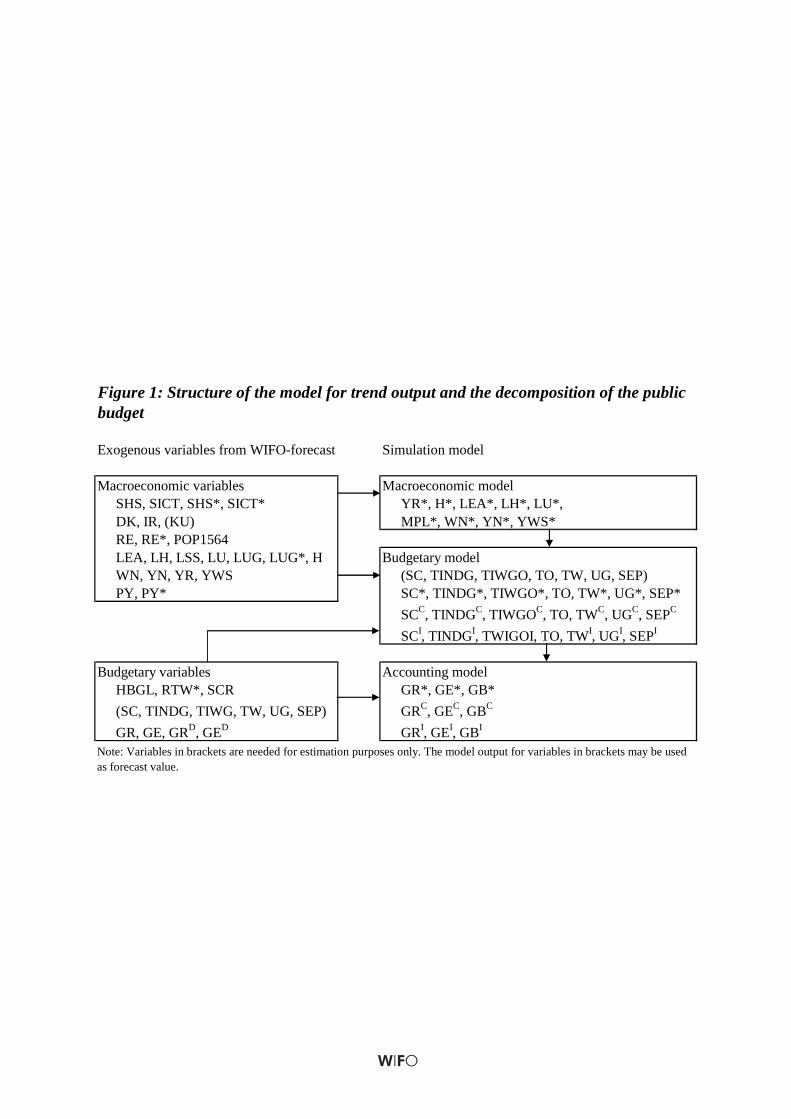
Exogenous variables from WIFO-forecast Simulation model

Macroeconomic variables Macroeconomic modelSHS, SICT, SHS*, SICT* YR*, H*, LEA*, LH*, LU*,DK, IR, (KU) MPL*, WN*, YN*, YWS*RE, RE*, POP1564LEA, LH, LSS, LU, LUG, LUG*, H Budgetary modelWN, YN, YR, YWS (SC, TINDG, TIWGO, TO, TW, UG, SEP)PY, PY* SC*, TINDG*, TIWGO*, TO, TW*, UG*, SEP*

SCC, TINDGC, TIWGOC, TO, TWC, UGC, SEPC

SCI, TINDGI, TWIGOI, TO, TWI, UGI, SEPI

Budgetary variables Accounting modelHBGL, RTW*, SCR GR*, GE*, GB*

(SC, TINDG, TIWG, TW, UG, SEP) GRC, GEC, GBC

GR, GE, GRD, GED GRI, GEI, GBI

Note: Variables in brackets are needed for estimation purposes only. The model output for variables in brackets may be used as forecast value.

Figure 1: Structure of the model for trend output and the decomposition of the public budget

– 36 –

Figure 2: Indicators of factor specific technical progress for the computation of trend output

Source: EUKLEMS, Statisitk Austria, Eigene Berechnungen. - Note: SHS represents the share of high skilled labor in the total labor force. - SICT represents the ratio of ICT-investment to total fixed investment net of ICT.

0

2

4

6

8

10

12

14

16

1976 1979 1982 1985 1988 1991 1994 1997 2000 2003 2006

SHS

SICT

In percent

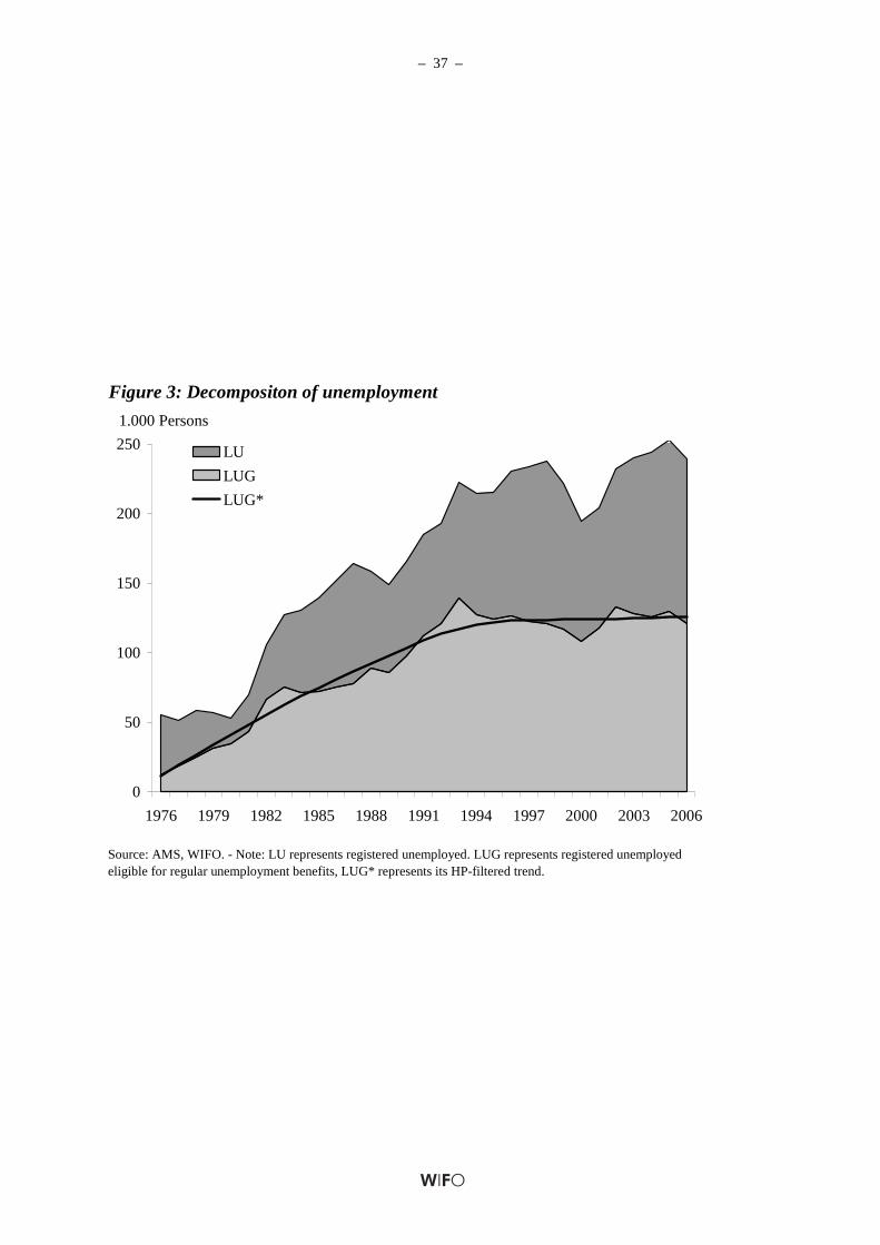
– 37 –

Figure 3: Decompositon of unemployment

Source: AMS, WIFO. - Note: LU represents registered unemployed. LUG represents registered unemployed eligible for regular unemployment benefits, LUG* represents its HP-filtered trend.

0

50

100

150

200

250

1976 1979 1982 1985 1988 1991 1994 1997 2000 2003 2006

LU

LUG

LUG*

1.000 Persons

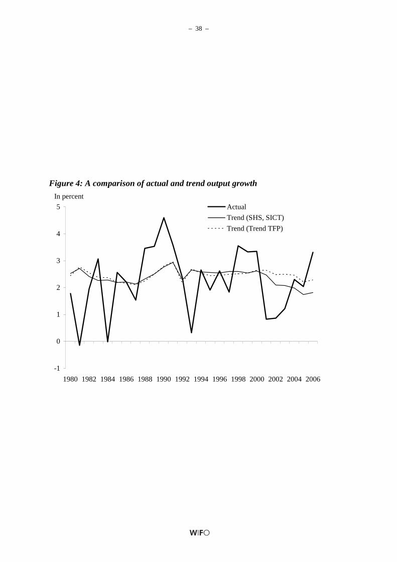
– 38 –

Figure 4: A comparison of actual and trend output growth

-1

0

1

2

3

4

5

1980 1982 1984 1986 1988 1990 1992 1994 1996 1998 2000 2002 2004 2006

Actual

Trend (SHS, SICT)

Trend (Trend TFP)

In percent

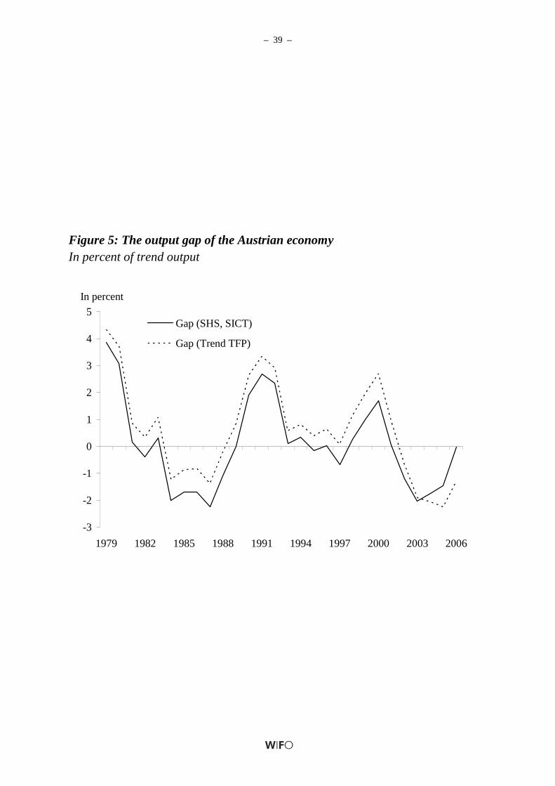
– 39 –

Figure 5: The output gap of the Austrian economyIn percent of trend output

-3

-2

-1

0

1

2

3

4

5

1979 1982 1985 1988 1991 1994 1997 2000 2003 2006

Gap (SHS, SICT)

Gap (Trend TFP)

In percent

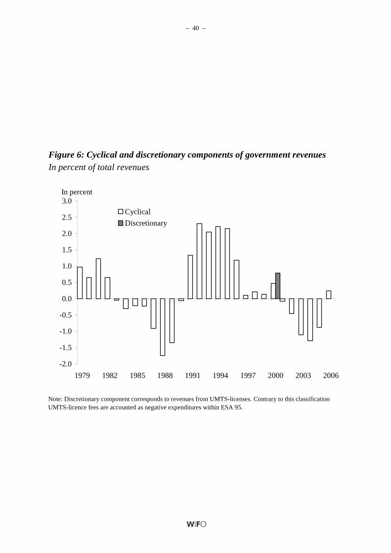
– 40 –

In percent of total revenuesFigure 6: Cyclical and discretionary components of government revenues

Note: Discretionary component corresponds to revenues from UMTS-licenses. Contrary to this classification UMTS-licence fees are accounted as negative expenditures within ESA 95.

-2.0

-1.5

-1.0

-0.5

0.0

0.5

1.0

1.5

2.0

2.5

3.0

1979 1982 1985 1988 1991 1994 1997 2000 2003 2006

Cyclical

Discretionary

In percent

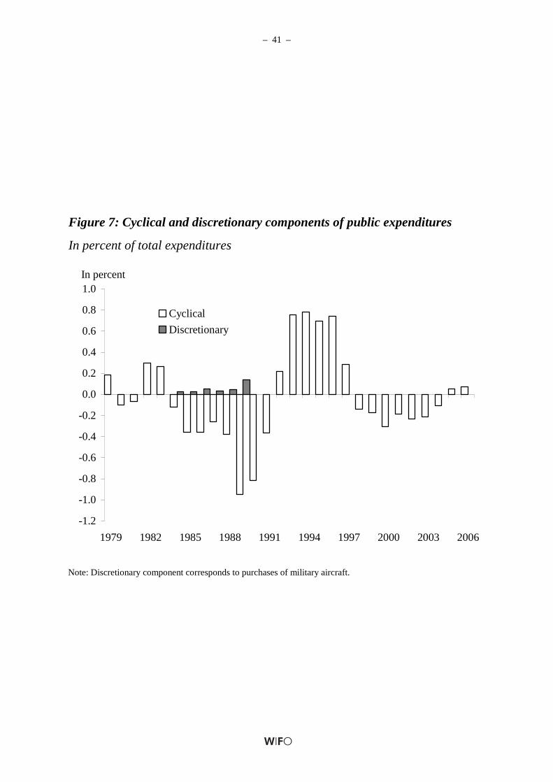
– 41 –

In percent of total expenditures

Note: Discretionary component corresponds to purchases of military aircraft.

Figure 7: Cyclical and discretionary components of public expenditures

-1.2

-1.0

-0.8

-0.6

-0.4

-0.2

0.0

0.2

0.4

0.6

0.8

1.0

1979 1982 1985 1988 1991 1994 1997 2000 2003 2006

Cyclical

Discretionary

In percent

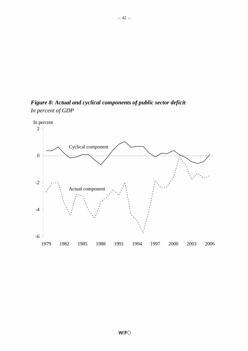
– 42 –

In percent of GDP

Figure 8: Actual and cyclical components of public sector deficit

-6

-4

-2

0

2

1979 1982 1985 1988 1991 1994 1997 2000 2003 2006

In percent

Cyclical component

Actual component

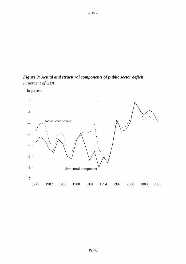
– 43 –

In percent of GDP

Figure 9: Actual and structural components of public sector deficit

-7

-6

-5

-4

-3

-2

-1

0

1979 1982 1985 1988 1991 1994 1997 2000 2003 2006

In percent

Structural component

Actual component

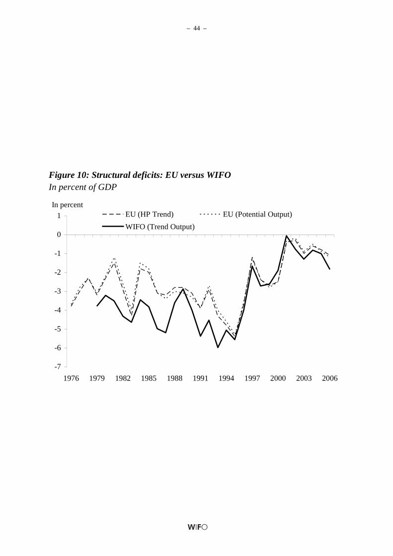
– 44 –

Figure 10: Structural deficits: EU versus WIFOIn percent of GDP

-7

-6

-5

-4

-3

-2

-1

0

1

1976 1979 1982 1985 1988 1991 1994 1997 2000 2003 2006

EU (HP Trend) EU (Potential Output)

WIFO (Trend Output)

In percent

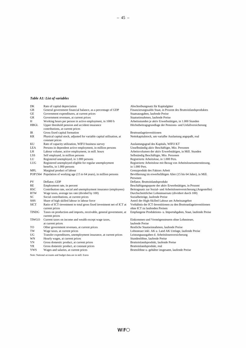
– 45 –

Table A1: List of variables

DK Rate of capital depreciation Abschreibungssatz für KapitalgüterGB General government financial balance, as a percentage of GDP Finanzierungssaldo Staat, in Prozent des BruttoinlandsproduktesGE Government expenditures, at current prices Staatsausgaben, laufende PreiseGR Government revenues, at current prices Staatseinnahmen, laufende PreiseH Working hours per person in active employment, in 1000 h Arbeitsstunden je aktiv Erwerbstätigen, in 1.000 StundenHBGL Upper threshold pension and accident insurance

contributions, at current pricesHöchstbeitragsgrundlage der Pensions- und Unfallversicherung

IR Gross fixed capital formation BruttoanlageinvestitionenKR Physical capital stock, adjusted for variable capital utilisation, at

constant pricesNettokapitalstock, um varialbe Auslastung angepaßt, real

KU Rate of capacity utilization, WIFO business survey Auslastungsgrad des Kapitals, WIFO KTLEA Persons in dependent active employment, in million persons Unselbständig aktiv Beschäftigte, Mio. PersonenLH Labour volume, active employment, in mill. hours Arbeitsvolumen der aktiv Erwerbstätigen, in Mill. StundenLSS Self employed, in million persons Selbständig Beschäftigte, Mio. PersonenLU Registered unemployed, in 1.000 persons Registrierte Arbeitslose, in 1.000 Pers.LUG Registered unemployed eligible for regular unemployment

benefits, in 1.000 personsRegistrierte Arbeitslose mit Bezug von Arbeitslosenunterstützung,in 1.000 Pers.

MPL Marginal product of labour Grenzprodukt des Faktors ArbeitPOP1564 Population of working age (15 to 64 years), in million persons Bevölkerung im erwerbsfähigen Alter (15 bis 64 Jahre), in Mill.

PersonenPY Deflator, GDP Deflator, BruttoinlandsproduktRE Employment rate, in percent Beschäftigungsquote der aktiv Erwerbstätigen, in ProzentRSC Contribution rate, social and unemployment insurance (employees) Beitragssatz zur Sozial- und Arbeitslosenversicherung (Angestellte)RTW Wage taxes, average tax rate (divided by 100) Durchschnittlicher Lohnsteuersatz (dividiert durch 100)SC Social contributions, at current prices Sozialbeiträge, laufende PreiseSHS Share of high skilled labour in labour force Anteil der High-Skilled Labour am ArbeitsangebotSICT Ratio of ICT-investment to total gross fixed investment net of ICT at

current prices Verhältnis der ICT-Investitionen zu den Bruttoanlageinvestitionen ohne ICT zu laufenden Preisen

TINDG Taxes on production and imports, receivable, general government, at current prices

Empfangene Produktions- u. Importabgaben, Staat, laufende Preise

TIWGO Current taxes on income and wealth except wage taxes,at current prices

Einkommen und Vermögensteuern ohne Lohnsteuer,laufende Preise

TO Other government revenues, at current prices Restliche Staatseinnahmen, laufende PreiseTW Wage taxes, at current prices Lohnsteuer inkl. AK u. Land AK Umlage, laufende PreiseUG Transfer expenditures, unemployment insurance, at current prices Leistungsausgaben d. ArbeitslosenversicherungWN Hourly wages, at current prices Stundenlöhne, laufende PreiseYN Gross domestic product, at current prices Bruttoinlandsprodukt, laufende PreiseYR Gross domestic product, at constant prices Bruttoinlandsprodukt, realYWS Wages and salaries, at current prices Bruttolöhne u.-gehälter insgesamt, laufende Preise

Note: National accounts and budget data are in mill. Euros

© 2008 Österreichisches Institut für Wirtschaftsforschung

Medieninhaber (Verleger), Hersteller: Österreichisches Institut für Wirtschaftsforschung • Wien 3, Arsenal, Objekt 20 • A-1103 Wien, Postfach 91 • Tel. (43 1) 798 26 01-0 • Fax (43 1) 798 93 86 • http://www.wifo.ac.at/ • Verlags- und Herstellungsort: Wien

Die Working Papers geben nicht notwendigerweise die Meinung des WIFO wieder

Kostenloser Download: http://www.wifo.ac.at/wwa/jsp/index.jsp?fid=23923&id=31859&typeid=8&display_mode=2