Institute of Economic Studies, Faculty of Social Sciences Charles University in Prague

Cyclical Bias in Cyclical Bias in Cyclical Bias in Cyclical Bias in Government Spending: Government Spending: Government Spending: Government Spending: Evidence from New EU Evidence from New EU Evidence from New EU Evidence from New EU Member Countries Member Countries Member Countries Member Countries

Jan Zápal

IES Working Paper: 15/2007

Institute of Economic Studies, Faculty of Social Sciences, Charles University in Prague

[UK FSV – IES]

Opletalova 26

CZ-110 00, Prague E-mail : ies@fsv.cuni.cz http://ies.fsv.cuni.cz

Institut ekonomických studií Fakulta sociálních věd

Univerzita Karlova v Praze

Opletalova 26 110 00 Praha 1

E-mail : ies@fsv.cuni.cz http://ies.fsv.cuni.cz

DisclaimerDisclaimerDisclaimerDisclaimer: The IES Working Papers is an online paper series for works by the faculty and students of the Institute of Economic Studies, Faculty of Social Sciences, Charles University in Prague, Czech Republic. The papers are peer reviewed, but they are not edited or formatted by the editors. The views expressed in documents served by this site do not reflect the views of the IES or any other Charles University Department. They are the sole property of the respective authors. Additional info at: ies@fsv.cuni.cz Copyright NoticeCopyright NoticeCopyright NoticeCopyright Notice: Although all documents published by the IES are provided without charge, they are licensed for personal, academic or educational use. All rights are reserved by the authors. CitationsCitationsCitationsCitations: All references to documents served by this site must be appropriately cited. Bibliographic informationBibliographic informationBibliographic informationBibliographic information: Zápal,J. (2007). “Cyclical Bias in Government Spending: Evidence from New EU Member Countries.” IES Working Paper 15/2007. IES FSV. Charles University.

This paper can be downloaded at: http://ies.fsv.cuni.cz

Cyclical Bias in Government Spending: Cyclical Bias in Government Spending: Cyclical Bias in Government Spending: Cyclical Bias in Government Spending: Evidence from New EU Member Evidence from New EU Member Evidence from New EU Member Evidence from New EU Member

CountriesCountriesCountriesCountries

Jan ZápalJan ZápalJan ZápalJan Zápal####

# London School of Economics and IES, Charles University Prague

E-mail: j.zapal@lse.ac.uk

May 2007 Abstract:Abstract:Abstract:Abstract: This paper focuses on dynamics of government spending over the business cycle. The literature on this topic has yet mainly focused on the issue of anti- or pro- cyclicality of fiscal policy. Only recently some researchers brought up a notion that response of fiscal policy might display great deal of asymmetry with respect to economic upturns and downturns. This is known as cyclical bias which arises when government expenditure increases more in cyclical downturns than it decreases in cyclical upturns, or vice versa. Empirical estimates of the sign and degree of cyclical bias show strong evidence in favour of the hypothesis that fiscal authorities do react with a great deal of asymmetry. Among other things, the presence of cyclical bias in government spending has been proposed as an explanation or mechanism which lies behind its unprecedented increase in most OECD countries over the last several decades. The aim of this paper is to show that a similar asymmetry of government spending dynamics can also be found in fiscal data of new EU member countries. We estimate the sign and degree of cyclical bias and compare it to estimates from other countries. Finally, we tackle the question of whether there is any statistically significant influence of political economy variables on the estimated degree of asymmetry. KeywordsKeywordsKeywordsKeywords: Cyclical Bias; New EU member states; Fiscal policy JELJELJELJEL:::: E32; E62; H30; H50.

Acknowledgements:Acknowledgements:Acknowledgements:Acknowledgements:

I would like to thank Ondřej Schneider, Kamil Dybczak, Asger Andersen and Zsofia Barany for helpful comments on the earlier drafts of the paper. All remaining errors are mine.

1

1. Introduction

This paper deals with dynamics of government expenditure over the course of the

business cycle. Our main focus is a possible asymmetry of this dynamics with respect to

economic upturns and downturns.

So far, both the theoretical and the empirical literature on this topic has mainly

focused on issues related to pro- or anti-cyclicality of government expenditure, implicitly

assuming that the reaction of government expenditure is symmetric with respect to the

business cycle.1 Yet, there is no reason to assume government spending behaves the same

way during recessions as it behaves during expansions. This is what we define as cyclical bias

in government spending: presence of asymmetric dynamics of government expenditure with

respect to the business cycle, more specifically, with respect to positive and negative output

gaps.

Is there any cyclical bias in government expenditure? How big is it and in what

direction? Is it common to all components of public spending or not? How does composition

of government, elections or other political economy factors influence it? And how does pro-

or anti-cyclicality of fiscal policy relates to it? Those are the question we try to answer.

An introduction of the basic econometric specification to be estimated will facilitate

the discussion. We estimate

ititititititiit gyyyygd εβββββα ++++++= −−

−−+

−+

15143121log (1)

where itg is government expenditure to GDP ratio in country i and year t and ity is the gap

between actual and potential output, which we split into expansionary periods ( +ity ) and

recessionary periods ( −ity ), iα is a country i specific constant and itε is assumed to be i.i.d.

zero-mean, constant-variance error.

This specification allows us to answer two questions. The first one is whether there is

an asymmetry in the behaviour of government spending. This would manifest itself as a

1 See Hercowitz and Strawczynski (2004) and Persson and Tabellini (2003) for rare exceptions.

2

difference in the estimates of 1β as compared to 3β or, alternatively, in different estimates of

2β and 4β . The second question is whether there is a cyclical bias in government spending.

To answer this question, we define the coefficient of cyclical bias as 4321 ββββφ −−+= .

Note that if government spending increases during expansions, then 01 >β and 02 >β and if

government spending increases during recessions, then 03 <β and 04 <β . What the

coefficient of cyclical bias tells us is that after a hypothetical four-year business cycle, during

which output rises one percent above potential in the first year, drops to its potential in the

second year, decreases one percent below its potential in the third year and returns back to

potential in the fourth year, government spending to GDP ratio will be φ -percent higher.

We must stress that the issue of cyclical bias is to a certain degree orthogonal to the

issue of pro- or anti-cyclicality of government spending. When 0, 21 <ββ and 0, 43 <ββ ,

fiscal policy is counter-cyclical and it is pro-cyclical if the inequalities are reversed.2 But

when all four coefficients are equal in absolute value, the coefficient of cyclical bias will be

zero. It is when fiscal policy is more anti-cyclical during recessions than during expansions or

alternatively, when fiscal policy is more pro-cyclical during expansions than during

recessions that cyclical bias arises.

Specification (1) also makes explicit an assumption which underlies most of the

literature on pro- or anti-cyclicality of fiscal policy. Most of this literature implicitly assumes

that the elasticity of government expenditure with respect to the output gap is equal in

economic upturns and downturns, i.e. that 31 ββ = and 42 ββ = , and subsequently fails to

separate positive and negative output gaps. But if the true data generating process is given by

(1), then regressions of public expenditure on a lumped measure of the output gap will be

misspecified.

Since evidence about cyclical bias in government spending for OECD countries is

presented in Hercowitz and Strawczynski (2004), which also served as major inspiration for

our work, we investigate the issue at hand using fiscal and economic data for ten new EU

member countries.3 The reason for using data for new EU member states is twofold. First,

fiscal behaviour of those countries has so far received only limited attention. In this respect

our work contributes to already existing literature. Second, using dataset for a different

sample of countries allows us to compare our estimates with those for the OECD countries,

which in itself can be of interest.

To give a flavour of our findings, we regard two of our conclusions as most important.

Using data on new EU member countries, we do find a great deal of asymmetry of fiscal

2 Some of the existing literature seems to be rather unclear on this, so we must clarify meaning of pro-

or anti-cyclicality. Note that when the public expenditure to GDP ratio is a-cyclical then public expenditure

expressed in levels moves proportionally with GDP, in other words, if expressed in level terms, it is pro-cyclical.

On the other hand, when public expenditure in level terms is a-cyclical, it is anti-cyclical when expressed as

GDP ratio. What we mean when we say pro-cyclical fiscal policy is that expenditure to GDP ratio (our

dependent variable) is positively correlated with the GDP gap, i.e. increases during good times. The reverse

holds for anti-cyclicality and gives rise to inequalities and their interpretation just mentioned. 3 Ten new member countries which joined EU on May 2004 are Cyprus, Czech Republic, Estonia,

Hungary, Latvia, Lithuania, Malta, Poland, Slovenia and Slovakia.

3

policy with respect to business cycle. Government spending increases over the course of the

business cycle mainly as a result of strong increases during recessions which are not offset by

equivalent decreases during expansions.

The second thing our data reveal is that some of the asymmetry is influenced or

induced by political economy factors. Probably the most important factor is the composition

of government and, to a lower degree, the occurrence of general parliamentary elections.

We proceed as follows. Next section relates our work to the existing literature and we

try to motivate and structure our thinking about cyclical bias within a non-formal and verbal

model, capturing what we think are the most important features determining cyclical

behaviour of government spending. This guides our empirical strategy which is the substance

of the third section. Section four tackles questions related to robustness of our findings and

other econometric issues. Section five concludes the paper. Details about data are given in the

appendix.

2. Relation to Existing Literature

This paper is broadly related to several strands of existing literature. The first is a

rather technical literature which estimates the elasticity of the budget surplus with respect to

output fluctuations in order to compute cyclically adjusted budget balance.4

The second body of work compares cyclicality of fiscal policy across a wider sample

of countries. The conventional wisdom that emerged is that fiscal policy is anti-cyclical or a-

cyclical in most developed countries (usually defined as OECD countries), while it is (often

strongly) pro-cyclical in developing countries – see e.g. Talvi and Vegh (2000). Several

explanations have been offered to account for this observed pattern of cyclical behaviour.

Catao and Sutton (2002) and Kaminsky, Reinhart and Vegh (2004) argue that developing

countries become credit constrained during economic downturns which precludes government

from effectively smoothing economic fluctuations. As a result, government expenditure

increases during good times and decreases during bad times, i.e. fiscal policy becomes pro-

cyclical.

This view has been challenged based on the argument that it seems unlikely that

financial markets would systematically limit governments in developing countries from

borrowing during recessions. Alesina and Tabellini (2005) show that most of the pro-

cyclicality of fiscal policy in developing countries can be explained by high levels of

corruption in those countries. Several other political economy factors have been shown to

have an impact on cyclical behaviour of fiscal policy. Hallerberg and Strauch (2002) show

that fiscal policy is less anti-cyclical in EMU countries in election years. Sorensen, Wu and

Yosha (2001) document similar impact in U.S. states and document also an impact of

conservativeness of political representation and of presence of fiscal rules on the cyclical

behaviour of fiscal policy. Lane (2003) finds that higher power dispersion (more players

4 See Suyker (1999) and Noord (2000) for OECD, Bouthevillain et al. (2001) for European Central

Bank and Hagemann (1999) for IMF’s approach. Röger and Ongena (1999) and European Commission (2000;

2002) provide overview of approach to cyclically adjusted budget balance in context of Stability and Growth

Pact.

4

within political system with veto power) increases pro-cyclicality of fiscal policy in OECD

countries. Similarly, Henisz (2004) finds that political systems with stronger checks and

balances display lower volatility in a wide range of public spending categories.

The only work we are aware of which systematically investigates the possible

asymmetry of fiscal policy with respect to the business cycle is Hercowitz and Strawczynski

(2004) who document on data for OECD countries strong increases in government spending

during recessions, which are not offset by equal decreases in expansions. As a result, they

estimate that over the stylized business cycle mentioned above, government expenditure to

GDP ratio increases by 0.86 percent, that is, their estimate of the coefficient of cyclical bias is

86.0=�φ .

Several theoretical models have been proposed to explain empirically observed

phenomena. Aizenman, Gavin and Hausmann (1996) build a model with endogenous credit

constraints. Alesina and Tabellini (2005) build a model where a high degree of corruption

means that surpluses accumulated in good times when fiscal policy is anti-cyclical are not

optimal because the electorate knows that corrupt political representation would

misappropriate them. It is then rational for the electorate to demand higher spending during

expansions, i.e. pro-cyclical fiscal policy.

In Persson and Tabellini (2000, ch.4) imperfect information about the true state of the

economy by electorate allows politicians to divert some extra resources to discretionary use in

good times, but to spend all tax revenues on public goods provision during bad times. If we

interpret discretionary spending, for example, as subsidies, one would expect pro-cyclical

behaviour of this spending category.

Within the model of Austen-Smith (2000) a positive technology shock induces

previously unemployed voters to enter the workforce which lowers average employee’s

income with the implication that the preferred income tax rate and degree of redistribution

increases. Similarly, Tornell and Lane (1998; 1999) build a model where positive

technological shocks induce a voracity effect. The voracity effect arises because demand for

specific transfers by special interest groups increases in expectation of higher government

revenue in the future. This higher demand, if met, results in an increase of public expenditure

which more than offsets the increase in revenue, resulting in pro-cyclical fiscal policy.

Unfortunately, none of the models mentioned above attempt to model asymmetric

behaviour of fiscal policy. Because we don’t want to be left unguided in our empirical

investigation of the matter, we want to outline a model which would structure our thinking.

Consider a two-stage game with three players. One player is the finance minister who

sets the budget in the first stage knowing that in the second stage, nature determines whether

the economy is in a good or bad state. If the economy happens to be in the good state, the

previously budgeted expenditure turns out to be unnecessarily high, while if the economy

happens to be in the bad state, previously budgeted expenditure turns out to be too low.

Suppose further that the finance minister prefers the public budget to be optimal in a sense

that it corresponds to the state the economy happens to be in, but because he does not know

nature’s move, cannot set it optimally in advance.

5

It is then finance minister’s task in the second stage to propose a change to the budget

within a government. This change has to be approved by majority rule. Suppose that there are

two other players, spending ministers, who prefer not optimal, but higher expenditure under

any state of the economy. One possible way to model the second stage would be a bargaining

game in the spirit of Baron and Ferejohn (1989).

Now it is easy to see the implications of our setup. If the economy happens to be in a

bad state, the finance minister’s proposal will be to increase the expenditure of (possibly) both

spending ministers. Clearly, such a proposal finds only limited opposition and public

expenditure increases.

On the other hand, during good times, finance minister’s proposal would be to lower

public expenditure. Such a proposal would not gain much support from spending ministers

and would be turned down. In other words, during expansions, public expenditure would be

too high. Note that this setup yields an extreme prediction of increase of public expenditure

during recessions and constancy during expansions.5

To make the predictions less extreme, suppose that one of the spending ministers is

from the same party as the finance minister and thus internalizes part of his disutility from

non-optimal budget. Then this spending minister can vote for a decrease of public expenditure

during good times. In the terminology of Baron and Ferejohn (1989), a spending minister

from the same party is a cheaper coalition partner than the other spending minister.

Note that this opens two possible ways for the finance minister to bring the budget

closer to the optimal value in a good state of the economy. One way is when the government

is not too fragmented, in the sense that he can find allies who can be induced to vote for his

proposal. Another way is for the finance minister to lover the expenditure of only one

spending minister and bring the budget closer to optimality in this way.

This argument also suggests that we should expect different cyclical behaviour for

different spending categories. Some spending ministers might be more important or powerful

than others or opposition by the general public might force the finance minister not to propose

cuts for certain types of spending. Or one can add influence of interest groups who demand

higher spending during good times in the sense of the voracity effect mentioned above which

increases opposition to proposed spending cuts. Another important factor can be the strength

of the finance minister within the cabinet.

Thus we have several predictions about cyclical behaviour of public spending. First,

we expect expenditure to increase by a larger amount in recessions than it decreases during

economic expansions, especially for politically sensitive parts of the budget, with social

spending as our prime suspect.

Second, we expect composition of government to influence the degree of cyclical bias.

Based on the argument given above, we would expect lower cyclical bias for less fragmented

5 The finance minister could solve his problem by setting the budget in the first stage optimal for good

times, which would subsequently require adjustment (increase) only if the state of the economy turns out to be

bad. However, this is true only if finance minister knows exactly how bad or good times look like and if he sets

the budget to his full discretion in the first stage. If good and bad times are distributed, for example, uniformly,

meaning that there can be different good and different bad states, the finance minister cannot solve his problem

in this way, if he does not have full discretion over the budget in the first stage.

6

governments. On the other hand, less fragmented governments can be more prone to electoral

manipulation of the budget and thus, besides stronger cyclical bias in election years, we

cannot say anything about effect of government fragmentation a priory.

Third, based on the voracity effect argument, we expect those parts of the public

budget which benefit special interest groups to increase in expansions, with subsidies and

capital spending as prime examples.

Finally, we expect a weaker position of the finance minister to be associated with

stronger cyclical bias. In the next section, we shall see how our priors square with the data.

3. Cyclical Bias Estimates

This section presents our key findings regarding dynamics of public spending in new

EU member countries. We first focus on general government expenditure dynamics and

compare it with findings from two other samples of countries. We then shift our attention to

dynamics of different components of public budgets and finally investigate the impact of

political economy variables.

Throughout this section, the basic econometric specification will be of the form

ititititititiit gyyyygd εβββββα ++++++= −−

−−+

−+

15143121log (2)

where itgd log is (log) change of the fiscal variable under consideration expressed as the ratio

to GDP in country i and year t . On the RHS, variable +

ity (−

ity ) is positive (negative) output

gap defined as (log) deviation of GDP from its Hodrik-Prescott trend in country i and year t ,

iα is a country specific constant and itε is zero-mean constant-variance error.

Given the likelihood of lag in timing of government expenditure during the business

cycle, we include one year lag of cyclical variables. We are concerned with reaction of public

spending to output fluctuations on the one hand and with the sign and size of the coefficient

of cyclical bias which we define as 4321 ββββφ −−+= on the other.

All the estimations are fixed effect panel estimates. Use of fixed effect model is in

most cases implied by Hausman test (against use of random effect model). Since

heterogeneity across countries can be of concern, we use fixed effect estimation with cross

section weights and use heteroskedasticity consistent (robust) standard errors.

3.1. Government Expenditure

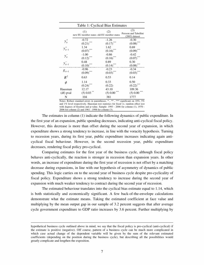
Table 1 shows estimates of specification (2). Column (1) is based on general

government expenditure for new EU member countries. As a benchmark we also include

estimates for 15 old EU member countries6 based on general government expenditure in

column (2). Column (3) shows estimates for a panel of 60 countries used by Persson and

Tabellini (2003), where the dependent variable is central government expenditure.7

6 Old EU member countries are the 12 Eurozone members: Austria, Belgium, Finland, France,

Germany, Greece, Ireland, Italy, Luxembourg, Netherlands, Portugal, Spain plus Denmark, Sweden and UK. 7 See data appendix for description of variables and their sources. Also, when interpreting the estimation

results, we use following terminology for the estimates on the output gap variables (top to bottom in the table):

first expansion year, second expansion year, first recession year and second recession year. Keeping our

7

Table 1: Cyclical Bias Estimates

(1) new EU member states

(2) old EU member states

(3) Persson and Tabellini

(2003) dataset +

ity -0.72

(0.21)***

-1.26

(0.17)***

-0.30

(0.08)***

+

−1ity 1.34

(0.07)***

1.62

(0.16)***

0.69

(0.09)***

−

ity -1.00

(0.12)***

-0.86

(0.16)***

-0.42

(0.07)***

−

−1ity 0.48

(0.10)***

0.89

(0.14)***

0.30

(0.08)***

1−itg -0.96

(0.09)***

-0.23

(0.03)***

-0.34

(0.03)***

2R 0.63 0.53 0.14

φ 1.14

(0.24)***

0.33

(0.22)

0.50

(0.22)***

Hausman

(df) pval

12.17

(5) 0.03 **

43.10

(5) 0.00 ***

109.36

(5) 0.00 ***

N 104 381 1777

Notes: Robust standard errors in parentheses. * , ** , *** significant on 10%, 5%

and 1% level respectively. Hausman test statistics for fixed vs. random effect test

with degrees of freedom and p-value. Sample: 1993 - 2006 for column (1), 1970 -

2006 for column (2) and 1961 - 1998 for column (3).

The estimates in column (1) indicate the following dynamics of public expenditure. In

the first year of an expansion, public spending decreases, indicating anti-cyclical fiscal policy.

However, this decrease is more than offset during the second year of expansion, in which

expenditure shows a strong tendency to increase, in line with the voracity hypothesis. Turning

to recession years, during its first year, public expenditure increases indicating again anti-

cyclical fiscal behaviour. However, in the second recession year, public expenditure

decreases, rendering fiscal policy pro-cyclical.

Comparing estimates for the first year of the business cycle, although fiscal policy

behaves anti-cyclically, the reaction is stronger in recession than expansion years. In other

words, an increase of expenditure during the first year of recession is not offset by a matching

decrease during expansions, in line with our hypothesis of asymmetry of dynamics of public

spending. This logic carries on to the second year of business cycle despite pro-cyclicality of

fiscal policy. Expenditure shows a strong tendency to increase during the second year of

expansion with much weaker tendency to contract during the second year of recession.

The estimated behaviour translates into the cyclical bias estimate equal to 1.14, which

is both statistically and economically significant. A few back-of-the-envelope calculations

demonstrate what the estimate means. Taking the estimated coefficient at face value and

multiplying by the mean output gap in our sample of 3.2 percent suggests that after average

cycle government expenditure to GDP ratio increases by 3.6 percent. Further multiplying by

hypothetical business cycle outlined above in mind, we say that the fiscal policy is pro-cyclical (anti-cyclical) if

the estimate is positive (negative). Off course, pattern of a business cycle can be much more complicated in

which case actual change of the dependent variable will be given by the sum of the relevant estimated

coefficients (depending on the position during the business cycle), but describing all the possibilities would

greatly complicate and lengthen the exposition.

8

the mean government expenditure to GDP ratio of 44 percent suggests increase by 1.6 percent

of GDP.

A similar pattern emerges from estimates in column (3). Estimates suggest precisely

the same logic as estimates for new EU member states with the difference that the estimated

coefficient of cyclical bias is approximately half in size, yet still statistically significant.

Column (2) shows some notable differences. For old EU member countries, the drop in public

spending during the first expansion year is larger than the increase of expenditure during first

recession year, contrary to our hypothesis that it is easier to increase than decrease public

expenditure. However, this is ‘compensated’ by strong pro-cyclical expenditure increase

during second expansion year, which is only partially offset by pro-cyclical decrease during

second recession year. Overall, estimated coefficient of cyclical bias is still positive but

statistically insignificant at conventional levels (p-value of 0.14).

Our explanation of the different degree of cyclical bias in new EU member countries

compared to the estimates in columns (2) and (3) is that the estimates in column (1) are based

on a considerably shorter time period. Obviously, government expenditure to GDP ratio

cannot increase for ever. Sooner or later cyclical ratcheting of government expenditure has to

come to an end (or requires repeating corrective spending cuts if it prevails). The fact that

eight out of ten new EU member countries are post-communist economies which might still

be on its way to ‘steady state’ level of public expenditure to GDP ratio might be the reason

behind the relatively high estimate of cyclical bias.

3.2. Decomposition of Expenditure

We now turn to the dynamics of different components of public expenditure in new

EU member countries. Table 2 columns (1) through (5) include estimates for compensation of

employees (EMP), social expenditure (SOC), final consumption expenditure (FCE), subsidies

(SUB) and finally for capital expenditure (CAP).

Table 2: Cyclical Bias of Expenditure Items

(1)

EMPg it = (2)

SOCg it =

(3)

FCEg it =

(4)

SUBg it =

(5)

CAPg it =

+

ity -0.12

(0.37)

-0.15

(0.60)

-1.80

(1.07)*

5.56

(3.47)

0.57

(0.97) +

−1ity 0.17

(0.30)

0.51

(0.57)

0.17

(0.52)

-2.74

(1.98)

0.97

(0.57)*

−

ity -0.79

(0.24)***

-1.06

(0.60)*

-0.06

(0.57)

0.92

(1.25)

-0.65

(0.49) −

−1ity 0.38

(0.17)**

0.33

(0.36)

-0.15

(0.40)

-0.08

(1.29)

0.60

(0.66)

1−itg -4.41

(0.63)***

-1.39

(0.45)***

-2.72

(0.73)***

-13.95

(3.46)***

-12.91

(2.20)***

2R 0.80 0.39 0.49 0.33 0.26

φ 0.47

(0.39)**

1.09

(0.65)*

-1.41

(1.75)

1.97

(3.29)

1.59

(1.00)

Hausman

(df) pval

39.77

(5) 0.00 ***

18.43

(5) 0.00 ***

17.40

(5) 0.00 ***

7.61

(5) 0.18

13.28

(5) 0.02 **

N 120 118 123 120 112

Notes: Robust standard errors in parentheses. * , ** , *** significant on 10%, 5% and 1% level

respectively. Hausman test statistics for fixed vs. random effect test with degrees of freedom and p-value. Sample: 1991 - 2006 for all columns.

9

The first thing to notice about the estimates included in table 2 is generally much

lower precision compared to the estimates in table 1. Our explanation is that the dynamics of

separate components of expenditure is much more given by idiosyncratic shocks which ‘even’

out in aggregate total expenditure category.

Nevertheless, the estimates in columns (1) and (2) show similar behaviour.

Compensation of employees and social spending show no tendency to decrease during

expansions and a strong tendency to increase during recessions, in line with our hypothesis of

asymmetric behaviour. As a result, for both spending categories, the coefficient of cyclical

bias is statistically significant.

The estimates in column (3) are in general insignificant with the exception of a strong

anti-cyclical response during the first expansion year. Similar results hold for column (4)

where only the estimate for the first expansion year comes close to statistical significance (p-

value of 0.11), suggesting a strong pro-cyclical reaction of subsidies. Column (5) then in

general points to pro-cyclical behaviour of capital expenditure with the exception of the first

recession year, although the only estimate which is significant is for the second year of

expansion. Overall, the estimates of cyclical bias in columns (3) through (5) are insignificant

and closest to statistical significance is the estimate for capital expenditure (p-value 0.11).

Overall, the estimates for the different categories of public spending give a much

fuzzier picture than the estimates for total expenditure. The estimates for social spending and

employee compensation categories, which can be regarded as politically sensitive ones, come

close to what we expected. The combination of increases during recessions and no decreases

during expansions results in cyclical ratcheting. Subsidies and capital expenditure, spending

categories where we expected the voracity effect to play a key role, fulfil our expectations

only partially. Although the estimate of cyclical bias for both spending categories is positive,

sizeable and given by strong pro-cyclical behaviour during expansions, it is not statistically

significant.

3.3. Political Economy Influence

This section investigates how political economy factors influence the degree of

cyclical bias. Throughout the section, our dependent variable will be the general government

expenditure and we will expand our basic specification to

ititititititititit

itititititiit

yzyzyzyz

gyyyygd

εγγγγ

βββββα

+++++

+++++=−

−−

−+

−−

+

−

−

−

−+

−

+

11431121

15143121log (3)

where all the variables are defined as before and itz is a political economy variable in country

i and year t .

We must stress that results in this section should be taken with a grain of salt. The first

thing to notice is that by adding one political variable itz we are effectively adding four RHS

variables and coefficients to be estimated. Having at most 14 observations for any country in

the sample and despite the fact that we add only one political variable at a time, we might be

stretching the data too much.

10

Second, although Hausman statistics suggests in several cases that the random effect

model should be used, we use fixed effect estimation. There are several reasons for this. One

is that the random effect model requires that the number of coefficients to be estimated is

lower than the number of cross sections. Since we have ten coefficients in (3) and equal

number of cross sections, we do not want to push the data too far. Another reason is that

estimating the model with fixed effects when random effect estimation should have been used

still yields consistent estimates. The only thing we jeopardize is loss of efficiency. And lastly,

Hausman statistics are in most cases just within a reach of the rejection region, which leaves

considerable hope that error we fall into is not substantial. We still use fixed effect estimation

with cross section weights and report heteroskedasticity consistent (robust) standard errors.

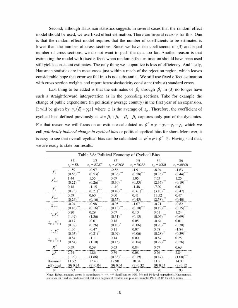
Last thing to be added is that the estimates of 1β through 4β in (3) no longer have

such a straightforward interpretation as in the preceding sections. Take for example the

change of public expenditure (in politically average country) in the first year of an expansion.

It will be given by ( )zyit 11 γβ ++ where z is the average of itz . Therefore, the coefficient of

cyclical bias defined previously as 4321 ββββφ −−+= captures only part of the dynamics.

For that reason we will focus on an estimate calculated as 4321 γγγγφ −−+=P which we

call politically induced change in cyclical bias or political cyclical bias for short. Moreover, it

is easy to see that overall cyclical bias can be calculated as zP ⋅+=′ φφφ . Having said that,

we are ready to state our results.

Table 3A: Political Economy of Cyclical Bias

(1)

ELzit = (2)

ELSTzit = (3)

NOCPzit = (4)

NOPPzit = (5)

NSMz it = (6) MFCHzit =

+

ity -1.59

(0.56)***

-0.97

(0.53)*

-2.56

(0.36)***

-1.91

(0.58)***

-8.94

(0.76)***

-1.63

(0.44)***

+

−1ity 1.44

(0.22)***

1.55

(0.26)***

0.69

(0.30)**

1.05

(0.55)*

7.63

(2.36)***

1.25

(0.19)***

−

ity 0.18

(0.73)

-1.15

(0.21)***

-1.10

(0.49)**

-1.48

(0.61)**

-7.09

(3.10)**

0.61

(0.47) −

−1ity 0.59

(0.24)**

0.60

(0.16)***

0.00

(0.55)

0.41

(0.45)

13.52

(2.58)***

0.47

(0.40)

1−itg -0.94

(0.16)***

-0.98

(0.16)***

-0.95

(0.13)***

-1.07

(0.10)***

-0.71

(0.19)***

-0.82

(0.15)***

+

itit yz 0.20

(1.49)

0.29

(1.36)

0.67

(0.31)**

0.10

(0.15)

0.61

(0.06)***

1.24

(0.69)*

+

−− 11 itit yz -0.17

(0.32)

-0.01

(0.26)

0.18

(0.10)*

0.05

(0.06)

-0.64

(0.20)***

0.01

(0.30) −

itit yz -1.36

(0.63)**

-0.47

(0.21)**

0.11

(0.09)

0.07

(0.06)

0.58

(0.28)**

-1.84

(0.39)***

−

−− 11 itit yz -0.84

(0.54)

-1.11

(1.10)

0.14

(0.15)

0.00

(0.04)

-0.87

(0.22)***

0.25

(0.26) 2R 0.59 0.59 0.63 0.84 0.67 0.63

Pφ 2.24

(1.92)

1.86

(1.86)

0.59

(0.33)*

0.08

(0.19)

0.26

(0.47)

2.84

(1.00)***

Hausman

(df) pval

11.52

(9) 0.24

17.40

(9) 0.04

17.90

(9) 0.04

10.34

(9) 0.32

11.51

(9) 0.24

14.03

(9) 0.12

N 93 93 93 93 70 93

Notes: Robust standard errors in parentheses. * , ** , *** significant on 10%, 5% and 1% level respectively. Hausman test

statistics for fixed vs. random effect test with degrees of freedom and p-value. Sample: 1993 - 2005 for all columns.

11

Electoral Influence

We first look at the influence of elections on the degree of cyclical bias. For this

purpose, itz in (3) is a dummy variable which takes the value of unity in years of general

parliamentary elections. The first two columns of table 3 show our results.

Focusing on column (1), we see that elections during expansionary years do not

change the behaviour of public expenditure. What matters is when elections take place in the

first recession year, in which case they are associated with a stronger anti-cyclical response or

in other words, with a stronger increase of public expenditure. A similar result holds for the

second recession year although the estimated coefficient is not statistically significant at

conventional level (p-value of 0.12). As a result, the political cyclical bias is positive

indicating that the asymmetry in expenditure dynamics found in the preceding sections is

more of a concern in election years. However, as a result of no impact of elections during

expansions, it turns out to be statistically insignificant.

One possible concern with elections is that, at least some of them might be

endogenous. Column (2) addresses this question by excluding those elections which took

place before the end of regular electoral cycle from our election dummy variable. The fact

that the results almost do not change suggests that electoral endogeneity is of no concern.

Political Fragmentation

Next we want to address the question how political fragmentation interacts with the

dynamics of public expenditure. Existing literature on this topic usually investigates how the

number of different political parties in the cabinet or parliament affects fiscal outcomes.

Roubini and Sachs (1989a; 1989b) were among the first to focus on government

fragmentation. They use a variable ranging from zero for a majority government composed of

one political party to three for a minority government in their regressions. They find that

minority governments are characterized by more lax fiscal policies and higher budget deficits.

Their findings have later been challenged by Haan and Sturm (1997) and Haan, Sturm and

Beekhuis (1999) who show the that original variable capturing fragmentation of government

is inappropriate. Subsequently Volkerink and Haan (2001), Balassone and Giordano (2001),

Perotti and Kontopoulos (2002) and Ricciuti (2004) use several different variables to capture

political fragmentation and in general find more fragmentation to be associated with ‘worse’

fiscal outcomes.

Variables often found significant are number of effective parties in cabinet or

parliament,8 number of political parties in the cabinet or parliament, or number of spending

ministers in the cabinet. Columns (3) through (5) of table 3 show our results when we use

those variables.

8 Effective number of parties is defined as the reciprocal of the sum of squared vote shares of individual

parties either in cabinet or parliament, or in other words, as a reciprocal of Herfindahl’s index of concentration.

We experimented with this measure of concentration and results turned out to be disappointing and thus are not

reported. We also experimented with a variable defined as in Roubini and Sachs (1989a; 1989b) with similar

(disappointing and not reported) results.

12

In column (3), the political variable itz is the number of political parties in cabinet

(NOCP). What the estimates show is that fragmented governments influence the dynamics of

public expenditure mainly through a more pro-cyclical response during the first year of

economic expansion, in other words, through a strong increase of public expenditure during

those years. A similar logic holds for the second expansionary year, while the number of

political parties in the cabinet does not seem to have an impact on the dynamics of public

expenditure during recession periods. The resulting political cyclical bias is positive and

unlike electoral influence, it is statistically significant.

Column (4) displays estimates for the number of political parties in parliament

(NOPP). As opposed to the number of political parties in cabinet, parliaments composed of

more parties do not, according to our estimates, have any effect on the dynamics of public

expenditure.

Column (5) investigates the impact of the number of spending ministers (NSM) on the

cyclical bias. The estimated coefficients show a rather puzzling pattern characterized by

stronger pro-cyclical behaviour associated with more spending ministers in the first expansion

and recession years. On the other hand, cabinets with more spending ministers pursue more

anti-cyclical fiscal policy during second expansion and recession years.

Nevertheless, the fact that the estimated coefficients are all statistically significant is in

line with the findings of Perotti and Kontopoulos (2002) who find the number of spending

ministers to have an especially strong effect on the behaviour of public expenditure. Despite

that, the implied political cyclical bias is too low to be statistically and economically

significant.

Weak Finance Minister

One of the features of the model we outlined is that the cyclical bias is caused by the

fact that the finance minister faces opposition of spending ministers when the decision about

public expenditure in the cabinet is made. This suggests that a weaker position of the finance

minister should be associated with a stronger cyclical bias. For this reason we use a dummy

(MFCH) taking the value of unity in years when the minister of finance has been replaced.

Results are depicted in column (6).9 However imperfect this measure of the finance minister’s

strength might be, we hope that new finance ministers find it harder to resist the pressure for

expenditure increases or are less able to push their colleagues into expenditure cuts.

The results partially confirm our intuition. Governments with a new finance minister

engage in more pro-cyclical fiscal policy during the first expansion year and more anti-

cyclical policy during the first recession year. As before, such a behaviour points to a stronger

increase (weaker decrease) of public expenditure during recessions (expansions). As a result,

9 We are aware of the literature which tries to capture different institutional features of budget process

and their impact on fiscal outcomes and which usually constructs index of minister of finance influence or

power. However, such an index is inappropriate for our empirical strategy because it does not change over time

and thus cannot be used in panel data estimation. We refer interested reader to Hagen and Harden (1995),

Hallerberg and Hagen (1999), Hallerberg, Strauch, and Hagen (2001), Gleich (2003), Ylaoutinen (2004) or

Hallerberg, Strauch, and Hagen (2004) for this line of research.

13

politically induced cyclical bias caused by a weaker finance minister is quite sizeable and

statistically significant.

To summarize our findings, we have (maybe tediously) repeated over and over a

similar scenario with respect to interaction of political economy variables with the dynamics

of public expenditure. A stronger pro-cyclical response during expansions combined with a

stronger anti-cyclical response during recessions results in a positive estimated politically

induced change in cyclical bias. This is true especially for the impact of general parliamentary

elections, the number of political parties in government and governments with new finance

ministers.

On the other hand, results also show that the number of political parties in the

parliament has no impact on the dynamics of public expenditure and thus induces no political

cyclical bias. And lastly, despite the fact that the number of spending ministers in the cabinet

has an impact on the dynamics of public expenditure, it is hard to interpret its pattern and

results in statistically and economically insignificant political cyclical bias.

4. Econometric Issues and Robustness Checks

In this section, we want to tackle several econometric issues which have gone

previously unmentioned and to subject our findings to several robustness checks, so as to

make us confident that they are not the result of spurious correlation. Especially, we will be

interested in whether the asymmetric dynamics of public expenditure and the resulting

cyclical bias we reported in the first column of table 1 for new EU member countries which

we regards as our main finding survives closer inspection.

Bias in Dynamic Panels

The first issue is the well known bias in dynamic panels estimated with fixed effects

(see for example Baltagi (2005)). It is also known that the size of this bias is inversely

proportional to (time) length of the panel. Having on average ten observations for each

country, we hope that this problem cannot put our findings into serious doubts.

Also, since we are in many cases interested in the size of the cyclical bias, which is

given as 4321 ββββφ −−+= , any bias in individual estimated coefficients will not affect

resulting φ .

Poolability of Data

Another question is whether the data used are suitable to be estimated by a method

which imposes the restriction that 1β through 5β are equal across countries when estimating

specification (2). To check whether the data used are suitable for pooling, we estimate a

specification analogous to (2) for each country separately and compute the mean group

estimator given as ∑=

=n

i

iMGn 1

1ψψ , where iψ is a vector of the estimated coefficients 1β

through 5β for each country i . As Pesaran and Smith (1995) show, this estimator is

asymptotically consistent but less efficient when the homogeneity assumption holds. We want

14

to compare MGψ with the estimated coefficients for the new EU member countries in table 1

which we will denote by FEψ . We use a Hausman test to compare MGψ and FEψ , using test

statistics given by ( ) ( ) ( )( ) ( )FEMGFEMGFEMG VVH ψψψψψψ −−′

−=−1

where ( )MGV ψ and

( )FEV ψ are estimated variance-covariance matrices of the mean group and fixed effect

estimators respectively. As suggested by Pesaran, Smith and Im (1996) the variance-

covariance matrix of the mean group estimator can be computed as

( )( )

( )( )∑=

′−−

−=

n

i

MGiMGiMGnn

V11

1ψψψψψ .

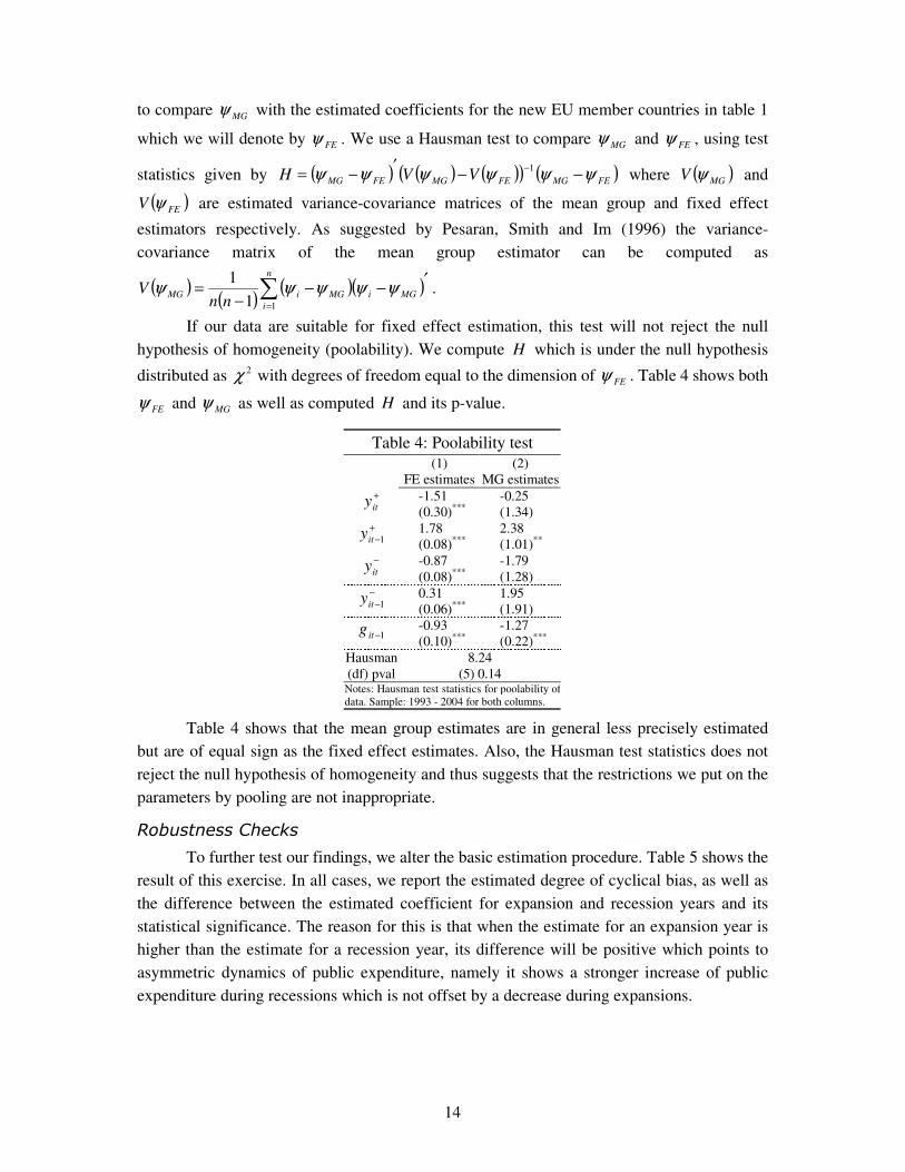
If our data are suitable for fixed effect estimation, this test will not reject the null

hypothesis of homogeneity (poolability). We compute H which is under the null hypothesis

distributed as 2χ with degrees of freedom equal to the dimension of FEψ . Table 4 shows both

FEψ and MGψ as well as computed H and its p-value.

Table 4: Poolability test

(1)

FE estimates

(2)

MG estimates +

ity -1.51

(0.30)***

-0.25

(1.34) +

−1ity 1.78

(0.08)***

2.38

(1.01)**

−

ity -0.87

(0.08)***

-1.79

(1.28) −

−1ity 0.31

(0.06)***

1.95

(1.91)

1−itg -0.93

(0.10)***

-1.27

(0.22)***

Hausman

(df) pval

8.24

(5) 0.14 Notes: Hausman test statistics for poolability of

data. Sample: 1993 - 2004 for both columns.

Table 4 shows that the mean group estimates are in general less precisely estimated

but are of equal sign as the fixed effect estimates. Also, the Hausman test statistics does not

reject the null hypothesis of homogeneity and thus suggests that the restrictions we put on the

parameters by pooling are not inappropriate.

Robustness Checks

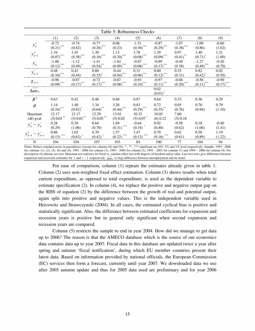
To further test our findings, we alter the basic estimation procedure. Table 5 shows the

result of this exercise. In all cases, we report the estimated degree of cyclical bias, as well as

the difference between the estimated coefficient for expansion and recession years and its

statistical significance. The reason for this is that when the estimate for an expansion year is

higher than the estimate for a recession year, its difference will be positive which points to

asymmetric dynamics of public expenditure, namely it shows a stronger increase of public

expenditure during recessions which is not offset by a decrease during expansions.

15

Table 5: Robustness Checks

(1) (2) (3) (4) (5) (6) (7) (8) (9)

+

ity -0.72

(0.21)***

-0.74

(0.82)

-0.77

(0.26)***

0.08

(0.23)

-1.51

(0.30)***

-0.87

(0.29)***

-1.07

(0.38)***

-1.09

(0.86)

-0.60

(1.02) +

−1ity 1.34

(0.07)***

1.45

(0.38)***

1.30

(0.16)***

1.13

(0.20)***

1.78

(0.08)***

1.29

(0.09)***

0.97

(0.41)**

1.40

(0.71)*

1.21

(1.00) −

ity -1.00

(0.12)***

-1.12

(0.49)**

-1.41

(0.54)**

-1.62

(0.09)***

-0.87

(0.08)***

-0.89

(0.17)***

-0.49

(0.38)

-1.27

(0.48)***

-0.20

(0.70) −

−1ity 0.48

(0.10)***

0.43

(0.44)

0.60

(0.35)*

-0.44

(0.04)***

0.31

(0.06)***

0.60

(0.12)***

0.35

(0.31)

0.82

(0.42)*

0.02

(0.50)

1−itg -0.96

(0.09)***

-0.87

(0.17)***

-0.72

(0.17)***

-0.87

(0.08)***

-0.93

(0.10)***

-0.97

(0.11)***

-0.68

(0.20)***

-0.58

(0.11)***

-0.90

(0.17)***

itun∆ 0.02

(0.01)*

2R 0.63 0.42 0.48 0.66 0.87 0.64 0.33 0.36 0.29

φ 1.14

(0.24)***

1.40

(0.82)*

1.34

(0.64)**

3.26

(0.44)***

0.83

(0.29)***

0.72

(0.35)**

0.05

(0.76)

0.76

(0.94)

0.79

(1.10)

Hausman

(df) pval

12.17

(5) 0.03 **

12.17

(5) 0.03 **

12.29

(5) 0.03 **

13.01

(5) 0.02

10.33

(5) 0.07 *

10.05

(6) 0.12

7.60

(5) 0.18

−+ − itit yy 0.28

(0.29)

0.38

(1.06)

0.64

(0.70)

1.69

(0.31) ***

-0.64

(0.34) *

0.02

(0.40)

-0.58

(0.62)

0.18

(1.06)

-0.40

(1.41) −

−

+

− − 11 itit yy 0.86

(0.13) ***

1.02

(0.62) *

0.70

(0.42) *

1.57

(0.22) ***

1.47

(0.12) ***

0.70

(0.16) ***

0.62

(0.61)

0.58

(0.89)

1.19

(1.22)

N 104 104 107 103 84 100 77 104 94

Notes: Robust standard errors in parentheses (except for columns (8) and (9)). * , ** , *** significant on 10%, 5% and 1% level respectively. Sample: 1993 - 2006

for columns (1), (2), (4), (6) and (8), 1992 - 2006 for column (3), 1993 - 2004 for column (5), 1991 - 2001 for column (7) and 1994 – 2006 for column (9). For description of columns see text. Hausman test statistics for fixed vs. random effect test with degrees of freedom and p-value. Last two rows give difference between

expansion and recession estimates for t and 1−t respectively. itun∆ is (log) difference between unemployment and its trend.

For ease of comparison, column (1) repeats the estimates already given in table 1.

Column (2) uses non-weighted fixed effect estimation. Column (3) shows results when total

current expenditure, as opposed to total expenditure, is used as the dependent variable to

estimate specification (2). In column (4), we replace the positive and negative output gap on

the RHS of equation (2) by the difference between the growth of real and potential output,

again split into positive and negative values. This is the independent variable used in

Hercowitz and Strawczynski (2004). In all cases, the estimated cyclical bias is positive and

statistically significant. Also, the difference between estimated coefficients for expansion and

recession years is positive but in general only significant when second expansion and

recession years are compared.

Column (5) restricts the sample to end in year 2004. How did we manage to get data

up to 2006? The reason is that the AMECO database which is the source of our economics

data contains data up to year 2007. Fiscal data in this database are updated twice a year after

spring and autumn ‘fiscal notification’, during which EU member countries present their

latest data. Based on information provided by national officials, the European Commission

(EC) services then form a forecast, currently until year 2007. We downloaded data we use

after 2005 autumn update and thus for 2005 data used are preliminary and for year 2006

16

predicted. Since we repeatedly struggle with shortage of data, we sinned by running

regressions on sample ranging up to 2006.10

Column (6) adds change in trend unemployment into specification (2). The reason for

adding unemployment is that it might influence the dynamics of public expenditure, since at

least part of it is tailored to relieve the consequences of difficult social position of citizens.

The reason for adding trend unemployment is that we want to avoid problems with

collinearity with output variables.

Both columns (5) and (6) show that our basic results about positive cyclical bias do

not change considerably, although the estimated cyclical bias is reduced somehow. Also, in

both cases the difference between the estimates for second year of expansions and recessions

is positive and statistically significant. However, the difference between the coefficients for

first year of expansions and recessions is negative in column (5) and insignificant in column

(6).

Column (7) displays results when we use central government expenditure taken from

IMF’s government finance statistics (GFS) as the dependent variable. Overall discrepancy of

the results in this column with the rest of our results is immediately evident. Not only do both

recession coefficients lose statistical significance, but the overall estimate of cyclical bias is

virtually zero. One immediate explanation is that the previously reported cyclical bias is in

fact due to behaviour of local governments and thus shows only in general government data.

Nevertheless, we do not favour this explanation for several reasons. The first one is linked to

the low number of observations we were able to obtain from GFS database.

But the key to the absence of cyclical bias is in our view the methodology of GFS used

to compile fiscal data. GFS is based on a cash principle, as opposed to the accrual principle

which lies behind ESA95 methodology on which the AMECO database from which most of

the data used so far come.11

This difference means that the GFS database and methodology

leaves much public expenditure unrecorded and contains notable errors. Its low precision is

also the reason why GFS 2001 has been developed by IMF and is now being used to record

public expenditure instead. However, GFS 2001 has not been retroactively applied to years

preceding its introduction which means that it contains only few observations for each

country.

On the other hand, the ESA95 methodology based on the accrual principle, on which

national accounts data are also based, is meant to be as comprehensible as possible and tries

to capture governmental operations which would under GFS be left off-budget. Stress on

accuracy of ESA95 is also given by the fact that it serves as official statistics of the EC and

decisions in Stability and Growth Pact framework are based upon it.

10

Note that all estimations in section where we study impact of political economy variables end in year

2005. Also, Hausman test statistics calculated for test of data poolability has been derived on sample ending in

year 2004 and thus left column in table 4 is equal to column (5) in table 5. 11

Loosely speaking, expenditure under the cash methodology are recorded at the time when the

payment is made. The accrual principle assigns expenditure to the time period where they objectively belong and

immediately upon the point when they become apparent. Also, GFS has contained several loopholes regarding

formal definition of government entities which offered opportunity to leave many in nature public expenditure

unrecorded.

17

We believe that the combination of a small number of observations and measurement

error lies behind the non-significance of the findings in column (7).

The last two columns display estimates when we allow for autocorrelation of

disturbances. Column (8) uses a random effect specification and column (9) fixed effect

specification. All the estimates still keep the expected signs, but generally loose some

statistical significance. The estimated cyclical bias is still positive but reduced in size and is

now closer to the estimates reported in columns (5) and (6).

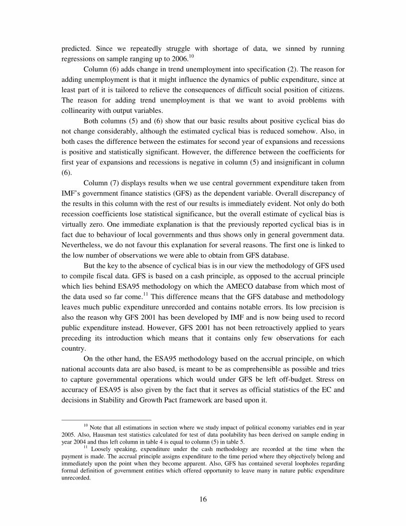
We further tested whether the cyclical bias reported in table 1 for new EU member

countries is sensitive to exclusion of individual countries from our panel. Table 6 show results

of this exercise.

Table 6: Cyclical bias - countries excluded one at a time

(1) (2) (3) (4)

Cyprus 1.21

(0.23)***

0.86

(0.29)***

1.34

(0.67)**

1.45

(0.74)*

Czech

Republic

1.08

(0.34)***

1.04

(0.39)***

1.35

(0.58)**

1.49

(0.71)**

Estonia 1.14

(0.24)***

0.95

(0.31)***

1.35

(0.66)**

1.28

(0.71)*

Hungary 1.17

(0.23)***

0.85

(0.28)***

1.41

(0.64)**

1.53

(0.71)**

Latvia 0.59

(0.50)

0.82

(0.46)*

0.99

(0.51)*

0.91

(0.57)

Lithuania 0.98

(0.28)***

0.91

(0.30)***

1.29

(0.59)**

1.34

(0.66)**

Malta 1.66

(0.20)***

1.33

(0.40)***

1.72

(0.78)**

1.93

(0.81)**

Poland 1.03

(0.26)***

0.66

(0.28)**

1.58

(0.71)**

1.83

(0.77)**

Slovakia 0.22

(0.30)

0.11

(0.31)

0.89

(0.57)

0.75

(0.62)

Slovenia 0.71

(0.34)**

0.85

(0.36)**

1.29

(0.61)**

1.34

(0.69)*

Notes: Dependent variable is total government expenditure to GDP ratio in columns (1)

and (2) and total current government expenditure to GDP ratio in columns (3) and (4).

Robust standard errors in parentheses. * , ** , *** significant on 10%, 5% and 1% level

respectively. Sample: 1993 - 2006 for column (1), 1993 - 2004 for column (2), 1992 -

2006 for column (3) and 1992 - 2004 for column (4).

The entries in the cells of table 6 show the estimated cyclical bias when we exclude

one country at a time. Columns (1) and (2) are based on the total government expenditure to

GDP ratio and columns (3) and (4) are based on the total current government expenditure to

GDP ratio. As a further check, odd columns use data up to year 2006, while even columns use

data only up to year 2004.

As table 6 shows, in most cases the estimated cyclical bias is still economically and

statistically significant, with the exception of cases when we exclude Slovakia from the

estimations. One natural explanation is that the estimated cyclical bias is driven by a high

cyclical bias in Slovakia. To check this, we estimated cyclical bias separately for each

country, expecting the highest one in Slovakia. However, this turned out not to be the case.

Only for one combination of dependent variable and sample period in table 6 did Slovakia

have the largest cyclical bias and even in this case it was highest only by a small margin. In

18

three other cases, Slovakia does not have the largest cyclical bias (Malta, Czech Republic and

Lithuania lead in the three remaining cases).

Although we do not have an explanation for the impact of the exclusion of Slovakia,

we regard the robustness of the estimates of the cyclical bias to exclusion of other countries as

confirmation of our basic results.

Overall, the robustness checks we pursued suggest that the results reported are not due

to spurious correlation. Nevertheless, in the light of some of the estimates in table 5 we regard

the estimated cyclical bias from column (1) of this table to be the most optimistic and upper

bound.

Note on ‘Standard’ Elasticity Estimation

This section tries to show that traditional estimates of the elasticity of public

expenditure with respect to output fluctuations based on one (possibly lagged) output gap

variable taking on both positive and negative values might be misleading. This is true

especially for that part of the literature which uses estimated coefficients of cyclical behaviour

of fiscal policy as a dependent variable in a second stage of investigation, trying to explain

their cross-country pattern. For recent examples of this approach, see Lane (2003) or Alesina

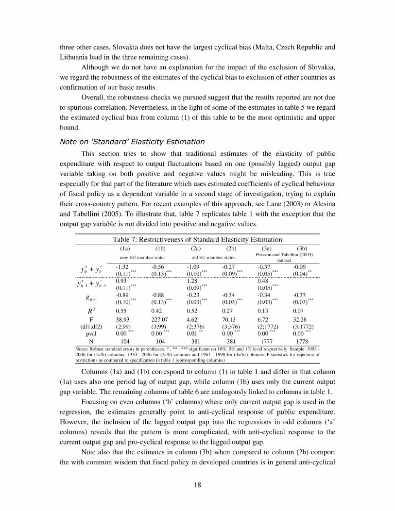
and Tabellini (2005). To illustrate that, table 7 replicates table 1 with the exception that the

output gap variable is not divided into positive and negative values.

Table 7: Restrictiveness of Standard Elasticity Estimation

(1a) (1b) (2a) (2b) (3a) (3b)

new EU member states old EU member states Persson and Tabellini (2003)

dataset −+ + itit yy -1.32

(0.11)***

-0.56

(0.13)***

-1.09

(0.10)***

-0.27

(0.09)***

-0.37

(0.05)***

-0.09

(0.04)**

−

−

+

− + 11 itit yy 0.93

(0.11)***

1.28

(0.09)***

0.48

(0.05)***

1−itg -0.89

(0.10)***

-0.88

(0.13)***

-0.23

(0.03)***

-0.34

(0.03)***

-0.34

(0.03)***

-0.37

(0.03)***

2R 0.55 0.42 0.52 0.27 0.13 0.07

F

(df1;df2)

pval

38.93

(2;99)

0.00 ***

227.07

(3;99)

0.00 ***

4.62

(2;376)

0.01 **

70.13

(3;376)

0.00 ***

6.72

(2;1772)

0.00 ***

32.28

(3;1772)

0.00 ***

N 104 104 381 381 1777 1778

Notes: Robust standard errors in parentheses. * , ** , *** significant on 10%, 5% and 1% level respectively. Sample: 1993 -

2006 for (1a/b) columns, 1970 - 2006 for (2a/b) columns and 1961 - 1998 for (3a/b) columns. F-statistics for rejection of

restrictions as compared to specification in table 1 (corresponding columns)

Columns (1a) and (1b) correspond to column (1) in table 1 and differ in that column

(1a) uses also one period lag of output gap, while column (1b) uses only the current output

gap variable. The remaining columns of table 6 are analogously linked to columns in table 1.

Focusing on even columns (‘b’ columns) where only current output gap is used in the

regression, the estimates generally point to anti-cyclical response of public expenditure.

However, the inclusion of the lagged output gap into the regressions in odd columns (‘a’

columns) reveals that the pattern is more complicated, with anti-cyclical response to the

current output gap and pro-cyclical response to the lagged output gap.

Note also that the estimates in column (3b) when compared to column (2b) comport

the with common wisdom that fiscal policy in developed countries is in general anti-cyclical

19

which is not true for developing countries. Since column (2b) is estimated for old EU member

countries it can be regarded as representative of fiscal dynamics in developed countries. On

the other hand, data underlying column (3b) come from many developing countries.

More importantly, the last rows of table 6 show computed F-statistics for the test that

the restrictions put on the estimates by estimating with the overall output gap as an

independent variable can be rejected. The unrestricted model in each case corresponds to the

one given in table 1. Put differently, the F-statistics corresponds to the hypothesis that running

a regression on the overall output gap does not do much harm to the data. We see that in all

cases this hypothesis is strongly rejected.

One obvious objection is that the results in table 6 are fixed effect panel estimates,

while the usual procedure to estimate the cyclical response of public expenditure is to run a

regression for each country separately. For this reason we ran a similar regression for each

country separately and a tested similar hypothesis.

For the sample of 25 EU member countries, the hypothesis that including a single

output gap variable taking on positive and negative values is appropriate, as opposed to a

model with split output gap variables, was rejected for 8 countries on 10 percent significance

level (8 times for 5 percent) when we also included the lagged output gap and for 20 countries

on 10 percent significance level when only the current output gap was included in the model

(15 times for 5 percent). Similar numbers for the sample of 60 countries used by Persson and

Tabellini (2003) are 16 times on 10 percent significance level when the lagged output gap is

included (10 times for 5 percent) and 31 times on 10 percent significance when only the

current output gap is included in the model (26 times on 5 percent).

Overall, the evidence in table 7 and the results of the tests for individual countries

suggest that asymmetry in cyclical dynamics of public expenditure is a widespread

phenomenon which has so far gone almost unnoticed. It also suggests that attempts to explain

cyclical behaviour of fiscal authorities based on estimates of the elasticity of public

expenditure from a regression model which includes a single output gap variable taking on

positive and negative values might be misleading.

5. Conclusion

We hope everything what has been said so far gives a quite clear picture that the

government spending behaves asymmetrically over the course of the business cycle. There are

several consequences and related points to this observation.

First, the evidence we provided for the sample of ten new EU member countries points

to a behaviour which exhibits an anti-cyclical response of public expenditure to economic

recessions, in other words, an increase of public spending during bad times. This increase is

not subsequently matched by an alike decrease of public expenditure during expansions and,

thus, the government spending to GDP ratio displays ratcheting behaviour.

Second, the extent of observed asymmetry is influenced by political economy

variables. Whether we focus on the occurrence of the general parliamentary elections,

governments composed of more political parties or governments with new finance minister,

we find positive politically induced cyclical bias. With the exception of the general

20

parliamentary elections, the estimated change due to political economy variables is also

statistically significant. On the other hand, we were not able to detect any meaningful

influence of the number of political parties in the parliament. Lastly, the number of spending

ministers within a cabinet does not increase cyclical bias, despite the effect of this variable on

the dynamics of public expenditure.

Third, we hope the reported findings are not mere coincidence or result of spurious

correlation. We subjected our findings to a number of robustness checks with encouraging

results, which point to the fact that asymmetry in the behaviour of public spending over the

business cycle should be taken seriously, not only in new EU member countries, but

elsewhere as well.

This brings us to our last point. We tried to show that the standard econometric

practice of estimating the degree of pro- or anti- cyclicality of fiscal policy using an output

gap variable taking on both positive and negative values can yield misleading results. This

practise is in many cases rejected by the data as being too restrictive when put under standard

econometric tests.

6. References

• Aizenman, J., Gavin, M. and Hausmann, R., (1996) “Optimal Tax and Debt Policy with Endogenously

Imperfect Creditworthiness”, NBER working paper, no.5558, 1996.

• Alesina, A. and Tabellini, G., (2005) “Why Is Fiscal Policy Often Procyclical?”, NBER working paper,

no.11600, 2005.

• Austen-Smith, D., (2000) “Redistributing Income under Proportional Representation”, The Journal of

Political Economy, vol.108, no.6, 2000, 1235-1269.

• Balassone, F. and Giordano, R., (2001) “Budget Deficits and Coalition Governments”, Public Choice,

vol.106, 2001,327-349.

• Baltagi, B.H., (2005) “Econometric Analysis of Panel Data”, John Wiley, Chichester, 2005.

• Baron, D.P. and Ferejohn, J.A., (1989) “Bargaining in Legislature”, The American Political Science

Review, vol.83, no.4, 1989, 1181-1206.

• Bouthevillain, C., et al. (2001) “Cyclically Adjusted Budget Balances: An Alternative Approach”, ECB

working paper, no.77, 2001.

• Catao, L. and Sutton, B., (2002) “Sovereign Defaults: The Role of Volatility”, IMF working paper, no.149,

2002.

• European Commission, (2000) “Public Finances in EMU – 2000”, European Economy Reports and Studies,

no.3, European Commission, Brussels, 2000.

• European Commission, (2002) “Public Finances in EMU – 2002”, European Economy Reports and Studies,

no.3, European Commission, Brussels, 2002.

• Gleich, H., (2003) “Budget Institutions and Fiscal Performance in Central and Eastern European Countries”,

ECB working paper, no.215, 2003.

• Haan, de J. and Sturm, J.E., (1997) “Political and Economic Determinants of OECD Budget Deficits and

Government Expenditures: A Reinvestigation”, European Journal of Political Economy, vol.13,1997, 739-

750.

• Haan, de J., Sturm, J.E. and Beekhuis, G., (1999) “The Weak Government Thesis: Some New Evidence”,

Public Choice, vol.101, 1999, 163-176.

• Hagemann, R., (1999) “The Structural Budget Balance: The IMF’s Methodology”, Banca d’Italia,

Proceedings from ‘Indicators of Structural Budget Balances’ Conference, 1999, 53-70.

• Hagen, von J. and Harden, I.J., (1995) “Budget Processes and Commitment to Fiscal Discipline”, European

Economic Review, vol.39, 1995, 771-779.

• Hallerberg, M. and Hagen, von. J. (1999) “Electoral Institutions, Cabinet Negotiations, and Budget Deficits

in the European Union”, in: Poterba, J. and Hagen, von. J., (eds.), “Fiscal Institutions and Fiscal

Performance”, University Chicago Press, Chicago, 1999, 209-232.

• Hallerberg, M. and Strauch, R., (2002) “On the Cyclicality of Public Finances in Europe”, Empirica, vol.29,

2002, 183-207.

21

• Hallerberg, M., Strauch, R. and Hagen, von J., (2004) “The Design of Fiscal Rules and Forms of

Governance in European Union Countries”, ECB working paper, no.419, 2004.

• Hallerberg, M., Strauch, R. and Hagen, von J., (2001) “The Use and Effectiveness of Budgetary Rules and

Norms in EU Member States”, ZEI, Bonn, 2001.

• Henisz, W.J., (2004) “Political Institutions and Policy Volatility”, Economics & Politics, vol.16, no.1, 2004,

1-27.

• Hercowitz, Z. and Strawczynski, M., (2004) “Cyclical Ratcheting in Government Spending: Evidence from

the OECD”, Review of Economics and Statistics, vol.86, no.1, 2004, 353-361.

• Kaminsky, G.L., Reinhart, C.M. and Vegh, C.A., (2004) “When It Rains, It Pours: Procyclical Capital

Flows and Macroeconomic Policies”, NBER working paper, no.10780, 2004.

• Lane, P.R., (2003) “The Cyclical Behaviour of Fiscal Policy: Evidence from the OECD”, Journal of Public

Economics, vo.87, 2003, 2661-2675.

• Noord, van den P., (2000) “The Size and Role of Automatic Fiscal Stabilizers in the 1990s and Beyond”,

OECD Economics Department working paper, no.230, 2000.

• Perotti, R. and Kontopoulos, Y., (2002) “Fragmented Fiscal Policy”, Journal of Public Economics, vol.86,

2002, 191-222.

• Persson, T. and Tabellini, G., (2000) “Political Economics: Explaining Economic Policy”, MIT Press,

Cambridge, Massachusetts, USA, 2000.

• Persson, T. and Tabellini, G., (2003) “The Economic Effects of Constitutions”, MIT Press, Cambridge,

Massachusetts, USA, 2003.

• Pesaran, M.H. and Smith, R.P., (1995) “Estimating Long-run Relationship from Dynamic Heterogeneous

Panels”, Journal of Econometrics, vol.68, 1995, 79-113.

• Pesaran, M.H., Smith, R.P. and Im, K.S., (1996) “Dynamic Linear Models for Heterogeneous Panels”, in:

Lasylo, M. and Sevestre, P., (eds.), “The Econometrics of Panel Data – A Handbook of the Theory and

Applications”, Kluwer Academic Publishers, London, 1996, 145-195.

• Ricciuti, R., (2004) “Political Fragmentation and Fiscal Outcomes”, Public Choice, vol.118, 2004, 365-388.

• Roubini, N. and Sachs, J., (1989a) “Government Spending and Budget Deficits in the Industrial Countries”,

Economic Policy, vol.8, 1989, 99-132.

• Roubini, N. and Sachs, J., (1989b) “Political and Economic Determinants of Budget Deficits in the

Industrial Democracies”, European Economic Review, vol.33, 1989, 903-938.

• Röger, W. and Ongena, H., (1999) “The Commission Services’ Cyclical Adjusted Method”, Banca d’Italia,

Proceedings from ‘Indicators of Structural Budget Balances’ Conference, 1999, 17-52.

• Sorensen, B.E., Wu, L. and Yosha, O., (2001) “Output Fluctuations and Fiscal Policy: U.S. State and Local

Governments 1978-1994”, European Economic Review, vol.45, 2001, 1271-1310.

• Suyker, W., (1999) “Structural Budget Balances: The Method Applied by the OECD”, Banca d’Italia,

Proceedings from ‘Indicators of Structural Budget Balances’ Conference, 1999, 71-96.

• Talvi, E. and Vegh, C.A., (2000) “Tax Base Variability and Procyclical Fiscal Policy”, NBER working

paper, no.7499, 2000.

• Tornell, A. and Lane, P.R., (1998) “Are Windfalls a Curse? A Non-Representative Agent Model of the

Current Account”, Journal of International Economics, vol.44, 1998, 83-112.

• Tornell, A. and Lane, P.R., (1999) “The Voracity Effect”, The American Economic Review, vol.89, no.1,

1999, 22-46.

• Volkerink, B. and Haan, de J., (2001) “Fragmented Government Effects on Fiscal Policy: New Evidence”,

Public Choice, vol.109, 2001, 221-242.

• Ylaoutinen, S., (2004) “Fiscal Frameworks in the Central and Eastern European Countries”, Finish Ministry

of Finance working paper, no.72, 2004.

7. Data Appendix

This appendix describes the data used in the main body of the paper and lists the

sources. We first briefly introduce the data other than those for new EU member countries we

used for comparison (columns (2) and (3) of table 1) and then describe the main dataset used

in the paper.

Old EU member countries

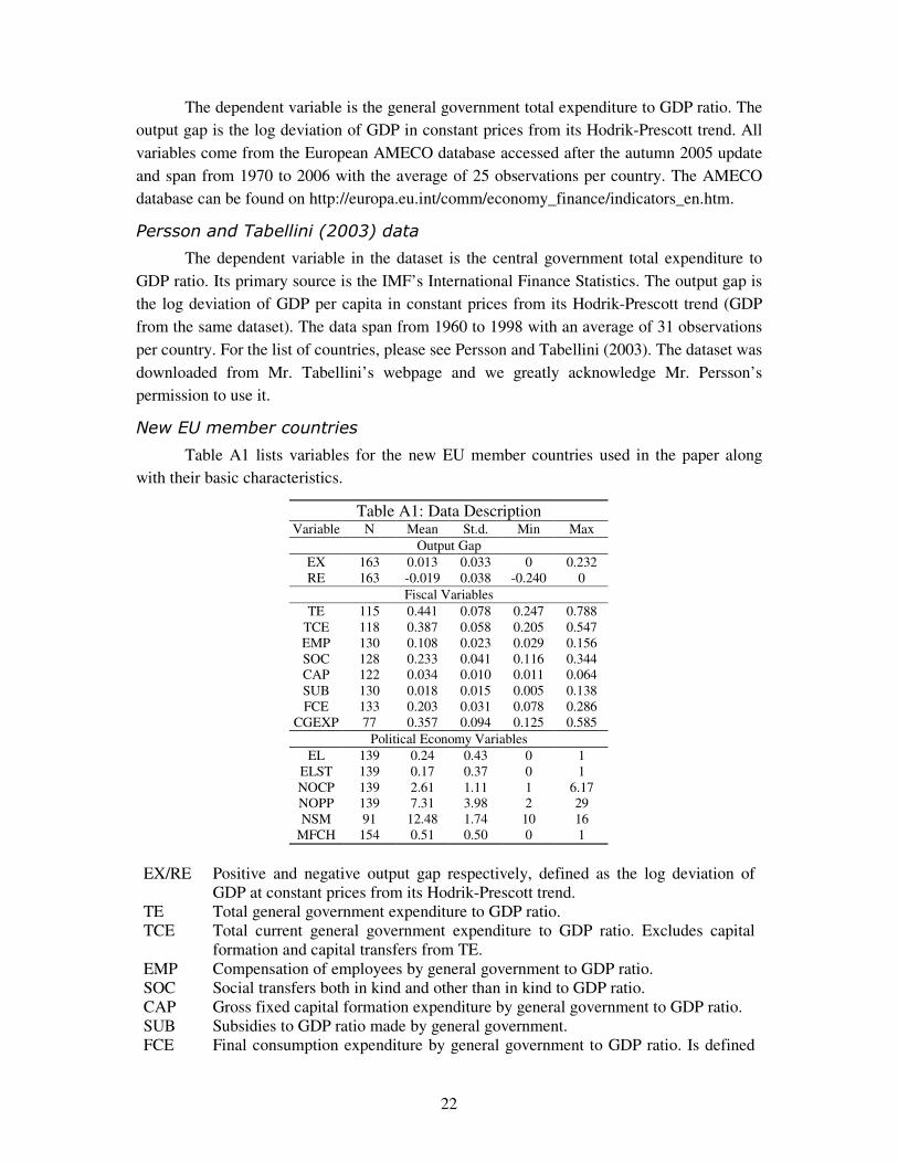
22

The dependent variable is the general government total expenditure to GDP ratio. The

output gap is the log deviation of GDP in constant prices from its Hodrik-Prescott trend. All

variables come from the European AMECO database accessed after the autumn 2005 update

and span from 1970 to 2006 with the average of 25 observations per country. The AMECO

database can be found on http://europa.eu.int/comm/economy_finance/indicators_en.htm.

Persson and Tabellini (2003) data

The dependent variable in the dataset is the central government total expenditure to

GDP ratio. Its primary source is the IMF’s International Finance Statistics. The output gap is

the log deviation of GDP per capita in constant prices from its Hodrik-Prescott trend (GDP

from the same dataset). The data span from 1960 to 1998 with an average of 31 observations

per country. For the list of countries, please see Persson and Tabellini (2003). The dataset was

downloaded from Mr. Tabellini’s webpage and we greatly acknowledge Mr. Persson’s

permission to use it.

New EU member countries

Table A1 lists variables for the new EU member countries used in the paper along

with their basic characteristics.

Table A1: Data Description Variable N Mean St.d. Min Max

Output Gap

EX 163 0.013 0.033 0 0.232

RE 163 -0.019 0.038 -0.240 0

Fiscal Variables

TE 115 0.441 0.078 0.247 0.788

TCE 118 0.387 0.058 0.205 0.547

EMP 130 0.108 0.023 0.029 0.156

SOC 128 0.233 0.041 0.116 0.344

CAP 122 0.034 0.010 0.011 0.064

SUB 130 0.018 0.015 0.005 0.138

FCE 133 0.203 0.031 0.078 0.286

CGEXP 77 0.357 0.094 0.125 0.585

Political Economy Variables

EL 139 0.24 0.43 0 1

ELST 139 0.17 0.37 0 1

NOCP 139 2.61 1.11 1 6.17

NOPP 139 7.31 3.98 2 29

NSM 91 12.48 1.74 10 16

MFCH 154 0.51 0.50 0 1

EX/RE Positive and negative output gap respectively, defined as the log deviation of

GDP at constant prices from its Hodrik-Prescott trend.

TE Total general government expenditure to GDP ratio.

TCE Total current general government expenditure to GDP ratio. Excludes capital

formation and capital transfers from TE.

EMP Compensation of employees by general government to GDP ratio.

SOC Social transfers both in kind and other than in kind to GDP ratio.

CAP Gross fixed capital formation expenditure by general government to GDP ratio.

SUB Subsidies to GDP ratio made by general government.

FCE Final consumption expenditure by general government to GDP ratio. Is defined

23

as ‘expenditure incurred by general government on goods or services that are

used for the direct satisfaction of individual needs or wants or the collective

needs of members of the community’ (AMECO data manual).

CGEXP Central government expenditure to GDP ratio.

All output gap and fiscal variables come from the AMECO database (except CGEXP)

accessed after the autumn 2005 update. The data span from 1993 to 2006 with an average of

more than 10 observations for each country. The CGEXP variable comes from the IMF’s

Government Finance Statistics and spans from 1991 to 2001 with an average of 7

observations per country.

EL Dummy taking on value of unity in years of the general parliamentary elections.

ELST EL dummy which excludes those general parliamentary elections which took

place before the end of the regular electoral cycle.

NOCP Number of political parties in the cabinet. For years when the government change

took place is weighted average of the number of parties in each cabinet, where

the number of months the relevant cabinet has been in power is used as the

weighing variable.

NOPP Number of political parties in parliament (lower house) defined and weighted

similarly as NOCP.

NSM Number of spending ministers in the cabinet. The definition of a spending

minister is similar to that used by Perotti and Kontopoulos (2002). Weighted in

similar manner as NOCP and NOPP in years when change of cabinet took place.

MFCH Dummy taking on value of unity in year when the change of minister of finance

took place.

We used numerous sources for political economy variables which include:

i) Zarate’s Political Collections

http://www.terra.es/personal2/monolith/

ii) European Journal of Political Research annual summary of political events called

‘Political Data in X’, where X denotes year and we used issues for years from

1996 to 2004.

iii) Elections in Central and Eastern Europe: Results and Legislation – Joint project

of the University of Essex, IFES and ACEEO

http://www2.essex.ac.uk/elect/database/election.asp

iv) Websites of national statistical offices, government websites, websites of

ministries of finance and in several cases direct contact with government

officials.

IES Working Paper Series 2006200620062006 1. Martin Gregor: Globální, americké, panevropské a národní rankingy ekonomických

pracovišť 2. Ondřej Schneider: Pension Reform in the Czech Republic: Not a Lost Case? 3. Ondřej Knot and Ondřej Vychodil: Czech Bankruptcy Procedures: Ex-Post Efficiency

View 4. Adam Geršl: Development of formal and informal institutions in the Czech Republic and

other new EU Member States before the EU entry: did the EU pressure have impact? 5. Jan Zápal: Relation between Cyclically Adjusted Budget Balance and Growth Accounting

Method of Deriving ‘Net fiscal Effort’ 6. Roman Horváth: Mezinárodní migrace obyvatelstva v České republice: Role likviditních

omezení 7. Michal Skořepa: Zpochybnění deskriptivnosti teorie očekávaného užitku 8. Adam Geršl: Political Pressure on Central Banks: The Case of the Czech National Bank 9. Luděk Rychetník: Čtyři mechanismy příjmové diferenciace 10. Jan Kodera, Karel Sladký, Miloslav Vošvrda: Neo-Keynesian and Neo-Classical

Macroeconomic Models: Stability and Lyapunov Exponents 11. Petr Jakubík: Does Credit Risk Vary with Economic Cycles? The Case of Finland 12. Julie Chytilová, Natálie Reichlová: Systémy s mnoha rozhodujícími se jedinci v teoriích F.

A. Hayeka a H. A. Simona 13. Jan Zápal, Ondřej Schneider: What Are Their Words Worth? Political Plans And

Economic Pains Of Fiscal Consolidations In New Eu Member States 14. Jiří Hlaváček, Michal Hlaváček: Poptávková funkce na trhu s pojištěním: porovnání

maximalizace paretovské pravděpodobnosti přežití s teorií EUT von-Neumanna a Morgensterna a s prospektovou teorií Kahnemana a Tverského

15. Karel Janda, Martin Čajka: Státní podpora českého zemědělského úvěru v období před vstupem do Evropské unie

16. Nauro F. Campos, Roman Horváth: Reform Redux: Measurement, Determinants and Reversals

17. Michal Skořepa: Three heuristics of search for a low price when initial information about the market is obsolete

18. Michal Bauer, Julie Chytilová: Opomíjená heterogenita lidí aneb Proč afrika dlouhodobě neroste

19. Vít Bubák, Filip Žikeš: The Price of Stock Trades: Evidence from the Prague Stock Exchange

20. Vladimír Benáček, Jiří Podpiera a Ladislav Prokop: Command Economy after the Shocks of Opening up: The Factors of Adjustment and Specialisation in the Czech Trade

21. Lukáš Vácha, Miloslav Vošvrda: Wavelet Applications to Heterogeneous Agents Model 22. Lukáš Vácha, Miloslav Vošvrda: “Morální hazard“ a „nepříznivý výběr“ při maximalizaci

pravděpodobnosti ekonomického přežití 23. Michal Bauer, Julie Chytilová, Pavel Streblov: Effects of Education on Determinants of

High Desired Fertility Evidence from Ugandan Villages 24. Karel Janda: Lender and Borrower as Principal and Agent 25. Karel Janda: Optimal Deterministic Debt Contracts

26. Jiří Hlaváček: Pojištění vkladů: současný stav, srovnání a perspektiva v kontextu EU 27. Pavel Körner: The determinants of corporate debt maturity structure: evidence from

Czech firms 28. Jarko Fidrmuc, Roman Horváth: Credibility of Exchange Rate Policies in Selected EU New

Members: Evidence from High Frequency Data 29. Natálie Reichlová, Petr Švarc: Strategic Referring in Labor Market Social Networks 30. František Turnovec: Publication Portfolio of the Czech Economists and Problems of

Rankings 31. Petr Kadeřábek : Correcting Predictive Models of Chaotic Reality 32. Wadim Strielkowski : People of the road: the role of ethnic origin in migration decisions.

A study of Slovak Roma asylum-seekers in the Czech Republic in 1998-2006

2007200720072007

1. Roman Horváth : Estimating Time-Varying Policy Neutral Rate in Real Time 2. Filip Žikeš : Dependence Structure and Portfolio Diversification on Central European

Stock Markets 3. Martin Gregor : The Pros and Cons of Banking Socialism 4. František Turnovec : Dochází k reálné diferenciaci ekonomických vysokoškolských

vzdělávacích institucí na výzkumně zaměřené a výukově zaměřené? 5. Jan Ámos Víšek : The Instrumental Weighted Variables. Part I. Consistency

6. Jan Ámos Víšek : The Instrumental Weighted Variables. Part II. n - consistency 7. Jan Ámos Víšek : The Instrumental Weighted Variables. Part III. Asymptotic

Representation 8. Adam Geršl : Foreign Banks, Foreign Lending and Cross-Border Contagion: Evidence from

the BIS Data 9. Miloslav Vošvrda, Jan Kodera : Goodwin's Predator-Prey Model with Endogenous

Technological Progress 10. Michal Bauer, Julie Chytilová : Does Education Matter in Patience Formation? Evidence

from Ugandan Villages 11. Petr Jakubík : Credit Risk in the Czech Economy 12. Kamila Fialová : Minimální mzda: vývoj a ekonomické souvislosti v České republice 13. Martina Mysíková : Trh práce žen: Gender pay gap a jeho determinanty 14. Ondřej Schneider : The EU Budget Dispute – A Blessing in Disguise?

All papers can be downloaded at: http://ies.fsv.cuni.cz•

Univerzita Karlova v Praze, Fakulta sociálních věd

Institut ekonomických studií [UK FSV – IES] Praha 1, Opletalova 26

E-mail : ies@fsv.cuni.cz http://ies.fsv.cuni.cz