University of South FloridaScholar Commons

Graduate Theses and Dissertations Graduate School

2010

A computational kinematics and evolutionaryapproach to model molecular flexibility forbionanotechnologyAthina N. BrintakiUniversity of South Florida

Follow this and additional works at: http://scholarcommons.usf.edu/etd

Part of the American Studies Commons

This Dissertation is brought to you for free and open access by the Graduate School at Scholar Commons. It has been accepted for inclusion inGraduate Theses and Dissertations by an authorized administrator of Scholar Commons. For more information, please contactscholarcommons@usf.edu.

Scholar Commons CitationBrintaki, Athina N., "A computational kinematics and evolutionary approach to model molecular flexibility for bionanotechnology"(2010). Graduate Theses and Dissertations.http://scholarcommons.usf.edu/etd/1579

A Computational Kinematics and Evolutionary Approach to Model Molecular Flexibility

for Bionanotechnology

by

Athina N. Brintaki

A dissertation submitted in partial fulfillment of the requirements for the degree of

Doctor of Philosophy Department of Industrial and Management Systems Engineering

College of Engineering University of South Florida

Major Professor: Susana K. Lai-Yuen, Ph.D. Les Piegl, Ph.D.

Alfredo Cardenas, Ph.D. Tapas Das, Ph.D.

Kimon Valavanis, Ph.D. Ali Yalcin, Ph.D.

Date of Approval: November 3, 2009

Keywords: collision detection, molecular conformational search, flexible molecules, molecular stability, computational geometry, differential evolution

© Copyright 2010 , Athina N. Brintaki

Dedication

To the living memory of my father Nikolao E. Brintaki for his exceptional strength,

boundless love and support as well as for his unforgettable spirit!

And to my mom ... my love harbor!

i

Table of Contents

List of Tables iv

List of Figures v

Abstract ix

Preface xi

Chapter 1: Introduction 1 1.1 Motivation 1 1.2 Dissertation Objectives and Contributions 2 1.3 Dissertation Outline 4

Chapter 2: Literature Review 5 2.1 Molecular Mechanics Model 5 2.2 Evolutionary Algorithms (EAs) 6 2.2.1 EAs in Molecular Docking 6 2.2.2 EAs in Molecular Conformational Search 7 2.3 Haptic Rendering Approaches 8 2.4 Computational Geometry 9 2.4.1 Collision Detection in Molecular Conformational Search 9 2.4.2 Geometric-Based Molecular Docking 11 2.5 Current Literature Limitations 12

Chapter 3: A Geometric Interpretation of Molecular Mechanics 14 3.1 Background on Molecules 14 3.2 Molecular Energy 17 3.3 A Geometric Molecular Methodology from Molecular Mechanics 18

Chapter 4: BioGeoFilter (BGF) Methodology 23 4.1 Overview of the Proposed BGF Model 23 4.2 BGF: Lower Level Hierarchy 24

ii

4.3 BGF: Upper Level Hierarchy 27 4.3.1 Constructing the Hierarchy 27 4.3.2 Molecular Geometric Constraints 28 4.3.3 Updating the Hierarchy and Self-Collision Detection 29 4.4 Computer Implementation and Results 29 4.5 Conclusions 33

Chapter 5: Enhanced BioGeoFilter (eBGF) Molecular Model 34 5.1 Differences Between eBGF and BGF Models 34 5.2 Proposed eBGF Overview 35 5.3 eBGF: Lower Layer Hierarchy 36 5.4 eBGF: Upper Layer Hierarchy 38 5.4.1 Constructing the BVH 39 5.4.2 Randomization 40 5.4.3 Updating the Hierarchy 40 5.4.4 Self-Collision Detection 41 5.5 Computer Implementation and Results 44 5.6 Conclusions 49

Chapter 6: Generic Enhanced BioGeoFilter (g.eBGF) Model 50 6.1 Differences Between eBGF and g.eBGF Models 50 6.2 Ligand Modeling 51 6.3 Protein Modeling 51 6.4 Proposed g.eBGF Methodology 53 6.4.1 Overview of the Proposed g.eBGF Model 53 6.4.2 Chemically-Artificial Bonds for the g.eBGF Method 54 6.4.3 Description of the g.eBGF Algorithm 56 6.5 Computer Implementation and Results 58 6.6 Conclusions 65

Chapter 7: Identifying the Molecular Stability 67 7.1 Fundamentals of Evolutionary Algorithms (EAs) 67 7.2 EAs Advantages, Limitations and How to Compensate 69 7.3 Differential Evolution 71 7.4 Proposed kDE Model 74 7.4.1 Overview of the Kinematics-Based Differential Evolution (kDE) Model 74 7.4.2 Pre-Computation Module 75 7.4.3 DE-Loop Module 75 7.4.4 Computer Implementation and Results 77 7.4.5 Conclusions 82

7.5 Proposed BioDE Approach 83 7.5.1 BioDE Overview 83

iii

7.5.2 Input Files 85 7.5.3 Pre-Computation Module 86 7.5.4 DE-Loop Module 87 7.5.5 Computer Implementation and Results 88 7.5.6 Conclusions 93

7.6 Comparison Between the kDE and BioDE Approaches 94

Chapter 8: Conclusions, Discussion and Future Work 97 8.1 Research Summary 97 8.2 Future Research Work 99

References 102

About the Author End Page

iv

List of Tables

Table 4.1 Statistical data for four different ligand molecules 32

Table 5.1 Performance analysis of the proposed eBGF algorithm for two proteins 44

Table 5.2 Performance analysis of current approaches 48

Table 6.1 Performance analysis of the proposed g.eBGF methodology 59

Table 6.2 Computational complexity comparison 65

Table 7.1 Performance analysis of the kDE algorithm on ligands 78

Table 7.2 Performance analysis of the kDE algorithm on proteins 79

Table 7.3 RMSD performance of the kDE algorithm 82

Table 7.4 Performance analysis of the BioDE algorithm on ligands 90

Table 7.5 Performance analysis of the BioDE algorithm on proteins 90

Table 7.6 RMSD performance of the BioDE algorithm 93

Table 7.7 Comparison between kDE and BioDE approaches 95

v

List of Figures

Figure 1.1 Receptor and ligand molecules used in drug design 2

Figure 2.1 Molecular manipulation and assembly with haptics 8

Figure 3.1 Graphical representation of three different molecular structures 15

Figure 3.2 Graphical representation of amino acids’ topology and link procedure through a covalent bond 16

Figure 3.3 Pattern of a protein’s backbone chain 16

Figure 3.4 Mechanical molecular model 19

Figure 3.5 Example of a drug-like molecule as an articulated body 19

Figure 3.6 Three geometric molecular models developed in this research work 22

Figure 4.1 Overall structure of the proposed BioGeoFilter methodology 24

Figure 4.2 1STP ligand molecule divided into AtomGroups based on the location of the torsion bonds 25

Figure 4.3 AtomGroups for a hypothetical small molecule 25

Figure 4.4 Local Cartesian coordinate frame assigned to iGroup and 1−iGroup 26

vi

Figure 4.5 Schematic representation of the smallest enclosing sphere of spheres 27

Figure 4.6 Proposed hierarchical structure for 1STP ligand molecule 27

Figure 4.7 Computational time comparison for four different ligand molecules 30

Figure 4.8 Examples of random conformations for three ligand molecules 31

Figure 5.1 Overview of the proposed eBGF approach 36

Figure 5.2 Graphical representation of the degrees of freedom of a protein 37

Figure 5.3 Graphical representation of the AtomGroup concept along with the proposed splitting procedure for a hypothetical protein segment 37

Figure 5.4 Schematics representation of the rigid and flexible AtomGroups within a hypothetical protein segment and the accordance BVH 39

Figure 5.5 Graphical representation of the proposed collision detection algorithm 42

Figure 5.6 Two example macromolecules tested in this work 43

Figure 5.7 Comparison of the average collision time by the proposed eBGF vs. the average energy calculation time for different sets of pre-selected flexible-residues/dof 45

Figure 5.8 Average total time comparison between the proposed eBGF algorithm and the energy calculation approach to output feasibility for 1STP and1DO3 proteins in a logarithmic scale 46

Figure 5.9 Schematic demonstration of the accuracy of the proposed eBGF methodology 47

Figure 6.1 Examples of ligand molecules 51

vii

Figure 6.2 VDW representation of two different protein molecule examples 52

Figure 6.3 Graphical representation of the degrees of freedom of a protein 52

Figure 6.4 Overview of the proposed g.eBGF methodology 54

Figure 6.5 Structure of the protein with PDB ID: 1NS1 55

Figure 6.6 Closest residue-pair between the first helices of the two 1NS1 protein’s chains 55

Figure 6.7 Graphical representation of the AtomGroup concept along with the proposed splitting procedure for a hypothetical protein segment with two chains 57

Figure 6.8 Time comparison between the traditional energy calculation approach and the proposed g.eBGF methodology for ligand

molecules 60

Figure 6.9 Time comparison between the traditional energy calculation approach and the proposed g.eBGF methodology for protein

molecules 61

Figure 6.10 Computational time performance of the proposed g.eBGF approach for molecules of different size and dof 62

Figure 6.11 Splitting threshold impact on the g.eBGF results for protein modeling 63

Figure 6.12 Accuracy comparison between the traditional energy calculation approach and the proposed g.eBGF method 63

Figure 7.1 One-point crossover (recombination) operator 68

Figure 7.2 Uniform mutation operator 68

viii

Figure 7.3 Overview of the proposed kDE model 75

Figure 7.4 Schematic representation of the chromosome structure used in this work 76

Figure 7.5 Ligand molecules tested with the kDE model 77

Figure 7.6 Protein molecules tested with the kDE model 78

Figure 7.7 kDE’s convergence performance for ligands 80

Figure 7.8 kDE’s convergence performance for proteins 81

Figure 7.9 Overview of the proposed BioDE approach 84

Figure 7.10 Ligand molecules tested with the BioDE model 89

Figure 7.11 Protein molecules tested with the BioDE model 89

Figure 7.12 Convergence performance of the BioDE method for ligands 91

Figure 7.13 Convergence performance of the BioDE method for proteins 92

ix

A Computational Kinematics and Evolutionary Approach to Model Molecular Flexibility

for Bionanotechnology

Athina N. Brintaki

ABSTRACT

Modeling molecular structures is critical for understanding the principles that

govern the behavior of molecules and for facilitating the exploration of potential

pharmaceutical drugs and nanoscale designs. Biological molecules are flexible bodies

that can adopt many different shapes (or conformations) until they reach a stable

molecular state that is usually described by the minimum internal energy. A major

challenge in modeling flexible molecules is the exponential explosion in computational

complexity as the molecular size increases and many degrees of freedom are considered

to represent the molecules’ flexibility. This research work proposes a novel generic

computational geometric approach called enhanced BioGeoFilter (g.eBGF) that

geometrically interprets inter-atomic interactions to impose geometric constraints during

molecular conformational search to reduce the time for identifying chemically-feasible

conformations. Two new methods called Kinematics-Based Differential Evolution (kDE)

and Biological Differential Evolution (BioDE) are also introduced to direct the molecular

conformational search towards low energy (stable) conformations. The proposed kDE

method kinematically describes a molecule’s deformation mechanism while it uses

differential evolution to minimize the inta-molecular energy. On the other hand, the

proposed BioDE utilizes our developed g.eBGF data structure as a surrogate

x

approximation model to reduce the number of exact evaluations and to speed the

molecular conformational search. This research work will be extremely useful in

enabling the modeling of flexible molecules and in facilitating the exploration of

nanoscale designs through the virtual assembly of molecules. Our research work can also

be used in areas such as molecular docking, protein folding, and nanoscale computer-

aided design where rapid collision detection scheme for highly deformable objects is

essential.

xi

Preface

Four years of learning filled with contradictory experiences enforced facing

myself, realizing my strengths and limitations while maturing me as a person and as a

scientist. This has been a savory adventure within one’s emotions: balancing between

hope and despair, happiness and sadness, solitude and networking. For this reason, I have

to express my sincere gratitude to those who made this journey possible and all people

that helped and supported me during this adventure.

First and foremost, I would like to thank my advisor Dr. Lai-Yuen for providing

the opportunity to work towards enhancing computer-aided molecular design and

engineering which really captured my imagination and inspired me as both a student and

a researcher. Her continuing support, guidance and encouragement throughout the

challenging years we have worked together, has been invaluable. She allowed me to find

my own research path, always listening to my ideas and offering sound advice. I have

learned much from her on how to be a scientist, conduct research and, I hope, an

inspiring teacher.

I would also like to thank Dr. Cardenas and his research group from the

Department of Chemistry at USF, who taught me much of the biology I know, and for all

their helpful discussions and suggestions. Their feedback and comments were very

helpful in establishing the biological relevance of my work.

I owe special thanks to Dr. Piegl from the Department of Computer Science &

Engineering at USF for letting me into his CAD & Graphics research group, supporting

and guiding me throughout this research journey. Numerous times I have been challenged

by Dr. Piegl on how to justify and support my research. I have learned much from him on

how to present and project my work as a critical component of some of the emerging

areas of engineering research in 21st century. I would also like to thank my CAD &

xii

Graphics colleagues Olya and Khairan, for being always attentive and encouraging as

well as for our exceptional collaboration.

My sincere thanks also to my colleagues Konstantino Dalamakidi and

Soumayaroop Roy from the Department of Computer Science & Engineering at USF for

helping me with C++ programming, being patient and accessible in answering my

numerous questions.

Very genuine thanks to my former advisor Dr. Nikolos from the Production

Engineering & Management Department at Technical University of Greece for initiating

my research and teaching experiences. I am grateful for all his guidance, discussions and

support that allowed my preparation for accomplishing this challenging adventure. I

would also like to thank him for his collaboration in one of the projects that made up this

dissertation as well as for allowing me to have at my disposal his lab equipment to

conduct some of my final experiments.

I also owe very special thanks to my former advisor Dr. Valavanis from the

Electrical & Computer Engineering Department at University of Denver for believing in

me and inviting me to continue my Ph.D. studies at USF. I am truthfully grateful for the

offered opportunity as well as for inspiring me to conduct robotics research and transfer

this knowledge at the bionanoscale.

I am also extremely thankful towards my Committee Members Dr. Das and Dr.

Yalcin and my committee Chair Dr. Tsokos for their insightful feedback, support and

attention to my research work. I would like to give thanks to my colleagues Wilkistar,

Chaitra, Vishnu, Patricio, Laila, Alfredo, Diana, Dayna, Andres, Alcides, Ozan, Sinan,

Fethullah, all my IMSE Professors, Chair Dr. Zayas and of course Jackie and Gloria for

our excellent collaboration, their support and attention to my research work and academic

development.

I truthfully would like to thank my family and friends for their unconditional and

continued support to this challenging and exciting adventure. I am extremely grateful for

all the unreserved support and motivation received from my true friends Kaliopi,

Katerina, Despoina, Nikoleta, Maria and of course my very good friend Ahna for always

being there for me to strengthen my confidence during all the difficulties I faced. But

xiii

above all, my sincere thanks to my parents Nikolao and Euagelia, my sister Evi, my

cousin Gianni, my aunt Vagia and my grandparents Athanasio and Pinelopi for strongly

believing in me, supporting me throughout this long journey and all the years preceding

it. I am deeply grateful to them for reinforcing me to pursue my dreams and accomplish

this goal while teaching me to be a sincere person. They are the source of my strength,

joy and love.

My only regret however, is for not finishing my dissertation earlier, before my

father passed away. I miss watching my father’s eyes filled with sincere love and pride. I

am confident, though, that in his eternal peace he is proud of me as he was through all my

life and as I have been proud of him. My sincere love, love without ego, for my father

reinforced my efforts for accomplishing this work while he was fighting for his life. This

is my gift to my father for all his courage, strength and for his unforgettable spirit!

1

Chapter 1

Introduction

The scope of this chapter is to introduce the motivation underneath this research

work as well as the current molecular modeling challenges. The proposed research

objectives and contributions are also discussed followed by the dissertation outline.

1.1 Motivation

Bionanotechnology is the new frontier in research and technology and is vital for

the realization of biomedical and nanoscale products. It consists of manipulating

biological molecules to create structures or devices with new molecular arrangements.

The control, manipulation, and assembly of molecules will enable the design of

innovative materials, new pharmaceutical drugs, enhanced textiles, and precise nanoscale

devices with new capabilities for diagnosis and treatment of diseases. It is estimated that

within the next 10 years, “at least half of the newly designed advanced materials and

manufacturing processes will be build at the nanoscale” [NIST].

To achieve bionanotechnology, it is crucial to enable real-time visualization of

interactions between biological molecules during the design stage so that fully functional

nanoscale products can be designed and evaluated prior to actual fabrication. A main key

for enabling the visualization of biological components is the understanding and effective

modeling of molecules’ behavior. Molecules are very flexible in nature and can adopt

many molecular conformations (or shapes) while searching for a stable or low-energy

molecular state. The major challenge in modeling flexible molecules (or molecular

conformations) lies on the exponential explosion in computational complexity as the

molecular size increases and a large number of degrees of freedom (dof) are considered

to represent the molecules’ flexibility. For example, Figure 1.1 shows a small drug

molecule (called a ligand) that can dock or assemble into a larger molecule (called a

receptor) leading to the identification of pharmaceutical drugs and new molecular

arrangements with specific capabilities. Receptor molecules can consist of hundreds or

thousands of atoms with hundreds or even thousands of degrees of freedom. Therefore,

modeling molecular conformations is a highly intensive computational task and remains

the main challenge in molecular design.

Figure 1.1: Receptor and ligand molecules used in drug design.

1.2 Dissertation Objectives and Contributions

The proposed research aims to address the main molecular modeling challenge

and current literature limitations for modeling flexible molecules and identifying stable

conformations. This research work presents a novel computational geometric and

evolutionary inspired approach for the effective identification of chemically-feasible,

low-energy molecular structures of any size, shape and topology.

The main expected research outcome is the design of novel algorithms to

minimize molecular conformational search and to speed collision detection queries that

will enable the visualization and virtual manipulation of flexible molecules for interactive

molecular design. The major objectives of this dissertation are:

2

3

1. to develop a novel bounding volume data structure called BioGeoFilter (BGF)

for the effective and real-time identification of feasible conformations for

flexible drug-like or ligand molecules

2. to develop a generic biologically-inspired data structure called generic

enhanced BioGeoFilter (g.eBGF) methodology for simplifying the molecular

representation regardless of type, size and shape. This methodology considers

certain chemical factors that influence the molecular flexibility to effectively

provide more realistic and chemically-feasible molecular conformations.

3. to investigate and design a kinematics and evolutionary based direct search

technique called kinematics differential evolution or kDE model that

effectively searches for stable or low-energy molecular conformations with a

good convergence performance.

4. to design a novel direct search method called biological differential evolution

(BioDE) that will utilize our proposed g.eBGF approach as a surrogate

approximation model to speed the search towards alternative low-energy

molecular conformations and to achieve a good convergence performance.

The proposed computational geometric and evolutionary based research work

contributes to the molecular modeling and differential evolution literature through the

design of a new geometric-based model for simplifying the molecular representation and

two innovative evolutionary-based algorithms for directing the search towards low-

energy molecular conformations. This hybrid approach will impact nanoscale design by

speeding the modeling of flexible molecules and enabling the development of an

indispensable computer-aided design tool for bionanotechnology. The proposed research

can be applied in areas such as molecular docking/ assembly and protein folding where a

rapid collision detection scheme for highly deformable objects is essential.

This research has resulted in two journal papers [Brintaki and Lai-Yuen, 2008a,

2009a], two submitted journal papers [Brintaki et.al. 2010a,d], five conference

proceedings [Brintaki and Lai-Yuen 2008a,b, 2009b, 2010b,c], three papers in progress

and several poster presentations. The research work has been partially supported by NSF,

SME and USF grants.

4

1.3 Dissertation Outline

Chapter 2 discusses current research work in molecular modeling, geometric

techniques and evolutionary approaches in molecular applications. Chapter 3 describes

our computational geometric interpretation of molecular inter-atomic interactions for

addressing the molecular conformational search problem for highly deformable objects.

Chapters 4, 5, and 6 present the development of three computational geometric models

for the effective identification of feasible molecular conformations. The first model called

BioGeoFilter or BGF, effectively identifies feasible conformations for small molecules in

real-time as discussed in Chapter 4. The second model called enhanced BioGeoFilter or

eBGF analyzes the structure of much larger molecules such as proteins to model them

more effectively as discussed in Chapter 5. Chapter 6 introduces the generic eBGF or

g.eBGF model that incorporates chemically-based constraints that result in more realistic

molecular conformations for molecules of different type, size, shape and topology.

Chapter 7 proposes two new energy minimization algorithms: the kinematics

differential evolution or kDE and the biological differential evolution or BioDE methods.

Both kDE and BioDE models utilize our previously developed differential evolution

(DE) algorithm to direct the search towards low-energy molecular conformations. The

main algorithmic difference between the kDE and BioDE models is that the latest utilizes

the g.eBGF data structure as a surrogate approximation model to speed convergence.

Chapter 8 provides a summary of the research methodologies presented and future

research work.

5

Chapter 2

Literature Review

This chapter provides the background on previous work in the areas of molecular

modeling, evolutionary algorithms and computational geometry techniques in molecular

applications. Previous work is analyzed and their limitations identified.

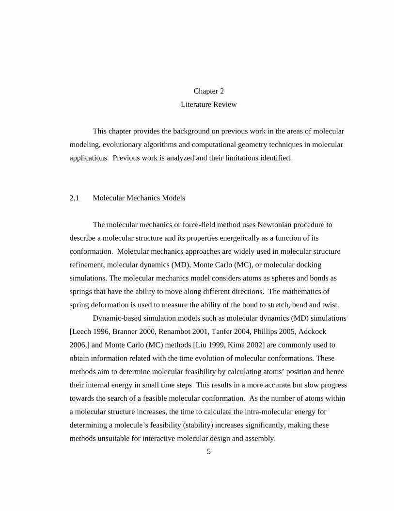
2.1 Molecular Mechanics Models

The molecular mechanics or force-field method uses Newtonian procedure to

describe a molecular structure and its properties energetically as a function of its

conformation. Molecular mechanics approaches are widely used in molecular structure

refinement, molecular dynamics (MD), Monte Carlo (MC), or molecular docking

simulations. The molecular mechanics model considers atoms as spheres and bonds as

springs that have the ability to move along different directions. The mathematics of

spring deformation is used to measure the ability of the bond to stretch, bend and twist.

Dynamic-based simulation models such as molecular dynamics (MD) simulations

[Leech 1996, Branner 2000, Renambot 2001, Tanfer 2004, Phillips 2005, Adckock

2006,] and Monte Carlo (MC) methods [Liu 1999, Kima 2002] are commonly used to

obtain information related with the time evolution of molecular conformations. These

methods aim to determine molecular feasibility by calculating atoms’ position and hence

their internal energy in small time steps. This results in a more accurate but slow progress

towards the search of a feasible molecular conformation. As the number of atoms within

a molecular structure increases, the time to calculate the intra-molecular energy for

determining a molecule’s feasibility (stability) increases significantly, making these

methods unsuitable for interactive molecular design and assembly.

6

2.2 Evolutionary Algorithms (EAs)

The choice of an appropriate optimization method is essential for directing the

conformational search to identify the desired solution or the best potential molecular

conformation. The optimization of molecular geometry was one of the very first

applications of evolutionary algorithms (EAs) in chemistry. EAs have shown good

results in problems where other methods have struggled. In addition, their governing

principles are clearly understood, intuitively appealing and relatively easy to implement.

In this section, we focus on EAs applications in chemical problems that require

optimization such as molecular docking and molecular conformational search. Detailed

information on EAs is provided in Chapter 7.

2.2.1 EAs in Molecular Docking

Current literature in molecular docking demonstrates the effectiveness of

Evolutionary Algorithms (EAs) for describing complex systems [Thomsen 2003, 2006]

and for solving problems involving large search spaces, where traditional optimization

techniques are less efficient [Yang 2001]. Genetic Algorithms (GAs) are presented as an

effective local search method that behaves really well for median energy solutions

[Westhead 1997, Jones 1997]. Additionally, Morris et al. compared the efficiency of

Monte Carlo (MC) simulated annealing method against a classic GA and Lamarckian GA

(LGA) for predicting the bound association of flexible ligands to macromolecule targets.

Results showed that both LGA and GA are the most reliable, efficient and successful

methods. However, many modifications have been proposed to improve the solution

quality and to speed convergence.

One of the best EAs for solving real-valued energy functions is Differential

Evolution (DE) initially proposed by [Storn & Price 1995, 2005]. DE is a population

based stochastic function minimizer that adds the weighted difference between two

individual vectors to a third vector (donor). Currently DE has been implemented by

[Yang 2001, Thomsen 2003, 2006] for investigating the docking of a flexible ligand to a

7

rigid receptor where their numerical results indicate the algorithms’ robustness and

remarkable performance in terms of convergence speed.

2.2.2 EAs in Molecular Conformational Search

Wehrens presented a survey focused on the differences, strengths and weaknesses

between EAs and other structure optimization methods such as distance geometry, eigen

value decomposition, simulated annealing, Monte Carlo or molecular dynamics

simulations [Wehrens 2000]. The main conclusion was that EAs are consistently among

the best performing general search algorithms. On the other hand, GAs are particularly

useful for rapidly producing a family of low energy conformations but are less successful

in fine-tuning these conformations towards the exact global optimum.

Various evolutionary-based studies have been performed to study flexible ligand,

flexible protein or polypeptide molecules conformational search. Wawer et al. [Wawer

2004] presented a real-coded (as opposed with the binary coding of the classic GAs)

genetic algorithm to analyze the conformational behavior of Vitamin E (a small

molecule). Wang and Ersoy [Wang and Ersoy 2005] presented a Mixture Gaussian

Optimization (MGO) algorithm as a continuous stochastic approach for flexible ligand

conformational search. The MGO method was compared against a systematic and a

stochastic conformational search algorithm and it was concluded that the MGO algorithm

can locate the global minimum faster as the molecular size increases. On the other hand,

as the molecular size increases, the systematic search method became non-applicable

whereas the stochastic was trapped in local minima. However, the MGO was tested for

small molecular structures only and was not applied to large molecules such as proteins.

Chong and Tremayne [Chong and Tremayne 2006] presented a new DE algorithm

based on Cultural Evolution concepts called CDE to study the structure search for ligand

molecules. The CDE algorithm was compared against a classic DE method and it was

concluded that both methods succeeded to find the global minimum and the convergence

performance of the CDE algorithm was 54% faster.

Damsbo et al. [Damsbo 2004] presented the FOLDAWAY system, an

evolutionary based approach for finding the low-energy conformations of polypeptides.

The proposed model found large groups of low-energy structures within the expected

low-energy globule that were not identified in previously developed MD simulations.

Bitello and Lopes [Bitello and Lopes 2004] used a DE algorithm to solve the

protein folding problem. Their approach was consistent in finding the global minimum

for structures consisted up to 64 amino acids (relatively small protein size) and performed

better compared with a classic GA.

Figure 2.1: Molecular manipulation and assembly with haptics.

2.3 Haptic Rendering Approaches

In recent years, new methods have been investigated to facilitate molecular design

and nanoscale engineering by providing real-time force feedback using haptic devices

[Sherill, Baxter 1998, Nagata 2002, Grayson 2003, Lee 2004, Lai-Yuen 2006a,b, Morin

2007]. Haptic devices are electromechanical devices that exert forces on users giving

them the illusion of touching something in the virtual world. These devices have been

used to manipulate virtual molecules and to feel the forces as the molecules interact with

each other providing an essential design and visualization tool as shown in Figure 2.1.

However, current methods using haptics either model molecules as rigid bodies or are 8

9

limited to local molecular motions and short periods of simulation time. Modeling

molecules as rigid bodies can simplify the calculation of forces but does not represent the

molecular interactions realistically. To achieve a realistic molecular representation, it is

necessary to model molecules as flexible bodies that attain different conformations while

searching for a stable molecular state. Incorporating real-time haptic force feedback into

molecular design requires rapid update and modeling of molecular conformations for

providing realistic and continuous visualization and sense of touch to the users.

2.4 Computational Geometry

Recently, computational geometry has been successfully used in molecular design

since important constraints influencing molecular behavior can have geometrical

interpretation. The representation of intra-molecular interactions through a

computational geometric approach can allow the approximation of molecules’ behavior

rapidly and efficiently for real-time molecular design. From a geometric point of view, a

molecular conformation can be considered feasible when there are no overlapping atoms

or all possible atomic interactions are collision-free. Collision detection (CD) is an

essential problem in robotics, computational geometry, and computer graphics and is a

major bottleneck in any interactive simulation. A wide range of techniques have been

proposed to deal with collision detection such as hierarchical representations, spatial

partitioning, analytical methods, and geometric reasoning. The algorithmic design

depends on the representation of the model, the query types, and the simulated

environment [Lin 1998].

2.4.1 Collision Detection in Molecular Conformational Search

Bounding volume hierarchies (BVH) are the most popular methods for capturing

self-collision and collisions between objects [Teschner 2005]. The key idea is to use a

hierarchical structure to describe the shape of an object at successive levels of detail. The

object of interest is enclosed by bounding volumes that can have various shapes such as

spheres, axis-aligned bounding boxes (AABBs), and oriented bounding boxes (OBBs)

[Lin 1998]. These bounding volumes become the tree leaves of the hierarchy that are

enclosed by subsequent bounding volumes forming a hierarchical data structure.

For molecular structures, collision detection is a computationally expensive

problem given the many degrees of freedom that a molecule can have. Lotan et al.

[Lotan 2002] used a kinematics chain model to represent proteins flexibility. In respect to

the chain topology the authors built a BVH using object-oriented bounding boxes to

detect overlapping atoms. They tested various proteins of different size and concluded an

updated and testing computational time ranging in hundreds milliseconds. Their proposed

approach requires performance for building the BVH and computational

complexity for the collision detection queries.

)N(O )N(O 3/4

Agarwal et al. [Agarwal 2004] used a BVH with the objects being modeled as

spheres to detect collisions for deforming and moving necklaces (sequence of

balls/beads). The authors built a balanced binary tree with spheres as bounding volumes

to assist in the search for overlapping atoms within flexible protein molecules. They

proposed two methods for computing the spheres: wrapped and layered hierarchy that

provides an upper bound of in 2D space or in d-dimensional

space for the collision detection plan.

)NlogN(O )N(O d/32−

Angulo et al. [Angulo 2005] proposed the BioCD algorithm for efficient self-

collision search and distance computations. The algorithm maintains two levels of

bounding volume hierarchies (BVH). In the low level, it identifies the rigid groups of the

articulated model and builds a hierarchy for each of them. In the upper level, it arranges

the roots of the low level hierarchies. The authors tested various proteins with different

size and they reached a collision detection time measured in tens of milliseconds with

performance and a complexity for building the BVH. )N(O )NlogN(O

Redon et al. [Redon 2005] proposed an adaptive dynamic algorithm (ADA) for

articulated bodies built upon “the divide-and-conquer algorithm” (DCA). An articulated

body is the recursive link pair of articulated parts. The series of the assembly actions is

10

represented by a binary tree. Each node in the tree represents a sub-assembly motion.

Morin and Redon [Morin 2007] utilized the ADA algorithm and proposed a force-

feedback algorithm for adaptive dynamic simulation of proteins. The authors used a

multithreaded structure to couple the adaptive dynamic simulation loop from the

computation of the force applied to the user (through the haptics) requiring a force

feedback of complexity. )N(logO

2.4.2 Geometric-Based Molecular Docking

Current computational docking methods come from the areas of surface matching,

object recognition and motion planning. Motion planning is a fundamental problem in

robotics that consists of finding a valid sequence of configurations that moves an object

from an initial position to a target point. Automatic motion planning is applicable not

only to robotics, but also to virtual reality systems, computer-aided design and

computational biology.

Recently, researchers realized that both automatic motion planning and molecular

docking problem relies upon the same basic principles. A drug molecule can be

considered like a robot with many degrees of freedom (dof) whose motion can be

predicted by an automatic planner determining its ability to bind with a protein. The

binding configuration should satisfy all the geometric, electrostatic and chemical

constraints of the problem. A good binding site should also be reachable to the ligand

from an outside location. Hence, the path to the binding site is highly important and

motivates the use of motion planning in the molecular docking problem. These methods

are known as probabilistic roadmap methods (PRMs) and are widely used in robotics,

intelligent CAD systems and lately in computational biology. PRMs randomly construct a

graph in C-space (configuration space), a roadmap, as it is called. The motion planning is

then solved by connecting the start and goal configurations in the roadmap and searching

for the feasible path on it [Bayazit 2003, Cortes 2003, 2005, 2007].

A modification of the PRM framework is the rapidly- exploring random trees

(RRT) for solving single-query problems without preprocessing the complete roadmap. 11

12

These algorithms are well fitted for highly constrained problems [Cortes 2002, 2003,

2005, 2007, La Valle 1999, 2000a,b]. A recently developed PRM variation to study

molecular motions is the Stochastic Roadmap Simulation (SRS) [Bayazit 2000, Apaydin

2002a, b, 2003, Chiang 2006]. A stochastic roadmap contains many Monte Carlo (MC)

simulation paths at the same time. The SRS studied all the paths together in a closed form

and resulted in significant computational time reduction.

Zhang and Kavraki [Zhang and Kavraki 2002] compared their proposed atom-

group-local-frame method with the simple rotations and Denavit-Hartenburg model

[Hartenburg and Denavit 1955]. It was concluded that the atom-group-local-frame

method not only eliminates all the disadvantages of the other two but also resulted in a

lazy evaluation of atom positions and in computational time reduction. This technique

appears extremely useful in cases that deal with many conformations. Zhang et al. [Zhang

2005] extended the atom-group-local-frame work by adding a geometric screening phase

for identifying feasible molecular conformations.

2.5 Current Literature Limitations

Although remarkable advances in computational biology have been performed

over the years, modeling molecular flexibility remains the main challenge in molecular

design. Most of the above discussed methods do not address the modeling of molecules

for real-time rendering or only allow a limited number of degrees of freedom to change.

In addition, a more generic methodology is required that:

1. is not limited to the topology of the molecules for self-collisions or collisions

between them,

2. evaluates arbitrary conformations independently of the previous query,

3. is adaptive to the molecular structure by exploiting the fact that when limited

degrees of freedom change some of the atomic distances remain constant,

4. identifies molecular feasibility rapidly, efficiently and is evaluated in terms of

both computational time and accuracy,

13

5. incorporates the chemical information that controls molecules’ flexibility into

the molecular design to simplify and realistically represent the molecular

interactions

6. effectively directs the search towards low energy and chemically-feasible

molecular conformations.

To address current literature limitations, this research work presents a new

biologically-inspired geometric method for simplifying the representation of molecules of

different type, size, shape and topology while considering certain chemical factors that

influence molecules’ flexibility. To direct the search towards low-energy molecular

conformations, we propose the use of a new evolutionary based algorithm that will utilize

the developed geometric method as a surrogate approximation model for reducing the

algorithm’s convergence rate and finding the global minimum. The proposed work can

facilitate interactive molecular modeling and nanoscale design.

14

Chapter 3

A Geometric Interpretation of Molecular Mechanics

This chapter introduces the basic molecular concepts and presents our proposed

geometric interpretation of molecular mechanics. A brief background on the various

types of molecules and their basic functions is provided where molecules are categorized

into ligands and receptors. The central concepts on the internal molecular energy and our

geometric interpretation of the molecular conformation mechanics are also explained in

this chapter to provide the basis for our developed algorithms presented in Chapters 4, 5

and 6.

3.1 Background on Molecules

A molecule is a sufficiently stable electrically neutral group of at least two atoms,

in a definite arrangement, held together by very strong chemical bonds or covalent bonds.

A covalent bond is a chemical bond where electrons are shared between atoms. As

shown in Figure 3.1, the size, shape and topology of a molecular structure varies

according to its chemical characteristics and function. These molecules are displayed

using the VMD software [Humphrey 1999] as shown in Figure 3.1. Geometrically, a

molecule can be considered as a collection of atoms and bonds between each atom pair.

Each atom can be represented as a sphere with van der Waals radius while chemical

bonds can be represented as springs.

(a) 1A5Z ligand (b) 1HVR ligand (c) 1DO3 protein molecules, displayed with VMD software

Figure 3.1: Graphical representation of three different molecular structures.

Molecules are essential to a variety of biological processes and activities of

fundamental importance to life. There are four basic types of molecules that are the

major players in biological systems: carbohydrates, lipids, nucleic acids and proteins.

Both carbohydrates and lipids are small molecules that are less complex compared with

the nucleic acids and proteins. Carbohydrates tend to be the least complicated molecular

structures used as energy sources for cell processes. Lipids are also fairly simple organic

molecules that have several uses in living organisms such as acting as water barriers in

cell membranes. Lipids are also used for extra waterproofing or as insulation around

nerves for long-term storage of energy in the form of fat, or used as heat insulation, as

cushions, and as messenger molecules. Nucleic acids and proteins are typically much

larger complex molecules. The primary role of the nucleic acids or DNA (one type of

nucleic acid) is to store proteins’ main information. Proteins are very important

macromolecules in living organisms and perform many distinct functions. The functions

of a protein depend on its 3-dimensional shape, which can be virtually infinite in variety.

Most proteins are enzymes performing biochemical functions such as bond-making and

bond-breaking reactions. Other proteins act as molecular motors or structural

components by performing biophysical functions.

15

The understanding and modeling of the molecular functions and behaviors is very

important in nanoscale design since many problems associated with the development of

bionanotechnology require specifically-designed molecules. For example, drug design

and discovery relies increasingly on structured-based methods for improving efficiency.

The main objective in drug design is to find or build molecules (ligands) that target

proteins (receptors) crucial to the proliferation of microbes, cancer cells or viruses. This

is a very long and expensive process called molecular docking that typically requires

years of research, experimentation, and resources.

A ligand or drug-like molecule is a small molecular structure that usually consists

of at most 50 atoms as shown in Figure 3.1(a) and Figure 3.1(b). A ligand molecule has a

tendency to bind to large molecules called receptors that can lead to the identification of

new pharmaceutical drugs and the creation of new molecular structures with specific

capabilities for diagnosis and treatment of diseases.

Figure 3.2: Graphical representation of amino acids’ topology and link procedure

through a covalent bond.

Figure 3.3: Pattern of a protein’s backbone chain.

As shown in Figure 3.1(c), a protein or a receptor molecule is a much larger

molecular structure that consists of hundreds or even thousands of atoms. Proteins are

chains of smaller molecular entities called amino acids. The amino acids consist of a

central carbon atom, denoted as , connected to an amino group , a carboxyl aC 2NH16

groupCOOH , a single hydrogen atom H , and a side chain , specific for each amino

acid, as shown in Figure 3.2(a). There are 20 basic amino acids that serve as building

blocks of proteins. Amino acids differ from each other by their side chains, which also

determine their chemical characteristics. The amino acids may be linked to each other by

the peptide bond (a covalent bond) between an amino group of one amino acid and a

carboxyl group of another amino acid releasing a water molecule, as shown in Figure

3.2(b). These peptide bonds lead to a linear sequence of amino acids forming a

polypeptide chain. The backbone of the chain is formed by a peptide sequential pattern

schematically shown in Figure 3.3. Therefore, any protein can be considered as a

polypeptide chain characterized by the amino acid sequence along the chain in order.

R

3.2 Molecular Energy

Molecules are very flexible in nature and can attain different conformations. A

feasible molecular conformation indicates a stable molecular state that is usually

described by the minimum intra-molecular energy. This energy is a function composed

of different energy factors that depict the interactions between bonded and non-bonded

atoms. The major energy contributors are the non-bonded van der Waals (VDW)

potential and electrostatic forces. A mathematical representation of the non-bonded

molecular energy is given by Eqn. 3.1: nbE

∑∑∑∑1 11 1

6ij

ij +12 -n

i

n

j ij

jin

i

n

j ij

ijnb r

qqk

r

A

r

BE

= == == (3.1)

The first term in Eqn. 3.1 represents the VDW interaction that models the pair-

wise potential over all pairs of non-bonded atoms i, j. and are the VDW repulsion

and attraction parameters, respectively; and is the distance between every exclusive

non-bonded atom pair i and j. The second term in Eqn. 3.1 represents the electrostatic

forces between any non-bonded atom-pair. The electrostatic contribution is modeled

ijB ijA

ijr

17

through a Coulomb potential where represent the atomic charges, the inter-

atomic distance, and k describes a molecular dielectric constant.

ji qq , ijr

As the number of atoms within a molecular structure increases, the time to

calculate the intra-molecular energy for determining a molecule’s feasibility (stability)

increases significantly. This makes the energy calculation method unsuitable for real-

time molecular design and assembly. For this reason, alternative approaches for

identifying feasible molecular conformations are needed. Recently, computational

geometry has been successfully used in molecular design since important constraints

influencing molecular behavior can have geometrical interpretation. The representation

of intra-molecular interactions through a computational geometric approach can allow the

approximation of molecules’ behavior rapidly and efficiently. Hence, this research work

focuses on developing a new computational geometry approach to effectively identify

feasible molecular conformations for molecular design and assembly.

3.3 A Geometric Molecular Methodology from Molecular Mechanics

The molecular mechanics or force-field method uses Newtonian procedure to

describe a molecular structure and its properties energetically as a function of its

conformation. The internal forces experienced in the model structure are described using

simple mathematics functions. For example, Hooke’s law is commonly used to describe

bonded interactions, whereas the unbounded atoms might be treated as inelastic hard

spheres that interact according to the Lennard-Jones potential. Based on these

mathematical models, molecular dynamics simulations numerically solve Newton’s

equation of motion to observe the structural motions with respect of time. These

simulations consider atoms as spheres and bonds as springs that have the ability to move

along different directions. The mathematics of spring deformation is used to measure the

ability of the bond to stretch, bend and twist as shown in Figure 3.4.

18

Figure 3.4: Mechanical molecular model.

As shown in Eqn. 3.1, the internal non-bonded energy is calculated based on the

VDW potential and the electrostatic forces for every non-bonded atom pair within the

molecular structure. Both VDW and electrostatic forces are usually computed for atoms

connected by no less than two atoms (non-bonded atoms in a 1, 4 relationship or further

apart). In the mechanical model, non-bonded atoms are those atoms linked by three or

more chemical bonds as indicated by the blue-colored spheres in Figure 3.4.

Figure 3.5: Example of a drug-like molecule as an articulated body.

From a geometric point of view, a molecule can be modeled as an articulated

body with at least six degrees of freedom (dof): three translational and three rotational.

In addition, each chemical bond within a molecular structure carries information

related to the van der Waals radius . This information is linked to the bond length; the

bond angle (the angle between bond and ) and the set of torsion angles

ib

ir

ib 1−ib )2,0[ πθ ∈i .

A torsion bond is the bond’s capability to rotate along its own axis. In most molecular

studies, the bond length and angles are kept fixed since they do not contribute

19

significantly to the molecular shape. Therefore, a molecular conformation is defined in

this work as the changes in the angles of the torsion bonds iθ as shown in Figure 3.5.

From molecular mechanics, the VDW repulsion force between two non-bonded

atoms increases exponentially as the distance between the atoms decreases. The VDW

attraction occurs at short range until the non-bonded atoms’ relative distance d is equal to

their equilibrium distance ji rrd +=0 and fades away as the interacting atoms move

apart. A geometric interpretation of the VDW atomic interactions is given by Eqn. 3.2

under which an overlapping atom-pair exists:

1≤0

)(,

ρ

ρ

<

+< jiatoms rrdji (3.2)

Where represents the distance between the non-bonded atoms i and j; are

the VDW radii for the non-bonded atoms i and j, respectively; and

jiatomsd, ji rr ,

ρ is a constant

parameter that controls the impact of the VDW equilibrium distance on each non-bonded

atomic interaction. The electrostatic potential provides a smooth transition between the

attraction and repulsion regimes. The overall impact of the non-bonded atomic

interactions can be geometrically interpreted by Eqn. 3.3:

1≤<0

+)+(<,

ρ

rrrρd ijjiatoms ji (3.3)

A stable molecular state can be represented by a feasible molecular conformation

with low internal energy E. In a force field, the VDW forces are the dominant energy

contributors while the electrostatic interactions dominate the computational time

[Sherrill]. Thus, identifying a molecular conformation with E lower or equal than the

VDW interactions guarantees that E will be less than or equal to the total non-bonded

energy : nbE

20

onconformatimolecularstableEE

thatguaranteesr

A

r

BEfinding

thenrqq

kr

A

r

Bgiven

rqq

kr

A

r

BE

nb

n

i

n

j ij

ij

ij

ij

ij

ji

ij

ij

ij

ij

n

i

n

j ij

jin

i

n

j ij

ij

ij

ijnb

⇔≤

-≤

≤-

+-=

∑∑

∑∑∑∑

1= 1=612

612

1= 1=1= 1=612

(3.4)

Similarly, as shown in Eqn. 3.3, a molecular conformation is considered

infeasible when overlapping atoms exist within the molecular structure. Finding a pair-

wise atomic distance d that satisfies Eqn. 3.2 ensures that a self-collision occurs as it is

demonstrated below:

occurscollisionselfddthatguarantees

rrdfindingthenrrrgivenwhere

rrrd

ji

ji

atoms

jiijji

ijjiatoms

⇔≤

)(≤≤)(1≤0

)(

,

,

+ρ+ρρ<

++ρ<

(3.5)

Given that the VDW potential dominates the molecular interactions chemically

and geometrically as demonstrated in Eqn. 3.6 and Eqn. 3.2, respectively, the intra-

molecular energy can be approximated by the VDW interactions only as follows:

∑∑1 1

612 -≈n

i

n

j ij

ij

ij

ijnb

r

A

r

BE

= = (3.6)

Given that the number of possible molecular conformations grows in proportion

to the power of the number of torsion bonds, identifying feasible molecular

conformations remains the main challenge in molecular design. This research work

presents a biologically-inspired geometric method that incorporates the above

assumptions on atoms’ connectivity and chemical factors to rapidly identify chemically-

feasible molecular conformations. Our approach aims to geometrically approximate the

behavior of molecules of any size, shape, and topology efficiently while minimizing

molecular conformational search and collision detection queries.

21

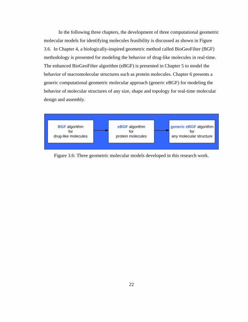
In the following three chapters, the development of three computational geometric

molecular models for identifying molecules feasibility is discussed as shown in Figure

3.6. In Chapter 4, a biologically-inspired geometric method called BioGeoFilter (BGF)

methodology is presented for modeling the behavior of drug-like molecules in real-time.

The enhanced BioGeoFilter algorithm (eBGF) is presented in Chapter 5 to model the

behavior of macromolecular structures such as protein molecules. Chapter 6 presents a

generic computational geometric molecular approach (generic eBGF) for modeling the

behavior of molecular structures of any size, shape and topology for real-time molecular

design and assembly.

BGF algorithmfor

drug-like molecules

eBGF algorithmfor

protein molecules

generic eBGF algorithmfor

any molecular structure

Figure 3.6: Three geometric molecular models developed in this research work.

22

23

Chapter 4

BioGeoFilter (BGF) Methodology

In this chapter, a new methodology called BioGeoFilter (BGF) is introduced to

approximate drug-like molecules’ behavior in real-time subject to both chemical and

geometric constraints. The BGF approach consists of a two-layer hierarchical data

structure that simplifies the molecular representation to effectively identify molecular

self-collisions. Experimental results show that the BGF approach significantly decreases

the computational time for identifying feasible conformations. This can facilitate the

real-time modeling of molecular components to enable interactive molecular design and

assembly.

4.1 Overview of the Proposed BGF Model

The proposed BGF model consists of a hierarchical structure that comprises two

layers: a lower level and an upper level as shown in Figure 4.1. At the lower level, the

molecule is modeled as an articulated body with the internal degrees of freedom

representing the number of torsion bond angles. At the upper level, a bounding volume

hierarchy (BVH) is introduced to identify atoms within the molecule that are in collision.

A new updating scheme for the BVH is presented to identify self-collisions during the

update phase of the algorithm. This significantly speeds the computational time so the

proposed BGF methodology can be used for both real-time molecular modeling and for

reducing the energy minimization time. The following sections describe the two levels of

the proposed BGF algorithm.

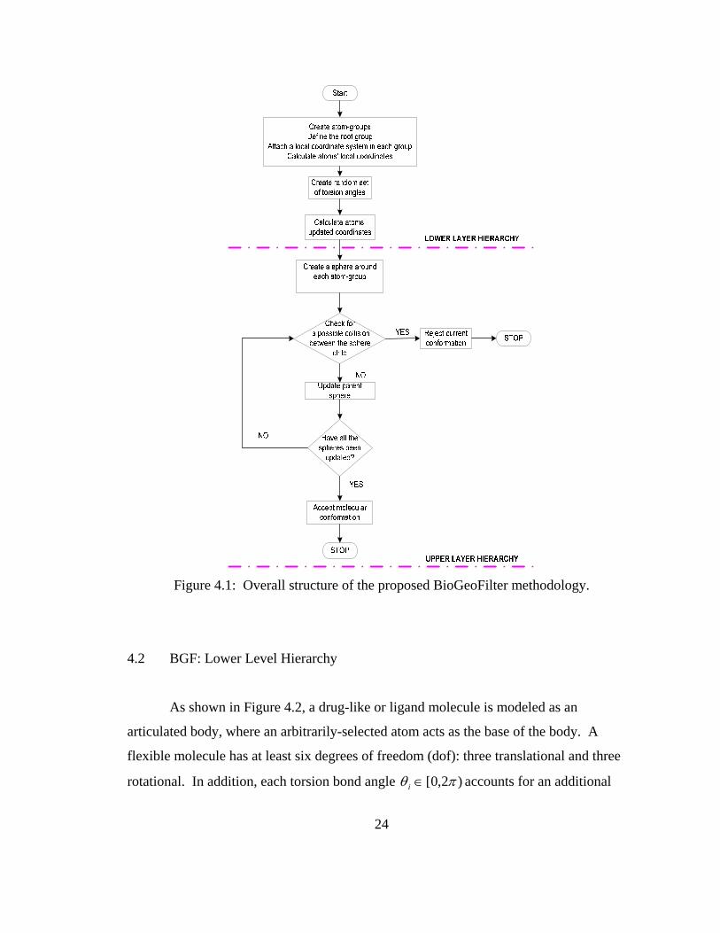
Figure 4.1: Overall structure of the proposed BioGeoFilter methodology.

4.2 BGF: Lower Level Hierarchy

As shown in Figure 4.2, a drug-like or ligand molecule is modeled as an

articulated body, where an arbitrarily-selected atom acts as the base of the body. A

flexible molecule has at least six degrees of freedom (dof): three translational and three

rotational. In addition, each torsion bond angle )2,0[ πθ ∈i accounts for an additional

24

dof. Hence, a molecular conformation is defined as the changes in the angles of the

torsion bonds.

1θ2θ3θ

Figure 4.2: 1STP ligand molecule divided into AtomGroups based on the location of the

torsion bonds.

To reduce the computational complexity of a molecular structure, atoms of a

molecule are clustered into AtomGroups based on the approach by [Zhang and Kavraki

2004]. Based on the location of the torsion bonds, atoms are clustered into AtomGroups.

In other words, all the atoms within an AtomGroup are connected by rigid bonds while

AtomGroups are connected by torsion bonds, as shown in Figure 4.2. Therefore, the

number of the AtomGroups required to represent molecules’ flexibility is equal to the

number of the torsion angles plus one.

25

1θ2θ

3θ4θ

5θ

6θ

Figure 4.3: AtomGroups for a hypothetical small molecule.

Once the AtomGroups are defined, one group is chosen as the root Atomgroup.

The root Atomgroup is important since it represents the base of the molecular structure

where the molecular motions will be projected. The lower hierarchical layer of the

proposed BGF is a tree where each vertex represents an AtomGroup and each edge

denotes a torsion bond as shown in Figure 4.3.

Figure 4.4: Local Cartesian coordinate frame assigned to and . iGroup 1−iGroup

To speed the update of molecular conformations, each is assigned a

local Cartesian coordinate frame and a relationship is generated between all the

AtomGroups. Since each AtomGroup contains atoms whose distance will not change

when torsion changes occur, the distance between atoms in the same AtomGroup do not

need to be checked for collision. Only non-bonded atoms that correspond to different

AtomGroups will be checked thus reducing the time to identify geometrically feasible

conformations. This significantly reduces the computational time and decreases

calculation inaccuracies when updating atom positions during conformational changes.

The clustering of atoms in groups will be used to form the upper level hierarchy of the

proposed BioGeoFilter approach as described in following section.

iAtomGroup

iF

26

4.3 BGF: Upper Level Hierarchy

4.3.1 Constructing the Hierarchy

Once the different AtomGroups of the molecule have been built at the lower level

hierarchy, the smallest enclosing sphere that contains all the atoms within each

AtomGroup is calculated as shown in Figure 4.5. The spheres (each containing an

AtomGroup) are organized into a binary tree-like data structure that will serve to detect

molecular self-collisions subject to both chemical and geometric constraints during

conformational search.

Figure 4.5: Schematic representation of the smallest enclosing sphere of spheres.

Level 0

Level 1

Level 2

1S 2S 3S 4S

5S 6S

7S

1S3S

1θ2θ3θ

1S

2S

3S4S

Figure 4.6: Proposed hierarchical structure for 1STP ligand molecule.

27

Figure 4.6 shows the proposed bounding volume hierarchy for the molecule

previously shown in Figure 4.2. At the bottom of the tree there are four spheres (called

leaf nodes) representing the four AtomGroups for the 1STP ligand molecule. For each

pair of nodes, an intermediate node is created that encloses the two nodes. This process

continues in a bottom-up manner until all the spheres result into one single root sphere as

shown by the number S7 in Figure 4.6.

4.3.2 Molecular Geometric Constraints

The VDW interactions are converted into geometric constraints to decrease the

time to identify infeasible molecular conformations. As discussed in Sections 3.2 and

3.3, the VDW repulsion between two non-bonded atoms increases exponentially as the

distance between the atoms decreases. The VDW attraction occurs at short range until

the non-bonded atoms’ relative distance d is equal to their equilibrium distance :

. Hence, based on these interactions, we introduce the first geometric constraint

that no neighboring atoms or atoms within neighboring AtomGroups should be checked

for self-collision.

0d

0= dd

The distance between non-bonded atoms within a molecule can often become

very short leading to large values in the non-bonded energy and forces. For this reason,

the VDW interaction for non-bonded atoms is modeled as a pair-wise potential over all

pairs of atoms except 1-2 and 1-3 bonded atoms pairs based on the concept of [Dendzik

2005]. Thus, the second geometric constraint consists of considering as non-bonded

atoms the atoms linked by four or more chemical bonds. Moreover, the detection of an

actual self-collision between a non-bonded atom pair along with the algorithm’s

selectivity mechanism depends on the constant ρ of the equilibrium distance where

. Therefore, the third geometric constraint is the constraint given by Eqn.

3.2 that detects atoms self-collisions. If Eqn. 3.2 is satisfied, then an actual self collision

occurs between the non-bonded atoms i and j.

0d

)+(=0 ji rrd

28

By decreasing the ρ value, the output set of feasible solutions obtained by the

BGF algorithm increases as it is further analyzed in Section 4.4. Therefore, based on the

above geometric constraints, the BGF methodology rejects any molecular conformation

that does not satisfy the geometric filtering as described in the following section.

4.3.3 Updating the Hierarchy and Self-Collision Detection

As new conformations are being searched through changes in the torsion bonds,

the new position of the atoms needs to be calculated. The new atom positions affect the

location and radius of the spheres in the hierarchy so they need to be updated

accordingly. In this work, the spheres in the hierarchy are updated in a bottom-up

manner and one level at a time. Therefore, the tree nodes are updated from the leaf nodes

to their parents and this process continues until the root node is reached and updated.

During the update phase, a new updating algorithm is introduced so that if a self-

collision is detected, the algorithm will immediately stop and reject the conformation due

to overlapping atoms (self-collision) as shown in Figure 4.1. The algorithm first updates

the leaf nodes (e.g., S1, S2, S3, and S4 in Figure 4.6). One level at a time, the algorithm

updates the spheres’ radius and centers based on the new atom locations. Then, the

parent nodes of the leaf nodes are tested for update. If there is a collision between the

children nodes, the algorithm returns that the conformation is infeasible and stops. If no

collision is detected, the process continues until the root node is reached and updated.

4.4 Computer Implementation and Results

The presented method and algorithms have been implemented on Intel Pentium 4

with 2.7 GHz personal computers using Visual C++ programming language, the OpenGL

and CGAL libraries [CGAL]. Four different molecules with different number of atoms

and number of degrees of freedom were tested using the proposed BioGeoFilter

methodology. The molecules were obtained from the Protein Data Bank (PDB) [Berman 29

2000] with PDB IDs as follows: 1HVR, 1HTB, 1A5Z, and 1JBO. Their corresponding

number of atoms and degrees of freedom are indicated in Table 4.1 presented below.

0

0.2

0.4

0.6

0.8

1

1.2

1HVR 1HTB 1A5Z 1JBO

(4 DOF) (10 DOF) (11 DOF) (13 DOF)

time

in m

sT_energy

T_BGF

Figure 4.7: Computational time comparison for four different ligand molecules.

Figure 4.7 compares the performance of the proposed BGF algorithm and the

energy calculation for the four different molecules with different pre-selected dof. For

each example molecule, random conformations were generated and tested for feasibility

using both methods. As shown in Figure 4.7, the proposed BGF methodology greatly

reduces the computational time needed to identify feasible molecular conformations

compared to the energy calculation approach. This reduction in time is significant as

multiple flexible molecules will need to be modeled in real-time at the same time for

nanoscale assembly. It can also be observed that as the dof increases, the time reduction

percentage also increases. The computational times for all the tested molecules satisfy

the real-time haptic constraint and scale well as the number of degrees of freedom

increases.

30

Various feasible conformations obtained from the BGF approach are shown in

Figure 4.8(c) for the example molecule 1A5Z. These conformations satisfy the geometric

constraints of the BGF methodology and have been validated using the energy values

obtained from the energy calculation method.

Conformation A

Conformation B

Conformation C

Figure 4.8: Examples of random conformations for three ligand molecules.

Table 4.1 shows the results in terms of computational time (milliseconds) and

accuracy (number of feasible conformations identified) between the energy calculation

approach (T_en, and F_en. columns) and BGF approach (T_BGF, and F_BGF columns).

In the proposed methodology, the same molecular conformation is used for comparing

the two methods. As shown in the percentage time reduction (T_red) in Table 4.1, the

proposed algorithm can identify feasible conformations at least twice faster than the

energy calculation method and with similar accuracy. It can also be observed that as the

dof increases, the time reduction percentage obtained from the BGF methodology also

increases.

31

Table 4.1: Statistical data for four different ligand molecules.

# of Ligand atoms DOF p T_en. T_BGF F_en F_BGF T_red.

0.8 0.6 0.1 13/100 0/100 83%0.7 0.5 0.2 14/100 6/100 60%0.6 0.72 0.158 17/100 14/100 78%0.8 0.586 0.218 18/100 18/100 63%0.7 0.6 0.3 43/100 39/100 50%

1HVR 46 4 1 0.7 0.3 0/100 2/100 57%0.8 0.7 0.4 69/100 43/100 43%0.7 1.1 0.2 77/100 67/100 82%0.6 0.6 0.1 85/100 78/100 83%

1A5Z 44

1HTB 44

1JBO 43

11

10

13

Table 4.1 also shows the sensitivity analysis performed to study the impact of the

different values for ρ of the equilibrium distance on the results. The entire range of ρ

values, where , was tested for each molecule but only the most significant 1<0 ρ < ρ

values are shown in the table for explanation purposes. As shown in Table 4.1, it was

found that by varying ρ and depending on the size of the molecule, the selectivity of the

BGF methodology can be adjusted. As ρ decreases, BGF accepts more molecular

conformations as feasible, which leads to a relaxed filtering. The main objective of the

BGF methodology is to identify infeasible conformations while not rejecting any feasible

conformations. Hence, the selection of an appropriate ρ value for each molecule

depends on the molecule and the desired level of selectivity. In Table 4.1, the grey

colored rows denote the best ρ values for each molecule in terms of selectivity and

accuracy. An analysis on the relationship between the ρ value and the molecule’s size is

addressed in Chapter 5.

The sensitivity analysis was performed by relaxing the third geometric constraint

( ρ value) only. The relaxation of the other geometric constraints was shown to increase

the acceptance of unfeasible molecular conformations and computational time. For this

reason, the sensitivity analysis only focused on relaxing the third constraint while

keeping other constraints fixed.

32

33

4.5 Conclusions

This chapter presents a new method called BioGeoFilter (BGF) for modeling and

approximating the molecular behavior subject to geometric constraints in real-time. BGF

consists of a novel two-layer hierarchical structure that identifies self-collisions during

the hierarchy’s updating phase. The proposed methodology is presented as a filtering

tool based on chemical and geometric concepts for effectively identifying feasible

molecular conformations. Computer implementation and results demonstrate that the

proposed BGF approach significantly decreases the computational time for identifying

feasible ligand conformations to satisfy real-time update requirements. The proposed

BGF methodology can facilitate the real-time modeling and visualization of molecular

components and enable the development of an essential interactive nanoscale computer-

aided design tool for bionanotechnology. The following chapter presents the extended

BGF algorithm for macromolecular structures.

34

Chapter 5

Enhanced BioGeoFilter (eBGF) Molecular Model

This chapter analyzes the structure of much larger molecules such as proteins to

model them more effectively using an enhanced BGF (eBGF) model. The proposed

eBGF approach addresses current limitations in protein modeling through a biologically-

inspired geometric filter for speeding self-collision detection queries. The presented

eBGF methodology can facilitate the modeling of flexible macromolecules for

applications such as molecular docking, nanoscale assembly, and protein folding.

5.1 Differences Between eBGF and BGF Models

The proposed enhanced BioGeoFilter (eBGF) algorithm is similar to the BGF

approach presented in Chapter 4 in that they both build a hierarchical data structure that

consists of two layers: a lower level and an upper level. Both algorithms geometrically

interpret the inter-atomic interactions to impose the geometric constraints that define a

feasible molecular conformation. However, given that a protein molecule can consist of

hundreds or thousands of atoms with hundreds or even thousands degrees of freedom,

the modeling of proteins requires: 1. a further AtomGroup subdivision of the protein’s

backbone structure, 2. an independent updating of the BVH and collision detection

functions, and 3. an additional geometric constraint for the collision detection queries.

To effectively model protein molecules, the eBGF algorithm incorporates new

algorithmic concepts. The core differences between the eBGF and BGF models are:

1. Given the particular structure of proteins, a new algorithm to divide the

protein backbone into smaller groups is incorporated into the eBGF model to

handle protein updating and collision detection more effectively.

35

2. The eBGF algorithm updates the BVH independently from the collision

detection query compared to the combined updating and collision detection

approach in the BGF model. This resulted in a significantly faster model that

is more suitable for large molecules such as proteins.

3. To compensate with the not so tight fitting that results from the selection of

spheres as bounding volumes, the eBGF algorithm incorporates an additional

geometric constraint for the collision detection query.

5.2 Proposed eBGF Overview

Figure 5.1 shows the overview of the enhanced BioGeoFilter methodology that

consists of two layers: the lower and upper hierarchical layers as indicated by the white

colored boxes. At the lower layer of the hierarchy, the eBGF algorithm starts with any

molecular conformation. The dof of the molecular structure are defined to form atom

groups following the concept presented in Chapter 4. A further simplification in

molecular representation is proposed by splitting the backbone atom cluster into smaller

groups of atoms as it is discussed in Section 5.3. At the upper layer of the proposed

approach, we build a BVH for the initial molecular conformation as it is described in

Section 5.4. New random molecular conformations are obtained by arbitrary changing

the values for each degree of freedom. For each candidate molecular conformation, the

BVH is updated to incorporate the corresponding changes in the dof as it is presented in

Section 5.4.3. A collision detection scheme is then performed to identify the feasibility

of each random molecular conformation as it is described in Section 5.4.4. At the end of

the eBGF algorithm, the intramolecular energy value for each random conformation is

calculated for evaluating the proposed approach as it is discussed in Section 5.5. The

following sections describe in details each hierarchical layer of the proposed eBGF

methodology.

Lower Level Hierarchy

Input AnyProtein

Conformation

Read DOF

Histidine

Lysine

Arginine

... ...A segment of a protein’s backbone atoms

Split BackBoneAtomGroup

Upper Level Hierarchy

EnergyCalculation

Build BVHUpdate BVH &Collision Detection

RandomizeProtein

Create AtomGroups

.

.

. ...

eBGF Figure 5.1: Overview of the proposed eBGF approach.

5.3 eBGF: Lower Layer Hierarchy

Torsion changes can occur anywhere within a protein’s topology. However,

considering random torsions within a protein’s backbone can break its structure making it

extremely difficult to evaluate whether the generated molecular conformation is

chemically feasible. Therefore, in this paper, torsions are assumed only between the

central carbon atom of a protein’s backbone (CA) and a side chain atom (CB) or within

the side chain atoms as shown in Figure 5.2. Furthermore, given the increasing

complexity by a protein’s size, torsions at the end of each side chain are neglected (i.e.

the bond between CD and OE1 atoms in Figure 5.2(a) since they do not contribute

significantly to the molecular conformation.

36

 

Figure 5.2: Graphical representation of the degrees of freedom of a protein.

Once the torsion bonds of a protein are identified, the atoms are clustered into

AtomGroups based on the approach proposed by [Zhang and Kavraki 2004] and

analytically shown in Chapter 4. However, the application of the AtomGroup concept in

a protein molecule results in the generation of two different sized atom clusters: clusters

of side chain atoms and a cluster of backbone atoms as shown in Figure 5.3(a). The

cluster of backbone atoms contains hundreds of atoms whereas the clusters of side chain

atoms contain tens of atoms. This large size difference in the atom clusters increases the

time needed to determine if an actual molecular self-collision occurs.

Figure 5.3: Graphical representation of the AtomGroup concept along with the proposed

splitting procedure for a hypothetical protein segment.

37

38

To address this challenge, this research work proposes to split the backbone atom

cluster into smaller AtomGroups based on a threshold defined by the maximum number

of atoms allowed within each atom cluster. By splitting the backbone cluster, a flexible

AtomGroup (i.e. the green and pink sphere in Figure 5.3(b) is obtained along with a

number of rigid AtomGroups (i.e. the six pink/dashed-line spheres shown in Figure

5.3(b)). This splitting procedure further simplifies the molecular representation by

reducing the collision queries while eliminating the collision searches between the rigid

groups. Hence, the collision detection is now performed between similar sized flexible

groups of atoms significantly reducing the computational time for identifying a

molecule’s feasibility.

The splitting of the backbone cluster into smaller groups of atoms significantly

reduces the computational time for updating the atoms’ positions by eliminating the

calculation of the relation matrices for the rigid groups of atoms. As shown in Figure

5.3(b), the relation matrix for the big green sphere (initial flexible AtomGroup) is the

same as the relation matrix of the green and pink sphere (modified flexible AtomGroup)

and as the relation matrices of the pink/dashed-line spheres (rigid AtomGroups).

Therefore, instead of calculating relation matrices for all the seven new groups of atoms,

we just calculate a single relation matrix for the modified flexible group as depicted by

the specific protein segment shown in Figure 5.3. The clustering of atoms into both rigid

and flexible groups will be used to form the upper layer of the hierarchy of the proposed

eBGF methodology as described in the following section.

5.4 eBGF: Upper Layer Hierarchy

At the upper level of the eBGF method, a bounding volume hierarchy (BVH)

depicted as a balanced binary tree similar to the BGF model is introduced to identify

atoms’ self-collisions. The main difference between the bounding volume hierarchies of

the BGF and eBGF models is that the leaves in the BGF model only represent flexible

group of atoms whereas the leaves of the eBGF model can represent both flexible and

rigid atom clusters. This impacts both the updating and collision detection time.

Furthermore, an additional geometric constraint is proposed to compensate the not so

tight fitting that results from the selection of spheres as bounding volumes.

5.4.1 Constructing the BVH

Once the different AtomGroups (both flexible and rigid) have been defined at the

lower layer of the hierarchy, the smallest enclosing sphere that contains all the atoms

within each AtomGroup is calculated as in [Fischer and Gartner 2003]. The spheres

(each containing an AtomGroup) are organized into a binary tree-like data structure that

will serve to detect molecular self-collisions subject to both chemical and geometric

constraints during conformational search as it will be discussed in Section 5.4.4.

Figure 5.4: Schematic representation of the rigid and flexible AtomGroups within a

hypothetical protein segment and the accordance BVH.

Figure 5.4(a) shows a hypothetical protein segment with its corresponding

bounding volume hierarchy shown in Figure 5.4(b). At the bottom of the tree are the 14

spheres (called leaf nodes) representing the 14 AtomGroups of the molecule that includes

flexible (green colored) and rigid (pink colored or dashed-lines). For each pair of nodes,

an intermediate node is created that encloses the two nodes. This process continues in a

bottom-up manner until all the spheres result into one single root sphere as shown by the

39

purple colored sphere in Figure 5.4, which is the sphere that encloses the whole protein

segment.

The BVH is built only once at the beginning of the algorithm allowing a total

construction time of where )N(O

⎩⎨⎧

−=

+=++=

w/o,1N2oddNifN2

rOfNodesTotalNumbe

srigidGroupoupsflexibleGrsrigidGroup1DOFN (5.1)

5.4.2 Randomization

As soon as the pre-selected dof have been defined for the specific protein

molecule, a uniform generator is used to create random values for the torsion angles iθ ,

where . When random torsion changes occur, the new atom positions are

updated based on the concept presented in Chapter 4 to obtain a new molecular

conformation. For each new random molecular state, the BVH is updated and the new

molecular conformation is tested for self-collision.

)2,0[i π∈θ

5.4.3 Updating the Hierarchy

Every time the torsion bonds change, a new molecular conformation is generated.

The new atom positions affect the location and radius of the spheres in the hierarchy so

they need to be updated accordingly. In this work, the spheres in the BVH are updated in

a bottom-up manner and one level at a time. Therefore, the tree nodes are updated from

the leaf nodes to their parents until the root node of the tree is reached and updated.

As shown in Figure 5.4(b), the BVH is formed by both flexible (green colored)

and rigid (pink colored) spheres. It can be observed that the updating of the spheres

around the rigid groups (pink colored spheres and their parents) can be neglected since

the atom distances within and between the rigid groups remain unchanged. This occurs

when the atom cluster of the molecule’s backbone has been defined as the root

40

AtomGroup or else the base of the molecule’s body. Omitting the update of the rigid

nodes (k) results in a reduction of the computational time for updating the BVH and for

identifying molecular feasibility. This contributes to a total updating time of )(kN

O that

never exceeds . )(NO

5.4.4 Self-Collision Detection

The fundamental concept underneath the proposed collision detection algorithm is

the geometric interpretation of the chemical information provided by the van der Waals

(VDW) interaction as discussed in Chapter 3 and in Section 4.3.3. The main difference

lies in that the collision search presented in the eBGF model is handled independently

from the BVH update procedure. In other words, the BVH is updated first and then the

tree is traversed down (in a top-bottom mode) to check for possible overlapping atoms.

The geometric constraints used in this work to handle the collision detection

queries are depicted by Eqn. 5.2. As shown by the first relation in Eqn. 5.2, an additional

constraint is considered to search for overlapping spheres.

1≤,<0

)+(<

)+(<

21

2

1

ρρ

atomRadiusatomRadiusρd

ussphereRadiussphereRadiρd

jiatoms

jispheres

ij

ij

(5.2)

Where, denotes the distance between the sphere objects i and j;

represents the distance between the non-bonded atoms i and j; and are constants

that control the proposed algorithm’s selectivity mechanism.

jisphered, jiatomsd

,

1ρ 2ρ

The first constraint in Eqn. 5.2 (the additional constraint for the eBGF model)

embodies a primary filtering while checking for possible collisions between two spherical

objects. If this constraint is satisfied, then a possible collision occurs between the sphere

objects i and j. The second constraint in Eqn. 5.2 ensures that an actual self-collision

occurs by comparing pair-wise atomic distances. The physical interpretation of the

parameter is that it controls the not so tight object fitting that result from the selection of

1ρ

41

spheres as the type of bounding volumes. The parameter controls the algorithm’s

selectivity or the number of feasible solutions generated. By decreasing the value of

selectivity parameter, the proposed eBGF algorithm accepts more solutions (molecular

conformations) as feasible. From a biological point of view, handles the impact that

the VDW equilibrium distance has on the results.

2ρ

2ρ

2ρ

Figure 5.5: Graphical representation of the proposed collision detection algorithm.

Figure 5.5 shows an intermediate and the worst case scenario of the proposed

collision detection scheme for a protein segment. During the tree traversal, each non-

constraint pair of nodes is checked for a possible collision using the first constraint in

Eqn. 5.2, where the actual self-collision detection is performed between non-bonded atom

pairs by using the second constraint in Eqn. 5.2. A constrained node pair embodies any

of the following properties:

1. For self-collision queries, collision detection between the root of the tree

against itself should be omitted.

2. The collision search between rigid AtomGroups should be ignored since the

atomic distances within and between these groups remain unchanged.

3. Collision queries between bonded neighboring AtomGroups should also be

eliminated since the atomic distances between these two groups do not change

significantly.

42

4. Given that the impact of the VDW interaction increases as the pair-wise

atomic distances decreases, the collision detection between any atom pair

linked by three or less chemical bonds should be avoided as discussed in

Section 3.3. Therefore, non-bonded atoms are the atoms linked by four or

more chemical bonds.

Under these assumptions, if the root’s child nodes are collision free, then the

specific molecular conformation is feasible and is accepted. Otherwise, the tree is

traversed down to identify whether any atoms are actually in collision to reject the current

molecular conformation. The computation collision detection time has )(logkN

O

performance that never exceeds , where k is a constant that represents the

number of constraint nodes (i.e. rigid AtomGroups) that are neglected in the proposed

collision detection scheme. Finally, each random molecular conformation is tested with

both the proposed eBGF approach and the traditional energy calculation method using

Eqn. 3.4.

)(logNO

Figure 5.6: Two example macromolecules tested in this work.

43

5.5 Computer Implementation and Results

The presented method and algorithms have been implemented on a dual 3 GHz

CPU workstation using Visual C++ programming language, OpenGL and CGAL libraries

[CGAL]. Two different protein molecules with different number of atoms, residues, and

number of degrees of freedom have been tested using the proposed eBGF methodology

as shown in Figure 5.6. The molecules were obtained from the Protein Data Bank (PDB)

[Berman 2000] with PDB IDs as follows: 1STP and 1DO3 protein molecules. They are

displayed using the VMD [Humphrey 1999].

Table 5.1: Performance analysis of the proposed eBGF algorithm for two proteins.

Table 5.1 shows a representative list of the performance analysis for the proposed

eBGF method applied to the two example macromolecules. The molecules have been

tested for feasibility after random torsion changes have occurred. The same

conformations for both molecules have been examined with both the energy

(TimeEnergy, FeasibleEnergy, and TH columns) and eBGF (TimeBVHUpdate,

TimeCollision, TimeRand, FeasibleCollision columns) approaches and compared in terms

of computational time (in milliseconds) and accuracy (percentage of feasible

conformations identified). Furthermore, different case scenarios regarding the number,

arrangement and the location of the pre-selected dof have been tested for assessing their

44

impact on the proposed eBGF methodology (FreeResidues and DOF columns). Column

FreeResidues indicates the allowed number of completely flexible residues and column

DOF represents the total number of dof assumed. For example, in 1DO3 protein section

at the bottom of Table 5.1: column-pair 35-36 (FreeResidues-DOF) indicates that 35

completely flexible residues have been tested for the 1DO3 protein that results in a total

of 36 dof; the pair 35-14 indicates that 14 dof were tested only between backbone and

side chain atoms; and the pair 35-22 corresponds to torsions only within the side chains

of the 35 flexible residues. Further discussion of the impact in molecular behavior by the

pre-selected number of flexible residues and dof is performed below. In addition,

different values for the algorithm’s selectivity control parameters ( , and columns)

have been tested and discussed below.

1ρ 2ρ

Figure 5.7: Comparison of the average collision time by the proposed eBGF vs. the

average energy calculation time for different sets of pre-selected flexible-residues/dof.

Figure 5.7 compares the performance of the eBGF method against the energy

calculation approach in terms of computational time needed to identify molecules’

feasibility for the two protein (1STP and 1DO3) examples. As shown in Figure 5.7, the

eBGF algorithm significantly reduces the computational time needed to identify feasible

molecular conformations compared to the energy approach. In fact, the time reduction is

so enormous that two different scales were needed to schematically display the two

methods in the same graph. The left scale for both figures denotes the time in

45

milliseconds (ms) required by the energy approach to determine the feasibility of a

molecular conformation whereas the right scale denotes the computational time (in ms)

for the proposed collision detection algorithm to identify molecular feasibility. For both

molecules and in all tested sets of pre-selected flexible-residues/dof, the eBGF requires

less than 1ms to output if the tested molecular conformation is feasible. This time

reduction is noteworthy as multiple flexible molecules will need to be modeled in real-

time simultaneously for the molecular assembly or molecular docking problems.

0

0.5

1

1.5

2

2.5

3

3.5

1STP(78) 1DO3(153)

log(

Tim

e in

ms)

Energy Method

eBGF Method

Figure 5.8: Average total time comparison between the proposed eBGF algorithm and the

energy calculation approach to output feasibility for 1STP and 1DO3 proteins in a

logarithmic scale.

46

Similarly, Figure 5.8 compares the computational time performance for the two

methods (eBGF vs. energy calculation) while considering the scenario that both protein

molecules are completely flexible (the total number of residues forming each protein

structure assumed to be completely flexible). Analytically, Figure 5.8 displays the total

computational time (in ms) for the eBGF method (the collision detection time + BVH

update time + update atoms’ position time) against the energy approach in a logarithmic

scale. As it is shown in Figure 5.8, the proposed eBGF methodology is significantly

faster than the energy calculation approach in identifying feasible molecular

conformations. In addition, the eBGF algorithm scales very well as the protein size and

problem’s complexity increases.

0

10

20

30

40

50

60

70

1DO3 (1) 1DO3 (5) 1DO3 (10) 1DO3 (35) 1DO3 (153)

Energy MethodEnhanced BGF Method

0102030405060708090

100

1STP(1) 1STP(5) 1STP(10) 1STP(16) 1STP(78)

Energy Method

Enhanced BGF Method

Figure 5.9: Schematic demonstration of the accuracy of the proposed eBGF

methodology.

Figure 5.9 measures the accuracy (percentage of feasible conformations

identified) of our proposed method under different considerations regarding the allowed

number of flexible residues within each protein structure. For both protein examples, the

two methods demonstrate similar accuracy. In fact, the selectivity of the eBGF algorithm

can be adjusted by varying the control parameters ( , and ). In other words, by

decreasing the values, the proposed algorithm can accept more molecular

conformations as feasible leading to a relaxed filtering. The physical interpretation of

selectivity parameter is that it handles the not so tight object fitting resulted by the

selection of spheres as the type of bounding volumes whereas the selectivity

parameter controls the impact that the VDW equilibrium distance has on the results as it

has been analyzed in Section 5.3.4. The main objective of the eBGF approach is to

identify infeasible molecular conformations rapidly while not rejecting any feasible ones.

Hence, the selection of appropriate values for each molecule depends on the

molecule’s size along with the desired level of selectivity by the user. It is also worth

mentioning here that the molecules’ feasibility is traditionally measured using the energy

calculation shown in Eqn. 3.4. A conformation might be considered as feasible or not

depending on the molecular internal energy value. If a candidate conformation has

negative internal energy, then it corresponds to a stable molecular state. However,

feasible molecular conformations exist while having positive intramolecular energy.

1ρ 2ρ

ρ

1ρ

2ρ

ρ

47

Therefore, a threshold (TH column in Table 5.1) has been selected based on the protein’s

size to define the maximum energy value for which a molecular conformation is

considered to be feasible.

Moreover, as it is shown in Table 5.1 and Figure 5.9, there is a significant

dependency among the pre-selected number of flexible residues and dof considered in

each protein molecule and the output (percentage of feasible molecular conformations)

derived by both (eBGF and energy) methods. Computer implementation and results

demonstrate that as the number of dof considered increases, the output set of feasible

solutions obtained by the energy approach decreases; whereas the output set by the eBGF

algorithm can be adjusted as it has been discussed previously. In addition, when many

dof are assumed between backbone atom and side chain atoms, the output set of feasible

solutions by the energy calculation approach decreases. Therefore, an additional direct

search method is essential to identify arbitrarily low energy molecular conformations

after they have been filtered by the proposed eBGF methodology.

Table 5.2: Performance analysis of current approaches.

Methods Build BVH Update

BVH

Collision

Detection

ChainTree

[Lotan et.al. 2002]

)(NO

)(NO

)( 3/4NO

SpatialAdaptiveHierarchy

[Angulo et.al. 2005]

---

)log( NNO

)(NO

DeformingNecklaces

[Aqarwal et.al. 2004]

)log( NNO

)log( NNO

)( 3/4NO

BGF model

[Brintaki & Lai-Yuen 2008]

---

)(NO

)(log NO

eBGF model

[Brintaki & Lai-Yuen 2009]

)(NO

)(NO

)(log NO

48

Table 5.2 demonstrates the worst case scenarios in terms of computational

complexity for eBGF and current methods in the literature. The proposed eBGF

methodology requires performance for building and updating the BVH and never

exceeds when searching for overlapping atoms. Hence, the eBGF algorithm

succeeds to keep the BVH complexity in the lower level ( ) while significantly

reducing collision detection complexity from toO .

)(NO

)(logNO

)(NO

)(logN)(NO

5.6 Conclusions

This chapter presents the enhanced BioGeoFilter (eBGF) methodology for

modeling the behavior of macromolecules such as proteins. The proposed approach is

presented as a rapid filtering tool for the identification of molecules’ feasibility. The

eBGF algorithm has been tested against the traditional energy calculation approach in

terms of computational time and accuracy under different cases. Computer

implementation and results demonstrate that the proposed eBGF algorithm significantly

decreases the computational time for identifying feasible molecular conformations

without sacrificing accuracy. Therefore, the eBGF method facilitates the modeling of

flexible macromolecules that can be used in molecular modeling, protein folding, and

nanoscale design.

49

50

Chapter 6

Generic Enhanced BioGeoFilter (g.eBGF) Model

This chapter presents the generic enhanced BioGeoFilter (g.eBGF) algorithm for

simplifying the representation of molecules of different type, size, shape and topology by

considering certain chemical factors that influence molecules’ flexibility. The

incorporation of chemically-based constraints can provide more realistic molecular

conformations that will significantly improve molecular modeling. The proposed

methodology can be used to enable the interactive modeling of molecules for molecular

docking or assembly, and for protein folding applications.

6.1 Differences Between eBGF and g.eBGF Models

Both geometric methods rely upon the same basic algorithmic concepts for

modeling molecules conformation mechanism during conformational search. The main

differences between the two methods are that the g.eBGF approach:

1. incorporates certain chemically-based factors that

a. control molecules flexibility for providing more realistic and chemically-

feasible molecular conformations

b. further simplifies the molecular representation since they reduce the

allowed number of degrees of freedom for the molecule.

2. is a generic model applicable to molecules of different type, size, shape and

topology. The g.eBGF methodology can effectively model molecular

structures such as ligands and proteins with one or multiple chains.

6.2 Ligand Modeling

A ligand or drug-like molecule is a small molecular structure that usually consists

of at most 50 atoms. Ligand molecules may contain rings of atoms as graphically shown

with [Humphrey 1999] molecular graphics software in Figure 6.1. These rings are

considered rigid during modeling as the location of the ring atoms does not change with

respect to each other. Therefore, torsion can be assumed everywhere within a ligand’s

topology except within the rings and within double- and triple-bonded atoms, which

correspond to stronger (not easily breakable) chemical bonds. The proposed generic

eBGF approach considers the above information for defining the chemically-feasible dof

within a ligand molecule.

Figure 6.1: Examples of ligand molecules.

6.3 Protein Modeling

A protein molecule may contain one chain (backbone) as shown by using the

molecular graphics software [Humphrey 1999] in Figure 6.2(a) or multiple chains as

shown in Figure 6.2(b). Multiple chains are usually not connected by chemical bonds but

by electrostatic forces that keep the chains close to each other. In contrast to ligand

51

modeling, macromolecules such as proteins consist of hundreds or thousands of atoms

with hundreds or even thousands dof. A protein molecule can also be considered as a

highly articulated body where an arbitrarily-selected atom or atom-group acts as the base

of the body. A protein that contains more than one chain can be viewed as multiple

kinematics chains with hundreds or thousands of links and joints.

Figure 6.2: VDW representation of two different protein molecule examples.

  

N CA CO

CBCG

CD

OE1

OE2GLU residue/amino-acid

Histidine

Lysine

Arginine

... ...

A segment of a protein’s backbone atoms

Figure 6.3: Graphical representation of the degrees of freedom of a protein.

Torsion changes can occur everywhere within a protein’s topology, except within

rings and double- and triple-bonded atoms. However, random torsions within a protein’s

backbone (chain) can break its structure making it extremely difficult to evaluate whether

the generated molecular conformation is chemically feasible. For this reason, similar

with Section 5.3 for the generic eBGF model, torsions are assumed only between the

52

53

central carbon atom of a protein’s backbone (CA) and a side chain atom (CB) or within

the side chain atoms as shown in Figure 6.3. Furthermore, torsions at the end of each

side chain are neglected (i.e. the bond between CD and OE1 atoms in Figure 6.3(a) since

they do not contribute significantly to the molecular conformation.

Some regions within a protein structure attain higher flexibility. These higher

flexible regions are the remote protein’s portions or the amino acids (residues) located at

the end of the chain. The residues within the turns of a protein’s chain should also be

considered as highly flexible molecular bodies since those have a tendency to move

more. These highly flexible regions are considered in the proposed g.eBGF model for

determining the chemically-feasible dof that controls the molecular flexibility.

6.4 Proposed g.eBGF Methodology

6.4.1 Overview of the Proposed g.eBGF Model

Figure 6.4 shows the overview of the proposed generic enhanced BioGeoFilter

(g.eBGF) methodology that aims to effectively identify feasible conformations for

molecular structures of different type, size, shape or topology while considering the

underlying chemical information. The g.eBGF approach similarly with the BGF and

eBGF models consists of two layers as indicated by the two larger boxes in Figure 6.4.

At the lower layer of the hierarchy, any molecular conformation can be input into the

g.eBGF algorithm. The pre-selected dof for a molecular structure are defined based on

the concepts presented in Sections 6.2 and 6.3 to form the atom groups. A further

simplification in macromolecular representation is proposed by splitting the backbone

atom cluster (or clusters) into smaller groups of atoms. At the upper layer of the g.eBGF

algorithm, the corresponding bounding volume hierarchy (BVH) of the initial molecular

conformation is built. New random molecular conformations are obtained by arbitrarily

changing the values for each degree of freedom. For each candidate molecular

conformation, the BVH is updated and a collision detection scheme is performed to

identify the feasibility of the molecular conformation. At the end of the g.eBGF

algorithm, the intramolecular energy value for each random conformation is calculated to

evaluate the proposed approach.

Figure 6.4: Overview of the proposed g.eBGF methodology.

6.4.2 Chemically-Artificial Bonds for the g.eBGF Method

When a protein molecule contains more than one chain as shown with the VMD

molecular graphics software [Humphrey 1999] in (Figure 6.5(a)), an artificial rigid bond

is introduced between the closest residue-pair of the chains by the proposed generic

eBGF approach. This artificial bond is used to simulate the electrostatic forces that keep

the chains in contact and should be created in the least flexible region of the protein to

avoid the risk of breaking its structure. For example, the least flexible region in the 1NS1

protein shown previously in Figure 6.5(a) is the area between the first helixes of the two

chains as shown in Figure 6.5(b). However, an artificial bond should not be placed

54

arbitrarily between any residue-pair within the 1st helices but between the closest possible

residue-pair as shown by the circle in Figure 6.6. Moreover, the selected residue pair

should have the same polarity. In other words, the closest residues that are both either

hydrophobic, polar or ionized would be good candidates for placing an artificial rigid

bond.

Figure 6.5: Structure of the protein with PDB ID: 1NS1.

Figure 6.6: Closest residue-pair between the first helices of the two 1NS1 protein’s

chains.

55

56

6.4.3 Description of the g.eBGF Algorithm

The proposed g.eBGF methodology for identifying feasible molecular

conformations requires two input files: the atomic coordinate information and the atoms

within the molecular topology that share a torsion bond. The first input file is usually the

PDB file obtained from the Protein Data Bank (PDB) [Berman 2000] and the second

input file is the file that describes the pre-selected dof considered for each experiment.

The VMD software [Humphrey 1999] is used to define atoms’ connectivity information

for proteins and to construct the first input file (coordinate file). If the protein contains

multiple chains, an artificial bond is added as described in Section 6.4.2. Finally, to

create the file that contains the pre-selected dof, the concepts about the allowed number

and location of the pre-selected dof (torsion angles) presented in Sections 6.2 and 6.3 (i.e.

torsions are not allowed within the rings or double-bonded atoms, etc.) are incorporated

for studying chemically-feasible random molecular conformations.

Once the two required input files have been defined, groups of atoms are formed

following the concept presented in Section 4.2 to create the lower layer of the proposed

g.eBGF approach. Based on the location of the torsion bonds, atoms are clustered into

AtomGroups where all the atoms within an AtomGroup are connected by rigid bonds

while AtomGroups are connected by torsion bonds. Figure 6.7(a), schematically

represents the Atomgroups for a hypothetical protein segment consisted by two

symmetric chains. As it is shown in Figure 6.7(a), since the two chains are symmetric, the

defined Atomgroups for both chains are the same in terms of both number and atom

clustering.

If the tested molecular structure is a protein molecule, then an additional step

within the g.eBGF algorithm is performed for splitting the backbone atom cluster (or

clusters in the case of multiple chain proteins) into smaller AtomGroups. The purpose of

this additional step is to reduce the time needed to identify an actual molecular self-

collision while decreasing the computational time for updating the atoms’ positions as

discussed in Section 5.3. The size of these AtomGroups is based on a threshold defined

by the maximum number of atoms allowed within each atom cluster. By splitting a

backbone cluster, a flexible AtomGroup (i.e. the green-pink sphere in Figure 6.7(b)) is

obtained along with a number of rigid AtomGroups (i.e. the six pink spheres shown in

Figure 6.7(b)) for each chain within a protein molecule. The splitting of the backbone

group eliminates collision detection within and between the rigid groups since the atomic

distances remain unchanged between and within these groups. Moreover, after splitting

the backbone cluster, collision search is performed between similar sized flexible groups

of atoms.

Figure 6.7: Graphical representation of the AtomGroup concept along with the proposed

splitting procedure for a hypothetical protein segment with two chains.

At the upper hierarchical layer of the proposed g.eBGF method similarly with the

eBGF model, a BVH depicted as a balanced binary tree is introduced to identify

overlapping atoms. In respect the BVH the difference between the two models lays on the

geometric representation of the preselected dof. Based on the location of the torsion bond

angles (dof) within the molecule, groups of atoms are generated for both models. To

construct the hierarchy a sphere is attached around each atom cluster. The spheres around

each generated AtomGroup depict the leaves of the BVH for each method. As opposed to

eBGF method the g.eBGF model defines the chemically-allowed torsion movements for

each molecular structure. These chemically-oriented factors influence both the number

and location of the generated AtomGroups and hence, the size and location of the

57

generated spheres for the BVH. Therefore, even if the same protein molecule is tested

with both models (eBGF and g.eBGF) the resulted spheres for each method will have

different size and location in respect to the world coordinate frame. In view that the

chemically-allowed torsion movements (dof) provide a more realistic representation for

molecules deformation mechanism, the g.eBGF compared with the eBGF model provides

a more realistic geometric representation of molecules flexibility. The BVH is built only

once at the beginning of the algorithm allowing a total construction time of where: )(NO

testedareproteinswhenonlyexist:srigidGroupw/o1N2

oddNifN2rOfNodesTotalNumbe

srigidGroupoupsflexibleGrsrigidGroup1DOFN

⎩⎨⎧

−=

+=++=

(6.1)

Likewise with the eBGF model presented in Section 5.4.3, the BVH for the

g.eBGF method is updated for each new molecular conformation as the torsion angles are

randomly modified contributing to a total updating time of )(kN

O that never

exceeds . Where, k is the number of rigid nodes that remain unchanged. )(NO

As soon as the BVH is updated, a collision detection algorithm is performed to

search for overlaps between non-bonded atoms within the new molecular conformation.

The collision detection queries follow the same concepts of the eBGF model as analyzed

in Section 5.4.4, attaining a total )(logkN

O performance that never exceeds .

Where, k is a constant that represents the number of constraint nodes (i.e. rigid

AtomGroups).

)(logNO

6.5 Computer Implementation and Results

The presented method and algorithms have been implemented on a dual 3.0 GHz

CPU workstation using Visual C++ programming language, OpenGL and CGAL libraries

[CGAL]. Different molecules with different number of atoms, chains, residues and dof

58

have been tested with the proposed g.eBGF algorithm. The example molecules were

obtained from the Protein Data Bank (PBD) [Berman 2000] with PDB IDs as follows:

1STP, 1A5Z, 1HVR, 1HTB, and 1JBO ligand molecules, along with 1STP, 1DO3, and

1NS1 protein molecules.

Table 6.1: Performance analysis of the proposed g.eBGF methodology. Molecule Number Number Time Time  Time Time % Feasible TH % Feasible Flex Flex Flex THPDB Name Chains Atoms Energy BVHupdate Collision Rand by Energy Energy by Collision Helixes Turns Residues Split

1STP 16 0.183 0.1 0.0016 0.0082 100 100 31JBO 43 1.37 0.23 0.23 0.024 17 20 131HTB 44 1.38 0.21 0.014 0.025 52 52 101A5Z 44 1.72 0.23 0.016 0.024 56 55 111HVR 46 1.87 0.17 0.004 0.01 100 100 4

1STP 16 0.18 0.1 0.0027 0.0088 100 100 31JBO 43 1.58 0.24 0.018 0.024 9 10 131HTB 44 1.62 0.22 0.02 0.022 40 43 0.7 0.8 101A5Z 44 1.74 0.23 0.002 0.02 50 41 111HVR 46 1.42 0.17 0.004 0.018 100 100 4

233.16 1.5 0.21 0.32 85 90 10220.96 0.74 0.73 0.3 80 90 15222.45 0.64 0.88 0.31 90 90 20224.15 1.38 0.12 0.33 80 90 10218.9 0.67 0.19 0.31 70 70 15219.56 0.57 0.2 0.28 70 70 20214.35 1.33 0.28 0.31 4 5 10230 0.89 0.71 0.31 2 6 15

225.02 0.76 0.95 0.31 3 4 20

1456.04 4.47 0.3 0.8 30 25 101515.64 2.76 1.09 0.79 27 30 151461.59 2.23 2.61 0.74 15 15 201479.41 4.3 0.07 0.83 6 3 101513 2.91 0.77 0.81 8 10 15

1491.05 2.42 2.77 0.8 4 2 201398.63 3.69 0.06 0.75 0 0 101511.75 3.34 0.065 0.85 0 0 151469.47 2.76 0.13 0.78 0 0 20

x100x

4218

5

2 6 7

4 18 18

3

30 58

2nd,3rd 34 98

x

4

0.6

x

1

1STP 1 903

100000 0.5

1NS1 2 2342

Rho1 Rho2 DOF

0.6 0.7

x

Table 6.1 shows a representative list of the performance analysis for the proposed

g.eBGF methodology on different example molecules. For each molecule, sets of

random torsion angles were randomly generated. The same random molecular

conformation was tested with both the g.eBGF (TimeBVHUpdate, TimeCollision,

TimeRand, %FeasibleByCollision columns) and the energy (TimeEnergy,

%FeasibleByEnergy, and TH Energy columns) approaches and evaluated in terms of

computational time (in milliseconds) and accuracy (percentage of feasible conformations

identified). A molecular conformation can be considered as feasible based on the internal

molecular energy value. Therefore, a threshold (TH column in Table 6.1) has been

59

selected based on the molecules’ size to define the maximum energy value for which a

molecular conformation is considered to be feasible with the energy approach.

Different scenarios regarding the number, arrangement and the location of the

pre-selected dof were studied for assessing their impact on the proposed g.eBGF

algorithm. Columns FlexHelixes, FlexTurns and FlexResidues denote the number of

flexible helixes, residues and turns respectively, where column dof states the total number

of chemically and geometrically feasible dof considered for each experiment. In

addition, different values for the algorithm’s selectivity parameters ( and ) have been

tested for evaluating their impact on the g.eBGF results. Table 6.1 shows the results for

the ligand molecules using two different pair-values for the selectivity parameters (rho

values) and for the protein molecules using one selectivity parameter pair. A detailed

analysis on the impact of the rho values on protein modeling can be found in our Chapter

5. Finally, three different values for the splitting threshold have been tested for each

protein molecule as shown by the last column (TH Split) in Table 6.1.

1ρ 2ρ

00.20.40.60.81

1.21.41.61.82

1STP(3) 1HVR(4) 1HTB(10) 1A5Z(11) 1JBO(13)

ligands

Tim

e in

mill

isec

onds

Energy vs. Generic eBGF Approach

Time_eBGF

Time_Energy

Figure 6.8: Time comparison between the traditional energy calculation approach and the

proposed g.eBGF methodology for ligand molecules.

60

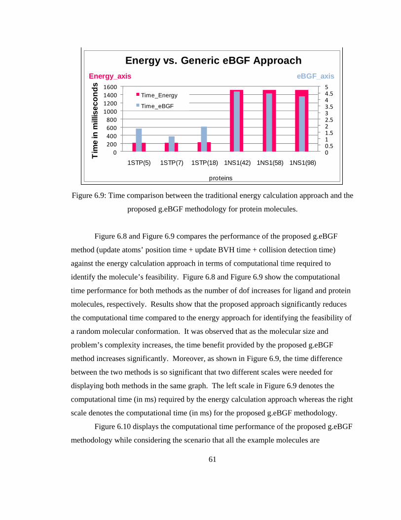
00.511.522.533.544.55

02004006008001000120014001600

1STP(5) 1STP(7) 1STP(18) 1NS1(42) 1NS1(58) 1NS1(98)

proteins

Tim

e in

mill

isec

onds

Energy vs. Generic eBGF Approach

Time_Energy

Time_eBGF

eBGF_axisEnergy_axis

Figure 6.9: Time comparison between the traditional energy calculation approach and the

proposed g.eBGF methodology for protein molecules.

Figure 6.8 and Figure 6.9 compares the performance of the proposed g.eBGF

method (update atoms’ position time + update BVH time + collision detection time)

against the energy calculation approach in terms of computational time required to

identify the molecule’s feasibility. Figure 6.8 and Figure 6.9 show the computational

time performance for both methods as the number of dof increases for ligand and protein

molecules, respectively. Results show that the proposed approach significantly reduces

the computational time compared to the energy approach for identifying the feasibility of

a random molecular conformation. It was observed that as the molecular size and

problem’s complexity increases, the time benefit provided by the proposed g.eBGF

method increases significantly. Moreover, as shown in Figure 6.9, the time difference

between the two methods is so significant that two different scales were needed for

displaying both methods in the same graph. The left scale in Figure 6.9 denotes the

computational time (in ms) required by the energy calculation approach whereas the right

scale denotes the computational time (in ms) for the proposed g.eBGF methodology.

Figure 6.10 displays the computational time performance of the proposed g.eBGF

methodology while considering the scenario that all the example molecules are

61

completely flexible. The tested molecules are assumed to be fully flexible bodies by

randomly varying the total allowed number of chemically-feasible dof as presented in

Sections 6.2 and 6.3. Results show that the proposed g.eBGF approach scales very well

as the molecular size and problem’s complexity increase.

00.51

1.52

2.53

3.54

4.5

1STP(3) 1HVR(4) 1HTB(10) 1A5Z(11) 1JBO(13) 1STP(18) 1NS1(98)

ligands proteins

Time in millisecon

ds

eBGF Performance Over Molecules of Different Size

Figure 6.10: Computational time performance of the proposed g.eBGF approach for

molecules of different size and dof.

The impact of the splitting threshold selection value on the g.eBGF algorithm is

shown in Figure 6.11. As discussed in Section 6.4.3, the splitting threshold (TH Split

column in Table 6.1) defines the maximum allowed number of atoms in each atom

cluster. As the splitting threshold value decreases, it can be observed from Figure 6.11

that the following occur:

• the computational time required to update the BVH increases,

• the computational time for self-collision detection decreases, and

• the overall computational time for the g.eBGF algorithm remains

approximately the same.

62

Figure 6.11: Splitting threshold impact on the g.eBGF results for protein modeling.

Figure 6.12: Accuracy comparison between the traditional energy calculation approach

and the proposed g.eBGF method.

Therefore, incorporating the splitting concept for the backbone atom clusters into

the proposed algorithm speeds the identification of molecular feasibility while it does not

affect the overall performance of the algorithm. The best selection for a splitting

threshold depends on the pre-selected set of dof. A good splitting threshold is a value

that allows the construction of similar sized groups of atoms while reducing the

63

computational time for self-collision. In this work, it was found that a splitting threshold

value of 15 atoms for each atom cluster provided similar-sized atom groups and the best

results for self-collision detection time.

Figure 6.12 demonstrates the accuracy (percentage of feasible molecular

conformations identified) between the traditional energy method and the proposed

g.eBGF methodology. For the ligand molecules, two different pairs of the selectivity

parameters are presented to show their impact on the results, whereas one selectivity pair

is shown for the protein molecules. As shown in Figure 6.12, both methods (g.eBGF and

Energy) demonstrate similar accuracy for all tested molecules. In fact, the selectivity of

the g.eBGF algorithm can be adjusted by varying the control parameters ( , and ). In

other words, by decreasing the values, the proposed algorithm can accept more

molecular conformations as feasible leading to a relaxed filtering. It is important to

select appropriate values based on the molecule’s size and the desired level of

selectivity by the user to avoid rejecting molecular conformations that are feasible.

1ρ 2ρ

ρ

ρ

As shown in Table 6.1 and Figure 6.12, there is a significant dependency between

the pre-selected number of chemically-feasible dof considered in each molecule and the

percentage of feasible molecular conformations from both the g.eBGF and energy

methods. Results demonstrate that as the number of dof increases, the output set of

feasible solutions obtained by the energy approach decreases; whereas the output set by

the g.eBGF algorithm can be adjusted as it has been discussed previously. In addition,

when a macromolecule is assumed to be a fully flexible body, the output set of feasible

solutions by the energy calculation approach decreases and tends to approach zero.

Therefore, an additional direct search method is necessary to identify low-energy

molecular conformations after they have been filtered by the proposed g.eBGF

methodology.

Table 6.2 demonstrates the worst case scenarios in terms of computational

complexity for g.eBGF and current methods in the literature. The proposed g.eBGF

methodology requires performance for building and updating the BVH and never

exceeds when searching for overlapping atoms. Hence, the g.eBGF algorithm

)(NO

)(logNO

64

succeeds to keep the BVH complexity in the lower level ( ) while significantly

reducing collision detection complexity from toO .

)(NO

)(logN)(NO

Table 6.2: Computational complexity comparison.

Methods Build BVH Update

BVH

Collision

Detection

ChainTree

[Lotan et.al. 2002]

)O

65

)N(O N(

)N(O 3/4

SpatialAdaptiveHierarchy

[Angulo et.al. 2005]

---

)NlogN(O

)N(O

DeformingNecklaces

[Aqarwal et.al. 2004]

)NlogO N(

)NO logN(

)N(O 3/4

BGF model

[Brintaki & Lai-Yuen 2008]

---

)N(O

)N(logO

eBGF model

[Brintaki & Lai-Yuen 2009]

)N(O

)N(O

)N(logO

Generic eBGF model

[submitted to CAD journal 2009]

)N(O

)

)N(logO N(O

6.6 Conclusions

This chapter presented a new generic molecular modeling tool called enhanced

BioGeoFilter (g.eBGF) for effectively identifying chemically-feasible conformations for

molecules of different type, size and topology. The proposed g.eBGF methodology

incorporates chemical factors that control molecules’ conformation into a bounding

volume hierarchy to rapidly identify chemically-feasible molecular conformations. The

g.eBGF approach is presented as a filtering tool to rapidly identify molecular

66

conformations for speeding molecular conformational search and collision detection

queries. Computer implementation and results demonstrate that the g.eBGF methodology

significantly decreases the computational time for identifying feasible molecular

conformations while maintaining accuracy. Therefore, the g.eBGF method can be used

to facilitate the modeling of flexible molecular structures for applications such as

molecular docking and assembly, and protein folding.

67

Chapter 7

Identifying the Molecular Stability

The scope of this chapter is to investigate the performance of evolutionary-based

optimization methods on effectively searching for low-energy molecular conformations.

Two novel differential evolution- based methods are presented. The first proposed

method is a kinematics-based DE algorithm called kDE model that kinematically

represents and simplifies the molecular representation to direct the conformational search

towards stable solutions. The second approach, called Biological Differential Evolution

(BioDE) is based on our previously developed differential evolution algorithm and our

developed biologically-inspired geometric representation of molecules conformation

mechanism. The BioDE algorithm utilizes the g.eBGF model as a surrogate

approximation model to reduce the number of exact evaluations and to reduce the

algorithm’s convergence rate. Both proposed methodologies will be extremely useful in

speeding the search for low-energy molecular conformations while enabling the modeling

of flexible molecules for molecular design.

7.1 Fundamentals of Evolutionary Algorithms (EAs)

Evolutionary Algorithms (EA) simulates the natural selection process using a

number (population) of individuals (candidate solutions to the problem) to evolve

through certain procedures. Similar to nature, each individual is represented as a

chromosome – a string of numbers (bit strings, integers or floating point numbers) which

contain the design variables for the optimization problem. Each individual’s quality is

represented by a fitness function tailored to the problem under consideration.

Classic Genetic Algorithms (GAs) use binary coding for the representation of the

genotype. However, floating point coding moves EAs closer to the problem space. This

allows the operators to be more problem specific while providing a better physical

representation of the space constraints.

In general, EA starts by generating, randomly, the initial chromosome population

with their genes (the design variables in the case of floating point coding) taking values

inside the desired constrained space of each design variable. The lower and higher

constraints of each gene may be chosen in a way that specific undesirable solutions may

be avoided. Although the shortening of the search space reduces the computation time, it

may also lead to sub-optimal solutions due to the lower variability between the potential

solutions.

Figure 7.1: One-point crossover (recombination) operator.

After the evaluation of each individual’s fitness function, operators are applied to

the population, simulating the natural processes. Applied operators include various forms

of recombination, mutation and selection, which are used to provide the next generation

of chromosomes. The first classic operator applied to the selected chromosomes is the

one-point crossover scheme. In this operator, two randomly selected chromosomes are

divided in the same (random) position while the first part of the first one is connected to

the second part of the second one and vice-versa as shown in Figure 7.1. The crossover

operator is used to provide information exchange between different potential solutions to

the problem.

Figure 7.2: Uniform mutation operator.

68

69

The second classic operator applied to the selected chromosomes is the uniform

mutation scheme. This asexual operator alters a randomly selected gene of a

chromosome as shown in Figure 7.2. The new gene takes its random value from the

constrained space that is determined at the beginning of the process. The mutation

operator is used to introduce some extra variability into the population.

The resulting intermediate population is evaluated and a fitness function is

assigned to each member of the population. Using a selection procedure (different for

each type of EA), the best individuals of the intermediate population (or the best

individuals of the intermediate and the previous population) will form the next

generation. The process of a new generation evaluation and creation is successively

repeated, resulting in individuals with higher values of fitness function.

7.2 EAs Advantages, Limitations and How to Compensate

Evolutionary algorithms are a class of search methods with remarkable balance

between exploitation of the best solutions and exploration of the search space. They

combine elements of directed and stochastic search and consequently, are more robust

than directed search methods. The EAs are algorithms parallel by nature and may be

easily tailored to the specific application of interest taking into account the special

characteristics of the problem under consideration. In addition, the EAs are easy to

implement in problems with a relatively high number of constraints and design variables,

as well as with many and contradictory objectives [Michalewicz 1999, Goldberg 1989,

Holland 1992].

However, EAs main limitations are the convergence uncertainty and trapping into

local minima. To compensate for the algorithm’s failure, the first step is to adjust the

algorithm’s selective pressure, which is defined as the predominance of exploitation

versus exploration. By increasing the selective pressure, the algorithm’s convergence

rate and the probability of trapping into local minima are enhanced. Therefore, a balance

between exploration and exploitation is essential. The crossover and mutation operators

70

are responsible for exploring the solution space (exploration) while leading to an

increasing variation of the population. On the other hand, the selection process pushes

the search into the region with the best fitness function values (exploitation) aiming to

decrease the population variation. Thus, the balance between exploration and exploitation

is given by the specific type of selection operator for the problem under consideration.

Typically, high selective pressure requires high variation in the population to avoid any

local minima traps.

Another way to compensate for algorithm’s potential failure is to define

“suitable” values for the control parameters of the EA. The control parameters for an

evolutionary algorithm are the crossover and mutation probabilities. These probabilities

remain constant during the search process while affecting the convergence behavior and

algorithm’s robustness. The values for the crossover and mutation probabilities are

strongly dependent on the objective function, the characteristics of the problem, and the

population size. Usually, when an algorithm is mostly based on a crossover operator, it

requires low selective pressure to avoid trapping into local minima solutions.

Additionally, when a high mutation probability is applied, the algorithm entails a high

selective pressure to compensate for failure. Based on these concepts, a trial and error

testing for the EA’s control parameters will tune the algorithm’s robustness and

convergence rate.

An alternative approach is the use of a differential evolution (DE) algorithm since

it has shown a better convergence performance compared with other EAs [Storn and

Price 1995, 2005, Nikolos and Brintaki 2005a,b,c, 2007, Thomsen 2003, 2006].

Incorporating the scheme presented by [Hui-Yuan 2003] for determining the donor

scheme for the mutation operator accelerates the algorithm’s convergence rate, without

sacrificing accuracy or the algorithm’s robustness. In this scheme, the donor is randomly

selected (with uniform distribution) from the region within the “hyper triangle” formed

by the three members of the triplet. With this scheme, the donor comprises the local

information of all members of the triplet. This provides a better starting-point for the

mutation operation and results in a better distribution of the trial-vectors.

71

Besides using special operators, a substitute solution for compensating for the

algorithm’s convergence failure and for decreasing the computational time is the

utilization of surrogating models and approximations. Surrogate models are auxiliary

simulations that are less accurate, but also less computationally costly than the expensive

(exact model) simulations. Surrogate approximations are algebraic summaries obtained

from previous runs of the expensive simulation [Torczon 1998, Giannakoglou 2002].

Such approximations are the various types of Artificial Neural Networks (ANN)

[Giannakoglou 2002, Nikolos and Brintaki 2005b, 2007]. The basic concept of using an

approximation method is to replace the costly exact evaluations with fast inexact

approximations while maintaining the algorithm’s robustness. The surrogate model

predictions replace exact and costly evaluations only for the less-promising individuals,

while the more-promising ones are always exactly evaluated. Our developed

biologically-inspired geometric filter (generic eBGF method) presented in Chapter 6 can

also set the base for a surrogate approximation model as it is analyzed in Section 7.4.

7.3 Differential Evolution

In this work, a Differential Evolution (DE) algorithm based on the concepts by

[Storn and Price 1995, 2005], improved by [Hui-Yuan 2003] and presented in [Nikolos

and Brintaki 2005a,b,c, 2007] is used to direct the search towards low energy molecular

conformations. The DE algorithm is a simple evolutionary algorithm to implement and

demonstrates better convergence performance compared with other EAs. Differential

Evolution embodies a type of evolutionary strategy (ES) especially formed to deal with

continuous optimization problems often encountered in engineering design.

The classic DE algorithm evolves a fixed population size consisted by candidate

problem solutions (population members or else chromosomes), randomly initialized.

After initializing the population, an iterative process starts to direct the search towards

better fitted population members. At each iteration (generation), a new population of

candidate solutions is produced until a stopping condition is satisfied. At each generation,

each element (member) of the population can be replaced with a new generated one. The

new element is a linear combination between a randomly selected population member

and a difference between two other randomly selected members. Below is the analytical

description of the algorithm’s structure.

Given an objective function as shown by Eqn. 7.1:

RRXF paramnobjective →:)( (7.1)

the optimization goal is to minimize the objective function value by optimizing the values

of its parameters (design variables) as shown as follows:

RxxxxX jnparam∈),,...,,( 21= (7.2)

where X denotes the vector composed of objective function parameters (design

variables). The design variables take values between the specific upper and lower

bounds:

paramn

paramUjj

Lj njxxx ,...,1,≤≤ = (7.3)

The DE algorithm implements real-number encoding for the design variables.

Often, the only information available is the boundaries of the parameters. Hence, to

obtain a starting point for the algorithm, we initialize the population by randomly

assigning values to the design variables within their boundaries as given by Eqn. 7.4:

parampopLj

Lj

Uj njnixxxr ,...,1,,...,1,)(x0

ji, ==+= (7.4)

where r is a uniformly distributed random value within the range [0, 1].

DE’s mutation operator is based on a triplet of randomly selected individuals

(different from each other). A new parameter vector is generated by adding the weighted

difference vector between the two members of the triplet to the third one (the donor). In

this way, a perturbed individual is generated. The perturbed individual and the initial

population member are then subject to a crossover operation for generating the final

candidate solution as shown as follow:

⎪⎩

⎪⎨⎧ ==+

=+

wox

njkjCrifxxFxx G

ji

paramrG

jBG

jAG

jcGji

iii

/

,...,1∨)∨≤(),()(

,

)(,

)(,

)(,)1('

, (7.5)

72

⎪⎭

⎪⎬

⎫

+

==

]1,0[∈,]1,0[∈],1,0[∈

],...,1[∈,],...,1[∈],,...,1[∈

,...,1,,...,1

rFCnCnBnA

njni

r

popipopipopi

parampop (7.6)

Where is called the “donor”, G is the current generation, and k a random integer

within [1, ], chosen once for all members of the population. The random number r

is seeded for every gene of each chromosome. F and Cr are DE control parameters,

which remain constant during the search process and affect the convergence behavior and

robustness of the algorithm. Their values also depend on the objective function, the

characteristics of the problem, and the population size.

)(,

Gjci

x

nparam

The population for the next generation is selected between the current population

and the final candidates. If each candidate vector is better fitted than the corresponding

current one, the new vector replaces the vector with which it was compared. The DE

selection scheme for a minimization problem is described as follow:

⎪⎩

⎪⎨⎧ ≤

=++

+

woX

XFXFifXX G

i

Giobj

Giobj

GiG

i/

)()(,)(

)()1(')1(')1( (7.7)

In this research work, the new improved scheme by [Hui-Yuan 2003] for

determining the donor for the mutation operation is used to accelerate the convergence

rate. In this scheme, the donor is randomly selected (with uniform distribution) from the

region within the “hyper triangle”, formed by the three members of the triplet. With this

scheme, the donor comprises the local information of all the members of the triplet,

providing a better starting-point for the mutation operation that result in a better

distribution of the trial-vectors. As it is reported in [Hui-Yuan 2003], the modified donor

scheme accelerated the DE convergence rate, without sacrificing the solution precision or

robustness of the DE algorithm. The random number generation (with uniform

probability) is based on the algorithm presented in [Hui-Yuan 2003], which computes the

remainder of divisions involving integers that are longer than 32 bits, using 32-bit

(including the sign bit) words. The corresponding algorithm, using an initial seed,

produces a new seed and a random number. In each different operation inside the DE

73

algorithm that requires a random number generation, a different sequence of random

74

e

7.4 roposed kDE Model

In this section, a novel kinematics and evolutionary inspired approach called

kinema l

.4.1 Overview of the Kinematics-Based Differential Evolution (kDE) Model

Figure 7.3 shows the overview of the proposed kinematics-based differential

evoluti -

e

es a number

numbers is produced, by using a different initial seed for each operation and a separat

storage of the corresponding produced seeds. By using specific initial seeds for each

operation, it is ensured that the different sequences differ by 100,000 numbers.

P

tics-based differential evolution (kDE) is proposed to model flexible biologica

molecules and to rapidly identify low-energy molecular conformations. The proposed

kDE model consists of two modules: the pre-computation and the DE-loop. The kDE

model provides the global minimum region for molecular structures of different type,

size, shape and topology. This region consists of a number of alternative stable

molecular conformations that attain the same low-energy value.

7

on (kDE) model that consists of two modules: the pre-computation and the DE

loops. During the pre-computation, a molecule is represented as a highly articulated

body that can adopt different conformations. As shown in Figure 7.3, the kDE model

starts with any random molecular conformation where the dof of the molecular structur

are defined to form groups of atoms. During the DE-loop, our previously developed DE

algorithm is incorporated to direct the search towards low-energy molecular

conformations and to provide the global minimum region. This region includ

of alternative stable molecular conformations that attain the same low-energy value.

Figure 7.3: Overview of the proposed kDE model.

7.4.2 Pre-Computation Module

During the pre-computation module, a geometric interpretation of the underlying

chemical information is performed to represent the molecules’ flexibility mechanism as

discussed in Section 3.3. As a result, each molecular structure is represented as a highly

articulated body able to deform and adopt different molecular conformations. A further

simplification in the molecular representation is performed by applying the atom

clustering approach presented in Section 4.2 to form groups of atoms based on the

number and location of the torsion bonds.

7.4.3 DE-Loop Module

75

Once the various atom clusters within each molecular structure are formed during

the pre-calculation stage, the DE algorithm presented in Section 7.3 is incorporated into

the kDE model. The DE algorithm is used to direct the search towards low-energy

molecular conformations. As shown in Figure 7.3, two steps are required in the DE loop:

formulate the chromosome structure and define the fitness function. Each chromosome

structure through the defined genotype represents a candidate solution to the problem

under consideration, whereas the chromosome genes represent the design variables.

Hence, to direct the search towards low-energy molecular conformations, the

chromosome for the proposed kDE model should represent a candidate molecular

conformation. The simplest possible chromosome structure for describing a molecular

conformation is to consider each gene to be a degree of freedom or in our case, a torsion

bond angle as shown in Figure 7.4. iθ

totalθ•••θθ 21 Figure 7.4: Schematic representation of the chromosome structure used in this work.

The fitness function (ff) plays the role of the evaluation criterion for each

candidate solution. Choosing a “good” mathematical representation for the ff is very

important and challenging since it directs the search towards the optimal solution or in

our case, towards stable (low-energy) molecular conformations. A good mathematical

representation for the fitness function is the use of the total intra-molecular energy. As

discussed in Section 3.2, the internal energy of a molecule is a function composed of

different energy factors that depict the interactions between bonded and non-bonded

atoms. However, the major energy contributors are the non-bonded van der Waals

(VDW) potential and electrostatic forces. Given that the VDW potential dominates the

molecular interactions chemically and geometrically at short-range and the electrostatic

forces dominate the computational time, the internal molecular energy can be

approximated by the VDW interactions measurement as demonstrated in Section 3.3.

Therefore, to evaluate the fitness of each candidate chromosome (molecular

conformation), we propose the use of the VDW non-bonded atoms potential as shown by

Eqn. 7.8:

∑∑1 1

612-

n

i

n

j ij

ij

ij

ij

r

A

r

Bff

= == (7.8)

76

77

is

Where , and are the VDW repulsion and attraction parameters, respectively; and

the distance between every exclusive non-bonded atom pair i and j.

ijB ijA ijr

7.4.4 Computer Implementation and Results

The presented method and algorithms have been implemented on a dual 3.0 GHz

CPU workstation using Visual C++, Visual Basic programming languages and OpenGL.

Different molecules with different number of atoms, chains, residues and dof have been

tested with the proposed kDE approach. The example molecules were obtained from the

Protein Data Bank (PDB) [Berman 2000] with PDB IDs as follows: BTN, CYC, NAD,

XK2 for ligand molecules and 1STP, 1DO3, 1NS1 for protein molecules. Figure 7.5 and

Figure 7.6 show some of the tested molecules that are graphically displayed using the

VMD package [Humphrey 1999].

Figure 7.5: Ligand molecules tested with the kDE model.

The kDE algorithm’s termination criterion for each experiment but the 1NS1

protein was set to maxgen = 500 generations performed and popsize = 100 candidate

molecular conformations (population members) considered in each generation. For the

1NS1 protein, given the large number of dof considered in each experimental scenario,

the maxgen was set to 600 generations and 300 population members used as popsize.

Finally, the DE’s control parameters used in all experiments were F = 0.6 for the

mutation parameter, and Cr = 0.45 for the crossover probability.

Figure 7.6: Protein molecules tested with the kDE model.

Tables 7 alysis for the

roposed kDE approach on different ligand and protein molecules, respectively. As

shown

ach

. The

analysis of the kDE algorithm on ligands.

.1 and 7.2, show a representative list of the performance an

p

in Tables 7.1 and 7.2, the first columns indicate the PDB IDs for the tested

molecules. The second column in both tables specifies the number of atoms within e

molecular structure and the third column shows the dof considered in each scenario

preselected dof for each experiment are the chemically-allowed dof to study chemically-

feasible molecular conformations.

Table 7.1: Performance

Ligands Number Atoms DOF E_crystal E_kDE Conv.Gener. T_kDE(kcal/mol) (kcal/mol) (ms)

BTN 16 3 ‐3.25 ‐3.59 85/500 2.57CYC 43 13 ‐16.75 ‐17.93 209/500 2.1NAD 44 11 ‐12.42 ‐13.68 125/500 2.18XK2 46 4 ‐10.91 ‐11.35 117/500 2.34

78

79

Table 7.2: Performance analysis of the kDE algorithm on proteins.

Proteins Number Atoms DOF E_crystal E_kDE Conv.Gener. T_kDE (s)

1STP 903 7 ‐554.78 ‐576.16 118/500 0.359 ‐876.37 189/500 2.5522 ‐881.53 191/500 2.6236 ‐879.38 211/500 2.5842 ‐1127.49 170/600 2.358 ‐1128.061 172/600 2.2798 ‐1126.076 138/600 2.25

1DO3 2466 ‐876.33

1NS1 2342 ‐1126.35

(kcal/mol) (kcal/mol)

To evaluate our proposed kDE molecular model, we compared our obtained

results with the crystal structures published in the Protein Data Bank [Berman 2000].

Analyt re

onding

tion

generation is the generation

where t

r,

t

ically, we calculated the van der Waals (VDW) energy for each crystal structu

(E_crystal) and compared it against the obtained VDW energy value by the kDE

algorithm (E_kDE) accordingly. As shown in Tables 7.1 and 7.2, the kDE algorithm

succeeded to converge in a smaller VDW energy value compared with the corresp

VDW energy of the crystal structure for all the performed experiments. This phenomenon

occurs since all the incorporated energy terms (i.e., VDW potential or electrostatic

forces) in a molecule’s internal energy are in fact an approximation of the potential

energy and not the molecule’s free energy, which requires entropy calculations, among

others. Therefore, the proposed kDE model managed to output a stable molecular

conformation for all the tested molecules. This is very important given that most

evolutionary algorithms suffer from local minima traps.

The sixth column (Conv.Gener.) in Tables 7.1 and 7.2 indicates the genera

when the BioDE algorithm converged. This convergence

he fitness function of the worst population member equals with the fitness

function of the best one, which is also the same as the obtained E_kDE value. Moreove

Figure 7.7 shows the convergence performance of the kDE algorithm over differen

tested ligand molecules. Similarly, Figure 7.8 demonstrates the convergence performance

of the kDE model for 1STP, 1NS1 and 1DO3 protein molecules over a selection of

experimental scenarios based on the dof considered. As shown in these figures, the kDE

algorithm converges really fast. This is very important given that one of the main

drawbacks in an evolutionary-based algorithm is the convergence uncertainty.

-4

-3.8

-3.6

-3.4

-3.2

-3

-2.8

-2.6

-2.4

-2.2

-20 100 200 300 400 500

Inte

rnal

Ene

rgy

(kca

l/mol

)

Number of Generations Performed

Convergence Performance, BTN Ligand

80

Best ff valueWorst ff value

-30

-20

-10

0

10

20

30

40

50

0 100 200 300 400 500

Inte

rnal

Ene

rgy

(kca

l/mol

)

Number of Generations Performed

ndConvergence Performance, CYC Liga

Best ff valueWorst ff value

-30

-20

-10

0

10

20

30

40

50

0 100 200 300 400 500

Inte

rnal

Ene

rgy

(kca

l/mol

)

Number of Generations Performed

Convergence Performance, NAD Ligand

Best ff valueWorst ff value

-13

-12

-11

-10

-9

-8

-7

-6

-50 100 200 300 400 500

Inte

rnal

Ene

rgy

(kca

l/mol

)

Number of Generations Performed

Convergence Performance, XK2 Ligand

Best ff valueWorst ff value

 

Figure 7.7: kDE’s convergence performance for ligands.

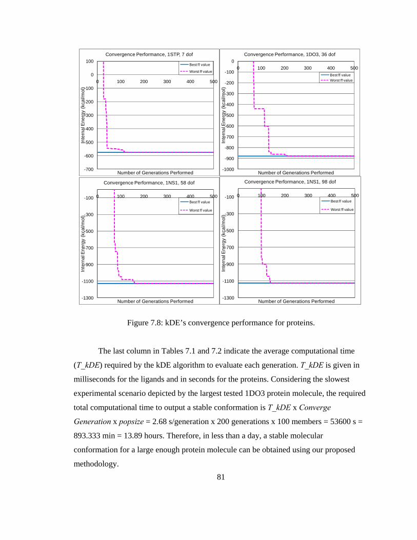
81

-700

-600

-500

-400

-300

-200

-100

0

100

0 100 200 300 400 500In

tern

al E

nerg

y (k

cal/m

ol)

Number of Generations Performed

Convergence Performance, 1STP, 7 dof

Best ff value

Worst ff value

-1000

-900

-800

-700

-600

-500

-400

-300

-200

-100

00 100 200 300 400 500

Inte

rnal

Ene

rgy

(kca

l/mol

)

Number of Generations Performed

Convergence Performance, 1DO3, 36 dof

Best ff valueWorst ff value

-1300

-1100

-900

-700

-500

-300

-100 0 100 200 300 400 500

Inte

rnal

Ene

rgy

(kca

l/mol

)

Number of Generations Performed

Convergence Performance, 1NS1, 58 dof

Best ff value

Worst ff value

-1300

-1100

-900

-700

-500

-300

-100 0 100 200 300 400 500

Inte

rnal

Ene

rgy

(kca

l/mol

)

Number of Generations Performed

Convergence Performance, 1NS1, 98 dof

Best ff value

Worst ff value

Figure 7.8: kDE’s convergence performance for proteins.

The last column in Tables 7.1 and 7.2 indicate the average computational time

(T_kDE) required by the kDE algorithm to evaluate each generation. T_kDE is given in

milliseconds for the ligands and in seconds for the proteins. Considering the slowest

experimental scenario depicted by the largest tested 1DO3 protein molecule, the required

total computational time to output a stable conformation is T_kDE x Converge

Generation x popsize = 2.68 s/generation x 200 generations x 100 members = 53600 s =

893.333 min = 13.89 hours. Therefore, in less than a day, a stable molecular

conformation for a large enough protein molecule can be obtained using our proposed

methodology.

Table 7.3: RMSD performance for the kDE algorithm.

min_RMSD 2.09287 1.17923 1.4377 0.10494 0.15097 0.06455 0.28908 0.49195 0.94288max_RMSD 2.40881 9.94754 2.17494 0.35987 0.23343 0.24466 0.31183 0.69252 1.25286

average_RMSD 2.26475 6.11804 1.82515 0.23722 0.1942 0.1698 0.30067 0.61111 1.09315molecules CYC NAD XK2 1STP

dof 13 11 4 7 9 22 36 58 981DO3

kDE1NS1

ProteinsLigands

At the end, the kDE algorithm outputs the final population of stable solutions or

the obtained global minimum region for any tested ligands and protein molecules. This

final population contains a large number of different molecular conformations for each

tested molecule that attains the same low-energy value. However, to evaluate the

structural feasibility of each obtained molecular solution, we have calculated their Root

Mean Square Deviation (RMSD) in Angstroms from their corresponding crystal

structure. Generally, lower RMSD values indicate closer resemblance between observed

and predicted structures with RMSD values below or near 2.0 usually considered

being sufficiently close.

oA

As shown in Table 7.3, the kDE algorithm succeeded to identify stable structures

with RMSD values in the range of 0.10 to 0.94 for any tested protein and in the range of

1.18 to 2.09 for the tested ligands. This means that the results of the kDE method lie

within the acceptable structural range of [0, 3) for all tested molecules. Therefore, the

kDE approach outputs a large number of alternative stable molecular conformations that

can be clustered based on their structures to identify those closest to their crystal

structure.

7.4.5 Conclusions

This section presented a new kinematics-based differential evolution (kDE) model

for effectively searching for low-energy molecular conformations. The proposed model

consists of two modules: the pre-computation and the DE-loop. At the pre-computation

module, a molecule is represented as a highly articulated body able to adopt different

82

molecular conformations. At the DE-loop, a differential evolution algorithm is used as a

direct search technique towards low-energy molecular conformations. Computer

implementation and results demonstrate that the proposed kDE approach rapidly and

accurately finds low-energy (stable) molecular conformations for molecular structures of

different size, shape and topology. Results also show that the kDE algorithm attains a

very good convergence performance while it outputs the global minimum region for any

tested molecule. This region provides a number of alternative stable molecular solutions

that have the same low internal energy value. As demonstrated the proposed kDE model

outputs sufficient molecular conformations with RMSD values below or near 2.0 .

The predicted molecular conformations can then be clustered based on their structure

similarity to identify those closest to their crystal structure.

oA

7.5 Proposed BioDE Approach

This section presents a new algorithmic scheme called Biological Differential

Evolution (BioDE) to minimize the molecular energy based on the differential evolution

algorithm presented in Section 7.3 and the hierarchical data structure presented in

Chapter 6. The proposed BioDE utilizes our previously developed data structure called

g.eBGF, as a surrogate approximation model to reduce the number of exact evaluations,

speed molecular conformational search, and reduce the algorithm’s convergence rate as

discussed in this section.

7.5.1 BioDE Overview

83

The proposed BioDE methodology is a novel, generic evolutionary and

geometric-based direct search technique to identify molecules’ minimum internal energy.

The BioDE algorithm aims to effectively identify stable conformations for any molecular

structure regardless of type, size and shape while considering the underlying chemical

information. The main algorithmic difference between the kDE and BioDE approaches is

that the latest utilizes our previously developed g.eBGF data structure as a primary filter

of molecules’ feasibility to speed convergence.

Figure 7.9: Overview of the proposed BioDE approach.

Figure 7.9 illustrates the overview of the proposed BioDE approach. As shown in

Figure 7.9, the BioDE approach employs two modules: the pre-computation and the DE-

loop modules. At the pre-computation stage, a geometric interpretation of the inter-

atomic interactions is performed to set the constraints under which a molecular

conformation is considered as feasible as discussed in Section 3.3. During this stage, our

previously developed g.eBGF data structure is utilized as a primary filter for feasible

molecular conformations. As shown in Figure 7.9, a molecular conformation (coordinate

file) is input into the BioDE algorithm. The pre-selected dof (TorsionAtoms file) for a

molecular structure are defined to form the atom groups. To further simplify the

macromolecular representation, the backbone atom cluster(s) is split into smaller groups

of atoms based on the concepts discussed in Section 5.3. A bounding volume hierarchy

(BVH) denoted as a balanced binary tree is constructed for the initial molecular

conformation to capture the molecular shape at successive level of details and to assist in

84

85

the collision detection queries. The type of bounding volumes used in this work is

spheres since spheres are invariant to rotations and simpler to implement.

At the DE-loop module, the DE algorithm presented in Section 7.3 is used to

direct the search towards low-energy minima or stable molecular conformations. For each

candidate molecular conformation (population member) in each generation, the BVH is

updated and a collision detection scheme is performed to determine the feasibility of the

molecular conformation. The fundamental concept underneath the proposed collision

detection algorithm is the geometric interpretation of the chemical information provided

by the intra-molecular energy. If the collision detection queries output a feasible

molecular conformation, then the fitness function for that conformation measures the van

der Waals energy value; otherwise, a penalty function is computed to reject the specific

unfit solution. This is an iterative process to provide better fitted individuals. As soon as

the termination criterion denoted by the maximum allowed number of generations

performed is satisfied, the BioDE algorithm outputs the final population of stable

molecular conformations. This final population describes the global minimum region that

provides a number of different molecular conformations that attain the same low-energy

value and hence, provides alternative stable molecular solutions.

7.5.2 Input Files

The proposed BioDE methodology consists of two modules: the pre-computation

and the DE-loop modules. Our proposed algorithm requires two input files for the pre-

computation module: the atomic coordinate information (coordinate file) and the atoms

within the molecular topology that share a torsion bond (torsionAtoms file). In addition,

the BioDE algorithm requires one input file for the DE-loop module, the chromosome

file.

The coordinate input file is usually the PDB file obtained from the Protein Data

Bank (PDB) [Berman 2000]. The VMD software [Humphrey 1999] is used to define the

atoms’ connectivity information for proteins and to construct the coordinate input file.

The torsionAtoms input file is the file that describes the atoms that share a torsion bond

and hence, depicts the number and the location of the pre-selected dof considered for

each experiment. To create this file, the concepts about the allowed number and location

of the pre-selected dof (torsion bond angles) presented in Section 6.2 and Section 6.3 are

incorporated for studying chemically-feasible molecular conformations.

Finally, the chromosome file denotes the required dof or design variables for

representing a candidate molecular conformation. Similar to nature, each chromosome

structure through the defined genotype embodies a candidate solution to the problem

under consideration whereas the chromosome genes represent the design variables that

take values within their constrained space. Hence, to direct the search towards low-

energy molecular conformations, the chromosome for the BioDE algorithm should

represent a candidate molecular conformation with the genes accounting for the dof or

the torsion bond angles in the [0, 360) range. iθ

7.5.3 Pre-Computation Module

During the pre-computation module, once the two input files (coordinate and

torsionAtoms files) have been defined, groups of atoms are formed following the concept

presented in Section 4.2 to simplify the molecular representation. If the tested molecular

structure is a protein molecule, then an additional step within the BioDE algorithm is

performed for splitting the backbone atom cluster (or clusters in the case of multiple

chain proteins) into smaller AtomGroups as discussed in Section 5.3. As soon as the atom

clusters both rigid and flexible have been defined, a bounding volume hierarchy (BVH)

depicted as a balanced binary tree is introduced to capture the shape of the molecule at

successive levels of detail and to facilitate the collision detection search for overlapping

atoms. The BVH is built only once at the beginning of the algorithm during the pre-

computation stage.

86

7.5.4 DE-Loop Module

At the beginning of the DE-loop module, similarly to the kDE model, the

chromosome file is input to the BioDE algorithm to define a candidate molecular

conformation as a function of the torsion bond angles iθ as shown in Figure 7.4. The DE

algorithm evolves a fixed population size (popsize) composed of candidate problem

solutions (population members or chromosomes), randomly initialized. Consequently,

each population member corresponds to a candidate molecular conformation. After

initializing the population, an iterative process starts to direct the search towards better

fitted population members or stable molecular solutions. At each generation (iteration), a

new population of candidate solutions (conformations) is produced until a stopping

criterion is satisfied. In this work, the termination criterion is the maximum allowed

number of generations performed (maxgen). At each generation, each population member

(candidate molecular conformation) can be replaced with a new generated one. The new

member is a linear combination between a randomly selected member (the donor) and a

difference between two other randomly selected members. Genetic operators (mutation,

crossover, and selection) are applied to provide the next generation of better fitted

candidate problem solutions (molecular conformations).

For each candidate molecular conformation (population member) in each

generation, the BVH is updated and a collision detection scheme is performed to

determine the feasibility of the molecular conformation. The BVH is updated for each

new molecular conformation as the torsion angles are randomly modified. As soon as the

BVH is updated, the collision detection algorithm presented in Chapter 5 and Chapter 6,

is performed to search for potential overlaps between non-bonded atoms within the tested

molecular conformation.

One of the major components in an evolutionary-based algorithm is to define an

appropriate fitness function ff. The ff plays the role of the evaluation criterion for each

candidate problem solution. Choosing a “good” mathematical representation for the ff is

very important and challenging since it directs the search towards the optimal solution or

in our case, towards stable molecular conformations. A good mathematical representation 87

for the ff is the use of the total intra-molecular energy. However, as discussed in Section

3.2, this would result in a very slow progress towards the search for low-energy solutions.

Therefore, we propose an alternative fitness function definition utilizing our developed

g.eBGF data structure as an approximation model of molecules feasibility. In other

words, if the collision detection algorithm outputs a feasible molecular conformation,

then the fitness function for that conformation measures the van der Waals (VDW)

energy value, else a penalty function is computed to reject the specific bad solution as

shown by Eqn. 7.9:

⎪⎪

⎩

⎪⎪

⎨

⎧

−⋅=⋅=

=

=

∑ +ρ∑ −==

= =

wommpenalty

feasibleonconformatiifr

A

r

BalVDWpotenti

ffm

kkjki

m

kkjik

n

i

n

j ij

ij

ij

ij

rrdd /)1(

-

1,,

22

1,,,0

21 1

612

)()(

∑∑(7.9)

Where, and are the equilibrium distance and the relative inter-atomic distance

for the kth colliding non-bonded pair of atoms i and j, and m is the total number of

colliding atom pairs within the tested molecular conformation. As shown in Eqn. 7.9, the

proposed penalty function is a distance function between the equilibrium and the relative

inter-atomic distances for each overlapping atom pair within the molecular topology. The

purpose of using this penalty function is to train the algorithm to avoid searching space

regions mostly occupied by infeasible solutions. This training is defined as a function of

“how” much infeasible these solutions are or alternatively how many overlapping atom

pairs exist within the examined molecular conformation.

kd ,0 kjid ,,

7.5.5 Computer Implementation and Results

The presented method and algorithms have been implemented on a dual 3.0 GHz

CPU workstation using Visual C++, Visual Basic programming languages, OpenGL and

CGAL libraries [CGAL]. As shown in Figure 7.10 and Figure 7.11, different molecular

structures with different number of atoms, chains, residues and dof are tested with the

proposed BioDE approach. The example molecules were obtained from the Protein Data

88

Bank (PDB) [Berman 2000] with PDB IDs as follows: BTN, CYC, NAD, XK2 ligand

molecules and 1STP, 1DO3, 1NS1 protein molecules. These molecules are the same ones

used to evaluate the kDE method presented in Section 7.4. Using these molecules as the

test-bed for the BioDE algorithm, a performance comparison between BioDE and kDE

models is provided in the following Section 7.6.

Figure 7.10: Ligand molecules tested with the BioDE model.

Figure 7.11: Protein molecules tested with the BioDE model.

The termination criterion for the BioDE algorithm was set to maxgen = 500

generations performed and popsize = 100 candidate molecular conformations (population

members) considered in each generation for each experiment except for the 1NS1

protein. For the 1NS1 protein, given the large number of dof considered in each

experimental scenario, the maxgen was set to 600 generations and 300 population

89

members used as popsize. Finally, the DE’s control parameters used in all experiments

were F = 0.6 for the mutation parameter, and Cr = 0.45 for the crossover probability.

Tables 7.4 and 7.5, show a representative list of the performance analysis for the

proposed BioDE approach on different ligand and protein molecules, respectively. As

shown in Tables 7.4 and 7.5, the first columns indicate the PDB IDs for the tested

molecules. The second column on each table specifies the number of atoms within each

molecular structure, whereas the third column denotes the dof considered in each

scenario. The preselected dof for each experiment are the chemically-allowed dof for the

molecules.

Table 7.4: Performance analysis of the proposed BioDE algorithm on ligands.

Ligands Number Atoms DOF E_crystal E_BioDE Conv.Gener. T_BioDE (kcal/mol) (kcal/mol) (ms)

BTN 16 3 ‐3.25 ‐3.59 87/500 1.86CYC 43 13 ‐16.75 ‐17.93 132/500 2.07NAD 44 11 ‐12.42 ‐13.68 162/500 2.31XK2 46 4 ‐10.91 ‐11.35 117/500 2.36

Table 7.5: Performance analysis of the BioDE algorithm on proteins.

Proteins Number Atoms DOF E_crystal  E_BioDE Conv.Gener. T_BioDE (kcal/mol) (kcal/mol) (s)

1STP 903 7 ‐554.78 ‐576.16 187/500 0.349 ‐876.37 180/500 2.4922 ‐881.53 188/500 2.4936 ‐879.38 175/500 2.4642 ‐1127.49 150/600 2.2858 ‐1128.061 127/600 2.298 ‐1126.076 150/600 2.21

2342

‐876.33

‐1126.35

1DO3

1NS1

2466

To evaluate our proposed BioDE molecular model, we compared our results with

the results for crystal structures published in the Protein Data Bank [Berman 2000].

Analytically, we calculated the van der Waals (VDW) energy for each crystal structure

(E_crystal) and compared it against the VDW energy value obtained from the BioDE

90

algorithm (E_BioDE). As shown in Tables 7.4 and 7.5, the BioDE algorithm succeeded

to converge in a smaller VDW energy value compared with the corresponding VDW

energy for the crystal structure on all the performed experiments. This phenomenon

occurs since when measuring a molecule’s internal energy all the incorporated energy

terms (i.e. VDW or electrostatic forces) are in fact an approximation of the potential

energy and not the molecule’s free energy, which among other requires entropy

calculations. Therefore, the proposed BioDE algorithm succeeded to output a stable

molecular conformation for all the tested molecules. This is very important given that

most evolutionary algorithms suffer from local minima traps.

91

-4

-3.8

-3.6

-3.4

-3.2

-3

-2.8

-2.6

-2.4

-2.2

-20 100 200 300 400 500

Inte

rnal

Ene

rgy

(kca

l/mol

)

Number of Generations Performed

Convergence Performance, BTN Ligand

Best ff valueWorst ff value

 -40

-30

-20

-10

0

10

20

30

40

0 100 200 300 400 500

Inte

rnal

Ene

rgy

(kca

l/mol

)

Number of Generations Performed

Convergence Performance, CYC Ligand

Best ff valueWorst ff value

 

-20

-10

0

10

20

30

40

0 100 200 300 400 500Inte

rnal

Ene

rgy

(kca

l/mol

)

Number of Generations Performed

Convergence Performance, NAD Ligand

Best ff value

Worst ff value

 -13

-12

-11

-10

-9

-8

-7

-6

-50 100 200 300 400 500

Inte

rnal

Ene

rgy

(kca

l/mol

)

Number of Generations Performed

Convergence Performance, XK2 Ligand

Best ff valueWorst ff value

 

Figure 7.12: Convergence performance of the BioDE method for ligands.

The sixth column (Conv.Gener.) in Tables 7.4 and 7.5 indicates the BioDE

algorithm’s convergence generation. This convergence generation is the generation where

the fitness function of the worst population member equals with the fitness function of

the best individual, which is also the same as the E_BioDE value. Figure 7.12 shows the

convergence performance of the BioDE algorithm over the different tested ligand

molecules. Figure 7.13 demonstrates BioDE’s convergence performance for 1NS1, 1DO3

and 1STP proteins, over different number of dof. As shown in these figures, the BioDE

algorithm attains a very good convergence performance. This is very important given that

one of the main drawbacks in an evolutionary-based algorithm is the convergence

uncertainty.

92

-800

-700

-600

-500

-400

-300

-200

-100

0

100

0 100 200 300 400 500

Inte

rnal

Ene

rgy

(kca

l/mol

)

Number of Generations Performed

Convergence Performance, 1STP, 7 dof

Best ff valueWorst ff value

-1000

-800

-600

-400

-200

0

200

0 100 200 300 400 500

Inte

rnal

Ene

rgy

(kca

l/mol

)

Number of Generations Performed

Convergence Performance, 1DO3, 36 dof

Best ff value

Worst ff value

-1300

-1100

-900

-700

-500

-300

-100

100

0 100 200 300 400 500

Inte

rnal

Ene

rgy

(kca

l/mol

)

Number of Generations Performed

Convergence Performance, 1NS1, 58 dof

Best ff value

Worst ff value

-1300

-1100

-900

-700

-500

-300

-100

100

300

0 100 200 300 400 500

Inte

rnal

Ene

rgy

(kca

l/mol

)

Number of Generations Performed

Convergence Performance, 1NS1, 98 dof

Best ff valueWorst ff value

 

Figure 7.13: Convergence performance of the BioDE method for proteins.

The last column in Tables 7.4 and 7.5 indicates the average computational time

(T_BioDE) required by the BioDE algorithm to evaluate each generation. The T_BioDE

is given in milliseconds for the ligands and in seconds for the proteins.

Similarly to the kDE model, at the end of the BioDE algorithm the final

population of stable solutions is obtained. This final population contains a large number

of different molecular conformations for each tested molecule that attains the same low-

energy value. To evaluate the structural feasibility of each obtained molecular solution,

we have calculated their Root Mean Square Deviation (RMSD) in Angstroms from their

corresponding crystal structure. Generally, lower RMSD values indicate closer

resemblance between observed and predicted structures with RMSD values below or near

2.0 usually considered being sufficiently close. oA

Table 7.6: RMSD performance of the BioDE algorithm.

min_RMSD 3.13168 1.17923 1.4377 0.08278 0.00335 0.29471 0.44538 0.48878 0.88915max_RMSD 12.6164 10.0217 2.17394 0.50226 0.35859 0.51279 0.77254 0.6937 1.2621

average_RMSD 8.70862 6.21425 1.82367 0.33243 0.27351 0.40033 0.64655 0.60418 1.08408molecules CYC NAD XK2 1STP

dof 13 11 4 7 9 22 36 58 98

Ligands

1DO3 1NS1BioDE

Proteins

As shown in Table 7.6, the BioDE algorithm succeeded to identify stable

structures with RMSD values in the range of 0.003 to 0.889 for any tested protein and

with RMSD values of 1.17 and 1.43 for NAD and XK2 ligands, respectively. However,

the result for CYC ligand is relatively higher. This means that the BioDE method lies

within the acceptable structural range of [0, 3) for all tested molecules except for the

CYC ligand.

7.5.6 Conclusions

Section 7.5 presented a novel generic computational geometric and evolutionary-

based molecular methodology called biologically-inspired differential evolution (BioDE)

93

94

approach for effectively identifying chemically-feasible and low-energy conformations

for molecules of different type, size, shape and topology. The proposed BioDE approach

employs a differential evolution algorithm to direct the search towards stable molecular

conformations. It incorporates the underlying geometric interpretation of the inter-atomic

interactions as a primary filter for feasible molecular conformations to reduce the number

of exact evaluations performed and to speed the molecular conformational search.

Computer implementation and results demonstrate that the proposed BioDE algorithm

accurately and rapidly identifies low-energy molecular conformations for different

molecular structures. The proposed BioDE approach attains a very good convergence

performance while it outputs the global minimum region for the tested molecule. It also

provides a set of alternative low-energy molecular conformations for researchers to test

during molecular design. As demonstrated the BioDE algorithm outputs sufficient

molecular conformations for all the tested proteins and most of the tested ligands. These

predicted molecular conformations can then be clustered based on their structures to

identify those closest to their crystal structure.

7.6 Comparison Between the kDE and BioDE Approaches

The main algorithmic difference between the BioDE and kDE approaches is that

the BioDE algorithm utilizes the g.eBGF technique presented in Chapter 6, as a surrogate

approximation model to speed convergence and to reject any unfeasible generated

solution. This is possible through a penalty function that is assigned to those individuals

(population members or else conformations) that attain overlapping atoms within their

generated topology. Therefore, the g.eBGF algorithm is used by the BioDE model as a

primary filter of molecules’ feasibility. If a candidate molecular conformation passes this

first filtering step (no overlapping atoms: penalty = 0), then the fitness function (ff)

measures its VDW energy to define the individual’s feasibility level. Different to this

algorithmic scheme, the kDE model is a much simpler methodology that calculates the

VDW energy for all candidate molecular conformations to determine their fitness level.

As demonstrated in Section 7.4.4 and Section 7.5.5, both kDE and BioDE

methods are effectively pushing the molecular conformational search towards the global

minimum region occupied by a large number of alternative stable conformations. Both

methods succeeded in identifying molecules’ stability for any type of molecular structure

tested while attaining a very good convergence performance. However, given the

algorithmic difference of the two approaches, the main question lies in which from the

proposed direct search algorithms perform better.

Table 7.7: Comparison between kDE and BioDE approaches.

Proteins Number Atoms DOF BioDE_Conv.Gener. kDE_Conv.Gener. T_BioDE (s) T_kDE (s)1STP 903 7 187/500 118/500 0.34 0.35

9 180/500 189/500 2.49 2.5522 188/500 191/500 2.49 2.6236 175/500 211/500 2.46 2.5842 150/600 170/600 2.28 2.358 127/600 172/600 2.2 2.2798 150/600 138/600 2.21 2.25

1DO3 2466

1NS1 2342

To evaluate and validate the kDE and BioDE models, we compared the obtained

molecular structures (kDE and BioDE outputs) against their corresponding crystal

structures published in PDB [Berman 2000]. Two different performance assessments

were performed: an energy-oriented (lowest obtained VDW energy values) and a

structural-based (RMSD) performed. To compare the BioDE algorithm against the kDE

method, we have tested both methods using the same molecular structures and

workstations.

Computer implementation and results demonstrate that for ligand molecules both

methods perform approximately the same. For protein molecules, there is no significant

computational time improvement of using the BioDE approach for identifying the

molecular feasibility as shown in Table 7.7. However, the BioDE provides a convergence

enhancement over the kDE method for proteins. As shown in Table 7.7, the BioDE

algorithm converged about 25% faster on over 70% of the experiments performed.

95

96

Therefore, the BioDE algorithm provides convergence enhancement while identifying

alternative low-energy molecular conformations.

In regards to the identified molecular structure, both the kDE and BioDE methods

succeeded to converge in conformations close to the crystal structures for any tested

flexible protein and for most of the examined flexible ligands. As shown in Tables 7.3

and 7.6, the RMSD values obtained by the BioDE approach are much smaller compared

with those obtained by the kDE model for all the tested proteins but 1DO3 protein with

36 dof. Regarding the predicted ligand structures, it appears that both models had the

same performance for all the tested ligands but CYC ligand where the kDE model

calculated a smaller RMSD value.

97

Chapter 8

Conclusions, Discussion and Future Work

The scope of this chapter is to provide a summary of the research methodologies

presented to study the molecular flexibility and stability mechanism. The general

conclusions, including encountered challenges and limitations, are also discussed here,

followed by a description of future research work.

8.1 Research Summary

This research work presented three different molecular models: the g.eBGF, kDE

and BioDE algorithms. Two computational geometric models (BGF and eBGF) were also

implemented to assist in the development of the g.eBGF approach. The g.eBGF

algorithm is responsible for rapidly and accurately identifying the molecular feasibility

whereas the kDE and BioDE algorithms direct the conformational search towards stable

molecular conformations. All proposed algorithms rely upon the basic algorithmic

concepts for kinematically representing the molecular structure. They also integrate

concepts from robotics, evolutionary-oriented optimization, computational geometry and

computational biology.

The core algorithmic architecture of the BGF, eBGF and g.eBGF methods is a

two layer hierarchical data structure that kinematically represents the molecular

flexibility using a bounding volume hierarchy to assist in the collision detection. The

BGF or BioGeoFilter approach effectively identifies the molecular feasibility for ligands

(drug-like) molecules and performs really well in identifying the molecular feasibility

rapidly and accurately. In addition, the BGF algorithm satisfies the haptic-rate

requirement, enabling real-time ligand design.

98

The eBGF or enhanced BioGeoFilter algorithm presented in Chapter 5 is a

significant enhancement of the BGF approach as it can model macromolecules such as

proteins. The proposed eBGF method effectively studies the flexibility mechanism of

proteins while addressesing current limitations in protein modeling. Therefore, the eBGF

algorithm is presented as a rapid and accurate filtering tool of proteins’ feasibility,

significantly facilitating protein modeling and design.

The generic eBGF or g.eBGF approach discussed in Chapter 6 is a generic

molecular modeling tool able to represent the flexibility mechanism of any molecule

independently of type, size, shape and topology. The proposed g.eBGF model is the

generic enhancement of the eBGF algorithm. The g.eBGF model considers some

chemically-based constraints to provide more realistic and chemically-feasible molecular

conformations compared with those of the eBGF. This is a significant improvement in

computational-aided molecular design.

The kDE and BioDE models presented in Chapter 7 direct the molecular

conformational search towards low-energy (stable) solutions. To achieve this, both

models employ our previously developed DE algorithm. The main algorithmic difference

is that the BioDE algorithm utilizes the g.eBGF method as a surrogate approximation

model to speed convergence. Both approaches effectively identify stable molecular

conformations for any molecular structure independently of type, size, shape and

topology. Both models also succeed in providing the global minimum region for any

tested molecule while attaining a very good convergence performance. However, the

BioDE algorithm slightly speeds the computational time for identifying stable protein

solutions while significantly speeding the algorithm’s convergence rate in protein

conformational search.

To evaluate and validate our proposed research work, we have tested the BGF,

eBGF and g.eBGF algorithms against the traditional energy calculation approach. All

methods succeeded in significantly decreasing the computational time for identifying

feasible molecular conformations without sacrificing accuracy.

To evaluate and validate the kDE and BioDE models, we compared the obtained

molecular structures (kDE and BioDE outputs) against the corresponding crystal

99

structures published in [Berman 2000]. Two different performance assessments were

performed: an energy-oriented and a structural-based. Both methods succeeded to

converge in a smaller VDW energy value compared with the VDW energy for the

corresponding crystal structure, thus identifying the molecules’ stability state. The

structures of the obtained molecular conformations were compared to the corresponding

crystal structure using the Root Mean Square Deviation (RMSD). Both methods

managed to output molecular conformations close to the crystal structure for all the tested

proteins and for most of the tested ligands while attaining a very good convergence

performance.

8.2 Future Research Work

Studying the atomic-scale processes is an open research problem that requires

many disciplines to collaborate for providing reliable results and enabling

bionanotechnology applications. Our proposed research work facilitates the modeling of

flexible molecules and the identification of stable or low-energy conformations. This

work can be used in molecular docking, nanoscale assembly problems and towards the

development of an indispensable computer-aided design tool for bionanotechnology. To

build a fully functional molecular system, many challenges need to be addressed and

many different research pathways can be pursued.

One of the fundamental principles of Industrial Systems Engineering is that the

first step in a product/system development is the idea itself, followed by the design and

production stages. It is also well known that any candidate product/system modifications

are better performed during the design stage for the product/system to be cost-effective.

Under these assumptions, future research work lies within the real-time visualization of

the molecular interactions during the design stage so that fully functional bionanoscale

products can be designed and evaluated prior to actual fabrication. In this research work,

new methods have been investigated that provide real-time force feedback using haptic

devices. These devices are currently used to manipulate virtual molecules and to feel the

forces as the molecules interact with each other providing an essential design and

100

visualization tool. However, to achieve a realistic molecular representation, continuous

visualization as well as sense of touch to the users, a rapid molecular tool is essential that

satisfies the haptic-rate requirement. To achieve haptic-rate performance, the rapid update

and modeling of molecular conformations are the main prerequisites.

Focusing towards this objective, our research work presented the BGF algorithm

for real-time ligand modeling that satisfies the haptic-rate requirement. Although the

proposed eBGF and g.eBGF are fast molecular feasibility tools, they do not satisfy the

haptic constraint. Further research work is required for speeding the identification of a

protein’s flexibility mechanism to allow haptic interaction between macromolecules. As

shown in Table 6.1, the bottleneck function of the proposed g.eBGF algorithm is the

update of the bounding volume hierarchy. The GPU-oriented modeling technique seems a

promising approach for speeding the BVH update and hence, to enable haptic interactions

between flexible proteins or between a flexible ligand and a flexible protein. As soon as a

molecular modeling system that satisfies the haptic constraint is developed, haptic

devices can be utilized to study the real-time molecular docking and/or assembly

problems.

In addition, the main limitation of the proposed kDE and BioDE methods is that

both methods require approximately one to three days outputting a stable molecular

solution. Although these results are significantly faster than current literature, they are

unsuitable for real-time haptic design. To allow haptic molecular interactions in a virtual

environment, further research work is required to speed the molecular conformational

search. Parallel computing is a very promising approach towards this direction. In other

words, instead of using the DE algorithm presented in Section 7.3, we could utilize

parallel computing such as a parallel DE algorithm to direct the molecular conformational

search. This is expected to enable the haptic manipulation of molecules in a virtual

environment and facilitate bionanoscale design and engineering.

An off-line improvement of the current research work is to target the molecular

docking/assembly problem through a molecular path planning approach. Under this

perspective, the BioDE or kDE algorithm can be enhanced by using a modified

chromosome structure, which represents a candidate problem solution. Currently in the

101

kDE and BioDE models, the genes of the chromosome measure the torsion bond angles

representing a candidate molecular conformation. The chromosome for the molecular

path planning operation will depict both the torsion bond angles and the way-points along

the “optimum” trajectory”. This trajectory is the “optimum” path of a totally flexible

ligand towards the cavity site of a total flexible protein. The location of the cavity site

will be assumed to be known and will define the last chromosome gene, signifying the

molecular path planning target.

Alternatively, an on-line molecular path-planning improvement can be envisioned

by utilizing the aforementioned concepts about GPUs and/or parallel computing as well

as haptic-rendering approaches. Using haptics to control a flexible ligand around a

flexible protein with unknown binding site may lead to the identification of the protein’s

binding site. This may also provide strong insights for identifying feasible land-marks

(coordinate points) along the molecules’ “optimum” trajectories. These land-marks may

be used as path planning targets through the corresponding chromosome’s genes to speed

the algorithm convergence.

As mentioned above, studying the molecular flexibility is only a step closer to

fully understand and model the molecular behavior. Molecules are very flexible bodies in

nature that usually exist in a solvent environment. Further research is required to

holistically model the molecular interactions in a solvent environment. Additionally,

future research work lies in studying the protein folding problem for providing structural

insights for artificial macromolecular design. To conclude, bionanoscale research is still

at the early stages and all the possible research ideas, concepts and pathways can be

limited only by the researcher’s vision and imagination.

102

References

1. Adcock S.A, McCammo JA. Molecular Dynamics: Survey of Methods for Simulating the Activity of Proteins. Chem. Rev. 2006; 106: 1589-1615.

2. Agarwal PK, Guibas L, Nguyen A, Russell D, Zhang L. Collision detection for deforming necklaces. Computational Geometry: Theory and Applications 2004; 28(2-3).

3. Angulo VR, Cortez J, Simeon T. BioCD: an efficient algorithm for self-collision and distance computation between highly articulated molecular models. Conference on Robotics: Science and Systems, Boston, MA, 2005.

4. Apaydin MS, Guestrin CE, Varma C, Brutlag DL, and Latombe JC. Stochastic Roadmap Simulation for the Study of Ligand-Protein Interactions. Bioinformatics 2002a; 18(2): S18-S26.

5. Apaydin MS, Brutlag DL Guestrin CE, Hsu D, and Latombe JC. Stochastic Conformational Roadmaps for Computing Ensemble Properties of Molecular Motion. Proc. Workshop on the Algorithmic Foundations of Robotics (WAFR ) 2002b.

6. Apaydin MS, Guestrin CE, Hsu D, Brutlag DL, and Latombe JC. Stochastic Roadmap Simulation: An Efficient Representation and Algorithm for Analyzing Molecular Motion. Journal of Computational Biology 2003; 10(3-4).

7. Baxter CA, Murray CW, Clark DE, Westhead DR, Eldridge MD. Flexible docking using tabu search and an empirical estimate of binding affinity. Proteins: Structure, Function, and Genetics 1998; 33: 367-382.

8. Bayazit OB, Song G, and Amato NM. Ligand Binding with OBPRM and Haptic User Input: Enchancing Automatic Motion Planning with Virtual Touch. Technical Report TR00-025, Department of Computer Science, Texas A&M University, College Station, Texas, 77843-3112, October 9, 2000.

9. Bayazit OB. Solving Motion Planning Problems by Iterative Relaxation of Constraints. PhD Dissertation, Department of Computer Science, Texas A&M University, May 2003.

103

10. Berman HM, Westbrook J, Feng Z, Gilliland G, Bhat TN, Weissig H, et al. The Protein Data Bank. Nucleic Acids Research 2000; 28: 235-242.

11. Bitello R, and Lopes HS. A Differential Evolution Approach for Protein Folding. Proceedings of the IEEE Symposium on Computational Intelligence in Bioinformatics and Computational Biology 2006: 1-5.

12. Brintaki A and Nikolos IK. Coordinated UAV Path Planning Using Differential Evolution. Transactions of the Operations Research International Journal 2005c; 5(3).

13. Brintaki AN, Lai-Yuen SK. BioGeoFilter.: A Tool For Identifying Geometrically Feasible Molecular Conformations In Real-Time For Bionanomanufacturing. Transactions of the North American Manufacturing Research Institution of SME, NAMRC 36, Monterrey, Mexico, 2008a: 153-160.

14. Brintaki AN, Lai-Yuen SK. eBGF: An Enhanced Geometric Hierarchical Representation for Protein Modeling and Rapid Self-Collision Detection. Transactions of the Computer-Aided Design and Applications Journal, 2009a; 6 (6): 625-638.

15. Brintaki AN, Lai-Yuen SK. eBGF: An Enhanced Geometric Hierarchical Representation for Protein Modeling and Rapid Self-Collision Detection. Proceedings of the International Computer-Aided Design and Applications Conference, Orlando, FL, 2008b.

16. Brintaki AN, Lai-Yuen SK, and Nikolos IK. BioDE: A Biological Differential

Evolution Approach for Molecular Design. submitted to IEEE Transactions on Evolutionary Computation, 2010a.

17. Brintaki AN, Lai-Yuen SK, and Nikolos IK. A Kinematics-Based Differential

Evolution Method for Molecular Design. To be presented at the IERC 2010, Cancun Mexico, June 5-9, 2010b.

18. Brintaki AN, Lai-Yuen SK, and Nikolos IK. A Hybrid Molecular Model Towards Low-Energy Conformations. Proceedings of the IERC09, Institute of Industrial Engineers (IIE) Annual Conference & Expo 2009, Miami, FL, May30-June3, 2009b.

19. Brintaki AN, Lai-Yuen SK, and Nikolos IK. A Kinematics Based Heuristic Approach

to Minimiza Molecular Conformational search. To be presented at the International Computer-Aided Design (CAD) Conference & Exhibition, Dubai, United Arab Emirates, June 21- 25, 2010c.

 

104

20. Brintaki AN, Lai-Yuen SK, and Nikolos IK. A Kinematics Based Heuristic Approach to Minimiza Molecular Conformational search. Submitted at Computer-Aided Design and Applications Journal, 2010d.

21. Brunner RK, Phillips JC, Laxmikant VK. Scalable Molecular Dynamics for Large Biomolecular Systems. Conference of High Performance Networking and Computing. Proceedings of the ACM/ IEEE on Supercomputing 2000; (45), ISBN: 0-7803-9802-5.

22. Chiang TH, Apaydin MS, Brutlag DL, and Latombe JC. Predicting Experimental Quantities in Protein Folding Kinetics Using Stochastic roadmap Simulation. International Conference on Research in Computational Molecular Biology (RECOMB) 2006.

23. Cortes J, Simeon T, and Laumond J P. A Random Loop Generator for Planning the Motions of Closed Kinematic Chains Using PRM Methods. Proceedings of the IEEE International Conference on Robotics and Automation, Washington, DC, May 2002.

24. Cortes J. Motion Planning Algorithms for General Closed-Chain Mechanisms. PhD Thesis; Institute National Polytechnique de Toulouse 2003.

25. Cortes J, Simeon T, Angulo VR, Guieysse D, Simeon MR, and Tran V. A Path Planning Approach for Computing Large-Amplitude Motions of Flexible Molecules. Bioinformatics 2005; 21(1): i116-i125.

26. Cortes J, Jaillet L, and Simeon T. Molecular Disassembly With Rrt-Like Algorithms. IEEE International Conference on Robotics and Automation, Roma, Italy, 10-14 April 2007.

27. CGAL. http://www.cgal.org. Computational Geometry Algorithms Library.

28. Chong SY, and Tremayne M. Compined Optimization Using Cultural and Differential Evolution: Application to Crystal Stucture Solution From Powder Diffraction Data. Chemistry Communication, Royal Society of Chemistry Journal 2006; 4078-4080.

29. Damsbo M, Kinnear BS, Hartings MR, Ruhoff PT, Jarrold MF, and Ratner MA. Application of Evolutionary Algorithm Methods to Polypeptide Folding: Comparison with Experimental Results for Unsolvated Ac-(Ala-Gly-Gly)5-LysH+. PNAS 2004; 101(19): 7215-7222.

105

30. Dendzik Z, Kosmnder M, Dawid A, and Gbarski Z. Interaction Induced Depolarized Light Scattering From Ultrathin Ne Film Covering Single-Walled Carbon Nanotubes of Different Chiralities. Molecular Structure Journal 2005; 744-747 (3): 577-580.

31. Fischer K, and Gartner B. The Smallest Enclosing Ball of Balls: Combinatorial

Structure and Algorithms. SoCG’03, San Diego, California, June 8-10, 2003.

32. Giannakoglou KC. Design of Optimal Aerodynamic Shapes Using Stochastic Optimization Methods and Computational Intelligence. Progress in Aerospace Sciences 2002; 38: 43–76.

33. Goldberg DE. Genetic Algorithms in Search, Optimization and Machine Learning. Addison-Wesley 1989.

34. Gottschalk S, Lin MC, and Manocha D. OBBTree: A hierarchical structure for rapid interference detection. Comp. Graphics 30 (Annual Conf. Series) 1996: 171-180.

35. Grayson P, Tajkhorshid E, Schulten K. Mechanisms of selectivity in channels and enzymes studied with interactive molecular dynamics. Biophysical Journal 2003; 85: 36-48.

36. Hartenburg RS, and Denavit J. A kinematic notation for lower pair mechanisms based on matrices. Applied Mechanics Journal 1955; 77: 215-221.

37. Holland JH. Adaptation in Natural and Artificial Systems. The MIT Press 1992.

38. Humphrey W, Dalke A, Schulten K. VMD-Visual Molecular Dynamics, Molecular Graphics Journal 1999; 14: 33-38.

39. Jones G, Willett P, Glen RC, Leach AR, and Taylor R. Development and Validation of a Genetic Algorithm for Flexible Docking. Molecular Biology Journal 1997; 267: 727-748.

40. Kima H, Choib J, Kimc HW, Jung S. Monte Carlo Docking Simulations of Cyclomaltoheptaose and Dimethyl Cyclomaltoheptaose with Paclitaxel. Carbohydrate Research, 15 March 2002; 337(6): 549-555.

41. Lai-Yuen, SK, Lee Y-S. Interactive Computer-Aided Design for Molecular Docking and Assembly. Computer-Aided Design and Applications Journal 2006a; 3(1-4).

42. Lai-Yuen SK, Lee YS. Energy-Field Optimization and Haptic-Based Molecular Docking and Assembly Search System for Computer-Aided Molecular Design (CAMD). Proceedings of the 14th Symposium Haptic Interfaces for Virtual Environment and Teleoperator Systems, IEEE Virtual Reality Conference, Alexandria, VA, 2006b: 25-29.

106

43. La Valle SM, and Kuffnerr JJ. Rapidly-Exploring Random Trees: Progress and Prospects. Algorithmic and Computational Robotics, New Directions, WAFR 2000a.

44. La Valle SM, Finn PW, Kavraki LE, and Latombe JC. A Randomized Kinematics-Based Approach to Pharmacophore-Constrained Conformational Search and Database Screening. Computational Chemistry Journal 2000; 21(9): 731-747, 2000b.

45. La Valle SM, Finn PW, Kavraki LE, and Latombe JC. Efficient Database Screening for Rational Drug Design Using Pharmacophore-Constrained Conformational Search. Proceeding of the 3rd International Conference on Computational Biology, Lyon, France, 1999.

46. Lee Y-G, Lyons KW. Smoothing Haptic Interaction using Molecular Force Calculations. Computer-Aided Design Journal 2004; 36 (1): 75-90.

47. Leech J, Prins J.E, Hermans J. SMD: Visual Steering of Molecular Dynamics for Protein Design. IEEE Computational Science & Engineering 1996.

48. Lotan I, Schwarzer F, Halperin D, Latombe JC. Efficient Maintenance and Self-Collision Testing for Kinematic Chains. SoCG, Barcelona, Spain, 2002.

49. Lin MC. Collision Detection Between Geometric Models: A Survey. Proceedings of IMA Conference on Mathematics of Surfaces 1998.

50. Liu M, Wang S. MCDOCK: A Monte Carlo Simulation Approach to the Molecular Docking Problem. Computer Aided Molecular Design Journal, 13 Sep 1999, 5: 435-451.

51. Michalewicz Z. Genetic Algorithms + Data Structures = Evolution Programs. Springer Publications 1999.

52. Morin S, Redon S. A Force-Feedback Algorithm for Adaptive Articulated-Body Dynamics Simulation. IEEE International Conference on Robotics and Automation, Rome, Italy, 2007.

53. Morris GM, Goodshell DS, Halliday RS, Huey R, Hart WE, Bellew RK, and Olson AJ. Automated Docking Using a Lamarckian Genetic Algorithm and an Empirical Binding Free Energy Function. Computational Chemistry Journal 1998; 19 (14):1639-1662.

54. Nagata H, Mizushima H, Tanaka H. Concept and Prototype of Protein-Ligand Docking Simulator with Force Feedback Technology. Bioinformatics 2002; 18 (1): 140-146.

107

55. Nikolos IK and Brintaki A,.Coordinated UAV Path Planning Using Differential Evolution. Proceedings of the 13th Mediterranean Conference on Control and Automation, IEEE, Cyprus 2005a: 549-556.

56. Nikolos IK, Brintaki A, Zografos ES. Coordinated UAV Path Planning Using an ANN Assisted Differential Evolution Algorithm. Proceedings of the EUROGEN 2005 Conference (Sixth Conference on Evolutionary and Deterministic Methods for Design, Optimization and Control with Applications to Industrial and Societal Problems), Munich, Sep. 12-14; 2005b.

57. Nikolos IK, Zografos ES, Brintaki A. UAV Path Planning Using Evolutionary Algorithms. Springer Publications, Studies in Computational Intelligence Book Series, Innovations in Intelligent Machines Book-1 2007; 70:77-111.

58. NIST. Nano@NIST : Maximizing the Benefits and Minimizing the Risks of Nanotechnology. http://www.nist.gov/public_affairs/nanotech.htm.

59. Phillips JC, Braun R, Wang W, Gumbart J, Tajkhorshid E, Villa E, et al. Scalable

Molecular Dynamics with NAMD, Published online in Wiley InterScience, 26 May 2005 (www.interscience.wiley.com).

60. Price KV, Storn RM, and Lampinen JA. Differential Evolution, a Practical Approach to Global Optimization. Springer-Verlag, Berlin Heidelberg 2005.

61. Redon S, Galoppo N, Lin MC. Adaptive Dynamics of Articulated Bodies. ACM Transactions on Graphics 2005; 24(3).

62. Renambot L, and Bal HE. CAVEStudy: An Infrastructure for Computational Steering and Measuring in Virtual Reality Environments. Kluwer Academic Publishers, Cluster Computing 4 2001:79–87.

63. Sherrill CD. Introduction to Molecular Mechanics. School of Chemistry and Biochemistry. Georgia Institute of Technology. http://130.207.37.140/courses/chem8840/pdf/molmech-lecture.pdf. Web Book.

64. Storn R, and Price K. DE - a Simple and Efficient Adaptive Scheme for Global Optimization over Continuous Space. ICSI, Technical Report TR-95-012 1995.

65. Taufer M, Crowley M, Price D, Chien AA, and Brooks III CL. Study of a Highly Accurate and Fast Protein-Ligand Docking Algorithm Based on Molecular Dynamics. Proceedings of the 18th International Parallel and Distributed Processing Symposium 2004 (IPDPS’04).

108

66. Teschner M, Kimmerle S, Heidelberger B, Zachmann G, Raghupathi L, Fuhrmann A, et al. Collision Detection for Deformable Objects. Computer Graphics Forum 2005; 24(1): 61-81.

67. Thomsen Rene. Flexible Ligand Docking Using Differential Evolution. Proceedings of the 2003 Congress on Evolutionary Computation, IEEE 2003; 4: 2354-2361.

68. Thomsen R, and Christensen MH. MolDock: A New Technique for High-Accuracy Molecular Docking. American Chemical Society, Med. Chem. Journal 2006; 49: 3315-3321.

69. Torczon V, Trosset MW. Using Approximations to Accelerate Engineering Design Optimization. NASA/CR-1998-208460, ICASE Report 1998; 98-33.

70. Wang H, and Ersoy OK. A Novel Evolutionary Global Optimization Algorithm and its Application in Bioinformatics. Electrical and Computer Engineering ECE Technical Reports, Purdue Libraries 2005.

71. Wawer A, Seredynski F, and Bouvry P. Application of Evolutionary Computing to Conformational Analysis. In Mieczyslaw A. Klopotek, Slawomir T. Wierzchon, and Krzysztof Trojanowski, editors, Intelligent Information Processing and Web Mining, Springer 2004. Proceedings of the International IIS: IIPWM’04 Conference, Advances in Soft Computing, Akopane, Poland, May 2004: 161-168.

72. Wehrens r. Small-Molecule Geometry Optimization and Conformational Search. Evolutionary Algorithms in Molecular Design 2000.

73. Westhead DR, Clark DE, and Murray CW. A Comparison of Heuristic Search Algorithms for Molecular Docking. Computer-Aided Molecular Design Journal 1997; 11(3): 209-228(20).

74. Yang JM, Horng JT, and Kao CY. Integrating Adaptive Mutations and Family Competition with Differential Evolution for Flexible Ligand Docking. IEEE 2001.

75. Hui-Yuan F, Lampinen J, Dulikravich GS. Improvements to Mutation Donor Formulation of Differential Evolution. Proceedings of EUROGEN 2003 Conference on Evolutionary Methods for Design, Optimization and Control, Applications to Industrial and Societal Problems, CIMNE, Barcelona 2003.

76. Zhang M, and Kavraki LE. A new method for fast and accurate derivation of molecular conformations. Chemical Information and Computing Sciences Journal 2004; 42: 64-70.

109

77. Zhang M, White RA, Wang L, Goldman R, Kavraki L, and Hassett B. Improving Conformational Searches By Geometric Screening. Bioinformatics 2005; 21(5): 624-630.

About the Author

Athina N. Brintaki was born on April 26, 1978, in Athens, Greece. She received

her B.S. and M.S. degrees from the Department of Production Engineering &

Management at Technical University of Crete, Greece, in 2004 and 2006, respectively. In

2005, she received a graduate fellowship from the University of South Florida (USF) to

continue her graduate studies and completed her Ph.D. in Industrial Engineering in 2010.

From 2005-2010, she worked as a research assistant at USF, where she received the 2008

College of Engineering Research Poster Award and the 2010 Graduate and Professional

Student Council Award from USF. She published 3 journal and 6 conference papers and

currently has 2 journal papers submitted, 1 journal paper to be submitted, 3 working

papers in different stages of completion and a number of conference and poster

presentations. She continues conducting research to understand the bionanoscale

processes.