A component-based approach for assessing reliability of ...
85
A component-based approach for assessing reliability of compound software Monica Kristiansen
-
Upload
khangminh22 -
Category
Documents
-
view
0 -
download
0
Transcript of A component-based approach for assessing reliability of ...

A component-based approach for assessing reliability
of compound software
Monica Kristiansen

© Monica Kristiansen, 2011 Series of dissertations submitted to the Faculty of Mathematics and Natural Sciences, University of Oslo No. 1081 ISSN 1501-7710 All rights reserved. No part of this publication may be reproduced or transmitted, in any form or by any means, without permission. Cover: Inger Sandved Anfinsen. Printed in Norway: AIT Oslo AS. Produced in co-operation with Unipub. The thesis is produced by Unipub merely in connection with the thesis defence. Kindly direct all inquiries regarding the thesis to the copyright holder or the unit which grants the doctorate.

Acknowledgement
The research in this PhD thesis has been carried out at the Faculty of Computer
Sciences at Østfold University College in collaboration with the Institute of Energy
Technology and the University of Oslo. It has been funded by a 4 year long recruitment
scholarship from Østfold University College including a 25 % teaching position at the
Faculty of Computer Sciences. I warmly thank Østfold University College for their
financial support.
My main supervisor has been Associate Professor Rune Winther (former employee
at the Faculty of Computer Sciences at Østfold University College). Professor Bent
Natvig (Department of Mathematics at University of Oslo) and Senior Researcher
Gustav Dahll (former employee at Institute of Energy Technology in Halden) have
been my co-supervisors. This thesis consists of an introduction, six enclosed papers
and a Statistical Research Report as an appendix. The papers address various issues
related to the problem of assessing reliability of compound software (systems consisting
of several software components), with special emphasis on failure dependencies between
software components.
I wish to acknowledge the people who have contributed to this research. First,
I want to thank my main supervisor Rune Winther, the person who has taken ac-
tive part in all the discussions behind this research, for his enormous creativity, his
guidance, his belief in me, support and understanding. Furthermore, I want to thank
my co-supervisors Bent Natvig and Gustav Dahll for sharing with me their enormous
knowledge and experience. A special thank goes to Bent Natvig for spending his time
carefully reading through my papers and for always being helpful. This thesis would
never have been finished without my fantastic supervisors.
I want to thank the management at the Institute for Energy Technology in Halden,
represented by Fridtjov Øwre and Øivind Berg, for supporting my PhD. I also want
to thank my former colleagues at the Institute for Energy Technology in Halden and
my present colleagues at Østfold University College who have shown great interest
in my research. A special thank goes to my fellow PhD student Harald Holone for
introducing me to the programming language Python, to the R language for statistical
programming and graphics and to Linux shell scripting. His knowledge and help have
been invaluable.
Finally, I want to thank my family and friends for their patience and encouragement.
A special thank goes to my mum and dad who have always supported me and to my
wonderful children, Oliver and Iselin, because they are the greatest gift of all.
Halden, March 2011
Monica Kristiansen
i


Contents
Acknowledgement i
1 Introduction 1
2 Background 2
3 The story behind the research 3
3.1 Paper I . . . . . . . . . . . . . . . . . . . . . . . . . . . . . . . . . . . . 4
3.2 Paper II . . . . . . . . . . . . . . . . . . . . . . . . . . . . . . . . . . . 6
3.3 Paper III . . . . . . . . . . . . . . . . . . . . . . . . . . . . . . . . . . . 8
3.4 Paper IV . . . . . . . . . . . . . . . . . . . . . . . . . . . . . . . . . . . 9
3.5 Paper V . . . . . . . . . . . . . . . . . . . . . . . . . . . . . . . . . . . 12
3.6 Paper VI . . . . . . . . . . . . . . . . . . . . . . . . . . . . . . . . . . . 13
4 Summary, discussion and further work 15
References 18
Papers I-VI and Appendix A 23
iii


1 Introduction
It is a well-known fact that the railway industry and the nuclear industry, as well as
many other industries, are increasing the use of computerised systems for instrumen-
tation and control (I&C). However, before computerised systems can be used in any
kind of critical applications, evidences that these systems are dependable are required.
Considering that most computerised systems are built as a structure of several software
components, of which some might have been pre-developed and used in other contexts,
there is a need for methods for assessing reliability of compound software 1. The ob-
jective of this thesis is to report the work on developing a component-based approach
for assessing reliability of compound software. Special emphasis is put on addressing
failure dependencies between software components. The approach utilises a Bayesian
hypothesis testing principle [2, 20] for finding upper bounds for probabilities that pairs
of software components fail simultaneously. In the approach, both prior information
regarding software components and results from testing are taken into account.
The following papers are in included in the thesis:
I. Finding Upper Bounds for Software Failure Probabilities - Experiments and Re-
sults. Published in Computer Safety, Reliability and Security, Safecomp 2005.
II. Assessing Reliability of Compound Software. Published in Risk, Reliability and
Social Safety, ESREL 2007.
III. On the Modelling of Failure Dependencies between Software Components. Pub-
lished in Safety and Reliability for Managing Risk, ESREL 2006.
IV. On Component Dependencies in Compound Software. Published in International
Journal of Reliability, Quality and Safety Engineering, 2010.
V. The Use of Metrics to Assess Software Component Dependencies. Published in
Risk, Reliability and Safety, ESREL 2009.
VI. A Bayesian Hypothesis Testing Approach for Finding Upper Bounds for Prob-
abilities that Pairs of Software Components Fail Simultaneously. To appear in
International Journal of Reliability, Quality and Safety Engineering, 2011.
1Software systems consisting of multiple software components.
1

2 Background
The use of computerised components in critical systems introduces a new challenge:
how to produce dependable software. In many application areas it is therefore necessary
to perform a thorough dependability assessment and to show evidences that the system,
including its software components, is dependable [33].
The problem of assessing software reliability has been a research topic for more than
30 years, and several successful methods for predicting the reliability of an individual
software component based on testing have been presented in Frankl et al. [7], Goel [8],
Hamlet [14], Lyu [33], Miller et al. [34], Musa [35], Ramamoorthy and Bastani [40], and
Voas and Miller [49]. However, there are still no methods proved fully successful for
predicting reliability of compound software based on reliability data on the system’s
individual software components [9, 11, 50].
For hardware, even in critical systems, it is accepted to base the reliability assess-
ment on failure statistics, i.e. to measure the failure probability of individual hardware
components and then compute system reliability on this basis. This is applied for ex-
ample in safety instrumented systems in petroleum [17]. However, the characteristics
of software make it difficult to carry out such a reliability assessment. Software is not
subject to ageing and any failure that occurs during operation is due to faults that
are inherent in the software from the beginning. Any randomness in software failure is
due to randomness in input data. It is also a fact that environments such as hardware,
operating system and user needs change over time and that software reliability may
change over time due to these activities [3].
Furthermore, having a system consisting of several software components explicitly
requires an assessment of the software components’ failure dependencies. This is dis-
cussed more thoroughly in, among others, Cortellessa and Grassi [1], Dai et al. [4],
Gokhale and Trivedi [10], Guo et al. [13], Littlewood et al. [31], Lyu [33], Nicola and
Goyal [37], Popic et al. [38], Popov et al. [39], and Tomek et al. [46]. In addition to
the fact that software reliability assessment is inherently difficult due to software com-
plexity and that software is sensitive to changes in usage, failure dependencies between
software components represent a substantial problem.
Although different approaches to construct component-based software reliability
models have been proposed in, among others, Cortellessa and Grassi [1], Gokhale and
Trivedi [9], Gokhale [10], Goseva-Popstojanova and Trivedi [11], Hamlet [15, 16], Krish-
namurthy and Mathur [19], Krka et al. [27], Kuball et al. [28], Popic et al. [38], Reussner
et al. [41], Singh et al. [44], Trung and Thang [47], Vieira and Richardson [48], and
Yacoub et al. [51], most of these approaches tend to ignore failure dependencies be-
tween software components [5, 18, 29]. In principle, the failure probability of a single
software component can be assessed through statistical testing [6, 42]. However, since
2

critical software components usually have low failure probabilities [31], in practise the
number of tests required to obtain adequate confidence in such probabilities becomes
very large. An even more non-trivial situation arises when probabilities for simultane-
ous failures 2 of several software components need to be assessed, since they are likely
to be significantly smaller than single failure probabilities.
The focus of this research has been to develop a practicable component-based ap-
proach for assessing reliability of compound software in which failure dependencies
between software components are explicitly addressed.
3 The story behind the research
Based on the fact that software components rarely fail independently and that statis-
tical testing alone (for assessing the probability for software components failing simul-
taneously) is practically impossible, our research started by analysing two interesting
papers written by Cukic et al. [2] and Smidts et al. [45]. These papers present a
Bayesian hypothesis testing approach for finding upper bounds for failure probabilities
of single software components. The authors’ idea is to complement testing with avail-
able prior information regarding the software components so that adequate confidence
can be obtained with a feasible amount of testing.
In the approach, the null hypothesis (H0) and the alternative hypothesis (H1) are
specified as: H0 : θ ≤ θ0 and H1 : θ > θ0, where θ0 is a probability in the interval (0, 1)
representing the upper bound for the failure probability θ of a software component.
The upper bound θ0 is assumed to be context specific and predefined and is typically
derived from standards, regulation authorities, customers, etc. In this case, the null
hypothesis and alternative hypotheses state that the probability of software component
failure is lower and higher than the given upper bound θ0, respectively.
Furthermore, the authors describe the prior belief in the failure probability (π(θ))
of a single software component using two separate uniform probability distributions,
one under the null hypothesis and one under the alternative hypothesis (see Figure 1).
Based on this assumption, the authors show that the number of tests required to
obtain an adequate confidence level (C0) can be significantly reduced compared to the
situation where no prior belief regarding the software component is described. By
assuming that prior belief in the null hypothesis P (H0) is 0.01, the predefined upper
bound θ0 is 0.0001, and the confidence level C0 is 0.99, the authors show that it
requires 6831 fault-free tests to reach the confidence level by using Bayesian hypothesis
testing compared to 46050 fault-free tests by using classical statistical testing. It is
2Simultaneous failure is defined as the event that several software components fail on the same
system input. Component failures do not have to occur at the same instant; it is sufficient that they
are all in a failed state at some point in time.
3

Figure 1: Prior probability distribution proposed by Cukic et al. [2] and Smidts et
al. [45].
also demonstrated that the higher the prior belief in the null hypothesis is, the fewer
tests are needed to obtain adequate confidence in the software component.
3.1 Paper I
Title: Finding Upper Bounds for Software Failure Probabilities - Experiments and
Results.
Author : Monica Kristiansen
Although we think that the principles of the Bayesian hypothesis testing approach
proposed in Cukic et al. [2] and Smidts [45] are usable, even for compound software,
our main concern is related to the use of two separate uniform probability distributions
to describe the prior belief in the failure probability of a single software component.
This concern is addressed in Paper 1 [20], in which an evaluation of the Bayesian
hypothesis testing approach is performed. In this paper, three different prior proba-
bility distributions for the failure probability of a software component are evaluated,
and their influence on the number of tests required to obtain adequate confidence in a
software component is presented. In this evaluation, the first case is based on earlier
work done by Cukic and Smidts et al. [2, 45] and assumes two separate uniform prior
probability distributions, one under the null hypothesis and one under the alternative
hypothesis (see Figure 1). In the second case, the effect of using a flat distribution
under the alternative hypothesis is mitigated by allowing an expert to set an upper
bound on the failure probability under H1, i.e. to state a value θ1 for which the proba-
bility of having a failure probability higher than θ1 is zero (see Figure 2). In the third
case, the effect of discontinuity in the prior probability distribution is mitigated by
using a continuous probability distribution for θ over the entire interval (0, 1). A beta
4

Figure 2: Prior probability distribution where the upper bound of the failure probability
is set by expert judgement.
distribution is used to accurately reflect prior belief because this distribution is a rich
and tractable family that forms a conjugate family to the binomial distribution. Fig-
ure 3 illustrates three possible prior probability distributions for θ for different choices
of parameter values in the beta distribution.
The evaluation in Paper 1 clearly shows that using two separate uniform distribu-
tions to describe the failure probability of a software component does not represent a
conservative approach at all, even though the use of a uniform probability distribution
over the entire interval is usually seen as an ignorance prior. In fact, the number of
tests required to obtain adequate confidence in a software component increases signif-
icantly when other more realistic distributions for the failure probability of a software
component are used.
Moreover, it is shown that the total number of tests required by using this approach
can both result in fewer and in even more tests compared to classical statistical testing.
This means that in the Bayesian hypothesis testing approach, the number of required
tests is highly dependent on the choice of prior distribution. It should therefore be
emphasised that it is the underlying prior distribution for the failure probability of a
Figure 3: Beta distribution with (a) α and β < 1, (b) α < 1 and β > 1 and (c) α and
β > 1.
5

Figure 4: A component-based approach for assessing the reliability of compound soft-
ware.
software component and underlying assumptions that lead to fewer tests rather than
the Bayesian hypothesis testing approach.
3.2 Paper II
Title: Assessing Reliability of Compound Software.
Author : Monica Kristiansen and Rune Winther
In Paper II [21], a component-based approach for assessing reliability of compound
software is proposed. In this approach, failure dependencies between software compo-
nents are addressed explicitly. The idea behind the approach is to assess and include
dependency aspects in software reliability models by finding upper bounds for probabil-
ities that pairs of software components fail simultaneously and then include these into
the reliability models. To find the upper bounds, the approach applies the principles
of Bayesian hypothesis testing [2, 20, 45] on simultaneous failure probabilities. It is
assumed that failure probabilities of individual software components are known. The
approach is illustrated in Figure 4 and consists of five basic steps:
1. Identify the most important component failure dependencies : based on the struc-
ture of the software components in the compound software and information re-
garding individual software components, identify those dependencies between
pairs of software components which are of greatest importance for the calcula-
tion of the system reliability [22]. Repeat steps 2-4 for all relevant component
6

dependencies in the system.
2. Define the hypotheses : let q0,ij represent an accepted upper bound for the prob-
ability (qij) that a pair (i, j) of software components fails simultaneously. The
upper bound q0,ij is assumed to be context specific and predefined and is typi-
cally derived from standards, regulation authorities, customers, etc. Define the
following hypotheses:
H0 : aij ≤ qij ≤ q0,ij
H1 : q0,ij < qij ≤ bij
where qij is defined in the interval [aij, bij]. The interval limits aij and bij represent
the lower and upper limit for qij, respectively, and are decided by the restrictions
the components’ marginal failure probabilities put on the components’ simulta-
neous failure probabilities [22].
3. Describe prior belief regarding probability qij: establish a prior probability distri-
bution π(qij) for the probability that a pair of software components fails simul-
taneously [24]. Based on this probability distribution the prior belief in the null
hypothesis P (H0) must be quantified.
4. Update your belief in hypothesis H0: based on the prior belief in the null hypoth-
esis P (H0) from step 3 and a predefined confidence level C0,ij, the number of
tests required to obtain an adequate upper bound for the probability of simulta-
neous failure can be found for different numbers of failures encountered during
testing. The more failures that occur during testing, the more tests are required
to reach C0,ij. For further details on when to stop testing see Cukic et al. [2] or
Kristiansen et al. [22].
5. Calculate the complete system’s failure probability : information regarding fail-
ure probabilities of individual software components (which are assumed to be
known) and upper bounds for the most important simultaneous failure probabil-
ities (found in step 1-4) can finally be combined to obtain an upper bound for
the failure probability of the entire system. This can be performed by various
methods, e.g. by discrete event simulation when direct calculation becomes too
complicated. To calculate the failure probability of the complete system, a sim-
ulator that mimics the failure behaviour of dependent software components has
been developed [25].
In the component-based approach described above, there are two main challenges:
1. How to identify those dependencies between pairs of software components that
are of greatest importance for calculating the system reliability. This is necessary
since it is not realistic to handle all possible dependencies in compound software.
2. How to establish prior probability distributions for probabilities that pairs of
7

software components fail simultaneously.
The first challenge is investigated in Paper IV, whereas the second challenge is inves-
tigated in Paper V and in Paper VI.
3.3 Paper III
Title: On the Modelling of Failure Dependencies between Software Components.
Author : Rune Winther and Monica Kristiansen
To handle the challenges identified in Subsection 3.2, an improved understanding of
the nature of software component dependencies is needed. For this reason, in Paper
III [50] we take a deeper look at the meaning of software component dependencies and
try to increase our understanding of the mechanisms that cause dependencies between
software components.
In Paper III, we begin by presenting different component-based approaches for
assessing compound software. Referring to Goseva-Popstojanova and Trivedi [12], three
different classes of approaches can be identified:
- State-based approaches which describe compound software by applying Markov
chains.
- Path-based approaches which compute reliability of compound software by con-
sidering all possible execution paths.
- Additive models which predict the time-dependent failure rate of compound soft-
ware based on the components’ failure data.
Within each class, only few methods make a serious attempt at treating dependencies
between software components. In fact, Goseva-Popstojanova and Trivedi [12] conclude
that all the models they reviewed assumed independence. However, some of the pub-
lished papers discuss the problem of component dependency although usually limited
to somewhat narrow problem definitions and consequently narrow solutions [50].
Paper III proceeds by reviewing research more explicitly related to understanding
and modelling dependencies between software components. This work has primarily
been done for parallel components typically related to diverse and redundant compo-
nents in fault tolerant design and N-version programming [5, 10, 18, 29, 30, 31, 39].
Although previous work on software component dependencies is valuable, our review
concludes that the scope of this work is too narrow. We argue that failure dependencies
must be viewed more generally and that possible causes of dependent failure behaviour
are more complex than any current method takes into account.
We conclude Paper III with a detailed discussion on the meaning of dependency
between software components. In addition, we make a clear distinction between the
degree of dependency between software components which can be expressed through
8

conditional or simultaneous failure probabilities, and the mechanisms that either cause
or exclude events to occur together. We divide these mechanisms into two distinct
categories:
- Development-cultural aspects (DC-aspects):mechanisms which cause different peo-
ple, tools, methods, etc. to make the same mistakes.
- Structural aspects (S-aspects): mechanisms which allow a failure in one compo-
nent to affect the execution of another component.
The first category can typically be assessed using component specific information
sources, e.g. programming language, development team, specifications, etc. On the
other hand, the second category cannot be completely assessed using only component
specific information. Information sources on how components are used in a specific
context or in the compound software is also needed, e.g. sharing of resources, struc-
tural isolation, structural relation, etc. All these underlying information sources can
possibly indicate if two software components are likely to fail simultaneously or not
and can be used to find prior probability distributions for probabilities that pairs of
software components fail simultaneously [24].
3.4 Paper IV
Title: On Component Dependencies in Compound Software.
Author : Monica Kristiansen, Rune Winther and Bent Natvig
The first challenge of our component-based approach, i.e. how to identify the most
important component dependencies for calculating the system reliability, is discussed
in Paper IV [22]. In this paper, we introduce the following definitions:
Definition 1. Data-serial components: two components i and j are said to be
data-serial components if either i or j receives data (d), directly or indirectly through
other components, from the other.
id→ j or j
d→ i (1)
Definition 2. Data-parallel components: two components i and j are said to
be data-parallel components if neither i nor j receives data (d), directly or indirectly
through other components, from the other.
id� j and j
d� i (2)
These concepts contribute to a deeper understanding of how to include component
dependencies in reliability modelling and are essential for identification of possible
rules for selecting the most important component dependencies.
9

0.0 0.2 0.4 0.6 0.8 1.0
0.9990
0.9994
0.9998
a)
p2||1
p 2||1
0.0 0.2 0.4 0.6 0.8 1.0
0.9990
0.9994
0.9998
b)
p2||1
0.0 0.2 0.4 0.6 0.8 1.0
0.9990
0.9994
0.9998
c)
p2||1
Figure 5: Possible values for the conditional reliabilities in a two components system
when a) p1 = 0.999 and p2 = 0.999, b) p1 = 0.999 and p2 = 0.9999 and c) p1 = 0.9999
and p2 = 0.999.
Paper IV proceeds by illustrating how the components’ marginal reliabilities di-
rectly restrict the components’ conditional reliabilities in general systems consisting
of two and three components. Examples of how the marginal reliabilities p1 and p2
influence the conditional reliabilities p2|1 and p2|1̄ in a general two components system
are illustrated in Figure 5. The graphs clearly show that the restrictions on the condi-
tional reliabilities depend heavily on the values of the marginal reliabilities. In fact, in
some cases the conditional reliabilities are restricted into narrow intervals. In the same
way, it is shown how the marginal reliabilities p1, p2, and p3 influence the conditional
reliabilities p2|1, p2|1̄, p3|1, p3|1̄, p3|2, p3|2̄, p3|12 and p3|1̄2̄ in a general three components
system. It is also shown that the degrees of freedom are much fewer than first an-
ticipated when it comes to conditional probabilities. For example if the components’
marginal reliabilities and four of the components’ conditional probabilities are known
in a simple three components system, the remaining 44 conditional probabilities can
be expressed using general rules of probability theory.
At last, a test system consisting of five components is investigated to identify pos-
sible rules for selecting the most important component dependencies (those depen-
dencies that cannot be ignored without resulting in major changes in the predicted
reliability of the system). The test system is basically a redundant system with a hot
standby and forward recovery. The system switches to a “high-assurance” controller
if the normal “high-performance” controller causes the system to enter states outside
a predetermined boundary. This type of structure is often referred to as a simplex ar-
chitecture [43] and is used for instance on software controllers in Boeing 777 aircrafts.
To investigate the test system, three different techniques are applied:
1. Direct calculation: since the marginal and conditional reliabilities of all compo-
nents in the system are assumed to be known, it is possible to assess the system’s
“true” failure probability when all dependencies are taken into account. This
10

“true” failure probability can then be compared to the failure probability predic-
tions one gets when various component dependencies are ignored.
2. Birnbaum’s importance measure: Birnbaum’s importance measure can be used to
check if the importance of the software components in the system changes when
various component dependencies are ignored. If this is the case, it may indicate
that some component dependencies are more important than others.
3. Principal Component Analysis (PCA): the predicted failure probabilities of the
system when various component dependencies are ignored represent the variables
in the PCA. By identifying the variables which explain the same type of variation
in data as the variable in which all component dependencies are included may
indicate which component dependencies are the most important ones.
Results from the analyses show that the three techniques identify the same compo-
nent dependencies as the most important component dependencies in the compound
software. The results can be summarised as follows:
- Including only partial dependency information may give a substantial improve-
ment in the reliability predictions compared to assuming independence between
all software components as long as the most important component dependencies
are included.
- It is also clear that dependencies between data-parallel components are far more
important than dependencies between data-serial components.
For a system consisting of both data-parallel and data-serial components, the results
indicate that:
- Including only dependencies between data-serial components may result in a ma-
jor underestimation of the system’s failure probability. In some cases, the results
are even worse than by assuming independence between all components.
- Including only dependencies between data-parallel components may give predic-
tions close to the system’s true failure probability as long as the dependency
between the most unreliable components is included.
- Including additional dependencies between data-parallel components may further
improve the predictions.
- Including additional dependencies between data-serial components may also give
better predictions as long as the dependency between the most reliable compo-
nents is included.
These rules are in accordance to the results achieved when other well-known software
structures were investigated (see test cases 1 and 3 in the Statistical Research Report
in Appendix A which presents the non-reduced version of Paper IV [22]).
11

3.5 Paper V
Title: The Use of Metrics to Assess Software Components Dependencies.
Author : Monica Kristiansen, Rune Winther, Meine van der Meulen and Miguel Revilla.
The second challenge of our component-based approach, i.e. how to establish prior
probability distributions for probabilities that pairs of software components fail simul-
taneously, is discussed in Paper V [26] and in Paper VI [24]. In Paper V, the results
from an experimental study which investigates the relations between a set of internal
software metrics (McCabe’s cyclomatic complexity, Halstead volume, program depth,
Source Lines Of Code, etc.) and stochastic failure dependency between software com-
ponents are presented. This experiment was performed by analysing a large collection
of program versions submitted to the same specification in a programming competi-
tion on the Internet: the Online Judge 3. For each program version, the following
information was available:
• The source code which makes it possible to calculate a set of relevant internal
software metrics for each program version.
• The performance of the program version (if it fails or succeeds) for a large set of
possible input values.
The experimental study was divided into two groups. In the first group, premature
program versions (where little debugging had been performed) were investigated. In
the second group, mature program versions (where extensive debugging had been per-
formed) were investigated. In both groups, pairs of program versions were investigated.
To measure the probability that a pair of program versions fails dependently the study
used the simultaneous failure probability of the program versions. If any relations be-
tween the probabilities that pairs of software components fail simultaneously and their
difference in software metrics can be identified, one possible step forward will be to use
this information as prior information in the Bayesian hypothesis testing approach for
finding upper bounds for simultaneous failures between pairs of software components.
Results from univariate analyses show that if the difference between metric values of
two program versions is small, it is impossible to decide the degree of failure dependency
between those two program versions. However, given that the metric values for a pair
of program versions differ significantly and the program versions are reasonable mature
(from the second group), results indicate that the probability for simultaneous failure is
less than the probability calculated if the metric values were similar. This is illustrated
for two different internal software metrics (Halstead program volume and vocabulary)
in Figures 6 and 7, respectively. We also observe that if the metric values for pairs of
program versions differ significantly, the probability for simultaneous failure is close to
3http://icpcres.ecs.baylor.edu/onlinejudge
12

zero.
●●
●
●●●●●●●●●●●●●●●●●●●●●●
●
●●●●●●●●●●●●●●●●●●●●●●●●●●●●●●●
●
●●● ●●●●●●●●●● ●●●●●●●
●
●●●●●●●●●●●●●●●●●●●●●●●●●●●●●●●●●●● ●●●●●●●●●●●●●●●●●●●●●●●●●●
●
●●●●●●●●●●●●●●●●●●●●●●●●●●●●●●●●●●●●●●● ●●●●●●●●●●●●●●●●●●●●●●●●●● ●●●●●●●●●●●●●●●●●●●●●●
●
●●●●●●●●●●●●●●●●●●●●●●●●●●●●●●●●
●
●●●●●●●●●●●●●●●●●●●●●●●●●●●●●●●●●
●
●●●●●●●●●●●●●●●●●●●●●●●●●●●●●●●●●●●●●●●●●●●●●●●●●●●●●●●●●●●●●●●●●●●●●●●●●●●●●●●●●●●●●●●●●●●●●●●●●●●●●●●●●●●●●●●●●●●●
●
●●●●●●●●●●●●●●●●●●●●●●●
●
●●●●●●●●●●●●●●●●●●●●●●●
●
●●●●●●●●●●●●●●●●●●●●
●
●●●●●●●●●●●●●●●●●●●●●●●●●●●●●●●●●●●●●●●●●●●●●●●
●
●●●●●●●●●●●●●●●●●●●●●●●●●●●●●●●●●●●●●●●●●●●●●●●●●●●●●●●●●●●●●●●●●●●●●●●●●●● ●●●●●●●●●●●●●●●●●●●●●●●●●●●●●●●●●●● ●●●●●●●●●●●●●●●● ●●●●●●●●●●●●●●●●●●●●●●●●●●●●●●●●●●●●●●●●●●●●●●●●●●●●●●●●●●●●●●
●
●●●●●●●●
●
●●●●●●●●●●●●●●●●●●●●●●●●●●●●●●●●●●●●●●●●●●●●●●●●●●●●●●●●●●●●●●●●●●●●●●●●●●●●●●●● ●●●●●●●●●●●●●●●●●●●●●●●●●●●●●●●●●●●●●●●●●●●●●●●●●●●●●●●●●●●●●●●●●●●●●●●●●●●●●●●●●●●●●●●●●●●●●●●●●●●●●●●●●●●●●●●●●●●●●●●●
●
●●●●●●●
●
●●●●●●●●●●●●●●●●●●●●●●●●●●
●
●●●●●●●●●●●●●●●●
●
●●●● ●●●●●●●●●●●●●● ●●●●●●●●●●●●●●●●●●●●●●●●●●●●●●●●●●● ●●●●●●●●●●●●●●●●●●● ●●●●●●●●●●●●●●●●●●●●●●●●●●●●●●●●●●●●●●●●●●●●●●●●●●●●●●●●●●●●●●●●●●●●●●●●●●●●●●●●●●●●●●
●
●●●●●●●●●●●●●●●●●●●●●●●●●●●●●●●●●●●●●●●●●●●●●●●●●●●●●●●●●●
●
●●●●●●●●●●●●●●●●●●●●●●●●●●●●●●●●●●●●●●●●
●
●●●●●●●●●●●●●●●●●
●
●●●●●●●●●●●●●●●●●●●●●●●●●●●●●●●●●●●●●●●●● ●●●●●●●●●●●●●●●●●●●●●●●●●●●●●●●●●●●●●●●●●●●●●●●●●●●●●●●●●●●●●●●●●●●●●●●●●●●●●●●●●●●●●●●●●●●●●●●●●●●●●●●●●●●●●●●●●●●●●●●●●●●●●●●●●●●●●●●●●●●●●●●●●●●●●●●●●●● ●●●●●●●●●
●
●●●●●●●●●●●●●●●●●●●●●●●● ●●●●●●●●
●
●●
●
●●●●●●●●●●●●●●●●●●●●●●●●●●
●
●●●●●●●●●●●●●●●●●●●●●●●●●●●●●●●●●●●●●●●●●●●●●●●●●●●●●●●●●●●●●●●●●●●●●●●●●●●●●●●●●●●●●●●●●●●●●●●●●●●●●●●●●●●●●●●● ●●●●●●
●
●●●●●●●●●●●●●●●●●●●
●
●●●●●●●●●●●●●●●●●●●●●●●●●●●●●●●●●●●●●●●●●●●●
●●●●●●●
●
●●●●●●●● ●●●●●●●●●●●●●●●●●●●●●●●●●●●●●●●●●●●●●●●●●●●●●●●●●●●●●●●●●●●●●●●●●●●●
●
●●●●●●●●●●●●●●●●●●●●●●●●●●●●●●●●●●●●●●●●●●●●●●●●●●●●●●●●●●●●●●●●●●●● ●●●●●●
●
●●●●●●●●●●●●●●●●●●
●
●●●●●●●●●●●●●●●●●●●●●●●●●●●●●●●●●●●●●●●●●●●●●●●●●●●●●
●
●●●●● ●●●●●●●●●●●●●●●●●●●●●●●●●●●●●●●●●●●●●●●●●●●●●●●●●●●●●
●
●●●●●●●●●●●●●●●●●●●●●●●●●●●●●●●●●●●●●●●●●
●
●●●●●●●● ●●●●●●●●●●●●●●●●●●●●●●●●●●●●●●●●●●●●●●●●●●●●●●●●●●●●●●●●●●●●●●●●●
●
●●●●●
●
●●●●●●●●●●●●●●●●●●●●●●●●●●●●●●●●●●●●●●●●●●●●●●
●
●●●●●●●●●●●●●●●●●●●●●●●●●●●●●●●●●●●●●●●●●●●●●●●●●●●●●●●●●●●●●●●●●●●●
●
●●●●●●●●●●●●●●●●●●●●●●●●●●●●●●●●●●●●●●●●●●●●●●●●●●●●●●●●●●●●●●●
●
●●●●●●●●●●●●●●●●●●●●●●●●●●●●●●●●●●●●●●●●●●●●●● ●●●●●●●●●●●●●●●●●●●●●●●●●●●●●●●●●●●●●●●●●●●●●●●●●●●●●●●●●●●●●●●●●●●●●●●●●●●●●●●●●●●●●●●●●●●●●●●●●●●●●●●●●●●●●●●●●●●●●●●●●●●●●●●●●●●●●●●●●●●●●●●●●●●●●●●●●●●●●●●●●●●●●●●●●●●●●●●●●●●●●●●●●● ●●
●
●●●●●●●●●●●●●●●●●●●●●●●●●●●●●●●●●●●●●●●●●●●●●●●●●●●●●●●●●●●●●●●●●●●●●●●●●●●●●●●●●●●●●●●●●●●●●●●●
●
●●●●●●●●●●●●●●●●●●●●●●●●●●●●●●●●●
●
●●●●●●●●●●●●●●●●●●●●●
●
●●●●●●●●●●●●●●●●●●●●● ●●●●●●●●●●●●●●● ●●●●●●●●●●●●●●●●●●●●●●●●●●●●●●●●●●●●●●●●●●●●●●●●●●●●●●●●●●●
●
●●●●●●●●●●●●●●●●●
●
●●●●
●
●●●●●●●●●●●●●●●●
●
●●●●●●●●●●●●●●●●●●●●●●●●●●●●●●●●●●●●●●●●●●●●●●●●●●●●●●●●●●●●●●●●●●●●●●●●●●●●●●●●●●●●●●●●●●●●●●●●●●●●●●●●●●●●●●●●●●●●●●●●●●●●●●●●●●●●●●●●●●●●●●●●
●
●●●●●●●●●●●●●●●●●●●●●●●●●●●●●●●●●●●●●●●●●●●●●●●●●●●●●●●●●●●●●●●●●● ●●●●●●●●●●●●●●●●●●●
●
●●●●●●●●●●●●●●●●●●●●●●●●●●●●●●●●●●●●●●●●●●●●●●●●●●●●●●●●●●●●●●●●●●●●●●●●●●●●●●●●●●●●●●●●●●●●●●●●
●
●●●●●●●●●●●● ●●●●●●●●●●
●
●●●●●●●●●●●●●●●
●
●● ●●●●●●● ●●●●●●
●
●●●●●●●●●●●●●●●●●●●●●●●●●●●●●●●●●●●●●●●●●●●●●●●●●●●●●●●●●●●●●●●●●●●●●●●●●●●●●●●●●●●●●●●●●●●●●●●●●●●●●●●●●●●
●
●●●●●●●●●●●●●●●●●●●●●●●●●●●●●●●●●●
●
●●●●●
●
●●●●●●●●●●●●●●●● ●
●
●●●●●●●●● ●●●●●●●●●●●●●●●●●●●●●●●●●●●●●●●●●●●●●●●●
●●
●●●●●●●●●●●●●●●●●●●●●●●●●●●●●●●●●●●●●●●●●●●●●●●●●●●●●●●●●●●●●●●●●●●●●●●●●●●●●●●●●●●●●●●●
●
●●●●●●●●●●●●●●●●●●●●●●●●●●●●●●●●●●●●●●●●●●●●●●●●●●●●
●
●●●●●●●●●●●●●●●●●●●●●●●●●●●●●●●●●●●●●●●●●●●●●●●●●●●●●●●●●●●●●●●●●●●●●●●●●●●●●●●●●●
●
●●●●●●●●
●
●●●●●●●●●●●●●●●●●●●●●●●●●●●●●●●●●●●●●●●●●●●●●●●●●● ●●●●●●●●●●●●●●●●●●●●●●●●●●●●●●●●●●●●●●●●●
●
●●●●●●●●●●●●●●●●●●●●
●
●●●●●●●●●●●●●●●●●●●●●●●●●●●●●●●●
●
●●●●●●●●●●●●●●●●●●●●●●●●●●●●●●●●●●●●●●●●●●●●●●●●●●●●●●●●●●●●●●●●●●●●●●●●●●●●●●●●●
●
●●●●●●●●●●
●
●●●●●●●●●●●●●●●●●●●●●●●●●●●●●●●●●●●●●●●●●●●●●●●●●●●●●●●●●●●●●●●●●●●●●●●●●●●● ●●●●●●●●●●
●
●●●●●●●●●●●●●●●●●●●
●
●●●●●●●●●●●●●●●●●●●●●●●●●●●●●●●●●●●●●●●●●●●●●●●● ●●●●●●●●●●●●●●●●●●●●●●●●●●●●●●●●●●●●●●
●
●●●●●●●●●●●●●●●●●●●●●●●●●●●●●●●●●●●●●●●●●●●●●●● ●●●●●●●●●●●●●●●●●●●●●●●●●●
●
●●●●●●●●●●●●●●●●●●●●●●●●●●●●●●●●●●●●●●●●●●●●●●●●●●●●●●●●●●●
0 1000 2000 3000
0.0
0.2
0.4
0.6
0.8
1.0
Scatterplot of P(simult_failures) vs diff_prog_vocabulary
diff_prog_vocabulary
P(simult_failures)
Figure 6: Relation between the probabilities that pairs of program versions fail simul-
taneously and their differences in metric values of the internal software metric Halstead
program vocabulary.
●●
●
●●●●●●●●●●●●●●●●●●●●●●
●
●●●●●●●●●●●●●●●●●●●●●●●●●●●●●●●
●
●●● ●●●●●●●●●● ●●●●●●●
●
●●●●●●●●●●●●●●●●●●●●●●●●●●●●●●●●●●● ●●●●●●●●●●●●●●●●●●●●●●●●●●
●
●●●●●●●●●●●●●●●●●●●●●●●●●●●●●●●●●●●●●●● ●●●●●●●●●●●●●●●●●●●●●●●●●● ●●●●●●●●●●●●●●●●●●●●●●
●
●●●●●●●●●●●●●●●●●●●●●●●●●●●●●●●●
●
●●●●●●●●●●●●●●●●●●●●●●●●●●●●●●●●●
●
●●●●●●●●●●●●●●●●●●●●●●●●●●●●●●●●●●●●●●●●●●●●●●●●●●●●●●●●●●●●●●●●●●●●●●●●●●●●●●●●●●●●●●●●●●●●●●●●●●●●●●●●●●●●●●●●●●●●
●
●●●●●●●●●●●●●●●●●●●●●●●
●
●●●●●●●●●●●●●●●●●●●●●●●
●
●●●●●●●●●●●●●●●●●●●●
●
●●●●●●●●●●●●●●●●●●●●●●●●●●●●●●●●●●●●●●●●●●●●●●●
●
●●●●●●●●●●●●●●●●●●●●●●●●●●●●●●●●●●●●●●●●●●●●●●●●●●●●●●●●●●●●●●●●●●●●●●●●●●● ●●●●●●●●●●●●●●●●●●●●●●●●●●●●●●●●●●●●●●●●●●●●●●●●●●● ●●●●●●●●●●●●●●●●●●●●●●●●●●●●●●●●●●●●●●●●●●●●●●●●●●●●●●●●●●●●●●
●
●●●●●●●●
●
●●●●●●●●●●●●●●●●●●●●●●●●●●●●●●●●●●●●●●●●●●●●●●●●●●●●●●●●●●●●●●●●●●●●●●●●●●●●●●●●●●●●●●●●●●●●●●●●●●●●●●●●●●●●●●●●●●●●●●●●●●●●●●●●●●●●●●●●●●●●●●●●●●●●●●●●●●●●●●●●●●●●●●●●●●●●●●●●●●●●●●●●●●●●●●●●●●●●●●●●
●
●●●●●●●
●
●●●●●●●●●●●●●●●●●●●●●●●●●●
●
●●●●●●●●●●●●●●●●
●
●●●● ●●●●●●●●●●●●●● ●●●●●●●●●●●●●●●●●●●●●●●●●●●●●●●●●●● ●●●●●●●●●●●●●●●●●●●●●●●●●●●●●●●●●●●●●●●●●●●●●●●●●●●●●●●●●●●●●●●●●●●●●●●●●●●●●●●●●●●●●●●●●●●●●●●●●●●●●●●●●
●
●●●●●●●●●●●●●●●●●●●●●●●●●●●●●●●●●●●●●●●●●●●●●●●●●●●●●●●●●●
●
●●●●●●●●●●●●●●●●●●●●●●●●●●●●●●●●●●●●●●●●
●
●●●●●●●●●●●●●●●●●
●
●●●●●●●●●●●●●●●●●●●●●●●●●●●●●●●●●●●●●●●●●●●●●●●●●●●●●●●●●●●●●●●●●●●●●●●●●●●●●●●●●●●●●●●●●●●●●●●●●●●●●●●●●●●●●●●●●●●●●●●●●●●●●●●●●●●●●●●●●●●●●●●●●●●●●●●●●●●●●●●●●●●●●●●●●●●●●●●●●●●●●●●●●●●●●●●●●●●●●●●●●●●●●
●
●●●●●●●●●●●●●●●●●●●●●●●● ●●●●●●●●
●
●●
●
●●●●●●●●●●●●●●●●●●●●●●●●●●
●
●●●●●●●●●●●●●●●●●●●●●●●●●●●●●●●●●●●●●●●●●●●●●●●●●●●●●●●●●●●●●●●●●●●●●●●●●●●●●●●●●●●●●●●●●●●●●●●●●●●●●●●●●●●●●●●●●●●●●●
●
●●●●●●●●●●●●●●●●●●●
●
●●●●●●●●●●●●●●●●●●●●●●●●●●●●●●●●●●●●●●●●●●●●
●●●●●●●
●
●●●●●●●● ●●●●●●●●●●●●●●●●●●●●●●●●●●●●●●●●●●●●●●●●●●●●●●●●●●●●●●●●●●●●●●●●●●●●
●
●●●●●●●●●●●●●●●●●●●●●●●●●●●●●●●●●●●●●●●●●●●●●●●●●●●●●●●●●●●●●●●●●●●● ●●●●●●
●
●●●●●●●●●●●●●●●●●●
●
●●●●●●●●●●●●●●●●●●●●●●●●●●●●●●●●●●●●●●●●●●●●●●●●●●●●●
●
●●●●● ●●●●●●●●●●●●●●●●●●●●●●●●●●●●●●●●●●●●●●●●●●●●●●●●●●●●●
●
●●●●●●●●●●●●●●●●●●●●●●●●●●●●●●●●●●●●●●●●●
●
●●●●●●●● ●●●●●●●●●●●●●●●●●●●●●●●●●●●●●●●●●●●●●●●●●●●●●●●●●●●●●●●●●●●●●●●●●
●
●●●●●
●
●●●●●●●●●●●●●●●●●●●●●●●●●●●●●●●●●●●●●●●●●●●●●●
●
●●●●●●●●●●●●●●●●●●●●●●●●●●●●●●●●●●●●●●●●●●●●●●●●●●●●●●●●●●●●●●●●●●●●
●
●●●●●●●●●●●●●●●●●●●●●●●●●●●●●●●●●●●●●●●●●●●●●●●●●●●●●●●●●●●●●●●
●
●●●●●●●●●●●●●●●●●●●●●●●●●●●●●●●●●●●●●●●●●●●●●●●●●●●●●●●●●●●●●●●●●●●●●●●●●●●●●●●●●●●●●●●●●●●●●●●●●●●●●●●●●●●●●●●●●●●●●●●●●●●●●●●●●●●●●●●●●●●●●●●●●●●●●●●●●●●●●●●●●●●●●●●●●●●●●●●●●●●●●●●●●●●●●●●●●●●●●●●●●●●●●●●●●●●●●●●●●●●●●●●●●●●●●●●● ●●
●
●●●●●●●●●●●●●●●●●●●●●●●●●●●●●●●●●●●●●●●●●●●●●●●●●●●●●●●●●●●●●●●●●●●●●●●●●●●●●●●●●●●●●●●●●●●●●●●●
●
●●●●●●●●●●●●●●●●●●●●●●●●●●●●●●●●●
●
●●●●●●●●●●●●●●●●●●●●●
●
●●●●●●●●●●●●●●●●●●●●● ●●●●●●●●●●●●●●● ●●●●●●●●●●●●●●●●●●●●●●●●●●●●●●●●●●●●●●●●●●●●●●●●●●●●●●●●●●●
●
●●●●●●●●●●●●●●●●●
●
●●●●
●
●●●●●●●●●●●●●●●●
●
●●●●●●●●●●●●●●●●●●●●●●●●●●●●●●●●●●●●●●●●●●●●●●●●●●●●●●●●●●●●●●●●●●●●●●●●●●●●●●●●●●●●●●●●●●●●●●●●●●●●●●●●●●●●●●●●●●●●●●●●●●●●●●●●●●●●●●●●●●●●●●●●
●
●●●●●●●●●●●●●●●●●●●●●●●●●●●●●●●●●●●●●●●●●●●●●●●●●●●●●●●●●●●●●●●●●●●●●●●●●●●●●●●●●●●●●
●
●●●●●●●●●●●●●●●●●●●●●●●●●●●●●●●●●●●●●●●●●●●●●●●●●●●●●●●●●●●●●●●●●●●●●●●●●●●●●●●●●●●●●●●●●●●●●●●●
●
●●●●●●●●●●●● ●●●●●●●●●●
●
●●●●●●●●●●●●●●●
●
●● ●●●●●●●●●●●●●
●
●●●●●●●●●●●●●●●●●●●●●●●●●●●●●●●●●●●●●●●●●●●●●●●●●●●●●●●●●●●●●●●●●●●●●●●●●●●●●●●●●●●●●●●●●●●●●●●●●●●●●●●●●●●
●
●●●●●●●●●●●●●●●●●●●●●●●●●●●●●●●●●●
●
●●●●●
●
●●●●●●●●●●●●●●●● ●
●
●●●●●●●●● ●●●●●●●●●●●●●●●●●●●●●●●●●●●●●●●●●●●●●●●●
●●
●●●●●●●●●●●●●●●●●●●●●●●●●●●●●●●●●●●●●●●●●●●●●●●●●●●●●●●●●●●●●●●●●●●●●●●●●●●●●●●●●●●●●●●●
●
●●●●●●●●●●●●●●●●●●●●●●●●●●●●●●●●●●●●●●●●●●●●●●●●●●●●
●
●●●●●●●●●●●●●●●●●●●●●●●●●●●●●●●●●●●●●●●●●●●●●●●●●●●●●●●●●●●●●●●●●●●●●●●●●●●●●●●●●●
●
●●●●●●●●
●
●●●●●●●●●●●●●●●●●●●●●●●●●●●●●●●●●●●●●●●●●●●●●●●●●● ●●●●●●●●●●●●●●●●●●●●●●●●●●●●●●●●●●●●●●●●●
●
●●●●●●●●●●●●●●●●●●●●
●
●●●●●●●●●●●●●●●●●●●●●●●●●●●●●●●●
●
●●●●●●●●●●●●●●●●●●●●●●●●●●●●●●●●●●●●●●●●●●●●●●●●●●●●●●●●●●●●●●●●●●●●●●●●●●●●●●●●●
●
●●●●●●●●●●
●
●●●●●●●●●●●●●●●●●●●●●●●●●●●●●●●●●●●●●●●●●●●●●●●●●●●●●●●●●●●●●●●●●●●●●●●●●●●● ●●●●●●●●●●
●
●●●●●●●●●●●●●●●●●●●
●
●●●●●●●●●●●●●●●●●●●●●●●●●●●●●●●●●●●●●●●●●●●●●●●● ●●●●●●●●●●●●●●●●●●●●●●●●●●●●●●●●●●●●●●
●
●●●●●●●●●●●●●●●●●●●●●●●●●●●●●●●●●●●●●●●●●●●●●●● ●●●●●●●●●●●●●●●●●●●●●●●●●●
●
●●●●●●●●●●●●●●●●●●●●●●●●●●●●●●●●●●●●●●●●●●●●●●●●●●●●●●●●●●●
−1e+05 0e+00 1e+05 2e+05
0.0
0.2
0.4
0.6
0.8
1.0
Scatterplot of P(simult_failures) vs diff_prog_volume
diff_prog_volume
P(simult_failures)
Figure 7: Relation between the probabilities that pairs of program versions fail simul-
taneously and their differences in metric values of the internal software metric Halstead
program volume.
3.6 Paper VI
Title: A Bayesian Hypothesis Testing Approach for Finding Upper Bounds for Prob-
abilities that Pairs of Software Components Fail Simultaneously.
Author : Monica Kristiansen, Rune Winther and Bent Natvig.
13

In Paper VI [24], the theory on how to apply Bayesian hypothesis testing [2, 20, 45] to
find upper bounds for probabilities that pairs of software components fail simultane-
ously is described in detail. This approach uses all relevant information sources which
are available prior to testing and consists of two main steps:
1. Establishing prior probability distributions for probabilities that pairs of software
components fail simultaneously.
2. Updating these prior probability distributions by performing statistical testing.
In Paper VI, the focus is on the first step of the Bayesian hypothesis testing approach.
The main motivation for establishing a prior probability distribution for qij is to
utilise all relevant information sources available prior to testing in order to compensate
for the enormous number of tests which is usually required to satisfy a predefined
confidence level C0,ij. In case reasonable prior information is available, the number of
tests which must be run to achieve C0,ij can be greatly reduced.
Paper VI proposes two procedures for establishing a prior probability distribution
for the simultaneous failure probability qij. Both procedures consist of two steps, the
first step being common for both of them.
1. Establish a starting point for qij based on a transformed beta distribution.
2. Adjust this starting point up or down by applying expert judgement on relevant
information sources available prior to testing.
In the first procedure, the prior probability distribution for qij is determined by letting
experts adjust the initial mean and variance of qij in the transformed beta distribution
based on relevant information sources. In the second procedure, the prior transformed
beta distribution for qij is adjusted numerically by letting experts express their belief
in the total number of tests and the number of simultaneous failures that all relevant
information sources correspond to.
Both procedures assume that relevant information sources can be assigned values
in the interval [0, 1]. A value close to 0 can for example indicate substantial differ-
ence in development methodologies, great diversity between development teams, or
low complexity of the interface between software components. On the other hand, a
value close to 1 can for example indicate use of identical development methodologies,
extreme complexity of the interface between software components, or that components
are developed by the same development team. The idea is that the larger (i.e. closer
to 1) the values of the relevant information sources Ii are, the larger is the mean for
simultaneous failure in the first procedure and the number of simultaneous failures in
the second procedure.
A critical question is if experts are able to express their belief about relevant in-
formation sources using a numerical scale from 0 to 1. One possible simplification is
to let experts express their beliefs on an ordinal scale first and then map this onto a
numerical scale. For example, for a five point ordinal scale {very low, low, medium,
14

high, very high}, “very low” can be associated with the interval [0, 0.2), ”low” can be
associated with the interval [0.2, 0.4) and so on.
4 Summary, discussion and further work
The research presented in Section 3 has lead to the development of a component-based
approach for assessing reliability of compound software. This approach applies well-
based probabilistic models to explicitly handle failure dependencies between software
components and has been elaborated through several experimental studies.
The approach is based on the following assumptions:
• The states of the software components are positively correlated.
• All data-flow relations between the software components are known.
• The reliabilities of the individual software components are known.
• The system and its components have only two possible states (functioning and
failed).
• The system has a monotone structure [36].
Furthermore, the research is restricted to on-demand types of situations where the
compound software is given an input and execution is considered to be finished when
a corresponding output has been produced.
During development of the component-based approach, two major challenges have
been tackled:
1. How to identify those dependencies between pairs of software components that
are of greatest importance for calculating the system reliability.
2. How to establish prior probability distributions for probabilities that pairs of
software components fail simultaneously.
The first challenge has been discussed in detail in Paper IV [22]. The main contri-
bution of Paper IV has been to show that the difficult task of including component
dependencies in reliability calculations can be simplified in three ways by accounting
for the following facts:
1. The components’ marginal reliabilities put direct restrictions on the components’
conditional reliabilities in compound software.
2. The degrees of freedom are much fewer than first anticipated when it comes to
conditional probabilities. For example if the components’ marginal reliabilities
and four of the components’ conditional probabilities are known in a simple three
components system, the remaining 44 conditional probabilities can be expressed
using general rules of probability theory. This is proved mathematically in Paper
IV.
3. Including only partial dependency information may give substantial improve-
15

ments in the reliability predictions compared to assuming independence between
all software components as long as the most important component dependencies
are included. In Paper IV, a set of rules for selecting the most important compo-
nent dependencies have been proposed. It should be emphasised that these rules
are based on an experimental study concerning different test cases [23] in which
the reliabilities of the individual components are assumed to be known.
Furthermore, the paper defines two new concepts: data-parallel and data-serial com-
ponents. These concepts contribute to a deeper understanding of how to include com-
ponent dependencies in reliability modelling and they are essential in the identification
of possible rules for selecting the most important component dependencies.
The second challenge has been discussed in detail in Paper VI [24]. The main con-
tribution of this paper amounts to two procedures for establishing a prior probability
distribution for the probability qij that a pair of software components fails simultane-
ously. In the first procedure, the prior probability distribution for qij is determined
by letting experts adjust the initial mean and variance of qij in the transformed beta
distribution based on relevant information sources. In the second procedure, the prior
transformed beta distribution for qij is adjusted numerically by letting experts express
their belief in the total number of tests and the number of simultaneous failures that
all relevant information sources correspond to.
Both procedures consist of two main steps, the first step being common for both of
them.
1. Establish a starting point for the probability of simultaneous failure between a
pair of software components based on a transformed beta distribution.
2. Adjust this starting point up or down by applying expert judgement on relevant
information sources available prior to testing.
By covering the second and last challenge of our approach in Paper VI, we finally come
to the definition of a complete component-based approach for assessing reliability of
compound software in which failure dependencies are explicitly addressed. However,
it should be emphasised that the procedures in Paper VI represent only proposals
on how to find prior probability distributions for probabilities that pairs of software
components fail simultaneously. The validation of these procedures has not yet been
performed and is one of the main tasks for further work. Furthermore, testing the
complete component-based approach on a realistic case will be prioritised.
It should also be emphasised that the goal of this research has been to include
dependency aspects in the reliability calculations of critical systems and not to handle
component dependencies in systems consisting of a very large amount of components.
With regard to the assumptions which forms the basis of the developed approach,
positive correlation between two software components is normally expected essentially
because some inputs are more difficult (more error-prone) than others. Even if two
16

diverse software components are developed “independently”, failures are more likely
to happen on certain inputs than on others. Assuming positive correlation is therefore
rather realistic in many cases and far more conservative than assuming independence
between software components when it comes to predicting the system’s reliability. In
addition, recent calculations have shown that assuming positive correlation has only
minor influence on the restrictions that the marginal component reliabilities put on the
conditional reliabilities in a simple two components system. However, more research
on systems consisting of more than two components is needed and will be carried out
as further work.
It is natural to assume that some design documents defining the architecture, com-
ponent interfaces and other characteristics of the system are available when a compound
software is assessed. Structure charts which graphically show the flow of data and con-
trol information between components in a compound software are of special interest.
They give an overview of the software structure and are fundamental for identifying
the most important component dependencies in the system, i.e. those dependencies
that influence the system reliability the most.
Although the issue on how to predict reliability of individual software components is
by no means trivial, our approach assumes that these probabilities are already known.
How to assess these probabilities has been studied by several researchers over the years
and an overview of different techniques for predicting the reliability of a particular
software component based on testing can be found in, among others, Littlewood and
Strigini [32], Lyu [33] and Musa [35].
Assuming that the compound software is a monotone system and that the com-
pound software and its components have only two possible states represents a limita-
tion made to simplify our approach. Software components and compound software do
usually have a number of possible failure modes and more research on how to include
multiple failure modes is needed.
17

References
[1] V. Cortellessa and V. Grassi. A modeling approach to analyze the impact of
error propagation on reliability of component-based systems. Proceedings of the
10th International Conference on Component-based Software Engineering, pages
140–156, 2007.
[2] B. Cukic, E. Gunel, H. Singh, and L. Guo. The Theory of Software Reliability Cor-
roboration. IEICE Transactions on Information and Systems, E86-D(10):2121–
2129, 2003.
[3] G. Dahll and B. A. Gran. The Use of Bayesian Belief Nets in Safety Assessment
of Software Based Systems. International Journal of General Systems, 29(2):205–
229, 2000.
[4] Y. Dai, M. Xie, K. Poh, and S. Ng. A model for correlated failures in N-version
programming. IIE Transactions, 36(12):1183–1192, 2004.
[5] D. E. Eckhardt and L. D. Lee. A theoretical basis for the analysis of redundant
software subject to coincident errors. Technical report, Memo 86369, NASA, 1985.
[6] P. G. Frankl, D. Hamlet, B. Littlewood, and L. Strigini. Choosing a testing
method to deliver reliability. 19th International Conference on Software Engi-
neering (ICSE’97), pages 68–78, 1997.
[7] P. G. Frankl, D. Hamlet, B. Littlewood, and L. Strigini. Evaluating testing
methods by delivered reliability. IEEE Transactions on Software Engineering,
24(8):586–601, 1998.
[8] A. L. Goel. Software reliability models: Assumptions, limitations, and applicabil-
ity. IEEE Transactions on Software Engineering, 11(12):1411–1423, 1985.
[9] S. S. Gokhale. Architecture-based software reliability analysis: Overview and
limitations. IEEE Transactions on Dependable and Secure Computing, 4(1):32–
40, 2007.
[10] S. S. Gokhale and K. S. Trivedi. Dependency Characterization in Path-Based Ap-
proaches to Architecture-Based Software Reliability Prediction. IEEE Workshop
on Application-Specific Software Engineering and Technology, pages 86–90, 1998.
[11] K. Goseva-Popstojanova and K. S. Trivedi. Architecture-based approach to relia-
bility assessment of software systems. Performance Evaluation, 45(2-3):179–204,
2001.
18
[12] K. Goseva-Popstojanova and K. S. Trivedi. How Different Architecture Based
Software Reliability Models Are Related? Performance Evaluation, 45(2-3):179–
204, 2001.
[13] P. Guo, X. Liu, and Q. Yin. Methodology for Reliability Evaluation of N-Version
Programming Software Fault Tolerance System. International Conference on
Computer Science and Software Engineering, pages 654–657, 2008.
[14] D. Hamlet. Predicting dependability by testing. Proceedings of the 1996 ACM
SIGSOFT International Symposium on Software Testing and Analysis, pages 84–
91, 1996.
[15] D. Hamlet. Software component composition: a subdomain-based testing-theory
foundation. Software Testing, Verification and Reliability, 17(4):243–269, 2007.
[16] D. Hamlet, D. Mason, and D. Woit. Theory of Software Reliability Based on Com-
ponents. International Conference on Software Engineering, 23:361–370, 2001.
[17] S. Hauge, M. A. Lundteigen, P. R. Hokstad, and S. Haabrekke. Reliability Predic-
tion Method for Safety Instrumented Systems - PDS Method Handbook. Technical
report, Sintef, 2010.
[18] J. C. Knight and N. G. Leveson. An experimental evaluation of the assumption
of independence in multiversion programming. IEEE Transactions on Software
Engineering, 12(1):96–109, 1986.
[19] S. Krishnamurthy and A. Mathur. On the Estimation of Reliability of a Software
System Using Reliabilities of its Components. Proceedings of the 8th International
Symposium on Software Reliability Engineering (ISSRE’97), pages 146–155, 1997.
[20] M. Kristiansen. Finding Upper Bounds for Software Failure Probabilities - Exper-
iments and Results. Computer Safety, Reliability and Security (Safecomp 2005),
pages 179–193, 2005.
[21] M. Kristiansen and R. Winther. Assessing Reliability of Compound Software.
Risk, Reliability and Social Safety (ESREL 2007), pages 1731–1738, 2007.
[22] M. Kristiansen, R. Winther, and B. Natvig. On Component Dependencies in
Compound Software. International Journal of Reliability, Quality and Safety En-
gineering (IJRQSE), 17(5):465–493, 2010.
[23] M. Kristiansen, R. Winther, and B. Natvig. On Component Dependencies in
Compound Software. Technical report, Department of Mathematics, University
of Oslo, 2010.
19

[24] M. Kristiansen, R. Winther, and B. Natvig. A Bayesian Hypothesis Testing Ap-
proach for Finding Upper Bounds for Probabilities that Pairs of Software Com-
ponents Fail Simultaneously. To appear in International Journal of Reliability,
Quality and Safety Engineering (IJRQSE), 2011.
[25] M. Kristiansen, R. Winther, and J. E. Simensen. Identifying the Most Important
Component Dependencies in Compound Software. Risk, Reliability and Safety
(ESREL 2009), pages 1333–1340, 2009.
[26] M. Kristiansen, R. Winther, M. van der Meulen, and M. Revilla. The Use of
Metrics to Assess Software Component Dependencies. Risk, Reliability and Safety
(ESREL 2009), pages 1359–1366, 2009.
[27] I. Krka, G. Edwards, L. Cheung, L. Golubchik, and N. Medvidovic. A com-
prehensive exploration of challenges in Architecture-Based reliability estimation.
Architecting Dependable Systems VI, pages 202–227, 2009.
[28] S. Kuball, J. May, and G. Hughes. Building a system failure rate estimator by
identifying component failure rates. Proceedings of the 10th International Sympo-
sium on Software Reliability Engineering (ISSRE’99), pages 32–41, 1999.
[29] B. Littlewood and D. R. Miller. Conceptual Modeling of Coincident Failures in
Multiversion Software. IEEE Transactions on Software Engineering, 15(12):1596–
1614, 1989.
[30] B. Littlewood, P. Popov, and L. Strigini. Assessing the Reliability of Diverse
Fault-Tolerant Systems. Proceedings of the INucE International Conference on
Control and Instrumentation in Nuclear Installations, 2000.
[31] B. Littlewood, P. Popov, and L. Strigini. Modelling software design diversity: a
review. ACM Computing Surveys, 33(2):177–208, 2001.
[32] B. Littlewood and L. Strigini. Guidelines for the statistical testing of software.
Technical report, City University, London, 1998.
[33] M. R. Lyu, editor. Handbook of Software Reliability Engineering. IEEE Computer
Society Press, 1995.
[34] K. W. Miller, L. J. Morell, R. E. Noonan, S. K. Park, D. M. Nicol, B. W. Murrill,
and J. M. Voas. Estimating the Probability of Failure When Testing Reveals No
Failures. IEEE Transactions of Software Engineering, 18(1):33–43, 1992.
[35] J. D. Musa. Software Reliability Engineering. McGraw-Hill, 1998.
20

[36] B. Natvig. Reliability analysis with technological applications (in Norwegian). De-
partment of Mathematics, University of Oslo, 1998.
[37] V. F. Nicola and A. Goyal. Modeling of correlated failures and community error
recovery in multiversion software. IEEE Transactions on Software Engineering,
16(3):350–359, 1990.
[38] P. Popic, D. Desovski, W. Abdelmoez, and B. Cukic. Error Propagation in the
Reliability Analysis of Component based Systems. Proceedings of the 16th IEEE
International Symposium on Software Reliability (ISSRE’05), pages 53–62, 2005.
[39] P. Popov, L. Strigini, J. May, and S. Kuball. Estimating Bounds on the Reliability
of Diverse Systems. IEEE Transactions on Software Engineering, 29(4):345–359,
2003.
[40] C. V. Ramamoorthy and F. B. Bastani. Software reliability—status and perspec-
tives. IEEE Transactions on Software Engineering, pages 354–371, 1982.
[41] R. H. Reussner, H. W. Schmidt, and I. H. Poernomo. Reliability prediction
for component-based software architectures. Journal of Systems and Software,
66(3):241–252, 2003.
[42] J. A. Scott and J. D. Lawrence. Testing existing software for safety-related appli-
cations. Technical report, Lawrence Livermore National Laboratory, 1995.
[43] L. Sha, J. B. Goodenough, and B. Pollak. Simplex architecture: Meeting the
challenges of using COTS in high-reliability systems. Crosstalk, pages 7–10, 1998.
[44] H. Singh, V. Cortellessa, B. Cukic, E. Gunel, and V. Bharadwaj. A Bayesian
approach to reliability prediction and assessment of component based systems.
Proceedings of the 12th IEEE International Symposium on Software Reliability
Engineering (ISSRE’01), pages 12–19, 2001.
[45] C. Smidts, B. Cukic, E. Gunel, M. Li, and H. Singh. Software Reliability Cor-
roboration. Proceedings of the 27’th Annual NASA Goddard Software Engineering
Workshop (SEW-27’02), pages 82–87, 2002.
[46] L. A. Tomek, J. K. Muppala, and K. S. Trivedi. Modeling Correlation in Software
Recovery Blocks. IEEE Transactions on Software Engineering, 19(11):1071–1086,
1993.
[47] P. T. Trung and H. Q. Thang. Building the reliability prediction model of
component-based software architectures. Int’l Journal of Information Technol-
ogy, 5(1):18–25, 2009.
21

[48] M. Vieira and D. Richardson. The role of dependencies in component-based sys-
tems evolution. Proceedings of the International Workshop on Principles of Soft-
ware Evolution, pages 62–65, 2002.
[49] J. M. Voas and K. W. Miller. Software testability: The new verification. IEEE
Software, pages 17–28, 1995.
[50] R. Winther and M. Kristiansen. On the Modelling of Failure Dependencies
Between Software Components. Safety and Reliability for Managing Risk (ES-
REL’06), pages 1443–1450, 2006.
[51] S. Yacoub, B. Cukic, and H. Ammar. A Scenario-Based Reliability Analy-
sis Approach for Component-based Software. IEEE Transactions on Reliability,
53(4):465–480, 2004.
22

Papers I - VI and Appendix A
23


I


II


III


IV


V


VI


Appendix A


International Journal of Reliability, Quality and Safety Engineeringc© World Scientific Publishing Company
Dept. of Math. University of OsloStatistical Research Report No 5ISSN 0806–3842 July 2010
ON COMPONENT DEPENDENCIES IN COMPOUND SOFTWARE
MONICA KRISTIANSEN ∗
Østfold University College
1757 Halden, Norway
RUNE WINTHER
Consultant at Risikokonsult
Oslo Area, Norway
BENT NATVIG
Department of Mathematics
University of Oslo, Norway
Received (2 July 2010)
Predicting the reliability of software systems based on a component approach is in-
herently difficult, in particular due to failure dependencies between the software compo-
nents. Since it is practically difficult to include all component dependencies in a system’s
reliability calculation, a more viable approach would be to include only those dependen-
cies that have a significant impact on the assessed system reliability. This paper starts
out by defining two new concepts: data-serial and data-parallel components. These con-
cepts are illustrated on a simple compound software, and it is shown how dependencies
between data-serial and data-parallel components, as well as combinations of these,
can be expressed using conditional probabilities. Secondly, this paper illustrates how the
components’ marginal reliabilities put direct restrictions on the components’ conditional
probabilities. It is also shown that the degrees of freedom are much fewer than first antic-
ipated when it comes to conditional probabilities. At last, this paper investigates three
test cases, each representing a well-known software structure, to identify possible rules
for selecting the most important component dependencies. To do this, three different
techniques are applied: 1) direct calculation, 2) Birnbaum’s measure and 3) Principal
Component Analysis (PCA). The results from the analyses clearly show that includ-
ing partial dependency information may give substantial improvements in the reliability
predictions, compared to assuming independence between all software components.
Keywords: Compound software; component dependencies; Birnbaum’s measure; Prin-
cipal Component Analysis (PCA); system reliability; probability of failure on demand
(pfd).
∗Corresponding author.
1

2 Kristiansen, Winther and Natvig
1. Introduction
The problem of assessing reliability of software has been a research topic for more
than 30 years, and several successful methods for predicting the reliability of an in-
dividual software component based on testing have been presented 23,25. There are,
however, still no really successful methods for predicting the reliability of compound
software (software systems consisting of multiple software components) based on
reliability data on the system’s individual software components9,29,32.
1.1. Motivation
For hardware components, even in critical systems, it is accepted to base the relia-
bility assessment on failure statistics, i.e. to measure the failure probability of the
individual components and compute the system reliability on the basis of this. This
is for example applied for safety instrumented systems in petroleum 11.
The characteristics of software, however, make it difficult to carry out such
a reliability assessment. Software is not subject to ageing, and any failure that
occurs during operation is due to faults that are inherent in the software from the
beginning. Any randomness in software failure is due to randomness in the input
data. It is also a fact that environments, such as hardware, operating system and
user needs change over time, and that the software reliability may change over time
due to these activities 3.
Furthermore, having a system consisting of several software components, explic-
itly requires an assessment of the software components’ failure dependencies 22. So
in addition to the fact that assessing the reliability of software is inherently difficult
due to the complexity of software, and that software is sensitive to changes in its
usage, failure dependencies between software components is a substantial problem.
Although several approaches to construct component-based software reliability
models have been proposed 10,15,20, most of these approaches tend to ignore the
failure dependencies that usually exist between software components, in spite of
the fact that previous research shows that this is often unrealistic 5,14,21.
In principle, a single software component’s failure probability can be assessed
through statistical testing. However, since critical software components usually need
to have low failure probabilities 22, the number of tests required to obtain adequate
confidence in these failure probabilities often becomes practically very difficult to ex-
ecute. An even more difficult situation arises when the probability for simultaneous
failure of several software components need to be assessed, since these probabilities
are likely to be significantly smaller than single failure probabilities.
Based on the fact that:
• software components rarely fail independently, and that
• using statistical testing alone to assess the probability for software compo-
nents failing simultaneously is practically impossible in most situations
the main focus has been to develop a component-based approach for assessing
the reliability of compound software, which is practicable in real situations, and

On Component Dependencies in Compound Software 3
where failure dependencies between the software components are explicitly ad-
dressed 16,17,18,19.
This paper starts out by defining two new concepts: data-serial and data-parallel
components a. These concepts are illustrated on a simple compound software, and
it is shown how dependencies between data-serial and data-parallel components,
as well as combinations of these, can be expressed using conditional probabili-
ties. Secondly, this paper illustrates how the components’ marginal reliabilities put
direct restrictions on the components’ conditional probabilities. It is also shown
that the degrees of freedom are much fewer than first anticipated when it comes
to conditional probabilities. If the components’ marginal reliabilities and four of
the components’ conditional probabilities are known in a simple three components
system, the remaining 44 conditional probabilities can be expressed using general
rules of probability theory. At last, this paper investigates three test cases, each
representing a well-known software structure, to identify possible rules for selecting
the most important component dependencies b. To do this, three different tech-
niques are applied: 1) direct calculation, 2) Birnbaum’s measure and 3) Principal
Component Analysis (PCA).
The results from the analyses clearly show that including partial dependency
information may give substantial improvements in the reliability predictions, com-
pared to assuming independence between all software components. However, this
is only as long as the most important component dependencies are included in the
reliability calculations. It is also apparent that dependencies between data-parallel
components are far more important than dependencies between data-serial com-
ponents. Further the analyses indicate that including only dependencies between
data-parallel components may give predictions close to the system’s true failure
probability, as long as the dependency between the most unreliable components is
included. Including only dependencies between data-serial components may how-
ever result in predictions even worse than by assuming independence between all
software components.
1.2. Notation
In this paper, capital letters are used to denote random variables and lower case
letters are used for their realizations.
To indicate the state of the i th component, a binary value xi is assigned to
component i 1.
xi =
{0 if component i is in the failed state1 if component i is in the functioning state
(1)
Similarly, the binary variable φ denotes the state of the system.
aSee Definitions 3 and 4 in Section 1.3.bSee Definition 1 in Section 1.3.

4 Kristiansen, Winther and Natvig
φ =
{0 if the system is in the failed state1 if the system is in the functioning state
(2)
It is assumed that the state of the system is uniquely determined by the states of
the components, i.e. φ = φ(x), where x = (x1, x2, . . . , xn) and n is the number of
components in the system. φ is usually called the structure function of the system.
A serial structure functions if and only if all the components in the system function.
The structure function of a serial structure consisting of n components is given in
Equation 3.
φ(x) = x1 · x2 · · ·xn =
n∏i=1
xi (3)
A parallel structure functions if and only if at least one of the components in the
system functions. The structure function of a parallel structure consisting of n
components is given in Equation 4.
φ(x) = 1−n∏
i=1
(1− xi) (4)
The reliability of component i are given as follows:
pi = P (Xi = 1) (5)
In addition, a simplified notation is used to describe conditional reliabilities. An
example is given in Equation 6.
p3|12̄ = P (x3 = 1|x1 = 1, x2 = 0) (6)
The main task of this paper is to find the system reliability h(p), where p includes
both the component reliabilities as well as their conditional reliabilities.
1.3. Definitions
Definition 1. The most important component dependencies are those dependen-
cies that influence the system reliability the most, i.e. those dependencies that
cannot be ignored without resulting in major changes in the predicted reliability of
the system.
Definition 2. A dependency combination (DC) is a subset of the actual compo-
nent dependencies in a compound software.

On Component Dependencies in Compound Software 5
� �
�
�
Fig. 1. An illustrative example.
Definition 3. Two components i and j are said to be data-serial components if
either: 1) i receives data, directly or indirectly through other components, from j,
or 2) j receives data, directly or indirectly through other components, from i.
id→ j or j
d→ i (7)
Definition 4. Two components i and j are said to be data-parallel components if
neither i or j receives data, directly or indirectly through other components, from
the other.
id� j and j
d� i (8)
To explain the concepts of data-serial and data-parallel components, the compound
software given in Figure 1 is used as an illustrative example. The system consists
of four components, and in Table 1 different pairs of data-serial and data-parallel
components are listed. In addition, possible conditional reliabilities which can be
used to express the dependency between these components are given.
Table 1. Different pairs of data-serial and data-parallel com-
ponents.
data-serial component pairs stochastic dependence
C1 and C2 p2|1 or p1|2C1 and C4 p4|1 or p1|4C2 and C4 p4|2 or p2|4C3 and C4 p4|3 or p3|4
data-parallel component pairs stochastic dependence
C1 and C3 p3|1 or p1|3C2 and C3 p3|2 or p2|3
To express dependencies for sets of data-serial and data-parallel components,
different conditional reliabilities can be used. For example, to express the depen-
dency between the data-serial components 1 and 4 and the data-serial components
2 and 4, the conditional reliability p4|12 can be used. In the same way, to express

6 Kristiansen, Winther and Natvig
the dependency between the data-parallel components 1 and 3 and between the
data-serial components 1 and 4, the conditional reliability p1|34 can be used.
1.4. Assumptions
In this study, a software component is considered to be an entity that has a pre-
defined and specified boundary and which is atomic, in the sense that it can’t or
won’t be divided into sub-components. It is made no special assumptions whether
the component is available in binary format or as source code. The context is
essentially an Off-The-Shelf (OTS) situation, where custom developed and previ-
ously developed software (PDS) components are combined to achieve a larger piece
of software.
In this paper, only on-demand types of situations are considered, i.e. situations
where the system is given an input and execution is considered to be finished when
a corresponding output has been produced.
The following assumptions are made:
• All structural relations between the components are known.
• The individual component reliabilities are known.
• The components, as well as the system, only have two possible states, a
functioning state and a failure state.
• It is assumed positive correlation between the software components.
• The system has a monotone structure 27.
1.5. The structure of this paper
In Section 2, some of the work that has been done with regard to understanding
the nature of failure dependency between software components is reviewed. Section
3 illustrates how the software components’ marginal reliabilities put direct restric-
tions on the components’ conditional reliabilities and failure probabilities. It is also
shown that the degrees of freedom are much fewer than first anticipated when it
comes to conditional probabilities. Section 4 describes the methods and analysis
techniques used to identify possible rules for selecting the most important compo-
nent dependencies. Section 5 presents the selected test cases, and Section 6 presents
the results from the analyses. Section 7 summarizes the results and tries to come
up with possible rules for selecting the most important component dependencies.
Section 8 concludes and presents ideas for further work.
2. Earlier Work Related to the Problem of Component
Dependency
The dominating case for discussions on software component dependency is multi-
version designs, typically the N -version approach where output is decided by a
voter using the results from N components as input. The idea behind N -version
programming is that by forcing various aspects of the development process to be

On Component Dependencies in Compound Software 7
different, i.e. development team, methods, tools, programming languages etc. the
likelihood of having the same fault in several components would become negligible.
The hypothesis that independently developed components would fail indepen-
dently has been investigated from various perspectives. A direct test of this hy-
pothesis was done in 14 where a total of 27 components were developed by different
people. Although the results can be debated, this experiment indicated that as-
suming independence should be done with caution. The experiment showed that
the number of tests for which several components failed was much higher than an-
ticipated under the assumption of independence. While there are many different
mechanisms that might cause even independently developed components to fail on
the same inputs, it doesn’t seem implausible that the simple fact that programmers
are likely to approach a problem in much the same way would cause them to make
the same mistakes, and thus cause dependency between the components’ failure
behavior.
A more theoretical approach on the same issue was presented in Eckhardt and
Lee 5 and elaborated on a few years later in Littlewood and Miller 21. Although
Eckhardt and Lee present several interesting results, our primary interest is related
to the considerations regarding whether independent development processes pro-
duce software components that fail independently. Note that a more comprehensive
discussion is provided in 22.
The key variable in the Eckhardt and Lee model is the difficulty function θ(x),
defined to be the probability that a component version chosen at random will fail
on a particular input demand, x. The more difficult an input x is, the greater we
would believe the chance that an unknown program will fail.
The main result in the Eckhardt and Lee model is that independently developed
components do not imply independent components. The key point is that as long as
some inputs are more difficult to process than others, even independently developed
components will fail dependently. In fact, the more the difficulty varies between the
inputs, the greater is the dependence in failure behavior between the components.
Only in the special situation where all inputs are equally difficult, i.e. the difficulty
function θ(x) is constant for all x ∈ Ω, independently developed components will
fail independently.
The Littlewood and Miller model 21 is a generalization of the Eckhardt and
Lee model in which the different component versions are developed using diverse
methodologies. In this context, the different development methodologies might rep-
resent different development environments, different types of programmers, different
languages, different testing regimes etc.
The main result in the Littlewood and Miller model is that the use of diverse
methodologies decreases the probability of simultaneous failure of several compo-
nent versions. In fact, they show that it is theoretically possible to obtain component
versions which exhibit better than independent failure behavior. So while it is nat-
ural to try to justify an assumption of independence, it is worthwhile noting that
having independent components is not necessarily the optimal situation with regard

8 Kristiansen, Winther and Natvig
to maximizing reliability.
Other relevant work on how to include component failure dependencies are sum-
marized below.
Gokhale and Trivedi 8 look into problems associated with assuming indepen-
dence in path-based approaches. The problem they address is that assuming in-
dependence of successively executing components is likely to produce pessimistic
results, especially considering that the same component may be executed several
times in a single path due to loop structures. The knowledge that a component did
not fail on the previous loop iteration is likely to be a good indication that it will
not fail on the next iteration either. This is an interesting observation and it indi-
cates that thinking in terms of reliability block diagrams when it comes to software
components is not straightforward. As a possible way to overcome the problem of
a pessimistic estimate, the authors propose to treat multiple executions as a single
execution. Their solution relies on 1) time-dependent notation of reliability and 2)
time-dependent failure intensities of the individual components.
Zavala and Huhns 33 present an initial empirical study on the correlation of
code complexity measures and coincident failures in multi-version systems (when
two or more program versions are identically incorrect). Their study is based on 28
Java implementations and clearly shows a correlation between software metrics and
coincident failures. At the current state the results cannot be generalized, however
the authors have shown that the use of software complexity metrics as indicators of
proneness to coincident failures in multi-version systems is worth exploring further.
In Popic et al. 28, the authors extend their previous work on Bayesian reliabil-
ity prediction of component based systems by introducing the error propagation
probability into the model. Like most other component-based reliability models,
their old model assumed that system components will fail independently. The au-
thors define the error propagation probability as the probability that an erroneous
state generated in one component propagates to other components instead of being
successfully detected and masked at its source. To describe error propagation, the
model of Nassar et al. 26 is applied. Based on a case study, the authors conclude that
error propagation may have significant impact on the system reliability prediction
and argue that future architecture-based models should not ignore it.
Fricks and Trivedi 7 study the effect of failure dependencies in reliability models
developed using stochastic Petri nets (SPN) and continuous-time Markov chains.
Based on a set of examples, the authors conclude that failure dependencies highly
influence the reliability models and that failure dependencies therefore never should
be ignored. Of special interest is the authors classification of different types of failure
dependencies that can arise in reliability modeling. The authors then illustrate how
several of these failure dependencies can be incorporated into stochastic Petri net
models.
Vieira and Richardson 31 argue that component dependencies should be treated
as a first class problem in component-based systems (CBSs). They discuss issues re-
lated to component-based system dependencies and present a conceptual model for

On Component Dependencies in Compound Software 9
describing and analyzing dependencies in a CBS. To describe component dependen-
cies, the authors use denotational semantics of partial-order multi-sets(pomsets).
In Huang et al. 12, the authors combine analytical models with simulation tech-
niques for software reliability measurement. The authors present two failure-rate
simulation techniques, which both take the functional dependency and error corre-
lation among the components in a software system into account. In the first tech-
nique, the authors use a dependency coefficient to include dependencies between
the components. This coefficient is based on test data from each component in the
system. In the second technique, the transition probabilities between the compo-
nents in the system are used. The authors do however not suggest any approaches
to find these probabilities. The main contribution of their work is demonstrating
an architecture-oriented simulation framework to analyze reliability measures for
software systems with dependent components.
Reliability block diagrams (RBDs), fault trees (FTs) and reliability graphs
(RGs) are all limited in their modelling capability, due to the assumption of stochas-
tic independence among the system’s units. Dynamic reliability block diagrams
(DRBDs), presented in 4, extend RBDs with elements specific for representing dy-
namic behaviors. Examples of dynamic-dependent behaviors that can be handled
in a DRBD include dependent, cascade, on-demand and/or common cause fail-
ures, as well as interferences between the system’s units such as load sharing and
inter/sequence-dependency. The DRBDs are based on the concept of dependency.
The authors consider a dependency as the simplest dynamic relationship between
two system units. A dependency is a unidirectional, one-way, dynamic relationship,
which represents and quantifies the influence of one unit on another unit. More
complex dynamic behaviors are than expressed as compositions of these simple de-
pendencies. In 4, the authors investigate the reliability in two case studies and show
that dynamic aspects and behaviors, usually not analyzable by other methodologies,
can be handled in DRBDs.
Although previous work on software component dependencies is valuable, it was
in 32 concluded that the scope of this work is too narrow. In 32, the authors take a
deeper look at the nature of software component dependencies and try to increase
the reader’s understanding of the mechanisms that cause dependencies between
software components. In the paper, the authors differ between degree of depen-
dence between software components, which can be expressed through conditional
or simultaneous failure probabilities, and the mechanisms that either cause or ex-
clude events to occur together. These mechanisms are divided into two distinct
categories:
• Development-cultural aspects (DC-aspects): Includes factors that cause dif-
ferent people, tools, methods, etc. to make the same mistakes, e.g. identical
programming language, compiler, etc.
• Structural aspects (S-aspects): Includes factors that allow a failure in one
component to affect the execution of another component, e.g. through
shared resources, structural relation, etc.

10 Kristiansen, Winther and Natvig
0.0 0.2 0.4 0.6 0.8 1.0
0.9990
0.9994
0.9998
a)
P2||1
P2||1
0.0 0.2 0.4 0.6 0.8 1.0
0.9990
0.9994
0.9998
b)
P2||1
0.0 0.2 0.4 0.6 0.8 1.0
0.9990
0.9994
0.9998
c)
P2||1
Fig. 2. Possible values for the conditional reliabilities in a two components system when a)
p1 = 0.999 and p2 = 0.999, b) p1 = 0.999 and p2 = 0.9999 and c) p1 = 0.9999 and p2 = 0.999.
The main conclusions in 32 are that inter-dependencies between software compo-
nents are more complicated than any existing methods consider.
3. Prior Information from the Software Components’ Marginal
Reliabilities
In the following, it will be shown how single components’ marginal reliabilities,
as well as the assumption of positive correlation, put directly restrictions on the
components’ conditional reliabilities. These restrictions may be used as direct input
into a Bayesian belief net for establishing prior probability distributions for the
probabilities that sets of software components will fail simultaneously. It may also
be used as guidance for the experts as to which conditional reliabilities it is easiest
to make any decisions about.
3.1. Two components system
Consider a general system consisting of only two software components. Assume
further that the two components’ marginal reliabilities p1 and p2 are known. In
addition, positive correlation between component 1 and 2 is assumed (p2|1 ≥ p2).
This means that information that component 1 is functioning cannot reduce the
reliability of component 2. This is a reasonable assumption when the components
are in series with each other. However, when the components are in parallel, this
may not always be a natural assumption. If the components have been developed by
different development teams, using different development methods and languages,
it might in fact be natural to assume negative correlation. This means that if
one component fails, this increases the reliability of the other component and visa
versa. However, the consequences of assuming independence between all software
components in a compound software are far more severe than by assuming positive
correlation.
In a simple two components system, there are eight possible conditional proba-
bilities between component 1 and 2 (p2|1, p2|1̄, p1|2, p1|2̄ etc.). If one of these con-

On Component Dependencies in Compound Software 11
Table 2. Restrictions on the conditional reliabilities p2|1and p2|1̄ in a simple two components system for different
combinations of the marginal reliabilities p1 and p2.
Marginal Conditional
reliabilities reliabilities
C1 C2
p1 = 0.9 p2 = 0.9999 p2|1 ∈ [0.9999, 1]
p2|1̄ ∈ [0.999, 0.9999]
p1 = 0.99 p2 = 0.9999 p2|1 ∈ [0.9999, 1]
p2|1̄ ∈ [0.99, 0.9999]
p1 = 0.999 p2 = 0.9999 p2|1 ∈ [0.9999, 1]
p2|1̄ ∈ [0.9, 0.9999]
p1 = 0.9 p2 = 0.999 p2|1 ∈ [0.999, 1]
p2|1̄ ∈ [0.99, 0.999]
p1 = 0.99 p2 = 0.999 p2|1 ∈ [0.999, 1]
p2|1̄ ∈ [0.9, 0.999]
p1 = 0.999 p2 = 0.999 p2|1 ∈ [0.999, 1]
p2|1̄ ∈ [0, 0.999]
p1 = 0.9999 p2 = 0.999 p2|1 ∈ [0.999, 0.9990999]
p2|1̄ ∈ [0, 0.999]
p1 = 0.99999 p2 = 0.999 p2|1 ∈ [0.999, 0.99900999]
p2|1̄ ∈ [0, 0.999]
p1 = 0.999 p2 = 0.99 p2|1 ∈ [0.99, 0.99099099]
p2|1̄ ∈ [0, 0.99]
p1 = 0.9999 p2 = 0.99 p2|1 ∈ [0.99, 0.990099]
p2|1̄ ∈ [0, 0.99]
p1 = 0.99999 p2 = 0.99 p2|1 ∈ [0.99, 0.9900099]
p2|1̄ ∈ [0, 0.99]
ditional probabilities is known, the others can easily be expressed by using general
rules in probability theory. See proof in Appendix A.
Based on the law of total probability, the linear relationship between p2|1 and
p2|1̄ is given in Equation 9.
p2|1 =p2p1
− (1− p1)
p1p2|1̄ (9)
Equation 9 is used as basis for investigating the relation between the marginal
reliabilities p1 and p2 and the conditional reliabilities p2|1 and p2|1̄. In Table 2,
different sets of marginal reliabilities and their restrictions on the components’

12 Kristiansen, Winther and Natvig
conditional reliabilities are given. Restrictions on the conditional reliabilities p2|1and p2|1̄ for three different sets of marginal reliabilities p1 and p2 are also illustrated
graphically in Figure 2.
The results in Table 2 and Figure 2 clearly shows that the marginal reliabilities
p1 and p2 put direct restrictions on the conditional reliabilities p2|1 and p2|1̄. Infact, in some cases the conditional reliabilities are restricted into small intervals.
The restrictions depend heavily on the values of the marginal reliabilities.
3.2. Three components system
Let’s move a step forward and look at a simple system consisting of three com-
ponents. As for the two components system, it is assumed that the components’
marginal reliabilities p1, p2 and p3 are known. In addition, positive correlations are
assumed.
In a simple three components system there are 48 possible conditional proba-
bilities between components 1, 2 and 3 (p3|1, p3|1̄, p3|2, p3|2̄, p3|12 etc.), including
the eight possible conditional probabilities between components 1 and 2. If four
of these conditional probabilities are known, the others can easily be expressed
by using general rules of probability theory (see proof in Appendix A). In a three
components system, one therefore for instance needs to know one conditional prob-
ability between components 1 and 2 and three conditional probabilities between
components 1, 2 and 3 to find all the remaining conditional probabilities. One pos-
sible set of conditional probabilities may for example be: p2|1, p3|1, p3|2 and p3|12.However, this is only one possible selection of conditional probabilities that can
be chosen. Another set may for example be: p2|1̄, p3|1̄, p3|2̄ and p3|1̄2̄. Which set to
choose should be considered thoroughly, since some conditional probabilities may
be easier for an expert to determine than others.
The linear relationships between p3|1 and p3|1̄ and between p3|2 and p3|2̄ are
parallel to the linear relationship between components 1 and 2 in Equation 9. The
relations between the conditional reliabilities p3|12, p3|12̄, p3|1̄2 and p3|1̄2̄ are shown
in Appendix A to be:.
p3|12̄ =p3|1 − p3|12p2|1
1− p2|1(10)
p3|1̄2 =p3|2p2 − p3|12p2|1p1
p2 − p2|1p1(11)
p3|1̄2̄ =p3 − p3|1p1 − p3|2p2 + p3|12p2|1p1
1− p2 + (p2|1 − 1)p1(12)
Equation 9 and the corresponding ones for p3|1 and p3|2, and Equations 10 - 12
are used as basis for investigating the relation between the marginal reliabilities p1,
p2 and p3 and the conditional reliabilities p2|1, p3|1, p3|2 and p3|12. In Tables 3 - 5,

On Component Dependencies in Compound Software 13
Table 3. Restrictions on the conditional reliabilities p2|1,p3|1, p3|2 and p3|12 in a simple three components system
when p1 = 0.9999, p2 = 0.999 and p3 = 0.99.
Example 1
First assumption:
p1 = 0.9999
p2 = 0.999
p3 = 0.99
Results in:
p2|1 ∈ [0.999, 0.9990999] p2|1̄ ∈ [0, 0.999]
p3|1 ∈ [0.99, 0.990099] p3|1̄ ∈ [0, 0.99]
p3|2 ∈ [0.99, 0.99099099] p3|2̄ ∈ [0, 0.99]
p3|12 ∈ [0.99, 0.99099999] p3|1̄2̄ ∈ [0, 0.99]
Second assumption:
p2|1 = 0.99905
p3|1 = 0.990085
Results in:
p3|2 ∈ [0.990043, 0.990964] p3|2̄ ∈ [0.026468, 0.947503]
p3|12 ∈ [0.990085, 0.990999] p3|1̄2̄ ∈ [0, 0.140085]
Third assumption:
p3|2 = 0.9903
Results in:
p3|12 ∈ [0.990336, 0.990342] p3|1̄2̄ ∈ [0, 0.140085]
three different sets of marginal reliabilities and their restrictions on the components’
conditional reliabilities are given. These tables should be read as follows:
• In the first assumption, it is assumed that the components’ marginal re-
liabilities are known. Knowing these reliabilities put direct restrictions on
all the remaining conditional reliabilities in the system. In some cases they
limit the conditional reliabilities into small intervals.
• In the second assumption, it is assumed that the conditional reliabilities
p2|1 and p3|1 are known, in addition to the marginal reliabilities. This put
more strict restrictions on the remaining conditional reliabilities p3|2 and
p3|12.• In the third assumption, the conditional reliability p3|2 is also assumed
to be known and it can easily be seen that the more information that is
available, the more strict are the restrictions on the remaining reliabilities.
4. Methods and Analysis
In this section, the techniques used to identify possible rules for selecting the most
important component dependencies are described in detail. The techniques are ap-
plied on three test cases, each representing a well-known software structure. For
detailed descriptions of the test cases and the sets of marginal and conditional
reliabilities used see Section 5.

14 Kristiansen, Winther and Natvig
Table 4. Restrictions on the conditional reliabilities
p2|1, p3|1, p3|2 and p3|12 in a simple three components
system when p1 = 0.99, p2 = 0.999 and p3 = 0.9999.
Example 2
First assumptions:
p1 = 0.99
p2 = 0.999
p3 = 0.9999
Results in:
p2|1 ∈ [0.999, 1] p2|1̄ ∈ [0.9, 0.999]
p3|1 ∈ [0.9999, 1] p3|1̄ ∈ [0.99, 0.9999]
p3|2 ∈ [0.9999, 1] p3|2̄ ∈ [0.9, 0.9999]
p3|12 ∈ [0.9999, 1] p3|1̄2̄ ∈ [0, 0.9999]
Second assumptions:
p2|1 = 0.9999
p3|1 = 0.99999
Results in:
p3|2 ∈ [0.9999081, 1] p3|2̄ ∈ [0.9, 0.9918081]
p3|12 ∈ [0.99999, 1] p3|1̄2̄ ∈ [0.9, 0.99099]
Third assumptions:
p3|2 = 0.99995
Results in:
p3|12 ∈ [0.99999, 0.999995] p3|1̄2̄ ∈ [0.94446, 0.94995]
4.1. Direct calculation
In the “direct calculation”, the effects of including only a subset of the actual com-
ponent dependencies when assessing the failure probability of compound software
are examined. In this analysis, all marginal and conditional reliabilities are assumed
to be known. This makes it possible to assess the system’s “true” failure probability
when all dependencies are taken into account. The system’s “true” failure proba-
bility can then be compared to the failure probability predictions one gets when
various component dependencies are ignored.
4.2. Birnbaum’s reliability importance measure
Birnbaum’s measure 2 for the reliability importance of component i, IBi , is defined
by:
IBi =δh
δpi(13)
Hence, Birnbaum’s measure is found by partial differentiation of the system reli-
ability with respect to pi. This approach is well known from classical sensitivity
analysis and assumes independence between the components. If IBi is large, a small
change in the reliability of component i will give a relatively large change in system
reliability.

On Component Dependencies in Compound Software 15
Table 5. Restrictions on the conditional reliabilities p2|1,p3|1, p3|2 and p3|12 in a simple three components system
when p1 = 0.99, p2 = 0.9999 and p3 = 0.999.
Example 3
First assumptions:
p1 = 0.99
p2 = 0.9999
p3 = 0.999
Results in:
p2|1 ∈ [0.9999, 1] p2|1̄ ∈ [0.99, 0.9999]
p3|1 ∈ [0.999, 1] p3|1̄ ∈ [0.9, 0.999]
p3|2 ∈ [0.999, 0.9990999] p3|2̄ ∈ [0, 0.999]
p3|12 ∈ [0.999, 1] p3|1̄2̄ ∈ [0, 0.999]
Second assumptions:
p2|1 = 0.99999
p3|1 = 0.9999
Results in:
p3|2 ∈ [0.9990802, 0.9990999] p3|2̄ ∈ [0, 0.918808]
p3|12 ∈ [0.9999, 0.99990999] p3|1̄2̄ ∈ [0, 0.9099]
Third assumptions:
p3|2 = 0.999085
Results in:
p3|12 ∈ [0.9999, 0.9999085] p3|1̄2̄ ∈ [0.0556, 0.149085]
Pivotal decomposition gives that:
h(p) = pih(1i,p) + (1− pi)h(0i,p)
= pi(h(1i,p− h(0i,p)) + h(0i,p) (14)
Birnbaum’s measure can therefore be written as:
IBi =δh
δpi= h(1i,p)− h(0i,p) (15)
Since h(·i,p) = E[φ(·i,X)], the Birnbaum’s measure can be written as:
IBi = E[φ(1i,X)]− E[φ(0i,X)]
= E[φ(1i,X)− φ(0i,X)] (16)
When φ(X) is monotone, it can only take the values 0 and 1. IBi can therefore be
given by:
IBi = P (φ(1i,X)− φ(0i,X) = 1)
= P (φ(1i,X) = 1)− P (φ(0i,X) = 1) (17)

16 Kristiansen, Winther and Natvig
Birnbaum’s measure is therefore the probability that the system is in such a state
that component i is critical for the system. If the components are dependent, which
often is the case for software systems, the probability in Equation 17 can be used
as the definition of the Birnbaum’s measure.
In the experimental study, the idea is to use Birnbaum’ measure to check if
the importance of the software components changes when various component de-
pendencies are ignored. If this is the case, it may indicate that some component
dependencies are more important than others.
In Section 6, the results from using Birnbaum’s measure are presented as one
or more of the following measures:
• Original Birnbaum’s measures.
• Standardized Birnbaum’s measures.
• Squared difference between the true Birnbaum’s measures and the measures
one gets when various component dependencies are ignored.
• Squared difference between the true standardized Birnbaum’s measures and
the standardized measures one gets when various component dependencies
are ignored.
4.3. Principal Component Analysis (PCA)
A principal component analysis is concerned with explaining the covariance struc-
ture or the correlation structure of a set of variables through a few linear com-
binations of these variables 13. These linear combinations are called the principal
components (PC).
The objective of a principal component analysis is usually data reduction. Al-
though p variables are required to reproduce the total system’s variability, often
much of this variability can be explained by a small number of k uncorrelated prin-
cipal components (k ≤ p). If this is the case, the k principal components can replace
the p variables, and the data set can be reduced.
Let’s assume that the system’s predicted failure probabilities under different
dependency combinationsc represent the variables in a PCA. For example; variable 1
can be the system’s failure probability when all dependencies are included, variable
2 can be the system’s failure probability when all components are independent and
so on. All these variables are than calculated for n unique observation vectors.
These observation vectors represent different variations in the values for each of the
test cases’ conditional reliabilities and are identified using a “factorial design” 24.
One of the main results from a PCA analysis is a graphical representation of the
data. These graphs should be studied in detail. Score plots express graphically the
variation in data and loading plots express the original variables contribution to
describe this variation. To get a better understanding of the variation in data, score
plots and loading plots should be examined simultaneously. Especially, points that
cSee Definition 2 in Section 1.3.

On Component Dependencies in Compound Software 17
�
��
Fig. 3. Minimal path set representation of test case 1.
fall close together in the loading plots are of special interest. This indicates that
the variables are highly correlated and therefore explain the same type of variation
in data.
A good starting point would therefore be to try to identify the variables that
load equally to the variable where all component dependencies are included. In this
way the most important component dependencies may be identified.
5. Test Cases
To identify possible rules for selecting the most important component dependencies,
this paper investigates three test cases, each representing a well-known software
structure. In all test cases, the components are assumed to execute sequentially
according to their numbers.
5.1. Test case 1
Test case 1 is a typical recovery block structure and consists of two independently
developed, functionally identical software components that receive the same input
data (see Figure 3). The first component is a super component consisting of sub
components 1 and 2. Both the super component and component 3 receive the same
input data, but they are not run in parallel like in N-version programming. First,
the super component is run and its output is checked using an acceptance test. An
acceptance test is a program specific fault detecting mechanism, which checks the
results from a program execution. If the super component passes the acceptance
test, its outcome is regarded as successful and the recovery block can be exited.
If the test fails or if any errors are detected by other means during execution,
an exception is raised and backward recovery is invoked. This restores the state
of the system to what it was at entry, and component 3 is executed. Then the
acceptance test is applied again. If both the super component and component 3 fail
the acceptance test, the system fails.
Figure 3 only illustrates the redundant and diverse software components in the
system. This is done to simplify the analysis. It should, however, be emphasized that
the system is not complete without an additional component giving the redundant
components inputs and an acceptance test validating the operation of the software
components.

18 Kristiansen, Winther and Natvig
Table 6. The selected marginal and conditional
reliabilities for test combinations 1.1 and 1.2.
Test combination 1.1 Test combination 1.2
p1 = 0.999 p1 = 0.9999
p2 = 0.999 p2 = 0.999
p3 = 0.9999 p3 = 0.99
p2|1 = 0.9999 p2|1 = 0.99905
p3|1 = 0.99999 p3|1 = 0.990085
p3|2 = 0.999985 p3|2 = 0.9903
p3|12 = 0.999992 p3|12 = 0.99034
The system in Figure 3 is evaluated in two different ways, representing test com-
bination 1.1 and test combination 1.2. In test combination 1.1, it is assumed that
component 3 is the “high-assurance” component, whereas the super component con-
stitutes the “high-performance” component. In test combination 1.2, it is assumed
that the super component is the “high-assurance” component, whereas component
3 is the “high-performance” component. In both combinations, it is assumed that
the “high-assurance” component is more reliable than the “high-performance” com-
ponent.
Based on the system’s minimal path sets, the system reliability of test case 1 is
given in Equation 18.
P (φ(x) = 1) = p2|1p1 + p3 − p3|12p2|1p1 (18)
Since the main point of this paper is to investigate and evaluate the effect of in-
cluding only partial dependency information when assessing a system’s reliability,
all the essential marginal and conditional reliabilities must be defined. Based on
the assumptions made for test case 1 and the restrictions from the marginal relia-
bilities (see Section 3), a valid set of marginal and conditional reliabilities for test
combination 1.1 and test combination 1.2 are given in Table 6.
The system’s failure probability was assessed for the following dependency com-
binationsd:
1. Including all software component dependencies.
2. Assuming independence between all software components.
3. Including only the dependency between data-serial components 1 and 2.
4. Including the dependencies between data-parallel components 1 and 3, and
between data-parallel components 2 and 3.
5. Including only the dependency between data-parallel components 1 and 3.
6. Including only the dependency between data-parallel components 2 and 3.
7. Including the dependencies between data-parallel components 1 and 3, and
between data-serial components 1 and 2.
dSee Definition 2 in Section 1.3.

On Component Dependencies in Compound Software 19
Fig. 4. System drawing of test case 2 and test case 3.
8. Including the dependencies between data-parallel components 2 and 3, and
between data-serial components 1 and 2.
5.2. Test case 2
The second test case represents a more complex fault tolerant system capable of
switching between two redundant components in case of failure. This type of struc-
ture is referred to as a simplex architecture 30, and are for instance used on software
controllers in Boeing 777. The system consists of five components and includes both
data-serial and data-parallel components (see Figure 4).
The test system is basically a redundant system with a hot standby and forward
recovery. This means that the system switches to a “high-assurance” controller
(component 4) if the normal “high-performance” controller (component 3) causes
the system to enter states outside a predetermined boundary.
In this system, the sensor manager (component 1) receives data from the sen-
sors that are monitoring the equipment under control (EUC). This information
is collected by the manager and sent to the monitor (component 2) and the two
controllers (components 3 and 4). Based on the information sent from the sensor
manager, the monitor selects which controller to be used. The switch (component
5) will receive input from the monitor as to which controller to take its input from.
Notice that both controllers continuously receive data and send output. It is only
up to the monitor to decide which of the controllers that actually will be allowed to
control the system. Data from the selected controller will be sent to the actuators
which in turn control the EUC.
For simplicity, two assumptions are made. First of all, it is assumed that the
switch does not fail. Secondly, it is assumed that the controllers are independent
of the monitor. The system will function as long as the sensor manager functions
in combination with either both controllers or with at least one controller and the
monitor.
A minimal path set representation of the simplified system is illustrated in
Figure 5. Based on the system’s minimal path sets and the assumptions that are
made, the system’s reliability is given in Equation 19.

20 Kristiansen, Winther and Natvig
�
�
�
�
�
�
�
�
�
Fig. 5. Minimal path set representation of test case 2.
P (φ(x) = 1) = p3|1p2|1p1 + p4|1p2|1p1 + p4|13p3|1p1− 2p4|13p3|1p2|1p1 (19)
Based on the assumptions made for test case 2 and the restrictions from the
marginal reliabilities (see Section 3), a valid set of marginal and conditional re-
liabilities for test case 2 is given in Table 7.
The system’s failure probability was assessed for the following dependency com-
binations:
1. Including all software component dependencies.
2. Assuming independence between all software components.
3. Including only the dependency between data-parallel components 3 and 4.
4. Including only the dependency between data-serial components 1 and 2.
5. Including the dependencies between data-serial components 1 and 2, and
between data-parallel components 3 and 4.
6. Including the dependencies between data-serial components 1 and 3, and
between data-parallel components 3 and 4.
7. Including the dependencies between data-serial components 1 and 4, and
between data-parallel components 3 and 4.
8. Including the dependencies between data-serial components 1 and 3, be-
tween data-serial components 1 and 4, and between data-parallel compo-
nents 3 and 4.
9. Including only the dependency between data-serial components 1 and 3.
10. Including only the dependencies between data-serial components 1 and 4.
11. Including the dependencies between data-serial components 1 and 3, and
between data-serial components 1 and 4.
12. Including the dependencies between data-serial components 1 and 2, be-
tween data-serial components 1 and 3 and between data-serial components
1 and 4.
13. Including the dependencies between data-serial components 1 and 2 and
between data-serial components 1 and 3.
14. Including the dependencies between data-serial components 1 and 2 and
between data-serial components 1 and 4.
Note that we somewhat imprecisely use the characterizations data-serial and data-

On Component Dependencies in Compound Software 21
Table 7. The selected marginal
and conditional reliabilities for
test cases 2 and 3.
Test case 2 and 3
p1 = 0.99999
p2 = 0.999
p3 = 0.99
p4 = 0.9999
p2|1 = 0.999005
p3|1 = 0.990005
p4|1 = 0.999905
p4|3 = 0.999995
p4|13 = 0.9999965
parallel also in the simplified system. The same is done in test case 3.
5.3. Test case 3
Test case 3 is equal to test case 2, except that a failure of component 1 does not
necessarily cause system failure. This is counterintuitive since component 1 is in
series with the rest of the system, i.e. all other components are downstream of this
component. To see that failure in component 1 doesn’t necessarily cause the system
to fail, what is meant by failure in component 1 must be defined.
It must be remembered that the context is a system consisting of multiple
software components. For each of these components it is assumed that reliability
data are available. This means that the reliability assessment of these components
must have been done with reference to a given specification. It will in many cases,
however, be uncertain whether this specification is completely in accordance with
the requirements of the system the component is put into. Thus, what constitutes
a failure, according to the component’s specification, is not necessarily a failure in
the context of the system. Limited accuracy of outputs is one example of “failures”
that might not constitute a failure in a given context. As can be seen from the
reliabilities in Table 7, failures in component 1 are considered to be serious. E.g.,
the reliability of component 3 is 0.990005 when component 1 is OK and 0.490005
when component 1 fails.
By assuming that a failure of component 1 does not necessary cause system
failure, the assumption in Section 1.4 on binary component states is violated. If
the system is robust to a failure in component 1, the component has two possible
failure modes instead of one: 1) component 1 fails and leads to system failure and
2) component 1 fails but does not lead to system failure.
Birnbaum’s measure assumes binary component states and can therefore not
be calculated for components having multiple failure modes. One possible way to
overcome the problem of multiple failure modes in component 1, is to treat compo-
nent 1 as an environmental factor and not as a regular component in the system.

22 Kristiansen, Winther and Natvig
Another way is to redefine what is meant by a failure of component 1, and say that
component 1 only fails if it leads to system failure as well. In test case 3, component
1 is treated as an environmental factor and Birnbaum measures are only calculated
for components 2, 3 and 4.
The system in test case 3 will function as long as either both controllers function,
or if at least one controller and the monitor function. Based on the simplified
system’s minimal path sets, the assumptions that are made and the law of total
probability, the system reliability is given in Equation 20.
P (φ(x) = 1) = (p3|1p2|1 + p4|1p2|1 + p4|13p3|1− 2p4|13p3|1p2|1)p1+ (p3|1̄p2|1̄ + p4|1̄p2|1̄ + p4|1̄3p3|1̄− 2p4|1̄3p3|1̄p2|1̄)q1 (20)
The system’s failure probability was assessed for same dependency combinations as
in test case 2.
6. Results
For each test case described in Section 5, the following procedure was applied:
1. Direct calculation was performed using a selected set of marginal and con-
ditional reliabilities.
2. Birnbaum’s measures were studied assuming the same marginal and con-
ditional reliabilities.
3. PCA was performed by varying the values of the test case’s conditional
reliabilities.
The results from the analyses are summarized below.
6.1. Test case 1.1
6.1.1. Direct calculation
Using the marginal and conditional reliabilities in Table 6, the system’s failure prob-
ability in test case 1.1 was calculated assuming the eight dependency combinations
listed in Section 5.1. The results are summarized in the line plot in Figure 6 and
clearly show that the system’s failure probability divides into four different groups
depending on the dependency combination used. The groups are summarized below.
• Group 1 consists of dependency combinations 1 and 4. Both these de-
pendency combinations result in the system’s exact failure probability
(0.000092). This indicates that dependency combination 4, which includes
the dependencies between data-parallel components 1 and 3 and between
data-parallel components 2 and 3, can replace the true dependency combi-
nation in test case 1.1 without significantly underestimating the system’s
failure probability.

On Component Dependencies in Compound Software 23
�
���������
����� ���
����������� ��
���
��������
��� ����������
��������
�������
�� ��!�
���������
Fig. 6. Results from direct calculation in test case 1.1.
• Group 2 consists of dependency combinations 5 and 7, which both include
the dependency between data-parallel components 1 and 3. Using one of
these dependency combinations results in a minor underestimation of the
system’s failure probability (0.00009).
• Group 3 consists of dependency combinations 6 and 8, which both include
the dependency between data-parallel components 2 and 3. Using one of
these dependency combinations results in a minor to average underestima-
tion of the system’s failure probability (0.000085).
• Group 4 consists of dependency combinations 2 and 3. Common for these
two dependency combinations is that none of them include any dependen-
cies between data-parallel components. Dependency combination 2 assumes
independence between all software components whereas dependency com-
bination 3 only includes the dependency between data-serial components
1 and 2. Using one of these dependency combinations results in a major
underestimation of the system’s failure probability (0.0000001).
6.1.2. Birnbaum’s measure
Based on the original Birnbaum measures in Table 8, it can easily be seen that de-
pendency combination 4 is the dependency combination that alters the Birnbaum
measures the least. This is especially apparent for the Birnbaum measures of compo-
nents 1 and 2. While dependency combination 4 has the same Birnbaum measures
for components 1 and 2 as the correct dependency combination, the remaining
dependency combinations significantly overestimate these measures. Dependency
Table 8. Original Birnbaum measures and standardized
squared difference for components 1, 2 and 3 in test case 1.1.
DC IB1 IB2 IB3 st. sqrd. diff.
1 8.0× 10⁻⁶ 8.0× 10⁻⁶ 1.1× 10⁻³ 0
2 1.0× 10⁻⁴ 1.0× 10⁻⁴ 2.0× 10⁻³ 8.8× 10⁻³
3 1.0× 10⁻⁴ 1.0× 10⁻⁴ 1.1× 10⁻³ 2.9× 10⁻²
4 8.0× 10⁻⁶ 8.0× 10⁻⁶ 2.0× 10⁻³ 6.1× 10⁻⁵
5 1.0× 10⁻⁵ 1.0× 10⁻⁵ 2.0× 10⁻³ 2.9× 10⁻⁵
6 1.5× 10⁻⁵ 1.5× 10⁻⁵ 2.0× 10⁻³ 2.9× 10⁻⁷
7 1.0× 10⁻⁵ 1.0× 10⁻⁵ 1.1× 10⁻³ 1.9× 10⁻⁵
8 1.5× 10⁻⁵ 1.5× 10⁻⁵ 1.1× 10⁻³ 2.2× 10⁻⁴

24 Kristiansen, Winther and Natvig
Fig. 7. Loading plot for test case 1.1.
combinations 2 and 3, which are the combinations that overestimates the Birnbaum
measures the most, are also the dependency combinations that underestimates the
system’s failure probability the most.
6.1.3. PCA
Variables that fall close together in a PCA loading plot indicate that the variables
are highly correlated and that they explain the same type of variation in data. The
loading plot in Figure 7 shows that the different dependency combinations in test
case 1.1 divide into four different groups based on their PCA loadings. The groups
are summarized below.
• Group 1 consists of dependency combinations 1 and 4, since these depen-
dency combinations fall close together in the loading plot. The results from
the PCA analysis show that using dependency combination 4 results in the
exact or a minor overestimation of the system’s failure probability. Using
all other dependency combinations will in almost all cases underestimate
the system’s failure probability, however to varies degrees.
• Group 2 consists of dependency combinations 5 and 7. The results from
the PCA analysis show that using one of these dependency combinations
mainly results in a minor underestimation of the system’s failure proba-
bility. However, in some special cases these dependency combinations may
result in a major underestimation of the system’s failure probability.
• Group 3 consists of dependency combinations 6 and 8. The results from
the PCA analysis show that using one of these dependency combinations
mainly will result in a minor underestimation of the system’s failure proba-
bility. However, in some special cases these dependency combinations may
result in a major underestimation of the system’s failure probability.
• Group 4 consists of dependency combinations 2 and 3, which constantly

On Component Dependencies in Compound Software 25
���
�������
��� ��� �
������������������
���
�������
��������������
������
�������
��� ���
Fig. 8. Results from direct calculation in test case 1.2.
result in a major underestimation of the system’s failure probability. Re-
sults from the PCA analysis show that these dependency combinations
may underestimate the failure probability by a factor of 1000 compared
to the system’s true failure probability. In addition, the results show that
by only including the dependency between data-serial components 1 and 2
may result in even worse results than by assuming independence between
all components.
6.1.4. Results test case 1.1
The results from the analyses performed on test case 1.1 show that:
• Since the data-parallel components 1 and 3 and the data-parallel compo-
nents 2 and 3 have equal reliabilities, both dependencies should be included
in the reliability prediction. In fact, including only one of the dependencies
may result in a major underestimation of the system’s failure probability.
• Including only the dependency between the data-serial components 1 and
2 results in a major underestimation of the system’s failure probability.
In some cases, the results are even worse than by assuming independence
between all components.
6.2. Test case 1.2
6.2.1. Direct calculation
Using the marginal and conditional reliabilities in Table 6, the system’s failure prob-
ability in test case 1.2 was calculated assuming the same dependency combinations
as in test case 1.1. The results are summarized in the line plot in Figure 8 and
clearly show that the system’s failure probability divides into four different groups
depending on the dependency combination used. The groups are summarized below.
• Group 1 consists of dependency combinations 1 and 4. Both these de-
pendency combinations result in the system’s exact failure probability
(0.00035). This indicates that dependency combination 4 can replace the
true dependency combination in test case 1.2 without significantly under-
estimating the system’s failure probability.
• Group 2 consists of dependency combinations 6 and 8. Using one of these
dependency combinations results in a minor underestimation of the sys-

26 Kristiansen, Winther and Natvig
Table 9. Original Birnbaum measures and
squared difference for components 1, 2 and 3
in test case 1.2.
DC IB1 IB2 IB3 sqrd. diff.
1 0.0097 0.0097 0.001 0
2 0.01 0.01 0.0011 2.3× 10⁻⁷
3 0.01 0.01 0.001 2.3× 10⁻⁷
4 0.0097 0.0097 0.0011 2.5× 10⁻⁹
5 0.0099 0.0099 0.0011 1.3× 10⁻⁷
6 0.0097 0.0097 0.0011 5.7× 10⁻⁹
7 0.0099 0.0099 0.001 1.4× 10⁻⁷
8 0.0097 0.0097 0.001 3.2× 10⁻⁹
tem’s failure probability (0.00031).
• Group 3 consists of dependency combinations 5 and 7. Using one of these
dependency combinations results in an average underestimation of the sys-
tem’s failure probability (0.0001).
• Group 4 consists of dependency combinations 2 and 3. Using one of these
dependency combinations results in a major underestimation of the sys-
tem’s failure probability (0.00001).
6.2.2. Birnbaum’s measure
Based on the original Birnbaum measures and the squared differences in Table 9,
it can easily be seen that dependency combinations 4, 6 and 8 are the depen-
dency combinations that alter the Birnbaum measures the least. This is especially
apparent for the Birnbaum measures of components 1 and 2. While dependency
combinations 4, 6 and 8 have the same Birnbaum measures for components 1 and
2 as the correct dependency combination, the remaining dependency combinations
overestimate these measures. Dependency combinations 2 and 3, which are the
combinations that overestimates the Birnbaum measures the most, are also the
dependency combinations that underestimates the system’s failure probability the
most. In addition, it can easily be seen that dependency combinations 2 and 3 have
the highest squared difference between their Birnbaum measures and the Birnbaum
measures calculated including all component dependencies.
6.2.3. PCA
The loading plot in Figure 9 shows that the different dependency combinations in
test case 1.2 can be divided into four different groups based on their PCA loadings.
The groups are summarized below.
• Group 1 consists of dependency combinations 1 and 4, since these depen-
dency combinations fall close together in the loading plot. This indicates
that dependency combination 4 can replace dependency combination 1 in
test case 1.1 without any serious consequences. In fact, the results from
the PCA analysis show that using dependency combination 4 results in the
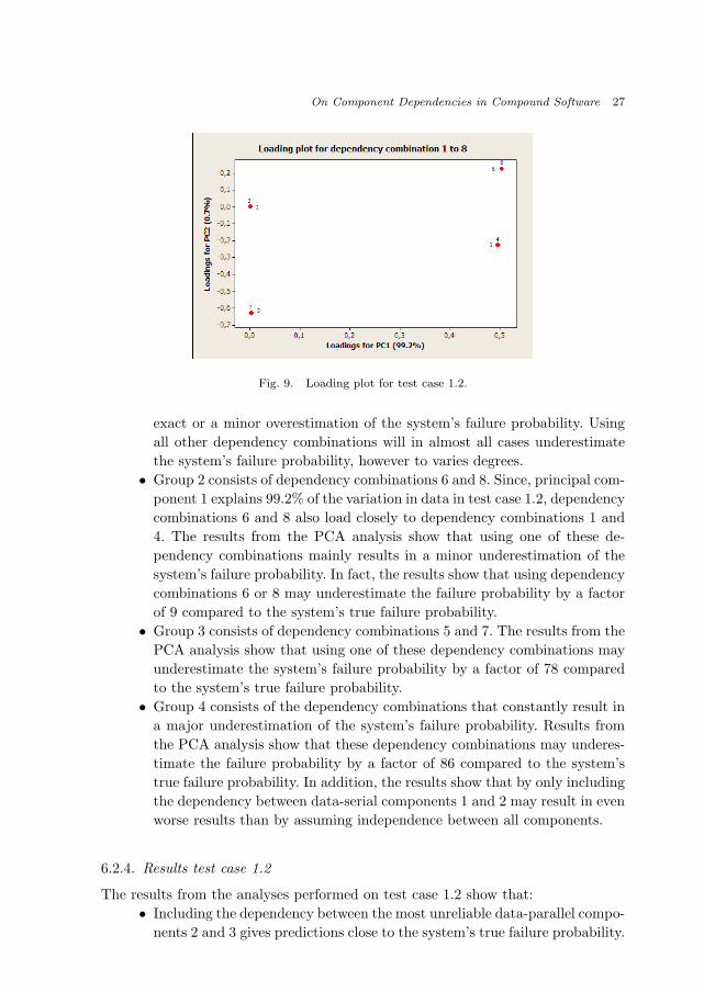
On Component Dependencies in Compound Software 27
Fig. 9. Loading plot for test case 1.2.
exact or a minor overestimation of the system’s failure probability. Using
all other dependency combinations will in almost all cases underestimate
the system’s failure probability, however to varies degrees.
• Group 2 consists of dependency combinations 6 and 8. Since, principal com-
ponent 1 explains 99.2% of the variation in data in test case 1.2, dependency
combinations 6 and 8 also load closely to dependency combinations 1 and
4. The results from the PCA analysis show that using one of these de-
pendency combinations mainly results in a minor underestimation of the
system’s failure probability. In fact, the results show that using dependency
combinations 6 or 8 may underestimate the failure probability by a factor
of 9 compared to the system’s true failure probability.
• Group 3 consists of dependency combinations 5 and 7. The results from the
PCA analysis show that using one of these dependency combinations may
underestimate the system’s failure probability by a factor of 78 compared
to the system’s true failure probability.
• Group 4 consists of the dependency combinations that constantly result in
a major underestimation of the system’s failure probability. Results from
the PCA analysis show that these dependency combinations may underes-
timate the failure probability by a factor of 86 compared to the system’s
true failure probability. In addition, the results show that by only including
the dependency between data-serial components 1 and 2 may result in even
worse results than by assuming independence between all components.
6.2.4. Results test case 1.2
The results from the analyses performed on test case 1.2 show that:
• Including the dependency between the most unreliable data-parallel compo-
nents 2 and 3 gives predictions close to the system’s true failure probability.

28 Kristiansen, Winther and Natvig
�������������������� ����
���
�����
���
����
� ������� ��
��������� ���������
�����
���
�����
���� !��� ��
Fig. 10. Results from direct calculation in test case 2.
Ignoring this dependency may, however, result in a major underestimation
of the system’s failure probability.
• Including the additional dependency between data-parallel components 1
and 3 may improve the predictions even more.
• Including only the dependency between data-serial components 1 and 2
results in a major underestimation of the system’s failure probability. In
some cases, the results are even worse than by assuming independence
between all components.
6.3. Test case 2
6.3.1. Direct calculation
Using the marginal and conditional reliabilities in Table 7, the system’s failure prob-
ability in test case 2 was calculated assuming the fourteen dependency combinations
listed in Section 5.2. The results are summarized in the line plot in Figure 10 and
clearly show that the system’s failure probability divides into three different groups
depending on the dependency combination used. The groups are summarized below:
• Group 1 consists of dependency combinations 1, 7 and 8. All these de-
pendency combinations result in the system’s exact failure probability
(0.000111). This indicates that dependency combinations 7 and 8, which
both include the dependencies between data-parallel components 3 and 4
and between data-serial components 1 and 4, can replace the true depen-
dency combination in the system, without significantly underestimating the
system’s failure probability.
• Group 2 consists of dependency combinations 3, 5 and 6, which all include
the dependency between data-parallel components 3 and 4. Using one of
these dependency combinations results in a minor overestimation of the
system’s failure probability (0.000115).).
• Group 3 consists of dependency combinations 2, 4, 9, 10, 11, 12, 13 and 14.
Using one of these dependency combinations results in a major underes-
timation of the system’s failure probability (0.000021). Common for these
dependency combinations is that none of them include the dependency
between data-parallel components 3 and 4. Dependency combination 2 as-
sumes independence between all software components, whereas the other
combinations only include dependencies between data-serial components.

On Component Dependencies in Compound Software 29
Table 10. Standardized Birnbaum measures and squared
difference for components 1, 2, 3 and 4 in test case 2.
DC IB1 IB2 IB3 IB4 st. sqrd. diff.
1 0.9786 0.0097 0.001 0.0107 0
2 0.9783 0.0099 0.0011 0.0107 1.3× 10⁻⁷
3 0.9786 0.0097 0.001 0.0107 5.0× 10⁻¹⁰
4 0.9783 0.0099 0.0011 0.0107 1.2× 10⁻⁷
5 0.9786 0.0097 0.001 0.0107 1.0× 10⁻¹⁰
6 0.9786 0.0097 0.001 0.0107 1.0× 10⁻¹⁰
7 0.9786 0.0097 0.001 0.0107 5.0× 10⁻¹⁰
8 0.9786 0.0097 0.001 0.0107 1.0× 10⁻¹⁰
9 0.9783 0.0099 0.0011 0.0107 1.2× 10⁻⁷
10 0.9783 0.0099 0.0011 0.0107 1.2× 10⁻⁷
11 0.9783 0.0099 0.0011 0.0107 1.2× 10⁻⁷
12 0.9783 0.0099 0.0011 0.0107 1.1× 10⁻⁷
13 0.9783 0.0099 0.0011 0.0107 1.1× 10⁻⁷
14 0.9783 0.0099 0.0011 0.0107 1.2× 10⁻⁷
6.3.2. Birnbaum’s measure
Based on the standardized Birnbaum measures and squared differences in Table 10,
it can easily be seen that dependency combinations 3, 5, 6, 7 and 8 are the depen-
dency combinations that alter the standardized Birnbaum measures the least. In
addition, it can easily be seen that dependency combinations 2, 4, 9, 10, 11, 12,
13 and 14 have the highest squared difference between their standardized Birn-
baum measures and the standardized Birnbaum measures calculated including all
component dependencies.
6.3.3. PCA
The loading plot in Figure 11 shows that the different dependency combinations in
test case 2 can be divided into three different groups based on their PCA loadings.
The groups are summarized below.
• Group 1 consists of dependency combinations 1, 7 and 8, since these depen-
dency combinations fall close together in the loading plot. This indicates
that dependency combinations 7 and 8 can replace dependency combination
1 in test case 2 without any serious consequences. In fact, the results from
the PCA analysis show that using dependency combination 7 or 8 results
in the exact or a minor overestimation of the system’s failure probability.
• Group 2 consists of dependency combinations 3, 5 and 6, which all fall close
together in the loading plot. Since, principal component 1 explains 99.9%
of the variation in data in test case 2, dependency combinations 3, 5 and 6
also load closely to dependency combinations 1, 7 and 8 .The results from
the PCA analysis show that using one of these dependency combinations
mainly results in a minor overestimation of the system’s failure probability.
• Group 3 consists of the dependency combinations that constantly under-
estimate the system’s failure probability, and includes dependency combi-

30 Kristiansen, Winther and Natvig
Fig. 11. Loading plot for test case 2.
nations 2, 4, 9, 10, 11, 12, 13 and 14. Results from the PCA analysis show
that these dependency combinations may underestimate the failure prob-
ability by a factor of 5 compared to the system’s true failure probability.
In addition, the results show that by only including dependencies between
data-serial components may result in even worse results than by assuming
independence between all components.
6.3.4. Results test case 2
The results from the analyses performed on test case 2 show that:
• Including the dependency between data-parallel components 3 and 4 gives
predictions close to the system’s true failure probability. Ignoring this de-
pendency will have major consequences on the system’s failure probability.
• Including the additional dependency between the most reliable data-serial
components 1 and 4 results in even better predictions.
• Including only dependencies between data-serial components results in a
major underestimation of the system’s failure probability. In some cases,
the results are even worse than by assuming independence between all
components.
6.4. Test case 3
6.4.1. Direct calculation
Using the marginal and conditional reliabilities in Table 7, the system’s failure prob-
ability in test case 3 was calculated assuming the same dependency combinations as
in test case 2. The results are summarized in the line plot in Figure 12 and clearly
show that the system’s failure probability divides into two major groups depending
on the dependency combination used. The groups are summarized below.

On Component Dependencies in Compound Software 31
�������� �����
��������
��������
���� �����
� �������� ������
�
��������
������ �����
��������
��������
��������
��
��������
Fig. 12. Results from direct calculation in test case 3.
• Group 1 consists of dependency combinations 1, 3, 5, 6, 7, and 8. Using
one of these dependency combinations only results in a minor underestima-
tion of the system’s failure probability (0.000103, 0.000105). This indicates
that all these dependency combinations can replace the correct dependency
combination in test case 3 without any major consequences on the system’s
failure probability.
• Group 2 consists of dependency combinations 2, 4, 9, 10, 11, 12, 13 and 14.
Using one of these dependency combinations results in a major underesti-
mation of the system’s failure probability (0.000011).
6.4.2. Birnbaum’s measure
Based on the standardized Birnbaum measures and squared differences in Table 11,
it can easily be seen that dependency combinations 3, 5, 6, 7 and 8 are the depen-
dency combinations that alter the standardized Birnbaum measures the least. In
addition, it can easily be seen that dependency combinations 2, 4, 9, 10, 11, 12,
13 and 14 have the highest squared difference between their standardized Birn-
baum measures and the standardized Birnbaum measures calculated including all
component dependencies.
Table 11. Standardized Birnbaum measures and
squared difference for components 2, 3 and 4 in
test case 3.
DC. IB2 IB3 IB4 st. sqrd. diff.
1 0.4527 0.0458 0.5014 0
2 0.4553 0.0496 0.4951 6.1× 10⁻⁵
3 0.4526 0.0459 0.5015 2.7× 10⁻⁸
4 0.4553 0.0496 0.4951 6.1× 10⁻⁵
5 0.4526 0.0459 0.5015 2.7× 10⁻⁸
6 0.4526 0.0459 0.5015 2.7× 10⁻⁸
7 0.4527 0.046 0.5014 2.2× 10⁻⁸
8 0.4526 0.046 0.5016 4.4× 10⁻⁸
9 0.4553 0.0496 0.4951 6.1× 10⁻⁵
10 0.4553 0.0496 0.4951 6.1× 10⁻⁵
11 0.4552 0.0496 0.4952 5.9× 10⁻⁵
12 0.4554 0.0494 0.4952 5.7× 10⁻⁵
13 0.4554 0.0496 0.4950 6.3× 10⁻⁵
14 0.4554 0.0494 0.4952 5.8× 10⁻⁵

32 Kristiansen, Winther and Natvig
Fig. 13. Loading plot for test case 3.
6.4.3. PCA
The loading plot in Figure 13 shows that the different dependency combinations in
test case 3 can be divided into four different groups based on their PCA loadings.
The groups are summarized below:
• Group 1 consists of dependency combinations 1, 3, 5, 6 and 8, since these
dependency combinations fall close together in the loading plot. This indi-
cates that these dependency combinations can replace dependency combi-
nation 1 in test case 3 without any serious consequences. The results from
the PCA analysis show that using one of the dependency combinations in
group 1 may result in the exact or a minor underestimation of the system’s
failure probability.
• Group 2 consists of dependency combination 7. Since, principal component
1 explains 99.7% of the variation in data in test case 3, dependency combi-
nation 7 also load closely to the dependency combinations in group 1. The
results from the PCA analysis show that using dependency combination 7
may result in the exact or a minor underestimation of the system’s failure
probability.
• Group 3 consists of dependency combinations 11, 12, 13 and 14. The results
from the PCA analysis show that using one of the dependency combinations
in group 2 may underestimate the system’s failure probability by a factor
of 9.
• Group 4 consists of the dependency combinations 2, 4, 9 and 10. Since,
principal component 1 explains 99.7% of the variation in data in test case 3,
dependency combinations 2, 4, 9 and 10 also load closely to the dependency
combinations in group 3. The results from the PCA analysis show that
using one of the dependency combinations in group 4 may underestimate
the system’s failure probability by a factor of 10.

On Component Dependencies in Compound Software 33
6.4.4. Results test case 3
The results from the analyses performed on test case 3 show that:
• Including the dependency between data-parallel components 3 and 4 gives
predictions close to the system’s true failure probability. Ignoring this de-
pendency will have major consequences on the system’s failure probability.
• Including only dependencies between data-serial components results in a
major underestimation of the system’s failure probability. In some cases,
the results are even worse than by assuming independence between all
components.
7. Summary of the Results and Discussion
The results from the analyses performed in Section 6 show that the three techniques
“direct calculation”, Birnbaum’s measure and PCA in most cases identify the same
dependency combinations as the “best” dependency combinations. The results can
be summarized as follows:
• Including only partial dependency information may give a substantial im-
provement in the reliability predictions, compared to assuming indepen-
dence between all software components. However, this is only as long as
the most important component dependencies are included.
• It is also apparent that dependencies between data-parallel components are
far more important than dependencies between data-serial components.
For a system consisting of both data-parallel and data-serial components, the results
indicate that:
• Including only dependencies between data-serial components may result
in a major underestimation of the system’s failure probability. In some
cases, the results are even worse than by assuming independence between
all components.
• Including only dependencies between data-parallel components may give
predictions close to the system’s true failure probability, as long as the
dependency between the most unreliable components is included.
• Including additional dependencies between data-parallel components may
improve the predictions further.
• Including additional dependencies between data-serial components may
also give better predictions, as long as the dependency between the most
reliable components is included.
One of the key results in 6 is the following theorem:
Theorem 1.
Let X1 . . . Xn be associated random variables such that 0 ≤ Xi ≤ 1 for i =
1 . . . n. Then

34 Kristiansen, Winther and Natvig
E
n∏i=1
Xi ≥n∏
i=1
EXi (21)
En∐
i=1
Xi ≤n∐
i=1
EXi (22)
By using this theorem on components having binary states, the theorem says that
falsely assuming independence between components in a series structure will overes-
timate the system’s failure probability. The theorem also says that falsely assuming
independence between components in a parallel structure will underestimate the
system’s failure probability. The author of 27 therefore concludes that for an ar-
bitrary component structure, the consequence of assuming independence will be
impossible to predict.
The results in Section 6 do, however, indicate that it may in fact be possible
to say something about the consequences of assuming independence between some
components in an arbitrary system structure. For a system where there are de-
pendencies between both data-serial and data-parallel components, it is quite clear
that the effect of falsely assuming independence between data-serial components is
greatly diminished as long as the dependencies between data-parallel components
are included. In the opposite case, when wrongly assuming independence between
data-parallel components and including the dependencies between data-serial com-
ponents, the system’s failure probability may however be underestimated even more
than by assuming independence between all software components in the system.
8. Conclusions and Further Work
In this paper, it is shown that the difficult task of including component dependencies
in the reliability calculations can be simplified in three ways:
1. The components’ marginal reliabilities put direct restrictions on the com-
ponents’ conditional reliabilities in a compound software.
2. The degrees of freedom are much fewer than first anticipated when it comes
to conditional probabilities. If the components’ marginal reliabilities and
four of the components’ conditional probabilities are known in a simple
three components system, the remaining 44 conditional probabilities can
be expressed using general rules of probability theory. This is shown math-
ematically in Appendix A.
3. Including only partial dependency information may give substantial im-
provements in the reliability predictions, compared to assuming indepen-
dence between all software components. However, this is only as long as
the most important component dependencies are included.
It should be emphasized that the rules for selecting the most important component
dependencies are based on case studies, where the individual component reliabilities

On Component Dependencies in Compound Software 35
are assumed to be known. It is also assumed that all components in the test cases,
as well as the system, only have two possible states. In addition, the research is
restricted to on-demand types of situations.
It should also be emphasized that the objective of this research is to include de-
pendency aspects in the reliability calculations of critical systems, and not to handle
component dependencies in systems consisting of a huge amount of components.
To follow up on these results, a more analytical approach should be consid-
ered. In addition, an evaluation of the proposed rules by studying other well-known
software structures is essential.
Acknowledgements
This work has been performed as part of a PhD-study in collaboration between
Østfold University College, Institute for Energy Technology and the University of
Oslo.
Appendix A. Theorems and Proofs
Theorem 1. Consider a general system consisting of two components. Assume
further that the components’ marginal reliabilities p1 and p2 are known. In such a
system there are eight possible conditional probabilities between components 1 and 2:
p2|1, p2̄|1, p2|1̄, p2̄|1̄, p1|2, p1̄|2, p1|2̄ and p1̄|2̄. If one of these conditional probabilities
is known, the remaining seven can be found using general rules in probability theory.
Proof. This proof uses Bayes theorem, the rule of complementation and the fol-
lowing rule of total probability:
p2 = p2|1p1 + p2|1̄p1̄ (A.1)
Assume that the conditional probability p2|1 is known. As shown in Equations A.2-
A.8, the seven remaining conditional probabilities can be expressed as functions of
p1, p2 and p2|1.
p2̄|1 = 1− p2|1 (A.2)
p2|1̄ =p2 − p2|1p1
1− p1(A.3)
p2̄|1̄ = 1− p2 − p2|1p11− p1
(A.4)
p1|2 =p2|1p1p2
(A.5)

36 Kristiansen, Winther and Natvig
p1̄|2 = 1− p2|1p1p2
(A.6)
p1|2̄ =(1− p2|1)p1
1− p2(A.7)
p1̄|2̄ = 1− (1− p2|1)p11− p2
(A.8)
Theorem 2. Consider a general system consisting of three components. Assume
further that the components’ marginal reliabilities p1, p2 and p3 are known. In such
a system there are 48 possible conditional probabilities between components 1, 2 and
3: p2|1, p2̄|1, p2|1̄, p2̄|1̄, p1|2, p1̄|2, p1|2̄, p1̄|2̄, p3|1, p3̄|1, p3|1̄, p3̄|1̄, p1|3, p1̄|3, p1|3̄, p1̄|3̄,p3|2, p3̄|2, p3|2̄, p3̄|2̄, p2|3, p2̄|3, p2|3̄, p2̄|3̄, p3|12, p3̄|12, p3|1̄2, p3̄|1̄2, p3|12̄, p3̄|12̄, p3|1̄2̄,p3̄|1̄2̄, p2|13, p2̄|13, p2|1̄3, p2̄|1̄3, p2|13̄, p2̄|13̄, p2|1̄3̄, p2̄|1̄3̄, p1|23, p1̄|23, p1|2̄3, p1̄|2̄3, p1|23̄,p1̄|23̄, p1|2̄3̄, p1̄|2̄3̄. If four of these conditional probabilities are known, the remaining
44 can be found using general rules in probability theory.
Proof. This proof uses Bayes theorem, the rule of complementation and the fol-
lowing rules of total probability:
p3 = p3|12p2|1p1 + p3|12̄p2̄|1p1+ p3|1̄2p2|1̄p1̄ + p3|1̄2̄p2̄|1̄p1̄ (A.9)
p3|1 = p3|12p2|1 + p3|12̄p2̄|1 (A.10)
p3|2 = p3|12p1|2 + p3|1̄2p1̄|2 (A.11)
Assume that the conditional probabilities p2|1, p3|1, p3|2 and p3|12 are known. As
shown in Theorem 1, p2̄|1, p2|1̄, p2̄|1̄, p1|2, p1̄|2, p1|2̄, p1̄|2̄ can be expressed as functions
of p1, p2 and p2|1. In the same way p3̄|1, p3|1̄, p3̄|1̄, p1|3, p1̄|3, p1|3̄, p1̄|3̄ can be
expressed as functions of p1, p3 and p3|1, and p3̄|2, p3|2̄, p3̄|2̄, p2|3, p2̄|3, p2|3̄, p2̄|3̄ can
be expressed as functions of p2, p3 and p3|2.The conditional probabilities p3̄|12, p3|1̄2, p3̄|1̄2, p3|12̄, p3̄|12̄, p3|1̄2̄ and p3̄|1̄2̄ can
further be expressed as functions of p1, p2, p3, p2|1, p3|1, p3|2 and p3|12. This is
shown in Equations A.12 - A.18. Especially, to express p3|1̄2̄ in Equation A.17,
Equations A.9, A.13, A.15, A.3 and A.4 are used as basis (the equations are listed
in the sequence of their usage).
p3̄|12 = 1− p3|12 (A.12)

On Component Dependencies in Compound Software 37
p3|12̄ =p3|1 − p3|12p2|1
1− p2|1(A.13)
p3̄|12̄ = 1− p3|1 − p3|12p2|11− p2|1
(A.14)
p3|1̄2 =p3|2p2 − p3|12p2|1p1
p2 − p2|1p1(A.15)
p3̄|1̄2 = 1− p3|2p2 − p3|12p2|1p1p2 − p2|1p1
(A.16)
p3|1̄2̄ =p3 − p3|1p1 − p3|2p2 + p3|12p2|1p1
1− p2 + (p2|1 − 1)p1(A.17)
p3̄|1̄2̄ = 1− p3 − p3|1p1 − p3|2p2 + p3|12p2|1p11− p2 + (p2|1 − 1)p1
(A.18)
In the same way as shown above,
p2|13 =p3|12p2|1p1p3|1p1
(A.19)
gives p2̄|13, p2|1̄3, p2̄|1̄3, p2|13̄, p2̄|13̄, p2|1̄3̄ and p2̄|1̄3̄.Furthermore,
p1|23 =p3|12p2|1p1p3|2p2
(A.20)
is leading to p1̄|23, p1|2̄3, p1̄|2̄3, p1|23̄, p1̄|23̄, p1|2̄3̄ and p1̄|2̄3̄.
References
1. T. Aven, Reliability and Risk Analysis, Elsevier, London (1992)2. Z. W. Birnbaum, On the importance of different components in a multicomponent
system, Multivariate analysis-II, ed. P. R. Krishnaiah, Academic Press, New York, p.581–592, (1969)
3. Gustav Dahll and Bjørn Axel Gran, The Use of Bayesian Belief Nets in Safety Assess-ment of Software Based Systems, International Journal of General Systems, 29 (2), p.205–229, (2000)
4. S. Distefano and A. Puliafito, Reliability and availability analysis of dependent-dynamic systems with DRBDs, Reliability Engineering and System Safety, 94 (9), pp.1381–1393, Elsevier, (2009)
5. D. E. Eckhardt and L. D. Lee, A theoretical basis for the analysis of redundant softwaresubject to coincident errors, NASA tech. Memo 86369, (1985)

38 Kristiansen, Winther and Natvig
6. J. D. Esary, F. Proshan and D. W. Walkup, Association of Random Variables, withApplications, The Annals of Mathematical Statistics, 38 (5), pp. 1466–1474, (1967)
7. Fricks, R.M. and Trivedi, K.S., Modeling Failure Dependencies in Reliability AnalysisUsing Stochastic Petri Nets, Proc. of 11th European Simulation Multiconf., Citeseer,(1997)
8. S. S. Gokhale and K. S. Trivedi, Dependency Characterization in Path-Based Ap-proaches to Architecture-Based Software Reliability Prediction, IEEE Workshop onApplication-Specific Software Engineering and Technology, IEEE Computer Society,pp. 86–90, (1998)
9. K. Goseva-Popstojanova and K. S. Trivedi, Architecture-based approach to reliabilityassessment of software systems, Performance Evaluation, Elsevier, 45 (2-3), pp. 179–204, (2001)
10. D. Hamlet, D. Mason, and D. Woit, Theory of Software Reliability Based on Compo-nents, International Conference on Software Engineering, 23, pp. 361–370, (2001)
11. S. Hauge, M. A. Lundteigen, P. R. Hokstad and S. Haabrekke, Reliability PredictionMethod for Safety Instrumented Systems - PDS Method Handbook, Sintef report no.A13503, ISBN 978-82-1404850-4, Sintef, (2010)
12. () R. Huang and M. R. Lyu and K. Kanoun, Simulation Techniques for Component-Based Software Reliability Modeling with Project Application, Proceedings of Interna-tional Symposium on Information Systems and Engineering (ISE’01), CSREA Press,pp. 283–289, (2001)
13. R. A. Johnson and D. W. Wichern, Applied Multivariate Statistical Analysis, PrenticeHall, New York, ISBN 0-13-834194-x, (1998)
14. J. C. Knight and N. G. Leveson, An experimental evaluation of the assumption ofindependence in multiversion programming, IEEE Transactions on Software Engineer-ing, 12 (1), pp. 96–109, (1986)
15. S. Krishnamurthy and A. Mathur, On the Estimation of Reliability of a SoftwareSystem Using Reliabilities of its Components, Proceedings of the 8th InternationalSymposium on Software Reliability Engineering (ISSRE’97), IEEE Computer SocietyPress, pp. 146–155, (1997)
16. M. Kristiansen, Finding Upper Bounds for Software Failure Probabilities - Exper-iments and Results, Proceedings of the 24th International Conference on ComputerSafety, Reliability and Security (Safecomp’05), winther, Gran & Dahll, Balkema, pp.179–193, (2005)
17. M. Kristiansen and R. Winther, Assessing Reliability of Compound Software, Risk,Reliability and Social Safety (ESREL 2007), Aven & Vinnem, Taylor & Francis Group,pp. 1731–1738, (2007)
18. M. Kristiansen and R. Winther and John E. Simensen, Identifying the Most ImportantComponent Dependencies in Compound Software, Risk, Reliability and Safety (ESREL2009), Bris, Soares & Martorell, Taylor & Francis Group, pp. 1333–1340, (2009)
19. M. Kristiansen and R. Winther and M. van der Meulen and M. Revilla, The Useof Metrics to Assess Software Component Dependencies, Risk, Reliability and Safety(ESREL 2009), Bris, Soares & Martorell, Taylor & Francis Group, pp. 1359–1366,(2009)
20. Building a system failure rate estimator by identifying component failure rates, Pro-ceedings of the 10th International Symposium on Software Reliability Engineering (IS-SRE’99), pp. 32–41, (1999)
21. B. Littlewood and D. R. Miller, Conceptual Modeling of Coincident Failures in Multi-version Software, IEEE Transactions on Software Engineering, 15 (12), pp. 1596–1614,(1989)

On Component Dependencies in Compound Software 39
22. B. Littlewood, P. Popov and L. Strigini, Modelling software design diversity: a review,ACM Computing Surveys, 33 (2), pp. 177–208, (2001)
23. M. R. Lyu, editor. Handbook of Software Reliability Engineering, IEEE ComputerSociety Press, ISBN 0-07-039400-8, (1995)
24. Douglas C. Montgomery, Design and Analysis of Experiments, John Wiley & Sons,ISBN 0-471-15746-5, (1997)
25. John D. Musa, Software Reliability Engineering, McGraw-Hill, ISBN 0-07-913271-5, (1998)
26. D. M. Nassar, W. A. Rabie, M. Shereshevsky , N. Gradetsky, H. H. Ammar, B.Yu, S. Bogazzi, and A. Mili, A., Estimating Error Propagation Probabilities in Soft-ware Architectures, International Symposium on Software Metrics No10, Chicago IL,ETATS-UNIS, pp. 384–393, Citeseer, (2004)
27. B.Natvig, Reliability analysis with technological applications (in Norwegian), Insti-tute for Mathematics, University of Oslo, (1998)
28. Petar Popic, Dejan Desovski, Walid Abdelmoez and Bojan Cukic, Error Propagationin the Reliability Analysis of Component based Systems, Proceedings of the 16th IEEEInternational Symposium on Software Reliability (ISSRE’05), IEEE Computer Society,pp. 53–62, (2005)
29. S. S.Gokhale, Architecture-based software reliability analysis: Overview and limita-tions, IEEE Transactions on dependable and secure computing, 4 (1), pp. 32–40, (2007)
30. L. Sha, J. B. Goodenough and B. Pollak, Simplex architecture: Meeting the challengesof using COTS in high-reliability systems, Crosstalk, Citeseer, pp. 7–10, (1998)
31. Vieira, M. and Richardson, D., The role of dependencies in component-based sys-tems evolution, Proceedings of the International Workshop on Principles of SoftwareEvolution, ACM, pp. 62–65, (2002)
32. R. Winther and M. Kristiansen, On the Modelling of Failure Dependencies BetweenSoftware Components, Safety and Reliability for Managing Risk (ESREL’06), GuedesSoares & Zio, Taylor & Francis Group, pp.1443-1450, (2006)
33. L. Zavala and M.N. Huhns, Analysis of coincident failing ensembles in multi-versionsystems, Presented at the 19th IEEE International Symposium on Software ReliabilityEngineering - Dependable Software Engineering Workshop (ISSRE’08), IEEE Com-puter Society, (2008)