arX

iv:h

ep-l

at/9

3040

08v2

10

Aug

199

3

A Comparative Study of

Some Pseudorandom Number Generators

I. Vattulainen1, K. Kankaala1,2, J. Saarinen1, and T. Ala-Nissila1,3

1Department of Electrical Engineering

Tampere University of Technology

P.O. Box 692

FIN - 33101 Tampere, Finland

2Centre for Scientific Computing

P.O. Box 405, FIN - 02100 Espoo, Finland

3Research Institute for Theoretical Physics

P.O. Box 9 (Siltavuorenpenger 20 C)

FIN - 00014 University of Helsinki, Finland

Abstract

We present results of an extensive test program of a group of pseudo-

random number generators which are commonly used in the applications of

physics, in particular in Monte Carlo simulations. The generators include

public domain programs, manufacturer installed routines and a random num-

ber sequence produced from physical noise. We start by traditional statistical

tests, followed by detailed bit level and visual tests. The computational speed

of various algorithms is also scrutinized. Our results allow direct comparisons

between the properties of different generators, as well as an assessment of the

efficiency of the various test methods. This information provides the best

available criterion to choose the best possible generator for a given problem.

However, in light of recent problems reported with some of these generators,

we also discuss the importance of developing more refined physical tests to

find possible correlations not revealed by the present test methods.

PACS numbers: 02.50.-r, 02.50.Ng, 75.40.Mg.

Key words: Randomness, random number generators, Monte Carlo simulations.

1

1 Introduction

“Have you generated any

new random numbers today?”

J. Kapyaho

Long sequences of random numbers are currently required in numerous applications,

in particular within statistical mechanics, particle physics, and applied mathematics.

The methods utilizing random numbers include Monte Carlo simulation techniques

[5], stochastic optimization [1], and cryptography [6, 12, 61], all of which usually

require fast and reliable random number sources. In practice, the random num-

bers needed for these methods are produced by deterministic rules, implemented as

(pseudo)random number generator algorithms which usually rely on simple aritme-

thic operations. By their definition, the maximum - length sequences produced by

all these algorithms are finite and reproducible, and can thus be “random” only in

some limited sense [8, 9].

Despite the importance of creating good pseudorandom number generators, fairly

little theoretical work exists on random number generation. Thus, the properties of

many generators are not well understood in depth. Some random number generator

algorithms have been studied in the general context of cellular automata [8], and

deterministic chaos [4]. In particular, number theory has yielded exact results on the

periodicity and lattice structure for linear congruential and Tausworthe generators

[11, 40, 30, 55]. These results have led to theoretical methods of evaluating the

algorithms, the most notable being the so called spectral test. However, most of

these theoretical results are derived for the full period of the generator while in

practice the behavior of subsequences of substantially shorter lengths is of particular

importance in applications. In addition, the actual implementation of the random

number generator algorithm may affect the quality of its output. Thus, in situ tests

of implemented programs are usually needed.

Despite this obvious need for in situ testing of pseudorandom number generators,

only relatively few authors have presented results to this end [32, 33, 49, 42]. Most

likely, there are two main reasons for this. The first is the persistence of underlying

fundamental problems in the actual definitions of “randomness” and “random” se-

quences which have given no unique practical recipe for testing a finite sequence of

numbers [31]. Thus various authors have developed an array of different tests which

mostly probe some of the statistical properties of the sequences, or test correlations

e.g. on the binary level. Recently, Compagner and Hoogland [8] have presented a

2

somewhat more systematic approach to randomness as embodied in finite sequences.

They propose testing the values of all possible correlation coefficients of an ensem-

ble of a given sequence and all of its “translations” (iterated variations) [10], a task

which nevertheless appears rather formidable for practical purposes. We are not

aware of any attempts to actually carry out their program. The second reason is

probably more practical, namely the gradual evolution of improved pseudorandom

number generator algorithms, which has led to a diversity of generators available in

computer software, public domain and so on. For many of these algorithms (and

their implementations) only a few rudimentary tests have been performed.

In this work we have undertaken an extensive test program [58] of a group of

pseudorandom number generators, which are often employed in the applications

of physics. These generators which are described in detail in Section 2 include

public domain programs GGL, RANMAR, RAN3, RCARRY and R250, a library

subroutine G05FAF, manufacturer installed routines RAND and RANF, and even

a sequence generated from physical noise (PURAN II). Our strategy is to perform

a large set of different tests for all of these generators, whose results can then be

directly compared with each other. There are two main reasons for this. Namely,

there is a difficulty associated with most quantitative tests in the choice of the test

parameters and final criteria for judging the results. Thus, we think that full compar-

ative tests of a large group of generators using identical test parameters and criteria

can yield more meaningful results, in particular when there is a need for a reliable

generator with a good overall performance. Second, performing a large number of

tests also allows a comparison of exactly how efficient each test is in finding certain

kinds of correlations.

As discussed in Section 3, we first employ an array of standard statistical tests,

which measure the degree of uniformity of the distribution of numbers, as well as

correlations between them. Following this, we perform a series of bit level tests, some

of which should be particularly efficient in finding correlations between consecutive

bits in the random number sequences. Third part of our testing utilizes visual

pictures of random numbers and their bits on a plane. Finally, for the sake of

completeness we have also included a relative performance test of the generators

in our results. A complete summary of the test results is presented in Section 4.

As our main result we find three generators, namely GGL, G05FAF, and R250

with an overall best performance in all our tests, although some other generators

such as RANF and RANMAR perform almost as convincingly. We also find that

the bit level tests are most efficient in finding local correlations in the random

3

numbers, but do not nevertheless guarantee good statistical properties, as shown in

the case of RCARRY. Our results also show that visual tests can indeed reveal spatial

correlations not clearly detected in the quantitative tests. Our work thus provides a

rather comprehensive test bench which can be utilized in choosing a random number

generator for a given application. However, choosing a “good quality” random

number generator for all applications may not be trivial as discussed in Section

5, in light of the recent results reporting anomalous correlations in Monte Carlo

simulations [14, 23] using the here almost impeccably performing R250. Thus, more

physical ways of testing random number sequences are probably needed, a project

which is currently underway [59].

4

2 Generation of Random Numbers

“The generation of random numbers

is too important to be left to chance.”

R. Coveyou

Pseudorandom number sequences needed for high speed applications are usually

generated at run time using an algorithm which often is a relatively simple nonlinear

deterministic map. The implementation of the corresponding recurrence relation

must also ensure that the stream of numbers is reproducible from identical initial

conditions. The deterministic nature of generation means that the designer has to be

careful in the choice of the precise relationship of the recursion, otherwise unwanted

correlations will appear as amply demonstrated in the literature [8].

However, even the best generator algorithm can be defeated by a poor computer

implementation. Whenever an exact mathematical algorithm is translated into a

computer subroutine, different possibilities for its implementation may exist. Only

if the operation of a generator can be exactly specified on the binary level, has

the implementation a chance to be unambiguous; otherwise, machine dependent

features become incorporated into the routine. These include finite precision of real

numbers, limited word size of the computer, and numerical accuracy of mathematical

functions. Furthermore, it would often be desirable that the implemented routine

performed identically in each environment in which it is to be executed, i.e. it would

be portable.

Some of the desired properties of good pseudorandom number generators are easily

defined but often difficult to achieve simultaneously. Namely, besides good “ran-

domness” properties portability, repeatability, performance speed, and a very long

period are often required. Ideally, a random number generator would be designed

for each application, and then tested within that application to ensure that the in-

evitable correlations that do exist in a deterministic algorithm, cause no observable

effects. In practice, this is seldom possible, which is another reason why extensive

tests of pseudorandom number generators are needed.

Most commonly used pseudorandom number generator algorithms are the linear

congruential method, the lagged Fibonacci method, the shift register method, and

combination methods. A special case are nonalgorithmic or physical generators which

are used for creating a non - reproducible sequence of random numbers. These are

usually based on “random” physical events, e.g. changes in physical characteristics

5

of devices, cosmic ray bursts or electromagnetic interference. Details and properties

of the algorithms will be summarized in the next section. Following this, we shall

describe in more detail the particular generators chosen for our tests. Reviews of

current state of generation methods can be found in e.g. Marsaglia [42], James [27],

L’Ecuyer [34], and Anderson [3].

2.1 Classification of Generation Methods

“Anyone who considers arithmethical methods

of producing random digits is, of course,

in a state of sin.”

J. von Neumann

Among the simplest algorithms are the linear congruential generators which use the

integer recursion

Xi+1 = (aXi + b ) mod m, (1)

where the integers a, b and m are constants. It generates a sequence X1, X2, . . . of

random integers between 0 and m − 1 (or in the case b = 0, between 1 and m − 1).

Each Xi is then scaled into the interval [0,1). Parameter m is often chosen to be

equal or nearly equal to the largest integer in the computer. Linear congruential

generators can be classified into mixed (b > 0) and multiplicitive (b = 0) types, and

are usually denoted by LCG(a, b, m) and MLCG(a, m), respectively.

Since the introduction of this algorithm by Lehmer [35], its properties have been

researched in detail. Marsaglia [40] pointed out about 20 years ago that the random

numbers in d dimensions lie on a relatively small number of parallel hyperplanes.

Further theoretical work [11, 15, 16] has been done to weed out bad choices of the

constants a, b and m but so far no consensus has evolved on a unique best choice

for these parameters.

To increase the period of the linear congruential algorithm, it is natural to generalize

it to the form

Xi = (a1 Xi−1 + · · · + ap Xi−p) mod m, (2)

where p > 1 and ap 6= 0. The period is the smallest positive integer λ for which

(X0, . . . , Xp−1) = (Xλ, . . . , Xλ+p−1). (3)

Since there are mp possible p − tuples, the maximum period is mp − 1. In this

category the simplest algorithm is of the Fibonacci type. The use of p = 2, a1 =

6

a2 = 1 leads to the Fibonacci generator

Xi = (Xi−1 + Xi−2) mod m. (4)

Since no multiplications are involved, this implementation has the advantage of

being fast.

A lagged Fibonacci generator requires an initial set of elements X1, X2, . . . , Xr and

then uses the integer recursion

Xi = Xi−r ⊗ Xi−s, (5)

where r and s are two integer lags satisfying r > s and ⊗ is a binary operation (+, −,

×, ⊕ (exclusive-or)). The corresponding generators are designated by LF(r, s,⊗).

Typically, the initial elements are chosen as integers and the binary operation is

addition modulo 2n. Lagged Fibonacci generators are elaborated in e.g. Ref. [42].

An alternative generator type is the shift register generator. Feedback shift register

generators are also sometimes called Tausworthe generators [54]. The feedback

shift register algorithm is based on the theory of primitive trinomials of the form

xp+xq+1. Given such a primitive trinomial and p binary digits x0, x1, x2, . . . , xp−1, a

binary shift register sequence can be generated by the following recurrence relation:

xk = xk−p ⊕ xk−p+q, (6)

where ⊕ is the exclusive-or operator, which is equivalent to addition modulo 2. l-bit

vectors can be formed from bits taken from this binary sequence as

Wk = xk xk+d xk+2d · · ·xk+(l−1)d, (7)

where d is a chosen delay between elements of this binary vector. The resulting

binary vectors are then treated as random numbers. Such a generated sequence of

random integers will have the maximum possible period of 2p − 1, if xp + xq + 1 is

a primitive trinomial and if this trinomial divides xn − 1 for n = 2p − 1, but for

no smaller n. These conditions can easily be met by choosing p to be a Mersenne

prime, i.e. a prime number p for which 2p − 1 is also a prime. A list of Mersenne

primes can be found e.g. in Refs. [60, 62, 6, 25]. Generators based on small values

of p do not perform well on the tests [42]. According to some statistical tests on

computers [57] the value of q should be small or close to p/2.

Lewis and Payne [37] formed l-bit words by introducing a delay between the words.

The corresponding generator is called the generalized feedback shift register gener-

ator, denoted by GFSR(p, q,⊕). In a GFSR generator the words Wk satisfy the

7

recurrence relation:

Wk = Wk−p ⊕ Wk−p+q. (8)

Under special conditions, maximal period length of 2p − 1 can be achieved. Lewis

and Payne [37] and Niederreiter [47] have also studied the properties of the algorithm

theoretically. An important aspect of the GFSR algorithm concerns its initialization,

where p initial seeds are required. This question has been studied theoretically in

Refs. [18, 19, 55, 56, 20].

Given the inevitable dependencies that will exist in a pseudorandom sequence, it

seems natural that one should try to shuffle a sequence [26] or to combine separate

sequences. An example of such approach is given by MacLaren and Marsaglia [39]

who were apparently the first to suggest the idea of combining two generators to-

gether to produce a single sequence of random numbers. The essential idea is that

if X1, X2, . . . and Y1, Y2, . . . are two random number sequences, then the sequence

Z1, Z2, . . . defined by Zi = Xi ⊗ Yi will not only be more uniform than either

of the two sequences but will also be more independent. Algorithms using this idea

are often called mixed or combination generators.

As mentioned before, physical devices have also been used in the creation of random

number sequences. Usually, however, such sequences are generated too slowly to

be used in real time, but rather stored in the computer memory where they can be

easily accessed. This also guarantees the reproducability of the chosen sequence in

applications. However, physical memory restrictions often severely limit the number

of stored numbers. Unwanted and unknown physical correlations may also affect the

quality of physical random numbers. As a result, physical random numbers have not

been commonly used in simulations. One implementation of a physical generator

can be found in Ref. [52].

2.2 Descriptions of Generators

In this section, we shall describe in more detail the generators which have been

chosen for the tests. Since many combinations of possible parameters exist, we

have tried to choose those particular algorithms which have been most commonly

used in physics applications, or which have been previously tested. At the end of

this section, we shall also describe a sequence of random numbers generated from

8

physical noise, which has been included for purposes of comparison.

• GGL

GGL is a uniform random number generator based on the linear congruential method

[48]. The form of the generator is MLCG(16807, 231 − 1) or

Xi+1 = (16807 Xi) mod (231 − 1). (9)

This generator has been particularly popular [48]. It has seen extensive use in the

IBM computers [65], and is also available in some commercial software packages

such as subroutine RNUN in the IMSL library [66] and subroutine RAND in the

MATLAB software [67]. MLCG(16807, 231 − 1) generators are quite fast and have

been argued to have good statistical properties [36]. Results of tests with and

without shuffling are reported by Learmonth and Lewis [32]. Other test results on

implementations of this algorithm have been given in [29, 2, 3, 34]. Its drawback

is its cycle length 231 − 1 (≈ 2 × 109 steps) [29], which can be exhausted fast on

a modern high speed computer. We also note that our Fortran implementation of

GGL is particularly sensitive to the arithmetic accuracy of its implementation (cf.

Section 4). Our Fortran implementation of GGL produces the same sequence as

RNUN of the IMSL library 1

• RAND

RAND uses a linear congruential random number algorithm with a period of 232

[63] to return successive pseudorandom numbers in the range from 0 to 231 −1. The

generator is LCG(69069, 1, 232) or

Xi+1 = (69069 Xi + 1) mod 232. (10)

The multiplier 69069 has been used in many generators, probably because it was

strongly recommended in 1972 by Marsaglia [41], and is part of the SUPER - DUPER

generator [3]. Test results on various implementations of the LCG(69069, 1, 232)

algorithm have been reported in [32, 42, 3, 44]. The generator tested here is the

implementation by Convex Corp. on the Convex C3840 computer system [63].

• RANF1We also unsuccessfully tried the IBM assembly code implementation of Lewis et al. [36] on an

IBM 3090 computer.

9

The RANF algorithm uses two equations for generation of uniform random numbers.

It utilizes the multiplicative congruential method with modulus 248. The algorithms

are MLCG(M1, 248) and MLCG(M64, 2

48):

Xi+1 = (M1 Xi) mod 248, (11)

Xi+64 = (M64 Xi) mod 248, (12)

where M1 = 44485709377909 and M64 = 247908122798849. Period length of the

RANF generator is 246 [45]. Spectral test results on the RANF generator have been

given in Refs. [3, 17]. On the CRAY-X/MP and CRAY-Y/MP systems, RANF is a

standard vectorized library function [64]. The operations (M1Xi) and (M64Xi) are

done as integer multiplications in such a way as to preserve the lower 48 bits. We

tested RANF on a Cray X-MP/432.

• G05FAF

G05FAF is a library routine in the NAG software package [68]. It calls G05CAF

which is a multiplicative congruential algorithm MLCG(1313, 259) or

Xi+1 = (1313 Xi) mod 259. (13)

G05FAF can be used to generate a vector of n pseudorandom numbers which are

exactly the same as n successive calls to the G05CAF routine. Generated pseudo-

random numbers are uniformly distributed over the specified interval [a, b). The

period of the basic generator is 257 [68]. Its performance has been analyzed by the

spectral test [30].

• R250

R250 is an implementation of a generalized feedback shift register generator [37].

The 31-bit integers are generated by a recurrence of the form GFSR(250, 103,⊕) or

Xi = Xi−250 ⊕ Xi−(250−103). (14)

Implementation of the algorithm is straightforward, and p = 250 words of memory

are needed to store the 250 latest random numbers. A new term of the sequence can

be generated by a simple exclusive - or operation. An IBM assembly language im-

plementation of this generator has been presented by Kirkpatrick and Stoll [29] who

use a MLCG(16807, 231−1) to produce the first 250 initializing integers. Due to the

popularity of R250, there have been many different approaches for its initialization

10

[50, 18, 7, 20]. The period of the generator is 2250−1 [29]. Some test results of R250

generator have been reported by Kirkpatrick and Stoll [29]. We have implemented

R250 on Fortran [24].

• RAN3

RAN3 generator is a lagged Fibonacci generator LF(55,24,−) or

Xi = Xi−55 − Xi−24. (15)

The algorithm has also been called a subtractive method. The period length of

RAN3 is 255 − 1 [30], and it requires an initializing sequence of 55 numbers. The

generator was originally Knuth’s suggestion [30] for a portable routine but with

an add operation instead of a subtraction. This was translated to a real Fortran

implementation by Press et al. [51]. We were unable to find any published test

results for RAN3.

• RANMAR

RANMAR is a combination of two different generators [27, 43]. The first is a lagged

Fibonacci generator

Xi =

Xi−97 − Xi−33, if Xi−97 ≥ Xi−33;

Xi−97 − Xi−33 + 1, otherwise.(16)

Only 24 most significant bits are used for single precision reals. The second part

of the generator is a simple arithmetic sequence for the prime modulus 224 − 3 =

16777213. The sequence is defined as

Yi =

Yi − c, if Yi ≥ c;

Yi − c + d, otherwise,(17)

where c = 7654321/16777216 and d = 16777213/16777216.

The final random number Zi is then produced by combining the obtained Xi and Yi

as

Zi =

Xi − Yi, if Xi ≥ Yi;

Xi − Yi + 1, otherwise.(18)

11

The total period of RANMAR is about 2144 [43]. A scalar version of the algorithm

has been tested on bit level with good results [43]. We used the implementation

by James [27] which is available in the Computer Physics Communications (CPC)

software library, and has been recommended for a universal generator.

• RCARRY

RCARRY [44] is based on the operation known as “subtract - and - borrow”. The

algorithm is similar to that of lagged Fibonacci, but it has the occasional addition

of an extra bit. The extra bit is added if the Fibonacci sum is greater than one.

The basic formula is:

Xi = (Xi−24 ± Xi−10 ± c) mod b. (19)

The carry bit c is zero if the sum is less than or equal to b, and otherwise “c = 1 in

the least significant bit position” [27]. The choice for b is 224.

The period of the generator is about 21407 [44] when 24-bit integers are used for the

random numbers. We were unable to find any published test results for RCARRY.

We used the implementation of James [27], again available in the CPC software

library.

• PURAN II

PURAN II is a physical random number generator created by Richter [52]. It uses

random noise from a semiconductor device. The generated data has been perma-

nently stored on a computer disk, from which it can be transferred by request. In

this work, we have tested the PURAN II data on bit level only (cf. Section 4), and

also used it to verify the correct operation of our test programs.

12

3 Description of the Tests

“Of course, the quality of a generator can

never be proven by any statistical test.”

P. L’Ecuyer

A fundamental problem in testing finite pseudorandom number sequences stems from

the fact that the definition of randomness for such sequences is not unique [31]. Thus,

one usually has to decide upon some criteria which test at least the most fundamental

properties that such sequences should possess, such as correct values of the moments

of their probability distribution. This has lead to the emergence of a large number

of tests which can be divided into three approximate categories: Statistical (or

traditional) tests for testing random numbers in real or integer representation, bit

level tests for binary representations of random numbers, and more phenomenological

visual tests. In this work, we have employed several tests belonging to each of these

categories, as will be discussed below. Also, the spectral test for LCG generators

was included. We should note here that recently Compagner and Hoogland [8] have

suggested a more systematic test program for finite sequences. We shall not employ

it in this work, however.

The traditional utilitarian approach has been to subject pseudorandom number

sequences to tests, which derive from mathematical statistics [30]. In their simplest

form, tests in this category reveal possible deviations of the distribution of numbers

from an uniform distribution, such as the χ2 test. However, some of the more

sophisticated tests should actually probe correlations between successive numbers

as well [33].

Another approach is to test the properties of random numbers on the bit level. Of

the traditional tests, some can be performed in this manner also. Marsaglia [42]

has proposed additional tests which explicitly probe the individual bits of random

number sequences represented as binary computer words. Some of these tests have

been further refined [2]. We have included two of these tests here, in particular to

examine possible correlations between bits of successive binary words.

A rather different way of testing spatial correlations between random numbers is pos-

sible by using direct visualization. This can most easily be done in two dimensions

by plotting pairs of points on a plane, or visualizing the bits of binary numbers. In

addition to yielding qualitative information, such tests offer a possibility to develop

more physical quantitative tests through interpretation of the visualized configu-

13

rations as representations of physical systems, such as the Ising model [8, 59]. In

this work, however, we have simply used a few different types of visual tests to

complement our quantitative tests.

Before discussing each test in detail, we would like to emphasize that although some

of the generators we have tested have previously been subjected to similar tests, an

extensive comparative testing of a large collection of generators has been lacking up

to date. The importance of this becomes obvious when one considers the freedom

of choice of various parameters in the tests, as discussed below. Only compara-

tive testing with identical parameters allows a direct comparison between different

generators. Another difficulty concerns the implementation of random number gen-

erator algorithms and the testing routines [53, 48, 3, 22]. Problems in either may

actually lead to significant differences in the results. In fact, as an example we shall

explicitly demonstrate for GGL and RAND how slightly different implementations

of the same generator can lead to completely different results.

3.1 Statistical tests

The statistical tests included in our test bench were the uniformity test, the serial

test, the gap test, the maximum of t test, the collision test, and the run test. In

addition, we carried out the park test [42]. A review of the statistical tests can be

found e.g. in Ref. [30], and a suggestion for implementing them in Ref. [13].

The leading idea in carrying out the statistical tests was to improve the statis-

tical accuracy of these tests by utilizing a one way Kolmogorov - Smirnov (KS)

test. This was achieved by repeating each individual test described below N times,

and then submitting the obtained empirical distribution to a KS test (for the park

test, however, this was not possible). Similar approach has been suggested earlier

by Dudewicz and Ralley [13] and realized by L’Ecuyer [33]. The KS test reveals

deviations of an empirical distribution function (Fn(x)) from the theoretical one

(F (x)). This can be quantified by test variables K+ and K−, which are defined by

K+ =√

n sup{Fn(x) − F (x)} and K− =√

n sup{F (x) − Fn(x)}. K+ measures the

maximum deviation of Fn(x) from F (x) when Fn(x) > F (x) and K− measures the

respective quantity for Fn(x) < F (x). The tests are as follows:

(i) To test the uniformity of a random number sequence, a standard χ2 test was

used [30]. n random numbers were generated in the half open interval [0, 1),

then multiplied by ν and truncated to integers in the interval [0, ν). The

14

number of occurrences in each of the ν bins was compared to the theoretical

prediction using the χ2 test.

(ii) Serial correlations were tested [32, 30] by studying the occurrence of d-tuples

of n random numbers distributed in the interval [0, 1). For example, in the

case of pairs, we tabulated the number of occurrences of (x2i, x2i+1) for all i ∈[0, n). Each d-tuple occurs with the probability ν−d where ν is the number of

bins in the interval. The results were then subjected to the χ2 test.

(iii) The gap test [30] probes the uniformity of the random number sequence of

length n. Once a random number xi falls within a given interval [α, β], we

observe the number of subsequent numbers xi+1 . . . xi+j−1 6∈ [α, β]. When

again xj ∈ [α, β], it defines a gap of length j. For finite sequences, it is useful

to define a maximum gap length l. Then we can test the results against the

theoretical probability using the χ2 test.

(iv) The maximum of t test [30] is a simple uniformity test. If we take a random

number sequence of length n (xi ∈ [0, 1), i = 1, . . . , n) and divide it into

subsequences of length t and pick the maximum value for each subsequence,

the maxima should follow the xt distribution.

(v) The collision test [30] can be used to test the uniformity of the sequence when

the number of available random numbers (n) is much less than the number of

bins (w). We then study how many times a random number falls in the same

bin, i.e. how many collisions occur. The probability for j collisions is:

w(w − 1) · · · (w − n + j + 1)

wn

(

n

n − j

)

, (20)

where w = sd, d is the dimension and s can be chosen.

(vi) In the run test [32, 30], we calculate the number of occurrences of increasing

or decreasing subsequences of length 1 ≤ i < l for a given random number

sequence x1, x2, . . . , xn. To carry out this test we chose l = 6 and followed

Knuth [30] in the choice of the relevant test quantity.

(vii) In the park test [42], we choose randomly points in a d-dimensional space and

allocate a diameter for each point. Within each diameter, “a car is parked”.

The aim is to park as many non - overlapping cars as possible, and study the

distribution of k cars. Unfortunately, since the theoretical distribution is not

known, this test can only be used for qualitative comparative studies.

15

3.2 Bit level tests

Two of the tests included in the previous section on statistical tests, namely the run

test and the collision test could equally well be included in the category of bit level

tests as they can also be performed for binary representations of random numbers.

Recently, Marsaglia [42] has introduced new tests in his DIEHARD random number

generator test bench. Of these we carried out the d-tuple and the rank tests. We

shall briefly describe both of them below.

(i) The d-tuple test realized here is a modified version [2] of the original [42].

We extended the test by improving its statistical accuracy by submitting the

empirically obtained distribution to a Kolmogorov - Smirnov test. In the d-

tuple test, we represent a random integer Ii as a binary sequence of s bits

bi,j , (j = 1, . . . , s):

I1 = b1,1b1,2b1,3 · · · b1,s,

I2 = b2,1b2,2b2,3 · · · b2,s,...

In = bn,1bn,2bn,3 · · · bn,s, (21)

where an obvious choice for the parameter s = 31 (in testing RAN3, we used

s = 30). Each of the binary sequences Ii is divided into subsequences of length

l which can be used to form n new binary sequences I ′

i = bi,1bi,2 . . . bi,l. These

sequences are then joined into one more binary sequence of length d× l in such

a way that these final sequences Ii partially overlap:

I1 = b1,1 · · · b1,lb2,1 · · · b2,l · · · bd,1 · · · bd,l,

I2 = b2,1 · · · b2,lb3,1 · · · b3,l · · · bd+1,1 · · · bd+1,l,...

In = bn,1 · · · bn,lbn+1,1 · · · bn+1,l · · · bn+d−1,1 · · · bn+d−1,l. (22)

Each of these new integers falls within Ii ∈ [0, 2dl−1]. In the test, the values Ii

of the new random numbers are calculated as well as the number of respective

occurrences. A statistic which follows the χ2 distribution can be calculated

although the subsequent sequences are correlated [2]. The N results of the χ2

test were finally subjected to a KS test.

(ii) For the rank test, we construct a (v × w) random binary matrix from the

random numbers. The probability that the rank r of such a matrix equals

16

r = 0, 1, 2, . . . , min(w, v) can be calculated [42] allowing us to perform the χ2

test, followed by a KS test.

3.3 Spectral test

The spectral test was included for the sake of completeness. Unlike other tests,

it relies on the theoretical properties of LCG algorithms independent of their im-

plementation. It has been used extensively to characterize the properties of linear

congruential generators [11, 30, 15, 16, 33, 48, 3, 17], mainly in order to find “good”

values for the parameters within them. It probes the maximal distance between

hyperplanes on which the random numbers produced by an LCG generator fall [40].

The smaller the distance, the “better” the generator.

All the linear congruential generators used in this study were subjected to the spec-

tral test. We used two figures of merit [30], namely

κd =νd

γdm1

d

, (23)

where d is dimensionality and m is the period of the LCG generator in question.

The wave number νd is the inverse of the maximal distance between the hyperplanes

in d dimensions, and the coefficient γd depends on dimension and is tabulated e.g.

in Knuth [30]. Basically, the denominator is the inverse of the theoretical minimal

distance between hyperplanes [33], and thus κd is the normalized distance between

hyperplanes. The other figure of merit is

λd = log2(νd), (24)

which gives the number of bits uniformly distributed in d dimensions [30, 3]. The

larger λd, the “better” the generator.

3.4 Visual tests

Visual tests can provide additional qualitative information about the properties of

random number generators and can further corroborate the results of quantitative

tests. We submitted the generators to four visual tests:

(i) The distribution of random number pairs was plotted in two dimensions to see

if there exists any ordered structures. For an LCG generator, one should be

17

able to distinguish the hyperplanes on which the random numbers fall [40, 30].

The shorter the interplanar distance, the “better” the generator. Also lagged

Fibonacci generators as well as shift register ones are known to produce some

structure which should be visible with some choices of parameters [8, 3].

(ii) To study binary sequences visually one can plot the random numbers as binary

computer words on a plane. Ones were mapped onto black squares and zeros

onto white ones. The consequent figure can also be interpreted as a configura-

tion of a two dimensional Ising model at an infinite temperature which could

be subjected to quantitative tests [59].

(iii) First n random numbers were generated. Then the distance |xi − xj | from xi

was calculated for all j = 1, . . . , n. This was done for all xi (i = 1, . . . , n),

and then the distance was plotted in two dimensions with gray scale colors:

the lighter the color, the larger the difference. Areas of uniform gray shade

indicate possible local correlations in the random number sequence.

(iv) The gap test was visualized by calculating the difference |xi − xj |, where i ∈[α, β] and j = 1, . . . , l where l is the maximum gap length as in section 3.1.

The difference was plotted in gray shade colors as in (iii) above. Uniform

darkening or lightening of gray shades indicates a gap.

18

4 Results

“A random number generator is much like sex:

when it’s good it’s wonderful,

and when it’s bad it’s still pretty good.”

G. Marsaglia

The random number generators were initialized with the seed 667790

(= 101000110000100011102) except for R250 which was initialized with GGL (to

24 significant bits) using this seed. Following initialization, consequtively gener-

ated sequences of random numbers were subjected to statistical and bit level tests

which were repeated N times, after which the one way Kolmogorov - Smirnov test

was applied to the N results to further improve the statistics. Thus, the final

test variables are the K− and K+ values. The only exception is the maximum

of t test where an additional KS test was applied to the results of the first KS

test. A generator was considered to fail a test if the descriptive level δ− or δ+

was less than 0.05 [33] or larger than 0.95. In other words, a failure occurred if

the empirical distribution followed too closely or was too far from the theoretical

one. We note that to verify the independence of the results on the choice of the

seed, two other choices for initial seeds for RAND and RAN3 were tested namely

1415926535 (= 10101000110010101010011000001112) (from the decimals of π), and

215 (= 32768 = 10000000000000002). No changes in the results of the d-tuple test

were found. Our tests were performed on a Convex C3840, a Silicon Graphics Iris

4D380 VGX and a Kubota Titan 3000. A Cray X-MP was used for testing RANF.

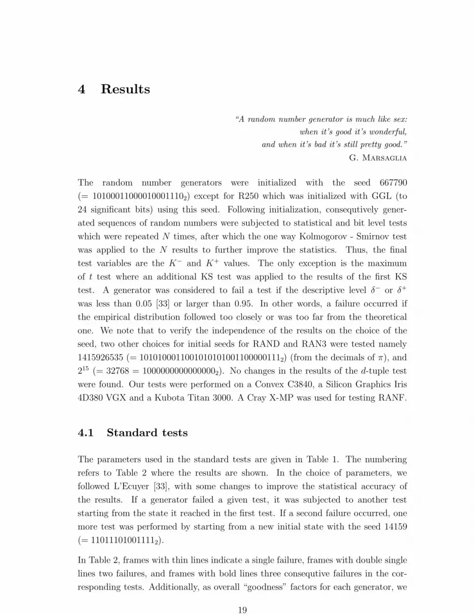
4.1 Standard tests

The parameters used in the standard tests are given in Table 1. The numbering

refers to Table 2 where the results are shown. In the choice of parameters, we

followed L’Ecuyer [33], with some changes to improve the statistical accuracy of

the results. If a generator failed a given test, it was subjected to another test

starting from the state it reached in the first test. If a second failure occurred, one

more test was performed by starting from a new initial state with the seed 14159

(= 110111010011112).

In Table 2, frames with thin lines indicate a single failure, frames with double single

lines two failures, and frames with bold lines three consequtive failures in the cor-

responding tests. Additionally, as overall “goodness” factors for each generator, we

19

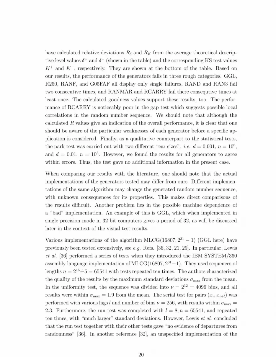
have calculated relative deviations Rδ and RK from the average theoretical descrip-

tive level values δ+ and δ− (shown in the table) and the corresponding KS test values

K+ and K−, respectively. They are shown at the bottom of the table. Based on

our results, the performance of the generators falls in three rough categories. GGL,

R250, RANF, and G05FAF all display only single failures, RAND and RAN3 fail

two consecutive times, and RANMAR and RCARRY fail there consequtive times at

least once. The calculated goodness values support these results, too. The perfor-

mance of RCARRY is noticeably poor in the gap test which suggests possible local

correlations in the random number sequence. We should note that although the

calculated R values give an indication of the overall performance, it is clear that one

should be aware of the particular weaknesses of each generator before a specific ap-

plication is considered. Finally, as a qualitative counterpart to the statistical tests,

the park test was carried out with two different “car sizes”, i.e. d = 0.001, n = 106,

and d = 0.01, n = 105. However, we found the results for all generators to agree

within errors. Thus, the test gave no additional information in the present case.

When comparing our results with the literature, one should note that the actual

implementations of the generators tested may differ from ours. Different implemen-

tations of the same algorithm may change the generated random number sequence,

with unknown consequences for its properties. This makes direct comparisons of

the results difficult. Another problem lies in the possible machine dependence of

a “bad” implementation. An example of this is GGL, which when implemented in

single precision mode in 32 bit computers gives a period of 32, as will be discussed

later in the context of the visual test results.

Various implementations of the algorithm MLCG(16807, 231 − 1) (GGL here) have

previously been tested extensively, see e.g. Refs. [36, 32, 21, 29]. In particular, Lewis

et al. [36] performed a series of tests when they introduced the IBM SYSTEM/360

assembly language implementation of MLCG(16807, 231−1). They used sequences of

lengths n = 216+5 = 65541 with tests repeated ten times. The authors characterized

the quality of the results by the maximum standard deviations σmax from the mean.

In the uniformity test, the sequence was divided into ν = 212 = 4096 bins, and all

results were within σmax = 1.9 from the mean. The serial test for pairs (xi, xi+l) was

performed with various lags l and number of bins ν = 256, with results within σmax =

2.3. Furthermore, the run test was completed with l = 8, n = 65541, and repeated

ten times, with “much larger” standard deviations. However, Lewis et al. concluded

that the run test together with their other tests gave “no evidence of departures from

randomness” [36]. In another reference [32], an unspecified implementation of the

20

generator has also been subjected to the run test with a two way KS test and has

been found to pass it, as well as a serial test for triples (d = 3) but to fail a serial

test for pairs (d = 2). In the run test, the sequence length was n = 65536, the runs

were counted up to l = 8 and the test was repeated one hundred times (N = 100).

Similarly, in the serial test n = 65541 and N = 100 [32]. We should note that in our

tests, where better statistics was used (N = 1000) GGL passed the run test and all

the serial tests for d = 2, 3, 4.

RAND is an implementation of LCG(69069, 1, 232) by Convex Corp. [63]. Lear-

month and Lewis [32] have also tested their assembly language implementation of

LCG(69069, 1, 232) with the same test as the MLCG(16807, 231 − 1) generator dis-

cussed above. LCG(69069, 1, 232) passed the serial test for both d = 2 and d = 3, as

well as the run test. In our tests, RAND passed all these tests as well.

An IBM assembly language implementation of GFSR(250, 103,⊕) has been found

to perform well in a run test with parameters n = 106, N = 30, l = 9 [29]. Our

Fortran implementation of it, namely R250 also passed the run test.

Finally, we have been unable to find any published data on statistical tests for any

implementations of RANMAR, RCARRY, RAN3, RANF or G05FAF.

4.2 Spectral test

The results of the spectral test for the LCG generators of this paper are presented in

Table 3. In the case of RANF, we show results for the two generators which comprise

it, namely MLCG(44485709377909,248) (RANF1) and

MLCG(247908122798849,248) (RANF2). Overall, the generator G05FAF from the

NAG library is the most successful in the test. On the other hand, GGL displays

the known flaw of this generator performing poorly at low dimensions. All genera-

tors, however, gave worse results in most dimensions than the minimum acceptable

values suggested by Fishman and Moore [16, 3]. We note that since the results

of this test are independent of the implementations of the algorithms, our results

for RAND agree with previous results for LCG(69069, 1, 232) [3], for GGL with

MLCG(16807, 231 − 1) [16, 33, 3] and for RANF1 with MLCG(44485709377909,248)

[3, 17].

21

4.3 Bit level tests

The bit level tests probe the properties of the individual bits which comprise the ran-

dom numbers thus testing properties somewhat different from the statistical tests.

We chose to use the generalized d-tuple test and the rank of a random matrix test

for studying correlations on the bit level.

The d-tuple test (d = 3) was carried out for n = 5000 random numbers, each of

which was coded into a 31 bit binary sequence (for RAN3, the sequence length was

30). Of this sequence, we chose bit strips of width l = 3. The χ2 test was performed

N = 1000 times, and the results were then subjected to a KS test2. This test

was performed twice for each generator (excluding PURAN II) and we considered

“failed” only those bits that failed twice in succession.

The rank test was carried out with parameters v = w = 2, n = 1000 and N = 1000.

The (2× 2) random matrices were formed systematically using the ith and (i + 1)th

(1 ≤ i ≤ 31) bit pairs from each two successive numbers. The test was performed

twice to all pseudorandom number generators with the same failing criteria as in

the d-tuple test.

Results for the d-tuple and rank tests are shown in Table 4. Details of the im-

plementations and initializations of the generators are also shown there. In our

notation, the bit number one is the most significant bit. GGL, G05FAF, and R250

pass both tests with an impeccable performance, in that none of the 31 bits show

observable correlations. The physically generated random numbers of PURAN II

also pass both tests. For RANMAR and RCARRY, only the 24 most significant

bits are guaranteed to be good [27], which our tests confirm. On the other hand,

RAND and RAN3 show significant correlations. In particular, the correlations in

RAN3 are serious since they affect the five most significant bits. When RAND was

called in integer form, it gave one more correlated bit than the calls in floating point

representation both in the d-tuple and rank tests.

Previously, an unspecified implementation of MLCG(16807, 231−1) (GGL here) has

been shown to pass a simpler version of the d-tuple test (d = l = 3, n = 2000, test re-

peated five times) [2]. An unspecified implementation of LCG(69069, 1, 232) (RAND

here) failed the same test with 11 failing bits [2]. An IBM assembly language im-

plementation of GFSR(250, 103,⊕) (R250 here) and an unspecified implementation

2Results of a systematic study indicate [59] that with these parameters, the d-tuple test can

detect correlations up to about fifty numbers apart.

22

of MLCG(16807, 231 − 1) (GGL here) have been shown to pass a test which probed

possible correlations in the five most significant bits by studying triples of random

numbers by placing them on a unit cube with a resolution of 32 × 32 × 32 cells

(n = 106 and the test was repeated “several” times) [29]. Kirkpatrick and Stoll [29]

further argue that as all columns of bits generated by a GFSR(250, 103,⊕) generator

have the same statistical characteristics, their results of this test should apply to

any subset of bits in a random number sequence produced by this generator. This

is in accordance with our results, where no correlations were found in the 31 bits of

R250 (see Table 4).

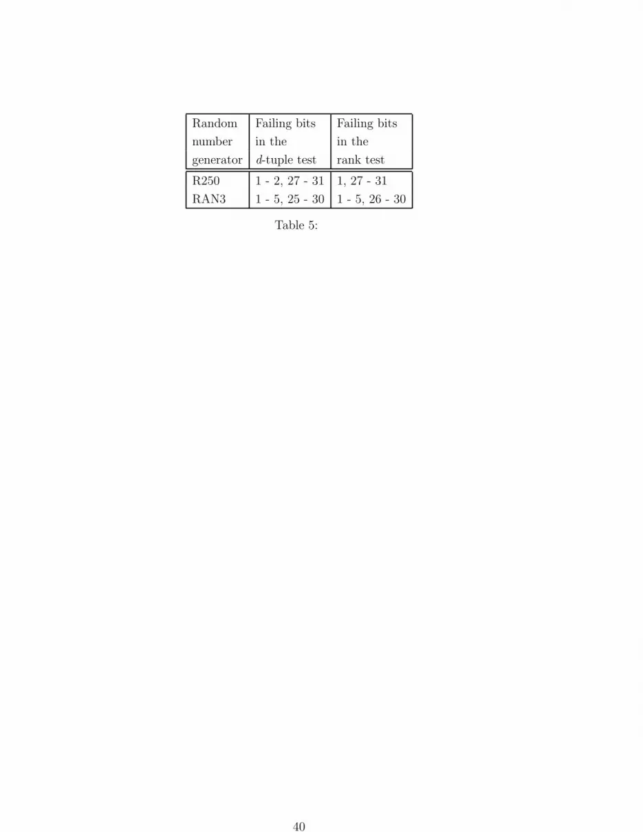
The initialization of R250 deserves a more detailed discussion. Already Kirkpatrick

and Stoll [29] have pointed out that the algorithm GFSR(250,103,⊕) requires a

careful initialization. Our results in Table 5 clearly show this to be true as the

results for R250 initialized with RAN3 show correlations in the most significant bits,

an obvious consequence of the bad quality of RAN3. It is particularly important to

notice, that these correlations once present seem to persist in R250.

Finally, for testing purposes we also realized our own Fortran implementation of

LCG(69069, 1, 232) in double precision accuracy. In this implementation, whenever

the sign bit equalled one it was flipped to zero. Thus, the random numbers remained

between zero and 231−1. This implementation produced exactly the same sequence

as RAND on a Convex C3840. Another possible implementation of the same algo-

rithm was then realized in such a way that whenever the sign bit equalled one, the

whole computer word was shifted to the right (with periodic boundary conditions)

until a zero was obtained for the sign bit. When bit level tests were done for this

implementation, all 31 bits failed. This dramatically highlights the effect of a poor

implementation on the performance of the same algorithm.

4.4 Visual tests

The two dimensional distribution of 20 000 random number pairs (xi, xi+1) from

GGL, RAND and R250 is shown in Figs. 1(a) − (f). When plotted on the scale

from zero to one (Figs. 1(a), (c), (e)), no generator shows any discernible structure.

However, when the 20 000 random numbers are plotted on an expanded scale (Figs.

1(b), (d), (f)) one can clearly see the random numbers ordering on planes in the cases

of GGL and RAND. This kind of behavior is expected for LCG generators [40], and

the results are in accordance with the spectral test of Section 3.3. We note that no

structure on other generators was observed on this scale.

23

In Figs. 2(a) and (b), we depict subsequent random numbers in binary form on a

124 × 124 matrix from our best implementations of GGL and R250, respectively.

Although the former showed clear lattice structure in the test above, in binary

form it is very difficult to find any differences between these two generators. More

quantitative tests of the bit maps shown here are in progress [59]. When we further

compare the binary representations of R250 with different initializations, the visual

tests corroborate the findings of the qualitative tests: In Fig. 2(b), R250 is initialized

with GGL with double precision modulo operation, returning integers. However, if

we initialize R250 with real numbers from GGL implemented in single precision,

the result is catastrophic as seen in Fig. 3. Clearly this is an improper way to

implement MLCG(16807, 231 − 1) in 32 bit word computers. It is interesting to

note, that already Lewis et al. [36] pointed out the need to use double precision

accuracy with the assembly implementation of MLCG(16807, 231 − 1).

The visualization of the difference between random numbers (test (iii)) and the gap

test visualization (test (iv)) gave rather inconclusive results and thus yielded no

further insight to the properties of the generators.

Finally, a problem was encountered with the decoding program which was included

with the physical PURAN II random numbers [52]. When used to extract random

numbers in floating point representation, we found that it produced numbers which

fell on planes similarly to the linear congruential generators, although PURAN II

passed all bit level tests. However, when using the decoding algorithm in integer

format the problem disappeared.

4.5 Speed of generators

We tested the computational speed of the eight generators both on a Cray X-MP/432

and a Convex C3840. All generators were compiled in two ways: first, only scalar

optimization was allowed and second, also vectorization was allowed. The testing

was done for sequences of lengths n = 1, 10, 100, 1000, 10000 and 100000.

Results are in Table 6 for n = 1 and n = 1000 in units of microseconds (µs)

per random number call. The speedup for longer sequences (n > 1000) per random

number call is nonexistent. First, Cray’s own generator RANF was always the fastest

on it which indicates a successful implementation in this sense. Other generators

are almost equally fast for short sequences, except for R250. On the other hand,

the performance for longer sequences is fastest for R250 and G05FAF if vectorizing

24

is allowed. The code for RAN3 as given in Numerical Recipes [51] was incompatible

with Cray and is thus omitted from its performance results.

25

5 Summary and Discussion

“The whole history of

pseudorandom number generation

is riddled with myths and extrapolations

from inadequate examples.

A healthy dose of sceptisism is needed

in reading the literature.”

B. D. Ripley

In this work, we have carried out an extensive test program of a collection of random

number generators, which are commonly used in the applications of physics. These

include public domain programs GGL, RANMAR, RAN3, RCARRY and R250, a

library subroutine G05FAF, and manufacturer installed routines RAND and RANF.

Also, a sequence of random numbers produced from physical noise has been included

for purposes of comparison. Our test bench consists of standard statistical tests, bit

level tests and qualitative visual tests. If we use the first two quantitative tests as

criteria, three of the generators, namely GGL, G05FAF, and R250 display an overall

best performance in all tests, and could thus be recommended for most applications.

They fail statistical tests only once, and produce 31 “good” bits. Other generators

show somewhat less convincing performance in one or more test category, although

RANF performs very well in statistical tests. If the least significant bits are not

important for the application, both RANF and RANMAR are good choices. On the

other hand, the clear bit level correlations of RAN3 and poor statistical properties

of RCARRY suggest problems in these generators [38]. Finally, RAND suffers from

an overall lackluster performance. In Table 7 we show a qualitative summary of the

performance of all of the generators in statistical and bit level tests.

Our results also demonstrate the existence of two fundamental problems which may

plague some random number generators. First, a bad implementation of a generator

algorithm may cause total corruption of the output, as we have demonstrated for

GGL and RAND. Second problem concerns the initialization of generators such as

R250, which require several seed values. This issue has received relatively little

attention in the past, but our results in Section 4.3 demonstrate that as a result of

a bad initialization, correlations in the seeds of R250 transform into the generated

random number sequences. Thus even a good generator can be corrupted by careless

use.

Despite the extensive test program presented here, there may still exist correlations

26

which may be of significance. To this end, direct physical, application specific tests

of various generators play an important role and have been conducted in some special

cases [29, 28, 49, 46, 14, 23, 59]. These tests are of particular importance in Monte

Carlo simulations, where physical systems may be very sensitive to spatial corre-

lations. In particular, it has recently been suggested that biased results in Monte

Carlo simulations of the Ising model [14] and self - avoiding random walks [23] result

from yet undetected correlations present in the GFSR(250, 103,⊕) algorithm (R250

here). In both cases, special simulation algorithms were used. In Ref. [14] the au-

thors suggest that bit level correlations in the most significant bits of this generator

are responsible for this. However, our results of Sec. 4.3 do not lend support to this

claim, since no discernible correlations exist up to at least 50 numbers apart. We

have in fact recently extended the bit level tests to check correlations up to about

1000 numbers apart, but find no correlations for our R250 [59]. Results of Ref. [14]

thus remain unexplained at the moment. On the other hand, Ref. [23] claims to

confirm these anomalous correlations for GFSR(250, 103,⊕), and finds poor per-

formance also for LF(55,24,+) (our RAN3 is LF(55,24,−)). RAN3 spectacularly

fails our bit level tests, which probably explains results of Ref. [23] for the lagged

Fibonacci generator. However, concerning GFSR(250,103,⊕) Ref. [23] goes as far

as to reinforce the claim [42] that “shift register generators using XOR’s are among

the worst random number generators and should never have been used”. Based

on our test results this is a somewhat unfair statement, since R250 when properly

implemented and initialized certainly performs well enough for many applications.

However, we agree with Ref. [14] on the need of careful physical tests before a “good

quality” generator is chosen for a given application. To unravel possible anomalous

correlations in R250, a new generation of test methods is clearly needed since no

test carried out here can support this claim. Work in this direction is currently

underway [59].

6 Acknowledgments

We would like to thank Juha Haataja, Jukka Helin, Pentti Huuhtanen, Kimmo

Kaski, Juhani Kapyaho, Petri Laurikainen, Jussi Rahola, Robert Swendsen, and

Jukka Vanhala for useful discussions and Fred James and Manfred Richter for cor-

respondence. Veikko Nyfors of Cray Finland Oy, Greg Astfalk of Convex Computer

Corporation and Julie Gulla of Mathworks Inc. have provided information of the

random number generators used in their products. Aarno Hauru, Pekka Kytolaakso,

27

Klaus Lindberg and Juha Ruokolainen have given valuable technical assistance. The

Finnish Center for Scientific Computing and Tampere University of Technology have

generously provided the computing resources. This research was partially supported

by the Academy of Finland and the Foundation of Tampere University of Technol-

ogy.

28

E-mail addresses: Ilpo.Vattulainen@csc.fi, Kari.Kankaala@csc.fi,

jukkas@ee.tut.fi, and ala@phcu.helsinki.fi

References

[1] E. Aarts and J. Korst, Simulated Annealing and Boltzmann Machines,

A Stochastic Approach to Combinatorial Optimization and Neural Computing

(John Wiley & Sons, Chichester, 1989).

[2] N. S. Altman, SIAM J. Sci. Stat. Comput. 9, 941 (1988).

[3] S. L. Anderson, SIAM Review 32, 221 (1990).

[4] L. M. Berliner, Stat. Science 7, 69 (1992).

[5] K. Binder, in Monte Carlo Methods in Condensed Matter Physics, edited by

K. Binder (Springer - Verlag, Berlin, 1992).

[6] H. S. Bright and R. L. Enison, Computing Surveys 11, 357 (1979).

[7] B. J. Collings and G. B. Hembree, J. ACM 33, 706 (1986).

[8] A. Compagner and A. Hoogland, J. Comp. Phys. 71, 391 (1987).

[9] A. Compagner, Am. J. Phys. 59, 700 (1991).

[10] A. Compagner, J. Stat. Phys. 63, 883 (1991).

[11] R. R. Coveyou and R. D. MacPherson, J. ACM 14, 100 (1967).

[12] D. W. Davies and W. L. Price, Security for Computer Networks, An In-

troduction to Data Security in Teleprocessing and Electronic Funds Transfer,

2nd ed. (John Wiley & Sons, Chichester, 1989).

[13] E. J. Dudewicz and T. G. Ralley, in The Handbook of Random Number

Generation and Testing with TESTRAND Computer Code, Am. Series in Math.

and Manag. Sci., Vol. 1 (American Science Press, Ohio, USA, 1981).

[14] A. M. Ferrenberg, D. P. Landau and Y. J. Wong, Phys. Rev. Lett.

69, 3382 (1992).

[15] G. S. Fishman and L. R. Moore III, J. Am. Stat. Assoc. 77, 129 (1982).

29

[16] G. S. Fishman and L. R. Moore III, SIAM J. Sci. and Stat. Comp. 7, 24

(1986).

[17] G. S. Fishman, Math. Comp. 54, 331 (1990).

[18] M. Fushimi and S. Tezuka, Comm. ACM 26, 516 (1983).

[19] M. Fushimi, Inform. Proc. Lett. 16, 189 (1983).

[20] M. Fushimi, SIAM J. Comp. 17, 89 (1988).

[21] S. Garpman and J. Randrup, Comp. Phys. Comm. 15, 5 (1978).

[22] J. E. Gentle, J. Comp. Appl. Math. 31, 119 (1990).

[23] P. Grassberger, Wuppertal University preprint WUB 93-03 (1993).

[24] J. Helin, unpublished work (1985).

[25] J. R. Heringa, H. W. J. Blote and A. Compagner, Int. J. Mod. Phys.

C 3, 561 (1992).

[26] N. Ito, M. Kikuchi, Y. Okabe, Cologne University preprint (1992), hep-

lat@ftp.scri.fsu.edu 9302002.

[27] F. James, Comp. Phys. Comm. 60, 329 (1990).

[28] C. Kalle and S. Wansleben, Comp. Phys. Comm. 33, 343 (1984).

[29] S. Kirkpatrick and E. P. Stoll, J. Comp. Phys. 40, 517 (1981).

[30] D. E. Knuth, The Art of Computer Programming, Volume 2: Seminumerical

Algorithms, 2nd ed. (Addison-Wesley, Reading, Massachusetts, 1981).

[31] M. van Lambalgen, J. Symbolic Logic 52, 725 (1987).

[32] G. P. Learmonth and P. A. W. Lewis, in Computer Science and Statistics:

7th Annual Symposium on the interaface, edited by W. J. Kennedy, (Statistical

Laboratory, Iowa State University, Ames, Iowa, 1973) p. 163.

[33] P. L’Ecuyer, Comm. ACM 31, 742 (1988).

[34] P. L’Ecuyer, Comm. ACM 33, 86 (1990).

[35] D. H. Lehmer, in Proc. 2nd Symp. on Large-Scale Digital Calculating Ma-

chinery (Harvard University Press, Cambridge, 1951), p. 141.

30

[36] P. A. Lewis, A. S. Goodman and J. M. Miller, IBM Syst. J. 8, 136

(1969).

[37] T. G. Lewis and W. H. Payne, J. Assoc. Comput. Mach. 20, 456 (1973).

[38] Recently, M. Lucher (unpublished) has noted that there’s a bug in the imple-

mentation of RCARRY, which affects its output. We have repeated the gap tests

for the corrected version, but find no significant improvement in the statistical

properties.

[39] M. D. MacLaren and G. Marsaglia, J. Assoc. Comput. Mach. 12, 83

(1965).

[40] G. Marsaglia, Proc. of the Nat. Acad. Sci. 61, 25 (1968).

[41] G. Marsaglia, in Applications of Number Theory to Numerical Analysis,

edited by S. K. Zaremba (Academic Press, New York, 1972), p. 249.

[42] G. A. Marsaglia, in Computer Science and Statistics: The Interface, edited

by L. Billard, (Elsevier, Amsterdam, 1985) p. 3.

[43] G. Marsaglia and A. Zaman, Stat. & Prob. Lett. 8, 329 (1990).

[44] G. Marsaglia, B. Narasimhan and A. Zaman, Comp. Phys. Comm. 60,

345 (1990).

[45] A. De Matteis and S. Pagnutti, Parallel Computing 13, 193 (1990).

[46] A. Milchev, K. Binder and D. W. Heermann, Z. Phys. B 63, 521 (1986).

[47] H. Niederreiter, SIAM J. Sci. Stat. Comput. 8, 1035 (1987).

[48] S. K. Park and K. W. Miller, Comm. ACM 31, 1192 (1988).

[49] J. Paulsen, J. Stat. Comput. Simul. 19, 23 (1984).

[50] W. H. Payne and K. L. McMillen, Comm. ACM 21, 259 (1978).

[51] W. H. Press, B. P. Flannery, S. A. Tenkolsky and W. T. Vetter-

ling, Fortran version (Cambridge University Press, 1989) p. 198.

[52] M. Richter, private communication. The random numbers by PURAN II are

available from an anonymous ftp site at dfv.rwth-aachen.de.

[53] L. Schrage, ACM Trans. Math. Soft. 5, 132 (1979).

31

[54] R. C. Tausworthe, Math. Comp. 19, 201 (1965).

[55] S. Tezuka, Comm. ACM 30, 731 (1987).

[56] S. Tezuka, J. Assoc. Comp. Mach. 34, 939 (1987).

[57] J. P. R. Tootill, W. D. Robinson and A. G. Adams, J. Assoc. Comput.

Mach. 18, 381 (1971).

[58] I. Vattulainen, K. Kankaala, J. Saarinen and T. Ala-Nissila, CSC

Research Report R05/92 (Centre for Scientific Computing, Espoo, Finland

1992). In Finnish.

[59] I. Vattulainen, K. Kankaala, J. Saarinen, and T. Ala-Nissila, to

be published.

[60] N. Zierler and J. Brillhart, Inform. and Control 13, 541 (1968).

[61] K. Zheng, C.-H. Yong, D.-Y. Wei, IEEE Computer 24, 8 (1991).

[62] N. Zierler, Inform. and Control 15, 67 (1969).

[63] Convex Fortran Guide, 1st edition (Convex Computer Corp., Richardson, USA,

1991), p. 553.

[64] Cray Unicos, Math and Scientific Library Reference Manual, SR-2081 6.0

(Cray Research Inc., USA, 1991).

[65] IBM Subroutine Library - Mathematics (User’s Guide program number 5736-

XM7, 1971).

[66] IMSL Stat/Library User’s Manual 3 (IMSL, Houston, Texas, 1989), p. 945.

[67] MATLAB User’s Guide, PRO-MATLAB for VAX/VMS Computers (The

MathWorks Inc., South Natick, MA, 1991), p. 3-158; J. Gulla, private com-

munication.

[68] NAG Fortran Library Manual, Mark 14, 7 (Numerical Algorithms Group Inc.,

1990).

32

7 Table captions

Table 1

Table 1. Parameters used in the standard tests. n is the length of the random num-

ber sequence and N is the number of times the test was repeated for the Kolmogorov

- Smirnov test. Other parameters are described in the text.

Table 2

Table 2. Results of the statistical tests. Depicted numbers are the values for the

descriptive levels δ+ and δ− from the Kolmogorov - Smirnov test variables K+ and

K−, and Rδ and RK denote average goodness values, as defined in the text (with

tests 1 and 2 excluded). The data for R’s comes from the first run only. A generator

was considered to fail the test if the descriptive level was less than 0.05 or more than

0.95. Single, double and triple consequtive failures are indicated by single, double,

and bold lines, respectively.

Table 3

Table 3. Results of the spectral test for linear congruential generators. See text

for details.

Table 4

Table 4. Results of the bit level d-tuple and rank tests. The bits marked failed

have failed the test twice. See text for details.

Table 5

Table 5. Results of d-tuple and rank tests for R250 initialized with RAN3.

Table 6

Table 6. Absolute speeds of the generators on a Cray X-MP/432 EA and a Convex

C3840. S denotes compiling when only scalar optimization was allowed and V when

also vectorizing was allowed. The timings are in units of microseconds per random

number call. RANF could only be tested on Cray and RAND on Convex. RAN3

produced erroneous results on Cray.

Table 7

Table 7. A summary of the performance of the tested generators in statistical and

bit level tests. For statistical tests, plus denotes at least one case of one consequtive

33

failure, zero at least one case of two consequtive failures, and minus at least one

case of three consequtive failures. For bit level tests, plus denotes an impeccable

performance, zero the failure of some of the least significant bits, and minus the

failure of more significant bits for RAND and RAN3. See text for more details.

34

8 Figure Captions

Figure 1

Fig. 1. Spatial distribution of 20 000 random number pairs in two dimensions on

a unit square as generated by GGL (a), (b), RAND (c), (d) and R250 (e), (f). The

second figure in each case has a greatly expanded scale on the x axis.

Figure 2

Fig. 2. 31 bit binary representations of random numbers produced by GGL (a)

and R250 (b) on a 124 × 124 matrix.

Figure 3

Fig 3. Binary representations of random numbers produced by R250 when initial-

ized with GGL in single precision mode.

35

Test n N Other parameters

(1) χ2 100000 10000 ν = 256

(2) χ2 10000 10000 ν = 128

(3) Serial test 100000 1000 d = 2 ν = 100

(4) Serial test 100000 1000 d = 3 ν = 20

(5) Serial test 100000 1000 d = 4 ν = 10

(6) Gap test 25000 1000 α = 0 β = 0.05 l = 30

(7) Gap test 25000 1000 α = 0.45 β = 0.55 l = 30

(8) Gap test 25000 1000 α = 0.95 β = 1 l = 30

(9) Maximum of t 2000 1000 t = 5

(10) Maximum of t 2000 1000 t = 3

(11) Collision test 16384 1000 d = 2 s = 1024

(12) Collision test 16384 1000 d = 4 s = 32

(13) Collision test 16384 1000 d = 10 s = 4

(14) Run test 100000 1000 l = 6

Table 1:

36

Table 2:

37

RAND GGL G05FAF RANF 1 RANF 2

d κd λd κd λd κd λd κd λd κd λd

2 0.9250 15.991 0.3375 14.037 0.8423 29.356 0.8269 22.8295 0.6499 22.482

3 0.7890 10.492 0.4412 9.319 0.7640 19.533 0.7416 15.069 0.7705 15.124

4 0.7548 7.844 0.5752 7.202 0.8472 14.260 0.3983 10.422 0.7071 11.250

5 0.8041 6.386 0.7361 6.058 0.7838 11.348 0.7307 9.047 0.3983 8.172

6 0.2990 3.959 0.6454 4.903 0.6333 9.209 0.6177 7.339 0.6282 7.364

7 0.4075 3.705 0.5711 4.049 0.5540 8.382 0.6670 6.416 0.2375 4.926

8 0.5762 3.705 0.6096 3.661 0.6597 7.271 0.5642 5.424 0.2135 4.022

Table 3:

38

Random Failing bits Failing bits Comments of

number in the in the rank implementation

generator d-tuple test test and initialization

GGL none none double precision mode

(return integers)

RAND 13-31 18-31 real mode

RANF 29-45 24,31-45 real mode

G05FAF none none double precision mode

R250 none none integer mode, initialized

with GGL in double precision

RAN3 1-5,25-30 1-5,26-30 integer mode

RANMAR 25-31 25-31 real mode

RCARRY 25-31 25-31 real mode

PURAN II none none integer mode

Table 4:

39

Random Failing bits Failing bits

number in the in the

generator d-tuple test rank test

R250 1 - 2, 27 - 31 1, 27 - 31

RAN3 1 - 5, 25 - 30 1 - 5, 26 - 30

Table 5:

40

Generator Optimization Cray Convex

n = 1 n = 1000 n = 1 n = 1000

GGL S 2.218 2.731 4.420 2.379

V 2.465 2.029 5.676 2.381

RAND S − − 4.446 4.582

V − − 6.661 4.369

RANF S 1.466 1.582 − −V 1.536 0.020 − −

G05FAF S 4.556 0.422 4.384 0.571

V 4.442 0.365 6.321 0.559

R250 S 260.0 1.672 126.7 1.094

V 10.88 0.055 55.87 0.476

RAN3 S 4.711 − 3.987 2.177

V 3.563 − 4.881 1.608

RANMAR S 7.132 3.407 5.672 1.932

V 4.801 1.053 5.742 1.508

RCARRY S 6.486 2.455 4.956 1.211

V 3.962 0.728 4.537 0.899

Table 6:

41

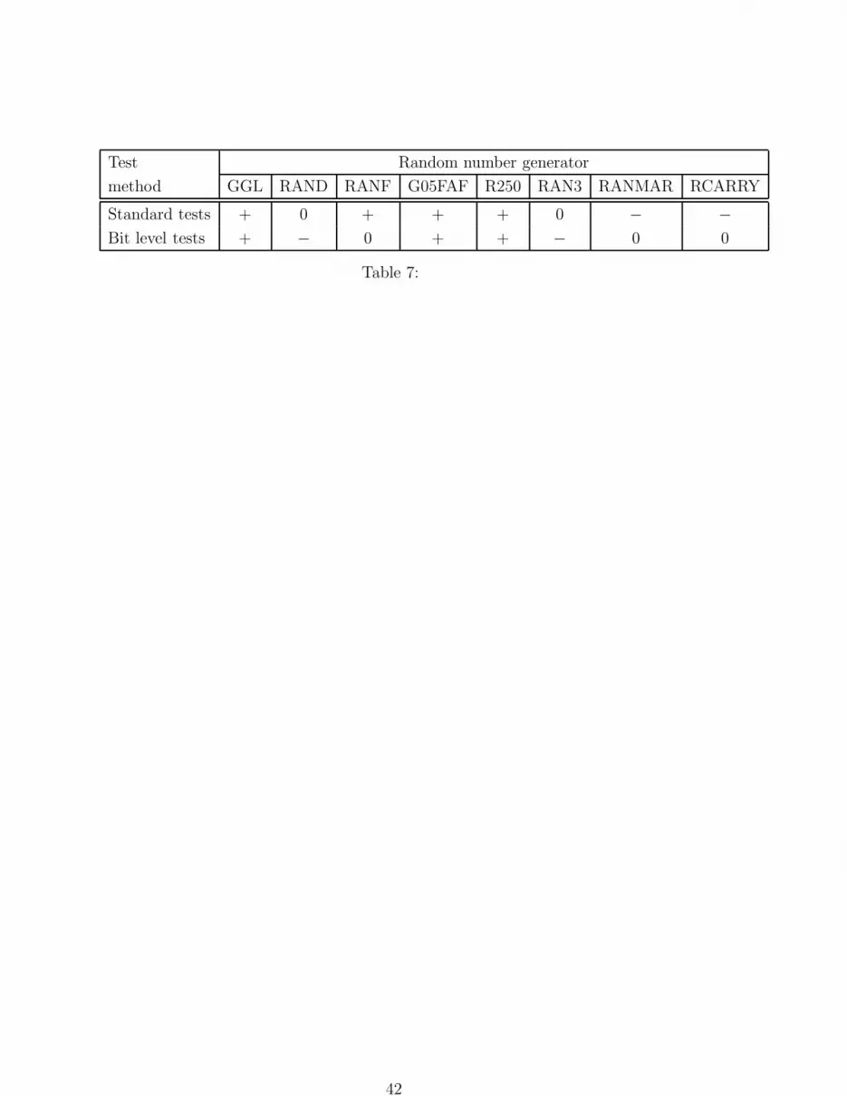
Test Random number generator

method GGL RAND RANF G05FAF R250 RAN3 RANMAR RCARRY

Standard tests + 0 + + + 0 − −Bit level tests + − 0 + + − 0 0

Table 7:

42

Test K+ K- K+ K- K+ K- K+ K- K+ K- K+ K- K+ K- K+ K-

1 0.205 0.249 0.829 0.490 0.562 0.655 0.609 0.049 0.112 0.518 0.709 0.748 0.963 0.202 0.194 0.639

2 0.718 0.907 0.043 0.982 0.592 0.421 0.391 0.778 0.907 0.713 0.966 0.149 0.219 0.490 0.690 0.213

3 0.672 0.380 0.228 0.895 0.924 0.039 0.700 0.570 0.678 0.292 0.798 0.903 0.419 0.482 0.070 0.570

4 0.642 0.238 0.280 0.541 0.242 0.667 0.702 0.095 0.256 0.573 0.553 0.762 0.262 0.666 0.175 0.494

5 0.780 0.465 0.134 0.697 0.582 0.788 0.494 0.380 0.991 0.103 0.734 0.040 0.031 0.929 0.961 0.274

6 0.900 0.649 0.559 0.479 0.562 0.472 0.609 0.143 0.544 0.079 0.049 0.927 0.545 0.486 0.000 1.000

7 0.976 0.100 0.987 0.344 0.368 0.582 0.957 0.018 0.343 0.929 0.379 0.484 0.795 0.274 0.169 0.909

8 0.768 0.048 0.380 0.816 0.630 0.305 0.986 0.161 0.332 0.415 0.494 0.664 0.492 0.317 0.000 1.000

9+ 0.490 0.331 0.326 0.981 0.900 0.115 0.255 0.133 0.294 0.365 0.761 0.029 0.661 0.311 0.436 0.968

9- 0.887 0.000 0.938 0.018 0.947 0.108 0.967 0.108 0.951 0.433 0.926 0.001 0.735 0.164 0.989 0.006

10+ 0.985 0.052 0.107 0.795 0.214 0.788 0.832 0.508 0.718 0.356 0.966 0.704 0.948 0.048 0.145 0.540

10- 0.864 0.028 0.981 0.001 1.000 0.000 0.998 0.000 0.750 0.162 0.999 0.101 0.684 0.000 0.999 0.026

11 0.161 0.561 0.974 0.076 0.906 0.146 0.105 0.653 0.807 0.670 0.049 0.769 0.977 0.093 0.069 0.553

12 0.654 0.159 0.888 0.071 0.093 0.426 0.175 0.909 0.720 0.237 0.847 0.119 0.799 0.350 0.854 0.102

13 0.411 0.551 0.102 0.137 0.363 0.607 0.430 0.413 0.480 0.347 0.809 0.069 0.654 0.344 0.383 0.417

14 0.073 0.755 0.356 0.946 0.276 0.297 0.124 0.637 0.368 0.226 0.785 0.154 0.268 0.375 0.339 0.851

GGL RAND RANF G05FAF R250 RAN3 RANMAR RCARRY

2.52% 6.62% 4.86% 0.62% 2.47% 7.74% 6.30% 7.66%R