A Central Rapidity Straw Tracker and Measurements on ...

A Central Rapidity Straw Tracker and Measurements

on Cryogenic Components for the Large Hadron Collider

Thesis for the degree of Doctor of Philosophy in Physics

by

Hans Danielsson

Title: lejon.epsCreator: Ofoto 1.0CreationDate: 10/20/92 10:51 AM

Elementary Particle PhysicsDepartment of Physics, University of Lund

Sweden

thes

is-2

000-

039

1997

ISBN 91-628-2511-9LUNFD6/(NFFL-7139)1997

A Central Rapidity Straw Tracker and Measurements

on Cryogenic Components for the Large Hadron Collider

Thesis for the degree of Doctor of Philosophy in Physics

by

Hans Danielsson

Title: lejon.epsCreator: Ofoto 1.0CreationDate: 10/20/92 10:51 AM

Elementary Particle PhysicsDepartment of Physics, University of Lund

Sweden

Lund 1997

Contents

1. Preface..............................................................................................................9

2. The LHC project ...........................................................................................11

2.1 The experiments......................................................................................122.2 The accelerator .......................................................................................132.3 References ..............................................................................................14

3. ATLAS...........................................................................................................15

3.1.1 The magnet system.......................................................................183.1.2 The inner detector ........................................................................203.1.3 The calorimeter ............................................................................213.1.4 The muon detectors ......................................................................223.1.5 The trigger system........................................................................22

3.2 References ..............................................................................................23

4. A central rapidity straw tracker ....................................................................24

4.1 The transition radiation tracker (TRT).....................................................244.2 Transition radiation (TR) ........................................................................264.3 Physics motivation for a transition-radiation detector ...............................284.4 Principal operation of the straws .............................................................29

4.4.1 Gas composition...........................................................................304.5 Electrical connections..............................................................................31

4.5.1 The ASDBLR ..............................................................................334.5.2 The DTMROC.............................................................................35

4.6 The design of the barrel TRT ..................................................................364.6.1 A modular approach.....................................................................364.6.2 Straw layout ................................................................................404.6.3 Support structure .........................................................................43

4.6.3.1 Module shells .......................................................................434.6.4 Radiators .....................................................................................454.6.5 Ventilation of the radiator.............................................................464.6.6 Design, assembly and testing of a 0.5 m barrel prototype ..............47

4.6.6.1 Design and assembly ............................................................474.6.6.2 Tests during assembly ..........................................................554.6.6.3 Experience learned from the assembly of the 0.5 m prototype 57

4.6.7 Cross-talk ....................................................................................584.6.7.1 Experimental set-up..............................................................584.6.7.2 Results.................................................................................614.6.7.3 Conclusion and discussion ....................................................63

4.6.8 Heat conductivity measurement on radiator materials....................644.6.8.1 Experimental set-up..............................................................64

4.6.8.2 Calculation method...............................................................644.6.8.3 Results.................................................................................654.6.8.4 Estimation of the error..........................................................66

4.6.9 Cooling of the modules.................................................................664.6.9.1 Requirements .......................................................................664.6.9.2 Analytical calculations .........................................................674.6.9.3 Experimental set-up..............................................................724.6.9.4 Results from measurements ..................................................724.6.9.5 Temperature gradient at the cooling-tube interface ................744.6.9.6 Conclusions and remarks on the module cooling....................75

4.6.10 Tracking performance for a modular layout ................................764.6.10.1 Geometry ...........................................................................764.6.10.2 Results ...............................................................................784.6.10.3 Estimation of the errors ......................................................814.6.10.4 Conclusions........................................................................82

4.6.11 Material in the barrel TRT .........................................................824.6.11.1 Geometry ...........................................................................834.6.11.2 Results from the material budget study................................86

4.6.12 TR performance .........................................................................864.6.12.1 Test beam set-up ................................................................884.6.12.2 Beam purity .......................................................................894.6.12.3 Radiator performance .........................................................904.6.12.4 Extrapolation to the full barrel TRT....................................934.6.12.5 Without carbon-fibre shells.................................................934.6.12.6 With carbon-fibre shells......................................................984.6.12.7 Conclusions and remarks .................................................. 103

4.7 Conclusions .......................................................................................... 1044.8 References ............................................................................................ 105

Appendix A - Number of straws in the modules................................................. 108

5. Measurements on cryogenic components for the Large Hadron Collider(LHC)............................................................................................................... 109

5.1 Introduction .......................................................................................... 1105.2 Superconducting technology for the accelerator magnets ........................ 1105.3 Superfluid helium as magnet coolant ..................................................... 1125.4 The LHC cooling scheme ...................................................................... 1145.5 Critical cryogenic components............................................................... 1165.6 The heat-inleak measuring bench........................................................... 1175.7 Short comments on the papers ............................................................... 1195.8 References ............................................................................................ 120

6. Acknowledgement ........................................................................................ 122

7. Glossary ....................................................................................................... 123

Paper I ............................................................................................................. 125

Paper II............................................................................................................ 126

Paper III .......................................................................................................... 127

9

1. PrefaceThis thesis describes the work performed on the Large Hadron Collider project(LHC). It contains two parts, the first of which is the more recent and deals with theTransition Radiation Tracker (TRT), one of the sub-detectors in ATLAS. Thesecond part deals with the accelerator and in particular thermal measurements oncryogenic components for the superconducting magnets in the LHC.

After an introduction to the LHC project in Chapter 2 and a generaldescription of the ATLAS detector in Chapter 3, the work on the TRT is discussedin detail in Chapter 4. It consisted of the development of a Transition RadiationTracker (TRT) for the inner detector in ATLAS. The work focused on the design ofthe barrel TRT, which resulted in the construction and operating of the first barrel-module prototype in August 1996. Numerous studies were carried out to find anoptimal solution for the detector layout, e.g. tracking optimization, thermal andmechanical calculations. After the construction of the first 0.5 m prototype, a seriesof tests were carried out including measurements in the test beam. This work is partof the ATLAS inner detector design report, currently undergoing extensive refereereview as a step towards the construction approval of the ATLAS experiment. Itwas carried out in close collaboration with the Technical Assistance group TA1 atCERN.

Chapter 5 deals with my work on the cryogenics, which is a vital part of theaccelerator itself as it will keep the superconducting magnets cold. Thesesuperconducting magnets will operate at a maximum temperature of 1.9 K in a bathof superfluid helium. This requires careful design with regard to the thermalinsulation properties of components in physical connection with both the cold massand the outside world as the heat load on the LHC cryogenic system is very muchdependent on the heat inleak through these components. In order to evaluate the fullsystem, the thermal behaviour of individual components is necessary. For thisreason, two measuring benches were built to test two different types of cryogeniccomponents: support posts and quench relief valves for the magnets. Precisemeasuring techniques had to be developed, able to detect very small heat flows. Thework on the first measuring bench was presented at the fourteenth InternationalCryogenic Engineering Conference (ICEC) in 1991 (Paper I). In Paper II, thethermal evaluation of different support posts was presented. A second measuringbench was built, dedicated to investigating the thermal behaviour of a quench reliefvalve. The results are presented in Paper III. I was the editor of Papers II and III.

This work has been carried out within a team of many other people. It isoften difficult to distinguish one’s own contribution from those of others. Thedifferent areas which are based on my work or where I think I have made significantcontributions are:

10

In Chapter 4:• Straw and module layout in the barrel TRT.• Overall design of the barrel, including connectivity and alignment principles for

the straws.• Tracking studies for the barrel and the optimization of the straw layout.• Detailed material-budget calculations following the design.• Cross-talk measurement on the 0.5 m barrel prototype.• Thermal calculations and the design and experimental verification of the cooling

principle for the barrel modules.• Analysis of the test-beam data and estimation of the TR performance for the

barrel TRT.

In Chapter 5:• Design and development of the heatmeters.• Design, construction and operation of the data acquisition system.• Calibration and validation of the measurement methods by cross-checking with

other measuring principles such as classical boil-off methods.• Thermal evaluation of various support-posts.• Design of the measuring system for the second measuring bench for the quench

relief valve.• Analysis of the test data for the quench relief valve.

11

2. The LHC projectThe Large Hadron Collider (LHC) will be the first high-energy project where thequark and gluon constituents of protons collide in the TeV range. Two proton-protondetectors, ATLAS and CMS, will be built to collect data from these collisions. Itwill penetrate even further into the structure of matter and will recreate theconditions in the early universe just 10-12 s after the Big Bang, when it is expectedthat the temperature was 1016 °K. Our present understanding of the forces in natureat short distances are summarized in the Standard Model. Both the weak and stronginteractions are of short range, i.e. less than ~ 10-13 cm The third force, theelectromagnetic interaction, has a much longer range and is responsible for thebound states in atoms and molecules. In this picture there are three types ofparticles: leptons∗, quarks and gauge bosons. All three types of particles areassumed to be fundamental, i.e. they have no inner structure and are pointlike.

Fundamental questions like why there seems to be a predominance of matterover antimatter in our universe or the origin of mass are not yet fully understood.These and perhaps other new questions will be addressed at LHC. In particular, theStandard Model predicts that vacuum is filled with a Higgs field and that the Higgsboson is the interaction particle. According to our Standard Model, it should bevisible at LHC. Before going into detail, there are some questions in experimentalhigh-energy physics that deserves answers.

• Why high energies?• Why collider?• Why high luminosity?• Why such big experiments?

To probe deep into the structure of matter one needs a good microscope.The wavelength of the probe will determine the smallest object we can see. Thesmaller the object, the shorter the wavelength has to be. When the particle energyincreases the wavelength becomes smaller, which is why we always need higherenergies to see even deeper inside matter. At LHC, the wavelength is of the order10-17 cm. A normal optical microscope has a wavelength of the order 10-5 cm andcan be used to see down to the bacteria level. This is the first reason why we needhigh energies.

From Einstein’s famous formula E = mc2, we know that energy and massare interchangeable. When particles like the protons in LHC collide head-on at highenergies, new particles may emerge. The higher the energy the heavier the particlesthat can be produced. The Higgs boson is an example of such a heavy particle which

* Words marked with an asterisk appear in the glossary on page 123.

12

has not been found experimentally yet. It is expected that the LHC will cover a bigpart of the possible mass range of the Higgs boson. This is the second reason whywe need high energies: heavier particles mean higher energy.

When one particle is at rest (fixed target), a large fraction of the energy isused to conserve the momentum, which has to be the same before and after thecollision. When particles with equal and opposite moments collide head-on, the totalmomentum is zero and the interaction energy is the sum of the two incomingenergies. The collider therefore offers higher available interaction energy for thesame beam energy. Unfortunately the probability of elementary processes falls withincreasing mass or momentum transfer. The rate of interesting events such as

Higgs Z→ →2 4µat LHC is therefore very low. To obtain detectable rates, the rate of interaction orluminosity must be increased to the limit of what is possible for both the machineand the detectors.

LHC will collide protons with protons (not protons with antiprotons) toachieve the required higher luminosity. A double beam chamber is required as thefield has to be opposite for the two beams. Antiprotons have been used in the SuperProton Synchrotron (SPS) at CERN before, but the probed mass scale was lower(of the order 100 GeV) and therefore the required luminosity. The problem withantiprotons is that they are difficult to produce in great quantities. It takes 300 000protons to obtain one antiproton!

Given the existing LEP (Large Electron Positron collider) tunnel geometry,the only way to obtain the very high guiding field required in LHC is by usingsuperconducting magnets and at superfluid-helium temperatures, i.e. 1.9 K.

2.1 The experimentsThe particle physics detector consists of several sub-detectors, each

designed for a specific task. The electromagnetic calorimeter measures the energy ofphotons and electrons and the hadronic calorimeter measures the energy of stronglyinteracting particles. To be able to measure precisely the energy of the particles, thedetector has to contain the full shower in the calorimeter volume. The higher theenergy the more material is necessary, therefore the detector becomes bigger withincreasing energy.

In addition, the detector needs to measure the momentum of the chargedparticles and this is done by measuring the curvature in a magnetic field. The energyof the muons is also measured through their momentum as they traverse all detectorlayers including the calorimeter. The higher the momentum the bigger the bendingradius of the particle and, therefore, the longer the required particle path to achievethe required precision. This results in a very large detector: the muon spectrometer,for example, dominates the overall dimensions of the ATLAS detector [1].

13

The physics in the LHC project will be explored by two proton-protondetectors: ATLAS and CMS. In addition there will be one experiment, ALICE,which will collect data from heavy-ion collisions. As a complement to thecapabilities of the LHC’s big detectors ATLAS and CMS to look for CP violation inB-meson decays, one dedicated experiment, called LHC-B, is being studied.

In LHC, the proton beams will collide every 25 ns. They will hit thedifferent detector elements in the detector at very high rates. The time between thecollision of two successive bunches is 25 ns, which means there will be events fromthree bunch crossings in the detector at the same time! This arises from the fact that25 ns represents a distance of 7.5 m at the speed of light and the detector is ~ 40 mlong. In each collision there will be in mean 23 inelastic proton-proton collisions.Clearly this puts very high accuracy requirements on the timing between thedifferent detector parts. In addition the rates at which particles traverse many of thedetector elements are very high and the detector occupancy is a limiting factor inLHC. When a detector element is hit by a charged particle it takes a certain time todevelop a signal which can be recorded and read out before the next particle arrives.For the TRT barrel straws the average occupancy is 20% and it takes ~ 45 ns toregister a hit and be ready for the next. The read out situation for the TRT isexplained in more detail in Chapter 4.

2.2 The acceleratorThe LHC machine will be situated in the 27-km-long LEP tunnel [2, 3]. Figure 2-1shows a schematic layout of the LHC injection scheme. The two proton beams, eachwith an energy of 7 TeV, will circulate in opposite directions and guided by a 8.4 Tfield generated by superconducting magnets. Proton-proton colliders require twoseparate beam channels with opposite fields of equal strength. As mentioned above,the interesting interactions occur at a very low frequency. To produce detectablerates of interesting events there is a need for high luminosity: the nominal LHCluminosity is 1034 cm-2 s-1. Luminosity is a measure of the interaction rate per unitarea and is used to define the performance of the collider. The most importantluminosity limitations come from the beam-beam effects. Beam-beam effect is acommon name for perturbations that the beams impose on each other in a collider.There is the unavoidable head-on interaction of the colliding beams at the interactionpoints and there is also the long-range interaction which occurs in the commonstretch of the beam on either side of the interaction regions. Here both beams runside by side in the same pipe. The bunch spacing will be 25 ns, resulting in a total of2835 possible bunches. In order to prevent them from colliding in many placesoutside the interaction regions, the beams collide at a small angle.

CERN has always used existing accelerator installations as injectors for thenew machine and LHC is no exception. Some modification has to be done to the RFsystems in the injection chain to be able to match the 25 ns bunch spacing.

14

Figure 2-1: Schematic layout of the CERN accelerator complex showing the fillingscheme of the LHC.

2.3 References

1. ATLAS Technical Proposal, LHCC/94-43 (1994).

2. The LHC Study Group, The Large Hadron Collider - Conceptual design, CERN/AC/95-05 (1995).

3. The Large Hadron Collider accelerator project, LHC CERN AC/93-03 (1993).

15

3. ATLASAt present, all experimental observations in particle physics are consistent with theStandard Model, in which the strong interaction is mediated by gluons and theelectroweak interaction by photons and Z and W bosons. But the Standard Modelleaves many questions to be confirmed experimentally, for example the origin ofmass. This is one of the major questions to be answered in future particle physicsexperiments. Therefore, one of the most crucial design criteria for the ATLASdetector is to cover the largest possible Higgs mass range. Figure 3-1 shows asimulated decay of H à 4µ.

Title: event2.ps (Portrait A 4)Creator: HIGZ Version 1.15/02CreationDate: 92/07/24 14.20

Figure 3-1: Simulation of a Higgs decay to four muons in the ATLAS detector.

For the Standard-Model Higgs, the detector has to be sensitive to the followingprocesses (l = electron or muon, H = Higgs):

16

• H b b→_

• H → γγ

• H ZZ*→ → ±4l

• H Z → → ± ±Z 4 2 2l l, ν• H WW, ZZ jets, 2 jets→ → ± ±l lν2 2

Figure 3-2 shows the discovery potential for the different decay channels indicatedabove.

Title: /afs/cern.ch/user/g/gianotti/ana/ntuple/paw.metafil (Portrait A 4)Creator: HIGZ Version 1.22/09CreationDate: 95/12/17 10.57

Figure 3-2: Expected significance in ATLAS of the Standard Model Higgs bosonsignal, as a function of the Higgs mass, for an integrated luminosity of 105 pb-1 andfor several decay channels (from Ref. [1]).

LHC will also allow searches for new phenomena like supersymmetric particles. Inaddition important physics is expected in the heavy-quark systems. As mentionedabove, one of the key questions today is why there seems to be an imbalance

17

between matter and antimatter in the universe. The observed small CP violation inthe neutral kaon system gives a small asymmetry between matter and antimatter.The Standard Model describes this effect and predicts a stronger effect with theneutral B-mesons. This will be measured by ATLAS and the TRT is a main

instrument for this measurement, both for the K s0 reconstruction and the pion

rejection for the J/ψ reconstruction. This is explained in more detail in Chapter 4.The requirements for the ATLAS detector can be summarized as:

• very good electromagnetic calorimetry for electron and photonidentification and measurements, complemented by hermetic jet andmissing ET-calorimetry.

• efficient tracking at high luminosity for momentum measurements, for b-quark tagging, and for enhanced electron and photon identification, aswell as tau and heavy-flavour vertexing and reconstruction capability ofsome B-decay final states at lower luminosity.

• stand-alone, high-precision, muon-momentum measurements up to thehighest luminosity, and very low pT

*-trigger capability at lowerluminosity.

The detectors at LHC will work in very extreme conditions. At highluminosity there can be up to 109 events per second. Most of these will produceuninteresting particles. But sometimes there will be an interesting event like theHiggs decay shown above.

The challenge here is to find these rare decays and eliminate this hugebackground as fast as possible with what is called a ‘trigger’. It is like looking for a‘needle in a haystack’. ATLAS has a hierarchical trigger system and also somededicated detectors for this task (see Section 3.1.5).

The layout of the detector is shown in Figure 3-3 [2]. Each detector focuseson a specific task, e.g. the tracker determines the trajectory of charged particles andthe hadronic and the electromagnetic calorimeters measure the energy of theparticles. ATLAS will be 20 m high, 44 m long and weigh ~ 6000 tons.

Today ATLAS incorporates about 1700 physicists and engineers from 140institutes.

18

Title: /localuser/dellacqu/temp/paw.metafile (Portrait A 4)Creator: HIGZ Version 1.20/11CreationDate: 94/09/23 22.44

Figure 3-3: The ATLAS detector. The detector is 42 m long with a radius of 11 m.

3.1.1 The magnet system

For a general purpose detector like ATLAS it is essential to measure the momenta ofthe charged particles. The ATLAS magnet system consists of a central solenoid anda large outer toroid. Charged particles with pT > 0.5 GeV are measured in thesolenoid field and muons with pT > 3 GeV are measured in the toroidal field. Onlythe muons are measured in the toroidal field as they are the only particles topenetrate the hadron calorimeter (except neutrinos). Toroids have the advantage thatthey produce a field close to perpendicular to the particle trajectory at all η∗ for bothend-cap and barrel, and in addition, the open structure of the toroidal magnetminimizes multiple scattering. High accuracy is very important in the search forHiggs-boson decay to four leptons for mh < 2 mz (see the dip in Figure 3-2) and thisis achieved with this toroidal field in combination with instrumentation outside the

19

calorimeter system. The size of the field volume, the moderately large bendingpower, the open structure and the demanding spatial resolution in the planes of themuon chambers yield momentum resolution of 2% for a transverse momentum of100 GeV.

Title: paw.metafileCreator: HIGZ Version 1.20/11CreationDate: 96/11/29 17.04

Figure 3-4: Longitudinal view of a quadrant of the inner detector and calorimeter.

The solenoid, which is placed inside the vacuum vessel of theelectromagnetic calorimeter to minimize the degradation of the calorimeterperformance, produces a 2 T field parallel to the beam axis. The momentumresolution varies from ~ 22% in the barrel region to ~70 % at |η| = 2.5 for muonswith pT = 500 GeV. The reason for this poorer resolution is that the solenoid onlyreaches to about η = 1.8 and in addition, there is reduced radial track length (seeFigure 3-4). The length of the solenoid is determined by the calorimeterperformance, which is degraded by the material in front of it. One could imagine abig solenoid outside the calorimeter as in CMS. This would take care of the problemof the material in front of the calorimeter, but the showers would broaden insteadbecause of the magnetic field. In addition, cost is an important parameter in theoverall design of the experiment and a smaller inner solenoid is cheaper.

20

3.1.2 The inner detector

The purpose of the inner detector (ID) is to perform tracking over the rapidity range|η| < 2.5. Furthermore, it should carry out momentum and vertex measurements andelectron identification. To achieve this, the ID combines high-resolution tracking atinner radii with continuous tracking at outer radii. At inner radii, for the high-precision points, semiconductor detectors (SCT) have been used and for thecontinuous tracking at the outer radius proportional tubes (TRT) have been used.The overall dimensions of the inner detector are r = 110 cm and 2×340 cm and it isdivided into three parts: one barrel and two end-caps. The layout of the innerdetector is shown in Figure 3-5. As mentioned above, a solenoid is situated insidethe cryostat of the electromagnetic calorimeter to produce a field of 2 T. The factthat it is integrated with the calorimeter saves material which is important for thecalorimeter performance. The inner radius of the inner detector is determined by howclose to the interaction point a detector can operate with respect to the radiation. Theouter radius is optimized with respect to calorimeter performance and cost, total sizeof the detector and required field integral for the magnetic tracking. The innerdetector length is determined by the required rapidity coverage of the tracking. Toensure optimal calorimeter performance it is absolutely essential that the material inthe inner detector is kept to a minimum. The aim is to place material such assupports and services at a large radius as far as possible. There are two reasons forthis. The first is that if the photons convert to a positron and an electron at innerradii, the reconstruction becomes more difficult as the positron and the electrondiverge in the magnetic field before they reach the electromagnetic calorimeter. Thesecond reason is purely geometrical: the traversed material becomes less as the radiiincreases if the amount of material stays constant. The latest technology, using fibrecomposite materials, has been applied to make precise and stable structures to holdthe different detector elements with a minimum amount of material. This put tightconstraints on the engineering design of the detector.

The aim for the inner detector is to have six precision points at small radiiand cross at least 36 straws in the TRT for 0 < |η| < 2.5. There is a dip in thenumber of crossed straws in the crack region between the barrel and the end-capTRT at 75 cm < |z| < 83 cm. As will be seen in the next Section, 36 hits is not fullyreached in the barrel TRT. In addition to the tracking capabilities, the TRT cancontribute to the identification of electrons by the detection of transition radiation.The physics motivation and features of the TRT are explained in more detail inChapter 4.

21

Title: /afs/cern.ch/user/p/paterjo/dice95/work/inner.epsCreator: HIGZ Version 1.22/09CreationDate: 97/02/17 14.13

Figure 3-5: The layout of the inner detector in ATLAS.

3.1.3 The calorimeter

The purpose of the calorimeter is to measure the energy of electrons, photons andjets, as well as measuring missing transverse energy. The calorimeter is divided intoa hadronic calorimeter and an electromagnetic (e.m.) calorimeter. The e.m.calorimeter consists of an inner barrel cylinder and two end-caps with lead plates asabsorbers in liquid argon. The calorimeter is of the sampling type which means theabsorbers and liquid argon are put in layers. The absorbers develop the showerswhich then are sampled by the ionization measurements in the argon layers. Thecalorimeter is segmented in squares of size ∆η × ∆φ = 0.025 × 0.025. The goal forthe e.m. calorimeter is to reach an energy resolution of

σ ( ).

. .E

E E E= ⊕ ⊕0 01

01 0 40(E in GeV)

where the first term is a constant, the second the sampling term and the last the noisein the electronics. The constant term which is most important at high energies comesfrom inaccuracies in the energy scale and the sampling term comes from statisticalfluctuations. Shower leakage behind the e.m. calorimeter contributes to the constantterm. A minimum depth of the of 26 Χ0

∗ is required in the barrel calorimeter and 28

Χ0 in the end-cap to achieve the desired value on the constant term.The purpose of the hadronic calorimeter is to measure and identify jets and

to measure their energy and direction, although a significant jet energy is alreadydeposited in the e.m. calorimeter (up to 50%). The hadron calorimeter consists of a

22

hadronic tile barrel calorimeter and liquid argon end-caps (see Figure 3-3). Theactive calorimeter depth at η = 0 is 11 absorption lengths λ*. A compromize has tobe made between calorimeter performance and cost: a thicker calorimeter performsbetter but is more expensive as the size of the muon spectrometer outside thecalorimeter has to be increased accordingly. A hadron calorimeter which is too thinresults in problems for the trigger as there is a risk of punch-through of hadrons intothe muon chambers. To reduce this effect a plug around the beam pipe of passivetungsten and iron has been added in the forward region.

3.1.4 The muon detectors

Among the important measurements to be made in the outermost detector layer (themuon spectrometer) is the four-muon signature of a Higgs decay. This requires goodstand alone performance with high momentum resolution. The muon-detector systemconsists of muon-chamber planes before, inside and outside the toroidal field and themuon system has three super-layers, each of which is one track segment. The threetrack segments are joined to one track with a measured curvature. There are alsospecial trigger chambers to fulfil the trigger demands. In addition to their primaryfunction, the trigger chambers also give information about the ‘secondary co-ordinate’ in the non-bending plane. As mentioned above, the muon detector will playan important role not only in the searches for a decaying Higgs, but also in the

search for rare decays like Bd0 → + −µ µ and searches for high-mass vector bosons

such as Z ' → + −µ µ .

3.1.5 The trigger system

The high rate of proton-proton interaction in the LHC experiments places greatdemands on the trigger and data acquisition system. The ability to produce physicswill be very much determined by the capability of the trigger and data acquisitionsystem to choose interesting events and acquire data at a very high speed. Thisselection is done in a multi-level trigger, which has to reduce the event rate by afactor ~ 106. Firstly, at the level-3 trigger a decision is made whether the data shouldbe saved and written to mass storage for further analysis. The input interaction rateis of the order 40 MHz and after the level 3-trigger, the data rate should not exceed100 Hz. The level-1 and -2 triggers will work on algorithms to identify high-pT

muons, electrons, photons, jets and missing transverse energy.As an example, the electron identification capabilities of the TRT will be

used at the level-2 trigger to select decays of the type

J e e/ ψ → + −

with electron transverse momenta down to 1 GeV.The electron identification features of the TRT will be discussed in detail inChapter 4.

23

The level-3 trigger contains more sophisticated selection algorithms and willhave to work correctly from the start. If not, valuable data will be lost for ever as itwill never reach the data storage.

In the LHC experiments, timing, trigger acceptance signals and controlsignals must be distributed from a small number of sources to many thousands offront-end chips. The LHC timing is crucial for a successful experiment, asmentioned earlier, and must be delivered with sub-nanosecond jitter.

3.2 References

1. ATLAS TDR 1, Calorimeter Performance, CERN/LHCC/96-40 (1996).

2. ATLAS Technical Proposal, LHCC/94-43 (1994).

24

4. A central rapidity straw tracker

4.1 The transition radiation tracker (TRT)The outer part of the inner detector in ATLAS will have a combined tracker andtransition radiation detector, which will cover the whole inner detector rapidity range[1, 2]. The TRT is divided into three parts: two end-caps and one barrel part.Figure 4-2 shows a cross-section of the TRT. The end-cap consists of 36 wheelswith a total of ~ 320 000 proportional tubes (straws) each with diameter of 4 mm.The basic properties of a straw are discussed in Section 4.4. The barrel has~ 54 000 straws which are grouped into three layers of modules. Each layer has 32modules giving a total of 96. In the end-cap the straws are placed radially and theyhave a length of ~ 40 cm (see Figure 4-1) [3]. There are three different types ofwheels with different straw densities and straw lengths to obtain as uniform anumber of hits as possible as a function of η.

Title: Creator: CreationDate:

Figure 4-1: One of the 36 end-cap wheels in the TRT containing ~ 12 000 strawsdivided into 16 straw planes. Stacks of foils (radiator) are placed in between thestraw planes. The dimensions are 48 cm < r < 103 cm and z = 13 cm.

25

Title: BERD0002PL_RA4.PS Creator: EUCLID EUCLICreationDate: 2-OCT-95

Figure 4-2: The layout of the transition radiation tracker in the ATLAS innerdetector (ID).

26

In the barrel the straws are parallel to the beam and are 150 cm long. Because of thehigh occupancy, the anode wires are electrically disconnected at z = 0. The barrel istherefore read out at both ends while the end-cap straws are read out only at theouter radius. Radiators are placed in between the straws to produce transitionradiation X-rays. These X-rays are then absorbed in the straws and in this way theTRT can be used to identify electrons. The production is discussed in more detail inSection 4.2. In the end-cap the radiator is made from stacks of polypropylene foils,placed in between the straw layers. Each stack contains 20 foils and each foil is15-20 µm thick. The distance between foils is 250 µm. In the barrelpolyethylene/polypropylene fibres are used with a fibre diameter of 15 µm (seeSection 4.6.4). In contrast to the barrel, which is water cooled, the cooling of theend-cap is performed with an increased flow of the CO2 which is also used for theventilation of the radiator. Ventilation of the radiator is necessary to evacuate anyXe that has escaped the detector gas volume either by diffusion or by leakage. Thereason for straw cooling is discussed in detail in Section 4.6.9. On the tracking part,the barrel gives information about the R and R-φ co-ordinates, while the end-capmeasures z and R-φ directly. There is also some indirect information from theentrance and exit of a track in the end-cap. The barrel part of the TRT is treatedthoroughly in Section 4.6.

The TRT provides continuous tracking inside its envelope over the fullrapidity range inside the inner detector. The crucial feature of the TRT for this taskis the drift-time measurement (see Section 4.4). It will determine to what precision athe position of a track can be determined with respect to the wire. This implies strictrequirements on the positioning of the wires and the geometrical stability over time.The drift-time accuracy at low luminosity is ~ 150 µm and degrades to ~ 180 µm athigh luminosity (1034 cm-2s-1) due to the high rate in the straws. Note that this is forthe worst case, i.e. straws at the inner radius of the barrel TRT, and the rate falls offas ~ r−2.5 [4]. The tracking makes use of a low-level threshold on the energy read outin the read-out chip to detect ionization particles. There is also a high-level thresholdused to detect the transition radiation photons.

4.2 Transition radiation (TR)TR is produced when ultra relativistic particles (γ > 1000) pass suddenly from onemedium into another. The reason for the emission of these TR photons is that theelectromagnetic properties are different in the two media and the accompanying fieldaround the particle is different in the two media. It is this ‘reorganization’ of thefield when the particle goes from one media to another which gives the emission ofTR photons. The radiation is emitted in the forward region within an angle of theorder 1/γ. In order to emit the TR, i.e. reorganize itself, the particle has to travel acertain distance in the new medium called the ‘formation zone’. The length of thisformation zone is approximately proportional to 1/ωp where ωp is the plasma

27

frequency. The formation zone for vacuum is of the order 1 mm and for polyethyleneit is 100 times smaller, i.e. ~ 10 µm. If the thickness of the new medium gets thinner,the TR tends to zero. From this point of view the TR is a macroscopic effect. Inpractice the thickness of a radiator foil is 10-20 µm (15 µm in our case), i.e. of theorder of the formation zone, which is not surprising. A rigorous elaboration of theproduction of the transition radiation can be found in Ref. [5, 6, 7, 8]. The TR isrelated to Cherenkov radiation but is not the same, as Cherenkov radiation is emittedwhenever a particle moves faster than the speed of light in that medium. The TRproperty can be used to identify particles when Cherenkov does not work due to atoo high γ. Figure 4-3 shows how the energy deposition in a straw varies as afunction of the Lorentz factor γ. It is this γ-dependency which is exploited in TRdetectors to distinguish particles of different masses at a given momentum. It canalso be used to measure the energy of particles with a known mass at very highenergy when other techniques becomes inoperative, i.e. above γ ≈ 1000. Theproblem is that the probability for emitting a TR photon is small. The technique toovercome this in TR detectors is to have series of boundaries. As mentioned, abovethis is achieved with a stack of foils in the end-cap. To gain maximum positiveinterference in TR production, it is important to have a minimal distance between thefoils: this distance is 250 µm between the end-cap foils. The end-cap geometry issuitable for such a mounting, where the stack of foils can be placed verticallybetween the straw planes.

Figure 4-3: The predicted γ-dependence (solid line) of the probability of an energydeposition of more than 5 keV per straw, compared with data (from Ref. [9]).

28

The barrel geometry and straw layout do not permit an efficient mounting of a foilradiator. For this reason the barrel has been equipped with a fibre radiator. Becauseof the non-optimized spacing of the boundaries in a fibre radiator the performance islower than for equally spaced foils. In addition, as the TRT is also a tracker where itis important to have many hits on a track, and the detector length is limited, theradiator cannot be arranged for optimal TR production.

Examples of other radiator materials than polyethylene and polypropyleneare: lithium and beryllium. These are all materials with low Z, i.e. as transparent toX-rays as possible. Lithium and beryllium have some disadvantages that make themdifficult to use compared to polypropylene and polyethylene. Lithium is inflammableand beryllium is expensive and difficult to handle due to its toxic character. More onthe radiators used in the barrel TRT can be found in Section 4.6.4. The price to payfor the electron identification capabilities increased material due to the radiator andXe gas, and a more complicated read-out scheme due to the TR threshold. Inaddition, the radiator material contributes significantly to the material in the TRT.The use of Xe gas puts special requirements on the engineering as the detector mustnot have any leaks due to the high price of the Xe gas (~ 27 000 SEK/m3 NPT) andit takes about 3 m3 to fill the active gas volume in the TRT.

4.3 Physics motivation for a transition-radiation detectorThe TRT in the ATLAS inner detector should be able to identify electrons.Furthermore, the TRT should provide ‘continuous’ tracking and match these trackswith the precision detectors at the smaller radii. The word ‘continuous’ is to someextent misleading as it refers to many measuring points uniformly distributed alongthe particle trajectory. The requirements on precision and granularity for the TRTare lower compared to the precision layers inside the TRT, which makes the TRT acost-effective choice in the region 0.5 m < r < 1.0 m. The precision in one singlestraw is in the worst case (high occupancy) ~ 180 µm (inner barrel layers). TheTRT will play an important role in the B-physics program which is planned at theinitial low-luminosity period of the LHC programme [10, 11]. In LHC there will be apossibility to observe CP violation, which has so far only been studied in the neutralkaon system, through

B J Kd s00

→ +/ Ψwith

J / e e , hadrons+Ψ → − + −µ µ ,The branching ratios for these decays are 7%, 7% and 86% respectively. With thedecay channel to an electron and positron, the statistics are doubled compared toonly using the muons. The TRT will play a major role, in identify the two electrons.

Figure 4-4 shows the invariant mass distribution for J / e e+Ψ → − with and withoutthe TR function. A rejection factor of about 20 can be achieved. As one will look for

29

two electrons with a total energy of ~ 3.1 GeV, the rejection against the hadronbackground will be the square of the electron efficiency for a single electron. Inaddition B-tagging can be used to identify

H bb→and the Higgs channel

H e→ 4will benefit from the TRT in the identification of the four electrons.

Title: /afs/cern.ch/user/l/labanca/sim/new/new/jpsi_newtr.Creator: HIGZ Version 1.23/07CreationDate: 97/04/11 19.29

Figure 4-4: Invariant mass distribution for J / e e+Ψ → − before and after thetransition radiation cuts.

4.4 Principal operation of the strawsThe basic elements of the TRT are the thin proportional tubes (straws). The strawsare made from polyimide film which has a conductive layer (2000 Å aluminium +4 µm carbon-loaded polyimide) on one side and an insulating polyurethane layer(3 µm) on the other [12]. Two tapes (4-8 cm wide) are wound together in spirals at~ 200 °C to form a straw which has a total wall thickness of ~ 60 µm. The strawsare reinforced by four carbon-fibre strands, which are glued along the straws. Each

J/Ψ −> e-e+

30

carbon-fibre strand contain 500-1000 filaments each with a diameter of 7 µm. Theoriginal argument for the reinforcement was the creep as the straws were put undertension in the end-cap wheels. Later it was found out that the signal properties of thestraws, i.e. the signal attenuation length, were improved by the carbon-fibrereinforcement. Inside each straw there is a gold plated tungsten wire with a diameterof 30 µm and each straw acts as proportional chamber [13]. When a chargedparticle traverses the straw it ionizes the gas and the electrons start to drift towardsthe wire while the positive ions drift towards the cathode. Close to the wire, typicallyat a few wire radii, the electrical field gets strong enough that the primary electronscreate new electrons and an ‘avalanche’ is created. This give rise to a current pulsewhich is read out at the end of the straw. Figure 4-5 shows the working principle ofthe straw. The fast-electron component contains only 3-5% of the total charge and alarge part of the dominant very-slow-ion component has to be eliminated. To be ableto determine which side of the anode wire the track passes, several layers of strawshave to be read out. There are two thresholds: a low-energy threshold of 100-200 eVto detect ionizing particles and a high-energy threshold for the TR photons. The drifttime for the electrons to the wire is measured and it gives, as mentioned earlier, aspatial accuracy of ~ 150 µm at low luminosity. The total drift time is about 38 nsand therefore the electronic resolution has to be of the order 2-3 ns. The intrinsicresolution is limited by the statistics of the primary collisions, electronics noise, gasgain and the electronics shaping time. The multiplication or gas gain should be 2.5-4×104, which corresponds to a high voltage (HV) of 1520-1570 V for a 30 µm wire.A lower limit of the gas gain is determined by the signal-to-noise ratio. The upperlimit is determined by space-charge effects, and in particular the streamer rate,which deteriorate the TR performance not only due to non-linearities in the energyresponse but also introduces dead time in the electronics. In addition these non-linearities depend on the deposited energy.

4.4.1 Gas composition

There are different requirements, very often conflicting, on the gas mixture to beused in the difficult conditions in LHC. There are three main requirements on such agas mixture

• It must be a good absorber of the TR photons produced in the radiator.This means a gas with a high Z has to be present and Xe has thisproperty.

• It must be fast to avoid pile-up in time. A fast gas like CH4 has to bepresent in as high a concentration as possible.

• It must provide stable operating conditions for the HV applied to thechamber, and for this purpose a so-called quench gas is used. In our caseCO2.

31

After extensive studies a gas mixture of 70% Xe, 20% CF4 and 10% CO2 waschosen. To avoid absorption of TR photons in the radiator volume due to leakingand diffusing Xe, the radiators are ventilated with a neutral gas like CO2 both in theend-cap and in the barrel. The Xe content is necessary for absorbing the TRphotons, but it is not as fast as, for example, Ar mixtures and this leads to a long iontail.

straw wall (cathode)

anode wire

drifting electrons

Figure 4-5: When a charged particle traverses the straw it ionizes the gas and theelectrons drift towards the anode wire. If the drift velocity of the electrons is knownthe distance from the track to the wire can be determined.

4.5 Electrical connectionsFigure 4-6 shows a principal layout of the electrical connection for the straws. Thestraws are divided into groups of 16 and each HV group is connected to the HVsupply through a resistor-fuse. Experiments have shown that the optimal value for Ri

is 300 Ω. The value of the decoupling capacitor is of the order 2000 pF. Thedecoupling capacitors are shared between 8 straws which means two capacitors perHV group. The discharge current of this chain goes through the input resistor of thepreamplifier. In the end-cap the straws are read out only at the outer radius. Becauseof the high occupancy at full luminosity, the barrel straws have an anode wire whichis electrically disconnected at z = 0 and the straws are read out at both ends.Figure 4-7 shows the glass joint which divides the two sides electrically. The glassjoint is 6 mm long and 250 µm in diameter and is melted on the wire [14].

32

fuse + resistor (1 per 16 straws)

HV supply

C ( 1 per 8 straws)

preamplifier

Ri

Ri = 300 Ohm

Cc~ 2000 pF

RHV ~ 100 kOhm

Ri

Ri

Figure 4-6: Principal view of the electrical connection of the straws to HV andpreamplifier. The modularity is 16 and 8 straws for the HV and de-couplingcapacitor respectively. In the barrel the straws are read out at both ends.


Figure 4-7: The mid-joint at (a) z = 0 for r > 63 cm and at (b) z = ±39 cm forr < 63 cm. The wire centring piece, called the twister, is shown around the glassjoints and at the wire ends.

a)

b)

33

The wire is supported and centred at both ends and in the middle of the straw forstraws at r > 63 cm. For straws at r < 63 cm, the anode wires are inactive for−39 cm < z < 39 cm due to the high occupancy at inner radii. The gas amplificationis eliminated with a thicker wire and two wire joints are used in this case.

It is important to have a noise level as low as possible for a good strawefficiency and it should be significantly less than the lower threshold of 100-200 eV.

4.5.1 The ASDBLR

The read-out electronics will be mounted near the straws; for the barrel this meansat the module ends (z ~ 76 cm) and for the end-cap at the outer radius (r ~ 105 cm).In the present design there is an ASDBLR (Amplifier-Shaper-Discriminator withBaseLine Restoration) first in the read-out chain [15]. Figure 4-8 shows a blockdiagram of this circuit and the main architectural features. The preamplifier convertsthe charge at the input to a voltage. After the amplification in the preamplifier thevery long tail due to Xe ions is removed with the shaper, leaving a pulse with a fullwidth less than 50 ns. Figure 4-9 shows schematically the effect of ion-tailcancellation. The need for this ion tail cancellation becomes clear when the timebetween tracks can be ~ 60 ns and more than 30% of the peak signal remains after100 ns. At this high luminosity there is a risk of pile-up and the baseline will drift.

Figure 4-8: Block diagram for the ASDBLR (from Ref. [15]).

34

Figure 4-9: Ion-tail cancellation leaving a pulse with full width below 50 ns (fromRef. [15]).

Figure 4-10: Output from the baseline restorer using 2 fC (solid) and 25 fC (dashed)signal, normalized to the same magnitude (from Ref. [15]).

35

If the baseline drifts threshold problems are experienced which are defined for acertain level of the signal. To avoid this and ensure an efficient tracking, there is abaseline restorer after the ion-tail cancellation. Figure 4-10 shows the shape of thesignal at the shaper output, normalized to the same magnitude. Larger signals have asmaller fraction of overshoot.

4.5.2 The DTMROC

The DTMROC (Drift-Time Measurement Read-Out Chip) is designed to measurethe time it takes for the electrons to drift from the particle trajectory to the wire, i.e.the distance from the wire [16]. It consists of two parts. One part measures the drifttime and it measures the time between the rising edge of the beam crossing and therising edge of low-threshold input signals. A special time measuring unit wasdesigned for this purpose [17]. This unit delays the beam-crossing signal until thelow threshold arrives and indicates how long the beam-crossing signal has beendelayed. The resolution is 3 bits, which gives a resolution of 3.125 ns as the beam-crossing period is 25 ns. The delay of the delay elements is controlled by the phasedetector and the loop filter (see Figure 4-11) which keeps exactly one period of thebeam crossing over the whole line of delay elements. The location of the beamcrossing in the delay is encoded into a digital word by an encoder.

Figure 4-11: Block diagram of the time measuring unit. The delay line together withthe phase detector and loop filter makes up the Phased Locked Loop (PLL).

36

The result is captured in a register which is read out when triggered by the arrival ofa low-level threshold.

The second part in the DTMROC deals with communication with the rest ofthe system and supplies reference signals, etc. Figure 4-12 shows the layout for thefront-end electronics. From the DTMROC the data is sent via twisted-pair cable tothe back-end electronics.

Figure 4-12: Schematic view of the read-out system. There are 8 straws perASDBLR giving 16 straws per DTMROC.

4.6 The design of the barrel TRT

4.6.1 A modular approach

The work on the design of the barrel TRT has concentrated on a modular approachwith three module layers [18]. A modular design has many advantages such astesting, parallel assembly, prototyping, etc. Many aspects, often contradictory, haveto be taken into account when choosing the module size, e.g. physics performance,cost, mechanical stability, cooling, alignment, etc. It is a big optimization problemwith many parameters and constraints and where it is important to find out thesensitivity of the different parameters. Many of the aspects will be discussed belowand it should be pointed out here that a series of considerations led to the presentdesign concept for the barrel TRT. In terms of the physics performance, there arethree major parts that have to be taken into consideration:

37

• The tracking. Any modular structure will create ‘cracks’ in the detectorvolume where there are no straws. A successful modular design shouldtherefore minimize the effect of these cracks. A special study was madeto investigate the effects on the tracking performance of differentmodular designs.

• The TR performance. Any introduction of material in the active volumeof the barrel TRT will absorb TR photons and degrade the TRperformance.

• The amount of material. The total amount of material in the innerdetector has to be kept as small as possible so as not to degrade thecalorimeter performance.

If the modules are too big, the advantages of a modular structure are lost. On theother hand, small modules introduce more material through the carbon-fibre shellsthat surround each module and degrade the performance according to the pointsmade above. In addition there are indirect effects on the physics performance. Forexample, the heat dissipation in the modules will change the density, i.e. the gasamplification, due to changes in the temperature. This has to be taken into accountwhen considering the module size. Real prototype experience will indicate theoptimal size. The present module geometry is based on three module layers with 32modules in each layer [19]. It was found to be a good compromize between thedifferent aspects mentioned above. As will be seen in the next section the modularstructure is intimately connected to the design of the support structure and themechanical and thermal behaviour of the modules. This is another ingredient in theconcept for the barrel design. The support structure with its symmetrical triangularshape is shown in Figure 4-13. The reason for this symmetrical triangular geometryis that it gives very small deflections because the spokes experience only tension orcompression and no bending moments. In addition, as will be seen in Section 4.6.9,an important feature of the present module size is that it allows water cooling of themodule shells and that the maximum temperature difference inside the modules staysapproximately the same for the three module types. The inner radius is at 56 cm andthe outer at 107 cm.

38


Figure 4-13: The barrel TRT showing the carbon-fibre support structure andmodules. There are 3 × 32 modules in the present design with 329, 520 and 793straws for the inner, middle and outer modules respectively [20] .

In addition, at the inner radius, the nine innermost straw layers contain wires with ashorter active length, see Figure 4-14. These short wires are essential in minimizingthe dip in the number of the TRT hits in the crack region between barrel and end-cap. As η increases above 0.7, the tracks start to leave the barrel at outer radii but,this is compensated by the short wires at the inner radii. The length of the activewires is 36 cm for 56 < r < 63 cm and 75 cm for straws at r > 63 cm. The shorteractive wires have two electrical disconnections at z = ±39 cm. There are 329, 520and 793 straws in the inner, middle and outer modules respectively. Some importantlayout parameters are summarized in Table 4-1.

The modules have a uniform shape, but the cross-section increases with theradius; they are formed by taking the two isosceles triangles ABC and BCD asshown in Figure 4-15. From the sine theorem we have

sin( )

'

sin( )β θR R dR

=+

(4-1)

where

39

RR

'cos( )

=α

and in additionα θ β= − .

By imposing three layers of modules, the tilt of the modules is determined by thenumber of modules as

α π= / N .

beam

η∼0.7η∼0.7

36 cm

152 cm

107 cm 56 cm 63 cm

Figure 4-14: Schematic side view of the barrel TRT. For r < ~ 63 cm, the straws areequipped with short active wires of 36 cm.


Figure 4-15: The geometrical principle of a triangular module geometry.

40

This geometry gives zigzag-shaped cracks between modules at an angle whichreduces the degradation of the tracking performance. It also gives a natural shiftbetween two neighbouring straw layers. It should be pointed out that, in principle, θcould be different for the three module layers leading to different sized modules, butstill keeping the advantageous geometry from a mechanical point of view. However,as will be seen in Section 4.6.8, the present three module sizes give almost equaltemperature differences inside the modules.

Inner Module Middle Module Outer moduleNumber of modules 32 32 32Straws/module 329 520 793Number of layers1 9 + 10 24 30Inner radius2 (mm) 560.00 697.14 863.68Outer radius3 (mm) 697.14 863.68 1070.00

Table 4-1: Layout parameters for the barrel TRT modules.

4.6.2 Straw layout

The straw distribution is determined to a great extent by the module shape, but thedistance between straws is kept at 6.8 mm as far as possible in both r and ϕ. Aprogram was developed to facilitate the calculation of the straw positions and enablefast optimization of the straw layout. The straw positions were calculated, written toa text file and directly generated on an AUTOCAD drawing. The straw co-ordinateswere then fed into a tracking program for tracking performance studies discussed inSection 4.6.10. The principle for positioning the straws is shown in Figure 4-16 andFigure 4-17. After the module boundaries have been defined, the next step is todefine the required clearance to the module boundary. From mechanicalconsiderations, the shortest (orthogonal) distance from the module boundaries to thenearest straws is 5.2 mm on all sides of the module. It is important to keep thisdistance small as it determines the crack where no straw hits are possible. Someminimal distance is needed to be able to fit the straw connectivity at the module endsand for HV reasons. The shell is conducting and at ground potential while the strawsare at HV. The influence on the tracking performance is discussed in Section 4.6.10.The lines A, B, C and D in Figure 4-16 are at 5.2 mm from the module boundariesand now define the outer boundary for straw centres.

1 The first nine layers are equipped with short wires, i.e. 36 cm.2 The inner radius is measured to the module corners except for the inner module where it is the tangent to the modulebase (Figure 4-18).3 The outer radius is measured to the corner of the modules.

41

Figure 4-16: The method for calculating the different straw layers in a module.

After defining the number of straw layers (distance between straws close to 6.8 mm)the lines A and B are divided into equal segments by introducing the vectors

r r r0 1 2, , . From Figure 4-16

r r r r V1 0 2 0= + = + ×t (4-2)where

V =

1

k

is a vector along A with the slope k and the segment length t . The segments nowdelimit the straw layers and also define the end straws in each straw layer as shownin Figure 4-17. The same procedure is used for the straws in each layer definedabove. As one moves out in radius straws have to be added to the layers to keep auniform straw density and, for example, for the inner module this means one extrastraw for each five layers. The number of straws per layer for all three modules islisted in Appendix A.

42

Figure 4-17: The principle of distributing the straws along a layer.


Figure 4-18: The three modules with 329, 520 and 793 straws for the inner, middleand outer modules respectively. Each module is equipped with two cooling pipesplaced in two opposite corners.

43

The cooling of the modules is foreseen with two cooling pipes per module runningdown two of the module corners, see Figure 4-18. To provide room for the coolingpipes, the straws in these corners are removed leaving the other straws in the moduleuntouched.

4.6.3 Support structure

The support structure consists of two end flanges, one inner and one outer cylinder.The total load on the structure will be ~ 450 kg, where 300 kg comes from the barrelmodules and the rest from SCT and services. The mechanical requirement on themaximum displacement is < 40 µm. To achieve this with a minimum amount ofmaterial, carbon-fibre composite material had to be used. A Swedish companyspecializing in composite materials was contracted to perform Finite Element Model(FEM) calculations in order to optimize the geometry and the material [21]. Theconclusion from the study is that only unidirectional fibres or unidirectional fibres incombination with an isotropic component are possible with the maximum alloweddisplacement of 40 µm. A ‘standard’ fibre, T300, is used in the calculation whichresults in a moderate Young’s modulus of 125 GPa in the fibre direction, assuming60% fibre content. Apart from its higher price, high-modulus fibre is very difficultto handle because of the brittleness of the fibres. The structure is made from carbon-fibre rings connected with a triangular cross-bracing structure. The rings (beams intangential directions) have a cross-section of 1×1cm2, and the spokes are 5 mm inthe R-φ direction and 10 mm in the z-direction. Figure 4-19 shows the calculateddeflection of the support structure. The critical part in the design of the supportstructure is the junction of the beams: several methods are under study. The two endflanges are joined together with two carbon-fibre cylinders to prevent torsion in theφ-direction. At the outer and inner radii, the cylinder has thicknesses of 3 and 2 mmrespectively.

The structure coincides with modules as shown in Figure 4-13. This designpermits maximum access to the module end-plates for electronics mounting.Furthermore it helps to minimize the crack in between end-cap and barrel as thespace between the spokes is used by the electronics.

4.6.3.1 Module shells

Each module is surrounded by a carbon-fibre shell which prevents the straws frombending under the weight of the radiators. Both analytical and FEM calculationshave been performed to optimize the design in terms of maximum stiffness for aminimum amount of material [22]. This study was performed by the sameengineering consultant as for the structure. The results from these calculations showthat a carbon-fibre composite skin of 400 µm is enough to satisfy a maximumdeflection of 40 µm. Figure 4-20 shows the calculated displacement with a 300 µm

44

skin and 200 µm polyimide partitions. An isotropic lamina with a Young’s modulusof 100 GPa was assumed in the calculation.

Figure 4-19: The displacement of the support structure. An amplification factor isapplied to visualize the deflection. The maximum displacement is 22 µm.

45

Figure 4-20: The calculated displacements for 200 µm polyimide partitions and a300 µm carbon-fibre shell.

4.6.4 Radiators

The radiator for the barrel cannot be made with foils as for the end-cap forgeometrical reasons. Even if it were possible to find a mechanical solution where thefoils could be put between straw layers it would not be efficient enough. For thisreason a fibre radiator was chosen for the barrel as it will fill up the whole availablevolume between the straws. At an earlier stage different foam radiators turned out to

46

be quite promising, but later fibre radiators were found to give more TR. Therefore,present efforts are concentrating on finding the best fibre radiator. A so-called‘oriented’ fibre is the solution. An oriented-fibre radiator has more fibres orientedperpendicular to the beam and more boundaries are traversed by the particles,producing more TR. The fibre is made from polyethylene and polypropylene. Animportant difference between these two materials is that polyethylene is moreradiation resistant. The fibres have a diameter of 15 µm and the density, wheninstalled, is 0.07 g/cm3. The fibre sheets have a thickness of 0.6 mm. Figure 4-21shows the principle difference between the oriented and the non-oriented fibre. Bothoriented and non-oriented fibres have been studied in terms of electron identificationperformance as part of the evaluation of the first barrel prototype. The results fromthis study are discussed in further detail in Section 4.6.12.

beam beam

non-oriented oriented

Figure 4-21: The difference between the oriented and non-oriented fibre. The fibresheets are ~ 0.6 mm thick.

4.6.5 Ventilation of the radiator

As mentioned earlier, Xe inside the straws is there to absorb the TR photons. It isimportant to keep the Xe concentration in the radiator below a value where itscontribution to absorption of the TR photons is negligible. In the present design theventilation is achieved radially in the barrel through holes in the carbon-fibre shells.The flow rate required for the ventilation depends on the leak rate and on thediffusion of Xe into the radiator volume. An estimate of the maximum tolerable Xeconcentration and the expected leak rate will give the required ventilation assuminguniform flow and Xe concentration in the radiator. Outside the straws the TRphotons are mainly absorbed in the radiator itself and the Xe concentration should

47

not increase this absorption significantly. 1% Xe concentration is estimated to beacceptable.

Measurements have been carried out to determine the pressure drop overone 1.5 m module for radial ventilation of the barrel. The measurement was carriedout on the 0.5 m prototype described in below. The holes in the shell, made for thealignment of the polyimide partition, were used as inlet and outlet holes for the gas.The equivalent total cross-section for the gas flow through the shell wall wascalculated to be 6.4 cm2 per metre of module and nitrogen was blown from the innerto the outer radius. The flow resistance was measured to be 30 l/h/Pa at a flow rateof 600 l/h, which is equivalent to 90 l/h/Pa for a 1.5 m module. It can be concludedfrom this measurement that the flow resistance in the module does not causeproblems for the ventilation of the module even with relatively small openings in themodule shells.

4.6.6 Design, assembly and testing of a 0.5 m barrel prototype

A 0.5 m barrel module prototype was built to evaluate the modular concept andassembly procedure. The prototype is an inner module with 329 straws and itcontains the full complexity of the mechanical structure and connectivity. A sectionof the space frame was built to study the fixation of the module. The feasibility ofthe tooling, e.g. the alignment jig, was also tested. HV behaviour and leak rates inthe active gas volume were studied using this prototype (see Section 4.6.9. andSection 4.6.12). After the assembly, the prototype was used for verification of thethermal calculations and for beam test analysis of the TR performance (see Section4.6.9 and Section 4.6.12).

4.6.6.1 Design and assembly

Figure 4-22 shows schematically how the module is designed. The mechanical partsare the shells, the partitions, the end-plates, the tension plates and the straws. Theshell is there to prevent the module, i.e. the straws, from deflecting more than ~ 40µm. The polyimide partitions ensure a correct positioning of the straws in R-φ atequidistant points and are absolutely essential as the weight of the radiator sheets aretaken by the straws (see Figure 4-23). In addition they prevent the straws frombuckling under the wire tension. It should be pointed out that there is a wire tensionto be taken by the module structure of about 70 g per straw which is 23 kg on thetension plate for the inner module. Cylinders around the decoupling capacitorstogether with the fibreglass end-plate and tension plate make a strong sandwichstructure. This prevents deformation of the tension plate and loss of wire tension.This design also permits an easy change of capacitor with a minimum amount ofdismounting, whilst keeping the capacitors close to the straws. Figure 4-24 showssome various parts used in the assembly the module and Figure 4-25 shows adetailed view of the end-plates which play a central role in the design.

48


Figure 4-22: Principal view of a barrel module. Polyimide partitions divide theradiator into sections and align the straws at equidistant points [20].


Figure 4-23: A polyimide partition with its eight alignment ears [20].

49

It is important to have a compact design in order to minimize the gap between thebarrel and the end-cap. The drawback is that the module regions become verycomplicated and crowded. A lot of time was spent on the design optimizationprocedure and to fit all the different components within the envelope.

Figure 4-24: Various parts in the barrel module. From upper left: v-piece (side view)for wire centring, v-piece (top view), insulation socket for the capacitor pin, wirefixation socket and pin, capacitor, straw fixation socket, cylinder around capacitor,twister for wire centring (two).

The HV is brought to the straws by a polyimide sheet and brought to the outside atthe two sides of the tension plates. Figure 4-26 shows the HV polyimide sheet. It hasa conducting flower with six petals which connect to the inside of the straw wheninserting the wire guides. Two different designs of the wire guides were tested andhalf of the straws are equipped with twisters, and the other half with v-pieces toevaluate their performance (Figure 4-24) [3]. In the case of the twister an additional60-µm-thick polyimide cylinder is inserted around the twister to avoid a short circuitbetween twister and anode wire. The signal plane is on the back side of the tensionplate and a complete ground plane is placed on the top side to shield the signal planefrom the electronics side. Figure 4-35 shows the tension plate with the signal planeand the layout of the daughter cards. In addition, there is the gas inlet/outlet for thedetector gas and water cooling of the module. A so-called ‘roof board’ will connectto the 16-channel daughter cards and bring in the cooling for the electronics. Thedesign of this board is under study.

50


Figure 4-25: Detailed view of the barrel end-plates (mm) [20].

51

Figure 4-26: The HV polyimide sheet. The module is divided into 21 HV groups[20]. The electrical contact with the straws is made by the six petals which arepushed into the straw when the wire centring piece is inserted.

The assembly of the module began with the alignment tooling and a schematic viewis shown in Figure 4-27. After the shell was put in place, a stack of fibre radiatorsheets was inserted together with the polyimide partitions. Figure 4-28 shows thesituation where the radiators, polyimide partitions, and the carbon-fibre end-plateshave been inserted and are ready to be aligned and glued. It was realized that thepartitions also helped in controlling the fibre density. The partitions were alignedwith the carbon-fibre end-plates (where the straws are fixed) in the tooling. Thepartitions were then glued to the carbon-fibre shell. Figure 4-29 shows the next step,where the straws are inserted with the help of a reinforcing steel bar. After insertion,

6 petals per straw

52

the straws were glued to the white insulation socket. The radiator volume (thevolume around the straws) was put at overpressure and filled with argon to detectleaks. The leaking straw joints were reglued. The next step in the assembly chainwas the HV sheets and the insertion of the wire guides. The petals were preformedwith a conical metallic head to facilitate the insertion of the wire guides. Thenfollowed the last part of the assembly before stringing, i.e. the tension plate wasmounted. The cylinders around the capacitors were preglued to the tension plate andthen glued to the HV sheet on the inside of the cylinders. A complete leak test of thedetector gas volume could be performed only after the wires had been put in. In thenext section the results from these measurements are presented.

2. stack of fibre sheets

3. polyimide partitions

shelltooling

5. straw

6. tension plate

4. carbon fibre end-plate

1. cooling tubes

Figure 4-27: Some major assembly steps of the 0.5 m prototype.

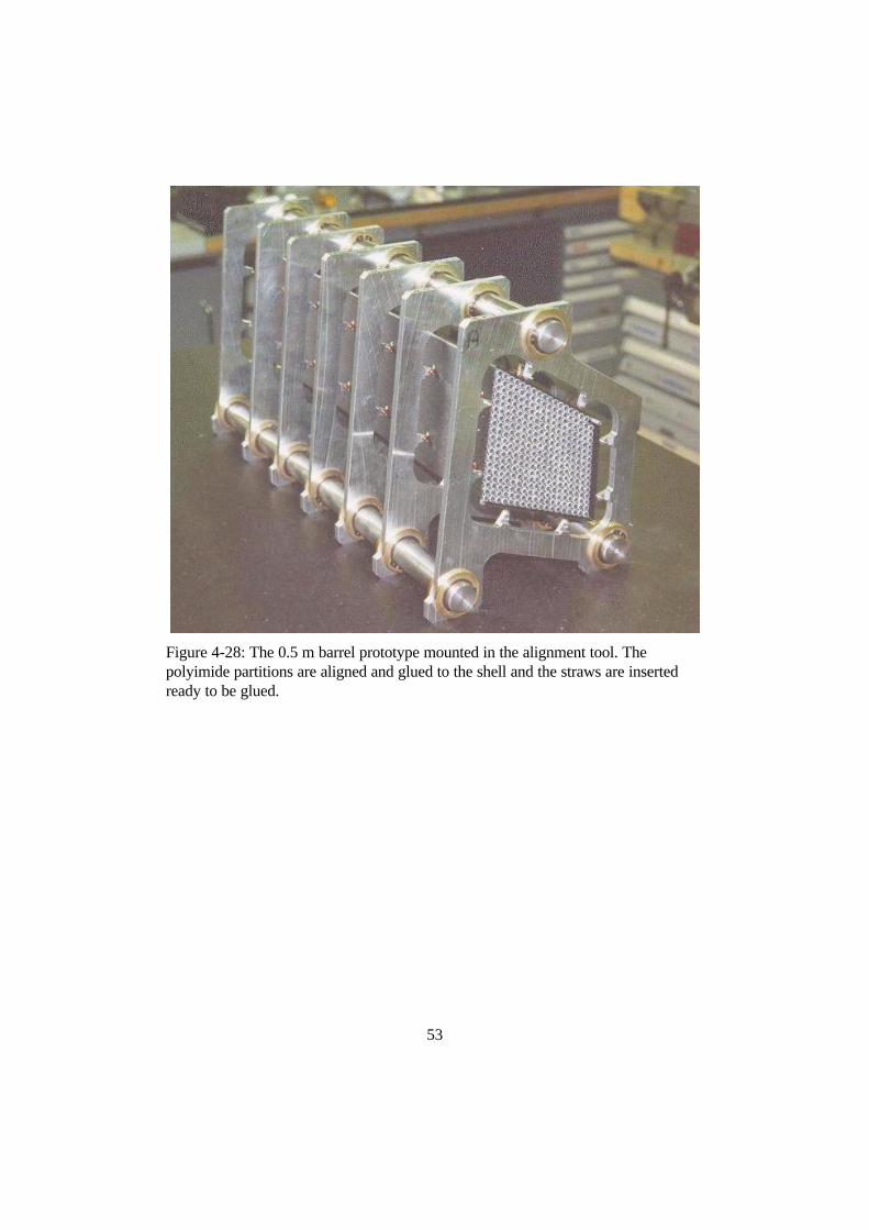
53

Figure 4-28: The 0.5 m barrel prototype mounted in the alignment tool. Thepolyimide partitions are aligned and glued to the shell and the straws are insertedready to be glued.

54

Title: ptrt4.epsCreator: DeskScan II - Hewlett-Packard CompanyCreationDate: L: Version 1.07 Nov 3 14:29:44 1996

Figure 4-29: Insertion of the straws using a steel bar.

Figure 4-30: The 0.5 m barrel prototype mounted in a section of the space frame.

55

4.6.6.2 Tests during assembly

Various measurements were carried out on the prototype during assembly:

• Test of the HV system.• Leak tests of the active gas volume.• Survey measurements on the tooling.• Wire tension test.

After the straws and the HV circuits had been installed, the HV was put onthe HV groups one by one. The current was monitored as the voltage was raisedslowly. It was realized at an early stage that it was necessary to work in inertconditions. Not only was the surface current too high but discharges were observedbetween the HV circuit and the carbon-fibre end-plate. In addition sparks werenoticed inside the barrel volume. After drying out with dry nitrogen, the problemsdisappeared. The HV could be brought up to 2 kV and was stable for several hourswith no discharges being observed. The working voltage is expected to be not higherthan 1540 V, which corresponds to an amplification of ~ 3×104.

All straws were leak tested before installation at the level of ~ 1.6% leak perminute at an overpressure of ~ 200 mbar [23]. Figure 4-31 shows a principal viewof the straw leak-test set-up. The limiting factor in the precision of the measurementwas the silicon rubber joints at the straw ends. The threshold for accepting a strawwas a change of 1 mbar in 30 s. The straw volume is estimated to be 10% of thetotal pressurized volume.

N2

silicon plugP

Straw

Figure 4-31: Schematic view of the test set-up for the straw leak test. The straw waspressurized with 200 mbar relative to the outside and changes in the pressure (P)were recorded.

The first leak test on the module was performed after installation of the straws totest the glue joint between the straws and the carbon-fibre end-plate. The radiatorvolume around the straws was given a small overpressure using CO2 and a gas-leakdetector was used to check for leaking glue joints between the straws and the end-plate. The leaking glue joints were repaired before the HV distribution circuit andthe tension plates were installed. After the stringing of the wires and installation of

56

the capacitor cylinders between tension plate and end-plate, a global leak-ratemeasurement was performed. After repair of leaks, the leak rate was found to be10 l/h at 4 mbar overpressure in the active gas volume. Remaining leaks were foundin the shell itself between the tension plate and the end-plate (see Figure 4-25).

Before installation, the positions of the alignment pins for the partitionswere measured on a flat table. The alignment pins for the polyimide partitions werepositioned with an accuracy better than 50 µm in r-φ and 0.1 mm in z. After thegluing of the partitions and the tension plates and before cutting the polyimide ears,the actual positions of the module fixation holes (the connection with the supportstructure) were measured. The fixation holes were found to be in position to within0.1 mm in r-φ relative to the theoretical values.

The wire tension was measured with a dedicated device [24]. It makes use ofa permanent magnet and of an amplifier to excite and maintain the self-oscillation ofthe wires. Any displacement of the wire gives rise to a signal which is amplified inpositive feedback loop. Thus an oscillation of the wire is maintained either at thefundamental resonant frequency or at a harmonic. It is similar to any electro-mechanical oscillator. A uniform constant dipole field of 4 kG over the whole strawlength was used. This gives the fundamental resonance frequency, which wasmeasured with a digital multimeter (DMM). Knowing the frequency (ν ), the length(l) of the wire and its mass per unit length (µ ), the wire tension is calculated as

ml

g=

× × ×4 2 2µ ν(4-3)

where g is the earth acceleration. The results from this wire tension test are shown inFigure 4-32. It shows first of all a shift in tension from the applied 50 g to ~ 27 g.Second, it shows a big standard deviation of ~ 8 g. One possible explanation for thiseffect is the wire fixation procedure in the tension plate. The wire was blocked witha conical pin in a socket, see Figure 4-25. No improvement was achieved afterrewiring 27 wires with the lowest tension (< 15 g). It should be noted that tungstenwire has a high Young’s modulus relative to, for example, copper-beryllium andtherefore, the elongation of a 0.5-m-long wire is relatively small. The elongation fora 30 µm wire is ~ 0.9 mm for a 50 g load. However, the elongation is three timeslonger for a full-length prototype and therefore the problem will be three timessmaller assuming that the loss in tension comes from pushing back the wire in thepinning procedure. The shift will decrease to ~ 8 g and the standard deviation to ~2.7 g. This shift can easily be compensated for by applying a bigger load. It shouldbe noted that this method for measuring the wire tension cannot be used in the full-length prototypes because of the electrical disconnection at z = 0. Instead anothermethod will be applied which makes use of a mechanical excitation of the moduleand measures the capacitance variance between wire and straw.

57

0

10

20

30

40

50

60

70

8 16 24 32 40 48 56 64

Wire tension (gram)

Nu

mb

er o

f st

raw

s

Figure 4-32: The measured wire-tension distribution (313 straws) with an appliedweight of 50 g.

4.6.6.3 Experience learned from the assembly of the 0.5 m prototype

The experience gained from the first barrel prototype has verified the design and theassembly procedure. In particular, the feasibility of the very complicated moduleends, the HV scheme and the alignment of the polyimide partitions has beendemonstrated. Additional studies have been carried out, after assembly, on criticaldesign issues, e.g. cross-talk, temperature distribution and TR performance. Theassembly experience has resulted in the following modifications to the connectivityand assembly procedure [25]:

• During the alignment procedure the partitions were aligned with the

straw fixation plate. The positioning of the tension plate, i.e. the fixationholes for the support frames, relied on the mechanical precision of thetension plate and the shell. Even though the result turned out to besatisfactory, an improvement would be to have the holes for the strawsand the module fixation pins in one piece.

• Additional support (other than the polyimide ears) for the module when itis in the tooling.

• The leak-tightness of the shell at the module ends is not good enough. Ascan be seen from Figure 4-25, the shell is part of the gas volume and itwas found that small capillaries in the shell made it possible for the

58

detector gas to leak into the radiator volume. A leak-tight seal on theinside of the shell will solve this problem.

• Capacitor sockets are difficult to glue to the HV polyimide sheet and area potential source of gas leaks. New solutions for this are proposed andwill be tested on the next prototypes.

• The end-plate should be fibreglass instead of carbon fibre for HVreasons.

• A different gluing procedure for the straws is necessary to improve leak-tightness and reduce the assembly time. Moulded pieces for the strawsare under study.

Several of the above problems have already been corrected in the design of the nextgeneration of barrel-module prototypes which are now under construction.Two 1.5-m -long modules are planned to be assembled and tested in summer 1997.

4.6.7 Cross-talk

The straws in the barrel TRT have an anode wire which is electrically disconnectedat z = 0 to reduce the occupancy, while the 158-m-long straws (cathode) arecontinuous. The cross-talk between the two straw ends should be low in order not toincrease the occupancy. The 0.5 m prototype was equipped with electricallydisconnected wires at z = 0 (one HV group with 16 straws). The 30 µm tungstenwires were electrically divided using a 0.8-cm-long glass tube with an outer diameterof 240 µm. The 0.5 m barrel prototype was used to measure the cross-talk from oneside of the straw to the other [26]. The cross-talk in the end-plate traces was alsomeasured.

4.6.7.1 Experimental set-up

Three different measurements were performed with two different set-ups:

1. Cross-talk on electrically divided wires at z = 0 using a Fe55 source4;2. Cross-talk on electrically divided wires using a pulse-generator;3. Cross-talk between straws using a pulse generator .

In the first set-up, a gas mixture of 70% Ar and 30% CO2 was used and theHV was set to 1595 V. This corresponds to a gas gain of ~ 2.6×104. The gas flowthrough the detector was in this case 15 l/h. A Fe55 source was placed half-way in onone side of the straw to study cross-talk induced on the opposite side (Figure 4-33a).The signal passed a preamplifier and a shaper before arriving at the oscilloscope.

4 Fe55 radiates γ-rays with an energy of 5.9 keV.

59

Figure 4-33b shows the connection scheme for the second set-up. A pulsegenerator was used to produce a square wave with amplitude 1 V and a period ofT = 350 ns. The rise time was ~ 15 ns. The opposite side of the straw was measuredwith the oscilloscope.

a) b)

Fe55

ground

Oscilloscope

trigger signal

P.A P.A

Sh. Sh. Oscilloscope

trigger signal

Pulse generator

out

Figure 4-33: Set-up for cross-talk measurement on the broken wire with (a) a Fe55

source and (b) a pulse generator.

Figure 4-34 shows the third experiment. The signal was sent through differentstraws with continuous wires marked R1 to R10 in Figure 4-35. The cross-talk toneighbouring straws numbered 1.1 to 10.1 was measured with the oscilloscope. Thesame square wave as above was used and the rise time of the signal was 15 and 20ns before and after the straw, respectively, as shown in Figure 4-36. As can be seenfrom Figure 4-35, some traces from wire fixation pin to connector are longer. Anattempt was made to select first the channels with the longest parallel traces, i.e. thelargest cross-talk.

Oscilloscope

trigger signal

ground

Pulse generator

out

~6.8 mmground

Figure 4-34: Set-up for cross-talk measurement between individual straws.

60


Figure 4-35: View of the tension-plate layout where the signal straws are markedwith R1 to R10 and the measured straws 1.1 to 10.1.

61

a) b)

1.0 V

350 ns

U

t

15 ns

10 %

90%

0.6 V

350 ns

U

t

90%

10 %

20 ns

Figure 4-36: Signal shape (a) before and (b) after the straw.

4.6.7.2 Results

• Cross-talk over electrically divided wire.Figure 4-37 shows the signal on the source side which was used to trigger thereading of the opposite side of the straw. A threshold of 65 mV was usedwhich corresponds to ~ 5% of the signal on the opposite side of the straw. Nocross-talk could be seen at this threshold. With the pulse generator, a fewstraws out of the 16 possible were measured and the cross-talk was found tobe less than 0.5% in all cases.a) b)

U

t

90 mV

~75 ns U

t

1.4 V

40 ns

Figure 4-37: Signal from a Fe55 source (a) before and (b) after the shaper.

• Cross-talk between different strawsThe cross-talk was defined as the ratio between the maximum inducedamplitude (Ec) on a straw and a pulse with amplitude Ei on a neighbouringstraw, as shown in Figure 4-38.

The cross-talk between straws was found to be dominated by thecross-talk in the tension plate. Straws far away from each other were found tohave a cross-talk below ~ 1%. If traces in the tension plate were long andclose to each other the cross-talk could be as high as ~ 8%. Neighbouringstraws corresponding to well separated traces in the tension plate showed a

62

cross-talk of ~ 1-2%, i.e. close to that measured for straws far away fromeach other. Detailed values for different measured straws are given in Table4-2. Figure 4-39 shows the correlation between the cross-talk and thedimensionless parameter L/d, where L is the length of the traces and d is thedistance between them. A mean value of L and d was estimated from theAUTOCAD drawing. The error in the cross-talk measurement is estimated tobe ~ 0.5%.

U

t

cross-talk

input pulseEi

Ec

Figure 4-38: Typical cross-talk between two neighbouring straws where thetraces on the tension plate are close to each other. Measured values aregiven in Table 4-2.

Signalstraw

Measuredstraw

Cross-talk(%)

Signalstraw

Measuredstraw

Cross-talk(%)

R1 1.1 4.1 R5 5.1 6.7“ 1.2 3.3 “ 5.2 3.3“ 1.3 0.3 R6 6.1 6.7“ 1.4 1.6 R7 7.1 6.7

R2 2.1 8.3 “ 7.2 2.5“ 2.2 1.6 R8 8.1 6.7

R3 3.1 4.1 R9 9.1 5.8R4 4.1 2.5 R10 10.1 5.0“ 4.2 2.5“ 4.3 4.1

Table 4-2: Cross-talk between different straws (see Figure 4-35).

63

012

34

56

789

0 5 10 15 20

L/d

Cro

ss-t

alk

(%)

y=0.378*x+1.01

Figure 4-39: Cross-talk as a function of L/d, where L is the length of thetraces and d is the distance between them (from Table 4-2).

4.6.7.3 Conclusion and discussion

• The results from the first measurement with the broken wires show thatthe cross-talk is below threshold when using the Fe55 source. Thethreshold in this case was ~ 5% after the shaper. With the pulsegenerator the cross-talk was found to be < 0.5%.

• In the second experiment the cross-talk between neighbouring straws wasfound to be dominated by the cross-talk in the tension plate. A typicalvalue is 1-2% for neighbouring straws, but it can be as high as ~ 8%(one straw) if nearby traces in the tension plate are long. It is importantto note that channels with very long and close traces were picked outfirst. By adding measured straws above 5% plus the correspondingsignal straws in Table 4-2, it can be estimated that the cross-talk ishigher than 5% in ~ 5% of the channels.

• A typical figure of merit would be to relate the cross-talk to the averagedE/dx pulse height of ~ 2 keV expected per straw. If the cross-talk werenot to significantly increase the measured noise of ~ 70 eV, then it shouldnot exceed about 2%.

• The tension plate has now been redesigned, based on the information inFigure 4-39.

64

4.6.8 Heat conductivity measurement on radiator materials

4.6.8.1 Experimental set-up

A schematic view of the experimental set-up is shown in Figure 4-40. A 50 mminner diameter aluminium tube defines an isothermal surface around the radiator tobe tested. In the centre of the radiator sample, a 5 mm hole is drilled to house astraw with a heating wire in the centre. The outer diameter of the straw is 4.4 mm.Two platinum resistors (Pt-1005) are mounted on the straw wall (T1) and on theouter aluminium cylinder (T2). A current is applied on the heating wire and thetemperature difference between T2 and T1 is measured. Both the current I and thevoltage U of the heater wire are measured with a digital voltmeter over the strawlength of 0.5 m and the current is adjusted to obtain a temperature differencebetween the two sensors of a few degrees.

Three radiator samples were tested: two fibre radiators and one foamradiator. The fibre radiators are 50% polypropylene and 50% polyethylene, whilethe foam radiator is 100% polypropylene. The orientation is ~ 80/20 for the orientedfibre.

T1

T2

500 mm

50 mm

strawheating wire

Figure 4-40: Schematic view of the thermal conductivity set-up.

4.6.8.2 Calculation method

Cylindrical co-ordinates and the temperature equation give

Q dr r dT× = × × × ×2 π λ (4-4)

5 Pt-100 is a calibrated resistive thermal sensor.

65

where r is the radius, λ is the thermal conductivity and dT the temperaturedifference. The heat Q is expressed in W/m and is calculated as

QU I

l=

× . (4-5)

From equation (4-4) follows

λπ

=×

×∫Q dr

r

Ta

b

2

∆ (4-6)

and finally

λπ

=× ×

×Q

T

b

a2 ∆ln( ) (4-7)

4.6.8.3 Results

The results from the measurements are summarized in Table 4-3. The measurementswere carried out in air at 20 °C. Despite its lower density, the oriented fibre radiatorseems to have a greater thermal conductivity than the foam. This can be explainedby the fact that the fibre is more transparent to convection.

Material Density(kg/m3)

Conductivity(W/m/K)

Foam 85 0.042 ± 0.006

Fibre non-oriented (installed in the 0.5 m prototype) 120 0.059 ± 0.008

Fibre oriented (installed in the 0.5 m prototype) 70 0.052 ± 0.007

Table 4-3: The measured thermal conductivities for some radiator materials andtheir estimated errors.

66

4.6.8.4 Estimation of the error

Assuming that the errors are uncorrelated and by differentiating equation (4-7), theerror in λ can be estimated as follows:

σ∂ λ

∂σ

∂ λ∂

σ∂ λ∂

σ∂ λ∂

σλ2

22

22

22

22=

× +

× +

× +

×∆ ∆

T Q b aT Q b a

(4-8)

where σb = 1mm, σa = 0.5 mm, σQ = 5 × 10-3 W, σ∆T = 50 × 10-3 K.With ∆T = 5 K, Q = 0.5 W/m, b = 25 mm and a = 2.4 mm the relative error in λbecomes

σλ

λ = + + + ≈0 01 0 01 0 017 0 089 012 2 2 2. . . . . .

It is concluded that the main error comes from the uncertainty in the positioning ofthe temperature sensor at the inner radius. The total error is estimated at 10%.

4.6.9 Cooling of the modules

4.6.9.1 Requirements

In the ATLAS TRT, heat is generated in the proportional tubes (straws) as thepositive ions, created by the ionizing particles, form a current driven by the HV onthe straws. This heat has to be removed and the barrel modules are cooled by waterrunning along two cooling tubes on opposite corners of each module [27, 28]. Thecooling tubes are thermally grounded to the shell to minimize the temperaturedifference between the shell and the coolant. The shell forms a semi-isothermalsurface around each module. Even though the heat production is low the moduleswill experience a temperature difference (∆T) because of the insulating properties ofthe radiator material. The ∆T, if it exceeds a certain value, can create problems. Oneproblem is changes of the dimensions and displacement of the wires. Temperaturechanges will also influence the gas amplification due to changes in the gas density.The change in the amplification degrades the electron identification performance asthe thresholds for TR hits are related to one value of the gas amplification. It alsochanges the threshold for the drift-time measurement. It has been shown that thelimiting factor for the temperature differences in the barrel is the electronidentification and mechanical aspects [29]. A 25% change in gas gain is acceptableand corresponds to a change of 15 K for a 30 µm wire and 10 K for a 50 µm wire.A maximum temperature difference of 10 K is considered acceptable. Therefore,

67

from a physics performance point of view, a temperature difference of 10 K containssome margin of safety when using the 30 µm wire.

cooling tube

cooling tube

Figure 4-41: Schematic view of the heat transport and cooling of the barrel TRTmodules.

4.6.9.2 Analytical calculations

In the calculation below, the shell is assumed to have infinite thermalconductivity and isothermal boundaries, but in reality a temperature gradient ispresent in the shell to drive the heat towards the cooling tubes. A schematic of theheat transport is shown in Figure 4-41. Results on thermal conductivitymeasurements of the shell material are reported in Ref. [30]. From thesemeasurements of the thermal conductivity, the maximum ∆T in the shell walls can beestimated to be < 4 K.

Before the temperature difference in the modules is calculated, we considerthe heat dissipation in the straws. The heat dissipation arises from the ions, createdby the ionizing particles, drifting from the anode wire to the cathode. This current Ican be written as

I Gain Rate q N= × × × (4-9)

where N is the mean number of primary ions. At full luminosity, the maximumexpected values for a 1.6-m-long straw at a radius of 63 cm are [4]:

68

Gain

N

Rate

q

= ×=

= ×

= ×

−

−

4 10

65

3 10

1602 10

4

7 1

19

s

C.

Normalized to a 1-m-long straw and assuming a uniform rate distribution along thestraw, the current density is I = 7.8×10-6 A/m, and for a potential U = 1800 V, thepower dissipation per 1-m-long straw is

P I U= × = 14mW / m (4-10)

Because of the rapidly decreasing particle fluxes in the barrel TRT as the radiusincreases, the rate varies with radius as ~ r−2.5, and therefore a mean heat dissipationper 1-m-long straw (qm) is calculated, which is used in both calculations and in theexperiment below. The mean heat dissipation is calculated as

qR R

Q r drR

R

mo i

i

o

=−

× ×∫1

( ) (4-11)

where

Q rq

rs( ).

=2 51

(4-12)

and Ri and Ro are the inner and outer radii, respectively, of the inner module. Theheat density is calculated to be 14 mW/m per straw, which is approximately thesame as the heat dissipation at r = 63 cm. For the two outer modules thecorresponding values are 8.2 mW/m (middle) and 4.8 mW/m (outer). The estimateof the heat dissipation in the inner module is on the conservative side for the totalheat as the wires have a passive part for r < 63 cm as discussed in Section4.6.1. Onthe other hand all the wires are active over a considerable length (36 cm) at bothends of the modules.

The total heat production for the 329 straws in the 0.5 m prototype, with thevalues above, is then given by

Ptot = × × =329 0 5 14 2 3. .mmW

mW (4-13)

69

Furthermore, the module is approximately described as a rectangular block asshown in Figure 4-42, with the same volume per unit length and a = b [5]. Theequivalent sides for the three modules were calculated from the AUTOCAD file as12.8 cm , 16.0 cm and 19.7 cm for the inner, middle and outer modules respectively.The total heat production in the module is translated into a uniform heat density q bydividing by the module volume. The temperature equation

∇ + =2 0T x y zq

( , , )λ

(4-14)

is solved in the volume and with isothermal boundaries where λ is the thermalconductivity of the bulk. The maximum temperature, i.e. in the centre, is calculated.The temperature difference between a point in the volume and the isothermalboundaries can be expressed as

∆ T( ),,x y z ..64

π 3

q

λ= 0

∞

l = 0

∞

m = 0

∞

n

..sin ..( ).2 l 1 π x

asin ..( ).2 m 1 π y

bsin ..( ).2 n 1 π z

c

....π 2 ( ).2 l 1 2

a2

( ).2 m 1 2

b2

( ).2 n 1 2

c2( ).2 l 1 ( ).2 m 1 ( ).2 n 1

(4-15)

by using Green’s functions [31]. For a given geometry the maximum ∆T varieslinearly with (q/λ). The value of the thermal conductivity is taken from themeasurements on the two fibre radiators installed in the prototype, presented in theprevious section. 10% of the fibre sheets were oriented and 90% non-oriented. Theaverage of the two radiators is calculated as

( )λ = × + ××

= ××

0 9 0 059 01 0 0520 058

. . . ..W

m K

W

m K(4-16)

Note that this is an estimate of the bulk conductivity based on pure radiator materialwithout straws, carbon reinforcements, wires, etc. Figure 4-43 shows thetemperature difference as a function of the module length c, for the three moduletypes. The inner module represents the worst case because of the strong radialdependence of the occupancy even though the outer module contains more than twiceas many straws.

70

x

y

z

a

b

c

Figure 4-42: Geometrical model of the barrel module used in Equation 4-15.

By taking the maximum temperature difference in the centre one obtains

Ta b

Ta b

( , ,.

) ( , ,.

) .2 2

15

2 2 2

0 5

201

m mK− < (4-17)

It is clear that a 0.5-m-long module is a good approximation of a 1.5-m-longmodule. The maximum calculated temperature differences are 5.9, 5.4 and 4.8 K forthe inner, middle, and outer modules respectively.

71

0 10 20 30 40 50 60 70 800

0.5

1

1.5

2

2.5

3

3.5

4

4.5

5

5.5

6

Module length (cm)

Tem

pera

ture

dif

fere

nce(

K)

Figure 4-43: Calculated maximum temperature difference between the centre of themodule and the shell, as a function of the module length for the inner, middle, andouter modules respectively, assuming isothermal boundaries.

Figure 4-44: Experimental set-up showing the daughter cards on the tension plateand the positions of the thermal sensors T1 to T5. T6 is mounted on the aluminiumsupport plate (not shown in picture).

T5

T1-T4

x

y

z

inner modulemiddle “outer “

72

4.6.9.3 Experimental set-up.

Pt-100s were used to measure the temperatures in six different positions: four insidethe detector volume, one on the shell and one on the aluminium structure. The foursensors inside the module are placed in the centre of the module (in x, y). A side-view of the experimental set-up and the positions of the thermal sensors are shown inFigure 4-44. In the z-direction, T1 is placed at 32 cm, T2 at 24 cm , T3 at 16 cmand T4 at 8 cm from the module end-plate. A constant current of 100 mA was sentthrough the temperature sensors. The voltages were read by a DVM/scannerconnected to a PC where the readings were converted to temperatures and written toa file. To simulate the heat dissipation in the ionization gas, as calculated inEquation (4-13), a current was sent through the wires. Groups of 16 channels wereconnected in parallel using small daughter-cards. The HV group which wasequipped with the wire joints at z = 0 was not connected, but was compensated forby increasing the current through the other straws so that the total power was 2.3 W.It should be noted that the sensors integrate to some extent since they have a lengthof 10 mm. Taking into account both the error in the sensor positions and theirdimensions, the uncertainty is less than ~ 0.1 K. The shell is considered to beisothermal and is cooled by convection by the surrounding air. In the final modules,the heat will be conducted by the semi-isothermal carbon-fibre shell to the twocooling tubes in the module corners.

4.6.9.4 Results from measurements

The measurements were recorded over a period of ~ 23 h, for which the full heatingpower of 2.3 W was switched on only after ~ 200 min. The measured absolutetemperatures are shown in Figure 4-45. The room was air-conditioned and gave riseto temperature oscillations of ~ 2 K, but a mean value was calculated for 800 min <t < 1300 min. The temperature differences for T1 to T4 are defined as

∆Ti Ti T= − 5 where i = −1 4 (4-18)

and are shown in Figure 4-46. In Figure 4-47, a comparison between calculationsand the experimental points is shown. The calculations agree well with themeasurements (with λ = 0.058 W/m/K as measured in Section 4.6.8) for the fourmeasuring points at different z. Note how the boundary effects from the end-platesbecome important at z = 8 cm (T4). For T1 to T3 on the other hand, the boundaryeffect is small. The maximum measured temperature difference is 5.8 K whichcorresponds to an effective bulk conductivity of λ = 0.059W/m/K.

73

294

295

296

297

298

299

300

301

302

0 200 400 600 800 1000 1200 1400

Time (min)

Tem

pera

ture

(K

)

T1 to T3

T4

T5

T6

2.3 W

Figure 4-45: Temperatures measured by T1 to T6 over a period of 23 h. Note thefluctuations observed in the ambient air as measured by T5 (shell reference), whichare smoothed out for T6 (aluminium structure).

0.000

1.000

2.000

3.000

4.000

5.000

6.000

7.000

0 200 400 600 800 1000 1200 1400

Time (min)

T (

K)

∆T1 to ∆T3∆T4

Figure 4-46: Measured temperature differences between the shell and the centre ofthe module.

74

0 10 20 30 40 500

2

4

6

z (cm)

Tem

pera

ture

dif

fere

nce

(K)

Figure 4-47: Calculated temperature difference in the centre of the module atdifferent z (solid curve) and the experimental points (T1 to T4).

4.6.9.5 Temperature gradient at the cooling-tube interface

Different design options have been under consideration for the cooling of the shells.Figure 4-48 shows a cross-section of one of the module corners. An aluminium tubeis glued on the inside of the shell in two opposite corners. A second tube is insertedin the first one. This second tube, which is longer than the module itself, permits theconnection to be made away from the crowded module ends and avoiding joints closeto the HV and the electronics. The ∆T along the tube is assumed to be negligible.With the notations of Figure 4-48, the temperature difference can be calculated as

∆Tq d

rnn

n n

=×

× × ×2 π λ(4-19)

for the individual material components, where q is the heat flow per metre of tube,dn the thickness, rn the radius and the λn the conductivity in layer n. The estimatedfraction of the tube surface in contact with the shell is 25%. The total ∆T is the sumof the temperature differences and is calculated to be below 2 K even taking intoaccount a double tube. The main contribution comes from the air gap between thetwo cooling tubes. It should be noted that this is conservative as in reality the tubeswill inevitably be in contact with each other at certain points along the tube, whichwill help to decrease the ∆T. It should be pointed out that the ∆T between cooling

75

tube and coolant does not affect the temperature gradient in the shell itself, but onlyincreases the absolute temperature.

d1

d2

d3

d4

H2O

epoxyinner tube

outer tube

shell

Figure 4-48: Schematic view of the cooling tube in the shell corner .

The temperature of the coolant therefore has to be adjusted so that the absolutemodule temperature is stable at the desired value.

4.6.9.6 Conclusions and remarks on the module cooling

The maximum acceptable temperature difference inside the barrel TRT has beendetermined to be 10 K. To achieve this, the barrel modules are cooled individuallywith water. Two cooling tubes are glued axially in two opposite corners, on theinside of each carbon-fibre shell.

We have demonstrated with both measurement and calculation that the ∆T isbelow 6 K in the barrel TRT modules assuming isothermal boundaries. Themeasurements are in good agreement with calculations. Taking into account the heatconductivity of the shells, the maximum total ∆T will be less than 10 K. In addition,the CO2 ventilation of the radiator is expected to decrease the ∆T, but how muchdepends on the final flow rate.

The thermal conductivity between the shell and the coolant has beencalculated, assuming reasonable design parameters. The ∆T over the joint wasdetermined to be below 2 K.

One remark should be made concerning the electronics on the module ends.The calculation and measurements above assume that the electronics cooling issufficiently efficient to avoid a flow of heat into the detector volume. To guaranteethis the electronics cooling has to be able to keep the tension plate below themaximum temperature difference calculated above (6 K).

76

4.6.10 Tracking performance for a modular layout

An important consideration in the development of the barrel layout and theintroduction of a modular geometry is the tracking performance. A dedicatedprogram was developed to compare different straw layouts and module shapes[32, 33]. Of particular interest is the difference between an optimized uniform strawdistribution and a straw distribution based on a modular layout. In all simulations1000 tracks at η = 0 have been generated at random φ, for each momentum andlayout. The study is purely geometric, i.e. only the number of traversed straws arecounted. A magnetic field of 2 T was used and the effective straw radius is assumedto be 1.9 mm. As a measure of the performance of the different layouts thefollowing parameters are considered:

• mean number of crossed straws for each track (NSTRAW);• rms of NSTRAW;

• maximum number of consequent missed layers for each track (NSPACE);• rms of NSPACE.

NSTRAW gives information about any dead zone and NSPACE indicates the uniformityof hits along the tracks. Both negative and positive tracks are generated to indicateany charge asymmetry between the different straw layouts. In the layout below, apositive track is defined as a deflection to the left and a negative track to the right. Inaddition, the fraction of tracks with 31 and 30 hits or more is shown for the differentlayouts.

4.6.10.1 Geometry

The number of straws in the three modules is: 329, 520 and 793 for the inner,middle and outer modules respectively. Two straws are removed from each moduleto provide space for cooling pipes. The generated tracks are totally enclosed in thebarrel (|η| < 0.7), only producing hits if 63 cm < r < 107 cm as the wires areinactive at r < 63 cm. This reduces the number of active straws in the inner modulefrom 329 to 182. The number of active layers is 10, 24 and 34 for the inner, middleand outer modules respectively. This is the same total number of layers as for theuniformly distributed straw layout without module boundaries referred to as Layout1 below [34]. The mean distance between the straws in all layouts is close to 6.8mm. Four different layouts were studied :

1. no modular layout and the layers are in groups of eight with the same

number of straws (see Figure 4-49a);2. two cooling pipes per module and d = 5.2 mm (see Figure 4-49b);3. same as 2, but no cooling pipes;4. same as 2, but no cooling pipes and d = 0;

77

5. same as 2, but d = 6 mm.

Layout 1:This geometry has no modules and the straws are uniformly distributed. The totalnumber of straws is 50 288, which corresponds to a mean distance between thestraws of a approximately 6.8 mm, see Figure 4-49a. The number of straws perlayer is constant within a group of eight straws. There are 64 layers in total. Thisgeometry is described in more detail in Ref. [34]. It can be considered as a‘reference layout’ in the discussion of the tracking performance of the differentmodular layouts.

Layout 2:The 3 × 32 module layout contains 182, 520 and 793 active straws for the inner,middle and outer modules respectively at η = 0. The 64 straw layers give a total of47 840 active straws. The total number of straws is less than in Layout 1 because ofthe introduction of module shells for approximately equal straw density. Theminimum distance between the straws and any boundary is d = 5.2mm, seeFigure 4-49.

Layout 3:The same Layout 2 except there are no cooling pipes and there are 183, 522 and 795active straws in the inner, middle and outer modules, respectively. The distance fromthe boundary to the nearest straw is d = 5.2 mm.

Layout 4:The same number of straws as in Layout 3 and a slightly increased distance betweenthe straws as d = 0.

Layout 5:This layout contains two cooling pipes, i.e. the same number of straws as inLayout 2, but the distance between the module boundary and the nearest straw isincreased to d = 6 mm.

78

a) b)



Figure 4-49: (a) Straw geometry as proposed in [34] with eight superlayers of eightlayers; (b) a modular geometry with 3×32 modules, two cooling pipes per moduleand d = 5.2 mm (between each module boundary and the nearest straw).

4.6.10.2 Results

The results from the simulations are presented in Table 4-4 to 4-11.

100GeV

1 GeVpositive

1 GeVnegative

2 GeVpositive

2 GeVnegative

3 GeVpositive

3 GeVnegative

NSTRAW 35.8 37.1 37.0 36.0 35.9 35.7 35.7rms 1.85 2.71 2.44 1.83 2.01 2.40 2.30

NSPACE 2.76 4.51 4.19 3.44 3.28 3.40 3.63rms 0.43 0.84 0.67 0.60 0.48 0.60 0.67

> 31 hits(%)

99.9 98.3 98.6 99.1 98.4 97.1 97.4

Table 4-4: Tracking performance for Layout 1.

79

Layout 1 Layout 2 Layout 3 Layout 4 Layout 5

NSTRAW 35.8 34.14 34.36 34.34 34.09rms 1.85 2.16 2.16 2.07 2.62

NSPACE 2.76 4.05 3.92 3.25 4.49rms 0.43 0.87 0.77 0.54 1.07

> 30 hits(%)

- 95.6 96.7 97.1 92.1

> 31 hits(%)

99.9 89.4 91.5 91.2 83.8

Table 4-5: Tracking performance for 100 GeV particles.


NSTRAW 37.1 35.47 35.43 35.75 35.48rms 2.71 3.36 3.42 3.33 3.34

NSPACE 4.51 5.72 5.58 5.21 6.23rms 0.84 1.57 1.59 1.34 1.99

> 30 hits(%)

- 92.8 93.5 94.2 92.4

> 31 hits(%)

98.3 88.0 87.4 90.3 89.1

Table 4-6: Tracking performance for positive 1 GeV particles.


NSTRAW 37.0 35.44 35.53 35.51 35.38rms 2.44 2.76 2.69 2.61 2.77

NSPACE 4.19 5.13 5.02 4.68 5.42rms 0.67 1.31 1.26 1.31 1.77

> 30 hits(%)

- 96.1 97.2 97.9 95.7

> 31 hits(%)

98.6 91.5 93.6 93.9 91.5

Table 4-7: Tracking performance for negative 1 GeV particles.

80


NSTRAW 36.0 34.41 34.45 34.57 34.53rms 1.83 2.44 2.47 2.53 2.66

NSPACE 3.44 4.35 4.3 3.71 4.92rms 0.60 0.84 0.86 0.70 1.1

> 30 hits(%)

- 95.2 95.2 93.1 94.2

> 31 hits(%)

99.1 90.5 89.6 88.6 87.8



NSTRAW 35.9 34.35 34.54 34.62 34.49rms 2.01 2.19 2.22 2.15 2.63

NSPACE 3.28 4.38 4.24 3.58 4.73rms 0.48 0.91 0.89 0.61 1.09

> 30 hits(%)

- 96.4 95.9 96.7 94.2

> 31 hits(%)

98.4 91.2 88.2 92.6 88.2



NSTRAW 35.7 34.37 34.44 34.4 34.34rms 2.40 2.53 2.47 2.41 2.78

NSPACE 3.40 4.24 4.17 3.50 4.71rms 0.60 0.78 0.75 0.61 1.01

> 30 hits(%)

- 94.3 94.6 94.8 94.1

> 31 hits(%)

97.1 88.7 88.3 89.7 88.3


81


NSTRAW 35.7 34.32 34.56 34.45 34.40rms 2.30 2.33 2.35 2.33 2.69

NSPACE 3.63 4.16 4.11 3.43 4.56rms 0.67 0.87 0.86 0.59 1.08

> 30 hits(%)

- 95.5 96.1 95.6 93.0

> 31 hits(%)

97.4 88.5 89.9 90.9 85.5


4.6.10.3 Estimation of the errors

Suppose s is an estimate of σ and x is the arithmetic mean, then

x m

s n

−×

follows a t-distribution with f degrees of freedom.

The probability of getting

− <−

<t fX m

s nt fα α/ /( )

/( )2 2 is 1 − α,

where f = N − 1. The confidence interval follows from

I x t fs

nx t f

s

nm = − × + ×

α α/ /( ) , ( )2 2 .

As an example we take values from column 3 in Table 4-5;

No cooling pipes d = 5.2 mm

NSTRAW 34.36rms 2.16NSPACE 3.92rms 0.77

With α = 0.01, x = 34.36, s = 2.16 and n = 1000, we obtain for NSTRAW

82

[ ]Im = − × + ×

=34 36 2 582 16

100034 36 2 58

2 16

100034 18 34 53. .

., . .

.. , .

and with x = 3.92, s = 0.77 we obtain for NSPACE

[ ]Im = − × + ×

=3 92 2 58

0 77

1000392 2 58

0 77

1000386 3 98. .

., . .

.. , . .

4.6.10.4 Conclusions

This study shows that the present layout (d = 5.2 mm and two cooling pipes permodule) of the barrel TRT gives > 34 hits, as a mean, for stiff tracks with η < 0.7.This is just a scaling down with the total number of straws of what was found in theuniform straw distribution with no modules (Layout 1). There is a loss of about 1.5hits for an approximately constant straw density. The rms values are also slightlyincreased. The minimum efficiency to obtain more than 31 hits is 89.4% for thedesigned modular layout, compared with 99.9% for a uniform straw distribution(Layout 1).

The results show also that the reduced number of straws produced by theintroduction of cooling lines and carbon-fibre walls only introduces minor variationsin the track qualities. It will not be difficult to maintain a high efficiency byrequiring a slightly smaller number of hits on a track, without significantlyincreasing the fake track rate.

All modular layouts show some charge asymmetry including Layout 4. Thisis due to the asymmetry in the angular shift between successive module layers,imposed by the boundaries.

4.6.11 Material in the barrel TRT

The amount of material in the TRT in terms of radiation length should be kept aslow as possible. A dedicated material budget program was formulated to facilitatethe study of different designs and to study the contribution from individualcomponents to the total material budget [35]. The program makes it possible toobtain a fast response and to change parameters such as the material and thedimensions of objects. The calculation is based on the present barrel TRT design asdiscussed above with 3 × 32 modules and 52 544 straws, and an extrapolation fromthe detailed design of the innermost module to the two outer modules was made. Inaddition, the pipes and cables in the crack region between the barrel and the end-capare included as the only part of the services [36, 37].

83

4.6.11.1 Geometry

The detector is divided into several volumes (discs) in which the material isaveraged. Each component is placed in one of these discs. Figure 4-50 showsschematically how the material is divided into discs. A list of all componentsincluded in the calculation is given in Table 4-12. Electronics cooling, fuses and fuseboxes are not yet included in the calculation. The material budget has been estimatedfor 0 < |η| < 1.2 where η is defined as (see also glossary on page 123)

ηθ

= −

ln tan

2 . (4-20)

The material has been divided into three main discs as follows:

• a disc covering the electrical disconnection at z = 0;• the active volume;• the crack region with electronics, connections, services, etc.

z = 0z = 74cm

z = 85cm

active volume

θ

η

crack region

Figure 4-50: A schematic view of the division of the detector into discs.

84

Component X0 (cm) Weight perpiece (g)

Number ofpieces

d6 (cm) RadiusRout/Rin (cm)

Ventilation gas 18300.1 2460.19 1 # 107/56Shell (3 types) 25 1198.80 32 # 107/56

Radiator 48 98407.40 1 # 107/56Wire (W, d = 30 mm) 0.35 0.01 52544 # 107/56Straw Al 8.9 0.01 52544 # 107/56

polyimide 28 0.66 52544 # 107/56C-fibre7 25 0.30 52544 # 107/56

Xe+CO2+CF4 1576 0.05 52544 # 107/56Polyimide partitions 28.7 12.06 96 # 107/56Cooling pipes (Al) 8.9 3.22 2 # 107/56Water for cooling 36 18.60 96 # 107/56

Central partition (3 types) 28.7 12.06 32 0.2 107/56Mid twister 30 0.03 52544 0.5 107/56

Twister 30 0.05 52544 0.8 107/56Straw fixation 30 0.06 52544 0.8 107/56Inner end-plate 19.4 144.33 32 0.2 107/56

Detector gas 1576 123.27 1 0.8 107/56Capacitor + 2 female pins

+ 2 male pins1.43 0.25 6568 0.6 107/56

Capacitor socket 30 0.04 6568 0.6 107/56Tension plate 19.4 58.00 141 0.2 107/56

Wire fixation pin 1.43 0.06 52544 0.3 107/56Wire fixation socket 1.43 0.02 52544 0.2 107/56

Sockets for electronics 1.43 0.01 72248 0.3 107/56Support structure 25 149.00 32 1 107/56Electronics card 19.4 2.10 3284 0.1 107/56

‘ASDBLR’ 9.36 0.03 3284 0.1 107/56Protective components 11.7 0.03 105088 0.1 107/56

‘DTM ROC’ 9.36 0.02 1642 0.1 107/56Pins on electronics card 1.43 0.44 3284 0.3 107/56

Cables 1.43 2000.00 1 1 107/56Pipes 8.9 3000.00 1 1 107/56

Roof board 19.4 4439.73 1 0.2 107/56Resistor (1 per 16 straws) 25 0.1 3284 0.2 107/56

Table 4-12: Detector components and some of the parameters included in thecalculation. Heat exchangers for the electronics cooling, fuses and fuse boxes, arenot yet included.

6 Thickness of the doughnut.7 The fibre content is assumed to be 60%.

85

a)

Material in the active region in the barrel TRT.

0.00

2.00

4.00

6.00

8.00

10.00

12.00

14.00

16.00

18.00

0.00 0.20 0.40 0.60 0.80 1.00 1.20 1.40

ηη

Rad

iati

on

len

gth

%

o

b)

Material in the crack region in the barrel TRT.

0.00

2.00

4.00

6.00

8.00

10.00

12.00

14.00

0.00 0.20 0.40 0.60 0.80 1.00 1.20 1.40

ηη

Rad

iati

on

len

gth

%

o

c)

The total material in the barrel TRT.

0.00

5.00

10.00

15.00

20.00

25.00

30.00

0.00 0.20 0.40 0.60 0.80 1.00 1.20 1.40

ηη

Rad

iati

on

len

gth

%

o

Figure 4-51: Material distribution in the barrel TRT as a function of radiation lengthversus η for different parts of the barrel: (a) active volume (up to z = 74 cm), (b)end-flange and services, (c) total material.

86

Additional discs can be added as the design develops or existing discs can be dividedinto smaller discs to increase the granularity.A vertex spread with a σ = 5.6 cm has been used in all calculations. This is ofimportance at z = 0 and η = 0 as the anode wire is electrically disconnected at thisposition and, accordingly, there is a high concentration of material in the rφ-plane atz = 0.

4.6.11.2 Results from the material budget study

The material budget for the present design of the barrel TRT has been calculated indetail. Figure 4-51 shows the material distribution expressed in terms of percentageof X0 vs. η. A somewhat higher value has been found compared with previousestimates at z = 0 and in the crack region. At z = 0, the electrical disconnection ofthe anode wire, including the glass disconnection and a wire centring piece, adds∼ 4% X0, if averaged over the nominal spread of vertices. There are several smallcontributions to the sum of material, especially in the crack region, and there is noparticular component where savings can be made easily. For example, the fourlargest contributions (inner end-plate, wire fixation pin, tension plate and electronicscard) are all between 0.72% and 0.95%. The total amount of material adds up toabout 7% of X0 axially, excluding services (∼ 1% of X0) and there are still items tobe precisely defined, e.g. fuses, fuse boxes, and heat exchangers for electronicscooling.

It should also be pointed out, that the TR function costs in material and atη = 0, the contribution from radiator and Xe is ~ 6% of X0. As already mentioned inChapter 2, Section 2.1, the material in the inner detector degrades the performanceof the electromagnetic calorimeter and the tracker because of photon conversionsand bremsstrahlung.

4.6.12 TR performance

The ATLAS TRT is designed as a tracking device in the ATLAS inner detector withthe capability of identifying electrons [38, 39, 40]. The optimization of the strawlayout in the barrel TRT has been guided by tracking performance and mechanicalconsiderations. The 0.5 m barrel prototype discussed above was used in the August‘96 run to study different aspects of the design and assembly procedures [41]. Inaddition, it provided the possibility to study the TR performance for the barrel partunder realistic geometrical conditions. The energy spectra of individual straws atdifferent detector depths was measured and an extrapolation to the full detectorlength was made from these data.

87

TRT

SiBC2BC1

86630.0 93689568

Magnet

(mm)

Preshower

Lead Glass

Multiplicitycounter

9663 10028

e/ππ

PbS2 S3

Figure 4-52: The set-up of the 0.5 m barrel prototype (TRT) for the August run in1996. BC1 and BC2 indicate the beam chambers, Si the silicon counter, S2 and S3the scintillators. The magnetic field was off during the whole run.


Figure 4-53: Cross-section of the prototype showing the three different strawgroups: back, middle and front. One straw in the front group was used as amonitoring straw and did not acquire data.

137 mm

88

The number of clusters was predicted based on the knowledge of the individualstraw performance in combination with the expected number of hits per track. Twotypes of beams were at our disposal: pions at 50 GeV and electrons at 200 GeV.Because of the relativistic rise in the energy deposition to exceed the threshold, theprobability for pions is higher at 50 than at 20 GeV. As can be seen in Figure 4-3above, the curve flattens out for electrons above ~ 20 GeV but the 50 GeV pions areon a positive slope. This has to be remembered when making predictions for theelectron identification performance.

4.6.12.1 Test beam set-up

Figure 4-52 shows the test set-up. A scintillator S2 was used to trigger a reading ina straw. No tracking was carried out as only three straws at the time were equippedwith electronics. To obtain a clean pion or electron beam, a preshower and a lead-glass calorimeter were used. In addition a multiplicity counter ensured that only oneparticle at a time was registered in the straw. The beam was perpendicular to thestraws, i.e. parallel to the fibre sheets. The angle between the straws and the beamwas kept constant during all runs. The detector gas was a mixture of 70% Xe, 20%CF4 and 10% CO2. The gas flow was kept at 6 l/h and 0.5 l/h for the input flow andreturn flow respectively. To keep the radiators clean from Xe gas, the radiatorvolume was ventilated during the whole run with dry nitrogen at a flow rate of 150l/h. This ventilation kept the Xe concentration at an acceptable level of a few percent. Fe55 sources were used for calibration of the straws and this was performed atthe beginning of each data-taking period. In addition a ‘monitoring straw’, as shownin Figure 4-53, was used for operating-voltage stabilization. It used a feedback loopwhich measured the pulse height from a Fe55 source. The operating voltage was setto 1560 V which corresponds to a gas gain of ~ 3×104. Preamplifiers were mountednear the straws and connected to fast shapers. The straws were divided into threedifferent groups and one group was read out at a time. In the front group only twostraws were read out as one was used for operating-voltage monitoring. Theprototype was equipped with two different fibre radiators with the same basicmaterial, i.e. 50% polypropylene and 50% polyethylene. Table 4-13 shows thedifferent runs carried out in the test beam.

Group Oriented fibre Non-orientedfibre

Back e/π e/πMiddle e/π e/πFront e e

Table 4-13. The different combinations during the test-beam run.

89

The non-oriented fibre has a density of 0.120 g/cm3 while the oriented has a densityof 0.070g/cm3. This difference in density has to be taken into account whenevaluating the performance of the two radiators, as the radiator represents asignificant fraction of the total material in the barrel TRT.

4.6.12.2 Beam purity

As mentioned above, the purification of the pion or electron beam is carried out witha preshower and a lead-glass calorimeter. Figure 4-54 below shows how thedifferent cuts were applied to clean the beams. To determine the requirements on thebeam purity, the statistical error on the probability to exceed a certain threshold isused as a reference. The error from beam impurities should be significantly less thanthis statistical error. As will be shown in Section 4.6.12.4 below, the probability toexceed 6 keV is pe = 0.235 for electrons with a standard deviation de = 0.006. Forpions the corresponding values are pπ = 0.0635 and dπ = 0.003. The electron beam isestimated to contain ~ 60% electrons without any cuts. After cuts have been appliedin both the preshower and in the lead-glass calorimeter, the pion efficiency Rπ isestimated to be less than 10−3. The pion beam on the other hand is contaminated by~ 8% electrons. After the cuts are applied, the efficiency to find electrons Re ismeasured to be less than 10−3 . The increase in the probability to exceed the 6 keVfor pions, due to electrons, is calculated as

επ π= × = × <−p R de e 2 35 10 4. . (4-21)

Thus, it can be concluded that the pion beam is sufficiently cleaned of electrons.In an analogous way, the decrease in the probability to exceed 6 keV for electrons,due to a contamination from pions, is calculated as

ε π πe ep R d= × = × <<−0 635 10 4. . (4-22)

It is concluded that the electron beam is sufficiently pure.

90

Title: /afs/cern.ch/user/h/hdaniel/test.ps (Portrait A 4)Creator: HIGZ Version 1.23/07CreationDate: 97/02/13 13.55

Figure 4-54. Histograms with the different cuts for pions and electrons.

4.6.12.3 Radiator performance

Figure 4-55 and Figure 4-56 show the energy spectra and the integrated energyspectra for the back straws with both electrons and pions. The next step is to plot theprobability to exceed a certain threshold for pions against the probability to exceedthe probability for electrons and this is performed in Figure 4-57, taking the valuesfrom Figure 4-55b and Figure 4-56b. As can be seen from this figure, theperformance looks very similar for the two radiators, but the essential parameter isthe electron identification properties which will be discussed in the next section.

Electrons Pions

91

a) b)Title: /afs/cern.ch/user/h/hdaniel/dep2.ps (Portrait A 4)Creator: HIGZ Version 1.23/07CreationDate: 97/01/15 14.13

Title: /afs/cern.ch/user/h/hdaniel/prob2.ps (Portrait A 4)Creator: HIGZ Version 1.23/07CreationDate: 97/01/15 14.05

Figure 4-55: (a) Spectrum of energy deposition in straw and (b) the integratedenergy spectrum for the back group with 200 GeV electrons.

a) b)Title: /afs/cern.ch/user/h/hdaniel/dep3.ps (Portrait A 4)Creator: HIGZ Version 1.23/07CreationDate: 97/01/15 14.33

Title: /afs/cern.ch/user/h/hdaniel/prob3.ps (Portrait A 4)Creator: HIGZ Version 1.23/07CreationDate: 97/01/15 14.34

Figure 4-56: (a) Spectrum of energy deposition in straw and (b) the integratedenergy spectrum for the back group with 50 GeV pions.

Energy (keV) Energy (keV)

Energy (keV)Energy (keV)

92

Title: prob9.ps (Portrait A 4)Creator: HIGZ Version 1.23/07CreationDate: 97/01/28 15.28

Figure 4-57: pe as a function of pπ for different thresholds plotted for the tworadiators.

0

0.05

0.1

0.15

0.2

0.25

0.3

0 5 10 15 20

Layer

Prob

abili

ty to

exc

eed

6 ke

V

Figure 4-58: Probability to exceed the high threshold vs. straw layer for the oriented

fibre radiator. A fit was made with the function f x a e cbx( ) ( )= × − +−1 .

X orientedo non oriented

r electrons

¡ pions

93

Figure 4-58 shows the eight straws and their measured probabilities to exceed the6 keV threshold for pions and electrons. The TR reaches saturation in the last strawgroup, but there is a difference between the three straws. One explanation for thisdifference may be the amount of radiator in front of the straws, which differs due tothe geometrical arrangement of the straws. Furthermore, irregularities in the packingof the sheets and in the fibre sheets themself might play a role. To determine therelation between the amount of radiator in front of each straw and the energydeposition in the straws it is necessary to run a Monte Carlo simulation. Thepredictions in the next section are based on the mean value of last three straws(layers 16-18) with the oriented radiator.

4.6.12.4 Extrapolation to the full barrel TRT

It is clear that drawing conclusions from only three measured straws can result inconsiderable uncertainty as the probability to exceed the threshold differs withdifferent amounts of radiator in front of the straws. An estimate of the electronidentification capabilities is given below using the mean value of the three backstraws and assigning this probability to all the straws in the barrel. As will be seenin the next section, an attempt to take into account also the shell walls has beenmade by decreasing the probabilities for straws close behind any carbon-fibre wallin a systematic way.First we calculate the statistical error in the pion and electron probabilities to exceedthe high threshold: p is the estimated probability for having a hit above threshold andq = 1 − p is the estimated probability of for a hit below threshold. The standarderror, d, is estimated as

dp q

N=

×. (4-23)

With N = 5087, pe = 0.235 and pπ = 0.06 we obtain de = 0.06 for the electrons anddπ = 0.003 for the pions.

4.6.12.5 Without carbon-fibre shells

A relevant way to look at the barrel performance is the hadron rejection. Here it isdone by counting the number of clusters8, i.e. the number of hits above a certainthreshold. A crude estimate is performed below, to investigate the electronidentification performance for the full detector length in the barrel. For a track withη = 0 which is originating from 10 mm < z < 400 mm, the mean number of hits pertrack is 34 with σ = 2.6. The hit distribution with these values is shown inFigure 4-59. Assuming a normal distribution of the number of hits, an array with

8 There are other methods of electron identification, e.g. Ref. [7].

94

10 000 elements, each representing the number of hits per track, was created. Auniform probability to exceed a threshold of 6 keV was used and the mean value ofthe three back straws (Figure 4-53) was taken. The oriented fibre has a probabilityof pe = 0.235 for the electrons (200 GeV) and pπ = 0.0635 for the pions (50 GeV) toexceed 6 keV. For each n in this array, the binomial distributions were calculated forpions and electrons. Note that this is an approximation as for stiff tracks at η = 0,and the mean number of hits in the barrel is 34.4, assuming an effective strawdiameter of 1.9 mm. The sum of these distributions divided by the number of trackswas calculated and is plotted in Figure 4-60.

25 30 35 40 450

0.05

0.1

0.15

0.2

Figure 4-59: The hit distribution with n = 34 and σ = 2.6 [42].

5 10 15 200.01

0.1

1

pe = 0.235pπ = 0.0635

pions

electrons

95

Figure 4-60: The distribution of high-energy threshold hits, with error bars, forpions and electrons at 6 keV. The mean number of hits on a track is 34 with σ = 2.6.

The distributions for the non-oriented fibre have been calculated analogously. Thecorresponding electron identification performance for the two radiators is shown inFigure 4-61. It is clear from this graph that the performance of the two radiators isvery similar. As the density of the non-oriented radiator is 70% higher than thedensity of the oriented fibre, it adds a significant amount of material. The non-oriented fibre contributes with ~ 3.2% of Χ0 at η = 0, whereas the total material is~ 12% of Χ0 using the oriented fibre. Therefore, we can conclude that the orientedfibre performs better and it will be used exclusively in the calculations below.

0.01 0.1 10.6

0.7

0.8

0.9

1

pion efficiency

elec

tron

eff

icie

ncy

Figure 4-61: A comparison of pion efficiency vs. electron efficiency for the tworadiators with a threshold of 6 keV. The error bars indicate the error propagationfrom the error in pe and pπ. The mean pe and pπ of the back three straws for theoriented fibre were used.

It should be noted that different energy thresholds can be applied in theintegrated energy spectrum. Figure 4-60 shows the pion efficiency for differentthresholds at 90% electron efficiency. The starting point is the pion efficiency vs.electron efficiency for the oriented fibre as shown in Figure 4-61. To see how thepion efficiency varies as a function of the applied threshold, the plot was producedat different thresholds from 4.5 to 8 keV. An interpolation was made to obtain the

m oriented pπ = 0.0635, pe = 0.235x non-oriented pπ = 0.0564, pe = 0.220

96

pion efficiency at 90% electron efficiency. Figure 4-62 shows the pion efficiency asa function of threshold.

0.03

0.04

0.05

0.06

0.07

0.08

0.09

0.1

4 5 6 7 8 9

Threshold (keV)

Pio

n ef

ficie

ncy

Figure 4-62: Electron efficiency vs. pion efficiency for various thresholds at anelectron efficiency of 90%. A mean probability to exceed the threshold for the backthree straws and oriented fibre was used.

A 6 keV threshold was considered as adequate, even if the efficiency is higher at6.5 keV, and has also been used frequently by other authors [38, 40]. 6 keV is thethreshold used in the diagrams and calculations below.

As mentioned earlier, the electron beam energy was 200 GeV and the pionenergy 50 GeV. Figure 4-63 shows dE/dx as a function of γ. The relativistic rise inthe energy deposition for pions, results in a higher probability to exceed thethreshold at 50 GeV than at 20 GeV. For the electrons the probability to exceed thethreshold is assumed to be the same at 20 GeV and 200 GeV. If we would like tomake a comparison between 20 GeV electrons and 20 GeV pions, we have to scaledown the probability to exceed the threshold for the 50 GeV pions accordingly. Anextrapolation was done from the 50 GeV pions used in the test beam to 20 GeV and10 GeV pions, by taking the relative difference between the pion energies ascalculated from Figure 4-63. Figure 4-64 shows the electron identificationperformance for beam data at 50 GeV together with two extrapolated values at10 GeV and 20 GeV. The probability to exceed the high threshold for the pions wascalculated to be 19% higher at 50 GeV than at 20 GeV. Accordingly, pπ is changedfrom 0.0635 to 0.0534 and this value is kept in the subsequent analysis.

97

Figure 4-63: Measured pion rejection as a function of the number of straws (Ns)crossed for different pion momenta (from Ref. [7]).

0.01 0.1 10.6

0.7

0.8

0.9

1

pion efficiency

elec

tron

eff

icie

ncy

Figure 4-64: Calculated electron identification performance for 50 GeV, 20 GeVand 10 GeV pions where pπ = 0.0635 at 50 GeV (pe = 0.235).

¡ 50 GeV¨ 20 GeV x 10 GeV

98

0.01 0.1 10.6

0.7

0.8

0.9

1

pion efficiency

elec

tron

eff

icie

ncy

Figure 4-65: The electron identification performance for different numbers ofcrossed straws, where pe = 0.235 and pπ = 0.0534 as found above for 20 GeV pions.Note that it assumes an extension of the detector in length and not replacing radiatorwith straws.

An important parameter which to a great extent determines the TR performance isthe number of hits per track. It is important to distinguish between the case wherethe radiator is replaced by straws and the case where the detector length is increasedto keep the straw density constant. Figure 4-65 shows the electron identificationperformance for three different straw numbers where the ratio between straws andradiator has been kept constant. Note, by doubling the detector length from 20 to 40hits, the pion rejection is increased by a factor ten with pe = 0.235 and pπ = 0.0534.

4.6.12.6 With carbon-fibre shells

The interesting region for the TR photons is above a few keV and below ~ 20 keV.To estimate correctly the degradation from the shell walls, it is necessary to knowthe TR spectrum accompanying the electrons. Furthermore, the attenuation length isenergy dependent, i.e. low-energy photons have a higher probability to be absorbed.As an example, between 4 and 20 keV λ increases almost two orders of magnitude.The attenuation length, λ (g/cm2), in the carbon-fibre shells has been measured to be0.080 g/cm2 with an Fe55 source [43]. We can calculate the damping in the moduleshells for a photon energy of 5.9 keV (Fe55) as

Number of crossed strawso 40¡ 30X 20

99

( )I x I eo

x

= ×−

×

ρλ (4-24)

where the density ρ = 1800 kg/m3. The damping in the shells can roughly be dividedinto two geometrical cases (see Figure 4-66):

• through two successive modules where the tracks are close toperpendicular to the shell wall and x t= ×2 ;

• through two successive side walls and

xt

t=×

≈ ×2

4sin( )θ

where θ is the angle between shell wall and track and t is the shell thickness.

A

B

Figure 4-66: A schematic view of the two different angular regions of equal size inφ. A is the region where tracks pass few boundaries while the B region containstracks which pass through several boundaries.

The shell thickness is assumed to be 400 µm and θ = 25°. By inserting numbers into(4-25), we obtain I/Io = 17% and I/Io = 3% for cases (1) and (2) respectively. Theconclusion is that the TR spectrum has to be rebuilt almost completely for photonsin the lower part of the energy range, after traversing a shell boundary.

As indicated above, the absorption and production of the TR photons is avery complicated process. Here we have shown the absorption for only one energy(5.9 keV) without indicating what the TR spectrum looks like in detail or theabsorption inside the straw. Nevertheless an estimate of the influence of the carbon-fibre shell on the TR performance has been made by assuming total absorption of

100

the TR at any traversed module boundary. This is a pessimistic estimation,especially for photons in the upper part of the energy range. On the other hand, anon-conservative estimate has been made with regard to the rebuilding of the TR asonly the first few layers were degraded, as shown in Figure 4-67. A simplificationwas performed, dividing the straws into seven groups. Each group was assigned a pe

estimated from the results in Figure 4-58 with a saturation from the fifth layer.Figure 4-67 shows the resulting probabilities for straws in the middle module. Thesame exercise was carried out for the inner and outer modules. A simplifiedsimulation was performed by generating 10 000 tracks at 20 GeV at random φ. Therapidity was kept constant at η = 0. For each hit in a straw, a new random numberwas generated with the above described probability to exceed the threshold. Thenumber of hits above this threshold was calculated. The effective straw radius wasassumed to be 1.9 mm. By applying a cut on the number of clusters the pionefficiency was calculated as a function of the electron efficiency.


Figure 4-67: The middle module in the barrel TRT. The straws are divided intodifferent groups with different probabilities to exceed the high threshold due toabsorption in the carbon-fibre walls. A similar grouping is made for the inner andouter modules.

101

Figure 4-68 shows the difference in performance between damping of the TR fromthe carbon-fibre shells and no damping. As mentioned earlier, there is considerableuncertainty in pπ and pe because of the small number of measured straws.

0.98

0.930.96

0.89

0.78

0.85

0.6

0.7

0.8

0.9

1

0.01 0.1 1pion efficiency

elec

tro

n e

ffic

ien

cy

Figure 4-68: A comparison between uniform probability to exceed 6 keV with andwithout damping as shown in Figure 4-67. pπ = 0.0534 (20 GeV) and pe = 0.235 (20GeV) for the case of no damping due to boundaries. The TR degradation due toabsorption at the boundaries is estimated according to Figure 4-67.

0.72

0.85

0.94

0.83

0.92

0.97

0.6

0.7

0.8

0.9

1

0.01 0.1 1

pion efficiency

elec

tro

n e

ffic

ien

cy

Figure 4-69: An estimate of the uncertainty in the performance prediction, made bytaking highest (pe = 0.2504) and lowest (pe = 0.2168) values for the three backstraws in Figure 4-53. pπ = 0.0534 assuming 20 GeV pions. The calculation isperformed with absorption in the module shells according to Figure 4-67.

n fibre with boundaryΟ fibre with no boundary

¡ pe = 0.2504

u pe = 0.2116

102

Figure 4-69 shows the performance when applying the highest and the lowest valuesfor the back three straws as shown in Figure 4-58.

0.01 0.1 10.6

0.7

0.8

0.9

1

pion efficiency

elec

tron

eff

icie

ncy

Figure 4-70: A comparison between tracks in regions A and B as shown in Figure 4-66, with uniform pe and pπ. The difference in performance comes from the differencein the mean numbers of hits, which are found to be 35.3 and 33.3 for A and Brespectively.

As we have seen from Figure 4-66, the number of boundaries a track traverses in thebarrel depends on φ. For simplicity we assume stiff tracks, i.e. a track is eithertotally in A or totally in B. Figure 4-70 and Figure 4-71 show the difference betweenregion A and B. Figure 4-70 shows the difference if there were no boundaries toabsorb the TR. The difference between A and B comes from the fact that the densityof straws, i.e. number of hits per track, is less in B than in A. In region A, the meannumber of hits is 35.3 while in B it is 33.3. This is due to the space taken by themodule walls. Therefore, it can be concluded that the main difference between thetwo regions originates from the absorption of the TR photons in the carbon-fibreshells, assuming total absorption and rebuilding of the TR according to Figure 4-67.

¡ region A

r region B

103

0.01 0.1 10.5

0.6

0.7

0.8

0.9

1

pion efficiency

elec

tron

eff

icie

ncy

Figure 4-71: A comparison of tracks in regions A and B as shown in Figure 4-66,with the degradation as shown in Figure 4-67.

4.6.12.7 Conclusions and remarks

The results from measurements on the 0.5 m prototype in the August 1996 run,show small differences in TR performance between the non-oriented and the orientedfibre. The oriented fibre was chosen as the preferred radiator. The reason for thiswas its lower density and therefore its smaller contribution to the total material. Atη = 0, the total material is ~ 12% of Χ0 and 15% of Χ0 for the oriented and non-oriented fibre respectively, not taking into account the wire centring piece at z = 0.

From the probabilities to exceed 6 keV for the individual measured straws,an extrapolation was performed to the full TRT. It has been shown that the carbon-fibre shells will have a significant influence on the electron identificationperformance using a simplified model for the TR degradation. The shells alsointroduce an in-homogeneity in electron identification performance in φ. The resultsgive an indication of the optimal performance even though there is great uncertaintyin terms of absolute numbers. The most important assumptions are:

• a uniform probability (pe) for electrons to exceed 6 keV was used (fromtest beam data);

• an extrapolation of the probability (pπ) for pions to exceed 6keV from 50GeV pions in test beam to 20 GeV pions;

• total absorption of TR in module shells.

¡ region Ax region B

104

With this approach the rejection power in the barrel TRT at η = 0 wascalculated to be between 15 and 40. The uncertainty is mainly due to low statisticsand uncertainties about the degradation from the carbon-fibre shells. A full MonteCarlo simulation is necessary to simulate correctly the influence of the carbon-fibrewall on the electron identification performance. Alternatively, this can be measured,together with the rebuilding of the TR, but requires that many more straws are readout.

4.7 ConclusionsA modular concept of the ATLAS barrel TRT has been designed. It is based on aseries of geometrical, mechanical, thermal and physics performance considerations.Based on this design, a 0.5 m barrel-module prototype has been built and tested.Major design principles and functionality of the design have been demonstrated, e.g.connectivity, assembly procedure and cooling of the modules. The advantages interms of testing, repairing and prototyping cannot be stressed enough. The costs ofprototype work and mistakes are also reduced with a modular design.

The advantages of a modular design must be compared to the possible lossin physical performance. Tracking studies show that degradation in trackingperformance compared with a uniform straw distribution is acceptable even though asmall decrease in the mean number of hits is inevitable for a constant straw spacing.The electron identification performance has been estimated for the barrel fromexperimental data. It can be concluded that the depth of the detector is short and thisinfluences the electron identification performance. The introduction of a modularstructure in the barrel will have some degrading effect on the TR performance.However it can be concluded that a rejection factor of 20 for two electrons, asshown in Figure 4-4, will be achievd by the barrel TRT.

In summary I consider that the design, calculations, construction andmeasurements presented in this chapter have demonstrated the viability of thedetector.

105

4.8 References

1. ATLAS TDR 4, CERN/LHCC/97-16, (1997).

2. ATLAS TDR 5, CERN/LHCC/97-17, (1997).

3. RD6: Manufacture of the forward TRT prototype, ATLAS INDET-NO-78, (1994).

4. F. Luehring et al., Simulation of the TRT system rate response and occupancy, ATLAS INDET-NO-081,(1994).

5. B. Dolgoshein, Transition radiation detectors, NIM A326 (1993) 434-469.

6. X. Artru, G.B. Yodh and G. Mennessier, Practical theory of multilayered transition radiation detector, Physical Review D, (1975) 12(5):1289-1306.

7. Dolgoshein, Transition radiation detectors, NIM A326 (1993) 434-469.

8. J.D. Jackson, Classical Electrodynamics, Second Edition, John Wiley & Sons, (1975).

9. J.T Shank et al., Test-beam performance of a tracking TRD prototype, NIM A309 (1991) 377-385 B.

10.P. Eerola, B-physics potential of ATLAS: an update, ATLAS PHYSICS-NO-94,(1996).

11.The ATLAS Collaboration, B Physics with the ATLAS experiment at LHC, CERN/LHCC/93-53, (1993).

12.RD6 Collaboration, Systematic study of straw proportional tubes for the ATLAS inner detector, ATLAS INDET-NO-18, (1993).

13.F. Sauli, Principles of operation of multiwire proportional and drift chambers, CERN 77-09, (1977).

14.C. Wang, S. Oh, Duke University USA, ATLAS TRT collaboration meeting of 18.06.1996.

15.B. Bevensee, F.M. Newcomer, R. Van Berg, H. H. Williams, An Amplifier-Shaper-Discriminator for the ATLAS Transition Radiation Tracker, IEEE Trans. on Nucl. Sci. Vol. 43 (1996) 1725-1731.

16.H. Carling et al., Technical Specification of the ATLAS/TRT Drift Time Measuring Read-Out Chip. Revision 4.5 , LUNFD6/(NFFL-7118) (1995).

17.M. Thulesius, Design of time measuring unit for RD6 Read Out Chip, Lund University, Sweden, Revision 3 Dec 22, (1993).

106

18.H. Danielsson et al., A modular structure for the barrel TRT, CERN/TA1/94-31, (1994).

19.H. Danielsson et al., Straw layout in the barrel TRT modules, CERN/TA1/95-12, (1995).

20.E. David, CERN TA1 group, (1994).

21. J.-O. Aidanpää et al., Preliminary calculations on the ATLAS barrel support structures, ATLAS INDET-NO-84, (1994).

22. J.-O. Aidanpää, Stiffness of barrel TRT modules, LUNFD6/(NFFL-7117), (1995).

23.H. Danielsson, Leak test sensitivity with differential pressure for TRT straws, CERN/TA1/96-06, (1996).

24.G. Muratori, A device for measuring the tension of wires, EP Internal Report 76-14, (1976).

25.H. Danielsson, N. Dixon, Assembly of a 0.5 m barrel module prototype for the ATLAS TRT, CERN/TA1/97-02, (1997).

26.H. Danielsson, S. Mouraviev, Cross-talk in the 0.5 m barrel prototype, ATLAS INDET-NO-146, (1996)

27.H. Danielsson, Heat conductivity measurements on the 0.5 m barrel prototype, ATLAS INDET-NO-156, (1996).

28.H. Danielsson et al., Liquid cooling of the barrel TRT modules, ATLAS INDET-NO-155, (1996).

29.H. Danielsson et al., Cooling of the straws in the ATLAS TRT, ATLAS INDET-NO-82, (1994).

30.H. Ogren et al., Measurements of the thermal conductivity of the carbon fibre shell material for the TRT modules, 20 May (1996).

31.Carslaw & Jaeger, Conductivity of heat in solids, Oxford University Press, (1959).

32.H. Danielsson et al., Tracking performance for a modular straw geometry in the barrel TRT, CERN/TA1/95-11, (1995).

33.H. Danielsson et al., Tracking performance for different straw geometry’s in the barrel TRT, CERN/TA1/95-2, (1995).

34.P. Nevski, Straw geometry optimisation in the barrel TRT, RD-Note 396, (1993).

107

35.H. Danielsson, Estimate of the material distribution in the barrel TRT, ATLAS INDET-NO-147, (1996).

36.Ph. Farthouat, TRT services, CERN Technical Note (to be published).

37.R. Gebart, C. Menot, Fluid services for the ATLAS TRT detector, ATLAS INDET-NO-138, (1996).

38.U. Egede, Electron identification with the ATLAS detector at the Large Hadron Collider, Lund University, LUNFD6/(NFFL-7121), (1996).

39.R. Nünnerich, Transition Radiation yield in various materials for the ATLAS detector, Diplomarbeit, University of Siegen,(1996).

40.W. Funk, A systematic study of the particle identification performance in the Transition Radiation Tracker (TRT) of ATLAS, ATLAS INDET-NO-157, (1997).

41.H. Danielsson, Estimated particle identification performance of the ATLAS barrel TRT from beam studies on a barrel prototype, ATLAS INDET-NO,(to be published).

42 H. Danielsson et al., Tracking performance for a modular straw geometry in the barrel TRT, CERN/TA1/95-11, (1995).

43.D. Rust, C. Zawistoski, Measurements of the attenuation of low energy photons in several materials which are components of the proposed tracking system, Indiana University, (1996).

108

Appendix A - Number of straws in the modules

Module 1 Module 2 Module 3

layer # Number ofstraws ineach layer *)

layer # Number ofstraws ineach layer

layer # Number ofstraws ineach layer

1 15 1 19 1 232 16 2 20 2 243 16 3 20 3 244 16 4 20 4 245 16 5 20 5 246 17 6 20 6 257 17 7 21 7 258 17 8 21 8 259 17 9 21 9 25

10 17 10 21 10 2511 18 11 21 11 2612 18 12 22 12 2613 18 13 22 13 2614 18 14 22 14 2615 18 15 22 15 2616 19 16 22 16 2717 19 17 23 17 2718 19 18 23 18 2719 18 19 23 19 27

20 23 20 27Total: 329 21 23 21 28

22 24 22 2823 24 23 2824 23 24 28

25 28Total: 520 26 29

27 2928 29

*) The first 9 layers in module 1 contain short wires, i.e. 36 cm. 29 2930 28

Total: 793

Total number of straws in barrel: 52544

where 4704 are equipped with short wires.

Table 4-14:The number of straws per layer for the three modules.

109

5. Measurements on cryogenic components for the Large HadronCollider (LHC)

This part of the thesis is based on the following papers:

I. H. Danielsson, Ph. Lebrun, J-M. Rieubland, Precision Heat InleakMeasurements on Cryogenic Components, Cryogenics Vol. 32 (1992)ICEC Supplement 215-218.

II M. Blin, H. Danielsson, B. Evans, M. Mathieu, Design Construction andperformance of Superconducting Magnet Support Posts for the LargeHadron Collider, Advances in Cryogenic Engineering Vol. 39, 671-677,1993.

III. Cryogenic Performance of a Superfluid Helium Relief Valve for the LHCSuperconducting Magnets, H. Danielsson, G. Ferlin, B. Jenninger, C. Luguet, S-E. Milner, J-M. Rieubland, Advance.s in Cryogenic Engineering, Vol. 41 A, 805-810, 1996.

110

5.1 IntroductionLHC is limited by its overall dimensions as it will be seated in the LEP tunnel,which has a circumference of 27 km [1, 2]. The two proton beams, each with anenergy of 7 TeV, will circulate in opposite directions. Proton-proton colliders requiretwo separate beam channels with opposite fields of equal strength. High-energyLHC beams require high magnetic field. This calls for superconducting coils atsuperfluid*-helium temperature of 1.9 K, and to reach the required field level, NbTiwill be used. The only alternative superconductor niobium-tin (Nb3Sn), which wouldallow conventional cryogenics at 4.5 K, had to be rejected because it is not availableon a sufficiently large scale.

5.2 Superconducting technology for the accelerator magnetsSuperconductivity is a property that some materials acquire when they are cooled tovery low temperatures and their electrical resistance virtually disappears. Thecurrent in the superconducting coils is 11 500 A, which will give a magnetic field ofabout 8.4 T. Such a field is close to the maximum field possible without quenchingthe magnet. Quenching is when a superconductor with no electrical resistancebecomes normally conducting.

The technology of using copper-clad niobium-titanium cables was inventedat the Rutherford-Appelton Laboratory, UK. The coils in the LHC magnets consistof two layers of different cables. The inner (outer) cable layer consists of a numberof strands each with a diameter of 1.065 mm (0.825 mm) and each strand has 8900(6500) filaments each with a diameter of 7 µm (6 µm). These filaments can carryover 1000 A/mm2.

The magnetic channels will be housed in the same yoke and cryostat and thecold mass (14.2 m) will be bent to a 2700-m radius of curvature with a horizontalsagitta of 9.7 mm in the centre to match the beam path. This does not correspond toa perfect circle of 27 km, the reason being that the bending dipoles only cover a partof the total circumference. Figure 5-1 shows a cross-section of a dipole magnet. Thisis a unique configuration that saves space and up to 25% in costs compared withtwo separate channels. The weight of the cold mass is roughly 23.8 tons and it issupported by three feet made of composite material (see Paper II). To absorb thethermal movements during cool-down and warm-up, only the central support post isfixed. The other two support posts are mounted on rollers. Two thermal shields areinstalled in the cryostat to minimize the heat inleak to the cold mass at 1.9 K. Thereis one inner and one outer radiation screen operating at 5-10 K and 50-70 K,respectively, intercepting the largest fraction of the incoming heat. Both screens usea multilayer of super-insulation*, which in the case of the outer screen covers a self-supporting aluminium screen. In the latest design of the magnet cryostat, thecryogenics is placed in a separate cryogenic distribution line running parallel to the

111

magnet cryostats. Because of changes in the lattice in the latest design, the length ofthe dipole magnets has been increased to 14.2 m and the packing factor improved,which leads to a reduction of the nominal field of 0.3 T for the same beam energy.There will be a total of 1232 dipoles and 386 quadrupoles.

Figure 5-1: A cross-section of a superconducting dipole in LHC.

The very high bending field calls for superfluid helium at 1.9 K as thecoolant of the superconducting coils. Figure 5-2 shows a schematic view of how adecrease in temperature allows a higher magnetic field while still retaining thesuperconductivity for a selection of alloys.

The magnets are situated in a bath of pressurized superfluid helium and theheat is extracted through the heat-exchanger tube running in the direction of themagnets where saturated superfluid helium flows [3]. This solution gives a verysmall mass flow and the special properties of superfluid helium are fully exploited.Pressurized superfluid helium (1 bar) below 2 K will enhance the superconductingperformance of the coils. In addition, below 2.17 K helium becomes superfluid andit changes its properties drastically compared to normal fluids, e.g. lower viscosityand infinite thermal conductivity [4].

112

Figure 5-2: The upper critical field for a selection of alloys as a function oftemperature [5]. A higher critical field can be obtained at the expense of lowertemperature and lower heat capacity in the coils.

5.3 Superfluid helium as magnet coolantSuperfluid helium as the magnet coolant is very attractive from a thermal

point of view. In addition to low temperatures, high specific heat and low viscosity,superfluid helium has a maximum thermal conductivity at 1.9 K some 10 000 timesthat of copper. These properties can be exploited to provide a good stability of thesuperconductor and heat extraction from the magnet windings. As can be seen fromFigure 5-3, working with saturated helium at 1.9 K implies low pressure and hence arisk of air inleak and contamination. For this reason, the technology with sub-cooledhelium at 1 bar was invented at CEA in Grenoble and implemented in the ToreSupra tokamak [6]. In this very efficient heat-transfer system, kilowatts ofrefrigeration can be transported over more than one kilometre with a temperaturedrop of less than 0.1 K. However, the lower operating temperature considerablylowers the heat capacity of the windings, with a consequently increased risk ofquenching the magnets. Between 4.2 K and 1.8 K the heat capacity is decreased byalmost an order of magnitude which leads to a faster increase in temperature for agiven energy deposition.

When helium becomes superfluid at 2.17 K it goes through a phasetransition of the second order according to Erhrenfest’s classification. This meansthat there is a discontinuity in the specific heat and this discontinuity is often called

113

the λ-point of 4He (see Figure 5-4). The fact that the specific heat of helium below2.17 K increases as the temperature rises is something which helps to protect themagnets against a quench as it is a natural buffer for any deposited heat.

It is interesting to note that the transition from normal conductor tosuperconductor is also a phase transition of the second order if there is no externalfield. If an external field is present, it is a transition of the first order and heat isproduced when the sample becomes superconducting.

Figure 5-3: Phase diagram for 4He (from Ref. [7]).

114

Figure 5-4: The specific heat of helium around the so-called λ-point (from Ref. [8]).

5.4 The LHC cooling schemeThe LHC magnets will operate in a bath of pressurized superfluid helium below 2 Kand at a pressure of 1 bar (sub-cooled). The generated and deposited heat will betransported away by a heat-exchanger tube, penetrating the magnet string. In thistube, saturated superfluid helium at quasi-constant temperature will be circulated tocarry away the heat. Figure 5-5 shows a schematic view of the cooling principle inLHC. This design decreases the flow of helium in magnets as the heat transport iseffected by conduction in the superfluid to the heat-exchanger tube.

The cooling scheme is implemented in independent cooling loops and itcorresponds to one ‘half-cell’ (about 51 m) of the magnet lattice (see Figure 5-6).Sub-cooled superfluid helium distributed through line A is expanded to saturationthrough valve TCV1 and fed to the far end of the half-cell through the heat-exchanger tube. The helium absorbs heat and the superfluid helium graduallyevaporates as it flows back. The low saturation pressure is maintained by pumpingthrough pipe B. Global measurements have been performed on a long prototypecryomagnet [9, 10] and on the prototype test string [11]. The results prove thefunction of the proposed scheme, and the ability to extract the LHC heat loadsacross very small temperature differences (a few tens of mK). The price to pay is ofcourse the refrigeration power one has to invest to cool the helium to 1.8 K. It is alsothe reason it is important to keep the heat inleak low at this temperature level.

115

Cool-down and warm-up of each half-cell is achieved by forced circulationof high-pressure gaseous helium, supplied by line C, tapped through valve CFV andreturned through valve FV and line D to the refrigerator.

Figure 5-5: A schematic view of the LHC cooling principle of the superconductingmagnets.

Figure 5-6: Cryogenic flow scheme of an LHC half-cell.

116

5.5 Critical cryogenic componentsThe increased thermodynamic cost of refrigeration below 2 K is acceptable only ifthe heat inleak can be kept to a minimum. Heat will leak through critical componentsto the cold mass and increase the refrigeration power required. It is thereforenecessary to evaluate separately these cryogenic components such as support postsand quench relief valves. The support posts are made from non-metallic compositematerial and are the solid connection between the cold mass (1.9 K) and the cryostatwall (293 K) (see Figure 5-1). The quench relief valve (SRV) is there to evacuatethe helium in case of a magnet quench. The helium will be discharged into arecuperation line D (see Figure 5-6) to ensure that the pressure does not exceed thedesign pressure of 2 MPa in the cryostat helium vessel. Different prototype supportposts and a quench relief valve, for the LHC, were thermally evaluated and theresults from these measurements will provide inputs for the final design of thesecomponents. The results from the measurements were compared with analyticalcalculations.

There are two other sources of heat loads besides the heat inleaks: beam-induced heat and resistive heating. Beam-induced heating consists of synchrotronradiation, ohmic heating due to eddy currents induced in the conducting wall of thebeam channels, and loss of particles from the circulating beam. Resistive heatingarises from the ohmic dissipation in the magnet windings. Table 5-1 shows the heatinleaks per metre of magnet in an arc* for the different temperature levels. In thepresent design there are three support posts for a 15-m-long dipole magnet.

Temperature levelsSource of heat load 50-75 K

[W/m]4.5-20 K[W/m]

1.9 K[W/m]

Heat inleaks 6.38 0.125 0.269Resistive heating 0.036 0.107Beam-induced heating(nominal)9

0.659 0.057

Beam-induced heating(ultimate)

1.35 0.045

Total nominal 6.42 0.784 0.433Total ultimate 6.42 1.48 0.421

Table 5-1: Distributed heat loads in an arc of the LHC (from Ref. [2]).

9 ‘Nominal’ means operation at 7 TeV beam energy with 2 × 0.536 A beam currentand ‘ultimate’ means operation at 7 TeV beam energy with 2 × 0.848 A beamcurrent.

117

5.6 The heat-inleak measuring benchTo evaluate the heat loads from the different cryogenic components, dedicated heat-inleak measuring benches were developed. The measuring bench is constructedaround a standard test cryostat which houses three nested vessels.

Figure 5-7: The heat-inleak measuring bench for the quench relief valve. The uppercylindrical part houses a standard cryostat and the bottom part the quench reliefvalve to be tested.

118

The principle is to simulate the three temperature levels in the magnet cryostat, asexplained in Section 5.2, and to measure the heat inleak at the three temperaturelevels simultaneously. Both the quench relief valve and the support posts have awarm end, as they are connected to the magnet cryostat wall, which has atemperature of ~ 293 K. A thorough explanation of the design of the test cryostats ispresented in Paper I (support post) and in Paper III (quench relief valve). Figure 5-7shows the heat-inleak measuring bench used for the thermal evaluation of the quenchrelief valve.

The main instrument for measuring the heat loads is a calibrated thermalconductance, a so-called ‘heatmeter’. The heat flow to be measured generates asmall temperature difference which is measured by two thermal sensors. In additioneach heatmeter is equipped with a heater which permits calibration in situ.Figure 5-8 shows a heatmeter which was developed to measure heat loads ofdifferent cryogenic components. Calorimetric measurements and standard boil-offmethods were used to cross-measure the heat loads measured by the heatmeters.

Figure 5-8: A side view of the heatmeter. The thermal impedance is visible in thecentre and on the top part is mounted an electrical heater for calibration.

119

5.7 Short comments on the papers

I. Precision heat inleak measurements on cryogenic components.

In this paper we describe the cryostat design and measurement principlesused for thermal evaluation of cryogenic components at three differenttemperatures simultaneously, i.e. 50-70 K, 5 K and 1.8 K. Thesetemperatures are approximate because they depend on the heat load from thetested component. The development of the ‘heatmeters’ allows very accuratemeasurements, especially at the 1.8 K level, even when a very smalltemperature difference (typically 0.1 K with a heat load of 100 mW at1.8 K) is used over the heatmeter. We used two heatmeters in parallel ateach temperature level and as built , they are slightly different from the onesdescribed in this paper. The thermal resistance was increased at alltemperature levels to give a bigger temperature difference, which is easier tomeasure, and the calibration heater was changed to a demountable printedcircuit. The calorimetric measurement on the superfluid helium bath waslater tried out in a more detailed way and found to be at least as accurate asthe heatmeter and very easy to use.

II. Design construction and performance of superconducting-magnet support posts for the Large Hadron Collider.

Two prototype support posts from different firms were tested under similarconditions. A third carbon-epoxy prototype, made by CERN, was alsotested thermally at 5 K and 1.8 K. At lower temperatures, the carbon epoxyhas a lower thermal conductivity and at higher temperatures (≥ 40 K), ahigher conductivity. So, the optimum solution from a thermal point of viewwould be a mixed support post with carbon epoxy in the colder part (≤ 40K) and glass-fibre epoxy in the warmer part. Mechanical properties and thecost increase for manufacturing such a post must be taken into account andcompared with the gain in refrigeration power.

120

III. Cryogenic performance of a superfluid-helium relief valve for the LHCsuperconducting magnets.

A quench relief valve was designed and built at CERN. Followingmechanical tests, we report from the thermal evaluation of the valve underworking conditions, i.e. with pressurized superfluid helium. A dedicatedmeasuring bench was built for this purpose to the simulate the LHCconditions. The heat load was measured as a function of the temperature inthe helium recuperation line. Furthermore, the mass leak through the valvewas measured at different pressures on the valve poppet.

5.8 References

1. The LHC Study Group, Design study of the Large Hadron Collider (LHC), CERN 91-03 (1991).

2. The LHC Study Group, The Large Hadron Collider - Conceptual design, CERN/AC/95-05 (1995).

3. Ph. Lebrun, Superfluid helium cryogenics for the Large Hadron Collider project at CERN, Cryogenics 1994 Vol 34 ICEC Supplement (1994) 1-8.

4. S.W. Van Sciver, Helium Cryogenics, New York : Plenum, (1986).

5. CERN Accelerator School, Superconductivity in particle accelerators, CERN 96-03 (1996).

6. G. Claudet and R. Aymar, Tore Supra and helium II cooling of large high-field magnets, Adv. Cry. Eng. 35 A (1990) 55-67.

7. J. Wilks, An introduction to liquid helium, Clarendon Press, Oxford (1987).

8. F. London, Superfluids, Vol. 2, Wiley (1954).

9. L. Rossi, V. Sergo, B. Szeless, L. Tavian, B Vullierme, R. van Weelderen, and L. Williams, Thermal behaviour and cryogenic performance of the first CERN/INFN prototype dipole cryomagnet for the CERN LHC project, Cryogenics 34 , ICEC Supplement (1994) 697-700.

10.V. Benda, L. Dufay, G. Ferlin, Ph. Lebrun, J.M. Rieubland, G. Riddone, B. Szeless, L. Tavian, and L.R. Williams, Measurement and analysis of thermal performance of LHC prototype cryostats, Adv. Cry. Eng. 41 A (1996) 785-792.

11.A. Bézaguet, J. Casas-Cubillos, B. Flemsaeter, B. Gaillard-Grenadier, Th. Goiffon, H. Guinaudeau, Ph. Lebrun, M. Marquet, L. Serio, A. Suraci, L. Tavian, and R. van Weelderen, The superfluid helium cryogenic system for the

121

LHC Test String: design, construction and first operation, Adv. Cry. Eng. 41 A (1996) 777-784.

122

6. AcknowledgementI wish to express my sincere gratitude to:

My supervisor Torsten Åkesson for his constant support and skilful guidancethroughout my studies.

Mike Price for giving me the opportunity to work on the TRT within the TA1 team,and also for many brilliant ideas.

Claude Hauviller for valuable discussions concerning mechanics and for alwaysputting things in their right perspective.

Everyone in the ATLAS Lund group for a fruitful collaboration.

Everyone in the TA1 group for developing and constructing the barrel TRTprototype and for making the stay in the group enjoyable.

Daniel Froidevaux for giving me help and advice on everything concerning physicsand also for his constructive criticism.

All my colleagues in the TRT community who in various ways made this thesispossible.

Ulrik Egede for his valuable comments and criticism during the writing.

Philippe Lebrun for his encouraging guidance on everything concerning thecryogenics.

Jean-Michel Rieubland for his support and patience in the laboratory.

Rob van Weelderen for presenting the results in Paper II at the ICEC conference inColumbus, USA.

All my colleagues in the CERN central cryogenics laboratory for their supportduring the construction of the cryostats and for making my stay memorable.

123

7. GlossaryPart A

Χ0 Radiation length is defined as the thickness of a medium which reduces the mean energy of an electron beam by a factor e. This parameter is important for the inner detector as material in front of the calorimeter deteriorates the energy resolution.

η The pseudorapidity η is often defined as

η = −ln(tan(θ/2))

where θ is the angle to the beam axis. η is used instead of θ to define the direction of particle trajectories inside a detector. The pseudorapidity is not the same as the rapidity, but approximately equal for high pT.

λ Absorption length determines the scale for the longitudinal development of the shower. λ is often used in the discussion of the hadron calorimeter.

β v/c, were the c is the speed of light.

γ1

1 2− β

pT The momenta transverse to the beam axis.

hadron Strongly interacting particle composed from three quarks or a quark-antiquark pair.

lepton Elementary particle which carries an electrical charge of 0 or ±e,e.g. electrons and neutrinos. Leptons do not experience strong interactions.

luminosity The interaction rate per unit cross-section.

quark The fundamental particle with the fractional charge ± 2/3 e or ±1/3 e which is the building blocks of hadrons.

124

ASDBLR Amplifier-Shaper-Discriminator with BaseLine Restoration. It is a bipolar integrated circuit for the ATLAS TRT.

DTMROC Drift-Time Measurement Read-Out Chip. It measures the drift time of the electrons the straw.

SCT The semiconductor detector in ATLAS.

TR Transition Radiation.

TRT Transition Radiation Tracker.

Part B

arc The part of the ring occupied by regular half-cells with three dipoles and one quadrupole. One half-cell is about 50 m.

heatmeter Calibrated thermal impedance for measuring heat flows.

quench A sudden transition from a superconducting state to a normal resistive state.

quench relief valve A valve mounted on the magnet which opens on a quench trigger and discharges the helium into a recuperation line. This is necessary to protect the magnet from a too high helium pressure in case of a magnet quench.

superfluid Helium below 2.17 K (saturated pressure). It shows peculiar thermophysical properties, e.g. mass flow without resistance, high specific heat and highly effective thermal conductivity.

super-insulation A stack of thin aluminized foils, normally 10-20, which reduce the heat radiated from a warm to a cold surface.

support post Support made of composite material for the cold mass in the LHC superconducting magnets.

125

Paper I

126

Paper II

127

Paper III

A Central Rapidity Straw Tracker and Measurements on ...

Documents

Transcript of A Central Rapidity Straw Tracker and Measurements on ...