DEVELOPMENTS FOR THE TOF STRAW TRACKER
132
DEVELOPMENTS FOR THE TOF STRAW TRACKER Dissertation zur Erlangung des Doktorgrades (Dr.rer.nat) der Mathematisch-Naturwissenschaftlichen Fakult¨ at der Rheinischen Friedrich-Wilhelms-Universit¨ at Bonn vorgelegt von Aziz Ucar Bonn 2006
-
Upload
khangminh22 -
Category
Documents
-
view
4 -
download
0
Transcript of DEVELOPMENTS FOR THE TOF STRAW TRACKER

DEVELOPMENTS FOR THE TOFSTRAW TRACKER
Dissertationzur
Erlangung des Doktorgrades (Dr.rer.nat)der
Mathematisch-Naturwissenschaftlichen Fakultatder
Rheinischen Friedrich-Wilhelms-Universitat Bonn
vorgelegt vonAziz Ucar
Bonn 2006

Angefertigt mit Genehmigung der Mathematisch-Naturwissenschaftlichen Fakultat der Rheinis-chen Friedrich-Wilhelms-Universitat Bonn
1. Referent: Prof. Dr. Kurt Kilian2. Referent: Prof. Dr. Peter Herzog
Tag der Promotion: 17.11.2006
Diese Dissertation ist auf dem Hochschulschriftenserver der ULB Bonnhttp://hss.ulb.uni-bonn.de/diss online electronisch publiziert.
Erscheinungsjahr:2006

Abstract
COSY-TOF is a very large acceptance spectrometer for charged particles using precise infor-mation on track geometry and time of flight of reaction products. It is an external detectorsystem at the Cooler Synchrotron and storage ring COSY in Julich.
In order to improve the performance of the COSY-TOF, a new tracking detector ”StrawTracker” is being constructed which combines very low mass, operation in vacuum, very goodresolution, high sampling density and very high acceptance. A comparison of pp → dπ+ dataand a simulation using the straw tracker with geometry alone indicates big improvementswith the new tracker.
In order to investigate the straw tracker properties a small tracking hodoscope ”cosmicray test facility” was constructed in advance. It is made of two crossed hodoscopes consistingof 128 straw tubes arranged in 4 double planes.
For the first time Julich straws have been used for 3 dimensional reconstruction of cosmicray tracks. In this illuminating field the space dependent response of scintillators and a strawtube were studied.

II

Contents
I
Abstract I
1 Introduction 11.1 Motivation . . . . . . . . . . . . . . . . . . . . . . . . . . . . . . . . . . . . . 11.2 Scattering Experiments . . . . . . . . . . . . . . . . . . . . . . . . . . . . . . 31.3 Event Reconstruction and
Feasibility of an Experiment . . . . . . . . . . . . . . . . . . . . . . . . . . . 6
2 Experimental System 92.1 COSY Accelerator . . . . . . . . . . . . . . . . . . . . . . . . . . . . . . . . 9
2.1.1 Physics in COSY . . . . . . . . . . . . . . . . . . . . . . . . . . . . . 112.2 COSY-TOF Detector System . . . . . . . . . . . . . . . . . . . . . . . . . . 13
2.2.1 Target system . . . . . . . . . . . . . . . . . . . . . . . . . . . . . . . 152.2.2 Start Detector . . . . . . . . . . . . . . . . . . . . . . . . . . . . . . . 172.2.3 Tracker . . . . . . . . . . . . . . . . . . . . . . . . . . . . . . . . . . 172.2.4 Stop Detector . . . . . . . . . . . . . . . . . . . . . . . . . . . . . . . 19
3 New Geometry Spectrometer”Straw Tracker” for COSY-TOF 213.1 Requirements for the Straw Tracker . . . . . . . . . . . . . . . . . . . . . . . 213.2 The Julich Straws . . . . . . . . . . . . . . . . . . . . . . . . . . . . . . . . . 243.3 Basic Principles of the Straw Tube . . . . . . . . . . . . . . . . . . . . . . . 273.4 Basic Physics of Particle Detection in a Straw Tube . . . . . . . . . . . . . . 28
3.4.1 Ionization Process . . . . . . . . . . . . . . . . . . . . . . . . . . . . . 283.4.2 Drift and Diffusion of Electrons in Gases . . . . . . . . . . . . . . . . 303.4.3 Gas Amplification . . . . . . . . . . . . . . . . . . . . . . . . . . . . . 323.4.4 Gas Mixtures . . . . . . . . . . . . . . . . . . . . . . . . . . . . . . . 34
4 Straw Electronics 354.1 Straw Signal . . . . . . . . . . . . . . . . . . . . . . . . . . . . . . . . . . . . 354.2 Preamplifier . . . . . . . . . . . . . . . . . . . . . . . . . . . . . . . . . . . . 364.3 ASD-8 Input Board . . . . . . . . . . . . . . . . . . . . . . . . . . . . . . . . 394.4 ASD-8 Chip . . . . . . . . . . . . . . . . . . . . . . . . . . . . . . . . . . . . 40
III

IV CONTENTS
4.5 ECL Converter . . . . . . . . . . . . . . . . . . . . . . . . . . . . . . . . . . 404.6 Optimization of the ASD-8 Input Board . . . . . . . . . . . . . . . . . . . . 40
5 Tests and Measurements with Straw Tubes 435.1 Introduction . . . . . . . . . . . . . . . . . . . . . . . . . . . . . . . . . . . . 435.2 Wire Tension Measurement . . . . . . . . . . . . . . . . . . . . . . . . . . . 435.3 Test of Gas Leakage from the Straws . . . . . . . . . . . . . . . . . . . . . . 445.4 Plateau Measurements . . . . . . . . . . . . . . . . . . . . . . . . . . . . . . 455.5 Functionality Test with Beam . . . . . . . . . . . . . . . . . . . . . . . . . . 465.6 Aging Effects . . . . . . . . . . . . . . . . . . . . . . . . . . . . . . . . . . . 495.7 Visual Inspection of the aging Effects . . . . . . . . . . . . . . . . . . . . . . 515.8 Spatial Resolution and Efficiency of the Straw Tube . . . . . . . . . . . . . . 58
6 Expected Improvements by the Straw Tracker 616.1 Selection of pp → π+d Events
from the Beam Time Jan/2000 . . . . . . . . . . . . . . . . . . . . . . . . . 616.2 Simulation of pp → dπ+ events with the Straw Tracker . . . . . . . . . . . . 666.3 COSY-TOF with and without Straw Tracker . . . . . . . . . . . . . . . . . . 67
7 Cosmic Ray Test Facility 717.1 The Trigger . . . . . . . . . . . . . . . . . . . . . . . . . . . . . . . . . . . . 737.2 Data Acquisition System (DAQ) . . . . . . . . . . . . . . . . . . . . . . . . . 737.3 Cosmic Ray Tracking . . . . . . . . . . . . . . . . . . . . . . . . . . . . . . . 74
7.3.1 Measurement . . . . . . . . . . . . . . . . . . . . . . . . . . . . . . . 747.3.2 R(t)-Calibration . . . . . . . . . . . . . . . . . . . . . . . . . . . . . . 767.3.3 Tracking . . . . . . . . . . . . . . . . . . . . . . . . . . . . . . . . . . 77
7.4 Efficiency of the Test Facility . . . . . . . . . . . . . . . . . . . . . . . . . . 797.5 Geometry Reconstruction with the Test Facility . . . . . . . . . . . . . . . . 827.6 Position Dependency of the Scintillator Response . . . . . . . . . . . . . . . 887.7 Measurement of the Cherenkov Radiation . . . . . . . . . . . . . . . . . . . . 907.8 Straw Tube . . . . . . . . . . . . . . . . . . . . . . . . . . . . . . . . . . . . 91
Summary 97
A TofRoot Data Analysis Framework 99A.1 Introduction . . . . . . . . . . . . . . . . . . . . . . . . . . . . . . . . . . . . 99
A.1.1 TofRoot Data Containers . . . . . . . . . . . . . . . . . . . . . . . . . 99A.1.2 TofAna - The Loop Class . . . . . . . . . . . . . . . . . . . . . . . . 100A.1.3 TofCal - The Calibration Database . . . . . . . . . . . . . . . . . . . 101A.1.4 TofTrackParticle - The Track Class . . . . . . . . . . . . . . . . . . . 102
B Calibration of the Raw Data 103B.1 Introduction . . . . . . . . . . . . . . . . . . . . . . . . . . . . . . . . . . . . 103
B.1.1 Pedestal Subtraction . . . . . . . . . . . . . . . . . . . . . . . . . . . 103B.1.2 TDC Module Calibration . . . . . . . . . . . . . . . . . . . . . . . . . 104B.1.3 Walk Correction . . . . . . . . . . . . . . . . . . . . . . . . . . . . . 104

CONTENTS V
B.1.4 TDC Alignment Of The Torte Detector . . . . . . . . . . . . . . . . . 104B.1.5 Intern Quirl Ring TDC Calibration . . . . . . . . . . . . . . . . . . . 105B.1.6 Absolute flight time calibration . . . . . . . . . . . . . . . . . . . . . 107B.1.7 dE/dx Calibration of the ADS’s . . . . . . . . . . . . . . . . . . . . . 107
C Response Pattern and Single Straw Efficiency 109
Vita 119

VI CONTENTS

List of Figures
1.1 Principle of a scattering experiment on an external target. The beam passesthrough a cell with thin windows, which contains the target material. Reactionproducts are measured by surroundings detectors which cover the full solidangle in ideal case. . . . . . . . . . . . . . . . . . . . . . . . . . . . . . . . . 4
2.1 The COSY accelerator at the research center Julich and the positions of ex-periments on internal and external targets. . . . . . . . . . . . . . . . . . . . 10
2.2 Cross sections for pp interactions as a function of the beam momentum (datafrom CELSIUS, COSY, IUCF, SATURNE). Figure is taken from [26] . . . . 12
2.3 The COSY-TOF Detector. The beam enters from left, passes through thesmall cryotarget and the evacuated tank. Start detector and tracker are closeto the target. The big stop detector hodoscopes cover the inner surface of thevacuum tank. . . . . . . . . . . . . . . . . . . . . . . . . . . . . . . . . . . . 14
2.4 The target system. The cold parts below the flange are in vacuum. Thenecessary super isolation is removed in the picture. . . . . . . . . . . . . . . 16
2.5 Schematic view of the actual start detector and tracking system (Erlangerstart detector). . . . . . . . . . . . . . . . . . . . . . . . . . . . . . . . . . . 18
2.6 A sketch of the TOF spectrometer shows the Quirl, the Ring and one of thebarrels . . . . . . . . . . . . . . . . . . . . . . . . . . . . . . . . . . . . . . . 19
2.7 Schematic view of the Quirl detector showing the three layers. The elementswhich are hit by two particles are indicated in black . . . . . . . . . . . . . . 20
3.1 Two hodoscope planes can fake two possible Λ decay vertices due to insufficientinformation. . . . . . . . . . . . . . . . . . . . . . . . . . . . . . . . . . . . . 22
3.2 Construction elements for a single straw tube: aluminized Mylar tube, 1 cm ∅end caps with gas tubes, counting wire going through all elements and crimppins which are finally glued into the 3 mm ∅ extensions which are used fortransversal fixation. . . . . . . . . . . . . . . . . . . . . . . . . . . . . . . . 24
3.3 End structure of the straw double plane. The springs provide cathode con-tacting. The crimp pins make contact to the conducting wires. The strawsare fixed transversally by positioning the 3mm ∅ cylindrical extensions of theend-caps in corresponding holes in a > 1m long belt. The conductive belt isremoved. . . . . . . . . . . . . . . . . . . . . . . . . . . . . . . . . . . . . . 25
3.4 Three straw frames mounted in steps of 120o around the beam direction. Onealso sees the central aperture for beam passage. . . . . . . . . . . . . . . . . 26
VII

VIII LIST OF FIGURES
3.5 Time development of an avalanche in the Straw tube . . . . . . . . . . . . . 273.6 Time difference between creation of movable charges in the gas on the par-
ticle track and appearance of an avalanche signal on the counting wire. Thecoordinate information from a single straw is a ”cylinder of closest approach”[62]. . . . . . . . . . . . . . . . . . . . . . . . . . . . . . . . . . . . . . . . . 28
3.7 Ionization energy loss rate in various materials. The figure is taken from [73] 293.8 Cross sections for electron collisions in Ar. The figure is taken from [71] . . 313.9 Cross sections for electron collisions in CO2. The figure is taken from [71] . 32
4.1 Time development of the pulse in the straw tube. The pulse shape obtainedwith several differentiation time constants is also shown. Figure is taken from[63] . . . . . . . . . . . . . . . . . . . . . . . . . . . . . . . . . . . . . . . . 35
4.2 Picture of the ASD-8 chip (upper left), ASD-8 input board (upper right) andECL converter (lower) . . . . . . . . . . . . . . . . . . . . . . . . . . . . . . 36
4.3 Wiring diagram of the preamplifier . . . . . . . . . . . . . . . . . . . . . . . 374.4 Analog signal (from the cosmic particle) after preamplifier and digitized form
it behind the ECL converter. Two electron clusters appear in the event shown. 384.5 Simulated frequency response of the preamplifier [83]. Input signal -40 dB. . 394.6 Schematic of the ASD-8 input board . . . . . . . . . . . . . . . . . . . . . . 394.7 The schematic of the ASD-8 input board. R1 and R2 are selected such that
75 ohm impedance matching is fulfilled . . . . . . . . . . . . . . . . . . . . . 404.8 The ASD-8 threshold vs minimum signal amplitude . . . . . . . . . . . . . . 414.9 Left picture is the simulation of the input board with 4.7pF capacitor. The
signal shape of the straw output remains nearly unchanged. Right is thesimulation of the input board with 1pF capacitor. Triangle signal is given tothe board as an input signal. . . . . . . . . . . . . . . . . . . . . . . . . . . . 42
5.1 measured wire tension/g of 448 straws . . . . . . . . . . . . . . . . . . . . . . 445.2 The relationship between HV and count rate with a 5.9keV γ source (Fe55) for
three different pressures . . . . . . . . . . . . . . . . . . . . . . . . . . . . . . 455.3 HV vs signal amplitude for three different absolute pressures of 1.2, 1.6, 2bar. . . 465.4 Two crossed straw frames placed behind the TOF for the performance test with
the beam. Directly at the exit of the TOF tank one can see the quadratic frame ofthe 4mm thick fiber hodoscope which creates straggling. . . . . . . . . . . . . . 47
5.5 Yellow and blue: straw analog signals from the deuteron beam from COSY, pink:digital output derived from the blue signals. (Green is not used) . . . . . . . . . 48
5.6 Beam profile measured with one plane with 15 straw tubes. Channel 12 wasdefect. . . . . . . . . . . . . . . . . . . . . . . . . . . . . . . . . . . . . . . . 48
5.7 Signal amplitude from Fe55 source versus distance along the wire for two strawtubes at 2040 V and 1950V . The plot a) corresponds to a straw irradiatedlocally with upto 1011 deuterons per cm counting wire. b) shows a straw whichwas not strongly irradiated. The zero point is the preamplifier side of the tube. 50
5.8 Averaged signals of the illuminated straw tube from Fig.5.7 at the distancesof ≈ 50cm (small signal from degraded region) and ≈ 45cm (big signal fromgood counting region). . . . . . . . . . . . . . . . . . . . . . . . . . . . . . . 51

LIST OF FIGURES IX
5.9 Microscope picture of the irradiated region on the 20µ ∅ gold plated tungsten count-ing wire. Horizontal and vertical lengths of the picture are 0.77mm and 1.12mm
respectively. . . . . . . . . . . . . . . . . . . . . . . . . . . . . . . . . . . . . 52
5.10 Microscope picture of the same wire as in Fig.5.9 in an unirradiated region. Hori-zontal and vertical lengths of the picture are 0.77mm and 1.12mm respectively. . 53
5.11 Irradiated region of the aluminized Mylar (magnification lower by a factor 8 withrespect to Fig.5.9 and Fig.5.10). Clear traces of aging effect are seen on the alu-minum surface as cloudy strips precisely orthogonal to the wire direction. Theunderlying pattern of inclined fine strips is a property of the aluminum mirror onthe (undisturbed) Mylar surface. Horizontal and vertical lengths of the picture are6.17mm and 8.95mm respectively. . . . . . . . . . . . . . . . . . . . . . . . . 54
5.12 Same irradiated region on the cathode as in Fig.5.11 scaled up 8 times (same mag-nification as in Fig.5.9 and Fig.5.10). The black regions are undisturbed, shinyaluminum mirror surface. The cloudy white strips are 50µm to 300µm wide and upto cm long. There the mirror surface is damaged. Horizontal and vertical lengthsof the picture are 0.77mm and 1.12mm respectively. . . . . . . . . . . . . . . . . 55
5.13 Region of the aluminized Mylar which was not irradiated. No cloudy strips areseen. The upward going line is the counting wire. This pattern can be directlycompared to Fig.5.11 which has the same scale and orientation with respect tothe counting wire. Horizontal and vertical lengths of the picture are 6.17mm and8.95mm respectively. . . . . . . . . . . . . . . . . . . . . . . . . . . . . . . . . 56
5.14 χ2-distribution and isochrone residuals ∆ri of all reconstructed tracks. Meanand deviation (σ) of the residuals Gauss-fit are 4µm and 83µm respectively.Figure is taken from [93] . . . . . . . . . . . . . . . . . . . . . . . . . . . . . 58
5.15 Spatial resolution of the straw tube. . . . . . . . . . . . . . . . . . . . . . . . 59
5.16 Efficiency vs tube radius . . . . . . . . . . . . . . . . . . . . . . . . . . . . . 59
6.1 Geometrical impulse reconstruction from the vectorial sum of two outgoingdirections to the beam momentum vector. . . . . . . . . . . . . . . . . . . . 62
6.2 χ2-value distribution for the reaction pp → dπ+. The first peak correspondsto pp → dπ+ events. Figure is taken from [95] . . . . . . . . . . . . . . . . . 63
6.3 Collection of the world data on total cross section for the reaction pp → dπ+.The red points are the result of the Dr. Wissermann’s analysis (σtot = 46.6at 2950MeV/c and σtot = 31.5 at 3200MeV/c). Figure is taken from [95]. . . 64
6.4 Angular distribution for pp → dπ+. Figure is taken from [95]. . . . . . . . . 65
6.5 The longitudinal and transversal momentum components as obtained fromthe experimental data, using the actual TOF setup without straw tracker.Geometry and time of flight informations were used at the event reconstruc-tion. . . . . . . . . . . . . . . . . . . . . . . . . . . . . . . . . . . . . . . . . 67
6.6 The longitudinal and transversal momentum components from the simulationdata, with the straw tracker replacing the fiber hodoscopes. Only geometryinformation was used. Both resolution and acceptance are improved . . . . 67
6.7 Missing mass spectra for the reaction pp → dπ+ from experimental data ofJan/2000 (without straw tracker). . . . . . . . . . . . . . . . . . . . . . . . 69
X LIST OF FIGURES
6.8 Missing mass spectra for the reaction pp → dπ+ from simulation data withStraw tracker. . . . . . . . . . . . . . . . . . . . . . . . . . . . . . . . . . . 69
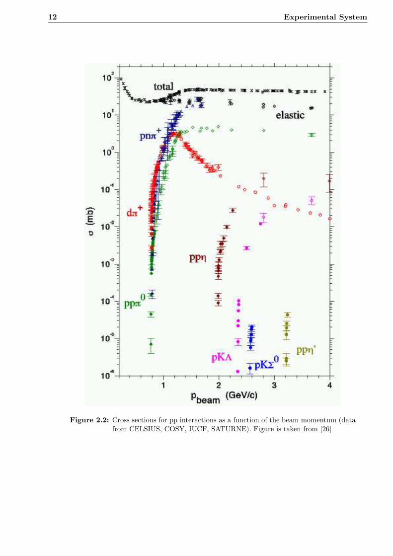
7.1 The cosmic ray test facility. Two orthogonal hodoscopes made from 90o crossedstraw tube double planes are sandwiched between the two plastic scintillators whichprovide a trigger coincidence. . . . . . . . . . . . . . . . . . . . . . . . . . . . . 72
7.2 Schematic side view of the cosmic ray test facility with distances as it was used forthe tests. . . . . . . . . . . . . . . . . . . . . . . . . . . . . . . . . . . . . . . 72
7.3 The electronic setup used in the measurements. . . . . . . . . . . . . . . . . . . 73
7.4 The DAQ Process. . . . . . . . . . . . . . . . . . . . . . . . . . . . . . . . . 74
7.5 Measured drift times from 4 different straw tubes. x-axis is drift time (nsec) andy-axis is the counts. . . . . . . . . . . . . . . . . . . . . . . . . . . . . . . . . 75
7.6 R(t) curves for the 4 straws from Fig.7.5 with 2 bar absolute pressure and 2040V
high voltage. . . . . . . . . . . . . . . . . . . . . . . . . . . . . . . . . . . . . 76
7.7 χ2 histogram for 8 responses tracks . . . . . . . . . . . . . . . . . . . . . . . . 77
7.8 Fitted plane in which track (blue line) lies together with straw tubes (black circles)and the cylinders (red circles) in 2 dimension (YZ-plane projection along x axis).Straw numbers (str 1,2,3,4) increase from bottom to top. . . . . . . . . . . . . . 78
7.9 Distribution of firing straws out of 8 straw responses (one per plane at most) inthe test facility. The corrected ratio (8 responses/7 responses) under geometryconsideration amounts to ≈ 95. . . . . . . . . . . . . . . . . . . . . . . . . . . 79
7.10 Dependence of firing number of straws out of 8 planes as function of a commonsingle straw efficiency ε. . . . . . . . . . . . . . . . . . . . . . . . . . . . . . . 80
7.11 Response multiplicity of the 4 double planes. 1. and 2. double planes are orthogonaland 3. 4. planes parallel to the trigger scintillators. . . . . . . . . . . . . . . . . 81
7.12 Simulated cosmic hit distribution between the two trigger scintillators. Close tothe scintillators the hit distribution is uniform. Between the scintillators the hitdistribution peaks in the center. . . . . . . . . . . . . . . . . . . . . . . . . . . 82
7.13 Illumination distribution of cosmic tracks on the circular test scintillator plane. 8and only 8 fired straws from 8 planes are required. The observed density fluctuationscome from a folding of different straw efficiencies. A χ2 < 5 (Fig.7.7) cut on trackfitting is applied. . . . . . . . . . . . . . . . . . . . . . . . . . . . . . . . . . 83
7.14 QDC (left) and TDC (right) values of the circular test scintillator. . . . . . . . . 84
7.15 Geometry of the circular test scintillator with some few Cherenkov light responsesfrom the plexi light guide. . . . . . . . . . . . . . . . . . . . . . . . . . . . . . 84
7.16 Left: hit points of the all cosmic tracks (same as in Fig.7.13) on the test scintillator’splane. Right: hit distribution with the test scintillator response as veto. . . . . . 85
7.17 Illumination distribution of cosmic tracks on the square test scintillator. . . . . . 86
7.18 QDC (left) and TDC (right) values of the square test scintillator. . . . . . . . . . 86
7.19 Geometry of test scintillators, after χ2cut. . . . . . . . . . . . . . . . . . . . . 87
7.20 Left: hit points of the all cosmic tracks on the square test scintillator’s plane (sameas in Fig.7.17). Right: hit distribution with the test scintillator response as veto. . 87
7.21 QDC values for light output of the circular test scintillator along the axis of lightguide a) and along the transversal axis b). . . . . . . . . . . . . . . . . . . . . 88

LIST OF FIGURES XI
7.22 Quasi focal point in a circular scintillator which gives about parallel reflected lightfrom the cylindrical boundary [14]. This focusing disappears when the light isemitted from points closer to the light guide (left). . . . . . . . . . . . . . . . . 89
7.23 QDC values of the square test scintillator along the axis of light guide a) and alongthe transversal axis b). . . . . . . . . . . . . . . . . . . . . . . . . . . . . . . . 89
7.24 Left geometry of the plastic light guide, right QDC values from the light guide. . 907.25 Superposition of the QDC spectra from scintillator and light guide. . . . . . . . 917.26 Left: hit distribution of the cosmic ray on the wire plane. Right: same distribution
with test straw as veto. . . . . . . . . . . . . . . . . . . . . . . . . . . . . . . 917.27 Reconstructed geometry of the straw tube. . . . . . . . . . . . . . . . . . . . . . 927.28 A few radial distance circles calculated from the R(t) calibration curve are drawn
around the track positions. The wire position appears as tangent to the distancecircles. . . . . . . . . . . . . . . . . . . . . . . . . . . . . . . . . . . . . . . . 93
7.29 The full set of distance circles together with the resulting tangent which approxi-mates the wire position. . . . . . . . . . . . . . . . . . . . . . . . . . . . . . . 94
7.30 The expected radius determined from wire position and hit points on horizontalaxis and radius determined from straw timing and R(t) calibration on vertical axis. 95
7.31 rR(t) calib - rhit points. . . . . . . . . . . . . . . . . . . . . . . . . . . . . . . . . 967.32 TDC resolution histogram. Obtained with pulser signals at two different time. . . 96
A.1 Each container class represent a sub-detector of COSY-TOF. Information ofeach triggered channel is stored as a hit-class . . . . . . . . . . . . . . . . . . 100
A.2 Conversion of detector data from tape using four intermediate data formats(RAW, LST, CALtemp, CAL). The CAL-format is fully calibrated and thebasis of all data analysis. . . . . . . . . . . . . . . . . . . . . . . . . . . . . 101
B.1 The TDC spectrum of the wound layers of the Quirl detector before (left) andafter (right) calibration. TDC values in units of 100 psec. Figure is takenfrom [55]. . . . . . . . . . . . . . . . . . . . . . . . . . . . . . . . . . . . . . 106
B.2 The ADC spectrum of the wound layers of the Quirl detector before (left) andafter (right) calibration. Figure is taken from [55]. . . . . . . . . . . . . . . . 108
C.1 P8(k) versus ε. . . . . . . . . . . . . . . . . . . . . . . . . . . . . . . . . . . . 110

XII LIST OF FIGURES

List of Tables
1.1 Quarks with their charges and masses. . . . . . . . . . . . . . . . . . . . . . 11.2 Some baryons and mesons together with their quark contents, electric charges,
masses, life times and decay modes. . . . . . . . . . . . . . . . . . . . . . . . 2
3.1 Circular acceptances of the first and second Fiber Hodoscopes (at their posi-tion in the TOF) and straw tracker planes at the same positions. . . . . . . 23
3.2 Anode wire and Cathode tube properties . . . . . . . . . . . . . . . . . . . . 253.3 Some properties of different gases. Z and A are charge and atomic weight.
EX , Ei excitation and ionization energy respectively, Wi is the average energyrequired to produce one electron-ion pair in the gas, dE/dx is the most prob-able energy loss by a minimum ionizing particle, X0 is the radiation length. 29
3.4 Experimental parameters for different gases. . . . . . . . . . . . . . . . . . . 34
4.1 Four configurations for the input board. . . . . . . . . . . . . . . . . . . . . 41
A.1 The most important TofRoot classes . . . . . . . . . . . . . . . . . . . . . . 99
XIII

Chapter 1
Introduction
1.1 Motivation
High energy physics deals basically with the study of the ultimate constituents of matterand nature of the interactions between them. Experimental research in this field of scienceis carried out with particle accelerators and their associated detection equipment. Highenergies are necessary for two reasons; first, in order to localize the investigations to verysmall scales of distance associated with the elementary constituents, secondly many of thefundamental constituents have large masses and require correspondingly high energies forcreation and study.
Nearly seventy years ago, only a few elementary particles the proton, neutron, the elec-tron and neutrino, together with the electromagnetic field quantum photon were known.The universe as we know it today appears indeed to be composed almost entirely of theseparticles. However, attempts to understand the details of the nuclear force between protonsand neutrons, as well as to follow up the pioneering discoveries of new, unstable particlesobserved in the cosmic rays, led to the construction of ever larger accelerators and to theobservation of many new particles. These so-called ”hadrons” or strongly interacting parti-cles are unstable under terrestrial conditions but are otherwise just as fundamental as thefamiliar proton and neutron [1]. Our present model of the constituents of matter is that theyconsist of fundamental point like spin 1/2 fermions the quarks [2], with fractional electriccharges and the leptons, like the electron and neutrino, carrying integral charges.
The known quarks are listed in Table-1.1 ([3]). Quarks are always confined in compound
Quark Electric charge (e) Massu (Up) 2/3 2-8 MeVd (Down) -1/3 5-15 MeVc (Charmed) 2/3 1-1.6 GeVs (Strange) -1/3 100-300 MeVt (Top) 2/3 168-192 GeVb (Bottom) -1/3 4.1-4.5 GeV
Table 1.1: Quarks with their charges and masses.
1

2 Introduction
systems which extend over distances of about 1fm. The most elementary quark systems arebaryons which have net quark number three, and mesons which have net quark number zero.
In Table-1.2 some baryons and mesons together with their quark contents, electric charges,masses, life times and decay modes are listed (the values are taken from [4]).
Particle Quark content Electric charge (e) Mass (MeV) cτ Decay Mode
p uud 1 938.27
n ddu 0 939.56 2.65 ∗ 108km pe−νe
pπ0(51.6%)Σ+ uus 1 1189.37 2.4 cm nπ+(48.3%)
Σ0 uds 0 1192.64 2.2 ∗ 10−11m Λγ
Σ− dds -1 1197.45 4.4cm nπ−(99.8%)pπ−(63.9%)
Λ uds 0 1115.68 7.89cm nπ0(35.8%)
π+ ud 1 139.57 7.80cm µ+νµ(99.99%)
π− du -1 139.57 7.80cm µ+νµ(99.99%)2γ(98.8%)
π0 (uu+dd)/√
2 0 134.97 25nm e+e−γ(1.2%)µ+νµ(63.5%)
K+ us 1 493.68 3.71m π+π0(21.2%)µ+νµ(63.5%)
K− su -1 493.68 3.71m π+π0(21.2%)
Table 1.2: Some baryons and mesons together with their quark contents, electric charges,masses, life times and decay modes.
Quantum Chromodynamics (QCD) is considered to be the underlying theory of the stronginteraction, with quarks and gluons as fundamental degrees of freedom.
QCD is simple and well understood at short-distance scales, much shorter than the sizeof a nucleon (< 10−15m) [5]. In this regime, the basic quark-gluon interaction is sufficientlyweak. Here, perturbation theory can be applied, a calculation technique of high predictivepower yielding accurate results when the coupling strength is small. In fact, many pro-cesses at high energies can quantitatively be described by perturbative QCD within thisapproximation.
The perturbative approach fails when the distance among quarks becomes comparableto the size of the nucleon, the characteristic dimension of our microscopic world. Underthese conditions, the force among the quarks becomes so strong that they cannot be furtherseparated. This unusual behavior is related to the self-interaction of gluons: gluons do notonly interact with quarks but also with each other, leading to the formation of gluonic flux

1.2 Scattering Experiments 3
tubes connecting the quarks [6]. As a consequence, quarks have never been observed as freeparticles and are confined within hadrons, complex particles made of 3 quarks (baryons) ora quark-antiquark pair (mesons). Baryons and mesons are the relevant degrees of freedomin our environment.
In the domain of low energies and momentum transfers (q2 ∼ 1−5GeV 2, medium-energyphysics) analytical QCD calculations are not reliable. In this domain, the useful methodsare: the chiral effective theory, lattice calculations and meson exchange models [7]. In thesetheories, the properties of nuclei and nuclear reactions are described in terms of nucleons andmesons, interacting on a scale of 1 fm or larger. The nucleon-nucleon interaction at thesedistances is described by potentials derived from meson exchange models and adjusted toexperimental data. The distance of interaction is governed by the mass of the meson. Lightpions (π0,+,−) mediate the long- and medium-distance interactions (> 0.7fm, attractive);heavy mesons (ω, ρ) are responsible for a strong short-range force (repulsive) [8].
The physics program at the medium energy hadron accelerators (TRIUMF, LAMPF,PSI, LEAR, SATURNE, IUCF, CELSIUS and COSY) was and is focusing on studies of theproduction and the decay of light mesons and baryon resonances and the conservation orviolation of symmetries [9].
Investigations of the production of mesons and their interactions with nucleons are basedon measurements determining the total and differential production cross sections and theirdependence on the energy of the interacting nucleons. When one wants to study excitedhadrons then the detector has to measure their stable decay products. This means that inthe exit there are normally more than two outgoing particles. To establish a comprehensivedescription of the medium-energy physics, high quality measurements are needed, for whichtwo very important requirements have to be fulfilled:
• a high acceptance detector system
• a beam of high quality and intensity
1.2 Scattering Experiments
Much of what we know about nuclei and elementary particles, the forces and interactions inatoms and nuclei has been learned from scattering experiments, in which atoms in a targetbombarded with beams of particles [10]. The earliest were the alpha-particle scatteringexperiments of Ernest Rutherford. In 1906, to probe the structure of the atom, Rutherfordobserved the deflection of alpha particles as they pass through bulk matter (a thin sheetof gold foil). He observed that alpha particles from radioactive decays occasionally scatterat angles greater than 90o, which is physically impossible unless they are scattering offsomething more massive than themselves. This led Rutherford to deduce that the positivecharge in an atom is concentrated into a small compact nucleus [11]. Thus, nucleons scatteredfrom atoms at various scattering angles reveal information about the nuclear forces as wellas about the structure of nuclei.
The important observables to extract the physics from the scattering experiments are e.g.the energy dependent total cross section σ(ε) and the differential cross section dσ/dcos(θ)depending on the angular correlation between entrance and exit directions. Observables

4 Introduction
are always of the type: number of events per some phase space interval and per number ofbeam particles. The cross section shows resonance masses MR and widths ΓR. The angulardistribution dσ/dcos(θ) depends on the square of the wave function and contains informationon spin, parity and angular momentum content of the reaction. Excited hadrons appear aspeaks in subsystem mass spectra.
In Fig.1.1 a typical scattering experiment illustrated. A stream of particles, all at thesame direction and energy, moves through the target (very small spot) where some of theparticles interact. The reaction particles are measured by a detector. The scatterer is
Figure 1.1: Principle of a scattering experiment on an external target. The beam passesthrough a cell with thin windows, which contains the target material. Reactionproducts are measured by surroundings detectors which cover the full solidangle in ideal case.
represented by an area σ called cross section. It is the measure of the probability that ascattering can happen. The available beam intensity (n= number of particles per second)and the target thickness (density · length · NA (Avogadro number) = target particles perunit area) define the luminosity L (reaction s−1cm2) which is:
L = n · ρ · d ·NA
The total reaction rate is given by:
Rate = L · σwhere σ is the cross section of the reaction or interaction probability between particles ofthe beam and target. The unit of σ is barn (1mb = 10−27cm2). With a 4mm thick liquidhydrogen target having the thickness of 1.7∗1022 protons/cm2 and a proton beam of 109 s−1,the luminosity is:
L = 109 s−1 × 1.7 ∗ 1022 cm−2 = 1.7 ∗ 1031 cm−2s−1

1.2 Scattering Experiments 5
With σpp = 40mb = 4 ∗ 10−26cm2, the reaction rate in the target is 6.8 ∗ 105s−1. In order tomeasure the differential cross section, the following informations are needed [12]:
• intensity of the beam,
• total measurement time,
• solid angle coverage of the detector,
• scattering angle,
• number of particles scattered into this solid angle,
• thickness of the target,
• density of the target,
• atomic weight of the target material,
• Avagadro number (NA = 6.022 ∗ 1023)
In general a detector covers only a certain part of the solid angle. One measures thedifferential cross section defined as:
dσ(θ, φ)
dΩ(θ, φ)=
number of particle scattered in to the dΩ
j (current density of the beam)
and tries to extrapolate the full angular range.If we consider the scattering of particles on a potential V (r) which is only nonzero at
|r| < a, the scattering process is described in the non-relativistic quantum mechanics by thesum of an incoming plane wave and an outgoing spherical wave [12]:
ΨT (~(r) = A
[ei~k~r + f(θ, φ)
eikr
r
]
where f(θ, φ) is the scattering amplitude. The density of the particles is given in quantummechanics by P = Ψ∗Ψ. For incoming particles with the velocity of vin, the current densityis jin = vinP = A2vin. Similarly for the outgoing particles the current density isjout = vout|Ψ|2 = vout|f(θ, φ)|2A2/r2. Using the current densities one can write the differentialcross section in terms of scattering amplitude [12]:
dσ(θ, φ)
dΩ(θ, φ)= |f(θ, φ)|2
f(θ, φ) is:
f(θ, φ) =−2πm
h2
∫ei~k~r′V (r′)ΨT (~r′)d3r′ (1.1)

6 Introduction
1.3 Event Reconstruction and
Feasibility of an Experiment
The detector volume is filled with devices which the particle traverse and in which theyleave pieces of information by creating light flashes or movable electric charges (excitationand ionization). The event record of an experiment consists of signals from all particles ofan interaction. After sorting out which informations are related to the same particle thekinematical properties of each particle have to be reconstructed to reveal the physical natureof the whole event [13].
In ideal case a detector must
• measure over the complete possible kinematical region for the desired reaction (100 %acceptance)
• make it possible to determine the four vectors (E, ~p) of all reaction particles (kinemat-ical completeness)
For kinematically complete events in which all four vectors are known (both in entranceand exit), all possible physical observables can be determined, but the precision which anexperiment can reach is limited by
• precision in the kinematical coordinates (four vector components)
• statistical accuracy (number of events per interval)
• amount of background
• efficiency with which the detector and reconstruction procedure cover the phase spaceof the reaction
The precision in the determination of the four vector of a charged particle depends onthe accuracies in the track direction, absolute momentum and identification of the particlemass. Except for the mass, these kinematical quantities can be measured by means of highgranularity but approximately massless geometry detectors when particles are charged.
If the detector provides more information than necessary (over constraints) one can andshould use the additional information to improve the precision in the event reconstructionby a fit procedure.
If we assume a reaction in which the beam and target particle go into several exit particles1 + 2 + · · ·, then we can write for that an equation for the four vectors P:
Pbeam + Ptarget = P1 + P2 · · ·In explicit four vector notation, this describes simply four equations for the simultaneousenergy and momentum conservation and writes:
Epx
py
pz
beam
+
Epx
py
pz
target
=
Epx
py
pz
1
+
Epx
py
pz
2
+ · · · (1.2)

1.3 Event Reconstruction andFeasibility of an Experiment 7
There holds the relativistic relation between energy and momentum E2i = m2
i + ~pi2
where ~p = (px, py, pz) = |~p|(nx, ny, nz) ~n is the unit vector of direction cosines (|~n| = 1 andn2
x + n2y + n2
z = 1).
In Eq.1.3 an equivalent information to the four vectors (in Eq.1.2) is written.
∣∣∣∣∣∣∣∣∣
mb
nbx
nby
±|pb|
∣∣∣∣∣∣∣∣∣⊕
∣∣∣∣∣∣∣∣∣
mt
ntx
nty
±|pt|
∣∣∣∣∣∣∣∣∣→
∣∣∣∣∣∣∣∣∣
m1
n1x
n1y
±|p1|
∣∣∣∣∣∣∣∣∣⊕
∣∣∣∣∣∣∣∣∣
m2
n2x
n2y
±|p2|
∣∣∣∣∣∣∣∣∣(1.3)
The directional unit vectors ~n are worth only two variables, since n2z = 1− n2
x + n2y. The
sign of nz is kept in the momentum ±|p| and distinguishes forward or backward going tracks.
This table allows to count over constraints and thus judge if a given experimental setupprovides enough information for a kinematically complete event construction [14].
For example, if we assume a pure geometry detector, for the reaction pp → dπ+ (novelocity measurement for d and π+), we have:
m →nx →ny →|p| →
∣∣∣∣∣∣∣∣∣∣∣∣∣∣
p
√√√√
∣∣∣∣∣∣∣∣∣∣∣∣∣∣
⊕
∣∣∣∣∣∣∣∣∣∣∣∣∣∣
p
√√√√
∣∣∣∣∣∣∣∣∣∣∣∣∣∣
→
∣∣∣∣∣∣∣∣∣∣∣∣∣∣
d
√√√0
∣∣∣∣∣∣∣∣∣∣∣∣∣∣
⊕
∣∣∣∣∣∣∣∣∣∣∣∣∣∣
π+
√√√0
∣∣∣∣∣∣∣∣∣∣∣∣∣∣
2 overconstraints
where√
means information produced by detector and 0 no information produced. We havetwo unknown momenta but four equations from the momentum conservation so we havealready two over constraints.
With a time of flight information, giving ~β and in turn ~p, (together with a mass assump-
tion ~p = m · ~β · γ) we have except the masses no unmeasured information and four overconstraints in this case.
∣∣∣∣∣∣∣∣∣∣∣∣∣∣
p
√√√√
∣∣∣∣∣∣∣∣∣∣∣∣∣∣
⊕
∣∣∣∣∣∣∣∣∣∣∣∣∣∣
p
√√√√
∣∣∣∣∣∣∣∣∣∣∣∣∣∣
→
∣∣∣∣∣∣∣∣∣∣∣∣∣∣
d
√√√√
∣∣∣∣∣∣∣∣∣∣∣∣∣∣
⊕
∣∣∣∣∣∣∣∣∣∣∣∣∣∣
π+
√√√√
∣∣∣∣∣∣∣∣∣∣∣∣∣∣
4 overconstraints
An example of three outgoing particles with a charged particle detector (like TOF) is
pbeam + ptarget → p + p + π0 (or γ, or ”nothing”)
We have the following information about the reaction (from geometry and time of flight
8 Introduction
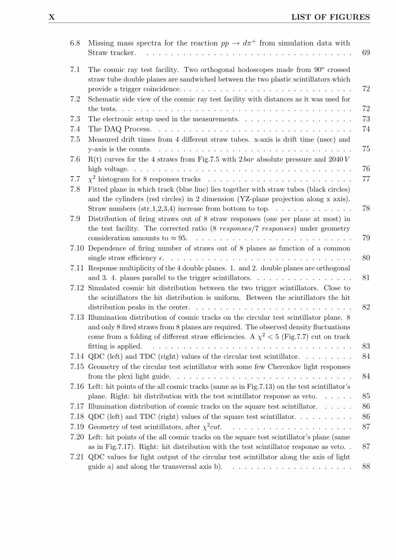
informations).
∣∣∣∣∣∣∣∣∣∣∣∣∣∣
p
√√√√
∣∣∣∣∣∣∣∣∣∣∣∣∣∣
⊕
∣∣∣∣∣∣∣∣∣∣∣∣∣∣
p
√√√√
∣∣∣∣∣∣∣∣∣∣∣∣∣∣
→
∣∣∣∣∣∣∣∣∣∣∣∣∣∣
p
√√√√
∣∣∣∣∣∣∣∣∣∣∣∣∣∣
⊕
∣∣∣∣∣∣∣∣∣∣∣∣∣∣
p
√√√√
∣∣∣∣∣∣∣∣∣∣∣∣∣∣
⊕
∣∣∣∣∣∣∣∣∣∣∣∣∣∣
π0 (γ)
√000
∣∣∣∣∣∣∣∣∣∣∣∣∣∣
1 overconstraint
In this case, we have three unknowns (momentum of the neutral particle) and 1 over con-straint.
At low energy close to the π0 threshold and with a time of flight information for thetwo protons three different hypothesis for the neutral particle are possible, pion, photonor nothing. This reaction pp → ppX0 was published by TOF [15]. A detector, havinggood enough resolution, allows to evaluate all three channels since the over constraint givesselectivity.

Chapter 2
Experimental System
2.1 COSY Accelerator
COSY is a cooler synchrotron and storage ring depicted in Fig.2.1. It delivers very highprecision polarized and unpolarized beams of upto ≈ 2 ∗ 1011 protons and deuterons permachine cycle in the momentum range from 300MeV/c to 3600MeV/c [16, 17]. This goal isaccomplished by using an electron cooling system and a stochastic cooling system.
The electron cooler of COSY is designed for electron energies up to 100keV , thus to coolprotons up to a momentum of 600MeV/c [18, 19]. An electron beam guided in parallel tothe protons (deuterons) reduces; the transversal and longitudinal momentum by friction andmakes phase-space-dense ion beams before acceleration to a requested energy [20]. Electroncooling is used after stripping injection of H− or D− ions. With the stochastic coolingcovering the range from 1.5GeV/c up to maximum momentum, deviations from the beamare determined for sub samples of the beam and then in each turn a correction on the samplesis applied. From turn to turn new samples are prepared by mixing [21, 22].
The beam preparation needs 2 to 12sec (acceleration upto 2sec, electron cooling upto10sec). The spill out time can be stretched from few seconds to minutes by stochasticextraction. On internal targets operation times can be upto hours for one cycle if stochasticcooling compensates the beam blow up by the target.
The COSY consists of two sources for unpolarized H−/D− - ions and one for polarizedH− -/ D−- ions, the injector cyclotron JULIC that accelerates the H− - ions up 300MeV/cand D− - ions up 600MeV/c, the cooler ring COSY with a circumference of 184 m deliveringprotons up desired momentum [16, 23]. Injection into COSY takes place via charge exchangeof the H−- or D−- ions over 20ms with a linearly decreasing closed orbit bump at the positionof the stripper foil. The polarized source presently delivers 8.5µA of polarized H− - ions[23].
Four internal target areas (ANKE, COSY-11, COSY-13, EDDA) are available for experi-ments with a circulating beam. The beam can also be extracted via the stochastic extractionmechanism and is guided to three external experiment areas (magnetic spectrometer BIGKARL, Time Of Flight spectrometer TOF and JESSICA). The emittance of the extractedcooled beam is only ε = 0.4π mm mrad [24].
9

10 Experimental System
Figure 2.1: The COSY accelerator at the research center Julich and the positions of ex-periments on internal and external targets.

2.1 COSY Accelerator 11
2.1.1 Physics in COSY
The COSY accelerator with the energy range and beam quality that it provides, makes itpossible to study the structure of mesons and baryons in the confinement regime of QCD.This field includes the analysis of decay properties of mesons and baryon excitations andinteractions of meson meson, meson baryon and baryon baryon systems. The experimentalstudies are characterized by keywords like threshold measurements (it is possible due to thehigh quality of beam and target. Beam diameters at targets are available with divergenciesbelow 1mrad.), strangeness production, final state interaction, medium modification andreaction mechanisms [25].
Threshold measurements are instructive for the interpretation of elementary interactions.The relative velocities of the ejectiles are low which favors s-waves and final state interac-tions. At threshold the momentum transfer is high since incoming particles have high andthe outgoing particles have small center of mass momenta. The transfer is practically thecenter of mass momentum of the input channel. This large momentum transfer and s-wavedominance at threshold enhance heavy meson exchanges [26].
The strangeness production is an excellent tool to study hadron dynamics [27]. Due tothe high selectivity for the detection of delayed decays of hyperons and Ks mesons it is exper-imentally particularly precise. Questions concerning the strangeness content of the nucleonsand the reaction mechanisms for the dissociation can be addressed by such studies. For thepp → pK+Λ [28] reaction it is comparatively easy and precise to measure the Λ polarizationvia the asymmetry of the parity violating weak decay Λ → pπ−. In a simple quark modelthis is related to the s-quark polarization. With a polarized beam and polarized target adetailed analysis of the spin degrees of freedom can be done in Λ production reactions.
Modifications of the properties and interactions of hadrons within the nuclear mediumare another interesting field. Questions here are for example the lifetime of hyper nuclei,specific reaction mechanisms and possible medium effects especially on K-mesons which maybe isolated in subthreshold production experiments [29].
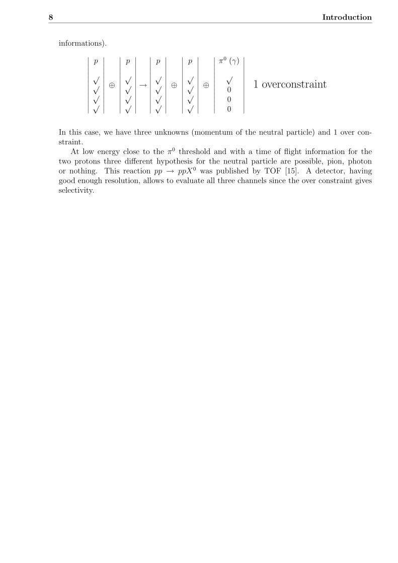
With COSY a wealth of experimental data has been accumulated during the last decade,which differ to previous measurements with respect to the quality and the amount of thedata. Fig.2.2 gives an overview of the world data (including COSY) on total cross sectionsin pp interactions below 4GeV/c beam momentum.
12 Experimental System
Figure 2.2: Cross sections for pp interactions as a function of the beam momentum (datafrom CELSIUS, COSY, IUCF, SATURNE). Figure is taken from [26]

2.2 COSY-TOF Detector System 13
2.2 COSY-TOF Detector System
Highly sophisticated detector systems are in operation either at the internal COSY beam orlocated at extracted beams in external areas. The time-of-flight spectrometer TOF is one ofthe main experimental facilities at the external beam lines of the COSY.
The investigations at COSY-TOF [30] concentrate mainly on the light and medium massmeson production, proton-proton bremsstrahlung and associated strangeness meson-baryonproduction by measuring following reactions
• pp → pK+Λ, pK+Σ0, pK0s Σ+ [28, 31, 32, 33]
• pp → pp, ppγ, ppπ0, ppη, ppη′ [15, 34, 35, 36, 37, 38]
• pp → pnπ+, dπ+, ppπ+π−, ppω [39, 40]
• pd →3 Heη, 3Heη′, 3Heω [41]
The COSY-TOF spectrometer is designed as a scintillator hodoscope for stable chargedparticles covering about 2π solid angle in the laboratory system. The main components of theTOF spectrometer are a liquid hydrogen target, a start detector, tracker system and a systemof three stop detector segments, forming a cylinder barrel with a circular endcap (Fig.2.3).The endcap consists of two concentric circular hodoscopes. Up to 3 barrel elements can becombined with the two planar front hodoscopes of 1.16 and 3 m outer diameter, providingvery large solid angle coverage without holes. Fig.2.3 shows the TOF spectrometer in a 3 mlong version. With two more existing barrel sections the maximal flight path in vacuum canbe extended to more than 8m. Since the typical velocities of the particles in the momentumrange of COSY are between approximately 25% and 99% of the speed of light [42], the flightlengths must amount to some meters in order to be able to determine the velocity sufficientlywell with the available time resolution of 2.5 ∗ 10−10sec (average over all detectors) [42].
The spectrometer components are housed in a big vacuum tank [43]. So it is guaranteedthat beam particles and reaction products do not undergo reactions with air, which wouldlead to many non-target originated events and to straggling.
A very important advantage of TOF is the absence of a vacuum tube for the beam. Sucha tube would occupy space for detectors at small angles and reaction particles would have topenetrate very thick layers of this tube if they are at small forward angles. TOF detectorscan be (and they are) positioned millimeters away from the passing cooled primary beam.This is particularly advantageous if one is going to detect Λ → pπ+ or Ks → π−π+ decayswhich have decay vertices close to the beam in the few cm distance from the target. TOF isunbeatable best suited for reaction studies with Λ and Ks.
In order to calibrate the time measurement, the start and stop scintillators are connectedto a nitrogen laser UV light calibration system by quartz light guides.

14 Experimental System
Figure 2.3: The COSY-TOF Detector. The beam enters from left, passes through thesmall cryotarget and the evacuated tank. Start detector and tracker are closeto the target. The big stop detector hodoscopes cover the inner surface of thevacuum tank.

2.2 COSY-TOF Detector System 15
2.2.1 Target system
A very light liquid hydrogen (or deuterium) target (Fig.2.4), which is very small in order totake advantage of the excellent beam quality of COSY, has been developed and used for theexternal experiments at COSY [44]. Since hydrogen or deuterium are gases and have verylow densities at room temperature and atmospheric pressure (0.08 g/l for H2 and 0.166 g/lforD2), leading to reduction of the reaction probability, they are liquefied. The liquid targetwith its very small amount of inactive material and thin beam windows is installed in theentrance of the TOF tank in a section with good vacuum of 10−6 − 10−7mbar. The targetconstruction is affected by the following requirements [45]:
• It has to stabilize the target temperature within ±0.05K in the range of liquid hydro-gen/deuterium
• The windows for the beam inlet and exit through the target cell have to be very thinbut nevertheless planar
• The target thickness has to be well defined. Therefore, the target liquid should havehomogenous density without any bubbles
• The time needed for large temperature changes during cooling down to the workingtemperature or heating up to the room temperature has to be as short as possible
• The cooling system and the heat conductors have to occupy minimum space and mini-mum solid angle. There must be minimum mass in the target region in order to reducebackground events and shadowing effects on reaction products before they can reachdetectors
• the target should have axial symmetry
The target system used in the TOF experiments has a target cell with 6mm in diameterand normally 4mm in length. It has very thin windows of 0.9µm Mylar foil. This is achievedby a stabilized pressure difference over windows of ≤ 0.2mbar in all conditions [46, 47].The small dimensions of the target minimize the background due to double scattering andenable measurements very close to threshold. If we consider the delayed decays of strangeparticles occurring a few centimeters after their production in the target, the target lengththerefore should be much smaller than the decay length of a few centimeters to get a welldefined interaction vertex. This is important for high quality kinematical reconstruction andunderstanding of the reactions. The very thin window foils reduce the background eventsfrom reactions on heavier nuclei in the target window foils, the energy losses and stragglingof the outgoing ejectiles. With the beam from COSY of ≈ 0.7mm∅ and 4mm lH2 thicknesswe obtain routinely a reaction vertex definition within < 2mm3. This has big advantagesfor geometrical reconstruction and background identification.
In order to keep the target in optimum conditions (constant temperature and stabledensity), a heat pipe-target system is developed [48, 49]. It is a closed system, which has anevaporator and condenser section where the target material acts as a working fluid whichevaporates and condenses. The condenser section and evaporator section (target cell) areconnected by a transport (or adiabatic) section that bridges large distances. Heat applied

16 Experimental System
to the evaporator section by an external source radiation vaporizes the working fluid. Theresulting vapor pressure drives the vapor through the adiabatic section to the condenser,where the vapor condenses, releasing the latent heat of vaporization to the heat sink (coolingmachine). The condensed liquid flows down to the evaporator section for re-evaporation.This gravity assisted circulation provides a stable dynamic equilibrium. The target materialis liquefied by using a cooling machine. The cooling time of the system for H2/D2 from roomtemperature (300K) to 15/19K is 50/45 minutes respectively [46].
Figure 2.4: The target system. The cold parts below the flange are in vacuum. Thenecessary super isolation is removed in the picture.

2.2 COSY-TOF Detector System 17
2.2.2 Start Detector
The actual start detector consists of two circular layers of 12 wedge shaped plastic scintillatorsectors (δφ = 30o) with 1mm thickness, placed in a distance of 23mm behind the target [50].They deliver a reference signal for the time of flight measurement with the resolution ofσ = 170ps. In order to cover the gaps between the wedges, the two layers are rotated toeach other by 15o leading to a φ information in steps of 15o. Its outer radius is 76 mm. Inthe center there is a hole of 1.4 mm radius for the beam.
2.2.3 Tracker
After the start detector, there is the ”Erlanger tracker” detector (Fig.2.5), made especiallyto investigate the strangeness and hyperon-production [51]. Its goal is track and vertexreconstruction. It consists of a Si-µ Strip detector followed by two fiber hodoscopes providinggeometry informations for the tracks of charged particles.
The Si-µ Strip detector with a thickness of 520µm is 30mm far from the target. It ismade of 100 concentric rings (∆r = 280µm) on one side and 128 in φ segmented elements(∆φ = 2.81o) on the other side. The detector has an outer radius of 31mm and a beamhole with a radius of 3.1mm. The 12800 pixels of the detector provide high resolution indetermination of the track direction. The detector also provides energy loss information [52].
Two fiber hodoscopes complete the tracker detector system. They are made from 2 ×2mm2 quadratic scintillating fibers, covered by cladding of about 0.1mm thickness. The firstone placed 100mm downstream from the target, consists of two layers each of 96 scintillatingfibers which are rotated 90o relative to each other. In 2004 a new third plane is added to theexisting system in order to increase the reconstruction efficiency. The second one is placed200 mm far from the target and made of two times 192 fibers. It covers the active areaof 1475cm2. Besides the energy loss of the particles, points for the primary and secondarytracks are provided by the fiber hodoscopes.
The straw tracker, having much higher resolution, much more depth and less mass, muchlarger surface will replace these fiber hodoscopes at the end of 2006. It will improve theoverall performance of the experiments.

18 Experimental System
Figure 2.5: Schematic view of the actual start detector and tracking system (Erlangerstart detector).

2.2 COSY-TOF Detector System 19
2.2.4 Stop Detector
The Quirl Ring and Barrel detectors constitute the stop detector Fig.2.6. There are noacceptance holes between these three components [53]. The barrel hodoscope consists of onelayer of 96 straight scintillators which are read out from both sides [54]. It covers the largereaction angles and provides time and position information by averaging the response of thetwo photomultipliers at each end of the scintillator bars.
Figure 2.6: A sketch of the TOF spectrometer shows the Quirl, the Ring and one of thebarrels
The central hodoscope (”quirl”) is a 3-layer (each 0.5 cm thick) scintillation counterhaving the inner- and outer radius of 4.2cm and 58cm. The first layer is divided into 48 wedgeshaped sectors (∆φ = 7.5o). The second and third layers consist of 24 left- and 24 right wound(Archimedes) spirals. The relationship between φ and r is r(φ) = rmax
φmaxφ where rmax = 58 cm
and φmax = 180o [52]. The overlapping area between three elements fired by a passing particleforms a triangular pixel giving the direction of the track (Fig.2.7). This type of hodoscopewas originally invented and build for measurements at the LEAR/JETSET experiments andthen for CELSIUS/WASA. The advantage of the three layer geometry is also that more thanone passing particle tracks can be determined unambiguously. Since all scintillator elementsare symmetric under rotations around the beam axis in steps of the azimuthal angular widthof an element, the Quirl detector plane is divided into equal, radially symmetric areas.Therefore, all individual scintillators in a plane are exposed to the same integral countingrate as they cover identical parts of the phase space [55]. Furthermore the hodoscope givesa fast online multiplicity and timing trigger and allows for dE/dx measurements.
The ring detector consists also of three layers of 5mm thick scintillator material. It hasan inner- and outer diameter of 1.136m and 3.08m. The design is basically the same as thatof the Quirl detector. The much larger surface of the ring detector is divided into 96 straightsegments and 48 left- and right spirals with only 120o winding angle for the bent scintillators[55].

20 Experimental System
Figure 2.7: Schematic view of the Quirl detector showing the three layers. The elementswhich are hit by two particles are indicated in black

Chapter 3
New Geometry Spectrometer”Straw Tracker” for COSY-TOF
3.1 Requirements for the Straw Tracker
The time of flight spectrometer TOF will be extended by a much better tracking system withhigher resolution, much higher sampling density, and lower mass [56, 57]. Three thousandstraw tubes arranged in 15 double planes will replace the existing tracking detector (fiberhodoscopes) of COSY-TOF.
The straw tracker will be placed behind the µ-strip detector and ≈ 6 cm down streamfrom the target. It will improve
• track resolution
• efficiency of the event reconstruction
• acceptance
• transparency
in COSY-TOF experiments.For reactions with two or three charged particles in the final state the particle momenta
can be determined by measuring the direction vectors alone (see chapter 6). In this casebetter angular and position (track resolution) resolution directly improves the momentumresolution.
Examples of such reactions are pp → dπ+, pp → pK+Λ (Λ → pπ−). In the last reactionthe direction of the neutral Λ hyperon can be determined by its production and decay vertexand decay plane. Both are given in first approximation by points of closest approach betweenthe p and K tracks and the secondary p and π− tracks, respectively. An intersection criterionon the simultaneous line fits must be imposed for the more precise final geometrical vertexdetermination. The momentum of a Λ can also be calculated from the decay angles of p andπ− with respect to the Λ track [58]. One main goal of the new track detector is to improvethe decay vertex reconstruction, to determine all the geometrical information for pKΛ muchmore precisely than now.
21

22New Geometry Spectrometer
”Straw Tracker” for COSY-TOF
Due to its high resolution (better than 200µm, see 5.8) and high sampling (30 planes= 30 coordinates per track), angular and position resolution will be increased significantly.This will improve the precision of all four vector components and exclude ambiguities.
If we compare θ resolution of the first fiber hodoscope with 2 mm thick fibers and placed100mm away from the target, we find ≈ 20mrad (arctan(2/100)), for a single straw at thesame distance from the target with the worst resolution of 0.2 mm, 10 times higher resolutionof ≈ 2mrad is obtained. One should notice that with 30 track points the track resolutionwill be much better than 0.1 mm in position and 0.5mrad in direction.
One of the main topics studied in the COSY-TOF experiments is hyperon production.Since the hyperons decay typically in the first 80 mm and therefore in front of the fiberhodoscopes (cτΣ+ = 24 mm, cτΣ− = 44 mm, cτΛ = 78.9 mm), the fibers are successful inreconstructing these decay patterns. But the weak points of these detectors is that dueto the low sampling (only two space points per track) and limited resolution, there arerather frequently ambiguities from tracks crossing each other at the same detector elementswhich can not be solved (see Fig.3.1). The straw tracker with high sampling and much betterresolution will solve such ambiguities very easily and in this way it will increase the efficiencyof the event reconstruction.
targetbeam
ambiguous points
Figure 3.1: Two hodoscope planes can fake two possible Λ decay vertices due to insufficientinformation.
Moreover the straw detector will help to identify the tracks of charged π and K beforethey decay inside the TOF detector. The decay length L of a particle with mass m in thelab system is related to its intrinsic lifetime τ and its relativistic velocity β or to its massand momentum p by:
L = cτβγ = cτp/m
For a charged π (K) meson with lifetime τ = 2.6 ∗ 10−8 (τ = 1.24 ∗ 10−8) we find cτ = 7.8m(3.7m). With a momentum of say p = 100MeV/c the decay length L = 7.8/1.4 = 5.6m
3.1 Requirements for the Straw Tracker 23
(0.74m). This means, that within ≈ 6cm flight pass 1% of the π± mesons (8% of the K±
mesons) decay. If one finds such a meson track within the first 12 cm flight pass then onehas a 98% (84%) chance to have the correct track direction [56]. It needs a very good trackerin order to avoid efficiency problems in reactions with several mesons.
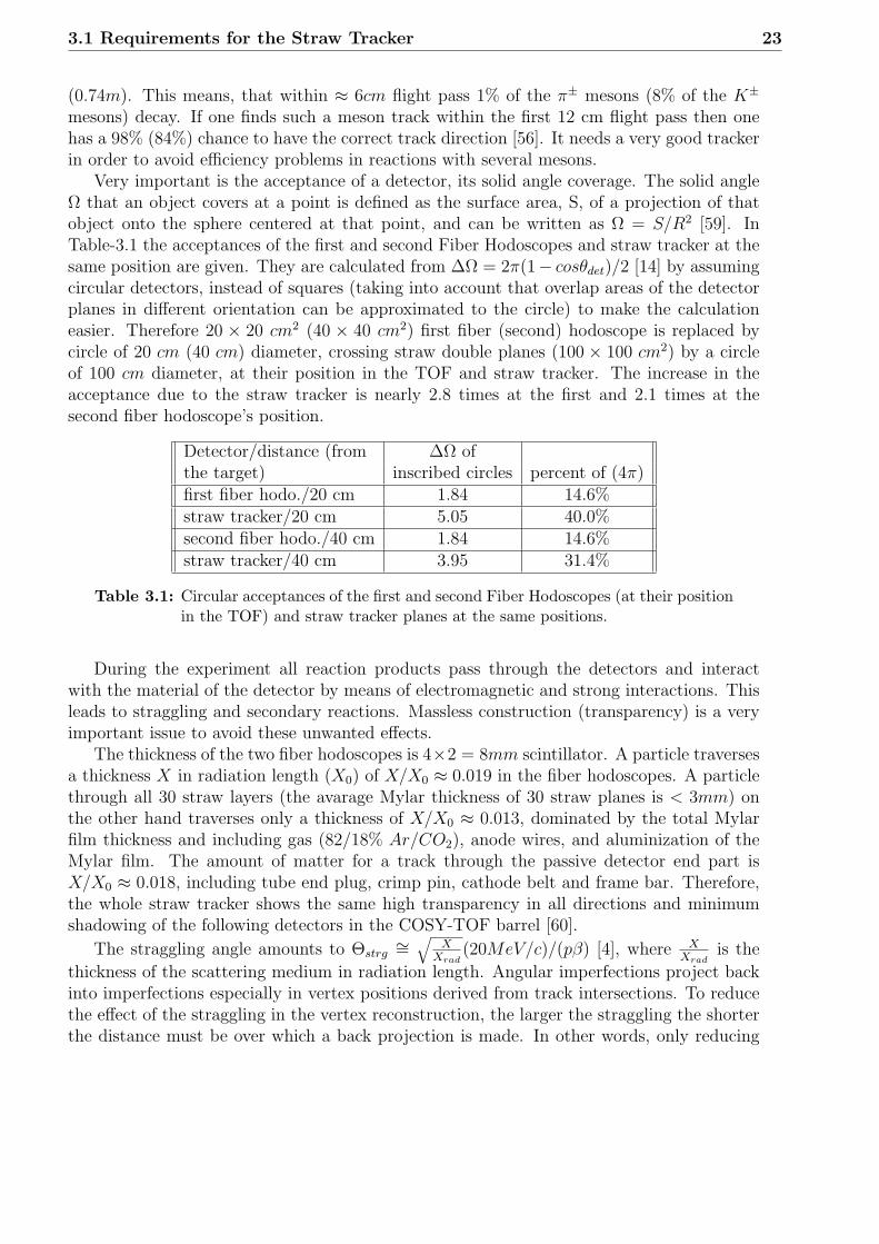
Very important is the acceptance of a detector, its solid angle coverage. The solid angleΩ that an object covers at a point is defined as the surface area, S, of a projection of thatobject onto the sphere centered at that point, and can be written as Ω = S/R2 [59]. InTable-3.1 the acceptances of the first and second Fiber Hodoscopes and straw tracker at thesame position are given. They are calculated from ∆Ω = 2π(1− cosθdet)/2 [14] by assumingcircular detectors, instead of squares (taking into account that overlap areas of the detectorplanes in different orientation can be approximated to the circle) to make the calculationeasier. Therefore 20 × 20 cm2 (40 × 40 cm2) first fiber (second) hodoscope is replaced bycircle of 20 cm (40 cm) diameter, crossing straw double planes (100 × 100 cm2) by a circleof 100 cm diameter, at their position in the TOF and straw tracker. The increase in theacceptance due to the straw tracker is nearly 2.8 times at the first and 2.1 times at thesecond fiber hodoscope’s position.
Detector/distance (from ∆Ω ofthe target) inscribed circles percent of (4π)first fiber hodo./20 cm 1.84 14.6%straw tracker/20 cm 5.05 40.0%second fiber hodo./40 cm 1.84 14.6%straw tracker/40 cm 3.95 31.4%
Table 3.1: Circular acceptances of the first and second Fiber Hodoscopes (at their positionin the TOF) and straw tracker planes at the same positions.
During the experiment all reaction products pass through the detectors and interactwith the material of the detector by means of electromagnetic and strong interactions. Thisleads to straggling and secondary reactions. Massless construction (transparency) is a veryimportant issue to avoid these unwanted effects.
The thickness of the two fiber hodoscopes is 4×2 = 8mm scintillator. A particle traversesa thickness X in radiation length (X0) of X/X0 ≈ 0.019 in the fiber hodoscopes. A particlethrough all 30 straw layers (the avarage Mylar thickness of 30 straw planes is < 3mm) onthe other hand traverses only a thickness of X/X0 ≈ 0.013, dominated by the total Mylarfilm thickness and including gas (82/18% Ar/CO2), anode wires, and aluminization of theMylar film. The amount of matter for a track through the passive detector end part isX/X0 ≈ 0.018, including tube end plug, crimp pin, cathode belt and frame bar. Therefore,the whole straw tracker shows the same high transparency in all directions and minimumshadowing of the following detectors in the COSY-TOF barrel [60].
The straggling angle amounts to Θstrg∼=
√X
Xrad(20MeV/c)/(pβ) [4], where X
Xradis the
thickness of the scattering medium in radiation length. Angular imperfections project backinto imperfections especially in vertex positions derived from track intersections. To reducethe effect of the straggling in the vertex reconstruction, the larger the straggling the shorterthe distance must be over which a back projection is made. In other words, only reducing

24New Geometry Spectrometer
”Straw Tracker” for COSY-TOF
straggling as much as possible allows to stay with the sensitive tracker volume far enoughfrom the target position where the track density may be easily too high.
A ”massless” construction is also needed in order to avoid secondary hadronic reactions.They could spoil the track pattern or result in shadowing effects on subsequent detectorcomponents thus cutting into the acceptance. This is a demanding criterion not only forthe sensitive parts but also for the mechanical structure material, like stretching frames ormounting and adjustment devices and electronic or gas supply components. The overpressurein the straw tubes is the trick which allows to avoid heavy frame construction in the TOFstraw tracker.
3.2 The Julich Straws
The straw tubes shown in Fig-3.2 consist of 1m long Mylar tubes with a diameter of 10mmaluminized on the inner surface. The wall thickness is 30µm. Mylar is the preferred materialbecause of its well suited mechanical properties like a high Young’s modulus and tensilestrength compared with Kapton [57]. Young’s Modulus (also known as modulus of elasticityor tensile modulus) is a measure of the stiffness of a given material. Young’s modulus(measured in pascals), Y, can be calculated by dividing the tensile stress by the tensilestrain [61]:
Y ≡ tensile stress
tensile strain=
F/A0
∆l/l0(3.1)
where F is the force applied to the object; A0 is the original cross-sectional area throughwhich the force is applied; ∆l is the amount by which the length of the object changes; andl0 is the original length of the object.
The advantage of a higher Young’s modulus is the possibility to avoid large changes ofthe tube length under pressure and therefore to hold the wire tension nearly constant overa larger pressure range.
Lightweight plastic end-caps glued into both ends of the Mylar tube provide gas tightness.The end-caps have a 3mm diameter and 5mm long cylindrical extension with a central
Figure 3.2: Construction elements for a single straw tube: aluminized Mylar tube, 1 cm ∅end caps with gas tubes, counting wire going through all elements and crimppins which are finally glued into the 3 mm ∅ extensions which are used fortransversal fixation.
hole for the crimp pins between which the counting tungsten wires with radius of 10µ are

3.2 The Julich Straws 25
stretched. These extensions are also used for a precise transversal fixation of all tubes on bothends in belts with precisely positioned holes. Gas flow is provided through thin plastic tubeswhich are glued into the end caps. Fig.3.3 shows the end structure of the straw tubes withcrimp pins contacting the counting wires and springs providing cathode contacts betweeninner aluminum layer of the Mylar tubes and positioning belt. The weight of a single strawtube is < 2.5g [56].
Figure 3.3: End structure of the straw double plane. The springs provide cathode con-tacting. The crimp pins make contact to the conducting wires. The strawsare fixed transversally by positioning the 3mm ∅ cylindrical extensions of theend-caps in corresponding holes in a > 1m long belt. The conductive belt isremoved.
Anode Wire W97/Re3, Au-plated (4%) ρ = 19.3g/cm3, σ = 6.3mg/LR/L = 314Ω/m (DC-resistance)
Cathode Tube Mylar film, aluminized ρ = 1.4g/cm3 R/L = 40Ω/mC/L ≈ 9.8pF/m
Table 3.2: Anode wire and Cathode tube properties
The simple but new idea of this detector development is to use the anyhow existingexcess pressure inside the tubes in the TOF vacuum tank to create the necessary wiretension and mechanical stability. 1bar overpressure creates on the 1cm diameter end-capsan axial force (7.85N) which is enough to make the tubes self-supporting and supply the force(0.4N) to stretch the counting wire. This means, that massive frame constructions are notnecessary [57]. As thickness defining element and in order to assure correct tube positionsand rectangular shape, each plane has a window like frame made of Rohacell (plastic foamdensity 0.05g/cm3) reinforced by 0.3mm carbon fiber compound plates. Into this frame also

26New Geometry Spectrometer
”Straw Tracker” for COSY-TOF
the adjustment belts are integrated. They provide at the same time the cathode contacts toeach tube via springs which connect the aluminization of the tubes with a copper layer onthe belts (Fig.3.3)[56]. In order to prevent the bending of the straws due to the gravitationthe tubes are glued to each other once with small drops of glue at about half length in theclosely-packed double-layers [60].
Two planes (each has 104 straw tubes) in the double plane are arranged on top of eachother by an half tube diameter offset to cover the low efficient regions near to the tube walls.15 such double plane modules will be stacked on to each other and rotated by 120o in orderto allow for unambiguous multi track reconstruction. Frames and tubes of adjacent doubleplanes lie flat on each other and stabilize each other in beam direction. A free passage of theprimary beam through the double planes is provided by cutting out 1cm in the center fromtwo central one meter straws in each plane. This gives an aperture of ≈ 1cm ∅ throughoutthe full stack. Fig.3.4 shows the arrangement of three double planes constructed. The fullset of straws plus preamplifiers will have a mass of about only 7.5kg. With the reinforcedRohacell it was possible to construct a frame of about the same mass including the gasdistributor and electronic contacts, so that the complete tracking detector has a total massof about 15kg only. It is worth noting, that the ≈ 3000 signal cables of 5m length and0.5mm diameter end up with a mass of ≈ 30kg comparable to the detector mass. One sees,that it makes sense to use very thin cables.
Figure 3.4: Three straw frames mounted in steps of 120o around the beam direction. Onealso sees the central aperture for beam passage.

3.3 Basic Principles of the Straw Tube 27
3.3 Basic Principles of the Straw Tube
Straw tubes are drift chambers (first operation drift chamber [62]) made of a gas filledconducting cylinder acting as cathode, and a sense wire stretched in the axis of the cylinder.
The electromagnetic interaction between the charged particles traversing the gas insidestraw tube forms the basis of detection. Coulomb interactions between the incoming chargedparticles and bound electrons in the gaseous medium result in ionization. Due to the appliedstatic electric field in the tube, electrons of primary ionization will drift to the positivelycharged anode wire and positive ions will move to the cathode. Since the electric field inthe straw tube increases with r−1 towards the anode wire, in the vicinity of the thin wire(at rc = few wire radii) the electric field gets strong enough so that electrons producedby the primary interaction can gain enough energy to produce an avalanche like secondaryionization process called gas amplification. In Fig.3.5 the gas amplification is depicted. A
Figure 3.5: Time development of an avalanche in the Straw tube
typical drop like ionization distribution close to the anode wire develops with all electronsin the front towards the wire surface and ions outside. Because of lateral diffusion and thesmall radius of the anode, the avalanche surrounds the wire; electrons are collected andpositive ions start to drift towards the cathode. From the gas amplification or avalanche,signal amplification of 104− 106 is obtained [63]. This leads to a significant simplification ofthe measurement electronics. Signals produced by the collected charges are further amplifiedby exterior electronics and processed by a data acquisition system (DAQ). The track of aparticle is mapped from the fired wires by registering the drift times of the electrons. Usingthese drift times, one can obtain the distance of closest approach of the track to the anodewire Fig.3.6. In a single straw the coordinate information is a ”cylinder of closest approach”.

28New Geometry Spectrometer
”Straw Tracker” for COSY-TOF
Preamplifier Discriminator
TDC Time measurment
Signal processing
straw tube with
R
drift time
minimal track distance (R) to wire
"cylinder of closest approach"
Figure 3.6: Time difference between creation of movable charges in the gas on the par-ticle track and appearance of an avalanche signal on the counting wire. Thecoordinate information from a single straw is a ”cylinder of closest approach”[62].
3.4 Basic Physics of Particle Detection in a Straw Tube
3.4.1 Ionization Process
When a charged particle passes through a gas, it will lose a part of its kinetic energy in themedium by means of electromagnetic interaction. Energy transfer from the charged particleleads to ionization of the gas along the path of the traversing particle. An expression for theaverage differential energy loss due to ionization has been obtained by Bethe and Livingstonin the framework of relativistic quantum mechanics [64]. The number of primary electron-ionpairs (Np) depends on the atomic number, density and ionization potential of the gas, andon the energy and charge of the incident particle. The created primary electrons may havesufficient energy to ionize further and create secondary electron-ion pairs (clusters). Theoverall outcome of the two processes is called total ionization. The total number of electron-ion pairs per cm is denoted by Nt. These numbers have been measured and computed fora variety of gases [63, 65, 66, 67, 68, 69, 70]. Table 3.3 lists some values for Np and Nt
(taken from [71]), along with other general properties. All numbers are given for normaltemperature and pressure.
Fig.3.7 shows the differential energy loses for various materials over a βγ scale. dE/dxdecreases fast due to β−2 dependence and reaches a minimum around βγ = 3 to 4 (minimumionization) and then starts to increase logarithmically (relativistic rise) as β → 1 [72]. Theminimum ionization energy for most materials is equal to about 2 MeV g−1cm2 [63].
The ionization energy loss is statistically distributed around its mean value. The distri-bution, often referred to as energy straggling, is approximately Gaussian for thick absorbers,but develops asymmetry and a tail towards high energies for decreasing thickness. The highenergy tail is related to the quasi free electron scattering in forward direction. It becomes a

3.4 Basic Physics of Particle Detection in a Straw Tube 29
Gas Z A Ex Ei Wi dE/dx Np Nt X0
(eV) (eV) eV (keV/cm) (cm−1) (cm−1) (m)He 2 4 19.8 24.5 41 0.32 4.2 8 745CH4 10 16 9.8 15.2 28 1.48 25 53 646Ar 18 39.9 11.6 15.7 26 2.44 23 94 110
CO2 22 44 5.2 13.7 33 3.01 35.5 91 183C2H6 34 58 6.5 10.6 23 5.93 84 195 169Xe 54 131.3 8.4 12.1 22 6.76 44 307 15
Table 3.3: Some properties of different gases. Z and A are charge and atomic weight.EX , Ei excitation and ionization energy respectively, Wi is the average energyrequired to produce one electron-ion pair in the gas, dE/dx is the most probableenergy loss by a minimum ionizing particle, X0 is the radiation length.
Figure 3.7: Ionization energy loss rate in various materials. The figure is taken from [73]
Landau distribution for very thin absorbers [74, 75].An approximate expression for the probability of an electron emission with the energy E
is given by [76]:
dP (E)
dEdx=
1
E2
2πNAZρe4
mec2Aβ2=
W
E2(3.2)
W =2πNAZρe4
mec2Aβ2
where Z, A, ρ are the the atomic number, mass and the density of the medium, me, e massand charge of the electron.

30New Geometry Spectrometer
”Straw Tracker” for COSY-TOF
Due to the 1/E2 dependence of electron emission probability (Eq.3.2), electrons havinglow energy dominate in the ionization. Electrons ejected with an energy above a few keVup to a few hundred keV are called δ-rays. Their range can be approximated in g/cm2 by[63]
Rp = 0.71E1.72 (3.3)
where E is the δ-electron energy in MeV .Integrating the Eq.3.2, one can obtain an expression for the number of electrons N(E ≥
E0) having an energy E0 or larger as
N(E ≥ E0) =∫ EM
E0
P (E)dE = W (1
E0
− 1
EM
) ≈ W
E0
(3.4)
One can derive by combining Eq.3.3 and Eq.3.2, that in 1cm of argon, one out of fiveminimum ionizing particles eject a δ-electron with a range 10µm and only one out of twentyparticles can produce a 3keV electron with a range more than 100µm. Thus, the track of aprojectile is determined precisely from the cluster positions.
3.4.2 Drift and Diffusion of Electrons in Gases
The motion of an electron in the gas is governed by two physical phenomena: drift anddiffusion. In the absence of electric field the free electrons in a gas will move randomlywith an agitation energy given by the Maxwell formula, 3/2 kT (about 4.10−2 eV at 18 0C)and experience collisions with the gas molecules [71]. If an electric field is applied, thenthe original Maxwellian energy distribution becomes more complicated since the electronsstart moving along the electric field. The free electrons will continue to have nondirectionalvelocity v (and energy ε) but they will exhibit drift along the field direction, with a meandrift velocity vd. This drift velocity of electrons is determined by the cross sections andelectric field. The average drift velocity, mean thermal velocity v, energy ε and the diffusioncoefficient are given in terms of the mean fractional energy loss per collision by [77]:
vd ≈ [2
3(1
3Λ)1/2eEle/m]1/2 (3.5)
< ε >≈ (3Λ)−1/2eEle (3.6)
v = [2(3Λ)−1/2eEle/m]1/2 (3.7)
D = [2
9(3Λ)−1/2eEle/m]1/2 (3.8)
where Λ is the mean fractional energy loss in a collision, le mean free path of the electrons(and inversely proportional to cross section), E electric field, and e, m charge and mass ofthe electron.It is seen that the shorter the mean free path, the lower the drift velocity, the thermal

3.4 Basic Physics of Particle Detection in a Straw Tube 31
velocity, and the diffusion coefficient. It is also seen from Eq.3.5, that with increasing meanfractional energy loss per collision, the drift velocity increases too.
One needs to know mean fractional energy loss per collision and mean free path or crosssections to get the drift velocity and diffusion coefficient. The Λ can be obtained from theBoltzmann transport equation ”classical theory of electrons in gases”. The solution of theequation is discussed in [78, 79]. The electron collisions cross sections for argon and carbon-dioxide are given in Fig.3.8 and Fig.3.9. As seen in in Fig.3.9, the behavior of electrons inmolecular gases is much more complicated than pure gases due to the additional excitationmodes (rotational and vibrational). The vibrational and rotational excitation cross sections
Figure 3.8: Cross sections for electron collisions in Ar. The figure is taken from [71]
dominating in the energy range 0.1 − 10 eV result in the mean fractional energy loss beinglarge and the mean electron thermal energy ε being low.

32New Geometry Spectrometer
”Straw Tracker” for COSY-TOF
Figure 3.9: Cross sections for electron collisions in CO2. The figure is taken from [71]
3.4.3 Gas Amplification
The electrons formed in the primary ionization process by the incident radiation move in theelectric field inside the active counter volume towards the anode gaining energy from the fieldand colliding with the gas molecules. Each electron formed in an additional ionizing collisionmoves again toward the anode gaining energy eventually causing new ionizing collisions. Insuch a way an electron avalanche develops in the electric field, and the number of electronsreaching the anode is much higher than the number of electrons initially produced by theionizing particle.This is called gas amplification.
The mean gas amplification factor M (gas gain) is defined as the number of avalancheelectrons produced by each initial electron and by its successors as it travels towards thecentral wire:
M =Ne
n(3.9)
where Ne is the total number of electrons collected at the anode and n is the number ofinitial electrons directly formed by ionization radiation.
The gas gain M is determined by the chamber geometry, the operating voltage, fillinggas or gas mixture, and the gas pressure. Using the assumptions that the gas multiplicationis only due to the accelerated electrons, photoelectric effects are negligible, no electron islost in negative ion formation or recombination, then the mean gas amplification factor Mis written as [80]:
lnM =∫ b
aα(r)dr (3.10)

3.4 Basic Physics of Particle Detection in a Straw Tube 33
where a and b are the anode and cathode positions, respectively, and α(r) is the firstTownsend ionization coefficient defined as the mean number of electrons produced by afree electron per unit pathlength in an electric field. This parameter depends on the natureof the gas, its pressure P , and applied electric field strength E. In a cylindrical proportionalcounter with the anode of radius a, and cathode (cylinder) of radius b, the electric fieldstrength E(r) at the radius r produced by a potential difference V between the cathode andthe anode is
E(r) =V
rln(a/b)(3.11)
To exclude the pressure dependence of the ionization coefficient one usually defines thereduced ionization coefficient, α/P , and the reduced electric field strength S = E/P . Sincethe electric field in a cylindrical counter varies with the position (Eq.3.11), it is usuallycharacterized by its reduced strength at the anode surface, Sa. The general expression forthe gas amplification factor then becomes [80]:
ln M = K∫ Sa
Sc
α(r)dr (3.12)
where K = V/ln(b/a), the integration in Eq.3.12 is carried out over the counter radius,a < r < b, but it may be limited to the region where gas amplification is possible, i.e., fromthe anode radius a to the critical radius rc beyond which the field is too low to support the gasamplification. Sc is the reduced electric field strengths at the critical radius rc. In practicethe evaluation of the integral fails because of the limited knowledge of α. It is difficult tofind a single analytical function that describes all the regions of the α curve equally well.There were attempts to approximate some regions of the α/P by various analytical formsleading to various expressions for the gas amplification factor. A general formula for α/Pderived from theoretical consideration of gas ionization by electrons in an electric field wasproposed by Aoyama [81]. The applicability of the general approach for the large number ofgases and gas mixtures used in proportional counters was verified. The reduced ionizationcoefficient thus obtained is
α
P= ASmexp(−BSm−1) (3.13)
where A, B and m (0 < m < 1) are coefficients which have to be determined experimentally.When α/P is substituted into Eq.3.12 and the integration carried out, the reduced gas gainbecomes
lnM
K=
A
(1−m)B[exp(−BSm−1
a )− exp(−BSm−1c )] (3.14)
It was found that m = 0.65 describes well measurements with noble gas hydrocarbonmixtures and pure hydrocarbon. Table 3.4 gives the parameters used for several gases andmixtures [82].

34New Geometry Spectrometer
”Straw Tracker” for COSY-TOF
Gas A(1/Torr mm) B(kV/Torr mm)m) mAr 1.40 0.018 1.0
CO2 2.0 0.0466 1.00.9 Ar/0.1 CH4 1.844 0.1044 0.65
Xe 2.60 0.035 1.0N2 1.2 0.0342 1.0
Table 3.4: Experimental parameters for different gases.
3.4.4 Gas Mixtures
The operating characteristics of a gaseous detector are highly dependent on the gas mix.One can select it for one or more of the following criteria:
• stability; low tendency to spurious discharges
• good detection efficiency; good amplification
• drift velocity; could be either slow (for good position measurement) or fast, for smalldead time
• non-flammability; for safety
• low diffusion; for better time and space resolution
• minimum aging effects; for longer operational life of the detector
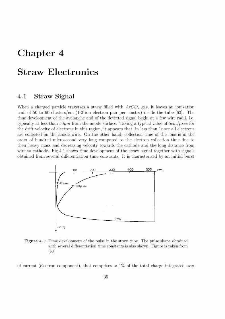
Chapter 4
Straw Electronics
4.1 Straw Signal
When a charged particle traverses a straw filled with ArCO2 gas, it leaves an ionizationtrail of 50 to 60 clusters/cm (1-2 ion electron pair per cluster) inside the tube [63]. Thetime development of the avalanche and of the detected signal begin at a few wire radii, i.e.typically at less than 50µm from the anode surface. Taking a typical value of 5cm/µsec forthe drift velocity of electrons in this region, it appears that, in less than 1nsec all electronsare collected on the anode wire. On the other hand, collection time of the ions is in theorder of hundred microsecond very long compared to the electron collection time due totheir heavy mass and decreasing velocity towards the cathode and the long distance fromwire to cathode. Fig.4.1 shows time development of the straw signal together with signalsobtained from several differentiation time constants. It is characterized by an initial burst
Figure 4.1: Time development of the pulse in the straw tube. The pulse shape obtainedwith several differentiation time constants is also shown. Figure is taken from[63]
of current (electron component), that comprises ≈ 1% of the total charge integrated over
35

36 Straw Electronics
the full ion drift time, and a remaining signal (ion tail) controlled by the motion of the ions.Ion movement in the high field close to the wire is still fast enough to contribute to a steepcurrent signal which can be used for timing purposes.
Since the long ion tail would increase the dead time of the detector, elimination of theion tail is one of the most crucial goals of the front-end electronics design. Only the firstvery fast response is used for the timing and the rest of the signal is canceled by employinga passive network that sharply differentiates the straw signal.
Main requirements for the electronics of the straw detector are:
• signal shaping corresponding to the detector properties
• low noise
• precise timing
• low per-channel cost
• low crosstalk
The straw tracker electronics consists of preamplifier, ASD-8 input board, ASD-8 chipcontaining amplifier and discriminator (analog to digital converter), and ECL converter(Fig.4.2).
Figure 4.2: Picture of the ASD-8 chip (upper left), ASD-8 input board (upper right) andECL converter (lower)
4.2 Preamplifier
The ASD-8 chips will be placed outside of the TOF tank in air for cooling reasons and inorder to minimize the amount of material in the detection region. The analog signal fromthe straw tube will be transmitted to the ASD-8 chip via 5m long thin coax cables (0, 9mmdiameter, 75Ω). In order to avoid noise problems due to the signal loss in the long cable

4.2 Preamplifier 37
between straw chamber and ASD-8 chip, the analog signal of some mV is amplified by meansof a very small preamplifier developed in research center Julich. The preamplifiers matchto the 75Ω coax cables. They are directly connected to the straw tubes in vacuum. With< 40mW power dissipation, the preamps have no cooling problem even in vacuum. Fig.4.3shows the wiring diagram of the preamplifier. The capacitor C3 decouples the high voltage
Figure 4.3: Wiring diagram of the preamplifier
and is also responsible for the differentiation of the straw signal in order to cancel the iontail. The resistors R1 and R2 define the amount of fed back and in turn the value of totalamplification. The time constants of the preamplifier are < 10nsec rise time and ≈ 150nsecdecay time.
Fig.4.4 shows the analog signal of a cosmic particle after the preamplifier. In the eventshown two clusters of electrons are resolved in analog and digitization electronics.

38 Straw Electronics
Figure 4.4: Analog signal (from the cosmic particle) after preamplifier and digitized formit behind the ECL converter. Two electron clusters appear in the event shown.
The most important properties of the preamplifier are:
• high band width ([83] Fig.4.5)
• low noise < 10mV (Fig.4.4)
• low mass ≈ 0.37gr
• adjustable amplification with dc supply
The preamplifier boards (width: 0.57cm, height: 0.1cm, length: 3.5cm) are much smallerthan the 1cm diameter straw tubes. They are mounted within the 1.98cm height of thedouble planes inside of the Rohacell frames which thus can be stapled.

4.3 ASD-8 Input Board 39
Figure 4.5: Simulated frequency response of the preamplifier [83]. Input signal -40 dB.
4.3 ASD-8 Input Board
Since the signal amplitude from the preamplifier at the end of the 5m cable is too big forthe ASD-8 chip, it is reduced and shaped using an input board in front of the ASD-8. Thewiring diagram is shown in Fig.4.6. Resistors R7 and R8 provide a reduction of the signal
Coaxial cable
+5 VR9=10 ohm
R6=1.5k ohm
C8=100 nFC7=10 nF
Coaxial cable
GND GND
GND
C7=10 nF
R7=68 ohm
R8=4.7 ohm
to ASD−8C5=4.7 pF
Figure 4.6: Schematic of the ASD-8 input board
amplitude and impedance matching for the driving cable. C5 is used to set the signal levellow enough in the ASD-8 and to block the direct current from the transmission line.
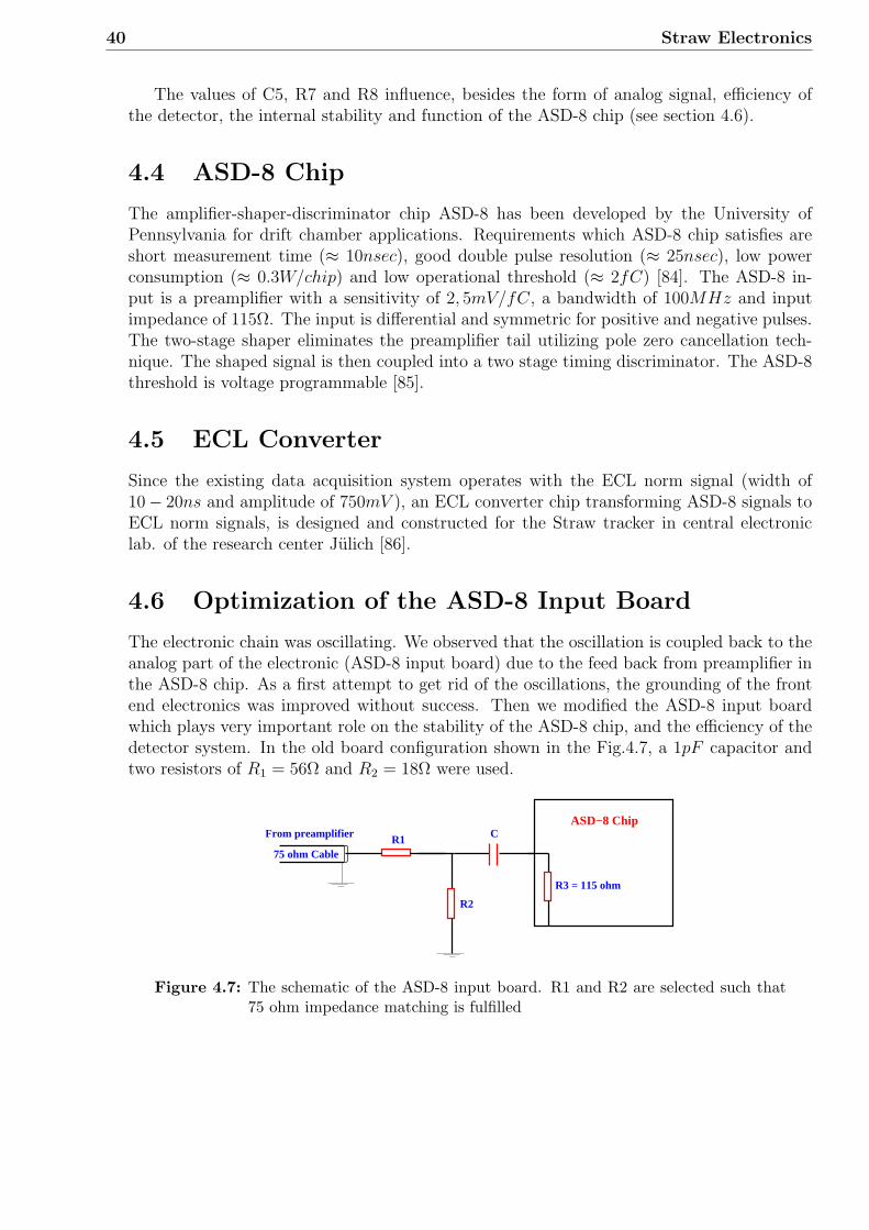
40 Straw Electronics
The values of C5, R7 and R8 influence, besides the form of analog signal, efficiency ofthe detector, the internal stability and function of the ASD-8 chip (see section 4.6).
4.4 ASD-8 Chip
The amplifier-shaper-discriminator chip ASD-8 has been developed by the University ofPennsylvania for drift chamber applications. Requirements which ASD-8 chip satisfies areshort measurement time (≈ 10nsec), good double pulse resolution (≈ 25nsec), low powerconsumption (≈ 0.3W/chip) and low operational threshold (≈ 2fC) [84]. The ASD-8 in-put is a preamplifier with a sensitivity of 2, 5mV/fC, a bandwidth of 100MHz and inputimpedance of 115Ω. The input is differential and symmetric for positive and negative pulses.The two-stage shaper eliminates the preamplifier tail utilizing pole zero cancellation tech-nique. The shaped signal is then coupled into a two stage timing discriminator. The ASD-8threshold is voltage programmable [85].
4.5 ECL Converter
Since the existing data acquisition system operates with the ECL norm signal (width of10− 20ns and amplitude of 750mV ), an ECL converter chip transforming ASD-8 signals toECL norm signals, is designed and constructed for the Straw tracker in central electroniclab. of the research center Julich [86].
4.6 Optimization of the ASD-8 Input Board
The electronic chain was oscillating. We observed that the oscillation is coupled back to theanalog part of the electronic (ASD-8 input board) due to the feed back from preamplifier inthe ASD-8 chip. As a first attempt to get rid of the oscillations, the grounding of the frontend electronics was improved without success. Then we modified the ASD-8 input boardwhich plays very important role on the stability of the ASD-8 chip, and the efficiency of thedetector system. In the old board configuration shown in the Fig.4.7, a 1pF capacitor andtwo resistors of R1 = 56Ω and R2 = 18Ω were used.
From preamplifier
75 ohm Cable
ASD−8 Chip
R3 = 115 ohm
R1 C
R2
Figure 4.7: The schematic of the ASD-8 input board. R1 and R2 are selected such that75 ohm impedance matching is fulfilled

4.6 Optimization of the ASD-8 Input Board 41
Four different board configurations shown in the Table 4.1 were tested. Except for the1pF configuration, with all of these three configurations, we obtained positive results. Thewhole system was oscillation free and stable. In order to select the best solution or to seethe differences among them, the relationship between ASD-8 threshold and minimum signalamplitude exceeding this threshold was measured.
R1(Ω) R2(Ω) C(pF )56 18 1 oscillation68 4.7 4.7 no oscillation, best efficiency68 4.7 6.8 no oscillation, less efficiency75 1.8 10 no oscillation, less efficiency
Table 4.1: Four configurations for the input board.
We used a pulser to simulate the straw signal. The simulated signal is connected directlyto the preamplifier. As the threshold increases, we increased the amplitude of the strawsignal until it exceeds this threshold and using an oscilloscope we recorded both values. Asseen in the Fig.4.8 the best solution is the configuration with the capacitor of 4.7pF . Itenables the detection of the smaller signals and more stable state for the whole system.
threshold setting potential -V0 0.2 0.4 0.6 0.8 1 1.2 1.4 1.6 1.8 2
min
sig
nal
am
plit
ide
- m
V
0
20
40
60
80
100
120
140
threshold setting potential -V0 0.2 0.4 0.6 0.8 1 1.2 1.4 1.6 1.8 2
min
sig
nal
am
plit
ide
- m
V
0
20
40
60
80
100
120
140
4.7pF 68ohm 4.7ohm
6.8pF 68ohm 4.7ohm
10pF 75ohm 1.8ohm
noisy level
ASD-8 threshold vs min signal amplitude
Figure 4.8: The ASD-8 threshold vs minimum signal amplitude
In order to see how these configurations affect the signal transmission, a simulation of theinput board for 1 pF and 4.7 pF configuration is made [14] (observation behind the capacitorC at the ASD-8 input board is not possible). A triangle signal with the amplitude of 150mVand rising time of 2nsec is used as an input in the simulation.
As seen in Fig.4.9, the configuration with 1pf capacitor (right picture) changes the signalform very much due to the strong differentiation, producing a bipolar signal. This leads to

42 Straw Electronics
efficiency problem in ASD-8, since the discriminator needs some certain amount of energyto work. With the bipolar signal the amount of charge in turn the energy delivered to theASD-8 is less. Unlike the 1pF capacitor configuration, the other configurations do not changethe form of the signal much as seen in left picture in Fig.4.9, the polarity of the potentialchanges very close to the end of the original signal. In the 1pF configuration it changesnearly in the middle of the input signal which means that just the typical lower frequenciesin the straw signals are suppressed.
Figure 4.9: Left picture is the simulation of the input board with 4.7pF capacitor. Thesignal shape of the straw output remains nearly unchanged. Right is thesimulation of the input board with 1pF capacitor. Triangle signal is given tothe board as an input signal.

Chapter 5
Tests and Measurements with StrawTubes
5.1 Introduction
To control production and performance of the straws, series of measurements and tests havebeen done. Some of them (high rate performance of the straws with beam, aging effect,first three dimensional tracking with cosmic rays etc.) were performed by using the strawprototype detector ”Cosmic Ray Test Facility”. It is the first realistic application of theJulich straws (see chapter 7).
5.2 Wire Tension Measurement
The wires in the straw tubes have to be held under proper mechanical tension. Too lowtension leads to deviation of the wires from the ideal position caused by gravitational andelectrostatic forces. Deviation in the position in turn results in changes in spatial resolutionand reduction in high voltage stability. On the other hand, too strong tension can pull thewires out of the crimp pins or break the wires.
The wires in the tubes are stretched by using a weight of 40g and overpressure of 1.25bar(2.25 bar absolute) inside the straw tubes [87]. After the construction, tensions of the allstraws are measured to check the quality of the production. The wire tension T is derivedfrom the resonance frequency f of the mechanical wire oscillation via the relationship:
T = 4f 2L2ρL
where L being length of the wire and ρL the wire mass per unit length [88]. The oscillationsare excited with low-frequency AC current which is driven through the wire in the presenceof a magnetic field. The resonance frequency can be found by inspection of phase relationbetween the current and voltage driving the wire oscillation. The details of the measurementsare explained in [87]. The histogram in Fig.5.1 shows the result of the measurements for 448straw tubes. The RMS of the wire tensions is ≈ 0.6g showing the high quality of production.
43

44 Tests and Measurements with Straw Tubes
Figure 5.1: measured wire tension/g of 448 straws
5.3 Test of Gas Leakage from the Straws
COSY-TOF is a huge (≈ 30m3) vacuum tank at some 10−3mbar. It is very important forthe functioning (especially for the cryo target) that the vacuum state of the tank stays thesame after the installation of the full straw tracker inside it.
The gas leakage from the straw tubes in vacuum is measured by Dr. Wintz by usingfollowing method: 24 straw tubes filled with 100% at a time CO2 and Ar up to a 1.2bar areplaced in a vacuum container (having the volume of ≈ 11.5l and the pressure of ≈ 10−3).When vacuum pump is switched off, the gas leakage of the straws leads to a pressure rise.By measuring pressure rise in the vacuum container, it was obtained that the leak rate QL of24 straw tubes in the vacuum container is 3.3∗10−3mbar l/sec [89]. Using this information,one can calculate the end pressure of the TOF with 3000 straw tubes by using basic equationof the flow [90]:
V (dP/dt) = QL − SP
where S is pumping speed (Roots pump with S ≈ 70l/s in the TOF tank), QL is gas leakage,V total volume and P pressure of the vacuum tank.At steady state (dP/dt = 0), the end pressure of the vacuum tank due to the gas leakagefrom 3000 straw tubes will be:
Pend =QL
S≈ 6.10−3 mbar

5.4 Plateau Measurements 45
This amount of leakage through diffusion produces no danger for the vacuum state of theTOF.
5.4 Plateau Measurements
We measured the high voltage dependency of the count rate and signal amplitude by usinga Fe55 source radiating photons with a energy of 5.9keV . The Fe55 source is fixed fewmm over the straw tube. With the help of a scalar the rate of the absorbed photons fromFe55 source and with an oscilloscope (Tektronix TDS 754D) the signal amplitudes and theirdependencies on the high voltage are measured.
Fig.5.2 shows the relationship between count rate and high voltage for three different gaspressures. We can divide each curve into three regions. In the first region, the count rateincreases linearly with increasing high voltage. In this part electric field may be insufficientto separate the ion pair from each other and the two particles may recombine to reformthe gas atom. In the second region which is called plateau, the count rate is constant. Allprimary ionization processes are converted into registered signals. The gas amplification isrising along the plateau (Fig.5.3). After the plateau, the count rate increases sharply withincreasing high voltage. This is due to the on set of steady gas discharging.
Figure 5.2: The relationship between HV and count rate with a 5.9keV γ source (Fe55)for three different pressures
The straws work in the region of the plateau with a length of 150V . Setting the highvoltage to the end of the plateau gives the highest possible gas gain (signal amplitude vshigh voltage, shown in Fig.5.3) improving the efficiency and resolution, but at the same timethis leads to increase in dead time of the counter, since more electrons and ions are producedin the gas amplification process. The higher space charge needs more time to be collected.

46 Tests and Measurements with Straw Tubes
Low dead time can be achieved when running at small amplification. This however needsgood low noise preamplifiers.
Fig.5.2 shows that, the plateau shifts to higher voltage, and count rate increases withincreasing pressure. The higher pressure means higher resistivity to the charge movement.As a result more electric field is needed for the charge collection.
If a beam of photons of intensity I0 is incident upon a gas with N absorber atoms perunit volume, each of effective cross section σ, then the intensity I that penetrates to theother side goes as I = I0 exp[(−Nσ)x], where x is the thickness [91]. With increasingpressure (N increases), I decreases and as a result count rate (I0 − I) increases.
The relationship between high voltage and signal amplitude is measured for three differentgas pressures. Signals are measured behind the preamplifier. As seen in Fig.5.3 the amountof collected charge and the high voltage are nearly linearly dependent to each other. Abovea certain amplitude, the signal amplitude stays constant at 250mV due to the saturation ofthe preamplifier.
Figure 5.3: HV vs signal amplitude for three different absolute pressures of 1.2, 1.6, 2bar.
5.5 Functionality Test with Beam
During the beam time in February-2003, one of the small hodoscope of the ”cosmic ray testfacility” made from two perpendicular double planes (2× 16 straws per each double plane)was exposed for 5 days to the direct deuteron beam with the momentum of 2.15GeV/c andthe rate of 6 ∗ 106s−1 − 13 ∗ 106s−1.
Straw tubes in the hodoscope were filled with the gas mixture of Ar/CO2(82/18) to apressure of 1.4bar absolute and operated with a high voltage of 1800V .

5.5 Functionality Test with Beam 47
The aim was to test the performance and possible aging effects of the straws with a veryhigh rate beam leaving the TOF vacuum tank through a 100µ Mylar window and passingthen through fiber hodoscopes with 4mm total scintillator thickness. The beam was spreadout by divergence and straggling over a spot of about 5cm diameter on the straw plane. Theexperimental setup is shown in Fig.5.4. The straw planes were placed in air 10m far fromthe target position.
The straw signals were amplified and then transmitted to the electronics area via 25mlong coaxial cables of 75Ω impedance and only 0.9mm diameter.
Figure 5.4: Two crossed straw frames placed behind the TOF for the performance testwith the beam. Directly at the exit of the TOF tank one can see the quadraticframe of the 4mm thick fiber hodoscope which creates straggling.
During the 5 days we have not seen any high voltage break down or dark current. on thecontrary very clean ionization current from the beam.
Fig.5.5 shows two analog- and one digital channels of the straws. In the oscilloscopepicture, one sees 12 digital signals in 4µsec indicating the particle rate on the wire of 3∗106.
Fig.5.6 shows the beam profile measured for one straw plane.

48 Tests and Measurements with Straw Tubes
Figure 5.5: Yellow and blue: straw analog signals from the deuteron beam from COSY,pink: digital output derived from the blue signals. (Green is not used)
Figure 5.6: Beam profile measured with one plane with 15 straw tubes. Channel 12 wasdefect.

5.6 Aging Effects 49
5.6 Aging Effects
The use of drift chambers in a strong radiation environment can lead to the loss of gain,reduction of plateau, excessive currents, self-sustained current discharge and sparking. Allthese problems are generally combined under the term ”aging”.
On the straws of the prototype exposed to the beam (beam time Feb. 2003) we foundaging effects. Scanning with a Fe55 source along an irradiated straw tube a signal amplitudereduction (loss of gain) was found in the strongly illuminated regions. The same measurmenton a straw which was not strongly illimunated gives flat response.
Fig.5.7 shows for two straw tubes maximum signal amplitude (averaged over 200 signals)versus distance. In the upper figure (illuminated straw), we see that, the signal amplitudedecreases at two intervals (25 − 32cm and 42 − 64cm) to nearly 50%. These strong agingeffects appeared after ≈ 1011 deuterons per cm wire length under counting conditions withhigh voltage of 1.8kV . On the other hand, in the lower picture (unilluminated straw), we donot see any change in the signal amplitude. The small amplitude decrease along the countingwire towards the preamplifier position is due to the reflection of the signal (signal close tothe preamplifier is wider but smaller).
Fig.5.8 shows the oscilloscope pictures of the reduced signals at the positions ≈ 50cmand normal signals at ≈ 45cm in the illuminated straw tube.
It has been commonly experienced that the aging effects are the result of a wire surfacedegradation of the anode wire and that this occurs frequently, but not always, in the formof an organic ”deposit” that is a solid, but may also be liquid. During wire avalanches manymolecules break up by collisions with electrons, de-excitation of atoms, and UV-photonabsorption processes.
Especially for chamber gases which contain organic componenets like methane, isobuthanetc., the breaking of the chemical bonds in molecules and formation of free radicals requiresonly 3− 4eV (very low compared with the ionization process requaring greater than 10eV )and could lead to a large abundance of free radicals over the ions in the wire avalanches[92]. Since free radicals are chemically very active they will either recombine back to orginalmolecules or other volatile species, or form new cross-linked molecular structures, which couldreact further to produce chain like polymers of increasing molecular weight, thus loweringthe volatility of the resulting product. When the growing of polymerized chains becomeslarge enough for condensation to occur, it will diffuse to the electrode surface and depositthere.
For ArCO2 mixtures aging effects should be less important. Although CO2 is a stablequencher, the gradual decomposition of CO2 in Ar/CO2 mixtures also takes place and stableoperation was found to be possible up to charges of 0.5 − 0.7C/(cm wire) [92]. With thebeam rate of 1011 per cm wire length, a gas amplification of 3∗105 and 102 primary electronsper beam particle very roughly a charge of ≈ 0.5C/(cm wire) were collected during thebeam time. The collected charge is comparable with the limiting total charge given in theliterature. That explains the reduction of the gas gain in our straws.
It is also reported [92] that the wire chambers lifetime could be affected by the purity ofthe gas mixture, materials used in contact with the gas and superious contaminants.

50 Tests and Measurements with Straw Tubes
Figure 5.7: Signal amplitude from Fe55 source versus distance along the wire for two strawtubes at 2040 V and 1950V . The plot a) corresponds to a straw irradiatedlocally with upto 1011 deuterons per cm counting wire. b) shows a strawwhich was not strongly irradiated. The zero point is the preamplifier side ofthe tube.

5.7 Visual Inspection of the aging Effects 51
Figure 5.8: Averaged signals of the illuminated straw tube from Fig.5.7 at the distancesof ≈ 50cm (small signal from degraded region) and ≈ 45cm (big signal fromgood counting region).
5.7 Visual Inspection of the aging Effects
The irradiated straw (Fig.5.7) was opened. In the irradiated region there are both cleartraces on the aluminum surface and on the counting wire.
Fig.5.9 shows microscope picture of the irradiated region on the counting wire scaled up50 times. The black isolated spots with a length of 20µm - 80µm shows the aging effectclearly.

52 Tests and Measurements with Straw Tubes
Figure 5.9: Microscope picture of the irradiated region on the 20µ ∅ gold plated tungstencounting wire. Horizontal and vertical lengths of the picture are 0.77mm and1.12mm respectively.

5.7 Visual Inspection of the aging Effects 53
Fig.5.10 shows the wire region which was not irradiated. No black spots are seen.
Figure 5.10: Microscope picture of the same wire as in Fig.5.9 in an unirradiated region.Horizontal and vertical lengths of the picture are 0.77mm and 1.12mm re-spectively.

54 Tests and Measurements with Straw Tubes
Fig.5.11 shows the irradiated region of the aluminized Mylar cathode. Clear traces ofaging effects are seen on the aluminum surface in the form of cloudy strips with a width of50µm - 300µm and orthogonal to the counting wire direction.
Figure 5.11: Irradiated region of the aluminized Mylar (magnification lower by a factor8 with respect to Fig.5.9 and Fig.5.10). Clear traces of aging effect are seenon the aluminum surface as cloudy strips precisely orthogonal to the wiredirection. The underlying pattern of inclined fine strips is a property ofthe aluminum mirror on the (undisturbed) Mylar surface. Horizontal andvertical lengths of the picture are 6.17mm and 8.95mm respectively.

5.7 Visual Inspection of the aging Effects 55
Fig.5.12 is the same picture as in Fig.5.11 but scaled up 8 times.
Figure 5.12: Same irradiated region on the cathode as in Fig.5.11 scaled up 8 times (samemagnification as in Fig.5.9 and Fig.5.10). The black regions are undisturbed,shiny aluminum mirror surface. The cloudy white strips are 50µm to 300µmwide and up to cm long. There the mirror surface is damaged. Horizontaland vertical lengths of the picture are 0.77mm and 1.12mm respectively.

56 Tests and Measurements with Straw Tubes
Fig.5.13 shows the region of the aluminized Mylar which was not irradiated. We see nocloudy strips as in Fig.5.11
Figure 5.13: Region of the aluminized Mylar which was not irradiated. No cloudy stripsare seen. The upward going line is the counting wire. This pattern can bedirectly compared to Fig.5.11 which has the same scale and orientation withrespect to the counting wire. Horizontal and vertical lengths of the pictureare 6.17mm and 8.95mm respectively.
From the visual inspection of the anode wire Fig.5.9, we see that radius of the wire has
5.7 Visual Inspection of the aging Effects 57
not increased so much to explain the reduction of the signal amplitude. The reason for thatand for the strips on the Mylar is the whiskers which is very thin (≈ 10nm) hairlike carbondeposits on the wire. Due to the very high electric field around the whiskers the counting gasis ionized continously and space charge is produced around the wire. This is the producedspace charge capturing the primary ions by recombination and leading to signal amplitudereduction. The strips on the Mylar is due to the oxidation of the aluminum by the oxygenatoms released from the decomposition of CO2.

58 Tests and Measurements with Straw Tubes
5.8 Spatial Resolution and Efficiency of the Straw Tube
Intrinsic resolution of the straw tube is influenced by two factors: diffusion of the electroncloud drifting to the anode wire and the statistical spread of the primary ionization clustersalong the track. While clustering is dominating close to the anode wire, diffusion dominatesat the region far from the anode wire.
The spatial resolution and efficiency of the single straw tubes are studied inside a ver-tical double-layer frame by means of cosmic ray tracks by Dr. Wintz [93]. The tracks arereconstructed after R(t)-Calibration (see 7.3.2) in two dimension by applying a linear fit ofthe track parameters (direction and foot points of the track) minimizing the normalized χ2
(see 7.3.3).Fig.5.14 shows the χ2-distribution of the 1054 reconstructed tracks and isochrone resid-
uals ∆ri of the 5645 straw hits. Symmetric residuals’ distribution around a small mean of4µm is indication of no systematic error. The deviation (σ) from the mean is about 85µm
0
25
50
75
100
0 5 10 15
Chi2 Distribution
Entries 1054
Ent
ries
Residual Distribution (mm)
Entries 5645Constant 250.3
Mean 0.4416E-02Sigma 0.8322E-01
Ent
ries
(per
0.0
1 m
m)
0
100
200
300
-0.5 0 0.5 1
Figure 5.14: χ2-distribution and isochrone residuals ∆ri of all reconstructed tracks. Meanand deviation (σ) of the residuals Gauss-fit are 4µm and 83µm respectively.Figure is taken from [93]
Fig.5.15 shows the radial dependence of the resolution obtained from reconstructed tracks.The resolution gets worse closer to the anode wire as expected due to the effect of theclustering. A good agreement between measured and simulated (for the simulation of thestraws Garfield program package is used [94]) resolution is also seen.
In order to investigate the efficiency of the straw tube along the radius, 14 neighboringstraws are used and minimum 5 straw hits are required for the track reconstruction. Afterreconstruction of the track, all isochrones are checked in this 14 straws. If no isochrone within

5.8 Spatial Resolution and Efficiency of the Straw Tube 59
Track - Wire Distance (mm)
Spa
tial R
esol
utio
n (m
m)
data
Simulation
0.02
0.04
0.06
0.08
0.1
0.12
0.14
0.16
0.18
0 1 2 3 4 5
Figure 5.15: Spatial resolution of the straw tube.
a distance of 5σ to the track is found, this straw at this distance is counted as inefficient. Amean efficiency of 98.6% is found over the full straw radius of 5mm (Fig.5.16). Decrease inefficiency at a distance above 4.7mm is due to the decreasing track length in the countinggas consequently decreasing ionization. In this region the the number of ionization chargesis too low to produce a signal exceeding the discriminator threshold.
Track - Wire Distance (mm)
Effi
cien
cy (
per
0.1
mm
)
Mean Efficiency: 0.986
0.7
0.75
0.8
0.85
0.9
0.95
1
1.05
0 0.5 1 1.5 2 2.5 3 3.5 4 4.5 5
Figure 5.16: Efficiency vs tube radius

60 Tests and Measurements with Straw Tubes

Chapter 6
Expected Improvements by the StrawTracker
In order to illustrate the improvement with the straw tracker the experimental TOF data ofthe reaction pp → dπ+ from the beam time Jan/2000 (using the existing fiber hodoscopes)and simulation data of the reaction pp → dπ+ with the straw tracker are compared.
6.1 Selection of pp → π+d Events
from the Beam Time Jan/2000
The data from the Jan/2000 beam time were analyzed by Dr. Wissermann. Results arepresented in [95]. In order to obtain plots where experiment and straw tracker simulationdata could be compared, some runs of Jan/2000 were analyzed in the frame of this thesis.Analysis routines of Dr. Wissermann were used. The calibration of the experimental dataand data analysis software TofRoot is described in the appendix A and B
In two body reactions, the momenta of the outcoming particles can be calculated eitherfrom the time-of-flight or geometrically from the polar angles of the particles alone (in twoparticle reactions ejectiles and beam are co-planar).
The relative momentum resolution ∆p/p is given in terms of the time resolution ∆t(ignoring the error in position) as [96]:
∆p
p= γ2 · ∆t
t
Unfortunately, at β approaching one, it is not possible to calculate the particle momenta withreasonable resolution. However if one partner in the exit channel has high velocity (forwardin center of mass (cm) frame) then the other (backward in cm) comes with particularly smallvelocity. Under such circumstances at least one momentum may be well measured.
A vector addition of the two outgoing directions to the beam momentum vector (con-servation of momentum) allows to determine the absolute momenta for the two outgoingtracks (Fig.6.1) geometrically. In Fig.6.1 the hits in the detector plane are used togetherwith the start point the target to determine the polar angles θ1, θ2 of two planar outgoing
61

62 Expected Improvements by the Straw Tracker
particles. The longitudinal and transversal component of the particles are given in terms ofthe scattering angles by:
|~pT | = |~pB| · tan(θ1) · tan(θ2)
tan(θ1) + tan(θ2)(6.1)
|~pl1| = |~pB| · tan(θ2)
tan(θ1) + tan(θ2)(6.2)
|~pl2| = |~pB| · tan(θ1)
tan(θ1) + tan(θ2)(6.3)
Target
Track 2
Track 1
Quirl
Pt
Pl2Beam
Pl1,2 longitudinal momenta for particle 1, 2
Pl1
Pt
Pt1,2 transversal momenta for particle 1, 2
Beam momentumtheta 1
theta 2
Figure 6.1: Geometrical impulse reconstruction from the vectorial sum of two outgoingdirections to the beam momentum vector.
After obtaining the momenta of the outgoing particles by assuming two particles reaction,a χ2 test is applied in order to distinguish (select) the events pp → dπ+ from:
1. pp → pp
2. pp → ppγ
3. pp → ppπ0
4. pp → pnπ+

6.1 Selection of pp → π+d Eventsfrom the Beam Time Jan/2000 63
The test includes the angular and time-of-flight information from TOF. The coplanarityimposed by the two particle kinematics is the main geometrical selection criterion: due tothe conservation of momentum, beam direction and the scattered two particles must lie inthe same plane:
(~p1 × ~p2) · ~pbeam = 0
The time-of-flight information is also utilized advantageously: one can calculate the ex-pected time-of-flight from the assigned four momenta and detector geometry. This is thencompared to the actually measured time-of-flight:
∆TOF1,2 = (TOF1,2)meas − (TOF1,2)calc
Besides this information, the deviation from the expected missing mass Eq.6.4 and thedifference between β values calculated from time-of-flight and dE/dx measurements in theMicrostrip detector are also utilized in the χ2 test. The result of the χ2-test is shown inFig.6.2, the first peak separates the pp → dπ+ events from the rest.
Figure 6.2: χ2-value distribution for the reaction pp → dπ+. The first peak correspondsto pp → dπ+ events. Figure is taken from [95]

64 Expected Improvements by the Straw Tracker
The world data on total cross sections together with Dr. Wissermann’s results (σtot = 46.6at 2950MeV/c and σtot = 31.5 at 3200MeV/c) and differential cross sections from Dr.Wissermann’s analysis (for beam momenta 2950MeV/c and 3200MeV/c) are shown in theFig.6.3 and Fig.6.4 respectively. These TOF data are in reasonable agreement with theliterature. However the overall precision of the world data around 3GeV/c beam momentumis still surprisingly limited.
Figure 6.3: Collection of the world data on total cross section for the reaction pp → dπ+.The red points are the result of the Dr. Wissermann’s analysis (σtot = 46.6 at2950MeV/c and σtot = 31.5 at 3200MeV/c). Figure is taken from [95].

6.1 Selection of pp → π+d Eventsfrom the Beam Time Jan/2000 65
Figure 6.4: Angular distribution for pp → dπ+. Figure is taken from [95].

66 Expected Improvements by the Straw Tracker
6.2 Simulation of pp → dπ+ events with the Straw Tracker
The simulation of the straw tracker (geometry and response of the straw tracker in COSY-TOF) was added to the existing Monte Carlo simulation program of COSY-TOF in orderto demonstrate improvements with the tracker on the resolution in a simple reaction. Thedata analysis programs for the straw tracker (tracking and event reconstruction) had to beimplemented.
The Juelich Monte Carlo simulation program is based on the GEANT-3 package [97]developed at CERN. GEANT is a toolkit for both full and fast Monte Carlo simulation ofdetectors in High Energy Physics. The principal applications of GEANT in High EnergyPhysics are:
• the transport of particles (tracking) through an experimental setup for the simulationof detector response;
• the graphical representation of the setup and of the particle trajectories.
In view of these applications, the GEANT system allows to:
• describe an experimental setup by a structure of geometrical volumes.
• accept events simulated by Monte Carlo generators.
• transport particles through the various regions of the setup, taking into account geo-metrical volume boundaries and physical effects according to the nature of the particlesthemselves, their interactions with matter, and the magnetic field.
• record particle trajectories and the response of the detector components.
• visualize the detectors and the particle trajectories.
During the tracking through the simulated experimental setup, the distance betweentrack and each detector element is calculated. If the track passes through an element, ateach tracking step the energy loss is calculated and a new momentum is assigned to thetrack. If this element is defined as a sensitive detector, the total energy loss in it is savedas an ADC value. At the end of tracking, one can get out from the energy loss whether anelement is hit or not. GEANT delivers also the entrance and exit coordinates in a detectorelement which we used to simulate drift times in straw tubes. Using the entrance and exitpoints defining the track, one can calculate the minimum distance between anode wire andtrack from Eq.7.5. Using the resolution curve of the straw tube shown in Fig.5.15, one canvary the obtained distance to simulate the diffusion and clustering in the tube. As a laststep, TDC values as a response of the straw tubes are calculated by using R(t) calibrationfunction obtained from the measured TDC spectra of the straw tubes (see section 7.3.2).More information about the Juelich Monte Carlo simulation program can be found in [52].

6.3 COSY-TOF with and without Straw Tracker 67
6.3 COSY-TOF with and without Straw Tracker
From the pp → dπ+ events selected out of the experimental data, the angular and missingmass resolution of TOF were determined. Using the GEANT3 software package the Strawtracker is simulated with the same experimental conditions as in the beam time of Jan/2000in TOF as explained in section 6.2.
Fig.6.5 and Fig.6.6 show the longitudinal versus transversal momentum components ofthe d and π+ calculated from Eq.6.1 - Eq.6.3 using polar angles θ1 and θ2 of the particletracks from the real data of the beam time Jan/2000 (both geometry and time of flight in-formations were used at event reconstruction) without the straw tracker and simulation datawith the straw tracker (only geometry information was used) respectively. The significantimprovement in the momentum resolution is seen clearly from the both figures. It is due tothe improvement of the tracking resolution.
Figure 6.5: The longitudinal and transversal momentum components as obtained from theexperimental data, using the actual TOF setup without straw tracker. Ge-ometry and time of flight informations were used at the event reconstruction.
Figure 6.6: The longitudinal and transversal momentum components from the simulationdata, with the straw tracker replacing the fiber hodoscopes. Only geometryinformation was used. Both resolution and acceptance are improved
68 Expected Improvements by the Straw Tracker
The missing mass analysis in particle physics is a crucial tool for the identification ofparticles or events. Improvement in the missing mass resolution leads, besides the expres-siveness, to reduction of the background reactions in the results. Due to the misinterpretationof the experimental data (since there is no perfect measurement), background reactions arealways included in the results with a certain amount. The better the missing mass resolu-tion is, the less background reactions are included in the results. This can be understood byinspection of Fig.6.7 and Fig.6.8. If we assume an uniformly distributed background (≈ 3events per bin, estimated from the Fig.6.7) over the missing mass histogram, the amountof the background in the missing mass distribution of the experimental data is much higherthan in the simulated distribution in Fig.6.8. The wider the missing mass peak, like in theexperimental data, the more background events are included.
From the conservation of the total invariant mass (Eq.6.4), one can calculate the squareof the missing mass for the reaction pp → dπ+ in which four momenta of beam and target(P b
proton and P tproton) are known.
(P bproton + P t
proton − Pd − Pπ+)2 = P 2X = m2
X (6.4)
where PX is the four momentum of the unknown particle and must be a zero four vector ifthe reaction is pp → dπ+. The square of missing mass spectra from real and Monte-Carlodata are shown in Fig.6.7 and Fig.6.8. We see that the resolution of the missing mass is alsoimproved by a factor ≈ 10 with the improvement in the geometrical resolution.

6.3 COSY-TOF with and without Straw Tracker 69
Figure 6.7: Missing mass spectra for the reaction pp → dπ+ from experimental data ofJan/2000 (without straw tracker).
Figure 6.8: Missing mass spectra for the reaction pp → dπ+ from simulation data withStraw tracker.

70 Expected Improvements by the Straw Tracker

Chapter 7
Cosmic Ray Test Facility
Based on the developments for COSY-TOF straw tracker a small cosmic ray test facilitywas built (7.1). It allowed to do realistic tests, optimization and application of the trackercomponents. Measurements on scintillators and single straw tube were carried out withcosmic rays.
Primary cosmic rays are high energy charged particles, originating from outer space,which strike the Earth from all directions. Most cosmic rays are nuclei, ranging from thelightest to the heaviest elements in the periodic table. The high energy cosmic rays undergocollisions with atoms of the upper atmosphere, and produce a cascade of ”secondary” par-ticles that shower down through the atmosphere to the Earth’s surface. Secondary cosmicrays include pions which mostly decay before they reach the surface and produce muons,neutrinos, and gamma rays, as well as electrons and positrons produced by muon decay andgamma ray interactions with atmospheric atoms. Most secondary cosmic rays reaching theEarth’s surface are muons (≈ 80%), with a mean energy of 4 GeV and an average intensityof about 200/(m2 sec) [98].
The cosmic ray test facility 7.1 consists of 4 double planes of 128 straw tubes in total(16 straw tubes per plane), read out electronics, two scintillators for the trigger signal andthe data acquisition system (DAQ). The planes are arranged two orthogonal hodoscopessandwiched between the two trigger scintillators. It is possible to reconstruct tracks of thecosmic ray particles in three dimensions. Fig.7.2 shows the schematic side view of the cosmicray test facility with distances.
The read out electronics (see 4) consists of preamplifiers directly connected to the strawanode wires, ASD-8, and an ECL converter. The signals from the preamplifiers are transmit-ted to the ASD-8 digitizing unit via 5 m long cables having the impedance of 75Ω. After thedigitalization and conversion into the ECL norm, the signals are delayed for ≈ 200 nsec viaelectronic delay. Finally they are transmitted to the TDC module via twisted pair cables.
The delay became necessary since only old TDC modules were avaliable which workedwith common start. First twisted pair cable delays were tried which however deterioratedthe quality of the digital signal so much, that the TDC response even lost efficiency downto 85%. The electronic delays give full efficiency but still reduced time resolution.
71

72 Cosmic Ray Test Facility
Figure 7.1: The cosmic ray test facility. Two orthogonal hodoscopes made from 90o
crossed straw tube double planes are sandwiched between the two plastic scin-tillators which provide a trigger coincidence.
4cm
Trigger scintillator
Trigger scintillator
4cm
Cosmic rays
Straw double planes
1.87cm
18.515cm
Figure 7.2: Schematic side view of the cosmic ray test facility with distances as it wasused for the tests.
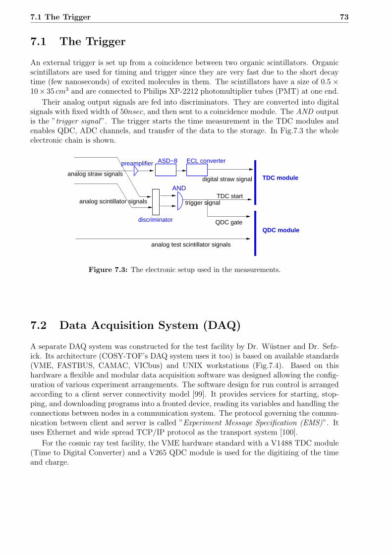
7.1 The Trigger 73
7.1 The Trigger
An external trigger is set up from a coincidence between two organic scintillators. Organicscintillators are used for timing and trigger since they are very fast due to the short decaytime (few nanoseconds) of excited molecules in them. The scintillators have a size of 0.5 ×10× 35 cm3 and are connected to Philips XP-2212 photomultiplier tubes (PMT) at one end.
Their analog output signals are fed into discriminators. They are converted into digitalsignals with fixed width of 50nsec, and then sent to a coincidence module. The AND outputis the ”trigger signal”. The trigger starts the time measurement in the TDC modules andenables QDC, ADC channels, and transfer of the data to the storage. In Fig.7.3 the wholeelectronic chain is shown.
TDC module
QDC module
analog scintillator signals
analog test scintillator signals
TDC start
QDC gate
ECL converter
AND
preamplifier ASD−8
discriminator
analog straw signalsdigital straw signal
trigger signal
Figure 7.3: The electronic setup used in the measurements.
7.2 Data Acquisition System (DAQ)
A separate DAQ system was constructed for the test facility by Dr. Wustner and Dr. Sefz-ick. Its architecture (COSY-TOF’s DAQ system uses it too) is based on available standards(VME, FASTBUS, CAMAC, VICbus) and UNIX workstations (Fig.7.4). Based on thishardware a flexible and modular data acquisition software was designed allowing the config-uration of various experiment arrangements. The software design for run control is arrangedaccording to a client server connectivity model [99]. It provides services for starting, stop-ping, and downloading programs into a fronted device, reading its variables and handling theconnections between nodes in a communication system. The protocol governing the commu-nication between client and server is called ”Experiment Message Specification (EMS)”. Ituses Ethernet and wide spread TCP/IP protocol as the transport system [100].
For the cosmic ray test facility, the VME hardware standard with a V1488 TDC module(Time to Digital Converter) and a V265 QDC module is used for the digitizing of the timeand charge.
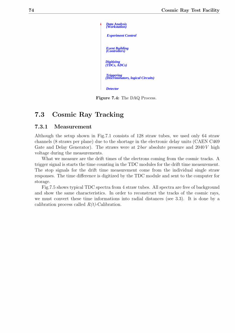
74 Cosmic Ray Test Facility
Digitizing
Detector
Triggering(Discriminators, logical Circuits)
Data Analysis(Workstation)
(TDCs, ADCs)
(Controllers)Event Building
Experiment Control
Figure 7.4: The DAQ Process.
7.3 Cosmic Ray Tracking
7.3.1 Measurement
Although the setup shown in Fig.7.1 consists of 128 straw tubes, we used only 64 strawchannels (8 straws per plane) due to the shortage in the electronic delay units (CAEN C469Gate and Delay Generator). The straws were at 2 bar absolute pressure and 2040 V highvoltage during the measurements.
What we measure are the drift times of the electrons coming from the cosmic tracks. Atrigger signal is starts the time counting in the TDC modules for the drift time measurement.The stop signals for the drift time measurement come from the individual single strawresponses. The time difference is digitized by the TDC module and sent to the computer forstorage.
Fig.7.5 shows typical TDC spectra from 4 straw tubes. All spectra are free of backgroundand show the same characteristics. In order to reconstruct the tracks of the cosmic rays,we must convert these time informations into radial distances (see 3.3). It is done by acalibration process called R(t)-Calibration.

7.3 Cosmic Ray Tracking 75
Figure 7.5: Measured drift times from 4 different straw tubes. x-axis is drift time (nsec)and y-axis is the counts.

76 Cosmic Ray Test Facility
7.3.2 R(t)-Calibration
The R(t)-calibration can be obtained from the shape of a measured drift time distribution.If we assume that the track density over the drift tube is independent of the distance to thewire, the probability P (r) that a hit corresponds to a track between distance r and distancer + dr from wire is given by
P (r)dr = c1η(r)dr (7.1)
where η is the hit efficiency of the tube and c1 is a normalization constant. If the drift time tis a one to one function of the distance r, the drift time distribution is related to the distancedistribution (7.1) by
P (r)dr = P (t)dt (7.2)
For times in the interval [ta, tb], R(t) relation can be obtained by integration of the tdcspectrum and the efficiency profile,
∫ r
ra
P (r′)dr′ =∫ t
taP (t′)dt′ (7.3)
If we assume that the efficiency is constant over the whole interval [ta, tb], Eq.7.3 reduces to
R(t) = rwire +
∫ t0 P (t′)dt′∫ tmax
0 P (t′)dt′(rstraw − rwire)
Figure 7.6: R(t) curves for the 4 straws from Fig.7.5 with 2 bar absolute pressure and2040V high voltage.

7.3 Cosmic Ray Tracking 77
7.3.3 Tracking
In order to reconstruct the tracks of the cosmic particles in 3 dimensions unambiguously, 8straw tubes (one and only one response from each plane) are required.
Each straw response corresponds in three dimensions to a cylinder with a radius ri cal-culated from the drift time by using the R(t) curve. The cosmic tracks are reconstructed by
applying a linear fit of the track parameters Pj=1...6 (denoting direction gi and foot points ~Pi
of the track), minimizing the χ2:
χ2 =1
N
N∑
i=1
(∆ri(P )
σri
)2 (7.4)
where ∆ri = (DCAi − ri) is the shortest distance between track and cylinder ri in straw icalculated by using ”Distance of Closest Approach (DCA)” (Eq.7.5). σr denotes the spatialresolution at ri and N the straw number on the track.
DCA =(g × gi)
|g × gi| · (~P − ~Pi) (7.5)
where g, gi direction vectors and ~P , ~Pi foot points of the wire and track.We used the minimization package ”TMinuit” of the ROOT framework [101] to find the
track parameters giving the lowest value of the χ2 in Eq.7.4. In Fig.7.7, the χ2-histogramfor 4815 reconstructed tracks is shown. Since we used a resolution (σr) of 0.250 mm which islarger than in reality in Eq.7.4, the peak in χ2 histogram, expected at 1, is shifted to about0.4. The resolution is therefore in the region of 0.16mm
Figure 7.7: χ2 histogram for 8 responses tracks
Fig.7.8 shows an example of a fitted track together with straw tubes (black circles) andcylinders (red circles) in two dimension.

78 Cosmic Ray Test Facility
Figure 7.8: Fitted plane in which track (blue line) lies together with straw tubes (blackcircles) and the cylinders (red circles) in 2 dimension (YZ-plane projectionalong x axis). Straw numbers (str 1,2,3,4) increase from bottom to top.

7.4 Efficiency of the Test Facility 79
7.4 Efficiency of the Test Facility
A cosmic track hitting 8 straws should provoke responses from 8 straws in ideal case. Fig.7.9shows the distribution of the number of responding straws in the cosmic ray test facility. Inthis histogram the events with more than one response per plane are not included (at mostone hit per plane is allowed).
Figure 7.9: Distribution of firing straws out of 8 straw responses (one per plane at most)in the test facility. The corrected ratio (8 responses/7 responses) undergeometry consideration amounts to ≈ 95.
In order to estimate the single straw tube efficiency in the test facility we used the relativeefficiency of event types ”7 responses out of 8 straws” and ”8 responses out of 8 straws”.From Fig.7.9 we have 8 responses/7 responses ≈ 0.83. In the case of 7 responses out of 8hits we have 3 fully functioning double planes. In one of the double planes only one strawresponds. There is 1cm width with only one straw in the double plane (±5mm offset) of8.5cm total width. So 1cm/8.5cm ≈ 12% of the 7 responses (one missing) is due to geometrynot due to inefficiency.
So we have to reduce the ”7 responses” number in Fig.7.9 by this percentage and get8 responses/7 responses ≈ 0.95.
If there would be no systematic errors and all straws behave in the same way thenstatistical considerations would lead to response distributions with ratios which are definedby the single straw efficiency ε alone. Only 7 and 8 response events are comparable due tothe same well defined geometrical acceptance.

80 Cosmic Ray Test Facility
In order to find out the straw efficiency we have calculated the dependency betweenprobability of getting a certain number of responses per event and the efficiency of strawtubes (see appendix C for the calculation). Fig.7.10 shows probabilities of getting 7 and 8response events versus the single straw efficiency. The point at which the relative probability
Figure 7.10: Dependence of firing number of straws out of 8 planes as function of a com-mon single straw efficiency ε.
P8/P7 is equal to 0.95,
P8(8)/P8(7) =ε
8(1− ε)= 0.95 (7.6)
results in an efficiency ε ≈ 88%. The observed inefficiency of ≈ 10% is mostly due to theaging effects of some of the straws exposed to the beam (see 5.5).
Of course we see that the numbers for less than 7 responses per 8 planes are by far higherthan expected by a purely statistical interpretation. This can be understood by inspectionof Fig.7.11 and is related to a much bigger acceptance for 6 (or less) response events.
Fig.7.11 shows the multiplicity distribution of the four double planes (in logarithmicscale). The clear peak at two responses per double plane shows proper functioning. Thezero response in the situation where straws (3. and 4. plane) and trigger scintillators areparallel are as expected lower than in the situation where straws (1. and 2. plane) and triggerscintillators are orthogonal to each other. If the straws are orthogonal to the trigger paddlesthe only 8cm occupied by straws out of the 30cm long paddles can make only relatively fewstraw responses and as consequence a fraction of about (30−8)/30 2.2 out of 3 triggers haveno straw response. This explains why 4 response events are maximum (7.9); two doubleplanes parallel to the trigger scintillators have the maximum overlap area with scintillators(giving maximum cosmic ray illumination area). By addition of other planes the the overlaparea with trigger scintillators decreases, therefore the number of events having higher strawresponses (> 4 straw responses) too.

7.4 Efficiency of the Test Facility 81
Figure 7.11: Response multiplicity of the 4 double planes. 1. and 2. double planes areorthogonal and 3. 4. planes parallel to the trigger scintillators.

82 Cosmic Ray Test Facility
In Fig.7.11 the cross talk dominating at 1 response (but existing up to 16 responses) isalso seen. The electronic shielding of the system must be improved in order to minimize thecross talk.
7.5 Geometry Reconstruction with the Test Facility
In order to assure that the test setup works properly, we reconstructed the geometries oftwo different test scintillators. One is with a circular shape having a diameter of 5 cmand thickness of 5 mm and the other one is a square shaped scintillator with a size of4× 3.8× 0.2cm3.
The reconstruction of the cosmic particle tracks provides us with the illuminating field.Fig.7.12 shows simulated hit distributions between two trigger scintillators (the radii corre-sponds to the hit density). One sees that the hit density is not flat due to the geometricalacceptance of the scintillators. Especially in a plane in the center one expects highest trackdensity in the middle. Close to the trigger scintillators the expected hit distributions becomeflat.
Figure 7.12: Simulated cosmic hit distribution between the two trigger scintillators. Closeto the scintillators the hit distribution is uniform. Between the scintillatorsthe hit distribution peaks in the center.

7.5 Geometry Reconstruction with the Test Facility 83
Fig.7.13 shows the measured points where the cosmic tracks pass the plane of the circulartest scintillator. The illuminating field distribution is more irregularly modulated than the
Figure 7.13: Illumination distribution of cosmic tracks on the circular test scintillatorplane. 8 and only 8 fired straws from 8 planes are required. The observeddensity fluctuations come from a folding of different straw efficiencies. Aχ2 < 5 (Fig.7.7) cut on track fitting is applied.
geometrical acceptance of the trigger scintillators alone could explain. This is due to thenonuniform efficiencies of the damaged straws (see section 5.5). Whenever one uses such atest facility this illumination density must be provided. It allows to calibrate the efficiencydistribution on the test object.
The test scintillators are connected to QDC and TDC modules for an identification oftheir position dependent responses. Fig.7.14 shows the QDC and TDC spectra of the circulartest scintillator.
The events in which the test scintillator is hit, are selected by setting a cut on scintillator’sTDC and QDC. For the circular scintillator we set 270 ≤ tdc ≤ 290 and qdc ≥ 90.
Fig.7.15 shows the remaining hit points of the cosmic ray illuminating field when thesecoincidence conditions and a χ2 < 5 (Fig.7.7) are required on the circular scintillator. 610hits are in the figure. The few points remaining outside are not background. They are due
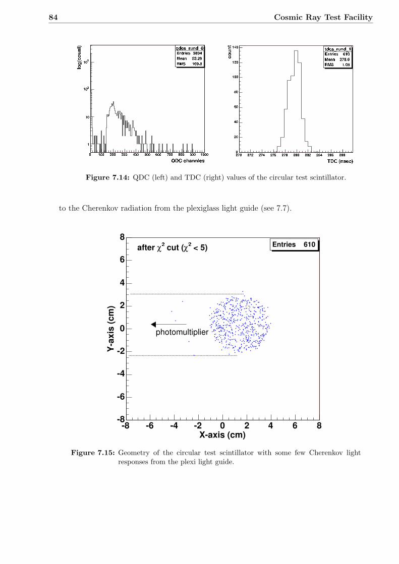
84 Cosmic Ray Test Facility
Figure 7.14: QDC (left) and TDC (right) values of the circular test scintillator.
to the Cherenkov radiation from the plexiglass light guide (see 7.7).
Figure 7.15: Geometry of the circular test scintillator with some few Cherenkov lightresponses from the plexi light guide.

7.5 Geometry Reconstruction with the Test Facility 85
Fig.7.16 shows all hit points of the cosmics on the test scintillator planes (same asFig.7.13) and the points with the test scintillator used as a veto (right). There we find
Figure 7.16: Left: hit points of the all cosmic tracks (same as in Fig.7.13) on the testscintillator’s plane. Right: hit distribution with the test scintillator responseas veto.
about 20 events remaining in the scintillator position if we exclude hits with scintillatorresponse. The 3% of irregular events might be either due to wrong track interpretationdue to the cross talk or to discriminator inefficiency for the test scintillator. This secondexplanation seems to be unprobable. We had the discriminator level for the TDC belowthe single electron amplitude. The chance to have 3% zero triggers would mean, that theaverage scintillator amplitude would be below ≈ 3.5 dynode electron amplitude. The realsignal (Fig.7.14) is definitely higher.
Fig.7.17 shows the illuminating field distribution on the square scintillator’s plane. Thereis difference compared to Fig.7.13 that can be simply explained by the different position ofthe two planes.
The TDC and QDC cut for the square scintillator (Fig.7.18 shows the TDC and QDCspectra) are 190 ≤ tdc ≤ 220 and qdc ≥ 450 respectively.
Applying these QDC, TDC conditions and χ2 cut we get the hit distribution in Fig.7.19.It shows the geometry of the square test scintillator with very few hits outside. The mirrorlight guide used here does not give Cherenkov light.

86 Cosmic Ray Test Facility
Figure 7.17: Illumination distribution of cosmic tracks on the square test scintillator.
Figure 7.18: QDC (left) and TDC (right) values of the square test scintillator.

7.5 Geometry Reconstruction with the Test Facility 87
Figure 7.19: Geometry of test scintillators, after χ2cut.
Fig.7.20 shows all hit points of the cosmics on the square scintillator planes like illumi-nating field Fig.7.17 and the remaining sample with the test scintillator hits used as a veto(right).
Figure 7.20: Left: hit points of the all cosmic tracks on the square test scintillator’splane (same as in Fig.7.17). Right: hit distribution with the test scintillatorresponse as veto.

88 Cosmic Ray Test Facility
7.6 Position Dependency of the Scintillator Response
The test facility allows to measure the light output from cosmics tracks depending on thehit positions (see section 7.5). This may produce quite strong effects (see appendix B).
Fig.7.21 and Fig.7.23 shows the QDC values along the axis of light guide (a) and alongthe transversal axis (b) for circular and square scintillators respectively. We see from theright figure in Fig.7.21 that the light gain along the y-axis is uniform, but in the left figure itis seen that the light gain increases strongly with increasing x by going away from the lightguide.
Figure 7.21: QDC values for light output of the circular test scintillator along the axis oflight guide a) and along the transversal axis b).
This strong enhancement of the light output is based on focusing of the light, reflectedfrom the open 1800 cylindrical boundary of the scintillator into the light guide which is gluedon the other 1800 of the cylinder surface [14]. This principle is indicated in Fig.7.22.

7.6 Position Dependency of the Scintillator Response 89
Figure 7.22: Quasi focal point in a circular scintillator which gives about parallel reflectedlight from the cylindrical boundary [14]. This focusing disappears when thelight is emitted from points closer to the light guide (left).
The square scintillator with its mirror light guide shows a uniform distribution (Fig.7.23).
Figure 7.23: QDC values of the square test scintillator along the axis of light guide a) andalong the transversal axis b).

90 Cosmic Ray Test Facility
7.7 Measurement of the Cherenkov Radiation
Cherenkov radiation is emitted whenever charged particles pass through matter with a ve-locity v exceeding the velocity of light in the medium [102],
v > vt =c
n(7.7)
where n is the refractive index of the medium, c velocity of the light in vacuum and vt
threshold velocity.
The square scintillator with its 10cm long mirror light guide shines its light into a 4cm∅,10cm long plexiglass light guide in front of the PM tube. Fig.7.24 shows the reconstructedhit distribution (left figure) and QDC values (right) of the response when this the plasticlight guide is moved into the illuminating field of cosmic track (the scintillator in this casefar out of the triggered region).
Fig.7.24 has no sharp boundary. This may be due to the reduced track lengths and lightoutput at the plexi cylinder boundary. The QDC spectrum from Cherenkov light (Fig.7.24right) is dominated by the single dynode electron peak which appears at about 160 onthe amplitude scale while zero amplitude is at about 130 in Fig.7.24. The single electronamplitude is about 30 units.
Figure 7.24: Left geometry of the plastic light guide, right QDC values from the lightguide.
In Fig.7.25 the superposition of the QDC spectra from square scintillator (Fig.7.18) andlight guide is shown. The scintillator response is at about 930, thus the scintillator amplitudeis 930 − 130 = 800. We find that the scintillator creates 800/30 ≈ 27 dynode electrons onthe PM.

7.8 Straw Tube 91
Figure 7.25: Superposition of the QDC spectra from scintillator and light guide.
7.8 Straw Tube
By using the test facility we measured also the response of a straw tube with the sameprocedures described in section 7.5.
Fig.7.26 shows cosmic hit distribution (illuminating field) on the test wire plane (left)and the same distribution without straw responses (right).
Figure 7.26: Left: hit distribution of the cosmic ray on the wire plane. Right: samedistribution with test straw as veto.

92 Cosmic Ray Test Facility
Fig.7.27 shows the hit positions in coincidence with the straw. The pattern is clean.
Figure 7.27: Reconstructed geometry of the straw tube.
Before we can determine the resolution of the test straw, we need to know the precisewire position (in space). There is a very simple method to find the position: for each hitpoint in coincidence with the test straw, we calculate the track distance to the anode wire.If we make circles with this distances as radius around the hit points, then we expect to seethe wire as tangent to all these circles (if the reference plane is correct by known). Fig.7.28shows an example with 8 hits and fitted tangent to the circles. In Fig.7.29 all circles togetherwith the fitted wire are shown.

7.8 Straw Tube 93
Figure 7.28: A few radial distance circles calculated from the R(t) calibration curve aredrawn around the track positions. The wire position appears as tangent tothe distance circles.

94 Cosmic Ray Test Facility
Figure 7.29: The full set of distance circles together with the resulting tangent whichapproximates the wire position.

7.8 Straw Tube 95
After the determination of the wire position one can calculate the distance betweenthis approximated ”best” wire position and the hit position determined by the cosmic raytracker, giving an expected radius. Fig.7.30 shows the expected radius determined from wireposition and hit points on horizontal axis and radius determined from straw timing and R(t)calibration on vertical axis.
Figure 7.30: The expected radius determined from wire position and hit points on hori-zontal axis and radius determined from straw timing and R(t) calibration onvertical axis.
Fig.7.31 shows the difference between the radii determined from R(t) calibration andfrom wire position and the hit position, giving the a folding of the tracker resolution andresolution of the test straw. The folded resolution of σ = 228µm is obtained. For the singlestraw we now expect σstraw ≈ 228µm/
√3 ≈ 132µm. It is comparable to the estimate in
section 7.3.3 but higher than 85µm measurement described in section 5.8. The differencemay be due to the systematic errors in the test facility. The straws in the test facility mayhave lost part of their positioning precision in the 3 years of test operation. One can seethat they are not exactly coplanar any more. The time resolution in the TDC channels doesnot seem to have significant impact on the overall space resolution. The time resolution ofthe electronic system (including electronic delays) was determined by using a pulser. Digitalsignal from pulser was duplicated: one for the trigger signal and the other delayed signal forthe TDC module (a constant time interval is expected at TDC spectrum). Fig.7.32 showsthe TDC spectrum at two different delay times. At both time positions we have a FWHMof ≈ 8nsec. With an average drift velocity of 5cm/µsec for the electrons in the gas we geta contribution of ∆r ≈ 20µm to the space resolution (only due to the time resolution of thesystem).

96 Cosmic Ray Test Facility
Figure 7.31: rR(t) calib - rhit points.
Figure 7.32: TDC resolution histogram. Obtained with pulser signals at two differenttime.

Summary
A new tracking detector ”Straw Tracker” is under construction for COSY-TOF. Its purpose isto improve the tracking resolution and efficiency and to reduce inactive material, stragglingand secondary reactions. Very important improvements in event reconstruction expectedwith the new tracker as shown by a Monte Carlo simulation.
A cosmic ray test facility from 128 straw tubes in 4 double planes was constructed inorder to investigate practical applications and straw tracker properties in advance. Achievedwere results on high rate capacity and aging effects. Aging with ArCO2 counting gas wasfound with 1011 particles per cm counting wire. Clearly visible effects on wire and cathodeappear.
The electronics of the test facility is optimized; the oscillation problem of the ASD-8 chipwas solved. A stable state of the electronics was obtained. A stand alone data acquisitionsystem (DAQ) was built. At present 64 channels are fully equipped which gives two workinghodoscopes of 8×8cm2. 8 QDC channels for inspection of test detector response are available.
After completing the test facility, cosmic ray tracks were reconstructed in three dimensionand test objects (2 test scintillators and a test straw tube) were investigated. The test facilityworks properly and is a very useful tool.
Some improvements should be made: some straw tubes which were degraded by testswith very high irradiation density should be exchanged. The number of active straw channelsshould be brought from 64 to 128 by adding the still missing 64 delay channels. This increasesthe useful tracker area by a factor four. Finally the mechanical precision of the straws shouldbe recovered.
97

98 Summary
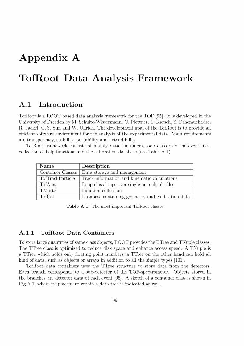
Appendix A
TofRoot Data Analysis Framework
A.1 Introduction
TofRoot is a ROOT based data analysis framework for the TOF [95]. It is developed in theUniversity of Dresden by M. Schulte-Wissermann, C. Plettner, L. Karsch, S. Dshemuchadse,R. Jaekel, G.Y. Sun and W. Ullrich. The development goal of the TofRoot is to provide anefficient software environment for the analysis of the experimental data. Main requirementsare transparency, stability, portability and extendibility .
TofRoot framework consists of mainly data containers, loop class over the event files,collection of help functions and the calibration database (see Table A.1).
Name DescriptionContainer Classes Data storage and managementTofTrackParticle Track information and kinematic calculationsTofAna Loop class-loops over single or multiple filesTMatte Function collectionTofCal Database containing geometry and calibration data
Table A.1: The most important TofRoot classes
A.1.1 TofRoot Data Containers
To store large quantities of same class objects, ROOT provides the TTree and TNuple classes.The TTree class is optimized to reduce disk space and enhance access speed. A TNuple isa TTree which holds only floating point numbers; a TTree on the other hand can hold allkind of data, such as objects or arrays in addition to all the simple types [101].
TofRoot data containers uses the TTree structure to store data from the detectors.Each branch corresponds to a sub-detector of the TOF-spectrometer. Objects stored inthe branches are detector data of each event [95]. A sketch of a container class is shown inFig.A.1, where its placement within a data tree is indicated as well.
99

100 TofRoot Data Analysis Framework
Figure A.1: Each container class represent a sub-detector of COSY-TOF. Information ofeach triggered channel is stored as a hit-class
A.1.2 TofAna - The Loop Class
The Loop class which is called TofAna makes the life easier for the data analyzer at commu-nication with the experimental data stored in trees. To analyze data, the following routineworks has to be carried out; opening the file, obtaining the tree/branch, creation of the datacontainer instances, and the connection of these instances to the branches of the tree. Allthese steps can be annoying and boring for more than one file or run. To aid the user andminimize the time needed for such standard procedures, the loop class TofAna is developed[95]. Some important features of the TofAna are as follows:
• Dataloop, either one or multiple files.
• Creation of data containers, connection to the data tree(s).
• Opening and closing of the calibration file.
• Correct calibration data for each run.
• Reading/writing of all or user selected branches.

A.1 Introduction 101
• Reading/writing of all or user selected events
• Reading/writing of all TofRoot data formats(RAW, LST, CALtemp, CAL).
• Run statistics.
A.1.3 TofCal - The Calibration Database
The calibration database TofCal contains offsets, factors and functions derived from thecalibration of the data. Beside the calibration data, all geometric information of the sub-detector positions and physical constants (e.g. speed of light, mass of the proton) are alsocontained in it.
A main feature of the TofRoot calibration chain and the TofCal calibration databaseis the automatic calibration of each run. This is a substantial difference to other analysispackages where only one calibration data-set is used for the total amount of data. Duringthe calibration/conversion, the involved programs communicate with the database. Theyeventually read necessary data, perform calibration routines, and finally, the data for eachindividual run is stored in a directory like structure within the database (one directory perrun). The TofCal is generated and filled during the calibration chain shown in Fig-A.2.
TRAW
TAPE
TCAL
tape2raw
ApplyList
lst2caltemp
TCALtemp
caltemp2cal
TLST
prog1.C
prog2.C
TofCal.root
prog3.C
prog4.C
prog5.C
prog6.C
prog7.C
private analysis using TofAna and TofTrackParticle
Walk, Pedestal, Binning
TofBarrel−decorrelation−data
TofTorte calibration
Quirl, Ring, COSYnus calibration
QdcCuts for Micro, Hodo, HodoNeu
Erlangen Start position calibration
Barrel tof− and position calibration
Figure A.2: Conversion of detector data from tape using four intermediate data formats(RAW, LST, CALtemp, CAL). The CAL-format is fully calibrated and thebasis of all data analysis.

102 TofRoot Data Analysis Framework
A.1.4 TofTrackParticle - The Track Class
The track class ”TofTrackParticle” contains all physical informations(β, p, v, φ, ...) about track and is designed to allow quick and easy access to these informations[95].
The TofTrackParticle is filled during the conversion from the CALtemp to the CALformat. By applying a linear fit algorithm to the hitted pixels of the start and stop detectors,one can discriminate the ”real tracks” from the background. If a track passes a χ2-test, itsdirection, time of flight, the χ2 value, the triggered QDC conversions and where to find theparticipating pixels in the data tree are stored in the class. All other physical observablesare calculated dynamically by member functions of the TofTrackParticle. The design of theTofTrackParticle classes is totally independent of the track search algorithms. Therefore itwill be no problem to implement a new track-search routine.

Appendix B
Calibration of the Raw Data
B.1 Introduction
During the experiment the raw data are stored in TDAS-Format (binary format) on magnetictapes. This raw data contains the digitized information on the events, the response ofeach detector element recorded by ADCs, TDCs and scalers. Since this format is rathercumbersome and redundant for use in offline analysis, it is therefore converted by meansof the program tdas2ascii to a ascii format convenient for the offline analysis. The offlineevaluation program reads this format and performs necessary tasks to get desired physicalobservables. In order to obtain a physical observable two main steps have to be undertaken:
• The calibration parameters have to be determined.
• The algorithm for this observable has to be implemented.
A calibration parameter can be a cut-off value, an offset, or a factor. Only after the cal-ibration process, the physical analysis can be started. The calibration process consists offollowing steps:
• Pedestal Subtraction
• TDC Module Calibration
• Walk Correction
• TDC Alignment of the Start Torte Quirl and Ring Detectors
• Absolute flight time calibration
• ADC Calibration
B.1.1 Pedestal Subtraction
Due to the charge integration of the base line, QDCs always show a positive nonzero conver-sion even in the absence of a hit. All these QDCs contribute to the data stream as a narrowand non physical peak at small QDC values; the so called pedestal or correct zero point of
103

104 Calibration of the Raw Data
the QDC [95]. In the pedestal subtraction, individual QDC-cut values (pedestals) for eachchannel are determined and subtracted from the measured QDC value.
B.1.2 TDC Module Calibration
The TDC module used in the TOF has channel width of 100 ps in ideal case. In theTDC module calibration, the actual channel width of the module is determined. For this, ameasurement using a time calibrator (ORTEC/EG&G 462) giving signals with ∆t = 10ns(corresponding to 100 TDC module channels) is done after each beam time [52].
B.1.3 Walk Correction
The output pulse from a discriminator appears at or just after the time instant when theinput pulse crosses the threshold. Thus the time of appearance varies, or ’walks’, with respectto the beginning of the pulse when either the pulse height or the threshold level changes [91].In other words, the bigger the photomultiplier signal is, the earlier the discriminator reactsand with it the TDC. In the TOF, this effect leads to a deviation of ∆t = 3ns in the timewhich must be corrected [52].
The walk correction measurements are done with the laser calibration system developedfor TOF. The light pulses from the laser are sent to the each elements of the start and stopdetectors via quartz fiber. The amplitude of the pulses is damped with up to eight filters,in order to cover all QDC spectrum.
The walk correction proceeds in three steps: Firstly, pedestal subtraction must be done.In the second step, the ADC values from the walk measurements and the correspondingTDC values are filled in a histogram. At the final step, from the all entries a walk curve, isfitted:
TDC = (a) +b
ADC + c
where a, b, c are fit parameters.
B.1.4 TDC Alignment Of The Torte Detector
The torte detector consists of two consecutive scintillating rings, each divided into 12 in φ.Due to different cable lengths and different transit time in photomultipliers, TDC valuesfrom these two layers are distinct from each other by a constant offset for a hit. In the torteTDC calibration, these offsets are determined and TDCs from two layers are aligned.
To evaluate these offsets the TDC differences of all overlapping segments are filled intohistograms. This yields 24 time differences between the segments, from which the 24 TDCoffsets can be determined [95]. As a result, the time of flight is calculated using:
tof = TDCstop − ((TDCi + offi) + (TDCj + offj))/2
To improve the time resolution arithmetic mean of TDCs from the two layers are taken.

B.1 Introduction 105
B.1.5 Intern Quirl Ring TDC Calibration
The stop detector quirl and ring consists of 3 layers: a straight-layer and two (left/right)wound layers. The time of flight of the particle is calculated from TDCs of these layers andstart detector. What we measure is not only the flight time of the particle but also lightpropagation time in the scintillator and signal run time in cable and electronic devices. Dueto the difference in the geometry of layers (straight and wound) and different run time ofsignals resulted from distinction in cable lengths, 3 layers give 3 different TDC values fora particle hit. In the intern quirl ring TDC calibration time deviation of layers from eachother are corrected and set to zero.
TDCstraight = TDCleft = TDCright
The measured time of flight can be written as:
tmeas(l = 0..2) = tflight(β, L) + tscint(l, r) + toffset(l, n)
where l is layer number, 0 is for straight, 1 for left wound and 2 is for right wound layer.tflight(β, L): true flight time of particle depending on velocity β and distance Ltscint(l, r): run time of light in the scintillator depending on hit position r in the scintillator.toffset(l, n): run time of signal in the cable and electronic devicesUsing the fact that the signal run time in the two wound layers is same
tscint(1, r) = tscint(2, r)
one can obtain the offsets between left and right wound layers:
∆tmeas(i, j) = tmeas(m = 1, i)− tmeas(m = 2, j)
= toffset(m = 1, i)− toffset(m = 2, j)
where i and j are the element numbers. After the calibration of the two wound layers witheach other, calibration between straight and wound layers is done using:
∆tmeas(k, r) = tmeas(m = 0, k)−(
tmeas(m = 1, i) + tmeas(m = 2, j)
2
)
= toffset(k)−(
toffset(m = 1, i) + toffset(m = 2, j)
2
)+ ∆tradial(r)
where
∆tradial(r) = tscint(m = 0, r)− tscint(m = 1, r)
and k is element number of straight layer i, j are element numbers of left and right woundlayers [96]. Fig.B.1 shows the TDC spectrum of the wound layers of the Quirl detectorbefore (left) and after (right) calibration.

106 Calibration of the Raw Data
Figure B.1: The TDC spectrum of the wound layers of the Quirl detector before (left) andafter (right) calibration. TDC values in units of 100 psec. Figure is takenfrom [55].

B.1 Introduction 107
B.1.6 Absolute flight time calibration
After intern calibration of the detectors, the offset between start- and stop detector is deter-mined. For this, either elastic proton scattering (pp → ppel) or deuteron pion (pp → dπ+)production reactions is used. In two particle reactions, one can calculate the momentums ofthe particles from the scattering angles θ (with a mass hypothesis). From the momentum,the velocity of the particles can be obtained. Using the velocity and flight distance of theparticle, one gets the expected flight time TOFexpected. The difference between measured andexpected flight time which is the offset, is added to the TDC value of the start detector.
B.1.7 dE/dx Calibration of the ADS’s
In addition to the TDC information there are three ADC values per pixel of the Quirl/Ringdetector. The idea of the ADC calibration is the conversion of the digital informationrecorded by the ADCs during the experiment to corresponding energy deposited in thedetector elements, which is calculated with the Bethe Bloch formula
−dE
dx= κz2Z
A
1
β2(1
2ln
2mec2γ2Tmax
I2− β2 − δ
2)
κ = 4πNAr2emec
2 = 0.307075MeV g−1cm2
the relativistic velocity β is determined from the absolutely calibrated time of flight. Theenergy loss, varies with 1/β2 and decreases with increasing β until β ≈ 0.9, where a minimumis reached which defines the minimum ionizing energy. The minimum value of energy ofdE/dx is almost the same for all particles with the same charge.
A pixel consists of one straight segment, two spiral segments wound in opposite direc-tions. An advantage of the used geometry is that each pixel provides the same accuracyin determination of polar and azimuthal angle (θ and φ ) of the track independently of thescattering angle. There are 24x24x2 = 1152 pixels, with neglecting the central beam hole,and so 3x1152 histograms are defined, which describe the hit pixel of all detector segments.The light collection efficiency depend on the impact position of the detector elements, andvaries particularly, for the curved segments along the radius [55].
In general the light output decreases from larger radii down to a minimum at radius of≈ 30 cm for the bent scintillator segments, and increases at the top of the elements. Thevariation of the light collection over a straight segment is smaller, as expected.
A calibration with raw data, where the energy and angle of a particle are correlated,are used to refine the calibration constants. A veto cut is applied on the used raw datafor calibration to exclude the halo events and events not created in the target (non targetassociated particles). When the different detector hits have been combined into tracks, theimpact position of the particle in each detector element is calculated. The ADC calibrationsubprogram is executed after absolute TDC calibration. For each pixel, the ADC and thecalculated energy loss in the three layers are stored in three Histograms. Thus 3 × 1152(total number of pixels) ADC calibration parameters are extracted.
For each detector segment the correction factors could be formulated as:
FADC =ADCmeasured
Radcor(θ, φ)

108 Calibration of the Raw Data
where θ and φ determine the position of the hit pixel. Further corrections (offset and factor) similar to the TDC calibration also involved in the calibration subprogram. The ADCspectrum for the three layers of the Quirl detector versus the pixel number before and aftercalibration is shown in FigB.2.
Figure B.2: The ADC spectrum of the wound layers of the Quirl detector before (left)and after (right) calibration. Figure is taken from [55].

Appendix C
Response Pattern and Single StrawEfficiency
For a given experiment and an event A with a probability of P (A) = p and P (A) = q wherep + q = 1, the probability that the event A occurs exactly k times in any order at n trail isgiven [103]:
Pn(k) =n!
(n− k)! · k!· pk · qn−k
If we consider that the straw responds with a probability ε on a hit (the efficiency ofthe single straw), and assume instead of 8 straws (from 4 double planes) 8 trials on a singlestraw tube, we can write the probability that the straw is responding k times from 8 trialsas:
P8(k) =8!
(8− k)! · k!· εk · (1− ε)8−k
P8(8) = ε8
P8(7) = 8 · ε7 · (1− ε)1
P8(6) = 28 · ε6 · (1− ε)2
...
Fig.C.1 shows the plots of P8(0), . . . , P8(8).
109

110 Response Pattern and Single Straw Efficiency
Figure C.1: P8(k) versus ε.

Bibliography
[1] H. Perkins Donald. Introduction to High Energy Physics. Addison-Wesley, Oxford,1982.
[2] M. Gell-Mann. Phys. Lett., 8:214, 1964.
[3] W. N. Cottingham and D. A. Greenwood. An Introduction to the Standard Model ofParticle Physics. Cambridge University Press, Cambridge, 1998.
[4] Particel Data Group. Review of Particle Physics/Particle Physics Booklet. C. Caso etal., Phys. J., C3, 1998.
[5] D. Flamm and F. Schorebel. Introduction to the Quark Model of Elementary Particles.Gordon and Breach Science Publishers, New York, 1982.
[6] G. Dissertori, G. Knowles Ian, and M. Schmelling. Quantum Chromodynamics. Claren-don Press, Oxford, 2003.
[7] B. L. Ioffe. QCD at Low Energies. 2005.
[8] M. Judah Eisenberg and S. Koltun Daniel. Theory of Meson Interactions with Nuclei.A Wiley-Interscience Publication, New York, 1980.
[9] C. Hanhart. Meson production in nucleon nucleon collisions close to the threshold.Phys. Rept., 397:155–256, 2004.
[10] E. Merzbacher. Quantum Mechanics. JOHN WILEY & SONS, New York, 1961.
[11] M. Schmidt. Rutherford Scattering Experiment.http://www.pha.jhu.edu/∼ mschmid7/rutherford.pdf.
[12] H. Machner. Einfuehrung in die Kern- und Elementarteilchenphysik. WILEY-VCH,Weinheim, 2005.
[13] R. Mankel. Patern recognition and event reconstruction in particle physics experiments.Rep. Prog. Phys., 67:553–622, 2004.
[14] Private communication Prof. Dr. Kilian K. Research Center Julich.
[15] R. Bilger et al. Proton proton bremsstrahlung at 797-MeV/c. Phys. Lett., 429:195,1998.
111

112 BIBLIOGRAPHY
[16] U. Bechstedt et al. Status of the Cooler Synchrotron COSY Julich. Presented at IEEEParticle Accelerator Conference (PAC2001), Chicago, Illinois, 18-22 Jun 2001.
[17] H. Stockhorst et al. The Cooler Synchrotron COSY Facility. Prepared for 17th IEEEParticle Accelerator Conference (PAC 97): Accelerator Science, Technology and Ap-plications, Vancouver, British Columbia, Canada, 12-16 May 1997.
[18] R.A Maier. Cooler Synchrotron COSY - performance and perspectives. Nucl. Inst.Meth., A390, 1997.
[19] D. Prasuhn et al. Electron and stochastic cooling at COSY. Nucl. Instrum. Meth.,A441:167–174, 2000.
[20] D. Prasuhn et al. Stabilization of an Electron Cooled Proton Beam at Injection withSextupoles. IKP Annual Report 2002, Julich/Germany, 2002.
[21] D. Prasuhn et al. Stochastic Cooling System in COSY. Proc. EPAC94, 1994.
[22] R. Toelle et al. The cooler synchrotron cosy in julich. NIM B, 113, no.1-4:26–29, 1996.
[23] H. Stockhorst et al. The Medium Energy Proton Synchrotron COSY. Prepared for7th European Particle Accelerator Conference (EPAC 2000), Vienna, Austria, 26-30Jun 2000.
[24] H. Machner. Recent physics at COSY: A review. 2005.
[25] D. Grzonka and K. Kilian. Associated hyperon production at COSY. Acta Phys.Polon., B29:3463–3472, 1998.
[26] H. Machner and J. Haidenbauer. Meson production close to threshold. PiN Newslett.,15:311–314, 1999.
[27] J. M. Laget. Strangeness production in nucleon-nucleon collisions. Phys. Lett.,B259:24–28, 1991.
[28] The COSY-TOF Collaboration. Hyperon production in the channel pp− > K+pΛnear the reaction threshold. Physics Letters, B632:27, 2006.
[29] O. Schult et al. Nucl. Phys, A583:629, 1995.
[30] E. Roderburg et al. Studies of p p and p d interactions with the time-of-flight spec-trometer at cosy. Acta Phys. Polon., B27:2953–2957, 1996.
[31] The COSY-TOF Collaboration. Evidence for a narrow resonance at 1530-MeV/c2 inthe K0p system of the reaction pp → Σ+K0p from the COSY-TOF experiment”. Phys.Lett., B595:127–134, 2004.
[32] D. Grzonka and K. Kilian. Overview of the experimental program of strangenessproduction at COSY. Nucl. Phys., A691:473–482, 2001.

BIBLIOGRAPHY 113
[33] W. Eyrich et al. Strangeness production in proton proton reactions at cosy- tof. PiNNewslett., 13:373–376, 1997.
[34] E. Kuhlmann et al. Light meson production and p p bremsstrahlung at the cosytime-of-flight spectrometer. Phys. Scripta, 48:226–228, 1993.
[35] The COSY-TOF Collaboration. Study of the reaction pp → ppπ0 within 10-MeV abovethe threshold. Eur. Phys. J., A17:595–606, 2003.
[36] The COSY-TOF Collaboration. Measurement of the eta production in proton protoncollisions with the COSY time of flight spectrometer. Eur. Phys. J., A16:127–137,2003.
[37] K. T. Brinkmann et al. Three-particle final states measured at the pion threshold withthe cosy-tof spectrometer. Acta Phys. Polon., B29:2993–2997, 1998.
[38] E. Roderburg et al. Studies of eta and eta-prime measurements with the time-of- flightspectrometer at cosy. Acta Phys. Polon., B24:1629–1640, 1994.
[39] K. Brinkmann et al. Vector meson production in collisions of nucleons. Int. J. Mod.Phys., A20:427–435, 2005.
[40] S. Abd El-Samad et al. Production of omega mesons in proton proton collisions. Phys.Lett., B522:16–21, 2001.
[41] R. Bilger et al. Measurement of the pd →3 Heη cross section between 930 and 1100MeV. Phys. Rev., C65:044608, 2002.
[42] TOF-Collaboration. Juelich, Germany.http://www.fz-juelich.de/ikp/COSY-TOF/detektor/DetektorPrinzip e.html.
[43] The COSY-TOF Collaboration. The COSY-TOF barrel detector. Nuclear Instrumentsand Methods in Physics Research Section A: Accelerators, Spectrometers, Detectors andAssociated Equipment, 443:238–253, 2000.
[44] V. Jaeckle et al. A liquid hydrogen / deuterium target with very thin windows. Nucl.Instrum. Meth., A349:15–17, 1994.
[45] K. Kilian et al. A liquid hydrogen/deuterium target with very thin windows. NuclearInstruments and Methods in Physics Research Section A: Accelerators, Spectrometers,Detectors and Associated Equipment, 349:15–17, 1994.
[46] S. Abdel-Samad, M. Abdel-Bary, and K. Kilian. New developments in cryo-targts forthe external cosy experiments. Nuclear Instruments and Methods in Physics Research,A 495:1–7, 2002.
[47] S. Abdel-Samad et al. Cryogenic target with very thin gold finger heat pipe. NuclearInstruments and Methods in Physics Research, A556:20, 2006.

114 BIBLIOGRAPHY
[48] Mamdouh Mohamed Abd El-Bary Dewidar. Development of a Cryogenic TargetSystem with Optimal Access to Reaction Detectors. Ph. D Thesis, der Rheinisch-Westfaellischen Technischen Hochschule Aachen, 2004.
[49] S. Abdel-Samad. Improving the Properties of Cryogenic Targets for the external CoolerSynchroton (COSY) Experiments. Ph. D Thesis, der Rheinisch-Westfaellischen Tech-nischen Hochschule Aachen, 2001.
[50] P. Michel et al. Mars: A start detector system for the cosy time-of-flight spectrometertof. Nuclear Instruments and Methods in Physics Research, A408:453, 1998.
[51] W. Eyrich et al. A detector system for hyperon production at the cosy time- of-flightspectrometer. Phys. Scripta, 48:115–116, 1993.
[52] D. Hesselbarth. Experimentelle Untersuchungen zur Hyperon-Produktion im Proton-Protan-Stoss. Ph. D Thesis, der Rheinischen Friedrich-Wilhelms-Universitaet Bonn,2001.
[53] M. Dahmen et al. The quirl scintillator. Nuclear Instruments and Methods in PhysicsResearch, A348:97, 1994.
[54] A. Bohm et al. The cosy-tof barrel detector. Nuclear Instruments and Methods inPhysics Research, A443:238, 2000.
[55] Amein Mohamed Abdel-Ghaffar Hassan. Two Step Processes for Meson Productionat the Time Of Flight Spectrometer at COSY. Ph. D Thesis, Institut fuer KernphysikForschungszentrum Julich, Germany, 1998.
[56] K. Kilian. Straw tracker with very low total mass. FP6/I3NS application July 2002.
[57] K. Nunighoff et al. A light straw tracker detector working in vacuum. Nucl. Instrum.Meth., A477:410–413, 2002.
[58] K. Kilian et al. Development of a Very Light Track Detector for TOF. IKP AnnualReport 1997, Julich/Germany.
[59] http://en.wikipedia.org/wiki/Solid angle.
[60] P. Wintz et al. The New Straw Tracker For COSY-TOF. IKP Annual Report 2003,Julich/Germany.
[61] http://en.wikipedia.org/wiki/Young’s modulus.
[62] A. H. Walenta, J. Heintze, and B. Schuerlein. The multiwire drift chamber, a new typeof proportional wire chamber. Nucl. Instrum. Meth., 92:373–380, 1971.
[63] F. Sauli. Principles of Operation of Multiwire Proportional and Drift Chambers. Ex-perimental Techniques in Nuclear and Particle Physics, T. Ferbel ed., World Scientific,1991.

BIBLIOGRAPHY 115
[64] H. Bethe and M. Livingston. Rev. Mod. Phys., 9:285, 1937.
[65] E.N. Lassestre et al. J. Chem. Phys., 49:2382, 1968.
[66] S.F. Biagi. Nucl. Instr. and Meth., A283:716, 1989.
[67] B. Schmidt and K. Martens. HD-PY, 92/02:1992, 1992.
[68] R. Bouclier et al. Recent developments of the multi drift tube. Nucl. Instr. and Meth.,A283:509, 1989.
[69] F.F. Reike and W. Prepejchal. Phys. Rev. D, A6:1507, 1972.
[70] D. Denisov. Nucl. Instr. and Meth., A306:200, 1991.
[71] A. Sharma. Properties of some gas mixtures used in tracking detectors. SLAC-J-ICFA-16-3.
[72] http://rkb.home.cern.ch/rkb/PH14pp/node62.html.
[73] http://www.upscale.utoronto.ca/PVB/DBailey/SubAtomic/Lectures/LectF04/Lect04.htm.
[74] http://besch2.physik.uni-siegen.de/∼depac/DePAC/DePAC tutorial database.
[75] D. H. Wilkinson. Ionization energy loss by charged particles. I: The Landau distribu-tion. Nucl. Instrum. Meth., A383:513–515, 1996.
[76] A. Sokolow. Development of proportional chamber detector and simulations to measurecharm hadrons in antiproton-proton annihilation. Ph. D Thesis, Justus Liebig Uni.Giessen, 2005.
[77] V. Palladino and B. Sadoulet. Nuclear Instruments and Methods, 128:323, 1975.
[78] V. Palladino and B. Sadoulet. Application of the classical theory of electrons in gases tomultiwire proportional and drift chamber. Lawrence Berkeley Lab. Report LBL-3013,1974.
[79] T. Holstein. Phys. Rev., 70:367, 1946.
[80] K. B. Ines and B. Grosswendt. Nuclear Instruments and Methods in Physics ResearchSection B: Beam Interactions with Materials and Atoms, 142:219–244, 1998.
[81] T. Aoyama. Nuclear Instruments and Methods in Physics Research Section A: Accel-erators, Spectrometers, Detectors and Associated Equipment, 234:125–131, 1985.
[82] A. H. Walenta et al. Laboratory Course on Silicon Sensors.
[83] Private communication Mr. Mohos I. Research Center Julich.
[84] H. Albrecht et al. The Outer Tracker detector of the HERA-B experiment. Part II:Front-end electronics. Nucl. Instrum. Meth., A541:610–629, 2005.
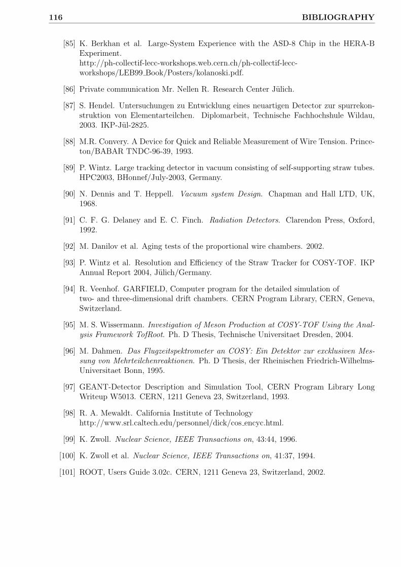
116 BIBLIOGRAPHY
[85] K. Berkhan et al. Large-System Experience with the ASD-8 Chip in the HERA-BExperiment.http://ph-collectif-lecc-workshops.web.cern.ch/ph-collectif-lecc-workshops/LEB99 Book/Posters/kolanoski.pdf.
[86] Private communication Mr. Nellen R. Research Center Julich.
[87] S. Hendel. Untersuchungen zu Entwicklung eines neuartigen Detector zur spurrekon-struktion von Elementarteilchen. Diplomarbeit, Technische Fachhochshule Wildau,2003. IKP-Jul-2825.
[88] M.R. Convery. A Device for Quick and Reliable Measurement of Wire Tension. Prince-ton/BABAR TNDC-96-39, 1993.
[89] P. Wintz. Large tracking detector in vacuum consisting of self-supporting straw tubes.HPC2003, BHonnef/July-2003, Germany.
[90] N. Dennis and T. Heppell. Vacuum system Design. Chapman and Hall LTD, UK,1968.
[91] C. F. G. Delaney and E. C. Finch. Radiation Detectors. Clarendon Press, Oxford,1992.
[92] M. Danilov et al. Aging tests of the proportional wire chambers. 2002.
[93] P. Wintz et al. Resolution and Efficiency of the Straw Tracker for COSY-TOF. IKPAnnual Report 2004, Julich/Germany.
[94] R. Veenhof. GARFIELD, Computer program for the detailed simulation oftwo- and three-dimensional drift chambers. CERN Program Library, CERN, Geneva,Switzerland.
[95] M. S. Wissermann. Investigation of Meson Production at COSY-TOF Using the Anal-ysis Framework TofRoot. Ph. D Thesis, Technische Universitaet Dresden, 2004.
[96] M. Dahmen. Das Flugzeitspektrometer an COSY: Ein Detektor zur excklusiven Mes-sung von Mehrteilchenreaktionen. Ph. D Thesis, der Rheinischen Friedrich-Wilhelms-Universitaet Bonn, 1995.
[97] GEANT-Detector Description and Simulation Tool, CERN Program Library LongWriteup W5013. CERN, 1211 Geneva 23, Switzerland, 1993.
[98] R. A. Mewaldt. California Institute of Technologyhttp://www.srl.caltech.edu/personnel/dick/cos encyc.html.
[99] K. Zwoll. Nuclear Science, IEEE Transactions on, 43:44, 1996.
[100] K. Zwoll et al. Nuclear Science, IEEE Transactions on, 41:37, 1994.
[101] ROOT, Users Guide 3.02c. CERN, 1211 Geneva 23, Switzerland, 2002.

BIBLIOGRAPHY 117
[102] http://rd11.web.cern.ch/RD11/rkb/PH14pp/node26.html.
[103] Athanasios Papoulis. Probability, Random Variables, and Stochastic Processes.McGRAW-Hill, New York, 1991.