991022173536103411.pdf - PolyU Electronic Theses
273
Copyright Undertaking This thesis is protected by copyright, with all rights reserved. By reading and using the thesis, the reader understands and agrees to the following terms: 1. The reader will abide by the rules and legal ordinances governing copyright regarding the use of the thesis. 2. The reader will use the thesis for the purpose of research or private study only and not for distribution or further reproduction or any other purpose. 3. The reader agrees to indemnify and hold the University harmless from and against any loss, damage, cost, liability or expenses arising from copyright infringement or unauthorized usage. IMPORTANT If you have reasons to believe that any materials in this thesis are deemed not suitable to be distributed in this form, or a copyright owner having difficulty with the material being included in our database, please contact [email protected] providing details. The Library will look into your claim and consider taking remedial action upon receipt of the written requests. Pao Yue-kong Library, The Hong Kong Polytechnic University, Hung Hom, Kowloon, Hong Kong http://www.lib.polyu.edu.hk
-
Upload
khangminh22 -
Category
Documents
-
view
0 -
download
0
Transcript of 991022173536103411.pdf - PolyU Electronic Theses
Copyright Undertaking
This thesis is protected by copyright, with all rights reserved.
By reading and using the thesis, the reader understands and agrees to the following terms:
1. The reader will abide by the rules and legal ordinances governing copyright regarding the use of the thesis.
2. The reader will use the thesis for the purpose of research or private study only and not for distribution or further reproduction or any other purpose.
3. The reader agrees to indemnify and hold the University harmless from and against any loss, damage, cost, liability or expenses arising from copyright infringement or unauthorized usage.
IMPORTANT
If you have reasons to believe that any materials in this thesis are deemed not suitable to be distributed in this form, or a copyright owner having difficulty with the material being included in our database, please contact [email protected] providing details. The Library will look into your claim and consider taking remedial action upon receipt of the written requests.
Pao Yue-kong Library, The Hong Kong Polytechnic University, Hung Hom, Kowloon, Hong Kong
http://www.lib.polyu.edu.hk
THEORY AND APPLICATION OF SECOND-
ORDER DIRECT ANALYSIS IN STATIC
AND DYNAMIC DESIGN OF FRAME
STRUCTURES
DU ZUOLEI
PhD
The Hong Kong Polytechnic University
2019
The Hong Kong Polytechnic University
Department of Civil and Environmental Engineering
THEORY AND APPLICATION OF SECOND-
ORDER DIRECT ANALYSIS IN STATIC
AND DYNAMIC DESIGN OF FRAME
STRUCTURES
DU Zuolei
A thesis submitted in
partial fulfillment of the requirements for
the degree of Doctor of Philosophy
May 2018

Certificate of originality
CERTIFICATE OF ORIGINALITY
I hereby declare that this thesis is my own work and that, to the best of my knowledge
and belief, it reproduces no material previously published or written, nor material that
has been accepted for the award of any other degree or diploma, except where due
acknowledgment has been made in the text.
___________________________ (Signed)
DU Zuo-Lei (Name of student)

To my wife & parents
for their love and encouragements
Abstract
ABSTRACT
The modern design codes such as Eurocode3 (2005), AISC360 (2016), CoPHK (2011)
and GB50017 (2017) recommend the use of direct analysis method (DAM) instead of
traditional effective length method for daily design. However, the research and
applications of DAM mainly focus on frame structures subjected to static loads.
Performance-based seismic design (PBSD) is a new trend in structural engineering
and appears in most of the modern design codes or specifications such as Eurocode-8
(2005) and FEMA356 (2000). The philosophy inherent to the approach is to accurately
capture the structural behavior under earthquake actions which is substantially in line
with DAM, and the demanded performance according to the occupied functions is
estimated. It is found that little work has been carried out on the extension of DAM to
PBSD. The pushover analysis and time history analysis should be used with effective
length method for PBSD in current practice as the member imperfections have not
been taken into account. The DAM requires explicit consideration of member initial
imperfections to suppress the use of effective length factor while PBSD needs to
simulate progressive yielding along the section depth and member length. Thus, an
advanced and high-performance beam-column element with member imperfection is
urgently required for static and dynamic design.
In the past decades, the stiffness and flexibility methods have been extensively used
to derive beam-column elements. As the flexibility-based type elements can meet the
compatibility and equilibrium conditions at the element level, they are more competent
in direct analysis considering both geometrical and material nonlinearities. In this
research project, an advanced flexibility-based beam-column element with member
Abstract
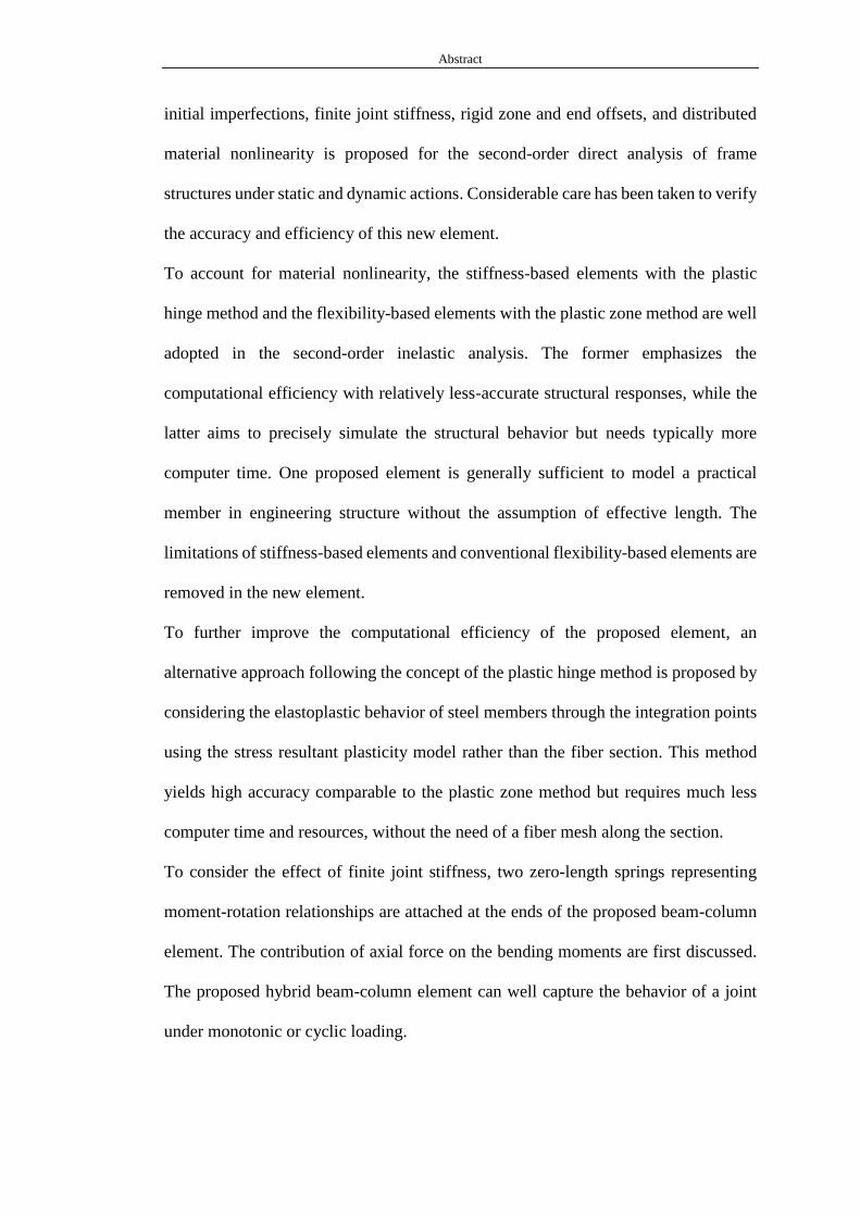
initial imperfections, finite joint stiffness, rigid zone and end offsets, and distributed
material nonlinearity is proposed for the second-order direct analysis of frame
structures under static and dynamic actions. Considerable care has been taken to verify
the accuracy and efficiency of this new element.
To account for material nonlinearity, the stiffness-based elements with the plastic
hinge method and the flexibility-based elements with the plastic zone method are well
adopted in the second-order inelastic analysis. The former emphasizes the
computational efficiency with relatively less-accurate structural responses, while the
latter aims to precisely simulate the structural behavior but needs typically more
computer time. One proposed element is generally sufficient to model a practical
member in engineering structure without the assumption of effective length. The
limitations of stiffness-based elements and conventional flexibility-based elements are
removed in the new element.
To further improve the computational efficiency of the proposed element, an
alternative approach following the concept of the plastic hinge method is proposed by
considering the elastoplastic behavior of steel members through the integration points
using the stress resultant plasticity model rather than the fiber section. This method
yields high accuracy comparable to the plastic zone method but requires much less
computer time and resources, without the need of a fiber mesh along the section.
To consider the effect of finite joint stiffness, two zero-length springs representing
moment-rotation relationships are attached at the ends of the proposed beam-column
element. The contribution of axial force on the bending moments are first discussed.
The proposed hybrid beam-column element can well capture the behavior of a joint
under monotonic or cyclic loading.
Abstract
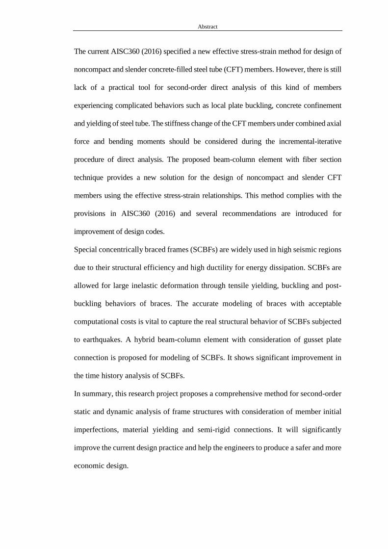
The current AISC360 (2016) specified a new effective stress-strain method for design of
noncompact and slender concrete-filled steel tube (CFT) members. However, there is still
lack of a practical tool for second-order direct analysis of this kind of members
experiencing complicated behaviors such as local plate buckling, concrete confinement
and yielding of steel tube. The stiffness change of the CFT members under combined axial
force and bending moments should be considered during the incremental-iterative
procedure of direct analysis. The proposed beam-column element with fiber section
technique provides a new solution for the design of noncompact and slender CFT
members using the effective stress-strain relationships. This method complies with the
provisions in AISC360 (2016) and several recommendations are introduced for
improvement of design codes.
Special concentrically braced frames (SCBFs) are widely used in high seismic regions
due to their structural efficiency and high ductility for energy dissipation. SCBFs are
allowed for large inelastic deformation through tensile yielding, buckling and post-
buckling behaviors of braces. The accurate modeling of braces with acceptable
computational costs is vital to capture the real structural behavior of SCBFs subjected
to earthquakes. A hybrid beam-column element with consideration of gusset plate
connection is proposed for modeling of SCBFs. It shows significant improvement in
the time history analysis of SCBFs.
In summary, this research project proposes a comprehensive method for second-order
static and dynamic analysis of frame structures with consideration of member initial
imperfections, material yielding and semi-rigid connections. It will significantly
improve the current design practice and help the engineers to produce a safer and more
economic design.

Abstract
Keywords: Flexibility-based; beam-column element; direct analysis; second-order;
initial imperfection; residual stress; distributed nonlinearity; noncompact and slender
CFT members; special concentrically braced frames;
Publications
PUBLICATIONS
Journal paper:
(1) Du, Zuo-Lei, Yao-Peng Liu, and Siu-Lai Chan. "A second-order flexibility-based
beam-column element with member imperfection." Engineering Structures 143
(2017): 410-426.
(2) Du, Zuo-Lei, Yao-Peng Liu, and Siu-Lai Chan. "A practical analytical model for
special concentrically braced frames." Journal of Constructional Steel Research.
(Under Review)
(3) Du, Zuo-Lei, Yao-Peng Liu, and Siu-Lai Chan. "A force-based element for direct
analysis using stress-resultant plasticity model." Steel and Composite Structures.
(Under Review)
(4) Du, Zuo-Lei, Yao-Peng Liu, and Siu-Lai Chan. "Direct analysis method for
noncompact and slender CFT members." Thin-Walled Structures. (Under Review)
(5) Du, Zuo-Lei, Yao-Peng Liu, and Siu-Lai Chan. "A consistent analytical model for
tapered steel members with symmetric or asymmetric variations." International
Journal of Structural Stability and Dynamics. (to be submitted)
Conference paper:
(1) Du, Zuo-Lei, Yao-Peng Liu, Siu-Lai Chan, and Wei-Qi Tan. "A flexibility-based
element for second-order inelastic analysis using plastic hinge method." 8th
European Conference on Steel and Composite Structures 1.2-3 (2017): 1056-1065.

Publications
(2) Du, Zuo-Lei, Yao-Peng Liu, Siu-Lai Chan, and Wei-Qi Tan. "Consideration of
imperfections in special concentrically braced frames." The 8th International
Conference on Steel and Aluminium Structures (2016).
(3) Yao-Peng Liu, Du, Zuo-Lei, Siu-Lai Chan. " Distributed plastic hinge analysis by
a new flexibility-based beam-column element." 第九屆海峽兩岸及香港鋼、組
合及金屬結構技術研討會 (2017).
(4) Liu, Yao-Peng, Siu-Lai Chan, Zuo-Lei Du, and Jian-Wei He. "Second-order direct
analysis of long-span roof structures." 8th European Conference on Steel and
Composite Structures 1.2-3 (2017): 3930-3939.
(5) Liu, Yao-Peng, Siu-Lai Chan, Zuo-Lei Du. "Second order plastic hinge analysis
for seismic and static design of building structures." 11th International Conference
on Advances in Steel and Concrete Composite Structures (2015)

Acknowledgements
ACKNOWLEDGMENTS
I would like to express my appreciation to Professor Siu-Lai Chan, my research
advisor, for his informative guidance, valuable support during my doctoral program. I
also wish to thank Dr. Yao-Peng Liu for the knowledge and foresight transmitted about
the academic research and programming technology. This long relationship with such
friendly and enthusiastic supervisors brought happiness to me and will keep
encouraging me in my future life.
I also would like to thank the financial support of the research project “Development
of an energy absorbing device for flexible rock-fall barriers (ITS/059/16FP)” funded
by the Research Grant Council grant from the Hong Kong SAR Government, and
Hong Kong Polytechnic University for providing resources in the completion of my
doctoral program.
I wish to express my deepest gratitude to my wife, Hong Liu, for her love, support,
encouragement, and sacrifice during my doctoral studies. I will never be able to thank
her enough for accompanying me to accomplish this arduous task. I am thankful for
the boundless love from my parents Xin-Shi Du and Ru-Xin Xiong. I am appreciated
for their effort in raising and cultivating my brother and me, and being patient in
waiting for me to complete my doctoral study.
Finally, I wish to thank the NIDA team members, who include but are not limited to
Dr. Z. H. Zhou, Dr. S. W. Liu, Dr. S. H. Cho, Dr. H. Yu, Mr. Sam Chan, Mr. Y. Q.
Tang, Mr. R. Bai, Mr. W. F. Chen, Miss W. Q. Tan, Mr. J. W. He, Mr. L. Chen, Mr.

Acknowledgements
Jake Chan, Mr. W. Du, Mr. P. S. Zheng and Mr. S. B. Ji for their great help during my
studies.
Contents
I
CONTENTS
CERTIFICATE OF ORIGINALITY ....................................................................... 3
ABSTRACT ................................................................................................................ 5
PUBLICATIONS ....................................................................................................... 9
ACKNOWLEDGMENTS ....................................................................................... 11
CONTENTS ................................................................................................................ I
LIST OF FIGURES .................................................................................................IV
LIST OF TABLES ............................................................................................... VIII
LIST OF SYMBOLS ...............................................................................................IX
CHAPTER 1. INTRODUCTION ........................................................................ 12
1.1 Background ................................................................................................ 12
1.2 Objectives ................................................................................................... 14
1.3 Organization ............................................................................................... 16
CHAPTER 2. LITERATURE REVIEW ............................................................ 19
2.1 Beam-column elements for second-order analysis .................................... 19
2.2 Plasticity models for material nonlinearity ................................................ 25
2.3 Modeling of member initial imperfections ................................................ 30
2.4 Modeling of semi-rigid connections .......................................................... 32
2.5 Design method for CFT members with noncompact and slender sections 33
2.6 Design method of special concentrically braced frames ............................ 35
CHAPTER 3. FLEXIBILITY-BASED BEAM-COLUMN ELEMENT
CONSIDERING MEMBER IMPERFECTION ................................................... 41
Contents
II
3.1 Introduction ................................................................................................ 41
3.2 Element formulations ................................................................................. 44
3.3 Member imperfection ................................................................................. 60
3.4 Numerical examples ................................................................................... 64
3.5 Concluding remarks ................................................................................... 72
3.6 Appendix – Analytical Solutions of Single Imperfect Column under Axial
Load .................................................................................................................... 74
CHAPTER 4.TWO PLASTICITY MODELS FOR MATERIAL
NONLINEARITY .................................................................................................. 89
4.1 Introduction ................................................................................................ 89
4.2 Distributed plasticity analysis .................................................................... 91
4.3 Stress-resultant plasticity model ................................................................ 92
4.4 Integration of rate equations and section tangent stiffness ............................ 95
4.5 Verification examples ................................................................................ 99
4.6 Concluding remarks ................................................................................. 104
CHAPTER 5. SEMI-RIGID CONNECTIONS UNDER MONOTONIC
AND CYCLIC LOADS ......................................................................................... 118
5.1 Introduction .............................................................................................. 118
5.2 Modeling of connection behavior under monotonic loading ................... 119
5.3 Modeling of connection behavior under cyclic loading ........................... 126
5.4 Flexibility-based beam-column element accounting for semi-rigid joints
.................................................................................................................. 130
5.5 Numerical examples ................................................................................. 133
5.6 Concluding remarks ................................................................................. 140
Contents
III
CHAPTER 6. DIRECT ANALYSIS OF NONCOMPACT AND SLENDER
CFT MEMBERS .................................................................................................... 167
6.1 Introduction .............................................................................................. 167
6.2 Design methods for CFT members with noncompact or slender sections in
AISC360 ............................................................................................................... 171
6.3 Direct analysis method .............................................................................. 176
6.4 Validation examples .................................................................................. 181
6.5 Concluding remarks ................................................................................. 186
CHAPTER 7. DIRECT ANALYSIS OF SPECIAL CONCENTRICALLY
BRACED FRAMES ............................................................................................... 201
7.1 Introduction .............................................................................................. 201
7.2 Semi-rigid connection and rigid end zone for gusset plate connections .. 206
7.3 Material representation and residual stress .............................................. 208
7.4 Analytical model for SCBF system.......................................................... 211
7.5 Numerical examples ................................................................................. 216
7.6 Concluding remarks ................................................................................. 220
CHAPTER 8. SUMMARY AND FUTURE WORK ....................................... 236
8.1 Summary .................................................................................................. 236
8.2 Future work .............................................................................................. 239
REFERENCES ....................................................................................................... 241
List of Figures
IV
LIST OF FIGURES
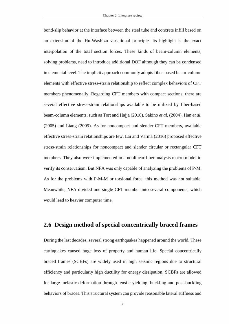
Fig. 2.1 Section discretization ............................................................................ 39
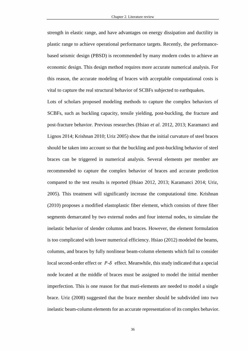
Fig. 2.2 Commonly used configurations of SCBFs ........................................... 40
Fig. 2.3 Structural behavior of brace and failure locations ................................ 40
Fig. 3.1 Basic forces versus displacements relations ......................................... 75
Fig. 3.2 Layout of columns ................................................................................ 75
Fig. 3.3 Load vs. deflection curves for “pinned-pinned”: (a) = (b) =
.................................................................................................................... 77
Fig. 3.4 Load vs. deflection curves for “pinned-fixed”: (a) = (b) =
.................................................................................................................... 78
Fig. 3.5 Load vs. deflection curves for “fixed-fixed”: (a) = (b) = 80
Fig. 3.6 A single fixed-ended beam under a member point load ....................... 80
Fig. 3.7 Load-displacement curves of point B ................................................... 81
Fig. 3.8 Deformation of integration points along the member ........................... 82
Fig. 3.9 Layout and load pattern of the planar frame by Ziemian and McGuire
(2002) ......................................................................................................... 83
Fig. 3.10 Imperfection pattern of the planar frame by Ziemian and McGuire (2002)
.................................................................................................................... 83
Fig. 3.11 Response curves of the frame by Ziemian and McGuire (2002) ........ 84
Fig. 3.12 Bending moment, axial force and percentage of the cross-section
yielded ........................................................................................................ 84
Fig. 3.13 Layout and load pattern of Harrison’s space frame ............................ 85
Fig. 3.14 Horizontal displacement of the top point ............................................ 85
Fig. 4.1 Distributed plasticity by fiber section approach ................................. 106
List of Figures
V
Fig. 4.2 Fiber discretization for wide-flange section ....................................... 106
Fig. 4.3 Yield function and limit function for section state ............................. 107
Fig. 4.4 Backward-Euler return procedure ....................................................... 107
Fig. 4.5. Full surface under interaction of force resultants .............................. 108
Fig. 4.6 Layout of cantilever column and loading patterns ............................. 108
Fig. 4.7 Bending moment-plastic rotation about y-axis for case 1 .................. 109
Fig. 4.8 Bending moment-plastic rotation about y-axis for case 2 .................. 109
Fig. 4.9 Layout and loading pattern of the Vogel’s six-story frame ................ 110
Fig. 4.10 Horizontal displacement of the Vogel’s six-story frame .................. 110
Fig. 4.11 Layout and loading pattern of the high strength steel frame (Unit: mm)
.................................................................................................................. 111
Fig. 4.12 Loading protocol for the top displacement ....................................... 111
Fig. 4.13 Base shear versus overall drift ratio .................................................. 112
Fig. 4.14 Layout of four-story 3D steel frame ................................................. 112
Fig. 4.15 Displacement under four earthquakes............................................... 114
Fig. 4.16 Base Shear under four earthquakes ................................................... 116
Fig. 4.17 Consuming time of time history analysis under four earthquakes.... 117
Fig. 5.1 Finite element model of the end-plate connection using solid elements
.................................................................................................................. 141
Fig. 5.2 Finite element model of the end-plate connection using shell elements
.................................................................................................................. 141
Fig. 5.3 Modeling of a semi-rigid jointed member .......................................... 142
Fig. 5.4 Layouts and load patterns of the frames ............................................. 143
Fig. 5.5 Loading-deflection curves of models with various connection types. 143
Fig. 5.6 Layouts of sway and non-sway frames ............................................... 144
List of Figures
VI
Fig. 5.7 Applied force vs. horizontal displacement ......................................... 145
Fig. 5.8 Layouts and load patterns of three-story sway frames ....................... 147
Fig. 5.9 Loading-deflection curves for models of three-story sway frames .... 148
Fig. 5.10 Layouts and load patterns for William’s toggle frame ..................... 150
Fig. 5.11 Loading-deflection curves of William’s toggle frame ...................... 153
Fig. 5.12 Vertical load history.......................................................................... 154
Fig. 5.13 Layouts and dynamic loadings for William’s toggle frame ............. 155
Fig. 5.14 The transient response of William’s toggle frame ............................ 156
Fig. 5.15 Layout of one-story frame ................................................................ 157
Fig. 5.16 Frequency against joint stiffness....................................................... 158
Fig. 5.17 Layout and load pattern of one-story frame...................................... 158
Fig. 5.18 The transient response of the frame .................................................. 160
Fig. 5.19 Layout and load pattern of a column ................................................ 160
Fig. 5.20 Cyclic load history ............................................................................ 161
Fig. 5.21 Load-deformation response of the Pinch type model ....................... 161
Fig. 5.22 The load-displacement histories of various pinch type models ........ 164
Fig. 6.1. Typical fiber mesh of CFT member .................................................. 189
Fig. 6.2. Effective stress-strain relationships for steel tube ............................. 190
Fig. 6.3. Effective stress-strain relationships for concrete infill ...................... 191
Fig. 6.4. Dimensions and material properties of KOM2001 ............................ 191
Fig. 6.5. Load-deflection curves of KOM2001 ................................................ 192
Fig. 6.6. Dimensions and material properties for two rectangular CFT members
.................................................................................................................. 193
Fig. 6.7. Layout and loading scheme for two rectangular CFT tests ............... 193
Fig. 6.8. Load-deflection curves for S-150-2.0 and BRA4-2-5-02.................... 194
List of Figures
VII
Fig. 6.9. Dimensions and material properties of CC4-D-4-1 ........................... 195
Fig. 6.10. Load-deflection curves for CC4-D-4-1............................................ 195
Fig. 6.11. Dimensions and material properties for two circular CFT members
.................................................................................................................. 196
Fig. 6.12. Layout and loading scheme for two circular CFT tests ................... 197
Fig. 6.13. Load-deflection curves for TB002 and EC4-D-4-0 ......................... 198
Fig. 7.1 Configuration and modelling of gusset plate connection ................... 222
Fig. 7.2 Moment-rotation function of gusset plate connection ........................ 222
Fig. 7.3 Fracture model of steel material ......................................................... 223
Fig. 7.4 Residual stress patterns ....................................................................... 224
Fig. 7.5 Comparison of analytical models for SCBFs ..................................... 225
Fig. 7.6 Configuration of a single HSS brace .................................................. 225
Fig. 7.7 Symmetrical loading protocol ............................................................. 226
Fig. 7.8 Brace hysteretic curves for different models: (a) M1, (b) M2, (c) M3 and
(d) M4 ...................................................................................................... 228
Fig. 7.9 Finite element model of SCBF ........................................................... 229
Fig. 7.10 Seismic performance of SCBF with different number of elements .. 229
Fig. 7.11 Test specimen of single-story frame ................................................. 230
Fig. 7.12 Analytical model ............................................................................... 230
Fig. 7.13 Asymmetrical loading protocol ........................................................ 231
Fig. 7.14 Response of single-story frame ........................................................ 231
Fig. 7.15 Test specimen of three-story one-bay frame..................................... 232
Fig. 7.16 Analytical model ............................................................................... 233
Fig. 7.17 Symmetrical loading protocol ........................................................... 233
Fig. 7.18 Response of three-story one-bay frame ............................................ 234
List of Tables
VIII
LIST OF TABLES
Table 3-1 Numerical integration methods for flexibility-based beam-column
element ....................................................................................................... 86
Table 3-2 Numerical integration methods for flexibility-based beam-column
element ....................................................................................................... 86
Table 3-3 Theory results of a fixed-ended beam under different point loads .... 87
Table 3-4 Models (M1~M7) for the planar frame by Ziemian and McGuire (2002)
.................................................................................................................... 87
Table 5-1 Comparison of the critical load values for a non-sway frame ......... 165
Table 5-2 Comparison of the critical load values for a sway frame ................ 165
Table 5-3 Comparison of the critical load values for multistory sway frame .. 166
Table 6-1 Classification of steel elements in composite members .................. 199
Table 6-2. Definitions of 𝑐𝑝 and 𝑐𝑚 ............................................................. 200
Table 7-1 Four models for simulation of the single HSS brace ....................... 235
List of Tables
IX
LIST OF SYMBOLS
𝐍 Shape function
𝐁 Strain-displacement transformation matrix
P Element forces in basic axis system
D Element displacements in basic axis system
𝐮 Displacement field
𝛆 Strain field
𝛔 Stress field
𝚿 Transformation matrix
𝐝 Section displacements
Π𝐻𝑅 Total work potential term
Π𝑒𝑥𝑡(𝐮) External work potential term
𝛺 Volume of element
𝐒 Stress resultants of cross-sections
𝐴 Area of cross-sections
𝐛 Matrix of displacement-dependent force interpolation functions
v, w Lateral displacement
𝑣0, 𝑤0 Initial imperfection
𝐛∗ Matrix of end forces-section forces interpolation functions
𝐤𝑠 Section tangent stiffness matrix
𝐄𝑡 Material tangent stiffness at an arbitrary point
𝐟𝑠 Section tangent flexibility matrix
𝑙𝑖𝑗∗ 𝑗th integrated Lagrangian polynomial at integration point 𝜉𝑖
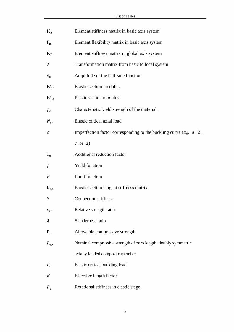
List of Tables
X
𝐊𝒆 Element stiffness matrix in basic axis system
𝐅𝒆 Element flexibility matrix in basic axis system
𝐊𝑻 Element stiffness matrix in global axis system
𝑻 Transformation matrix from basic to local system
𝛿0 Amplitude of the half-sine function
𝑊𝑒𝑙 Elastic section modulus
𝑊𝑝𝑙 Plastic section modulus
𝑓𝑦 Characteristic yield strength of the material
𝑁𝑐𝑟 Elastic critical axial load
𝛼 Imperfection factor corresponding to the buckling curve (𝑎0, 𝑎, 𝑏,
𝑐 or 𝑑)
𝜏𝑏 Additional reduction factor
𝑓 Yield function
𝐹 Limit function
𝐤𝑠𝑒 Elastic section tangent stiffness matrix
S Connection stiffness
𝑐𝑠𝑟 Relative strength ratio
𝜆 Slenderness ratio
Pc Allowable compressive strength
𝑃𝑛𝑜 Nominal compressive strength of zero length, doubly symmetric
axially loaded composite member
𝑃𝑒 Elastic critical buckling load
𝐾 Effective length factor
𝑅𝑒 Rotational stiffness in elastic stage

List of Tables
XI
e Distance of the rigid zone
𝐄 Eccentricity transform matrix
Introduction
XII
CHAPTER 1. INTRODUCTION
1.1 Background
The modern design codes such as Eurocode-3 (2005), AISC360 (2016), CoPHK (2011)
and GB50017 (2017) recommend the use of direct analysis method (DAM) instead of
traditional effective length method for daily design. However, the research and
applications of DAM mainly focus on frame structures subjected to static loads.
Performance-based seismic design (PBSD) is a new trend in structural engineering
and appears in most of the modern design codes or specifications such as Eurocode-8
(2005) and FEMA356 (2000). The philosophy inherent to the approach is to accurately
capture the structural behavior under earthquake actions which is essentially in line
with DAM, and the demanded performance according to the occupied functions is
estimated.
Compared to current seismic analysis approaches such as the lateral force (LF) and
the response spectrum (RS) analysis methods based on linear and elastic assumptions,
the analysis method for performance-based design requires consideration of the
material and geometrical nonlinearities. The nonlinear static and dynamic analysis,
which are also commonly called “push-over” and “time-history” analysis respectively,
are two well-accepted methods for performance-based seismic design.
AISC360 (2016) provides detailed requirements in direct analysis, which should
include: (1) deformation of members, connections and other components; (2) 𝑃-∆
and 𝑃-𝛿 effects; (3) initial geometric imperfections; (4) material inelasticity and

Chapter 1. Introduction
13
residual stresses; and (5) uncertainty of strength and stiffness in the system, members
and connection. Similar requirements are also presented in CoPHK (2011) and
Eurocode-3 (2005). It can be seen that the above requirements should be also
considered in the seismic analysis so that the actual structural behavior can be
predicted for PBSD.
It is found that little work has been carried out on the extension of DAM to PBSD.
The pushover analysis and time history analysis should be used with effective length
method for PBSD in current practice as the member imperfections have not been taken
into account. The DAM requires explicit consideration of member initial
imperfections to suppress the use of effective length factor while PBSD needs to
simulate progressive yielding along the section depth and member length. Thus, an
advanced and high-performance beam-column element with member imperfection is
urgently required for the static and dynamic design.
In the past decades, the stiffness and flexibility methods have been extensively used
to derive beam-column elements. The stiffness-based elements have achieved great
successes in handling large elastic deflection problems while the conventional
flexibility-based elements have played a dominant role in second-order inelastic
analysis. The accuracy of the former can be improved by enforcing equilibrium along
mid-span or “stations” along the member length to achieve equilibrium which is not
guaranteed along an element. However, as the actual location of plastic hinge can be
anywhere along the element, the shape function becomes inadequate to describe the
sharp angle due to formation of plastic hinge such that several stiffness-based elements
should be used to represent the material yielding, which will significantly increase
computer time and even cause difficulties in modeling of member imperfections. In
contrast, the equilibrium along a flexibility-based element can always be guaranteed.
Chapter 1. Introduction
14
However, the conventional flexibility-based elements cannot meet the codified
requirements of direct analysis because they did not take member initial imperfections
into account. Being aware of the above, it motivates the author to develop a new
element for direct analysis of static and dynamic problems by safety and economic
design principles.
For the practical design of frame structures using direct analysis method (DAM), the
beam-column element adopted should have the merits of the above two types of
elements. As the flexibility-based type elements can meet the compatibility and
equilibrium conditions at the element level, they are more competent in direct analysis
considering both geometrical and material nonlinearities.
Thus, an advanced flexibility-based beam-column element with member initial
imperfections, finite joint stiffness, rigid zone and end offsets, and distributed material
nonlinearity is proposed for second-order direct analysis of frame structures under
static and dynamic actions in this research project. Considerable care has been taken
to verify the accuracy and efficiency of this new element. Further, the proposed
element is applied to conduct direct analysis of two widely used structural forms, i.e.
structures with concrete-filled steel tube (CFT) members and special concentrically
braced frames (SCBFs).
1.2 Objectives
The main objective of this research project is to propose an advanced and high-
performance beam-column element explicitly considering member initial
imperfections and distributed plasticity so that the direct analysis method (DAM) can
be smoothly extended to performance-based seismic design (PBSD) without the need
Chapter 1. Introduction
15
of effective length method. The proposed element should have high accuracy even
using one element per member and consequently, the computational efficiency in
nonlinear dynamic analysis can be significantly enhanced. Furthermore, the
requirements of direct analysis method need to be satisfied by incorporating the
features into the proposed element.
Currently, the direct analysis method (DAM) is mainly implemented via the stiffness-
based beam-column elements. Though being efficient in second-order elastic analysis,
they face difficulties in second-order inelastic analysis which is required in PBSD. In
contrast, the flexibility-base beam-columns show excellent performance in handling
elastoplastic problems because they strictly satisfy the equilibrium of bending
moments and axial force along the element. For this reason, the flexibility-based type
element is selected as the candidate for PBSD under the framework of direct analysis.
First, a new flexibility-based beam-column element considering member initial
geometrical imperfection is derived. Several typical imperfection mode shapes such
as sine function and polynomial function are allowed in this element. Second, the
residual stress can be explicitly modeled by the proposed element via the fiber section
technology through which the influence of residual stress on the structural response
can be assessed. To save computer time and resource, an alternative method to form
the sectional stiffness is proposed. The effects such as joint flexibility, rigid zone and
end offsets, are also considered and finally an advanced hybrid beam-column element
is developed to meet the general requirements of direct analysis. In summary, the goals
of this research project are listed as:
• To develop an advanced flexibility-based beam-column element with initial
member imperfections to minimize the degrees of freedom and improve the
convergence of nonlinear analysis;
• To consider residual stress in the proposed element with fiber section
Chapter 1. Introduction
16
technology to improve accuracy;
• To propose a distributed plastic hinge method to improve computational
efficiency in second-order inelastic analysis;
• To program and incorporate the proposed element and plastic methods into the
existing computer program for practical use;
• To consider joint flexibility in the proposed element;
• To consider end rigid zone and end offsets in the proposed element;
• To apply the proposed method in direct analysis of frame structures with
noncompact and slender CFT members;
• To apply the proposed method in the performance-based seismic design of
special concentrically braced frames (SCBFs).
1.3 Organization
The outline of this thesis is presented as follows:
Chapter 1 introduces the background, objectives, and organization of this thesis.
Chapter 2 presents a literature survey. First, the beam-column elements for direct
analysis are discussed. Plasticity models adopted in the beam-column elements for
material nonlinearity are commented. Further, the modeling approaches of member
initial imperfections and semi-rigid connection are reviewed. Finally, the design
methods for CFT members with noncompact and slender sections, and special
concentrically braced frames are outlined.
Chapter 3 describes a new flexibility-based beam-column element with member
imperfection. First, the equilibrium and compatibility equations are derived on the
basis of Hellinger-Reissner variational functional. Second, the element flexibility
matrix is formed by the integration of the section flexibility matrix along the member.
Meanwhile, the curvature-based displacement interpolation (CBDI) for second-order
flexibility-based elements is introduced. Further, the transformation from the basic
Chapter 1. Introduction
17
coordinate system to the global coordinate system and the process of element state
determination are presented. The advantage of the proposed element for consideration
of member imperfection is highlighted. Finally, several numerical examples are used
to verify the accuracy and validation of the proposed element.
Chapter 4 describes two plasticity models used in beam-column elements for the
consideration of material nonlinearity. First, a conventional method, a distributed
plasticity model with fiber sections technology, is illustrated. Second, a new stress-
resultant plasticity model is incorporated into the proposed flexibility-based element
to enhance numerical efficiency. The critical steps of forming section tangent stiffness,
i.e., the integration algorithm and return mapping algorithm, are presented to allow for
hysteretic behavior. The proposed method is evaluated with the conventional method
via several benchmarking examples.
In Chapter 5, the joint flexibility, as an essential factor affecting structural behavior,
is considered by improving the proposed element described in Chapter 3. First, several
semi-rigid connection models for the joints subjected to monotonic or cyclic loading
are introduced. Then, the proposed flexibility-based beam-column element is modified
to account for semi-rigid behavior. Finally, several static and dynamic examples are
adopted to verify the performance of the hybrid element to model frame structures
with semi-rigid connections under static or dynamic loads.
In Chapter 6, the proposed method is applied to design of frame structures with CFT
members made of noncompact and slender sections. First, the design methods
suggested by AISC360 (2016) are introduced and discussed. Second, the direct
analysis method is extended to analyze CFT members with noncompact and slender
sections. Finally, four experiments from literature, including rectangular and circular
CFT members, are adopted to verify the proposed method.

Chapter 1. Introduction
18
In Chapter 7, the proposed method is applied to design of special concentrically braced
frames (SCBFs). First, the special features of SCBFs are discussed. The proposed
element is improved to incorporate the effect of rigid end zones, material nonlinearity,
and residual stress. Then, a practical analytical model for SCBF systems is proposed.
Finally, a considerable number of benchmark examples are used to illustrate the
accuracy and efficiency of the proposed model.
In Chapter 8, the conclusions drawn from this study are illustrated. Some suggestions
for future work are also presented.
Chapter 2. Literature review
19
CHAPTER 2. LITERATURE REVIEW
This chapter presents a review on the development of beam-column elements and its
related problems in regarding practical application. It mainly includes the review on
the several existing beam-column elements, geometrical imperfection, approaches to
model material nonlinearity, joint flexibility, modeling of concrete filled steel tube
(CFT) members and the design of special concentrically braced frame.
2.1 Beam-column elements for second-order analysis
Finite element method was invented to solve complex elasticity and structural analysis
problems in civil and aeronautical engineering in the early 1940s. Beam-column, as
an effective kind of finite element to model beams and columns, attracted a
considerable amount of research. Several kinds of beam-column elements with unique
features were developed. Numerous scholars had made substantial efforts on nonlinear
engineering problems. Generally, these elements can be divided into three categories:
displacement, flexibility and mixed element. Extensive researches have been
conducted on the structural analysis of frame structures with consideration of
geometrical and material nonlinearities. Meanwhile, some reliable numerical methods
were developed to solve the nonlinear problems. For instance, Chan (1988) proposed
an approach, called minimizing the residual displacements, to solve geometric and
material nonlinear problems. Chan and Zhou (1994) proposed a pointwise-
equilibrating-polynomial (PEP) element which can model one member with one
element and show excellent performance on solving nonlinear geometrical problems.
Chen and Chan (1995) proposed an element with plastic hinges at the mid-span and
Chapter 2. Literature review
20
two ends which can be used to model material nonlinearity. Izzuddin and Smith (1996)
proposed a new formulation to consider elastoplastic material behavior using
distributed plasticity. Izzuddin (1996) introduced geometrical imperfection in a local
Eulerian system to beam-columns. Spacone (1996) proposed a mixed beam-column
element, which has a high accuracy in the nonlinear analysis of structural members.
Neuenhofer and Filippou (1998) proposed a flexibility-based beam-column element
for geometrically nonlinear analysis of frame structures. Pi et al. (2006) employed an
accurate rotation matrix to derive nonlinear strain, and proposed a beam-column
element to model steel and concrete composite members based on total Lagrangian
framework.
In this section, these three kinds of beam-column elements have been reviewed and
their features are discussed.
2.1.1 Displacement-based beam-column element
The displacement-based beam-column element is most widely used element and is
embedded in most commercial software packages. This kind of element assumes a
shape function to discrete and interpolate the displacement fields along the element.
The general derivation process of stiffness matrix will be stated concisely.
Conceptionally, the displacement field of the element can be described by shape
function and the nodal displacements at two ends as,
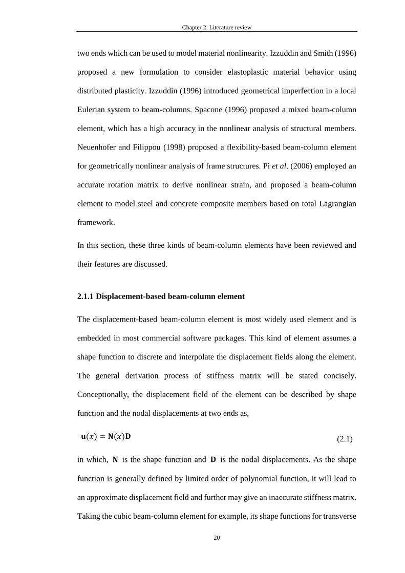
𝐮(𝑥) = 𝐍(𝑥)𝐃 (2.1)
in which, 𝐍 is the shape function and 𝐃 is the nodal displacements. As the shape
function is generally defined by limited order of polynomial function, it will lead to
an approximate displacement field and further may give an inaccurate stiffness matrix.
Taking the cubic beam-column element for example, its shape functions for transverse
Chapter 2. Literature review
21
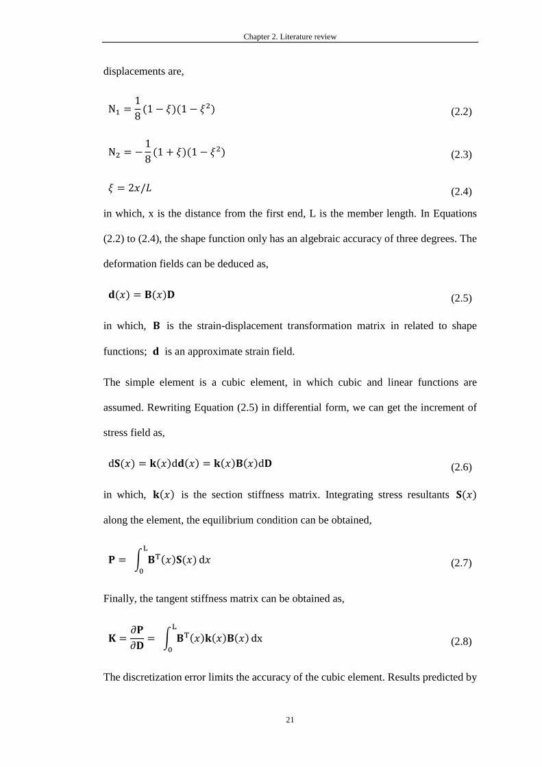
displacements are,
N1 =1
8(1 − 𝜉)(1 − 𝜉2) (2.2)
N2 = −1
8(1 + 𝜉)(1 − 𝜉2) (2.3)
𝜉 = 2𝑥/𝐿 (2.4)
in which, x is the distance from the first end, L is the member length. In Equations
(2.2) to (2.4), the shape function only has an algebraic accuracy of three degrees. The
deformation fields can be deduced as,
𝐝(𝑥) = 𝐁(𝑥)𝐃 (2.5)
in which, 𝐁 is the strain-displacement transformation matrix in related to shape
functions; 𝐝 is an approximate strain field.
The simple element is a cubic element, in which cubic and linear functions are
assumed. Rewriting Equation (2.5) in differential form, we can get the increment of
stress field as,
d𝐒(𝑥) = 𝐤(𝑥)d𝐝(𝑥) = 𝐤(𝑥)𝐁(𝑥)d𝐃 (2.6)
in which, 𝐤(𝑥) is the section stiffness matrix. Integrating stress resultants 𝐒(𝑥)
along the element, the equilibrium condition can be obtained,
𝐏 = ∫ 𝐁T(𝑥)𝐒(𝑥)L
0
d𝑥 (2.7)
Finally, the tangent stiffness matrix can be obtained as,
𝐊 =∂𝐏
∂𝐃= ∫ 𝐁T(𝑥)𝐤(𝑥)𝐁(𝑥)
L
0
dx (2.8)
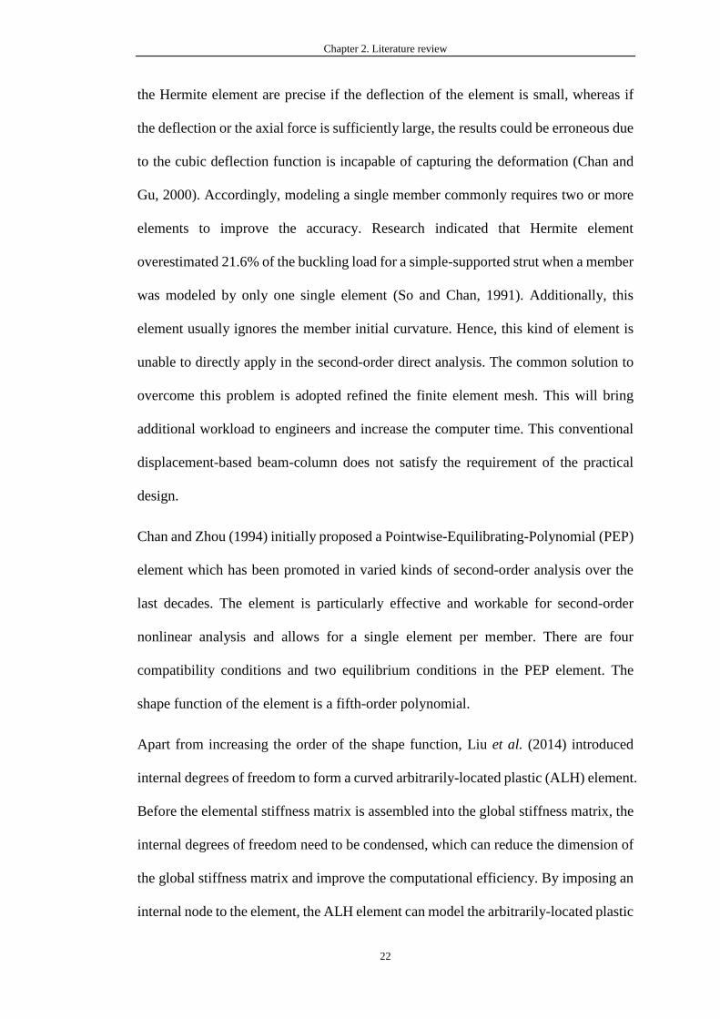
The discretization error limits the accuracy of the cubic element. Results predicted by
Chapter 2. Literature review
22
the Hermite element are precise if the deflection of the element is small, whereas if
the deflection or the axial force is sufficiently large, the results could be erroneous due
to the cubic deflection function is incapable of capturing the deformation (Chan and
Gu, 2000). Accordingly, modeling a single member commonly requires two or more
elements to improve the accuracy. Research indicated that Hermite element
overestimated 21.6% of the buckling load for a simple-supported strut when a member
was modeled by only one single element (So and Chan, 1991). Additionally, this
element usually ignores the member initial curvature. Hence, this kind of element is
unable to directly apply in the second-order direct analysis. The common solution to
overcome this problem is adopted refined the finite element mesh. This will bring
additional workload to engineers and increase the computer time. This conventional
displacement-based beam-column does not satisfy the requirement of the practical
design.
Chan and Zhou (1994) initially proposed a Pointwise-Equilibrating-Polynomial (PEP)
element which has been promoted in varied kinds of second-order analysis over the
last decades. The element is particularly effective and workable for second-order
nonlinear analysis and allows for a single element per member. There are four
compatibility conditions and two equilibrium conditions in the PEP element. The
shape function of the element is a fifth-order polynomial.
Apart from increasing the order of the shape function, Liu et al. (2014) introduced
internal degrees of freedom to form a curved arbitrarily-located plastic (ALH) element.
Before the elemental stiffness matrix is assembled into the global stiffness matrix, the
internal degrees of freedom need to be condensed, which can reduce the dimension of
the global stiffness matrix and improve the computational efficiency. By imposing an
internal node to the element, the ALH element can model the arbitrarily-located plastic
Chapter 2. Literature review
23
hinge along the member. Its capability of material nonlinearity will be discussed in the
following section.
Through the increasing order of the shape function or adding internal nodes, the
accuracy of the displacement-based element is improved. However, these approaches
also lead to the complexity of formula derivation. Miguel Ferreria et al. (2017)
proposed an improved displacement-based element (IDBE) by adding the corrective
fields to alleviate error of the shape functions. The corrective nonlinear strain fields
dNL,0,s are defined as
∫ 𝐁(𝑥)𝐝𝑁𝐿,0,𝑠(𝑥)d𝑥 = 0L
0
(2.9)
Compared with the conventional displacement-based element, its accuracy can be
easily improved by increasing integration points. But internal iteration steps are
needed to determine the element status, and additional parameters associated with
element state are needed to be stored.
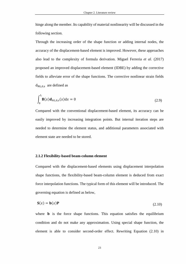
2.1.2 Flexibility-based beam-column element
Compared with the displacement-based elements using displacement interpolation
shape functions, the flexibility-based beam-column element is deduced from exact
force interpolation functions. The typical form of this element will be introduced. The
governing equation is defined as below,
𝐒(𝑥) = 𝐛(𝑥)𝐏 (2.10)
where 𝐛 is the force shape functions. This equation satisfies the equilibrium
condition and do not make any approximation. Using special shape function, the
element is able to consider second-order effect. Rewriting Equation (2.10) in
Chapter 2. Literature review
24
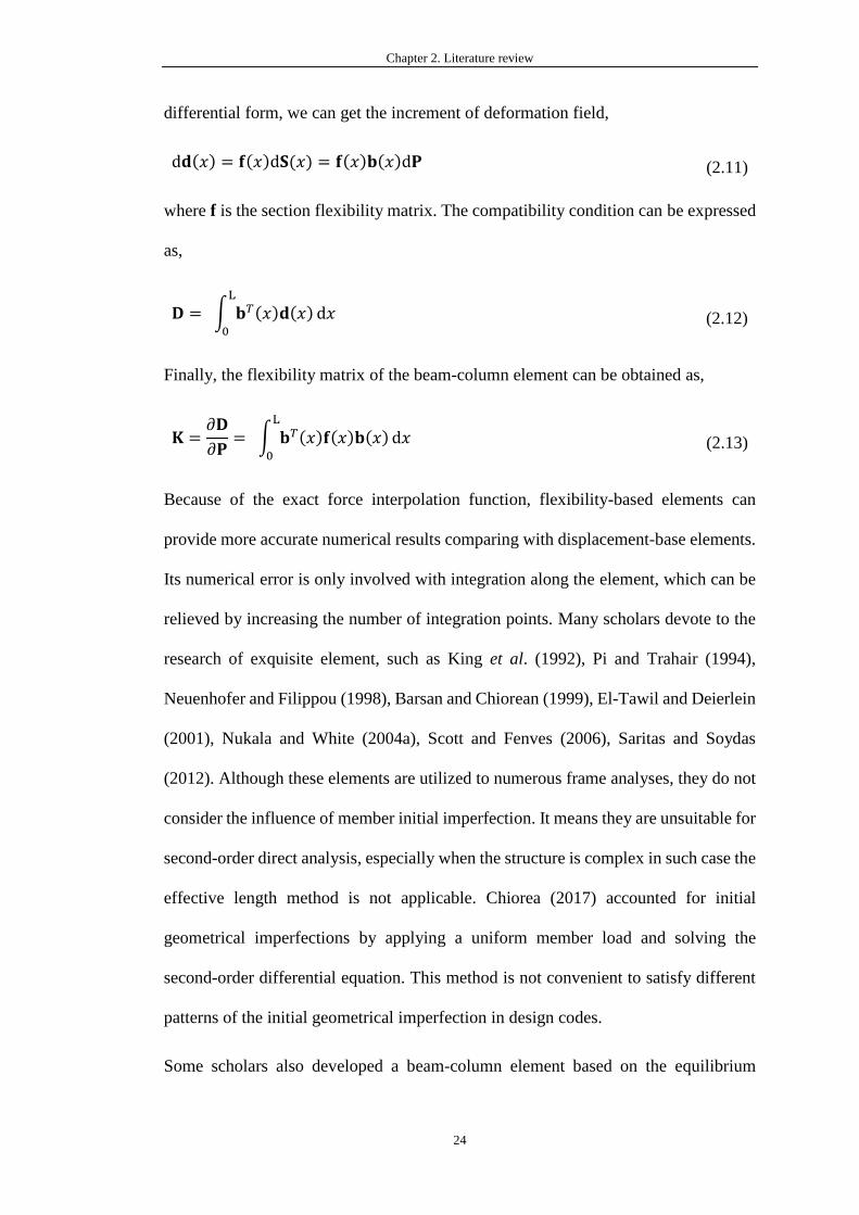
differential form, we can get the increment of deformation field,
d𝐝(𝑥) = 𝐟(𝑥)d𝐒(𝑥) = 𝐟(𝑥)𝐛(𝑥)d𝐏 (2.11)
where f is the section flexibility matrix. The compatibility condition can be expressed
as,
𝐃 = ∫ 𝐛𝑇(𝑥)𝐝(𝑥)L
0
d𝑥 (2.12)
Finally, the flexibility matrix of the beam-column element can be obtained as,
𝐊 =∂𝐃
∂𝐏= ∫ 𝐛𝑇(𝑥)𝐟(𝑥)𝐛(𝑥)
L
0
d𝑥 (2.13)
Because of the exact force interpolation function, flexibility-based elements can
provide more accurate numerical results comparing with displacement-base elements.
Its numerical error is only involved with integration along the element, which can be
relieved by increasing the number of integration points. Many scholars devote to the
research of exquisite element, such as King et al. (1992), Pi and Trahair (1994),
Neuenhofer and Filippou (1998), Barsan and Chiorean (1999), El-Tawil and Deierlein
(2001), Nukala and White (2004a), Scott and Fenves (2006), Saritas and Soydas
(2012). Although these elements are utilized to numerous frame analyses, they do not
consider the influence of member initial imperfection. It means they are unsuitable for
second-order direct analysis, especially when the structure is complex in such case the
effective length method is not applicable. Chiorea (2017) accounted for initial
geometrical imperfections by applying a uniform member load and solving the
second-order differential equation. This method is not convenient to satisfy different
patterns of the initial geometrical imperfection in design codes.
Some scholars also developed a beam-column element based on the equilibrium
Chapter 2. Literature review
25
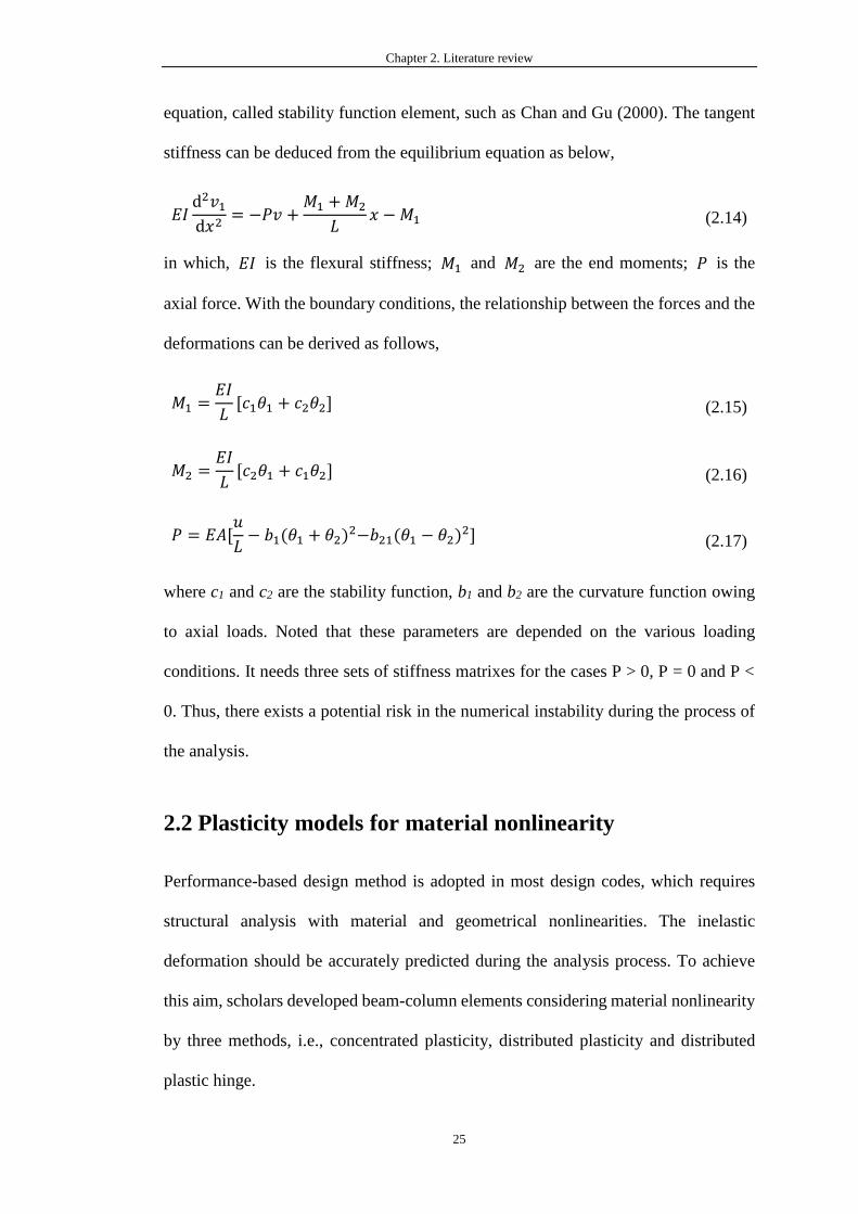
equation, called stability function element, such as Chan and Gu (2000). The tangent
stiffness can be deduced from the equilibrium equation as below,
𝐸𝐼d2𝑣1d𝑥2
= −𝑃𝑣 +𝑀1 +𝑀2
𝐿𝑥 −𝑀1 (2.14)
in which, 𝐸𝐼 is the flexural stiffness; 𝑀1 and 𝑀2 are the end moments; 𝑃 is the
axial force. With the boundary conditions, the relationship between the forces and the
deformations can be derived as follows,
𝑀1 =𝐸𝐼
𝐿[𝑐1𝜃1 + 𝑐2𝜃2] (2.15)
𝑀2 =𝐸𝐼
𝐿[𝑐2𝜃1 + 𝑐1𝜃2] (2.16)
𝑃 = 𝐸𝐴[𝑢
𝐿− 𝑏1(𝜃1 + 𝜃2)
2−𝑏21(𝜃1 − 𝜃2)2] (2.17)
where c1 and c2 are the stability function, b1 and b2 are the curvature function owing
to axial loads. Noted that these parameters are depended on the various loading
conditions. It needs three sets of stiffness matrixes for the cases P > 0, P = 0 and P <
0. Thus, there exists a potential risk in the numerical instability during the process of
the analysis.
2.2 Plasticity models for material nonlinearity
Performance-based design method is adopted in most design codes, which requires
structural analysis with material and geometrical nonlinearities. The inelastic
deformation should be accurately predicted during the analysis process. To achieve
this aim, scholars developed beam-column elements considering material nonlinearity
by three methods, i.e., concentrated plasticity, distributed plasticity and distributed
plastic hinge.
Chapter 2. Literature review
26
2.2.1 Concentrated plasticity
As we known, time history analysis, due to small time increment and some iterations
during the incremental-iterative process, is time-consuming. Concentrated plasticity
method, also well-known as plastic hinge method, is a good compromise between the
accuracy and the computational efficiency and therefore is widely used to consider
material nonlinearity. Plastic hinge method assumes that ideally plastic behavior
occurs at the end of members, and the length of plastic hinge is considered as zero.
Noted that the plastic hinge is lumped only at the end of beam-column elements, while
the rest of the element remains elastic during the analysis. Through defining different
plastic hinge models, the beam-column element with plastic hinge can have various
performance. Several plasticity models will be discussed in the following subsections.
2.2.1.1 Perfectly elastic-plastic hinge model
This model assumes that two ends of the beam-column element remain elastic before
their internal forces reach the cross-section plastic strength. When the internal force
violates the yield criteria surface, the section will be assumed to fully yield and a fully
plastic hinge happens. This model is simple and adopted by many design codes, such
as AISC-LRFD (2011), but it does not consider the gradually yielding process from
elastic to plastic state.
2.2.1.2 Elastic-plastic hinge model
Unlike perfectly elastic-plastic hinge model, the elastic-plastic hinge model can reflect
the degradation of frame section stiffness, which is closer to the actual situation. There
are three types of elastic-plastic hinge models: column tangent modulus model,
Chapter 2. Literature review
27
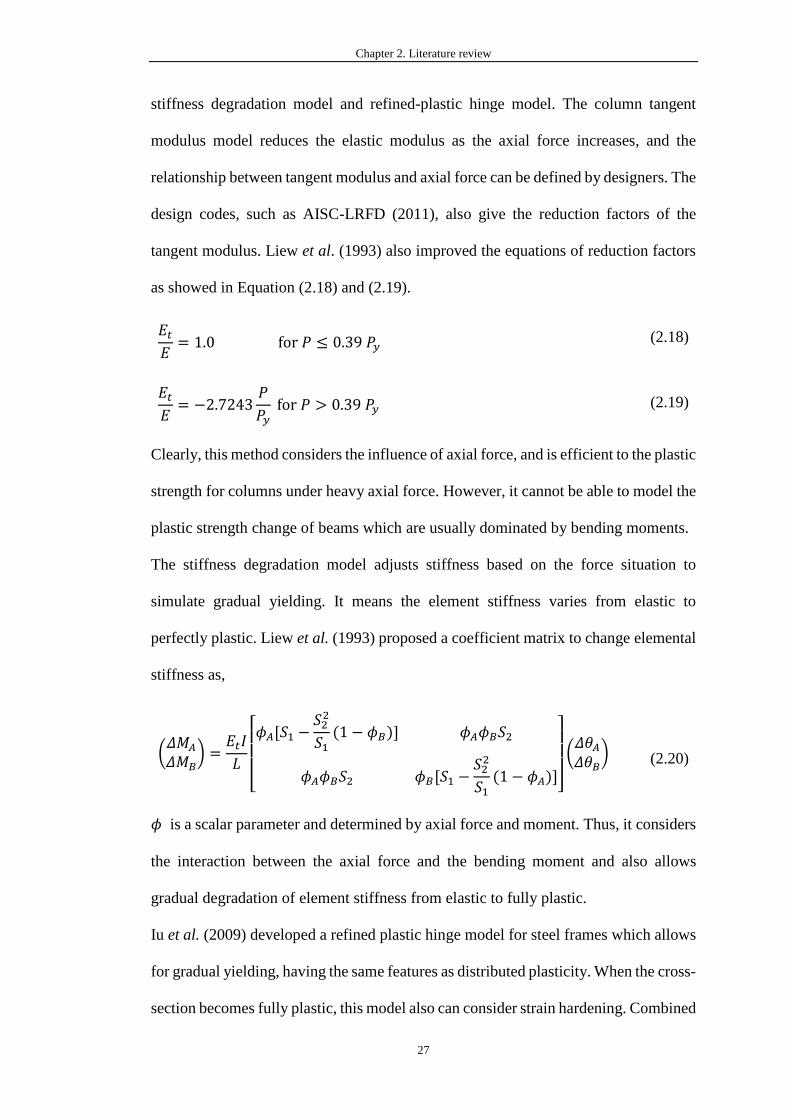
stiffness degradation model and refined-plastic hinge model. The column tangent
modulus model reduces the elastic modulus as the axial force increases, and the
relationship between tangent modulus and axial force can be defined by designers. The
design codes, such as AISC-LRFD (2011), also give the reduction factors of the
tangent modulus. Liew et al. (1993) also improved the equations of reduction factors
as showed in Equation (2.18) and (2.19).
𝐸𝑡𝐸= 1.0 for 𝑃 ≤ 0.39 𝑃𝑦 (2.18)
𝐸𝑡𝐸= −2.7243
𝑃
𝑃𝑦 for 𝑃 > 0.39 𝑃𝑦 (2.19)
Clearly, this method considers the influence of axial force, and is efficient to the plastic
strength for columns under heavy axial force. However, it cannot be able to model the
plastic strength change of beams which are usually dominated by bending moments.
The stiffness degradation model adjusts stiffness based on the force situation to
simulate gradual yielding. It means the element stiffness varies from elastic to
perfectly plastic. Liew et al. (1993) proposed a coefficient matrix to change elemental
stiffness as,
(𝛥𝑀𝐴𝛥𝑀𝐵
) =𝐸𝑡𝐼
𝐿
[ 𝜙𝐴[𝑆1 −
𝑆22
𝑆1(1 − 𝜙𝐵)] 𝜙𝐴𝜙𝐵𝑆2
𝜙𝐴𝜙𝐵𝑆2 𝜙𝐵[𝑆1 −𝑆22
𝑆1(1 − 𝜙𝐴)]]
(𝛥𝜃𝐴𝛥𝜃𝐵
) (2.20)
𝜙 is a scalar parameter and determined by axial force and moment. Thus, it considers
the interaction between the axial force and the bending moment and also allows
gradual degradation of element stiffness from elastic to fully plastic.
Iu et al. (2009) developed a refined plastic hinge model for steel frames which allows
for gradual yielding, having the same features as distributed plasticity. When the cross-
section becomes fully plastic, this model also can consider strain hardening. Combined

Chapter 2. Literature review
28
with a fourth-order beam-column element, it achieves high accuracy and fewer
iterations when solving material nonlinearity problems. In this model, partial plasticity
is modeled by initial yield and full yield functions, and accordingly the axial stiffness
and bending stiffness varies from infinity to zero. For seismic design, Dides and De la
Llera (2005) conducted a dynamic analysis of building structures by the lumped
plasticity models.
The concentrated plasticity model is used not only in modeling steel structures but also
in modeling RC structures. Zhao et al. (2012) adopted the lumped plasticity model to
model RC flexural members and evaluated the plastic-hinge length by comparing with
distributed plasticity model. Babazdeh et al. (2016) also investigated the plastic-hinge
length of RC bridge columns. They found that the plastic hinge model developed for
shorter columns produces a conservative prediction of long RC bridge columns.
Compared with steel structures, the behavior of RC or composite structures is largely
affected by the reinforcement ratio. Generally, the plastic hinge models for RC or
composite structures are section-dependent, and therefore it is inconvenient for
practical use.
2.2.1.3 Stress resultant model
The stress resultant model is also able to model the gradual yielding of frame sections.
This kind of model is derived from the classical material constitutive model. The latter
one is presented in stress space, while the former is described in stress-resultant space.
This model has been used to simulate material nonlinearity of shell sections and frame
sections. Stress resultant model is studied by many scholars, such as Orbison (1982),
Hajjar (1998), Ma (2004), Alemdar (2005). El-Tawil (1998) proposed a bounding
surface plasticity model, which can obtain a better result when using Mroz’s kinematic
Chapter 2. Literature review
29
rule in stress-resultant space. Generalized plasticity firstly was used to model metal
behaviors. This model has only two parameters with clear physical meaning and can
describe the process from elastic to plastic. Auricchio and Taylor (1999, 1995 and
1993) also developed a return map algorithm to determine the stress state, which was
proved to be very efficient. Some scholars extended generalized plasticity concept to
describe stress resultants of frame sections. Kostic (2013, 2016) proposed a
generalized plasticity model to represent the gradual yielding of frame sections. This
model has two surfaces: loading surface and limited surface. The interaction between
the axial force and bending moments has been taken into account. Long and Hung
(2008) introduced the effective strain and the plastic modulus to model gradual
yielding. However, these two parameters are difficult to determine, which lead
inconvenience to practical use.
2.2.2 Distributed plasticity
Though the aforementioned concentrated plasticity models are effective in elastic-
plastic analysis, they are unable to reflect the distribution of plasticity along the
members due to its zero-length assumption. The distributed plasticity models are
developed to overcome the disadvantages of the concentrated plasticity models.
Generally, the distributed plasticity is achieved by fiber section approach. This method
is section-independent, and any frame sections can be discretized to several finite
regions to get more accuracy inelastic response, as seen in Fig. 2.1. The uniaxial
material is imposed to each fiber. It means that the state of each fiber can be
determined by axial strain and curvature of the frame section. The constitutive
relationship of uniaxial material can be defined by users. The models such as elastic-
perfectly plastic with zero tensile strength for concrete and Giuffre-Menegotto-Pinto
Chapter 2. Literature review
30
model for steel have been widely used. Filippou (1983) and Botez et al. (2014)
compared concentrated plastic hinge and distributed plasticity by conducting
progressive collapse analysis. They found that though distributed plasticity costs more
run-time than the plastic hinge method, it can provide more trustful results and make
better progressive collapse verdict. Astroza et al. (2014) adopted distributed plasticity
using fiber sections to identify damage by a nonlinear stochastic filtering technique.
The accuracy of distributed plasticity is affected by the integration scheme and number
of integration points. Scott and Fenves (2006) evaluated several integration schemes
and reported their precision with different number of integration points. He et al. (2016)
tried to resolve this disadvantage by studying the relationship between the optimal
element size and the number of integration points. Though evaluating the possible
plastic-hinge length, the optimal element size can be used to mesh members. In
practice, this method can be used to model frame structures with any sections, such as
steel, RC or composite sections. Based on the distributed plasticity models, Kucukler
et al. (2014) used the stiffness reduction method to capture the effects of residual stress
and geometrical imperfections. Pan et al. (2016) investigated the effect of
reinforcement anchorage slip in the footing by efficient fiber beam-column elements.
In general, the distributed plasticity model performs well in computational accuracy
with wider application range. The main obstacle of this model lies in the less
computational efficiency.
2.3 Modeling of member initial imperfections
As mentioned above, the Pointwise-Equilibrating-Polynomial (PEP) element can
consider member initial imperfection and allow large deflection via only a single
element per member. The PEP element was used for the second-order inelastic

Chapter 2. Literature review
31
analysis of steel frameworks was proposed by Zhou and Chan (2004). An arbitrary
elastic-perfectly plastic hinge can be formed along the element length. The PEP
element was employed to the second-order analysis of single angle trusses and further
validated by experiment results (Chan and Cho, 2008; Cho and Chan, 2008; Fong et
al., 2009). The PEP element was extended to the nonlinear analysis of composite steel
and concrete members and frameworks and verified by a range of experiments (Fong
et al., 2009, 2011). Liu et al. (2010) adopted this element to conduct the pushover
analysis for performance-based seismic design. An imperfection truss element is
proposed by Zhou et al. (2014) to consider geometrically nonlinear buckling and
seismic performance of suspend-dome. However, their work did not consider material
nonlinearity. The ALH element (Liu et al., 2014a, 2014b) can not only model member
P-δ effect directly but also material nonlinearities using the plastic hinge method. Bar-
spring models were developed by Meimand et al. (2013) to simulate geometrical
imperfections and nonlinear material behavior. A set of slope-deflection equations or
closed-form equations (Smith-Pardo and Aristizábal-Ochoa, 1999; Chan and Gu 2000;
Aristizabal-Ochoa 2010) based on the classical stability functions were used to capture
the imperfections by the corresponding beam-column elements. The geometrical-
nonlinear axial factor (Aristizabal-Ochoa, 2000) can include transverse forces caused
by initial imperfections, but these formulas are limited to elastic members. The
stability functions were further refined by Goto and Chen (1987) through a power
series without truncations. Following this research, the power series was formulated,
and a full set of stiffness equations for nonlinear analysis was proposed by Goto and
Chen (1987). Ekhande et al. (1989) recommended a new expression of the stability
functions for the sake of the analysis of three-dimensional frames. Chan and Gu (2000)
developed the stability function including the member initial imperfection for second-
Chapter 2. Literature review
32
order elastic analysis allowing for one element per member. A stability function
accounting for lateral-torsional buckling was proposed by Kim et al. (2006) with
sufficient accuracy for engineering practice.
In summary, there is lack of study on the flexibility-based beam-column elements
incorporating member initial imperfection at the elemental level for second-order
inelastic analysis. Although the studies of stiffness-based beam-column elements
considering initial imperfection are sufficient, this kind of elements does not show
good performance on second-order inelastic analysis.
2.4 Modeling of semi-rigid connections
The connection behavior may significantly affect the system behavior. In such case,
the joint flexibility should be carefully considered in the process of second-order direct
analysis. It is hard to propose a generalized model for connection systems due to their
variety and especially the different geometry of the connected members. Therefore,
experimental tests are commonly used to explore the joint behavior and then some
empirical formulas are developed according to experimental data. A rather
considerable amount of research works on monotonic loading tests and cyclic loading
tests for different connection systems have been conducted in the past few decades,
for example, Prabha et al. (2010). Valuable data about joint behavior have been
collected to form various mathematical functions representing the different nonlinear
behavior of diverse connection types. The details about modeling of connection will
be described in Chapter 5.
After obtaining the formulation of connection models, different semi-rigid connection
modeling approaches are proposed. Asgarian et al. (2015) developed a three-
dimensional joint flexibility element to represent the local behavior of a tubular joint.
Chapter 2. Literature review
33
This element has two nodes with one located at the intersection of diagonal braces and
chord and horizontal braces and chord, and the other one located at the intersection of
the brace centerline with wall of chord. Hence, local joint deformation can be taken
into account during the analysis, and relatively accurate predictions can be produced
by this element. Yu and Zhu (2016) introduced an independent zero-length element to
simulate the connections in the nonlinear dynamic collapse analysis with finite particle
method (FPM). The zero-length element with the hysteretic relationship of moment
and rotation can absorb energy and therefore improve the anti-collapse capacity of the
whole structure. On the contrary, fully rigid or ideally pinned connections do not make
any contribution to the energy absorbing. More importantly, this effect also is in
conjunction with axial forces, which has been ignored by many researchers.
2.5 Design method for CFT members with noncompact and
slender sections
The concrete-filled steel tube (CFT) members have been studied by many researchers
based on experimental tests or numerical simulation. Various loading conditions such
as axial compression, flexural, and their combination were set up to test the complex
behaviors of CFT members. Several parameters, such as yield stress 𝐹𝑦 of the steel
tube, the compressive strength of the concrete infill, width-to-thickness ratios of the
steel tube, column length to depth ratio and so on, were investigated through numerous
tests. However, most experiments force on compact CFT members, such as Nishiyama
et al. (2002), Kim (2005), Gourley et al. (2008) and Hajjar (2013). In contrast, there
is few tests on the noncompact and slender CFT members, which brings about few
researches on the development of design method for these kinds of CFT members.
Chapter 2. Literature review
34
In the field of numerical simulation, the complex behaviors of CFT such as steel tube
yielding, local buckling, concrete confinement, crack, and slippage between the steel
tube and the concrete infill, make them difficult to be directly modeled by numerical
methods for practical use. Generally, there are two categories of modeling methods to
predict the behavior of CFT members: detailed 3D finite element models and simple
beam-column element models. The first method can explicitly account for the effects
of local buckling and hoop stresses in the steel tube, and the effects of confinement on
the concrete infill. Due to the accurate and relative detailing modeling of CFT
members, this method often is used to conduct parameter studies with true experiments
or calibrate other numerical modeling methods by researchers. Lai et al. (2014) built
detailed 3D finite element models to model noncompact or slender rectangular CFT
members to address gaps in the experimental database. Lai and Varma (2015)
conducted varies of parametric studies of noncompact and slender circular CFT
members to by 3D finite element modes. Lam et al. (2012) adopted three-dimensional
8-node solid elements to model the stub concrete-filled steel tubular column with
tapered members. Liew and Xiong (2009) used continuum solid and shell elements to
study the behavior of CFT members with initial preload. Du et al. (2017) adopted 8-
node reduced integration brick elements to study the behaviors of high-strength steel
in CFT members.
The second method adopts beam-column elements to consider the complex behaviors
of CFT members explicitly or implicitly. The explicit one adds extra degrees-of-
freedom to the end nodes of beam-column elements. Tort and Hajjar (2010) extended
the conventional 12 DOF beam element into 18 DOF beam element to consider the
slip deformation between the steel tube and the concrete infill of rectangular CFT
members. Lee and Filippou (2015) proposed a composite frame element to capture the
Chapter 2. Literature review
35
bond-slip behavior at the interface between the steel tube and concrete infill based on
an extension of the Hu-Washizu variational principle. Its highlight is the exact
interpolation of the total section forces. These kinds of beam-column elements,
solving problems, need to introduce additional DOF although they can be condensed
in elemental level. The implicit approach commonly adopts fiber-based beam-column
elements with effective stress-strain relationship to reflect complex behaviors of CFT
members phenomenally. Regarding CFT members with compact sections, there are
several effective stress-strain relationships available to be utilized by fiber-based
beam-column elements, such as Tort and Hajja (2010), Sakino et al. (2004), Han et al.
(2005) and Liang (2009). As for noncompact and slender CFT members, available
effective stress-strain relationships are few. Lai and Varma (2016) proposed effective
stress-strain relationships for noncompact and slender circular or rectangular CFT
members. They also were implemented in a nonlinear fiber analysis macro model to
verify its conservatism. But NFA was only capable of analyzing the problems of P-M.
As for the problems with P-M-M or torsional force, this method was not suitable.
Meanwhile, NFA divided one single CFT member into several components, which
would lead to heavier computer time.
2.6 Design method of special concentrically braced frames
During the last decades, several strong earthquakes happened around the world. These
earthquakes caused huge loss of property and human life. Special concentrically
braced frames (SCBFs) are widely used in high seismic regions due to structural
efficiency and particularly high ductility for energy dissipation. SCBFs are allowed
for large inelastic deformation through tensile yielding, buckling and post-buckling
behaviors of braces. This structural system can provide reasonable lateral stiffness and
Chapter 2. Literature review
36
strength in elastic range, and have advantages on energy dissipation and ductility in
plastic range to achieve operational performance targets. Recently, the performance-
based seismic design (PBSD) is recommended by many modern codes to achieve an
economic design. This design method requires more accurate numerical analysis. For
this reason, the accurate modeling of braces with acceptable computational costs is
vital to capture the real structural behavior of SCBFs subjected to earthquakes.
Lots of scholars proposed modeling methods to capture the complex behaviors of
SCBFs, such as buckling capacity, tensile yielding, post-buckling, the fracture and
post-fracture behavior. Previous researches (Hsiao et al. 2012, 2013; Karamanci and
Lignos 2014; Krishnan 2010; Uriz 2005) show that the initial curvature of steel braces
should be taken into account so that the buckling and post-buckling behavior of steel
braces can be triggered in numerical analysis. Several elements per member are
recommended to capture the complex behavior of braces and accurate prediction
compared to the test results is reported (Hsiao 2012, 2013; Karamanci 2014; Uriz,
2005). This treatment will significantly increase the computational time. Krishnan
(2010) proposes a modified elastoplastic fiber element, which consists of three fiber
segments demarcated by two external nodes and four internal nodes, to simulate the
inelastic behavior of slender columns and braces. However, the element formulation
is too complicated with lower numerical efficiency. Hsiao (2012) modeled the beams,
columns, and braces by fully nonlinear beam-column elements which fail to consider
local second-order effect or 𝑃-𝛿 effect. Meanwhile, this study indicated that a special
node located at the middle of braces must be assigned to model the initial member
imperfection. This is one reason for that muti-elements are needed to model a single
brace. Uriz (2008) suggested that the brace member should be subdivided into two
inelastic beam-column elements for an accurate representation of its complex behavior.
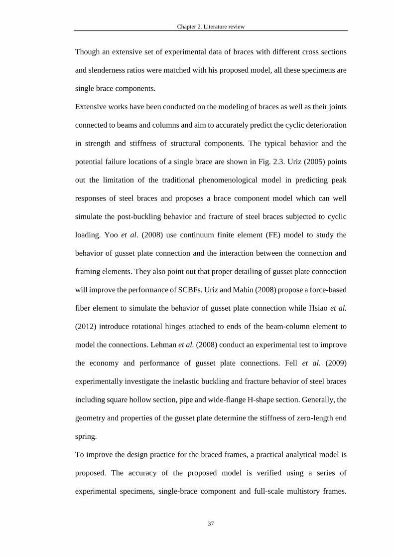
Chapter 2. Literature review
37
Though an extensive set of experimental data of braces with different cross sections
and slenderness ratios were matched with his proposed model, all these specimens are
single brace components.
Extensive works have been conducted on the modeling of braces as well as their joints
connected to beams and columns and aim to accurately predict the cyclic deterioration
in strength and stiffness of structural components. The typical behavior and the
potential failure locations of a single brace are shown in Fig. 2.3. Uriz (2005) points
out the limitation of the traditional phenomenological model in predicting peak
responses of steel braces and proposes a brace component model which can well
simulate the post-buckling behavior and fracture of steel braces subjected to cyclic
loading. Yoo et al. (2008) use continuum finite element (FE) model to study the
behavior of gusset plate connection and the interaction between the connection and
framing elements. They also point out that proper detailing of gusset plate connection
will improve the performance of SCBFs. Uriz and Mahin (2008) propose a force-based
fiber element to simulate the behavior of gusset plate connection while Hsiao et al.
(2012) introduce rotational hinges attached to ends of the beam-column element to
model the connections. Lehman et al. (2008) conduct an experimental test to improve
the economy and performance of gusset plate connections. Fell et al. (2009)
experimentally investigate the inelastic buckling and fracture behavior of steel braces
including square hollow section, pipe and wide-flange H-shape section. Generally, the
geometry and properties of the gusset plate determine the stiffness of zero-length end
spring.
To improve the design practice for the braced frames, a practical analytical model is
proposed. The accuracy of the proposed model is verified using a series of
experimental specimens, single-brace component and full-scale multistory frames.

Chapter 2. Literature review
38
The computation cost of the proposed model was also compared with other fiber-type
finite element model, which uses several elements to model one brace.
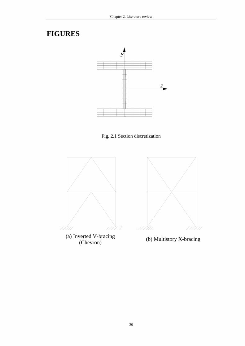
Chapter 2. Literature review
39
FIGURES
Fig. 2.1 Section discretization
z
x
y
Integration Sections
z
y
(a) Inverted V-bracing
(Chevron)(b) Multistory X-bracing (c) X-bracing (d) V-bracing
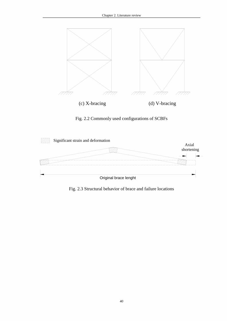
Chapter 2. Literature review
40
Fig. 2.2 Commonly used configurations of SCBFs
Fig. 2.3 Structural behavior of brace and failure locations
(a) Inverted V-bracing
(Chevron)(b) Multistory X-bracing (c) X-bracing (d) V-bracing
Original brace lenght
Significant strain and deformation Axial
shortening
Chapter 3. Flexibility-based beam-column element considering member imperfection
41
CHAPTER 3. FLEXIBILITY-BASED BEAM-
COLUMN ELEMENT CONSIDERING
MEMBER IMPERFECTION
3.1 Introduction
The modern design codes such as AISC360 (2016) and Eurocode-3 (2005) specify a
rational approach, i.e., second-order direct analysis method (DAM), for stability
analysis and design. “Direct Analysis” is also well-known as “Second-order Analysis”
or “Advanced Analysis”. This method has several advantages compared with the
conventional effective length method (ELM). Firstly, it has a wider range of
application as it can be applied to all types of structural systems. Secondly, more
accurate internal forces and moments of members can be captured by direct analysis.
Thirdly, accurate consideration of column restraints brings a rotational design of
beams and connections. Lastly, accessing the member and system stability in an
integrated way makes the whole design procedure simpler without the need of
effective length factor.
General speaking, the factors such as initial imperfection, material yielding, second-
order effects and joint flexibility may affect the deflection and instability of the
structural system. Regarding initial imperfection, it consists of geometrical
imperfections and residual stress. In comparison of DAM, “Indirect Analysis” means
that the analysis ignores one or several key factors above. The second-order effects,
the member initial bowing and their coupling effects make a big contribution to the
geometrical nonlinearity of individual members and the structural system. Therefore,

Chapter 3. Flexibility-based beam-column element considering member imperfection
42
it is necessary to develop a practical second-order beam-column element to consider
the member initial bowing for global analysis. The first global buckling mode is
commonly adopted to determine the frame imperfection as well as the member initial
imperfections in accordance with design codes. The practical design requires a simple
modeling method, using as fewer elements as possible, to model initial out-of-
straightness because more elements will lead to significant increase of modeling
efforts and computer time.
There are several researches focusing on the development of beam-columns elements.
As for displacement-based elements, Chan and Zhou (1995) directly incorporated
member initial bowing in the elemental formulation. And this element has high
accuracy. Liu et al. (2014a, 2014b) also developed a beam-column, using condense
degrees of freedom (DOFs) technology, for second-order direct analysis. Based on the
stability function, Chan and Gu (2000) developed a nonlinear beam-column element
which performs well on modeling highly slender members under axial compressional
force. Furthermore, the refined plastic hinge technique is introduced to the beam-
column element to consider material nonlinearity of steel and composite structures
(Liu et al. 2010, 2012). The element stiffness matrices of the beam-column elements
developed by Chan (1995, 2000) and Liu et al. (2014a, 2014b) were formed by exact
integration method which is better than the numerical integration method regarding
numerical efficiency. Excellent performance and fast convergence are reported in their
works. Ziemian and McGuire (2002) proposed a modified tangent modulus approach
considering residual stress and plastic hinge for second-order inelastic analysis. Their
method is simple and can be easily incorporated into the conventional displacement-
based beam-column elements, but the geometric imperfections are not included at the
element level.
Chapter 3. Flexibility-based beam-column element considering member imperfection
43
For the flexibility-based beam-column elements, extensive works have been done to
improve their performance (Alemdar, 2005; De-Souza, 2000; Jafari, 2010;
Neuenhofer, 1997, 1998; Rezaiee-Pajand 2015; Spacone 1996). Neuenhofer and
Filippou extended the elastic flexibility-based beam-column to consider material
nonlinearity (1997) and second-order effect (1998). Neuenhofer and Filippou (1998)
introduced Newton-Raphson method to determine elemental state and form element
stiffness matrix. Nukala and White (2004a) summarized four algorithms to determine
element state for nonlinear beam-column elements based on Hellinger-Reissner (HR)
variational principle. This principle was adopted by De Souza (2000) to derive the
weak form of equilibrium and compatibility equations for a new flexibility-based
element. With the corotational technology, this new element was capable of large
displacement inelastic analysis of 3-dimensional frame. Though flexibility-based
beam-column elements have been improved largely, they still cannot explicitly model
initial member geometric imperfections which is a vital factor emphasized by
Eurocode-3 (2005) and CoPHK (2011) in the practical design.
From above, displacement-based elements and flexibility-based elements show unique
superiority for computational efficiency and wide application range. The former can
solve problems of geometric nonlinearity with a simple procedure and quick
convergence to get reasonably accurate results, which save much computer time. On
the other hand, the latter shows powerful capacity on geometric and material
nonlinearity. Strict satisfaction of force equilibrium enables it to erase fitting errors of
shape function. Although increasing the number of modeling elements can increase
the accuracy by displacement-based elements, it will bring extra works for modeling
the member initial imperfection and post-processing. Elastic-plasticity problems can
be handled by the displacement-based elements equipped with refined plastic hinge
Chapter 3. Flexibility-based beam-column element considering member imperfection
44
technique by Liew (1993). Recently, the plastic hinges can be formed in arbitrary
location along the member in some elements proposed by Liu et al. (2014a, 2014b).
But they may give inadequate results for the more complicated plastic behavior of
member under complex loading scenarios.
In this study, a second-order flexibility-based beam-column element is proposed for
direct analysis. The equilibrium and compatibility equations are derived by Hellinger-
Reissner (HR) functional. The original work by Neuenhofer (1998) is improved here
by incorporating member initial geometric imperfection at the elemental level to
satisfy the requirements of the practical design. As for geometric nonlinearity, the
effect of 𝑃 − 𝛿 and 𝑃 − 𝛿0 can be directly accounted for. In terms of material
nonlinearity, the distributed plasticity approach is used in the proposed element. The
stiffness matrix of cross-sections at integration points can be assembled by fiber
section technology or be directly calculated by stress-resultant plasticity model, which
will be introduced in Chapter 4.
3.2 Element formulations
The flexibility-based beam-column element proposed by Neuenhofer and Filippou
(1998) will be improved by incorporating initial member geometric imperfection at
the elemental level for direct analysis.
The following assumptions have been adopted in the proposed element:
1. The effect of warping and shear deformation is ignored;
2. Euler-Bernoulli beam theory is adopted by the proposed element.
For simplicity, the proposed element is derived in the elemental basic coordinate
system excluding the rigid body movement. The description of the proposed element
will be arranged as:

Chapter 3. Flexibility-based beam-column element considering member imperfection
45
1. The kinematic hypothesis is presented for the proposed element.
2. The equilibrium and compatibility equations are introduced by the Hellinger-
Reissner (HR) functional.
3. The section flexibility matrix is formed by the integration along the cross-section to
assemble the elemental flexibility matrix.
4. The curvature-based displacement interpolation (CBDI) technique proposed by
Neuenhofer and Filippou (1998) will be briefly introduced to calculate the
displacements of integration points.
5. The transformation from basic coordination system to global coordination system
will be carried out by a corotational approach.
3.2.1 Basic coordinate system
In the global coordinate system, there are six degrees of freedom for each node, i.e.,
three translational and three rotational DOFs, as shown in Fig. 3.1. Excluding the rigid
body modes, the proposed beam-column element can be simply expressed in the
elemental basic coordinate system. In the basic coordinate system, the total degrees of
freedom (DOF) are six, with P for element forces and D for the corresponding end
displacements. They are given below,
𝐏 = {𝑃1 𝑃2 𝑃3 𝑃4 𝑃5 𝑃6}𝑇 = {𝑁 𝑀𝐼𝑧 𝑀𝐽𝑧 𝑀𝐼𝑦 𝑀𝐽𝑦 𝑇}
𝑇 (3.1)
𝐃 = {𝐷1 𝐷2 𝐷3 𝐷4 𝐷5 𝐷6}𝑇 = {𝑢 𝜃𝐼𝑧 𝜃𝐽𝑧 𝜃𝐼𝑦 𝜃𝐽𝑦 𝜓}
𝑇 (3.2)
3.2.2 Kinematic hypothesis
Ignoring the effect of warping, the displacement field of the three-dimensional beam-
column element based on Bernoulli-Euler beam theory can be given as,
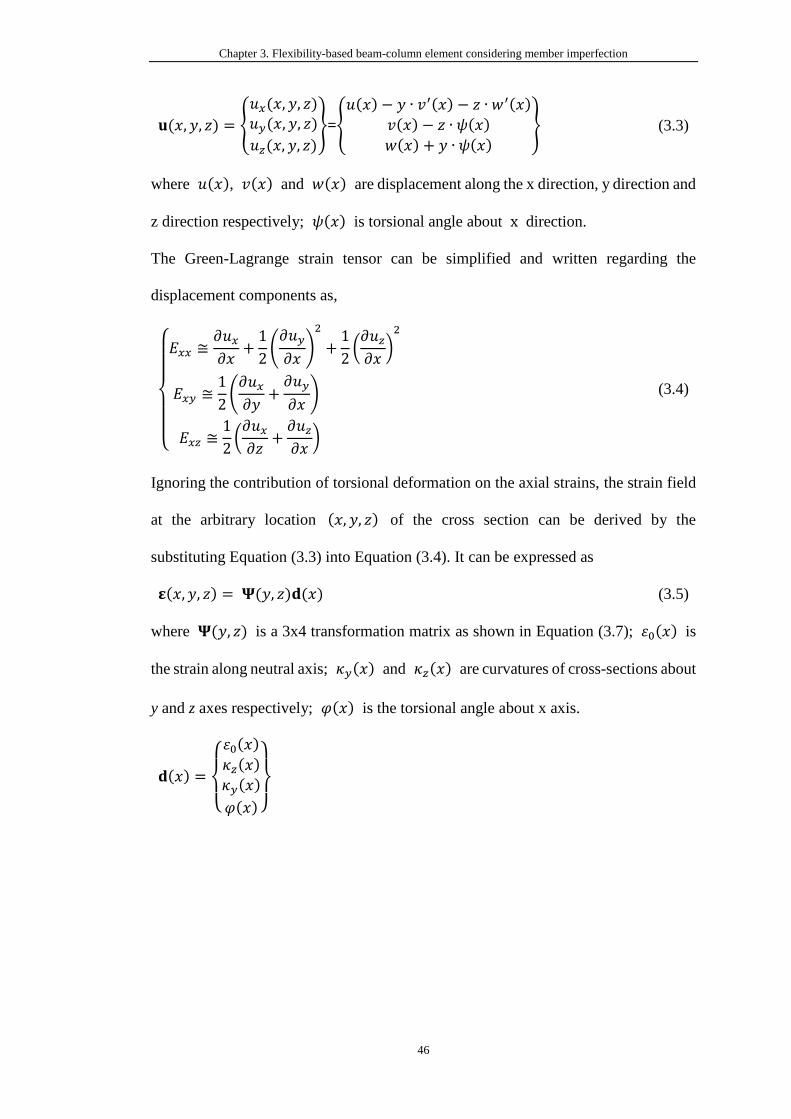
Chapter 3. Flexibility-based beam-column element considering member imperfection
46
𝐮(𝑥, 𝑦, 𝑧) = {
𝑢𝑥(𝑥, 𝑦, 𝑧)𝑢𝑦(𝑥, 𝑦, 𝑧)
𝑢𝑧(𝑥, 𝑦, 𝑧)
}={
𝑢(𝑥) − 𝑦 ∙ 𝑣′(𝑥) − 𝑧 ∙ 𝑤′(𝑥)
𝑣(𝑥) − 𝑧 ∙ 𝜓(𝑥)
𝑤(𝑥) + 𝑦 ∙ 𝜓(𝑥)} (3.3)
where 𝑢(𝑥), 𝑣(𝑥) and 𝑤(𝑥) are displacement along the x direction, y direction and
z direction respectively; 𝜓(𝑥) is torsional angle about x direction.
The Green-Lagrange strain tensor can be simplified and written regarding the
displacement components as,
{
𝐸𝑥𝑥 ≅
𝜕𝑢𝑥𝜕𝑥
+1
2(𝜕𝑢𝑦
𝜕𝑥)
2
+1
2(𝜕𝑢𝑧𝜕𝑥)2
𝐸𝑥𝑦 ≅1
2(𝜕𝑢𝑥𝜕𝑦
+𝜕𝑢𝑦
𝜕𝑥)
𝐸𝑥𝑧 ≅1
2(𝜕𝑢𝑥𝜕𝑧
+𝜕𝑢𝑧𝜕𝑥)
(3.4)
Ignoring the contribution of torsional deformation on the axial strains, the strain field
at the arbitrary location (𝑥, 𝑦, 𝑧) of the cross section can be derived by the
substituting Equation (3.3) into Equation (3.4). It can be expressed as
𝛆(𝑥, 𝑦, 𝑧) = 𝚿(𝑦, 𝑧)𝐝(𝑥) (3.5)
where 𝚿(𝑦, 𝑧) is a 3x4 transformation matrix as shown in Equation (3.7); 휀0(𝑥) is
the strain along neutral axis; 𝜅𝑦(𝑥) and 𝜅𝑧(𝑥) are curvatures of cross-sections about
y and z axes respectively; 𝜑(𝑥) is the torsional angle about x axis.
𝐝(𝑥) =
{
휀0(𝑥)
𝜅𝑧(𝑥)
𝜅𝑦(𝑥)
𝜑(𝑥) }
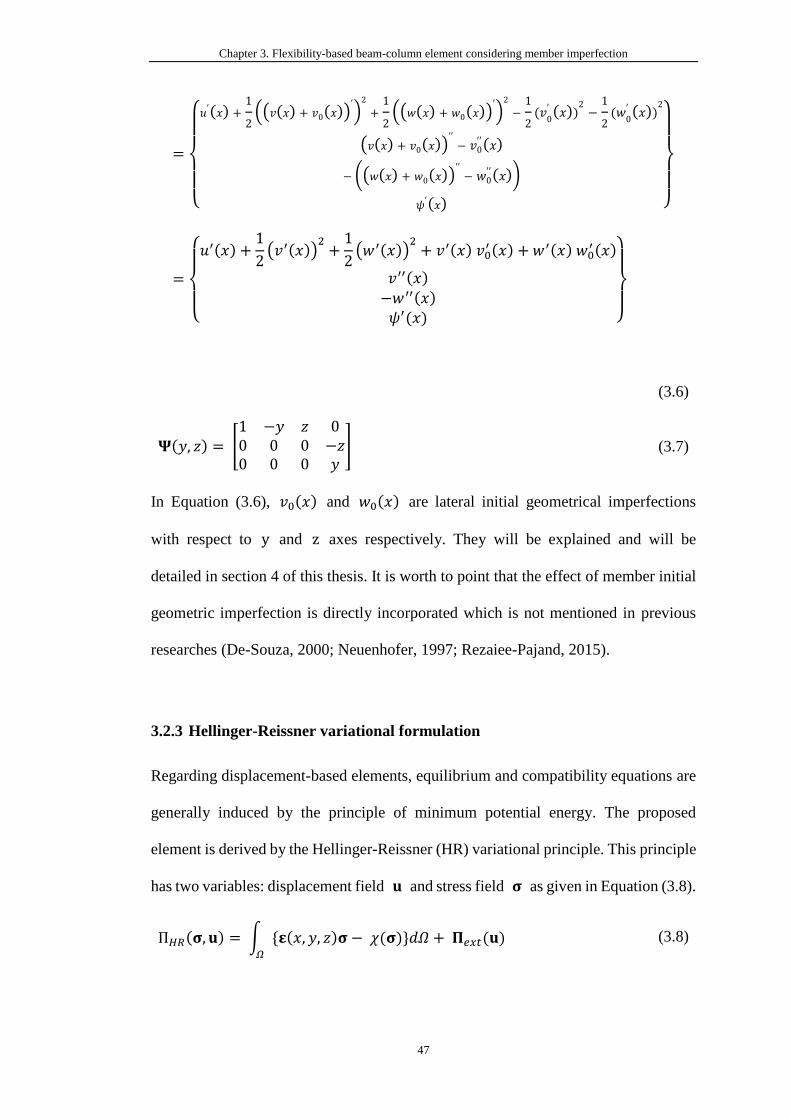
Chapter 3. Flexibility-based beam-column element considering member imperfection
47
=
{
𝑢
′(𝑥) +1
2((𝑣(𝑥) + 𝑣0(𝑥))
′)2
+1
2((𝑤(𝑥) + 𝑤0(𝑥))
′)2
−1
2(𝑣0′ (𝑥))
2−1
2(𝑤
0′ (𝑥))
2
(𝑣(𝑥) + 𝑣0(𝑥))′′− 𝑣0
′′(𝑥)
− ((𝑤(𝑥) + 𝑤0(𝑥))′′− 𝑤0
′′(𝑥))
𝜓′(𝑥) }
=
{
𝑢′(𝑥) +
1
2(𝑣′(𝑥))
2+1
2(𝑤′(𝑥))
2+ 𝑣′(𝑥) 𝑣0
′ (𝑥) + 𝑤′(𝑥) 𝑤0′(𝑥)
𝑣′′(𝑥)
−𝑤′′(𝑥)
𝜓′(𝑥) }
(3.6)
𝚿(𝑦, 𝑧) = [1 −𝑦 𝑧 00 0 0 −𝑧0 0 0 𝑦
] (3.7)
In Equation (3.6), 𝑣0(𝑥) and 𝑤0(𝑥) are lateral initial geometrical imperfections
with respect to y and z axes respectively. They will be explained and will be
detailed in section 4 of this thesis. It is worth to point that the effect of member initial
geometric imperfection is directly incorporated which is not mentioned in previous
researches (De-Souza, 2000; Neuenhofer, 1997; Rezaiee-Pajand, 2015).
3.2.3 Hellinger-Reissner variational formulation
Regarding displacement-based elements, equilibrium and compatibility equations are
generally induced by the principle of minimum potential energy. The proposed
element is derived by the Hellinger-Reissner (HR) variational principle. This principle
has two variables: displacement field 𝐮 and stress field 𝛔 as given in Equation (3.8).
Π𝐻𝑅(𝛔, 𝐮) = ∫ {𝛆(𝑥, 𝑦, 𝑧)𝛔 − 𝜒(𝛔)}𝑑𝛺𝛺
+ 𝚷𝑒𝑥𝑡(𝐮) (3.8)
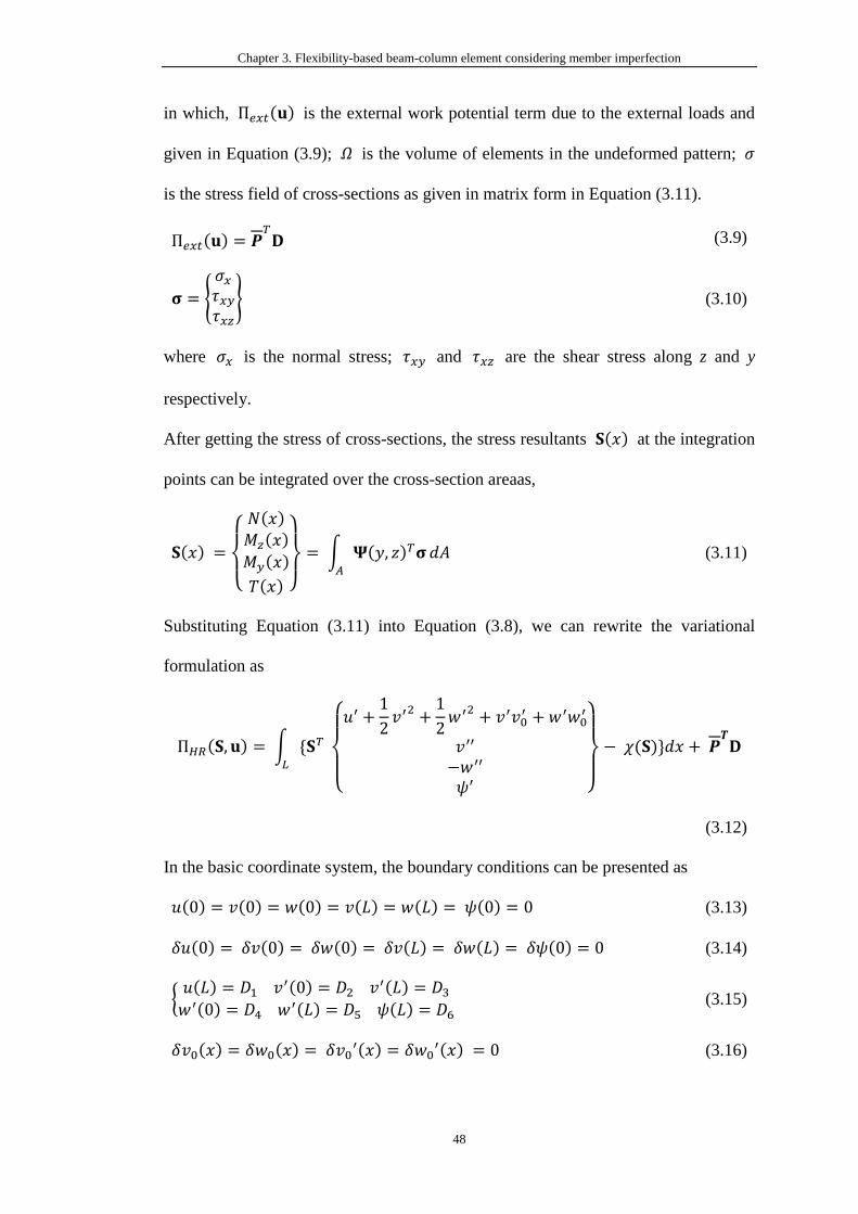
Chapter 3. Flexibility-based beam-column element considering member imperfection
48
in which, Π𝑒𝑥𝑡(𝐮) is the external work potential term due to the external loads and
given in Equation (3.9); 𝛺 is the volume of elements in the undeformed pattern; 𝜎
is the stress field of cross-sections as given in matrix form in Equation (3.11).
Π𝑒𝑥𝑡(𝐮) = 𝑷𝑇𝐃 (3.9)
𝛔 = {
𝜎𝑥𝜏𝑥𝑦𝜏𝑥𝑧} (3.10)
where 𝜎𝑥 is the normal stress; 𝜏𝑥𝑦 and 𝜏𝑥𝑧 are the shear stress along z and y
respectively.
After getting the stress of cross-sections, the stress resultants 𝐒(𝑥) at the integration
points can be integrated over the cross-section areaas,
𝐒(𝑥) =
{
𝑁(𝑥)
𝑀𝑧(𝑥)
𝑀𝑦(𝑥)
𝑇(𝑥) }
= ∫ 𝚿(𝑦, 𝑧)𝑇𝛔𝐴
𝑑𝐴 (3.11)
Substituting Equation (3.11) into Equation (3.8), we can rewrite the variational
formulation as
Π𝐻𝑅(𝐒, 𝐮) = ∫ {𝐒𝑇
{
𝑢′ +
1
2𝑣′2+1
2𝑤′2 + 𝑣′𝑣0
′ + 𝑤′𝑤0′
𝑣′′
−𝑤′′
𝜓′ }
− 𝜒(𝐒)}𝑑𝑥𝐿
+ 𝑷𝑻𝐃
(3.12)
In the basic coordinate system, the boundary conditions can be presented as
𝑢(0) = 𝑣(0) = 𝑤(0) = 𝑣(𝐿) = 𝑤(𝐿) = 𝜓(0) = 0 (3.13)
𝛿𝑢(0) = 𝛿𝑣(0) = 𝛿𝑤(0) = 𝛿𝑣(𝐿) = 𝛿𝑤(𝐿) = 𝛿𝜓(0) = 0 (3.14)
{𝑢(𝐿) = 𝐷1 𝑣
′(0) = 𝐷2 𝑣′(𝐿) = 𝐷3
𝑤′(0) = 𝐷4 𝑤′(𝐿) = 𝐷5 𝜓(𝐿) = 𝐷6
(3.15)
𝛿𝑣0(𝑥) = 𝛿𝑤0(𝑥) = 𝛿𝑣0′(𝑥) = 𝛿𝑤0
′(𝑥) = 0 (3.16)
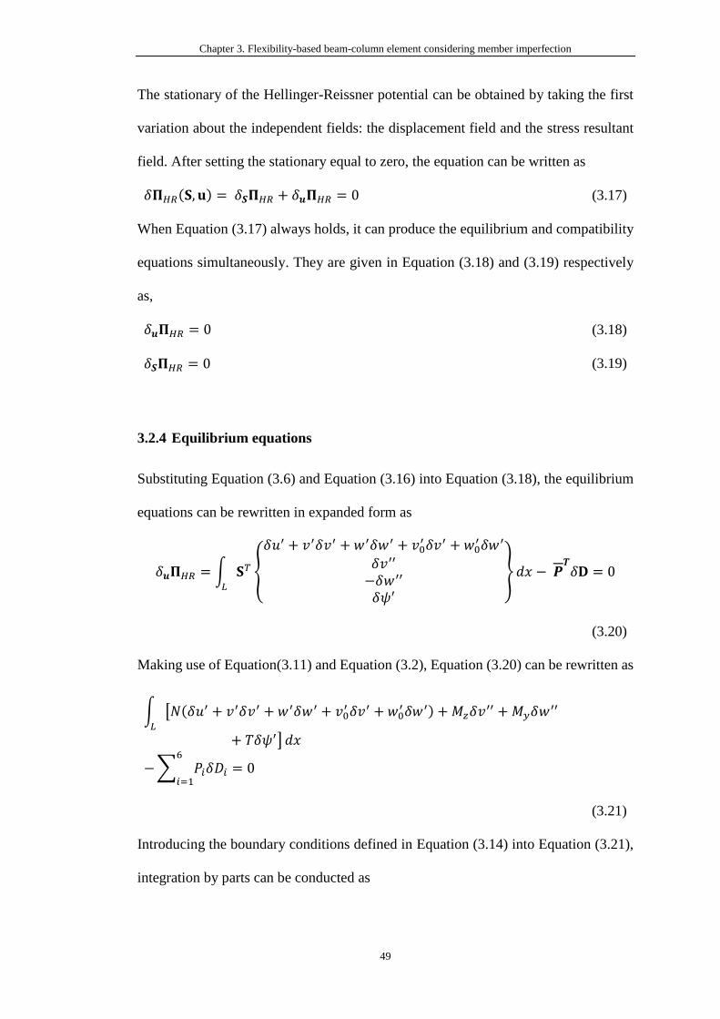
Chapter 3. Flexibility-based beam-column element considering member imperfection
49
The stationary of the Hellinger-Reissner potential can be obtained by taking the first
variation about the independent fields: the displacement field and the stress resultant
field. After setting the stationary equal to zero, the equation can be written as
𝛿𝚷𝐻𝑅(𝐒, 𝐮) = 𝛿𝑺𝚷𝐻𝑅 + 𝛿𝒖𝚷𝐻𝑅 = 0 (3.17)
When Equation (3.17) always holds, it can produce the equilibrium and compatibility
equations simultaneously. They are given in Equation (3.18) and (3.19) respectively
as,
𝛿𝒖𝚷𝐻𝑅 = 0 (3.18)
𝛿𝑺𝚷𝐻𝑅 = 0 (3.19)
3.2.4 Equilibrium equations
Substituting Equation (3.6) and Equation (3.16) into Equation (3.18), the equilibrium
equations can be rewritten in expanded form as
𝛿𝒖𝚷𝐻𝑅 = ∫ 𝐒𝑇
𝐿
{
𝛿𝑢′ + 𝑣′𝛿𝑣′ + 𝑤′𝛿𝑤′ + 𝑣0′𝛿𝑣′ + 𝑤0
′𝛿𝑤′
𝛿𝑣′′
−𝛿𝑤′′
𝛿𝜓′
}𝑑𝑥 − 𝑷𝑻𝛿𝐃 = 0
(3.20)
Making use of Equation(3.11) and Equation (3.2), Equation (3.20) can be rewritten as
∫ [𝑁(𝛿𝑢′ + 𝑣′𝛿𝑣′ + 𝑤′𝛿𝑤′ + 𝑣0′𝛿𝑣′ +𝑤0
′𝛿𝑤′) + 𝑀𝑧𝛿𝑣′′ +𝑀𝑦𝛿𝑤
′′
𝐿
+ 𝑇𝛿𝜓′] 𝑑𝑥
−∑ 𝑃𝑖𝛿𝐷𝑖6
𝑖=1= 0
(3.21)
Introducing the boundary conditions defined in Equation (3.14) into Equation (3.21),
integration by parts can be conducted as
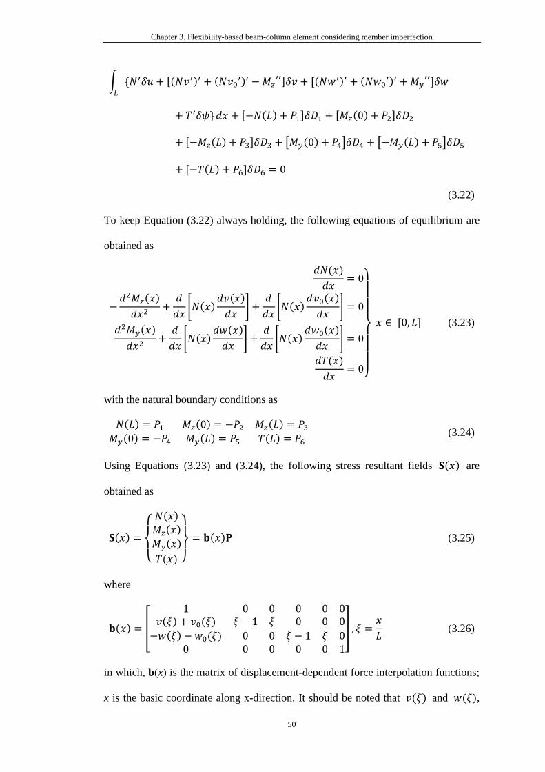
Chapter 3. Flexibility-based beam-column element considering member imperfection
50
∫ {𝑁′𝛿𝑢 + [(𝑁𝑣′)′ + (𝑁𝑣0′)′ −𝑀𝑧
′′]𝛿𝑣 + [(𝑁𝑤′)′ + (𝑁𝑤0′)′ +𝑀𝑦
′′]𝛿𝑤𝐿
+ 𝑇′𝛿𝜓} 𝑑𝑥 + [−𝑁(𝐿) + 𝑃1]𝛿𝐷1 + [𝑀𝑧(0) + 𝑃2]𝛿𝐷2
+ [−𝑀𝑧(𝐿) + 𝑃3]𝛿𝐷3 + [𝑀𝑦(0) + 𝑃4]𝛿𝐷4 + [−𝑀𝑦(𝐿) + 𝑃5]𝛿𝐷5
+ [−𝑇(𝐿) + 𝑃6]𝛿𝐷6 = 0
(3.22)
To keep Equation (3.22) always holding, the following equations of equilibrium are
obtained as
𝑑𝑁(𝑥)
𝑑𝑥= 0
−𝑑2𝑀𝑧(𝑥)
𝑑𝑥2+𝑑
𝑑𝑥[𝑁(𝑥)
𝑑𝑣(𝑥)
𝑑𝑥] +
𝑑
𝑑𝑥[𝑁(𝑥)
𝑑𝑣0(𝑥)
𝑑𝑥] = 0
𝑑2𝑀𝑦(𝑥)
𝑑𝑥2+𝑑
𝑑𝑥[𝑁(𝑥)
𝑑𝑤(𝑥)
𝑑𝑥] +
𝑑
𝑑𝑥[𝑁(𝑥)
𝑑𝑤0(𝑥)
𝑑𝑥] = 0
𝑑𝑇(𝑥)
𝑑𝑥= 0}
𝑥 ∈ [0, 𝐿] (3.23)
with the natural boundary conditions as
𝑁(𝐿) = 𝑃1 𝑀𝑧(0) = −𝑃2 𝑀𝑧(𝐿) = 𝑃3𝑀𝑦(0) = −𝑃4 𝑀𝑦(𝐿) = 𝑃5 𝑇(𝐿) = 𝑃6
(3.24)
Using Equations (3.23) and (3.24), the following stress resultant fields 𝐒(𝑥) are
obtained as
𝐒(𝑥) =
{
𝑁(𝑥)
𝑀𝑧(𝑥)
𝑀𝑦(𝑥)
𝑇(𝑥) }
= 𝐛(𝑥)𝐏 (3.25)
where
𝐛(𝑥) = [
1 0 0 0 0 0𝑣(𝜉) + 𝑣0(𝜉) 𝜉 − 1 𝜉 0 0 0
−𝑤(𝜉) − 𝑤0(𝜉) 0 0 𝜉 − 1 𝜉 00 0 0 0 0 1
] , 𝜉 =𝑥
𝐿 (3.26)
in which, b(x) is the matrix of displacement-dependent force interpolation functions;
x is the basic coordinate along x-direction. It should be noted that 𝑣(𝜉) and 𝑤(𝜉),

Chapter 3. Flexibility-based beam-column element considering member imperfection
51
being included in Equation (3.25), are denoted the P- effect due to external loads.
Meanwhile, 𝑣0(𝜉) and 𝑤0(𝜉) represent the initial imperfections.
3.2.5 Compatibility equations
The compatibility equations are introduced weakly using Equation (3.19), which can
be further expressed as
𝛿𝑺𝚷𝐻𝑅 = ∫ 𝛿𝐒𝑇
𝐿
[
{
𝑢′ +
1
2𝑣′2+1
2𝑤′2 + 𝑣′𝑣0
′ +𝑤′𝑤0′
𝑣′′
−𝑤′′
𝜓′ }
−𝜕𝜒(𝐒)
𝜕𝐒
]
𝑑𝑥 = 0
(3.27)
Based on the definition of the complementary energy density, the deformation of
cross-sections can be given as
𝜕𝜒(𝐒)
𝜕𝐒= 𝐝(𝑥) =
{
휀0(𝑥)
𝜅𝑧(𝑥)
𝜅𝑦(𝑥)
𝜑(𝑥) }
(3.28)
Then, substituting Equation (3.28) into Equation (3.27), we have
∫ [𝛿𝑁 (𝑢′ +1
2𝑣′2 +
1
2𝑤′2 + 𝑣′𝑣0
′ + 𝑤′𝑤0′ − 휀0) + 𝛿𝑀𝑧(𝑣
′′ − 𝜅𝑧)𝐿
+ 𝛿𝑀𝑦(−𝑤′′ − 𝜅𝑦) + 𝛿𝑇(𝜓
′ − 𝜑)] 𝑑𝑥 = 0
(3.29)
Considering the boundary conditions in Equation (3.15), Equation (3.29) can be
integrated by parts as
∫ {𝛿𝑁′𝑢 + [1
2(𝛿𝑁𝑣′)′ + (𝛿𝑁𝑣0
′)′ − 𝛿𝑀𝑧′′] 𝑣 + [
1
2(𝛿𝑁𝑤′)′ + (𝛿𝑁𝑤0
′)′ + 𝛿𝑀𝑦′′]𝑤
𝐿
+𝛿𝑁휀0 + 𝛿𝑀𝑧𝜅𝑧 + 𝛿𝑀𝑦𝜅𝑦 + 𝛿𝑇𝜑}𝑑𝑥
−𝛿𝑁(𝐿)𝐷1 + 𝛿𝑀𝑧(0)𝐷2 − 𝛿𝑀𝑧(𝐿)𝐷3 + 𝛿𝑀𝑦(0)𝐷4 − 𝛿𝑀𝑦(𝐿)𝐷5 − 𝛿𝑇(𝐿)𝐷6 = 0
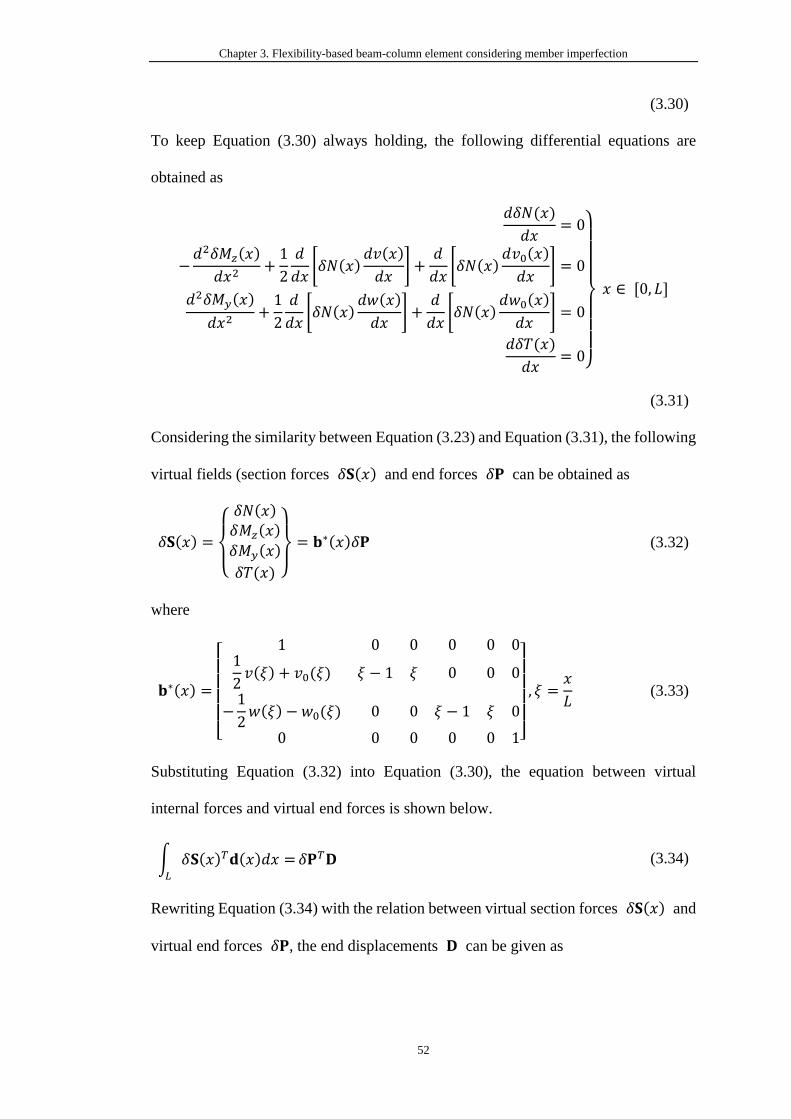
Chapter 3. Flexibility-based beam-column element considering member imperfection
52
(3.30)
To keep Equation (3.30) always holding, the following differential equations are
obtained as
𝑑𝛿𝑁(𝑥)
𝑑𝑥= 0
−𝑑2𝛿𝑀𝑧(𝑥)
𝑑𝑥2+1
2
𝑑
𝑑𝑥[𝛿𝑁(𝑥)
𝑑𝑣(𝑥)
𝑑𝑥] +
𝑑
𝑑𝑥[𝛿𝑁(𝑥)
𝑑𝑣0(𝑥)
𝑑𝑥] = 0
𝑑2𝛿𝑀𝑦(𝑥)
𝑑𝑥2+1
2
𝑑
𝑑𝑥[𝛿𝑁(𝑥)
𝑑𝑤(𝑥)
𝑑𝑥] +
𝑑
𝑑𝑥[𝛿𝑁(𝑥)
𝑑𝑤0(𝑥)
𝑑𝑥] = 0
𝑑𝛿𝑇(𝑥)
𝑑𝑥= 0}
𝑥 ∈ [0, 𝐿]
(3.31)
Considering the similarity between Equation (3.23) and Equation (3.31), the following
virtual fields (section forces 𝛿𝐒(𝑥) and end forces 𝛿𝐏 can be obtained as
𝛿𝐒(𝑥) =
{
𝛿𝑁(𝑥)
𝛿𝑀𝑧(𝑥)
𝛿𝑀𝑦(𝑥)
𝛿𝑇(𝑥) }
= 𝐛∗(𝑥)𝛿𝐏 (3.32)
where
𝐛∗(𝑥) =
[
1 0 0 0 0 01
2𝑣(𝜉) + 𝑣0(𝜉) 𝜉 − 1 𝜉 0 0 0
−1
2𝑤(𝜉) − 𝑤0(𝜉) 0 0 𝜉 − 1 𝜉 0
0 0 0 0 0 1]
, 𝜉 =𝑥
𝐿 (3.33)
Substituting Equation (3.32) into Equation (3.30), the equation between virtual
internal forces and virtual end forces is shown below.
∫ 𝛿𝐒(𝑥)𝑇𝐝(𝑥)𝑑𝑥 =𝐿
𝛿𝐏𝑇𝐃 (3.34)
Rewriting Equation (3.34) with the relation between virtual section forces 𝛿𝐒(𝑥) and
virtual end forces 𝛿𝐏, the end displacements 𝐃 can be given as
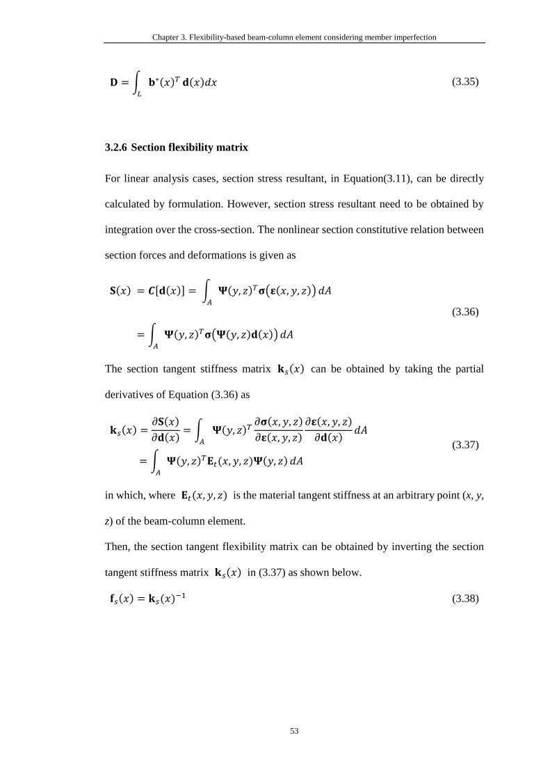
Chapter 3. Flexibility-based beam-column element considering member imperfection
53
𝐃 = ∫ 𝐛∗(𝑥)𝑇
𝐿
𝐝(𝑥)𝑑𝑥 (3.35)
3.2.6 Section flexibility matrix
For linear analysis cases, section stress resultant, in Equation(3.11), can be directly
calculated by formulation. However, section stress resultant need to be obtained by
integration over the cross-section. The nonlinear section constitutive relation between
section forces and deformations is given as
𝐒(𝑥) = 𝑪[𝐝(𝑥)] = ∫ 𝚿(𝑦, 𝑧)𝑇𝛔(𝛆(𝑥, 𝑦, 𝑧))𝐴
𝑑𝐴
= ∫ 𝚿(𝑦, 𝑧)𝑇𝛔(𝚿(𝑦, 𝑧)𝐝(𝑥))𝐴
𝑑𝐴
(3.36)
The section tangent stiffness matrix 𝐤𝑠(𝑥) can be obtained by taking the partial
derivatives of Equation (3.36) as
𝐤𝑠(𝑥) =𝜕𝐒(𝑥)
𝜕𝐝(𝑥)= ∫ 𝚿(𝑦, 𝑧)𝑇
𝜕𝛔(𝑥, 𝑦, 𝑧)
𝜕𝛆(𝑥, 𝑦, 𝑧)
𝜕𝛆(𝑥, 𝑦, 𝑧)
𝜕𝐝(𝑥)𝐴
𝑑𝐴
= ∫ 𝚿(𝑦, 𝑧)𝑇𝐄𝑡(𝑥, 𝑦, 𝑧)𝚿(𝑦, 𝑧)𝐴
𝑑𝐴
(3.37)
in which, where 𝐄𝑡(𝑥, 𝑦, 𝑧) is the material tangent stiffness at an arbitrary point (x, y,
z) of the beam-column element.
Then, the section tangent flexibility matrix can be obtained by inverting the section
tangent stiffness matrix 𝐤𝑠(𝑥) in (3.37) as shown below.
𝐟𝑠(𝑥) = 𝐤𝑠(𝑥)−1 (3.38)
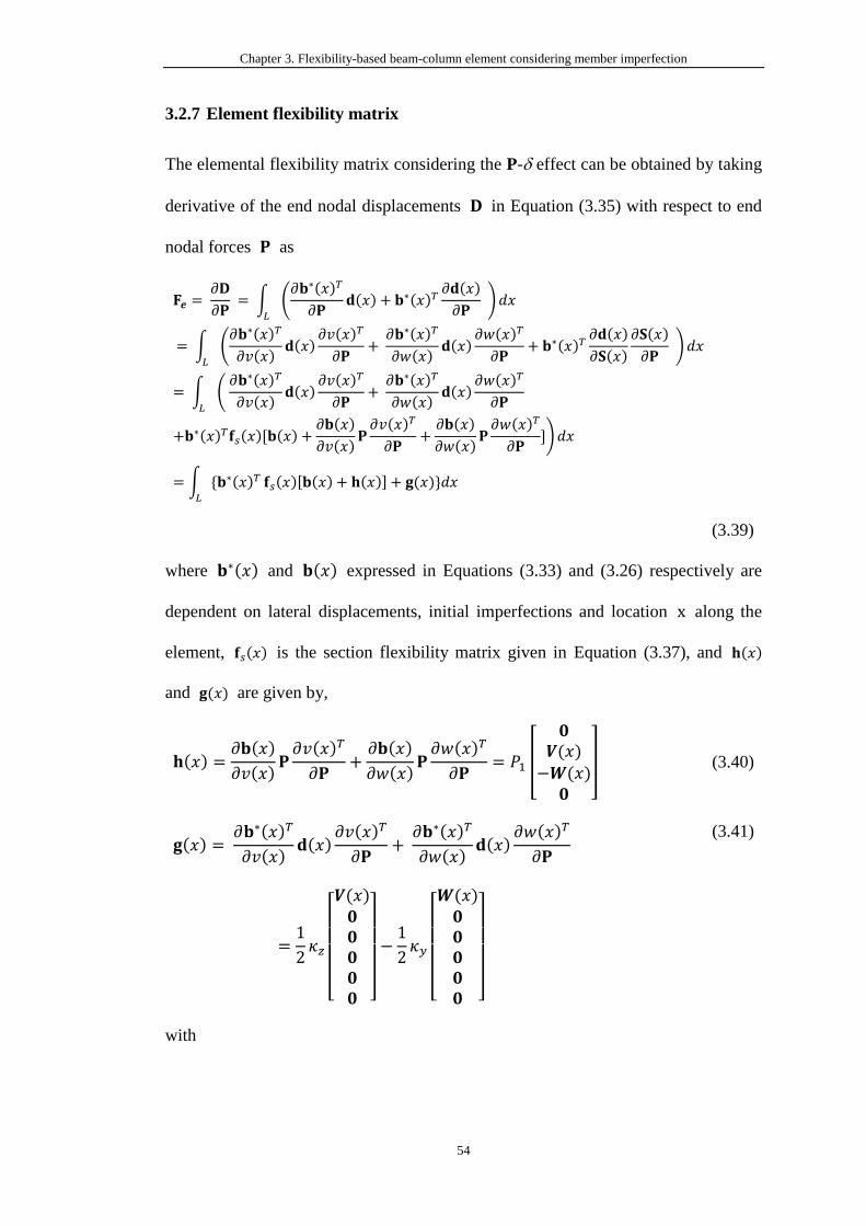
Chapter 3. Flexibility-based beam-column element considering member imperfection
54
3.2.7 Element flexibility matrix
The elemental flexibility matrix considering the P- effect can be obtained by taking
derivative of the end nodal displacements 𝐃 in Equation (3.35) with respect to end
nodal forces 𝐏 as
𝐅𝒆 = 𝜕𝐃
𝜕𝐏 = ∫ (
𝜕𝐛∗(𝑥)𝑇
𝜕𝐏𝐝(𝑥) + 𝐛∗(𝑥)𝑇
𝜕𝐝(𝑥)
𝜕𝐏 ) 𝑑𝑥
𝐿
= ∫ (𝜕𝐛∗(𝑥)𝑇
𝜕𝑣(𝑥)𝐝(𝑥)
𝜕𝑣(𝑥)𝑇
𝜕𝐏+ 𝜕𝐛∗(𝑥)𝑇
𝜕𝑤(𝑥)𝐝(𝑥)
𝜕𝑤(𝑥)𝑇
𝜕𝐏+ 𝐛∗(𝑥)𝑇
𝜕𝐝(𝑥)
𝜕𝐒(𝑥)
𝜕𝐒(𝑥)
𝜕𝐏 ) 𝑑𝑥
𝐿
= ∫ ( 𝜕𝐛∗(𝑥)𝑇
𝜕𝑣(𝑥)𝐝(𝑥)
𝜕𝑣(𝑥)𝑇
𝜕𝐏+ 𝜕𝐛∗(𝑥)𝑇
𝜕𝑤(𝑥)𝐝(𝑥)
𝜕𝑤(𝑥)𝑇
𝜕𝐏𝐿
+𝐛∗(𝑥)𝑇𝐟𝑠(𝑥)[𝐛(𝑥) +𝜕𝐛(𝑥)
𝜕𝑣(𝑥)𝐏𝜕𝑣(𝑥)𝑇
𝜕𝐏+𝜕𝐛(𝑥)
𝜕𝑤(𝑥)𝐏𝜕𝑤(𝑥)𝑇
𝜕𝐏])𝑑𝑥
= ∫ {𝐛∗(𝑥)𝑇
𝐿
𝐟𝑠(𝑥)[𝐛(𝑥) + 𝐡(𝑥)] + 𝐠(𝑥)}𝑑𝑥
(3.39)
where 𝐛∗(𝑥) and 𝐛(𝑥) expressed in Equations (3.33) and (3.26) respectively are
dependent on lateral displacements, initial imperfections and location x along the
element, 𝐟𝑠(𝑥) is the section flexibility matrix given in Equation (3.37), and 𝐡(𝑥)
and 𝐠(𝑥) are given by,
𝐡(𝑥) =𝜕𝐛(𝑥)
𝜕𝑣(𝑥)𝐏𝜕𝑣(𝑥)𝑇
𝜕𝐏+𝜕𝐛(𝑥)
𝜕𝑤(𝑥)𝐏𝜕𝑤(𝑥)𝑇
𝜕𝐏= 𝑃1 [
𝟎𝑽(𝑥)−𝑾(𝑥)𝟎
] (3.40)
𝐠(𝑥) = 𝜕𝐛∗(𝑥)𝑇
𝜕𝑣(𝑥)𝐝(𝑥)
𝜕𝑣(𝑥)𝑇
𝜕𝐏+ 𝜕𝐛∗(𝑥)𝑇
𝜕𝑤(𝑥)𝐝(𝑥)
𝜕𝑤(𝑥)𝑇
𝜕𝐏
=1
2𝜅𝑧
[ 𝑽(𝑥)𝟎𝟎𝟎𝟎𝟎 ]
−1
2𝜅𝑦
[ 𝑾(𝑥)𝟎𝟎𝟎𝟎𝟎 ]
(3.41)
with
Chapter 3. Flexibility-based beam-column element considering member imperfection
55
𝑽(𝑥) =𝜕𝑣(𝑥)
𝜕𝑷= [
𝜕𝑣(𝑥)
𝜕𝑃1
𝜕𝑣(𝑥)
𝜕𝑃2
𝜕𝑣(𝑥)
𝜕𝑃3
𝜕𝑣(𝑥)
𝜕𝑃4
𝜕𝑣(𝑥)
𝜕𝑃5
𝜕𝑣(𝑥)
𝜕𝑃6] (3.42)
𝑾(𝑥) =𝜕𝑤(𝑥)
𝜕𝑷= [
𝜕𝑤(𝑥)
𝜕𝑃1
𝜕𝑤(𝑥)
𝜕𝑃2
𝜕𝑤(𝑥)
𝜕𝑃3
𝜕𝑤(𝑥)
𝜕𝑃4
𝜕𝑤(𝑥)
𝜕𝑃5
𝜕𝑤(𝑥)
𝜕𝑃6] (3.43)
3.2.8 Curvature-based displacement interpolation (CBDI)
Regarding the displacement 𝑣(𝑥) and 𝑤(𝑥), they are directly given by the shape
functions of displacement-based elements. However, only curvatures are obtained by
the flexibility-based elements explicitly. Therefore, 𝑣(𝑥) and 𝑤(𝑥) need to be
calculated by curvatures as so to get the flexibility matrix. Neuenhofer and Filippou
(1998) proposed a method to an interpolation function to get displacements by
curvatures, called CBDI. The displacements, 𝑣𝑖 and 𝑤𝑖, at every integration point
𝜉𝑖 (for i= 1,… , 𝑛) are represented by integration of all curvatures 𝑘𝑧𝑗 and 𝑘𝑦𝑗 (for
j= 1,… , 𝑛). The interpolation function is given as
𝑣𝑖 = ∑ 𝑙𝑖𝑗∗ 𝑘𝑧𝑗
𝑛𝑗=1 𝑤𝑖 = ∑ 𝑙𝑖𝑗
∗ 𝑘𝑦𝑗𝑛𝑗=1 (3.44)
where n represents the number of integration points along the element; 𝑙𝑖𝑗∗ is the 𝑗th
integrated Lagrangian polynomial at the integration point 𝜉𝑖 . As obtaining
displacements 𝑣𝑖 and 𝑤𝑖 , V(x) and W(x) in Equations (3.42) and (3.43) can be
expressed as follows
∂𝒗
∂𝐏=
[ 𝜕𝑣1𝜕𝑃1
𝜕𝑣1𝜕𝑃2
𝜕𝑣1𝜕𝑃3
𝜕𝑣1𝜕𝑃4
𝜕𝑣1𝜕𝑃5
𝜕𝑣1𝜕𝑃6
⋮ ⋮ ⋮ ⋮ ⋮ ⋮𝜕𝑣𝑛𝜕𝑃1
𝜕𝑣𝑛𝜕𝑃2
𝜕𝑣𝑛𝜕𝑃3
𝜕𝑣𝑛𝜕𝑃4
𝜕𝑣𝑛𝜕𝑃5
𝜕𝑣𝑛𝜕𝑃6]
(3.45)
Chapter 3. Flexibility-based beam-column element considering member imperfection
56
∂𝒘
∂𝐏=
[ 𝜕𝑤1𝜕𝑃1
𝜕𝑤1𝜕𝑃2
𝜕𝑤1𝜕𝑃3
𝜕𝑤1𝜕𝑃4
𝜕𝑤1𝜕𝑃5
𝜕𝑤1𝜕𝑃6
⋮ ⋮ ⋮ ⋮ ⋮ ⋮𝜕𝑤𝑛𝜕𝑃1
𝜕𝑤𝑛𝜕𝑃2
𝜕𝑤𝑛𝜕𝑃3
𝜕𝑤𝑛𝜕𝑃4
𝜕𝑤𝑛𝜕𝑃5
𝜕𝑤𝑛𝜕𝑃6 ]
(3.46)
For simplicity, the above two equations can also be given in matrix form as
[
∂𝒗
∂𝐏∂𝒘
∂𝐏
] = [𝐀𝒛 𝐁𝐁 𝐀𝒚
]−1
[𝐥∗𝐚𝑧−𝐥∗𝐚𝑦
] (3.47)
in which, influence matrix 𝐥∗ is given as
𝐥∗
= 𝐿2
[ 1
2(𝜉1
2 − 𝜉1)1
2(𝜉1
3 − 𝜉1) ⋯1
𝑛(𝑛 + 1)(𝜉1
𝑛+1 − 𝜉1)
⋮ ⋮ ⋱ ⋮1
2(𝜉𝑛
2 − 𝜉𝑛)1
6(𝜉𝑛
3 − 𝜉𝑛) ⋯1
𝑛(𝑛 + 1)(𝜉𝑛
𝑛+1 − 𝜉𝑛)]
𝐆−1
(3.48)
and
𝐆 = [
1 𝜉1 𝜉12 ⋯ 𝜉1
𝑛−1
⋮ ⋮ ⋮ ⋱ ⋮
1 𝜉𝑛 𝜉𝑛2 ⋯ 𝜉𝑛
𝑛−1
] (3.49)
𝐀𝒛, 𝐀𝑦 and 𝐁 are the 2𝑛 × 2𝑛 matrixes and the corresponding elements are given
below
{
𝐴𝑧𝑖𝑗 = 𝛿𝑖𝑗 − 𝑙𝑖𝑗∗ 𝑓22(𝜉𝑗)𝑃1
𝐴𝑦𝑖𝑗 = 𝛿𝑖𝑗 − 𝑙𝑖𝑗∗ 𝑓33(𝜉𝑗)𝑃1
𝐵𝑖𝑗 = 𝑙𝑖𝑗∗ 𝑓23(𝜉𝑗)𝑃1
(3.50)
Where
𝛿𝑖𝑗 = {1, for 𝑖 = 𝑗 0, for 𝑖 ≠ 𝑗
(3.51)
and 𝑓2𝑙(𝜉𝑗) and 𝑓3𝑙(𝜉𝑗) are the section flexibility matrixes at the integration point
𝜉𝑖 as
Chapter 3. Flexibility-based beam-column element considering member imperfection
57
{
𝑓2𝑙(𝜉𝑗) =
𝜕𝑘𝑧(𝜉)
𝜕𝑆𝑙(𝜉)|𝜉=𝜉𝑗
𝑓3𝑙(𝜉𝑗) = 𝜕𝑘𝑦(𝜉)
𝜕𝑆𝑙(𝜉)|𝜉=𝜉𝑗
(𝑙 = 2, 3) (3.52)
𝐚𝒛 and 𝐚𝒚 are the 2𝑛 × 6 matrixes and the corresponding elements are given below
{
𝑎𝑧𝑗𝑘 =∑ 𝑓2𝑙(𝜉𝑗)𝑏𝑙𝑘(𝜉𝑗)4
𝑙=1
𝑎𝑦𝑗𝑘 =∑ 𝑓3𝑙(𝜉𝑗)𝑏𝑙𝑘(𝜉𝑗)4
𝑙=1
(𝑘 = 1, 2, … , 6) (3.53)
in which 𝑏𝑙𝑘(𝜉𝑗) is given in Equation (25).
Theoretically, when a plastic hinge (fully plastic state) forms in a section (an
integration point), the curvature 𝑘𝑧𝑗 or 𝑘𝑦𝑗 will be infinity mathematically, which
will lead to numerical difficulty. In practical design, the rotation of plastic hinge
should meet the requirements of design codes and cannot be infinite. During the
analysis, the element will be removed from the structural system once its internal
curvatures exceed the design limit. However, the proposed element has advantages on
modelling member imperfection. To archive this, the conventional flexibility-based
elements need at least two elements per member, which not only bring heavy computer
time but also may cause the numerical problem when several plastic hinges are formed.
The problem can be overcome by the proposed element allowing for “one element per
member”.
3.2.9 Transformation from basic to global system
The conventional solvers in software like NIDA (2018) are generally based on
stiffness matrix. It is also noted that the shell elements for shear walls and concrete
slabs were commonly developed on the basis of stiffness method. Thus, the flexibility
Chapter 3. Flexibility-based beam-column element considering member imperfection
58
matrix in Equation (3.39) needs to be inverted to get the element stiffness matrix 𝐊𝒆
as
𝐊𝒆 = 𝐅𝒆−𝟏 (3.54)
It should be pointed out that the above derivation is formulated in the basic system
without rigid body modes. Hence, a transformation between the basic system and the
global system is required to include the rigid body modes. In this thesis, the
transformation following the co-rotational method by Chan and Zhou (1994) is
adopted and therefore the elemental tangent stiffness matrix 𝐊𝑻 can be expressed as
𝐊𝑻 = 𝑳(𝑻𝑻𝐊𝒆𝑻 + 𝑵)𝑳
𝑻 (3.55)
where, 𝑻 and 𝑳 are the matrices to transfer the stiffness matrix from basic to local
system and from local to global system respectively; 𝑵 is the matrix to consider the
work contributed by the initial force and the translational displacements. More details
about these matrices can be found in the paper of Chan and Zhou (1994).
3.2.10 Element state determination
According to the classic procedure in finite element programs, the nodal displacements
can be obtained by solving the global equations about the global stiffness matrix and
external forces. Then the status of beam-columns is updated by the nodal displacement.
The process of updating is easy for displacement-based beam-column elements whose
shape functions can determine the internal forces and deformations directly. But this
way is not applicable for flexibility-based beam-column elements because the nodal
force is still unknown, and their shape function cannot be used directly. Therefore, an
additional step of element state determination should be conducted before carrying out
the standard procedure. Using nodal displacements to get nodal forces involves a trial-
and-error process. The process can be executed in global level or local level.
Chapter 3. Flexibility-based beam-column element considering member imperfection
59
In the global level, the nodal forces are corrected in every incremental-iterative
numerical iteration, such as Newton-Raphson method and Arc-length method. Global
equations are needed to be solved in the global iteration, which will cause huge
computer time to achieve global and local convergence. If elements can be convergent
in the local iteration, it can save much compute time especially when there are some
plastic hinges formed in some members. The iteration in local level involves two sub-
levels: elemental level and section level. Four types of iterations are discussed by
Nukala and White (2004b) for flexibility-based beam-columns elements to deal with
combination problems of geometric and material nonlinearity. They suggested that the
N-L algorithm (“N” stands for nonlinear iteration at element level and “L” for a linear
solution at section level) can reduce the number of global iterations. Therefore, the
proposed element adopts the N-L algorithm to determine the status when conducting
elemental update.
For the N-L algorithm, the status of sections is only updated as the iteration of
elements. The details of the N-L algorithm are given in blow. In the following, the
subscript i stands for the iteration index of global iteration. The subscript j represents
the iteration index of elemental iteration.
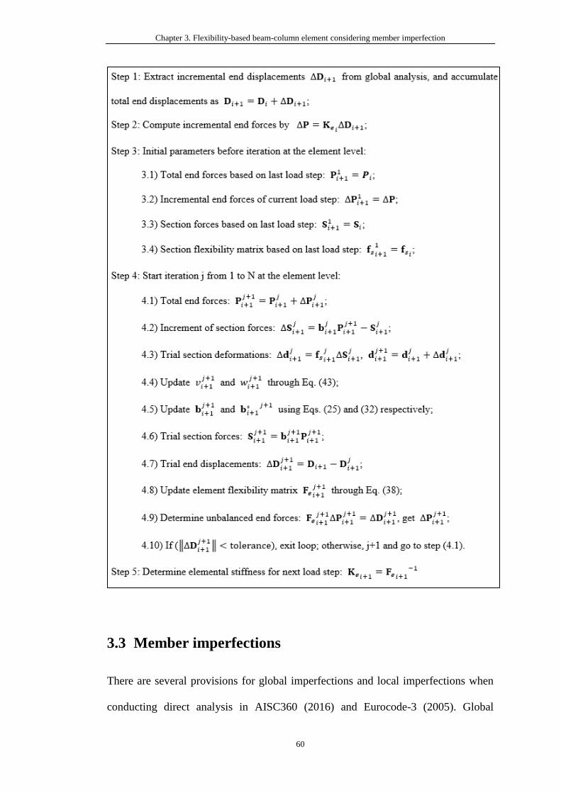
Chapter 3. Flexibility-based beam-column element considering member imperfection
60
3.3 Member imperfections
There are several provisions for global imperfections and local imperfections when
conducting direct analysis in AISC360 (2016) and Eurocode-3 (2005). Global
Chapter 3. Flexibility-based beam-column element considering member imperfection
61
imperfections generally refer to structural sway and local imperfections are member
bowing. They are caused by practical construction tolerance and manufacturing
process of the steel members. In the numerical simulation, it is easy to deal with the
global imperfections by adjusting nodal coordinates or introducing notional horizontal
load. As a consequence, the details of the global imperfections will not be discussed
in this thesis. The application of member initial imperfection on numerical modeling
for direct analysis will be explained herein. Generally, there are two methods, i.e.,
equivalent geometrical imperfection method and modified modulus approach, for
considering local imperfection. They will be briefly discussed here.
3.3.1 Equivalent geometrical imperfection method
In steel structures, there unavoidably exist member initial imperfections, including the
geometrical imperfections and the mechanical imperfections (residual stresses). These
imperfections cannot be ignored during the analysis procedure as they will affect the
structural behavior. The traditional design approach, indirect analysis, uses column
buckling curves to consider these unfavorable factors. Column buckling curves are
determined by section types and production process, which is based on individual
members. In the global analysis, this method ignores the coupling effect between
structural components and structural system, which may lead to an unrealistic
prediction of structural behavior.
Equivalent geometrical imperfection approach is suggested by Eurocode-3 (2005) to
consider these imperfections in a uniform form, i.e., the equivalent geometrical
imperfection. The concept of this method was proposed by Ayrton and Perry (1886).
It assumes that the imperfection shape of members is a half-sine function. The
amplitude of the half-sine function is represented by 𝛿0 which varies upon section
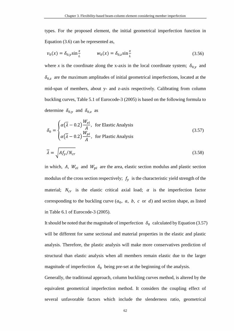
Chapter 3. Flexibility-based beam-column element considering member imperfection
62
types. For the proposed element, the initial geometrical imperfection function in
Equation (3.6) can be represented as,
𝑣0(𝑥) = 𝛿0,𝑦sin𝑥
𝐿 𝑤0(𝑥) = 𝛿0,𝑧sin
𝑥
𝐿 (3.56)
where x is the coordinate along the x-axis in the local coordinate system; 𝛿0,𝑦 and
𝛿0,𝑧 are the maximum amplitudes of initial geometrical imperfections, located at the
mid-span of members, about y- and z-axis respectively. Calibrating from column
buckling curves, Table 5.1 of Eurocode-3 (2005) is based on the following formula to
determine 𝛿0,𝑦 and 𝛿0,𝑧 as
𝛿0 = {𝛼(𝜆 − 0.2)
𝑊𝑒𝑙
𝐴, for Elastic Analysis
𝛼(𝜆 − 0.2)𝑊𝑝𝑙
𝐴, for Plastic Analysis
(3.57)
𝜆 = √𝐴𝑓𝑦 𝑁𝑐𝑟⁄ (3.58)
in which, 𝐴, 𝑊𝑒𝑙 and 𝑊𝑝𝑙 are the area, elastic section modulus and plastic section
modulus of the cross section respectively; 𝑓𝑦 is the characteristic yield strength of the
material; 𝑁𝑐𝑟 is the elastic critical axial load; 𝛼 is the imperfection factor
corresponding to the buckling curve (𝑎0, 𝑎, 𝑏, 𝑐 or 𝑑) and section shape, as listed
in Table 6.1 of Eurocode-3 (2005).
It should be noted that the magnitude of imperfection 𝛿0 calculated by Equation (3.57)
will be different for same sectional and material properties in the elastic and plastic
analysis. Therefore, the plastic analysis will make more conservatives prediction of
structural than elastic analysis when all members remain elastic due to the larger
magnitude of imperfection 𝛿0 being pre-set at the beginning of the analysis.
Generally, the traditional approach, column buckling curves method, is altered by the
equivalent geometrical imperfection method. It considers the coupling effect of
several unfavorable factors which include the slenderness ratio, geometrical

Chapter 3. Flexibility-based beam-column element considering member imperfection
63
imperfections, residual stress as well as loading eccentricity in the global analysis. The
equivalent geometrical imperfection method can be used in practical design for
considering these unfavorable factors in some modern design codes, such as
Eurocode-3 (2005) and CoPHK (2011). To satisfy the requirements of design codes,
the proposed element can incorporate the initial geometrical member imperfection
directly. Besides, the residual stresses can also be considered explicitly by the fiber
section technology.
3.3.2 Modified modulus approach
Surovek-Maleck and White (2004) and Ziemian and McGuire (2002) proposed an
approach, called the modified modulus method, to model the two kinds of
imperfections mentioned above. This method has been included in AISC360 (2016).
It does not consider the initial bowing imperfection explicitly during the procedure of
analysis. The flexural check at the design stage considers the effect of the local
member imperfection. Regarding the material residual stress, AISC360 (2016) reduces
the stiffness of members to reflect its influence explicitly. An overall stiffness
reduction factor, 0.8 is suggested by AISC360 (2016) to reduce the stiffness of
structural systems. The properties of cross sections with considering the reduction
factor is shown as,
𝐸𝐴𝑒 = 0.8𝐸𝐴 𝐸𝐼𝑒,𝑦 = 0.8𝜏𝑏𝐸𝐼𝑦 𝐸𝐼𝑒,𝑧 = 0.8𝜏𝑏𝐸𝐼𝑧 (3.59)
𝜏𝑏 =
{
1, for
𝑃
𝑃𝑦≤ 0.5
4𝑃
𝑃𝑦(1 −
𝑃
𝑃𝑦) , for
𝑃
𝑃𝑦> 0.5
(3.60)
where 𝜏𝑏 is determined by applied axial force P and the axial yield strength 𝑃𝑦. The
calculation of the flexural stiffness needs to consider this additional reduction factor 𝜏𝑏.
Chapter 3. Flexibility-based beam-column element considering member imperfection
64
Maleck and White (2004) believed that 𝜏𝑏 reflects the influence of residual stress and
the factor 0.8 considers the coupling effect between axial force and flexural moments.
Taking I-shape section, for example, the Lehigh residual stress pattern proposed by
Galambos and Ketter (1959) will lead to different reduction factor τb for major-axis
and minor-axis if equation (3.58) is applied.
3.4 Numerical examples
To verify the accuracy, efficiency and versatility of the proposed, four examples,
involving geometrical nonlinearity, or material nonlinearity, or both, are studied. The
first three examples are planar problems and the last one is a space problem.
Displacement-based beam-column elements generally adopt cubic shape function or
other higher-order shape functions to fit the member deflection. While the flexibility-
based beam-column elements use the numerical integration. The proposed element,
one of the flexibility-based beam-column elements, also adopts numerical integration
approach along the member to form the elemental stiffness. The section stiffness at
integration points should reflect the stiffness of the weight length. Thus, the integration
scheme plays an important role in the prediction of the behavior of the proposed
element. In the inelastic analysis, the integration points are better to be located as near
as possible to the place of plastic hinges formed. Table 3-1 shows the features of
common approaches which has been studied by Scott (2006). All these integration
methods have high accuracy when using more than five integration points. The
difference between the methods is the location of integrations. For example, Gauss-
Lobatto has integration points at two ends of the element, while none of Gauss-
Legendre’s integration points locates at the ends though it has the highest accuracy.
Chapter 3. Flexibility-based beam-column element considering member imperfection
65
Therefore, the Gauss-Legendre method is suggested to be applied to the elastic
analysis. In the inelastic analysis, it is better to use the Gauss-Lobatto method because
plastic hinges of practical structures often form at the locations of its integration points.
Newton-Cotes integration method with uniform integration points along the element
is applicable for simple cases. In the following examples, suitable integration scheme
will be adopted.
3.4.1 Single initially-curved column under different boundary conditions
Fig. 3.2 shows the column with three boundary conditions: pinned-pinned, pinned-
fixed and fixed-fixed. The column is subjected to an axial force. This example is
usually employed for buckling check. Various amplitudes of the initial member
imperfection of columns are studied to check the performance of the proposed element
for direct analysis. The analytical result of this example can be obtained by solving
differential equilibrium equations, also given in Appendix I, to verify the accuracy of
the proposed element.
In the numerical models, the material is assumed to be elastic so that the capability of
geometrical nonlinearity of the proposed element can be directly verified. The material
and section properties are unitless for simplicity. The Young’s modulus E is 107; the
area of cross section A is 1.0; the moment of inertia I is 0.833. Therefore, the
integration procedure across the section in equation (3.37) is not needed. Gauss-
Legendre integration scheme, with five integration points, is adopted to accumulate
the elemental stiffness along the column.
In practice, the slenderness ratio of columns affects the critical buckling loading in
related to column instability. In this example, the column with same end condition is
assumed to have three slenderness ratios, i.e., 50, 100 and 150. The slenderness ratio
Chapter 3. Flexibility-based beam-column element considering member imperfection
66
λ = L/√I A⁄ is changed by setting different member lengths, which can verify the
practicability of the proposed element to model columns ranging from short to long.
Besides, the amplitude of the local member imperfection, δ0, is also studied by taking
as L/1000, L/500 and L/200, which covers most situations in practical structures.
Figs. 3.3 to 3.5 show the results of the column subjected to axial compression with
three slenderness ratios under three typical boundary conditions. Both numerical
results and analytical results are plotted with three kinds of the amplitude of member
imperfection. From these figures, all results under different conditions produced by
the proposed element agree well with the analytical results obtained by equations in
Appendix I. This example illustrates the high accuracy of the proposed element.
Ignoring the influence of member imperfection, the critical loads of three typical
boundary conditions: “pinned-pinned”, “pinned-fixed” and “fixed-fixed” are 1.0,
2.0408 and 4.0 respectively with multiplying by π2EI/L. The ultimate loads shown
in figures is less than the Euler buckling critical loads. The difference comes from the
consideration of member imperfection in the proposed method. Therefore, the
ignorance of member imperfection will overestimate the column capacity and lead to
unsafe design.
3.4.2 Distributed plasticity analysis of a fixed-ended beam
Fig. 3.6 shows the layout of a single beam with member length L of 6 m. The beam is
subjected to a concentrated point load. This example is also used to verify the ability
dealing with member load of the proposed element. Several plastic hinges will be
formed in this example. The cross-section is W30x99, with cross-sectional area A of
1.87e-2 m2, and second-moment area I of 1.661e-3 m4. The section plastic modulus is
5.113e-4 m3. The steel grade is S275, with Young’s modulus E of 205 GPa and yield

Chapter 3. Flexibility-based beam-column element considering member imperfection
67
stress fy of 275 MPa. The local member imperfection is ignored in this example for
easy comparison with analytical results.
Chen and Sohal (1995) also studied this example and provided the analytical results
using the plastic hinge method. They also indicated the number and forming sequence
the plastic hinges. In the numerical model, the web of the cross-section is meshed into
16 x 4 fibers, and flanges at top and bottom of the cross-section are divided into 4 x
16 fibers. The constitutive relationship of each fiber is assumed to be elastic-perfectly
plastic. The beam is modeled by one or two proposed elements. To explore the
influence of different integration scheme on the analysis, three models are built as
shown Table 3-2. For the models using two element, a node is inserted at the point B.
Table 3-3 gives the analytical result of details about hinge sequence, applied load and
deflection by Chen and Sohal (1995). The load vs. deflection curves of the present
study with the analytical solution are plotted in Fig. 3.7. From the figure, the results
of Model 1, Model 2 and Model 3, calculated by the proposed element, agree well
with the analytical solutions. The ultimate load capacities obtained by these models
are almost same. Apparently, the curve obtained by plastic hinge method is less
smooth than the proposed method.
From the figure, Model 2 has similar load-deflection curves with Model 3. Therefore,
two elements with 5 Newton-Cotes’ integration points make a same accurate
prediction as that of 2 elements with 7 Newton-Cotes’ integration points. Both Model
2 and Model 3 have integration points accurately located at where the plastic hinges
appear. Therefore, they can make an accurate prediction of deformation and internal
forces of members. However, though Model 1 has ten integration points along the
member, integration points do not accurately locate at same places. Fig. 3.8 shows the
detailed deflection of the beam when the load factor is 8.0. The deflection values of
Chapter 3. Flexibility-based beam-column element considering member imperfection
68
integration points are also shown in the figure. Both Model 1 and Model 2 have
integration points located at point B and two ends of the beam. Therefore, their
ultimate capacities are similar though the deflection curves are slightly different.
The proposed element is verified by the example that exhibits highly nonlinearity of
material with three plastic hinges. Meanwhile, the member loads can also be properly
considered at the element level if the proper integration scheme is used. For practical
design, the two ends and the middle point of members have relatively larger moment
than other locations in such case the plastic hinges often form at these points. Gauss-
Lobatto integration scheme with 5 or 7 integration points covers these locations, which
can produce acceptable results. Generally, increasing the number of elements per
member or increasing the number of integration points are two approaches to improve
the accuracy of plastic analysis. Though the first approach can largely improve the
accuracy, it increases the number of global degree of freedom (DOF) and then
increases the number of equilibrium equations which leads to more computer time.
Besides, it also leads to numerical problems when some elements located at the inside
of the member fail. In contrast, the increase of integration points will only lead to more
computer time at the elemental level which does not increase the dimension of system
stiffness matrix. Therefore, the integration scheme can be selected according to
applied loads and end conditions of members, which can be automatically carried out
by the program, such as NIDA (2018). Thus, the proposed element is practical in the
second-order inelastic analysis.
3.4.3 Second-order direct analysis of a two-story 2D steel frame
This benchmark example is firstly studied by Ziemian et al. (1992). This example
exhibits highly geometrical and material nonlinearities and is suitable to verify the
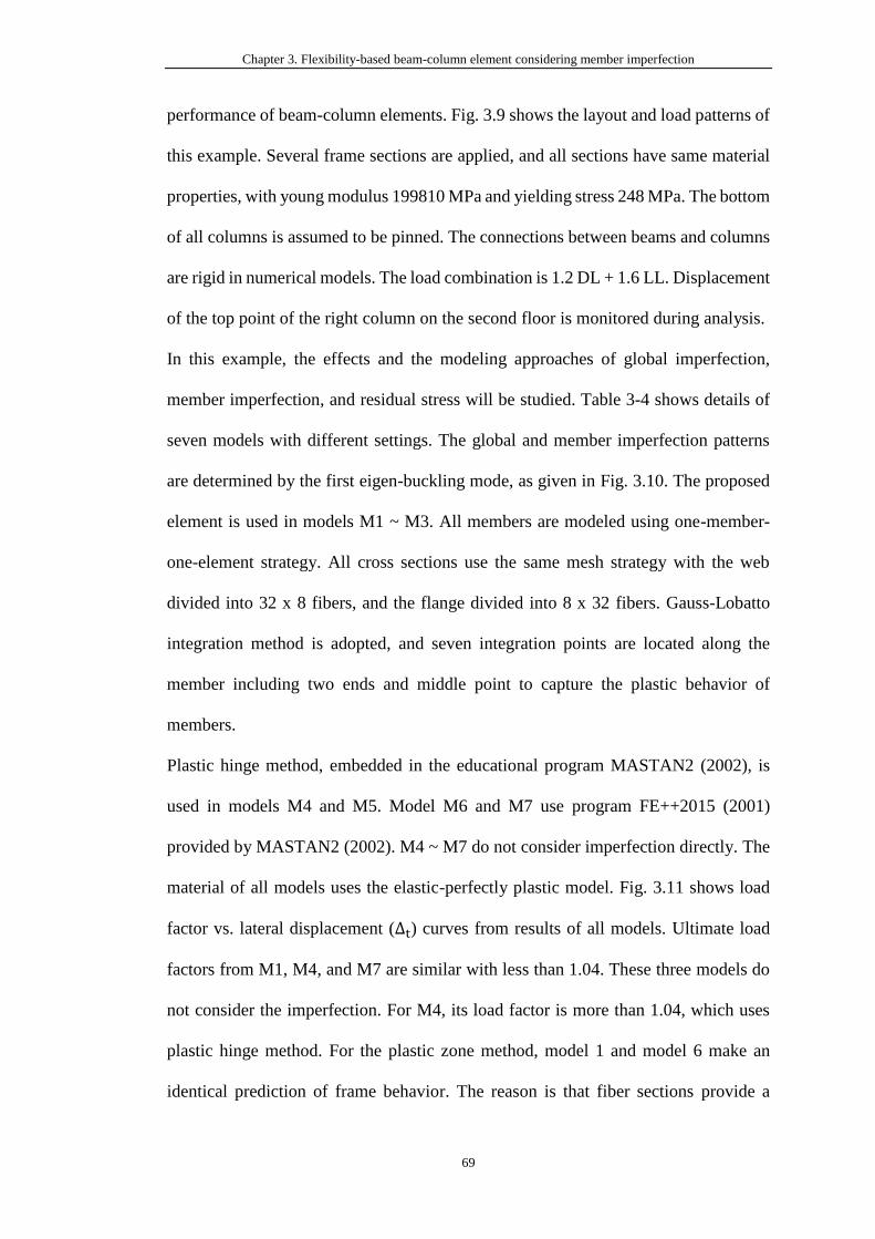
Chapter 3. Flexibility-based beam-column element considering member imperfection
69
performance of beam-column elements. Fig. 3.9 shows the layout and load patterns of
this example. Several frame sections are applied, and all sections have same material
properties, with young modulus 199810 MPa and yielding stress 248 MPa. The bottom
of all columns is assumed to be pinned. The connections between beams and columns
are rigid in numerical models. The load combination is 1.2 DL + 1.6 LL. Displacement
of the top point of the right column on the second floor is monitored during analysis.
In this example, the effects and the modeling approaches of global imperfection,
member imperfection, and residual stress will be studied. Table 3-4 shows details of
seven models with different settings. The global and member imperfection patterns
are determined by the first eigen-buckling mode, as given in Fig. 3.10. The proposed
element is used in models M1 ~ M3. All members are modeled using one-member-
one-element strategy. All cross sections use the same mesh strategy with the web
divided into 32 x 8 fibers, and the flange divided into 8 x 32 fibers. Gauss-Lobatto
integration method is adopted, and seven integration points are located along the
member including two ends and middle point to capture the plastic behavior of
members.
Plastic hinge method, embedded in the educational program MASTAN2 (2002), is
used in models M4 and M5. Model M6 and M7 use program FE++2015 (2001)
provided by MASTAN2 (2002). M4 ~ M7 do not consider imperfection directly. The
material of all models uses the elastic-perfectly plastic model. Fig. 3.11 shows load
factor vs. lateral displacement (∆t) curves from results of all models. Ultimate load
factors from M1, M4, and M7 are similar with less than 1.04. These three models do
not consider the imperfection. For M4, its load factor is more than 1.04, which uses
plastic hinge method. For the plastic zone method, model 1 and model 6 make an
identical prediction of frame behavior. The reason is that fiber sections provide a

Chapter 3. Flexibility-based beam-column element considering member imperfection
70
smoother transition of the stiffness from elastic to fully plastic than that provided by
the plastic hinge method. Under the combined effect of both geometrical and material
nonlinearities, the plastic hinge leads to a less accurate simulation due to its
assumption of discontinuous transition.
In direct analysis, it is inevitable to consider initial member imperfection, eccentricity
of applied load and residual stress of cross-sections. As for the local member
imperfection, several different methods are adopted by model 2, 5 and 7. In Model 2,
only local imperfections are modeled with an amplitude of L/300, and the global
imperfection is ignored. Model 5 uses the modified modulus method to consider the
local member imperfection. Residual stress is considered by Model 7. Model 2 and
Model 5 make the similar prediction when the load factor is less than 0.75. Then, their
results are diverse. Model 2 has a larger ultimate load factor than Model 5. Comparing
the results of Model 6 and Model 7, residual stress slightly reduces the ultimate
capacity of the frame.
The results of Model 3 show that imperfections in local and global level largely
decrease the ultimate capacity of the frame. The stiffness of the structural system is
more flexible than other models when the load factor is less than 0.7. Fig. 3.12 shows
the status of yielding about the cross-section and internal forces of members when the
load factor is 1.0. The percentage of section area yielded in some locations is bigger
than 90%. Meanwhile, some fibers of beam sections, located at the middle of members,
become plastic.
In this example, results obtained by several methods are adopted to verify the accuracy
and ability of the proposed element. This element can be a powerful tool for practical
design.
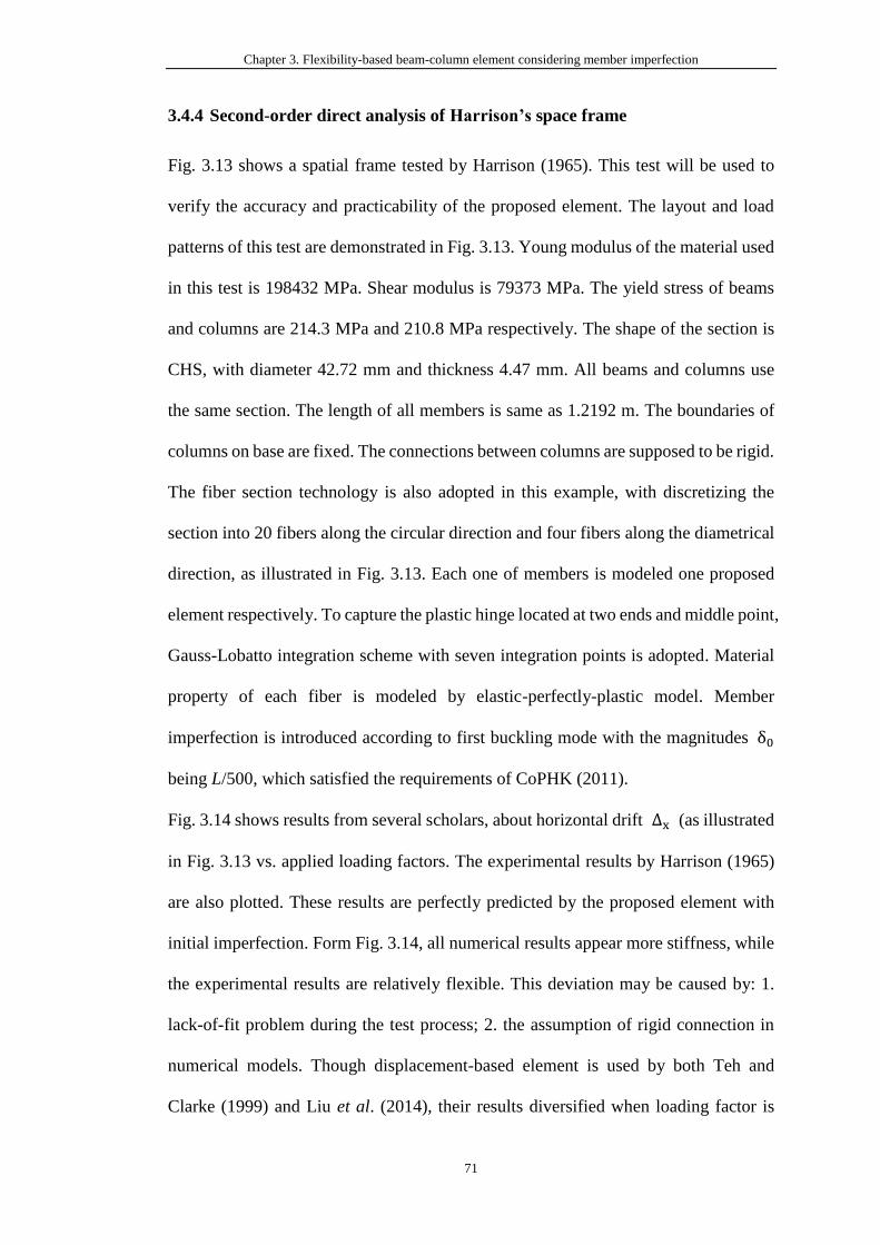
Chapter 3. Flexibility-based beam-column element considering member imperfection
71
3.4.4 Second-order direct analysis of Harrison’s space frame
Fig. 3.13 shows a spatial frame tested by Harrison (1965). This test will be used to
verify the accuracy and practicability of the proposed element. The layout and load
patterns of this test are demonstrated in Fig. 3.13. Young modulus of the material used
in this test is 198432 MPa. Shear modulus is 79373 MPa. The yield stress of beams
and columns are 214.3 MPa and 210.8 MPa respectively. The shape of the section is
CHS, with diameter 42.72 mm and thickness 4.47 mm. All beams and columns use
the same section. The length of all members is same as 1.2192 m. The boundaries of
columns on base are fixed. The connections between columns are supposed to be rigid.
The fiber section technology is also adopted in this example, with discretizing the
section into 20 fibers along the circular direction and four fibers along the diametrical
direction, as illustrated in Fig. 3.13. Each one of members is modeled one proposed
element respectively. To capture the plastic hinge located at two ends and middle point,
Gauss-Lobatto integration scheme with seven integration points is adopted. Material
property of each fiber is modeled by elastic-perfectly-plastic model. Member
imperfection is introduced according to first buckling mode with the magnitudes δ0
being L/500, which satisfied the requirements of CoPHK (2011).
Fig. 3.14 shows results from several scholars, about horizontal drift ∆x (as illustrated
in Fig. 3.13 vs. applied loading factors. The experimental results by Harrison (1965)
are also plotted. These results are perfectly predicted by the proposed element with
initial imperfection. Form Fig. 3.14, all numerical results appear more stiffness, while
the experimental results are relatively flexible. This deviation may be caused by: 1.
lack-of-fit problem during the test process; 2. the assumption of rigid connection in
numerical models. Though displacement-based element is used by both Teh and
Clarke (1999) and Liu et al. (2014), their results diversified when loading factor is
Chapter 3. Flexibility-based beam-column element considering member imperfection
72
achieving 0.85. All members remain elastic when loading factor is less than 0.85. And
there is no plastic hinge forming in the structural system. When plastic hinge appears,
plastic zone method and plastic hinge method work and reveal different features. Both
of their results exhibit slightly stiffer than the experimental results, which may be
caused by ignorance of initial geometrical imperfections in their numerical models.
This phenomenon also can be seen in results predicted the proposed element without
setting member imperfections.
This experimental test shows that the proposed element is capable of satisfying the
requirements of SODA. It can predict relatively high results and applies to space
frames.
3.5 Concluding remarks
In this chapter, a new flexibility-based beam-column element is proposed. This
element inherits advantages of flexibility-based elements, having high accuracy. The
highlight of the proposed element is that it is capable to incorporate member
imperfection explicitly. Meanwhile the distributed plasticity method is adopted to
capture the plastic behavior. The fiber section approach also makes it possible to
consider residual stress. These features of the proposed element will be a powerful
tool for practical design to satisfy requirements of second-order direct analysis
(SODA).
The capacity about both geometrical and material nonlinearities of the proposed
element is confirmed by several benchmarked examples. The first two examples
provide closed-form solutions to check its accuracy. The last two examples
demonstrate its application. The results obtained by the proposed element are also
Chapter 3. Flexibility-based beam-column element considering member imperfection
73
verified by that produced by other scholars using other methods. Some meaningful
conclusions are obtained as,
(1) Member imperfection can be explicitly modeled by the proposed element at the
elemental level without introducing internal forces, which is convenient and
practical.
(2) Fiber section technology is adopted by the proposed element, which can capture
the process of gradually yielding and makes it easy to incorporate residual stress
effect.
(3) Because distributed plasticity analysis method uses limited integration points to
monitor the plastic status of the member, appropriate integration method should
be employed to capture the accurate location of plastic hinges.
(4) The proposed element, having acceptable accuracy for practical design when one
member being modeled by one proposed element, can save much computer time.
Besides, it could not produce numerical problem due to member failure.
(5) To make full use of flexibility-based element and displacement-based element, the
first one can be used to model these members being controlled by material
nonlinearity, and the second one is efficient to simulate the other that remain
elastic or are dominated by geometrical nonlinearity. This strategy can maintain
accuracy and also save much computer time.
(6) Without considering geometrical imperfection in structural systems or individual
members will overestimate the ultimate resistance of structural systems. Though
design codes provide the other method to model geometrical imperfection, like
through applying notional force. But they are practical to limited structural types,
like regular structures. The proposed eradicate these shortages and can model
initial imperfection explicitly.
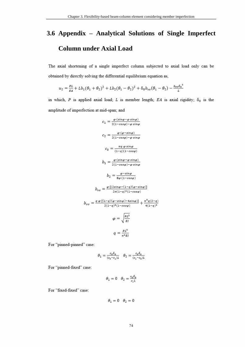
Chapter 3. Flexibility-based beam-column element considering member imperfection
74
3.6 Appendix – Analytical Solutions of Single Imperfect
Column under Axial Load
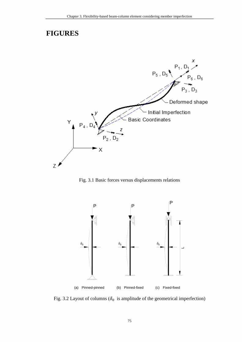
Chapter 3. Flexibility-based beam-column element considering member imperfection
75
FIGURES
Fig. 3.1 Basic forces versus displacements relations
Fig. 3.2 Layout of columns (𝛿0 is amplitude of the geometrical imperfection)
P PP
L
δ0δ0δ0
(a) Pinned-pinned (b) Pinned-fixed (c) Fixed-fixed
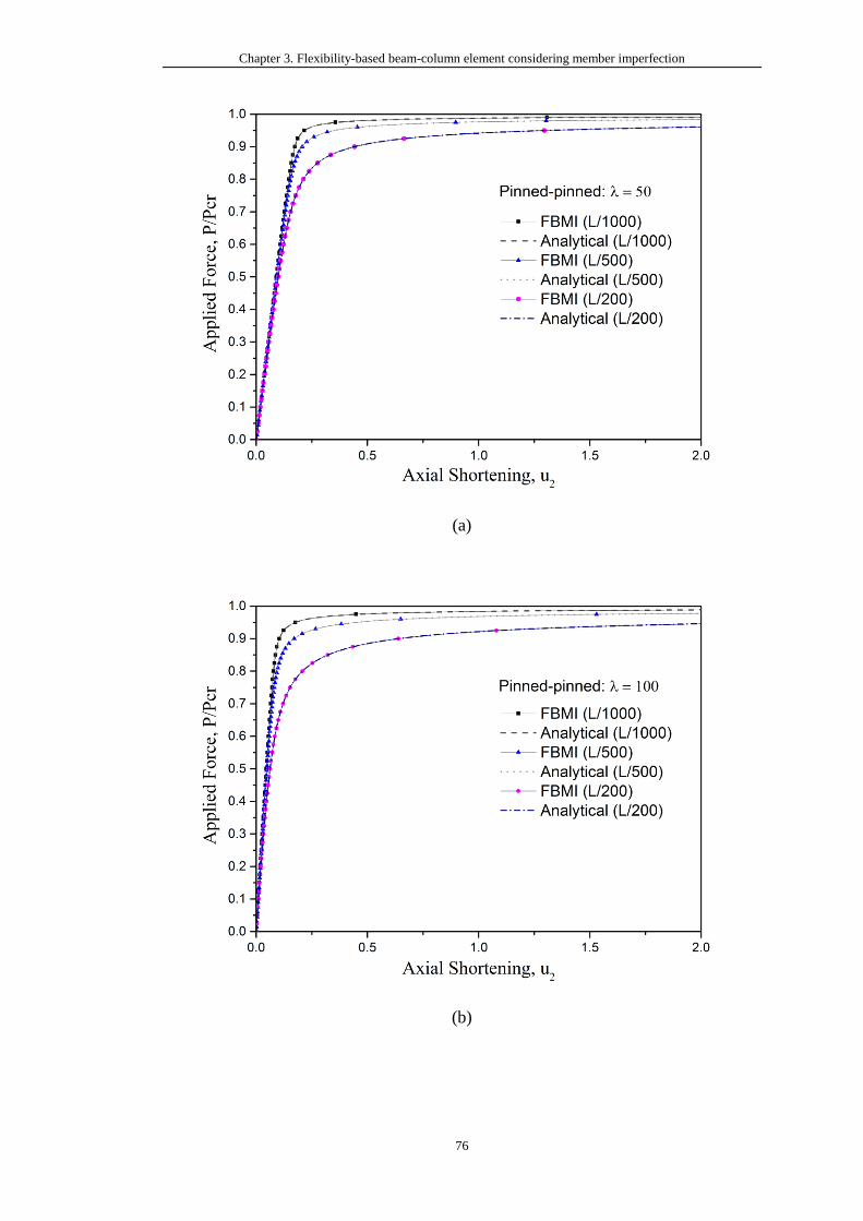
Chapter 3. Flexibility-based beam-column element considering member imperfection
76
(a)
(b)
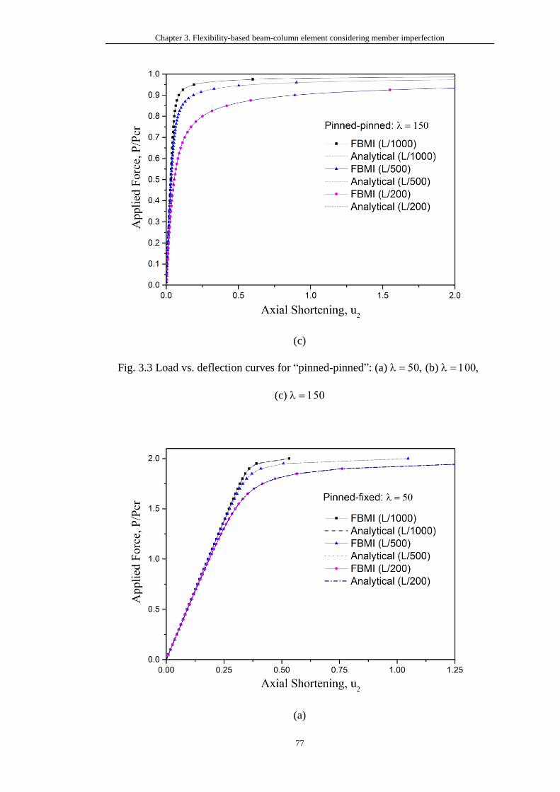
Chapter 3. Flexibility-based beam-column element considering member imperfection
77
(c)
Fig. 3.3 Load vs. deflection curves for “pinned-pinned”: (a) = (b) =
(c) =
(a)
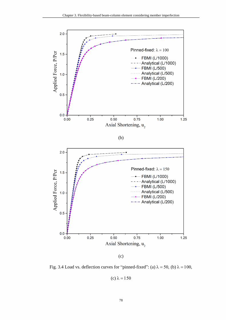
Chapter 3. Flexibility-based beam-column element considering member imperfection
78
(b)
(c)
Fig. 3.4 Load vs. deflection curves for “pinned-fixed”: (a) = (b) =
(c) =
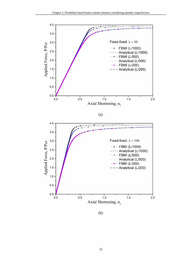
Chapter 3. Flexibility-based beam-column element considering member imperfection
79
(a)
(b)
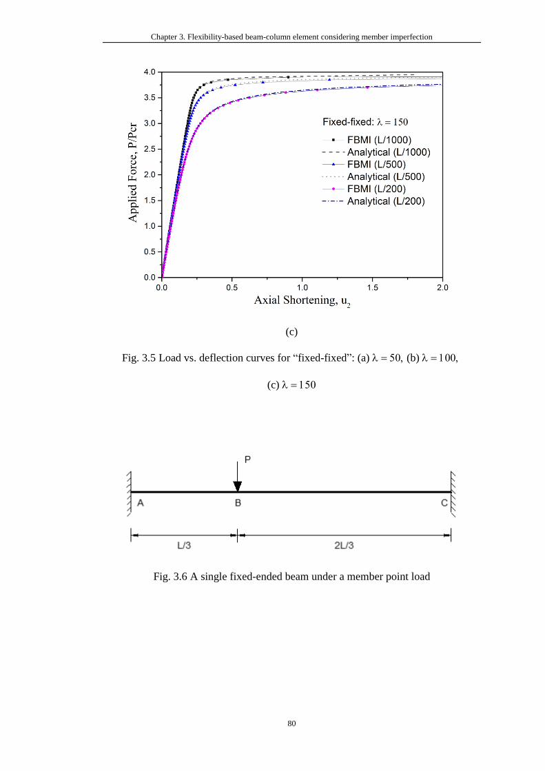
Chapter 3. Flexibility-based beam-column element considering member imperfection
80
(c)
Fig. 3.5 Load vs. deflection curves for “fixed-fixed”: (a) = (b) =
(c) =
Fig. 3.6 A single fixed-ended beam under a member point load
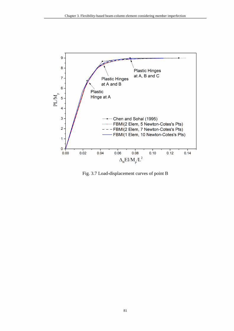
Chapter 3. Flexibility-based beam-column element considering member imperfection
81
Fig. 3.7 Load-displacement curves of point B
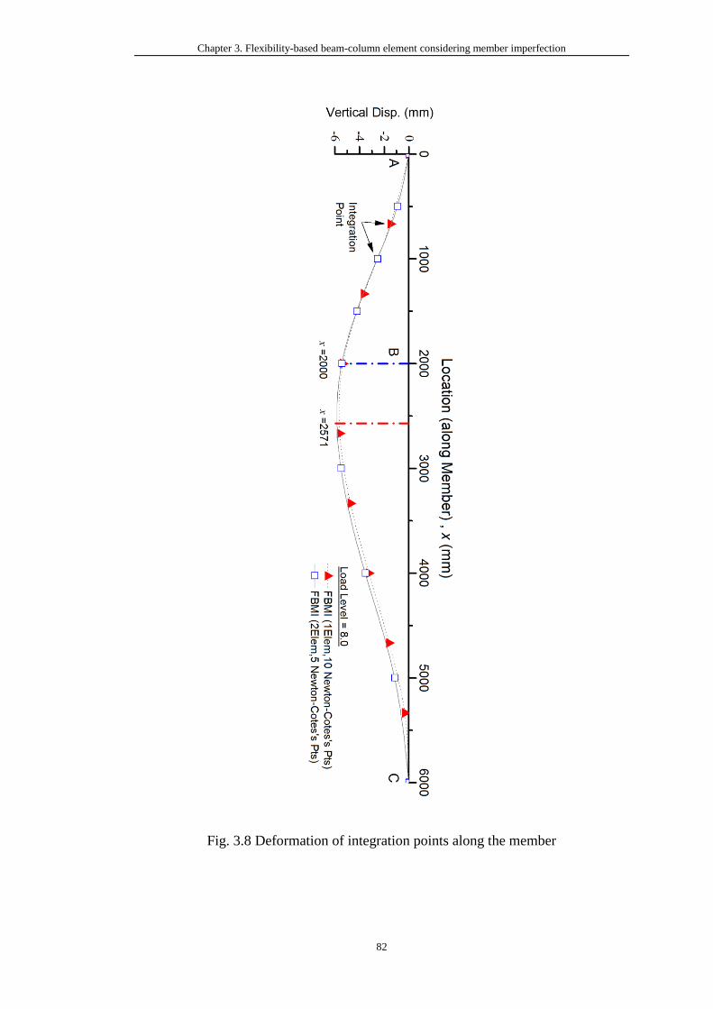
Chapter 3. Flexibility-based beam-column element considering member imperfection
82
Fig. 3.8 Deformation of integration points along the member
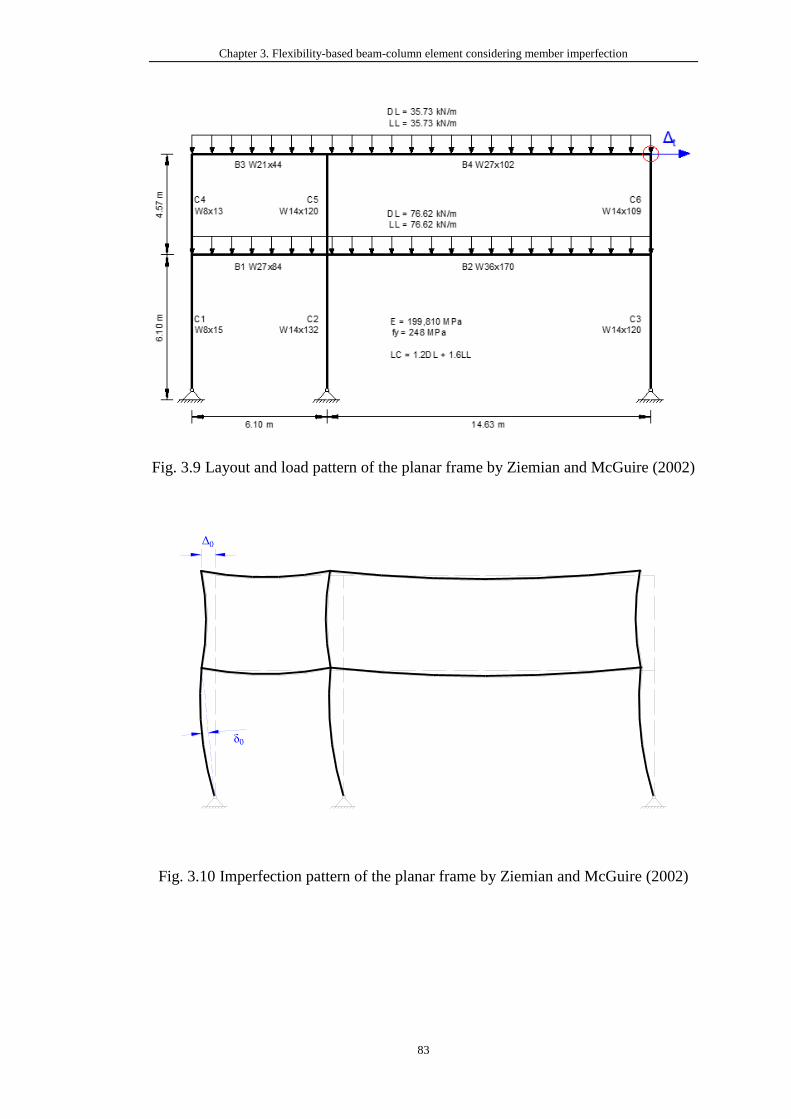
Chapter 3. Flexibility-based beam-column element considering member imperfection
83
Fig. 3.9 Layout and load pattern of the planar frame by Ziemian and McGuire (2002)
Fig. 3.10 Imperfection pattern of the planar frame by Ziemian and McGuire (2002)
Δ0
δ0
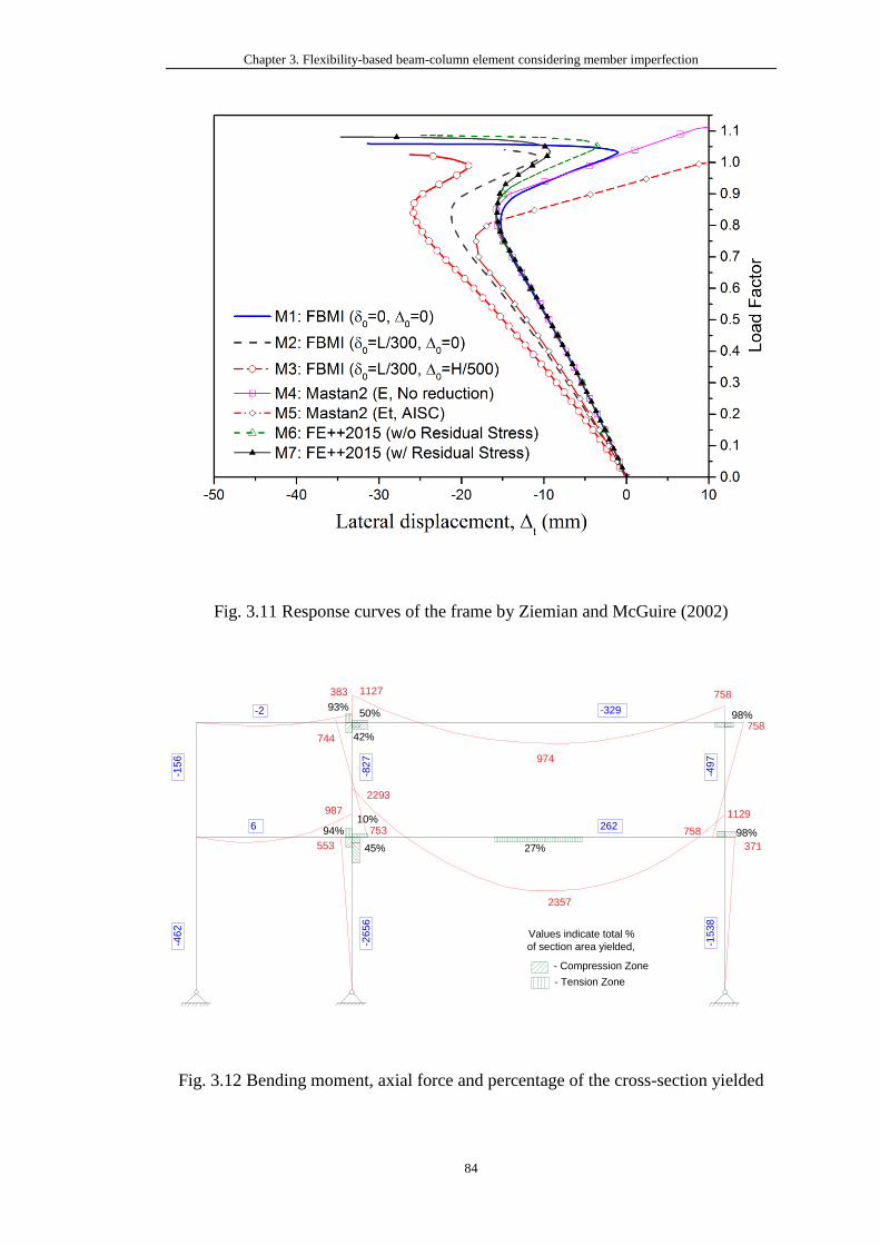
Chapter 3. Flexibility-based beam-column element considering member imperfection
84
Fig. 3.11 Response curves of the frame by Ziemian and McGuire (2002)
Fig. 3.12 Bending moment, axial force and percentage of the cross-section yielded
27%45%
94%10%
50%93%
42%
98%
98%
Values indicate total %
of section area yielded,
- Compression Zone
- Tension Zone
-462
-2656
-1538
-156
-827
-497
-329
6 262
-2
2357
758
371
974
987
744
383
553
1127 758
2293
1129
758753
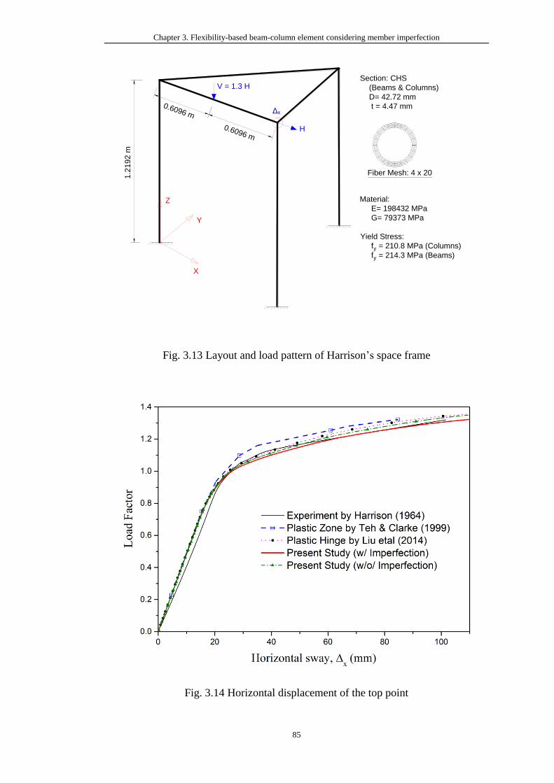
Chapter 3. Flexibility-based beam-column element considering member imperfection
85
Fig. 3.13 Layout and load pattern of Harrison’s space frame
Fig. 3.14 Horizontal displacement of the top point
H
V = 1.3 H
1.2
192 m
0.6096 m
0.6096 m
Section: CHS
(Beams & Columns)
D= 42.72 mm
t = 4.47 mmΔx
X
Y
Z Material:
E= 198432 MPa
G= 79373 MPa
Yield Stress:
fy = 210.8 MPa (Columns)
fy = 214.3 MPa (Beams)
Fiber Mesh: 4 x 20
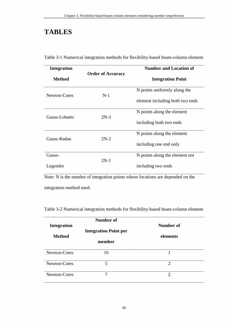
Chapter 3. Flexibility-based beam-column element considering member imperfection
86
TABLES
Table 3-1 Numerical integration methods for flexibility-based beam-column element
Integration
Method
Order of Accuracy
Number and Location of
Integration Point
Newton-Cotes N-1
N points uniformly along the
element including both two ends
Gauss-Lobatto 2N-3
N points along the element
including both two ends
Gauss-Radau 2N-2
N points along the element
including one end only
Gauss-
Legendre
2N-1
N points along the element not
including two ends
Note: N is the number of integration points whose locations are depended on the
integration method used.
Table 3-2 Numerical integration methods for flexibility-based beam-column element
Integration
Method
Number of
Integration Point per
member
Number of
elements
Newton-Cotes 10 1
Newton-Cotes 5 2
Newton-Cotes 7 2
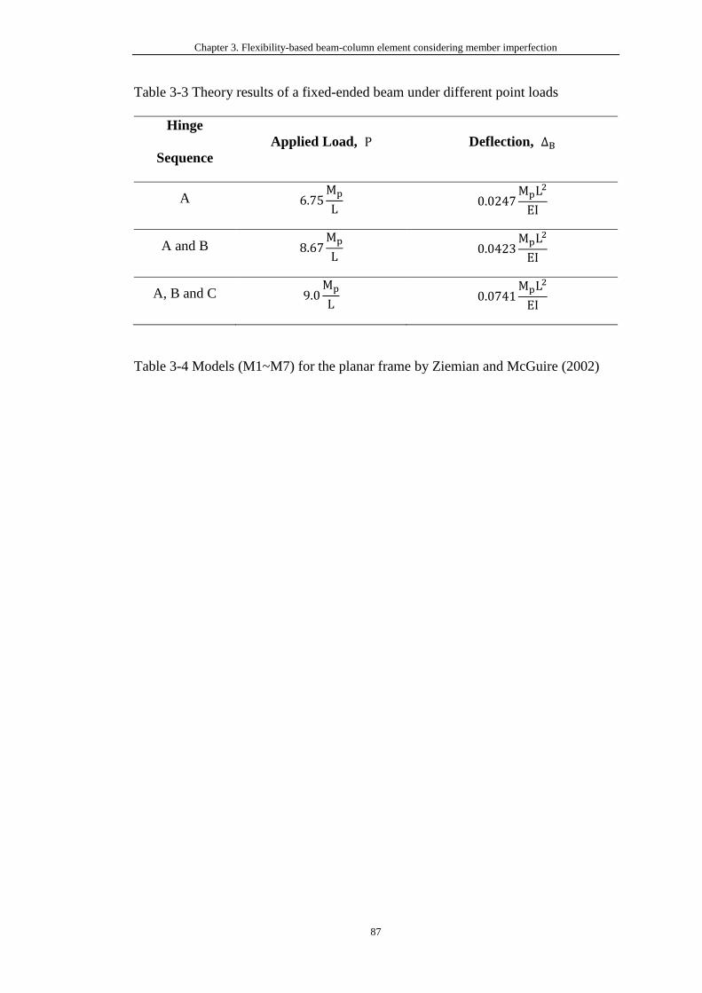
Chapter 3. Flexibility-based beam-column element considering member imperfection
87
Table 3-3 Theory results of a fixed-ended beam under different point loads
Hinge
Sequence
Applied Load, P Deflection, ∆B
A 6.75Mp
L 0.0247
MpL2
EI
A and B 8.67Mp
L 0.0423
MpL2
EI
A, B and C 9.0Mp
L 0.0741
MpL2
EI
Table 3-4 Models (M1~M7) for the planar frame by Ziemian and McGuire (2002)
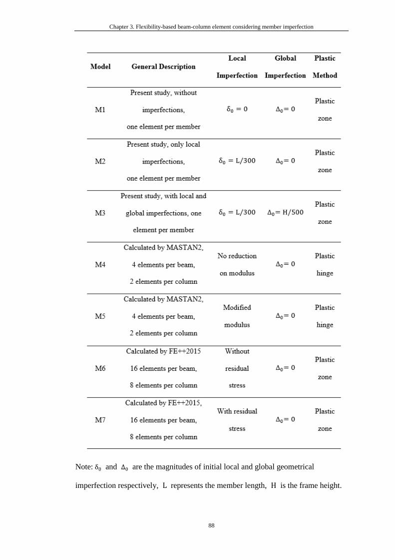
Chapter 3. Flexibility-based beam-column element considering member imperfection
88
Note: δ0 and ∆0 are the magnitudes of initial local and global geometrical
imperfection respectively, L represents the member length, H is the frame height.

Chapter 4. Two plasticity models for material nonlinearity
89
CHAPTER 4. TWO PLASTICITY MODELS FOR
MATERIAL NONLINEARITY
4.1 Introduction
Many modern design codes, such as AISC360 (2016) and Eurocode-3 (2005), have
specified “Direct analysis”, “Second-order Analysis” or “Advanced Analysis” for
daily design of steel structures, through which the structural stability and safety can
be assessed by checking the members and the system in an integrated manner rather
than checking individual member using the effective length method (ELM). The ELM
is simply based on the first-order linear analysis without consideration of many effects
while the direct analysis method (DAM) considers the important factors affecting
member and system strength, such as the second-order P–δ and P-∆ effects, initial
geometrical imperfections, residual stress, material yielding and joint behavior.
Several different beam-column elements have been proposed to incorporate initial
geometrical imperfection at the element level. Chan and Zhou (1995) and Liu et al.
(2014a, 2014b) proposed stiffness-based beam-column elements considering initial
bowing for second-order direct analysis, which show high computational efficiency
and accuracy. Chiorean (2017) and Du et al. (2017) proposed two flexibility-based
elements which can also directly incorporate initial imperfection in different manners
and exhibit high performance when using one-element-per-member modeling.
Regarding material nonlinearity, there are two widely used methods, i.e., plastic hinge
method and plastic zone method. The plastic hinge method (also named as
concentrated plasticity method) is widely adopted in the stiffness-based beam-column
elements due to its simplicity and computational efficiency, while the plastic zone
Chapter 4. Two plasticity models for material nonlinearity
90
method (also well-known as distributed plasticity method) is usually used to calibrate
the accuracy of plastic hinge method in previous research. Although the latter can
obtain more accurate results, it costs more computer time as well as computer storage
in the analysis as it is required to mesh a section into some fibers and several
integration points are needed along the member length. This problem will be more
serious in the nonlinear dynamic (time-history) analysis. With the recently fast
development of computer hardware, it is possible to adopt the plastic zone method in
the second-order inelastic analysis so that the structural behavior can be well predicted.
However, the lack of consideration of initial imperfection in traditional flexibility-
based elements and tedious determination of fiber state require too many computer
resources, especially in high-rise buildings and long-span structures. Thus, it is urgent
to improve the current analysis method so that more accurate results can be provided
for design purpose with enhancement of computational efficiency.
Generalized plasticity method was firstly proposed by Auricchio and Taylor (1995)
for material yielding and then extended to a stress resultant section model used in
beam-column element developed by Kostic et al. (2013). Their element adopts
concentrated plasticity model, whose feature is described by generalized plasticity
using yield and limit surfaces. Thus, their method can take the benefit of well-accepted
interaction functions between the axial force and the bending moments specified in
design codes or more accurate yield functions in literature. However, the plastic hinges
can be only formed at the ends of the element. It means that more elements are required
if one or more plastic hinges are formed along the member. Further, their study does
not take the P–δ effect into account and as a result their outcome cannot fulfill the
requirement of direct analysis.
Chapter 4. Two plasticity models for material nonlinearity
91
This thesis is intended to improve the computational efficiency of the flexibility-based
element with distributed plasticity proposed by Du et al. (2017). The time-consuming
fiber section integration will be replaced by the robust stress-resultant plasticity model
based on the concept of the generalized plasticity method. As the discretization of
cross-section into fibers is no longer required, the proposed method will significantly
enhance the computational efficiency by directly using the relationship between
section deformations and stress resultants. Also, good numerical convergence is
observed when using the backward-Euler algorithm in the determination of section
state. Thus, a practical solution will be proposed for second-order inelastic analysis
through which a safer and more economical design can be achieved.
4.2 Distributed plasticity analysis
Comparing with displacement-based beam-column elements with high numerical
efficiency, the biggest advantage of flexibility-based beam-column elements is the
excellent performance in the second-order inelastic analysis. This highlighted feature
is carried out by distributed plasticity method with fiber section technique. This
technique is widely adopted in flexibility-based elements to consider distributed
plasticity along the section height and member length,as seen in Fig. 4.1. Along the
element, numerical integration scheme is used to represent the member with several
integration points located in special locations. The cross-section is discretized into
some fibers as integration points as shown in Fig. 4.2. For arbitrary shapes of cross-
sections, the Blossom-Quad algorithm (2013) can be used to mesh them into
quadrilateral fibers. Each of them is an independent region, which is defined by its
centroid coordinates (𝑦𝑗, 𝑧𝑗) and area (𝐴𝑗). Their mechanics behaviors are modeled
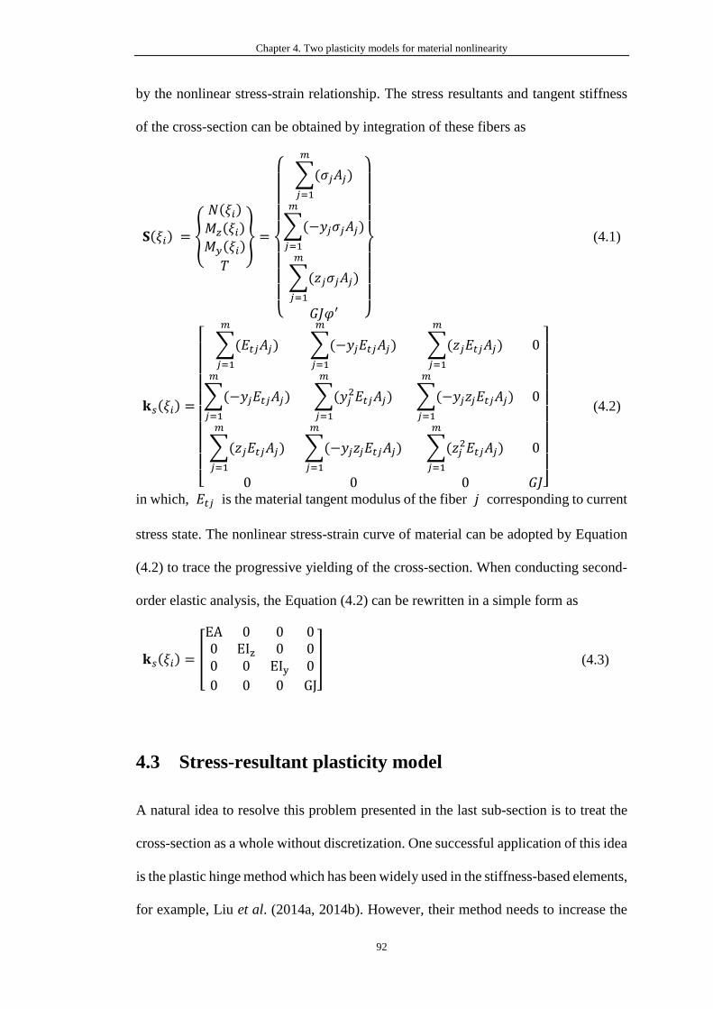
Chapter 4. Two plasticity models for material nonlinearity
92
by the nonlinear stress-strain relationship. The stress resultants and tangent stiffness
of the cross-section can be obtained by integration of these fibers as
𝐒(𝜉𝑖) = {
𝑁(𝜉𝑖)
𝑀𝑧(𝜉𝑖)
𝑀𝑦(𝜉𝑖)
𝑇
} =
{
∑(𝜎𝑗𝐴𝑗)
𝑚
𝑗=1
∑(−𝑦𝑗𝜎𝑗𝐴𝑗)
𝑚
𝑗=1
∑(𝑧𝑗𝜎𝑗𝐴𝑗)
𝑚
𝑗=1
𝐺𝐽𝜑′ }
(4.1)
𝐤𝑠(𝜉𝑖) =
[ ∑(𝐸𝑡𝑗𝐴𝑗)
𝑚
𝑗=1
∑(−𝑦𝑗𝐸𝑡𝑗𝐴𝑗)
𝑚
𝑗=1
∑(𝑧𝑗𝐸𝑡𝑗𝐴𝑗)
𝑚
𝑗=1
0
∑(−𝑦𝑗𝐸𝑡𝑗𝐴𝑗)
𝑚
𝑗=1
∑(𝑦𝑗2𝐸𝑡𝑗𝐴𝑗)
𝑚
𝑗=1
∑(−𝑦𝑗𝑧𝑗𝐸𝑡𝑗𝐴𝑗)
𝑚
𝑗=1
0
∑(𝑧𝑗𝐸𝑡𝑗𝐴𝑗)
𝑚
𝑗=1
∑(−𝑦𝑗𝑧𝑗𝐸𝑡𝑗𝐴𝑗)
𝑚
𝑗=1
∑(𝑧𝑗2𝐸𝑡𝑗𝐴𝑗)
𝑚
𝑗=1
0
0 0 0 𝐺𝐽]
(4.2)
in which, 𝐸𝑡𝑗 is the material tangent modulus of the fiber 𝑗 corresponding to current
stress state. The nonlinear stress-strain curve of material can be adopted by Equation
(4.2) to trace the progressive yielding of the cross-section. When conducting second-
order elastic analysis, the Equation (4.2) can be rewritten in a simple form as
𝐤𝑠(𝜉𝑖) = [
EA 0 0 00 EIz 0 00 0 EIy 0
0 0 0 GJ
] (4.3)
4.3 Stress-resultant plasticity model
A natural idea to resolve this problem presented in the last sub-section is to treat the
cross-section as a whole without discretization. One successful application of this idea
is the plastic hinge method which has been widely used in the stiffness-based elements,
for example, Liu et al. (2014a, 2014b). However, their method needs to increase the
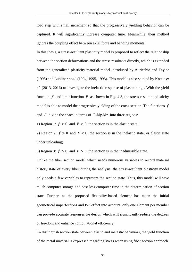
Chapter 4. Two plasticity models for material nonlinearity
93
load step with small increment so that the progressively yielding behavior can be
captured. It will significantly increase computer time. Meanwhile, their method
ignores the coupling effect between axial force and bending moments.
In this thesis, a stress-resultant plasticity model is proposed to reflect the relationship
between the section deformations and the stress resultants directly, which is extended
from the generalized plasticity material model introduced by Auricchio and Taylor
(1995) and Lubliner et al. (1994, 1995, 1993). This model is also studied by Kostic et
al. (2013, 2016) to investigate the inelastic response of plastic hinge. With the yield
function 𝑓 and limit function 𝐹 as shown in Fig. 4.3, the stress-resultant plasticity
model is able to model the progressive yielding of the cross-section. The functions 𝑓
and 𝐹 divide the space in terms of P-My-Mz into three regions:
1) Region 1: 𝑓 < 0 and 𝐹 < 0, the section is in the elastic state;
2) Region 2: 𝑓 > 0 and 𝐹 < 0, the section is in the inelastic state, or elastic state
under unloading;
3) Region 3: 𝑓 > 0 and 𝐹 > 0, the section is in the inadmissible state.
Unlike the fiber section model which needs numerous variables to record material
history state of every fiber during the analysis, the stress-resultant plasticity model
only needs a few variables to represent the section state. Thus, this model will save
much computer storage and cost less computer time in the determination of section
state. Further, as the proposed flexibility-based element has taken the initial
geometrical imperfections and P- effect into account, only one element per member
can provide accurate responses for design which will significantly reduce the degrees
of freedom and enhance computational efficiency.
To distinguish section state between elastic and inelastic behaviors, the yield function
of the metal material is expressed regarding stress when using fiber section approach.
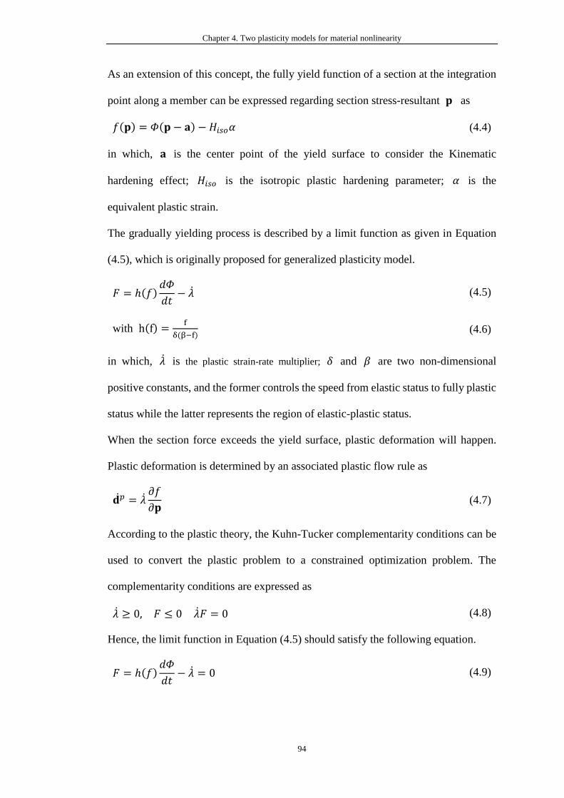
Chapter 4. Two plasticity models for material nonlinearity
94
As an extension of this concept, the fully yield function of a section at the integration
point along a member can be expressed regarding section stress-resultant 𝐩 as
𝑓(𝐩) = 𝛷(𝐩 − 𝐚) − 𝐻𝑖𝑠𝑜𝛼 (4.4)
in which, 𝐚 is the center point of the yield surface to consider the Kinematic
hardening effect; 𝐻𝑖𝑠𝑜 is the isotropic plastic hardening parameter; 𝛼 is the
equivalent plastic strain.
The gradually yielding process is described by a limit function as given in Equation
(4.5), which is originally proposed for generalized plasticity model.
𝐹 = ℎ(𝑓)𝑑𝛷
𝑑𝑡− �̇� (4.5)
with h(f) =f
δ(β−f) (4.6)
in which, �̇� is the plastic strain-rate multiplier; 𝛿 and 𝛽 are two non-dimensional
positive constants, and the former controls the speed from elastic status to fully plastic
status while the latter represents the region of elastic-plastic status.
When the section force exceeds the yield surface, plastic deformation will happen.
Plastic deformation is determined by an associated plastic flow rule as
�̇�𝑝 = �̇�𝜕𝑓
𝜕𝐩 (4.7)
According to the plastic theory, the Kuhn-Tucker complementarity conditions can be
used to convert the plastic problem to a constrained optimization problem. The
complementarity conditions are expressed as
�̇� ≥ 0, 𝐹 ≤ 0 �̇�𝐹 = 0 (4.8)
Hence, the limit function in Equation (4.5) should satisfy the following equation.
𝐹 = ℎ(𝑓)𝑑𝛷
𝑑𝑡− �̇� = 0 (4.9)
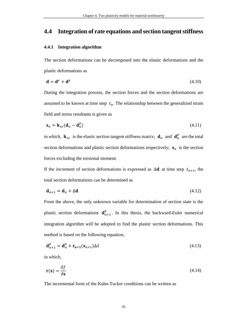
Chapter 4. Two plasticity models for material nonlinearity
95
4.4 Integration of rate equations and section tangent stiffness
4.4.1 Integration algorithm
The section deformations can be decomposed into the elastic deformations and the
plastic deformations as
𝐝 = 𝐝𝑒 + 𝐝𝑝 (4.10)
During the integration process, the section forces and the section deformations are
assumed to be known at time step 𝑡𝑛. The relationship between the generalized strain
field and stress resultants is given as
𝐬𝑛 = 𝐤𝑠𝑒(𝐝𝑛 − 𝐝𝑛𝑝) (4.11)
in which, 𝐤𝑠𝑒 is the elastic section tangent stiffness matrix; 𝐝𝑛 and 𝐝𝑛𝑝
are the total
section deformations and plastic section deformations respectively; 𝐬𝑛 is the section
forces excluding the torsional moment.
If the increment of section deformations is expressed as ∆𝐝 at time step 𝑡𝑛+1, the
total section deformations can be determined as
𝐝𝑛+1 = 𝐝𝑛 + ∆𝐝 (4.12)
From the above, the only unknown variable for determination of section state is the
plastic section deformations 𝐝𝑛+1𝑝
. In this thesis, the backward-Euler numerical
integration algorithm will be adopted to find the plastic section deformations. This
method is based on the following equation,
𝐝𝑛+1𝑝 = 𝐝𝑛
𝑝 + 𝐫𝒏+𝟏(𝐬𝑛+1)∆𝜆 (4.13)
in which,
𝐫(𝐬) =𝜕𝑓
𝜕𝐬 (4.14)
The incremental form of the Kuhn-Tucker conditions can be written as
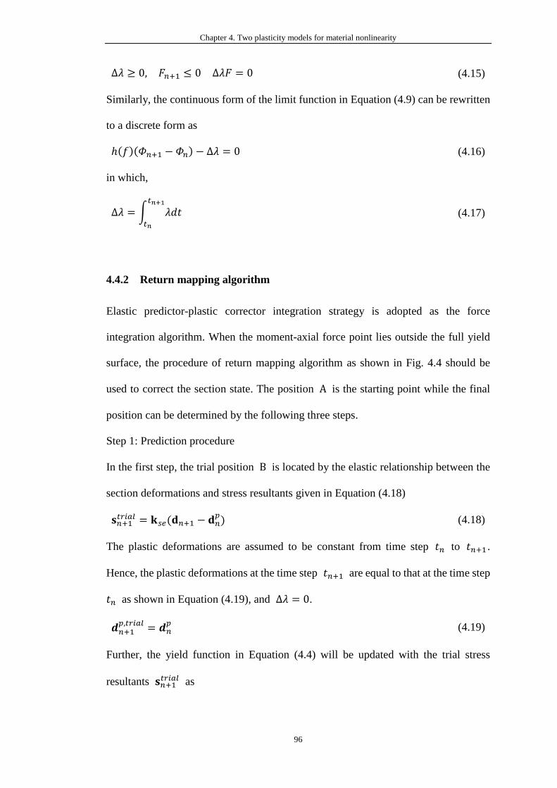
Chapter 4. Two plasticity models for material nonlinearity
96
∆𝜆 ≥ 0, 𝐹𝑛+1 ≤ 0 ∆𝜆𝐹 = 0 (4.15)
Similarly, the continuous form of the limit function in Equation (4.9) can be rewritten
to a discrete form as
ℎ(𝑓)(𝛷𝑛+1 − 𝛷𝑛) − ∆𝜆 = 0 (4.16)
in which,
∆𝜆 = ∫ 𝜆𝑑𝑡𝑡𝑛+1
𝑡𝑛
(4.17)
4.4.2 Return mapping algorithm
Elastic predictor-plastic corrector integration strategy is adopted as the force
integration algorithm. When the moment-axial force point lies outside the full yield
surface, the procedure of return mapping algorithm as shown in Fig. 4.4 should be
used to correct the section state. The position A is the starting point while the final
position can be determined by the following three steps.
Step 1: Prediction procedure
In the first step, the trial position B is located by the elastic relationship between the
section deformations and stress resultants given in Equation (4.18)
𝐬𝑛+1𝑡𝑟𝑖𝑎𝑙 = 𝐤𝑠𝑒(𝐝𝑛+1 − 𝐝𝑛
𝑝) (4.18)
The plastic deformations are assumed to be constant from time step 𝑡𝑛 to 𝑡𝑛+1 .
Hence, the plastic deformations at the time step 𝑡𝑛+1 are equal to that at the time step
𝑡𝑛 as shown in Equation (4.19), and ∆𝜆 = 0.
𝒅𝑛+1𝑝,𝑡𝑟𝑖𝑎𝑙 = 𝒅𝑛
𝑝 (4.19)
Further, the yield function in Equation (4.4) will be updated with the trial stress
resultants 𝐬𝑛+1𝑡𝑟𝑖𝑎𝑙 as
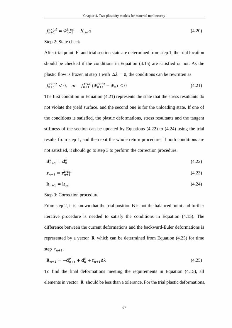
Chapter 4. Two plasticity models for material nonlinearity
97
𝑓𝑛+1𝑡𝑟𝑖𝑎𝑙 = 𝛷𝑛+1
𝑡𝑟𝑖𝑎𝑙 − 𝐻𝑖𝑠𝑜𝛼 (4.20)
Step 2: State check
After trial point B and trial section state are determined from step 1, the trial location
should be checked if the conditions in Equation (4.15) are satisfied or not. As the
plastic flow is frozen at step 1 with ∆𝜆 = 0, the conditions can be rewritten as
𝑓𝑛+1𝑡𝑟𝑖𝑎𝑙 < 0, 𝑜𝑟 𝑓𝑛+1
𝑡𝑟𝑖𝑎𝑙(𝛷𝑛+1𝑡𝑟𝑖𝑎𝑙 − 𝛷𝑛) ≤ 0 (4.21)
The first condition in Equation (4.21) represents the state that the stress resultants do
not violate the yield surface, and the second one is for the unloading state. If one of
the conditions is satisfied, the plastic deformations, stress resultants and the tangent
stiffness of the section can be updated by Equations (4.22) to (4.24) using the trial
results from step 1, and then exit the whole return procedure. If both conditions are
not satisfied, it should go to step 3 to perform the correction procedure.
𝒅𝑛+1𝑝 = 𝒅𝑛
𝑝 (4.22)
𝒔𝑛+1 = 𝒔𝑛+1𝑡𝑟𝑖𝑎𝑙 (4.23)
𝐤𝑛+1 = 𝐤𝑠𝑒 (4.24)
Step 3: Correction procedure
From step 2, it is known that the trial position B is not the balanced point and further
iterative procedure is needed to satisfy the conditions in Equation (4.15). The
difference between the current deformations and the backward-Euler deformations is
represented by a vector 𝐑 which can be determined from Equation (4.25) for time
step 𝑡𝑛+1.
𝐑𝑛+1 = −𝐝𝑛+1𝑝 + 𝐝𝑛
𝑝 + 𝐫𝑛+1∆𝜆 (4.25)
To find the final deformations meeting the requirements in Equation (4.15), all
elements in vector 𝐑 should be less than a tolerance. For the trial plastic deformations,
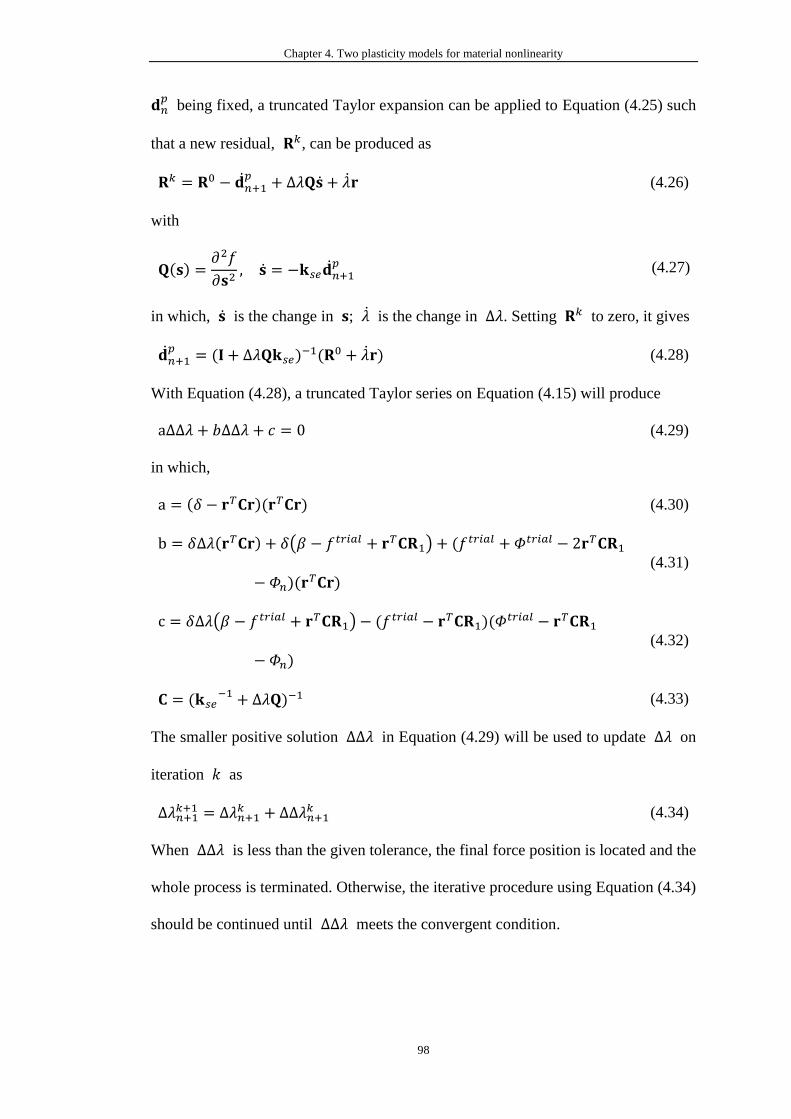
Chapter 4. Two plasticity models for material nonlinearity
98
𝐝𝑛𝑝
being fixed, a truncated Taylor expansion can be applied to Equation (4.25) such
that a new residual, 𝐑𝑘, can be produced as
𝐑𝑘 = 𝐑0 − �̇�𝑛+1𝑝 + ∆𝜆𝐐�̇� + �̇�𝐫 (4.26)
with
𝐐(𝐬) =𝜕2𝑓
𝜕𝐬2, �̇� = −𝐤𝑠𝑒�̇�𝑛+1
𝑝 (4.27)
in which, �̇� is the change in 𝐬; �̇� is the change in ∆𝜆. Setting 𝐑𝑘 to zero, it gives
�̇�𝑛+1𝑝 = (𝐈 + ∆𝜆𝐐𝐤𝑠𝑒)
−1(𝐑0 + �̇�𝐫) (4.28)
With Equation (4.28), a truncated Taylor series on Equation (4.15) will produce
a∆∆𝜆 + 𝑏∆∆𝜆 + 𝑐 = 0 (4.29)
in which,
a = (𝛿 − 𝐫𝑇𝐂𝐫)(𝐫𝑇𝐂𝐫) (4.30)
b = 𝛿∆𝜆(𝐫𝑇𝐂𝐫) + 𝛿(𝛽 − 𝑓𝑡𝑟𝑖𝑎𝑙 + 𝐫𝑇𝐂𝐑1) + (𝑓𝑡𝑟𝑖𝑎𝑙 + 𝛷𝑡𝑟𝑖𝑎𝑙 − 2𝐫𝑇𝐂𝐑1
− 𝛷𝑛)(𝐫𝑇𝐂𝐫)
(4.31)
c = 𝛿∆𝜆(𝛽 − 𝑓𝑡𝑟𝑖𝑎𝑙 + 𝐫𝑇𝐂𝐑1) − (𝑓𝑡𝑟𝑖𝑎𝑙 − 𝐫𝑇𝐂𝐑1)(𝛷
𝑡𝑟𝑖𝑎𝑙 − 𝐫𝑇𝐂𝐑1
− 𝛷𝑛)
(4.32)
𝐂 = (𝐤𝑠𝑒−1 + ∆𝜆𝐐)−1 (4.33)
The smaller positive solution ∆∆𝜆 in Equation (4.29) will be used to update ∆𝜆 on
iteration 𝑘 as
∆𝜆𝑛+1𝑘+1 = ∆𝜆𝑛+1
𝑘 + ∆∆𝜆𝑛+1𝑘 (4.34)
When ∆∆𝜆 is less than the given tolerance, the final force position is located and the
whole process is terminated. Otherwise, the iterative procedure using Equation (4.34)
should be continued until ∆∆𝜆 meets the convergent condition.
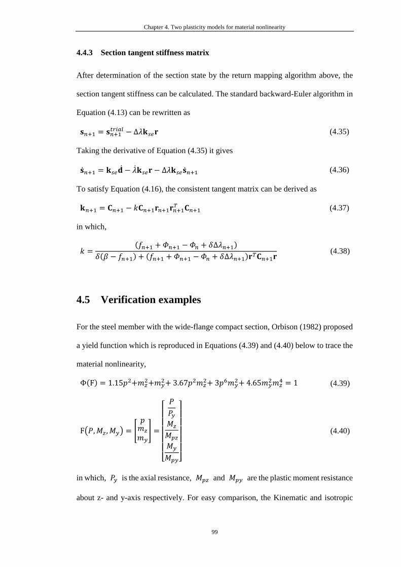
Chapter 4. Two plasticity models for material nonlinearity
99
4.4.3 Section tangent stiffness matrix
After determination of the section state by the return mapping algorithm above, the
section tangent stiffness can be calculated. The standard backward-Euler algorithm in
Equation (4.13) can be rewritten as
𝐬𝑛+1 = 𝐬𝑛+1𝑡𝑟𝑖𝑎𝑙 − ∆𝜆𝐤𝑠𝑒𝐫 (4.35)
Taking the derivative of Equation (4.35) it gives
�̇�𝑛+1 = 𝐤𝑠𝑒�̇� − �̇�𝐤𝑠𝑒𝐫 − ∆𝜆𝐤𝑠𝑒�̇�𝑛+1 (4.36)
To satisfy Equation (4.16), the consistent tangent matrix can be derived as
𝐤𝑛+1 = 𝐂𝑛+1 − 𝑘𝐂𝑛+1𝐫𝑛+1𝐫𝑛+1𝑇 𝐂𝑛+1 (4.37)
in which,
𝑘 =(𝑓𝑛+1 + 𝛷𝑛+1 − 𝛷𝑛 + 𝛿∆𝜆𝑛+1)
𝛿(𝛽 − 𝑓𝑛+1) + (𝑓𝑛+1 + 𝛷𝑛+1 − 𝛷𝑛 + 𝛿∆𝜆𝑛+1)𝐫𝑇𝐂𝑛+1𝐫 (4.38)
4.5 Verification examples
For the steel member with the wide-flange compact section, Orbison (1982) proposed
a yield function which is reproduced in Equations (4.39) and (4.40) below to trace the
material nonlinearity,
Φ(F) = 1.15𝑝2+𝑚𝑧2+𝑚𝑦
2+ 3.67𝑝2𝑚𝑧2+ 3𝑝6𝑚𝑦
2+ 4.65𝑚𝑦2𝑚𝑧
4 = 1 (4.39)
F(𝑃,𝑀𝑧 , 𝑀𝑦) = [
𝑝𝑚𝑧
𝑚𝑦
] =
[ 𝑃
𝑃𝑦𝑀𝑧
𝑀𝑝𝑧
𝑀𝑦
𝑀𝑝𝑦]
(4.40)
in which, 𝑃𝑦 is the axial resistance, 𝑀𝑝𝑧 and 𝑀𝑝𝑦 are the plastic moment resistance
about z- and y-axis respectively. For easy comparison, the Kinematic and isotropic
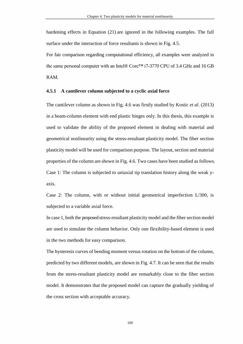
Chapter 4. Two plasticity models for material nonlinearity
100
hardening effects in Equation (21) are ignored in the following examples. The full
surface under the interaction of force resultants is shown in Fig. 4.5.
For fair comparison regarding computational efficiency, all examples were analyzed in
the same personal computer with an Intel® Core™ i7-3770 CPU of 3.4 GHz and 16 GB
RAM.
4.5.1 A cantilever column subjected to a cyclic axial force
The cantilever column as shown in Fig. 4.6 was firstly studied by Kostic et al. (2013)
in a beam-column element with end plastic hinges only. In this thesis, this example is
used to validate the ability of the proposed element in dealing with material and
geometrical nonlinearity using the stress-resultant plasticity model. The fiber section
plasticity model will be used for comparison purpose. The layout, section and material
properties of the column are shown in Fig. 4.6. Two cases have been studied as follows.
Case 1: The column is subjected to uniaxial tip translation history along the weak y-
axis.
Case 2: The column, with or without initial geometrical imperfection L/300, is
subjected to a variable axial force.
In case 1, both the proposed stress-resultant plasticity model and the fiber section model
are used to simulate the column behavior. Only one flexibility-based element is used
in the two methods for easy comparison.
The hysteresis curves of bending moment versus rotation on the bottom of the column,
predicted by two different models, are shown in Fig. 4.7. It can be seen that the results
from the stress-resultant plasticity model are remarkably close to the fiber section
model. It demonstrates that the proposed model can capture the gradually yielding of
the cross section with acceptable accuracy.
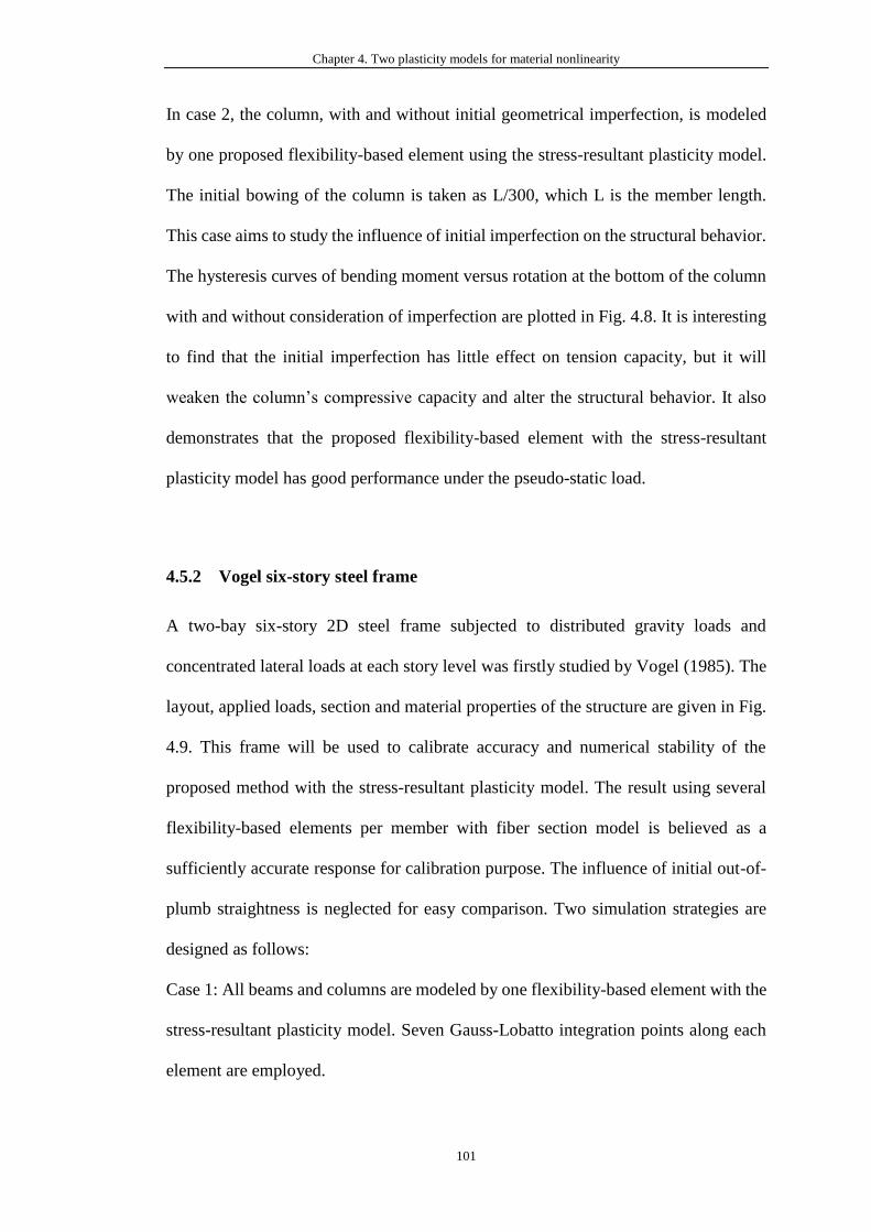
Chapter 4. Two plasticity models for material nonlinearity
101
In case 2, the column, with and without initial geometrical imperfection, is modeled
by one proposed flexibility-based element using the stress-resultant plasticity model.
The initial bowing of the column is taken as L/300, which L is the member length.
This case aims to study the influence of initial imperfection on the structural behavior.
The hysteresis curves of bending moment versus rotation at the bottom of the column
with and without consideration of imperfection are plotted in Fig. 4.8. It is interesting
to find that the initial imperfection has little effect on tension capacity, but it will
weaken the column’s compressive capacity and alter the structural behavior. It also
demonstrates that the proposed flexibility-based element with the stress-resultant
plasticity model has good performance under the pseudo-static load.
4.5.2 Vogel six-story steel frame
A two-bay six-story 2D steel frame subjected to distributed gravity loads and
concentrated lateral loads at each story level was firstly studied by Vogel (1985). The
layout, applied loads, section and material properties of the structure are given in Fig.
4.9. This frame will be used to calibrate accuracy and numerical stability of the
proposed method with the stress-resultant plasticity model. The result using several
flexibility-based elements per member with fiber section model is believed as a
sufficiently accurate response for calibration purpose. The influence of initial out-of-
plumb straightness is neglected for easy comparison. Two simulation strategies are
designed as follows:
Case 1: All beams and columns are modeled by one flexibility-based element with the
stress-resultant plasticity model. Seven Gauss-Lobatto integration points along each
element are employed.
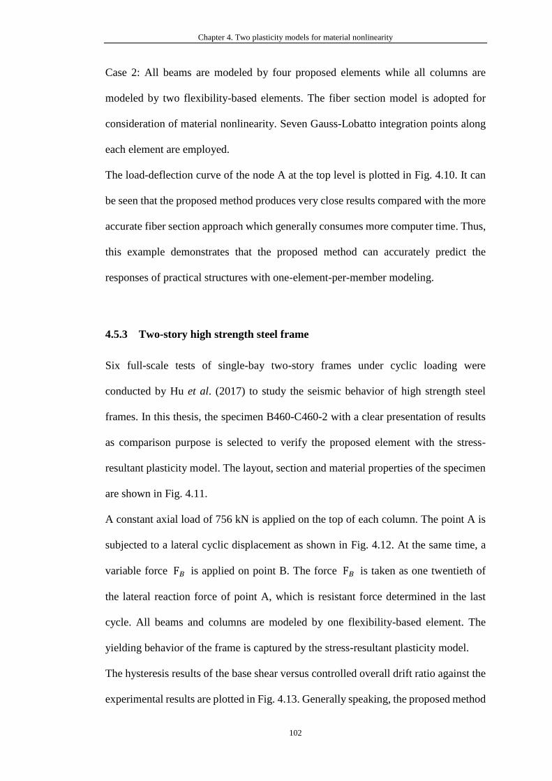
Chapter 4. Two plasticity models for material nonlinearity
102
Case 2: All beams are modeled by four proposed elements while all columns are
modeled by two flexibility-based elements. The fiber section model is adopted for
consideration of material nonlinearity. Seven Gauss-Lobatto integration points along
each element are employed.
The load-deflection curve of the node A at the top level is plotted in Fig. 4.10. It can
be seen that the proposed method produces very close results compared with the more
accurate fiber section approach which generally consumes more computer time. Thus,
this example demonstrates that the proposed method can accurately predict the
responses of practical structures with one-element-per-member modeling.
4.5.3 Two-story high strength steel frame
Six full-scale tests of single-bay two-story frames under cyclic loading were
conducted by Hu et al. (2017) to study the seismic behavior of high strength steel
frames. In this thesis, the specimen B460-C460-2 with a clear presentation of results
as comparison purpose is selected to verify the proposed element with the stress-
resultant plasticity model. The layout, section and material properties of the specimen
are shown in Fig. 4.11.
A constant axial load of 756 kN is applied on the top of each column. The point A is
subjected to a lateral cyclic displacement as shown in Fig. 4.12. At the same time, a
variable force F𝐵 is applied on point B. The force F𝐵 is taken as one twentieth of
the lateral reaction force of point A, which is resistant force determined in the last
cycle. All beams and columns are modeled by one flexibility-based element. The
yielding behavior of the frame is captured by the stress-resultant plasticity model.
The hysteresis results of the base shear versus controlled overall drift ratio against the
experimental results are plotted in Fig. 4.13. Generally speaking, the proposed method
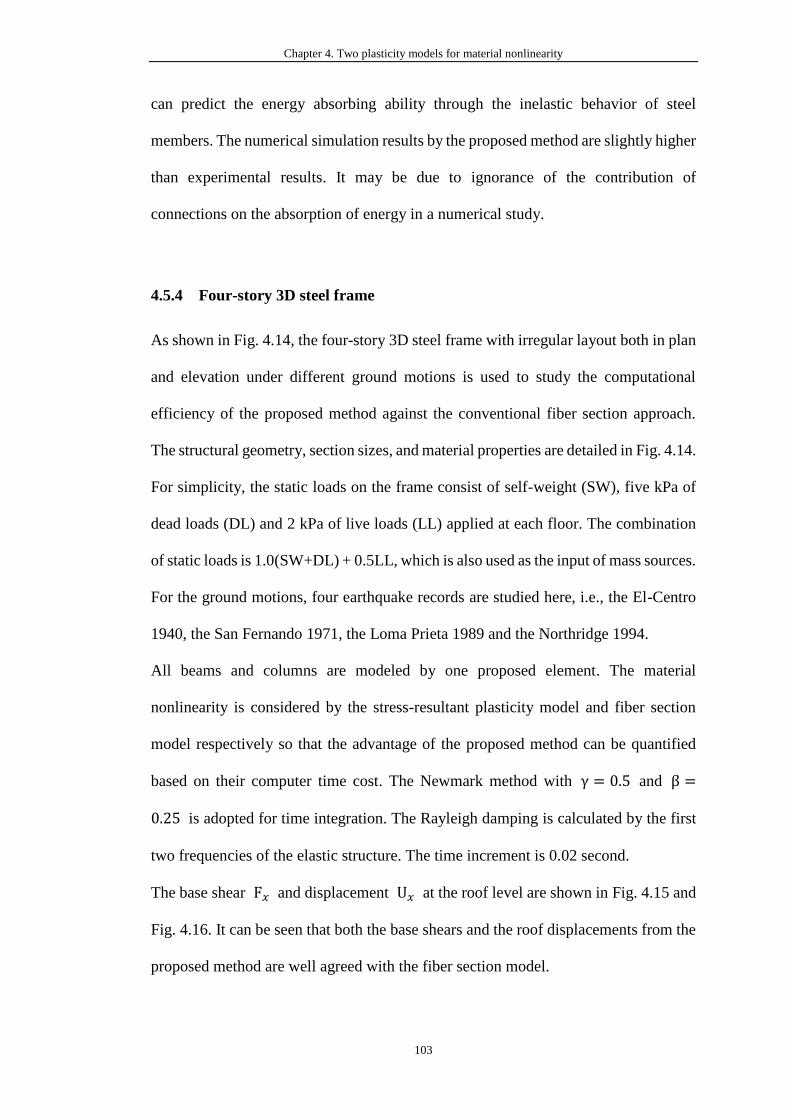
Chapter 4. Two plasticity models for material nonlinearity
103
can predict the energy absorbing ability through the inelastic behavior of steel
members. The numerical simulation results by the proposed method are slightly higher
than experimental results. It may be due to ignorance of the contribution of
connections on the absorption of energy in a numerical study.
4.5.4 Four-story 3D steel frame
As shown in Fig. 4.14, the four-story 3D steel frame with irregular layout both in plan
and elevation under different ground motions is used to study the computational
efficiency of the proposed method against the conventional fiber section approach.
The structural geometry, section sizes, and material properties are detailed in Fig. 4.14.
For simplicity, the static loads on the frame consist of self-weight (SW), five kPa of
dead loads (DL) and 2 kPa of live loads (LL) applied at each floor. The combination
of static loads is 1.0(SW+DL) + 0.5LL, which is also used as the input of mass sources.
For the ground motions, four earthquake records are studied here, i.e., the El-Centro
1940, the San Fernando 1971, the Loma Prieta 1989 and the Northridge 1994.
All beams and columns are modeled by one proposed element. The material
nonlinearity is considered by the stress-resultant plasticity model and fiber section
model respectively so that the advantage of the proposed method can be quantified
based on their computer time cost. The Newmark method with γ = 0.5 and β =
0.25 is adopted for time integration. The Rayleigh damping is calculated by the first
two frequencies of the elastic structure. The time increment is 0.02 second.
The base shear F𝑥 and displacement U𝑥 at the roof level are shown in Fig. 4.15 and
Fig. 4.16. It can be seen that both the base shears and the roof displacements from the
proposed method are well agreed with the fiber section model.
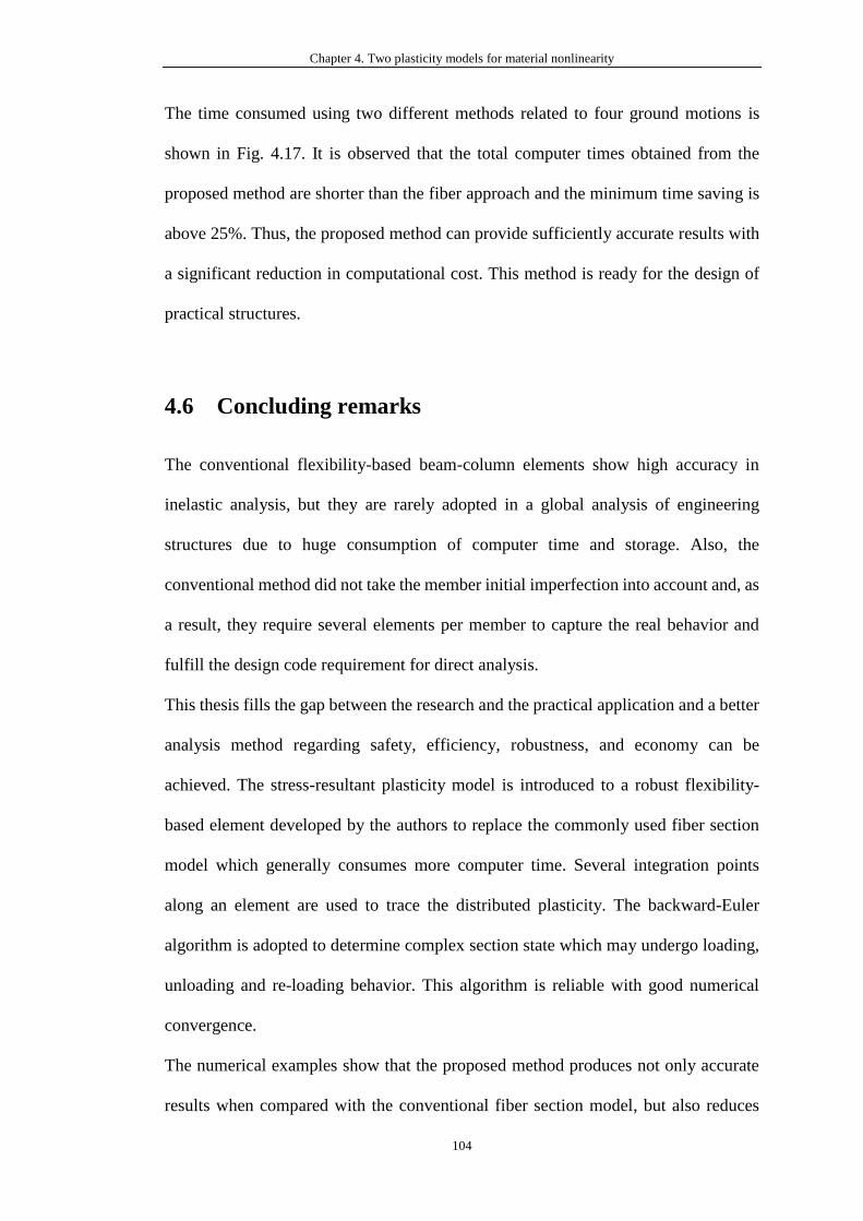
Chapter 4. Two plasticity models for material nonlinearity
104
The time consumed using two different methods related to four ground motions is
shown in Fig. 4.17. It is observed that the total computer times obtained from the
proposed method are shorter than the fiber approach and the minimum time saving is
above 25%. Thus, the proposed method can provide sufficiently accurate results with
a significant reduction in computational cost. This method is ready for the design of
practical structures.
4.6 Concluding remarks
The conventional flexibility-based beam-column elements show high accuracy in
inelastic analysis, but they are rarely adopted in a global analysis of engineering
structures due to huge consumption of computer time and storage. Also, the
conventional method did not take the member initial imperfection into account and, as
a result, they require several elements per member to capture the real behavior and
fulfill the design code requirement for direct analysis.
This thesis fills the gap between the research and the practical application and a better
analysis method regarding safety, efficiency, robustness, and economy can be
achieved. The stress-resultant plasticity model is introduced to a robust flexibility-
based element developed by the authors to replace the commonly used fiber section
model which generally consumes more computer time. Several integration points
along an element are used to trace the distributed plasticity. The backward-Euler
algorithm is adopted to determine complex section state which may undergo loading,
unloading and re-loading behavior. This algorithm is reliable with good numerical
convergence.
The numerical examples show that the proposed method produces not only accurate
results when compared with the conventional fiber section model, but also reduces
Chapter 4. Two plasticity models for material nonlinearity
105
significantly the computational cost. Thus, this innovative solution, complying with
the codified requirement of second-order direct analysis, is readily applicable to the
design of practical steel structures.
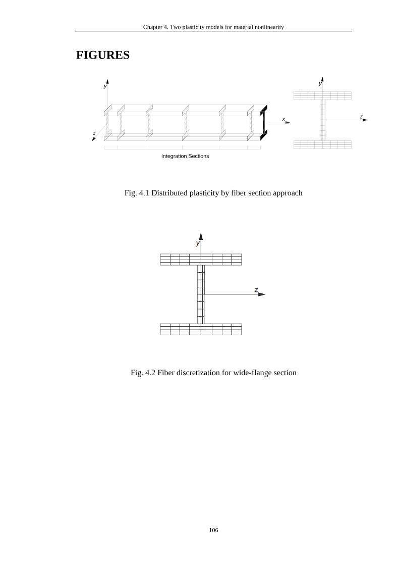
Chapter 4. Two plasticity models for material nonlinearity
106
FIGURES
Fig. 4.1 Distributed plasticity by fiber section approach
Fig. 4.2 Fiber discretization for wide-flange section
z
x
y
Integration Sections
z
y

Chapter 4. Two plasticity models for material nonlinearity
107
Fig. 4.3 Yield function and limit function for section state
Fig. 4.4 Backward-Euler return procedure
N
Mz
My
F=0
f =0
F<0
f <0
F<0
f >0
F>0
f >0
Moment
Axial force
sn
sn+1trial
sn+1 sn+1k+1
sn+1k
yield surface
A
BC
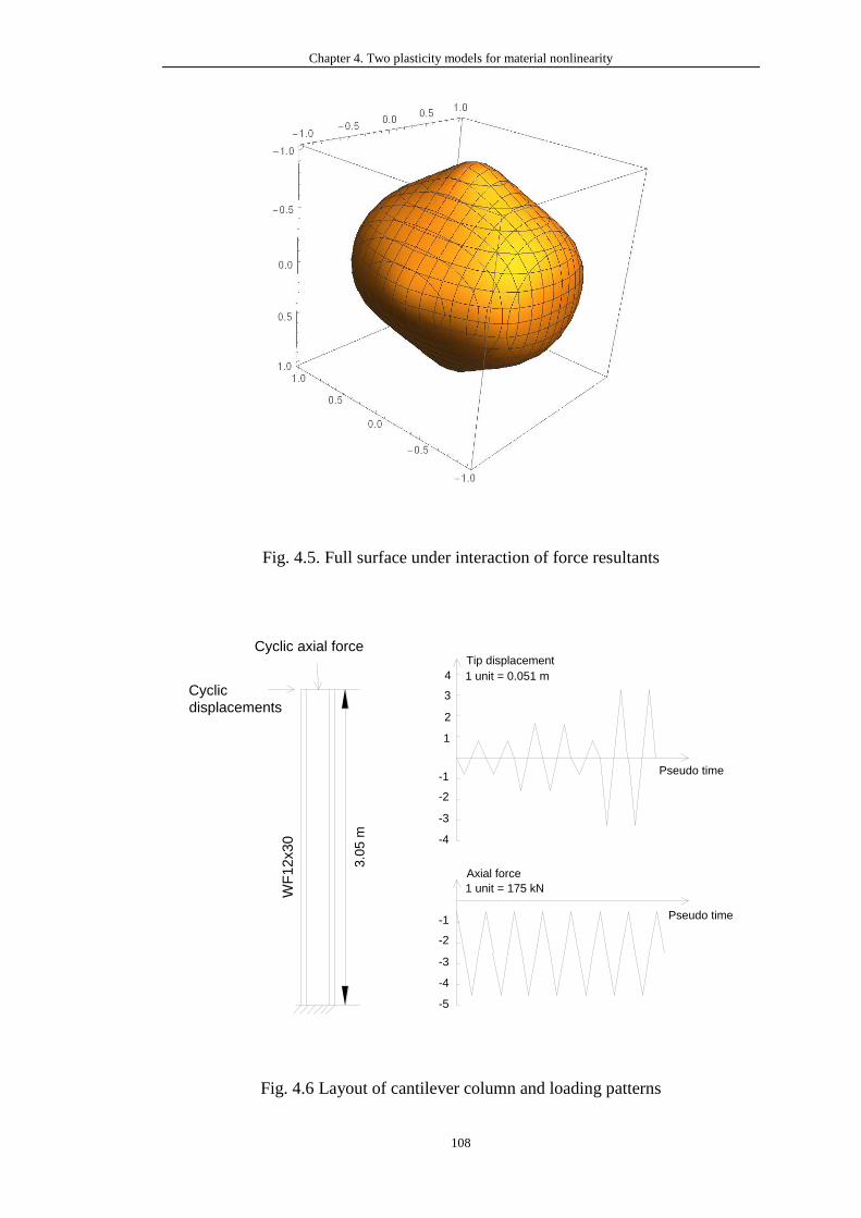
Chapter 4. Two plasticity models for material nonlinearity
108
Fig. 4.5. Full surface under interaction of force resultants
Fig. 4.6 Layout of cantilever column and loading patterns
3.0
5 m
WF
12
x3
0
Cyclic axial force
Cyclic
displacements
Tip displacement
Pseudo time
Axial force
Pseudo time-1
-2
-3
-4
4
3
2
1
-1
-2
-3
-4
1 unit = 0.051 m
1 unit = 175 kN
-5
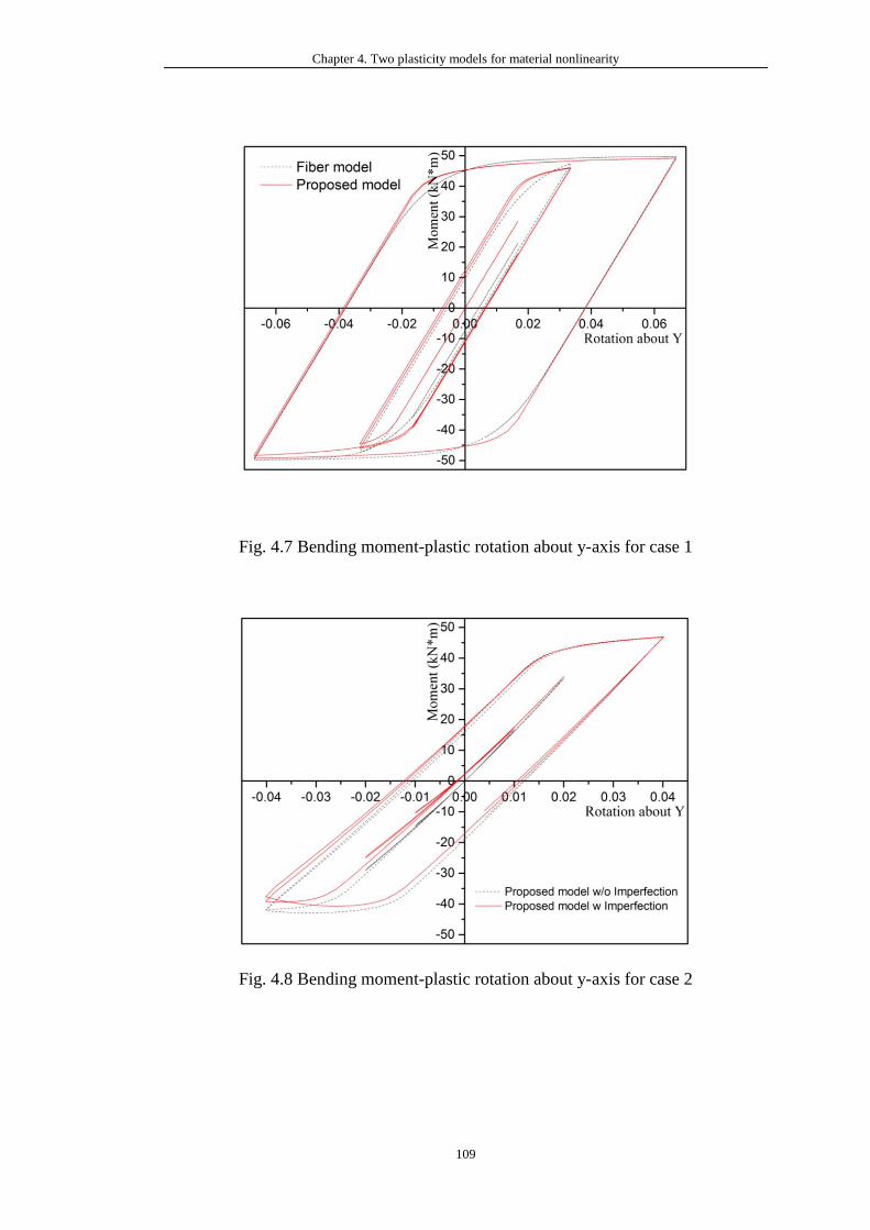
Chapter 4. Two plasticity models for material nonlinearity
109
Fig. 4.7 Bending moment-plastic rotation about y-axis for case 1
Fig. 4.8 Bending moment-plastic rotation about y-axis for case 2
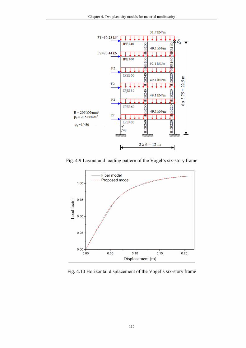
Chapter 4. Two plasticity models for material nonlinearity
110
Fig. 4.9 Layout and loading pattern of the Vogel’s six-story frame
Fig. 4.10 Horizontal displacement of the Vogel’s six-story frame
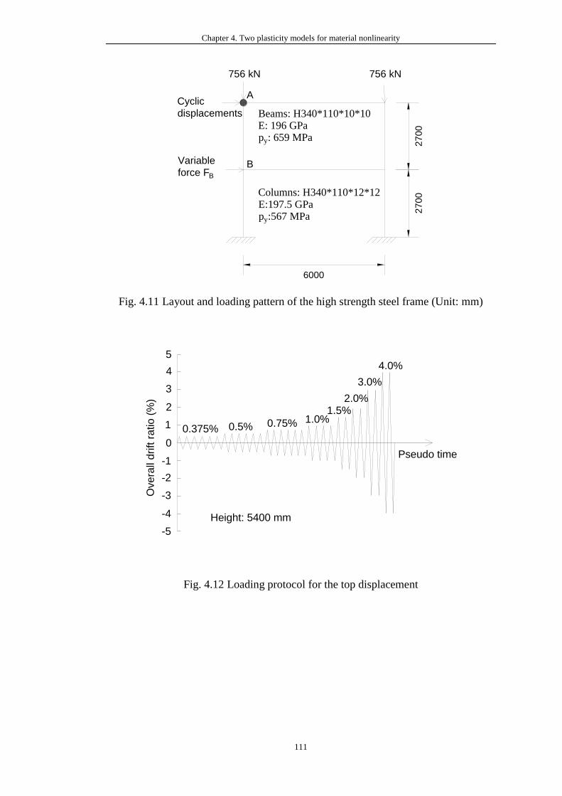
Chapter 4. Two plasticity models for material nonlinearity
111
Fig. 4.11 Layout and loading pattern of the high strength steel frame (Unit: mm)
Fig. 4.12 Loading protocol for the top displacement
27
00
27
00
6000
Beams: H340*110*10*10E: 196 GPapy: 659 MPa
Columns: H340*110*12*12E:197.5 GPapy:567 MPa
Cyclic
displacements
A
BVariable
force FB
756 kN 756 kN
Overa
ll drift r
atio (
%)
0
1
2
3
4
5
-5
-4
-3
-2
-1
0.375% 0.5% 0.75% 1.0%1.5%
2.0%
3.0%
4.0%
Height: 5400 mm
Pseudo time

Chapter 4. Two plasticity models for material nonlinearity
112
Fig. 4.13 Base shear versus overall drift ratio
Fig. 4.14 Layout of four-story 3D steel frame
3.8
1m
x 4
= 1
5.2
4m
6.35 m
6.35 m 6.35 m
6.35 m
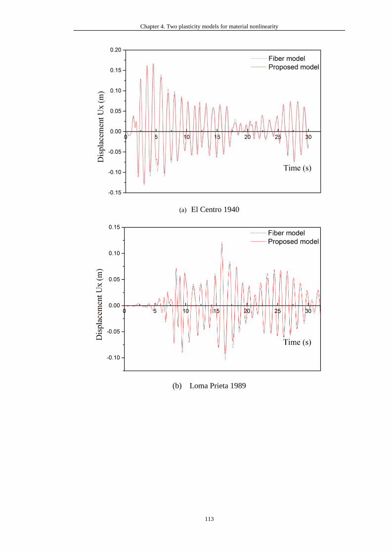
Chapter 4. Two plasticity models for material nonlinearity
113
(a) El Centro 1940
(b) Loma Prieta 1989
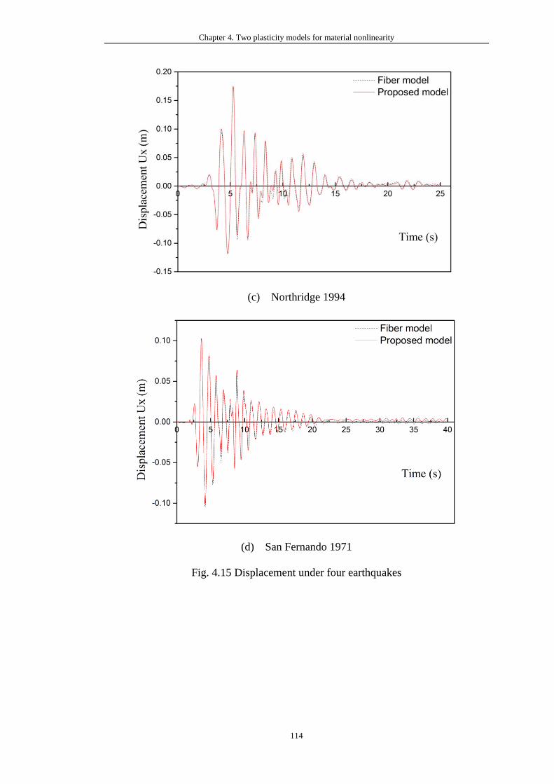
Chapter 4. Two plasticity models for material nonlinearity
114
(c) Northridge 1994
(d) San Fernando 1971
Fig. 4.15 Displacement under four earthquakes
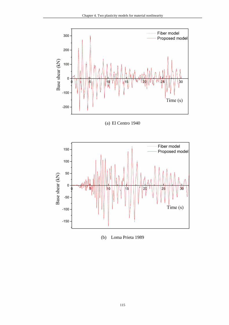
Chapter 4. Two plasticity models for material nonlinearity
115
(a) El Centro 1940
(b) Loma Prieta 1989
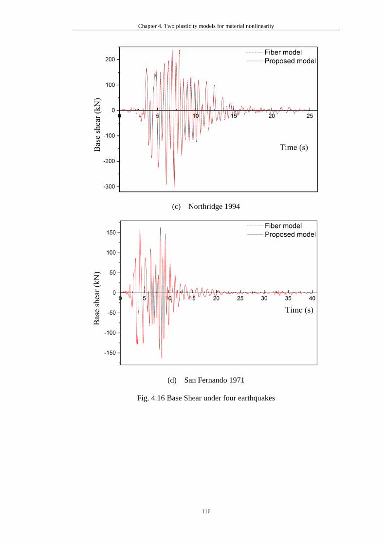
Chapter 4. Two plasticity models for material nonlinearity
116
(c) Northridge 1994
(d) San Fernando 1971
Fig. 4.16 Base Shear under four earthquakes
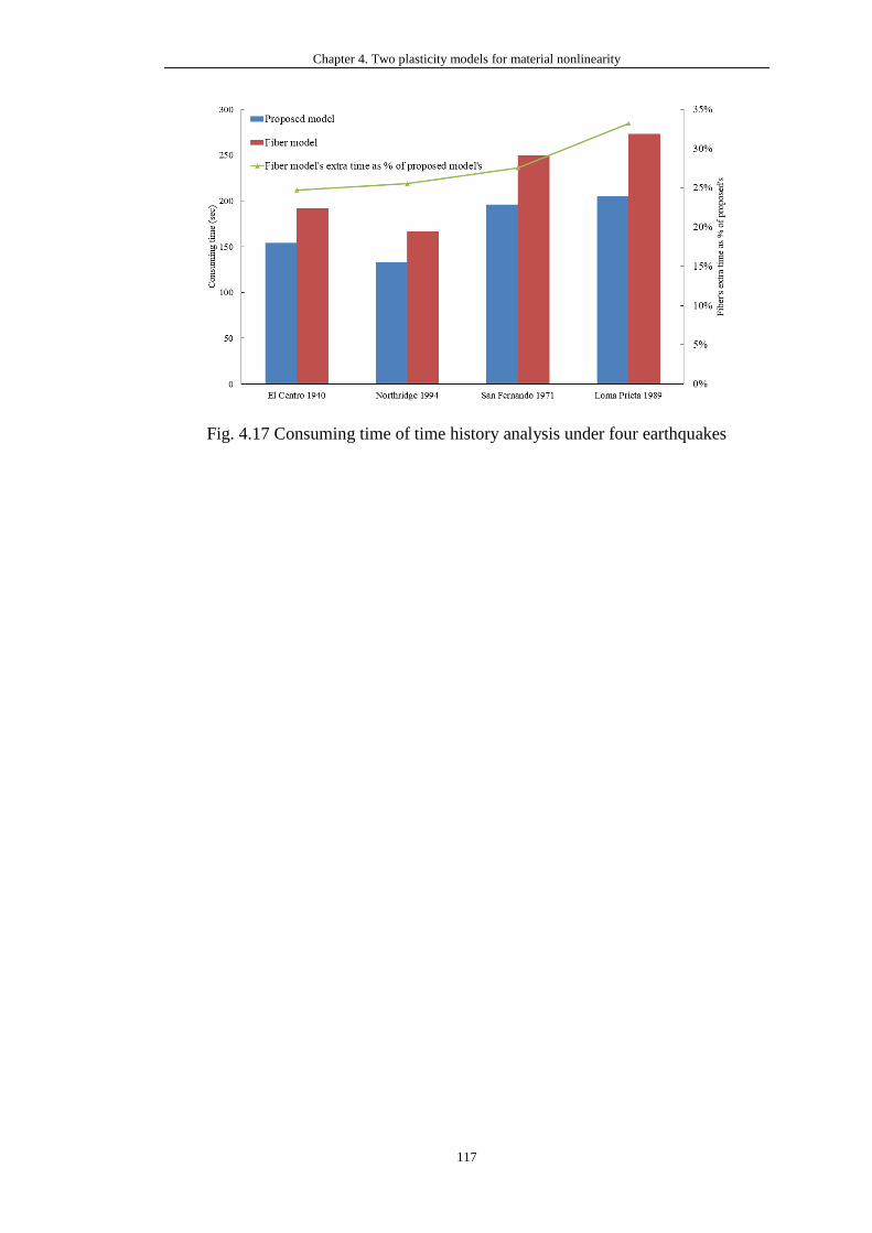
Chapter 4. Two plasticity models for material nonlinearity
117
Fig. 4.17 Consuming time of time history analysis under four earthquakes
Chapter 5. Semi-rigid connections under monotonic and cyclic loads
118
CHAPTER 5. SEMI-RIGID CONNECTIONS
UNDER MONOTONIC AND CYCLIC LOADS
5.1 Introduction
Connection systems play important role in the skeletal space structures. A large
number of connection details have been proposed in the practical projects with great
success, such as solid ball joint systems, socket joint systems, plate joint systems, slot
joint systems and so on. These joint systems are usually analyzed and designed with
the simple assumption that they are either perfectly rigid or frictionlessly pinned for
convenience. In fact, the actual joints may have completely different features
compared with the rigid and pinned joints. This lead to increasing concerns on the
joint behaviors as many collapse events were initiated by connection failure. To satisfy
the moment transfer between the beams and the columns, heavily detailed connections
between these members are required, which cause larger size of beams required. Extra
lateral resisting systems are needed in the pinned-joint structures due to zero rotational
connection stiffness between these members. Noted that, connection systems will
certainly affect the overall behavior of the entire structure. Many national steel design
codes, such as AISC360 (2016) and Eurocode-3-1-8 (2005), have the provisions of
semi-rigid connections to consider joint flexibility to overcome the drawbacks
described above. Many scholars have noticed this phenomenon and conducted many
experimental tests to explore the overall effects of joint flexibility. For example,
Csébfalvi (2007) used an optimal method to design structures with consideration of
semi-rigid joints, which lead to the redistribution of the internal forces between
Chapter 5. Semi-rigid connections under monotonic and cyclic loads
119
members. Ahmadizadeh and Maalek (2014) investigated the effects of socket joint
flexibility on the overall behavior of full-scale space structures and demonstrated that
the rigid-connection assumption made unsafe prediction of displacements and ultimate
load-carrying capacity of the studied structure. Thus, they suggested that the analysis
and design of space structures should directly include the effects of socket joint
flexibility. Sagiroglu and Aydin (2015) reported that the semi-rigid connection design
could lead to a better prediction of the response and reliability of structures. Truong et
al. (2017) utilized the zero-length element model to simulate the nonlinear behavior
of steel connection when optimizing space steel frames with the micro-genetic
algorithm. During the optimization process, the type of semi-rigid connection was also
a variable. They reported that the column sizes should be increased due to the
degradation of connection stiffness. In summary, the joint flexibility should be
reflected in the direct analysis with proper beam-column elements.
In this chapter, the modeling methods for the connections under static and cyclic loads
will be introduced. Further, the semi-rigid models will be directly incorporated into
the proposed element as described in Chapter 3. Several numerical examples will be
studied to verify the practicability and accuracy of the proposed approach. Finally,
several concluding remarks will be listed to highlight the priorities.
5.2 Modeling of connection behavior under monotonic
loading
To consider the joint flexibility in numerical analysis, several linear or nonlinear
models have been proposed in the past decades. Generally, the models for static
analysis ignored the unloading phase. There are three methods to get the moment-

Chapter 5. Semi-rigid connections under monotonic and cyclic loads
120
rotation or force-displacement curves for modeling of semi-rigid connection, i.e.
experimental approaches, empirical approaches, and numerical approaches.
5.2.1 Experimental approaches
Among all approaches exploring joint behaviors, the experimental approaches are the
accurate way to investigate the characterization of joints. In the past few decades,
many monotonic loading tests have been conducted to study the moment-rotation
curves of different types of beam-column connections including single/double web
cleats, header plates, top and seat angles, extend/flush end plates, etc. These rich
experimental results can provide accurate and reliable data for modeling the different
types of beam-column connections. Nevertheless, the cost of these experiments was
high compared with other approaches, and it was hard to cover all the circumstances.
Although there are many disadvantages of these approaches, the basic data regarding
joint systems are vital for other methods as the benchmark and calibration purposes.
5.2.2 Empirical approaches
The models from empirical approaches are often calibrated by the experimental test
results. By collecting numerous test results, the moment versus rotation curves of
various connection types were proposed which can be used for mathematical modeling
of beam-column connections. Because these moment-rotation curves are obtained
from the limited experimental data, it may not be that accurate for studying the real
connection behavior. Moreover, it is difficult to propose an appropriate model for the
uncommonly used connection type due to the lack of data.
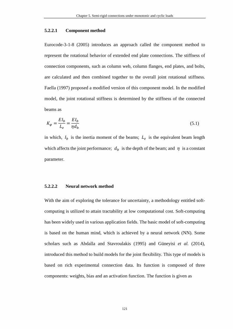
Chapter 5. Semi-rigid connections under monotonic and cyclic loads
121
5.2.2.1 Component method
Eurocode-3-1-8 (2005) introduces an approach called the component method to
represent the rotational behavior of extended end plate connections. The stiffness of
connection components, such as column web, column flanges, end plates, and bolts,
are calculated and then combined together to the overall joint rotational stiffness.
Faella (1997) proposed a modified version of this component model. In the modified
model, the joint rotational stiffness is determined by the stiffness of the connected
beams as
𝐾𝜑 =𝐸𝐼𝑏𝐿𝑒
=𝐸𝐼𝑏𝜂𝑑𝑏
(5.1)
in which, 𝐼𝑏 is the inertia moment of the beams; 𝐿𝑒 is the equivalent beam length
which affects the joint performance; 𝑑𝑏 is the depth of the beam; and 𝜂 is a constant
parameter.
5.2.2.2 Neural network method
With the aim of exploring the tolerance for uncertainty, a methodology entitled soft-
computing is utilized to attain tractability at low computational cost. Soft-computing
has been widely used in various application fields. The basic model of soft-computing
is based on the human mind, which is achieved by a neural network (NN). Some
scholars such as Abdalla and Stavroulakis (1995) and Güneyisi et al. (2014),
introduced this method to build models for the joint flexibility. This type of models is
based on rich experimental connection data. Its function is composed of three
components: weights, bias and an activation function. The function is given as

Chapter 5. Semi-rigid connections under monotonic and cyclic loads
122
𝑈𝑘 = 𝐵𝑖𝑎𝑠𝑘 +∑(𝑤𝑗,𝑘𝐼𝑘)
𝑛
𝑗=1
(5.2)
in which, 𝐼𝑘 is the input parameter; 𝑤𝑗,𝑘 is the weight; 𝐵𝑖𝑎𝑠𝑘 is the bias; and 𝑈𝑘
is the output value. Before training a NN, the database of experimental tests is
collected. Then the mathematical formulation is used to generate the artificial neural
network. The training quality is generally evaluated by the mean square errors and
correlation coefficients. After training, equation (5.1) can be used to predict the
ultimate moment and rotation values.
Though the neural network method is an alternative method for modeling joint
connections, this method is case-dependent and drastically influenced by the optimal
choice of the network configuration. Meanwhile, the speed of the learning procedure
is also a critical problem.
5.2.3 Numerical approaches
Based on the concepts of mechanics theory, such as equilibrium equations,
compatibility equations and material properties, the relationship between the joint
rotational stiffness and the moment resistance can be derived. Compared with the
empirical approaches which should be mainly depended on experiments, the
numerical approaches have several advantages: (1) due to their lower computational
expense, sufficient data can be obtained quickly and conveniently, as opposed to
conducting numerous experimental tests; (2) the local behavior of joints can be
investigated while this is difficult for experimental approaches because of the limited
observation instruments; (3) parametric analysis can be conducted by numerical
approaches to study joint behavior more thoroughly.
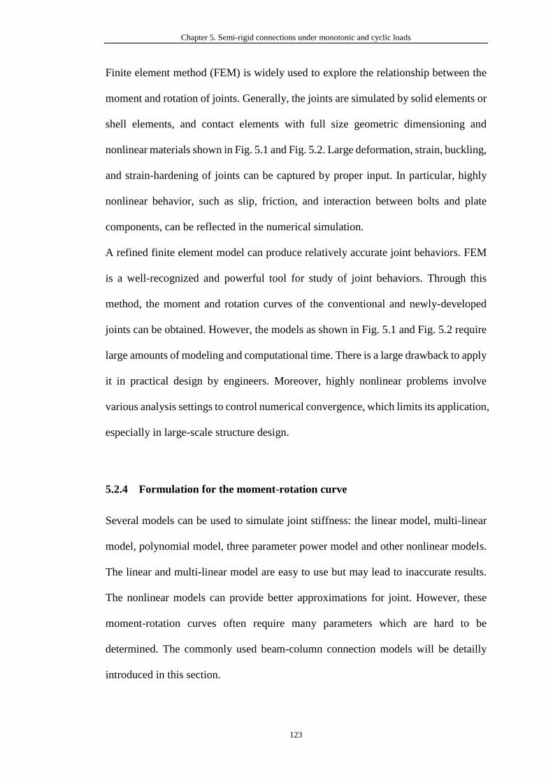
Chapter 5. Semi-rigid connections under monotonic and cyclic loads
123
Finite element method (FEM) is widely used to explore the relationship between the
moment and rotation of joints. Generally, the joints are simulated by solid elements or
shell elements, and contact elements with full size geometric dimensioning and
nonlinear materials shown in Fig. 5.1 and Fig. 5.2. Large deformation, strain, buckling,
and strain-hardening of joints can be captured by proper input. In particular, highly
nonlinear behavior, such as slip, friction, and interaction between bolts and plate
components, can be reflected in the numerical simulation.
A refined finite element model can produce relatively accurate joint behaviors. FEM
is a well-recognized and powerful tool for study of joint behaviors. Through this
method, the moment and rotation curves of the conventional and newly-developed
joints can be obtained. However, the models as shown in Fig. 5.1 and Fig. 5.2 require
large amounts of modeling and computational time. There is a large drawback to apply
it in practical design by engineers. Moreover, highly nonlinear problems involve
various analysis settings to control numerical convergence, which limits its application,
especially in large-scale structure design.
5.2.4 Formulation for the moment-rotation curve
Several models can be used to simulate joint stiffness: the linear model, multi-linear
model, polynomial model, three parameter power model and other nonlinear models.
The linear and multi-linear model are easy to use but may lead to inaccurate results.
The nonlinear models can provide better approximations for joint. However, these
moment-rotation curves often require many parameters which are hard to be
determined. The commonly used beam-column connection models will be detailly
introduced in this section.
Chapter 5. Semi-rigid connections under monotonic and cyclic loads
124
5.2.4.1 Linear model
The linear model provides the simplest moment-rotation curve and only requires one
parameter. The cM − curve can be written as
o
c cM S = (5.3)
in which o
cS is a constant value representing the initial connection stiffness and can
be obtained from experimental results. According to Lightfoot and LeMessurier’s
assumption (1974), the initial stiffness can be expressed as
4o
c
EIS
L= (5.4)
in which, is the rigidity index which indicates the degree of connection flexibility.
The value of varies from zero to infinite based on the joint type. Alternatively,
o
cS can be written as
4
1
o
c
EIS
L
=
− (5.5)
in which, is a fixity factor proposed by Romstad and Subramanian (1970) and Yu
and Shanmugam (1986). The factor is zero for a pinned joint and unity for a rigid
joint.
5.2.4.2 Multi-linear model
The linear model can be used only on the premise of small joint deflection. Regarding
large deflection, the degradation of the connection stiffness should be considered.
Therefore, the multi-linear model is proposed to improve the accuracy of connection
behavior and model the degradation of the stiffness of connections in the large
Chapter 5. Semi-rigid connections under monotonic and cyclic loads
125
deflection problem. In fact, another nonlinear model can be described approximately
by the multi-linear model with sufficient segmentations.
5.2.4.3 Polynomial model
The first non-dimensional polynomial model of connection behavior was proposed by
Frye and Morris (1975). This model can provide a smoother moment-rotation curve
and is included in IS: 800 (1893). The original form is
𝜙𝑐 = 𝐶1(𝐾 𝑀)1 + 𝐶2(𝐾 𝑀)
3 + 𝐶3(𝐾 𝑀)5 (5.6)
where 𝐾 is a constant parameter determined by geometrical characteristics, such as
member size, throat thickness and so on; 𝑀 is the moment applied on the joint; 𝐶1,
𝐶2 , and 𝐶3 are fitting parameters; and 𝜙𝑐 is the joint rotation. The Frye-Morris
model provides a generalized form that can be extended to different connection types.
For example, Prabha et al. (2010) proposed a polynomial model for pallet rack
connection based on this model with 𝐾 defined by the thickness of columns (𝑡𝑢),
depth of beams (𝑑𝑏) and the depth of the connector (𝑑𝑐).
Generally, the polynomial model exhibits good performance in the initial stiffness
prediction, but less accuracy in the ultimate capacity of the connection. Also, the
stiffness of the connection is derived by Equation (5.6), which may lead to negative
stiffness. This case does not conform to reality and causes difficulty in numerical
computation.
5.2.4.4 Three-parameter power model
Kishi and Chen (1987a, 1987b) proposed a three-parameter power model as
Chapter 5. Semi-rigid connections under monotonic and cyclic loads
126
( )1 /
1
n nn
c i
u
MS K
M
+
= −
(5.7)
in which, the parameters iK , uM and n are the initial stiffness, the ultimate
moment capacity and the shape parameter of the cM − curve respectively.
The power model can always produce positive connection stiffness and has a better
numerical performance compared with the polynomial model. Meanwhile, this model
is convenient to engineers for practical design due to the reduced number of
parameters obtained from experiments. However, it sometimes may have less
accuracy in predicting the stiffness of joint connections when remaining elastic.
5.3 Modeling of connection behavior under cyclic loading
5.3.1 M-𝝓 approach
5.3.1.1 Connection models without degradation
The concept of the constitutive relationship between stress and strain can be extended
to generate new M-𝜙 models. Taking the Giuffré-Menegotto-Pinto hysteretic material
model (1983) for example, it is a uni-axial material with isotropic strain hardening for
steel material. The smooth transition of stiffness is widely adopted in nonlinear
analysis. When rewriting this relationship for moment and rotation, the transitional
portion from elastic to plastic state is as given in Equation (5.8) below.
𝑀∗ = 𝑏휀∗ +(1 − 𝑏)𝜙∗
(1 + 𝜙∗ 𝑅)1𝑅
(5.8)
in which, 𝑀∗ and 𝜙∗ are the normalized moment and rotation respectively; and 𝑏
is the strain hardening ratio between the post-yield tangent and initial elastic tangent;
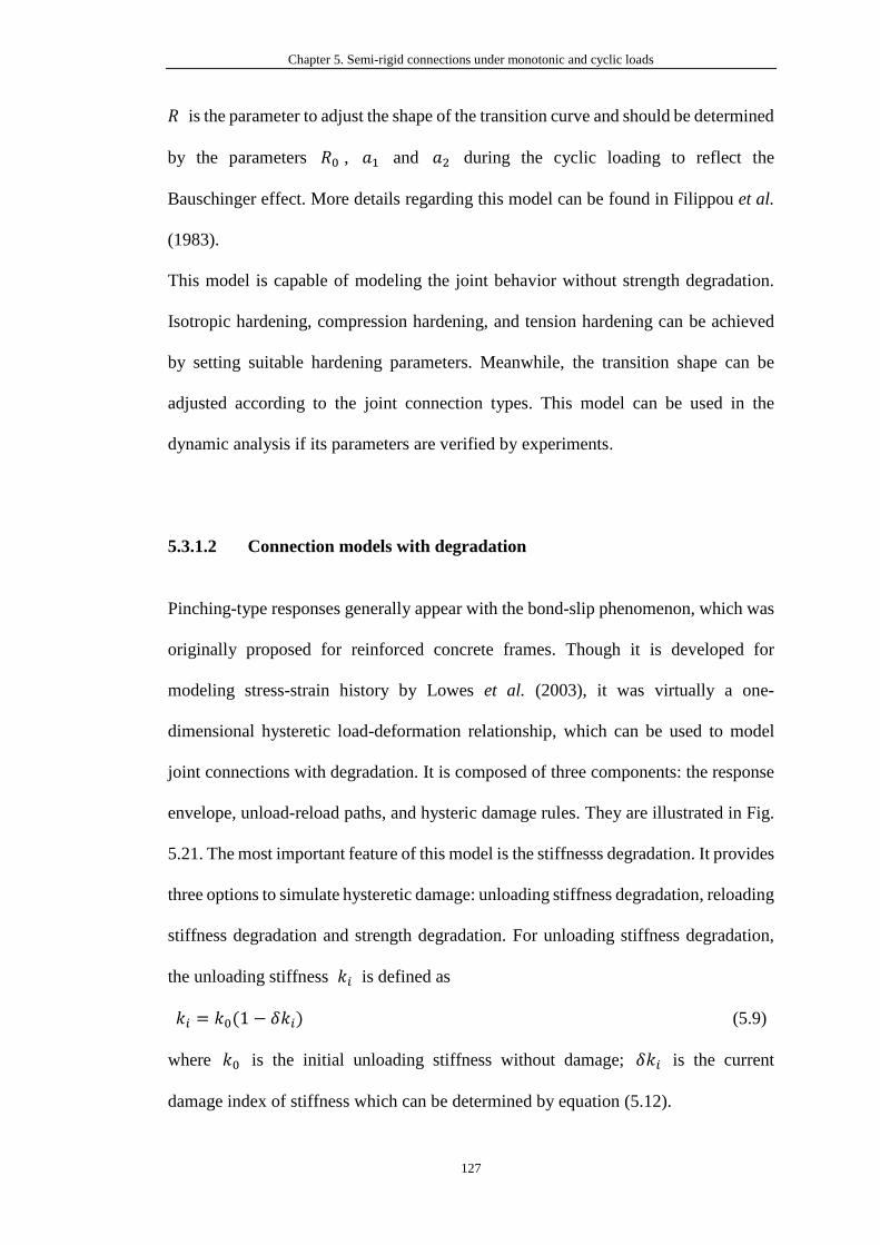
Chapter 5. Semi-rigid connections under monotonic and cyclic loads
127
𝑅 is the parameter to adjust the shape of the transition curve and should be determined
by the parameters 𝑅0 , 𝑎1 and 𝑎2 during the cyclic loading to reflect the
Bauschinger effect. More details regarding this model can be found in Filippou et al.
(1983).
This model is capable of modeling the joint behavior without strength degradation.
Isotropic hardening, compression hardening, and tension hardening can be achieved
by setting suitable hardening parameters. Meanwhile, the transition shape can be
adjusted according to the joint connection types. This model can be used in the
dynamic analysis if its parameters are verified by experiments.
5.3.1.2 Connection models with degradation
Pinching-type responses generally appear with the bond-slip phenomenon, which was
originally proposed for reinforced concrete frames. Though it is developed for
modeling stress-strain history by Lowes et al. (2003), it was virtually a one-
dimensional hysteretic load-deformation relationship, which can be used to model
joint connections with degradation. It is composed of three components: the response
envelope, unload-reload paths, and hysteric damage rules. They are illustrated in Fig.
5.21. The most important feature of this model is the stiffnesss degradation. It provides
three options to simulate hysteretic damage: unloading stiffness degradation, reloading
stiffness degradation and strength degradation. For unloading stiffness degradation,
the unloading stiffness 𝑘𝑖 is defined as
𝑘𝑖 = 𝑘0(1 − 𝛿𝑘𝑖) (5.9)
where 𝑘0 is the initial unloading stiffness without damage; 𝛿𝑘𝑖 is the current
damage index of stiffness which can be determined by equation (5.12).
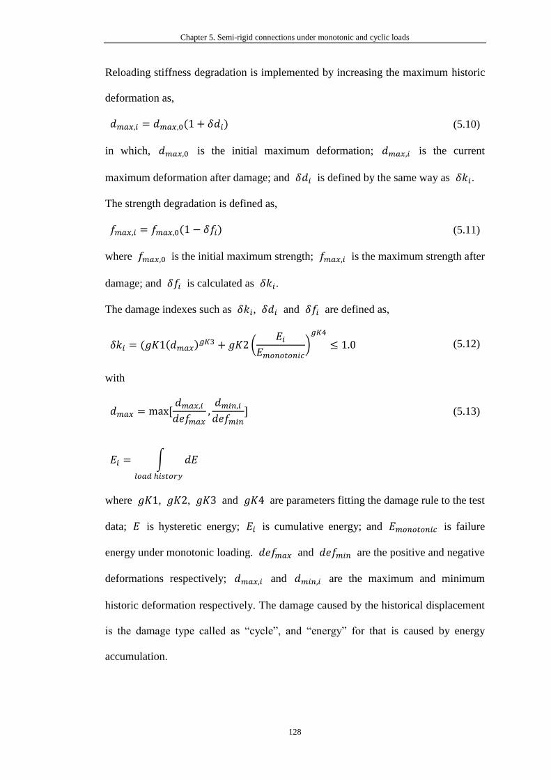
Chapter 5. Semi-rigid connections under monotonic and cyclic loads
128
Reloading stiffness degradation is implemented by increasing the maximum historic
deformation as,
𝑑𝑚𝑎𝑥,𝑖 = 𝑑𝑚𝑎𝑥,0(1 + 𝛿𝑑𝑖) (5.10)
in which, 𝑑𝑚𝑎𝑥,0 is the initial maximum deformation; 𝑑𝑚𝑎𝑥,𝑖 is the current
maximum deformation after damage; and 𝛿𝑑𝑖 is defined by the same way as 𝛿𝑘𝑖.
The strength degradation is defined as,
𝑓𝑚𝑎𝑥,𝑖 = 𝑓𝑚𝑎𝑥,0(1 − 𝛿𝑓𝑖) (5.11)
where 𝑓𝑚𝑎𝑥,0 is the initial maximum strength; 𝑓𝑚𝑎𝑥,𝑖 is the maximum strength after
damage; and 𝛿𝑓𝑖 is calculated as 𝛿𝑘𝑖.
The damage indexes such as 𝛿𝑘𝑖, 𝛿𝑑𝑖 and 𝛿𝑓𝑖 are defined as,
𝛿𝑘𝑖 = (𝑔𝐾1(𝑑𝑚𝑎𝑥)𝑔𝐾3 + 𝑔𝐾2(
𝐸𝑖𝐸𝑚𝑜𝑛𝑜𝑡𝑜𝑛𝑖𝑐
)𝑔𝐾4
≤ 1.0 (5.12)
with
𝑑𝑚𝑎𝑥 = max [𝑑𝑚𝑎𝑥,𝑖𝑑𝑒𝑓𝑚𝑎𝑥
,𝑑𝑚𝑖𝑛,𝑖𝑑𝑒𝑓𝑚𝑖𝑛
] (5.13)
𝐸𝑖 = ∫ 𝑑𝐸
𝑙𝑜𝑎𝑑 ℎ𝑖𝑠𝑡𝑜𝑟𝑦
where 𝑔𝐾1, 𝑔𝐾2, 𝑔𝐾3 and 𝑔𝐾4 are parameters fitting the damage rule to the test
data; 𝐸 is hysteretic energy; 𝐸𝑖 is cumulative energy; and 𝐸𝑚𝑜𝑛𝑜𝑡𝑜𝑛𝑖𝑐 is failure
energy under monotonic loading. 𝑑𝑒𝑓𝑚𝑎𝑥 and 𝑑𝑒𝑓𝑚𝑖𝑛 are the positive and negative
deformations respectively; 𝑑𝑚𝑎𝑥,𝑖 and 𝑑𝑚𝑖𝑛,𝑖 are the maximum and minimum
historic deformation respectively. The damage caused by the historical displacement
is the damage type called as “cycle”, and “energy” for that is caused by energy
accumulation.

Chapter 5. Semi-rigid connections under monotonic and cyclic loads
129
This model provides three optional types for modeling degradation, which can be
applied for the modeling of RC or composite joint connections after calibration of
the model.
5.3.2 P-My-Mz approach
All models described in the previous sections are one-dimensional models, ignoring
the coupling effect of the axial force and the bending moments. The P-My-Mz
approach provides a smooth transition from ideally elastic to plastic states of semi-
rigid connections. Generally, this method is implemented by integration of fibers
along cross-sections as shown in Fig. 4.2. Each fiber can be assigned a one-
dimensional stress-strain model according to the properties of joint connections. When
updated by the axial strain and curvature about the y- and z- axes, the axial force and
bending moments can be integrated along the cross section. Then, the stiffness of
connections is determined by the following equation when becoming semi-rigid.
𝑘 𝑖,𝑗 = 𝑘𝑖,0(|𝑓𝑖𝑝 − 𝑓𝑖,𝑗
𝑓𝑖,𝑗 − 𝑓𝑖𝑒|) (5.14)
in which, 𝑘𝑖,0 is the initial stiffness of DOF i; 𝑘 𝑖,𝑗 is the stiffness after the update.
𝑓𝑖,𝑗 is the input force; 𝑓𝑖𝑒 and 𝑓𝑖
𝑝 are the yield force and ultimate plastic force about
DOF i of the joint connections. And 𝑓𝑖,𝑗 ranges from 𝑓𝑖𝑒 to 𝑓𝑖
𝑝. When 𝑓𝑖,𝑗 is less
than 𝑓𝑖𝑒
, the connection remains rigid. If 𝑓𝑖,𝑗 is larger than 𝑓𝑖𝑒
, the connection
becomes semi-rigid.
The P-My-Mz approach based on the fiber section concept provides a new solution to
consider the coupling effect of the section forces. If the stress-strain relationship of
each fiber of the cross-sections is the hysteric type, the P-My-Mz model of joint
connections is workable for dynamic analysis.
Chapter 5. Semi-rigid connections under monotonic and cyclic loads
130
5.4 Flexibility-based beam-column element accounting for
semi-rigid joints
Ihaddoudène et al. (2017) proposed a 2D beam-column element derivated from the
stability function which has high accuracy for modeling one member with one element.
A joint model was directly incorporated into the beam-column element. However, this
2D element can only be used in plane steel frames. It should be also noted that the
coupling effect between the axial force and the bending moment is not considered.
Thus, the semi-rigid connection was set in the beams almost without axial force in all
calibrated examples in their work. The beam-column element proposed by them shows
many limitations and therefore it cannot be used in practical design.
The novelty of the proposed flexibility-based beam-column element with initial
geometric imperfection in Chapter 3 (hereafter called FBMI) with a semi-rigid
connection not only reserves all excellent quality as described in the previous chapters,
but can also consider the effects of the joint flexibility which is an indispensable factor
in the modern direct analysis and design. The coupling effect between the axial force
and the bending moment, which has been generally ignored in previous studies, is
implicitly included in the proposed element. As demonstrated in previous chapter,
only one element is required over the length of the element to model the member. This
is a marked contribution and the proposed method shows many advantages in terms
of simplicity and accuracy in solving practical problems with significant enhancement
of computational effort.
It is evident that the gusset plate connection linking a brace and its framing elements
exhibits semi-rigid behavior which is different from the conventional fully rigid and
ideally pinned behaviors (Hsiao et al., 2012; Uriz et al., 2008; Yoo et al., 2008). The
Chapter 5. Semi-rigid connections under monotonic and cyclic loads
131
required strength, stiffness and ductility should be provided when designing a semi-
rigid connection. The moment versus rotation ( 𝑀 - 𝜃 ) curve of a connection
representing its semi-rigid behavior can be determined by experimental test,
sophisticated finite element analysis or design codes based on an analytical model.
It is a common practice for a joint to be modeled as dimensionless with its location at
the intersection of the element centerlines. Furthermore, a rotational spring element
satisfying the 𝑀-𝜃 relationship can be inserted into each end of the beam-column
element to model the connection behavior. The joint equilibrium condition can be
simply expressed as,
𝑀𝑖𝑘𝑏 +𝑀𝑖𝑘
𝑐 = 0 (5.15)
in which 𝑀𝑖𝑘𝑏 and 𝑀𝑖𝑘
𝑐 are the moments at the ends of the members and connection
respectively; the subscript 𝑖 stands for the first or the second end of the brace; the
subscript 𝑘 represents the y- or z- axis, as seen in Fig. 5.3. The internal node is
connected to the beam-column element while the external node is associated with the
global node.
The connection stiffness 𝑆𝑖𝑘𝑐 is related to relative rotations at the connection spring
ends by
𝑆𝑖𝑘𝑐 =
𝑀𝑖𝑘𝑏
(𝜃𝑖𝑘𝑏 − 𝜃𝑖𝑘
𝑐 )=
𝑀𝑖𝑘𝑐
(𝜃𝑖𝑘𝑐 − 𝜃𝑖𝑘
𝑏 ) (5.16)
where 𝜃𝑖𝑘𝑏 and 𝜃𝑖𝑘
𝑐 are the conjugate rotations for the moments 𝑀𝑖𝑘𝑏 and 𝑀𝑖𝑘
𝑐
respectively (see Fig. 5.3). Rewriting Equation (5.16) in an incremental form using
matrix format, the spring stiffness matrix will be written as
[𝑆𝑖𝑘𝑐 −𝑆𝑖𝑘
𝑐
−𝑆𝑖𝑘𝑐 𝑆𝑖𝑘
𝑐 ] [∆𝜃𝑖𝑘
𝑏
∆𝜃𝑖𝑘𝑐 ] = [
∆𝑀𝑖𝑘𝑏
∆𝑀𝑖𝑘𝑐 ] (5.17)
A typical elemental bending stiffness matrix can be expressed as
Chapter 5. Semi-rigid connections under monotonic and cyclic loads
132
[
𝑘11 𝑘12 𝑘13𝑘21 𝑘22 𝑘23𝑘31 𝑘32 𝑘33
] [
Δ휀Δ𝜃𝑖𝑘
𝑏
Δ𝜃𝑗𝑘𝑏] = [
Δ𝑁∆𝑀𝑖𝑘
𝑏
∆𝑀𝑗𝑘𝑏] (5.18)
in which 𝑘𝑖𝑗 is the stiffness coefficient associated with the axial force and the
bending moments about one of the principal axes of the element FBMI given in
Equation (3.55). Therefore, a hybrid element can be formed by adding the connection
stiffness at two ends to the bending part of FBMI as
[ 𝑘110𝑘21𝑘310
0𝑆𝑖𝑘𝑐
−𝑆𝑖𝑘𝑐
00
𝑘12−𝑆𝑖𝑘
𝑐
𝑆𝑖𝑘𝑐 + 𝑘22𝑘320
𝑘130𝑘23
𝑆𝑗𝑘𝑐 + 𝑘33−𝑆𝑗𝑘
𝑐
000
−𝑆𝑗𝑘𝑐
𝑆𝑗𝑘𝑐]
[ Δ𝑢∆𝜃𝑖𝑘
𝑐
Δ𝜃𝑖𝑘𝑏
Δ𝜃𝑗𝑘𝑏
∆𝜃𝑗𝑘𝑐]
=
[ Δ𝑁∆𝑀𝑖𝑘
𝑐
∆𝑀𝑖𝑘𝑏
∆𝑀𝑗𝑘𝑏
∆𝑀𝑗𝑘𝑐]
(5.19)
in which the subscripts i and j refers to nodes i and j respectively; the subscript k refers
to the y- or z-axis. To eliminate internal degrees of freedom due to the connection
spring, the standard static condensation procedure in the finite element textbook
should be adopted. Finally, the hybrid element’s stiffness expression with a pair of
springs at both ends about one of the principal axes can be written as
[𝑘𝑐][Δ𝐷𝑐] = [Δ𝑃𝑐] (5.20)
in which
[Δ𝐷𝑐] = [Δ𝑢 ∆𝜃𝑖𝑘𝑐 ∆𝜃𝑗𝑘
𝑐 ]𝑇 , [Δ𝑃𝑐] = [Δ𝑁 ∆𝑀𝑖𝑘𝑐 ∆𝑀𝑗𝑘
𝑐 ]𝑇 (5.21)
[𝑘𝑐]
= [
𝑘11 0 0
0 𝑆𝑖𝑘𝑐 0
0 0 𝑆𝑗𝑘𝑐]
+ [
𝑘12 𝑘13−𝑆𝑖𝑘
𝑐 0
0 −𝑆𝑗𝑘𝑐] [𝑆𝑖𝑘𝑐 + 𝑘22 𝑘23𝑘32 𝑆𝑗𝑘
𝑐 + 𝑘33]
−1
[𝑘21 −𝑆𝑖𝑘
𝑐 0
𝑘32 0 −𝑆𝑗𝑘𝑐 ]
(5.22)
where 𝑆𝑖𝑘𝑐 and 𝑆𝑗𝑘
𝑐 are the connection stiffness values at nodes i and j, respectively.
Specially, when the spring stiffness 𝑆𝑐 is zero, it means that the corresponding end
Chapter 5. Semi-rigid connections under monotonic and cyclic loads
133
is an ideally pinned end; when the spring stiffness 𝑆𝑐 is infinite, it means that the
corresponding end is a fully rigid end. For the semi-rigid case, the spring stiffness 𝑆𝑐
can be determined by the given 𝑀-𝜃 function from the experimental test, continuum
finite element analysis and so on. The complete stiffness matrix 𝐊𝒄 considering both
principal axes can be simply expanded from Equation (5.22) and is not shown here.
It is worth emphasizing that the coupling effect of the axial force and bending
moments, which was generally overlooked in previous research studies, has been
considered in Equation (5.22). In previous studies, the semi-rigid connections were
mainly applied at the beam ends dominated by the bending moment so that the
influence of the axial force on the connection can be ignored. However, some members,
such as the braces in SCBFs, undergo considerably large axial forces and dissipate
energy through tensile yielding, buckling and post-buckling behaviors. In this study,
the member stiffness coefficients 𝑘𝑖𝑗 ( 𝑖 = 1, 𝑗 = 2,3; 𝑗 = 1, 𝑖 = 2,3; ) due to
bending moments may be not be zero as in previous research studies. This means that
their interaction can be considered at the element level. This proposed stiffness
expression in Equation (5.22) can be applied not only in the connections of braces but
also in those of beams and columns if the associated connections cannot be simply
classified as pinned or rigid.
5.5 Numerical examples
To validate the proposed approach described in this chapter, several static and dynamic
examples, which have been widely studied by other scholars, will be analyzed by the
proposed element FBMI considering joint flexibility. In addition, a new example will
Chapter 5. Semi-rigid connections under monotonic and cyclic loads
134
be introduced to demonstrate the influence of joint stiffness on the stability of the
entire structure.
5.5.1 Non-sway frame under static loads
The structural layout of the non-sway frame steel frame as shown in Fig. 5.4 was
originally studied by Mageirou et al. (2006). In Fig. 5.4(a), the lower of the column is
pinned and the upper is connected with a semi-rigid joint. The right joint of the beam
is also fixed. The length of a column is 10 m, and the EI and EA are 9.0699e4 kN*m2
and 1.2726e6 kN respectively. The length of the beam is 20 m, and the EI and EA are
4.8573e4 kN*m2 and 8.9649e5 kN respectively. The stiffness of the joint connecting a
beam and column is assumed to be linear with k1 = 150 kN*m/rad. This example is
designed to explore the influence of the semi-rigid connection on column stability.
Therefore, the only difference between Model B and Model C as shown in Fig. 5.4(b)
and Fig. 5.4(c) is the right boundary condition of a beam. The stiffness of the right
connection is 500 kN*m/rad in Model 2. All connections of the beam in Model 3 are
rigid. Whether it will affect the critical loading will be analyzed by comparing the
results obtained from two cases. All members are modeled using the one-member-
one-element strategy by the proposed method.
Table 5-1 shows the critical load for Model A and Model B from the prediction of the
proposed method, as well as that from Mageirou et al. (2006). From the table, the
proposed method obtains similar results. It is worth noting that F.E.M-MSC-
NASTRAN used 3D solid elements to model this simple frame. Accurate results can
be produced, but it requires huge computer time, which is hard to apply in practical
design. In contrast, the proposed method can obtain accurate results at the same level
with lower computational cost.
Chapter 5. Semi-rigid connections under monotonic and cyclic loads
135
Fig. 5.5 shows the curves of applied force vs. displacements about the top point of a
column. From the figure, the end condition of the right joint of a beam has less effect
on the ultimate bearing capacity of the frame. However, the joint flexibility between
a beam and column makes a large difference in the frame capacity. The ultimate load
of a rigid connection is 10377 kN, which is improved 13% compared with a semi-rigid
connection. Thus, it may lead to an overestimated design if assuming the connections
between beams and columns are assumed to be rigid in this situation.
5.5.2 Sway and non-sway frame subjected to static loads
Fig. 5.6(a) and (b) show a one-story non-sway frame and a one-story sway frame,
which have been studied by Mageirou et al. (2006) and Ihaddoudène et al. (2017)
respectively. In both models, the length of a beam is 20 m, and the length of a column
is 10 m. The section of all columns is HEB360 with a moment of inertia of 4.319e-4
m4. The section of all beams is IPE400 with a moment of inertia of 2.313 e-4 m4. The
bottom end conditions of all columns are considered to be pinned. The joint
connections between beams and columns are assumed to be semi-rigid with a linear
stiffness of 150 kN*m. In model B, there is a horizontal support on the right node of
the beam. The Young’s modulus is 2.1e8 kN/m2. All members are modeled using the
one-member-one-element strategy by the proposed method.
Table 5-2 shows the critical load for Model A and Model B from the prediction of the
proposed method, as well as from Ihaddoudène et al. (2017). The beam-column
element allowing for joint flexibility proposed by this study makes a similar prediction
of ultimate loading capacity as the refined modeling with F.E.M-MSC-NASTRAN.
Nevertheless, the proposed method can save much modeling time as well as
computational time.
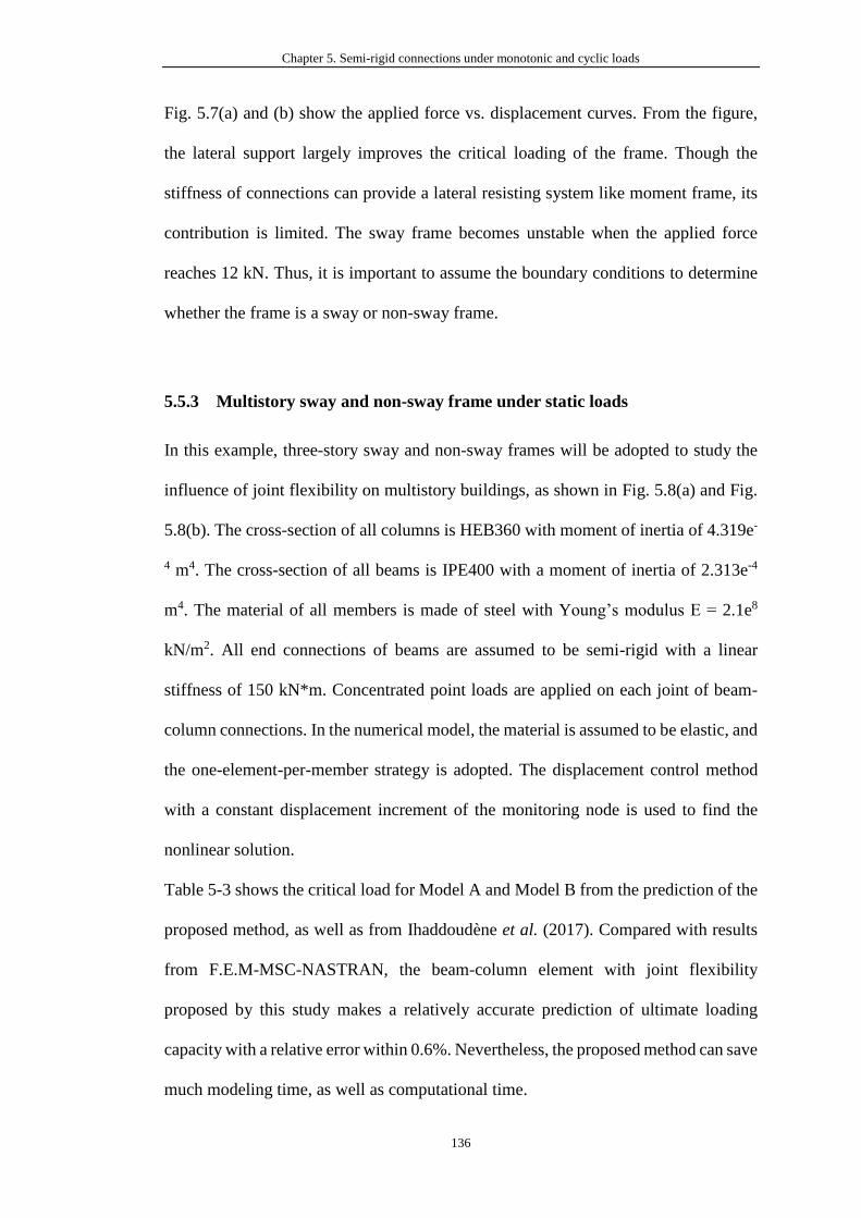
Chapter 5. Semi-rigid connections under monotonic and cyclic loads
136
Fig. 5.7(a) and (b) show the applied force vs. displacement curves. From the figure,
the lateral support largely improves the critical loading of the frame. Though the
stiffness of connections can provide a lateral resisting system like moment frame, its
contribution is limited. The sway frame becomes unstable when the applied force
reaches 12 kN. Thus, it is important to assume the boundary conditions to determine
whether the frame is a sway or non-sway frame.
5.5.3 Multistory sway and non-sway frame under static loads
In this example, three-story sway and non-sway frames will be adopted to study the
influence of joint flexibility on multistory buildings, as shown in Fig. 5.8(a) and Fig.
5.8(b). The cross-section of all columns is HEB360 with moment of inertia of 4.319e-
4 m4. The cross-section of all beams is IPE400 with a moment of inertia of 2.313e-4
m4. The material of all members is made of steel with Young’s modulus E = 2.1e8
kN/m2. All end connections of beams are assumed to be semi-rigid with a linear
stiffness of 150 kN*m. Concentrated point loads are applied on each joint of beam-
column connections. In the numerical model, the material is assumed to be elastic, and
the one-element-per-member strategy is adopted. The displacement control method
with a constant displacement increment of the monitoring node is used to find the
nonlinear solution.
Table 5-3 shows the critical load for Model A and Model B from the prediction of the
proposed method, as well as from Ihaddoudène et al. (2017). Compared with results
from F.E.M-MSC-NASTRAN, the beam-column element with joint flexibility
proposed by this study makes a relatively accurate prediction of ultimate loading
capacity with a relative error within 0.6%. Nevertheless, the proposed method can save
much modeling time, as well as computational time.
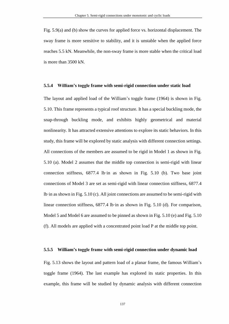
Chapter 5. Semi-rigid connections under monotonic and cyclic loads
137
Fig. 5.9(a) and (b) show the curves for applied force vs. horizontal displacement. The
sway frame is more sensitive to stability, and it is unstable when the applied force
reaches 5.5 kN. Meanwhile, the non-sway frame is more stable when the critical load
is more than 3500 kN.
5.5.4 William’s toggle frame with semi-rigid connection under static load
The layout and applied load of the William’s toggle frame (1964) is shown in Fig.
5.10. This frame represents a typical roof structure. It has a special buckling mode, the
snap-through buckling mode, and exhibits highly geometrical and material
nonlinearity. It has attracted extensive attentions to explore its static behaviors. In this
study, this frame will be explored by static analysis with different connection settings.
All connections of the members are assumed to be rigid in Model 1 as shown in Fig.
5.10 (a). Model 2 assumes that the middle top connection is semi-rigid with linear
connection stiffness, 6877.4 lb·in as shown in Fig. 5.10 (b). Two base joint
connections of Model 3 are set as semi-rigid with linear connection stiffness, 6877.4
lb·in as shown in Fig. 5.10 (c). All joint connections are assumed to be semi-rigid with
linear connection stiffness, 6877.4 lb·in as shown in Fig. 5.10 (d). For comparison,
Model 5 and Model 6 are assumed to be pinned as shown in Fig. 5.10 (e) and Fig. 5.10
(f). All models are applied with a concentrated point load P at the middle top point.
5.5.5 William’s toggle frame with semi-rigid connection under dynamic load
Fig. 5.13 shows the layout and pattern load of a planar frame, the famous William’s
toggle frame (1964). The last example has explored its static properties. In this
example, this frame will be studied by dynamic analysis with different connection
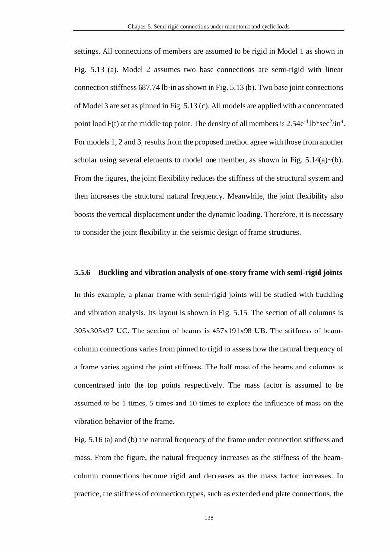
Chapter 5. Semi-rigid connections under monotonic and cyclic loads
138
settings. All connections of members are assumed to be rigid in Model 1 as shown in
Fig. 5.13 (a). Model 2 assumes two base connections are semi-rigid with linear
connection stiffness 687.74 lb·in as shown in Fig. 5.13 (b). Two base joint connections
of Model 3 are set as pinned in Fig. 5.13 (c). All models are applied with a concentrated
point load F(t) at the middle top point. The density of all members is 2.54e-4 lb*sec2/in4.
For models 1, 2 and 3, results from the proposed method agree with those from another
scholar using several elements to model one member, as shown in Fig. 5.14(a)~(b).
From the figures, the joint flexibility reduces the stiffness of the structural system and
then increases the structural natural frequency. Meanwhile, the joint flexibility also
boosts the vertical displacement under the dynamic loading. Therefore, it is necessary
to consider the joint flexibility in the seismic design of frame structures.
5.5.6 Buckling and vibration analysis of one-story frame with semi-rigid joints
In this example, a planar frame with semi-rigid joints will be studied with buckling
and vibration analysis. Its layout is shown in Fig. 5.15. The section of all columns is
305x305x97 UC. The section of beams is 457x191x98 UB. The stiffness of beam-
column connections varies from pinned to rigid to assess how the natural frequency of
a frame varies against the joint stiffness. The half mass of the beams and columns is
concentrated into the top points respectively. The mass factor is assumed to be
assumed to be 1 times, 5 times and 10 times to explore the influence of mass on the
vibration behavior of the frame.
Fig. 5.16 (a) and (b) the natural frequency of the frame under connection stiffness and
mass. From the figure, the natural frequency increases as the stiffness of the beam-
column connections become rigid and decreases as the mass factor increases. In
practice, the stiffness of connection types, such as extended end plate connections, the
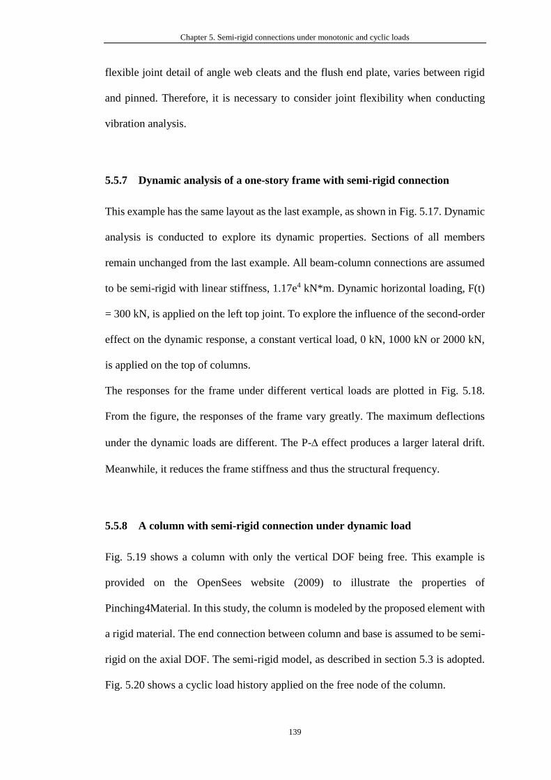
Chapter 5. Semi-rigid connections under monotonic and cyclic loads
139
flexible joint detail of angle web cleats and the flush end plate, varies between rigid
and pinned. Therefore, it is necessary to consider joint flexibility when conducting
vibration analysis.
5.5.7 Dynamic analysis of a one-story frame with semi-rigid connection
This example has the same layout as the last example, as shown in Fig. 5.17. Dynamic
analysis is conducted to explore its dynamic properties. Sections of all members
remain unchanged from the last example. All beam-column connections are assumed
to be semi-rigid with linear stiffness, 1.17e4 kN*m. Dynamic horizontal loading, F(t)
= 300 kN, is applied on the left top joint. To explore the influence of the second-order
effect on the dynamic response, a constant vertical load, 0 kN, 1000 kN or 2000 kN,
is applied on the top of columns.
The responses for the frame under different vertical loads are plotted in Fig. 5.18.
From the figure, the responses of the frame vary greatly. The maximum deflections
under the dynamic loads are different. The P- effect produces a larger lateral drift.
Meanwhile, it reduces the frame stiffness and thus the structural frequency.
5.5.8 A column with semi-rigid connection under dynamic load
Fig. 5.19 shows a column with only the vertical DOF being free. This example is
provided on the OpenSees website (2009) to illustrate the properties of
Pinching4Material. In this study, the column is modeled by the proposed element with
a rigid material. The end connection between column and base is assumed to be semi-
rigid on the axial DOF. The semi-rigid model, as described in section 5.3 is adopted.
Fig. 5.20 shows a cyclic load history applied on the free node of the column.
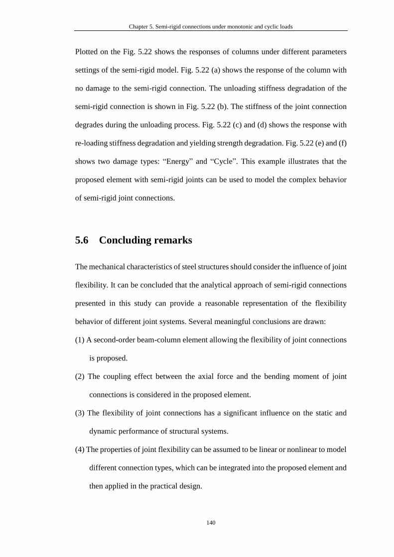
Chapter 5. Semi-rigid connections under monotonic and cyclic loads
140
Plotted on the Fig. 5.22 shows the responses of columns under different parameters
settings of the semi-rigid model. Fig. 5.22 (a) shows the response of the column with
no damage to the semi-rigid connection. The unloading stiffness degradation of the
semi-rigid connection is shown in Fig. 5.22 (b). The stiffness of the joint connection
degrades during the unloading process. Fig. 5.22 (c) and (d) shows the response with
re-loading stiffness degradation and yielding strength degradation. Fig. 5.22 (e) and (f)
shows two damage types: “Energy” and “Cycle”. This example illustrates that the
proposed element with semi-rigid joints can be used to model the complex behavior
of semi-rigid joint connections.
5.6 Concluding remarks
The mechanical characteristics of steel structures should consider the influence of joint
flexibility. It can be concluded that the analytical approach of semi-rigid connections
presented in this study can provide a reasonable representation of the flexibility
behavior of different joint systems. Several meaningful conclusions are drawn:
(1) A second-order beam-column element allowing the flexibility of joint connections
is proposed.
(2) The coupling effect between the axial force and the bending moment of joint
connections is considered in the proposed element.
(3) The flexibility of joint connections has a significant influence on the static and
dynamic performance of structural systems.
(4) The properties of joint flexibility can be assumed to be linear or nonlinear to model
different connection types, which can be integrated into the proposed element and
then applied in the practical design.
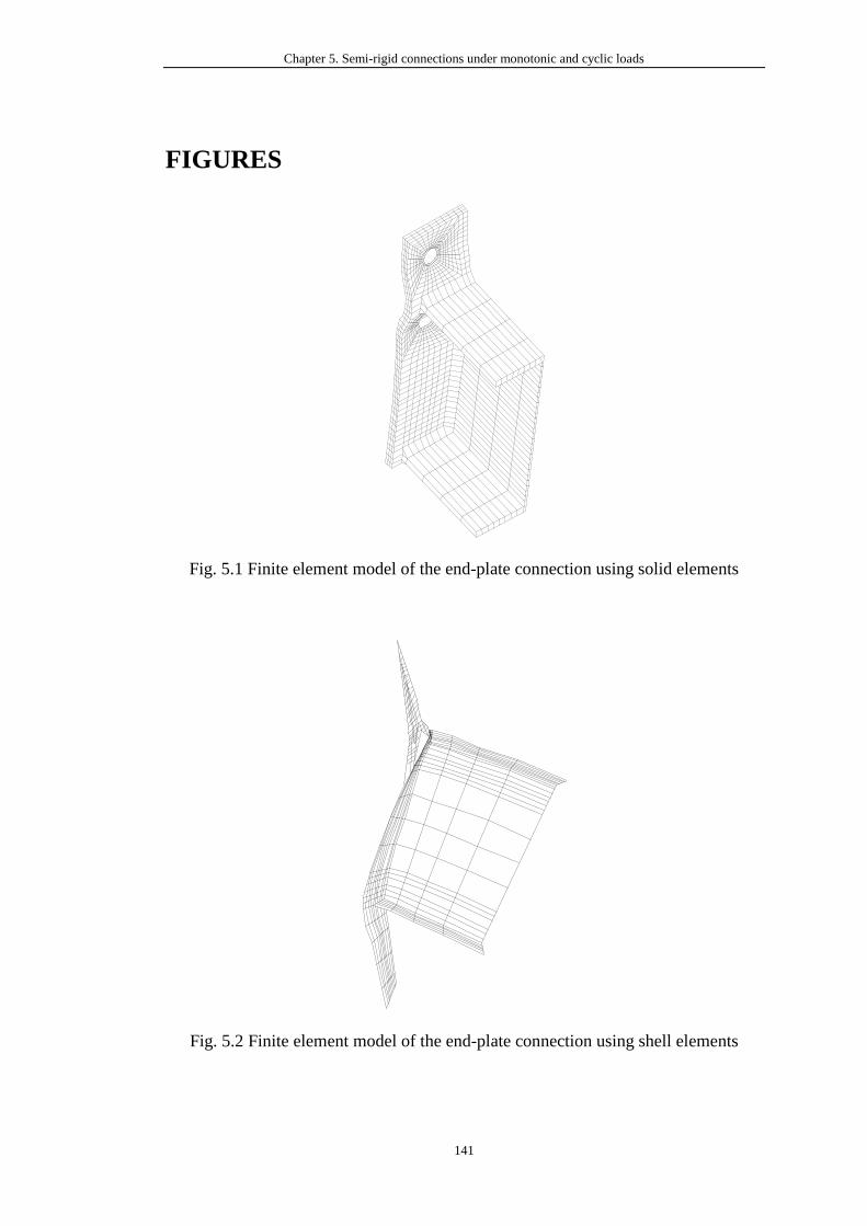
Chapter 5. Semi-rigid connections under monotonic and cyclic loads
141
FIGURES
Fig. 5.1 Finite element model of the end-plate connection using solid elements
Fig. 5.2 Finite element model of the end-plate connection using shell elements
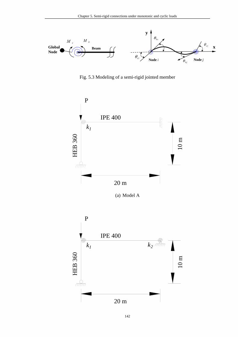
Chapter 5. Semi-rigid connections under monotonic and cyclic loads
142
Fig. 5.3 Modeling of a semi-rigid jointed member
(a) Model A
IPE 400
HE
B 3
60
P
k1
20 m10 m
IPE 400
HE
B 3
60
P
k1
20 m
10
m
k2
Global
Node
Beam x
y
Node i Node j
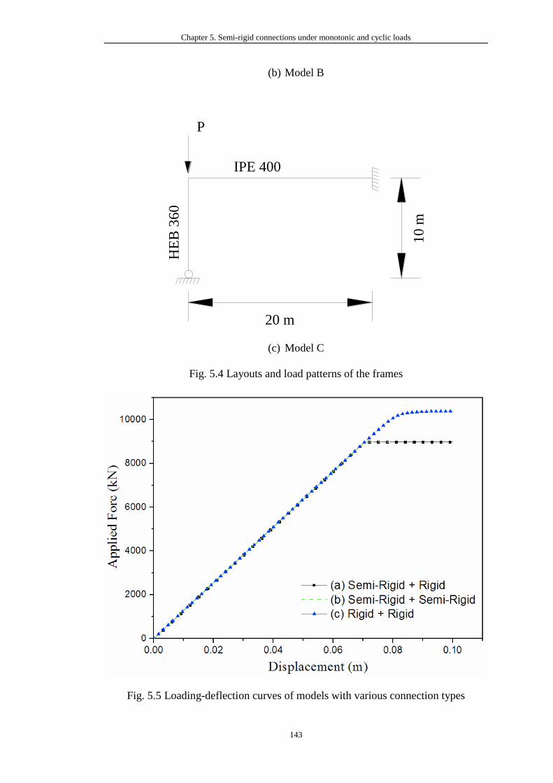
Chapter 5. Semi-rigid connections under monotonic and cyclic loads
143
(b) Model B
(c) Model C
Fig. 5.4 Layouts and load patterns of the frames
Fig. 5.5 Loading-deflection curves of models with various connection types
IPE 400H
EB
36
0
P
20 m
10
m
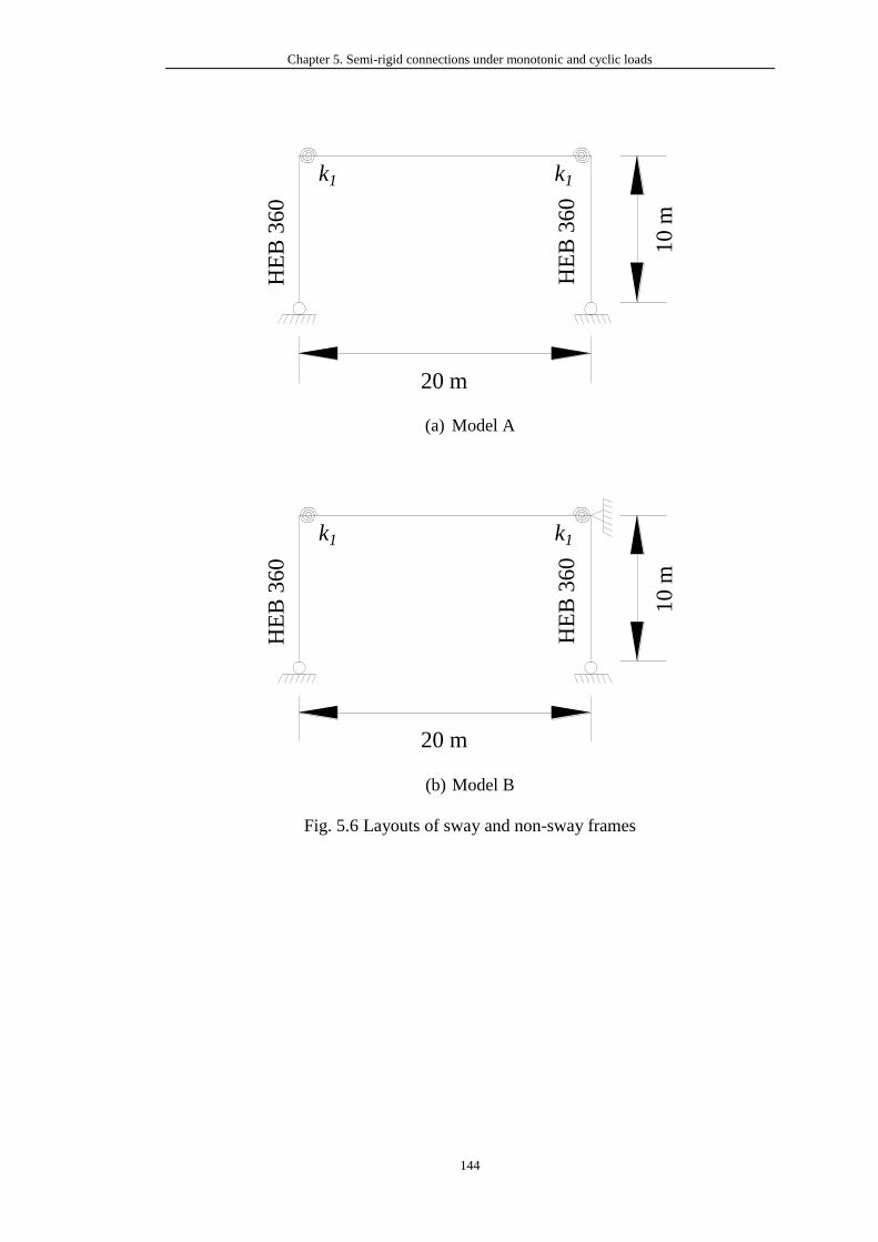
Chapter 5. Semi-rigid connections under monotonic and cyclic loads
144
(a) Model A
(b) Model B
Fig. 5.6 Layouts of sway and non-sway frames
HE
B 3
60
k1
20 m
10 m
k1
HE
B 3
60
HE
B 3
60
k1
20 m
10
m
k1
HE
B 3
60
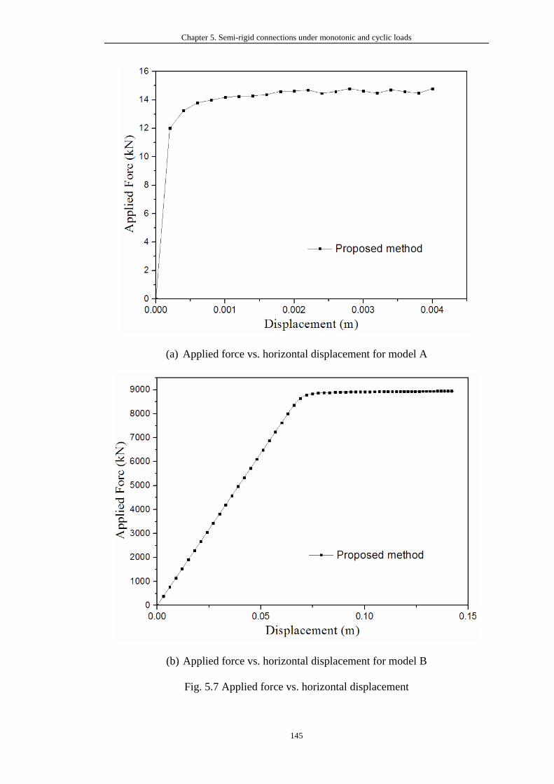
Chapter 5. Semi-rigid connections under monotonic and cyclic loads
145
(a) Applied force vs. horizontal displacement for model A
(b) Applied force vs. horizontal displacement for model B
Fig. 5.7 Applied force vs. horizontal displacement
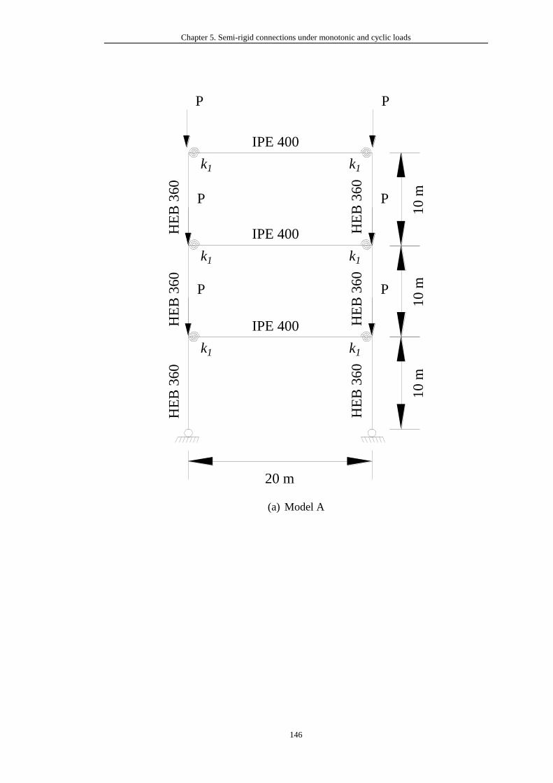
Chapter 5. Semi-rigid connections under monotonic and cyclic loads
146
(a) Model A
IPE 400
HE
B 3
60
k1
20 m
10
m
k1H
EB
36
0
IPE 400
HE
B 3
60
k1 k1
HE
B 3
60
IPE 400
HE
B 3
60
k1 k1
HE
B 3
60
P P
P P
P P
10
m1
0 m
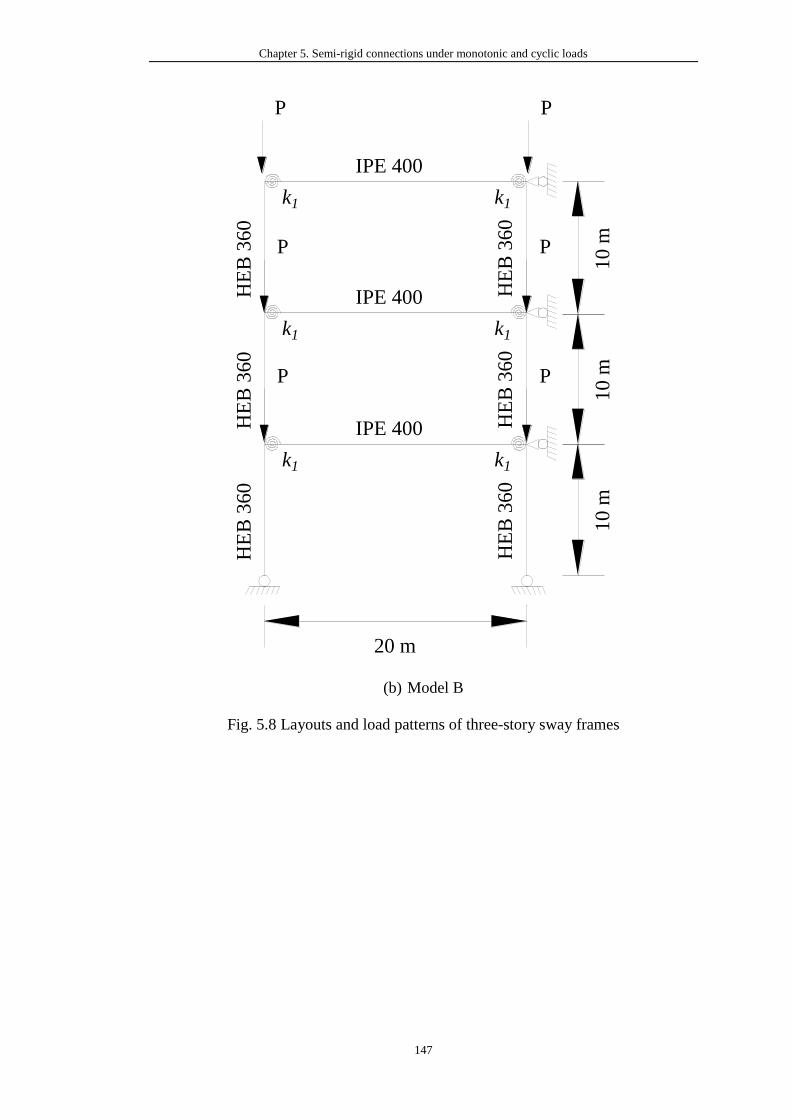
Chapter 5. Semi-rigid connections under monotonic and cyclic loads
147
(b) Model B
Fig. 5.8 Layouts and load patterns of three-story sway frames
IPE 400
HE
B 3
60
k1
20 m
10 m
k1
HE
B 3
60
IPE 400
HE
B 3
60
k1 k1
HE
B 3
60
IPE 400
HE
B 3
60
k1 k1
HE
B 3
60
P P
P P
P P
10 m
10 m
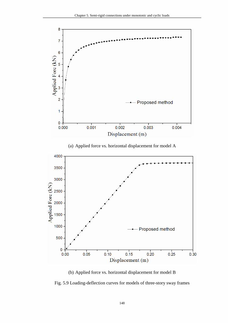
Chapter 5. Semi-rigid connections under monotonic and cyclic loads
148
(a) Applied force vs. horizontal displacement for model A
(b) Applied force vs. horizontal displacement for model B
Fig. 5.9 Loading-deflection curves for models of three-story sway frames
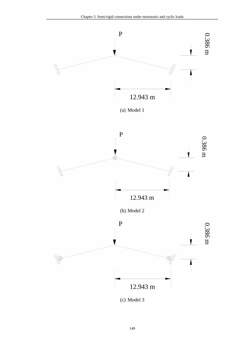
Chapter 5. Semi-rigid connections under monotonic and cyclic loads
149
(a) Model 1
(b) Model 2
(c) Model 3
12.943 m
0.3
86 m
P
12.943 m
0.3
86 m
P
12.943 m
0.3
86 m
P
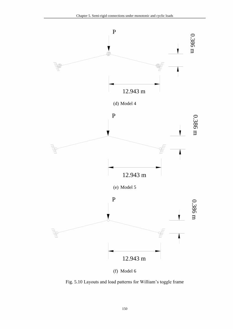
Chapter 5. Semi-rigid connections under monotonic and cyclic loads
150
(d) Model 4
(e) Model 5
(f) Model 6
Fig. 5.10 Layouts and load patterns for William’s toggle frame
12.943 m
0.3
86 m
P
12.943 m
0.3
86 m
P
12.943 m
0.3
86 m
P
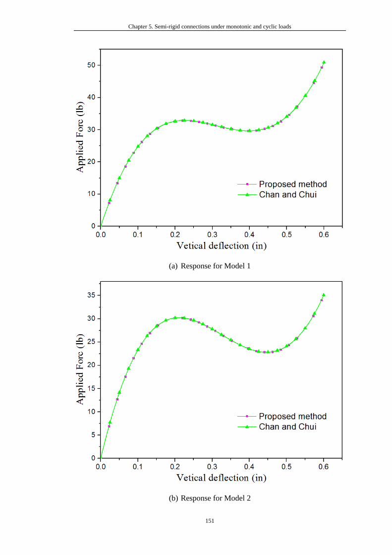
Chapter 5. Semi-rigid connections under monotonic and cyclic loads
151
(a) Response for Model 1
(b) Response for Model 2
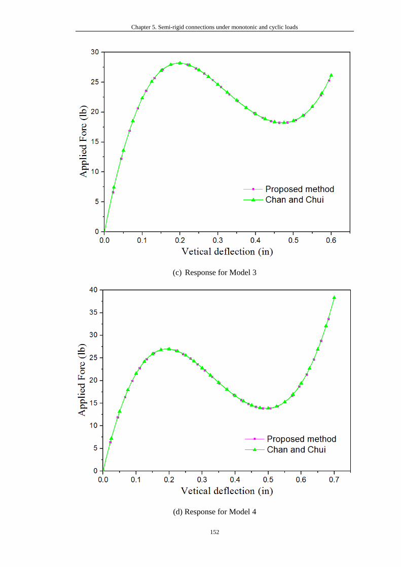
Chapter 5. Semi-rigid connections under monotonic and cyclic loads
152
(c) Response for Model 3
(d) Response for Model 4
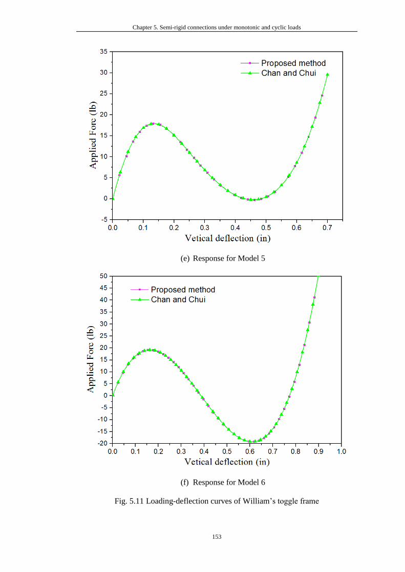
Chapter 5. Semi-rigid connections under monotonic and cyclic loads
153
(e) Response for Model 5
(f) Response for Model 6
Fig. 5.11 Loading-deflection curves of William’s toggle frame
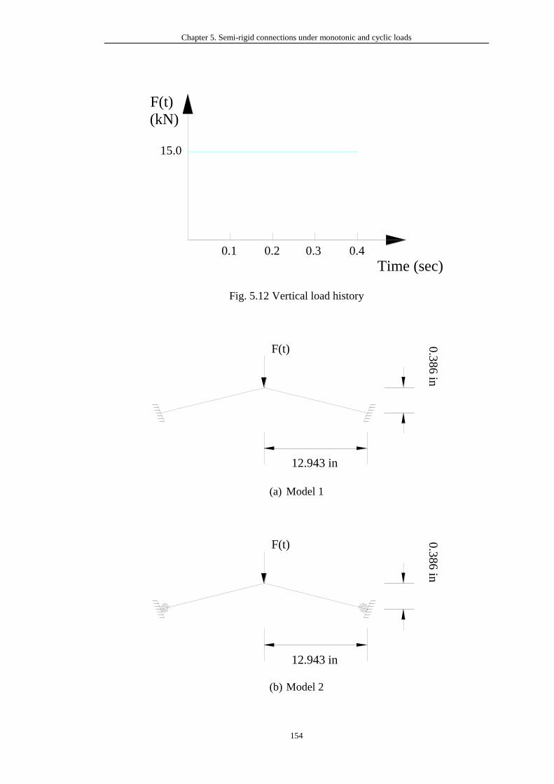
Chapter 5. Semi-rigid connections under monotonic and cyclic loads
154
Fig. 5.12 Vertical load history
(a) Model 1
(b) Model 2
Time (sec)
F(t)
(kN)
0.1 0.2 0.3 0.4
15.0
12.943 in
0.3
86
in
F(t)
12.943 in
0.3
86 in
F(t)
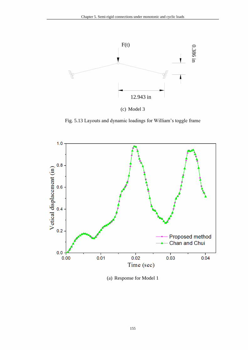
Chapter 5. Semi-rigid connections under monotonic and cyclic loads
155
(c) Model 3
Fig. 5.13 Layouts and dynamic loadings for William’s toggle frame
(a) Response for Model 1
12.943 in
0.3
86 in
F(t)
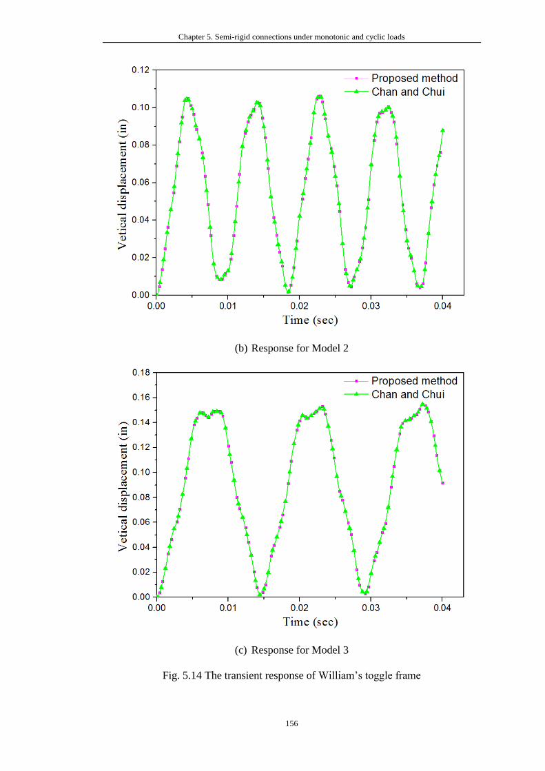
Chapter 5. Semi-rigid connections under monotonic and cyclic loads
156
(b) Response for Model 2
(c) Response for Model 3
Fig. 5.14 The transient response of William’s toggle frame
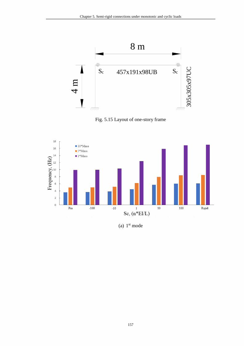
Chapter 5. Semi-rigid connections under monotonic and cyclic loads
157
Fig. 5.15 Layout of one-story frame
(a) 1st mode
4 m
8 m
457x191x98UB
305x305x97U
CSc Sc
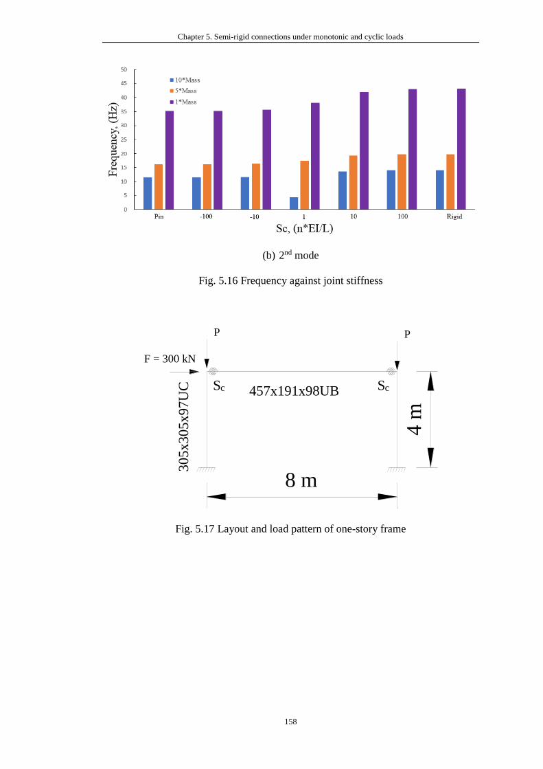
Chapter 5. Semi-rigid connections under monotonic and cyclic loads
158
(b) 2nd mode
Fig. 5.16 Frequency against joint stiffness
Fig. 5.17 Layout and load pattern of one-story frame
305x305x97U
C 457x191x98UB
8 m
4 m
P P
F = 300 kN
Sc Sc
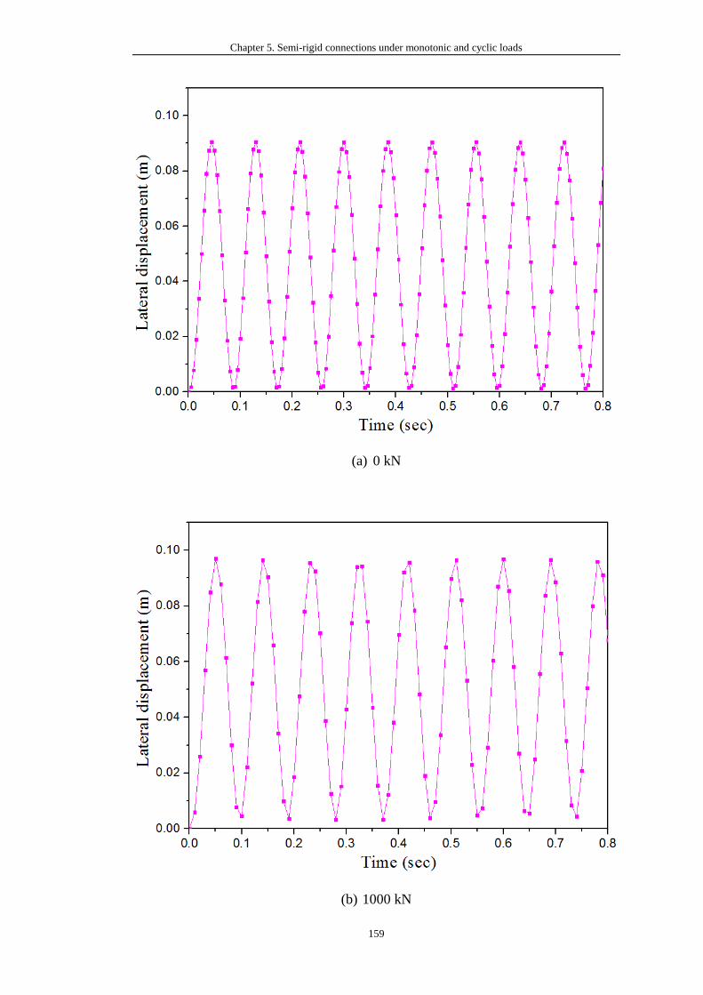
Chapter 5. Semi-rigid connections under monotonic and cyclic loads
159
(a) 0 kN
(b) 1000 kN
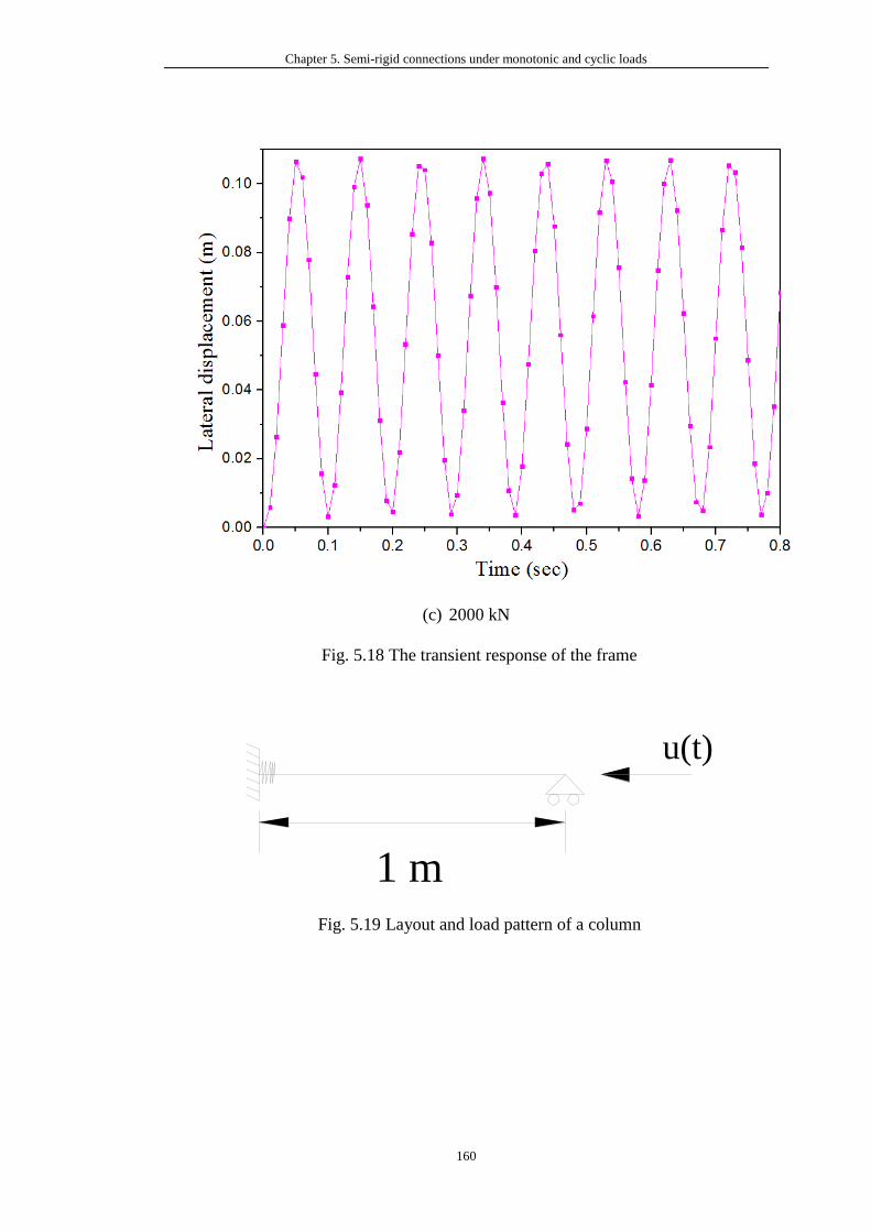
Chapter 5. Semi-rigid connections under monotonic and cyclic loads
160
(c) 2000 kN
Fig. 5.18 The transient response of the frame
Fig. 5.19 Layout and load pattern of a column
1 m
u(t)
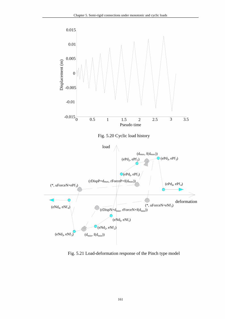
Chapter 5. Semi-rigid connections under monotonic and cyclic loads
161
Fig. 5.20 Cyclic load history
Fig. 5.21 Load-deformation response of the Pinch type model
0 0.5 1 1.5 2 2.5 3 3.5
0.015
0.01
0.005
0
-0.005
-0.01
-0.015
Pseudo time
Dis
pla
cem
ent
(m)
deformation
load
(ePd2, ePf2)
(ePd1, ePf1)
(ePd3, ePf3)
(ePd4, ePf4)
(eNd1, eNf1)
(eNd2, eNf2)
(eNd3, eNf3)
(eNd4, eNf4)
(dmax, f(dmax))
(*, uForceN×eNf3)
(*, uForceN×ePf3)
(rDispP×dmax, rForceP×f(dmax))
(rDispN×dmin, rForceN×f(dmin))
(dmin, f(dmin))
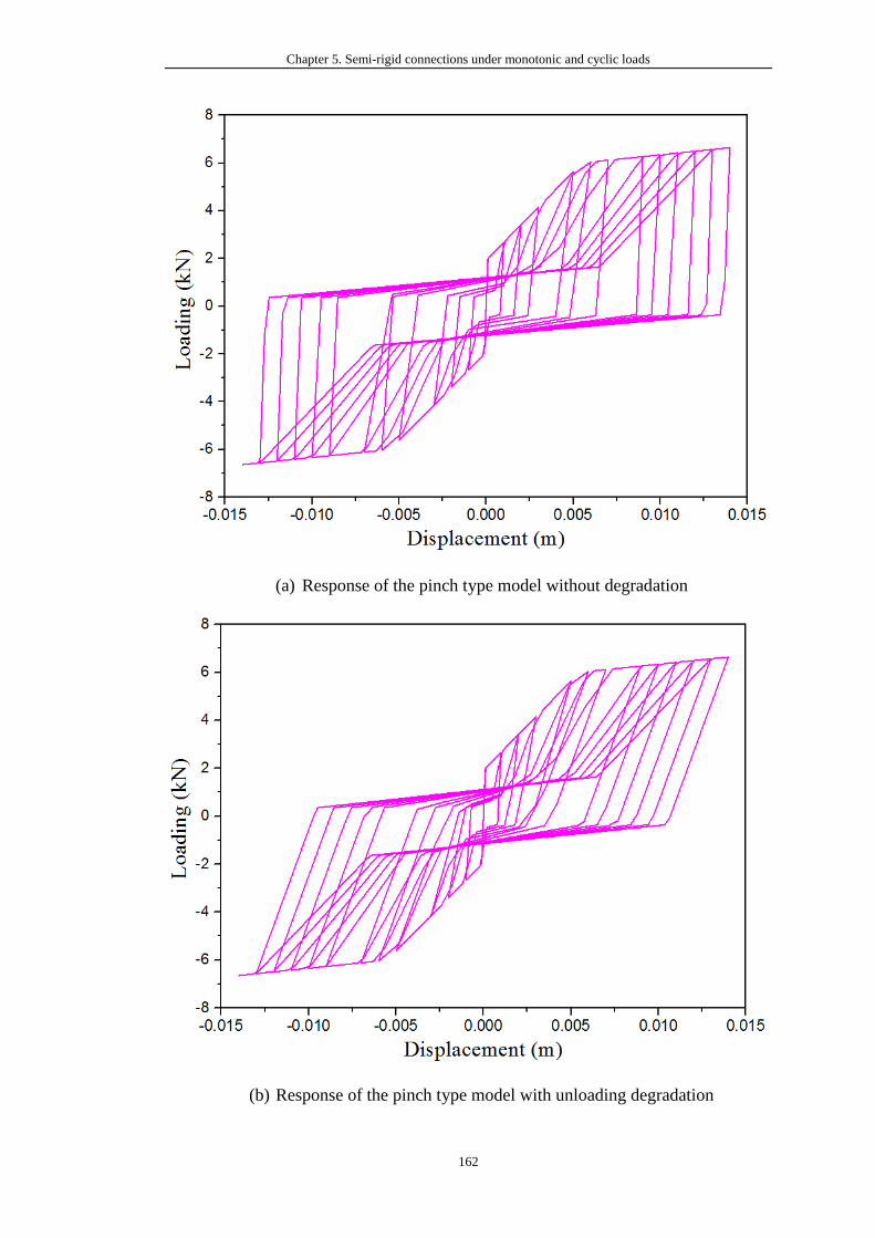
Chapter 5. Semi-rigid connections under monotonic and cyclic loads
162
(a) Response of the pinch type model without degradation
(b) Response of the pinch type model with unloading degradation
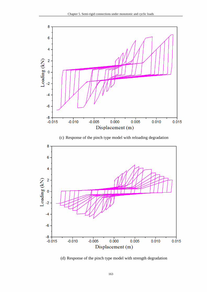
Chapter 5. Semi-rigid connections under monotonic and cyclic loads
163
(c) Response of the pinch type model with reloading degradation
(d) Response of the pinch type model with strength degradation
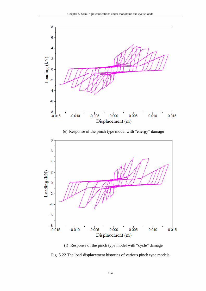
Chapter 5. Semi-rigid connections under monotonic and cyclic loads
164
(e) Response of the pinch type model with “energy” damage
(f) Response of the pinch type model with “cycle” damage
Fig. 5.22 The load-displacement histories of various pinch type models
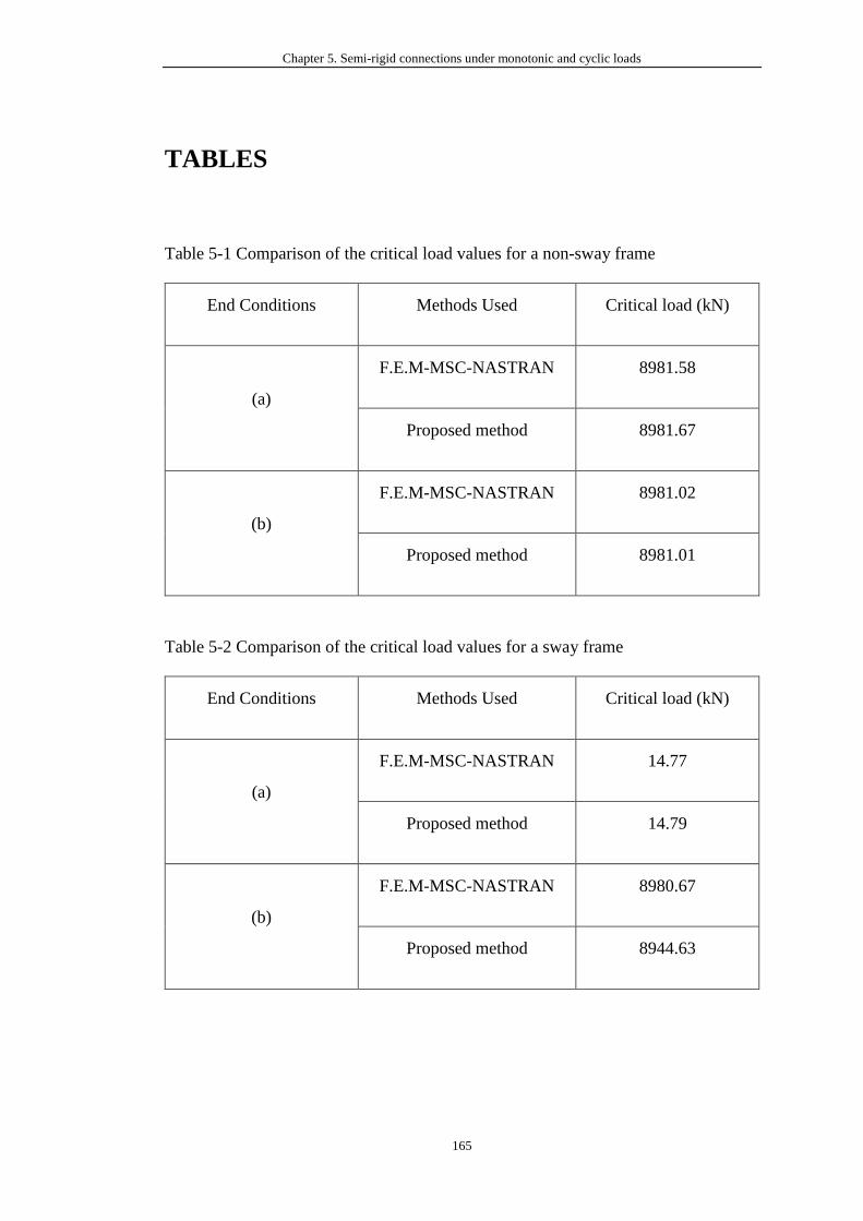
Chapter 5. Semi-rigid connections under monotonic and cyclic loads
165
TABLES
Table 5-1 Comparison of the critical load values for a non-sway frame
End Conditions Methods Used Critical load (kN)
(a)
F.E.M-MSC-NASTRAN 8981.58
Proposed method 8981.67
(b)
F.E.M-MSC-NASTRAN 8981.02
Proposed method 8981.01
Table 5-2 Comparison of the critical load values for a sway frame
End Conditions Methods Used Critical load (kN)
(a)
F.E.M-MSC-NASTRAN 14.77
Proposed method 14.79
(b)
F.E.M-MSC-NASTRAN 8980.67
Proposed method 8944.63
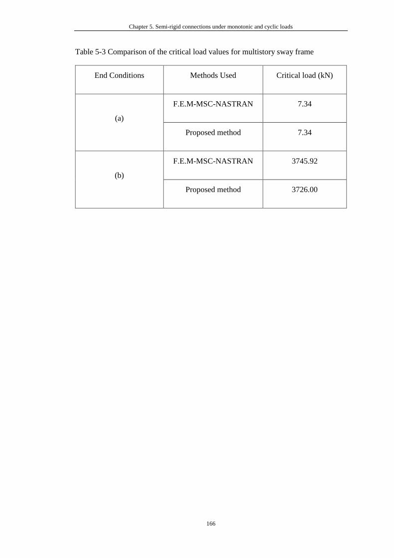
Chapter 5. Semi-rigid connections under monotonic and cyclic loads
166
Table 5-3 Comparison of the critical load values for multistory sway frame
End Conditions Methods Used Critical load (kN)
(a)
F.E.M-MSC-NASTRAN 7.34
Proposed method 7.34
(b)
F.E.M-MSC-NASTRAN 3745.92
Proposed method 3726.00
Chapter 6. Direct analysis of noncompact and slender CFT members
167
CHAPTER 6. DIRECT ANALYSIS OF
NONCOMPACT AND SLENDER CFT
MEMBERS
6.1 Introduction
Concrete-filled steel tube (CFT) members are widely designed to sustain axial
compression, flexure, or their combination due to structural efficiency compared with
bare steel and reinforced concrete members. The outer steel tube in rectangular or
circular shape often serves as formworks during the concrete casting period to reduce
labor costs. This innovative structural member makes full use of steel tubes and the
concrete infill. The local buckling of outer steel tubes can be restricted by the concrete
infill whose strength will be improved by the confinement effect from steel tubes in
return.
To account for local buckling, the steel tubes of CFT members can be classified as
compact, noncompact, or slender section according to the limiting width-to-thickness
ratios specified in Table I1.1a and I1.1b of AISC 360-16 (2016), which is also
reproduced in Table 6-1 for easy reference. In AISC 360-16, the compressive strength
𝑓𝑐′ of the concrete infill is limited from 21 MPa to 69 MPa and 41 MPa for normal
weight concrete and light weight concrete, respectively. The yield stress of the steel
tube shall not exceed 525 MPa. Eurocode 4 (2004) makes no distinction between
compact, noncompact, and slender section, but simply gives limiting width-to-
thickness ratios. For example, D/t is limited to 90√235
𝑓𝑦 for circular CFT members;
Chapter 6. Direct analysis of noncompact and slender CFT members
168
h/t and b/t are limited to 52√235
𝑓𝑦 for rectangular CFT members. Compared with
AISC 360-16 (2016), the sections of CFT members are required to be more compact
in Eurocode 4 (2004).
Generally, the noncompact and slender CFT members experience complex behaviors
such as yielding and local buckling of steel tube, confinement and crack of concrete,
and slippage between the steel tube and the concrete infill. Thus, it is a challenging
task to model a CFT member by conventional numerical methods. The three-
dimensional (3D) finite solid element analysis and the one-dimensional beam-column
element analysis are two well-recognized methods.
The first method can explicitly account for the effects of local buckling and hoop
stresses in the steel tube as well as the effects of confinement on the concrete infill.
However, as this method requires many modeling skills and involves huge computer
time with difficult interpretation results for engineers, it is rarely adopted in routine
design. This method is mainly used to conduct parametric studies with limited
experimental results or calibrate new numerical modeling methods. Lai et al. (2014)
built detailed 3D finite element models to study noncompact or slender rectangular
CFT members and address the gaps in the experimental database. Lai and Varma
(2015) conducted parametric studies on noncompact and slender circular CFT
members by 3D finite element models. Lam et al. (2012) adopted 8-node solid
elements to model the stub concrete-filled steel tubular column with tapered members,
and similar work has been done by Hassan et al. (2016). Liew and Xiong (2009) used
continuum solid and shell elements to study the behavior of CFT members with initial
preload. Du et al. (2017), Ding et al. (2017), Javed et al. (2017) and Aslani et al.
(2016) adopted 8-node brick elements with reduced integration to study the behaviors
of CFT members.
Chapter 6. Direct analysis of noncompact and slender CFT members
169
The second method adopts the one-dimensional beam-column elements to explicitly
or implicitly consider the complex behaviors of CFT members. The explicit one adds
extra degrees of freedom (DOFs) to the end nodes of beam-column elements. Tort and
Hajjar (2010) extended the conventional 12 DOFs beam element into 18 DOFs beam
element to consider the slip deformation between the steel tube and the concrete infill
of rectangular CFT members. Lee and Filippou (2015) proposed a composite frame
element to capture the bond-slip behavior at the interface between the steel tube and
concrete infill based on an extension of the Hu-Washizu variational principle. The
underlying theory of this method is the exact interpolation of the total section forces.
Noted that to solve these particular problems, additional DOFs need to be introduced
in the special beam-column element and further condensed at the elemental level. The
whole procedure involves complicated numerical operations. In contrast, the implicit
approach simply adopts fiber-based beam-column elements with effective stress-strain
relationships to indirectly simulate the complex behaviors of CFT members. The
whole analysis and design procedure is simple without additional numerical work and
requires less computer time. Thus, this method is more competent than other methods
in the daily design of CFT members.
Regarding CFT members with compact sections, several effective stress-strain
relationships are available for the fiber-based beam-column elements, for instance,
Tort and Hajja (2010), Sakino et al. (2004), Han et al. (2005) and Liang (2009). As
for noncompact and slender CFT members, few effective stress-strain relationships
can be used for design purpose. Lai and Varma (2016) proposed effective stress-strain
relationships for noncompact and slender circular and rectangular CFT members.
They also proposed a nonlinear fiber analysis (NFA) macro model to design CFT
members. However, their model is only for two-dimensional problems with axial force
Chapter 6. Direct analysis of noncompact and slender CFT members
170
and uni-axial moment but not for spatial CFT members subjected to bi-axial moments.
The latter is a common case, for example, the corner columns. Furthermore, their
model needs to divide one single CFT member into several segments, which brings
inconvenience in structural modeling and also significantly increases the computer
time.
AISC 360-16 (2016) firstly provides threes methods for design of noncompact and
slender CFT members. The first two methods use interaction equations for strength
checking with stability design by effective length method. The system stiffness is
approximately simulated based on reduced or effective member stiffness, and
therefore they cannot accurately capture the structural behaviors. The third method
uses effective stress-strain relationships, which reflect the fundamental behaviors and
strengths of CFT members with sufficient accuracy in a simple manner, for practical
design. Noted that this method ignores the influence of slenderness effects and
therefore the traditional effective length method is still needed for stability check.
Alternatively, the member initial imperfections can be included in the direct analysis
so that the effective length assumption is no longer required. However, the magnitude
of member imperfection for noncompact/slender CFT members should be further
studied.
In this chapter, a second-order flexibility-based beam-column with member
imperfections and incorporates the effective stress-strain models into the fiber section
is proposed for direct analysis of noncompact/slender CFT members. The gradual
change of member stiffness and the actual section capacity can be accurately reflected
in the analysis process and as a result, the traditional effective length method is no
longer required in the proposed direct analysis. It is also found that the initial
imperfection of L/1000 is insufficient for CFT members.

Chapter 6. Direct analysis of noncompact and slender CFT members
171
The outline of this chapter is as follows. Firstly, three design methods suggested by
ASCI 360-16 (2016) are presented and discussed. Next, a comprehensive direct
analysis method for CFT members made of noncompact or slender sections is
introduced. At last, several experimental tests from literatures are used to verify the
proposed method.
6.2 Design methods for CFT members with noncompact or
slender sections in AISC360
The design methods for compact CFT members can be found in the extensive research
papers and design codes such as Eurocode 4 (2004) and AISC 360-16 (2016), and
therefore they will be not repeated here. In contrast, the design methods, especially the
effective stress-strain method, for noncompact and slender CFT members are newly
developed and firstly specified in AISC 360-16 (2016). The practical design tools and
the applications are limited. Thus, it is worth to conduct more research on this topic
and provide more comprehensive solutions or recommendations for structural
engineers to design noncompact and slender CFT members. In this section, the
available design methods will be briefly introduced.
6.2.1 General interaction method
AISC 360-16 (2016) provides a general method for the design of doubly symmetric CFT
members subjected to compression and flexure. Equations (6.1a) and (6.1b) are the
interaction equations considering different levels of axial force, which is directly extended
from bare steel members to compact, noncompact and slender CFT members.

Chapter 6. Direct analysis of noncompact and slender CFT members
172
𝑃𝑟𝑃𝑐+8
9(𝑀𝑟𝑥
𝑀𝑐𝑥+𝑀𝑟𝑦
𝑀𝑐𝑦) ≤ 1.0, for
𝑃𝑟𝑃𝑐≥ 0.2, (6.1a)
𝑃𝑟2𝑃𝑐
+8
9(𝑀𝑟𝑥
𝑀𝑐𝑥+𝑀𝑟𝑦
𝑀𝑐𝑦) ≤ 1.0, for
𝑃𝑟𝑃𝑐< 0.2 (6.1b)
in which, 𝑃𝑐 is the available axial strength; 𝑀𝑐𝑥 and 𝑀𝑐𝑦 are the major and minor
flexural strengths; 𝑃𝑟 is the required axial strength; 𝑀𝑟𝑥 and 𝑀𝑟𝑦 are the major and
minor required flexural strength.
Clearly, although these equations can consider bi-axially bending problems, the beneficial
effect of axial compression on the flexural strength has been ignored. It was reported by
Lai et al. (2015) that these equations are over-conservative for checking the strength of
noncompact and slender CFT members. Therefore, this method belongs to one of optional
methods for the design of compact and noncompact/slender CFT members in AISC 360-
16 (2016).
Both the direct analysis method and first-order analysis method can be used to determine
the required strengths 𝑃𝑟, 𝑀𝑟𝑥 and 𝑀𝑟𝑦. When using the former for the ultimate limit
state, the deduced stiffness for compression and flexure given in Equation (6.2) should be
adopted in the second-order elastic analysis.
𝐸𝐴𝐼𝐼 = 0.8(𝐸𝑠𝐴𝑠 + 𝐸𝑠𝐴𝑠𝑟 + 𝐸𝑐𝐴𝑐) (6.2a)
𝐸𝐼𝐼𝐼 = 0.8τ𝑏𝐸𝐼𝑒𝑓𝑓 with τ𝑏 = 0.8 (6.2b)
𝐸𝐼𝑒𝑓𝑓 = 𝐸𝑠𝐼𝑠 + 𝐸𝑠𝐼𝑠𝑟 + 𝐶1𝐸𝑐𝐼𝑐 (6.2c)
𝐶1 = 0.25 +𝐴𝑠 + 𝐴𝑠𝑟𝐴𝑔
≤ 0.7 (6.2d)
in which, Es and Ec are Young’s moduli of steel and concrete respectively; As, Ac
and Asr are the total areas of the steel tube, concrete infill, and reinforcement respectively
while Ag is the total area of all components; Is, Ic and Isr are the second moment of
areas of the steel tube, concrete infill and reinforcement respectively.
Chapter 6. Direct analysis of noncompact and slender CFT members
173
Denavit et al. (2015) confirmed that the stiffness in Equation (6.2) does not always give a
conservative design. However, AISC 360-16 (2016) does not provide detailed limitation
its use.
For the first-order analysis with effective length method, the stiffness given in Equation
(6.3) should be employed in the global structural analysis.
𝐸𝐴𝐼 = 𝐸𝑠𝐴𝑠 + 𝐸𝑠𝐴𝑠𝑟 + 𝐸𝑐𝐴𝑐 (6.3a)
𝐸𝐼𝐼 = 𝐸𝐼𝑒𝑓𝑓 (6.3b)
When using the effective length method to check the flexural buckling, the compressive
strength Pc is obtained by multiplying resistance factor or dividing safety factor with
nominal compressive strength 𝑃𝑛, which can be calculated from Equation (6.4).
𝑃𝑛 = 𝑃𝑛𝑜0.658𝑃𝑛𝑜/𝑃𝑒, for
𝑃𝑛𝑜
𝑃𝑒≤ 2.25 (6.4a)
𝑃𝑛 = 0.877𝑃𝑛𝑜, for 𝑃𝑛𝑜
𝑃𝑒> 2.25 (6.4b)
𝑃𝑒 =𝜋2(𝐸𝐼𝑒𝑓𝑓)
(𝐾𝐿)2 (6.4c)
in which, 𝑃𝑛𝑜 is the nominal compressive strength without consideration of slenderness
effect; 𝑃𝑒 is elastic critical buckling load; 𝐾𝐿 is the effective length.
6.2.2 Direct interaction method
To account for the beneficial effects due to axial compression on limiting crack of infilled
concrete and increasing flexural strength by confinement, AISC 360-16 (2016) introduces
two coefficients 𝑐𝑝 and 𝑐𝑚 corresponding to the balance point into Equation (6.1) and
then can be rewritten in Equation (6.5) as
𝑃𝑟𝑃𝑐+1 − 𝑐𝑝
𝑐𝑚(𝑀𝑟
𝑀𝑐) ≤ 1.0, for
𝑃𝑟𝑃𝑐≥ 𝑐𝑝 (6.5a)
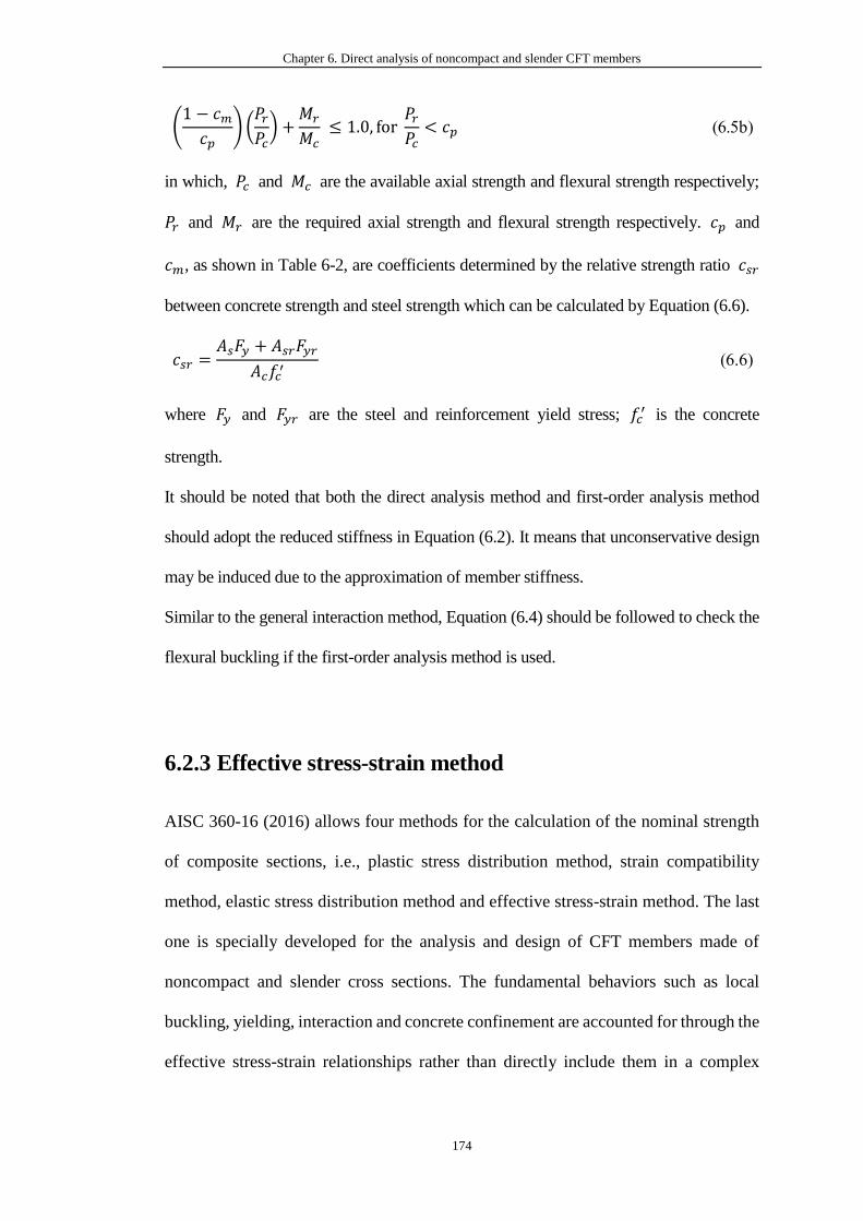
Chapter 6. Direct analysis of noncompact and slender CFT members
174
(1 − 𝑐𝑚𝑐𝑝
) (𝑃𝑟𝑃𝑐) +
𝑀𝑟
𝑀𝑐 ≤ 1.0, for
𝑃𝑟𝑃𝑐< 𝑐𝑝 (6.5b)
in which, 𝑃𝑐 and 𝑀𝑐 are the available axial strength and flexural strength respectively;
𝑃𝑟 and 𝑀𝑟 are the required axial strength and flexural strength respectively. 𝑐𝑝 and
𝑐𝑚, as shown in Table 6-2, are coefficients determined by the relative strength ratio 𝑐𝑠𝑟
between concrete strength and steel strength which can be calculated by Equation (6.6).
𝑐𝑠𝑟 =𝐴𝑠𝐹𝑦 + 𝐴𝑠𝑟𝐹𝑦𝑟
𝐴𝑐𝑓𝑐′ (6.6)
where 𝐹𝑦 and 𝐹𝑦𝑟 are the steel and reinforcement yield stress; 𝑓𝑐′ is the concrete
strength.
It should be noted that both the direct analysis method and first-order analysis method
should adopt the reduced stiffness in Equation (6.2). It means that unconservative design
may be induced due to the approximation of member stiffness.
Similar to the general interaction method, Equation (6.4) should be followed to check the
flexural buckling if the first-order analysis method is used.
6.2.3 Effective stress-strain method
AISC 360-16 (2016) allows four methods for the calculation of the nominal strength
of composite sections, i.e., plastic stress distribution method, strain compatibility
method, elastic stress distribution method and effective stress-strain method. The last
one is specially developed for the analysis and design of CFT members made of
noncompact and slender cross sections. The fundamental behaviors such as local
buckling, yielding, interaction and concrete confinement are accounted for through the
effective stress-strain relationships rather than directly include them in a complex

Chapter 6. Direct analysis of noncompact and slender CFT members
175
analysis model. Lai and Varma (2016) proposed effective stress-strain relationships
for analysis of noncompact and slender filled composite members.
Generally speaking, this method is particularly suitable for the fiber-based element to
form sectional tangent stiffness and then perform direct analysis to check the actual
section capacity and system resistance without the use of effective length assumption.
Most importantly, the inelastic behavior of CFT members can be well captured. The
accurate member stiffness can be formed by fiber integration approach rather than the
approximate effective stiffness or reduced stiffness used in the interaction methods
aforementioned. Although the strain compatibility is required based on beam-column
theory, the modified material stress-strain relationships have implicitly considered the
macro effects such as local buckling, yielding, and concrete confinement and therefore
it provides an innovative solution on structural analysis and design of frame structures
with CFT members under the framework of direct analysis.
6.2.4 Discussion on design methods
The general interaction method ignores the beneficial effects due to the restraint of
steel tube on the concrete infill while the other methods have been implicitly taken
them into account. Thus, the first method generally produces a conservative design
regarding strength checking.
It is noted that the two P-M interaction methods need to use reduced or effective
stiffness either in direct analysis or in the first-order analysis. It means that the change
of member stiffness associated with its complex behaviors is approximately reflected
in the analysis process. As a consequence, the traditional effective length should be
further adopted for stability checking. It will bring uncertainty in stability design as
the effective length is difficult to know due to the changing of system stiffness under
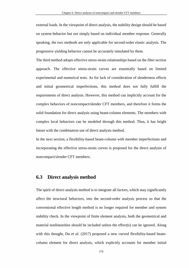
Chapter 6. Direct analysis of noncompact and slender CFT members
176
external loads. In the viewpoint of direct analysis, the stability design should be based
on system behavior but not simply based on individual member response. Generally
speaking, the two methods are only applicable for second-order elastic analysis. The
progressive yielding behavior cannot be accurately simulated by them.
The third method adopts effective stress-strain relationships based on the fiber section
approach. The effective stress-strain curves are essentially based on limited
experimental and numerical tests. As for lack of consideration of slenderness effects
and initial geometrical imperfections, this method does not fully fulfill the
requirements of direct analysis. However, this method can implicitly account for the
complex behaviors of noncompact/slender CFT members, and therefore it forms the
solid foundation for direct analysis using beam-column elements. The members with
complex local behaviors can be modeled through this method. Thus, it has bright
future with the combination use of direct analysis method.
In the next section, a flexibility-based beam-column with member imperfections and
incorporating the effective stress-strain curves is proposed for the direct analysis of
noncompact/slender CFT members.
6.3 Direct analysis method
The spirit of direct analysis method is to integrate all factors, which may significantly
affect the structural behaviors, into the second-order analysis process so that the
conventional effective length method is no longer required for member and system
stability check. In the viewpoint of finite element analysis, both the geometrical and
material nonlinearities should be included unless the effect(s) can be ignored. Along
with this thought, Du et al. (2017) proposed a new curved flexibility-based beam-
column element for direct analysis, which explicitly accounts for member initial
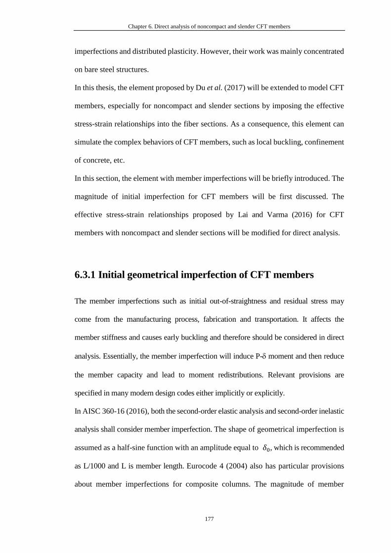
Chapter 6. Direct analysis of noncompact and slender CFT members
177
imperfections and distributed plasticity. However, their work was mainly concentrated
on bare steel structures.
In this thesis, the element proposed by Du et al. (2017) will be extended to model CFT
members, especially for noncompact and slender sections by imposing the effective
stress-strain relationships into the fiber sections. As a consequence, this element can
simulate the complex behaviors of CFT members, such as local buckling, confinement
of concrete, etc.
In this section, the element with member imperfections will be briefly introduced. The
magnitude of initial imperfection for CFT members will be first discussed. The
effective stress-strain relationships proposed by Lai and Varma (2016) for CFT
members with noncompact and slender sections will be modified for direct analysis.
6.3.1 Initial geometrical imperfection of CFT members
The member imperfections such as initial out-of-straightness and residual stress may
come from the manufacturing process, fabrication and transportation. It affects the
member stiffness and causes early buckling and therefore should be considered in direct
analysis. Essentially, the member imperfection will induce P- moment and then reduce
the member capacity and lead to moment redistributions. Relevant provisions are
specified in many modern design codes either implicitly or explicitly.
In AISC 360-16 (2016), both the second-order elastic analysis and second-order inelastic
analysis shall consider member imperfection. The shape of geometrical imperfection is
assumed as a half-sine function with an amplitude equal to 𝛿0, which is recommended
as L/1000 and L is member length. Eurocode 4 (2004) also has particular provisions
about member imperfections for composite columns. The magnitude of member
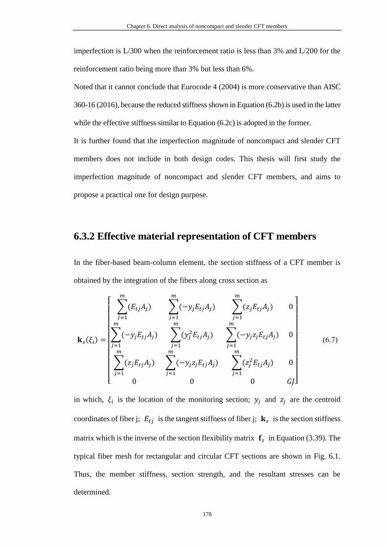
Chapter 6. Direct analysis of noncompact and slender CFT members
178
imperfection is L/300 when the reinforcement ratio is less than 3% and L/200 for the
reinforcement ratio being more than 3% but less than 6%.
Noted that it cannot conclude that Eurocode 4 (2004) is more conservative than AISC
360-16 (2016), because the reduced stiffness shown in Equation (6.2b) is used in the latter
while the effective stiffness similar to Equation (6.2c) is adopted in the former.
It is further found that the imperfection magnitude of noncompact and slender CFT
members does not include in both design codes. This thesis will first study the
imperfection magnitude of noncompact and slender CFT members, and aims to
propose a practical one for design purpose.
6.3.2 Effective material representation of CFT members
In the fiber-based beam-column element, the section stiffness of a CFT member is
obtained by the integration of the fibers along cross section as
𝐤𝑠(𝜉𝑖) =
[ ∑(𝐸𝑡𝑗𝐴𝑗)
𝑚
𝑗=1
∑(−𝑦𝑗𝐸𝑡𝑗𝐴𝑗)
𝑚
𝑗=1
∑(𝑧𝑗𝐸𝑡𝑗𝐴𝑗)
𝑚
𝑗=1
0
∑(−𝑦𝑗𝐸𝑡𝑗𝐴𝑗)
𝑚
𝑗=1
∑(𝑦𝑗2𝐸𝑡𝑗𝐴𝑗)
𝑚
𝑗=1
∑(−𝑦𝑗𝑧𝑗𝐸𝑡𝑗𝐴𝑗)
𝑚
𝑗=1
0
∑(𝑧𝑗𝐸𝑡𝑗𝐴𝑗)
𝑚
𝑗=1
∑(−𝑦𝑗𝑧𝑗𝐸𝑡𝑗𝐴𝑗)
𝑚
𝑗=1
∑(𝑧𝑗2𝐸𝑡𝑗𝐴𝑗)
𝑚
𝑗=1
0
0 0 0 𝐺𝐽]
(6.7)
in which, 𝜉𝑖 is the location of the monitoring section; 𝑦𝑗 and 𝑧𝑗 are the centroid
coordinates of fiber j; 𝐸𝑡𝑗 is the tangent stiffness of fiber j; 𝐤𝑠 is the section stiffness
matrix which is the inverse of the section flexibility matrix 𝐟𝑠 in Equation (3.39). The
typical fiber mesh for rectangular and circular CFT sections are shown in Fig. 6.1.
Thus, the member stiffness, section strength, and the resultant stresses can be
determined.
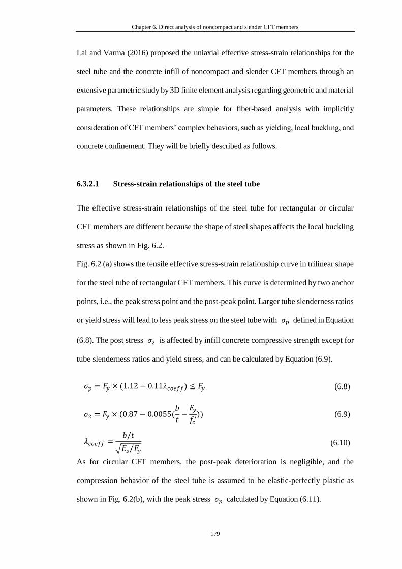
Chapter 6. Direct analysis of noncompact and slender CFT members
179
Lai and Varma (2016) proposed the uniaxial effective stress-strain relationships for the
steel tube and the concrete infill of noncompact and slender CFT members through an
extensive parametric study by 3D finite element analysis regarding geometric and material
parameters. These relationships are simple for fiber-based analysis with implicitly
consideration of CFT members’ complex behaviors, such as yielding, local buckling, and
concrete confinement. They will be briefly described as follows.
6.3.2.1 Stress-strain relationships of the steel tube
The effective stress-strain relationships of the steel tube for rectangular or circular
CFT members are different because the shape of steel shapes affects the local buckling
stress as shown in Fig. 6.2.
Fig. 6.2 (a) shows the tensile effective stress-strain relationship curve in trilinear shape
for the steel tube of rectangular CFT members. This curve is determined by two anchor
points, i.e., the peak stress point and the post-peak point. Larger tube slenderness ratios
or yield stress will lead to less peak stress on the steel tube with 𝜎𝑝 defined in Equation
(6.8). The post stress 𝜎2 is affected by infill concrete compressive strength except for
tube slenderness ratios and yield stress, and can be calculated by Equation (6.9).
𝜎𝑝 = 𝐹𝑦 × (1.12 − 0.11𝜆𝑐𝑜𝑒𝑓𝑓) ≤ 𝐹𝑦 (6.8)
𝜎2 = 𝐹𝑦 × (0.87 − 0.0055(𝑏
𝑡−𝐹𝑦
𝑓𝑐′)) (6.9)
𝜆𝑐𝑜𝑒𝑓𝑓 =𝑏/𝑡
√𝐸𝑠 𝐹𝑦⁄ (6.10)
As for circular CFT members, the post-peak deterioration is negligible, and the
compression behavior of the steel tube is assumed to be elastic-perfectly plastic as
shown in Fig. 6.2(b), with the peak stress 𝜎𝑝 calculated by Equation (6.11).
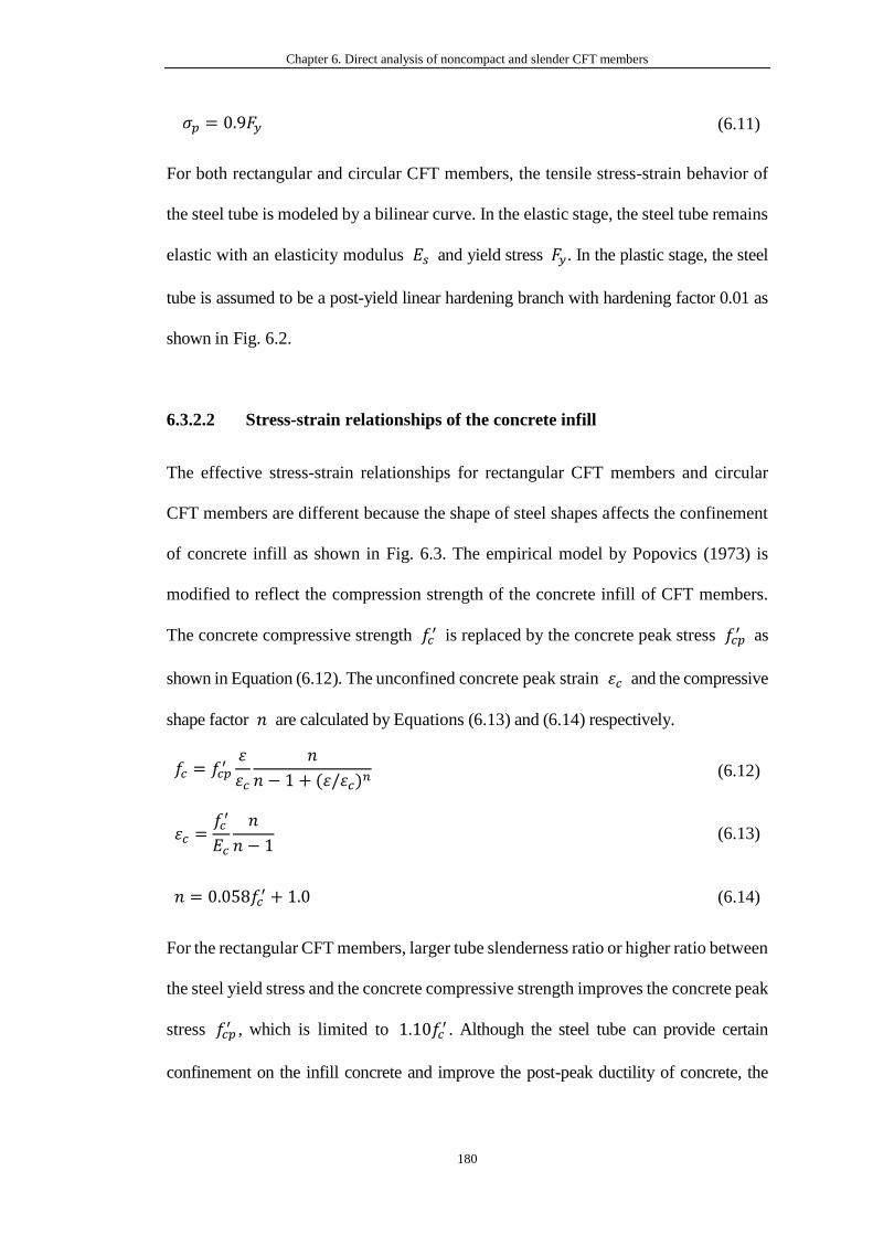
Chapter 6. Direct analysis of noncompact and slender CFT members
180
𝜎𝑝 = 0.9𝐹𝑦 (6.11)
For both rectangular and circular CFT members, the tensile stress-strain behavior of
the steel tube is modeled by a bilinear curve. In the elastic stage, the steel tube remains
elastic with an elasticity modulus 𝐸𝑠 and yield stress 𝐹𝑦. In the plastic stage, the steel
tube is assumed to be a post-yield linear hardening branch with hardening factor 0.01 as
shown in Fig. 6.2.
6.3.2.2 Stress-strain relationships of the concrete infill
The effective stress-strain relationships for rectangular CFT members and circular
CFT members are different because the shape of steel shapes affects the confinement
of concrete infill as shown in Fig. 6.3. The empirical model by Popovics (1973) is
modified to reflect the compression strength of the concrete infill of CFT members.
The concrete compressive strength 𝑓𝑐′ is replaced by the concrete peak stress 𝑓𝑐𝑝
′ as
shown in Equation (6.12). The unconfined concrete peak strain 휀𝑐 and the compressive
shape factor 𝑛 are calculated by Equations (6.13) and (6.14) respectively.
𝑓𝑐 = 𝑓𝑐𝑝′휀
휀𝑐
𝑛
𝑛 − 1 + (휀/휀𝑐)𝑛 (6.12)
휀𝑐 =𝑓𝑐′
𝐸𝑐
𝑛
𝑛 − 1 (6.13)
𝑛 = 0.058𝑓𝑐′ + 1.0 (6.14)
For the rectangular CFT members, larger tube slenderness ratio or higher ratio between
the steel yield stress and the concrete compressive strength improves the concrete peak
stress 𝑓𝑐𝑝′ , which is limited to 1.10𝑓𝑐
′ . Although the steel tube can provide certain
confinement on the infill concrete and improve the post-peak ductility of concrete, the

Chapter 6. Direct analysis of noncompact and slender CFT members
181
confinement effect is really limited. For this reason, the post-peak behavior of the concrete
infill is modeled as the unconfined concrete as shown in Fig. 6.3(a) for conservative.
𝑓𝑐𝑝′ = 𝑓𝑐
′ × (0.8 + 0.18 (𝑏/𝑡
100+𝐹𝑦/𝑓𝑐
′
30)) (6.15)
Equation (6.16) defines the concrete peak stress. Unlike the rectangular CFT members,
larger tube slenderness ratio degrades the concrete peak stress of the circular CFT
members. Besides, the steel tube provides better confinement than that of the
rectangular CFT members. Consequently, an elastic-perfectly plastic curve is used to
model the post-peak behavior of the infill concrete as shown in Fig. 6.3(b).
𝑓𝑐𝑝′ = 𝑓𝑐
′ × (1.0 − 0.11 (𝐷/𝑡
100−𝐹𝑦/𝑓𝑐
′
9)) (6.16)
AISC 360-16 (2016) suggests that the tensile strength of the concrete shall be
neglected in the determination of the nominal strength of composite members. Thus,
the tensile strength is not considered in tensile stress-strain relationships as shown in
Fig. 6.3.
6.4 Validation examples
In this thesis, six experimental tests from literature, including noncompact and slender
rectangular or circular CFT members under flexure, axial compression or their
combination, are selected to verify the accuracy of the proposed method in line with AISC
360-16 (2016). The strength of steel tube and concrete infill used in the tests satisfies
the requirements in design code. The proposed element incorporating the effective
stress-strain curves introduced in section 2 was coded into the software NIDA (2018)
for this study.
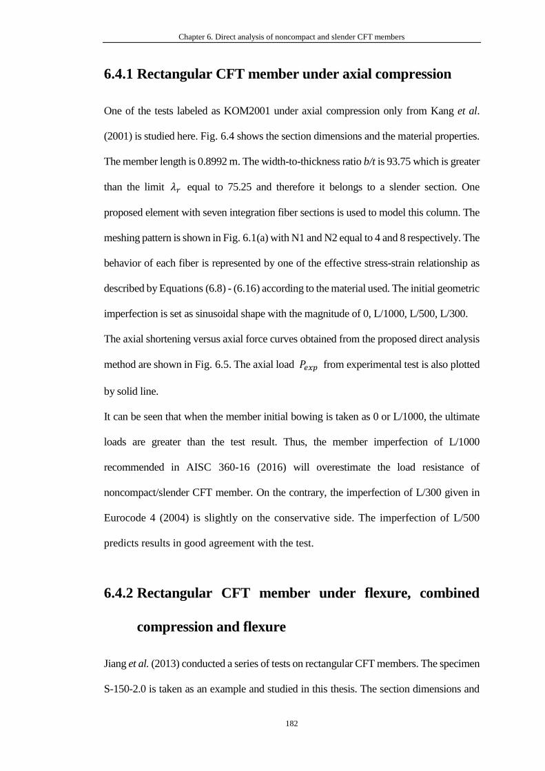
Chapter 6. Direct analysis of noncompact and slender CFT members
182
6.4.1 Rectangular CFT member under axial compression
One of the tests labeled as KOM2001 under axial compression only from Kang et al.
(2001) is studied here. Fig. 6.4 shows the section dimensions and the material properties.
The member length is 0.8992 m. The width-to-thickness ratio b/t is 93.75 which is greater
than the limit 𝜆𝑟 equal to 75.25 and therefore it belongs to a slender section. One
proposed element with seven integration fiber sections is used to model this column. The
meshing pattern is shown in Fig. 6.1(a) with N1 and N2 equal to 4 and 8 respectively. The
behavior of each fiber is represented by one of the effective stress-strain relationship as
described by Equations (6.8) - (6.16) according to the material used. The initial geometric
imperfection is set as sinusoidal shape with the magnitude of 0, L/1000, L/500, L/300.
The axial shortening versus axial force curves obtained from the proposed direct analysis
method are shown in Fig. 6.5. The axial load 𝑃𝑒𝑥𝑝 from experimental test is also plotted
by solid line.
It can be seen that when the member initial bowing is taken as 0 or L/1000, the ultimate
loads are greater than the test result. Thus, the member imperfection of L/1000
recommended in AISC 360-16 (2016) will overestimate the load resistance of
noncompact/slender CFT member. On the contrary, the imperfection of L/300 given in
Eurocode 4 (2004) is slightly on the conservative side. The imperfection of L/500
predicts results in good agreement with the test.
6.4.2 Rectangular CFT member under flexure, combined
compression and flexure
Jiang et al. (2013) conducted a series of tests on rectangular CFT members. The specimen
S-150-2.0 is taken as an example and studied in this thesis. The section dimensions and
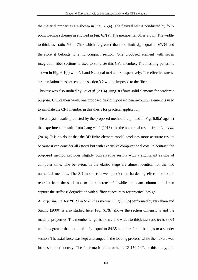
Chapter 6. Direct analysis of noncompact and slender CFT members
183
the material properties are shown in Fig. 6.6(a). The flexural test is conducted by four-
point loading schemes as showed in Fig. 6.7(a). The member length is 2.0 m. The width-
to-thickness ratio h/t is 75.0 which is greater than the limit 𝜆𝑝 equal to 67.34 and
therefore it belongs to a noncompact section. One proposed element with seven
integration fiber sections is used to simulate this CFT member. The meshing pattern is
shown in Fig. 6.1(a) with N1 and N2 equal to 4 and 8 respectively. The effective stress-
strain relationships presented in section 3.2 will be imposed to the fibers.
This test was also studied by Lai et al. (2014) using 3D finite solid elements for academic
purpose. Unlike their work, one proposed flexibility-based beam-column element is used
to simulate the CFT member in this thesis for practical application.
The analysis results predicted by the proposed method are plotted in Fig. 6.8(a) against
the experimental results from Jiang et al. (2013) and the numerical results from Lai et al.
(2014). It is no doubt that the 3D finite element model produces more accurate results
because it can consider all effects but with expensive computational cost. In contrast, the
proposed method provides slightly conservative results with a significant saving of
computer time. The behaviors in the elastic stage are almost identical for the two
numerical methods. The 3D model can well predict the hardening effect due to the
restraint from the steel tube to the concrete infill while the beam-column model can
capture the stiffness degradation with sufficient accuracy for practical design.
An experimental test “BRA4-2-5-02” as shown in Fig. 6.6(b) performed by Nakahara and
Sakino (2000) is also studied here. Fig. 6.7(b) shows the section dimensions and the
material properties. The member length is 0.6 m. The width-to-thickness ratio h/t is 98.04
which is greater than the limit 𝜆𝑝 equal to 84.35 and therefore it belongs to a slender
section. The axial force was kept unchanged in the loading process, while the flexure was
increased continuously. The fiber mesh is the same as “S-150-2.0”. In this study, one
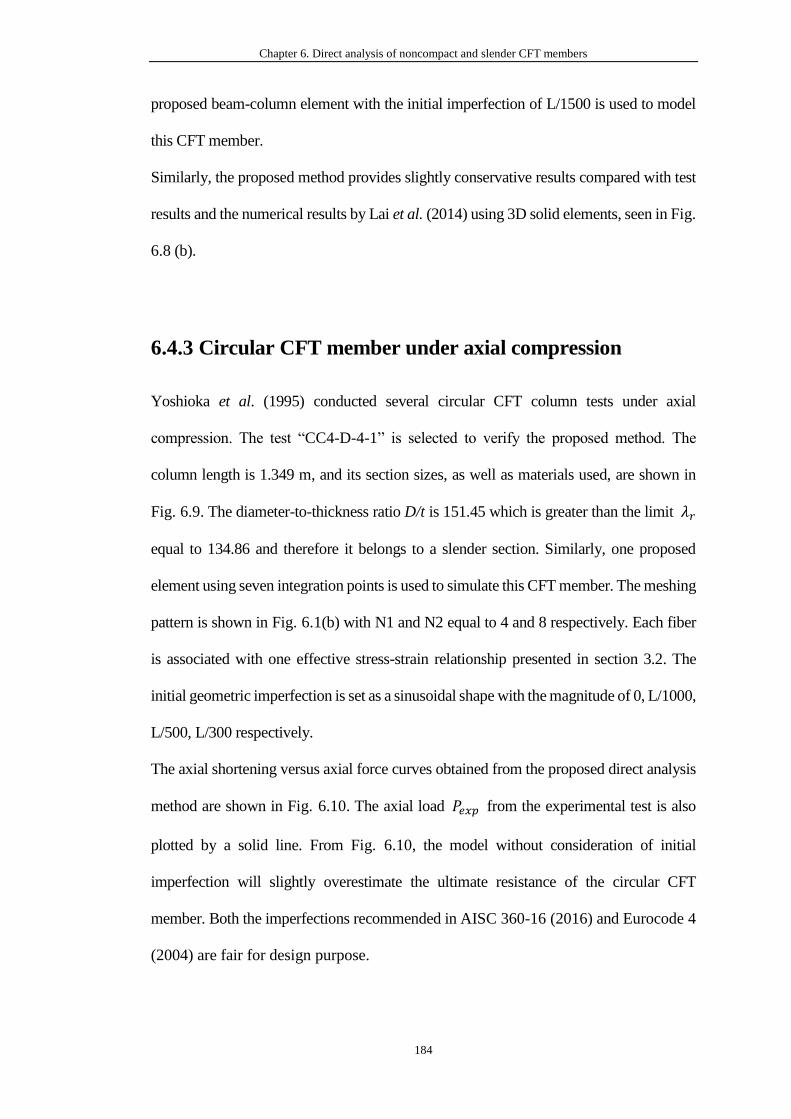
Chapter 6. Direct analysis of noncompact and slender CFT members
184
proposed beam-column element with the initial imperfection of L/1500 is used to model
this CFT member.
Similarly, the proposed method provides slightly conservative results compared with test
results and the numerical results by Lai et al. (2014) using 3D solid elements, seen in Fig.
6.8 (b).
6.4.3 Circular CFT member under axial compression
Yoshioka et al. (1995) conducted several circular CFT column tests under axial
compression. The test “CC4-D-4-1” is selected to verify the proposed method. The
column length is 1.349 m, and its section sizes, as well as materials used, are shown in
Fig. 6.9. The diameter-to-thickness ratio D/t is 151.45 which is greater than the limit 𝜆𝑟
equal to 134.86 and therefore it belongs to a slender section. Similarly, one proposed
element using seven integration points is used to simulate this CFT member. The meshing
pattern is shown in Fig. 6.1(b) with N1 and N2 equal to 4 and 8 respectively. Each fiber
is associated with one effective stress-strain relationship presented in section 3.2. The
initial geometric imperfection is set as a sinusoidal shape with the magnitude of 0, L/1000,
L/500, L/300 respectively.
The axial shortening versus axial force curves obtained from the proposed direct analysis
method are shown in Fig. 6.10. The axial load 𝑃𝑒𝑥𝑝 from the experimental test is also
plotted by a solid line. From Fig. 6.10, the model without consideration of initial
imperfection will slightly overestimate the ultimate resistance of the circular CFT
member. Both the imperfections recommended in AISC 360-16 (2016) and Eurocode 4
(2004) are fair for design purpose.
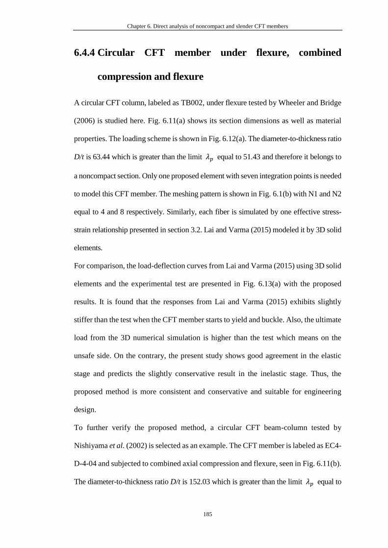
Chapter 6. Direct analysis of noncompact and slender CFT members
185
6.4.4 Circular CFT member under flexure, combined
compression and flexure
A circular CFT column, labeled as TB002, under flexure tested by Wheeler and Bridge
(2006) is studied here. Fig. 6.11(a) shows its section dimensions as well as material
properties. The loading scheme is shown in Fig. 6.12(a). The diameter-to-thickness ratio
D/t is 63.44 which is greater than the limit 𝜆𝑝 equal to 51.43 and therefore it belongs to
a noncompact section. Only one proposed element with seven integration points is needed
to model this CFT member. The meshing pattern is shown in Fig. 6.1(b) with N1 and N2
equal to 4 and 8 respectively. Similarly, each fiber is simulated by one effective stress-
strain relationship presented in section 3.2. Lai and Varma (2015) modeled it by 3D solid
elements.
For comparison, the load-deflection curves from Lai and Varma (2015) using 3D solid
elements and the experimental test are presented in Fig. 6.13(a) with the proposed
results. It is found that the responses from Lai and Varma (2015) exhibits slightly
stiffer than the test when the CFT member starts to yield and buckle. Also, the ultimate
load from the 3D numerical simulation is higher than the test which means on the
unsafe side. On the contrary, the present study shows good agreement in the elastic
stage and predicts the slightly conservative result in the inelastic stage. Thus, the
proposed method is more consistent and conservative and suitable for engineering
design.
To further verify the proposed method, a circular CFT beam-column tested by
Nishiyama et al. (2002) is selected as an example. The CFT member is labeled as EC4-
D-4-04 and subjected to combined axial compression and flexure, seen in Fig. 6.11(b).
The diameter-to-thickness ratio D/t is 152.03 which is greater than the limit 𝜆𝑝 equal to
Chapter 6. Direct analysis of noncompact and slender CFT members
186
134.28 and therefore it belongs to a slender section. Only one proposed element with
seven integration points is needed to model this CFT member. The meshing pattern is
shown in Fig. 6.1(b) with N1 and N2 equal to 4 and 8 respectively. The magnitude of
initial geometric imperfection is L/1000.
Three set results are shown in Fig. 6.13(b), i.e., numerical model from Denavit and Hajjar
(2012), the proposed method and the test by Nishiyama et al. (2002). Clearly, the present
study is closer to the experimental test than Denavit and Hajjar (2012), but requires fewer
computer resources. The two numerical models give slightly conservative ultimate
resistance. However, both of them show stiffer behavior in the post-buckling stage.
6.5 Concluding remarks
The noncompact/slender concrete-filled steel tube (CFT) members generally exhibit
complex behaviors such as local buckling, concrete confinement, and slippage
between the steel and concrete components. The latest AISC 360-16 firstly provides
two types of methods for design of noncompact/slender CFT members. However, the
reduced or effective stiffness method with P-M interaction curves only approximately
captures the actual behavior of CFT members. The effective length assumption with
many uncertainties is still needed in this method. For the effective stress-strain method,
the recommended initial geometrical imperfection is insufficient and may bring
unconservative design. In a word, the methods specified in AISC 360-16 are not fully
met the requirements of direct analysis. For this reason, a comprehensive method is
proposed in this thesis for a direct analysis of frame structures with
noncompact/slender CFT members.
The following conclusions can be drawn from this study.
Chapter 6. Direct analysis of noncompact and slender CFT members
187
1. The flexibility-based beam-column with member imperfections and incorporating
the effective stress-strain curves is capable for direct analysis of noncompact/slender
CFT members.
2. One proposed element per CFT member is adequate with excellent accuracy and a
significant saving of modeling and computational cost.
3. The effective stress-strain method can implicitly account for the complex behaviors
of noncompact/slender CFT members, and therefore it forms the solid foundation for
direct analysis using beam-column elements.
4. The effective length method for flexural buckling check can be completely
abandoned in the proposed direct analysis method.
5. The initial geometrical imperfections recommended in AISC 360-16 (2016) and
Eurocode 4 (2004) are on the unconservative and conservative side respectively. The
imperfection of L/500 is recommended for noncompact/slender CFT members.
It is also noted the effective stress-strain curves are essentially based on limited
experimental and numerical tests. Thus, more test results are recommended to improve
the accuracy of the effective stress-strain curves.
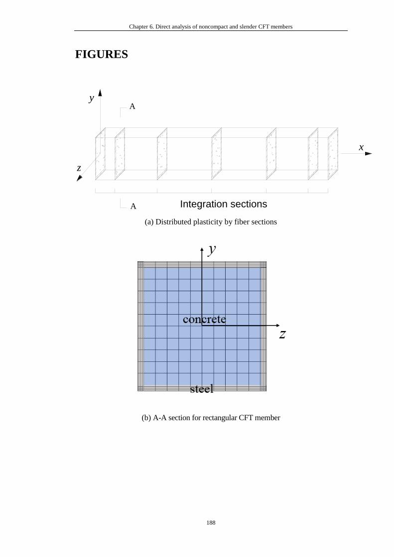
Chapter 6. Direct analysis of noncompact and slender CFT members
188
FIGURES
(a) Distributed plasticity by fiber sections
(b) A-A section for rectangular CFT member
z
x
y
Integration sections
A
A
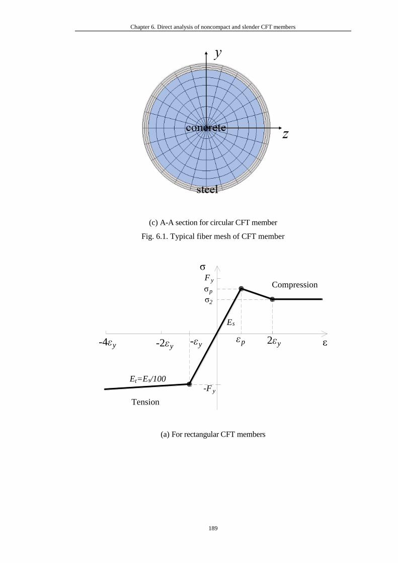
Chapter 6. Direct analysis of noncompact and slender CFT members
189
(c) A-A section for circular CFT member
Fig. 6.1. Typical fiber mesh of CFT member
(a) For rectangular CFT members
ε
σF y
σp
σ2
Es
Compression
Tension
Et=Es/100-F y
εp 2εy-2εy-4εy -εy
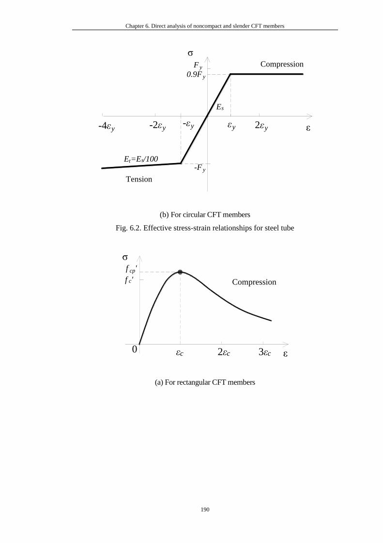
Chapter 6. Direct analysis of noncompact and slender CFT members
190
(b) For circular CFT members
Fig. 6.2. Effective stress-strain relationships for steel tube
(a) For rectangular CFT members
-F y
F y
0.9F y
σ
ε2εy-2εy-4εy-εy εy
Es
Et=Es/100
Compression
Tension
ε
σ
Compression
εc 2εc 3εc0
f cp'
f c'
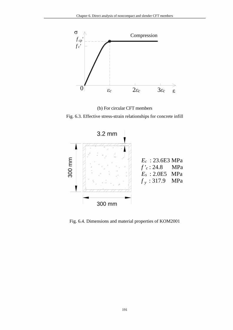
Chapter 6. Direct analysis of noncompact and slender CFT members
191
(b) For circular CFT members
Fig. 6.3. Effective stress-strain relationships for concrete infill
Fig. 6.4. Dimensions and material properties of KOM2001
ε
σCompression
εc 2εc 3εc0
f cp'
f c'
300 mm
300
mm
3.2 mm
Ec : 23.6E3 MPa
f 'c : 24.8 MPa
Es : 2.0E5 MPa
f y : 317.9 MPa
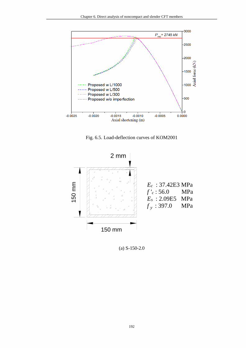
Chapter 6. Direct analysis of noncompact and slender CFT members
192
Fig. 6.5. Load-deflection curves of KOM2001
(a) S-150-2.0
150 mm
15
0 m
m
2 mm
Ec : 37.42E3 MPa
f 'c : 56.0 MPaEs : 2.09E5 MPa
f y : 397.0 MPa
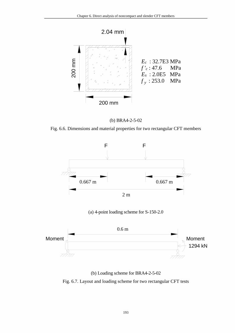
Chapter 6. Direct analysis of noncompact and slender CFT members
193
(b) BRA4-2-5-02
Fig. 6.6. Dimensions and material properties for two rectangular CFT members
(a) 4-point loading scheme for S-150-2.0
(b) Loading scheme for BRA4-2-5-02
Fig. 6.7. Layout and loading scheme for two rectangular CFT tests
200 mm
20
0 m
m
2.04 mm
Ec : 32.7E3 MPa
f 'c : 47.6 MPa
Es : 2.0E5 MPa
f y : 253.0 MPa
F
2 m
0.667 m
F
0.667 m
Moment
0.6 m
Moment
1294 kN
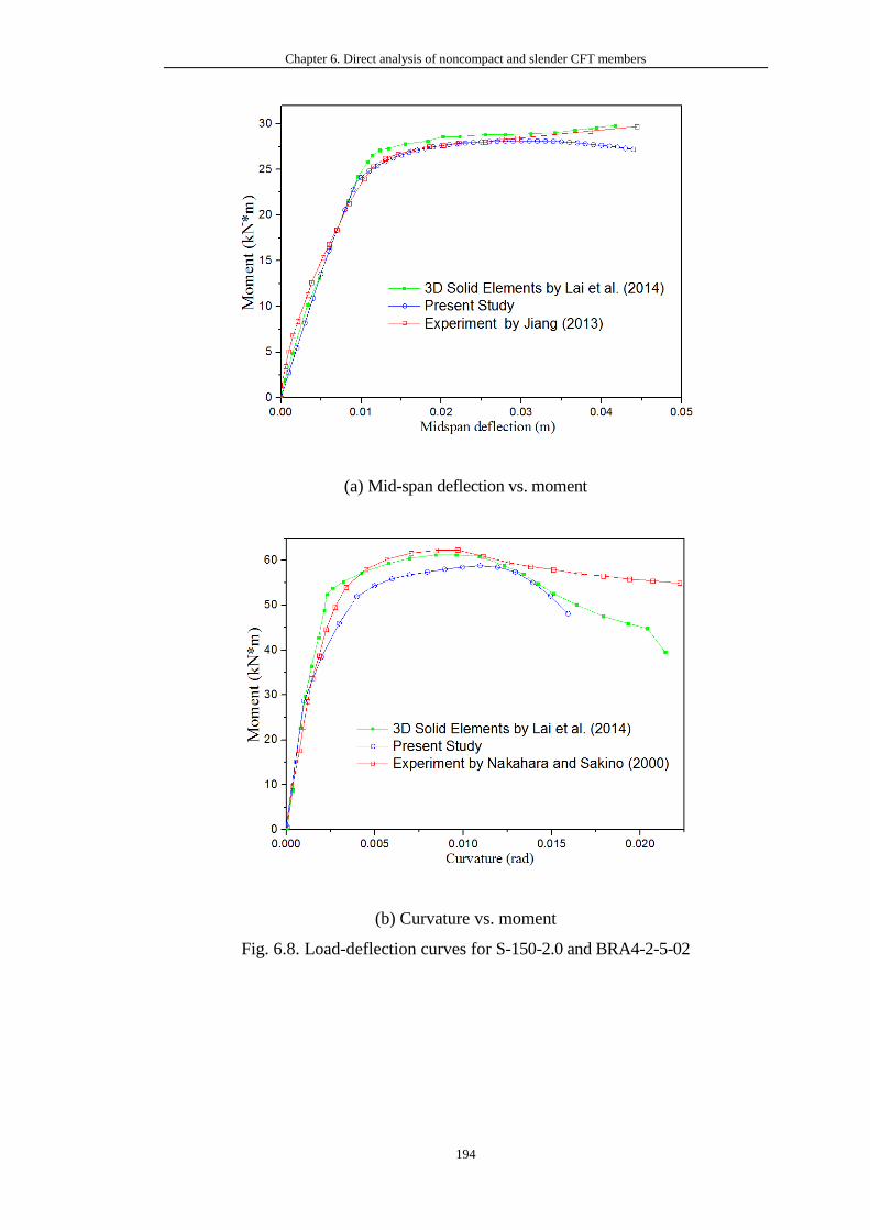
Chapter 6. Direct analysis of noncompact and slender CFT members
194
(a) Mid-span deflection vs. moment
(b) Curvature vs. moment
Fig. 6.8. Load-deflection curves for S-150-2.0 and BRA4-2-5-02
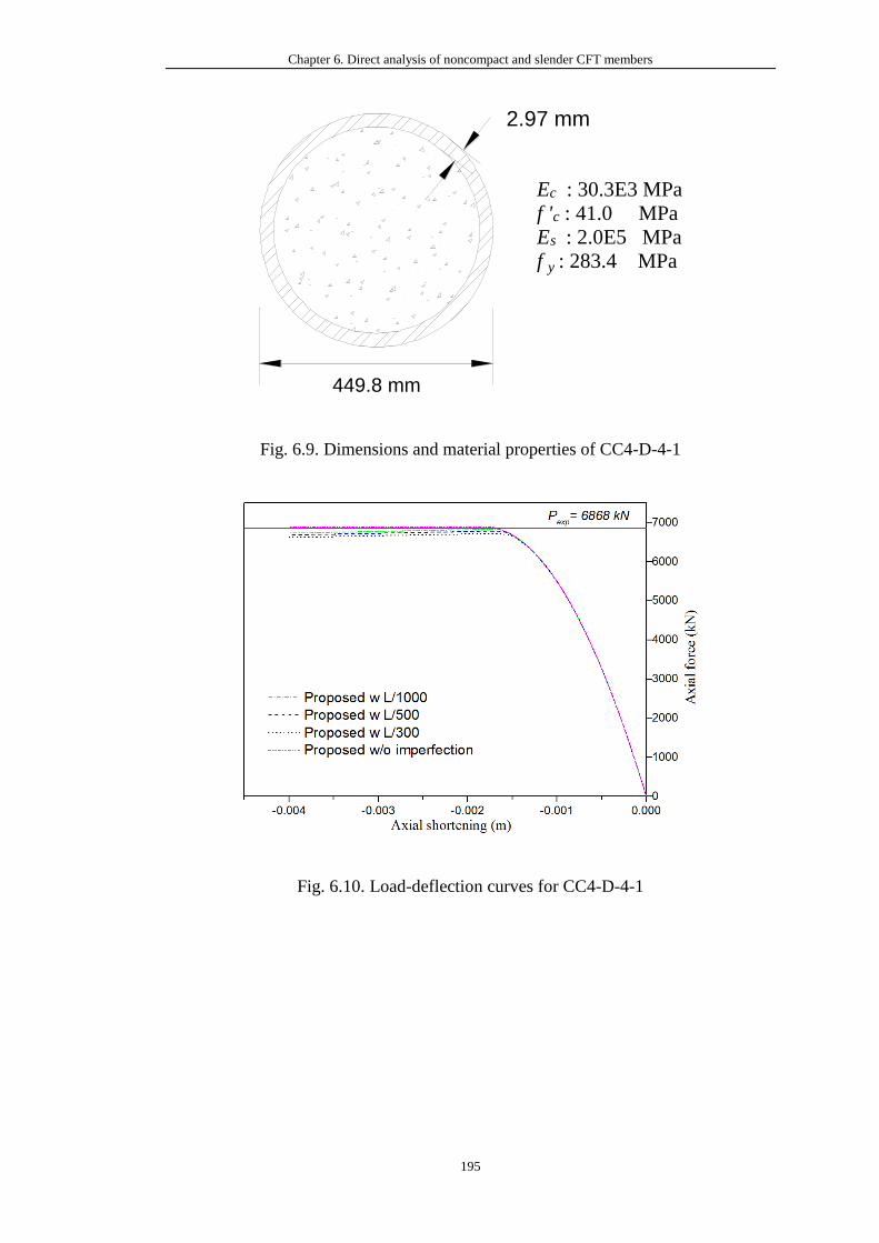
Chapter 6. Direct analysis of noncompact and slender CFT members
195
Fig. 6.9. Dimensions and material properties of CC4-D-4-1
Fig. 6.10. Load-deflection curves for CC4-D-4-1
Ec : 30.3E3 MPa
f 'c : 41.0 MPa
Es : 2.0E5 MPa
f y : 283.4 MPa
449.8 mm
2.97 mm
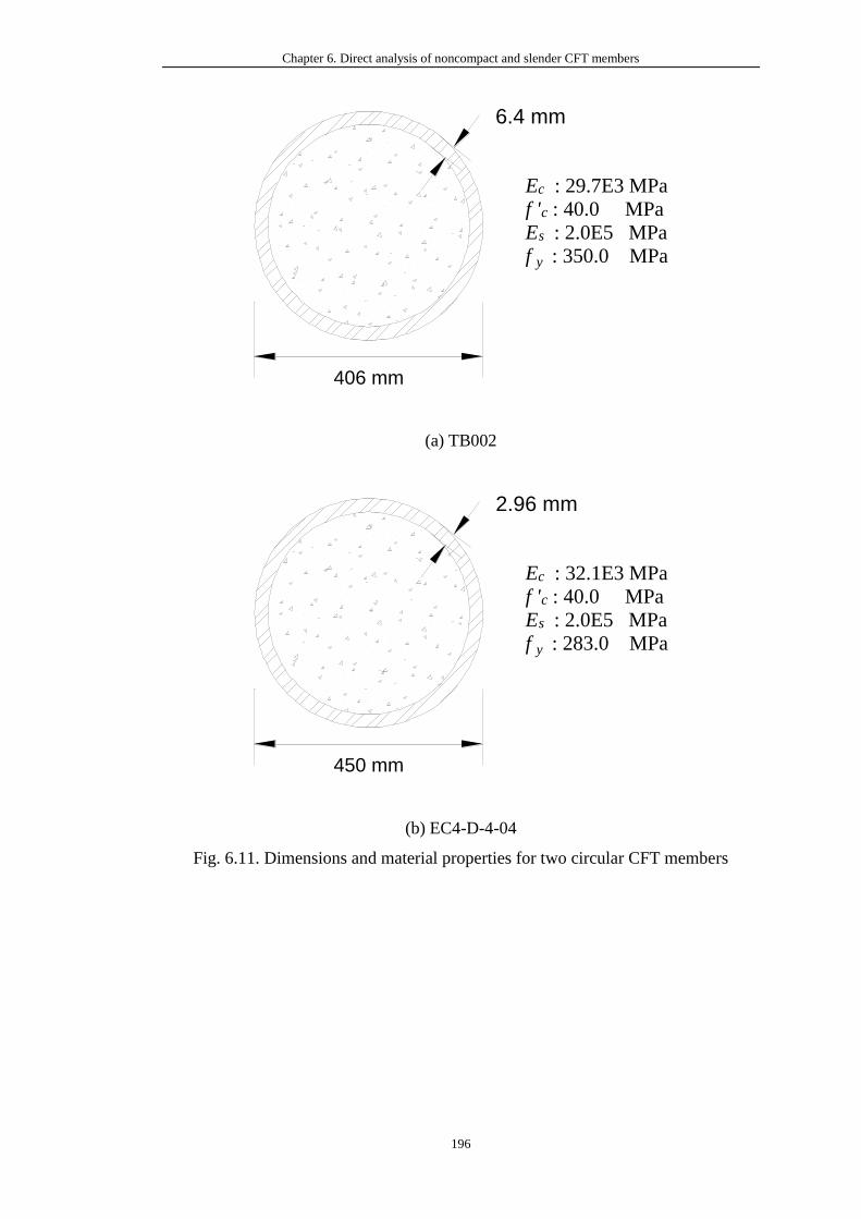
Chapter 6. Direct analysis of noncompact and slender CFT members
196
(a) TB002
(b) EC4-D-4-04
Fig. 6.11. Dimensions and material properties for two circular CFT members
Ec : 29.7E3 MPaf 'c : 40.0 MPa
Es : 2.0E5 MPa
f y : 350.0 MPa
406 mm
6.4 mm
Ec : 32.1E3 MPaf 'c : 40.0 MPa
Es : 2.0E5 MPa
f y : 283.0 MPa
450 mm
2.96 mm
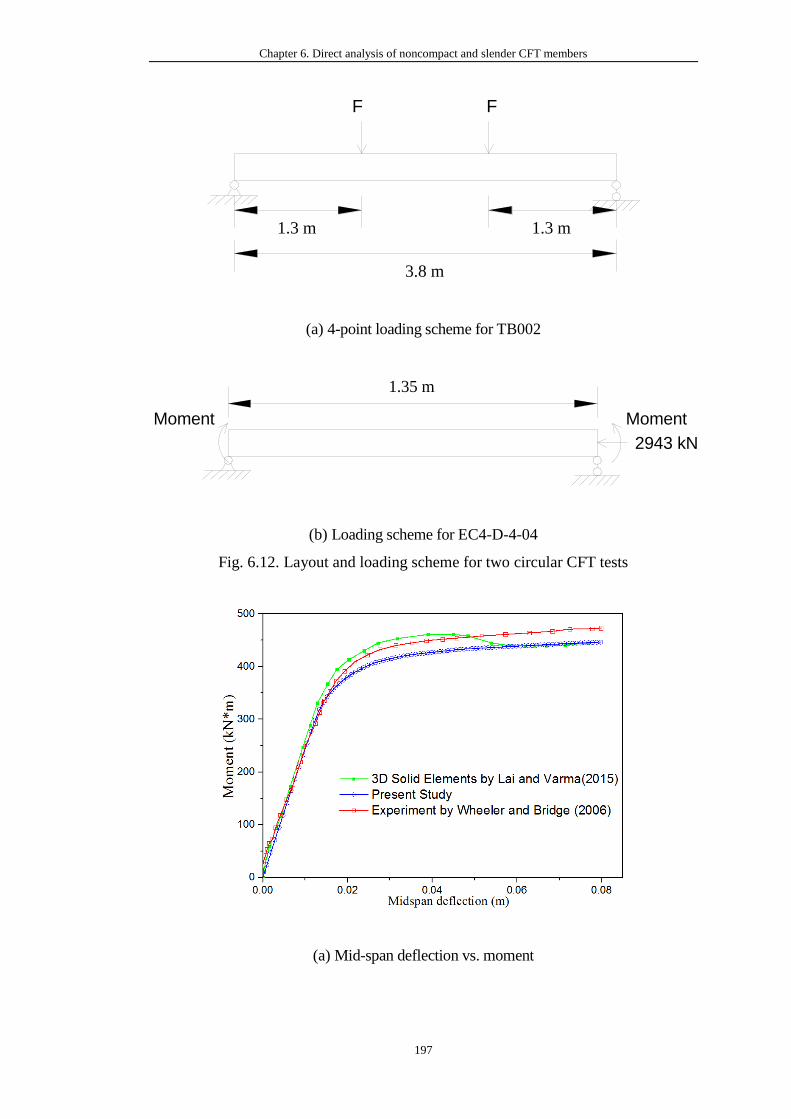
Chapter 6. Direct analysis of noncompact and slender CFT members
197
(a) 4-point loading scheme for TB002
(b) Loading scheme for EC4-D-4-04
Fig. 6.12. Layout and loading scheme for two circular CFT tests
(a) Mid-span deflection vs. moment
1.3 m 1.3 m
F
3.8 m
F
Moment
1.35 m
Moment
2943 kN
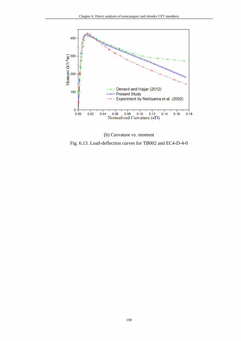
Chapter 6. Direct analysis of noncompact and slender CFT members
198
(b) Curvature vs. moment
Fig. 6.13. Load-deflection curves for TB002 and EC4-D-4-0
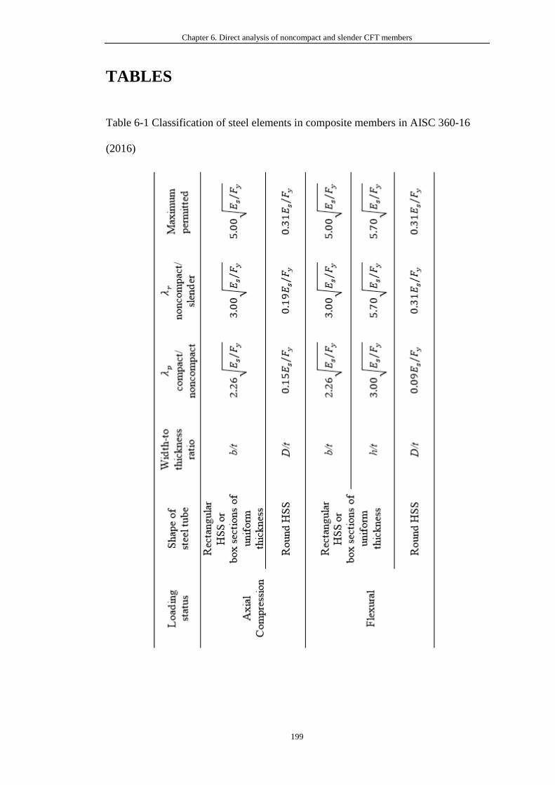
Chapter 6. Direct analysis of noncompact and slender CFT members
199
TABLES
Table 6-1 Classification of steel elements in composite members in AISC 360-16
(2016)
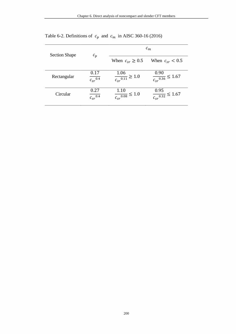
Chapter 6. Direct analysis of noncompact and slender CFT members
200
Table 6-2. Definitions of 𝑐𝑝 and 𝑐𝑚 in AISC 360-16 (2016)
Section Shape 𝑐𝑝
𝑐𝑚
When 𝑐𝑠𝑟 ≥ 0.5 When 𝑐𝑠𝑟 < 0.5
Rectangular 0.17
𝑐𝑠𝑟0.4
1.06
𝑐𝑠𝑟0.11≥ 1.0
0.90
𝑐𝑠𝑟0.36≤ 1.67
Circular 0.27
𝑐𝑠𝑟0.4
1.10
𝑐𝑠𝑟0.08≤ 1.0
0.95
𝑐𝑠𝑟0.32≤ 1.67
Chapter 7. Direct analysis of special concentrically braced frames
201
CHAPTER 7. DIRECT ANALYSIS OF SPECIAL
CONCENTRICALLY BRACED FRAMES
7.1 Introduction
Special concentrically braced frames (SCBFs) are extensively employed in high
seismicity regions due to structural efficiency and particularly high ductility for energy
dissipation through tensile yielding, buckling and post-buckling behaviors of braces.
The commonly used configurations of SCBFs are shown in Fig. 2.2. The inverted V-
bracing configuration is most welcomed for easy accommodation of doors and
windows. Generally, the bracing systems should be designed in pairs to account for
tension and compression in both directions. The SCBFs with properly detailed
connections can meet various performance levels for performance-based seismic
design. The shape of steel brace could be rectangular, square or circular hollow section
and H-shape section.
Many experimental tests have been conducted to study the behaviors of isolated
components such as braces and gusset plate connections, and the system performance
of SCBFs. Fell et al. (2009) experimentally investigated the inelastic buckling and
fracture behavior of steel braces including square hollow section, pipe and wide-flange
H-shape section. Tremblay et al. (2003) validated the effective brace slenderness
adopted in the design and proposed an empirical model to predict brace fracture by
testing fourteen single braces and ten X-braces. Han et al. (2007) examined energy
dissipation capacity of braces with different width-thickness ratios by quasi-static
reversed cyclic experiments. Lehman et al. (2008) conducted several full-scale tests
of one-story one-bay SCBFs to evaluate the economy and performance of gusset plate
Chapter 7. Direct analysis of special concentrically braced frames
202
connections. Palmer et al. (2012) investigated the seismic behavior of a two-story,
one-bay by one-bay frame. Lumpkin et al. (2012) explored the seismic response of
two three-story SCBFs and proposed several recommendations for enhancing ductility
of SCBFs. In summary, the experimental tests provide valuable information for the
codified design of SCBFs and motivate the researchers to develop and improve their
analytical models so that the routine design should not merely rely on experimental
tests which are limited to many idealized conditions.
Extensive works have been carried out on the numerical modeling of braces as well as
their connections linking to the framing beams and columns. The researchers attempt
to accurately predict the cyclic strength and stiffness deterioration of structural
components. The typical structural behavior and the potential failure locations of a
single brace are shown in Fig. 2.3. Significant yielding and local plate buckling
behaviors are commonly observed. There are four numerical methods proposed for
simulation of SCBFs, i.e., phenomenological model (Nilforoushan, 1973), simplified
phenomenological model (Soroushian, 1988), fiber-type finite element model
(Gunnarsson, 2004) and continuum finite element model (Haddad and Tremblay,
2006). Uriz (2005) pointed out the limitation of the traditional phenomenological
model in predicting peak responses of steel braces and proposed a brace component
model which can well simulate the post-buckling and fracture of steel braces under
cyclic loading. However, his analytical model required several elements to model a
brace and introduced a small initial camber which does not fully comply with the code
requirement to trigger buckling. Yoo et al. (2008) used continuum finite element (FE)
model to investigate the behavior of gusset plate connection and the interaction
between the connection and framing elements. They pointed out that the proper
detailing of gusset plate connection can improve the performance of SCBFs. Uriz and

Chapter 7. Direct analysis of special concentrically braced frames
203
Mahin (2008) proposed a force-based fiber element to represent the gusset plate
connection while Hsiao et al. (2012) introduced rotational hinges attached to ends of
the beam-column element to model the connections. Their model employed several
different types of elements in series to model a brace with end connections which leads
to an impractical model for daily use. Generally speaking, the previous researches
(Hsiao, 2012, 2013; Karamanci, 2014; Krishnan, 2010; Uriz, 2005) clearly show that
the initial curvature of steel braces should be taken into account so that the buckling
and post-buckling behavior of steel braces can be captured in numerical analysis.
Consequently, several elements per member are compulsively required to simulate the
complex behavior of braces. The calibration works with experimental test results can
be found in references (Hsiao, 2012, 2013; Karamanci, 2014; Krishnan, 2010).
Although Krishnan (2010) has proposed a modified elasto-plastic fiber element, which
consists of three fiber segments formed by two external nodes and four internal nodes,
to simulate the inelastic behavior of slender columns and braces, it is essential a multi-
element per member model (MEPMM) which cannot truly reduce the computer time.
The MEPMM not only increases the modeling effort, but also occupies more computer
resources, especially in the nonlinear dynamic analysis (NDA, also well known as
time history analysis). Most importantly, MEPMM becomes more prone to induce
numerical problems when a plastic hinge is formed at the member mid-span in such
case the stiffness matrix of the associated node approaches singular. Thus, one-
element per member model (OEPMM) is preferred in practical applications.
Theoretically speaking, the three-dimensional solid elements or two-dimensional shell
elements can produce more accurate responses for both the components and the SCBF
system. However, the two types of finite elements are rarely adopted in a global
analysis of engineering structures owing to time-consuming and inconvenience in
Chapter 7. Direct analysis of special concentrically braced frames
204
codified design. A number of displacement-based beam-column elements (Chan, 1995,
2000; Liu et al. 2014) with concentrated plastic hinge method have been proposed for
second-order inelastic analysis. Although the elements can account for member initial
geometric imperfection, their application on inelastic analysis face challenges because
of the inherent shortcomings of displacement-based elements and concentrated plastic
hinge assumption. To obtain more accurate results, more elements for the member
undergoing significant buckling and plastic behavior such as the braces in SCBFs are
inevitably required. Du et al. (2017) firstly proposed a flexibility-based beam-column
element with initial geometric imperfection for second-order inelastic analysis.
However, their work does not take the residual stress, semi-rigid connection, and rigid
end-offset into account and therefore their outcome cannot be directly used for the
design of SCBFs.
From the above, it can be seen that more efforts are needed to narrow the gap between
the research and practical design on SCBFs. First, the previous models required multi-
elements per member as well as individual elements for gusset plate connections and
rigid end zone. Hence, the models generally lead to more modeling and computational
efforts and numerical convergent problem. Second, the influence of initial geometric
imperfection and residual stress has not been properly considered in the analysis, and
therefore the design of SCBFs may be on the unsafe side. It is also noted that the direct
analysis method (DAM) which is well specified in the modern design codes such as
AISC360 (2016), Eurocode-3 (2005) and COPHK (2011). However, these codes have
not been well linked to the seismic design codes. Thus, this thesis aims to provide a
comprehensive solution for the seismic design of SCBFs and, simultaneously, extends
the DAM to nonlinear dynamic analysis (NDA) to achieve a consistent design practice.
Chapter 7. Direct analysis of special concentrically braced frames
205
In this thesis, the element FBMI allowing member initial bowing proposed by Du et
al. (2017) based on Hellinger-Reissner (HR) functional is modified into a new hybrid
element for second-order dynamic analysis of SCBFs. This innovative element
considers member initial geometric imperfection, residual stress, finite joint stiffness
and rigid end zone at the element level for three-dimensional frame analysis. The
proposed element inherits the high accuracy of the original element with consideration
of progressive yielding in cross section and along the member length. Fiber section
approach is adopted to account for member distributed plasticity with the inclusion of
residual stress which has not been reported in the previous SCBFs models. Moreover,
the semi-rigid connection technique in the literature was mainly proposed to the beam
ends dominated by bending moment and as a result, the influence of axial force on the
connection can be ignored. Thus, this conventional method will be improved here as
the braces in SCBFs undergo considerably large axial forces.
The layout of this chapter is as follows: the element FBMI allowing member initial
imperfection is briefly introduced in section 7.2; the semi-rigid connection technique
as well as the treatment of rigid end zone is presented in section 7.3; the material model
and residual stress pattern are shown in section 7.4; the comprehensive modeling of
SCBFs and the verification works will be presented in section 7.5 and 7.6 respectively.
Finally, the conclusions with highlights of this study and several recommendations for
SCBF modeling will be made.
Chapter 7. Direct analysis of special concentrically braced frames
206
7.2 Semi-rigid connection and rigid end zone for gusset
plate connections
The gusset plate connection, as an important component of SCBFs connecting brace
to beam and column, transfers the axial force and bending moments between the brace
and the framing system. It needs to be carefully designed with proper stiffness to
tolerate the end rotation of the brace and sustain less damage before the brace fracture.
The change of the gusset plate stiffness affects the end conditions of the brace and
consequently influents the buckling resistance of the brace. More importantly, the
gusset plate connection absorbs a portion of energy from ground motion by hysteretic
behavior. Thus, it is worth to capture these features in the analytical model of SCBFs
to have a better prediction of SCBFs’ behaviors.
Mathematically, a semi-rigid connection can be introduced to reflect the behavior
between a brace and a gusset plate connection. To reflect the actual length of the gusset
plate connection and the physical length of brace, a rigid zone will be introduced at
the end of a brace. The former one technique has been introduced in Chapter 3. The
latter one will be incorporated into the proposed FBMI element to form a hybrid
element for nonlinear dynamic analysis (NDA) of SCBFs with significant
improvement of result accuracy and enhancement of numerical efficiency.
7.2.1 Semi-rigid behavior of gusset plate connection
The bi-linear 𝑀-𝜃 model is widely used in frame analysis to consider semi-rigid
behavior for simplicity. To more accurately reflect the hysteretic response of the gusset
plates under cyclic loading or strong ground motions, more sophisticated model should
be adopted in the design of SCBFs. In this thesis, the 𝑀-𝜃 function of gusset plate
connection proposed by Hsiao (2012) with calibration of experimental test results and
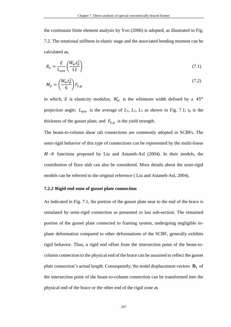
Chapter 7. Direct analysis of special concentrically braced frames
207
the continuum finite element analysis by Yoo (2006) is adopted, as illustrated in Fig.
7.2. The rotational stiffness in elastic stage and the associated bending moment can be
calculated as,
𝑅𝑒 =𝐸
𝐿𝑎𝑣𝑒(𝑊𝑤𝑡𝑝
2
12) (7.1)
𝑀𝑦 = (𝑊𝑤𝑡𝑝
2
6)𝐹𝑦,𝑔
(7.2)
in which, E is elasticity modulus; 𝑊𝑤 is the whitmore width defined by a 45o
projection angle; 𝐿𝑎𝑣𝑒 is the average of L1, L2, L3 as shown in Fig. 7.1; tp is the
thickness of the gusset plate; and 𝐹𝑦,𝑔 is the yield strength.
The beam-to-column shear tab connections are commonly adopted in SCBFs. The
semi-rigid behavior of this type of connections can be represented by the multi-linear
𝑀 -𝜃 functions proposed by Liu and Astaneh-Asl (2004). In their models, the
contribution of floor slab can also be considered. More details about the semi-rigid
models can be referred to the original reference ( Liu and Astaneh-Asl, 2004).
7.2.2 Rigid end zone of gusset plate connection
As indicated in Fig. 7.1, the portion of the gusset plate near to the end of the brace is
simulated by semi-rigid connection as presented in last sub-section. The remained
portion of the gusset plate connected to framing system, undergoing negligible in-
plane deformation compared to other deformations of the SCBF, generally exhibits
rigid behavior. Thus, a rigid end offset from the intersection point of the beam-to-
column connection to the physical end of the brace can be assumed to reflect the gusset
plate connection’s actual length. Consequently, the nodal displacement vectors 𝐃𝒊 of
the intersection point of the beam-to-column connection can be transformed into the
physical end of the brace or the other end of the rigid zone as
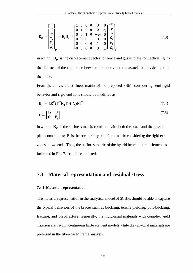
Chapter 7. Direct analysis of special concentrically braced frames
208
𝐃𝒑 =
[ 𝑢𝑣𝑤𝜃𝑥𝜃𝑦𝜃𝑧]
𝒑
= 𝐄𝒊𝐃𝒊 =
[ 100000
010000
001000
000100
00−e𝑖010
0e𝑖0001]
[ 𝑢𝑣𝑤𝜃𝑥𝜃𝑦𝜃𝑧]
𝒊
(7.3)
in which, 𝐃𝒑 is the displacement vector for brace and gusset plate connection; 𝑒𝑖 is
the distance of the rigid zone between the node i and the associated physical end of
the brace.
From the above, the stiffness matrix of the proposed FBMI considering semi-rigid
behavior and rigid end zone should be modified as
𝐊𝑻 = 𝐋𝐄𝑻(𝐓𝑻𝐊𝒄𝐓 + 𝐍)𝐄𝐋
𝑻 (7.4)
𝐄 = [𝐄𝒊 𝟎𝟎 𝐄𝒋
] (7.5)
in which, 𝐊𝒄 is the stiffness matrix combined with both the brace and the gusset
plate connections; 𝐄 is the eccentricity transform matrix considering the rigid end
zones at two ends. Thus, the stiffness matrix of the hybrid beam-column element as
indicated in Fig. 7.1 can be calculated.
7.3 Material representation and residual stress
7.3.1 Material representation
The material representation in the analytical model of SCBFs should be able to capture
the typical behaviors of the braces such as buckling, tensile yielding, post-buckling,
fracture, and post-fracture. Generally, the multi-axial materials with complex yield
criterion are used in continuum finite element models while the uni-axial materials are
preferred in the fiber-based frame analysis.
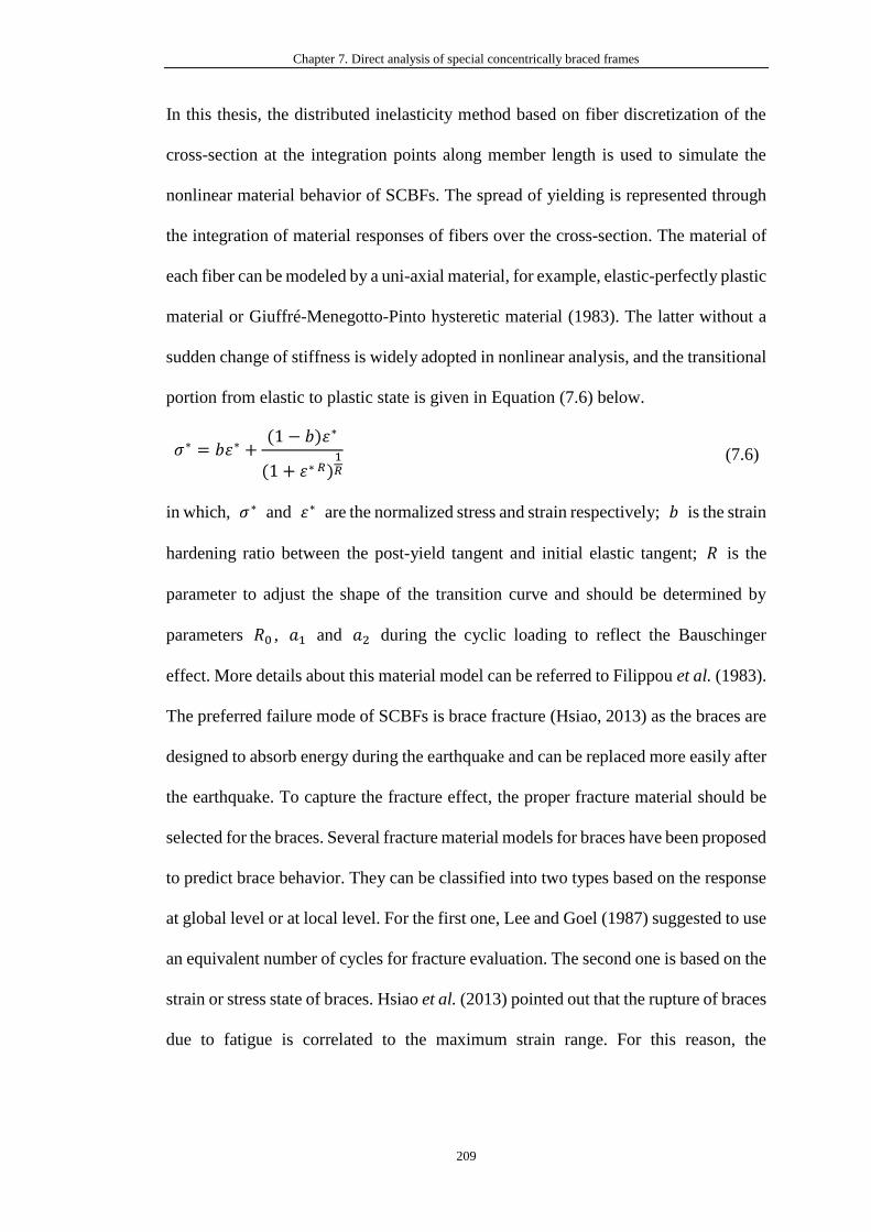
Chapter 7. Direct analysis of special concentrically braced frames
209
In this thesis, the distributed inelasticity method based on fiber discretization of the
cross-section at the integration points along member length is used to simulate the
nonlinear material behavior of SCBFs. The spread of yielding is represented through
the integration of material responses of fibers over the cross-section. The material of
each fiber can be modeled by a uni-axial material, for example, elastic-perfectly plastic
material or Giuffré-Menegotto-Pinto hysteretic material (1983). The latter without a
sudden change of stiffness is widely adopted in nonlinear analysis, and the transitional
portion from elastic to plastic state is given in Equation (7.6) below.
𝜎∗ = 𝑏휀∗ +(1 − 𝑏)휀∗
(1 + 휀∗ 𝑅)1𝑅
(7.6)
in which, 𝜎∗ and 휀∗ are the normalized stress and strain respectively; 𝑏 is the strain
hardening ratio between the post-yield tangent and initial elastic tangent; 𝑅 is the
parameter to adjust the shape of the transition curve and should be determined by
parameters 𝑅0 , 𝑎1 and 𝑎2 during the cyclic loading to reflect the Bauschinger
effect. More details about this material model can be referred to Filippou et al. (1983).
The preferred failure mode of SCBFs is brace fracture (Hsiao, 2013) as the braces are
designed to absorb energy during the earthquake and can be replaced more easily after
the earthquake. To capture the fracture effect, the proper fracture material should be
selected for the braces. Several fracture material models for braces have been proposed
to predict brace behavior. They can be classified into two types based on the response
at global level or at local level. For the first one, Lee and Goel (1987) suggested to use
an equivalent number of cycles for fracture evaluation. The second one is based on the
strain or stress state of braces. Hsiao et al. (2013) pointed out that the rupture of braces
due to fatigue is correlated to the maximum strain range. For this reason, the
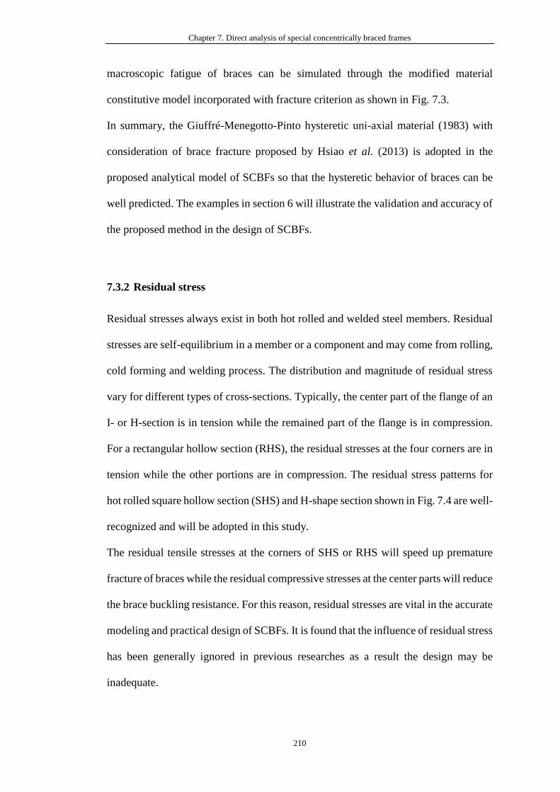
Chapter 7. Direct analysis of special concentrically braced frames
210
macroscopic fatigue of braces can be simulated through the modified material
constitutive model incorporated with fracture criterion as shown in Fig. 7.3.
In summary, the Giuffré-Menegotto-Pinto hysteretic uni-axial material (1983) with
consideration of brace fracture proposed by Hsiao et al. (2013) is adopted in the
proposed analytical model of SCBFs so that the hysteretic behavior of braces can be
well predicted. The examples in section 6 will illustrate the validation and accuracy of
the proposed method in the design of SCBFs.
7.3.2 Residual stress
Residual stresses always exist in both hot rolled and welded steel members. Residual
stresses are self-equilibrium in a member or a component and may come from rolling,
cold forming and welding process. The distribution and magnitude of residual stress
vary for different types of cross-sections. Typically, the center part of the flange of an
I- or H-section is in tension while the remained part of the flange is in compression.
For a rectangular hollow section (RHS), the residual stresses at the four corners are in
tension while the other portions are in compression. The residual stress patterns for
hot rolled square hollow section (SHS) and H-shape section shown in Fig. 7.4 are well-
recognized and will be adopted in this study.
The residual tensile stresses at the corners of SHS or RHS will speed up premature
fracture of braces while the residual compressive stresses at the center parts will reduce
the brace buckling resistance. For this reason, residual stresses are vital in the accurate
modeling and practical design of SCBFs. It is found that the influence of residual stress
has been generally ignored in previous researches as a result the design may be
inadequate.
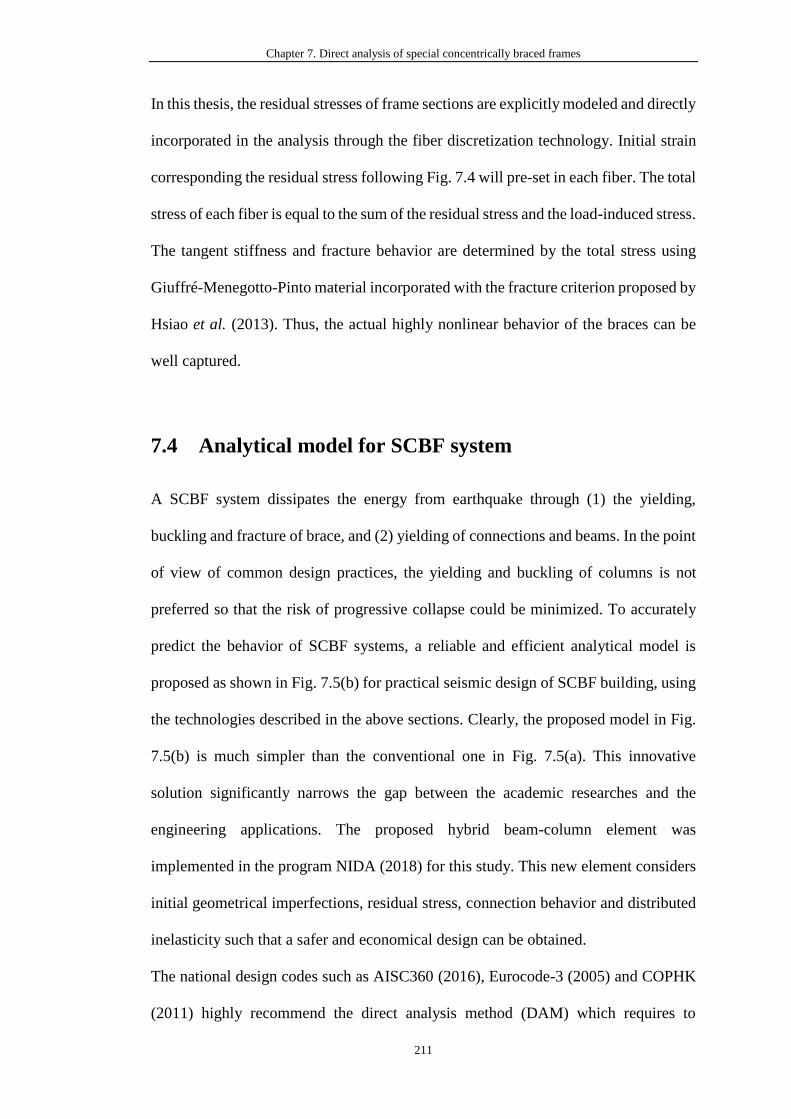
Chapter 7. Direct analysis of special concentrically braced frames
211
In this thesis, the residual stresses of frame sections are explicitly modeled and directly
incorporated in the analysis through the fiber discretization technology. Initial strain
corresponding the residual stress following Fig. 7.4 will pre-set in each fiber. The total
stress of each fiber is equal to the sum of the residual stress and the load-induced stress.
The tangent stiffness and fracture behavior are determined by the total stress using
Giuffré-Menegotto-Pinto material incorporated with the fracture criterion proposed by
Hsiao et al. (2013). Thus, the actual highly nonlinear behavior of the braces can be
well captured.
7.4 Analytical model for SCBF system
A SCBF system dissipates the energy from earthquake through (1) the yielding,
buckling and fracture of brace, and (2) yielding of connections and beams. In the point
of view of common design practices, the yielding and buckling of columns is not
preferred so that the risk of progressive collapse could be minimized. To accurately
predict the behavior of SCBF systems, a reliable and efficient analytical model is
proposed as shown in Fig. 7.5(b) for practical seismic design of SCBF building, using
the technologies described in the above sections. Clearly, the proposed model in Fig.
7.5(b) is much simpler than the conventional one in Fig. 7.5(a). This innovative
solution significantly narrows the gap between the academic researches and the
engineering applications. The proposed hybrid beam-column element was
implemented in the program NIDA (2018) for this study. This new element considers
initial geometrical imperfections, residual stress, connection behavior and distributed
inelasticity such that a safer and economical design can be obtained.
The national design codes such as AISC360 (2016), Eurocode-3 (2005) and COPHK
(2011) highly recommend the direct analysis method (DAM) which requires to

Chapter 7. Direct analysis of special concentrically braced frames
212
consider initial geometrical imperfections and residual stress so that the member
buckling behavior can be directly reflected in the analysis stage rather than separately
in the design stage. When using the DAM, the effective length for individual member
check is no longer required as the second-order P-Δ and P-δ effects have been
considered during the analysis process and as a result, only the section capacity check
is needed. It should also be pointed out that the local joint behavior should be carefully
captured in the analysis if the joint like the gusset plate connection of SCBFs
significantly affects the load distribution of the structural system according to the
requirement of DAM. However, the DAM is rarely adopted in the seismic design. To
some extent, it is because the two design theories were developed and improved in a
parallel manner. If the behaviors of members and connections cannot be well
represented in the nonlinear dynamic analysis (NDA), the responses for identifying
plastic hinges may be inaccurate, and consequently, the more realistic responses of the
structural system cannot be predicted which lead to an unsafe design. Being aware of
the above, this thesis aims to promote the DAM to seismic design using NDA so that
a consistent design method linking the static and dynamic design together can be
provided for design office.
The modeling details for braces, gusset plate connections, beams and columns in
SCBF system will be introduced in this section. The features and advantages of the
proposed model will be highlighted and discussed as followings.
7.4.1 Modeling of beams and columns
In the conventional nonlinear dynamic analysis (NDA), the initial geometrical
imperfections and residual stresses, which are inherent in the steel beams and columns,
have generally been overlooked. It should be pointed out that the P - δ effect
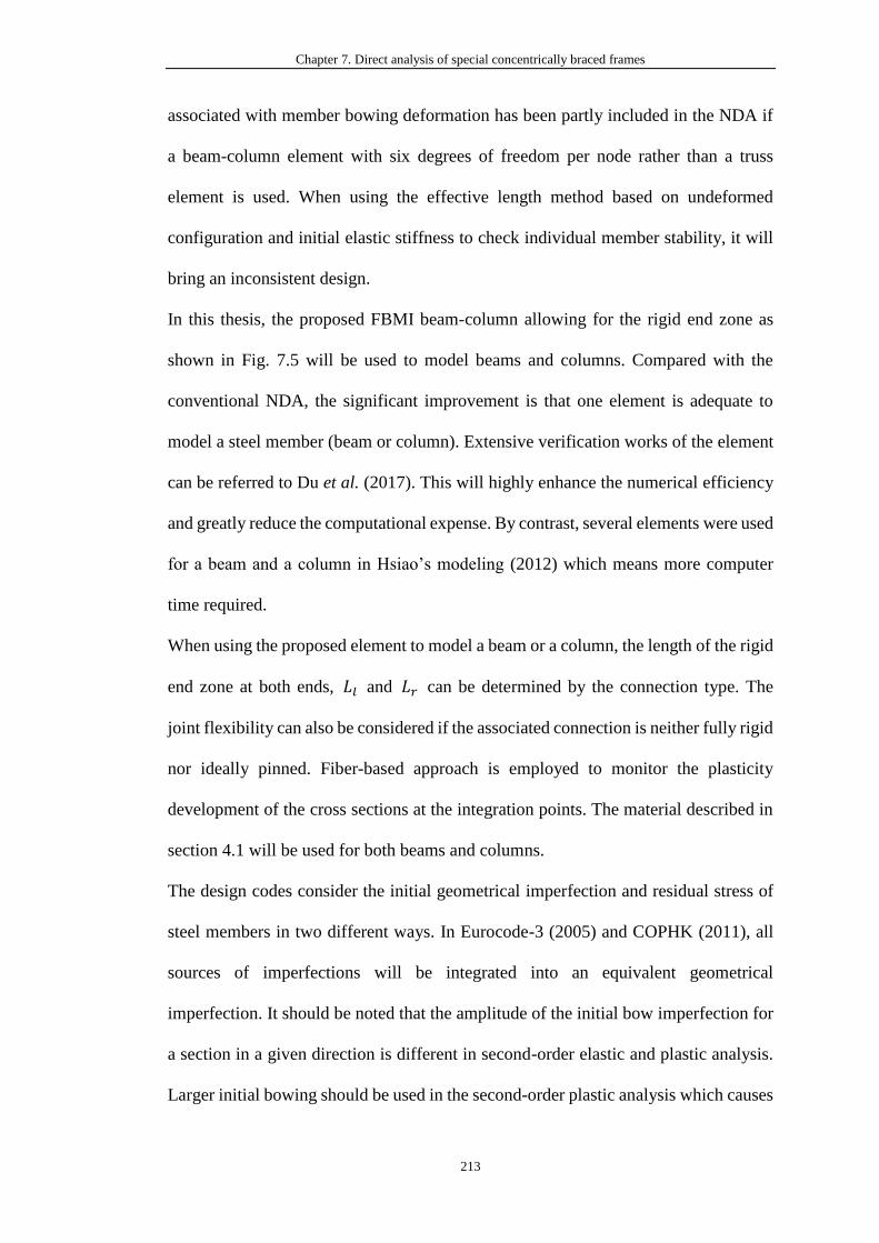
Chapter 7. Direct analysis of special concentrically braced frames
213
associated with member bowing deformation has been partly included in the NDA if
a beam-column element with six degrees of freedom per node rather than a truss
element is used. When using the effective length method based on undeformed
configuration and initial elastic stiffness to check individual member stability, it will
bring an inconsistent design.
In this thesis, the proposed FBMI beam-column allowing for the rigid end zone as
shown in Fig. 7.5 will be used to model beams and columns. Compared with the
conventional NDA, the significant improvement is that one element is adequate to
model a steel member (beam or column). Extensive verification works of the element
can be referred to Du et al. (2017). This will highly enhance the numerical efficiency
and greatly reduce the computational expense. By contrast, several elements were used
for a beam and a column in Hsiao’s modeling (2012) which means more computer
time required.
When using the proposed element to model a beam or a column, the length of the rigid
end zone at both ends, 𝐿𝑙 and 𝐿𝑟 can be determined by the connection type. The
joint flexibility can also be considered if the associated connection is neither fully rigid
nor ideally pinned. Fiber-based approach is employed to monitor the plasticity
development of the cross sections at the integration points. The material described in
section 4.1 will be used for both beams and columns.
The design codes consider the initial geometrical imperfection and residual stress of
steel members in two different ways. In Eurocode-3 (2005) and COPHK (2011), all
sources of imperfections will be integrated into an equivalent geometrical
imperfection. It should be noted that the amplitude of the initial bow imperfection for
a section in a given direction is different in second-order elastic and plastic analysis.
Larger initial bowing should be used in the second-order plastic analysis which causes

Chapter 7. Direct analysis of special concentrically braced frames
214
inconvenience as many members may remain elastic during inelastic analysis. On the
contrary, AISC360 (2016) recommends to consider the two sources of imperfections
separately. Generally speaking, the former is more welcomed in the stiffness-based
beam-column elements with plastic hinge method while the latter is more suitable for
flexibility-based beam-column elements with distributed plasticity. In this thesis, the
latter will be adopted so that more accurate responses of SCBFs can be obtained.
7.4.2 Modeling of brace and gusset plate connection
The gusset plate connections in SCBFs should be properly designed with detailing
requirements specified in AISC341 (2016) so that the brace fracture occurs first and
then the connection ruptures. The failure of gusset plate connection early before brace
fracture is undesirable as the SCBF will absorb less energy in this situation. The gusset
plate connections play an important role in SCBF system, and therefore their behavior
should be well represented in the analytical model.
Like the beams and columns, the initial geometrical imperfections and residual stress
of braces should be included in the analytical model so that the brace yielding,
buckling, and fracture can be precisely captured.
In this thesis, one proposed hybrid element based on FBMI beam-column with rigid
end zone, zero-length end spring and initial imperfections is adequate to model a brace
with two associated gusset plate connections. Rigid end zones are placed at both ends
of the element to reflect the length of connection while two zero-length end springs
located between the rigid end zone and the brace are used to simulate the semi-rigid
behavior of the gusset plate connections. The associated technologies are described in
section 3. The remaining middle part of the element is the actual length of the brace
and the fiber-based approach is employed to trace its stability and distributed plasticity.
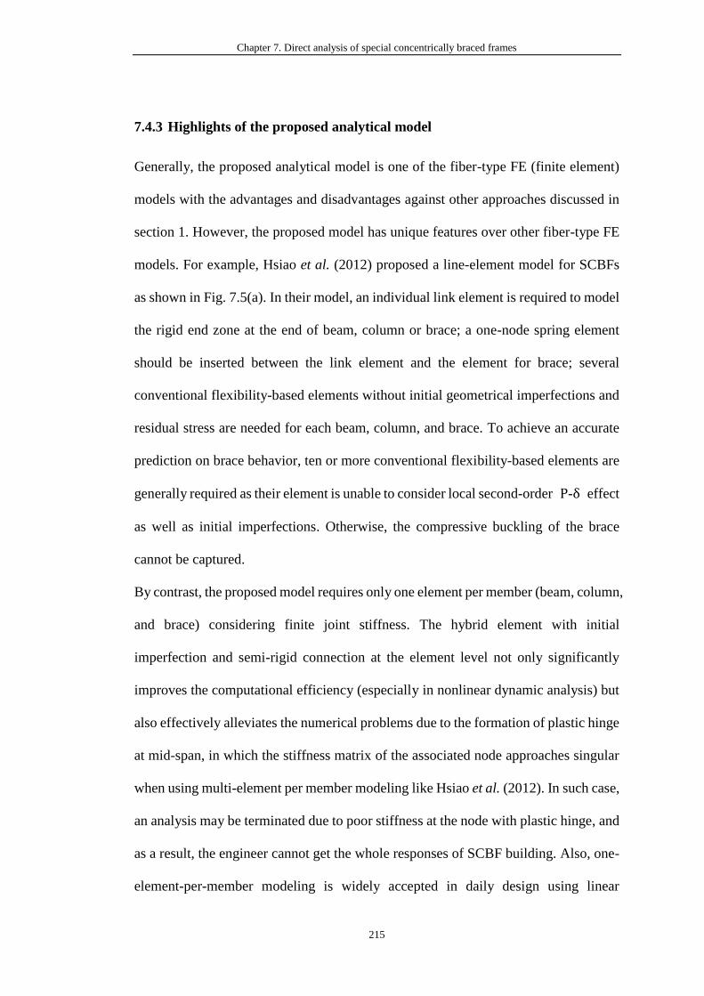
Chapter 7. Direct analysis of special concentrically braced frames
215
7.4.3 Highlights of the proposed analytical model
Generally, the proposed analytical model is one of the fiber-type FE (finite element)
models with the advantages and disadvantages against other approaches discussed in
section 1. However, the proposed model has unique features over other fiber-type FE
models. For example, Hsiao et al. (2012) proposed a line-element model for SCBFs
as shown in Fig. 7.5(a). In their model, an individual link element is required to model
the rigid end zone at the end of beam, column or brace; a one-node spring element
should be inserted between the link element and the element for brace; several
conventional flexibility-based elements without initial geometrical imperfections and
residual stress are needed for each beam, column, and brace. To achieve an accurate
prediction on brace behavior, ten or more conventional flexibility-based elements are
generally required as their element is unable to consider local second-order P-δ effect
as well as initial imperfections. Otherwise, the compressive buckling of the brace
cannot be captured.
By contrast, the proposed model requires only one element per member (beam, column,
and brace) considering finite joint stiffness. The hybrid element with initial
imperfection and semi-rigid connection at the element level not only significantly
improves the computational efficiency (especially in nonlinear dynamic analysis) but
also effectively alleviates the numerical problems due to the formation of plastic hinge
at mid-span, in which the stiffness matrix of the associated node approaches singular
when using multi-element per member modeling like Hsiao et al. (2012). In such case,
an analysis may be terminated due to poor stiffness at the node with plastic hinge, and
as a result, the engineer cannot get the whole responses of SCBF building. Also, one-
element-per-member modeling is widely accepted in daily design using linear
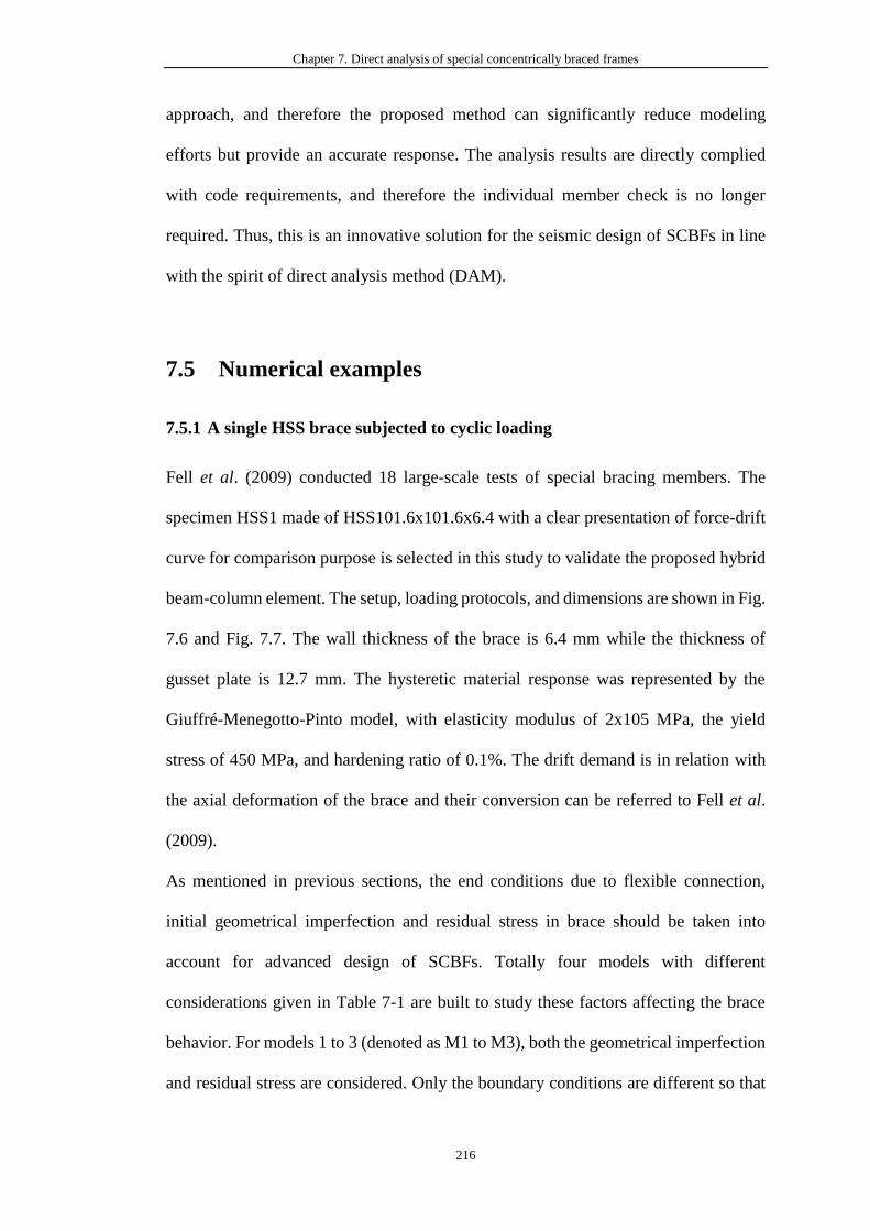
Chapter 7. Direct analysis of special concentrically braced frames
216
approach, and therefore the proposed method can significantly reduce modeling
efforts but provide an accurate response. The analysis results are directly complied
with code requirements, and therefore the individual member check is no longer
required. Thus, this is an innovative solution for the seismic design of SCBFs in line
with the spirit of direct analysis method (DAM).
7.5 Numerical examples
7.5.1 A single HSS brace subjected to cyclic loading
Fell et al. (2009) conducted 18 large-scale tests of special bracing members. The
specimen HSS1 made of HSS101.6x101.6x6.4 with a clear presentation of force-drift
curve for comparison purpose is selected in this study to validate the proposed hybrid
beam-column element. The setup, loading protocols, and dimensions are shown in Fig.
7.6 and Fig. 7.7. The wall thickness of the brace is 6.4 mm while the thickness of
gusset plate is 12.7 mm. The hysteretic material response was represented by the
Giuffré-Menegotto-Pinto model, with elasticity modulus of 2x10⁵ MPa, the yield
stress of 450 MPa, and hardening ratio of 0.1%. The drift demand is in relation with
the axial deformation of the brace and their conversion can be referred to Fell et al.
(2009).
As mentioned in previous sections, the end conditions due to flexible connection,
initial geometrical imperfection and residual stress in brace should be taken into
account for advanced design of SCBFs. Totally four models with different
considerations given in Table 7-1 are built to study these factors affecting the brace
behavior. For models 1 to 3 (denoted as M1 to M3), both the geometrical imperfection
and residual stress are considered. Only the boundary conditions are different so that
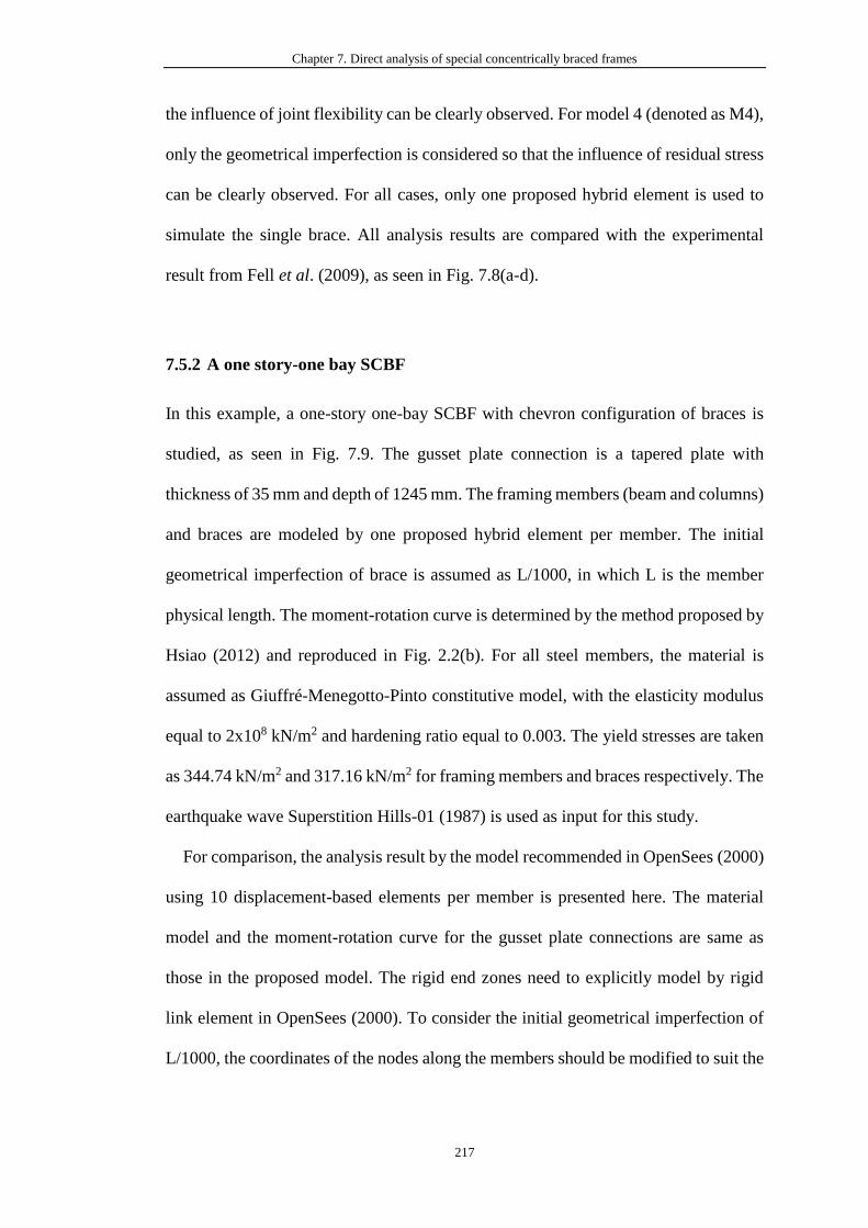
Chapter 7. Direct analysis of special concentrically braced frames
217
the influence of joint flexibility can be clearly observed. For model 4 (denoted as M4),
only the geometrical imperfection is considered so that the influence of residual stress
can be clearly observed. For all cases, only one proposed hybrid element is used to
simulate the single brace. All analysis results are compared with the experimental
result from Fell et al. (2009), as seen in Fig. 7.8(a-d).
7.5.2 A one story-one bay SCBF
In this example, a one-story one-bay SCBF with chevron configuration of braces is
studied, as seen in Fig. 7.9. The gusset plate connection is a tapered plate with
thickness of 35 mm and depth of 1245 mm. The framing members (beam and columns)
and braces are modeled by one proposed hybrid element per member. The initial
geometrical imperfection of brace is assumed as L/1000, in which L is the member
physical length. The moment-rotation curve is determined by the method proposed by
Hsiao (2012) and reproduced in Fig. 2.2(b). For all steel members, the material is
assumed as Giuffré-Menegotto-Pinto constitutive model, with the elasticity modulus
equal to 2x10⁸ kN/m2 and hardening ratio equal to 0.003. The yield stresses are taken
as 344.74 kN/m2 and 317.16 kN/m2 for framing members and braces respectively. The
earthquake wave Superstition Hills-01 (1987) is used as input for this study.
For comparison, the analysis result by the model recommended in OpenSees (2000)
using 10 displacement-based elements per member is presented here. The material
model and the moment-rotation curve for the gusset plate connections are same as
those in the proposed model. The rigid end zones need to explicitly model by rigid
link element in OpenSees (2000). To consider the initial geometrical imperfection of
L/1000, the coordinates of the nodes along the members should be modified to suit the
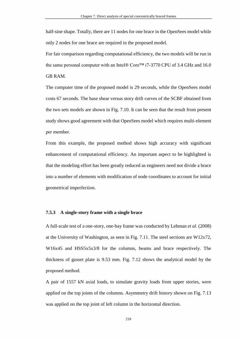
Chapter 7. Direct analysis of special concentrically braced frames
218
half-sine shape. Totally, there are 11 nodes for one brace in the OpenSees model while
only 2 nodes for one brace are required in the proposed model.
For fair comparison regarding computational efficiency, the two models will be run in
the same personal computer with an Intel® Core™ i7-3770 CPU of 3.4 GHz and 16.0
GB RAM.
The computer time of the proposed model is 29 seconds, while the OpenSees model
costs 67 seconds. The base shear versus story drift curves of the SCBF obtained from
the two sets models are shown in Fig. 7.10. It can be seen that the result from present
study shows good agreement with that OpenSees model which requires multi-element
per member.
From this example, the proposed method shows high accuracy with significant
enhancement of computational efficiency. An important aspect to be highlighted is
that the modeling effort has been greatly reduced as engineers need not divide a brace
into a number of elements with modification of node coordinates to account for initial
geometrical imperfection.
7.5.3 A single-story frame with a single brace
A full-scale test of a one-story, one-bay frame was conducted by Lehman et al. (2008)
at the University of Washington, as seen in Fig. 7.11. The steel sections are W12x72,
W16x45 and HSS5x5x3/8 for the columns, beams and brace respectively. The
thickness of gusset plate is 9.53 mm. Fig. 7.12 shows the analytical model by the
proposed method.
A pair of 1557 kN axial loads, to simulate gravity loads from upper stories, were
applied on the top joints of the columns. Asymmetry drift history shown on Fig. 7.13
was applied on the top joint of left column in the horizontal direction.
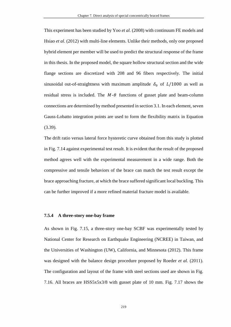
Chapter 7. Direct analysis of special concentrically braced frames
219
This experiment has been studied by Yoo et al. (2008) with continuum FE models and
Hsiao et al. (2012) with multi-line elements. Unlike their methods, only one proposed
hybrid element per member will be used to predict the structural response of the frame
in this thesis. In the proposed model, the square hollow structural section and the wide
flange sections are discretized with 208 and 96 fibers respectively. The initial
sinusoidal out-of-straightness with maximum amplitude 𝛿0 of 𝐿/1000 as well as
residual stress is included. The 𝑀-𝜃 functions of gusset plate and beam-column
connections are determined by method presented in section 3.1. In each element, seven
Gauss-Lobatto integration points are used to form the flexibility matrix in Equation
(3.39).
The drift ratio versus lateral force hysteretic curve obtained from this study is plotted
in Fig. 7.14 against experimental test result. It is evident that the result of the proposed
method agrees well with the experimental measurement in a wide range. Both the
compressive and tensile behaviors of the brace can match the test result except the
brace approaching fracture, at which the brace suffered significant local buckling. This
can be further improved if a more refined material fracture model is available.
7.5.4 A three-story one-bay frame
As shown in Fig. 7.15, a three-story one-bay SCBF was experimentally tested by
National Center for Research on Earthquake Engineering (NCREE) in Taiwan, and
the Universities of Washington (UW), California, and Minnesota (2012). This frame
was designed with the balance design procedure proposed by Roeder et al. (2011).
The configuration and layout of the frame with steel sections used are shown in Fig.
7.16. All braces are HSS5x5x3/8 with gusset plate of 10 mm. Fig. 7.17 shows the
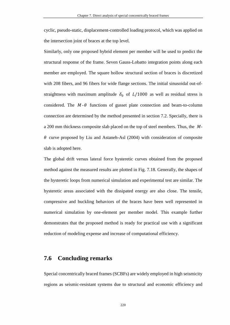
Chapter 7. Direct analysis of special concentrically braced frames
220
cyclic, pseudo-static, displacement-controlled loading protocol, which was applied on
the intersection joint of braces at the top level.
Similarly, only one proposed hybrid element per member will be used to predict the
structural response of the frame. Seven Gauss-Lobatto integration points along each
member are employed. The square hollow structural section of braces is discretized
with 208 fibers, and 96 fibers for wide flange sections. The initial sinusoidal out-of-
straightness with maximum amplitude 𝛿0 of 𝐿/1000 as well as residual stress is
considered. The 𝑀 -𝜃 functions of gusset plate connection and beam-to-column
connection are determined by the method presented in section 7.2. Specially, there is
a 200 mm thickness composite slab placed on the top of steel members. Thus, the 𝑀-
𝜃 curve proposed by Liu and Astaneh-Asl (2004) with consideration of composite
slab is adopted here.
The global drift versus lateral force hysteretic curves obtained from the proposed
method against the measured results are plotted in Fig. 7.18. Generally, the shapes of
the hysteretic loops from numerical simulation and experimental test are similar. The
hysteretic areas associated with the dissipated energy are also close. The tensile,
compressive and buckling behaviors of the braces have been well represented in
numerical simulation by one-element per member model. This example further
demonstrates that the proposed method is ready for practical use with a significant
reduction of modeling expense and increase of computational efficiency.
7.6 Concluding remarks
Special concentrically braced frames (SCBFs) are widely employed in high seismicity
regions as seismic-resistant systems due to structural and economic efficiency and

Chapter 7. Direct analysis of special concentrically braced frames
221
particularly high ductility for energy dissipation. The steel braces are the key members
to absorb energy through tensile yield, compressive buckling, post-buckling and
fracture behavior. As the braces exhibit highly nonlinear behavior, the precious
modeling methods are generally required several elements to simulate a brace with
initial curvature. Also, the influence of residual stress on the structural performance
of SCBFs has been largely overlooked. Thus, a practical and innovative analytical
model is proposed in this thesis for the performance-based seismic design of SCBFs.
This new solution provides an accurate prediction with a significant saving of
computer time, and therefore it will be extremely helpful for daily design by nonlinear
dynamic analysis. The examples verified by experimental test results show the
accuracy, efficiency, and validity of the proposed method.
In summary, there are five novel aspects of the proposed model as follows:
(1) The initial geometrical imperfection and residual stress are explicitly considered
at the element level.
(2) The joint flexibility effect as well as the rigid end zone duo to gusset plate
connection is explicitly considered at the element level.
(3) The distributed plasticity with consideration of fatigue fracture allowing for
hysteretic behavior has been included in the proposed model.
(4) One-element-per-member modeling is adequate, and therefore it can significantly
reduce the computational cost.
(5) This thesis extends the direct analysis method (DAM) which is well specified in
the modern design codes such as AISC360 (2016), Eurocode-3 (2005) and
COPHK (2011) from nonlinear static analysis to dynamic analysis. Thus, a
consistent method linking the static and dynamic design together is provided for
practical engineering use to achieve a safer and economic design.
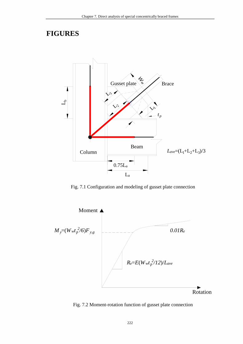
Chapter 7. Direct analysis of special concentrically braced frames
222
FIGURES
Fig. 7.1 Configuration and modeling of gusset plate connection
Fig. 7.2 Moment-rotation function of gusset plate connection
L 1L 2
L 3
Ww
tp
BeamColumn
BraceGusset plate
Lave=(L1+L2+L3)/3
La
0.75La
Lb
Rotation
Moment
0.01ReM y=(Wwtp2/6)F y,g
Re=E(Wwtp2/12)/Lave
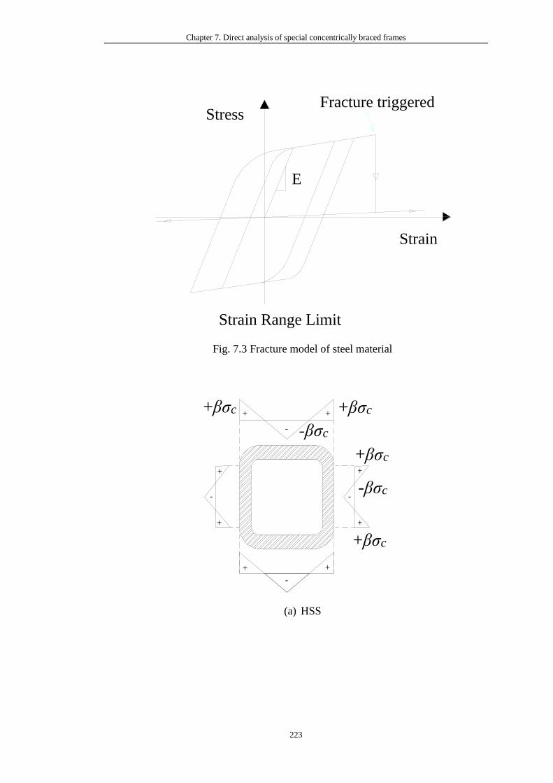
Chapter 7. Direct analysis of special concentrically braced frames
223
Fig. 7.3 Fracture model of steel material
(a) HSS
Fracture triggered
Strain Range Limit
Strain
Stress
E
-ασy
+ασy
-ασy
+ασy
-ασy
+ασyb
h
tw
For hb ≥ 1.2, α = 0.5
For hb > 1.2, α = 0.3
+βσc
+βσc
+βσc+βσc
-βσc
-βσc-
-
+
+
++
+
+
-
-
t f
+
+
-
-
-
+
+
+
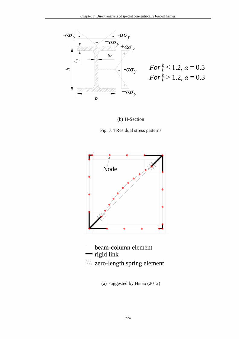
Chapter 7. Direct analysis of special concentrically braced frames
224
(b) H-Section
Fig. 7.4 Residual stress patterns
(a) suggested by Hsiao (2012)
-ασy
+ασy
-ασy
+ασy
-ασy
+ασyb
h
tw
For hb ≤ 1.2, α = 0.5
For hb > 1.2, α = 0.3
+βσc
+βσc
+βσc+βσc
-βσc
-βσc-
-
+
+
++
+
+
-
-
t f
+
+
-
-
-
+
+
+
beam-column elementrigid link
zero-length spring element
zero-length end spring
proposed hybrid element for brace
rigid end zone
Ll Lr
initial geometrical imperfection
Node Node
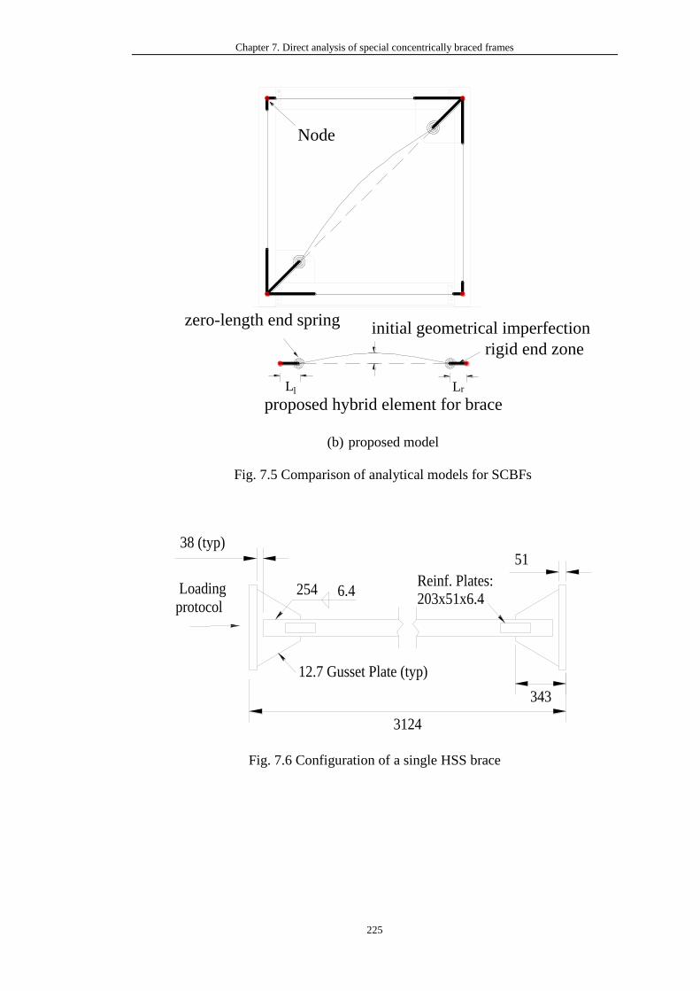
Chapter 7. Direct analysis of special concentrically braced frames
225
(b) proposed model
Fig. 7.5 Comparison of analytical models for SCBFs
Fig. 7.6 Configuration of a single HSS brace
beam-column elementrigid link
zero-length spring element
zero-length end spring
proposed hybrid element for brace
rigid end zone
Ll Lr
initial geometrical imperfection
Node Node
Loading
protocol
51
343
12.7 Gusset Plate (typ)
38 (typ)
254 6.4Reinf. Plates:203x51x6.4
3124
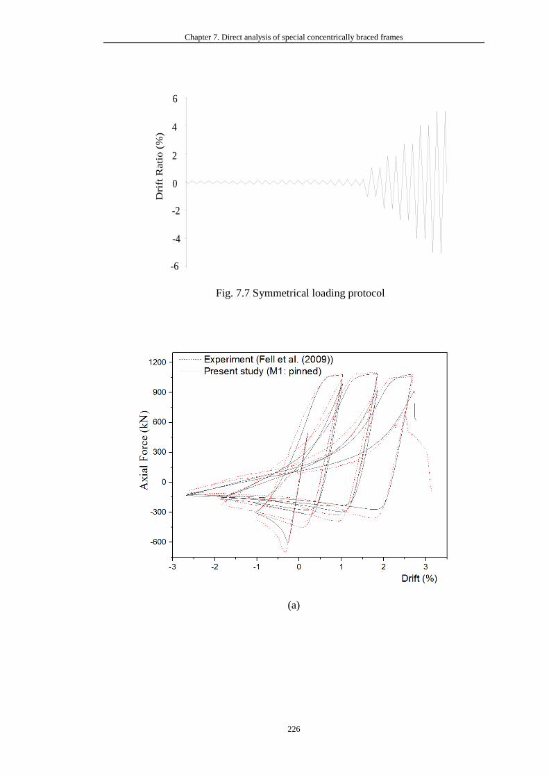
Chapter 7. Direct analysis of special concentrically braced frames
226
Fig. 7.7 Symmetrical loading protocol
(a)
Dri
ft R
ati
o (
%)
6
4
2
0
-2
-4
-6
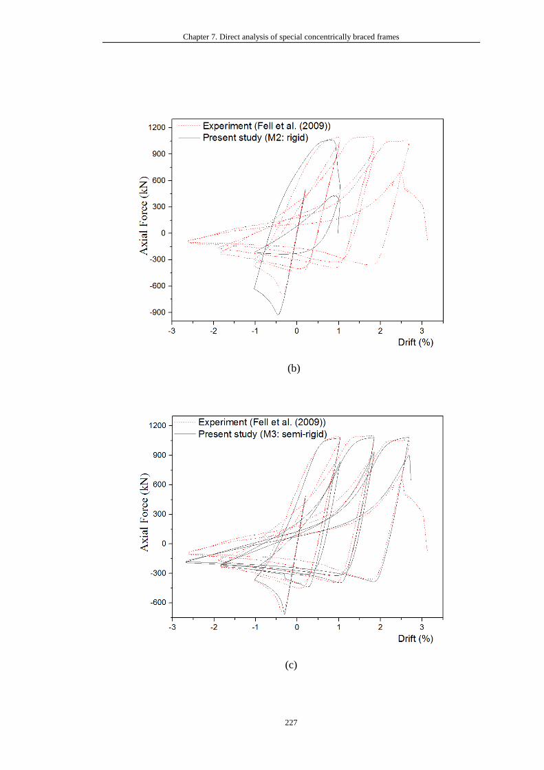
Chapter 7. Direct analysis of special concentrically braced frames
227
(b)
(c)
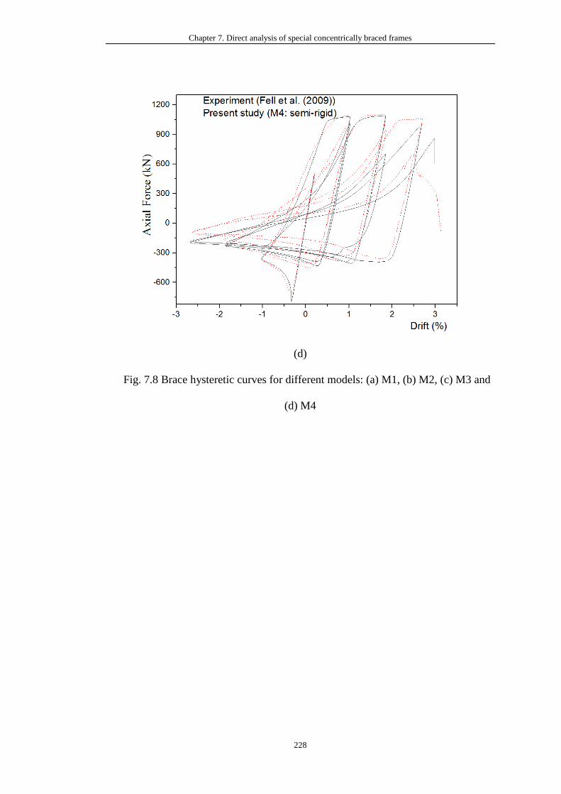
Chapter 7. Direct analysis of special concentrically braced frames
228
(d)
Fig. 7.8 Brace hysteretic curves for different models: (a) M1, (b) M2, (c) M3 and
(d) M4
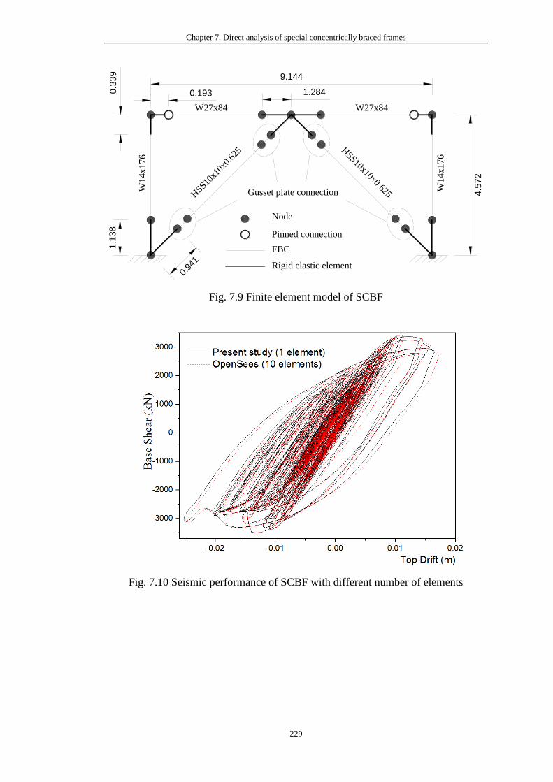
Chapter 7. Direct analysis of special concentrically braced frames
229
Fig. 7.9 Finite element model of SCBF
Fig. 7.10 Seismic performance of SCBF with different number of elements
W27x84
W14x176
HSS10
x10x
0.62
5 HSS10x10x0.625Gusset plate connection W
14x176
Node
Pinned connection
FBC
Rigid elastic element
9.144
1.1
38
0.3
39
0.94
1
1.2840.193
W27x84
4.5
72
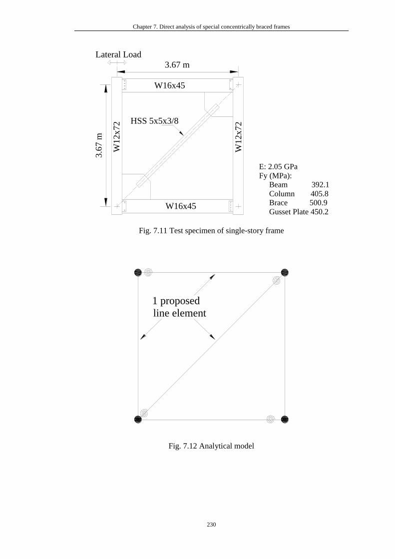
Chapter 7. Direct analysis of special concentrically braced frames
230
Fig. 7.11 Test specimen of single-story frame
Fig. 7.12 Analytical model
3.6
7 m
3.67 m
W16x45
W16x45
W12x72
W12x72 HSS 5x5x3/8
E: 2.05 GPa
Fy (MPa): Beam 392.1
Column 405.8 Brace 500.9
Gusset Plate 450.2
1 proposed
line element
Lateral Load
Dri
ft R
atio
(%
)
3
2
1
0
-1
-2
-3
3.6
7 m
3.67 m
W16x45
W16x45
W1
2x
72
W1
2x
72 HSS 5x5x3/8
E: 2.05 GPa
Fy (MPa): Beam 392.1
Column 405.8 Brace 500.9
Gusset Plate 450.2
1 proposed
line element
Lateral Load
Dri
ft R
atio
(%
)
3
2
1
0
-1
-2
-3
3.6
7 m
3.67 m
W16x45
W16x45
W1
2x
72
W1
2x
72 HSS 5x5x3/8
E: 2.05 GPa
Fy (MPa): Beam 392.1
Column 405.8 Brace 500.9
Gusset Plate 450.2
1 proposed
line element
Lateral Load
Dri
ft R
atio
(%
)
3
2
1
0
-1
-2
-3
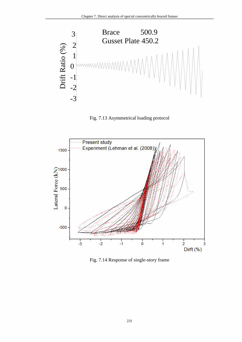
Chapter 7. Direct analysis of special concentrically braced frames
231
Fig. 7.13 Asymmetrical loading protocol
Fig. 7.14 Response of single-story frame
3.6
7 m
3.67 m
W16x45
W16x45
W1
2x72
W12
x72 HSS 5x5x3/8
E: 2.05 GPa
Fy (MPa): Beam 392.1
Column 405.8 Brace 500.9
Gusset Plate 450.2
1 proposed
line element
Lateral Load
Dri
ft R
atio
(%
)
3
2
1
0
-1
-2
-3
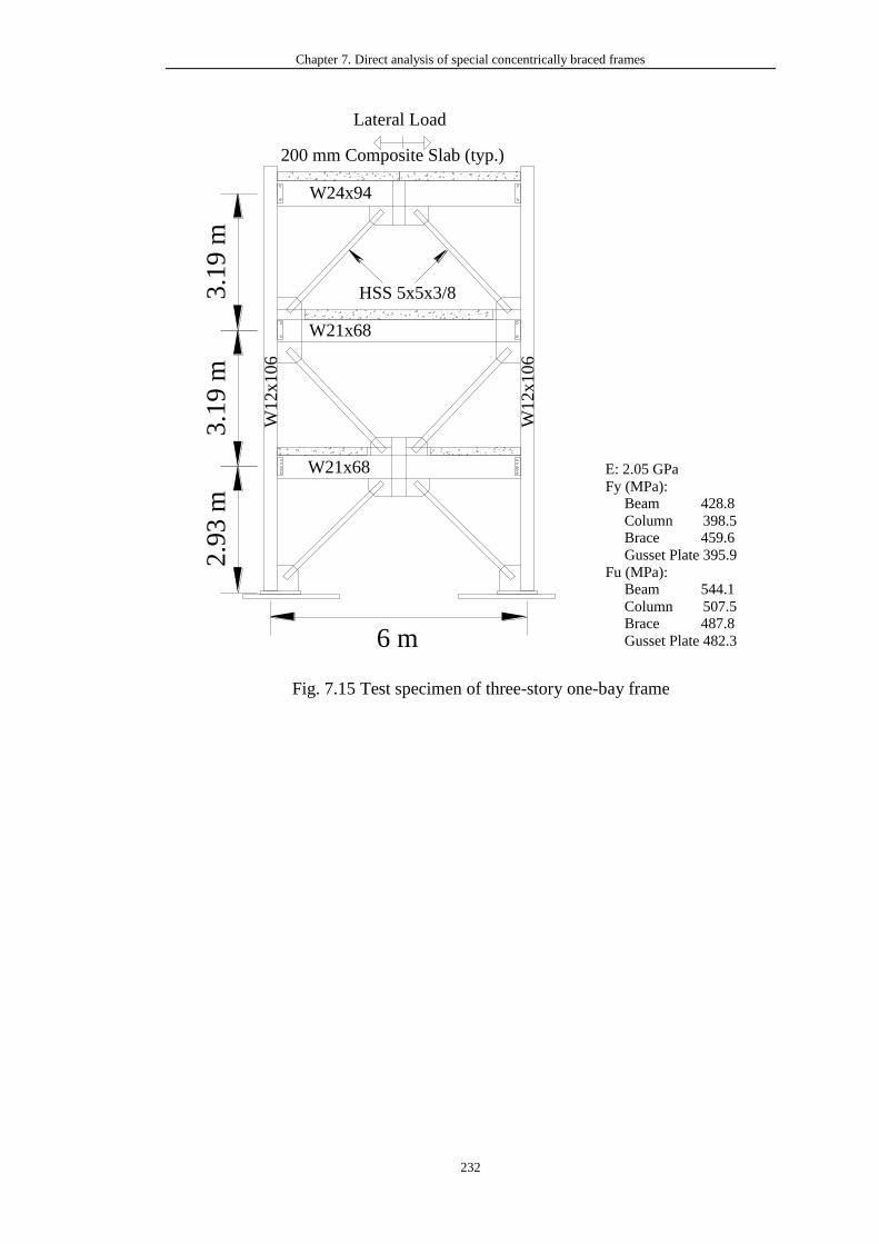
Chapter 7. Direct analysis of special concentrically braced frames
232
Fig. 7.15 Test specimen of three-story one-bay frame
1 3 5 7 9 11 13 15 17 19 -2
-1
0
1
2
Cycle
Dri
ft r
atio
(%
)
W24x94
W21x68
W21x68
HSS 5x5x3/8
2.9
3 m
3.1
9 m
3.1
9 m
6 m
200 mm Composite Slab (typ.)
W1
2x
106
W1
2x
106
E: 2.05 GPa
Fy (MPa): Beam 428.8
Column 398.5 Brace 459.6
Gusset Plate 395.9
Fu (MPa): Beam 544.1
Column 507.5 Brace 487.8
Gusset Plate 482.3
1 proposed
line element
Lateral Load
Lateral Load
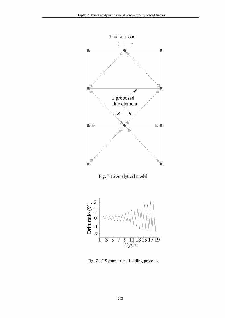
Chapter 7. Direct analysis of special concentrically braced frames
233
Fig. 7.16 Analytical model
Fig. 7.17 Symmetrical loading protocol
1 3 5 7 9 11 13 15 17 19 -2
-1
0
1
2
Cycle
Dri
ft r
atio
(%
)
W24x94
W21x68
W21x68
HSS 5x5x3/8
2.9
3 m
3.1
9 m
3.1
9 m
6 m
200 mm Composite Slab (typ.)
W1
2x
106
W1
2x
106
E: 2.05 GPa
Fy (MPa): Beam 428.8
Column 398.5 Brace 459.6
Gusset Plate 395.9
Fu (MPa): Beam 544.1
Column 507.5 Brace 487.8
Gusset Plate 482.3
1 proposed
line element
Lateral Load
Lateral Load
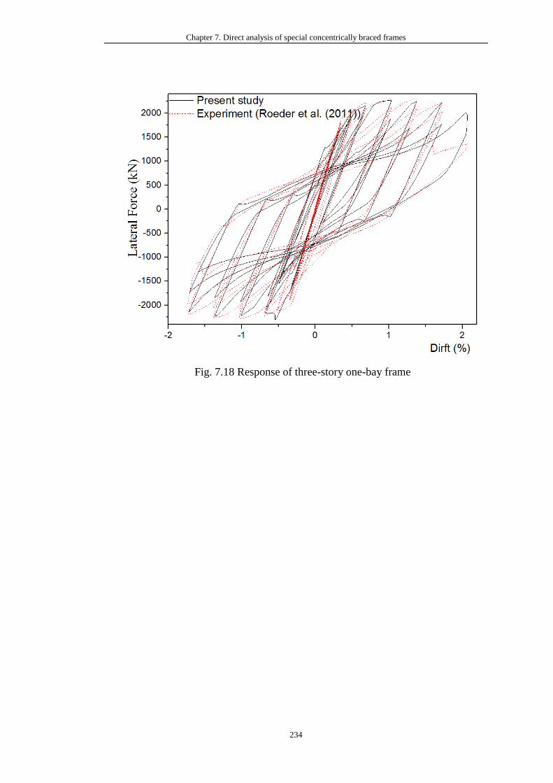
Chapter 7. Direct analysis of special concentrically braced frames
234
Fig. 7.18 Response of three-story one-bay frame
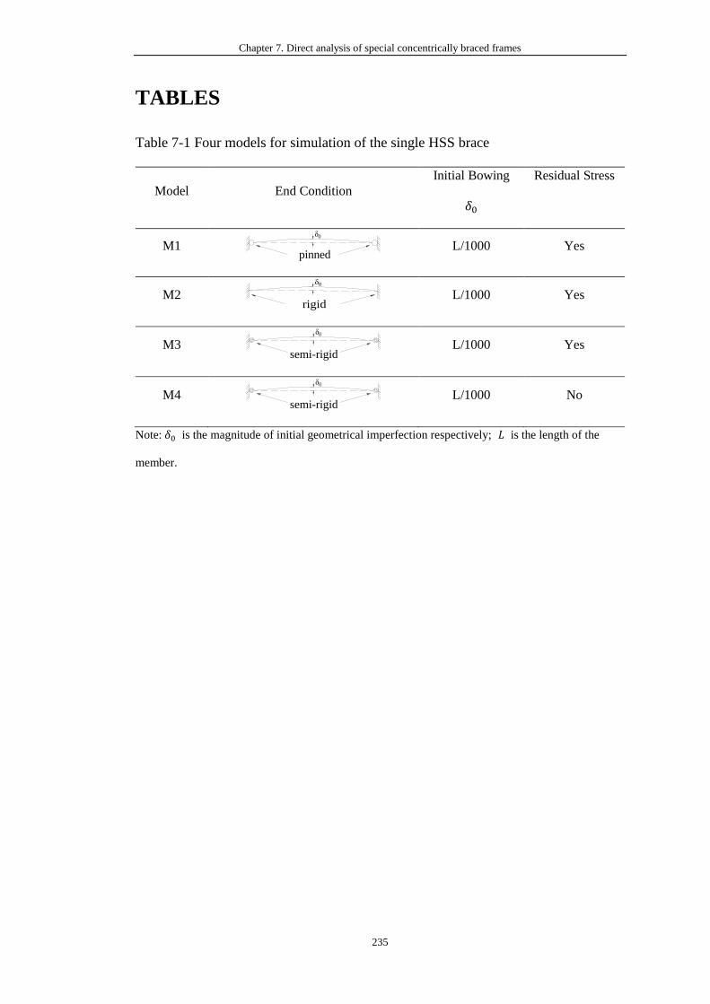
Chapter 7. Direct analysis of special concentrically braced frames
235
TABLES
Table 7-1 Four models for simulation of the single HSS brace
Model End Condition
Initial Bowing
𝛿0
Residual Stress
M1
L/1000 Yes
M2
L/1000 Yes
M3
L/1000 Yes
M4
L/1000 No
Note: 𝛿0 is the magnitude of initial geometrical imperfection respectively; 𝐿 is the length of the
member.
pinned
δ0
rigid
δ0
semi-rigid
δ0
semi-rigid
δ0
Chapter 8. Summary and future work
236
CHAPTER 8. SUMMARY AND FUTURE WORK
In this chapter, the main findings of this research project will be summarized, and the
future work is also presented.
8.1 Summary
In this thesis, a new flexibility-based beam-column element allowing for member
imperfections, semi-rigid connections, rigid end zone and end offsets, and distributed
plasticity is proposed for the second-order direct analysis of frame structures under static
and dynamic loads. The work that incorporates member initial bowing into the flexibility-
based element has not been done before. The plastic zone method in conjunction with the
fiber section approach is adopted in the proposed flexibility-based element to conduct
second-order inelastic analysis. The geometrical initial imperfection is formulated in the
element stiffness matrix while the residual stress is considered by fiber section, and as a
result, the inelastic behavior of steel structures can be well predicted in accordance with
design codes. As the second-order direct analysis requires the consideration of material
yielding and initial imperfections, this new element provides a practical solution for
engineering applications with higher computational efficiency and better numerical
convergence than the conventional methods. Meanwhile, the section constitutive model
derived from the section yield function can replace the section integration using the fiber
section approach to represent the relationships between the internal forces and
deformations. This technique will significantly enhance the computational efficiency of
Chapter 8. Summary and future work
237
both static and dynamic nonlinear analysis considering material yielding. Generally
speaking, the proposed method can predict the actual behaviors of frame structures using
one element per member. Finally, the proposed method is applied to design of frame
structures with noncompact and slender CFT members under static loads and special
concentrically braced frames (SCBFs) subjected to dynamic loads.
The main findings and contributions of this study are summarized as follows:
(1) The proposed flexibility-based beam-column element can consider member initial
imperfections explicitly. Meanwhile, it inherits the advantages of flexibility-based
elements, having high accuracy and being powerful in the inelastic analysis. The
geometrical and material nonlinearities of frame structures under static and dynamic
loads can be well considered. For geometrical nonlinearity, the 𝑃 -𝛿 effect is
incorporated into the proposed method at the element level while the 𝑃-∆ effect is
accounted for by corotational technology. In terms of material nonlinearity, the
distributed plasticity method is adopted to capture the plastic behavior. The fiber
section approach also makes it possible to directly consider the influence of residual
stress. These futures make the proposed element able to simulate one member by one
element. Therefore, it significantly reduces the engineers’ modeling workload as well
as the computational time of static and dynamic nonlinear analysis.
(2) A section constitutive model derived from the section yield function can replace the
section integration using the fiber section approach to represent the relationships
between the internal forces and deformations. This technique will further reduce
computer time and resource with same accuracy as fiber section method and therefore
it is ready for static and dynamic nonlinear analysis.
Chapter 8. Summary and future work
238
(3) Two zero-length springs are attached at the ends of the proposed element to account
for joint flexibility required in direct analysis if the joint is not ideally pinned or fully
rigid. The coupling effect of axial force and bending moments, which has been
ignored by other researchers, can be taken into consideration. This hybrid element is
able to capture the structural behaviour of a member with semi-rigid connections
under monotonic or cyclic loading. Thus, the proposed method is applicable for static
or dynamic nonlinear analysis of frame structures allowing semi-rigid connections.
(4) An innovative method in line with direct analysis and satisfying the provisions in
AISC360 (2016) is proposed for the design of noncompact and slender CFT members.
Using the effective stress-strain relationships of the steel tube and the concrete infill,
the proposed element with geometrical imperfections can well predict the complex
behaviors of noncompact and slender CFT members. This approach considers all
factors affecting member behaviors in the analysis process in accordance with code
requirements. Both the geometrical and material nonlinearities are reflected in the
second-order direct analysis. The effective stress-strain relationships implicitly
account for the complex behaviors of noncompact and slender CFT members, for
examples, local plate buckling, concrete confinement, material yielding. Furthermore,
the proposed element has high accuracy such that one CFT member can be modeled
by one proposed element. This method can be applied to direct analysis of compact,
noncompact and slender CFT member.
(5) The proposed element is extended to consider the effects of the rigid end zone and end
offsets at the element level to simplify the model. A practical and innovative
analytical model is proposed for the performance-based seismic design of special
Chapter 8. Summary and future work
239
concentrically braced frames (SCBFs). The gusset plate at the end of brace in SCBFs
is simulated by a semi-rigid connection with rigid end zone. The joint stiffness of the
beam-to-column connections can also be simulated by the proposed model. To this
end, the brace complex behaviors such as tensile yield, compressive buckling and
post-buckling during second-order dynamic analysis can be accurately captured by
one proposed element per brace. Using the fracture constitutive relations of steel
material, the proposed model can capture the fracture behavior of braces under cyclic
loading. This new solution provides accurate predictions with significant savings of
computational time, and therefore it will be extremely helpful for PBSD by dynamic
nonlinear analysis.
8.2 Future work
This study presents a high-performance flexibility-based beam-column element
considering many practical features for daily design. It is highly recommended for use in
direct analysis of frame structures subjected to static and dynamic loads. There are still
many detailed works on applying the direct analysis method to performance-based
seismic design. In the future, the following aspects are recommended so that the
innovative second-order direct analysis can be extended to routine seismic design.
(1) To adopt the yield surface, provided in design codes or generated by cross-sectional
analysis software, in the distributed fiber hinge method;
(2) To study the behavior of SCBFs by the proposed method with more experimental test
results;
(3) To introduce warping and shear deformation effects into the proposed element;

Chapter 8. Summary and future work
240
(4) To study the critical imperfection mode of frame structures under dynamic loads;
(5) To improve the computational efficiency by employing CPU + GPU heterogeneous
computing techniques and cloud techniques;
REFERENCES
241
REFERENCES
Abdalla, K., and Stavroulakis, G. (1995). "A Backpropagation Neural Network Model
for Semi‐rigid Steel Connections." Computer‐Aided Civil and Infrastructure
Engineering, 10(2), 77-87.
Ahmadizadeh, M., and Maalek, S. (2014). "An investigation of the effects of socket
joint flexibility in space structures." Journal of Constructional Steel Research,
102, 72-81.
AISC (2011). "Manual of steel construction load resistance factor design", 14th Edition,
AISC, Chicago, USA.
AISC341 (2016). "Seismic provisions for structural steel buildings", American Institute
of Steel Construction, AISC, Inc., 130 EAST RANDOLPH STREET, SUITE
2000, Chicago, Illinois, 60601-6204.
AISC360 (2010). "Specification for Structural Steel Buildings." American Institute of
Steel Construction, AISC, Inc., One East Wacker Driver, Suite 700, Chicago,
Illinois 60601-1802.
AISC360 (2016). "Specification for Structural Steel Buildings." American Institute of
Steel Construction, AISC, Inc., 130 EAST RANDOLPH, SUITE 2000, Chicago,
Illinois 60601-6204.
Alemdar, B. N. (2001). "Distributed plasticity analysis of steel building structural
systems." PhD Thesis, Department of Civil and Environmental Engineering,
Georgia Institute of Technology, Atlanta.
REFERENCES
242
Alemdar, B. N., and White, D. W. (2005). "Displacement, flexibility, and mixed beam–
column finite element formulations for distributed plasticity analysis." Journal
of structural engineering, 131(12), 1811-1819.
Aristizabal-Ochoa, J. D. (2000). "Second-order axial deflections of imperfect 3-D
beam-column." Journal of engineering mechanics, 126(11), 1201-1208.
Aristizabal-Ochoa, J. D. (2010). "Second-order slope–deflection equations for
imperfect beam–column structures with semi-rigid connections." Engineering
Structures, 32(8), 2440-2454.
Asgarian, B., Alanjari, P., and Aghaeidoost, V. (2015). "Three-dimensional joint
flexibility element for modeling of tubular offshore connections." Journal of
Marine Science and Technology, 20(4), 629-639.
Astroza, R., Ebrahimian, H., and Conte, J. P. (2014). "Material parameter identification
in distributed plasticity FE models of frame-type structures using nonlinear
stochastic filtering." Journal of Engineering Mechanics, 141(5), 04014149.
Auricchio, F., and Taylor, R. (1999). "A return-map algorithm for general associative
isotropic elasto-plastic materials in large deformation regimes." International
Journal of Plasticity, 15(12), 1359-1378.
Auricchio, F., and Taylor, R. L. (1994). "A generalized elastoplastic plate theory and
its algorithmic implementation." Int J Numer Meth Eng, 37(15), 2583-2608.
Auricchio, F., and Taylor, R. L. (1995). "Two material models for cyclic plasticity:
nonlinear kinematic hardening and generalized plasticity." International
Journal of Plasticity, 11(1), 65-98.
REFERENCES
243
Babazadeh, A., Burgueño, R., and Silva, P. F. (2016). "Evaluation of the critical plastic
region length in slender reinforced concrete bridge columns." Engineering
Structures, 125, 280-293.
Barsan, G. M., and Chiorean, C. G. (1999). "Computer program for large deflection
elasto-plastic analysis of semi-rigid steel frameworks." Computers & Structures,
72(6), 699-711.
Botez, M. D., Bredean, L. A., and Ioani, A. M. (2014). "Plastic hinge vs. distributed
plasticity in the progressive collapse analysis." Acta Technica Napocensis: Civil
Engineering & Architecture, 57(1), 24-36.
Chan, S. L. (1988). "Geometric and material non-linear analysis of beam-columns and
frames using the minimum residual displacement method." John Wiley & Sons,
Ltd, 2657-2669.
Chan, S. L., and Chui, P. T. (2000). Non-linear static and cyclic analysis of steel frames
with semi-rigid connections, Elsevier.
Chan, S. L., and Gu, J. X. (2000). "Exact tangent stiffness for imperfect beam-column
members." J Struct Eng-Asce, 126(9), 1094-1102.
Chan, S. L., and Zhou, Z. H. (1994). "Pointwise equilibrating polynomial element for
nonlinear analysis of frames." Journal of Structural Engineering, 120(6), 1703-
1717.
Chan, S. L., and Zhou, Z. H. (1995). "2Nd-Order Elastic Analysis of Frames Using
Single Imperfect Element Per Member." J Struct Eng-Asce, 121(6), 939-945.
REFERENCES
244
Chen, W.-F., and Kishi, N. (1987). Moment-rotation Relation of Top and Seat-angle
Connections.
Chen, W. F., and Chan, S. L. (1995). "2nd-order inelastic analysis of steel frames using
element with midspan and end springs." Journal of Structural Engineering,
121(3), 530-541.
Chen, W. F., and Sohal, I. (1995). "Plastic Design and Second-Order Analysis of Steel
Frames." Springer-Verlag New York Inc.
Chiorean, C. G. (2017). "Second-order flexibility-based model for nonlinear inelastic
analysis of 3D semi-rigid steel frameworks." Engineering Structures, 136, 547-
579.
Cho, S. H., and Chan, S. L. (2008). "Second-order analysis and design of angle trusses,
Part II: Plastic analysis and design." Engineering Structures, 30(3), 626-631.
COPHK (2011). "Code of Practice for the Structural Use of Steel 2011." Buildings
Department, Hong Kong SAR Government.
Csébfalvi, A. (2007). "Optimal design of frame structures with semi-rigid joints."
Periodica Polytechnica. Civil Engineering, 51(1), 9.
de_Souza, R. M. (2000). "Force-based finite element for large displacement inelastic
analysis of frames." PhD Thesis, Department of Civil and Environmental
Engineering, University of California, Berkeley.
Denavit, M. D. (2012). Characterization of behavior of steel-concrete composite
members and frames with applications for design, University of Illinois at
Urbana-Champaign.
REFERENCES
245
Denavit, M. D., Hajjar, J. F., Perea, T., and Leon, R. T. (2015). "Stability analysis and
design of composite structures." Journal of Structural Engineering, 142(3),
04015157.
Dides, M. A., and De la Llera, J. C. (2005). "A comparative study of concentrated
plasticity models in dynamic analysis of building structures." Earthq Eng
Struct D, 34(8), 1005-1026.
Ding, F.X., Zhang, T., Liu, X.M., Lu, Z.-H., Guo, Q., and Jiang, G.-s. (2017). "Behavior
of steel-reinforced concrete-filled square steel tubular stub columns under axial
loading." Thin-Walled Structures, 119, 737-748.
Du, Y., Chen, Z., Wang, Y.-B., and Liew, J. R. (2017). "Ultimate resistance behavior
of rectangular concrete-filled tubular beam-columns made of high-strength
steel." Journal of Constructional Steel Research, 133, 418-433.
Du, Z.-L., Liu, Y.-P., and Chan, S.-L. (2017). "A second-order flexibility-based beam-
column element with member imperfection." Engineering Structures, 143, 410-
426.
Ekhande, S. G., Selvappalam, M., and Madugula, M. K. (1989). "Stability functions for
three-dimensional beam-columns." Journal of Structural Engineering, 115(2),
467-479.
El-Tawil, S., and Deierlein, G. G. (1998). "Stress-resultant plasticity for frame
structures." Journal of engineering mechanics, 124(12), 1360-1370.
El-Tawil, S., and Deierlein, G. G. (2001). "Nonlinear analysis of mixed steel-concrete
frames. I: Element formulation." J Struct Eng-Asce, 127(6), 647-655.
REFERENCES
246
Eurocode3 (2005). "EN 1993-1-1: Design of steel structures - General rules and rules
for buildings." European Committee for Standardization.
Faella, C., Piluso, V., and Rizzano, G. (1997). "A new method to design extended end
plate connections and semirigid braced frames." Journal of Constructional Steel
Research, 41(1), 61-91.
Fell, B. V., Kanvinde, A. M., Deierlein, G. G., and Myers, A. T. (2009). "Experimental
Investigation of Inelastic Cyclic Buckling and Fracture of Steel Braces." J Struct
Eng-Asce, 135(1), 19-32.
FEMA-356 (2000). "Commentary for the Seismic Rehabilitation of Buildings."
Federal Emergency Management Agency, Washington, DC.
Ferreira, M., Providência, P., Gala, P., and Almeida, J. (2017). "Improved displacement
based alternative to force based finite element for nonlinear analysis of framed
structures." Engineering Structures, 135, 95-103.
Filippou, F. C., Bertero, V. V., and Popov, E. P. (1983). "Effects of bond deterioration
on hysteretic behavior of reinforced concrete joints."
Fong, M., Chan, S. L., and Uy, B. (2011). "Advanced design for trusses of steel and
concrete-filled tubular sections." Engineering Structures, 33(12), 3162-3171.
Fong, M., Cho, S. H., and Chan, S. L. (2009). "Design of angle trusses by codes and
second-order analysis with experimental verification." Journal of
Constructional Steel Research, 65(12), 2140-2147.
Frye, M. J., and Morris, G. A. (1975). "Analysis of flexibly connected steel frames."
Canadian journal of civil engineering, 2(3), 280-291.
REFERENCES
247
Güneyisi, E. M., D'Aniello, M., Landolfo, R., and Mermerdaş, K. (2014). "Prediction
of the flexural overstrength factor for steel beams using artificial neural
network." Steel and Composite Structures, 17(3), 215-236.
Goto, Y., and Chen, W. F. (1987). "Second-order elastic analysis for frame design."
Journal of Structural Engineering, 113(7), 1501-1519.
Gourley, B. C., Tort, C., Denavit, M. D., Schiller, P. H., and Hajjar, J. F. (2008). "A
synopsis of studies of the monotonic and cyclic behavior of concrete-filled steel
tube members, connections, and frames." Newmark Structural Engineering
Laboratory. University of Illinois at Urbana-Champaign.
Gunnarsson, I. R. (2004). "Numerical performance evaluation of braced frame
systems." University of Washington.
Haddad, M., and Tremblay, R. "Influence of connection design on the inelastic seismic
response of HSS steel bracing members." Proc., TUBULAR STRUCTURES-
INTERNATIONAL SYMPOSIUM-, 639.
Hajjar, J., Gourley, B., Tort, C., Denavit, M., and Schiller, P. (2013). "Steel-concrete
composite structural systems." Dept. of Civil and Environmental Engineering,
Northeastern Univ., Boston.
Hajjar, J. F., Molodan, A., and Schiller, P. H. (1998). "A distributed plasticity model
for cyclic analysis of concrete-filled steel tube beam-columns and composite
frames." Engineering Structures, 20(4-6), 398-412.
REFERENCES
248
Han, L.-H., Yao, G.-H., and Zhao, X.-L. (2005). "Tests and calculations for hollow
structural steel (HSS) stub columns filled with self-consolidating concrete
(SCC)." Journal of Constructional Steel Research, 61(9), 1241-1269.
Han, S.W., Kim, W. T., and Foutch, D. A. (2007). "Seismic behavior of hss bracing
members according to width–thickness ratio under symmetric cyclic loading."
Journal of Structural Engineering, 133(2), 264-273.
Harrison, H. (1965). "The Application of the Principles of Plastic Analysis of Three
Dimensional Steel Structures." University of Sydney.
He, Z., Liu, W., Wang, X., and Ye, A. (2016). "Optimal Force-Based Beam-Column
Element Size for Reinforced-Concrete Piles in Bridges." Journal of Bridge
Engineering, 21(11), 06016006.
Hsiao, P. C. (2012). Seismic performance evaluation of concentrically braced frames,
University of Washington.
Hsiao, P.-C., Lehman, D. E., and Roeder, C. W. (2012). "Improved analytical model
for special concentrically braced frames." Journal of Constructional Steel
Research, 73, 80-94.
Hsiao, P. C., Lehman, D. E., and Roeder, C. W. (2012). "Improved analytical model
for special concentrically braced frames." Journal of Constructional Steel
Research, 73, 80-94.
Hsiao, P. C., Lehman, D. E., and Roeder, C. W. (2013). "A model to simulate special
concentrically braced frames beyond brace fracture." Earthq Eng Struct D,
42(2), 183-200.
REFERENCES
249
Hu, F., Shi, G., and Shi, Y. (2017). "Experimental study on seismic behavior of high
strength steel frames: Global response." Engineering Structures, 131, 163-179.
Ihaddoudène, A., Saidani, M., and Jaspart, J. (2017). "Mechanical model for
determining the critical load of plane frames with semi-rigid joints subjected to
static loads." Engineering Structures, 145, 109-117.
Institution, B. S. (2004). "Eurocode 4: Design of composite steel and concrete structures.
part 1-1: General rules and rules for buildings." BSI, London, BS EN 1994.
Iu, C., Bradford, M., and Chen, W. (2009). "Second-order inelastic analysis of
composite framed structures based on the refined plastic hinge method."
Engineering Structures, 31(3), 799-813.
Izzuddin, B. A. (1996). "Quartic formulation for elastic beam-columns subject to
thermal effects." Journal of Engineering Mechanics, 122(9), 861-871.
Jafari, V., Vahdani, S. H., and Rahimian, M. (2010). "Derivation of the consistent
flexibility matrix for geometrically nonlinear Timoshenko frame finite
element." Finite Elem Anal Des, 46(12), 1077-1085.
Javed, M. F., Sulong, N. R., Memon, S. A., Rehman, S. K. U., and Khan, N. B. (2017).
"FE modelling of the flexural behaviour of square and rectangular steel tubes
filled with normal and high strength concrete." Thin-Walled Structures, 119,
470-481.
Jiang, A.-y., Chen, J., and Jin, W.-l. (2013). "Experimental investigation and design of
thin-walled concrete-filled steel tubes subject to bending." Thin-Walled
Structures, 63, 44-50.
REFERENCES
250
Kang, C.-H., Oh, Y.-S., and Moon, T.-S. (2001). "Strength of Axially Loaded Concrete-
Filled Tubular Stub Column." Journal of Korean Society of Steel Construction,
13(3), 279-287.
Karamanci, E., and Lignos, D. G. (2014). "Computational Approach for Collapse
Assessment of Concentrically Braced Frames in Seismic Regions." Journal of
Structural Engineering, 140(8).
Kim, D. K. (2005). "A database for composite columns." Georgia Institute of
Technology.
Kim, S. E., Uang, C. M., Choi, S. H., and An, K. Y. (2006). "Practical advanced analysis
of steel frames considering lateral-torsional buckling." Thin-walled structures,
44(7), 709-720.
King, W. S., White, D. W., and Chen, W. F. (1992). "Second-order inelastic analysis
methods for steel-frame design." Journal of Structural Engineering, 118(2),
408-428.
Kishi, N., Chen, W., Matsuoka, K., and Nomachi, S. (1987). Moment-rotation relation
of top-and seat-angle with double web-angle connections, School of Civil
Engineering, Purdue University.
Kostic, S. M., Filippou, F. C., and Deretic-Stojanovic, B. (2016). "Generalized
plasticity model for inelastic RCFT column response." Computers & Structures,
168, 56-67.

REFERENCES
251
Kostic, S. M., Filippou, F. C., and Lee, C.-L. (2013). "An efficient beam-column
element for inelastic 3D frame analysis." Computational Methods in
Earthquake Engineering, Springer, 49-67.
Krishnan, S. (2010). "Modified Elastofiber Element for Steel Slender Column and
Brace Modeling." J Struct Eng-Asce, 136(11), 1350-1366.
Lai, Z., and Varma, A. H. (2015). "Noncompact and slender circular CFT members:
Experimental database, analysis, and design." Journal of Constructional Steel
Research, 106, 220-233.
Lai, Z., and Varma, A. H. (2016). "Effective stress-strain relationships for analysis of
noncompact and slender filled composite (CFT) members." Engineering
Structures, 124, 457-472.
Lai, Z., Varma, A. H., and Griffis, L. G. (2015). "Analysis and design of noncompact
and slender CFT beam-columns." Journal of Structural Engineering, 142(1),
04015097.
Lai, Z., Varma, A. H., and Zhang, K. (2014). "Noncompact and slender rectangular
CFT members: Experimental database, analysis, and design." Journal of
Constructional Steel Research, 101, 455-468.
Lam, D., Dai, X., Han, L.-H., Ren, Q.-X., and Li, W. (2012). "Behaviour of inclined,
tapered and STS square CFST stub columns subjected to axial load." Thin-
Walled Structures, 54, 94-105.
REFERENCES
252
Lee, C.-L., and Filippou, F. C. (2015). "Frame Element with Mixed Formulations for
Composite and RC Members with Bond Slip. I: Theory and Fixed-End
Rotation." Journal of Structural Engineering, 141(11), 04015039.
Lee S, G. S. (1987). "Seismic behavior of hollow and concrete-filled square tubular
bracing members." Research Report UMCE 87-11, Department of Civil
Engineering, University of Michigan, Ann Arbor, MI.
Lehman, D. E., Roeder, C. W., Herman, D., Johnson, S., and Kotulka, B. (2008).
"Improved seismic performance of gusset plate connections." J Struct Eng-Asce,
134(6), 890-901.
Liang, Q. Q. (2009). "Performance-based analysis of concrete-filled steel tubular
beam–columns, Part I: Theory and algorithms." Journal of Constructional Steel
Research, 65(2), 363-372.
Liew, J. R., and Xiong, D. (2009). "Effect of preload on the axial capacity of concrete-
filled composite columns." Journal of Constructional Steel Research, 65(3),
709-722.
Liew, J. Y. R., White, D. W., and Chen, W. F. (1993). "Second-Order Refined Plastic-
Hinge Analysis for Frame Design : Part 1 and 2." J Struct Eng-Asce, 119(11),
3196-3216.
Lightfoot, E., and Le Messurier, A. (1974). "Elastic analysis of frameworks with elastic
connections." Journal of the Structural Division, 100(Proc. Paper 10632).
Liu, J., and Astaneh-Asl, A. (2004). "Moment–rotation parameters for composite shear
tab connections." Journal of Structural Engineering, 130(9), 1371-1380.
REFERENCES
253
Liu, S.-W., Liu, Y.-P., and Chan, S.-L. (2014a). "Direct analysis by an arbitrarily-
located-plastic-hinge element—part 1: planar analysis." Journal of
Constructional Steel Research, 103, 303-315.
Liu, S.-W., Liu, Y.-P., and Chan, S.-L. (2014b). "Direct analysis by an arbitrarily-
located-plastic-hinge element—part 2: spatial analysis." Journal of
Constructional Steel Research, 103, 316-326.
Liu, S. W., Liu, Y. P., and Chan, S. L. (2010). "Pushover Analysis by One Element Per
Member for Performance-Based Seismic Design." Int J Struct Stab Dy, 10(1),
111-126.
Liu, S. W., Liu, Y. P., and Chan, S. L. (2012). "Advanced analysis of hybrid steel and
concrete frames Part 2: Refined plastic hinge and advanced analysis." Journal
of Constructional Steel Research, 70, 337-349.
Lowes, L. N., Mitra, N., and Altoontash, A. (2003). "A beam-column joint model for
simulating the earthquake response of reinforced concrete frames."
Lubliner, J., Taylor, R., and Auricchio, F. (1993). "A new model of generalized
plasticity and its numerical implementation." International Journal of Solids
and Structures, 30(22), 3171-3184.
Lumpkin, E. J., Hsiao, P.-C., Roeder, C. W., Lehman, D. E., Tsai, C.-Y., Wu, A.-C.,
Wei, C.-Y., and Tsai, K.-C. (2012). "Investigation of the seismic response of
three-story special concentrically braced frames." Journal of Constructional
Steel Research, 77, 131-144.
REFERENCES
254
Ma, K., and Richard Liew, J. (2004). "Nonlinear plastic hinge analysis of three-
dimensional steel frames in fire." Journal of Structural Engineering, 130(7),
981-990.
Mageirou, G. E., and Gantes, C. J. (2006). "Buckling strength of multi-story sway, non-
sway and partially-sway frames with semi-rigid connections." Journal of
Constructional Steel Research, 62(9), 893-905.
McKenna, F., Fenves, G., Filippou, F., and Mazzoni, S. (2009). "Open system for
earthquake engineering simulation (OpenSees), 2000." URL http://opensees.
berkeley. edu/wiki/index. php/Main_Page.
McKenna, F., Fenves, G., and Scott, M. (2000). "Open system for earthquake
engineering simulation." University of California, Berkeley, CA.
Nakahara, H., and Sakino, K. "Flexural behavior of concrete filled square steel tubular
beam-columns." Proc., 12th World Conference on Earthquake Engineering.
Neuenhofer, A., and Filippou, F. C. (1997). "Evaluation of nonlinear frame finite-
element models." J Struct Eng-Asce, 123(7), 958-966.
Neuenhofer, A., and Filippou, F. C. (1998). "Geometrically nonlinear flexibility-based
frame finite element." Journal of Structural Engineering, 124(6), 704-711.
NIDA (2018). "User's Manual, Nonlinear Integrated Design and Analysis." NIDA 10.0
HTML Online Documentation. (http://www.nidacse.com).
Nilforoushan, R. (1973). Seismic behavior of multistory K-braced frame structures,
University of Michigan, Depatment of Civil Engineering.
REFERENCES
255
Nishiyama, I. (2002). Summary of research on concrete-filled structural steel tube
column system carried out under the US-Japan cooperative research program
on composite and hybrid structures, Building Research Inst.
Nukala, P. K. V. V., and White, D. W. (2004a). "A mixed finite element for three-
dimensional nonlinear analysis of steel frames." Comput Method Appl M,
193(23-26), 2507-2545.
Nukala, P. K. V. V., and White, D. W. (2004b). "Variationally consistent state
determination algorithms for nonlinear mixed beam finite elements." Comput
Method Appl M, 193(33-35), 3647-3666.
Orbison, J. G., McGuire, W., and Abel, J. F. (1982). "Yield surface applications in
nonlinear steel frame analysis." Comput Method Appl M, 33(1-3), 557-573.
Palmer, K. D., Roeder, C. W., Lehman, D. E., Okazaki, T., and Shield, C. (2012).
"Experimental performance of steel braced frames subjected to bidirectional
loading." Journal of Structural Engineering, 139(8), 1274-1284.
Pi, Y.-L., Bradford, M. A., and Uy, B. (2006). "Second order nonlinear inelastic
analysis of composite steel–concrete members. I: Theory." Journal of structural
engineering, 132(5), 751-761.
Pi, Y., and Trahair, N. (1994). "Nonlinear inelastic analysis of steel beam-columns. I:
Theory." Journal of Structural Engineering, 120(7), 2041-2061.
Popovics, S. (1973). "A numerical approach to the complete stress-strain curve of
concrete." Cement and concrete research, 3(5), 583-599.
REFERENCES
256
Prabha, P., Marimuthu, V., Saravanan, M., and Jayachandran, S. A. (2010). "Evaluation
of connection flexibility in cold formed steel racks." Journal of Constructional
Steel Research, 66(7), 863-872.
Remacle, J. F., Henrotte, F., Carrier-Baudouin, T., Bechet, E., Marchandise, E.,
Geuzaine, C., and Mouton, T. (2013). "A frontal Delaunay quad mesh generator
using the L-infinity norm." Int J Numer Meth Eng, 94(5), 494-512.
Rezaiee-Pajand, M., and Gharaei-Moghaddam, N. (2015). "Analysis of 3D
Timoshenko frames having geometrical and material nonlinearities." Int J Mech
Sci, 94-95, 140-155.
Roeder, C. W., Lumpkin, E. J., and Lehman, D. E. (2011). "A balanced design
procedure for special concentrically braced frame connections." Journal of
Constructional Steel Research, 67(11), 1760-1772.
Romstad, K. M., and Subramanian, C. V. (1970). "Analysis of frames with partial
connection rigidity." Journal of the Structural Division, 96(11), 2283-2300.
Sagiroglu, M., and Aydin, A. C. (2015). "Design and analysis of non-linear space
frames with semi-rigid connections." Steel and Composite Structures, 18(6),
1405-1421.
Sakino, K., Nakahara, H., Morino, S., and Nishiyama, I. (2004). "Behavior of centrally
loaded concrete-filled steel-tube short columns." Journal of Structural
Engineering, 130(2), 180-188.
REFERENCES
257
Saritas, A., and Soydas, O. (2012). "Variational base and solution strategies for non-
linear force-based beam finite elements." International Journal of non-linear
Mechanics, 47(3), 54-64.
Scott, M. H., and Fenves, G. L. (2006). "Plastic hinge integration methods for force-
based beam–column elements." Journal of Structural Engineering, 132(2), 244-
252.
Smith-Pardo, J. P., and Aristizábal-Ochoa, J. D. (1999). "Buckling reversals of axially
restrained imperfect beam-column." Journal of engineering mechanics, 125(4),
401-409.
So, A. K. W., and Chan, S. L. (1991). "Buckling and geometrically nonlinear analysis
of frames using one element/member." Journal of Constructional Steel
Research, 20(4), 271-289.
Soroushian, P., and Alawa, M. S. (1988). "Efficient formulation of physical theory
brace models." Journal of Structural Engineering, 114(11), 2457-2473.
Spacone, E., Ciampi, V., and Filippou, F. (1996). "Mixed formulation of nonlinear
beam finite element." Computers & Structures, 58(1), 71-83.
Standard, I. (1893). "Criteria for earthquake resistant design of structures." Indian
Standards Institution, New Delhi, IS, 1975.
Surovek-Maleck, A. E., and White, D. W. (2004). "Alternative approaches for elastic
analysis and design of steel frames. I: Overview." J Struct Eng-Asce, 130(8),
1186-1196.
REFERENCES
258
Teh, L. H., and Clarke, M. J. (1999). "Plastic-zone analysis of 3D steel frames using
beam elements." J Struct Eng-Asce, 125(11), 1328-1337.
Tort, C., and Hajjar, J. F. (2010). "Mixed finite element for three-dimensional nonlinear
dynamic analysis of rectangular concrete-filled steel tube beam-columns."
Journal of engineering mechanics, 136(11), 1329-1339.
Tremblay, R., Archambault, M.-H., and Filiatrault, A. (2003). "Seismic response of
concentrically braced steel frames made with rectangular hollow bracing
members." Journal of Structural Engineering, 129(12), 1626-1636.
Truong, V.-H., Nguyen, P.-C., and Kim, S.-E. (2017). "An efficient method for
optimizing space steel frames with semi-rigid joints using practical advanced
analysis and the micro-genetic algorithm." Journal of Constructional steel
research, 128, 416-427.
Uriz, P. (2005). "Towards earthquake resistant design of concentrically braced steel
structures." PhD dissertation, Dept. of Civil and Environmental Engineering,
University of California, Berkeley, CA.
Uriz, P., Filippou, F. C., and Mahin, S. A. (2008). "Model for cyclic inelastic buckling
of steel braces." Journal of structural engineering, 134(4), 619-628.
Uriz, P., and Mahin, S. A. (2008). "Towards earthquake resistant design of
concentrically braced steel structures." PEER 2008/08, Pacific Earthquake
Engineering Research Center, University of California at Berkeley, Berkeley,
CA.
REFERENCES
259
Van Long, H., and Hung, N. D. (2008). "Second-order plastic-hinge analysis of 3-D
steel frames including strain hardening effects." Engineering Structures, 30(12),
3505-3512.
Vogel, U. (1985). "Calibrating Frames." Stahlbau, 54 (october), 295-311.
Wheeler, A., and Bridge, R. (2006). "The behaviour of circular concrete-filled thin-
walled steel tubes in flexure." Composite Construction in Steel and Concrete V,
412-423.
Williams, F. (1964). "An approach to the non-linear behaviour of the members of a
rigid jointed plane framework with finite deflections." The Quarterly Journal
of Mechanics and Applied Mathematics, 17(4), 451-469.
Yoo, J.-H., Roeder, C. W., and Lehman, D. E. (2008). "Analytical performance
simulation of special concentrically braced frames." Journal of Structural
Engineering, 134(6), 881-889.
Yoo, J. H. (2006). Analytical investigation on the seismic performance of special
concentrically braced frames, ProQuest.
Yoo, J. H., Lehman, D. E., and Roeder, C. W. (2008). "Influence of connection design
parameters on the seismic performance of braced frames." Journal of
Constructional Steel Research, 64(6), 607-623.
Yoshioka, K., Inai, E., Hukumoto, N., Kai, M., Murata, Y., Noguchi, T., Tanaka, Y.,
Tokinoya, H., and Mukai, A. (1995). "Compressive Tests on CFT Short
Columns Part 1: Circular CFT Columns." Proceedings of the Second Joint
REFERENCES
260
Technical Coordinating Committee (JTCC) on Composite and Hybird
Structures.
Yu, C., and Shanmugam, N. (1986). "Stability of frames with semirigid joints."
Computers & structures, 23(5), 639-648.
Yu, Y., and Zhu, X. (2016). "Nonlinear dynamic collapse analysis of semi-rigid steel
frames based on the finite particle method." Engineering Structures, 118, 383-
393.
Zhao, X.-M., Wu, Y.-F., and Leung, A. (2012). "Analyses of plastic hinge regions in
reinforced concrete beams under monotonic loading." Engineering Structures,
34, 466-482.
Zhou, Z. H., and Chan, S. L. (2004). "Elastoplastic and large deflection analysis of steel
frames by one element per member. I: One hinge along member." Journal of
Structural Engineering, 130(4), 538-544.
Ziemian, R. D., and McGuire, W. (2002). "MASTAN2." 1 June 2011, Online
Documentation. (http://www.mastan2.com).
Ziemian, R. D., and McGuire, W. (2002). "Modified tangent modulus approach, a
contribution to plastic hinge analysis." J Struct Eng-Asce, 128(10), 1301-1307.
Ziemian, R. D., Mcguire, W., and Deierlein, G. G. (1992). "Inelastic Limit States
Design .1. Planar Frame Studies." J Struct Eng-Asce, 118(9), 2532-2549.