b28982381.pdf - PolyU Electronic Theses

Copyright Undertaking

This thesis is protected by copyright, with all rights reserved.

By reading and using the thesis, the reader understands and agrees to the following terms:

1. The reader will abide by the rules and legal ordinances governing copyright regarding the use of the thesis.

2. The reader will use the thesis for the purpose of research or private study only and not for distribution or further reproduction or any other purpose.

3. The reader agrees to indemnify and hold the University harmless from and against any loss, damage, cost, liability or expenses arising from copyright infringement or unauthorized usage.

IMPORTANT

If you have reasons to believe that any materials in this thesis are deemed not suitable to be distributed in this form, or a copyright owner having difficulty with the material being included in our database, please contact [email protected] providing details. The Library will look into your claim and consider taking remedial action upon receipt of the written requests.

Pao Yue-kong Library, The Hong Kong Polytechnic University, Hung Hom, Kowloon, Hong Kong

http://www.lib.polyu.edu.hk

EVOLUTIONARY OPTIMIZATION FOR SALES

FORECASTING AND ORDER SCHEDULING IN

FASHION SUPPLY CHAIN MANAGEMENT

DU WEI

Ph.D

The Hong Kong Polytechnic University

2016

The Hong Kong Polytechnic University

Institute of Textiles and Clothing

Evolutionary Optimization for SalesForecasting and Order Scheduling inFashion Supply Chain Management

Du Wei

A thesis submitted in partial fulfillment of the requirements

for the degree of Doctor of Philosophy

September 2015

TO MY FAMILY

For their constant love, support and encouragement

Abstract

Facing with the increasingly fierce market competition, it is of paramount

significance for apparel companies to establish effective and efficient fashion

supply chains, which facilitate the reduction of costs, the improvement

of service quality, and the enhancement of the competition ability of the

companies. To build a competitive supply chain in fashion industry, it

is necessary to improve its decision-making ability to manage problems,

such as inventory problems, assembly line balancing problems, and so on.

Among these problems, sales forecasting and order scheduling problems

attract greater attention, because they largely influence the retailing and

manufacturing in fashion supply chains. The primary purpose of this research

is to solve sales forecasting and order scheduling problems in fashion supply

chains via two hot branches of evolutionary optimization (multiobjective

evolutionary optimization and robust evolutionary optimization) for the first

time, and hence to establish a competitive and robust supply chain in fashion

industry. The thesis consists of three main parts: algorithm development

(Chapter 4), the application of the multiobjective optimization-based neural

network model in fashion sales forecasting (Chapter 5), and the application of

robust evolutionary optimization for fashion order scheduling (Chapter 6).

The algorithms developed in this thesis are evolutionary algorithms and

they belong to a new branch of artificial intelligence. The first algorithm

in this thesis is called nondominated sorting adaptive differential evolution

(NSJADE), it is a part of the forecasting model for addressing the fashion

sales forecasting problems. The second algorithm, known as event-triggered

impulsive control scheme based differential evolution (ETI-DE), is developed

as the optimization tool to get the robust schedules in fashion order scheduling.

In detail, NSJADE is a new multiobjective evolutionary algorithm (MOEA),

which is developed based on a classic MOEA, i.e., nondominated sorting

genetic algorithm II (NSGA-II). NSJADE replaces the search engine of

NSGA-II with adaptive differential evolution (JADE), and the proposed

NSJADE shows better performance on multimodal problems according

i

to the experimental results. NSJADE is utilized for the fashion sales

forecasting problems. In addition, a new scheme called ETI is presented

in the framework of differential evolution (DE), and a powerful DE variant

ETI-DE is obtained. The experimental results demonstrate that ETI can

greatly enhance the performance of ten DE variants, and success-history

based adaptive differential evolution with ETI (ETI-SHADE) has the best

performance among all the variants. ETI-SHADE is modified to fit into the

robust evolutionary optimization, and then to optimize the order scheduling

problem in fashion supply chains after forecasting.

A multiobjective optimization-based neural network model (MOONN) is

developed to handle a short-term replenishment forecasting problem in

fashion supply chains. The model employs a new MOEA called NSJADE

to optimize the input weights and hidden biases of NN for the short-term

replenishment forecasting problem, which acquires the forecasting accuracy

while alleviating the overfitting effect at the same time. Furthermore, the

MOONN model also selects the appropriate number of hidden nodes of

NN in terms of different replenishment forecasting cases. Experimental

results demonstrate that the presented MOONN model can handle the short-

term replenishment forecasting problem effectively, and show much superior

performance to several popular forecasting models.

Robust ETI-SHADE is applied to develop robust order schedules in fashion

supply chains. Unlike non-robust optimization, robust ETI-SHADE uses

the mean effective objective value f eff as the optimization objective. And

the schedules obtained by ETI-SHADE are robust to the uncertain daily

production quantity during the real production process. Experimental results

show that schedules obtained by robust ETI-SHADE have uncertainty-

tolerant ability, and benefit the real-world production in fashion supply chains.

The results of this research demonstrate that the utilization of multiobjective

evolutionary optimization can offer satisfactory performance for the fashion

sales forecasting problems, and the introduction of robust evolutionary

optimization can generate robust schedules for fashion order scheduling

ii

problems. It is revealed that these two branches of evolutionary optimization

are of paramount significance to the establishment of an effective and efficient

fashion supply chain.

iii

Acknowledgements

First of all, I would like to express my sincere gratitude to my chief supervisor,

Dr. S. Y. S. Leung, for his constructive guidance, advice, and encouragement

during this research. His enthusiastic attitude towards research will always

motivate me in future endeavors. I also thank my co-supervisor, Dr. C. K.

Kwong, for his guidance and many helpful suggestions in this research.

I extend my thanks to my colleagues, Yang Tang, Wenbing Zhang, Zhi Li,

Lottie Mak, and all others for their helps during these three years. I also

extend my thanks to my friends, Ran Bi, Pengwei Hu, Zhijie Zhang, Haiquan

Jing, Lei Fang, Limei Ji, and all others for making my stay in PolyU most

memorable.

Finally, I am forever indebted to my wife Le Tong, my parents Jun Du and

Yidong Xiao, my parents-in-law Libo Tong and Ruihua Zhang. It is their love,

support and encouragement which makes this thesis possible.

v

Contents

Abstract i

Acknowledgements v

1 Introduction 1

1.1 Background . . . . . . . . . . . . . . . . . . . . . . . . . . . 1

1.1.1 Background of Fashion Sales Forecasting . . . . . . . 2

1.1.2 Background of Fashion Order Scheduling . . . . . . . 4

1.2 Problem Statement . . . . . . . . . . . . . . . . . . . . . . . 6

1.3 Objectives . . . . . . . . . . . . . . . . . . . . . . . . . . . . 7

1.4 Methodology . . . . . . . . . . . . . . . . . . . . . . . . . . 8

1.5 Significance of this Research . . . . . . . . . . . . . . . . . . 9

1.6 Structure of this Thesis . . . . . . . . . . . . . . . . . . . . . 10

2 Literature Review 12

2.1 Fashion Sales Forecasting . . . . . . . . . . . . . . . . . . . . 14

2.1.1 Introduction . . . . . . . . . . . . . . . . . . . . . . . 14

vii

viii CONTENTS

2.1.2 Techniques for sales forecasting . . . . . . . . . . . . 17

2.1.3 Techniques for fashion sales forecasting . . . . . . . . 21

2.2 Order Scheduling in Fashion Production

Planning . . . . . . . . . . . . . . . . . . . . . . . . . . . . . 23

2.2.1 Decision-making Problems in Production Planning . . 23

2.2.2 Order Scheduling in Fashion Supply Chains . . . . . . 24

2.3 Evolutionary Optimization . . . . . . . . . . . . . . . . . . . 26

2.3.1 Evolutionary Optimization for Fashion Sales

Forecasting . . . . . . . . . . . . . . . . . . . . . . . 27

2.3.2 Evolutionary Optimization for Fashion Order

Scheduling . . . . . . . . . . . . . . . . . . . . . . . 28

2.4 Summary . . . . . . . . . . . . . . . . . . . . . . . . . . . . 30

3 Research Methodology 31

3.1 Multiobjective Evolutionary Optimization-Based Neural Net-

work Model . . . . . . . . . . . . . . . . . . . . . . . . . . . 33

3.1.1 Multiobjective Optimization . . . . . . . . . . . . . . 33

3.1.2 Neural Network . . . . . . . . . . . . . . . . . . . . . 35

3.1.3 Extreme Learning Machine . . . . . . . . . . . . . . . 36

3.2 Robust Evolutionary Optimization . . . . . . . . . . . . . . . 37

3.2.1 Robust optimization . . . . . . . . . . . . . . . . . . 38

3.2.2 Differential Evolution . . . . . . . . . . . . . . . . . 40

3.3 Summary . . . . . . . . . . . . . . . . . . . . . . . . . . . . 45

CONTENTS ix

4 Newly Proposed Evolutionary Algorithms for Fashion Supply

Chains 46

4.1 Nondominated Sorting Adaptive Differential Evolution . . . . 46

4.1.1 Motivation . . . . . . . . . . . . . . . . . . . . . . . 47

4.1.2 Nondominated Sorting Adaptive Differential

Evolution . . . . . . . . . . . . . . . . . . . . . . . . 48

4.1.3 Experiments with Test Functions . . . . . . . . . . . . 50

4.2 Differential Evolution with Event-triggered Impulsive Con-

trol Scheme . . . . . . . . . . . . . . . . . . . . . . . . . . . 51

4.2.1 Motivation . . . . . . . . . . . . . . . . . . . . . . . 51

4.2.2 An Event-Triggered Impulsive Control Scheme . . . . 54

4.2.3 Experimental Results and Analysis . . . . . . . . . . 63

4.3 Summary . . . . . . . . . . . . . . . . . . . . . . . . . . . . 66

5 Multiobjective Evolutioanry Optimization for Sales Forecasting

in Fashion Supply Chains 67

5.1 Problem Formulation . . . . . . . . . . . . . . . . . . . . . . 68

5.2 Multiobjective Optimization-Based Neural

Network Model for the Problem . . . . . . . . . . . . . . . . 69

5.2.1 Representation . . . . . . . . . . . . . . . . . . . . . 69

5.2.2 Population Initialization . . . . . . . . . . . . . . . . 71

5.2.3 Evolution of Vector Ω . . . . . . . . . . . . . . . . . 71

5.2.4 Evolution of Vector Φ . . . . . . . . . . . . . . . . . 73

x CONTENTS

5.2.5 Selection . . . . . . . . . . . . . . . . . . . . . . . . 74

5.3 Experimental Results and Discussion . . . . . . . . . . . . . . 76

5.3.1 Fashion Sales Data . . . . . . . . . . . . . . . . . . . 76

5.3.2 Accuracy Measures . . . . . . . . . . . . . . . . . . . 77

5.3.3 Forecasting Models Used for Comparison and Their

Parameters . . . . . . . . . . . . . . . . . . . . . . . 77

5.3.4 Experiment 1: Short-Term Replenishment

Forecasting of 7 Categories of Products in Cities X∼Z 80


Forecasting of 2 Categories of Products in Cities Y∼Z 85

5.3.6 Performance Comparison of the Models . . . . . . . . 88

5.3.7 Summary of the Experiments . . . . . . . . . . . . . . 89

5.4 Summary . . . . . . . . . . . . . . . . . . . . . . . . . . . . 91

6 Robust Evolutionary Optimization for Order Scheduling in Fashion

Supply Chains 92

6.1 Problem Formulation . . . . . . . . . . . . . . . . . . . . . . 93

6.2 Robust Evolutionary Algorithm for the

Problem . . . . . . . . . . . . . . . . . . . . . . . . . . . . . 95

6.2.1 Representation . . . . . . . . . . . . . . . . . . . . . 96

6.2.2 Population Initialization . . . . . . . . . . . . . . . . 97

6.2.3 Evaluation of the Population . . . . . . . . . . . . . . 97

6.2.4 Mutation . . . . . . . . . . . . . . . . . . . . . . . . 98

CONTENTS xi

6.2.5 Crossover . . . . . . . . . . . . . . . . . . . . . . . . 99

6.2.6 Selection . . . . . . . . . . . . . . . . . . . . . . . . 100

6.2.7 Parameter Adaptation . . . . . . . . . . . . . . . . . . 100

6.2.8 Further Exploration and Exploitation . . . . . . . . . 101

6.3 Experimental Results and Discussion . . . . . . . . . . . . . . 102

6.3.1 Fast React . . . . . . . . . . . . . . . . . . . . . . . . 103

6.3.2 Test Data . . . . . . . . . . . . . . . . . . . . . . . . 103

6.3.3 Experiment 1: Order Scheduling Problems of 20

Orders in Fashion Supply Chains . . . . . . . . . . . 105


Orders in Fashion Supply Chains . . . . . . . . . . . 107

6.3.5 Summary of the Experiments . . . . . . . . . . . . . . 110

6.4 Summary . . . . . . . . . . . . . . . . . . . . . . . . . . . . 112

7 Conclusions 113

7.1 Development of Novel Evolutionary

Algorithms . . . . . . . . . . . . . . . . . . . . . . . . . . . 114

7.2 Multiobjective Evolutionary Optimization for Fashion Sales

Forecasting . . . . . . . . . . . . . . . . . . . . . . . . . . . 115

7.3 Robust Evolutionary Optimization for

Fashion Order Scheduling . . . . . . . . . . . . . . . . . . . 115

7.4 Contributions of this Research . . . . . . . . . . . . . . . . . 116

7.5 Limitations and Future Work . . . . . . . . . . . . . . . . . . 118

7.6 Related Publications . . . . . . . . . . . . . . . . . . . . . . 119

Appendix 121

Bibliography 130

xii

List of Tables

4.1 Holm test on the fitness, reference algorithm = ETI-SHADE

(rank=15.33) for functions F01-F30 at D = 30. . . . . . . . . 65





5.1 The models used in the experiments. . . . . . . . . . . . . . . 78

5.2 The Parameters of MOONN1, MOONN2 and MOONN3,

where N={1,2,3,...}. . . . . . . . . . . . . . . . . . . . . . . 79

5.3 The Parameters of ELME, where N={1,2,3,...}. . . . . . . . . 80

5.4 The Parameters of HI and HI2, where N={1,2,3,...}. . . . . . . 80

5.5 Specific mapping of products and cities. . . . . . . . . . . . . 81

5.6 Forecasting results of MOONN1, ELME, HI, HI2, MOONN2

and MOONN3 in city X. . . . . . . . . . . . . . . . . . . . . 82


and MOONN3 in city Y. . . . . . . . . . . . . . . . . . . . . 82

xiii

xiv LIST OF TABLES


and MOONN3 in city Z. . . . . . . . . . . . . . . . . . . . . 82

5.9 Size of the evolved neural network in MOONN1. . . . . . . . 84

5.10 Size of the evolved neural network in MOONN1 and MOONN3. 85


and MOONN3. . . . . . . . . . . . . . . . . . . . . . . . . . 87

5.12 Size of the evolved neural network in MOONN1. . . . . . . . 87

5.13 Size of the evolved neural network in MOONN1 and MOONN3. 88

6.1 Notations used in the mathematical model. . . . . . . . . . . . 93

6.2 The details of the 6 production lines. . . . . . . . . . . . . . . 103

6.3 The details of the 30 orders. . . . . . . . . . . . . . . . . . . 104

6.4 The finish dates of the 20 orders in schedule A and schedule B. 106

6.5 The details of the order assignments on 6 production lines in

schedule A. . . . . . . . . . . . . . . . . . . . . . . . . . . . 106


schedule B. . . . . . . . . . . . . . . . . . . . . . . . . . . . 107

6.7 The finish dates of the 20 orders in schedule A when

uncertainty is introduced. . . . . . . . . . . . . . . . . . . . . 108

6.8 The finish dates of the 30 orders in schedule C and schedule D. 109


schedule C. . . . . . . . . . . . . . . . . . . . . . . . . . . . 109


schedule D. . . . . . . . . . . . . . . . . . . . . . . . . . . . 110

6.11 The finish dates of the 30 orders in schedule C when uncer-

tainty is introduced. . . . . . . . . . . . . . . . . . . . . . . . 111

A.1 Experimental results of DE/rand/1/bin, DE/best/1/bin, jDE,

JADE and the related ETI-based variants for functions F01-

F30 at D = 30. . . . . . . . . . . . . . . . . . . . . . . . . . 121

A.2 Experimental results of CoDE, SaDE, ODE, EPSDE and the

related ETI-based variants for functions F01-F30 at D = 30. . 122

A.3 Experimental results of SHADE, OXDE and the related ETI-

based variants for functions F01-F30 at D = 30. . . . . . . . . 123



F30 at D = 50. . . . . . . . . . . . . . . . . . . . . . . . . . 124




based variants for functions F01-F30 at D = 50. . . . . . . . . 126



F30 at D = 100. . . . . . . . . . . . . . . . . . . . . . . . . . 127




based variants for functions F01-F30 at D = 100. . . . . . . . 129

xv

List of Figures

3.1 Illustration of the relationship between dominated and non-

dominated solutions. . . . . . . . . . . . . . . . . . . . . . . 35

3.2 An example of SLFN. . . . . . . . . . . . . . . . . . . . . . . 36

3.3 Illustration of global best solution (A) vs. robust solution (B)

in a single-objective optimization problem. . . . . . . . . . . 39

4.1 Illustration of the NSGA-II procedure. . . . . . . . . . . . . . 48

4.2 Comparison of nondominated solutions with NSGA-II &

NSJADE on ZDT functions. (a) ZDT1; (b) ZDT2; (c) ZDT3;

(d) ZDT4; (e) ZDT6. . . . . . . . . . . . . . . . . . . . . . . 52

5.1 Flowchart of the forecasting process. 1©: training model; 2©:

test model. . . . . . . . . . . . . . . . . . . . . . . . . . . . . 70

5.2 Flowchart of the optimization process. . . . . . . . . . . . . . 70

5.3 An example of mutation process of Φ. . . . . . . . . . . . . . 74

5.4 Comparison of the best forecasting performance of different

models. . . . . . . . . . . . . . . . . . . . . . . . . . . . . . 89

5.5 Comparison of the worst forecasting performance of different

models. . . . . . . . . . . . . . . . . . . . . . . . . . . . . . 90

xvii

6.1 Chromosome representation. . . . . . . . . . . . . . . . . . . 96

6.2 An example of chromosome representation. . . . . . . . . . . 97

6.3 The learning curve of the blouse production. . . . . . . . . . . 104

6.4 The learning curve of the skirts/pants production. . . . . . . . 104

6.5 The learning curve of the jackets production. . . . . . . . . . . 105

xviii

Chapter 1

Introduction

1.1 Background

Fashion supply chain is a system that is composed of people, organizations,

technology, activities, resources, and information. An apparel product, from

concept to customer, usually involves the following three steps: 1) the product

is produced by manufacturers with raw materials from suppliers based on

the ideas of designers; 2) the product is then distributed to retailers; 3) the

product is finally delivered to the end customer. Facing with the increasingly

fierce market competition, it is of great significance for apparel companies to

establish an effective and efficient fashion supply chain, which facilitates the

reduction of costs, the improvement of service quality, and the enhancement

of the competition ability of the companies.

To build a competitive supply chain in fashion industry, there are many

decision-making problems that should be solved beforehand, such as in-

ventory problems, assembly line balancing problems, and so on. Among

these problems, sales forecasting and order scheduling attract much attention,

and they greatly influence the manufacturing and retailing in fashion supply

chains. An accurate and timely sales forecasting helps retailers closely

1

match the demand and supply of their products, which benefits the control of

inventory costs and the minimization of stockouts. In apparel manufacturing,

the orders received by manufacturers have many product styles, different

quantities, and different due dates. And an efficient and flexible order

schedule is able to maximize the resource utilization and minimize the

completion time of orders, which is also beneficial to the distribution and

retailing in fashion supply chains.

1.1.1 Background of Fashion Sales Forecasting

Fashion sales forecasting plays an indispensable role in retailing in fashion

supply chains, and it estimates the future sales of an apparel product according

to the historical data, market trends, and other related factors. Without fashion

sales forecasting, there will be a great number of problems emerging in

fashion supply chains: retroactive responses of operations, poor production

planning, lost orders, inadequate customer service, poorly utilized resources,

and so on [1]. Moreover, the fashion industry is characterized by short product

life cycles, volatile customer demands, massive product varieties, and long

supply processes [2]. And these features make the fashion sales forecasting

very specific and complicated.

In the fashion industry, sales forecasting activities mostly depend on qualita-

tive methods, like panel consensus and historical analogy. These methods

are usually based on subjective assessment and experience of marketing

personnel with simple statistical analysis of limited historical sales data.

However, in order to get more flexible and robust methodology for fashion

sales forecasting, it is necessary to design sophisticated forecasting models

that are capable of considering both endogenous and exogenous factors. In

the past two decades, a great number of models have been presented for

the fashion sales forecasting. For example, a multivariate fuzzy forecasting

2

model was presented for forecasting the sales of women’s apparel, which used

historical sales, color and size as inputs [3]. The model showed superior

forecasting performance to univariate models. An automatic forecasting

system was developed for apparel sales forecasting, which consisted of two

complementary models [4]. The first one obtained medium-term forecasting

by using fuzzy logic to quantify the influence of explanatory variables, while

the second fulfilled short-term forecasting by readjusting the medium-term

forecasts. Their experimental results exhibited that the proposed model had

better forecasting performance than three classical models. An evolutionary

neural network (NN) model was developed to predict the future sales of

apparel items with features of low demand uncertainty and weak seasonal

trends [5]. The results revealed that the model performed better than the

traditional autoregressive integrated moving average (ARIMA) model.

Among these models presented for the fashion sales forecasting, NN-based

methods attracted much attention. As introduced above, NN provides

promising performance of effective forecasts because of the capacities of

nonlinearity, generalization and universal function approximation [6]. When

NN was first introduced to the fashion sales forecasting problems, back-

propagation (BP) algorithm was employed as the learning rule for NN.

However, BP is a gradient-based learning algorithm, which has been criticized

for a long time because of its slow convergence speed. In recent years, a

novel learning algorithm called extreme learning machine (ELM) has been

presented [7], which tends to provide good generalization performance and

fast learning speed at the same time. Thereafter, ELM was introduced to

fashion sales forecasting by Sun et al. [8], whose experiments demonstrated

that ELM-based NN had superior forecasting performance BP-based NN.

However, ELM may require far more hidden neurons due to the random

determination of the input weights and hidden biases [9]. To handle

this, Wong et al. optimized the input weights and hidden biases by

3

integrating ELM with harmony search algorithm, which is a newly developed

evolutionary algorithm [10]. Their research in fashion sales forecasting

exhibited the necessity of searching for the optimal values of input weights

and hidden biases of ELM-based NN. In their research, training error was

the only objective optimized by the evolutionary algorithm; the NN with

the minimum training error was selected as the final network for the sales

forecasting problem. In this case, the NN with the smallest training error

is considered to have the best forecasting performance when it encounters

the unseen data. Nevertheless, the features of the training samples do not

represent the inherent underlying distribution of the new observations due to

the existence of noise, which means the prediction effect of the “optimal”

NN may be deteriorated by the overfitting phenomenon [11]. So it is not

reasonable to merely minimize the training error of NN when executing the

forecasting. While actually, for the forecasting problem solved by NN, there

are other objectives that need to be optimized besides training error, like the

number of hidden layer nodes or the sum of the absolute weights [12, 13].

1.1.2 Background of Fashion Order Scheduling

In fashion supply chains, order scheduling is one of the decision-making

problems in production planning. Fashion order scheduling aims to assign

the orders that are received from retailers to the production lines, so that

all the orders can be finished before the due dates. Schedules should be

made by the planners before the production. Because of the characteristics of

fashion industry, like labor-intensive industry, rising labor costs, short product

life cycles, and massive product varieties [14], more attention needs to be

paid to fashion order scheduling problems. For the past few decades, order

scheduling problems in fashion supply chains have been investigated from

different perspectives. For example, Chen and Pundoor [15] studied order

4

assignment and scheduling problems in three aspects: to determine which

orders should be allocated to each plant, to schedule the allocated orders at

each plant, and to schedule the shipping of finished orders from each plant

to the distribution center. Leung et al. [16] addressed the multi-site order

scheduling problem for a multinational lingerie company in Hong Kong. Guo

et al. [17] investigated a multiobjective order allocation planning problem in

a labor-intensive manufacturing company producing sportswear in Mainland

China with the consideration of various real-world production features.

In recent years, as a powerful optimization tool [18], evolutionary algorithms

(EAs) have been introduced to solve the order scheduling problems in

fashion supply chains. For instance, Wong et al. utilized genetic algorithm

(GA) to plan the production schedules in fabric-cutting department, which

improved both makespan and cut-piece fulfilment rates [19]. Guo et al.

adopted nondominated sorting genetic algorithm II (NSGA-II) to tackle the

multiobjective scheduling problem for an apparel manufacturing company in

China, which allowed for multiple plants, multiple production departments,

and multiple production processes [20]. Wong et al. proposed a novel

evolution strategy-based Pareto optimization algorithm (ESPO) to cope with

the production planning problem in a labor-intensive manufacturing company

producing knitwear products in China, which aimed at allocating production

processes of each order to appropriate plants [21]. It has been widely

recognized that EAs can find more efficient and flexible order schedules

than traditional order scheduling methods in fashion industry, which largely

depend on the experience of the planners. In the studies above, when the

schedules were made before the real production, it was assumed that the daily

production quantity of each order was fixed. However, in real production

process, as a result of various uncertainties, like machine breakdown or

operator absenteeism, the daily production quantity of each order is not

always as expected. In this case, the schedules obtained in [19–21] need

5

to be updated frequently, which means these schedules are very sensitive.

Moreover, when visiting some garment factories in Mainland China, it is

found that most of the time, operators cannot finish the daily production

quantity that was assigned to them and the production plans were shifted very

often. After production starts, frequent modification of production plans will

increase labor and time cost, which may reduce production efficiency and fail

to complete the orders before their delivery dates.

1.2 Problem Statement

Recently, sales forecasting and order scheduling problems in fashion supply

chains are modeled as evolutionary optimization problems, and evolutionary

algorithms (EAs) have been widely utilized for these problems. In the

framework of evolutionary optimization, this research solves sales forecasting

and order scheduling problems in fashion supply chains via multiobjective

evolutionary optimization and robust evolutionary optimization for the first

time. Besides, a novel multiobjective evolutionary algorithm (MOEA) and

a new scheme for differential evolution (DE) have been proposed, which is

prepared for the optimization of fashion sales forecasting problem and fashion

order scheduling problem.

(1) Newly proposed EAs: A new MOEA called nondominated sorting

adaptive differential evolution (NSJADE) is developed based on a classic

MOEA. NSJADE is utilized for the fashion sales forecasting problem in the

following chapter. Besides, a new scheme called event-triggered impulsive

control scheme (ETI) is presented in the framework of DE, and a powerful

DE variant ETI-DE is obtained. ETI-DE is modified to fit into the robust

optimization, and then to optimize the order scheduling problem in fashion

industry later on.

6

(2) Fashion sales forecasting problem: A multiobjective optimization-based

neural network model (MOONN) is developed to handle a short-term

replenishment forecasting problem in fashion supply chains. The model

employs a new MOEA called NSJADE to optimize the input weights

and hidden biases of NN for the short-term replenishment forecasting

problem, which acquires the forecasting accuracy while alleviating the

overfitting effect at the same time. Furthermore, the MOONN model also

selects the appropriate number of hidden nodes of NN in terms of different

replenishment forecasting cases.

(3) Fashion order scheduling problem: A robust evolutionary algorithm

called robust success-history based adaptive differential evolution with event-

triggered impulsive control scheme (robust ETI-SHADE) is applied to

develop robust order schedules in fashion supply chains. The schedules

obtained do not have to be updated very often, because they have uncertainty-

tolerant ability when facing with the uncertainty in real-world production.

1.3 Objectives

The primary objective of this research is to solve sales forecasting and

order scheduling problems in fashion supply chains via two hot branches

of evolutionary optimization (multiobjective evolutionary optimization and

robust evolutionary optimization) for the first time, and hence to establish a

competitive and robust supply chain in fashion industry. Before that, a novel

MOEA and a new scheme for DE have been proposed. The two developed

EAs enrich the set of EAs and serve as the tools for the following optimization

of fashion sales forecasting problem and fashion order scheduling problem:

(1) To develop the EAs for the two optimization problems in this research:

sales forecasting problem and order scheduling problem in fashion supply

7

chains.

(2) To introduce multiobjective evolutionary optimization into fashion sales

forecasting, which acquires the forecasting accuracy while alleviating the

overfitting effect at the same time.

(3) To introduce robust evolutionary optimization into fashion order scheduling,

which aims to obtain robust schedules with uncertainty-tolerant ability.

1.4 Methodology

This research solves two crucial decision-making problems in fashion supply

chains: fashion sales forecasting and fashion order scheduling by means

of evolutionary algorithms (EAs) or EA-based models. Two different

methodologies are developed based on EA, and are described as follows:

(1) A multiobjective optimization-based neural network model (MOONN)

is developed to handle a short-term replenishment forecasting problem in

fashion supply chains. NN is responsible for detecting the underlying pattern

of the training samples. A new MOEA called NSJADE is presented to

optimize the input weights and hidden biases of NN for the forecasting

problem.

(2) A robust EA is employed to search the robust schedules for the production

planning in fashion supply chains. Unlike non-robust EAs, robust EAs

evaluate the HN neighbouring points of the individual, and then calculate the

average value of these HN values as the optimization objective of the order

scheduling problem.

8

1.5 Significance of this Research

The significance of this research can be summarized as the following four

aspects:

(1) The presented NSJADE enriches the set of the MOEAs, which derive

from the idea of NSGA-II. Furthermore, the research of ETI-DE is an

interdisciplinary one, which utilizes event-triggered mechanism (ETM) and

impulsive control, two concepts in control theory, to improve the search

performance of DE. The proposed ETI sheds light on the understandings of

ETM and impulsive control in evolutionary computation, which broadens the

applications of ETM and impulsive control in wider areas.

(2) A multiobjective optimization-based neural network model (MOONN)

is proposed for the sales forecasting problems in fashion supply chains. It

is the first work that investigates the sales forecasting problems in fashion

supply chains by using MOO-based model. Different from other popular

models, MOONN can ensure better forecasting performance and alleviate the

overfitting effect at the same time.

(3) Order scheduling problems in fashion supply chains are investigated

within the framework of robust evolutionary optimization for the first time.

The order schedules obtained by robust evolutionary algorithms are robust

to the perturbation of daily production quantities. When robust schedules

are adopted, planners will reduce the times of modifying the order schedules

during the production process, which increases the efficiency of the produc-

tion in fashion supply chains. Besides, in this research, matching problem

and learning effect are also considered in the optimization process, which

makes the experimental environment more close to the real-world production

environment.

(4) Two key decision-making problems in fashion supply chain management

9

are investigated within the framework of evolutionary optimization. Accord-

ing to the experimental results, multiobjective evolutionary optimization and

robust evolutionary optimization exhibit effectiveness in sales forecasting and

order scheduling problems in fashion supply chain management. Therefore,

the performance of fashion supply chains can be greatly enhanced by

introducing multiobjective evolutionary optimization and robust evolutionary

optimization.

1.6 Structure of this Thesis

The structure of this research can be summarized as follows:

In Chapter 2, a comprehensive literature review is provided including the

existing research of fashion sales forecasting, order scheduling in fashion

production planning, and evolutionary optimization.

In Chapter 3, the research methodology is introduced in detail, including the

concepts and principles of multiobjective optimization, neural network, and

extreme learning machine, robust evolutionary optimization, and differential

evolution.

In Chapter 4, a novel multiobjective evolutionary algorithm called nondomi-

nated sorting adaptive differential evolution (NSJADE) is proposed. Then a

event-triggered impulsive control scheme (ETI) is developed to improve the

performance of differential evolution (DE), hence a new DE called ETI-DE

can be obtained.

In Chapter 5, a short-term replenishment forecasting problem in fashion

supply chains is handled by a NSJADE-based neural network model. And

extensive experiments are conducted to show the effectiveness and superiority

of the proposed model.

10

In Chapter 6, a robust evolutionary algorithm called robust success-history

based adaptive differential evolution with event-triggered impulsive control

scheme (robust ETI-SHADE) is proposed for developing robust order sched-

ules in fashion supply chains. And two groups of experiments are carried out

to display the effectiveness and superiority of introducing robust evolutionary

optimization into fashion order scheduling problems.

In Chapter 7, the conclusions and the contributions of this research are

summarized. Meanwhile, future work is also discussed in detail.

11

Chapter 2

Literature Review

Fashion supply chain is a system that consists of people, organizations,

technology, activities, resources, and information. In this system, apparel

products are produced by manufacturers with raw materials from suppliers,

then distributed to retailers, and finally delivered to the end customer. It is

of great importance for apparel companies to build an effective and efficient

fashion supply chain, which can reduce costs, improve the service quality, and

enhance the competition ability of the companies.

To establish a competitive supply chain in fashion industry, many decision-

making problems should be solved beforehand. For instance, retailers have

to control inventory costs and minimize stockouts, which are two main

objectives of handling inventory problems. In the selling season, if some

popular goods are out of stock, retailers may encounter loss of profit and

decrease of customer satisfaction, which means temporary stockout has

a significant downside on sales, profitability, and customer relationships.

Therefore, for retailers, it is of paramount importance to make an accurate

and timely forecasting, which helps them closely match the demand and

supply in the competitive global market. While for manufacturers, during

the manufacturing, they also need to cope with a number of decision-

12

making problems of production planning, such as assembly line balancing

problems, order scheduling problems, and so on. Among these problems,

order scheduling is a complicated and important task in fashion supply chains,

since the orders received by manufacturers have massive product styles,

different quantities, and different delivery dates. An efficient and flexible

order schedule aims to maximize the resource utilization and minimize the

completion time of orders, which also benefits the distribution and retailing

in fashion supply chains.

For fashion sales forecasting, in the past few decades, a large number of

classical or intelligent techniques have been proposed, and neural network

(NN) is one of them. Recently, some researchers introduced single-objective

evolutionary algorithms to optimize NN-based forecasting models, and

training error is as the optimization objective. However, this operation may

lead to the overfitting phenomenon of the forecasting model, which indicates

more objectives are needed for the optimization. Therefore, multiobjective

evolutionary algorithms are firstly utilized for the NN-based forecasting mod-

el in fashion supply chains. For order scheduling, evolutionary algorithms

(EAs) are also a powerful tool for the optimization of effective order schedules

in fashion supply chains. When the schedules are made by EAs before the

real production, it is assumed that the daily production quantity of each

order is fixed. However, in real production process, as a result of various

uncertainties, like machine breakdown or operator absenteeism, the daily

production quantity of each order is not always as expected. In this case,

the schedules optimized by EAs need to be updated frequently, which means

these schedules are very sensitive. Therefore, robust evolutionary algorithms

are firstly introduced into the order scheduling problems in fashion supply

chains.

This research applies evolutionary optimization to solve the two crucial

decision-making problems, i.e., sales forecasting and order scheduling, in

13

fashion supply chains. In the following, the previous research in fashion sales

forecasting and fashion order scheduling is reviewed respectively in Section

2.1 and Section 2.2. The previous applications of evolutionary optimization

in fashion sales forecasting and fashion order scheduling are introduced in

Section 2.3. Finally, the concluding remarks are provided in Section 2.4.

2.1 Fashion Sales Forecasting

Fashion sales forecasting plays an indispensable role in retailing in fashion

supply chains, and it estimates the future sales of an apparel product according

to the historical data, market trends, and other related factors. Without fashion

sales forecasting, there will be a great number of problems emerging in

fashion supply chains: retroactive responses of operations, poor production

planning, lost orders, inadequate customer service, poorly utilized resources,

and so on [1].

2.1.1 Introduction

The fashion industry is characterized by short product life cycles, volatile

customer demands, tremendous product varieties, and long supply processes

[2]. Uncertain customer demands in frequently changing market environment

and numerous explanatory variables that influence fashion sales lead to

an increase in irregularity or randomness of sales data [10]. Besides

these features, there are other particularities of the clothing that should be

considered [22]:

(1) Sales are of strong seasonality because most garments are related to

weather conditions. Seasonal data provide general trends, while unpre-

14

dictable variations of weather will result in significant peaks or hollows

of the sales data.

(2) Many external variables disturb the sales, such as end-of-season sale,

sales promotion, purchasing power of consumers, and so on.

(3) Sales are greatly depend on fashion trends, which means certain garments

will only show up in one or two seasons. So historical sales of some items

are not always available since they are ephemeral.

(4) Each item may have many variations in sizes and colors.

All these constraints make the sales forecasts for fashion companies very

specific and complex. In order to make more accurate forecasting, two main

forecasting models are widely used: univariate forecasting model [5, 10]

and multivariate forecasting model [8, 23]. In univariate forecasting model,

researchers handle the sales forecasting problem relying on the historical

sales data of the time series being predicted, which assumes the underlying

variation of data is constant. For instance, Wong et al. utilized one-step-ahead

sales data to predict the sales of medium-priced fashion products in Mainland

China [10]. Au et al. predicted the sales of T-shirt and jeans from several

shops with the previous time series data [5]. However, as mentioned above,

the sales of fashion products are volatile, often influenced by fashion trends

and weather conditions. So it is invalid to hypothesize that the trend of the

time series sales data is unchanged during the forecasting period. To cope with

this, researchers integrate other influencing factors as the inputs of forecasting

models besides the historical time series data, which is known as multivariate

forecasting. In the fashion industry, the following influencing factors are often

taken into account when the multivariate forecasting is conducted:

(1) Weather index: The weather in the selling season will influence the sales

of the products. Usually, the average temperature during the selling

15

season is recorded for use.

(2) Calendar data: These data often involve significant fluctuations in sales.

Like in holidays, the sales of some items may increase along with more

consumers.

(3) Marketing strategy: It includes promotion and advertising strategy with

or without the decrease of price. Different strategies have different impact

on the sales volumes of retail products.

(4) Features of items: Items’ features indicate the number of colors and sizes,

the material type, the style, as well as their match with the fashion trend,

which have effects on the sales.

(5) Retail information: It corresponds to the shop quantity, the location of

stores. These factors might change year after year, which should be

considered in the sales forecasts.

(6) Economic indices: Various indices reflecting economic performance

should be taken into consideration, like Consumer Confidence Index

(CCI), Consumer Price Index (CPI), Gross Domestic Product (GDP),

Producer Price Index (PPI), and so on.

Guo et al. predicted the future sales for a large fashion retail company by

considering product attributes, climate index and economic indices [23]. Sun

et al. achieved the forecasting according to the sales condition of a category

of apparel with different sizes, colors and prices [8]. Price, the starting time

of the sales and the life span of items were utilized to predict the future sales

of certain products by Thomassey et al. [24].

From the perspective of fashion industry, the supply strategy of distributors

or retailers is based on two steps: supply in a long-term or medium-

term horizon and replenishment in a short-term horizon [22]. The first

16

step means distributing a certain number of products to the stores at the

beginning of the sales season; the second step explains the replenishment

for some fashion items during the sales season. Therefore, fashion sales

forecasting is being studied according to these two horizons for clothing

companies. Accurate long-term sales forecasting requires the company to be

well-prepared before the selling season, which is basic for apparel companies;

while successful short-term replenishment forecasting reflects the company’s

quick and efficient coping capacity. For example, Tanaka performed the long-

term sales prediction based on the early sales and the correlations between

short- and long-term accumulated sales within similar product groups [25].

Thomassey et al. achieved the medium-term sales forecasting at different

sales aggregation levels [4]. And both long-term and short-term sales

forecasts of women’s sweater were conducted by Thomassey [22].

2.1.2 Techniques for sales forecasting

As introduced before, sales forecasting problems can be classified into two

categories according to the difference of the input variable number: univariate

sales forecasting and multivariate sales forecasting. To generate these two

kinds of sales forecasts, forecasting models need to be firstly established

based on specific forecasting technique, which can approximate the future

data based on available training samples.

Varieties of forecasting techniques have been widely employed in sales

forecasting. In general, all of the forecasting methods can be divided into

two categories: subjective and objective. For subjective forecasting methods,

they rely most heavily on judgment and educated guesses, which include

sales force composites, customer surveys, jury of executive opinion, Delphi

method, and so on. Subjective forecasting methods often work when there is

little data available for forecasting, especially for long-range forecasting. For

17

objective forecasting methods, historical data are of great significance. Time

series methods belong to the objective forecasting methods, and they employ

past data as the basis for forecasting future outcomes.

A time series is a sequence of data points, measured typically at successive

points in time spaced at uniform time intervals. To predict time series

data, historical data are collected to estimate future results. Time series

forecasting methods can be divided into two groups: classical time series

techniques based on mathematical and statistical models, and intelligent time

series techniques. Classical time series forecasting techniques include Naıve,

exponential smoothing [26, 27], autoregressive integrated moving average

(ARIMA) [28], Kalman filtering [29], and so on. These techniques will be

briefly introduced in the following paragraphs.

(1) Naıve. Naıve model is the simplest forecasting technique, and provides

a benchmark against which more sophisticated models can be compared. A

seasonal Naıve model was to predict the seasonal data, where all forecasts

were equal to the most recent observation of the corresponding season [30].

For stationary time series data, Naıve model assumes that the forecast for any

period equals the historical average.

(2) Exponential smoothing. Exponential smoothing models are widely used

in forecasting time series. It makes an exponentially smoothing weighted

average of past sales, trends, and seasonality to derive a forecast. A simple

exponential smoothing was used to tackle the short-term sales forecasting, but

it does not perform well when there is a trend in the data to be predicted [31].

While a robust Holt–Winters exponential smoothing method was developed

for time series forecasting, where an easily implemented mechanism that

automatically identifies outliers was presented [32]. The disadvantage of

exponential smoothing is that it might smooth away important trends or

cyclical changes within the data as well as the random variation, and thereby

18

distort the forecasting.

(3) ARIMA. ARIMA model is the generalization of autoregressive (AR),

moving average (MA), and autoregressive moving average (ARMA) model

[33]. The model is generally referred to as an ARIMA(p,d,q), where p, d,

q indicate the order of the autoregressive, integrated, and moving average

parts of the model respectively. This technique is one of the most popular

benchmark techniques [10, 28, 34]. However, the underlying theoretical

model and structural relationships of ARIMA are not distinct.

(4) Kalman filtering. The standard Kalman filter is a state estimation

technique. For example, a improved Kalman filter was proposed to estimate

the new product diffusion models [29]. Kalman filtering is based on a

probabilistic treatment of process and measurement noises, and it is a type

of linear forecasting method.

These classical time series forecasting techniques approximate data generat-

ing process of the time series to be predicted based on the assumption that

the future data imply the same or similar mathematical relationship with the

classical technique. They are categorized as linear models that employ a

linear functional form for time-series modeling. When it comes to predict

the series featured by strong nonlinearity, these models often fail to work

[35]. However, a series of nonlinear models, which are called intelligent

forecasting techniques, have been proposed to handle these cases, like expert

systems [36], fuzzy systems [37], neural network (NN) models [6, 38], and

so on. Next, these techniques will be explained briefly.

(1) Expert systems. Expert systems utilize the knowledge of one or more

forecasting experts to develop decision rules to form a forecast. It has been

pointed out that an expert system could be easily developed to help executives

in forecasting [39]. An application of expert systems for selecting techniques

for demand forecasting was presented [36]. The expert system was built

19

to capture expert knowledge and acted as an advisor for choosing suitable

demand forecasting techniques under various general business circumstances.

(2) Fuzzy systems. Fuzzy systems use fuzzy logic theory to tackle fuzzy and

uncertain information in forecasting process. A fuzzy forecasting system was

established based on fuzzy logic and a multiple regressive model, to predict

the number of cans dispensed daily [40]. A multivariate fuzzy system was

developed, which was used for forecasting women’s casual sales [41]. The

difficulty is how to express the knowledge of human experts in the form of

fuzzy rules.

(3) Neural networks. NN is a mathematical model consisting of a group of

artificial neurons connecting with each other; the strength of a connection

between two nodes is called “weight”. Learning rules adjust the weights of the

network to better fit the underlying relation of the given data. NN techniques

have been proved to have the potential to generate effective forecasts because

of their capacities of nonlinearity, generalization and universal function

approximation [6]. Back-propagation (BP) algorithm was employed as the

learning rule to train the NN, where the model was to analyze the behavior

of sales in a medium-size enterprise [42]. The forecasts generated by the NN

model were found more accurate than those by ARIMA model. Recently,

evolutionary algorithms have been introduced to NN models, which also

exhibit impressive performance [10, 43–45].

Among the intelligent forecasting techniques, NN models are mostly utilized

owing to their satisfactory ability of detecting and extracting nonlinear

relationships of the given information; furthermore, many research works

have shown that they exhibit much better performance than other traditional

forecasting methods [5, 6, 10]. NN techniques can be employed to construct

both univariate and multivariate forecasting models by using different number

of input variables. For instance, if there are only historical observations

20

of sales time series as inputs, univariate NN models are obtained; while if

there are other exogenous variables besides the historical data of time series,

multivariate NN models are obtained. In addition, by setting different NN

structures and parameters, different NN forecasting models can be built.

2.1.3 Techniques for fashion sales forecasting

As discussed in 2.1.1, the fashion industry is characterized by short product

life cycles, inconstant customer demands, massive product varieties, and long

supply processes [2]. And these features make the fashion sales forecasting

very specific and complicated. Therefore, it is of great importance to develop

particular techniques for fashion sales forecasting.

In the fashion industry, sales forecasting activities mostly depend on qualita-

tive methods, like panel consensus and historical analogy. These methods

are usually based on subjective assessment and experience of marketing

personnel with simple statistical analysis of limited historical sales data.

However, in order to get more flexible and robust methodology for fashion

sales forecasting, it is necessary to design sophisticated forecasting models

that are capable of considering both endogenous and exogenous factors. In

the past two decades, a great number of models have been presented for

the fashion sales forecasting. For example, a multivariate fuzzy forecasting

model was presented for forecasting the sales of women’s apparel, which used

historical sales, color and size as inputs [3]. The model showed superior

forecasting performance to univariate models. An automatic forecasting

system was developed for apparel sales forecasting, which consisted of two

complementary models [4]. The first one obtained medium-term forecasting

by using fuzzy logic to quantify the influence of explanatory variables, while

the second fulfilled short-term forecasting by readjusting the medium-term

forecasts. Their experimental results exhibited that the proposed model had

21

better forecasting performance than three classical models. An evolutionary

NN model was developed to predict the future sales of apparel items with

features of low demand uncertainty and weak seasonal trends [5]. The results

revealed that the model performed better than the traditional ARIMA model.

Among these models presented for the fashion sales forecasting, NN-based

methods attracted much attention. As introduced above, NN provides

promising performance of effective forecasts because of the capacities of

nonlinearity, generalization and universal function approximation [6]. When

NN was first introduced to the fashion sales forecasting problems, back-

propagation (BP) algorithm was employed as the learning rule for NN.

However, BP is a gradient-based learning algorithm, which has been criticized

for a long time because of its slow convergence speed. In recent years, a

novel learning algorithm called extreme learning machine (ELM) has been

presented [7], which tends to provide good generalization performance and

fast learning speed at the same time. Thereafter, ELM was introduced to

fashion sales forecasting by Sun et al. [8], whose experiments demonstrated

that ELM-based NN had superior forecasting performance BP-based NN.

However, ELM may require far more hidden neurons due to the random

determination of the input weights and hidden biases [9]. To handle

this, Wong et al. optimized the input weights and hidden biases by

integrating ELM with harmony search algorithm, which is a newly developed

evolutionary algorithm [10]. Their research in fashion sales forecasting

exhibited the necessity of searching for the optimal values of input weights

and hidden biases of ELM-based NN. In their research, training error was

the only objective optimized by the evolutionary algorithm; the NN with

the minimum training error was selected as the final network for the sales

forecasting problem. In this case, the NN with the smallest training error

is considered to have the best forecasting performance when it encounters

the unseen data. Nevertheless, the features of the training samples do not

22

represent the inherent underlying distribution of the new observations due to

the existence of noise, which means the prediction effect of the “optimal”

NN may be deteriorated by the overfitting phenomenon [11]. So it is not

reasonable to merely minimize the training error of NN when executing the

forecasting. While actually, for the forecasting problem solved by NN, there

are other objectives that need to be optimized besides training error, like the

number of hidden layer nodes or the sum of the absolute weights [12, 13].

2.2 Order Scheduling in Fashion Production

Planning

The fashion industry is primarily concerned with the production of apparel

products and accessories, which usually involves three stages: design,

manufacturing and retailing. Among them, apparel manufacturing is the

process of turning designers’ ideas into products and distributing to retailers,

which includes three main operational processes: pre-production, production,

and finishing. During the process of apparel manufacturing, there are many

decision-making problems, such as assembly line balancing problem [46, 47],

garment cutting problem [48, 49], multi-plant order tracking problem [50],

seam quality evaluation problem [51], and so on; and order scheduling is one

of them. In fashion supply chains, order scheduling considers the assignment

of each order or its production process to proper production lines, with the

purpose of making sure that orders can be finished before delivery dates.

2.2.1 Decision-making Problems in Production Planning

In manufacturing industry, production planning is of great importance to

successful and efficient production management, since its performance large-

23

ly influences the supply chain performance of the company. During the

process of production planning, various decision-making problems have been

considered, such as manufacturing resources planning [52, 53], material

requirements planning [54, 55], aggregate planning [56–58], and so on.

In detail, the production planning problems have been investigated as

follows. Zhao et al. researched the key factors that affect the benefits

from implementing manufacturing resources planning systems in China [53].

Jamalnia and Soukhakian modeled an aggregate planning problem in a fuzzy

environment, which optimized several qualitative and quantitative objectives

by genetic algorithm (GA) [56]. Man et al. proposed a multiobjective genetic

algorithm (MOGA) to handle the earliness/tardiness production scheduling

planning problems, which considered multi-product production and multi-

process capacity balance [59]. Leung et al. studied order scheduling

problems in an environment with dedicated resources in parallel, and two

novel heuristics were developed to solve these problems [60]. Ashby and

Uzsoy solved an order scheduling problem by considering order release,

order sequencing, and group scheduling in a single-stage production system

[61]. Guo et al. took multiple plants, multiple production departments,

and multiple production processes into consideration when dealing with a

multiobjective order scheduling problem; and Pareto optimization model

was provided [20]. Chen and Pundoor researched a static and deterministic

order assignment and scheduling problem, the objectives of which were: 1)

assigning a set of orders to different plants; 2) delivering the completed orders

to the distribution center in an intelligent and efficient way [15].

2.2.2 Order Scheduling in Fashion Supply Chains

Because of the characteristics of fashion industry, like labor-intensive in-

dustry, rising labor costs, short product life cycles, and massive product

24

varieties [14], more attention needs to be paid to fashion order scheduling

problems. For the past few decades, order scheduling problems in fashion

supply chains have been investigated by many researchers from different

perspectives. For example, Chen and Pundoor [15] studied order assignment

and scheduling problems in three aspects: to determine which orders should

be allocated to each plant, to schedule the allocated orders at each plant, and

to schedule the shipping of finished orders from each plant to the distribution

center. Leung et al. [16] addressed the multi-site order scheduling problem

for a multinational lingerie company in Hong Kong. Guo et al. [17]

investigated a multiobjective order allocation planning problem in a labor-

intensive manufacturing company producing sportswear in Mainland China

with the consideration of various real-world production features.

In recent years, as a powerful optimization tool [18], evolutionary algorithms

(EAs) have been introduced to solve the order scheduling problems in

fashion supply chains. For instance, Wong et al. utilized genetic algorithm

(GA) to plan the production schedules in fabric-cutting department, which

improved both makespan and cut-piece fulfilment rates [19]. Guo et al.

adopted nondominated sorting genetic algorithm II (NSGA-II) to tackle the

multiobjective scheduling problem for an apparel manufacturing company in

China, which allowed for multiple plants, multiple production departments,

and multiple production processes [20]. Wong et al. proposed a novel

evolution strategy-based Pareto optimization algorithm (ESPO) to cope with

the production planning problem in a labor-intensive manufacturing company

producing knitwear products in China, which aimed at allocating production

processes of each order to appropriate plants [21]. It has been widely

recognized that EAs can find more efficient and flexible order schedules

than traditional order scheduling methods in fashion industry, which largely

depend on the experience of the planners. In the studies above, when the

schedules were made before the real production, it was assumed that the daily

25

production quantity of each order was fixed. However, in real production

process, as a result of various uncertainties, like machine breakdown or

operator absenteeism, the daily production quantity of each order is not

always as expected. In this case, the schedules obtained in [19–21] need

to be updated frequently, which means these schedules are very sensitive.

Moreover, when visiting some garment factories in Mainland China, it is

found that most of the time, operators cannot finish the daily production


often. It can be figured out that the production is in dynamic environments.

And if static schedules are used, after production starts, frequent modification

of production schedules will increase labor and time cost, which may reduce

production efficiency and fail to complete the orders before their delivery

dates.

In addition, in manufacturing systems, dynamic scheduling has been defined

under three categories: completely reactive scheduling, predictive-reactive

scheduling, and robust pro-active scheduling [62–66]. When uncertainty is

taken into consideration, robustness is one of the key factors to maintain

the stability of manufacturing systems. And so far, little research has

been conducted to generate robust schedules [67]. Moreover, based on the

discussions above, dynamic scheduling problems in fashion supply chain

management also attracted little attention, and more research work is needed

on the generation of robust order schedules.

2.3 Evolutionary Optimization

Evolutionary optimization solves the optimization problems by a category

of optimization algorithms that mimics the biological process of evolution

[68]. This kind of optimization algorithms is called evolutionary algorithms

26

(EAs), which is a subset of evolutionary computation in artificial intelligence.

The mechanism of EAs derives from biological evolution, which contains

crossover, mutation, selection, and so on. EA is a population-based algorithm,

and each individual in the population represents a candidate solution to the

optimization problem. Fitness function of the optimization problem evaluates

the quality of the solutions. At each generation, these individuals undergo

crossover, mutation, and selection, and individuals with better fitness values

can enter into the next generation. According to the different numbers of the

optimization objectives, EAs can be divided into single-objective EAs and

multiobjective EAs.

Since the 1970s and 1980s, some algorithmic implementations have been

proposed based on the idea of natural evolution, like evolutionary strategies

[69], evolutionary programming [70–72], genetic algorithms [73], and genetic

programming [74]. In the past two decades, various EAs have been

developed, such as differential evolution (DE) [75, 76], particle swarm

optimization (PSO) [77, 78], ant colony optimization (ACO) [79, 80], and so

on. Over the past years, EAs have proven to be highly efficient when solving

complicated optimization problems in various application fields [81], such as

engineering design [82–84], image processing [85], data mining [86], robot

control [87, 88], supply chain management [20, 89], and so on.

2.3.1 Evolutionary Optimization for Fashion Sales

Forecasting

As introduced above, neural networks (NNs) have shown their superior

performance in fashion sales forecasting problems. Evolutionary optimization

have not been introduced into fashion sales forecasting problems until

extreme learning machine (ELM) [7] is developed as the learning algorithm

for NN. Since then, “EA + ELM” has attracted increasing attentions of

27

researchers in the fashion sales forecasting area. For instance, a novel EA

called harmony search was employed to optimize the ELM-based NN model

for medium-term sales forecasting in fashion retail supply chains. And

extensive experiments in terms of real fashion sales data demonstrated the

effectiveness of their proposed model [10]. Besides, a multivariate intelligent

decision-making model was developed by combining harmony search and

ELM for a NN, which showed better performance than some non-EA models

for the early sales-based retail forecasting problems in fashion industry [23].

It is worth noticing that in the literature above, the EAs used are single-

objective, and the NN with the minimum training error is selected as the

final network for the fashion sales forecasting problem. In this case, the

NN with the smallest training error is considered to have the best forecasting

performance when it encounters the unseen data. However, the features of the

training samples do not represent the inherent underlying distribution of the

new observations due to the existence of noise, which means the prediction

effect of the “optimal” NN may be deteriorated by the overfitting phenomenon

[11]. So it is not reasonable to merely minimize the training error of NN when

executing the forecasting. While actually, for the forecasting problem solved

by NN, there are other objectives that need to be optimized besides training

error, like the number of hidden layer nodes or the sum of the absolute weights

[12, 13]. Therefore, multiobjective EAs will be a promising candidate to

replace single-objective EAs to optimize ELM-based NNs in the fashion sales

forecasting problems.

2.3.2 Evolutionary Optimization for Fashion Order

Scheduling

Recently, evolutionary algorithms (EAs) have been introduced to solve

the order scheduling problems in fashion industry. For example, genetic

28

algorithm (GA) was utilized to plan the production schedules in fabric-cutting

department, which improves both makespan and cut-piece fulfilment rates

[19]. Nondominated sorting genetic algorithm II (NSGA-II) was adopted to

tackle the multiobjective scheduling problem for an apparel manufacturing

company in China, which allows for multiple plants, multiple production

departments, and multiple production processes [20]. A novel evolution

strategy-based Pareto optimization algorithm (ESPO) was proposed to cope

with the production planning problem in a labor-intensive manufacturing

company producing knitwear products in China, which aims at allocating

production processes of each order to appropriate plants [21]. It has

been widely recognized that EAs can find more efficient and flexible order

schedules than traditional order scheduling methods in fashion industry,

which largely depend on the experience of the planners.

In the studies above, when the schedules were made before the real produc-

tion, it was assumed that the daily production quantity of each order was fixed.

However, in real production process, as a result of various uncertainties, like

machine breakdown or operator absenteeism, the daily production quantity

of each order is not always as expected. In this case, the schedules obtained

in [19–21] need to be updated frequently, which means these schedules are

very sensitive. Moreover, when visiting some garment factories in Mainland

China, it is found that most of the time, operators cannot finish the daily

production quantity that was assigned to them and the production plans

were shifted very often. After production begins, frequent modification

of production plans will increase labor and time cost, which may reduce

production efficiency and fail to complete the orders before their delivery

dates. Therefore, it will solve the problem if planners can make a schedule

that is optimized by EA, and shows robustness to the uncertainty at the same

time.

29

2.4 Summary

According to the above literature review, the conclusions can be made as

follows:

(1) In single-objective EA-based NN models for fashion sales forecasting,

minimizing the training error is the only objective to be optimized, which

means the NN with the smallest training error is used for predicting the

future data. However, in order to alleviate the overfitting phenomenon, it

is necessary to consider more optimization objectives when EA is used for

fashion sales forecasting problems.

(2) For order scheduling problems in fashion supply chains, the schedules

obtained by EA are sensitive to stochastic variation of daily production

quantity during the process of real production. Therefore, it is necessary to

develop robust order schedules in terms of EA for order scheduling problems

in fashion industry.

In summary, based on the two conclusions, firstly, this research investigates

the fashion sales forecasting problems by multiobjective EA-based models,

the purpose of which is to alleviate the overfitting phenomenon in the

forecasting and increase the prediction accuracy. Secondly, this research

introduces robust evolutionary optimization into order scheduling problems

in fashion supply chains, in order to obtain robust order schedules which are

not sensitive to stochastic variation of daily production quantity during the

process of real production, which means planners will reduce the times of

modifying the order schedules during the production process.

30

Chapter 3

Research Methodology

In this research, sales forecasting and order scheduling problems in fashion

supply chains are investigated. An accurate and timely forecasting helps re-

tailers closely match the demand and supply in the competitive global apparel

market. And an efficient and flexible order schedule benefits the distribution

and retailing in fashion supply chains. These two decision-making problems

are of paramount importance to manufacturing and retailing, which are two

key components in fashion supply chains.

For fashion sales forecasting, neural network-based models have attracted

much attention in recent years. In these NN-based models, extreme learning

machine (ELM) and single-objective evolutionary algorithms (SOEAs) play a

significant role in adjusting and optimizing the parameters of NN. ELM takes

the place of back-propagation (BP) algorithm as the learning algorithm of

NN, and is able to provide good generalization performance and fast learning

speed for NN at the same time. While SOEAs are used to search the optimal

values of input weights and hidden biases of ELM-based NN, where training

error is set as the only optimization objective. However, the features of

the training samples do not represent the inherent underlying distribution

of the new observations due to the existence of noise. In order to alleviate

31

the overfitting phenomenon, we think that it is necessary to introduce more

objectives when optimizing the ELM-based NN. Therefore, in this research,

multiobjective evolutionary optimization is integrated into ELM-based NN

model, which are utilized for the fashion sales forecasting problem.

For fashion order scheduling, evolutionary algorithms (EAs) have also been

introduced as a powerful tool recently. The order scheduling problem

is modeled as an optimization problem, and EAs are utilized to search

the optimal schedules according to different predefined objectives. In the

modelling, when the schedules are made before the real production, it is

assumed that the daily production quantity of each order is fixed. However,

in real-world production, as a result of various uncertainties, like machine

breakdown or operator absenteeism, the daily production quantity of each

order is not always as expected. In this case, the schedules need to

be updated frequently, which means these schedules are very sensitive to

perturbations. Therefore, in this research, robust evolutionary optimization is

firstly introduced into the order scheduling problems in fashion supply chains,

and robust EAs are adopted to search optimal and robust schedules for the

problems.

Based on the discussions above, evolutionary optimization serves as the

basis of the research methodologies in this research, and novel EAs or

EA-based models are proposed to solve the sales forecasting and order

scheduling problems in fashion supply chains. EAs belong to the optimization

methods in artificial intelligence. The mechanism of EA derives from

biological evolution, which contains crossover, mutation, selection, and

so on. EA is a population-based algorithm, and each individual in the

population represents a candidate solution to the optimization problem.

Unlike traditional gradient-based optimization methods, EA is able to jump

out of the local optima of the problem, which makes EA a popular and

powerful tool when facing with the optimization problems in various research

32

fields. In this research, the methodologies can be divided two parts: 1)

multiobjective evolutionary optimization-based NN model for fashion sales

forecasting; 2) robust evolutionary optimization for fashion order scheduling.

In the following, the research methodologies are introduced from these two

aspects, including the concepts and principles of multiobjective optimization,

neural network, extreme learning machine, differential evolution, and robust

optimization.

3.1 Multiobjective Evolutionary Optimization-Based

Neural Network Model

In this research, a multiobjective evolutionary optimization-based neural

network (MOONN) model is developed to solve the fashion sales forecasting

problem. MOONN is a NN model, the learning algorithm of which is extreme

learning machine (ELM). The optimization of the parameters in this NN

model is modeled as a multiobjective optimization problem. And a novel

multiobjective evolutionary algorithm (MOEA) is developed to search the

optimal parameters for the NN model. In the following, we will briefly

introduce the concepts of multiobjective optimization, neural network, and

extreme learning machine.

3.1.1 Multiobjective Optimization

Nowadays, many real-world optimization problems involve various objectives

that often conflict with each other. A multiobjective optimization problem

can be formulated as follows (without any loss of generality, a minimization

33

problem is considered with a decision space Ω):

minimize F (x) = (f1(x), ..., fn(x))

s.t. x ∈ Ω,(3.1)

where Ω is a decision space and x ∈ Ω is a decision vector. F (x) =

(f1(x), ..., fn(x)) is the objective vector with n objectives to be minimized.

The objectives in (3.1) are conflicting pairs, which means that there is not a

single solution optimizing all the objectives simultaneously. So it is necessary

to seek a group of solutions that can balance all the objectives. Here the

definitions of Pareto dominance, Pareto optimal solution, Pareto front and

nondomination level are introduced below.

Definition 3.1. (Pareto Dominance): Given two objective vectors X1, X2 ∈Rn, then X1 dominates X2, denoted as X1 ≺ X2, iff x1i ≤ x2i, ∀i ∈{1, 2, ..., n} and x1j < x2j , ∃j ∈ {1, 2, ..., n}.

Definition 3.2. (Pareto Optimal Solution): A feasible solution x∗ ∈ Ω of (3.1)

is called a Pareto optimal solution, iff �x ∈ Ω such that F (x) < F (x∗).

Definition 3.3. (Pareto Front): The image of all the Pareto optimal solutions

in the objective space is called the Pareto front (PF).

Definition 3.4. (Nondomination Level): For a group of vectors X1, X2,...,

XN ∈ Rn, if none of the vectors in this group is dominated by the rest

members of the group, we call this group of vectors belongs to the same

nondomination level.

Figure 3.1 illustrates the dominance relationships between different solutions,

where the solutions represented by closed blue circles are dominated by the

solutions denoted by closed red squares. And all the blue solutions belong

to the same nondomination level, while the whole red ones belong to another

nondomination level.

34

f1

f2

nondominatedsolutions

dominatedsolutions

Figure 3.1: Illustration of the relationship between dominated and

nondominated solutions.

3.1.2 Neural Network

Neural network, also called artificial neural network, is a mathematical model

consisting of a group of artificial neurons connecting with each other; the

strength of a connection between two nodes is called “weight”. Neural

networks have been greatly employed in pattern classification, clustering,

function approximation, forecasting, optimization, and so on [90]. An NN

typically has three types of parameters: the connection pattern between the

different layers of neurons; the learning process for updating the weights of

the connections; and the activation function that converts a neuron’s weighted

input to its output activation. According to the connection pattern, NNs

can be grouped into two categories: feedforward networks and recurrent

networks. In feedforward networks, graphs have no loops, while in recurrent

networks; loops occur because of feedback connections. In terms of learning,

there are three main learning paradigms: supervised, unsupervised, and

hybrid. Under each paradigm, there are four basic types of learning rules:

error-correction, Boltzmann, Hebbian, and competitive learning [90]. Based

on different paradigm and learning rule, various learning algorithms have

35

been proposed, like back-propagation algorithm, linear discriminant analysis,

principal component analysis, and so on. Activation function is crucial to NN,

which determines the new level of activation based on the effective input and

the current activation. There are several commonly-used activation functions:

sigmoid, piecewise linear, and Gaussian function.

Figure 3.2: An example of SLFN.

Among all types of neural networks, feedforward neural networks have been

extensively applied in many fields. Meanwhile, the universal approximation

capability theorem [91] proves that a single hidden layer of neurons is totally

enough for approximating any given function. Therefore, single hidden layer

feedforward neural network (SLFN) is one of the most popular feedforward

neural networks. Figure 3.2 shows an example of SLFN. In the figure, x1, x2,

x3 are inputs of the network, “+1” is the bias, while y is the output.

3.1.3 Extreme Learning Machine

The extreme learning machine (ELM) algorithm was firstly proposed by

Huang et al. [7], which aims to provide a better generalization performance

36

and much faster learning speed than gradient learning algorithms (like back-

propagation algorithm). It makes use of the SLFN. The main concept behind

ELM lies in the random initialization of the weights and biases in SLFN, from

which the hidden layer output matrix and output weights can be calculated

using the Moore-Penrose generalized inverse. The network is obtained with

very few steps and very low computational cost. The summarized ELM

algorithm is given below.

Algorithm 1 Extreme learning machine (ELM)1: Given a training set (xi,yi), xi ∈ Rd1 , yi ∈ Rd2 , an activation function f : R→R, and the number of hidden

nodes N :

2: Randomly assign input weights wi and biases bi, 1≤ i ≤ N ;

3: Calculate the hidden layer output matrix H;

4: Calculate the output weights matrix β = H†Y.

In Algorithm 1, H is the hidden layer output matrix, which can be calculated

by the input, input weights and biases. H† is the Moore-Penrose generalized

inverse of matrix H, which is the minimum norm least-square solution.

3.2 Robust Evolutionary Optimization

In this research, fashion order scheduling problems are solved via a robust

differential evolution algorithm called robust success-history based adaptive

differential evolution with event-triggered impulsive control scheme (ETI-

SHADE). The fashion order scheduling problem is modeled as a single-

objective robust optimization problem, in which perturbations are considered.

By using robust ETI-SHADE, the scheduling process can be viewed as

forward scheduling, because the optimization objective is to minimize the

total tardiness of all the orders (schedule the orders as early as possible). In

the following, we briefly introduce the definitions of robust optimization and

differential evolution (DE). The details of ETI-SHADE will be explained in

Chapters 4 and 6.

37

3.2.1 Robust optimization

Robust optimization deals with a type of optimization problems, the solutions

of which are sensitive to variable perturbations. In robust optimization,

practitioners may not be interested in searching the so-called global optimal

solutions, especially when these solutions are sensitive to variable perturba-

tions. In real-world optimization problems, practitioners prefer solutions that

are less sensitive to small perturbations, and these are called robust solutions.

According to the different number of optimization objectives, robust opti-

mization can be categorized into: single-objective robust optimization and

multiobjective robust optimization.

For a single-objective optimization problem:

minimize f(x), x ∈ Ω, (3.2)

where Ω is a decision space, x = [x1, x2, ..., xD]T is a decision vector, and

D is the dimension size, representing the number of the decision variables

involved in the problem. In Fig. 3.3, A and B are two minimum solutions

of the problem. Of these two solutions, although B is the theoretical global

best solution, it is quite sensitive to the variable perturbation, which means a

small perturbation of B will alter the objective function value by a significant

amount. While for A, we can find that the same perturbation of A only causes

a small change to the objective function value, which indicates solution A is

robust to the small perturbation. So for robust optimization, the target is to

find solutions like A, while not like B.

For a robust optimization problem, there are several ways to find a robust

solution. And one of the most popular and effective methods is to utilize

a mean effective objective function for optimization, instead of using the

original objective function. In the following, the definition of a robust solution

38

Figure 3.3: Illustration of global best solution (A) vs. robust solution (B) in a

single-objective optimization problem.

is given.

Definition 3.5. (Robust Solution): For the minimization of an objective

function f(x), a solution x∗ is called a robust solution, if it is the global

minimum of the mean effective function f eff(x) defined with respect to a δ-

neighborhood as follows:

minimize f eff(x) =1

|Bδ(x)|∫

y∈Bδ(x)f(y)d(y), x ∈ Ω, (3.3)

where Bδ(x) is the δ-neighborhood of the solution x and |Bδ(x)| is the

hypervolume of the neighborhood.

According to Definition 3.5, f eff(x) replaces f(x) to be the objective

function of the optimization problem. For the past decade and more, robust

optimization has gained increasing attention, and has been incorporated

into the framework of EAs [92–97]. The target of robust EAs is to deal

with uncertainties in optimization problems by EAs, especially in real-world

optimization problems [96, 98–100].

39

3.2.2 Differential Evolution

Differential evolution (DE) is a population-based evolutionary algorithm for a

numerical optimization problem. It initializes a population of NP individuals

in a D-dimensional search space. Each individual represents a potential

solution to the optimization problem. After initialization, at each generation,

three operators: mutation, crossover and selection are employed to generate

the offspring for the current population.

Mutation

Mutation is the most consequential operator in DE. Each vector xi,G in the

population at the Gth generation is called target vector. A mutant vector

called donor vector is obtained through the differential mutation operation.

For simplicity, the notation “DE/a/b” is used to represent different mutation

operators, where “DE” denotes the differential evolution, “a” stands for the

base vector, and “b” indicates the number of difference vectors utilized. In

DE, there are six mutation operators that are most widely used:

i) “DE/rand/1”

vi,G = xr1,G + F · (xr2,G − xr3,G), (3.4)

ii) “DE/rand/2”

vi,G = xr1,G + F · (xr2,G − xr3,G) + F · (xr4,G − xr5,G), (3.5)

iii) “DE/best/1”

vi,G = xbest,G + F · (xr1,G − xr2,G), (3.6)

40

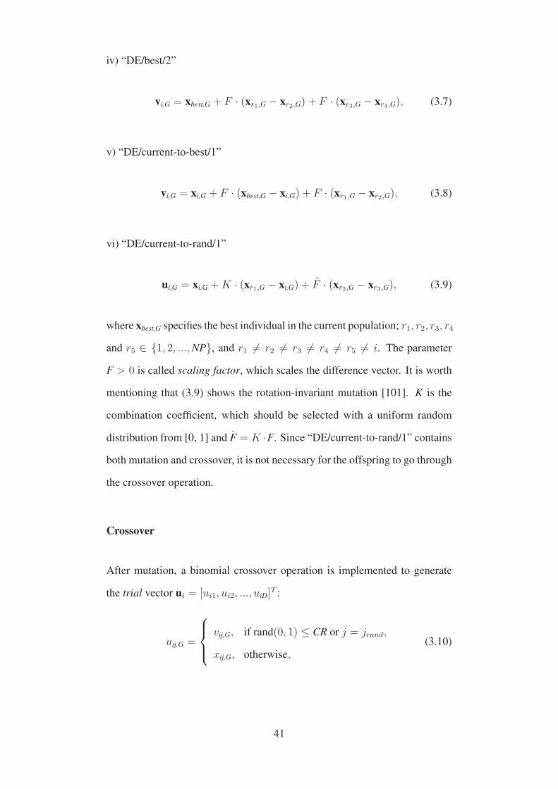
iv) “DE/best/2”

vi,G = xbest,G + F · (xr1,G − xr2,G) + F · (xr3,G − xr4,G), (3.7)

v) “DE/current-to-best/1”

vi,G = xi,G + F · (xbest,G − xi,G) + F · (xr1,G − xr2,G), (3.8)

vi) “DE/current-to-rand/1”

ui,G = xi,G +K · (xr1,G − xi,G) + F · (xr2,G − xr3,G), (3.9)

where xbest,G specifies the best individual in the current population; r1, r2, r3, r4

and r5 ∈ {1, 2, ...,NP}, and r1 = r2 = r3 = r4 = r5 = i. The parameter

F > 0 is called scaling factor, which scales the difference vector. It is worth

mentioning that (3.9) shows the rotation-invariant mutation [101]. K is the

combination coefficient, which should be selected with a uniform random

distribution from [0, 1] and F = K ·F. Since “DE/current-to-rand/1” contains

both mutation and crossover, it is not necessary for the offspring to go through

the crossover operation.

Crossover

After mutation, a binomial crossover operation is implemented to generate

the trial vector ui = [ui1, ui2, ..., uiD]T :

uij,G =

⎧⎪⎨⎪⎩

vij,G, if rand(0, 1) ≤ CR or j = jrand,

xij,G, otherwise,(3.10)

41

where rand(0, 1) is a uniform random number in the range [0, 1]. CR ∈ [0, 1]

is called crossover probability, which determines how much the trial vector is

inherited from the mutant vector. jrand is an integer randomly selected from 1

to D and newly generated for each i, which ensures at least one dimension of

the trial vector will be different from the corresponding target vector. If uij,G

is out of the boundary, it will be reinitialized in the range [Lj, Uj].

Selection

The selection operator employs a one-to-one swapping strategy, which picks

the better one from each pair of xi,G and ui,G for the next generation:

xi,G+1 =

⎧⎪⎨⎪⎩

ui,G, if f(ui,G) ≤ f(xi,G),

xi,G, otherwise.(3.11)

Some variants of DE

In recent years, various DE variants have been proposed to solve the global

numerical optimization problems. In this subsection, we choose several

popular and powerful DE variants, and briefly describe the principles of them.

1) Differential evolution with self-adapting parameters (jDE)

A new version of DE called jDE was proposed recently, in which a self-

adaptive approach are developed for parameters F and CR [102]. The

parameters are calculated as follows:

Fi,G+1 =

⎧⎪⎨⎪⎩

Fl + rand1 ∗ Fu, if rand2 < τ1,

Fi,G, otherwise,(3.12)

CRi,G+1 =

⎧⎪⎨⎪⎩

rand3, if rand4 < τ2,

CRi,G, otherwise,(3.13)

42

where randj, j ∈ {1, 2, 3, 4} are uniform random values from [0, 1]; τ1 and

τ2 are probabilities to adjust F and CR, respectively; Fl and Fu indicate the

lower and upper bounds of F , respectively. The settings affect the mutation,

crossover, and selection operations of the new vector.

2) Adaptive differential evolution with optional external archive (JADE)

JADE was developed by Zhang et al. [103], which is dedicated to solving sin-

gle objective optimization problems. This algorithm shows its effectiveness in

both unimodal and multimodal functions. The strategy “DE/current-to-pbest”

with optional archive helps JADE achieve good balance between “greedy”

and “diverse”, which is as follows:

vi,G = xi,G + Fi · (xpbest,G − xi,G) + Fi · (xr1,G − xr2,G), (3.14)

where xpbest,G is randomly selected as one of the top 100p% individuals in

the current population with p ∈ (0, 1]. xr2,G is stochastically chosen from

the current population and a set of archived inferior solutions. Fi denotes

the scaling factor, which is updated independently in terms of a Cauchy

distribution with location parameter μF and scale parameter 0.1:

Fi = randci(μF , 0.1), (3.15)

μF = (1− c) · μF + c · meanL(SF ), (3.16)

meanL(SF ) =

∑F∈SF

F 2∑F∈SF

F, (3.17)

where SF stores all the successful scaling factors at the current generation;

μF is initialized as 0.5. Similarly, the crossover probability CRi of each

individual is generated according to a normal distribution of mean μCR and

43

standard deviation 0.1:

CRi = randni(μCR, 0.1), (3.18)

μCR = (1− c) · μCR + c · meanA(SCR), (3.19)

where SCR is the set of all successful crossover probabilities at the current

generation.

3) Composite differential evolution (CoDE)

Recently, CoDE was presented by Wang et al. [104], which combines

three effective trial vector generation strategies with three groups of proper

parameter settings. The three strategies and the corresponding parameter

settings are listed as follows:

DE/rand/1 [F = 1.0, CR = 0.1]

DE/rand/2 [F = 1.0, CR = 0.9]

DE/current-to-rand/1 [F = 0.8, CR = 0.2]

In CoDE, three trial vectors are generated for each target vector; and the best

one can enter into the next generation if it is better than the target vector.

4) Differential evolution with Strategy Adaptation (SaDE)

A self-adaptive DE called SaDE was developed, in which both trial vector

generation strategies and control parameter settings are updated according to

the historical experiences in breeding superior solutions [105]. The candidate

strategy pool consists of four trail vector generation strategies: DE/rand/1,

DE/rand/2, DE/rand-to-best/2, and DE/current-to-rand/1. The probability of

choosing each strategy can be calculated as follows:

pk,G =Sk,G∑4k=1 Sk,G

, (3.20)

44

Sk,G denotes the success rate of the trial vector, which is generated by the kth

strategy and successfully replaces its target vector.

3.3 Summary

This chapter presents research methodologies from two aspects: 1) mul-

tiobjective evolutionary optimization-based NN model for fashion sales

forecasting; 2) robust evolutionary optimization for fashion order scheduling.

The concepts and principles of multiobjective optimization, differential

evolution, robust optimization, neural network, and extreme learning machine

are introduced in detail. The methodologies are utilized to solve the sales

forecasting problems and order scheduling problems in fashion supply chains

in the following chapters.

45

Chapter 4

Newly Proposed Evolutionary

Algorithms for Fashion Supply

Chains

In this chapter, first of all, a novel multiobjective evolutionary algorithm

called nondominated sorting adaptive differential evolution (NSJADE) is pro-

posed. Then a event-triggered impulsive control scheme (ETI) is developed

to improve the performance of differential evolution (DE), hence a new DE

called ETI-DE can be obtained. In the later chapters, NSJADE-based model

is developed for fashion sales forecasting problems; ETI-DE is modified to

solve the order scheduling problems in fashion supply chains.

4.1 Nondominated Sorting Adaptive Differential

Evolution

In this section, a new multiobjective evolutionary algorithm (MOEA) is pro-

posed, which is called nondominated sorting adaptive differential evolution

46

(NSJADE). Based on NSJADE, a sales forecasting problem in fashion supply

chains is handled in the next chapter. In the following, firstly, the motivation

of presenting NSJADE is provided; secondly, the detailed framework of

the algorithm is given; thirdly, a group of experiments demonstrate the

effectiveness of NSJADE.

4.1.1 Motivation

In the past two decades, MOEAs have attracted increasing attentions in the

area of evolutionary computation. The objective of a MOEA is to search

the Pareto front (see Definition 3.3) of the optimization problem as fast

as possible. Recently, a variety of MOEAs have been proposed, such as

nondominated sorting genetic algorithm II (NSGA-II) [106], a multiobjective

evolutionary algorithm based on decomposition (MOEA/D) [107], a general

indicator-based evolutionary algorithm (IBEA) [108], the strength Pareto

evolutionary algorithm 2 (SPEA2) [109], and so on. Among them, NSGA-

II is one of the most popular MOEAs. In NSGA-II, there are two critical

operations: 1) fast nondominated sorting operation; 2) crowded-comparison

operation. In fast nondominated sorting operation, all the solutions obtained

at the current generation can be quickly sorted into different nondomination

levels. While crowded-comparison operation differs individuals in the same

nondomination level, which means the individual located in a less crowded

area is preferred. The brief procedure of NSGA-II is shown in Fig. 4.1.

It is worth mentioning that NSGA-II fails to find the Pareto fronts of some

multimodal problems (e.g., ZDT4 and ZDT6 of the ZDT test suite) in [106].

And we impute it to the genetic algorithm (GA), which serves as the search

engine in NSGA-II. Although GA has proven to be an effective method for

many optimization problems, its performance will deteriorate when facing

complicated problems. The reason is that GA does not take advantage of

47

Figure 4.1: Illustration of the NSGA-II procedure.

the useful historical information to guide the search. Recently, a novel

differential evolution (DE) algorithm called adaptive differential evolution

(JADE) was proposed by Zhang and Sanderson [103]. JADE utilizes the

top 100p% individuals in the current population with p ∈ (0, 1] to direct

the search of the population, and forces the individuals away from the

archived inferior solutions (see Section 3.2.2). And the experimental results in

[103] demonstrate the superior performance of JADE in solving multimodal

problems. Therefore, it is reasonable to replace the non-adaptive GA part

in NSGA-II with JADE, and a nondominated sorting adaptive differential

evolution (NSJADE) is proposed in the following.

4.1.2 Nondominated Sorting Adaptive Differential

Evolution

NSJADE is developed based on NSGA-II, and the purpose is to improve

the search efficiency of the population by substituting GA with JADE as the

search engine. The pseudocode of NSJADE is given in Algorithm 2.

Firstly, the settings of parameters are provided; and a population containing

NP individuals is initialized. Then different levels of Pareto fronts are

48

generated by the Nondominated Sort function according to the objectives

in the optimization problem, and the crowding-distance value is assigned to

each individual x [106]. Step 5 to step 28 indicate the search engine part

of the proposed NSJADE, which is similar to JADE except for the selection

operator (from step 22 to step 24). Three parent individuals are selected from

100p% best individuals, the current population P and the current population P

combined with an archive A, respectively. Then after mutation and crossover,

a new offspring is generated. A parent individual will be added into the

optional archive A if it is dominated by its offspring. After checking the

size of A and updating the values of μCR and μF, the parent and the offspring

individuals are combined by the Combine function. Then the new generation

is generated after the Nondominated Sort and Select Elitism operations.

Algorithm 2 Nondominated sorting adaptive differential evolution (NSJADE)1: Begin2: Set μCR = 0.5; μF = 0.5; A = ∅3: Create a random initial population {xi,0|i = 1, 2, ...,NP}4: x=Nondominated Sort(x)5: for g = 1 to G do6: SF = ∅; SCR = ∅7: for i = 1 to NP do8: Generate CRi = randni(μCR, 0.1), Fi = randci(μF, 0.1)9: Randomly select xp

best,g from 100p% best individuals

10: Randomly select xr1,g �= xi,g from current population P11: Randomly select xr2,g �= xr1,g �= xi,g from P ∪ A12: vi,g = xi,g + Fi · (xp

best,g − xi,g) + Fi · (xr1,g − xr2,g)

13: Check the boundary of vi,g14: Generate jrand = randint(1,D)15: for j = 1 to D do16: if j = jrand or rand(0, 1) < CRi then17: uj,i,g = vj,i,g18: else19: uj,i,g = xj,i,g20: end if21: end for22: if f(ui,g) ≺ f(xi,g) then23: xi,g → A; CRi → SCR, Fi → SF24: end if25: end for26: Randomly remove individuals from A to maintain size(A) = NP27: μCR = (1− c) · μCR + c · meanA(SCR)28: μF = (1− c) · μF + c · meanL(SF)29: xall = Combine(x, u)30: xall = Nondominated Sort(xall)31: x = Select Elitism(xall)32: end for33: End

It is worth noticing that from step 22 to step 24, an individual dominated

by its offspring is dominated as a loser, and it will be stored into archive

49

A. Here a situation is left out: the parent has the same rank with its

offspring, but has a smaller crowding distance. In terms of the comparison

rules defined in [106], this parent individual is also a loser and should be

kept in A. However, if this situation is considered in NSJADE, which means

the crowding-distance values of these two individuals should be computed,

the worst-case complexity of this operation is O (NPlog(2NP)). Therefore,

in order to reduce the computation complexity of the algorithm, only the

dominance relationship between these two individuals is calculated, instead

of the crowding distance if they are in the same Pareto front.

4.1.3 Experiments with Test Functions

Deb et al. used the ZDT test suite (ZDT1-ZDT4, ZDT6) to examine the

performance of NSGA-II in [106]. Among them, ZDT4 is a complicated

multimodal problem, which has 219 or 7.94(1011) different local Pareto

optimal fronts in the search space, merely one of which is the global best

Pareto front. The experimental results in [106] show that real-coded NSGA-

II gets stuck at different local Pareto optimal sets when solving ZDT4. For

ZDT6, which is a nonconvex and nonuniform problem, NSGA-II also cannot

converge to the true Pareto front. Next, we test the convergence effect

of NSJADE and NSGA-II on ZDT4 and ZDT6. For the integrity of the

experiments, we also list the results of these two algorithms on the rest ZDT

functions. Both algorithms are run for 250 generations, and have the same

population size NP = 100. For NSGA-II, we use the same distribution indices

for crossover and mutation operators as in [106]: ηc = 20, ηm = 20. For

NSJADE, the parameters in JADE part are the same with [103]: the value

of parameter c is 0.1; the size of the optional archive is the same as that of

the population; the parameter p in pbest mechanism is assigned to 0.05; other

parameters are provided in Algorithm 2.

50

Fig. 4.2 shows the nondominated solutions obtained by NSJADE and NSGA-

II on ZDT functions. From Fig. 4.2, we find that for ZDT1-ZDT3, NSJADE

and NSGA-II have the similar convergence performance, which means the

solutions obtained overlap the true Pareto front of each test function. While

for ZDT4 and ZDT6, the solutions found by NSGA-II are a little bit far

from the true Pareto front, which indicates that NSGA-II fails to find the

Pareto front of these two functions. However, our proposed NSJADE

can successfully help the population converge to the global Pareto optimal

fronts of ZDT4 and ZDT6, which can be attributed to the powerful search

performance of the modified search engine: JADE.

4.2 Differential Evolution with Event-triggered

Impulsive Control Scheme

In this section, an event-triggering-based impulsive control scheme (ETI) is

introduced to improve the performance of differential evolution (DE). In the

rest of this section, firstly, the motivation of proposing ETI is given; secondly,

the four components of ETI are described in detail; thirdly, extensive

experiments are conducted to display the effectiveness of the proposed ETI.

4.2.1 Motivation

Differential evolution (DE), firstly proposed by Storn and Price [75, 76],

has proven to be a reliable and powerful population-based evolutionary

algorithm for global numerical optimization. Generally, DE employs three

main operators: mutation, crossover, and selection at each generation for

the population production [110–112]. The mutation operator provides the

individuals with a sudden change or perturbation, which helps explore the

51

0 0.2 0.4 0.6 0.8 10

0.2

0.4

0.6

0.8

1

1.2

1.4

f1

f2

NSGA−IITrue Pareto FrontNSJADE

(a)

0 0.2 0.4 0.6 0.8 10

0.2

0.4

0.6

0.8

1

1.2

1.4

f1

f2


(b)

0 0.1 0.2 0.3 0.4 0.5 0.6 0.7 0.8 0.9−0.8

−0.6

−0.4

−0.2

0

0.2

0.4

0.6

0.8

1

1.2

f1

f2


(c)

0 0.2 0.4 0.6 0.8 10

0.2

0.4

0.6

0.8

1

1.2

1.4

1.6

1.8

f1

f2


(d)

0.2 0.3 0.4 0.5 0.6 0.7 0.8 0.9 10

0.2

0.4

0.6

0.8

1

1.2

1.4

f1

f2


(e)

Figure 4.2: Comparison of nondominated solutions with NSGA-II &

NSJADE on ZDT functions. (a) ZDT1; (b) ZDT2; (c) ZDT3; (d) ZDT4;

(e) ZDT6.

52

search space. In order to increase the diversity of the population, the

crossover operator is implemented after the mutation operation. The selection

operator chooses the better one between a parent and its offspring, which

guarantees that the population never deteriorates. In addition to these three

basic operators, there are three control parameters which greatly influence the

performance of DE: the mutation scale factor F, the crossover rate CR, and

the population size NP. Most of the current research on DE has focused on

four aspects to enhance the performance of DE: developing novel mutation

operators [103, 113–120], designing new parameter control strategies [102,

103, 113, 114, 121–125], improving crossover operator [114, 126–128], and

pooling multiple mutation strategies [104, 105, 129, 130].

Despite numerous efforts on improving DE from the above four aspects, there

are some DE variants which take advantage of ideas from other disciplines.

For instance, Rahnamayan et al. [131] presented opposition-based DE

(ODE), which adopts opposition-based learning, a new scheme in machine

intelligence, to speed up the convergence rate of DE. Laelo and Ali [132]

made use of the attraction-repulsion concept in electromagnetism to boost the

performance of the original DE. Vasile et al. [133] proposed a novel DE,

which is inspired by discrete dynamical systems. These improvements on

DE enlighten us to look through techniques in other areas, which might be

introduced to the development of DE variants.

On another research frontier, as an important component in control theory,

impulsive control has attracted much attention in recent years due to its high

efficiency. As exemplified in [134, 135], impulsive effects can be detected in

various dynamical system, like communication networks, electronic systems,

biological networks, and so on. Besides, impulsive control is able to

manipulate the states of a network to a desired value by adding impulsive

signals to some specific nodes at certain instants. In addition, another

effective technique, event-triggered mechanism (ETM), has also been widely

53

utilized [136–138]. In ETM, the state of the controller is updated when the

system’s state exceeds a given threshold. This way, ETM avoids the periodical

execution of data updating, which efficiently saves communication resources.

Taking a look at how DE works in an optimization problem, the population

in the evolution process can be treated as a complicated dynamical system,

where individuals in the population can be regarded as nodes in complex

networks or multi-agent systems. Furthermore, after initialization, the

population begins to evolve by updating the positions in the search range.

The update rate (UR) of the population in each generation reflects the current

search status. The decrease of UR indicates that the population gradually

encounters stagnation. The worst situation is that UR drops to zero before

the global best solution is found. Therefore, it is possible for us to embed

impulsive control or ETM into DE so that the search performance of DE can

be improved.

4.2.2 An Event-Triggered Impulsive Control Scheme

In this section, an event-triggered impulsive control scheme (ETI) for DE is

proposed. In the following, firstly, the proposed ETI is introduced in detail,

which involves four components, i.e., stabilizing impulses, destabilizing

impulses, ranking assignment, and an adaptive mechanism. Afterwards,

ETI is combined with DE to develop ETI-DE, the pseudo-code and the

computational complexity analysis of which are also given.

In the proposed approach, ETM and impulsive control are integrated into

the framework of DE algorithms. ETM identifies when the individuals

should be injected with impulsive controllers, while impulsive control alters

the positions of partial individuals when triggering conditions are violated.

Specifically, two types of impulses, i.e., stabilizing impulses and destabilizing

54

impulses, are imposed on the selected individuals (sorted by an index

according to the fitness value and the number of consecutive stagnation

generation) when UR in the current generation decreases or equals to zero.

On one hand, when UR begins to decrease, stabilizing impulses drive the

individuals with lower rankings in the current population to approach the

individuals with better fitness values. The purpose of stabilizing impulsive

control is to help update some inferior individuals and to enhance the

exploitation capability of the algorithm. On the other hand, when UR drops

to zero or stabilizing impulses fail to take effect, destabilizing impulses

randomly adjust the positions of the inferior individuals within the area of the

current population. This operation improves the diversity of the population

and hence improves the exploration ability of DE.

1) Stabilizing Impulses

Stabilizing impulses are employed when UR begins to decrease. As men-

tioned before, in control theory, stabilizing impulses can be employed to

regulate the states of a network to a desired value. Normally, the desired

state is set as the reference state for the nodes to be injected with stabilizing

impulsive controllers. In the framework of DE, stabilizing impulses mainly

focus on improving the exploitation ability of DE. In DE algorithms, it is

well known that good individuals (i.e., with smaller fitness values) usually

contain useful information, which may be helpful to other individuals’

evolution. Hence, these good individuals can be regarded as references. So

when stabilizing impulsive control is triggered during the evolution, we set

the individuals with smaller fitness values in the current generation as the

reference states. The pseudo-code of stabilizing impulsive control is exhibited

in Algorithm 3.

Assume that xi,G is one of the individuals at the Gth generation that are

chosen to undergo impulsive effects, where xi,G = [xi1,G, xi2,G, ..., xiD,G]T

55

Algorithm 3 Stabilizing Impulsive Control ()1: Begin2: /* xi,G is the individual that undergoes stabilizing impulsive control

3: /* ζi,G is a flag to indicate whether stabilizing impulsive control is to improve the fitness value

4: /* rand(a,b) uniformly generate a random number belonging to the interval (a,b)

5: /* DM is the number of dimensions selected to undergo stabilizing impulsive control in xi,G6: A = {1, 2, ...,D}; B = ∅; C = ∅7: Randomly select an individual xk,G from the current population

8: if f(xi,G) < f(xk,G) then9: Set xgbest,G as the reference state si,G10: Generate B by randomly selecting DM elements from A11: for j = 1 to D do12: if j ∈ B then13: Kij,G = rand(−1, 0)14: else15: Kij,G = 016: end if17: end for18: Ki,G = diag{Ki1,G,Ki2,G, ...,KiD,G}D×D, i = 1, 2, ...,NP19: ei,G = xi,G − si,G20: xi,G+ = xi,G + Ki,G · ei,G

21: else22: Set xk,G as the reference state si,G23: Generate C by randomly selecting DM elements from A24: for j = 1 to D do25: if j ∈ C then26: Kij,G = −127: else28: Kij,G = 029: end if30: end for31: Ki,G = diag{Ki1,G,Ki2,G, ...,KiD,G}D×D, i = 1, 2, ...,NP32: ei,G = xi,G − si,G33: xi,G+ = xi,G + Ki,G · ei,G

34: end if35: if f(xi,G+ ) ≤ f(xi,G) then36: xi,G = xi,G+

37: ζi,G = 138: else39: ζi,G = 040: end if41: End

and D is the dimension. We set si,G as the reference state for xi,G, which is

randomly selected from the best individual (gbest) or other individuals with

smaller fitness values than xi,G in the current population. For each xi,G, a

uniform random individual xk,G is firstly chosen from the current population.

If f(xi,G) < f(xk,G), which means the randomly selected individual is worse

than xi,G, then xgbest,G is the reference state for xi,G; if f(xi,G) ≥ f(xk,G), which

means xk,G is better than xi,G in the current population, then xk,G is set as the

reference state for xi,G.

The error between xi,G and its reference state si,G at the Gth generation can be

obtained:

ei,G = xi,G − si,G. (4.1)

56

Then at the end of the Gth generation, stabilizing impulses force the chosen

individuals to approach their reference state. Here we get:

xi,G+ = xi,G + Ki,G · ei,G, (4.2)

where Ki,G = diag{Ki1,G,Ki2,G, ...,KiD,G} is the impulsive strength for

individual xi at the Gth generation. Kij,G ∈ (−1, 0) shows that in the jth

dimension, xi,G lies on the line between the reference and the individual

itself; Kij,G = 0 means that in the jth dimension, xi,G is not injected with

impulsive controllers; Kij,G = −1 indicates that in the jth dimension, xi,G

reaches the reference state, j = 1, 2, ...,D. G+ denotes that stabilizing

impulses are imposed on xi,G at the end of the Gth generation. Every

time, DM dimensions of xi,G are selected in a random way to be injected

with impulsive controllers, where DM ∈ {1, 2, ...,D}. When xgbest,G

serves as the reference state, for the selected DM dimensions, the impulsive

strength Ki,G = diag{Ki1,G,Ki2,G, ...,KiDM,G}DM×DM, and Kij,G is a uniform

random number from −1 to 0, j = 1, 2, ...,D; for the rest D − DM

dimensions, Ki,G = diag{0, 0, ..., 0}(D−DM)×(D−DM). When xk,G is as the

reference state, for the selected DM dimensions, the impulsive strength

Ki,G = diag{−1,−1, ...,−1}DM×DM; for the rest D − DM dimensions, Ki,G =

diag{0, 0, ..., 0}(D−DM)×(D−DM). Ki,G is obtained from combining Ki,G and Ki,G.

It is noticed that ζ is a flag to indicate whether stabilizing impulsive control

is successful to improve the performance: when ζ = 1, it means that the

stabilizing impulsive control takes effect, and a new individual is introduced

to the population by replacing an old one; when ζ = 0, it shows that the

stabilizing impulsive control fails to take effect.

2) Destabilizing Impulses

When UR drops to zero (UR = 0) or stabilizing impulses fail to take

effect (ζ = 0), destabilizing impulses are introduced to provide some

57

randomness during the evolution. When destabilizing impulses are triggered,

the selected individuals can be moved to any position within the range of

the current population. The pseudo-code of injecting destabilizing impulses

is exhibited in Algorithm 4. Assume that xi,G is one of the individuals at

the Gth generation that are chosen to receive destabilizing impulses, where

xi,G = [xi1,G, xi2,G, ..., xiD,G]T . minj,G and maxj,G are the minimum and

maximum values of the jth dimension in the population at the Gth generation,

j = 1, 2, ...,D. The lower and upper bounds of the range of the population at

the Gth generation are:

xL,G = [min1,G,min2,G, ...,minD,G]T , (4.3)

xU,G = [max1,G,max2,G, ...,maxD,G]T . (4.4)

From Eqs. (4.3)-(4.4), we can obtain the error between xU,G and xL,G at the

Gth generation:

ei,G = xU,G − xL,G. (4.5)

Then at the end of the Gth generation, the positions of the chosen individuals

are randomly updated in the specified range. Here we have:

xi,G+ = xL,G + Ki,G · ei,G, (4.6)

where Ki,G = diag{Ki1,G,Ki2,G, ...,KiD,G} is the impulsive strength for

individual xi at the Gth generation. Similarly, DM dimensions of xi,G are

selected at random to be injected with impulses. Kij,G is a uniform random

number from 0 to 1, j = 1, 2, ...,D.

3) Ranking Assignment

In the following, we need to consider which individuals should be injected

with impulsive controllers. During the evolution process, we consider two

58

Algorithm 4 Injecting Destabilizing Impulses ()1: Begin2: /* xi,G is the individual that undergoes destabilizing impulses

3: /* minj,G and maxj,G are the minimum and maximum values of the jth dimension in the population at the Gth

generation

4: /* rand(a,b) uniformly generate a random number belonging to the interval (a,b)

5: xL,G = [min1,G,min2,G, ...,minD,G]T

6: xU,G = [max1,G,max2,G, ...,maxD,G]T

7: for j = 1 to D do8: Kij,G = rand(0, 1)9: end for10: Ki,G = diag{Ki1,G,Ki2,G, ...,KiD,G}D×D, i = 1, 2, ...,NP11: ei,G = xU,G − xL,G12: xi,G+ = xL,G + Ki,G · ei,G

13: End

measures to characterize the status of the individuals. The first one is the

fitness value of each individual, while the second one is the number of each

individual’s consecutive stagnant generation. Fitness value is the most direct

index to judge whether an individual should enter into the next generation

or not. The number of consecutive stagnant generation reflects the degree

of the activity of an individual in the evolution. If an individual does not

evolve for a relatively long time, it might be necessary to introduce some

additional operations to change its position. Based on these discussions, in

this paper, we rank the population based on the fitness value and the number

of consecutive stagnant generation, respectively. R is the ranking according

to the fitness value, and R is the ranking based on the number of consecutive

stagnation generation. These two rankings are both ordered in an ascending

way (i.e., from the best fitness value to the worst and from the smallest number

of consecutive stagnation generation to the largest). Then we combine R and

R to get R, which indicates that the individuals are sorted according to both

the fitness value and the number of consecutive stagnation generation.

R = R + R. (4.7)

R not only reflects the fitness value of an individual but also delivers the degree

of an individual’s activity.

When impulsive control is triggered during the evolution, we select the

59

individuals with larger values of R from the population as the candidates to

undergo stabilizing or destabilizing impulses. By specially displacing the

individuals with higher rankings (i.e., larger R), the evolution status of the

population can be improved.

4) An Adaptive Mechanism to Determine the Number of Individuals Taking

Impulsive Control

Finally, in order to further improve the performance of ETI, an adaptive

mechanism is proposed to determine the number of the individuals that should

be injected with impulsive controllers. We firstly discuss the number of

individuals (M) with stabilizing impulses. LN and UN represent the lower

and upper bound of M, respectively. When stabilizing impulsive control is

triggered for the first time, M = LN. After xi,G experiences the stabilizing

impulse, we get xi,G+ . xi,G+ can join the current population instead of xi,G

if and only if f(xi,G+) < f(xi,G). Every time xi,G is replaced with xi,G+

(i.e., ζ = 1, see step 36 in Algorithm 1), M keeps unchanged. If ζ = 0,

M = M + 1. We aim to increase the success rate of stabilizing impulsive

control by having more individuals to be injected with stabilizing impulsive

controllers. Besides, if a new gbest is generated in the population, M drops

to a random integer between [LN,M]. The reason for reducing M to a

random integer between [LN,M] instead of LN is to increase the times of

successful stabilizing impulsive control, especially in the later stage of the

evolution. Next, we explain how to choose the number of individuals that

undergo destabilizing impulses. As introduced above, destabilizing impulses

are added in two cases: when UR = 0 or ζ = 0. Unlike stabilizing impulses,

with the purpose of introducing some randomness, the selection operation

(i.e., compare the fitness values of xi,G and xi,G+) will not be used after

injecting destabilizing impulses, which means that xi,G+ replaces xi,G directly.

Therefore, in order not to bring too many individuals with large fitness values

into the population, we randomly select the individuals from M candidates to

60

Algorithm 5 Random Selection of Individuals ()1: Begin2: /* {xi,G|i = 1, 2, ...,M} are the candidates that undergo destabilizing impulses

3: /* pr is the probability for selecting individuals to be injected with destabilizing impulses

4: /* ε is a flag for judging whether it is necessary to increase pr5: for i = 1 to M do6: ri = rand

7: end for8: pr = 0.2, ε = 09: while ε = 0 do10: for i = 1 to M do11: if ri < pr then12: xi,G will undergo destabilizing impulsive control later

13: ε = 114: else15: ε = 016: end if17: end for18: pr = pr + 0.219: pr = min(pr, 1.0)20: end while21: End

be injected with destabilizing impulses. The selection process is described in

Algorithm 5.

5) DE with An Event-Triggered Impulsive Control Scheme

Combining the developed event-triggered impulsive control scheme (ETI)

with DE, the ETI-DE is proposed. The pseudo-code of ETI-DE with

“DE/rand/1” mutation operator is given in Algorithm 6. From step 3 to step

24, it is the original DE algorithm with “DE/rand/1” mutation operator. The

rest steps in Algorithm 6 illustrate the mechanism of ETI. ETM determines the

moment to add impulses to the individuals, and impulsive control modifies the

positions of partial individuals at the end of a certain generation. In detail, step

35 to step 42 and step 49 to step 56 describe the mechanism of destabilizing

impulses, which are triggered when UR = 0 or ζ = 0. While step 43 to step

48 shows the details of stabilizing impulsive control, which is triggered when

UR decreases and UR = 0. These two types of impulses are able to accelerate

the convergence of the population by updating some inferior individuals, and

improve the diversity of the population by introducing some randomness to

the search. Furthermore, ETI is flexible to be integrated into other advanced

DE variants, such as jDE [102], JADE [103], SaDE [105], and so on.

61

Algorithm 6 DE with event-triggered impulsive control scheme1: Begin2: /* UR is the update rate of the population in each generation

3: /* UR tp stores the temporary value of UR4: /* gbest is the best individual of the population in the current generation

5: /* gbest tp stores the temporary value of gbest6: /* rs records the number of individuals to be injected with destabilizing impulses

7: Set LN = 1; UN = NP; M = LN; UR = 0; F = 0.5; CR = 0.98: Create a random initial population {xi,0|i = 1, 2, ...,NP}9: Evaluate the fitness values of the population and record gbest10: while the maximum evaluation number is not achieved do11: for G = 1 to Gmax do12: UR tp = UR; gbest tp = gbest13: for i = 1 to NP do14: Select randomly three individuals r1 �= r2 �= r3 �= i15: vi,G = xr1,G + F · (xr2,G − xr3,G)16: Check the boundary of vi,G17: Generate jrand = randi(D, 1)18: for j = 1 to D do19: if j = jrand or rand < CR then20: uij,G = vij,G21: else22: uij,G = xij,G23: end if24: end for25: if f(ui,G) ≤ f(xi,G) then26: xi,G+1 = ui,G27: end if28: end for29: Evaluate the fitness values of the population and record gbest30: if gbest < gbest tp then31: M = randi([LN,M], 1)32: end if33: Calculate R and R of the population, R = R + R34: Calculate UR of the population

35: if UR = 0 then36: M = min(M,UN)37: Select M individuals with the largest R-value as {xi,G|i = 1, 2, ...,M}38: {xi,G|i = 1, 2, ..., rs} = Random Selection of Individuals ()39: for i = 1 to rs do40: xi,G = Injecting Destabilizing Impulsive ()41: Evaluate the fitness value of xi,G42: end for43: else if UR �= 0 and UR < UR tp then44: M = min(M,UN)45: Select M individuals with largest R-value as {xi,G|i = 1, 2, ...,M}46: for i = 1 to M do47: [xi,G, ζi,G] = Stabilizing Impulsive Control ()48: end for49: if sum(ζ1,G, ζ2,G, ..., ζM,G) = 0 then50: {xi,G|i = 1, 2, ..., rs} = Random Selection of Individuals ()51: for i = 1 to rs do52: xi,G = Injecting Destabilizing Impulsive ()53: Evaluate the fitness value of xi,G54: M = M + 155: end for56: end if57: Record the best individual of current population as gbest′58: if gbest′ < gbest then59: M = randi([LN,M], 1)60: end if61: end if62: end for63: end while64: End

62

4.2.3 Experimental Results and Analysis

In this section, we carry out extensive experiments to evaluate the per-

formance of our developed ETI-DE. The total 30 benchmark functions

presented in the CEC 2014 competition on single objective real-parameter

numerical optimization are selected as the test suite [139]. According to their

characteristics, the functions can be divided into four groups: 1) unimodal

functions (F01-F03); 2) simple multimodal functions (F04-F16); 3) hybrid

functions (F17-F22); 4) composition functions (F23-F30). More details of

these functions can be found in [139].

In the following experiments, the proposed event-triggered impulsive control

scheme is incorporated with ten state-of-the-art DE variants. The parameters

are set as follows:

1) DE/rand/1/bin with F = 0.5, CR = 0.9 [117];

2) DE/best/1/bin with F = 0.7, CR = 0.5 [116];

3) jDE with τ1 = 0.1, τ2 = 0.1 [102];

4) JADE with μF = 0.5, μCR = 0.5, c = 0.1, p = 0.05 [103];

5) CoDE with F = [1.0, 1.0, 0.8], CR = [0.1, 0.9, 0.2] [104];

6) SaDE with LP = 50 [105];

7) ODE with F = 0.5, CR = 0.9, Jr = 0.3 [131];

8) EPSDE with F = [0.1, 0.2, 0.3, 0.4, 0.5, 0.6, 0.7, 0.8, 0.9],

CR = [0.4, 0.5, 0.6, 0.7, 0.8, 0.9] [129];

9) SHADE with initial MF = 0.5, MCR = 0.5, H = NP [140];

10) OXDE with F = 0.5, CR = 0.9 [126].

63

For the incorporated ETI-DE algorithms, the lower and upper bounds of the

number of individuals that take impulsive control are set: LN = 1, UN = NP.

In order to make a fair comparison, like [116, 117, 119], the population size

NP is set as 100 for all the algorithms. The maximum number of function

evaluations (Max FES) is set to D · 10000. We run each function optimized

by each algorithm 51 times for the experiments [139]. The simulations are

performed on an Intel Core i7 personal computer with 2.10-GHz central

processing unit and 8-GB random access memory.

In the following, we assess the effectiveness of our developed scheme by

comparing ten popular DE algorithms and their corresponding ETI-based

variants on the test suite at D = [30, 50, 100]. The experimental results

are provided in Tables A.1-A.9 in Appendix. “+/≈/−” indicates that the

performance of DE algorithms with ETI is significantly better than, equal

to, and worse than those without ETI according to a Wilcoxon rank-sum test

at 5% significance level. The better values compared between the DE variants

and their corresponding ETI-based DEs are highlighted in boldface.

From Tables A.1-A.9, we can see that the ten ETI-DEs perform better than

their corresponding original DE algorithms, which indicates the effectiveness

of the proposed ETI. Next, the Holm-Bonferroni procedure with confidence

level 0.05 is conducted to investigate the differences among the total twenty

DE variants, i.e., ten DE algorithms and their corresponding ETI-based

variants. The results of D = [30, 50, 100] are provided in Tables 4.1-

4.3. According to these three tables, it can be found that ETI-SHADE has

the highest rank among the twenty variants when D = 30, 50 and 100,

respectively, which means ETI-SHADE performs best for the test problems

of different dimension sizes.

In summary, the presented ETI is very powerful and the ten ETI-DEs possess

strong capabilities of rapid convergence and accurate search for the test

64

Table 4.1: Holm test on the fitness, reference algorithm = ETI-SHADE

(rank=15.33) for functions F01-F30 at D = 30.

j Optimizer Rank zj pj δ/j Hypothesis1 ETI-OXDE 14.47 -5.67E-01 2.85E-01 2.63E-03 Accepted

2 ETI-DE/rand/1/bin 14.30 -6.76E-01 2.49E-01 2.50E-02 Accepted

3 ETI-jDE 13.70 -1.07E+00 1.42E-01 8.33E-03 Accepted

4 SHADE 13.37 -1.29E+00 9.90E-02 2.94E-03 Accepted

5 ETI-JADE 13.10 -1.46E+00 7.19E-02 6.25E-03 Accepted

6 ETI-EPSDE 12.23 -2.03E+00 2.12E-02 3.13E-03 Accepted

7 ETI-ODE 11.20 -2.71E+00 3.41E-03 3.57E-03 Accepted

8 ETI-SaDE 10.97 -2.86E+00 2.13E-03 4.17E-03 Accepted

9 JADE 10.37 -3.25E+00 5.74E-04 7.14E-03 Rejected

10 jDE 10.27 -3.32E+00 4.55E-04 1.00E-02 Rejected

11 OXDE 9.27 -3.97E+00 3.57E-05 2.78E-03 Rejected

12 SaDE 9.10 -4.08E+00 2.25E-05 4.55E-03 Rejected

13 DE/rand/1/bin 8.87 -4.23E+00 1.15E-05 5.00E-02 Rejected

14 EPSDE 8.83 -4.26E+00 1.04E-05 3.33E-03 Rejected

15 ETI-CoDE 8.80 -4.28E+00 9.47E-06 5.00E-03 Rejected

16 ODE 8.57 -4.43E+00 4.72E-06 3.85E-03 Rejected

17 ETI-DE/best/1/bin 7.17 -5.35E+00 4.49E-08 1.25E-02 Rejected

18 CoDE 6.03 -6.09E+00 5.71E-10 5.56E-03 Rejected

19 DE/best/1/bin 4.07 -7.38E+00 8.17E-14 1.67E-02 Rejected



j Optimizer Rank zj pj δ/j Hypothesis1 ETI-JADE 13.80 -8.51E-01 1.97E-01 6.25E-03 Accepted

2 ETI-OXDE 13.67 -9.38E-01 1.74E-01 2.63E-03 Accepted

3 ETI-DE/rand/1/bin 13.53 -1.03E+00 1.53E-01 2.50E-02 Accepted


5 SHADE 13.10 -1.31E+00 9.52E-02 2.94E-03 Accepted

6 ETI-jDE 12.43 -1.75E+00 4.04E-02 8.33E-03 Accepted

7 ETI-CoDE 11.80 -2.16E+00 1.54E-02 5.00E-03 Accepted

8 JADE 10.87 -2.77E+00 2.79E-03 7.14E-03 Rejected

9 ETI-ODE 10.70 -2.88E+00 1.99E-03 3.57E-03 Rejected

10 jDE 10.53 -2.99E+00 1.40E-03 1.00E-02 Rejected





15 ODE 8.53 -4.30E+00 8.58E-06 3.85E-03 Rejected

16 ETI-SaDE 8.40 -4.39E+00 5.77E-06 4.17E-03 Rejected




65



j Optimizer Rank zj pj δ/j Hypothesis1 SHADE 13.77 -5.24E-01 3.00E-01 2.94E-03 Accepted

2 ETI-jDE 13.40 -7.64E-01 2.23E-01 8.33E-03 Accepted

3 ETI-CoDE 13.40 -7.64E-01 2.23E-01 5.00E-03 Accepted

4 ETI-JADE 13.00 -1.03E+00 1.53E-01 6.25E-03 Accepted


6 ETI-OXDE 12.60 -1.29E+00 9.90E-02 2.63E-03 Accepted

7 jDE 11.80 -1.81E+00 3.51E-02 1.00E-02 Accepted

8 ETI-DE/rand/1/bin 11.63 -1.92E+00 2.74E-02 2.50E-02 Accepted

9 JADE 10.93 -2.38E+00 8.69E-03 7.14E-03 Accepted


11 ETI-ODE 9.93 -3.03E+00 1.21E-03 3.57E-03 Rejected

12 ETI-SaDE 9.37 -3.40E+00 3.32E-04 4.17E-03 Rejected






18 ODE 7.57 -4.58E+00 2.30E-06 3.85E-03 Rejected


functions. The results of the Wilcoxon rank-sum test confirm that our scheme

is of paramount importance to improve the performance of the considered DE

algorithms. Besides, the results of the Holm-Bonferroni procedure denote that

ETI-SHADE has the best performance on the test suite of different dimension

sizes.

4.3 Summary

This chapter presents a novel MOEA (i.e., nondominated sorting adaptive

differential evolution (NSJADE)) and a event-triggered impulsive control

scheme (ETI) for DE. Firstly, NSJADE is developed based on a popular

and classic MOEA: NSGA-II; and the experimental results demonstrate

that the proposed NSJADE has better performance on multimodal problems

than NSGA-II. Secondly, the idea of ETI derives from the concepts of

event-triggered mechanism and impulsive control in control theory. ETI is

developed to enhance both the exploration and exploitation abilities of DE.

According to the experimental results, ETI greatly improves the performance

of ten state-of-the-art DE variants.

66

Chapter 5

Multiobjective Evolutioanry

Optimization for Sales Forecasting

in Fashion Supply Chains

This chapter handles a short-term replenishment forecasting problem in

fashion supply chains by a neural network (NN)-based model, the parameters

of which are optimized by a new multiobjective evolutionary algorithm

(MOEA). Unlike the previous research, according to the different features of

the datasets to be predicted,the developed model selects the optimal weights

and the number of hidden nodes for NNs. Firstly, the mathematical model

of the short-term replenishment forecasting problem is established. Secondly,

a multiobjective optimization-based NN model is developed to deal with the

forecasting problem. Thirdly, extensive experiments are conducted to show

the effectiveness and superiority of our proposed model. Finally, the summary

of this chapter is provided.

67

5.1 Problem Formulation

To solve the short-term replenishment forecasting problem in fashion supply

chains, a NN-based forecasting model is proposed here. In previous NN-

based models, only the training error is minimized, which will result in the

overfitting phenomenon [11]. In this research, two objectives in the NN-based

model are optimized: one is to minimize the average root-mean-square error

of K-fold cross-validation (K-cv error) on the training data; the other is to

minimize the sum of the absolute weights of NN. These two objectives are

listed as follows:

1) Objective 1:

f1 =1

K

K∑k=1

Ek, (5.1)

where K is the number that the training samples are divided into, and Ek is

the root-mean-square error of predicting the kth part of the training data.

2) Objective 2:

f2 =M∑i=1

|ωi|, (5.2)

where ωi is a weight in the NN, and M is the total number of weights.

The first objective is related to the training error of the NN on the training

samples. In Eq. 5.1, due to the limited number of the real data in the

following experiments , the average root-mean-square error of K-cv error on

the training data is used as the first objective. While under other circumstances

that the training data is sufficient, it may be not necessary to carry out the

K-fold cross-validation on the training set, which means any other accuracy

measurement of the training can be selected as the objective. In Eq. 5.2,

the second objective is concerned with the structure of the NN used in the

forecasting model. On one hand, f1 is the training error of the model,

which reflects the accuracy of the prediction, and a smaller f1 is desirable.

68

On the other hand, in order to increase the generalization of the model,

the structure of the NN cannot be too complicated, which means a smaller

sum of the absolute weights, i.e., f2, is preferred. These two objectives are

conflicting with each other, and the improvement of one objective may cause

the deterioration of the other one [141].

5.2 Multiobjective Optimization-Based Neural

Network Model for the Problem

A multiobjective optimization-based neural network model (MOONN) is

proposed in this section for the short-term replenishment forecasting problem

in fashion supply chains. For solving the forecasting problem, there are

two processes: one is the forecasting process; the other is the optimization

process. The flowcharts of these two processes are given in Figs. 5.1-5.2. In

the forecasting process, two steps are involved: 1) In the first step, training

data are utilized to train the proposed MOONN model, and the weights and

the hidden node number of the model can be obtained. 2) In the second step,

test data are used as the input of the MOONN model which has already been

trained, and the output is the final sales forecast. The optimization process in

Fig. 5.2 illustrates how the parameters of the forecasting model are optimized

for the short-term replenishment forecasting problem. In the rest of this

section, the optimization process is introduced in detail.

5.2.1 Representation

The first step of the optimization process is to represent the solutions which

will be optimized. For the short-term fashion replenishment forecasting

problem, at the end of the optimization process, the NNs with the optimal

69

Figure 5.1: Flowchart of the forecasting process. 1©: training model; 2©: test

model.

Figure 5.2: Flowchart of the optimization process.

values of weights and hidden biases, as well as the number of hidden nodes are

obtained . Therefore, the representation of the solutions used in this research

consists of two parts: one vector Ω and one vector Φ. The dimension of

Ω is (I + 1) · H . Each element ωij ∈ Ω is the weight connecting the ith

70

input node and the jth hidden node. I and H denote the numbers of input

nodes and hidden nodes, respectively. I + 1 indicates that the hidden biases

are also considered. The vector Φ is of dimension H , where φh ∈ Φ is a

binary value (i.e., 0 and 1) used to display the existence of each hidden node.

In this research, each solution represents a NN candidate; and based on this

representation, the training of weights and the selection of hidden nodes can

be achieved at the same time.

It is worth pointing out that the learning algorithm of the NNs here is the

extreme learning machine (ELM), so there is no need to assign the output

weights in advance. The reason is that for ELM-based NNs, the output

weights can be calculated based on the input weights and hidden biases, which

is also an advantage of ELM-based NNs. So only the optimal values of input

weights and hidden biases are searched for during the optimization process.

5.2.2 Population Initialization

The initialization process involves two parts: initializing vector Ω and initial-

izing vector Φ for each individual in the population. For the initialization

of Ω, the real number in the specific range is randomly assigned to each

dimension of the weight vector. For initializing vector Φ, the maximum

number of hidden nodes Nmax is set firstly, then the number of hidden nodes

is stochastically initialized from 1 to Nmax for each individual.

5.2.3 Evolution of Vector Ω

After the initialization process, the population has to evolve observing certain

rules. Ω is optimized among the specific range of real number, while Φ is

searched from 1 to the maximum number of hidden nodes Nmax. In detail,

two separate evolution schemes are developed for the evolution of these two

71

parts, respectively. After each generation of the evolution, the combination

of Ω and Φ symbolizes a NN with particular parameters, which is used for

the sales forecasting cases. Here, the rules of evolving weight vector Ω are

introduced firstly.

In Section 4.1, a new multiobjective optimization algorithm is proposed,

which is called nondominated sorting adaptive differential evolution (NS-

JADE). Here, NSJADE is selected as the optimization algorithm in the fore-

casting model MOONN. As explained before, JADE [103] is elected as the

search engine of NSJADE; hence for Ω, the mutation and crossover strategies

of JADE are adopted. In the mutation stage, the strategy “DE/current-to-

pbest” guides the mutation of the parents:

vi,g = xi,g + Fi · (xpbest,g − xi,g) + Fi · (xr1,g − xr2,g) (5.3)

At the gth generation, for individual xi, three other individuals xpbest, xr1, and

xr2 are picked out in the mutation process. Among them, xpbest is chosen from

the top 100p% (p∈ (0, 1]) individuals of the population; xr1 is selected at

random from the current population; xr2 is from the current population along

with an archive, which stores the inferior individuals during the evolution

process. And xi, xpbest, xr1 and xr2 are different from each other. Moreover,

at each generation, the mutation factor Fi of each individual is adaptively

generated according to a Cauchy distribution.

After vi is generated, here we come to the crossover stage. In this stage,

binomial crossover is performed on each dimension of vector vi:

uj,i,g =

⎧⎪⎨⎪⎩

vj,i,g j = jrand or rand(0, 1) < CRi

xj,i,g otherwise(5.4)

In (5.4), jrand is a randomly selected index, which ensures that ui gets at least

one component from vi. And at each generation, the crossover probability

72

CRi is adaptively created based on a Normal distribution.

During the evolution process of Ω, the mutation strategy “DE/current-to-

pbest” and the crossover strategy guarantee a fast convergence speed and high

accuracy for the evolution.

5.2.4 Evolution of Vector Φ

Vector Φ stores a group of binary values, which indicates the existence of

hidden nodes. For the evolution of Φ, the search range is one-dimensional,

from 1 to Nmax. So only mutation operation is applied during the evolution

of Φ. In addition, mutation is adopted every few generations, which avoids

the structure of NNs to be changed very frequently. This operation ensures

that the weights of NN with specific structure can be trained for a longer time,

which provides more opportunities to find the optimal parameters for the NN.

The detailed mutation process is described as follows:

Step 1. For individual i, another two individuals: r1 and r2 are randomly

selected.

Step 2. Perform XOR on each dimension of vectors Φr1 and Φr2 , and vector

Φxor can be generated.

Step 3. Check each dimension of vector Φxor: if the value of this dimension

is 1, we also set 1 to the corresponding dimension of vector Φi.

Step 4. If there is no “1” in Φi, we initialize Φi again according to the

procedure of Population Initialization.

It is noticed that XOR operation is involved in the evolution of vector Φ, and

the reasons are listed here. Unlike vector Ω, vector Φ consists of a sequence

of binary values, the evolution of which should follow the rules of discrete

73

evolutionary algorithm. XOR operation calculates the distance between two

discrete vectors, which is the essence of binary DE algorithm. So XOR is

selected during the process of evolving vector Φ.

To better explain the mutation process of Φ, an example is provided in Fig.

5.3). Φr1 and Φr2 are two randomly selected vectors, each of which contains

10 dimensions. Φxor is the vector obtained after the XOR operation on Φr1

and Φr2 , which means for the 2nd, 4th, 6th, 7th, 8th and 10th elements, the

values of Φr1 and Φr2 are opposite. Moreover, combined with the value of the

original vector Φi, it is obvious that the values in the 2nd, 6th, 7th, 8th and

10th positions should be set to 1, hence the mutated one is obtained.

Figure 5.3: An example of mutation process of Φ.

5.2.5 Selection

In a single evolution, after each individual (including Ω and Φ) in the parent

population goes through the mutation or crossover, a new generation is needed

to select from the parent and the offspring population combined. Since there

are two objectives involved in the optimization process, the Pareto optimal

solutions of this problem need to be picked out. It is assumed that the parent

population contains NP individuals; therefore, after a single evolution, there

74

are 2NP individuals (each parent generates one offspring) in the candidate

pool. The specific procedure of selection is given as follows:

Step 1. Calculate the values of two objectives f1 and f2 for each individual

in the candidate pool.

Step 2. Rank the 2NP individuals according to f1 and f2 based on the

definition of Pareto dominance (see Definition 3.1 in Section 3.1.1).

In addition, the labels “rank 1, rank 2, ...” are assigned to the

individuals in different nondomination levels (see Definition 3.4 in

Section 3.1.1).

Step 3. In each rank, the crowding distance [106] is calculated for each

individual, which characterizes the degree of crowding where the

individual is located.

Step 4. After both the rank and the crowding distance of each individual in

the candidate pool are calculated, the individuals are sorted according

to these two indices. To be specific, the individual with the lower

rank and the larger crowding distance is preferred. Hence, NP

individuals are chosen from the candidate pool as the population of a

new generation.

The selection process needs to choose NP individuals from 2NP candidates.

These 2NP individuals are firstly sorted based on their objective values, and

then divided into different nondomination levels. This process is called

nondominated sorting [106]. At different nondomination levels, crowding

distance is computed and then assigned to each individual. Nondominated

sorting and crowding-distance assignment help balance between exploration

and exploitation for the algorithm.

At the end of one single evolution, there is another operation besides

selection: comparing a parent individual xi and its offspring ui. If xi is

75

dominated by ui, xi is recognized as a loser, which will be put into an archive

(mentioned in Section 4.1). Accordingly, the mutation factor Fi and the

crossover probability CRi used in generating ui are marked “successful”,

which helps produce the new Fi+1 and CRi+1 for the next generation.

5.3 Experimental Results and Discussion

To evaluate the performance of the proposed forecasting model, extensive

experiments were conducted in terms of the real-world sales data of apparel

products, which predicted the amount of replenishment for certain fashion

products during the selling season. In this section, the experimental setup

is firstly introduced in detail, including fashion sales data we used, the

accuracy measures, and the forecasting models used for comparison and their

parameters. Later, two groups of experiments are conducted to demonstrate

the effectiveness of the proposed model: 1) the short-term replenishment

forecasting of several categories of products in the shops of separate cities

are performed; 2) for the same categories of products, the sales of shops

in different cities are combined, and then the amount of replenishment is

predicted.

5.3.1 Fashion Sales Data

Real sales data were collected from one of the largest retailers in fashion

industry in Hong Kong and Mainland China, which include the sales data of

different types of T-shirts and pants in various cities from 01/1999 to 12/2009.

76

5.3.2 Accuracy Measures

Since there are various forecasting objectives, data scales and patterns, no

accuracy measure is generally applicable to all forecasting tasks [142]. In this

research, in order to reduce the possible bias generated by one single accuracy

measure, three measures of prediction accuracy are utilized, including root

mean absolute error (RMSE), mean absolute percentage error (MAPE) and

mean absolute error (MAE). Define Yt and Ft as the observation and forecast

at time t, respectively, the specific formulas of these three accuracy measures

are provided as follows:

RMSE =√

mean((Yt − Ft)2) (5.5)

MAPE = mean(|(Yt − Ft)/Yt|)× 100% (5.6)

MAE = mean(|Yt − Ft|) (5.7)

5.3.3 Forecasting Models Used for Comparison and Their

Parameters

In this research, 2 categories of experiments are performed: short-term

replenishment forecasting of fashion products in separate cities and in

combined cities. In each category, experiments are conducted from three

aspects: (1) the forecasting performance of the proposed model is compared

with two popular models and a variant of one of these two models: ELME [8],

HI [10], and HI2; (2) to examine the effect of the module that helps choose

the proper number of NN’s hidden node, the performance of our proposed

77

models with or without this module are compared, and the models are marked

as MOONN1 and MOONN2; (3) to observe the benefits brought by the K-

cv error as one of the objectives, the performance of the presented model is

compared with the similar MOONN model called MOONN3, which merely

replaces K-cv error with RMSE as one of the two objectives. The models

used in the experiments are summarized in Table 5.1.

Table 5.1: The models used in the experiments.

Model DescriptionMOONN1 proposed in this research

MOONN2 variant of MOONN1 (without the module of optimizing hidden node number)

MOONN3 variant of MOONN1 (K-cv error substituting RMSE as one objective)

ELME proposed in [8]

HI proposed in [10]

HI2 variant of HI (K-cv error substituting RMSE as the objective)

After introducing the models used in the experiments, the parameters of

each model are listed in Table 5.2. MOONN1 is the proposed model in

this research, while the variants MOONN2 and MOONN3 are used for

comparison, the main bodies of which are similar with MOONN1. Table

5.2 shows the parameters of these three MOONN models. For convenience,

in the last four rows of Table 5.2, some parameters that are only used in

part of these three models are also provided. Range of hidden node number

is set for MOONN2, because in MOONN2, the number of hidden nodes

is not picked intelligently, where the model is run repeatedly with different

number of hidden nodes from 1 to 10. While for MOONN1 and MOONN3,

Searching Range of hidden node number is set, as well as Generation interval

of evolving vector Φ, because each individual of the population in MOONN1

and MOONN3 seeks the appropriate number of hidden nodes during the

forecasting. The value of K for MOONN1 and MOONN2 is 10, because

10-fold cross-validation is most commonly used. While in MOONN3, K-cv

error is substituted by RMSE, it is not necessary to configure the value of K.

For the other three models used in the experiment, i.e., ELME, HI and HI2,

78

Table 5.2: The Parameters of MOONN1, MOONN2 and MOONN3, where

N={1,2,3,...}.

Parameter ValuePopulation size 100

Generation 300

Initial range of the input weights [-1, 1]

Activation function Sigmoid

Range of hidden node number (for MOONN2) [1, 10]⋂

NSearching range of hidden node number (for MOONN1, MOONN3) [1, 10]

⋂N

Generation interval of evolving vector ρ (for MOONN1, MOONN3) 30

Value of K (for MOONN1, MOONN2) 10

the parameters are the same as the original parameter settings [8, 10] (see

Tables 5.3-5.4). In Table 5.3, P is the parameter that makes the ELME more

stable, which is recommended to be selected from [100, 1000]. It has been

demonstrated that the larger value of P , the better forecasting performance

ELME can provide [8]; so here we choose 1000. In Table 5.4, PARmin

and PARmax are the minimum and the maximum of pitch adjustment rate

(PAR); bwmin and bwmax denote the minimum and the maximum of bandwidth

(bw); HMCR is the harmony memory consideration rate; HMS represents the

harmony memory size, like the population size in MOONN1, and is also set

as 100; NI is the number of improvisations; value of K indicates in HI2, K-cv

error substitutes RMSE as the objective to be optimized. Furthermore, for

ELME, in the original paper, the number of hidden nodes is fixed. In order

to reduce the randomness of output generated by ELME with a stationary

number of hidden nodes, we set a parameter called Range of hidden node

number, as shown in Table 5.3. The forecasting is carried out by running the

ELME model repeatedly with different number of hidden nodes from 1 to 10,

and then average these forecasts as the final result. For HI and HI2, the same

operation also appears in the experiment. While for MOONN1, the model

can select the appropriate number of hidden node from 1 to 10 intelligently

according to different datasets.

It is noticed that besides HI, our proposed MOONN1 is also compared with a

variant of HI, which is named HI2. The reason is as follows: In MOONN1,

79

Table 5.3: The Parameters of ELME, where N={1,2,3,...}.

Parameter ValueInitial range of the input weights [-1, 1]


Range of hidden node number [1, 10]⋂

NP 1000

Table 5.4: The Parameters of HI and HI2, where N={1,2,3,...}.

Parameter ValueInitial range of the input weights [-1, 1]


Range of hidden node number [1, 10]⋂

NValue of K (for HI2) 10

PARmin 0.45

PARmax 0.99

bwmin 1e-6

bwmax 4

HMCR 0.95

HMS 100

NI 1000

K-cv error of the training samples is as one of the objectives to be optimized.

While in HI model, the objective is the RMSE of the training samples, but not

K-cv error. Therefore, in order to fairly show the performance of both MOEA

and the module exploring the hidden-node-number space in MOONN1, the

variant of HI called HI2 is also provided in the comparison, which also utilizes

K-cv error as the objective.


Forecasting of 7 Categories of Products in Cities X∼Z

In this experiment, 7 categories (i.e., A, B, C, D, E, F and G) of products

are selected from cities X, Y and Z. The task is to forecast the amount of

replenishment for different categories of products separately in these cities.

Table 5.5 gives the specific mapping of products and cities. For each category

of products, there is a dataset which records the sales in all the shops in

the corresponding city, so in Table 5.5, the numbers in the brackets are the

samples in each dataset. Moreover, for each sample in city X, it includes

80

6 input variables, which are 3 early sales volumes (the first 3-, 7- and 14-

day sales volumes), 1 weather index (average temperature during the selling

season), and 2 economic indices (total retail sales index of consumer goods

and consumer price index for clothing and footwear); while for city Y and

Z, due to the lack of statistical data, total retail sales index of consumer

goods is not contained. The input variables are determined according to their

influence on fashion sales, which include weather data, economic data and

historical sales data [22]. As shown in Table 5.2, K-cv error is one of the two

objectives to be optimized in MOONN1 and MOONN2, and the value of K

is 10, which indicates during the optimization, training samples are evaluated

by 10-fold cross-validation. Therefore, the number of training samples needs

to be appointed as integral multiples of 10, which means that the number

of training samples should satisfy: Nts = 10 ∗ M , where M is a positive

integer. In this experiment, to predict the amount of replenishment of product

A: Nts=40, and the other 8 samples are for the test; for product B and D:

Nts = 10, and the rest are test samples; for product C and product F and G

in both cities Y and Z: Nts = 20, and the rest are utilized as test samples; for

product E: Nts = 30, and the rest are for the test.

Table 5.5: Specific mapping of products and cities.

City Category of productX A(48), B(17), C(25), D(21), E(39)

Y F(24), G(32)

Z F(30), G(31)

Comparison of MOONN1, ELME, HI and HI2

First of all, the forecasting is performed by using four different models: the

proposed MOONN1, ELME, HI and HI2. For MOONN1, HI and HI2, each

model is run 25 times; while for ELME, the original paper suggests 100 to

1000 times (i.e., the parameter P ), and here the ELME model is run 1000

times. The comparison of forecasting results is shown in Tables 5.6-5.8.

81

Table 5.6: Forecasting results of MOONN1, ELME, HI, HI2, MOONN2 and

MOONN3 in city X.

MOONN1 ELME HI HI2 MOONN2 MOONN3Training Test Training Test Training Test Training Test Training Test Training Test

A RMSE 1853.9 1615.6 1846.3 1973.5 1130.5 2054.2 1756.6 1985.3 1348.8 1783.6 1317.4 1713.3

MAPE 15.4% 15.1% 14.4% 16.9% 9.2% 18.3% 13.8% 17.7% 10.0% 14.5% 11.0% 14.3%MAE 1210.2 1194.1 1158.9 1399.0 705.0 1440.6 1095.2 1433.5 788.4 1181.3 857.4 1186.6

B RMSE 1185.9 449.2 866.1 2891.8 322.4 1296.2 778.4 1242.0 529.7 850.3 1010.9 511.1

MAPE 112.7% 14.9% 73.7% 65.3% 28.2% 30.5% 59.2% 32.6% 42.2% 14.0% 98.1% 17.2%

MAE 974.1 371.7 675.5 2286.2 250.7 1016.4 560.2 983.0 415.5 610.7 833.0 428.2

C RMSE 1257.1 826.4 971.2 1224.4 510.7 1450.8 894.6 1545.6 643.2 881.3 863.3 2301.5

MAPE 224.2% 18.9% 103.1% 25.8% 36.4% 31.1% 81.3% 30.6% 55.1% 22.4% 153.0% 33.5%

MAE 988.7 719.6 676.4 1063.0 366.6 1263.6 612.3 1312.5 449.2 783.8 680.2 1698.3

D RMSE 1320.1 725.8 931.8 1850.6 331.9 1611.3 835.7 5109.8 566.7 1339.4 1042.5 911.3

MAPE 103.5% 21.6% 57.9% 43.6% 19.0% 31.2% 49.8% 110.4% 38.2% 29.9% 78.5% 24.2%

MAE 1036.4 608.5 667.9 1372.1 240.4 1111.7 584.0 3858.6 408.1 984.6 784.8 722.1

E RMSE 2017.9 1426.7 1722.0 1651.7 1431.0 2596.1 1673.9 1782.4 1495.7 2578.7 1379.0 3079.7

MAPE 110.0% 34.4% 75.9% 41.1% 50.5% 64.1% 68.7% 44.5% 57.9% 63.2% 66.2% 70.9%

MAE 1676.5 1272.5 1372.3 1529.2 1161.6 2391.1 1345.0 1660.3 1213.0 2362.2 1134.1 2633.2


MOONN3 in city Y.


F RMSE 453.8 306.5 371.9 543.1 202.7 714.8 341.4 498.2 257.0 582.7 307.6 562.3

MAPE 36.7% 12.5% 26.2% 20.3% 10.6% 28.6% 23.4% 24.2% 17.7% 24.9% 24.7% 18.9%

MAE 385.2 242.2 302.8 444.9 142.5 627.7 277.5 454.7 208.8 530.0 254.4 465.2

G RMSE 169.5 96.9 136.4 133.3 63.6 160.2 117.2 131.4 91.9 112.2 128.5 151.0

MAPE 22.9% 15.4% 16.9% 19.2% 9.5% 20.5% 15.3% 18.6% 12.3% 16.5% 17.5% 21.1%

MAE 128.4 66.1 102.2 111.7 53.8 132.9 91.5 109.9 71.1 96.5 97.6 121.0


MOONN3 in city Z.


F RMSE 758.7 847.1 482.8 895.6 239.0 1158.8 419.3 1019.5 362.5 944.1 490.8 1389.1

MAPE 75.8% 18.2% 39.6% 19.1% 15.9% 28.7% 33.9% 21.9% 29.4% 21.6% 48.6% 34.4%

MAE 655.6 618.5 395.7 641.1 174.9 926.4 339.9 725.4 290.4 715.9 426.5 1119.2

G RMSE 226.4 135.4 192.2 165.5 87.7 236.5 173.9 172.7 123.5 201.6 187.0 174.1

MAPE 31.7% 12.3% 24.0% 14.5% 13.4% 18.5% 22.1% 15.4% 17.7% 17.2% 26.6% 13.5%

MAE 173.4 114.6 144.1 141.2 72.0 194.7 133.1 149.9 98.9 175.3 142.7 139.5

82

Among these models, MOONN1 is based on multiobjective algorithm, HI

and HI2 are grounded on single objective algorithm, while ELME does

not process any optimization algorithm. As discussed in Section 3.1.1, the

mechanism of multiobjective algorithms is different from single objective

ones—that is, for multiobjective algorithms, a set of solutions are obtained

at last, while we only choose the optimal solution when using single objective

algorithms. Therefore, in order to unify the metrics, for MOONN1, as well

as MOONN2 and MOONN3, the training results and test results obtained by

the whole population are averaged as the final training and test results.

For all forecasting cases, from the RMSE, MAPE and MAE results of the three

models, it can be figured out that HI performs the best on training samples.

Compared with ELME, HI adopts the harmony search algorithm to optimize

the NN, so it is reasonable that HI has the best results on training samples.

However, due to the data insufficiency of the fashion sales forecasting, HI fails

to extend the satisfying performance on training data to test data. From Tables

5.6-5.8, MOONN1 exhibits superior forecasting performance to ELME and

HI on all the test samples, which can be attributed to MOONN1’s strong

ability of balancing the training and test accuracy.

As mentioned above, the proposed MOONN model (i.e., MOONN1) owns

the module which evolves the number of hidden nodes, and this module

effectively selects the appropriate size of neural network for the forecasting

problem. In Table 5.9, the specific size of the evolved neural network in

MOONN1 is listed. The mean and standard deviation of maximum, minimum

and average number of hidden nodes during 25 runs are recorded in Table

5.9. According to the different characteristics of different cases, the sizes of

the neural network used in the forecasting problems are also different. For

instance, to predict the replenishment of product A in city X, the average size

of the neural network in MOONN1 is 3.3; while for product E in city X, the

average size of the neural network involved in the replenishment forecasting

83

problem is merely 1.4.

Table 5.9: Size of the evolved neural network in MOONN1.

City X City Y City ZA B C D E F G F G

max 7.7(1.2) 8.9(1.0) 6.6(1.5) 8.8(0.8) 2.2(0.4) 4.7(1.5) 8.1(1.5) 5.5(2.9) 5.7(1.2)

min 1.0(0) 1.0(0) 1.0(0) 1.0(0) 1.0(0) 1.0(0) 1.0(0) 1.0(0) 1.0(0)

avg 3.3(0.5) 2.7(0.4) 2.4(0.6) 2.4(0.2) 1.4(0.1) 2.3(0.6) 3.1(0.4) 2.5(1.1) 2.3(0.3)

Comparison of MOONN1 and MOONN2

As introduced earlier, the number of hidden nodes can be evolved when

using the proposed MOONN model (i.e., MOONN1). In this section, to

validate its effectiveness, this module is removed from MOONN1, and the

new model obtained is called MOONN2. The forecasting is performed by

repeatedly running MOONN2 with different number of hidden nodes from 1

to 10, and then the results are averaged as the final result. Here, MOONN1

and MOONN2 are employed to forecast the amount of replenishment for

the above products. Tables 5.6-5.8 exhibit the forecasting performance of

MOONN1 and MOONN2. For all the categories of products, from the

RMSE, MAPE and MAE results, MOONN2 behaves better on training

samples, but MOONN1 shows excellent forecasting performance on test

samples. It can be recognized that the module which selects the proper

number of NN’s hidden nodes helps MOONN1 perform better on 7 of 9

replenishment forecasting cases.


In this subsection, the forecasting performance of MOONN1 and MOONN3

is compared. In MOONN1, the average error of committing K-fold cross-

validation (K-cv error) on the training samples is set as one of the objectives

to be optimized; while in MOONN3, the K-cv error is replaced by RMSE as

one of the two objectives. Tables 5.6-5.8 show the forecasting performance

84

of MOONN1 and MOONN3. According to the results, it can be found

that MOONN1 presents superior performance over MOONN3 on 8 of 9

forecasting cases, which indicates the effectiveness of selecting K-cv error

as one of the two objectives.

In Table 5.10, the size of neural network after evolution in MOONN1 and

MOONN3 is provided when forecasting the replenishment amount of the 7

categories of products above. The mean and standard deviation of maximum,

minimum and average number of hidden nodes during 25 runs are recorded in

Table 5.10. From the table, it can be found that for each forecasting problem,

the maximum and average number of hidden nodes in MOONN3 is much

larger than that in MOONN1. And it is well explained why the RMSE, MAPE

and MAE generated by MOONN3 on training samples are much smaller than

those by MOONN1; because larger-size neural networks have more accurate

approximation ability.

Table 5.10: Size of the evolved neural network in MOONN1 and MOONN3.City X City Y City Z

A B C D E F G F G

MOONN1 max 7.7(1.2) 8.9(1.0) 6.6(1.5) 8.8(0.8) 2.2(0.4) 4.7(1.5) 8.1(1.5) 5.5(2.9) 5.7(1.2)

min 1.0(0) 1.0(0) 1.0(0) 1.0(0) 1.0(0) 1.0(0) 1.0(0) 1.0(0) 1.0(0)

avg 3.3(0.5) 2.7(0.4) 2.4(0.6) 2.4(0.2) 1.4(0.1) 2.3(0.6) 3.1(0.4) 2.5(1.1) 2.3(0.3)

MOONN3 max 10.0(0.2) 10.0(0) 10.0(0.2) 10.0(0) 9.8(0.5) 9.8(0.4) 10.0(0) 9.9(0.3) 9.9(0.3)

min 1.0(0) 1.0(0) 1.0(0) 1.0(0) 1.0(0) 1.0(0) 1.0(0) 1.0(0) 1.0(0)

avg 5.3(0.3) 3.2(0.2) 4.8(0.3) 3.1(0.3) 5.7(0.4) 5.3(0.3) 4.9(0.3) 5.0(0.3) 4.8(0.3)


Forecasting of 2 Categories of Products in Cities Y∼Z

In Experiment 1, the amount of replenishment for 7 categories of products in

city X, Y and Z is predicted. For instance, like product F and G, although

they were sold in both city Y and Z, the replenishment of F and G in city

Y (or Z) is predicted by means of the sales data merely in city Y (or Z).

While in this experiment, the sales data of the same category of products are

combined in different cities for the forecasting. According to the sales data

85

provided by the retailer, two categories of products are collected, which were

sold in two cities from 1999 to 2009. These two categories are F and G, and

their amounts of replenishment in city Y and Z are predicted in Experiment

1. Now, for product F and G, the sales data in city Y and Z are added; so

there are 54 and 63 samples of each product respectively. Like the previous

experiment, each sample includes 5 input variables, which are 3 early sales

volumes (the first 3-, 7- and 14-day sales volumes), 1 weather index (average

temperature during the selling season), and 1 economic index (consumer price

index for clothing and footwear). Like experiment 1, the number of training

samples should satisfy: Nts = 10 ∗M , where M is a positive integer. So for

category F, with the help of total 54 samples, the amount of replenishment

in city Y and Z is predicted respectively, where Nts = 40, and the rest 14

samples in either city are test data; similarly, to forecast the replenishment

amount of category G in city Y and Z, Nts = 50, and the rest 13 samples are

test data. In this experiment, the forecasting performance of MOONN1 and

other models is also compared, and the results are given in the following three

subsections.

Comparison of MOONN1, ELME, HI and HI2

First of all, as in Experiment 1, the forecasting performance of four different

models is compared: MOONN1, ELME, HI and HI2. For MOONN1, HI

and HI2, each model is run 25 times; while for ELME, the original paper

suggests 100 to 1000 times (i.e., the parameter P ), and here the ELME

model is run 1000 times. The forecasting results are given in Table 5.11.

Firstly, the forecasting performance among the four models is compared. For

both product F and product G in city Y, MOONN1 shows the superiority

of forecasting test samples on all of the three accuracy measures; for both

product F and product G in city Z, ELME and MOONN1 have better

86

forecasting performance than HI and HI2.


MOONN3.MOONN1 ELME HI HI2 MOONN2 MOONN3

Training Test Training Test Training Test Training Test Training Test Training Test

F city Y RMSE 758.2 495.9 548.7 490.3 380.5 661.1 518.0 486.8 443.5 473.9 524.8 626.4

MAPE 68.8% 13.3% 42.4% 13.8% 21.9% 16.0% 38.7% 14.3% 30.7% 13.0% 43.8% 18.2%

MAE 632.6 334.6 445.7 370.0 286.3 453.9 418.8 376.6 350.2 367.3 440.0 474.2

city Z RMSE 755.8 647.2 504.0 687.7 344.8 917.6 475.0 741.5 394.0 812.7 503.5 945.9

MAPE 70.5% 17.0% 39.1% 16.2% 20.6% 21.1% 36.5% 18.0% 28.9% 18.3% 44.4% 20.9%

MAE 638.8 473.4 417.0 465.9 262.8 618.2 388.0 510.2 323.2 542.1 427.4 587.7

G city Y RMSE 202.5 113.6 188.2 120.7 121.4 207.9 173.6 133.8 134.4 169.9 175.2 141.0

MAPE 25.2% 17.6% 20.0% 17.4% 12.73% 18.57% 18.8% 17.8% 14.8% 18.2% 21.8% 18.3%

MAE 146.5 93.5 128.0 102.3 86.1 143.5 121.7 112.2 93.7 130.1 125.8 109.6

city Z RMSE 214.6 134.9 192.8 144.5 136.3 172.0 178.2 138.3 142.7 166.7 178.9 175.2

MAPE 26.8% 11.5% 21.3% 12.1% 15.5% 13.1% 19.5% 12.3% 17.3% 11.8% 23.2% 12.8%

MAE 150.2 105.4 131.3 112.8 100.9 130.6 124.6 112.2 105.0 121.4 129.0 131.0

In addition, as mentioned above, the proposed MOONN model (i.e., MOON-

N1) owns the module which evolves the number of hidden nodes, and

this module effectively selects the appropriate size of neural network for

the forecasting problem. In Table 5.12, the specific size of the evolved

neural network in MOONN1 is listed. The mean and standard deviation of

maximum, minimum and average number of hidden nodes during 25 runs are

recorded in Table 5.12.

Table 5.12: Size of the evolved neural network in MOONN1.

City Y City ZF G F G

max 3.2(1.4) 7.3(1.8) 3.0(1.3) 6.3(1.4)

min 1.0(0) 1.0(0) 1.0(0) 1.0(0)

avg 1.7(0.4) 3.3(0.6) 1.6(0.2) 3.0(0.8)


As introduced earlier, the number of hidden nodes can be evolved when

employing MOONN1. In this section, to validate its effectiveness, this

module is removed from MOONN1 as in Experiment 1, and the new model

obtained is called MOONN2. The forecasting is performed by repeatedly

running MOONN2 with different number of hidden nodes from 1 to 10,

and then the results are averaged as the final result. Here, MOONN1 and

MOONN2 are employed to forecast the amount of replenishment for the

87

above products. Table 5.11 exhibits the forecasting performance of MOONN1

and MOONN2. According to Table 5.11, MOONN1 has better forecasting

accuracy for 3 cases, which are the replenishment of product F in city Z,

product G in both city Y and city Z.


In this subsection, the forecasting performance of MOONN1 and MOONN3

is compared. In MOONN1, the average error of committing K-fold cross-

validation (K-cv error) on the training samples is set as one of the objectives

to be optimized; while in MOONN3, the K-cv error is replaced by RMSE as

one of the two objectives. Table 5.11 shows the forecasting performance of

MOONN1 and MOONN3. According to the 3 accuracy measures, it can be

found that MOONN1 beats MOONN3 on all the forecasting cases.

In Table 5.13, the size of neural network after evolution in MOONN1 and

MOONN3 is offered when forecasting the replenishment amount of the

categories of products above. The mean and standard deviation of maximum,

minimum and average number of hidden nodes during 25 runs are recorded

in Table 5.13.

Table 5.13: Size of the evolved neural network in MOONN1 and MOONN3.

City Y City ZF G F G

MOONN1 max 3.2(1.4) 7.3(1.8) 3.0(1.3) 6.3(1.4)

min 1.0(0) 1.0(0) 1.0(0) 1.0(0)

avg 1.7(0.4) 3.3(0.6) 1.6(0.2) 3.0(0.8)

MOONN3 max 10.0(0.2) 9.8(0.4) 10.0(0) 10.0(0)

min 1.0(0) 1.0(0) 1.0(0) 1.0(0)

avg 5.1(0.4) 4.9(0.3) 5.5(0.3) 5.2(0.3)

5.3.6 Performance Comparison of the Models

Based on the two experiments presented in the previous two subsections, here

the forecasting performance of the models used in the former experiments

88

is further compared. Figures 5.4-5.5 illustrate the comparison of forecasting

performance generated by different models. In Figure 5.4, each bar indicates

the number of the best forecasting performance generated by its correspond-

ing model according to a specified accuracy measure; while in Figure 5.5,

each bar represents the number of the worst forecasting performance obtained

by the corresponding model in terms of different accuracy measure. From

these two figures, MOONN1 generates the best forecasting performance for

12, 8 and 11 cases when RMSE, MAPE and MAE are used as the accuracy

measure respectively. In addition, MOONN1 never has the worst forecasting

performance for all the cases when three different accuracy measures are

used. It is proved that the proposed model is able to provide much superior

forecasting performance to other models.

MOONN1 MOONN2 MOONN3 ELME HI HI20

2

4

6

8

10

12

Num

ber o

f obt

aini

ng th

e be

st fo

reca

stin

g pe

rform

ance 12

8

11

1

2

1

0

1

0 0

2

1

0 0 0 0 0 0

RMSEMAPEMAE

Figure 5.4: Comparison of the best forecasting performance of different

models.

5.3.7 Summary of the Experiments

From the above results, the proposed MOONN1 can not only outperform its

variants MOONN2 and MOONN3, but also show superior performance to

several popular models, like ELME, HI and HI2, when facing the short-term

89

MOONN1 MOONN2 MOONN3 ELME HI HI20

2

4

6

8

10

12

Num

ber o

f obt

aini

ng th

e w

orst

fore

cast

ing

perfo

rman

ce

0 0 0 0 0 0

5 5 5

1 1 1

6 6 6

1 1 1

RMSEMAPEMAE

Figure 5.5: Comparison of the worst forecasting performance of different

models.

replenishment forecasting problem in fashion industry. It can be attributed to

the innovations and improvements of MOONN1, which are summarized as

follows:

(1) MOONN is introduced to solve the short-term replenishment forecasting

problem in fashion industry, where JADE is selected as the search engine

to improve the search performance of the proposed MOONN1;

(2) A comprehensive module of exploring the hidden-node-number space is

developed in the proposed MOONN model;

(3) Instead of the common training error, K-cv error on the training samples

is set as one of the objectives we intend to optimize.

Based on these operations, more than one objective can be optimized when

making the short-term replenishment forecasting in fashion industry. In

addition, the appropriate number of hidden nodes of the neural network can be

found according to different problems. Therefore, MOONN1 is guaranteed to

acquire the forecasting accuracy while alleviating the overfitting effect at the

same time.

90

5.4 Summary

In this chapter, the short-term replenishment forecasting problem is investi-

gated based on the real-world sales data in fashion industry, which facilitates

related fashion retail companies to make reasonable replenishment prediction

when facing the increasingly fierce market competition. An effective

MOONN model was proposed to deal with the investigated problem. The

model employs a new multiobjective evolutionary algorithm named NSJADE

to optimize the input weights and hidden biases of NN for the short-term

replenishment forecasting problem, which acquires the forecasting accuracy

while alleviating the overfitting effect at the same time. Furthermore, the

MOONN model also selects the appropriate number of hidden nodes of NN

in terms of different replenishment forecasting cases. Meanwhile, in order

to reduce the side effects of insufficient historical data, the average error

of committing K-fold cross-validation on the training samples is substituted

for the general root mean square error as one of the two objectives in the

optimization process.

Extensive experiments in terms of the real-world fashion retail data were

conducted to validate the proposed MOONN model. The results of the

experiments indicate that the presented MOONN model can handle the short-



91

Chapter 6

Robust Evolutionary Optimization

for Order Scheduling in Fashion

Supply Chains

In this chapter, the order scheduling problems in fashion supply chains are

solved via robust evolutionary optimization for the first time. In detail, a

robust evolutionary algorithm called robust success-history based adaptive

differential evolution with event-triggered impulsive control scheme (robust

ETI-SHADE) is proposed for developing robust order schedules in fashion

supply chains. In the following, the mathematical model of the fashion

order scheduling problem is established at first. Secondly, robust ETI-

SHADE is presented to handle the fashion order scheduling problem. Thirdly,

two groups of experiments are carried out to display the effectiveness and

superiority of introducing robust evolutionary optimization into fashion order

scheduling problems. Lastly, the summary of this chapter is given.

92

6.1 Problem Formulation

At the manufacturing stage of fashion supply chains, manufacturers receive

orders from customers firstly, and then assign them to multiple factories.

In each factory, according to different production processes of producing

different product, orders are assigned to different production departments.

Usually, it involves several production processes when producing an apparel

product, such as cutting, sewing, pressing, tagging, and so on. Among these

processes, sewing is the most complicated one, which costs a large amount

of time during the manufacturing. Therefore, to simplify the problem, only

sewing process is considered when modeling the optimization problem in this

chapter. The notations used in developing the mathematical model of the

problem are listed in Table 6.1.

Table 6.1: Notations used in the mathematical model.

Notation Descriptionn the number of orders

m the number of production lines

Oi ith order, i = 1, 2, ..., nLk ith order, k = 1, 2, ...,mTi time (days) of producing ith order, i = 1, 2, ..., nqij production quantity of ith order on jth day, i = 1, 2, ..., n, j = 1, 2, ..., Ti

Di due date of ith order, i = 1, 2, ..., nFi finishing date of ith order, i = 1, 2, ..., n

The order scheduling problem investigated in this chapter considers m

production lines, which is numbered as 1 to m. Different production lines

have a group of operators with different machines and skills that are suited to

specific product types. And a mismatch of product to production line will lead

to the lower performance of the production. Additionally, for each production

line, when a new type of product is introduced into production, it takes a

period of time for operators to reach the highest efficiency. The variation

of efficiency when producing a new type of product can be illustrated by

the learning curve. For order Oi, qij indicates the production quantity of

order Oi on the jth day. The value of qij depends on the following three

93

factors: 1) the production line Lk that Oi is assigned to; 2) which order is

processed on Lk before Oi; 3) the learning curve of producing Oi. The first

factor reflects whether Oi matches Lk, and a match of product to production

line will result in larger qij. The second factor reflects the proficiency of

the operators on Lk when producing Oi. If the same type of product has

been processed on Lk before Oi, the operators will be more proficient when

processing Oi. The third factor indicates that the value of qij also depends

on the operator’s learning curve of processing Oi. In the previous studies,

it was assumed that the daily production quantity of each order was fixed.

However, in real production process, as a result of various uncertainties, like

machine breakdown or operator absenteeism, the daily production quantity of

each order is not always as expected. In this case, the schedules need to be

updated frequently, which means these schedules are very sensitive. While in

real-world manufacturing, operators often fail to finish the daily production


often. After production starts, frequent modification of production plans will

increase labor and time cost, which may reduce production efficiency and fail

to complete the orders before their delivery dates. Therefore, in this chapter,

the daily production quantity of each order varies in a certain interval, which

means the schedules obtained are not sensitive to stochastic variation of daily

production quantity during the process of real production.

The schedules obtained in this chapter achieve two objectives: 1) the

schedules can minimize the total tardiness of all orders; 2) the schedules are

robust to random variation of daily production quantity during the process

of real production. The first objective is set as the preliminary optimization

objective of the order scheduling problem, and is expressed as:

minimize f =n∑

i=1

(Fi −Di), (6.1)

94

where Di is the due date of ith order, and Fi is the finishing date of ith order,

i = 1, 2, ..., n.

In order to achieve the second objective, f needs to be converted into f eff

(see Definition 3.5). It is noticed that f is related to the production quantity

of ith order on jth day, i.e., qij, i = 1, 2, ..., n, j = 1, 2, ..., Ti. We assume

that qij varies in a certain interval [(1− σ1)qij, (1 + σ2)qij]. When calculating

f eff, HN neighbouring points will be selected around qij for each order on

each production day. And in the following, f eff will be optimized by a

robust evolutionary algorithm, the purpose of which is to obtain robust order

schedules in the fashion supply chains.

6.2 Robust Evolutionary Algorithm for the

Problem

In this section, a robust evolutionary algorithm called robust success-history

based adaptive differential evolution with event- triggered impulsive control

scheme (robust ETI-SHADE) is proposed for developing robust order sched-

ules in fashion supply chains. SHADE is a DE variant, which is recently

proposed by Tanabe and Fukunaga [140]. SHADE is an enhancement to

JADE (see Section 3.2.2), and a historical memory of successful control

parameter settings is utilized to guide the selection of future control parameter

values. In Section 4.2, ETI is proposed to improve the explorative and

exploitative performance of DE. From the results of the experiments in

Section 4.2, ETI-SHADE exhibits the best performance when dealing with

the CEC 2014 test suite at D = [30, 50, 100] (see Tables 4.1-4.3). Therefore,

robust ETI-SHADE is selected as the optimization algorithm to search the

optimal and robust schedules for fashion order scheduling problems. In the

rest of this section, the optimization process is described in detail.

95

6.2.1 Representation

The first step of the optimization is to encode the potential solutions of the

problem into chromosomes. For order scheduling problems, the potential

solutions are order schedules, which denotes the assignment of the orders

on the whole production lines. In this research, order split is considered, and

it is assumed that the orders can be at most divided into 2 sub-orders. And

each chromosome has two parts: part a and part b. In part a, every two bits

represent which production lines the orders will be assigned to; and part b

denotes the split percentage of each order. The chromosome representation is

illustrated in Fig. 6.1. The length of the chromosome is 3n, where n is the

number of the orders.

Figure 6.1: Chromosome representation.

Fig. 6.2 shows an example of the representation, which considers an order

scheduling problem of allocating 4 orders to 3 production lines. Part a

indicates which production lines these 4 orders are assigned to. In detail,

the first two bits show that order 1 is processed on line 1; the second two

bits denote that order 2 is produced on lines 2 and 3, respectively; the third

two bits signifies that order 3 is processed on lines 1 and 2, respectively; and

the last two bits in part a mean that order 4 is manufactured on lines 3 and

1, respectively. Part b shows the split percentage of each order during the

production. And part b is meaningful only when the orders are split into sub-

orders (e.g., orders 2,3 and 4). For example, 0.3 means that order 2 is split

into 2 sub-orders, the sizes of which are 30% and 70% of the original order

size; and these two sub-orders are processed on lines 2 and 3, respectively.

And there is no use for 0.9 since order 1 is not divided into sub-orders.

96

Figure 6.2: An example of chromosome representation.

6.2.2 Population Initialization

Since the chromosome contains two parts: part a and part b, the initialization

process needs to initialize these two parts respectively. For the initialization

of part a, integers in the range [1,m] are randomly assigned to each dimension

of part a, where m is the number of the production line. Part b shows the

split percentage of each order. And to simplify the optimization process, the

percentage value is selected from 0.1 0.9, with the interval of 0.1. So for

the initialization of part b, values from [0.1, 0.9] with the interval of 0.1 are

stochastically assigned to each dimension of part b.

6.2.3 Evaluation of the Population

After the population initialization, the fitness value f eff of each individual

needs to be evaluated. f eff is the mean effective objective value in the

robust optimization. To calculate f eff, HN neighbouring points will be

randomly selected around the individual within a predefined range. Then

these HN points will be evaluated, hence we will get f1, f2, ..., fHN . And

fi(i = 1, 2, ..., HN) is the total tardiness of all orders, which is expressed by

late days. Next, we explain how to calculate fi(i = 1, 2, ..., HN) in detail,

which involves the following five steps:

Step 1. Split the orders according to the split percentage in part b of the

chromosome if the orders will be processed on different production

lines based on the representation of part a.

97

Step 2. According to part a of the chromosome, assign the orders or sub-

orders to all the production lines.

Step 3. On each production line, calculate the daily production quantity qij of

each order according to the following three factors. Take order i on

production line j for example: 1) the efficiency of processing order i

on production line j; 2) the order processed on production line j before

order i; 3) the learning curve of order i.

Step 4. Generate a new value of qij by randomly select a value in [(1 −σ1)qij, (1 + σ2)qij].

Step 5. According to the newly generated value of qij, compare the finishing

date and the due date of each order, and calculate the total late days.

The minimum value of fi(i = 1, 2, ..., HN) is 0, which means all the

orders can be completed before their due dates. If fi(i = 1, 2, ..., HN)

is larger than 0, it indicates that some orders cannot be finished before

the deadline. After computing fi(i = 1, 2, ..., HN) of the individual’s H

neighbouring points, the fitness value f eff of the individual can be obtained

by average fi(i = 1, 2, ..., HN). Besides fi(i = 1, 2, ..., HN), another

value gi(i = 1, 2, ..., HN) will be computed during the evaluation process.

gi(i = 1, 2, ..., HN) records the early days of all the orders, and geff can be

obtained by averaging gi(i = 1, 2, ..., HN). In the later stage, geff helps the

selection of the population.

6.2.4 Mutation

In this research, robust ETI-SHADE is used to optimize the order scheduling

problem. Therefore, after the population initialization, the population will

undergo the mutation operation of robust ETI-SHADE. The mutation strategy

98

in robust ETI-SHADE is the same as that in JADE [103]. In the mutation

stage, the strategy “DE/current-to-pbest” guides the mutation of the parents:

vi,g = xi,g + Fi · (xpbest,g − xi,g) + Fi · (xr1,g − xr2,g) (6.2)

At the gth generation, for individual xi, three other individuals xpbest, xr1, and

xr2 are picked out in the mutation process. Among them, xpbest is chosen from

the top 100p% (p∈ (0, 1]) individuals of the population; xr1 is selected at

random from the current population; xr2 is from the current population along

with an archive, which stores the inferior individuals during the evolution

process. And xi, xpbest, xr1 and xr2 are different from each other. Moreover,

at each generation, the mutation factor Fi of each individual is adaptively

generated according to a Cauchy distribution.

6.2.5 Crossover

After vi is generated, the population will go through the crossover stage. In

this stage, binomial crossover is performed on each dimension of vector vi:

uj,i,g =

⎧⎪⎨⎪⎩

vj,i,g j = jrand or rand(0, 1) < CRi

xj,i,g otherwise(6.3)

In (6.3), jrand is a randomly selected index, which ensures that ui gets at least

one component from vi. And at each generation, the crossover probability

CRi is adaptively created based on a Normal distribution.

99

6.2.6 Selection

After mutation and crossover, ui will be compared with the target vector xi to

determine which individual can survive in the next generation:

xi,g+1 =

⎧⎪⎪⎪⎪⎨⎪⎪⎪⎪⎩

ui,g, if f eff(ui,g) < f eff(xi,g),

ui,g, if f eff(ui,g) = f eff(xi,g) and geff(ui,g) ≥ geff(xi,g),

xi,g, otherwise.

(6.4)

In selection operation, we select the individual with the smaller f eff value

(fewer late days). If two individuals have the same f eff value, the individual

with the larger geff value (more early days) will be chosen. This operation

ensures that the schedules obtained have the fewest late days and the most

early days.

6.2.7 Parameter Adaptation

For a DE algorithm, there are two critical parameters: scaling factor F and

crossover probability CR. In this research, robust ETI-SHADE is used as

the optimization algorithm, which is based on SHADE [140]. Therefore, the

update of F and CR conforms to the evolution rules proposed in SHADE,

which is a history-based parameter adaptation. The mechanism of the

parameter adaptation is described as follows:

1) For F and CR, a historical memory with H entries is established:

[MF,1, ...,MF,H ], [MCR,1, ...,MCR,H ]. In the beginning, the values of MF,i

and MCR,i, i = 1, 2, ..., H , are initialized as 0.5.

2) At each generation, Fi and CRi of each individual xi are generated by Eqs.

6.5-6.6:

Fi = randci(MF,k, 0.1), (6.5)

100

CRi = randni(MCR,k, 0.1), (6.6)

where randc() and randn() are applied to generate random numbers of Cauchy

distribution and normal distribution, and k is randomly chosen from [1, H].

3) After selection, if the individual xi is successfully replaced by ui, its

parameters F and CR will be recorded in SF and SCR. And the elements

in [MF,1, ...,MF,H ] and [MCR,1, ...,MCR,H ] will be updated as below:

MF,r,g+1 =

⎧⎪⎨⎪⎩

meanL(SF ), if SF = ∅,MF,r,g, otherwise,

(6.7)

MCR,r,g+1 =

⎧⎪⎨⎪⎩

meanA(SCR), if SCR = ∅,MCR,r,g, otherwise.

(6.8)

where meanA() is the arithmetic mean operation, and meanL() is the Lehmer

mean operation. r (1 ≤ r ≤ H) determines which element in [MF,1, ...,MF,H ]

and [MCR,1, ...,MCR,H ] will be updated.

6.2.8 Further Exploration and Exploitation

Unlike the original SHADE, an event-triggering-based impulsive control

scheme (ETI) is introduced to improve the performance of SHADE, and the

new variant is called ETI-SHADE.

ETI contains two concepts of the control theory: event-triggered mechanism

(ETM) and impulsive control. ETM and impulsive control are integrated

into the framework of DE algorithms. ETM identifies when the individuals

should be injected with impulsive controllers, while impulsive control alters

the positions of partial individuals when triggering conditions are violated.

Specifically, two types of impulses, i.e., stabilizing impulses and destabilizing

impulses, are imposed on the selected individuals (sorted by an index

101

according to the fitness value and the number of consecutive stagnation

generation) when the update rate (UR) in the current generation decreases

or equals to zero. On one hand, when UR begins to decrease, stabilizing

impulses drive the individuals with lower rankings in the current population to

approach the individuals with better fitness values. The purpose of stabilizing

impulsive control is to help update some inferior individuals and to enhance

the exploitation capability of the algorithm. On the other hand, when UR

drops to zero or stabilizing impulses fail to take effect, destabilizing impulses

randomly adjust the positions of the inferior individuals within the area of the

current population. This operation improves the diversity of the population

and hence improves the exploration ability of DE.

The experimental results in Section 4.2 reveal that ETI can enhance the

exploration and exploitation performance of the original DE algorithm. For

more details of ETI, please refer to Section 4.2.

6.3 Experimental Results and Discussion

To demonstrate the effectiveness and superiority of introducing robust evolutionary

optimization into fashion order scheduling problems, two groups of exper-

iments were conducted based on the test data from Fast React, a powerful

system for apparel production planning. In this section, Fast React is firstly

introduced. Secondly, the test data are provided in detail, which contain the

information of the production lines and the orders. Thirdly, two groups of

experiments with different number of orders are conducted, in which robust

ETI-SHADE is used to search the robust order schedules in fashion supply

chains.

102

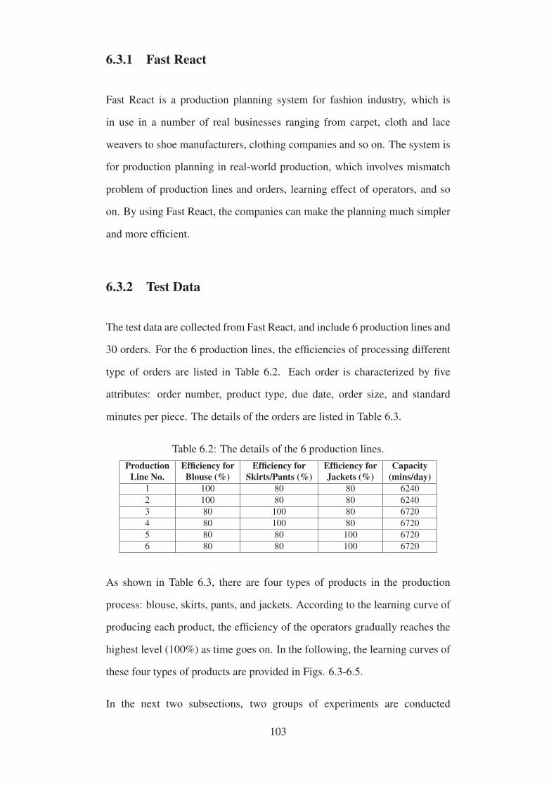
6.3.1 Fast React

Fast React is a production planning system for fashion industry, which is

in use in a number of real businesses ranging from carpet, cloth and lace

weavers to shoe manufacturers, clothing companies and so on. The system is

for production planning in real-world production, which involves mismatch

problem of production lines and orders, learning effect of operators, and so

on. By using Fast React, the companies can make the planning much simpler

and more efficient.

6.3.2 Test Data

The test data are collected from Fast React, and include 6 production lines and

30 orders. For the 6 production lines, the efficiencies of processing different

type of orders are listed in Table 6.2. Each order is characterized by five

attributes: order number, product type, due date, order size, and standard

minutes per piece. The details of the orders are listed in Table 6.3.

Table 6.2: The details of the 6 production lines.

ProductionLine No.

Efficiency forBlouse (%)

Efficiency forSkirts/Pants (%)

Efficiency forJackets (%)

Capacity(mins/day)

1 100 80 80 6240

2 100 80 80 6240

3 80 100 80 6720

4 80 100 80 6720

5 80 80 100 6720

6 80 80 100 6720

As shown in Table 6.3, there are four types of products in the production

process: blouse, skirts, pants, and jackets. According to the learning curve of

producing each product, the efficiency of the operators gradually reaches the

highest level (100%) as time goes on. In the following, the learning curves of

these four types of products are provided in Figs. 6.3-6.5.

In the next two subsections, two groups of experiments are conducted

103

Table 6.3: The details of the 30 orders.

Order No. Product Type Due Date(days)

Order Size(pieces) Standard Mins/Piece

1 Skirts 4 500 18.2

2 Skirts 4 700 18.2

3 Skirts 6 1000 16.7

4 Blouse 7 800 32.2

5 Skirts 8 800 16.7

6 Jackets 9 850 54.6

7 Skirts 9 1000 16.7

8 Skirts 7 400 16.7

9 Blouse 10 1250 15

10 Jackets 14 1000 53.78

11 Skirts 11 800 20.55

12 Blouse 13 1000 15

13 Pants 8 800 34

14 Blouse 20 3000 32.2

15 Skirts 15 800 20.55

16 Blouse 16 650 32.2

17 Skirts 14 1000 16.7

18 Jackets 16 500 53.78

19 Jackets 18 800 53.78

20 Skirts 10 870 14.2

21 Blouse 21 860 32.2

22 Skirts 19 1000 16.7

23 Skirts 18 800 20.55

24 Skirts 18 500 16.7

25 Blouse 20 700 32.2

26 Skirts 22 400 16.7

27 Jackets 26 850 54.6

28 Pants 22 600 34

29 Blouse 28 5000 12.6

30 Blouse 25 700 32.2

Figure 6.3: The learning curve of the blouse production.

Figure 6.4: The learning curve of the skirts/pants production.

104

Figure 6.5: The learning curve of the jackets production.

according to the test data. In the first experiment, 20 orders are assigned

to 6 production lines with the consideration of uncertain daily production

quantities. In the second experiment, we increase the number of orders to 30,

and these orders are also allocated to 6 production lines with the consideration

of uncertain daily production quantities.


Orders in Fashion Supply Chains

In the section, 20 orders are assigned to total 6 production lines in terms of

robust ETI-SHADE in fashion supply chains. The details of the 20 orders are

listed in Table 6.3, and the order number is from 1 to 20. The parameters

of ETI-SHADE are the same as the original work: MF = 0.5, MCR = 0.5,

H = NP, LN = 1, UN = NP, where NP is the population size and is set as

100 in this research. The number of neighbouring points HN = 10. The extent

of neighbourhood σ = [−σ1, σ2], where σ1 = 0.15, σ2 = 0.05. This setting

means that if the daily production quantity is set as 100, in real production

process, the quantity varies in the range of [85, 105]. The maximum number of

function evaluations (Max FES) is set to D ·10000, where D is the dimension

size of the problem.

Non-robust ETI-SHADE and robust ETI-SHADE are utilized to search the

optimal order schedules of the total 20 orders, respectively. The schedule

obtained by non-robust ETI-SHADE is called schedule A, and the one

105

achieved by robust ETI-SHADE is called schedule B. In Table 6.4, we record

the due date, finish date in schedule A and in schedule B respectively, which

are represented by the days from the beginning of the production. According

to the results in Table 6.4, it can be found that in both schedules, all the 20

orders can be finished before the due dates. While due to the uncertainty

introduced in schedule B, it costs more days to process 9 orders in schedule

B than that in schedule A, and these orders are highlighted in boldface. The

detailed order assignments on 6 production lines are provided in Tables 6.5-

6.6. The figures in the brackets denote the specific order size after order split.

Table 6.4: The finish dates of the 20 orders in schedule A and schedule B.

Order No. Due Date(days)

Finish Date inSchedule A (days)

Finish Date inSchedule B (days)

1 4 3 3

2 4 4 4

3 6 6 6

4 7 6 6

5 8 7 7

6 9 9 8

7 9 9 9

8 7 3 49 10 9 1010 14 13 1411 11 10 1112 13 12 12

13 8 7 814 20 20 20

15 15 13 1516 16 15 1617 14 11 1218 16 15 15

19 18 18 18

20 10 9 10

Table 6.5: The details of the order assignments on 6 production lines in

schedule A.Production

Line No. Order Assignments

1 O1(350), O3(800), O5(640), O7(500), O20(348), O17(500), O15(800)2 O1(150), O2(420), O3(200), O5(160), O13(400), O7(500), O11(560), O12(300), O14(1200)3 O4(800), O9(1250), O12(700), O16(65), O14(1800)4 O8(320), O13(400), O20(522), O11(240), O17(500), O16(585)5 O2(280), O8(80), O6(170), O10(700), O19(560)6 O6(680), O10(300), O18(500), O19(240)

In the following, we introduce uncertainty into schedule A, and the results

are given in Table 6.7. From the results, we can find that if uncertainty is

106


schedule B.Production


1 O2(350), O3(400), O5(480), O13(320), O20(870), O17(1000), O15(800)2 O1(250), O2(350), O3(600), O5(320), O7(600), O11(800), O14(1200)3 O8(400), O13(480), O7(400), O12(700), O16(650)4 O4(800), O9(1250), O12(300), O14(1800)5 O1(250), O6(255), O10(300), O18(500), O19(400)6 O6(595), O10(700), O19(400)

brought into schedule A, more days will be needed for 13 of the 20 orders,

which are highlighted in boldface. More seriously, for order 14 and order 19

(in boldface with gray background), they cannot be completed before their

due dates if uncertainty is considered in schedule A. Therefore, it can be

concluded that schedule A is sensitive to the perturbation, while schedule B

is robust to the perturbation. In practice, planners will update their schedule

during the production. If we consider the schedule like A, which is with fixed

daily production quantities, the schedule will be updated very often because of

the randomness in reality. While schedule B has uncertainty-tolerant ability.

So schedule B is recommended for the real-world production.


Orders in Fashion Supply Chains

In this section, the total 30 orders are assigned to 6 production lines in fashion

supply chains. The optimization algorithm is robust ETI-SHADE, which aims

to search the optimal and robust order schedules for the production. The

details of the orders and the production lines are listed in Tables 6.2-6.3. The

parameters of ETI-SHADE and the settings of the experiment are the same as

that in Experiment 1.

Non-robust ETI-SHADE and robust ETI-SHADE are applied to search the

optimal order schedules of the total 30 orders, respectively. The schedule

obtained by non-robust ETI-SHADE is called schedule C, and the one

107

Table 6.7: The finish dates of the 20 orders in schedule A when uncertainty is

introduced.


Finish Datein Schedule A

Finish Datein Schedule A

(With Uncertainty)1 4 3 3

2 4 4 4

3 6 6 6

4 7 6 6

5 8 7 86 9 9 9

7 9 9 9

8 7 3 49 10 9 1010 14 13 1411 11 10 1112 13 12 1313 8 7 814 20 20 2115 15 13 1416 16 15 1617 14 11 11

18 16 15 1619 18 18 1920 10 9 10

achieved by robust ETI-SHADE is called schedule D. In Table 6.8, we record

the due date, finish date in schedule C and in schedule D respectively, which

are represented by the days from the beginning of the production. According

to the results in Table 6.8, it can be found that in schedule C, all the orders can

be completed before their due dates. While due to the uncertainty introduced

in schedule D, it costs more days to process 16 orders in schedule D than that

in schedule C, and these orders are highlighted in boldface. More seriously, in

schedule D, four orders (i.e., orders 6, 7, 14, and 28) cannot be finished before

the due dates, which are highlighted in boldface with gray background. The

results indicate that uncertainty (i.e., varying daily production quantity) has a

great impact on the actual delivery date of the orders during the production

process. For these 4 four orders in schedule D, manufacturers can negotiate

earlier with the retailers who place these orders about the delay in delivery or

arrange operators to work extra hours. The detailed order assignments on 6

production lines are provided in Tables 6.9-6.10. The figures in the brackets

108

denote the specific order size after order split.

Table 6.8: The finish dates of the 30 orders in schedule C and schedule D.


Finish Date inSchedule C (days)

Finish Date inSchedule D (days)

1 4 3 42 4 4 4

3 6 6 6

4 7 6 6

5 8 8 8

6 9 9 107 9 9 108 7 6 6

9 10 9 9

10 14 11 11

11 11 11 11

12 13 11 11

13 8 8 8

14 20 20 2215 15 15 14

16 16 14 1517 14 12 1418 16 13 1519 18 16 1820 10 10 10

21 21 21 21

22 19 17 1923 18 15 1624 18 15 1725 20 20 20

26 22 18 2027 26 23 2528 22 21 2329 28 26 2830 25 24 25


schedule C.Production


1O1(250), O13(800), O7(600), O20(522), O11(160), O17(600),O23(800), O24(250), O22(600), O26(400), O28(600), O30(280)

2O2(560), O3(400), O8(400), O5(800), O7(400), O11(640),

O17(400), O15(800), O24(250), O22(400), O25(140), O21(430), O30(420)3 O1(250), O2(140), O3(600), O20(348), O12(200), O14(2100)4 O4(800), O9(1250), O12(800), O16(650), O14(900), O21(430), O29(2500)5 O6(85), O10(800), O18(250), O19(480), O27(850)6 O6(765), O10(200), O18(250), O19(320), O25(560), O29(2500)

In the following, we introduce uncertainty into schedule C, and the results

are given in Table 6.11. From the results, we can find that if uncertainty is

brought into schedule C, more days will be needed for 25 of the 30 orders,

which are highlighted in boldface. More seriously, for 10 orders (in boldface

109


schedule D.Production


1O1(50), O2(420), O3(200), O5(320), O13(400), O20(696), O11(560),

O17(900), O15(240), O23(560), O24(450), O22(700), O26(400), O28(420), O30(140)

2O2(280), O3(800), O13(400), O7(1000), O11(240), O17(100),

O15(560), O23(240), O24(50), O22(300), O25(490), O28(180), O27(85)

3O1(450), O8(400), O5(480), O20(174), O12(700),

O16(650), O25(210), O21(860), O30(560), O29(2000)4 O4(800), O9(1250), O12(300), O14(2100), O29(3000)5 O10(900), O18(500), O14(900)6 O6(850), O10(100), O19(800), O27(765)

with gray background), they cannot be completed before their due dates if

uncertainty is considered in schedule C. Look back at Table 6.8, in schedule

D, there are only total 4 orders that will violate the due dates. Therefore, it can

be concluded that schedule C is sensitive to the perturbation, while schedule

D is more robust to the perturbation.

6.3.5 Summary of the Experiments

In this section, non-robust and robust evolutionary algorithms (i.e., non-

robust and robust ETI-SHADE) are used for order scheduling problems in

fashion supply chains, respectively. According to the results shown above, it

can be concluded that order schedules obtained by non-robust ETI-SHADE

are sensitive to the perturbation in the real production, i.e., shifting daily

production quantity. And schedules obtained robust ETI-SHADE benefits the

real-world production in the following two ways: 1) if in the schedules, all

the orders can be finished before their due dates, the production can follow

these schedules; 2) if in the schedules, there are some orders that cannot

be completed before the due dates, manufacturers may be fully prepared

according to these schedules by negotiating earlier with the retailers who

place these orders about the delay in delivery or arranging operators to work

extra hours.

110

Table 6.11: The finish dates of the 30 orders in schedule C when uncertainty

is introduced.


Finish Datein Schedule C

Finish Datein Schedule C

(With Uncertainty)1 4 3 3

2 4 4 4

3 6 6 74 7 6 6

5 8 8 96 9 9 107 9 9 108 7 6 79 10 9 9

10 14 11 1211 11 11 1212 13 11 1213 8 8 8

14 20 20 2115 15 15 1616 16 14 1517 14 12 1318 16 13 1419 18 16 1720 10 10 1121 21 21 2222 19 17 1823 18 15 1624 18 15 1625 20 20 2226 22 18 1927 26 23 2428 22 21 2229 28 26 2830 25 24 25

111

6.4 Summary

In this chapter, robust evolutionary optimization is introduced to solve the

order scheduling problems in fashion supply chains. A robust evolutionary

algorithm called robust success-history based adaptive differential evolution

with event-triggered impulsive control scheme (robust ETI-SHADE) is pro-

posed for developing robust order schedules in fashion supply chains. Robust

ETI-SHADE aims to search optimal and robust schedules for the real-world

production. In addition, two groups of experiments are carried out to

display the effectiveness and superiority of introducing robust evolutionary

optimization into fashion order scheduling problems. The experimental

results show that schedules obtained by robust ETI-SHADE have uncertainty-

tolerant ability, and benefit the real-world production in fashion supply

chains.

112

Chapter 7

Conclusions

This research is set out to solve sales forecasting and order scheduling

problems in fashion supply chains via two hot branches of evolutionary op-

timization (multiobjective evolutionary optimization and robust evolutionary

optimization) for the first time, and hence to establish a competitive and robust

supply chain in fashion industry. This research has provided satisfactory

strategies for fashion sales forecasting and order scheduling problems by

means of multiobjective evolutionary optimization and robust evolutionary

optimization; meanwhile, the proposed models has also broadened the

applications of evolutionary optimization in wider areas. In this chapter,

firstly, the concluding remarks of this research are summarized, includ-

ing the summaries of the development of novel evolutionary algorithms,

multiobjective evolutionary optimization for fashion sales forecasting, and

robust evolutionary optimization for fashion order scheduling. Secondly, the

contributions of this research are given. Then the future work is presented

based on the limitations of this research. Lastly, the related publications are

listed at the end of this chapter.

113

7.1 Development of Novel Evolutionary

Algorithms

In Chapter 4, two variants of the evolutionary algorithms have been pro-

posed, one is a new multiobjective evolutionary algorithm (MOEA) called

nondominated sorting adaptive differential evolution (NSJADE), and the other

one is a novel differential evolution (DE) variant called differential evolution

with event-triggered impulsive control scheme (ETI-DE). Firstly, NSJADE

modifies the search engine of the classic MOEA called NSGA-II by replacing

genetic algorithm (GA) with an adaptive differential evolution (JADE). This

operation enhances the efficiency of the search, in which the useful historical

information of the population can be utilized. The experimental results reveal

that the presented NSJADE performs better than NSGA-II on multimodal

problems, which makes NSJADE a promising candidate for solving the

fashion sales forecasting in the later chapter. Secondly, ETI-DE integrates two

popular concepts in control theory, event-triggered mechanism and impulsive

control, into the design of DE. By means of ETI, both exploitation and

exploration abilities of the whole population in DE can be meliorated. The

experimental results show that ETI-DEs greatly improve the performance of

their original DEs on the test function at D = [30, 50, 100]. In addition, from

the results of the experiments in Section 4.2, ETI-SHADE exhibits the best

performance when dealing with the CEC 2014 test suite at D = [30, 50, 100].

Due to the superiority of ETI-SHADE in solving high-dimensional problems,

it is modified to fit into the robust optimization, and then to optimize the order

scheduling problem in fashion industry later on.

114

7.2 Multiobjective Evolutionary Optimization for

Fashion Sales Forecasting

In Chapter 5, fashion sales forecasting problems are investigated by a

multiobjective evolutionary optimization-based neural network model for

the first time. In detail, a multiobjective optimization-based neural net-

work model (MOONN) is developed to handle a short-term replenishment

forecasting problem in fashion supply chains. The model employs a new

multiobjective evolutionary algorithm called NSJADE to optimize the input

weights and hidden biases of NN for the short-term replenishment forecasting

problem, which acquires the forecasting accuracy while alleviating the

overfitting effect at the same time. Furthermore, the MOONN model also


replenishment forecasting cases. Meanwhile, in order to reduce the side

effects of insufficient historical data, the general root mean square error is

replaced with the average error of committing K-fold cross-validation on the

training samples as one of the two objectives in the optimization process.

Extensive experiments in terms of the real-world fashion retail data have

been carried out to validate the proposed MOONN model. The results of the

experiments indicate that the presented MOONN model can handle the short-



7.3 Robust Evolutionary Optimization for

Fashion Order Scheduling

In Chapter 6, fashion order scheduling problems are solved within the

framework of robust evolutionary optimization for the first time. In detail,

115

a robust evolutionary algorithm called robust success-history based adaptive

differential evolution with event-triggered impulsive control scheme (robust

ETI-SHADE) is employed to develop robust order schedules in fashion supply

chains. During the optimization process, robust ETI-SHADE evaluates the

HN neighbouring points of the individual, and then calculate the average

value of these HN values as the optimization objective of the order scheduling

problem. The intention is to obtain robust order schedules in fashion supply

chains. Two groups of experiments have been performed to show the

effectiveness of the introduction of robust evolutionary algorithms in fashion

order scheduling. It is revealed that the schedule got by non-robust ETI-

SHADE (schedule A) is sensitive to the perturbation, while the schedule

obtained by robust ETI-SHADE (schedule B) is robust to the perturbation.

In practice, planners will update their schedule during the production. If we

consider the schedule like A, which is with fixed daily production quantities,

the schedule will be updated very often because of the randomness in

reality. While schedule B has uncertainty-tolerant ability. So schedule B is

recommended for the real-world production.

7.4 Contributions of this Research

The contributions of this research include: 1) the contributions of proposing

the newly proposed evolutionary algorithms for fashion supply chains; 2)

the contributions of solving sales forecasting problems in fashion supply

chains by a multiobjective evolutionary optimization based neural network

model; 3) the contributions of solving order scheduling problems in fashion

supply chains within the framework of robust evolutionary optimization;

4) the performance of fashion supply chains can be greatly improved

by using multiobjective evolutionary optimization and robust evolutionary

optimization. In the following, these four contributions are discussed in detail.

116

Firstly, NSJADE is proposed based on a popular and classic MOEA: NSGA-

II. In recent years, many works have focused on the improvement of NSGA-

II, and our research belongs to one of them. The presented NSJADE

enriches the set of the MOEAs, which derive from the idea of NSGA-II.

Furthermore, a new scheme ETI is developed for the DE algorithms. Unlike

other research, this research is an interdisciplinary one, which utilizes event-

triggered mechanism (ETM) and impulsive control, two concepts in control

theory, to improve the search performance of DE. The development of ETI

reveal that it is promising to develop powerful evolutionary algorithms by

knowledge in other disciplines. The proposed ETI also sheds light on the

understandings of ETM and impulsive control in evolutionary computation,

which broadens the applications of ETM and impulsive control in wider areas.

Secondly, a multiobjective optimization-based neural network model (MOON-

N) is proposed for the sales forecasting problems in fashion supply chains. It

is the first work that investigates the sales forecasting problems in fashion

supply chains by using MOO-based model. Different from other popular

models, MOONN can ensure better forecasting performance and alleviate

the overfitting effect at the same time. In addition, the MOONN model also


forecasting cases; while in other models, the number of hidden nodes of NN

is not adaptive.

Thirdly, order scheduling problems in fashion supply chains are solved in

the framework of robust evolutionary optimization for the first time. When

visiting some garment factories in Mainland China, it is found that most of the

time, operators cannot finish the daily production quantity that was assigned

to them and the production plans were shifted very often. After production

starts, frequent modification of production plans will increase labor and time

cost, which may reduce production efficiency and fail to complete the orders

before their delivery dates. While the order schedules obtained by robust

117

evolutionary algorithms are robust to the perturbation of daily production

quantities. When robust schedules are adopted, planners will reduce the

times of modifying the order schedules during the production process, which

increases the efficiency of the production in fashion supply chains. Besides,

in this research, matching problem and learning effect are also considered in

the optimization process, which makes the experimental environment more

close to the real-world production environment.

Fourthly, two key decision-making problems in fashion supply chain man-

agement are investigated within the framework of evolutionary optimiza-

tion. According to the experimental results, multiobjective evolutionary

optimization and robust evolutionary optimization exhibit effectiveness in

sales forecasting and order scheduling problems in fashion supply chain

management. Therefore, the performance of fashion supply chains can be

greatly enhanced by introducing multiobjective evolutionary optimization and

robust evolutionary optimization.

7.5 Limitations and Future Work

In Chapter 5, MOONN model is used to solve the short-term replenishment

forecasting problem in fashion supply chains, which belongs to a multivariate

forecasting problem. As introduced before, forecasting problems can be

divided into two categories: univariate and multivariate. Therefore, the

performance of MOONN on univariate forecasting problems needs to be

examined in the future research. Furthermore, it is noticed that to solve

the forecasting problem in this research, the inputs of the MOONN model

include weather data, economic data and historical sales data. However, these

inputs may not be optimal, which means some inputs may be redundant. And

irrelevant input variables probably decrease the accuracy of the forecasting

118

model. So it is necessary to examine the redundancy of the input variables.

Since ELM was proposed by Huang et al. [7], it has been widely used

in fashion sales forecasting. While recently, a new ELM, called optimally

pruned extreme learning machine (OP-ELM), has been presented, which can

delete the irrelevant inputs for the forecasting problems [143, 144]. Hence, in

the future, we are interested to investigate whether OP-ELM is effective for

the fashion sales forecasting problems.

In Chapter 6, a robust evolutionary algorithm is employed to optimize the

order scheduling problems in fashion supply chains. In this work, the main

purpose is to introduce robust evolutionary algorithms into the optimization

of fashion order scheduling problems. So in order to simplify the problem,

we set several assumptions, such as only considering the sewing process,

the order can be at most split into two sub-orders, and so on. In the

future research, it is necessary to consider more processes and more sub-

orders. Moreover, in this research, it is assumed that all the orders are ready

for production when the production process starts. However, in real-world

apparel production, a series of activities need to be carried out before an order

can be put into production. And these activities are known as pre-production

events. In future research, pre-production events can be considered into the

robust order scheduling problems in the fashion industry, and the problem can

be modelled as a multiobjective optimization problem.

7.6 Related Publications

The author demonstrated the originality of this research through the following

publications:

[1] W. Du, S. Y. S. Leung, Y. Tang, A. V. Vasilakos. Differential evolution

with event-triggered impulsive control. IEEE Transactions on Cybernetics,

119

accepted, 2016.

[2] W. Du, S. Y. S. Leung, C. K. Kwong. Time series forecasting by

neural networks: A knee point-based multiobjective evolutionary algorithm

approach. Expert Systems with Applications, 2014, 41(18): 8049-8061.

[3] W. Du, S. Y. S. Leung, C. K. Kwong. A multiobjective optimization-based

neural network model for short-term replenishment forecasting in fashion

industry. Neurocomputing, 2015, 151: 342-353.

[4] W. Du, S. Y. S. Leung, C. K. Kwong, Y. Tang, Improving differential

evolution with impulsive control framework, in 2015 IEEE Congress on

Evolutionary Computation (CEC), pp. 3080-3087, IEEE, 2015.

120

Appendix

Table A.1: Experimental results of DE/rand/1/bin, DE/best/1/bin, jDE, JADE

and the related ETI-based variants for functions F01-F30 at D = 30.Function DE/rand/1/bin ETI-DE/rand/1/bin DE/best/1/bin ETI-DE/best/1/bin

F01 5.731E+04 ± 4.288E+04 9.916E+04 ± 6.514E+04− 2.395E+07 ± 8.307E+06 1.943E+06 ± 1.009E+06+F02 2.229E-15 ± 7.717E-15 0.000E+00 ± 0.000E+00+ 2.786E-14 ± 3.980E-15 2.341E-14 ± 1.094E-14+F03 5.573E-15 ± 1.707E-14 0.000E+00 ± 0.000E+00+ 2.003E-08 ± 1.465E-08 3.864E-09 ± 2.710E-09+F04 2.340E-01 ± 1.217E-01 1.638E+00 ± 8.823E+00− 6.658E+01 ± 2.845E+01 9.530E+00 ± 2.228E+01+F05 2.094E+01 ± 5.340E-02 2.036E+01 ± 9.584E-02+ 2.092E+01 ± 5.139E-02 2.037E+01 ± 1.520E-01+F06 4.206E-01 ± 7.135E-01 6.459E-01 ± 9.502E-01≈ 1.136E+00 ± 1.056E+00 1.491E+00 ± 1.247E+00≈F07 3.383E-04 ± 1.709E-03 0.000E+00 ± 0.000E+00≈ 5.068E-03 ± 8.609E-03 4.299E-03 ± 5.928E-03≈F08 1.256E+02 ± 2.355E+01 2.705E+01 ± 7.498E+00+ 8.643E+01 ± 1.907E+01 1.676E+01 ± 4.181E+00+F09 1.780E+02 ± 7.943E+00 2.620E+01 ± 1.143E+01+ 1.830E+02 ± 1.006E+01 3.922E+01 ± 1.097E+01+F10 5.153E+03 ± 7.884E+02 4.790E+02 ± 2.054E+02+ 1.447E+03 ± 1.012E+03 2.492E+02 ± 1.397E+02+F11 6.817E+03 ± 2.739E+02 1.659E+03 ± 6.172E+02+ 6.411E+03 ± 2.731E+02 2.042E+03 ± 6.790E+02+F12 2.426E+00 ± 2.209E-01 1.539E-01 ± 7.075E-02+ 2.061E+00 ± 2.656E-01 1.609E-01 ± 9.056E-02+F13 3.525E-01 ± 4.635E-02 1.294E-01 ± 4.294E-02+ 3.814E-01 ± 4.366E-02 2.266E-01 ± 5.200E-02+F14 2.834E-01 ± 3.250E-02 2.418E-01 ± 4.008E-02+ 3.352E-01 ± 1.816E-01 3.145E-01 ± 1.507E-01≈F15 1.548E+01 ± 9.788E-01 3.726E+00 ± 1.152E+00+ 1.653E+01 ± 1.111E+00 4.421E+00 ± 1.688E+00+F16 1.242E+01 ± 2.280E-01 8.754E+00 ± 9.531E-01+ 1.215E+01 ± 3.340E-01 9.596E+00 ± 8.715E-01+F17 1.331E+03 ± 2.044E+02 4.381E+02 ± 3.364E+02+ 5.478E+05 ± 3.288E+05 6.073E+04 ± 5.213E+04+F18 5.407E+01 ± 5.476E+00 1.061E+01 ± 4.898E+00+ 9.291E+02 ± 5.305E+02 1.979E+03 ± 2.396E+03≈F19 4.529E+00 ± 3.228E-01 2.279E+00 ± 6.371E-01+ 6.547E+00 ± 1.325E+00 4.723E+00 ± 1.589E+00+F20 3.354E+01 ± 7.184E+00 7.475E+00 ± 2.768E+00+ 9.802E+01 ± 1.407E+01 3.668E+01 ± 1.679E+01+F21 6.480E+02 ± 1.565E+02 2.353E+02 ± 2.406E+02+ 2.051E+04 ± 9.870E+03 1.143E+04 ± 1.013E+04+F22 3.902E+01 ± 3.470E+01 1.268E+02 ± 1.332E+02− 1.570E+02 ± 1.108E+02 1.964E+02 ± 1.157E+02≈F23 3.152E+02 ± 4.019E-13 3.152E+02 ± 4.019E-13≈ 3.152E+02 ± 4.019E-13 3.152E+02 ± 4.019E-13≈F24 2.185E+02 ± 8.658E+00 2.182E+02 ± 8.527E+00≈ 2.238E+02 ± 7.113E+00 2.228E+02 ± 8.438E+00≈F25 2.027E+02 ± 1.438E-01 2.027E+02 ± 1.201E-01≈ 2.089E+02 ± 2.326E+00 2.030E+02 ± 4.116E-01+F26 1.003E+02 ± 4.955E-02 1.001E+02 ± 4.295E-02+ 1.004E+02 ± 5.113E-02 1.002E+02 ± 4.926E-02+F27 3.592E+02 ± 4.864E+01 3.542E+02 ± 4.772E+01≈ 3.793E+02 ± 5.099E+01 3.804E+02 ± 5.094E+01≈F28 8.037E+02 ± 2.643E+01 8.111E+02 ± 2.479E+01≈ 7.832E+02 ± 5.699E+01 8.085E+02 ± 4.622E+01−F29 6.838E+02 ± 1.331E+02 6.930E+02 ± 1.155E+02− 1.775E+05 ± 1.249E+06 1.707E+05 ± 1.210E+06+F30 5.817E+02 ± 2.335E+02 6.597E+02 ± 2.440E+02− 1.985E+03 ± 7.121E+02 1.723E+03 ± 7.477E+02≈

+/≈/− - 18/7/5 - 20/9/1

Function jDE ETI-jDE JADE ETI-JADEF01 7.607E+04 ± 7.289E+04 6.028E+04 ± 5.206E+04≈ 6.786E+02 ± 1.513E+03 7.397E+02 ± 1.392E+03≈F02 1.672E-15 ± 6.754E-15 0.000E+00 ± 0.000E+00≈ 2.062E-14 ± 1.281E-14 0.000E+00 ± 0.000E+00+F03 1.895E-14 ± 2.706E-14 0.000E+00 ± 0.000E+00+ 7.013E-03 ± 4.473E-02 6.664E-04 ± 1.563E-03+F04 4.419E+00 ± 1.263E+01 1.510E+00 ± 8.925E-01≈ 9.140E-14 ± 5.094E-14 4.570E-14 ± 3.599E-14+F05 2.031E+01 ± 3.685E-02 2.018E+01 ± 7.198E-02+ 2.029E+01 ± 3.142E-02 2.000E+01 ± 6.736E-03+F06 9.958E+00 ± 5.049E+00 1.196E+00 ± 1.339E+00+ 9.776E+00 ± 2.184E+00 5.091E-01 ± 6.621E-01+F07 8.694E-14 ± 5.375E-14 0.000E+00 ± 0.000E+00+ 1.933E-04 ± 1.380E-03 1.450E-04 ± 1.036E-03+F08 0.000E+00 ± 0.000E+00 0.000E+00 ± 0.000E+00≈ 0.000E+00 ± 0.000E+00 0.000E+00 ± 0.000E+00≈F09 4.833E+01 ± 7.541E+00 3.024E+01 ± 7.435E+00+ 2.661E+01 ± 4.899E+00 2.215E+01 ± 6.311E+00+F10 8.164E-04 ± 5.831E-03 3.375E-02 ± 1.584E-01− 5.715E-03 ± 1.027E-02 4.450E-02 ± 2.533E-02−F11 2.467E+03 ± 2.574E+02 1.635E+03 ± 3.810E+02+ 1.609E+03 ± 1.860E+02 1.161E+03 ± 3.315E+02+F12 4.379E-01 ± 6.200E-02 1.086E-01 ± 3.883E-02+ 2.617E-01 ± 3.054E-02 7.452E-02 ± 2.892E-02+F13 2.983E-01 ± 4.292E-02 1.418E-01 ± 4.445E-02+ 2.108E-01 ± 3.266E-02 1.333E-01 ± 3.113E-02+F14 2.849E-01 ± 3.398E-02 2.312E-01 ± 3.912E-02+ 2.363E-01 ± 2.931E-02 1.653E-01 ± 2.401E-02+F15 5.760E+00 ± 7.449E-01 3.138E+00 ± 8.144E-01+ 3.071E+00 ± 3.652E-01 2.498E+00 ± 4.397E-01+F16 9.988E+00 ± 2.805E-01 8.749E+00 ± 6.316E-01+ 9.387E+00 ± 4.264E-01 8.034E+00 ± 5.731E-01+F17 2.421E+03 ± 2.324E+03 1.644E+03 ± 1.330E+03≈ 2.156E+04 ± 3.901E+02 7.018E+03 ± 4.133E+04+F18 1.624E+01 ± 7.817E+00 4.974E+01 ± 2.227E+02≈ 1.108E+02 ± 1.900E+02 5.322E+01 ± 2.940E+01+F19 4.667E+00 ± 7.450E-01 3.187E+00 ± 7.709E-01+ 4.712E+00 ± 9.733E-01 3.990E+00 ± 7.751E-01+F20 1.183E+01 ± 4.053E+00 9.888E+00 ± 3.417E+00+ 3.197E+03 ± 2.827E+03 1.503E+02 ± 1.329E+02+F21 2.704E+02 ± 1.978E+02 2.701E+02 ± 2.337E+02≈ 1.818E+04 ± 1.829E+04 1.010E+04 ± 3.108E+04+F22 1.385E+02 ± 7.209E+01 8.190E+01 ± 7.052E+01+ 1.574E+02 ± 5.828E+01 1.250E+02 ± 8.933E+01+F23 3.152E+02 ± 4.158E-13 3.152E+02 ± 3.591E-13≈ 3.152E+02 ± 4.019E-13 3.152E+02 ± 4.019E-13≈F24 2.244E+02 ± 1.327E+00 2.246E+02 ± 1.698E+00≈ 2.247E+02 ± 2.685E+00 2.257E+02 ± 3.520E+00≈F25 2.034E+02 ± 6.756E-01 2.033E+02 ± 5.580E-01≈ 2.039E+02 ± 1.286E+00 2.036E+02 ± 9.330E-01≈F26 1.003E+02 ± 4.065E-02 1.001E+02 ± 4.171E-02+ 1.002E+02 ± 3.378E-02 1.001E+02 ± 2.824E-02+F27 3.719E+02 ± 4.554E+01 3.615E+02 ± 4.769E+01≈ 3.479E+02 ± 5.006E+01 3.296E+02 ± 4.276E+01+F28 7.949E+02 ± 2.382E+01 8.093E+02 ± 2.925E+01− 7.939E+02 ± 3.596E+01 7.811E+02 ± 2.611E+01+F29 8.195E+02 ± 9.126E+01 8.497E+02 ± 1.694E+02≈ 7.382E+02 ± 1.024E+02 8.034E+02 ± 2.778E+02≈F30 1.594E+03 ± 7.014E+02 1.586E+03 ± 7.090E+02≈ 1.595E+03 ± 6.113E+02 1.599E+03 ± 5.335E+02≈

+/≈/− - 15/13/2 - 22/7/1

121

Table A.2: Experimental results of CoDE, SaDE, ODE, EPSDE and the

related ETI-based variants for functions F01-F30 at D = 30.Function CoDE ETI-CoDE SaDE ETI-SaDE

F01 2.184E+04 ± 1.332E+04 3.804E+04 ± 3.551E+04− 2.154E+05 ± 1.393E+05 3.172E+05 ± 2.056E+05−F02 5.669E+00 ± 2.394E+00 2.080E+00 ± 9.575E-01+ 0.000E+00 ± 0.000E+00 1.115E-15 ± 5.572E-15≈F03 1.333E-04 ± 6.273E-05 7.439E-05 ± 3.463E-05+ 6.353E-14 ± 1.997E-13 3.745E-13 ± 9.110E-13−F04 2.204E+01 ± 2.401E+01 1.509E+01 ± 2.130E+01+ 4.273E+01 ± 3.633E+01 5.201E+01 ± 3.374E+01≈F05 2.061E+01 ± 5.216E-02 2.042E+01 ± 1.322E-01+ 2.057E+01 ± 5.161E-02 2.001E+01 ± 1.948E-02+F06 2.124E+01 ± 1.822E+00 6.675E+00 ± 3.235E+00+ 1.719E+00 ± 1.057E+00 2.080E+00 ± 1.352E+00≈F07 5.371E-05 ± 5.881E-05 1.358E-05 ± 3.937E-05+ 3.183E-03 ± 8.174E-03 3.955E-03 ± 8.490E-03≈F08 1.824E+01 ± 1.636E+00 6.334E+00 ± 1.895E+00+ 0.000E+00 ± 0.000E+00 0.000E+00 ± 0.000E+00≈F09 1.399E+02 ± 9.160E+00 8.767E+01 ± 2.032E+01+ 5.952E+01 ± 1.560E+01 3.110E+01 ± 9.134E+00+F10 7.704E+02 ± 1.002E+02 2.423E+02 ± 4.743E+01+ 1.510E-01 ± 2.273E-01 1.282E-01 ± 2.626E-01≈F11 4.811E+03 ± 2.151E+02 3.511E+03 ± 6.444E+02+ 3.892E+03 ± 2.947E+02 1.619E+03 ± 4.800E+02+F12 9.812E-01 ± 1.267E-01 5.455E-01 ± 1.853E-01+ 8.832E-01 ± 1.056E-01 8.407E-02 ± 5.259E-02+F13 4.681E-01 ± 4.819E-02 3.347E-01 ± 4.548E-02+ 2.622E-01 ± 4.002E-02 1.299E-01 ± 3.373E-02+F14 2.747E-01 ± 3.585E-02 2.568E-01 ± 3.001E-02+ 2.321E-01 ± 2.717E-02 2.048E-01 ± 3.540E-02+F15 1.364E+01 ± 1.053E+00 1.104E+01 ± 1.529E+00+ 8.765E+00 ± 1.110E+00 2.943E+00 ± 7.349E-01+F16 1.166E+01 ± 2.212E-01 1.072E+01 ± 4.441E-01+ 1.115E+01 ± 3.483E-01 8.856E+00 ± 6.375E-01+F17 1.459E+03 ± 1.392E+02 1.111E+03 ± 2.613E+02+ 1.115E+03 ± 8.520E+02 1.057E+03 ± 6.486E+02≈F18 4.886E+01 ± 6.302E+00 3.932E+01 ± 8.687E+00+ 6.130E+01 ± 1.971E+01 6.963E+01 ± 2.024E+01−F19 7.146E+00 ± 9.217E-01 5.521E+00 ± 4.447E-01+ 4.416E+00 ± 6.744E-01 3.247E+00 ± 5.728E-01+F20 3.122E+01 ± 4.810E+00 1.868E+01 ± 4.791E+00+ 2.907E+01 ± 1.633E+01 2.618E+01 ± 1.286E+01≈F21 7.434E+02 ± 1.231E+02 4.671E+02 ± 1.650E+02+ 3.048E+02 ± 1.844E+02 3.479E+02 ± 3.775E+02≈F22 1.379E+02 ± 5.940E+01 6.633E+01 ± 6.230E+01+ 1.271E+02 ± 6.225E+01 1.336E+02 ± 7.198E+01≈F23 3.152E+02 ± 5.604E-07 3.152E+02 ± 2.420E-07+ 3.152E+02 ± 2.267E-13 3.152E+02 ± 3.591E-13−F24 2.259E+02 ± 5.965E-01 2.236E+02 ± 1.858E+00+ 2.245E+02 ± 9.550E-01 2.250E+02 ± 1.819E+00≈F25 2.029E+02 ± 1.372E-01 2.029E+02 ± 1.698E-01≈ 2.054E+02 ± 3.269E+00 2.063E+02 ± 2.749E+00≈F26 1.004E+02 ± 5.399E-02 1.003E+02 ± 5.619E-02+ 1.003E+02 ± 3.863E-02 1.001E+02 ± 3.469E-02+F27 4.006E+02 ± 2.169E-01 4.006E+02 ± 2.300E-01≈ 3.622E+02 ± 3.573E+01 3.665E+02 ± 3.922E+01≈F28 9.339E+02 ± 2.252E+01 8.144E+02 ± 3.637E+01+ 8.567E+02 ± 2.882E+01 8.638E+02 ± 3.121E+01≈F29 6.527E+02 ± 1.649E+02 5.619E+02 ± 2.108E+02≈ 7.988E+02 ± 1.499E+02 8.626E+02 ± 1.532E+02−F30 1.177E+03 ± 1.224E+02 8.947E+02 ± 1.353E+02+ 8.989E+02 ± 2.985E+02 9.272E+02 ± 2.869E+02≈

+/≈/− - 26/3/1 - 10/15/5

Function ODE ETI-ODE EPSDE ETI-EPSDEF01 1.170E+05 ± 8.746E+04 1.309E+05 ± 1.044E+05≈ 5.591E+04 ± 1.059E+05 3.511E+04 ± 4.930E+04+F02 1.112E+03 ± 2.697E+03 1.003E+03 ± 2.884E+03+ 3.065E-14 ± 1.783E-14 3.734E-14 ± 5.068E-14≈F03 2.786E-14 ± 2.870E-14 7.802E-15 ± 1.976E-14+ 2.848E-12 ± 1.696E-11 4.815E-13 ± 1.081E-12≈F04 6.494E+00 ± 1.809E+01 4.981E+00 ± 1.565E+01≈ 6.990E-04 ± 3.563E-03 8.933E-02 ± 1.970E-01−F05 2.079E+01 ± 1.377E-01 2.041E+01 ± 1.190E-01+ 2.040E+01 ± 3.218E-02 2.019E+01 ± 7.086E-02+F06 7.431E-01 ± 9.961E-01 6.091E-01 ± 9.048E-01≈ 2.127E+01 ± 1.216E+00 7.191E+00 ± 2.588E+00+F07 7.247E-04 ± 2.928E-03 9.662E-04 ± 4.326E-03− 9.140E-14 ± 5.094E-14 0.000E+00 ± 0.000E+00+F08 4.823E+01 ± 1.830E+01 3.366E+01 ± 1.211E+01+ 0.000E+00 ± 0.000E+00 0.000E+00 ± 0.000E+00≈F09 3.137E+01 ± 2.547E+01 2.273E+01 ± 6.578E+00≈ 5.620E+01 ± 7.875E+00 2.564E+01 ± 6.439E+00+F10 3.028E+03 ± 6.371E+02 1.250E+03 ± 3.774E+02+ 4.952E+01 ± 7.321E+01 7.127E-01 ± 7.791E-01+F11 3.015E+03 ± 1.585E+03 1.856E+03 ± 5.142E+02+ 4.026E+03 ± 2.773E+02 1.785E+03 ± 5.206E+02+F12 9.704E-01 ± 4.947E-01 2.141E-01 ± 1.401E-01+ 5.957E-01 ± 7.183E-02 1.541E-01 ± 6.239E-02+F13 3.238E-01 ± 5.479E-02 2.322E-01 ± 5.860E-02+ 2.641E-01 ± 3.122E-02 1.081E-01 ± 2.398E-02+F14 2.564E-01 ± 4.047E-02 2.407E-01 ± 3.660E-02+ 2.957E-01 ± 6.696E-02 2.462E-01 ± 5.273E-02+F15 6.645E+00 ± 3.582E+00 3.555E+00 ± 1.108E+00+ 6.666E+00 ± 6.908E-01 2.658E+00 ± 5.487E-01+F16 1.190E+01 ± 7.073E-01 9.955E+00 ± 8.098E-01+ 1.136E+01 ± 3.455E-01 9.872E+00 ± 7.322E-01+F17 1.499E+03 ± 1.747E+02 5.678E+02 ± 2.914E+02+ 1.483E+04 ± 2.057E+04 7.063E+03 ± 7.119E+03≈F18 1.117E+01 ± 1.004E+01 9.229E+00 ± 3.693E+00≈ 7.573E+01 ± 6.570E+01 6.578E+01 ± 6.310E+01≈F19 3.214E+00 ± 8.941E-01 2.381E+00 ± 5.002E-01+ 1.391E+01 ± 7.427E-01 1.046E+01 ± 2.087E+00+F20 3.754E+01 ± 5.030E+00 9.498E+00 ± 4.159E+00+ 2.419E+01 ± 7.229E+00 1.411E+01 ± 5.658E+00+F21 7.235E+02 ± 1.666E+02 2.892E+02 ± 2.336E+02+ 2.403E+03 ± 5.676E+03 8.514E+02 ± 1.585E+03+F22 2.172E+02 ± 1.255E+02 2.274E+02 ± 1.251E+02≈ 2.758E+02 ± 7.885E+01 1.719E+02 ± 1.085E+02+F23 3.152E+02 ± 4.019E-13 3.152E+02 ± 4.019E-13≈ 3.140E+02 ± 5.705E-13 3.140E+02 ± 2.034E-13+F24 2.152E+02 ± 1.083E+01 2.158E+02 ± 1.031E+01≈ 2.254E+02 ± 4.600E+00 2.252E+02 ± 3.434E+00≈F25 2.026E+02 ± 1.114E-01 2.027E+02 ± 1.049E-01≈ 2.003E+02 ± 2.107E-01 2.003E+02 ± 1.150E-01≈F26 1.003E+02 ± 3.882E-02 1.002E+02 ± 5.584E-02+ 1.003E+02 ± 4.216E-02 1.001E+02 ± 3.363E-02+F27 3.928E+02 ± 2.734E+01 3.929E+02 ± 2.736E+01≈ 8.960E+02 ± 1.116E+02 4.750E+02 ± 7.544E+01+F28 7.981E+02 ± 2.702E+01 8.028E+02 ± 2.941E+01≈ 3.805E+02 ± 5.494E+00 3.801E+02 ± 5.766E+00≈F29 6.989E+02 ± 9.394E+01 6.985E+02 ± 1.229E+02≈ 2.150E+02 ± 1.084E+00 2.121E+02 ± 1.643E+00+F30 5.822E+02 ± 1.637E+02 5.900E+02 ± 2.006E+02≈ 5.793E+02 ± 1.399E+02 4.034E+02 ± 1.060E+02+

+/≈/− - 16/13/1 - 21/8/1

122

Table A.3: Experimental results of SHADE, OXDE and the related ETI-based

variants for functions F01-F30 at D = 30.Function SHADE ETI-SHADE OXDE ETI-OXDE

F01 3.906E+02 ± 7.084E+02 8.130E+02 ± 1.615E+03≈ 6.857E+04 ± 4.661E+04 1.223E+05 ± 1.088E+05−F02 1.505E-14 ± 1.433E-14 0.000E+00 ± 0.000E+00+ 1.672E-15 ± 6.754E-15 0.000E+00 ± 0.000E+00≈F03 5.016E-14 ± 1.850E-14 0.000E+00 ± 0.000E+00+ 7.802E-15 ± 1.976E-14 0.000E+00 ± 0.000E+00+F04 7.691E-14 ± 3.909E-14 3.232E-14 ± 3.062E-14+ 3.840E-01 ± 1.739E-01 1.790E+00 ± 8.803E+00−F05 2.012E+01 ± 1.870E-02 2.001E+01 ± 1.381E-02+ 2.094E+01 ± 5.352E-02 2.035E+01 ± 1.120E-01+F06 2.020E-01 ± 4.562E-01 1.535E-01 ± 3.487E-01≈ 2.653E-01 ± 5.908E-01 4.959E-01 ± 7.787E-01≈F07 1.450E-04 ± 1.036E-03 0.000E+00 ± 0.000E+00+ 1.933E-04 ± 1.380E-03 0.000E+00 ± 0.000E+00+F08 0.000E+00 ± 0.000E+00 0.000E+00 ± 0.000E+00≈ 7.314E+01 ± 1.018E+01 2.262E+01 ± 6.532E+00+F09 1.716E+01 ± 2.587E+00 2.319E+01 ± 7.531E+00− 1.680E+02 ± 1.024E+01 2.331E+01 ± 8.349E+00+F10 6.123E-03 ± 1.199E-02 5.062E-02 ± 3.067E-02− 3.536E+03 ± 3.991E+02 4.691E+02 ± 1.807E+02+F11 1.466E+03 ± 2.063E+02 1.073E+03 ± 3.004E+02+ 6.778E+03 ± 2.403E+02 1.580E+03 ± 6.373E+02+F12 1.708E-01 ± 2.257E-02 9.390E-02 ± 2.741E-02+ 2.318E+00 ± 2.597E-01 1.542E-01 ± 8.034E-02+F13 1.939E-01 ± 3.422E-02 8.990E-02 ± 3.152E-02+ 3.048E-01 ± 4.257E-02 1.168E-01 ± 3.644E-02+F14 2.316E-01 ± 3.143E-02 2.330E-01 ± 4.701E-02≈ 2.786E-01 ± 2.713E-02 2.413E-01 ± 4.478E-02+F15 2.648E+00 ± 3.546E-01 2.723E+00 ± 5.139E-01≈ 1.497E+01 ± 9.149E-01 3.153E+00 ± 7.595E-01+F16 9.123E+00 ± 3.900E-01 8.287E+00 ± 9.698E-01+ 1.220E+01 ± 3.029E-01 8.626E+00 ± 9.342E-01+F17 1.026E+03 ± 3.523E+02 6.763E+02 ± 3.557E+02+ 1.369E+03 ± 1.878E+02 3.940E+02 ± 2.234E+02+F18 5.098E+01 ± 2.850E+01 2.632E+01 ± 1.758E+01+ 5.112E+01 ± 6.109E+00 9.004E+00 ± 3.580E+00+F19 4.387E+00 ± 8.805E-01 2.796E+00 ± 9.481E-01+ 4.370E+00 ± 4.166E-01 2.149E+00 ± 6.486E-01+F20 9.799E+00 ± 4.687E+00 1.013E+01 ± 5.200E+00≈ 3.386E+01± 6.464E+00 7.226E+00 ± 3.777E+00+F21 2.749E+02 ± 1.287E+02 2.048E+02 ± 9.481E+01+ 6.908E+02 ± 1.468E+02 2.036E+02 ± 2.099E+02+F22 1.298E+02 ± 6.434E+01 1.127E+02 ± 6.322E+01≈ 3.157E+01 ± 2.178E+01 8.262E+01 ± 9.952E+01≈F23 3.152E+02 ± 4.019E-13 3.152E+02 ± 4.019E-13≈ 3.152E+02 ± 4.019E-13 3.152E+02 ± 4.019E-13≈F24 2.248E+02 ± 2.067E+00 2.245E+02 ± 1.932E+00≈ 2.201E+02 ± 7.656E+00 2.222E+02 ± 3.318E+00≈F25 2.035E+02 ± 7.346E-01 2.033E+02 ± 6.748E-01≈ 2.027E+02 ± 2.035E-01 2.027E+02 ± 1.681E-01≈F26 1.002E+02 ± 2.962E-02 1.001E+02 ± 2.649E-02+ 1.003E+02 ± 4.333E-02 1.001E+02 ± 4.341E-02+F27 3.118E+02 ± 3.272E+01 3.169E+02 ± 3.601E+01≈ 3.442E+02 ± 4.998E+01 3.449E+02 ± 4.755E+01≈F28 8.333E+02 ± 3.827E+01 8.170E+02 ± 3.752E+01+ 7.990E+02 ± 2.660E+01 8.057E+02 ± 2.462E+01≈F29 7.241E+02 ± 1.024E+01 7.177E+02 ± 3.016E+01≈ 6.001E+02 ± 2.283E+02 6.650E+02 ± 1.651E+02≈F30 1.342E+03 ± 4.891E+02 1.383E+03 ± 4.858E+02≈ 5.173E+02 ± 1.192E+02 5.986E+02 ± 2.165E+02−

+/≈/− - 15/13/2 - 18/9/3

123



F01 1.399E+06 ± 5.347E+05 8.417E+05 ± 2.873E+05+ 1.002E+08 ± 2.370E+07 4.095E+06 ± 1.553E+06+F02 1.913E+02 ± 7.531E+02 3.045E+03 ± 4.719E+03− 4.361E+02 ± 7.096E+02 7.788E+03 ± 8.179E+03−F03 2.863E-01 ± 1.144E+00 3.588E-01 ± 7.479E-01≈ 2.509E+04 ± 3.903E+03 2.343E+03 ± 8.583E+02+F04 7.729E+01 ± 2.730E+01 8.793E+01 ± 8.976E+00≈ 9.695E+01 ± 3.682E+00 8.948E+01 ± 1.293E+01+F05 2.113E+01 ± 3.349E-02 2.042E+01 ± 1.022E-01+ 2.111E+01 ± 3.342E-02 2.021E+01 ± 1.193E-01+F06 1.215E+00 ± 1.384E+00 1.786E+00 ± 1.671E+00≈ 3.805E+00 ± 2.336E+00 3.646E+00 ± 1.741E+00≈F07 1.450E-04 ± 1.036E-03 1.450E-04 ± 1.036E-03+ 1.498E-03 ± 3.975E-03 2.560E-03 ± 6.209E-03−F08 1.942E+02 ± 4.580E+01 4.596E+01 ± 1.224E+01+ 2.521E+02 ± 1.859E+01 3.865E+01 ± 8.400E+00+F09 3.517E+02 ± 1.609E+01 4.258E+01 ± 1.185E+01+ 3.856E+02 ± 1.613E+01 8.326E+01 ± 2.356E+01+F10 9.467E+03 ± 1.349E+03 1.007E+03 ± 4.188E+02+ 7.469E+03 ± 7.172E+02 6.763E+02 ± 3.118E+02+F11 1.299E+04 ± 3.968E+02 3.912E+03 ± 1.003E+03+ 1.291E+04 ± 3.944E+02 4.712E+03 ± 1.271E+03+F12 3.243E+00 ± 2.661E-01 1.181E-01 ± 4.673E-02+ 3.135E+00 ± 3.174E-01 1.791E-01 ± 1.430E-01+F13 4.575E-01 ± 4.489E-02 2.078E-01 ± 4.905E-02+ 5.184E-01 ± 6.684E-02 3.322E-01 ± 6.814E-02+F14 3.369E-01 ± 1.081E-01 2.968E-01 ± 8.065E-02+ 6.317E-01 ± 3.148E-01 5.299E-01 ± 2.338E-01+F15 3.150E+01 ± 1.147E+00 6.090E+00 ± 1.801E+00+ 3.449E+01 ± 1.561E+00 8.260E+00 ± 3.338E+00+F16 2.211E+01 ± 3.114E-01 1.735E+01 ± 1.212E+00+ 2.205E+01 ± 1.885E-01 1.882E+01 ± 1.163E+00+F17 1.419E+04 ± 9.317E+03 1.726E+04 ± 1.479E+04≈ 5.585E+06 ± 1.832E+06 2.510E+05 ± 1.288E+05+F18 1.342E+02 ± 1.028E+01 3.080E+01 ± 2.020E+01+ 2.104E+03 ± 1.681E+03 1.942E+03 ± 1.779E+03≈F19 1.191E+01 ± 6.751E-01 5.682E+00 ± 1.329E+00+ 1.453E+01 ± 1.209E+00 1.021E+01 ± 2.430E+00+F20 9.887E+01 ± 1.069E+01 3.173E+01 ± 2.098E+01+ 6.342E+03 ± 2.346E+03 5.123E+02 ± 1.482E+02+F21 2.630E+03 ± 5.177E+02 1.980E+03 ± 3.372E+03+ 2.042E+06 ± 9.419E+05 1.297E+05 ± 6.660E+04+F22 7.133E+02 ± 4.126E+02 7.907E+02 ± 3.243E+02≈ 1.038E+03 ± 1.927E+02 6.956E+02 ± 2.660E+02+F23 3.440E+02 ± 4.168E-13 3.440E+02 ± 2.870E-13+ 3.440E+02 ± 4.593E-13 3.440E+02 ± 4.502E-13≈F24 2.704E+02 ± 2.504E+00 2.704E+02 ± 2.061E+00≈ 2.685E+02 ± 4.189E+00 2.682E+02 ± 3.990E+00≈F25 2.054E+02 ± 4.166E-01 2.055E+02 ± 4.956E-01≈ 2.207E+02 ± 5.461E+00 2.071E+02 ± 1.360E+00+F26 1.005E+02 ± 5.418E-02 1.002E+02 ± 5.262E-02+ 1.416E+02 ± 7.129E+01 1.362E+02 ± 6.714E+01+F27 3.662E+02 ± 3.538E+01 3.765E+02 ± 3.819E+01≈ 4.513E+02 ± 6.521E+01 4.613E+02 ± 5.697E+01≈F28 1.064E+03 ± 4.712E+01 1.086E+03 ± 3.219E+01− 1.117E+03 ± 7.357E+01 1.132E+03 ± 1.084E+02≈F29 9.907E+02 ± 2.505E+02 1.003E+03 ± 2.532E+02≈ 1.552E+04 ± 1.291E+04 2.235E+06 ± 9.030E+06−F30 8.296E+03 ± 3.421E+02 8.355E+03 ± 3.688E+02≈ 8.856E+03 ± 5.345E+02 9.202E+03 ± 7.778E+02−

+/≈/− - 18/10/2 - 20/6/4

Function jDE ETI-jDE JADE ETI-JADEF01 4.750E+05 ± 2.246E+05 5.481E+05 ± 2.832E+05≈ 1.491E+04 ± 1.146E+04 1.478E+04 ± 1.049E+04≈F02 1.903E-08 ± 5.204E-08 2.933E-04 ± 1.823E-03− 1.109E-13 ± 4.765E-14 4.291E-14 ± 2.300E-14+F03 2.975E-09 ± 8.334E-09 3.788E-08 ± 1.505E-07− 3.642E+03 ± 2.669E+03 2.410E+02 ± 1.470E+02+F04 8.501E+01 ± 1.683E+01 9.510E+01 ± 2.684E+00− 1.934E+01 ± 3.929E+01 2.059E+01 ± 3.936E+01≈F05 2.043E+01 ± 2.793E-02 2.020E+01 ± 7.078E-02+ 2.036E+01 ± 3.189E-02 2.000E+01 ± 1.558E-03+F06 1.879E+01 ± 1.075E+01 5.189E+00 ± 3.469E+00+ 1.516E+01 ± 7.311E+00 1.815E+00 ± 1.428E+00+F07 2.876E-13 ± 1.352E-13 1.115E-13 ± 1.592E-14+ 1.546E-03 ± 3.815E-03 1.497E-03 ± 4.123E-03+F08 8.917E-14 ± 4.722E-14 1.783E-14 ± 4.176E-14+ 0.000E+00 ± 0.000E+00 0.000E+00 ± 0.000E+00≈F09 9.724E+01 ± 1.169E+01 6.678E+01 ± 1.425E+01+ 5.273E+01 ± 7.892E+00 4.823E+01 ± 9.089E+00+F10 4.899E-04 ± 2.449E-03 9.954E-02 ± 1.997E-01− 9.797E-03 ± 1.306E-02 8.401E-02 ± 3.171E-02−F11 5.118E+03 ± 3.803E+02 4.076E+03 ± 7.188E+02+ 3.755E+03 ± 2.801E+02 2.762E+03 ± 5.427E+02+F12 4.531E-01 ± 4.543E-02 1.307E-01 ± 5.968E-02+ 2.568E-01 ± 3.108E-02 6.556E-02 ± 1.964E-02+F13 3.836E-01 ± 4.738E-02 1.941E-01 ± 5.446E-02+ 3.155E-01 ± 4.368E-02 2.170E-01 ± 3.634E-02+F14 3.334E-01 ± 6.863E-02 2.803E-01 ± 7.508E-02+ 2.997E-01 ± 6.446E-02 2.058E-01 ± 6.257E-02+F15 1.206E+01 ± 1.151E+00 5.837E+00 ± 1.207E+00+ 7.148E+00 ± 8.931E-01 5.201E+00 ± 9.448E-01+F16 1.842E+01 ± 3.976E-01 1.713E+01 ± 1.026E+00+ 1.769E+01 ± 4.703E-01 1.627E+01 ± 1.213E+00+F17 2.468E+04 ± 1.684E+04 1.812E+04 ± 1.050E+04+ 2.281E+03 ± 5.218E+02 2.419E+03 ± 7.839E+02≈F18 4.649E+02 ± 4.976E+02 3.494E+02 ± 4.942E+02+ 1.767E+02 ± 4.464E+01 1.711E+02 ± 6.012E+01≈F19 1.365E+01 ± 5.279E+00 1.038E+01 ± 2.366E+00+ 1.256E+01 ± 4.826E+00 8.597E+00 ± 2.887E+00+F20 5.216E+01 ± 2.186E+01 4.423E+01 ± 1.838E+01+ 7.550E+03 ± 6.804E+03 5.982E+02 ± 3.716E+02+F21 1.094E+04 ± 1.149E+04 8.675E+03 ± 7.983E+03≈ 1.287E+03 ± 3.467E+02 6.242E+03 ± 3.599E+04≈F22 5.653E+02 ± 1.379E+02 4.841E+02 ± 1.741E+02+ 5.167E+02 ± 1.434E+02 4.666E+02 ± 1.790E+02≈F23 3.440E+02 ± 4.601E-13 3.440E+02 ± 2.870E-13+ 3.440E+02 ± 5.291E-13 3.440E+02 ± 3.178E-13+F24 2.686E+02 ± 2.335E+00 2.684E+02 ± 2.794E+00≈ 2.741E+02 ± 2.603E+00 2.742E+02 ± 2.340E+00≈F25 2.078E+02 ± 2.195E+00 2.082E+02 ± 2.204E+00≈ 2.167E+02 ± 6.147E+00 2.149E+02 ± 6.860E+00≈F26 1.004E+02 ± 3.596E-02 1.061E+02 ± 2.374E+01− 1.023E+02 ± 1.396E+01 1.042E+02 ± 1.955E+01−F27 4.371E+02 ± 6.160E+01 4.212E+02 ± 5.894E+01≈ 4.562E+02 ± 7.799E+01 4.361E+02 ± 4.814E+01≈F28 1.115E+03 ± 4.899E+01 1.117E+03 ± 4.666E+01≈ 1.131E+03 ± 5.225E+01 1.091E+03 ± 4.202E+01+F29 1.041E+03 ± 1.626E+02 1.197E+03 ± 2.403E+02− 8.795E+02 ± 6.936E+01 8.893E+02 ± 6.632E+01≈F30 8.580E+03 ± 4.519E+02 8.882E+03 ± 4.267E+02− 9.827E+03 ± 6.665E+02 9.484E+03 ± 6.525E+02+

+/≈/− - 17/6/7 - 17/11/2

124



F01 7.877E+05 ± 3.093E+05 8.691E+05 ± 5.128E+05≈ 7.958E+05 ± 2.986E+05 8.604E+05 ± 2.710E+05≈F02 3.873E+03 ± 2.258E+03 3.161E+03 ± 1.944E+03≈ 3.436E+03 ± 3.353E+03 4.227E+03 ± 3.214E+03≈F03 5.828E-02 ± 7.029E-02 1.334E-01 ± 1.667E-01− 7.512E+02 ± 6.082E+02 1.328E+03 ± 1.112E+03−F04 9.092E+01 ± 6.637E+00 8.934E+01 ± 4.282E+00+ 8.122E+01 ± 4.663E+01 9.818E+01 ± 3.930E+01−F05 2.086E+01 ± 4.480E-02 2.042E+01 ± 1.358E-01+ 2.077E+01 ± 4.449E-02 2.001E+01 ± 1.835E-02+F06 2.794E+01 ± 1.217E+01 4.142E+00 ± 2.397E+00+ 1.182E+01 ± 2.452E+00 1.155E+01 ± 2.673E+00≈F07 7.102E-06 ± 3.582E-06 2.480E-06 ± 1.727E-06+ 1.000E-02 ± 8.789E-03 1.004E-02 ± 1.193E-02≈F08 7.428E+01 ± 4.396E+00 3.287E+01 ± 3.368E+00+ 0.000E+00 ± 0.000E+00 5.853E-02 ± 2.364E-01≈F09 2.973E+02 ± 2.075E+01 1.387E+02 ± 3.861E+01+ 9.482E+01 ± 3.865E+01 7.402E+01 ± 1.222E+01+F10 3.335E+03 ± 2.386E+02 8.018E+02 ± 1.169E+02+ 2.764E+01 ± 1.080E+01 9.854E-01 ± 6.320E-01+F11 1.033E+04 ± 3.671E+02 6.082E+03 ± 1.048E+03+ 8.556E+03 ± 3.558E+02 3.737E+03 ± 7.454E+02+F12 1.577E+00 ± 1.478E-01 5.616E-01 ± 1.854E-01+ 1.240E+00 ± 1.188E-01 7.364E-02 ± 3.258E-02+F13 5.543E-01 ± 5.591E-02 4.068E-01 ± 5.768E-02+ 4.209E-01 ± 4.735E-02 2.137E-01 ± 5.112E-02+F14 3.228E-01 ± 3.682E-02 2.830E-01 ± 3.709E-02+ 3.064E-01 ± 2.593E-02 2.544E-01 ± 3.891E-02+F15 2.825E+01 ± 1.545E+00 1.948E+01 ± 3.975E+00+ 2.112E+01 ± 6.862E+00 8.273E+00 ± 1.870E+00+F16 2.118E+01 ± 2.221E-01 1.929E+01 ± 5.568E-01+ 2.052E+01 ± 2.447E-01 1.732E+01 ± 9.682E-01+F17 2.964E+03 ± 3.952E+02 2.730E+03 ± 9.646E+02+ 3.006E+04 ± 2.625E+04 2.970E+04 ± 1.570E+04≈F18 1.027E+02 ± 1.810E+01 5.411E+01 ± 2.544E+01+ 3.981E+02 ± 2.776E+02 4.904E+02 ± 3.299E+02≈F19 1.330E+01 ± 1.182E+00 1.240E+01 ± 3.398E-01+ 2.502E+01 ± 1.880E+01 1.377E+01 ± 1.107E+01+F20 6.251E+01 ± 1.339E+01 3.067E+01 ± 7.307E+00+ 2.069E+02 ± 9.249E+01 2.397E+02 ± 2.002E+02≈F21 1.882E+03 ± 2.204E+02 1.047E+03 ± 3.777E+02+ 1.563E+04 ± 1.586E+04 2.222E+04 ± 2.260E+04≈F22 5.863E+02 ± 1.418E+02 4.275E+02 ± 1.660E+02+ 4.098E+02 ± 1.439E+02 4.653E+02 ± 2.154E+02≈F23 3.440E+02 ± 4.093E-08 3.440E+02 ± 1.359E-08+ 3.440E+02 ± 2.852E-13 3.440E+02 ± 2.852E-13≈F24 2.627E+02 ± 3.220E+00 2.638E+02 ± 2.756E+00≈ 2.726E+02 ± 4.279E+00 2.731E+02 ± 3.494E+00≈F25 2.059E+02 ± 6.269E-01 2.058E+02 ± 5.001E-01≈ 2.055E+02 ± 8.294E+00 2.076E+02 ± 9.299E+00≈F26 1.006E+02 ± 4.751E-02 1.004E+02 ± 5.514E-02+ 1.727E+02 ± 4.493E+01 1.746E+02 ± 4.396E+01≈F27 4.291E+02 ± 6.612E+01 3.766E+02 ± 4.335E+01+ 6.089E+02 ± 6.989E+01 6.078E+02 ± 6.185E+01≈F28 1.423E+03 ± 4.798E+01 1.122E+03 ± 4.648E+01+ 1.330E+03 ± 8.201E+01 1.331E+03 ± 8.932E+01≈F29 7.542E+02 ± 1.529E+02 7.855E+02 ± 1.798E+02≈ 1.236E+03 ± 2.526E+02 1.305E+03 ± 2.803E+02≈F30 8.309E+03 ± 2.630E+02 8.299E+03 ± 2.357E+02≈ 1.066E+04 ± 1.091E+03 1.085E+04 ± 1.159E+03≈

+/≈/− - 23/6/1 - 10/18/2

Function ODE ETI-ODE EPSDE ETI-EPSDEF01 2.160E+06 ± 8.911E+05 1.264E+06 ± 5.074E+05+ 5.228E+06 ± 1.114E+07 1.267E+05 ± 8.445E+04≈F02 5.682E+03 ± 4.416E+03 4.956E+03 ± 3.944E+03≈ 1.221E-09 ± 3.981E-09 1.136E-09 ± 2.786E-09+F03 6.914E-01 ± 1.059E+00 1.361E+00 ± 4.410E+00≈ 5.613E-04 ± 1.803E-03 2.138E-04 ± 9.474E-04+F04 9.261E+01 ± 5.486E+00 9.068E+01 ± 1.452E+01≈ 2.824E+01 ± 1.121E+01 3.209E+01 ± 8.036E+00−F05 2.104E+01 ± 1.054E-01 2.049E+01 ± 1.107E-01+ 2.065E+01 ± 3.530E-02 2.025E+01 ± 9.256E-02+F06 2.120E+00 ± 1.297E+00 1.888E+00 ± 1.558E+00≈ 4.897E+01 ± 2.112E+00 1.242E+01 ± 6.929E+00+F07 4.724E-03 ± 9.449E-03 4.492E-03 ± 6.837E-03+ 2.657E-03 ± 5.233E-03 3.334E-03 ± 5.139E-03−F08 8.073E+01 ± 4.452E+01 6.488E+01 ± 2.528E+01≈ 8.917E-14 ± 4.722E-14 0.000E+00 ± 0.000E+00+F09 5.367E+01 ± 3.510E+01 5.051E+01 ± 1.268E+01≈ 1.743E+02 ± 1.928E+01 5.662E+01 ± 1.497E+01+F10 6.508E+03 ± 1.215E+03 2.694E+03 ± 5.742E+02+ 1.759E+03 ± 7.739E+02 2.316E+01 ± 2.284E+01+F11 7.749E+03 ± 3.408E+03 3.917E+03 ± 1.057E+03+ 9.345E+03 ± 4.413E+02 3.916E+03 ± 7.314E+02+F12 1.791E+00 ± 8.211E-01 1.560E-01 ± 1.042E-01+ 9.649E-01 ± 1.050E-01 1.623E-01 ± 7.933E-02+F13 4.409E-01 ± 4.890E-02 3.321E-01 ± 6.496E-02+ 3.327E-01 ± 4.012E-02 1.672E-01 ± 3.822E-02+F14 3.229E-01 ± 3.573E-02 2.972E-01 ± 3.398E-02+ 3.462E-01 ± 6.003E-02 2.970E-01 ± 5.311E-02+F15 2.003E+01 ± 9.295E+00 6.188E+00 ± 1.467E+00+ 1.868E+01 ± 1.505E+00 5.094E+00 ± 9.808E-01+F16 2.164E+01 ± 8.085E-01 1.858E+01 ± 9.307E-01+ 2.104E+01 ± 2.848E-01 1.881E+01 ± 7.622E-01+F17 1.654E+04 ± 1.223E+04 2.280E+04 ± 1.954E+04≈ 1.582E+05 ± 1.004E+05 8.766E+04 ± 8.386E+04+F18 8.829E+01 ± 7.113E+01 7.208E+01 ± 5.898E+01≈ 1.677E+03 ± 2.241E+03 3.388E+03 ± 4.670E+03−F19 9.496E+00 ± 1.918E+00 7.733E+00 ± 1.228E+00+ 2.568E+01 ± 9.916E-01 1.020E+01 ± 3.064E+00+F20 1.006E+02 ± 1.232E+01 3.740E+01 ± 1.743E+01+ 1.838E+02 ± 1.937E+02 7.176E+01 ± 5.689E+01+F21 2.500E+03 ± 4.791E+02 1.814E+03 ± 1.365E+03+ 4.540E+04 ± 3.883E+04 2.011E+04 ± 2.559E+04+F22 7.028E+02 ± 2.918E+02 7.894E+02 ± 2.928E+02≈ 9.084E+02 ± 1.552E+02 7.126E+02 ± 2.173E+02+F23 3.440E+02 ± 4.362E-13 3.440E+02 ± 4.799E-13+ 3.370E+02 ± 1.247E-12 3.370E+02 ± 3.563E-13+F24 2.706E+02 ± 2.302E+00 2.697E+02 ± 2.725E+00≈ 2.677E+02 ± 5.315E+00 2.666E+02 ± 4.163E+00≈F25 2.051E+02 ± 1.334E+00 2.055E+02 ± 5.588E-01≈ 2.016E+02 ± 3.273E+00 2.003E+02 ± 3.397E-02≈F26 1.082E+02 ± 2.707E+01 1.101E+02 ± 2.996E+01− 1.003E+02 ± 4.575E-02 1.002E+02 ± 2.880E-02+F27 3.914E+02 ± 3.605E+01 3.894E+02 ± 4.092E+01≈ 1.631E+03 ± 4.400E+01 6.501E+02 ± 1.363E+02+F28 1.085E+03 ± 3.171E+01 1.080E+03 ± 4.628E+01≈ 3.759E+02 ± 8.858E+00 3.789E+02 ± 9.615E+00−F29 9.656E+02 ± 2.225E+02 1.099E+03 ± 2.646E+02− 2.269E+02 ± 3.544E+00 2.208E+02 ± 1.998E+00+F30 8.421E+03 ± 4.141E+02 8.390E+03 ± 3.966E+02≈ 1.227E+03 ± 1.994E+02 7.671E+02 ± 2.439E+02+

+/≈/− 14/14/2 - 23/3/4 -

125



F01 1.374E+04 ± 9.334E+03 3.188E+04 ± 1.375E+04− 1.047E+06 ± 4.357E+05 8.382E+05 ± 3.255E+05+F02 9.585E-14 ± 5.361E-14 4.625E-14 ± 5.209E-14+ 6.528E+02 ± 1.547E+03 4.519E+03 ± 4.998E+03−F03 2.808E-12 ± 7.062E-12 2.508E-13 ± 1.592E-13+ 9.332E-02 ± 3.010E-01 2.155E-01 ± 5.330E-01≈F04 1.450E+01 ± 3.446E+01 1.245E+01 ± 3.183E+01≈ 8.687E+01 ± 1.146E+01 8.564E+01 ± 1.452E+01≈F05 2.014E+01 ± 1.705E-02 2.000E+01 ± 2.948E-03+ 2.113E+01 ± 3.902E-02 2.038E+01 ± 1.104E-01+F06 3.527E+00 ± 1.365E+00 3.000E+00 ± 1.702E+00≈ 1.110E+00 ± 1.314E+00 1.305E+00 ± 1.351E+00≈F07 2.512E-03 ± 4.937E-03 1.643E-03 ± 3.439E-03+ 1.014E-03 ± 3.311E-03 4.833E-04 ± 1.973E-03+F08 1.070E-13 ± 2.702E-14 6.687E-15 ± 3.531E-14+ 1.075E+02 ± 2.251E+01 3.073E+01 ± 1.170E+01+F09 3.409E+01 ± 6.201E+00 4.269E+01 ± 9.900E+00− 3.336E+02 ± 1.278E+01 4.453E+01 ± 1.010E+01+F10 2.939E-03 ± 5.906E-03 6.417E-02 ± 2.691E-02− 6.362E+03 ± 7.719E+02 7.054E+02 ± 2.974E+02+F11 3.430E+03 ± 3.403E+02 2.724E+03 ± 5.724E+02+ 1.300E+04 ± 3.803E+02 3.631E+03 ± 1.096E+03+F12 1.585E-01 ± 1.990E-02 7.260E-02 ± 2.223E-02+ 3.222E+00 ± 2.889E-01 1.025E-01 ± 4.692E-02+F13 3.024E-01 ± 4.534E-02 1.554E-01 ± 3.601E-02+ 4.219E-01 ± 4.219E-02 2.090E-01 ± 4.733E-02+F14 2.982E-01 ± 6.684E-02 2.823E-01 ± 6.032E-02≈ 3.320E-01 ± 9.822E-02 2.774E-01 ± 3.406E-02+F15 5.860E+00 ± 7.329E-01 5.137E+00 ± 9.464E-01+ 3.014E+01 ± 9.878E-01 5.631E+00 ± 1.421E+00+F16 1.732E+01 ± 4.542E-01 1.672E+01 ± 1.933E+00+ 2.202E+01 ± 2.116E-01 1.724E+01 ± 1.148E+00+F17 2.599E+03 ± 6.941E+02 2.635E+03 ± 7.490E+02≈ 1.604E+04 ± 1.455E+04 2.193E+04 ± 2.142E+04≈F18 1.633E+02 ± 4.539E+01 1.439E+02 ± 4.042E+01+ 1.472E+02 ± 6.802E+01 2.830E+01 ± 1.472E+01+F19 1.096E+01 ± 2.903E+00 6.579E+00 ± 1.467E+00+ 1.214E+01 ± 1.011E+00 6.334E+00 ± 1.322E+00+F20 2.019E+02 ± 5.724E+01 1.076E+02 ± 5.150E+01+ 1.008E+02 ± 1.603E+01 2.687E+01 ± 1.081E+01+F21 1.358E+03 ± 3.495E+02 1.051E+03 ± 3.090E+02+ 2.725E+03 ± 1.230E+03 1.702E+03 ± 1.088E+03+F22 3.838E+02 ± 1.475E+02 4.002E+02 ± 1.615E+02≈ 4.735E+02 ± 3.008E+02 6.570E+02 ± 2.852E+02−F23 3.440E+02 ± 4.362E-13 3.440E+02 ± 2.870E-13+ 3.440E+02 ± 5.112E-13 3.440E+02 ± 2.870E-13+F24 2.733E+02 ± 2.020E+00 2.733E+02 ± 2.386E+00≈ 2.710E+02 ± 2.307E+00 2.709E+02 ± 2.414E+00≈F25 2.156E+02 ± 5.659E+00 2.109E+02 ± 5.524E+00+ 2.057E+02 ± 6.160E-01 2.058E+02 ± 6.393E-01≈F26 1.004E+02 ± 1.243E-01 1.002E+02 ± 1.095E-01+ 1.004E+02 ± 5.200E-02 1.002E+02 ± 4.163E-02+F27 4.145E+02 ± 5.602E+01 4.202E+02 ± 4.984E+01≈ 3.733E+02 ± 4.540E+01 3.797E+02 ± 4.113E+01≈F28 1.128E+03 ± 5.885E+01 1.142E+03 ± 4.453E+01≈ 1.086E+03 ± 3.947E+01 1.100E+03 ± 4.380E+01≈F29 9.038E+02 ± 5.998E+01 8.617E+02 ± 8.029E+01+ 9.716E+02 ± 2.646E+02 1.083E+03 ± 2.910E+02−F30 9.578E+03 ± 5.958E+02 9.140E+03 ± 5.998E+02+ 8.453E+03 ± 4.336E+02 8.495E+03 ± 4.222E+02≈

+/≈/− - 19/8/3 - 18/9/3

126



F1 4.492E+06 ± 1.385E+06 3.839E+06 ± 1.121E+06+ 8.224E+08 ± 1.595E+08 1.907E+07 ± 5.201E+06+F2 2.156E+04 ± 2.371E+04 1.706E+04 ± 1.555E+04≈ 1.348E+03 ± 1.893E+03 3.751E+04 ± 4.295E+04−F3 1.399E+03 ± 1.081E+03 1.571E+03 ± 1.199E+03≈ 1.150E+05 ± 1.502E+04 7.867E+03 ± 2.525E+03+F4 1.781E+02 ± 3.805E+01 1.795E+02 ± 3.485E+01≈ 1.980E+02 ± 3.322E+01 1.806E+02 ± 3.210E+01+F5 2.131E+01 ± 2.829E-02 2.046E+01 ± 1.129E-01+ 2.131E+01 ± 2.563E-02 2.008E+01 ± 4.757E-02+F6 1.186E+01 ± 3.390E+00 1.426E+01 ± 3.402E+00− 1.875E+01 ± 4.783E+00 1.602E+01 ± 4.572E+00+F7 4.833E-04 ± 1.973E-03 4.351E-04 ± 1.758E-03+ 5.025E-04 ± 2.462E-03 6.280E-04 ± 2.646E-03−F8 1.126E+02 ± 9.111E+01 8.837E+01 ± 1.537E+01≈ 7.333E+02 ± 2.221E+01 1.181E+02 ± 1.735E+01+F9 8.142E+02 ± 2.583E+01 1.106E+02 ± 2.601E+01+ 9.598E+02 ± 3.435E+01 2.072E+02 ± 3.442E+01+F10 1.589E+04 ± 4.471E+03 3.285E+03 ± 6.956E+02+ 2.246E+04 ± 1.054E+03 2.814E+03 ± 4.876E+02+F11 2.989E+04 ± 5.597E+02 1.100E+04 ± 2.049E+03+ 3.011E+04 ± 5.930E+02 1.184E+04 ± 1.966E+03+F12 3.952E+00 ± 2.244E-01 1.007E-01 ± 5.807E-02+ 3.963E+00 ± 2.473E-01 1.840E-01 ± 1.052E-01+F13 5.664E-01 ± 5.154E-02 3.129E-01 ± 6.513E-02+ 7.062E-01 ± 6.178E-02 5.128E-01 ± 6.996E-02+F14 3.467E-01 ± 2.972E-02 3.192E-01 ± 6.130E-02+ 5.375E-01 ± 3.111E-01 4.503E-01 ± 2.716E-01+F15 7.304E+01 ± 2.655E+00 1.257E+01 ± 3.170E+00+ 8.612E+01 ± 3.042E+00 1.735E+01 ± 4.187E+00+F16 4.645E+01 ± 2.328E-01 4.098E+01 ± 1.297E+00+ 4.637E+01 ± 3.278E-01 4.256E+01 ± 1.462E+00+F17 4.617E+05 ± 1.868E+05 3.286E+05 ± 1.602E+05+ 6.061E+07 ± 1.914E+07 1.462E+06 ± 5.263E+05+F18 1.160E+03 ± 1.304E+03 1.570E+03 ± 1.970E+03≈ 3.796E+03 ± 3.163E+03 2.775E+03 ± 2.967E+03+F19 9.509E+01 ± 3.930E+00 9.061E+01 ± 3.084E+00+ 9.717E+01 ± 4.583E+00 9.553E+01 ± 3.520E+00+F20 9.451E+02 ± 3.634E+02 1.144E+03 ± 5.922E+02≈ 3.399E+04 ± 9.231E+03 1.847E+03 ± 4.719E+02+F21 1.204E+05 ± 5.725E+04 9.581E+04 ± 4.694E+04+ 2.593E+07 ± 7.782E+06 6.532E+05 ± 2.852E+05+F22 3.755E+03 ± 5.746E+02 2.535E+03 ± 5.856E+02+ 4.160E+03 ± 2.416E+02 2.291E+03 ± 4.868E+02+F23 3.482E+02 ± 2.611E-12 3.482E+02 ± 7.560E-13+ 3.482E+02 ± 7.366E-05 3.482E+02 ± 8.509E-10+F24 3.869E+02 ± 4.720E+00 3.878E+02 ± 4.670E+00≈ 3.769E+02 ± 3.873E+00 3.813E+02 ± 4.991E+00−F25 2.245E+02 ± 3.278E+00 2.285E+02 ± 4.325E+00− 3.357E+02 ± 2.576E+01 2.291E+02 ± 4.170E+00+F26 1.886E+02 ± 3.247E+01 1.919E+02 ± 4.533E+01≈ 2.734E+02 ± 1.697E+01 2.004E+02 ± 2.706E+01+F27 5.679E+02 ± 8.023E+01 6.012E+02 ± 8.001E+01− 7.793E+02 ± 1.096E+02 7.523E+02 ± 1.213E+02≈F28 2.033E+03 ± 2.420E+02 2.054E+03 ± 1.984E+02≈ 2.168E+03 ± 2.775E+02 2.261E+03 ± 3.294E+02≈F29 1.776E+03 ± 1.798E+02 1.759E+03 ± 1.776E+02≈ 1.086E+04 ± 6.422E+03 2.339E+03 ± 2.936E+02+F30 5.861E+03 ± 1.089E+03 6.303E+03 ± 1.138E+03≈ 7.969E+03 ± 1.091E+03 8.473E+03 ± 1.015E+03−

+/≈/− - 16/11/3 - 24/2/4

Function jDE ETI-jDE JADE ETI-JADEF1 1.878E+06 ± 6.322E+05 2.053E+06 ± 6.477E+05≈ 1.078E+05 ± 6.721E+04 1.324E+05 ± 5.954E+04−F2 1.259E-07 ± 6.179E-07 1.378E+04 ± 1.571E+04− 5.697E-10 ± 1.756E-09 1.977E-10 ± 3.712E-10≈F3 3.568E-05 ± 1.022E-04 1.381E-05 ± 3.120E-05≈ 5.928E+03 ± 3.432E+03 1.725E+02 ± 1.471E+02+F4 1.746E+02 ± 3.132E+01 1.756E+02 ± 3.369E+01≈ 7.111E+01 ± 5.730E+01 9.431E+01 ± 5.167E+01≈F5 2.066E+01 ± 2.576E-02 2.021E+01 ± 6.850E-02+ 2.047E+01 ± 1.092E-01 2.000E+01 ± 1.460E-02+F6 6.800E+01 ± 1.182E+01 3.359E+01 ± 1.119E+01+ 4.683E+01 ± 1.551E+01 2.456E+01 ± 9.721E+00+F7 1.482E-12 ± 6.223E-13 7.334E-13 ± 3.539E-13+ 1.059E-03 ± 6.311E-03 1.932E-03 ± 4.706E-03−F8 1.137E-13 ± 0.000E+00 1.951E-02 ± 1.393E-01≈ 1.137E-13 ± 0.000E+00 1.115E-13 ± 1.592E-14≈F9 2.463E+02 ± 2.905E+01 1.858E+02 ± 2.431E+01+ 1.466E+02 ± 1.881E+01 1.412E+02 ± 2.340E+01≈F10 9.391E-03 ± 4.757E-02 2.652E-01 ± 2.648E-01− 1.249E-02 ± 7.495E-03 5.414E-01 ± 4.185E-01−F11 1.345E+04 ± 6.212E+02 1.160E+04 ± 1.315E+03+ 1.045E+04 ± 5.475E+02 9.279E+03 ± 1.231E+03+F12 6.235E-01 ± 6.179E-02 2.581E-01 ± 8.278E-02+ 3.323E-01 ± 2.376E-02 9.579E-02 ± 4.241E-02+F13 4.881E-01 ± 4.725E-02 2.954E-01 ± 5.444E-02+ 4.116E-01 ± 4.119E-02 3.080E-01 ± 3.904E-02+F14 3.491E-01 ± 2.215E-02 2.945E-01 ± 7.411E-02+ 3.189E-01 ± 3.032E-02 2.257E-01 ± 2.380E-02+F15 3.077E+01 ± 2.450E+00 1.611E+01 ± 2.556E+00+ 2.890E+01 ± 3.965E+00 2.006E+01 ± 4.605E+00+F16 4.062E+01 ± 3.575E-01 4.009E+01 ± 1.275E+00+ 4.000E+01 ± 5.816E-01 3.867E+01 ± 1.812E+00+F17 1.568E+05 ± 6.784E+04 1.239E+05 ± 4.630E+04+ 1.129E+04 ± 5.790E+03 1.238E+04 ± 4.222E+03≈F18 6.959E+02 ± 8.169E+02 8.355E+02 ± 1.221E+03≈ 1.220E+03 ± 1.088E+03 9.313E+02 ± 8.386E+02≈F19 9.250E+01 ± 2.114E+00 9.171E+01 ± 1.841E+00≈ 9.952E+01 ± 1.499E+01 9.546E+01 ± 1.560E+01+F20 3.267E+02 ± 1.272E+02 2.686E+02 ± 7.477E+01+ 8.725E+03 ± 1.411E+04 1.397E+03 ± 1.585E+03≈F21 6.641E+04 ± 3.030E+04 5.097E+04 ± 2.589E+04+ 3.670E+03 ± 1.247E+03 3.799E+03 ± 1.626E+03≈F22 1.799E+03 ± 2.215E+02 1.636E+03 ± 3.086E+02+ 1.542E+03 ± 2.369E+02 1.453E+03 ± 3.498E+02≈F23 3.482E+02 ± 6.059E-13 3.482E+02 ± 3.326E-13+ 3.482E+02 ± 8.632E-13 3.482E+02 ± 1.783E-13+F24 3.741E+02 ± 3.152E+00 3.736E+02 ± 3.478E+00≈ 3.982E+02 ± 5.171E+00 3.997E+02 ± 6.048E+00≈F25 2.674E+02 ± 1.097E+01 2.687E+02 ± 1.088E+01≈ 2.723E+02 ± 6.593E+00 2.709E+02 ± 7.059E+00≈F26 1.963E+02 ± 1.955E+01 1.963E+02 ± 1.957E+01 ≈ 2.001E+02 ± 5.518E-03 2.001E+02 ± 4.206E-03≈F27 9.959E+02 ± 3.216E+02 7.754E+02 ± 2.203E+02+ 1.040E+03 ± 1.195E+02 1.057E+03 ± 1.180E+02≈F28 2.248E+03 ± 1.736E+02 2.353E+03 ± 3.026E+02≈ 2.336E+03 ± 2.438E+02 2.383E+03 ± 3.300E+02≈F29 1.630E+03 ± 2.145E+02 1.543E+03 ± 1.427E+02+ 1.317E+03 ± 1.968E+02 1.371E+03 ± 1.514E+02≈F30 8.366E+03 ± 7.740E+02 8.883E+03 ± 7.220E+02− 8.442E+03 ± 1.316E+03 8.987E+03 ± 1.141E+03−

+/≈/− - 17/10/3 - 11/15/4

127



F1 7.302E+06 ± 2.209E+06 6.582E+06 ± 1.825E+06≈ 4.668E+06 ± 8.056E+05 5.645E+06 ± 1.094E+06−F2 2.087E+03 ± 1.182E+03 1.327E+03 ± 1.043E+03+ 1.182E+04 ± 6.929E+03 1.277E+04 ± 6.811E+03≈F3 5.783E+01 ± 6.644E+01 9.812E+01 ± 1.027E+02≈ 4.495E+03 ± 2.815E+03 6.066E+03 ± 2.713E+03−F4 1.658E+02 ± 3.064E+01 1.643E+02 ± 2.806E+01≈ 2.453E+02 ± 5.654E+01 2.331E+02 ± 5.522E+01≈F5 2.119E+01 ± 2.729E-02 2.044E+01 ± 1.738E-01+ 2.105E+01 ± 2.378E-02 2.000E+01 ± 1.347E-02+F6 1.819E+01 ± 5.910E+00 1.467E+01 ± 3.570E+00+ 6.068E+01 ± 4.398E+00 6.069E+01 ± 3.848E+00≈F7 1.413E-07 ± 8.612E-08 6.173E-08 ± 4.626E-08+ 4.245E-03 ± 8.185E-03 2.026E-03 ± 5.645E-03+F8 3.398E+02 ± 1.358E+01 1.053E+02 ± 8.744E+00+ 1.034E+00 ± 1.014E+00 4.936E+00 ± 2.379E+00−F9 5.033E+02 ± 1.730E+02 1.318E+02 ± 2.517E+01+ 2.475E+02 ± 2.351E+01 2.373E+02 ± 2.792E+01+F10 1.216E+04 ± 5.379E+02 2.151E+03 ± 2.908E+02+ 1.785E+02 ± 5.005E+01 7.752E+00 ± 1.672E+01+F11 2.643E+04 ± 7.001E+02 1.041E+04 ± 1.901E+03+ 2.200E+04 ± 5.744E+02 1.079E+04 ± 1.098E+03+F12 2.634E+00 ± 2.068E-01 5.697E-01 ± 2.227E-01+ 1.839E+00 ± 1.530E-01 1.298E-01 ± 6.013E-02+F13 6.183E-01 ± 5.293E-02 4.461E-01 ± 6.450E-02+ 4.711E-01 ± 4.466E-02 3.083E-01 ± 5.450E-02+F14 3.486E-01 ± 3.203E-02 3.086E-01 ± 3.041E-02+ 3.160E-01 ± 1.909E-02 2.786E-01 ± 2.310E-02+F15 6.540E+01 ± 6.259E+00 1.910E+01 ± 6.459E+00+ 4.542E+01 ± 1.324E+01 2.972E+01 ± 6.004E+00+F16 4.568E+01 ± 3.572E-01 4.116E+01 ± 8.476E-01+ 4.416E+01 ± 3.856E-01 3.993E+01 ± 1.101E+00+F17 2.973E+05 ± 1.670E+05 2.505E+05 ± 1.402E+05≈ 2.503E+05 ± 9.490E+04 2.927E+05 ± 1.190E+05≈F18 4.032E+02 ± 4.443E+02 5.427E+02 ± 7.248E+02≈ 6.416E+02 ± 4.535E+02 6.066E+02 ± 3.753E+02≈F19 9.428E+01 ± 1.070E+00 9.291E+01 ± 1.249E+00+ 8.265E+01 ± 2.814E+01 7.044E+01 ± 2.566E+01+F20 2.753E+02 ± 9.865E+01 2.968E+02 ± 1.159E+02≈ 2.463E+03 ± 1.301E+03 2.597E+03 ± 1.152E+03≈F21 7.940E+04 ± 4.935E+04 6.949E+04 ± 3.607E+04≈ 1.574E+05 ± 6.988E+04 1.624E+05 ± 7.355E+04≈F22 1.919E+03 ± 5.006E+02 1.637E+03 ± 4.148E+02+ 1.251E+03 ± 2.801E+02 1.536E+03 ± 3.443E+02−F23 3.482E+02 ± 2.969E-07 3.482E+02 ± 1.305E-07+ 3.482E+02 ± 1.964E-08 3.482E+02 ± 1.200E-05−F24 3.684E+02 ± 3.191E+00 3.692E+02 ± 3.532E+00≈ 3.857E+02 ± 5.626E+00 3.859E+02 ± 4.935E+00≈F25 2.017E+02 ± 8.472E+00 2.081E+02 ± 1.707E+01≈ 2.043E+02 ± 1.206E+01 2.076E+02 ± 1.573E+01≈F26 1.806E+02 ± 3.991E+01 1.884E+02 ± 3.245E+01− 2.001E+02 ± 2.022E-02 2.001E+02 ± 2.581E-02≈F27 4.591E+02 ± 5.613E+01 4.813E+02 ± 6.371E+01≈ 1.431E+03 ± 1.158E+02 1.435E+03 ± 1.117E+02≈F28 2.563E+03 ± 2.465E+02 2.131E+03 ± 1.056E+02+ 2.795E+03 ± 2.382E+02 2.759E+03 ± 1.942E+02≈F29 1.833E+03 ± 4.927E+02 1.682E+03 ± 6.330E+02≈ 1.943E+03 ± 2.238E+02 2.428E+03 ± 3.840E+02−F30 5.147E+03 ± 1.760E+03 4.950E+03 ± 1.669E+03≈ 9.534E+03 ± 3.439E+03 9.997E+03 ± 2.429E+03≈

+/≈/− - 17/12/1 - 11/13/6

Function ODE ETI-ODE EPSDE ETI-EPSDEF1 3.109E+06 ± 8.105E+05 2.925E+06 ± 9.690E+05≈ 2.388E+06 ± 1.041E+07 3.222E+05 ± 1.336E+05≈F2 2.718E+05 ± 1.819E+06 2.902E+05 ± 1.964E+06≈ 1.967E-05 ± 8.542E-05 2.241E-01 ± 1.021E+00−F3 1.644E+03 ± 1.183E+03 1.442E+03 ± 1.395E+03≈ 2.672E-01 ± 6.444E-01 2.124E-01 ± 6.074E-01≈F4 1.964E+02 ± 4.831E+01 2.039E+02 ± 5.111E+01≈ 1.376E+02 ± 3.623E+01 1.488E+02 ± 3.984E+01≈F5 2.130E+01 ± 4.209E-02 2.057E+01 ± 9.523E-02+ 2.109E+01 ± 4.071E-02 2.037E+01 ± 1.453E-01+F6 2.449E+01 ± 4.682E+00 2.386E+01 ± 4.307E+00≈ 1.331E+02 ± 4.369E+00 3.725E+01 ± 1.683E+01+F7 1.389E-02 ± 2.352E-02 9.160E-03 ± 1.550E-02≈ 3.088E-03 ± 6.560E-03 2.170E-03 ± 6.250E-03+F8 1.132E+02 ± 5.360E+01 1.271E+02 ± 4.461E+01≈ 1.823E+02 ± 2.928E+01 6.159E+00 ± 2.611E+00+F9 2.004E+02 ± 1.027E+02 1.698E+02 ± 3.374E+01≈ 6.493E+02 ± 3.099E+01 1.601E+02 ± 2.894E+01+F10 1.244E+04 ± 5.061E+03 6.249E+03 ± 1.206E+03+ 1.234E+04 ± 1.270E+03 5.827E+02 ± 1.901E+02+F11 1.526E+04 ± 6.792E+03 1.039E+04 ± 1.727E+03+ 2.684E+04 ± 1.085E+03 1.087E+04 ± 1.280E+03+F12 2.882E+00 ± 1.119E+00 8.405E-02 ± 7.344E-02+ 2.118E+00 ± 2.683E-01 2.295E-01 ± 7.314E-02+F13 5.335E-01 ± 5.856E-02 4.391E-01 ± 5.738E-02+ 4.275E-01 ± 4.395E-02 2.456E-01 ± 4.422E-02+F14 3.420E-01 ± 2.794E-02 2.974E-01 ± 2.983E-02+ 3.516E-01 ± 2.494E-02 3.202E-01 ± 3.074E-02+F15 5.464E+01 ± 2.483E+01 2.206E+01 ± 5.405E+00+ 6.995E+01 ± 6.923E+00 1.867E+01 ± 4.223E+00+F16 4.593E+01 ± 1.042E+00 4.138E+01 ± 1.323E+00+ 4.612E+01 ± 4.921E-01 4.174E+01 ± 1.044E+00+F17 7.537E+05 ± 2.784E+05 4.813E+05 ± 1.775E+05+ 3.851E+06 ± 1.048E+07 4.034E+05 ± 3.911E+05+F18 7.654E+02 ± 1.111E+03 8.292E+02 ± 8.662E+02≈ 2.540E+03 ± 2.848E+03 3.339E+03 ± 5.001E+03≈F19 9.844E+01 ± 9.179E+00 9.084E+01 ± 6.942E+00+ 6.088E+01 ± 1.880E+01 3.555E+01 ± 3.227E+00+F20 1.110E+03 ± 4.718E+02 1.074E+03 ± 5.110E+02≈ 1.612E+03 ± 5.652E+03 5.726E+02 ± 4.694E+02+F21 1.522E+05 ± 6.776E+04 1.242E+05 ± 6.395E+04+ 3.146E+05 ± 1.481E+05 1.107E+05 ± 1.434E+05+F22 2.015E+03 ± 6.075E+02 1.993E+03 ± 5.868E+02≈ 2.467E+03 ± 2.859E+02 1.943E+03 ± 4.307E+02+F23 3.482E+02 ± 1.116E-10 3.482E+02 ± 7.178E-11≈ 3.450E+02 ± 3.636E-11 3.450E+02 ± 4.482E-12+F24 3.852E+02 ± 5.792E+00 3.853E+02 ± 6.142E+00≈ 3.912E+02 ± 4.836E+00 3.915E+02 ± 4.675E+00≈F25 2.105E+02 ± 1.927E+01 2.127E+02 ± 2.030E+01≈ 2.220E+02 ± 2.864E+01 2.414E+02 ± 2.829E+01−F26 2.001E+02 ± 2.257E-02 2.001E+02 ± 2.617E-02+ 1.239E+02 ± 4.268E+01 1.257E+02 ± 4.393E+01−F27 8.551E+02 ± 1.064E+02 8.769E+02 ± 8.050E+01≈ 3.790E+03 ± 5.534E+01 1.004E+03 ± 1.944E+02+F28 2.009E+03 ± 2.382E+02 2.023E+03 ± 2.378E+02≈ 6.921E+02 ± 7.096E+01 7.101E+02 ± 8.571E+01≈F29 1.814E+03 ± 1.657E+02 1.852E+03 ± 1.419E+02≈ 2.581E+02 ± 1.353E+01 2.495E+02 ± 1.622E+01+F30 5.772E+03 ± 8.938E+02 6.403E+03 ± 1.033E+03− 3.142E+03 ± 3.861E+02 2.069E+03 ± 4.035E+02+

+/≈/− - 12/17/1 - 21/6/3

128



F01 1.154E+05 ± 6.252E+04 1.038E+05 ± 5.440E+04≈ 2.280E+06 ± 5.801E+05 2.588E+06 ± 6.312E+05−F02 1.667E-10 ± 5.476E-10 1.757E-10 ± 5.859E-10≈ 1.104E+04 ± 1.402E+04 1.056E+04 ± 1.126E+04≈F03 2.262E-02 ± 8.214E-02 7.922E-04 ± 1.708E-03+ 9.700E+02 ± 7.702E+02 1.438E+03 ± 1.488E+03≈F04 8.451E+01 ± 5.945E+01 6.752E+01 ± 5.021E+01≈ 1.796E+02 ± 3.941E+01 1.739E+02 ± 4.484E+01≈F05 2.020E+01 ± 1.718E-02 2.001E+01 ± 1.784E-02+ 2.132E+01 ± 2.440E-02 2.038E+01 ± 1.537E-01+F06 3.444E+01 ± 5.045E+00 3.174E+01 ± 4.229E+00+ 1.817E+01 ± 3.616E+00 1.888E+01 ± 3.213E+00≈F07 5.899E-03 ± 3.069E-02 1.160E-03 ± 3.283E-03+ 1.834E-03 ± 5.939E-03 1.111E-03 ± 3.663E-03+F08 1.404E-12 ± 8.454E-14 9.754E-02 ± 5.717E-01− 7.543E+01 ± 1.541E+01 7.464E+01 ± 1.095E+01≈F09 1.099E+02 ± 1.274E+01 1.199E+02 ± 2.039E+01− 7.734E+02 ± 1.031E+02 1.134E+02 ± 1.943E+01+F10 5.021E-03 ± 6.122E-03 1.312E-01 ± 1.011E-01− 7.227E+03 ± 4.329E+03 1.251E+03 ± 4.636E+02+F11 9.749E+03 ± 5.968E+02 8.588E+03 ± 1.120E+03+ 2.981E+04 ± 4.731E+02 1.021E+04 ± 1.767E+03+F12 2.244E-01 ± 2.403E-02 1.160E-01 ± 6.441E-02+ 3.987E+00 ± 2.189E-01 1.035E-01 ± 5.049E-02+F13 3.855E-01 ± 4.297E-02 2.983E-01 ± 4.113E-02+ 5.358E-01 ± 4.709E-02 2.940E-01 ± 5.152E-02+F14 3.033E-01 ± 2.806E-02 3.159E-01 ± 4.296E-02− 3.388E-01 ± 2.319E-02 3.052E-01 ± 2.711E-02+F15 2.456E+01 ± 3.324E+00 1.692E+01 ± 2.631E+00+ 6.797E+01 ± 9.027E+00 1.247E+01 ± 2.364E+00+F16 3.960E+01 ± 5.692E-01 3.996E+01 ± 2.544E+00− 4.631E+01 ± 2.927E-01 4.073E+01 ± 1.573E+00+F17 1.139E+04 ± 3.952E+03 1.427E+04 ± 5.114E+03− 3.879E+05 ± 1.678E+05 2.814E+05 ± 1.055E+05+F18 6.302E+02 ± 4.772E+02 6.563E+02 ± 6.080E+02≈ 1.277E+03 ± 1.480E+03 1.014E+03 ± 1.362E+03≈F19 9.419E+01 ± 1.562E+01 9.258E+01 ± 2.034E+01≈ 9.541E+01 ± 3.704E+00 9.089E+01 ± 6.182E+00+F20 4.802E+02 ± 1.106E+02 4.537E+02 ± 1.283E+02≈ 8.213E+02 ± 2.415E+02 1.097E+03 ± 4.562E+02−F21 3.463E+03 ± 9.418E+02 4.037E+03 ± 1.824E+03≈ 1.041E+05 ± 4.218E+04 8.985E+04 ± 3.736E+04≈F22 1.359E+03 ± 2.151E+02 1.417E+03 ± 3.207E+02≈ 3.839E+03 ± 4.987E+02 2.068E+03 ± 5.016E+02+F23 3.482E+02 ± 8.168E-13 3.482E+02 ± 1.783E-13+ 3.482E+02 ± 1.027E-12 3.482E+02 ± 9.326E-13+F24 3.954E+02 ± 4.165E+00 3.949E+02 ± 5.089E+00≈ 3.873E+02 ± 4.418E+00 3.876E+02 ± 4.741E+00≈F25 2.581E+02 ± 5.652E+00 2.593E+02 ± 5.942E+00≈ 2.381E+02 ± 1.186E+01 2.403E+02 ± 1.048E+01≈F26 2.001E+02 ± 2.648E-02 2.001E+02 ± 7.752E-03≈ 1.963E+02 ± 1.954E+01 1.982E+02 ± 1.400E+01−F27 9.514E+02 ± 8.835E+01 9.450E+02 ± 9.438E+01≈ 7.261E+02 ± 8.961E+01 7.491E+02 ± 1.013E+02≈F28 2.304E+03 ± 2.278E+02 2.281E+03 ± 2.121E+02≈ 2.048E+03 ± 2.318E+02 2.099E+03 ± 1.926E+02≈F29 1.309E+03 ± 1.976E+02 1.297E+03 ± 1.715E+02≈ 1.602E+03 ± 1.992E+02 1.688E+03 ± 1.616E+02−F30 8.480E+03 ± 1.309E+03 8.363E+03 ± 1.015E+03≈ 6.470E+03 ± 1.173E+03 6.387E+03 ± 1.143E+03≈

+/≈/− - 9/15/6 - 14/12/4

129

Bibliography

[1] R. Fildes and R. Hastings. The organization and improvement of

market forecasting. Journal of the Operational Research Society,

45(1):1–16, 1994.

[2] A. Sen. The US fashion industry: a supply chain review. International

Journal of Production Economics, 114(2):571–593, 2008.

[3] L. M. Sztandera, C. Frank, and B. Vemulapali. Prediction of women’s

apparel sales using soft computing methods. In Knowledge-Based

Intelligent Information and Engineering Systems, pages 506–512.

Springer, 2004.

[4] S. Thomassey, M. Happiette, and J.M. Castelain. A global forecasting

support system adapted to textile distribution. International Journal of

Production Economics, 96(1):81–95, 2005.

[5] K. F. Au, T. M. Choi, and Y. Yu. Fashion retail forecasting by

evolutionary neural networks. International Journal of Production

Economics, 114(2):615–630, 2008.

[6] C. W. Chu and G. P. Zhang. A comparative study of linear and

nonlinear models for aggregate retail sales forecasting. International

Journal of Production Economics, 86(3):217–231, 2003.

[7] G. B. Huang, Q. Y. Zhu, and C. K. Siew. Extreme learning machine:

theory and applications. Neurocomputing, 70(1):489–501, 2006.

130

[8] Z. L. Sun, T. M. Choi, K. F. Au, and Y. Yu. Sales forecasting

using extreme learning machine with applications in fashion retailing.

Decision Support Systems, 46(1):411–419, 2008.

[9] Q. Y. Zhu, A. K. Qin, P. N. Suganthan, and G. B. Huang. Evolutionary

extreme learning machine. Pattern Recognition, 38(10):1759–1763,

2005.

[10] W. K. Wong and Z. X. Guo. A hybrid intelligent model for medium-

term sales forecasting in fashion retail supply chains using extreme

learning machine and harmony search algorithm. International Journal

of Production Economics, 128(2):614–624, 2010.

[11] G. N. Karystinos and D. A. Pados. On overfitting, generalization,

and randomly expanded training sets. IEEE Transactions on Neural

Networks, 11(5):1050–1057, 2000.

[12] C. K. Goh, E. J. Teoh, and K. C. Tan. Hybrid multiobjective

evolutionary design for artificial neural networks. IEEE Transactions

on Neural Networks, 19(9):1531–1548, 2008.

[13] Y. Jin and B. Sendhoff. Pareto-based multiobjective machine learning:

An overview and case studies. IEEE Transactions on Systems, Man

and Cybernetics, Part C: Applications and Reviews, 38(3):397–415,

2008.

[14] Alper Sen. The US fashion industry: a supply chain review.

International Journal of Production Economics, 114(2):571–593,

2008.

[15] Zhi-Long Chen and Guruprasad Pundoor. Order assignment and

scheduling in a supply chain. Operations Research, 54(3):555–572,

2006.

131

[16] Stephen CH Leung, Sally OS Tsang, Wan Lung Ng, and Yue Wu. A

robust optimization model for multi-site production planning problem

in an uncertain environment. European Journal of Operational

Research, 181(1):224–238, 2007.

[17] ZX Guo, Wai Keung Wong, and SYS Leung. A hybrid intelligent

model for order allocation planning in make-to-order manufacturing.

Applied Soft Computing, 13(3):1376–1390, 2013.

[18] Agoston E Eiben and Jim Smith. From evolutionary computation to

the evolution of things. Nature, 521(7553):476–482, 2015.

[19] WK Wong, CK Chan, CK Kwong, PY Mok, and WH Ip. Optimization

of manual fabric-cutting process in apparel manufacture using genetic

algorithms. The International Journal of Advanced Manufacturing

Technology, 27(1-2):152–158, 2005.

[20] ZX Guo, Wai Keung Wong, Zhi Li, and Peiyu Ren. Modeling and

pareto optimization of multi-objective order scheduling problems in

production planning. Computers & Industrial Engineering, 64(4):972–

986, 2013.

[21] Wing-Keung Wong, ZX Guo, and SYS Leung. Intelligent multi-

objective decision-making model with RFID technology for production

planning. International Journal of Production Economics, 147:647–

658, 2014.

[22] S. Thomassey. Sales forecasts in clothing industry: the key success

factor of the supply chain managemen. International Journal of

Production Economics, 128(2):470–483, 2010.

[23] Z. X. Guo, W. K. Wong, and M. Li. A multivariate intelligent decision-

making model for retail sales forecasting. Decision Support Systems,

55(1):247–255, 2013.

132

[24] S. Thomassey and A. Fiordaliso. A hybird sales forecasting system

based on clustering and decision trees. Decision Support Systems,

42(1):408–421, 2006.

[25] K. Tanaka. A sales forecasting model for new-released and nonlinear

sales trend products. Expert Systems with Applications, 37(11):7387–

7393, 2010.

[26] J. W. Taylor. Forecasting daily supermarket sales using exponentially

weighted quantile regression. European Journal of Operational

Research, 178(1):154–167, 2007.

[27] E. Gardner. Exponential smoothing: The state of the art–part II.

International Journal of Forecasting, 22(4):637–666, 2006.

[28] C. Goh and R. Law. Modeling and forecasting tourism demand

for arrivals with stochastic nonstationary seasonality and intervention.

Tourism Management, 23(5):499–510, 2002.

[29] J. Xie, X. M. Song, M. Sirbu, and Q. Wang. Kalman filter estimation of

new product diffusion models. Journal of Marketing Research, pages

378–393, 1997.

[30] G. Athanasopoulos, R. J. Hyndman, H. Song, and D. C. Wu. The

tourism forecasting competition. International Journal of Forecasting,

27(3):822–844, 2011.

[31] P. J. Harrison. Exponential smoothing and short-term sales forecasting.

Management Science, 13(11):821–842, 1967.

[32] S. Gelper, R. Fried, and C. Croux. Robust forecasting with exponential

and holt–winters smoothing. Journal of Forecasting, 29(3):285–300,

2010.

133

[33] J. M. Mendel. Tutorial on higher-order statistics (spectra) in

signal processing and system theory: Theoretical results and some

applications. Proceedings of the IEEE, 79(3):278–305, 1991.

[34] F. L. Chen and T. Y. Ou. Gray relation analysis and multilayer

functional link network sales forecasting model for perishable food

in convenience store. Expert Systems with Applications, 36(3):7054–

7063, 2009.

[35] S. Makridakis, S. C. Wheelwright, and R. J. Hyndman. Forecasting:

Methods and Applications. Wiley, New York, 3rd edition, 1997.

[36] T. Lo. An expert system for choosing demand forecasting techniques.

International Journal of Production Economics, 33(1):5–15, 1994.

[37] P. C. Chang, C. H. Liu, and R. K. Lai. A fuzzy case-based reasoning

model for sales forecasting in print circuit board industries. Expert

Systems with Applications, 34(3):2049–2058, 2008.

[38] G. P. Zhang and M. Qi. Neural network forecasting for seasonal

and trend time series. European Journal of Operational Research,

160(2):501–514, 2005.

[39] S. Shahabuddin. Expert systems and forecasting. International Journal

of Systems Science, 21(10):1997–2004, 1990.

[40] H. Sakai, H. Nakajima, M. Higashihara, M. Yasuda, and M. Oosumi.

Development of a fuzzy sales forecasting system for vending machines.

Computers & Industrial Engineering, 36(2):427–449, 1999.

[41] C. Frank, L. Sztandera, B. Vemulapali, A. Garg, and A. Raheja. A

fuzzy forecasting model for women’s casual sales. National Textile

Center Annual Report (NTC Project: S01-PH10), USA, 2004.

134

[42] A. P. Ansuj, M. E. Camargo, R. Radharamanan, and D. G. Petry.

Sales forecasting using time series and neural networks. Computers

& Industrial Engineering, 31(1):421–424, 1996.

[43] R. J. Kuo. A sales forecasting system based on fuzzy neural network

with initial weights generated by genetic algorithm. European Journal

of Operational Research, 129(3):496–517, 2001.

[44] P. Doganis, A. Alexandridis, P. Patrinos, and H. Sarimveis. Time

series sales forecasting for short shelf-life food products based on

artificial neural networks and evolutionary computing. Journal of Food

Engineering, 75(2):196–204, 2006.

[45] I. Kuo, S. J. Horng, T. W. Kao, T. L. Lin, C. L. Lee, and Y. Pan.

An improved method for forecasting enrollments based on fuzzy

time series and particle swarm optimization. Expert Systems with

Applications, 36(3):6108–6117, 2009.

[46] ZX Guo, Wai Keung Wong, SYS Leung, JT Fan, and SF Chan. A

genetic-algorithm-based optimization model for solving the flexible

assembly line balancing problem with work sharing and workstation

revisiting. IEEE Transactions on Systems, Man, and Cybernetics, Part

C: Applications and Reviews, 38(2):218–228, 2008.

[47] PC-L Hui, Keith CC Chan, KW Yeung, and FS-F Ng. Fuzzy

operator allocation for balance control of assembly lines in apparel

manufacturing. IEEE Transactions on Engineering Management,

49(2):173–180, 2002.

[48] Leo Ho Wai Yeung and Wallace Kit-Sang Tang. A hybrid genetic

approach for garment cutting in the clothing industry. IEEE

Transactions on Industrial Electronics, 50(3):449–455, 2003.

135

[49] WK Wong, SYS Leung, and KF Au. Real-time ga-based rescheduling

approach for the pre-sewing stage of an apparel manufacturing process.

The International Journal of Advanced Manufacturing Technology,

25(1-2):180–188, 2005.

[50] ZX Guo, WK Wong, and Chunxiang Guo. A cloud-based intelligent

decision-making system for order tracking and allocation in apparel

manufacturing. International Journal of Production Research,

52(4):1100–1115, 2014.

[51] Claus Bahlmann, Gunther Heidemann, and Helge Ritter. Artificial

neural networks for automated quality control of textile seams. Pattern

recognition, 32(6):1049–1060, 1999.

[52] MA Wazed, Shamsuddin Ahmed, and N Nukman. A review of man-

ufacturing resources planning models under different uncertainties:

state-of-the-art and future directions: feature articles. South African

Journal of Industrial Engineering, 21(1):17–33, 2010.

[53] Xiande Zhao, Fujun Lai, and Scott Young. A study of manufacturing

resources planning (MRPII) implementation in china. International

journal of production research, 40(14):3461–3478, 2002.

[54] Vu T Le, Bruce M Gunn, and Saeid Nahavandi. MRP-production

planning in agile manufacturing. In Intelligent Systems, 2004.

Proceedings. 2004 2nd International IEEE Conference, volume 2,

pages 405–410. IEEE, 2004.

[55] Alexandre Dolgui and Caroline Prodhon. Supply planning under

uncertainties in MRP environments: A state of the art. Annual Reviews

in Control, 31(2):269–279, 2007.

[56] Abouzar Jamalnia and Mohammad Ali Soukhakian. A hybrid

fuzzy goal programming approach with different goal priorities to

136

aggregate production planning. Computers & Industrial Engineering,

56(4):1474–1486, 2009.

[57] Stephen CH Leung and Shirley SW Chan. A goal programming model

for aggregate production planning with resource utilization constraint.

Computers & Industrial Engineering, 56(3):1053–1064, 2009.

[58] Rafik A Aliev, Bijan Fazlollahi, BG Guirimov, and Rashad R Aliev.

Fuzzy-genetic approach to aggregate production–distribution planning

in supply chain management. Information Sciences, 177(20):4241–

4255, 2007.

[59] KF Man, KS Tang, S Kwong, and WH Ip. Genetic algorithm

to production planning and scheduling problems for manufacturing

systems. Production Planning & Control, 11(5):443–458, 2000.

[60] Joseph Y-T Leung, Haibing Li, and Michael Pinedo. Order scheduling

in an environment with dedicated resources in parallel. Journal of

Scheduling, 8(5):355–386, 2005.

[61] James R Ashby and Reha Uzsoy. Scheduling and order release in a

single-stage production system. Journal of manufacturing Systems,

14(4):290–306, 1995.

[62] Sanjay V Mehta. Predictable scheduling of a single machine

subject to breakdowns. International Journal of Computer Integrated

Manufacturing, 12(1):15–38, 1999.

[63] Guilherme E Vieira, Jeffrey W Herrmann, and Edward Lin. Analytical

models to predict the performance of a single-machine system under

periodic and event-driven rescheduling strategies. International

journal of production research, 38(8):1899–1915, 2000.

[64] Guilherme E Vieira, Jeffrey W Herrmann, and Edward Lin.

137

Rescheduling manufacturing systems: a framework of strategies,

policies, and methods. Journal of scheduling, 6(1):39–62, 2003.

[65] Haldun Aytug, Mark A Lawley, Kenneth McKay, Shantha Mohan,

and Reha Uzsoy. Executing production schedules in the face of

uncertainties: A review and some future directions. European Journal

of Operational Research, 161(1):86–110, 2005.

[66] Willy Herroelen and Roel Leus. Project scheduling under uncertainty:

Survey and research potentials. European journal of operational

research, 165(2):289–306, 2005.

[67] Djamila Ouelhadj and Sanja Petrovic. A survey of dynamic scheduling

in manufacturing systems. Journal of Scheduling, 12(4):417–431,

2009.

[68] Oliver Kramer. A Brief Introduction to Continuous Evolutionary

Optimization. Springer, 2014.

[69] Hans-Paul Schwefel. Numerical optimization of computer models.

John Wiley & Sons, Inc., 1981.

[70] Lawrence J Fogel, Alvin J Owens, and Michael J Walsh. Artificial

intelligence through simulated evolution. 1966.

[71] Thomas Back. Evolutionary algorithms in theory and practice:

evolution strategies, evolutionary programming, genetic algorithms.

Oxford university press, 1996.

[72] Xin Yao, Yong Liu, and Guangming Lin. Evolutionary programming

made faster. IEEE Transactions on Evolutionary Computation,

3(2):82–102, 1999.

[73] John Henry Holland. Adaptation in natural and artificial systems:

138

an introductory analysis with applications to biology, control, and

artificial intelligence. MIT press, 1992.

[74] John R Koza. Genetic programming: on the programming of

computers by means of natural selection, volume 1. MIT press, 1992.

[75] Rainer Storn and Kenneth Price. Differential evolution-a simple

and efficient adaptive scheme for global optimization over continuous

spaces, volume 3. ICSI Berkeley, 1995.

[76] Rainer Storn and Kenneth Price. Differential evolution–a simple

and efficient heuristic for global optimization over continuous spaces.

Journal of global optimization, 11(4):341–359, 1997.

[77] Russ C Eberhart and James Kennedy. A new optimizer using particle

swarm theory. In Proceedings of the sixth international symposium on

micro machine and human science, volume 1, pages 39–43. New York,

NY, 1995.

[78] James Kennedy. Particle swarm optimization. In Encyclopedia of

Machine Learning, pages 760–766. Springer, 2010.

[79] Marco Dorigo, Vittorio Maniezzo, and Alberto Colorni. Ant system:

optimization by a colony of cooperating agents. Systems, Man, and

Cybernetics, Part B: Cybernetics, IEEE Transactions on, 26(1):29–41,

1996.

[80] Marco Dorigo and Luca Maria Gambardella. Ant colony system:

a cooperative learning approach to the traveling salesman problem.

Evolutionary Computation, IEEE Transactions on, 1(1):53–66, 1997.

[81] VP Plagianakos, DK Tasoulis, and MN Vrahatis. A review of major

application areas of differential evolution. In Advances in differential

evolution, pages 197–238. Springer, 2008.

139

[82] Hong-Kyu Kim, Jin-Kyo Chong, Kyong-Yop Park, and David A

Lowther. Differential evolution strategy for constrained global

optimization and application to practical engineering problems. IEEE

Transactions on Magnetics, 43(4):1565–1568, 2007.

[83] Gregory Hornby, Jason D Lohn, Derek S Linden, et al. Computer-

automated evolution of an x-band antenna for nasa’s space technology

5 mission. Evolutionary computation, 19(1):1–23, 2011.

[84] Alfredo Arias-Monta, Carlos A Coello Coello, and Efren Mezura-

Montes. Multiobjective evolutionary algorithms in aeronautical

and aerospace engineering. IEEE Transactions on Evolutionary

Computation, 16(5):662–694, 2012.

[85] Soham Sarkar and Swagatam Das. Multi-level image thresholding

based on two-dimensional histogram and maximum tsallis entropy-

a differential evolution approach. IEEE Transactions on Image

Processing, 22(12):4788–4797, 2013.

[86] Swagatam Das, Ajith Abraham, and Amit Konar. Automatic clustering

using an improved differential evolution algorithm. IEEE Transactions

on Systems, Man and Cybernetics, Part A: Systems and Humans,

38(1):218–237, 2008.

[87] Ferrante Neri and Ernesto Mininno. Memetic compact differential

evolution for cartesian robot control. IEEE Computational Intelligence

Magazine, 5(2):54–65, 2010.

[88] Stefano Nolfi and Dario Floreano. Evolutionary robotics: The biology,

intelligence, and technology of self-organizing machines. MIT press,

2000.

[89] ZX Guo, Can Yang, Wei Wang, and Jing Yang. Harmony search-based

multi-objective optimization model for multi-site order planning with

140

multiple uncertainties and learning effects. Computers & Industrial

Engineering, 83:74–90, 2015.

[90] A. K. Jain, J. Mao, and K.M. Mohiuddin. Artificial neural networks:

A tutorial. Computer, 29(3):31–44, 1996.

[91] K. Hornik, M. Stinchcombe, and H. White. Multilayer feedforward

networks are universal approximators. Neural Networks, 2(5):359–

366, 1989.

[92] Shigeyoshi Tsutsui and Ashish Ghosh. Genetic algorithms with a

robust solution searching scheme. IEEE Transactions on Evolutionary

Computation, 1(3):201–208, 1997.

[93] Jurgen Branke. Efficient evolutionary algorithms for searching robust

solutions. In Evolutionary Design and Manufacture, pages 275–285.

Springer, 2000.

[94] Jurgen Branke and Christian Schmidt. Faster convergence by means of

fitness estimation. Soft Computing, 9(1):13–20, 2005.

[95] Yaochu Jin and Bernhard Sendhoff. Trade-off between performance

and robustness: an evolutionary multiobjective approach. In

Evolutionary Multi-Criterion Optimization, pages 237–251. Springer,

2003.

[96] Kalyanmoy Deb and Himanshu Gupta. Introducing robustness in

multi-objective optimization. Evolutionary Computation, 14(4):463–

494, 2006.

[97] Yaochu Jin and Jurgen Branke. Evolutionary optimization in

uncertain environments-a survey. IEEE Transactions on Evolutionary

Computation, 9(3):303–317, 2005.

141

[98] Yew-Soon Ong, Prasanth B Nair, and Kai Yew Lum. Max-min

surrogate-assisted evolutionary algorithm for robust design. IEEE

Transactions on Evolutionary Computation, 10(4):392–404, 2006.

[99] Nikolaus Hansen, Andre SP Niederberger, Lino Guzzella, and Petros

Koumoutsakos. A method for handling uncertainty in evolutionary

optimization with an application to feedback control of combustion.

IEEE Transactions on Evolutionary Computation, 13(1):180–197,

2009.

[100] Dirk Wiesmann, Ulrich Hammel, and Thomas Back. Robust design of

multilayer optical coatings by means of evolutionary algorithms. IEEE

Transactions on Evolutionary Computation, 2(4):162–167, 1998.

[101] Kenneth V Price. An introduction to differential evolution. In New

ideas in optimization, pages 79–108. McGraw-Hill Ltd., UK, 1999.

[102] Janez Brest, Saso Greiner, Borko Boskovic, Marjan Mernik, and

Viljem Zumer. Self-adapting control parameters in differential

evolution: a comparative study on numerical benchmark problems.


2006.

[103] J. Zhang and A. C. Sanderson. JADE: Adaptive differential evolution

with optional external archive. IEEE Transactions on Evolutionary

Computation, 13(5):945–958, 2009.

[104] Yong Wang, Zixing Cai, and Qingfu Zhang. Differential evolution with

composite trial vector generation strategies and control parameters.

IEEE Transactions on Evolutionary Computation, 15(1):55–66, 2011.

[105] A Kai Qin, Vicky Ling Huang, and Ponnuthurai N Suganthan. Differ-

ential evolution algorithm with strategy adaptation for global numerical

142

optimization. Evolutionary Computation, IEEE Transactions on,

13(2):398–417, 2009.

[106] Kalyanmoy Deb, Amrit Pratap, Sameer Agarwal, and TAMT

Meyarivan. A fast and elitist multiobjective genetic algorithm: NSGA-

II. IEEE Transactions on Evolutionary Computation, 6(2):182–197,

2002.

[107] Qingfu Zhang and Hui Li. Moea/d: A multiobjective evolutionary

algorithm based on decomposition. IEEE Transactions on

Evolutionary Computation, 11(6):712–731, 2007.

[108] Eckart Zitzler and Simon Kunzli. Indicator-based selection in

multiobjective search. In Parallel Problem Solving from Nature-PPSN

VIII, pages 832–842. Springer, 2004.

[109] Eckart Zitzler, Marco Laumanns, Lothar Thiele, Eckart Zitzler, Eckart

Zitzler, Lothar Thiele, and Lothar Thiele. Spea2: Improving the

strength pareto evolutionary algorithm, 2001.

[110] Ferrante Neri and Ville Tirronen. Recent advances in differential

evolution: a survey and experimental analysis. Artificial Intelligence

Review, 33(1-2):61–106, 2010.

[111] Swagatam Das and Ponnuthurai Nagaratnam Suganthan. Differential

evolution: a survey of the state-of-the-art. IEEE Transactions on


[112] Sayan Ghosh, Swagatam Das, Athanasios V Vasilakos, and Kaushik

Suresh. On convergence of differential evolution over a class of

continuous functions with unique global optimum. IEEE Transactions

on Systems, Man, and Cybernetics, Part B: Cybernetics, 42(1):107–

124, 2012.

143

[113] Lixin Tang, Yun Dong, and Jiyin Liu. Differential evolution with an

individual-dependent mechanism. IEEE Transactions on Evolutionary

Computation, to be published. doi: 10.1109/TEVC.2014.2360890.

[114] Sk Minhazul Islam, Swagatam Das, Saurav Ghosh, Subhrajit Roy,

and Ponnuthurai Nagaratnam Suganthan. An adaptive differential

evolution algorithm with novel mutation and crossover strategies for

global numerical optimization. IEEE Transactions on Systems, Man,

and Cybernetics, Part B: Cybernetics, 42(2):482–500, 2012.

[115] Wenyin Gong and Zhihua Cai. Differential evolution with ranking-

based mutation operators. IEEE Transactions on Cybernetics,

43(6):2066–2081, 2013.

[116] Shu-Mei Guo, Chin-Chang Yang, Pang-Han Hsu, and Jason Sheng-

Hong Tsai. Improving differential evolution with successful-

parent-selecting framework. IEEE Transactions on Evolutionary

Computation, to be published. doi: 10.1109/TEVC.2014.2375933.

[117] Yiqiao Cai and Jiahai Wang. Differential evolution with neighborhood

and direction information for numerical optimization. IEEE

Transactions on Cybernetics, 43(6):2202–2215, 2013.

[118] Michael G Epitropakis, Dimitris K Tasoulis, Nicos G Pavlidis,

Vassilis P Plagianakos, and Michael N Vrahatis. Enhancing

differential evolution utilizing proximity-based mutation operators.

IEEE Transactions on Evolutionary Computation, 15(1):99–119, 2011.

[119] Jiahai Wang, Jianjun Liao, Ying Zhou, and Yiqiao Cai. Differential

evolution enhanced with multiobjective sorting-based mutation opera-

tors. IEEE Transactions on Cybernetics, 44(12):2792–2805, 2014.

[120] Swagatam Das, Ajith Abraham, Uday K Chakraborty, and Amit Konar.

Differential evolution using a neighborhood-based mutation operator.

144


2009.

[121] Wu Zhu, Yang Tang, Jian-an Fang, and Wenbing Zhang. Adaptive

population tuning scheme for differential evolution. Information

Sciences, 223:164–191, 2013.

[122] W-J Yu, M Shen, W-N Chen, Z-H Zhan, Y-J Gong, Y Lin, O Liu, and

J Zhang. Differential evolution with two-level parameter adaptation.

IEEE Transactions on Cybernetics, 44(7):1080–1099, 2014.

[123] Wenyin Gong, Zhihua Cai, Charles X Ling, and Changhe Li.

Enhanced differential evolution with adaptive strategies for numerical

optimization. IEEE Transactions on Systems, Man, and Cybernetics,

Part B: Cybernetics, 41(2):397–413, 2011.

[124] Jason Teo. Exploring dynamic self-adaptive populations in differential

evolution. Soft Computing, 10(8):673–686, 2006.

[125] Ville Tirronen and Ferrante Neri. Differential evolution with

fitness diversity self-adaptation. In Nature-inspired algorithms for

optimisation, pages 199–234. Springer, 2009.

[126] Yong Wang, Zixing Cai, and Qingfu Zhang. Enhancing the

search ability of differential evolution through orthogonal crossover.

Information Sciences, 185(1):153–177, 2012.

[127] Yong Wang, Han-Xiong Li, Tingwen Huang, and Long Li. Differential

evolution based on covariance matrix learning and bimodal distribution

parameter setting. Applied Soft Computing, 18:232–247, 2014.

[128] Shu-Mei Guo and Chin-Chang Yang. Enhancing differential evolution

utilizing eigenvector-based crossover operator. IEEE Transactions on


145

[129] Rammohan Mallipeddi, Ponnuthurai N Suganthan, Quan-Ke Pan,

and Mehmet Fatih Tasgetiren. Differential evolution algorithm

with ensemble of parameters and mutation strategies. Applied Soft

Computing, 11(2):1679–1696, 2011.

[130] Bernabe Dorronsoro and Pascal Bouvry. Improving classical

and decentralized differential evolution with new mutation operator

and population topologies. IEEE Transactions on Evolutionary

Computation, 15(1):67–98, 2011.

[131] Shahryar Rahnamayan, Hamid R Tizhoosh, and Magdy MA Salama.

Opposition-based differential evolution. IEEE Transactions on


[132] P Kaelo and MM Ali. Differential evolution algorithms using hybrid

mutation. Computational Optimization and Applications, 37(2):231–

246, 2007.

[133] Massimiliano Vasile, Edmondo Minisci, and Marco Locatelli. An

inflationary differential evolution algorithm for space trajectory

optimization. IEEE Transactions on Evolutionary Computation,

15(2):267–281, 2011.

[134] Wenbing Zhang, Yang Tang, Xiaotai Wu, and Jian-An Fang.

Synchronization of nonlinear dynamical networks with heterogeneous

impulses. IEEE Transactions on Circuits and Systems-I: Regular

Papers, 61(4):1220–1228, 2014.

[135] Yang Tang, Huijun Gao, Wenbing Zhang, and Jurgen Kurths. Leader-

following consensus of a class of stochastic delayed multi-agent

systems with partial mixed impulses. Automatica, 53:346–354, 2015.

[136] Paulo Tabuada. Event-triggered real-time scheduling of stabilizing

146

control tasks. IEEE Transactions on Automatic Control, 52(9):1680–

1685, 2007.

[137] Xiaofeng Wang and Michael D Lemmon. Event-triggering in

distributed networked control systems. IEEE Transactions on

Automatic Control, 56(3):586–601, 2011.

[138] WPMH Heemels, MCF Donkers, and Andrew R Teel. Periodic event-

triggered control for linear systems. IEEE Transactions on Automatic

Control, 58(4):847–861, 2013.

[139] JJ Liang, BY Qu, and PN Suganthan. Problem definitions and

evaluation criteria for the CEC 2014 special session and competition on

single objective real-parameter numerical optimization. Computational

Intelligence Laboratory, 2013.

[140] Ryo Tanabe and Akira Fukunaga. Success-history based parameter

adaptation for differential evolution. In 2013 IEEE Congress on

Evolutionary Computation (CEC), pages 71–78. IEEE, 2013.

[141] A. Zhou, B.-Y. Qu, H. Li, S.-Z. Zhao, P. N. Suganthan, and Q. Zhang.

Multiobjective evolutionary algorithms: A survey of the state of the art.

Swarm and Evolutionary Computation, 1(1):32–49, 2011.

[142] R. J. Hyndman and A. B. Koehler. Another look at measures of forecast

accuracy. International Journal of Forecasting, 22(4):679–688, 2006.

[143] Y. Miche, A. Sorjamaa, P. Bas, O. Simula, C. Jutten, and A. Lendasse.

Op-elm: optimally pruned extreme learning machine. IEEE

Transactions on Neural Networks, 21(1):158–162, 2010.

[144] A. Grigorievskiy, Y. Miche, A. M. Ventela, E. Severin, and

A. Lendasse. Long-term time series prediction using op-elm. Neural

Networks, 51:50–56, 2014.

147

b28982381.pdf - PolyU Electronic Theses

Documents

Transcript of b28982381.pdf - PolyU Electronic Theses