b2551314x.pdf - PolyU Electronic Theses

Copyright Undertaking

This thesis is protected by copyright, with all rights reserved.

By reading and using the thesis, the reader understands and agrees to the following terms:

1. The reader will abide by the rules and legal ordinances governing copyright regarding the use of the thesis.

2. The reader will use the thesis for the purpose of research or private study only and not for distribution or further reproduction or any other purpose.

3. The reader agrees to indemnify and hold the University harmless from and against any loss, damage, cost, liability or expenses arising from copyright infringement or unauthorized usage.

IMPORTANT

If you have reasons to believe that any materials in this thesis are deemed not suitable to be distributed in this form, or a copyright owner having difficulty with the material being included in our database, please contact [email protected] providing details. The Library will look into your claim and consider taking remedial action upon receipt of the written requests.

Pao Yue-kong Library, The Hong Kong Polytechnic University, Hung Hom, Kowloon, Hong Kong

http://www.lib.polyu.edu.hk

The Hong Kong Polytechnic University Department of Building Services Engineering

Investigation on an Axial Passive Magnetic Bearing System (APMBS) and Its Application in Building

Integrated Vertical Axis Wind Turbines

Jan Kumbernuss

A thesis submitted in partial fulfillment of the requirements for the degree of Doctor of Philosophy

June 2012

lbsys

Text Box

This thesis in electronic version is provided to the Library by the author. In the case where its contents is different from the printed version, the printed version shall prevail.

II

Certificate of Originality

I hereby declare that this thesis is my own work and that, to the best of my

knowledge and belief, it reproduces no material previously published or written, nor

material that has been accepted for the award of any other degree or diploma, except

where due acknowledgement has been made in the text.

………………………………………………………………..

Jan Kumbernuss June 2012

Department of Building Services Engineering

The Hong Kong Polytechnic University

Hong Kong SAR, China

III

Dedication

Für Min

und meine Kinder Jan Lukas und Jan Felix

Hong Kong April 2012

IV

Abstract

This thesis is entitled: Investigation on an Axial Passive Magnetic Bearing

System (APMBS) and its application in Building

Integrated Vertical Axis Wind Turbines

Submitted by: Jan Kumbernuss

For the degree of: Doctor of Philosophy

At The Hong Kong Polytechnic University

April 2012

Obvious weather changes have been taking place in the world and global warming

and greenhouse gas emissions is still a hot topic. However, for many people global

warming is of less importance when faced with economic hardships. The link

between the economic development and the consumption of fossil fuel of the past is

analyzed first in this thesis by showing that a sustainable energy supply is crucial not

only for reducing greenhouse gases emissions, but also for the economic

development. The negative economic implication of the dependency on crude oil and

other fossil fuels is introduced. The instability of the world economy has been caused

partially by the crude oil price fluctuations. The only way to create a stable and

sustainable economy is to minimize the consumption of fossil fuels, and the money

that might otherwise be lost in future financial collapses could be used wisely now to

initiate the move away from a petrol-based economy. To facilitate this move, huge

investment is needed for the development of a smart utility grid, non-petroleum

based transportation and renewable energy-based energy supply economy, as along

V

the lines of the financial bailout packages and economic stimulus packages issued by

the American Government after the financial crisis in 2008. The current situation has

forced a number of governments to increase research and development investment in

the renewable energy sector. As one of the well-known renewable energy resources,

wind energy, which attracts a larger part of today’s total investments, is now playing

an increasingly important role, especially in China. The work developed in this thesis

is focusing wind energy utilization in urban areas.

The off-shore and on-shore wind farms are well known, but recently a new

application for wind turbines has attracted significant interest from architects,

engineers and developers, namely the building-integration wind turbine (BIWT).

Several prototype BIWT projects have been developed in Hong Kong, mainland

China and other countries, and it is estimated that future urban wind turbines can

produce a substantial amount of energy if they are integrated into urban buildings.

However, the integration of large rotating machines into buildings has some

structural effects on the buildings, like noise and vibration transmissions. The

purpose of this project was thus to develop a novel Axial Passive Magnetic Bearing

System (APMBS) and to investigate its application in Building Integrated Vertical

Axis Wind Turbines (BIVAWT) for wind power generation from buildings in urban

areas.

In order to get a good estimate of the vibrations of a VAWT, the air velocities and

the rotation speed of the wind turbine must be known, therefore the air velocities

surrounding a building in an urban area were investigated first in this study. A

VI

building in Hong Kong was chosen and its air velocities surrounding the building for

a one-year period were simulated at the beginning of this research project. The

results of the calculations were then used for wind tunnel tests of several Vertical

Axis Wind Turbines (VAWTs), which were designed and manufactured on the basis

of CFD simulations. Each constructed Savonius-type vertical axis wind turbine

(VAWT) was tested with different overlap ratios, shift angles, and the previously

found wind speeds. The wind tunnel test results produced the benchmarks of the

rotation speeds for the development of the novel axial passive magnetic bearing

system, an invention from this project.

An axial passive magnetic bearing system was then invented, which is thought to be

best suited for the VAWTs at inner city locations due to its vibration dampening

character, low maintenance and low friction. This novel and special Axial Passive

Magnetic Bearing System (APMBS) was developed specifically to minimize the

transmission of vibrations to buildings. This permanent magnetic bearing is much

cheaper and simpler than traditional magnetic bearing systems for achieving highly

reliable vertical supporting functions. Many current systems adopt ring magnets to

supply magnetic levitation force, but the current size of ring magnets produced is

limited because of the difficulty of charging the magnet evenly to produce a uniform

magnetic field. This new system consists of small, cuboidal magnets aligned along

the rotation path of the bearing. The only problem was that the repulsion force was

strong when the stator and the rotor magnets aligned, and weak when they did not

align, which caused a higher torque and would induce vibration. This problem was

VII

overcome by introducing a unique configuration of the location of the magnets, in

conjunction with a thin iron or mild steel sheet (mild steel is the most common form

of steel), which was able to unify, strengthen the magnetic field and protect the

magnets from aging. Using this method, thinner air-gaps are produced between the

rotor and stator, which can increase the stiffness of the bearing. Besides that will the

mild steel sheet also distribute the magnetic flux within the iron or mild steel plate

more uniformly, which will lead to reduced vibrations. Furthermore, due to the

enhanced strength of the magnetic field, cheaper magnets can be used, which makes

the bearing desirable for many high performing applications.

To optimize the magnetic block arrangement, countless simulations of the magnetic

field of the bearing were made and a number of prototypes of different versions of

such a bearing were developed from the study.

A test rig was constructed for testing the prototypes. The tests found the invented

system to be reliable during the wind tunnel test of the VAWT. A simulation using

the Finite Element Method (FEM) was carried out to predict the torque of the bearing

of any size and loading. This bearing was then tested extensively under different

rotation speeds for different air velocities. The torque of the bearing and the vibration

transmission form the rotating turbine to the structural frame were recorded and

analyzed. The simulation and experimental results demonstrated the advantages of

such a bearing. The test results showed that the bearing decoupled the wind turbine

VIII

from the building. Overall, this new bearing system can lower rotational friction

considerably, and minimizes vibration transmission as well.

This innovative bearing system should not only be applied to the VAWTs, but also to

other rotating devices like flywheels, which can benefit greatly from such a bearing

system. The findings of this study have shown that the novel bearing is very well

suited for decoupling the buildings from the turbines for renewable power generation

in an urban environment. This development has been condensed into a patent

application and a large VAWT with this bearing system has been designed and

constructed for the Hong Kong Water Services Department (HK WSD) for future on-

site tests.

Another remarkable finding from the wind tunnel tests of the Savonius wind turbines

is that a second performance peak at high Tip Speed Ratios (TSR) of the wind

turbines exists, which has been reported only rarely and not been explained in the

literature to date. The Savonius turbine has considerable lift properties, but the

turbine is commonly considered as a drag driven turbine. The reasons for the

existence of this second performance peak are explained in the thesis. The results of

the study demonstrated that a wider range of rotation speeds has to be considered

during the design of the bearing.

For further development of the VAWTs, the concept of a double rotor motor for

counter rotating VAWTs was also developed. This motor is based on the structure of

IX

a transfer flux machine, which was developed comparatively recently (1989) and has

been used commercially in large horizontal axis wind turbines for power production.

This new development of the double-rotor motor can be used in the VAWTs to solve

the problem of different air velocities at different heights, as well as to eliminate the

gear system. This system can be further developed in the future.

X

Key Words

Levitation; magnetic bearing; permanent magnet; repulsion; magnetic damper; vibration;

Overlap ratio; Shift angle; Vertical axis wind turbine; VAWT; Savonius wind turbine;

Overlap ratio; Phase-shift angle

XI

Publications Arising from the Thesis

Journal papers

1. Jan Kumbernuss, J. Chen, H.X. Yang and W. N. Fu. A novel magnetic

levitated bearing system for Vertical Axis Wind Turbines (VAWT).

International Journal of Applied Energy, Volume 90, Issue 1, Pages 148-153.

February 2012.

2. Jan Kumbernuss, J. Chen, H.X. Yang and L. Lu. Investigation into the

relation of the overlap ratio and shift angle of double stage three bladed

Vertical Axis Wind Turbine (VAWT). Accepted by the International Journal

of Wind Engineering and Industrial Aerodynamics. In press (Ref. No.:

INDAER2527).

3. J. Chen, Jan Kumbernuss, H. X. Yang and L. Lu. Influence of phase-shift and

overlap ratio on Savonius wind turbine’s performance. International Journal

of Solar Energy Engineering (ASME), Volume 134, 011016-1 to 011016-9,

February 2012.

Conference papers

1. Jan Kumbernuss, H.X. Yang. A novel magnetic levitated bearing system for

Vertical Axis Wind Turbines (VAWT) International Conference of Applied

Energy, ICAE 2010, Singapore 2010.

2. Jan Kumbernuss, Kaj Piippo, H. X. Yang, and C. K. Tang. The magnetic

dampening effect of a passive modular magnetic bearing for a Vertical Axis

XII

Wind Turbines (VAWT). International Conference of Applied Energy, ICAE

2012, Suzhou, China 2012, under review.

Patent

Jan Kumbernuss, H.X. Yang, The Hong Kong Polytechnic University.

Passive magnetic levitation system with a saturated metal sheet for track or

axial bearing systems.

Patent application number 12344324

XIII

Acknowledgements

I would like to express my deepest thanks to my Chief Supervisor, Prof. Yang Hong-

xing, from the Department of Building Services Engineering (BSE) of The Hong

Kong Polytechnic University. His ongoing encouragement, support, interest and

patience throughout the course of the last 4 years made this project possible.

Furthermore, special thanks also go to my Co-supervisor, Dr. Lin Lu, Vivien,

Assistant Professor from the BSE Department, for her guidance and patient support.

For the financial support of the research and my subsequent employment as a

research assistant, I would like to thank The Hong Kong Polytechnic University.

For his generous encouragement and endless discussions I would like to thank Dr. Fu

of the Electrical Engineering Department.

Thanks also go to the Industrial Center of The Hong Kong Polytechnic University for

their assistance and help to set up the experiments.

As well, I would like to thank my fellow student Mr. Chen Jian for his participation

and help during the extensive measurement series in Jinan, China and the

construction of the wind turbines.

And last but not least, I thank my wife, Min, and my two sons, Lukas and Felix, for

their understanding, encouragement and support.

XIV

Table of Contents

Certificate of Originality II

Dedication III

Abstract IV

Key Words X

Publications Arising from the Thesis XI

Acknowledgements XIII

Table of Contents XIV

Table of Figures XX

Table of Tables XXXII

Nomenclatures of the wind turbine design XXXIV

Nomenclatures of the magnetic bearing design XXXVII

The energy crisis 1

1.1 Introduction 1

1.2 Thinking of change 7

1.3 Conclusion 9

Chapter 2 Renewable energy – wind energy and buildings 10

2.1 Introduction 10

2.2 Project review: rising interest into a little researched area 12

XV

2.3 Current projects: the “Bahrain World Trade Center” 13

2.4 Current projects: the “Pearl River Tower” 15

2.5 Current projects: the STRATA SE1 - Castle House London” 17

2.6 Current projects: the “Beijing Century City” 18

2.7 Conclusion 21

Chapter 3 A Review on Wind Turbines 22

3.1 Introduction 22

3.2 Energy source: Wind - the theory 23

3.3 The wind resource: wind power density 24

3.4 General concepts of wind turbines 25

3.4.1 The Horizontal Axis Wind Turbine 28

3.4.2 The Vertical Axis Wind Turbine 29

3.4.3 The Darrieus turbine 30

3.4.4 The Savonius turbine 31

3.5 Conclusion 34

Chapter 4 Wind in urban areas 36

4.1 The statistical wind distribution over buildings 38

4.2 Wind speed variation with height 39

4.3 Wind distribution 41

4.4 The roof acceleration effect 42

4.5 Wind speed prediction calculated by CFD 44

4.6 The CFD calculation 47

4.7 Results of the CFD calculation: 49

4.8 Conclusion 50

Chapter 5 Testing the Savonius VAWT 51

5.1 The investigation 51

5.2 Data processing 53

5.3 Measurement uncertainty 54

XVI

5.4 Turbine layout and experiments 55

5.5 The wind tunnel 58

5.5.1 Air velocity correction 59

5.5.2 Reynolds number 60

5.6 Experimental Methodology 61

5.7 Measured Results 62

5.7.1 The static torque measurements 62

5.7.1.1 The effect of the Reynolds number and air velocity 63

5.7.1.2 Effect of the Phase Shift Angle (PSA) 64

5.7.1.3 Effect of the Overlap Ratio (OL) 64

5.7.2 Dynamic torque and power coefficient test results 65

5.7.2.1 The single stage turbines 65

5.7.2.2 The double stage wind turbines 71

5.8 Findings 82

5.8.1 Open questions 86

5.9 Conclusion 88

5.9.1 The turbines 88

5.9.2 The angular velocity 89

Chapter 6 Fundamentals of Magnetic Bearings 92

6.1 Review on Magnetic Bearings 92

6.1.1 The benefits of magnetic bearings 93

6.1.2 AMB Active Magnetic Bearings 94

6.1.3 HTSB High Temperature Superconductor Bearings 94

6.1.4 Passive Magnetic Bearings (PMBs) 95

6.2 Basics of Magnetism 96

6.2.1 Paramagnetism 96

6.2.2 Diamagnetism 96

6.2.3 Ferromagnetism 97

6.2.4 The magnetic field 97

6.2.5 Earnshaw Theorem 98

XVII

6.2.6 Analytical calculation methods for magnetic repulsion 100

6.3 Passive magnetic bearings (PMB) 105

6.4 Analytical approach of a multiple magnet ring bearing. 107

6.5 Conclusion 112

Chapter 7 Development of a novel Magnetic Bearing 113

7.1 The BH curve of the steel and its importance for the bearing. 114

7.1.1 Dimensioning the flux concentrator calculation. 119

7.2 Finite Element Analysis. 121

7.3 Simulation calibration. 124

7.4 The novel APMBS structure / prototype configuration 127

7.4.1 Limitations of the measurement equipment. 127

7.4.1.1 The design details of the bearing. 129

7.4.1.2 Simulation results of the APMB performance. 131

7.4.1.3 The results of the simulated bearing in comparison with the

manufactured prototype. 135

7.4.1.4 The simulated bearing. 136

7.4.1.5 Simulation data versus measured data - error calculation. 136

7.4.2 Measured performance of the prototype of the APMBS. 137

7.5 Conclusion 139

Chapter 8 Improvement of the developed bearing 140

8.1 Influential literature 140

8.1.1 Basic magnetic bearing configuration 0 142

8.1.2 Magnetic bearing configuration 1 143





8.1.7 The difference between ring magnets and ring configurations consisting

of multiple magnets 148

XVIII

8.1.8 Investigation into multiple magnet ring configurations 154

8.1.9 Magnet block locations between multiple magnet rings 163

8.2 Conclusion 169

Chapter 9 The second prototype –comparison to the simulated test results

171

9.1 The experimental setting 173

9.2 Data acquisition 176

9.3 Comparison between the measurements and the simulation 177

9.4 The magnetic field between the rotor and the stator magnets 180

9.5 Torque comparison of the magnetic bearing with ball bearings 182

9.6 The Vibration transmission 183

9.6.1 Data acquisition 184

9.6.2 The investigation 185

9.6.2.1 Vibration transmission comparison of the magnetic bearing with

the ball bearing 185

9.6.2.2 Torque comparison of the magnetic bearing with the ball bearing

190

9.6.2.3 Investigation of the magnetic bearing with decreasing air gap 191

9.6.3 Findings 195

9.7 Conclusion 196

Chapter 10 The patent application 198

10.1 The structure of the bearing 198

10.2 The stator of the bearing 200

10.3 The rotor of the bearing 200

10.3.1 The order of the magnets: 203

Chapter 11 The application of the bearing 205

11.1 Development of the turbine 206

11.2 The safety of the turbine design 209

XIX

11.3 The assembly 210

Chapter 12 Final Conclusion 214

Chapter 13 Other Innovative Work related with the Development of the

Novel Magnetic Bearing 218

13.1 Development of a double-rotor wind turbine generator 218

Appendix 220

References 226

XX

Table of Figures

Figure 1.2.1 Oil price development 2004-2010. 2

Figure 1.2.2 Oil price and government debt development 1970-2010. 2

Figure 1.2.3 Crude Oil price and GDP of the USA development 2000-2010. 3

Figure 1.2.4 Crude Oil price and GDP growth rate (in percent) of the USA

development 2000-2010. 3

Figure 1.2.5 Crude Oil price and the German GDP development of 2000-2010. 4

Figure 1.2.6 Crude Oil price and the German GDP growth rate (in percentage). 4

Figure 1.2.7 Crude Oil price and the GDP growth of German, Greece, China and

USA in 2000-2010. 6

Figure 1.2.8 Crude Oil price and the percentage of energy produced by alternative

sources in Germany, China and USA from 1960 to 2010. 7

Figure 1.2.9 Electric energy produced by all energy sources of Germany of 1960-

2010. 8

Figure 2.1 Electric energy produced by all energy sources of Germany of 1990-2010.

11

Figure 2.2 Recent picture of an ancient version vertical axial wind turbines used for

grinding grain. 11

Figure 2.3 Experimental setting at the University of Stuttgart, Germany. 12

Figure 2.4 Visualized building structure by the University of Stuttgart, Germany. 12

Figure 2.5 World trade center in Bahrain with 3 horizontal axis wind turbines

between the office towers. 13

Figure 2.6 World trade center in Bahrain night photo. 13

Figure 2.7 Shrouding effect of the two office tower of the World Trade Center 14

Figure 2.8 Visualization of the Pearl River Tower 16

Figure 2.9 The turbine opening in the façade of the Pearl River Tower. 16

Figure 2.10 Turbine location on the façade and strategy to increase the air velocity.16

Figure 2.11 Computational fluid dynamic (CFD) simulation estimating the increased

air velocity through the turbine openings of the façade. 16

XXI

Figure 2.12 The turbines of the “STRATA SE1” under construction. 17

Figure 2.13 Recent picture of an ancient version vertical axial wind turbines used for

grinding grain 17

Figure 2.14 The turbines of the “STRATA SE1” under construction. 18

Figure 2.15 Beijing Century City Plaza proposed in 2006 with a 2 MW VAWT

integrated in the design of the building. 19

Figure 2.16 Section of the “Century City Plaza” project by Paliburg Ltd. 2006. On

top is the turbine visible. 21

Figure 3.1 Explanatory picture of the “Beijing Century City” project. 22

Figure 3.2 Off shore based wind resource map of the USA by the 24

Figure 3.3 Estimated wind turbine type power coefficient versus turbine 26

Figure 3.4 Wind rose for San Po Kong in Hong Kong. 35

Figure 4.1 Example of a monthly wind distribution diagram at a Hong Kong site in

2007. 36

Figure 4.2 Wind direction from A to B 37

Figure 4.3 Schematic plan of the main wind direction (A to B) 37

Figure 4.4 Example of a yearly wind distribution diagram at a Hong Kong site in

2007 37

Figure 4.5 2D simulation of a section of an urban environment. The skyline was

chosen according to the main wind direction (Figure 4.2 and Figure 4.3).

38

Figure 4.6 Example of a table of the wind speed probability of January of 2007. 41

Figure 4.7 Example of a table of the Weibull distribution for probability of January

of 2007. 41

Figure 4.8 The bluff body.[Royal Institute of Technology Sweden (2012)] 43

Figure 4.9 The velocity magnitude of the moving air over an urban contour (the

colors depict the magnitude of velocity – red high - blue low). 43

Figure 4.10 The vorticity magnitude of the moving air over an urban contour (the

colors depict the magnitude of vorticity – red high - blue low). 45

Figure 4.11 Velocity vectors by velocity magnitude. 45

Figure 4.12 Magnitude of vorticity. 46

XXII

Figure 4.13 Magnitude of vorticity. 46

Figure 4.14 Positions on the roof with the acceleration area. 47

Figure 5.1 Photo of the finished VAWT with possible multiple configurations. 52

Figure 5.2 The VAWT with 15º phase shift 55

Figure 5.3 The VAWT in a wind tunnel. 55

Figure 5.4 Single stage turbine 56

Figure 5.5 Double stage turbine with 15 degree phase shift angle 56

Figure 5.6 Diagram of the experimental setup. 56

Figure 5.7 VAWT with 0 rotor overlap ratio. 57

Figure 5.8 VAWT with 0.16 rotor overlap ratio. 57

Figure 5.9 VAWT with 0.32 rotor overlap ratio. 57

Figure 5.10 The wind tunnel for the VAWT tests 58

Figure 5.11 The air flow field in the wind tunnel. 59

Figure 5.12 Values for flat plate and VAWT rotor versus AF/AT. 60

Figure 5.13 Diagram of the static torque measurement setting 62

Figure 5.14 Static torque coefficient measurement results of the wind turbine

DS0PSA0OL 63

Figure 5.15 Static torque coefficient measurement results for 3 wind turbines at 8m/s

air velocity. 64


air velocity. 65

Figure 5.17 Static torque coefficient results of 3 double stage wind turbines at 8m/s

air velocity and PSA 0. 66

Figure 5.18 Static torque coefficient results for 3 double stage wind turbines at 8m/s

air velocity at PSA 30. 66

Figure 5.19 Static torque coefficient of 3 double stage wind turbines at 8m/s air

velocity at PSA 60. 67

Figure 5.20 Static torque coefficient results of 3 single stage wind turbines at 8m/s

air velocity. 67

Figure 5.21 Static torque coefficient results for 3 double stage wind turbines at 8m/s

air velocity at PSA 30. 68

XXIII

Figure 5.22 Static torque coefficient of 3 double stage wind turbines at 8m/s air

velocity at PSA 60. 68

Figure 5.23 Power coefficients of 3 wind turbines at air velocity of 6m/s. 69

Figure 5.24 Power coefficients of the turbines SS0OL, SS0.16OL and SS0.32OL at

air velocity of 8m/ 69

Figure 5.25 Torque coefficients of 3 wind turbines at air velocity of 8 m/s 70

Figure 5.26 Power coefficients of the turbines SS0OL, SS0.16OL, and SS0.32OL at

air velocity of 10m/s. 70

Figure 5.27 Power coefficients of the turbines DS0PSA0OL, DS15PSA0OL,

DS30PSA0OL, DS45PSA0OL, and DS60PSA0OL at air velocity of

6m/s. 71



8m/s. 72

Figure 5.29 Torque coefficients of the turbines DS0PSA0OL, DS15PSA0OL,


8m/s. 72



10m/s 74

Figure 5.31 Power coefficients of the turbines DS0PSA0.16OL, DS15PSA0.16OL,

DS30PSA0.16OL, DS45PSA0.16OL and DS60PSA0.16OL at air velocity

of 6 m/s 74

Figure 5.32 Torque coefficients of the turbines DS0PSA0.16OL, DS15PSA0.16OL,

DS30PSA0.16OL, DS45PSA0.16OL and DS60PSA0.16OL at air

velocity of 6m/s 75



velocity of 8m/s 75

XXIV



velocity of 10m/s. 76







Figure 5.37 Torque coefficients of the turbines DS0PSA0.32OL, DS15PSA0.32OL,


velocity of 8m/s 79




Figure 5.39 Power coefficients of most of the double stage turbines at air velocity of

6m/s. 82


8m/s. 83


10m/s. 83

Figure 5.42 Fictional power coefficient. 87

Figure 6.1 Magnetising direction of magnetic cubes after J. P. Yonnet. 102

Figure 6.2 Explanatory drawing by J. P. Yonnet for the following Equations. 102

Figure 6.3 Ring configuration (Figure 8.17) 107

Figure 6.4 Red magnet in alignment. 107

Figure 6.5 Red magnet moved 1/10 of the distance between magnet 2 and 3 towards

magnet 2. 108


magnet 2. 108

XXV


magnet 2. 108


magnet 2. 108

Figure 6.9 The red magnet in centered over the gap between the blue magnets. 108

Figure 7.1 Measurement direction of the Gauss meter on the magnet with mild steel

plate. 114

Figure 7.2 Measurement direction of the Gauss meter on the magnet without mild

steel plate. 114

Figure 7.3 Magnetic field on the surface of magnet and mild steel sheet surface. 114

Figure 7.4 Magnets without mild steel plate and magnetic probe. 115

Figure 7.5 Magnets with mild steel plate and magnetic probe. 115

Figure 7.6 Results of probe measurements (Figure 7.4 and Figure 7.5). 115

Figure 7.7 B-H curve. 117

Figure 7.8 Steel saturation curves [downloaded from lh5.ggpht.com (2000)]. 118

Figure 7.9 Steel permeability curves [downloaded from lh5.ggpht.com (2000)]. 118

Figure 7.10 The BH curves of several materials 118

Figure 7.11 The basic bearing layout. 121

Figure 7.12 Here is the the effect of the mesh number on the precision of the

simulation shown. 122

Figure 7.13 The mesh number versus calculation time. 123

Figure 7.14 location of probe measurements. 124

Figure 7.15 Above are the measurement points 1 and 4 of Figure 7.14 shown. 125




Figure 7.19 Schematic lay out of the bearing: Green the rotor magnets. 128

Figure 7.20 Sectional schematic of the Permanent Magnetic Bearing (PMB). 128

Figure 7.21 First experiment setting. 129

Figure 7.22 Photo of the first experiment setting. 129

XXVI

Figure 7.23 Simulated schematic of a mild-steel plate attached to the rotor magnets.

131

Figure 7.24 Simulated levitation force of the PMB without a mild-steel plate at 300

rpm. 132

Figure 7.25 Simulated torque of the PMB without a mild-steel plate at 300 rpm. 132

Figure 7.26 Simulated torque of a PMB with a mild-steel plate at 300 rpm. 134

Figure 7.27 Simulated force of a PMB with a mild-steel plate at 300 rpm. 134

Figure 7.28 Simulated torque of a PMB with a mild-steel plate at 500 rpm. 134

Figure 7.29 Simulated results of the levitation force in z-direction of the PMB at 500

rpm. 135

Figure 7.30 Simulated results for the torque of the PMB at 500 rpm. 135

Figure 7.31 Diagram of the measured torque and rotation per minute 138

Figure 8.1 H field around the configuration 0. 142

Figure 8.2 H-field around the configuration 0. The blue dotts show the field

direction. 142


Figure 8.4 H-field around the configuration 1. The blue and red dots show the field

direction. 144



direction. 145

Figure 8.7 H field around the configuration 3. The mild steel yoke changes the

magnetic field. 146


direction. 146



direction. 147



direction. 147

XXVII

Figure 8.13 The H-field around the configurations 1 to 5. 148

Figure 8.14 RM SR SP 1AG A 1431mm2 149

Figure 8.15 CM SR SP 0G 1AG 149

Figure 8.16 CM SR SP 0.5G 1AG 149

Figure 8.17 CM SR SP 1G 1AG 149

Figure 8.18 Levitation force at 1mm air-gap distance. 150

Figure 8.19 Torque at 1mm air-gap distance. 150

Figure 8.20 Levitation force at 2.5mm air-gap distance. 151

Figure 8.21 Torque at 2.5mm air-gap distance. 151





Figure 8.26 The ring magnet RM SR SP 1AG A 2623mm2 155

Figure 8.27 Block magnets, double ring, single pole. CM DR SP 2G 1AG 155

Figure 8.28 Block magnets, double ring, single pole, single yoke. 155

Figure 8.29 Block magnets, double ring, single pole, single yoke. 155

Figure 8.30 Ring magnet and block magnets comparison. 156

Figure 8.31 Ring magnet and block magnets comparison. 156

Figure 8.32 Levitation force comparison of the block magnet configuration 157

Figure 8.33 Torque comparison of the block magnet configuration 158

Figure 8.34 Block magnets, double ring, double pole, single yoke. 159

Figure 8.35 Block magnets, double ring, double pole, double yoke. 159

Figure 8.36 Block magnets, double ring, double pole, double yoke. 159

Figure 8.37 Block magnets, double ring, double pole, triple yoke. 159

Figure 8.38 Levitation force comparison of the block magnet configurations to the

ring magnet RM SR SP 1AG A 2623. 160

Figure 8.39 Torque comparison of the block magnet configurations to the ring

magnet configuration RM SR SP 1AG A 2623. 161

Figure 8.40 Levitation force comparison of the block magnet configurations CM DR

DP 2G DY ML and CM DR DP 2G TY HML to the ring magnet RM SR

XXVIII

SP 1AG A 2623. The double yoke configuration has a lower levitation

force than the tripple yoke configuration. 161

Figure 8.41 Torque comparison of the block magnet configurations CM DR DP 2G

DY ML and CM DR DP 2G TY HML to the ring magnet RM SR SP

1AG A 2623. 162

Figure 8.42 The configuration A has an even number of north and south poles. 164

Figure 8.43 The configuration B has an uneven number of north and south poles. 165

Figure 8.44 The configuration C has an even number of north and south poles. 165

Figure 8.45 The Levitation force comparison at 1 mm air-gap between rotor and

stator. 166

Figure 8.46 The Levitation force of configuration A. 166

Figure 8.47 The torque comparison at 1 mm air-gap between rotor and stator. 167

Figure 8.48The Levitation force comparison at 2 mm air-gap between rotor and

stator. 167


Figure 8.50 The Levitation force comparison at 3 mm air-gap between rotor and

stator. 168


Figure 9.1 The rotor of the magnetic bearing installed with the mild steel yoke 171

Figure 9.2 The stator of the magnetic bearing with its mild steel yoke (here shown a

five ring configuration, but tested was a 4 ring configuration). 171

Figure 9.3 For determining the air gap and the levitation force is the rotor left

levitating over the stator. 172

Figure 9.4 During the test setup is the air-gap distance between rotor and stator

adjusted. 172

Figure 9.5 Schematic drawing of a commercial magnetic bearing prototype. 173

Figure 9.6 Schematic experiment layout 173

Figure 9.7 Experiment setting. 175

Figure 9.8 Measured torque of the four bearing configurations. 177



XXIX

Figure 9.11 Section of the bearing showing the stator and the rotor. 180

Figure 9.12 Magnetic field density and flux distribution at position 1. 181



Figure 9.15 Magnetic field density and flux distribution at position 4. Positions 1 to 4

are chosen close to each other, in order to show the magnetic field

change of a small section of the bearing. 182

Figure 9.16 The measured torque and simulated torque of air-gap A3. 183

Figure 9.17 The difference in vibrations between the rotor and stator at different

rotation speeds 186

Figure 9.18 The detail difference in vibrations between the rotor and stator at

different rotation speeds. 186


rotation speeds. 187




different rotation speeds. 188







Figure 9.25 The measured torque. 191

Figure 9.26 Magnetic bearing vibration comparison at rotor for different air gaps. 192

Figure 9.27 Magnetic bearing vibration comparison at stator for different air gaps 192


Figure 9.29 Magnetic bearing vibration comparison at stator for different air gaps 193


XXX

Figure 9.31 Magnetic bearing vibration comparison at stator for different air gaps.

194

Figure 10.1 Explanatory drawing of the (to be) patented product. 199

Figure 10.2 Explanatory drawing of the (to be) patented product. 199

Figure 10.3 Explanatory drawing of the stator design of the bearing. 200



Figure 11.1 Visulisation of the prototype turbine. 205

Figure 11.2 A VAWT, twin bladed, the generator mounted above the mast under the

rotor shaft (marked by a red box). 206

Figure 11.3 Overall Turbine design, left the elevation and some details, and right a

section with the braking system. 207

Figure 11.4 Horizontal force transmission via ball bearings 208

Figure 11.5 Vertical force transmission via magnetic bearing 208

Figure 11.6 The generator hub. Marked in red are the rotor parts of the turbine, and

blue are the stator parts. 209

Figure 11.7 The magnetic bearing hub. Marked in red are the rotor parts of the

turbine, and blue are the stator parts. 209

Figure 11.8 Structural simulation of the turbine under typhoon wind speeds in stand

still. 209

Figure 11.9 Structural simulation of the turbine under typhoon wind speeds in

motion. 210

Figure 11.10 Mild steel bearing rings with magnets. 211

Figure 11.11 Finished stator part of the magnetic bearing. 211

Figure 11.12 Testing the bearing. 212

Figure 11.13 Turbine assembly. 212

Figure 11.14 Turbine mast under construction. 213

Figure 11.15 Finished wind turbine with magnetic bearing. 213

Figure 13.1 Schematic picture of the generator. 218

Figure 13.2 Flux analysis. 219

XXXI

Appendix Figure 1: Angular velocity versus power coefficient of the wind turbine at

6m/s and 0 gap rate. 220


at 8m/s and 0 gap rate. 220


at 10 m/s and 0 gap rate. 221


at 6m/s and 0.16 gap rate. 221









Appendix Figure 9 Angular velocity versus power coefficient of the wind turbine at


XXXII

Table of Tables

Table 2.1 Feasibility study for the Beijing Project 2007. 20

Table 3.1 The largest HAWT produced by Enercon (2011). 29

Table 3.2 Pros and Cons of wind turbine typs. 33

Table 3.3 Table the Wind turbine types. 34

Table 4.1 Comparison of the results derived by Mertens (2005) methode to results

derived by CFD simulation. 48

Table 5.1 Uncertainty percentages. 55

Table 5.2 Reynolds numbers of double and single stage wind turbines. 61

Table 5.3 The maximum power coefficient at different air velocities. 70

Table 5.4 Maximum performance of the turbines with overlap ratio 0 with the

highest CP max values in color. 73

Table 5.5 Maximum performance of the turbines with the overlap ratio 0.16 with the

highest CP max values in color. 76

Table 5.6 Maximum performance of the turbines with the overlap ratio 0.32 with the

highest CP max in color. 81

Table 5.7 Summary chart of the CP max, the TSP and the CT. the CP max of each

turbine configuration are printed in red; colored in yellow the phase shift

ratios which have the best overall performance. 85

Table 5.8 Rotating velocities of the turbines. 90

Table 5.9 The Performance table of all double stage wind turbines. 91

Table 6.1 Explanation of Equations 6.18 to 6.25. 103

Table 6.2 Magnetizing direction of magnetic rings in PMB configurations 105

Table 6.3 dimensions of magnets. a, b and c are for the stator magnets, 110

Table 6.4 Magnet positions. Stator magnet (sm1) rotor magnet (rm1). 110

Table 6.5 The results show that the repulsion force differ depending on the

simulation and calculation. 111

Table 7.1 Design data of the magnetic bearing. 130

Table 7.2 Design data of the magnets used for the magnetic bearing. 131

XXXIII

Table 7.3 The error of measurements. 137

Table 8.1 The investigated bearing configurations. 154


Table 8.3 The investigated bearing configurations 160


Table 9.1 Design Data of the bearing rotor and stator. 174

Table 9.2 Design data of the bearing rotor and stator. 174

Table 9.3 Air velocity and Rotation speed. 175

Table 9.4 Investigated cases AG1, AG2, AG3 and AG4. 176

Table 9.5 Simulated torque for the air gap distance of A3 and measured torque

results. 180

Appendix Table 1 The turbine dimensions. 225

Appendix Table 2 Turbine abbreviations. 225

XXXIV

Nomenclatures of the wind turbine design

AR Aspect ratio Equation 5.3

A= As Turbine maximum frontal swept area of

the Savonius turbine

Equation 5.3

AT Wind tunnel area Equation 5.7

C Cord length of blade Equation 3.8

cs Weibull scale parameter Equation 4.6

CD Aerodynamic drag coefficient of the

Savonius turbine

Equation 3.8

CP Power coefficient Equation 3.3

CPS Power coefficient of the Savonius

turbine

Equation 3.8

Cst Static Torque coefficient Equation 5.2

Ct Torque coefficient Equation 5.4

Cx Instantaneous torque in x direction

Equation 3.9

Cy Instantaneous torque in y direction Equation 3.10

d Bucket diameter

Figure 5.7

Figure 5.8

Figure 5.9

D Rotor diameter

Figure 5.7

Figure 5.8

XXXV

Figure 5.9

Est Standard deviation

Equation 5.5

EW Wind tunnel blockage rate

Equation 5.8

H Rotor height Table 4.1

k Weibull shape parameter Equation 4.3

n Total number of measurement values

Equation 5.5

N Number of blades

OL Overlap ratio Figure 5.7

Figure 5.8

Figure 5.9

P Power Equation 3.2

PA Pressure difference between the two

sides of the rotor blades of Blade 1

Equation 3.9

PB Pressure difference between the two

sides of the rotor blades of Blade 2

Equation 3.10

R Radius of rotation of blade Figure 5.7

Figure 5.8

Figure 5.9

Re, Re Reynolds number Table 5.9

XXXVI

S Rotor overlap

Figure 5.7

Figure 5.8

Figure 5.9

T Torque

Equation 5.4

TSR Tip Speed Ratio Equation 3.4

Ts Static torque

Equation 5.2

Uc Corrected air velocity

Equation 5.9

Ur Relative air velocity

Equation 3.7

Ut Movement of turbine blade tip Equation 3.7

UU Uncorrected Air velocity Equation 3.7

Uw Free airstream velocity

Equation 3.7

v(z) Height adjusted air velocity Equation 4.8

v1, v2 and vn Measured values

Equation 5.5

va Mean measured values Equation 5.5

XXXVII

Greek Symbols:

β

Blockage ratio

Equation 5.7

ΔH Height adjustment Table 4.1

θ Position of blade in degrees Equation 3.9

φ Bucket rotation angle [degree]

λ TSR (Tip speed ratio) Equation 5.1

μa air viscosity Equation 5.10

σHAWT Rotor solidity HAWT Equation 3.5

σVAWT Rotor solidity VAWT Equation 3.6

ρ Density of air Equation 5.2

ω Rotor angular speed Equation 5.1

Nomenclatures of the magnetic bearing design

ag air-gap between the two magnets Equation 6.15

A Cross section of flux path Equation 7.2

B Magnetic flux density Equation 6.3

Br Remanent magnetic flux density Equation 7.1

XXXVIII

F Force Equation 6.10

Equation 6.18

Fmmf Magneto motive force Equation 7.4

ht thickness of magnet Equation 6.15

H (x, y, z) Magnetic field strength (x, y and z) Equation 6.1

I Electric current

J Current density

JP Polarization direction Equation 6.2

k Thermal conductivity

K(x, y, z, r) Stiffness (x, y, z and r) Equation 6.5

Equation 6.6

L Flux path length Equation 7.6

nm Number of magnets Equation 10.3

M Magnetization Equation 6.3

ML Length of magnet Equation 10.1

MW Width of magnet Equation 10.4

MH Height of magnet

r Relation of the magnet to each other Equation 6.23

rall Radius of ring of the magnet blocks Equation 10.1

rdm is the radius of the disk magnet Equation 6.15

rm is the radius of the bock magnet Equation 10.4

rm1 is the radius of the bock magnet Equation 10.5

XXXIX

rm2 is the radius of the bock magnet Equation 10.5

R Reluctance Equation 7.2

Uij, Relation of the surfaces of the magnet Equation 6.19

vkl, Relation of the surfaces of the magnet Equation 6.20

wpq, Relation of the surfaces of the magnet Equation 6.21

Greek Symbols:

µ0 Permeability Equation 6.4

μm Permeability of the material Equation 7.1

σ Polarization direction Equation 6.18

σ' Polarization direction Equation 6.18

Φ Magnetic flux Equation 6.23

ωoffset Offset angle between paired magnet rings

Equation 10.7

Chapter 1 The energy crisis

1.1 Introduction

The introduction for this thesis gives the opportunity to explain the main reasons

behind the research done and the urgency to implement a greater use of renewable

energies into large economies.

A survey conducted by the American broadcaster “ABC World News” [Langer

(2010)] stated that 58% of the interviewees were worried about their economic and

financial situations. It suggested that people worry most not about the “invisible

ghost” of climate change or global warming, but the economy and therefore their

jobs and livelihoods.

Today it is a well-known fact that economic activity depends on energy supply and

prices. This was demonstrated in the aftermath of the oil crisis in 1973, when most

OECD (Organization for Economic Co-operation and Development) economies went

into recession with declining Gross Domestic Products (GDP). This has been

repeated in recent years as similar effects, such as energy supply disruptions, have

occurred.

In 2008 the crude oil price rose until the American economy collapsed. One might

argue that the oil price was not the only factor for the economic decline, but it is a

major one, as research into the facts behind economic growth and decline has shown

(Figure 1.1.1 and Figure 1.1.2) [Stern (2002) and Tverberg (2012)].

It was after the oil crisis of 1973 that the factors of economic growth and its decline

were researched extensively [Rasche et al. (1977) and (1981)], and it has become an

2

undisputed fact, that the crude oil price volatility has a rapid negative impact on the

economy [Santini (1985), Carruth et al. (1998), Davis et al. (1996), Davis and

Haltiwanger (2001) ), Lee et al. (1995) and J. Muellbauer et al. ( 2001)], and the

society of developed nations [Cottrell (1955)] as shown in Figure 1.1.3 and Figure

1.1.4.

Figure 1.1.1 Oil price development 2004-2010. [World Bank (2012)]

Figure 1.1.2 Oil price and government debt development 1970-2010. The trend lines 1 and 2 in Figure 1.1.2 demonstrate the change of the American Government debt,

which seems to correlate with the increase of the oil price [World Bank (2012)]

3

The above figures clearly show visible is the negative growth rate from 2008 to 2010

[World Bank (2012)]. The direct impact of the oil prices can be seen in the declines

of the GDPs of OECD countries (Organization for Economic Co-operation and

Development), as indicated by economic data collected over the last 70 years by the

World Bank. Figure 1.1.4 and Figure 1.1.6 show the GDP growth and the crude oil

price for the years 2000 to 2010.

Figure 1.1.3 Crude Oil price and GDP of the USA development 2000-2010. Visible is the dent in the GDP after the Crude oil price hit its peak. [World Bank (2012)]

Figure 1.1.4 Crude Oil price and GDP growth rate (in percent) of the USA development 2000-2010. [World Bank (2012)]

4

A decline in GDP can be seen in most of the OECD countries’ economies during the

period of high oil prices. The past research as laid down by Tverberg and Stern, has

illustrated the underlying economic cycle, which starts (in a simplified version) with

a low economic growth rate and cheap and abundant crude oil.

During this time the manufacturing of goods is cheap and economic activity

increases. This increase in the economic activity in turn leads to increases in the

Figure 1.1.5 Crude Oil price and the German GDP development of 2000-2010. Clearly visible is the dent in the GDP after the Crude oil price hit its peak.

[World Bank (2012)]

Figure 1.1.6 Crude Oil price and the German GDP growth rate (in percentage). [World Bank (2012)]

5

demand for crude oil. With a rising GDP the price of the crude oil increases, until the

oil price reaches levels under which the economy cannot maintain its growth and

then starts to shrink.

As demand decreases so does the oil price, until it reaches a level in which the

economy is starting to grow again. Synchronal to this, does the supply of money to

the economic actors also increase or decrease. During growth times, companies have

easy access to money and therefore borrow more, which will enforce the economic

growth. However, during times of economic decline the opposite happens; access to

money for the economic actors is difficult, which adds to the difficulties that

company’s experience. This adds to the severity of the economic decline [Jiménez-

Rodríguez R. and Sánchez (2011)]. This cycle of economic growth and decline has

been observed many times over the course of the last 100 years. The last time was

the credit crunch of 2008 (Figure 1.1.1). When the oil price reached the highest level;

the supply of money (credit) tightened and the GDP growth decreased, which led to

the collapse of the American housing bubble, and a decline in GDP, which followed

in 2008 and 2010.

In this context, it is interesting that, at the height of the crude oil price in 2008, the oil

importing countries were spending 1.133x1010 US dollars per day on crude oil

(Figure 1.1.1, the highest crude oil price being 132 US dollars per Barrel times the

daily production of 85.836000 Barrels = 1.133x1010 US dollars).

Since the high oil price is one of the reasons for economic misery, the future

certainly does not look bright, with the rising price due to greater demand and

declining resources along with the other factors [Helbing (2011) and Diegel et al.

(2011)].

6

From the oil price chart from 1970 to 2010 (Figure 1.1.2), it is obvious, that the steep

rise of the oil price from 20 US dollars per barrel (in 1970) to more than 100 US

dollars today, is due in part to the rise of the emerging economies (and one could

even argue that the government debt is partially driven by the rising oil price).

Since 1990 are more countries competing for the available crude oil. These new

players are mainly China, India, Korea and Brazil, with China and India the largest

crude oil importers, as their high GDP growth rate demands (Figure 1.1.7). The dent

in the GDP after the Crude oil price hits its peak. However, China’s oil price declines

earlier and rises then [World Bank (2012)].

From 2001 the crude oil production rate has stagnated at around 85.000.000 barrels

per day (Figure 1.1.1). This means that the resource “crude oil” is currently getting

more scarce (due to increased demand), which explains the drastic price increases

seen over the last 10 years, peaking just before the financial crisis of 2008.

Figure 1.1.7 Crude Oil price and the GDP growth of German, Greece, China and USA in 2000-2010. [World Bank (2012)]

7

1.2 Thinking of change

Considering the growth of the emerging economies, the political instability in the oil

producing countries of the Middle East and the declining supply, it is likely that an

oil supply disruption in conjunction with high oil prices will be the norm in the

foreseeable future, which might stifle economic growth in the OECD countries.

There is only one solution for this problem, which is to minimize the dependence on

oil as an essential economic commodity. This could have several positive effects.

First, the money spend on oil (globally in 2008 over 1 trillion US dollars per day)

could be reinvested into economies and a more sustainable economic growth could

be the consequence.

Figure 1.1.8 Crude Oil price and the percentage of energy produced by alternative sources in Germany, China and USA from 1960 to 2010. [World Bank (2012)]

Furthermore, one could argue that the money spent on future bailouts of large

financial institutions or companies could be used better at the present time to change

the economy to a non-petrol based economy, by subsidizing new non-petrol cars,

8

energy storage devices, smart utility grids and new renewable energy production

projects.

Figure 1.1.9 Electric energy produced by all energy sources of Germany of 1960-2010. [World Bank (2012)]

That this is already happening can be seen in the increase of investment in renewable

energies (Figure 1.1.8 and Figure 1.1.9). The investment is well documented by the

number of new installed wind turbines and the dramatic increase of total power

output of wind turbines. This increased drastically during the time of high oil prices,

as shown in Figure 1.1.8.

Because oil is a finite energy source will a reduction of the dependency happen, and

wise investments, namely renewable energy production, non-oil based transport and

manufacturing systems must be made soon.

9

1.3 Conclusion

The risk of a prolonged dependence on crude oil as one of the essential commodities

for economic development is clear from analyses of the trends over the past 50 years.

The fact that crude oil is a scarce resource is mirrored clearly by its price rise over

the last decade. The task the developed nations are now facing is to initiate a large

effort to develop other energy resources, since a reduction in the availability of crude

oil is occurring due to declining resources [Federal Ministry for the Environment

(2011)], more users, and political situations.

Before this scarcity of crude oil can cause economic decline, the necessary

preparations have to be made. In order to do so, governments must focus on two key

sectors:

the replacement of petrol for transportation and manufacturing;

and an increase in the power generation capacity of available (renewable) sources.

10

Chapter 2 Renewable energy – wind energy and buildings

2.1 Introduction

Renewable energy is energy which can be replenished naturally. The currently

known renewable energy sources are:

• Hydro energy,

• Geothermal energy,

• Wind energy,

• Tidal and wave energy,

• Solar energy,

• Biomass.

Of these, wind is the most promising renewable energy source. The development of

renewable energy generating devices started during the first energy crises in 1973.

Since then large scale wind turbines have been developed and wind farms installed in

many countries. This is illustrated in Figure 2.1, which shows an increase of about

20% in the amount of renewable energy used in Germany during the period 1990 to

2009.

The increased interest in wind power has corresponded with investments. For

example, investments increased from 19.9 Billion Euro in 2009 to 26.6 Billion Euro

in 2010 [Smith J. et al. (2007)] (Figure 1.1.8). Germany is generating around 20% of

its total electric energy with renewable energy; 10% is generated by wind turbines

according to “Renewable Energy Sources in Figures”, published in July 2011 by the

Federal Ministry for the Environment, Nature Conservation and Nuclear Safety.

11

At the same time, the demand for sustainable or “green” buildings has grown as

Smith (2007) and Kats (2003) have shown. This is partially due to newer and

updated building standards, but also to clients’ requirements to make environmental

friendliness a selling point of a building.

Figure 2.2 Recent picture of an ancient version vertical axial wind turbines used for grinding grain. [downloaded at Mawer (2012)]

Figure 2.1 Electric energy produced by all energy sources of Germany of 1990-2010.

[World Bank (2012)]

12

2.2 Project review: rising interest into a little researched area

The boom in the renewable energy sector over the past years has led to several

attempts by architects [Huang and Huang (2005), Campbell and Stankovic (2001)

and Yeang (2011)] and engineers to unite buildings with energy conversion devices

like solar cells and wind turbines. Until 2000, however, the integration of wind

turbines was not researched very well, even though most of the ancient vertical axis

wind turbines were actually building integrated turbines (Figure 2.2) [Swift-Hook

(2012)].

Figure 2.3 Experimental setting at the University of Stuttgart, Germany.

[Picture found on the website of Buch der Synergie (2010)]

Figure 2.4 Visualized building structure by the University of Stuttgart, Germany.

[Picture found on the website of Buch der Synergie (2010)]

In 2001, as a consequence of increasing interest from architects and researchers,

some ground-breaking research in building integrated wind turbines was done by a

consortium led by Campbell and Stankovic (2001) including the BDSP, the

Imperial College, Mecal and the University Stuttgart, Germany. Overall, the

integration of wind turbines into the building structure has proven to be more

challenging [Dutton, et al. (2005)], (Figure 2.3 and Figure 2.4).

13

Most of the projects described in the following sections showcase a variety of energy

conversion systems, of which wind energy was one. However, in this thesis is only

the wind power application in buildings considered.

2.3 Current projects: the “Bahrain World Trade Center”

The most well-known prototype project is the Bahrain “World Trade Center”. It was

designed by Atkins Architects and was finished in 2007. In this project three

Horizontal Axis Wind Turbines (HAWT) were installed between two office towers

[Wu (2010)]. The concept was to shape the building in order to serve as a wind

concentrator (Figure 2.5 and Figure 2.6), which channels the wind towards the three

large 12.5m diameter horizontal axis wind turbines.

Figure 2.5 World trade center in Bahrain with 3 horizontal axis wind turbines

between the office towers. [Bahrain World Trade Center (2009)]

Figure 2.6 World trade center in Bahrain night photo.

[Bahrain World Trade Center (2009)]

14

Extensive wind tunnel testing and Computational Fluid Dynamics (CFD) simulation

were used to determine the effect of the building form on the turbine performance. It

was found that the form of the two towers has two positive effects on the

performance of the turbine (Figure 2.7):

1. to channel the wind into the turbine even if the wind is not coming from the

angle perpendicular to the rotor plane.

2. to increase the wind velocity by 30% according to Killa and Smith (2008),

the Architects.

Each wind turbine will reach its maximum power output at 15 to 20 m/s air velocity,

of 225KWh and, with an estimated operation time of 50 to 60%, it is estimated that

each of the turbines can produce 340 to 470MWh/year. This accounts for

approximately 11% to 15% of the yearly energy needs of the building. If the turbines

had been mounted higher, the energy yield would have been even greater.

Figure 2.7 Shrouding effect of the two office tower of the World Trade Center [Wu (2010)]

15

Figure 2.5 and Figure 2.6 show the turbines mounted on bridges. During the wind

tunnel testing it was found that the turbines emit vibrations to the structure of the

building. This is complicated further since the bridges connect three moving

structures:

• the wind turbine,

• the bridge itself,

• two towers.

After extensive simulations and testing, it was decided to make the bridges so stiff

that the natural frequencies of the bridge and the turbine would not resonate.

This was a crucial decision, because resonance could lead to high material fatigue

and possible collapse. Furthermore, the bridges were designed in a V-shape, in order

to avoid collision of the rotating blade with the bridge structure [Killa and Smith

(2008)].

2.4 Current projects: the “Pearl River Tower”

Another recent example of building integrated wind turbines is the recently finished

“Pearl River Tower“ in Guangzhou, designed by SOM Architects.

The office tower was designed by considering the prevailing wind direction to create

an obstacle for the wind stream. This causes a low pressure area on the leeward side

and a high pressure area on the windward side of the building. To harvest the energy

of this pressure difference, the building was equipped with four openings, which

connect the windward side with the leeward side. The dimensions of the openings are

3 by 4 meters (Figure 2.8 and Figure 2.9). The higher pressure on the wind ward side

and the lower pressure on the lee ward side of the building create an increase of air

16

velocity over the ambient air flow, which drives the Vertical Axial Wind Turbines

(VAWT) installed into for openings of the facades.

Figure 2.8 Visualization of the Pearl River Tower [SOM (2011)]

Figure 2.9 The turbine opening in the façade of the Pearl River Tower.

[SOM (2011)]

Figure 2.10 Turbine location on the façade and strategy to increase the air

velocity. [SOM (2011)]

Figure 2.11 Computational fluid dynamic (CFD) simulation estimating the increased air velocity through the

turbine openings of the façade. [SOM (2011)]

17

In the short note ”Towards Zero energy”, a case study of the Pear River Tower,

Guangzhou, China”, the author Frechette and Gilchrist (2011) claims that all of the

four wind turbines have a similar performance regardless of the height where they

are mounted in, and can operate even if the wind direction is not perpendicular to

main façade of the building.

However, since this building was just completed in 2011, no performance data were

available at the time of writing this thesis.

2.5 Current projects: the STRATA SE1 - Castle House London”

This building, scheduled for completion in 2012 and designed by BFLS Architects

London, pioneers a similar concept as the Pearl River Tower.

Figure 2.12 The turbines of the “STRATA SE1” under construction.

[Castle wind (2012)]

Figure 2.13 Recent picture of an ancient version vertical axial wind turbines used for grinding grain [Castle wind (2012)]

Integrated on the roof top of the 408-apartment tower are three 18 KWh horizontal-

axis wind turbines with a rotor diameter of 9m. Since the building is directed towards

the prevailing wind direction, it is estimated that the three Wind turbines can produce

about 8% of the building's total energy consumption.

18

Similar to the Pearl River Tower, the façade is optimized to create a high pressure

area on the windward side and a low pressure area on the lee side. This has been

enhanced by the slanted roof (Figure 2.12 to Figure 2.14). However, unlike the Pearl

River Tower, the turbines cannot work if the wind direction is reversed.

Figure 2.14 The turbines of the “STRATA SE1” under construction. [Castle wind (2012)]

2.6 Current projects: the “Beijing Century City”

This project was developed by the author for Paliburg Ltd. Hong Kong from 2006 to

2008. A vertical-axis wind turbine was to be installed on a 300 m Office and hotel

tower in Beijing (Figure 2.15). Although this project was not built, its concept is still

worth mentioning in this section.

A vertical-axis wind turbine (Figure 2.15) was to be mounted on the roof of a super

high-rise building. At this location much higher wind speeds occur, which would

increase the power production of the turbine. It seemed that the Savonius wind

19

turbine would be best suited for this purpose, as it is less affected by turbulences,

runs slower that other VAWT and HAWT turbines and is omnidirectional.

The turbine dimensions were designed with a height of 40m and a radius of 20m.

These dimensions were based on the notion that, since wind turbines convert power

from the area its rotor covers (Figure 2.16), the larger the turbine, the greater the

energy output. The installation of such large rotating machinery on the roof of a

super high-rise building is a challenging engineering task, since the machinery will

transmit vibration and noise to the building.

Figure 2.15 Beijing Century City Plaza proposed in 2006 with a 2 MW VAWT

integrated in the design of the building. [Picture taken from an explainatory brocure

produced by the author and MAPS Ltd. 2006]

20

One way to solve this problem is to levitate the rotor of the VAWT by a magnetic

bearing, which decouples the turbine from the building and transmits less vibration to

the structure.

A feasibility study was produced by the manufacturer Euro Wind, in which the

performance of the turbine was estimated based on the performance of similar sized

turbines and air velocity from Beijing airport, which was extrapolated to the height

of 320 meters while considering the inner-city conditions. It showed that the power

output at a wind speed of 4 m/s would be 122107.4 Watt (this estimate was given by

the turbine manufacturer and is not publicly available). This does not seem to be a lot

for the effort. However, if the wind speed increases by 2 m/s it means an increase of

412112.6 watts.

The wind power density calculation showed that an air velocity of 6.5m/s at 320m

height was a reasonable mean air velocity prediction, which formed the basis of the

following feasibility calculation (Table 2.1):

Table 2.1 Feasibility study for the Beijing Project 2007. [Table taken from a brocure produced by the author and MAPS Ltd. 2006]

Predicted energy output of the turbine in2006

Rated power output: 2.3 MW

Average energy output

of the turbine per month 424,296 kWh

Average energy output

of the turbine per year 5,091,552 kWh

Investment return: 2,036,620 RMB per year

(Generator’s efficiency: 80%; Gear system’s efficiency: 95%; Annual down time:

5% and 0.4 RMB/kWh feed in tariff given by the Government)

21

2.7 Conclusion

Over the last 10 years several buildings have been built with wind turbines integrated

into their designs, as the four chosen examples show. This demonstrates a clear

desire to unify energy producing applications with building design. Engineers,

investors and architects seem to have embraced the challenge.

Furthermore, the feasibility study (Table 2.1) seems to suggest that the turbine might

offset some of the electricity costs of the building, which translates into a more

energy-efficient and more cost-effective building.

It was estimated that the turbine could produce energy worth around 2,000,000

RMB/year (based on the presumed average wind speed), which led to the estimation

that the integration of such a turbine could be profitable for investors.

Figure 2.16 Section of the “Century City Plaza” project by Paliburg Ltd. 2006. On top is the turbine visible. [Picture taken from an explainatory brocure produced by

the author and MAPS Ltd. 2006]

22

Chapter 3 A Review on Wind Turbines

As previously reported, the transmission of vibration from large machinery such as

BIWT (Building Integrated Wind Turbines) to the building structure can be a

problem (Figure 3.1). This led to the idea to decouple the rotor from the building by

using a permanent magnetic bearing. However, in order to design such a bearing, the

conditions and requirements under which the bearing is going to be used have to be

known. This requires an investigation of the air velocities and turbine rotation

speeds.

3.1 Introduction

The wind condition plays an important role in the design of a magnetic bearing, since

the air velocity will drive the turbine, which rotates on the bearing. So it is necessary

to know how fast the turbine will turn in relation to air velocity, if the energy output

and the turbine efficiency are taken into account.

Figure 3.1 Explanatory picture of the “Beijing Century City” project.[Picture taken from an explainatory brocure produced by the author and MAPS Ltd. 2006]

23

A turbine will turn at a certain rotation speed under a certain air velocity. This

depends on the structure of the turbine. When the turbine is used for energy

production, a generator will slow it down as it produces electricity. For this reason it

was necessary to conduct an investigation into the rotation speed and torque of the

turbine since power is the product of torque and rotation speed.

The following sections explain the wind as a source of power, the main wind turbine

types and air velocity in urban areas in general, and then present a sample calculation

for a building in Hong Kong.

3.2 Energy source: Wind - the theory

Wind, along with the flow of water, is one of the oldest harvested energy sources

(Figure 2.2). Unlike flowing water, however, the speed and direction of wind change

often and rapidly, because it is influenced by the seasons, the weather, the landscape,

day and night etc.

Precise short term predictions of air velocities and direction are difficult to make. In

contrast, long-term predictions are possible and can be used to predict the

performance and power output of wind farms. The general Equation of the energy

content of the moving air is as follows Equation 3.1 [Eriksson, et al. 2008]

2

3UA WPρ

=

Equation 3.1

where A is the area of the wind turbine perpendicular to the wind direction, Uw is the

ambient air velocity and ρ is the density of air.

24

3.3 The wind resource: wind power density

Since wind is a power resource, its occurrence on land and sea is of great interest to

wind-farm investors. Wind resource maps (Figure 3.2) usually give the average

yearly or monthly air velocity, which may inform where to build a wind farm in

order to achieve the highest energy yield.

Figure 3.2 Off shore based wind resource map of the USA by the National Renewable Energy Laboratory (2001)

For the USA the National Renewable Energy Laboratory (NREL) provides online

maps of the average wind speeds and available wind power density per square meter.

Different maps are available in accordance with the height over the terrain, all color

coded and classified into 7 categories, of which the lowest is the category 1 at a

height of 50 m and a power density of 200 W/m2 (Figure 3.2). The highest is

category 7, with over 2000 W/m2. Economic feasible wind energy resources are

starting from category 3 [National Renewable Energy Laboratory (2002), Persaud et

al. (1999) and Jangamshetti and Rau (2001)].

25

3.4 General concepts of wind turbines

In the following section the basic turbine concept will be explained, with the focus

on the Savonius type of VAWT.

There are, in general, two types of wind turbines; the Horizontal Axis Wind Turbines

(HAWT) and the Vertical Axis Wind Turbines (VAWT). Although the turbines are

different in their power coefficients CP, tip speed ratio (TSR) etc., some of the basic

mathematical models are applicable to all of them.

To calculate the energy output of a turbine in an airstream, the turbine efficiency is

usually expressed in the power coefficient CP where the power generated by the

turbine is divided by the total power available in the moving air Equation 3.3 . The

CP will change in accordance with the air velocity and the torque. With the CP the

power output of the turbine can be estimated, if all other conditions are known

Equation 3.3 [Eriksson, et al. 2008].

2

3UAC WSpPρ

= Equation 3.2

UAC

WS

p

P3

21 ρ

=

Equation 3.3

Equation 3.3 states how much of the available energy of the wind can be converted

by the turbine. There is, however, a theoretical maximum of the power to be

converted, which is simple to understand. The higher the CP, the more power is

converted. The more power is converted, the slower is the air leaving the turbine. If

all of the power of the wind is converted, the air will stop moving and the turbine

will stop converting energy.

26

Consequently here is a theoretical maximum, which is around 16/27 for most wind

turbines. This limit is called the “Betz limit”, since it was first published by Betz

(1926).

Figure 3.3 Estimated wind turbine type power coefficient versus turbine tip speed ratio. [picture taken from Hau 2006)]

The power coefficient CP, as shown in Equation 3.3, is a function of the tip speed

ratio (TSR) and the energy content of the moving air. The Tip Speed Ratio is based

on the angular movement (ω) of the rotor blade tip, the rotor radius R versus the

moving air Equation 3.4.

U W

rotor RTSR ωλ =)(

Equation 3.4

Each vertical or horizontal axis wind turbine has its specific performance curve, and

will have a specific TSR. Overall the HAWT turbines have the highest TSR of 4 to 11

27

(which means that the blade tip will rotate 8 times faster than the ambient air

velocity), the VAWT (Darrieus type) will have a TSR of 3 to 7, whereas the “Savonius

type” of VAWT will have a TSR of 0.7 to maximal 1.8 (Figure 3.3).

However, a higher TSR does not necessarily mean more power conversion, because

at higher TSR the airstream will detach from the blade surface and will create

turbulence, which lowers the power conversion.

Another factor which can be used for all turbine types is the solidity of the rotor.

Since the air has to pass through the rotor of a turbine, a low rotor solidity will

increase the turbine performance, but will decrease the self-starting ability [National

Renewable Energy Laboratory (2001)]. For the HAWT the solidity is defined as

Equation 3.5 [Eriksson, et al. 2008]:

RCNBlades

HAWT πσ =

Equation 3.5

where NB is the number of blades, C is the chord length of the blades, and R is the

radius of the rotor. The solidity of a turbine has a direct impact on its performance, as

a turbine with a low solidity will only self-start in high wind speeds; and a high rotor

solidity turbine will have a low power coefficient. The equation to calculate the

solidity of a VAWT is shown in Equation 3.6 [Eriksson, et al. 2008].

RCNBlades

VAWT =σ

Equation 3.6

28

3.4.1 The Horizontal Axis Wind Turbine

The typification “Horizontal Axis Wind Turbines” (HAWT) is based on the fact that

the turbine rotates around a horizontal axis. This turbine type is the most researched

and developed one, and is the most widely used one today.

This turbine is mono directional, since it needs to turn into the wind to generate

power. For smaller turbines this is achieved by a rotor vane and larger turbines have

an array of sensors to find the wind direction and a yawing motor to turn into the

wind. The smaller turbines are driven directly, with the rotor fixed on the same shaft

which drives the generator. For larger turbines, a gear box is used to drive the

generator. However, the latest trend is to modify the generator, so that the gear box

can be omitted, since gearboxes are often the cause of turbine breakdowns [Eriksson,

et al. 2008].

The HAWT uses aerodynamically shaped rotor blades, which utilizes aerodynamic

lift to convert power. Larger HAWTs can change their pitch angles and therefore

optimize the angle of attack. This will generate an optimal air flow over the rotor

blades, which will insure an optimal power transfer from the wind to the rotor blade.

Since these turbines have a circular rotor area, the blade sections near the shaft travel

at a slower speed than the blade tips. Although the rotation numbers per minute are

low, the blade tips still travel at a very high TSR. The rotor blades are optimized to

suit this fact by a changing air foil length and shape.

Most of the HAWT turbines are upwind ones, since the turbulences caused by the

tower are considerable and cause structural fatigue in the blades. This requires the

turbine blades to be very stiff [Eriksson, et al. 2008].

http://dict.leo.org/ende?lp=ende&p=DOKJAA&search=typification&trestr=0x8001�

29

HAWT turbines operate best in undisturbed free wind streams with low turbulence

levels, which requires high towers since the air flow near the ground is turbulent. The

largest commercially available turbine since 2011 is produced by Enercon and is

called E126 (Table 3.1).

Table 3.1 The largest HAWT produced by Enercon[online (2011)].

Enercon E126 wind turbine

Rated power: 7,500 kW

Rotor diameter: 127 m

Hub height: 135 m

Turbine concept: Gearless, variable speed, single blade adjustment

Type: Upwind rotor with active pitch control

No. of blades: 3

Swept area: 12,668 m2

Rotational speed: Variable, 5 – 11.7 rpm

Pitch control: ENERCON single blade pitch system; one

independent pitch system per rotor

Main bearing: Single-row tapered roller bearing

Generator: ENERCON direct-drive annular generator

Brake systems: Rotor brake

Yaw system: Active via yaw gear, load-dependent damping

Cut-out wind speed: 28 – 34 m/s (with ENERCON storm control)

3.4.2 The Vertical Axis Wind Turbine

The typification “Vertical Axis Wind Turbine” (VAWT) is based on the fact that the

turbine rotates around a vertical axis. There are two main types of these turbines,

which can be distinguished by the types of rotor blades they use [Gupta et al. (2006)

http://dict.leo.org/ende?lp=ende&p=DOKJAA&search=typification&trestr=0x8001�

30

and Paraschivoiu (2002)]. The oldest one is the Savonius type, which does not use air

foils, and a newer model is the Darrieus type, which does use airfoils.

Today the VAWT turbine concept is deemed to be not commercially viable for large

wind turbines and most of the research on large VAWTs stopped after 1990.

However, there are some niches where the concept is still regarded as interesting.

One such niche is the small turbine market for home owners, and another is for

building integrated wind turbines such as those seen in the SOM project the Pearl

River Tower (Figure 2.8 and Figure 2.11). Both niches operate within the turbulent

flow layer near the surface, which implies rapidly changing wind directions, gusts

etc. For this the omni directional VAWTs are well suited.

3.4.3 The Darrieus turbine

The Darrieus turbine was invented and patented by the French engineer G. J. M.

Darrieus in 1931 [Darrieus (1931)]. Following this, a large number of variants

developed which optimized one or another aspect of this turbine structure, but the

core structure did not change.

Due to its use of air foils as rotor blades, the Darrieus turbine has a low rotor solidity,

which has the effect that the turbine will only self-start in high wind speeds. If this

turbine has high rotor solidity, it will have a lower power coefficient.

There are some strategies to overcome this, for example by having patchable rotor

blades, or by combining the Darrieus turbine with a Savonius turbine [Eriksson, et al.

2008].

31

3.4.4 The Savonius turbine

The Savonius turbine is of special interest for this thesis, since this type is installed

on a magnetic bearing. This vertical axis wind turbine (VAWT) has been studied

from the beginning of the last century to the present by many researchers and will be

further examined experimentally in this thesis. The engineer S. J. Savonius (1931)

first published research data in 1931. Although the Darrieus type of Vertical Axis

Wind Turbine is more efficient than the Savonius-type, the Savonius type still has

several advantages, like having a good starting torque, a simple mechanism, a lower

rotation speed, and omni directional characteristics. For a building integrated turbine

the robustness of the Savonius turbine is most important.

The Savonius type wind turbine is commonly considered as a drag driven type of

wind turbine, since it does not use airfoils as rotor blades, in contrast to the propeller

- or the Darrieus type of wind turbines [Darrieus (1931)].

The general theory of the Savonius turbine is simple. The wind exerts a force on a

surface and this surface is then moved around an axis. To estimate the power

coefficient (Cps) E. Hau et al. [Hau et al. (2006) and Strickland (1975)] gave the

equations shown below (Equation 3.7 and Equation 3.8) which are the most

commonly used, where Ur is the relative air velocity, Ut is the movement of turbine

blade tip, CD is the drag coefficient of the Savonius turbine and Uw is the free

airstream velocity:

twr UUU −= Equation 3.7

( )3

2

2

2

ws

rrwsD

ps

UA

UUUACC ρ

ρ −=

Equation 3.8

32

However, the above equation neglects the blade number, the gap ratio, the turbine

blade curvature, etc. since it just uses the CD of the turbine. A more detailed

analytical model to determine the performance of a Savonius turbine was developed

by Chauvin et al. (1983) Chauvin and Benghrib (1989), which was based on

experiments performed before 1989. Chauvin constructed a two-bladed Savonius

turbine with pressure sensors mounted on its rotor blades. The turbine was tested in

air velocities of 10 m/s and 12 m/s at Tip Speed Ratios (TSR) from λ=0.2 to λ=1. The

following equations for estimating the instantaneous dynamic torque were proposed

by Chauvin and Benghrib (Equation 3.9 and Equation 3.10):

{ }2

21

)cos()(

us

iiB

iA

ix

UA

PPRhC

ρ

θαθ Δ+Δ−Δ= ∑

Equation 3.9

{ }2

21

)cos()(

us

jjBj

Aj

y

UA

PPRhC

ρ

θαθ Δ+Δ−Δ= ∑

Equation 3.10

From the pressure difference between the two blade surfaces, the instantaneous

dynamic torque from both turbine blades can be calculated, and is then averaged.

This succeeds in relating the two blades and their force to each other, which gives a

better performance estimate, but does not provide a good estimation of the rotation

speed of the turbine, since the torque coefficient has to be known beforehand. So

wind tunnel testing is still necessary [Ushiyama and Nagai (1988)].The pros and cons

of the general turbine are shown in Table 3.2 Table of Pros and Cons for the Wind

turbine type (Table 3.2) [Eriksson et al. (2008)].

If a turbine is to be integrated into a building, however, it is important that it will not

impact upon the building negatively. Keeping this in mind, the turbines need to be

evaluated differently (Table 3.3).

33

Table 3.2 Pros and Cons of wind turbine typs.

VAWT without air foils (Savonius turbine) VAWT with air foils

(Darrieus turbine)

Less noise and vibration emissions

Lower rotation speed (0-1.8 TSR)

Omnidirectional, efficient operation even

in turbulent areas.

Performs well in “gusty” environments.

The rotor is the only moving part if no gear

box is used.

Will stall in too high wind speeds.

The solid appearance avoids bird deaths.

Robust construction, and

maintenance simple

Large rotors can be heavy + (large inertia).

Lowest efficiency

The appearance can be quite solid.

More noise and vibration emissions

than the Savonius turbine

Medium rotation speed(0-5 TSR)

Omnidirectional, efficient operation

even in turbulent areas.

Performs good in “gusty”

environments.

The rotor is the only moving part if no

gear box is used.

Will stall in too high wind speeds.

Robust construction, and

maintenance simple

Not as heavy as the Savonius rotors.

Medium efficiency

The appearance is not as solid as the

Savonius turbine.

HAWT pros HAWT cons

Operates well in steady wind conditions.

Aesthetically appealing.

Highest efficiency (<30%).

Highest rotation speed (0 to 8 TSR).

High noisy emissions

Not Bird friendly.

Prone to fatigue in turbine wind

conditions.

Not efficient in frequently changing

wind conditions.

Breaking/cut out mechanisms during

high wind speeds.

34

Table 3.3 Table the Wind turbine types with respect to the integration into buildings.

Performance Low (up to 25%) Medium (up to

30%)

High (up to 35%)

Direction of wind

for efficient

operation

Omnidirectional Omnidirectional Mono directional

The acceptable

level of turbulence

for efficient

operation

Much Medium Little

maintenance, Medium Medium Complicated

Performance in

“gustly”

environments.

Medium Medium Little

Number of moving

parts

Medium Medium Complicated

Stall in too high

wind speeds.

Stall, self

regulating

Stall, self

regulating

Stall, self

regulating

Robust

construction

Solid robust,

massive

Not very robust Not very robust

The rotation speed low Medium High

35

3.5 Conclusion

Normally the performance of a wind turbine is the main reason for choosing it, but in

the context of building integration, the effects of the turbine on the building play a

greater role. As shown in the introduction (Chapter 2, Sections 2.3, 2.4, 2.5 and 2.6),

some buildings are using HAWTs while others are using VAWTs, but all are using

the building mass to direct the wind towards the turbines; this is done on basis of an

analysis of the prevailing wind direction. If the wind is coming from more than one

direction over the period of a year, it might be more suitable to install an omni

directional wind turbine. This decision has to be based on the analysis of the wind

pattern, and can be found by evaluating a wind rose diagram (Figure 3.4) [Bivona et

al. (2003)].

The author chose the Savonius type turbine for further evaluation and testing (based

on Table 3.2 and Table 3.3), since it will have the least negative effects on the

building for building integrated wind power generation.

Figure 3.4 Wind rose for San Po Kong in Hong Kong.

[Picture found at Pland (2012)]

36

Chapter 4 Wind in urban areas

The following ideas, pictures, graphs, methods and wording of Chapter 4 were

partially taken from a term paper submitted to Dr. Yang Hong-xing, the supervisor of

this Dissertation in 2007 by the author).

The wind patterns in urban areas are difficult to predict, but some general

assumptions can be made when analyzing the measured wind data. This is usually

done on the basis of annual wind records, which will provide information about the

general wind energy potential of the site, whereas seasonal differences and daily

records will show the variations over day and night. These records usually contain

measurements for several years and can be purchased from the local weather station

if time does not allow for onsite measurements (Figure 4.1).

Figure 4.1 Example of a monthly wind distribution diagram at a Hong Kong site in 2007.

If no onsite measurements are available, the data have to be extrapolated to simulate

the estimated conditions of the site, in terms of elevation, location etc. Extrapolating

37

the given wind speed data will produce a general picture of the conditions, but will

not give information about the gusts and frequent direction changes. A CFD

simulation can be used to evaluate the conditions on the roof (Figure 4.5). After

evaluating the data, the mean wind speed and direction (Figure 4.2 and Figure 4.3)

can be used to predict the air velocity which will produce the most energy.

Figure 4.2 Wind direction from A to B Figure 4.3 Schematic plan of the main wind direction (A to B)

Figure 4.4 Example of a yearly wind distribution diagram at a Hong Kong site in 2007.

38

Figure 4.5 2D simulation of a section of an urban environment. The skyline was chosen according to the main wind direction (Figure 4.2 and Figure 4.3).

4.1 The statistical wind distribution over buildings

The Weibull and the Rayleigh distributions [Wieringa and Rijkoort (1983) and

Mertens (2005)] are the standard tools used to evaluate the wind speed statistically.

These show the probability of the wind speed occurrence. In the Rayleigh

distribution, v is the wind speed and v is the mean wind speed (Equation 4.1 to

Equation 4.5).

( )2

42

2

⎟⎠⎞

⎜⎝⎛−

= vv

evvvf

ππ Equation 4.1

However, the probability density function named after E. H. W. Weibull is used for

the following wind distribution calculation, as other researchers suggested [Fadare

(2008) and Jowder (2009)]:

( )⎥⎥⎦

⎤

⎢⎢⎣

⎡⎟⎟⎠

⎞⎜⎜⎝

⎛−⎟⎟

⎠

⎞⎜⎜⎝

⎛⎟⎟⎠

⎞⎜⎜⎝

⎛=

− k

s

k

ss cv

cv

ckvf exp

1

Equation 4.2

Here f(v) is a function of the wind speed v, k is the dimensionless Weibull shape

parameter and cs is the Weibull scale parameter. Both are referenced by the units of

39

wind speed according to Seguro and Lambert [Seguro and Lambert (2000), Akpinar

and Akpinar (2004)] (Equation 4.3 and Equation 4.6).

1086.0−

⎟⎠⎞

⎜⎝⎛=

vk σ

1<k<10 kvcs /11( +Γ

=

And

Equation 4.3

⎟⎠

⎞⎜⎝

⎛= ∑=

n

iiv

nv

1

1

Finally:

Equation 4.4

( )5.0

1

2

11

⎥⎦

⎤⎢⎣

⎡ −−

= ∑=

n

ii vv

nσ Equation 4.5

The corresponding cumulative probability function of the Weibull distribution is

given as (Equation 4.6):

( )⎥⎥⎥

⎦

⎤

⎢⎢⎢

⎣

⎡

⎟⎟⎠

⎞⎜⎜⎝

⎛−−=

k

scvvF exp1

Equation 4.6

4.2 Wind speed variation with height

After evaluating the probability of the wind speeds measured at a certain level, the

data can be extrapolated to the height on which the turbine is going to be installed.

The log law can be used for this purpose, which determines the wind speed profile.

In other words, the rate in which the wind speed increases is in logarithmic relation

with the height of the point of measurement above the ground.

An important factor is the ground roughness, which causes the wind to slow down.

This is due to the friction caused by geography, the vegetation or, in our case, the

40

buildings. This has been investigated by many researchers. An equation was given by

Wieringa and Rijkoort (1983) as follows:

( ) vz

zz

p

o

o

⎟⎟⎠

⎞⎜⎜⎝

⎛

⎟⎟⎠

⎞⎜⎜⎝

⎛

=60ln

ln

1.31 zv or ( )α

⎟⎟⎠

⎞⎜⎜⎝

⎛=

zv0

0

zzv

for the cityscape 2.0=α

Equation 4.7

where Z is the desired hub height of the turbine, and Z0 is the height of the taken

measurements [Mertens et al. (2005)]. However, this equation falls short of the

influence of the immediate direct surroundings of the building.

According to Mertens et al. (2005), the following equation expresses the conditions

of urban locations better (Equation 4.7 to Equation 4.11):

( ) vz

hz

zzh

p

o

k

o

oo

k

d

dz

⎟⎟⎠

⎞⎜⎜⎝

⎛ −⎟⎟⎠

⎞⎜⎜⎝

⎛

⎟⎟⎠

⎞⎜⎜⎝

⎛ −⎟⎟⎠

⎞⎜⎜⎝

⎛

=

21

21

ln60ln

lnln1.31 zv Equation 4.8

Where: ( )Ho AHd z −−= 13.4 if HAH <<2.0 Equation 4.9

And: ( ) HAcz Hz σ00 = ( )Hzc σ0 = 0.08 Equation 4.10

As well as: ( )8.0

max,0max,0

28.0 ⎟⎟⎠

⎞⎜⎜⎝

⎛=

Zxxh Zk and ( ) δ2.0<xhk

mxm 5000500 ≤≤

Equation 4.11

By integrating this equation into the Weibull distribution, the air velocity data can be

obtained.

41

4.3 Wind distribution

The wind speed data are recorded half hourly by most weather stations (in this case

by the Hong Kong Observatory) and have to be analysed statistically with Equation

4.7 to Equation 4.10.

Weibull windspeed distribution for January

0.00

0.20

0.40

0.60

0.80

1.00

1.20

-1 1 3 5 7 9 11 13 15

Windspeed in m/s

Prob

abili

ty in

Per

cent

Probability

Figure 4.6 Example of a table of the wind speed probability of January of 2007.

Weibull air velocity distribution diagram for January

0.00

0.02

0.04

0.06

0.08

0.10

0.12

0.14

0.16

0.18

0.00

0.90

1.80

2.70

3.60

4.50

5.30

6.20

7.10

8.00

8.90

9.80

10.6

011

.50

12.4

013

.30

14.2

015

.10

15.9

016

.80

17.7

018

.60

19.5

020

.40

21.2

022

.10

23.0

023

.90

24.8

025

.70

26.5

027

.40

28.3

029

.20

30.1

0

Air velocity in m/s

Prob

abili

ty

Weibull distribution

Figure 4.7 Example of a table of the Weibull distribution for probability of January

of 2007.

42

The probability density distribution can be derived from the time series data and the

distributional parameters which have been identified earlier. The wind energy

potential at the location can be evaluated with the Weibull model [Celik (2003)].

With these data, it is possible to estimate the feasibility of installing a wind turbine

(Figure 4.6 and Figure 4.7). The possible wind speeds, which can be height adjusted

with the earlier introduced equations, show the turbine feasibility. The given mean

wind speed will then show the classification of the wind as an energy source [Deaves

et al. (1997)] (Figure 3.2).

In addition to these methods of estimating the increase of the wind speed due to the

surrounding area and the height of the building, the wind speed will be increased

further due to the roof acceleration effect.

4.4 The roof acceleration effect

In the brief introduction of current building projects with integrated wind turbines in

Chapter 2 the architects claimed that the form of the building was used to channel

the wind to the wind turbines, which enhanced their performance. This was

investigated by researchers including Lu L. (2009) and Zhou et al. (2006). They

conducted a numerical investigation with the aim of finding the optimal building

configuration for the installation of wind power.

This investigation was divided into three scenarios. The first was to assess the

increase of flow between two buildings at three gap distances; the second was to

assess the effect of the building height on the air flow between and over two tower

43

buildings, and the third was to study the impact of differently shaped roofs on the air

flow.

In their conclusion, Lu et al. (2009) confirmed the architects’ claim that the height

and the gap distance of the buildings do play a great role in increasing the air

velocity between the buildings. In their simulations the air velocity between the two

tower buildings (diffuser principle) was roughly doubled, which increased the wind

power density eightfold.

Figure 4.8 The bluff body.[Royal Institute of Technology Sweden (2012)]

Figure 4.9 The velocity magnitude of the moving air over an urban contour (the

colors depict the magnitude of velocity – red high - blue low).

44

As well as the “Diffuser” principle, there is also the “Bluff Body” principle (Figure

4.8), which occurs when a stream of air hits an object [Maskell (1965)]. The wind

will decelerate and create turbulence. This will cause the air to rise upwards and to

flow over the top of the object; hence the wind speed over the object will increase.

Wind turbines in an urban environment are able to utilize this increased wind speed

if the right height over the building and the right position on the roof are chosen for

the turbine. This roof top acceleration is called the “wall effect”, and can be

predicted semi analytically [Mertens (2005)] or numerically, as shown in chapter 4.5.

4.5 Wind speed prediction calculated by CFD

A test building was chosen in Hong Kong to simulate this effect. For the 2D

simulation the commercial software “GAMBIT” (2005) was used to create the

model geometry. For the CFD model, a free stream flow was modeled to enter the

simulation (Figure 4.9 and Figure 4.10) from the left side and to leave the domain at

the right side. Hence the left side of the domain was defined as “Velocity Inlet”,

which allowed the magnitude of inlet flow and turbulent quantities to be specified.

The turbulent intensity of 1 % and length scale of 0.01m were applied. The right side

of the domain was defined as Outflow. A total mesh number was 2.5 million.

The other two sides of the domain (top and bottom) were defined as Symmetry and

wall, where the standard wall functions were applied. The relative wind speed was

set to vary from 0 m/s (on the ground) to 6.08 m/s (at 70 m height) to 7.4m/s (in

140m of height) for free-stream wind. Unstructured meshes were applied.

45

Figure 4.10 The vorticity magnitude of the moving air over an urban contour (the

colors depict the magnitude of vorticity – red high - blue low).

Figure 4.11 Velocity vectors by velocity magnitude. Positions on the roof with the angles towards the main wind direction (the colors depict the magnitude of

velocity – red high - blue low).

46

Figure 4.12 Magnitude of vorticity. The red rectangle shows the origin of the separation layer (the colors depict the magnitude of velocity – red high - blue low).

Figure 4.13 Magnitude of vorticity. The red rectangle shows the origin of the separation layer (the colors depict the magnitude of velocity – red high - blue low).

Fine meshes were used around the buildings and regions of interest. The quality of

the mesh was also checked by using the ‘Examine Mesh’ function of GAMBIT. The

standard functions of the commercial software of “FLUENT” (2006) were chosen,

such as the two equation turbulence models known as standard k-ε (since the

47

standard k-ε two equation settings were used, the equations are not reprinted here,

since they can be found in the fluent 6.3 manual, or downloaded under:

http://hpce.iitm.ac.in/website/Manuals/Fluent_6.3/fluent6.3/help/pdf/ug/chp12.pdf).

The settings of the turbulence model, the resultant flow field and the level of solution

accuracy were chosen based on past experience with calculation time and computer

memory constraints.

4.6 The CFD calculation

One problem of 2D Wind flow diagrams is that they are very likely to appear to be

higher than actual wind speeds, because the air can only flow over the obstacle rather

than around. The results were compared to results calculated with method found in

chapter “5.1.2 The acceleration at the roof” (page 70 to 72) by Mertens (2005).

Figure 4.14 Positions on the roof with the acceleration area (the colors depict the magnitude of velocity – red high - blue low).

48

Mertens methode is based on a wide range of CFD simulations, which were then

condensed into values. The values are used adjust the free stream air velocity. The

comparison showes (Table 4.1), that the center position results are very close (6.63

m/s and 6.70 m/s). The higher air velocitied over the center of the roof confirm the

best location of the turbine.

Table 4.1 Comparison of the results derived by Mertens (2005) methode to results derived by CFD simulation.

Mathematically derived results CFD derived results Center Corner Center Corner

25.0/H =Δ H =ΔH

17.5 m 05.0/H =Δ H

=ΔH3.5

25.0/H =Δ H =ΔH

17.5 m 05.0/H =Δ H

=ΔH3.5

Upwind 6.63 m/s 6.93 m/s 6.70 m/s 6.20 m/s Downwind 6.63 m/s 0.79m/s 6.70 m/s 4.88m/s

In Figure 4.9 and Figure 4.10, it can be seen that the buildings on the upwind side of

the building of interest are generating turbulences, which actually slow down the

wind speed. For a realistic simulation, enough buildings must be placed on the

upwind and downwind sides of the building of interest to create a realistic wind flow

at the point of interest. Small amounts of turbulences are, in most cases, the reason

for noise etc., and they slow the wind down. But in some cases they create a buffer

between high wind speeds and the buildings (Figure 4.11 and Figure 4.13). This

happens mostly in densely built up areas. The faster flowing air cannot penetrate the

narrow streets (there has been some discussion about the “wall effect” in Hong Kong

recently [Development Panel Meeting (2008)]). The width of this layer depends on

the wind speed of the faster flowing air masses besides others. This effect can be

seen in Figure 4.9 to Figure 4.14.

49

4.7 Results of the CFD calculation:

The results of the CFD simulation show that the wind speed above the building in the

corner position on the upwind side in 3.5m heights is 6.70m/s; on the downwind side

in 3.5m heights it is 4.88 m/s and in center position in 7.5m heights it is 6.20m/s

(Figure 4.11).

In Figure 4.13 and Table 4.1, the separation layer is shown in light blue. The wind

speed decreases within a small distance drastically from the fast moving 6.2 m/s in

6m height to 0.615m/s directly on the rooftop.

On the downwind side, next to the building, formed a large vortex (Figure 4.10 and

Figure 4.11), which influences the recirculation zone directly on the roof. With

regard to the location of the wind turbine to be placed, it should be noted that this

should be sited above the separation layer, or else the stresses on the rotor blades and

the turbulences caused by different wind speeds at the same time will lead to high

material fatigue.

When comparing the CFD results (Table 4.1), the measurement point is 5m elevated

over the roof and therefore not at precisely the same location as the calculated

location, and the result is therefore different. However, the two results are not too far

away, as the simulated one is around 6.7 m/s and the measured one is at 6.8 m/s.

50

4.8 Conclusion

For the turbine integration into buildings, an overview of different turbines types

(Table 3.2 and Table 3.3) was given. The Savonius type turbine was chosen for

further investigation. A building in Hong Kong was selected and an estimation of the

occurring air velocities was made. It was found that a turbine installed on the chosen

building in Hong Kong would experience air velocities of 6 to 10 m/s most often.

51

Chapter 5 Testing the Savonius VAWT

The following ideas, pictures, methods and wording of Chapter 5 were partially

taken from a paper submitted by the author to the International Journal of Wind

Engineering and Industrial Aerodynamics with the title:”Investigation into the

relation of the overlap ratio and shift angle of double stage three bladed Vertical Axis

Wind Turbine (VAWT)”.

To obtain the actual operation performance of the Savonius VAWT, a number of the

Savonius VAWTs (Figure 5.1) have been tested under wind speeds of 6m/s to 10m/s

to find out the rotation speeds under which the magnetic bearing is going to operate.

Around 20 vertical axial wind turbine configurations were tested in the Wind Tunnel

Lab of the Shandong Institute of Construction Engineering. The performance of the

turbines was compared through the Tip Speed ratio (TSR) and the power coefficient

(CP). Several unexpected findings were made. The angular velocity of the turbines is

summarized in Table 5.8 and Table 5.9.

5.1 The investigation

There are many ways to estimate the rotation speed of turbines and, with the recent

advancements in numerical simulation software, some of the flow phenomena can be

visualized and explained. However, wind tunnel testing still remains the most

reliable way to deliver the required test results. Today, some researchers [Menet and

Bourabaa (2004)] use software packages as investigation tools to estimate the flow

52

fields and performance of new turbine configurations. However, these numerical

models are also not able to predict the performance and rotation speed of the

Savonius turbines precisely. As Fujisawa et al. (1996) stated: “an analytical model

provides only rough information on the performance and flow”, which is still valid,

and makes experimental measurement necessary.

As mentioned above, the Savonius turbine is commonly considered to be a drag

driven turbine, but it became clear through this investigation that the turbine must

also have lift characteristics, which might be under estimated (details are discussed in

chapter 5.8). Recent research [Savonius (1931), Yasuyuki (2003), Chauvin and

Benghrib (1989), Hayashi et al. (2005) and Jones (1979)] showed that the

performance consisted of a mix of lift and drag. Chauvin and Benghrib (1989), stated

that the lift coefficient has a negative contribution to the total power coefficient (CP)

at low values of angular velocity ω or RPM (rounds per minute), which becomes

more significant at high values of the of angular velocity ω.

Figure 5.1 Photo of the finished VAWT with possible multiple configurations.

53

A lot of research has been carried out to improve the lift characteristics of the

Savonius turbine, such as changing the rotor blade design, or twisting the rotor

blades [Jones (1979) and Yasuyuki (2003)]. This improved the starting torque as well

as increased the power coefficient. Further investigations were made by Prabhu et al.

(2009). They found that the performance would increase if the shaft was removed.

This has a direct impact on the rotation speed of the rotor. Blackwell et al. (1978)

investigated this issue in 1978 and concluded that an overlap ratio (s/d) of 0.1 to 0.15

is likely to generate optimal rotation speed and performance.

For this investigation 3 single and 3 double stage vertical axis wind turbines were

investigated. A total of 20 turbine configurations were tested. The focus was on the

effect of the overlap ratio and the phase shift angle (PSA) on the power coefficient

(Cps) and rotation speed of Savonius type vertical-axis wind turbines.

5.2 Data processing

The following equations were used to process the experimental data. The tip speed

ratio (TSR) λ was calculated by using Equation 5.1:

uUD

2ωλ = Equation 5.1

where ω is the angular speed of the rotor. The static torque Cst coefficient was

calculated by Equation 5.2:

2

41

us

sst

DUA

TCρ

= Equation 5.2

54

in which the static torque TS is measured and AS is the turbine swept area calculated

with Equation 5.3:

DHAs = Equation 5.3

The torque coefficient Ct can be expressed by Equation 5.4:

2

41

us

t

DUA

TCρ

= Equation 5.4

5.3 Measurement uncertainty

The percentage of the measurement uncertainty is shown in Table 5.1, which was

derived by the standard deviation Equation 5.5.

After the ‘vmean’ was calculated, the standard deviation was derived. Here Est is the

standard deviation (Equation 5.5), v1, v2 and vn are the measured values. The mean

value of all measured values is vmean. The total number of measurement values is ‘n’.

( ) ( ) ( )⎟⎟⎠

⎞⎜⎜⎝

⎛

−−++−+−

=1

..... 222

21

nvvvvvv

E meannmeanmeanst

Equation 5.5

To find the percentage of uncertainty was Est related to the mean vmean and the

percentage of uncertainty calculated. For the wind tunnel air velocity were 150

measurement points collected, the standard deviation (Est) used and then the

uncertainty calculated. The same method was used to find the uncertainty of the

measured turbine rpm and torque.

100y uncertaint of percentagemean

st

vE

=

Equation 5.6

55

Table 5.1 Uncertainty percentages Parameter Uncertainty (%)

Tunnel air velocity +/- 1.8 Power coefficient +/- 8.24 Measured torque +/- 3.4

Measured turbine RPM +/- 3.2

Some measurements produced unforeseen results (Figure 5.23, Figure 5.39, Figure

5.40 and Figure 5.41 second and third performance peak), and were repeated several

times over a couple of days, to minimize measurement error. In order to compare the

turbine configurations the TSR was used.

5.4 Turbine layout and experiments

The Savonius type wind turbine consists of three semicircular buckets with a small

overlap (S) between two of them, as shown in Figure 5.7 to Figure 5.9.

Figure 5.2 The VAWT with 15º phase shift

Figure 5.3 The VAWT in a wind tunnel.

56

Figure 5.4 Single stage turbine Figure 5.5 Double stage turbine with 15

degree phase shift angle All the tested wind turbines were made with the same material, and had nearly the

same weight and structure. Their dimensions are shown in the Appendix Table 1.

They differ only in their blade forms, phase shift angles and overlap ratios (OL) as

shown in Figure 5.7 to Figure 5.9. However, the swept areas of all the double-stage

turbines are exactly the same.

Figure 5.6 Diagram of the experimental setup.

57

A single stage Savonius turbine (Figure 5.4) is a turbine with only one set of buckets,

where as a double stage turbine is a turbine with two sets of turbine buckets, which

can be twisted at an angle (Figure 5.2 and Figure 5.5), where the upper part (upper

stage Figure 5.3) of the turbine is not at the same angle as the lower part (lower stage

Figure 5.3) of the turbine.

The CNC milling process was employed to achieve a very high manufacturing

precision. The turbine blades have different radii depending on the overlap ratio as

shown in Figure 5.7 to Figure 5.9 and Appendix Table 1. Since each wind turbine

consists of several parts, each wind turbine could be arranged into several turbine

layouts.

Figure 5.7 VAWT with 0 rotor overlap ratio.

Figure 5.8 VAWT with 0.16 rotor overlap ratio.

Figure 5.9 VAWT with 0.32 rotor overlap ratio.

The overlap ratio could be changed from 0 to 0.16 and 0.32, as shown in Figure 5.7

to Figure 5.9, and the phase shift angle could be adjusted from 0 degree to 15, 30, 45

and 60 degree as shown in Figure 5.1 and Figure 5.2. The abbreviations of the

turbine names are shown in Appendix Table 1.

58

5.5 The wind tunnel

The open wind tunnel used for the experiments is shown in Figure 5.10, which

consists of a contraction section, developed air flow section, test section and diffuser

section. The test section has a square cross-section of about 1m by 1m. The air

velocity inside the wind tunnel was measured by a hotwire air velocity meter. The

wind turbine inside the wind tunnel and the experiment setting are shown Figure 5.3

and Figure 5.6.

A variable frequency controller drives the fan of the tunnel and regulates the air

velocity in the range of 0 to 30 m/s. Figure 5.11 shows the air velocity distribution of

the main flow field measured horizontally through the test section at five different

frequencies. The flow field inside the wind tunnel is uniform in the region from

0.12m to 0.88m. The turbulence intensity of the wind tunnel ranges from 0.32% to

0.47% at different frequencies. The Reynolds numbers of the wind turbines indicate

(Table 5.2) the flow in the wind tunnel turbulent.

Figure 5.10 The wind tunnel for the VAWT tests

59

5.5.1 Air velocity correction

The blockage ratio β was calculated by relating the maximum frontal area of the

turbine AF to the cross section area of the wind tunnel AT (Equation 5.7 and Equation

5.8).

Blockage ratio T

F

AA=β Equation 5.7

Wind tunnel blockage rate T

FW A

AE4

= Equation 5.8

In 1965, Pope (1966) and Maskell (1965) developed the basic equation to correct the

air velocity inside the wind tunnel. In 1978, Alexander et al. (1978-1 and 1978-2)

changed Maskell’s method and applied it to Savonius rotors, i.e. (Equation 5.9). This

method will be used in this report.

T

Fu

c

AmAU

U

−=

1

12

2

or T

F

uc

AmA

UU−

=1

2

Equation 5.9

Figure 5.11 The air flow field in the wind tunnel.

http://productsearch.barnesandnoble.com/search/results.aspx?store=book&ATH=Alan+Pope�

60

Uc is the corrected wind velocity, UU is the undisturbed wind velocity, AF is the

frontal area if the wind turbine and AT is the cross sectional area perpendicular to the

direction of the air stream in the wind tunnel; m is found by interpolation through the

datum in Figure 5.12, which was determined by the wind tunnel itself.

Alexander (1978-2) has shown that this method will produce reliable results up to a

blockage rate, β=0.334. The procedure was to determine the m value and then using

Equation 5.9 to find the corrected air velocities. The corrected air velocities for the

air velocities of 4m/s, 6m/s, 8m/s and 10m/s are shown in Table 5.2.

1

1.5

2

2.5

3

3.5

0 0.05 0.1 0.15 0.2 0.25 0.3 0.35

m

SQUARE PLATE

SAVONIUS ROTOR

Figure 5.12 Values for flat plate and VAWT rotor versus AF/AT. The m is the wake area divided by the tunnel cross sectional area, which is experimentally determined.

Equation 5.9.

5.5.2 Reynolds number

The Reynolds numbers were calculated based on Equation 5.10,

a

ue

DURμ

ρ= Equation 5.10

where Uu is the undisturbed air velocity, ρ is the density of air, μa is the air viscosity

and D is the diameter of the rotor. In order to compare the tested turbines in this

61

report with other wind turbines from other researchers, the Reynolds numbers are

shown in Table 5.2.

Table 5.2 Reynolds numbers of double and single stage wind turbines

Air

velocity

m/s

Reynolds number

(double stage

turbines)

Adjusted air

velocity (double

stage turbines)

Reynolds number

(single stage

turbines)

Adjusted air

velocity

(single stage

turbines)

4 m/s 7.31 x 104 4.9 m/s 6.64 x 104 4.4 m/s

6 m/s 1.1 x 105 7.3 m/s 0.99 x 105 6.6 m/s

8 m/s 1.46 x 105 9.8 m/s 1.33 x 105 8.9 m/s

10 m/s 1.83 x 105 12.2 m/s 1.66 x 105 11.1 m/s

A direct comparison of the single and double stage turbines seems not to be possible

considering the air velocity correction values of the single and double stage turbines.

To avoid confusion about the air velocities for different wind turbine configurations,

the Reynolds number and the air velocity of the wind tunnel are listed together; e.g.

4m/s at Re6.64 x 104.

5.6 Experimental Methodology

A schematic diagram of the experimental setting is shown in Figure 5.3 and Figure

5.6. The tested turbine was placed inside the test section of the wind tunnel, which

was connected by a shaft to the digital torque meter, rotation meter, adjustable brake

and DC motor. The turbine was fixed at the desired angle for the static torque

measurements, as shown in Figure 5.13, before the tunnel was switched on. After a

steady state of air velocity was reached, the data were recorded.

62

Figure 5.13 Diagram of the static torque measurement setting

For the dynamic torque measurements, a DC motor was used to drive the turbine up

to its maximum rotation speed, which was found when the torque meter read 0 Nm

torque. Each turbine was measured at 10 different rotation speeds.

5.7 Measured Results

Since the turbines measured are three bucket turbines, one rotation of the rotor was

divided into three phases, each of 120 degrees. The static torque was therefore

measured from 0 degree to 120 degrees, as shown in Figure 5.13.

5.7.1 The static torque measurements

The static torque coefficient (Cst) of the double stage turbine DS0PSA0OL is shown

in Figure 5.14. Four different air velocities were tested. The coefficients for the air

velocities of 8m/s (Re1.46 x 105) and 10m/s (1.83 x 105) are very close.

63

Figure 5.14 Static torque coefficient measurement results of the wind turbine DS0PSA0OL

The curves at 4m/s (Re7.31 x 104) and 6m/s (Re1.1 x 105) follow the trends of the

curves at 8m/s and 10m/s until the 90 degree mark. The results at 8m/s (Re1.46 x

105) and 10m/s (Re1.83 x 105) reach their lowest values at 85 to 90 degrees, whereas

the results at 4m/s and 6m/s have their lowest values at 95 to 100 degrees. After the

results at 4m/s and 6m/s reach their lowest points, they follow the trend of the curves

at 8m/s (Re1.46 x 105) and 10m/s (Re1.83 x 105) with an offset of 5 degrees.

5.7.1.1 The effect of the Reynolds number and air velocity

An interesting fact shown in Figure 5.14 is that Cst does not change a lot when the air

velocity or Reynolds number is changed. The same finding was also reported by

Prabhu et al. (2009) and Blackwell et al. (1978). Based on this, it was decided that

the air velocity of 8m/s (Re1.46 x 105) was sufficient for all further static torque

tests.

64

5.7.1.2 Effect of the Phase Shift Angle (PSA)

Figure 5.16 shows that the average Cst of the turbines with an overlap ratio of 0

increases in accordance with its phase shift angle. The turbine (DS60PSA0OL) with

60 degree phase shift angle shows the best Cst average, which is not surprising since

this Phase Shift Angle between the upper and lower turbine is 60 degrees.

5.7.1.3 Effect of the Overlap Ratio (OL)

Figure 5.17 presents the starting torque characteristics of the wind turbines

DS0PSA0OL, DS0PSA0.16OL and DS0PSA0.32OL. The turbine with 0 overlap ratio

shows a negative Cst for the PSA between 85 to 95 degrees, whereas the 0.16 and

0.32 overlap ratio turbines only show positive static torque. The average Cst increases

with a larger overlap ratio (OL). The same applies to the single stage turbines shown

in Figure 5.15.


air velocity.

65


air velocity.

A sharp increase between 95 to 110 degrees has been noted. Similar sharp increases

of the Cst were also found by other researchers [Jones (1979)]. Besides, Figure 5.18,

Figure 5.18 and Figure 5.19 demonstrate that the peak Cst moves according to the

phase shift angle.

5.7.2 Dynamic torque and power coefficient test results

The dynamic torque measurements under 4 m/s air velocity proved to be unreliable

and were not used for the dynamic torque analysis.

5.7.2.1 The single stage turbines

Figure 5.23, Figure 5.24 and show the power coefficient (CP) curves of the turbines

SS0OL, SS0.16OL and SS0.32OL at 6, 8 and 10 m/s air velocity (Re0.99 x 105,

Re1.33 x 105 and Re1.66 x 105). For the different tip speed ratios (TSR) of the

turbines at 6m/s air velocity as shown in Figure 5.25 and Figure 5.26 all of the

66

turbines have their CP max between λ=0.633 (turbine SS0.16OL at Re0.99 x 105) and

λ=0.621 (turbine SS0OL at Re0.99 x 105).

Figure 5.17 Static torque coefficient results of 3 double stage wind turbines at 8m/s air velocity and PSA 0.

Figure 5.18 Static torque coefficient results for 3 double stage wind turbines at 8m/s air velocity at PSA 30.

67

Figure 5.19 Static torque coefficient of 3 double stage wind turbines at 8m/s air velocity at PSA 60.

The same appears for the measurements of 10m/s air velocity ( ), where the CP max

occurred between λ=0.566 (turbine SS0.16OL at Re1.33 x 105) and λ=0.521 (turbine

SS0OL at Re1.33 x 105). The performance of the turbines SS0OL and SS0.32OL is

was similar. Their tip speed ratios (TSR) are very close but the generated dynamic

torque of the SS0OL is higher than that of the turbine SS0.32OL, as shown in Figure

5.25, i.e. the CP max for the SS0OL is higher by 14%.

Figure 5.20 Static torque coefficient results of 3 single stage wind turbines at 8m/s air velocity.

68

Figure 5.21 Static torque coefficient results for 3 double stage wind turbines at 8m/s air velocity at PSA 30.

Figure 5.22 Static torque coefficient of 3 double stage wind turbines at 8m/s air velocity at PSA 60.

Overall, the turbine SS0.16OL is superior to the turbines with the overlap ratios of 0

(turbine SS0OL Re0.99 x 105) and 0.32 (turbine SS0.32OL Re0.99 x 105) by about

25%, as shown in Figure 5.23 and Table 5.3). The same appears at the air velocity of

8m/s (Re1.33 x 105) in Figure 5.24 and Table 5.3, where the CP max of the turbine

SS0.16OL for Re1.33 x 105 is higher by about 40%.

69

Figure 5.23 Power coefficients of 3 wind turbines at air velocity of 6m/s.

Figure 5.24 Power coefficients of the turbines SS0OL, SS0.16OL and SS0.32OL at air velocity of 8m/

70

Figure 5.25 Torque coefficients of 3 wind turbines at air velocity of 8 m/s

Figure 5.26 Power coefficients of the turbines SS0OL, SS0.16OL, and SS0.32OL at

air velocity of 10m/s.

Table 5.3 The maximum power coefficient at different air velocities 6m/s air velocity

(Re 99598.3)

8m/s air velocity

(Re 132794)

10m/s air velocity

(Re 165997.3)

TSR λ CP max TSR λ CP max TSR λ CP max

Overlap ratio

0

0.621 0.125 0.481 0.114 0.521 0.147

Overlap ratio

0.16

0.633 0.189 0.571 0.178 0.566 0.155

Overlap ratio

0.32

0.623 0.109 0.624 0.093 0.534 0.122

71

Remarkably displays the CP of the SS0.16 a second CP peak under 8 and 10 m/s air

velocity. This phenomenon is visible in Figure 5.23 to and seems to become more

prominent with higher air velocities.

5.7.2.2 The double stage wind turbines

The measured results of the double stage turbines are shown in Figure 5.29 to Figure

5.41. Each chart shows the power coefficient curve (CP) of the phase shift 0, 15, 30,

45 and 60.

5.7.2.2.1 The 0 Overlap ratio (OL) Double Stage Turbines

Figure 5.27 seems to follow the example of the SS0OL curve (Figure 5.23). Out of

the turbines tested at 6m/s, the turbine DS0PSA0OL at Re1.1 x 105 (Figure 5.27)

produces the highest CP max of 0.136 at λ=0.53. The CP max of all turbines measured in

6m/s air velocity differs greatly in tip speed ratio as well as dynamic torque (Table

5.4).

Figure 5.27 Power coefficients of the turbines DS0PSA0OL, DS15PSA0OL, DS30PSA0OL, DS45PSA0OL, and DS60PSA0OL at air velocity of 6m/s.

72

When increasing the air velocity, the CP curves change. At 8m/s air velocity, the

performance peaks (CP max) between 0.127 and 0.139 at tip speed ratios of λ=0.51 to

0.53 (Table 5.4). Besides, the turbines DS30PSA0OL, DS45PSA0OL and

DS60PSA0OL show a slight CP increase to a second peak around CP 0.9 and 0.96 at λ

0.89 as shown in Figure 5.28 and Figure 5.29.

Figure 5.28 Power coefficients of the turbines DS0PSA0OL, DS15PSA0OL, DS30PSA0OL, DS45PSA0OL, and DS60PSA0OL at air velocity of 8m/s.

Figure 5.29 Torque coefficients of the turbines DS0PSA0OL, DS15PSA0OL, DS30PSA0OL, DS45PSA0OL, and DS60PSA0OL at air velocity of 8m/s.

73

For comparison, the single stage turbine SS0OL (at Re1.33 x 105) (Figure 5.25)

seems not displaying any increase of CP after the first peak although it has a different

Reynolds number.

5.7.2.2.1.1 The effect of the Phase Shift Angle (PSA)

The effect of the phase shift angle becomes visible when the CP max in Table 5.4 is

compared. At the air velocity of 6 m/s, the turbines with the PSA of 0, 15, 30, and 60

show their CP max at the same TSR (about 0.503 to 0.528), but the turbine with the

PSA of 45 degrees shows a higher TSR (of about 0.626) at its CP max.

The PSA affects the performance of the turbines as shown by the turbine

DS30PSA0OL at 6m/s air velocity, which reaches its CP max of 0.089 at TSR of

λ=0.513 and, as shown in Figure 5.30, its torque generation is much lower than other

turbines. If its CP max is compared to the CP max of the highest performing turbine, the

difference is 35% in power output. The test results of the turbine DS30PSA0OL

Table 5.4 Maximum performance of the turbines with overlap ratio 0 with the highest CP max values in color

Overlap ratio 0 at

6m/s air velocity

Overlap ratio 0

8m/s air velocity

Overlap ratio 0

10m/s air velocity


Phase shift

0 0.528792 0.136022 0.529797 0.125147 0.522251 0.122096

Phase shift

15 0.503938 0.109069 0.527472 0.13325 0.548467 0.132187

Phase shift

30 0.513864 0.088818 0.510052 0.138051 0.603679 0.115997

Phase shift

45 0.626788 0.123191 0.527615 0.139364 0.50815 0.106794

Phase shift

60 0.524909 0.133451 0.532156 0.127501 0.56625 0.123781

74

demonstrate how the CP max of a turbine depends on the turbine configuration and air

velocity. At an air velocity of 6m/s the turbine DS30PSA0OL shows the worst

performance (CP max); but under the air velocity of 8m/s it performs second best.

Overall, the performance curves of this test series are quite close to the results

before and after their CP max, which is because the dynamic torque generation and the

TSR are not very different among the turbines.

Figure 5.30 Power coefficients of the turbines DS0PSA0OL, DS15PSA0OL, DS30PSA0OL, DS45PSA0OL, and DS60PSA0OL at air velocity of 10m/s

Figure 5.31 Power coefficients of the turbines DS0PSA0.16OL, DS15PSA0.16OL, DS30PSA0.16OL, DS45PSA0.16OL and DS60PSA0.16OL at air velocity of 6 m/s

75

5.7.2.2.2 The 0.16 gap ratio

As shown in Figure 5.23 to Figure 5.25, a second CP peak occurs for the single stage

turbine SS0.16OL (Figure 5.25 to Figure 5.28). This phenomenon is also visible in

some of the performance graphs of the double stage turbines (Figure 5.31 to Figure

5.34) with the same overlap ratio.

Figure 5.32 Torque coefficients of the turbines DS0PSA0.16OL, DS15PSA0.16OL, DS30PSA0.16OL, DS45PSA0.16OL and DS60PSA0.16OL at air velocity of 6m/s

Figure 5.33 Power coefficients of the turbines DS0PSA0.16OL, DS15PSA0.16OL, DS30PSA0.16OL, DS45PSA0.16OL and DS60PSA0.16OL at air velocity of 8m/s

76

Figure 5.34 Power coefficients of the turbines DS0PSA0.16OL, DS15PSA0.16OL, DS30PSA0.16OL, DS45PSA0.16OL and DS60PSA0.16OL at air velocity of 10m/s.

Under the air velocity of 6m/s the turbines DS30PSA0.16OL, DS45PSA0.16OL and

DS60PSA0.16OL (at Re1.09 x 105),shown in Figure 5.31, display an increase of CP

after their first peak, which is also visible in the torque coefficient chart shown in

Table 5.5 Maximum performance of the turbines with the overlap ratio 0.16 with

the highest CP max values in color Overlap ratio 0.16 at

6m/s air velocity

Overlap ratio 0.16

8m/s air velocity

Overlap ratio 0.16

10m/s air velocity


Phase shift

0 0.631095 0.194032 0.589336 0.173885 0.578259 0.146456

Phase shift

15 0.635505 0.199079 0.57754 0.17358 0.559864 0.17197

Phase shift

30 0.674979 0.197465 0.572397 0.18309 0.596772 0.170686

Phase shift

45 0.676509 0.190639 0.575874 0.195432 0.595614 0.162934

Phase shift

60 0.672073 0.194316 0.565933 0.179597 0.606792 0.158561

77

Figure 5.32. A similar increase of CP is also displayed by the turbines

DS0PSA0.16OL and DS15PSA0.16OL (at Re1.46 x 105) under the air velocity of

8m/s. Their CP rises after their first CP max at λ 1.0 to 1.2 (Figure 5.33). The same

takes place under the air velocity of 10m/s in Figure 5.34.

5.7.2.2.3 The effect of the Phase Shift Angle (PSA)

In Table 5.5 the CP max values and the tip speed ratios of this test series are shown.

The 6m/s air velocity test series is interesting because the CP max values of all the

turbines range from 0.19 to 0.199, but their tip speed ratios are different due to their

different PSAs. The TSRs of the turbines DS0PSA0.16OL and DS15PSA0.16OL (at

Re1.09 x 105) are around λ=0.63, but those of the turbines DS30PSA0.16OL,

DS45PSA0.16OL and DS60PSA0.16OL (at Re1.09 x 105) are at a higher value of

about λ=0.67. This means that the turbines with 0 and 15 degrees of the PSA turn

more slowly, at a higher torque, and the rotation speed of the turbines with the PSA

of 30, 45 and 60 is higher but at a lower torque. At the air velocity of 8m/s the TSR

of all the turbines is quite close (between 0.565 and 0.589), but the CP max of each

turbine differs greatly. One example is the turbine DS0PSA0.16OL (at Re1.46 x 105),

which shows the second lowest CP max of 0.179 but has the highest TSR (λ=0.589).

Overall, the turbine which shows the highest CP max does not necessarily have the

highest TSR.

A remarkable result for this test series is that the PSA seems to be not so important at

lower air velocities like 6m/s (Table 5.5), as the CP max of the turbines did not change

greatly although the TSR and the dynamic torque are different. Under higher air

velocities like 8m/s or 10m/s (Figure 5.33 to Figure 5.34) becomes the influence of

78

the PSA on the dynamic torque generation more significant. The CP max can differ by

15%.

5.7.2.2.4 The 0.32 gap ratio

The CP curves of the turbines with the 0.32 overlap ratio are shown in Figure 5.37,

Figure 5.38 and Figure 5.40. The performance chart at 6m/s air velocity (Figure 5.38)

shows that the turbine DS60PSA0OL has its CP max at TSR λ=0.77, which is

surprising since the single-stage chart of the turbine (SS0.32OL) (Figure 5.23) does

not show such a high TSR as its CP max peak.


79


Figure 5.37 Torque coefficients of the turbines DS0PSA0.32OL, DS15PSA0.32OL, DS30PSA0.32OL, DS45PSA0.32OL and DS60PSA0.32OL at air velocity of 8m/s

80

5.7.2.2.4.1 The effect of the Phase Shift Angle (PSA)

Figure 5.38 shows an unusual performance curve for the turbines DS15PSA0.32OL,

DS30PSA0.32OL, DS45PSA0.32OL and DS60PSA0.32OL (at Re1.46 x 105) at 8m/s

air velocity.


First the CP rises to its first performance peak (CP max) of around 0.14, which lies at

the expected tip speed ratio value of λ=0.55, as do most of the other CP max (Table

5.3Table 5.3 to Table 5.5 - when wind speed is 8m/s). After its first peak, it decreases

but then it rises at the tip speed ratio of λ=0.82 to its second but higher CP peak of

around 0.15. After that, the turbines DS30PSA0.32OL, DS45PSA0.32OL and

DS60PSA0.32OL, seem to have a third peak at around λ=1.1.

81

This is interesting for two reasons:

• First, the first CP max of all other turbines is higher than the second peak (if

they display a second peak).

• Second, the second peak appears to be at a lower tip speed ratio. Most of the

measured turbines show their second peak at around λ=0.9 to λ=1.1 (Figure

5.31, Figure 5.32, and Figure 5.34).

The fact that neither the double stage 0 angle phase shift turbine (DS0PSA0.32OL),

nor the single stage turbine (SS0.32OL) display such a unique curvature leads to the

assumption that its appearance is due to the phase shift. Table 5.6 shows that any

phase shift angle larger than 0 will increase the performance of a turbine with 0.32

OL. The 45 degree one gives the best overall performance.

Table 5.6 Maximum performance of the turbines with the overlap ratio 0.32 with

the highest CP max in color

Overlap ratio 0.32 at

6m/s air velocity

Overlap ratio 0.32

8m/s air velocity

Overlap ratio 0.32

10m/s air velocity


Phase shift

0 0.645228 0.10857 0.546659 0.104601 0.688234 0.099497

Phase shift

15 0.634144 0.147031 0.545671 0.141697 0.554688 0.139607

Phase shift

30 0.631144 0.143427 0.826694 0.148523 0.546782 0.129514

Phase shift

45 0.622956 0.150464 0.828231 0.157007 0.551312 0.124674

Phase shift

60 0.777311 0.169944 0.820665 0.149854 0.556424 0.124942

82

5.8 Findings

As seen before, the overlap ratio has a direct influence on the overall performance of

the turbines, which is clear from Figure 5.39 to Figure 5.41, where different CP

values can be found easily for different overlap ratios (0, 0.16 and 0.32). The highest

performance is produced when the overlap ratio is 0.16, followed by the 0.32 overlap

ratio. The worst performance can be seen with the 0 overlap ratio.

Figure 5.39 Power coefficients of most of the double stage turbines at air velocity of 6m/s. The dotted line depicts the turbines with 0.16 overlap rate, the continuous line the 0.32 overlap rate and the dashed line shows the 0 overlap rate turbines. The focus here is on the general trend of the graphs, which shows that the graphs with the same

OL are performing similar regardless of their PSA.

83





84

The CP performance level is determined by the overlap ratio and, within those CP

performance levels, some phase shift angles perform better than others, which is

visible in Table 5.7. Each turbine performs differently according to its phase shift

angle, air velocity and overlap ratio.

The features of the second and third peaks (Figure 5.40) depend on the air velocity.

In general, the CP curves at air velocities like 6m/s do not show a second peak, but

higher ones of 8m/s and 10m/s show this phenomenon. The fact that most of the

second and third peaks are near or above the λ=1 mark (Figure 5.40 and Figure 5.41)

leads to the impression that the second and third peak phenomena are created by the

lift characteristics of the turbines. The phase shift rate has an effect on the curvature

of the graph but not on the appearance of the second peak. This is supported by the

fact that the single stage turbine displays a second peak as well (Figure 5.17 to

Figure 5.19).

However, there are exceptions. When studying Figure 5.40, it seems that the

phenomena of the third peak, as well as the fact that the CP peak value is found at

λ=0.95, are related to the phase shift angle. The curves of the double stage turbine

(DS0PSA0.32OL), as well as the single stage turbine (SS0.32OL) with the 0 phase

shift angle do not show such phenomena. The phenomenon appears as soon as there

is a phase shift angle. The TSR range in which the CP peak value is found seems to

indicate that the phase shift is enhancing the lift characteristics of the turbine (Figure

5.39 and Figure 5.41). More work is needed to explain this phenomenon.

85

Overlap ratio 0 Air

velocity 6 m/s 8 m/s 10 m/s

PSA TSR CT

CP

max TSR CT

CP

max TSR CT CP max

0 0.52 0.25 0.13 0.53 0.23 0.12 0.52 0.23 0.12

15 0.50 0.21 0.10 0.52 0.25 0.13 0.54 0.24 0.13

30 0.51 0.17 0.08 0.51 0.27 0.13 0.60 0.19 0.11

45 0.62 0.19 0.12 0.52 0.26 0.13 0.50 0.21 0.10

60 0.52 0.25 0.13 0.53 0.24 0.12 0.56 0.21 0.12

Overlap ratio 0.16 Air


PSA TSR CT

CP

max TSR CT

CP

max TSR CT CP max

0 0.63 0.30 0.19 0.589 0.29 0.17 0.57 0.25 0.14

15 0.63 0.31 0.19 0.57 0.30 0.17 0.56 0.30 0.17

30 0.67 0.29 0.19 0.57 0.32 0.18 0.59 0.28 0.17

45 0.67 0.28 0.19 0.57 0.33 0.19 0.59 0.27 0.16

60 0.67 0.28 0.19 0.56 0.31 0.18 0.60 0.26 0.15

Overlap ratio 0.32 Air


PSA TSR CT

CP

max TSR CT

CP

max TSR CT CP max

0 0.64 0.16 0.10 0.54 0.19 0.10 0.68 0.14 0.09

15 0.63 0.23 0.14 0.54 0.26 0.14 0.55 0.25 0.14

30 0.63 0.22 0.14 0.82 0.18 0.14 0.54 0.23 0.13

45 0.62 0.24 0.15 0.82 0.19 0.15 0.55 0.22 0.12

60 0.77 0.21 0.17 0.82 0.18 0.15 0.55 0.22 0.12

Table 5.7 Summary chart of the CP max, the TSP and the CT. the CP max of

each turbine configuration are printed in red; colored in yellow the phase shift

ratios which have the best overall performance.

86

5.8.1 Open questions

When λ approaches 1 the turbine rotates with the same turbine blade tip speed as the

passing air, which means that the drag influence on the torque approaches 0 and the

lift force becomes the dominant force to produce the torque. A larger overlap rate of

the turbine changes its lift characteristics drastically. However, the CP peak values of

the 0.32 overlap ratio are still lower than those of the 0.16 overlap ratio. Considering

this result, the conclusion could be drawn that we are actually looking at two curves

unified by the plotted graph (a fictional graph depicting this is shown in Figure 5.42).

The first peak shows the performance of a drag driven turbine, with the CP peak

value at λ=0.55, and the performance declines after that. The second peak indicates a

lift-driven turbine with its CP peak value at λ=1.15 and the performance declines

after that.

RNc=σ

Equation 5.11

The performance peak of a lift driven VAWT (Darrieus type (1931) for example)

depends on several key factors, like the airfoil, the rotation speed, and the turbine

solidity besides others. The solidity of a Darrieus turbine is expressed in Equation

5.11, where “σ” is the solidity, “N” the number of blades, “c” the chord length and

“R” is the radius of the turbine.

If applied to the Savonius turbine, the solidity is one. Paraschivoiu et al. (2002)

published an interesting comparison between Darrieus turbines with low solidity and

those with high solidity turbines, which was based on an earlier publication by

Strickland (1975). In this comparison, Paraschivoiu concluded that the optimal

solidity of a lift driven (Darrieus) turbine is around σ=0.3. If a lower solidity is

chosen the CP max will drop but the operational TSR range will be extended. If a

87

higher solidity is chosen, the CP max will also drop but the operational TSR range will

be shortened.

Figure 5.42 Fictional power coefficient. The dark blue colored graph above shows the power coefficient of DS15PSA0.16OL at 8m/s. The light blue colored graph

depicts a possible (assumed) performance of a drag driven turbine, and the orange color one shows a possible (assumed) performance of a lift driven turbine. The idea for future work is that the orange colored graph is in fact the result of both turbine

performances.

Although Strickland did not investigate very high solidities, it is possible that the

trend will continue until the solidity is σ=1. At this point, it is expected that the CP max

and the TSP will be considerably lower than that of σ=0.3.

Based on the above, a new investigation into the transmission of a Savonius turbine

layout into a Darrieus turbine layout at higher tips speed ratios (TSR) could provide

interesting results. This would be instrumental for designing improved turbine

structures, which could then possibly unify the strengths of the Savonius and the

Darrieus type of vertical axis wind turbines.

88

5.9 Conclusion

5.9.1 The turbines

For the performance of the wind turbine, the overlap ratio is of the highest

importance, since a small in- or decrease will cause a rapid decline of the power

coefficient (CP) from 0.16 to 0.32 and then 0 overlap ratio. The OL must be

determined carefully when designing a Savonius wind turbine since a too small and a

too big overlap ratio can decrease the performance of the turbine seriously.

The phase shift angle affects the performance of the turbine depending on the air

velocity. We have seen that larger phase shift angles will produce better performance

of the turbines at lower air velocities and smaller ones will increase the performance

at higher air velocities. With the extensive knowledge of the performance of this

turbine, the turbine design could be made according to the local wind conditions. If

higher wind speed is expected, one could choose a different PSA (Table 5.7) because

the CP for that wind speed is different. From this report the best phase shift angle can

be determined for each turbine (Table 5.7). The best overall CP for all air velocities

of the 0 OL turbines is 60 degrees, and the same applies for the 0.32 OL turbines, but

for the 0.16 OL turbines it is 30 degrees.

Figure 5.42 shows one of the tested wind turbines. It is a double stage turbine with a

0 Phase Shift Angle (PSA). From the testing results it is obvious that some turbine

configurations are performing better than others.

89

5.9.2 The angular velocity

The expected angular velocity range under which an APMBS would be used was

found in the above and is summarized in Table 5.8 and Table 5.9.

Table 5.8 and Table 5.9 show the rotation speeds chosen from the average

performances of the highest turbine power coefficient CP of all turbine

configurations. The performance graphs are shown in the Appendix Figure 1 to

Appendix Figure 9.

From Table 5.8 the conclusion can be drawn that an inner city turbine with a similar

turbine configuration (as seen in Chapter 5 , Section 5.4) will rotate with a similar

surface speed even if the turbine has a different size.

Central to the understanding of wind turbines is that the velocity of the air passing

over the rotor blade creates the lift- or drag-forces. It is therefore the rotor blade

velocity which is significant for the turbine performance and not the rotor radius.

This is significant for VAWT turbines, since the whole turbine blade rotates at the

same velocity in contrast to the HAWTs, where each section of turbine blade rotates

at a different angular velocity.

Since the power conversion requires a certain air movement in relation to the rotor

blade movement, a smaller rotor will turn faster than a larger rotor. At the same

surface speed a smaller radius will rotate faster than a larger one. This means, for the

bearing, that the larger the bearing diameter the lower the angular velocity. In this

case, it is therefore more useful to find the angular velocity rather than the rotation

speed. For this specific turbine dimension, the following values have been found and

are shown in Table 5.8.

90

The results show no linear increase of rotation speed, even if the air-velocity is

almost doubled from 6 m/s to 10 m/s. This result is surprising and means that the

bearing should be designed to show its best performance around 40 to 60 rad/s or at

5.5 m/s to 7.9m/s rotor blade velocity (angular velocity). The results of all wind

turbines are shown in Table 5.9.

Table 5.8 Rotating velocities of the turbines.

Turbine Turbine Turbine Air Velocity 6 m/s;* 8 m/s;* 10 m/s;*

Angular Velocity 39.806 rad/s* 52.494 rad/s* 57.760 rad/s*

Rotor Blade Velocity 5.433m/s* 7.165 m/s* 7.884 m/s*

*The numbers were derived by averaging the rotation speed of all turbines at the

measured Cp max.

91

Table 5.9 The Performance table of all double stage wind turbines.

VAWT at 6m/s and

0 overlap rate

VAWT at 8m/s and

0 overlap rate

VAWT at 10m/s and

0 overlap rate

Deg. Ct Cp Rad/s m/s Ct Cp Rad/s m/s Ct Cp Rad/s m/s

0 0.257 0.136 31.626 4.317 0.247 0.134 42.248 5.766 0.234 0.122 52.055 7.105

15 0.216 0.109 30.139 4.114 0.264 0.143 42.063 5.741 0.241 0.132 54.668 7.462

30 0.173 0.089 30.733 4.195 0.283 0.148 40.673 5.552 0.192 0.116 60.171 8.213

45 0.197 0.123 37.487 5.117 0.276 0.149 42.074 5.743 0.210 0.107 50.649 6.913

60 0.254 0.133 31.394 4.285 0.251 0.136 42.436 5.792 0.219 0.124 56.440 7.704

Average 0.219 0.118 32.276 4.405 0.264 0.142 41.899 5.719 0.219 0.120 54.796 7.479

VAWT at 6m/s and

0.16 overlap rate

VAWT at 8m/s and

0.16 overlap rate

VAWT at 10m/s and

0.16 overlap rate Deg. Ct Cp Rad/s m/s Ct Cp Rad/s m/s Ct Cp Rad/s m/s

0 0.317 0.200 37.744 5.152 0.309 0.186 46.996 6.415 0.253 0.146 57.637 7.867

15 0.313 0.199 38.008 5.188 0.315 0.186 46.055 6.286 0.280 0.157 55.804 7.617

30 0.293 0.197 40.369 5.510 0.335 0.196 45.645 6.230 0.286 0.171 59.482 8.119

45 0.282 0.191 40.461 5.523 0.355 0.209 45.922 6.268 0.274 0.163 59.367 8.103

60 0.284 0.191 40.195 5.486 0.332 0.192 45.130 6.160 0.261 0.159 60.481 8.255

Average 0.298 0.196 39.356 5.372 0.329 0.194 45.950 6.272 0.271 0.159 58.554 7.992

VAWT at 6m/s and

0.32 overlap rate

VAWT at 8m/s and

0.32 overlap rate

VAWT at 10m/s and

0.32 overlap rate Deg. Ct Cp Rad/s m/s Ct Cp Rad/s m/s Ct Cp Rad/s m/s

0 0.168 0.109 38.590 5.267 0.200 0.112 43.593 5.950 0.145 0.099 68.599 9.363

15 0.232 0.147 37.927 5.177 0.272 0.152 43.514 5.939 0.252 0.140 55.288 7.546

30 0.227 0.143 37.747 5.152 0.188 0.159 65.924 8.998 0.237 0.130 54.500 7.439

45 0.188 0.143 45.664 6.233 0.198 0.168 66.046 9.015 0.226 0.125 54.951 7.500

60 0.215 0.140 39.101 5.337 0.282 0.157 43.393 5.923 0.225 0.125 55.461 7.570

Average 0.206 0.137 39.806 5.433 0.228 0.149 52.494 7.165 0.217 0.124 57.760 7.884

Overall

Average 0.206 0.137 39.806 5.433 0.228 0.149 52.494 7.165 0.217 0.124 57.760 7.884

92

Chapter 6 Fundamentals of Magnetic Bearings

The idea of using magnetic levitation for any rotating machinery started at the

beginning of the last century, after the introduction of electricity. The early

experiments created a repulsion effect due to the alternating current which created

“eddie currents” in nearby conducting objects.

6.1 Review on Magnetic Bearings

Beginning in 1922, the German scientist Hermann Kemper [Kemper (1938)]

developed the concept of an Active Magnetic Bearing (AMB) by using a current

regulating device in conjunction with a position sensor. In 1936 he patented an AMB

to be used to levitate a train [Kemper (1934)] in a vacuum tube which could reach up

to 1000 km/h. He continued his research at the Aerodynamic Research Institute in

Göttingen. In 1969 he was the leading researcher to develop the first MAGLEV train,

the “Transrapid 07” [Heinrich (1989)], which was realized in 2001 in Shanghai,

China.

Japan also developed a MAGLEV train, the HSST (High Speed Surface Transport).

Since 1937, researchers [Beams (1937)] in the USA have focused their interest on

the development of rotating devices which were used after 1960 for flywheel energy

storage devices and position sensing in satellites and rockets or gyroscopes for

navigation. The industrial use increased with the invention of the personal computer

and the mass storage media, as it is used in the hard drive. Nowadays the applications

of magnetic bearings are widespread. They can be found in compressors, turbo

molecular pumps, turbo expanders, gas and steam turbines, turbo-generators, wind

93

sifters, spindles, pumps, blowers, centrifuges, neutron choppers, flywheels, wind

turbines and X-ray tubes [Allaire et al. (1991)]. Today the field of applications is still

expanding.

6.1.1 The benefits of magnetic bearings

Vertical axis wind turbines, flywheel rotors, motors, generators and other rotatable

components are usually supported and held in position by mechanical ball or roller

bearings. Those bearings are securing the positions of rotating parts against radially

and/or axially directed forces. Roller or ball bearings use rolls or balls to transfer the

mechanical forces, which cause friction and can transmit noise, heat and vibration.

Magnetic bearings, however, employ magnetic fields to transmit the forces acting on

the bearings and provide a non-contact, low friction alternative. Due to the benefits,

this technology is used today for a broad variety of applications [Schöb, (2007)].

The benefits of magnetic bearings include:

• No contact, no wear and tear;

• No lubricant required;

• Adjustable stiffness;

• Almost frictionless;

• Less maintenance;

• Reduced transmission of vibration and noise;

• Higher performance.

94

6.1.2 AMB Active Magnetic Bearings

AMBs (Active Magnetic Bearings) usually consist of an array of permanent magnets

and electro magnets, gap sensors and current drivers. The general scheme is that the

gap sensor will sense a change in the position of the rotor and will increase or

decrease the current of the necessary electromagnets. With an adjustable magnetic

field it is possible to achieve 6 degrees of freedom, full levitation. The disadvantages

are the need for a permanent energy supply, a complicated driver/gap-sensor system,

the need for an emergency energy backup system in case of energy black out and the

high cost of constructing the system.

6.1.3 HTSB High Temperature Superconductor Bearings

HTSBs (High Temperature Superconductor Bearings) consist of permanent magnets,

a high temperature superconductor which must be cooled to -177 degree Celsius, a

cooling system and gap and temperature sensors [Nagashima (1999)].

A superconductor has the unique ability to respond to a magnetic field by developing

surface currents (the transition to a superconductor is called the Meissner effect),

which repels the magnetic flux and therefore creates a repelling effect. Furthermore,

small impurities of the superconductor material create “pinning forces”, which can

hold the magnet at its current position [Yamada et al. (2004)]. With the pinning

forces and the repulsion from the superconductor, it is possible to achieve 6 degrees

of freedom.

The disadvantages are that the superconductor will lose its superconductivity if the

temperature is increased by a couple of degrees. To ensure the safe operation of such

95

a bearing, a permanent energy supply, a driver/gap-sensor system, an emergency

energy backup system, permanent cooling, and frequent maintenance are required.

6.1.4 Passive Magnetic Bearings (PMBs)

PMBs (Passive Magnetic bearings) usually consist of an array of permanent magnets

and conventional mechanical bearings. Their advantages are the relatively simple

construction; they are cheap, long lasting, and no electric power or driving systems

are required.

The disadvantages, however, are that only up to 4 degrees of levitation freedom can

be achieved and they are not frictionless, due to the use of classical bearings and a

low stiffness. The reason for the limitation of this technology is the magnetic

moment, which stems from the very fundamentals of magnet physics. The most

commonly used bearing configurations are shown in Table 6.2.

96

6.2 Basics of Magnetism

The phenomenon of magnetism is a subatomic property of certain materials, which

makes them respond to an externally applied magnetic field [Spaldin (2003)]. There

are different types of magnetisms, of which ferromagnetism is the most commonly

known due to the fact that it can exert a strong repulsion or attraction force. Besides

ferromagnetism there are other forms of magnetisms such as paramagnetism and

diamagnetism.

6.2.1 Paramagnetism

If a material is attracted to an externally exerted magnetic field, the phenomenon can

be paramagetism. This is due to its ability to become magnetized under the presence

of an external magnetic field, which leads to a positive magnetic susceptibility. The

phenomenon of paramagnetism is very weak if compared to ferromagnetism.

Typical paramagnetic materials are aluminum, (Al) and platinum (Pt).

6.2.2 Diamagnetism

If a material is repelled by an externally exerted magnetic field, the phenomenon can

be diamagnetism. This is due to a special property of the material, which prevents

any change of the magnetic field and thus creates a repulsion effect.

This effect is very weak at room temperature if compared to ferromagnetism.

Typical diamagnetic materials are:

hydrogen (H2), copper (Cu), bismuth (Bi), water (H2O), etc.

97

6.2.3 Ferromagnetism

As with all magnetisms, ferromagnetism has its origin in the spin and the orbital

magnetic moments of the electrons and atoms. The special property of ferromagnetic

material is that all of the magnetic moments on a nuclear level have the ability to

orient their spins to each other and thus enter a lower energy state due to their order.

This creates a magnetic field which strengthens as the number of aligned “magnetic

domains” increase.

If, in addition, an external magnetic field is applied, differently orientated domains

can align them to the applied magnetic field. The direction of the magnetization of

ferromagnetic material is described by the vector, M, which represents how strongly

the domain is magnetized (it is the magnetic moment per volume [Brown (1940)]).

Every magnetic domain has its own direction (vector), M, of magnetic moment.

Therefore the initial magnetization of ferromagnetic material is zero. However, if a

magnetic field is applied, the magnetic domains are lined up in one direction and a

permanent magnet is created.

6.2.4 The magnetic field

Every magnet has a magnetic field which surrounds it. This field is described in

terms of B and H values. There are many different names for the “B-field”, but we

will stick to the name “magnetic flux density” and for the “H-field”, and we will

stick to the name “magnetic field density” [Chikazumi (1997)].

HB μ 00 = Equation 6.1

98

where B0 is the magnetic flux density, µ0 is the permeability of space, and H is the

magnetic field density. Following are the Equation 6.2 to Equation 6.4, were Jp is

used to represent magnetic polarization and M is the magnetization:

which can be described as:

where µ0 is the permeability of free space, which can be expressed in units of Henry

per meter or in Newton per Ampere squared (Equation 6.4).

6.2.5 Earnshaw Theorem

In the context of magnetic repulsion the Earnshaw Theorem has to be mentioned.

The Earnshaw Theorem (1839)], written in 1839 to 1842, shows that the inverse-

square law of gravitational forces in relation with the repulsion or attraction forces of

magnets when applied in a magnetic suspension system will never achieve a stable

state of equilibrium (no stable levitation is possible in standstill).

Any levitated object has 6 degrees of freedom, 3 translational degrees and 3

rotational degrees. If no forces act on the object, or if all forces (F) are at

equilibrium, the object is at rest. This applies to objects with fixed (magnetic)

polarization (JP).

MJ p μ 0= Equation 6.2

)(0 MHB += μ

Equation 6.3

mH /10*4 7

0

−= πμ

Equation 6.4

99

However, in order to keep the object at its position, some force has to be applied, if

the object is moved from its position of equilibrium.

The strength of this force is called stiffness (Kx,y,z and r)). To keep the position of the

object, the stiffness must be greater than 0 (>0).

This means that each direction must provide a force against movements. If this object

is put into an external magnetic field, the interaction energy (W) is Equation 6.9:

And so the force acting on the object is Equation 6.10:

Therefore if the Laplacian of this energy is set to 0 (Equation 6.11),

dxdFK x

x = ,dy

dFK y

y = ,dz

dFK zz −= (in cartesian system)

Equation 6.5

drdFK r

r −= , dz

dFK zz −= (in cylindrical system)

Equation 6.6

0>=dx

dFK xx

, 0>=dy

dFK y

y, 0>−=

dzdFK z

z

(in cartesian system)

Equation 6.7

0>−=dr

dFK rr

, 0>−=dz

dFK zz

(in cylindrical system) Equation 6.8

∫→→

−= HdVJW m Equation 6.9

WF m−∇=→

Equation 6.10

100

The results are given in Equation 6.11 and Equation 6.12:

This is inconsistent with the previous conditions with the equilibrium of forces as

mentioned before. For this reason, stable levitation in stand-still for a permanent

magnetic bearing is not possible.

However, stable levitation can be achieved if the bearing is stabilized by, for

example, a ball bearing against the radial forces or against the axial forces (in active

magnetic bearings this can be done by electromagnets). However, the Earnshaw

Theorem does not apply to any system in motion. When the system is in motion, the

bearing will be spin-stabilized depending on the rotation speed (as the toy ”Levitron”

shows [Simon et al. (1997)].

6.2.6 Analytical calculation methods for magnetic repulsion

There are a number of methods to approximate the repelling force between magnets.

Most of them are based on the “coulombian model” which sums up the charged

surfaces of the involved magnet, and then relate them over the air-gap distance to

each other, which produces the attracting or repelling force. This is the meaning of

0=Δ→

H Equation 6.11

0=−=++ ∫→→

HdVJKKK zyx (in cartesian system) Equation 6.12

0=−=+ ∫→→

HdVJKK zr (in cylindrical system) Equation 6.13

101

the term “air-gap”, the distance between the rotor (the upper magnetic ring) and the

stator (the lower magnetic ring).

For small disks like magnets, Post et al. (1997) suggested the following equation

(Equation 6.14 to Equation 6.15).

)}/ln()/()]/21(5.0ln[)/21(]/1ln[)/1{(0

22 hahahahahahahrBF dmrZ +++−++= μ

Equation

6.14

⎥⎥⎦

⎤

⎢⎢⎣

⎡= μ0

2

)2ln(2(max) hrBF dmrZ

with possible maximum force at the minimum air-gap

Equation

6.15

where rdm is the radius of the disk-shaped magnet, ht is the thickness and ag is the air-

gap between the two magnets.

One of the pioneers in the development of analytical ways (Equation 6.16 to

Equation 6.25) to calculate the attraction or repulsion forces in 3 dimensional spaces

is the French researcher J. P. Yonnet. In 1974 he developed a set of basic Equations

which are used today in most of the analytical and computational calculations.

He derived a cubical system [Yonnet (1978)], which is based on the “coulombian

model”. The cubical permanent magnets can be simplified into two rectangular

planes, representing the two poles of each magnet. Both have the same magnetic pole

volume density (σ+ or σ-), and the magnetic field density (H) can be derived from

Equation 6.16 and Equation 6.17; calculations from Akoun and Yonnet (1984):

102

Figure 6.1 Magnetising direction of magnetic cubes after J. P. Yonnet.

With J=σ

The exerted force between two magnets can be calculated [Yonnet (1996)]:

Figure 6.2 Explanatory drawing by J. P. Yonnet for the following Equations.

])()][()()[(])()][()()[(ln

4 2222

2222

0ybxayaxaybxayaxaH x −+−+++

−++++−+= μπσ

Equation 6.16

⎥⎦

⎤⎢⎣

⎡++

+−

−+−

−−−= −−−−

byax

byax

byax

byaxH y

1111

0

tantantantan2 μπ

σ Equation 6.17

( ) ( )rwvuF pqklijq

qplkji

plkji,,,

4 1,01,01,01,01,01,00

1 φπ

σσμ ∑ −∑∑∑∑∑

=

+++++

=====

′=

Equation 6.18

103

Here σ and σ’ are the same as J, which represents magnetic polarization direction and

flux density, and F is the force and Φ represents the magnetic flux. u, v and w

represent the relations of different sides (Figure 6.2); and r defines the positions of

the center of magnet 1 in relation to the center of magnet 2.

The following Equation 6.19 to Equation 6.22 will be used to find the relationships

(Equation 6.18):

The two magnets are defined in Table 6.1.:

Table 6.1 Explanation of Equations 6.18 to 6.25. 2a = total length of magnet 1 2A = total length of magnet 2

2b = total width of magnet 1 2B = total width of magnet 2

2c = total height of magnet 1 2C = total height of magnet 2

α = centre of magnet 2 in x direction in relation to centre of magnet 1

β = centre of magnet 2 in y direction in relation to centre of magnet 1

γ = centre of magnet 2 in z direction in relation to centre of magnet 1

For uij aA ij

iju )1()1( −−−+=α Equation 6.19

For vkl bB lk

klv )1()1( −−−+= β Equation 6.20

For w pq cC pq

pqw )1()1( −−−+=γ Equation 6.21

For r ( ) 5.022 wvu pqklijr ++= Equation 6.22

104

For the force calculation (Equation 6.18), the following equations will be used

(Equation 6.23 to Equation 6.25):

Other analytical approaches were introduced by the research team of Marinescu and

Marinescu (1989). Their theory was expanded by Rakotoarison et al. (2007) into a

semi-analytical approach using the “coulombian model”. In 2009 the research team

of Ravaud [Ravaud, et al. (2009 - 1 ), (2009 - 2) and (2009 - 3)] published a number

of analytical solutions which deal with the 3 dimensional space around the axial and

radial bearings. He focused on an analytical way to determine the optimal forces,

stiffness and dimensions of the bearing magnets, by calculating the optimal air-gap

length. His effort was not followed up any further since his focus was on ring or

segmented ring magnets and not on multiple magnet rings.

However, it is important to develop analytical ways for calculating magnetic fields

and forces, since these can be used to improve the precision of the software

packages. Beside that, calculating the magnetic forces and fields using the analytical

way saves computer time, since some simple configurations can be calculated by

programmable pocket calculators.

Contrary to the above, the current trend is using the ever increasing calculation

power of computers for numerical simulations.

For F x ,( ) ( ) ( ) ru

rwuvvwvruvwvwvx 2

1lnln21 tan 122 ++−+−−= −φ

Equation 6.23

For F y , ( ) ( ) ( ) rv

rwuvuwuruvvrwuy 2

1lnln21 tan 122 ++−+−−= −φ

Equation 6.24

and for Fz, ( ) ( ) rw

rwuvuvvrvwuruw

z−+−−−−= −tan 1lnlnφ

Equation 6.25

105

6.3 Passive magnetic bearings (PMB)

Passive permanent magnetic bearings (PMB) are divided in two different types; the

attractive and the repulsive type bearings, which are designed as axial or radial

bearings.

Usually, if attraction is used, iron parts are integrated in the bearing to increase the

magnetic flux density for increasing the attraction forces.

According to Schöb (2007), for bearings using repulsion, no increase of repulsion

force can be achieved since iron cannot be used.

Table 6.2 Magnetizing direction of magnetic rings in PMB configurations [picture taken from Schöb, (2007)]

Depending on the required bearing properties, each bearing consists of either ring

magnets or segmented ring magnets. However, most recent research on PMB has

been based on ring magnets, as these provide the most uniform magnetic field.

In order to limit the scope of this thesis, only vertical axial permanent magnetic

bearings (APMB) were chosen for further investigation. Most bearing configurations

are shown in Table 6.2 (according to Schöb).

106

In the literature, many researchers have expressed the belief that the configuration

1R, 2R, 3A and 4A are most suitable, since they provide stiffness in 4 DOF.

However, current designs of Axial Passive Magnetic Bearing (APMB) systems are

limited by their size. Many current systems use ring magnets to supply the magnetic

levitation force [Chiba et al. (2005), Lemarquand and Yonnet (1998) and Yonnet, et

al. (1991)]. Others use segmented ring magnets [Ravaud R. (2009 - 4 ) and Ravaud et

al. (2009 - 3)]. Most of the configurations shown in Table 6.2 are well researched

and the design equations are available online [Brad et al. (2003)]. Due to the

difficulty of charging the magnet evenly and the brittleness of the material, the

current size of produced ring magnets is limited, and there is still some current

interest in finding other solutions.

One of the solutions is to design an APMB consisting of small magnets, aligned

along the rotation path of the bearing. But this comes with some problems, as the

repulsion force will be stronger at some rotor positions and weaker at others, which

causes a higher torque and induces vibration.

Bassani et al. (2001) and Simon et al. (1997) investigated passive magnetic bearings

in spite of this problem. They studied the instability of passive magnetic bearings and

confirmed that a stable levitation can only be achieved if the rotor is spinning with a

certain velocity. Other researchers have tried to investigate the vibration transmission

problem. One example is the team of Mukhopadhyay et al. (2003). They developed,

for the dairy industry, a pump with a levitated rotor. This machine uses repelling

disk-shaped magnets, which are arranged in a circle around the shaft. In their study

the arranged magnets differ in radii of the rotor and stator. This seemed to minimize

the vibration of the bearing.

107

6.4 Analytical approach of a multiple magnet ring bearing

If no iron is involved in the bearing (Figure 6.3), its properties can easily be

approximated analytically by the previously given equations (Equation 6.18 to

Equation 6.25). The task here is to determine the position of the rotor magnet in

relation to its stator magnet. This, however, requires some geometrical

simplifications.

In general, the multiple magnet ring is changed into a linear sequence of magnets.

For this the radius of the multiple magnet ring is measured from the center of the ring

to the center of the magnet and the circumference calculated.

The location of the magnet is then found by dividing the length of the circumference

by the number of magnets and assuming that the geometrical center of the first

magnet is at 0,0,0. The true length of the magnet on the ring has to be found by the

following equation:

90

arcsin22 r

rmr

m lcl

π⎟⎟⎠

⎞⎜⎜⎝

⎛

+=

Equation 6.26

Figure 6.3 Ring configuration (Figure 8.17)

108

Figure 6.4 Red magnet in alignment. Figure 6.5 Red magnet moved 1/10 of the distance between magnet 2 and 3

towards magnet 2.


magnet 2.

Figure 6.7 Red magnet moved 3/10 of the distance between magnet 2 and 3

towards magnet 2.


magnet 2.

Figure 6.9 The red magnet in centered over the gap between the blue magnets.

Where mcl is the length of the magnet on the circumference (which is in fact longer

since the magnet is a cube and the circumference is curved; the same applies to the

air gap), and ml is the real magnet length (as measured in mm) and ‘r’ is the radius of

the circumference. After the length of the magnet of the circumference is found, the

109

air-gap is calculated by dividing the circumference by the number of magnets and

subtracting mcl.

To get the best estimate the relation between fife magnets is calculated by assuming

that the influence of the other magnets of the ring on the red magnet will be small

(Figure 6.4 to Figure 6.9). (The number of five magnets was chosen to simulate a

longer “chain” of magnets, since the field of further away magnets will also

influence the repulsion force of the single magnet.) For this purpose, the positioning

of the magnets to each other is important. Since the magnets are rotating around an

axis, the movement is linear, which means that only one axis changes.

To calculate the maxima and minima of the bearing levitation force, only half a

phase has to be calculated. This is from the point where the centers of the rotor and

stator magnets are located over each other (Figure 6.4), to the point at which one

center of magnet is located over the center of the air gap between the two magnets

(Figure 6.9).

The force equation is as follows (suggested by the author and based on the work of

Yonnet Equation 6.18):

( ) ( ) ( )

( ) ( ) ( )

( ) ( ) ( )

( ) ( ) ( )

( ) ( ) ( )

m

jsmjsmjsmjsm

jsmjsmjsmjsmjsmjsmjsmjsmjsmjsmjsmijsm

q

qplkji

plkji

rmsm

jsmjsmjsmjsm


q

qplkji

plkji

rmsm

jsmjsmjsmjsm


q

qplkji

plkji

rmsm

jsmjsmjsmjsm


q

qplkji

plkji

rmsm

jsmjsmjsmjsm


q

qplkji

plkji

rmsm

mz n

wrwrvu

vuvrwvurwu

wrwrvu

vuvrwvurwu

wrwrvu

vuvrwvurwu

wrwrvu

vuvrwvurwu

wrwrvu

vuvrwvurwu

nF

⎥⎥⎥⎥⎥⎥⎥⎥⎥⎥⎥⎥⎥⎥⎥⎥⎥⎥

⎦

⎤

⎢⎢⎢⎢⎢⎢⎢⎢⎢⎢⎢⎢⎢⎢⎢⎢⎢⎢

⎣

⎡

⎥⎥⎦

⎤

⎢⎢⎣

⎡−+−−−−

+⎥⎥⎦

⎤

⎢⎢⎣

⎡−+−−−−

+⎥⎥⎦

⎤

⎢⎢⎣

⎡−+−−−−

+⎥⎥⎦

⎤

⎢⎢⎣

⎡−+−−−−

+⎥⎥⎦

⎤

⎢⎢⎣

⎡−+−−−−

=

−

=

+++++

=====

−

=

+++++

=====

−

=

+++++

=====

−

=

+++++

=====

−

=

+++++

=====

∑−∑∑∑∑∑

∑−∑∑∑∑∑

∑−∑∑∑∑∑

∑−∑∑∑∑∑

∑−∑∑∑∑∑

5555

5515555555555

1,01,01,01,01,01,00

15

4444

4414444444444

1,01,01,01,01,01,00

14

3333

3313333333333

1,01,01,01,01,01,00

13

2222

2212222222222

1,01,01,01,01,01,00

12

1111

1111111111111

1,01,01,01,01,01,00

11

tan1

tan1

tan1

tan1

tan1

lnln4

lnln4

lnln4

lnln4

lnln4

μ

μ

μ

μ

μ

πσσ

πσσ

πσσ

πσσ

πσσ

Equation 6.27

110

The dimensions of all magnets and gaps are the same for all magnets of the bearing

(Figure 6.3):

Table 6.3 dimensions of magnets. a, b and c are for the stator magnets, and A, B and C is for the rotor magnet.

Stator magnet (blue in Figure 6.4) Rotor magnet (red in Figure 6.4) σsm (magnetic flux density of stator magnet) σrm (magnetic flux density of stator magnet)

2a = total length of magnet 1 2A = total length of magnet 2

2b = total width of magnet 1 2B = total width of magnet 2

2c = total height of magnet 1 2C = total height of magnet 2

However, since each of the stator magnets has a different position, they will be

defined as shown in Table 6.4:

Table 6.4 Magnet positions. Stator magnet (sm1) rotor magnet (rm1). This has to be repeated for each of the 5 stator magnets.

Position definition for stator magnet 1 (Figure 6.4)

For uijsm1 aA ijsmijsmu )1()1(11 −−−+=α

For vklsm1 bB lk

smklsmv )1()1(11−−−+= β

For wqpsm1 cC pqsmpqsmw )1()1(11 −−−+=γ

For rsm1 ( ) 5.02

1

2

1

2

11 wvu pqsmklsmijsmsmr ++=

αsm1 Centre of magnet sm1 in x direction in relation to center of magnet rm1. Position of center of magnet circumference divided by number of magnets times two

βsm1 Centre of magnet sm1 in y direction in relation to center of magnet rm1 equal to 0

γsm1 Centre of magnet sm1 in z direction in relation to center of magnet rm1 air gap between stator and rotor plus the thickness of a magnet

To evaluate the Equation 6.27 the results for one position were calculated and

compared. The geometry chosen was similar to Figure 6.4. The results are shown in

Table 6.5, where the calculated values are lower than the simulated ones. However,

the final comparison between the calculated or simulated results (which are

introduced later) and the measured result is difficult, because of the uncertainty of

111

the Br value of the magnet. The manufacturer stated a Br of 1.1T and our

measurements show a slightly lower field of 1.08T. This discrepancy could be

caused by the aging of the magnet, or due to unknown reasons. Considering this, it

seems that the simulated result is quite close to the measured one.

Table 6.5 The results show that the repulsion force differ depending on the simulation and calculation. The repulsion force of the tested magnet is higher,

partially because its Br is higher as well. Method Repulsion force under the same

settings:

Br:

Equation 6.14 4.21 N 1.0749 T

Equation 6.18 4.39 N 1.0749 T

Simulation 4.68 N 1.0749 T

Experiment 4.73N Roughly 1.08 T

Since the complexity of the Equation 6.14 and Equation 6.18 increases with the

number of magnetic rings, and flux concentrators, this method was not developed

any further.

112

6.5 Conclusion

In Chapter 6 the basic principles of magnets and magnetic bearings were explained.

The magnetic moment, which causes the instability of magnetic repulsion was

discussed and the natural instability of permanent magnetic bearings explained by

Equation 6.5 to Equation 6.13, given by Earnshaw.

The general developments were explained and some of the problems were discussed.

It was noted that the commonly used magnetic rings have size limitations and that

currently segmented rings are being used to build large ring magnets.

Finally, the equations given by Yonnet (Equation 6.16 to Equation 6.25) were

adapted to calculate the repulsion of a multiple magnet bearing.

113

Chapter 7 Development of a novel Magnetic Bearing

The basic idea of the bearing developed in this thesis stems from the observation of

HTS (high temperature superconductor) bearings. The striking property of these

bearings is that the magnetic flux cannot penetrate the superconductor; the magnet is

therefore repelled and levitates. The fact that the magnetic flux cannot penetrate the

superconductor led to the idea that a similar effect could be created if a mild steel

sheet was thin enough to be saturated by an attached magnet. An approaching

magnet with the same polarization could then be repelled from the mild steel sheet.

Initial observations of thin mild steel plates with mounted magnets on one side,

confirmed that this was indeed the case, which depended on the material properties

and the thickness of the mild steel plate and on whether the approaching magnet was

repelled or not.

The measured configuration was a 0.3mm thick mild steel plate with a magnet

charged with Br=1.08T attached.

Measurements with a Tesla-meter along the surface of the mild steel plate showed

that the magnetic field will not completely be absorbed by the mild steel plate (in this

case) (Figure 7.2 and Figure 7.1). In Figure 7.3 we can see that the field is much

lower on the surface with the mild steel sheet attached, than without. Most of the

magnetic flux is kept inside the mild steel sheet, which is confirmed by the

measurements of the torque meter.

114

Figure 7.1 Measurement direction of the Gauss meter on the magnet with mild steel

plate.

Figure 7.2 Measurement direction of the Gauss meter on the magnet without

mild steel plate.

Figure 7.3 Magnetic field on the surface of magnet and mild steel sheet surface.

7.1 The BH curve of the steel and its importance for the bearing

This repulsion effect depends on the material properties of the mild steel, which can

be expressed in the virgin curve of the BH loop (Figure 7.7). The high permeability

of the mild steel in conjunction with its thickness, keeps the magnetic flux inside the

mild steel sheet (Figure 7.2 to Figure 7.3).

115

However, a slight over-saturation is necessary for the working of the bearing, and

therefore we measure a slight field on the surface of the mild steel sheet.

Figure 7.4 Magnets without mild steel plate and magnetic probe.

Figure 7.5 Magnets with mild steel plate and magnetic probe.

Measured H-field in horizontal direction

0

0,05

0,1

0,15

0,2

0,25

0 2 4 6 8 10Distance from center of magnet [mm]

B-fi

eld

[Tes

la]

Magnet surface Mild steel surface

Figure 7.6 Results of probe measurements (Figure 7.4 and Figure 7.5).

In Figure 7.4 to Figure 7.5, the difference between the measurements without the

mild steel plate (blue line, see Figure 7.3) and with the mild steel plate (red line, see

Figure 7.3) is shown. We see a great drop of the force from the measurement of the

surface of the magnet to the surface of the mild steel plate. The magnetic flux density

(B) drops within 3 mm by 72%. The measurements were performed with the same

116

magnets, therefore the magnetic flux density must be the same at the surface of the

magnet. The mild steel plate made the B-field value drop by two thirds to 60 mT,

whereas the field without the mild steel plate remains high.

If a material with a higher permeability was chosen, the drop would be even lower.

In Figure 7.6 the horizontal measurements of two magnets are shown with and

without the mild steel plate. The blue line shows the measurements without the mild

steel plate and the red line shows the measurements with it. The maxima and minima

of the blue line are much higher compared to the red line.

The difference between the maxima and the minima of the blue line is about 72%,

which is similar to the red line with about 74%.

However, the overall field strength of the red line (measurements of the mild steel

plate) is much lower. Therefore, the exerted (repulsion) force experienced by an

opposing magnetic field is exponentially lower. The permeability and the thickness

of the metal sheet create the decrease of the magnetic field. In return, a smoother

rotation of the rotor magnets is possible since the force changes are minimized.

For the optimal performance of the bearing a continuous slight oversaturation is

necessary. However, increases and decreases of the magnetic flux on the surface of

the mild steel sheet are not desirable for the bearing. This could be avoided by an

increase of steel thickness directly over the magnets, and a thinning of the material in

the gaps between the magnets. However, for the experiments shown here, only steel

sheets of even thickness were used, which created the measured magnetic field on

the surface as shown in Figure 7.6.

The material properties in terms of magnetization are usually shown in a BH curve.

The BH curve shows the properties of the materials and is the result of the alignment

117

of the magnetic domains when a magnet is close. The degree of alignment is

reflected in the curve, which shows an asymptotical approach to complete saturation

of the metal. It is saturated when all domains have been aligned with the direction of

the flow of magnetic flux (see Section 6.2.3 of Chapter 6 ).

Figure 7.7 B-H curve.

The usual form of the B-H-curve is determined by the iron losses, the permeability of

the material and the magnetic saturation of the material. The ideal form of the curve

would be a straight line, which is equal to the permeability of the material. In regard

to the magnetic bearing, it is the saturation point of the material (in this case mild

steel type - US steel type 2-S [downloaded from lh5.ggpht.com (2000)], as shown in

Figure 7.8, Figure 7.9 and Figure 7.10) which will determine the performance of the

bearing.

118

B H curve

0

0,5

1

1,5

2

2,5

3

1 10 100 1000 10000 100000 1000000

H [A/m]

B [T

]

US Steel 1008 US Steel 1010 US Steel Type 2-S US Steel 1006US Steel 12L14 US Steel 1018 Cast Iron Mild Steel 3% Silicon Iron Cobalt-Iron

Figure 7.8 Steel saturation curves [downloaded from lh5.ggpht.com (2000)]. Permeability diagram of steel types

0,0000001

0,000001

0,00001

0,0001

0,001

0,011 10 100 1000 10000 100000 1000000

material suceptability of increased magnetic flux (Permeability) [H/m]

Mag

netic

field streng

th [A

/m]

US Steel Type 2-S US Steel 1008 US Steel 12L14US Steel 1018 US Steel 1010 US Steel 1006Permeability of free space Cast Iron Mild Steel 3% Silicon Iron Cobalt-Iron

Figure 7.9 Steel permeability curves [downloaded from lh5.ggpht.com (2000)].

Figure 7.10 The BH curves of several materials [downloaded from lh5.ggpht.com (2000)].

119

7.1.1 Dimensioning the flux concentrator calculation

The author suggests the following equations (Equation 7.1 to Equation 7.6 to design

the mild steel sheet (yoke or flux-concentrator as it is commonly called).

The optimization of this system is based on the equations introduced in the previous

chapters. For a linear system the Fmmf (magneto motive force) is found by taking the

suppliers’ magnet specifications of the Br (remanent magnetic flux density)

multiplied by the length of the magnet Lm and divided by the permeability of the

material µm (a magnet for this case).

The reluctance of the circuit will be calculated by the length of the flux path L, the

permeability of the material µm and the cross sectional area perpendicular to the flux

path.

Then, the magnetic flux Φcircuit can be calculated by considering the total reluctance

RTotal of the circuit.

This cycle will be repeated until a good agreement between the magnetic flux Φcircuit

and the Fmmf (magneto motive force) is found.

However, in this case it is the thickness of the flux concentrator (called “yoke”), of

great importance, since it is crucial for the bearing that the yoke is completely

m

rmmf

BF μ−= Equation 7.1

ALRmμ

= Equation 7.2

Total

mmfcircuit R

F=Φ

Equation 7.3

Totalcircuitmmf RF Φ= Equation 7.4

120

saturated so that the magnetic flux of other magnets cannot enter the yoke. For this

reason a weak field should be measured on the surface of the mild steel sheet (yoke)

as seen in Figure 7.6, which means, for the discussed circuit, that not all of the flux

should pass through the yoke, and the design should be adjusted so that 5-10% will

travel on the surface (through the air) of the mild steel sheet (yoke). The following

equation can help to design the thickness of the yoke (mild steel sheet). However,

there can only be a rough estimation for the thickness of the steel yoke made, due to

the non-linearity of the system (due to the yokes and their BH curves). This is based

on the summation of all reluctances of the magnetic circuit (Equation 7.5).

The following Equation 7.6 gives greater detail. Today most researchers rely on

computational models to get an estimate on the magnetic field distribution.

Here Lma1 is the length of the magnet, µma1 is its permeability and Ama1is its cross

sectional area. The mild steel yoke is presented as LSt1, µ St1 and A St1; the same

applies for the second magnet Lma2, µma2 and Ama2, and for the air-gaps one, LA2, µA2

and AA2, and two the air gaps LA2, µA2 and AA2.

AirMagnetAirYoke

AirYokeMagnetTotal RR

RRRR

RR ++⎟⎟⎠

⎞⎜⎜⎝

⎛+

+= ∑ 21

Equation 7.5

22

2

22

2

11

1

11

1

11

1

11

1

11

1

AA

A

mama

ma

AA

A

StSt

St

AA

A

StSt

St

mama

maTotal A

LA

L

AL

AL

AL

AL

AL

Rμμ

μμ

μμμ

++

⎟⎟⎠

⎞⎜⎜⎝

⎛+⎟

⎟⎠

⎞⎜⎜⎝

⎛

⎟⎟⎠

⎞⎜⎜⎝

⎛⎟⎟⎠

⎞⎜⎜⎝

⎛

+=

Equation 7.6

121

Due to the above mentioned factors (field propagation in free space, and nonlinear

material properties) the computational method has been chosen for future

investigations.

7.2 Finite Element Analysis

In this section, the Finite Element Analysis (FEA) method was used as the

investigative tool. The software packages available today have matured considerably

over the last 10 years.

In the beginning the Maxwell 14 software, by Ansoft (2012), and JMAG (2012) were

considered for the calculations, but finally Maxwell 14 was chosen for this study

because it was easier to use. It is a very simple-to-use software, which can produce

reliable results within a short time. Some of the simulated results were validated with

the measured results and found to be in general agreement.

Figure 7.11 The basic bearing layout.

Today, for almost all simulation software packages, each part of the object is divided

into a three dimensional mesh. The software will then calculate each node of the

122

mesh. In general, the larger the mesh numbers, the higher the precision of the result.

Depending on the configuration of the software and the generated model, the

package can produce any details of an object with values like H- field, as values and

as vectors, current density, core loss etc. as well as a 3-dimensional visualisation.

This is extremely helpful when designing a motor or a bearing. The procedure to find

out if the mesh number is sufficient is a process by which a number of simulations

are necessary.

Usually three mesh numbers are chosen, based on past experience. The simulation

time is measured with a low mesh number, one medium and one with a high mesh

count. Based on the results, the desired precision based on calculation time,

Mesh number comparisons

0

10

20

30

40

50

60

0 0,1 0,2 0,3 0,4 0,5 0,6 0,7 0,8 0,9 1Degree

Forc

e [N

]

-400

-300

-200

-100

0

100

200

300

400

Levitation force mesh number 100000 Levitation force mesh number 170000 Levitation force mesh number 190000 Levitation force mesh number 170000 surface Torque mesh number 100000 Torque mesh number 170000 Torque mesh number 190000 Torque mesh number 170000 surface

Figure 7.12 Here is the the effect of the mesh number on the precision of the simulation shown. The simulated results of Torque mesh number 190000 (purple color) and Torque mesh number 170000 surface (blue color) are very close. This

shows that an increase of mesh numbers does not necessary improve the simulation result. The difference between meshing strategies becomes visible when comparing the graph of Torque mesh number 170000 with the graph of Torque mesh number

170000 surface. The solution of Torque mesh number 170000 surface is very close to the solution of Torque mesh number 190000 with a higher mesh number. This leads to the conclusion that a mixture of space and surface mash can improve the

solution and can reduce the calculation time (Figure 7.13).

123

simulation detail and the final mesh number will be adjusted. The right mesh number

is found when the result does not change much, when the mesh number is increased,

or when more detail is not necessary.

Figure 7.13 The mesh number versus calculation time.

Initial calculations for each model were made to find the best total mesh number and

meshing strategy.

The air-gap and the mild steel plate were particularly meshed with high numbers as

volume mesh as well as surface mesh. The term “Air-gap” means the distance

between the rotor (the upper magnetic ring) and the stator (the lower magnetic ring).

The results are displayed in the diagram above (Figure 7.12 and Figure 7.13). Figure

7.12 displays the different meshing methods and mesh numbers and Figure 7.13

displays the mesh number and the calculation time.

The two diagrams show that the increase of the total mesh number does not

necessarily improve the results. With the right meshing strategy of surface and

volume mesh the total calculation time can be shortened and the result improved.

124

Figure 7.14 location of probe measurements.

7.3 Simulation calibration

In order to produce reasonable simulation results it is necessary to compare the

measured results with the simulated ones. A simple 3D simulation model was

produced and then simulated. The computer model had the same dimensions as the

real model and the magnetic field strength was then compared at certain positions.

This had the advantage to verify the properties of the magnet. The strength of

magnets can vary considerably, especially when low cost magnets are chosen.

The measurement points on the magnet are shown in Figure 7.14. The probe

measurements proved difficult since the probe itself had a thickness of 0.5mm. It was

estimated that the magnetic flux was measured in the center of the probe. To get a

good average, a number of magnets were measured. The measured and simulated

results are shown below in Figure 7.15 to Figure 7.18. The measured magnetic flux

density Br and Hjb were calculated.

125

Figure 7.15 Above are the measurement points 1 and 4 of Figure 7.14 shown. In contrast to the measured values of the short side of the magnet show the measured and simulated values from the center of the magnet a close agreement as they are

located in close proximity. However, there is little agreement between the measurements and simulated curves measured on the center of the short side of the

magnet (light blue and brown graph).

Figure 7.16 Above are the measurement points 2 and 3 of Figure 7.14 shown. There is little agreement between the measurements and simulated curves, as they are located not in close proximity. This is displayed clearly by the green and the yellow

graph, (B[Z-axis] measured edge of magnet) and (B[Z-axis] simulated edge of magnet).

126

Figure 7.17 Above are the measurement points 1 and 4 of Figure 7.14 shown. The measured and simulated values from the center of the magnet show a close agreement, as the measured and simulated curves are located in close proximity.

Figure 7.18 Above are the measurement points 2 and 3 of Figure 7.14 shown. Namely are the measured and simulated values from the center of the magnet in

better agreement, as the measured and simulated curves are located in close proximity.

127

The simulation software “Maxwell” by Ansoft provides many ways of changing the

material properties. However, only the Hjb (in Z direction) of the magnet was

changed. It was actually lowered from 890,000 (according to the manufacturer) to

837,999, since a lower value had a better agreement with the measured values

(Figure 7.15 to Figure 7.18, the measurements shown above only show the H field in

Z direction).

7.4 The novel APMBS structure / prototype configuration

The following ideas, pictures, methods and wording of Chapter 7.4 were partially

taken from a paper submitted by the author to the International Journal of Applied

Energy in 2010 with the title: ”A novel magnetic levitated bearing system for

Vertical Axis Wind Turbines (VAWT)”.

With the previously made investigations and calibrations, a prototype bearing and an

experiment setting were produced (Figure 7.19 and Figure 7.22). Based on the

previously found requirements (Figure 7.6), the test rotation speed was determined to

be 500 rpm.

7.4.1 Limitations of the measurement equipment

Before starting the experiments the measurement equipment must be calibrated and

then evaluated. The torque meter was benchmarked with torque meters available at

the Electrical Engineering Department of The Hong Kong Polytechnic University. It

was found that the readings of torque, rounds per minute and power of both machines

128

were within 3% error of each other, which was deemed acceptable for the purpose.

The used torque meter was calibrated further, and the results showed an increased

error at the lower end of the measurement scope, which meant that at a low torque of

2 mNm, the error increased at low rotation speeds of 100 to 400 rpm.

Figure 7.19 Schematic lay out of the bearing: Green the rotor magnets. Grey-blue the mild-steel plate attached to the rotor. Red: the stator magnets.

Figure 7.20 Sectional schematic of the Permanent Magnetic Bearing (PMB) red: upper magnets poling north up; Grey: the mild steel plate; Green: the lower magnet

with the poling north downwards.

129

7.4.1.1 The design details of the bearing

The axial passive bearing was levitated in the vertical (Z) direction and held in radial

position (X and Y direction) by low torque ball-bearings. Pre-charged block magnets

(Table 7.1 and Table 7.2) were chosen for this model, and fitted in a circle with an

even distance between them. The uniform polarization of the magnets is very crucial.

As shown in Figure 7.20, the south poles of the green magnets are facing the south

poles of the red magnets; therefore, the red magnets will be repelled from the green

magnets.

Figure 7.21 First experiment setting. Figure 7.22 Photo of the first experiment setting.

Below a mild-steel sheet was positioned. A similar layout was produced for the stator

part of the bearing. The inner ring of magnets consists of fewer magnets than the

outer ring. For the simulation model were the dimensions shown in Table 7.1 and

Table 7.2 chosen. The proposed PMB system is shown in Figure 7.19, Figure 7.20,

and Figure 7.21.

130

The integrated mild steel plate (yoke, flux-concentrator) will short circuit the

magnetic flux of the rotor magnets, as the magnetic flux will pass through the mild

steel plate to the opposite pole of the magnet. This will create the desired effect of

lowering the magnetic field strength outside the mild steel plate, as seen previously

seen, and will therefore create a more or less even field strength on the surface of the

mild steel plate.

Table 7.1 Design data of the magnetic bearing.

Number of magnet rings 2

Number of magnets of the inner ring. 36

Number of magnets of the outer ring 42

Air-gap distance (g) 5 mm

Number of Mild-steel plates 1

Rotor diameter 155 mm

Magnet size: W: 5.5mm

H: 3mm

L: 7.3mm

Rotations per minute (rpm) 500

A simulated magnetic field is shown in Figure 7.23. The measurements shown in

Figure 7.6 confirm this effect, although in this experiment the gap between the two

magnets is minimized and therefore the “valley” between the magnets is much lower

than those shown in Figure 7.6.

131

Figure 7.23 Simulated schematic of a mild-steel plate attached to the rotor magnets; the field under the steel plate is considerable more uniform than without the mild-

steel plate.

Table 7.2 Design data of the magnets used for the magnetic bearing

Grade Remanence Coerecive Force Energy Product

Br Hcb Hcj (B.H)max Density

mT KA/m KA/m KJ/m3 g/cm3

KOe KOe MGOe

1.030 T 796 955 119

N27 10,300 10,000 12,000 25 4.5-4.9

7.4.1.2 Simulation results of the APMB performance

For the evaluation of the APMB, a computer simulation model was built with the

simulation software Maxwell 14.1. The properties of the magnets were adjusted to

the previously measured ones, opposite to the manufacturer’s specifications (Table

7.2). For the simulation the properties of the steel were chosen according to the

specifications known for US Steel 1007.

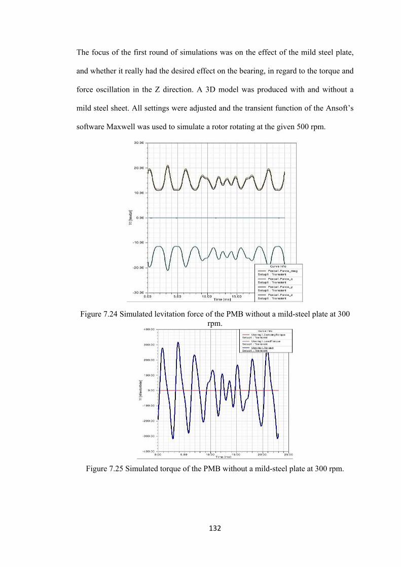
132

The focus of the first round of simulations was on the effect of the mild steel plate,

and whether it really had the desired effect on the bearing, in regard to the torque and

force oscillation in the Z direction. A 3D model was produced with and without a

mild steel sheet. All settings were adjusted and the transient function of the Ansoft’s

software Maxwell was used to simulate a rotor rotating at the given 500 rpm.

Figure 7.24 Simulated levitation force of the PMB without a mild-steel plate at 300

rpm.

Figure 7.25 Simulated torque of the PMB without a mild-steel plate at 300 rpm.

133

7.4.1.2.1 The results of the bearing without the mild-steel plate

Figure 7.25 (simulated torque of a PMB without a mild-steel plate) shows the results

when the torque is 325 mNm (mNewtonMeter) at its peak and about 70 mNm at its

minimum. The levitation force oscillates between 24 Newton at the maximum and 11

Newton at its minimum (Figure 7.24), which shows that the vibrations induced

during operation will be considerable.

7.4.1.2.2 The results of the bearing with the mild-steel plate

The results show that the torque is at -1.7 mNm at its peak and about 0.7 mNm at its

minimum (Figure 7.26, Figure 7.27, Figure 7.28 and Figure 7.29). The average

torque is negative at 0.4 mNm, which indicates an energy loss due to Eddie-currents.

The levitation force is stable at about 11 Newton (Figure 7.27). This means that there

will be no or very little vibration induced during operation.

The fact that the levitation force is very stable demonstrates the effect of the mild-

steel plate and the short circuited magnetic flux.

134

Figure 7.26 Simulated torque of a PMB with a mild-steel plate at 300 rpm.

Figure 7.27 Simulated force of a PMB with a mild-steel plate at 300 rpm. S im u la t e d t o r q u e r e s u l t s

( w i t h m i ld s t e e l p la t e )

- 2 .0 0

- 1 .5 0

- 1 .0 0

- 0 .5 0

0 .0 0

0 .5 0

1 .0 0

- 5 5 1 5 2 5 3 5 4 5M e a s u r e m e n t in te r v a ls [m S e c o n d s ]

Torq

ue [m

New

ton]

S e r ie s 1

Figure 7.28 Simulated torque of a PMB with a mild-steel plate at 500 rpm.

135

S im u la t e d fo r c e r e s u l t s in Z d i r e c t io n ( w i t h m i ld s t e e l p la t e )

- 1 5 . 0 0

- 1 0 . 0 0

- 5 . 0 0

0 . 0 0

5 . 0 0

1 0 . 0 0

1 5 . 0 0

- 5 5 1 5 2 5 3 5 4 5M e a s u r e m e n t i n t e r v a ls [ m S e c o n d s ]

Forc

e in

Z-d

irect

ion

[New

ton]

S e r i e s 1 S e r i e s 2

Figure 7.29 Simulated results of the levitation force in z-direction of the PMB at 500 rpm.

S i m u l a t e d l o s s r e s u l t s( w i t h m i l d s t e e l p l a t e )

0 . 0 0

5 . 0 0

1 0 . 0 0

1 5 . 0 0

2 0 . 0 0

2 5 . 0 0

3 0 . 0 0

3 5 . 0 0

4 0 . 0 0

- 5 5 1 5 2 5 3 5 4 5M e a s u r e m e n t i n t e r v a ls [ m S e c o n d s ]

Wat

t in

[mW

att]

S e r i e s 1

Figure 7.30 Simulated results for the torque of the PMB at 500 rpm.

7.4.1.3 The results of the simulated bearing in comparison with the manufactured

prototype

The simulation results bare little truth if they are not validated by real experiments.

Since the simulations are promising, prototypes were then produced and tested. Due

to differences that occurred during the manufacturing process, a new simulation

model was made and simulated as shown in (Figure 7.28 to Figure 7.30).

136

7.4.1.4 The simulated Bearing

During the simulation, the torque, shown in Figure 7.28, did not display a horizontal

straight line. This shows that the location of each magnet on the mild-steel plate

might be important since the field strength might vary. This might cause vibration in

the real model. However, the force needed to turn the bearing is very low. In fact the

average is 0.4 mNm.

In Figure 7.30, it should be noticed that the energy loss due to the Eddie-current is

minimal. The simulated average loss is 34.38 mWatt (Figure 7.30) and the levitation

force is 9.92N (Figure 7.29).

7.4.1.5 Simulation data versus measured data - error calculation

The process of the measured data is much more difficult, since the data represent the

reality. For a researcher it is sometimes difficult to understand the measured results,

as many factors need to be considered, which may be unknown by the researcher. In

the case of this research, the limitation of the measurement equipment and its error

had to be taken into account as well. The limitations of the torque meter had to be

considered, as it could only record 12 data points per second, whereas the simulation

could be adjusted to any amount of data points per second, which are applied to the

data recording of the torque and the rotation speed. During the experiments, vibration

and other energy loss due to friction could not be avoided, and an average value was

calculated and then deducted from the measured results. An average error calculated

for the rotation speed was found to be around 5.6%. The percentage of the

137

measurement uncertainty is shown in Table 7.3, which was derived by the standard

deviation Equation 5.5.

Table 7.3 The error of measurements. Parameter Uncertainty (%)

Rotation per minute (rpm) 5.6

Torque [Nm] 6.3

7.4.2 Measured performance of the prototype of the APMBS

The prototype bearing was installed in the testing rig (Figure 7.21 and Figure 7.22).

It was driven by a DC motor spinning a flywheel. This flywheel rotated a torque

meter which was attached to the test stator and the test rotor. The flywheel was

installed to provide a constant rotation speed through its inertia.

Vertical force was added by attaching weights to the shaft on top of the of the test

bearing until the force was equal to the force shown in the simulation, 9.92N (Figure

7.29).

138

Figure 7.31 Diagram of the measured torque and rotation per minute

The bearing was installed and tested at an average 506 rpm (Figure 7.31). The rotor

was levitated at an air-gap distance of 6mm in stand-still (the same as in the

simulation). The measurements showed that at a rotation speed of 506 rpm was the

measured torque 5.49 mNm (Figure 7.31) on average; with the highest point of 12.8

mNm and the lowest point of 0.8 mNm.

The friction of the radial ball bearings was measured previously to be 6.5 mNm, and

had to be deducted. Considering this, it can be said that the measured data confirms

the simulated data to some extent.

139

7.5 Conclusion

A novel magnetic bearing was developed in this chapter. Through testing this new

axial passive magnetic bearing system, it was confirmed that the bearing works very

well and adding a mild steel plate on the rotor of the bearing will enhance the

uniformity of the magnetic field on the surface, which will in turn enhance the

performance of the bearing. Averaged torque measurements were in good agreement

with the averaged simulated results.

140

Chapter 8 Improvement of the developed bearing

There were several questions arising from the testing of the first prototype magnetic

bearing, which could be answered by simulations in order to improve the

performance of the bearing. The computational investigation will focus on five areas

of interest:

1. the effect of the gap between the magnets;

2. the effect of single pole or multiple pole configuration;

3. the effect of the integration of mild steel yokes into the bearing;

4. the effect of the air gap (between stator and rotor) on the torque and

levitation;

5. The effect of the location of the magnets on the bearing rings.

8.1 Influential literature

After the testing the first prototype magnetic bearing some improvements were made

based on three publications which inspired some of the changes and are summarized

in the following:

• The first stated the effect of a 0.05mm thick stainless steel sheet (SUS 43)

which was applied to an axially magnetized ring magnet by Ohji et al. (2000).

The reason for applying the stainless steel sheet was that the magnetization

over a long time had lost its uniformity, which caused undesired vibration in

the flywheel system. The report stated that if a steel sheet was added, it

unified the magnetic field to the degree that little or no vibration and noise

were emitted.

141

• The second publication was an investigation by the researcher team around

Nagashima, et al. (1999) into the effect of iron yokes on an array of ring

magnets which levitated over bulk HTS. In this report different magnet sizes

as well as pole arrangements were investigated, and it was found that the

back yoke in relation with the pole number was very effective to strengthen

the levitation force. Therefore the researchers concluded that (quote:) “in

order to enhance the radial stability, an increase in the number of poles is

effective. For the design of the flywheel as well as other levitation systems, it

is important to optimize the thickness, the width, and the number of poles of

magnet for achieving a large EMF.” (Electro Magnetic Field) (Nagashima et

al. (1999) Page 143), which, in conjunction with the air-gap under which the

system is being operated, will determine the levitation force of the bearing.

• The third paper was published in 2009 by Ikeda et al. (2009). In short, it

reported the findings of magnetic rings made of multiple cuboidal magnets,

which were used to levitate a flywheel over HTS blocks. The researchers

used a similar approach as Nagashima, as they also used a back yoke and a

large pole number to increase the EMF. In their conclusion they stated that

the magnetic field measured close to the magnets showed large differences in

their field strength (when measured from magnet to magnet in the rotational

direction), but if measured at a 15mm distance over the surface of the

bearing, these differences in field strength were approaching 10 mT and

lower. This means that the further away from the magnetic ring, the more

uniform is the magnetic field.

142

Similar effects were found during this investigation.

The following section describes the investigation of five basic bearing configurations

(with the magnetic properties as shown in Chapter 7 ). For the purpose of

comparison the 3D simulation models were set up with the same magnetization (Br)

and the same surface area, and were rotated by 10 degrees (with the transient

function of Ansoft’s Maxwell).

8.1.1 Basic magnetic bearing configuration 0

This first model to be described here is the basic repulsion model, where two

repelling magnets are shown. The interest is here on the magnetic field.

Figure 8.1 H field around the configuration 0.

Figure 8.2 H-field around the configuration 0. The blue dotts show the

field direction.

Figure 8.1 and Figure 8.2 show two magnets, one dark green and one yellow. The

dark green one is the magnet with a polarization where the South Pole is facing the

yellow magnet and the North Pole is facing upward. For the yellow magnet the South

Pole is facing the dark green magnet and the North Pole is facing downwards.

143

The colored area around the magnets shows the magnetic field strength, where the

red area indicates a high strength field and the blue area means a low field strength.

In all of the following figures the magnetic polarization is determined by its color.

In Figure 8.1 the magnetic field density is shown. In this case the magnetic field is

emitted at the upper the center of the dark green magnet (North Pole) and is then

transmitted to center of the magnet (as the blue dots indicate in Figure 8.2).

The repulsion effect appears to be due to the field deformation. This is due to the

location of the South Pole of the second magnet. Both fields are deformed and repel

each other (the equations presented in Chapter 6.2.6 can be applied here).

There is an area of weak field strength (indicated by the color green) between the

upper and lower magnet, which indicates that the field is concentrated around the

corners of the magnet and is less dense at the center between the two magnets. This

is the case with any magnet, and the reason is that the traveling distance from the

North Pole to the South Pole is the shortest at the corner of the magnet, whereas the

traveling distance towards the center of the North or South Pole of the magnet

approaches infinity (theoretically). Since the magnetic strength depends on the

permeability (magnetic resistance/reluctance) of the material, the force traveling

through longer path means a weaker field. Therefore, a weak field (shown in green)

can be seen in the center of the magnet.

8.1.2 Magnetic bearing configuration 1

The second configuration doubles what was shown in the first configuration. It

shows the field deformation of the magnets due to the presence of other magnets.

144

The field deformation occurs due to the magnet below and beside. The magnet will

repel those beside and below it.


Figure 8.4 H-field around the configuration 1. The blue and red dots

show the field direction.

The field direction is indicated by the red dots for the upper magnets and the blue

dots for the lower magnets. It is interesting that there is an area of weak field strength

(indicated by green color) in the center of the four magnets. An explanation for this

could be that the field strength between two fields with the same direction must be 0.


The third configuration changed from a uniform pole configuration to an alternating

pole configuration. Here, the upper and lower magnets have their own North and

South Poles, which shortens the traveling length of the magnetic flux, and therefore

strengthens the magnetic field. Furthermore, this configuration uses the fact that the

magnetic fields traveling in the same direction will repel each other, which provides

the levitation for the bearing (as seen in Figure 8.5 and Figure 8.6).

145





The fourth configuration introduces a yoke into the system. As mentioned in Chapter

7.1.1, the resistance for the magnetic flux to travel through iron is much lower than it

is through air.

The effect of adding a mild steel sheet was demonstrated by measurements in

Chapter 7 , where it was shown that the magnetic field decreased on the surface of

the mild steel plate considerably, which means that most of the magnetic flux will

stay inside the mild steel plate.

The finding is indicated by the magnetic field shown in Figure 8.8 and Figure 8.9.

Furthermore, it is interesting that the formerly seen areas of weaker magnetic field

intensity (green spots in Figure 8.1 and Figure 8.3) have disappeared, which indicates

that, overall, the field is more uniform.

146

Figure 8.7 H field around the configuration 3. The mild steel yoke

changes the magnetic field.




In configuration 4 the effects of two mild steel yokes were investigated. Here it can

be seen that the magnetic field has changed considerably on the outside (above the

dark green and yellow magnet pair), where the yoke was installed. The magnetic

field strength over the upper magnets decreased considerably compared to the field

below the lower magnets. This shows that most of the magnetic flux travels through

the yoke of the upper magnets (the low field is indicated by the color yellow,

whereas it is red under the lower magnet pair without the yoke), which was also seen

in Figure 7.3 and Figure 7.6.

147





Configuration 5 is the version with three mild steel yokes, i.e. the effects of the

previous versions compiled into one configuration.




148

The details about configurations 1 to 5 will be discussed in Section 8.1.7. In Figure

8.13 the magnetic fields of the configurations 1 to 5 are shown. The concentration

effect of the mild steel plate is interesting, which shows clearly that the magnetic

field strength changes between the upper magnet pair and the lower magnet pair.

In configurations 1 and 2 is a green spot visible between the upper and lower

magnetic pair. The explanation for this is shown in Figure 8.1 and Figure 8.3.

In configurations 3 to 5 mild steel yokes have been integrated into the system, and

most of the magnetic flux will pass through the yoke(s) to the opposite pole. This

saturates the yoke and the magnetic field of the other magnet pair cannot penetrate

the yoke. This allows the other pair to create a more uniform field.

configuration

1

configuration

2

configuration

3

configuration

4

configuration

5

Figure 8.13 The H-field around the configurations 1 to 5.

8.1.7 The difference between ring magnets and ring configurations consisting of

multiple magnets

Taking the previously investigated configurations (Figure 8.1 to Figure 8.9), the

effects on the levitation force and torque can now be investigated and compared.

149

This comparison must start with the basic comparison between a ring magnet and a

multiple block magnet arrangement. The simulation settings for the air-gap distance

and block distance are the same as the ring magnet if not stated differently.

Figure 8.14 RM SR SP 1AG A 1431mm2 Figure 8.15 CM SR SP 0G 1AG

Figure 8.16 CM SR SP 0.5G 1AG Figure 8.17 CM SR SP 1G 1AG

Figure 8.14 to Figure 8.17 show the basic model configurations. The results are

shown in Figure 8.18 to Figure 8.23. The effect of the gap between the magnets of

each ring and the effect of an increased air-gap will be investigated. The gap between

the magnet blocks will be increased from 0 to 2 mm (Figure 8.14 to Figure 8.17), as

the air-gap distance will be increased from 1 mm (Figure 8.18 and Figure 8.19) to

150

2.5mm (Figure 8.20 and Figure 8.21) to 5 mm (Figure 8.22 and Figure 8.23) and

finally to 10mm (Figure 8.24 and Figure 8.25).

30

35

40

45

50

55

60

0 2 4 6 8 10

Levi

taio

n Fo

rce

[N]

Degree

Levitation Force Change over 10 degrees

ring magnet 1431mm area, 1mm airgap block magnet 0mm gap, 1mm airgapblock magnet 0,5mm gap, 1mm airgap block magnet 1mm gap, 1mm airgap

Figure 8.18 Levitation force at 1mm air-gap distance.

Figure 8.19 Torque at 1mm air-gap distance.

In Figure 8.18, the effect of the gap between two magnets is clearly visible. The rotor

starts rotating from a position where the magnets of the rotor and the stator are in

alignment, which provides the highest levitation force. After it has rotated for 5

151

degrees, the magnets are positioned over the gap and therefore experience a much

lower levitation force. This is the reason why the configuration with the largest gap

between the magnets provides the lowest repulsion force in this position. Even the

configurations with a 0 gap between the magnets experience a slight change in

levitation force.

Figure 8.20 Levitation force at 2.5mm air-gap distance.

Figure 8.21 Torque at 2.5mm air-gap distance.

The same applies to the torque in Figure 8.19, as it produces the largest negative and

positive torque. Similar trends are visible in Figure 8.20 to Figure 8.25.

152



When comparing Figure 8.18 with Figure 8.25, the simulation with the smallest air-

gap (1mm) to the simulation with the largest air-gap (10mm), it is interesting that the

effect described in the previous report becomes visible. Ikeda et al. (2009) also

reported an increasingly unified EMF at a larger (air-gap) distance for the bearing.

153



The results for the largest air gap investigated are shown in Figure 8.24 and Figure

8.25. The figures with the smallest air-gap (Figure 8.18 and Figure 8.19) show a

large change of levitation force and torque. With an increasing air-gap (between rotor

and stator) the total levitation force becomes smaller (Figure 8.20 and Figure 8.22).

The same applies to the change of the torque.

154

Overall the ring magnet shows the best performance in torque and levitation force.

However the 0 gap configuration comes very close to that performance, as shown in

Table 8.1.

Table 8.1 The investigated bearing configurations.

8.1.8 Investigation into multiple magnet ring configurations

This comparison is again for a ring magnet (configuration RM SR SP 1AG A

2623mm2), with the same properties and surface area as the multiple block

configurations. Knowing that a multiple pole configuration will increase the

magnetic field strength, it is interesting to see what the effect is on the torque and

levitation force of the bearings.

The simulation settings, the mesh number, the materials, the rotation speed and times

steps are the same for all simulations. In the following section are descriptions of the

investigations of the double ring single pole configurations CM DR SP 2G 1AG, CM

DR SP 2G 1AG SY M, CM DR SP 2G 0.5AG DY ML and CM DR SP 2G 1AG TY

Steel

Yoke

Con

figur

atio

n

Cub

oida

l Mag

nets

[CM

]

Rin

g M

agne

ts [R

M]

Sin g

le R

ing

[SR

]

Dou

ble

Rin

g [D

R]

Sing

le P

ole

[SP]

Dou

ble

Pole

[DP]

Air-

gap

1mm

[AG

]

Mag

net G

ap [G

]

Sin g

le Y

oke

[SY

]

Dou

ble

Yok

e [D

Y]

Tri p

le Y

oke

[TY

]

Are

a [A

]

Torq

ue A

vera

ge

[mN

m]

Ave

rage

Lev

itatio

n

Forc

e [N

]

M L H

Figure

8.14

RM SR SP 1AG A

1431mm2

1

X X X 1 X 0.79 120.6

Figure

8.15

CM SR SP 0G 1AG 1 X X X 1 0 0.62 99.3

Figure

8.16

CM SR SP 0.5G

1AG

1 X X X 1 0.5 9.3 108.8

Figure

8.17

CM SR SP 1G 1AG 1 X X X 1 1 11.82 99.31

CM SR SP 2G 1AG 1 X X X 1 1 149.89 72.7

155

MLH shown. The effect of the integration of a mild steel yoke is visible in the

following Figure 8.30 to Figure 8.36 and in Table 8.2.

Figure 8.31 shows the levitation force comparison between the ring magnet RM SR

SP 1AG A 2623mm2 and the double ring multiple magnet configurations CM DR SP

2G 1AG, CM DR SP 2G 0.5AG and CM DR SP 2G 1AG SY M.

Figure 8.26 The ring magnet RM SR SP 1AG A 2623mm2

Figure 8.27 Block magnets, double ring, single pole. CM DR SP 2G 1AG

Figure 8.28 Block magnets, double ring, single pole, single yoke. CM DR SP 2G

1AG SY L

Figure 8.29 Block magnets, double ring, single pole, single yoke. CM DR SP 2G

1AG SY M

156

Figure 8.30 Ring magnet and block magnets comparison. The ring magnet displays the best performance with no change in its levitation force, whereas the block magnet

show a large change in levitation force.

Figure 8.31 Ring magnet and block magnets comparison. The Ring magnet displays the best performance with no change in its torque, which is close to zero. But the

block magnet configurations show a large change in torque. The graph of RM SR SP 1AG A2623 and the graph of CM DR SP 2G 1AG TY MLH are very close. The

graph of RM SR SP 1AG A2623 is covered by the graph of CM DR SP 2G 1AG TY MLH. Figure 8.33 provides more details.

157

The difference between the ring magnet RM SR SP 1AG A22623 and the other

configurations is shown clearly. It is a straight line, opposite to all the other

configurations. Table 8.2 shows the difference in numbers.

Table 8.2 The investigated bearing configurations. Steel

Yoke

Con

figur

atio

n

Cub

oida

l Mag

nets

[CM

]

Rin

g M

agne

ts [R

M]

Sin g

le R

ing

[SR

]

Dou

ble

Rin

g [D

R]

Sing

le P

ole

[SP]

Dou

ble

Pole

[DP]

Air-

gap

1mm

[AG

]

Mag

net G

ap [G

]

Sin g

le Y

oke

[SY

]

Dou

ble

Yok

e [D

Y]

Tri p

le Y

oke

[TY

]

Are

a [A

]

Torq

ue A

vera

ge

[mN

m]

Ave

rage

Lev

itatio

n

Forc

e [N

] M L H

Figure

8.26

RM SR SP 1AG A

2623mm2

1 X X X 1 X 0.78 304.6

Figure

8.27

CM DR SP 2G 1AG 2 X X X 1 2 195.8 89.13

Figure

8.29

CM DR SP 2G 1AG

SY M

2 X X X 1 X 96.25 46.3 X

Not

shown

CM DR SP 2G

0.5AG DY ML

2 X X X 0.5 X 114.8 51.9 X X

Not

shown

CM DR SP 2G 1AG

TY MLH

2 X X X 1 X 0.12 56.7 X X X

Figure 8.32 Levitation force comparison of the block magnet configuration CM DR SP TY MLH to the ring magnet RM SR SP 1AG A 2623.

158

The levitation force of the ring magnet configuration is constant at 304 N. All other

configurations are experiencing very large force differences and are therefore not

useful for a bearing design.

However, unexpectedly, it shows that the torque of the bearing configuration CM DR

SP 2G 1AG TY MLH is a very low torque (Figure 8.32). This might be attributed to

the low repulsion force in conjunction with the field unifying effect of the mild steel

yoke (similar to what Ikeda et al. (2009) reported). The lower the levitation force, the

lower the force differences.

Finally the bearing configurations were investigated which consist of two multiple

magnet rings with opposite poles (Figure 8.34 to Figure 8.37).

Figure 8.33 Torque comparison of the block magnet configuration CM DR SP TY MLH to the ring magnet configuration RM SR SP 1AG A 2623. The erratic curve (red

line) of the ring magnet configuration RM SR SP 1AG A 2623 might be due to computational errors. In reality it should be a horizontal line

159

Figure 8.34 Block magnets, double ring, double pole, single yoke. CM DR DP 2G

1AG SY M

Figure 8.35 Block magnets, double ring, double pole, double yoke. CM

DR DP 2G 1AG DY LM

Figure 8.36 Block magnets, double ring, double pole, double yoke. CM DR DP 2G

1AG DY LH.

Figure 8.37 Block magnets, double ring, double pole, triple yoke. CM DR

DP 2G 1AG TY LMH.

Figure 8.38 displays the configurations CM DR DP 2G 1AG DY HL, CM DR DP 2G

1AG SY M and CM DR DP 2G 1AG, which show the pattern previously seen in

Figure 8.30 etc. The levitation force decreases when the magnets are not aligned and

increases when the magnets are aligned. Table 8.3 shows the differences.

160

Table 8.3 The investigated bearing configurations

Figure 8.38 Levitation force comparison of the block magnet configurations to the ring magnet RM SR SP 1AG A 2623.

However, there are similarities to the previously seen single pole configuration CM

DR SP 2G 1AG TY MLH. The performance of CM DR DP 2G 1AG TY HML

(Figure 8.37) and CM DR DP 2G 1AG DY ML (Figure 8.35) seen in Figure 8.38 and

Steel

Yoke

Con

figur

atio

n

Cub

oida

l Mag

nets

[CM

]

Rin

g M

agne

ts [R

M]

Sin g

le R

ing

[SR

]

Dou

ble

Rin

g [D

R]

Sing

le P

ole

[SP]

Dou

ble

Pole

[DP]

Air-

gap

1mm

[AG

]

Mag

net G

ap [G

]

Sin g

le Y

oke

[SY

]

Dou

ble

Yok

e [D

Y]

Tri p

le Y

oke

[TY

]

Are

a [A

]

Torq

ue A

vera

ge

[mN

m]

Ave

rage

Lev

itatio

n

Forc

e [N

]

M L H

Figure

8.26

RM SR SP 1AG A

2623mm2

1 X X X 1 X 0.78 304.6

not

shown

CM DR DP 2G 1AG 3 X X X 1 2 X 216.8 154.54

not

shown

CM DR DP 2G 1AG

SY M

3 X X X 1 2 X 129.9 56.7 X

Figure

8.34

CM DR DP 2G 1AG

DY ML

4 X X X 1 2 X 15.9 278.9 X X

Figure

8.36

CM DR DP 2G 1AG

DY HL

4 X X X 1 2 X 204.8 245.7 X X

Figure

8.37

CM DR DP 2G 1AG

TY HML

5 X X X 1 2 X 19.69 297.2 X X X

161

Figure 8.39 shows that the levitation force has increased and displays only slight

oscillations; the same applies to the torque.

Figure 8.39 Torque comparison of the block magnet configurations to the ring magnet configuration RM SR SP 1AG A 2623. The graph of CM DR DP 2G 2AG DY ML is very close to the graph of CM DR SP 2G 1AG TY MLH, and almost

covers it. More details are shown in Figure 8.41.

Figure 8.40 Levitation force comparison of the block magnet configurations CM DR DP 2G DY ML and CM DR DP 2G TY HML to the ring magnet RM SR SP 1AG A 2623.

The double yoke configuration has a lower levitation force than the tripple yoke configuration.

162

Figure 8.38 shows two configurations which come close to the performance of the

ring magnet. The configuration CM DR DP 2G 1AG DY ML has two yokes, and the

configuration CM DR DP 2G 1AG TY HML has three. The torque is shown in

Figure 8.39. The configuration CM DR DP 2G 1AG TY HML and CM DR DP 2G

1AG DY ML display almost a straight line, similar to the ring magnet.

lists the average torque and levitation force. Although the torque of both

configurations is still worse than the torque of the ring magnet, it is still quite close

considering that the levitation force of CM DR DP 2G 1AG TY HML is only 7 N (on

average) less than that of the ring magnet RM SR SP 1AG A 2623mm2.

Figure 8.40 shows the levitation force oscillation of the bearing configurations CM

DR DP 2G 1AG DY ML, CM DR DP 2G 1AG TY HML and RM SR SP 1AG A

2623mm2. Clearly is the effect seen when the magnets are aligned, as the torque and

levitation force increases or decreases. However, measured by the performance of the

Figure 8.41 Torque comparison of the block magnet configurations CM DR DP 2G DY ML and CM DR DP 2G TY HML to the ring magnet RM SR SP 1AG A 2623. The

double yoke configuration has a lower levitation force than the triple yoke configuration.

163

other configurations investigated, the yoke has a positive effect on the performance.

This leads to the next investigation about the location of each magnet on the ring.

8.1.9 Magnet block locations between multiple magnet rings

When looking at the previous simulation results, it seems to be clear that the location

of each magnet will have an effect on the performance of the bearing. This effect is

visible in the increase and decrease of the levitation force and torque and will be

investigated in the following.

Table 8.4 The investigated bearing configurations. Configuration A Configuration B Configuration C

Total number of magnets of

bearing

216 216 216

Rotor 18 South pole up 18 South pole up 18 South pole up Rotor/stator

multiple magnet

ring 1 (Inner ring) Stator 18 North pole up 18 North pole up 18 North pole up

Rotor 18 North pole up 24 North pole up 24 North pole up Rotor/stator

multiple magnet

ring 2 Stator 18 South pole up 24 South pole up 24 South pole up

Rotor 36 South pole up 30 South pole up 30 North pole up Rotor/stator

multiple magnet

ring 3 Stator 36 North pole up 30 North pole up 30 South pole up

Rotor 36 North pole up 36 North pole up 36 South pole up Rotor/stator

multiple magnet

ring 4

(outer ring)

Stator 36 South pole up 36 South pole up 36 North pole up

South 108 96 108 Poles

North 108 120 108

In Figure 8.42 to Figure 8.44, the blue cubes represent magnets with the South Pole

facing upwards, and the red cubes indicate that the North Pole is facing upwards.

Since the multiple magnet rings are concentric, the radius of the ring becomes larger,

which increases the number of magnets used on the rings. The configurations A, B,

164

and C are thus investigated as shown in Table 8.4. Configuration B shows that, due

to its ring polarization of south-north-south-north (for the rotor), it will have 96

South poles facing 120 North poles.

For the following investigations the mild steel yoke was omitted, since the focus was

on the effect of the magnet location, and a mild steel yoke would minimize its effect.

Figure 8.42 The configuration A has an even number of north and south poles. But the arrangements of the rotor and the stator magnets are not the same.

Configuration A (Figure 8.42) consists of two ring pairs with an even number of

North Poles to South Poles. The reason for this configuration was to minimize the

force and torque oscillation. This was thought to be achieved by locating the magnets

such that when the (rotor) magnets of the first and third ring are aligned with the

stator magnets the magnets of the second and the fourth ring are not. Three

simulations were performed with the air-gap length of 2mm 3mm and 4 mm (see

Figure 8.45 to Figure 8.51).

165

Figure 8.43 The configuration B has an uneven number of north and south poles.

Figure 8.43 shows configuration B, which has the same number of magnets as

configuration A, but has an uneven number of Poles (Table 8.4). There are 96 South

Poles to 120 North Poles.

Figure 8.44 The configuration C has an even number of north and south poles.

In configuration C a strategy is shown to keep the pole numbers even. The strategy is

to group the first ring with the fourth and the third to the second. In this way (as seen

in Table 8.4) the pole numbers can be kept even (North and South Poles 108, Table

8.4).

166

Figure 8.45 The Levitation force comparison at 1 mm air-gap between rotor and stator.

Figure 8.45 shows the configurations A, B and C. The highest levitation force is

recorded for configuration B. It seems that the number of poles is not as important as

the traveling distance of the magnetic flux.

Figure 8.46 The Levitation force of configuration A.

Although configuration C does provide an even number of poles for the bearing, it

seems that the magnetic flux path becomes longer, because of the arrangement of

South-North-North-South pole. This might be different if yokes were used for this

bearing. Configuration A shows the lowest levitation force (Figure 8.45).

167

The torque diagram is shown in Figure 8.46, where it is shown that configurations B

and C are close in the torque.

From the previously seen trend, that the levitation force and the torque oscillation

decrease with a widening air-gap, which is confirmed by Figure 8.47 to Figure 8.51.

-600

-400

-200

0

200

400

600

0 10 20 30 40 50 60

Levi

tatio

n Fo

rce

[N]

Degree

Comparison of the Torque of Configuration A, B and C

Torque configuration A 1mm Torque configuration B 1mm Torque configuration C 1mm

Figure 8.47 The torque comparison at 1 mm air-gap between rotor and stator.

Figure 8.48The Levitation force comparison at 2 mm air-gap between rotor and stator.

168


Figure 8.50 The Levitation force comparison at 3 mm air-gap between rotor and stator.


169

8.2 Conclusion

The computational investigation into the structure of the bearing and the location of

the magnets in the bearings has brought some interesting results. The results

indicated that there was a clear impact of the gap between the magnets if compared

with the ring magnet. The performance was poorer and oscillated between a high

levitation force when the magnets were aligned and a lower levitation force when the

magnets were not aligned, which can be explained, i.e. the gap (between the magnets

of each ring) will weaken the uniformity of the magnetic field. Wider gaps between

the magnets on the modular ring will have a larger impact than smaller ones (Figure

8.19). However, even if the magnets are arranged with a 0 gap between them (Figure

8.19), a change in the torque and levitation force is still noted. This negative effect

could be minimized with an increase of magnets for each ring and multiple rings.

When it comes to single or multi pole configurations, the multi pole configurations in

general offer a higher levitation performance but also higher torque if they are

located in close proximity. If combined with a yoke the levitation force can almost

reach the performance of a ring magnet (Figure 8.40 and Figure 8.41), with a much

lowered torque compared to other multiple magnet configurations.

The effect of a larger air-gap distance (between stator and rotor) on the torque and

levitation force is clear. As the torque is linked directly to a change of levitation

force, both will decrease when the air-gap is increased.

And finally, no special arrangement of the magnets is necessary as the test has

shown. Any other configuration will lead to longer flux paths, which lowers the

magnetic field and, in turn, decreases the levitation force. The following conculsions

can thus made:

170

• A difference in the magnetic field occurs, if the modular magnetic ring

consists of more than one magnet.

• If more than one modular magnetic ring configuration is used, multi pole

arrangements will increase the levitation force.

• The effect of the gaps between magnets (point 1) and the levitation force

(point 2) can be improved with yokes added (magnetic flux concentrators)

• A simple NSNS (north-south-north-south) ring pole configuration is the best.

171

Chapter 9 The second prototype –comparison to the

simulated test results


taken from a conference paper submitted by the author to the International

Conference of Applied Energy 2012 with the title: ”The magnetic dampening effect

of a passive modular magnetic bearing for a Vertical Axis Wind Turbines (VAWT).”

A second bearing prototype (Figure 9.1 to Figure 9.5) was produced in accordance

with the findings above. However, for this test the test settings were changed. The

rotor was put between the two sets of stator magnets, which restricted its vertical

Figure 9.1 The rotor of the magnetic bearing installed with the mild steel yoke

Figure 9.2 The stator of the magnetic bearing with its mild steel yoke (here shown a

five ring configuration, but tested was a 4 ring configuration).

172

movement (Figure 9.4). With this method, the bearing could achieve a very high

degree of stiffness by decreasing the upper and lower air-gap (between the rotor and

the stator). This is a necessary step to increase the usability of the bearing and to

create a possible product (Figure 9.5).

Figure 9.3 For determining the air gap and the levitation force is the rotor left levitating over the stator.

Figure 9.4 During the test setup is the air-gap distance between rotor and stator

adjusted.

173

Figure 9.5 Schematic drawing of a commercial magnetic bearing prototype.

`

Figure 9.6 Schematic experiment layout

174

9.1 The experimental setting

The bearing was installed in the testing rig (Figure 9.4 and Figure 9.6) and driven by

a DC motor. The details of the bearing are shown in Table 9.1.

The total weight of the shaft, the rotor and the wind turbine was equal to the force

shown in the simulation, 63.29 N (Table 9.2).

Table 9.1 Design Data of the bearing rotor and stator. Number of magnet rings on the stator and rotor 8

Number of magnets of the 1st ring 18

Number of magnets of the 2nd ring 24

Number of magnets of the 3rd ring 30

Number of magnets of the 4th ring 36

Air-gap distance (g) 5 mm

Number of Mild-steel plates 4

Rotor diameter 255 mm

Magnet size: W: 5.5mm

H: 3mm

L: 7.3mm

Rotations per minute (rpm) 108 rpm to 1084 rpm

Table 9.2 Design data of the bearing rotor and stator. Item Weight in N

Ball bearing 1 5.736

Ball bearing 2 1.618

Rotor incl. Metal sheets, Magnetic

bearing 1 and 2, fixings etc. 14.180

Shaft 3.442

Coupling 0.666

Wind turbine 37.648

Total 63.29

175

The settings were adjusted to those described in Chapter 7 for the Savonius wind

turbine.

Figure 9.7 Experiment setting.

The previously shown investigations gave the most often occurring wind speeds

under which a building integrated wind turbine operates (Table 5.8 and Table 5.9).

The investigated wind turbine operates at the wind speeds (air velocities) of 4m/s,

6m/s and 8 m/s. The measured rotation speeds are shown in Table 9.3.

Table 9.3 Air velocity and Rotation speed Air velocity Rotation speed range

4m/s 0-450 rpm

6m/s 0-768 rpm

8m/s 0-1084 rpm

As previously stated, the bearing does constrain the vertical movements of the

bearing rotor, which consists of two stator plates (Figure 9.4 and Figure 9.5). The

176

lower one restricts the downward movements and the upper one restricts the upward

movements of the rotor. During the experiments the upper stator plate was used to

decrease the air-gap of the bearing by lowering it, which made the bearing stiffer.

There was no change for the supported load, 63.29 N.

Four cases were investigated, and are hereafter referred to as AG1, AG2, AG3 and

AG4, which are referred with an air gap of 10.97mm, 8.35mm, 5.25mm and 3.7mm,

respectively (Table 9.4).

Table 9.4 Investigated cases AG1, AG2, AG3 and AG4.

Upper air-gap

distance

Lower air-gap

distance

Total air-gap including

rotor

AG1 19.86mm 10.97mm 42.83 mm

AG2 12.08mm 8.35mm 32.41mm

AG3 7.75mm 5.25mm 25mm

AG4 4.3mm 3.7mm 20mm

9.2 Data acquisition

The simulations were set up with the same load and the same air-gap distances

(Table 9.1 and Table 9.2). The experimental rig made for the experiment is similar to

the one used previously (Figure 7.21, Figure 7.22 and Figure 9.6).

A precise measurement requires a near perfect alignment of all parts of the

experiment rig. Even a small misalignment will distort the measurements. For this

reason CNC machining was used to achieve a very low tolerance (of a +/-0.05

millimeters).

177

The torque meter was connected to a computer via a RS-232 port (Figure 9.7).

During the measurements a computer recorded the data from the torque-meter into a

Microsoft Excel file. The data were recorded over a time of 30 seconds, which gave

about 300 to 400 measurement points. The uncertainty of the measurements was

calculated to be about 7% (as shown in Section 5.3). The average values of the above

recorded measurements were used for the study reported in this thesis.

Figure 9.8 Measured torque of the four bearing configurations.

9.3 Comparison between the measurements and the simulation

As seen in Section 7.4it is clear that the experimental results cannot be compared

directly to the simulated ones because of the limitations of the measurement

equipment. For that reason the measured values were averaged to a point value. The

same was done with the simulated results.

178

In Figure 9.8 and Figure 9.9 the recorded torque output is shown for the bearing.

There are small differences between the larger air-gap distances and the smaller ones.

Overall the torque increases with the rotation speed.


Figure 9.9 shows an enlarged part of Figure 9.8. Above the line chart are the torque

values of the smallest air-gap (A4, 20mm) shown. Below are the values of the largest

air-gap (A1 42.83mm) shown. The difference is in the mNm range.

Since the experimental setting (Figure 9.7) consists of an array of ball bearings and

the magnetic bearing, the actual magnetic bearing torque value must be found out by

calculation.

In order to be able to calculate the torque of the magnetic bearing, each of the

components had to be measured separately. Besides the previously performed tests,

three other tests were conducted. For test 1, the torque of all of the components

together was recorded (Figure 9.16), for test 2 the torque of all of the components

was recorded without the ball bearing 1; and for test 3 the torque of the components

179

was recorded without the ball bearing 2. Simple subtraction was then used to find the

resulting torque of the bearings 1 and 2 and the magnetic bearing etc.


Figure 9.10 shows the torque results for the complete experimental rig as recorded.

The top lines show an increasing trend in accordance with the increasing rotation

speed.

The increasing torque is due to the energy loss through vibration, vibration

transmission, friction (heat), air friction and others. Since the torque of the ball

bearings have been measured previously could the torque of the magnetic bearing be

found, and has been compared to the simulated torque results (Table 9.5).

The comparison shows, very clearly, that the simulated results are close to the

measured results. The simulated results show an average torque of 0.015 Nm (+/-

0.06 Nm). The measured results display a wider range with the average of 0.011Nm

180

with (+/- 0.004Nm). Based on the uncertainty calculation, it is within the range of

error and is deemed an acceptable result.

Table 9.5 Simulated torque for the air gap distance of A3 and measured torque results. Rotation

speed (rpm) 108 216 324 432 540 648 756 864 972 1080

Simulated torque (Nm)

0.016 0.016 0.017 0.015 0.014 0.018 0.015 0.017 0.018 0.016Measured

torque 0.011 0.015 0.010 0.009 0.012 0.011 0.011 0.013 0.013 0.012

9.4 The magnetic field between the rotor and the stator magnets

The simulation software offers the option to visualize the magnetic field at a chosen

location in 2 D or even 3D. This is an interesting tool to analyze and improve the

bearing. The field distribution for the bearing was investigated and showed the effect

of the mild steel yokes on the magnetic field in the air-gaps of the bearing. In the

following section some of the field distribution diagrams are shown.

Figure 9.11 Section of the bearing showing the stator and the rotor.

181

Figure 9.12 Magnetic field density and flux distribution at position 1.

Figure 9.11 to Figure 9.15 confirm the effect of the yoke on the magnetic field

between the rotor magnets and the stator magnets. The yoke concentrated the

magnetic flux of the rotor magnets with the effect that the magnetic field of the stator

magnets is repelled.


182


Figure 9.15 Magnetic field density and flux distribution at position 4. Positions 1 to 4 are chosen close to each other, in order to show the magnetic field change of a small

section of the bearing.

9.5 Torque comparison of the magnetic bearing with ball bearings

The torque of the magnetic bearing was compared to that of the axial ball bearings

over a rotation speed range of 90 rpm to 1090rpm.

As previously seen, the torque of the magnetic bearing stays constant when the

rotation speed increases. In contrast to the magnetic bearing, the torque of the ball

183

bearing increases with increasing rotation speed. Figure 9.16 also shows the

influence of the frame on the performance of the bearings.

Figure 9.16 The measured torque and simulated torque of air-gap A3.

9.6 The Vibration transmission

The vibration transmissions at certain rotation speeds are of great interest for the use

of this bearing for building integrated wind turbines (Table 3.2). In order to evaluate

the performance, a comparison was made between commonly used ball bearings and

this novel magnetic bearing.

The vibration pattern of wind turbines is non-linear and non-stationary during

operation. This is partially because of the complex operation conditions including

moving mechanical parts, friction, wind speed changes and wind direction changes.

184

It is therefore impossible to get usable results under outdoor conditions. For that

reason several air velocities and rotation speeds were chosen to be measured in the

laboratory.

Other researchers have investigated vibration patterns of horizontal axis wind

turbines [Hameed et al. (2009) and Kalvoda and Hwang (2010)], with the aim to

develop a turbine fault diagnostic.

9.6.1 Data acquisition

The B and K PULSETM multichannel analyzer was used for data acquisition and the

transducers were B and K’s DeltaTron® 4394 accelerometers. The transducers were

mounted on a protruding piece that was connected to the shaft, which allowed

vertical movement but kept it steady in the horizontal axis. They were also mounted

on the structure (stator) below the bearing at X, Y and Z directions. In this

investigation the vertical direction Z is the only one of interest. The vibrations were

recorded for 20 seconds, with a sampling frequency of 65536 samples per second.

The data were then normalized by the local gravitational acceleration constant, g

(~9.81m/s²). The Power Spectral Density, PSD, (or rather the Acceleration Spectral

Density, ASD), was calculated, using the Welch method [Welch (1967)]. The unit

can be expressed as [g²/Hz] as in this case, since the data are normalized by g, or in

metric units as [(m/sec²)²/Hz].

Welch’s method shows a way of “saving computational time by sectioning the record

and averaging their periodograms by using fast Fourier transforms…” [loosely taken

from the abstract of Welch (1967)].

The overall magnitudes (grms = root mean square acceleration) were calculated by

integrating the spectrum, and taking the square root of the value. Further, the values

185

were converted into a dimensionless index number (Equation 9.1) when the reference

case was compared to the others. The air gap distance between the rotor and the

stator of the bearing, when the bearing levitates freely, was chosen as the reference

case (AG1).

( ) ( )i

ii Valueref

kValuenIndex.

=

Equation 9.1

i = 45, 76, 90… 1084 [rpm], k = AG1, AG2, AG3, AG4

If the index value is larger than 1 it indicates a higher magnitude of vibrations

compared to the reference case while less than 1 indicates the opposite

9.6.2 The investigation

The experimental investigation of the magnetic bearing was divided into two parts.

The first part is focused on a comparison of the magnetic bearing to a ball bearing,

and the second part is focused on a comparison of the magnetic bearings with

different air gaps.

9.6.2.1 Vibration transmission comparison of the magnetic bearing with the ball

bearing

The most common bearing type is the ball bearing, which is used widely in all types

of machinery. Unfortunately it is not straightforward to compare the magnetic

bearing to a conventional ball bearing. Using a magnetic bearing decouples the mass

of the turbine from the structure to a certain degree, while the ball bearing is coupled

stiffly to the structure, which acts like a massive inertia block to absorb the

vibrations.

186

Figure 9.17 The difference in vibrations between the rotor and stator at different rotation speeds. : AG1, : AG2, : AG3, : AG4, *: BB. Case AG1 Is the

reference case.

Figure 9.18 The detail difference in vibrations between the rotor and stator at different rotation speeds. : AG2, : AG3, : BB. Case AG1 is the reference case.

The 4 mm air gapgarph (AG4) has been omitted to see the trend.

However, keeping this in mind, a valid comparison can be made by looking solely at

the difference in vibration transmission.

This is obtained by subtracting the stator values from the rotor values, as shown in

Figure 9.17 to Figure 9.24. In Figure 9.17 to Figure 9.24 the graph AG4 has been

omitted in order to get a more detailed image of the trend for the other air gaps.

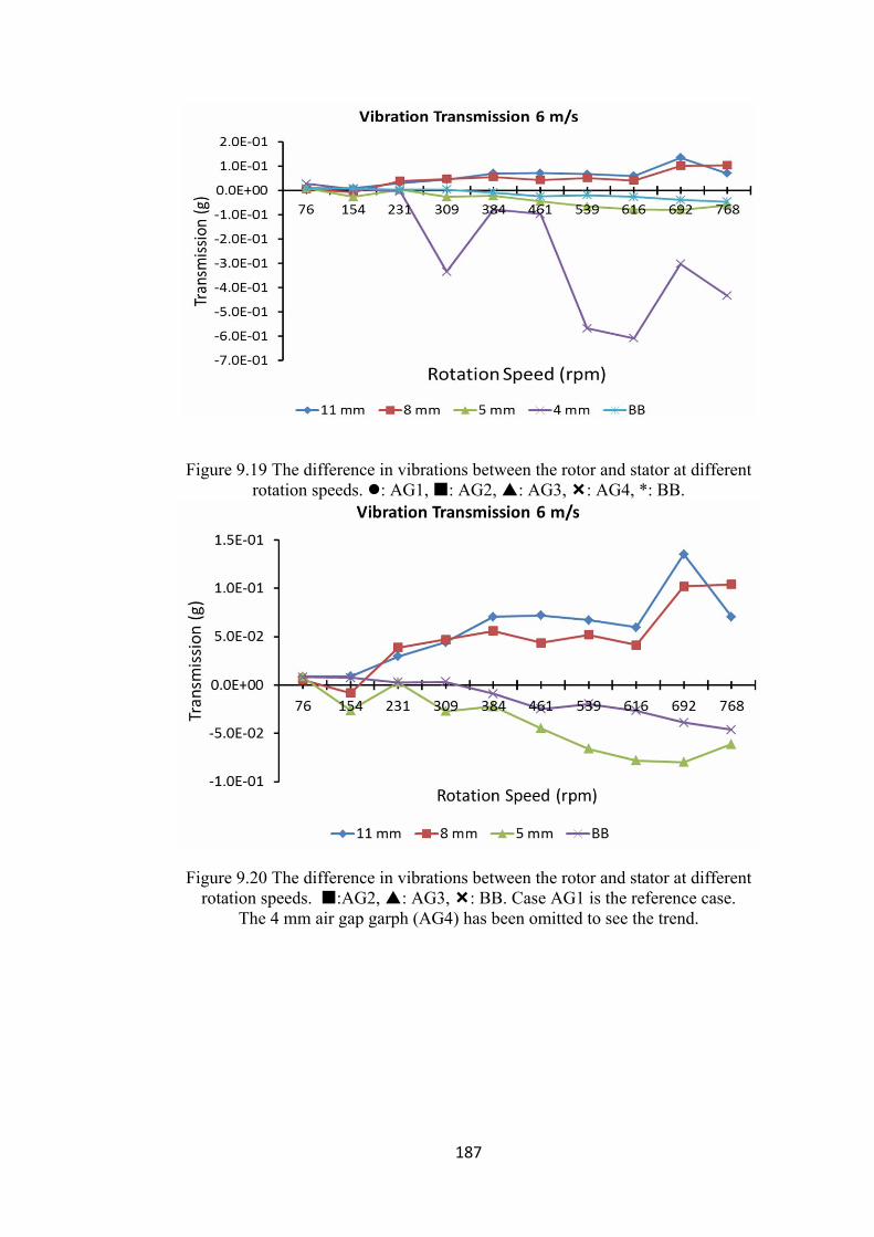
187

Figure 9.19 The difference in vibrations between the rotor and stator at different rotation speeds. : AG1, : AG2, : AG3, : AG4, *: BB.

Figure 9.20 The difference in vibrations between the rotor and stator at different rotation speeds. :AG2, : AG3, : BB. Case AG1 is the reference case.

The 4 mm air gap garph (AG4) has been omitted to see the trend.

188


different rotation speeds. : AG1, : AG2, : AG3, : AG4, *: BB. Case AG1 is the reference case.

Figure 9.22 The difference in vibrations between the rotor and stator at different rotation speeds. : AG2, : AG3, : AG4, *: BB. Case AG1 is the reference case.

The 4 mm air gap graph (AG1) has been omitted to see the trend.

189

Figure 9.23 The difference in vibrations between the rotor and stator at different rotation speeds. : AG2, : AG3, : AG4, *: BB. Case AG1 is the reference case.

A clear trend can be seen in the above figures, which shows that the vibration

transmission increase with decreasing air gap and increasing rotation speed.

However, when the rotation speed reaches ~650 rpm the vibration transmission starts

to decline (Figure 9.23 and Figure 9.24). As seen in the previous section, the

gyroscopic forces will decrease the vertical movement in the rotor with increasing

rotation speed. Therefore the transmitted vibrations will continue to decrease in the

same fashion. However, when looking at the ball bearing, such a trend cannot be

detected, but instead the vibration seems to increase in accordance with the rotation

speed.

190


rotation speeds. : AG2, : AG3, : AG4, *: BB. Case AG1 is the reference case.

9.6.2.2 Torque comparison of the magnetic bearing with the ball bearing

The torque of the magnetic bearing was compared to the torque of the ball bearing

over a rotation speed range of 90 rpm to 1090rpm.

For this purpose the components of the experiment were tested separately. Three

tests were conducted. For test 1 all of the components were tested together (Figure

9.25), for test 2 all of the components were tested without the ball bearing 1; and for

test 3 were all of the components were tested without the ball bearing 2. Simple

subtraction was then used to find the resulting torque of the bearings 1 and 2 and the

magnetic bearing.

191

Figure 9.25 The measured torque.

It is interesting that the torque of the magnetic bearing seems to stay constant when

the rotation speed increases. In contrast to the magnetic bearing, the torque of the

ball bearing increases with increasing rotation speed. Figure 9.25 also shows the

influence of the frame on the performance of the bearings. Each time, when the

frame is added, the torque increases drastically.

9.6.2.3 Investigation of the magnetic bearing with decreasing air gap

To compare the vibration transmission of the magnetic bearings to each other, the

values were converted into a dimensionless index number (Equation 9.1). Every

measured value was indexed against the bearing configuration with the largest air

gap (11 mm; AG1), since it was assumed that the largest air gap will transmit the

least vibrations, as it is the most decoupled system.

192

When the values are larger than 1, a higher overall acceleration magnitude

(vibration) can be measured compared to the measured acceleration magnitude of the

reference case under the same conditions.

When the index value is smaller than 1, the overall acceleration magnitude is lower

than the acceleration magnitude of the reference case value.

Figure 9.26 Magnetic bearing vibration comparison at rotor for different air gaps. Rotor: 45 – 450 rpm : 11 mm, : 8mm, : 5mm, : 4mm

Figure 9.27 Magnetic bearing vibration comparison at stator for different air gaps Stator: 45 – 450 rpm : 11 mm, : 8mm, : 5mm, : 4mm

193

Figure 9.28 Magnetic bearing vibration comparison at rotor for different air gaps. Rotor: 76 – 768 rpm : 11 mm, : 8mm, : 5mm, : 4mm

Figure 9.29 Magnetic bearing vibration comparison at stator for different air gaps Stator: 76 – 768 rpm : 11 mm, : 8mm, : 5mm, : 4mm

Figure 9.30 Magnetic bearing vibration comparison at rotor for different air gaps. Rotor (top): 108 – 1084 rpm : 11 mm, : 8mm, : 5mm, : 4mm

194

Figure 9.31 Magnetic bearing vibration comparison at stator for different air gaps. Stator (bottom): 108 – 1084 rpm : 11 mm, : 8mm, : 5mm, : 4mm

Looking at the rotor graphs, it can be observed that the vibrations decrease with

increasing rotation speed and a smaller air gap, due to the increasing stiffness of the

bearing. These factors stabilize the rotor in the vertical axis, but the oscillations only

decrease by approximately 5%.

The stator graphs show the effect of decreasing the air gap quite noticeably. When

the air gap is the smallest (4mm shown in Figure 9.26 to Figure 9.31), an increase of

as much as 15 – 20% in vibrations can be detected.

The magnetic bearing requires very little torque to be operated, however, with a

decreasing air gap the magnetic repelling force increases exponentially. This, in turn,

leads to more vibrations being transmitted into the structure. What also can be

observed is that the transmitted vibrations started to decay from 700 rpm onwards

(Figure 9.30 and Figure 9.31). This is most likely due to the gyroscopically

stabilizing forces which grow stronger with an increased rotation speed, and will

finally overcome the repelling forces of the magnets.

195

9.6.3 Findings

No final conclusion can be drawn from this preliminary investigation of the vibration

transmission properties of this novel bearing structure. However, the measured data

certainly indicate several trends.

The magnetic bearing AG1 (at 11mm air gap) is the most decoupled system and

transmits the least vibrations from the rotor to the frame, as can be seen in Figure

9.17 and Figure 9.24.

With a decreasing air gap distance the system becomes more coupled and we can see

more vibrations in the frame and fewer in the rotor. The most coupled system is the

ball bearing, with the highest vibrations in the frame.

In Figure 9.19 and Figure 9.20, it is interesting to notice that the rotation speed is

most important for the system with the smallest air gap (AG4), it is the stiffest tested

magnetic bearing configuration, and transmits most of the rotor vibrations to the

frame. However, the vibrations seem to become smaller with increasing rotation

speed. This is due to the increasing gyroscopic forces, which is making the system

stiffer and is increasing the natural frequency of the rotor. So fewer vibrations are

actually created by the rotor during rotation, and then transmitted to the frame. This

is also indicated by the torque measurements.

The torque measurements in Figure 9.25 clearly show the influence of the rotor (and

the connected wind turbine) as source of vibrations and energy loss.

It is most interesting that the measured trend of the magnetic bearing shows an

almost horizontal line when increasing the rotation speed, whereas the ball bearing

torque increases with increasing rotation speed.

196

Finally, when comparing the magnetic bearings in Figure 9.26 to Figure 9.31, the

stiffest bearing (AG4) has the highest levitation force, but will transmit most

vibrations. This is opposite to the effect of the largest air gap distance which has the

lowest levitation force but has also the lowest vibration transmission.

9.7 Conclusion

An attempt was made to determine the vibration transmission characteristics of a

passive modular magnetic bearing used with a VAWT. A previously constructed

prototype was used, and several air gaps between rotor and stator were investigated

and as well as a conventional ball bearing. The first part of the investigation was

focused on comparing the vibration transmissions from the rotor to the structure

(stator). The present results suggest that the most decoupled setting transmits the

least amount of vibrations to the structure, whereas the ball bearing shows a trend to

transmit the most amounts of vibrations.

The second part of the investigation was focused on determining the vibration

characteristics of the magnetic bearing, when decreasing the air gap between rotor

and stator. The results suggest that the rotor vibrations decrease with increasing

stiffness of the bearing, which is affected directly by increasing rotation speed and

decreasing air gap distance. The opposite was observed at the stator, until a breaking

point at ~700 rpm, where the vibrations started to decline, which was especially

noticeable with the smallest air gap setting.

Finally the torque measurements show clearly the energy saving characteristics of the

magnetic bearing, compared to the conventional ball bearing, where the torque of the

magnetic bearing does not increase opposite to the ball bearings.

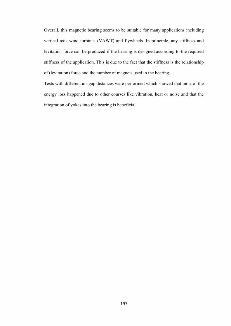
197

Overall, this magnetic bearing seems to be suitable for many applications including

vertical axis wind turbines (VAWT) and flywheels. In principle, any stiffness and

levitation force can be produced if the bearing is designed according to the required

stiffness of the application. This is due to the fact that the stiffness is the relationship

of (levitation) force and the number of magnets used in the bearing.

Tests with different air-gap distances were performed which showed that most of the

energy loss happened due to other courses like vibration, heat or noise and that the

integration of yokes into the bearing is beneficial.

198

Chapter 10 The patent application


taken from a patent application submitted by the author for the Polytechnic

University with the title: “Passive magnetic levitation system with a saturated metal

sheet for track or axial bearing systems.” Patent application number 12344324.

Due to the interest for promoting thus novel technology to the industry, a patent

application was developed. For this patent application the magnetization

(polarization) sequence North-South-South-North was chosen, since this has some

advantages during the manufacturing process.

10.1 The structure of the bearing

For the commercialization of the bearing the rotor and stator must be enclosed in a

bearing housing with mounting holes on the surface. This bearing housing consists of

two conventional bearings (Figure 10.1 and Figure 10.2), which can be active

magnetic bearings (AMB), roll or ball bearings, used to stabilize the X and Y

direction of the bearing and the permanent magnetic bearing, which stabilizes the

vertical (Z) direction.

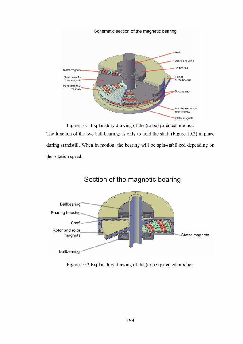
199

Figure 10.1 Explanatory drawing of the (to be) patented product.

The function of the two ball-bearings is only to hold the shaft (Figure 10.2) in place

during standstill. When in motion, the bearing will be spin-stabilized depending on

the rotation speed.

Figure 10.2 Explanatory drawing of the (to be) patented product.

200

10.2 The stator of the bearing

The two ball-bearings are integrated in the bearing housing (Figure 10.1 and Figure

10.2), which is made of a material that conducts magnetic flux (like mild steel, iron

etc.) and serves as the stator of the bearing. Since this bearing uses magnetic

repulsion to provide the levitation force, the bearing is made of two sets of concentric

rings of repelling magnets, which are arranged in a specific order (Equation 10.1 to

Equation 10.7.) The magnets of the stator are held in position by a recess (channel or

pocket) in the stator. This recess in the stator is four-fifths of the height of the

permanent magnets deep (Figure 10.3). The distance between the magnets is defined

by Equation 10.1 to Equation 10.7.

Figure 10.3 Explanatory drawing of the stator design of the bearing.

10.3 The rotor of the bearing

The rotor of the bearing is also made of a material which conducts magnetic flux

(like steel, iron etc.). However, the magnets are embedded in the rotor. The top of the

201

magnets is covered with a material which conducts magnetic flux (like steel, iron etc.

Figure 10.2). The fact that the magnets are covered with a flux-conducting metal

sheet is crucial as this unifies the field of the magnets and thus enables the rotor to

spin vibration less.

The distance between the magnets is defined by Equation 10.1 to Equation 10.7:


202

Although the bearing can use pre-charged magnets of any shape, form and

magnetization for the bearing, all of these must have the same shape, form and

magnetization. However, small differences (+/- 2.5%) will not have a great impact on

the performance of the bearing. As shown in Figure 10.4, if rectangular magnets are

used, the length (ML) and width (MW) are used for describing its dimension, which

can determine the number of the magnets (nm) per ring and radius (rall) of the ring.

There is a specific air gap included in the dimension; Figure 10.4 shows the magnet

with its dimensions.

The radius of the first and second

ring can be calculated by: )2360sin(2

m

L

n

Mr = Equation 10.1

The length of magnets: )2360sin(2

mL n

rM =

Equation 10.2

Number of magnets:

)2

(sin

1801

rMn

lm

−= Equation 10.3

The distance between the bearing

rings: wMrr 212 +=

Equation 10.4

The distance between all the

bearing rings: 21 rrrall −= Equation 10.5

The offset angle between the

paired rings of the stator: moffset n

360=ω Equation 10.6

The offset angle between the

paired rings of the rotor: moffset n

360−=ω Equation 10.7

203

The size of the air gap between two magnets is typically 0 to 0.2 of the length (ML)

of the magnet. If the size of the magnet is not larger than 20mm, the gap should be

decreased to 0.1 of the length (ML) of the magnet or even smaller. In general, a 0mm

air gap is considered to give the best performance.


10.3.1 The order of the magnets:

The minimum ring number should be 4 because the number of magnets of each pole

must be the same. Since the number of magnets increases with the radius of each

ring, and the distance between the magnets is always the same, the only logical order

of polarization is that the first ring and the fourth ring have the same direction and

204

the second and the third have the opposite direction to rings one and four (see Figure

10.5).

Since single magnets of any form are used, the size of the bearing is not defined. The

bearing can be designed to be very large and to support very large or very small

loads. It depends on the number of magnet and rings. In very large configurations the

bearing will become a track-like configuration; however the basic principles still

apply. The number of rings should be a multiple of four.

CLAIMS for the patent:

1. The inventor claims the specific location of each magnet based on Equations

10.1 to 10.7, in relation to the integration of a metal sheet to unify the

magnetic fields.

2. The inventor claims the invention of a magnetic flux conducting metal of

0.1mm to 2.0mm thickness covering the magnets for the purpose of creating a

uniform magnetic field or channeling the magnetic flux.

3. The inventor claims the recess depth of each magnet in the stator of the

bearing, which is one fifth of the height of the magnet.

4. The inventor claims that the number of the rings used in this bearing must be

a multiple of 4 in the stator and rotor of the bearing.

5. The inventor claims the sequence of poling of the magnets in each set of 4

must be that the first and the fourth ring have the opposite poling to the

second and the third ring.

205

Chapter 11 The application of the bearing

Figure 11.1 Visulisation of the prototype turbine.

From the beginning of the research the bearing was designed to be used for a VAWT

(Vertical-Axis-Wind-Turbine). The Hong Kong Water Services Department (WSD)

commissioned P-Tec (a subsidiary of The Hong Kong Polytechnic University) to

develop a Vertical-Axis-Wind-Turbine. (Figure 11.1). The main specifications of the

VAWT are as follows:

• Rated power 1.5kW

• Rotor Diameter 2-2.5m

• Rotor Height 2-3m

• Hub Height 5-6m

• Blade number 3 or 4

• Start-up wind speed 1.3m/s

• Cut-in wind speed 2.4m/s

• Rated wind speed 12m/s

• Cut-out wind speed 15m/s

• Survival wind speed 55m/s

• Rated rotor speed 250 rpm

• Total weight 200kg

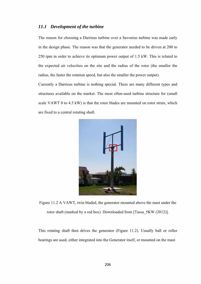
206

11.1 Development of the turbine

The reason for choosing a Darrieus turbine over a Savonius turbine was made early

in the design phase. The reason was that the generator needed to be driven at 200 to

250 rpm in order to achieve its optimum power output of 1.5 kW. This is related to

the expected air velocities on the site and the radius of the rotor (the smaller the

radius, the faster the rotation speed, but also the smaller the power output).

Currently a Darrieus turbine is nothing special. There are many different types and

structures available on the market. The most often-used turbine structure for (small

scale VAWT 0 to 4.5 kW) is that the rotor blades are mounted on rotor struts, which

are fixed to a central rotating shaft.

Figure 11.2 A VAWT, twin bladed, the generator mounted above the mast under the

rotor shaft (marked by a red box). Downloaded from [Tassa_5KW (2012)].

This rotating shaft then drives the generator (Figure 11.2). Usually ball or roller

bearings are used, either integrated into the Generator itself, or mounted on the mast.

207

Figure 11.3 Overall Turbine design, left the elevation and some details, and right a section with the braking system.

This is where the most decisive changes to a common design were made. In order to

lower the cut in wind speed, the bearing friction of the turbine had to be reduced;

since the bearing friction Mb is related to the force (F in this case the weight of the

rotor) acting on the bearing, fb the coefficient of the friction of the bearing and D, the

diameter of the bearing, it is clear that the friction increases with the rotor weight

(Equation 11.1).

To reduce the friction, a system was developed which allows for separating the

horizontal forces from the vertical forces. This way, the ball bearings responded to

the horizontal forces, and the vertical forces were transmitted by the Axial-Passive-

Magnetic-Bearing-System (APMBS) (Figure 11.3).

2d f F M torquefriction bearing The bb

r = Equation 11.1

208

The previously made calculations showed that a 1.25m radius rotor should supply

sufficient torque to overcome the inertia of the rotor to have it spinning at 2m/s air

velocity, if the torque of the rotor bearing was low enough. Through simulation and

testing it was established that the only measurable torque would come from the two

ball bearings.

Figure 11.4 Horizontal force transmission via ball bearings

Figure 11.5 Vertical force transmission via magnetic bearing

The integration of the magnetic bearing required a more complicated structure,

which is shown in Figure 11.6 and Figure 11.7.

As seen in Figure 11.4 and Figure 11.5, the horizontal forces are transmitted through

two radial ball bearings. This structure required a different generator position. Most

VAWTs place their generator under the turbine, above the mast; but in this case that

is not possible, and therefore it was placed on top of the mast. This position had

some advantages, as the generator can easily be replaced or maintained.

Furthermore, one important advantage of this design lies in its assembly.

Horizontal force

(Wind)

Vertical force

(Rotor weight)

209

Figure 11.6 The generator hub. Marked

in red are the rotor parts of the turbine,

and blue are the stator parts.

Figure 11.7 The magnetic bearing hub.

Marked in red are the rotor parts of the

turbine, and blue are the stator parts.

Figure 11.8 Structural simulation of the turbine under typhoon wind speeds in stand still. Picture given by P-Tec Company.

11.2 The safety of the turbine design

In order to verify the safety of the design, a 3D model was produced and the

occurring forces are calculated by our team member. However, as it is related to the

210

structural design of the turbine with the novel bearing, it is also shown here. The

simulation of the structural parts of the turbine showed clearly that the most critical

parts of the turbine were neither the mast nor the rotor hub.

The responsible engineer concluded, on the basis of the simulation, that the structure

is safe, because the yield stress of 275 MPa is more than 1.5 times (safety factor)

larger than the maximum stress in the rotating parts 178MPa. However, under

extreme conditions some deformation may occur.

Figure 11.9 Structural simulation of the turbine under typhoon wind speeds in motion. Picture given by P-Tec Company.

11.3 The assembly

During the design phase the question of how to assemble the turbine and mast was

considered and a concept developed.

211

The mast, with its electric wiring and mechanical brake, can be installed and erected

firstly (Figure 11.4, Figure 11.5, Figure 11.10 and Figure 11.11). After its completion

the complete rotor will be hoisted up and lowered on the inner mast, after which only

the generator has to be connected to the internal wiring. All bearings are preinstalled.

Figure 11.10 Mild steel bearing rings with magnets.

Figure 11.11 Finished stator part of the magnetic bearing.

The magnetic bearing consists of 17 rings (Figure 11.11), which were cut out of a 10

mm mild steel plate. The magnets are 3mm tall, 6mm long and 6 mm wide. They

were mass produced and, as such, charged with Br=0.5T. The magnetization was

parallel to their height. Around 4500 pieces were used to fill the 14 positions of the

212

17 rings (Figure 11.10). The magnetization of the rings was in north-south-north-

south. The system has been produced by a factory in Dongguan of Guangdong

Province and will be set up soon. A data monitoring system will be installed as well

for monitoring the performance of the system for at least one year.

Figure 11.12 Testing the bearing. Figure 11.13 Turbine assembly.

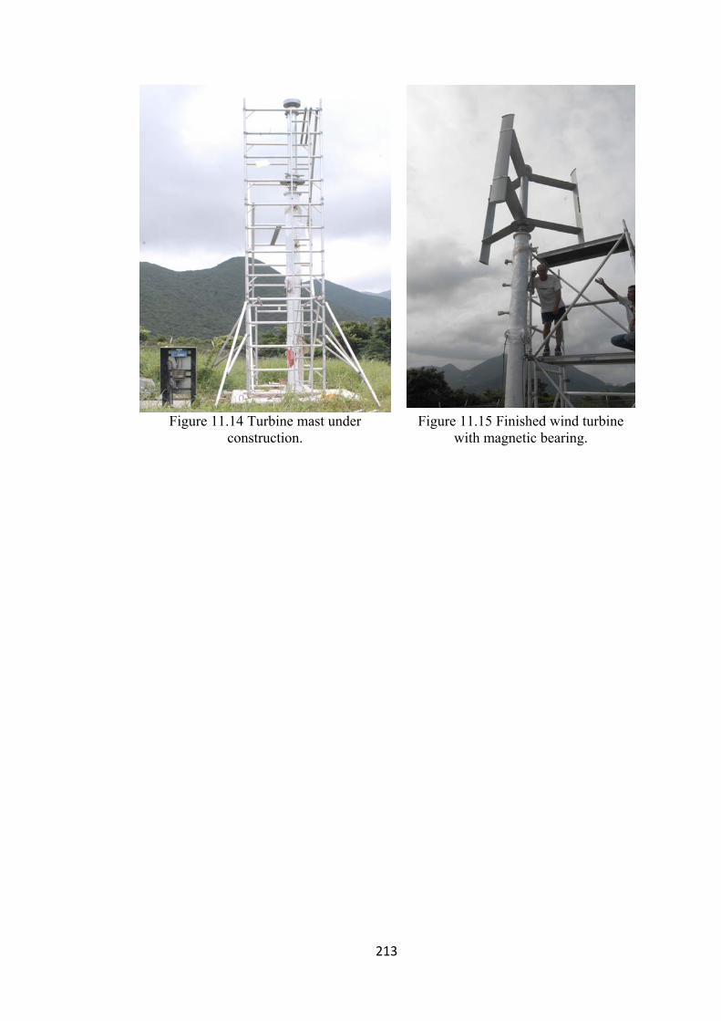
213

Figure 11.14 Turbine mast under

construction. Figure 11.15 Finished wind turbine

with magnetic bearing.

214

Chapter 12 Final Conclusion

This is the concluding chapter of this thesis. The thesis started with a discussion of

the increasing problem of oil scarcity and the problem of price fluctuations, and their

direct impacts on the economy.

Today (April 2012) the price per barrel of crude oil is above 100 US dollars.

According to an article in the South China Morning Post, titled “Mainland GDP

growth slowest in three years” [Huang (2012)], the economies of the USA, China,

Japan and Europe are showing signs of slowing, and there is no imminent recovery in

sight at the time of writing this thesis, due to the weak demand by the importing

economies. This is another indicator that change has to come. The question now is

how to guide the development in the right direction. One solution is that the

economies have to change, from a petrol to non-petrol based. Now is the time to

initiate the right developments in order to make the transition smooth.

In view of this, the production of useful energy from buildings in urban areas is a

step in the right direction. The building-integrated wind turbines (BIWT) have great

potential for renewable power generation. The technology developed in this project

came from this point, i.e. to develop a novel magnetic bearing system for supporting

the VAWTs for power generation from buildings.

Currently, there is a number of buildings under construction, which integrate wind

turbines. The finished wind-turbine buildings are very important as they will catalyze

the progress and development of wind turbine applications, which will lead to

standardized products.

215

Since some of the reports about the building projects reported vibration problems

[Killa and Smith (2008)], an initial investigation of turbine vibration was carried out.

It was discovered that vibration and noise transmissions are major problems for

BIWT applications in urban areas. To counter this problem, a novel passive magnetic

bearing was invented and developed, and the results are presented in this thesis.

To evaluate this novel bearing, the working conditions of building-integrated wind

turbines had to be assessed, which meant that the wind conditions and turbine

performance had to be investigated. It was found that the turbines will turn at blade

tip speeds of 5 to 8 m/s (under 5m/s to 10 m/s wind speeds), which is independent of

the size of the turbine rotor as the result is based on the aerodynamics of the rotor

blades (only for Savonius turbines). Hence, larger turbines will turn slower and

smaller turbines will turn faster.

Since the bearing is the connection point between the rotating machinery and the

building, its design properties are of great importance. It was necessary to invent a

bearing with vibration dampening properties. The solution of the problem was to use

permanent magnets to levitate the turbine and, therefore, to decouple the turbine

from the building.

However, the currently developed magnetic bearings could not be used because their

ring magnets could not be produced with large diameters, and segmented ring

magnets still had to be manufactured specifically according to the required ring

diameter. This issue led to the question of using premade magnetic blocks. However,

since a uniform magnetic field is crucial for the performance of the bearing, the idea

to use a thin mild steel sheet as a flux concentrator for unifying the magnetic field

gave rise for the new bearing developed in this thesis. The integration of the yokes

216

(flux concentrators) into the magnetic repulsion bearings is something new in the

field.

At first the performance of the magnetic bearing was not ideal and oscillated between

a high levitation force when the magnets were aligned and a low levitation force

when they were not. However, even if the magnets were arranged with a 0 gap

between them, a change was recorded in the torque and levitation force recorded.

This negative effect could be minimized with an increase in the number of magnets

used for each ring, multiple rings and the integration of a yoke.

When single or multi pole configurations are compared, the multi pole configuration

offers a better levitation performance, but also produces a higher torque if the air-gap

distance between rotor and stator is small. If the magnets are combined with a yoke

(flux-concentrator), the levitation force will increase and can almost reach the

performance of a ring magnet. At the same time the flux-concentrator will unify the

magnetic field and lower the torque.

The question of the arrangement of the magnets on the ring has also been

investigated, and showed that no special arrangement of the magnets on the ring is

necessary. This is because any different arrangement will lead to longer flux

pathways, which lowers the magnetic field strength and, in turn, lowers the levitation

force.

When the magnetic bearing was compared to a ball bearing, the measured torque of

the magnetic bearing showed an almost horizontal line when increasing the rotation

speed, whereas the torque of the ball bearing increased with the rotation speed.

The developed bearing was tested and the measured data indicate several trends. The

magnetic bearing with the largest air-gap is the most decoupled system and transmits

217

the least vibrations from the rotor, but if the air-gap distance decreases, the system

becomes more coupled and more vibrations are recorded in the frame and fewer in

the rotor. The most coupled system is the ball bearing, with the highest vibrations in

the frame.

In view of the test results, the rotation speed seems to be most important for the

system, with the smallest air-gap. The recorded data showed that it is the stiffest

tested magnetic bearing configuration, and transmits most of the rotor vibrations to

the frame. However, the vibration seems to become smaller with increasing rotation

speed.

This is due to the increasing gyroscopic forces, which make the system stiffer, but

also increase the natural frequency of the rotor. Hence fewer vibrations are created

by the rotor during rotation, and then transmitted to the frame.

Overall, this bearing seems to be suitable for many applications, including vertical

axis wind turbines (VAWT), pumps and flywheels.

As a direct result of this investigation, a real 1.5 vertical-axis-wind-turbine was

equipped with this novel magnetic bearing system. This turbine was designed and

produced for the Water Supplies Department of the Hong Kong SAR Government.

Since this wind turbine with the magnetic bearing is a pilot system, its performance

will be monitored and evaluated for one year. It is anticipated that this novel

magnetic bearing system can be promoted to the industry.

218

Chapter 13 Other Innovative Work related with the

Development of the Novel Magnetic Bearing

13.1 Development of a double-rotor wind turbine generator

As for most generators a high rotation speed will be used to generate electric power.

However, most VAWT generate high torque at low rotation speed. The solution is to

integrate a gear system to increase the rotation speed to the desired level or using

transverse flux machines [Grauers (1996), Henneberger and Bork (1997) and Dubois

et al. (2002)].

Figure 13.1 Schematic picture of the generator.

219

Figure 13.2 Flux analysis.

The counter rotating VAWTs could solve this problem, since they are rotating in

opposite directions. This doubles the rotating speed. The novel design introduced in

this report is a double rotor generator, where the rotor is fabricated by two counter

rotating rings. The structure is similar to a transverse flux machine [Henneberger and

Bork (1997)]. The stator and its windings are stationary (Figure 13.1 and Figure

13.2). The finite element method (FEM) was used to simulate the performance of this

machine.

220

Appendix


6m/s and 0 gap rate.

Appendix Figure 2: Angular velocity versus power coefficient of the wind turbine at at

8m/s and 0 gap rate.

221


10 m/s and 0 gap rate.


6m/s and 0.16 gap rate.

222





223





224

Appendix Figure 9 Angular velocity versus power coefficient of the wind turbine at at


225

Appendix Table 1 The turbine dimensions

Turbine design 1

(single or double stage)

Turbine design 2


Turbine design 3


Rotor diameter D 0.25 m 0.25 m 0.25 m

Rotor height (H) (double stage

turbine) 0.54 m 0.54 m 0.54 m

Rotor height (H) (single stage

turbine) 0.27 m 0.27 m 0.27 m

Overlap ratio (OL) 0 0.16 0.32

The rotor overlap (S) 0.012 m 0.034 m 0.06 m

Bucket diameter (d) depending on the

overlap ratio (OL) 61.25 mm (Figure7) 66.75 mm (Figure8) 73.25 mm (Figure9)

Adjusted phase shift Angle (PSA) 0, 15, 30, 45 and 60 0, 15, 30, 45 and 60 0, 15, 30, 45 and 60

Rotor diameter (D) 0.25 m 0.25 m 0.25 m

Swept area of the double stage

turbine As 0.135 m2 0.135 m2 0.135 m2

Swept area of the single stage turbine

As 0.0675m2 0.0675 m2 0.0675 m2

Blockage rate 0.135 0.135 0.135

Blockage rate 0.0675 0.0675 0.0675

Aspect ratio 2.16 2.16 2.16

Blockage rate 1.08 1.08 1.08

Appendix Table 2 Turbine abbreviations

Phase shift angle

0 (PSA) double

stage turbine (DS)

Phase shift angle

15 (PSA) double

stage turbine (DS)

Phase shift angle

30 (PSA) double

stage turbine

(DS)

Phase shift angle

45 (PSA) double

stage turbine

(DS)

Phase shift angle

60 (PSA) double

stage turbine

(DS)

Single

stage

turbine

(SS)

0 overlap

ratio (OL) DS0PSA0OL DS15PSA0OL DS30PSA0OL DS45PSA0OL DS60PSA0OL SS0OL

0.16 over

lap ratio

(OL)

DS0PSA0.16OL DS15PSA0.16OL DS30PSA0.16OL DS45PSA0.16OL DS60PSA0.16OL SS0.16OL

0.32 over

lap ratio

(OL)

DS0PSA0.32OL DS15PSA0.32OL DS30PSA0.32OL DS45PSA0.32OL DS60PSA0.32OL SS0.32OL

226

References

Akoun, G. and Yonnet, J. P.; 1984. 3D analytical calculation of the forces exerted

between two cuboidal magnets. Transactions on Magnetics, 5(20), p.

1962–1964.

Akpinar, E. K. and Akpinar, S.; 2004. Statistical analysis of wind energy potential

on the basis of the weibull and rayleigh distributions for Agin-Elazig.

Proceedings of the Institution of Mechanical Engineers, Part A: Journal of

Power and Energy 2004, 1 12.

Alexander, A. J. and Holownia, B. P.; 1978-1. Wind tunnel tests on a savonius rotor.

Journal of Industrial Aerodynamics, Volume 3, pp. 343-351.

Alexander, A. J.; 1978-2. Wind tunnel corrections for savonius rotors, 2nd

International Symposium on Wind Energy Systems, Paper E6, pp E6-69 –

E6-80, October 3rd – 6th,

Allaire, P.E.; Humphris, R.R. and Lewis, D.W.; 1991. Jesse W. Beams and the first

practical magnetic suspension. NASA Langley Research Center,

International Symposium on Magnetic Suspension Technology.

Anon.; 2012. Ansoft a commercial software by Ansys. s.l., s.n.

Bassani, R.; 2001. Permanent magnetic levitation and stability, fundamentals of

tribology. s.l.:Kluwer Academic Publishing.

Beams, J.W.; 1937. High rotation speeds. Journal of Applied Physics, pp. 795-806.

Betz, A.; 1926. Windenergie und ihre ausnutzung durch windmuehlen. Goettingen,

Germany : Vandenhoeck und Ruprecht.

227

Bivona, S.; Burlon, R. and Leone, C.; 2003. Hourly wind speed analysis in Sicily.

Renewable Energy, Volume 28, p. 1371–1385.

Blackwell, B. F.; Sheldahl, R. E. and Feltz, L. V.; 1978. Wind tunnel performance

data for two- and three-bucket savonius rotors. Energy , 2(3), p. 160–164.

Brad, P.; Nelson G. and James, F. A.; 2003. Design formulas for permanent-magnet

bearings. Journal of Mechanical Design, Volume 125, p. 734–738.

Brown, W. F.; 1940. Theory of the approach to magnetic saturation. Physics

Review, Volume 58, p. 736.

Buch der Synergie; 2010. Buch der synergie. [Online] Available at:

http://www.buch-der synergie.de/c_neu_html/c_08_11_windenergie_neue

_designs.htm [Accessed 17 March 2012].

Campbell, N. and Stankovic, S.; 2001. Wind energy for the built environment

(Project WEB). [Online] Available at: http://www.bdsp.com/web

[Accessed 2010].

Carruth, A. A.; Hooker, M. A. and Oswa, A. J.; 1998. Unemployment equilibria and

input prices: theory and evidence from the United States. [Online]

Available at: http://www.andrewoswald.com/docs/cho.pdf [Accessed 2

March 2012].

Castlewind; 2012. Inhabitat. [Online] Available at: http://inhabitat.com

/files/castlewind.jpg

Celik, A. N.; 2003. Weibull representative compressed wind speed data for energy

and performance calculations of wind energy systems. Energy Conversion

and Management, Volume 44, p. 3057–3072.

228

Chauvin, A. and Benghrib, D.; 1989. Drag and lift coefficients evolution of a

savonius rotor. Experiments in Fluids, 8(2), p. 118–120.

Chauvin, A.; Botrini, M.; Brun, R, and Beguier C.; 1983. Evaluation du coefficient

de puissance d’un rotor Savonius. Comptes Rendus de l’Acade´mie des

Sciences, Volume 298, p. 823 – 826.

Chiba, A.; Fukao, T.; Ichikawa, O.; Oshima, M.; Tak, M.; Fukao, T.; Ichikawa, O.;

Oshima, M. and Tak, M.; 2005. Magnetic bearings and bearing less

drives. ISBN 978-0-7506-5727-3 ed. Oxford,: Elsevier Newnes.

Chikazumi, S.; 1997. Physics of Ferromagnetism. New York: Oxford Univ. Press.

Cottrel, W.; 1955. Energy and society; the relation between energy, social changes,

and economic development. New York(USA): McGraw-Hill.

Darrieus, G. J. M.; 1931. U.S.A., Patent No. U.S. Patent No. 1,835.Cl18.

Davis, S. J. and Haltiwanger, J.; 2001. Sectoral job creation and destruction

responses to oil price changes. Journal of Monetary Economics , 48(1), p.

465–512.

Davis, S. J.; Loungani P. and Mahidhara R.; 1996. Regional labor fluctuations: oil

shocks, military spending, and other driving forces, Chicago: Working

paper, University of Chicago.

Deaves, D. M. and Lines I. G.; 1997. On the fitting of low mean wind speed data to

the Waybill distribution. Wind Engineering and Ind. Aerodynamics,

Volume 66, p. 169–178.

Diegel, S. W.; Boundy R. G. and Davis S. C.; 2011. Transportation energy data

book, s.l.: Oak Ridge National Laboratory.

229

Dubois, M.; Polinder, H. and Ferreira, J.; 2002. Transverse-flux permanent magnet

(TFPM) machine with toothed rotor. s.l., Proceedings of the Power

Electronics, Machines and Drives Conference.

Dutton, A. G.; Halliday, J. A. and Blanch, M. J.; 2005. The feasibility of building-

mounted/integrated wind turbines (BUWTs), UK: Council for the Central

Laboratory of the Research Councils.

Earnshaw, S.; 1839. On the nature of molecular forces which regulate the

constitution of luminiferous ether. Transactions of the Cambridge

Philosophical Society, Cambridge University Press, Volume 7, p. 97–112.

Enercon; 2011. Enercon. [Online] Available at:http://www.enercon.de/p/

downloads/EN_Productoverview_ 0710.pdf [Accessed 4 February 2012].

Eriksson, S.; Bernhoff H. and Leijon M.; 2008. Evaluation of different turbine

concepts for wind power. Renewable and Sustainable Energy Reviews ,

Volume 12, p. 1419–1434.

Fadare, D.; 2008. A statistical analysis of wind energy potential in ibadan, Nigeria,

based on weibull distribution function. The Pacific Journal of Science and

Technology, Volume 9. (Number 1.).

Federal Ministry for the Environment, Nature Conservation and Nuclear Safety.,

2011. Renewable energy sources in figures, Dessau, Germany: Federal

Ministry for the Environment, Nature Conservation and Nuclear Safety.

Fluent 6.3 users guide, 2006. s.l.:ANSYS Inc., Southpointe, 275 Technology Drive,

Canonsburg, Pennsylvania 15317, USA (2006).

Frechette, R. E. and Gilchrist, R.; 2011. Towards zero energy, a case study of the

Pear River Tower, Guangzhou, China. [Online]

230

Available at: http://som. com/resources/content/5/0/4/3/9/0/2/0/

documents/SOM_TowardsZeroEnergy.pdf [Accessed 22 March 2012].

Fujisawa, N.; 1996. Velocity measurements and numerical calculations of flow fields

in and around Savonius rotors. Journal of Wind Engineering and

Industrial Aerodynamics , Volume 59, p. 39–50.

Gambit 2.3.16 users guide, 2005. s.l.:Southpointe, 275 Technology Drive,

Canonsburg, Pennsylvania 15317, USA .

Grauers, A.; 1996. Design of direct-driven permanentmagnet generators for wind

turbines. Ph. D. dissertation, School Elect. and Computer Eng., Chalmers

Univ. Tech..

Gupta, R.; Das, R. and Sharma, K. K.; 2006. Experimental study of a Savonius –

Darrieus wind machine. Proceedings of the International Conference on

Renewable Energy for Developing Countries.

Hameed, Z.; Hong, Y.; Cho, Y.; Ahn, S. and Song, C., 2009. Condition monitoring

and fault detection of wind turbines and related algorithms: a review.

Renewable and Sustainable Energy Reviews, 13(1), pp. 1-39.

Hau, E.; 2006. Wind turbines. Berlin Heidelberg : Springer–Verlag.

Hayashi, T.; Li, Y. and Hara, Y.; 2005. Wind tunnel tests on a different phase three-

stage savonius rotor. Japan Society of Mechanical Engineers International

Journal, 48(1), p. 9–16.

Heinrich, K.; 1989. Magnetbahn transrapid. Darmstadt: Hestra-Verlag .

Helbling, T.; 2011. Oil scarcity, groth, and global imbalences, s.l.: International

Monetary Fund.

231

Henneberger, G. and Bork, M.; 1997. Development of a new transverse flux motor.

Proc. 1997 IEE Colloquium on New Topologies for PM Machines, pp. 1-

16.

Huang, C.; 2012. Mainland GDP growth slowest in three years. in the South china

morning post from the 14/04/2012., Issue 14/04/2012, p. 1.

Huang, Y. and Huang, J.; 2005. Interview research on the current situation and

trends of China green building movement. [Online]

Available at: http://:www.topgreen.org [Accessed 3 December 2011].

Ikeda, M.; Wongsatanawarid, A.; Seki, H. and Murakami, M.; 2009. Interaction of

bulk superconductors with flywheel rings made of multiple permanent

magnets. Physica , Volume 469, p. 1270–1273 .

Jangamshetti, S. H. and Rau, V. G.; 2001. Site matching of wind turbine

generators: a case study. Energy Conversion, Issue 16, p. 8–13.

Jiménez-Rodríguez, R. and Sánchez, M.; 2011. Oil price shocks and real GDP

growth emperical evidence for some OECD countries. Frankfurt: s.n.

JMAG; 2012; JMAG, commercial available software.. [Online]

Available at: http://www.jmag-international.com

Jones, C. N.; Litter, R. D. and Manse, B. L.; 1979. The Savonius rotor-performance

and flow. s.l., Proceedings of the First BWEA Wind Energy Workshop.

Jowder, A. F., 2009. Wind power analysis and site matching of wind turbine

generators in Kingdom of Bahrain. Applied Energy, Volume Applied

Energy 86, p. 538–545.

232

Kalvoda, T. and Hwang, Y.; 2010. Analysis of signals for monitoring of nonlinear

and non-stationary machining processes. Sensors and Actuators A:

Physical, 161(1), pp. 39-45.

Kats G., 2003. The costs and financial benefits of green buildings, California, USA:

Sustainable Building Task Force.

Kemper, H.; 1934. Schwebebahn mit räderlosen Fahrzeugen, die an eisernen

Fahrschienen mittels magnetischer Felder schwebend entlang geführt

werden. Germany, Patent No. Deutsches Patent 643316.

Kemper, H.; 1938. Schwebende Aufhängung durch elektromagnetische Kräfte; eine

Möglichkeit für eine grundsätzlich neue Fortbewegungsarten. Germany,

Patent No. ETZ 59 .

Killa, S. and Smith, R. F.; 2008. Harnessing energy in tall buildings: Bahrain

World Trade Center and beyond. s.l., CTBUH 8th World Congress .

National Renewable Energy Laboratory; 2002. Wind power density map. [Online]

Available at: http://www.nrel.gov/gis/wind.html [Accessed 12 March

2012].

Langer, G.; 2010. ABC WORLD NEWS POLL: THE MIDDLE CLASS; Within the

Middle Class, Four in 10 are Struggling. ABC WORLD NEWS.

Lee, K.; Ni, S. and Ratti, R.; 1995. Oil shocks and the macroeconomy: the role of

price variability. Energy Journal, 16(1), p. 39–56.

Lemarquand, G. and Yonnet, J. P.; 1998. A partially passive magnetic suspension

for a discoidal wheel. Applied Physics, 64(10), p. 5997–5999.

233

lh5.ggpht.com; 2000. Curve, BH. [Online] Available at: http://lh5.ggpht.com/-

6ktykYi25t0/TP1FgJ_r_jI/AAAAAAAAYzo/l3gaiz18ZyI/bhcurves.jpg

[Accessed 2012].

Lu, L.; Ip, K. Y.; 2009. Investigation into the feasibility and enhancement methods of

wind power utilisation in high-rise buildings of Hong Kong. Renewable

and Sustainable energy Reviews, 13(2), p. 450–461.

Marinescu, M.; Marinescu, N.; 1989. Compensation of anisotropy effects in flux-

confining permanent-magnet structures. Transactions on Magnetics, 25(5),

p. 3899–3901.

Maskell, E. C.; 1965. A theory of the blockage effects on bluff bodies and stalled

wings in a closed wind tunnel, Melbourne: ARC Research Memorandum.

Mawer, C.; 2012. carolinemawer.co.uk. [Online] Available at: http://www.

carolinemawer.co.uk/blog/wp-content/uploads/windmill-long-copy.jpg

[Accessed 9 March 2012].

Meeting of the Panel on Development; 2008. Wall effect. Hong Kong: LC Paper No.

CB(1)232/08-09(11); Ref: CB1/PL/DEV.

Menet, J. L. and Bourabaa, N.; 2004. Increase in the Savonius rotors efficiency via

a parametric investigation. European Wind Energy Conference.

Mertens, S.; 2005. Wind energy in the built environment. illustrated edition ed. s.l.:

Multi-Science Publishing Co. Ltd.

Modi, V. J. and Fernando, M.; 1989. On the performance of the Savonius wind

turbine. ASME Journal of Solar Energy Engineering, Volume 111, p. 71–

81.

234

Muellbauer, J. and Nunziata, L.; 2001. 2001. Credit, the stock market, and oil.,

Oxford: Working paper, University of Oxford.

Mukhopadhyay, S. C.; Donaldson, J.; Sengupta, G.; Yamada, S.; Chakraborty, C.

and Kacprzak, D.; 2003. Fabrication of a repulsive-type magnetic bearing

using a novel arrangement of permanent magnets for vertical-rotor

suspension. Transactions on Magnetics, 39(5).

Nagashima, K.; Otani, T. and Murakami M.; 1999. Magnetic interaction between

permanent magnets and bulk superconductors. Physica, Volume 328, p.

137–144.

National Renewable Energy Laboratory; 2001. Wind resource map of the USA.

[Online] Available at: http://www.nrel.gov/gis/images/ 80m_wind/USwind

300dpe4-11.jpg [Accessed 9 March 2012].

Ohji, T.; Mukhopadhyay, S. C.; Iwahara, M. and Yamada, S.; 2000. Performance of

repulsive type magnetic bearings under nonuniform magnetization of

permanent magnet. Transactions on Magnetics, 36(5).

Paraschivoiu, I.; 2002. Wind turbine design – with emphasis on Darrieus concept.

s.l.: Polytechnic International Press.

Persaud, S.; Flynn, D. and Fox, B.; 1999. Potential for wind generation of the

Guyana coastlands. Renewable energy, Volume 18, p. 175–189.

Pland; 2012. [Online] Available at: http://www.pland.gov.hk/pland_en/

info_serv/site_wind/SanPoKong_ site_wind.pdf [Accessed 9 March 2012].

Pope, A. and Harper, J. J.; 1966. Low Speed Wind Tunnel Testing, New York: John

Wiley and Sons.

235

Post, R. F. and Ryutov, D. D.; 1997. Ambient-temperature passive magnetic

bearings: theory and design equations. Cambridge Massachusetts August,

6th international Symposium on magnetic bearings.

Prabhu, S. V.; Kamoji, M.A. and Kedare, S.B.; 2009. Performance tests on helical

Savonius rotors. Renewable Energy , Volume 34, p. 521–529.

Rakotoarison, H.; Yonnet, J. P. and Delinchant, B.; 2007. Using coulombian

approach for modelling scalar potential and magnetic field of a permanent

magnet with radial polarization. Transactions on Magnetics, 43(4), p.

1261–1264.

Rasche, R. H. and Tatom, J. A.; 1977. Energy resources and potential GNP, St.

Louis: Federal Reserve Bank of St. Louis.

Rasche, R. H. and Tatom, J. A.; 1981. Energy price shocks, aggregate supply and

monetary policy: the theory and international evidence. s.l., Carnegie-

Rochester Conference Series on Public Policy, p. 9–33.

Ravaud, R.; Lemarquand, G.; Lemarquand, V. and Depollier, C.; 2009 - 4 .

Magnetic field produced by a tile permanent magnet whose polarization is

both uniform and tangential. Progress In Electromagnetics Research,

Volume 13, pp. 1-20.

Ravaud, R.; Lemarquand, G. and Lemarquand, V.; 2009 - 1 . Force and stiffness of

passive magnetic bearings using permanent magnets. Part 1: Axial

Magnetization. Transactions on Magnetics, 45(7), p. 2996–3002.

Ravaud, R.; Lemarquand, G. and Lemarquand, V.; 2009 - 2. Force and stiffness of

passive magnetic bearings using permanent magnets. Part 2: Radial

magnetization. Transactions on Magnetics, 45(7), p. 3003–3008.

236

Ravaud, R.; Lemarquand, G. and Lemarquand, V.; 2009 - 3. Magnetic field created

by tile permanent magnets. Transactions on Magnetics, 45(7), pp. 2920-

2926. [Accessed 12 March 2012].

Royal Institute of Technology Sweden, 2012. Bluffbodies. [Online]

Available at: http://www.mech.kth.se/courses/5C1211/BluffBodies.pdf

Santini, D.; 1985. The energy-squeeze model: energy price dynamics in U.S. business

cycles. International Journal of Energy Systems, Volume 5, p. 18–25.

Savonius, S. J.; 1931. The S-rotor and its applications. Journal of Mechanical

Engineering, 53(5), p. 333–338.

Schöb, R.; 2007. Theorie und praxis der magnetlagertechnik eine kurze Einführung.

Zuerich, Vorlesungs manuskript ETH Zuerich .

Seguro, J. V. and Lambert, T. W.; 2000. Modern estimation of the parameters of the

weibull wind speed distribution for wind energy analysis. Wind

Engineering and Ind. Aerodynamics, Volume 85, p. 75–84. And online

http://www.physics.ucla.edu /marty/levitron/. Retrieved 2006-12-06.

Simon, M.; Heflinger L. and Ridgway, S.; 1997. Spin stabilized magnetic levitation.

American Journal of Physics, 65(4), p. 286–292.

Smith, J. J.; Ellison, L. and Sayce, S.; 2007. Socially responsible property

investment: quantifying the relationship between sustainability and

investment property worth. Journal of Property Research , Volume 24, p.

191–219.

Smith, A.; 2007. The architecture of Adrian Smith, SOM, Toward a sustainable

future. 1 ed. Australia: Images Publishing Group Ltd..

237

SOM; 2011. Pearl River Tower. [Online] Available at: http://www.som.com/

content.cfm /pearl_river_tower [Accessed 9 March 2012].

Spaldin, N.; 2003. Magnetic materials; fundamentals and device applications.

s.l.:Cambridge University Press .

Stern, D. I.; 2002. Energy use and economic growth in the USA: a multivariate

approach. Energy Economics, 15(2), p. 137–150.

Strickland, J. H.; 1975. The darrieus turbine: A performance prediction model using

multiple streamtubes, s.l.: Sandia Laboratories Report SAND75-0431.

Swift-Hook, D., 2012. 2.03 – History of Wind Power. Wind Energy, Volume Volume

2, Pages 41–72.

Tassa_5KW; 2012. [Online] Available at: http://upload.wikimedia. org/wikipedia/en/

1/18/Tassa_5KW_2_ElectronSolarEnergy2.jpg [Accessed 9 March 2012].

The Bahrain World Trade Center; 2009. www.flickr.com. [Online]

Available at: www.flickr.com [Accessed 9 March 2012].

Tverberg, G. E.; 2012. Oil supply limits and the continuing financial crisis. s.l., s.n.,

p. 27–34.

Ushiyama, I., and Nagai, H.; 1988. Optimum design configurations and performance

of Savonius rotors. Wind Engineering , 12(1), p. 59 – 75.

Welch, P.; 1967. The use of fast fourier transform for the estimation of power

spectra: a method based on time averaging over short, modified

periodograms. Transactions On Audio And Electro acoustic, AU-15(2), p.

70 – 73.

Wieringa, J. and Rijkoort, P. J.; 1983. Wind klima der Niederland, Gravenhage:

Staatsuitgeverij.

238

World Bank; 2012. World Bank Data base. [Online] Available at: http://databank.

worldbank.org/data/ home.aspx [Accessed 26 March 2012].

Wu, K.; 2010. Green design. [Online] Available at: http://www.greendesignetc.net/

Buildings_09/Bulding_Wu_Kevin_paper.pdf [Accessed 21 March 2012].

Yamada, H.; Yamasak, H.; Develos-Bagarinao, K. and Naka, S.; 2004. The pinning

property of Bi-2212 single crystals with columnar defects. Superconductor

Science and Technology, 17(1), pp. 58-64.

Yasuyuki, N.; Ayumu, A. and Ushiyama, I.; 2003. A Study of the twisted Sweeney-

type wind turbine. Wind Engineering, 27(4), p. 317–322.

Yeang, K.; 2011. Eco skyscrapers: Volume 2. 2 ed. Australia: The Images Publishing

Group Pty. Ltd.

Yonnet, J. P.; 1978. Passive magnetic bearings with permanent magnets.

Transactions on Magnetics, 5(14), p. 803–805.

Yonnet, J. P.; 1996. Rare-earth iron permanent magnets. Oxford Science, pp. 430 -

451.

Yonnet, J. P.; Lemarquand, G.; Hemmerlin, S. and Rullier, E.; 1991. Stacked

structures of passive magnetic bearings. Applied Physics, 70(10), p. 6633–

6635.

Zhou, W.; Yang, H. and Zhauhong, F.; 2006. Wind power potential and

characteristic analysis of the Pearl river region, China. Renewable

energy, 31(6), pp. 739-753.

b2551314x.pdf - PolyU Electronic Theses

Documents

Transcript of b2551314x.pdf - PolyU Electronic Theses