3D Reconstruction of Anatomical Structures from Endoscopic ...

3D Reconstruction of AnatomicalStructures from Endoscopic Images

Chenyu Wu

CMU-RI-TR-10-04

Submitted in partial fulfillment of therequirements for the degree of

Doctor of Philosophy in Robotics

The Robotics InstituteCarnegie Mellon University

Pittsburgh, Pennsylvania 15213

01/2010

Thesis CommitteeBranislav Jaramaz (Co-chair)

Srinivasa Narasimhan (Co-chair)Yanxi Liu

Ko Nishino (Drexel University)

Copyright c© 2010 by Chenyu Wu. All rights reserved.

This thesis is dedicated to my father who taught me to use what I have learned to helppeople, It is also dedicated to my mother who taught me that if I make a wish and work

hard, it will come true. Finally this thesis is dedicated to my grandmothers who taught meto be brave and patient and to my beloved grandfather who moved to heaven last month.

Abstract

Endoscopy is attracting increasing attention for its role in minimally inva-sive, computer-assisted and tele-surgery. Analyzing images from endoscopesto obtain meaningful information about anatomical structures such as their 3Dshapes, deformations and appearances, is crucial to such surgical applications.However, 3D reconstruction of bones from endoscopic images is challengingdue to the small field of view of the endoscope, large image distortion, fea-tureless surfaces and occlusion by blood and particles. In this thesis, a novelmethodology is developed for accurate 3D bone reconstruction from endo-scopic images, by exploiting and enhancing computer vision techniques suchas shape from shading, tracking and statistical modeling.

We first designed a complete calibration scheme to estimate both geomet-ric and photometric parameters including the rotation angle, light intensityand light sources’ spatial distribution. This is crucial to our further analysis ofendoscopic images. A solution is presented to reconstruct the Lambertian sur-face of bones using a sequence of overlapped endoscopic images, where onlypartial boundaries are visible in each image. We extend the classical shape-from-shading approach to deal with perspective projection and near point lightsources that are not co-located with the camera center. Then, by tracking theendoscope, the complete occluding boundary of the bone is obtained by align-ing the partial boundaries from different images. A complete and consistentshape is obtained by simultaneously growing the surface normals and depthsin all views. Finally, in order to deal with over-smoothness and occlusions,we employ a statistical atlas to constrain and refine the multi-view shape fromshading. A two-level framework is also developed for efficient atlas construc-tion.

Acknowledgments

First and foremost I am heartily thankful to my advisor, Branislav Jaramaz, whose encour-agement, guidance and support from the initial to the final level enabled me to develop anunderstanding of the subject. This thesis would not have been possible without his insightinto this field and continuous advice on problem formulations. He has made available hissupport in a number of ways for my research, work and life, which has become a constantsource of inspiration and encouragement.

I owe my deepest gratitude to my co-advisor, Srinivasa Narasimhan. This thesis wouldnot have been completed without his commitment and diligent efforts which not only influ-enced the content of the thesis but also shaped my research methodology. His dedicationto research has deeply influenced and inspired me. The knowledge and skills that I havelearned from him will continue to guide me in the future.

I would like to thank the other members of my thesis committee, Yanxi Liu and KoNishino for their insightful discussion and comments on my thesis. Their expertise andguidance have helped me tremendously on my research. I would like to thank GeorgeStetten and Doug James for their valuable advice, and Suzanne Lyons Muth for her helpduring my graduate program. I would like to thank Leon Gu, Qifa Ke and Sanjeev J.Koppal for their helpful discussion on my thesis work. I would like to thank PatriciaMurtha, James E. Moody, and other ICAOS members for their help on collecting data. Iwould like to thank Sichen Sun and Jie Liu for their help on the final thesis editing.

I am indebted to Wenyi Zhao and Christopher J. Hasser from Intuitive Surgical, Inc.for a precious experience gained. I am also indebted to my officemates and fellow studentsat CMU for making my time in graduate school productive and rewarding.

I would like to show my gratitude to Jing Xiao and Tadashi Shiozaki from EpsonResearch and Development, Inc. for all their support in my thesis writing.

Finally, I owe everything to my dear parents. It is only through their love, encourageand dedication that I have accomplished my Ph.D.

vii

Contents

1 Introduction 1

1.1 Challenges from Endoscopic Images . . . . . . . . . . . . . . . . . . . . 1

1.2 Assumptions . . . . . . . . . . . . . . . . . . . . . . . . . . . . . . . . 2

1.3 Goals and Contributions . . . . . . . . . . . . . . . . . . . . . . . . . . 3

1.4 Outline of Dissertation . . . . . . . . . . . . . . . . . . . . . . . . . . . 4

2 State of the Art 5

2.1 Computer Assisted Diagnosis and Surgery . . . . . . . . . . . . . . . . . 5

2.2 Endoscopy . . . . . . . . . . . . . . . . . . . . . . . . . . . . . . . . . . 6

2.3 2D to 3D endoscopy . . . . . . . . . . . . . . . . . . . . . . . . . . . . 7

2.4 3D Vision for Regular Scenes . . . . . . . . . . . . . . . . . . . . . . . . 8

2.5 3D Vision for Surgery . . . . . . . . . . . . . . . . . . . . . . . . . . . . 9

3 Calibration of Endoscope’s Geometry and Photometry 11

3.1 Geometric Calibration . . . . . . . . . . . . . . . . . . . . . . . . . . . 12

3.1.1 Modeling Oblique-viewing Endoscope . . . . . . . . . . . . . . 14

3.1.2 Estimation of Rotation Angle Using Two Optical Markers . . . . 15

3.1.3 Estimation of the center of circle in 3D . . . . . . . . . . . . . . 16

3.1.4 Experimental Results . . . . . . . . . . . . . . . . . . . . . . . . 18

3.2 Photometric Calibration . . . . . . . . . . . . . . . . . . . . . . . . . . . 22

3.2.1 Image Irradiance Equation . . . . . . . . . . . . . . . . . . . . . 24

ix

3.2.2 Solution to h(·) . . . . . . . . . . . . . . . . . . . . . . . . . . . 25

3.2.3 Solution to γj . . . . . . . . . . . . . . . . . . . . . . . . . . . . 26

3.2.4 Solution to m(x, y) . . . . . . . . . . . . . . . . . . . . . . . . . 26

3.2.5 Experimental Results . . . . . . . . . . . . . . . . . . . . . . . . 27

3.3 Conclusions and Discussion . . . . . . . . . . . . . . . . . . . . . . . . 29

4 3D Reconstruction for Bones from Endoscopic Images 31

4.1 Shape-from-Shading under Near Point Sources and Perspective Projection 31

4.1.1 Solving Image Irradiance Equation . . . . . . . . . . . . . . . . 35

4.2 Global Shape-from-Shading using Multiple Partial Views . . . . . . . . . 39


5 Construction of Statistical Shape Prior for Bones from Population 47

5.1 Two-Level Framework . . . . . . . . . . . . . . . . . . . . . . . . . . . 49

5.1.1 Mesh Simplification . . . . . . . . . . . . . . . . . . . . . . . . 49

5.1.2 Low-Resolution Non-Rigid Registration . . . . . . . . . . . . . . 51

5.1.3 Low-Resolution to High-Resolution Interpolation . . . . . . . . . 51

5.1.4 Refining Registration . . . . . . . . . . . . . . . . . . . . . . . . 52

5.1.5 Atlas Construction . . . . . . . . . . . . . . . . . . . . . . . . . 54

5.1.6 Selection of Simplification Parameters . . . . . . . . . . . . . . . 55

5.2 Experiments and Results . . . . . . . . . . . . . . . . . . . . . . . . . . 56

5.2.1 Evaluation of Two-level Registration . . . . . . . . . . . . . . . . 56

5.2.2 Comparison to Other Registration Methods based on Femur Data 60

5.2.3 Femur Atlas . . . . . . . . . . . . . . . . . . . . . . . . . . . . . 61

5.2.4 Spine Vertebra Atlas . . . . . . . . . . . . . . . . . . . . . . . . 65


6 Improvement of Bone Reconstruction from Two-step Algorithm 69

6.1 Bottom-up Image based MISFS constrained by Statistical Shape Atlas . . 69

6.1.1 Aligning MISFS Shape with Atlas . . . . . . . . . . . . . . . . . 71

x

6.1.2 Constraining MISFS by Atlas . . . . . . . . . . . . . . . . . . . 72

6.2 Top-down Refinement by Maximizing Likelihood of Image Gradients . . 74

6.3 Experiments and Results . . . . . . . . . . . . . . . . . . . . . . . . . . 77

6.3.1 Simulations . . . . . . . . . . . . . . . . . . . . . . . . . . . . . 77

6.3.2 Artificial Lumbar Models . . . . . . . . . . . . . . . . . . . . . 77


7 Conclusions and Future Work 85

A Derivation of Eq. 4.17 89

B A comparison between Yamaguchi et al’s model and ours 91

C Initial Alignment for Femur Data 93

D Spine Vertebra Training Images 95

E Instruction for Selecting Points from Spine CT Images 99

Bibliography 103

xi

List of Figures

1.1 An artificial spine illuminated by an endoscope. . . . . . . . . . . . . . . 2

3.1 An oblique endoscope. . . . . . . . . . . . . . . . . . . . . . . . . . . . 12

3.2 A geometric model of an oblique endoscope. . . . . . . . . . . . . . . . 14

3.3 Estimation of rotation angles from markers. . . . . . . . . . . . . . . . . 17

3.4 Results of rotation angle estimation. . . . . . . . . . . . . . . . . . . . . 19

3.5 Devices used in the calibration experiments . . . . . . . . . . . . . . . . 20

3.6 Back projection error. . . . . . . . . . . . . . . . . . . . . . . . . . . . . 21

3.7 Results of geometric calibration . . . . . . . . . . . . . . . . . . . . . . 23

3.8 Results of photometric calibration. . . . . . . . . . . . . . . . . . . . . . 28

4.1 A near field lighting and perspective model. . . . . . . . . . . . . . . . . 33

4.2 Single image SFS results. . . . . . . . . . . . . . . . . . . . . . . . . . . 37

4.3 MISFS results for synthesized images. . . . . . . . . . . . . . . . . . . . 39

4.4 Images transformed from local to world coordinates. . . . . . . . . . . . 42

4.5 MISFS endoscopic results for endoscopic images. . . . . . . . . . . . . . 43

4.6 Comparison to the ground truth. . . . . . . . . . . . . . . . . . . . . . . 44

4.7 Comparison between orthographic and perspective projection. . . . . . . 44

5.1 Two-level non-rigid registration framework. . . . . . . . . . . . . . . . . 49

5.2 Local refining. . . . . . . . . . . . . . . . . . . . . . . . . . . . . . . . . 53

5.3 Leave-one-out experiment. . . . . . . . . . . . . . . . . . . . . . . . . . 55

xiii

5.4 Reconstruction error w.r.t. N lowref /Nhigh

ref . . . . . . . . . . . . . . . . . . . 57

5.5 Processing time w.r.t. N lowref /Nhigh

ref . . . . . . . . . . . . . . . . . . . . . . 57

5.6 Surface distance in each registration step . . . . . . . . . . . . . . . . . . 58

5.7 High-resolution surfaces XH and Y H . . . . . . . . . . . . . . . . . . . . 59

5.8 Low-resolution surfaces XL and Y L after mesh simplification. . . . . . . 59

5.9 Deformed XL(1) and Y L after TPS-RPM. . . . . . . . . . . . . . . . . . 60

5.10 Deformed XL(2) and Y L after refining. . . . . . . . . . . . . . . . . . . . 60

5.11 Deformed XH(1) and Y H after interpolation. . . . . . . . . . . . . . . . . 61

5.12 Deformed XH(2) and Y H after refining. . . . . . . . . . . . . . . . . . . 61

5.13 RMS and Mean error distributions for ICP and our method. . . . . . . . . 62

5.14 Femur data distribution w.r.t age and size. . . . . . . . . . . . . . . . . . 62

5.15 Femoral head atlas. . . . . . . . . . . . . . . . . . . . . . . . . . . . . . 63

5.16 Distal femur atlas. . . . . . . . . . . . . . . . . . . . . . . . . . . . . . . 64

5.17 Femur atlas: 1st mode. . . . . . . . . . . . . . . . . . . . . . . . . . . . 65

5.18 Femur atlas: 2nd mode. . . . . . . . . . . . . . . . . . . . . . . . . . . . 65

5.19 Femur atlas energy distribution. . . . . . . . . . . . . . . . . . . . . . . 66

5.20 Spine vertebra atlas - first three modes. . . . . . . . . . . . . . . . . . . . 67

5.21 Spine vertebra atlas energy distribution. . . . . . . . . . . . . . . . . . . 68

6.1 Bottom-up MISFS. . . . . . . . . . . . . . . . . . . . . . . . . . . . . . 71

6.2 Top-down refining. . . . . . . . . . . . . . . . . . . . . . . . . . . . . . 75

6.3 Synthesized shapes and images. . . . . . . . . . . . . . . . . . . . . . . 78

6.4 Reconstruction errors for synthesized vertebrae. . . . . . . . . . . . . . . 79

6.5 Experimental setup for artificial lumbar vertebrae reconstruction. . . . . . 80

6.6 Reconstruction errors for artificial L4 and L5. . . . . . . . . . . . . . . . 81

6.7 Reconstruction results for artificial L4. . . . . . . . . . . . . . . . . . . . 83

6.8 Reconstruction results for artificial L5. . . . . . . . . . . . . . . . . . . . 84

B.1 A comparison between Yamaguchi et al.’s system and ours. . . . . . . . . 92

xiv

C.1 Initial alignment before TPS. . . . . . . . . . . . . . . . . . . . . . . . . 94

D.1 Spine CT image: A To G. . . . . . . . . . . . . . . . . . . . . . . . . . 95

D.2 Spine CT image: Icaos. . . . . . . . . . . . . . . . . . . . . . . . . . . 96

D.3 Spine CT image: Sam. . . . . . . . . . . . . . . . . . . . . . . . . . . . 96

D.4 Spine CT image: Cadaver 2. . . . . . . . . . . . . . . . . . . . . . . . . 97

D.5 Spine CT image: Cadaver One. . . . . . . . . . . . . . . . . . . . . . . 97

D.6 Spine CT image: Janet. . . . . . . . . . . . . . . . . . . . . . . . . . . 98

E.1 Selecting points from the coronal view. . . . . . . . . . . . . . . . . . . . 100

E.2 Selecting points from the sagittal view. . . . . . . . . . . . . . . . . . . . 101

E.3 Selecting points from the transverse view. . . . . . . . . . . . . . . . . . 102

E.4 Difference between L2 and Th12. . . . . . . . . . . . . . . . . . . . . . 102

xv

List of Tables

3.1 Table of Notation in Sec. 3.1 . . . . . . . . . . . . . . . . . . . . . . . . 13

3.2 Pseudo RANSAC code for estimating the center of the circle . . . . . . . 18

3.3 Pseudo RANSAC code for estimating the rotation angle . . . . . . . . . 18




4.3 Global Shape-from-Shading: Key Steps . . . . . . . . . . . . . . . . . . 41




xvii

Chapter 1

Introduction

One of the main goals of contemporary surgery is to enable minimally invasive procedures.During surgery, an endoscope consisting of a camera and one or more light sources isinserted through a small incision into the body to acquire images for analysis. In additionto visualizing the interior of the anatomy, its role can be significantly enhanced by trackingthe endoscope in conjunction with surgical navigation systems or robotic surgical systems.

There are many kinds of endoscopes: rigid or flexible, forward viewing or obliqueviewing. The oblique viewing endoscope is the one most commonly used in orthopaedicsurgery. Fig. 1.1 shows an oblique endoscope illuminating and observing an artificialspine. This endoscope has two light sources placed at its tip for illumination.

1.1 Challenges from Endoscopic Images

Because the tip of the endoscope is typically a few millimeters away from the bone surface,we are only able to observe a small portion of the bone. As a result, it can be difficult evenfor a skilled surgeon to deduce actual bone shape from a single 2D endoscopic image.Thus, there is an immediate need for explicit computer reconstruction of bone shapesfrom endoscopic images. There are many advantages to reconstructing 3D shape fromendoscopic images, such as real-time, radiation free and low cost in-vivo visualization.

In the past several years researchers have explored many 3D reconstruction approaches[48]. For example, endoscopic images are overlaid on models from CT and MRI to local-ize the endoscopic views in a larger anatomic context [51, 13, 21, 86], where an expensiveCT or MRI and a complex registration procedure are required. Some researchers use spe-

1

(a) (b)

(c)

(d)

Figure 1.1: Illustration of an endoscope (a) and endoscopic images of an artificial spine (b,c,d).(It is difficult to perceive the shape of the object in the images because of small field of view,distortion, lack of texture, partial boundaries, and shading caused by near-field lighting.)

cial devices such as structured light [31, 45, 37]. This method requires the installation of aspecially designed high speed laser projector at the tip of the endoscope, which is not com-monly used in the operation rooms. For soft tissues with good features, standard computervision technologies can be easily applied to track and reconstruct the 3D information.

Classical approaches, including shape-from-shading [68, 111, 29, 66, 95, 110, 39] andshape-from-motion [19, 66, 67, 97, 7, 88, 108] cannot be directly applied to featurelessbone images. Besides, due to the small distances between the sources, the camera and thescene, the endoscopic images are very different from the images of natural scenes underdistant lighting, such as from the sun or the sky. Moreover, during minimally invasivesurgery, many substances (such as blood, pieces of bone, tissue) may obscure the bonesurface. This can mislead any local constraints used in shape recovery. In addition, envi-ronmental noise including fog, tools interaction, specularity, etc. need to be considered aswell.

1.2 Assumptions

This thesis takes the first step towards meeting the above challenges. We build a simplifiedsetup for ex-vivo experiments under the following assumptions:

2

1. Artificial bones with Lambertian reflectance are used in our experiments.

2. A monocular oblique endoscope is used for capturing images.

3. A surgical navigation system is used for tracking the endoscope.

4. Neither random occlusions nor environmental noise are taken into account.

5. The focus of the endoscope is fixed during experiments.

1.3 Goals and Contributions

Our goal for the ex-vivo setup is to reconstruct a large field of view of the bone using allthe information available during surgery. We will combine the shading information of thebone images and the motion information from the tracking system to achieve this goal.Specifically, this thesis makes the following contributions:

1. We developed a complete calibration scheme to obtain the parameters of the pho-tometry and geometry of the endoscope. The photometry parameters include thecamera response function, light source intensity and spatial distribution. The geo-metric parameters include intrinsic, extrinsic and rotation parameters. The rotationbetween the camera head and the scope cylinder creates an additional degree of free-dom which makes calibrating oblique endoscopes more difficult. All the calibratedparameters are used in our reconstruction algorithm.

2. We modeled the appearance of the bone under perspective projection and near-pointlighting, without assuming that the light sources are located at the center of the pro-jection, to reconstruct the shape from a single featureless bone image. Our methodextends the classical shape from shading algorithm to include near lighting and per-spective projection and recovers the scene depth Z explicitly in addition to recover-ing the surface normals.

3. We presented a multi-image shape-from-shading (MISFS) framework to reconstructa big part of the bone from multiple images by tracking the endoscope. We com-puted the global boundary constraints by aligning local contours in the world coor-dinates. One should notice that our global shape-from-shading framework does notreally merge shape-from-shading and shape-from-motion in the classical sense ofthe terms. We performed shape-from-shading for all images simultaneously and useglobal boundary constraints in each iteration.

3

4. We developed an semi-automatic two-level registration procedure to construct thestatistical shape prior for bone structures from population. This method segments,generates and aligns the 3D surface model from CT scanned images simultaneously.This statistical shape prior, also known as statistical atlas, is used to improve theMISFS algorithm in a global way.

5. We presented a two-step algorithm by combining bottom-up reconstruction and top-down refining. In the bottom-up step, we search for an atlas shape that most closelymatches the initial erroneous shape resulting from the MISFS algorithm. The sur-face normal and depth of the atlas shape are then used as initialization and geomet-ric constraints instead of the smoothness constraint in the MISFS. The bottom-upmethod exploits the atlas to improve the MISFS by solving the over-smoothness andpartial occlusion problems. The top-down step is inspired by the generative modelmethod. We compare the original endoscopic images with the synthesized imagesfrom the atlas shape obtained in the bottom-up step. The difference is used to refinethe atlas shape. The top-down refinement increases shape details and accuracy.

1.4 Outline of Dissertation

In Ch. 2, we will review literature, concerning current solutions for 3D estimation incomputer vision for both natural scenes and internal organs. We then introduce a completecalibration procedure for calibrating endoscopes’ geometry and photometry in Ch. 3. InCh. 4 we present a solution to the reconstruction of bone from multiple images. In Ch.5 we will introduce the statistical atlas and in Ch. 6, we present a two-step algorithm tofurther improve reconstruction. Summarization and discussion are in Ch. 7.

4

Chapter 2

State of the Art

The field of surgery has been revolutionized over the past twenty years as a result of theintroduction of endoscopic surgery, new imaging devices, computer assisted navigationsystems and robotic technologies in the operating room. Compared to traditional surgery,these technologies provide numerous advantages such as higher accuracy, smaller inci-sion, minimal invasiveness, less pain and blood loss, and faster recovery for patients. Withthe invention of the endoscope, surgeons are able to view interior anatomical structuresthrough a tiny incision, instead of through their naked eyes. In addition, a real-time endo-scopic image can be sent back to the computer for analysis. By using the position trackingtechnique, surgical tools can be localized in real-time. In some specific surgeries, for ex-ample, an orthopaedic surgery, e.g. bones and implants can also be tracked. These trackedobjects, along with endoscopic images, and previous augmented 3D models from CT orMRI scans can be displayed on the computer simultaneously, in order to provide a virtualguide for the surgeons.

2.1 Computer Assisted Diagnosis and Surgery

Since the invention of the first 2D radiography in 1895, more and more imaging modalitieshave been developed and applied in the medical field. For instance, the 2D ultrasound wasintroduced in several countries since the 1940s [23, 104] and the 3D CT was introduced byBritish engineer Godfrey Hounsfield in the 1970s [87]. With these modalities, doctors areable to examine interior anatomical structures without invasive operations. After the 3DMRI was introduced into the market in the 1980s [2], doctors have been able to gather moreinformation from the images due to the MRI’s strength in observing soft tissues. Later in

5

1987, the first 3D ultrasound scanner was developed at Duke University [24] to captureimages of the heart from outside the body. As technology enabled smaller ultrasoundarrays, researchers started to design probes that could fit within catheters threaded throughblood vessels for imaging the heart and its vasculature from the inside.

Conventional CT and MRI scans produce cross section ”slices” of the body that areviewed sequentially by radiologists who must imagine or extrapolate from these views theactual 3D anatomy. By using computer algorithms these cross sections can be rendered asthe direct 3D representations of human anatomy. Virtual endoscopy, a 3D representationbased navigation system for diagnosis was therefore proposed [77, 78, 99, 100, 62, 40,82]). Virtual endoscopy creates a 3D virtual environment of the human anatomy basedon CT or MRI images. A virtual camera is placed in such a virtual environment and isnavigated around. Then a series of virtual images can be synthesized and analyzed bycomputers. This technique provides a way to make surgery plannable. However, there isstill no texture information involved in the system. How to obtain a textured image duringsurgery? The answer is to capture real images via endoscopes. An endoscope has lenssystem and light sources at the tip that could be inserted into the body. With a near-fieldlighting, images of the interior structures are captured and sent back to the computer. Suchan instrument supports a better visualization for surgeons. For example, these endoscopicimages can be fused into the previous 3D CT models [51, 22].

2.2 Endoscopy

To view clearly through a tiny hole of the body requires a certain amount of lighting. Torecord what has been viewed requires a good lens system to transmit the light rays back tothe image recording device. Endoscopy meets the above requirements. A surgical proce-dure using endoscopes is referred as minimally invasive surgery, also known as endoscopy.

The history of endoscopy is long. Early in 1805, a German doctor, Philip Bozzini triedto use a candle to illuminate the interior structures through a hole on an animal. Other pi-oneers cited in medical journals include French surgeon Antoine Jean Desormeaux (1815-1894), American otolaryngologist Chevalier Jackson (1865-1958), Polish physician JanMikulicz-Radecki (1850-1905), German urologist Maximilian Nitze (1848-1906), Ger-man gastroenterologist Rudolph Schindler (1888-1968), and German gynecologist KurstSemm (1927-2003). The first ”endoscopy” in the world was conducted by a military sur-geon, William Beaumont, in 1922. He used a flashlight as a light source to examine awounded soldier’s abdomen through a tiny hole. At that time, however, the light sourcewas outside the body. Since the 1920s, electric light source has been utilized since it can

6

be transmitted through a rigid tube although not very deeply. After 1956, when the opticalfiber was invented, viewing of interior structures became practical.

Early endoscopes were designed to use as an eyepiece to view through the incision butnot for recording images. Because the tip of the instrument is very small (the diameter ofthe tip is around 10-15mm), the field of view is restricted. In 1929, the oblique viewingendoscope was designed in Germany by Kalk, who enlarged the field of view by rotatingthe scope cylinder. No image recording devices were available for endoscopes until 1954,when a viewfinder rod lens system was developed to capture images. And then, Soulas(France) developed the first televised bronchoscope (1956) and closed circuit televisionprogram (1959). CCD chip camera appeared in 1984 and high definition CCD has beenadopted by Olympus for endoscopes since 2003.

Since 1970s, nurses have been required to have laparoscopy training, and then rou-tine laparoscopy surgery started to operate in 1984. The state-of-the-art systems run thegamut from the possibility of disposable rigid endoscopes (Optiscope Technologies, Ltd.(Katzrin, Israel)), spectrally-encoded endoscopy (Massachusetts General Hospital’s Well-man Center for Photomedicine (Boston)), Minute On-Chip Sensor MT9V021 (MicronTechnology, Inc. (Meridian, Idaho and Glasgow, UK)), wireless ingestible imaging cap-sules (Tarun Mullick et el. Olympus Corp., Given Imaging Ltd. (1989-2006)), real-timestructured light endoscopy (University of North Carolina at Chapel Hill, 2003), to stereo-scopic endoscopy (da Vinci Surgical System manufactured by Intuitive Surgical Inc.) tobreakthrough three-dimensional imaging.

2.3 2D to 3D endoscopy

Early video cameras for endoscopic surgeries are monocular and allow only two-dimensionalvisualization. The lack of depth perception significantly reduces a surgeon’s ability to de-termine the precise size and location of anatomical structures and limits his/her capacityto maneuver, diagnose and operate efficiently.

Visionsense Corporation (Orangeburg, N.Y. and Petah-Tikva, Israel) developed a stereo-scopic sensor that provides the surgeon with real-time, high-resolution, natural stereo-scopic vision. The proprietary single sensor is based on multidisciplinary technologiescombined with sophisticated image processing algorithms. Since 2000, many other com-panies such as Olympus started to manufacture stereoscopic endoscopes, which have beenwidely used in surgical systems such as the da Vinci’s system (Intuitive Surgical Inc.). twooptical elements are put within a 12-millimeter diameter endoscope. One of them is forthe left eye and the other one is for the right eye, and both of them supply endoscopic

7

images to a separate video camera. They are combined together to provide a true three-dimensional visualization. Those image are then projected onto left and right monitorswhere the surgeon fuse a 3D perspective by watching both, simultaneously. However, pro-jecting stereo images to the left and right monitors cannot provide exact depth informationfor computer analysis. The researchers in the University of North Carolina at Chapel Hilllater developed a real-time structured light depth extraction for endoscopy [31, 50]. Ahigh speed projector projecting structured light into interior structures was designed to beinserted to the body and a high speed camera was used to sample the structured light pat-terns and outputs digital signals to computers. 3D ultrasound probe [24] was also designedto acquire real-time images of interior structures during endoscopy. With the developmentof the image processing techniques, software based solutions to 3D endoscopy becomespromising.

2.4 3D Vision for Regular Scenes

There is a long and rich history of 3D reconstruction in computer vision [42, 114, 74,73, 35]. For natural scenes captured by regular cameras, which contains lots of shapefeatures such as corners, edges, it is easy to locate the features and find correspondencesbetween adjacent views. If the camera is fixed, then we can mosaic images together toobtain a panorama. Otherwise if the camera is moving, we can apply stereo or structurefrom motion to reconstruct the 3D information of the scene. A brief comparison betweenthe different methods in listed below:

1. Multi-view Stereo: Rich texture features are required for establishing correspon-dences. Given both correspondences and calibrated camera motions, depth can berecovered. This method assumes that the lighting is distant and fixed. In otherwords, the texture features do not depend on the lighting conditions.

2. Shape-from-motion: Rich texture features are required for establishing correspon-dences. Given only correspondences, motion and shape structure can be computedby factorization. Same as the above approach, this method assumes that the texturefeatures do not depend on the lighting conditions.

3. Shape-from-shading: Constant surface albedos are assumed in this method. Dif-ferent methods have been developed to deal with distant or near-field lighting, andorthogonal or perspective projection camera models. Initial values on occludingboundaries are required as a starting point for this approach.

8

4. Shape-from-silhouette: Given camera motions and image silhouettes, surfaces of3D object can be reconstructed. This method requires multiple cameras workingsimultaneously to achieve high resolution reconstruction.

5. Photometric stereo: This method reconstructs the surface normal by using severalimages of the same surface taken from the same viewpoint but under illuminationfrom different directions. In each case there is a well-defined light source direc-tion from which to measure the surface orientation. Therefore, the change of theintensities in the images depends on both local surface orientations and illuminationdirections. Varying lightings are the key to this solution.

6. Shape-from-structured light: By projecting structured patterns onto the surface, thecorrespondences can be easily established between different views. This approachrequires special devices to create structured patterns such as laser projectors.

Most of the conventional methods assume distant lighting and require rich featuresand correspondences, or expensive experimental setups (e.g. structured light). So it isstill challenging to obtain an affordable solution for 3D reconstruction from endoscopicimages with the existing methods.

2.5 3D Vision for Surgery

Endoscopic images of anatomical structures are very different from what we have seenin the regular scenes. Small field of view, big distortion, varying illumination, feature-less bones, non-lambertian and deformable soft tissues, sub-surface scattering, fog, toolinteractions, etc., make the reconstruction procedure very hard.

Researchers have tried many existing methods for 3D visualization from endoscopicimages [48]. For example, overlaying endoscopic images with 3D models obtained fromCT or MRI scans [51, 13, 21, 86], which requires pre computing the 3D model and com-plicated registration procedure. Registration and referencing [102, 103] between surgicaltools and 3D CT models for endoscopy have been studied. Structured light [31, 45, 37] isa promising approach due to its high accuracy, but it needs special devices such as highspeed projector and cameras. Photometric stereo [105, 54, 55] requires images capturedunder different lighting conditions and is not applicable to experiments with a conventionalendoscope with fixed lighting directions.

In orthopaedic surgery, given bone surfaces have few identifiable features, surfaceshading is the primary cue for shape. Shape-from-shading has a long and rich history

9

in computer vision and biological perception [114, 25], however, most of the work fo-cused on distant lighting, orthographic projection and Lambertian surfaces [42, 56, 114].Few papers considered the more realistic scenarios. Real materials can be non-Lambertianmodel [60]. With a pin-hole camera, the projection is perspective instead of orthographic[71, 59, 36, 68, 81, 95]. For some special imaging devices, such as endoscopes, thelight sources are not located at infinity [68, 76], thus 1/r2 attenuation term of the illumi-nation need to be taken into account [76]. There are three papers that have establishedthe equations for the perspective projection [75, 94, 17], and also there are a variety ofmathematical tools that have been utilized to solve the perspective shape from shading(PSFS) problem [53, 17, 95, 76, 96]. The most relevant work about shape-from-shadingunder a near point light source and perspective projection for an endoscope was addressedin [68, 29, 66, 95], and they all assume that the light source and camera center are co-located. However, this assumption is inaccurate in the setting of our work, because thescene is 5-10 mm away from the endoscope and the distance between the source and thecamera center is 3.5mm, which is in the same order of magnitude as the distance to thescene.

Due to the small field of view of the endoscope, only a partial shape can be obtainedfrom a single image. By capturing image sequences while the endoscope is moving, itis possible to cover a larger part of the shape, which is easier to perceive [83]. Thereis a long and rich history of shape-from-motion in computer vision (both calibrated anduncalibrated) [73, 74, 35], and in the context of the anatomical reconstruction, the heartcoronary [66, 67], tissue phantom [88], and other internal organs [97, 7, 108] were recon-structed using motion cues (image features and correspondences). However, it is difficultto establish correspondences for textureless (or featureless) bones.

Neither shape-from-shading nor shape-from-motion can individually solve the prob-lem of bone reconstruction from endoscopic images. Our key idea in this thesis is toutilize the strengths of both to develop a multi-view shape-from-shading approach, and tointroduce a shape prior to deal with over-smoothness and partial occlusions.

10

Chapter 3

Calibration of Endoscope’s Geometryand Photometry

Camera geometric calibration, an important step in endoscope related applications, mostlybased on Tsai’s model [98], has been addressed in several work [21, 115, 84, 109]. How-ever, except for [109], most of those methods dealt with the forward-viewing endoscope,in which the viewing direction is aligned with the axis of the endoscope. Due to the size ofthe small incision, the range of movement for such a tool is restricted and the field of viewis very small. In order to view sideways, an oblique scope was designed with a tilted view-ing direction such that a wider viewing field can be reached by rotating the scope cylinder.Fig. 3.1 shows an oblique-viewing endoscope. A new degree of freedom, a rotation, hap-pens between the scope cylinder and the camera head. Yamaguchi et al. first modeled andcalibrated the oblique scopes [109]. They formulated the rotation of the scope cylinder asan additional extrinsic parameter. They also used two extra transformations to compensatethe rotation θ of the lens system and the stillness of the camera head. Yamaguchi et al’scamera model successfully compensates the rotation effect but their method requires fiveadditional parameters, and the model is complex. In this chapter we introduce an alterna-tive approach to simplify the calibration. We attach an optical marker to the scope cylinderinstead of the camera head, with a newly designed coupler (as Fig. 3.1(b) illustrates). Wecome up with a simpler model with only one additional intrinsic parameter.

Camera photometric calibration, another important process in illumination related ap-plications, is performed to find the relationship between the image irradiance and the im-age intensity for the camera. This relationship is called the camera response function.Traditional photometric calibration recovers only the camera response function by chang-ing the camera’s exposure time. However, compared to regular cameras, it is hard to

11

Scope Cylinder

Light Sources

Camera Lens

Marker Mount

Scope Cylinder

Coupler

Connect to Light Source Device

Camera Head

Connect to Video System

Scope Cylinder

Connect to Light Source Device

Connect to Coupler

(a)

(b)

(c)

Figure 3.1: An oblique endoscope consists of a scope cylinder with a lens and point lightsources at the tip (the tip has a tilt from the scope cylinder), a camera head that capturesvideo images, and a light source device that supports the illumination. Scope cylinder isconnected to the camera head via a coupler. This connection is flexible such that you canrotate either the scope cylinder or the camera head separately, or rotate them together.

control the exposure time for endoscopes. Given the near field sources, the light spatialdistribution can be anisotropy. And the light intensity can be changed during surgery. Wepresent a method to calibrate all the unknown parameters simultaneously.

3.1 Geometric Calibration

An orthopedic oblique endoscope is equipped with a single camera and one or more pointlight sources at the tip of the scope. In our work, we use two oblique endoscopes fortesting. One of them is shown in Fig. 3.1 and the other is in Fig. 3.5.

12

Table 3.1: Table of Notation in Sec. 3.1Ow - origin of world coordinates

Os - origin of scope coordinates

Oc - origin of camera coordinatesmTw,sTw - transformation from world to marker/scopecTs,

c Tm(θ) - transformation from scope/marker to camera

λ - arbitrary scale factor~Pw - 3D point in world coordinates

~µi - 2D image pixel with rotation θ

~µ′i - 2D image pixel without rotation θ

Ac - camera intrinsic matrix

θ - rotation angle~ls - axis of scope cylinder~lh - z-axis of lens system

TR(θ;~ls) - rotation around ~ls

TR(−θ;~lh(θ)) - inverse rotation around ~lh(θ)

cc - camera principal point

R(θ) - rotation function of θ

O1 - origin of Marker 1’s coordinates

O2 - origin of Marker 2’s coordinates~Pr - 3D point in Marker 2’s coordinates~PAr , ~PB

r , ~Pi - ~Pr in Marker 1’s coordinates at position A,B, i

~PBr - ~Pr in Marker 1’s coordinates at position B

~O - center of trajectory of Marker 2 in Marker 1’s coordinateso1Tow

i, o2Tow

i - transformation from world to O1, O2 for Marker 2’s position i

M - number of corner points in calibration image

13

Camera Coordinates

Scope Coordinatesywxw

zw

Ow

Optical Tracker

World Coordinates

Scope cylinderCouplerCamera head

Optical maker

ysxs

zs

Os

yc

xc

zc

Ocµ

sTw cTs

Coupler

Marker 1Marker 2

(a)

(b)

Figure 3.2: The geometric model of endoscope in conjunction with a tracking system. Anew coupler (see Fig. 3.1 (b))is designed for mounting an optical marker to the scopecylinder, which ensures that the transformation from the scope(marker) coordinates Os tothe lens system (camera) coordinates Oc is fixed. The world coordinates Ow is defined bythe optical tracker. Two optical markers are attached to the coupler and the camera headseparately for the use of calculating the rotation angle θ in between.

3.1.1 Modeling Oblique-viewing Endoscope

Yamaguchi et al’s camera model is based on Tsai’s model:

λ~µi = AccTm(θ)mTw

~Pw

cTm(θ) = TR(−θ;~lh(θ))TR(θ;~ls)cTm(0)

(3.1)

14

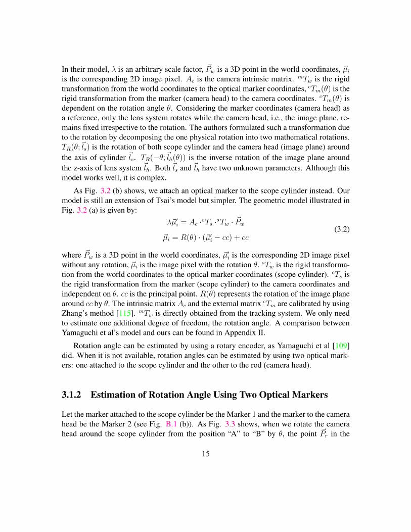
In their model, λ is an arbitrary scale factor, ~Pw is a 3D point in the world coordinates, ~µi

is the corresponding 2D image pixel. Ac is the camera intrinsic matrix. mTw is the rigidtransformation from the world coordinates to the optical marker coordinates, cTm(θ) is therigid transformation from the marker (camera head) to the camera coordinates. cTm(θ) isdependent on the rotation angle θ. Considering the marker coordinates (camera head) asa reference, only the lens system rotates while the camera head, i.e., the image plane, re-mains fixed irrespective to the rotation. The authors formulated such a transformation dueto the rotation by decomposing the one physical rotation into two mathematical rotations.TR(θ;~ls) is the rotation of both scope cylinder and the camera head (image plane) aroundthe axis of cylinder ~ls. TR(−θ;~lh(θ)) is the inverse rotation of the image plane aroundthe z-axis of lens system ~lh. Both ~ls and ~lh have two unknown parameters. Although thismodel works well, it is complex.

As Fig. 3.2 (b) shows, we attach an optical marker to the scope cylinder instead. Ourmodel is still an extension of Tsai’s model but simpler. The geometric model illustrated inFig. 3.2 (a) is given by:

λ~µ′i = Ac ·cTs ·sTw · ~Pw

~µi = R(θ) · (~µ′i − cc) + cc(3.2)

where ~Pw is a 3D point in the world coordinates, ~µ′i is the corresponding 2D image pixelwithout any rotation, ~µi is the image pixel with the rotation θ. sTw is the rigid transforma-tion from the world coordinates to the optical marker coordinates (scope cylinder). cTs isthe rigid transformation from the marker (scope cylinder) to the camera coordinates andindependent on θ. cc is the principal point. R(θ) represents the rotation of the image planearound cc by θ. The intrinsic matrix Ac and the external matrix cTm are calibrated by usingZhang’s method [115]. mTw is directly obtained from the tracking system. We only needto estimate one additional degree of freedom, the rotation angle. A comparison betweenYamaguchi et al’s model and ours can be found in Appendix II.

Rotation angle can be estimated by using a rotary encoder, as Yamaguchi et al [109]did. When it is not available, rotation angles can be estimated by using two optical mark-ers: one attached to the scope cylinder and the other to the rod (camera head).

3.1.2 Estimation of Rotation Angle Using Two Optical Markers

Let the marker attached to the scope cylinder be the Marker 1 and the marker to the camerahead be the Marker 2 (see Fig. B.1 (b)). As Fig. 3.3 shows, when we rotate the camerahead around the scope cylinder from the position “A” to “B” by θ, the point ~Pr in the

15

Marker 2’s coordinates O2 will move along a circular trajectory with respect to the point~O on the axis of the scope cylinder, which is in the Marker 1’s coordinates O1. We estimatethe center ~O of the circle first and compute θ by

θ = arccos‖ ~OPA

r ‖2 + ‖ ~OPBr ‖2 − ‖ ~PA

r PBr ‖2

2‖ ~OPAr ‖ · ‖ ~OPB

r ‖(3.3)

The center of the circle can be represented in terms of the transformations from theworld coordinates Ow to the Marker 1’s coordinates O1, and the Marker 2’s coordinatesO2. At least 3 different positions in the Marker 2’s coordinates (O2) (with different θ) arenecessary.

3.1.3 Estimation of the center of circle in 3D

We rotate the camera head around the cylinder to acquire 3 different positions with respectto the Marker 2. Let the transformation matrix from the world coordinates Ow to bothMarker 1’s coordinates O1 and Marker 2’s coordinates O2 for the position i be (o1Tow

i,o2Tow

i) (i = 1, 2, 3). Given any point ~Pr in O2, we compute the position ~Pi in O1 corre-sponding to different rotations as:

~Pi = o1Tow

i · (o2Tow

i)−1 · ~Pr, i = 1, 2, 3. (3.4)

~O is the center of the circumcircle of the triangle (∆ ~P1~P2

~P3).

Let ~R1 = ~P1 − ~P3, ~R2 = ~P2 − ~P3, the normal of the triangle is ~n∆ = ~R1 × ~R2. Theperpendicular bisector ~L1 of ~R1 and ~L2 of ~R2 can be computed as:

~L1 = ~P3 + ~R1/2 + λ1 · ~n∆ × ~R1

~L2 = ~P3 + ~R2/2 + λ2 · ~n∆ × ~R2

(3.5)

where λ1 and λ2 are parameters of the line ~L1 and ~L2. The intersection of the two linesrepresents the center of the circle. From Eq. 3.5 we can derive the center of the circle by

~O =( ~R2 − ~R1) · ~R1/2

| ~R1 × ~R2 |2· ( ~R1 × ~R2)× ~R2 + ~R2/2 + ~P3 (3.6)

It can be easily proved that ~O does not depend on the selection of ~Pr. Since at least 3different positions are necessary, we rotate the camera head around the scope cylinder by

16

Marker 1

O1

Marker 2

Marker 2

O2

A

B

Scope cylinder

Camera

head

Coupler

O2

Optical Tracker

Ow

2x

2x

2y

2y

2z

2z

Or

rPr

rPr

1z

1y

1x

θθ

wy

wx

wz

wO T1

)0(2w

O T

)(2 θwO T

Figure 3.3: Illustration of the relationship between the rotation angle θ and two markers’coordinates. The Marker 1 is attached to the scope cylinder and the Marker 2 is attachedto the camera head. “A” indicates the position of the Marker 2 when θ = 0 and “B”indicates the position of the Marker 2 with a rotation θ. For any point ~Pr in the Marker 2’scoordinates, its trace with the rotation of the camera head follows a circular trajectory inthe Marker 1’s coordinates (It moves from the position ~PA

r to ~PBr ). This circle is also in

the plane perpendicular to the axis of the scope cylinder. ~O is the center of the circle.

N different angles. We apply a RANSAC algorithm to estimate ~O using random positions,and finally select ~O∗ corresponding to the smallest variance as the center of the circle. Thepseudo code of RANSAC is listed in Table 4.3. It can also be proved that θ does not dependon the selection of Pr as well. A similar RANSAC algorithm, as Table 3.3 shows, is usedto compute θ. Fig. 3.4 shows estimated rotation angles using the RANSAC algorithm for

17

Table 3.2: Pseudo RANSAC code for estimating the center of the circle

Loop k=1:K (K=2000)Generate a random point Pr from 3D spaceGenerate random number x,y,z between [1,N]Compute Px,Py,Pz using Eq. 3.4Compute Ok using Eq. 3.6Compute | OkPj |, j ∈ [1, N ], j 6= x, y, zCompute vk

Save Ok, vk

End loopReturn Oq, q = argkmin(vk)

Table 3.3: Pseudo RANSAC code for estimating the rotation angle

Loop k=1:K (K=1000)Generate a random point Pr from 3D spaceCompute PA and PB using Eq. 6.2Compute θk using Eq. 3.3

End loopReturn θ = 1

K

∑k θk

two different endoscopes. The red curves are estimated angles from different RANSACiterations, and the black curve is the average. We can see that the variance of the estimationis very small (less than 0.2 degree).

3.1.4 Experimental Results

We tested our algorithm using two different systems. We first tested it in our lab. Weused a Stryker 344-71 arthroscope Vista (70 degree, 4mm) oblique-viewing endoscope, aDYONICS DyoCamTM 750 video camera, a DYONICS DYOBRITE 3000 light source,and Polaris (Northern Digital Inc., Ontario, Canada) optical tracker. Next we tested it in

18

0 10 20 30 40 50 600

20

40

60

80

100

120

0 5 10 15 20 25 30 35 400

20

40

60

80

100

120

140

Number of trials (Stryker arthroscope Vista)

Number of trials (Smith & Nephew arthroscope)

Ro

tati

on

an

gle

s (d

egre

e)R

ota

tio

n a

ng

les

(deg

ree)

RANSAC outputs

Average rotation angles

RANSAC outputs

Average rotation angles

Figure 3.4: Estimated rotation angles for two endoscopes. In each trial, we rotated thecamera head with respect to the scope cylinder and captured an image. We captured a fewimages for the initial position. After that we took two images for each rotation angle. Thered curves are estimated rotation angles from different RANSAC iterations. The blackcurve is the average.

19

(a)

(b)

(c) (d)

Figure 3.5: Optical trackers and endoscopes used in the experiments. (a) OPTOTRAK op-tical tracker (Northern Digital Inc., Ontario, Canada). (b) Polaris optical tracker (NorthernDigital Inc., Ontario, Canada). (c) Smith & Nephew video arthroscope - autoclavable SN-OH 272589 (30 degree, 4mm). (d) Stryker 344-71 arthroscope Vista (70 degree, 4mm).

the operating room. We used a Smith & Nephew video arthroscope - autoclavable SN-OH 272589 (30 degree, 4mm), a DYONICS video camera and light source, OPTOTRAK(Northern Digital Inc., Ontario, Canada) optical tracker. Fig. 3.5 shows the differentendoscopes and optical trackers.

The endoscope was first fixed and the calibration pattern was rotated on the table forcapturing images. A set of images were captured without a rotation between the scopecylinder and the camera head. They were used to estimate both the intrinsic matrix A(including the focal length and radial distortion coefficients) and extrinsic matrix cTs usingZhang’s method [115] (implemented using OpenCV functions). After that, while rotating

20

(a) (b)

Figure 3.6: (a) Illustration of the back projection with and without a rotation compensation.Green points are ground truth - 2D corner pixels on the image of the calibration pattern.Red points are back projection of the 3D world positions of the corners using the firstequation of Eq. 3.2, which has no rotation compensation. Blue points are back projectionusing both equations of Eq. 3.2. Since the rotation is included in the camera model, theback projected pixels are much closer to the ground truth than the red points. (b) An imageused in Yamaguchi et al. [109]’s paper. This image has a higher resolution, better lightingand less distortion than ours.

the camera head with respect to the scope cylinder, another set of images were captured andthe center of the circle can be computed by using Eq. 3.6. Next, we fixed the calibrationpattern, with two optical markers attached to the scope cylinder and the camera head, wecaptured the third set of images by applying normal operations to the endoscope (movingthe whole scope body or rotating the camera head with respect to the scope cylinder (ormore natural description: rotating the scope cylinder with respect to the camera head)).This set of images were used to evaluating the calibration. The initial position of thecamera head was considered as the reference position A illustrated in Fig. 3.3. Fig. 3.6illustrates the back projection of 3D corners of the calibration pattern with (blue) andwithout (red) a rotation compensation. Green points are ground truth. For each rotationangle of the endoscope, we calculated the average back projection error for this angle

ε(θ) =1

M

M∑i=1

| ~µi − ~µ( ~P iw, θ) | (3.7)

21

where ~Pi is a 3D point in the world coordinates, ~µi is the corresponding 2D image pixel,~µ( ~P i

w, θ) is the back projected 2D image pixel of ~Pi computed by using Eq. 3.2. M is thenumber of corners on the calibration pattern. We used different grid patterns (3x4, 4x5,5x6, 6x7. The size of each checker is 2mm x 2mm). In order to obtain enough light on thegrid pattern, the endoscope needs to be placed very close to the target (usually 5-15mm).Since smaller grids cannot capture the radial distortion and the bigger grids will exceedthe field of view, the 5x6 grid was selected to provide the best results.

We did many trials by moving and rotating the endoscope randomly and estimated θsimultaneously. The averaged back projection error with respect to the different rotationangles are shown in Fig. 3.7. Fig. 3.7 (a) shows the result using the Stryker 344-71 arthro-scope Vista (70 degree, 4mm) and Polaris optical tracker. Fig. 3.7 (b) shows the resultusing the Smith & Nephew video arthroscope - autoclavable SN-OH 272589 (30 degree,4mm) and OPTOTRAK optical tracker. The red curve represents the back projection er-ror without taking into account of the rotation angle, and the blue curve shows the errorconsidering the rotation angle. The results show that including the rotation angle into thecamera model significantly improves the accuracy of the calibration.

Fig. 3.7 shows that different endoscopes have different accuracy. The reason is thatendoscopes have different magnification and optical trackers have different accuracy (ac-cording to the manufacturer, RMS error is 0.1mm for OPTOTRAK and 0.3mm for Polaris).Yamaguchi et al. [109] used an OTV-S5C laparoscope (Olympus Optical Co. Ltd., Tokyo,Japan) and Polaris optical tracker. They achieved a high accuracy of less than 5mm backprojection error when the rotation angle is within 140 degrees. Our results show that wecan achieve the same level accuracy when the rotation angle is within 75 degrees. Beyondthis range, due to the bigger magnification, larger radial distortion and poorer lighting (acomparison between images used in Yamaguchi et al.’s experiments and ours is shown inFig. 3.6), the back projection error is increased to 13mm when the rotation angle is 100degrees. Given endoscopes with the same level of quality, we should be able to achievethe same level of accuracy, with a simpler setup and procedure.

3.2 Photometric Calibration

Until now, photometric calibration for the endoscope is seldomly addressed in literature.We propose a method to compute the radiometric response function of the endoscope, andalso simultaneously calibrate the directional/spatial intensity distribution of the near lightsources (the camera and the sources are “on/off” at the same time) and light intensities.Our method is inspired by Litvinov et al.’s work [61].

22

(a)

(b)

0 20 40 60 80 1000

50

100

150

No Rotation CompensationWith Rotation Compensation

0 20 40 60 80 1000

50

100

150

200

250

No Rotation CompensationWith Rotation Compensation

0 34 65

0 36 69

Rotation angle (degrees)

Rotation angle (degrees)

(a)

Bac

k p

roje

ctio

n e

rro

r (p

ixel

s)B

ack

pro

ject

ion

err

or

(pix

els)

(b)

Figure 3.7: Back projection errors with respect to the rotation angles for two systems.(a) Stryker 344-71 arthroscope Vista and Polaris optical tracker in our lab. (b) Smith &Nephew video arthroscope and OPTOTRAK optical tracker in the operating room. Imagesin the top row of (a) and (b) correspond to different rotation angles (the number is shown onthe top of each image). The red curves in (a) and (b) represent the errors without a rotationcompensation. The blue curves in (a) and (b) are errors with a rotation compensation.

23

Table 3.4: Table of Notation in Sec. 3.2R - scene radiance

I0, I0j - light intensity

ρ, ρi - surface albedo

~n - surface normal

s1, s2 - light sources

l1, l2 - light rays

r1, r2 - distance from light source to the surface point

P - surface point

I(·) - image irradiance function

x, y - image coordinates

x, y, z - world coordinates

H(·) - camera response function

v(·) - intensity value

M(·) - source spatial distribution function

M(·) - modified source spatial distribution function

h(·), etai, γj, m - log representation of H−1, ρi, I0j, M

3.2.1 Image Irradiance Equation

Assuming the bone surface is Lambertian, the scene radiance can be computed accordingto Lambertian cosine law:

R(x, y, z) = I0ρ(~n · ~l1r21

+~n · ~l2r22

) (3.8)

where I0 is the light intensity of ~s1 and ~s2, ρ is the surface albedo. We use the unit vector~n to represent the surface normal at ~P , ~l1 and ~l2 are two light rays incident at ~P , and r1 andr2 are the distance from each light source to the surface. (x, y, z) indicates the 3D locationof the scene point P (see details in Ch. 4).

On the other hand, The image irradiance I(x, y) is related to the image intensity, also

24

known as gray level v, through the camera response function H(·):

I(x, y) =H−1[v(x, y)]

M(x, y)(3.9)

where M(x, y) represents the anisotropy of the source spatial distribution. The two sourcesare identical and they are oriented in the same way so we assume that their spatial distri-bution functions M(x, y) are equal. From Eqs 3.8 and 3.9 we have:

H−1[v(x, y)] = ρ · I0 · M(x, y)

where M(x, y) = M(x, y) · (~n ·~l1

r31

+~n · ~l2r32

)(3.10)

During the calibration, we used a Macbeth color chart with known albedos for eachpatch. We captured a set of images by varying the source intensity for each patch. Weapplied log to both sides of Eq. 3.10 and obtained a linear system:

h[vji (x, y)] = ηi + γj + m(x, y) (3.11)

where i indicates the surface albedo and j indexes the light intensity. h[vji (x, y)] =

log{H−1[vji (x, y)]}, ηi = log(ρi), γj = log(I0j) and m(x, y) = log[M(x, y)]. The un-

knowns (h(·), γj , m(x, y)) can be estimated by solving this linear system of equations.The cosine term is then estimated by physically measuring the distance to the chart fromthe scope tip and finally M(x, y) is recovered.

3.2.2 Solution to h(·)Given the fixed light intensity γj and pixel value v(x, y) but two different albedos ηi1 andηi2 , we have {

h[vji1(x, y)]− γj − m(x, y)− ηi1 = 0

h[vji2(x, y)]− γj − m(x, y)− ηi2 = 0

(3.12)

Subtract the first line from the second line of Eq. 3.12 we obtain

h[vji2(x, y)]− h[vj

i1x, y)] = ηi2 − ηi1 (3.13)

We selected different pixels in the same image (albedo) or different images (albedos)to make as many equations as Eq. 3.13, as long as we fixed the light intensity for each pair

25

of albedos. Since vji1(x, y) changes from 0 to 255(image intensity), we only need 256 such

equations and stack them as:

· · · 1∗ −1∗ · · ·· · · −1# 1# · · ·

· · · · · ·

·

h(0)h(1)

...h(255)

=

ηi2−ηi1

ηi4−ηi3...

(3.14)

where 1∗ and−1∗ correspond to the column vji2(x, y)+1 and vj

i1(x, y)+1, respectively. 1#

and −1# correspond to the column vji4(x, y) + 1 and vj

i3(x, y) + 1, respectively. Therefore

h(v) is solved from Eq. 3.14 and H(·) = {exp[h(v)]}−1.

3.2.3 Solution to γj

Given the fixed albedo ηi and pixel value v(x, y) but two different light intensities γj1 andγj2 we have {

h[vj1i (x, y)]− γj1 − m(x, y)− ηi = 0

h[vj2i (x, y)]− γj2 − m(x, y)− ηi = 0

(3.15)

Subtract the first line from the second line of Eq. 3.15:

h[vj2i (x, y)]− h[vj1

i (x, y)] = γj2 − γj1 (3.16)

We use the minimum light intensity γ1 as a reference, for other light intensities γj, j =2, · · · , Nlight, we have

γj = γ1 + {h[vji (x, y)]− h[v1

i (x, y)]} (3.17)

With the estimated h[v(x, y)] and by changing the albedos and pixels, we compute theaverage for each γj as below and I0j = exp(γ1) · exp(γj).

γj = γ1 +1

Nalbedo

· 1

Npixels

Nalbedo∑i

Npixels∑x,y

{h[vji (x, y)]− h[v1

i (x, y)]} (3.18)

3.2.4 Solution to m(x, y)

Again, Given the fixed albedo ηi and light intensity γj but two different pixels (xp, yp) and(xq, yq) we have {

h[vji (xp, yp)]− γj − m(xp, yp)− ηi = 0

h[vji (xq, yq)]− γj − m(xq, yq)− ηi = 0

(3.19)

26

Subtract the first line from the second line of Eq. 3.19:

h[vji (xq, yq)]− h[vj

i (xp, yp)] = m(xq, yq)− m(xp, yp) (3.20)

For each γj and ηi, instead of using C2Npixels

different pairs of pixels, we choose onlyNpixels = 720× 480 pairs and stack the equations as below:

1 −11 −1

··

−1 1

︸︷︷︸Φ

·

m(x1, y1)m(x2, y2)

...m(xNpixels

, yNpixels)

=

h[vji (x1, y1)]− h[vj

i (x2, y2)]

h[vji (x2, y2)]− h[vj

i (x3, y3)]...

h[vji (xNpixels

, yNpixels)]− h[vj

i (x1, y1)]

(3.21)

It’s not practical to solve Eq. 3.21 using SVD directly since matrix Φ requires a hugeamount of memory. Instead we have noticed that the matrix Φ in Eq. 3.21 is a specialNpixels by Npixels matrix therefore we calculate the inverse directly by using Gauss-JordanElimination:

Φ−1 =

0 0 −1−1 0 0 −1−1 −1 0 0 −1

......

... · · · 0 −1−1 −1 −1 · · · −1 −1

(3.22)

Finally we can efficiently compute each element of m(x, y) independently and again,M(x, y) = exp[m(x, y)].

3.2.5 Experimental Results

A series of images of color chart were used for photometric calibration. We tested 6different levels of image intensities. In Fig. 3.8, (a),(b) and (c) show the camera responsefunction in Red,Green,Blue channels. (d) shows the recovered light intensity in differentlevels and compared to the ground truth. The smaller number in x-axis corresponds to thehigher intensity. We noticed a bit variance when light intensity is high due to saturation.(e) shows the original image and (f) shows m. (g) shows the cosine term (n)·l1

r21

+ (n)·l2r22

and(h) shows the spatial distribution function m(x, y).

27

50

60

70

80

90

100

1 2 3 4 5

Ground Truth Calibration

(a) (b)

(c) (d)

(e) (f)

(g) (h)

0 0.5 1 1.5 2 2.5 3 3.5 40

50

100

150

200

250

300 Red ChannelNonlinear Fit

0 1 2 3 4 5 6 7 80

50

100

150

200

250

300 Green ChannelNonlinear Fit

0 0.5 1 1.5 2 2.5 3 3.5 4 4.5 50

50

100

150

200

250

300 Blue ChannelNonlinear Fit

Figure 3.8: Results of photometric calibration. (a) camera response function in Red chan-nel. Red dots represents the data points and magenta line represents the nonlinear fit. (b)camera response function in Green channel. Green dots represents the data points andmagenta line represents the nonlinear fit. (c) camera response function in Blue channel.Blue dots represents the data points and magenta line represents the nonlinear fit. (d) Cal-ibrated light intensity in different levels (blue) and ground truth (green). We use the level6 as a reference and plot level 1-5. A small level corresponding to a high light intensity.A bit variation in the range of high intensities may be caused by saturation. (e) Originalimage of color chart. (f) m. (g) cosine term (n)·l1

r21

+ (n)·l2r22

. (h) spatial distribution functionm(x, y).

28

3.3 Conclusions and Discussion

We have developed a comprehensive calibration procedure for estimating both geometricand photometric parameters for oblique endoscopes. Our geometric calibration methodsimplifies the previous work given a newly designed coupler attached to the scope cylinder.It is easy to implement and practical to apply with the standard operating room equipmentssuch as the navigation system. The only drawback of this method is that it requires thetwo markers to be visible to the optical tracker all the time, otherwise the method will fail.

According to our knowledge, photometric calibration for endoscopes has been lessstudied. Most of related work did not rely on the physical model of light sources, orthey restricted the changing of light sources during the operation. A few of recent workapplied shape-from-shading to endoscopic images based on a simplified light source modelwithout calibrating endoscopes. However, in order to reconstruct an accurate shape fromendoscopic images, the knowledge of light sources is necessary and important.

Both geometrical and photometrical parameters are very useful for 3D visualizationand reconstruction of anatomical structures such as bones from endoscopic images. Wewill use calibrated endoscopes for artificial spine reconstruction (see Chaps. 4 and 6).The results demonstrate that using calibrated endoscopes can achieve good reconstructionresult, which is promising for the real surgical applications.

29

Chapter 4

3D Reconstruction for Bones fromEndoscopic Images

To reconstruct the 3D shape of bones from endoscopic images, we formulate the problemas a near-lighting shape-from-shading with a pinhole camera (perspective projection) andpresent a solution to reconstruct the Lambertian surface of bones using a sequence ofoverlapped endoscopic images, with partial boundaries in each image. First we formulatethe shape-from-shading problem to deal with perspective projection and near point lightsources that are not co-located with the camera center. Secondly, we propose a multi-image framework which aligns partial shapes obtained from different images in the worldcoordinates by tracking the endoscope. An iterative closest point (ICP) algorithm is usedto improve the matching and recover complete occluding boundaries of the bones. Finally,a complete and consistent shape is obtained by simultaneously re-growing the surfacenormals and depths in all views. We demonstrate the accuracy of our technique by runningsimulations and conducting experiments with artificial bones.

4.1 Shape-from-Shading under Near Point Sources andPerspective Projection

With the special design of endoscopes, we formulate the shape-from-shading under nearpoint lighting and a perspective projection, where the light sources are not located at theprojection center. As Fig. 4.1 shows, given two point light sources ~s1 and ~s2, we computethe scene radiance emitted by the surface point ~P according to the Lambertian cosine law

31

Table 4.1: Table of Notation in Sec. 4.1R - scene radiance

I0 - light intensity

ρ - surface albedo

~n - surface normal

s1, s2 - light sources

l1, l2 - light rays

r1, r2 - distance from light source to surface point

P - surface point

I(·) - image irradiance function



a, b - endoscope parameters

F - focal length

p, q - partial derivatives of z w.r.t. image coordinates x, y

e(·) - total error function

ei(·) - irradiance error function

es(·) - smoothness constraint

λ - Lagrange multiplier

(k, l) - image indices

zk,l, pk,l, qk,l - value of z, p, q at pixel (k, l)

n - iteration number

¯zk,ln, ¯pk,l

n, ¯qk,ln - average of neighborhood in the nth iteration

ψ(·) - local robust regularizer constraint

ρσ(·) - robust error kernel function

ξ - symbol for p, q, z

ξx, zy - partial derivatives of ξ w.r.t. image coordinates x, y

ˆξk,l

m- local robust regularizer term in the nth iteration

32

Or

],~,~[ Fyxp =r

],~,~[],,[ zF

zy

F

zxzyxP ==

rnr

X

Y

Z

Image plane

F

(Surface Normal)

(Scene Point)

Optical axis

Lens & light sources plane

(Focal length)

1lr

2lr)0( <zz

]0,,[1 bas −=r

]0,,[2 bas =r

(Depth)

X

Y~

~

Figure 4.1: A perspective projection model for an endoscope imaging system with twonear point light sources: ~O is the camera projection center. ~s1 and ~s2 are two light sources.We assume that the plane consisting of ~O, ~s1 and ~s2 is parallel to the image plane. Thecamera coordinate system (X−Y − Z) is centered at ~O and Z-axis is parallel to theoptical axis and is pointing toward the image plane. X-axis and Y-axis are parallel tothe image plane. F is the focal length. a and b are two parameters related to the positionof the light sources. Given a scene point ~P = (x, y, z), the projected image pixel is~p = (x, y, F ), where (x, y) are image coordinates. Assuming a Lambertian surface, thesurface illumination therefore depends on the surface albedo, light source intensity andfall-off, and the angle between the normal and light rays.

and inverse square distance fall-off law of isotropic point sources [43]:

R = I0ρ(cos θ1

r21

+cos θ2

r22

) (4.1)

where I0 is the light intensity of ~s1 and ~s2, ρ is the surface albedo. We use the unit vector~n to represent the surface normal at ~P . ~l1 and ~l2 are two light rays incident at ~P , and r1

and r2 are the distances from each light source to the surface. We have

cos θ1 =~n · ~l1‖~l1‖

, ~l1 = ~s1 − ~P , r1 = ‖~l1‖

cos θ2 =~n · ~l2‖~l2‖

, ~l2 = ~s2 − ~P , r2 = ‖~l2‖(4.2)

33

According to [42], the surface normal ~n can be represented in terms of the partial deriva-tives of depth z with respect to x and y ((x, y, z) are camera coordinates):

~n = [−∂z

∂x,−∂z

∂y, 1]/

√(∂z

∂x)2 + (

∂z

∂y)2 + 1 (4.3)

Note that for the orthographic projection ∂z/∂x and ∂z/∂y are used to represent surfacenormals, where (x, y) are image coordinates. Under the perspective projection we have

x = xz

Fy = y

z

F

(4.4)

where F is the focal length and z < 0. We take the derivatives of both sides of Eq. 4.4w.r.t x and y and obtain

∂z

∂x=

1

x(F − z

∂x/∂x)

∂z

∂y=

1

y(F − z

∂y/∂y)

(4.5)

We also take the derivatives of both sides of Eq. 4.4 w.r.t x and y and obtain

∂x

∂x=

1

F(z + x

∂z

∂x)

∂y

∂y=

1

F(z + y

∂z

∂y)

(4.6)

Let p = ∂z/∂x and q = ∂z/∂y, from Eqs 4.5 and 4.6 we have

∂z

∂x=

Fp

z + xp

∂z

∂y=

Fq

z + yq

(4.7)

Given two light sources s1 = [−a, b, 0] and s2 = [a, b, 0] (calibration of a, b and F werediscussed in Ch. 3), we can explicitly write light source vectors as follows:

~l1 = [−a− xz

F, b− y

z

F,−z]

~l2 = [a− xz

F, b− y

z

F,−z]

(4.8)

34

Combining Eqs 4.1, 4.2, 4.3, 4.7 and 4.8, we obtain the reflectance map R as a functionof x, y, z, p, q:

R(x, y, z, p, q) = I0ρ

(~n(x, y, z, p, q) · ~l1(x, y, z)

r1(x, y, z)3+

~n(x, y, z, p, q) · ~l2(x, y, z)

r2(x, y, z)3

)

= I0ρ

p(z + yq)(a + xz

F)− q(z + xp)(b− y

z

F)− z

F(z + xp)(z + yq)

√p2(z + yq)2 + q2(z + xp)2 +

(z + xp)2(z + yq)2

F 2·(√

(−a− xz

F)2 + (b− y

z

F)2 + (z)2

)3

+−p(z + yq)(a− x

z

F)− q(z + xp)(b− y

z

F)− z

F(z + xp)(z + yq)

√p2(z + yq)2 + q2(z + xp)2 +

(z + xp)2(z + yq)2

F 2·(√

(a− xz

F)2 + (b− y

z

F)2 + (z)2

)3

(4.9)

Eq. 4.9 is similar to Eq. 2 in [95] and Eq.2 in [75], but we consider the 1/r2 as thefall-off since the light sources are very close to the bone surface. Eq. 4.9 can be easilyextended to multiple point sources as below (M is the number of sources):

R(x, y, z, p, q) = I0ρ

M∑i

(~n(x, y, z, p, q) · ~li(x, y, z)

ri(x, y, z)3) (4.10)

4.1.1 Solving Image Irradiance Equation

Given the image irradiance function I(x, y), the image irradiance equation [42] is

R(x, y, z, p, q) = I(x, y) (4.11)

According to [25], different mathematical methods have been proposed to solve the equa-tion for PSFS, including methods of resolution of PDEs [95, 96, 53, 76] and methodsusing optimization [17]. The optimization methods based on the variational approacheswork well in most of general cases and does not need to set values to the singular and localminimum points [25], so we adopt the optimization method and plug it in the multi-imageframework. Specifically, we solve Eq. 4.11 by minimizing the error between the imageirradiance I(x, y) and the reflectance map R(x, y, z, p, q) given in Eq. 4.9. Image irradi-ance is obtained from the image intensity given the calibrated camera response function

35

and spatial distribution (see details in Sec. 3.2). Different from the previous optimizationmethods [44], the depth z is explicitly included in R. We compute the error as:

e(z, p, q) = λei(z, p, q) + (1− λ)es(z, p, q) (4.12)

andei(z, p, q) =

∫ ∫image

[I(x, y)−R(x, y, z, p, q)]2dxdy

es(z, p, q) =∫ ∫

image[(z2

x + z2y) + (p2

x + p2y) + (q2

x + q2y)]dxdy

(4.13)

where ei(z, p, q) is the irradiance error and es(z, p, q) is the smoothness constraint for z, pand q. λ is a Lagrange multiplier. We find the solution to (z, p, q) by minimizing the errore(z, p, q) [58]:

[z∗, p∗, q∗] = argz,p,q

min(λei + (1− λ)es) (4.14)

Similar to [41], we discretize Eq. 4.12 and obtain:

e(zk,l, pk,l, qk,l) =∑

k

∑

l

(λeik,l + (1− λ)esk,l) (4.15)

The solution to Eq. 4.15 is to find [p∗k,l, q∗k,l, z

∗k,l] that minimize e:

∂e

∂pk,l

|p∗k,l= 0,

∂e

∂qk,l

|q∗k,l= 0,

∂e

∂zk,l

|z∗k,l= 0 (4.16)

Combining Eq. 4.15 to 4.16 yields update functions for pk,l, qk,l and zk,l in each iteration[41]:

pn+1k,l = pn

k,l +λ

4(1− λ)[Ik,l −R(k, l, zn

k,l, pnk,l, q

nk,l)]

∂R

∂pk,l

|pnk,l

qn+1k,l = qn

k,l +λ

4(1− λ)[Ik,l −R(k, l, zn

k,l, pnk,l, q

nk,l)]

∂R

∂qk,l

|qnk,l

zn+1k,l = zn

k,l +λ

4(1− λ)[Ik,l −R(k, l, zn

k,l, pnk,l, q

nk,l)]

∂R

∂zk,l

|znk,l

(4.17)

pnk,l, qn

k,l and znk,l are local 8-neighborhood average around the pixel (k, l). Detailed deriva-

tion can be found in Appendix I. The value for the (n + 1)th iteration can be estimatedfrom the nth iteration. During the iteration, the Lagrange multiplier λ is gradually in-creased such that the smoothness constraint is reduced as well. In our experiment, settingof Lagrance multiplier is empirical. We set it to 0.005 at the beginning and increase it by0.02 whenever the error in Eq. 4.15 is reduced by 1%.

Given the initial values of p, q and z on the boundary, we compute a numerical solu-tion to the bone shape. Variational methods usually rely on good initial guesses, so we

36

(1)

(2)

(3)

(4)

(5)

(a) (b)

Figure 4.2: Results of shape from shading from a single image. (a) input image. (b) shapefrom shading. (1)-(5) are captured from different viewpoints.

37

manually label the boundaries of each images. After that, z is set to −1 for each pixel inthe image. p and q are set to 0 for pixels that are not on the occluding boundaries. p andq at each pixel on the occluding boundaries are computed as the cross product of viewingvector (starting from the optical center) and the edge vector. Because it is difficult to esti-mate the initial values of z, we reset z values by integrating the normals using the methodin [30], after several iterations when the error in Eq. 4.15 is reduced by 10%. We keepperforming such an adjustment until the algorithm converges.

One of the drawbacks of this method is its tendency that overly smoothes out localdiscontinuities because only smoothness constraints are enforced. Therefore we introducea local robust regularizer based on surface geometry [107], which considers that the re-constructed surface should be smooth, except where the probability of a discontinuity ishigh. The robust regularizer constraint function is defined as

ψ(ξ|σ) = ρσ(‖∂ξ

∂x‖) + ρσ(‖∂ξ

∂y‖), ρσ(ω) =

σ

πlog cosh

(πω

σ

)(4.18)

where ξ ∈ {η|p, q, z}. The robust error kernel function ρσ(ω), the sigmoidal derivativeM-estimator (a continuous version of Huber’s estimator), is proved to possess the bestproperties for handling surface discontinuities [107]. By discretizing Eq. 4.18 and ap-plying the calculus of variations, we obtain the update term for ξ in terms of the robustregularizer constraint.

ξnk,l =

(ξnk+1,l + ξn

k−1,l

)

‖ξnx‖

tanh(π

σ‖ξn

x‖)

+π

σ

[‖ξn

x‖sech2(π

σ‖ξn

x‖)− tanh

(π

σ‖ξn

x‖)]

+

(ξnk,l+1 + ξn

k,l−1

)

‖ξny ‖

tanh(π

σ‖ξn

y ‖)

+π

σ

[‖ξn

y ‖sech2(π

σ‖ξn

y ‖)− tanh

(π

σ‖ξn

y ‖)]

(4.19)

where ξx and ξy are average of the forward and backward difference with respect to xand y. i.e. ξx = [(ξk+1,l− ξk,l)+ (ξk,l− ξk−1,l)]/2, ξy = [(ξk,l+1− ξk,l)+ (ξk,l− ξk,l−1)]/2.Note that Eq. 4.19 is in essential a scalar version of Eq. 26 in [107]. We will use ξn

k,l

instead of the average ξnk,l in Eq. 4.17.

By these means, some local discontinuities can be partially recovered. However, therecovered shape is still partial with limited information due to the small field of view.

38

Table 4.2: Table of Notation in Sec. 4.2Si - 3D point set reconstructed from image i in camera coordinates

Ni - number of points in shape Si

wTmi- transformation from marker coordinates to world coordinates

M - transformation from marker coordinates to camera coordinates

Siw, Si−1

w - transformed 3D point set in world coordinatesi−1Si

w - aligned 3D point set with respect to adjacent point set Si−1w

i−1Ti - rigid transformation from the ith position to the i− 1th position


p, q - partial derivatives of z w.r.t. image coordinates x, y

(a) (b)

(c) (d) (e)

Figure 4.3: Simulation results of shape from shading from multiple views. (a)-(d) Synthe-sized images of different parts of a sphere. (e) Reconstructed sphere.

4.2 Global Shape-from-Shading using Multiple Partial Views

As shown in Fig. 4.2, most images include a small fraction of visible contours. How do weestimate the complete shape reliably? An intuitive solution is to merge individual shapesrecovered from different views as shown in Fig. 4.3.

However, each image is defined in a view dependent local coordinates. We must firsttransform them to the world coordinates before we merge individual shapes. We solvethis problem by using a navigation tracking system. We attach optical markers to theendoscope (as showed in Fig. 3.2) and track them to obtain transformations between the

39

local and the world coordinates for each image.

Consider a 3D-point set [Si]3×Nireconstructed from the image i, where Ni is the num-

ber of points on the shape Si. If all the shapes are reconstructed correctly, without any er-rors from the tracking system and the calibration process, they should be perfectly alignedin the world coordinates. Let wTmi

denote the transformation from the marker at the po-sition capturing the ith image to the world coordinates, and M denote the transformationfrom the marker coordinates to the camera coordinates (image distortion has been cor-rected in advance). Thus, any 3D-point set Si in the local camera coordinates can betransformed to the world coordinates Si

w by:

Siw =w Tmi

· [M−1 · Si;11×Ni] (4.20)

where Siw is represented using homogenous coordinates in the world reference frame. As

shown in Fig. 4.4, each shape from single image is transformed to the world coordinates.However, due to the tracking error (less than 0.3mm) and the calibration error (less than6 pixels), individual shapes Si

w are not initially well matched with each other (e.g. Fig.4.4 (c) and (d)). Since the bone is rigid, we use ICP [4] to improve the matching betweendifferent views by ensuring overlapped fields of view in adjacent images. Then, for eachshape Si

w, ICP results in an aligned shape i−1Siw with respect to the adjacent shape Si−1

w :

i−1Siw =i−1 Ti ∗ Si

w (4.21)

where i−1Ti is the rigid transformation computed from ICP.

Using ICP, we can align all the shapes from one view with respect to the shape in thereference view, i.e. the shape S1

w in the first image. Combining Eq. 4.20 and 4.21, we have

1Siw =

i−1∏j=1

jTj+1 ·wTmi· [M−1 · Si;11×Ni

] (4.22)

where 1Siw is the aligned shape of Si

w with respect to the reference shape S1w, as shown in

Fig. 4.5 (a) and (b).

Once the contours are aligned, we ”re-grow” the shape in the local views from theglobal boundaries. We compute the average on boundaries in Eg. 4.17 using the neighborsin the world coordinates. The key idea is to keep the values on the global boundary updatedbased on the shape developed in the local view, and therefore SFS in the local views areguided towards convergence under global boundary constraints.

We restart the SFS in the local coordinates simultaneously for all images. After initial-izing (z, p, q) in each image, we initialize values on the corresponding global boundary.

40

Table 4.3: Global Shape-from-Shading: Key Steps

* Loop k=1:number of images1) Compute SFS from single image using Eq. 4.172) Track endoscope motions3) Transform local views to the world coordinates using Eq. 4.204) Align each shape to the previous shape using ICP using Eq. 4.21End loop

* Compute global boundaries using Eq. 4.22* Compute global constraints (z, p, q) in the world coordinates* Loop until converge

1)Loop k=1:number of imagesa) Update (z, p, q) in the local views according to the global constraintsb) Compute new (z, p, q) by using Eq. 4.17End loop

2)Update (z, p, q) in the world coordinatesEnd loop

If there are two or more points from different views that are mapped to the same point inthe world coordinates, (z, p, q) at those points are computed using the average. In eachiteration, we grow each image and update the values on the global boundary. Comparedto the single image shape-from-shading (see Fig. 4.4 (a)), we obtain more informationfrom global boundaries (see Fig. 4.5 (c)). At the end of each iteration, we update thelocal (z, p, q) given the global constraints. We proceed this until the algorithm converges.With the global boundary constraints, our algorithm converges quickly although not inreal-time (around 5 minutes for 18 images in Matlab with P4 2.4G CPU). Table 4.3 liststhe key steps in the multi-view shape from shading.

We use a laser range scanner to build a ground truth shape of the spine. The maximum,minimum, mean and RMS errors are 2.8mm, 0.0mm, 1.24mm and 1.45mm respectively.This level of accuracy is practical for surgery. More views of the reconstructed surfacecompared to the ground truth are shown in Fig. 4.6. We also compare our results withthe results under the orthographic projection assumption in Fig. 4.7. Compared to thereal shape captured by a regular camera, we find that the shape under the orthographicprojection is over grown near the boundaries.

41

(1)(5)(11)(18)

(a) Undistorted radiance images with manually labeled boundary

(b) Shape from single image

(c) Unaligned individual shapes in the world coordinates

(d) Unaligned 3D contours in the world coordinates

Figure 4.4: Problems of directly merging the individual shapes in the world coordinates.18 images are captured by moving the endoscope horizontally (only translation). Four ofthem are shown as an example. (a) After removing the distortion and illumination effects,the boundaries in each image are labelled by hand, and the initial (p, q) are computedautomatically on the boundaries. (b) Shape from each single image are reconstructed usingthe method described in Section 4.1. (c) Mis-aligned shapes in the world coordinates. (d)Mis-aligned 3D contours in the world coordinates.

42

(a) Aligned individual shapes in the world coordinates

(b) Aligned 3D contours in the world coordinates

(1)(5)(11)(18)

(c) Projection of global contours on individual images

(d) Reconstruction from global constraints

Figure 4.5: Illustration of the multi-image shape-from-shading. (a) Aligned shape in theworld coordinates. (b) Aligned 3D contours in the world coordinates. (c) Projection ofthe global constraints onto each image. (d) Final shape reconstructed using the methoddescribed in Section 4.2.

43

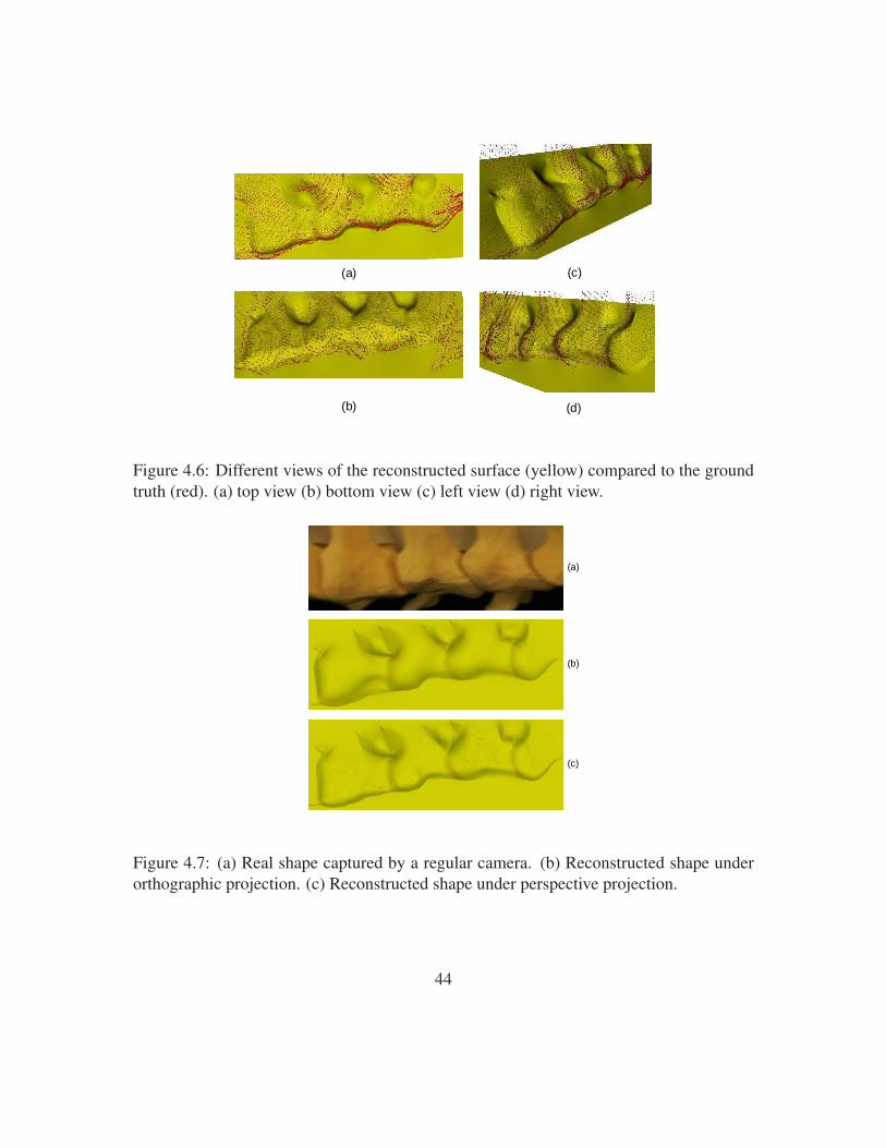
(c)(a)

(b) (d)

Figure 4.6: Different views of the reconstructed surface (yellow) compared to the groundtruth (red). (a) top view (b) bottom view (c) left view (d) right view.

(a)

(b)

(c)

Figure 4.7: (a) Real shape captured by a regular camera. (b) Reconstructed shape underorthographic projection. (c) Reconstructed shape under perspective projection.

44


Shape-from-shading and shape-from-motion have been successfully applied in many com-puter vision applications, but both have difficulties for 3D reconstruction from orthopedicendoscopy due to the featureless bone surface and partial occluding boundaries in a smallfield of view. In this work, we propose a method to combine the strengths of both ap-proaches to solve our problem: we reformulate the shape-from-shading for endoscopes un-der near point light sources and perspective projection, and develop a multi-image shape-from-shading framework. To deal with the tracking and calibration errors, we use ICP toimprove the alignment of partial shapes and contours in the world coordinates. As a result,we reconstruct the shape of a larger bone area and provide useful visualization for surgicalnavigation during minimally invasive procedures.

A couple of issues are worthy of further discussion. We build a near-field lighting andperspective shape-from-shading (NLPSFS) model without assuming that the light sourcesare located at the optical center. Our contribution is to present a new model for medicalendoscopes, instead of a new solution to any existing models. We adopt the variationaloptimization method since it is effective for most general cases and no pre-defined valuesare involved for the singular and local minimum points. Since our multi-image approach isvery general, other PSFS solutions such as Prados et al.’s [76] and Tankus et al.’s approach[95] can be employed to solve the NLPSFS problem as well. We plan to compare differentSFS methods in the future work. In this thesis we focus on the formulation of the NLPSFSmodel and multi-image framework.

As mentioned in the previous section, in the real operating environment, the bonesurfaces are usually 5-10 mm away from the endoscope. The light sources and cameraseparation distance is 3.5mm in our case. These two numbers are in the same order ofmagnitude as the distance to the scene. The approximation becomes inaccurate if weignore the parameters a and b in Eq. 4.9. However, it is a reasonable approximation whenthe endoscope is far away from the scene. In our work we attempt to build a generaland accurate model to handle more realistic cases, thus we have calibrated all parametersbeforehand.

One advantage of our method is that the computation of single image SFS (see thefirst step of Table 1) can be parallelized since the error function in Eq. 4.15 uses only onesingle image. Note in the last step of Table 1, the computation of single image SFS cannotbe parallelized because the global constraints need updates for each iteration.

By using ICP in our multi-image framework, we are able to deal with tracking andcalibration errors. Moreover, our algorithm can tolerant some shape errors caused by the

45

single image SFS in the first step of Table 1. Therefore we use an early stop strategy duringthe single image SFS by terminating the iterations before the error in Eq. 4.15 reaches zero(we set the threshold to 15% of the initial error). With this strategy, we significantly speedup the algorithm. This is one of the reasons why the result from a single image tends to beflat. Other reasons include partial occluding boundaries and the smoothness constraints.

The results from multi-image SFS (MISFS) still lack high frequency shape details dueto over-smoothing. Besides, it cannot deal with occlusions due to blood and tissues [57] insurgery, and inaccurate shapes caused by endoscope rotations. To overcome above issues,we will introduce a global shape prior in the following chapters. In Ch. 5, a statisticalshape prior, also known as a statistical atlas, is introduced. An efficient framework ofconstructing the atlas is described as well. In Ch. 6, we modify the bottom-up MISFS byenforcing the statistical atlas as a new global constraint. We also develop a top-down eval-uation refinement to improve reconstruction. Please see details in the following chapters.

46

Chapter 5

Construction of Statistical Shape Priorfor Bones from Population

The MISFS framework proposed in Ch. 4 results in shapes that are often over-smoothed,which makes it hard to apply the method to intricate structures such as spine vertebrae.This is because shape-from-shading is a fundamentally under-constrained problem and re-quires additional constraints to help solve it. In the absence of any other knowledge, con-straints enforcing smoothness are used, often leading to shapes that are overly smoothedand lack detail. In addition, we assume that images are captured using pure translation ofthe endoscope. The rotation of the endoscope can result in wrong correspondences of theoccluding boundaries across different views in turn leading to inaccurate reconstruction.Moreover, many substances (such as blood, pieces of bone, tissue) in surgery may obscurethe bone surface and mislead any local constraints used in reconstruction.

Therefore, a global model is needed to recover the shape detail and correct the inac-curate reconstruction due to the endoscope rotations and occlusions. For example Honget al. take the advantage of the tubular nature of the colon to design their reconstructionalgorithm [39]. In this chapter, we introduce a statistical shape prior, also known as statis-tical atlas, for bone structures. In Ch. 6 we will present a new algorithm using this shapeprior to improve the MISFS method.

Statistical atlases are used as references to interpret CT/MRI images [64], and to rep-resent the shape or appearance of human anatomical structures [91, 90]. Some atlasesare based on physical properties, such as elastic models [6, 3],“snakes” [47], geometricsplines [27], and finite elements based models [70]. Others are modeled from the statisti-cal perspective. Szeliski [92] introduced the statistical atlas to analyze the shape variationbetween patients. In order to analyze the shape and appearance variation, principal compo-

47

nent analysis (PCA) is widely used [14, 65, 80]. The two most common statistical atlasesare the shape atlas [16] and the appearance atlas [15]. The shape atlas uses only geometricinformation, such as landmarks, surfaces (boundaries of 3D objects) or crest lines [90].The appearance atlas uses both geometric features and intensity of pixels or voxels.

As a key to build atlases, 3D registration has been studied for years in computer vi-sion, but it still remains a critical problem in the medical image field due to the geometricalcomplexity of anatomical shapes, and computational complexity caused by the enormoussize of volume data. It has numerous clinical applications such as statistical atlas con-struction for group study and statistical parameters analysis [12, 38], mapping anatomicalatlases to individual patient images for disease analysis [10, 28, 46] and image segmenta-tion [79, 89].

Depending on the type of the transformation being involved, registration can be rigidor non-rigid. If the shape has no change between the two images, registration shouldbe rigid. For example, the intra-subject inter-modality (same patient; different imagingsystem) registration aligns images that are captured at the same time. However, when wetake into account the time, i.e., when two images are captured at different time, such asin intra-subject registrations, most of them are non-rigid due to the shape variation of theanatomical structures caused by swelling, bone fractures, tumor growth changes, intestinalmovements etc. In addition, inter-subject (different patients) registrations are usually non-rigid due to the local anatomical difference between patients. So far non-rigid (also knownas deformable) registration is still a challenging problem [18].

Non-rigid registration is used to find a non-rigid transformation from one 3D surfaceto the reference surface by minimizing the distance between two surfaces. In general, anon-rigid transformation is represented by a global rigid or affine transformation plus alocal non-linear deformation, which can be represented by radial basis functions (RBF)[113], octree-spline [93], thin-plate spline [11, 12], geometric splines [27], finite elements[70], or free form B-spline [80], etc. To evaluate the results of registration, different sim-ilarity measurements will be selected according to different image features and imagingmodalities. For example, sum of squared distance (SSD) is usually used for geometricfeatures [5], but correlation coefficients (CC) [52], Ratio Image Uniformity (RIU) [106],and mutual information (MI) [101] are used for intensity features. Registration can besimplified given known correspondences, for example, using markers [63]. Nevertheless,markers are not allowed to be used or even available in many scenarios. Alternate estima-tion of correspondences and transformations are widely used for both rigid cases [5] andnon-rigid cases [12, 11, 33]. Moreover, with the increase of the data size and geometri-cal complexity, multi-resolution strategy has been adopted to the registration framework[46, 26, 85]. Sparse matrices are also used to handle the computational complexity [69].

48

MeshSimplification

Non-RigidRegistration

LocalDeformation

High-ResolutionSurface Mesh

Low-ResolutionSurface Mesh

Low-ResolutionSurface MeshRegistered

Interpolation

High-ResolutionSurface MeshRegistered

LocalDeformation

Figure 5.1: Two-level non-rigid registration framework.

In this chapter, we developed a two-level approach inspired by Chui and Rangarajan’sthin-plate spline based algorithm [11] and the previous multi-resolution work [85]. SinceChui and Rangarajan’s algorithm [11] is not able to handle more than 2000 3D points [69],we broke down the registration into a two-level process to deal with both computationaland geometrical complexity. We first applied Chui and Rangarajan’s algorithm [11] to thesimplified low-resolution surfaces. To improve efficiency, instead of successively match-ing each resolution from coarse to fine, we directly propagated the correspondences fromlow resolution to high resolution by interpolation. A local refine procedure was introducedfor both low-resolution and high-resolution surfaces to improve matching. Finally we ap-plied PCA to the aligned surfaces to construct the femur atlas. Fig. 5.1 illustrates theflowchart of our two-level framework.

5.1 Two-Level Framework

5.1.1 Mesh Simplification

Garland’s quadric error metrics (QEM) based mesh simplification [32] method was usedto compute low-resolution surfaces. QEM is based on iterative contraction of vertex pairs.The cost of contraction is represented by a quadric error and the whole process is an iter-

49

Table 5.1: Table of Notation in Sec. 5.1XL, Y L - low resolution surface

XH , Y H - high resolution surface

xLi , yL

i - vertex on low resolution surface

xHj , yH

j - vertex on high resolution surface

c1 - coefficients for radial basis functions

c2, c3 - coefficients for affine transformation

ϕ(·) - symmetric radial basis function

X ,Y ,Z - coordinates axes

N, N lowref - number of vertices on low resolution reference surface XL

M, Nhighref - number of vertices on high resolution reference surface XH

S1, S2, S3 - neighboring triangles sharing the same vertex yi

y1i , y

2i , y

3i - projection of xi onto S1, S2, S3

d1, d2, d3 - distance from xi to S1, S2, S3

vi - surface vector

K - number of training surfaces

κ - mean surface vector

Ψ - covariance matrix

ηi - PCA coefficient vector

Ui - eigenmatrix

USi - first S columns of eigenmatrix

d(·) - point to surface distance

dm(·) - surface mean error

dRMS(·) - surface RMS error

T - processing time

ative minimization of the quadric error. Since QEM provides a fast, simple way to guidethe entire process with relatively minor storage costs, the simplification step is extremelyfast.

An important parameter involved in the simplification process is the number of ver-

50

tices in the low-resolution surfaces. To maintain the tradeoff between the accuracy andefficiency, a reasonable number is selected based on a series of leave-one-out experiments(See details in Sec. 5.1.6).

5.1.2 Low-Resolution Non-Rigid Registration

We applied Chui and Rangarajan’s non-rigid registration method [11] to the simplified sur-faces. With this method, fuzzy correspondences and a smoother optimization process canbe achieved. A dual update strategy conjuncted with a deterministic annealing techniqueis adopted to estimate the correspondences and transformation alternately. The non-rigidtransformation is parameterized using thin-plate splines to generate a smooth spatial map-ping.

5.1.3 Low-Resolution to High-Resolution Interpolation

To improve the efficiency, instead of successively matching each resolution from coarse tofine, we directly propagate the correspondences from low resolution (XL and Y L) to highresolution (XH and Y H) by interpolation. The surface interpolation method is a derivativeof methods known jointly as “moving least squares” [112]. Radial basis functions (RBF),finite element, multivariate spline such as thin-plate spline (2D bivariate spline) and tri-harmonic thin-plate spline, are popular techniques used for surface interpolation. Carr etal. [9] applied multivariate splines method into radial basis functions by using splinesas kernel functions. In this work we chose Gaussian kernel due to its simple mathemat-ical representation and less restrictions on nodes [9]. More specifically, we used a linearaffine function plus a series of radial basis functions (RBFs) to construct the interpolationfunction:

yLi = g(xL

i ) = c1 · [ϕ(‖xLi ,xL

1 ‖), · · · , ϕ(‖xLi ,xL

N‖)]′ + c2 + c3 · xLi︸︷︷︸

g(xLi )

(5.1)

where xLi is a vertex on the low-resolution surface XL, whose correspondence on the low-

resolution surface Y L is yLi , i = 1, 2, · · · , N (N is the number of vertices on XL). xL

i

and yLi are both 3×1 vectors with three coordinates. c1 is a 3×N coefficient matrix of

radial basis functions. ϕ(‖xLi ,xL

j ‖) is a symmetric radial basis function. We selected aGaussian kernel ϕ(ui,uj) = exp(−‖ui − uj‖/0.5), as suggested by [72]. c2 and c3 arecoefficients for the affine transformation. c2 is a 3×1 vector and c3 is a 3×3 matrix. Given

51

N correspondences, there are N equations for each axis (X , Y and Z):

ϕ(xL1 ,xL

1 ) · · · ϕ(xL1 ,xL

N) 1 xL1

T

...ϕ(xL

N ,xL1 ) · · · ϕ(xL

N ,xLN) 1 xL

NT

︸︷︷︸Pk

·

ck1T

ck2T

ck3T

︸︷︷︸ck

=

yL1

k

...yL

Nk

︸︷︷︸yvk

(5.2)

where c1k, c2

k and c3k denote the kth row of c1, c2 and c3, respectively. yL

ik denotes the

kth row of yLi , k can be 1,2 or 3, corresponding to the axis X , Y , and Z . There are 3N

equations in total:

P = [P1,P2,P3]′, c = [c1, c2, c3]′,y = [y1,y2,y3]′ (5.3)

P is a 3N×(N + 4) matrix. In order to ensure smooth interpolation, additional orthog-onality constraints

∑i x

Li

Tc1,i = 0 [8] were added to Eq. 5.2, where c1,i denotes the ith

column of c1: [P

xL1 xL

2 · · · xLN 04×4

]

︸︷︷︸Q

· c =

[y

04×1

]

︸︷︷︸w

(5.4)

The least-squares solution for this linear system, Qc = w, is given by c = (QTQ)−1QTw.

Finally, the correspondence of a vertex xHj in the high-resolution surface XH is com-

puted by Eq. 5.1: yHj = g(xH

j ), for j = 1, · · · ,M (M is the number of vertices onXH).

5.1.4 Refining Registration

For both low-resolution and high-resolution surfaces, we applied a refining procedure toimprove accuracy. The refining procedure includes both local and global steps.

Local Refining

The registration results can be further improved by minimizing the point-to-surface dis-tances. This idea is illustrated by Fig. 5.2. xi is a vertex on the deformed surface X ,whose corresponding vertex on the surface Y is yi. The neighboring triangles which sharethe same vertex yi are S1,S2 and S3. We can compute the distance from xi to each neigh-boring triangle (the distance computed from the vertex xi to the plane where the triangle

52

Deformed Vertex on Surface X

Corresponding Vertex on Surface Y

Figure 5.2: Illustration of the local refine procedure between the vertex and surface. xi is a vertexon the deformed surface X , whose correspondence on the surface Y is yi. The projection of xi toeach triangle St sharing yi is denoted by yi

t. dt is the distance between xi and yit. (t = 1, 2, 3, · · · )

lies), i.e. d1, d2 and d3. If any of them is smaller than d0 = ‖xi − yi‖, we will use thecorresponding projected surface point to replace yi to achieve a smaller surface distance.

For cases where different vertices on the surface X correspond to the same surfacepoint on Y , we will assign this corresponding surface point to the vertex on X with thesmallest distance and mark it unavailable to other vertices on X .

Global Refining

For training surfaces with sparse points, we cannot directly apply the local refining pro-cedure since no high-resolution surface can be used as a target shape, for example, thespine data. Compared to bones such as femur and knee, spine vertebrae have complexshapes which make it hard to automatically segment from CT images (using for example,marching cubes algorithm). On the other hand it is tedious to manually label over ten thou-sand points to obtain high-resolution surfaces. Given some shape information, Kaus et al.[49] use learned deformable models to generate aligned 3D meshes. In our case withoutknowing any shape prior, we propose a semi-automatic strategy by taking advantage ofthe two-level framework to generate high-resolution surfaces from sparse labeled points.Given a reasonable amount of manual labeling, for instance 250 points per model, we are

53

able to combine surface segmentation and registration in the same procedure, and reducemanual work to a minimal.

The sparse points set is first used as the low resolution input for the two-level frame-work. In the final refining step, instead of the local refining, we propose a global refiningwhich uses the sparse labeled points as a target shape. We apply a RBF based warping torefine the high-resolution surface towards the original labeled points. We employ the sameRBF functions used for the low-resolution to high-resolution interpolation (see Sec. 5.1.3)but different sigma for the RBF kernel. Here we choose σ as 250. The larger σ representsstronger global deformation.

5.1.5 Atlas Construction

Given aligned high-resolution surfaces, rigid pose alignment is applied to eliminate theeffect of imaging poses [34] prior to atlas construction. Suppose we have K aligned sur-faces and each surface is represented by a 3M×1 vector vi(i = 1, · · · , K), where M isthe number of vertices on each surface and each vertex has 3 components along X , Y , andZ axes. We compute the mean vector κ and covariance matrix Ψ, and then apply PCA tofind the low dimensional representation of the data:

κ=1

K

∑v, Ψ=

1

M − 1[v1−κ,· · ·,vK−κ]·[v1−κ,· · ·,vK−κ]′ (5.5)

Ψ = UΛU′ (5.6)

Therefore, a compact representation of any surface model is given by a mean vector plusa linear combination of principal components (modes):

vi = κ + Uηi (5.7)

where ηi is a K×1 coefficient vector obtained by projecting vi onto each principal axis.New surface models, not included in the data set, can be generated by manipulating thecoefficient ηi.

Without losing generality, femur and spine data have been used to demonstrate ourmethod. Given a big number of femur data, we are able to study the parameters used toimprove the algorithm. The spine atlas is later used to enhance the MISFS method (seedetails in Ch. 6).

54

Atlas

Samples

Reconstructed

Error

Atlas Reconstructed

Error

Figure 5.3: Leave one out experiment.

5.1.6 Selection of Simplification Parameters

In the two-level framework, the resolution of the simplified surfaces affects the final re-sult. The fewer the number of points, the faster low-resolution registration is achieved butresults in high-resolution registration are less accurate. To maintain both accuracy and ef-ficiency, an appropriate number is selected based on a series of leave-one-out experiments.For some extreme cases with symmetry shapes, the fewer points may result in a perfectmatch in the low resolution yet a misalignment in the high-resolution. Thereby not onlythe resolution parameter but also some landmarks are needed to handle such ambiguity.In our work, since shapes of the femur and spine vertebra are complex enough, we do notconsider such extreme situations. Thus we do not require any landmarks in our method.

Let N lowref denote the number of vertices in the low-resolution surfaces. As Fig. 5.3

shows,

for each surface vi(i = 1, · · · , K), K = 87, we used other K− 1 surfaces to constructthe atlas using Eq. 5.5 and 5.6. Let US

i denote the first S columns of the principal compo-nent matrix Ui, which consists of 95% of the shape variation. Then vi(i = 1, · · · , K) canbe reconstructed by this atlas:

vi = κ + USi U

Si

T(vi − κ) (5.8)

We compared surface distance between the original surface vi and the reconstructed sur-face vi by computing the mean error and root mean square error. We repeated this proce-dure for each surface and computed the averaged mean error and RMS error based on K

55

leave-one-out experiments:

dtm =

1

K

∑i

dm(vi, vi), dtRMS =

1

K

∑i

dRMS(vi, vi) (5.9)

By tuning the number N lowref , we compared the error dt

m and dtm, and processing time T t

for the two-level registration as well. Fig. 5.4 shows when N lowref ≥ 0.2%Nhigh

ref , dtm will be

less than 1mm, which is a practical number for clinical applications. Fig. 5.5 shows whenN low

ref ≥ 0.3%Nhighref , the averaged processing time of the two-level registration will exceed

5 mins (2.4GHz Pentium PC with 1GB RAM). So N lowref = 0.2%Nhigh

ref was finally used inour algorithm to build atlases and estimate the error distributions.

5.2 Experiments and Results

5.2.1 Evaluation of Two-level Registration

We use the bottom portion of the femur as an example given its important relationship withthe knee. Fig. 5.6 shows an example that how the surface distance is decreased in eachstep of the two-level framework, and visual results are shown in Figs. 5.7-5.12. In thisexample we have two high-resolution surfaces XH (21130 vertices, 42256 triangles, 65.8mm in z-axis) and Y H (26652 vertices, 53300 triangles, 105.9 mm in z-axis) (Patient X isa 79 years old female, her femur length is 472.6 mm; Patient Y is a 53 years old female,his femur length is 477.6 mm). We first computed point-to-surface distance from XH toY H [1]:

d(p, Y H) = minp′∈Y H

‖p− p′‖2, p ∈ XH (5.10)

where ‖ · ‖2 is Euclidean norm. The HSV color (HSV stands for hue, saturation, value)of each vertex on XH denotes the distance d(p, Y H). We also computed the mean errordm(XH , Y H) and root mean square (RMS) error dRMS(XH , Y H) between XH and Y H

based on Eq. 5.10:

dm(XH , Y H) = 1|XH |

∑p∈XH d(p, Y H)dXH

dRMS(XH , Y H) =√

1|XH |

∑p∈XH d(p, Y H)2dXH

(5.11)

1. Fig. 5.7 shows the high-resolution surfaces XH and Y H . With respect to the bound-ing box diagonal of Y H (158.5mm), the mean error is 6.49% and root mean squareerror is 7.70%.

56

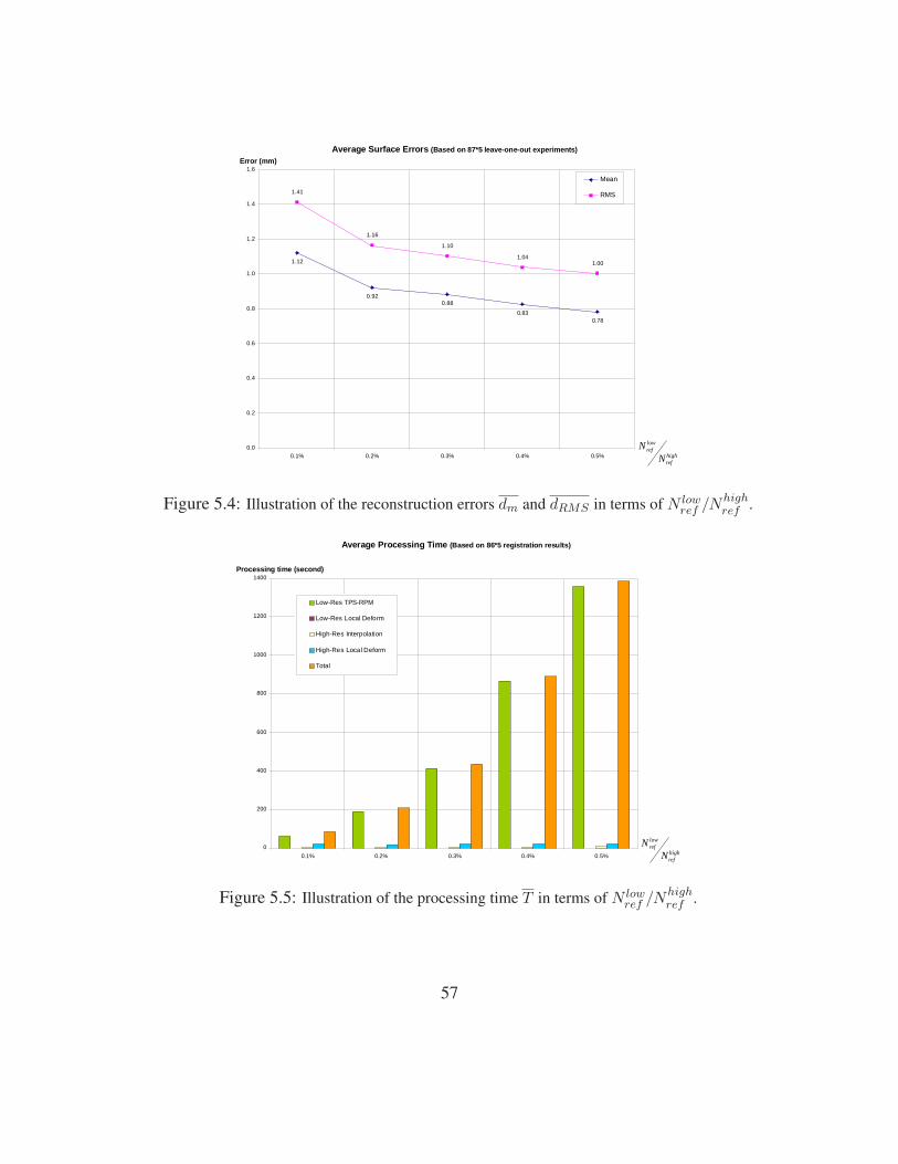
1.12

0.920.88

0.830.78

1.41

1.16

1.10

1.041.00

0.0

0.2

0.4

0.6

0.8

1.0

1.2

1.4

1.6

0.1% 0.2% 0.3% 0.4% 0.5%

Mean

RMS

Average Surface Errors (Based on 87*5 leave-one-out experiments)

Error (mm)

highref

lowref

NN

Figure 5.4: Illustration of the reconstruction errors dm and dRMS in terms of N lowref /Nhigh

ref .

0

200

400

600

800

1000

1200

1400

0.1% 0.2% 0.3% 0.4% 0.5%

Low-Res TPS-RPM

Low-Res Local Deform

High-Res Interpolation

High-Res Local Deform

Total

Average Processing Time (Based on 86*5 registration results)

Processing time (second)

highref

lowref

NN

Figure 5.5: Illustration of the processing time T in terms of N lowref /Nhigh

ref .

57

Registration error decrased by two-level framework

0.00%

1.00%

2.00%

3.00%

4.00%

5.00%

6.00%

7.00%

8.00%

9.00%

High-res Low-res Low-res after TPS Low-res afterrefine

High-res afterinterpolation

High-res afterrefine

Surface model

Su

rfac

e d

ista

nn

ce (

%)

Mean

RMS

Figure 5.6: Illustration of how the surface distance is decreased in each step of the two-levelframework.

2. Fig. 5.8 shows the low-resolution surfaces XL (169 vertices, 334 triangles) and Y L

(213 vertices, 422 triangles) after simplification. With respect to the bounding boxdiagonal of Y L (158.3mm), the mean error is 6.53% and root mean square error is7.74%.

3. Fig. 5.9 shows the deformed low-resolution surfaces XL(1) and Y L after apply-ing Chui and Rangarajan’s non-rigid registration [11] to XL. With respect to thebounding box diagonal of Y L, the mean error is 1.68% and root mean square er-ror is 2.13%. The surface distance has been significantly decreased by Chui andRangarajan’s non-rigid registration method [11].

4. Fig. 5.10 shows the deformed low-resolution surfaces XL(2) and Y L after applyinga local refining process to XL(1). With respect to the bounding box diagonal of Y L,the mean error is 0.68% and root mean square error is 1.42%, which demonstratesthat local point-to-surface refinement can decrease surface distance further.

58

Surface XH

Surface YH

High-Resolution

Surface Distance from XH to YH

0

0.33

0.66

0.99

1.32

1.65

1.98

2.31

2.64

Figure 5.7: Illustration of the high-resolutionsurfaces XH and Y H . Point-to-surface distancesfrom XH to Y H are illustrated by a HSV colormap: the color of each vertex on XH representsthe distance d(p, Y H), p ∈ XH . (Both surface(left) and mesh (right) are showed in the bottomrow.)

Low-Resolution

Simplified Surface XL

Simplified Surface YL

Surface Distance from XL to YL

0

0.33

0.66

0.99

1.32

1.65

1.98

2.31

2.64

Figure 5.8: Illustration of the low-resolutionsurfaces XL and Y L after applying the meshsimplification (see Sec. 5.1.1) to both XH andY H . Point-to-surface distances from XL to Y L

are illustrated by a HSV color map: the colorof each vertex on XL represents the distanced(p, Y L), p ∈ XL. (Both surface (left) and mesh(right) display modes are showed in the bottomrow.)

5. Fig. 5.11 shows the interpolated high-resolution surfaces XH(1) and Y H after ap-plying the interpolation to XH . With respect to the bounding box diagonal of Y H ,the mean error is 1.65% and root mean square error is 2.10%. The reason whythe surface distance slightly increases by interpolation is: only 0.80% of verticeson XH(1) have correspondences computed from low-resolution registration, othercorrespondences were obtained by interpolation.

6. Fig. 5.12 shows the deformed high-resolution surfaces XH(2) and Y H after applyinga local refining process to XH(1). With respect to the bounding box diagonal of Y H ,the mean error is 0.28% and root mean square error is 1.26%, which once againdemonstrates that local point-to-surface refining procedure is helpful for decreasingsurface distance.

59

Low-Resolution

RegisteredSurface XL(1)

Surface YL

Surface Distance from XL(1) to YL

0.21

0.42

0.63

0.84

1.05

1.26

1.47

1.68

0

Figure 5.9: Illustration of the deformed low-resolution surfaces XL(1) and Y L after apply-ing Chui and Rangarajan’s non-rigid registrationmethod (see Sec. 5.1.2) to XL. Point-to-surfacedistances from XL(1) to Y L are illustrated bya HSV color map: the color of each vertexon XL(1) represents the distance d(p, Y L), p ∈XL(1). (Both surface (left) and mesh (right) dis-play modes are showed in the bottom row.)

Low-Resolution

Refined Surface XL(2)

Surface YL

Surface Distance from XL(2) to YL

0.21

0.42

0.63

0.84

1.05

1.26

1.47

1.68

0

Figure 5.10: Illustration of the deformed low-resolution surfaces XL(2) and Y L after apply-ing the refinement ( see Sec. 5.1.4) to XL(1).Point-to-surface distances from XL(2) to Y L areillustrated by a HSV color map: the color ofeach vertex on XL(2) represents the distanced(p, Y L), p ∈ XL(2). (Both surface (left) andmesh (right) display modes are showed in the bot-tom row.)

5.2.2 Comparison to Other Registration Methods based on FemurData

We compared our registration algorithm with the classical iterative closet point (ICP)method since it is widely used in many medical image registration problems. Given 87training surfaces, the distribution of RMS error and mean error of the two approaches areshowed in Fig. 5.13. For RMS error, they are centered between 0.6-1.0mm (the maxi-mum is 1.4mm) in our method, but in ICP the range is between 3.1-6.5mm (the maximumis 8.5mm). For the mean error, they are centered between 0.5-0.7mm (the maximum is0.9mm) in our method, but in ICP the range is 2.5-6.5mm (the maximum is 7.5mm). It isobvious that the two-level non-rigid registration has a better performance than ICP does.

Since Chui and Rangarajan’s thin-plate spine (TPS) based method [11] cannot dealwith the complexity of our data, we cannot directly compare two methods. Alternatively,

60

Surface YH

High-Resolution

Interpolated Surface XH(1)

Surface Distance from XH(1) to YH

0.21

0.42

0.63

0.84

1.05

1.26

1.47

1.68

0

Figure 5.11: Illustration of the deformed high-resolution surfaces XH(1) and Y H after applyinginterpolation (see Sec. 5.1.3) to XH . Point-to-surface distances from XH(1) to Y H is illustratedby a HSV color map: the color of each vertexon XH(1) represents the distance d(p, Y H), p ∈XH(1). (Both surface (left) and mesh (right) dis-play modes are showed in the bottom row.)

Surface YH

High-Resolution

Refined Surface XH(2)

Surface Distance from XH(2) to YH

0.21

0.42

0.63

0.84

1.05

1.26

1.47

1.68

0

Figure 5.12: Illustration of the deformed high-resolution surfaces XH(2) and Y H after apply-ing the refinement (see Sec. 5.1.4) to XH(1).Point-to-surface distances from XH(2) to Y H isillustrated by a HSV color map: the color ofeach vertex on XH(2) represents the distanced(p, Y H), p ∈ XH(2). (Both surface (left) andmesh (right) display modes are showed in the bot-tom row.)

we have noticed from Fig. 5.5 that our method only needs 5 minutes or less to match anysize of surfaces with less than 200,000 vertices. However, Chui and Rangarajan’s methodcosts 5 minutes for 350 vertices, 10 minutes for 460 vertices, 20 minutes for 610 vertices,etc. It is obvious that our algorithm significantly improves the efficiency. To maintaina good accuracy for practical applications, a best simplification parameter was selectedbased on a series of leave-one-out experiments (see details in Sec. 5.1.6).

5.2.3 Femur Atlas

We have collected CT scans of 87 different patients all with one healthy femur. The scanswere acquired at the West Pennsylvania Hospital (Pittsburgh, PA) and UPMC ShadysideHospital (Pittsburgh, PA) over a period of 10 years, and annonymized before use. There

61

0%

2%

4%

6%

8%

10%

12%

14%

16%

18%

0.60 0.70 0.80 0.90 1.00 1.10 1.20 1.30 1.40 (mm)0%

2%

4%

6%

8%

10%

12%

14%

16%

2.0 3.0 4.0 5.0 6.0 7.0 8.0 9.0 (mm)

0%

2%

4%

6%

8%

10%

12%

14%

16%

18%

0.50 0.54 0.58 0.62 0.66 0.70 0.74 0.78 0.82 (mm)0%

2%

4%

6%

8%

10%

12%

14%

16%

18%

20%

1.0 2.0 3.0 4.0 5.0 6.0 7.0 8.0 (mm)

RMS Error Distribution for Our Method (Based on 87 patients)

RMS Error Distribution for ICP (Based on 87 patients)

Mean Error Distribution for Our Method (Based on 87 patients)

Mean Error Distribution for ICP (Based on 87 patients)

Figure 5.13: RMS and Mean error distributions ICP and our method.

0%

5%

10%

15%

20%

25%

40 50 60 70 800%

4%

8%

12%

16%

20%

410 430 450 470 490 510 530

Age (years) Femur Length (mm)

Figure 5.14: Data distributions in terms of age (left) and femur length (right).

are 53 males and 34 females. 43 are left femurs and 44 are right ones. The patients’ ageranges from 39 to 78 and their femur length ranges from 400mm to 540mm (Fig. 5.14shows the data distribution in terms of the age and femur length). The CT volumes weresegmented to provide triangulated surface models using Marching Cube (MC) algorithm.All surface models were smoothed by the method proposed in [20]. The scans were ac-

62

σ2−y σ−y y σ+y σ2+y

mode 2(19.8%)

mode 1(41.5%)

mode 3(7.6%)

Figure 5.15: Femoral head atlas: illustration of shape variation in the first, second and third mode.The first mode encodes 41.50% of shape variation, the second and third modes encode 19.78% and7.64% of shape variation. The color shapes highlight the local shape variation.

quired under a protocol for computer assisted total hip replacement, and contained only theproximal portion of the femur including the femoral head and the distal portion includingthe condyles. Thereby each femur model has two seperate surfaces containing the femoralhead and condyles, respectively. Given the particularity of the femur data, we need to do apre-alignment to get rid of the effect caused by the missing portions. Please see details inAppendix C. Experiments show that the rate of convergence has been improved from 78%to 95.2% by applying such an alignment.

Fig. 5.15 shows shape variation in the first three modes of the femoral head atlas. Thecolor shapes (pink and blue) are used to highlight the local variation. For example, the sizeof the femoral head (denoted by the pink circle) gradually reduces along the first mode, butremains almost the same along the second mode. The greater trochanter (denoted by theblue area) becomes longer but narrower along the first mode. It remains the same lengthbut becomes wider along the third mode.

Fig. 5.16 shows shape variation in the first three modes of the condyles atlas. Wenoticed that the top of the condyles (denoted by the blue area) changes a lot along each

63


mode 2(9.8%)

mode 1(25.7%)

mode 3(8.2%)

Figure 5.16: Condyles atlas: illustration of shape variation in the first, second and third mode.The first mode encodes 25.70% of shape variation, the second and third modes encode 9.75% and8.21% of shape variation. The color shapes highlight the local shape variation.

mode. This is because each scan was cut differently. The top area can only be estimatedfrom the reference surface without any refining from the original surfaces. The lateralepicondyle (denoted by the blue point on the right) becomes larger along the first mode,compared to the medial epicondyle (denoted by the blue point on the left). It is similar tothe third mode but the change is smaller. The condyles become longer but narrower alongthe second mode.

Figs. 5.17-5.18 show shape variation in the first two modes of the entire femur atlas.For the first mode, the femoral head and greater trochanter follow the similar change asFig. 5.15 shows, and the condyles become longer and narrower as Fig. 5.16 shows. Theatlas of the entire femur behaves in a similar way as the individual portion does for thefirst mode. For the second mode, the greater trochanter becomes shorter but it remains thesame as in Fig. 5.15. The condyles become much longer but they keep the same length asin Fig. 5.16. It means that the second dominant mode in the individual atlas may not bethe second dominant mode in the conjunction case.

Fig. 5.19 shows the shape variation encoded in each mode of three atlases. To keep95% of shape variation we only need 26 modes for the femoral head atlas, 49 modes forthe condyles atlas and 20 modes for the entire femur atlas. The reason why the condylesatlas needs more modes to keep most of shape variation is because the training surfaces ofthe bottom portion of the femur change a lot in shape (i.e. Each surface contains differentlength of femur shaft).

64


Top part

Bottom part

mode 1 (27.7%)

Figure 5.17: Femur atlas: 27.67% of shape variation is encoded in the first mode. The colorshapes highlight the local shape variation.


Top part

Bottom part

mode 2 (18.6%)

Figure 5.18: Femur atlas: 18.63% of shape variation is encoded in the second mode. The colorshapes highlight the local shape variation.

5.2.4 Spine Vertebra Atlas

In our endoscopic reconstruction experiments we use lumbar vertebrae. Lumbar vertebraeare the largest segments of the movable part of the vertebral column. We select all fivelumbar vertebrae (L1-L5) and the last thoracic vertebra (T12) for our study.

We acquired CT scans of three cardavers at the University of Pittsburgh Medical Center

65

0.00%

25.00%

50.00%

75.00%

100.00%

1 21 41 61 81

Femoral head atlas Distal femur atlas Combined femur atlas

95.00%90.00%

Figure 5.19: Illustration of the shape variation encoded in modes of the femoral head atlas(blue),condyles atlas(pink) and entire femur atlas(green).

(UPMC) and collected the data in the DICOM format (GE Medical Systems; DICOMformat; LightSpeed QX/I; SliceThickness=1.2500; Width = 182; Height = 177; BitDepth= 16; PixelSpacing = [2x1 double]; Protocol Name = 8.1 Pelvis for Fracture). To enlargethe dataset, we have also scanned three human-size artificial spines by the same protocol.We used the solid white plastic sawbones model (Pacific Research Laboratories, Inc., #1352-31) made of rigid plastic. The shape of the sawbones models are cast from differentnatural real specimens (See Appendix D for our collection of spine images).

We have collected a high-resolution 3D surface of vertebra generated by triangulating40682 points which were carefully selected by hand. This step takes several hours but onlyneed to be done once. We trimmed each spine CT images into small files with individualvertebra. We manually selected about 250 surface points (of the same resolution as thesimplified reference surface) for each DICOM file. It took 10-15 minutes to label eachvertebra. Basically we selected around 8-9 points on each image slice (12 slices fromthe coronal view, 12 slides from the sagittal view and 6 slices from the transverse view).Examples about selecting points are shown in Appendix E. The selection is assumed to beconsistent since it was conducted by the same person based on the study of the structure ofthe spine vertebrae and DICOM images. However, no specific anatomic landmarks needto be labeled, it is sufficient as long as points are selected on the bone surface.

66

mode 1 (39.0%)

y σ5.0+y σ+yσ5.0−yσ−y

mode 2 (20.4%)


mode 3 (12.8%)


Figure 5.20: Spine vertebra atlas: 39.0% of shape variations is encoded in the first mode. Thesecond and third modes encode 20.4% and 12.8% of shape variations.

Fig. 5.20 shows shape variations in the first three modes of the spine vertebra atlas.We can see that the vertebra becomes narrower but remains the same length among thefirst mode. The vertebral body (centrum) becomes larger along both the second and thirdmodes. The spinous process becomes longer along the second mode but shorter along thethird mode. It is twisted in the same way from the left to the right. We have noticed that thesampled surfaces given the bigger standard deviation (e.g. 1σ ) have odd shapes. This maybe caused by the insufficient number of training data. Fig. 5.21 shows shape variationsencoded in each mode of the spine vertebra atlas. To keep 95% of shape variation we onlyneed 10 modes.


The semi-automatic procedure requires some manual input, e.g. selection of 40682 pointsfor a reference model. But this procedure is a one-time task and can be conducted off line.

67

95.00%

Number of Principal Components

Energ

y (%

)

Figure 5.21: Illustration of shape variations encoded in each mode of the spine vertebra atlas.

It also requires selecting 250 points for each study image without any prior informationabout the shape. It normally takes 10-15 minutes, which is much less than several hourswhich could be used for complete manual segmentation of high resolution model. In thefuture e will consider using the atlas as a prior to enhance the performance and reducemanual work.

The salient points may be removed during the surface simplification and then mis-matching may occur. To handle this problem, we need to find a proper resolution for thesimplified surface. The lower the faster but the more mis-matching could be established.That is why we apply the leave-one-out experiments to find a appropriate parameter for theresolution. Besides, we proposed a refining process by using the original data (either thehigh resolution surface or sparse labeled points) as a reference to reduce the mis-matchingcaused by simplification.

Experiments demonstrate that our two-level framework significantly improves effi-ciency of registration without decreasing accuracy of atlases. Shape variation learnedfrom the training samples can be used for clinical studies and diagnosis. The shape atlascan also be used as a statistical shape prior for bone reconstruction from other imagingmodalities such as endoscopes. We will discuss more details in Ch. 6.

68

Chapter 6

Improvement of Bone Reconstructionfrom Two-step Algorithm

As we have discussed in Ch.5, to solve over smoothness, inaccurate reconstruction andpartial occlusions, a shape prior is needed to constrain the MISFS algorithm. We pro-pose a two-step algorithm in this chapter to improve the reconstruction. A global shapeconstraint is enforced in the MISFS algorithm (see Sec. 6.1). The shape constraint iscomputed by aligning the inaccurate shape from the MISFS and the statistical shape at-las. Such a procedure is iterated as well as the shape constraints and inaccurate shape areupdated in each iteration until the algorithm converges. To further improve reconstructionespecially on the discontinued boundaries, we evaluate the reconstructed shape by com-paring to the original endoscopic images (see Sec. 6.2). By maximizing the likelihoodof gradient images synthesized from the reconstructed shape, a better reconstruction andmore accurate shape is obtained.

6.1 Bottom-up Image based MISFS constrained by Sta-tistical Shape Atlas

In this section we will discuss how to constrain the MISFS with a statistical atlas. Theprocedure is illustrated in Fig. 6.1. The pre-processing MISFS results in an initial shapeS1, given initial normals on global contours. S1 is then aligned with the statistical atlas andthe most closely matched atlas shape Sa

1 is computed from sparse-to-dense reconstruction.Sa

1 is used to update the initial normals and depths for the MISFS. The two steps, alignment

69

Table 6.1: Table of Notation in Sec. 6.1S1, S2, Sk, SK - MISFS result after the 1st, 2nd, kth, Kth iteration

Smean - mean shape

s, r, t, s∗, r∗, t∗ - transformation parameters

N - number of surface vertices

S ′1 - aligned partial shape after applying rigid transformation to S1

E - eigenmatrix

Esub1 - sub matrix of E

Esub1

+ - pseudo inverse of Esub1

S ′mean - sub vector of Smean

S ′′1 - atlas shape corresponding to S ′1Sa

1 - aligned atlas shape after applying inverse rigid transformation to S ′′1nax, nay, naz - three components of surface normal at surface point on Sa

1



F - focal length

za - depth on Sa1

pa, qa - partial derivatives of za w.r.t. image coordinates x, y

ea - atlas constraint

λ1, λ2 - Lagrange multipliers

k, l - image indices

m - iteration number

and MISFS are iterated until the best reconstruction is achieved. By these means, betterknowledge of bones of interest are taken into account in the MISFS therefore a moreaccurate shape can be recovered.

70

Initial normal on global contours

Reconstruction

MISFS

Atlas Counterpart

Sparse2Dense ReconstructionRegistration

Atlas

Converge

No

Updated depth (za) and normal (pa, qa)

za(pa, qa)

Yes

ConvergeYes

No

Top-down Method

MISFS

Figure 6.1: Illustration of the bottom-up MISFS: the pre-processing MISFS results in an initialshape S1, given initial normals on global contours. S1 is then aligned with the statistical atlas andthe most closely matched atlas shape Sa

1 is computed from sparse-to-dense reconstruction. Sa1 is

used to update the initial normals (pa, qa) and depths za for the MISFS. The two steps, alignmentand MISFS are iterated until the best reconstruction is achieved.

6.1.1 Aligning MISFS Shape with Atlas

Due to the limited range of motion for the endoscope and limited bone exposure duringsurgery, it is impossible to capture images of bones from 360 degrees and reconstruct acomplete shape. In other words, S1 represents a part of the atlas shape.

We first apply a scaled-ICP algorithm [5] to align S1 with the atlas mean shape Smean.We find the scaling factor s∗ by comparing the model size in the 3D Eigenspace, and thencompute the rotation and translation by minimizing the surface distance. i.e.

(r∗, t∗) = arg minN∑i

{[r|t](s∗ · S1(i))− Smean(near(i))}2 (6.1)

where near(i) is the index of the closest point of S1(i) on the mean shape. The initialstarting position is roughly estimated based on the field of view of the reconstructed shape.We apply the transformation (r∗, t∗, s∗) to S1 and obtain the aligned shape S ′1 at the atlaspose:

S ′1 = [r∗|t∗](s∗ · S1) (6.2)

71

Given the aligned partial shape S ′1, a complete atlas shape is generated from sparse-to-dense reconstruction. In other words, we first project S ′1 into a subspace of the atlasspace to retrieve coefficients for each mode. These coefficients are used to reconstruct acomplete shape from the original atlas space. Let E denote the eigenvector matrix of theatlas, and Esub

1 denote a sub matrix of E. Extracted from E, each row of Esub1 corresponds

to every vertex on the partial shape S ′1. Since Esub1 is not an orthogonal matrix anymore, we

use the pseudo inverse (Esub1 )+ instead of the matrix transpose to compute the coefficients

and then reconstruct the shape:

S ′′1 = E · (Esub1 )+ · (S ′1 − S ′mean) + Smean (6.3)

where S ′mean is the partial mean shape corresponding to S ′1.

The complete shape S ′′1 is reconstructed from 10 modes of the atlas. Since we use themean shape Smean as the target shape for the initial alignment, wrong correspondences mayexist. Thus we use S ′′1 as a new target shape and iterative the alignment and reconstructionseveral times until S ′1 and the atlas are well aligned. Finally we transform S ′′1 to the originalpose and scale, by applying the inverse transformation (Eq. 6.2):

Sa1 =

([r∗T | − t∗

]S ′′1

)/s∗ (6.4)

where the complete shape Sa1 is considered as the most closest atlas shape for S1.

6.1.2 Constraining MISFS by Atlas

In this section we use the surface geometry information of Sa1 to constrain the MISFS.

Given each surface point Pi on Sa1 , the surface normal ~n = [nax, nay, naz] is computed

as the average of the surface normals from adjacent triangles. Recall Eq. 4.3 and 4.7, wehave

~n = [−∂z

∂x,−∂z

∂y, 1]/

√(∂z

∂x)2 + (

∂z

∂y)2 + 1

∂z

∂x=

Fpa

za + xpa

,∂z

∂y=

Fqa

za + yqa

(6.5)

where pa = ∂z/∂x and qa = ∂z/∂y, (x, y) are image coordinates, F is the focal lengthand za is the depth at Pi. We compute the prior (pa, qa) from Sa

1 using Eq. 6.5

pa = − (nax/naz) · za

(nax/naz) · x + F, qa = − (nay/naz) · za

(nay/naz) · y + F(6.6)

72

The atlas constraint ea is defined by minimizing the errors of surface normals anddepths compared to the aligned atlas shape Sa

1 :

ea =

∫ ∫

aligned vertices

[(p− pa)2 + (q − qa)

2 + (z − za)2]dxdy (6.7)

Recall Eq. 4.12 and Eq. 4.19, the entire error is represented by two terms, the imageirradiance error ei(z, p, q) and the local geometry constraint es(z, p, q) (smoothness con-straint is used in Ch. 4). Now we add ea to the error function as another soft constraint:

e(z, p, q) = λ1ei(z, p, q) + λ2ea(z, p, q) + (1− λ1 − λ2)es(z, p, q) (6.8)

By discretizing Eq. 6.8 we obtain:

e(zk,l, pk,l, qk,l) =∑

k

∑

l

[λ1eik,l + λ2eak,l + (1− λ1 − λ2)esk,l] (6.9)

whereeak,l = (pk,l − pak,l)

2 + (qk,l − qak,l)2 + (zk,l − zak,l)

2 (6.10)

The derivative of ea with respect to ηk,l (η represents p, q or z) are:

∂ea

∂ηk,l

= 2(ηk,l − ηak,l) (6.11)

Similarly to Ch. 4 we have

∂es

∂ηk,l

= 8(ηk,l − ηk,l),∂ei

∂ηk,l

= −2(Ik,l −Rk,l)∂R

∂ηk,l

(6.12)

In Eq. 6.12, the smoothness term ηk,l is replaced by the local robust regularizer ηk,l. Weminimize Eq. 6.9 and obtain update functions for ηk,l (η represents p, q or z):

ηm+1k,l =

λ1

4(1− λ1 − λ2) + λ2

[Ik,l −R(k, l, zmk,l, p

mk,l, q

mk,l)]

∂R

∂ηk,l

|ηmk,l

+λ2

4(1− λ1 − λ2) + λ2

ηak,l +1− λ1 − λ2

(1− λ1 − λ2) + λ2/4ηm

k,l

(6.13)

Constrained by the statistical atlas, the new MISFS reconstructs a new shape S2. Werepeat the alignment and reconstruction discussed in the previous section to S2, whosemost closest atlas shape Sa

2 is used to update the atlas constraint for MISFS. The abovetwo steps are iterated to generate the shape S3, S4, ..., until SK when the surface distance‖SK−SK−1‖ < ε. The most closest atlas shape of SK is denoted by Sa

K and correspondingcoefficients as ca

K .

73

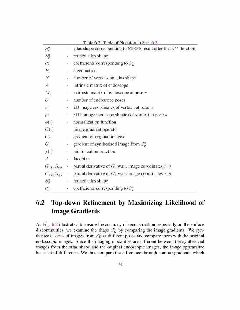
Table 6.2: Table of Notation in Sec. 6.2Sa

K - atlas shape corresponding to MISFS result after the Kth iteration

SaF - refined atlas shape

caK - coefficients corresponding to Sa

K

E - eigenmatrix

N - number of vertices on atlas shape

A - intrinsic matrix of endoscope

Mu - extrinsic matrix of endoscope at pose u

U - number of endoscope poses

vui - 2D image coordinates of vertex i at pose u

pui - 3D homogeneous coordinates of vertex i at pose u

φ(·) - normalization function

G(·) - image gradient operator

Go - gradient of original images

Ga - gradient of synthesized image from SaK

f(·) - minimization function

J - Jacobian

Gox, Goy - partial derivative of Go w.r.t. image coordinates x, y

Gax, Gay - partial derivative of Ga w.r.t. image coordinates x, y

SaF - refined atlas shape

caK - coefficients corresponding to Sa

F

6.2 Top-down Refinement by Maximizing Likelihood ofImage Gradients

As Fig. 6.2 illustrates, to ensure the accuracy of reconstruction, especially on the surfacediscontinuities, we examine the shape Sa

K by comparing the image gradients. We syn-thesize a series of images from Sa

K at different poses and compare them with the originalendoscopic images. Since the imaging modalities are different between the synthesizedimages from the atlas shape and the original endoscopic images, the image appearancehas a lot of difference. We thus compare the difference through contour gradients which

74

Endoscope

(a) OpenGL Rendering

(b) Original image (d) Normalized image

(c) Synthesized image (e) Gradient Ga

(f) Gradient Go

Update CK

ReconstructionAtlas Counterpart

CK

Bottom-up Method

Converge

No

YesDone

Figure 6.2: Illustration of top-down method: (a) OpenGL rendering SaK . (b) Corresponding

endoscopic image. (c) Synthesized endoscopic image from the same camera pose. (d) Normalizedendoscopic image. (e) Gradient of synthesized image Ga. (f) Gradient of normalized image Go.

are most robust to lighting variations and strongly respond to surface discontinuities. Bymanipulating the coefficients ca

K , the refined atlas shape is obtained and noted as SaF .

Let E denote the 3N × 10 eigenvectors matrix of the atlas, Ei(3(i − 1) + 1 : 3i, :)caK

represents the vertex i(i = 1, 2, · · · , N) reconstructed from the atlas. Given the cali-brated intrinsic and extrinsic matrices of the endoscope A3x3 and Mu

3x4 (at pose u, u =1, · · · , U ), the corresponding image pixel vector is vu

i = φ(pui ), p

ui = AMu[Eic

aK ; 1].

φ(p) = [px/pz; py/pz] normalize the 3D homogeneous coordinates to 2D image coordi-nates. Let G(·) denote image gradient operator, our goal is to maximize the likelihood ofthe image gradients, i.e., minimize δG = Go − Ga, where Go computes the gradient ofnormalized endoscopic image (the image is normalized by removing the geometric distor-tion and illumination effect), Ga computes the gradient of OpenGL rendered image from

75

SaK (see Fig. 6.2). Let

f(caK) =

1

2

U∑u

N∑i

[Go(vui )−Ga(v

ui )]2 (6.14)

Using Taylor expansion, we obtain δcaK = −J−1f(ca

K), where

J =∂f

∂caK

=U∑u

N∑i

[∂Go

∂vui

− ∂Ga

∂vui

]T · ∂vui

∂caK

∂vui

∂caK

=∂φ

∂pui

· ∂pui

∂caK

(6.15)

Since

∂Go

∂vui

− ∂Ga

∂vui

=

[Gox(v

ui )−Gax(v

ui )

Goy(vui )−Gay(v

ui )

]

∂φ

∂pui

=

1

pui (z)

0−pu

i (x)

(pui (z))2

01

pui (z)

−pui (y)

(pui (z))2

∂pui

∂caK

= AMuEi

(6.16)

Jacobian J can be rewritten as:

J =U∑u

N∑i

[Gox(v

ui )−Gax(v

ui )

Goy(vui )−Gay(v

ui )

]T

·

1

pui (z)

0−pu

i (x)

(pui (z))2

01

pui (z)

−pui (y)

(pui (z))2

·AMuEi (6.17)

pui (x), pu

i (y), pui (z) are three components of the homogenous coordinates pu

i , which is thefunction of ca

K . In each iteration, we use previous caK to compute pu

i and vui , and then the

Jacobian J of Eq. 6.14. Thus caK can be updated by Eq. 6.17. The final coefficients ca

F areused to generate the refined shape Sa

F from the atlas.

76

6.3 Experiments and Results

6.3.1 Simulations

We first conducted several simulation trials on synthesized data. Given the statistical atlas,we manipulated the first ten coefficients and generated 10 different shapes with variousposes shown in Fig. 6.3. For each virtual shape model, we rendered it in 3D graphicscontext and moved a virtual endoscope around to collect a set of synthesized images (seeFig. 6.3). The virtual endoscope has the fixed camera parameters thus the calibration errorwas not considered, neither did the tracking error. We directly called the OpenGL functionto obtain the view-port vector, model-view and projection matrices. We used a bright spotlight source which enables a good image quality, so we placed the virtual endoscope a bitfar away from the 3D model and still captured good images. By these means we wereable to image more area of the model in a single image and used much less images toreconstruct one side of the view. We collected 6-10 images for each synthesized shape.

We conducted our two-step approach on each set of synthesized images and recon-structed corresponding shapes. We compared the reconstructed shapes with the originalones in Fig. 6.4. The simulation results show clear improvement by introducing the atlasconstraint, so does the refinement. Since the synthesized shapes are sampled from theatlas space, the ideal reconstruction error for Sa

F should be close to zero if the correct cor-respondences can be achieved. Without calibration and tracking errors, only the arbitrarycamera motions will cause the misalignment and increase the reconstruction error. Fig.6.4 shows the averaged RMS error for SK , Sa

K and SaF is 0.76 mm, 0.54 mm and 0.42 mm,

respectively. These numbers provide a rough lower bound for accuracy of our algorithm.

6.3.2 Artificial Lumbar Models

Real cases are more complicated due to the errors introduced by camera calibration andtracking system. And the real vertebra shape may not belong to the atlas population. Theimage quality also affect the contour extraction and shape-from-shading algorithm. Weuse the artificial lumbar vertebrae L4 and L5 to test our algorithm. For each model wecaptured 4 image sets from different range of views: top, bottom, left side and right side(Note that we could never have access to some views in real surgery, for example, thetop view). In each image set, we collected a set of images. For instance, we captured145 endoscopic images at 29 positions from the top view of the vertebra L4 (for eachposition we took 5 images and used the averaged image for reconstruction). Fig. 6.5shows the artificial vertebra and averaged endoscopic images. The colored circles illustrate

77

Figure 6.3: Illustration of 10 synthesized shapes from the atlas for simulation experiments. Foreach shape, we moved the virtual endoscope to collet a set of images, for example, the bottomimages were collected from the 8th shape.

the endoscope poses with different rotations and translations. The displayed images aregeometric rectified and normalized for illumination. In the preprocessing MISFS withlocal robust regularizer, we chose λ1 = 0.001 and increased it by 0.02 whenever the errorin Eq. 6.8 decreased by 1%. Fig. 6.1 shows the resulted shape S1. We can see somediscontinuities are kept. Fig. 6.1 also shows the aligned atlas shape Sa

1 , the updatedsurface normals (pa, qa) and the depths za, which were used for the second round MISFSwith the atlas constraint. From the second round MISFS, we selected λ1 = 0.01 (increasedby 0.01) and λ2 = 0.1 (increase by 0.05).

We compare the MISFS reconstruction SK , bottom-up result SaK and top-down result

SaF with the laser scanned ground truth (L4: 72.6 x 77.1 x 38.2 mm, scanned from 13 view

points; L5: 92.9 x 73.4 x 37.8 mm, scanned from 16 view points). The RMS errors over 8data sets are shown in Figs. 6.6, and visual results are shown in Figs. 6.7-6.8. We can seea significant improvement from the two-step method, although we have more complicatedshapes, larger range of motions including rotations (In Ch. 4 we only handle the transla-tion). Since we captured images from one side of the spine vertebra model, the MISFSresult SK can only recover the shape information for this side. Although Sa

K and SaF rep-

resent a complete atlas shape, most of vertices on SaK and Sa

F have no correspondenceson SK . Those points do not have any support from images thus correspond bigger errors.That’s why the overall RMS errors are slightly worse for the atlas shape Sa

K and SaF : the

78

0

0.1

0.2

0.3

0.4

0.5

0.6

0.7

0.8

0.9

1

MISFS Bottom-up (Partial) Top-down (Partial)

Trial 1Trial 2Trial 3Trial 4Trial 5Trial 6Trial 7Trial 8Trial 9Trial 10

0

0.2

0.4

0.6

0.8

1

1.2

Bottom-up Top-down

RMS Error for 10 Simulation Trials

(mm)

0

0.1

0.2

0.3

0.4

0.5

0.6

0.7

0.8

0.9

1


Average

(mm)

0

0.1

0.2

0.3

0.4

0.5

0.6

0.7

0.8

0.9

1

Bottom-up Top-down

Average

(mm) (mm)

(a) (b)

(c) (d)

Figure 6.4: Reconstruction errors for ten synthesized shapes. The RMS errors are calculated bycomparing three shapes (MISFS, bottom-up and top-down) of each synthesized images given thesynthesized shape. Since we captured images from one side of synthesized shape, the reconstructedshape from MISFS can only recover the shape information for this side. Although the bottom-upresult and top-down result represent complete atlas shapes, most of vertices on these two atlasshapes have no correspondences on the MISFS result. Those points do not have any support fromimages thus correspond bigger errors. That’s why the overall RMS errors are slightly worse forthe bottom-up and top-down method, as shown in (b). However, when we look at the partial RMSerrors by only considering points having correspondences in the images, we can see a big improve-ment from the two-step algorithm in (a). (c) and (d) show the average and standard deviation over10 trials.

averaged RMS error over eight data sets is 2.07 mm and 1.95 mm respectively. However,when we look at the RMS errors by only considering points having correspondences inthe images, we can find better accuracy: the averaged RMS error over eight data sets forSK , Sa

K and SaF is 1.60 mm, 1.36 mm and 1.17 mm, respectively. The standard deviation

is 0.45 mm, 0.25 mm and 0.21 mm, respectively.

79

Pose 1

Pose 5

Pose 9

Pose 13Pose 17

Pose 21

Pose 24

Pose 29

Figure 6.5: Experimental setup for lumbar vertebrae reconstruction. The artificial lumbar vertebraL4 is showed in the middle. Surrounding images are captured by an oblique endoscope fromdifferent poses involving rotations and translations, which are illustrated by colored circles. All theimages are geometric rectified and normalized for illumination.

From the result of the top view of L4, we can see large errors in the vertebra body(the top area of the shape), which is due to the ambiguity during the individual shaperegistration, since the captured images from the pose 26 to 29 look very similar. It is thelimitation of the bottom-up appearance based method. A better representation of this areacan be found in top-down result. The bottom view of L5 shows an occlusion example,where some portions of the vertebra body were not imaged. The MISFS result cannotrecover the occluded part but the corresponding atlas shape provides an estimation of themissing portions.

We have noticed large local errors in the mamillary process and superior articular pro-cess of L4 (the area corresponding to the pose 5 and 17 in Fig. 6.5) and L5, and in thespinous process and transverse process of L5. We have also noticed RMS errors of L5is slightly bigger than L4. It is due to the limited number of training samples to recoverthe various shape variation, especially for L5. We use Th12 and L1-L5 to learn the sta-tistical atlas. Among those vertebrae, L5 is much more different from others: its body ismuch deeper in front than behind, its spinous process is smaller, the interval between theinferior articular process is wider, and its transverse process are thicker. The result can beimproved by collecting more training shapes in the future.

For the right view of L4 and top view of L5, the refining step decreases the partialsurface distance but increases the overall difference (see Figs. 6.7-6.8). It is because the

80

RMS Error for L4 and L5

(mm) (mm)(a) (b)

0

0.5

1

1.5

2

2.5


L4 TopL4 BottomL4 LeftL4 RightL4 AvgL5 TopL5 BottomL5 LeftL5 RightL5 Avg

0

0.5

1

1.5

2

2.5

Bottom-up Top-down

0

0.5

1

1.5

2

2.5


Average0

0.5

1

1.5

2

2.5

Bottom-up Top-down

Average

(mm) (mm)(c) (d)

Figure 6.6: Reconstruction errors for all data sets of L4 and L5. The RMS errors are calculatedby comparing three shapes (MISFS, bottom-up and top-down) of each synthesized images giventhe synthesized shape. Since we captured images from one side of synthesized shape, the recon-structed shape from MISFS can only recover the shape information for this side. Although thebottom-up result and top-down result represent complete atlas shapes, most of vertices on thesetwo atlas shapes have no correspondences on the MISFS result. Those points do not have anysupport from images thus correspond bigger errors. That’s why the overall RMS errors are slightlyworse for the bottom-up and top-down method, as shown in (b). However, when we look at thepartial RMS errors by only considering points having correspondences in the images, we can seea big improvement from the two-step algorithm in (a). (c) and (d) show the average and standarddeviation over 8 data sets.

top-down method is basically a gradient decent procedure which may converge to a localminimum. Images from side views cannot give enough constraint for the entire shape,that’s why the reconstruction errors for the left and right views are slightly bigger thanthe other two views. Note that lack of images from other sides of the vertebra leads mis-alignment and inaccurate reconstruction for invisible points.

81


By introducing the statistical shape atlas as a new global constraint for the MISFS, we areable to deal with local discontinuities, inaccurate reconstruction and partial occlusions.We modified the bottom-up image based MISFS by introducing a global shape atlas. Wealso develop a top-down refining procedure to evaluate and improve the reconstruction byminimizing the difference of image gradients.

Note that since we use artificial spine vertebrae in our experiments, some views inFig. 6.5 could never be accessed in real surgery. Although in practice we can only get alimited exposure of the shape and the errors for parts from the other sides of view maybe significant, the occlusion occurs from the current imaging view can be successfullyrecovered by the atlas.

We have noticed that some samples from the atlas look non-natural. It is due to thelack of sufficient training data. Even with such a roughly estimated atlas, we are able tosee an improvement. We believe more data collected in the future will improve our resultfurther. So far our method has been tested in Matlab for ex vivo data only. It takes about15 minutes for a data set with 30 images (PC:2.4GCPU/2GRAM). The computation canbe paralleled to achieve much faster performance. Due to the quality of the endoscopewe used in experiments, automatic contour extrapolation failed in many images. Manuallabeling of boundaries is still required for our current system. Aligning the MISFS shapeand the atlas also needs an initial manual alignment to achieve a good matching. The userinteraction thus hinders the real-time implementation and in-vivo testing.

Above issues will be studied and addressed in our future work. We hope our systemwill soon be ready for in-vivo testing.

82

(a) Top (b) Bottom (c) Left (d) Right

(3) Bottom-up

(4) Compared with ground truth

(1) MISFS


(5) Top-down


2.27

0

4.18

0 0

5.23 4.35

0

5.22

0

4.50

0

5.58

0

5.21

0

6.50

0

0

3.61 3.42

00

3.54

Figure 6.7: Reconstruction results for different views of L4. For each data set, we show theMISFS, bottom-up and top-down results, also show the Housdorff surface distance from each resultto the ground truth. The surface distance is displayed using a JET color map. Each distance map isassociated with a color bar displayed on the left (with the maximum and minimum distance (mm)labeled on the side). 83

(a) Top (b) Bottom (c) Left (d) Right

2.39

0

3.90

0

3.82

0

3.82

0

6.78

0

5.50

0

6.09

0

7.10

0

6.43

0

6.13

0

5.06

0

6.08

0

(3) Bottom-up


(1) MISFS


(5) Top-down


Figure 6.8: Reconstruction results for different views of L5. For each data set, we show theMISFS, bottom-up and top-down results, also show the Housdorff surface distance from each resultto the ground truth. The surface distance is displayed using a JET color map. Each distance map isassociated with a color bar displayed on the left (with the maximum and minimum distance (mm)labeled on the side). 84

Chapter 7

Conclusions and Future Work

Endoscope is a key tool used for minimally invasive surgery, and endoscopy-related imageanalysis attracts increasing attention. In this thesis, we have taken the first steps to developa methodology for reconstruction of bone shape from multiple endoscopic images. Theresearch experiments were performed in a simplified ex-vivo setup. Our contributions arelisted below:

1. We developed a novel methodology to calibrate oblique-viewing endoscopes bothgeometrically and photometrically.

2. We formulated a novel scene radiance model for the endoscope imaging systemunder near point lighting and perspective projection, without assuming that the lightsources are located at the projection center, to reconstruct the shape from a singleimage.

3. We developed a multi-image shape-from-shading algorithm by tracking the endo-scope in the world coordinates and aligning partial shapes obtained from differ-ent images. Then the global contours are used to constrain the shape-from-shadingacross different images simultaneously. Finally, a consistent shape is reconstructedby re-growing the surface normals and depths in all views.

4. In order to deal with over-smoothness and ambiguity caused by the smoothnessconstraints, rotation of the endoscope and partial occlusions, we developed a two-step approach using the statistical atlas as a global shape constraint.

5. In order to fulfill the two-step reconstruction algorithm, we develop a semi-automatictwo-level registration procedure to construct the statistical atlas for bone structures.

85

All our experiments are based on a clear ex-vivo setup. Without calibrating and track-ing errors, the simulations show an average of 0.3 mm accuracy, which can be consideredas an error generated by the algorithm. When the calibrating and tracking errors are takeninto account, the system error is increased to 0.8 mm. This error can be further enlargedin in-vivo experiments with other environmental noise and when our assumptions outlinedin Ch. 1 are not met. How much accuracy is needed depends on the surgical application.For example, bone cutting and drilling may require much higher accuracy then the 3Dvisualization for diagnosis and inspection.

Our current system still requires some manual input such as contour labeling or manualadjustment for initial atlas matching to improve alignment. In addition, the current algo-rithm does not run in real-time. We hope to speed up the system to real-time performanceby rewriting the Matlab portion of the code in C++, using GPU acceleration and applyingparallel computing to shape-from-shading in different images. The endoscope used in thisstudy is relatively old and the images are low resolution video-capture images. In the fu-ture, we plan to use high-resolution endoscope with better image quality, such that we canextract contours automatically and more accurately.

As long as we can handle the above two issues, we are ready to move to the next step,the in-vivo testing. In the in-vivo testing phase, we will evaluate the effects of environmen-tal noise (tools, fog, specularity, subsurface scattering, etc.), random occlusions (blood,pieces of bones, tissues, ligaments, etc.), changing of focus of the scope, non-Lambertiansurface, and so on.

In the two-step algorithm, the top-down step uses the original images to improve thesurface details and reconstruction accuracy by comparing the contour gradients images.However, the experimental results did not show significant improvement, which can becaused by the limited atlas modes we used. Improving the atlas quality by collecting alarger database of images will be critical for improved performance of this step. As of now,we just subtract two gradient images to compute the difference, which can be improvedin the future by computing the distance transformed between two sets of contours, forexample, using ICP.

In some cases, the target bone shape may contain an anomaly that can not be recon-structed from the atlas, the reconstruction error from the two-step algorithm might then beincreased, since the atlas is derived from healthy population. Therefore, if the reconstruc-tion error exceeds a threshold, we should go back to MISFS and use the original imagesfor final reconstruction in that region.

Another possible solution for improving the local shape detail is to learn multiple localpartial atlases. In other words, the whole shape will be segmented into several important

86

parts and each part will be refined by the local shape variation. The problem with thismethod is how to segment the parts and determining how many parts are enough.

Lambertian surface is assumed in our setup. Non-Lambertian surface will make thescene radiation function more complicated. Although Lambertian is a good rough as-sumption for the artificial bones, how to select a good albedo still requires lots of studiesand evaluations. In this thesis we manually chose a constant albedo for all different artifi-cial bones. Additional study is needed to determine whether the assumptions used in thiswork can be extended to a realistic arthroscopy environment.

As far as we know, human bones show significant symmetry although it is not perfect.We should be able to use this cue to help the reconstruction, as an additional global shapeconstraint. Usually asymmetry is related to some anatomical abnormalities.

Our training samples for atlas construction are not sufficient, which causes the unnat-ural shape variation generated from the atlas space. A more theoretical way to judge if thenumber of training sample is enough is to use leave-one-out experiments. Our femur atlasconstruction is evaluated by the leave-one-out experiments which show sufficient trainingsamples and thus smoothing and natural shape variation.

If multiple bone parts exist in the same image, the automatic contour extraction al-gorithm may extract contours from different bone parts and assign it to the same bone,which will cause inaccurate reconstruction, the discontinuity between two bone parts willbe removed and modified. To handle such a case user interaction seems necessary at thispoint.

Finally, we hope our research will eventually benefit future surgical processes by mak-ing them more reliable and accurate.

87

Appendix A

Derivation of Eq. 4.17

In this appendix we show the derivation for Eq. 4.17. To minimize the error e, we take thederivative of e w.r.t. pk,l, where (k, l) is the position of an image pixel:

∂e

∂pk,l

=∂

∂pk,l

[(1− λ)es + λei]

= (1− λ)∂es

∂pk,l

+ λ∂ei

∂pk,l

(A.1)

for each pixel (k, l) we have

esk,l = (pk+1,l − pk,l)2 + (pk,l+1 − pk,l)

2 + (qk+1,l − qk,l)2

+(qk,l+1 − qk,l)2 + (zk+1,l − zk,l)

2 + (zk,l+1 − zk,l)2

eik,l = [Ik,l −R(k, l, zk,l, pk,l, qk,l)]2

(A.2)

Given smoothness constraints:

∂es

∂pk,l

=∂esk,l

∂pk,l

+∂esk−1,l

∂pk,l

+∂esk,l−1

∂pk,l

= 2((pk,l − pk+1,l) + (pk,l − pk,l+1)) + 2(pk,l − pk−1,l) + 2(pk,l − pk,l−1)

= 8(pk,l − 1

4(pk+1,l + pk,l+1 + pk−1,l + pk,l−1))

= 8(pk,l − pk,l)

(A.3)

where pk,l represents an 8-neighbor average:

pnk,l=

1

5(pn

k,l−1+pnk,l+1+pn

k+1,l+pnk−1,l)+

1

20(pn

k−1,l−1+pnk−1,l+1+pn

k+1,l−1+pnk+1,l+1) (A.4)

89

Given brightness error:

∂ei

∂pk,l

=∂eik,l

∂pk,l

= −2(Ik,l −R(k, l, zk,l, pk,l, qk,l))∂R

∂pk,l

(A.5)

From Eq. A.3 and A.5 we have

∂e

∂pk,l

= 8(1− λ)(pk,l − pk,l)− 2λ(Ik,l −Rk,l)∂R

∂pk,l

(A.6)

Setting Eq. A.6 to zero yields:

pk,l = pk,l +λ

4(1− λ)(Ik,l −R(k, l, zk,l, pk,l, qk,l))

∂R

∂pk,l

(A.7)

In order to make the algorithm robust, we use the average p, q and z when computing thereflectance map R(x, y, z, p, q) in Eq. A.7. We apply the same procedure to derive theupdate functions for q and z as below:

pk,l = pk,l +λ


∂R

∂pk,l

|pk,l

qk,l = qk,l +λ


∂R

∂qk,l

|qk,l

zk,l = zk,l +λ


∂R

∂zk,l

|zk,l

(A.8)

90

Appendix B

A comparison between Yamaguchi etal’s model and ours

In Fig. B.1, Yamaguchi et al’s use the camera head as a reference coordinates in theirhand-eye calibration system. Since surgeons rotate the scope cylinder with respect to thecamera head in order to view sideways, it is a natural way to consider the camera head asa reference. However it makes the cameral model very complex. To think it in an oppositeway, no matter how surgeons rotate the scope cylinder, if the reference coordinates is on thecylinder, the lens system is fixed with respect to the cylinder but the camera head rotatesby θ. Thus the external parameters are not affected by the rotation anymore. Since theimage plane is in the camera head, the rotation only affects the image plane. Our methodis therefore developed based on above observation. Yamaguchi et al.’s model needs fiveadditional parameters but we only need one. They use two optical markers and one rotaryencoder, and we only need two optical markers.

91

z z

Rotary Encoder

Optical marker for estimating the axis of

the scope cylinder

New designed coupler for mounting the optical marker to the scope cylinder

Ymaguchi et al.’s system Our system

System

Reference part Rod (Camera head)

Scope cylinder

Rod (Camera head)

Scope cylinder

Rotated part Scope cylinder Rod (Camera head)

Fact1. Lens system is rotated around the

scope cylinder by2. Image plane is fixed

1. Image plane is rotated around the principal point by

2. Lens system is fixed

Extra Transformation

1. Rotate the scope cylinder around its axis by

2. Inversely rotate the image plane around z-axis of the lens system by

1. Rotate the image plane around the principal point by

Unknown parameters

1.2. Axis of the scope cylinder3. Axis of the lens system

1.2. Principal point

Figure B.1: A comparison between Yamaguchi et al.’s system and ours. In Yamaguchi etal.’s system, the camera head is tracked such that the transformation from the marker to thelens system is not fixed but depends on the rotation angle θ. Let the marker coordinates bethe reference, the lens system is rotated around the scope cylinder by θ, but the image plane(in the camera head) remains still. They use two additional transformations to describe theeffect of the rotation, which results in a complex model. Moreover, they need to calibratethe axis of both the scope cylinder and the lens system by using another optical makerattached to the scope cylinder. Based on our observation, it is possible to simplify thismodel if we fix the transformation between the marker and the lens system. We designa coupler that enables the mounting of an optical marker onto the scope cylinder. We letthe marker coordinates be the reference, thus the lens system is fixed. The rotation onlyaffects the image plane while the camera head is rotating around the cylinder (reference).And the image plane only rotates around the principal point. As a result, we come up witha simple model (see details in the text).

92

Appendix C

Initial Alignment for Femur Data

As Fig. C.1 shows, the bottom portion of the femur is used as an example. The surfaceY has more femur shaft, but less shaft remains on the the surface X . If we directly alignboth centers, which is the same as the previous work [11] did, experiments show that theregistration process will be very slow and may not converge in several cases. The reasonis that a portion of the surface Y ( highlighted in blue in Fig. C.1) has no counterpart onthe surface X . In order to improve upon the process, we estimate the pseudo center of Yinstead of the true center. After that the pose of two surfaces are estimated and aligned.

The height of X is used to estimate the pseudo height of Y . Assuming the axis Z isalong the scan direction from the knee to hip, we selected points bounded by the pseudoheight of Y (denoted by black in Fig. C.1) to estimate the pseudo center κY ′ and thecovariance matrices for the point set {pX} and {pY ′}:

κX = 1NX

∑pX

κY ′ = 1NY ′

∑pY ′

(C.1)

ΨX = 1NX−1

[p1X − κX , · · · ,pNX

X − κX ] · [p1X − κX , · · · ,pNX

X − κX ]′

ΨY ′ = 1NY ′−1

[p1Y ′ − κY ′ , · · · ,p

NY ′Y ′ − κY ′ ] · [p1

Y ′ − κY ′ , · · · ,pNY ′Y ′ − κY ′ ]

′ (C.2)

where NY ′ is the number of points {pY ′} in Y which satisfy (zY −min zY ) < (max zX −min zX). We can solve for the principle axes by decomposing the covariance matrix usingthe moment analysis:

ΨX = UXΛXUX′, ΨY ′ = UY ′ΛY ′UY ′

′ (C.3)

Each column of UX represents a principle axis of the point set {pX}, and UY ′ for {pY ′}.As Fig. C.1 shows, three axes represent the pose of the point set: red for {pX} and green

93

Surface X Surface Y

Translate Surface X to the pseudo center of Surface Y

Rotate Surface X to the same pose as Surface Y

Surface X & Y

h

z

Figure C.1: Initial alignment between the surface X and Y. The first row compares the translatedX to Y. Black points on Y are used to compute the pseudo center. The second row compares thetranslated and rotated X to Y. Red axes represent the pose of X, green axes for Y.

for {pY ′}. The rotation from coordinates of X to Y ′ is given by UY ′ ·UX′. We apply a

rigid transformation [UY ′ ·UX′|(κY ′−κX)] to the point set {pX} and the two point are

aligned.

94

Appendix D

Spine Vertebra Training Images

Figs. D.1-D.6. show CT scans of three artificial spines (labeled by “JanetSpine”, “Cadaver One”,“Cadaver 2”) and three real spines (labeled by “Icaos Spine”, “Sam Spiney”, and“A To G”).

Figure D.1: Spine CT image: A To G, which is an artificial spine with human size.

95

Figure D.2: Spine CT image: Icaos, which is an artificial spine with human size.

Figure D.3: Spine CT image: Sam, which is an artificial spine with human size.

96

(a) (b)

Figure D.4: Spine CT image: Cadaver 2, which is from a cadaver.

(a) (b)

Figure D.5: Spine CT image: Cadaver One, which is from a cadaver.

97

Figure D.6: Spine CT image: Janet, which is from a patient.

98

Appendix E

Instruction for Selecting Points fromSpine CT Images

For people who have no anatomical background of spine and vertebrae, it is difficult forthem to select appropriate surface points on individual vertebrae from CT images. In thisappendix we use several examples to illustrate how to select points from different views.Fig. E.1 shows an example from the coronal view. Fig. E.2 shows an example from thesagittal view. Fig. E.3 shows an example from the transverse view.

Since Th12 is a bit different from lumbar vertebrae, we need to be careful when label-ing Th12. Fig. E.4 shows the difference between Th12 and L2 from the transverse view.(a) shows L2, (b) and (c) show Th12. The area highlighted in red in (c) does not belong toTh12 but is often mis-assigned to Th12.

99

(a) (b) (c)

(d) (e) (f)

(g) (h) (i)

(j) (k) (l)

Figure E.1: Examples for selecting from the coronal view. (a)-(f) show different positions fromthe back to the front.

100

(a) (b) (c)

(d) (e) (f)

(g) (h) (i)

(j) (k) (l)

Figure E.2: Examples for selecting from the sagittal view. (a)-(l) show different positions fromthe middle to the left.

101

(a) (b) (c)

(d) (e) (f)

Figure E.3: Examples for selecting from the transverse view. (a)-(l) show different positions fromthe top to the bottom.

(a) (b) (c)

Figure E.4: An illustration of the the difference between Th12 L2 vertebra from the transverseview. (a) shows L2, (b) and (c) show Th12. The area highlighted in red in (c) does not belong toTh12 but is often mis-assigned to Th12.

102

Bibliography

[1] N. Aspert, D. Santa-Cruz, and T. Ebrahimi. Mesh: measuring errors between sur-faces using the hausdorff distance. Proceedings of IEEE International Conferenceon Multimedia and Expo (ICME’02), 1:705–708, 2002.

[2] A. Aziz and M. Uetani. Introduction to mri - history. http://www.med.nagasaki-u.ac.jp/radiolgy/MRIhistory.html, 2002.

[3] R. Bajcsy and S. Kovacic. Multiresolution elastic matching. Proceedings of IPPRConference on Computer Vision, Graphics and Image Processing (CVGIP’89),46:1–21, 1989.

[4] P. J. Besl and N. D. McKay. A method for registration of 3-d shapes. IEEE Trans-actions on Pattern Analysis and Machine Intelligence, 14(2):239–256, 1992.

[5] P.J. Besl and N.D. McKay. A method for registration of 3-d shapes. IEEE Transac-tions on Patter Analysis and Machine Intelligence, 14(2):239–256, 1992.

[6] C. Broit. Optimal registration of deformed images. PhD thesis, Computer andInformation Science Department, Univ. of Pennyslvania.

[7] D. Burschka, M. Li, R. Taylor, and G.D. Hager. Scale-invariant registration ofmonocular stereo images to 3d surface models. Proceedings of Intelligent Robotsand Systems (IROS’04), 3:2581–2586, 2004.

[8] J. C. Carr, R. K. Beatson, J. B. Cherrie, T. J. Mitchell, W. R. Fright, B. C. Mccallum,and T. R. Evans. Reconstruction and representation of 3d objects with radial basisfunctions. In Proceedings of ACM Annual Conference on Special Interest Group onGraphics and Interactive Techniques (SIGGRAPH’01), pages 67–76, 2001.

[9] J. C. Carr, W. R. Fright, and R. K. Beatson. Surface interpolation with radial basisfunctions for medical imaging. IEEE Transactions on Medical Imaging, 16(1):96–107, 1997.

103

[10] M. Chen. 3-D Deformable registration using a statistical atlas with applicationsin medicine. PhD thesis, Robotics Institute, School of Computer Science, CarnegieMellon University, 5000 Forbes Avenue, Pittsburgh, PA, 1999.

[11] H. Chui and A. Rangarajan. A new point matching algorithm for non-rigid regis-tration. Computer Vision and Image Understanding, 89(2-3):114–141, 2003.

[12] H. Chui, A. Rangarajan, J. Zhang, and C. M. Leonard. Unsupervised learning of anatlas from unlabeled point-sets. IEEE Transactions on Patter Analysis and MachineIntelligence, 2.

[13] M. J. Clarkson, D. Rueckert, A. P. King, P. J. Edwards, D. L. G. Hill, and D. J.Hawkes. Registration of video images to tomographic images by optimising mutualinformation using texture mapping. Proceedings of the Second International Con-ference on Medical Image Computing and Computer-Assisted Intervention (MIC-CAI’99), LNCS 1679:579–588, 1999.

[14] T.F. Cootes, C. Beeston, G.J. Edwards, and C.J. Taylor. A unified framework for at-las matching using active appearance models. IEEE Transactions on Patter Analysisand Machine Intelligence, pages 322–333, 1999.

[15] T.F. Cootes and C.J. Taylor. Statistical models of appearance for medical imageanalysis and computer vision. Proceedings of SPIE Image Processing, 4322:238–248, 2001.

[16] T.F. Cootes, C.J. Taylor, D. Cooper, and J. Graham. Active shape models: theirtraining and application. Computer Vision and Image Understanding, 61(1):38–59,1995.

[17] F. Courteille, A. Crouzil, Jean-Denis Durou, and P. Gurdjos. Towards shape fromshading under realistic photographic conditions. Proceedings of the 17th Interna-tional Conference on Pattern Recognition (ICPR’04), 2:277–280, 2004.

[18] B.M. Dawant. Non-rigid registration of medical images: purpose and methods, ashort survey. Proceedings of IEEE International Symposium on Biomedical Imag-ing, pages 465–468, 2002.

[19] K. Deguchi, T. Sasano, H. Arai, and H. Yoshikawa. 3d shape reconstruction fromendosope iamge sequences by the factorization method. IEICE Transactions onInformation and Systems, E79-D(9):1329–36, 1996.

104

[20] M. Desbrun, M. Meyer, P. Schroder, and A.H. Barr. Implicit fairing of irregu-lar meshes using diffusion and curvature flow. Proceedings of ACM Annual Con-ference on Special Interest Group on Graphics and Interactive Techniques (SIG-GRAPH’99), pages 317–324, 1999.

[21] D. Dey, D. G. Gobbi, P. J. Slomka, K. J. Surry, and T. M. Peters. Automatic fusionof freehand endoscopic brain images to three-dimensional surfaces: creating stereo-scopic panoramas. IEEE Transactions on Medical Imaging, 21(1):23–30, 2002.

[22] D. Dey, D. G. Gobbi, P. J. Slomka, K. J. M. Surry, and T. M. Peters. Automaticfusion of freehand endoscopic brain images to three-dimensional surfaces: Creat-ing stereoscopic panoramas. IEEE Transactions on Medical Imaging, 21(1):23–30,2002.

[23] I. Donald, J. MacVicar, and T. G. Brown. Investigation of abdominal masses bypulsed ultrasound. The Lancet, 1:1188–95, 1958.

[24] N.C. Durham. 3d ultrasound device poised to advance minimally invasive surgery.http://www.pratt.duke.edu/news/?id=417, 2006.

[25] Jean-Denis Durou, Maurizio Falcone, and Manuela Sagona. Numerical methods forshape-from-shading: A new survey with benchmarks. Computer Vision and ImageUnderstanding, 109(1):22–43, 2008.

[26] L. M. Ellingsen and J. L. Prince. Deformable registration of ct pelvis images us-ing mjolnir. Proceedings of SPIE Conference on Medical Imaging, 6144:329–337,2006.

[27] G Farin. Curves and surfaces for CAGD. New York, 1993.

[28] M. Fleute, S. Lavallee, and L. Desbat. Integrated approach for matching statis-tical shape models with intra-operative 2d and 3d data. Proceedings of the FifthInternational Conference on Medical Image Computing and Computer-Assisted In-tervention (MICCAI’02), 2:364–372, 2002.

[29] C. H. Q. Forster and C. L. Tozzi. Toward 3d reconstruction of endoscope images us-ing shape from shading. Proceedings of the 13th Brazilian Symposium on ComputerGraphics and Image Processing (SIBGRAPHI’00), pages 90–96, 2000.

[30] R. T. Frankot and R. Chellappa. A method for enforcing integrability in shapefrom shading algorithms. IEEE Transactions on Pattern Analysis and MachineIntelligence, 10(4):439–451, 1988.

105

[31] H. Fuchs, M. A. Livingston, R. Raskar, D. Colucci, K. Keller, A. State, J. R. Craw-ford, P. Rademacher, S. H. Drake, and A. A. Meyer. Augmented reality visualiza-tion for laparoscopic surgery. Proceedings of the First International Conferenceon Medical Image Computing and Computer-Assisted Intervention (MICCAI’98),LNCS 1496:934–943, 1998.

[32] M. Garland and P.S. Heckbert. Surface simplification using quadric error metrics.Proceedings of ACM Annual Conference on Special Interest Group on Graphicsand Interactive Techniques (SIGGRAPH’97), pages 209–216, 1997.

[33] J. Glaunes, A. Trouve, and L. Younes. Diffeomorphic matching of distributions: anew approach for unlabelled point-sets and sub-manifolds matching. Proceedings ofInternational Conference on Computer Vision and Pattern Recognition (CVPR’04),2:712–718, 2004.

[34] D. Goryn and S. Hein. On the estimation of rigid body rotation from noisy data.IEEE Transactions on Patter Analysis and Machine Intelligence, 17(2):1219–1220,1995.

[35] R. Hartley and A. Zisserman. Multiple View Geometry in Computer Vision. Cam-bridge University Press, 2nd edition, 2004.

[36] J. K. Hasegawa and C. L. Tozzi. Shape from shading with perspective projectionand camera calibration. Computers and Graphics, 20(3):351–364, 1996.

[37] M. Hayashibe, N. Suzuki, and Y. Nakamura. Laser-scan endoscope system forintraoperative geometry acquisition and surgical robot safety management. MedicalImage Analysis, 10:509–519, 2006.

[38] D.L.G. Hill, P.G. Batchelor, M. Holden, and D.J. Hawkes. Medical image registra-tion. Physics in Medicine and Biology, 46(3):1–45, 2001.

[39] Dongho Hong, Wallapak Tavanaponq, Johnny Wong, JungHwan Oh, and Piet C.de Groen. 3d reconstruction of colon segments from colonoscopy images. Pro-ceedings of the Ninth IEEE International Conference on Bioinformatics and Bio-engineering, pages 53–60, June 2009.

[40] L. Hong, A. Kaufamn, Y-C. Wei, A. Viswambharan, M. Wax, and Z. Liang. 3dvirtual colonoscopy. IEEE Symposium on Frontiers in Biomedical Visualization,pages 26–32, 1995.

106

[41] B. K. P. Horn and M. J. Brooks. The variational approach to shape from shading.Computer Vision, Graphics, and Image Processing (CVGIP’86), 33(2):174–208,1986.

[42] B. K. P. Horn and M. J. Brooks. Shape from Shading. The MIT Press, Cambridge,Massachusetts, 1989.

[43] B. K. P. Horn and R. W. Sjoberg. Calculating the reflectance map. Applied Optics,18(11):1770–1779, 1979.

[44] K. Ikeuchi and B. K. P. Horn. Numerical shape from shading and occluding bound-aries. Artificial Intelligence, 17(1-3):141–184, 1981.

[45] A. K. S. Iyengar, H. Sugimoto, D. B. Smith, and M. S. Sacks. Dynamic in vitroquantification of bioprosthetic heart valve leaflet motion using structured light pro-jection. Annals of Biomedical Engineering, 29(11):963–973, 2001.

[46] S. Jaume, B. Macq, and S. K. Warfield. Labeling the brain surface using a de-formable multiresolution mesh. Proceedings of the Fifth International Conferenceon Medical Image Computing and Computer-Assisted Intervention (MICCAI’02),pages 451–458, 2002.

[47] M. Kass, A. Witkin, and D. Terzopoulos. Snakes: Active contour models. Interna-tional Journal on Computer Vision, 1(4):321–331, 1988.

[48] A. Kaufman and J. Wang. Visualization in Medicine and Life Sciences, chapter 3DSurface Reconstruction from Endoscopic Videos, pages 61–74. Mathematics andVisualization. Springer Berlin Heidelberg, 2007.

[49] M. R. Kaus, V. Pekar, C. Lorenz, R. Truyen, S. Lobregt, and J. Weese. Automated 3-d pdm construction from segmented images using deformable models. IEEE Trans.on Pattern Analysis and Machine Intelligence, 22(8):1005–1013, 2003.

[50] K. P. Keller, J. D. Ackerman, M. H. Rosenthal, H. Fuchs, and A. State. Methods andsystems for real-time structured light depth extraction and endoscope using real-time structured light depth extraction. http://www.patentstorm.us/patents/6503195-fulltext.html, US Patent Issued on January 7, 2003.

[51] R. Kikinis, G. P. Langham, and F. A. Jolesz. Surgical planning using computer-assisted three-dimensional reconstructions. Computer Integrated Surgery, pages147–154, 1995.

107

[52] J. Kim and J. A. Fessler. Intensity-based image registration using robust correla-tion coefficients. IEEE Transactions on Patter Analysis and Machine Intelligence,23(11):1430–1444, 2004.

[53] Ron Kimmel and James A. Sethian. Optimal algorithm for shape from shading andpath planning. Journal of Mathematical Imaging and Vision, 14(3):237–244, 2001.

[54] R. Kozera. Existence and uniqueness in photometric stereo. Applied Maths andComputation, 44(1):1–103, 1991.

[55] R. Kozera. On shape recovery from two shading patterns. International Journal ofPattern Recognition and Artificial Intelligence, 6(4):673–698, 1992.

[56] R. Kozera. An overview of the shape from shading problem. Machine Graphicsand Vision, 7(1):291–312, 1998.

[57] R. Kozera and L. Noakes. Noise reduction in photometric stereo with non-distantlight sources. Proceedings of the International Conference on Computer Vision andGraphics (ICCVG’04), 32:103–110, 2004.

[58] Y. G. Leclerc and A. F. Bobick. the direct computation of height from shading.Proceedings of IEEE Computer Society Conference on Computer Vision and PatternRecognition (CVPR’91), pages 552–558, 1991.

[59] K. M. Lee and C.-C. J. Kuo. Shape from shading with perspective projection. Com-puter Vision, Graphics, and Image Processing: Image Understanding, 59(2):202–212, 1994.

[60] K. M. Lee and C.-C. J. Kuo. Shape from shading with a generalized reflectancemap model. Computer Vision and Image Understanding, 67(2):143–160, 1997.

[61] A. Litvinov and Y. Y. Schechner. Addressing radiometric nonidealities: a unifiedframework. Proceedings of the 2005 IEEE Computer Society Conference on Com-puter Vision and Pattern Recognition (CVPR’05), 2:52–59, 2005.

[62] W. E. Lorensen, F. A. Jolesz, and R. Kikinis. The exploration of cross-sectionaldata with a virtual endoscope. Interactive Technology and the New Paradigm forHealthcare, pages 221–230, 1995.

[63] C. R. Maurer, J. M. Fitzpatrick, M. Y. Wang, R. L. Galloway, R. J. Maciunas, andG. G. Allen. Registration of head volume images using implatable fiducial markers.IEEE Transactions on Patter Analysis and Machine Intelligence, 16:447–462, 1997.

108

[64] T. McInerney and D. Terzopoulos. Deformable models in medical image analysis:a survey. Medical Image Analysis, 1(2):91–10, 1996.

[65] S. Meller and W.A. Kalender. Building a statistical shape model of the pevis. Inter-national Congress Series, 1268:561–566, 2004.

[66] F. Mourgues, F. Devernay, G. Malandain, and E. Coste-Maniere. 3d reconstructionof the operating field for image overlay in 3d-endoscopic surgery. Proceedingsof the IEEE and ACM International Symposium on Augmented Reality (ISAR’01),pages 191–192, 2001.

[67] F. Mourgues, F. Devernay, and G. Malandain nd E. Coste-Maniere. 3d reconstruc-tion of the operating field for image overlay in 3d-endoscopic surgery. Proceedingsof IEEE and ACM International Symposium on Augmented Reality (ISAR’01), pages191–194, 2001.

[68] T. Okatani and K. Deguchi. Shape reconstruction from an endoscope image byshape from shading technique for a point light source at the projection center. Com-puter Vision and Image Understanding, 66(2):119–131, 1997.

[69] X. Papademetris, A.P. Jackowski, R.T. Schultz, L.H. Staib, and J.S. Duncan. Non-rigid brain registration using extended robust point matching for composite multi-subject fmri analysis. Proceedings of the Sixth International Conference on MedicalImage Computing and Computer-Assisted Intervention (MICCAI’03), 2879:788–795, 2003.

[70] J. Park, D. Mataxas, A. Young, and L. Axel. Deformable models with parameterfunctions for cardiac motion analysis from tagged mri data. IEEE Transactions onMedical Imaging, 15:278–289, 1996.

[71] M. A. Penna. A shape from shading analysis for a single perspective image ofa polyhedron. IEEE Transactions on Pattern Analysis and Machine Intelligence,11(6):545–554, 1989.

[72] F. Pighin, J. Hecker, D. Lischnski, R. Szeliski, and D.H. Salesin. Synthesizingrealistic facial expressions from photographs. Proceedings of ACM Annual Con-ference on Special Interest Group on Graphics and Interactive Techniques (SIG-GRAPH’98), pages 75–84, 1998.

[73] C. J. Poelman and T. Kanade. A paraperspective factorization method for shape andmotion recovery. IEEE Transactions on Pattern Analysis and Machine Intelligence,19(3):206–218, 1997.

109

[74] M. Pollefeys, R. Koch, and L. V. Gool. Self-calibration and metric reconstructioninspite of varying and unknown intrinsic camera parameters. International Journalof Computer Vision, 32(1):7–25, 1999.

[75] E. Prados and O. Faugeras. “perspective shape from shading” and viscosity solu-tion. Proceedings of the Ninth IEEE International Conference on Computer Vision(ICCV’03), 2:826–831, 2003.

[76] E. Prados and O. Faugeras. Shape from shading: a well-posed problem? Pro-ceedings of the 2005 IEEE Computer Society Conference on Computer Vision andPattern Recognition (CVPR’05), 2:870–877, 2005.

[77] R. A. Robb and C. Barillot. Interactive display and analysis of 3-d medical images.IEEE Transactions on Medical Imaging, 8(3):217–226, 1989.

[78] R. A. Robb and D. P. Hanson. The analyze software system for visualization andanalysis in surgery simulation. Computer Integrated Surgery, 8(3):217–226, 1989.

[79] T. Rohlfing, D.B. Russakoff, and C.R. Maurer. Performance-based classifier com-bination in atlas-based image segmentation using expectation-maximization param-eter estimation. IEEE Transactions on Medical Imaging, 23(8):983–994, 2004.

[80] D. Rueckert, A.F. Frangi, and J.A. Schnabel. Automatic construction of 3-d statisti-cal deformation models of the brain using nonrigid registration. IEEE Transactionson Medical Imaging, 22(8):1014–1025, 2003.

[81] D. Samaras and D. N. Metaxas. Coupled lighting direction and shape estimationfrom single images. Proceedings of the International Conference on ComputerVision (ICCV’99), 2:868–874, 1999.

[82] R. M. Satava and R. A. Robb. Virtual endocopy: Application of 3-d visualizationto medical diagnosis. Presence, 6(2):179–197, 1997.

[83] S. Seshamani, W. Lau, and G. Hager. Real-time endoscopic mosaicking. Pro-ceedings of the Ninth International Conference on Medical Image Computing andComputer-Assisted Intervention (MICCAI’06), LNCS 4190:355–363, 2006.

[84] R. Shahidi, M. R. Bax, C. R. Maurer, J. A. Johnson, E. P. Wilkinson, B. Wang, J. B.West, M. J. Citardi, K. H. Manwaring, and R. Khadem. Implementation, calibrationand accuracy testing of an image-enhanced endoscopy system. IEEE Transactionson Medical Imaging, 21(12):1524–1535, 2002.

110

[85] C. Shen, D. Davatzikos. Hammer: hierarchical attribute matching mechanism forelastic registration. IEEE Transactions on Medical Imaging, 21(11):1421–1439,2002.

[86] H. Shinichi, M. Daichi, N. Toshiya, T. Norimichi, and M. Yoichi. Reconstruction of3d organ image using endoscope with magneto-position-sensor. IEIC Technical Re-port (Institute of Electronics, Information and Communication Engineers, Japan),106(145):13–18, 2006.

[87] J. Simon and T Richard. Introduction to ct physics. Cross-Sectional Imaging MadeEasy ”Made Easy” Series, Chapter 1, 2004.

[88] D. Stoyanov, A. Darzi, and G. Z. Yang. A practical approach towards accuratedense 3d depth recovery for robotic laparoscopic surgery. Computer Aided Surgery,10(4):199–208, 2005.

[89] M. Straka, A.L. Cruz, L.I. Dimitrov, M. Sramek, D. Fleischmann, and E. Groller.Bone segmentation in ct-angiography data using a probabilistic atlas. Proceedingsof Vision, Modeling, Visualization (VMV’03), pages 505–512, 2003.

[90] G. Subsol, J.P. Thirion, and Ayache N. A general scheme for automatically buildingof anatomical atlas: application to a skull atlas. INRIA, France 2586, May 1995.

[91] Ayache N. Subsol G., Thirion J.P. First steps towards automatic building of anatom-ical atlas. INRIA, France 2216, March 1994.

[92] R. Szeliski. Bayesian modeling of uncertainty in low-level vision. InternationalJournal on Computer Vision, 5:271–301, 1990.

[93] R. Szeliski and S. Lavallee. Matching 3-d anatomical surfaces with non-rigid defor-mations using octree-splines. International Journal on Computer Vision, 18:171–186, 1996.

[94] A. Tankus, N. Sochen, and Y. Yeshurun. A new perspective [on] shape-from-shading. Proceedings of the Ninth IEEE International Conference on ComputerVision (ICCV’03), 2:862–869, 2003.

[95] Ariel Tankus, Nir Sochen, and Yehezkel Yeshurun. Reconstruction of medical im-ages by perspective shape-from-shading. Proceedings of the Pattern Recognition,17th International Conference on (ICPR’04), 3:778 – 781, 2004.

111

[96] Ariel Tankus, Nir Sochen, and Yehezkel Yeshurun. Shape-from-shading under per-spective projection. International Journal of Computer Vision, 63(1):21–43, 2005.

[97] T. Thormahlen, H. Broszio, and P. N. Meier. Three-dimensional endoscopy.http://citeseer.ist.psu.edu/thormaehlen02threedimensional.html, 2002.

[98] R. Y. Tsai. A versatile camera calibration technique for high-accuracy 3d ma-chine vision metrology using off-the-shelf tv cameras and lenses. IEEE Journalof Robotics and Automation, 3:323–344, 1987.

[99] D. J. Vining and D. W. Gelfand. Noninvasive colonoscopy using helical ct scanning,3d reconstruction, and virtual reality (abstr.). SGR Scientific Program, 70, 1994.

[100] D. J. Vining, R. Y. Shifrin, and Grishaw E. K. Virtual colonoscopy. Radiology,193:446, 1994.

[101] W. M. Wells, P. Viola, H. Atsumi, S. Nakajima, and R. Kikinis. Multi-modal vol-ume registration by maximization of mutual information. Medical Image Analysis,1(1):35–51, 1996.

[102] C. Wengert, P. C. Cattin, J. M. Duff, and G. Szekely. Markerless endoscopicregistration and referencing. Proceedings of the Ninth International Conferenceon Medical Image Computing and Computer-Assisted Intervention (MICCAI’06),4190:816–823, October 2006.

[103] C. Wengert, J. M. Duff, C. Baur, G. Szekely, and P. C. Cattin. Fiducial-free en-doscopic vertebra referencing. International Meeting for Computer Assisted Or-thopaedic Surgery (CAOS 2007), June 2007.

[104] J. Woo. A short history of the development of ultrasound in obstetrics and gynecol-ogy. Obstetric Ultrasound http://www.ob-ultrasound.net/history1.html, 2006.

[105] R. J. Woodham. Photometric method for determining surface orientation from mul-tiple images. Optical Engineering, 19(1):139–144, 1980.

[106] R. P. Woods, J. C. Mazziotta, and S. R. Cherry. Mri-pet registration with automatedalgorithm. Journal of Computer Assisted Tomography, 17:536–546, 1994.

[107] Philip L. Worthington and Edwin R. Hancock. New constraints on data-closenessand needle map consistency for shape-from-shading. IEEE Trans. Pattern Analysisand Machine Intelligence, 21(12):1250–1267, 1999.

112

[108] Chia-Hsiang Wu. 3D Reconstruction of Human Inner Structure from Video by UsingGeometric Constraints. PhD thesis, Computer Science and Information Engineer-ing Department, National Cheng Kung University, Taiwan, 2007.

[109] T. Yamaguchi, M. Nakamoto, Y. Sato, K. Konishi, M. Hashizume, N. Sugano,H. Yoshikawa, and S. Tamura. Development of a camera model and calibrationprocedure for oblique-viewing endoscopes. Computer Aided Surgery, 9(5):203–214, 2004.

[110] Lei Yang and Jiu qiang Han. 3d shape reconstruction of medical images using aperspective shape-from-shading method. Measurement Science and Technology,19(065502), 2008.

[111] S. Y. Yeung, H. T. Tsui, and A. Yim. Global shape from shading for an endo-scope image. Proceedings of the Second International Conference on Medical Im-age Computing and Computer-Assisted Intervention (MICCAI’99), pages 328–32,1999.

[112] G. Yngve and G. Turk. Robust creation of implicit surfaces from polygonal meshes.IEEE Transactions on Vizualization and Computer Graphics, 8(4):346–359, 2002.

[113] H. Yu. Automatic rigid and deformable medical image registration. PhD thesis,Mechanical Engineering Department, Worcester Polytechnic Institute, Worcester,MA.

[114] R. Zhang, P. S. Tsai, J. E. Cryer, and M. Shah. Shape from shading: A survey. IEEETransactions on Pattern Analysis and Machine Intelligence, 21(8):690–706, 1999.

[115] Z. Zhang. A flexible new technique for camera calibration. Technical Report MSR-TR-98-71, Microsoft Research, 1998.

113

3D Reconstruction of Anatomical Structures from Endoscopic ...

Documents

Transcript of 3D Reconstruction of Anatomical Structures from Endoscopic ...