3D INVERSE PROBLEM SOLUTION USED TO REDESIGN ...
15
Paper ID: ETC2019-202 Proceedings of 12th European Conference on Turbomachinery Fluid dynamics & Thermodynamics ETC13, April 8-12, 2019; Lausanne, Switzerland OPEN ACCESS Downloaded from www.euroturbo.eu 1 Copyright © by the Authors 3D INVERSE PROBLEM SOLUTION USED TO REDESIGN SIX-STAGE HIGHLY LOADED HIGH PRESSURE COMPRESSOR WITH THE VIEW OF DESIGNED PARAMETERS ACHIEVEMENT Mileshin V. - Orekhov I. - Kozhemyako P. - Shchipin S. Central Institute of aviation motors, Moscow, Russia, [email protected] ABSTRACT Flow structure and integral performances for a six-stage high pressure compressor (HPC) are found based on 3D viscous through-flow computation within RANS aided by the modified S.K. Godunov's implicit scheme, “3D-IMP-MULTI” software developed at CIAM. To increase the surge margin a decision was made to modify (R1) operates on the left branch of the characteristic line in the mode with a detached shock. To increase the surge margin a decision was made to modify R1, R3, R4 and R6 of HPC on the basis of 3D inverse problem solution by “3D-INVERSE.EXBL” software developed at CIAM. Results of HPC computations with the modified R1, R3, R4 and R6 showed an increase in the surge margin by 14.0%. Comparison of numerical and experimental data for individual stages and for the whole modified HPC are to be presented for verification of the numerical method of HPC performance computation and redesign. KEY WORDS HIGH PRESSURE COMPRESSOR, 3D INVERSE PROBLEM, EXPERIMENTAL PERFORMANCES NOMENCLATURE R clearance relative tip clearance P out static pressure Р/*а* 2 in the outlet P static pressure а* critical sonic speed of incoming flow * critic density of incoming flow, *=f(M) ∗ = 0 ( 2 +1 ) 1 −1 0 stagnation density of incoming flow specific heat ratio Х longitudinal coordinate which is coincident with the compressor axis LE; TE leading edge; trailing edge Cu Curant number Z bl number of blades G flow rate, kg/s G ref reference flow rate G cor corrected flow rate PR, π * total pressure ratio * ad , EFF adiabatic efficiency
-
Upload
khangminh22 -
Category
Documents
-
view
0 -
download
0
Transcript of 3D INVERSE PROBLEM SOLUTION USED TO REDESIGN ...
Paper ID: ETC2019-202 Proceedings of 12th European Conference on Turbomachinery Fluid dynamics & Thermodynamics ETC13, April 8-12, 2019; Lausanne, Switzerland
OPEN ACCESS Downloaded from www.euroturbo.eu
1 Copyright © by the Authors
3D INVERSE PROBLEM SOLUTION USED TO REDESIGN
SIX-STAGE HIGHLY LOADED HIGH PRESSURE COMPRESSOR
WITH THE VIEW OF DESIGNED PARAMETERS
ACHIEVEMENT
Mileshin V. - Orekhov I. - Kozhemyako P. - Shchipin S.
Central Institute of aviation motors, Moscow, Russia, [email protected]
ABSTRACT
Flow structure and integral performances for a six-stage high pressure compressor (HPC)
are found based on 3D viscous through-flow computation within RANS aided by the modified
S.K. Godunov's implicit scheme, “3D-IMP-MULTI” software developed at CIAM.
To increase the surge margin a decision was made to modify (R1) operates on the left
branch of the characteristic line in the mode with a detached shock.
To increase the surge margin a decision was made to modify R1, R3, R4 and R6 of HPC on
the basis of 3D inverse problem solution by “3D-INVERSE.EXBL” software developed at
CIAM. Results of HPC computations with the modified R1, R3, R4 and R6 showed an
increase in the surge margin by 14.0%.
Comparison of numerical and experimental data for individual stages and for the whole
modified HPC are to be presented for verification of the numerical method of HPC
performance computation and redesign.
KEY WORDS
HIGH PRESSURE COMPRESSOR, 3D INVERSE PROBLEM, EXPERIMENTAL
PERFORMANCES
NOMENCLATURE
Rclearance relative tip clearance
Pout static pressure Р/*а*2 in the outlet
P static pressure
а* critical sonic speed of incoming flow
* critic density of incoming flow, *=f(M)
𝜌∗ = 𝜌0 (2
𝛾 + 1)
1𝛾−1
0 stagnation density of incoming flow
specific heat ratio
Х longitudinal coordinate which is coincident with the compressor axis
LE; TE leading edge; trailing edge
Cu Curant number
Zbl number of blades
G flow rate, kg/s
Gref reference flow rate
Gcor corrected flow rate
PR, π* total pressure ratio
*ad,
EFF adiabatic efficiency

2
Gdes,
PRdes,
Effdes
parameters in design point
PS, SS profile pressure side; profile suction side
OL, SL operating line, surge line
MP mixing plane
M Mach number
SM surge margin SM = (πSL
πOL∙
GOL
GSL− 1) ∙ 100%
turbulent kinematic energy, (𝑢′2 + 𝑣′2 + 𝑤′2)/2
specific dissipate rate
𝑢′, 𝑣′, 𝑤′ fluctuating velocity components
molecular viscosity
t turbulent viscosity
Tu inlet free-stream turbulence level, 100√2/3∙
𝑈∞
𝑈∞ inlet velocity
ini; mod initial; modified
INTRODUCTION
Multistage axial compressor often put a strain on CFD modeling, especially when dealing with
off-design operating conditions. However, the need for increasing efficiency and operating range of
existing machines pushed the diffusion of CFD tools able to handle multistage computational
domains within industrial R&D departments (Mansour et al. (2008); Denton, J.D., (1983); Gisbert
F. and Corral R., (2016)). Multistage 3D steady-state RANS simulations started to appear and be
used in the 1990’s (Adamczyk J.J., (1999)), but some decisive aspects of this kind of analysis are
still open. Probably the most crucial one is the way to model the interface between stator and rotor
rows, in which a circumferential averaging of some sort must be introduced to remove the effects of
unsteadiness that are inherent in turbomachinery applications.
The averaging process is performed at the interface between adjacent rows in relative motion,
called “mixing plane”. The example of multi-row steady-state simulation with the use of mixing
planes was published by Cozzi L., (2017).
Steady-state multistage analysis is nowadays a standard for industrial design and design-
validation purposes, but understanding the limitations of this kind of modeling is important for
contemporary designers as pointed out by Denton, J.D., (2010). Some experiences in accounting for
unsteady effects in turbomachinery can be found in Rubechini et al. (2015) and Holmes et al.
(2011). As the computational cost of unsteady simulations on high stage count turbomachines is not
yet suitable for industrial needs, assessing the level of accuracy of steady-state approximation still
has a great interest.
Simulations of an 8-stage shrouded, high speed axial compressor using steady state RANS are
presented by Wang et al. (2017). The objective of the paper is to examine the effect of turbulence
models and end wall features on the prediction of the compressor performance. The paper also
shows that an accurate representation of the end wall geometry and an effective turbulence model,
together with a good quality and sufficiently refined grid result in credible predictions of the
performance with steady state mixing planes both at design speed and at part speed. Shroud cavities
are found to be essential to capture the flow features towards the hub at both design and part speeds.
It has also been shown that the capability of existing meshing techniques and turbulence models is
such that empirical models can be confidently replaced by CFD calculations for these components.
The direct effect of the shroud cavities at the design speed is confined close to the hub but this
effect is more pronounced at part speed. The simulations without the shroud cavities at part speed
under-predict the flow separation at S1 hub and this leads to a failure in predicting the hub corner
3
stall at R2. Because of this, the shape of the radial profiles of total pressure at S2 leading edge is
inaccurately predicted.
Presented by Dent et al. (2017) is a comparison between steady and unsteady CFD results by
performing a CFD investigation on a 3-stage industrial transonic compressor (Li et al. (1999)). The
overall efficiency is broken down into individual blade row efficiencies so that it can be determined
where the efficiency predictions for steady and unsteady simulations differ. Results are presented
from isolated simulations of the front 1.5 stages of the compressor, with an analysis of each blade
row individually for the design speed. Then results for off-design speeds are presented to show how
the difference between steady and unsteady simulations changes as the speed varies. Finally, results
are presented from multistage simulations to assess the impact of the downstream blade rows on the
front stage efficiency predictions.
The idea of this work stems from the analysis of the experimental data accumulated in tests of six-
stage HPC. The HPC tests at Rclearance=100% (the nominal tip clearance) revealed a contact
between R1 blade and the casing. It is worth noting that the design value of the tip clearance is
approximately Rclearance=35% of nominal tip clearance. HPC for initial tests was assembled with an
increased tip clearance up to Rclearance=100% to prevent possible contacts between rotating blades
and the casing, nevertheless they were found by tests. An obvious decision was taken to avoid these
contacts - an increase of the R1 tip clearance by 50%, i.e. Rclearance=150%. But again, contacts
between R1 blades and the casing as well as a sudden increase in pressure pulsations at the blade
tips and an increase in R1 blade vibration amplitude resulted in blade damage were registered in
tests with the increased tip clearance by 50% (relatively to the nominal value).
To analyze physical reasons of this phenomena causing failure of several HPC R1 blades, a HPC
mathematical model was developed on the basis of 3D viscous through-flow computation. Based on
this mathematical model within RANS aided by S.K. Godunov's modified implicit scheme, flow
structure and integral performances of the six-stage HPC were found at four tip clearance values.
As a result of these calculations (Mileshin et al. (2007)) it was found that the tip clearance has a
strong effect not only on HPC surge margin but also flow structure in HPC. First of all, this effect
becomes apparent in supersonic and transonic HPC rotors.
Mileshin et al. (2007) discovered that HPC R1 at 75%Rclearance100% operates in modes with
detached shock, and a decrease in the tip clearance down to 35%Rclearance50% causes a shift of
the detached shock inside the blade passage towards the trailing edge. Existence of detached shock
at the HPC inlet leads to HPC stall (decrease in surge margin) and consequent contacts between
blades and the casing as the casing over R1 has decreasing tip diameter. Subsequent tests of the six-
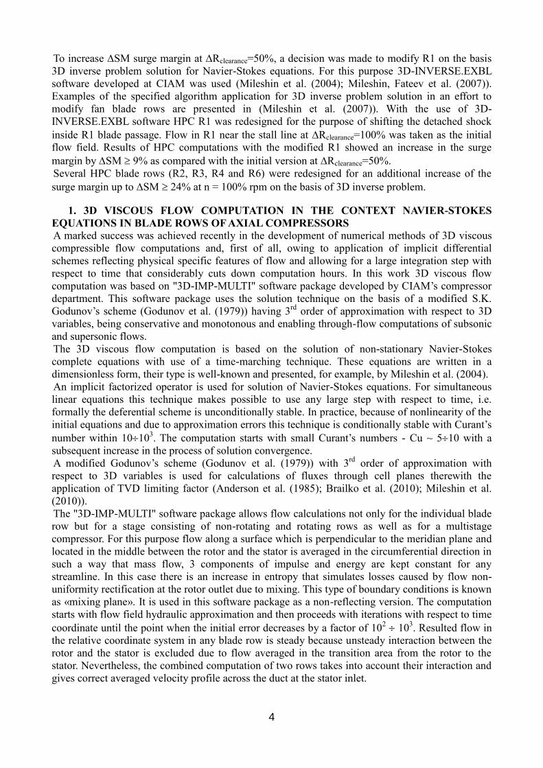
stage HPC (Fig. 1) with Rclearance=50% of the nominal value gave the evidence that there are no
contacts between R1 and the casing in operating modes near to the HPC operating line.
Figure 1: HPC under study
4
To increase SM surge margin at Rclearance=50%, a decision was made to modify R1 on the basis
3D inverse problem solution for Navier-Stokes equations. For this purpose 3D-INVERSE.EXBL
software developed at CIAM was used (Mileshin et al. (2004); Mileshin, Fateev et al. (2007)).
Examples of the specified algorithm application for 3D inverse problem solution in an effort to
modify fan blade rows are presented in (Mileshin et al. (2007)). With the use of 3D-
INVERSE.EXBL software HPC R1 was redesigned for the purpose of shifting the detached shock
inside R1 blade passage. Flow in R1 near the stall line at Rclearance=100% was taken as the initial
flow field. Results of HPC computations with the modified R1 showed an increase in the surge
margin by SM 9% as compared with the initial version at Rclearance=50%.
Several HPC blade rows (R2, R3, R4 and R6) were redesigned for an additional increase of the
surge margin up to SM 24% at n = 100% rpm on the basis of 3D inverse problem.
1. 3D VISCOUS FLOW COMPUTATION IN THE CONTEXT NAVIER-STOKES
EQUATIONS IN BLADE ROWS OF AXIAL COMPRESSORS
A marked success was achieved recently in the development of numerical methods of 3D viscous
compressible flow computations and, first of all, owing to application of implicit differential
schemes reflecting physical specific features of flow and allowing for a large integration step with
respect to time that considerably cuts down computation hours. In this work 3D viscous flow
computation was based on "3D-IMP-MULTI" software package developed by CIAM’s compressor
department. This software package uses the solution technique on the basis of a modified S.K.
Godunov’s scheme (Godunov et al. (1979)) having 3rd
order of approximation with respect to 3D
variables, being conservative and monotonous and enabling through-flow computations of subsonic
and supersonic flows.
The 3D viscous flow computation is based on the solution of non-stationary Navier-Stokes
complete equations with use of a time-marching technique. These equations are written in a
dimensionless form, their type is well-known and presented, for example, by Mileshin et al. (2004).
An implicit factorized operator is used for solution of Navier-Stokes equations. For simultaneous
linear equations this technique makes possible to use any large step with respect to time, i.e.
formally the deferential scheme is unconditionally stable. In practice, because of nonlinearity of the
initial equations and due to approximation errors this technique is conditionally stable with Curant’s
number within 10103. The computation starts with small Curant’s numbers - Сu ~ 510 with a
subsequent increase in the process of solution convergence.
A modified Godunov’s scheme (Godunov et al. (1979)) with 3rd
order of approximation with
respect to 3D variables is used for calculations of fluxes through cell planes therewith the
application of TVD limiting factor (Anderson et al. (1985); Brailko et al. (2010); Mileshin et al.
(2010)).
The "3D-IMP-MULTI" software package allows flow calculations not only for the individual blade
row but for a stage consisting of non-rotating and rotating rows as well as for a multistage
compressor. For this purpose flow along a surface which is perpendicular to the meridian plane and
located in the middle between the rotor and the stator is averaged in the circumferential direction in
such a way that mass flow, 3 components of impulse and energy are kept constant for any
streamline. In this case there is an increase in entropy that simulates losses caused by flow non-
uniformity rectification at the rotor outlet due to mixing. This type of boundary conditions is known
as «mixing plane». It is used in this software package as a non-reflecting version. The computation
starts with flow field hydraulic approximation and then proceeds with iterations with respect to time
coordinate until the point when the initial error decreases by a factor of 102 10
3. Resulted flow in
the relative coordinate system in any blade row is steady because unsteady interaction between the
rotor and the stator is excluded due to flow averaged in the transition area from the rotor to the
stator. Nevertheless, the combined computation of two rows takes into account their interaction and
gives correct averaged velocity profile across the duct at the stator inlet.
5
The "3D-IMP-MULTI" software enables 3D viscous flow computations with account of tip
clearances as well as radial clearances at the stator hub in case of cantilever-type mounting of stator
vanes. The two-parameter differential model of turbulence k- (Wilcox D.C., (1986)) was used in
the computations.
2. BOUNDARY CONDITIONS
Flow angles in the circumferential direction and in the meridian plane in the direction from the hub
to the tip as well as total pressure and temperature distributions along the radius are specified at the
inlet; static pressure at the hub is specified at the outlet; and the static pressure distribution from the
hub to the tip is derived from the radial balance equation. A boundary condition for a wall is
sticking condition and for a periodic boundary - periodicity condition. Non-reflecting boundary
conditions can be used at the inlet and the outlet in case of troubles with problem convergence and
implemented by specifying corresponding Riemann’s invariants. To calculate kinetic energy of
pulsations, , and specific dissipation rate, , the turbulent-to-laminar viscosity ratio, t/=50, and
the intensity of turbulent pulsations at the inlet, Tu=5%, are specified at the computational domain
inlet.
3. RESULTS OF 3D VISCOUS FLOW COMPUTATIONS FOR THE INITIAL VERSION
OF SIX-STAGE HPC
Computations were based on the upgraded “3D-IMP-MULTI” code. The computation goal is
assessment of the whole HPC and its separate rows local and integral performances for the
rotational speed 100% (ncor=100%, u1R=370 m/s) and for partial speeds ncor=25%100%.
Computations of viscous flow in the compressor (13 blade rows including IGV) were made for the
corrected parameters at the inlet (Т* = 288К, Р* = 101325 Pa).
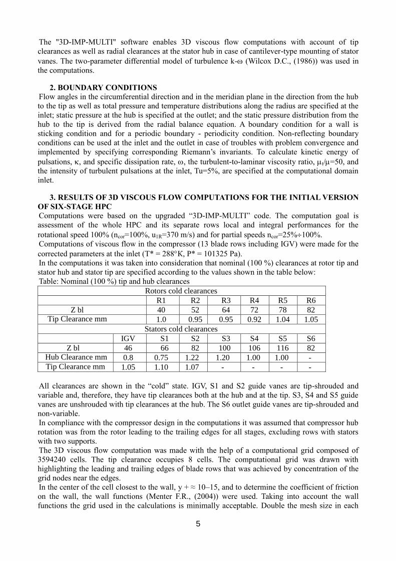
In the computations it was taken into consideration that nominal (100 %) clearances at rotor tip and
stator hub and stator tip are specified according to the values shown in the table below:
Table: Nominal (100 %) tip and hub clearances
Rotors cold clearances
R1 R2 R3 R4 R5 R6
Z bl 40 52 64 72 78 82 Tip Clearance mm 1.0 0.95 0.95 0.92 1.04 1.05
Stators cold clearances
IGV S1 S2 S3 S4 S5 S6
Z bl 46 66 82 100 106 116 82 Hub Clearance mm 0.8 0.75 1.22 1.20 1.00 1.00 - Tip Clearance mm 1.05 1.10 1.07 - - - -
All clearances are shown in the “cold” state. IGV, S1 and S2 guide vanes are tip-shrouded and
variable and, therefore, they have tip clearances both at the hub and at the tip. S3, S4 and S5 guide
vanes are unshrouded with tip clearances at the hub. The S6 outlet guide vanes are tip-shrouded and
non-variable.
In compliance with the compressor design in the computations it was assumed that compressor hub
rotation was from the rotor leading to the trailing edges for all stages, excluding rows with stators
with two supports.
The 3D viscous flow computation was made with the help of a computational grid composed of
3594240 cells. The tip clearance occupies 8 cells. The computational grid was drawn with
highlighting the leading and trailing edges of blade rows that was achieved by concentration of the
grid nodes near the edges.
In the center of the cell closest to the wall, y + ≈ 10–15, and to determine the coefficient of friction
on the wall, the wall functions (Menter F.R., (2004)) were used. Taking into account the wall
functions the grid used in the calculations is minimally acceptable. Double the mesh size in each
6
direction, i.e. a total of 8 times, leads to an increase in adiabatic efficiency of 1.0 ÷ 1.2%. However
the flow rate and the degree of increase in the total pressure change slightly, the flow pattern
remains the same.
At the operating point of the characteristic line for the initial version of HPC at 100 % speed the
following parameters (see Fig. 20) are found: adiabatic efficiency - *ad/*des=0.94 at
*c/*des=0.87
total pressure ratio, i.e. the HPC under study demonstrates low parameters as to pressure ratio and
efficiency. The compressor surge margin is equal only to SM=1.716% that is not high,
(Gdes-GINI)/Gdes0.1100%10%. The operating point is the cross-point of
c=
c(Gcor)
characteristic line and the operating line.
.
4. AERODYNAMICS OF THE INITIAL COMPRESSOR VERSION AT 100 % SPEED
AND NOMINAL TIP CLEARANCE
The detailed study of compressor aerodynamics at 100% r.p.m. was performed at the operating
point. Aerodynamics of the HPC initial version is presented by Mach number contours (see Fig. 2a,
Fig. 3а) at the operating point at 100% rpm and tip clearance Rclearance=50%.
Rclearance(50%)=0.5Rclearance(100%), that is approximately equal to tip clearances in the “hot”
state in the design condition.
a)
b)
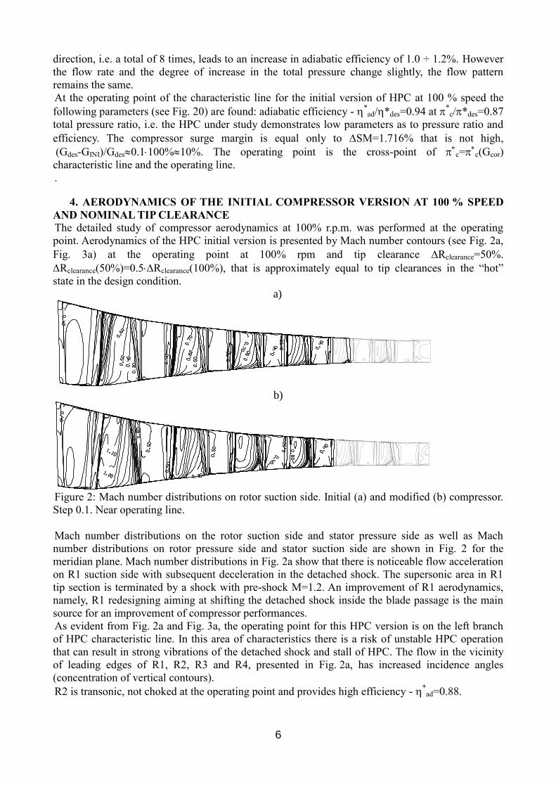
Figure 2: Mach number distributions on rotor suction side. Initial (a) and modified (b) compressor.
Step 0.1. Near operating line.
Mach number distributions on the rotor suction side and stator pressure side as well as Mach
number distributions on rotor pressure side and stator suction side are shown in Fig. 2 for the
meridian plane. Mach number distributions in Fig. 2a show that there is noticeable flow acceleration
on R1 suction side with subsequent deceleration in the detached shock. The supersonic area in R1
tip section is terminated by a shock with pre-shock M=1.2. An improvement of R1 aerodynamics,
namely, R1 redesigning aiming at shifting the detached shock inside the blade passage is the main
source for an improvement of compressor performances.
As evident from Fig. 2a and Fig. 3a, the operating point for this HPC version is on the left branch
of HPC characteristic line. In this area of characteristics there is a risk of unstable HPC operation
that can result in strong vibrations of the detached shock and stall of HPC. The flow in the vicinity
of leading edges of R1, R2, R3 and R4, presented in Fig. 2a, has increased incidence angles
(concentration of vertical contours).
R2 is transonic, not choked at the operating point and provides high efficiency - *ad=0.88.
7
Efficiency of R3 is high enough because of low losses in Stator3. Efficiency of last stages at the
operating point of the characteristic line smoothly decreases from the inlet to the outlet and
efficiency of the 6-th stage is equal to *ad=0.8. Mainly, this is caused by a decrease in efficiency of
rotors because of strengthening the adverse effect of the tip clearance in last stages. Losses in guide
vanes are kept constant and even slightly decrease in last stages.
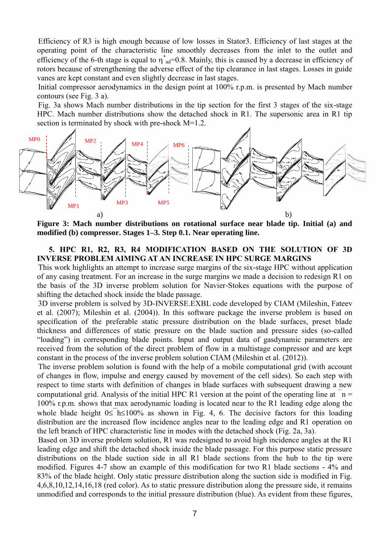
Initial compressor aerodynamics in the design point at 100% r.p.m. is presented by Mach number
contours (see Fig. 3 a).
Fig. 3a shows Mach number distributions in the tip section for the first 3 stages of the six-stage
HPC. Mach number distributions show the detached shock in R1. The supersonic area in R1 tip
section is terminated by shock with pre-shock M=1.2.
a) b)
Figure 3: Mach number distributions on rotational surface near blade tip. Initial (a) and
modified (b) compressor. Stages 1–3. Step 0.1. Near operating line.
5. HPC R1, R2, R3, R4 MODIFICATION BASED ON THE SOLUTION OF 3D
INVERSE PROBLEM AIMING AT AN INCREASE IN HPC SURGE MARGINS
This work highlights an attempt to increase surge margins of the six-stage HPC without application
of any casing treatment. For an increase in the surge margins we made a decision to redesign R1 on
the basis of the 3D inverse problem solution for Navier-Stokes equations with the purpose of
shifting the detached shock inside the blade passage.
3D inverse problem is solved by 3D-INVERSE.EXBL code developed by CIAM (Mileshin, Fateev
et al. (2007); Mileshin et al. (2004)). In this software package the inverse problem is based on
specification of the preferable static pressure distribution on the blade surfaces, preset blade
thickness and differences of static pressure on the blade suction and pressure sides (so-called
“loading”) in corresponding blade points. Input and output data of gasdynamic parameters are
received from the solution of the direct problem of flow in a multistage compressor and are kept
constant in the process of the inverse problem solution CIAM (Mileshin et al. (2012)).
The inverse problem solution is found with the help of a mobile computational grid (with account
of changes in flow, impulse and energy caused by movement of the cell sides). So each step with
respect to time starts with definition of changes in blade surfaces with subsequent drawing a new
computational grid. Analysis of the initial HPC R1 version at the point of the operating line at n =
100% r.p.m. shows that max aerodynamic loading is located near to the R1 leading edge along the
whole blade height 0h100% as shown in Fig. 4, 6. The decisive factors for this loading
distribution are the increased flow incidence angles near to the leading edge and R1 operation on
the left branch of HPC characteristic line in modes with the detached shock (Fig. 2а, 3а).
Based on 3D inverse problem solution, R1 was redesigned to avoid high incidence angles at the R1
leading edge and shift the detached shock inside the blade passage. For this purpose static pressure
distributions on the blade suction side in all R1 blade sections from the hub to the tip were
modified. Figures 4-7 show an example of this modification for two R1 blade sections - 4% and
83% of the blade height. Only static pressure distribution along the suction side is modified in Fig.
4,6,8,10,12,14,16,18 (red color). As to static pressure distribution along the pressure side, it remains
unmodified and corresponds to the initial pressure distribution (blue). As evident from these figures,
MP1
MP0 MP2 MP4
MP3 MP5
MP6
8
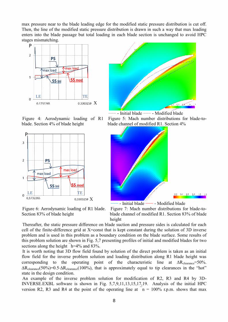
max pressure near to the blade leading edge for the modified static pressure distribution is cut off.
Then, the line of the modified static pressure distribution is drawn in such a way that max loading
enters into the blade passage but total loading in each blade section is unchanged to avoid HPC
stages mismatching.
X
−−− - Initial blade −−− - Modified blade
Figure 4: Aerodynamic loading of R1
blade. Section 4% of blade height
Figure 5: Mach number distributions for blade-to-
blade channel of modified R1. Section 4%
Х −−− - Initial blade −−− - Modified blade
Figure 6: Aerodynamic loading of R1 blade.
Section 83% of blade height
Figure 7: Mach number distributions for blade-to-
blade channel of modified R1. Section 83% of blade
height
Thereafter, the static pressure difference on blade suction and pressure sides is calculated for each
cell of the finite-difference grid at X=const that is kept constant during the solution of 3D inverse
problem and is used in this problem as a boundary condition on the blade surface. Some results of
this problem solution are shown in Fig. 5,7 presenting profiles of initial and modified blades for two
sections along the height h=4% and 83%.
It is worth noting that 3D flow field found by solution of the direct problem is taken as an initial
flow field for the inverse problem solution and loading distribution along R1 blade height was
corresponding to the operating point of the characteristic line at Rclearance=50%.
Rclearance(50%)=0.5Rclearance(100%), that is approximately equal to tip clearances in the “hot”
state in the design condition.
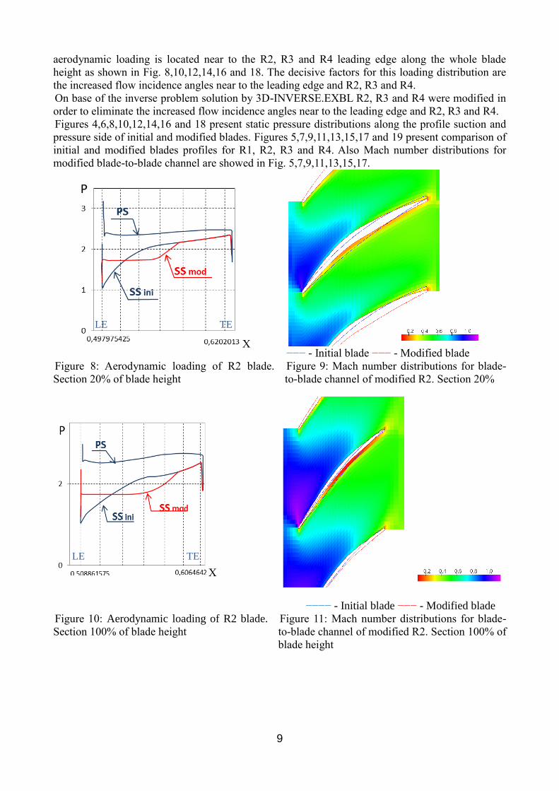
An example of the inverse problem solution for modification of R2, R3 and R4 by 3D-
INVERSE.EXBL software is shown in Fig. 5,7,9,11,13,15,17,19. Analysis of the initial HPC
version R2, R3 and R4 at the point of the operating line at n = 100% r.p.m. shows that max
LE TE
LE TE
9
aerodynamic loading is located near to the R2, R3 and R4 leading edge along the whole blade
height as shown in Fig. 8,10,12,14,16 and 18. The decisive factors for this loading distribution are
the increased flow incidence angles near to the leading edge and R2, R3 and R4.
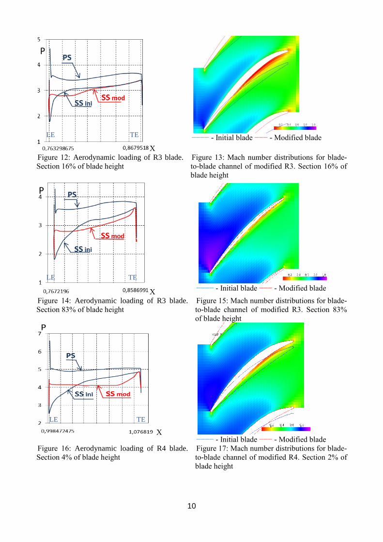
On base of the inverse problem solution by 3D-INVERSE.EXBL R2, R3 and R4 were modified in
order to eliminate the increased flow incidence angles near to the leading edge and R2, R3 and R4.
Figures 4,6,8,10,12,14,16 and 18 present static pressure distributions along the profile suction and
pressure side of initial and modified blades. Figures 5,7,9,11,13,15,17 and 19 present comparison of
initial and modified blades profiles for R1, R2, R3 and R4. Also Mach number distributions for
modified blade-to-blade channel are showed in Fig. 5,7,9,11,13,15,17.
Х −−− - Initial blade −−− - Modified blade
Figure 8: Aerodynamic loading of R2 blade.
Section 20% of blade height
Figure 9: Mach number distributions for blade-
to-blade channel of modified R2. Section 20%
Х
−−−− - Initial blade −−− - Modified blade
Figure 10: Aerodynamic loading of R2 blade.
Section 100% of blade height
Figure 11: Mach number distributions for blade-
to-blade channel of modified R2. Section 100% of
blade height
LE TE
LE TE
10
Х
−−−− - Initial blade −−− - Modified blade
Figure 12: Aerodynamic loading of R3 blade.
Section 16% of blade height
Figure 13: Mach number distributions for blade-
to-blade channel of modified R3. Section 16% of
blade height
Х
−−−− - Initial blade −−− - Modified blade
Figure 14: Aerodynamic loading of R3 blade.
Section 83% of blade height
Figure 15: Mach number distributions for blade-
to-blade channel of modified R3. Section 83%
of blade height
Х −−−− - Initial blade −−− - Modified blade
Figure 16: Aerodynamic loading of R4 blade.
Section 4% of blade height
Figure 17: Mach number distributions for blade-
to-blade channel of modified R4. Section 2% of
blade height
LE TE
LE TE
LE TE
11
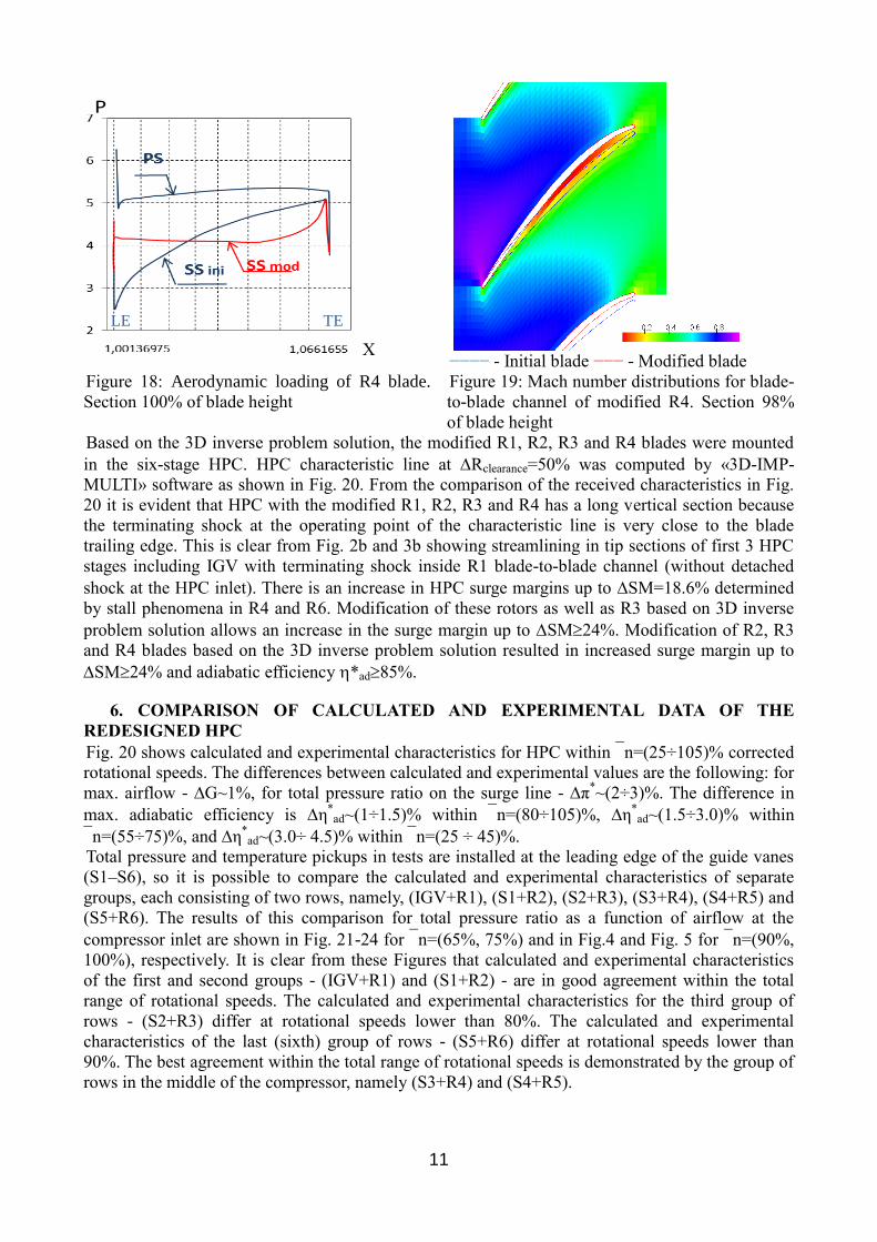
Х −−−− - Initial blade −−− - Modified blade
Figure 18: Aerodynamic loading of R4 blade.
Section 100% of blade height
Figure 19: Mach number distributions for blade-
to-blade channel of modified R4. Section 98%
of blade height
Based on the 3D inverse problem solution, the modified R1, R2, R3 and R4 blades were mounted
in the six-stage HPC. HPC characteristic line at Rclearance=50% was computed by «3D-IMP-
MULTI» software as shown in Fig. 20. From the comparison of the received characteristics in Fig.
20 it is evident that HPC with the modified R1, R2, R3 and R4 has a long vertical section because
the terminating shock at the operating point of the characteristic line is very close to the blade
trailing edge. This is clear from Fig. 2b and 3b showing streamlining in tip sections of first 3 HPC
stages including IGV with terminating shock inside R1 blade-to-blade channel (without detached
shock at the HPC inlet). There is an increase in HPC surge margins up to SM=18.6% determined
by stall phenomena in R4 and R6. Modification of these rotors as well as R3 based on 3D inverse
problem solution allows an increase in the surge margin up to SM24%. Modification of R2, R3
and R4 blades based on the 3D inverse problem solution resulted in increased surge margin up to
SM24% and adiabatic efficiency *ad85%.
6. COMPARISON OF CALCULATED AND EXPERIMENTAL DATA OF THE
REDESIGNED HPC
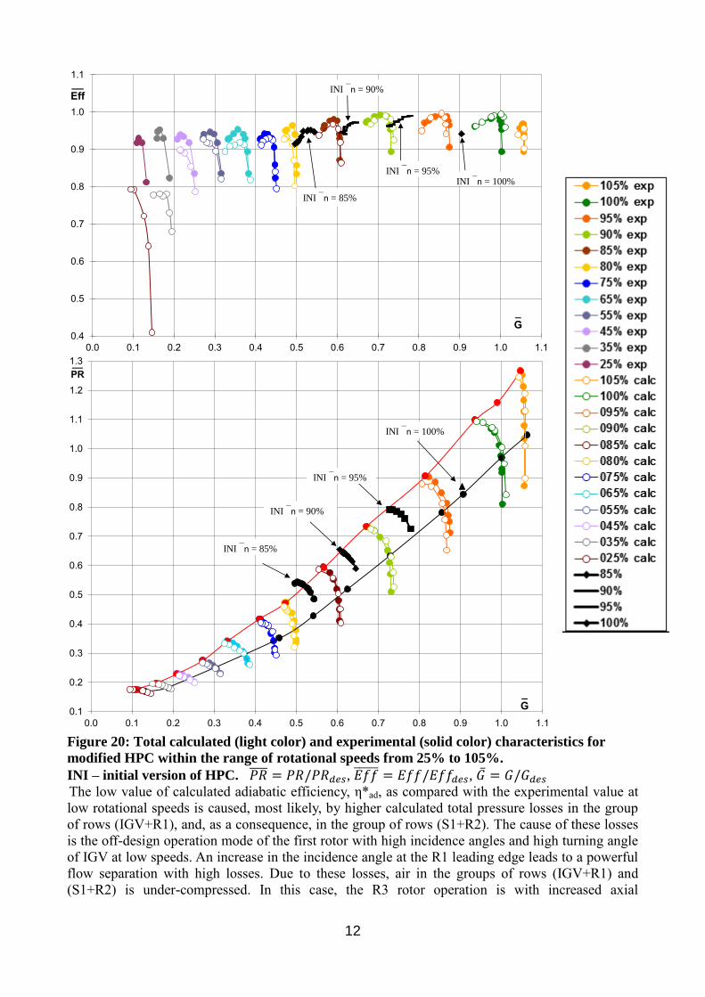
Fig. 20 shows calculated and experimental characteristics for HPC within n=(25÷105)% corrected
rotational speeds. The differences between calculated and experimental values are the following: for
max. airflow - ∆G~1%, for total pressure ratio on the surge line - ∆π*~(2÷3)%. The difference in
max. adiabatic efficiency is ∆η*ad~(1÷1.5)% within n=(80÷105)%, ∆η
*ad~(1.5÷3.0)% within
n=(55÷75)%, and ∆η*ad~(3.0÷ 4.5)% within n=(25 ÷ 45)%.
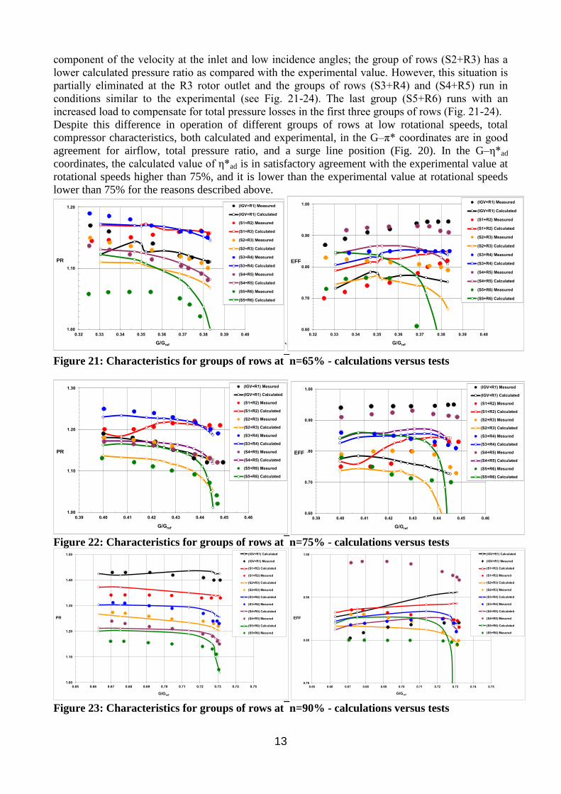
Total pressure and temperature pickups in tests are installed at the leading edge of the guide vanes
(S1–S6), so it is possible to compare the calculated and experimental characteristics of separate
groups, each consisting of two rows, namely, (IGV+R1), (S1+R2), (S2+R3), (S3+R4), (S4+R5) and
(S5+R6). The results of this comparison for total pressure ratio as a function of airflow at the
compressor inlet are shown in Fig. 21-24 for n=(65%, 75%) and in Fig.4 and Fig. 5 for n=(90%,
100%), respectively. It is clear from these Figures that calculated and experimental characteristics
of the first and second groups - (IGV+R1) and (S1+R2) - are in good agreement within the total
range of rotational speeds. The calculated and experimental characteristics for the third group of
rows - (S2+R3) differ at rotational speeds lower than 80%. The calculated and experimental
characteristics of the last (sixth) group of rows - (S5+R6) differ at rotational speeds lower than
90%. The best agreement within the total range of rotational speeds is demonstrated by the group of
rows in the middle of the compressor, namely (S3+R4) and (S4+R5).
LE TE
12
Figure 20: Total calculated (light color) and experimental (solid color) characteristics for
modified HPC within the range of rotational speeds from 25% to 105%.
INI – initial version of HPC. 𝑃𝑅̅̅ ̅̅ = 𝑃𝑅/𝑃𝑅𝑑𝑒𝑠, 𝐸𝑓𝑓̅̅ ̅̅ ̅ = 𝐸𝑓𝑓/𝐸𝑓𝑓𝑑𝑒𝑠, �̅� = 𝐺/𝐺𝑑𝑒𝑠
The low value of calculated adiabatic efficiency, η*ad, as compared with the experimental value at
low rotational speeds is caused, most likely, by higher calculated total pressure losses in the group
of rows (IGV+R1), and, as a consequence, in the group of rows (S1+R2). The cause of these losses
is the off-design operation mode of the first rotor with high incidence angles and high turning angle
of IGV at low speeds. An increase in the incidence angle at the R1 leading edge leads to a powerful
flow separation with high losses. Due to these losses, air in the groups of rows (IGV+R1) and
(S1+R2) is under-compressed. In this case, the R3 rotor operation is with increased axial
0.4
0.5
0.6
0.7
0.8
0.9
1.0
1.1
0.0 0.1 0.2 0.3 0.4 0.5 0.6 0.7 0.8 0.9 1.0 1.1
__Eff
_G
INI n = 85%
INI n = 90%
INI n = 95%INI n = 100%
0.1
0.2
0.3
0.4
0.5
0.6
0.7
0.8
0.9
1.0
1.1
1.2
1.3
0.0 0.1 0.2 0.3 0.4 0.5 0.6 0.7 0.8 0.9 1.0 1.1
__PR
_G
INI n = 85%
INI n = 90%
INI n = 95%
INI n = 100%
13
component of the velocity at the inlet and low incidence angles; the group of rows (S2+R3) has a
lower calculated pressure ratio as compared with the experimental value. However, this situation is
partially eliminated at the R3 rotor outlet and the groups of rows (S3+R4) and (S4+R5) run in
conditions similar to the experimental (see Fig. 21-24). The last group (S5+R6) runs with an
increased load to compensate for total pressure losses in the first three groups of rows (Fig. 21-24).
Despite this difference in operation of different groups of rows at low rotational speeds, total
compressor characteristics, both calculated and experimental, in the G–π* coordinates are in good
agreement for airflow, total pressure ratio, and a surge line position (Fig. 20). In the G–η*ad
coordinates, the calculated value of η*ad is in satisfactory agreement with the experimental value at
rotational speeds higher than 75%, and it is lower than the experimental value at rotational speeds
lower than 75% for the reasons described above.
`
Figure 21: Characteristics for groups of rows atn=65% - calculations versus tests
Figure 22: Characteristics for groups of rows atn=75% - calculations versus tests
Figure 23: Characteristics for groups of rows atn=90% - calculations versus tests
1.00
1.10
1.20
0.32 0.33 0.34 0.35 0.36 0.37 0.38 0.39 0.40
G/Gref
(IGV+R1) Measured
(IGV+R1) Calculated
(S1+R2) Measured
(S1+R2) Calculated
(S2+R3) Measured
(S2+R3) Calculated
(S3+R4) Measured
(S3+R4) Calculated
(S4+R5) Measured
(S4+R5) Calculated
(S5+R6) Measured
(S5+R6) Calculated
PR
0.60
0.70
0.80
0.90
1.00
0.32 0.33 0.34 0.35 0.36 0.37 0.38 0.39 0.40
G/Gref
(IGV+R1) Measured
(IGV+R1) Calculated
(S1+R2) Measured
(S1+R2) Calculated
(S2+R3) Measured
(S2+R3) Calculated
(S3+R4) Measured
(S3+R4) Calculated
(S4+R5) Measured
(S4+R5) Calculated
(S5+R6) Measured
(S5+R6) Calculated
EFF
1.00
1.10
1.20
1.30
0.39 0.40 0.41 0.42 0.43 0.44 0.45 0.46
G/Gref
(IGV+R1) Mesured
(IGV+R1) Calculated
(S1+R2) Mesured
(S1+R2) Calculated
(S2+R3) Mesured
(S2+R3) Calculated
(S3+R4) Mesured
(S3+R4) Calculated
(S4+R5) Mesured
(S4+R5) Calculated
(S5+R6) Mesured
(S5+R6) Calculated
PR
0.60
0.70
0.80
0.90
1.00
0.39 0.40 0.41 0.42 0.43 0.44 0.45 0.46
G/Gref
(IGV+R1) Mesured
(IGV+R1) Calculated
(S1+R2) Mesured
(S1+R2) Calculated
(S2+R3) Mesured
(S2+R3) Calculated
(S3+R4) Mesured
(S3+R4) Calculated
(S4+R5) Mesured
(S4+R5) Calculated
(S5+R6) Mesured
(S5+R6) Calculated
EFF
1.00
1.10
1.20
1.30
1.40
1.50
0.65 0.66 0.67 0.68 0.69 0.70 0.71 0.72 0.73 0.74 0.75
G/Gref
(IGV+R1) Calculated
(IGV+R1) Mesured
(S1+R2) Calculated
(S1+R2) Mesured
(S2+R3) Calculated
(S2+R3) Mesured
(S3+R4) Calculated
(S3+R4) Mesured
(S4+R5) Calculated
(S4+R5) Mesured
(S5+R6) Calculated
(S5+R6) Mesured
PR
0.70
0.80
0.90
1.00
0.65 0.66 0.67 0.68 0.69 0.70 0.71 0.72 0.73 0.74 0.75
G/Gref
(IGV+R1) Calculated
(IGV+R1) Mesured
(S1+R2) Calculated
(S1+R2) Mesured
(S2+R3) Calculated
(S2+R3) Mesured
(S3+R4) Calculated
(S3+R4) Mesured
(S4+R5) Calculated
(S4+R5) Mesured
(S5+R6) Calculated
(S5+R6) Mesured
EFF
14
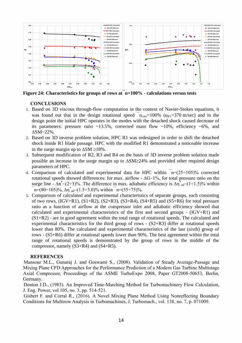
Figure 24: Characteristics for groups of rows atn=100% - calculations versus tests
CONCLUSIONS
1. Based on 3D viscous through-flow computation in the context of Navier-Stokes equations, it
was found out that in the design rotational speed ncorr=100% (uR1=370 m/sec) and in the
design point the initial HPC operates in the modes with the detached shock caused decrease of
its parameters: pressure ratio ~13.5%, corrected mass flow ~10%, efficiency ~6%, and
ΔSM~22%.
2. Based on 3D inverse problem solution, HPC R1 was redesigned in order to shift the detached
shock inside R1 blade passage. HPC with the modified R1 demonstrated a noticeable increase
in the surge margin up to SM 18%.
3. Subsequent modification of R2, R3 and R4 on the basis of 3D inverse problem solution made
possible an increase in the surge margin up to SM24% and provided other required design
parameters of HPC.
4. Comparison of calculated and experimental data for HPC within n=(25÷105)% corrected
rotational speeds showed differences: for max. airflow - ∆G~1%, for total pressure ratio on the
surge line - ∆π*~(2÷3)%. The difference in max. adiabatic efficiency is ∆η
*ad~(1÷1.5)% within
n=(80÷105)%, ∆η*ad~(1.5÷3.0)% within n=(55÷75)%.
5. Comparison of calculated and experimental characteristics of separate groups, each consisting
of two rows, (IGV+R1), (S1+R2), (S2+R3), (S3+R4), (S4+R5) and (S5+R6) for total pressure
ratio as a function of airflow at the compressor inlet and adiabatic efficiency showed that
calculated and experimental characteristics of the first and second groups - (IGV+R1) and
(S1+R2) - are in good agreement within the total range of rotational speeds. The calculated and
experimental characteristics for the third group of rows - (S2+R3) differ at rotational speeds
lower than 80%. The calculated and experimental characteristics of the last (sixth) group of
rows - (S5+R6) differ at rotational speeds lower than 90%. The best agreement within the total
range of rotational speeds is demonstrated by the group of rows in the middle of the
compressor, namely (S3+R4) and (S4+R5).
REFERENCES
Mansour M.L., Gunaraj J. and Goswami S., (2008). Validation of Steady Average-Passage and
Mixing Plane CFD Approaches for the Performance Prediction of a Modern Gas Turbine Multistage
Axial Compressor, Proceedings of the ASME TurboExpo 2008, Paper GT2008-50653, Berlin,
Germany.
Denton J.D., (1983). An Improved Time-Marching Method for Turbomachinery Flow Calculation,
J. Eng. Power, vol.105, no. 3, pp. 514-521.
Gisbert F. and Corral R., (2016). A Novel Mixing Plane Method Using Nonreflecting Boundary
Conditions for Multirow Analysis in Turbomachines, J. Turbomach., vol. 138, no. 7, p. 071009.
1.00
1.10
1.20
1.30
1.40
1.50
1.60
1.70
1.80
0.92 0.93 0.94 0.95 0.96 0.97 0.98 0.99 1.00 1.01 1.02
G/Gref
(IGV+R1) Calculated
(IGV+R1) Mesured
(S1+R2) Calculated
(S1+R2) Mesured
(S2+R3) Calculated
(S2+R3) Mesured
(S3+R4) Calculated
(S3+R4) Mesured
(S4+R5) Calculated
(S4+R5) Mesured
(S5+R6) Calculated
(S5+R6) Mesured
PR
0.70
0.80
0.90
1.00
0.92 0.93 0.94 0.95 0.96 0.97 0.98 0.99 1.00 1.01 1.02
G/Gref
(IGV+R1) Calculated
(IGV+R1) Mesured
(S1+R2) Calculated
(S1+R2) Mesured
(S2+R3) Calculated
(S2+R3) Mesured
(S3+R4) Calculated
(S3+R4) Mesured
(S4+R5) Calculated
(S4+R5) Mesured
(S5+R6) Calculated
(S5+R6) Mesured
EFF
15
Adamczyk J.J., (1999). Aerodynamic Analysis of Multistage Turbomachinery Flows in Support of
Aerodynamic Design, in ASME 1999 International Gas Turbine and Aeroengine Congress and
Exhibition, Paper No. 99-GT-080, Indianapolis, USA.
Cozzi L., Rubechini F., Marconcini M., Arnone A., Astrua P., Schneider A., Silingardi A., (2017).
Facing the challenges in CFD modelling of multistage axial compressors, in ASME Turbo Expo
2017, Paper No. GT2017-63240, Charlotte, USA.
Denton J.D., (2010). Some Limitations of Turbomachinery CFD, in ASME Turbo Expo 2010, Paper
No. GT2010-22540, Glasgow, UK.
Rubechini F., Marconcini M., Giovannini M., Bellucci J. and Arnone A., (2015). Accounting for
Unsteady Interaction in Transonic Stages, J. Eng. Gas Turbines Power, vol. 137, no. 5, pp. 052602-
052602-9.
Holmes, D. G., Moore, B. J., and Connell, S. D. (July 10–14 2011) Unsteady vs. Steady
Turbomachinery Flow Analysis: Exploiting Large-Scale Computations to Deepen our
Understanding of Turbomachinery Flows. In Sci-DAC conference, Denver, CO, USA.
Wang F., Carnevale M., di Mare L., Gallimore S., (2017). Simulation of multi-stage compressor at
off-design conditions, in ASME TurboExpo 2017, Paper GT2017-64964, Charlotte, USA.
Dent A., Xu L., Wells R., (2017). Assessment of the severity of unsteady Mach number effects in a
3-stage transonic compressor, in ASME TurboExpo 2017, Paper GT2017-64022, Charlotte, USA.
Li, Y.S., and Wells, R. G., (1999). The Three-Dimensional Aerodynamic Design and Test of a
Three-Stage Transonic Compressor. ASME Paper 99-GT-068.
Mileshin V.I., I.K. Orekhov, V.A. Fateyev, S.K. Shchipin, (2007). Effect of tip clearance on flow
structure and integral performances of six-stage HPC, Proceedings of ISABE Conference, ISABE-
2007-1179-Paper, Beijing, China.
Mileshin, V.I., Orekhov, I.K., Shchipin, S.K., and Startsev, A.N., (2004). New 3D Inverse Navier-
Stokes Based Method Used to Design Turbomachinery Blade Rows, ASME HF-FED-2004-56436,
Charlotte, USA.
Mileshin, V.I., Orekhov, I.K., Shchipin, S.K., and Startsev, A.N., (2007). 3D inverse design of
transonic fan rotors efficient for a wide range of RPM, ASME TURBO EXPO 2007 Power for
Land, Sea and Air, GT2007-27817, Montreal, Canada.
Godunov S.K., Zabrodine A., Ivanov M., Kraiko A., and Prokopov G., (1979). Résolution
numérique des problèmes multidimensionnels de la dynamique des gaz. Edition Mir, Moscou.
Anderson, W.К., Thomas, J.L. and Van Leer, B., (1985). A Comparison of Finite Volume Flux
Vector Splittings for the Euler Equations, AIAA Paper No. 85-0122.
Brailko I.A., Mileshin V.I., Volkov A.M., Korzhnev V.N., (2010). Numerical and experimental
investigations of CRF with simulation of flow non-uniformity in the basic flight conditions.
Proceedings of 27th International Congress of Aeronautical Sciences, pp.2619, paper ICAS2010-
420, Nice, France.
Mileshin V.I., Orekhov I.K, Pankov S.V., Stepanov E.I., (2010). Numerical and experimental
investigations of a high-loaded typical middle stage model of HPC. Proceedings of 27th
International Congress of Aeronautical Sciences, ICAS2010, pp.2628, Nice, France.
Wilcox D.C., (1986). Multiscale Model for Turbulent Flows. In AIAA 24th
Aerospace Sciences
Meeting. American Institute of Aeronautics and Astronautics.
Menter F.R., Langtry R., Hansen T., (2004). CFD simulation of turbomachinery flows - verification,
validation and modelling. Proceedings of European Congress on Computational Methods in
Applied Sciences and Engineering, ECCOMAS 2004, Jyvaskyla, Finland.
Mileshin V.I., Kozhemyako P.G., Orekhov I.K., Fateev V.A., (2012). Experimental and numerical
study of two first highly-loaded stages of compressors as a part of HPC and separate test unit.
Proceedings of 28th International Congress of Aeronautical Sciences pp.2675, paper ICAS2012-
474, Brisbane, Australia.