Mechanical Vibrations

Course no. MAE 4024

Section: 01

Instructor: Dr. Beshoy Morkos

Term Project: Proposed Redesign and Analysis of BMW X3 Side View Mirror

Report Due: 11/03/2013

By:

Omar Galil

Toluwalase Olajoyegbe

Abstract

The BMW X3 SAV has developed some characteristics that have proven to be an inconvenience

to customers. It has been reported that the mirrors are emitting unpleasant noise and also exhibit

some misalignment over a period of time. The following report gives an analytical report of the

current system while pinpointing some of its likely issues, and a detailed outline of the proposed

solution, which will address the problem while inquiring minimal cost in the event of a recall.

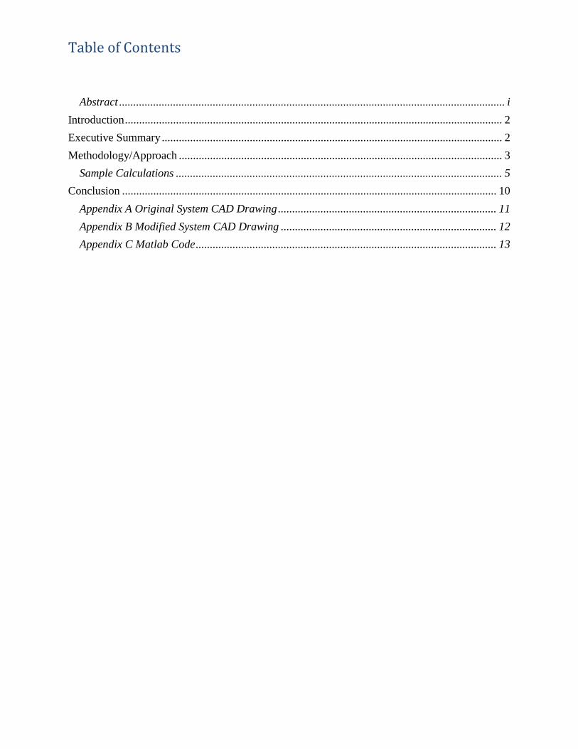
Table of Contents

Abstract ........................................................................................................................................ i

Introduction ..................................................................................................................................... 2

Executive Summary ........................................................................................................................ 2

Methodology/Approach .................................................................................................................. 3

Sample Calculations ................................................................................................................... 5

Conclusion .................................................................................................................................... 10

Appendix A Original System CAD Drawing ............................................................................. 11

Appendix B Modified System CAD Drawing ............................................................................ 12

Appendix C Matlab Code .......................................................................................................... 13

2

Introduction

As technology has advanced, machinery has gotten quicker, more precise and reliable. But with

these advancements have come new problems which must be solved with the arrival of more

advanced high performance mechanical systems. The major effects in these systems are of

vibrational origin. It is evident that, as engineers, the analysis of a system or the parts it consists

of, cannot simply end once the safety factors of each part is below a particular threshold. The

study of the system must also be stable when exposed to frequencies to which the parts operate

at. Improper analysis of these systems could lead to a wide variety of issues from unpleasant

noise to a completely instable system. Through the years of design development, engineers have

witnessed bolts in automotive transmission falling out and even the destruction of bridges due to

the fact that they were not designed to operate at frequencies they were exposed to.

The following analysis preformed in the report applies some knowledge about vibrational

systems to help stabilize an issue with one of BMWs’ OEM parts.

Executive Summary

The problem statement laid out in this project was to modify the side mirror system of a BMW

X3 vehicle. The path taken to approach this dilemma was based upon checking, first, the

accuracy of the given data; then, constructing a set of equations to explain the system and hence

allowing the team to attempt modification suggestions. The equations of force was chosen by

this team in the aim of creating a simple way of understanding the system; in addition, it assisted

in looking at the separate parts of the system simultaneously and focus on how they vary based

on the alterations taking place.

The sample calculations are presented in the Methodology section while the detailed analysis is

provided in the appendices section in the back of this report. The graphs that show the response

of both the current system and the modified suggestion have produced using MATLAB coding.

Furthermore, the team presented a CAD model of the system using SolidWorks, providing the

detailed drawings as well.

3

Methodology/Approach

The analysis of the system began with acquiring a suitable weight for the side few mirrors. From

the resources acquired on the internet it was estimated that the mass of the system under load

would be about 2.75lb. All work within this report has been converted to SI units as was

preferable to the team and analysis.

The first step in this particular analysis was to determine the x, y and z components of the

telemetry data and find the effective ratio between these three values to the original spring. The

spring equivalents in the corresponding axis were by using the table supplied to us in the

preliminary analysis data.

It was discovered that there was an error within the preliminary analysis was the fact that the

modulus of rigidity was 11.6Mpa was actually a psi. We accounted for this mistake and

converted our given value to metric unit (pa). This gave a Modulus of Rigidity of 79.98Gpa. The

Physical spring constant was found using the following equation and gave the corresponding

result:

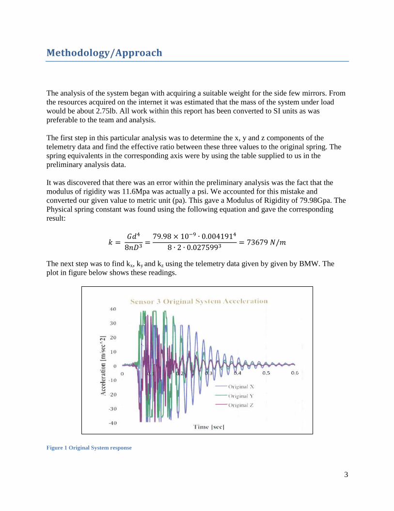
The next step was to find kx, ky and kz using the telemetry data given by given by BMW. The

plot in figure below shows these readings.

Figure 1 Original System response

4

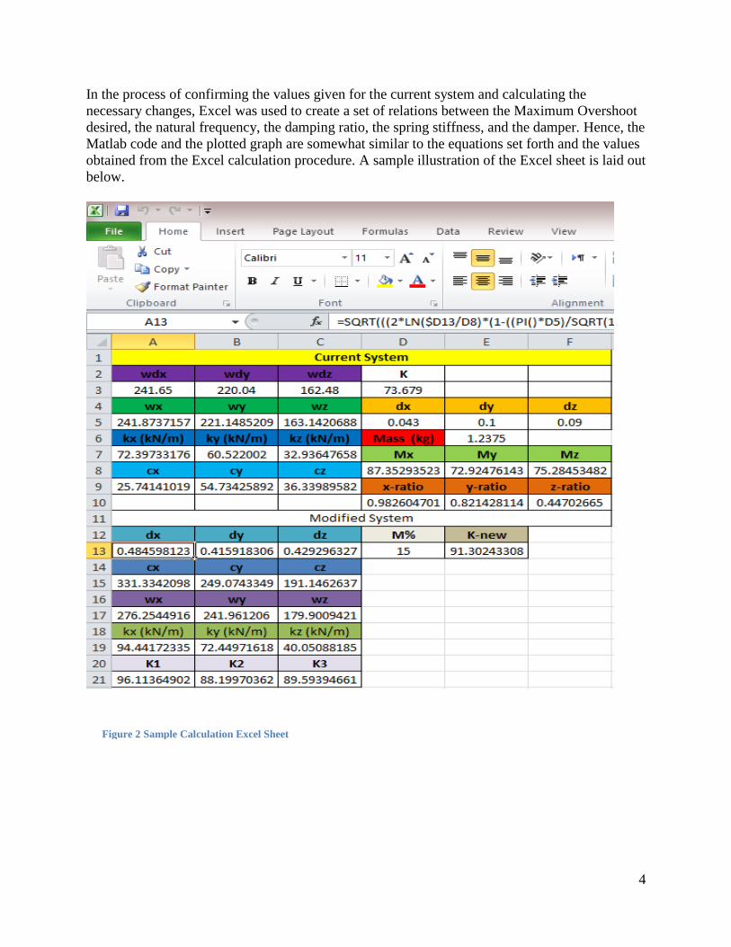
In the process of confirming the values given for the current system and calculating the

necessary changes, Excel was used to create a set of relations between the Maximum Overshoot

desired, the natural frequency, the damping ratio, the spring stiffness, and the damper. Hence, the

Matlab code and the plotted graph are somewhat similar to the equations set forth and the values

obtained from the Excel calculation procedure. A sample illustration of the Excel sheet is laid out

below.

Figure 2 Sample Calculation Excel Sheet

5

Sample Calculations

The following sections of the report layout some sample calculation to show how the data was

processed consider a known mass of the system to be approximately . The sample

calculations are shown below.

Current System Calculations

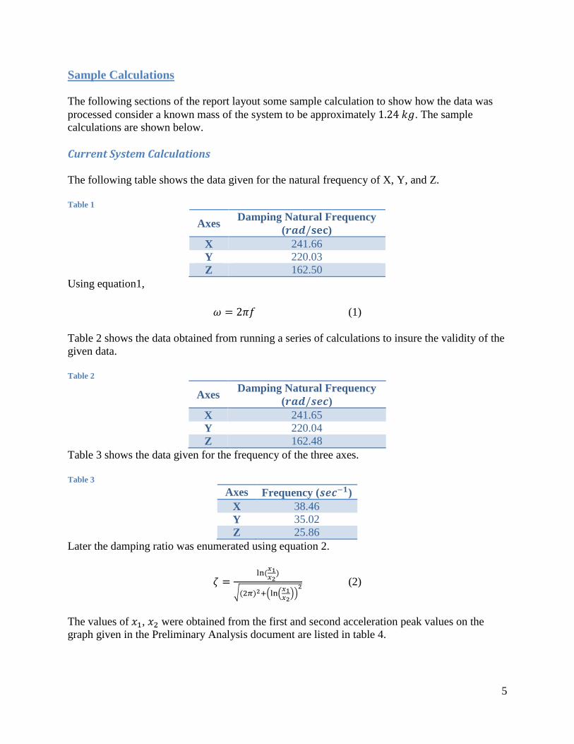
The following table shows the data given for the natural frequency of X, Y, and Z.

Table 1

Axes Damping Natural Frequency

( ) X 241.66

Y 220.03

Z 162.50

Using equation1,

(1)

Table 2 shows the data obtained from running a series of calculations to insure the validity of the

given data.

Table 2

Axes Damping Natural Frequency

( )

X 241.65

Y 220.04

Z 162.48

Table 3 shows the data given for the frequency of the three axes.

Table 3

Axes Frequency ( )

X 38.46

Y 35.02

Z 25.86

Later the damping ratio was enumerated using equation 2.

√ ( (

)) (2)

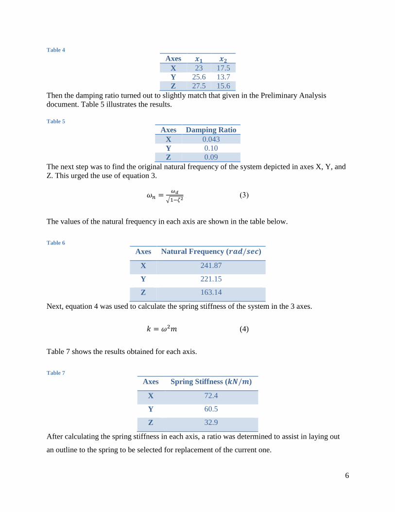
The values of , were obtained from the first and second acceleration peak values on the

graph given in the Preliminary Analysis document are listed in table 4.

6

Table 4

Axes

X 23 17.5

Y 25.6 13.7

Z 27.5 15.6

Then the damping ratio turned out to slightly match that given in the Preliminary Analysis

document. Table 5 illustrates the results.

Table 5

Axes Damping Ratio

X 0.043

Y 0.10

Z 0.09

The next step was to find the original natural frequency of the system depicted in axes X, Y, and

Z. This urged the use of equation 3.

√ 𝜁 (3)

The values of the natural frequency in each axis are shown in the table below.

Table 6

Axes Natural Frequency ( )

X 241.87

Y 221.15

Z 163.14

Next, equation 4 was used to calculate the spring stiffness of the system in the 3 axes.

(4)

Table 7 shows the results obtained for each axis.

Table 7

Axes Spring Stiffness ( )

X 72.4

Y 60.5

Z 32.9

After calculating the spring stiffness in each axis, a ratio was determined to assist in laying out

an outline to the spring to be selected for replacement of the current one.

7

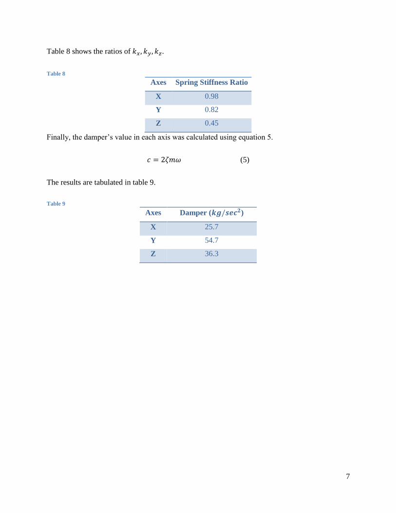
Table 8 shows the ratios of .

Table 8

Axes Spring Stiffness Ratio

X 0.98

Y 0.82

Z 0.45

Finally, the damper’s value in each axis was calculated using equation 5.

(5)

The results are tabulated in table 9.

Table 9

Axes Damper ( )

X 25.7

Y 54.7

Z 36.3

8

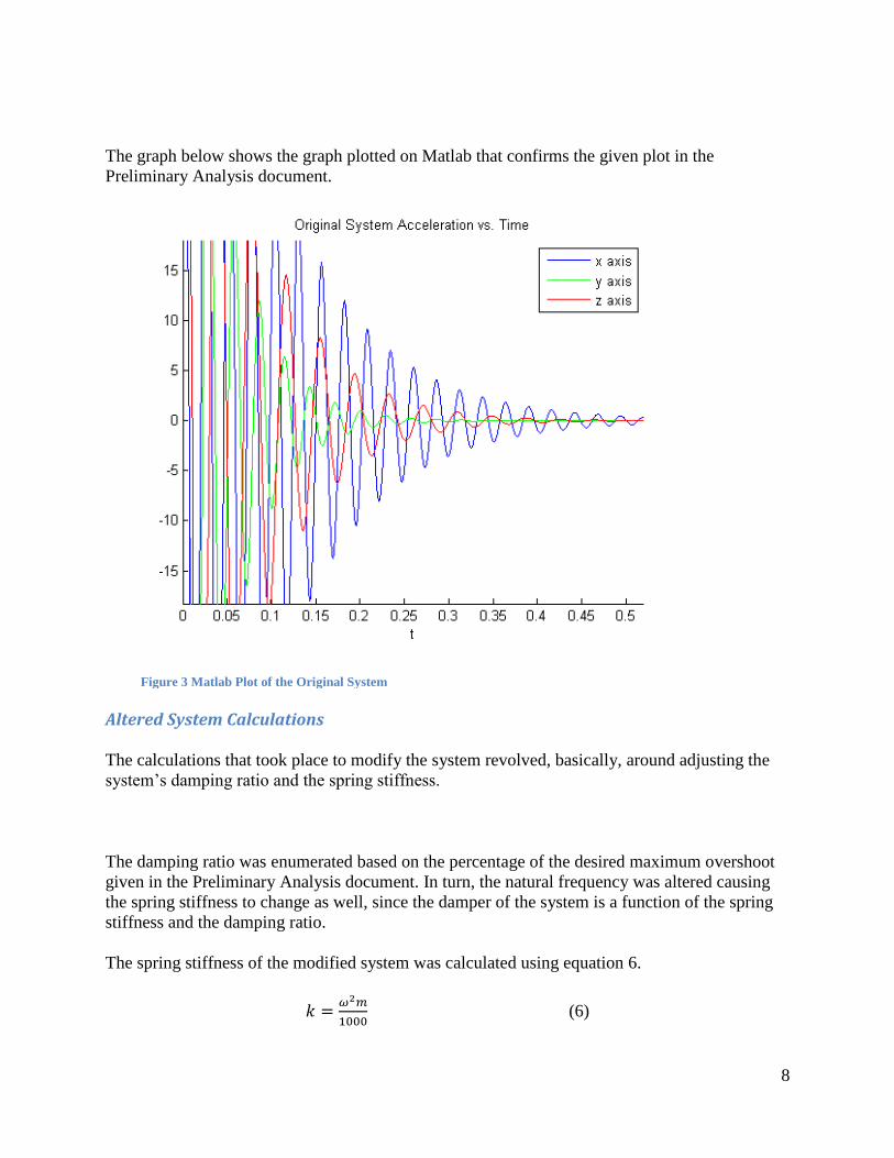
The graph below shows the graph plotted on Matlab that confirms the given plot in the

Preliminary Analysis document.

Altered System Calculations

The calculations that took place to modify the system revolved, basically, around adjusting the

system’s damping ratio and the spring stiffness.

The damping ratio was enumerated based on the percentage of the desired maximum overshoot

given in the Preliminary Analysis document. In turn, the natural frequency was altered causing

the spring stiffness to change as well, since the damper of the system is a function of the spring

stiffness and the damping ratio.

The spring stiffness of the modified system was calculated using equation 6.

(6)

Figure 3 Matlab Plot of the Original System

9

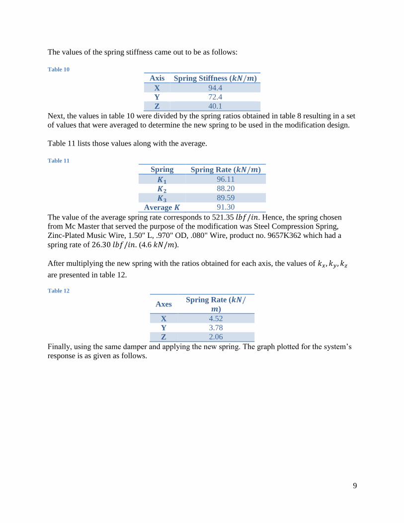
The values of the spring stiffness came out to be as follows:

Table 10

Axis Spring Stiffness ( )

X 94.4

Y 72.4

Z 40.1

Next, the values in table 10 were divided by the spring ratios obtained in table 8 resulting in a set

of values that were averaged to determine the new spring to be used in the modification design.

Table 11 lists those values along with the average.

Table 11

Spring Spring Rate ( )

96.11

88.20

89.59

Average 91.30

The value of the average spring rate corresponds to 521.35 . Hence, the spring chosen

from Mc Master that served the purpose of the modification was Steel Compression Spring,

Zinc-Plated Music Wire, 1.50" L, .970" OD, .080" Wire, product no. 9657K362 which had a

spring rate of . (4.6 ).

After multiplying the new spring with the ratios obtained for each axis, the values of

are presented in table 12.

Table 12

Axes Spring Rate (

)

X 4.52

Y 3.78

Z 2.06

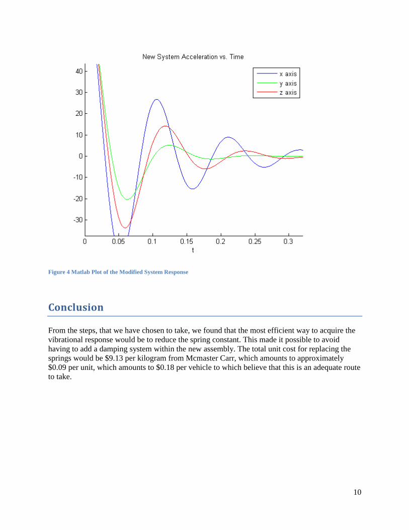
Finally, using the same damper and applying the new spring. The graph plotted for the system’s

response is as given as follows.

10

Figure 4 Matlab Plot of the Modified System Response

Conclusion

From the steps, that we have chosen to take, we found that the most efficient way to acquire the

vibrational response would be to reduce the spring constant. This made it possible to avoid

having to add a damping system within the new assembly. The total unit cost for replacing the

springs would be $9.13 per kilogram from Mcmaster Carr, which amounts to approximately

$0.09 per unit, which amounts to $0.18 per vehicle to which believe that this is an adequate route

to take.

11

Appendices

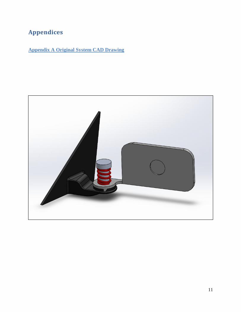
Appendix A Original System CAD Drawing

12

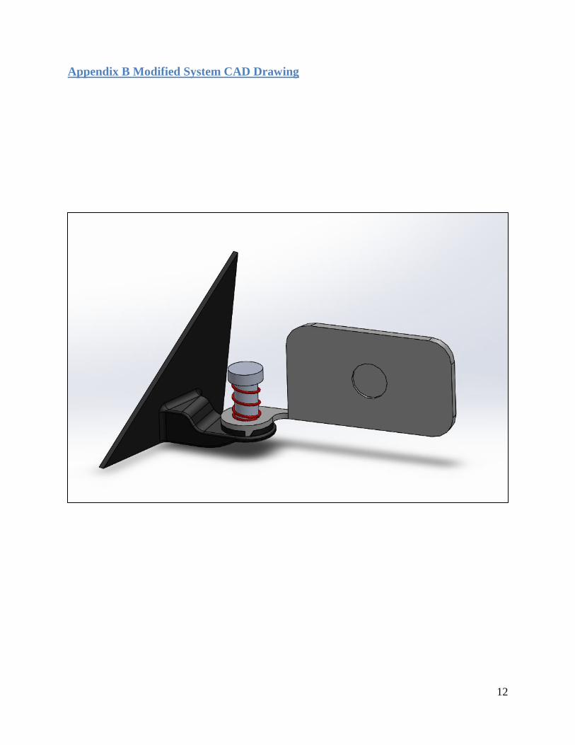
Appendix B Modified System CAD Drawing

13

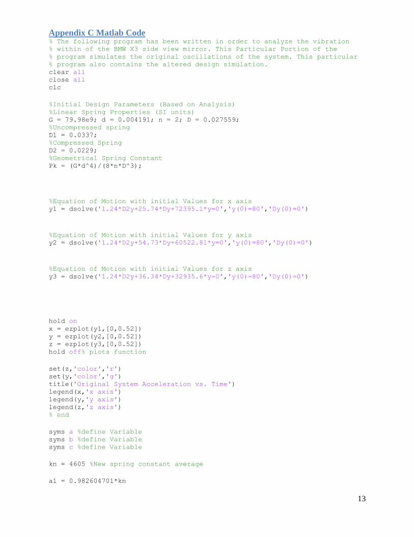
Appendix C Matlab Code % The following program has been written in order to analyze the vibration % within of the BMW X3 side view mirror. This Particular Portion of the % program simulates the original oscillations of the system. This particular % program also contains the altered design simulation. clear all close all clc

%Initial Design Parameters (Based on Analysis) %Linear Spring Properties (SI units) G = 79.98e9; d = 0.004191; n = 2; D = 0.027559; %Uncompressed spring D1 = 0.0337; %Compressed Spring D2 = 0.0229; %Geometrical Spring Constant Pk = (G*d^4)/(8*n*D^3);

%Equation of Motion with initial Values for x axis y1 = dsolve('1.24*D2y+25.74*Dy+72395.1*y=0','y(0)=80','Dy(0)=0')

%Equation of Motion with initial Values for y axis y2 = dsolve('1.24*D2y+54.73*Dy+60522.81*y=0','y(0)=80','Dy(0)=0')

%Equation of Motion with initial Values for z axis y3 = dsolve('1.24*D2y+36.34*Dy+32935.6*y=0','y(0)=80','Dy(0)=0')

hold on x = ezplot(y1,[0,0.52]) y = ezplot(y2,[0,0.52]) z = ezplot(y3,[0,0.52]) hold off% plots function

set(z,'color','r') set(y,'color','g') title('Original System Acceleration vs. Time') legend(x,'x axis') legend(y,'y axis') legend(z,'z axis') % end

syms a %define Variable syms b %define Variable syms c %define Variable

kn = 4605 %New spring constant average

a1 = 0.982604701*kn

14

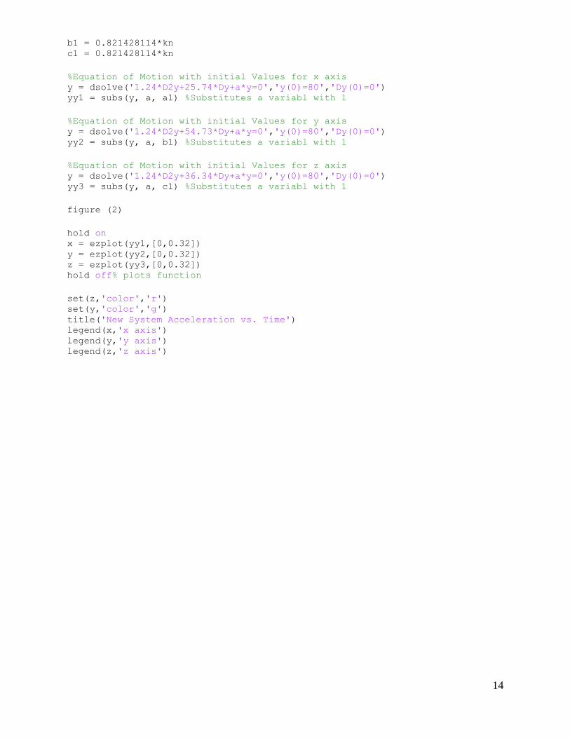
b1 = 0.821428114*kn c1 = 0.821428114*kn

%Equation of Motion with initial Values for x axis y = dsolve('1.24*D2y+25.74*Dy+a*y=0','y(0)=80','Dy(0)=0') yy1 = subs(y, a, a1) %Substitutes a variabl with 1

%Equation of Motion with initial Values for y axis y = dsolve('1.24*D2y+54.73*Dy+a*y=0','y(0)=80','Dy(0)=0') yy2 = subs(y, a, b1) %Substitutes a variabl with 1

%Equation of Motion with initial Values for z axis y = dsolve('1.24*D2y+36.34*Dy+a*y=0','y(0)=80','Dy(0)=0') yy3 = subs(y, a, c1) %Substitutes a variabl with 1

figure (2)

hold on x = ezplot(yy1,[0,0.32]) y = ezplot(yy2,[0,0.32]) z = ezplot(yy3,[0,0.32]) hold off% plots function

set(z,'color','r') set(y,'color','g') title('New System Acceleration vs. Time') legend(x,'x axis') legend(y,'y axis') legend(z,'z axis')