3.2 Memory for time

Marc W. HowardDepartment of Psychological and Brain Sciences

Boston University

submitted to Oxford Handbook of Human Memory

Abstract

The brain maintains a record of recent events including information aboutthe time at which events were experienced. We review behavioral and neuro-physiological evidence as well as computational models to better understandmemory for time. Neurophysiologically, populations of neurons that recordthe time of recent events have been observed in many brain regions. Timecells fire in long sequences after a triggering event demonstrating memory forthe past. Populations of exponentially-decaying neurons record past eventsat many delays by decaying at different rates. Both kinds of representa-tions record distant times with less temporal resolution. The work reviewedhere converges on the idea that the brain maintains a representation of pastevents along a scale-invariant compressed timeline.

It has long been appreciated that our experience of time is central to mnemonic func-tioning. Indeed awareness of the passage of time requires memory—how could one appreci-ate the “past” in relation to the “present” without the ability to simultaneously apprehendboth (Husserl, 1966). Many philosophers arrived at the notion that our internal experienceof time is in some sense organized analogous to the way a spatial dimension is organized,with information about distance and order (see also Bergson, 1910). James (1890) proposedsomething that sounds roughly akin to a short-term memory with temporally-ordered slots:“Objects fade out of consciousness slowly. If the present thought is of a b c d e f g, thenext one will be of b c d e f g h, and the one after that of c d e f g h i—the lingerings ofthe past dropping successively away, and the incomings of the future making up the loss.”Similarly, considering the phenomonology of time, Husserl (1966) notes that our experienceof the recent past has a temporally ordered character. Events further in the past are notmerely weaker, but “feel” further in the past and recede further from the present as timeelapses. Moreover, Husserl (1966) argues that when the future can be predicted—for in-stance while listening to a familiar melody—our anticipated future similarly has a temporalcharacter. Events further in the future “feel” more distant and they approach the presentwith the passage of time. To summarize, James and Husserl argue that as time unfoldsour experience of the recent past is organized like a timeline with information about whatevents happened at what temporal distance from the present—i.e., our experience of thepresent contains a record of what happened when in the recent past. One may imagine this

MEMORY FOR TIME 2

timeline as something like a musical score that tells the player what notes to play when.Imagine how the song would sound if the score contained only information about what notesto play and how often to play them without providing information about when and in whatorder to play them!

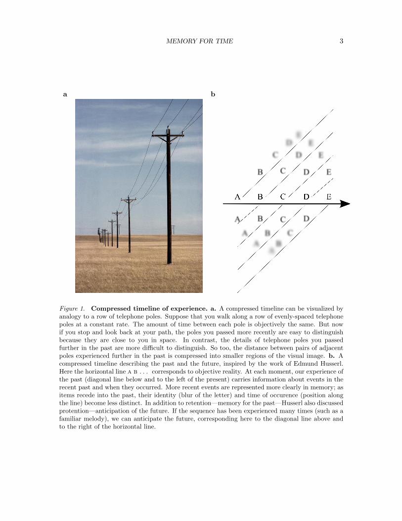
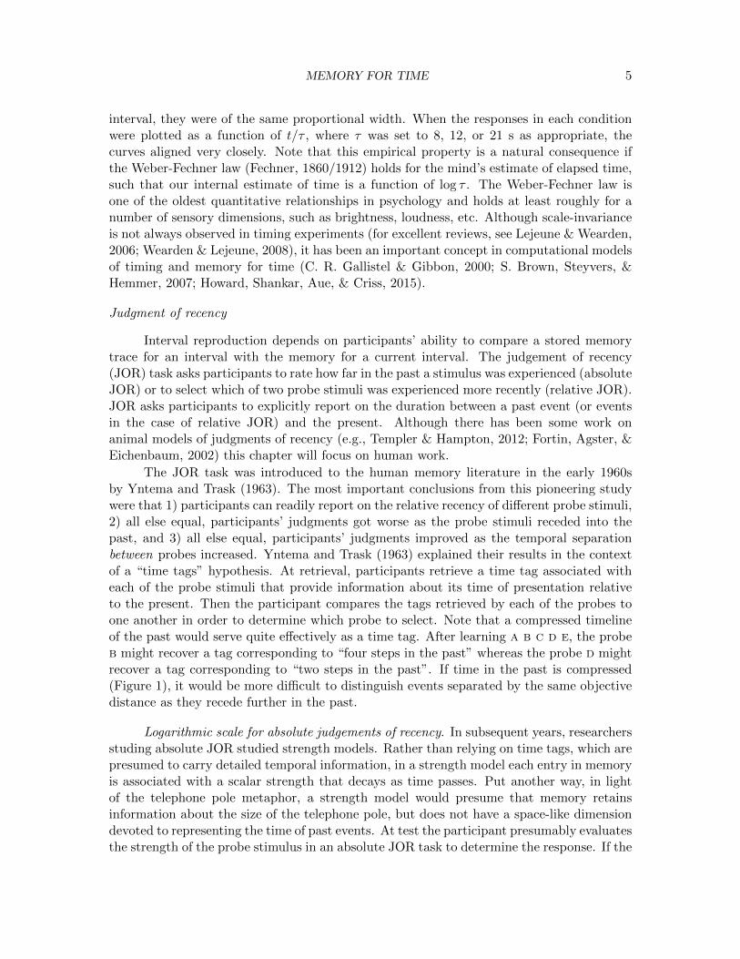
Evidence from psychological and neural science converges on the idea that many formsof memory rely on a timeline of the recent past, with many of the properties James andHusserl proposed from simply observing our internal experience of the passage of time.Although we will consider other hypotheses in this chapter, they will all have serious lim-itations. In the end, this chapter is not so much about people’s memory for the time ofevents, but about how memory for the time of events, in both the mind and brain, couldaffect many different forms of memory. We review behavioral evidence that bears on thisquestion, even though in many cases the tasks do not require the participant to rate thetime of events in memory. The primary result is that many tasks could be understood asa consequence of a timeline, much like that hypothesized by James and Husserl with theadded constraint that the timeline is compressed. That is, as they suggested, memory forthe past contains information about order. And, as they both suggested, memory for eventsfurther in the past are less well-remembered than events closer in time to the present. Inaddition, however, the neural and behavioral evidence suggest that the timeline grows morecompressed for events further in the past such that the resolution of when an event tookplace is less clear for events further in the past. The visual image of a line of telephonepoles has been suggested as a visual metaphor to understand what is meant by compression(Figure 1a,b Crowder, 1976).

Behavioral paradigms that constrain the neural representation fortime

In this section, we will start by reviewing data from the interval reproduction task, inwhich participants reproduce delays of various lengths. This subsection will introduce theconcept of scale-invariance and logarithmic compression, which will be important later on.The next subsection covers judgments of recency (JOR), in which participants explicitlyrate how long in the past probe stimuli were experienced. We will find that data fromthe JOR task over long time intervals support logarithmic compression. Moreover, datafrom the short-term JOR task suggest that participants perform the task by sequentiallyexamining an ordered timeline of experience, not unlike scanning one’s eyes along a visualdisplay. Following this, we will review evidence from classical conditioning paradigms whichsupport the “temporal encoding hypothesis.” Briefly, the temporal encoding hypothesisstates that associations between stimuli are not direct, but are mediated by a timeline ofthe past. Finally, we will discuss temporal effects in episodic memory. The vivid experienceof episodic memory has led to it being described as “mental time travel” (Tulving, 1983). Ifthe experience of the present is a consequence of the current state of a compressed timeline,then it would stand to reason that reinstating a previous state of the timeline would resultin the re-experience of that prior moment from one’s life.

Interval reproduction

Many behavioral paradigms have been developed to evaluate the ability of animalsand humans to time intervals over the range of a few hundred milliseconds up to about an

MEMORY FOR TIME 3

a b

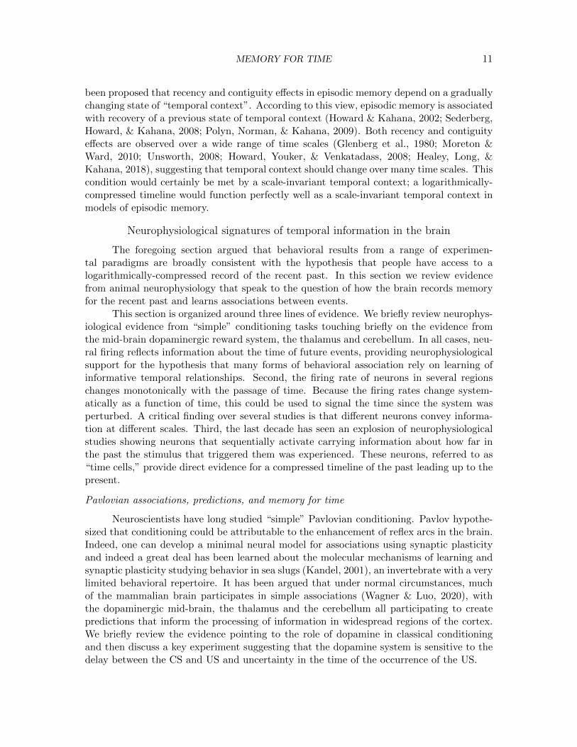
Figure 1. Compressed timeline of experience. a. A compressed timeline can be visualized byanalogy to a row of telephone poles. Suppose that you walk along a row of evenly-spaced telephonepoles at a constant rate. The amount of time between each pole is objectively the same. But nowif you stop and look back at your path, the poles you passed more recently are easy to distinguishbecause they are close to you in space. In contrast, the details of telephone poles you passedfurther in the past are more difficult to distinguish. So too, the distance between pairs of adjacentpoles experienced further in the past is compressed into smaller regions of the visual image. b. Acompressed timeline describing the past and the future, inspired by the work of Edmund Husserl.Here the horizontal line a b . . . corresponds to objective reality. At each moment, our experience ofthe past (diagonal line below and to the left of the present) carries information about events in therecent past and when they occurred. More recent events are represented more clearly in memory; asitems recede into the past, their identity (blur of the letter) and time of occurence (position alongthe line) become less distinct. In addition to retention—memory for the past—Husserl also discussedprotention—anticipation of the future. If the sequence has been experienced many times (such as afamiliar melody), we can anticipate the future, corresponding here to the diagonal line above andto the right of the horizontal line.

MEMORY FOR TIME 4

hour. A number of paradigms have been developed to evaluate this ability. We focus hereon a task referred to as interval reproduction. In interval reproduction, the participant ispresented with some stimulus with a characteristic duration. For instance a square mightchange color for some interval τ and then terminate. After experiencing the interval τ , theparticipant is instructed to reproduce it. For instance the participant might press a buttonto change the color of the square and then press it again after a time τ has elapsed. Inhuman participants care is typically taken to prevent the participant from simply countingduring the interval (for instance, by requiring the participant to say random numbers aloudat irregular intervals). In order to decide when to press the button the participant mustcompare their current memory for the time since the square changed color to a storedmemory for the instructed interval. That is, to learn the temporal interval the participantmust store something like “the square changed to this color at a time τ in the past”. Afterpressing the button, the participant compares their current memory for the time since thebutton press to this memory for the instructed interval and respond when the match issufficiently strong. Accuracy is measured in interval reproduction by comparing the time atwhich the participant responds to the actual delay. Analyses of accuracy take into accountnot only the mean response, but the distribution of responses across trials and participants.

Perhaps the most remarkable finding in interval reproduction is the fact that partic-ipants can can reproduce intervals over a large range of intervals. In a particularly heroicexperiment Lewis and Miall (2009) had participants reproduce intervals over an extremelywide range from 68 ms (much faster than typical human RTs) up to 16.7 minutes. Notsurprisingly participants were not able to reproduce the extremely fast intervals with anyprecision—68 ms was chosen based on the refresh rate of the monitor on which the stimuliwere presented! However, from about a couple of hundred milliseconds up to 16.7 minutes,participants’ mean responses were about the same proportion of the true duration—roughly0.7τ despite changes in τ over about four orders of magnitude.

This type of finding led to the extremely influential idea that the brain’s representationof time is scale-invariant (Gibbon, 1977; C. R. Gallistel & Gibbon, 2000; Balsam & Gallistel,2009). That is, if we prepare an experiment described by a time series of events f(t), theresults of the experiment will be comparable if we rescale time as f(at). Note that the factorof a “stretches” the time axis if a > 1 and “squashes” the time axis if a < 1. This propertyis not what one would expect if temporal memory at different values of τ were supported bydifferent memory systems—such as short-term memory and long-term memory (Atkinson& Shiffrin, 1968). Note that if time is equally spaced on a logarithmic scale, this leadsnaturally (but not uniquely) to a scale-invariant representation of time; on a logarithmicscale the distance between 2 and 20 is the same as the distance between 10 and 100.

Scale-invariance predicts not only that the mean reproduction time is a constantproportion of τ , but that the errors should also rescale. That is, if in one condition we findthat participants’ errors in reproducing an interval τ1 is δ1, scale-invariance requires thatthe error would rescale with the interval such that δ2

τ2= δ1

τ1. Interval timing experiments

have frequently observed this rescaling of errors (see Gibbon, Malapani, Dale, & Gallistel,1997; Buhusi & Meck, 2005, for reviews). For instance, Rakitin et al. (1998) observedthis strong form of scale-invariance for intervals ranging from 8 s to 12 s to 21 s. In thisexperiment they were interested not so much in the mean response time, but the distributionof errors. Although the errors in timing the 21 s interval were wider than the errors in the 8 s

MEMORY FOR TIME 5

interval, they were of the same proportional width. When the responses in each conditionwere plotted as a function of t/τ , where τ was set to 8, 12, or 21 s as appropriate, thecurves aligned very closely. Note that this empirical property is a natural consequence ifthe Weber-Fechner law (Fechner, 1860/1912) holds for the mind’s estimate of elapsed time,such that our internal estimate of time is a function of log τ . The Weber-Fechner law isone of the oldest quantitative relationships in psychology and holds at least roughly for anumber of sensory dimensions, such as brightness, loudness, etc. Although scale-invarianceis not always observed in timing experiments (for excellent reviews, see Lejeune & Wearden,2006; Wearden & Lejeune, 2008), it has been an important concept in computational modelsof timing and memory for time (C. R. Gallistel & Gibbon, 2000; S. Brown, Steyvers, &Hemmer, 2007; Howard, Shankar, Aue, & Criss, 2015).

Judgment of recency

Interval reproduction depends on participants’ ability to compare a stored memorytrace for an interval with the memory for a current interval. The judgement of recency(JOR) task asks participants to rate how far in the past a stimulus was experienced (absoluteJOR) or to select which of two probe stimuli was experienced more recently (relative JOR).JOR asks participants to explicitly report on the duration between a past event (or eventsin the case of relative JOR) and the present. Although there has been some work onanimal models of judgments of recency (e.g., Templer & Hampton, 2012; Fortin, Agster, &Eichenbaum, 2002) this chapter will focus on human work.

The JOR task was introduced to the human memory literature in the early 1960sby Yntema and Trask (1963). The most important conclusions from this pioneering studywere that 1) participants can readily report on the relative recency of different probe stimuli,2) all else equal, participants’ judgments got worse as the probe stimuli receded into thepast, and 3) all else equal, participants’ judgments improved as the temporal separationbetween probes increased. Yntema and Trask (1963) explained their results in the contextof a “time tags” hypothesis. At retrieval, participants retrieve a time tag associated witheach of the probe stimuli that provide information about its time of presentation relativeto the present. Then the participant compares the tags retrieved by each of the probes toone another in order to determine which probe to select. Note that a compressed timelineof the past would serve quite effectively as a time tag. After learning a b c d e, the probeb might recover a tag corresponding to “four steps in the past” whereas the probe d mightrecover a tag corresponding to “two steps in the past”. If time in the past is compressed(Figure 1), it would be more difficult to distinguish events separated by the same objectivedistance as they recede further in the past.

Logarithmic scale for absolute judgements of recency. In subsequent years, researchersstuding absolute JOR studied strength models. Rather than relying on time tags, which arepresumed to carry detailed temporal information, in a strength model each entry in memoryis associated with a scalar strength that decays as time passes. Put another way, in lightof the telephone pole metaphor, a strength model would presume that memory retainsinformation about the size of the telephone pole, but does not have a space-like dimensiondevoted to representing the time of past events. At test the participant presumably evaluatesthe strength of the probe stimulus in an absolute JOR task to determine the response. If the

MEMORY FOR TIME 6

“telephone pole appears large” in memory, it was presumably presented more recently thana telephone pole that appears smaller. As we will see later, data from short-term JOR isextremely difficult to reconcile with a strength model and we will discard this hypothesis—aconclusion reached by most researchers studying the problem in the 1970s. However, thekey finding from this early work for our purposes is that to account for the behavioraldata with a strength model, strength must decay with the logarithm of the probe’s recency,consistent with a logarithmically-compressed timeline implementing a Weber-Fechner scalefor the past.

The first question one may ask in JOR is how ratings of recency change as a functionof the actual recency of the probe. Hinrichs and Buschke (Hinrichs, 1970; Hinrichs &Buschke, 1968) observed that numerical estimates of the recency of a probe presented τsteps in the past increase like log τ . As a consequence, they proposed a strength model inwhich the strength of a memory trace decays like − log τ . This model is consistent with theYntema and Trask (1963) results.

Despite the intuititive simplicity of logarithmic strength models, it is clear thatstrength models (whether logarithmic or not) are insufficient to describe many phenom-ena in human JOR performance. For instance, Hintzman (2010) did an experiment inwhich probes in an absolute JOR task were presented more than once (see also Flexser &Bower, 1974). In this experiment, probe items can be presented three times, correspondingto the initial presentation, the first test and the second test. Let us refer to the time lagbetween the initial presentation and the first test as τ1 and refer to the time between thefirst test and the second test as τ2. On the first repetition, the well-known logarithmic re-lationship between absolute rating and actual τ1 was observed. If JOR relies on a strengthfor each probe item, and if that strength decays with time, we would expect repeated itemsto be judged as much more recent than non-repeated items. In contrast to this prediction,on the second presentation the judgment depended on log τ2; repetition of an item, and thelag at the first presentation τ1 had a barely measurable effect on participants’ ratings ofrecency. The results are as if participants can remember multiple occurrences of the samenominal stimulus as distinct events, as predicted by multiple-trace models of memory (e.g.,Hintzman, 1986). One can account for these findings with a memory store that containsmultiple traces of the past if the traces are spaced appropriately to give the logarithmicrelationship.

Scanning along a timeline in short-term JOR. Consistent with these conclusions fromJOR in list learning experiments, evidence from short-term JOR experiments suggests thatdifferent events give rise to separate traces in a temporally-organized memory store, muchlike the timeline proposed by James and Husserl. In short-term JOR experiments, a shortlist is presented, usually quickly (e.g., Hacker, 1980; Muter, 1979). In many cases thestimuli come from a small pool that are reused across many lists (e.g., consonants). Thequalitative patterns observed by Yntema and Trask (1963)—that all else equal pushing thetwo probes into the past decreases accuracy and increasing the separation between probesincreases accuracy are both observed. The interesting finding comes when one considers RTdata which support a self-terminating serial scanning model (Hacker, 1980; Muter, 1979;Hockley, 1984). According to this account, memory for the list is organized like a timeline.Given a pair of probes, participants compare the probe stimuli one-by-one to the contents of

MEMORY FOR TIME 7

memory starting with the entries closer to the present and moving towards the past. Whenthey find one of the probe stimuli in memory, they terminate their search. In this model,errors happen because occasionally degraded memory traces cause the match to fail; underthese circumstances the search continues.

This self-terminating serial scanning model makes a number of straightforward pre-dictions. First, the RT for a correct response should increase as the more-recent probebecomes less recent. Second, correct RT should not depend on the recency of the less-recent probe. Third, the pattern for error RT, in which one selects the less-recent probe,should depend on the recency of the less-recent probe but not of the more recent probe. Allthree of these phenomena are consistently observed (Hacker, 1980; Muter, 1979; Hockley,1984; Singh, Oliva, & Howard, 2017).

The basic premise of the self-terminating model is that memory has a temporal or-ganization and that participants can sequentially direct attention to different parts of thistimeline, analogous to the way people can shift their gaze through the visual field. Thisinterpretation is bolstered by evidence that when the instructions are reversed, so too doesthe apparent direction of scanning. That is, in the standard JOR experiment the partic-ipant is asked to pick the more recent probe and RT goes up as if the participant starts“looking at the timeline” close to the present and gradually “moves their attention” to-wards the beginning of the list. In one set of experiments Caplan and colleagues askedabout what would happen if participants were asked which of the probes came earlier inthe list (M. Chan, Ross, Earle, & Caplan, 2009; Y. S. Liu, Chan, & Caplan, 2014). Theyfound that participants were now faster to choose the items at the beginning of the list.That is, when asked to choose the probe closest to the beginning of the list, participantswere slower to select probes that were closer in time to the present. The pattern of resultsis just as one would expect if the participants first “directed their attention to the timeof the beginning of the list” and then sequentially moved their attention forward in timetowards the present.

JOR data are consistent with a logarithmically compressed timeline. So, there arethese two streams of evidence from JOR. The argument from absolute JOR is that memoryuses a logarithmic scale to measure the amount of past time but that a strength modelis insufficient to account for important properties of JOR. The argument from short-termJOR is that memory consists of a temporally-organized representation that can be exam-ined sequentially not unlike how people can direct attention to different parts of visualspace. It has been proposed (Howard et al., 2015; Howard, 2018) that these two findingscan be reconciled if memory consists of a temporally-organized representation that is log-arithmically compressed. That is, memories for different events are organized in multipletraces along a timeline, but the timeline is not evenly-spaced. Logarithmic compression,like that seen in the visual system as a function of distance from the fovea (Daniel & Whit-teridge, 1961; Hubel & Wiesel, 1974; Van Essen, Newsome, & Maunsell, 1984), means thatthe amount of objective distance covered moving from one cell’s receptive field to the nextgoes up quickly, like the numerical sequence 1, 2, 4, 8 . . .. This suggests that the time ittakes to scan to a particular time in the past goes up more slowly than linear because eachsubsequent step travels further into the past. To test this hypothesis (Singh & Howard,2017) replicated the standard short-term JOR experiment and found that the indeed the

MEMORY FOR TIME 8

rate of scanning was sublinear, consistent with sequentially directing attention along alogarithmically-compressed timeline.

It should be noted that although the “short-term” JOR (e.g., Hacker, 1980; Muter,1979) results and “long-term JOR” (e.g., Hintzman, 2010; Yntema & Trask, 1963) resultsemphasize different aspects of performance, they do not contradict one another. Indeed ascanning model built on a logarithmically-compressed representation of temporal contextcan account for both sets of results (Howard et al., 2015).

Classical conditioning and “temporal mapping”

JOR explicitly evaluates participants’ memory for the time of past events. However,tasks that do not explicitly require assessment of the time of past events can also shed lighton how the brain and mind maintain information about the past. Pavlov’s dog learned atemporal relationship between the bell and the food. If the time of the bell and the time ofthe food were uncorrelated there would be no association. In this sense even simple classicalconditioning expresses memory for time. It is not necessary that the conditioned stimulus(CS, e.g., the bell) and the unconditioned stimulus (US, e.g., the food) are experiencedsimultaneously. In delay conditioning, the US is presented at the time the CS terminates,so they do not overlap. In trace conditioning, there is a nonzero temporal gap between theoffset of the CS and the onset of the US. We know a great deal about the neurobiologyof simple Pavlovian conditioning in rodents and the neural circuitry that supports theseassociations (see Thompson, 2005, for a review of the pioneering work). At the end of theday, however, the animal’s goal is to predict the future—the bell in the present predictsthat food will become available five seconds in the future. Viewed in this way, at leastsome forms of classical conditioning could also utilize an ordered timeline of the past, withfunctional associations between stimuli (the bell and the food) mediated by the effect thesestimuli have on timelines.

The centrality of temporal relationships in classical conditioning has led to the tem-poral encoding hypothesis (e.g., Arcediano & Miller, 2002), which argues that time is afundamental component of even simple associations. Evolutionarily, this property is adap-tive insofar as it enables animals to learn contingencies between events and thus betterpredict the future (Balsam & Gallistel, 2009). Mechanistically, one can understand thetemporal encoding hypothesis as the idea that connections between two stimuli are formednot by directly linking the representations of the stimuli, but by linking and aligning time-lines including the two stimuli. This proposal is dramatically supported by findings fromsecond order conditioning. These experiments falsify the hypothesis that the associationbetween a CS and a US is a simple scalar value. Because this point is extremely importantin understanding the relationship between memory and time, we explain this phenomenonin some detail.

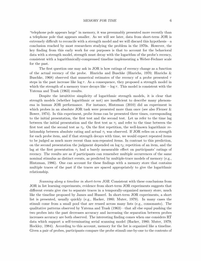
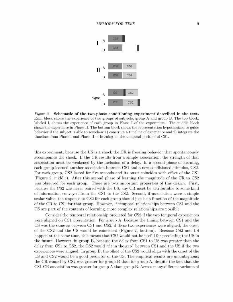
Consider an experiment by Cole, Barnet, and Miller (1995); Figure 2 provides aschematic of the experimental design. Two groups of rats learned a relationship between aconditioned stimulus (CS) and an unconditioned stimulus (US, in this experiment a mildfootshock). Because there will be two conditioned stimuli, we will refer to the CS in this firstphase of learning as CS1. In group A, the US was presented immediately after offset of CS1.In group B, five seconds intervened between the offset of CS1 and the US. Not surprisingly,the CS1 elicited a greater conditioned response, or CR, for group A than for group B. In

MEMORY FOR TIME 9

Figure 2. Schematic of the two-phase conditioning experiment described in the text.Each block shows the experience of two groups of subjects, group A and group B. The top block,labeled I, shows the experience of each group in Phase I of the experiment. The middle blockshows the experience in Phase II. The bottom block shows the representation hypothesized to guidebehavior if the subject is able to somehow 1) construct a timeline of experience and 2) integrate thetimelines from Phase I and Phase II of learning on the temporal position of CS1.

this experiment, because the US is a shock the CR is freezing behavior that spontaneouslyaccompanies the shock. If the CR results from a simple association, the strength of thatassociation must be weakened by the inclusion of a delay. In a second phase of learning,each group learned another association between CS1 and a new conditioned stimulus, CS2.For each group, CS2 lasted for five seconds and its onset coincides with offset of the CS1(Figure 2, middle). After this second phase of learning the magnitude of the CR to CS2was observed for each group. There are two important properties of this design. First,because the CS2 was never paired with the US, any CR must be attributable to some kindof information conveyed from the CS1 to the CS2. Second, if association were a simplescalar value, the response to CS2 for each group should just be a function of the magnitudeof the CR to CS1 for that group. However, if temporal relationships between CS1 and theUS are part of the contents of learning, more complex relationships are possible.

Consider the temporal relationship predicted for CS2 if the two temporal experienceswere aligned on CS1 presentation. For group A, because the timing between CS1 and theUS was the same as between CS1 and CS2, if these two experiences were aligned, the onsetof the CS2 and the US would be coincident (Figure 2, bottom). Because CS2 and UShappen at the same time, this means that CS2 would not be useful for predicting the US inthe future. However, in group B, because the delay from CS1 to US was greater than thedelay from CS1 to CS2, the CS2 would “fit in the gap” between CS1 and the US if the twoexperiences were aligned. In group B, the offset of the CS2 would align with the onset of theUS and CS2 would be a good predictor of the US. The empirical results are unambiguous;the CR caused by CS2 was greater for group B than for group A, despite the fact that theCS1-CR association was greater for group A than group B. Across many different variants of

MEMORY FOR TIME 10

this kind of experiment the findings are consistently in favor of the idea that “associations”are not simple links, but rather convey information about temporal relationships betweenevents (e.g., Barnet, Cole, & Miller, 1997; Savastano & Miller, 1998; Arcediano, Escobar,& Miller, 2003).

The temporal encoding hypothesis has been formalized by Balsam and Gallistel(2009). They argued that the degree of association between a CS and a US ought tobe a consequence of the amount of information that observing the CS conveys about thetime at which the US will occur in the future. For instance, if the US is presented at ran-dom times and there is no correlation between the time of the CS and the time of the US,the best estimate one could make of the time of the US will occur is a uniform probabilitydistribution proportional to its rate of occurrence. However, if the CS and US have a con-sistent temporal relationship (for instance every time the CS is presented the US follows fiveseconds in the future) then the estimate of the time at which the US will occur followingthe CS is more precise than the prediction one can make without observing the CS. Onecan quantify the difference between the uncertainty in the absence of pairing to the CSand the uncertainty after observation of the CS. The CS predicts the US to the extent thedistribution after presentation of the CS is more certain. This hypothesis accounts for manyimportant results in classical conditioning (see C. Gallistel, Craig, & Shahan, 2019).

Another key finding from classical conditioning that bears on the neural representationof time comes from autoshaping. In the autoshaping paradigm, the subject (usually pigeonsin these experiments) is presented with a CS, for instance illumination of a light. Some timelater—say, several seconds—a food pellet is dispensed from a nearby hopper. After somenumber of temporally-separated pairings, the pigeon will peck at the CS, as if it has acquiredsome of the reinforcing value from the food. Let us refer to the time between the CS andthe arrival of the food as τ . All else equal, the animal learns faster if τ is small. Let usrefer to the time between one trial and the next as T . All else equal, the animal learnsfaster if T is large. The remarkable finding is that the number of reinforcements necessarydepends only on the ratio τ/T (Gibbon, Baldock, Locurto, Gold, & Terrace, 1977). That is,if τ = 2 s and T = 20 s the animal learns after as many pairings as it would have requiredif τ = 10 s and T = 100 s. This finding implies that there is not a characteristic scale forassociative learning—however we change τ → aτ we can change T by the same factor a andrecover the same rate of learning. To the extent classical conditioning can be understoodas constructing and aligning timelines relating the past to the future, this finding suggeststhat the timelines are logarithmically compressed.

Episodic memory

It has long been argued that episodic memory corresponds to “mental time travel”in which the rememberer reexperiences a specific moment of past time. Although we willnot dwell on the topic here because it is well-covered in other chapters (see especiallyChs. 2.1, 5.5, and 5.12), it is worth noting that the recency and contiguity effects, which arerobustly observed in episodic memory paradigms (Kahana, Howard, & Polyn, 2008) maybe understood as memory for time. The recency effect is the finding that, all else equal,we remember events that happened more recently in the past than further in the past.The contiguity effect is the finding that, all else equal, when an event is remembered, thisbrings to mind events that were experienced close in time to the remembered events. It has

MEMORY FOR TIME 11

been proposed that recency and contiguity effects in episodic memory depend on a graduallychanging state of “temporal context”. According to this view, episodic memory is associatedwith recovery of a previous state of temporal context (Howard & Kahana, 2002; Sederberg,Howard, & Kahana, 2008; Polyn, Norman, & Kahana, 2009). Both recency and contiguityeffects are observed over a wide range of time scales (Glenberg et al., 1980; Moreton &Ward, 2010; Unsworth, 2008; Howard, Youker, & Venkatadass, 2008; Healey, Long, &Kahana, 2018), suggesting that temporal context should change over many time scales. Thiscondition would certainly be met by a scale-invariant temporal context; a logarithmically-compressed timeline would function perfectly well as a scale-invariant temporal context inmodels of episodic memory.

Neurophysiological signatures of temporal information in the brain

The foregoing section argued that behavioral results from a range of experimen-tal paradigms are broadly consistent with the hypothesis that people have access to alogarithmically-compressed record of the recent past. In this section we review evidencefrom animal neurophysiology that speak to the question of how the brain records memoryfor the recent past and learns associations between events.

This section is organized around three lines of evidence. We briefly review neurophys-iological evidence from “simple” conditioning tasks touching briefly on the evidence fromthe mid-brain dopaminergic reward system, the thalamus and cerebellum. In all cases, neu-ral firing reflects information about the time of future events, providing neurophysiologicalsupport for the hypothesis that many forms of behavioral association rely on learning ofinformative temporal relationships. Second, the firing rate of neurons in several regionschanges monotonically with the passage of time. Because the firing rates change system-atically as a function of time, this could be used to signal the time since the system wasperturbed. A critical finding over several studies is that different neurons convey informa-tion at different scales. Third, the last decade has seen an explosion of neurophysiologicalstudies showing neurons that sequentially activate carrying information about how far inthe past the stimulus that triggered them was experienced. These neurons, referred to as“time cells,” provide direct evidence for a compressed timeline of the past leading up to thepresent.

Pavlovian associations, predictions, and memory for time

Neuroscientists have long studied “simple” Pavlovian conditioning. Pavlov hypothe-sized that conditioning could be attributable to the enhancement of reflex arcs in the brain.Indeed, one can develop a minimal neural model for associations using synaptic plasticityand indeed a great deal has been learned about the molecular mechanisms of learning andsynaptic plasticity studying behavior in sea slugs (Kandel, 2001), an invertebrate with a verylimited behavioral repertoire. It has been argued that under normal circumstances, muchof the mammalian brain participates in simple associations (Wagner & Luo, 2020), withthe dopaminergic mid-brain, the thalamus and the cerebellum all participating to createpredictions that inform the processing of information in widespread regions of the cortex.We briefly review the evidence pointing to the role of dopamine in classical conditioningand then discuss a key experiment suggesting that the dopamine system is sensitive to thedelay between the CS and US and uncertainty in the time of the occurrence of the US.

MEMORY FOR TIME 12

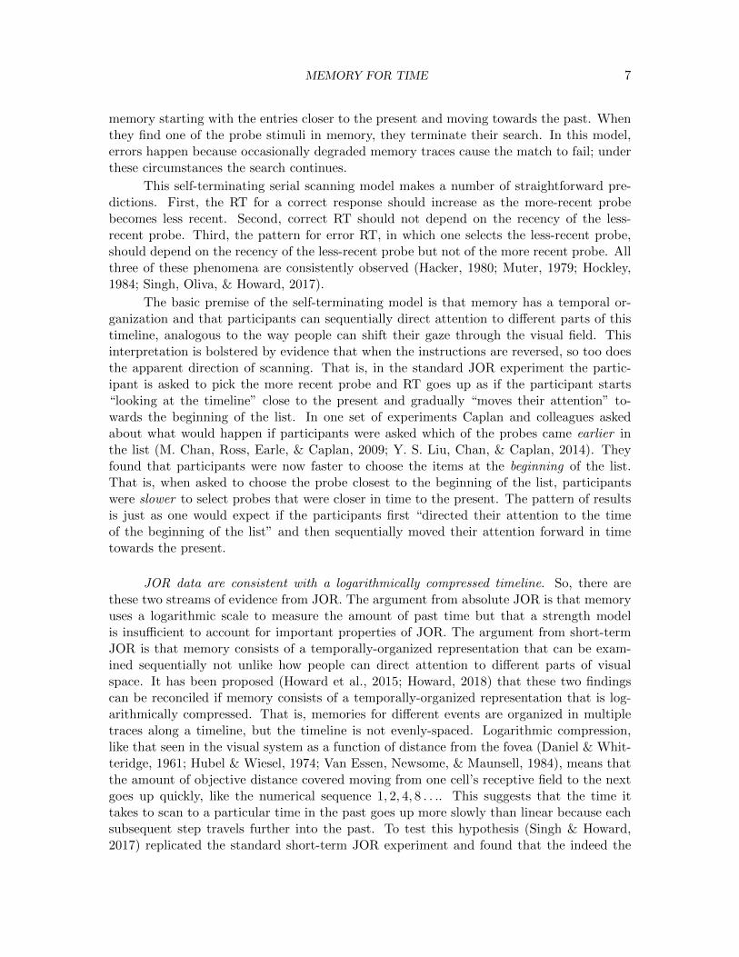
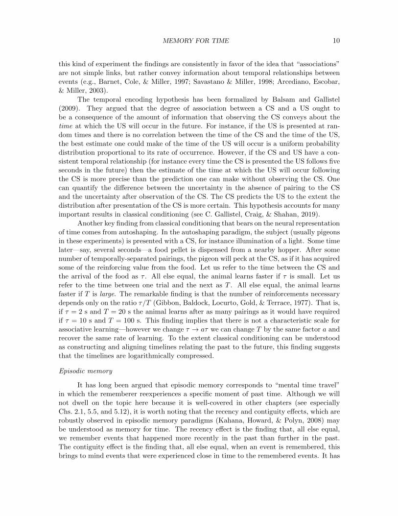
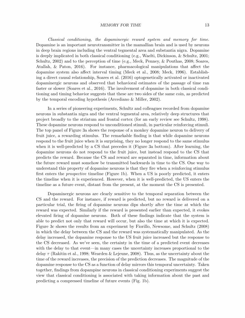
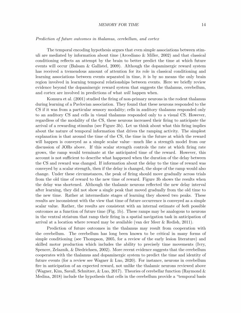
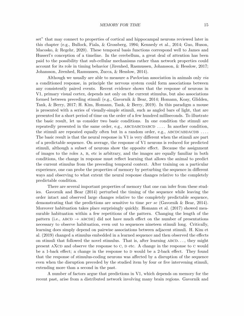
Figure 3. Neurophysiology of timing information in classical conditioning. a. Dopaminecells respond to unpredicted rewards (top). After learning they no longer respond to the rewardingstimulus, but rather respond to the CS that predicts it. Note that the CS and the reward areseparated in time (Schultz et al. 1997). b. Non-primary neurons in the thalamus show evidence oftemporal predictions. After learning that a CS predicts a reward, the thalamic neuron ramps to thetime of the reward (black line). This requires that the neuron has access to the future time at whichthe reward will be experienced immediately after the CS. After learning, the time to the reward isshortened and the animal gradually learns the new relationship (pink and red lines). Rather thana single peak that gradually moves earlier in time, the firing rate shows two peaks (Komura et al.,2001). c. Effect of temporal separation on the dopamine response. In this experiment the timedelay between a visual CS and a juice reward was systematically varied. Left: Response to the CS.As the delay increases, there is less response of dopamine neurons to the CS. Right: Response tothe juice reward. As the delay increases there is more firing of the dopamine neurons at the time ofjuice delivery (Fiorillo, et al., 2008).

MEMORY FOR TIME 13

Classical conditioning, the dopaminergic reward system and memory for time.Dopamine is an important neurotransmitter in the mamallian brain and is used by neuronsin deep brain regions including the ventral tegmental area and substantia nigra. Dopamineis deeply implicated in both classical conditioning (e.g., Waelti, Dickinson, & Schultz, 2001;Schultz, 2002) and to the perception of time (e.g., Meck, Penney, & Pouthas, 2008; Soares,Atallah, & Paton, 2016). For instance, pharmacological manipulations that affect thedopamine system also affect interval timing (Meck et al., 2008; Meck, 1996). Establish-ing a direct causal relationship, Soares et al. (2016) optogenetically activated or inactivateddopaminergic neurons and observed that behavioral estimates of the passage of time ranfaster or slower (Soares et al., 2016). The involvement of dopamine in both classical condi-tioning and timing behavior suggests that these are two sides of the same coin, as predictedby the temporal encoding hypothesis (Arcediano & Miller, 2002).

In a series of pioneering experiments, Schultz and colleagues recorded from dopamineneurons in substantia nigra and the ventral tegmental area, relatively deep structures thatproject broadly to the striatum and frontal cortex (for an early review see Schultz, 1998).These dopamine neurons respond to unconditioned stimuli, in particular reinforcing stimuli.The top panel of Figure 3a shows the response of a monkey dopamine neuron to delivery offruit juice, a rewarding stimulus. The remarkable finding is that while dopamine neuronsrespond to the fruit juice when it is surprising, they no longer respond to the same stimuluswhen it is well-predicted by a CS that precedes it (Figure 3a bottom). After learning, thedopamine neurons do not respond to the fruit juice, but instead respond to the CS thatpredicts the reward. Because the CS and reward are separated in time, information aboutthe future reward must somehow be transmitted backwards in time to the CS. One way tounderstand this property of dopamine neurons is that they fire when a reinforcing stimulusfirst enters the prospective timeline (Figure 1b). When a US is poorly predicted, it entersthe timeline when it is experienced. However, when it is well-predicted, the US enters thetimeline as a future event, distant from the present, at the moment the CS is presented.

Dopaminergic neurons are clearly sensitive to the temporal separation between theCS and the reward. For instance, if reward is predicted, but no reward is delivered on aparticular trial, the firing of dopamine neurons dips shortly after the time at which thereward was expected. Similarly if the reward is presented earlier than expected, it evokeselevated firing of dopamine neurons. Both of these findings indicate that the system isable to predict not only that reward will occur, but also the time at which it is expected.Figure 3c shows the results from an experiment by Fiorillo, Newsome, and Schultz (2008)in which the delay between the CS and the reward was systematically manipulated. As thedelay increased, the dopamine response to the US fruit juice increased but the response tothe CS decreased. As we’ve seen, the certainty in the time of a predicted event decreaseswith the delay to that event—in many cases the uncertainty increases proportional to thedelay τ (Rakitin et al., 1998; Wearden & Lejeune, 2008). Thus, as the uncertainty about thetime of the reward increases, the precision of the prediction decreases. The magnitude of thedopamine response to the CS as a function of delay mirrors this temporal uncertainty. Takentogether, findings from dopampine neurons in classical conditioning experiments suggest theview that classical conditioning is associated with taking information about the past andpredicting a compressed timeline of future events (Fig. 1b).

MEMORY FOR TIME 14

Prediction of future outcomes in thalamus, cerebellum, and cortex

The temporal encoding hypothesis argues that even simple associations between stim-uli are mediated by information about time (Arcediano & Miller, 2002) and that classicalconditioning reflects an attempt by the brain to better predict the time at which futureevents will occur (Balsam & Gallistel, 2009). Although the dopaminergic reward systemhas received a tremendous amount of attention for its role in classical conditioning andlearning associations between events separated in time, it is by no means the only brainregion involved in learning temporal relationships between events. Here we briefly reviewevidence beyond the dopaminergic reward system that suggests the thalamus, cerebellum,and cortex are involved in predictions of what will happen when.

Komura et al. (2001) studied the firing of non-primary neurons in the rodent thalamusduring learning of a Pavlovian association. They found that these neurons responded to theCS if it was from a particular sensory modality; cells in auditory thalamus responded onlyto an auditory CS and cells in visual thalamus responded only to a visual CS. However,regardless of the modality of the CS, these neurons increased their firing to anticipate thearrival of a rewarding stimulus (see Figure 3b). Let us think about what this firing impliesabout the nature of temporal information that drives the ramping activity. The simplestexplanation is that around the time of the CS, the time in the future at which the rewardwill happen is conveyed as a simple scalar value—much like a strength model from ourdiscussion of JORs above. If this scalar strength controls the rate at which firing rategrows, the ramp would terminate at the anticipated time of the reward. However, thisaccount is not sufficient to describe what happened when the duration of the delay betweenthe CS and reward was changed. If information about the delay to the time of reward wasconveyed by a scalar strength, then if the delay is changed, the slope of the ramp would alsochange. Under these circumstances, the peak of firing should move gradually across trialsfrom the old time of reward to the new time of reward. Figure 3b shows the results whenthe delay was shortened. Although the thalamic neurons reflected the new delay intervalafter learning, they did not show a single peak that moved gradually from the old time tothe new time. Rather at intermediate stages of learning they showed two peaks. Theseresults are inconsistent with the view that time of future occurrence is conveyed as a simplescalar value. Rather, the results are consistent with an internal estimate of both possibleoutcomes as a function of future time (Fig. 1b). These ramps may be analogous to neuronsin the ventral striatum that ramp their firing in a spatial navigation task in anticipation ofarrival at a location where reward may be available (van der Meer & Redish, 2011).

Prediction of future outcomes in the thalamus may result from cooperation withthe cerebellum. The cerebellum has long been known to be critical in many forms ofsimple conditioning (see Thompson, 2005, for a review of the early lesion literature) andskilled motor production which includes the ability to precisely time movements (Ivry,Spencer, Zelaznik, & Diedrichsen, 2002). More recent evidence suggests that the cerebellumcooperates with the thalamus and dopaminergic system to predict the time and identity offuture events (for a review see Wagner & Luo, 2020). For instance, neurons in cerebellumfire in anticipation of an expected reward, not unlike the thalamic neurons reviewed above(Wagner, Kim, Savall, Schnitzer, & Luo, 2017). Theories of cerebellar function (Raymond &Medina, 2018) include the hypothesis that cells in the cerebellum provide a “temporal basis

MEMORY FOR TIME 15

set” that may connect to properties of cortical and hippocampal neurons reviewed later inthis chapter (e.g., Bullock, Fiala, & Grossberg, 1994; Kennedy et al., 2014; Guo, Huson,Macosko, & Regehr, 2020). These temporal basis functions correspond well to James andHusserl’s conception of a timeline. In the cerebellum, a great deal of attention has beenpaid to the possibility that sub-cellular mechanisms rather than network properties couldaccount for its role in timing behavior (Jirenhed, Rasmussen, Johansson, & Hesslow, 2017;Johansson, Jirenhed, Rasmussen, Zucca, & Hesslow, 2014).

Although we usually are able to measure a Pavlovian association in animals only viaa conditioned response, in principle the nervous system could form associations betweenany consistently paired events. Recent evidence shows that the response of neurons inV1, primary visual cortex, depends not only on the current stimulus, but also associationsformed between preceding stimuli (e.g., Gavornik & Bear, 2014; Homann, Koay, Glidden,Tank, & Berry, 2017; H. Kim, Homann, Tank, & Berry, 2019). In this paradigm a mouseis presented with a series of visually-simple stimuli, such as angled bars of light, that arepresented for a short period of time on the order of a few hundred milliseconds. To illustratethe basic result, let us consider two basic conditions. In one condition the stimuli arerepeatedly presented in the same order, e.g., abcdabcdabcd . . . . In another condition,the stimuli are repeated equally often but in a random order, e.g., abcdcabdacdb . . . .The basic result is that the neural response in V1 is very different when the stimuli are partof a predictable sequence. On average, the response of V1 neurons is reduced for predictedstimuli, although a subset of neurons show the opposite effect. Because the assignmentof images to the roles a, b, etc is arbitrary, and the images are equally familiar in bothconditions, the change in response must reflect learning that allows the animal to predictthe current stimulus from the preceding temporal context. After training on a particularexperience, one can probe the properties of memory by perturbing the sequence in differentways and observing to what extent the neural response changes relative to the completelypredictable condition.

There are several important properties of memory that one can infer from these stud-ies. Gavornik and Bear (2014) perturbed the timing of the sequence while leaving theorder intact and observed large changes relative to the completely predictable sequence,demonstrating that the predictions are sensitive to time per se (Gavornik & Bear, 2014).Moreover habituation takes place surprisingly quickly. Homann et al. (2017) showed mea-surable habituation within a few repetitions of the pattern. Changing the length of thepattern (i.e., abcd → abcde) did not have much effect on the number of presentationsnecessary to observe habituation, even out to sequences nineteen stimuli long. Critically,learning does simply depend on pairwise associations between adjacent stimuli. H. Kim etal. (2019) changed a stimulus embedded in a learned sequence and then observed the effectson stimuli that followed the novel stimulus. That is, after learning abcd. . . , they mightpresent aXcd and observe the response to c, d etc. A change in the response to c wouldbe a 1-back effect; a change in the response to d would be a 2-back effect. They foundthat the response of stimulus-coding neurons was affected by a disruption of the sequenceeven when the disruption preceded by the studied item by four or five intervening stimuli,extending more than a second in the past.

A number of factors argue that predictions in V1, which depends on memory for therecent past, arise from a distributed network involving many brain regions. Gavornik and

MEMORY FOR TIME 16

Bear (2014) noted that the earliest signs of predictive habituation arise in the layers ofV1 that receive input from the thalamus. Moreover, lesions to the hippocampus, whichis not directly connected to V1, impair the sensitivity of habituation to temporal contextbut do not impair the ability of V1 to distinguish completely novel stimuli from familiarstimuli (Finnie, Komorowski, & Bear, 2021). There is abundant evidence (reviewed later inthis chapter) that the firing of hippocampal neurons codes for information about the timeand identity of stimulus presentations. Taken together, these results suggest that stimulusprocessing in V1 is affected by a temporal prediction derived from the recent past thatdepends on widespread brain structures, that extends at least 4-5 items into the past, andis conveyed to V1 via the thalamus.

Temporal information about the past conveyed by monotonically-changing firing rates

How does the brain estimate the time of past events? One simple way to build such amodel is to have different neurons that are triggered at the time a particular event occurs.As time passes after presentation of the event, the firing rate of these neurons relax graduallyas a function of time back to baseline firing. Depending on how the triggering event perturbsthe ongoing firing rate, this general procedure could lead to firing rates that increase withthe passage of time, analogous to ramping neurons in the thalamus or striatum, or firingrates that decrease with the passage of time, decaying back to their baseline firing rate. Ifone knows the shape of the function describing a cell’s firing rate as a function of time, onecould observe the firing rate at a particular moment and infer the time since the neuron wastriggered. To the extent different neurons are triggered by different events, a populationof such neurons would convey information about what event was experienced in the past.In this way, a population of neurons whose firing rates change monotonically could conveyinformation about what happened when in the past, as demanded by James’ and Husserl’sdescription of our experience of the passage of time.

There is ample evidence that cortical neurons in a wide variety of regions expresstemporal information by monotonically relaxing. Pioneering studies provided evidence fora range of ramping behavior in many different brain regions (e.g., Lebedev, O’Doherty,& Nicolelis, 2008; Leon & Shadlen, 2003; Matell, Meck, & Nicolelis, 2003; Matell, Shea-Brown, Gooch, Wilson, & Rinzel, 2011; J. Kim, Ghim, Lee, & Jung, 2013; Sakon, Naya,Wirth, & Suzuki, 2014; Naya & Suzuki, 2011). In this review, we focus our attention onfour recent studies that converge on a common form of coding over many cortical regions.These studies all show evidence for neurons that reflect information about the past time ofa triggering event by decaying approximately exponentially after they are perturbed. Thatis shortly after some triggering event, the firing rate of the neuron changes quickly thenrelaxes slowly back to its baseline firing rate following an exponential function. If the timeof the triggering stimulus is t = 0, the firing rate changes after t = 0 like the exponentialfunction e−st. At t = 0, the exponential function is at its maximum. Near t = 0 its valuedecreases quickly, slowing down gradually as it falls back to zero. The parameter s is knownas the “rate constant” of the function and its inverse 1/s is known as the time constant.When s is large, the function decays quickly and has a small time constant. When s issmall, the function decays slowly and has a large time constant.

The important findings common to these studies are that 1) different stimuli triggerdifferent subpopulations of cells, 2) different neurons decay with different characteristic

MEMORY FOR TIME 17

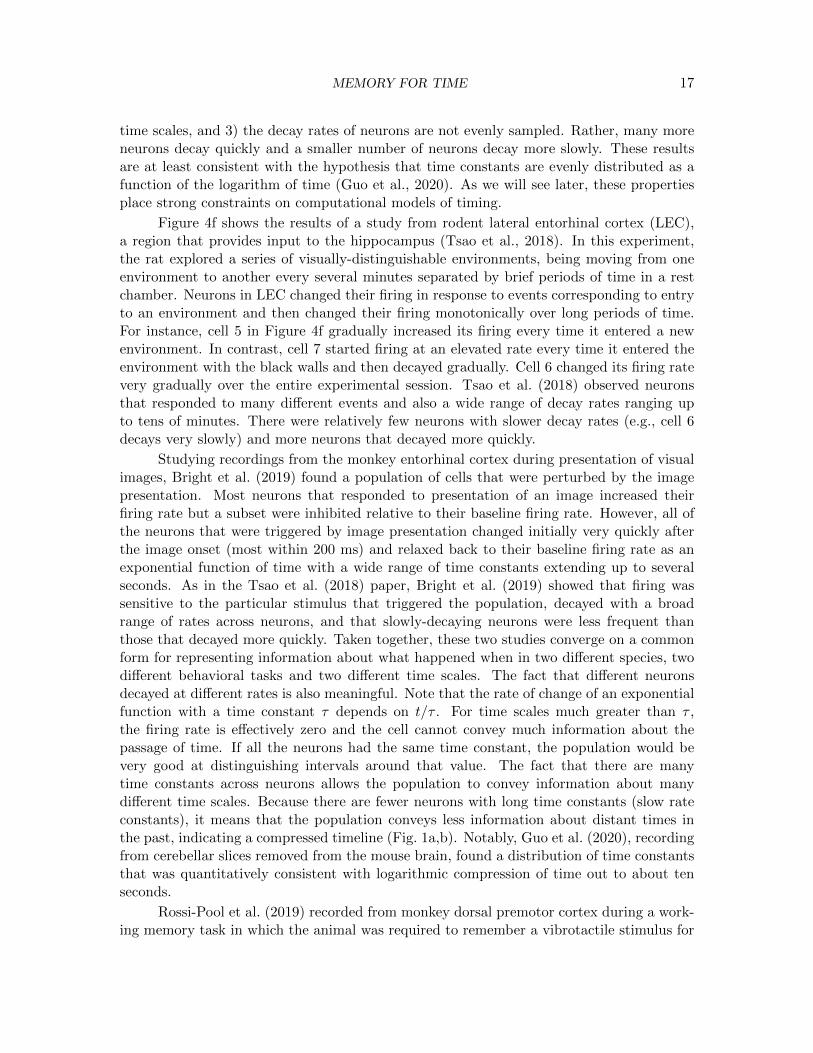
time scales, and 3) the decay rates of neurons are not evenly sampled. Rather, many moreneurons decay quickly and a smaller number of neurons decay more slowly. These resultsare at least consistent with the hypothesis that time constants are evenly distributed as afunction of the logarithm of time (Guo et al., 2020). As we will see later, these propertiesplace strong constraints on computational models of timing.

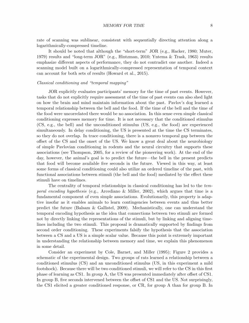
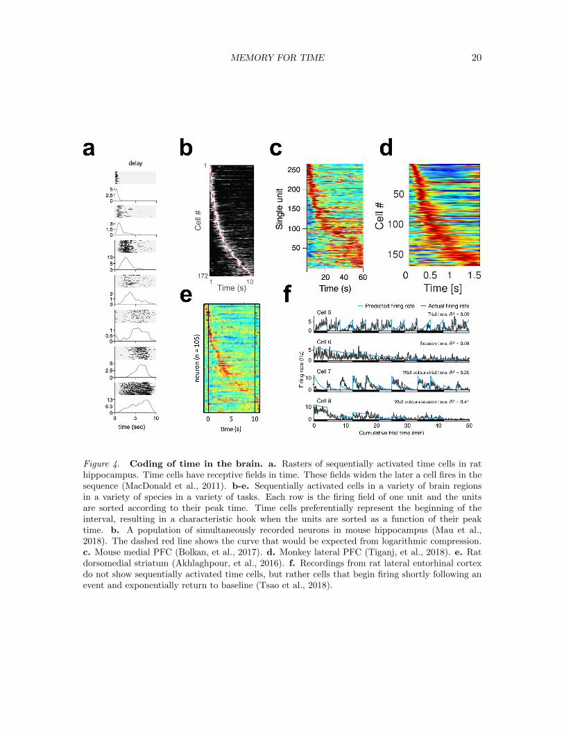
Figure 4f shows the results of a study from rodent lateral entorhinal cortex (LEC),a region that provides input to the hippocampus (Tsao et al., 2018). In this experiment,the rat explored a series of visually-distinguishable environments, being moving from oneenvironment to another every several minutes separated by brief periods of time in a restchamber. Neurons in LEC changed their firing in response to events corresponding to entryto an environment and then changed their firing monotonically over long periods of time.For instance, cell 5 in Figure 4f gradually increased its firing every time it entered a newenvironment. In contrast, cell 7 started firing at an elevated rate every time it entered theenvironment with the black walls and then decayed gradually. Cell 6 changed its firing ratevery gradually over the entire experimental session. Tsao et al. (2018) observed neuronsthat responded to many different events and also a wide range of decay rates ranging upto tens of minutes. There were relatively few neurons with slower decay rates (e.g., cell 6decays very slowly) and more neurons that decayed more quickly.

Studying recordings from the monkey entorhinal cortex during presentation of visualimages, Bright et al. (2019) found a population of cells that were perturbed by the imagepresentation. Most neurons that responded to presentation of an image increased theirfiring rate but a subset were inhibited relative to their baseline firing rate. However, all ofthe neurons that were triggered by image presentation changed initially very quickly afterthe image onset (most within 200 ms) and relaxed back to their baseline firing rate as anexponential function of time with a wide range of time constants extending up to severalseconds. As in the Tsao et al. (2018) paper, Bright et al. (2019) showed that firing wassensitive to the particular stimulus that triggered the population, decayed with a broadrange of rates across neurons, and that slowly-decaying neurons were less frequent thanthose that decayed more quickly. Taken together, these two studies converge on a commonform for representing information about what happened when in two different species, twodifferent behavioral tasks and two different time scales. The fact that different neuronsdecayed at different rates is also meaningful. Note that the rate of change of an exponentialfunction with a time constant τ depends on t/τ . For time scales much greater than τ ,the firing rate is effectively zero and the cell cannot convey much information about thepassage of time. If all the neurons had the same time constant, the population would bevery good at distinguishing intervals around that value. The fact that there are manytime constants across neurons allows the population to convey information about manydifferent time scales. Because there are fewer neurons with long time constants (slow rateconstants), it means that the population conveys less information about distant times inthe past, indicating a compressed timeline (Fig. 1a,b). Notably, Guo et al. (2020), recordingfrom cerebellar slices removed from the mouse brain, found a distribution of time constantsthat was quantitatively consistent with logarithmic compression of time out to about tenseconds.

Rossi-Pool et al. (2019) recorded from monkey dorsal premotor cortex during a work-ing memory task in which the animal was required to remember a vibrotactile stimulus for

MEMORY FOR TIME 18

a brief delay. Different neurons responded to the identity of the different stimuli that wereto be remembered. During the delay time the population of neurons changed their firingrate systematically in a way that enabled decoding of the time since the probe stimuluswas presented. The neurons within the population did not all change at the same rate.Although the authors of this study did not directly evaluate whether firing rates changedexponentially, examination of the figures (and examination of their raw data which is postedon a public repository) show that the firing rates change quickly after presentation of thefirst stimulus and then decay monotonically and non-linearly, very much like an exponentialfunction. Rossi-Pool et al. (2019) measured the relaxation time of each neuron, analogousto the time constant of an exponential function, and found that there was a broad range ofrelaxation times. Although there was not an explicit requirement for the monkey to reporttiming information in this task, this temporal signal was dramatically reduced when themonkey was not required to remember the probe stimulus, suggesting that timing informa-tion in this population is intimately related to working memory maintenance.

Bernacchia, Seo, Lee, and Wang (2011) studied the response of cortical neurons froma number of brain regions, including anterior cingulate cortex, dorsolateral prefrontal cor-tex and lateral intraparietal cortex, across trials of a task in which reward was availableprobabilistically. Unlike the foregoing studies, this population of neurons did not maintainan elevated firing rate during the time between trials. Indeed, firing rate for this populationchanged dynamically throughout the trial with a variety of forms. However, this relativelycomplicated time course was modulated by an overall value that depended on the recenthistory of reward on previous trials. They estimated the effect of reward history as an ex-ponential function over trials. Critically, different neurons decayed at different rates, withthe slowest decaying neurons showing effects from tens of trials in the past; a period of timeextending about a minute. As in the previously described studies (especially Tsao et al.,2018; Bright et al., 2019), the distribution of rates was not uniform. As in those studies,relatively fewer neurons had slow decay rates than those that decayed more quickly.

Taken as a group, these four studies (Tsao et al., 2018; Bright et al., 2019; Bernacchiaet al., 2011; Rossi-Pool et al., 2019) begin to tell a coherent story about the nature of thetiming signal from populations with firing rates that change monotonically over time. Toreiterate, all four studies showed roughly exponential decay for a wide range of neurons.However, the firing rates did not decay at the same rate for each neuron; instead a spectrumof rates was observed across neurons. This suggests that scale-invariance at the populationlevel results from different neurons conveying information about different scales. Becausethere are fewer neurons that decay very slowly, these populations record the distant pastwith less temporal resolution than the recent past. Moreover, across studies the same typeof decay behavior was found to decode the time since different events: a rewarded trial(Bernacchia et al., 2011), a vibroactile stimulus (Rossi-Pool et al., 2019), entry into a roomin a spatial task (Tsao et al., 2018) or the presentation of a visual image (Bright et al.,2019). In all of these studies, there was evidence that the population of exponentially-changing cells contained information about the type of event that was experienced in thepast, suggesting that the population contains information about what and when. Theobservation of a similar form of temporal representation in a wide variety of tasks and brainregions believed to support different “forms of memory” (e.g., Eichenbaum, 2012) suggeststhat this compressed temporal representation serves a general function in different forms of

MEMORY FOR TIME 19

memory and cognition.

Sequentially-activated “time cells” in the hippocampus and beyond

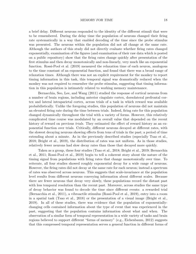
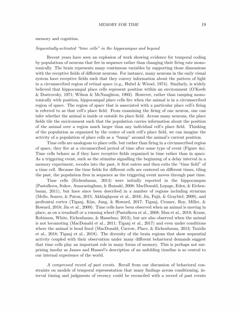
Recent years have seen an explosion of work showing evidence for temporal codingby populations of neurons that fire in sequence rather than changing their firing rate mono-tonically. The brain represents many continuous variables by supporting those dimensionswith the receptive fields of different neurons. For instance, many neurons in the early visualsystem have receptive fields such that they convey information about the pattern of lightin a circumscribed region of retinal space (e.g., Hubel & Wiesel, 1974). Similarly, is widelybelieved that hippocampal place cells represent position within an environment (O’Keefe& Dostrovsky, 1971; Wilson & McNaughton, 1993). However, rather than ramping mono-tonically with position, hippocampal place cells fire when the animal is in a circumscribedregion of space. The region of space that is associated with a particular place cell’s firingis referred to as that cell’s place field. From examining the firing of one neuron, one caninfer whether the animal is inside or outside its place field. Across many neurons, the placefields tile the environment such that the population carries information about the positionof the animal over a region much larger than any individual cell’s place field. Thinkingof the population as organized by the center of each cell’s place field, we can imagine theactivity of a population of place cells as a “bump” around the animal’s current position.

Time cells are analogous to place cells, but rather than firing in a circumscribed regionof space, they fire at a circumscribed period of time after some type of event (Figure 4a).Time cells behave as if they have receptive fields organized in time rather than in space.As a triggering event, such as the stimulus signalling the beginning of a delay interval in amemory experiment, recedes into the past, it first enters and then exits the “time field” ofa time cell. Because the time fields for different cells are centered on different times, tilingthe past, the population fires in sequence as the triggering event moves through past time.

Time cells (Eichenbaum, 2014) were initially reported in the hippocampus(Pastalkova, Itskov, Amarasingham, & Buzsaki, 2008; MacDonald, Lepage, Eden, & Eichen-baum, 2011), but have since been described in a number of regions including striatum(Mello, Soares, & Paton, 2015; Akhlaghpour et al., 2016; Jin, Fujii, & Graybiel, 2009), andprefrontal cortex (Tiganj, Kim, Jung, & Howard, 2017; Tiganj, Cromer, Roy, Miller, &Howard, 2018; Jin et al., 2009). Time cells have been observed when an animal is moving inplace, as on a treadmill or a running wheel (Pastalkova et al., 2008; Mau et al., 2018; Kraus,Robinson, White, Eichenbaum, & Hasselmo, 2013), but are also observed when the animalis not locomoting (MacDonald et al., 2011; Tiganj et al., 2017) and even under conditionswhere the animal is head fixed (MacDonald, Carrow, Place, & Eichenbaum, 2013; Taxidiset al., 2018; Tiganj et al., 2018). The diversity of the brain regions that show sequentialactivity coupled with their observation under many different behavioral demands suggestthat time cells play an important role in many forms of memory. This is perhaps not sur-prising insofar as James and Husserl’s description of an unfolding timeline is so central toour internal experience of the world.

A compressed record of past events. Recall from our discussion of behavioral con-straints on models of temporal representation that many findings across conditioning, in-terval timing and judgments of recency could be reconciled with a record of past events

MEMORY FOR TIME 20

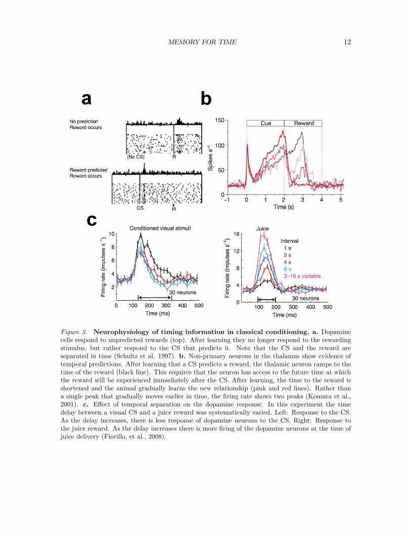
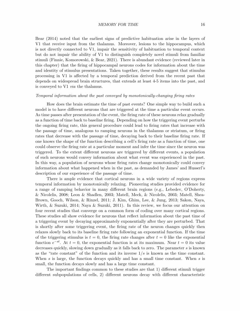
Figure 4. Coding of time in the brain. a. Rasters of sequentially activated time cells in rathippocampus. Time cells have receptive fields in time. These fields widen the later a cell fires in thesequence (MacDonald et al., 2011). b-e. Sequentially activated cells in a variety of brain regionsin a variety of species in a variety of tasks. Each row is the firing field of one unit and the unitsare sorted according to their peak time. Time cells preferentially represent the beginning of theinterval, resulting in a characteristic hook when the units are sorted as a function of their peaktime. b. A population of simultaneously recorded neurons in mouse hippocampus (Mau et al.,2018). The dashed red line shows the curve that would be expected from logarithmic compression.c. Mouse medial PFC (Bolkan, et al., 2017). d. Monkey lateral PFC (Tiganj, et al., 2018). e. Ratdorsomedial striatum (Akhlaghpour, et al., 2016). f. Recordings from rat lateral entorhinal cortexdo not show sequentially activated time cells, but rather cells that begin firing shortly following anevent and exponentially return to baseline (Tsao et al., 2018).

MEMORY FOR TIME 21

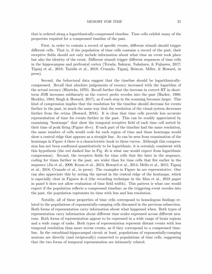
that is ordered along a logarithmically-compressed timeline. Time cells exhibit many of theproperties required for a compressed timeline of the past.

First, in order to contain a record of specific events, different stimuli should triggerdifferent cells. That is, if the population of time cells contains a record of the past, theirreceptive fields should not only include information about what time an event took placebut also the identity of the event. Different stimuli trigger different sequences of time cellsin the hippocampus and prefrontal cortex (Terada, Sakurai, Nakahara, & Fujisawa, 2017;Tiganj et al., 2018; Taxidis et al., 2018; Cruzado, Tiganj, Brincat, Miller, & Howard, inpress).

Second, the behavioral data suggest that the timeline should be logarithmically-compressed. Recall that absolute judgements of recency increased with the logarithm ofthe actual recency (Hinrichs, 1970). Recall further that the increase in correct RT in short-term JOR increases sublinearly as the correct probe recedes into the past (Hacker, 1980;Hockley, 1984; Singh & Howard, 2017), as if each step in the scanning becomes larger. Thiskind of compression implies that the resolution for the timeline should decrease for eventsfurther in the past, in much the same way that the resolution of the visual system decreasesfurther from the retina (Howard, 2018). It is clear that time cells provide less accuraterepresentation of time for events further in the past. This can be readily appreciated byexamining “heatmaps” that show the temporal receptive field of each time cell sorted bytheir time of peak firing (Figure 4b-e). If each part of the timeline had the same resolution,the same number of cells would code for each region of time and these heatmaps wouldshow a central ridge that appears as a straight line. As can be seen from examination of theheatmaps in Figure 4 there is a characteristic hook to these curves. Although this compres-sion has not been confirmed quantitatively to be logarithmic, it is certainly consistent withthis hypothesis (the red dashed line in Fig. 4b is what one would expect from logarithmiccompression). Second, the receptive fields for time cells that fire later in the sequence,coding for times further in the past, are wider than for time cells that fire earlier in thesequence (Jin et al., 2009; Kraus et al., 2013; Howard et al., 2014; Mello et al., 2015; Tiganjet al., 2018; Cruzado et al., in press). The examples in Figure 4a are representative. Onecan also appreciate this by noting the spread in the central ridge of the heatmaps, whichis especially clear in Figures 4c-d (the recording technique in the Mau et al., 2018 paperin panel b does not allow evaluation of time field width). This pattern is what one wouldexpect if the population reflects a compressed timeline; as the triggering event recedes intothe past, the population represents its time with less and less resolution.

Notably, all of these properties of time cells correspond to homologous findings re-lated to the populations of exponentially-ramping cells discussed in the previous subsection.Both forms of representation carry information about what happened when. Both types ofrepresentation carry information about different time scales expressed across different neu-rons. Both forms of representation appear to be expressed in a wide range of brain regionsand a wide range of tasks. Both types of representation represent distant events with lesstemporal resolution than more recent events, as if they correspond to a compressed time-line. In the entorhinal-hippocampal circuit at least, populations of exponentially-rampingneurons are directly (and reciprocally) connected to populations of time cells, suggestingthat the two forms of temporal representation are intimately related.

MEMORY FOR TIME 22

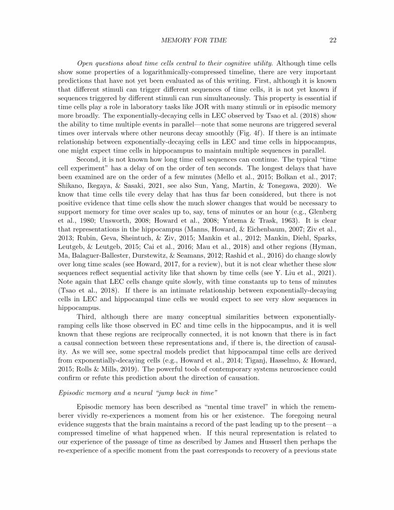
Open questions about time cells central to their cognitive utility. Although time cellsshow some properties of a logarithmically-compressed timeline, there are very importantpredictions that have not yet been evaluated as of this writing. First, although it is knownthat different stimuli can trigger different sequences of time cells, it is not yet known ifsequences triggered by different stimuli can run simultaneously. This property is essential iftime cells play a role in laboratory tasks like JOR with many stimuli or in episodic memorymore broadly. The exponentially-decaying cells in LEC observed by Tsao et al. (2018) showthe ability to time multiple events in parallel—note that some neurons are triggered severaltimes over intervals where other neurons decay smoothly (Fig. 4f). If there is an intimaterelationship between exponentially-decaying cells in LEC and time cells in hippocampus,one might expect time cells in hippocampus to maintain multiple sequences in parallel.

Second, it is not known how long time cell sequences can continue. The typical “timecell experiment” has a delay of on the order of ten seconds. The longest delays that havebeen examined are on the order of a few minutes (Mello et al., 2015; Bolkan et al., 2017;Shikano, Ikegaya, & Sasaki, 2021, see also Sun, Yang, Martin, & Tonegawa, 2020). Weknow that time cells tile every delay that has thus far been considered, but there is notpositive evidence that time cells show the much slower changes that would be necessary tosupport memory for time over scales up to, say, tens of minutes or an hour (e.g., Glenberget al., 1980; Unsworth, 2008; Howard et al., 2008; Yntema & Trask, 1963). It is clearthat representations in the hippocampus (Manns, Howard, & Eichenbaum, 2007; Ziv et al.,2013; Rubin, Geva, Sheintuch, & Ziv, 2015; Mankin et al., 2012; Mankin, Diehl, Sparks,Leutgeb, & Leutgeb, 2015; Cai et al., 2016; Mau et al., 2018) and other regions (Hyman,Ma, Balaguer-Ballester, Durstewitz, & Seamans, 2012; Rashid et al., 2016) do change slowlyover long time scales (see Howard, 2017, for a review), but it is not clear whether these slowsequences reflect sequential activity like that shown by time cells (see Y. Liu et al., 2021).Note again that LEC cells change quite slowly, with time constants up to tens of minutes(Tsao et al., 2018). If there is an intimate relationship between exponentially-decayingcells in LEC and hippocampal time cells we would expect to see very slow sequences inhippocampus.

Third, although there are many conceptual similarities between exponentially-ramping cells like those observed in EC and time cells in the hippocampus, and it is wellknown that these regions are reciprocally connected, it is not known that there is in facta causal connection between these representations and, if there is, the direction of causal-ity. As we will see, some spectral models predict that hippocampal time cells are derivedfrom exponentially-decaying cells (e.g., Howard et al., 2014; Tiganj, Hasselmo, & Howard,2015; Rolls & Mills, 2019). The powerful tools of contemporary systems neuroscience couldconfirm or refute this prediction about the direction of causation.

Episodic memory and a neural “jump back in time”

Episodic memory has been described as “mental time travel” in which the remem-berer vividly re-experiences a moment from his or her existence. The foregoing neuralevidence suggests that the brain maintains a record of the past leading up to the present—acompressed timeline of what happened when. If this neural representation is related toour experience of the passage of time as described by James and Husserl then perhaps there-experience of a specific moment from the past corresponds to recovery of a previous state

MEMORY FOR TIME 23

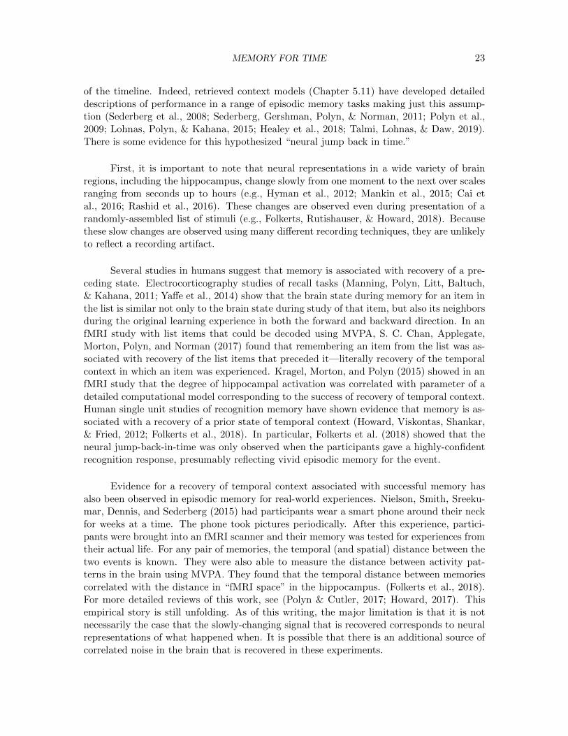
of the timeline. Indeed, retrieved context models (Chapter 5.11) have developed detaileddescriptions of performance in a range of episodic memory tasks making just this assump-tion (Sederberg et al., 2008; Sederberg, Gershman, Polyn, & Norman, 2011; Polyn et al.,2009; Lohnas, Polyn, & Kahana, 2015; Healey et al., 2018; Talmi, Lohnas, & Daw, 2019).There is some evidence for this hypothesized “neural jump back in time.”

First, it is important to note that neural representations in a wide variety of brainregions, including the hippocampus, change slowly from one moment to the next over scalesranging from seconds up to hours (e.g., Hyman et al., 2012; Mankin et al., 2015; Cai etal., 2016; Rashid et al., 2016). These changes are observed even during presentation of arandomly-assembled list of stimuli (e.g., Folkerts, Rutishauser, & Howard, 2018). Becausethese slow changes are observed using many different recording techniques, they are unlikelyto reflect a recording artifact.

Several studies in humans suggest that memory is associated with recovery of a pre-ceding state. Electrocorticography studies of recall tasks (Manning, Polyn, Litt, Baltuch,& Kahana, 2011; Yaffe et al., 2014) show that the brain state during memory for an item inthe list is similar not only to the brain state during study of that item, but also its neighborsduring the original learning experience in both the forward and backward direction. In anfMRI study with list items that could be decoded using MVPA, S. C. Chan, Applegate,Morton, Polyn, and Norman (2017) found that remembering an item from the list was as-sociated with recovery of the list items that preceded it—literally recovery of the temporalcontext in which an item was experienced. Kragel, Morton, and Polyn (2015) showed in anfMRI study that the degree of hippocampal activation was correlated with parameter of adetailed computational model corresponding to the success of recovery of temporal context.Human single unit studies of recognition memory have shown evidence that memory is as-sociated with a recovery of a prior state of temporal context (Howard, Viskontas, Shankar,& Fried, 2012; Folkerts et al., 2018). In particular, Folkerts et al. (2018) showed that theneural jump-back-in-time was only observed when the participants gave a highly-confidentrecognition response, presumably reflecting vivid episodic memory for the event.

Evidence for a recovery of temporal context associated with successful memory hasalso been observed in episodic memory for real-world experiences. Nielson, Smith, Sreeku-mar, Dennis, and Sederberg (2015) had participants wear a smart phone around their neckfor weeks at a time. The phone took pictures periodically. After this experience, partici-pants were brought into an fMRI scanner and their memory was tested for experiences fromtheir actual life. For any pair of memories, the temporal (and spatial) distance between thetwo events is known. They were also able to measure the distance between activity pat-terns in the brain using MVPA. They found that the temporal distance between memoriescorrelated with the distance in “fMRI space” in the hippocampus. (Folkerts et al., 2018).For more detailed reviews of this work, see (Polyn & Cutler, 2017; Howard, 2017). Thisempirical story is still unfolding. As of this writing, the major limitation is that it is notnecessarily the case that the slowly-changing signal that is recovered corresponds to neuralrepresentations of what happened when. It is possible that there is an additional source ofcorrelated noise in the brain that is recovered in these experiments.

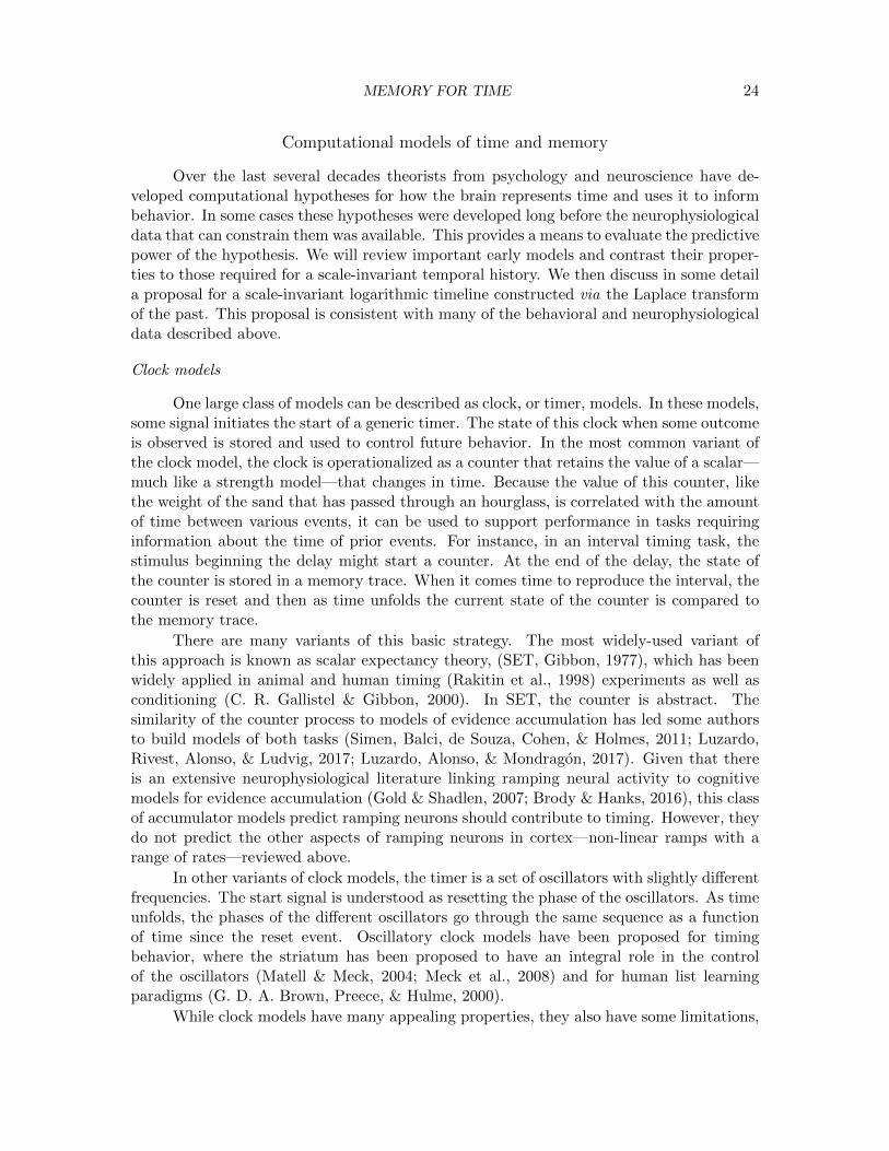
MEMORY FOR TIME 24

Computational models of time and memory

Over the last several decades theorists from psychology and neuroscience have de-veloped computational hypotheses for how the brain represents time and uses it to informbehavior. In some cases these hypotheses were developed long before the neurophysiologicaldata that can constrain them was available. This provides a means to evaluate the predictivepower of the hypothesis. We will review important early models and contrast their proper-ties to those required for a scale-invariant temporal history. We then discuss in some detaila proposal for a scale-invariant logarithmic timeline constructed via the Laplace transformof the past. This proposal is consistent with many of the behavioral and neurophysiologicaldata described above.

Clock models

One large class of models can be described as clock, or timer, models. In these models,some signal initiates the start of a generic timer. The state of this clock when some outcomeis observed is stored and used to control future behavior. In the most common variant ofthe clock model, the clock is operationalized as a counter that retains the value of a scalar—much like a strength model—that changes in time. Because the value of this counter, likethe weight of the sand that has passed through an hourglass, is correlated with the amountof time between various events, it can be used to support performance in tasks requiringinformation about the time of prior events. For instance, in an interval timing task, thestimulus beginning the delay might start a counter. At the end of the delay, the state ofthe counter is stored in a memory trace. When it comes time to reproduce the interval, thecounter is reset and then as time unfolds the current state of the counter is compared tothe memory trace.

There are many variants of this basic strategy. The most widely-used variant ofthis approach is known as scalar expectancy theory, (SET, Gibbon, 1977), which has beenwidely applied in animal and human timing (Rakitin et al., 1998) experiments as well asconditioning (C. R. Gallistel & Gibbon, 2000). In SET, the counter is abstract. Thesimilarity of the counter process to models of evidence accumulation has led some authorsto build models of both tasks (Simen, Balci, de Souza, Cohen, & Holmes, 2011; Luzardo,Rivest, Alonso, & Ludvig, 2017; Luzardo, Alonso, & Mondragon, 2017). Given that thereis an extensive neurophysiological literature linking ramping neural activity to cognitivemodels for evidence accumulation (Gold & Shadlen, 2007; Brody & Hanks, 2016), this classof accumulator models predict ramping neurons should contribute to timing. However, theydo not predict the other aspects of ramping neurons in cortex—non-linear ramps with arange of rates—reviewed above.

In other variants of clock models, the timer is a set of oscillators with slightly differentfrequencies. The start signal is understood as resetting the phase of the oscillators. As timeunfolds, the phases of the different oscillators go through the same sequence as a functionof time since the reset event. Oscillatory clock models have been proposed for timingbehavior, where the striatum has been proposed to have an integral role in the controlof the oscillators (Matell & Meck, 2004; Meck et al., 2008) and for human list learningparadigms (G. D. A. Brown, Preece, & Hulme, 2000).

While clock models have many appealing properties, they also have some limitations,

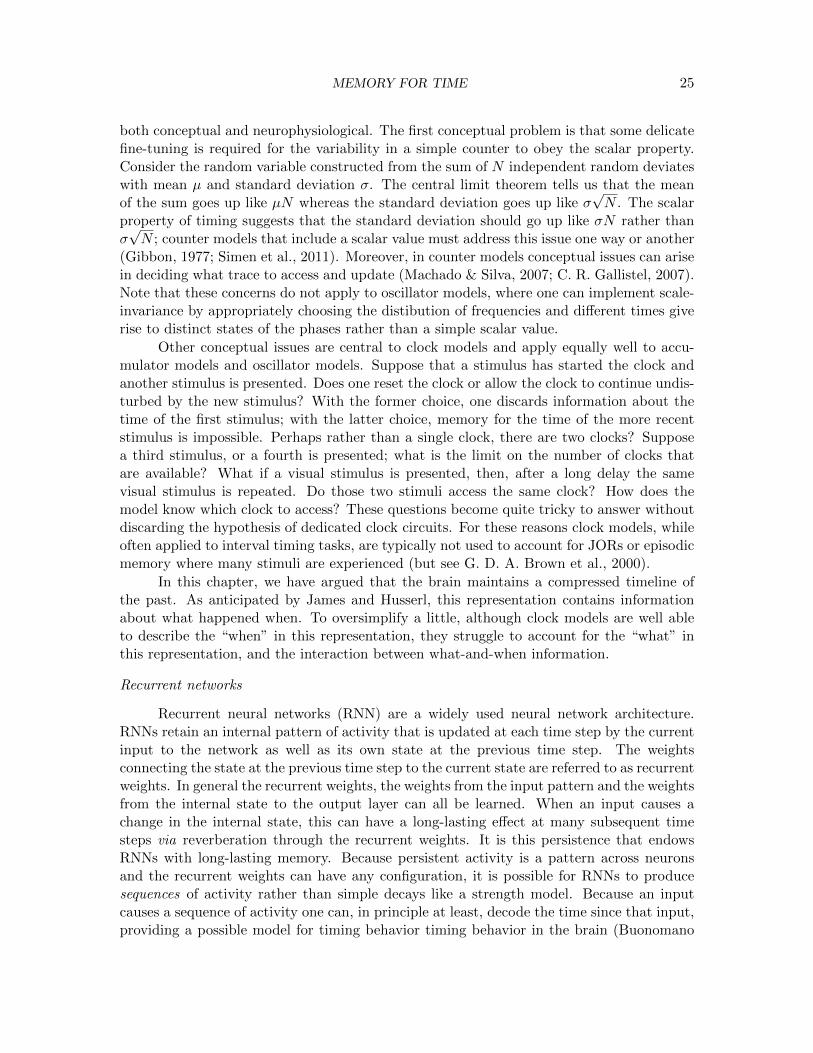
MEMORY FOR TIME 25

both conceptual and neurophysiological. The first conceptual problem is that some delicatefine-tuning is required for the variability in a simple counter to obey the scalar property.Consider the random variable constructed from the sum of N independent random deviateswith mean µ and standard deviation σ. The central limit theorem tells us that the meanof the sum goes up like µN whereas the standard deviation goes up like σ

√N . The scalar

property of timing suggests that the standard deviation should go up like σN rather thanσ√N ; counter models that include a scalar value must address this issue one way or another

(Gibbon, 1977; Simen et al., 2011). Moreover, in counter models conceptual issues can arisein deciding what trace to access and update (Machado & Silva, 2007; C. R. Gallistel, 2007).Note that these concerns do not apply to oscillator models, where one can implement scale-invariance by appropriately choosing the distibution of frequencies and different times giverise to distinct states of the phases rather than a simple scalar value.

Other conceptual issues are central to clock models and apply equally well to accu-mulator models and oscillator models. Suppose that a stimulus has started the clock andanother stimulus is presented. Does one reset the clock or allow the clock to continue undis-turbed by the new stimulus? With the former choice, one discards information about thetime of the first stimulus; with the latter choice, memory for the time of the more recentstimulus is impossible. Perhaps rather than a single clock, there are two clocks? Supposea third stimulus, or a fourth is presented; what is the limit on the number of clocks thatare available? What if a visual stimulus is presented, then, after a long delay the samevisual stimulus is repeated. Do those two stimuli access the same clock? How does themodel know which clock to access? These questions become quite tricky to answer withoutdiscarding the hypothesis of dedicated clock circuits. For these reasons clock models, whileoften applied to interval timing tasks, are typically not used to account for JORs or episodicmemory where many stimuli are experienced (but see G. D. A. Brown et al., 2000).

In this chapter, we have argued that the brain maintains a compressed timeline ofthe past. As anticipated by James and Husserl, this representation contains informationabout what happened when. To oversimplify a little, although clock models are well ableto describe the “when” in this representation, they struggle to account for the “what” inthis representation, and the interaction between what-and-when information.

Recurrent networks

Recurrent neural networks (RNN) are a widely used neural network architecture.RNNs retain an internal pattern of activity that is updated at each time step by the currentinput to the network as well as its own state at the previous time step. The weightsconnecting the state at the previous time step to the current state are referred to as recurrentweights. In general the recurrent weights, the weights from the input pattern and the weightsfrom the internal state to the output layer can all be learned. When an input causes achange in the internal state, this can have a long-lasting effect at many subsequent timesteps via reverberation through the recurrent weights. It is this persistence that endowsRNNs with long-lasting memory. Because persistent activity is a pattern across neuronsand the recurrent weights can have any configuration, it is possible for RNNs to producesequences of activity rather than simple decays like a strength model. Because an inputcauses a sequence of activity one can, in principle at least, decode the time since that input,providing a possible model for timing behavior timing behavior in the brain (Buonomano

MEMORY FOR TIME 26

& Maass, 2009).

RNNs have found broad use in a range of fields. In cognitive science, RNNs wereinitially extremely influential in connectionist models of language (Elman, 1990) and laterapplied to the problem of serial order in list learning experiments (Botvinick & Plaut,2004, 2006). Under some well-specified conditions, it can be proven that the internal stateprovides a record of events in the past (Maass, Natschlager, & Markram, 2002) and RNNscan be mathematically tractable (White, Lee, & Sompolinsky, 2004; Rajan & Abbott,2006). RNNs can have rich dynamics; by setting the weights appropriately they can be usedfor a number of computational applications and have attracted a great deal of attentionin machine learning applications (e.g., Graves, 2013; Graves, Mohamed, & Hinton, 2013;Sutskever, Martens, & Hinton, 2011). In recent years, RNNs have also attracted a greatdeal of attention in computational neuroscience. Because an input can trigger a sequenceof states, RNNs are capable of modeling sequentially-activating neurons that behave liketime cells (Rajan, Harvey, & Tank, 2016; Wang, Narain, Hosseini, & Jazayeri, 2018).

There are limitations to RNNs as a model of timing behavior in the brain. Thetypical method for training RNNs, back-propogation through time, requires that the numberof training steps necessary to learn a relationship separated by time τ goes up with τ(Mozer, 1992). This property does not seem to be consistent with empirical data, leadingto proposals to augment RNNs with other mechanisms to identify long-time dependencies(e.g., Ke et al., 2018). In general, RNNs are not scale-invariant, although it is possible towrite out RNNs that are scale-invariant (Y. Liu & Howard, 2020). RNNs can be trainedto scale-invariant, and to exhibit many different properties (Wang et al., 2018), but thisbegs the question of how the teaching signal could be constructed. Put another way, ifyou already had a scale-invariant timeline of the past, you could use it to train an RNN tomaintain a scale-invariant timeline of the past. But it is not at all clear how an RNN couldgenerate such a representation de novo.

Spectral models for temporal history

One approach to the problem of scale-invariance is to simply have an ensemble ofprocessing elements, each with a different scale (in an RNN, this is analogous to having awide spectrum of eigenvalues). Across the population, all scales are represented so that thesystem has similar properties no matter what scale is used in the experiment. Tank andHopfield (1987) wrote out a set of temporal filters with a wide range of scales for use in anattractor model of sequence learning. The Multiple Time Scale (MTS) model (J. E. R. Stad-don, 2005; J. E. Staddon & Higa, 1999) of Staddon and colleagues described conditioningbehavior with a strength model in which a stimulus is associated with many strengths, eachwith a different decay rate (see also Pashler, Cepeda, Lindsey, Vul, & Mozer, 2009). Spec-tral resonance theory (Grossberg & Merrill, 1992; Bullock et al., 1994; Grossberg & Merrill,1996) describes a neural network model in which a spectrum of time constants gives rise tosequentially-activated cells, not unlike time cells, which can be used to model behavior inmany conditioning and timing tasks. Working primarily in the context of computationalmodels of vision, Lindeberg and colleagues (e.g., Lindeberg & Fagerstrom, 1996; Lindeberg,1997, 2016, 2021) proposed that memory for the past ought to be maintained by a popu-lation of cells with exponential receptive fields extending over past time. Lindeberg (1997)proposed that these exponential receptive fields could be cascaded to develop compact re-

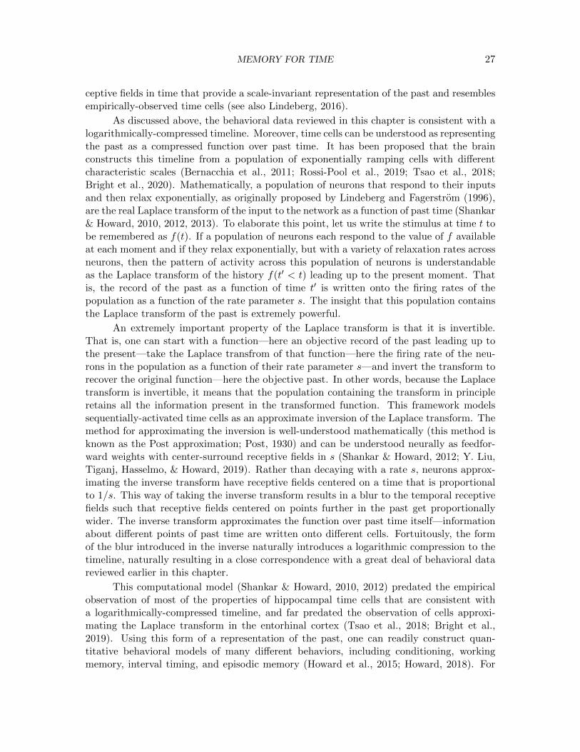
MEMORY FOR TIME 27

ceptive fields in time that provide a scale-invariant representation of the past and resemblesempirically-observed time cells (see also Lindeberg, 2016).

As discussed above, the behavioral data reviewed in this chapter is consistent with alogarithmically-compressed timeline. Moreover, time cells can be understood as representingthe past as a compressed function over past time. It has been proposed that the brainconstructs this timeline from a population of exponentially ramping cells with differentcharacteristic scales (Bernacchia et al., 2011; Rossi-Pool et al., 2019; Tsao et al., 2018;Bright et al., 2020). Mathematically, a population of neurons that respond to their inputsand then relax exponentially, as originally proposed by Lindeberg and Fagerstrom (1996),are the real Laplace transform of the input to the network as a function of past time (Shankar& Howard, 2010, 2012, 2013). To elaborate this point, let us write the stimulus at time t tobe remembered as f(t). If a population of neurons each respond to the value of f availableat each moment and if they relax exponentially, but with a variety of relaxation rates acrossneurons, then the pattern of activity across this population of neurons is understandableas the Laplace transform of the history f(t′ < t) leading up to the present moment. Thatis, the record of the past as a function of time t′ is written onto the firing rates of thepopulation as a function of the rate parameter s. The insight that this population containsthe Laplace transform of the past is extremely powerful.

An extremely important property of the Laplace transform is that it is invertible.That is, one can start with a function—here an objective record of the past leading up tothe present—take the Laplace transfrom of that function—here the firing rate of the neu-rons in the population as a function of their rate parameter s—and invert the transform torecover the original function—here the objective past. In other words, because the Laplacetransform is invertible, it means that the population containing the transform in principleretains all the information present in the transformed function. This framework modelssequentially-activated time cells as an approximate inversion of the Laplace transform. Themethod for approximating the inversion is well-understood mathematically (this method isknown as the Post approximation; Post, 1930) and can be understood neurally as feedfor-ward weights with center-surround receptive fields in s (Shankar & Howard, 2012; Y. Liu,Tiganj, Hasselmo, & Howard, 2019). Rather than decaying with a rate s, neurons approx-imating the inverse transform have receptive fields centered on a time that is proportionalto 1/s. This way of taking the inverse transform results in a blur to the temporal receptivefields such that receptive fields centered on points further in the past get proportionallywider. The inverse transform approximates the function over past time itself—informationabout different points of past time are written onto different cells. Fortuitously, the formof the blur introduced in the inverse naturally introduces a logarithmic compression to thetimeline, naturally resulting in a close correspondence with a great deal of behavioral datareviewed earlier in this chapter.

This computational model (Shankar & Howard, 2010, 2012) predated the empiricalobservation of most of the properties of hippocampal time cells that are consistent witha logarithmically-compressed timeline, and far predated the observation of cells approxi-mating the Laplace transform in the entorhinal cortex (Tsao et al., 2018; Bright et al.,2019). Using this form of a representation of the past, one can readily construct quan-titative behavioral models of many different behaviors, including conditioning, workingmemory, interval timing, and episodic memory (Howard et al., 2015; Howard, 2018). For

MEMORY FOR TIME 28

instance, RT findings from the judgment of recency task can be modeled by scanning along alogarithmically-compressed timeline (Howard et al., 2015; Singh, Tiganj, & Howard, 2018).Similarly, one can construct a good model of recency and contiguity across scales in episodicmemory by assuming that episodic memory is associated with recovery of a previous stateof the timeline (Howard et al., 2015). Temporal mapping experiments (e.g., Fig 2 Cole etal., 1995) can be understood as associations mediated by recovered timelines.

Summary

Philosophers considering the phenomenology of time have long proposed that themind constructs a “space-like” internal dimension for time (Husserl, 1966; James, 1890).Behavioral data from a variety of paradigms is consistent with this account, with the addedconstraint that the internal dimension of time is “compressed” estimate of objective time.The mapping appears to be such that internal time is a logarithmic function of externaltime, consistent with the Weber-Fechner law. In this view, classical conditioning arises asan attempt to predict the future from a logarithmically-compressed estimate of the past.A wealth of neurophysiological evidence is consistent with this understanding of memoryfor time. Neurons in many brain regions can be used to decode what happened when inthe past. Time cells, observed in many different brain regions, suggest that the brain quiteliterally places receptive fields along a temporal axis (Eichenbaum, 2014). There is ampleevidence that the neural representation of the past is compressed as suggested by behavioralconsiderations. Computational models that account for time cells have been developed thatcan be used to both model behavioral data and also predict neurophysiological findings.

References

Akhlaghpour, H., Wiskerke, J., Choi, J. Y., Taliaferro, J. P., Au, J., & Witten, I. (2016). Dissociatedsequential activity and stimulus encoding in the dorsomedial striatum during spatial workingmemory. eLife, 5 , e19507.

Arcediano, F., Escobar, M., & Miller, R. R. (2003). Temporal integration and temporal backwardassociations in human and nonhuman subjects. Learning & Behavior , 31 (3), 242-56.

Arcediano, F., & Miller, R. R. (2002). Some constraints for models of timing: A temporal codinghypothesis perspective. Learning and Motivation, 33 , 105-123.

Atkinson, R. C., & Shiffrin, R. M. (1968). Human memory: A proposed system and its controlprocesses. In K. W. Spence & J. T. Spence (Eds.), The psychology of learning and motivation(Vol. 2, p. 89-105). New York: Academic Press.

Balsam, P. D., & Gallistel, C. R. (2009). Temporal maps and informativeness in associative learning.Trends in Neuroscience, 32 (2), 73–78.

Barnet, R. C., Cole, R. P., & Miller, R. R. (1997). Temporal integration in second-order conditioningand sensory preconditioning. Animal Learning & Behavior , 25 , 221–233.

Bergson, H. (1910). Time and free will: An essay on the immediate data of consciousness. G. Allen& Unwin.

Bernacchia, A., Seo, H., Lee, D., & Wang, X. J. (2011). A reservoir of time constants for memorytraces in cortical neurons. Nature Neuroscience, 14 (3), 366-72.

Bolkan, S. S., Stujenske, J. M., Parnaudeau, S., Spellman, T. J., Rauffenbart, C., Abbas, A. I.,. . . Kellendonk, C. (2017). Thalamic projections sustain prefrontal activity during workingmemory maintenance. Nature Neuroscience, 20 (7), 987–996.

Botvinick, M. M., & Plaut, D. C. (2004). Doing without schema hierarchies: a recurrent connectionistapproach to normal and impaired routine sequential action. Psychological review , 111 (2), 395.

MEMORY FOR TIME 29

Botvinick, M. M., & Plaut, D. C. (2006). Short-term memory for serial order: a recurrent neuralnetwork model. Psychological Review , 113 (2), 201.

Bright, I. M., Meister, M. L. R., Cruzado, N. A., Tiganj, Z., Buffalo, E. A., & Howard, M. W. (2020).A temporal record of the past with a spectrum of time constants in the monkey entorhinalcortex. Proceedings of the National Academy of Sciences, 117 , 20274-20283.

Bright, I. M., Meister, M. L. R., Cruzado, N. A., Tiganj, Z., Howard, M. W., & Buffalo, E. A. (2019).A temporal record of the past with a spectrum of time constants in the monkey entorhinalcortex. bioRxiv , 688341.

Brody, C. D., & Hanks, T. D. (2016). Neural underpinnings of the evidence accumulator. CurrentOpinion in Neurobiology , 37 , 149-157. doi: 10.1016/j.conb.2016.01.003

Brown, G. D. A., Preece, T., & Hulme, C. (2000). Oscillator-based memory for serial order.Psychological Review , 107 (1), 127-181.

Brown, S., Steyvers, M., & Hemmer, P. (2007). Modeling experimentally induced strategy shifts.Psychological Science, 18 (1), 40-5.

Buhusi, C. V., & Meck, W. H. (2005). What makes us tick? Functional and neural mechanisms ofinterval timing. Nature Reviews Neuroscience, 6 (10), 755-65. doi: 10.1038/nrn1764

Bullock, D., Fiala, J. C., & Grossberg, S. (1994). A neural model of timed response learning in thecerebellum. Neural Networks, 7 (6-7), 1101–1114.

Buonomano, D. V., & Maass, W. (2009). State-dependent computations: spatiotemporal processingin cortical networks. Nature Reviews Neuroscience, 10 (2), 113-25. doi: 10.1038/nrn2558

Cai, D. J., Aharoni, D., Shuman, T., Shobe, J., Biane, J., Song, W., . . . Silva, A. (2016). A sharedneural ensemble links distinct contextual memories encoded close in time. Nature, 534 (7605),115–118.

Chan, M., Ross, B., Earle, G., & Caplan, J. B. (2009). Precise instructions determine participants’memory search strategy in judgments of relative order in short lists. Psychonomic Bulletin &Review , 16 (5), 945-51.

Chan, S. C., Applegate, M. C., Morton, N. W., Polyn, S. M., & Norman, K. A. (2017). Lingeringrepresentations of stimuli influence recall organization. Neuropsychologia, 97 , 72–82.

Cole, R. P., Barnet, R. C., & Miller, R. R. (1995). Temporal encoding in trace conditioning. AnimalLearning & Behavior , 23 (2), 144-153.

Crowder, R. G. (1976). Principles of learning and memory. Hillsdale, NJ: Erlbaum.Cruzado, N. A., Tiganj, Z., Brincat, S. L., Miller, E. K., & Howard, M. W. (in press). Conjunctive

representation of what and when in monkey hippocampus and lateral prefrontal cortex duringan associative memory task. Hippocampus.

Daniel, P. M., & Whitteridge, D. (1961). The representation of the visual field on the cerebralcortex in monkeys. Journal of Physiology , 159 , 203-21.

Eichenbaum, H. (2012). The cognitive neuroscience of memory: An introduction (2nd ed.). NewYork, NY: Oxford University Press.

Eichenbaum, H. (2014). Time cells in the hippocampus: a new dimension for mapping memories.Nature Reviews Neuroscience, 15 (11), 732-44. doi: 10.1038/nrn3827

Elman, J. L. (1990). Finding structure in time. Cognitive Science, 14 , 179-211.Fechner, G. (1860/1912). Elements of psychophysics. Vol. I. Houghton Mifflin.Finnie, P., Komorowski, R., & Bear, M. (2021). The spatiotemporal organization of expe-

rience dictates hippocampal involvement in primary visual cortical plasticity. bioRxiv ,2021.03.01.433430 .

Fiorillo, C. D., Newsome, W. T., & Schultz, W. (2008). The temporal precision of reward predictionin dopamine neurons. Nature Neuroscience. doi: 10.1038/nn.2159

Flexser, A. J., & Bower, G. H. (1974). How frequency affects recency judgments: a model for recencydiscrimination. Journal of Experimental Psychology , 103 (4), 706-16.

Folkerts, S., Rutishauser, U., & Howard, M. (2018). Human episodic memory retrieval is accompa-nied by a neural contiguity effect. Journal of Neuroscience, 38 , 4200-4211.

MEMORY FOR TIME 30

Fortin, N. J., Agster, K. L., & Eichenbaum, H. B. (2002). Critical role of the hippocampus inmemory for sequences of events. Nature Neuroscience, 5 (5), 458-62.

Gallistel, C., Craig, A. R., & Shahan, T. A. (2019). Contingency, contiguity, and causality in con-ditioning: Applying information theory and weber’s law to the assignment of credit problem.Psychological review , 126 (5), 761.

Gallistel, C. R. (2007). Flawed foundations of associationism? comments on Machado and Silva(2007). American Psychologist , 62 (7), 682-5. doi: 10.1037/0003-066X.62.7.682

Gallistel, C. R., & Gibbon, J. (2000). Time, rate, and conditioning. Psychological Review , 107 (2),289-344.

Gavornik, J. P., & Bear, M. F. (2014). Learned spatiotemporal sequence recognition and predictionin primary visual cortex. Nature neuroscience, 17 (5), 732–737.

Gibbon, J. (1977). Scalar expectancy theory and Weber’s law in animal timing. PsychologicalReview , 84 (3), 279-325.

Gibbon, J., Baldock, M., Locurto, C., Gold, L., & Terrace, H. (1977). Trial and intertrial durationsin autoshaping. Journal of Experimental psychology: Animal behavior processes, 3 (3), 264.

Gibbon, J., Malapani, C., Dale, C. L., & Gallistel, C. R. (1997). Toward a neurobiology of temporalcognition: advances and challenges. Current opinion in neurobiology , 7 (2), 170–184.

Glenberg, A. M., Bradley, M. M., Stevenson, J. A., Kraus, T. A., Tkachuk, M. J., & Gretz, A. L.(1980). A two-process account of long-term serial position effects. Journal of ExperimentalPsychology: Human Learning and Memory , 6 , 355-369.

Gold, J. I., & Shadlen, M. N. (2007). The neural basis of decision making. Annual Review Neuro-science, 30 , 535–574.

Graves, A. (2013). Generating sequences with recurrent neural networks. arXiv preprintarXiv:1308.0850 .

Graves, A., Mohamed, A.-r., & Hinton, G. (2013). Speech recognition with deep recurrent neuralnetworks. In 2013 IEEE international conference on acoustics, speech and signal processing(pp. 6645–6649).

Grossberg, S., & Merrill, J. (1992). A neural network model of adaptively timed reinforcementlearning and hippocampal dynamics. Cognitive Brain Research, 1 , 3-38.

Grossberg, S., & Merrill, J. (1996). The hippocampus and cerebellum in adaptively timed learning,recognition, and movement. Journal of Cognitive Neuroscience, 8 , 257-277.

Guo, C., Huson, V., Macosko, E., & Regehr, W. G. (2020). Graded heterogeneity of metabotropicsignaling underlies a continuum of cell-intrinsic temporal responses. bioRxiv .

Hacker, M. J. (1980). Speed and accuracy of recency judgments for events in short-term memory.Journal of Experimental Psychology: Human Learning and Memory , 15 , 846-858.

Healey, M. K., Long, N. M., & Kahana, M. J. (2018). Contiguity in episodic memory. Psychonomicbulletin & review , 1–22.

Hinrichs, J. V. (1970). A two-process memory-strength theory for judgment of recency. PsychologicalReview , 77 (3), 223-233.

Hinrichs, J. V., & Buschke, H. (1968). Judgment of recency under steady-state conditions. Journalof Experimental Psychology , 78 (4), 574-579.

Hintzman, D. L. (1986). ‘Schema abstraction’ in a multiple-trace memory model. PsychologicalReview , 93 , 411-428.

Hintzman, D. L. (2010). How does repetition affect memory? Evidence from judgments of recency.Memory & Cognition, 38 (1), 102-15.

Hockley, W. E. (1984). Analysis of response time distributions in the study of cognitive processes.Journal of Experimental Psychology: Learning, Memory, and Cognition, 10 (4), 598-615.

Homann, J., Koay, S. A., Glidden, A. M., Tank, D. W., & Berry, M. J. (2017). Predictive coding ofnovel versus familiar stimuli in the primary visual cortex. bioRxiv , 197608.

Howard, M. W. (2017). Temporal and spatial context in the mind and brain. Current Opinion inBehavioral Sciences, 17 , 14-19.

MEMORY FOR TIME 31

Howard, M. W. (2018). Memory as perception of the past: Compressed time in mind and brain.Trends in Cognitive Sciences, 22 , 124-136.

Howard, M. W., & Kahana, M. J. (2002). A distributed representation of temporal context. Journalof Mathematical Psychology , 46 (3), 269-299.

Howard, M. W., MacDonald, C. J., Tiganj, Z., Shankar, K. H., Du, Q., Hasselmo, M. E., &Eichenbaum, H. (2014). A unified mathematical framework for coding time, space, andsequences in the hippocampal region. Journal of Neuroscience, 34 (13), 4692-707. doi:10.1523/JNEUROSCI.5808-12.2014

Howard, M. W., Shankar, K. H., Aue, W., & Criss, A. H. (2015). A distributed representation ofinternal time. Psychological Review , 122 (1), 24-53.

Howard, M. W., Viskontas, I. V., Shankar, K. H., & Fried, I. (2012). Ensembles of human MTLneurons “jump back in time” in response to a repeated stimulus. Hippocampus, 22 (9), 1833-1847.

Howard, M. W., Youker, T. E., & Venkatadass, V. (2008). The persistence of memory: Contiguityeffects across several minutes. Psychonomic Bulletin & Review , 15 (PMC2493616), 58-63.

Hubel, D. H., & Wiesel, T. N. (1974). Uniformity of monkey striate cortex: a parallel relation-ship between field size, scatter, and magnification factor. Journal of Comparative Neurology ,158 (3), 295-305. doi: 10.1002/cne.901580305

Husserl, E. (1966). The phenomenology of internal time-consciousness. Bloomington, IN: IndianaUniversity Press.

Hyman, J. M., Ma, L., Balaguer-Ballester, E., Durstewitz, D., & Seamans, J. K. (2012). Contex-tual encoding by ensembles of medial prefrontal cortex neurons. Proceedings of the NationalAcademy of Sciences USA, 109 , 5086-91. doi: 10.1073/pnas.1114415109

Ivry, R. B., Spencer, R. M., Zelaznik, H. N., & Diedrichsen, J. (2002). The cerebellum and eventtiming. Annals of the new York Academy of Sciences, 978 (1), 302–317.

James, W. (1890). The principles of psychology. New York: Holt.

Jin, D. Z., Fujii, N., & Graybiel, A. M. (2009). Neural representation of time in cortico-basal gangliacircuits. Proceedings of the National Academy of Sciences, 106 (45), 19156–19161.

Jirenhed, D.-A., Rasmussen, A., Johansson, F., & Hesslow, G. (2017). Learned response sequencesin cerebellar purkinje cells. Proceedings of the National Academy of Sciences, 114 (23), 6127–6132.

Johansson, F., Jirenhed, D.-A., Rasmussen, A., Zucca, R., & Hesslow, G. (2014). Memory trace andtiming mechanism localized to cerebellar purkinje cells. Proceedings of the National Academyof Sciences, 111 (41), 14930–14934.

Kahana, M. J., Howard, M., & Polyn, S. (2008). Associative processes in episodic memory. InH. L. Roediger III (Ed.), Cognitive psychology of memory, Vol. 2 of learning and memory - acomprehensive reference (J. Byrne, Editor) (p. 476-490). Oxford: Elsevier.

Kandel, E. R. (2001). The molecular biology of memory storage: a dialogue between genes andsynapses. Science, 294 (5544), 1030-8.

Ke, N. R., Goyal, A., Bilaniuk, O., Binas, J., Mozer, M. C., Pal, C., & Bengio, Y. (2018). Sparseattentive backtracking: Temporal credit assignment through reminding. In Advances in neuralinformation processing systems (pp. 7640–7651).

Kennedy, A., Wayne, G., Kaifosh, P., Alvina, K., Abbott, L., & Sawtell, N. B. (2014). A temporalbasis for predicting the sensory consequences of motor commands in an electric fish. Natureneuroscience, 17 (3), 416–422.

Kim, H., Homann, J., Tank, D. W., & Berry, M. J. (2019). A long timescale stimulus history effectin the primary visual cortex. bioRxiv , 585539.

Kim, J., Ghim, J.-W., Lee, J. H., & Jung, M. W. (2013). Neural correlates of intervaltiming in rodent prefrontal cortex. Journal of Neuroscience, 33 (34), 13834-47. doi:10.1523/JNEUROSCI.1443-13.2013

MEMORY FOR TIME 32

Komura, Y., Tamura, R., Uwano, T., Nishijo, H., Kaga, K., & Ono, T. (2001). Retrospective andprospective coding for predicted reward in the sensory thalamus. Nature, 412 (6846), 546-9.doi: 10.1038/35087595

Kragel, J. E., Morton, N. W., & Polyn, S. M. (2015). Neural activity in the medial temporal lobereveals the fidelity of mental time travel. Journal of Neuroscience, 35 (7), 2914–2926.

Kraus, B. J., Robinson, R. J., 2nd, White, J. A., Eichenbaum, H., & Hasselmo, M. E. (2013).Hippocampal “time cells”: time versus path integration. Neuron, 78 (6), 1090-101. doi:10.1016/j.neuron.2013.04.015

Lebedev, M. A., O’Doherty, J. E., & Nicolelis, M. A. (2008). Decoding of temporal intervals fromcortical ensemble activity. Journal of Neurophysiology , 99 (1), 166–186.

Lejeune, H., & Wearden, J. H. (2006). Scalar properties in animal timing: conformity and violations.Quarterly Journal of Experimental Psychology , 59 (11), 1875-908.

Leon, M. I., & Shadlen, M. N. (2003). Representation of time by neurons in the posterior parietalcortex of the macaque. Neuron, 38 (2), 317–327.

Lewis, P. A., & Miall, R. C. (2009). The precision of temporal judgement: milliseconds, manyminutes, and beyond. Philosophical Transcripts of the Royal Society London B: BiologicalSciences, 364 (1525), 1897-905. doi: 10.1098/rstb.2009.0020

Lindeberg, T. (1997). On automatic selection of temporal scales in time-causal scale-space. InInternational workshop on algebraic frames for the perception-action cycle (pp. 94–113).

Lindeberg, T. (2016). Time-causal and time-recursive spatio-temporal receptive fields. Journal ofMathematical Imaging and Vision, 55 (1), 50–88.

Lindeberg, T. (2021). Normative theory of visual receptive fields. Heliyon, 7 (1), e05897.Lindeberg, T., & Fagerstrom, D. (1996). Scale-space with casual time direction. In European

conference on computer vision (pp. 229–240).Liu, Y., & Howard, M. W. (2020). Generation of scale-invariant sequential activity in linear recurrent

networks. Neural Computation, 32 (7), 1379–1407.Liu, Y., Levy, S. J., Mau, W., Geva, N., Rubin, A., Ziv, Y., . . . Howard, M. (2021). Consistent

population activity on the scale of minutes in the mouse hippocampus. bioRxiv .Liu, Y., Tiganj, Z., Hasselmo, M. E., & Howard, M. W. (2019). A neural microcircuit model for a

scalable scale-invariant representation of time. Hippocampus, 29 (3), 260–274.Liu, Y. S., Chan, M., & Caplan, J. B. (2014). Generality of a congruity effect in judgements of

relative order. Memory & Cognition, 1–20.Lohnas, L. J., Polyn, S. M., & Kahana, M. J. (2015). Expanding the scope of memory search:

Modeling intralist and interlist effects in free recall. Psychological Review , 122 (2), 337-63.doi: 10.1037/a0039036

Luzardo, A., Alonso, E., & Mondragon, E. (2017). A Rescorla-Wagner drift-diffusion model ofconditioning and timing. PLOS Computational Biology , 13 (11), e1005796. Retrieved fromhttp://dx.plos.org/10.1371/journal.pcbi.1005796 doi: 10.1371/journal.pcbi.1005796

Luzardo, A., Rivest, F., Alonso, E., & Ludvig, E. A. (2017). A drift–diffusion model of inter-val timing in the peak procedure. Journal of Mathematical Psychology , 77 , 111–123. doi:10.1016/j.jmp.2016.10.002

Maass, W., Natschlager, T., & Markram, H. (2002). Real-time computing without stable states: anew framework for neural computation based on perturbations. Neural Computation, 14 (11),2531-60. doi: 10.1162/089976602760407955

MacDonald, C. J., Carrow, S., Place, R., & Eichenbaum, H. (2013). Distinct hippocampal timecell sequences represent odor memories immobilized rats. Journal of Neuroscience, 33 (36),14607–14616.

MacDonald, C. J., Lepage, K. Q., Eden, U. T., & Eichenbaum, H. (2011). Hippocampal “time cells”bridge the gap in memory for discontiguous events. Neuron, 71 (4), 737-749.

Machado, A., & Silva, F. J. (2007). Toward a richer view of the scientific method: The role ofconceptual analysis . American Psychologist , 62 (7), 671-681.

MEMORY FOR TIME 33

Mankin, E. A., Diehl, G. W., Sparks, F. T., Leutgeb, S., & Leutgeb, J. K. (2015). Hippocampal CA2activity patterns change over time to a larger extent than between spatial contexts. Neuron,85 (1), 190-201. doi: 10.1016/j.neuron.2014.12.001

Mankin, E. A., Sparks, F. T., Slayyeh, B., Sutherland, R. J., Leutgeb, S., & Leutgeb, J. K. (2012).Neuronal code for extended time in the hippocampus. Proceedings of the National Academyof Sciences, 109 , 19462-7. doi: 10.1073/pnas.1214107109

Manning, J. R., Polyn, S. M., Litt, B., Baltuch, G., & Kahana, M. J. (2011). Oscillatory patterns intemporal lobe reveal context reinstatement during memory search. Proceedings of the NationalAcademy of Science, USA, 108 (31), 12893-7.

Manns, J. R., Howard, M. W., & Eichenbaum, H. B. (2007). Gradual changes in hippocampalactivity support remembering the order of events. Neuron, 56 (3), 530-540.

Matell, M. S., & Meck, W. H. (2004). Cortico-striatal circuits and interval timing: coincidencedetection of oscillatory processes. Brain Research: Cognitive Brain Research, 21 (2), 139-70.doi: 10.1016/j.cogbrainres.2004.06.012

Matell, M. S., Meck, W. H., & Nicolelis, M. A. (2003). Interval timing and the encoding of signalduration by ensembles of cortical and striatal neurons. Behavioral Neuroscience, 117 (4), 760.

Matell, M. S., Shea-Brown, E., Gooch, C., Wilson, A. G., & Rinzel, J. (2011). A heterogeneouspopulation code for elapsed time in rat medial agranular cortex. Behavioral Neuroscience,125 (1), 54-73.

Mau, W., Sullivan, D. W., Kinsky, N. R., Hasselmo, M. E., Howard, M. W., & Eichenbaum, H.(2018). The same hippocampal CA1 population simultaneously codes temporal informationover multiple timescales. Current Biology , 28 , 1499-1508.

Meck, W. H. (1996). Neuropharmacology of timing and time perception. Cognitive Brain Research,3 (3-4), 227–242.

Meck, W. H., Penney, T. B., & Pouthas, V. (2008). Cortico-striatal representation of time in animalsand humans. Current Opinion in Neurobiology , 18 (2), 145–152.

Mello, G. B., Soares, S., & Paton, J. J. (2015). A scalable population code for time in the striatum.Current Biology , 25 (9), 1113–1122.

Moreton, B. J., & Ward, G. (2010). Time scale similarity and long-term memory for autobiographicalevents. Psychonomic Bulletin & Review , 17 , 510-515.

Mozer, M. C. (1992). Induction of multiscale temporal structure. In Advances in neural informationprocessing systems (pp. 275–282).

Muter, P. (1979). Response latencies in discriminations of recency. Journal of Experimental Psy-chology: Human Learning and Memory , 5 , 160-169.

Naya, Y., & Suzuki, W. (2011). Integrating what and when across the primate medial temporallobe. Science, 333 (6043), 773-776.

Nielson, D. M., Smith, T. A., Sreekumar, V., Dennis, S., & Sederberg, P. B. (2015). Humanhippocampus represents space and time during retrieval of real-world memories. Proceedingsof the National Academy of Sciences, 112 (35), 11078–11083.

O’Keefe, J., & Dostrovsky, J. (1971). The hippocampus as a spatial map. preliminary evidence fromunit activity in the freely-moving rat. Brain Research, 34 (1), 171-175.

Pashler, H., Cepeda, N., Lindsey, R. V., Vul, E., & Mozer, M. C. (2009). Predicting the optimalspacing of study: A multiscale context model of memory. In Advances in neural informationprocessing systems (pp. 1321–1329).

Pastalkova, E., Itskov, V., Amarasingham, A., & Buzsaki, G. (2008). Internally generated cellassembly sequences in the rat hippocampus. Science, 321 (5894), 1322-7.

Polyn, S. M., & Cutler, R. A. (2017). Retrieved-context models of memory search and the neuralrepresentation of time. Current Opinion in Behavioral Sciences, 17 , 203–210.

Polyn, S. M., Norman, K. A., & Kahana, M. J. (2009). A context maintenance and retrieval modelof organizational processes in free recall. Psychological Review , 116 , 129-156.

MEMORY FOR TIME 34

Post, E. (1930). Generalized differentiation. Transactions of the American Mathematical Society ,32 , 723-781.

Rajan, K., & Abbott, L. F. (2006). Eigenvalue spectra of random matrices for neural networks.Physical Review Letters, 97 (18), 188104.

Rajan, K., Harvey, C. D., & Tank, D. W. (2016). Recurrent network models of sequence generationand memory. Neuron, 90 (1), 128-42. doi: 10.1016/j.neuron.2016.02.009

Rakitin, B. C., Gibbon, J., Penny, T. B., Malapani, C., Hinton, S. C., & Meck, W. H. (1998). Scalarexpectancy theory and peak-interval timing in humans. Journal of Experimental Psychology:Animal Behavior Processes, 24 , 15-33.

Rashid, A. J., Yan, C., Mercaldo, V., Hsiang, H.-L. L., Park, S., Cole, C. J., . . . others (2016). Com-petition between engrams influences fear memory formation and recall. Science, 353 (6297),383–387.

Raymond, J. L., & Medina, J. F. (2018). Computational principles of supervised learning in thecerebellum. Annual review of neuroscience, 41 , 233–253.

Robinson, N. T., Priestley, J. B., Rueckemann, J. W., Garcia, A. D., Smeglin, V. A., Marino, F. A.,& Eichenbaum, H. (2017). Medial entorhinal cortex selectively supports temporal coding byhippocampal neurons. Neuron, 94 (3), 677–688.

Rolls, E. T., & Mills, P. (2019). The generation of time in the hippocampal memory system. Cellreports, 28 (7), 1649–1658.

Rossi-Pool, R., Zizumbo, J., Alvarez, M., Vergara, J., Zainos, A., & Romo, R. (2019). Temporal sig-nals underlying a cognitive process in the dorsal premotor cortex. Proceedings of the NationalAcademy of Sciences, 116 , 7523–7532.

Rubin, A., Geva, N., Sheintuch, L., & Ziv, Y. (2015). Hippocampal ensemble dynamics timestampevents in long-term memory. eLife, 4 , e12247.

Sakon, J. J., Naya, Y., Wirth, S., & Suzuki, W. A. (2014). Context-dependent incremental timingcells in the primate hippocampus. Proceedings of the National Academy of Sciences, 111 (51),18351–18356.

Savastano, H. I., & Miller, R. R. (1998). Time as content in Pavlovian conditioning. BehaviouralProcesses, 44 , 147–162.

Schultz, W. (1998). Predictive reward signal of dopamine neurons. Journal of Neurophysiology ,80 (1), 1-27.

Schultz, W. (2002). Getting formal with dopamine and reward. Neuron, 36 (2), 241–263.

Sederberg, P. B., Gershman, S. J., Polyn, S. M., & Norman, K. A. (2011). Human memoryreconsolidation can be explained using the temporal context model. Psychonomic Bulletin &Review , 18 (3), 455-68.

Sederberg, P. B., Howard, M. W., & Kahana, M. J. (2008). A context-based theory of recency andcontiguity in free recall. Psychological Review , 115 , 893-912.

Shankar, K. H., & Howard, M. W. (2010). Timing using temporal context. Brain Research, 1365 ,3-17.

Shankar, K. H., & Howard, M. W. (2012). A scale-invariant internal representation of time. NeuralComputation, 24 (1), 134-193.

Shankar, K. H., & Howard, M. W. (2013). Optimally fuzzy temporal memory. Journal of MachineLearning Research, 14 , 3753-3780.

Shankar, K. H., Singh, I., & Howard, M. W. (2016). Neural mechanism to simulate a scale-invariantfuture. Neural Computation, 28 , 2594–2627.

Shikano, Y., Ikegaya, Y., & Sasaki, T. (2021). Minute-encoding neurons in hippocampal-striatalcircuits. Current Biology , 31 (7), 1438–1449.

Simen, P., Balci, F., de Souza, L., Cohen, J. D., & Holmes, P. (2011). A model of in-terval timing by neural integration. Journal of Neuroscience, 31 (25), 9238-53. doi:10.1523/JNEUROSCI.3121-10.2011

MEMORY FOR TIME 35

Singh, I., & Howard, M. W. (2017). Recency order judgments in short term memory: Replicationand extension of Hacker (1980). bioRxiv , 144733.

Singh, I., Oliva, A., & Howard, M. W. (2017). Visual memories are stored along a logarithmically-compressed representation of the past. Psychological Science.

Singh, I., Tiganj, Z., & Howard, M. W. (2018). Is working memory stored along a logarithmic time-line? converging evidence from neuroscience, behavior and models. Neurobiology of Learningand Memory , 153 , 104-110.

Soares, S., Atallah, B. V., & Paton, J. J. (2016). Midbrain dopamine neurons control judgment oftime. Science, 354 (6317), 1273-1277. doi: 10.1126/science.aah5234

Staddon, J. E., & Higa, J. J. (1999). Time and memory: towards a pacemaker-free theory ofinterval timing. Journal of the Experimental Analysis of Behavior , 71 (2), 215-51. doi:10.1901/jeab.1999.71-215

Staddon, J. E. R. (2005). Interval timing: memory, not a clock. Trends in Cognitive Sciences, 9 (7),312-4. doi: 10.1016/j.tics.2005.05.013

Sun, C., Yang, W., Martin, J., & Tonegawa, S. (2020). Hippocampal neurons represent events astransferable units of experience. Nature Neuroscience.

Sutskever, I., Martens, J., & Hinton, G. E. (2011). Generating text with recurrent neural networks.In Proceedings of the 28th international conference on machine learning (icml-11) (pp. 1017–1024).

Talmi, D., Lohnas, L. J., & Daw, N. D. (2019). A retrieved context model of the emotionalmodulation of memory. Psychological Review , 126 (4), 455.

Tank, D., & Hopfield, J. (1987). Neural computation by concentrating information in time. Pro-ceedings of the National Academy of Sciences, 84 (7), 1896–1900.

Taxidis, J., Pnevmatikakis, E., Mylavarapu, A. L., Arora, J. S., Samadian, K. D., Hoffberg, E. A.,& Golshani, P. (2018). Emergence of stable sensory and dynamic temporal representations inthe hippocampus during working memory. bioRxiv , 474510.

Templer, V. L., & Hampton, R. R. (2012). Cognitive mechanisms of memory for order in rhesusmonkeys (macaca mulatta). Hippocampus. doi: 10.1002/hipo.22082

Terada, S., Sakurai, Y., Nakahara, H., & Fujisawa, S. (2017). Temporal and rate coding for discreteevent sequences in the hippocampus. Neuron, 94 , 1-15.

Thompson, R. F. (2005). In search of memory traces. Annual Review of Psychology , 56 , 1-23.

Tiganj, Z., Cromer, J. A., Roy, J. E., Miller, E. K., & Howard, M. W. (2018). Compressed timelineof recent experience in monkey lPFC. Journal of Cognitive Neuroscience, 30 , 935-950.

Tiganj, Z., Hasselmo, M. E., & Howard, M. W. (2015). A simple biophysically plausible model forlong time constants in single neurons. Hippocampus, 25 (1), 27-37.

Tiganj, Z., Kim, J., Jung, M. W., & Howard, M. W. (2017). Sequential firing codes for time inrodent mPFC. Cerebral Cortex , 27 , 5663-5671.

Tsao, A., Sugar, J., Lu, L., Wang, C., Knierim, J. J., Moser, M.-B., & Moser, E. I. (2018). Integratingtime from experience in the lateral entorhinal cortex. Nature, 561 , 57-62.

Tulving, E. (1983). Elements of episodic memory. New York: Oxford.

Unsworth, N. (2008). Exploring the retrieval dynamics of delayed and final free recall: Furtherevidence for temporal-contextual search. Journal of Memory and Language, 59 , 223-236.

van der Meer, M. A. A., & Redish, A. D. (2011). Theta phase precession in rat ventral stria-tum links place and reward information. Journal of Neuroscience, 31 (8), 2843-54. doi:10.1523/JNEUROSCI.4869-10.2011

Van Essen, D. C., Newsome, W. T., & Maunsell, J. H. (1984). The visual field representation instriate cortex of the macaque monkey: asymmetries, anisotropies, and individual variability.Vision Research, 24 (5), 429-48.

Waelti, P., Dickinson, A., & Schultz, W. (2001). Dopamine responses comply with basic assumptionsof formal learning theory. Nature, 412 (6842), 43-8.

MEMORY FOR TIME 36

Wagner, M. J., Kim, T. H., Savall, J., Schnitzer, M. J., & Luo, L. (2017). Cerebellar granule cellsencode the expectation of reward. Nature, 544 (7648), 96–100.

Wagner, M. J., & Luo, L. (2020). Neocortex–cerebellum circuits for cognitive processing. Trends inneurosciences, 43 (1), 42–54.

Wang, J., Narain, D., Hosseini, E. A., & Jazayeri, M. (2018). Flexible timing by temporal scalingof cortical responses. Nature Neuroscience, 21 (1), 102.

Wearden, J. H., & Lejeune, H. (2008). Scalar properties in human timing: conformity and violations.Quarterly Journal of Experimental Psychology , 61 (4), 569-87.

White, O. L., Lee, D. D., & Sompolinsky, H. (2004). Short-term memory in orthogonal neuralnetworks. Physical Review Letters, 92 (14), 148102.

Wilson, M. A., & McNaughton, B. L. (1993). Dynamics of the hippocampal ensemble code forspace. Science, 261 , 1055-8.

Yaffe, R. B., Kerr, M. S. D., Damera, S., Sarma, S. V., Inati, S. K., & Zaghloul, K. A. (2014).Reinstatement of distributed cortical oscillations occurs with precise spatiotemporal dynamicsduring successful memory retrieval. Proceedings of the National Academy of Sciences, 111 (52),18727-32. doi: 10.1073/pnas.1417017112

Yntema, D. B., & Trask, F. P. (1963). Recall as a search process. Journal of Verbal Learning andVerbal Behavior , 2 , 65-74.

Ziv, Y., Burns, L. D., Cocker, E. D., Hamel, E. O., Ghosh, K. K., Kitch, L. J., . . . Schnitzer, M. J.(2013). Long-term dynamics of CA1 hippocampal place codes. Nature Neuroscience, 16 (3),264-6. doi: 10.1038/nn.3329