42

3 Experimental Results

3.1 Introduction

Experimental results are presented in this chapter. The presentation is first focused

on the observations of the behavior of full and small scale specimens during the tests.

Results of small scale series #1 specimens which gave the general indication of the effect

of edge web restraining, shear span, slab thickness, end details and slenderness are

presented next. Then results of small scale series #2 and full scale tests are presented and

compared. Loads at a span/360 deflection limit and a comparison with the design load is

presented. Discussions on failure mode to indicate the ductility of the specimens are also

presented. Lastly, strain gage readings from full scale tests are presented to provide

experimental evidence as to whether or not the steel had yielded when the slab failed.

Through out the discussions the specimens are identified either by ID labels or by

the test numbers as given in Table 2.2, 2.3 and 2.4 for full scale, small scale series #1 and

small scale series #2, respectively. When comparison between the full scale and small

scale tests are made, a letter s or f was added to the specimen ID. Because two tests were

performed for each configuration, a capital letter A or B is used for the two specimens. It

should be noted also that the term compact slab is used to refer to short and thick

specimens, particularly those 6.5 and 7 in. thick with span length 7 and 8 ft or shorter. On

43

the other hand, the term slender slab refers to the 4 and 5 in. thick specimens with spans

ranging from 9 to 14 ft.

To facilitate comparison between results, all loads are presented as equivalent

uniform loads. The calculation was made by equating the maximum moments in the test

specimen to the maximum moment of a uniformly loaded simply supported specimen. For

full scale specimens and small scale specimens in series #2, equivalent uniform loads were

calculated based on clear span lengths measured between the interior edges of support

beam flanges. For series #1, the length was measured from centers of supports. Loading

beam and spreader beam weight were added to the load cell reading. The slab and deck self

weight was neglected in all results because their effect was small and negligible in the

composite action. The deck deflection due to fresh concrete was also neglected in the

composite slab measurement.

3.2 Non composite deck

The measured and theoretical deflections of the steel decks under fresh concrete for

full scale specimens are shown in Table 3.1. The theoretical calculation was made

according to the linear elastic flexural deflection equation as given by45

384 s

wLEI

∆ = , where

w = weight of deck and fresh concrete taken as 150 pcf, L = clear span length, E = modulus

of elasticity, taken as 29500 ksi, and Is = moment of inertia of steel deck. The measured-to-

calculated deflection ratios are generally in the range of 1.1-1.4. The difference was due to

the use of clear span length which theoretically increased the deck stiffness and this may

not represent the stiffness of the actual decks that were fixed to the support beam by puddle

welds at 1 ft on centers. Span B of 3VL16-8-7.5 was an exception, as the difference was

44

exceptionally large. An instrumentation error or malfunction was suspected to have

occurred but was not confirmed.

Table 3.1 Measured and calculated deflections due to fresh concrete for non-composite deck of full scale specimens

Specimen Span

Measured deflection, ∆tat mid span

(in.)

Calculated deflection, ∆ at mid span (in.)

∆t/∆

Span A 0.209 1.15 3VL20-8-7.5 Span B 0.238

0.181 1.31

Span A 0.541 1.27 3VL20-11-5 Span B 0.539

0.425 1.27

Span A 0.181 1.32 3VL18-8-7.5 Span B 0.187

0.137 1.36

Span A 0.822 1.25 3VL18-13-5 Span B 0.808

0.657 1.23

Span A 0.131 1.19 3VL16-8-7.5 Span B 0.27

0.110 2.46

Span A 0.797 1.10 3VL16-14-5 Span B 0.811

0.722 1.12

Span A 0.268 1.29 2VL20-7-6.5 Span B 0.26

0.208 1.25

Span A 0.31 0.89 2VL20-9-4 Span B 0.433

0.347 1.25

Span A 0.175 1.11 2VL18-7-6.5 Span B 0.181

0.157 1.15

Span A 0.811 1.30 2VL18-11-4 Span B 0.787

0.626 1.26

Span A 0.166 1.32 2VL16-7-6.5 Span B 0.161

0.126 1.28

Span A 0.893 1.22 2VL16-12-4 Span B 0.834

0.729 1.14

45

3.3 Behavior results for full scale tests

The behavior of full scale specimens are discussed here in detail. For small scale

specimens especially those in series #2, the behavior was identical to the full scale

specimens and therefore will only be touched on briefly following this section.

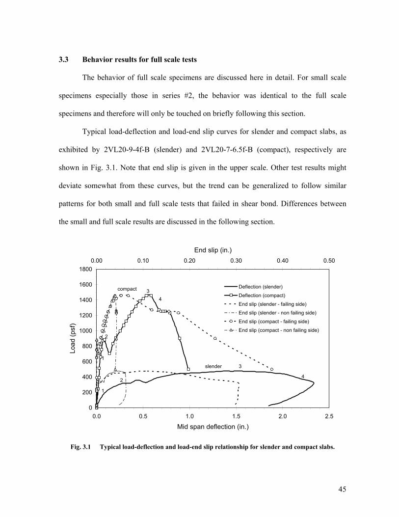
Typical load-deflection and load-end slip curves for slender and compact slabs, as

exhibited by 2VL20-9-4f-B (slender) and 2VL20-7-6.5f-B (compact), respectively are

shown in Fig. 3.1. Note that end slip is given in the upper scale. Other test results might

deviate somewhat from these curves, but the trend can be generalized to follow similar

patterns for both small and full scale tests that failed in shear bond. Differences between

the small and full scale results are discussed in the following section.

0

200

400

600

800

1000

1200

1400

1600

1800

0.0 0.5 1.0 1.5 2.0 2.5

Mid span deflection (in.)

Load

(psf

)

0.00 0.10 0.20 0.30 0.40 0.50

End slip (in.)

Deflection (slender)

Deflection (compact)

End slip (slender - failing side)

End slip (slender - non failing side)

End slip (compact - failing side)

End slip (compact - non failing side)

2

1

3

4

1

2

34

slender

compact

Fig. 3.1 Typical load-deflection and load-end slip relationship for slender and compact slabs.

46

Generally, for the full scale specimens, the concrete began to crack over the interior

support in the early stages of loading. In some cases cracks were already visible before the

load was applied. This implied that the continuity of the concrete without negative

reinforcement was not effective in providing rotational stiffness at the interior support. In

the beginning of loading, the slabs displacement responded linearly with the loads up to

level 1 of Fig. 3.1, then flexural cracks began to develop near the line loads and in the

constant moment region. Popping sounds were heard during this period indicating the

breaking of chemical bond. As the loads increased between points 1 and 2, new cracks

developed, existing ones enlarged and end slip initiated. Slender slabs developed a larger

number of vertical cracks in the constant moment region than the compact ones.

At some point during the tests, which is qualitatively indicated by point 2, the pour

stop welds at exterior ends failed and the slab end rotated and appeared to be bearing only

on the interior flange edge of the support beam. The weld failure was usually accompanied

by a loud sound and a significant reduction of slab stiffness. This failure is indicated in the

graphs by reduction of applied load and significant increment of vertical deflection. Also at

this point the end slip rate increased. On the interior support, the negative moment crack

enlarged and the slab also appeared to rotate freely. However no sign of weld failure was

observed at the interior support. Fig. 3.2(a) and (b) show typical end conditions of the slabs

at failure while Fig. 3.3(a) shows a typical crack at critical section under or near line load

as a result of shear bond failure along the shear span.

It was also observed that for the slabs that failed by shear bond, the top flange of the

deck buckled at the critical section as shown in Fig. 3.3(b). The buckling of the flange

occurred shortly after the ultimate load was attained. Typically, the buckling was

47

noticeable when the loads had reduced to point 4, after which the specimens lost composite

action and the load resistance was completely attributable to steel deck alone. For compact

slabs, the top flange buckling occurred more suddenly than the slender ones and in some

cases, was accompanied by a loud sound and abrupt formation of a hinge. As the full scale

experiments were used to substantiate the admissibility of the small scale test procedure

developed in this research, their quantitative results will be presented together with the

small scale result later in Sec. 3.6.

(a) (b)

Fig. 3.2 Typical end condition at failure (a) Exterior support (b) Interior support

Slip

(a) (b)

Fig. 3.3 Concrete cracking and flange buckling (a) Major crack due to slip failure. (b) Buckling of deck top flange

48

CrackCrack

Fig. 3.4 Typical concrete cracking after failure

At final condition, the major crack grew up to the concrete top fiber resulting in the

concrete being completely separated into two parts (Fig. 3.4). This crack behavior is

observed in all compact slabs. In slender slabs the crack also grew up to the top fiber but

the complete concrete separation was not obvious. None of the slabs had indication of

concrete crushing.

3.4 Behavior results for small scale tests – series #1 and series #2

3.4.1 Small scale series #1

All specimens in series #1 failed by shear bond with significant slips recorded at the

ends and major cracks occurring at the critical section below one of the two point loads.

Small cracks due to bending were also observed in the constant moment region. No attempt

was made to measure the vertical separation. However it was observed that the concrete

and the decks were separated vertically as a result of concrete overriding as shown in Fig.

3.5. Specimens with fewer straps, namely Specimen #13 in series #1 exhibited larger

vertical separation than those with more straps in the same series. Due to this observation,

it was decided that the frequency of straps in series #2 be increased to 4 in. interval along

49

the entire length. Test A of specimens #20 where the concrete cover was 2 in. above deck

top flange also cracked longitudinally along the shear span as shown in Fig. 3.6.

Vertical separation

(a) (b)

Fig. 3.5 Vertical separation (a) End of slab, (b) Side of slab

crack

Crack line

(a) (b)

Fig. 3.6 Longitudinal cracking of concrete along shear span for test A of specimen #20: 3VL16-8-5s-A (a) End of slab, (b) Top view

50

3.4.2 Small scale series #2

The observed behavior suggested that most small scale slabs in series #2 failed

earlier (or at lesser deflection) and were more brittle than the full scale specimens (refer

graphs in Appendix C.2). However the amount of end slips for small scale specimens were

compatible with the full scale specimens (refer graphs in Appendix C.3). The maximum

loads of the small scale specimens were comparatively similar to the maximum loads of the

full scale specimens. The magnitude of vertical separation along the sides of small scale

specimens in series #2 was generally less than that in series #1. It was also observed that

the pour stop welding in the compact specimens of series #2 failed in a sudden manner.

After this failure, which also accompanied by loud sound especially in the specimens with

2VL decks, the slabs lost their strengths also in a sudden manner. This can be seen by steep

descending lines of load-deflection graphs after reaching peak loads (refer graphs in

Appendix C.2). Compact specimens with 2VL decks lost their strengths in a more abrupt

manner than the compact specimens with 3VL decks.

3.5 Result for small scale series #1 – Factors effecting slab strength

3.5.1 Maximum loads and deflections

Maximum loads and the corresponding mid-span deflections and end slips, and the

load at first end slip of 0.02 in. for small scale series #1 are tabulated in Table 3.2. Load-

deflection graphs are given in the following sections when the effects of particular

parameters are discussed. The load-end slip relationships are compiled in Appendix C.1.

51

3.5.2 Effect of web curling

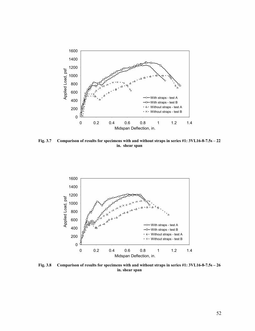
The effect of restraining the webs from curling using angle straps for small scale

specimens in series #1, which were tested at different shear spans, are illustrated in the

load-deflection graphs in Fig. 3.7, Fig. 3.8 and Fig. 3.9. The graphs show that the

strengthening of webs using angle straps significantly increased the capacity of the slabs

specimens. The average increment of the maximum loads ranged between 30% and 48%.

Table 3.2 Quantitative results of small scale series #1 tests

Test number Specimen ID Shear

span TestMaximum

Load (psf)

Mid-span deflection at

max. load (in.)

End slip at max. load

(in.)

Load at first slip (0.02 in.)

(psf) A 1250 0.796 0.187 840 13 3VL16-8-7.5 22 B 1320 0.84 0.169 760 A 1010 0.976 0.175 420 14 3VL16-8-7.5 22 B 840 0.474 0.170 480 A 1220 0.602 0.122 980 15 3VL16-8-7.5 26 B 1210 0.770 0.216 560 A 910 0.855 0.206 420 16 3VL16-8-7.5 26 B 1070 0.829 0.159 510 A 1540 0.689 0.14 1080 17 3VL16-8-7.5 30 B 1490 0.713 0.175 870 A 1000 0.922 0.193 440 18 3VL16-8-7.5 30 B 1070 0.974 0.207 550 A 1180 0.972 0.184 670 19 3VL16-8-6.5 22 B 1160 0.804 0.178 680 A 860 0.923 0.13 510 20 3VL16-8-5 22 B 850 0.946 0.162 460

52

0

200

400

600

800

1000

1200

1400

1600

0 0.2 0.4 0.6 0.8 1 1.2 1.4Midspan Deflection, in.

App

lied

Load

, psf

With straps - test AWith straps - test BWithout straps - test AWithout straps - test B

Fig. 3.7 Comparison of results for specimens with and without straps in series #1: 3VL16-8-7.5s – 22 in. shear span

0

200

400

600

800

1000

1200

1400

1600

0 0.2 0.4 0.6 0.8 1 1.2 1.4Midspan Deflection, in.

App

lied

Load

, psf

With straps - test AWith straps - test BWithout straps - test AWithout straps - test B

Fig. 3.8 Comparison of results for specimens with and without straps in series #1: 3VL16-8-7.5s – 26

in. shear span

53

0

200

400

600

800

1000

1200

1400

1600

0 0.2 0.4 0.6 0.8 1 1.2 1.4Midspan Deflection, in.

App

lied

Load

, psf

With straps - test AWith straps - test BWithout straps - test AWithout straps - test B

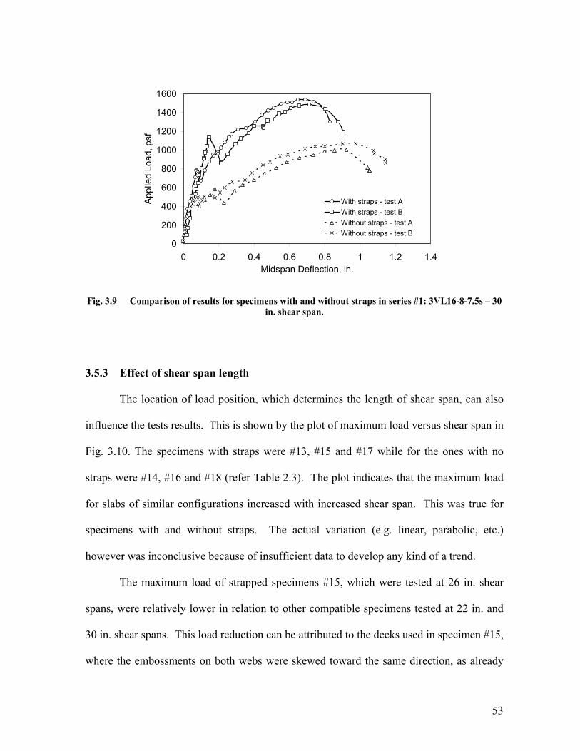
Fig. 3.9 Comparison of results for specimens with and without straps in series #1: 3VL16-8-7.5s – 30 in. shear span.

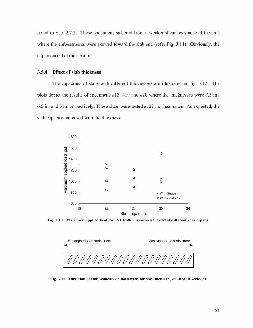
3.5.3 Effect of shear span length

The location of load position, which determines the length of shear span, can also

influence the tests results. This is shown by the plot of maximum load versus shear span in

Fig. 3.10. The specimens with straps were #13, #15 and #17 while for the ones with no

straps were #14, #16 and #18 (refer Table 2.3). The plot indicates that the maximum load

for slabs of similar configurations increased with increased shear span. This was true for

specimens with and without straps. The actual variation (e.g. linear, parabolic, etc.)

however was inconclusive because of insufficient data to develop any kind of a trend.

The maximum load of strapped specimens #15, which were tested at 26 in. shear

spans, were relatively lower in relation to other compatible specimens tested at 22 in. and

30 in. shear spans. This load reduction can be attributed to the decks used in specimen #15,

where the embossments on both webs were skewed toward the same direction, as already

54

noted in Sec. 2.7.2. These specimens suffered from a weaker shear resistance at the side

where the embossments were skewed toward the slab end (refer Fig. 3.11). Obviously, the

slip occurred at this section.

3.5.4 Effect of slab thickness

The capacities of slabs with different thicknesses are illustrated in Fig. 3.12. The

plots depict the results of specimens #13, #19 and #20 where the thicknesses were 7.5 in.,

6.5 in. and 5 in. respectively. These slabs were tested at 22 in. shear spans. As expected, the

slab capacity increased with the thickness.

600

800

1000

1200

1400

1600

1800

18 22 26 30 34Shear span, in.

Max

imum

app

lied

load

, psf

With StrapsWithout straps

Fig. 3.10 Maximum applied load for 3VL16-8-7.5s series #1 tested at different shear spans.

Weaker shear resistanceStronger shear resistance

Fig. 3.11 Direction of embossments on both webs for specimen #15, small scale series #1

55

0

200

400

600

800

1000

1200

1400

1600

0 0.2 0.4 0.6 0.8 1 1.2 1.4Midspan Deflection, in.

App

lied

Load

, psf

7.5 in. thick - Test A7.5 in. thick - Test B6.5 in. thick - Test A6.5 in. thick - Test B5 in. thick - Test A5 in. thick - Test B

Fig. 3.12 3VL16-8 slabs with variable concrete thickness

3.5.5 Effect of end constraint

End anchorage details can affect the response of composite slab tests (Easterling

and Young, 1992; Terry and Easterling, 1994). Three identical specimens from small scale

test series #2 and one full scale test configuration, namely 3VL16-8-7.5, were compared to

illustrate the effect of end anchorage. The first was specimen #17 from small scale series

#1, which was supported by roller and pin details at the ends and without pour stop (see

Sec. 2.7.2). The second specimen was #26 from small scale series #2 (see Table 2.4) where

pour stops at both ends were welded to ½ in. thick and 4 in. wide steel plates, which were

then supported on pin and roller supports. The third specimen was #27 from series #2 (see

Table 2.4) where pour stops at both ends were welded to the support beams. The last was

the compatible specimens from full scale test (specimen #5 Table 2.2) where the end detail

was similar to specimen #27 series #2.

Load-deflection graphs for these specimens are shown in Fig. 3.13. The results

show that the average maximum loads, as a ratio of the full scale slab maximum load, for

56

the first, second and third specimens are 0.69, 0.81 and 0.97 respectively. This indicated

clearly that the end details could exert a significant effect on the performance of the slab.

Furthermore, both small and full scale specimens whose end details were identical

exhibited almost equal strength even though the small scale specimens were slightly stiffer

in the beginning and failed faster than the full scale specimens.

0

400

800

1200

1600

2000

2400

0.0 0.5 1.0 1.5 2.0Midspan Deflection, in.

App

lied

load

, psf

1A - no end restraint, simply supported1B - no end restraint, simply support2A - pour stops, simply supported2B - pour stops, simply supported3A - pour stops, welded 3B - pour stosp, welded4A - full scale4B - full scale

Fig. 3.13 3VL16-8-7.5 specimens with different end constraint

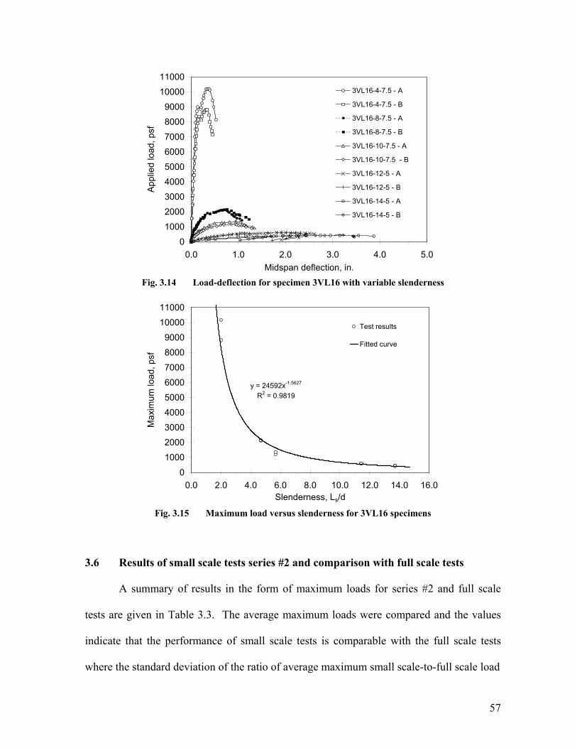
3.5.6 Effect of slab slenderness, Ls / d

Load-deflection results of specimen 3VL16-4-7.5, 3VL16-4-7.5, 3VL16-10-7.5,

3VL16-12-5 and 3VL16-14-5 from small scale series #2 are shown in Fig. 3.14 to illustrate

the pattern of slab response due to variable slenderness. The maximum loads were plotted

against slab slenderness, as shown in Fig. 3.15. The pattern of the maximum load was best

fitted with a power function as shown in the figure. The slab capacity increased

exponentially as the slenderness decreased.

57

0

1000

2000

3000

4000

5000

6000

7000

8000

9000

10000

11000

0.0 1.0 2.0 3.0 4.0 5.0Midspan deflection, in.

App

lied

load

, psf

3VL16-4-7.5 - A

3VL16-4-7.5 - B

3VL16-8-7.5 - A

3VL16-8-7.5 - B

3VL16-10-7.5 - A

3VL16-10-7.5 - B

3VL16-12-5 - A

3VL16-12-5 - B

3VL16-14-5 - A

3VL16-14-5 - B

Fig. 3.14 Load-deflection for specimen 3VL16 with variable slenderness

y = 24592x-1.5627

R2 = 0.9819

0

1000

2000

3000

4000

5000

6000

7000

8000

9000

10000

11000

0.0 2.0 4.0 6.0 8.0 10.0 12.0 14.0 16.0Slenderness, Ls/d

Max

imum

load

, psf

Test results

Fitted curve

Fig. 3.15 Maximum load versus slenderness for 3VL16 specimens

3.6 Results of small scale tests series #2 and comparison with full scale tests

A summary of results in the form of maximum loads for series #2 and full scale

tests are given in Table 3.3. The average maximum loads were compared and the values

indicate that the performance of small scale tests is comparable with the full scale tests

where the standard deviation of the ratio of average maximum small scale-to-full scale load

58

Table 3.3 Maximum load for small and full scale specimens

Full scale tests Small scale tests

Specimen ID Test Max. load (psf)

Average max. load, Wuf (psf)

Max. load (psf)

Average max. load, Wus (psf)

Wus / Wuf

A 1670 1390 3VL20-8-7.5 B 1650

1660 1370

1380 0.83

A 420 510 3VL20-11-5

B 450 435

410 460 1.06

A 1790 1490 3VL18-8-7.5

B 1840 1815

1570 1530 0.84

A 390 410 3VL18-13-5

B 390 390

420 415 1.06

A - 10170 3VL16-4-7.5

B - -

8820 9495 -

A 2140 2100 3VL16-8-7.5

B 2230 2185

2160 2130 0.97

A - 1350 3VL16-10-7.5

B - -

1190 1270 -

A - 610 3VL16-12-5

B - -

610 610 -

A 380 430 3VL16-14-5

B 410 395

440 435 1.10

A 1540 1600 2VL20-7-6.5 B 1460

1500 1480

1540 1.03

A 460 480 2VL20-9-4

B 480 470

460 470 1.00

A 1940 1830 2VL18-7-6.5

B 1790 1865

1950 1890 1.01

A 430 450 2VL18-11-4

B 470 450

450 450 1.00

A 1860 2620 2VL16-7-6.5

B 2380 2120

2390 2505 1.18

A 480 470 2VL16-12-4

B 470 475

500 485 1.02

Mean 1.01 Standard deviation 0.10

59

is 0.1 with the mean value of 1.01. Most results were within 10% difference, except for

specimen 3VL20-8-7.5s and 3VL18-8-7.5s, which were weaker than the full scale

specimens by 17%. This difference can be attributed to the full scale specimens being

tested using the airbag as already explained in Sec. 2.6.6. The uniform pressure exerted by

the airbag exerted extra clamping along the length of the slabs. The clamping restricted the

movement of the concrete during slipping which eventually resulted in stiffness behavior.

Full scale specimen 2VL16-7-6.5s was 18% stronger than full scale specimen. The

difference was particularly due to outlying results of test A of the full scale specimen

which was unexplainably weak compared to test B.

Graphs comparing the applied load versus mid-span deflection for full and small

scale series #2 specimens are presented in Appendix C.2. There was an anomalous

behavior of compact small scale specimens that deserves discussion. The graphs depict that

all compact small scale specimens were stiffer than their corresponding full scale tests in

load region below the maximum values. This behavior could be attributed to the welding of

pour stops and steel decks at both ends of the small scale specimens, which might have

provided additional resistance against rotation during the early stage of loading. In the full

scale specimens, the amount of similar resistance existed only at the exterior supports,

while at the interior supports, the continuity of the concrete was unable to provide the same

resistance against rotation. This is because at the interior support, the concrete cracked at a

very low load and the slabs were more flexible to move or rotate (refer also to discussion in

Sec. 3.3). In addition to this, the amount of welding in the small scale specimens was larger

than that in full scale specimens. In small scale specimens, two welding points per one ft

wide specimen were provided compare to seven welding points per six ft wide in full scale

60

specimens. For slender specimens, the difference of stiffness between full and small scale

specimens was insignificant because the behavior was mainly dominated by the

slenderness and deflection of the specimens rather than the end conditions.

3.7 Load-end slip results

Fig. 3.16 shows typical graphs of the load versus end slip relationship obtained

from small scale tests. The slip measured at the slab ends (location 1 as labeled in Fig.

2.19a) was of the same magnitude as the slip measured near point loads (location 2). As

such, average values were considered and plotted as representative slip along the shear

span. Load-end slip graphs for all small scale series #2 and full scale specimens are

presented in Appendix C.3. Only slips at the failure sides of the specimens are presented. It

should be noted also that for most results, slips were also recorded at the non failure ends

of the specimens but for clarity, they are not presented in these graphs.

0

200

400

600

800

1000

1200

1400

1600

0.00 0.10 0.20 0.30 0.40 0.50 0.60End slip, in.

App

lied

load

, psf

Location 1 (3VL20-11-5s - A)Location 2 (3VL20-11-5s - A)Location 1 (3VL20-8-7.5s - A)Location 2 (3VL20-8-7.5s - A)

Compact

Slender

Fig. 3.16 Typical end slip measured at location 1 (end of slab) and location 2 (near applied load) for

slender and compact slabs

61

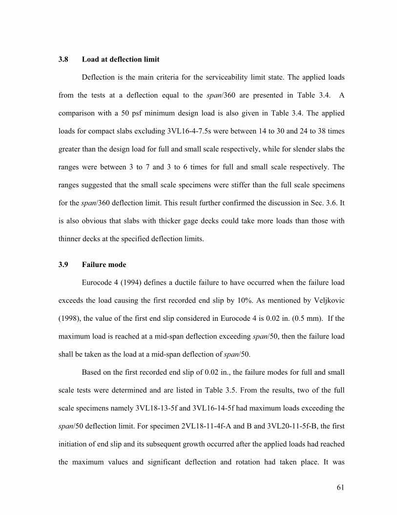
3.8 Load at deflection limit

Deflection is the main criteria for the serviceability limit state. The applied loads

from the tests at a deflection equal to the span/360 are presented in Table 3.4. A

comparison with a 50 psf minimum design load is also given in Table 3.4. The applied

loads for compact slabs excluding 3VL16-4-7.5s were between 14 to 30 and 24 to 38 times

greater than the design load for full and small scale respectively, while for slender slabs the

ranges were between 3 to 7 and 3 to 6 times for full and small scale respectively. The

ranges suggested that the small scale specimens were stiffer than the full scale specimens

for the span/360 deflection limit. This result further confirmed the discussion in Sec. 3.6. It

is also obvious that slabs with thicker gage decks could take more loads than those with

thinner decks at the specified deflection limits.

3.9 Failure mode

Eurocode 4 (1994) defines a ductile failure to have occurred when the failure load

exceeds the load causing the first recorded end slip by 10%. As mentioned by Veljkovic

(1998), the value of the first end slip considered in Eurocode 4 is 0.02 in. (0.5 mm). If the

maximum load is reached at a mid-span deflection exceeding span/50, then the failure load

shall be taken as the load at a mid-span deflection of span/50.

Based on the first recorded end slip of 0.02 in., the failure modes for full and small

scale tests were determined and are listed in Table 3.5. From the results, two of the full

scale specimens namely 3VL18-13-5f and 3VL16-14-5f had maximum loads exceeding the

span/50 deflection limit. For specimen 2VL18-11-4f-A and B and 3VL20-11-5f-B, the first

initiation of end slip and its subsequent growth occurred after the applied loads had reached

the maximum values and significant deflection and rotation had taken place. It was

62

concluded that the failure for these specimens was a combination of slip and flexure and

occurred in a ductile manner.

Table 3.4 Load at span/360 deflection limit and comparison with design load

Load at span/360 limit, Ws (psf)

Specimens Tests Full scale

tests Small

scale tests

Ws/50 full

scale

Ws/50 small scale

3VL20-8-7.5 A 850 1200 17.0 24.0 B 730 1220 14.6 24.4

3VL20-11-5 A 250 220 5.0 4.4 B 230 300 4.6 6.0

3VL18-8-7.5 A 1150 1250 23.0 25.0 B 1100 1210 22.0 24.2

3VL18-13-5 A 210 190 4.2 3.8 B 230 150 4.6 3.0

3VL16-4-7.5 A - 7800 - 156.0 B - 9000 - 180.0

3VL16-8-7.5 A 1080 1550 21.6 31.0 B 1160 1700 23.2 34.0

3VL16-10-7.5 A - 870 - 17.4 B - 1010 - 20.2

3VL16-12-5 A - 310 - 6.2 B - 300 - 6.0

3VL16-14-5 A 170 180 3.4 3.6 B 160 150 3.2 3.0

2VL20-7-6.5 A 1000 1380 20.0 27.6 B 900 1430 18.0 28.6

2VL20-9-4 A 370 210 7.4 4.2 B 310 230 6.2 4.6

2VL18-7-6.5 A 1200 1650 24.0 33.0 B 1150 1700 23.0 34.0

2VL18-11-4 A 260 230 5.2 4.6 B 240 260 4.8 5.2

2VL16-7-6.5 A 1490 1900 29.8 38.0 B 1500 1900 30.0 38.0

2VL16-12-4 A 240 180 4.8 3.6 B 220 170 4.4 3.4

63

Table 3.5 Failure mode of the specimens

Full scale tests Small scale tests

Specimens Span Failure load, Wuf

(psf)

Load at 1st

slip, Ws (psf)

Wuf/WsFailure mode

Failure load, Wus

(psf)

Load at 1st slip, Ws

(psf) Wus/Ws

Failure mode

A 1670 1400 1.19 Ductile 1390 1150 1.21 Ductile3VL20-8-7.5 B 1650 1300 1.27 Ductile 1370 1100 1.25 DuctileA 420 310 1.35 Ductile 510 350 1.46 Ductile

3VL20-11-5 B 450 - - Ductile 410 320 1.28 DuctileA 1790 1200 1.49 Ductile 1490 1170 1.27 Ductile

3VL18-8-7.5 B 1840 1060 1.74 Ductile 1570 1220 1.29 DuctileA 390 290 1.34 Ductile 410 350 1.17 Ductile

3VL18-13-5 B 390 290 1.34 Ductile 420 270 1.56 DuctileA - - - - 10170 8900 1.14 Ductile

3VL16-4-7.5 B - - - - 8820 7000 1.26 DuctileA 2140 1450 1.48 Ductile 2100 1590 1.32 Ductile

3VL16-8-7.5 B 2230 1350 1.65 Ductile 2160 1520 1.42 DuctileA - - - - 1350 1030 1.31 Ductile

3VL16-10-7.5 B - - - - 1190 830 1.43 DuctileA - - - - 610 500 1.22 Ductile

3VL16-12-5 B - - - - 610 510 1.20 DuctileA 380 280 1.36 Ductile 430 370 1.16 Ductile

3VL16-14-5 B 410 330 1.24 Ductile 440 160 2.75 Ductile

A 1540 1200 1.28 Ductile 1600 1400 1.14 Ductile2VL20-7-6.5 B 1460 1100 1.33 Ductile 1480 1220 1.21 DuctileA 460 350 1.31 Ductile 480 330 1.45 Ductile

2VL20-9-4 B 480 380 1.26 Ductile 460 420 1.10 DuctileA 1940 1200 1.62 Ductile 1830 1420 1.29 Ductile

2VL18-7-6.5 B 1790 1200 1.49 Ductile 1950 1730 1.13 DuctileA 430 - - Ductile 450 280 1.61 Ductile

2VL18-11-4 B 470 - - Ductile 450 360 1.25 DuctileA 1860 1800 1.03 Brittle 2620 2500 1.05 Brittle

2VL16-7-6.5 B 2380 1900 1.25 Ductile 2390 1900 1.26 DuctileA 480 420 1.14 Ductile 470 350 1.34 Ductile

2VL16-12-4 B 470 350 1.34 Ductile 500 280 1.79 Ductile

64

Other specimens including all small scale tests failed by shear bond but also

exhibited ductile behavior, except for 2VL16-7-6.5f-A and 2VL16-7-6.5s-A which,

according to the definition, failed in the brittle manner. It is suspected that these particular

specimens had undetected imperfections because their results differed too greatly, and

unexplainably, from the compatible specimens.

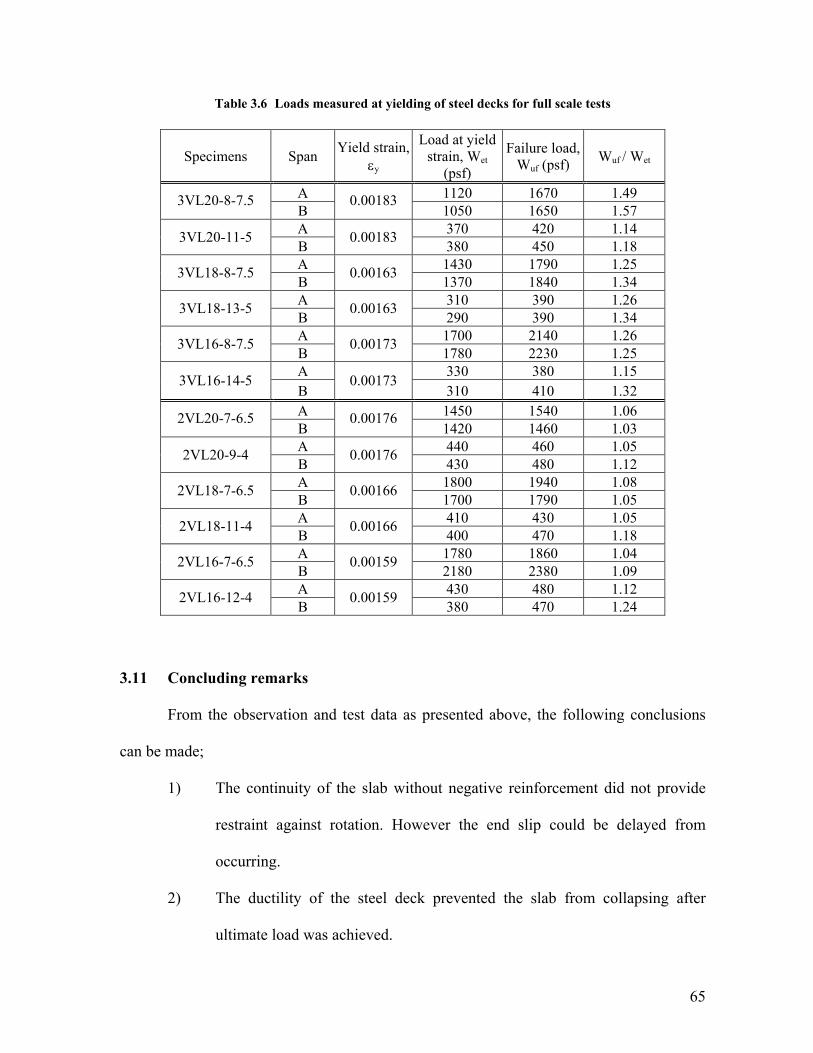
3.10 Strain gage results for full scale specimens

It was not possible to observe yielding during the tests. For yielding measurement it

was assumed here that the deck began to yield at the strain, εy = Fy / Es where Fy is the deck

yield stresses obtained from coupon tests and Es is the modulus of elasticity taken as 29500

ksi. At this strain value, the corresponding yield loads were read from the load-strain plots

at mid-span and the values are presented in Table 3.6. For all full scale specimens,

yielding of steel decks was observed at the bottom flanges. The top flange strains did not

undergo tension yielding because the strains reduced after slip occurred. This slip resulted

in the formation of double neutral axes, one for the partially composite action and the other

was for the remaining strength of the deck.

65

Table 3.6 Loads measured at yielding of steel decks for full scale tests

Specimens Span Yield strain, εy

Load at yield strain, Wet

(psf)

Failure load, Wuf (psf) Wuf / Wet

A 1120 1670 1.49 3VL20-8-7.5 B

0.00183 1050 1650 1.57

A 370 420 1.14 3VL20-11-5 B 0.00183 380 450 1.18 A 1430 1790 1.25 3VL18-8-7.5 B 0.00163 1370 1840 1.34 A 310 390 1.26 3VL18-13-5 B 0.00163 290 390 1.34 A 1700 2140 1.26 3VL16-8-7.5 B 0.00173 1780 2230 1.25 A 330 380 1.15 3VL16-14-5 B

0.00173 310 410 1.32

A 1450 1540 1.06 2VL20-7-6.5 B

0.00176 1420 1460 1.03

A 440 460 1.05 2VL20-9-4 B 0.00176 430 480 1.12 A 1800 1940 1.08 2VL18-7-6.5 B 0.00166 1700 1790 1.05 A 410 430 1.05 2VL18-11-4 B 0.00166 400 470 1.18 A 1780 1860 1.04 2VL16-7-6.5 B 0.00159 2180 2380 1.09 A 430 480 1.12 2VL16-12-4 B 0.00159 380 470 1.24

3.11 Concluding remarks

From the observation and test data as presented above, the following conclusions

can be made;

1) The continuity of the slab without negative reinforcement did not provide

restraint against rotation. However the end slip could be delayed from

occurring.

2) The ductility of the steel deck prevented the slab from collapsing after

ultimate load was achieved.

66

3) When the slab failed by shear bond, the concrete slipped along the shear

span causing cracking at the critical section. The crack grew until top fiber.

The concrete did not fail by crushing.

4) Relative slip can be assumed uniform along the shear span.

5) Slabs with relatively shallow deck failed more abruptly in a more brittle

fashion than with deeper decks.

6) Edge curling had a significant influence on the slab strength and behavior.

Angle straps can provide sufficient restraint to the edge web, thus enabling

small scale specimens to behave in a manner similar to full scale specimens.

7) Concrete thickness, embossment orientation, end anchorage and support

type affect the response and behavior of small scale specimens. Concrete

cover that is too thin may result in longitudinal cracking along the shear

span. Embossments on opposite webs that are oriented in the same direction

can weaken the slab specimen. Specimens anchored with pour stops welded

to fixed supports were stronger than those bearing on the simple supports.

8) Thickness and shear span influenced the slab capacity significantly.

9) Slender slabs sustained load at least three times larger than the load at a

deflection equal to span/360. Compact slabs sustained load approximately

20 times the load reached at a deflection of span/360.

10) All specimens except one exhibited ductile failure.

11) Strain gage readings indicated that the steel deck bottom flange yielded at a

load below the ultimate load.

67

12) With sufficient number of angle straps and with compatible end condition,

the small scale specimen developed in this experimental study can be used

as an alternative to the full scale specimen.

68

4 Analytical methods

4.1 Introduction

It has been recognized that the mechanism of horizontal shear resistance between

the steel deck and the concrete in composite slabs is complex. Because of the complexity,

it is not possible to develop an analytical method that is suitable for all slab conditions

without using data from tests. Because of the need for test data, it is imperative to develop

an efficient, simple and economical testing method such as the one developed in this

research. In addition to being simple and cost effective, the test must more importantly

produce data that is suitable for use with analytical methods in all conditions. Otherwise

the testing method itself will have less practical value. This chapter deals with putting the

small scale test data into practical use.

4.2 Objective

The main objective of this portion of the research was to verify that the small scale

test procedure developed and presented in the previous chapters is an admissible tool for

use in the design of composite slabs. The most established design methods to date, namely

the m-k (ASCE, 1992; BS-5950, 1994; Eurocode 4, 1994) and the PSC (Eurocode 4 1994)

methods, were chosen for this study. The second objective was to develop a procedure for

calculating a shear bond stress versus slip relationship from the same test for use in

modeling the slab using the FE method. In doing so, two calculation procedures were

69

proposed, namely the work method and the force equilibrium method. By introducing these

procedures the practical use of the small scale test can be diversified.

In the following sections, methods of analysis available in the literature are briefly

reviewed. Then the m-k and the PSC methods are discussed in detail. After that, the work

method and force equilibrium method are presented. Small scale test data obtained in the

previous chapter are then analyzed with these methods and the results are compared. The

application of the shear bond stress-slip property in the FE analysis is studied in the next

chapter.

4.3 Review of the analysis and design methods

4.3.1 The shear bond (m-k) method

The first standard method for composite slab design that is widely accepted and has

been implemented in many specifications around the world is the shear bond method. The

development of this method began from the work of Schuster (1970) and later was

improved by Porter et al. (1976), Porter and Ekberg (1971, 1975a, 1975b). This method

uses full scale test data where the slab shear strength is related linearly with the slab

geometry. The linear equation uses m and k as variables for the slope and intercept, hence

they became the name for the method. Because of its accuracy and simplicity the m-k

method was chosen for analyzing the small scale test data developed in this research. The

m-k method according to (ASCE, 1992) and (Eurocode 4, 1994) are presented in detail in

the Sec. 4.4.

The major drawback of the m-k method is that it is semi-empirical, in that it does

not provide a clear mechanical model that can separate factors that contribute to the

performance of the composite slabs. These factors include shear bond strength, end

70

anchorage, frictional force at supports and additional reinforcements. The m-k method

depends heavily on full scale test data in which different series of full-scale tests are

needed for each new sheeting profile, sheeting thickness, embossment type, end anchorage,

etc. This design process is costly, tedious and less than desirable to deck manufacturers

because prototypes of all new products have to be built and tested at full-scale before the

profile can be evaluated. Additional drawbacks associated with the lack of a mechanical

model are discussed by Bode and Sauerborn (1992).

4.3.2 The Partial Shear Connection (PSC) method

To overcome the deficiencies of the m-k method, especially the lack of a

mechanical model that reflects the influence of composite slab parameters, and to reduce

dependency on full scale tests, researchers in Europe developed the partial shear

connection (PSC) method. This method was first proposed by Stark (1978) and

subsequently improved by Stark and Brekelmans (1990), Bode and Sauerborn (1992),

Bode et al. (1996), and Bode and Dauwel (1999). The method was adopted in Annex E of

Eurocode 4 (1994) as an alternative to the m-k method. It became part of the Eurocode 4

design specification in the newer edition (Eurocode 4, 2001). Because the PSC method

uses a sound mechanical model and has potential for inclusion into the ASCE specification

(ASCE, 1992), it was also chosen for analyzing the small scale test data developed in this

research. Details of the PSC method are given in Sec. 4.5.

4.3.3 Other methods

Research at West Virginia University resulted in an empirical approach to calculate

the bending strength for composite slabs (Luttrell and Davidson, 1973; Luttrell and

Prasannan, 1984; Luttrell, 1986). It was implemented in Appendix D of the ASCE (1992)

71

standard as a complement to the m-k method discussed earlier. In this method, the

theoretical bending moment capacity of the slab is calculated based on the assumption that

the deck bottom flange yields. The first yield moment is modified by coefficients that are a

function of the shear transfer anchorage forces that developed along the shear span. The

modification factors were empirically based, hence the application is limited to certain

types of deck profiles and embossments. Experimental work reported on trapezoidal

profiles with embossment sizes and patterns outside the prescribed limits gave satisfactory

results when calculated using this method (Shen, 2001). On the other hand, Wright and

Evans (1990) reported that the method did not provide acceptable results for slabs

constructed with deck profiles available in the United Kingdom. Despite producing less

accurate results, this method is still useful especially for predicting the slab strength during

product development and for predicting maximum load before the actual test is carried out.

Research done at the University of Waterloo resulted in another empirical equation

for predicting the strength of composite slabs that fail by shear bond (Seleim, 1979; Seleim

and Schuster, 1985). The equation, which requires multi linear regression analysis, is based

on experimental evidence of composite slabs exhibiting early end slip prior to ultimate load

and it contains steel deck thickness as a parameter. The authors indicate that the presence

of the steel deck thickness parameter can result in a reduction of up to 75% of the required

number of laboratory performance tests. The method is incorporated in the CSSBI (1996)

design specification.

An alternative formulation to predict the strength of composite slabs for design

purposes is reported by Heagler et al. (1991). The method uses a traditional reinforced

concrete flexural model and also includes the influence of shear stud strength at the slab

72

ends. Linear interpolation can be made between the value for full nominal moment

capacity (completely studded slab) and first yield moment capacity (non studded slab) for

slabs having insufficient number of shear studs (Terry and Easterling, 1994). The method

does not directly consider or account for the behavior of the interface between the steel

deck and the concrete.

Patrick (1990) developed a method for design of composite slabs that does not

require full-scale slab tests. The method uses the average mechanical interlocking (shear

bond) and friction at the support and is applicable only to ductile behavior. The shear

resistance parameters are obtained from slip block test as discussed in Sec. 2.3.6. By

inclusion of the friction force at the support, the calculated slab strength is increased. The

advantage of Patrick’s approach is that the interface property was obtained through

elemental tests instead of full-scale performance tests. This could significantly reduce the

product development cost. However the method requires moment curvature analysis,

which has to be performed at small discretized layers of the slab section under varying load

levels and at small intervals along the length of the slab to generate a moment envelope for

use in design. This requires a lot of computer programming effort, without which the

method is rendered impractical for regular practice.

Another method of design was proposed by Veljkovic (1996b). The method uses

three parameters, namely, the mechanical interlocking resistance, coefficient of friction,

and a reduction function for mechanical interlocking due to high strain in the sheeting.

These parameters are obtained from elemental tests (see Sec. 2.3.9) hence the method is

called the Three Parameters Partial Connection Strength Method (3P PCSM). Using these

parameters a FE analysis is performed on slabs with variable slenderness. Regression

73

analysis is then carried out on the FE results to obtain two correction functions. The first

function accounts for the difference between the real distribution of stress in the concrete

and the assumed rectangular stress block in the analysis (uncertainty in lever arm and

tensile force). The second function accounts for the difference between the real (non-

uniform) distribution of longitudinal shear stress at the sheeting and concrete interface and

the assumed uniform distribution in the analysis. All parameters obtained from the

elemental tests and the correction functions obtained from the FE analysis are then used in

a design equation for calculating the slab strength, expressed in terms of reaction force.

Compared to the Eurocode’s PSC method, the results from this procedure showed a better

agreement with the m-k method. The design equation was simple to use, however because

the design parameters have to be derived from elemental tests and FE analysis, the method

is cumbersome for use in design practice.

In a subsequent study, Veljkovic (1998, 2000) found that the longitudinal shear

resistance of the slab increased as the loading became more uniform. The increment of the

resistance with respect to 2-point loading was 20%, 30% and 40% for 4-point, 8-point and

16-point loading respectively. To account for the influence of the load arrangement and the

distribution of horizontal shear when the connection becomes less ductile, he modified the

3P PCSM method. The modified method uses a new concept called transfer length, which

is defined as the length between the section of maximum bending moment and the support.

The transfer length needed to cause yielding of the sheeting together with the resistance

produced by the friction force at the support are used to construct the moment resistance

envelope, from which the slab design can be done. Veljkovic indicated that this method is

suitable for both ductile and brittle shear connection.

74

Other methods for calculating the strength of composite slabs can be found in the

literature (Plooksawasdi, 1977; Wright and Evans, 1990; Widjaja and Easterling, 1996;

Widjaja, 1997; Schumacher et al., 2000; Crisinel and Marimon, 2003). None of these

methods are developed further in this research.

4.4 Details of the m-k method

In the m-k method, the strength of a composite slab, which is measured by an

applied shear force, is related to the geometry of the slab by Eq. 4.1 (ASCE, 1992);

' ' 'e

ct i ct

V m d kbd f l f

ρ= + (4.1)

where

Ve = maximum experimental shear at failure obtained from full scale slab tests

(not including weight of slab)

b = unit width of slab

d = effective slab depth measured from extreme concrete compression fiber to

the centroidal axis of full cross section of steel deck

m = slope of reduced experimental shear-bond line

ρ = ratio of steel deck area to effective concrete area, sAbd

k = ordinate intercept of reduced experimental shear-bond line

l’i = length of shear span in inches;

f’ct = compressive test cylinder strength of concrete at time of slab testing.

75

The values of m and k, which represent the shear bond characteristics of a particular

deck profile, are determined from a series of full-scale tests, where the test results are

plotted with '

e

ct

Vbd f

on the y-axis and ' 'i ct

dl f

ρ on the x-axis as shown in Fig. 4.1.

Region A

Region B

m

k

Regression line

Reduced regression line

'e

ct

Vbd f

' 'i ct

dl f

ρ

Fig. 4.1 Typical shear bond plot showing the regression line for m and k

Once the test results for Region A (slender specimens) and Region B (compact

specimens) are obtained, a linear regression is performed on the data and the m and k

values are obtained. For design purpose the slope and intercept are reduced as shown. The

ASCE (1992) specifies the reduction of 10% or 15% depending on the number of tests. The

reduction is to account for test variations and also to assure that the line approaches a lower

bound for experimental values and is therefore somewhat conservative. To obtain reliable

data, a minimum of two specimens each for Region A and B are suggested by the ASCE

(1992) but three each are more recommended. Porter and Ekberg (1976) suggested using

76

data points from at least eight tests of each deck thickness and product type while the BS

5950 (1994) and Eurocode 4 (1994) suggest six tests.

To design other slabs whose length and thickness fall between the two test regions

the m and k values are applied into Eq. 4.2;

'' 2

s fn c

i

W lm dV bd k fl

γρ⎡ ⎤⎛ ⎞Φ = Φ + +⎢ ⎥⎜ ⎟

⎝ ⎠⎣ ⎦ (4.2)

where,

Φ = strength reduction factor

Vn = nominal shear bond strength, lbs per ft of width

f’c = specified compressive strength of concrete, psi

γ = coefficient for proportion of dead load added upon removal of shore

Ws = weight of slab

lf = length of span or shored span, ft. The last term in the equation is to account

for the shoring load if applicable.

Eurocode 4 omits the concrete strength from the equations because it may give

unsatisfactory values for m and k if the concrete strength varies widely within a series of

tests (Johnson, 1994). Many researchers have reported that the concrete strength does not

have a significant effect on the slab capacity (Seleim and Schuster, 1985; Luttrell, 1987;

Daniels, 1988; Bode and Sauerborn, 1992; Veljkovic, 1994). Eurocode 4 does not include

the shoring removal term as in Eq. (4.2) but specifies that the slab shall be cast on “full

prop.” The m-k equation according to Eurocode 4 (2001) is;

77

s

s

AV m kbd bL

⎛ ⎞= +⎜ ⎟

⎝ ⎠ (4.3)

where,

Ls = shear span length, and other variables are similar to Eq. 4.1.

4.5 Details of the PSC method

In the PSC method the slab is assumed to fail in horizontal shear where the concrete

can slip relative to the steel deck considerably without losing the load carrying capacity. In

other word, the horizontal shear stress at the slip surface remains constant. This assumption

requires a ductile shear failure.

The procedure for the PSC method begins with generating a theoretical partial

interaction curve of .p Rm

MM

versus η as typically shown in Fig. 4.2(a). The calculations for

the curve are made using measured dimensions and strength of concrete and steel

components. The x-axis of the partial interaction curve, η , is the degree of interaction, for

which the values are chosen at fixed intervals from 0 to 1. The moment resistance of

composite slabs under partial interaction is denoted by M, while Mp.Rm is the moment

resistance of composite slabs under full interaction.

78

B

(b)

fyp fyp

0.85fcm

Nc

A

fyp fyp

Mpr

C

Ncf

0.85fcm

fyp

x a

A

B

C

(a)

1.0ηtest

12

3

1.0

Mp, Rm

Mtest

Ncf

Nc=η

Mp, Rm

M

Fig. 4.2 Partial shear connection method

(a) Partial interaction curve, (b) Stress distributions at points A, B and C (Eurocode, 1994)

Points A and C in the curve of Fig. 4.2(a) are two extreme cases corresponding to

no interaction and full interaction where M = 0 and M = Mp.Rm respectively and the

corresponding stress blocks are depicted in Fig. 4.2(a) and (c). The partial interaction state

lies in between these two points, such as at point B where M is calculated following the

stress block of Fig. 4.2(b);

c prM N z M= + (4.4)

where,

79

Nc = concrete compressive force under partial interaction

z = moment arm whose value depends on the degree of shear connection

Mpr = reduced moment capacity of the steel deck

The concrete compressive force under partial interaction is a fraction of the

concrete compressive force under full interaction, Ncf and the amount depends on the

degree of interaction;

c cfN Nη= (4.5)

The moment arm of Eq. 4.4 is;

0.5 ( )t p pz h x e e e η= − − + − (4.6)

where

ht = total slab thickness.

x = depth of concrete compressive zone.

ep = distance from the plastic neutral axis of the steel deck to its extreme bottom

fiber.

e = distance from the centroid of the effective area of the sheeting to its extreme

bottom fiber.

The steel deck assumes dual functions under partial composite interaction. First, it

serves as tension reinforcement in composite action, which is already considered in the first

term of Eq. 4.4. Second it serves as an independent bending element where the deck bends

about its own axis. The bending capacity however is reduced from the full capacity

depending on the amount of composite action. The reduced moment, Mpr, is calculated by;

80

[ ]1.25 1pr pa paM M Mη= − ≤ (4.7)

where,

Mpa = plastic moment of the effective cross section of the steel deck.

The depth of concrete compressive zone, x in Eq. 4.6 is given by;

(0.85 )c

ccm

Nx hb f

= ≤ (4.8)

where,

b = width of slab

fcm = concrete compressive strength

hc = thickness of concrete cover above the steel deck.

Mp.Rm in the y-axis of partial interaction curve is the moment resistance of

composite slabs under full interaction. It is given by;

( 0.5 )pRm cf pM N d a= − (4.9)

where,

dp = effective depth of the slab

a = depth of concrete compressive zone at full interaction, 0.85

p yp

cm

A fa

f b=

Ncf in Eq. 4.5 and 4.9 is the concrete compressive force for full interaction;

cf p ypN A f= (4.10)

where,

Ap = effective area of the steel deck

fyp = yield strength of the steel sheeting.

81

Equation 4.4 to 4.10 are applicable to under reinforced sections where the neutral

axis lies in the concrete, which is the case for shallow depth profiles.

The next step is obtaining the degree of interaction from the partial interaction

curve just plotted. In this step, full scale tests are required from which the maximum

bending moment, Mtest is obtained. Using Mtest, the degree of interaction ηtest is read from

the curve as shown by path 1-2-3 in Fig. 4.2(a). Knowing the degree of interaction the

ultimate shear stress, τu can now be calculated;

0( )test cf

us

Nb L Lη

τ =+

(4.11)

where,

Ls = shear span length

Lo = overhanging length beyond support

To satisfy the required level of confidence, Eurocode 4 suggests at least six full

scale tests be performed to obtain the characteristic value of shear strength, τu.Rk. Eurocode

4 allows for taking the minimum value of all tests, reduced by 10%. The design strength of

the shear connection, τu.Rd is then obtained by dividing the characteristic strength with the

partial safety factor, γv;

..

u Rku Rd

v

ττγ

= (4.12)

Once the design shear strength is known, the design partial interaction curve or

more exactly the design moment envelope for the particular deck profile can be drawn

using Eq. 4.13 through 4.18 given below. The plot is illustrated in Fig. 4.3.

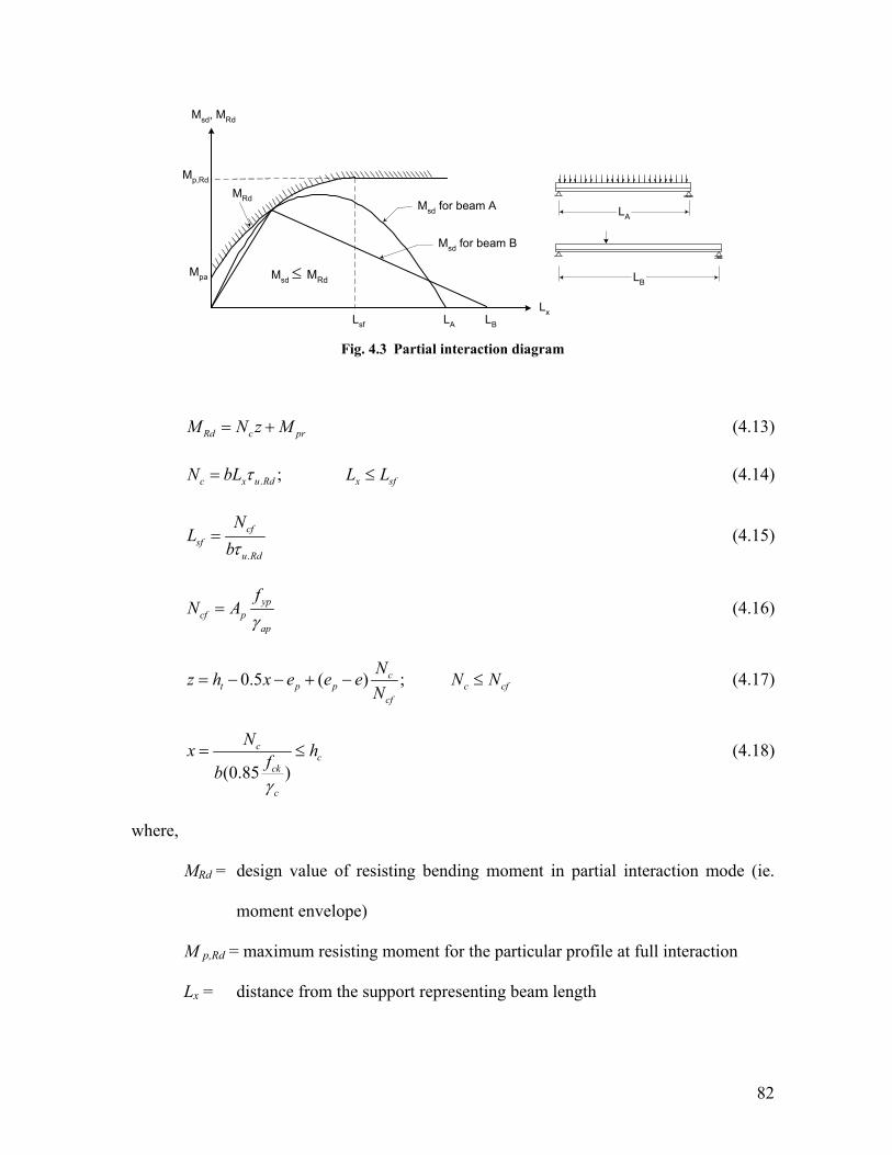
82

Lsf LA LB

Msd, MRd

Mp,Rd

Mpa Msd ≤ MRd

MRdMsd for beam A

Msd for beam B

Lx

LA

LB

Fig. 4.3 Partial interaction diagram

Rd c prM N z M= + (4.13)

. ;c x u Rd x sfN bL L Lτ= ≤ (4.14)

.

cfsf

u Rd

NL

bτ= (4.15)

ypcf p

ap

fN A

γ= (4.16)

0.5 ( ) ;ct p p c cf

cf

Nz h x e e e N NN

= − − + − ≤ (4.17)

(0.85 )

cc

ck

c

Nx hfbγ

= ≤ (4.18)

where,

MRd = design value of resisting bending moment in partial interaction mode (ie.

moment envelope)

M p,Rd = maximum resisting moment for the particular profile at full interaction

Lx = distance from the support representing beam length

83

Lsf = shear span length required for full shear connection

γv = partial safety factor for full shear resistance

γap = partial safety factor for profile steel sheeting

γc = partial safety factor for concrete

fck = characteristic compressive strength of concrete, and other variables are as

defined before.

The design partial interaction curve is independent of loading type and magnitude.

Hence, the allowable load for beams, such as those shown in Fig. 4.3, can be determined

easily by plotting the applied moment diagram below or just touching the envelope of the

design curve. One advantage of the PSC method is that it is based on a clear mechanical

model where the effect of other parameters such as end anchorage, additional

reinforcement and friction at the support can be incorporated separately in the equations.

The use of plastic design for continuous composite slabs is also possible (Bode and

Dauwel, 1999, Bode et al., 1996).

A procedure to incorporate the effects of end anchorage, frictional interlock and

mechanical interlock for use in the PSC method was proposed by Calixto et al. (1998).

They suggested plotting test data using ( )

ut

s o

Vb L L+

for the x-axis and τu = ( )cf

s o

Nb L L

η+

for the

y-axis and then obtaining the regression line. The equation is,

( ) ( )cf ut

ums o s o

N Vb L L b L L

η µτ= ++ +

(4.19)

where,

τum = mechanical shear bond strength

84

µ = friction coefficient given by the intercept and the slope of the regression

line. This method showed a much better correlation with the test data when

compared to the Eurocode’s method.

4.6 Proposed method for calculating shear stress from small scale test

In this section, two approaches, namely the work method and the force equilibrium

method for calculating shear bond stress history along the shear span and its relation with

the end slip, are presented. Because the methods are based on slab bending, they can be

applied to both full and small scale bending tests as long as the test are conducted

according to the same test procedure. The shear bond-slip relationship is useful for

numerical modeling while the maximum shear stress value can be used in other analytical

methods, such as the PSC method, for design.

4.6.1 Work method

The principle of the work method used for composite slab analysis was presented

by Wright and Evans (1990). They referred to it as the plastic collapse method. In this

procedure, the calculation is made for an ultimate condition where the concrete crack has

propagated up to the top fiber at the critical section. The shear bond stress value obtained

by the plastic collapse method is therefore a single point at the ultimate load condition. An

(1993) used the work method for calculating shear bond stress history from block bending

tests (Sec. 2.3.8) but without considering the remaining strength of the steel deck. The

method to calculate the shear bond stress history, which considers the remaining strength of

the steel deck is described here forth.

The method was derived based on the following assumptions;

85

1) The relative slip is uniform along the shear span as shown by the test results

presented in Sec. 3.7.

2) Slip is only dominant at one end while at the non-failing end, slip is small

and negligible.

3) Distribution of horizontal shear stress is uniform along the shear span.

4) Small displacement theory is valid.

5) The curvatures of both concrete and steel deck are equal.

6) Due to slip, two neutral axes exist and therefore the steel deck is always

taking a fraction of load by bending about its own axis.

7) The work done by the shear bond force can be calculated only after the slip

has occurred. Before that the shear force is assumed to increase linearly

from zero to the value calculated at the first end slip. For this purpose the

first end slip is considered as 0.02 in.

8) Steel deck is assumed to behave elastically up to the maximum load.

Fig. 4.4 shows typical plots of applied load versus slip from bending tests and Fig.

4.5 is the slab in the cracked condition. Consider at any instance during the test after first

end slip has taken place, the external work done by the applied load from instant i-1 to i

can be written as,

( ) ( )

( )

1 11 1 2 2

11 2 1 2

11 2

2 4 2 4

2 4

2 4

i i i ie i i i i

i ii i i i

i ii i

P P P PW

P P

P P

δ δ δ δ

δ δ δ δ

δ δ

− −

−

−

∆ ∆= ∆ + ∆ + ∆ + ∆

∆= ∆ + ∆ + ∆ + ∆

∆⎛ ⎞= + ∆ + ∆⎜ ⎟⎝ ⎠

(4.20)

where,

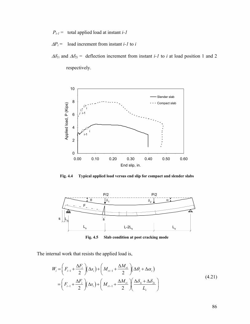
86

Pi-1 = total applied load at instant i-1

∆Pi = load increment from instant i-1 to i

∆δ1i and ∆δ2i = deflection increment from instant i-1 to i at load position 1 and 2

respectively.

0

2

4

6

8

10

0.00 0.10 0.20 0.30 0.40 0.50 0.60End slip, in.

App

lied

load

, P (K

ips)

Slender slab

Compact slab

i-1i

i-1i

Fig. 4.4 Typical applied load versus end slip for compact and slender slabs

δ1

Ls Ls

Los

δ2F

L-2Ls

P/2P/2

s

θ α

Fig. 4.5 Slab condition at post cracking mode

The internal work that resists the applied load is,

( ) ( )

( )

1 1

1 21 1

2 2

2 2

i rii i i ri i i

i ri i ii i ri

s

F MW F s M

F MF s ML

θ α

δ δ

− −

− −

∆ ∆⎛ ⎞ ⎛ ⎞= + ∆ + + ∆ + ∆⎜ ⎟ ⎜ ⎟⎝ ⎠ ⎝ ⎠

⎛ ⎞∆ ∆ ∆ + ∆⎛ ⎞ ⎛ ⎞= + ∆ + + ⎜ ⎟⎜ ⎟ ⎜ ⎟⎝ ⎠ ⎝ ⎠⎝ ⎠

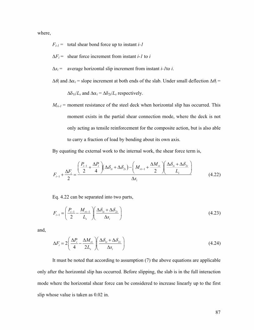
(4.21)

87

where,

Fi-1 = total shear bond force up to instant i-1

∆Fi = shear force increment from instant i-1 to i

∆si = average horizontal slip increment from instant i-1to i.

∆θi and ∆αi = slope increment at both ends of the slab. Under small deflection ∆θi =

∆δ1i/Ls and ∆αi = ∆δ2i/Ls respectively.

Mri-1 = moment resistance of the steel deck when horizontal slip has occurred. This

moment exists in the partial shear connection mode, where the deck is not

only acting as tensile reinforcement for the composite action, but is also able

to carry a fraction of load by bending about its own axis.

By equating the external work to the internal work, the shear force term is,

( )1 1 21 2 1

1

2 4 22

i i ri i ii i ri

sii

i

P P MMLFF

s

δ δδ δ−−

−

⎛ ⎞∆ ∆ ∆ + ∆⎛ ⎞ ⎛ ⎞+ ∆ + ∆ − + ⎜ ⎟⎜ ⎟ ⎜ ⎟∆ ⎝ ⎠ ⎝ ⎠⎝ ⎠+ =∆

(4.22)

Eq. 4.22 can be separated into two parts,

1 1 1 21 2

i ri i ii

s i

P MFL s

δ δ− −−

⎛ ⎞⎛ ⎞∆ + ∆= −⎜ ⎟⎜ ⎟∆⎝ ⎠⎝ ⎠

(4.23)

and,

1 224 2

i ri i ii

s i

P MFL s

δ δ⎛ ⎞⎛ ⎞∆ ∆ ∆ + ∆∆ = −⎜ ⎟⎜ ⎟∆⎝ ⎠⎝ ⎠

(4.24)

It must be noted that according to assumption (7) the above equations are applicable

only after the horizontal slip has occurred. Before slipping, the slab is in the full interaction

mode where the horizontal shear force can be considered to increase linearly up to the first

slip whose value is taken as 0.02 in.

88

Therefore the limit of end slip is,

0.02is∆ ≥ (4.25)

From Eq. 4.23 and4.24, the shear bond force at instance i can be determined,

1i i iF F F−= + ∆ (4.26 )

Because the deck is assumed elastic up to the maximum load, moment can be

related to the curvature by,

1

s s

ME I R

= (4.27)

where,

Is = moment of inertia of steel deck

Es = modulus of elasticity of steel deck

R = radius of curvature

M = bending moment

The above equation is approximate, as full scale test results presented in Sec. 3.8

indicated that yielding did occur in the deck bottom flange before the maximum load was

reached.

It can be shown from the geometry of Fig. 4.6 that,

1 1 1

1

12

ri i i

s s i s

ME I R L L

θ α− − −

−

+= =

− (4.28)

and,

( )1

1 12

ri i i

s s i i s

ME I R R L L

θ α

−

⎛ ⎞∆ ∆ + ∆= − =⎜ ⎟ −⎝ ⎠

(4.29)

Substituting 1 1 1 2 11 1, ,i i i

i i is s sL L L

δ δ δθ θ α− −− −

∆= ∆ = = and 2i

isL

δα ∆∆ = into Eq. 4.28 and

Eq.4.29, the bending moment terms of Eq. 4.23 and 4.24 are,

89

( )( )

1 1 2 11 2

i iri s s

s s

M E IL L Lδ δ− −

−

+=

− (4.30)

and,

( )1 2

2i i

ri s ss s

M E IL L L

δ δ∆ + ∆∆ =

− (4.31)

δ1 δ2θ

R

LsLs

L

θ

α

P/2 P/2

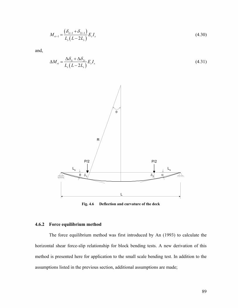
Fig. 4.6 Deflection and curvature of the deck

4.6.2 Force equilibrium method

The force equilibrium method was first introduced by An (1993) to calculate the

horizontal shear force-slip relationship for block bending tests. A new derivation of this

method is presented here for application to the small scale bending test. In addition to the

assumptions listed in the previous section, additional assumptions are made;

90

1) Plane section remains plane (no shear deformation).

2) Concrete stress in tension is neglected.

3) The neutral axis of the composite section is less than the concrete cover

above the deck top flange. Otherwise the neutral axis is considered equal to

the concrete depth. This assumption is made based on the observation

during the tests that the concrete failed primarily by cracking and the crack

tips were always above the deck top flanges.

4) As observed in the test the concrete in compression did not fail by crushing.

A major crack was dominant at the critical section where it progressed

upward as the end slip increased. The stress-strain behavior of concrete in

compression and steel deck in tension is therefore considered linear until the

maximum load is obtained.

5) The steel deck section is fully effective.

Fig. 4.7(a) shows the free body diagram of the section of a test specimen at failure,

and Fig. 4.7(b) and Fig. 4.7(c) are the corresponding strain and internal force distributions

at the critical sections. At any instance during the test, the horizontal shear force Fi is equal

to the axial force, Ti in the steel deck which resulted from the composite action. As

discussed in the previous section, the steel deck can also take a fraction of the applied load

by bending about its own axis. The moment resistance in the steel deck is denoted by Mri.

Neglecting the concrete self weight, the shear force, Fi can be calculated by taking moment

about the compression force, C;

2i

s ri

i ii

P L MF T

z

⎛ ⎞−⎜ ⎟⎝ ⎠= = (4.32)

91

where Pi , Ls , and Mri are as defined before, and zi is the moment arm between tension and

compression force.

F

T

C

Mr

P/2

P/2s Lo

z

ycc

(a)

(b) (c)

T

C

φ

εsl

a

b

c

d

e

ycsMr

Ls

Fig. 4.7 Model for failure section

(a) Free body diagram of the critical section, (b) Strain distribution diagram, (c) Stress diagram

The concrete and the steel deck are assumed to have small vertical separation so

that they deflect under the same curvature. Therefore Mri can be determined in a similar

manner as in Eq. 4.30;

( )1 2

2i i

ri s ss s

M E IL L L

δ δ+=

− (4.30)

The moment arm, zi, is an unknown parameter that is difficult to determine. Its

value depends on the location of the composite section neutral axis, which moves upward

as the load increases. An approximate location of the composite neutral axis, ycc, is

assumed to exist at the first cracking of concrete and then moves upward as the slip and

deflection increase. The value off ycc at first cracking is calculated based on a cracked

section analysis of full interaction as indicated by line abc of Fig. 4.7(b). The calculation

can follow Eq. B-1 of ASCE (1992);

92

1

2 22 ( )ccy d n n nρ ρ ρ⎧ ⎫

⎡ ⎤= + −⎨ ⎬⎣ ⎦⎩ ⎭

(4.33)

where

d = effective depth of deck section

ρ = ratio of steel area to effective concrete area, ρ = As /(bd)

n = modular ratio = Es /Ec

Thereafter, ycc moves upwards while the crack length, ycs increases. From geometry,

as in Fig. 4.5, the crack length, which depends on the test data, can be estimated by;

( )1 2

scs

sLyδ δ

=+

(4.34)

Therefore,

; 0cc cs cc cy d y y h= − ≤ ≤ (4.35)

where

hc = concrete cover depth above deck top flange.

The moment arm is;

13 ccz d y= − (4.36)

4.7 Analysis results

Data from the small scale tests was analyzed using the m-k, PSC, work and force

equilibrium methods as discussed in the previous sections. The analyses were performed

following the steps below and the results are presented in the following sub-sections.

1) For the m-k method, the coefficients m and k were obtained in accordance

with Eq. 4.1 and 4.2 using data from compact and slender specimens for

each deck profile. For the PSC method, the maximum shear bond stress, τ

93

was evaluated according to the method presented in Sec. 4.5. The shear

bond stress history versus end slip was calculated according to the work and

force equilibrium methods as explained in Sec. 4.6.1 and 4.6.2.

2) The coefficients were then used to evaluate the theoretical load capacity of

slabs whose geometries correspond to full scale configurations. No strength

reduction factor was applied in the calculations.

3) The theoretical loads obtained in step 2 were then compared with the

maximum loads from full scale tests.

4) The standard deviation of the values obtained in step 3 was determined.

4.7.1 Results of the m-k method

The results of analysis according to the ASCE (1992) equation are tabulated in

Table 4.1 while the results for the Eurocode 4 (1994) equation are in Table 4.2. The largest

difference between the full scale test loads and the calculated loads according to the ASCE

equation was 37%. The mean for the ratio of full scale-to-calculated value is 1.04 with the

standard deviation 0.16, which indicate that the full scale test results are in good agreement

with the calculated values. The same comparisons for the Eurocode 4 equation were 26%

for the largest difference, and the mean and standard deviation for the ratio of full scale-to-

calculated values are 1.00 and 0.11, respectively. These values suggest that by omitting

concrete strength as was prescribed in the Eurocode equation, the spread of results between

full scale tests and calculated values can be minimized.

94

Table 4.1 Results of analysis according to the m-k method (ASCE, 1992) and comparison with full scale tests

m-k method from small scale tests Full scale tests

Specimen ID Test X Y m k f'ct (psi) Wum-k (psf) Wuf (psf)

Wuf /Wum-k

A 0.0000249 0.809 1225 1670 1.36 3VL20-8-7.5

B 0.0000249 0.7973200

1225 1650 1.35 A 0.0000193 0.799 456 420 0.92

3VL20-11-5 B 0.0000193 0.646

14568 0.441

5000 456 450 0.99

A 0.0000330 0.848 1339 1790 1.34 3VL18-8-7.5

B 0.0000330 0.8972900

1339 1840 1.37 A 0.0000204 0.705 427 390 0.91

3VL18-13-5 B 0.0000204 0.717

12808 0.4505000

427 390 0.91 A 0.0000970 2.787 - - -

3VL16-4-7.5 B 0.0000970 2.417

- - - -

A 0.0000441 1.263 2112 2140 1.01 3VL16-8-7.5

B 0.0000441 1.3033600

2112 2230 1.06

A 0.0000342 1.023 - - - 3VL16-10-7.5

B 0.0000342 0.902-

- - -

A 0.0000291 0.993 - - - 3VL16-12-5

B 0.0000291 1.000-

- - -

A 0.0000257 0.859 406 380 0.93 3VL16-14-5

B 0.0000257 0.891

24447 0.219

3300 406 410 1.01

A 0.0000267 0.886 1539 1540 1.00 2VL20-7-6.5

B 0.0000267 0.8154500

1539 1460 0.95 A 0.0000199 0.651 473 460 0.97

2VL20-9-4 B 0.0000199 0.624

31587 0.008

4600 473 480 1.01

A 0.0000353 0.996 1751 1940 1.11 2VL18-7-6.5

B 0.0000353 1.0602800

1751 1790 1.02 A 0.0000223 0.759 430 430 1.00

2VL18-11-4 B 0.0000223 0.760

20605 0.3004100

430 470 1.09 A 0.0000446 1.420 2474 1860 0.75

2VL16-7-6.5 B 0.0000446 1.297

4500 2474 2380 0.96

A 0.0000270 0.919 480 480 1.00 2VL16-12-4

B 0.0000270 0.969

23588 0.3084300

480 470 0.98 Mean 1.04 ,

' ' 'e

ct i ct

V dX Ybd f l f

ρ= =

Standard deviation 0.16

95

Table 4.2 Results of analysis according to the m-k method (Eurocode 4, 1994) and comparison with

full scale tests

m-k method from small scale tests Full scale tests Specimen ID Test

X Y m k Wum-k (psf) Wuf (psf) Wuf /Wum-k

A 0.00177 57.50 1380 1670 1.21 3VL20-8-7.5

B 0.00177 56.63 1380 1650 1.20 A 0.00138 56.78 458 420 0.92

3VL20-11-5 B 0.00138 45.90

14568 31.31

458 450 0.98 A 0.00234 60.24 1530 1790 1.17

3VL18-8-7.5 B 0.00234 63.72 1530 1840 1.20 A 0.00137 47.28 413 390 0.95

3VL18-13-5 B 0.00137 48.09

14644 27.68

413 390 0.95 A 0.00690 198.06 9448 - -

3VL16-4-7.5 B 0.00690 171.75 9448 - -

A 0.00296 84.75 2162 2140 0.99 3VL16-8-7.5

B 0.00296 87.38 2162 2230 1.03

A 0.00243 72.73 1384 - - 3VL16-10-7.5

B 0.00243 64.10 1384 - -

A 0.00207 70.59 563 - - 3VL16-12-5

B 0.00207 71.05 563 - -

A 0.00172 57.60 425 380 0.89 3VL16-14-5

B 0.00172 59.75

24538 14.87

425 410 0.97

A 0.00190 62.95 1540 1540 1.00 2VL20-7-6.5

B 0.00190 57.89 1540 1460 0.95 A 0.00134 43.68 473 460 0.97

2VL20-9-4 B 0.00134 41.87

31641 0.43

473 480 1.01 A 0.00251 70.76 1892 1940 1.03

2VL18-7-6.5 B 0.00251 75.31 1892 1790 0.95 A 0.00159 53.92 448 430 0.96

2VL18-11-4 B 0.00159 54.04

20605 21.31

448 470 1.05 A 0.00317 100.91 2506 1860 0.74

2VL16-7-6.5 B 0.00317 92.20 2506 2380 0.95 A 0.00181 61.62 484 480 0.99

2VL16-12-4 B 0.00181 65.02

24491 19.00

484 470 0.97 Mean 1.00

, p

s

AVX Ybd bL

= = Standard deviation 0.11

96

4.7.2 Result of the PSC method

Maximum loads from full scale tests and theoretical loads calculated according to

the PSC method utilizing small scale data are listed in Table 4.3.

Table 4.3 Results of analysis according to the PSC method and comparison with full scale tests

PSC method using small scale test data Specimens ID Test Max. shear stress,

τu (psi) Average, τu

(psi) Max. load, WtPSC (psf)

Max. load from full scale tests,

Wuf (psf) Wuf / WtPSC

A 30.46 1280 1670 1.30 3VL20-8-7.5 B 29.74

30.10 1280 1650 1.29

A 32.02 475 420 0.88 3VL20-11-5

B 19.61 25.82

475 450 0.95 A 29.58 1420 1790 1.26

3VL18-8-7.5 B 32.52

31.05 1420 1840 1.30

A 26.22 420 390 0.93 3VL18-13-5

B 27.26 26.74

420 390 0.93 A 86.98 7350 - -

3VL16-4-7.5 B 67.68

77.33 7350 - -

A 43.59 1980 2140 1.08 3VL16-8-7.5

B 45.89 44.74

1980 2230 1.13 A 39.14 1270 - -

3VL16-10-7.5 B 31.54

35.34 1270 - -

A 35.34 627 - - 3VL16-12-5

B 35.93 35.64

627 - - A 28.69 445 380 0.85

3VL16-14-5 B 31.51

30.10 445 410 0.92

A 38.57 1350 1540 1.14 2VL20-7-6.5 B 34.29

36.43 1350 1460 1.08

A 23.66 445 460 1.03 2VL20-9-4

B 21.66 22.66

445 480 1.08 A 41.67 1680 1940 1.15

2VL18-7-6.5 B 45.59

43.63 1680 1790 1.07

A 34.69 455 430 0.95 2VL18-11-4

B 34.85 34.77

455 470 1.03 A 64.24 2250 1860 0.83

2VL16-7-6.5 B 56.51

60.38 2250 2380 1.06

A 41.42 490 480 0.98 2VL16-12-4

B 46.28 43.85

490 470 0.96 Mean 1.05 Standard deviation 0.14

97

The full scale test results were mostly larger than the calculated values with the

ratio of full scale-to-calculated value ranged from 0.83 to 1.31. The mean and the standard

deviation of the same ratio were 1.05 and 0.14, respectively. The values suggest that the

PSC method is comparable with the m-k method.

Data from Table 4.1, 4.2 and 4.3 were plotted in Fig. 4.8 to graphically depict the

comparison between the three results. It is clear from the graph that most of the data are

spread within 20%4 with the PSC method generally more conservative that the m-k method.

0

500

1000

1500

2000

2500

3000

0 500 1000 1500 2000 2500 3000

Max. load by m-k and PSC methods (psf)

Max

. loa

d fro

m fu

ll sc

ale

test

s (p

sf)

Series6Series5Series4m-k (ASCE)m-k (Eurocode)PSC (Eurocode)

-20%

+20%

Fig. 4.8 Comparison of results between full scale tests and the m-k and PSC methods

Even though the PSC method seems acceptably accurate when compared to full

scale tests, its application in design still deserves a comment. The PSC method is only

accurate for designing slabs whose geometries are similar to the tested specimens. In the

above exercise, the PSC method was applied on each small scale specimen and the

calculated values were compared with the full scale specimens of the same geometries. 4 20% is, in the author’s opinion, a reasonable percentage to indicate a good comparison between two series of data in this study.

98

Therefore the accuracy is merely depending on the performance of the test specimen and

how close the small scale behavior is to the full scale behavior. If the PSC data was

compared with the full scale slab of different geometry then the result would not be as

accurate. This can be seen by looking at the shear stress values in column 4 of Table 4.3

where the difference of the shear stress values between compact and slender slabs of the

same deck are very high. This difference is a source of inaccuracy and lack of flexibility in

the PSC method. For example, if one wants to design a slab whose slenderness is different

from the slenderness of the tested specimen the result would not be as accurate in that it

will be either too conservative for slab that is more compact than the tested specimen or

unsafe for slab that is slenderer than the tested specimen. This renders the PSC method

suitable only for designing slabs of the same dimension as the tested specimen. A detailed

discussion on this inaccuracy and a proposed improvement for the PSC method is given in

Sec. 6.5. The same problem is not an issue in the m-k method because data from one test

group can be used to calculate the capacity of slab of different dimensions and slenderness.

This is done through linear interpolation as was laid out in the method.

4.7.3 Result of the work method

The calculation for the work method was done by first plotting the sum of the

deflections under line load 1 and 2 against average end slip for all data points beginning

from first end slip until the end of the test. Both tests A and B are plotted together as shown

in Fig. 4.9(a) and Fig. 4.9(b). As depicted by the graphs, vertical deflections are linearly

related to the end slips. Generally, data from compact slabs exhibited less scatter than the

data from slender slabs.

99

Linear regression analysis was then performed on the data and the slope of the line

was substituted as a constant value into the 1 2i i

isδ δ∆ + ∆

∆ terms in Eq. 4.23 and Eq. 4.24.

Horizontal shear stress was calculated by dividing the total shear bond force obtained from

Eq. 4.26 by the surface area of the steel deck along the shear span. Typical results of shear

bond stresses versus end slips are shown in Fig. 4.10. Results of other tests are compiled in

Appendix D.

y = 4.0866x + 0.4491R2 = 0.9832

0.0

0.5

1.0

1.5

2.0

2.5

0.0 0.1 0.2 0.3 0.4 0.5End slip, in.

Def

lect

ion

δ 1+ δ

2, in

.

(a)

y = 20.085x + 1.7799R2 = 0.7702

0.0

1.0

2.0

3.0

4.0

5.0

6.0

7.0

0.00 0.05 0.10 0.15 0.20 0.25 0.30End slip, in.

Def

lect

ion

δ 1+ δ

2, in

.

(b)

Fig. 4.9 Total deflection at points 1 and 2 versus end slip

(a) 3VL16-8-7.5s (compact), (b) 3VL16-14-5s (slender)

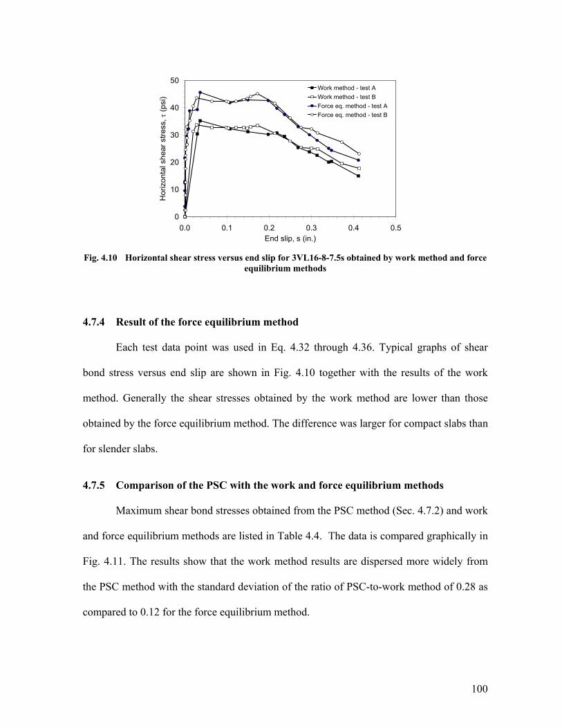
100

0

10

20

30

40

50

0.0 0.1 0.2 0.3 0.4 0.5End slip, s (in.)

Hor

izon

tal s

hear

stre

ss, τ

(psi

)

Work method - test AWork method - test BForce eq. method - test AForce eq. method - test B

Fig. 4.10 Horizontal shear stress versus end slip for 3VL16-8-7.5s obtained by work method and force

equilibrium methods

4.7.4 Result of the force equilibrium method

Each test data point was used in Eq. 4.32 through 4.36. Typical graphs of shear

bond stress versus end slip are shown in Fig. 4.10 together with the results of the work

method. Generally the shear stresses obtained by the work method are lower than those

obtained by the force equilibrium method. The difference was larger for compact slabs than

for slender slabs.

4.7.5 Comparison of the PSC with the work and force equilibrium methods

Maximum shear bond stresses obtained from the PSC method (Sec. 4.7.2) and work

and force equilibrium methods are listed in Table 4.4. The data is compared graphically in

Fig. 4.11. The results show that the work method results are dispersed more widely from

the PSC method with the standard deviation of the ratio of PSC-to-work method of 0.28 as

compared to 0.12 for the force equilibrium method.

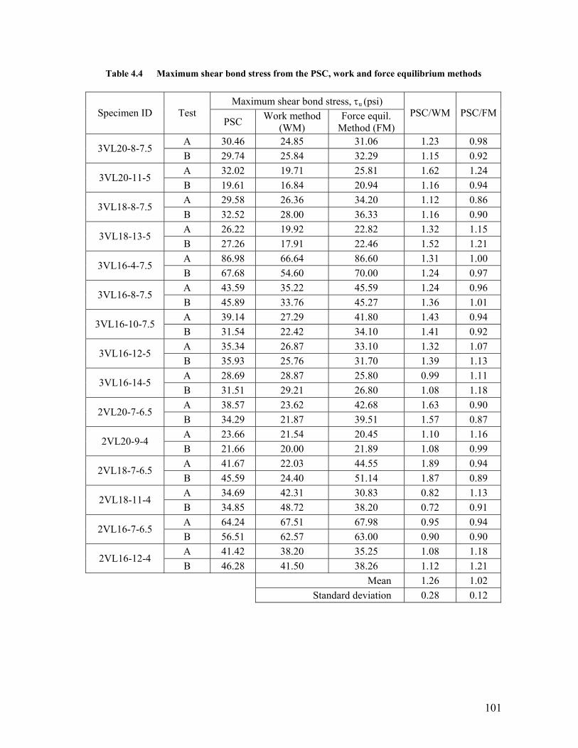
101

Table 4.4 Maximum shear bond stress from the PSC, work and force equilibrium methods

Maximum shear bond stress, τu (psi) Specimen ID Test

PSC Work method (WM)

Force equil. Method (FM)

PSC/WM PSC/FM

A 30.46 24.85 31.06 1.23 0.98 3VL20-8-7.5

B 29.74 25.84 32.29 1.15 0.92 A 32.02 19.71 25.81 1.62 1.24

3VL20-11-5 B 19.61 16.84 20.94 1.16 0.94 A 29.58 26.36 34.20 1.12 0.86

3VL18-8-7.5 B 32.52 28.00 36.33 1.16 0.90 A 26.22 19.92 22.82 1.32 1.15

3VL18-13-5 B 27.26 17.91 22.46 1.52 1.21 A 86.98 66.64 86.60 1.31 1.00

3VL16-4-7.5 B 67.68 54.60 70.00 1.24 0.97 A 43.59 35.22 45.59 1.24 0.96

3VL16-8-7.5 B 45.89 33.76 45.27 1.36 1.01 A 39.14 27.29 41.80 1.43 0.94

3VL16-10-7.5 B 31.54 22.42 34.10 1.41 0.92 A 35.34 26.87 33.10 1.32 1.07

3VL16-12-5 B 35.93 25.76 31.70 1.39 1.13 A 28.69 28.87 25.80 0.99 1.11

3VL16-14-5 B 31.51 29.21 26.80 1.08 1.18 A 38.57 23.62 42.68 1.63 0.90

2VL20-7-6.5 B 34.29 21.87 39.51 1.57 0.87 A 23.66 21.54 20.45 1.10 1.16

2VL20-9-4 B 21.66 20.00 21.89 1.08 0.99 A 41.67 22.03 44.55 1.89 0.94

2VL18-7-6.5 B 45.59 24.40 51.14 1.87 0.89 A 34.69 42.31 30.83 0.82 1.13

2VL18-11-4 B 34.85 48.72 38.20 0.72 0.91 A 64.24 67.51 67.98 0.95 0.94

2VL16-7-6.5 B 56.51 62.57 63.00 0.90 0.90 A 41.42 38.20 35.25 1.08 1.18

2VL16-12-4 B 46.28 41.50 38.26 1.12 1.21

Mean 1.26 1.02 Standard deviation 0.28 0.12

102

0

10

20

30

40

50

60

70

80

0 10 20 30 40 50 60 70 80τ by work and force equil. methods (psi)

τ by

PSC

met

hod

(psi

)

Series3Series4Series5PSC/WMPSC/FM

-20%

+20%

Fig. 4.11 Maximum shear bond stress from PSC, work and force equilibrium methods

Most results from the work method were too conservative with the largest different

between the PSC and the work method as high as 89%. There were also unconservative

results from the work method with the maximum difference of 28%. On the other hand,

results of force equilibrium method showed a better correlation with the PSC method

where the difference was less than 14% for the unconservative results and not more than

24% for the conservative results.

The reason for wide dispersion of the work method is that it is too dependent on the

test data, especially the end slip. The magnitude of end slip was not consistent between

tests of similar configurations. One test might have larger end slip than the companion

specimen. The inconsistency of end slip magnitudes influenced the slope of regression line

as shown in Fig. 4.9, where the values can become either too large or too small. This would

result in incorrect magnification of the shear bond force, which is calculated according to

Eq. 4.23 and Eq. 4.24.

103

4.8 Concluding remarks

1) Application of small scale test data in the m-k and the PSC methods was

able to predict the capacity of the compatible full scale specimen within

acceptable accuracy.

2) The m-k method using the Eurocode 4 equation produced more consistent

results than the ASCE equation.

3) The m-k method produced more accurate and less dispersed results but less

conservative results than the PSC method.

4) Both the work and force equilibrium methods can be used for calculating the

shear bond stress-slip history from a bending test. In addition to this, the

maximum shear bond stress value obtained from this calculation also can be

used in other design methods that need the value such as the PSC method.

The force equilibrium method demonstrated good correlation with the PSC

method while the work method was too conservative.

5) Results in Table 4.4 suggest that the shear bond stress changed with the

slenderness where compact slabs possessed larger ultimate shear bond than

the slender slabs.