RESEARCH PAPER

Comparative study between computational and experimentalresults for binary rarefied gas flows through long microchannels

Lajos Szalmas • Jeerasak Pitakarnnop •

Sandrine Geoffroy • Stephane Colin •

Dimitris Valougeorgis

Received: 18 February 2010 / Accepted: 19 April 2010 / Published online: 21 May 2010

� Springer-Verlag 2010

Abstract A comparative study between computational

and experimental results for pressure-driven binary gas

flows through long microchannels is performed. The the-

oretical formulation is based on the McCormack kinetic

model and the computational results are valid in the whole

range of the Knudsen number. Diffusion effects are taken

into consideration. The experimental work is based on the

Constant Volume Method, and the results are in the slip

and transition regime. Using both approaches, the molar

flow rates of the He–Ar gas mixture flowing through a

rectangular microchannel are estimated for a wide range of

pressure drops between the upstream and downstream

reservoirs and several mixture concentrations varying from

pure He to pure Ar. In all cases, a very good agreement is

found, within the margins of the introduced modeling and

measurement uncertainties. In addition, computational

results for the pressure and concentration distributions

along the channel are provided. As far as the authors are

aware of, this is the first detailed and complete comparative

study between theory and experiment for gaseous flows

through long microchannels in the case of binary mixtures.

Keywords Binary rarefied gas flows �McCormack model � Discrete velocity method �Flow rate measurement

1 Introduction

During the last decade, rarefied gas flows through long

channels have attracted considerable attention. This

increasing interest has been mainly stimulated by their

wide applicability in various technological fields including

the emerging field of nano- and microfluidics (Ho and Tai

1998; Kandlikar et al. 2006). In order to understand such

flows, both theoretical and experimental studies have been

carried out.

From theoretical standpoint, the most commonly

applied approaches include extended hydrodynamics

(Colin 2005; Szalmas 2007; Morini et al. 2005; Pita-

karnnop et al. 2008; Lockerby and Reese 2008), the

DSMC method (Bird 1994), and kinetic theory, as speci-

fied by the Boltzmann equation or alternatively by reliable

kinetic model equations (Ferziger and Kaper 1972; Cer-

cignani 1988; Sharipov and Seleznev 1998). It has been

shown that for flows with small Mach numbers (such as

the ones investigated here) and the Knudsen number

varying from the free molecular through the transition up

to the hydrodynamic regimes, linearized kinetic theory is

the most efficient approach providing reliable results with

modest computational effort. The discrete velocity method

has been successfully developed for solving such kinetic

equations, simulating flows through long channels of

various cross sections for both single component gases

L. Szalmas � D. Valougeorgis (&)

Department of Mechanical Engineering, University of Thessaly,

38334 Pedion Areos, Volos, Greece

e-mail: diva@mie.uth.gr

L. Szalmas

e-mail: lszalmas@gmail.com

J. Pitakarnnop � S. Geoffroy � S. Colin

INSA, UPS, Mines Albi, ISAE, ICA (Institut Clement Ader),

Universite de Toulouse, 135 avenue de Rangueil,

31077 Toulouse, France

e-mail: pitakarnnop_j@hotmail.com

S. Geoffroy

e-mail: sandrine.geoffroy@insa-toulouse.fr

S. Colin

e-mail: stephane.colin@insa-toulouse.fr

123

Microfluid Nanofluid (2010) 9:1103–1114

DOI 10.1007/s10404-010-0631-2

(Sharipov 1999; Aoki 2001; Valougeorgis and Naris 2003;

Breyiannis et al. 2008) and gaseous mixtures (Sharipov

and Kalempa 2002; Takata et al. 2003; Naris et al. 2004,

2005; Kosuge and Takata 2008). In addition, in the case of

one-dimensional flows the semi-analytical discrete ordi-

nate method has been developed to solve kinetic equations

associated with gaseous mixtures in a very elegant and

computationally efficient manner (Siewert and Valou-

georgis 2004).

The experimental work for flows through long channels

has been based mainly on the Constant Volume and the

Droplet Tracking methods. By implementing the corre-

sponding test rigs, flow rates through various channels have

been measured (Harley et al. 1995; Zohar et al. 2002;

Maurer et al. 2003; Colin et al. 2004; Ewart et al. 2006,

2007; Marino 2009; Pitakarnnop et al. 2010). All those

studies, which also include comparisons between theory

and experiments, as well as efforts for estimating the

accommodation coefficients characterizing the gas-surface

interaction, have been focused on single component gases.

Recently, one of these studies has been applied to binary

gaseous mixtures (Pitakarnnop et al. 2010), where an

introductory comparison between theory and experiment

has been performed. However, in this latter study, the

comparison has been limited to Kn \ 0.05, and also, it has

been based on the measured and computed mass flow rates

and not on the molar flow rates, which as described later, in

the case of binary mixture flows, remain the proper quan-

tity for comparisons between computational and experi-

mental results.

In that framework, in this study, a detailed and sys-

tematic comparison between computational and experi-

mental results for binary gas flows through long

microchannels is performed in the slip and transition

regimes. In particular, the flow configuration under inves-

tigation includes the gaseous mixture of He–Ar flowing

through a rectangular microchannel for a wide range of

pressure drops between the upstream and downstream

reservoirs and several mixture concentrations varying from

pure He to pure Ar. The comparative study is based on the

computed and measured molar flow rates. The diffusion

effects including the concentration variation along the

channel are also considered in the computations, and for

several indicative cases, pressure and concentration distri-

butions along the channel are provided.

In Sect. 2, the definition of the problem under investi-

gation is given, followed by the description of the com-

putational formulation and the experimental setup as

detailed in Sects. 3 and 4, respectively. In Sect. 5, the

comparative study based on the computed and measured

flow rates is presented, supplemented by some comple-

mentary computational results. Finally, concluding remarks

are presented in Sect. 6.

2 Definition of the problem

The isothermal pressure-driven flow of a binary gas mix-

ture through a microchannel, connecting two reservoirs, is

considered. The channel has rectangular cross section with

height H = 1.88 lm, width W = 21.2 lm, and length

L = 5000 lm, with H being the characteristic length. Since

H, W � L, end effects at the inlet and outlet of the channel

may be neglected. The channel axis lies in the z0 direction,

while the cross section is in the x0, y0 coordinate sheet.

The gas mixture is consisting of two species, namely He

and Ar, having molecular masses m1 = 0.004003 kg/mol

and m2 = 0.03995 kg/mol, respectively. The concentration

of the light species in the gas mixture is defined by

Cðz0Þ ¼ n1ðz0Þn1ðz0Þ þ n2ðz0Þ

; ð1Þ

where na(z0), with a = 1, 2, denotes the molar density of the

two species, while n = n1 ? n2 is the molar density of the

mixture. Index 1 refers always to He, since it is the lighter gas

compared to Ar. Also, from now on, we will refer to C as the

concentration of the gas mixture. Furthermore, the molecular

mass of the mixture is defined by

mðCÞ ¼ Cm1 þ ð1� CÞm2: ð2Þ

Other quantities of the mixture of some importance in this

study are its viscosity l(C) and the characteristic molecular

speed of the mixture vðCÞ ¼ffiffiffiffiffiffiffiffiffiffiffiffiffiffiffiffiffiffiffiffiffi

2kT=mðCÞp

; where

k = 1.3807 9 10-23 J/K is the Boltzmann constant and T

a constant temperature characterizing the isothermal flow.

Also, the pressure of the mixture along the channel is given

by the equation of state

Pðz0Þ ¼ nðz0ÞkT : ð3Þ

It is seen that all quantities specified in this paragraph

(except m1, m2, and T) depend explicitly or implicitly on z0

and, therefore, vary in the flow direction.

The pressure and concentration of the gas mixture in the

reservoirs are defined as (PA, CA) and (PB, CB), with the

indexes A and B denoting the upstream and downstream

reservoirs, respectively. In this study, the flow is purely due

to an externally imposed pressure gradient and, therefore,

PA [ PB, while CA = CB. The concentration CA is taken as

the reference concentration of the gas mixture. It is

emphasized, that although the concentration of the mixture

at the two reservoirs is the same, a variation of the mixture

concentration along the channel may appear due to the fact

that the particles of the two species are traveling with

different molecular speeds. This phenomenon, known as

separation effect, has been discussed in the past by several

authors (Sharipov and Kalempa 2005; Takata et al. 2007;

Szalmas and Valougeorgis 2010). It is also noted that

during the flow process the concentration of the mixture in

1104 Microfluid Nanofluid (2010) 9:1103–1114

123

the reservoirs is considered as constant, since the number

of gas molecules flowing through the channel is negligible

compared to the gas molecules in the reservoirs.

Based on the above, the local dimensionless pressure

and concentration gradients are defined as

XP ¼H

P

oP

oz0and XC ¼

H

C

oC

oz0; ð4Þ

respectively.

A very important flow parameter is the local rarefaction

parameter given by

d ¼ Pðz0ÞHlðCÞvðCÞ ; ð5Þ

with PA B P(z0) B PB. The rarefaction parameter varies

along the channel between the rarefaction parameters in the

upstream and downstream reservoirs, denoted by dA and

dB, respectively. In general, the rarefaction parameter is

proportional to the inverse Knudsen number. For the pur-

poses of this study, the reference rarefaction parameter,

d0 = (dA ? dB)/2 and the corresponding Knudsen number,

Kn0 = 1/d0, are defined. As is seen from the definition of d,

the Knudsen number is defined in terms of the channel

height H, while the mean free path is defined via the

mixture viscosity l(C).

The quantity of major importance in this study, upon

which the comparison study between theory and experi-

ment is based, is the total molar flow rate defined as

J ¼ J1 þ J2; ð6Þ

which consists of the sum of the molar flow rates J1 and J2

of He and Ar, respectively. The molar flow rates of each

species are given by the integrals

Ja ¼ naðz0ÞZZ

A0u0aðx0; y0Þdx0dy0; ð7Þ

with a = 1, 2, where u0aðx0; y0Þ is the macroscopic velocity,

and A0 = H 9 W is the area of the cross section. It is seen,

from Eq. 7, that the molar flow rates correspond to the

amount of molecules in mol unit passing through a cross

section of the channel per unit time. It is emphasized that

although, at the right-hand side of Eq. 7, the molar density

and the integral term vary along the flow, their product and,

therefore, the molar flow rates J1, J2, and J, due to particle

conservation, remain invariant at each cross section. In the

flow configuration presented here, this invariance of the

molar flow rates at each cross section is always satisfied.

3 Computational approach

The solution of the flow of a binary gas mixture through a

channel of rectangular cross section has been obtained in

Naris et al. (2005) in the whole range of the Knudsen

number based on the McCormack kinetic model (Mc-

Cormack 1973). This model is considered as a reliable

alternative of the Boltzmann equation, since it satisfies all

collision invariants, fulfills the H-theorem, and provides

the correct expressions for all transport coefficients. It is

also noted that while solving the viscous slip problem for

binary gas mixtures, very good agreement has been found

between the corresponding solutions of the linearized

Boltzmann equation (Ivchenko et al. 1997) and of the

McCormack model (Sharipov and Kalempa 2003) (see

Table 2 in Sharipov and Kalempa (2003)). Of course, it is

clarified that, strictly speaking, the present theoretical/

computational study is valid for monatomic dilute gas

mixtures, which is also the case for the Boltzmann

equation. This description is well suited for rarefied gases.

For the flow under consideration, i.e., binary gas flow

through a rectangular channel an advanced discrete

velocity algorithm (Naris et al. 2004a, b) has been applied

in Naris et al. (2005) to solve the resulting system of

linear integro-differential equations. The results are in

dimensionless form and include the so-called kinetic

coefficients.

In this study, the kinetic coefficients for the specific

geometry, data and parameters imposed in the present flow

configuration are computed. It is emphasized that the

realistic potential (Kestin et al. 1984; Naris et al. 2004b,

2005) is chosen for the computations. This model ensures

the correct value of the binary gas mixture viscosity, which

has been defined by applying the Chapman-Enskog theory

to the McCormack model (Sharipov and Kalempa 2002).

Furthermore, for the needs of this study, a methodology has

been developed to convert the dimensionless results into

dimensional molar flow rates, taking into account the

variation of the flow quantities, including diffusion effects,

along the channel.

To start with, the molar flow rates JP and JC conjugated

to the local gradients XP and XC are introduced as (De

Groot and Mazut 1984; Sharipov and Kalempa 2002)

JP ¼ �n

ZZ

A0wdx0dy0; ð8Þ

JC ¼ �n1

ZZ

A0u01 � u02� �

dx0dy0; ð9Þ

where

wðx0; y0Þ ¼ n1u01 þ n2u02n1 þ n2

ð10Þ

is the averaged velocity. Also, it is noted that JP and JC are

connected to the pressure and concentration gradients

according to (Sharipov and Kalempa 2002; Naris et al.

2005)

Microfluid Nanofluid (2010) 9:1103–1114 1105

123

JP ¼nA0vðCÞ

2½KPPXP þ KPCXC�; ð11Þ

JC ¼nA0vðCÞ

2½KCPXP þ KCCXC�; ð12Þ

where KPP, KCP, KPC, and KCC, with KCP = KPC due to

the Onsager-Casimir relation, are the kinetic coefficients

(Sharipov 1994). The kinetic formulation on the basis of JP

and JC provides a theoretically well-established and con-

venient way of the problem definition.

It is useful to point that, in the formulation which fol-

lows, all four kinetic coefficients, which may contribute to

the calculation of the molar flow rates J1 and J2 are con-

sidered. In particular, the coefficients KPP and KCP are due

to the externally imposed pressure gradient, while the

coefficients KPC and KCC are due to a concentration gra-

dient along the channel, which is not externally imposed

but is developed due to separation.

Using Eqs. 8–10 and the definition of the molar flow

rates Ja, a = 1, 2, given in Eq. 7, it is readily seen that

J1 ¼ �CJP � ð1� CÞJC; ð13ÞJ2 ¼ �ð1� CÞðJP � JCÞ: ð14Þ

Combining these expressions with Eqs. 11 and 12 and

using the ideal gas law (see Eq. 3), the following system

of equations is obtained (Szalmas and Valougeorgis

2010):

J1 ¼�PA0H

mðCÞvðCÞL

�

CKPP þ ð1� CÞKCPð Þ oP

oz

1

P

þ CKPC þ ð1� CÞKCCð Þ oC

oz

1

C

�

;

ð15Þ

J2 ¼ �PA0H

mðCÞvðCÞL

ð1� CÞ KPP � KCPð Þ oP

oz

1

Pþ KPC � KCCð Þ oC

oz

1

C

� �

;

ð16Þ

where, 0� z� 1; defined by z ¼ z0=L; is the non-

dimensional coordinate along the axis of the channel.

These equations are supplemented with the boundary

conditions for the pressure and the concentration at the

inlet and the outlet of the channel:

Pð0Þ ¼ PA; Pð1Þ ¼ PB; ð17ÞCð0Þ ¼ CA; Cð1Þ ¼ CB: ð18Þ

Equations 15 and 16 constitute a nonlinear system of two

first-order ordinary differential equations, subject to (17)

and (18). It can be solved to yield the unknown axial

distributions P ¼ PðzÞ and C ¼ CðzÞ; while the unknown

flow rates Ja are defined by satisfying the conditions at

z ¼ 1:

Finally, the solution of Eqs. 15 and 16 is carried out

numerically. Initial estimates of J1 and J2 are provided and

then the system is solved by the Euler’s method, starting

from z ¼ 0 and marching with a discrete step Dz up to z ¼ 1:

At each node along the channel, based on the values of the

kinetic coefficients of the previous node, the values of P and

C are estimated. Reaching the end of the channel at z ¼ 1;

the computed values of the pressure and the concentration

are compared to the corresponding boundary conditions. If

the agreement is not satisfactory, then updated values of J1

and J2 based on the bisector method are provided, and the

solution of the system is repeated. This iteration process

terminates when some relative convergence criterion

imposed on the outlet pressure and concentration is satisfied.

Upon convergence, the distributions PðzÞ and CðzÞ; as well

as the quantities J1 and J2 are determined. Finally, the total

flow rate J is calculated from Ja using Eq. 6.

As we conclude this section, the discretization parameters

implemented in the computations are provided. The numerical

algorithm used for the computation of the kinetic coefficients

in Eqs. 15 and 16 is based on a computational grid consisting

of 201 9 201 nodes for Kn0 C 1, and 301 9 301 nodes for

Kn0 \ 1 in the physical space, and of 64 magnitudes and 280

polar angles for all Knudsen numbers in the molecular

velocity space. The iteration process for the estimation of the

kinetic coefficients is terminated when the relative conver-

gence error is less than 10-7. Also, the Euler method involved

in the solution of Eqs. 15 and 16 is based on a marching step of

z ¼ 1=500; while the convergence criterion imposed on the

outlet pressure and concentration is equal to 10-6. Based on

the above discretization, the results thus obtained are con-

sidered as accurate up to at least three significant figures.

4 Experimental approach

All the experimental data are obtained from an experimental

setup described in Pitakarnnop et al. (2010), using the

so-called Constant Volume Method. The microsystem is

composed of a series of 45 identical microchannels etched by

deep reactive ion etching (DRIE) in a silicon wafer, and

closed by anodic bonding with a Pyrex plate. The height of

the microchannels, H = 1.88 lm, has been measured by a

TENCOR P1 profilometer, and the initial uncertainty of

±0.1 lm was finally reduced to ±0.01 lm, after comparison

between measured and simulated flow rates in the hydro-

dynamic regime, at low Knudsen numbers (Colin et al.

2004). The width of the microchannels is W = 21.2 ±

0.3 lm, and their length is L = 5000 ± 10 lm. The mi-

crochannels are connected to large upstream and down-

stream reservoirs, the constant volumes of which have been

accurately measured using a specific setup, with an accuracy

of ±1.3%. During the flow of the gas through the

1106 Microfluid Nanofluid (2010) 9:1103–1114

123

microsystem, the pressure inside each reservoir is measured

by means of Inficon� capacitance diaphragm gauges, and the

molar flow rates can be deduced from the ideal gas equation

of state. The accuracy of the pressure measurements by the

capacitance pressure gauges is 0.2% of reading. In order to

maintain isothermal conditions, the setup is thermally reg-

ulated by two Peltier modules, which allow maintaining a

constant and uniform temperature inside the whole setup,

i.e., inside the reservoirs as well as around the microsystem

and all the connecting lines. Before each experiment, the

whole circuit can be outgassed using a vacuum pump. Then,

the upstream and downstream reservoirs are filled with the

gas mixture from a high pressure tank. The pressure level is

independently controlled in each reservoir with a pressure

regulator. As soon as the waiting until thermal equilibrium is

reached, valves are opened allowing the gas flow from the

upstream to the downstream reservoir, through the micro-

system. During the measure, upstream and downstream

pressures are submitted to a small (typically 1–2%) decrease

and increase, respectively. The temperature in the experi-

ments is 298.5 K, and during operation, the temperature

variation is measured with four PT100 temperature sensors

(with a 0.15 K accuracy). Based on these measurements, the

temperature standard deviation during each experiment is

less than 0.1 K. Most of the setup is made of stainless steel,

aluminum, or glass, and the connections are insured by ISO-

KF and Swagelok Ultra-Torr� components to avoid any

leakage during low pressure operation. Air tightness has

been checked by means of helium detection, with a portable

high precision leak detector.

From the measurement of the pressure variation in each

reservoir, two experimental values of the molar flow rate

can be deduced from

JeA ¼ �

dNA

dt¼ �VA

Rg

d

dt

PA

TA

� �

; JeB ¼

dNB

dt¼ VB

Rg

d

dt

PB

TB

� �

;

ð19Þ

where t is the time, NA and NB are the amounts of gas

molecules in mol units in the upstream and downstream

reservoirs, respectively. PA and TA, PB and TB are the

pressures and temperatures in these reservoirs of respective

volumes VA and VB, and Rg = k 9 (6.022 9 1023/mol) is

the global gas constant. The experimental molar flow rate

leaving the upstream reservoir is compared with the

experimental molar flow rate entering the downstream

reservoir. It is verified that deviation between the two

values is well within the experimental uncertainty, and the

average experimental molar flow rate can be defined as

Je ¼ JeA þ Je

B

2: ð20Þ

At this point, a discussion on the definition of the molar

and mass flow rates is needed. In experiments with single

component gases, the mass flow rate dM/dt, instead of the

molar flow rate dN/dt, is commonly introduced. Since, in

general, M = N 9 m*, with m* denoting the average

molecular mass of the particles flowing through the

channel during the experiment, the mass flow rate is

obtained from Eq. 19 as

dM

dt¼ � V

RT

dP

dt; ð21Þ

where, R = k/m* is the specific gas constant. For single

component gases, the average mass m* is equal to the

molecular mass. However, for gaseous mixtures, m* cannot

be defined, since it refers to that gas portion which has

flowed through the channel during the experiment. Because

of the diffusion effects, that is the lighter particle has larger

velocity than the heavier one, the concentration of this gas

portion, denoted by C*, is different from the concentrations

in the two reservoirs (CA and CB), and it is not determined.

In fact, this concentration can be expressed as C* = J1/

(J1 ? J2), and then the average mass is obtained by

m* = C*m1 ? (1 - C*)m2. However, the component

fluxes, J1 and J2 and consequently m*, cannot be deter-

mined from the present experimental approach. They are

estimated only from the computational approach. There-

fore, the experimental results and the comparative study

are based on the molar and not on the mass flow rates.

Following from Eq. 19, the total molar flow rate through

the channel is expressed by

JeA ¼ �

dNA

dt¼ � VA

RgTA

dPA

dt1� dTA=TA

dPA=PA

� �

;

JeB ¼

dNB

dt¼ VB

RgTB

dPB

dt1� dTB=TB

dPB=PB

� �

:

ð22Þ

As mentioned above, high-thermal stability is ensured

by two temperature-regulation systems. The relative

temperature variation dT/T is then, of the order of

4 9 10-4, to be compared with the relative pressure

variation dP/P & 2 9 10-2. As a consequence, Eq. 22 can

be written as

JeA ¼ �

VA

RgTAaAcA; Je

B ¼VB

RgTBaBcB; ð23Þ

where a = dP/dt is calculated from a least-square linear fit

of the upstream or downstream measured pressure

PAðtÞ ¼ aAt þ bA; JeB ¼ aBt þ bB; ð24Þ

and c = 1 - (dT/T)/(dP/P) = 1 ± 2%. More than 1000

pressure data are used for determining coefficients a and b.

The standard deviation of coefficient a is calculated

following the method proposed in Pitakarnnop et al.

(2010) and is found to be less than 0.5%. Therefore, the

overall uncertainty of the molar flow rate measurement is

calculated from

Microfluid Nanofluid (2010) 9:1103–1114 1107

123

DJeA

JeA

¼ DJeB

JeB

¼ DV

Vþ DT

Tþ Da

aþ Dc

c; ð25Þ

and is less than ±(1.3 ? 0.2 ? 0.5 ? 2)% = ±4%.

Finally, it should be noted that outgassing from the setup

when operating at low pressure could generally not be

neglected, and, consequently, must be measured. In that

case, a three-step procedure is used:

1. Outgassing is first quantified in the downstream circuit

B, including reservoir B and all connections up to the

microsystem outlet. In order to avoid flow through the

microsystem during this operation, both upstream and

downstream circuits are pressurized to the downstream

operating pressure, and the valve placed between

circuit A and the microchannel is closed. As soon as

thermal stability is reached, the pressure rise in circuit

B, which now is only due to outgassing, is measured.

2. After this step, pressure in the upstream circuit A is

increased up to the desired upstream value and once

thermal stability is reached, the pressure variations in

circuits A and B are measured during the flow of the

gas mixture from circuit A to circuit B through the

microsystem.

3. Finally, outgassing is quantified in circuit A, including

all connections up to the microsystem inlet. For this

purpose, pressure in circuit B is increased to the same

level as in circuit A, to avoid flow through the

microsystem due to a pressure gradient, and the valve

between circuit B and the microsystem is closed; then,

the pressure rise in circuit A is monitored.

Outgassing rates in each circuit are calculated using

Eqs. 23 and 24 and used to correct the flow rate data. The

uncertainties shown in Eq. 25 are also taken into account

for the calculation of the outgassed flow rate, and the total

uncertainty represented by vertical bars in Figs. 1, 2, and 3

takes into account all uncertainties introduced in the three

steps of the operating procedure. As a consequence, when

outgassing is not negligible, the total uncertainty is given

by

DJeA

JeA

¼ �0:04 1þ 2Je

ogA

JeA

� �

;DJe

B

JeB

¼ �0:04 1þ 2Je

ogB

JeB

� �

;

ð26Þ

where JogAe is the molar flow rate due to outgassing in

circuit A calculated from the third step of the procedure,

and JogBe is the molar flow rate due to outgassing in circuit

B calculated from the first step of the procedure. The

coefficient 2 in the brackets of the right-hand side terms of

Eq. 26 is due to the fact that outgassing occurs in steps 2

and 3 (respectively 1 and 2) necessary for calculating JAe

(respectively JBe ). It should be outlined that outgassing is

essentially due to the manufactured parts of circuits A and

B, although outgassing from the walls of the microchannels

can be neglected, first because silicon and glass wafers

have very clean surfaces and second because the surface

area of the microchannels walls is typically ten orders of

magnitude lower than the total surface area of circuits A or

B.

Finally, the comparison of the upstream and downstream

resulting flow rates JAe and JB

e is an indirect mean for ver-

ifying that the outgassing effects are well taken into

account by the procedure described above, whatever the

level of outgassing.

5 Results

Computational and experimental results in tabulated and

graphical form are provided for the flow of the He–Ar

gaseous mixture through the microsystem consisting of a

series of 45 identical rectangular microchannels. The

reference concentration CA of the gas mixture, which as

0

1e-10

2e-10

3e-10

4e-10

3 4 5 6 7

J (m

ol/s

)

PA/PB

0

1e-11

2e-11

3e-11

3 4 5 6 7

J (m

ol/s

)

PA/PB

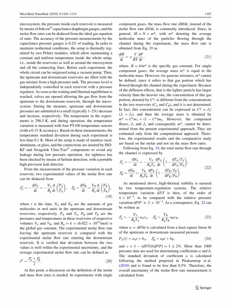
Fig. 1 Computational and experimental total molar flow rates of

He–Ar (CA = 0.1017), with (i) PB & 15 kPa (up) and (ii)

PB & 2 kPa (down). The symbols circle, open triangle, and filledtriangle represent J, JA

e , and JBe , respectively. The solid line is plotted

to guide the eyes for the computational results of J

1108 Microfluid Nanofluid (2010) 9:1103–1114

123

defined before, refers to the concentration of He in the

mixture varies between zero and one, taking the following

values: CA = [0.0, 0.1017, 0.3012, 0.5010, 0.7019, 0.9014,

1.0]. These values cover the whole range of the concen-

tration interval from pure Ar (CA = 0) to pure He

(CA = 1). For these values of exact concentration, the

corresponding uncertainties are [0, ±0.002, ±0.006,

±0.010, ±0.006, ±0.002, 0], respectively. The effect of

the concentration uncertainty on the numerical calculations

has been verified, and it was found that the introduced

uncertainty for the flow rates is less than ±0.5%. Two

values of downstream pressure PB, namely, PB & 15 kPa

and PB & 2 kPa, are considered. In both cases, the

upstream to downstream pressure ratio varies approxi-

mately from three to seven. Therefore, the results are

presented into two groups depending on PB. The average

Knudsen number varies in the first group with PB &15 kPa, as 0.1 \ Kn0 \ 0.6, and in the second group with

PB & 2 kPa, as 1.0 \ Kn0 \ 4.0. It is seen that the largest

portion of the transition regime is covered. Results in the

slip regime may be found in Pitakarnnop et al. (2010).

Based on the above flow parameters, Tables 1 and 2

present computational and experimental flow rates for

PB & 15 kPa and PB & 2 kPa, respectively. In these

tables, the first three columns provide the values of the

reference concentration CA, the pressure ratio PA/PB, and

Table 1 Computational and

experimental molar flow rates of

He–Ar for various

concentrations CA and pressure

ratios PA/PB, with PB & 15 kPa

CA PA/PB Kn0 J1 (mol/s) J2 (mol/s) J (mol/s) Je (mol/s) D

0.0 3.06 0.175 0.00 7.57 (-11) 7.57 (-11) 7.28 (-11) 3.97

4.06 0.165 0.00 1.26 (-10) 1.26 (-10) 1.21 (-10) 3.62

5.06 0.159 0.00 1.86 (-10) 1.86 (-10) 1.79 (-10) 3.40

6.01 0.154 0.00 2.51 (-10) 2.51 (-10) 2.43 (-10) 3.45

7.00 0.151 0.00 3.28 (-10) 3.28 (-10) 3.13 (-10) 4.90

0.1017 3.03 0.197 8.80 (-12) 6.70 (-11) 7.58 (-11) 7.56 (-11) 0.23

4.08 0.184 1.42 (-11) 1.14 (-10) 1.29 (-10) 1.29 (-10) -0.77

5.04 0.178 1.99 (-11) 1.65 (-10) 1.85 (-10) 1.94 (-10) -4.79

6.01 0.173 2.64 (-11) 2.23 (-10) 2.50 (-10) 2.49 (-10) 0.15

7.04 0.169 3.44 (-11) 2.94 (-10) 3.28 (-10) 3.26 (-10) 0.50

0.3012 3.04 0.225 2.85 (-11) 5.62 (-11) 8.48 (-11) 8.38 (-11) 1.16

4.02 0.212 4.39 (-11) 9.20 (-11) 1.36 (-10) 1.36 (-10) 0.19

5.03 0.203 6.27 (-11) 1.35 (-10) 1.98 (-10) 2.00 (-10) -0.80

6.04 0.197 8.37 (-11) 1.84 (-10) 2.68 (-10) 2.70 (-10) -0.50

7.00 0.194 1.06 (-10) 2.37 (-10) 3.43 (-10) 3.42 (-10) 0.24

0.5010 3.10 0.262 5.40 (-11) 4.54 (-11) 9.93 (-11) 9.80 (-11) 1.38

4.09 0.246 8.28 (-11) 7.42 (-11) 1.57 (-10) 1.59 (-10) -1.03

5.05 0.237 1.14 (-10) 1.05 (-10) 2.20 (-10) 2.16 (-10) 1.41

6.02 0.231 1.51 (-10) 1.41 (-10) 2.92 (-10) 2.90 (-10) 0.48

7.00 0.226 1.91 (-10) 1.82 (-10) 3.73 (-10) 3.73 (-10) -0.18

0.7019 3.05 0.309 8.49 (-11) 3.02 (-11) 1.15 (-10) 1.07 (-10) 7.24

4.03 0.291 1.31 (-10) 4.91 (-11) 1.80 (-10) 1.73 (-10) 4.15

5.02 0.280 1.82 (-10) 7.11 (-11) 2.53 (-10) 2.39 (-10) 5.69

5.98 0.272 2.38 (-10) 9.45 (-11) 3.32 (-10) 3.15 (-10) 5.60

7.01 0.267 3.03 (-10) 1.22 (-10) 4.25 (-10) 4.09 (-10) 3.96

0.9014 2.99 0.402 1.28 (-10) 1.16 (-11) 1.40 (-10) 1.38 (-10) 1.24

4.04 0.376 2.05 (-10) 1.97 (-11) 2.24 (-10) 2.23 (-10) 0.80

5.03 0.361 2.85 (-10) 2.83 (-11) 3.13 (-10) 3.11 (-10) 0.57

6.09 0.351 3.79 (-10) 3.87 (-11) 4.18 (-10) 4.17 (-10) 0.04

6.96 0.345 4.63 (-10) 4.78 (-11) 5.11 (-10) 5.09 (-10) 0.46

1.0 3.03 0.511 1.65 (-10) 0.00 1.65 (-10) 1.68 (-10) -2.15

4.00 0.481 2.55 (-10) 0.00 2.55 (-10) 2.57 (-10) -0.94

5.01 0.461 3.58 (-10) 0.00 3.58 (-10) 3.65 (-10) -1.90

6.01 0.449 4.70 (-10) 0.00 4.70 (-10) 4.77 (-10) -1.42

6.94 0.440 5.83 (-10) 0.00 5.83 (-10) 6.00 (-10) -2.74

Microfluid Nanofluid (2010) 9:1103–1114 1109

123

the resulting average Knudsen number Kn0, respectively.

For each concentration examined, five different pressure

ratios are considered. The fourth and fifth columns provide

the computational results of the molar flow rates of each

species, J1 and J2, followed in the sixth column with the

total computational flow rate J = J1 ? J2. The flow rates

are presented in a normalized floating-point form. All

values are given with an accuracy of three significant fig-

ures, and the exponents with base 10 are provided in

parenthesis. This notation is common in rarefied gas cal-

culations. The experimental total molar flow rates, denoted

by Je are given in the seventh column, while in the last

column of both tables (column 8 in Table 1 and column 10

in Table 2), the relative deviation between J and Je, defined

as D = 100(J/Je - 1), is shown. Finally, the total experi-

mental uncertainties are provided. The uncertainty for the

experimental molar flow rates in Table 1 with PB &15 kPa, where outgassing is negligible, is in all cases ±4%.

However, the uncertainties for the results in Table 2 with

PB & 2 kPa, where outgassing is not negligible, is case

dependent. In this latter situation, the uncertainties for the

inlet and outlet flow rates, denoted by DJAe and DJB

e , are

given in percentages in the eighth and ninth columns of

Table 2.

Table 2 Computational and experimental molar flow rates of He–Ar for various concentrations CA and pressure ratios PA/PB, with PB& 2 kPa

CA PA/PB Kn0 J1 (mol/s) J2 (mol/s) J (mol/s) Je (mol/s) DJAe DJB

e D

0.0 3.10 1.31 0.00 6.56 (-12) 6.56 (-12) 6.51 (-12) 9.67 9.58 0.82

4.02 1.26 0.00 9.31 (-12) 9.31 (-12) 8.86 (-12) 8.59 8.56 5.02

4.79 1.18 0.00 1.22 (-11) 1.22 (-11) 1.20 (-11) 7.30 7.76 1.93

5.96 1.17 0.00 1.59 (-11) 1.59 (-11) 1.51 (-11) 6.84 7.50 4.97

6.61 1.11 0.00 1.89 (-11) 1.89 (-11) 1.83 (-11) 6.03 6.55 3.08

0.1017 3.02 1.48 1.47 (-12) 5.85 (-12) 7.32 (-12) 6.96 (-12) 9.24 9.14 5.20

3.96 1.39 2.05 (-12) 8.68 (-12) 1.07 (-11) 1.03 (-11) 7.42 7.22 3.65

5.21 1.32 2.73 (-12) 1.25 (-11) 1.52 (-11) 1.44 (-11) 5.95 7.09 5.88

6.08 1.29 3.18 (-12) 1.53 (-11) 1.85 (-11) 1.78 (-11) 5.40 5.88 3.93

6.62 1.28 3.44 (-12) 1.71 (-11) 2.05 (-11) 1.97 (-11) 5.50 6.25 4.33

0.3012 3.07 1.68 4.76 (-12) 5.00 (-12) 9.76 (-12) 8.82 (-12) 7.90 8.33 10.6

4.03 1.58 6.67 (-12) 7.44 (-12) 1.41 (-11) 1.27 (-11) 6.44 6.95 10.8

5.00 1.52 8.43 (-12) 9.98 (-12) 1.84 (-11) 1.75 (-11) 5.75 5.60 5.34

5.94 1.50 9.94 (-12) 1.24 (-11) 2.23 (-11) 2.12 (-11) 5.39 5.53 5.30

6.67 1.45 1.13 (-11) 1.47 (-11) 2.60 (-11) 2.40 (-11) 5.19 5.83 8.17

0.5010 3.03 1.97 8.38 (-12) 3.78 (-12) 1.22 (-11) 1.13 (-11) 6.12 6.35 7.11

4.06 1.85 1.21 (-11) 5.80 (-12) 1.79 (-11) 1.66 (-11) 5.20 5.66 7.45

5.03 1.78 1.54 (-11) 7.81 (-12) 2.32 (-11) 2.11 (-11) 4.80 5.27 9.76

5.91 1.73 1.82 (-11) 9.72 (-12) 2.79 (-11) 2.54 (-11) 4.67 5.11 10.06

6.42 1.71 1.98 (-11) 1.09 (-11) 3.07 (-11) 2.83 (-11) 4.71 4.92 8.23

0.7019 3.06 2.32 1.29 (-11) 2.50 (-12) 1.54 (-11) 1.41 (-11) 5.63 5.78 9.22

3.94 2.20 1.78 (-11) 3.67 (-12) 2.15 (-11) 2.00 (-11) 4.92 5.22 7.05

5.42 2.07 2.58 (-11) 5.77 (-12) 3.16 (-11) 2.90 (-11) 4.59 4.95 8.92

5.87 2.05 2.81 (-11) 6.43 (-12) 3.46 (-11) 3.13 (-11) 4.50 4.89 10.6

6.33 2.03 3.05 (-11) 7.15 (-12) 3.77 (-11) 3.41 (-11) 4.46 4.83 10.4

0.9014 3.01 3.01 1.78 (-11) 8.97 (-13) 1.87 (-11) 1.80 (-11) 5.47 5.53 3.63

3.95 2.83 2.56 (-11) 1.37 (-12) 2.70 (-11) 2.60 (-11) 4.86 5.05 3.79

5.20 2.70 3.56 (-11) 2.06 (-12) 3.77 (-11) 3.56 (-11) 4.66 5.18 5.77

5.88 2.64 4.11 (-11) 2.46 (-12) 4.35 (-11) 4.08 (-11) 4.43 4.74 6.67

6.31 2.62 4.45 (-11) 2.71 (-12) 4.72 (-11) 4.53 (-11) 4.27 4.61 4.11

1.0 3.12 3.95 2.12 (-11) 0.00 2.12 (-11) 1.95 (-11) 6.63 6.44 9.04

3.92 3.61 2.99 (-11) 0.00 2.99 (-11) 2.77 (-11) 5.58 5.96 7.81

4.97 3.44 4.04 (-11) 0.00 4.04 (-11) 3.82 (-11) 5.05 5.34 5.69

5.83 3.40 4.83 (-11) 0.00 4.83 (-11) 4.62 (-11) 4.83 5.02 4.41

6.81 3.34 5.76 (-11) 0.00 5.76 (-11) 5.45 (-11) 4.52 4.92 5.74

1110 Microfluid Nanofluid (2010) 9:1103–1114

123

Comparing the quantities in Table 1 with those in

Table 2, it is seen that in Table 1, the average Knudsen

numbers and flow rates are about one order of magnitude

smaller than the ones in Table 2. The deviation D in

Table 1 varies between -4.79 and 7.24% with an average

value of 1.07%, while in Table 2 it is between 0.82 and

10.8% with the average value equal to 6.41%. It is seen that

in the latter case the experimental results are always less

than the corresponding computational ones. Also, in gen-

eral, the deviations D in Table 1 are much smaller than the

corresponding ones in Table 2.

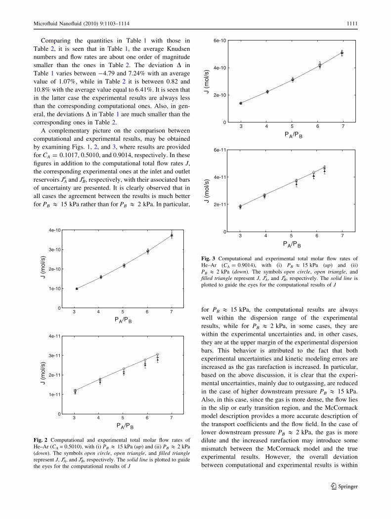
A complementary picture on the comparison between

computational and experimental results, may be obtained

by examining Figs. 1, 2, and 3, where results are provided

for CA = 0.1017, 0.5010, and 0.9014, respectively. In these

figures in addition to the computational total flow rates J,

the corresponding experimental ones at the inlet and outlet

reservoirs JAe and JB

e , respectively, with their associated bars

of uncertainty are presented. It is clearly observed that in

all cases the agreement between the results is much better

for PB & 15 kPa rather than for PB & 2 kPa. In particular,

for PB & 15 kPa, the computational results are always

well within the dispersion range of the experimental

results, while for PB & 2 kPa, in some cases, they are

within the experimental uncertainties and, in other cases,

they are at the upper margin of the experimental dispersion

bars. This behavior is attributed to the fact that both

experimental uncertainties and kinetic modeling errors are

increased as the gas rarefaction is increased. In particular,

based on the above discussion, it is clear that the experi-

mental uncertainties, mainly due to outgassing, are reduced

in the case of higher downstream pressure PB & 15 kPa.

Also, in this case, since the gas is more dense, the flow lies

in the slip or early transition region, and the McCormack

model description provides a more accurate description of

the transport coefficients and the flow field. In the case of

lower downstream pressure PB & 2 kPa, the gas is more

dilute and the increased rarefaction may introduce some

mismatch between the McCormack model and the true

experimental results. However, the overall deviation

between computational and experimental results is within

0

1e-10

2e-10

3e-10

4e-10

3 4 5 6 7

J (m

ol/s

)

PA/PB

0

1e-11

2e-11

3e-11

4e-11

3 4 5 6 7

J (m

ol/s

)

PA/PB

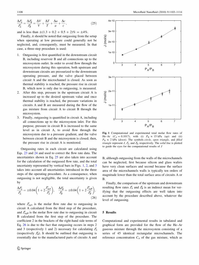
Fig. 2 Computational and experimental total molar flow rates of

He–Ar (CA = 0.5010), with (i) PB & 15 kPa (up) and (ii) PB & 2 kPa

(down). The symbols open circle, open triangle, and filled trianglerepresent J, JA

e , and JBe , respectively. The solid line is plotted to guide

the eyes for the computational results of J

0

2e-10

4e-10

6e-10

3 4 5 6 7

J (m

ol/s

)

PA/PB

0

2e-11

4e-11

6e-11

3 4 5 6 7

J (m

ol/s

)

PA/PB

Fig. 3 Computational and experimental total molar flow rates of

He–Ar (CA = 0.9014), with (i) PB & 15 kPa (up) and (ii)

PB & 2 kPa (down). The symbols open circle, open triangle, and

filled triangle represent J, JAe , and JB

e , respectively. The solid line is

plotted to guide the eyes for the computational results of J

Microfluid Nanofluid (2010) 9:1103–1114 1111

123

the introduced modeling and measurement uncertainties

and, therefore, it is considered as very good.

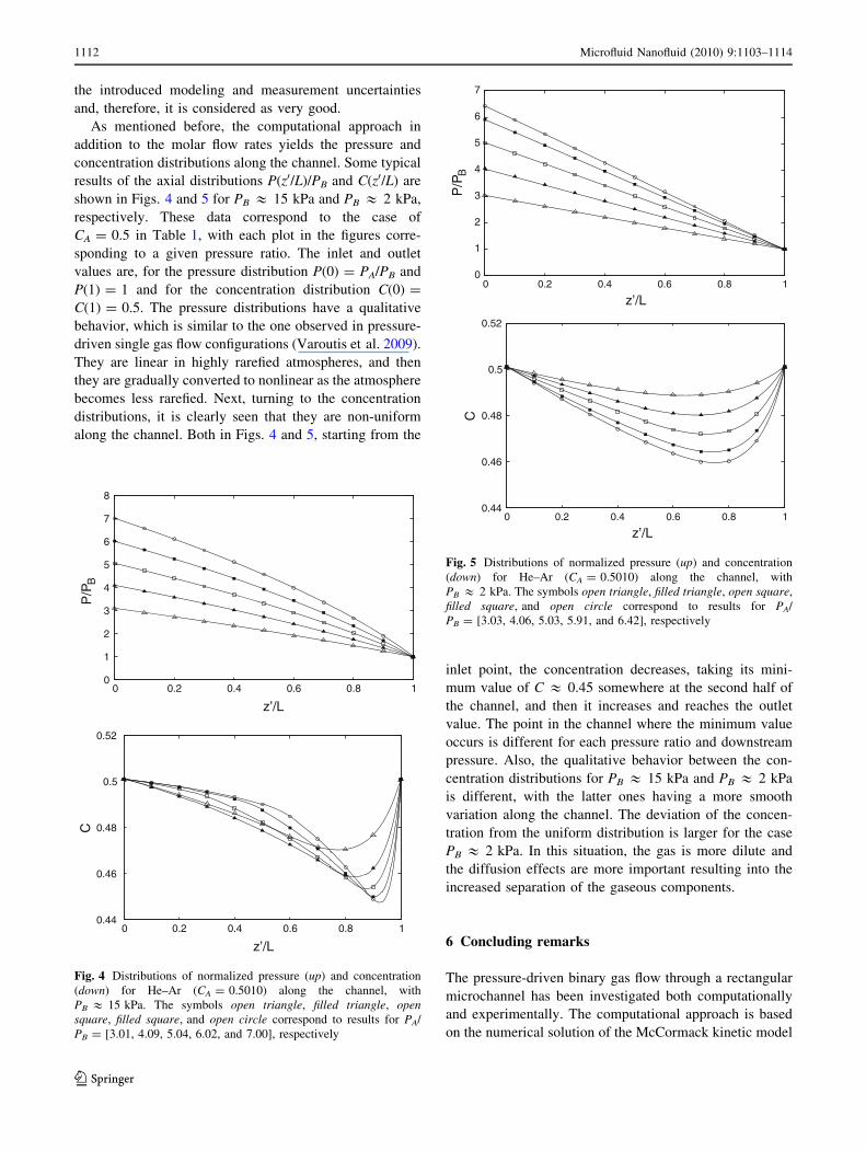
As mentioned before, the computational approach in

addition to the molar flow rates yields the pressure and

concentration distributions along the channel. Some typical

results of the axial distributions P(z0/L)/PB and C(z0/L) are

shown in Figs. 4 and 5 for PB & 15 kPa and PB & 2 kPa,

respectively. These data correspond to the case of

CA = 0.5 in Table 1, with each plot in the figures corre-

sponding to a given pressure ratio. The inlet and outlet

values are, for the pressure distribution P(0) = PA/PB and

P(1) = 1 and for the concentration distribution C(0) =

C(1) = 0.5. The pressure distributions have a qualitative

behavior, which is similar to the one observed in pressure-

driven single gas flow configurations (Varoutis et al. 2009).

They are linear in highly rarefied atmospheres, and then

they are gradually converted to nonlinear as the atmosphere

becomes less rarefied. Next, turning to the concentration

distributions, it is clearly seen that they are non-uniform

along the channel. Both in Figs. 4 and 5, starting from the

inlet point, the concentration decreases, taking its mini-

mum value of C & 0.45 somewhere at the second half of

the channel, and then it increases and reaches the outlet

value. The point in the channel where the minimum value

occurs is different for each pressure ratio and downstream

pressure. Also, the qualitative behavior between the con-

centration distributions for PB & 15 kPa and PB & 2 kPa

is different, with the latter ones having a more smooth

variation along the channel. The deviation of the concen-

tration from the uniform distribution is larger for the case

PB & 2 kPa. In this situation, the gas is more dilute and

the diffusion effects are more important resulting into the

increased separation of the gaseous components.

6 Concluding remarks

The pressure-driven binary gas flow through a rectangular

microchannel has been investigated both computationally

and experimentally. The computational approach is based

on the numerical solution of the McCormack kinetic model

0

1

2

3

4

5

6

7

8

0 0.2 0.4 0.6 0.8 1

P/P

B

z’/L

0.44

0.46

0.48

0.5

0.52

0 0.2 0.4 0.6 0.8 1

C

z’/L

Fig. 4 Distributions of normalized pressure (up) and concentration

(down) for He–Ar (CA = 0.5010) along the channel, with

PB & 15 kPa. The symbols open triangle, filled triangle, opensquare, filled square, and open circle correspond to results for PA/

PB = [3.01, 4.09, 5.04, 6.02, and 7.00], respectively

0

1

2

3

4

5

6

7

0 0.2 0.4 0.6 0.8 1

P/P

B

z’/L

0.44

0.46

0.48

0.5

0.52

0 0.2 0.4 0.6 0.8 1

C

z’/L

Fig. 5 Distributions of normalized pressure (up) and concentration

(down) for He–Ar (CA = 0.5010) along the channel, with

PB & 2 kPa. The symbols open triangle, filled triangle, open square,

filled square, and open circle correspond to results for PA/

PB = [3.03, 4.06, 5.03, 5.91, and 6.42], respectively

1112 Microfluid Nanofluid (2010) 9:1103–1114

123

and the experimental approach on the Constant Volume

method. Based on the computed and measured total molar

flow rates, a systematic and detailed comparison has been

performed finding very good agreement in a wide range of

the Knudsen numbers inside the transition regime. This

outcome clearly demonstrates that the McCormack model

and the associated numeric scheme can be successfully

implemented to simulate pressure-driven microflows of

gaseous mixtures, providing accurate results with modest

computational effort. This remark is important taking into

account the feasibility of the theoretical–computational

scheme to easily provide solutions to other micro-flow

configurations and its potential to investigate complex non-

equilibrium phenomena such as diffusion effects.

Acknowledgment The research leading to these results has

received funding from the European Community’s Seventh Frame-

work Programme (FP7/2007-2013) under grant agreement no 215504.

References

Aoki K (2001) Dynamics of rarefied gas flows: asymptotic and

numerical analyses of the Boltzmann equation. In: 39th AIAA

aerospace science meeting and exhibit, Reno, 2001-0874

Bird GA (1994) Molecular gas dynamics and the direct simulation of

gas flows. Oxford University Press, Oxford

Breyiannis G, Varoutis S, Valougeorgis D (2008) Rarefied gas flow in

concentric annular tube: estimation of the Poiseuille number and

the exact hydraulic diameter. Eur J Mech B Fluids 27:609–622

Cercignani C (1988) The Boltzmann equation and its application.

Springer-Verlag, New York

Colin S (2005) Rarefaction and compressibility effects on steady and

transient gas flows in microchannels. Microfluid Nanofluidics

1:268–279

Colin S, Lalonde P, Caen R (2004) Validation of a second-order slip

flow model in rectangular microchannels. Heat Transf Eng

25:23–30

De Groot SR, Mazut P (1984) Non-equilibrium thermodynamics.

Dover, New York

Ewart T, Perrier P, Graur I, Meolans JG (2006) Mass flow rate

measurements in gas micro flow. Exp Fluids 41:487–498

Ewart T, Perrier P, Graur IA, Meolans JG (2007) Mass flow rate

measurements in a microchannel, from hydrodynamic to near

free molecular regimes. J Fluid Mech 584:337–356

Ferziger JH, Kaper HG (1972) Mathematical theory of transport

processes in gases. North Holland, Amsterdam

Harley JC, Huang Y, Bau HH, Zemel JN (1995) Gas flow in micro-

channels. J Fluid Mech 284:257–274

Ho CM, Tai YC (1998) Micro-electro-mechanical-systems (MEMS)

and fluid flows. Annu Rev Fluid Mech 30:579–612

Ivchenko IN, Loyalka SK, Tompson RV (1997) Slip coefficients for

binary gas mixture. J Vac Sci Technol A 15:2375–2381

Kandlikar SG, Garimella S, Li D, Colin S, King MR (2006) Heat

transfer and fluid flow in minichannels and microchannels.

Elsevier, Oxford

Kestin J, Knierim K, Mason EA, NajaB B, Ro ST, Waldman M

(1984) Equilibrium and transport properties of the noble gases

and their mixture at low densities. J Phys Chem Ref Data

13:229–303

Kosuge S, Takata S (2008) Database for flows of binary mixtures

through a plane microchannel. Eur J Mech B Fluids 27:444–465

Lockerby DA, Reese JM (2008) On the modelling of isothermal gas

flows at the microscale. J Fluid Mech 604:235–261

Marino L (2009) Experiments on rarefied gas flows through tubes.

Microfluid Nanofluidics 6:109–119

Maurer J, Tabeling P, Joseph P, Willaime H (2003) Second-order slip

laws in microchannels for helium and nitrogen. Phys Fluids

15:2613–2621

McCormack FJ (1973) Construction of linearized kinetic models for

gaseous mixtures and molecular gases. Phys Fluids 16:2095–

2105

Morini GL, Lorenzini M, Spiga M (2005) A criterion for experimen-

tal validation of slip-flow models for incompressible rarefied

gases through microchannels. Microfluid Nanofluidics 1:190–

196

Naris S, Valougeorgis D, Kalempa D, Sharipov F (2004a) Discrete

velocity modelling of gaseous mixture flows in MEMS. Super-

lattices Microstruct 35:629-643

Naris S, Valougeorgis D, Kalempa D, Sharipov F (2004b) Gaseous

mixture flow between two parallel plates in the whole range of

the gas rarefaction. Physica A 336:294–318

Naris S, Valougeorgis D, Kalempa D, Sharipov F (2005) Flow of

gaseous mixtures through rectangular microchannels driven by

pressure, temperature and concentration gradients. Phys Fluids

17:100607.1–100607.12

Pitakarnnop J (2009) Analyse experimentale et simulation numerique

d’ecoulements rarefies de gaz simples et de melanges gazeux

dans les microcanaux. Ph.D. thesis, University of Toulouse

Pitakarnnop J, Geoffroy S, Colin S, Baldas L (2008) Slip flow in

triangular and trapezoidal microchannels. Int J Heat Technol

26:167–174

Pitakarnnop J, Varoutis S, Valougeorgis D, Geoffroy S, Baldas L,

Colin S (2010) A novel experimental setup for gas microflows.

Microfluid Nanofluidics 8:57–72

Sharipov F (1994) Onsager-Casimir reciprocity relations for open

gaseous systems at arbitrary rarefaction III. Theory and its

application for gaseous mixtures. Physica A 209:457–476

Sharipov F (1999) Rarefied gas flow through a long rectangular

channel. J Vac Sci Technol A 17:3062–3066

Sharipov F, Seleznev V (1998) Data on internal rarefied gas flows.

J Phys Chem Ref Data 27:657–706

Sharipov F, Kalempa D (2002) Gaseous mixture flow through a long

tube at arbitrary Knudsen number. J Vac Sci Technol A 20:

814–822

Sharipov F, Kalempa D (2003) Velocity slip and temperature jump

coefficients for gaseous mixtures. I. Viscous slip problem. Phys

Fluids 15:1800–1806

Sharipov F, Kalempa D (2005) Separation phenomena for gaseous

mixture flowing through a long tube into vacuum. Phys Fluids

17:127102.1–127102.8

Siewert CE, Valougeorgis D (2004) The McCormack model: channel

flow of a binary gas mixture driven by temperature, pressure and

density gradients. Eur J Mech B Fluids 23:645–664

Szalmas L (2007) Multiple-relaxation time lattice Boltzmann method

for the finite Knudsen number region. Physica A 379:401–408

Szalmas L, Valougeorgis D (2010) Rarefied gas flow of binary

mixtures through long channels with triangular and trapezoidal

cross sections. Microfluid Nanofluidics. doi:10.1007/s10404-

010-0564-9

Takata S, Yasuda S, Kosuge S, Aoki K (2003) Numerical analysis of

thermal-slip and diffusion-slip flows of a binary mixture of hard-

sphere molecular gases. Phys Fluids 15:3745-3766

Takata S, Sugimoto H, Kosuge S (2007) Gas separation by means of

the Knudsen compressor. Eur J Mech B Fluids 26:155–181

Microfluid Nanofluid (2010) 9:1103–1114 1113

123

Valougeorgis D, Naris S (2003) Acceleration schemes of the discrete

velocity method: gaseous flows in rectangular microchannels.

SIAM J Sci Comput 25:534–552

Varoutis S, Naris S, Hauer V, Day C, Valougeorgis D (2009)

Computational and experimental study of gas flows through long

channels of various cross sections in the whole range of the

Knudsen number. J Vac Sci Technol A 27:89–100

Wagner W (1992) A convergence proof for Bird direct simulation

Monte Carlo method for the Boltzmann equation. J Stat Phys

66:1011–1044

Zohar Y, Lee SYK, Lee WY, Jiang L, Tong P (2002) Subsonic gas

flow in a straight and uniform microchannel. J Fluid Mech

472:125–151

1114 Microfluid Nanofluid (2010) 9:1103–1114

123