Tracking Multiple Targets Using Binary Proximity Sensors ∗

Jaspreet SinghUpamanyu Madhow

Electrical and ComputerEngineering, University ofCalifornia, Santa Barbara

CA 93106 USA{ jsingh , madhow }@ece.ucsb.edu

Rajesh Kumar

Subhash Suri

Computer ScienceUniversity of California

Santa BarbaraCA 93106 USA{ rajesh , suri }@cs.ucsb.edu

Richard Cagley

Toyon Research CorporationGoleta, CA 93117, USArcagley@toyon.com

ABSTRACTRecent work has shown that, despite the minimal informa-tion provided by a binary proximity sensor, a network ofsuch sensors can provide remarkably good target trackingperformance. In this paper, we examine the performanceof such a sensor network for tracking multiple targets. Webegin with geometric arguments that address the problemof counting the number of distinct targets, given a snapshotof the sensor readings. We provide necessary and sufficientcriteria for an accurate target count in a one-dimensionalsetting, and provide a greedy algorithm that determines theminimum number of targets that is consistent with the sen-sor readings. While these combinatorial arguments bringout the difficulty of target counting based on sensor read-ings at a given time, they leave open the possibility of ac-curate counting and tracking by exploiting the evolution ofthe sensor readings across time. To this end, we develop aparticle filtering algorithm based on a cost function that pe-nalizes changes in velocity. An extensive set of simulations,as well as experiments with passive infrared sensors, are re-ported. We conclude that, despite the combinatorial com-plexity of target counting, probabilistic approaches based onfairly generic models for the trajectories yield respectabletracking performance.

Categories and Subject DescriptorsI.4.8 [Scene Analysis ]: Tracking, Sensor fusion;G.2 [Discrete Mathematics]: Counting Problems;

∗This work was supported by the National Science Foun-dation under grants CCF-0431205, CNS-0520335, CNS-0626954 and CCF-0514738, by the Office of Naval Researchunder grants N00014-06-1-0066 and N00014-06-M-0260, andby the Institute for Collaborative Biotechnologies undergrant DAAD19-03-D-0004 from the US Army Research Of-fice.

Permission to make digital or hard copies of all or part of this work forpersonal or classroom use is granted without fee provided that copies arenot made or distributed for profit or commercial advantage and that copiesbear this notice and the full citation on the first page. To copy otherwise, torepublish, to post on servers or to redistribute to lists, requires prior specificpermission and/or a fee.IPSN’07, April 25-27, 2007, Cambridge, Massachusetts, USA.Copyright 2007 ACM 978-1-59593-638-7/07/0004 ...$5.00.

G.3 [Probability And Statistics]: Probabilistic algorithms

KeywordsTarget Tracking, Sensor Networks, Binary Sensing, Count-ing Resolution, Particle Filters

1. INTRODUCTION

We investigate the problem of tracking targets using anetwork of binary proximity sensors. Each sensor producesa single bit of output, which is 1 when one or more targetsare in its sensing range and 0 otherwise. These sensors arenot able to distinguish individual targets, decide how manydistinct targets are in the range, or provide any location-specific information. Despite the minimal information pro-vided by a single binary sensor, a collaborative network ofbinary sensors has been shown in prior work [18] to yield re-spectable tracking performance: the resolution with whicha target can be localized is inversely proportional to ρRd−1,where ρ is the sensor density, R is the sensing range, andd is the dimension of the space. In this paper, we extendthe work of [18], which considered a single target, and in-vestigate the problem of tracking multiple targets, withouta priori knowledge of the number of targets.

We have chosen to focus on the simple and minimalisticsetting of binary sensors because the cost and power con-sumption of sensor nodes is a severe constraint in large-scaledeployments, and both can be significantly reduced by re-stricting the nodes to provide binary detection. Thus, byconstraining ourselves to a binary sensing model, we canwork with low-power, low-cost sensor nodes that can formthe basis for a highly scalable architecture for wide areasurveillance. This information can, of course, be augmentedby a small number of more capable sensors (e.g., cameras),although we do not explore such enhancements in this paper.

Examples of sensor modalities that are suitable for low-cost nodes include [1] Seismic, Acoustic, Passive infrared(PIR), Active infrared, Ultra wide band radar imaging, Mil-limeter wave radar, Magnetometer and Ultrasonic. For manytypes of sensors, it is possible to use simple thresholding toget a binary reading or perform onboard signal processingfor rough classification. The former option requires drasti-cally reduced processing, and leads to significant power sav-ings. As an example, for acoustic sensing (e.g., the Knowles

EA-21842 sensor) and magnetometer sensing (e.g., the Hon-eywell HMC1002 sensor), the power consumption can bereduced five-fold by using binary mode rather than classifi-cation mode. In our lab-scale experiments, we employ PIRsensors due to their good performance, low cost, and ease ofsystems integration [11].

As shown in [18], the binary sensing model is analogous tocoarse-grained analog-to-digital conversion that filters outrapid variations in the target’s trajectory. This motivatesalgorithms that attempt to track only “lowpass” versions ofthe trajectory. For multiple targets, however, we encountersignificant additional difficulties, since we cannot tell howmany targets are within a sensor’s range when it outputs a 1.Our first task in this paper, therefore, is to understand howwell we can count the number of targets, given a snapshotof the sensor readings. We employ geometric arguments tocharacterize when an accurate count is possible, and providea lower bound on the number of targets, based on a greedyalgorithm for explaining the sensor’s observations with theminimum number of targets. While these arguments bringout the difficulty of target counting based on a snapshot,they do not preclude the possibility of accurate countingand tracking when we account for the evolution of the sen-sor readings in time, using a model for the targets’ behavior.To this end, we develop a particle filtering algorithm whichemploys a cost function penalizing changes in velocity. Itis shown by simulations that the particle filter algorithmis effective in tracking targets even when their trajectorieshave significant overlap. The algorithm is general enough toincorporate a simple model for non-ideal sensing, and pro-vides acceptable tracking performance for our experimentalsystem with PIR sensors even when one of the sensors fails.

We restrict attention to one-dimensional systems through-out this paper. This enables us to gain fundamental in-sight, as well as to easily display multiple trajectories ontwo-dimensional space-time plots. However, both our geo-metric target counting arguments and the particle filteringalgorithm generalize to higher dimensions.

Our focus in this paper is on the efficacy of collaborativetracking rather on the communication protocols used by thesensor nodes. Thus, we assume that all of the sensor read-ings are available at a centralized processor, which can thenestimate the targets’ locations and trajectories. Distributedimplementations of our algorithms, in which neighbors col-laborate to estimate segments of trajectories, are possible,but are not considered here. We note that the binary sens-ing model has minimal communication requirements, hencethis assumption of centralized processing is quite practical:a sensor need only convey the intervals at which it switches“on” and “off” (assuming that the readings are averagedso as to remain reasonably steady, this is far more efficientthan sending a sample of the sensor’s readings at regularintervals).

The rest of the paper is organized as follows. Section 2discusses the problem of target counting based on a snap-shot of the sensor readings. In Section 3, we describe ourparticle filtering algorithm. Section 4 provides simulationresults, while Section 5 describes our experimental set-upand results. We end with the conclusions in Section 6.

Related WorkThe problem of tracking multiple targets using sensor net-works has been explored by many prior references [15, 16, 13,

5, 19, 9, 17]. Owing to its simplicity and minimal commu-nication requirements, the specific use of binary proximitysensors for tracking applications has also drawn consider-able attention of late. However, most of the work relatedto binary sensing has been applied to the case of tracking asingle target [3, 8, 18]. The tracking techniques employed inthe large-scale deployment in [2] can be loosely interpretedin terms of a binary sensing model, even though a variety ofsensing modalities and a variety of targets are considered.Reference [12] contains a distributed tracking algorithm for abinary sensor network, but assumes perfect knowledge aboutthe number of targets and their identities, unlike the presentwork.

In our work, we investigate both target counting and track-ing. Prior work on counting targets includes [14], but itassumes more detailed sensing capabilities than our simplebinary model. The classical framework for tracking is basedon Kalman filtering, with Gaussian assumptions for the sen-sor readings; for example, [10] investigates the use of Kalmanfiltering for distributed tracking. In recent years, the use ofparticle filters, which can handle more general observationmodels, has become popular. However, most prior work onthe use of particle filters for tracking in sensor networks [4,6, 7] assumes a richer sensing model than the binary modelwe consider. An exception is our own prior work in [18] onthe use of particle filters for tracking a single target usingnon-ideal binary sensing. In this paper, we build on theseideas to develop particle filters for tracking multiple targets.

2. TARGET COUNTABILITYIn order to develop fundamental geometric insights, we

restrict attention in this section to an idealized model inwhich each sensor’s coverage area is a circular disk of radiusR: each sensor detects a target without fail if it falls withinthis disk, and does not produce false positives or negatives.While we develop our basic ideas and theorems in one di-mension, we comment on their relevance and extensions tohigher dimensions as appropriate.

We want to understand and articulate the conditions un-der which an algorithm can track multiple targets with prov-able guarantees. A first step for any tracking algorithm mustdeduce how many distinct targets are present in the field,and so we begin our investigation by asking under what cir-cumstances an algorithm can reliably determine the numberof distinct targets in the field, given a snapshot of the sen-sor readings. This is a worst-case model which applies, forexample, when the rate at which the sensors report theirreadings is low compared to the rates at which the targetscross the boundaries of the sensors’ coverage areas. Put an-other way, this section addresses the most general scenario,in which we have no model for the targets’ trajectories. Aswe shall see in Section 3, when we do employ a plausiblemodel corresponding to a scenario in which the sensor read-ings are available at a “high enough” rate, then it is indeedpossible to do better than what is promised by the worst-case model considered in this section.

2.1 Target Counting with Binary SensingSome spatial separation among the targets is clearly a

necessary precondition for accurately disambiguating amongdifferent targets, but what does that mean, and how muchseparation is enough? For instance, is the following simple

condition adequate: each target moves sufficiently (arbitrar-ily) far from the remaining targets at some point during themotion. Let us call this the condition of individual separa-tion. Unfortunately, as the following simple result shows,this alone is not enough to count the number of targets ac-curately.

Theorem 1. Even arbitrarily large individual separationis not sufficient to reliably count a set of targets using binarysensors.

Proof. We give a construction in one dimension estab-lishing the claim. Imagine a group of m targets moving atuniform speed along a straight line L. Initially, all targetsare clustered and appear as one target to the sensor field.Now let target 1 speed up and move away from the rest ofthe group. Once it moves sufficiently far to the right, we caninfer that there are at least two targets. Next, target 1 stopsand waits until the rest of the group meets up with it, andthen they all resume their motion. Then, target 2 separatesfrom the rest of the group and repeats the action of target1, and so on. One can easily see that in this scenario, ev-ery target achieves large individual separation from the rest,and yet no binary sensing-based algorithm can ever decidewhether there are two targets or m targets, for an arbitraryvalue of m.

On the other hand, if the group of targets has pairwiseseparation more than 4R, then binary sensing permits pre-cise counting of targets.

Theorem 2. Suppose every pair in a set of targets hasseparation more than 4R in d-dimensional Euclidean space,where R is the sensing range, and suppose that the aver-age sensor density (per unit area) is ρ. Then, using binaryproximity sensors, we can precisely determine the number ofdistinct targets as well as localize each target within spatialerror at most Θ(1/ρRd−1).

Proof. Suppose there are m targets, and let Si be theset of sensors that sense target i. Because each sensor’srange has radius R, by the assumption of pairwise targetseparation, we must have Si ∩ Sj = ∅, for any two targets iand j. (This follows because the union of two overlappingranges has diameter less than 4R, while any two targets areassumed to be more than 4R apart.) As a result, the “on”sensors are naturally partitioned into m groups, one per tar-get: all sensors in the ith group are on precisely because ofone target. Thus, the target sensed by the ith group Si canbe localized to the common intersection of all the ranges inSi and the complement of the ranges of all the “off” sensors.The analysis of our single target localization [18] shows thatthe diameter of this intersection region (which need not beconnected) is Θ(1/ρRd−1). This completes the proof.

In some sense, the preceding example and the theoremsettle the “easy” case: when the objects are pairwise farapart, they can be counted as well as localized quite pre-cisely, but individual separation does not help in tracking.We now delve into the more complex (and interesting) sit-uation when these easy conditions do not hold. We pointout that there is no local fundamental limit based purely onminimum separation among targets: two targets no matterhow close can always be disambiguated if two sensors withnon-overlapping sensing ranges detect them. At the same

ON

OFF OFF

g1 g2ON

Figure 1: A sample illustration for the feasible tar-get space (F ). Here, g1 and g2 represent the contri-butions of the ‘ON’ sensors to F .

time, simply increasing the sensor density to disambiguatecloseby targets does not seem possible either. (However, asour earlier work shows the “localization” of an individualtarget does improve linearly with the increasing density.) Itseems that we need a more global argument to understandthe limit of target counting.

We now focus on one-dimensional space: much of thedifficulty in the binary sensing model has less to do with thedimension of the ambient space and more to do with the“interference” between the influence of different targets onthe sensor readings. Any impossibility or hardness results weprove in one dimension naturally hold in higher dimensionsas well.

2.2 The Geometry of Target Counting

We begin with some geometric preliminaries. Suppose wehave N binary proximity sensors deployed along a line. Eachsensor’s range is then an interval of length 2R. We use thenotation Ci to denote the interval covered by sensor i (thatis, sensor i outputs a 1 if and only if a target falls in Ci). Weassume that the domain of interest is covered by the unionof the {Ci}, i.e., that there are no gaps in coverage.

Any positioning of targets along the line leads to a vectorof binary outputs from the sensors. In particular, we havecontiguous groups of “on-sensors” separated by groups of“off-sensors.” Geometrically, the on-sensors inform us aboutthe intervals on the line where the targets might be, andthe off-sensors tell us about the regions where there are notargets. If we let I be the set of sensors whose binary outputis 1 and Z be the set of sensors whose output is 0, then allthe targets must lie in the region F , which we call the feasibletarget space:

F =⋃i∈I

Ci −⋃j∈Z

Cj

The region F is a subset of the line, whose connectedcomponents are unions of portions of the sensing ranges ofthe on-sensors. In particular, for sensor i, the portion ofits sensing range that appears in F is gi = Ci −

⋃j∈Z Cj ,

namely, the part not clipped by the off-sensors. An exampleis shown in Figure 1. The feasible target space is simply theunion of these (overlapping) subintervals: F =

⋃i∈I gi.

The feasible target space has an interesting geometricstructure. While each on or off sensor contributes exactlyone bit, the information content of the off sensors seemsricher, especially in localizing the targets: the 1 bit onlytells us that there is at least one target somewhere in thesensor’s range, the 0 bit assures us that there is no targetanywhere in the sensor’s range. This observation leads tothe following geometric property of the region F .

ON

Case 1

ON

OFF

ONON

Case 2

Figure 2: Positively independent sensors: Case 1-sufficiently far apart, Case 2-separated by an off sen-sor.

Lemma 1. Any two connected components of the feasibletarget space F are separated by at least distance 2R.

Proof. Choose a point x that is between two connectedcomponents of F . Since x must lie in the range of somesensor, and x 6∈ F , that sensor must have binary output 0.A sensor with binary output zero eliminates length 2R of theline for possible locations of the targets, and so the “gap”containing the point x must be at least as wide as 2R.

Fundamental Counting Resolution

We now use this geometric framework to establish a theo-rem on the fundamental limit of target counting. Towardsthat goal, let us define two sensors to be positively indepen-dent if (i) they both have binary output 1, and (ii) eithertheir sensing ranges are disjoint or they belong to differentconnected components of the feasible target space F . (Notethat the independence property is defined with respect to aparticular instant, for a given vector of sensor outputs.) Inother words, as illustrated in Figure 2, two sensors are pos-itively independent if they are both detecting targets andare either sufficiently far apart (case 1) or are separated byan off sensor (case 2). Then, the following result gives anecessary and sufficient condition for correctly counting thenumber of targets along a line.

Theorem 3. A set of k targets on a line can be countedcorrectly if and only if there exist k (pairwise) positivelyindependent sensors.

Proof. We recall that by definition independent sensorshave output 1. The “if” part of the claim is therefore imme-diate: due to their independence, no two sensors can be onbecause of the same target, and so there must be at least ktargets. In order to show the “only if” part, we argue thatif k independent sensors do not exist, then the counting isnot guaranteed to be correct. In other words, the sensorscannot distinguish between two scenarios, one with k tar-gets and one with fewer than k targets, thereby violatingthe correctness.

Without loss of generality, let us number the targets 1, . . . , kin the left-to-right order along the line, and generate a list ofsensors s1, s2, . . . , sj as follows. Let s1 be the leftmost sen-sor with binary output 1. In general, let si be the leftmostsensor with output 1 that is independent of si−1. Since wehave assumed that k independent sensors do not exist, wemust have j < k. By the pigeon-hole principle, therefore,there must be a sensor among s1, s2, . . . , sj whose range in

F includes at least 2 targets. We now observe that the bi-nary outputs of none of the sensors will be affected if wetranslated all the targets to the right until each target wasat the rightmost point of their independent sensor’s rangegi. The sensor with two or more targets clearly has a re-dundancy, and the binary outputs will not change if one ofthose targets was eliminated. It follows that the countingalgorithm cannot distinguish between the case of k targetsand the k − 1 targets. This completes the proof.

Remark on Counting Resolution

By the previous theorem, the number of distinct targets thatcan be “resolved” at any snapshot of the sensing outputequals the number of positively independent sensors. Eachsuch sensor is either distance 2R away from its left neigh-bor (if that neighbor is in the same connected component),or it is preceded by a sensor with binary output 0, whichguarantees that no target is present in its coverage area oflength 2R. This can be interpreted “geometrically” to meanthat in a space of length 2`R, at most ` + 1 targets can beresolved. Thus, irrespective of sensor density, we can onlyhope to achieve the counting resolution of about 1 targetper distance 2R. The payoff of a higher density deploymentcomes either in tracking widely separated targets or in re-solving two closely spaced targets.

2.3 A Lower Bound on the Target CountGiven the ambiguity in the mapping between sensor read-

ings and target locations, it is of interest to ask what thesimplest explanation for a given snapshot of sensor readingsis. This Occam’s razor viewpoint translates to determiningthe minimum number of targets consistent with the sen-sor readings. Interestingly, in one dimension, this minimumnumber matches precisely the maximum number of indepen-dent sensors used in Theorem 3.

Theorem 4. Given a one-dimensional field of binary prox-imity sensors, let F be the feasible target space correspondingto their signals at a particular time. Let T be a minimal setof targets consistent with F and let S be a maximum set ofpositively independent sensors for F . Then, we must have|T | = |S|.

Proof. Let s1, s2, . . . , sm be the sensors with binary out-put 1, and let g1, g2, . . . , gm be the intervals they contributeto F , (Recall that gi is just the range of si clipped bythe off sensors’ ranges.) We can now think of T as theminimum number of points needed to “hit” all the inter-vals g1, g2, . . . , gm, and S as the maximum number of pair-wise non-overlapping intervals in this collection. That thesequantities are equal can be seen by the following simplegreedy scheme, illustrated in Figure 3:

sort the intervals g1, g2, . . . , gm in the increasingorder of their right endpoints; pick the first in-terval (call it h) in this order and add it to S;delete all intervals that overlap with h; pick thenext available interval; and repeat until no moreintervals are left.

A simple analysis shows that this greedy scheme finds themaximum possible non-overlapping intervals in the set, andthis correctly returns S. It is also clear that by putting

Step 1

Step 2

s3

g3s2

g2

g4

s5

g5

s1

g1

s4

s5g5

offs̄

s4

g4

Figure 3: Illustration of the greedy scheme in Theo-rem 4. s̄ indicates an off sensor, while other sensorsare on. The interval h in Step 1 is g1, while in Step2, it is g4.

a target at the right endpoint of each of these intervals,we get the minimum possible set T : since intervals of Sare disjoint, we clearly need at least one member in T foreach member in S; that this is also sufficient follows becausethe only intervals not considered are the ones that overlapwith members of S at their right endpoints, where the targetpoint is placed. This shows that |T | = |S|, and the proof isfinished.

The previous theorem establishes a pleasing fact that aminimal target hypothesis is consistent with the fundamen-tal limit of target countability using binary sensors. More-over, the greedy algorithm in the proof can be used to de-termine a set of target locations that provides a minimalexplanation for the readings, and can be used as a buildingblock for tracking across snapshots. The algorithm is alsohighly efficient: it requires a single sorting and a scan, sotakes O(n log n) time, if n is the number of intervals. How-ever, we find that probabilistic, model-based, techniques fortracking are more effective in exploiting the continuity oftrajectories in time. The latter approach is pursued in Sec-tion 3, where we investigate particle filter algorithms fortracking.

The ideas of the minimum target set T as well as the max-imum independent sensor set S extend naturally to two ormore dimensions, although computing them becomes prov-ably intractable (NP-complete). In addition, while boththese quantities offer an Occam-like minimalism, in two ormore dimensions, they do not always have the same value.In general, however, we always have the inequality that|S| ≤ |T |; that is, the maximum number of independentsensors is a lower bound on the minimum number of targetsthat are consistent with F .

The preceding geometric arguments highlight the intrinsiclimits of target counting and tracking using sensor snapshotsonly. In a worst-case, where the targets move along arbitrary(adversarial) trajectories with arbitrarily changing veloci-

ties, we cannot hope to do better. However, in a more be-nign and practical setting where targets move smoothly, thetemporal correlation in their trajectories can be exploited totrack them with much greater resolution than promised byour worst-case results. In the following section, we developa particle filter algorithm that takes advantage of our geo-metric framework for its sampling, and show through simu-lations and lab-scale experiments that it is quite effective intracking multiple targets.

3. PARTICLE FILTER ALGORITHM

We consider a centralized model in which a tracker nodecollects the information gathered by all the sensors over acertain interval of time, and processes the collected data toestimate the trajectories. This centralized architecture maybe the most practical option in many settings, given theminimal communication needed to convey the binary sen-sor readings. However, there are many possible approachesfor obtaining distributed or hierarchical versions of our al-gorithms, and some of these may be fruitful topics for futurework.

Before providing details of the particle filter algorithm,we first provide a formal problem statement. Suppose thatthere are Q targets, moving in a field of binary proxim-ity sensors. Each sensor reports its 1-bit reading, regard-ing the presence or absence of targets within its range, atthe discrete set of time instants t ∈ {1, 2, · · · T}. Based onthe sensor readings, let the set of feasible target spaces beF = {F [t]}, where F [t] denotes the feasible target space atinstant t. Denote the location of the qth target at the timeinstant t by xq[t], for q ∈ {1, · · · Q}. The true trajectory ofthe qth target is given by the set of its locations at the Ttime instants, that is, {xq[t] : t ∈ {1, · · · , T}}. Given theset F , and without any prior information about the numberof targets Q, we wish to generate estimates of the targettrajectories, denoted by {yq[t] : t ∈ {1, · · · T}}, where yq[t]is an estimate of the location of the qth target at instant t.

The use of particle filters for tracking a single target hasbeen illustrated before in [18]. We next provide an outlineof the approach used in [18], discuss its limitations in thesetting of multiple targets, and then present its modifiedversion tailored to the multiple target problem.

The particle filter algorithm for a single target (Q = 1known beforehand) works as follows. We begin at t = 1,and proceed step by step to t = T , while maintaining a(large) set of K candidate trajectories (or particles) at eachinstant. Each of the K particles at an intermediate time tis a candidate for the estimated trajectory till time t, i.e.,a candidate for {y1[t

′] : t′ ∈ {1, · · · t}}. Let us denote thekth particle at time t by Pt

k, for 1 ≤ k ≤ K. For each k,Pt

k is a vector of length t, and let it be specified by the setof locations (x̂k[1], · · · , x̂k[t]). For instance, at t = 3, eachparticle would be a vector of length 3, and would be a can-didate for an estimate of the true target path till the firstthree time instants. The algorithm is initialized by pickingK points in a uniform manner from the set F [1] to get theset of K particles at the first time instant {P1

k}. Each ofthese is extended to t = 2 by picking a point randomly (ina uniform manner) from the set F [2]. This generates theset {P2

k}. Now, given K particles at time t ≥ 2, the Kparticles at time t+1 are obtained in the following manner.Each of the particles Pt

k is extended to time t + 1 by choos-

ing m > 1 candidates for x̂k[t + 1], using uniform samplingover the feasible set F [t + 1]. This produces a total of mKparticles, each of length (t + 1). Based on a cost function(specified shortly), the K lowest cost particles out of thesemK particles are picked and designated as the K survivingparticles at time (t + 1). At the last instant T , the parti-cle with the smallest cost function out of the K particles{PT

k } is picked and designated as {y1[t] : t ∈ {1, · · · T}},i.e., it is our estimate of the true target trajectory. Thebasic premise underlying this approach is that, if the costfunction is picked in accordance with the anticipated modelof the target motion (e.g., small change in velocity betweensuccessive time instants), then particles that do not conformto this anticipated motion will eventually drop out due tolarge cost functions, while the surviving particles would begood estimates of the true trajectory.

We now specify the cost function used to prune the set ofparticles at each time instant. In keeping with the notionthat high frequency variations in a trajectory cannot be cap-tured by binary sensors [18], we choose the cost function tobe an additive metric that penalizes changes in velocity. LetP = (x̂[1], · · · x̂[n]) denote a particle. The instantaneous es-timate of this particle’s velocity vector at time t is the incre-ment in position x̂[t+1]−x̂[t]. The corresponding incrementin the cost function in going from time t to t + 1, which istaken to be the norm of the change in velocity, therefore is

c[t] = ||(x̂[t + 1]− x̂[t])− (x̂[t]− x̂[t− 1])||= ||x̂[t + 1] + x̂[t− 1]− 2x̂[t]||

where ||·|| denotes Euclidean norm. Assuming that rapid ac-celerations are unlikely in smooth paths, the cost c[t] shouldbe inversely related to the probability that a target movesfrom the location x̂[t] at time t to x̂[t + 1] at time (t + 1),given that it had moved from x̂[t − 1] to x̂[t] between timeinstants (t−1) and t. The net cost function associated withthe particle P is simply the sum of the incremental costs:∑n−1

a=2 c[a].While the “best” particle (i.e., the lowest cost particle at

the last time instant T ) provided by the above algorithmwould hopefully fit the true trajectory the best, we also ex-pect that a large fraction of the K particles {PT

k } wouldnot differ appreciably from each other, and would tend toform a cluster of “good” particles around the “best” one.This observation is crucial as we now consider multiple tar-gets, since the clustering of particles enables us to distin-guish between, and track, multiple targets. Specifically, ifthe paths taken by any two targets are reasonably separableover time, we would expect that the K surviving particlesat the last time instant would be comprised of two distinctclusters, corresponding to the two targets. This leads tothe intuition that the particle filtering approach can be em-ployed to track multiple targets by looking for clusters ofparticles among the survivors at the last time instant, in-stead of choosing a single best particle. Unfortunately, thisnaive extension of single target tracking does not quite serveour purpose. First, the naive scheme is likely to fail to dis-tinguish between targets whose trajectories have significantoverlap, since the corresponding clusters of particles wouldnot be very distinct. Moreover, even when all trajectoriesare clearly distinguishable, the naive scheme can miss someof the targets. This can happen, for instance, when one ofthe targets (say q1) is far from the others, and moves in aregular manner that leads to a small value of the cost func-

tion. Since the particle filter algorithm retains the K bestparticles, it is quite possible that all of these “lock onto” thetrajectory of target q1, discarding particles corresponding toother targets. A brute force approach to this problem wouldbe to increase the number of particles as a function of time,but the number of particles needed to make this work, andthe associated computational complexity, can be excessive.Instead, we propose an algorithm in which we identify clus-ter formation as we go, and limit the number of particlesallocated to each cluster.

3.1 The ClusterTrack AlgorithmWe call our proposed scheme ClusterTrack. The method

is specifically designed to prevent a single target from mo-nopolizing all of the available particles. To this end, insteadof looking for clusters at the end, we monitor their forma-tion throughout the tracking process, and limit the numberof particles per cluster. We still retain K particles at eachtime instant. However, instead of picking the K best parti-cles, we pick the K best particles subject to the constraintthat the number of particles per cluster does not exceed athreshold H. A cluster is defined as a group of particleswhich are “similar”, where similarity between two particlesis measured in terms of a distance metric to be specified.Thus, we scan the set of particles in increasing order of costfunctions as before, but we retain a particle only if the num-ber of similar particles retained thus far is less than thethreshold H. This procedure enhances the likelihood thatthe particle filter catches all of the targets. In order to en-sure that we do not end up scanning the entire sequence ofparticles at each instant, we can also put a limit L (L > K)on the number of particles that we consider. In this case,we stop the search for particles when either K particles havebeen retained, or L of them have been scanned, whicheverhappens first. The actual number of particles retained attime t is denoted by Kt, where Kt ≤ K.

At the last time instant, we take the best particle fromeach of the clusters obtained, and designate it as our esti-mate of the trajectory followed by one of the targets. Analternative would be to choose a ‘consensus path’ (e.g., basedon a median filter at each time instant) for each cluster.

The pseudo code description for the ClusterTrack at aparticular time instant (t) is given in Algorithm 1. Clusterj

represents the jth cluster, countj denotes the number of par-ticles retained in Clusterj , NC is the number of clusters, His the maximum number of particles to be retained from aparticular cluster, and L is the maximum number of parti-cles to be inspected in order to find the surviving particlesat time t.

Step 2 of the Algorithm requires the generation of samplesfrom the feasible target space F [t]. We employ the followingsimple sampling strategy. Suppose that F [t] consists of Nt

disjoint intervals (for higher dimensions, we would need toconsider connected sets rather than intervals). These inter-vals are obtained from the set of subintervals gi mentionedin section 2.2, by repeatedly merging overlapping subinter-vals till a disjoint set is obtained. We pick mo samples ran-domly (in a uniform manner) from each of these Nt intervals,thereby generating a total of mt = moNt samples. (This isdone for each of the Kt−1 surviving particles from time t−1).

The decision in step 6 of the algorithm (whether the par-

ticle under consideration, P̂i, belongs to any of the existingclusters) is made as follows. For each of the NC existing

Algorithm 1 ClusterTrack (F) at time (t)

1: Get the set {Pt−1k } of Kt−1 surviving particles from time

t− 1.2: Extend this set to time t, generating a total of mtKt−1

particles.3: Sort the mtKt−1 particles in ascending order of cost to

get the set {P̂1, . . . , P̂mtKt−1}4: Put P̂1 in Cluster1, Pt

1 = P̂1, NC = 1, Count1 = 1,i = 2, k = 1

5: while (i ≤ L and k ≤ K) do

6: if (P̂i ∈ Clusterj for some j) then7: if Countj < H then8: Countj ← Countj + 1, k ← k + 1

9: Retain P̂i and Ptk = P̂i

10: else11: Abandon P̂i

12: end if13: else14: Make new cluster for P̂i, NC ← NC + 1, k ← k + 115: Pt

k = P̂i

16: end if17: i ← i + 118: end while

clusters, denote by CHj the first particle that joined thejth cluster, where j ∈ {1, · · · , NC}. We refer to this firstparticle CHj as the cluster-head of the jth cluster. For time

instant t, both P̂i and CHj are vectors of length t. Definethe distance between them to be the sum of the absolute dif-ferences between their components, that is, D(P̂i,CHj) =∑t

l=1 |P̂i[l]−CHj [l]|. Compute D(P̂i,CHj) for each j, andcompare the minimum of these distances against a thresholdD0(t). (Note that the threshold is a function of the lengthof the particles). If the minimum is smaller than the thresh-

old, conclude that the particle P̂i belongs to that clusterwhose cluster-head has the minimum distance from it. Oth-erwise, conclude that the particle does not belong to any ofthe existing clusters. The performance of ClusterTrackdepends on the choice of the threshold sequence D0(t). Ournumerical results bring out this dependence, and provideguidance for arriving at good choices for it.

For any particular time instant t, it is not guaranteedthat the particles eventually selected by Clustertrack willcover all the disjoint intervals that form the feasible targetspace F [t]. In practice, the particles do cover the feasibletarget space when sensors behave reliably, but this may notbe the case when sensors exhibit severe non-idealities. Inthis situation, a simple extension of ClusterTrack canbe used to generate new trajectories until all “unused” in-tervals are covered. For simplicity of exposition, we omita detailed description of this scheme, although some of thepresented results rely on this modification. (Details of thismodification are available from the authors upon request).

4. SIMULATION RESULTS

We now present simulation results to evaluate the perfor-mance of our tracking algorithm. We begin with an idealsensing model for each sensor, wherein each sensor has afixed range, and detects the targets within its range with-out any misses.

5 10 15 200

200

400

600

800

1000

timelo

catio

n

(B) ClusterTrack

5 10 15 200

200

400

600

800

1000

time

loca

tion

(A) Naive Particle Filter

Figure 4: Comparison of the naive particle filterwith ClusterTrack. The naive approach locks ontoa single clearly distinguishable path. ClusterTracktracks all paths quite well.

4.1 Tracking with Ideal Sensing

We consider a one-dimensional system with 30 sensorsplaced uniformly along a straight line (X-axis) starting from0, and separated by a distance of 35 units each. The sens-ing radius of each sensor is 30 units (i.e., each sensor coversan interval of length 60). Five targets were considered, andwe generated trajectories of 20 time instants for each oneof them. The velocity of a particular target at each instantwas picked randomly within 20% (on either side) of somemean value, using a uniform distribution. The model ap-plies, for instance, if we consider the motion of vehicles ona freeway, over a reasonably short time window. Each ofthe plots shown ahead is an x–t plot (location along theX-axis plotted against time). Solid curves are used to de-note the actual target paths, while dashed curves denote theestimated trajectories.

We took K = 500 and m0 = 12. For different choices ofmean target velocities, we tested the performance of Clus-terTrack, and also the naive particle filter. Fig. 4 depictsthe results obtained for one such case. As can be seen, thenaive approach is not able to detect all the targets and endsup giving a big cluster around the target that has a smoothpath far away from the other trajectories. Insight into thefailure of the naive algorithm is obtained from Fig. 5, whichshows the surviving particles at different time instants. Wecan see that the particles corresponding to other targetsdrop out as the algorithm progresses.

1 2 3 4 50

200

400

600

800

1000

time

loca

tion

t=5

2 4 6 8 100

200

400

600

800

1000

time

t=10

5 10 150

200

400

600

800

1000

time

t=15

5 10 15 200

200

400

600

800

1000

time

t=20

Figure 5: The progress of the Naive particle filter. All surviving particles lock onto one path as timeprogresses.

For ClusterTrack, we took the threshold sequenceD0(t) = 45t: that is, the threshold at time t is propor-tional to the length t of the particles being compared. Themaximum number of particles retained for any cluster, H,was taken to be 30, while the maximum number of parti-cles scanned at any particular time instant, L, was takento be 5K = 2500. The plot in Fig. 4(B) shows that theperformance is quite good. The algorithm generates 5 clus-ters finally, and the best particle from each cluster is plottedin the figure. However, the dependence of ClusterTrackon the choice of parameters we make becomes evident if forthe same example we take D0(t) = 15t. Since the thresholdhas been lowered, we expect more clusters to arise 1, andindeed, the algorithm now generates 9 clusters. Picking thebest particle from each of them provides us 9 estimated tra-jectories. However, we observe that 5 amongst these 9 stillprovide excellent approximations for the actual target paths.Furthermore, the additional spurious trajectories that weobtain are typically seen to be built out of portions of thetrue trajectories, and depending on the nature of the truetrajectories2, a subset of these spurious paths can usuallybe identified by their relatively higher cost functions. In-deed, such high-cost trajectories could be a perfectly goodexplanation of the sensor readings if our model allowed fortrajectories which could exhibit rapid changes on occasion.

In general, for sensing radius R, we find that a thresh-old D0(t) between Rt and 2Rt works well for ensuring thatClusterTrack catches all of the paths most of the time.While our simulations yield useful design criteria, obtain-ing analytical rules of thumb for design of the thresholdsequence D0(t) is an important topic for future work.

Next, we consider target motion where velocities vary ap-preciably, but smoothly with uniform accelerations. Weevaluated the performance for different choices of acceler-ations, and observed that ClusterTrack still gives ac-ceptable performance. Fig. 6 shows the performance for5 targets moving with constant accelerations; the estimatedtrajectories are fairly good representations of the true paths.For multiple simulation runs, we observe that the number

1While we intuitively expect more clusters for low thresh-olds, this may not always be true. For instance, making thethreshold too small means that ClusterTrack approachesthe naive scheme, which in this example would generate justone big cluster.2If the true trajectories allow smooth transitions from oneto another, then we may get spurious estimates that havelow cost functions.

5 10 15 200

200

400

600

800

1000

time

loca

tion

Figure 6: An example of the performance of Clus-terTrack with constant acceleration motion.

Ri

Ro

Figure 7: The non-ideal sensing model.

of trajectories obtained varies between 5 and 10, with 5 ofthe best 6 almost always approximating the true paths.

Next, we consider tracking with non-ideal sensing.

4.2 Tracking with Non-Ideal SensingFor real world deployments with imperfect and noisy sen-

sors, it is necessary to extend the ideal sensing model con-sidered thus far. For instance, a sensor may fail to detect atarget within its nominal sensing range, or may sometimesdetect targets outside the range. We use a simple model forthis non-ideal behavior (Fig. 7). A target within the innerinterval of radius Ri is always detected, and a target out-side the outer interval of radius Ro is never detected. Theinterval between Ri and Ro is a region of uncertainty, andthe algorithm that we consider does not require a specificmodel for the sensor output when the target falls in thisregion. This is because we use a worst-case interpretation

5 10 15 200

100

200

300

400

500

600

700

800

time

loca

tion

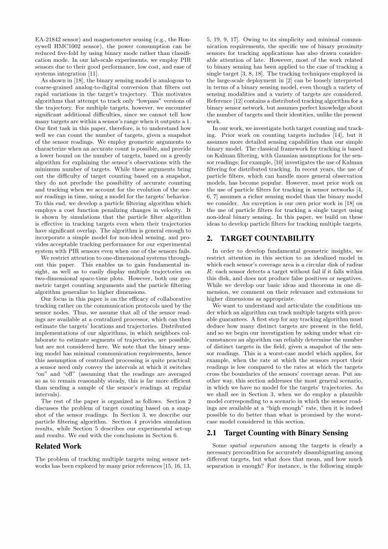
Figure 8: Performance with non-ideal sensing. Inthis particular example, ClusterTrack finds 7 trajec-tories, 5 of which approximate the actual paths.

of the model to generate the feasible target space from thesensor data, assuming the maximum uncertainty consistentwith the sensor readings. An on-sensor tells us that thetarget is somewhere inside the outer interval of radius Ro,while an off-sensor indicates that there is no target insidethe inner interval of radius Ri. Despite its simplicity, this isa fairly generic model for non-ideal behavior, since it arisesnaturally if sensors integrate noisy samples over a reason-able time scale to make binary decisions regarding targetpresence or absence.

The set up for simulation is kept the same as before, withthe modification that each sensor now has an Ri = 30 units,and an Ro = 50 units. In order to simulate the sensor read-ings, we assume that a target falling in the region of uncer-tainty of a particular sensor is detected with probability 0.5by that sensor. 5 targets are considered, each moving within20% (on either side) of its mean velocity. As shown in Fig.8, ClusterTrack performs well. For different choices ofD0(t), the number of trajectories obtained varies between 5and 7. The figure shows a simulation run in which 7 trajec-tories were output. The best 5 are quite close to the actualpaths. The remaining two trajectories are marked with plussigns (+), and we can see that they are made up of piecesof true paths. The costs associated with these 7 trajectoriesare [31.54 38.08 41.67 54.54 57.36 80.45 95.87] units, withthe last two corresponding to the spurious paths. The re-sults above demonstrate the robustness of the particle filterapproach to non-ideal sensing.

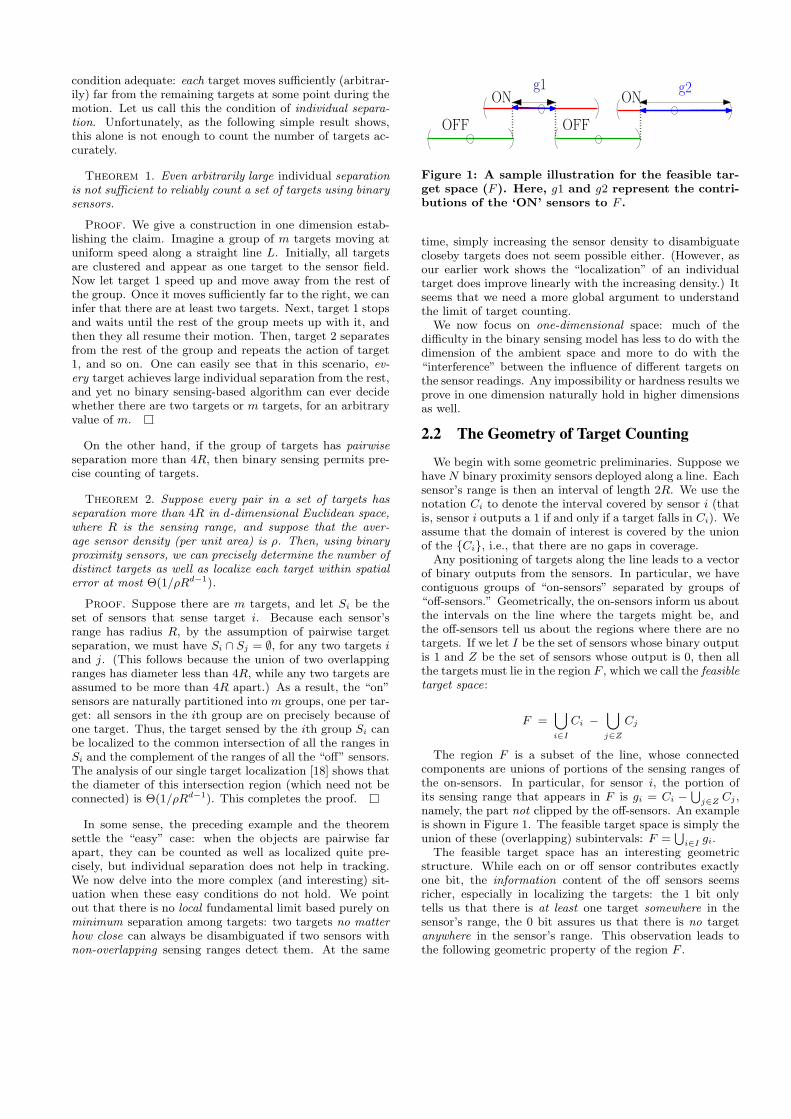
Finally, we present some experimental tracking resultsfrom a lab-scale testbed with PIR sensors.

5. EXPERIMENTSWe use a small testbed with 5 PIR sensors placed uni-

formly along a line; see Figure 9. Each sensor sends a mea-surement to the base station when it changes state, and thebase station is interfaced to a PC through a serial port. Thedata gets time stamped at the PC, so that each of the fi-nal set of measurements includes : ‘value, position (mappedfrom node ID), and time’. For the ground truth regardingtarget trajectories, the (human) targets are provided withseparate sensor nodes (equipped with localization engines)

Figure 9: A view of the experimental set-up, withsensor modules placed uniformly along a line.

1 2 3 4 5 6 7 8 90

0.2

0.4

0.6

0.8

1

Distance (feet)

Prob

abilit

y of d

etec

tion

Figure 10: Probability of target detection againstdistance for a particular sensor module.

with buttons, which they press as they pass by a set ofknown locations on the way.

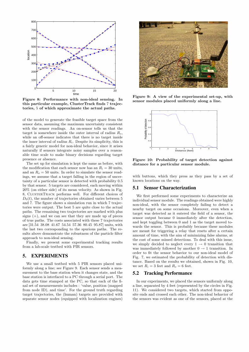
5.1 Sensor CharacterizationWe first performed some experiments to characterize an

individual sensor module. The readings obtained were highlynon-ideal, with the sensor completely failing to detect anearby target on some occasions. Moreover, even when atarget was detected as it entered the field of a sensor, thesensor output became 0 immediately after the detection,and kept toggling between 0 and 1 as the target moved to-wards the sensor. This is probably because these modulesare meant for triggering a relay that resets after a certainamount of time, with the aim of minimizing false alarms, atthe cost of some missed detections. To deal with this issue,we simply decided to neglect every 1 → 0 transition thatwas immediately followed by another 0 → 1 transition. Inorder to fit the sensor behavior to our non-ideal model ofFig. 7, we estimated the probability of detection with dis-tance. Based on the results we obtained, shown in Fig. 10,we set Ri = 3 feet and Ro = 6 feet.

5.2 Tracking PerformanceIn our experiments, we placed the sensors uniformly along

a line, separated by 4 feet (represented by the circles in Fig.11). We considered two targets, which started from oppo-site ends and crossed each other. The non-ideal behavior ofthe sensors was evident as one of the sensors, placed at the

2 4 6 8 10 12 14 160

5

10

15

20

25

30

time

loca

tion

Experimental results with ClusterTrack

T1

T2

Figure 11: Experimental results with the sensormodules. Respectable performance is achieved, inspite of one sensor not even detecting a target.

location of 16 feet (shown by an asterisk ∗ inside the cir-cle) completely missed the presence of target T1. With thethreshold sequence D0(t) = 2R0t, we ran ClusterTrackmultiple times. In spite of the missed detection, we foundthat respectable to good tracking performance was achievedin most of the simulation runs (about 70%), as shown in thefigure for one such good run.

6. CONCLUSIONSThe promising results obtained here, as well as prior re-

sults in [8, 18] for the same sensing model, indicate thatbinary proximity sensors, can form the basis for a robust ar-chitecture for wide area surveillance and tracking. Our tar-get counting results show that interesting conclusions can bedrawn regarding the number of targets and the feasible tar-get space even without any model for the target paths. Onthe other hand, when the target paths are smooth enough,our ClusterTrack particle filter algorithm gives excellentperformance in terms of identifying and tracking differenttarget trajectories.

A host of questions remain to be investigated in futurework, of which we provide a partial list as follows. Is therea good way of combining the combinatorial techniques fortarget counting with the probabilistic techniques of particlefiltering to enhance performance? Are there analytical rulesof thumb for design of the threshold sequence {D0(t)} usedin ClusterTrack? How broadly does our particle filteralgorithm apply, in terms of robustness to different modelsfor the targets’ trajectories? When does it break down?How does tracking performance depend on the dimension ofthe space we operate in (in particular, how well can we trackand count targets in two dimensions)?

7. REFERENCES[1] I. F. Akyildiz, W. Su, Y. Sankarasubramaniam, and

E. Cayirci. A survey on sensor networks. IEEECommunications Magazine, 40:102–114, Aug. 2002.

[2] A. Arora and et. al. A line in the sand: A wirelesssensor network for target detection, classification, andtracking. The International J. of Computer andTelecom. Networking, 46:605–634, Dec. 2004.

[3] J. Aslam, Z. Butler, F. Constantin, V. Crespi,G. Cybenko, and D. Rus. Tracking a moving objectwith a binary sensor network. In Proc. ACM SenSys,2003.

[4] M. Coates. Distributed particle filters for sensornetworks. In Proc. of IPSN, pages 99–107, 2004.

[5] B. Jung and G. S. Sukhatme. Tracking targets usingmultiple robots: The effect of environment occlusion.Autonomous Robots, 13(3):191–205, Nov 2002.

[6] Z. Khan, T. Balch, and F. Dellaert. Efficient particlefilter-based tracking of multiple interacting targetsusing an mrf-based motion model. In Proc. IEEE/RSJConference on Intelligent Robots and Systems, 2003.

[7] Z. Khan, T. Balch, and F. Dellaert. Mcmc-basedparticle filtering for tracking a variable number ofinteracting targets. IEEE Trans. Pattern Analysis andMachine Intelligence, 27(11):1805–1819, Dec. 2005.

[8] W. Kim, K. Mechitov, J.-Y. Choi, and S. Ham. Ontarget tracking with binary proximity sensors. In Proc.IPSN, 2005.

[9] J. Liu, M. Chu, J. Liu, J. Reich, and F. Zhao.Distributed state representation for tracking problemsin sensor networks. In Proc. of IPSN, 2004.

[10] D. McErlean and S. Narayanan. Distributed detectionand tracking in sensor networks. In Proc. of 36thAsilomar Conference on Signals, Systems andComputers, volume 2, pages 1174–1178, 2002.

[11] M. Moghavvemi and L. C. Seng. Pyroelectric infraredsensor for intruder detection. In Proc. TENCON,pages 656 – 659, Nov. 2004.

[12] S. Oh and S. Sastry. Tracking on a graph. In Proc. ofIPSN, April 2005.

[13] S. Oh, L. Schenato, and S. Sastry. A hierarchicalmultiple-target tracking algorithm for sensornetworks. In Proc. International Conference onRobotics and Automation (ICRA), April 2005.

[14] F. Z. Qing Fang and L. Guibas. Counting targets:Building and managing aggregates in wireless sensornetworks. In Palo Alto Research Center (PARC)Technical Report, June 2002.

[15] D. Reid. Aan algorithm for tracking multiple targets.IEEE Trans. Automatic Control, 24:843–854, Dec1979.

[16] Y. B. Shalom and X. R. Li. Multisensor, MultitargetTracking: Principles and Techniques. YBS Publishing,1979.

[17] J. Shin, L. Guibas, and F. Zhao. A distributedalgorithm for managing multi-target identities inwireless ad-hoc sensor networks. In Proc. of IPSN,April 2003.

[18] N. Shrivastava, R. Mudumbai, U. Madhow, andS. Suri. Target tracking with binary proximity sensors:Fundamental limits, minimal descriptions, andalgorithms. In Proc. of ACM SenSys, 2006.

[19] K. R. Songhwai Oh, Inseok Hwang and S. Sastry. Afully automated distributed multiple-target trackingand identity management algorithm. In Proc. AIAAGuidance, Navigation, and Control Conference,August 2005.