Rarefied gas flow of binary mixtures through long channels with triangular and trapezoidal cross...

RESEARCH PAPER

Rarefied gas flow of binary mixtures through long channelswith triangular and trapezoidal cross sections

Lajos Szalmas • Dimitris Valougeorgis

Received: 16 October 2009 / Accepted: 15 December 2009 / Published online: 21 January 2010

� Springer-Verlag 2010

Abstract The flow of binary gas mixtures through long

micro-channels with triangular and trapezoidal cross sec-

tions is investigated in the whole range of the Knudsen

number. The flow is driven by pressure and concentration

gradients. The McCormack kinetic model is utilized to

simulate the rarefied flow of the gas mixture, and the

kinetic equations are solved by an upgraded discrete

velocity algorithm. The kinetic dimensionless flow rates

are tabulated for selected noble gas mixtures flowing

through micro-channels etched by KOH in silicon (trian-

gular and trapezoidal channels with acute angle of 54.74�).

Furthermore, the complete procedure to obtain the mass

flow rate for a gas mixture flowing through a channel,

based on the dimensionless kinetic results, which are valid

in each cross section of the channel, is presented. The study

includes the effect of the separation phenomenon. It is

shown that gas separation may change significantly the

estimated mass flow rate. The presented methodology can

be used for engineering purposes and for the accurate

comparison with experimental results.

Keywords Rarefied gas flows � Binary mixtures �Gas separation � Discrete velocity method

1 Introduction

The non-equilibrium gas flow through channels of various

cross sections has recently attracted considerable attention.

This increased interest is well justified by the implementation

of such flows in several technological fields including the

emerging field of microfluidics (Ho and Tai 1998; Karni-

adakis and Beskok 2002; Kandlikar et al. 2006; Li 2008).

The majority of the research has been performed for

flows through circular and rectangular micro-channels,

where both theoretical and experimental studies have been

implemented. The theoretical study has been based on

hydrodynamics beyond the Navier–Stokes limit (Colin

2005; Lockerby and Reese 2008; Szalmas 2007), the Direct

Simulation Monte Carlo method (Bird 1994), and kinetic

theory as described by the Boltzmann and model kinetic

equations (Ferziger and Kaper 1972; Cercignani 1988). It is

important to note that for flows through long channels,

where the flow may be considered as fully developed,

linearized kinetic theory is overall, the most powerful

theoretical approach, since it is capable of producing

accurate results in the whole range of the Knudsen number

with modest computational effort (Aoki 2001; Sharipov

1999). Experimental study in long micro-channels is also

very extensive, and the most common experimental

approaches include the constant volume and the droplet

tracking methods (Colin et al. 2004; Ewart et al. 2007).

Flows through long channels of other cross sections

have also been studied. In particular, rarefied gas flow

through long tubes with elliptical cross section has been

recently solved by using linearized kinetic models (Graur

and Sharipov 2007, 2008). The linearized BGK model has

been also solved for annular tubes (Breyiannis et al. 2008).

Based on Navier–Stokes solvers, with slip boundary con-

ditions, the pressure-driven flow through channels of tri-

angular and trapezoidal cross sections in the slip regime

has been solved (Morini et al. 2004, 2005; Pitakarrnop

et al. 2008). Also, in more recent studies, the same flow

configuration has been solved in the whole range of the

Knudsen number by using the linearized BGK kinetic

L. Szalmas (&) � D. Valougeorgis

Department of Mechanical and Industrial Engineering,

University of Thessaly, Pedion Areos, Volos 38334, Greece

e-mail: [email protected]

123

Microfluid Nanofluid (2010) 9:471–487

DOI 10.1007/s10404-010-0564-9

model (Naris and Valougeorgis 2008; Varoutis et al. 2009).

In Varoutis et al. (2009), a comparison between computa-

tional and experimental results has been performed finding,

in all the cases, very good agreement. It is noted that

channels with triangular and trapezoidal cross sections,

with an acute angle of 54.74�, manufactured by chemical

etching on silicon wafers, known as microchannels etched

by KOH in silicon, are very common in microflow appli-

cations (Morini et al. 2004, 2005).

The majority of all this research study has been per-

formed for single gases, while the corresponding study for

gaseous mixtures is quite limited. In the latter case, the

McCormack kinetic model (McCormack 1973) has been

applied for flows of binary mixtures through channels of

circular and rectangular cross sections (Sharipov and Kal-

empa 2002; Naris et al. 2005). In addition to flows through

channels, the McCormack model has been solved for

Couette flow (Sharipov et al. 2004) or heat flow between

two parallel plates (Sharipov et al. 2007). The analytical

discrete ordinate method has been also used to solve var-

ious one-dimensional flow problems on the basis of the

McCormack kinetic model (Siewert and Valougeorgis

2004a, b). A first attempt to measure pressure-driven mass

flow rates for binary mixtures through rectangular channels

is reported in Pitakarnnop (2010). The small amount of

study in the case of gas mixture flows may be explained by

the increased complexity of the flow due to the large

number of parameters involved in the solution of the

problem. However, gaseous mixture, compared to single

gas flows, have increased theoretical and practical interest.

In the case of gas mixtures, additional non-equilibrium

transport phenomena (e.g., barodiffusion) appear, as the

rarefaction of the flow is increased. Also, in microfluidic

applications, the flow in most cases consists of gas mix-

tures and not of single gases. Another important transport

phenomenon of great practical interest appearing in flows

of gas mixtures is the separation phenomenon. The light

particles are traveling faster than the heavier ones resulting

to the change of the concentration of the gas mixture as it

flows along the channel. This situation, known as the

separation effect, must be taken into account in simulations

and may be useful in the design of gaseous microsystems

(Sharipov and Kalempa 2005; Takata et al. 2007; Sugim-

oto 2009).

In this article, a fully developed binary rarefied gas flow

through long triangular and trapezoid channels is investi-

gated. Pressure- and concentration-driven microflows are

considered. The flow is modeled by the McCormack

kinetic model subject to Maxwell diffuse-specular bound-

ary conditions. The kinetic integro-differential equations

are solved in a very efficient manner, and the obtained

results are valid in the whole range of the rarefaction from

the free molecular through the transition up to the

hydrodynamic limit. Numerical results are presented for

the noble-gas mixtures of Ne/Ar and He/Xe. Even more, a

detailed procedure is presented for calculating the mass

flow rate from the dimensionless kinetic coefficients taking

into account the separation phenomenon. The presented

methodology and results can be used for comparing

experiments with theory, as well as to the design and

optimization of micro devices.

2 Flow configuration

Consider the isothermal flow of a gaseous mixture through

a channel of length L, with triangular or trapezoidal cross

sections. The cross sections are defined by the x0 and y0

coordinates, while the flow is assumed to be in the direc-

tion of the z0 coordinate. The perimeter and the area of the

channel are denoted by C0 and A0, respectively. The

hydrodynamic diameter of the channel Dh = 4A0/C0 is

utilized as the characteristic length of the problem. End

effects are ignored by taking Dh \\ L.

The dimensionless spatial variables x = x0/Dh, y = y0/Dh, and z = z0/Dh are introduced, while the dimensionless

perimeter and area are defined as C = C0/Dh and A = A0/Dh2,

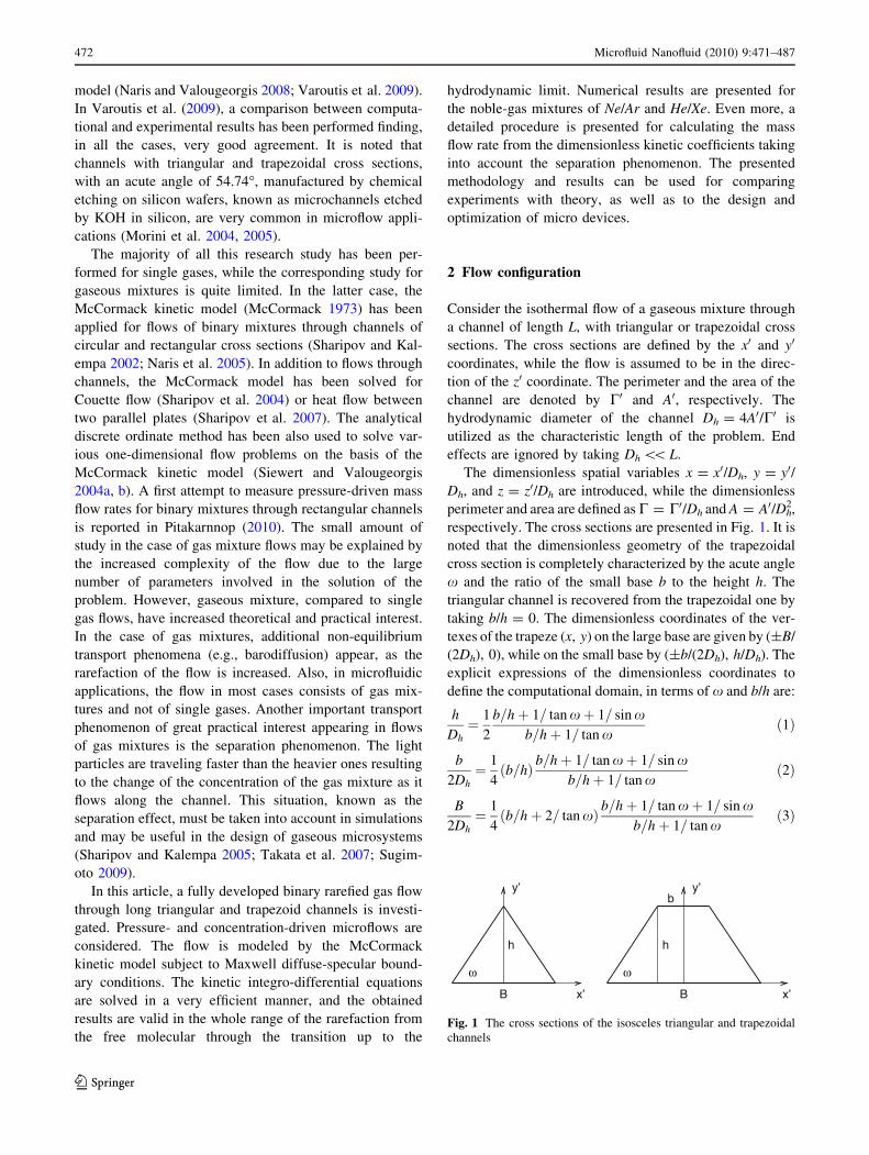
respectively. The cross sections are presented in Fig. 1. It is

noted that the dimensionless geometry of the trapezoidal

cross section is completely characterized by the acute angle

x and the ratio of the small base b to the height h. The

triangular channel is recovered from the trapezoidal one by

taking b/h = 0. The dimensionless coordinates of the ver-

texes of the trapeze (x, y) on the large base are given by (±B/

(2Dh), 0), while on the small base by (±b/(2Dh), h/Dh). The

explicit expressions of the dimensionless coordinates to

define the computational domain, in terms of x and b/h are:

h

Dh¼ 1

2

b=hþ 1= tan xþ 1= sin xb=hþ 1= tan x

ð1Þ

b

2Dh¼ 1

4ðb=hÞ b=hþ 1= tan xþ 1= sin x

b=hþ 1= tan xð2Þ

B

2Dh¼ 1

4b=hþ 2= tan xð Þ b=hþ 1= tan xþ 1= sin x

b=hþ 1= tan xð3Þ

x’ x’

y’ y’

h

b

ω ω

h

B B

Fig. 1 The cross sections of the isosceles triangular and trapezoidal

channels

472 Microfluid Nanofluid (2010) 9:471–487

123

By setting in Eqs. 1 and 3, b/h = 0, the dimensionless

coordinates of the isosceles triangular are deduced.

The mixture consists of two components. The molecular

masses and the number densities of the two species are

denoted by ma and na for components a = 1, 2. In this

study, without loss of generality, m1 will always refer to the

light species of the mixture. The average molecular mass of

the mixture is defined by

mðCÞ ¼ Cm1 þ ð1� CÞm2; ð4Þ

where

C ¼ n1

n1 þ n2

; ð5Þ

is the concentration of the light species in the mixture. The

total number density of the mixture is obtained by

n = n1 ? n2. Other important quantities of the mixture, for

the purposes of this study, are its viscosity l(C) and its

characteristic molecular velocity vðCÞ ¼ffiffiffiffiffiffiffiffiffiffiffiffiffiffiffiffiffiffiffiffiffi

2kT=mðCÞp

;

with k denoting the Boltzmann constant and T the tem-

perature of the flow. Since this is an isothermal flow, both

quantities depend only on the concentration of the mixture.

The flow is maintained by a pressure and/or concentra-

tion gradient defined by

XP ¼Dh

P

oP

oz0¼ 1

P

oP

ozð6Þ

and

XC ¼Dh

C

oC

oz0¼ 1

C

oC

ozð7Þ

respectively. Here, P = P(z) and C = C(z) are the pressure

and concentration distributions along the channel and, in

general, their gradients are not constant. It is important to

note that under the assumption of Dh \\ L both the

dimensionless gradients are always much less than one,

i.e., |XP| \\ 1, |XC| \\ 1, independently of the magnitude

of the pressure and concentration differences between the

inlet and the outlet of the channel.

The flow is characterized by the rarefaction parameter

defined by

d ¼ DhPðzÞlðCÞvðCÞ ; ð8Þ

It is emphasized that the rarefaction parameter varies in the

flow direction, i.e., d = d(z), according to the variation of

the pressure, viscosity, and characteristic velocity along the

channel. The rarefaction parameter is proportional to the

inverse Knudsen number.

Under the assumption of the long channel (fully devel-

oped flow) the only non-zero component of the macro-

scopic (bulk) velocity vectors u0a of the two species is the z0

component, which is the function of the transverse coor-

dinates, i.e., u0a ¼ ð0; 0; u0aðx0; y0ÞÞ; with a = 1, 2. Other

relevant macroscopic quantities concerning the flow prob-

lem are the heat flow vectors having non-zero element only

for the z0 component q0a ¼ ð0; 0; q0aðx0; y0ÞÞ and the traceless

pressure tensors having non-zero elements only for

p0axzðx0; y0Þ; p0ayzðx0; y0Þ, with a = 1, 2.

In addition to the bulk velocity of the two species, we

are introducing the mean velocity of the mixture as

wðx0; y0Þ ¼ n1u01 þ n2u02n1 þ n2

: ð9Þ

We are interested in the overall quantities of the mass flow

rate given by

_M ¼ZZ

A0ðn1m1u01 þ n2m2u02Þdx0dy0 ð10Þ

and of the particle and concentration fluxes defined by

(Sharipov and Kalempa 2002; Naris et al. 2005)

JP ¼ �n

ZZ

A0wdx0dy0; ð11Þ

JC ¼ �n1

ZZ

A0ðu01 � u02Þdx0dy0: ð12Þ

It is readily seen that these overall quantities are

interconnected by the expression

_M ¼ �mðCÞJP þ ðm2 � m1Þð1� CÞJC: ð13Þ

The particle and concentration fluxes are connected to

the gradients of the pressure and the concentration via the

dimensionless kinetic coefficients, namely, KPP, KCP, KPC,

KCC in the following way:

JP ¼nA0vðCÞ

2½KPPXP þ KPCXC�; ð14Þ

JC ¼nA0vðCÞ

2½KCPXP þ KCCXC�: ð15Þ

It is noted that the JP and JC fluxes are two independent

variables since JP describes the total particle flow rate,

while JC is related to the velocity difference between the

components. The driving terms, XP and XC, are also

independent quantities. XP is related to the total number

density, while XC to the ratio of the component densities.

The use of the XP, XC driving terms are straightforward

and advantageous since the pressure and the concentra-

tion are the two main quantities in the description of

gaseous mixtures and the related micro-gas flow

applications.

The cross kinetic coefficients are not independent, and

they are connected via the Onsager–Casimir relationship

KPC = KCP, as it was shown in Sharipov (1994).

The rarefied gas flow in the channel is completely charac-

terized by the above mentioned kinetic coefficients. It is

important to emphasize that these are local quantities and

Microfluid Nanofluid (2010) 9:471–487 473

123

describe the flow in a given cross section with the corre-

sponding XP and XC gradients. In this article, our goal is to

calculate and tabulate the kinetic coefficients for different

values of d and C and then, based on these kinetic results, to

provide the detailed procedure for estimating the overall mass

flow rate, taking into account the pressure and concentration

variation along the channel including the separation effect.

3 Kinetic description

In order to simulate the flow, a kinetic description, based

on the McCormack model subject to the Maxwell diffuse-

specular boundary conditions is adapted. The approach is

valid in the whole range of the rarefaction.

The basic quantity in the description of the problem is

the distribution function faðca; x; y; zÞ for components

a = 1, 2. Here, ca ¼ ðcax; cay; cazÞ is the dimensionless

molecular velocity defined by ca ¼ vaðma=2kTÞ1=2with va

being the molecular velocity. The distribution function is

linearized such that

faðca; x; y; zÞ ¼ f ð0Þa ðca; zÞð1þ haðca; x; yÞÞ; ð16Þ

where haðca; x; yÞ is the perturbation function and fð0Þa ðca; zÞ

is the equilibrium distribution

f ð0Þa ðca; zÞ ¼ naðzÞma

2pkT

� ��3=2

e�c2a : ð17Þ

The perturbation function obeys the McCormack kinetic

model

caxoha

oxþ cay

oha

oy¼ xa

X

2

b¼1

Labha � caz½XP þ gaXC�; ð18Þ

where Lab is the McCormack collision term, which,

together with xa, are defined in Appendix 1. In addition,

the quantity ga is given by

g1 ¼ 1; g2 ¼ �C

1� C: ð19Þ

The non-dimensional velocity, heat flow, and traceless

pressure tensor are obtained as the moments of the

perturbation function:

ua ¼ p�3=2 m

ma

� �1=2 Z1

�1

hacaze�c2

adca;

qa ¼ p�3=2 m

ma

� �1=2 Z1

�1

hacaz c2a �

5

2

� �

e�c2adca;

paiz ¼ p�3=2

Z

1

�1

hacaicaze�c2

adca:

ð20Þ

In this formulation, the index i refers to the coordinates

x or y.

In the present flow configuration, the problem can be

described by the following two reduced distribution functions:

Ua ¼1ffiffiffi

pp

ffiffiffiffiffiffi

m

ma

rZ

1

�1

Z

1

�1

hacaze�c2

a�c2adcaz; ð21Þ

Wa ¼1ffiffiffi

pp

ffiffiffiffiffiffi

m

ma

rZ

1

�1

Z

1

�1

hac3aze�c2

a�c2adcaz: ð22Þ

In accordance with the McCormack model, Eq. 18, the

reduced distribution functions obey the following system of

four linear integro-differential equations:

caxoUa

oxþ cay

oUa

oyþ caxaUa ¼ �

1

2

ffiffiffiffiffiffi

m

ma

r

½XP þ gaXC�

þ xa

X

2

b¼1

�

Aab þ 2Babxcax þ 2Babycay

þ 2

5Cabðc2

ax þ c2ay � 1Þ

�

ð23Þ

and

caxoWa

oxþ cay

oWa

oyþ caxaWa ¼ �

3

4

ffiffiffiffiffiffi

m

ma

r

½XP þ gaXC�

þ xa

X

2

b¼1

�

3

2Aab þ 3Babxcax þ 3Babycay

þ 3

5Cab c2

ax þ c2ay

� �

�

; ð24Þ

with a = 1, 2.

The coefficients Aab, Babi and Cab are connected to the

bulk quantities of velocity ua, heatflow qa, and pressure

paiz such that

Aab ¼ cabua � mð1Þab ðua � ubÞ �1

2mð2Þab qa �

ma

mbqb

� �

; ð25Þ

Babi ¼ cab � mð3Þab

� �

ffiffiffiffiffiffi

m

ma

r

paiz þ mð4Þab

ffiffiffiffiffiffi

m

ma

r

pbiz; ð26Þ

Cab ¼ cab � mð5Þab

� �

qa þ mð6Þab

ffiffiffiffiffiffi

mb

ma

r

qb �5

4mð2Þab ðua � ubÞ:

ð27Þ

The parameters cab and mab are presented in Appendix 1.

Utilizing the reduced distribution functions, the bulk

quantities are obtained by

ua ¼1

p

Z

1

�1

Z

1

�1

Uae�c2ax�c2

ay dcaxdcay; ð28Þ


123

qa ¼1

p

Z

1

�1

Z

1

�1

Waþ c2axþ c2

ay�5

2

� �

Ua

� �

e�c2ax�c2

ay dcaxdcay;

ð29Þ

paiz ¼1

p

ffiffiffiffiffiffi

m

ma

rZ

1

�1

Z

1

�1

caiUae�c2ax�c2

ay dcaxdcay: ð30Þ

For the reduced distribution functions, the boundary

conditions are written by

Uþ ¼ ð1� rÞU�; Wþ ¼ ð1� rÞW�; ð31Þ

where 0 B r B 1 is the accommodation coefficient, while

the ? and - superscripts denote distributions representing

particles departing from and arriving to the walls,

respectively.

The above system of kinetic Eqs. 23 and 24 with the

associated moments (28–30), subject to boundary condi-

tions (31), has been solved numerically by discretizing in

the physical space using a finite difference scheme on a

boundary fitted triangular grid and in the molecular

velocity space the discrete velocity method. The dis-

cretized equations are solved in an iterative manner. This

numerical scheme has been extensively used in the

past and for further details, the interested reader may

refer to Naris and Valougeorgis (2008), Sharipov and

Kalempa (2002), and Naris et al. (2005). The triangular

grid is structured and consists of identical triangular

elements (Naris and Valougeorgis 2008). In addition,

in this study, in order to make the overall computation

more efficient, a diffusion-type acceleration scheme

is used to speed up the slow convergence of the algo-

rithm in the nearly continuum region. The diffusion

equations of the accelerated method are presented in

Appendix 2.

Once the solution of the integro-differential system is

obtained, the dimensionless flow rates of the components

are deduced as

Ga ¼ �2

A

ZZ

A

uadxdy; a ¼ 1; 2: ð32Þ

It is noted that the above described kinetic problem is

linear, and, as a consequence, the solution may be

decomposed in terms of XP and XC. This is also the case

for the dimensionless flow rate, which can be decomposed

by

Ga ¼ GðPÞa XP þ GðCÞa XC: ð33Þ

Then, for a pressure-driven flow, the kinetic coefficients

KPP and KCP are calculated from

KPP¼CGðPÞ1 þð1�CÞGðPÞ2 ; KCP¼C G

ðPÞ1 �G

ðPÞ2

� �

; ð34Þ

while for a concentration-driven flow, the kinetic

coefficients KPC and KCC are calculated from

KPC ¼ CGðCÞ1 þ ð1� CÞGðCÞ2 ; KCC ¼ CðGðCÞ1 � G

ðCÞ2 Þ:ð35Þ

In Sect. 6.1, tabulated results are presented for the kinetic

coefficients of two typical binary gas mixtures in terms of dand C, flowing through one triangular and two trapezoidal

channels.

4 Mass flow rate of gaseous mixture flowing through

a channel

In applications, the mass flow rate _M , defined by Eq. 10, of a

gaseous mixture flowing through a channel, connecting two

reservoirs, is a very important quantity. Utilizing the kinetic

coefficients, the mass flow rate can be calculated for realistic

situations, provided that the pressure and the concentration

of the upstream and downstream reservoirs, denoted by I and

II, respectively, as well as the geometry of the channel are

known. In this section, the detailed methodology for

deducing _M is presented for flow caused by either a pressure

or a concentration gradient. This section provides an

approximation for the mass flow rate with the assumption

that the concentration (or the pressure) is constant for the

pressure (or concentration-)-driven flow. The analysis is

valid for any pressure or concentration differences between

the reservoirs as long as the restriction Dh/L \\ 1 holds.

4.1 Pressure-driven flow

In this case, the flow is maintained by a constant pressure

drop between the containers. The pressures in the upstream

and downstream reservoirs are given by PI and PII,

respectively, while the concentration in the containers and

along the channels is considered constant and equal to C0.

Substituting Eqs. 14 and 15 for the JP and JC fluxes, with

XC = 0, into Eq. 13 and utilizing the ideal gas law

P = nkT, as well as the definition of the characteristic

velocity, the mass flow rate can be written as

_M ¼ �KPP þm2 � m1

mðC0Þð1� C0ÞKCP

� �

A0

vðC0ÞdP

dz: ð36Þ

It is important to note that in Eq. 36, the mass flow rate is

given in terms of quantities which vary along the channel and

refer to a given cross section. Of course, the mass flow rate is

a quantity, which, due to mass conservation, is constant at

each cross section. Then, the mass flow rate may be also


123

defined in terms of reference quantities, which do not vary

along the channel according to the auxiliary expression:

_M ¼ �K�PP þm2 � m1

mðC0Þð1� C0ÞK�CP

� �

A0

vðC0ÞPII � PI

LDh:

ð37Þ

Here,K�PP and K�PC are the average kinetic coefficients, which

will be deduced such that Eq. 37 yields the correct mass flow

rate. We note that the average kinetic coefficient has been

earlier used for single gases (Sharipov and Seleznev 1998).

Now, it is applied for mixtures with the assumption that the

concentration is constant for the pressure-driven flow.

In order to achieve that the right-hand side of Eqs. 36

and 37 are equated to find

KPPdP

PII � PI¼ K�PPdz

Dh

Lð38Þ

KCPdP

PII � PI¼ K�CPdz

Dh

L: ð39Þ

Based on the definition of d, given in Eq. 8, it is easily

deduced that dP/(PII - PI) = dd/(dII - dI), where the

rarefaction parameters dI and dII refer to pressures PI and

PII, respectively. Next, Eqs. 38 and 39 are integrated over din the interval [dI, dII] and 0 B z B L/Dh to yield

K�PP ¼1

dII � dI

Z

dII

dI

KPPdd; ð40Þ

K�CP ¼1

dII � dI

Z

dII

dI

KCPdd: ð41Þ

The average kinetic coefficients can be calculated by

Eqs. 40 and 41, provided that the kinetic coefficients for a

specific gas mixture as a function of the rarefaction

parameter along the channel have been estimated. Then,

the mass flow rate is estimated from Eq. 37.

4.2 Concentration-driven flow

In this case, the flow is caused by a concentration drop

between the two reservoirs. The concentrations in the

upstream and downstream containers are given by CI and

CII, respectively, while the pressure and, therefore, the

number density remain constant and equal to P0 and n0,

respectively. The calculation is similar to the pressure-

driven flow. Substituting Eqs. 14 and 15, with XP = 0, into

Eq. 13 the mass flow rate is given by

_M ¼ �KPC þm2 � m1

mðCÞ ð1� CÞKCC

� �

n0mðCÞA0vðCÞ2C

dC

dz:

ð42Þ

The mass flow rate is also defined in terms of reference

quantities as

_M ¼ �K�PC þm2 � m1

mðC0Þð1� C0ÞK�CC

� �

� n0mðC0ÞA0vðC0Þ2C0

CII � CI

LDh:

ð43Þ

Here, it is recalled that the pressure is considered constant

for the present situation. As a consequence, the average

kinetic coefficients can be applied. For the concentration-

driven flow, since the concentration varies along the

channel, the reference concentration C0 is chosen as the

average value between the two reservoirs, i.e.,

C0 = (CI ? CII)/2. This also defines the reference mass

m(C0) and characteristic velocity v(C0). Then, the right-

hand sides of Eqs. 42 and 43 are equated to deduce

KPCdC

CII � CI

C0

C

mðCÞvðCÞmðC0ÞvðC0Þ

¼ K�PCdzDh

L; ð44Þ

KCCdC

CII � CI

C0

C

1� C

1� C0

v

vðC0Þ¼ K�CCdz

Dh

L: ð45Þ

Integrating these equations along the channel, the average

kinetic coefficients are obtained by

K�PC ¼1

CII � CI

Z

CII

CI

C0

C

mðCÞvðCÞmðC0ÞvðC0Þ

KPCdC; ð46Þ

K�CC ¼1

CII � CI

Z

CII

CI

C0

C

1� C

1� C0

vðCÞvðC0Þ

KCCdC: ð47Þ

Having calculated the average kinetic coefficients in terms

of the concentration C and the corresponding d(C), the

mass flow rate is obtained from Eq. 43 for the concentra-

tion-driven flow. In conclusion, we note that when the flow

is driven by both pressure and concentration gradients, then

the total mass flow rate is obtained by superimposing the

two solutions.

5 Separation effect in rarefied binary gaseous flow

It is well known that in gas mixtures, consisting of various

species, the particles of different types travel with different

speeds. As the flow becomes more rarefied and the number

of intermolecular collisions is reduced, this difference in

the molecular velocities results to different macroscopic

velocities for each species of the mixture as well. As a

result, for gas mixtures flowing through long channels, the


123

concentration of the mixture may alter significantly in the

flow direction. This phenomenon is known as the separa-

tion effect. It is observed in gaseous mixtures, but it is

absent for single gases. The separation effect is very

important in many applications including pumping, sam-

pling, filtering, etc. (Sharipov and Kalempa 2005; Takata

et al. 2007; Sugimoto 2009) and should be taken into

consideration in the estimation of the mass flow rate.

A detailed investigation of the separation effect has been

presented in Sharipov and Kalempa (2005) for binary gas

flow through long tubes into vacuum, based on the pre-

scribed number densities of the two reservoirs. Here, this

procedure is slightly modified having as primitive vari-

ables, the pressure and concentration distributions. This

treatment is equivalent to the one in Sharipov and Kalempa

(2005), but it is considered as more straightforward and

suitable for microflow applications, where, in general, the

downstream pressure is not equal to zero, while the con-

centration of the gas in the downstream reservoir is known.

The analysis, in addition to the exact estimation of the mass

flow rate, provides in parallel the concentration and pres-

sure variation along the channel.

The procedure is starting by introducing the mass flow

rate of each component of the mixture, namely,

_Ma ¼ nama

Z Z

A0

u0adx0dy0; ð48Þ

with a = 1, 2, while _M ¼ _M1 þ _M2: Our aim is to derive

an expression for these fluxes as a function of the pressure

and concentration gradients as driving terms. Utilizing

Eq. 13, straightforward calculation shows that the

component mass flow rates are connected to the fluxes JP

and JC according to

_M1 ¼ �m1 CJP þ ð1� CÞJCð Þ; ð49Þ_M2 ¼ �m2ð1� CÞðJP � JCÞ: ð50Þ

At this point, we introduce the non-dimensional flow rates

Ja ¼mðCIÞvðCIÞL

maPIA0Dh

_Ma; ð51Þ

where a = 1, 2. The mass flow rates of each species, given

by Eqs. 49 and 50, are introduced into Eq. 51 and then the

fluxes JP and JC, given by Eqs. 14 and 15, respectively, are

substituted into the resulting equations to obtain

J1 ¼ �PvðCÞL

PIvðCIÞDhCKPP þ ð1� CÞKCPð ÞXP½

þ CKPC þ ð1� CÞKCCð ÞXC�; ð52Þ

J2 ¼ �PvðCÞL

PIvðCIÞDhð1

� CÞ KPP � KCPð ÞXP þ KPC � KCCð ÞXC½ �: ð53Þ

Utilizing the definitions of the characteristic velocity, the

pressure and concentration gradients and the ideal gas law,

Eqs. 52 and 53 are rewritten as

J1 ¼�P

PI

ffiffiffiffiffiffiffiffiffiffiffiffi

mðCIÞmðCÞ

s

��

CKPP þ ð1� CÞKCPð Þ oP

oz

1

P

þ CKPC þ ð1� CÞKCCð Þ oC

oz

1

C

�

; ð54Þ

J2 ¼�P

PI

ffiffiffiffiffiffiffiffiffiffiffiffi

mðCIÞmðCÞ

s

ð1� CÞ

� KPP � KCPð Þ oP

oz

1

Pþ KPC � KCCð ÞoC

oz

1

C

� �

; ð55Þ

where 0 � z � 1; defined as z ¼ z0=L; is the non-

dimensional coordinate along the axis of the channel.

The coupled ordinary differential Eqs. 54 and 55 are the

main equations to be solved for the unknown distributions

PðzÞ and CðzÞ: These equations are supplemented by the

following boundary conditions at the inlet and outlet of the

micro-channel

Pð0Þ ¼ PI ; Pð1Þ ¼ PII ; ð56ÞCð0Þ ¼ CI ; Cð1Þ ¼ CII : ð57Þ

It is mentioned that the reservoirs are considered large. As

a consequence, the pressure and the concentrations are

constant in the containers, and Eqs. 56 and 57 are well

defined.

It is noted that the quantities J1 and J2 are unknown, and

they will be deduced in an iterative manner such that the

outlet boundary conditions at z ¼ 1 are satisfied. Initially

some estimates of J1 and J2 are provided, and then the

system of the ordinary differential equations is solved,

starting from z ¼ 0 and moving up to z ¼ 1 , by applying a

typical marching integration scheme, such as the Euler

method. The computed values of the pressure and the

concentration at the exit of the channel, z ¼ 1 , are com-

pared to the corresponding boundary conditions. In order to

find the values of J1, J2, a bisection root-finding method

has been developed. Initially, two intervals are selected for

J1 and J2. Then, the fluxes are determined in two joint

iterations. The fluxes are always fixed at the middle values

of the intervals. In each stage of the iteration, the corre-

sponding interval is bisected, and the flux is reassigned to

the new middle value. The changes of the fluxes in the

algorithm are determined as follows. First, assuming the

given value for the J2 flux, J1 is calculated depending on

the concentration at the exit of the channel C(1). If C(1) is

smaller (or larger) than CII then J1 is decreased (or

increased). In this way, J1 is obtained, provided that the


123

concentration boundary condition is satisfied with a con-

vergence criterion. After this procedure, the overall itera-

tion starts with an updated value of J2 depending on the

pressure at the exit P(1). If P(1) is smaller (or larger) than

PII then J2 is decreased (or increased). The iteration on J2 is

repeated until the pressure boundary condition at the outlet

is satisfied with a convergence criterion. Utilizing this

method, PðzÞ and CðzÞ , as well as the quantities J1 and J2

are calculated. Finally, utilizing Eq. 51, the mass flow rates

of each species and obviously of the gas mixture may be

obtained.

In Sect. 6.2, based on the above methodology, results are

presented for the mass flow rate for pressure-driven rarefied

binary gas mixture flows through the triangular channel

taking into account the separation effect. For this purpose,

the normalized mass flow rate is introduced as

JM ¼vðCIÞLPIA0Dh

_M: ð58Þ

This quantity can be expressed in terms of Ja, a = 1, 2,

by utilizing Eq. 51, in the more convenient form:

JM ¼m1

mðCIÞJ1 þ

m2

mðCIÞJ2: ð59Þ

In addition to the estimation of JM , the corresponding

quantity without including the correction due to separation,

is estimated. In order to achieve that and to be able to

examine the importance of separation, it is necessary to

introduce the quantities:

J�1 ¼ �½CK�PP þ ð1� CÞK�CP�PII � PI

PI; ð60Þ

J�2 ¼ �ð1� CÞ½K�PP � K�CP�PII � PI

PI; ð61Þ

The fluxes J�a ; a = 1, 2 are based on the average kinetic

coefficients, which are obtained from Eqs. 54 and 55

assuming zero concentration gradient (XC = 0). Also, these

fluxes correspond to Ja, a = 1, 2, obtained above including

the separation effect. Finally, the normalized total mass

flow on the basis of the average kinetic coefficients is given

by

J�M ¼m1

mðCIÞJ�1 þ

m2

mðCIÞJ�2 : ð62Þ

We note that J�M is the total mass flow rate without accounting

for separation, and it corresponds to the mass flow rate

given by Eq. 37 utilizing the normalization of Eq. 58.

6 Results

In this section, numerical results are presented in tabulated

and graphical forms for the kinetic coefficients, the

concentration and pressure variations along the channel,

and the mass flow rates for certain flow configurations. In

particular, the simulations include two binary mixtures,

namely, the Ne/Ar mixture, with m1 = 20.183 g/mol,

m2 = 39.948 g/mol and the He/Xe mixture, with

m1 = 4.0026 g/mol, m2 = 131.30 g/mol, and the following

three different cross sections: Two isosceles trapezoidal

with b/h = 0.5 and 3, and one isosceles triangular (b/

h = 0). In all these three cross sections, the angle

x = 54.74� (Fig. 1), which is the angle of micro-channels

etched by KOH in silicon. In all the cases, purely diffuse

accommodation is considered (r = 1), while the collision

frequencies in the kinetic equations are computed based on

experimental data for the specific binary mixtures (Shari-

pov and Kalempa 2002; Naris et al. 2005).

6.1 Kinetic coefficients

The integro-differential system of equations, described in

Sect. 3, is solved to obtain the kinetic coefficients.

Depending upon the values of d and the geometry, the

discretization has been progressively refined to ensure grid-

independent results up to several significant figures. The

presented results have been obtained by utilizing the fol-

lowing discretization: In the molecular velocity space, the

number of discrete velocities is set to M 9 N = 16 9 300

for d\ 1 and M 9 N = 16 9 72 for dC1. Here, M and N

denote the number of magnitudes and polar angles of the

discrete velocity vector, respectively. In the physical space,

for the triangular cross section, the number of nodes along

its base is set equal to 1000 for d B 1 and to 1400 for

d[ 1, while for the trapezoidal cross section, the number

of nodes along its large base B is set equal to 1500 for all

values of d. The iteration process is terminated when the

absolute difference between subsequent values of the

dimensionless flow rates is less than 10-6.

Tables 1, 2, and 3 depict the kinetic coefficients KPP, KCP,

and KCC for the whole range of C and for a very wide range of

0 B d B 100. As mentioned before KCP = KPC. With

regard to KPP, it can be deduced that it has a minimum in the

transient region for all the cases. This corresponds to the so-

called Knudsen-minimum phenomenon, that is, the total

flow rate has a minimum in the transition region. The

Knudsen-minimum appears for pressure-driven gas flows

through channels or between plates in the transient region. It

can be observed in both single component gases and gaseous

mixtures. Considering KCP, which is a cross effect and cor-

responds to a diffusion flux due to a pressure gradient, it can

be seen that it increases as the rarefaction parameter d is

decreased. This demonstrates that the velocity difference

between the components of the binary mixture, which causes

the diffusion flux, becomes larger as the flow becomes more


123

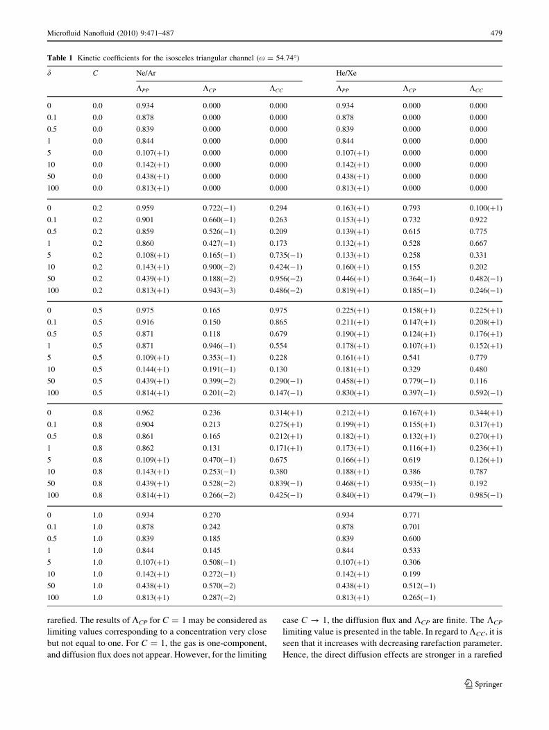
rarefied. The results of KCP for C = 1 may be considered as

limiting values corresponding to a concentration very close

but not equal to one. For C = 1, the gas is one-component,

and diffusion flux does not appear. However, for the limiting

case C ? 1, the diffusion flux and KCP are finite. The KCP

limiting value is presented in the table. In regard to KCC, it is

seen that it increases with decreasing rarefaction parameter.

Hence, the direct diffusion effects are stronger in a rarefied

Table 1 Kinetic coefficients for the isosceles triangular channel (x = 54.74�)

d C Ne/Ar He/Xe

KPP KCP KCC KPP KCP KCC

0 0.0 0.934 0.000 0.000 0.934 0.000 0.000

0.1 0.0 0.878 0.000 0.000 0.878 0.000 0.000

0.5 0.0 0.839 0.000 0.000 0.839 0.000 0.000

1 0.0 0.844 0.000 0.000 0.844 0.000 0.000

5 0.0 0.107(?1) 0.000 0.000 0.107(?1) 0.000 0.000

10 0.0 0.142(?1) 0.000 0.000 0.142(?1) 0.000 0.000

50 0.0 0.438(?1) 0.000 0.000 0.438(?1) 0.000 0.000

100 0.0 0.813(?1) 0.000 0.000 0.813(?1) 0.000 0.000

0 0.2 0.959 0.722(-1) 0.294 0.163(?1) 0.793 0.100(?1)

0.1 0.2 0.901 0.660(-1) 0.263 0.153(?1) 0.732 0.922

0.5 0.2 0.859 0.526(-1) 0.209 0.139(?1) 0.615 0.775

1 0.2 0.860 0.427(-1) 0.173 0.132(?1) 0.528 0.667

5 0.2 0.108(?1) 0.165(-1) 0.735(-1) 0.133(?1) 0.258 0.331

10 0.2 0.143(?1) 0.900(-2) 0.424(-1) 0.160(?1) 0.155 0.202

50 0.2 0.439(?1) 0.188(-2) 0.956(-2) 0.446(?1) 0.364(-1) 0.482(-1)

100 0.2 0.813(?1) 0.943(-3) 0.486(-2) 0.819(?1) 0.185(-1) 0.246(-1)

0 0.5 0.975 0.165 0.975 0.225(?1) 0.158(?1) 0.225(?1)

0.1 0.5 0.916 0.150 0.865 0.211(?1) 0.147(?1) 0.208(?1)

0.5 0.5 0.871 0.118 0.679 0.190(?1) 0.124(?1) 0.176(?1)

1 0.5 0.871 0.946(-1) 0.554 0.178(?1) 0.107(?1) 0.152(?1)

5 0.5 0.109(?1) 0.353(-1) 0.228 0.161(?1) 0.541 0.779

10 0.5 0.144(?1) 0.191(-1) 0.130 0.181(?1) 0.329 0.480

50 0.5 0.439(?1) 0.399(-2) 0.290(-1) 0.458(?1) 0.779(-1) 0.116

100 0.5 0.814(?1) 0.201(-2) 0.147(-1) 0.830(?1) 0.397(-1) 0.592(-1)

0 0.8 0.962 0.236 0.314(?1) 0.212(?1) 0.167(?1) 0.344(?1)

0.1 0.8 0.904 0.213 0.275(?1) 0.199(?1) 0.155(?1) 0.317(?1)

0.5 0.8 0.861 0.165 0.212(?1) 0.182(?1) 0.132(?1) 0.270(?1)

1 0.8 0.862 0.131 0.171(?1) 0.173(?1) 0.116(?1) 0.236(?1)

5 0.8 0.109(?1) 0.470(-1) 0.675 0.166(?1) 0.619 0.126(?1)

10 0.8 0.143(?1) 0.253(-1) 0.380 0.188(?1) 0.386 0.787

50 0.8 0.439(?1) 0.528(-2) 0.839(-1) 0.468(?1) 0.935(-1) 0.192

100 0.8 0.814(?1) 0.266(-2) 0.425(-1) 0.840(?1) 0.479(-1) 0.985(-1)

0 1.0 0.934 0.270 0.934 0.771

0.1 1.0 0.878 0.242 0.878 0.701

0.5 1.0 0.839 0.185 0.839 0.600

1 1.0 0.844 0.145 0.844 0.533

5 1.0 0.107(?1) 0.508(-1) 0.107(?1) 0.306

10 1.0 0.142(?1) 0.272(-1) 0.142(?1) 0.199

50 1.0 0.438(?1) 0.570(-2) 0.438(?1) 0.512(-1)

100 1.0 0.813(?1) 0.287(-2) 0.813(?1) 0.265(-1)


123

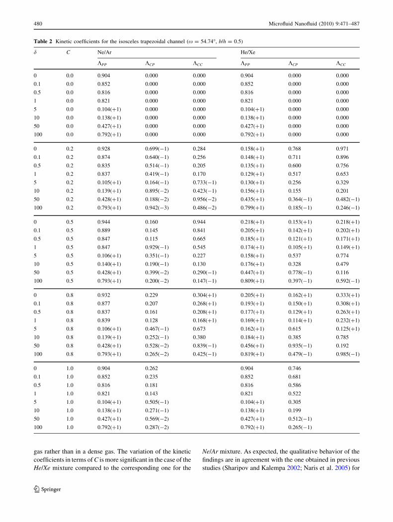
gas rather than in a dense gas. The variation of the kinetic

coefficients in terms of C is more significant in the case of the

He/Xe mixture compared to the corresponding one for the

Ne/Ar mixture. As expected, the qualitative behavior of the

findings are in agreement with the one obtained in previous

studies (Sharipov and Kalempa 2002; Naris et al. 2005) for

Table 2 Kinetic coefficients for the isosceles trapezoidal channel (x = 54.74�, b/h = 0.5)

d C Ne/Ar He/Xe

KPP KCP KCC KPP KCP KCC

0 0.0 0.904 0.000 0.000 0.904 0.000 0.000

0.1 0.0 0.852 0.000 0.000 0.852 0.000 0.000

0.5 0.0 0.816 0.000 0.000 0.816 0.000 0.000

1 0.0 0.821 0.000 0.000 0.821 0.000 0.000

5 0.0 0.104(?1) 0.000 0.000 0.104(?1) 0.000 0.000

10 0.0 0.138(?1) 0.000 0.000 0.138(?1) 0.000 0.000

50 0.0 0.427(?1) 0.000 0.000 0.427(?1) 0.000 0.000

100 0.0 0.792(?1) 0.000 0.000 0.792(?1) 0.000 0.000

0 0.2 0.928 0.699(-1) 0.284 0.158(?1) 0.768 0.971

0.1 0.2 0.874 0.640(-1) 0.256 0.148(?1) 0.711 0.896

0.5 0.2 0.835 0.514(-1) 0.205 0.135(?1) 0.600 0.756

1 0.2 0.837 0.419(-1) 0.170 0.129(?1) 0.517 0.653

5 0.2 0.105(?1) 0.164(-1) 0.733(-1) 0.130(?1) 0.256 0.329

10 0.2 0.139(?1) 0.895(-2) 0.423(-1) 0.156(?1) 0.155 0.201

50 0.2 0.428(?1) 0.188(-2) 0.956(-2) 0.435(?1) 0.364(-1) 0.482(-1)

100 0.2 0.793(?1) 0.942(-3) 0.486(-2) 0.799(?1) 0.185(-1) 0.246(-1)

0 0.5 0.944 0.160 0.944 0.218(?1) 0.153(?1) 0.218(?1)

0.1 0.5 0.889 0.145 0.841 0.205(?1) 0.142(?1) 0.202(?1)

0.5 0.5 0.847 0.115 0.665 0.185(?1) 0.121(?1) 0.171(?1)

1 0.5 0.847 0.929(-1) 0.545 0.174(?1) 0.105(?1) 0.149(?1)

5 0.5 0.106(?1) 0.351(-1) 0.227 0.158(?1) 0.537 0.774

10 0.5 0.140(?1) 0.190(-1) 0.130 0.176(?1) 0.328 0.479

50 0.5 0.428(?1) 0.399(-2) 0.290(-1) 0.447(?1) 0.778(-1) 0.116

100 0.5 0.793(?1) 0.200(-2) 0.147(-1) 0.809(?1) 0.397(-1) 0.592(-1)

0 0.8 0.932 0.229 0.304(?1) 0.205(?1) 0.162(?1) 0.333(?1)

0.1 0.8 0.877 0.207 0.268(?1) 0.193(?1) 0.150(?1) 0.308(?1)

0.5 0.8 0.837 0.161 0.208(?1) 0.177(?1) 0.129(?1) 0.263(?1)

1 0.8 0.839 0.128 0.168(?1) 0.169(?1) 0.114(?1) 0.232(?1)

5 0.8 0.106(?1) 0.467(-1) 0.673 0.162(?1) 0.615 0.125(?1)

10 0.8 0.139(?1) 0.252(-1) 0.380 0.184(?1) 0.385 0.785

50 0.8 0.428(?1) 0.528(-2) 0.839(-1) 0.456(?1) 0.935(-1) 0.192

100 0.8 0.793(?1) 0.265(-2) 0.425(-1) 0.819(?1) 0.479(-1) 0.985(-1)

0 1.0 0.904 0.262 0.904 0.746

0.1 1.0 0.852 0.235 0.852 0.681

0.5 1.0 0.816 0.181 0.816 0.586

1 1.0 0.821 0.143 0.821 0.522

5 1.0 0.104(?1) 0.505(-1) 0.104(?1) 0.305

10 1.0 0.138(?1) 0.271(-1) 0.138(?1) 0.199

50 1.0 0.427(?1) 0.569(-2) 0.427(?1) 0.512(-1)

100 1.0 0.792(?1) 0.287(-2) 0.792(?1) 0.265(-1)


123

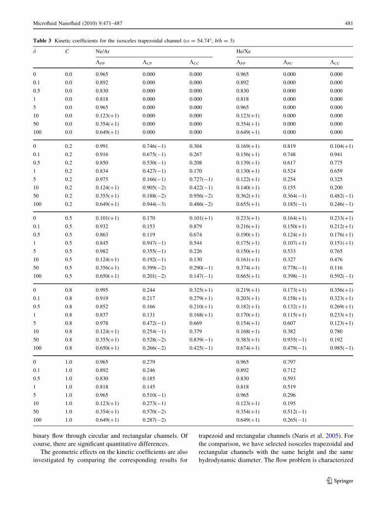
binary flow through circular and rectangular channels. Of

course, there are significant quantitative differences.

The geometric effects on the kinetic coefficients are also

investigated by comparing the corresponding results for

trapezoid and rectangular channels (Naris et al. 2005). For

the comparison, we have selected isosceles trapezoidal and

rectangular channels with the same height and the same

hydrodynamic diameter. The flow problem is characterized

Table 3 Kinetic coefficients for the isosceles trapezoidal channel (x = 54.74�, b/h = 3)

d C Ne/Ar He/Xe

KPP KCP KCC KPP KPC KCC

0 0.0 0.965 0.000 0.000 0.965 0.000 0.000

0.1 0.0 0.892 0.000 0.000 0.892 0.000 0.000

0.5 0.0 0.830 0.000 0.000 0.830 0.000 0.000

1 0.0 0.818 0.000 0.000 0.818 0.000 0.000

5 0.0 0.965 0.000 0.000 0.965 0.000 0.000

10 0.0 0.123(?1) 0.000 0.000 0.123(?1) 0.000 0.000

50 0.0 0.354(?1) 0.000 0.000 0.354(?1) 0.000 0.000

100 0.0 0.649(?1) 0.000 0.000 0.649(?1) 0.000 0.000

0 0.2 0.991 0.746(-1) 0.304 0.169(?1) 0.819 0.104(?1)

0.1 0.2 0.916 0.675(-1) 0.267 0.156(?1) 0.748 0.941

0.5 0.2 0.850 0.530(-1) 0.208 0.139(?1) 0.617 0.775

1 0.2 0.834 0.427(-1) 0.170 0.130(?1) 0.524 0.659

5 0.2 0.975 0.166(-1) 0.727(-1) 0.122(?1) 0.254 0.325

10 0.2 0.124(?1) 0.905(-2) 0.422(-1) 0.140(?1) 0.155 0.200

50 0.2 0.355(?1) 0.188(-2) 0.956(-2) 0.362(?1) 0.364(-1) 0.482(-1)

100 0.2 0.649(?1) 0.944(-3) 0.486(-2) 0.655(?1) 0.185(-1) 0.246(-1)

0 0.5 0.101(?1) 0.170 0.101(?1) 0.233(?1) 0.164(?1) 0.233(?1)

0.1 0.5 0.932 0.153 0.879 0.216(?1) 0.150(?1) 0.212(?1)

0.5 0.5 0.863 0.119 0.674 0.190(?1) 0.124(?1) 0.176(?1)

1 0.5 0.845 0.947(-1) 0.544 0.175(?1) 0.107(?1) 0.151(?1)

5 0.5 0.982 0.355(-1) 0.226 0.150(?1) 0.533 0.765

10 0.5 0.124(?1) 0.192(-1) 0.130 0.161(?1) 0.327 0.476

50 0.5 0.356(?1) 0.399(-2) 0.290(-1) 0.374(?1) 0.778(-1) 0.116

100 0.5 0.650(?1) 0.201(-2) 0.147(-1) 0.665(?1) 0.398(-1) 0.592(-1)

0 0.8 0.995 0.244 0.325(?1) 0.219(?1) 0.173(?1) 0.356(?1)

0.1 0.8 0.919 0.217 0.279(?1) 0.203(?1) 0.158(?1) 0.323(?1)

0.5 0.8 0.852 0.166 0.210(?1) 0.182(?1) 0.132(?1) 0.269(?1)

1 0.8 0.837 0.131 0.168(?1) 0.170(?1) 0.115(?1) 0.233(?1)

5 0.8 0.978 0.472(-1) 0.669 0.154(?1) 0.607 0.123(?1)

10 0.8 0.124(?1) 0.254(-1) 0.379 0.168(?1) 0.382 0.780

50 0.8 0.355(?1) 0.528(-2) 0.839(-1) 0.383(?1) 0.935(-1) 0.192

100 0.8 0.650(?1) 0.266(-2) 0.425(-1) 0.674(?1) 0.479(-1) 0.985(-1)

0 1.0 0.965 0.279 0.965 0.797

0.1 1.0 0.892 0.246 0.892 0.712

0.5 1.0 0.830 0.185 0.830 0.593

1 1.0 0.818 0.145 0.818 0.519

5 1.0 0.965 0.510(-1) 0.965 0.296

10 1.0 0.123(?1) 0.273(-1) 0.123(?1) 0.195

50 1.0 0.354(?1) 0.570(-2) 0.354(?1) 0.512(-1)

100 1.0 0.649(?1) 0.287(-2) 0.649(?1) 0.265(-1)


123

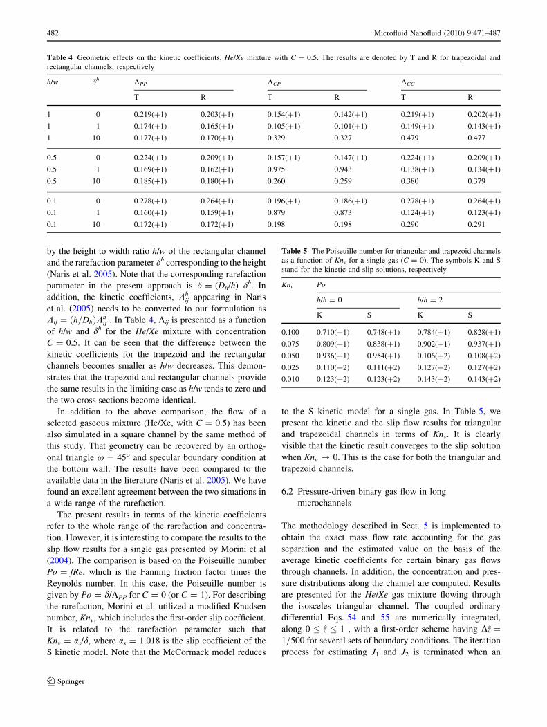
by the height to width ratio h/w of the rectangular channel

and the rarefaction parameter dh corresponding to the height

(Naris et al. 2005). Note that the corresponding rarefaction

parameter in the present approach is d = (Dh/h) dh. In

addition, the kinetic coefficients, Khij appearing in Naris

et al. (2005) needs to be converted to our formulation as

Kij ¼ ðh=DhÞKhij . In Table 4, Kij is presented as a function

of h/w and dh for the He/Xe mixture with concentration

C = 0.5. It can be seen that the difference between the

kinetic coefficients for the trapezoid and the rectangular

channels becomes smaller as h/w decreases. This demon-

strates that the trapezoid and rectangular channels provide

the same results in the limiting case as h/w tends to zero and

the two cross sections become identical.

In addition to the above comparison, the flow of a

selected gaseous mixture (He/Xe, with C = 0.5) has been

also simulated in a square channel by the same method of

this study. That geometry can be recovered by an orthog-

onal triangle x = 45� and specular boundary condition at

the bottom wall. The results have been compared to the

available data in the literature (Naris et al. 2005). We have

found an excellent agreement between the two situations in

a wide range of the rarefaction.

The present results in terms of the kinetic coefficients

refer to the whole range of the rarefaction and concentra-

tion. However, it is interesting to compare the results to the

slip flow results for a single gas presented by Morini et al

(2004). The comparison is based on the Poiseuille number

Po = fRe, which is the Fanning friction factor times the

Reynolds number. In this case, the Poiseuille number is

given by Po = d/KPP for C = 0 (or C = 1). For describing

the rarefaction, Morini et al. utilized a modified Knudsen

number, Knv, which includes the first-order slip coefficient.

It is related to the rarefaction parameter such that

Knv = as/d, where as = 1.018 is the slip coefficient of the

S kinetic model. Note that the McCormack model reduces

to the S kinetic model for a single gas. In Table 5, we

present the kinetic and the slip flow results for triangular

and trapezoidal channels in terms of Knv. It is clearly

visible that the kinetic result converges to the slip solution

when Knv ? 0. This is the case for both the triangular and

trapezoid channels.

6.2 Pressure-driven binary gas flow in long

microchannels

The methodology described in Sect. 5 is implemented to

obtain the exact mass flow rate accounting for the gas

separation and the estimated value on the basis of the

average kinetic coefficients for certain binary gas flows

through channels. In addition, the concentration and pres-

sure distributions along the channel are computed. Results

are presented for the He/Xe gas mixture flowing through

the isosceles triangular channel. The coupled ordinary

differential Eqs. 54 and 55 are numerically integrated,

along 0 � z � 1 , with a first-order scheme having Dz ¼1=500 for several sets of boundary conditions. The iteration

process for estimating J1 and J2 is terminated when an

Table 4 Geometric effects on the kinetic coefficients, He/Xe mixture with C = 0.5. The results are denoted by T and R for trapezoidal and

rectangular channels, respectively

h/w dh KPP KCP KCC

T R T R T R

1 0 0.219(?1) 0.203(?1) 0.154(?1) 0.142(?1) 0.219(?1) 0.202(?1)

1 1 0.174(?1) 0.165(?1) 0.105(?1) 0.101(?1) 0.149(?1) 0.143(?1)

1 10 0.177(?1) 0.170(?1) 0.329 0.327 0.479 0.477

0.5 0 0.224(?1) 0.209(?1) 0.157(?1) 0.147(?1) 0.224(?1) 0.209(?1)

0.5 1 0.169(?1) 0.162(?1) 0.975 0.943 0.138(?1) 0.134(?1)

0.5 10 0.185(?1) 0.180(?1) 0.260 0.259 0.380 0.379

0.1 0 0.278(?1) 0.264(?1) 0.196(?1) 0.186(?1) 0.278(?1) 0.264(?1)

0.1 1 0.160(?1) 0.159(?1) 0.879 0.873 0.124(?1) 0.123(?1)

0.1 10 0.172(?1) 0.172(?1) 0.198 0.198 0.290 0.291

Table 5 The Poiseuille number for triangular and trapezoid channels

as a function of Knv for a single gas (C = 0). The symbols K and S

stand for the kinetic and slip solutions, respectively

Knv Po

b/h = 0 b/h = 2

K S K S

0.100 0.710(?1) 0.748(?1) 0.784(?1) 0.828(?1)

0.075 0.809(?1) 0.838(?1) 0.902(?1) 0.937(?1)

0.050 0.936(?1) 0.954(?1) 0.106(?2) 0.108(?2)

0.025 0.110(?2) 0.111(?2) 0.127(?2) 0.127(?2)

0.010 0.123(?2) 0.123(?2) 0.143(?2) 0.143(?2)


123

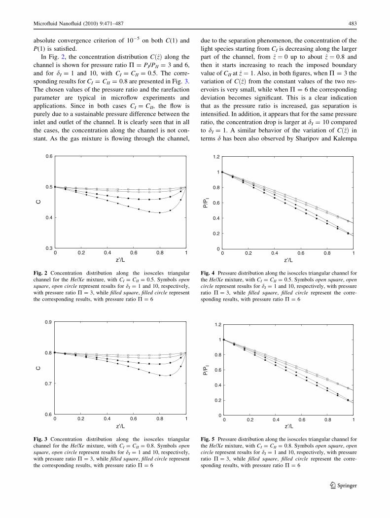
absolute convergence criterion of 10-5 on both C(1) and

P(1) is satisfied.

In Fig. 2, the concentration distribution CðzÞ along the

channel is shown for pressure ratio P = PI/PII = 3 and 6,

and for dI = 1 and 10, with CI = CII = 0.5. The corre-

sponding results for CI = CII = 0.8 are presented in Fig. 3.

The chosen values of the pressure ratio and the rarefaction

parameter are typical in microflow experiments and

applications. Since in both cases CI = CII, the flow is

purely due to a sustainable pressure difference between the

inlet and outlet of the channel. It is clearly seen that in all

the cases, the concentration along the channel is not con-

stant. As the gas mixture is flowing through the channel,

due to the separation phenomenon, the concentration of the

light species starting from CI is decreasing along the larger

part of the channel, from z ¼ 0 up to about z ¼ 0:8 and

then it starts increasing to reach the imposed boundary

value of CII at z ¼ 1: Also, in both figures, when P = 3 the

variation of CðzÞ from the constant values of the two res-

ervoirs is very small, while when P = 6 the corresponding

deviation becomes significant. This is a clear indication

that as the pressure ratio is increased, gas separation is

intensified. In addition, it appears that for the same pressure

ratio, the concentration drop is larger at dI = 10 compared

to dI = 1. A similar behavior of the variation of CðzÞ in

terms d has been also observed by Sharipov and Kalempa

0.3

0.4

0.5

0.6

0 0.2 0.4 0.6 0.8 1

C

z’/L

Fig. 2 Concentration distribution along the isosceles triangular

channel for the He/Xe mixture, with CI = CII = 0.5. Symbols opensquare, open circle represent results for dI = 1 and 10, respectively,

with pressure ratio P = 3, while filled square, filled circle represent

the corresponding results, with pressure ratio P = 6

0.6

0.7

0.8

0.9

0 0.2 0.4 0.6 0.8 1

C

z’/L

Fig. 3 Concentration distribution along the isosceles triangular

channel for the He/Xe mixture, with CI = CII = 0.8. Symbols opensquare, open circle represent results for dI = 1 and 10, respectively,

with pressure ratio P = 3, while filled square, filled circle represent

the corresponding results, with pressure ratio P = 6

0

0.2

0.4

0.6

0.8

1

1.2

0 0.2 0.4 0.6 0.8 1

P/P

I

z’/L

Fig. 4 Pressure distribution along the isosceles triangular channel for

the He/Xe mixture, with CI = CII = 0.5. Symbols open square, opencircle represent results for dI = 1 and 10, respectively, with pressure

ratio P = 3, while filled square, filled circle represent the corre-

sponding results, with pressure ratio P = 6

0

0.2

0.4

0.6

0.8

1

1.2

0 0.2 0.4 0.6 0.8 1

P/P

I

z’/L

Fig. 5 Pressure distribution along the isosceles triangular channel for

the He/Xe mixture, with CI = CII = 0.8. Symbols open square, opencircle represent results for dI = 1 and 10, respectively, with pressure

ratio P = 3, while filled square, filled circle represent the corre-

sponding results, with pressure ratio P = 6


123

(2005). The pressure distributions along the channel are

presented in Figs. 4 and 5, corresponding to the cases

shown in Figs. 2 and 3, respectively. In both figures, the

effect of the rarefaction parameter is clearly observed. At

higher values of the rarefaction parameter, the pressure

distribution becomes increasingly nonlinear. This nonlinear

behaviour vanishes as the gas becomes more dilute.

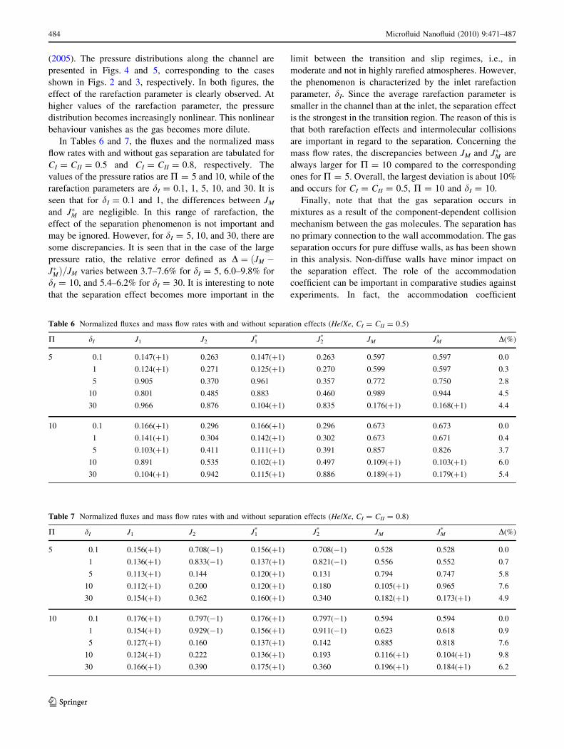
In Tables 6 and 7, the fluxes and the normalized mass

flow rates with and without gas separation are tabulated for

CI = CII = 0.5 and CI = CII = 0.8, respectively. The

values of the pressure ratios are P = 5 and 10, while of the

rarefaction parameters are dI = 0.1, 1, 5, 10, and 30. It is

seen that for dI = 0.1 and 1, the differences between JM

and J�M are negligible. In this range of rarefaction, the

effect of the separation phenomenon is not important and

may be ignored. However, for dI = 5, 10, and 30, there are

some discrepancies. It is seen that in the case of the large

pressure ratio, the relative error defined as D ¼ ðJM �J�MÞ=JM varies between 3.7–7.6% for dI = 5, 6.0–9.8% for

dI = 10, and 5.4–6.2% for dI = 30. It is interesting to note

that the separation effect becomes more important in the

limit between the transition and slip regimes, i.e., in

moderate and not in highly rarefied atmospheres. However,

the phenomenon is characterized by the inlet rarefaction

parameter, dI. Since the average rarefaction parameter is

smaller in the channel than at the inlet, the separation effect

is the strongest in the transition region. The reason of this is

that both rarefaction effects and intermolecular collisions

are important in regard to the separation. Concerning the

mass flow rates, the discrepancies between JM and J�M are

always larger for P = 10 compared to the corresponding

ones for P = 5. Overall, the largest deviation is about 10%

and occurs for CI = CII = 0.5, P = 10 and dI = 10.

Finally, note that that the gas separation occurs in

mixtures as a result of the component-dependent collision

mechanism between the gas molecules. The separation has

no primary connection to the wall accommodation. The gas

separation occurs for pure diffuse walls, as has been shown

in this analysis. Non-diffuse walls have minor impact on

the separation effect. The role of the accommodation

coefficient can be important in comparative studies against

experiments. In fact, the accommodation coefficient

Table 6 Normalized fluxes and mass flow rates with and without separation effects (He/Xe, CI = CII = 0.5)

P dI J1 J2 J1* J2

* JM JM* D(%)

5 0.1 0.147(?1) 0.263 0.147(?1) 0.263 0.597 0.597 0.0

1 0.124(?1) 0.271 0.125(?1) 0.270 0.599 0.597 0.3

5 0.905 0.370 0.961 0.357 0.772 0.750 2.8

10 0.801 0.485 0.883 0.460 0.989 0.944 4.5

30 0.966 0.876 0.104(?1) 0.835 0.176(?1) 0.168(?1) 4.4

10 0.1 0.166(?1) 0.296 0.166(?1) 0.296 0.673 0.673 0.0

1 0.141(?1) 0.304 0.142(?1) 0.302 0.673 0.671 0.4

5 0.103(?1) 0.411 0.111(?1) 0.391 0.857 0.826 3.7

10 0.891 0.535 0.102(?1) 0.497 0.109(?1) 0.103(?1) 6.0

30 0.104(?1) 0.942 0.115(?1) 0.886 0.189(?1) 0.179(?1) 5.4

Table 7 Normalized fluxes and mass flow rates with and without separation effects (He/Xe, CI = CII = 0.8)

P dI J1 J2 J1* J2

* JM JM* D(%)

5 0.1 0.156(?1) 0.708(-1) 0.156(?1) 0.708(-1) 0.528 0.528 0.0

1 0.136(?1) 0.833(-1) 0.137(?1) 0.821(-1) 0.556 0.552 0.7

5 0.113(?1) 0.144 0.120(?1) 0.131 0.794 0.747 5.8

10 0.112(?1) 0.200 0.120(?1) 0.180 0.105(?1) 0.965 7.6

30 0.154(?1) 0.362 0.160(?1) 0.340 0.182(?1) 0.173(?1) 4.9

10 0.1 0.176(?1) 0.797(-1) 0.176(?1) 0.797(-1) 0.594 0.594 0.0

1 0.154(?1) 0.929(-1) 0.156(?1) 0.911(-1) 0.623 0.618 0.9

5 0.127(?1) 0.160 0.137(?1) 0.142 0.885 0.818 7.6

10 0.124(?1) 0.222 0.136(?1) 0.193 0.116(?1) 0.104(?1) 9.8

30 0.166(?1) 0.390 0.175(?1) 0.360 0.196(?1) 0.184(?1) 6.2


123

depends on the gas and the channel surface and may not be

equal to unity (Ewart et al. 2007; Graur et al. 2009; Maurer

et al. 2003). In such cases, the accommodation coefficient

can be adjusted in the theory and the method.

The present method for calculating the flow rate can be

used in practical applications. The advantageous nature of

the method is that it is based on the kinetic description of

the flow and properly takes into account the diffusion

effects. The kinetic problem is solved locally with modest

computational effort. In comparison, solving kinetic prob-

lems by the DSMC method is computationally more

demanding for low speed flows which is the case in micro-

gas flow applications.

7 Concluding remarks

The flow of binary gaseous mixtures through channels with

triangular and trapezoidal cross section, due to pressure and

concentration gradients, has been investigated in the whole

range of the Knudsen number. The flow is modeled by the

McCormack kinetic model subject to diffuse-specular

boundary conditions. The system of linear integro-differ-

ential equations has been solved by discretizing in the

physical space using a finite difference scheme on a

boundary fitted triangular lattice, and in the molecular

velocity space by an upgraded version of the discrete

velocity method. The kinetic coefficients have been cal-

culated for Ne/Ar and He/Xe mixtures. In addition, a

detailed methodology has been presented for converting

the dimensionless kinetic results to mass flow rates by

taking into account the variation of the concentration of the

mixture as it is flowing through the channel due to the well-

known gas separation effect. Results are presented for

isosceles triangular and trapezoidal channels with an acute

angle of 54.74�, which are very common in microfluidics

applications. For the examined flow configurations, the

discrepancies between the estimated total mass flow rate

with and without taking into account gas separation may be

up to about 10%. The presented analysis and results may be

useful in the design of micro-systems and for accurate

comparison with corresponding experimental study.

Acknowledgments This research obtained financial support from

the European Community’s Seventh Framework programme (FP7/

2007-2013) under grant agreement no 215504. The views and opin-

ions expressed herein do not necessarily reflect those of the European

Commission.

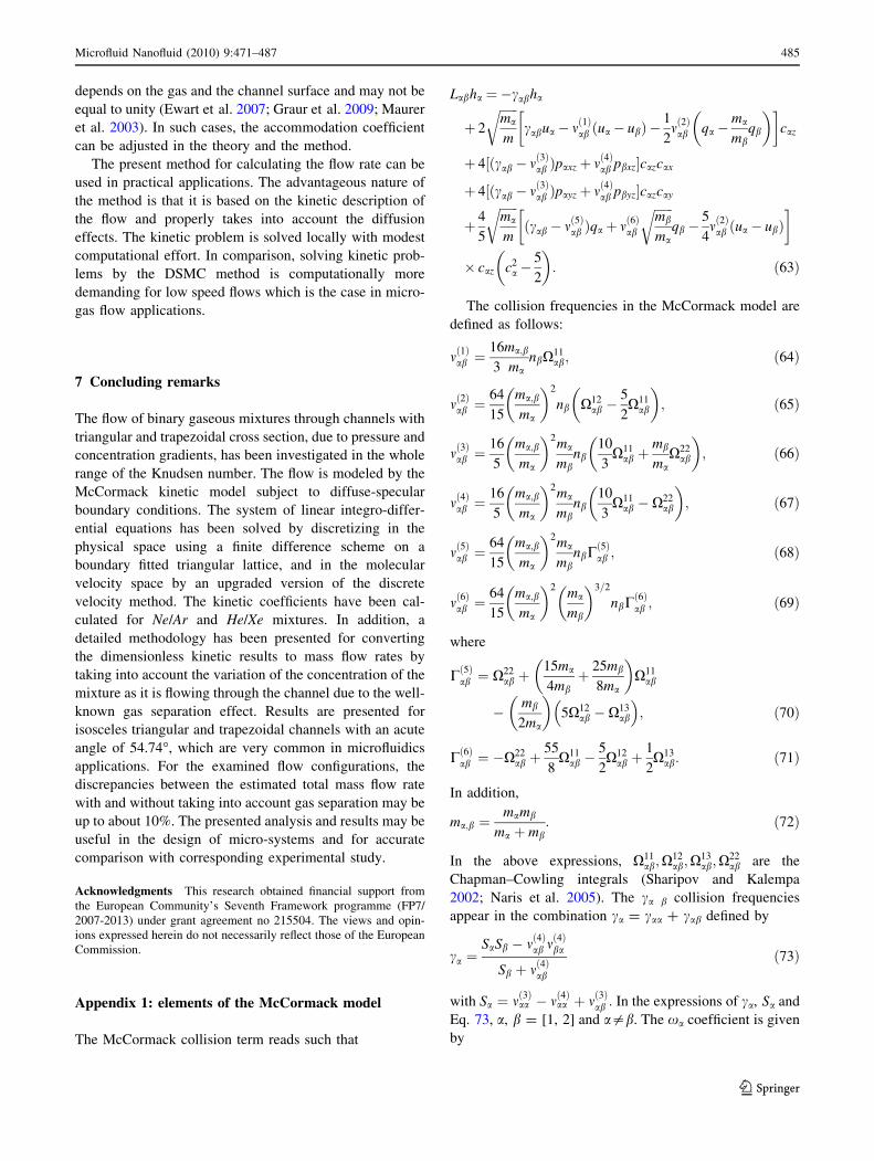
Appendix 1: elements of the McCormack model

The McCormack collision term reads such that

Labha ¼�cabha

þ 2

ffiffiffiffiffiffi

ma

m

r

cabua� mð1Þab ðua� ubÞ �1

2mð2Þab qa�

ma

mbqb

� ��

caz

þ 4½ðcab� mð3Þab Þpaxz þ mð4Þab pbxz�cazcax

þ 4½ðcab� mð3Þab Þpayz þ mð4Þab pbyz�cazcay

þ 4

5

ffiffiffiffiffiffi

ma

m

r

ðcab� mð5Þab Þqaþ mð6Þab

ffiffiffiffiffiffi

mb

ma

r

qb�5

4mð2Þab ðua� ubÞ

� �

� caz c2a�

5

2

� �

: ð63Þ

The collision frequencies in the McCormack model are

defined as follows:

mð1Þab ¼16

3

ma;b

manbX

11ab; ð64Þ

mð2Þab ¼64

15

ma;b

ma

� �2

nb X12ab �

5

2X11

ab

� �

; ð65Þ

mð3Þab ¼16

5

ma;b

ma

� �2ma

mbnb

10

3X11

ab þmb

maX22

ab

� �

; ð66Þ

mð4Þab ¼16

5

ma;b

ma

� �2ma

mbnb

10

3X11

ab � X22ab

� �

; ð67Þ

mð5Þab ¼64

15

ma;b

ma

� �2ma

mbnbC

ð5Þab ; ð68Þ

mð6Þab ¼64

15

ma;b

ma

� �2ma

mb

� �3=2

nbCð6Þab ; ð69Þ

where

Cð5Þab ¼ X22ab þ

15ma

4mbþ 25mb

8ma

� �

X11ab

� mb

2ma

� �

5X12ab � X13

ab

� �

; ð70Þ

Cð6Þab ¼ �X22ab þ

55

8X11

ab �5

2X12

ab þ1

2X13

ab: ð71Þ

In addition,

ma;b ¼mamb

ma þ mb: ð72Þ

In the above expressions, X11ab;X

12ab;X

13ab;X

22ab are the

Chapman–Cowling integrals (Sharipov and Kalempa

2002; Naris et al. 2005). The ca b collision frequencies

appear in the combination ca = caa ? cab defined by

ca ¼SaSb � mð4Þab mð4Þba

Sb þ mð4Þab

ð73Þ

with Sa ¼ mð3Þaa � mð4Þaa þ mð3Þab : In the expressions of ca, Sa and

Eq. 73, a, b = [1, 2] and a=b. The xa coefficient is given

by


123

xa ¼ffiffiffiffiffiffi

ma

m

r

C

c1

þ 1� C

c2

� �

d: ð74Þ

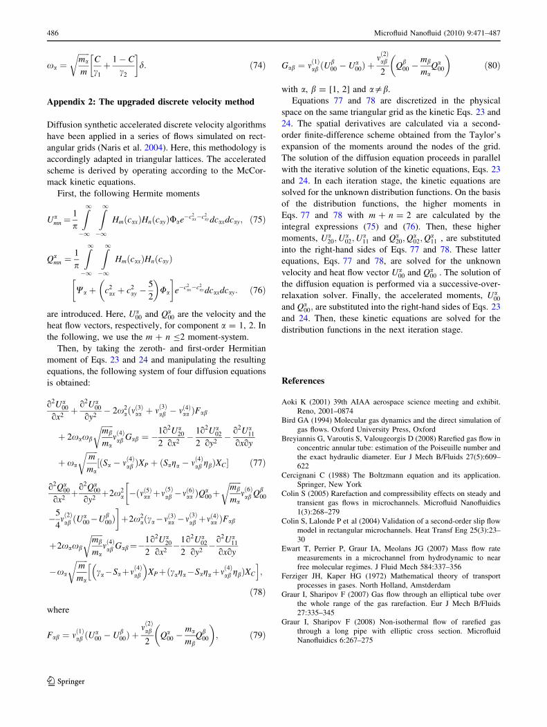
Appendix 2: The upgraded discrete velocity method

Diffusion synthetic accelerated discrete velocity algorithms

have been applied in a series of flows simulated on rect-

angular grids (Naris et al. 2004). Here, this methodology is

accordingly adapted in triangular lattices. The accelerated

scheme is derived by operating according to the McCor-

mack kinetic equations.

First, the following Hermite moments

Uamn ¼

1

p

Z

1

�1

Z

1

�1

HmðcaxÞHnðcayÞUae�c2ax�c2

ay dcaxdcay; ð75Þ

Qamn ¼

1

p

Z

1

�1

Z

1

�1

HmðcaxÞHnðcayÞ

Wa þ c2ax þ c2

ay �5

2

� �

Ua

� �

e�c2ax�c2

ay dcaxdcay: ð76Þ

are introduced. Here, Ua00 and Qa

00 are the velocity and the

heat flow vectors, respectively, for component a = 1, 2. In

the following, we use the m ? n B2 moment-system.

Then, by taking the zeroth- and first-order Hermitian

moment of Eqs. 23 and 24 and manipulating the resulting

equations, the following system of four diffusion equations

is obtained:

o2Ua00

ox2þ o2Ua

00

oy2� 2x2

aðmð3Þaa þ mð3Þab � mð4Þaa ÞFab

þ 2xaxb

ffiffiffiffiffiffi

mb

ma

r

mð4Þab Gab ¼ �1

2

o2Ua20

ox2� 1

2

o2Ua02

oy2� o2Ua

11

oxoy

þ xa

ffiffiffiffiffiffi

m

ma

r

½ðSa � mð4Þab ÞXP þ ðSaga � mð4Þab gbÞXC� ð77Þ

o2Qa00

ox2þo2Qa

00

oy2þ2x2

a �ðmð5Þaa þmð5Þab �mð6Þaa ÞQa00þ

ffiffiffiffiffiffi

mb

ma

r

mð6Þab Qb00

�

�5

4mð2Þab ðU

a00�Ub

00Þ�

þ2x2aðca�mð3Þaa �mð3Þab þmð4Þaa ÞFab

þ2xaxb

ffiffiffiffiffiffi

mb

ma

r

mð4Þab Gab¼�1

2

o2Ua20

ox2�1

2

o2Ua02

oy2�o2Ua

11

oxoy

�xa

ffiffiffiffiffiffi

m

ma

r

ca�Saþmð4Þab

� �

XPþðcaga�Sagaþmð4Þab gbÞXC

h i

;

ð78Þ

where

Fab ¼ mð1Þab ðUa00 � Ub

00Þ þmð2Þab

2Qa

00 �ma

mbQb

00

� �

; ð79Þ

Gab ¼ mð1Þab ðUb00 � Ua

00Þ þmð2Þab

2Qb

00 �mb

maQa

00

� �

ð80Þ

with a, b = [1, 2] and a=b.

Equations 77 and 78 are discretized in the physical

space on the same triangular grid as the kinetic Eqs. 23 and

24. The spatial derivatives are calculated via a second-

order finite-difference scheme obtained from the Taylor’s

expansion of the moments around the nodes of the grid.

The solution of the diffusion equation proceeds in parallel

with the iterative solution of the kinetic equations, Eqs. 23

and 24. In each iteration stage, the kinetic equations are

solved for the unknown distribution functions. On the basis

of the distribution functions, the higher moments in

Eqs. 77 and 78 with m ? n = 2 are calculated by the

integral expressions (75) and (76). Then, these higher

moments, Ua20;U

a02;U

a11 and Qa

20;Qa02;Q

a11 , are substituted

into the right-hand sides of Eqs. 77 and 78. These latter

equations, Eqs. 77 and 78, are solved for the unknown

velocity and heat flow vector Ua00 and Qa

00 . The solution of

the diffusion equation is performed via a successive-over-

relaxation solver. Finally, the accelerated moments, Ua00

and Qa00; are substituted into the right-hand sides of Eqs. 23

and 24. Then, these kinetic equations are solved for the

distribution functions in the next iteration stage.

References

Aoki K (2001) 39th AIAA aerospace science meeting and exhibit.

Reno, 2001–0874

Bird GA (1994) Molecular gas dynamics and the direct simulation of

gas flows. Oxford University Press, Oxford

Breyiannis G, Varoutis S, Valougeorgis D (2008) Rarefied gas flow in

concentric annular tube: estimation of the Poiseuille number and

the exact hydraulic diameter. Eur J Mech B/Fluids 27(5):609–

622

Cercignani C (1988) The Boltzmann equation and its application.

Springer, New York

Colin S (2005) Rarefaction and compressibility effects on steady and

transient gas flows in microchannels. Microfluid Nanofluidics

1(3):268–279

Colin S, Lalonde P et al (2004) Validation of a second-order slip flow

model in rectangular microchannels. Heat Transf Eng 25(3):23–

30

Ewart T, Perrier P, Graur IA, Meolans JG (2007) Mass flow rate

measurements in a microchannel from hydrodynamic to near

free molecular regimes. J Fluid Mech 584:337–356

Ferziger JH, Kaper HG (1972) Mathematical theory of transport

processes in gases. North Holland, Amstderdam

Graur I, Sharipov F (2007) Gas flow through an elliptical tube over

the whole range of the gas rarefaction. Eur J Mech B/Fluids

27:335–345

Graur I, Sharipov F (2008) Non-isothermal flow of rarefied gas

through a long pipe with elliptic cross section. Microfluid

Nanofluidics 6:267–275


123

Graur IA, Perrier P, Ghozlani W, Molans JG (2009) Measurements of

tangential momentum accommodation coefficient for various

gases in plane microchannel. Phys Fluids 21:102004

Ho CM, Tai YC (1998) Micro-electro-mechanical systems (MEMS)

and fluid flows. Ann Rev Fluid Mech 30:579–612

Kandlikar SG, Garimella S et al (2006) Heat transfer and fluid flow in

minichannels and microchannels. Elsevier, Oxford

Karniadakis GE, Beskok A (2002) Micro flows. Springer, New York

Li D (ed) (2008) Encyclopedia of microfluidics and nanofluidics.

Springer, New York

Lockerby DA, Reese JM (2008) On the modelling of isothermal gas

flows at the microscale. J Fluid Mech 604:235–261

Maurer J, Tabeling P, Joseph P, Willaime H (2003) Second-order slip

laws in microchannels for helium and nitrogen. Phys Fluids

15:2613–2621

McCormack FJ (1973) Construction of linearized kinetic models for

gaseous mixtures and molecular gases. Phys Fluids 16(12):2095–

2105

Morini GL, Spiga M, Tartarini P (2004) The rarefaction effect on the

friction factor of gas flow in microchannels. Superlattice Microst

35:587–599

Morini GL, Lorenzini M, Spiga M (2005) A criterion for experimen-

tal validation of slip-flow models for incompressible rarefied

gases through microchannels. Microfluid Nanofluidics 1:190–

196

Naris S, Valougeorgis D (2008) Rarefied gas flow in a triangular duct

based on a boundary fitted lattice. Eur J Mech B/Fluids 27:810–

822

Naris S, Valougeorgis D, Sharipov F, Kalempa D (2004) Discrete

velocity modelling of gaseous mixture flows in MEMS. Super-

lattice Microst 35(3–6):629–643

Naris S, Valougeorgis D, Sharipov F, Kalempa D (2005) Flow of

gaseous mixtures through rectangular microchannels driven by

pressure, temperature and concentration gradients. Phys Fluids

17(10):100607.1–100607.12

Pitakarrnop J, Geoffroy S, Colin S, Baldas L (2008) Slip flow in

triangular and trapezoidal microchannels. Int J Heat Technol

26(1):167–174

Pitakarnnop J, Varoutis S, Valougeorgis D, Geoffroy S, Baldas L,

Colin S (2010) A novel experimental setup for gas microflows.

Microfluid Nanofluidics 8:57–72

Sharipov F (1994) Onsager-Casimir reciprocity relations for open

gaseous systems at arbitrary rarefaction. III. Theory and its

application for gaseous mixtures. Phys A 209:457–476

Sharipov F (1999) Rarefied gas flow through a long rectangular

channel. J Vac Sci Technol A 17:3062

Sharipov F, Kalempa D (2002) Gaseous mixture flow through a long

tube at arbitrary Knudsen number. J Vac Sci Technol A

20(3):814–822

Sharipov F, Kalempa D (2005) Separation phenomena for gaseous

mixture flowing through a long tube into vacuum. Phys Fluids

17:127102.1–8

Sharipov F, Seleznev V (1998) Data on internal rarefied gas flows.

J Phys Chem Ref Data 27:657–706

Sharipov F, Cumin LMG, Kalempa D (2004) Plane Couette flow of

binary gaseous mixture in the whole range of the Knudsen

number. Eur J Mech B/Fluids 23:899–906

Sharipov F, Cumin LMG, Kalempa D (2007) Heat flux through a

binary gaseous mixture over the whole range of the Knudsen

number. Phys A 378:183–193

Siewert CE, Valougeorgis D (2004a) Concise and accurate solutions

to half-space binary-gas flow problems defined by the McCor-

mack model and specular-diffuse wall conditions. Eur J Mech B/

Fluids 23:709–726

Siewert CE, Valougeorgis D (2004b) The McCormack model:

channel flow of a binary gas mixture driven by temperature,

pressure and density gradients. Eur J Mech B/Fluids 23:645–664

Sugimoto H (2009) Experiment on the gas separation effect of the

pump driven by the thermal edge flow. Rarefied gas dynamics:

26th international symposium, AIP 978-0-7354-0615-5/09

Szalmas L (2007) Multiple-relaxation time lattice Boltzmann method

for the finite Knudsen number region. Phys A 379(2):401–408

Takata S, Sugimoto H, Kosuge S (2007) Gas separation by means of

the Knudsen compressor. Eur J Mech B/Fluids 26:155–181

Varoutis S, Naris S, Hauer V, Day C, Valougeorgis D (2009)

Experimental and computational investigation of gas flows

through long channels of various cross sections in the whole

range of the Knudsen number. J Vac Sci Technol A 27(1):

89–100


123

Rarefied gas flow of binary mixtures through long channels with triangular and trapezoidal cross...

Documents

Transcript of Rarefied gas flow of binary mixtures through long channels with triangular and trapezoidal cross...