Rarefied gas flow over an in-line array of circular cylinders

　　Kobe University Repository : Kernel

Title Rarefied gas flow over an in-line array of circularcylinders

Author(s) Taguchi, Satoshi / Charrier, Pierre

Citation Physics of Fluids, 20(6): 067103

Issue date 2008-06-24

Resource Type Journal Article / 学術雑誌論文

Resource Version publisher

URL http://www.lib.kobe-u.ac.jp/handle_kernel/90000747

Create Date: 2011-05-18

Rarefied gas flow over an in-line array of circular cylindersSatoshi Taguchi1,a� and Pierre Charrier2,b�

1Organization of Advanced Science and Technology, Kobe University, Kobe 657-8501, Japan2Mathématiques Appliquées, Université de Bordeaux, UMR 5251, Bordeaux F-33000, France

�Received 24 December 2007; accepted 5 May 2008; published online 24 June 2008�

A steady rarefied gas flow through periodic porous media kept at a uniform temperature isconsidered on the basis of the Bhatnagar–Gross–Krook equation and the diffuse reflection conditionon the solid boundary. Under the assumption that the period is much smaller than the length scaleof variation of the global pressure distribution, a macroscopic fluid model describing the pressuredistribution and the mass flux of the gas in the medium is derived by the homogenization previouslyproposed by Charrier and Dubroca �Multiscale Model. Simul. 2, 124 �2003��. The effectivediffusion coefficient contained in the model is constructed numerically as a function of the Knudsennumber, in the case of the medium consisting of an in-line array of circular cylinders, with the helpof the numerical analysis of a rarefied gas flow in an infinite expanse of the cylinder array driven bya uniform small pressure gradient. An application of the model to an isothermal flow in a porous slabinduced by a pressure difference is presented. © 2008 American Institute of Physics.�DOI: 10.1063/1.2937461�

I. INTRODUCTION

Recently, kinetic theory of gases �or molecular gasdynamics�1–5 is attracting great attention in connection withmicrofluidics.6–9 Flows of rarefied gas induced by the ther-mal effect, such as the thermal creep flow �thermaltranspiration�,10–14 the thermal stress slip flow,15,16 the non-linear thermal stress flow,16,17 and the thermal edge flow,18,19

have potential applicability as nonmechanical flow control-lers in microscale systems. A prototypical thermal pump us-ing the thermal edge flow has been recently fabricated inRef. 20. On the other hand, the thermal pump using the ther-mal transpiration, also known as the Knudsen pump �or com-pressor�, has been the subject of a large amount of work.21–35

The Knudsen pump is typically a series of narrow andwide pipes connected one after the other, with a periodictemperature distribution along the pipe.4,5 Because of itspractical importance and theoretical interest, the flow and thepumping effect for this Knudsen pump have been extensivelyinvestigated and many successful results have been obtainedboth theoretically24,28,33,34 and experimentally.27,29,30 The ap-plicability of the Knudsen pump to a gas separator has beennumerically demonstrated in Ref. 35.

Meanwhile, another type of pumping device was pro-posed by Kayashima36 on the basis of the same idea as theKnudsen pump. He proposed to use porous media, whosepore sizes are of the same order as the mean free path of thegas molecules, in place of the pipes. This pumping deviceusing porous media seems to be as attractive as the Knudsenpump using pipes, since we can benefit not only from thethermal creep flow but also from other thermally drivenflows, by devising the pore geometries. However, because ofits geometrical complexity, no result has been reported forthis device so far. For practice purpose, it would be very

useful if we have a simple macroscopic model to describe theglobal flow field in porous media, as in the case of the origi-nal Knudsen pump.33,34

In this paper, as a first step toward the theoretical assess-ment of the Kayashima’s device, we try to derive such amacroscopic model, called the fluid model here, on the basisof kinetic theory for a porous medium consisting ofan in-line array of circular cylinders. As the basic kineticequation, we employ the Bhatnagar–Gross–Krook �BGK�equation37–39 and assume the diffuse reflection condition onthe boundary. In addition, in order to simplify the analysisand to concentrate on the numerical results we obtained, weconsider here the isothermal case, i.e., the temperature of thesolid boundary is uniform throughout the medium. The in-clusion of the thermal effect is necessary for the full analysisof the pumping effect. However, it is straightforward andwill be treated in a subsequent paper.

In Sec. II, we consider a rarefied gas in a periodic porousmedium kept at a uniform temperature and derive a macro-scopic equation that describes the global �steady� pressuredistribution and the mass-flow rate by a systematic analysisof the kinetic system. Here, for possible future extension, theformal analysis is carried out for the general periodic struc-ture not limited to the in-line array of circular cylinders. As amethod of analysis, we adopt the homogenization techniqueintroduced by Charrier and Dubroca.40 Here, our basic as-sumption for the derivation is the smallness of the periodcompared to the length scale of variation of the global pres-sure distribution.

The derived model contains a diffusion tensor whosecomponents are essentially given by the mass-flow rates �inthe unit cell� of a flow induced in an infinite expanse of theperiodic structure by a uniform pressure gradient. Therefore,Sec. III is devoted to the numerical analysis of a steady rar-efied gas flow over an in-line array of circular cylindersdriven by a small uniform pressure gradient. We obtain nu-

a�Electronic mail: [email protected]�Electronic mail: [email protected].

PHYSICS OF FLUIDS 20, 067103 �2008�

1070-6631/2008/20�6�/067103/16/$23.00 © 2008 American Institute of Physics20, 067103-1

Downloaded 02 Jun 2009 to 133.30.51.104. Redistribution subject to AIP license or copyright; see http://pof.aip.org/pof/copyright.jsp

http://dx.doi.org/10.1063/1.2937461

http://dx.doi.org/10.1063/1.2937461

merically the mass-flow rate as a function of the Knudsennumber. This completes the derivation of the macroscopicfluid model.

Finally, in Sec. IV, we show a simple application of thefluid model to an isothermal flow in a porous slab made of anin-line array of cylinders, whose two ends are maintained atdifferent pressures.

II. FLUID MODEL FOR RAREFIED GAS FLOWSIN POROUS MEDIA WITH PERIODIC STRUCTURE

A. Problem and basic equations

1. Problem

We consider a rarefied gas in a porous medium withperiodic structure with a period �. The solid phase is kept ata uniform and constant temperature T0 and the gas is drivenby the pressure gradient. Let us denote the length scale ofvariation of the global pressure distribution by L. We inves-tigate the steady behavior of the gas under the followingassumptions:

�i� The behavior of the gas is described by the BGKmodel.

�ii� The gas molecules are reflected diffusely on the solidboundary.

�iii� The period � is much smaller than the length scale ofvariation of the overall pressure distribution L, i.e.,��L.

For the sake of clarity, we suppose that there is no iso-lated pore so that there is no confinement of the gas inside apore.

2. Basic equations

Let p* denote the reference pressure, R the specific gasconstant, �*= p* /RT0 the reference density, Lx �or Lxi� thespace rectangular coordinates, �2RT0�1/2� �or �2RT0�1/2�i� the

molecular velocity, �*�2RT0�−3/2 f�x ,�� the distribution func-tion, �*� the density, �2RT0�1/2v �or �2RT0�1/2vi� the flow

velocity, T0T the temperature, and p*p the pressure of thegas. Let us denote by Df the region inside the porous me-dium occupied by the gas in the dimensionless x space. TheBGK equation is written in the following dimensionlessform:

� · �x f =2

��

1

K*�� f e − f� �x � Df� , �1�

f e =�

��T�3/2exp�−

�� − v�2

T� , �2�

� = fd� , �3a�

v =1

� � fd� , �3b�

p = �T =2

3 �� − v�2 fd� , �3c�

� =�

L, K* =

�*

�. �4�

where �x is the gradient operator with respect to x and d�=d�1d�2d�3. Here and in what follows, the domain of inte-gration with respect to � is the whole space unless the con-trary is stated. � is the ratio of the period to the global lengthscale of variation, �* is the mean free path of the gas mol-ecules in the equilibrium state at rest with density �* andtemperature T0, and K* is the Knudsen number based on theperiod. For the BGK model, �* is given by �*= �2 /��2RT0�1/2 /Ac�*, where Ac is a constant �Ac�* is the colli-sion frequency in the reference equilibrium state, which isindependent of the molecular speed�.5 �* is related to thecorresponding viscosity �* by �*= �� /2�p*�2RT0�−1/2�*.

Let Afs denote the surface of the solid phase �in thedimensionless x space�. The diffuse reflection condition onthe solid boundary is given by

f = �wE�� for � · n � 0 �x � Afs� , �5�

with

E�� = �−3/2 exp�− ��2� , �6�

�w�x� = − 2��·n0

� · n f�x,��d� , �7�

where n �or ni� is the unit normal vector to Afs pointed to thegas. It should be noted that the diffuse reflection condition�Eq. �5� with Eq. �7�� implies that there is no net mass fluxacross the interface �impermeability condition�, i.e.,

� · n f�x,��d� = 0 �x � Afs� . �8�

Suppose that the geometrical configuration of the unitcell is specified. Then, the present system is characterized bythe following dimensionless parameters:

� =�

L, K* =

�*

�. �9�

� is a small parameter because of the assumption �iii�. On theother hand, we assume that K* is of the order of unity, i.e.,K*=O�1�.

B. Homogenization and fluid model

In this subsection, we derive a macroscopic fluid modeldescribing the global pressure distribution inside the periodicporous medium by homogenization. The homogenizationmethod is based on an asymptotic expansion using twolength scales, one describing the spatial variation over theglobal length scale, and the other describing the spatial varia-tion over the length scale characterized by the period. Thereader interested in the principal ideas and concepts of thehomogenization approach can refer to Ref. 41 and to

067103-2 S. Taguchi and P. Charrier Phys. Fluids 20, 067103 �2008�


Refs. 40 and 42–44 for its application to kinetic models. Itshould also be mentioned that the homogenization method isused to derive global diffusion models for the Knudsen pumpin Refs. 33 and 34.

Now let us start our analysis. Because of the periodicity,the global structure is composed of many unit cells withperiod � �or � in the dimensional space�. We denote by X abasic unit cell fixed in the x space. Let us introduce thefollowing new variable:

y = �y1,y2,y3� =x

�. �10�

The variable x describes the long scale variation over theglobal length scale, whereas the variable y corresponds to the

short scale variation over the period. We assume that f is afunction of x, y, and �, i.e.,

f = f�x,y,�� , �11�

and that f is periodic in y with period 1. The validity of theseassumptions can be verified from the result of analysis. Letus denote by Y the unit cube in the stretched y space corre-sponding to the unit cell X, by Y f the part of Y correspondingto the gas region, and by S the solid boundary in Y. Then,with these new variables, the system �1�–�3�, �5�, and �7� isrecast as

�� · �x f + � · �y f =2

��

1

K*�� f e − f� �x � Df, y � Y f� , �12�

f = �wE�� for � · n � 0 �x � Afs, y � S� , �13�

�w = − 2��·n0

� · n fd� , �14�

f: periodic �y � �Y f � �Y� , �15�

where �y is the gradient operator with respect to y, �Y f ��Yis the boundary of Y occupied by the gas, and the range of yis restricted to Y f with the periodic condition �15�.

We look for a solution f�x ,y ,�� of the above system�12�–�15� in the form of simple expansion in �, i.e.,

f = f �0� + f �1�� + f �2��2 + ¯ . �16�

Corresponding to the expansion �16�, the macroscopic quan-

tities of the gas h=h�x ,y� �h= �, v, T, p� are expanded in � as

h = h�0� + h�1�� + h�2��2 + ¯ . �17�

The relations between h�m� and f �m� �m=0,1 , . . . � are ob-

tained by substituting the expansions of h and f into thedefinition of the macroscopic quantities, Eqs. �3a�–�3c�, andequating the coefficient of the same power of �. We also

expand the local Maxwellian f e in �, i.e.,

f e = f e�0� + f e�1�� + f e�2��2 + ¯ . �18�

Here, the coefficients f e�m� are expressed in terms of h�n� �nm�. If we substitute Eqs. �16�–�18� into the equations and

the boundary conditions, and balance order by order in �, weobtain a sequence of problems which can be solved from thelowest order.

1. Zeroth order approximation in �

The equation and the boundary condition for the �0 orderare given by

� · �y f �0� =2

��

1

K*��0�� f e�0� − f �0�� y � Y f� , �19�

f e�0� =��0�

��T�0��3/2exp�−

�� − v�0��2

T�0�� , �20�

f �0� = �w�0�E��, � · n � 0 �y � S� , �21�

�w�0� = − 2��·n0

� · n f �0�d� , �22�

where the system should be supplemented by the periodic

boundary condition for f �0� on �Y f ��Y. The zeroth order

macroscopic quantities of the gas ��0�, v�0�, T�0�, and p�0� are

related to f �0� by the following relations:

��0� = f �0�d� , �23a�

v�0� =1

��0� � f �0�d� , �23b�

p�0� = ��0�T�0� =2

3 �� − v�0��2 f �0�d� . �23c�

It should be noted that the variable x appears in the equationsonly as a parameter.

The solution of this problem is shown to be independentof y and is given by

f �0� = ��0��x�E�� =��0��x�

�3/2 exp�− ��2� , �24�

where ��0� is an undetermined function of x. The proof isanalogous to that of Ref. 40 and therefore omitted here. Inparticular, if we substitute Eq. �24� into Eqs. �23b� and �23c�,we obtain

v�0� = 0, T�0� = 1, p�0� = ��0�. �25�

2. First order approximation in �

With the aid of the solution for the zeroth order approxi-mation, our system for the first order approximation becomes

� · �y f �1� =2

��

1

K*��0�� f e�1� − f �1�� − � · �x f �0� �y � Y f� ,

�26�

067103-3 Rarefied gas flow over an in-line array Phys. Fluids 20, 067103 �2008�


f e�1� = ��0�E�� 1�

��0�+ 2v�1� · � + ��2 −

3

2�T�1�� , �27�

f �1� = �w�1�E��, � · n � 0 �y � S� , �28�

�w�1� = − 2��·n0

� · n f �1�d� . �29�

The above system should be supplemented by the periodic

boundary condition for f �1� on �Y f ��Y. Here, it is noted thatEq. �26� is the linearized BGK equation with the inhomoge-

neous term −� ·�x f �0�=−� ·�xp�0�E��. The first order macro-scopic quantities of the gas are given by

��1� = f �1�d� , �30a�

v�1� =1

��0� � f �1�d� , �30b�

p�1� = ��0�T�1� =2

3 ��2 −

3

2� f �1�d� . �30c�

The solution to the problem �26�–�29� can be expressedin the following form:

f �1� = f �0� �p�1� f

p�0�+ ��y,�;K0�x�� · �x ln p�0�� , �31�

where �p�1� f is the average of p�1� with respect to y over thefluid part Y f and is an undetermined function of x, K0 is akind of local Knudsen number defined by

K0�x� =K*

��0��x�=

K*

p�0��x�, �32�

and the vector function � �or �i� depending on y and � is thesolution of the following boundary-value problem:

� · �y�i =

2��

1

K0LBGK��i� − �i �y � Y f� , �33�

�i = �wi for � · n � 0 �y � S� , �34�

�wi = − 2��

�·n0� · n�iE��d� , �35�

�i: periodic �y � �Y f � �Y� ,

subsidiary condition: �36�

Yf

�iE��d�dy = 0. �37�

Here, LBGK is the linearized BGK collision operator definedby

LBGK�g� = 1 + 2� · �* +2

3��2 −

3

2��*�2 −

3

2��

�g��*�E��*�d�* − g , �38�

where g is a function of �. It should be noted that � dependsnot only on the geometry of the unit cell but also on xthrough K0. Its dependence on x is explicitly shown inEq. �31�.

The solution �i to Eqs. �33�–�37� corresponds to thesolution of an elemental flow problem of rarefied gases as-sociated with periodic porous media, i.e., the flow induced ina periodically structured matrix �with a uniform temperature�when there is a �small� uniform pressure gradient applied inthe yi direction. The problem may be called the cell auxiliaryproblem �Ref. 40�.

With the aid of the expression for f �1�, one can computethe macroscopic quantities corresponding to the first orderapproximation from Eqs. �30a�–�30c�. The results are givenby

��1� = �p�1� f + � · �xp�0�, �39a�

v�1� = u�x ln p�0�, �39b�

T�1� = � · �x ln p�0�, �39c�

p�1� = �p�1� f + P · �xp�0�, �39d�

where the vector functions � �or i�, � �or �i�, and P �or Pi�are given by

i�y;K0� = �i�y,�;K0�E��d� , �40a�

�i�y;K0� =2

3 ��2 −

3

2��i�y,�;K0�E��d� , �40b�

Pi = i + �i, �40c�

and u is the 3�3 matrix with its �i , j� component given by

uij�y;K0� = �i�

j�y,�;K0�E��d� . �41�

3. Second order approximationin � and fluid model

Now, we consider the problem for �2-order approxima-tion. The equation for the second order approximation is asfollows:

� · �y f �2� =2

��

1

K*��0�� f e�2� − f �2�� + ��1�� f e�1� − f �1��

− � · �x f �1� �y � Y f� . �42�

Here, the explicit form of f e�2� and the boundary condition

for f �2� on S have been omitted for shortness. Again, thesystem should be supplemented by the periodic boundary



condition for f �2� on �Y f ��Y. In this section, we derive amacroscopic fluid model by considering the necessary con-dition for the above problem.

We integrate Eq. �42� with respect to � over the wholespace and subsequently with respect to y over the wholedomain of Y f. Since the contribution from the first term onthe right-hand side of Eq. �42� vanishes by the former inte-gration, we obtain

�x · ��0�Yf

v�1�dy� + Yf

� · �y f �2�d�dy = 0, �43�

where dy=dy1dy2dy3. Here, we have used the fact that ��0� isindependent of y. It is also noted that the second integral onthe left-hand side of Eq. �43� vanishes because of the peri-

odicity of f �2� on �Y f ��Y as well as the impermeability con-dition

� · n f �2�d� = 0 �y � S� , �44�

which is derived from the boundary condition for f �2� that isnot given here �cf. Eq. �8��. Thus, with the aid of Eq. �39b�,Eq. �43� can be rewritten as

�x · �MP�xp�0�� = 0, �45�

where MP �or MPij� is the 3�3 matrix with its �i , j� compo-nent given by

MPij�K0� = Yf

uij�y;K0�dy , �46�

and the relation ��0�= p�0� has been used. Equation �46� canbe further transformed into the following form:

MPij�K0� = Si

uij��y;K0��y�Si

dyi, �47�

where Si is a cross section of Y f perpendicular to the yi axisand dyi is the surface element on Si, i.e., �dy1 ,dy2 ,dy3�= �dy2dy3 ,dy1dy3 ,dy1dy2�. Thus, MPij is the dimensionlessmass-flow rate in the unit cell in the yi �or xi� direction due tothe pressure gradient in the yj �or xj� direction. It should benoted that MPij is independent of the way of choosing Si. It isalso noted that MP depends on the geometry of the unit cell.

To summarize, the fluid model describing the global be-havior of the gas is written in the following form:

�x · M = 0, �48a�

M = MP�K0��xp�0�, �48b�

K0 =K*

p�0�. �48c�

Here, M �or Mi� represents the dimensionless mass-flow rate,i.e., if the dimensional mass-flow rate in the unit cell �per

unit time� in the xi direction is denoted by Mi, it is related toMi by

Mi/�2�*�2RT0�1/2 = �Mi + O��2� . �49�

Let us suppose that MP is known. Then, Eqs.�48a�–�48c� form a closed set of equations for the leadingorder pressure p�0� and the equation is of elliptic type. If wespecify the ambient pressure distribution �its variation maybe large� as the boundary condition, Eqs. �48a�–�48c� deter-mine the overall pressure distribution as well as the massflux in the porous medium.

Equation �48� is similar to the isothermal version of thediffusion equation derived in Ref. 34 for a flow in a narrowpipe. Models in the same spirit have also been derived forunidirectional rarefied gas flows33,35,45 and applied tomicroflows.46–49 On the other hand, the macroscopic modelsfor rarefied gas flows in porous media have been classicallyderived on the basis of the dusty gas model50 or more re-cently on the basis of the modified Boltzmann equations withadditional collision terms which take into account the effectof the collisions of the gas molecules with the solidmatrix.51–53 It should be stressed that, in the present ap-proach, the effect of the solid boundary is included in theeffective diffusion tensor entirely through the boundary-value problem �or the cell auxiliary problem� for �. In thisconnection, it should be mentioned that, although the diffusereflection condition is assumed in the present analysis, theextension to more general boundary conditions is straightfor-ward �see, e.g., Ref. 34�. In this case, the general form of thefluid model does not change, and the effect of the boundaryappears in the diffusion tensor MP through the cell auxiliaryproblem. It should also be mentioned that the diffusion ap-proximations of the kinetic system have been made math-ematically rigorous for a collisionless gas; see Refs. 54–57for the case of channel or pipe and Ref. 58 for the case ofcircular cylinders in a staggered arrangement.

III. NUMERICAL ANALYSIS OF A RAREFIED GASFLOW OVER AN IN-LINE ARRAY OF CIRCULARCYLINDERS DRIVEN BY PRESSURE GRADIENT

In this section, we assume that the porous medium ismade of an in-line array of circular cylinders and we carryout an actual numerical analysis to obtain MP. To be morespecific, the problem to determine MP �i.e., the cell auxiliaryproblem� is equivalent to the problem of a steady rarefied gasflow over an in-line array of circular cylinders driven by asmall uniform pressure gradient, and MP is essentially themass-flow rate in the unit cell. In this section, we solve thisproblem numerically to obtain MP.

A. Formulation of the problem

We begin with the physical description of the problem.Consider a rarefied gas around infinitely many circular cyl-inders whose centers are located at �m� ,n�� m, n: integers;��0: constant� in the �Y1 ,Y2� plane, where Yi is the rectan-gular coordinate system �Fig. 1�. The cylinders are kept at auniform temperature T0 and the common radius of the cylin-ders is denoted by rc �rc /�0.5�. The gas is subject to auniform pressure gradient in the Y1 direction. That is, thepressure of the gas is given by p0�1+CPY1 /�� p0, CP: con-



stants� in the absence of the cylinders. Investigate the steadybehavior of the gas disturbed by the presence of the cylindersunder the following assumptions: �i� the behavior of the gasis described by the BGK equation; �ii� the molecules arereflected diffusely on the cylinders; and �iii� the gradient CP

is so small that the equation and the boundary condition canbe linearized around the reference equilibrium state at restwith pressure p0 and temperature T0.

In this section, we use the dimensionless space coordi-nates yi=Yi /� and introduce the following new notations:

�0�2RT0�−3/2E��1+�� is the velocity distribution function,�0�1+ � is the density of the gas, �2RT0�1/2ui its flow veloc-

ity �u3=0�, T0�1+ �� its temperature, p0�1+ P� its pressure,�0= p0 /RT0 is the reference density, �0 is the mean free pathof the gas molecules at the reference equilibrium state at restwith temperature T0 and density �0, and Kn=�0 /� is theKnudsen number.

The linearized BGK equation for the present steady two-dimensional problem is given by

�1��

�y1+ �2

��

�y2=

2��

1

Kn + 2uj� j + �� j

2 −3

2�� − �� , �50�

= �E��d� , �51a�

ui = �i�E��d� , �51b�

� = �2/3� �� j2 − 3/2��E��d� . �51c�

Here, we note that the linearized equation of state holds, i.e.,

P = + � . �52�

The boundary condition on the cylinders is given by

� = �w for � jnj � 0, �53�

with

�w = − 2��jnj0

� jnj�E��d� , �54�

where ni �n3=0� is the unit normal vector to the cylindersurface pointed to the gas region.

Let us set the perturbed velocity distribution function �in the form

� = CP�y1 + ��y1,y2,�i�� , �55�

where � is periodic in yi with period 1. Correspondingly, themacroscopic quantities are expressed as

= CP�y1 + �y1,y2�� , �56a�

ui = CP�ui�y1,y2�� , �56b�

� = CP��y1,y2�� , �56c�

P = CP�y1 + P�y1,y2�� , �56d�

where , ui, �, and P, which are also periodic in yi withperiod 1, are defined in terms of � by Eqs. �51a�–�51c� and

�52� without tilde � �.The equation and the boundary condition for � are as

follows:

�1��

�y1+ �2

��

�y2=

2��

1

Kn + 2uj� j + �� j

2 −3

2�� − �� − �1

�y � Y f� , �57�

� = �w for � jnj � 0 �y � S� , �58�

�w = − 2��jnj0

� jnj�E��d� , �59�

�: periodic �y1 = � 0.5, y2 = � 0.5� , �60�

where Y f and S are defined by

Y f = ��y1,y2��y12 + y2

2�1/2� � rc, �y1� � 0.5, �y2� � 0.5� ,

�61�S = ��y1,y2��y1

2 + y22�1/2 = rc� ,

with

rc = rc/� �62�

�see Fig. 2�, and the range of y= �y1 ,y2� is restricted to Y f

with the periodic condition �60�. Thus, the problem is re-duced to solving the boundary-value problem �57�–�60� for agiven set of parameters �rc ,Kn�.

( (

FIG. 1. A rarefied gas flow over an in-line array of circular cylinders in-duced by a pressure gradient.



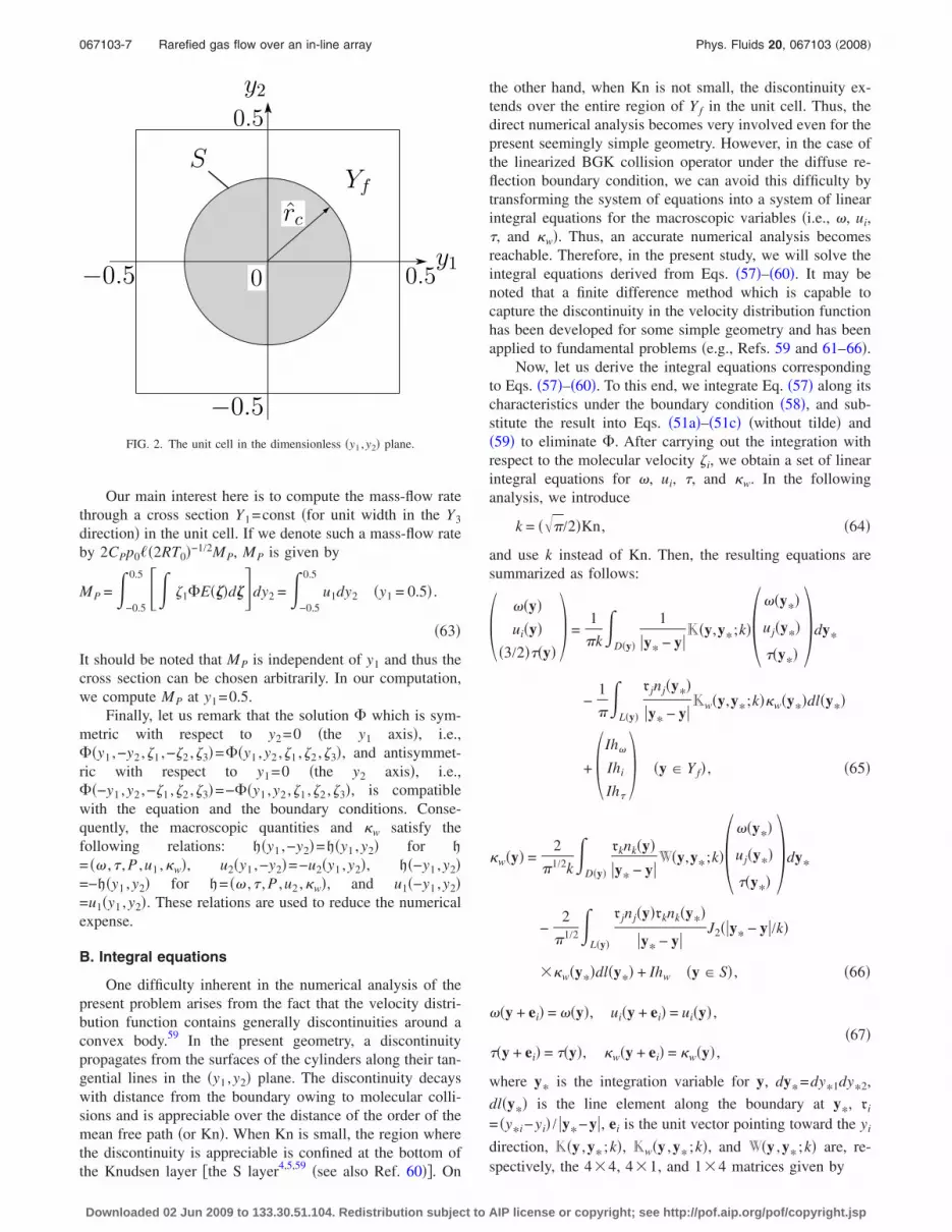
Our main interest here is to compute the mass-flow ratethrough a cross section Y1=const �for unit width in the Y3

direction� in the unit cell. If we denote such a mass-flow rateby 2CPp0��2RT0�−1/2MP, MP is given by

MP = −0.5

0.5 �1�E��d��dy2 = −0.5

0.5

u1dy2 �y1 = 0.5� .

�63�

It should be noted that MP is independent of y1 and thus thecross section can be chosen arbitrarily. In our computation,we compute MP at y1=0.5.

Finally, let us remark that the solution � which is sym-metric with respect to y2=0 �the y1 axis�, i.e.,��y1 ,−y2 ,�1 ,−�2 ,�3�=��y1 ,y2 ,�1 ,�2 ,�3�, and antisymmet-ric with respect to y1=0 �the y2 axis�, i.e.,��−y1 ,y2 ,−�1 ,�2 ,�3�=−��y1 ,y2 ,�1 ,�2 ,�3�, is compatiblewith the equation and the boundary conditions. Conse-quently, the macroscopic quantities and �w satisfy thefollowing relations: h�y1 ,−y2�=h�y1 ,y2� for h

= � ,� , P ,u1 ,�w�, u2�y1 ,−y2�=−u2�y1 ,y2�, h�−y1 ,y2�=−h�y1 ,y2� for h= � ,� , P ,u2 ,�w�, and u1�−y1 ,y2�=u1�y1 ,y2�. These relations are used to reduce the numericalexpense.

B. Integral equations

One difficulty inherent in the numerical analysis of thepresent problem arises from the fact that the velocity distri-bution function contains generally discontinuities around aconvex body.59 In the present geometry, a discontinuitypropagates from the surfaces of the cylinders along their tan-gential lines in the �y1 ,y2� plane. The discontinuity decayswith distance from the boundary owing to molecular colli-sions and is appreciable over the distance of the order of themean free path �or Kn�. When Kn is small, the region wherethe discontinuity is appreciable is confined at the bottom ofthe Knudsen layer �the S layer4,5,59 �see also Ref. 60��. On

the other hand, when Kn is not small, the discontinuity ex-tends over the entire region of Y f in the unit cell. Thus, thedirect numerical analysis becomes very involved even for thepresent seemingly simple geometry. However, in the case ofthe linearized BGK collision operator under the diffuse re-flection boundary condition, we can avoid this difficulty bytransforming the system of equations into a system of linearintegral equations for the macroscopic variables �i.e., , ui,�, and �w�. Thus, an accurate numerical analysis becomesreachable. Therefore, in the present study, we will solve theintegral equations derived from Eqs. �57�–�60�. It may benoted that a finite difference method which is capable tocapture the discontinuity in the velocity distribution functionhas been developed for some simple geometry and has beenapplied to fundamental problems �e.g., Refs. 59 and 61–66�.

Now, let us derive the integral equations correspondingto Eqs. �57�–�60�. To this end, we integrate Eq. �57� along itscharacteristics under the boundary condition �58�, and sub-stitute the result into Eqs. �51a�–�51c� �without tilde� and�59� to eliminate �. After carrying out the integration withrespect to the molecular velocity �i, we obtain a set of linearintegral equations for , ui, �, and �w. In the followinganalysis, we introduce

k = ��/2�Kn, �64�

and use k instead of Kn. Then, the resulting equations aresummarized as follows:

� �y�ui�y�

�3/2��y�� =

1

�k

D�y�

1

�y* − y�K�y,y*;k��

�y*�

uj�y*�

��y*� �dy*

−1

�

L�y�

r jnj�y*�

�y* − y�Kw�y,y*;k��w�y*�dl�y*�

+ �Ih

Ihi

Ih�

� �y � Y f� , �65�

�w�y� =2

�1/2k

D�y�

rknk�y��y* − y�

W�y,y*;k�� y*�

uj�y*�

��y*� �dy*

−2

�1/2L�y�

r jnj�y�rknk�y*�

�y* − y�J2��y* − y�/k�

��w�y*�dl�y*� + Ihw �y � S� , �66�

�y + ei� = �y�, ui�y + ei� = ui�y� ,

�67��y + ei� = ��y�, �w�y + ei� = �w�y� ,

where y* is the integration variable for y, dy*=dy*1dy*2,

dl�y*� is the line element along the boundary at y*, ri

= �y*i−yi� / �y*−y�, ei is the unit vector pointing toward the yi

direction, K�y ,y*;k�, Kw�y ,y*;k�, and W�y ,y*;k� are, re-spectively, the 4�4, 4�1, and 1�4 matrices given by

FIG. 2. The unit cell in the dimensionless �y1 ,y2� plane.



K =�J0 − 2J1r1 − 2J1r2 J2 − J0

− J1r1 2J2r12 2J2r1r2 − �J3 − J1�r1

− J1r2 2J2r1r2 2J2r22 − �J3 − J1�r2

J2 − J0 − 2�J3 − J1�r1 − 2�J3 − J1�r2 J4 − 2J2 + �3/2�J0

� , �68a�

Kw =�J1

− J2r1

− J2r2

J3 − J1

� , �68b�

W = �J1,− 2J2r1,− 2J2r2,J3 − J1� , �68c�

and the inhomogeneous terms �Ih , Ihi , Ih� , Ihw� are given by

�Ih

Ihi

Ih�

� =k

�

L�y�r1

r jnj�y*�

�y* − y� � J2

− J3ri

J4 − J2�dl�y*� − � 0

�k/2��i1

0� ,

�69a�

Ihw =2k

�1/2L�y�

r1

r jnj�y�rknk�y*�

�y* − y�J3dl�y*� +

�1/2

2kn1 �69b�

��ij is the Kronecker delta�. Jn is the Abramowitz function67

defined by

Jn�x� = 0

�

�n exp�− �2 −x

��d� . �70�

The arguments of Jn in Eqs. �68� and �69� are commonly�y*−y� /k. The domain of area integration D�y� is the regionoccupied by the gas visible from y in the �y1 ,y2� plane, andthat of the line integration L�y� is the surfaces of the cylin-ders visible from y in the �y1 ,y2� plane �see Fig. 3�. In car-rying out the integrations, the periodic condition �67� shouldbe applied when the variable y* is outside Y f. The details ofthe derivation of these integral equations can be found inRef. 5. Equations �65� and �66� are advantageous because thevelocity distribution function has been eliminated from theequations. The numerical difficulty associated with the dis-continuity in the velocity distribution function is now re-duced to the level of numerical integrations in a complexdomain which varies with the point y.

Equations �65�–�67� can be solved by the method of suc-cessive approximation. The actual computation is carried outfollowing Ref. 68, where the same type of integral equationshas been solved to investigate a rarefied gas flow betweentwo noncoaxial circular cylinders maintained at two differentuniform temperatures. We only mention that a spatially fixedrectangular grid system was used for the variable y �the spe-cific choice of this grid will be given in Sec. III C below�,and an overlapped plane polar grid system with its origin aty was used for the variable y* to carry out the area and line

integrations, where the values needed for numerical integra-tions are obtained from those associated with the rectangulargrid system by interpolation.

It should be also noted that, in the present problem,�y*−y� can be arbitrarily large for a given y, and therefore,we have to restrict the domain of integration to a finite do-main in order to perform numerical integrations. Since theAbramowitz function Jn�x� is a rapidly decaying function,this is safely done by choosing a sufficiently large numberRD such that the integrands are negligibly small for �y*−y��RD. More precisely, if we denote by DR�y� the circulardomain centered at y with a radius RD in the �y*1 ,y*2� plane,

the actual area �line� integrals in Eqs. �65� and �66� are car-ried out in D�y��DR�y� �L�y��DR�y��. In the actual com-putation, we set RD=krD and specify rD rather than RD. Thevalue of rD used in our numerical computations is 21.8 for

FIG. 3. The domain of integration. D�y� is the region occupied by the gasvisible from y, whereas L�y� is the surfaces of the cylinders visible from y.



0.1�k�0.15, 16.7 for k=0.2, 12.0 for 0.3�k�0.7, and 7.9for 0.8�k�5. We refer to Ref. 68 for the further details ofthe numerical computation, where the detailed description ofthe numerical method can be found.

C. Rectangular grid system fixed in space

First, we approximate the cylinder by a regular polygon

with 4K sides, where the vertices are the intersections of the

cylinder surface and the 4K radial lines emitted isotropicallyfrom the center of the cylinder. Then, the domain �y1��0.5and �y2��0.5 is divided by �2M +1� parallel lines perpen-dicular to the y1 axis and by �2N+1� parallel lines perpen-dicular to the y2 axis. The �2M +1� �or �2N+1�� lines are

composed of �2K+1� lines passing through the vertices ofthe polygon in the interval �y1�� rc �or �y2�� rc� and 2�M− K� �or 2�N− K�� uniformly spaced lines in the interval rc

�y1��0.5 �or rc �y2��0.5�.In the present computation, we used three different sizes

of the rectangular grid system for accuracy and comparison:

�I� M =N=20, K=10; �II� M =N=40, K=20; and �III� M

=N=80, K=40 �see Fig. 4�.

D. Asymptotic analysis for small k

Before presenting numerical results, in this subsection,we return to the original system �57�–�60� and discuss thesolution for small k �or Kn�. When k is small, the mean freepath of the gas is small compared to the cell size, and theflow field in the unit cell is expected to be described by themacroscopic variables via fluid-dynamic equations. A gen-eral theory describing flows of slightly rarefied gases�asymptotic theory for small Knudsen numbers� has been

developed by Sone and co-workers4,5,69–74 for a wide class ofproblems. Thus, we can make use of this theory to investi-gate the present problem for small k.

According to the theory,4,5 the solution � can be writtenin the following form:

� = �G + �K, �71�

where �G is the moderately varying overall solution �theGrad–Hilbert solution� and �K is the Knudsen-layer correc-tion to �G only appreciable in a thin layer �the Knudsenlayer� adjacent to the boundary whose length scale of varia-tion is of the order of k �or of the mean free path� in thedirection normal to the boundary. �G and �K are expandedin k as follows:

�G =1

k��G�0� + �G�1�k + �G�2�k

2 + ¯ � , �72a�

�K =1

k��K�1�k + �K�2�k

2 + ¯ � . �72b�

Correspondingly, the macroscopic quantities h �h= , ui, �,or P� are also expanded as

h = hG + hK, �73a�

hG =1

k�hG�0� + hG�1�k + hG�2�k

2 + ¯ � , �73b�

hK =1

k�hK�1�k + hK�2�k

2 + ¯ � , �73c�

where hG is the Grad–Hilbert part of h corresponding to �G

and hK is its Knudsen-layer correction corresponding to �K.The expansion coefficients hG�m� of the Grad–Hilbert part aresubject to the Stokes set of equations.4,5 Here, we only givethe explicit equations which determine the flow velocityuiG�m� for conciseness. That is, the equations are given by

�uiG�m�

�yi= 0, �74a�

�PG�m+1�

�yi−

�2uiG�m�

�yj2 = − �i1�m0 �74b�

�m=0,1 ,2 , . . . �. The corresponding boundary conditions onthe surface of the cylinder �i.e., r= rc with r= �y�� up to m=1 are given by

urG�0� = u�G�0� = 0, �75�

for m=0 and

urG�1� = 0, �76a�

u�G�1� = − k0

�u�G�0�

�r, �76b�

for m=1, where urG�m� and u�G�m� are the radial and circum-ferential components of uiG�m�, respectively. The numerical

FIG. 4. Rectangular grid system in the unit cell fixed in space. System �I�for rc=0.25. A circle with the radius rc is shown to indicate the cylindersurface.



value of the slip coefficient k0 for the BGK equation underthe diffuse reflection condition is given by4,5

k0 = − 1.016 19. �77�

The above system of equations should be supplemented bythe periodic condition on �Y f ��Y.

The leading order flow velocity uiG�0� is determined to-gether with PG�1� as the solution of the Stokes set of equa-tions �74a� and �74b� �with m=0� under the nonslip bound-ary condition �75�, and the next order flow velocity uiG�1� isdetermined together with PG�2� as the solution of the Stokesset of equations �74a� and �74b� �with m=1� under the slipboundary conditions �76a� and �76b�. Moreover, if we set

�uiG�1� , PG�2��=k0�uiG�1� , PG�2��, we can get rid of k0 from theequations. In the present study, these Stokes equations werenumerically solved by a finite difference method to obtainuiG�0� and uiG�1�.

Once we obtain uiG�0� and uiG�1�, we can readily computethe approximate value of MP for small k �or Kn�. That is, ifwe write MP as

MP =1

kMP�0� + k0MP�1� + O�k� , �78�

the coefficients MP�0� and MP�1� are given by

MP�0�

MP�1�� =

−0.5

0.5 u1G�0�

u1G�1��dy2 �y1 = 0.5� . �79�

Here, we have taken into account the fact that the Knudsen-layer correction u1K�1� is appreciable only in the Knudsenlayer adjacent to the boundary with the thickness of the order

of k. MP�0� and MP�1� depend only on rc �i.e., geometry� and

their numerical values are obtained as �MP�0� ,MP�1��= �−0.019 90,0.2154� for rc=0.25 and �MP�0� ,MP�1��= �−0.010 98,0.1447� for rc=0.3. The result for MP based onthe asymptotic expression �78� is also included in the nu-merical results given in the following subsection. Inciden-

tally, the coefficients MP�0� and k0MP�1� are directly related tothe permeability constant and the Klinkenberg factor appear-ing in the Klinkenberg’s law75 describing the effective per-meability of the low pressure gas flow through a porous me-dium. The relation to the Klinkenberg’s law is given inAppendix A.

E. Numerical results

In this section, we show some numerical results. Thecomputations were made for two different diameters of thecylinders, i.e., rc=0.25 and 0.3, and for various Kn rangingfrom 0.1 to 5. The results presented in the following arebased on the grid system �II� �see Sec. III C� except those inTable I. In Fig. 5, we show MP versus k for rc=0.25 and 0.3.Table I shows the numerical values of MP, where the com-parison of the results for the three grid systems is made. Inthe figure, numerical values of MP based on the direct nu-merical solutions of the integral equations are shown by thesymbols. −MP first decreases with k and then increases. −MP

takes its minimum value at an intermediate value of k�around k=0.9 for rc=0.25 and around k=0.8 for rc=0.3�.This corresponds to the Knudsen minimum, which has beenknown for rarefied gas flows through a channel or a pipe.The present result confirms the existence of the minimum inthe case of the in-line array of circular cylinders. −MP takes

TABLE I. MP vs k for rc=0.25 and 0.3. Comparison of the results for threegrid systems �cf. Sec. III C�.

k

−MP

rc=0.25 rc=0.3

�I� �II� �III� �I� �II� �III�

0.1 0.4195 0.4191 0.2582 0.2579

0.15 0.3554 0.3550 0.2221 0.2218

0.2 0.3243 0.3238 0.2045 0.2041

0.3 0.2945 0.2940 0.1876 0.1871

0.4 0.2810 0.2804 0.1802 0.1796

0.5 0.2739 0.2733 0.2731 0.1764 0.1759 0.1757

0.6 0.2700 0.2694 0.1746 0.1740

0.8 0.2667 0.2660 0.1735 0.1728

1 0.2669 0.2661 0.2659 0.1742 0.1735 0.1734

1.2 0.2684 0.2676 0.2674 0.1757 0.1750 0.1749

1.4 0.2706 0.2698 0.1775 0.1768

1.6 0.2732 0.2724 0.1794 0.1788

1.8 0.2760 0.2752 0.1815 0.1808

2 0.2789 0.2780 0.2778 0.1834 0.1828 0.1826

3 0.2931 0.2921 0.1929 0.1922

4 0.3059 0.3048 0.2011 0.2004

5 0.3171 0.3160 0.2080 0.2074

k

FIG. 5. MP vs k for rc=0.25 and 0.3. MP based on the direct numericalsolutions of the integral equations is shown by the symbols which are con-nected with solid lines. MP based on the asymptotic expression up to theorder of k0 �i.e., the first two terms of Eq. �78�� is shown by the dashed lines.For comparison, MP based on the solution of the Stokes equations withnonslip boundary condition �i.e., the first term of Eq. �78�� is also shown bythe dot-dashed lines.



larger values for smaller rc. In the figure, we also includedMP based on the asymptotic solutions up to the order of k0

�i.e., the first two terms of Eq. �78�� as well as MP based onthe asymptotic solutions up to the order of k−1 �i.e., the firstterm of Eq. �78��. The former takes into account the velocityslip on the boundary due to the gas-rarefaction effect,whereas the latter does not. Compared to the latter, theformer �the asymptotic solutions up to the order k0� agreeswell with the direct numerical solutions. The discrepancy ofthe asymptotic solutions from the direct solutions is less than0.5% at k=0.1 for both values of rc. The asymptotic ap-proach seems to provide a useful alternative to the directnumerical solution for small k �k0.2�.

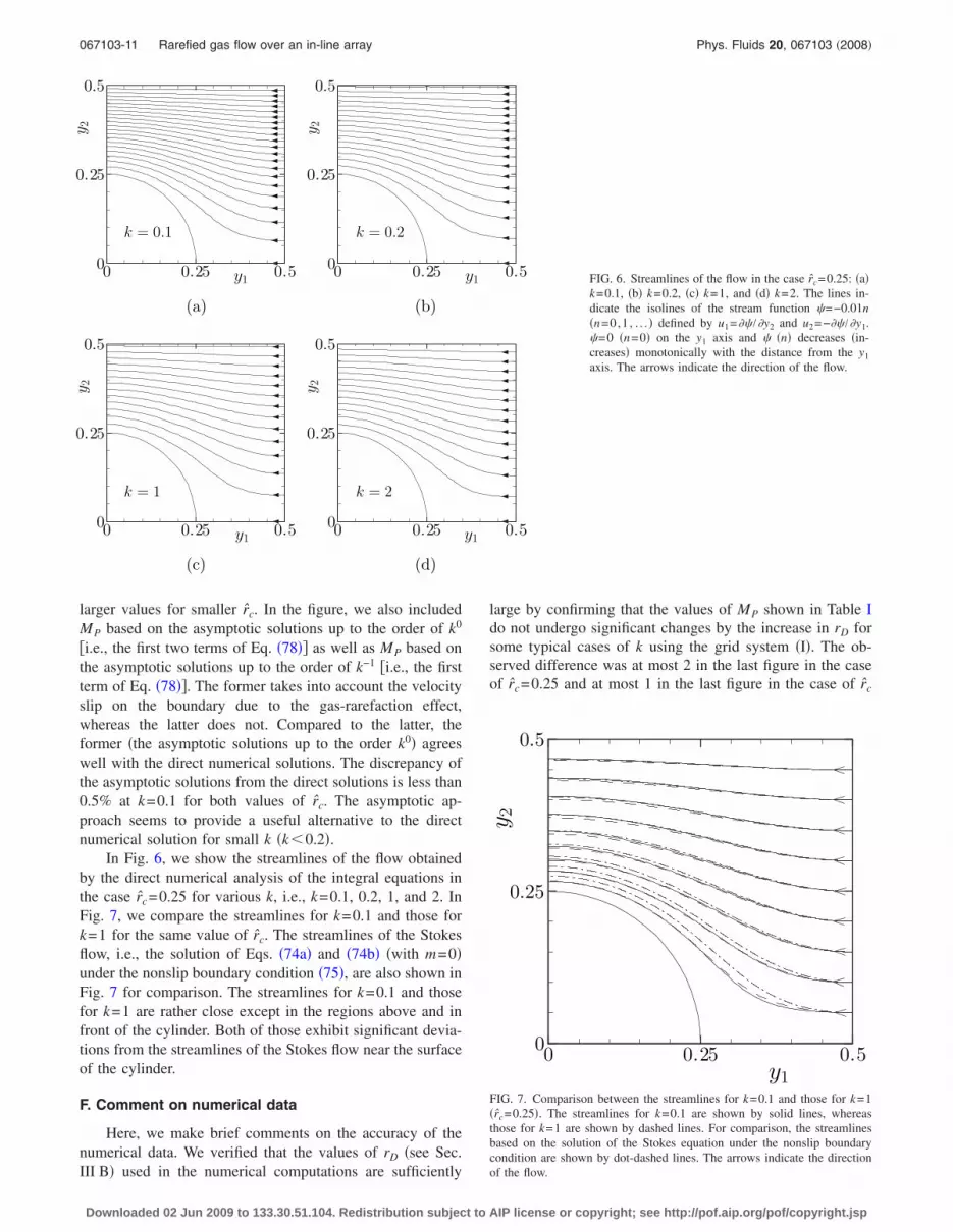
In Fig. 6, we show the streamlines of the flow obtainedby the direct numerical analysis of the integral equations inthe case rc=0.25 for various k, i.e., k=0.1, 0.2, 1, and 2. InFig. 7, we compare the streamlines for k=0.1 and those fork=1 for the same value of rc. The streamlines of the Stokesflow, i.e., the solution of Eqs. �74a� and �74b� �with m=0�under the nonslip boundary condition �75�, are also shown inFig. 7 for comparison. The streamlines for k=0.1 and thosefor k=1 are rather close except in the regions above and infront of the cylinder. Both of those exhibit significant devia-tions from the streamlines of the Stokes flow near the surfaceof the cylinder.

F. Comment on numerical data

Here, we make brief comments on the accuracy of thenumerical data. We verified that the values of rD �see Sec.III B� used in the numerical computations are sufficiently

large by confirming that the values of MP shown in Table Ido not undergo significant changes by the increase in rD forsome typical cases of k using the grid system �I�. The ob-served difference was at most 2 in the last figure in the caseof rc=0.25 and at most 1 in the last figure in the case of rc

FIG. 6. Streamlines of the flow in the case rc=0.25: �a�k=0.1, �b� k=0.2, �c� k=1, and �d� k=2. The lines in-dicate the isolines of the stream function �=−0.01n�n=0,1 , . . . � defined by u1=�� /�y2 and u2=−�� /�y1.�=0 �n=0� on the y1 axis and � �n� decreases �in-creases� monotonically with the distance from the y1

axis. The arrows indicate the direction of the flow.

FIG. 7. Comparison between the streamlines for k=0.1 and those for k=1�rc=0.25�. The streamlines for k=0.1 are shown by solid lines, whereasthose for k=1 are shown by dashed lines. For comparison, the streamlinesbased on the solution of the Stokes equation under the nonslip boundarycondition are shown by dot-dashed lines. The arrows indicate the directionof the flow.



=0.3. Here, we have increased rD from �21.8, 16.7, 12.0, 7.9�to �27.1, 21.8, 16.7, 12.0� depending on the value of k.

Because of the conservation of mass, MP should be in-dependent of y1. We computed MP at every grid line y1

=const and confirmed that the mass conservation is satisfiedwith sufficient accuracy. For the grid system �II�, the varia-tion is less than 0.21% in the case of rc=0.25 and less than0.25% in the case of rc=0.3.

G. Diffusion coefficient of the fluid model

We conclude this section by deriving the diffusion tensorMP in Eq. �48b� for the in-line array of circular cylinders.Here, the fluid model �48a�–�48c� is considered to be two-dimensional �i.e., �x3

=0� and MP should be interpreted as a2�2 matrix. We first note the following correspondence be-tween the two-dimensional version of the cell auxiliary prob-lem �33�–�37� �with �y3

=0� and the boundary-value problemconsidered in this section, i.e., Eqs. �57�–�60�: the quantities�� , ,ui ,� , P ,�w ,Kn� in this section correspond to the quan-tities ��1 , 1 ,ui

1 ,�1 , P1 ,�w1 ,K0� in Sec. II �the subsidiary

condition �37� is satisfied by ��. Consequently, the mass-flow rate MP in this section corresponds to MP11 in Sec. II.Since MP is isotropic �MP11=MP22 and MP12=MP21=0� andsince MP has been obtained as a function of k�=�� /2�Kn�,the diffusion tensor MP is expressed as

MP = MP��

2K0�I , �80�

where I is the 2�2 identity matrix.Since we have obtained the diffusion tensor �or coeffi-

cient MP�, we can now apply the fluid model �48a�–�48c��with Eq. �80�� to investigate isothermal flows through a po-rous medium consisting of an in-line array of cylinders in-duced by the pressure gradient �or difference�. A simple ex-ample of such a flow will be given in the next section.Incidentally, the diffusion coefficient MP is likely to divergein the free molecular limit K0→�. This is attributed to themolecules which come from the infinity without undergoingany collision with the cylinders. If the cylinders are arrangedin a staggered way, making the radius of the cylinders suffi-ciently large, the diffusion coefficient remains finite in thefree molecular limit.58

IV. APPLICATION

In this section, we present an application of the fluidmodel to an isothermal pressure-driven flow through a po-rous medium. That is, we consider a porous slab made of anin-line array of circular cylinders, as shown in Fig. 8. Thedimensions of the porous slab are L in the X1 direction andinfinitely long in the X2 and X3 directions, where Xi is thespace rectangular coordinates. As before, the linear dimen-sion of the unit cell is denoted by � and the radius of thecylinder is denoted by rc �rc /�0.5�. The pressures of thegas at the two ends X1=0 and L are kept at p0 and p1, re-spectively, while the temperatures �at both ends� are kept atan equal temperature T0. The temperature of the cylinders �orthat of the porous slab� is also kept at T0. When p1� p0, a

flow is induced in the slab in the negative X1 direction due tothe pressure difference. We investigate the steady behavior ofthe flow on the basis of the BGK model by assuming that themolecular reflection on the solid boundary is diffusive.

Let us take L and p0 as the reference length and thereference pressure, respectively, i.e., p*= p0. The presentproblem is characterized by the parameters

� =�

L, K* =

�*

�, rc =

rc

�, p1 =

p1

p0, �81�

where �* is the mean free path of the gas in the equilibriumstate at rest with temperature T0 and pressure p0 �or density�0= p0 /RT0�. In this section, we use the dimensional pressurep, density �, and flow velocity v �or vi� in addition to theirdimensionless counterparts. When � is small, we can applythe fluid model �48a�–�48c� to describe the dimensionlesspressure p�=p / p0� �or the dimensionless density��=� /�0= p��. Thus, p is governed by the following equation:

d

dx1M1 = 0, �82a�

M1 = MP��

2K0� dp

dx1, �82b�

K0 =K*

p, �82c�

where the subscript “�0�” which indicates the leading orderquantity in � is omitted. It should be noted that MP dependsalso on rc. The above equations �82a�–�82c� will be solvedunder the following boundary conditions:

p = 1 �x1 = 0� ,

�83�p = p1 = p1/p0 �x1 = 1� .

The mass-flow rate M in the X1 direction through the unitcell �for unit width in the X3 direction� is given by

M/��0�2RT0�1/2 = �M1 + O��2� . �84�

From Eqs. �82a�–�82c� and �83�, the dimensionlessmass-flow rate M1 is simply expressed as

FIG. 8. A rarefied gas flow through a porous slab made of an in-line array ofcylinders induced by the pressure difference.



M1 = 1

p1

MP��

2

K*

p�dp . �85�

Once M1 is determined from the above integral, the pressureprofile is obtained from

x1 =1

M1

1

p

MP��

2

K*

t�dt . �86�

The integrals in Eqs. �85� and �86� are evaluated numericallywith the aid of the numerical data for the diffusion coeffi-cient MP obtained in the previous section �Fig. 5 and TableI�. More precisely, we have interpolated the numerical dataobtained by the direct numerical analysis of the integralequations for 0.1�k�5, and used the asymptotic formula�78� for k0.1, where k= �� /2�K0. The results are pre-sented in Figs. 9–11. In Fig. 9, we show the dimensionlessmass-flow rate M1 versus p1 for various values of K* and forrc=0.25 and 0.3. For a fixed K*, −M1 increases with thepressure ratio p1 and decreases with the radius of the cylin-der rc. The curves for K*=0.5 and 1 are convex with respectto p1 for the entire range of p1 shown in the figure for bothrc=0.25 and 0.3. However, though it is rather hard to see itfrom the figure, the curves for K*=2 and 5 are concave withrespect to p1 up to a certain value of p1, and then they be-come convex for larger p1. The curves for K*=5 take largervalues of −M1 than those for K*=2 in the range 0 p1

�5.5. This result will be explained in the following para-graphs.

To simplify the following calculation, we introduce a

new function MP�K0�=MP��K0 /2� and use MP rather thanMP. If we differentiate Eq. �85� with respect to p1 twice, weobtain

FIG. 9. M1 vs p1 / p0 for various K*

for rc /�=0.25 and 0.3. The numericalresults are shown by the symbols which are connected by the solid lines.

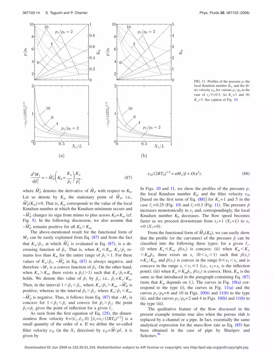
FIG. 10. Profiles of the pressure p, thelocal Knudsen number K0, and the fil-ter velocity vD for various p1 / p0 in thecase of rc /�=0.25: �a� K

*=1 and �b�

K*

=5. In the upper panels, the profilesof the pressure are shown by solidlines and those of the local Knudsennumber by dashed lines.



d2M1

dp12 = − MP��K0 =

K*

p1�K*

p12

, �87�

where MP� denotes the derivative of MP with respect to K0.

Let us denote by Km the stationary point of MP, i.e.,

MP��Km�=0. That is, Km corresponds to the value of the localKnudsen number at which the Knudsen minimum occurs and

−MP� changes its sign from minus to plus across K0=Km �cf.Fig. 5�. In the following discussion, we also assume that

−MP� remains positive for all K0�Km.The above-mentioned result for the functional form of

M1 can be easily explained from Eq. �87� and from the fact

that K* / p1, at which MP� is evaluated in Eq. �87�, is a de-creasing function of p1. That is, when K*�Km, K* / p1 re-mains less than Km for the entire range of p1�1. For these

values of K* / p1, −MP� in Eq. �87� is always negative, andtherefore −M1 is a convex function of p1. On the other hand,when K*�Km, there exists a p1��1� such that K* / p1=Km

holds. We denote this value of p1 by pc, i.e., pc=K* /Km.

Then, in the interval 1 p1 pc, where K* / p1�Km, −MP� ispositive, whereas in the interval p1� pc, where K* / p1Km,

−MP� is negative. Thus, it follows from Eq. �87� that −M1 isconcave for 1 p1 pc and convex for p1� pc; the pointp1= pc gives the point of inflection for a given rc.

As seen from the first equation of Eq. �25�, the dimen-sionless flow velocity v= �v1 , v2 ,0� �vi=vi / �2RT0�1/2� is asmall quantity of the order of �. If we define the so-called

filter velocity vD �in the X1 direction� by vD=M /��, it isgiven by

vD/�2RT0�1/2 = �M1/p + O��2� . �88�

In Figs. 10 and 11, we show the profiles of the pressure p,the local Knudsen number K0, and the filter velocity vD

�based on the first term of Eq. �88�� for K*=1 and 5 in thecase rc=0.25 �Fig. 10� and rc=0.3 �Fig. 11�. The pressure pincreases monotonically in x1 and, correspondingly, the localKnudsen number K0 decreases. The flow speed becomesfaster as we proceed downstream from x1=1 �X1=L� to x1

=0 �X1=0�.From the functional form of MP�K0�, we can easily show

that the profile �or the curvature� of the pressure p can beclassified into the following three types: for a given rc,�i� when K*�Km, p�x1� is concave; �ii� when KmK*Kmp1, there exists an xc �0xc1� such that p�xc�=K* /Km, and p�x1� is convex in the range 0�x1xc and isconcave in the range xcx1�1 �i.e., x1=xc is the inflectionpoint�; �iii� when K*�Kmp1, p�x1� is convex. Here, Km is thesame as that introduced in the paragraph containing Eq. �87��note that Km depends on rc�. The curves in Fig. 10�a� cor-respond to the type �i�, the curves in Fig. 11�a� and thecurves p1 / p0=6 and 10 in Figs. 10�b� and 11�b� to the type�ii�, and the curves p1 / p0=2 and 4 in Figs. 10�b� and 11�b� tothe type �iii�.

The qualitative feature of the flow discussed in thepresent example remains true also when the porous slab isreplaced by a channel or a pipe. In fact, essentially the sameanalytical expression for the mass-flow rate as Eq. �85� hasbeen obtained in the case of pipe by Sharipov andSeleznev.46

FIG. 11. Profiles of the pressure p, thelocal Knudsen number K0, and the fil-ter velocity vD for various p1 / p0 in thecase of rc /�=0.3: �a� K

*=1 and �b�

K*

=5. See caption of Fig. 10.



V. CONCLUSION

In this paper, we have considered a steady rarefied gasflow over an in-line array of circular cylinders on the basis ofthe BGK equation and the diffuse reflection boundary condi-tion on the cylinders. First, we have considered a steadyrarefied gas flow in a periodic porous medium kept at a uni-form temperature. We have derived, by homogenization, afluid model that describes the global pressure distribution aswell as the mass-flow rate �Sec. II�. The derived model con-tains an effective diffusion tensor which is given by themass-flow rate resulting from an associated elementary flowproblem. For the case of an in-line array of circular cylin-ders, this problem is equivalent to investigating a flow ofrarefied gas around infinitely many circular cylinders in-duced by a small uniform pressure gradient. We have solvedthis problem numerically and prepared the numerical data forthe mass-flow rate �Sec. III�. The derived model has a simpleform and can be used as a practical tool. A simple applicationof the derived model to an isothermal flow through an arrayof circular cylinders induced by a pressure difference is pre-sented in Sec. IV.

ACKNOWLEDGMENTS

S.T. expresses his cordial thanks to Professor KazuoAoki for his valuable advice and encouragement. He alsothanks Professor Shigeru Takata for his interest and valuablecomments. The present work was supported by the Grant-in-Aid for Scientific Research �No. 19760118� from the JapanSociety for the Promotion of Science.

APPENDIX A: RELATION TO THE KLINKENBERG’SLAW

According to Klinkenberg,75 the effective permeabilityKg for low pressure gas flows through isotropic porous mediais given by

Kg = K�1 +b

p� , �A1�

where K is the absolute permeability constant which dependsonly on the material, p is the pressure of the gas, and b iscalled the Klinkenberg factor. The coefficients MP�0� and

k0MP�1� in Eq. �78� are related to the coefficients K and b inEq. �A1�, and the relation is as follows:

K = − MP�0��2, �A2�

b = k0

MP�1�

MP�0�

��2RT0�1/2

�, �A3�

where � is the viscosity. Thus, b is proportional to k0. Here,we have identified the pressure p as the leading order term ofthe expansion �17�, i.e., p= p*p�0�.

1M. N. Kogan, Rarefied Gas Dynamics �Plenum, New York, 1969�.2C. Cercignani, The Boltzmann Equation and Its Applications �Springer-Verlag, Berlin, 1988�.

3C. Cercignani, Rarefied Gas Dynamics, From Basic Concepts to ActualCalculations �Cambridge University Press, Cambridge, 2000�.

4Y. Sone, Kinetic Theory and Fluid Dynamics, “Modeling and Simulationin Science, Engineering and Technology” �Birkhäuser, Boston, 2002�.

5Y. Sone, Molecular Gas Dynamics: Theory, Techniques, and Applications�Birkhäuser, Boston, 2006�.

6G. M. Karniadakis and A. Beskok, Micro Flows: Fundamentals and Simu-lation �Springer-Verlag, New York, 2002�.

7G. Karniadakis, A. Beskok, and N. Aluru, Microflows and Nanoflows:Fundamentals and Simulation �Springer Science�Business Media, NewYork, 2005�

8C. Cercignani, Slow Rarefied Flows: Theory and Application to Micro-Electro-Mechanical Systems �Birkhäuser, Basel, 2006�.

9N. G. Hadjiconstantinou, “The limits of Navier–Stokes theory and kineticextensions for describing small-scale gaseous hydrodynamics,” Phys.Fluids 18, 111301 �2006�.

10E. H. Kennard, Kinetic Theory of Gases �McGraw-Hill, New York, 1938�.11Y. Sone, “Thermal creep in rarefied gas,” J. Phys. Soc. Jpn. 21, 1836

�1966�.12Y. Sone and K. Yamamoto, “Flow of rarefied gas through a circular pipe,”

Phys. Fluids 11, 1672 �1968�.13T. Ohwada, Y. Sone, and K. Aoki, “Numerical analysis of the shear and

thermal creep flows of a rarefied gas over a plane wall on the basis of thelinearized Boltzmann equation for hard-sphere molecules,” Phys. Fluids A1, 1588 �1989�.

14T. Ohwada, Y. Sone, and K. Aoki, “Numerical analysis of the Poiseuilleand thermal transpiration flows between two parallel plates on the basis ofthe Boltzmann equation for hard-sphere molecules,” Phys. Fluids A 1,2042 �1989�.

15Y. Sone, “Flows induced by thermal stress in rarefied gas,” Phys. Fluids15, 1418 �1972�.

16Y. Sone, in Annual Review of Fluid Mechanics �Annual Reviews, PaloAlto, 2000�, p. 779.

17M. N. Kogan, V. S. Galkin, and O. G. Fridlender, “Stresses produced ingases by temperature and concentration inhomogeneities. New type of freeconvection,” Sov. Phys. Usp. 19, 420 �1976�.

18K. Aoki, Y. Sone, and N. Masukawa, in Rarefied Gas Dynamics, edited byJ. Harvey and G. Lord �Oxford University Press, Oxford, 1995�, p. 35.

19Y. Sone and M. Yoshimoto, “Demonstration of a rarefied gas flow inducednear the edge of a uniformly heated plate,” Phys. Fluids 9, 3530 �1997�.

20H. Sugimoto and Y. Sone, in Rarefied Gas Dynamics, edited by M. Capi-telli �AIP, Melville, 2005�, p. 168.

21M. Knudsen, “Eine revision der gleichgewichtsbedingung der gase. Ther-mische Molekularströmung,” Ann. Phys. 31, 205 �1910�.

22M. Knudsen, “Thermischer molekulardruck der gase in röhren,” Ann.Phys. 33, 1435 �1910�.

23G. Pham-Van-Diep, P. Keeley, E. P. Muntz, and D. P. Weaver, in RarefiedGas Dynamics, edited by J. Harvey and G. Lord �Oxford University Press,Oxford, 1995�, p. 715.

24Y. Sone, Y. Waniguchi, and K. Aoki, “One-way flow of a rarefied gasinduced in a channel with a periodic temperature distribution,” Phys.Fluids 8, 2227 �1996�.

25S. E. Vargo and E. P. Muntz, in Rarefied Gas Dynamics, edited by C. Shen�Peking University Press, Peking, 1997�, p. 995.

26M. L. Hudson and T. J. Bartel, in Rarefied Gas Dynamics, edited by R.Brun, R. Campargue, R. Gatignol, and J.-C. Lengrand �Cépaduès-Éditions,Toulouse, 1999�, Vol. 1, p. 719.

27Y. Sone and K. Sato, “Demonstration of a one-way flow of a rarefied gasinduced through a pipe without average pressure and temperature gradi-ents,” Phys. Fluids 12, 1864 �2000�.

28K. Aoki, Y. Sone, S. Takata, K. Takahashi, and G. A. Bird, in Rarefied GasDynamics, edited by T. J. Bartel and M. A. Gallis �AIP, Melville, 2001�, p.940.

29Y. Sone, T. Fukuda, T. Hokazono, and H. Sugimoto, in Rarefied GasDynamics, edited by T. J. Bartel and M. A. Gallis �AIP, Melville, 2001�, p.948.

30Y. Sone and H. Sugimoto, in Rarefied Gas Dynamics, edited by E. P.Muntz and A. Ketsdever �AIP, Melville, 2003�, p. 1041.

31Y. L. Han, M. Young, E. P. Muntz, and G. Shiflett, in Rarefied Gas Dy-namics, edited by M. Capitelli �AIP, Melville, 2005�, p. 162.

32M. Young, Y. L. Han, E. P. Muntz, and G. Shiflett, in Rarefied Gas Dy-namics, edited by M. Capitelli �AIP, Melville, 2005�, p. 174.

33K. Aoki and P. Degond, “Homogenization of a flow in a periodic channelof small section,” Multiscale Model. Simul. 1, 304 �2003�.

34K. Aoki, P. Degond, S. Takata, and H. Yoshida, “Diffusion models forKnudsen compressors,” Phys. Fluids 19, 117103 �2007�.



http://dx.doi.org/10.1063/1.2393436

http://dx.doi.org/10.1063/1.2393436

http://dx.doi.org/10.1143/JPSJ.21.1836

http://dx.doi.org/10.1063/1.857304

http://dx.doi.org/10.1063/1.857478

http://dx.doi.org/10.1063/1.1694102

http://dx.doi.org/10.1070/PU1976v019n05ABEH005261

http://dx.doi.org/10.1063/1.869461

http://dx.doi.org/10.1002/andp.19103381618

http://dx.doi.org/10.1002/andp.19103381618

http://dx.doi.org/10.1063/1.869101

http://dx.doi.org/10.1063/1.869101

http://dx.doi.org/10.1063/1.870432

http://dx.doi.org/10.1137/S1540345902409931

http://dx.doi.org/10.1063/1.2798748

35S. Takata, H. Sugimoto, and S. Kosuge, “Gas separation by means of theKnudsen compressor,” Eur. J. Mech. B/Fluids 26, 155 �2007�.

36M. Kayashima, Japan Patent No. 1513106 �27 July 1984�.37P. L. Bhatnagar, E. P. Gross, and M. Krook, “A model for collision pro-

cesses in gases. I. Small amplitude processes in charged and neutral one-component systems,” Phys. Rev. 94, 511 �1954�.

38P. Welander, “On the temperature jump in a rarefied gas,” Ark. Fys. 7, 507�1954�.

39M. N. Kogan, “On the equations of motion of a rarefied gas,” Appl. Math.Mech. 22, 597 �1958�.

40P. Charrier and B. Dubroca, “Asymptotic transport models for heat andmass transfer in reactive porous media,” Multiscale Model. Simul. 2, 124�2003�.

41A. Bensoussan, J. L. Lions, and G. Papanicolaou, Asymptotic Analysis forPeriodic Structures �North-Holland, Amsterdam, 1978�.

42E. W. Larsen, “Neutron transport and diffusion in inhomogeneous media.I,” J. Math. Phys. 16, 1421 �1975�; “Neutron transport and diffusion ininhomogeneous media. II,” Nucl. Sci. Eng. 60, 357 �1976�.

43L. Dumas and F. Golse, “Homogenization of transport equations,” SIAMJ. Appl. Math. 60, 1447 �2000�.

44T. Goudon and F. Poupaud, “Approximation by homogenization and dif-fusion of kinetic equations,” Commun. Partial Differ. Equ. 26, 537�2001�.

45S. Fukui and R. Kaneko, “Analysis of ultra-thin gas film lubrication basedon linearized Boltzmann equation: First report-derivation of a generalizedlubrication equation including thermal creep flow,” J. Tribol. 110, 253�1988�.

46F. M. Sharipov and V. D. Seleznev, “Rarefied gas flow through a long tubeat any pressure ratio,” J. Vac. Sci. Technol. A 12, 2933 �1994�.

47F. Sharipov, “Rarefied gas flow through a long tube at any temperatureratio,” J. Vac. Sci. Technol. A 14, 2627 �1996�.

48C. Cercignani, M. Lampis, and S. Lorenzani, in Rarefied Gas Dynamics,edited by M. Capitelli �AIP, Melville, 2005�, p. 719.

49C. Shen, “Use of the degenerated Reynolds equation in solving the micro-channel flow problem,” Phys. Fluids 17, 046101 �2005�.

50E. A. Mason and A. P. Malinauskas, Gas Transport in Porous Media: TheDusty-Gas Model �Elsevier, Amsterdam, 1983�.

51A. A. Shapiro, “A kinetic theory of the filtration of rarified gas in ananisotropic porous media,” Theor. Found. Chem. Eng. 27, 140 �1993�.

52L. M. de Socio, N. Ianiro, and L. Marino, “A model for the compressibleflow through a porous medium,” Math. Models Meth. Appl. Sci. 11, 1273�2001�.

53V. Pavan and L. Oxarango, “A new momentum equation for gas flow inporous media: The Klinkenberg effect seen through the kinetic theory,” J.Stat. Phys. 126, 355 �2006�.

54H. Babovsky, “On Knudsen flows within thin tubes,” J. Stat. Phys. 44,865 �1986�.

55H. Babovsky, C. Bardos, and T. Platkowski, “Diffusion approximation fora Knudsen gas in a thin domain with accommodation on the boundary,”Asymptotic Anal. 3, 265 �1991�.

56C. Börgers, C. Greengard, and E. Thomann, “The diffusion limit of freemolecular flow in thin plane channels,” SIAM J. Appl. Math. 52, 1057�1992�.

57F. Golse, “Anomalous diffusion limit for the Knudsen gas,” AsymptoticAnal. 17, 1 �1998�.

58C. Bardos, L. Dumas, and F. Golse, “Diffusion approximation for billiardswith totally accommodating scatters,” J. Stat. Phys. 86, 351 �1997�.

59Y. Sone and S. Takata, “Discontinuity of the velocity distribution functionin a rarefied gas around a convex body and the S layer at the bottom of theKnudsen layer,” Transp. Theory Stat. Phys. 21, 501 �1992�.

60Y. Sone, “New kind of boundary layer over a convex solid boundary in ararefied gas,” Phys. Fluids 16, 1422 �1973�.

61H. Sugimoto and Y. Sone, “Numerical analysis of steady flows of a gasevaporating from its cylindrical condensed phase on the basis of kinetictheory,” Phys. Fluids A 4, 419 �1992�.

62Y. Sone and H. Sugimoto, “Kinetic theory analysis of steady evaporatingflows from a spherical condensed phase into a vacuum,” Phys. Fluids A 5,1491 �1993�.

63S. Takata, Y. Sone, and K. Aoki, “Numerical analysis of a uniform flow ofa rarefied gas past a sphere on the basis of the Boltzmann equation forhard-sphere molecules,” Phys. Fluids A 5, 716 �1993�.

64Y. Sone, S. Takata, and M. Wakabayashi, “Numerical analysis of a rarefiedgas flow past a volatile particle using the Boltzmann equation for hard-sphere molecules,” Phys. Fluids 6, 1914 �1994�.

65Y. Sone and H. Sugimoto, “Evaporation of a rarefied gas from a cylindri-cal condensed phase into a vacuum,” Phys. Fluids 7, 2072 �1995�.

66S. Takata and Y. Sone, “Flow induced around a sphere with a nonuniformsurface temperature in a rarefied gas, with application to the drag andthermal force problems of a spherical particle with an arbitrary thermalconductivity,” Eur. J. Mech. B/Fluids 14, 487 �1995�.

67M. Abramowitz and I. A. Stegun, Handbook of Mathematical Functionswith Formulas, Graphs, and Mathematical Tables �Dover, New York,1972�, p. 1001.

68K. Aoki, Y. Sone, and T. Yano, “Numerical analysis of a flow induced ina rarefied gas between noncoaxial circular cylinders with different tem-peratures for the entire range of the Knudsen number,” Phys. Fluids A 1,409 �1989�.

69Y. Sone, in Rarefied Gas Dynamics, edited by L. Trilling and H. Y. Wach-man �Academic, New York, 1969�, Vol. 1, p. 243.

70Y. Sone and K. Yamamoto, “Flow of rarefied gas over plane wall,” J.Phys. Soc. Jpn. 29, 495 �1970�; see also Y. Sone and Y. Onishi, ibid. 47,672 �1979�.

71Y. Sone, in Rarefied Gas Dynamics, edited by D. Dini �Editrice TecnicoScientfica, Pisa, 1971�, Vol. 2, p. 737.

72Y. Sone, in Advances in Kinetic Theory and Continuum Mechanics, editedby R. Gatignol and Soubbaramayer �Springer-Verlag, Berlin, 1991�, p. 19.

73Y. Sone, K. Aoki, S. Takata, H. Sugimoto, and A. V. Bobylev, “Inappro-priateness of the heat-conduction equation for description of a temperaturefield of a stationary gas in the continuum limit: Examination byasymptotic analysis and numerical computation of the Boltzmann equa-tion,” Phys. Fluids 8, 628 �1996�; 8, 841 �E� �1996�.

74Y. Sone, C. Bardos, F. Golse, and H. Sugimoto, “Asymptotic theory of theBoltzmann system, for a steady flow of a slightly rarefied gas with a finiteMach number: General theory,” Eur. J. Mech. B/Fluids 19, 325 �2000�.

75L. J. Klinkenberg, in Drilling and Production Practice �American Petro-leum Institute, New York, 1941�, p. 200.



http://dx.doi.org/10.1016/j.euromechflu.2006.05.002

http://dx.doi.org/10.1103/PhysRev.94.511

http://dx.doi.org/10.1137/S1540345902411736

http://dx.doi.org/10.1063/1.522714

http://dx.doi.org/10.1137/S0036139997332087

http://dx.doi.org/10.1137/S0036139997332087

http://dx.doi.org/10.1081/PDE-100002237

http://dx.doi.org/10.1116/1.578969

http://dx.doi.org/10.1116/1.579991

http://dx.doi.org/10.1063/1.1867474

http://dx.doi.org/10.1007/s10955-006-9110-2

http://dx.doi.org/10.1007/s10955-006-9110-2

http://dx.doi.org/10.1007/BF01011911

http://dx.doi.org/10.1137/0152062

http://dx.doi.org/10.1007/BF02180210

http://dx.doi.org/10.1080/00411459208203796

http://dx.doi.org/10.1063/1.1694535

http://dx.doi.org/10.1063/1.858313

http://dx.doi.org/10.1063/1.858587

http://dx.doi.org/10.1063/1.858655

http://dx.doi.org/10.1063/1.868248

http://dx.doi.org/10.1063/1.868454

http://dx.doi.org/10.1063/1.857463




http://dx.doi.org/10.1063/1.868846

http://dx.doi.org/10.1016/S0997-7546(00)00110-2

Rarefied gas flow over an in-line array of circular cylinders

Documents

Transcript of Rarefied gas flow over an in-line array of circular cylinders