Oscillation shaping in uncertain linear

plants with nonlinear PI control: analysis

and experimental results

Alessandro Pilloni Alessandro Pisano and Elio Usai∗

∗ Dept. of Electrical and Electronic Engineering (DIEE),University of Cagliari, Cagliari, Italy

(e–mail: alessandro.pilloni,pisano,eusai@diee.unica.it).

Abstract: Linear systems controlled by a nonlinear version of the PI algorithm are understudy. The modified PI controller in question is known in the literature as the Super–Twisting(STW) algorithm (see Levant (1993)), and it belongs to the family of second order slidingmode controllers. The considered closed–loop system exhibits self–sustained stable oscillations(chattering) when the relative degree of the linear plant is higher than one (see Boiko andFridman (2005)) and it is the task of the present paper to present a systematic yet simpleprocedure for tuning the STW algorithm parameters in order to obtain pre–specified frequencyand magnitude of the resulting chattering oscillation. The proposed methodology is based onthe Describing Function (DF) approach. The approach is theoretically illustrated and verifiedby means of, both, simulation analysis and experiments carried out by making references to aDC motor.

Keywords: Second order sliding modes, Super–Twisting algorithm, Frequency analysis,Chattering adjustment, Nonlinear PI control.

1. INTRODUCTION

PI controllers are widely used in many industrial controlsystems mainly due to their simplicity, effectiveness andtransparency of implementation. Nevertheless, the result-ing performance can be unsatisfactory in the presenceof strong nonlinearities and/or when non–constant set–point/disturbance need to be tracked/rejected. To over-come these limitations without loosing in simplicity ofimplementation, a synergic use of PI and sliding modecontrol (SMC) may be appropriate.

The main drawbacks of classical relay–based SMC (alsocalled “first–order” SMC, or 1–SMC) are principally re-lated to the so–called chattering effect (Utkin et al.(1999)), i.e. undesired high–frequency steady–state vibra-tions affecting the variables of the plant. To mitigate thechattering effect, a possible solution is the use of higher–order sliding mode control algorithms (HOSM) (Bartoliniet al. (1998); Levant (2003)), a set of advanced algorithmsthat constitute the core of modern SMC theory (Bartoliniet al. (2008)).

In this paper we focus our attention on one of the mostpopular second order sliding mode algorithms knownas Super–Twisting algorithm (STW) (Levant (1993)).Among the reasons for the popularity of the STW algo-rithm, its similarity with the conventional PI, and the factthat it gives rise to a continuous control law, are worth tomention. Whenever applied to linear plants with relativegreater than one, STW controlled systems always exhibitchattering (Boiko and Fridman (2005)) in the form ofperiodic oscillations of the output variable.We propose in this paper a procedure for selecting the

algorithm parameters in order to assign prescribed valuesto the frequency and amplitude of chattering. The abilityto affect the frequency of the residual steady state oscil-lations may be useful, for example, to mitigate resonantbehaviours.

In the literature there are two main approaches to chat-tering analysis that provide an exact solution in terms ofmagnitude and frequency of the periodic oscillation:

• time–domain analysis by PoincareMaps (see Goncalveset al. (2001));

• frequency domain techniques as Tsypikin Locus (seeTsypkin (1984)), and LPRS Method (see Boiko(2009)).

All these approaches require lengthy computations. There-fore, the application of approximate analysis methods hasbeen found useful whenever the plant under analysis ful-fill the filtering hypothesis (Atherton (1975)). Under thishypothesis, the Described Function (DF) method is a well–established approach. In fact it has already been usedto analyze periodic motions for both 1–SMC (Shtesseland Lee (1996)) and second order SMC (2–SMC) systems(Boiko and Fridman (2005); Boiko et al. (2004, 2006)), andthe results obtained via the use of exact techniques oftenfeature a satisfactory similarity with those obtained viathe approximate DF method (Boiko (2003)).

In this paper DF–based tools of analysis are exploitedfor design purposes in the frequency domain in order toprovide effective tuning rules for chattering adjustment inlinear plants controlled by the STW algorithm.

IFAC Conference on Advances in PID Control PID'12 Brescia (Italy), March 28-30, 2012 WeB1.4

This paper is organized as follows sections: Section 2and 3 present the STW algorithm and recall its DF–Based analysis (Boiko and Fridman (2005)). Section 4states the problem under investigation and presents thetuning procedure for setting the parameters of the STWalgorithm in order to assign prescribed amplitude andfrequency to the periodic chattering motion. In Sections 5and 6 the proposed tuning procedure is verified by meansof simulations and experimental tests. Section 7 providessome concluding remarks and hints for next research.

2. CONVENTIONAL AND NONLINEAR PICONTROL FOR LTI PLANTS

Conventional Proportional–Integral (PI) controllers areundoubtedly the most employed controllers in industry.Main advantages of classical PIs are their simplicity, satis-factory performance for “slow” processes, and the avail-ability of effective automatic tuning rules, such as theZiegler–Nichols or Astrom–Hagglund methods (Astromand Hagglund (2005)). Internal model principle estab-lishes their capability of providing the asymptotic rejectionof constant disturbances and zero steady–state error forconstant set–point signals. However, PI controllers maybehave unsatisfactorily in presence of strong nonlinearityeffects (i.e. friction, hysteresis, backlash) and/or rapidlyvarying set–point and disturbance signals.

Here we shall investigate linear systems controlled bymeans of a feedback algorithm which implements a nonlin-ear version of a PI. The considered controller is known as“Super–Twisting” (STW) Algorithm (see Levant (1993))and it is described as follows

u(t) = u1(t) + u2(t) , (1)

u1 = −γ sign (σ) , u1 (0) = 0 , (2)

u2 = −λ | σ | 12 sign (σ) , (3)

where λ, γ are positive design parameters. It belongsto the family of, so–called, Second Order Sliding Modecontrollers. A block scheme representing its structure isdepicted in Fig. 1. The similarity between the classicalPI controller and the nonlinear PI (1)–(3) is evident (seeFig. 2) in that they both possess a static component (aconstant proportional gain, for the PI, and a nonlineargain with infinite slope at the origin for the nonlinearPI) and an integral action (error integration for the PI,and integration of the sign of the error variable for thenonlinear PI).

The STW controller gives rise to a continuous non–smooth control action which possesses significant robust-ness properties against nonlinearities, uncertainties anddisturbances. In recent years it has became the most stud-ied SMC algorithm and it has been applied to addresscontrol, estimation and fault detection tasks for someclasses of linear and nonlinear processes (see Fridman et al.(2007, 2008)).

Whenever applied to systems (possibly nonlinear) havingrelative degree one, the STW algorithm provides:

• rejection of smooth disturbances of arbitrary shape;• tracking of smooth references of arbitrary shape;• finite–time convergence to the set–point.

Fig. 1. Block diagram of a linear plant with the Super–Twisting Algorithm.

Fig. 2. Architecture Comparison between linear (left) andnonlinear PI.

Fig. 3. Decomposition of the arbitrary relative degree plantW (s).

Although the STW algorithm guarantees the finite–timeexact convergence for a rather limited class of plantshaving input–output relative degree one, it was proved its“practical stability” for a wider class of arbitrary relativedegree systems admitting a certain decomposition (seeLevant and Fridman (2010)). In particular, the followingtheorem holds once the considered dynamics is formedby the cascade of a stable actuator, of arbitrary relativedegree, and a relative degree one dynamics.

Theorem 1. Consider a LTI plant W (s) = Y (s)/U(s), ad-mitting the decomposition shown in Fig. 3, where H(s) =Z(s)/U(s) is an asymptotically stable dynamics with arbi-trary relative degree, with the positive coefficient µ scalingits poles as an equivalent time constant, and G(s) is ofrelative degree one. Then, the feedback control system inFig. 1 provides the following steady–state condition

|σ| < O(µ2) . (4)

Theorem 1 follows from (Levant and Fridman (2010)),Lemma 1. The motion within the O(µ2) boundary layer(4), established in Theorem 1, proves to be periodic,thereby amenable to be investigated by means of the DFconcept (see, e.g. Atherton (1975)).

3. SUPER–TWISTING ALGORITHM AND ITS DFANALYSIS

We consider a linear SISO system, described by the follow-ing state–space representation which comprises principaland parasitic dynamics:

x(t) = Ax(t) +Bu(t), x ∈ Rn, u ∈ Ry(t) = Cx(t), y ∈ R

, (5)

where A, B, C are matrices of appropriate dimensions, xis the state vector, u is the actuator input, and y the plant

IFAC Conference on Advances in PID Control PID'12 Brescia (Italy), March 28-30, 2012 WeB1.4

output. We shall use the plant description in the form oftransfer function as follows

W (s) =Y (s)

U(s)= C (sI −A)

−1B . (6)

We assume that the plant transfer function satisfies thefiltering hypothesis property. Using the STW algorithm(1)–(3), the control system under analysis can be repre-sented in the form of the block diagram in Fig. 1 whereσ(t) = r(t) − y(t) is the error variable. The DF of thenonlinear function (3) was derived in (Boiko and Fridman(2005)) as follows:

N2 (ay) =2λ

π√ay

∫ π

0

(sinψ)3

2 dψ =2λ

√πay

Γ (1.25)

Γ (1.75)

≈ 1.1128λ

√ay

,

(7)

where ay is the oscillation amplitude of the error variableσ, to be determined, and Γ(·) is the Euler’s Gammafunction. The DF of the nonlinear integral component (2)can be written as follows:

N1 (ay, ω) =4γ

πay

1

jω, (8)

which is the cascade connection of an ideal relay (withthe DF equal to 4γ/πay (see Atherton (1975))), and anintegrator with the frequency response 1/jω. Taking intoaccount both control components in (1), the DF of theSTW algorithm (1)–(3) can be finally written as

N (ay, ω) = N1 (ay, ω) +N2 (ay)

=4γ

πay

1

jω+ 1.1128

λ√ay

.(9)

Let us note that the DF of the STW algorithm dependson, both, the amplitude ay and frequency ω of the periodicsolution.

In general, the parameters of the periodic limit cycle canbe approximately found via the solution of the followingcomplex equation

1 +W (jω) ·N (ay, ω) = 0 , (10)

so–called, harmonic balance (Atherton (1975)). The har-monic balance equation (10) can be rewritten as

W (jω) = −N−1 (ay, ω) , (11)

and a periodic oscillation of frequency Ω and amplitude Ay

exists when an intersection between the Nyquist plot of theplant W (jω) and the negative reciprocal DF N−1(Ay , ω)occurs at ω = Ω. Thus, the parameters of the limit cyclecan be found via solution of (10) where the DF is given by(9). The negative reciprocal of the DF (9) can be writtenin explicit form as

− 1

N= −0.8986

√ay

λ+ j1.0282 γ

ωλ2

1 + 1.3091ay

(

γ

ωλ

)2. (12)

It is of interest to plot the negative reciprocal of the DF(12) in the complex plane. It depends on the two variablesay and ω; which are both nonnegative by construction. Itis clear from (12) that with positive gains λ and γ thelocus is entirely contained in the lower–left quadrant ofthe complex plane when the variables ay and ω vary from

Fig. 4. Plots of the negative reciprocal DF (12) for differentvalues of ω.

zero to infinity. In Fig. 4, the curves obtained for λ = 0.6and γ = 0.8, some values ω = ωi, and by letting ay to varyfrom 0 to ∞ are displayed.

3.1 Existence of the Periodic Solution

The harmonic balance (10) can be also expressed as

N (Ay,Ω) =W−1(jΩ) , (13)

which, considering (9), specializes to

4γ

πAy

1

jΩ+ 1.1128

λ√

Ay

= −W−1(jΩ) . (14)

Separating the complex equation (14) in its real andimaginary parts it yields

1.1128λ

√

Ay

= −ReW−1(jΩ)

4γ

πΩ

1

Ay

= ImW−1(jΩ)

. (15)

Obtaining Ay from the first of (15) and substituting thisvalue in the second equation of (15), it yields

4γ

πΩ

1

ImW−1(jΩ)−(

1.1128λ

−ReW−1(jΩ)

)2

= 0 , (16)

which allows to compute the frequency Ω. Solution of (16)cannot be derived in closed form, and a numerical, orgraphical, approach is mandatory.

Once obtained Ω , the amplitude of the periodic solutioncan be expressed as

Ay =4γ

πΩ

1

ImW−1(jΩ). (17)

As noticed in (Boiko and Fridman (2005)), a point ofintersection between the Nyquist plot of the plant and thenegative reciprocal of the STW DF (9) always exists if therelative degree of the plant transfer function is higher thanone, and this point is located in the third quadrant of thecomplex plane. From Fig. 4, it is also apparent that thefrequency of the periodic solution induced by the STW isalways lower than the frequency of the periodic motion forthe system controlled by the conventional relay.

The orbital asymptotic stability of the periodic solutioncan be assessed using the Loeb Criterion (see Atherton(1975); Gelb and Vander Velde (1968)), that is not men-tioned here for the sake of brevity.

IFAC Conference on Advances in PID Control PID'12 Brescia (Italy), March 28-30, 2012 WeB1.4

4. PROBLEM FORMULATION AND PROPOSEDTUNING PROCEDURE

4.1 Problem Formulation

Consider the feedback control system in Fig. 1, wherethe plant is modelled by an unknown transfer functionW (s) having relative degree greater than one. Given thesteady–state performance requirements in terms of desiredfrequency Ωd and amplitude Ayd

of the chattering motion,we aim to define a tuning procedure, based on the DFmethod, devoted to derive constructive controller tuningrules for the algorithm (1)–(3).

To begin with, let us substitute (12) into (11) and rewritethe harmonic balance equation as

W (jω) = − c1a1.5y

λ

ay + c3(

γ

ωλ

)2− j

c2ayγ

ωλ2

ay + c3(

γ

ωλ

)2, (18)

with c1 = 0.8986, c2 = 1.0282, c3 = 1.3091. Let

K1 (ω) =γ

ω, K2 (ω) =

γ

ωλ. (19)

Multiplying both sides of (18) by γ/ω, we derive

K1 (ω)W (jω) = −c1a

1.5y K2 (ω)

ay + c3K2

2(ω)

− jc2ayK

2

2(ω)

ay + c3K2

2(ω)

.

(20)Once considered the design requirements ay = Ayd

andω = Ωd, separating the complex equation (20) in itsmagnitude and phase as follows

K1 (Ωd) |W (jΩd)| =√

c21A3

ydK2 (Ωd) + c2

2A2

ydK2 (Ωd)

(Ayd+ c3K2

2(Ωd))

2

(21)

arg W (jΩd) = atan

c2K2 (Ωd)

c1√

Ayd

(22)

we obtain a well–posed system of equations, where Kd1=

K1 (Ωd) and Kd2= K2 (Ωd) are the two unknowns. The

magnitude and phase of W (jω) at the desired chatteringfrequency Ωd can be identified by a simple test on theplant. Therefore, solving (21)–(22), and then considering(19) with ω = Ωd, we derive the controller parameters λand γ that guarantee a steady–state periodic motion withdesired characteristics. Corresponding formulas are

γ = ΩdKd1

λ =γ

ΩdKd2

=Kd

1

Kd2

(23)

Direct solution of the nonlinear equations (21)–(22) can beavoided. By following a graphical approach it is convenientto refer to the curves in Fig. 5, where each curve representsa specific instance of the right–hand side of (20) in thecomplex plane, for different values of Ayd

, by letting K2

to vary from 0 to ∞. Drawing in the abacus a segmentconnecting the origin of the complex plane and the pointP of the curve associated to Ayd

, with phase equal toarg W (jΩd) (see Fig. 10), we can extrapolate the lengthof the segment OP which corresponds to the right–handside of (21). Then, once known OP , we can compute Kd

1

and Kd2by the following relationship

Fig. 5. Level sets of the right–hand of (20) for differentvalues of ay and K2 ∈ (0,∞).

Kd1=

OP

|W (jΩd)|

Kd2=c1√

Ayd

c2tan arg W (jΩd)

(24)

Remark 1. It is important to underline that the intersec-tion between the Nyquist plot of W (jω) and −N−1(ay , ω)always lies in the lower–left quadrant of the complex plane,so the desired frequency of chattering oscillation Ωd mustsatisfy the sector condition

Ω1 < Ωd < Ω2 (25)

where

arg W (jΩ1) =π

2, arg W (jΩ2) = π (26)

Remark 2. The right–hand side of (20) is independent ofthe plant transfer function. Therefore the set of curves inFig. 5 represents an abacus, independent of the plant, too,hence very useful to simplify the solution of (20).

4.2 Proposed Tuning Procedure

Given a low–pass plant with relative degree greater thanone, we can summarize the proposed procedure:

Procedure 1.

A. Let Aydand Ωd be the desired chattering character-

istics;B. Evaluate by an harmonic response test on the plant

the quantities |W (jΩd)| and argW (jΩd) and checkif π/2 < argW (jΩd) < π, otherwise chose adifferent value for Ωd and go back to step A;

C. Draw in the abacus a segment connecting the originand the point P of the curve ay = Ayd

with phaseequal to arg W (jΩd);

D. Use (23) to compute λ and γ.

5. SIMULATION RESULTS

In order to outline the proposed methodology, we considerthe cascade connection of a linear plant G(s) and a stable

IFAC Conference on Advances in PID Control PID'12 Brescia (Italy), March 28-30, 2012 WeB1.4

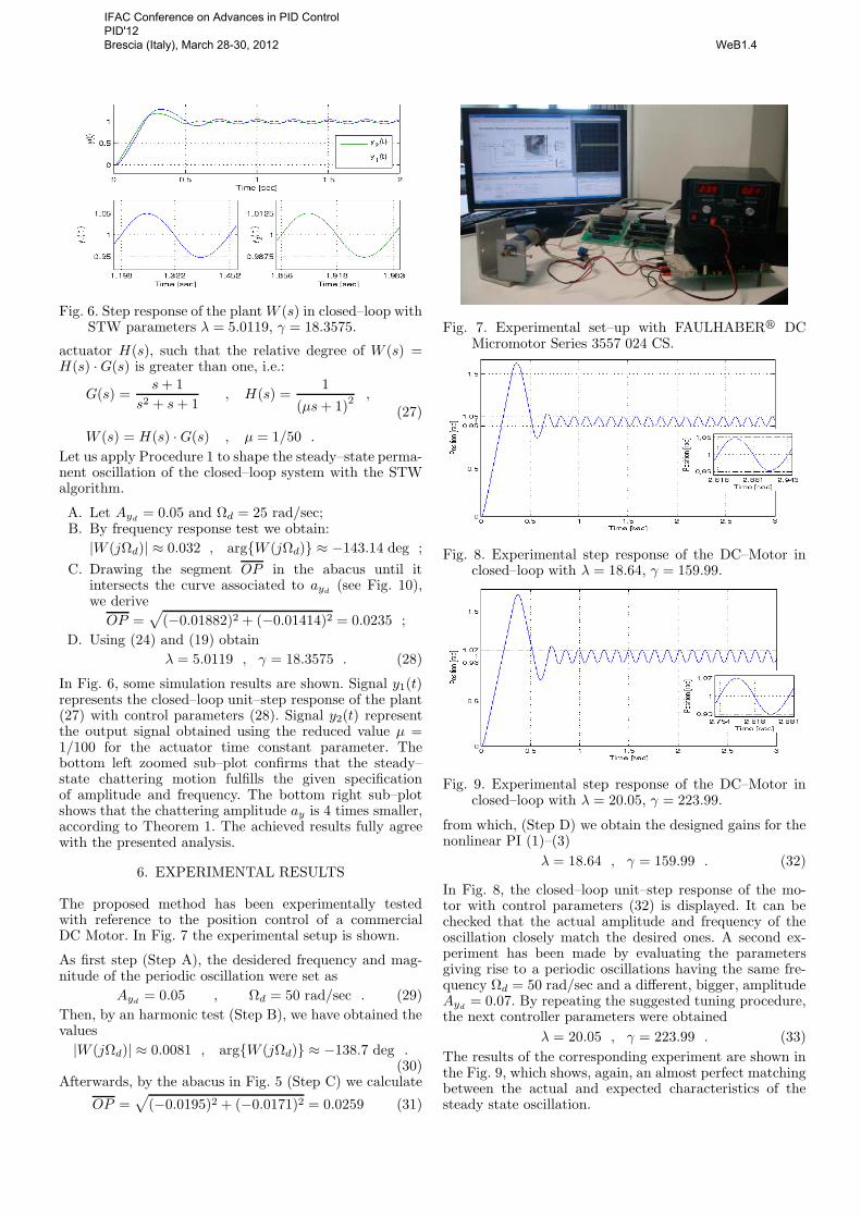
Fig. 6. Step response of the plantW (s) in closed–loop withSTW parameters λ = 5.0119, γ = 18.3575.

actuator H(s), such that the relative degree of W (s) =H(s) ·G(s) is greater than one, i.e.:

G(s) =s+ 1

s2 + s+ 1, H(s) =

1

(µs+ 1)2,

W (s) = H(s) ·G(s) , µ = 1/50 .

(27)

Let us apply Procedure 1 to shape the steady–state perma-nent oscillation of the closed–loop system with the STWalgorithm.

A. Let Ayd= 0.05 and Ωd = 25 rad/sec;

B. By frequency response test we obtain:

|W (jΩd)| ≈ 0.032 , argW (jΩd) ≈ −143.14 deg ;

C. Drawing the segment OP in the abacus until itintersects the curve associated to ayd

(see Fig. 10),we derive

OP =√

(−0.01882)2 + (−0.01414)2 = 0.0235 ;

D. Using (24) and (19) obtain

λ = 5.0119 , γ = 18.3575 . (28)

In Fig. 6, some simulation results are shown. Signal y1(t)represents the closed–loop unit–step response of the plant(27) with control parameters (28). Signal y2(t) representthe output signal obtained using the reduced value µ =1/100 for the actuator time constant parameter. Thebottom left zoomed sub–plot confirms that the steady–state chattering motion fulfills the given specificationof amplitude and frequency. The bottom right sub–plotshows that the chattering amplitude ay is 4 times smaller,according to Theorem 1. The achieved results fully agreewith the presented analysis.

6. EXPERIMENTAL RESULTS

The proposed method has been experimentally testedwith reference to the position control of a commercialDC Motor. In Fig. 7 the experimental setup is shown.

As first step (Step A), the desidered frequency and mag-nitude of the periodic oscillation were set as

Ayd= 0.05 , Ωd = 50 rad/sec . (29)

Then, by an harmonic test (Step B), we have obtained thevalues

|W (jΩd)| ≈ 0.0081 , argW (jΩd) ≈ −138.7 deg .(30)

Afterwards, by the abacus in Fig. 5 (Step C) we calculate

OP =√

(−0.0195)2 + (−0.0171)2 = 0.0259 (31)

Fig. 7. Experimental set–up with FAULHABERr DCMicromotor Series 3557 024 CS.

Fig. 8. Experimental step response of the DC–Motor inclosed–loop with λ = 18.64, γ = 159.99.

Fig. 9. Experimental step response of the DC–Motor inclosed–loop with λ = 20.05, γ = 223.99.

from which, (Step D) we obtain the designed gains for thenonlinear PI (1)–(3)

λ = 18.64 , γ = 159.99 . (32)

In Fig. 8, the closed–loop unit–step response of the mo-tor with control parameters (32) is displayed. It can bechecked that the actual amplitude and frequency of theoscillation closely match the desired ones. A second ex-periment has been made by evaluating the parametersgiving rise to a periodic oscillations having the same fre-quency Ωd = 50 rad/sec and a different, bigger, amplitudeAyd

= 0.07. By repeating the suggested tuning procedure,the next controller parameters were obtained

λ = 20.05 , γ = 223.99 . (33)

The results of the corresponding experiment are shown inthe Fig. 9, which shows, again, an almost perfect matchingbetween the actual and expected characteristics of thesteady state oscillation.

IFAC Conference on Advances in PID Control PID'12 Brescia (Italy), March 28-30, 2012 WeB1.4

Fig. 10. Example of abacus utilization for the system W (s) (27).

7. CONCLUSIONS AND FUTURE WORKS

A describing function approach to controller tuning hasbeen presented, to be adopted for linear SISO plants drivenby a nonlinear PI controller. The main property of the sug-gested tuning procedure is that it allows to set a–priori theamplitude and the frequency of the self–sustained steadystate periodic oscillations that take place in this class ofsystem when the relative degree is higher than one. Theproposed procedure has been tested by means of computersimulations and experiments. Among some interesting di-rections for improving the present result, the analysis,and shaping, of the transient oscillations is of specialinterest to avoid possibly large transient overshoots. Themathematical treatment presented in Boiko (2011) and the“dynamic harmonic balance” could be a starting point forgeneralizing the present procedure along that direction.Additionally, strategies for the on–line adjustment of thecontroller parameters could be devised within the presentline of investigation to achieve satisfactory transient andsteady state performance at the same time.

REFERENCES

Astrom, K. and Hagglund, T. (2005). Advanced PIDControl. ISA - The Instrumentation, Systems, and Au-tomation Society. Research Triangle Park, NC 27709,

Atherton, D. (1975). Nonlinear Control Engineering–Describing Function Analysis and Design. WorkinghamBerks, U.K.

Bartolini, G., Ferrara, A., and Usai, E. (1998). Chatteringavoidance by second–order sliding mode control. IEEETrans. Aut. Contr., 43(2), 241–246.

Bartolini, G., Fridman, L., Pisano, A., and Usai, E., (Eds)(2008). Modern Sliding Mode Control Theory. NewPerspectives and Applications. Springer Lecture Notesin Control and Information Sciences, Vol. 375.

Boiko, I. (2003). Analysis of sliding mode control systemsin the frequency domain. In Proc. of the 2003 AmericanControl Conference (ACC 2003), volume 1, 186–191.

Boiko, I. (2009). Discontinuous control systems:frequency–domain analysis and design. Boston,Birkhauser, 2009.

Boiko, I. Dynamic harmonic balance and its applicationto analysis of convergence of second–order sliding modecontrol algorithms. In Proc. of the 2011 AmericanControl Conference (ACC 2011), volume 1, 208–213.

Boiko, I. and Fridman, L. (2005). Analysis of chattering incontinuous sliding–mode controllers. IEEE Trans. Aut.Contr., 50(9), 1442–1446.

Boiko, I., Fridman, L., and Castellanos, M. (2004). Anal-ysis of second–order sliding–mode algorithms in the fre-quency domain. IEEE Trans. Aut. Contr., 49(6), 946–950.

Boiko, I., Fridman, L., Iriarte, R., Pisano, A., and Usai, E.(2006). Parameter tuning of second–order sliding modecontrollers for linear plants with dynamic actuators.Automatica, 42(5), 833–839.

Burton, J. (1986). Continuous approximation of variablestructure control. Int. J. of Systems Science, 17(6), 875–886. Taylor and Francis.

Fridman, L., Davila, J., and Levant, A. (2007). High–ordersliding–mode observation and fault detection. In Proc.of the 2007 IEEE Conference on Decision and Control(CDC 2007), 43174322.

Fridman, L., Shtessel, Y., Edwards, C., and Yan, X. (2008).Higher–order sliding–mode observer for state estimationand input reconstruction in nonlinear systems. Int. J.of Robust and Nonlinear Control, 18(4–5), 399–412.

Gelb, A. and Vander Velde, W. (1968). Multiple–input describing functions and nonlinear system design.McGraw–Hill, New York.

Goncalves, J., Megretski, A., and Dahleh, M. (2001).Global stability of relay feedback systems. IEEE Trans.Aut. Contr., 46(4), 550–562.

Levant, A. (1993). Sliding order and sliding accuracy insliding mode control. Int. J. of Control, 58(6), 1247–1263.

Levant, A. (2003). Higher–order sliding modes, differenti-ation and output–feedback control. Int. J. of Control,76, 9(10), 924–941.

Levant, A. and Fridman, L. (2010). Accuracy of homo-geneous sliding modes in the presence of fast actuators.IEEE Trans. Aut. Contr., 55(3), 810–814.

Shtessel, Y. and Lee, Y. (1996). New approach to chat-tering analysis in systems with sliding modes. In Proc.of the 1996 IEEE Conference on Decision and Control(CDC 1996), volume 4, 4014–4019.

Tsypkin, Y.Z. (1984). Relay control systems. CambridgeUniversity Press.

Utkin, V., Guldner, J., and J., S. (1999). Sliding modecontrol in electromechanical systems. Taylor and Fran-cis, London, 1999.

IFAC Conference on Advances in PID Control PID'12 Brescia (Italy), March 28-30, 2012 WeB1.4