
2.3 PDF - Brian 2 Documentation
769
Brian 2 Documentation Release 2.3 Brian authors Jan 15, 2020
-
Upload
khangminh22 -
Category
Documents
-
view
0 -
download
0
Transcript of 2.3 PDF - Brian 2 Documentation

Brian 2 DocumentationRelease 2.3
Brian authors
Jan 15, 2020


Contents
1 Introduction 31.1 Installation . . . . . . . . . . . . . . . . . . . . . . . . . . . . . . . . . . . . . . . . . . . . . . . . 31.2 Running Brian scripts . . . . . . . . . . . . . . . . . . . . . . . . . . . . . . . . . . . . . . . . . . 61.3 Release notes . . . . . . . . . . . . . . . . . . . . . . . . . . . . . . . . . . . . . . . . . . . . . . . 71.4 Changes for Brian 1 users . . . . . . . . . . . . . . . . . . . . . . . . . . . . . . . . . . . . . . . . 321.5 Known issues . . . . . . . . . . . . . . . . . . . . . . . . . . . . . . . . . . . . . . . . . . . . . . . 631.6 Support . . . . . . . . . . . . . . . . . . . . . . . . . . . . . . . . . . . . . . . . . . . . . . . . . . 651.7 Contributor Covenant Code of Conduct . . . . . . . . . . . . . . . . . . . . . . . . . . . . . . . . . 65
2 Tutorials 672.1 Introduction to Brian part 1: Neurons . . . . . . . . . . . . . . . . . . . . . . . . . . . . . . . . . . 672.2 Introduction to Brian part 2: Synapses . . . . . . . . . . . . . . . . . . . . . . . . . . . . . . . . . . 842.3 Introduction to Brian part 3: Simulations . . . . . . . . . . . . . . . . . . . . . . . . . . . . . . . . 100
3 User’s guide 1173.1 Importing Brian . . . . . . . . . . . . . . . . . . . . . . . . . . . . . . . . . . . . . . . . . . . . . 1173.2 Physical units . . . . . . . . . . . . . . . . . . . . . . . . . . . . . . . . . . . . . . . . . . . . . . . 1183.3 Models and neuron groups . . . . . . . . . . . . . . . . . . . . . . . . . . . . . . . . . . . . . . . . 1213.4 Numerical integration . . . . . . . . . . . . . . . . . . . . . . . . . . . . . . . . . . . . . . . . . . 1273.5 Equations . . . . . . . . . . . . . . . . . . . . . . . . . . . . . . . . . . . . . . . . . . . . . . . . . 1293.6 Refractoriness . . . . . . . . . . . . . . . . . . . . . . . . . . . . . . . . . . . . . . . . . . . . . . 1343.7 Synapses . . . . . . . . . . . . . . . . . . . . . . . . . . . . . . . . . . . . . . . . . . . . . . . . . 1363.8 Input stimuli . . . . . . . . . . . . . . . . . . . . . . . . . . . . . . . . . . . . . . . . . . . . . . . 1453.9 Recording during a simulation . . . . . . . . . . . . . . . . . . . . . . . . . . . . . . . . . . . . . . 1503.10 Running a simulation . . . . . . . . . . . . . . . . . . . . . . . . . . . . . . . . . . . . . . . . . . . 1543.11 Multicompartment models . . . . . . . . . . . . . . . . . . . . . . . . . . . . . . . . . . . . . . . . 1603.12 Computational methods and efficiency . . . . . . . . . . . . . . . . . . . . . . . . . . . . . . . . . 1683.13 Converting from integrated form to ODEs . . . . . . . . . . . . . . . . . . . . . . . . . . . . . . . . 172
4 Advanced guide 1754.1 Functions . . . . . . . . . . . . . . . . . . . . . . . . . . . . . . . . . . . . . . . . . . . . . . . . . 1754.2 Preferences . . . . . . . . . . . . . . . . . . . . . . . . . . . . . . . . . . . . . . . . . . . . . . . . 1814.3 Logging . . . . . . . . . . . . . . . . . . . . . . . . . . . . . . . . . . . . . . . . . . . . . . . . . . 1874.4 Namespaces . . . . . . . . . . . . . . . . . . . . . . . . . . . . . . . . . . . . . . . . . . . . . . . 1884.5 Custom progress reporting . . . . . . . . . . . . . . . . . . . . . . . . . . . . . . . . . . . . . . . . 1894.6 Random numbers . . . . . . . . . . . . . . . . . . . . . . . . . . . . . . . . . . . . . . . . . . . . . 1904.7 Custom events . . . . . . . . . . . . . . . . . . . . . . . . . . . . . . . . . . . . . . . . . . . . . . 191
i
4.8 State update . . . . . . . . . . . . . . . . . . . . . . . . . . . . . . . . . . . . . . . . . . . . . . . 1944.9 How Brian works . . . . . . . . . . . . . . . . . . . . . . . . . . . . . . . . . . . . . . . . . . . . . 1964.10 Interfacing with external code . . . . . . . . . . . . . . . . . . . . . . . . . . . . . . . . . . . . . . 197
5 Examples 1995.1 Example: COBAHH . . . . . . . . . . . . . . . . . . . . . . . . . . . . . . . . . . . . . . . . . . . 1995.2 Example: CUBA . . . . . . . . . . . . . . . . . . . . . . . . . . . . . . . . . . . . . . . . . . . . . 2015.3 Example: IF_curve_Hodgkin_Huxley . . . . . . . . . . . . . . . . . . . . . . . . . . . . . . . . . . 2035.4 Example: IF_curve_LIF . . . . . . . . . . . . . . . . . . . . . . . . . . . . . . . . . . . . . . . . . 2045.5 Example: adaptive_threshold . . . . . . . . . . . . . . . . . . . . . . . . . . . . . . . . . . . . . . 2055.6 Example: non_reliability . . . . . . . . . . . . . . . . . . . . . . . . . . . . . . . . . . . . . . . . . 2075.7 Example: phase_locking . . . . . . . . . . . . . . . . . . . . . . . . . . . . . . . . . . . . . . . . . 2085.8 Example: reliability . . . . . . . . . . . . . . . . . . . . . . . . . . . . . . . . . . . . . . . . . . . 2095.9 advanced . . . . . . . . . . . . . . . . . . . . . . . . . . . . . . . . . . . . . . . . . . . . . . . . . 2115.10 compartmental . . . . . . . . . . . . . . . . . . . . . . . . . . . . . . . . . . . . . . . . . . . . . . 2265.11 frompapers . . . . . . . . . . . . . . . . . . . . . . . . . . . . . . . . . . . . . . . . . . . . . . . . 2455.12 frompapers/Brette_2012 . . . . . . . . . . . . . . . . . . . . . . . . . . . . . . . . . . . . . . . . . 2985.13 frompapers/Stimberg_et_al_2018 . . . . . . . . . . . . . . . . . . . . . . . . . . . . . . . . . . . . 3085.14 standalone . . . . . . . . . . . . . . . . . . . . . . . . . . . . . . . . . . . . . . . . . . . . . . . . 3435.15 synapses . . . . . . . . . . . . . . . . . . . . . . . . . . . . . . . . . . . . . . . . . . . . . . . . . 347
6 brian2 package 3636.1 check_cache function . . . . . . . . . . . . . . . . . . . . . . . . . . . . . . . . . . . . . . . . . . 3636.2 clear_cache function . . . . . . . . . . . . . . . . . . . . . . . . . . . . . . . . . . . . . . . . . . . 3636.3 hears module . . . . . . . . . . . . . . . . . . . . . . . . . . . . . . . . . . . . . . . . . . . . . . 3646.4 numpy_ module . . . . . . . . . . . . . . . . . . . . . . . . . . . . . . . . . . . . . . . . . . . . . 3676.5 only module . . . . . . . . . . . . . . . . . . . . . . . . . . . . . . . . . . . . . . . . . . . . . . 3676.6 Subpackages . . . . . . . . . . . . . . . . . . . . . . . . . . . . . . . . . . . . . . . . . . . . . . . 367
7 Developer’s guide 6917.1 Coding guidelines . . . . . . . . . . . . . . . . . . . . . . . . . . . . . . . . . . . . . . . . . . . . 6917.2 Units . . . . . . . . . . . . . . . . . . . . . . . . . . . . . . . . . . . . . . . . . . . . . . . . . . . 7057.3 Equations and namespaces . . . . . . . . . . . . . . . . . . . . . . . . . . . . . . . . . . . . . . . . 7087.4 Variables and indices . . . . . . . . . . . . . . . . . . . . . . . . . . . . . . . . . . . . . . . . . . . 7087.5 Preferences system . . . . . . . . . . . . . . . . . . . . . . . . . . . . . . . . . . . . . . . . . . . . 7127.6 Adding support for new functions . . . . . . . . . . . . . . . . . . . . . . . . . . . . . . . . . . . . 7187.7 Code generation . . . . . . . . . . . . . . . . . . . . . . . . . . . . . . . . . . . . . . . . . . . . . 7197.8 Devices . . . . . . . . . . . . . . . . . . . . . . . . . . . . . . . . . . . . . . . . . . . . . . . . . . 7257.9 Multi-threading with OpenMP . . . . . . . . . . . . . . . . . . . . . . . . . . . . . . . . . . . . . . 7267.10 Solving differential equations with the GNU Scientific Library . . . . . . . . . . . . . . . . . . . . . 729
8 Indices and tables 735
Bibliography 737
Python Module Index 739
Index 741
ii

Brian 2 Documentation, Release 2.3
Brian is a simulator for spiking neural networks. It is written in the Python programming language and is availableon almost all platforms. We believe that a simulator should not only save the time of processors, but also the time ofscientists. Brian is therefore designed to be easy to learn and use, highly flexible and easily extensible.
To get an idea of what writing a simulation in Brian looks like, take a look at a simple example, or run our interactivedemo.
Once you have a feel for what is involved in using Brian, we recommend you start by following the installationinstructions, and in case you are new to the Python programming language, having a look at Running Brian scripts.Then, go through the tutorials, and finally read the User Guide.
While reading the documentation, you will see the names of certain functions and classes are highlighted links (e.g.PoissonGroup). Clicking on these will take you to the “reference documentation”. This section is automaticallygenerated from the code, and includes complete and very detailed information, so for new users we recommendsticking to the User’s guide. However, there is one feature that may be useful for all users. If you click on, for example,PoissonGroup, and scroll down to the bottom, you’ll get a list of all the example code that uses PoissonGroup.This is available for each class or method, and can be helpful in understanding how a feature works.
Finally, if you’re having problems, please do let us know at our support page.
Please note that all interactions (e.g. via the mailing list or on github) should adhere to our Code of Conduct.
Contents:
Contents 1

Brian 2 Documentation, Release 2.3
2 Contents

CHAPTER 1
Introduction
1.1 Installation
• Installation with Anaconda
• Installation with pip
• Requirements for C++ code generation
• Development version
• Testing Brian
We recommend users to use the Anaconda distribution by Continuum Analytics. Its use will make the installation ofBrian 2 and its dependencies simpler, since packages are provided in binary form, meaning that they don’t have to bebuild from the source code at your machine. Furthermore, our automatic testing on the continuous integration servicestravis and appveyor are based on Anaconda, we are therefore confident that it works under this configuration.
However, Brian 2 can also be installed independent of Anaconda, either with other Python distributions (EnthoughtCanopy, Python(x,y) for Windows, . . . ) or simply based on Python and pip (see Installation with pip below).
1.1.1 Installation with Anaconda
Installing Anaconda
Download the Anaconda distribution for your Operating System. Note that the choice between Python 2.7 and Python3.x is not very important at this stage, Anaconda allows you to create a Python 3 environment from Python 2 Anacondaand vice versa.
After the installation, make sure that your environment is configured to use the Anaconda distribution. You shouldhave access to the conda command in a terminal and running python (e.g. from your IDE) should show a headerlike this, indicating that you are using Anaconda’s Python interpreter:
3
Brian 2 Documentation, Release 2.3
Python 2.7.10 |Anaconda 2.3.0 (64-bit)| (default, May 28 2015, 17:02:03)[GCC 4.4.7 20120313 (Red Hat 4.4.7-1)] on linux2Type "help", "copyright", "credits" or "license" for more information.
Here’s some documentation on how to set up some popular IDEs for Anaconda: https://docs.anaconda.com/anaconda/user-guide/tasks/integration
Installing Brian 2
Note: The provided Brian 2 packages are only for 64bit systems. If you want to install Brian 2 in a 32bit environment,please use the Installation with pip instead.
You can either install Brian 2 in the Anaconda root environment, or create a new environment for Brian 2 (https://conda.io/projects/conda/en/latest/user-guide/tasks/manage-environments.html). The latter has the advantage that youcan update (or not update) the dependencies of Brian 2 independently from the rest of your system.
Brian 2 is not part of the main Anaconda distribution, but built using the community-maintained conda-forge project.You will therefore have to to install it from the conda-forge channel. To do so, use:
conda install -c conda-forge brian2
You can also permanently add the channel to your list of channels:
conda config --add channels conda-forge
This has only to be done once. After that, you can install and update the brian2 packages as any other Anacondapackage:
conda install brian2
Installing other useful packages
There are various packages that are useful but not necessary for working with Brian. These include: matplotlib (forplotting), nose (for running the test suite), ipython and jupyter-notebook (for an interactive console). To install themfrom anaconda, simply do:
conda install matplotlib nose ipython notebook
You should also have a look at the brian2tools package, which contains several useful functions to visualize Brian 2simulations and recordings. You can install it with pip or anaconda, similar to Brian 2 itself (but as of now, it is notincluded in the conda-forge channel, you therefore have to install it from our own brian-team channel), e.g.with:
conda install -c brian-team brian2tools
1.1.2 Installation with pip
If you decide not to use Anaconda, you can install Brian 2 from the Python package index: https://pypi.python.org/pypi/Brian2
To do so, use the pip utility:
4 Chapter 1. Introduction
Brian 2 Documentation, Release 2.3
pip install brian2
You might want to add the --user flag, to install Brian 2 for the local user only, which means that you don’t needadministrator privileges for the installation.
Note that when installing brian2 from source with pip, support for using numerical integration with the GSL requiresa working installation of the GSL development libraries (e.g. the package libgsl-dev on Debian/Ubuntu Linux).
1.1.3 Requirements for C++ code generation
C++ code generation is highly recommended since it can drastically increase the speed of simulations (see Compu-tational methods and efficiency for details). To use it, you need a C++ compiler and either Cython or weave (onlyavailable for Python 2.x). Cython/weave will be automatically installed if you perform the installation via Anaconda,as recommended. Otherwise you can install them in the usual way, e.g. using pip install cython or pipinstall weave.
Linux and OS X
On Linux and Mac OS X, the conda package will automatically install a C++ compiler. But even if you install Brianfrom source, you will most likely already have a working C++ compiler installed on your system (try calling g++--version in a terminal). If not, use your distribution’s package manager to install a g++ package.
Windows
On Windows, the necessary steps to get Runtime code generation (i.e. Cython/weave) to work depend on the Pythonversion you are using (also see the notes in the Python wiki):
• Python >= 3.5
– Install the Microsoft Build Tools for Visual Studio 2017.
– Make sure that your setuptools package has at least version 34.4.0 (use conda update setuptools when using Anaconda, orpip install --upgrade setuptools when using pip).
• Python 2.7
– Download and install the Microsoft Visual C++ Compiler for Python 2.7
For Standalone code generation, you can either use the compiler installed above or any other version of Visual Studio– in this case, the Python version does not matter.
Try running the test suite (see Testing Brian below) after the installation to make sure everything is working as ex-pected.
1.1.4 Development version
To run the latest development code, you can directly clone the git repository at github (https://github.com/brian-team/brian2) and then run pip install -e ., to install Brian in “development mode”. With this installation, updatingthe git repository is in general enough to keep up with changes in the code, i.e. it is not necessary to install it again.
Another option is to use pip to directly install from github:
pip install https://github.com/brian-team/brian2/archive/master.zip
1.1. Installation 5
Brian 2 Documentation, Release 2.3
1.1.5 Testing Brian
If you have the nose testing utility installed, you can run Brian’s test suite:
import brian2brian2.test()
It should end with “OK”, showing a number of skipped tests but no errors or failures. For more control about the teststhat are run see the developer documentation on testing.
1.2 Running Brian scripts
Brian scripts are standard Python scripts, and can therefore be run in the same way. For interactive, explorative work,you might want to run code in a jupyter notebook or in an ipython shell; for running finished code, you might want toexecute scripts through the standard Python interpreter; finally, for working on big projects spanning multiple files, adedicated integrated development environment for Python could be a good choice. We will briefly describe all theseapproaches and how they relate to Brian’s examples and tutorial that are part of this documentation. Note that none ofthese approaches are specific to Brian, so you can also search for more information in any of the resources listed onthe Python website.
• Jupyter notebook
• IPython shell
• Python interpreter
• Integrated development environment (IDE)
1.2.1 Jupyter notebook
The Jupyter Notebook is an open-source web application that allows you to create and share documentsthat contain live code, equations, visualizations and narrative text.
(from jupyter.org)
Jupyter notebooks are a great tool to run Brian code interactively, and include the results of the simulations, as well asadditional explanatory text in a common document. Such documents have the file ending .ipynb, and in Brian weuse this format to store the Tutorials. These files can be displayed by github (see e.g. the first Brian tutorial), but inthis case you can only see them as a static website, not edit or execute any of the code.
To make the full use of such notebooks, you have to run them using the jupyter infrastructure. The easiest option is touse the free mybinder.org web service, which allows you to try out Brian without installing it on your own machine.Links to run the tutorials on this infrastructure are provided as “launch binder” buttons on the Tutorials page, andalso for each of the Examples at the top of the respective page (e.g. Example: COBAHH). To run notebooks on yourown machine, you need an installation of the jupyter notebook software on your own machine, as well as Brian itself(see the Installation instructions for details). To open an existing notebook, you have to download it to your machine.For the Brian tutorials, you find the necessary links on the Tutorials page. When you have downloaded/installedeverything necessary, you can start the jupyter notebook from the command line (using Terminal on OS X/Linux,Command Prompt on Windows):
jupyter notebook
6 Chapter 1. Introduction

Brian 2 Documentation, Release 2.3
this will open the “Notebook Dashboard” in your default browser, from which you can either open an existing notebookor create a new one. In the notebook, you can then execute individual “code cells” by pressing SHIFT+ENTER onyour keyboard, or by pressing the play button in the toolbar.
For more information, see the jupyter notebook documentation.
1.2.2 IPython shell
An alternative to using the jupyter notebook is to use the interactive Python shell IPython, which runs in the Termi-nal/Command Prompt. You can use it to directly type Python code interactively (each line will be executed as soonas you press ENTER), or to run Python code stored in a file. Such files typically have the file ending .py. You caneither create it yourself in a text editor of your choice (e.g. by copying&pasting code from one of the Examples), orby downloading such files from places such as github (e.g. the Brian examples), or ModelDB. You can then run themfrom within IPython via:
%run filename.py
1.2.3 Python interpreter
The most basic way to run Python code is to run it through the standard Python interpreter. While you can also usethis interpreter interactively, it is much less convenient to use than the IPython shell or the jupyter notebook describedabove. However, if all you want to do is to run an existing Python script (e.g. one of the Brian Examples), then youcan do this by calling:
python filename.py
in a Terminal/Command Prompt.
1.2.4 Integrated development environment (IDE)
Python is a widely used programming language, and is therefore support by a wide range of integrated developmentenvironments (IDE). Such IDEs provide features that are very convenient for developing complex projects, e.g. theyintegrate text editor and interactive Python console, graphical debugging tools, etc. Popular environments includeSpyder, PyCharm, and Visual Studio Code, for an extensive list see the Python wiki.
1.3 Release notes
1.3.1 Brian 2.3
This release contains the usual mix of bug fixes and new features (see below), but also makes some important changesto the Brian 2 code base to pave the way for the full Python 2 -> 3 transition (the source code is now directly compatiblewith Python 2 and Python 3, without the need for any translation at install time). Please note that this release will be thelast release that supports Python 2, given that Python 2 reaches end-of-life in January 2020. Brian now also uses pytestas its testing framework, since the previously used nose package is not maintained anymore. Since brian2hears hasbeen released as an independent package, using brian2.hears as a “bridge” to Brian 1’s brian.hears packageis now deprecated.
Finally, the Brian project has adopted the “Contributor Covenant” Contributor Covenant Code of Conduct, pledging“to make participation in our community a harassment-free experience for everyone”.
1.3. Release notes 7
Brian 2 Documentation, Release 2.3
New features
• The restore() function can now also restore the state of the random number generator, allowing for exactreproducibility of stochastic simulations (#1134)
• The functions expm1(), log1p(), and exprel() can now be used (#1133)
• The system for calling random number generating functions has been generalized (see Functions with context-dependent return values), and a new poisson function for Poisson-distrubted random numbers has been added(#1111)
• New versions of Visual Studio are now supported for standalone mode on Windows (#1135)
Selected improvements and bug fixes
• run_regularly operations are now included in the network, even if they are created after the parent objectwas added to the network (#1009). Contributed by Vigneswaran Chandrasekaran.
• No longer incorrectly classify some equations as having “multiplicative noise” (#968). Contributed by Vi-gneswaran Chandrasekaran.
• Brian is now compatible with Python 3.8 (#1130), and doctests are compatible with numpy 1.17 (#1120)
• Progress reports for repeated runs have been fixed (#1116), thanks to Ronaldo Nunes for reporting the issue.
• SpikeGeneratorGroup now correctly works with restore() (#1084), thanks to Tom Achache for re-porting the issue.
• An indexing problem in PopulationRateMonitor has been fixed (#1119).
• Handling of equations referring to -inf has been fixed (#1061).
• Long simulations recording more than ~2 billion data points no longer crash with a segmentation fault (#1136),thanks to Rike-Benjamin Schuppner for reporting the issue.
Backward-incompatible changes
• The fix for run_regularly operations (#1009, see above) entails a change in how objects are stored withinNetwork objects. Previously, Network.objects stored a complete list of all objects, including objectssuch as StateUpdater that – often invisible to the user – are a part of major objects such as NeuronGroup.Now, Network.objects only stores the objects directly provided by the user (NeuronGroup, Synapses,StateMonitor, . . . ), the dependent objects (StateUpdater, Thresholder, . . . ) are taken into accountat the time of the run. This might break code in some corner cases, e.g. when removing a StateUpdaterfrom Network.objects via Network.remove().
• The brian2.hears interface to Brian 1’s brian.hears package has been deprecated.
Infrastructure and documentation improvements
• The same code base is used on Python 2 and Python 3 (#1073).
• The test framework uses pytest (#1127).
• We have adapoted a Code of Conduct (#1113), thanks to Tapasweni Pathak for the suggestion.
8 Chapter 1. Introduction

Brian 2 Documentation, Release 2.3
Contributions
Github code, documentation, and issue contributions (ordered by the number of contributions):
• Marcel Stimberg (@mstimberg)
• Dan Goodman (@thesamovar)
• Vigneswaran Chandrasekaran (@Vigneswaran-Chandrasekaran)
• Moritz Orth (@morth)
• Tristan Stöber (@tristanstoeber)
• @ulyssek
• Wilhelm Braun (@wilhelmbraun)
• @flomlo
• Rike-Benjamin Schuppner (@Debilski)
• @sdeiss
• Ben Evans (@bdevans)
• Tapasweni Pathak (@tapaswenipathak)
• @jonathanoesterle
• Richard C Gerkin (@rgerkin)
• Christian Behrens (@chbehrens)
• Romain Brette (@romainbrette)
• XiaoquinNUDT (@XiaoquinNUDT)
• Dylan Muir (@DylanMuir)
• Aleksandra Teska (@alTeska)
• Felix Z. Hoffmann (@felix11h)
• @baixiaotian63648995
• Carlos de la Torre (@c-torre)
• Sam Mathias (@sammosummo)
• @Marghepano
• Simon Brodeur (@sbrodeur)
• Alex Dimitrov (@adimitr)
Other contributions outside of github (ordered alphabetically, apologies to anyone we forgot. . . ):
• Ronaldo Nunes
• Tom Achache
1.3.2 Brian 2.2.2.1
This is a bug-fix release that fixes several bugs and adds a few minor new features. We recommend all users of Brian2 to upgrade.
1.3. Release notes 9

Brian 2 Documentation, Release 2.3
As always, please report bugs or suggestions to the github bug tracker (https://github.com/brian-team/brian2/issues)or to the brian-development mailing list ([email protected]).
[Note that the original upload of this release was version 2.2.2, but due to a mistake in the released archive, it has beenuploaded again as version 2.2.2.1]
Selected improvements and bug fixes
• Fix an issue with the synapses generator syntax (#1037).
• Fix an incorrect error when using a SpikeGeneratorGroup with a long period (#1041). Thanks to KévinCuallado-Keltsch for reporting this issue.
• Improve the performance of SpikeGeneratorGroup by avoiding a conversion from time to integer timestep (#1043). This time step is now also available to user code as t_in_timesteps.
• Function definitions for weave/Cython/C++ standalone can now declare additional header files and libraries.They also support a new sources argument to use a function definition from an external file. See the Functionsdocumentation for details.
• For convenience, single-neuron subgroups can now be created with a single index instead of with a slice (e.g.neurongroup[3] instead of neurongroup[3:4]).
• Fix an issue when -inf is used in an equation (#1061).
Contributions
Github code, documentation, and issue contributions (ordered by the number of contributions):
• Marcel Stimberg (@mstimberg)
• Dan Goodman (@thesamovar)
• Felix Z. Hoffmann (@Felix11H)
• @wjx0914
• Kévin Cuallado-Keltsch (@kevincuallado)
• Romain Cazé (@rcaze)
• Daphne (@daphn3cor)
• Erik (@parenthetical-e)
• @RahulMaram
• Eghbal Hosseini (@eghbalhosseini)
• Martino Sorbaro (@martinosorb)
• Mihir Vaidya (@MihirVaidya94)
• @hellolingling
• Volodimir Slobodyanyuk (@vslobody)
• Peter Duggins (@psipeter)
10 Chapter 1. Introduction
Brian 2 Documentation, Release 2.3
1.3.3 Brian 2.2.1
This is a bug-fix release that fixes a few minor bugs and incompatibilites with recent versions of the dependencies. Werecommend all users of Brian 2 to upgrade.
As always, please report bugs or suggestions to the github bug tracker (https://github.com/brian-team/brian2/issues)or to the brian-development mailing list ([email protected]).
Selected improvements and bug fixes
• Work around problems with the latest version of py-cpuinfo on Windows (#990, #1020) and no longerrequire it for Linux and OS X.
• Avoid warnings with newer versions of Cython (#1030) and correctly build the Cython spike queue for Python3.7 (#1026), thanks to Fleur Zeldenrust and Ankur Sinha for reporting these issues.
• Fix error messages for SyntaxError exceptions in jupyter notebooks (##964).
Dependency and packaging changes
• Conda packages in conda-forge are now avaible for Python 3.7 (but no longer for Python 3.5).
• Linux and OS X no longer depend on the py-cpuinfo package.
• Source packages on pypi now require a recent Cython version for installation.
Contributions
Github code, documentation, and issue contributions (ordered by the number of contributions):
• Marcel Stimberg (@mstimberg)
• Dan Goodman (@thesamovar)
• Christopher (@Chris-Currin)
• Peter Duggins (@psipeter)
• Paola Suárez (@psrmx)
• Ankur Sinha (@sanjayankur31)
• @JingjinW
• Denis Alevi (@denisalevi)
• @lemonade117
• @wjx0914
• Sven Leach (@SvennoNito)
• svadams (@svadams)
• @ghaessig
• Varshith Sreeramdass (@varshiths)
1.3. Release notes 11
Brian 2 Documentation, Release 2.3
1.3.4 Brian 2.2
This releases fixes a number of important bugs and comes with a number of performance improvements. It also makessure that simulation no longer give platform-dependent results for certain corner cases that involve the division ofintegers. These changes can break backwards-compatiblity in certain cases, see below. We recommend all users ofBrian 2 to upgrade.
As always, please report bugs or suggestions to the github bug tracker (https://github.com/brian-team/brian2/issues)or to the brian-development mailing list ([email protected]).
Selected improvements and bug fixes
• Divisions involving integers now use floating point division, independent of Python version and code generationtarget. The // operator can now used in equations and expressions to denote flooring division (#984).
• Simulations can now use single precision instead of double precision floats in simulations (#981, #1004). Thisis mostly intended for use with GPU code generation targets.
• The timestep, introduced in version 2.1.3, was further optimized for performance, making the refractorinesscalculation faster (#996).
• The lastupdate variable is only automatically added to synaptic models when event-driven equations areused, reducing the memory and performance footprint of simple synaptic models (#1003). Thanks to DenisAlevi for bringing this up.
• A from brian2 import * imported names unrelated to Brian, and overwrote some Python builtins suchas dir (#969). Now, fewer names are imported (but note that this still includes numpy and plotting tools:Importing Brian).
• The exponential_euler state updater is no longer failing for systems of equations with differential equa-tions that have trivial, constant right-hand-sides (#1010). Thanks to Peter Duggins for making us aware of thisissue.
Backward-incompatible changes
• Code that divided integers (e.g. N/10) with a C-based code generation target, or with the numpy target onPython 2, will now use floating point division instead of flooring division (i.e., Python 3 semantics). A warningwill notify the user of this change, use either the flooring division operator (N//10), or the int function(int(N/10)) to make the expression unambiguous.
• Code that directly referred to the lastupdate variable in synaptic statements, without using any event-drivenvariables, now has to manually add lastupdate : second to the equations and update the variable at theend of on_pre and/or on_post with lastupdate = t.
• Code that relied on from brian2 import * also importing unrelated names such as sympy, now has toimport such names explicitly.
Documentation improvements
• Various small fixes and additions (e.g. installation instructions, available functions, fixes in examples)
• A new example, Izhikevich 2007, provided by Guillaume Dumas.
12 Chapter 1. Introduction
Brian 2 Documentation, Release 2.3
Contributions
Github code, documentation, and issue contributions (ordered by the number of contributions):
• Marcel Stimberg (@mstimberg)
• Dan Goodman (@thesamovar)
• Denis Alevi (@denisalevi)
• Thomas Nowotny (@tnowotny)
• @neworderofjamie
• Paul Brodersen (@paulbrodersen)
• @matrec4
• svadams (@svadams)
• XiaoquinNUDT (@XiaoquinNUDT)
• Peter Duggins (@psipeter)
• @nh17937
• Patrick Nave (@pnave95)
• @AI-pha
• Guillaume Dumas (@deep-introspection)
• @godelicbach
• @galharth
1.3.5 Brian 2.1.3.1
This is a bug-fix release that fixes two bugs in the recent 2.1.3 release:
• Fix an inefficiency in the newly introduced timestep function when using the numpy target (#965)
• Fix inefficiencies in the unit system that could lead to slow operations and high memory use (#967). Thanks toKaustab Pal for making us aware of the issue.
1.3.6 Brian 2.1.3
This is a bug-fix release that fixes a number of important bugs (see below), but does not introduce any new features.We recommend all users of Brian 2 to upgrade.
As always, please report bugs or suggestions to the github bug tracker (https://github.com/brian-team/brian2/issues)or to the brian-development mailing list ([email protected]).
Selected improvements and bug fixes
• The Cython cache on disk now uses significantly less space by deleting unnecessary source files (set the code-gen.runtime.cython.delete_source_files preference to False if you want to keep these files for debugging).In addition, a warning will be given when the Cython or weave cache exceeds a configurable size (code-gen.max_cache_dir_size). The clear_cache function is provided to delete files from the cache (#914).
1.3. Release notes 13

Brian 2 Documentation, Release 2.3
• The C++ standalone mode now respects the profile option and therefore no longer collects profiling infor-mation by default. This can speed up simulations in certain cases (#935).
• The exact number of time steps that a neuron stays in the state of refractoriness after a spike could vary by upto one time step when the requested refractory time was a multiple of the simulation time step. With this fix,the number of time steps is ensured to be as expected by making use of a new timestep function that avoidsfloating point rounding issues (#949, first reported by @zhouyanasd in issue #943).
• When restore() was called twice for a network, spikes that were not yet delivered to their target were notrestored correctly (#938, reported by @zhouyanasd).
• SpikeGeneratorGroup now uses a more efficient method for sorting spike indices and times, leading to amuch faster preparation time for groups that store many spikes (#948).
• Fix a memory leak in TimedArray (#923, reported by Wilhelm Braun).
• Fix an issue with summed variables targetting subgroups (#925, reported by @AI-pha).
• Fix the use of run_regularly on subgroups (#922, reported by @AI-pha).
• Improve performance for SpatialNeuron by removing redundant computations (#910, thanks to MoritzAugustin for making us aware of the issue).
• Fix linked variables that link to scalar variables (#916)
• Fix warnings for numpy 1.14 and avoid compilation issues when switching between versions of numpy (#913)
• Fix problems when using logical operators in code generated for the numpy target which could lead to issuessuch as wrongly connected synapses (#901, #900).
Backward-incompatible changes
• No longer allow delay as a variable name in a synaptic model to avoid ambiguity with respect to the synapticdelay. Also no longer allow access to the delay variable in synaptic code since there is no way to distinguishbetween pre- and post-synaptic delay (#927, reported by Denis Alevi).
• Due to the changed handling of refractoriness (see bug fixes above), simulations that make use of refractorinesswill possibly no longer give exactly the same results. The preference legacy.refractory_timing can be set toTrue to reinstate the previous behaviour.
Infrastructure and documentation improvements
• From this version on, conda packages will be available on conda-forge. For a limited time, we will copy overpackages to the brian-team channel as well.
• Conda packages are no longer tied to a specific numpy version (PR #954)
• New example (Brunel & Wang, 2001) contributed by Teo Stocco and Alex Seeholzer.
Contributions
Github code, documentation, and issue contributions (ordered by the number of contributions):
• Marcel Stimberg (@mstimberg)
• Dan Goodman (@thesamovar)
• Teo Stocco (@zifeo)
• Dylan Muir (@DylanMuir)
14 Chapter 1. Introduction

Brian 2 Documentation, Release 2.3
• scarecrow (@zhouyanasd)
• @fuadfukhasyi
• Aditya Addepalli (@Dyex719)
• Kapil kumar (@kapilkd13)
• svadams (@svadams)
• Vafa Andalibi (@Vafa-Andalibi)
• Sven Leach (@SvennoNito)
• @matrec4
• @jarishna
• @AI-pha
• @xdzhangxuejun
• Denis Alevi (@denisalevi)
• Paul Pfeiffer (@pfeffer90)
• Romain Brette (@romainbrette)
• @hustyanghui
• Adrien F. Vincent (@afvincent)
• @ckemere
• @evearmstrong
• Paweł Kopec (@pawelkopec)
• Moritz Augustin (@moritzaugustin)
• Bart (@louwers)
• @amarsdd
• @ttxtea
• Maria Cervera (@MariaCervera)
• ouyangxinrong (@longzhixin)
Other contributions outside of github (ordered alphabetically, apologies to anyone we forgot. . . ):
• Wilhelm Braun
1.3.7 Brian 2.1.2
This is another bug fix release that fixes a major bug in Equations’ substitution mechanism (#896). Thanks to TeoStocco for reporting this issue.
1.3.8 Brian 2.1.1
This is a bug fix release that re-activates parts of the caching mechanism for code generation that had been erroneouslydeactivated in the previous release.
1.3. Release notes 15

Brian 2 Documentation, Release 2.3
1.3.9 Brian 2.1
This release introduces two main new features: a new “GSL integration” mode for differential equation that offers tointegrate equations with variable-timestep methods provided by the GNU Scientific Library, and caching for the runpreparation phase that can significantly speed up simulations. It also comes with a newly written tutorial, as well asadditional documentation and examples.
As always, please report bugs or suggestions to the github bug tracker (https://github.com/brian-team/brian2/issues)or to the brian-development mailing list ([email protected]).
New features
• New numerical integration methods with variable time-step integration, based on the GNU Scientific Library(see Numerical integration). Contributed by Charlee Fletterman, supported by 2017’s Google Summer of Codeprogram.
• New caching mechanism for the code generation stage (application of numerical integration algorithms, anal-ysis of equations and statements, etc.), reducing the preparation time before the actual run, in particular forsimulations with multiple run() statements.
Selected improvements and bug fixes
• Fix a rare problem in Cython code generation caused by missing type information (#893)
• Fix warnings about improperly closed files on Python 3.6 (#892; reported and fixed by Teo Stocco)
• Fix an error when using numpy integer types for synaptic indexing (#888)
• Fix an error in numpy codegen target, triggered when assigning to a variable with an unfulfilled condition (#887)
• Fix an error when repeatedly referring to subexpressions in multiline statements (#880)
• Shorten long arrays in warning messages (#874)
• Enable the use of if in the shorthand generator syntax for Synapses.connect() (#873)
• Fix the meaning of i and j in synapses connecting to/from other synapses (#854)
Backward-incompatible changes and deprecations
• In C++ standalone mode, information about the number of synapses and spikes will now only be displayed whenbuilt with debug=True (#882).
• The linear state updater has been renamed to exact to avoid confusion (#877). Users are encouraged to useexact, but the name linear is still available and does not raise any warning or error for now.
• The independent state updater has been marked as deprecated and might be removed in future versions.
Infrastructure and documentation improvements
• A new, more advanced, tutorial “about managing the slightly more complicated tasks that crop up in researchproblems, rather than the toy examples we’ve been looking at so far.”
• Additional documentation on Custom events and Converting from integrated form to ODEs (including examplecode for typical synapse models).
• New example code reproducing published findings (Platkiewicz and Brette, 2011; Stimberg et al., 2018)
16 Chapter 1. Introduction
Brian 2 Documentation, Release 2.3
• Fixes to the sphinx documentation creation process, the documentation can be downloaded as a PDF once again(705 pages!)
• Conda packages now have support for numpy 1.13 (but support for numpy 1.10 and 1.11 has been removed)
Contributions
Github code, documentation, and issue contributions (ordered by the number of contributions):
• Marcel Stimberg (@mstimberg)
• Charlee Fletterman (@CharleeSF)
• Dan Goodman (@thesamovar)
• Teo Stocco (@zifeo)
• @k47h4
Other contributions outside of github (ordered alphabetically, apologies to anyone we forgot. . . ):
• Chaofei Hong
• Lucas (“lucascdst”)
1.3.10 Brian 2.0.2.1
Fixes a bug in the tutorials’ HMTL rendering on readthedocs.org (code blocks were not displayed). Thanks to FloraBouchacourt for making us aware of this problem.
1.3.11 Brian 2.0.2
New features
• molar and liter (as well as litre, scaled versions of the former, and a few useful abbreviations such asmM) have been added as new units (#574).
• A new module brian2.units.constants provides physical constants such as the Faraday constants orthe gas constant (see Constants for details).
• SpatialNeuron now supports non-linear membrane currents (e.g. Goldman–Hodgkin–Katz equations) bylinearizing them with respect to v.
• Multi-compartmental models can access the capacitive current via Ic in their equations (#677)
• A new function scheduling_summary() that displays information about the scheduling of all objects (seeScheduling for details).
• Introduce a new preference to pass arguments to the make/nmake command in C++standalone mode (devices.cpp_standalone.extra_make_args_unix for Linux/OS X and de-vices.cpp_standalone.extra_make_args_windows for Windows). For Linux/OS X, this enables parallelcompilation by default.
• Anaconda packages for Brian 2 are now available for Python 3.6 (but Python 3.4 support has been removed).
1.3. Release notes 17

Brian 2 Documentation, Release 2.3
Selected improvements and bug fixes
• Work around low performance for certain C++ standalone simulations on Linux, due to a bug in glibc (see#803). Thanks to Oleg Strikov (@xj8z) for debugging this issue and providing the workaround that is now inuse.
• Make exact integration of event-driven synaptic variables use the linear numerical integration algorithm(instead of independent), fixing rare occasions where integration failed despite the equations being linear(#801).
• Better error messages for incorrect unit definitions in equations.
• Various fixes for the internal representation of physical units and the unit registration system.
• Fix a bug in the assignment of state variables in subtrees of SpatialNeuron (#822)
• Numpy target: fix an indexing error for a SpikeMonitor that records from a subgroup (#824)
• Summed variables targeting the same post-synaptic variable now raise an error (previously, only the one exe-cuted last was taken into account, see #766).
• Fix bugs in synapse generation affecting Cython (#781) respectively numpy (#835)
• C++ standalone simulations with many objects no longer fail on Windows (#787)
Backwards-incompatible changes
• celsius has been removed as a unit, because it was ambiguous in its relation to kelvin and gave wrongresults when used as an absolute temperature (and not a temperature difference). For temperature differences,you can directly replace celsius by kelvin. To convert an absolute temperature in degree Celsius to Kelvin,add the zero_celsius constant from brian2.units.constants (#817).
• State variables are no longer allowed to have names ending in _pre or _post to avoid confusion with refer-ences to pre- and post-synaptic variables in Synapses (#818)
Changes to default settings
• In C++ standalone mode, the clean argument now defaults to False, meaning that make clean will not beexecuted by default before building the simulation. This avoids recompiling all files for unchanged simulationsthat are executed repeatedly. To return to the previous behaviour, specify clean=True in the device.build call (or in set_device if your script does not have an explicit device.build).
Contributions
Github code, documentation, and issue contributions (ordered by the number of contributions):
• Marcel Stimberg (@mstimberg)
• Dan Goodman (@thesamovar)
• Thomas McColgan (@phreeza)
• Daan Sprenkels (@dsprenkels)
• Romain Brette (@romainbrette)
• Oleg Strikov (@xj8z)
• Charlee Fletterman (@CharleeSF)
18 Chapter 1. Introduction
Brian 2 Documentation, Release 2.3
• Meng Dong (@whenov)
• Denis Alevi (@denisalevi)
• Mihir Vaidya (@MihirVaidya94)
• Adam (@ffa)
• Sourav Singh (@souravsingh)
• Nick Hale (@nik849)
• Cody Greer (@Cody-G)
• Jean-Sébastien Dessureault (@jsdessureault)
• Michele Giugliano (@mgiugliano)
• Teo Stocco (@zifeo)
• Edward Betts (@EdwardBetts)
Other contributions outside of github (ordered alphabetically, apologies to anyone we forgot. . . ):
• Christopher Nolan
• Regimantas Jurkus
• Shailesh Appukuttan
1.3.12 Brian 2.0.1
This is a bug-fix release that fixes a number of important bugs (see below), but does not introduce any new features.We recommend all users of Brian 2 to upgrade.
As always, please report bugs or suggestions to the github bug tracker (https://github.com/brian-team/brian2/issues)or to the brian-development mailing list ([email protected]).
Improvements and bug fixes
• Fix PopulationRateMonitor for recordings from subgroups (#772)
• Fix SpikeMonitor for recordings from subgroups (#777)
• Check that string expressions provided as the rates argument for PoissonGroup have correct units.
• Fix compilation errors when multiple run statements with different report arguments are used in C++ stan-dalone mode.
• Several documentation updates and fixes
Contributions
Code and documentation contributions (ordered by the number of commits):
• Marcel Stimberg (@mstimberg)
• Dan Goodman (@thesamovar)
• Alex Seeholzer (@flinz)
• Meng Dong (@whenov)
Testing, suggestions and bug reports (ordered alphabetically, apologies to anyone we forgot. . . ):
1.3. Release notes 19

Brian 2 Documentation, Release 2.3
• Myung Seok Shim
• Pamela Hathway
1.3.13 Brian 2.0 (changes since 1.4)
Major new features
• Much more flexible model definitions. The behaviour of all model elements can now be defined by arbitraryequations specified in standard mathematical notation.
• Code generation as standard. Behind the scenes, Brian automatically generates and compiles C++ code tosimulate your model, making it much faster.
• “Standalone mode”. In this mode, Brian generates a complete C++ project tree that implements your model.This can be then be compiled and run entirely independently of Brian. This leads to both highly efficient code,as well as making it much easier to run simulations on non-standard computational hardware, for example onrobotics platforms.
• Multicompartmental modelling.
• Python 2 and 3 support.
New features
• Installation should now be much easier, especially if using the Anaconda Python distribution. See Installation.
• Many improvements to Synapses which replaces the old Connection object in Brian 1. This includes:synapses that are triggered by non-spike events; synapses that target other synapses; huge speed improvementsthanks to using code generation; new “generator syntax” when creating synapses is much more flexible andefficient. See Synapses.
• New model definitions allow for much more flexible refractoriness. See Refractoriness.
• SpikeMonitor and StateMonitor are now much more flexible, and cover a lot of what used to be coveredby things like MultiStateMonitor, etc. See Recording during a simulation.
• Multiple event types. In addition to the default spike event, you can create arbitrary events, and have thesetrigger code blocks (like reset) or synaptic events. See Custom events.
• New units system allows arrays to have units. This eliminates the need for a lot of the special casing that wasrequired in Brian 1. See Physical units.
• Indexing variable by condition, e.g. you might write G.v['x>0'] to return all values of variable v inNeuronGroup G where the group’s variable x>0. See State variables.
• Correct numerical integration of stochastic differential equations. See Numerical integration.
• “Magic” run() system has been greatly simplified and is now much more transparent. In addition, if thereis any ambiguity about what the user wants to run, an erorr will be raised rather than making a guess. Thismakes it much safer. In addition, there is now a store()/restore() mechanism that simplifies restartingsimulations and managing separate training/testing runs. See Running a simulation.
• Changing an external variable between runs now works as expected, i.e. something like tau=1*ms;run(100*ms); tau=5*ms; run(100*ms). In Brian 1 this would have used tau=1*ms for both runs.More generally, in Brian 2 there is now better control over namespaces. See Namespaces.
• New “shared” variables with a single value shared between all neurons. See Shared variables.
20 Chapter 1. Introduction
Brian 2 Documentation, Release 2.3
• New Group.run_regularly() method for a codegen-compatible way of doing things that used to be donewith network_operation() (which can still be used). See Regular operations.
• New system for handling externally defined functions. They have to specify which units they accept in their ar-guments, and what they return. In addition, you can easily specify the implementation of user-defined functionsin different languages for code generation. See Functions.
• State variables can now be defined as integer or boolean values. See Equations.
• State variables can now be exported directly to Pandas data frame. See Storing state variables.
• New generalised “flags” system for giving additional information when defining models. See Flags.
• TimedArray now allows for 2D arrays with arbitrary indexing. See Timed arrays.
• Better support for using Brian in IPython/Jupyter. See, for example, start_scope().
• New preferences system. See Preferences.
• Random number generation can now be made reliably reproducible. See Random numbers.
• New profiling option to see which parts of your simulation are taking the longest to run. See Profiling.
• New logging system allows for more precise control. See Logging.
• New ways of importing Brian for advanced Python users. See Importing Brian.
• Improved control over the order in which objects are updated during a run. See Custom progress reporting.
• Users can now easily define their own numerical integration methods. See State update.
• Support for parallel processing using the OpenMP version of standalone mode. Note that all Brian tests passwith this, but it is still considered to be experimental. See Multi-threading with OpenMP.
Backwards incompatible changes
See Detailed Brian 1 to Brian 2 conversion notes.
Behind the scenes changes
• All user models are now passed through the code generation system. This allows us to be much more flexibleabout introducing new target languages for generated code to make use of non-standard computational hardware.See Code generation.
• New standalone/device mode allows generation of a complete project tree that can be compiled and built inde-pendently of Brian and Python. This allows for even more flexible use of Brian on non-standard hardware. SeeDevices.
• All objects now have a unique name, used in code generation. This can also be used to access the object throughthe Network object.
Contributions
Full list of all Brian 2 contributors, ordered by the time of their first contribution:
• Dan Goodman (@thesamovar)
• Marcel Stimberg (@mstimberg)
• Romain Brette (@romainbrette)
• Cyrille Rossant (@rossant)
1.3. Release notes 21
Brian 2 Documentation, Release 2.3
• Victor Benichoux (@victorbenichoux)
• Pierre Yger (@yger)
• Werner Beroux (@wernight)
• Konrad Wartke (@Kwartke)
• Daniel Bliss (@dabliss)
• Jan-Hendrik Schleimer (@ttxtea)
• Moritz Augustin (@moritzaugustin)
• Romain Cazé (@rcaze)
• Dominik Krzeminski (@dokato)
• Martino Sorbaro (@martinosorb)
• Benjamin Evans (@bdevans)
1.3.14 Brian 2.0 (changes since 2.0rc3)
New features
• A new flag constant over dt can be applied to subexpressions to have them only evaluated once pertimestep (see Models and neuron groups). This flag is mandatory for stateful subexpressions, e.g. expressionsusing rand() or randn(). (#720, #721)
Improvements and bug fixes
• Fix EventMonitor.values() and SpikeMonitor.spike_trains() to always return sortedspike/event times (#725).
• Respect the active attribute in C++ standalone mode (#718).
• More consistent check of compatible time and dt values (#730).
• Attempting to set a synaptic variable or to start a simulation with synapses without any preceding connect callnow raises an error (#737).
• Improve the performance of coordinate calculation for Morphology objects, which previously made plottingvery slow for complex morphologies (#741).
• Fix a bug in SpatialNeuron where it did not detect non-linear dependencies on v, introduced via pointcurrents (#743).
Infrastructure and documentation improvements
• An interactive demo, tutorials, and examples can now be run in an interactive jupyter notebook on the mybinderplatform, without any need for a local Brian installation (#736). Thanks to Ben Evans for the idea and help withthe implementation.
• A new extensive guide for converting Brian 1 simulations to Brian 2 user coming from Brian 1: Changes forBrian 1 users
• A re-organized User’s guide, with clearer indications which information is important for new Brian users.
22 Chapter 1. Introduction

Brian 2 Documentation, Release 2.3
Contributions
Code and documentation contributions (ordered by the number of commits):
• Marcel Stimberg (@mstimberg)
• Dan Goodman (@thesamovar)
• Benjamin Evans (@bdevans)
Testing, suggestions and bug reports (ordered alphabetically, apologies to anyone we forgot. . . ):
• Chaofei Hong
• Daniel Bliss
• Jacopo Bono
• Ruben Tikidji-Hamburyan
1.3.15 Brian 2.0rc3
This is another “release candidate” for Brian 2.0 that fixes a range of bugs and introduces better support for randomnumbers (see below). We are getting close to the final Brian 2.0 release, the remaining work will focus on bug fixes,and better error messages and documentation.
As always, please report bugs or suggestions to the github bug tracker (https://github.com/brian-team/brian2/issues)or to the brian-development mailing list ([email protected]).
New features
• Brian now comes with its own seed() function, allowing to seed the random number generator and therebyto make simulations reproducible. This function works for all code generation targets and in runtime and stan-dalone mode. See Random numbers for details.
• Brian can now export/import state variables of a group or a full network to/from a pandas DataFrame andcomes with a mechanism to extend this to other formats. Thanks to Dominik Krzeminski for this contribution(see #306).
Improvements and bug fixes
• Use a Mersenne-Twister pseudorandom number generator in C++ standalone mode, replacing the previouslyused low-quality random number generator from the C standard library (see #222, #671 and #706).
• Fix a memory leak in code running with the weave code generation target, and a smaller memory leak related tounits stored repetitively in the UnitRegistry .
• Fix a difference of one timestep in the number of simulated timesteps between runtime and standalone that couldarise for very specific values of dt and t (see #695).
• Fix standalone compilation failures with the most recent gcc version which defaults to C++14 mode (see #701)
• Fix incorrect summation in synapses when using the (summed) flag and writing to pre-synaptic variables (see#704)
• Make synaptic pathways work when connecting groups that define nested subexpressions, instead of failing witha cryptic error message (see #707).
1.3. Release notes 23

Brian 2 Documentation, Release 2.3
Contributions
Code and documentation contributions (ordered by the number of commits):
• Marcel Stimberg (@mstimberg)
• Dominik Krzeminski (@dokato)
• Dan Goodman (@thesamovar)
• Martino Sorbaro (@martinosorb)
Testing, suggestions and bug reports (ordered alphabetically, apologies to anyone we forgot. . . ):
• Craig Henriquez
• Daniel Bliss
• David Higgins
• Gordon Erlebacher
• Max Gillett
• Moritz Augustin
• Sami Abdul-Wahid
1.3.16 Brian 2.0rc1
This is a bug fix release that we release only about two weeks after the previous release because that release introduceda bug that could lead to wrong integration of stochastic differential equations. Note that standard neuronal noise modelswere not affected by this bug, it only concerned differential equations implementing a “random walk”. The releasealso fixes a few other issues reported by users, see below for more information.
Improvements and bug fixes
• Fix a regression from 2.0b4: stochastic differential equations without any non-stochastic part (e.g. dx/dt =xi/sqrt(ms)`) were not integrated correctly (see #686).
• Repeatedly calling restore() (or Network.restore()) no longer raises an error (see #681).
• Fix an issue that made PoissonInput refuse to run after a change of dt (see #684).
• If the rates argument of PoissonGroup is a string, it will now be evaluated at every time step instead ofonce at construction time. This makes time-dependent rate expressions work as expected (see #660).
Contributions
Code and documentation contributions (ordered by the number of commits):
• Marcel Stimberg (@mstimberg)
Testing, suggestions and bug reports (ordered alphabetically, apologies to anyone we forgot. . . ):
• Cian O’Donnell
• Daniel Bliss
• Ibrahim Ozturk
• Olivia Gozel
24 Chapter 1. Introduction
Brian 2 Documentation, Release 2.3
1.3.17 Brian 2.0rc
This is a release candidate for the final Brian 2.0 release, meaning that from now on we will focus on bug fixes anddocumentation, without introducing new major features or changing the syntax for the user. This release candidateitself does however change a few important syntax elements, see “Backwards-incompatible changes” below.
As always, please report bugs or suggestions to the github bug tracker (https://github.com/brian-team/brian2/issues)or to the brian-development mailing list ([email protected]).
Major new features
• New “generator syntax” to efficiently generate synapses (e.g. one-to-one connections), see Creating synapsesfor more details.
• For synaptic connections with multiple synapses between a pair of neurons, the number of the synapse can nowbe stored in a variable, allowing its use in expressions and statements (see Creating synapses).
• Synapses can now target other Synapses objects, useful for some models of synaptic modulation.
• The Morphology object has been completely re-worked and several issues have been fixed. The newSection object allows to model a section as a series of truncated cones (see Creating a neuron morphology).
• Scripts with a single run() call, no longer need an explicit device.build() call to run with the C++standalone device. A set_device() in the beginning is enough and will trigger the build call after the run(see Standalone code generation).
• All state variables within a Network can now be accessed by Network.get_states() and Network.set_states() and the store()/restore() mechanism can now store the full state of a simulation todisk.
• Stochastic differential equations with multiplicative noise can now be integrated using the Euler-Heun method(heun). Thanks to Jan-Hendrik Schleimer for this contribution.
• Error messages have been significantly improved: errors for unit mismatches are now much clearer and errormessages triggered during the intialization phase point back to the line of code where the relevant object (e.g. aNeuronGroup) was created.
• PopulationRateMonitor now provides a smooth_ratemethod for a filtered version of the stored rates.
Improvements and bug fixes
• In addition to the new synapse creation syntax, sparse probabilistic connections are now created much faster.
• The time for the initialization phase at the beginning of a run() has been significantly reduced.
• Multicompartmental simulations with a large number of compartments are now simulated more efficiently andare making better use of several processor cores when OpenMP is activated in C++ standalone mode. Thanks toMoritz Augustin for this contribution.
• Simulations will use compiler settings that optimize performance by default.
• Objects that have user-specified names are better supported for complex simulation scenarios (names no longerhave to be unique at all times, but only across a network or across a standalone device).
• Various fixes for compatibility with recent versions of numpy and sympy
1.3. Release notes 25

Brian 2 Documentation, Release 2.3
Important backwards-incompatible changes
• The argument names in Synapses.connect() have changed and the first argument can no longer bean array of indices. To connect based on indices, use Synapses.connect(i=source_indices,j=target_indices). See Creating synapses and the documentation of Synapses.connect() for moredetails.
• The actions triggered by pre-synaptic and post-synaptic spikes are now described by the on_pre and on_postkeyword arguments (instead of pre and post).
• The Morphology object no longer allows to change attributes such as length and diameter after its creation.Complex morphologies should instead be created using the Section class, allowing for the specification of alldetails.
• Morphology objects that are defined with coordinates need to provide the start point (relative to the end pointof the parent compartment) as the first coordinate. See Creating a neuron morphology for more details.
• For simulations using the C++ standalone mode, no longer call Device.build (if using a single run() call),or use set_device() with build_on_run=False (see Standalone code generation).
Infrastructure improvements
• Our test suite is now also run on Mac OS-X (on the Travis CI platform).
Contributions
Code and documentation contributions (ordered by the number of commits):
• Marcel Stimberg (@mstimberg)
• Dan Goodman (@thesamovar)
• Moritz Augustin (@moritzaugustin)
• Jan-Hendrik Schleimer (@ttxtea)
• Romain Cazé (@rcaze)
• Konrad Wartke (@Kwartke)
• Romain Brette (@romainbrette)
Testing, suggestions and bug reports (ordered alphabetically, apologies to anyone we forgot. . . ):
• Chaofei Hong
• Kees de Leeuw
• Luke Y Prince
• Myung Seok Shim
• Owen Mackwood
• Github users: @epaxon, @flinz, @mariomulansky, @martinosorb, @neuralyzer, @oleskiw, @prcastro, @su-doankit
26 Chapter 1. Introduction
Brian 2 Documentation, Release 2.3
1.3.18 Brian 2.0b4
This is the fourth (and probably last) beta release for Brian 2.0. This release adds a few important new featuresand fixes a number of bugs so we recommend all users of Brian 2 to upgrade. If you are a user new to Brian, we alsorecommend to directly start with Brian 2 instead of using the stable release of Brian 1. Note that the new recommendedway to install Brian 2 is to use the Anaconda distribution and to install the Brian 2 conda package (see Installation).
This is however still a Beta release, please report bugs or suggestions to the github bug tracker (https://github.com/brian-team/brian2/issues) or to the brian-development mailing list ([email protected]).
Major new features
• In addition to the standard threshold/reset, groups can now define “custom events”. These can be recorded withthe new EventMonitor (a generalization of SpikeMonitor) and Synapses can connect to these eventsinstead of the standard spike event. See Custom events for more details.
• SpikeMonitor and EventMonitor can now also record state variable values at the time of spikes (orcustom events), thereby offering the functionality of StateSpikeMonitor from Brian 1. See Recordingvariables at spike time for more details.
• The code generation modes that interact with C++ code (weave, Cython, and C++ standalone) can now bemore easily configured to work with external libraries (compiler and linker options, header files, etc.). See thedocumentation of the cpp_prefs module for more details.
Improvemements and bug fixes
• Cython simulations no longer interfere with each other when run in parallel (thanks to Daniel Bliss for reportingand fixing this).
• The C++ standalone now works with scalar delays and the spike queue implementation deals more efficientlywith them in general.
• Dynamic arrays are now resized more efficiently, leading to faster monitors in runtime mode.
• The spikes generated by a SpikeGeneratorGroup can now be changed between runs using theset_spikes method.
• Multi-step state updaters now work correctly for non-autonomous differential equations
• PoissonInput now correctly works with multiple clocks (thanks to Daniel Bliss for reporting and fixing this)
• The get_states method now works for StateMonitor. This method provides a convenient way to accessall the data stored in the monitor, e.g. in order to store it on disk.
• C++ compilation is now easier to get to work under Windows, see Installation for details.
Important backwards-incompatible changes
• The custom_operation method has been renamed to run_regularly and can now be called withoutthe need for storing its return value.
• StateMonitor will now by default record at the beginning of a time step instead of at the end. See Recordingvariables continuously for details.
• Scalar quantities now behave as python scalars with respect to in-place modifications (augmented assignments).This means that x = 3*mV; y = x; y += 1*mV will no longer increase the value of the variable x aswell.
1.3. Release notes 27
Brian 2 Documentation, Release 2.3
Infrastructure improvements
• We now provide conda packages for Brian 2, making it very easy to install when using the Anaconda distribution(see Installation).
Contributions
Code and documentation contributions (ordered by the number of commits):
• Marcel Stimberg (@mstimberg)
• Dan Goodman (@thesamovar)
• Daniel Bliss (@dabliss)
• Romain Brette (@romainbrette)
Testing, suggestions and bug reports (ordered alphabetically, apologies to everyone we forgot. . . ):
• Daniel Bliss
• Damien Drix
• Rainer Engelken
• Beatriz Herrera Figueredo
• Owen Mackwood
• Augustine Tan
• Ot de Wiljes
1.3.19 Brian 2.0b3
This is the third beta release for Brian 2.0. This release does not add many new features but it fixes a number ofimportant bugs so we recommend all users of Brian 2 to upgrade. If you are a user new to Brian, we also recommendto directly start with Brian 2 instead of using the stable release of Brian 1.
This is however still a Beta release, please report bugs or suggestions to the github bug tracker (https://github.com/brian-team/brian2/issues) or to the brian-development mailing list ([email protected]).
Major new features
• A new PoissonInput class for efficient simulation of Poisson-distributed input events.
Improvements
• The order of execution for pre and post statements happending in the same time step was not well defined(it fell back to the default alphabetical ordering, executing post before pre). It now explicitly specifies theorder attribute so that pre gets executed before post (as in Brian 1). See the Synapses documentation fordetails.
• The default schedule that is used can now be set via a preference (core.network.default_schedule). New auto-matically generated scheduling slots relative to the explicitly defined ones can be used, e.g. before_resetsor after_synapses. See Scheduling for details.
28 Chapter 1. Introduction
Brian 2 Documentation, Release 2.3
• The scipy package is no longer a dependency (note that weave for compiled C code under Python 2 is nowavailable in a separate package). Note that multicompartmental models will still benefit from the scipy packageif they are simulated in pure Python (i.e. with the numpy code generation target) – otherwise Brian 2 will fallback to a numpy-only solution which is significantly slower.
Important bug fixes
• Fix SpikeGeneratorGroup which did not emit all the spikes under certain conditions for some code gen-eration targets (#429)
• Fix an incorrect update of pre-synaptic variables in synaptic statements for the numpy code generation target(#435).
• Fix the possibility of an incorrect memory access when recording a subgroup with SpikeMonitor (#454).
• Fix the storing of results on disk for C++ standalone on Windows – variables that had the same name whenignoring case (e.g. i and I) where overwriting each other (#455).
Infrastructure improvements
• Brian 2 now has a chat room on gitter: https://gitter.im/brian-team/brian2
• The sphinx documentation can now be built from the release archive file
• After a big cleanup, all files in the repository have now simple LF line endings (see https://help.github.com/articles/dealing-with-line-endings/ on how to configure your own machine properly if you want to contribute toBrian).
Contributions
Code and documentation contributions (ordered by the number of commits):
• Marcel Stimberg (@mstimberg)
• Dan Goodman (@thesamovar)
• Konrad Wartke (@kwartke)
Testing, suggestions and bug reports (ordered alphabetically, apologies to everyone we forgot. . . ):
• Daniel Bliss
• Owen Mackwood
• Ankur Sinha
• Richard Tomsett
1.3.20 Brian 2.0b2
This is the second beta release for Brian 2.0, we recommend all users of Brian 2 to upgrade. If you are a user new toBrian, we also recommend to directly start with Brian 2 instead of using the stable release of Brian 1.
This is however still a Beta release, please report bugs or suggestions to the github bug tracker (https://github.com/brian-team/brian2/issues) or to the brian-development mailing list ([email protected]).
1.3. Release notes 29
Brian 2 Documentation, Release 2.3
Major new features
• Multi-compartmental simulations can now be run using the Standalone code generation mode (this is not yetwell-tested, though).
• The implementation of TimedArray now supports two-dimensional arrays, i.e. different input per neuron (orsynapse, etc.), see Timed arrays for details.
• Previously, not setting a code generation target (using the codegen.target preference) would mean that thenumpy target was used. Now, the default target is auto, which means that a compiled language (weaveor cython) will be used if possible. See Computational methods and efficiency for details.
• The implementation of SpikeGeneratorGroup has been improved and it now supports a period argumentto repeatedly generate a spike pattern.
Improvements
• The selection of a numerical algorithm (if none has been specified by the user) has been simplified. See Numer-ical integration for details.
• Expressions that are shared among neurons/synapses are now updated only once instead of for every neu-ron/synapse which can lead to performance improvements.
• On Windows, The Microsoft Visual C compiler is now supported in the cpp_standalone mode, see therespective notes in the Installation and Computational methods and efficiency documents.
• Simulation runs (using the standard “runtime” device) now collect profiling information. See Profiling fordetails.
Infrastructure and documentation improvements
• Tutorials for beginners in the form of ipython notebooks (currently only covering the basics of neurons andsynapses) are now available.
• The Examples in the documentation now include the images they generated. Several examples have been adaptedfrom Brian 1.
• The code is now automatically tested on Windows machines, using the appveyor service. This complements theLinux testing on travis.
• Using a version of a dependency (e.g. sympy) that we don’t support will now raise an error when you importbrian2 – see Dependency checks for more details.
• Test coverage for the cpp_standalone mode has been significantly increased.
Important bug fixes
• The preparation time for complicated equations has been significantly reduced.
• The string representation of small physical quantities has been corrected (#361)
• Linking variables from a group of size 1 now works correctly (#383)
30 Chapter 1. Introduction
Brian 2 Documentation, Release 2.3
Contributions
Code and documentation contributions (ordered by the number of commits):
• Marcel Stimberg (@mstimberg)
• Dan Goodman (@thesamovar)
• Romain Brette (@romainbrette)
• Pierre Yger (@yger)
Testing, suggestions and bug reports (ordered alphabetically, apologies to everyone we forgot. . . ):
• Conor Cox
• Gordon Erlebacher
• Konstantin Mergenthaler
1.3.21 Brian 2.0beta
This is the first beta release for Brian 2.0 and the first version of Brian 2.0 we recommend for general use. Fromnow on, we will try to keep changes that break existing code to a minimum. If you are a user new to Brian, we’drecommend to start with the Brian 2 beta instead of using the stable release of Brian 1.
This is however still a Beta release, please report bugs or suggestions to the github bug tracker (https://github.com/brian-team/brian2/issues) or to the brian-development mailing list ([email protected]).
Major new features
• New classes Morphology and SpatialNeuron for the simulation of Multicompartment models
• A temporary “bridge” for brian.hears that allows to use its Brian 1 version from Brian 2 (Brian Hears)
• Cython is now a new code generation target, therefore the performance benefits of compiled code are now alsoavailable to users running simulations under Python 3.x (where scipy.weave is not available)
• Networks can now store their current state and return to it at a later time, e.g. for simulating multiple trialsstarting from a fixed network state (Continuing/repeating simulations)
• C++ standalone mode: multiple processors are now supported via OpenMP (Multi-threading with OpenMP),although this code has not yet been well tested so may be inaccurate.
• C++ standalone mode: after a run, state variables and monitored values can be loaded from disk transparently.Most scripts therefore only need two additional lines to use standalone mode instead of Brian’s default runtimemode (Standalone code generation).
Syntax changes
• The syntax and semantics of everything around simulation time steps, clocks, and multiple runs have beencleaned up, making reinit obsolete and also making it unnecessary for most users to explicitly generateClock objects – instead, a dt keyword can be specified for objects such as NeuronGroup (Running a simu-lation)
• The scalar flag for parameters/subexpressions has been renamed to shared
• The “unit” for boolean variables has been renamed from bool to boolean
• C++ standalone: several keywords of CPPStandaloneDevice.build have been renamed
1.3. Release notes 31
Brian 2 Documentation, Release 2.3
• The preferences are now accessible via prefs instead of brian_prefs
• The runner method has been renamed to custom_operation
Improvements
• Variables can now be linked across NeuronGroups (Linked variables)
• More flexible progress reporting system, progress reporting also works in the C++ standalone mode (Progressreporting)
• State variables can be declared as integer (Equation strings)
Bug fixes
57 github issues have been closed since the alpha release, of which 26 had been labeled as bugs. We recommend allusers of Brian 2 to upgrade.
Contributions
Code and documentation contributions (ordered by the number of commits):
• Marcel Stimberg (@mstimberg)
• Dan Goodman (@thesamovar)
• Romain Brette (@romainbrette)
• Pierre Yger (@yger)
• Werner Beroux (@wernight)
Testing, suggestions and bug reports (ordered alphabetically, apologies to everyone we forgot. . . ):
• Guillaume Bellec
• Victor Benichoux
• Laureline Logiaco
• Konstantin Mergenthaler
• Maurizio De Pitta
• Jan-Hendrick Schleimer
• Douglas Sterling
• Katharina Wilmes
1.4 Changes for Brian 1 users
• Physical units
• Unported packages
• Replacement packages
32 Chapter 1. Introduction
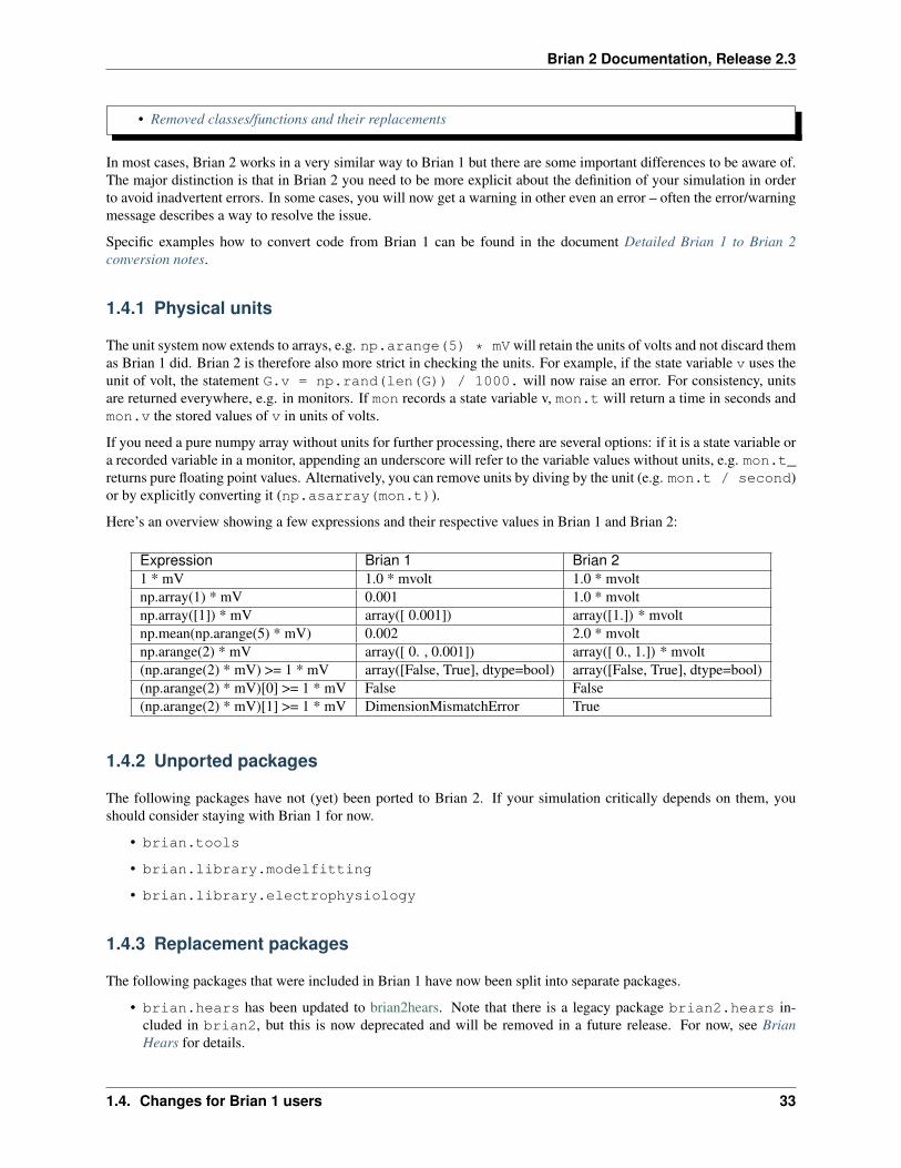
Brian 2 Documentation, Release 2.3
• Removed classes/functions and their replacements
In most cases, Brian 2 works in a very similar way to Brian 1 but there are some important differences to be aware of.The major distinction is that in Brian 2 you need to be more explicit about the definition of your simulation in orderto avoid inadvertent errors. In some cases, you will now get a warning in other even an error – often the error/warningmessage describes a way to resolve the issue.
Specific examples how to convert code from Brian 1 can be found in the document Detailed Brian 1 to Brian 2conversion notes.
1.4.1 Physical units
The unit system now extends to arrays, e.g. np.arange(5) * mVwill retain the units of volts and not discard themas Brian 1 did. Brian 2 is therefore also more strict in checking the units. For example, if the state variable v uses theunit of volt, the statement G.v = np.rand(len(G)) / 1000. will now raise an error. For consistency, unitsare returned everywhere, e.g. in monitors. If mon records a state variable v, mon.t will return a time in seconds andmon.v the stored values of v in units of volts.
If you need a pure numpy array without units for further processing, there are several options: if it is a state variable ora recorded variable in a monitor, appending an underscore will refer to the variable values without units, e.g. mon.t_returns pure floating point values. Alternatively, you can remove units by diving by the unit (e.g. mon.t / second)or by explicitly converting it (np.asarray(mon.t)).
Here’s an overview showing a few expressions and their respective values in Brian 1 and Brian 2:
Expression Brian 1 Brian 21 * mV 1.0 * mvolt 1.0 * mvoltnp.array(1) * mV 0.001 1.0 * mvoltnp.array([1]) * mV array([ 0.001]) array([1.]) * mvoltnp.mean(np.arange(5) * mV) 0.002 2.0 * mvoltnp.arange(2) * mV array([ 0. , 0.001]) array([ 0., 1.]) * mvolt(np.arange(2) * mV) >= 1 * mV array([False, True], dtype=bool) array([False, True], dtype=bool)(np.arange(2) * mV)[0] >= 1 * mV False False(np.arange(2) * mV)[1] >= 1 * mV DimensionMismatchError True
1.4.2 Unported packages
The following packages have not (yet) been ported to Brian 2. If your simulation critically depends on them, youshould consider staying with Brian 1 for now.
• brian.tools
• brian.library.modelfitting
• brian.library.electrophysiology
1.4.3 Replacement packages
The following packages that were included in Brian 1 have now been split into separate packages.
• brian.hears has been updated to brian2hears. Note that there is a legacy package brian2.hears in-cluded in brian2, but this is now deprecated and will be removed in a future release. For now, see BrianHears for details.
1.4. Changes for Brian 1 users 33

Brian 2 Documentation, Release 2.3
1.4.4 Removed classes/functions and their replacements
In Brian 2, we have tried to keep the number of classes/functions to a minimum, but make each of them flexible enoughto encompass a large number of use cases. A lot of the classes and functions that existed in Brian 1 have thereforebeen removed. The following table lists (most of) the classes that existed in Brian 1 but do no longer exist in Brian 2.You can consult it when you get a NameError while converting an existing script from Brian 1. The third columnlinks to a document with further explanation and the second column gives either:
1. the equivalent class in Brian 2 (e.g. StateMonitor can record multiple variables now and therefore replacesMultiStateMonitor);
2. the name of a Brian 2 class in square brackets (e.g. [Synapses] for STDP), this means that the class can beused as a replacement but needs some additional code (e.g. explicitly specified STDP equations). The “Moredetails” document should help you in making the necessary changes;
3. “string expression”, if the functionality of a previously existing class can be expressed using the generalstring expression framework (e.g. threshold=VariableThreshold('Vt', 'V') can be replaced bythreshold='V > Vt');
4. a link to the relevant github issue if no equivalent class/function does exist so far in Brian 2;
5. a remark such as “obsolete” if the particular class/function is no longer needed.
Brian 1 Brian 2 More detailsAdEx [Equations] Library models (Brian 1 –> 2 conversion)aEIF [Equations] Library models (Brian 1 –> 2 conversion)AERSpikeMonitor #298 Monitors (Brian 1 –> 2 conversion)alpha_conductance [Equations] Library models (Brian 1 –> 2 conversion)alpha_current [Equations] Library models (Brian 1 –> 2 conversion)alpha_synapse [Equations] Library models (Brian 1 –> 2 conversion)AutoCorrelogram [SpikeMonitor] Monitors (Brian 1 –> 2 conversion)biexpr_conductance [Equations] Library models (Brian 1 –> 2 conversion)biexpr_current [Equations] Library models (Brian 1 –> 2 conversion)biexpr_synapse [Equations] Library models (Brian 1 –> 2 conversion)Brette_Gerstner [Equations] Library models (Brian 1 –> 2 conversion)CoincidenceCounter [SpikeMonitor] Monitors (Brian 1 –> 2 conversion)CoincidenceMatrixCounter [SpikeMonitor] Monitors (Brian 1 –> 2 conversion)Compartments #443 Multicompartmental models (Brian 1 –> 2 conversion)Connection Synapses Synapses (Brian 1 –> 2 conversion)Current #443 Multicompartmental models (Brian 1 –> 2 conversion)CustomRefractoriness [string expression] Neural models (Brian 1 –> 2 conversion)DefaultClock Clock Networks and clocks (Brian 1 –> 2 conversion)EmpiricalThreshold string expression Neural models (Brian 1 –> 2 conversion)EventClock Clock Networks and clocks (Brian 1 –> 2 conversion)exp_conductance [Equations] Library models (Brian 1 –> 2 conversion)exp_current [Equations] Library models (Brian 1 –> 2 conversion)exp_IF [Equations] Library models (Brian 1 –> 2 conversion)exp_synapse [Equations] Library models (Brian 1 –> 2 conversion)FileSpikeMonitor #298 Monitors (Brian 1 –> 2 conversion)FloatClock Clock Networks and clocks (Brian 1 –> 2 conversion)FunReset [string expression] Neural models (Brian 1 –> 2 conversion)FunThreshold [string expression] Neural models (Brian 1 –> 2 conversion)hist_plot no equivalent –HomogeneousPoissonThreshold string expression Neural models (Brian 1 –> 2 conversion)
Continued on next page
34 Chapter 1. Introduction
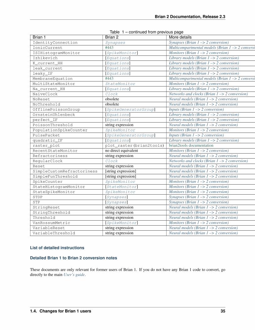
Brian 2 Documentation, Release 2.3
Table 1 – continued from previous pageBrian 1 Brian 2 More detailsIdentityConnection Synapses Synapses (Brian 1 –> 2 conversion)IonicCurrent #443 Multicompartmental models (Brian 1 –> 2 conversion)ISIHistogramMonitor [SpikeMonitor] Monitors (Brian 1 –> 2 conversion)Izhikevich [Equations] Library models (Brian 1 –> 2 conversion)K_current_HH [Equations] Library models (Brian 1 –> 2 conversion)leak_current [Equations] Library models (Brian 1 –> 2 conversion)leaky_IF [Equations] Library models (Brian 1 –> 2 conversion)MembraneEquation #443 Multicompartmental models (Brian 1 –> 2 conversion)MultiStateMonitor StateMonitor Monitors (Brian 1 –> 2 conversion)Na_current_HH [Equations] Library models (Brian 1 –> 2 conversion)NaiveClock Clock Networks and clocks (Brian 1 –> 2 conversion)NoReset obsolete Neural models (Brian 1 –> 2 conversion)NoThreshold obsolete Neural models (Brian 1 –> 2 conversion)OfflinePoissonGroup [SpikeGeneratorGroup] Inputs (Brian 1 –> 2 conversion)OrnsteinUhlenbeck [Equations] Library models (Brian 1 –> 2 conversion)perfect_IF [Equations] Library models (Brian 1 –> 2 conversion)PoissonThreshold string expression Neural models (Brian 1 –> 2 conversion)PopulationSpikeCounter SpikeMonitor Monitors (Brian 1 –> 2 conversion)PulsePacket [SpikeGeneratorGroup] Inputs (Brian 1 –> 2 conversion)quadratic_IF [Equations] Library models (Brian 1 –> 2 conversion)raster_plot plot_raster (brian2tools) brian2tools documentationRecentStateMonitor no direct equivalent Monitors (Brian 1 –> 2 conversion)Refractoriness string expression Neural models (Brian 1 –> 2 conversion)RegularClock Clock Networks and clocks (Brian 1 –> 2 conversion)Reset string expression Neural models (Brian 1 –> 2 conversion)SimpleCustomRefractoriness [string expression] Neural models (Brian 1 –> 2 conversion)SimpleFunThreshold [string expression] Neural models (Brian 1 –> 2 conversion)SpikeCounter SpikeMonitor Monitors (Brian 1 –> 2 conversion)StateHistogramMonitor [StateMonitor] Monitors (Brian 1 –> 2 conversion)StateSpikeMonitor SpikeMonitor Monitors (Brian 1 –> 2 conversion)STDP [Synapses] Synapses (Brian 1 –> 2 conversion)STP [Synapses] Synapses (Brian 1 –> 2 conversion)StringReset string expression Neural models (Brian 1 –> 2 conversion)StringThreshold string expression Neural models (Brian 1 –> 2 conversion)Threshold string expression Neural models (Brian 1 –> 2 conversion)VanRossumMetric [SpikeMonitor] Monitors (Brian 1 –> 2 conversion)VariableReset string expression Neural models (Brian 1 –> 2 conversion)VariableThreshold string expression Neural models (Brian 1 –> 2 conversion)
List of detailed instructions
Detailed Brian 1 to Brian 2 conversion notes
These documents are only relevant for former users of Brian 1. If you do not have any Brian 1 code to convert, godirectly to the main User’s guide.
1.4. Changes for Brian 1 users 35
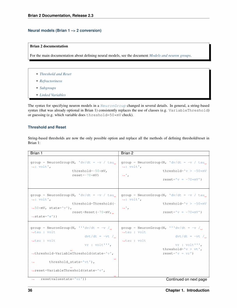
Brian 2 Documentation, Release 2.3
Neural models (Brian 1 –> 2 conversion)
Brian 2 documentation
For the main documentation about defining neural models, see the document Models and neuron groups.
• Threshold and Reset
• Refractoriness
• Subgroups
• Linked Variables
The syntax for specifying neuron models in a NeuronGroup changed in several details. In general, a string-basedsyntax (that was already optional in Brian 1) consistently replaces the use of classes (e.g. VariableThreshold)or guessing (e.g. which variable does threshold=50*mV check).
Threshold and Reset
String-based thresholds are now the only possible option and replace all the methods of defining threshold/reset inBrian 1:
Brian 1 Brian 2
group = NeuronGroup(N, 'dv/dt = -v / tau→˓: volt',
threshold=-50*mV,reset=-70*mV)
group = NeuronGroup(N, 'dv/dt = -v / tau→˓: volt',
threshold='v > -50*mV→˓',
reset='v = -70*mV')
group = NeuronGroup(N, 'dv/dt = -v / tau→˓: volt',
threshold=Threshold(-→˓50*mV, state='v'),
reset=Reset(-70*mV,→˓state='w'))
group = NeuronGroup(N, 'dv/dt = -v / tau→˓: volt',
threshold='v > -50*mV→˓',
reset='v = -70*mV')
group = NeuronGroup(N, '''dv/dt = -v /→˓tau : volt
dvt/dt = -vt /→˓tau : volt
vr : volt''',
→˓threshold=VariableThreshold(state='v',
→˓ threshold_state='vt'),
→˓reset=VariableThreshold(state='v',
→˓ resetvaluestate='vr'))
group = NeuronGroup(N, '''dv/dt = -v /→˓tau : volt
dvt/dt = -vt /→˓tau : volt
vr : volt''',threshold='v > vt',reset='v = vr')
Continued on next page
36 Chapter 1. Introduction

Brian 2 Documentation, Release 2.3
Table 2 – continued from previous pageBrian 1 Brian 2
group = NeuronGroup(N, 'rate : Hz',
→˓threshold=PoissonThreshold(state='rate→˓'))
group = NeuronGroup(N, 'rate : Hz',threshold='rand()
→˓<rate*dt')
There’s no direct equivalent for the “functional threshold/reset” mechanism from Brian 1. In simple cases, they canbe implemented using the general string expression/statement mechanism (note that in Brian 1, reset=myreset isequivalent to reset=FunReset(myreset)):
Brian 1 Brian 2
def myreset(P,spikes):P.v_[spikes] = -
→˓70*mV+rand(len(spikes))*5*mV
group = NeuronGroup(N, 'dv/dt = -v / tau→˓: volt',
threshold=-50*mV,reset=myreset)
group = NeuronGroup(N, 'dv/dt = -v / tau→˓: volt',
threshold='v > -50*mV→˓',
reset='-70*mV +→˓rand()*5*mV')
def mythreshold(v):return (v > -50*mV) & (rand(N) > 0.5)
group = NeuronGroup(N, 'dv/dt = -v / tau→˓: volt',
→˓threshold=SimpleFunThreshold(mythreshold,→˓
→˓ state='v'),reset=-70*mV)
group = NeuronGroup(N, 'dv/dt = -v / tau→˓: volt',
threshold='v > -→˓50*mV and rand() > 0.5',
reset='v = -70*mV')
For more complicated cases, you can use the general mechanism for User-provided functions that Brian 2 provides.The only caveat is that you’d have to provide an implementation of the function in the code generation target languagewhich is by default C++ or Cython. However, in the default Runtime code generation mode, you can chose differentcode generation targets for different parts of your simulation. You can thus switch the code generation target for thethreshold/reset mechanism to numpy while leaving the default target for the rest of the simulation in place. The detailsof this process and the correct definition of the functions (e.g. global_reset needs a “dummy” return value) aresomewhat cumbersome at the moment and we plan to make them more straightforward in the future. Also note that ifyou use this kind of mechanism extensively, you’ll lose all the performance advantage that Brian 2’s code generationmechanism provides (in addition to not being able to use Standalone code generation mode at all).
1.4. Changes for Brian 1 users 37

Brian 2 Documentation, Release 2.3
Brian 1 Brian 2
def single_threshold(v):# Only let a single neuron spikecrossed_threshold = np.nonzero(v > -
→˓50*mV)[0]should_spike = np.zeros(len(P),
→˓dtype=np.bool)if len(crossed_threshold):
choose = np.random.→˓randint(len(crossed_threshold))
should_spike[crossed_→˓threshold[choose]] = True
return should_spike
def global_reset(P, spikes):# Reset everythingif len(spikes):
P.v_[:] = -70*mV
neurons = NeuronGroup(N, 'dv/dt = -v /→˓tau : volt',
→˓threshold=SimpleFunThreshold(single_→˓threshold,
→˓ state='v'),reset=global_reset)
@check_units(v=volt, result=bool)def single_threshold(v):
pass # ... (identical to Brian 1)
@check_units(spikes=1, result=1)def global_reset(spikes):
# Reset everythingif len(spikes):
neurons.v_[:] = -0.070
neurons = NeuronGroup(N, 'dv/dt = -v /→˓tau : volt',
threshold='single_→˓threshold(v)',
reset='dummy =→˓global_reset(i)')# Set the code generation target for→˓threshold/reset only:neuron.thresholder['spike'].codeobj_→˓class = NumpyCodeObjectneuron.resetter['spike'].codeobj_class =→˓NumpyCodeObject
For an example how to translate EmpiricalThreshold, see the section on “Refractoriness” below.
Refractoriness
For a detailed description of Brian 2’s refractoriness mechanism see Refractoriness.
In Brian 1, refractoriness was tightly linked with the reset mechanism and some combinations of refractoriness andreset were not allowed. The standard refractory mechanism had two effects during the refractoriness: it preventedthe refractory cell from spiking and it clamped a state variable (normally the membrane potential of the cell). InBrian 2, refractoriness is independent of reset and the two effects are specified separately: the refractory keywordspecifies the time (or an expression evaluating to a time) during which the cell does not spike, and the (unlessrefractory) flag marks one or more variables to be clamped during the refractory period. To correctly translatethe standard refractory mechanism from Brian 1, you’ll therefore need to specify both:
Brian 1 Brian 2
group = NeuronGroup(N, 'dv/dt = (I - v)/→˓tau : volt',
threshold=-50*mV,reset=-70*mV,refractory=3*ms)
group = NeuronGroup(N, 'dv/dt = (I - v)/→˓tau : volt (unless refractory)',
threshold='v > -50*mV→˓',
reset='v = -70*mV',refractory=3*ms)
38 Chapter 1. Introduction
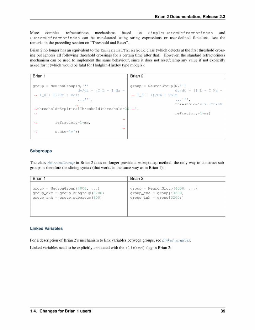
Brian 2 Documentation, Release 2.3
More complex refractoriness mechanisms based on SimpleCustomRefractoriness andCustomRefractoriness can be translatated using string expressions or user-defined functions, see theremarks in the preceding section on “Threshold and Reset”.
Brian 2 no longer has an equivalent to the EmpiricalThreshold class (which detects at the first threshold cross-ing but ignores all following threshold crossings for a certain time after that). However, the standard refractorinessmechanism can be used to implement the same behaviour, since it does not reset/clamp any value if not explicitlyasked for it (which would be fatal for Hodgkin-Huxley type models):
Brian 1 Brian 2
group = NeuronGroup(N,'''dv/dt = (I_L - I_Na -
→˓ I_K + I)/Cm : volt...''',
→˓threshold=EmpiricalThreshold(threshold=20*mV,→˓
→˓ refractory=1*ms,
→˓ state='v'))
group = NeuronGroup(N,'''dv/dt = (I_L - I_Na -
→˓ I_K + I)/Cm : volt...''',threshold='v > -20*mV
→˓',refractory=1*ms)
Subgroups
The class NeuronGroup in Brian 2 does no longer provide a subgroup method, the only way to construct sub-groups is therefore the slicing syntax (that works in the same way as in Brian 1):
Brian 1 Brian 2
group = NeuronGroup(4000, ...)group_exc = group.subgroup(3200)group_inh = group.subgroup(800)
group = NeuronGroup(4000, ...)group_exc = group[:3200]group_inh = group[3200:]
Linked Variables
For a description of Brian 2’s mechanism to link variables between groups, see Linked variables.
Linked variables need to be explicitly annotated with the (linked) flag in Brian 2:
1.4. Changes for Brian 1 users 39
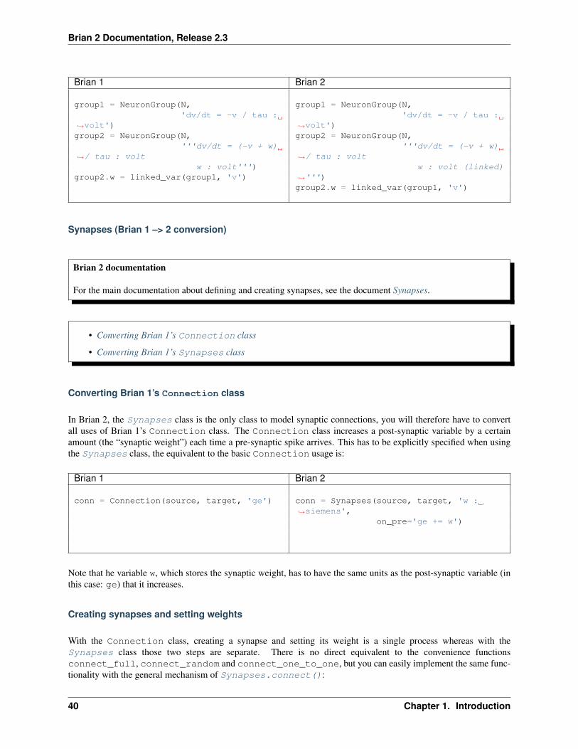
Brian 2 Documentation, Release 2.3
Brian 1 Brian 2
group1 = NeuronGroup(N,'dv/dt = -v / tau :
→˓volt')group2 = NeuronGroup(N,
'''dv/dt = (-v + w)→˓/ tau : volt
w : volt''')group2.w = linked_var(group1, 'v')
group1 = NeuronGroup(N,'dv/dt = -v / tau :
→˓volt')group2 = NeuronGroup(N,
'''dv/dt = (-v + w)→˓/ tau : volt
w : volt (linked)→˓''')group2.w = linked_var(group1, 'v')
Synapses (Brian 1 –> 2 conversion)
Brian 2 documentation
For the main documentation about defining and creating synapses, see the document Synapses.
• Converting Brian 1’s Connection class
• Converting Brian 1’s Synapses class
Converting Brian 1’s Connection class
In Brian 2, the Synapses class is the only class to model synaptic connections, you will therefore have to convertall uses of Brian 1’s Connection class. The Connection class increases a post-synaptic variable by a certainamount (the “synaptic weight”) each time a pre-synaptic spike arrives. This has to be explicitly specified when usingthe Synapses class, the equivalent to the basic Connection usage is:
Brian 1 Brian 2
conn = Connection(source, target, 'ge') conn = Synapses(source, target, 'w :→˓siemens',
on_pre='ge += w')
Note that he variable w, which stores the synaptic weight, has to have the same units as the post-synaptic variable (inthis case: ge) that it increases.
Creating synapses and setting weights
With the Connection class, creating a synapse and setting its weight is a single process whereas with theSynapses class those two steps are separate. There is no direct equivalent to the convenience functionsconnect_full, connect_random and connect_one_to_one, but you can easily implement the same func-tionality with the general mechanism of Synapses.connect():
40 Chapter 1. Introduction

Brian 2 Documentation, Release 2.3
Brian 1 Brian 2
conn1 = Connection(source, target, 'ge')conn1[3, 5] = 3*nS
conn1 = Synapses(source, target, 'w:→˓siemens',
on_pre='ge += w')conn1.connect(i=3, j=5)conn1.w[3, 5] = 3*nS # (or conn1.w =→˓3*nS)
conn2 = Connection(source, target, 'ge')conn2.connect_full(source, target, 5*nS)
conn2 = ... # see aboveconn2.connect()conn2.w = 5*nS
conn3 = Connection(source, target, 'ge')conn3.connect_random(source, target,
sparseness=0.02,weight=2*ns)
conn3 = ... # see aboveconn3.connect(p=0.02)conn3.w = 2*nS
conn4 = Connection(source, target, 'ge')conn4.connect_one_to_one(source, target,
weight=4*nS)
conn4 = ... # see aboveconn4.connect(j='i')conn4.w = 4*nS
conn5 = IdentityConnection(source,→˓target,
weight=3*nS)
conn5 = Synapses(source, target,'w : siemens (shared)')
conn5.w = 3*nS
Weight matrices
Brian 2’s Synapses class does not support setting the weights of a neuron with a weight matrix. However,Synapses.connect() creates the synapses in a predictable order (first all synapses for the first pre-synapticcell, then all synapses for the second pre-synaptic cell, etc.), so a reshaped “flat” weight matrix can be used:
1.4. Changes for Brian 1 users 41

Brian 2 Documentation, Release 2.3
Brian 1 Brian 2
# len(source) == 20, len(target) == 30conn6 = Connection(source, target, 'ge')W = rand(20, 30)*nSconn6.connect(source, target, weight=W)
# len(source) == 20, len(target) == 30conn6 = Synapses(source, target, 'w:→˓siemens',
on_pre='ge += w')W = rand(20, 30)*nSconn6.connect()conn6.w = W.flatten()
However note that if your weight matrix can be described mathematically (e.g. random as in the example above),then you should not create a weight matrix in the first place but use Brian 2’s mechanism to set variables based onmathematical expressions (in the above case: conn5.w = 'rand()'). Especially for big connection matrices thiswill have better performance, since it will be executed in generated code. You should only resort to explicit weightmatrices when there is no alternative (e.g. to load weights from previous simulations).
In Brian 1, you can restrict the functions connect, connect_random, etc. to subgroups. Again, there is no directequivalent to this in Brian 2, but the general string syntax allows you to make connections conditional on logicalstatements that refer to pre-/post-synaptic indices and can therefore also used to restrict the connection to a subgroupof cells. When you set the synaptic weights, you can however use subgroups to restrict the subset of weights you wantto set.
Brian 1 Brian 2
conn7 = Connection(source, target, 'ge')conn7.connect_full(source[:5],→˓target[5:10], 5*nS)
conn7 = Synapses(source, target, 'w:→˓siemens',
on_pre='ge += w')conn7.connect('i < 5 and j >=5 and j <10→˓')# Alternative (more efficient):# conn7.connect(j='k in range(5, 10) if→˓i < 5')conn7.w[source[:5], target[5:10]] = 5*nS
Connections defined by functions
Brian 1 allowed you to pass in a function as the value for the weight argument in a connect call (and also forthe sparseness argument in connect_random). You should be able to replace such use cases by the the general,string-expression based method:
42 Chapter 1. Introduction
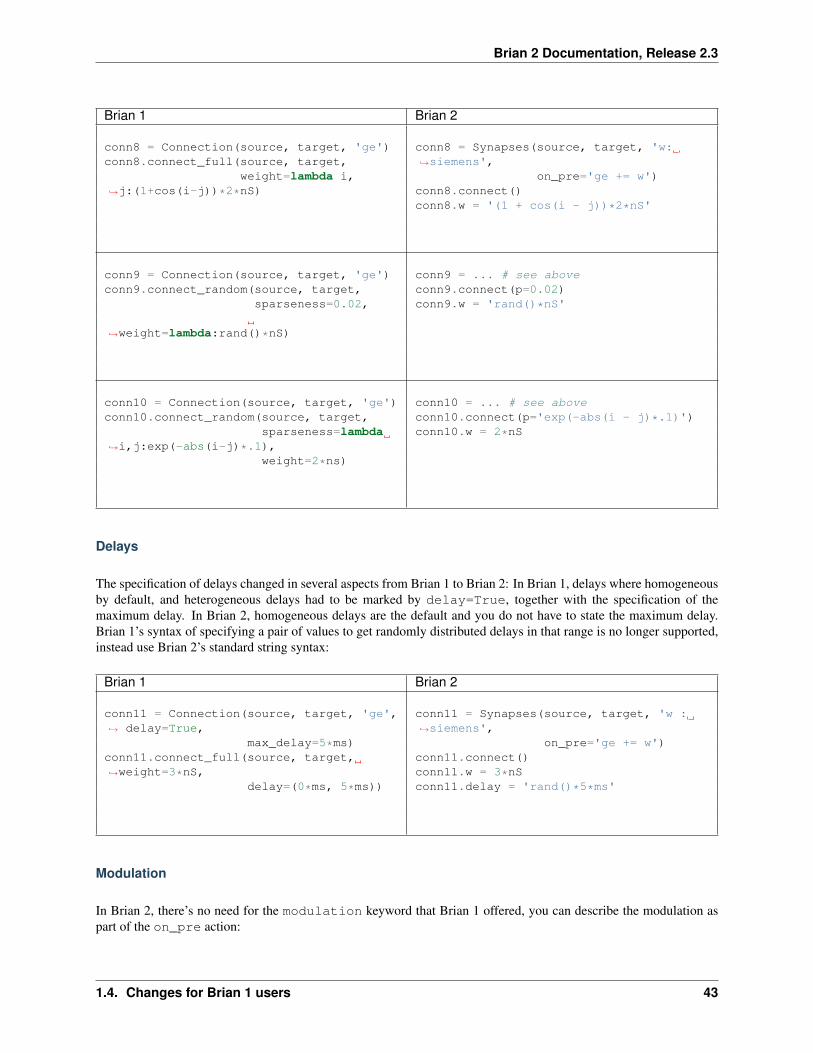
Brian 2 Documentation, Release 2.3
Brian 1 Brian 2
conn8 = Connection(source, target, 'ge')conn8.connect_full(source, target,
weight=lambda i,→˓j:(1+cos(i-j))*2*nS)
conn8 = Synapses(source, target, 'w:→˓siemens',
on_pre='ge += w')conn8.connect()conn8.w = '(1 + cos(i - j))*2*nS'
conn9 = Connection(source, target, 'ge')conn9.connect_random(source, target,
sparseness=0.02,
→˓weight=lambda:rand()*nS)
conn9 = ... # see aboveconn9.connect(p=0.02)conn9.w = 'rand()*nS'
conn10 = Connection(source, target, 'ge')conn10.connect_random(source, target,
sparseness=lambda→˓i,j:exp(-abs(i-j)*.1),
weight=2*ns)
conn10 = ... # see aboveconn10.connect(p='exp(-abs(i - j)*.1)')conn10.w = 2*nS
Delays
The specification of delays changed in several aspects from Brian 1 to Brian 2: In Brian 1, delays where homogeneousby default, and heterogeneous delays had to be marked by delay=True, together with the specification of themaximum delay. In Brian 2, homogeneous delays are the default and you do not have to state the maximum delay.Brian 1’s syntax of specifying a pair of values to get randomly distributed delays in that range is no longer supported,instead use Brian 2’s standard string syntax:
Brian 1 Brian 2
conn11 = Connection(source, target, 'ge',→˓ delay=True,
max_delay=5*ms)conn11.connect_full(source, target,→˓weight=3*nS,
delay=(0*ms, 5*ms))
conn11 = Synapses(source, target, 'w :→˓siemens',
on_pre='ge += w')conn11.connect()conn11.w = 3*nSconn11.delay = 'rand()*5*ms'
Modulation
In Brian 2, there’s no need for the modulation keyword that Brian 1 offered, you can describe the modulation aspart of the on_pre action:
1.4. Changes for Brian 1 users 43
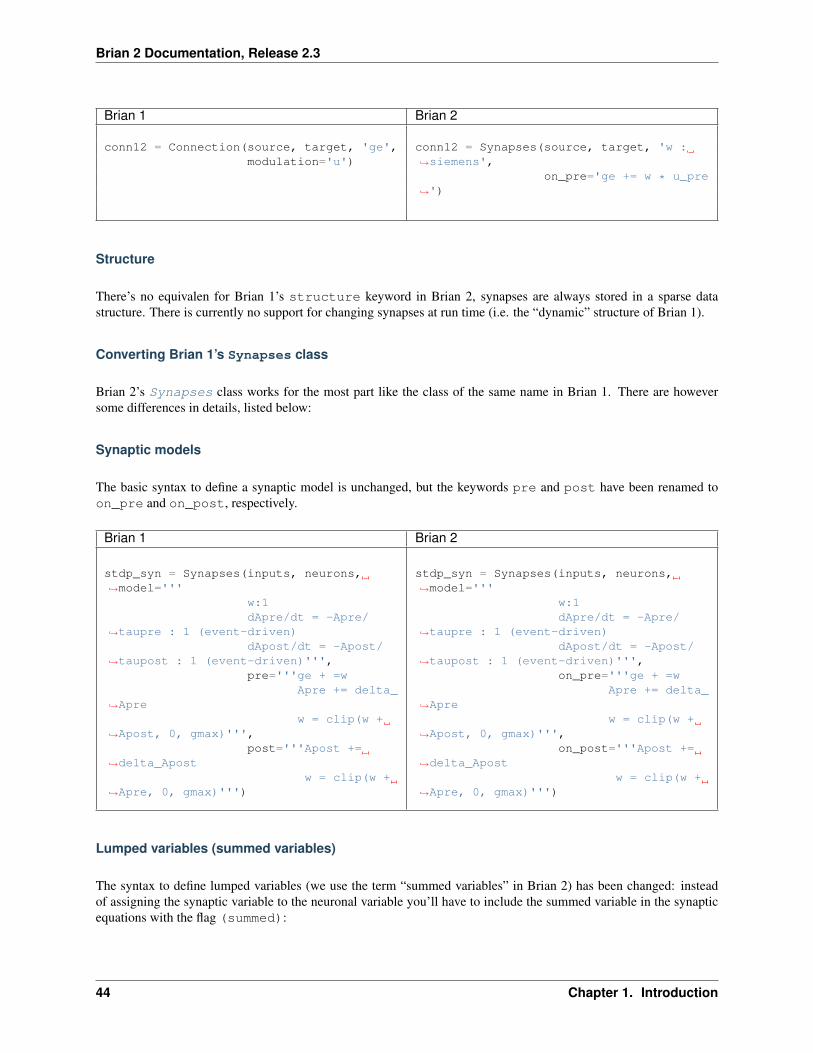
Brian 2 Documentation, Release 2.3
Brian 1 Brian 2
conn12 = Connection(source, target, 'ge',modulation='u')
conn12 = Synapses(source, target, 'w :→˓siemens',
on_pre='ge += w * u_pre→˓')
Structure
There’s no equivalen for Brian 1’s structure keyword in Brian 2, synapses are always stored in a sparse datastructure. There is currently no support for changing synapses at run time (i.e. the “dynamic” structure of Brian 1).
Converting Brian 1’s Synapses class
Brian 2’s Synapses class works for the most part like the class of the same name in Brian 1. There are howeversome differences in details, listed below:
Synaptic models
The basic syntax to define a synaptic model is unchanged, but the keywords pre and post have been renamed toon_pre and on_post, respectively.
Brian 1 Brian 2
stdp_syn = Synapses(inputs, neurons,→˓model='''
w:1dApre/dt = -Apre/
→˓taupre : 1 (event-driven)dApost/dt = -Apost/
→˓taupost : 1 (event-driven)''',pre='''ge + =w
Apre += delta_→˓Apre
w = clip(w +→˓Apost, 0, gmax)''',
post='''Apost +=→˓delta_Apost
w = clip(w +→˓Apre, 0, gmax)''')
stdp_syn = Synapses(inputs, neurons,→˓model='''
w:1dApre/dt = -Apre/
→˓taupre : 1 (event-driven)dApost/dt = -Apost/
→˓taupost : 1 (event-driven)''',on_pre='''ge + =w
Apre += delta_→˓Apre
w = clip(w +→˓Apost, 0, gmax)''',
on_post='''Apost +=→˓delta_Apost
w = clip(w +→˓Apre, 0, gmax)''')
Lumped variables (summed variables)
The syntax to define lumped variables (we use the term “summed variables” in Brian 2) has been changed: insteadof assigning the synaptic variable to the neuronal variable you’ll have to include the summed variable in the synapticequations with the flag (summed):
44 Chapter 1. Introduction
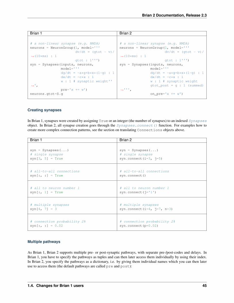
Brian 2 Documentation, Release 2.3
Brian 1 Brian 2
# a non-linear synapse (e.g. NMDA)neurons = NeuronGroup(1, model='''
dv/dt = (gtot - v)/→˓(10*ms) : 1
gtot : 1''')syn = Synapses(inputs, neurons,
model='''dg/dt = -a*g+b*x*(1-g) : 1dx/dt = -c*x : 1w : 1 # synaptic weight''
→˓',pre='x += w')
neurons.gtot=S.g
# a non-linear synapse (e.g. NMDA)neurons = NeuronGroup(1, model='''
dv/dt = (gtot - v)/→˓(10*ms) : 1
gtot : 1''')syn = Synapses(inputs, neurons,
model='''dg/dt = -a*g+b*x*(1-g) : 1dx/dt = -c*x : 1w : 1 # synaptic weightgtot_post = g : 1 (summed)
→˓''',on_pre='x += w')
Creating synapses
In Brian 1, synapses were created by assigning True or an integer (the number of synapses) to an indexed Synapsesobject. In Brian 2, all synapse creation goes through the Synapses.connect() function. For examples how tocreate more complex connection patterns, see the section on translating Connections objects above.
Brian 1 Brian 2
syn = Synapses(...)# single synapsesyn[3, 5] = True
syn = Synapses(...)# single synapsesyn.connect(i=3, j=5)
# all-to-all connectionssyn[:, :] = True
# all-to-all connectionssyn.connect()
# all to neuron number 1syn[:, 1] = True
# all to neuron number 1syn.connect(j='1')
# multiple synapsessyn[4, 7] = 3
# multiple synapsessyn.connect(i=4, j=7, n=3)
# connection probability 2%syn[:, :] = 0.02
# connection probability 2%syn.connect(p=0.02)
Multiple pathways
As Brian 1, Brian 2 supports multiple pre- or post-synaptic pathways, with separate pre-/post-codes and delays. InBrian 1, you have to specify the pathways as tuples and can then later access them individually by using their index.In Brian 2, you specify the pathways as a dictionary, i.e. by giving them individual names which you can then lateruse to access them (the default pathways are called pre and post):
1.4. Changes for Brian 1 users 45
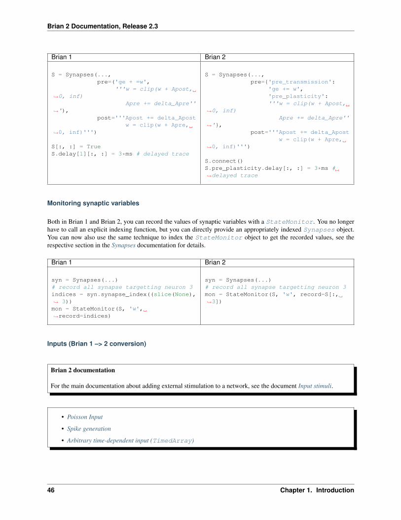
Brian 2 Documentation, Release 2.3
Brian 1 Brian 2
S = Synapses(...,pre=('ge + =w',
'''w = clip(w + Apost,→˓0, inf)
Apre += delta_Apre''→˓'),
post='''Apost += delta_Apostw = clip(w + Apre,
→˓0, inf)''')
S[:, :] = TrueS.delay[1][:, :] = 3*ms # delayed trace
S = Synapses(...,pre={'pre_transmission':
'ge += w','pre_plasticity':'''w = clip(w + Apost,
→˓0, inf)Apre += delta_Apre''
→˓'},post='''Apost += delta_Apost
w = clip(w + Apre,→˓0, inf)''')
S.connect()S.pre_plasticity.delay[:, :] = 3*ms #→˓delayed trace
Monitoring synaptic variables
Both in Brian 1 and Brian 2, you can record the values of synaptic variables with a StateMonitor. You no longerhave to call an explicit indexing function, but you can directly provide an appropriately indexed Synapses object.You can now also use the same technique to index the StateMonitor object to get the recorded values, see therespective section in the Synapses documentation for details.
Brian 1 Brian 2
syn = Synapses(...)# record all synapse targetting neuron 3indices = syn.synapse_index((slice(None),→˓ 3))mon = StateMonitor(S, 'w',→˓record=indices)
syn = Synapses(...)# record all synapse targetting neuron 3mon = StateMonitor(S, 'w', record=S[:,→˓3])
Inputs (Brian 1 –> 2 conversion)
Brian 2 documentation
For the main documentation about adding external stimulation to a network, see the document Input stimuli.
• Poisson Input
• Spike generation
• Arbitrary time-dependent input (TimedArray)
46 Chapter 1. Introduction

Brian 2 Documentation, Release 2.3
Poisson Input
Brian 2 provides the same two groups that Brian 1 provided: PoissonGroup and PoissonInput. The mechanismfor inhomogoneous Poisson processes has changed: instead of providing a Python function of time, you’ll now haveto provide a string expression that is evaluated at every time step. For most use cases, this should allow a directtranslation:
Brian 1 Brian 2
rates = lambda→˓t:(1+cos(2*pi*t*1*Hz))*10*Hzgroup = PoissonGroup(100, rates=rates)
rates = '(1 + cos(2*pi*t*1*Hz)*10*Hz)'group = PoissonGroup(100, rates=rates)
For more complex rate modulations, the expression can refer to User-provided functions and/or you can replace thePoissonGroup by a general NeuronGroup with a threshold condition rand()<rates*dt (which allows youto store per-neuron attributes).
There is currently no direct replacement for the more advanced features of PoissonInput (record, freeze,copies, jitter, and reliability keywords), but various workarounds are possible, e.g. by directly usinga BinomialFunction in the equations. For example, you can get the functionality of the freeze keyword(identical Poisson events for all neurons) by storing the input in a shared variable and then distribute the input to allneurons:
Brian 1 Brian 2
group = NeuronGroup(10,'dv/dt = -v/(10*ms)
→˓: 1')input = PoissonInput(group, N=1000,→˓rate=1*Hz,
weight=0.1, state='v→˓',
freeze=True)
group = NeuronGroup(10, '''dv/dt = -v /→˓(10*ms) : 1
shared_input→˓: 1 (shared)''')poisson_input = BinomialFunction(n=1000,→˓p=1*Hz*group.dt)group.run_regularly('''shared_input =→˓poisson_input()*0.1
v += shared_input'→˓'')
Spike generation
SpikeGeneratorGroup provides mostly the same functionality as in Brian 1. In contrast to Brian 1, there is onlyone way to specify which neurons spike and when – you have to provide the index array and the times array as separatearguments:
1.4. Changes for Brian 1 users 47
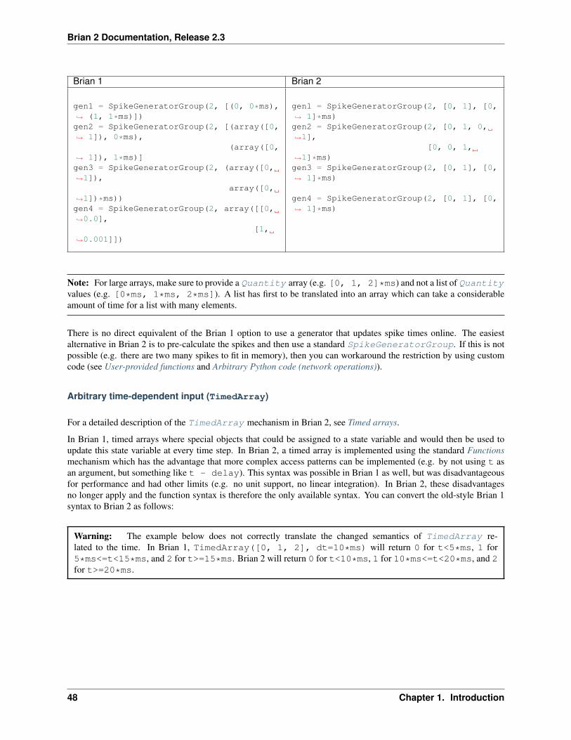
Brian 2 Documentation, Release 2.3
Brian 1 Brian 2
gen1 = SpikeGeneratorGroup(2, [(0, 0*ms),→˓ (1, 1*ms)])gen2 = SpikeGeneratorGroup(2, [(array([0,→˓ 1]), 0*ms),
(array([0,→˓ 1]), 1*ms)]gen3 = SpikeGeneratorGroup(2, (array([0,→˓1]),
array([0,→˓1])*ms))gen4 = SpikeGeneratorGroup(2, array([[0,→˓0.0],
[1,→˓0.001]])
gen1 = SpikeGeneratorGroup(2, [0, 1], [0,→˓ 1]*ms)gen2 = SpikeGeneratorGroup(2, [0, 1, 0,→˓1],
[0, 0, 1,→˓1]*ms)gen3 = SpikeGeneratorGroup(2, [0, 1], [0,→˓ 1]*ms)
gen4 = SpikeGeneratorGroup(2, [0, 1], [0,→˓ 1]*ms)
Note: For large arrays, make sure to provide a Quantity array (e.g. [0, 1, 2]*ms) and not a list of Quantityvalues (e.g. [0*ms, 1*ms, 2*ms]). A list has first to be translated into an array which can take a considerableamount of time for a list with many elements.
There is no direct equivalent of the Brian 1 option to use a generator that updates spike times online. The easiestalternative in Brian 2 is to pre-calculate the spikes and then use a standard SpikeGeneratorGroup. If this is notpossible (e.g. there are two many spikes to fit in memory), then you can workaround the restriction by using customcode (see User-provided functions and Arbitrary Python code (network operations)).
Arbitrary time-dependent input (TimedArray)
For a detailed description of the TimedArray mechanism in Brian 2, see Timed arrays.
In Brian 1, timed arrays where special objects that could be assigned to a state variable and would then be used toupdate this state variable at every time step. In Brian 2, a timed array is implemented using the standard Functionsmechanism which has the advantage that more complex access patterns can be implemented (e.g. by not using t asan argument, but something like t - delay). This syntax was possible in Brian 1 as well, but was disadvantageousfor performance and had other limits (e.g. no unit support, no linear integration). In Brian 2, these disadvantagesno longer apply and the function syntax is therefore the only available syntax. You can convert the old-style Brian 1syntax to Brian 2 as follows:
Warning: The example below does not correctly translate the changed semantics of TimedArray re-lated to the time. In Brian 1, TimedArray([0, 1, 2], dt=10*ms) will return 0 for t<5*ms, 1 for5*ms<=t<15*ms, and 2 for t>=15*ms. Brian 2 will return 0 for t<10*ms, 1 for 10*ms<=t<20*ms, and 2for t>=20*ms.
48 Chapter 1. Introduction

Brian 2 Documentation, Release 2.3
Brian 1 Brian 2
# same input for all neuronseqs = '''
dv/dt = (I - v)/tau : voltI : volt'''
group = NeuronGroup(1, model=eqs,reset=0*mV,
→˓threshold=15*mV)group.I = TimedArray(linspace(0*mV,→˓20*mV, 100),
dt=10*ms)
# same input for all neuronsI = TimedArray(linspace(0*mV, 20*mV,→˓100),
dt=10*ms)eqs = '''
dv/dt = (I(t) - v)/tau : volt'''
group = NeuronGroup(1, model=eqs,reset='v = 0*mV',threshold='v > 15*mV
→˓')
# neuron-specific inputeqs = '''
dv/dt = (I - v)/tau : voltI : volt'''
group = NeuronGroup(5, model=eqs,reset=0*mV,
→˓threshold=15*mV)values = (linspace(0*mV, 20*mV, 100)[:,→˓None] *
linspace(0, 1, 5))group.I = TimedArray(values, dt=10*ms)
# neuron-specific inputvalues = (linspace(0*mV, 20*mV, 100)[:,→˓None] *
linspace(0, 1, 5))I = TimedArray(values, dt=10*ms)eqs = '''
dv/dt = (I(t, i) - v)/tau : volt'''
group = NeuronGroup(5, model=eqs,reset='v = 0*mV',threshold='v > 15*mV
→˓')
Monitors (Brian 1 –> 2 conversion)
Brian 2 documentation
For the main documentation about recording network activity, see the document Recording during a simulation.
• Monitoring spiking activity
• Monitoring variables
Monitoring spiking activity
The main class to record spiking activity is SpikeMonitor which is created in the same way as in Brian 1. However,the internal storage and retrieval of spikes is different. In Brian 1, spikes were stored as a list of pairs (i, t), theindex and time of each spike. In Brian 2, spikes are stored as two arrays i and t, storing the indices and times. Youcan access these arrays as attributes of the monitor, there’s also a convenience attribute it that returns both at thesame time. The following table shows how the spike indices and times can be retrieved in various forms in Brian 1and Brian 2:
1.4. Changes for Brian 1 users 49
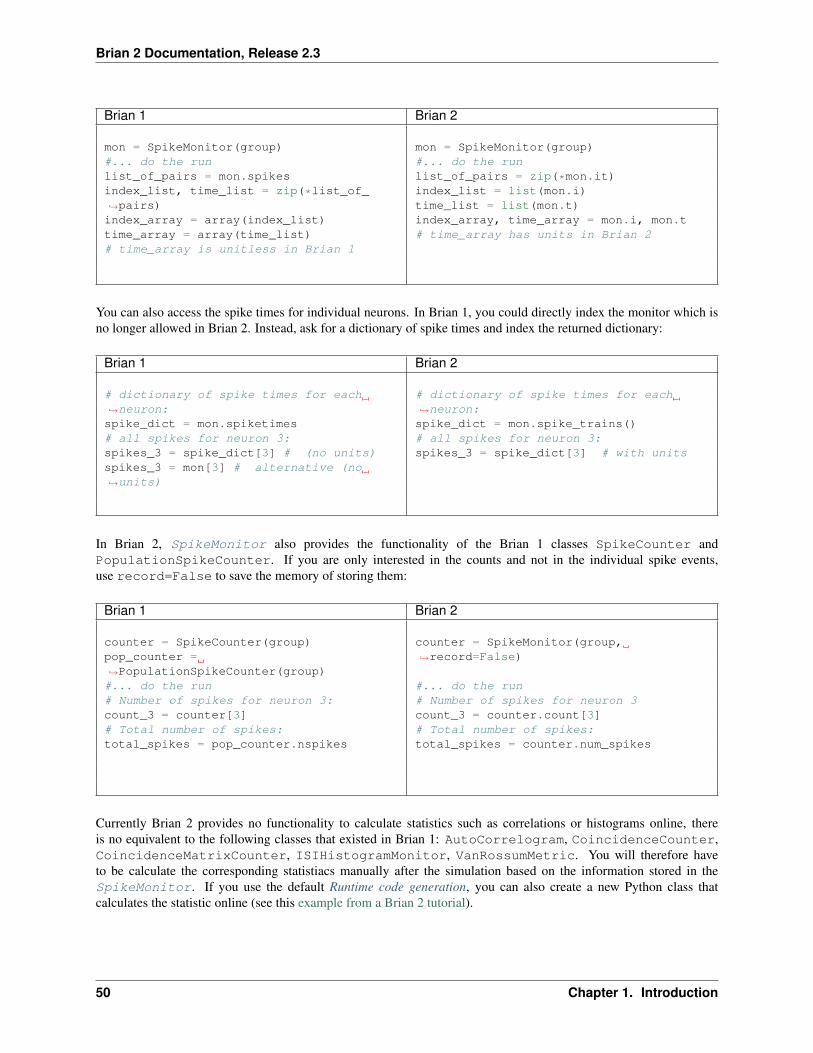
Brian 2 Documentation, Release 2.3
Brian 1 Brian 2
mon = SpikeMonitor(group)#... do the runlist_of_pairs = mon.spikesindex_list, time_list = zip(*list_of_→˓pairs)index_array = array(index_list)time_array = array(time_list)# time_array is unitless in Brian 1
mon = SpikeMonitor(group)#... do the runlist_of_pairs = zip(*mon.it)index_list = list(mon.i)time_list = list(mon.t)index_array, time_array = mon.i, mon.t# time_array has units in Brian 2
You can also access the spike times for individual neurons. In Brian 1, you could directly index the monitor which isno longer allowed in Brian 2. Instead, ask for a dictionary of spike times and index the returned dictionary:
Brian 1 Brian 2
# dictionary of spike times for each→˓neuron:spike_dict = mon.spiketimes# all spikes for neuron 3:spikes_3 = spike_dict[3] # (no units)spikes_3 = mon[3] # alternative (no→˓units)
# dictionary of spike times for each→˓neuron:spike_dict = mon.spike_trains()# all spikes for neuron 3:spikes_3 = spike_dict[3] # with units
In Brian 2, SpikeMonitor also provides the functionality of the Brian 1 classes SpikeCounter andPopulationSpikeCounter. If you are only interested in the counts and not in the individual spike events,use record=False to save the memory of storing them:
Brian 1 Brian 2
counter = SpikeCounter(group)pop_counter =→˓PopulationSpikeCounter(group)#... do the run# Number of spikes for neuron 3:count_3 = counter[3]# Total number of spikes:total_spikes = pop_counter.nspikes
counter = SpikeMonitor(group,→˓record=False)
#... do the run# Number of spikes for neuron 3count_3 = counter.count[3]# Total number of spikes:total_spikes = counter.num_spikes
Currently Brian 2 provides no functionality to calculate statistics such as correlations or histograms online, thereis no equivalent to the following classes that existed in Brian 1: AutoCorrelogram, CoincidenceCounter,CoincidenceMatrixCounter, ISIHistogramMonitor, VanRossumMetric. You will therefore haveto be calculate the corresponding statistiacs manually after the simulation based on the information stored in theSpikeMonitor. If you use the default Runtime code generation, you can also create a new Python class thatcalculates the statistic online (see this example from a Brian 2 tutorial).
50 Chapter 1. Introduction
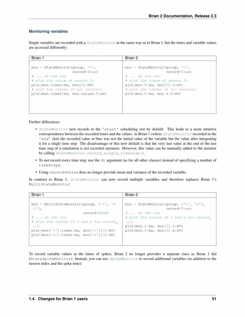
Brian 2 Documentation, Release 2.3
Monitoring variables
Single variables are recorded with a StateMonitor in the same way as in Brian 1, but the times and variable valuesare accessed differently:
Brian 1 Brian 2
mon = StateMonitor(group, 'v',record=True)
# ... do the run# plot the trace of neuron 3:plot(mon.times/ms, mon[3]/mV)# plot the traces of all neurons:plot(mon.times/ms, mon.values.T/mV)
mon = StateMonitor(group, 'v',record=True)
# ... do the run# plot the trace of neuron 3:plot(mon.t/ms, mon[3].v/mV)# plot the traces of all neurons:plot(mon.t/ms, mon.v.T/mV)
Further differences:
• StateMonitor now records in the 'start' scheduling slot by default. This leads to a more intuitivecorrespondence between the recorded times and the values: in Brian 1 (where StateMonitor recorded in the'end' slot) the recorded value at 0ms was not the initial value of the variable but the value after integratingit for a single time step. The disadvantage of this new default is that the very last value at the end of the lasttime step of a simulation is not recorded anymore. However, this value can be manually added to the monitorby calling StateMonitor.record_single_timestep().
• To not record every time step, use the dt argument (as for all other classes) instead of specifying a number oftimesteps.
• Using record=False does no longer provide mean and variance of the recorded variable.
In contrast to Brian 1, StateMonitor can now record multiple variables and therefore replaces Brian 1’sMultiStateMonitor:
Brian 1 Brian 2
mon = MultiStateMonitor(group, ['v', 'w→˓'],
record=True)# ... do the run# plot the traces of v and w for neuron→˓3:plot(mon['v'].times/ms, mon['v'][3]/mV)plot(mon['w'].times/ms, mon['w'][3]/mV)
mon = StateMonitor(group, ['v', 'w'],record=True)
# ... do the run# plot the traces of v and w for neuron→˓3:plot(mon.t/ms, mon[3].v/mV)plot(mon.t/ms, mon[3].w/mV)
To record variable values at the times of spikes, Brian 2 no longer provides a separate class as Brian 1 did(StateSpikeMonitor). Instead, you can use SpikeMonitor to record additional variables (in addition to theneuron index and the spike time):
1.4. Changes for Brian 1 users 51
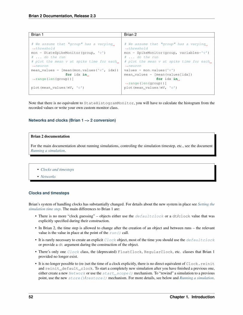
Brian 2 Documentation, Release 2.3
Brian 1 Brian 2
# We assume that "group" has a varying→˓thresholdmon = StateSpikeMonitor(group, 'v')# ... do the run# plot the mean v at spike time for each→˓neuronmean_values = [mean(mon.values('v', idx))
for idx in→˓range(len(group))]
plot(mean_values/mV, 'o')
# We assume that "group" has a varying→˓thresholdmon = SpikeMonitor(group, variables='v')# ... do the run# plot the mean v at spike time for each→˓neuronvalues = mon.values('v')mean_values = [mean(values[idx])
for idx in→˓range(len(group))]plot(mean_values/mV, 'o')
Note that there is no equivalent to StateHistogramMonitor, you will have to calculate the histogram from therecorded values or write your own custom monitor class.
Networks and clocks (Brian 1 –> 2 conversion)
Brian 2 documentation
For the main documentation about running simulations, controling the simulation timestep, etc., see the documentRunning a simulation.
• Clocks and timesteps
• Networks
Clocks and timesteps
Brian’s system of handling clocks has substantially changed. For details about the new system in place see Setting thesimulation time step. The main differences to Brian 1 are:
• There is no more “clock guessing” – objects either use the defaultclock or a dt/clock value that wasexplicitly specified during their construction.
• In Brian 2, the time step is allowed to change after the creation of an object and between runs – the relevantvalue is the value in place at the point of the run() call.
• It is rarely necessary to create an explicit Clock object, most of the time you should use the defaultclockor provide a dt argument during the construction of the object.
• There’s only one Clock class, the (deprecated) FloatClock, RegularClock, etc. classes that Brian 1provided no longer exist.
• It is no longer possible to (re-)set the time of a clock explicitly, there is no direct equivalent of Clock.reinitand reinit_default_clock. To start a completely new simulation after you have finished a previous one,either create a new Network or use the start_scope() mechanism. To “rewind” a simulation to a previouspoint, use the new store()/restore() mechanism. For more details, see below and Running a simulation.
52 Chapter 1. Introduction
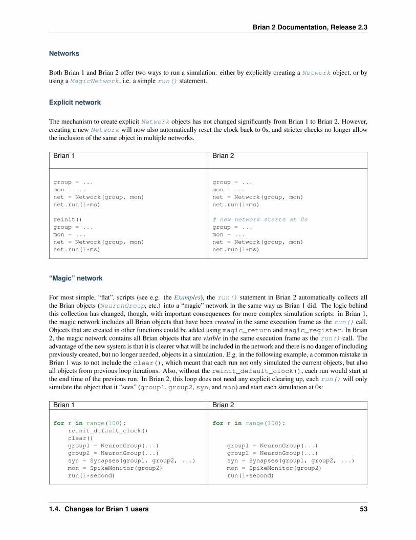
Brian 2 Documentation, Release 2.3
Networks
Both Brian 1 and Brian 2 offer two ways to run a simulation: either by explicitly creating a Network object, or byusing a MagicNetwork, i.e. a simple run() statement.
Explicit network
The mechanism to create explicit Network objects has not changed significantly from Brian 1 to Brian 2. However,creating a new Network will now also automatically reset the clock back to 0s, and stricter checks no longer allowthe inclusion of the same object in multiple networks.
Brian 1 Brian 2
group = ...mon = ...net = Network(group, mon)net.run(1*ms)
reinit()group = ...mon = ...net = Network(group, mon)net.run(1*ms)
group = ...mon = ...net = Network(group, mon)net.run(1*ms)
# new network starts at 0sgroup = ...mon = ...net = Network(group, mon)net.run(1*ms)
“Magic” network
For most simple, “flat”, scripts (see e.g. the Examples), the run() statement in Brian 2 automatically collects allthe Brian objects (NeuronGroup, etc.) into a “magic” network in the same way as Brian 1 did. The logic behindthis collection has changed, though, with important consequences for more complex simulation scripts: in Brian 1,the magic network includes all Brian objects that have been created in the same execution frame as the run() call.Objects that are created in other functions could be added using magic_return and magic_register. In Brian2, the magic network contains all Brian objects that are visible in the same execution frame as the run() call. Theadvantage of the new system is that it is clearer what will be included in the network and there is no danger of includingpreviously created, but no longer needed, objects in a simulation. E.g. in the following example, a common mistake inBrian 1 was to not include the clear(), which meant that each run not only simulated the current objects, but alsoall objects from previous loop iterations. Also, without the reinit_default_clock(), each run would start atthe end time of the previous run. In Brian 2, this loop does not need any explicit clearing up, each run() will onlysimulate the object that it “sees” (group1, group2, syn, and mon) and start each simulation at 0s:
Brian 1 Brian 2
for r in range(100):reinit_default_clock()clear()group1 = NeuronGroup(...)group2 = NeuronGroup(...)syn = Synapses(group1, group2, ...)mon = SpikeMonitor(group2)run(1*second)
for r in range(100):
group1 = NeuronGroup(...)group2 = NeuronGroup(...)syn = Synapses(group1, group2, ...)mon = SpikeMonitor(group2)run(1*second)
1.4. Changes for Brian 1 users 53
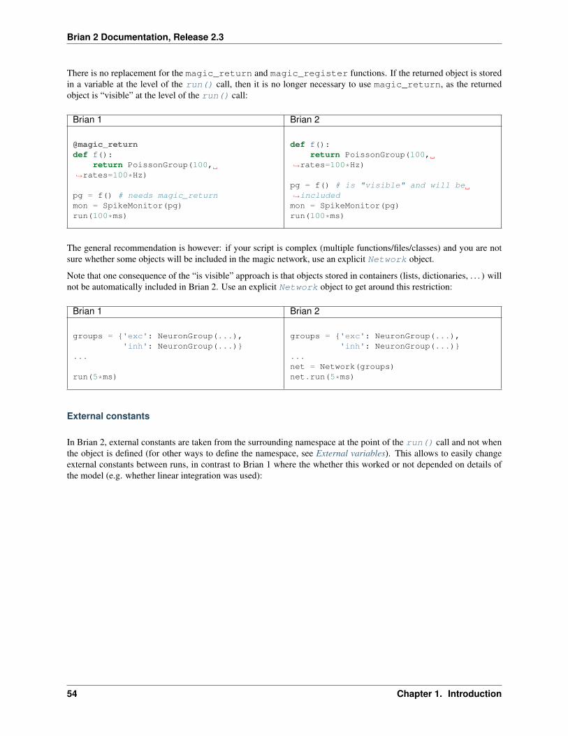
Brian 2 Documentation, Release 2.3
There is no replacement for the magic_return and magic_register functions. If the returned object is storedin a variable at the level of the run() call, then it is no longer necessary to use magic_return, as the returnedobject is “visible” at the level of the run() call:
Brian 1 Brian 2
@magic_returndef f():
return PoissonGroup(100,→˓rates=100*Hz)
pg = f() # needs magic_returnmon = SpikeMonitor(pg)run(100*ms)
def f():return PoissonGroup(100,
→˓rates=100*Hz)
pg = f() # is "visible" and will be→˓includedmon = SpikeMonitor(pg)run(100*ms)
The general recommendation is however: if your script is complex (multiple functions/files/classes) and you are notsure whether some objects will be included in the magic network, use an explicit Network object.
Note that one consequence of the “is visible” approach is that objects stored in containers (lists, dictionaries, . . . ) willnot be automatically included in Brian 2. Use an explicit Network object to get around this restriction:
Brian 1 Brian 2
groups = {'exc': NeuronGroup(...),'inh': NeuronGroup(...)}
...
run(5*ms)
groups = {'exc': NeuronGroup(...),'inh': NeuronGroup(...)}
...net = Network(groups)net.run(5*ms)
External constants
In Brian 2, external constants are taken from the surrounding namespace at the point of the run() call and not whenthe object is defined (for other ways to define the namespace, see External variables). This allows to easily changeexternal constants between runs, in contrast to Brian 1 where the whether this worked or not depended on details ofthe model (e.g. whether linear integration was used):
54 Chapter 1. Introduction

Brian 2 Documentation, Release 2.3
Brian 1 Brian 2
tau = 10*ms# to be sure that changes between runs→˓are taken into# account, define "I" as a neuronal→˓parametergroup = NeuronGroup(10, '''dv/dt = (-v +→˓I) / tau : 1
I : 1''')group.v = linspace(0, 1, 10)group.I = 0.0mon = StateMonitor(group, 'v',→˓record=True)run(5*ms)group.I = 0.5run(5*ms)group.I = 0.0run(5*ms)
tau = 10*ms
# The value for I will be updated at→˓each rungroup = NeuronGroup(10, 'dv/dt = (-v +→˓I) / tau : 1')
group.v = linspace(0, 1, 10)I = 0.0mon = StateMonitor(group, 'v',→˓record=True)run(5*ms)I = 0.5run(5*ms)I = 0.0run(5*ms)
Preferences (Brian 1 –> 2 conversion)
Brian 2 documentation
For the main documentation about preferences, see the document Preferences.
In Brian 1, preferences were set either with the function set_global_preferences or by creating a modulesomewhere on the Python path called brian_global_config.py.
Setting preferences
The function set_global_preferences no longer exists in Brian 2. Instead, importing from brian2 gives youa variable prefs that can be used to set preferences. For example, in Brian 1 you would write:
set_global_preferences(weavecompiler='gcc')
In Brian 2 you would write:
prefs.codegen.cpp.compiler = 'gcc'
Configuration file
The module brian_global_config.py is not used by Brian 2, instead we search for configuration files in thecurrent directory, user directory or installation directory. In Brian you would have a configuration file that looks likethis:
from brian.globalprefs import *set_global_preferences(weavecompiler='gcc')
In Brian 2 you would have a file like this:
1.4. Changes for Brian 1 users 55
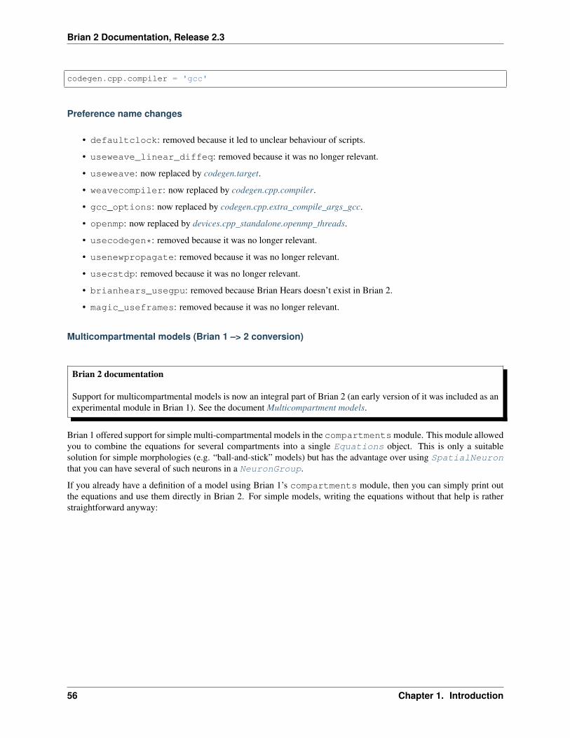
Brian 2 Documentation, Release 2.3
codegen.cpp.compiler = 'gcc'
Preference name changes
• defaultclock: removed because it led to unclear behaviour of scripts.
• useweave_linear_diffeq: removed because it was no longer relevant.
• useweave: now replaced by codegen.target.
• weavecompiler: now replaced by codegen.cpp.compiler.
• gcc_options: now replaced by codegen.cpp.extra_compile_args_gcc.
• openmp: now replaced by devices.cpp_standalone.openmp_threads.
• usecodegen*: removed because it was no longer relevant.
• usenewpropagate: removed because it was no longer relevant.
• usecstdp: removed because it was no longer relevant.
• brianhears_usegpu: removed because Brian Hears doesn’t exist in Brian 2.
• magic_useframes: removed because it was no longer relevant.
Multicompartmental models (Brian 1 –> 2 conversion)
Brian 2 documentation
Support for multicompartmental models is now an integral part of Brian 2 (an early version of it was included as anexperimental module in Brian 1). See the document Multicompartment models.
Brian 1 offered support for simple multi-compartmental models in the compartmentsmodule. This module allowedyou to combine the equations for several compartments into a single Equations object. This is only a suitablesolution for simple morphologies (e.g. “ball-and-stick” models) but has the advantage over using SpatialNeuronthat you can have several of such neurons in a NeuronGroup.
If you already have a definition of a model using Brian 1’s compartments module, then you can simply print outthe equations and use them directly in Brian 2. For simple models, writing the equations without that help is ratherstraightforward anyway:
56 Chapter 1. Introduction

Brian 2 Documentation, Release 2.3
Brian 1 Brian 2
V0 = 10*mVC = 200*pFRa = 150*kohmR = 50*Mohmsoma_eqs = (MembraneEquation(C) +
IonicCurrent('I=(vm-V0)/R :→˓amp'))dend_eqs = MembraneEquation(C)neuron_eqs = Compartments({'soma': soma_→˓eqs,
'dend': dend_→˓eqs})
neuron = NeuronGroup(N, neuron_eqs)
V0 = 10*mVC = 200*pFRa = 150*kohmR = 50*Mohmneuron_eqs = '''dvm_soma/dt = (I_soma + I_soma_dend)/C :→˓voltI_soma = (V0 - vm_soma)/R : ampI_soma_dend = (vm_dend - vm_soma)/Ra :→˓ampdvm_dend/dt = -I_soma_dend/C : volt'''
neuron = NeuronGroup(N, neuron_eqs)
Library models (Brian 1 –> 2 conversion)
• Neuron models
• Ionic currents
• Synapses
Neuron models
The neuron models in Brian 1’s brian.library.IF package are nothing more than shorthands for equations. Thefollowing table shows how the models from Brian 1 can be converted to explicit equations (and reset statements inthe case of the adaptive exponential integrate-and-fire model) for use in Brian 2. The examples include a “current” I(depending on the model not necessarily in units of Ampère) and could e.g. be used to plot the f-I curve of the neuron.
Perfect integrator
Brian 1 Brian 2
eqs = (perfect_IF(tau=10*ms) +Current('I : volt'))
group = NeuronGroup(N, eqs,threshold='v > -50*mV
→˓',reset='v = -70*mV')
tau = 10*mseqs = '''dvm/dt = I/tau : volt
I : volt'''group = NeuronGroup(N, eqs,
threshold='v > -50*mV→˓',
reset='v = -70*mV')
1.4. Changes for Brian 1 users 57
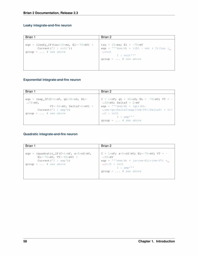
Brian 2 Documentation, Release 2.3
Leaky integrate-and-fire neuron
Brian 1 Brian 2
eqs = (leaky_IF(tau=10*ms, El=-70*mV) +Current('I : volt'))
group = ... # see above
tau = 10*ms; El = -70*mVeqs = '''dvm/dt = ((El - vm) + I)/tau :→˓volt
I : volt'''group = ... # see above
Exponential integrate-and-fire neuron
Brian 1 Brian 2
eqs = (exp_IF(C=1*nF, gL=30*nS, EL=-→˓70*mV,
VT=-50*mV, DeltaT=2*mV) +Current('I : amp'))
group = ... # see above
C = 1*nF; gL = 30*nS; EL = -70*mV; VT = -→˓50*mV; DeltaT = 2*mVeqs = '''dvm/dt = (gL*(EL-→˓vm)+gL*DeltaT*exp((vm-VT)/DeltaT) + I)/→˓C : volt
I : amp'''group = ... # see above
Quadratic integrate-and-fire neuron
Brian 1 Brian 2
eqs = (quadratic_IF(C=1*nF, a=5*nS/mV,EL=-70*mV, VT=-50*mV) +Current('I : amp'))
group = ... # see above
C = 1*nF; a=5*nS/mV; EL=-70*mV; VT = -→˓50*mVeqs = '''dvm/dt = (a*(vm-EL)*(vm-VT) +→˓I)/C : volt
I : amp'''group = ... # see above
58 Chapter 1. Introduction

Brian 2 Documentation, Release 2.3
Izhikevich neuron
Brian 1 Brian 2
eqs = (Izhikevich(a=0.02/ms, b=0.2/ms) +Current('I : volt/second'))
group = ... # see above
a = 0.02/ms; b = 0.2/mseqs = '''dvm/dt = (0.04/ms/mV)*vm**2+(5/→˓ms)*vm+140*mV/ms-w + I : volt
dw/dt = a*(b*vm-w) : volt/secondI : volt/second'''
group = ... # see above
Adaptive exponential integrate-and-fire neuron (“Brette-Gerstner model”)
Brian 1 Brian 2
# AdEx, aEIF, and Brette_Gerstner all→˓refer to the same modeleqs = (aEIF(C=1*nF, gL=30*nS, EL=-70*mV,
VT=-50*mV, DeltaT=2*mV,→˓tauw=150*ms, a=4*nS) +
Current('I:amp'))group = NeuronGroup(N, eqs,
threshold='v > -20*mV→˓',
→˓reset=AdaptiveReset(Vr=-70*mV, b=0.→˓08*nA))
C = 1*nF; gL = 30*nS; EL = -70*mV; VT = -→˓50*mV; DeltaT = 2*mV; tauw = 150*ms; a→˓= 4*nSeqs = '''dvm/dt = (gL*(EL-→˓vm)+gL*DeltaT*exp((vm-VT)/DeltaT) -w +→˓I)/C : volt
dw/dt=(a*(vm-EL)-w)/tauw : ampI : amp'''
group = NeuronGroup(N, eqs,threshold='vm > -
→˓20*mV',reset='vm=-70*mV; w
→˓+= 0.08*nA')
Ionic currents
Brian 1’s functions for ionic currents, provided in brian.library.ionic_currents correspond to the follow-ing equations (note that the currents follow the convention to use a shifted membrane potential, i.e. the membranepotential at rest is 0mV):
1.4. Changes for Brian 1 users 59
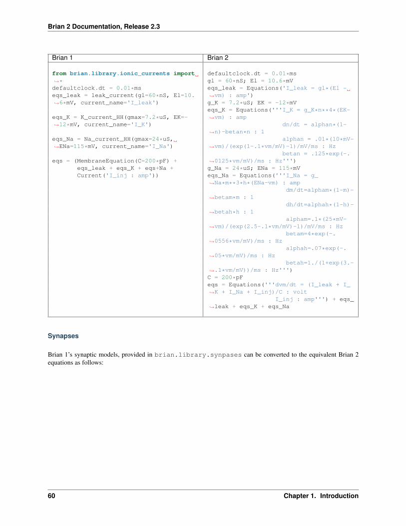
Brian 2 Documentation, Release 2.3
Brian 1 Brian 2
from brian.library.ionic_currents import→˓*defaultclock.dt = 0.01*mseqs_leak = leak_current(gl=60*nS, El=10.→˓6*mV, current_name='I_leak')
eqs_K = K_current_HH(gmax=7.2*uS, EK=-→˓12*mV, current_name='I_K')
eqs_Na = Na_current_HH(gmax=24*uS,→˓ENa=115*mV, current_name='I_Na')
eqs = (MembraneEquation(C=200*pF) +eqs_leak + eqs_K + eqs+Na +Current('I_inj : amp'))
defaultclock.dt = 0.01*msgl = 60*nS; El = 10.6*mVeqs_leak = Equations('I_leak = gl*(El -→˓vm) : amp')g_K = 7.2*uS; EK = -12*mVeqs_K = Equations('''I_K = g_K*n**4*(EK-→˓vm) : amp
dn/dt = alphan*(1-→˓n)-betan*n : 1
alphan = .01*(10*mV-→˓vm)/(exp(1-.1*vm/mV)-1)/mV/ms : Hz
betan = .125*exp(-.→˓0125*vm/mV)/ms : Hz''')g_Na = 24*uS; ENa = 115*mVeqs_Na = Equations('''I_Na = g_→˓Na*m**3*h*(ENa-vm) : amp
dm/dt=alpham*(1-m)-→˓betam*m : 1
dh/dt=alphah*(1-h)-→˓betah*h : 1
alpham=.1*(25*mV-→˓vm)/(exp(2.5-.1*vm/mV)-1)/mV/ms : Hz
betam=4*exp(-.→˓0556*vm/mV)/ms : Hz
alphah=.07*exp(-.→˓05*vm/mV)/ms : Hz
betah=1./(1+exp(3.-→˓.1*vm/mV))/ms : Hz''')C = 200*pFeqs = Equations('''dvm/dt = (I_leak + I_→˓K + I_Na + I_inj)/C : volt
I_inj : amp''') + eqs_→˓leak + eqs_K + eqs_Na
Synapses
Brian 1’s synaptic models, provided in brian.library.synpases can be converted to the equivalent Brian 2equations as follows:
60 Chapter 1. Introduction
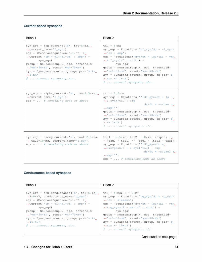
Brian 2 Documentation, Release 2.3
Current-based synapses
Brian 1 Brian 2
syn_eqs = exp_current('s', tau=5*ms,→˓current_name='I_syn')eqs = (MembraneEquation(C=1*nF) +→˓Current('Im = gl*(El-vm) : amp') +
syn_eqs)group = NeuronGroup(N, eqs, threshold=→˓'vm>-50*mV', reset='vm=-70*mV')syn = Synapses(source, group, pre='s +=→˓1*nA')# ... connect synapses, etc.
tau = 5*mssyn_eqs = Equations('dI_syn/dt = -I_syn/→˓tau : amp')eqs = (Equations('dvm/dt = (gl*(El - vm)→˓+ I_syn)/C : volt') +
syn_eqs)group = NeuronGroup(N, eqs, threshold=→˓'vm>-50*mV', reset='vm=-70*mV')syn = Synapses(source, group, on_pre='I_→˓syn += 1*nA')# ... connect synapses, etc.
syn_eqs = alpha_current('s', tau=2.5*ms,→˓current_name='I_syn')eqs = ... # remaining code as above
tau = 2.5*mssyn_eqs = Equations('''dI_syn/dt = (s -→˓I_syn)/tau : amp
ds/dt = -s/tau :→˓amp''')group = NeuronGroup(N, eqs, threshold=→˓'vm>-50*mV', reset='vm=-70*mV')syn = Synapses(source, group, on_pre='s→˓+= 1*nA')# ... connect synapses, etc.
syn_eqs = biexp_current('s', tau1=2.5*ms,→˓ tau2=10*ms, current_name='I_syn')eqs = ... # remaining code as above
tau1 = 2.5*ms; tau2 = 10*ms; invpeak =→˓(tau2 / tau1) ** (tau1 / (tau2 - tau1))syn_eqs = Equations('''dI_syn/dt =→˓(invpeak*s - I_syn)/tau1 : amp
ds/dt = -s/tau2 :→˓amp''')eqs = ... # remaining code as above
Conductance-based synapses
Brian 1 Brian 2
syn_eqs = exp_conductance('s', tau=5*ms,→˓E=0*mV, conductance_name='g_syn')eqs = (MembraneEquation(C=1*nF) +→˓Current('Im = gl*(El-vm) : amp') +
syn_eqs)group = NeuronGroup(N, eqs, threshold=→˓'vm>-50*mV', reset='vm=-70*mV')syn = Synapses(source, group, pre='s +=→˓10*nS')# ... connect synapses, etc.
tau = 5*ms; E = 0*mVsyn_eqs = Equations('dg_syn/dt = -g_syn/→˓tau : siemens')eqs = (Equations('dvm/dt = (gl*(El - vm)→˓+ g_syn*(E - vm))/C : volt') +
syn_eqs)group = NeuronGroup(N, eqs, threshold=→˓'vm>-50*mV', reset='vm=-70*mV')syn = Synapses(source, group, on_pre='g_→˓syn += 10*nS')# ... connect synapses, etc.
Continued on next page
1.4. Changes for Brian 1 users 61
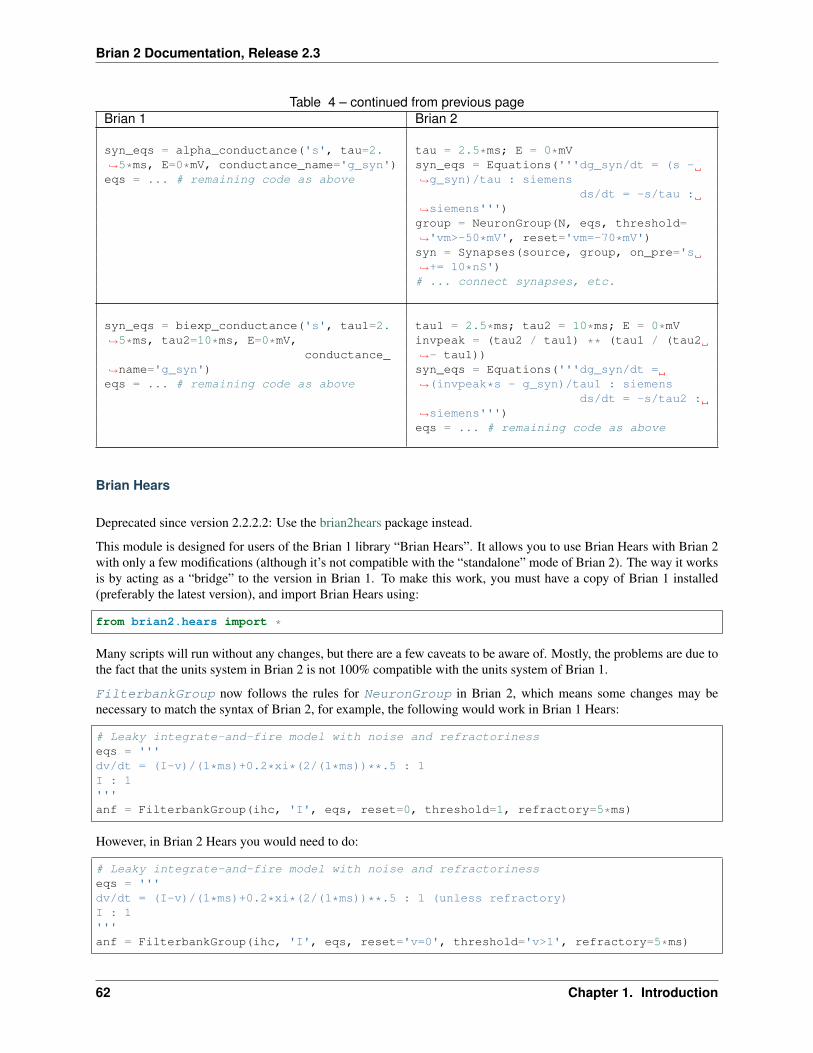
Brian 2 Documentation, Release 2.3
Table 4 – continued from previous pageBrian 1 Brian 2
syn_eqs = alpha_conductance('s', tau=2.→˓5*ms, E=0*mV, conductance_name='g_syn')eqs = ... # remaining code as above
tau = 2.5*ms; E = 0*mVsyn_eqs = Equations('''dg_syn/dt = (s -→˓g_syn)/tau : siemens
ds/dt = -s/tau :→˓siemens''')group = NeuronGroup(N, eqs, threshold=→˓'vm>-50*mV', reset='vm=-70*mV')syn = Synapses(source, group, on_pre='s→˓+= 10*nS')# ... connect synapses, etc.
syn_eqs = biexp_conductance('s', tau1=2.→˓5*ms, tau2=10*ms, E=0*mV,
conductance_→˓name='g_syn')eqs = ... # remaining code as above
tau1 = 2.5*ms; tau2 = 10*ms; E = 0*mVinvpeak = (tau2 / tau1) ** (tau1 / (tau2→˓- tau1))syn_eqs = Equations('''dg_syn/dt =→˓(invpeak*s - g_syn)/tau1 : siemens
ds/dt = -s/tau2 :→˓siemens''')eqs = ... # remaining code as above
Brian Hears
Deprecated since version 2.2.2.2: Use the brian2hears package instead.
This module is designed for users of the Brian 1 library “Brian Hears”. It allows you to use Brian Hears with Brian 2with only a few modifications (although it’s not compatible with the “standalone” mode of Brian 2). The way it worksis by acting as a “bridge” to the version in Brian 1. To make this work, you must have a copy of Brian 1 installed(preferably the latest version), and import Brian Hears using:
from brian2.hears import *
Many scripts will run without any changes, but there are a few caveats to be aware of. Mostly, the problems are due tothe fact that the units system in Brian 2 is not 100% compatible with the units system of Brian 1.
FilterbankGroup now follows the rules for NeuronGroup in Brian 2, which means some changes may benecessary to match the syntax of Brian 2, for example, the following would work in Brian 1 Hears:
# Leaky integrate-and-fire model with noise and refractorinesseqs = '''dv/dt = (I-v)/(1*ms)+0.2*xi*(2/(1*ms))**.5 : 1I : 1'''anf = FilterbankGroup(ihc, 'I', eqs, reset=0, threshold=1, refractory=5*ms)
However, in Brian 2 Hears you would need to do:
# Leaky integrate-and-fire model with noise and refractorinesseqs = '''dv/dt = (I-v)/(1*ms)+0.2*xi*(2/(1*ms))**.5 : 1 (unless refractory)I : 1'''anf = FilterbankGroup(ihc, 'I', eqs, reset='v=0', threshold='v>1', refractory=5*ms)
62 Chapter 1. Introduction
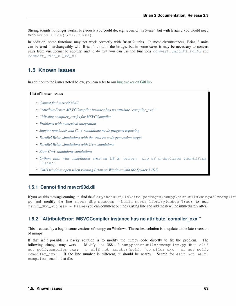
Brian 2 Documentation, Release 2.3
Slicing sounds no longer works. Previously you could do, e.g. sound[:20*ms] but with Brian 2 you would needto do sound.slice(0*ms, 20*ms).
In addition, some functions may not work correctly with Brian 2 units. In most circumstances, Brian 2 unitscan be used interchangeably with Brian 1 units in the bridge, but in some cases it may be necessary to convertunits from one format to another, and to do that you can use the functions convert_unit_b1_to_b2 andconvert_unit_b2_to_b1.
1.5 Known issues
In addition to the issues noted below, you can refer to our bug tracker on GitHub.
List of known issues
• Cannot find msvcr90d.dll
• “AttributeError: MSVCCompiler instance has no attribute ‘compiler_cxx’”
• “Missing compiler_cxx fix for MSVCCompiler”
• Problems with numerical integration
• Jupyter notebooks and C++ standalone mode progress reporting
• Parallel Brian simulations with the weave code generation target
• Parallel Brian simulations with C++ standalone
• Slow C++ standalone simulations
• Cython fails with compilation error on OS X: error: use of undeclared identifier'isinf'
• CMD windows open when running Brian on Windows with the Spyder 3 IDE
1.5.1 Cannot find msvcr90d.dll
If you see this message coming up, find the file PythonDir\Lib\site-packages\numpy\distutils\mingw32ccompiler.py and modify the line msvcr_dbg_success = build_msvcr_library(debug=True) to readmsvcr_dbg_success = False (you can comment out the existing line and add the new line immediately after).
1.5.2 “AttributeError: MSVCCompiler instance has no attribute ‘compiler_cxx’”
This is caused by a bug in some versions of numpy on Windows. The easiest solution is to update to the latest versionof numpy.
If that isn’t possible, a hacky solution is to modify the numpy code directly to fix the problem. Thefollowing change may work. Modify line 388 of numpy/distutils/ccompiler.py from elifnot self.compiler_cxx: to elif not hasattr(self, 'compiler_cxx') or not self.compiler_cxx:. If the line number is different, it should be nearby. Search for elif not self.compiler_cxx in that file.
1.5. Known issues 63

Brian 2 Documentation, Release 2.3
1.5.3 “Missing compiler_cxx fix for MSVCCompiler”
If you keep seeing this message, do not worry. It’s not possible for us to hide it, but doesn’t indicate any problems.
1.5.4 Problems with numerical integration
In some cases, the automatic choice of numerical integration method will not be appropriate, because of a choice ofparameters that couldn’t be determined in advance. In this case, typically you will get nan (not a number) values inthe results, or large oscillations. In this case, Brian will generate a warning to let you know, but will not raise an error.
1.5.5 Jupyter notebooks and C++ standalone mode progress reporting
When you run simulations in C++ standalone mode and enable progress reporting (e.g. by using report='text'as a keyword argument), the progress will not be displayed in the jupyter notebook. If you started the notebook froma terminal, you will find the output there. Unfortunately, this is a tricky problem to solve at the moment, due to thedetails of how the jupyter notebook handles output.
1.5.6 Parallel Brian simulations with the weave code generation target
When using the weave code generation target (the default runtime target on Python 2.x, see Runtime code generationfor details), you should avoid running multiple Brian simulations in parallel. The weave package caches compiledfiles, but this cache is not prepared for multiple concurrent updates. If two Python scripts (or two processes startedfrom the same Python script, e.g. via the multiprocessing package) try to store compilation results at the sametime, weave will crash with an error message. The numpy and cython targets are not affected by this problem.
1.5.7 Parallel Brian simulations with C++ standalone
Simulations using the C++ standalone device will create code and store results in a dedicated directory (output, bydefault). If you run multiple simulations in parallel, you have to take care that these simulations do not use the samedirectory – otherwise, everything from compilation errors to incorrect results can happen. Either chose a differentdirectory name for each simulation and provide it as the directory argument to the set_device or build call,or use directory=None which will use a randomly chosen unique temporary directory (in /tmp on Unix-basedsystems) for each simulation. If you need to know the directory name, you can access it after the simulation run viadevice.project_dir.
1.5.8 Slow C++ standalone simulations
Some versions of the GNU standard library (in particular those used by recent Ubuntu versions) have a bugthat can dramatically slow down simulations in C++ standalone mode on modern hardware (see #803). As aworkaround, Brian will set an environment variable LD_BIND_NOW during the execution of standalone simula-tions which changes the way the library is linked so that it does not suffer from this problem. If this environ-ment variable leads to unwanted behaviour on your machine, change the prefs.devices.cpp_standalone.run_environment_variables preference.
1.5.9 Cython fails with compilation error on OS X: error: use of undeclaredidentifier 'isinf'
Try setting the environment variable MACOSX_DEPLOYMENT_TARGET=10.9.
64 Chapter 1. Introduction
Brian 2 Documentation, Release 2.3
1.5.10 CMD windows open when running Brian on Windows with the Spyder 3 IDE
This is due to the interaction with the integrated ipython terminal. Either change the run configuration to “Executein an external system terminal” or patch the internal Python function used to spawn processes as described in githubissue #1140.
1.6 Support
If you are stuck with a problem using Brian, please do get in touch at our email support list.
You can save time by following this procedure when reporting a problem:
1. Do try to solve the problem on your own first. Read the documentation, including using the search feature, indexand reference documentation.
2. Search the mailing list archives to see if someone else already had the same problem.
3. Before writing, try to create a minimal example that reproduces the problem. You’ll get the fastest response ifyou can send just a handful of lines of code that show what isn’t working.
1.7 Contributor Covenant Code of Conduct
1.7.1 Our Pledge
In the interest of fostering an open and welcoming environment, we as contributors and maintainers pledge to makingparticipation in our project and our community a harassment-free experience for everyone, regardless of age, body size,disability, ethnicity, sex characteristics, gender identity and expression, level of experience, education, socio-economicstatus, nationality, personal appearance, race, religion, or sexual identity and orientation.
1.7.2 Our Standards
Examples of behavior that contributes to creating a positive environment include:
• Using welcoming and inclusive language
• Being respectful of differing viewpoints and experiences
• Gracefully accepting constructive criticism
• Focusing on what is best for the community
• Showing empathy towards other community members
Examples of unacceptable behavior by participants include:
• The use of sexualized language or imagery and unwelcome sexual attention or advances
• Trolling, insulting/derogatory comments, and personal or political attacks
• Public or private harassment
• Publishing others’ private information, such as a physical or electronic address, without explicit permission
• Other conduct which could reasonably be considered inappropriate in a professional setting
1.6. Support 65

Brian 2 Documentation, Release 2.3
1.7.3 Our Responsibilities
Project maintainers are responsible for clarifying the standards of acceptable behavior and are expected to take appro-priate and fair corrective action in response to any instances of unacceptable behavior.
Project maintainers have the right and responsibility to remove, edit, or reject comments, commits, code, wiki edits,issues, and other contributions that are not aligned to this Code of Conduct, or to ban temporarily or permanently anycontributor for other behaviors that they deem inappropriate, threatening, offensive, or harmful.
1.7.4 Scope
This Code of Conduct applies both within project spaces and in public spaces when an individual is representing theproject or its community. Examples of representing a project or community include using an official project e-mailaddress, posting via an official social media account, or acting as an appointed representative at an online or offlineevent. Representation of a project may be further defined and clarified by project maintainers.
1.7.5 Enforcement
Instances of abusive, harassing, or otherwise unacceptable behavior may be reported by contacting the project teamat [email protected]. All complaints will be reviewed and investigated and will result in a response that isdeemed necessary and appropriate to the circumstances. The project team is obligated to maintain confidentiality withregard to the reporter of an incident. Further details of specific enforcement policies may be posted separately.
Project maintainers who do not follow or enforce the Code of Conduct in good faith may face temporary or permanentrepercussions as determined by other members of the project’s leadership.
1.7.6 Attribution
This Code of Conduct is adapted from the Contributor Covenant, version 1.4, available at https://www.contributor-covenant.org/version/1/4/code-of-conduct.html
For answers to common questions about this code of conduct, see https://www.contributor-covenant.org/faq
66 Chapter 1. Introduction
CHAPTER 2
Tutorials
The tutorial consists of a series of Jupyter Notebooks1.
For more information about how to use Jupyter Notebooks, see the Jupyter Notebook documentation.
2.1 Introduction to Brian part 1: Neurons
All Brian scripts start with the following. If you’re trying this notebook out in the Jupyter notebook, you should startby running this cell.
from brian2 import *
Later we’ll do some plotting in the notebook, so we activate inline plotting in the notebook by doing this:
%matplotlib inline
If you are not using the Jupyter notebook to run this example (e.g. you are using a standard Python terminal, or youcopy&paste these example into an editor and run them as a script), then plots will not automatically be displayed. Inthis case, call the show() command explicitly after the plotting commands.
2.1.1 Units system
Brian has a system for using quantities with physical dimensions:
20*volt
20.0 V
All of the basic SI units can be used (volt, amp, etc.) along with all the standard prefixes (m=milli, p=pico, etc.), aswell as a few special abbreviations like mV for millivolt, pF for picofarad, etc.
1 Formerly known as “IPython Notebooks”.
67
Brian 2 Documentation, Release 2.3
1000*amp
1.0 k A
1e6*volt
1.0 M V
1000*namp
1.0𝜇A
Also note that combinations of units with work as expected:
10*nA*5*Mohm
50.0 m V
And if you try to do something wrong like adding amps and volts, what happens?
5*amp+10*volt
DimensionMismatchErrorTraceback (most recent call last)
<ipython-input-8-245c0c0332d1> in <module>()----> 1 5*amp+10*volt
/home/marcel/programming/brian2/brian2/units/fundamentalunits.pyc in __add__(self,→˓other)
1427 return self._binary_operation(other, operator.add,1428 fail_for_mismatch=True,
-> 1429 operator_str='+')14301431 def __radd__(self, other):
/home/marcel/programming/brian2/brian2/units/fundamentalunits.pyc in _binary_→˓operation(self, other, operation, dim_operation, fail_for_mismatch, operator_str,→˓inplace)
1367 _, other_dim = fail_for_dimension_mismatch(self, other,→˓message,
1368 value1=self,-> 1369 value2=other)
13701371 if other_dim is None:
/home/marcel/programming/brian2/brian2/units/fundamentalunits.pyc in fail_for_→˓dimension_mismatch(obj1, obj2, error_message, **error_quantities)
184 raise DimensionMismatchError(error_message, dim1)185 else:
--> 186 raise DimensionMismatchError(error_message, dim1, dim2)187 else:188 return dim1, dim2
(continues on next page)
68 Chapter 2. Tutorials
Brian 2 Documentation, Release 2.3
(continued from previous page)
DimensionMismatchError: Cannot calculate 5. A + 10. V, units do not match (units are→˓amp and volt).
If you haven’t see an error message in Python before that can look a bit overwhelming, but it’s actually quite simpleand it’s important to know how to read these because you’ll probably see them quite often.
You should start at the bottom and work up. The last line gives the error type DimensionMismatchError alongwith a more specific message (in this case, you were trying to add together two quantities with different SI units, whichis impossible).
Working upwards, each of the sections starts with a filename (e.g. C:\Users\Dan\...) with possibly the name ofa function, and then a few lines surrounding the line where the error occurred (which is identified with an arrow).
The last of these sections shows the place in the function where the error actually happened. The section above itshows the function that called that function, and so on until the first section will be the script that you actually run.This sequence of sections is called a traceback, and is helpful in debugging.
If you see a traceback, what you want to do is start at the bottom and scan up the sections until you find your own filebecause that’s most likely where the problem is. (Of course, your code might be correct and Brian may have a bug inwhich case, please let us know on the email support list.)
2.1.2 A simple model
Let’s start by defining a simple neuron model. In Brian, all models are defined by systems of differential equations.Here’s a simple example of what that looks like:
tau = 10*mseqs = '''dv/dt = (1-v)/tau : 1'''
In Python, the notation ''' is used to begin and end a multi-line string. So the equations are just a string with oneline per equation. The equations are formatted with standard mathematical notation, with one addition. At the end ofa line you write : unit where unit is the SI unit of that variable. Note that this is not the unit of the two sides ofthe equation (which would be 1/second), but the unit of the variable defined by the equation, i.e. in this case 𝑣.
Now let’s use this definition to create a neuron.
G = NeuronGroup(1, eqs)
In Brian, you only create groups of neurons, using the class NeuronGroup. The first two arguments when you createone of these objects are the number of neurons (in this case, 1) and the defining differential equations.
Let’s see what happens if we didn’t put the variable tau in the equation:
eqs = '''dv/dt = 1-v : 1'''G = NeuronGroup(1, eqs)run(100*ms)
BrianObjectExceptionTraceback (most recent call last)
<ipython-input-11-97ed109f5888> in <module>()
(continues on next page)
2.1. Introduction to Brian part 1: Neurons 69
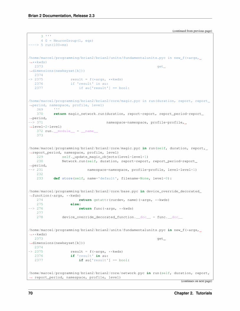
Brian 2 Documentation, Release 2.3
(continued from previous page)
3 '''4 G = NeuronGroup(1, eqs)
----> 5 run(100*ms)
/home/marcel/programming/brian2/brian2/units/fundamentalunits.pyc in new_f(*args,→˓**kwds)
2373 get_→˓dimensions(newkeyset[k]))
2374-> 2375 result = f(*args, **kwds)
2376 if 'result' in au:2377 if au['result'] == bool:
/home/marcel/programming/brian2/brian2/core/magic.pyc in run(duration, report, report_→˓period, namespace, profile, level)
369 '''370 return magic_network.run(duration, report=report, report_period=report_
→˓period,--> 371 namespace=namespace, profile=profile,→˓level=2+level)
372 run.__module__ = __name__373
/home/marcel/programming/brian2/brian2/core/magic.pyc in run(self, duration, report,→˓report_period, namespace, profile, level)
229 self._update_magic_objects(level=level+1)230 Network.run(self, duration, report=report, report_period=report_
→˓period,--> 231 namespace=namespace, profile=profile, level=level+1)
232233 def store(self, name='default', filename=None, level=0):
/home/marcel/programming/brian2/brian2/core/base.pyc in device_override_decorated_→˓function(*args, **kwds)
274 return getattr(curdev, name)(*args, **kwds)275 else:
--> 276 return func(*args, **kwds)277278 device_override_decorated_function.__doc__ = func.__doc__
/home/marcel/programming/brian2/brian2/units/fundamentalunits.pyc in new_f(*args,→˓**kwds)
2373 get_→˓dimensions(newkeyset[k]))
2374-> 2375 result = f(*args, **kwds)
2376 if 'result' in au:2377 if au['result'] == bool:
/home/marcel/programming/brian2/brian2/core/network.pyc in run(self, duration, report,→˓ report_period, namespace, profile, level)
(continues on next page)
70 Chapter 2. Tutorials

Brian 2 Documentation, Release 2.3
(continued from previous page)
949 namespace = get_local_namespace(level=level+3)950
--> 951 self.before_run(namespace)952953 if len(self.objects)==0:
/home/marcel/programming/brian2/brian2/core/base.pyc in device_override_decorated_→˓function(*args, **kwds)
274 return getattr(curdev, name)(*args, **kwds)275 else:
--> 276 return func(*args, **kwds)277278 device_override_decorated_function.__doc__ = func.__doc__
/home/marcel/programming/brian2/brian2/core/network.pyc in before_run(self, run_→˓namespace)
841 obj.before_run(run_namespace)842 except Exception as ex:
--> 843 raise brian_object_exception("An error occurred when→˓preparing an object.", obj, ex)
844845 # Check that no object has been run as part of another network before
BrianObjectException: Original error and traceback:Traceback (most recent call last):
File "/home/marcel/programming/brian2/brian2/core/network.py", line 841, in before_→˓run
obj.before_run(run_namespace)File "/home/marcel/programming/brian2/brian2/groups/neurongroup.py", line 811, in
→˓before_runself.equations.check_units(self, run_namespace=run_namespace)
File "/home/marcel/programming/brian2/brian2/equations/equations.py", line 963, in→˓check_units
*ex.dims)DimensionMismatchError: Inconsistent units in differential equation defining variable→˓v:Expression 1-v does not have the expected unit hertz (unit is 1).
Error encountered with object named "neurongroup_1".Object was created here (most recent call only, full details in debug log):
File "<ipython-input-11-97ed109f5888>", line 4, in <module>G = NeuronGroup(1, eqs)
An error occurred when preparing an object. DimensionMismatchError: Inconsistent→˓units in differential equation defining variable v:Expression 1-v does not have the expected unit hertz (unit is 1).(See above for original error message and traceback.)
An error is raised, but why? The reason is that the differential equation is now dimensionally inconsistent. Theleft hand side dv/dt has units of 1/second but the right hand side 1-v is dimensionless. People often find thisbehaviour of Brian confusing because this sort of equation is very common in mathematics. However, for quantitieswith physical dimensions it is incorrect because the results would change depending on the unit you measured it in.For time, if you measured it in seconds the same equation would behave differently to how it would if you measuredtime in milliseconds. To avoid this, we insist that you always specify dimensionally consistent equations.
2.1. Introduction to Brian part 1: Neurons 71
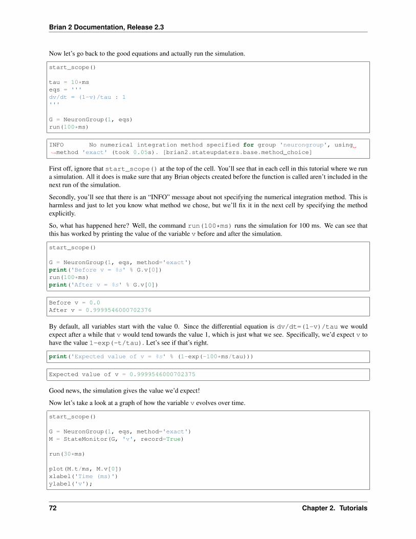
Brian 2 Documentation, Release 2.3
Now let’s go back to the good equations and actually run the simulation.
start_scope()
tau = 10*mseqs = '''dv/dt = (1-v)/tau : 1'''
G = NeuronGroup(1, eqs)run(100*ms)
INFO No numerical integration method specified for group 'neurongroup', using→˓method 'exact' (took 0.05s). [brian2.stateupdaters.base.method_choice]
First off, ignore that start_scope() at the top of the cell. You’ll see that in each cell in this tutorial where we runa simulation. All it does is make sure that any Brian objects created before the function is called aren’t included in thenext run of the simulation.
Secondly, you’ll see that there is an “INFO” message about not specifying the numerical integration method. This isharmless and just to let you know what method we chose, but we’ll fix it in the next cell by specifying the methodexplicitly.
So, what has happened here? Well, the command run(100*ms) runs the simulation for 100 ms. We can see thatthis has worked by printing the value of the variable v before and after the simulation.
start_scope()
G = NeuronGroup(1, eqs, method='exact')print('Before v = %s' % G.v[0])run(100*ms)print('After v = %s' % G.v[0])
Before v = 0.0After v = 0.9999546000702376
By default, all variables start with the value 0. Since the differential equation is dv/dt=(1-v)/tau we wouldexpect after a while that v would tend towards the value 1, which is just what we see. Specifically, we’d expect v tohave the value 1-exp(-t/tau). Let’s see if that’s right.
print('Expected value of v = %s' % (1-exp(-100*ms/tau)))
Expected value of v = 0.9999546000702375
Good news, the simulation gives the value we’d expect!
Now let’s take a look at a graph of how the variable v evolves over time.
start_scope()
G = NeuronGroup(1, eqs, method='exact')M = StateMonitor(G, 'v', record=True)
run(30*ms)
plot(M.t/ms, M.v[0])xlabel('Time (ms)')ylabel('v');
72 Chapter 2. Tutorials

Brian 2 Documentation, Release 2.3
This time we only ran the simulation for 30 ms so that we can see the behaviour better. It looks like it’s behaving asexpected, but let’s just check that analytically by plotting the expected behaviour on top.
start_scope()
G = NeuronGroup(1, eqs, method='exact')M = StateMonitor(G, 'v', record=0)
run(30*ms)
plot(M.t/ms, M.v[0], 'C0', label='Brian')plot(M.t/ms, 1-exp(-M.t/tau), 'C1--',label='Analytic')xlabel('Time (ms)')ylabel('v')legend();
2.1. Introduction to Brian part 1: Neurons 73
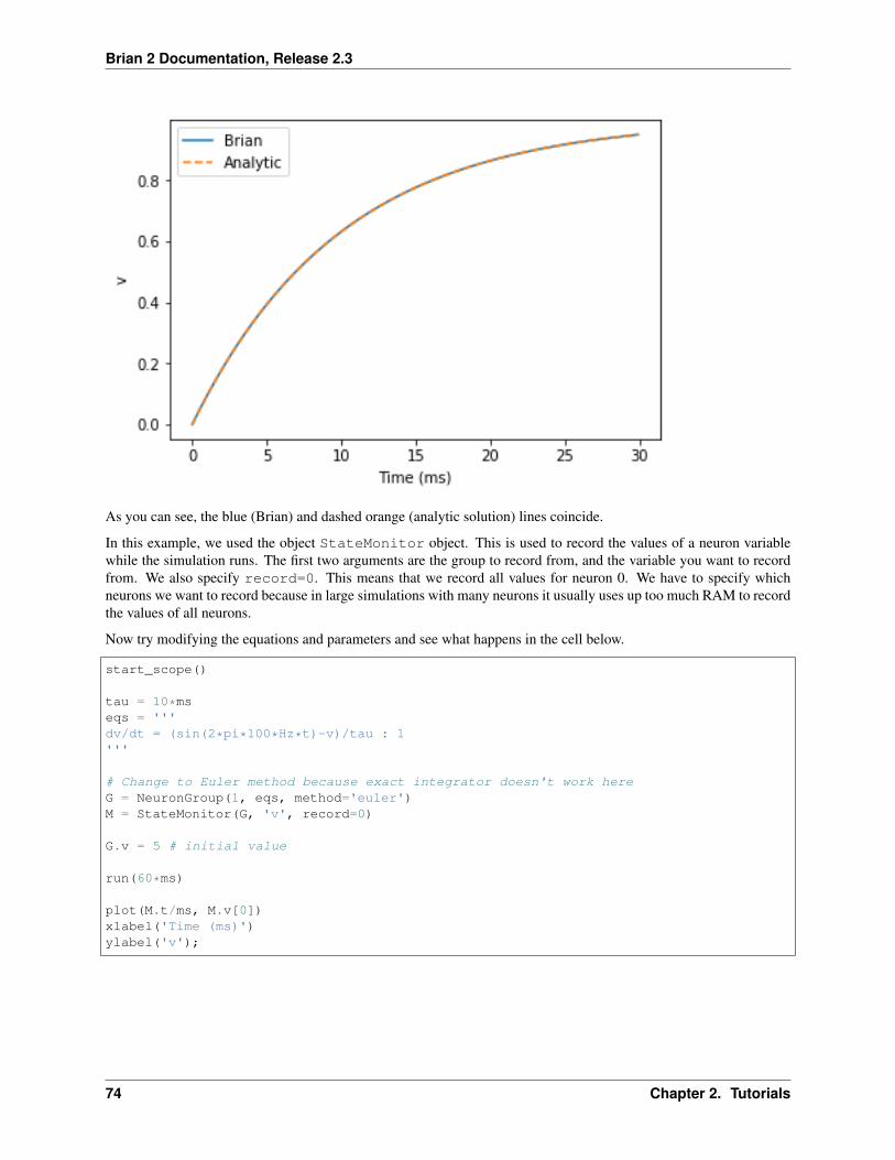
Brian 2 Documentation, Release 2.3
As you can see, the blue (Brian) and dashed orange (analytic solution) lines coincide.
In this example, we used the object StateMonitor object. This is used to record the values of a neuron variablewhile the simulation runs. The first two arguments are the group to record from, and the variable you want to recordfrom. We also specify record=0. This means that we record all values for neuron 0. We have to specify whichneurons we want to record because in large simulations with many neurons it usually uses up too much RAM to recordthe values of all neurons.
Now try modifying the equations and parameters and see what happens in the cell below.
start_scope()
tau = 10*mseqs = '''dv/dt = (sin(2*pi*100*Hz*t)-v)/tau : 1'''
# Change to Euler method because exact integrator doesn't work hereG = NeuronGroup(1, eqs, method='euler')M = StateMonitor(G, 'v', record=0)
G.v = 5 # initial value
run(60*ms)
plot(M.t/ms, M.v[0])xlabel('Time (ms)')ylabel('v');
74 Chapter 2. Tutorials

Brian 2 Documentation, Release 2.3
2.1.3 Adding spikes
So far we haven’t done anything neuronal, just played around with differential equations. Now let’s start addingspiking behaviour.
start_scope()
tau = 10*mseqs = '''dv/dt = (1-v)/tau : 1'''
G = NeuronGroup(1, eqs, threshold='v>0.8', reset='v = 0', method='exact')
M = StateMonitor(G, 'v', record=0)run(50*ms)plot(M.t/ms, M.v[0])xlabel('Time (ms)')ylabel('v');
2.1. Introduction to Brian part 1: Neurons 75
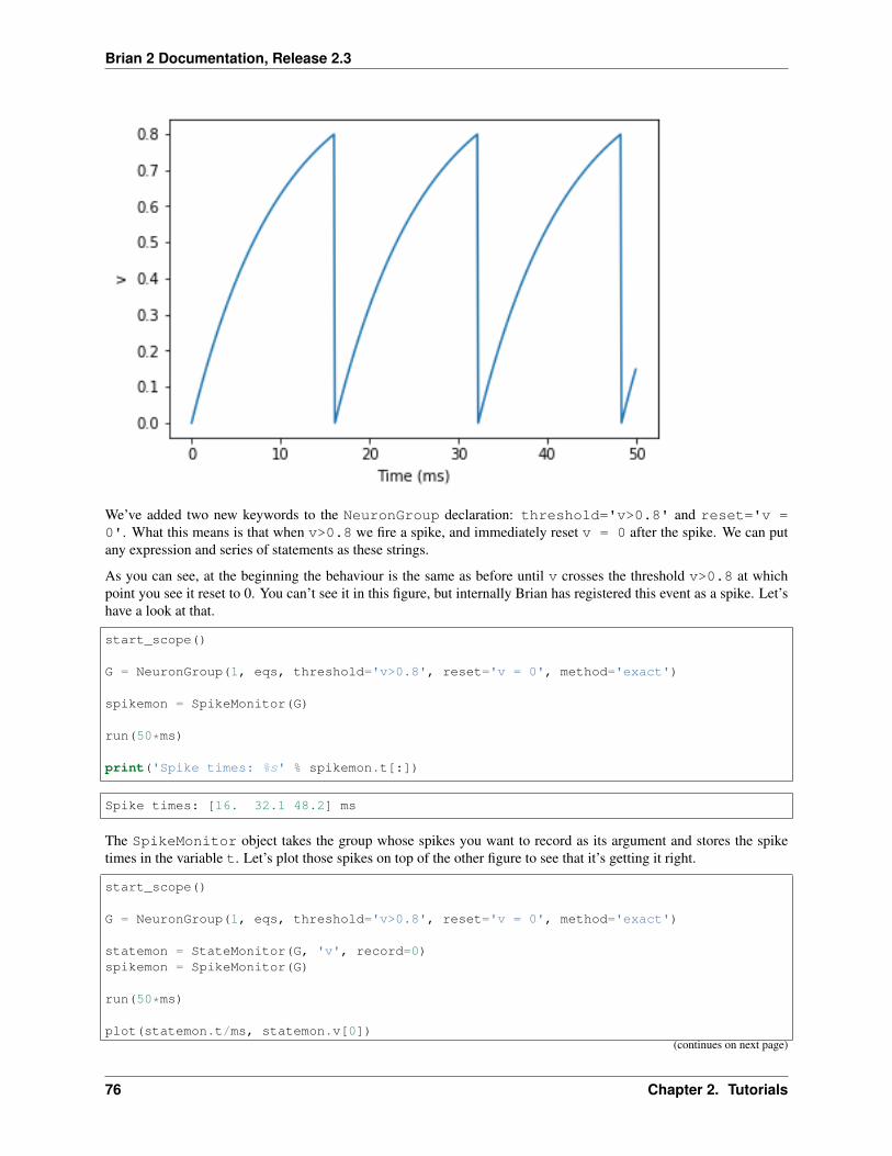
Brian 2 Documentation, Release 2.3
We’ve added two new keywords to the NeuronGroup declaration: threshold='v>0.8' and reset='v =0'. What this means is that when v>0.8 we fire a spike, and immediately reset v = 0 after the spike. We can putany expression and series of statements as these strings.
As you can see, at the beginning the behaviour is the same as before until v crosses the threshold v>0.8 at whichpoint you see it reset to 0. You can’t see it in this figure, but internally Brian has registered this event as a spike. Let’shave a look at that.
start_scope()
G = NeuronGroup(1, eqs, threshold='v>0.8', reset='v = 0', method='exact')
spikemon = SpikeMonitor(G)
run(50*ms)
print('Spike times: %s' % spikemon.t[:])
Spike times: [16. 32.1 48.2] ms
The SpikeMonitor object takes the group whose spikes you want to record as its argument and stores the spiketimes in the variable t. Let’s plot those spikes on top of the other figure to see that it’s getting it right.
start_scope()
G = NeuronGroup(1, eqs, threshold='v>0.8', reset='v = 0', method='exact')
statemon = StateMonitor(G, 'v', record=0)spikemon = SpikeMonitor(G)
run(50*ms)
plot(statemon.t/ms, statemon.v[0])(continues on next page)
76 Chapter 2. Tutorials

Brian 2 Documentation, Release 2.3
(continued from previous page)
for t in spikemon.t:axvline(t/ms, ls='--', c='C1', lw=3)
xlabel('Time (ms)')ylabel('v');
Here we’ve used the axvline command from matplotlib to draw an orange, dashed vertical line at the time ofeach spike recorded by the SpikeMonitor.
Now try changing the strings for threshold and reset in the cell above to see what happens.
2.1.4 Refractoriness
A common feature of neuron models is refractoriness. This means that after the neuron fires a spike it becomesrefractory for a certain duration and cannot fire another spike until this period is over. Here’s how we do that in Brian.
start_scope()
tau = 10*mseqs = '''dv/dt = (1-v)/tau : 1 (unless refractory)'''
G = NeuronGroup(1, eqs, threshold='v>0.8', reset='v = 0', refractory=5*ms, method=→˓'exact')
statemon = StateMonitor(G, 'v', record=0)spikemon = SpikeMonitor(G)
run(50*ms)
plot(statemon.t/ms, statemon.v[0])(continues on next page)
2.1. Introduction to Brian part 1: Neurons 77
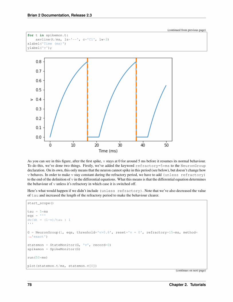
Brian 2 Documentation, Release 2.3
(continued from previous page)
for t in spikemon.t:axvline(t/ms, ls='--', c='C1', lw=3)
xlabel('Time (ms)')ylabel('v');
As you can see in this figure, after the first spike, v stays at 0 for around 5 ms before it resumes its normal behaviour.To do this, we’ve done two things. Firstly, we’ve added the keyword refractory=5*ms to the NeuronGroupdeclaration. On its own, this only means that the neuron cannot spike in this period (see below), but doesn’t change howv behaves. In order to make v stay constant during the refractory period, we have to add (unless refractory)to the end of the definition of v in the differential equations. What this means is that the differential equation determinesthe behaviour of v unless it’s refractory in which case it is switched off.
Here’s what would happen if we didn’t include (unless refractory). Note that we’ve also decreased the valueof tau and increased the length of the refractory period to make the behaviour clearer.
start_scope()
tau = 5*mseqs = '''dv/dt = (1-v)/tau : 1'''
G = NeuronGroup(1, eqs, threshold='v>0.8', reset='v = 0', refractory=15*ms, method=→˓'exact')
statemon = StateMonitor(G, 'v', record=0)spikemon = SpikeMonitor(G)
run(50*ms)
plot(statemon.t/ms, statemon.v[0])
(continues on next page)
78 Chapter 2. Tutorials
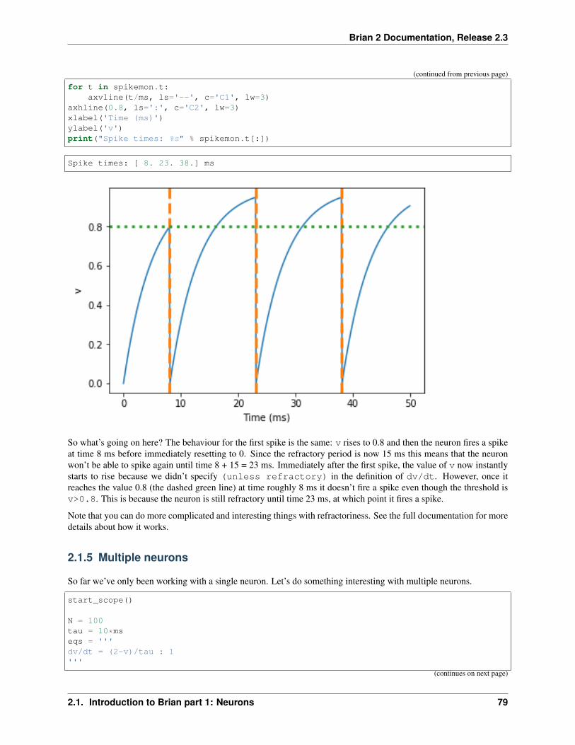
Brian 2 Documentation, Release 2.3
(continued from previous page)
for t in spikemon.t:axvline(t/ms, ls='--', c='C1', lw=3)
axhline(0.8, ls=':', c='C2', lw=3)xlabel('Time (ms)')ylabel('v')print("Spike times: %s" % spikemon.t[:])
Spike times: [ 8. 23. 38.] ms
So what’s going on here? The behaviour for the first spike is the same: v rises to 0.8 and then the neuron fires a spikeat time 8 ms before immediately resetting to 0. Since the refractory period is now 15 ms this means that the neuronwon’t be able to spike again until time 8 + 15 = 23 ms. Immediately after the first spike, the value of v now instantlystarts to rise because we didn’t specify (unless refractory) in the definition of dv/dt. However, once itreaches the value 0.8 (the dashed green line) at time roughly 8 ms it doesn’t fire a spike even though the threshold isv>0.8. This is because the neuron is still refractory until time 23 ms, at which point it fires a spike.
Note that you can do more complicated and interesting things with refractoriness. See the full documentation for moredetails about how it works.
2.1.5 Multiple neurons
So far we’ve only been working with a single neuron. Let’s do something interesting with multiple neurons.
start_scope()
N = 100tau = 10*mseqs = '''dv/dt = (2-v)/tau : 1'''
(continues on next page)
2.1. Introduction to Brian part 1: Neurons 79
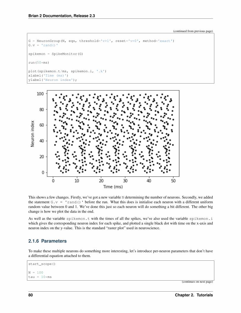
Brian 2 Documentation, Release 2.3
(continued from previous page)
G = NeuronGroup(N, eqs, threshold='v>1', reset='v=0', method='exact')G.v = 'rand()'
spikemon = SpikeMonitor(G)
run(50*ms)
plot(spikemon.t/ms, spikemon.i, '.k')xlabel('Time (ms)')ylabel('Neuron index');
This shows a few changes. Firstly, we’ve got a new variable N determining the number of neurons. Secondly, we addedthe statement G.v = 'rand()' before the run. What this does is initialise each neuron with a different uniformrandom value between 0 and 1. We’ve done this just so each neuron will do something a bit different. The other bigchange is how we plot the data in the end.
As well as the variable spikemon.t with the times of all the spikes, we’ve also used the variable spikemon.iwhich gives the corresponding neuron index for each spike, and plotted a single black dot with time on the x-axis andneuron index on the y-value. This is the standard “raster plot” used in neuroscience.
2.1.6 Parameters
To make these multiple neurons do something more interesting, let’s introduce per-neuron parameters that don’t havea differential equation attached to them.
start_scope()
N = 100tau = 10*ms
(continues on next page)
80 Chapter 2. Tutorials
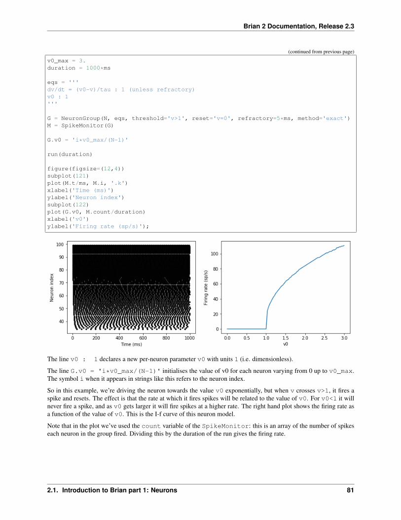
Brian 2 Documentation, Release 2.3
(continued from previous page)
v0_max = 3.duration = 1000*ms
eqs = '''dv/dt = (v0-v)/tau : 1 (unless refractory)v0 : 1'''
G = NeuronGroup(N, eqs, threshold='v>1', reset='v=0', refractory=5*ms, method='exact')M = SpikeMonitor(G)
G.v0 = 'i*v0_max/(N-1)'
run(duration)
figure(figsize=(12,4))subplot(121)plot(M.t/ms, M.i, '.k')xlabel('Time (ms)')ylabel('Neuron index')subplot(122)plot(G.v0, M.count/duration)xlabel('v0')ylabel('Firing rate (sp/s)');
The line v0 : 1 declares a new per-neuron parameter v0 with units 1 (i.e. dimensionless).
The line G.v0 = 'i*v0_max/(N-1)' initialises the value of v0 for each neuron varying from 0 up to v0_max.The symbol i when it appears in strings like this refers to the neuron index.
So in this example, we’re driving the neuron towards the value v0 exponentially, but when v crosses v>1, it fires aspike and resets. The effect is that the rate at which it fires spikes will be related to the value of v0. For v0<1 it willnever fire a spike, and as v0 gets larger it will fire spikes at a higher rate. The right hand plot shows the firing rate asa function of the value of v0. This is the I-f curve of this neuron model.
Note that in the plot we’ve used the count variable of the SpikeMonitor: this is an array of the number of spikeseach neuron in the group fired. Dividing this by the duration of the run gives the firing rate.
2.1. Introduction to Brian part 1: Neurons 81
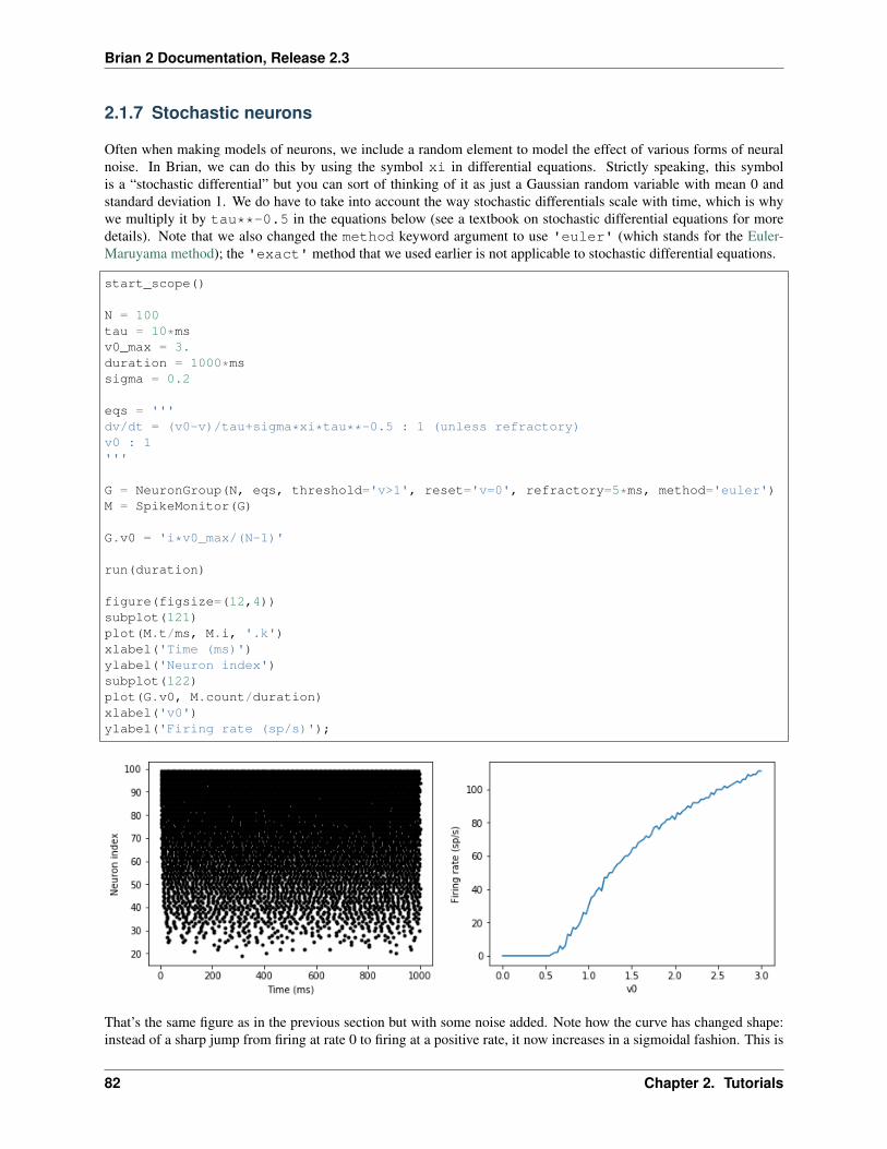
Brian 2 Documentation, Release 2.3
2.1.7 Stochastic neurons
Often when making models of neurons, we include a random element to model the effect of various forms of neuralnoise. In Brian, we can do this by using the symbol xi in differential equations. Strictly speaking, this symbolis a “stochastic differential” but you can sort of thinking of it as just a Gaussian random variable with mean 0 andstandard deviation 1. We do have to take into account the way stochastic differentials scale with time, which is whywe multiply it by tau**-0.5 in the equations below (see a textbook on stochastic differential equations for moredetails). Note that we also changed the method keyword argument to use 'euler' (which stands for the Euler-Maruyama method); the 'exact' method that we used earlier is not applicable to stochastic differential equations.
start_scope()
N = 100tau = 10*msv0_max = 3.duration = 1000*mssigma = 0.2
eqs = '''dv/dt = (v0-v)/tau+sigma*xi*tau**-0.5 : 1 (unless refractory)v0 : 1'''
G = NeuronGroup(N, eqs, threshold='v>1', reset='v=0', refractory=5*ms, method='euler')M = SpikeMonitor(G)
G.v0 = 'i*v0_max/(N-1)'
run(duration)
figure(figsize=(12,4))subplot(121)plot(M.t/ms, M.i, '.k')xlabel('Time (ms)')ylabel('Neuron index')subplot(122)plot(G.v0, M.count/duration)xlabel('v0')ylabel('Firing rate (sp/s)');
That’s the same figure as in the previous section but with some noise added. Note how the curve has changed shape:instead of a sharp jump from firing at rate 0 to firing at a positive rate, it now increases in a sigmoidal fashion. This is
82 Chapter 2. Tutorials

Brian 2 Documentation, Release 2.3
because no matter how small the driving force the randomness may cause it to fire a spike.
2.1.8 End of tutorial
That’s the end of this part of the tutorial. The cell below has another example. See if you can work out what it isdoing and why. Try adding a StateMonitor to record the values of the variables for one of the neurons to help youunderstand it.
You could also try out the things you’ve learned in this cell.
Once you’re done with that you can move on to the next tutorial on Synapses.
start_scope()
N = 1000tau = 10*msvr = -70*mVvt0 = -50*mVdelta_vt0 = 5*mVtau_t = 100*mssigma = 0.5*(vt0-vr)v_drive = 2*(vt0-vr)duration = 100*ms
eqs = '''dv/dt = (v_drive+vr-v)/tau + sigma*xi*tau**-0.5 : voltdvt/dt = (vt0-vt)/tau_t : volt'''
reset = '''v = vrvt += delta_vt0'''
G = NeuronGroup(N, eqs, threshold='v>vt', reset=reset, refractory=5*ms, method='euler→˓')spikemon = SpikeMonitor(G)
G.v = 'rand()*(vt0-vr)+vr'G.vt = vt0
run(duration)
_ = hist(spikemon.t/ms, 100, histtype='stepfilled', facecolor='k',→˓weights=ones(len(spikemon))/(N*defaultclock.dt))xlabel('Time (ms)')ylabel('Instantaneous firing rate (sp/s)');
2.1. Introduction to Brian part 1: Neurons 83

Brian 2 Documentation, Release 2.3
2.2 Introduction to Brian part 2: Synapses
If you haven’t yet read part 1: Neurons, go read that now.
As before we start by importing the Brian package and setting up matplotlib for IPython:
from brian2 import *%matplotlib inline
2.2.1 The simplest Synapse
Once you have some neurons, the next step is to connect them up via synapses. We’ll start out with doing the simplestpossible type of synapse that causes an instantaneous change in a variable after a spike.
start_scope()
eqs = '''dv/dt = (I-v)/tau : 1I : 1tau : second'''G = NeuronGroup(2, eqs, threshold='v>1', reset='v = 0', method='exact')G.I = [2, 0]G.tau = [10, 100]*ms
# Comment these two lines out to see what happens without SynapsesS = Synapses(G, G, on_pre='v_post += 0.2')S.connect(i=0, j=1)
(continues on next page)
84 Chapter 2. Tutorials

Brian 2 Documentation, Release 2.3
(continued from previous page)
M = StateMonitor(G, 'v', record=True)
run(100*ms)
plot(M.t/ms, M.v[0], label='Neuron 0')plot(M.t/ms, M.v[1], label='Neuron 1')xlabel('Time (ms)')ylabel('v')legend();
There are a few things going on here. First of all, let’s recap what is going on with the NeuronGroup. We’ve createdtwo neurons, each of which has the same differential equation but different values for parameters I and tau. Neuron 0has I=2 and tau=10*ms which means that is driven to repeatedly spike at a fairly high rate. Neuron 1 has I=0 andtau=100*ms which means that on its own - without the synapses - it won’t spike at all (the driving current I is 0).You can prove this to yourself by commenting out the two lines that define the synapse.
Next we define the synapses: Synapses(source, target, ...) means that we are defining a synaptic modelthat goes from source to target. In this case, the source and target are both the same, the group G. The syntaxon_pre='v_post += 0.2' means that when a spike occurs in the presynaptic neuron (hence on_pre) it causesan instantaneous change to happen v_post += 0.2. The _post means that the value of v referred to is the post-synaptic value, and it is increased by 0.2. So in total, what this model says is that whenever two neurons in G areconnected by a synapse, when the source neuron fires a spike the target neuron will have its value of v increased by0.2.
However, at this point we have only defined the synapse model, we haven’t actually created any synapses. The nextline S.connect(i=0, j=1) creates a synapse from neuron 0 to neuron 1.
2.2.2 Adding a weight
In the previous section, we hard coded the weight of the synapse to be the value 0.2, but often we would to allow thisto be different for different synapses. We do that by introducing synapse equations.
2.2. Introduction to Brian part 2: Synapses 85

Brian 2 Documentation, Release 2.3
start_scope()
eqs = '''dv/dt = (I-v)/tau : 1I : 1tau : second'''G = NeuronGroup(3, eqs, threshold='v>1', reset='v = 0', method='exact')G.I = [2, 0, 0]G.tau = [10, 100, 100]*ms
# Comment these two lines out to see what happens without SynapsesS = Synapses(G, G, 'w : 1', on_pre='v_post += w')S.connect(i=0, j=[1, 2])S.w = 'j*0.2'
M = StateMonitor(G, 'v', record=True)
run(50*ms)
plot(M.t/ms, M.v[0], label='Neuron 0')plot(M.t/ms, M.v[1], label='Neuron 1')plot(M.t/ms, M.v[2], label='Neuron 2')xlabel('Time (ms)')ylabel('v')legend();
This example behaves very similarly to the previous example, but now there’s a synaptic weight variable w. The string'w : 1' is an equation string, precisely the same as for neurons, that defines a single dimensionless parameterw. We changed the behaviour on a spike to on_pre='v_post += w' now, so that each synapse can behavedifferently depending on the value of w. To illustrate this, we’ve made a third neuron which behaves precisely thesame as the second neuron, and connected neuron 0 to both neurons 1 and 2. We’ve also set the weights via S.w ='j*0.2'. When i and j occur in the context of synapses, i refers to the source neuron index, and j to the target
86 Chapter 2. Tutorials
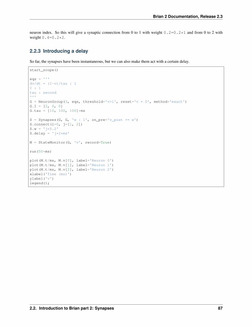
Brian 2 Documentation, Release 2.3
neuron index. So this will give a synaptic connection from 0 to 1 with weight 0.2=0.2*1 and from 0 to 2 withweight 0.4=0.2*2.
2.2.3 Introducing a delay
So far, the synapses have been instantaneous, but we can also make them act with a certain delay.
start_scope()
eqs = '''dv/dt = (I-v)/tau : 1I : 1tau : second'''G = NeuronGroup(3, eqs, threshold='v>1', reset='v = 0', method='exact')G.I = [2, 0, 0]G.tau = [10, 100, 100]*ms
S = Synapses(G, G, 'w : 1', on_pre='v_post += w')S.connect(i=0, j=[1, 2])S.w = 'j*0.2'S.delay = 'j*2*ms'
M = StateMonitor(G, 'v', record=True)
run(50*ms)
plot(M.t/ms, M.v[0], label='Neuron 0')plot(M.t/ms, M.v[1], label='Neuron 1')plot(M.t/ms, M.v[2], label='Neuron 2')xlabel('Time (ms)')ylabel('v')legend();
2.2. Introduction to Brian part 2: Synapses 87

Brian 2 Documentation, Release 2.3
As you can see, that’s as simple as adding a line S.delay = 'j*2*ms' so that the synapse from 0 to 1 has a delayof 2 ms, and from 0 to 2 has a delay of 4 ms.
2.2.4 More complex connectivity
So far, we specified the synaptic connectivity explicitly, but for larger networks this isn’t usually possible. For that,we usually want to specify some condition.
start_scope()
N = 10G = NeuronGroup(N, 'v:1')S = Synapses(G, G)S.connect(condition='i!=j', p=0.2)
Here we’ve created a dummy neuron group of N neurons and a dummy synapses model that doens’t actually do any-thing just to demonstrate the connectivity. The line S.connect(condition='i!=j', p=0.2) will connectall pairs of neurons i and j with probability 0.2 as long as the condition i!=j holds. So, how can we see thatconnectivity? Here’s a little function that will let us visualise it.
def visualise_connectivity(S):Ns = len(S.source)Nt = len(S.target)figure(figsize=(10, 4))subplot(121)plot(zeros(Ns), arange(Ns), 'ok', ms=10)plot(ones(Nt), arange(Nt), 'ok', ms=10)for i, j in zip(S.i, S.j):
plot([0, 1], [i, j], '-k')xticks([0, 1], ['Source', 'Target'])ylabel('Neuron index')
(continues on next page)
88 Chapter 2. Tutorials

Brian 2 Documentation, Release 2.3
(continued from previous page)
xlim(-0.1, 1.1)ylim(-1, max(Ns, Nt))subplot(122)plot(S.i, S.j, 'ok')xlim(-1, Ns)ylim(-1, Nt)xlabel('Source neuron index')ylabel('Target neuron index')
visualise_connectivity(S)
There are two plots here. On the left hand side, you see a vertical line of circles indicating source neurons on the left,and a vertical line indicating target neurons on the right, and a line between two neurons that have a synapse. On theright hand side is another way of visualising the same thing. Here each black dot is a synapse, with x value the sourceneuron index, and y value the target neuron index.
Let’s see how these figures change as we change the probability of a connection:
start_scope()
N = 10G = NeuronGroup(N, 'v:1')
for p in [0.1, 0.5, 1.0]:S = Synapses(G, G)S.connect(condition='i!=j', p=p)visualise_connectivity(S)suptitle('p = '+str(p))
2.2. Introduction to Brian part 2: Synapses 89
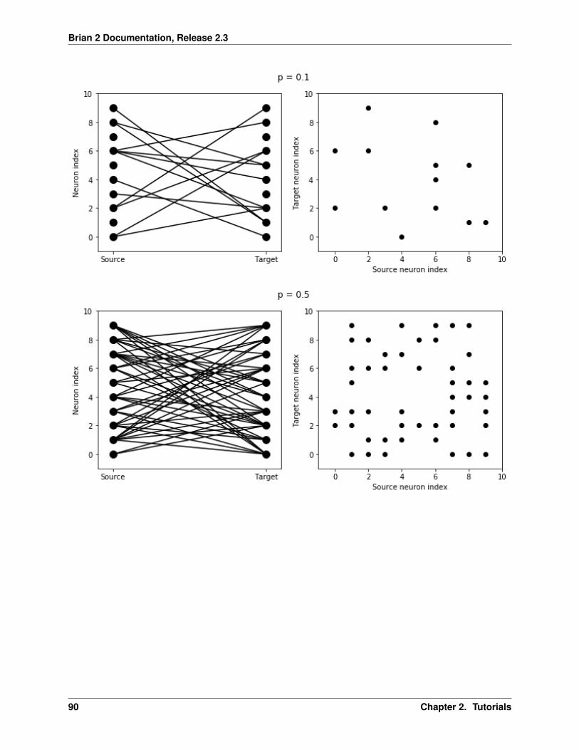
Brian 2 Documentation, Release 2.3
90 Chapter 2. Tutorials

Brian 2 Documentation, Release 2.3
And let’s see what another connectivity condition looks like. This one will only connect neighbouring neurons.
start_scope()
N = 10G = NeuronGroup(N, 'v:1')
S = Synapses(G, G)S.connect(condition='abs(i-j)<4 and i!=j')visualise_connectivity(S)
Try using that cell to see how other connectivity conditions look like.
You can also use the generator syntax to create connections like this more efficiently. In small examples like this,it doesn’t matter, but for large numbers of neurons it can be much more efficient to specify directly which neuronsshould be connected than to specify just a condition. Note that the following example uses skip_if_invalid toavoid errors at the boundaries (e.g. do not try to connect the neuron with index 1 to a neuron with index -2).
2.2. Introduction to Brian part 2: Synapses 91
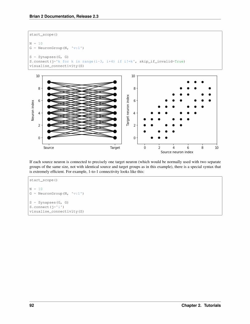
Brian 2 Documentation, Release 2.3
start_scope()
N = 10G = NeuronGroup(N, 'v:1')
S = Synapses(G, G)S.connect(j='k for k in range(i-3, i+4) if i!=k', skip_if_invalid=True)visualise_connectivity(S)
If each source neuron is connected to precisely one target neuron (which would be normally used with two separategroups of the same size, not with identical source and target groups as in this example), there is a special syntax thatis extremely efficient. For example, 1-to-1 connectivity looks like this:
start_scope()
N = 10G = NeuronGroup(N, 'v:1')
S = Synapses(G, G)S.connect(j='i')visualise_connectivity(S)
92 Chapter 2. Tutorials

Brian 2 Documentation, Release 2.3
You can also do things like specifying the value of weights with a string. Let’s see an example where we assign eachneuron a spatial location and have a distance-dependent connectivity function. We visualise the weight of a synapseby the size of the marker.
start_scope()
N = 30neuron_spacing = 50*umetrewidth = N/4.0*neuron_spacing
# Neuron has one variable x, its positionG = NeuronGroup(N, 'x : metre')G.x = 'i*neuron_spacing'
# All synapses are connected (excluding self-connections)S = Synapses(G, G, 'w : 1')S.connect(condition='i!=j')# Weight varies with distanceS.w = 'exp(-(x_pre-x_post)**2/(2*width**2))'
scatter(S.x_pre/um, S.x_post/um, S.w*20)xlabel('Source neuron position (um)')ylabel('Target neuron position (um)');
2.2. Introduction to Brian part 2: Synapses 93

Brian 2 Documentation, Release 2.3
Now try changing that function and seeing how the plot changes.
2.2.5 More complex synapse models: STDP
Brian’s synapse framework is very general and can do things like short-term plasticity (STP) or spike-timing dependentplasticity (STDP). Let’s see how that works for STDP.
STDP is normally defined by an equation something like this:
∆𝑤 =∑𝑡𝑝𝑟𝑒
∑𝑡𝑝𝑜𝑠𝑡
𝑊 (𝑡𝑝𝑜𝑠𝑡 − 𝑡𝑝𝑟𝑒)
That is, the change in synaptic weight w is the sum over all presynaptic spike times 𝑡𝑝𝑟𝑒 and postsynaptic spike times𝑡𝑝𝑜𝑠𝑡 of some function 𝑊 of the difference in these spike times. A commonly used function 𝑊 is:
𝑊 (∆𝑡) =
{𝐴𝑝𝑟𝑒𝑒
−Δ𝑡/𝜏𝑝𝑟𝑒 ∆𝑡 > 0
𝐴𝑝𝑜𝑠𝑡𝑒Δ𝑡/𝜏𝑝𝑜𝑠𝑡 ∆𝑡 < 0
This function looks like this:
tau_pre = tau_post = 20*msA_pre = 0.01A_post = -A_pre*1.05delta_t = linspace(-50, 50, 100)*msW = where(delta_t>0, A_pre*exp(-delta_t/tau_pre), A_post*exp(delta_t/tau_post))plot(delta_t/ms, W)xlabel(r'$\Delta t$ (ms)')ylabel('W')axhline(0, ls='-', c='k');
94 Chapter 2. Tutorials

Brian 2 Documentation, Release 2.3
Simulating it directly using this equation though would be very inefficient, because we would have to sum over allpairs of spikes. That would also be physiologically unrealistic because the neuron cannot remember all its previousspike times. It turns out there is a more efficient and physiologically more plausible way to get the same effect.
We define two new variables 𝑎𝑝𝑟𝑒 and 𝑎𝑝𝑜𝑠𝑡 which are “traces” of pre- and post-synaptic activity, governed by thedifferential equations:
𝜏𝑝𝑟𝑒d
d𝑡𝑎𝑝𝑟𝑒 = −𝑎𝑝𝑟𝑒 (2.1)
𝜏𝑝𝑜𝑠𝑡d
d𝑡𝑎𝑝𝑜𝑠𝑡 = −𝑎𝑝𝑜𝑠𝑡(2.2)
When a presynaptic spike occurs, the presynaptic trace is updated and the weight is modified according to the rule:
𝑎𝑝𝑟𝑒 → 𝑎𝑝𝑟𝑒 + 𝐴𝑝𝑟𝑒 (2.3)𝑤 → 𝑤 + 𝑎𝑝𝑜𝑠𝑡(2.4)
When a postsynaptic spike occurs:
𝑎𝑝𝑜𝑠𝑡 → 𝑎𝑝𝑜𝑠𝑡 + 𝐴𝑝𝑜𝑠𝑡 (2.5)𝑤 → 𝑤 + 𝑎𝑝𝑟𝑒(2.6)
To see that this formulation is equivalent, you just have to check that the equations sum linearly, and consider twocases: what happens if the presynaptic spike occurs before the postsynaptic spike, and vice versa. Try drawing apicture of it.
Now that we have a formulation that relies only on differential equations and spike events, we can turn that into Briancode.
start_scope()
taupre = taupost = 20*mswmax = 0.01
(continues on next page)
2.2. Introduction to Brian part 2: Synapses 95
Brian 2 Documentation, Release 2.3
(continued from previous page)
Apre = 0.01Apost = -Apre*taupre/taupost*1.05
G = NeuronGroup(1, 'v:1', threshold='v>1')
S = Synapses(G, G,'''w : 1dapre/dt = -apre/taupre : 1 (event-driven)dapost/dt = -apost/taupost : 1 (event-driven)''',on_pre='''v_post += wapre += Aprew = clip(w+apost, 0, wmax)''',on_post='''apost += Apostw = clip(w+apre, 0, wmax)''')
There are a few things to see there. Firstly, when defining the synapses we’ve given a more complicated multi-line string defining three synaptic variables (w, apre and apost). We’ve also got a new bit of syntax there,(event-driven) after the definitions of apre and apost. What this means is that although these two vari-ables evolve continuously over time, Brian should only update them at the time of an event (a spike). This is becausewe don’t need the values of apre and apost except at spike times, and it is more efficient to only update them whenneeded.
Next we have a on_pre=... argument. The first line is v_post += w: this is the line that actually applies thesynaptic weight to the target neuron. The second line is apre += Apre which encodes the rule above. In thethird line, we’re also encoding the rule above but we’ve added one extra feature: we’ve clamped the synaptic weightsbetween a minimum of 0 and a maximum of wmax so that the weights can’t get too large or negative. The functionclip(x, low, high) does this.
Finally, we have a on_post=... argument. This gives the statements to calculate when a post-synaptic neuron fires.Note that we do not modify v in this case, only the synaptic variables.
Now let’s see how all the variables behave when a presynaptic spike arrives some time before a postsynaptic spike.
start_scope()
taupre = taupost = 20*mswmax = 0.01Apre = 0.01Apost = -Apre*taupre/taupost*1.05
G = NeuronGroup(2, 'v:1', threshold='t>(1+i)*10*ms', refractory=100*ms)
S = Synapses(G, G,'''w : 1dapre/dt = -apre/taupre : 1 (clock-driven)dapost/dt = -apost/taupost : 1 (clock-driven)''',on_pre='''v_post += wapre += Apre
(continues on next page)
96 Chapter 2. Tutorials
Brian 2 Documentation, Release 2.3
(continued from previous page)
w = clip(w+apost, 0, wmax)''',on_post='''apost += Apostw = clip(w+apre, 0, wmax)''', method='linear')
S.connect(i=0, j=1)M = StateMonitor(S, ['w', 'apre', 'apost'], record=True)
run(30*ms)
figure(figsize=(4, 8))subplot(211)plot(M.t/ms, M.apre[0], label='apre')plot(M.t/ms, M.apost[0], label='apost')legend()subplot(212)plot(M.t/ms, M.w[0], label='w')legend(loc='best')xlabel('Time (ms)');
2.2. Introduction to Brian part 2: Synapses 97

Brian 2 Documentation, Release 2.3
A couple of things to note here. First of all, we’ve used a trick to make neuron 0 fire a spike at time 10 ms, and neuron1 at time 20 ms. Can you see how that works?
Secondly, we’ve replaced the (event-driven) by (clock-driven) so you can see how apre and apostevolve over time. Try reverting this change and see what happens.
Try changing the times of the spikes to see what happens.
Finally, let’s verify that this formulation is equivalent to the original one.
start_scope()
taupre = taupost = 20*msApre = 0.01
(continues on next page)
98 Chapter 2. Tutorials

Brian 2 Documentation, Release 2.3
(continued from previous page)
Apost = -Apre*taupre/taupost*1.05tmax = 50*msN = 100
# Presynaptic neurons G spike at times from 0 to tmax# Postsynaptic neurons G spike at times from tmax to 0# So difference in spike times will vary from -tmax to +tmaxG = NeuronGroup(N, 'tspike:second', threshold='t>tspike', refractory=100*ms)H = NeuronGroup(N, 'tspike:second', threshold='t>tspike', refractory=100*ms)G.tspike = 'i*tmax/(N-1)'H.tspike = '(N-1-i)*tmax/(N-1)'
S = Synapses(G, H,'''w : 1dapre/dt = -apre/taupre : 1 (event-driven)dapost/dt = -apost/taupost : 1 (event-driven)''',on_pre='''apre += Aprew = w+apost''',on_post='''apost += Apostw = w+apre''')
S.connect(j='i')
run(tmax+1*ms)
plot((H.tspike-G.tspike)/ms, S.w)xlabel(r'$\Delta t$ (ms)')ylabel(r'$\Delta w$')axhline(0, ls='-', c='k');
2.2. Introduction to Brian part 2: Synapses 99
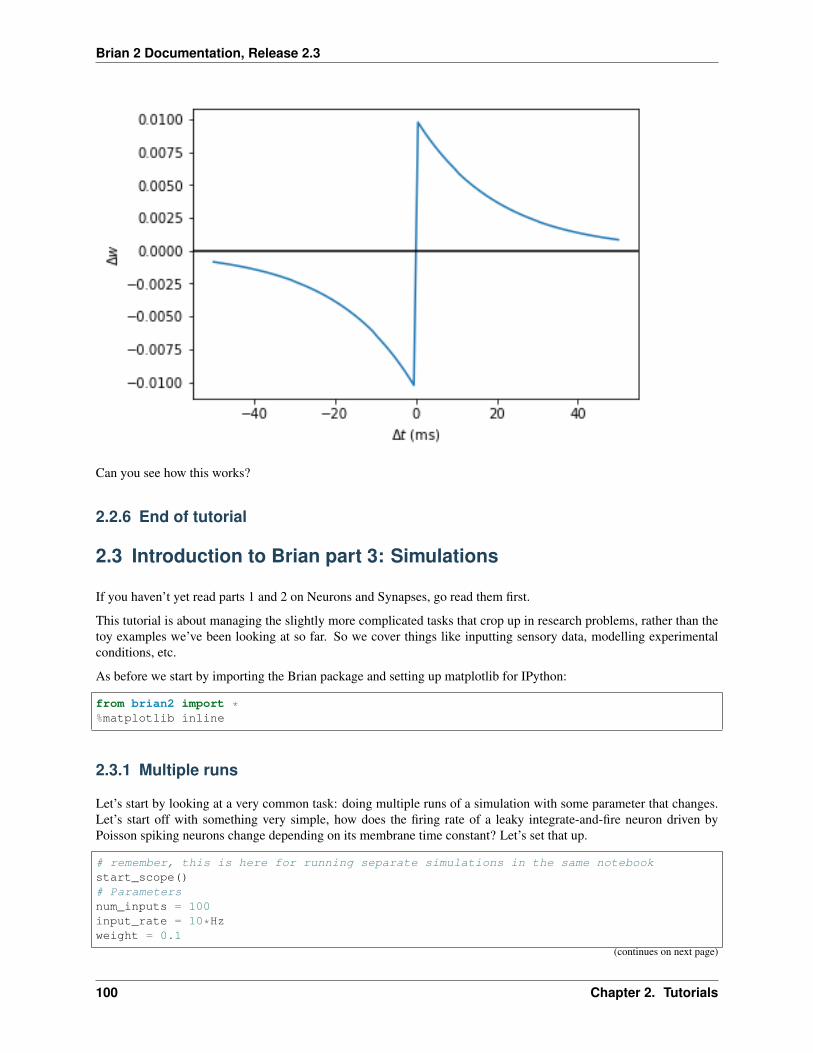
Brian 2 Documentation, Release 2.3
Can you see how this works?
2.2.6 End of tutorial
2.3 Introduction to Brian part 3: Simulations
If you haven’t yet read parts 1 and 2 on Neurons and Synapses, go read them first.
This tutorial is about managing the slightly more complicated tasks that crop up in research problems, rather than thetoy examples we’ve been looking at so far. So we cover things like inputting sensory data, modelling experimentalconditions, etc.
As before we start by importing the Brian package and setting up matplotlib for IPython:
from brian2 import *%matplotlib inline
2.3.1 Multiple runs
Let’s start by looking at a very common task: doing multiple runs of a simulation with some parameter that changes.Let’s start off with something very simple, how does the firing rate of a leaky integrate-and-fire neuron driven byPoisson spiking neurons change depending on its membrane time constant? Let’s set that up.
# remember, this is here for running separate simulations in the same notebookstart_scope()# Parametersnum_inputs = 100input_rate = 10*Hzweight = 0.1
(continues on next page)
100 Chapter 2. Tutorials

Brian 2 Documentation, Release 2.3
(continued from previous page)
# Range of time constantstau_range = linspace(1, 10, 30)*ms# Use this list to store output ratesoutput_rates = []# Iterate over range of time constantsfor tau in tau_range:
# Construct the network each timeP = PoissonGroup(num_inputs, rates=input_rate)eqs = '''dv/dt = -v/tau : 1'''G = NeuronGroup(1, eqs, threshold='v>1', reset='v=0', method='exact')S = Synapses(P, G, on_pre='v += weight')S.connect()M = SpikeMonitor(G)# Run it and store the output firing rate in the listrun(1*second)output_rates.append(M.num_spikes/second)
# And plot itplot(tau_range/ms, output_rates)xlabel(r'$\tau$ (ms)')ylabel('Firing rate (sp/s)');
Now if you’re running the notebook, you’ll see that this was a little slow to run. The reason is that for each loop,you’re recreating the objects from scratch. We can improve that by setting up the network just once. We store a copyof the state of the network before the loop, and restore it at the beginning of each iteration.
start_scope()num_inputs = 100input_rate = 10*Hzweight = 0.1
(continues on next page)
2.3. Introduction to Brian part 3: Simulations 101
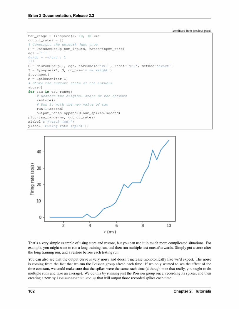
Brian 2 Documentation, Release 2.3
(continued from previous page)
tau_range = linspace(1, 10, 30)*msoutput_rates = []# Construct the network just onceP = PoissonGroup(num_inputs, rates=input_rate)eqs = '''dv/dt = -v/tau : 1'''G = NeuronGroup(1, eqs, threshold='v>1', reset='v=0', method='exact')S = Synapses(P, G, on_pre='v += weight')S.connect()M = SpikeMonitor(G)# Store the current state of the networkstore()for tau in tau_range:
# Restore the original state of the networkrestore()# Run it with the new value of taurun(1*second)output_rates.append(M.num_spikes/second)
plot(tau_range/ms, output_rates)xlabel(r'$\tau$ (ms)')ylabel('Firing rate (sp/s)');
That’s a very simple example of using store and restore, but you can use it in much more complicated situations. Forexample, you might want to run a long training run, and then run multiple test runs afterwards. Simply put a store afterthe long training run, and a restore before each testing run.
You can also see that the output curve is very noisy and doesn’t increase monotonically like we’d expect. The noiseis coming from the fact that we run the Poisson group afresh each time. If we only wanted to see the effect of thetime constant, we could make sure that the spikes were the same each time (although note that really, you ought to domultiple runs and take an average). We do this by running just the Poisson group once, recording its spikes, and thencreating a new SpikeGeneratorGroup that will output those recorded spikes each time.
102 Chapter 2. Tutorials

Brian 2 Documentation, Release 2.3
start_scope()num_inputs = 100input_rate = 10*Hzweight = 0.1tau_range = linspace(1, 10, 30)*msoutput_rates = []# Construct the Poisson spikes just onceP = PoissonGroup(num_inputs, rates=input_rate)MP = SpikeMonitor(P)# We use a Network object because later on we don't# want to include these objectsnet = Network(P, MP)net.run(1*second)# And keep a copy of those spikesspikes_i = MP.ispikes_t = MP.t# Now construct the network that we run each time# SpikeGeneratorGroup gets the spikes that we created beforeSGG = SpikeGeneratorGroup(num_inputs, spikes_i, spikes_t)eqs = '''dv/dt = -v/tau : 1'''G = NeuronGroup(1, eqs, threshold='v>1', reset='v=0', method='exact')S = Synapses(SGG, G, on_pre='v += weight')S.connect()M = SpikeMonitor(G)# Store the current state of the networknet = Network(SGG, G, S, M)net.store()for tau in tau_range:
# Restore the original state of the networknet.restore()# Run it with the new value of taunet.run(1*second)output_rates.append(M.num_spikes/second)
plot(tau_range/ms, output_rates)xlabel(r'$\tau$ (ms)')ylabel('Firing rate (sp/s)');
2.3. Introduction to Brian part 3: Simulations 103
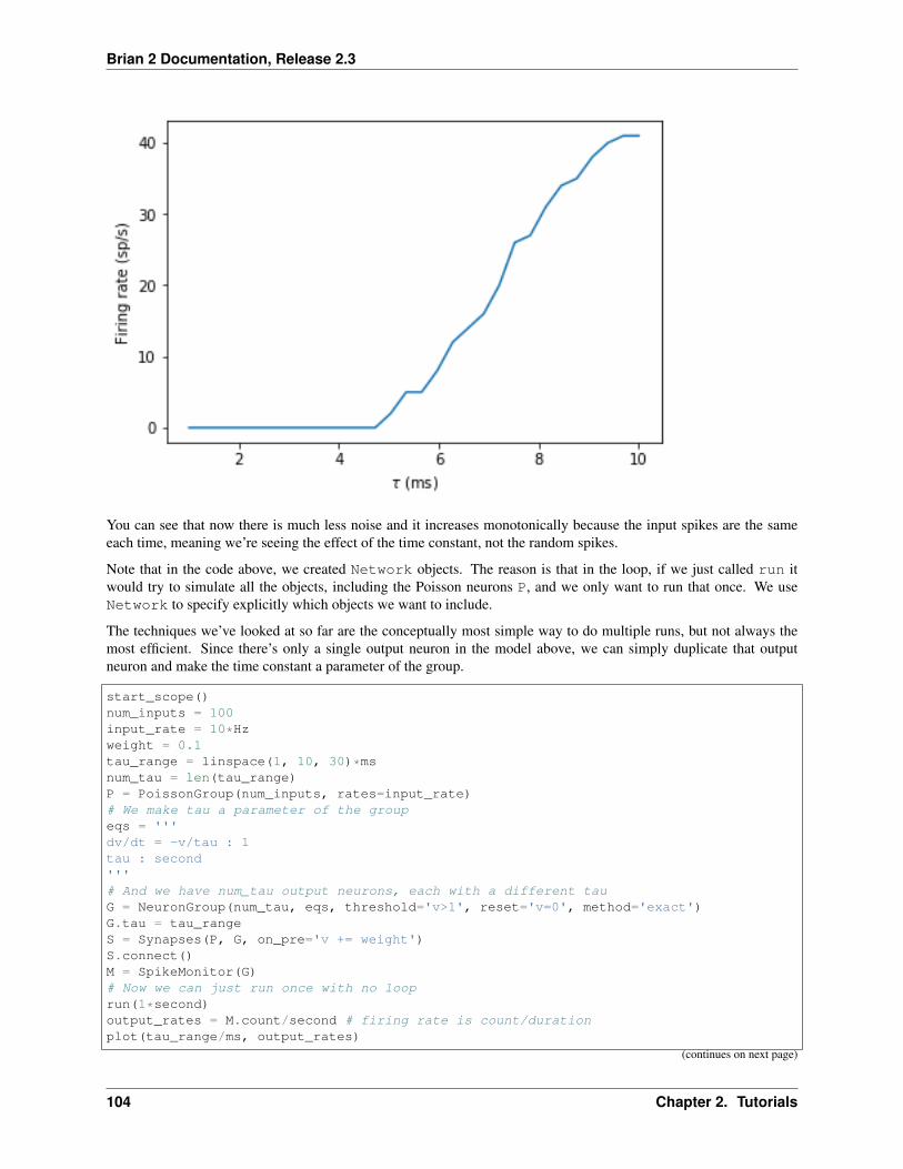
Brian 2 Documentation, Release 2.3
You can see that now there is much less noise and it increases monotonically because the input spikes are the sameeach time, meaning we’re seeing the effect of the time constant, not the random spikes.
Note that in the code above, we created Network objects. The reason is that in the loop, if we just called run itwould try to simulate all the objects, including the Poisson neurons P, and we only want to run that once. We useNetwork to specify explicitly which objects we want to include.
The techniques we’ve looked at so far are the conceptually most simple way to do multiple runs, but not always themost efficient. Since there’s only a single output neuron in the model above, we can simply duplicate that outputneuron and make the time constant a parameter of the group.
start_scope()num_inputs = 100input_rate = 10*Hzweight = 0.1tau_range = linspace(1, 10, 30)*msnum_tau = len(tau_range)P = PoissonGroup(num_inputs, rates=input_rate)# We make tau a parameter of the groupeqs = '''dv/dt = -v/tau : 1tau : second'''# And we have num_tau output neurons, each with a different tauG = NeuronGroup(num_tau, eqs, threshold='v>1', reset='v=0', method='exact')G.tau = tau_rangeS = Synapses(P, G, on_pre='v += weight')S.connect()M = SpikeMonitor(G)# Now we can just run once with no looprun(1*second)output_rates = M.count/second # firing rate is count/durationplot(tau_range/ms, output_rates)
(continues on next page)
104 Chapter 2. Tutorials

Brian 2 Documentation, Release 2.3
(continued from previous page)
xlabel(r'$\tau$ (ms)')ylabel('Firing rate (sp/s)');
WARNING "tau" is an internal variable of group "neurongroup_2", but also exists in→˓the run namespace with the value 10. * msecond. The internal variable will be used.→˓[brian2.groups.group.Group.resolve.resolution_conflict]
You can see that this is much faster again! It’s a little bit more complicated conceptually, and it’s not always possibleto do this trick, but it can be much more efficient if it’s possible.
Let’s finish with this example by having a quick look at how the mean and standard deviation of the interspike intervalsdepends on the time constant.
trains = M.spike_trains()isi_mu = full(num_tau, nan)*secondisi_std = full(num_tau, nan)*secondfor idx in range(num_tau):
train = diff(trains[idx])if len(train)>1:
isi_mu[idx] = mean(train)isi_std[idx] = std(train)
errorbar(tau_range/ms, isi_mu/ms, yerr=isi_std/ms)xlabel(r'$\tau$ (ms)')ylabel('Interspike interval (ms)');
2.3. Introduction to Brian part 3: Simulations 105
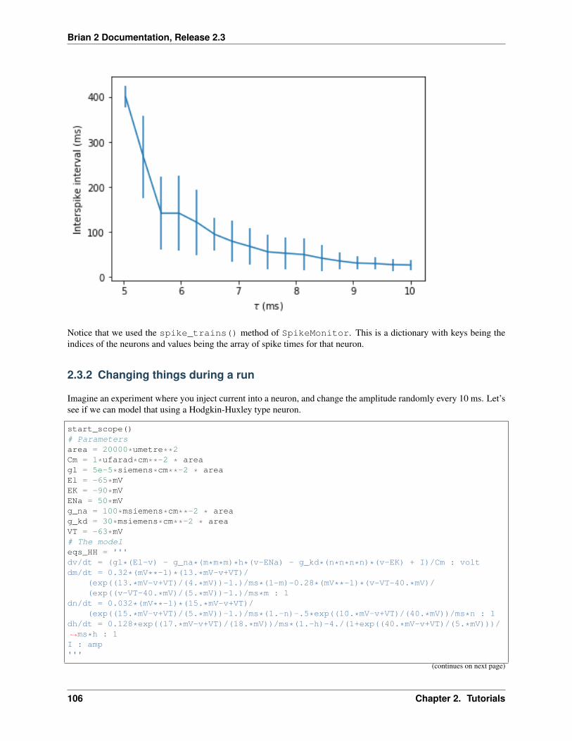
Brian 2 Documentation, Release 2.3
Notice that we used the spike_trains() method of SpikeMonitor. This is a dictionary with keys being theindices of the neurons and values being the array of spike times for that neuron.
2.3.2 Changing things during a run
Imagine an experiment where you inject current into a neuron, and change the amplitude randomly every 10 ms. Let’ssee if we can model that using a Hodgkin-Huxley type neuron.
start_scope()# Parametersarea = 20000*umetre**2Cm = 1*ufarad*cm**-2 * areagl = 5e-5*siemens*cm**-2 * areaEl = -65*mVEK = -90*mVENa = 50*mVg_na = 100*msiemens*cm**-2 * areag_kd = 30*msiemens*cm**-2 * areaVT = -63*mV# The modeleqs_HH = '''dv/dt = (gl*(El-v) - g_na*(m*m*m)*h*(v-ENa) - g_kd*(n*n*n*n)*(v-EK) + I)/Cm : voltdm/dt = 0.32*(mV**-1)*(13.*mV-v+VT)/
(exp((13.*mV-v+VT)/(4.*mV))-1.)/ms*(1-m)-0.28*(mV**-1)*(v-VT-40.*mV)/(exp((v-VT-40.*mV)/(5.*mV))-1.)/ms*m : 1
dn/dt = 0.032*(mV**-1)*(15.*mV-v+VT)/(exp((15.*mV-v+VT)/(5.*mV))-1.)/ms*(1.-n)-.5*exp((10.*mV-v+VT)/(40.*mV))/ms*n : 1
dh/dt = 0.128*exp((17.*mV-v+VT)/(18.*mV))/ms*(1.-h)-4./(1+exp((40.*mV-v+VT)/(5.*mV)))/→˓ms*h : 1I : amp'''
(continues on next page)
106 Chapter 2. Tutorials
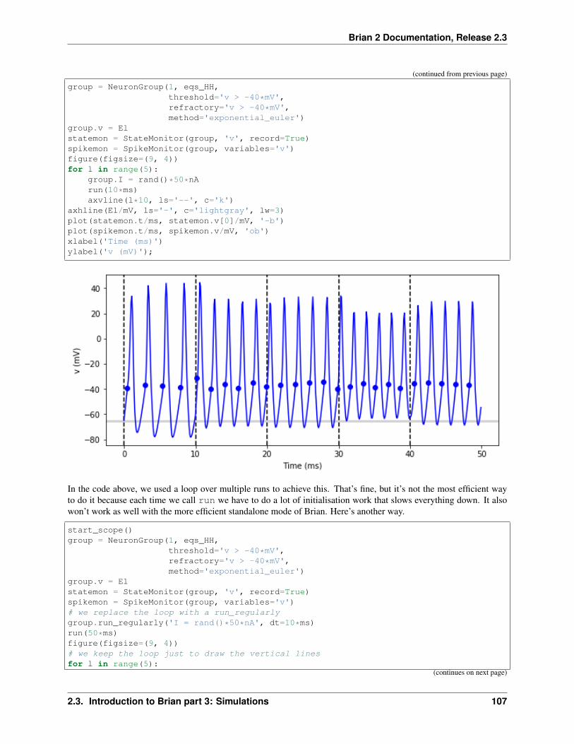
Brian 2 Documentation, Release 2.3
(continued from previous page)
group = NeuronGroup(1, eqs_HH,threshold='v > -40*mV',refractory='v > -40*mV',method='exponential_euler')
group.v = Elstatemon = StateMonitor(group, 'v', record=True)spikemon = SpikeMonitor(group, variables='v')figure(figsize=(9, 4))for l in range(5):
group.I = rand()*50*nArun(10*ms)axvline(l*10, ls='--', c='k')
axhline(El/mV, ls='-', c='lightgray', lw=3)plot(statemon.t/ms, statemon.v[0]/mV, '-b')plot(spikemon.t/ms, spikemon.v/mV, 'ob')xlabel('Time (ms)')ylabel('v (mV)');
In the code above, we used a loop over multiple runs to achieve this. That’s fine, but it’s not the most efficient wayto do it because each time we call run we have to do a lot of initialisation work that slows everything down. It alsowon’t work as well with the more efficient standalone mode of Brian. Here’s another way.
start_scope()group = NeuronGroup(1, eqs_HH,
threshold='v > -40*mV',refractory='v > -40*mV',method='exponential_euler')
group.v = Elstatemon = StateMonitor(group, 'v', record=True)spikemon = SpikeMonitor(group, variables='v')# we replace the loop with a run_regularlygroup.run_regularly('I = rand()*50*nA', dt=10*ms)run(50*ms)figure(figsize=(9, 4))# we keep the loop just to draw the vertical linesfor l in range(5):
(continues on next page)
2.3. Introduction to Brian part 3: Simulations 107

Brian 2 Documentation, Release 2.3
(continued from previous page)
axvline(l*10, ls='--', c='k')axhline(El/mV, ls='-', c='lightgray', lw=3)plot(statemon.t/ms, statemon.v[0]/mV, '-b')plot(spikemon.t/ms, spikemon.v/mV, 'ob')xlabel('Time (ms)')ylabel('v (mV)');
We’ve replaced the loop that had multiple run calls with a run_regularly. This makes the specified block of coderun every dt=10*ms. The run_regularly lets you run code specific to a single NeuronGroup, but sometimesyou might need more flexibility. For this, you can use network_operation which lets you run arbitrary Pythoncode (but won’t work with the standalone mode).
start_scope()group = NeuronGroup(1, eqs_HH,
threshold='v > -40*mV',refractory='v > -40*mV',method='exponential_euler')
group.v = Elstatemon = StateMonitor(group, 'v', record=True)spikemon = SpikeMonitor(group, variables='v')# we replace the loop with a network_operation@network_operation(dt=10*ms)def change_I():
group.I = rand()*50*nArun(50*ms)figure(figsize=(9, 4))for l in range(5):
axvline(l*10, ls='--', c='k')axhline(El/mV, ls='-', c='lightgray', lw=3)plot(statemon.t/ms, statemon.v[0]/mV, '-b')plot(spikemon.t/ms, spikemon.v/mV, 'ob')xlabel('Time (ms)')ylabel('v (mV)');
108 Chapter 2. Tutorials
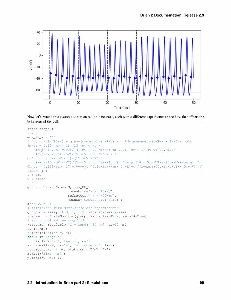
Brian 2 Documentation, Release 2.3
Now let’s extend this example to run on multiple neurons, each with a different capacitance to see how that affects thebehaviour of the cell.
start_scope()N = 3eqs_HH_2 = '''dv/dt = (gl*(El-v) - g_na*(m*m*m)*h*(v-ENa) - g_kd*(n*n*n*n)*(v-EK) + I)/C : voltdm/dt = 0.32*(mV**-1)*(13.*mV-v+VT)/
(exp((13.*mV-v+VT)/(4.*mV))-1.)/ms*(1-m)-0.28*(mV**-1)*(v-VT-40.*mV)/(exp((v-VT-40.*mV)/(5.*mV))-1.)/ms*m : 1
dn/dt = 0.032*(mV**-1)*(15.*mV-v+VT)/(exp((15.*mV-v+VT)/(5.*mV))-1.)/ms*(1.-n)-.5*exp((10.*mV-v+VT)/(40.*mV))/ms*n : 1
dh/dt = 0.128*exp((17.*mV-v+VT)/(18.*mV))/ms*(1.-h)-4./(1+exp((40.*mV-v+VT)/(5.*mV)))/→˓ms*h : 1I : ampC : farad'''group = NeuronGroup(N, eqs_HH_2,
threshold='v > -40*mV',refractory='v > -40*mV',method='exponential_euler')
group.v = El# initialise with some different capacitancesgroup.C = array([0.8, 1, 1.2])*ufarad*cm**-2*areastatemon = StateMonitor(group, variables=True, record=True)# we go back to run_regularlygroup.run_regularly('I = rand()*50*nA', dt=10*ms)run(50*ms)figure(figsize=(9, 4))for l in range(5):
axvline(l*10, ls='--', c='k')axhline(El/mV, ls='-', c='lightgray', lw=3)plot(statemon.t/ms, statemon.v.T/mV, '-')xlabel('Time (ms)')ylabel('v (mV)');
2.3. Introduction to Brian part 3: Simulations 109
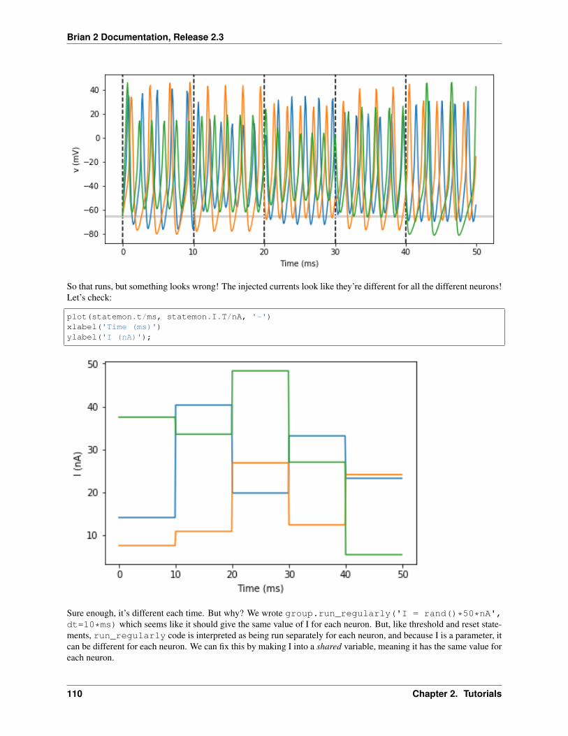
Brian 2 Documentation, Release 2.3
So that runs, but something looks wrong! The injected currents look like they’re different for all the different neurons!Let’s check:
plot(statemon.t/ms, statemon.I.T/nA, '-')xlabel('Time (ms)')ylabel('I (nA)');
Sure enough, it’s different each time. But why? We wrote group.run_regularly('I = rand()*50*nA',dt=10*ms) which seems like it should give the same value of I for each neuron. But, like threshold and reset state-ments, run_regularly code is interpreted as being run separately for each neuron, and because I is a parameter, itcan be different for each neuron. We can fix this by making I into a shared variable, meaning it has the same value foreach neuron.
110 Chapter 2. Tutorials
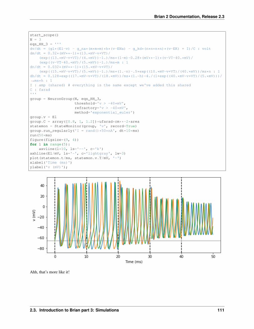
Brian 2 Documentation, Release 2.3
start_scope()N = 3eqs_HH_3 = '''dv/dt = (gl*(El-v) - g_na*(m*m*m)*h*(v-ENa) - g_kd*(n*n*n*n)*(v-EK) + I)/C : voltdm/dt = 0.32*(mV**-1)*(13.*mV-v+VT)/
(exp((13.*mV-v+VT)/(4.*mV))-1.)/ms*(1-m)-0.28*(mV**-1)*(v-VT-40.*mV)/(exp((v-VT-40.*mV)/(5.*mV))-1.)/ms*m : 1
dn/dt = 0.032*(mV**-1)*(15.*mV-v+VT)/(exp((15.*mV-v+VT)/(5.*mV))-1.)/ms*(1.-n)-.5*exp((10.*mV-v+VT)/(40.*mV))/ms*n : 1
dh/dt = 0.128*exp((17.*mV-v+VT)/(18.*mV))/ms*(1.-h)-4./(1+exp((40.*mV-v+VT)/(5.*mV)))/→˓ms*h : 1I : amp (shared) # everything is the same except we've added this sharedC : farad'''group = NeuronGroup(N, eqs_HH_3,
threshold='v > -40*mV',refractory='v > -40*mV',method='exponential_euler')
group.v = Elgroup.C = array([0.8, 1, 1.2])*ufarad*cm**-2*areastatemon = StateMonitor(group, 'v', record=True)group.run_regularly('I = rand()*50*nA', dt=10*ms)run(50*ms)figure(figsize=(9, 4))for l in range(5):
axvline(l*10, ls='--', c='k')axhline(El/mV, ls='-', c='lightgray', lw=3)plot(statemon.t/ms, statemon.v.T/mV, '-')xlabel('Time (ms)')ylabel('v (mV)');
Ahh, that’s more like it!
2.3. Introduction to Brian part 3: Simulations 111

Brian 2 Documentation, Release 2.3
2.3.3 Adding input
Now let’s think about a neuron being driven by a sinusoidal input. Let’s go back to a leaky integrate-and-fire tosimplify the equations a bit.
start_scope()A = 2.5f = 10*Hztau = 5*mseqs = '''dv/dt = (I-v)/tau : 1I = A*sin(2*pi*f*t) : 1'''G = NeuronGroup(1, eqs, threshold='v>1', reset='v=0', method='euler')M = StateMonitor(G, variables=True, record=True)run(200*ms)plot(M.t/ms, M.v[0], label='v')plot(M.t/ms, M.I[0], label='I')xlabel('Time (ms)')ylabel('v')legend(loc='best');
So far, so good and the sort of thing we saw in the first tutorial. Now, what if that input current were something wehad recorded and saved in a file? In that case, we can use TimedArray. Let’s start by reproducing the picture abovebut using TimedArray.
start_scope()A = 2.5f = 10*Hztau = 5*ms# Create a TimedArray and set the equations to use itt_recorded = arange(int(200*ms/defaultclock.dt))*defaultclock.dtI_recorded = TimedArray(A*sin(2*pi*f*t_recorded), dt=defaultclock.dt)
(continues on next page)
112 Chapter 2. Tutorials

Brian 2 Documentation, Release 2.3
(continued from previous page)
eqs = '''dv/dt = (I-v)/tau : 1I = I_recorded(t) : 1'''G = NeuronGroup(1, eqs, threshold='v>1', reset='v=0', method='exact')M = StateMonitor(G, variables=True, record=True)run(200*ms)plot(M.t/ms, M.v[0], label='v')plot(M.t/ms, M.I[0], label='I')xlabel('Time (ms)')ylabel('v')legend(loc='best');
Note that for the example where we put the sin function directly in the equations, we had to use themethod='euler' argument because the exact integrator wouldn’t work here (try it!). However, TimedArrayis considered to be constant over its time step and so the linear integrator can be used. This means you won’t getthe same behaviour from these two methods for two reasons. Firstly, the numerical integration methods exact andeuler give slightly different results. Secondly, sin is not constant over a timestep whereas TimedArray is.
Now just to show that TimedArray works for arbitrary currents, let’s make a weird “recorded” current and run it onthat.
start_scope()A = 2.5f = 10*Hztau = 5*ms# Let's create an array that couldn't be# reproduced with a formulanum_samples = int(200*ms/defaultclock.dt)I_arr = zeros(num_samples)for _ in range(100):
a = randint(num_samples)(continues on next page)
2.3. Introduction to Brian part 3: Simulations 113
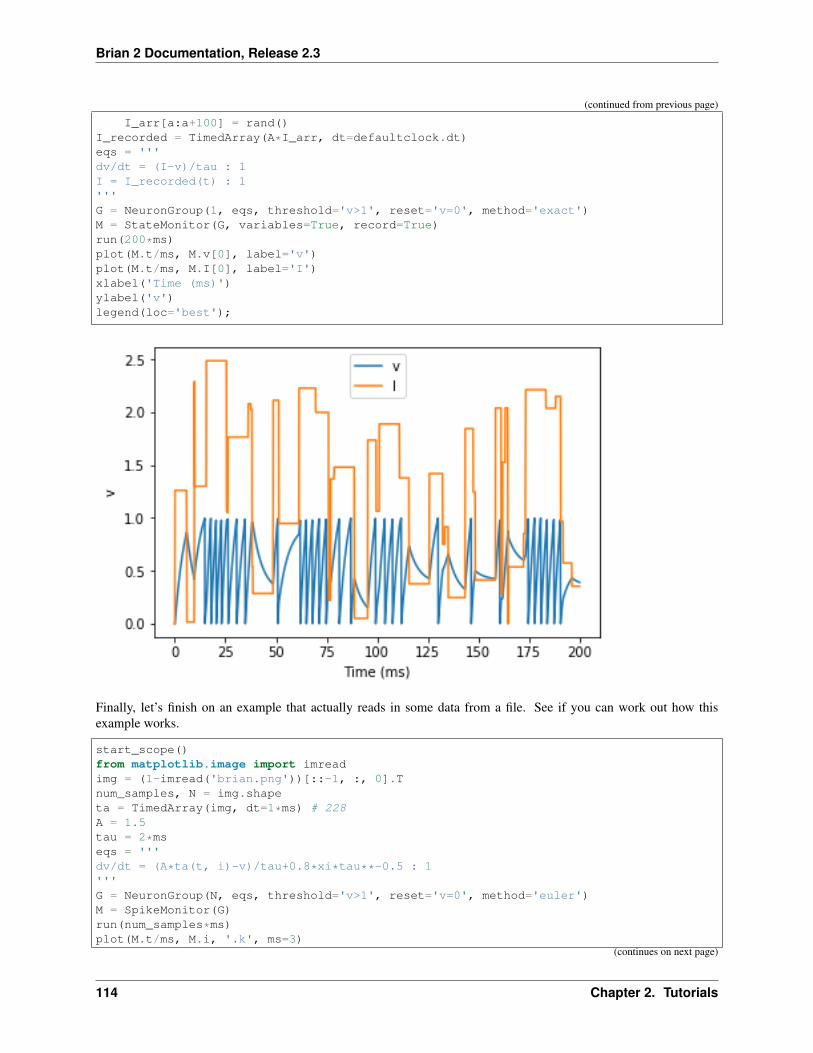
Brian 2 Documentation, Release 2.3
(continued from previous page)
I_arr[a:a+100] = rand()I_recorded = TimedArray(A*I_arr, dt=defaultclock.dt)eqs = '''dv/dt = (I-v)/tau : 1I = I_recorded(t) : 1'''G = NeuronGroup(1, eqs, threshold='v>1', reset='v=0', method='exact')M = StateMonitor(G, variables=True, record=True)run(200*ms)plot(M.t/ms, M.v[0], label='v')plot(M.t/ms, M.I[0], label='I')xlabel('Time (ms)')ylabel('v')legend(loc='best');
Finally, let’s finish on an example that actually reads in some data from a file. See if you can work out how thisexample works.
start_scope()from matplotlib.image import imreadimg = (1-imread('brian.png'))[::-1, :, 0].Tnum_samples, N = img.shapeta = TimedArray(img, dt=1*ms) # 228A = 1.5tau = 2*mseqs = '''dv/dt = (A*ta(t, i)-v)/tau+0.8*xi*tau**-0.5 : 1'''G = NeuronGroup(N, eqs, threshold='v>1', reset='v=0', method='euler')M = SpikeMonitor(G)run(num_samples*ms)plot(M.t/ms, M.i, '.k', ms=3)
(continues on next page)
114 Chapter 2. Tutorials
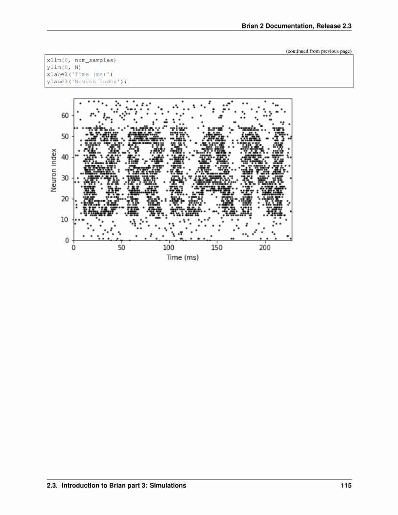
Brian 2 Documentation, Release 2.3
(continued from previous page)
xlim(0, num_samples)ylim(0, N)xlabel('Time (ms)')ylabel('Neuron index');
2.3. Introduction to Brian part 3: Simulations 115

Brian 2 Documentation, Release 2.3
116 Chapter 2. Tutorials

CHAPTER 3
User’s guide
3.1 Importing Brian
After installation, Brian is available in the brian2 package. By doing a wildcard import from this package, i.e.:
from brian2 import *
you will not only get access to the brian2 classes and functions, but also to everything in the pylab package,which includes the plotting functions from matplotlib and everything included in numpy/scipy (e.g. functions such asarange, linspace, etc.).
The following topics are not essential for beginners.
3.1.1 Precise control over importing
If you want to use a wildcard import from Brian, but don’t want to import all the additional symbols provided bypylab, you can use:
from brian2.only import *
Note that whenever you use something different from the most general from brian2 import * statement, youshould be aware that Brian overwrites some numpy functions with their unit-aware equivalents (see Units). If youcombine multiple wildcard imports, the Brian import should therefore be the last import. Similarly, you should notimport and call overwritten numpy functions directly, e.g. by using import numpy as np followed by np.sinsince this will not use the unit-aware versions. To make this easier, Brian provides a brian2.numpy_ package
117

Brian 2 Documentation, Release 2.3
that provides access to everything in numpy but overwrites certain functions. If you prefer to use prefixed names, therecommended way of doing the imports is therefore:
import brian2.numpy_ as npimport brian2.only as br2
Note that it is safe to use e.g. np.sin and numpy.sin after a from brian2 import *.
3.1.2 Dependency checks
Brian will check the dependency versions during import and raise an error for an outdated dependency. An outdateddependency does not necessarily mean that Brian cannot be run with it, it only means that Brian is untested on thatversion. If you want to force Brian to run despite the outdated dependency, set the core.outdated_dependency_errorpreference to False. Note that this cannot be done in a script, since you do not have access to the preferences beforeimporting brian2. See Preferences for instructions how to set preferences in a file.
3.2 Physical units
• Using units
• Removing units
• Temperatures
• Constants
• Importing units
• In-place operations on quantities
Brian includes a system for physical units. The base units are defined by their standard SI unit names: amp/ampere,kilogram/kilogramme, second, metre/meter, mole/mol, kelvin, and candela. In addition to thesebase units, Brian defines a set of derived units: coulomb, farad, gram/gramme, hertz, joule, liter/litre, molar, pascal, ohm, siemens, volt, watt, together with prefixed versions (e.g. msiemens =0.001*siemens) using the prefixes p, n, u, m, k, M, G, T (two exceptions to this rule: kilogram isnot defined with any additional prefixes, and metre and meter are additionaly defined with the “centi” prefix, i.e.cmetre/cmeter). For convenience, a couple of additional useful standard abbreviations such as cm (instead ofcmetre/cmeter), nS (instead of nsiemens), ms (instead of msecond), Hz (instead of hertz), mM (instead ofmmolar) are included. To avoid clashes with common variable names, no one-letter abbreviations are provided (e.g.you can use mV or nS, but not V or S).
3.2.1 Using units
You can generate a physical quantity by multiplying a scalar or vector value with its physical unit:
>>> tau = 20*ms>>> print(tau)20. ms>>> rates = [10, 20, 30]*Hz>>> print(rates)[ 10. 20. 30.] Hz
118 Chapter 3. User’s guide
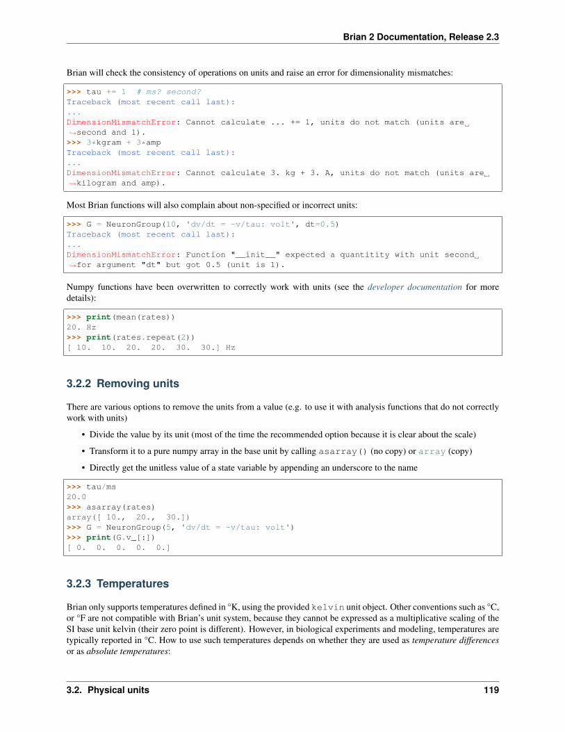
Brian 2 Documentation, Release 2.3
Brian will check the consistency of operations on units and raise an error for dimensionality mismatches:
>>> tau += 1 # ms? second?Traceback (most recent call last):...DimensionMismatchError: Cannot calculate ... += 1, units do not match (units are→˓second and 1).>>> 3*kgram + 3*ampTraceback (most recent call last):...DimensionMismatchError: Cannot calculate 3. kg + 3. A, units do not match (units are→˓kilogram and amp).
Most Brian functions will also complain about non-specified or incorrect units:
>>> G = NeuronGroup(10, 'dv/dt = -v/tau: volt', dt=0.5)Traceback (most recent call last):...DimensionMismatchError: Function "__init__" expected a quantitity with unit second→˓for argument "dt" but got 0.5 (unit is 1).
Numpy functions have been overwritten to correctly work with units (see the developer documentation for moredetails):
>>> print(mean(rates))20. Hz>>> print(rates.repeat(2))[ 10. 10. 20. 20. 30. 30.] Hz
3.2.2 Removing units
There are various options to remove the units from a value (e.g. to use it with analysis functions that do not correctlywork with units)
• Divide the value by its unit (most of the time the recommended option because it is clear about the scale)
• Transform it to a pure numpy array in the base unit by calling asarray() (no copy) or array (copy)
• Directly get the unitless value of a state variable by appending an underscore to the name
>>> tau/ms20.0>>> asarray(rates)array([ 10., 20., 30.])>>> G = NeuronGroup(5, 'dv/dt = -v/tau: volt')>>> print(G.v_[:])[ 0. 0. 0. 0. 0.]
3.2.3 Temperatures
Brian only supports temperatures defined in °K, using the provided kelvin unit object. Other conventions such as °C,or °F are not compatible with Brian’s unit system, because they cannot be expressed as a multiplicative scaling of theSI base unit kelvin (their zero point is different). However, in biological experiments and modeling, temperatures aretypically reported in °C. How to use such temperatures depends on whether they are used as temperature differencesor as absolute temperatures:
3.2. Physical units 119

Brian 2 Documentation, Release 2.3
temperature differences Their major use case is the correction of time constants for differences in temperaturesbased on the Q10 temperature coefficient. In this case, all temperatures can directly use kelvin even thoughthe temperatures are reported in Celsius, since temperature differences in Celsius and Kelvin are identical.
absolute temperatures Equations such as the Goldman–Hodgkin–Katz voltage equation have a factor that dependson the absolute temperature measured in Kelvin. To get this temperature from a temperature reported in °C, youcan use the zero_celsius constant from the brian2.units.constants package (see below):
from brian2.units.constants import zero_celsius
celsius_temp = 27abs_temp = celsius_temp*kelvin + zero_celsius
Note: Earlier versions of Brian had a celsius unit which was in fact identical to kelvin. While this gave thecorrect results for temperature differences, it did not correctly work for absolute temperatures. To avoid confusion andpossible misinterpretation, the celsius unit has therefore been removed.
3.2.4 Constants
The brian2.units.constants package provides a range of physical constants that can be useful for detailedbiological models. Brian provides the following constants:
Constant Symbol(s) Brian name ValueAvogadro constant 𝑁𝐴, 𝐿 avogadro_constant 6.022140857× 10²³ mol−1
Boltzmann constant 𝑘 boltzmann_constant 1.38064852× 10⁻²³ J K−1
Electric constant 𝜖0 electric_constant 8.854187817× 10⁻¹² F m−1
Electron mass 𝑚𝑒 electron_mass 9.10938356× 10⁻³¹ kgElementary charge 𝑒 elementary_charge 1.6021766208× 10⁻¹⁹ C
Faraday constant 𝐹 faraday_constant 96485.33289 C mol−1
Gas constant 𝑅 gas_constant 8.3144598 J mol−1 K−1
Magnetic constant 𝜇0 magnetic_constant 12.566370614× 10⁻⁷ N A−2
Molar mass constant 𝑀𝑢 molar_mass_constant 1× 10⁻³ kg mol−1
0°C zero_celsius 273.15 K
Note that these constants are not imported by default, you will have to explicitly import them from brian2.units.constants. During the import, you can also give them shorter names using Python’s from ... import ...as ... syntax. For example, to calculate the 𝑅𝑇
𝐹 factor that appears in the Goldman–Hodgkin–Katz voltage equationyou can use:
from brian2 import *from brian2.units.constants import zero_celsius, gas_constant as R, faraday_constant→˓as F
celsius_temp = 27T = celsius_temp*kelvin + zero_celsiusfactor = R*T/F
The following topics are not essential for beginners.
120 Chapter 3. User’s guide
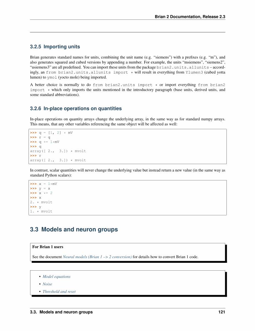
Brian 2 Documentation, Release 2.3
3.2.5 Importing units
Brian generates standard names for units, combining the unit name (e.g. “siemens”) with a prefixes (e.g. “m”), andalso generates squared and cubed versions by appending a number. For example, the units “msiemens”, “siemens2”,“usiemens3” are all predefined. You can import these units from the package brian2.units.allunits – accord-ingly, an from brian2.units.allunits import * will result in everything from Ylumen3 (cubed yottalumen) to ymol (yocto mole) being imported.
A better choice is normally to do from brian2.units import * or import everything from brian2import * which only imports the units mentioned in the introductory paragraph (base units, derived units, andsome standard abbreviations).
3.2.6 In-place operations on quantities
In-place operations on quantity arrays change the underlying array, in the same way as for standard numpy arrays.This means, that any other variables referencing the same object will be affected as well:
>>> q = [1, 2] * mV>>> r = q>>> q += 1*mV>>> qarray([ 2., 3.]) * mvolt>>> rarray([ 2., 3.]) * mvolt
In contrast, scalar quantities will never change the underlying value but instead return a new value (in the same way asstandard Python scalars):
>>> x = 1*mV>>> y = x>>> x *= 2>>> x2. * mvolt>>> y1. * mvolt
3.3 Models and neuron groups
For Brian 1 users
See the document Neural models (Brian 1 –> 2 conversion) for details how to convert Brian 1 code.
• Model equations
• Noise
• Threshold and reset
3.3. Models and neuron groups 121

Brian 2 Documentation, Release 2.3
• Refractoriness
• State variables
• Subgroups
• Shared variables
• Storing state variables
• Linked variables
• Time scaling of noise
3.3.1 Model equations
The core of every simulation is a NeuronGroup, a group of neurons that share the same equations defining theirproperties. The minimum NeuronGroup specification contains the number of neurons and the model description inthe form of equations:
G = NeuronGroup(10, 'dv/dt = -v/(10*ms) : volt')
This defines a group of 10 leaky integrators. The model description can be directly given as a (possibly multi-line)string as above, or as an Equations object. For more details on the form of equations, see Equations. Brian needsthe model to be given in the form of differential equations, but you might see the integrated form of synapses in sometextbooks and papers. See Converting from integrated form to ODEs for details on how to convert between theserepresentations.
Note that model descriptions can make reference to physical units, but also to scalar variables declared outside of themodel description itself:
tau = 10*msG = NeuronGroup(10, 'dv/dt = -v/tau : volt')
If a variable should be taken as a parameter of the neurons, i.e. if it should be possible to vary its value across neurons,it has to be declared as part of the model description:
G = NeuronGroup(10, '''dv/dt = -v/tau : volttau : second''')
To make complex model descriptions more readable, named subexpressions can be used:
G = NeuronGroup(10, '''dv/dt = I_leak / Cm : voltI_leak = g_L*(E_L - v) : amp''')
For a list of some standard model equations, see Neural models (Brian 1 –> 2 conversion).
3.3.2 Noise
In addition to ordinary differential equations, Brian allows you to introduce random noise by specifying a stochasticdifferential equation. Brian uses the physicists’ notation used in the Langevin equation, representing the “noise” as aterm 𝜉(𝑡), rather than the mathematicians’ stochastic differential d𝑊𝑡. The following is an example of the Ornstein-Uhlenbeck process that is often used to model a leaky integrate-and-fire neuron with a stochastic current:
G = NeuronGroup(10, 'dv/dt = -v/tau + sigma*sqrt(2/tau)*xi : volt')
122 Chapter 3. User’s guide
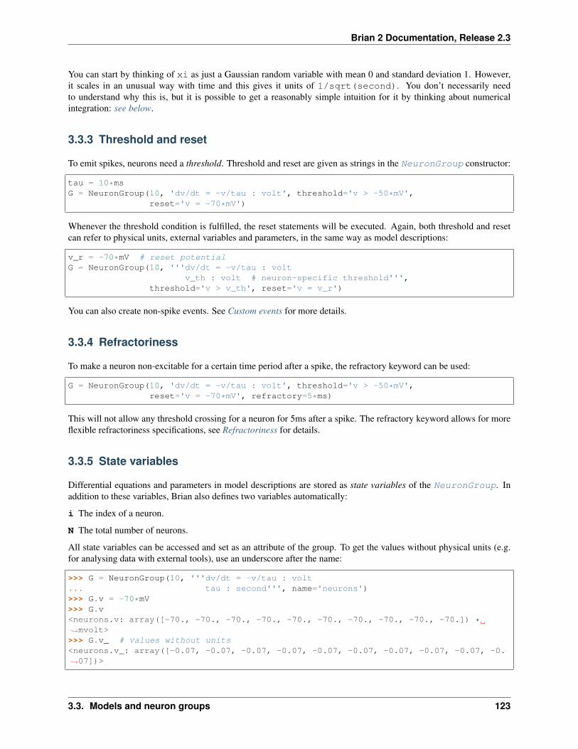
Brian 2 Documentation, Release 2.3
You can start by thinking of xi as just a Gaussian random variable with mean 0 and standard deviation 1. However,it scales in an unusual way with time and this gives it units of 1/sqrt(second). You don’t necessarily needto understand why this is, but it is possible to get a reasonably simple intuition for it by thinking about numericalintegration: see below.
3.3.3 Threshold and reset
To emit spikes, neurons need a threshold. Threshold and reset are given as strings in the NeuronGroup constructor:
tau = 10*msG = NeuronGroup(10, 'dv/dt = -v/tau : volt', threshold='v > -50*mV',
reset='v = -70*mV')
Whenever the threshold condition is fulfilled, the reset statements will be executed. Again, both threshold and resetcan refer to physical units, external variables and parameters, in the same way as model descriptions:
v_r = -70*mV # reset potentialG = NeuronGroup(10, '''dv/dt = -v/tau : volt
v_th : volt # neuron-specific threshold''',threshold='v > v_th', reset='v = v_r')
You can also create non-spike events. See Custom events for more details.
3.3.4 Refractoriness
To make a neuron non-excitable for a certain time period after a spike, the refractory keyword can be used:
G = NeuronGroup(10, 'dv/dt = -v/tau : volt', threshold='v > -50*mV',reset='v = -70*mV', refractory=5*ms)
This will not allow any threshold crossing for a neuron for 5ms after a spike. The refractory keyword allows for moreflexible refractoriness specifications, see Refractoriness for details.
3.3.5 State variables
Differential equations and parameters in model descriptions are stored as state variables of the NeuronGroup. Inaddition to these variables, Brian also defines two variables automatically:
i The index of a neuron.
N The total number of neurons.
All state variables can be accessed and set as an attribute of the group. To get the values without physical units (e.g.for analysing data with external tools), use an underscore after the name:
>>> G = NeuronGroup(10, '''dv/dt = -v/tau : volt... tau : second''', name='neurons')>>> G.v = -70*mV>>> G.v<neurons.v: array([-70., -70., -70., -70., -70., -70., -70., -70., -70., -70.]) *→˓mvolt>>>> G.v_ # values without units<neurons.v_: array([-0.07, -0.07, -0.07, -0.07, -0.07, -0.07, -0.07, -0.07, -0.07, -0.→˓07])>
3.3. Models and neuron groups 123
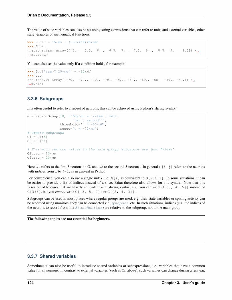
Brian 2 Documentation, Release 2.3
The value of state variables can also be set using string expressions that can refer to units and external variables, otherstate variables or mathematical functions:
>>> G.tau = '5*ms + (1.0*i/N)*5*ms'>>> G.tau<neurons.tau: array([ 5. , 5.5, 6. , 6.5, 7. , 7.5, 8. , 8.5, 9. , 9.5]) *→˓msecond>
You can also set the value only if a condition holds, for example:
>>> G.v['tau>7.25*ms'] = -60*mV>>> G.v<neurons.v: array([-70., -70., -70., -70., -70., -60., -60., -60., -60., -60.]) *→˓mvolt>
3.3.6 Subgroups
It is often useful to refer to a subset of neurons, this can be achieved using Python’s slicing syntax:
G = NeuronGroup(10, '''dv/dt = -v/tau : volttau : second''',
threshold='v > -50*mV',reset='v = -70*mV')
# Create subgroupsG1 = G[:5]G2 = G[5:]
# This will set the values in the main group, subgroups are just "views"G1.tau = 10*msG2.tau = 20*ms
Here G1 refers to the first 5 neurons in G, and G2 to the second 5 neurons. In general G[i:j] refers to the neuronswith indices from i to j-1, as in general in Python.
For convenience, you can also use a single index, i.e. G[i] is equivalent to G[i:i+1]. In some situations, it canbe easier to provide a list of indices instead of a slice, Brian therefore also allows for this syntax. Note that thisis restricted to cases that are strictly equivalent with slicing syntax, e.g. you can write G[[3, 4, 5]] instead ofG[3:6], but you cannot write G[[3, 5, 7]] or G[[5, 4, 3]].
Subgroups can be used in most places where regular groups are used, e.g. their state variables or spiking activity canbe recorded using monitors, they can be connected via Synapses, etc. In such situations, indices (e.g. the indices ofthe neurons to record from in a StateMonitor) are relative to the subgroup, not to the main group
The following topics are not essential for beginners.
3.3.7 Shared variables
Sometimes it can also be useful to introduce shared variables or subexpressions, i.e. variables that have a commonvalue for all neurons. In contrast to external variables (such as Cm above), such variables can change during a run, e.g.
124 Chapter 3. User’s guide

Brian 2 Documentation, Release 2.3
by using run_regularly(). This can be for example used for an external stimulus that changes in the course of arun:
>>> G = NeuronGroup(10, '''shared_input : volt (shared)... dv/dt = (-v + shared_input)/tau : volt... tau : second''', name='neurons')
Note that there are several restrictions around the use of shared variables: they cannot be written to in contexts wherestatements apply only to a subset of neurons (e.g. reset statements, see below). If a code block mixes statementswriting to shared and vector variables, then the shared statements have to come first.
By default, subexpressions are re-evaluated whenever they are used, i.e. using a subexpression is completely equivalentto substituting it. Sometimes it is useful to instead only evaluate a subexpression once and then use this value for therest of the time step. This can be achieved by using the (constant over dt) flag. This flag is mandatoryfor subexpressions that refer to stateful functions like rand() which notably allows them to be recorded with aStateMonitor – otherwise the monitor would record a different instance of the random number than the one thatwas used in the equations.
For shared variables, setting by string expressions can only refer to shared values:
>>> G.shared_input = '(4.0/N)*mV'>>> G.shared_input<neurons.shared_input: 0.4 * mvolt>
3.3.8 Storing state variables
Sometimes it can be convenient to access multiple state variables at once, e.g. to set initial values from a dictionary ofvalues or to store all the values of a group on disk. This can be done with the get_states() and set_states()methods:
>>> group = NeuronGroup(5, '''dv/dt = -v/tau : 1... tau : second''', name='neurons')>>> initial_values = {'v': [0, 1, 2, 3, 4],... 'tau': [10, 20, 10, 20, 10]*ms}>>> group.set_states(initial_values)>>> group.v[:]array([ 0., 1., 2., 3., 4.])>>> group.tau[:]array([ 10., 20., 10., 20., 10.]) * msecond>>> states = group.get_states()>>> states['v']array([ 0., 1., 2., 3., 4.])
The data (without physical units) can also be exported/imported to/from Pandas data frames (needs an installation ofpandas):
>>> df = group.get_states(units=False, format='pandas')>>> df
N dt i t tau v0 5 0.0001 0 0.0 0.01 0.01 5 0.0001 1 0.0 0.02 1.02 5 0.0001 2 0.0 0.01 2.03 5 0.0001 3 0.0 0.02 3.04 5 0.0001 4 0.0 0.01 4.0>>> df['tau']0 0.01
(continues on next page)
3.3. Models and neuron groups 125
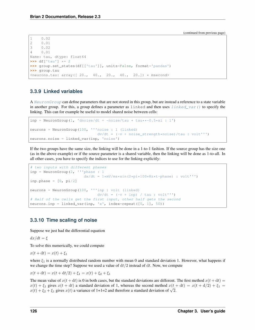
Brian 2 Documentation, Release 2.3
(continued from previous page)
1 0.022 0.013 0.024 0.01Name: tau, dtype: float64>>> df['tau'] *= 2>>> group.set_states(df[['tau']], units=False, format='pandas')>>> group.tau<neurons.tau: array([ 20., 40., 20., 40., 20.]) * msecond>
3.3.9 Linked variables
A NeuronGroup can define parameters that are not stored in this group, but are instead a reference to a state variablein another group. For this, a group defines a parameter as linked and then uses linked_var() to specify thelinking. This can for example be useful to model shared noise between cells:
inp = NeuronGroup(1, 'dnoise/dt = -noise/tau + tau**-0.5*xi : 1')
neurons = NeuronGroup(100, '''noise : 1 (linked)dv/dt = (-v + noise_strength*noise)/tau : volt''')
neurons.noise = linked_var(inp, 'noise')
If the two groups have the same size, the linking will be done in a 1-to-1 fashion. If the source group has the size one(as in the above example) or if the source parameter is a shared variable, then the linking will be done as 1-to-all. Inall other cases, you have to specify the indices to use for the linking explicitly:
# two inputs with different phasesinp = NeuronGroup(2, '''phase : 1
dx/dt = 1*mV/ms*sin(2*pi*100*Hz*t-phase) : volt''')inp.phase = [0, pi/2]
neurons = NeuronGroup(100, '''inp : volt (linked)dv/dt = (-v + inp) / tau : volt''')
# Half of the cells get the first input, other half gets the secondneurons.inp = linked_var(inp, 'x', index=repeat([0, 1], 50))
3.3.10 Time scaling of noise
Suppose we just had the differential equation
𝑑𝑥/𝑑𝑡 = 𝜉
To solve this numerically, we could compute
𝑥(𝑡 + d𝑡) = 𝑥(𝑡) + 𝜉1
where 𝜉1 is a normally distributed random number with mean 0 and standard deviation 1. However, what happens ifwe change the time step? Suppose we used a value of d𝑡/2 instead of d𝑡. Now, we compute
𝑥(𝑡 + d𝑡) = 𝑥(𝑡 + d𝑡/2) + 𝜉1 = 𝑥(𝑡) + 𝜉2 + 𝜉1
The mean value of 𝑥(𝑡+ d𝑡) is 0 in both cases, but the standard deviations are different. The first method 𝑥(𝑡+ d𝑡) =𝑥(𝑡) + 𝜉1 gives 𝑥(𝑡 + d𝑡) a standard deviation of 1, whereas the second method 𝑥(𝑡 + d𝑡) = 𝑥(𝑡 + d/2) + 𝜉1 =𝑥(𝑡) + 𝜉2 + 𝜉1 gives 𝑥(𝑡) a variance of 1+1=2 and therefore a standard deviation of
√2.
126 Chapter 3. User’s guide
Brian 2 Documentation, Release 2.3
In order to solve this problem, we use the rule 𝑥(𝑡 + d𝑡) = 𝑥(𝑡) +√
d𝑡𝜉1, which makes the mean and standarddeviation of the value at time 𝑡 independent of d𝑡. For this to make sense dimensionally, 𝜉 must have units of 1/sqrt(second).
For further details, refer to a textbook on stochastic differential equations.
3.4 Numerical integration
By default, Brian chooses an integration method automatically, trying to solve the equations exactly first (for linearequations) and then resorting to numerical algorithms. It will also take care of integrating stochastic differentialequations appropriately.
Note that in some cases, the automatic choice of integration method will not be appropriate, because of a choice ofparameters that couldn’t be determined in advance. In this case, typically you will get nan (not a number) values inthe results, or large oscillations. In this case, Brian will generate a warning to let you know, but will not raise an error.
3.4.1 Method choice
You will get an INFO message telling you which integration method Brian decided to use, together with informationabout how much time it took to apply the integration method to your equations. If other methods have been triedbut were not applicable, you will also see the time it took to try out those other methods. In some cases, checkingother methods (in particular the 'exact' method which attempts to solve the equations analytically) can take aconsiderable amount of time – to avoid wasting this time, you can always chose the integration method manually (seebelow). You can also suppress the message by raising the log level or by explicitly suppressing 'method_choice'log messages – for details, see Logging.
If you prefer to chose an integration algorithm yourself, you can do so using the method keyword for NeuronGroup,Synapses, or SpatialNeuron. The complete list of available methods is the following:
• 'exact': exact integration for linear equations (alternative name: 'linear')
• 'exponential_euler': exponential Euler integration for conditionally linear equations
• 'euler': forward Euler integration (for additive stochastic differential equations using the Euler-Maruyamamethod)
• 'rk2': second order Runge-Kutta method (midpoint method)
• 'rk4': classical Runge-Kutta method (RK4)
• 'heun': stochastic Heun method for solving Stratonovich stochastic differential equations with non-diagonalmultiplicative noise.
• 'milstein': derivative-free Milstein method for solving stochastic differential equations with diagonal mul-tiplicative noise
Note: The 'independent' integration method (exact integration for a system of independent equations, whereall the equations can be analytically solved independently) should no longer be used and might be removed in futureversions of Brian.
Note: The following methods are still considered experimental
• 'gsl': default integrator when choosing to integrate equations with the GNU Scientific Library ODE solver:the rkf45 method. Uses an adaptable time step by default.
3.4. Numerical integration 127

Brian 2 Documentation, Release 2.3
• 'gsl_rkf45': Runge-Kutta-Fehlberg method. A good general-purpose integrator according to the GSLdocumentation. Uses an adaptable time step by default.
• 'gsl_rk2': Second order Runge-Kutta method using GSL. Uses an adaptable time step by default.
• 'gsl_rk4': Fourth order Runge-Kutta method using GSL. Uses an adaptable time step by default.
• 'gsl_rkck': Runge-Kutta Cash-Karp method using GSL. Uses an adaptable time step by default.
• 'gsl_rk8pd': Runge-Kutta Prince-Dormand method using GSL. Uses an adaptable time step by default.
The following topics are not essential for beginners.
3.4.2 Technical notes
Each class defines its own list of algorithms it tries to apply, NeuronGroup and Synapses will use the first suitablemethod out of the methods 'exact', 'euler' and 'heun' while SpatialNeuron objects will use 'exact','exponential_euler', 'rk2' or 'heun'.
You can also define your own numerical integrators, see State update for details.
3.4.3 GSL stateupdaters
The stateupdaters preceded with the gsl tag use ODE solvers defined in the GNU Scientific Library. The benefitof using these integrators over the ones written by Brian internally, is that they are implemented with an adaptabletimestep. Integrating with an adaptable timestep comes with two advantages:
• These methods check whether the estimated error of the solutions returned fall within a certain error bound. Forthe non-gsl integrators there is currently no such check.
• Systems no longer need to be simulated with just one time step. That is, a bigger timestep can be chosenand the integrator will reduce the timestep when increased accuracy is required. This is particularly useful forsystems where both slow and fast time constants coexist, as is the case with for example (networks of neuronswith) Hodgkin-Huxley equations. Note that Brian’s timestep still determines the resolution for monitors, spiketiming, spike propagation etc. Hence, in a network, the simulation error will therefore still be on the order ofdt. The benefit is that short time constants occurring in equations no longer dictate the network time step.
In addition to a choice between different integration methods, there are a few more options that can be specified whenusing GSL. These options can be specified by sending a dictionary as the method_options key upon initializationof the object using the integrator (NeuronGroup, Synapses or SpatialNeuron). The available method optionsare:
• 'adaptable_timestep': whether or not to let GSL reduce the timestep to achieve the accuracy definedwith the 'absolute_error' and 'absolute_error_per_variable' options described below. Ifthis is set to False, the timestep is determined by Brian (i.e. the dt of the respective clock is used, seeScheduling). If the resulted estimated error exceeds the set error bounds, the simulation is aborted. When usingcython or weave this is reported with an IntegrationError. Defaults to True.
• 'absolute_error': each of the methods has a way of estimating the error that is the result of using numer-ical integration. You can specify the maximum size of this error to be allowed for any of the to-be-integratedvariables in base units with this keyword. Note that giving very small values makes the simulation slow and
128 Chapter 3. User’s guide
Brian 2 Documentation, Release 2.3
might result in unsuccessful integration. In the case of using the 'absolute_error_per_variable'option, this is the error for variables that were not specified individually. Defaults to 1e-6.
• 'absolute_error_per_variable': specify the absolute error per variable in its own units. Variablesfor which the error is not specified use the error set with the 'absolute_error' option. Defaults to None.
• 'max_steps': The maximal number of steps that the integrator will take within a single “Brian timestep” inorder to reach the given error criterion. Can be set to 0 to not set any limits. Note that without limits, it can takea very long time until the integrator figures out that it cannot reach the desired error level. This will manifest asa simulation that appears to be stuck. Defaults to 100.
• 'use_last_timestep': with the 'adaptable_timestep' option set to True, GSL tries different timesteps to find a solution that satisfies the set error bounds. It is likely that for Brian’s next time step the GSL timestep will be somewhat similar per neuron (e.g. active neurons will have a shorter GSL time step than inactiveneurons). With this option set to True, the time step GSL found to satisfy the set error bounds is saved per neuronand given to GSL again in Brian’s next time step. This also means that the final time steps are saved in Brian’smemory and can thus be recorded with the StateMonitor: it can be accessed under '_last_timestep'.Note that some extra memory is required to keep track of the last time steps. Defaults to True.
• 'save_failed_steps': if 'adaptable_timestep' is set to True, each time GSL tries a time step andit results in an estimated error that exceeds the set bounds, one is added to the '_failed_steps' variable.For purposes of investigating what happens within GSL during an integration step, we offer the option of savingthis variable. Defaults to False.
• 'save_step_count': the same goes for the total number of GSL steps taken in a single Brian time step:this is optionally saved in the '_step_count' variable. Defaults to False.
Note that at the moment recording '_last_timestep', '_failed_steps', or '_step_count' requires acall to run() (e.g. with 0 ms) to trigger the code generation process, before the call to StateMonitor.
More information on the GSL ODE solver itself can be found in its documentation.
3.5 Equations
• Equation strings
• Arithmetic operations and functions
• External variables
• Flags
• List of special symbols
• Event-driven equations
• Equation objects
• Examples of Equation objects
3.5.1 Equation strings
Equations are used both in NeuronGroup and Synapses to:
• define state variables
• define continuous-updates on these variables, through differential equations
3.5. Equations 129

Brian 2 Documentation, Release 2.3
Note: Brian models are defined by systems of first order ordinary differential equations, but you might see theintegrated form of synapses in some textbooks and papers. See Converting from integrated form to ODEs for detailson how to convert between these representations.
Equations are defined by multiline strings.
An Equation is a set of single lines in a string:
(1) dx/dt = f : unit (differential equation)
(2) x = f : unit (subexpression)
(3) x : unit (parameter)
Each equation may be spread out over multiple lines to improve formatting. Comments using # may also be included.Subunits are not allowed, i.e., one must write volt, not mV. This is to make it clear that the values are internally alwayssaved in the basic units, so no confusion can arise when getting the values out of a NeuronGroup and discarding theunits. Compound units are of course allowed as well (e.g. farad/meter**2). There are also three special “units”that can be used: 1 denotes a dimensionless floating point variable, boolean and integer denote dimensionlessvariables of the respective kind.
Note: For molar concentration, the base unit that has to be used in the equations is mmolar (or mM), not molar.This is because 1 molar is 103 mol/m3 in SI units (i.e., it has a “scale” of 103), whereas 1 millimolar corresponds to 1mol/m3.
Some special variables are defined: t, dt (time) and xi (white noise). Variable names starting with an underscoreand a couple of other names that have special meanings under certain circumstances (e.g. names ending in _pre or_post) are forbidden.
For stochastic equations with several xi values it is necessary to make clear whether they correspond to the same ordifferent noise instantiations. To make this distinction, an arbitrary suffix can be used, e.g. using xi_1 several timesrefers to the same variable, xi_2 (or xi_inh, xi_alpha, etc.) refers to another. An error will be raised if youuse more than one plain xi. Note that noise is always independent across neurons, you can only work around thisrestriction by defining your noise variable as a shared parameter and update it using a user-defined function (e.g. withrun_regularly), or create a group that models the noise and link to its variable (see Linked variables).
3.5.2 Arithmetic operations and functions
Equation strings can make use of standard arithmetic operations for numerical values, using the Python 3 syntax. Thesupported operations are +, -, *, / (floating point division), // (flooring division), % (remainder), ** (power). Forvariable assignments, e.g. in reset statements, the corresponding in-place assignments such as += can be used as well.For comparisons, the operations == (equality), != (inequality), <, <=, >, and >= are available. Truth values canbe combined using and and or, or negated using not. Note that Brian does not support any operations specific tointegers, e.g. “bitwise AND” or shift operations.
Warning: Brian versions up to 2.1.3.1 did not support // as the floor division operator and potentially useddifferent semantics for the / operator depending on whether Python 2 or 3 was used. To write code that correctlyand unambiguously works with both newer and older Brian versions, you can use expressions such as 1.0*a/bto enforce floating point division (if one of the operands is a floating point number, both Python 2 and 3 willuse floating point division), or floor(a/b) to enforce flooring division Note that the floor function alwaysreturns a floating point value, if it is important that the result is an integer value, additionally wrap it with the intfunction.
130 Chapter 3. User’s guide
Brian 2 Documentation, Release 2.3
Brian also supports standard mathematical functions with the same names as used in the numpy library (e.g. exp,sqrt, abs, clip, sin, cos, . . . ) – for a full list see Default functions. Note that support for such functions isprovided by Brian itself and the translation to the various code generation targets is automatically taken care of. Youshould therefore refer to them directly by name and not as e.g. np.sqrt or numpy.sqrt, regardless of the wayyou imported Brian or numpy. This also means that you cannot directly refer to arbitrary functions from numpy orother libraries. For details on how to extend the support to non-default functions see User-provided functions.
3.5.3 External variables
Equations defining neuronal or synaptic equations can contain references to external parameters or functions. Thesereferences are looked up at the time that the simulation is run. If you don’t specify where to look them up, it will lookin the Python local/global namespace (i.e. the block of code where you call run()). If you want to override this, youcan specify an explicit “namespace”. This is a Python dictionary with keys being variable names as they appear in theequations, and values being the desired value of that variable. This namespace can be specified either in the creationof the group or when you can the run() function using the namespace keyword argument.
The following three examples show the different ways of providing external variable values, all having the same effectin this case:
# Explicit argument to the NeuronGroupG = NeuronGroup(1, 'dv/dt = -v / tau : 1', namespace={'tau': 10*ms})net = Network(G)net.run(10*ms)
# Explicit argument to the run functionG = NeuronGroup(1, 'dv/dt = -v / tau : 1')net = Network(G)net.run(10*ms, namespace={'tau': 10*ms})
# Implicit namespace from the contextG = NeuronGroup(1, 'dv/dt = -v / tau : 1')net = Network(G)tau = 10*msnet.run(10*ms)
See Namespaces for more details.
The following topics are not essential for beginners.
3.5.4 Flags
A flag is a keyword in parentheses at the end of the line, which qualifies the equations. There are several keywords:
event-driven this is only used in Synapses, and means that the differential equation should be updated only at thetimes of events. This implies that the equation is taken out of the continuous state update, and instead a event-based state update statement is generated and inserted into event codes (pre and post). This can only qualifydifferential equations of synapses. Currently, only one-dimensional linear equations can be handled (see below).
3.5. Equations 131

Brian 2 Documentation, Release 2.3
unless refractory this means the variable is not updated during the refractory period. This can only qualify differentialequations of neuron groups.
constant this means the parameter will not be changed during a run. This allows optimizations in state updaters. Thiscan only qualify parameters.
constant over dt this means that the subexpression will be only evaluated once at the beginning of the time step.This can be useful to e.g. approximate a non-linear term as constant over a time step in order to use thelinear numerical integration algorithm. It is also mandatory for subexpressions that refer to stateful func-tions like rand() to make sure that they are only evaluated once (otherwise e.g. recording the value with aStateMonitor would re-evaluate it and therefore not record the same values that are used in other places).This can only qualify subexpressions.
shared this means that a parameter or subexpression is not neuron-/synapse-specific but rather a single value for thewhole NeuronGroup or Synapses. A shared subexpression can only refer to other shared variables.
linked this means that a parameter refers to a parameter in another NeuronGroup. See Linked variables for moredetails.
Multiple flags may be specified as follows:
dx/dt = f : unit (flag1,flag2)
3.5.5 List of special symbols
The following lists all of the special symbols that Brian uses in equations and code blocks, and their meanings.
dt Time step width
i Index of a neuron (NeuronGroup) or the pre-synaptic neuron of a synapse (Synapses)
j Index of a post-synaptic neuron of a synapse
lastspike Last time that the neuron spiked (for refractoriness)
lastupdate Time of the last update of synaptic variables in event-driven equations (only defined when event-drivenequations are used).
N Number of neurons (NeuronGroup) or synapses (Synapses). Use N_pre or N_post for the number ofpresynaptic or postsynaptic neurons in the context of Synapses.
not_refractory Boolean variable that is normally true, and false if the neuron is currently in a refractory state
t Current time
t_in_timesteps Current time measured in time steps
xi, xi_* Stochastic differential in equations
3.5.6 Event-driven equations
Equations defined as event-driven are completely ignored in the state update. They are only defined as variables thatcan be externally accessed. There are additional constraints:
• An event-driven variable cannot be used by any other equation that is not also event-driven.
• An event-driven equation cannot depend on a differential equation that is not event-driven (directly, or indirectlythrough subexpressions). It can depend on a constant parameter.
Currently, automatic event-driven updates are only possible for one-dimensional linear equations, but this may beextended in the future.
132 Chapter 3. User’s guide

Brian 2 Documentation, Release 2.3
3.5.7 Equation objects
The model definitions for NeuronGroup and Synapses can be simple strings or Equations objects. Suchobjects can be combined using the add operator:
eqs = Equations('dx/dt = (y-x)/tau : volt')eqs += Equations('dy/dt = -y/tau: volt')
Equations allow for the specification of values in the strings, but does this by simple string replacement, e.g. youcan do:
eqs = Equations('dx/dt = x/tau : volt', tau=10*ms)
but this is exactly equivalent to:
eqs = Equations('dx/dt = x/(10*ms) : volt')
The Equations object does some basic syntax checking and will raise an error if two equations defining the samevariable are combined. It does not however do unit checking, checking for unknown identifiers or incorrect flags – allthis will be done during the instantiation of a NeuronGroup or Synapses object.
3.5.8 Examples of Equation objects
Concatenating equations
>>> membrane_eqs = Equations('dv/dt = -(v + I)/ tau : volt')>>> eqs1 = membrane_eqs + Equations('''I = sin(2*pi*freq*t) : volt... freq : Hz''')>>> eqs2 = membrane_eqs + Equations('''I : volt''')>>> print(eqs1)I = sin(2*pi*freq*t) : Vdv/dt = -(v + I)/ tau : Vfreq : Hz>>> print(eqs2)dv/dt = -(v + I)/ tau : VI : V
Substituting variable names
>>> general_equation = 'dg/dt = -g / tau : siemens'>>> eqs_exc = Equations(general_equation, g='g_e', tau='tau_e')>>> eqs_inh = Equations(general_equation, g='g_i', tau='tau_i')>>> print(eqs_exc)dg_e/dt = -g_e / tau_e : S>>> print(eqs_inh)dg_i/dt = -g_i / tau_i : S
Inserting values
>>> eqs = Equations('dv/dt = mu/tau + sigma/tau**.5*xi : volt',... mu=-65*mV, sigma=3*mV, tau=10*ms)>>> print(eqs)dv/dt = (-65. * mvolt)/(10. * msecond) + (3. * mvolt)/(10. * msecond)**.5*xi : V
3.5. Equations 133
Brian 2 Documentation, Release 2.3
3.6 Refractoriness
• Defining the refractory period
• Defining model behaviour during refractoriness
• Arbitrary refractoriness
Brian allows you to model the absolute refractory period of a neuron in a flexible way. The definition of refractorinessconsists of two components: the amount of time after a spike that a neuron is considered to be refractory, and whatchanges in the neuron during the refractoriness.
3.6.1 Defining the refractory period
The refractory period is specified by the refractory keyword in the NeuronGroup initializer. In the simplestcase, this is simply a fixed time, valid for all neurons:
G = NeuronGroup(N, model='...', threshold='...', reset='...',refractory=2*ms)
Alternatively, it can be a string expression that evaluates to a time. This expression will be evaluated after every spikeand allows for a changing refractory period. For example, the following will set the refractory period to a randomduration between 1ms and 3ms after every spike:
G = NeuronGroup(N, model='...', threshold='...', reset='...',refractory='(1 + 2*rand())*ms')
In general, modelling a refractory period that varies across neurons involves declaring a state variable that stores therefractory period per neuron as a model parameter. The refractory expression can then refer to this parameter:
G = NeuronGroup(N, model='''...refractory : second''', threshold='...',
reset='...', refractory='refractory')# Set the refractory period for each cellG.refractory = ...
This state variable can also be a dynamic variable itself. For example, it can serve as an adaptation mechanism byincreasing it after every spike and letting it relax back to a steady-state value between spikes:
refractory_0 = 2*mstau_refractory = 50*msG = NeuronGroup(N, model='''...
drefractory/dt = (refractory_0 - refractory) / tau_→˓refractory : second''',
threshold='...', refractory='refractory',reset='''...
refractory += 1*ms''')G.refractory = refractory_0
In some cases, the condition for leaving the refractory period is not easily expressed as a certain time span. Forexample, in a Hodgkin-Huxley type model the threshold is only used for counting spikes and the refractoriness is usedto prevent to count multiple spikes for a single threshold crossing (the threshold condition would evaluate to True forseveral time points). When a neuron should leave the refractory period is not easily expressed as a time span but more
134 Chapter 3. User’s guide
Brian 2 Documentation, Release 2.3
naturally as a condition that the neuron should remain refractory for as long as it stays above the threshold. This canbe achieved by using a string expression for the refractory keyword that evaluates to a boolean condition:
G = NeuronGroup(N, model='...', threshold='v > -20*mV',refractory='v >= -20*mV')
The refractory keyword should be read as “stay refractory as long as the condition remains true”. In fact, specify-ing a time span for the refractoriness will be automatically transformed into a logical expression using the current timet and the time of the last spike lastspike. Specifying refractory=2*ms is basically equivalent to specifyingrefractory='(t - lastspike) <= 2*ms'. However, this expression can give inconsistent results for thecommon case that the refractory period is a multiple of the simulation timestep. Due to floating point impreciseness,the actual value of t - lastspike can be slightly above or below a multiple of the simulation time step; com-paring it directly to the refractory period can therefore lead to an end of the refractory one time step sooner or later.To avoid this issue, the actual code used for the above example is equivalent to refractory='timestep(t -lastspike, dt) <= timestep(2*ms, dt)'. The timestep function is provided by Brian and takes careof converting a time into a time step in a safe way.
New in version 2.1.3: The timestep function is now used to avoid floating point issues in the refractoriness calcu-lation. To restore the previous behaviour, set the legacy.refractory_timing preference to True.
3.6.2 Defining model behaviour during refractoriness
The refractoriness definition as described above only has a single effect by itself: threshold crossings during therefractory period are ignored. In the following model, the variable v continues to update during the refractory periodbut it does not elicit a spike if it crosses the threshold:
G = NeuronGroup(N, 'dv/dt = -v / tau : 1',threshold='v > 1', reset='v=0',refractory=2*ms)
There is also a second implementation of refractoriness that is supported by Brian, one or several state variables canbe clamped during the refractory period. To model this kind of behaviour, variables that should stop being updatedduring refractoriness can be marked with the (unless refractory) flag:
G = NeuronGroup(N, '''dv/dt = -(v + w)/ tau_v : 1 (unless refractory)dw/dt = -w / tau_w : 1''',
threshold='v > 1', reset='v=0; w+=0.1', refractory=2*ms)
In the above model, the v variable is clamped at 0 for 2ms after a spike but the adaptation variable w continues toupdate during this time. In addition, a variable of a neuron that is in its refractory period is read-only: incomingsynapses or other code will have no effect on the value of v until it leaves its refractory period.
The following topics are not essential for beginners.
3.6.3 Arbitrary refractoriness
In fact, arbitrary behaviours can be defined using Brian’s refractoriness mechanism.
A NeuronGroup with refractoriness automatically defines two variables:
3.6. Refractoriness 135

Brian 2 Documentation, Release 2.3
not_refractory A boolean variable stating whether a neuron is allowed to spike.
lastspike The time of the last spike of the neuron.
The variable not_refractory is updated at every time step by checking the refractoriness condition – for a refrac-toriness defined by a time period, this means comparing lastspike to the current time t. The not_refractoryvariable is then used to implement the refractoriness behaviour. Specifically, the threshold condition is replaced bythreshold and not_refractory and differential equations that are marked as (unless refractory)are multiplied by int(not_refractory) (so that they have the value 0 when the neuron is refractory).
This not_refractory variable is also available to the user to define more sophisticated refractoriness behaviour.For example, the following code updates the w variable with a different time constant during refractoriness:
G = NeuronGroup(N, '''dv/dt = -(v + w)/ tau_v : 1 (unless refractory)dw/dt = (-w / tau_active)*int(not_refractory) + (-w / tau_
→˓ref)*(1 - int(not_refractory)) : 1''',threshold='v > 1', reset='v=0; w+=0.1', refractory=2*ms)
3.7 Synapses
For Brian 1 users
Synapses is now the only class for defining synaptic interactions, it replaces Connection, STDP, etc. See thedocument Synapses (Brian 1 –> 2 conversion) for details how to convert Brian 1 code.
• Defining synaptic models
• Creating synapses
• Accessing synaptic variables
• Delays
• Monitoring synaptic variables
• Synaptic connection/weight matrices
• Creating synapses with the generator syntax
• Summed variables
• Creating multi-synapses
• Multiple pathways
• Numerical integration
• Technical notes
3.7.1 Defining synaptic models
The most simple synapse (adding a fixed amount to the target membrane potential on every spike) is described asfollows:
136 Chapter 3. User’s guide

Brian 2 Documentation, Release 2.3
w = 1*mVS = Synapses(P, Q, on_pre='v += w')
This defines a set of synapses between NeuronGroup P and NeuronGroup Q. If the target group is not specified,it is identical to the source group by default. The on_pre keyword defines what happens when a presynaptic spikearrives at a synapse. In this case, the constant w is added to variable v. Because v is not defined as a synaptic variable,it is assumed by default that it is a postsynaptic variable, defined in the target NeuronGroup Q. Note that this doesnot create synapses (see Creating Synapses), only the synaptic models.
To define more complex models, models can be described as string equations, similar to the models specified inNeuronGroup:
S = Synapses(P, Q, model='w : volt', on_pre='v += w')
The above specifies a parameter w, i.e. a synapse-specific weight. Note that to avoid confusion, synaptic variablescannot have the same name as a pre- or post-synaptic variables.
Synapses can also specify code that should be executed whenever a postsynaptic spike occurs (keyword on_post)and a fixed (pre-synaptic) delay for all synapses (keyword delay).
As shown above, variable names that are not referring to a synaptic variable are automatically understood to be post-synaptic variables. To explicitly specify that a variable should be from a pre- or post-synaptic neuron, append thesuffix _pre or _post. An alternative but equivalent formulation of the on_pre statement above would therefore bev_post += w.
Model syntax
The model follows exactly the same syntax as for NeuronGroup. There can be parameters (e.g. synaptic variablew above), but there can also be named subexpressions and differential equations, describing the dynamics of synapticvariables. In all cases, synaptic variables are created, one value per synapse.
Brian also automatically defines a number of synaptic variables that can be used in equations, on_pre and on_poststatements, as well as when assigning to other synaptic variables:
i The index of the pre-synaptic source of a synapse.
j The index of the post-synaptic target of a synapse.
N The total number of synapses.
N_incoming The total number of synapses connected to the post-synaptic target of a synapse.
N_outgoing The total number of synapses outgoing from the pre-synaptic source of a synapse.
lastupdate The last time this synapse has applied an on_pre or on_post statement. There is normally no needto refer to this variable explicitly, it is used to implement Event-driven updates (see below). It is only definedwhen event-driven equations are used.
Event-driven updates
By default, differential equations are integrated in a clock-driven fashion, as for a NeuronGroup. This is potentiallyvery time consuming, because all synapses are updated at every timestep and Brian will therefore emit a warning. Ifyou are sure about integrating the equations at every timestep (e.g. because you want to record the values continu-ously), then you should specify the flag (clock-driven). To ask Brian 2 to simulate differential equations in anevent-driven fashion use the flag (event-driven). A typical example is pre- and postsynaptic traces in STDP:
3.7. Synapses 137

Brian 2 Documentation, Release 2.3
model='''w:1dApre/dt=-Apre/taupre : 1 (event-driven)dApost/dt=-Apost/taupost : 1 (event-driven)'''
Here, Brian updates the value of Apre for a given synapse only when this synapse receives a spike, whether it ispresynaptic or postsynaptic. More precisely, the variables are updated every time either the on_pre or on_postcode is called for the synapse, so that the values are always up to date when these codes are executed.
Automatic event-driven updates are only possible for a subset of equations, in particular for one-dimensional linearequations. These equations must also be independent of the other ones, that is, a differential equation that is not event-driven cannot depend on an event-driven equation (since the values are not continuously updated). In other cases, theuser can write event-driven code explicitly in the update codes (see below).
Pre and post codes
The on_pre code is executed at each synapse receiving a presynaptic spike. For example:
on_pre='v+=w'
adds the value of synaptic variable w to postsynaptic variable v. Any sort of code can be executed. For example, thefollowing code defines stochastic synapses, with a synaptic weight w and transmission probability p:
S=Synapses(input,neurons,model="""w : 1p : 1""",
on_pre="v+=w*(rand()<p)")
The code means that w is added to v with probability p. The code may also include multiple lines.
Similarly, the on_post code is executed at each synapse where the postsynaptic neuron has fired a spike.
3.7.2 Creating synapses
Creating a Synapses instance does not create synapses, it only specifies their dynamics. The following commandcreates a synapse between neuron 5 in the source group and neuron 10 in the target group:
S.connect(i=5, j=10)
Multiple synaptic connections can be created in a single statement:
S.connect()S.connect(i=[1, 2], j=[3, 4])S.connect(i=numpy.arange(10), j=1)
The first statement connects all neuron pairs. The second statement creates synapses between neurons 1 and 3, andbetween neurons 2 and 4. The third statement creates synapses between the first ten neurons in the source group andneuron 1 in the target group.
Conditional
One can also create synapses by giving (as a string) the condition for a pair of neurons i and j to be connected by asynapse, e.g. you could connect neurons that are not very far apart with:
S.connect(condition='abs(i-j)<=5')
138 Chapter 3. User’s guide
Brian 2 Documentation, Release 2.3
The string expressions can also refer to pre- or postsynaptic variables. This can be useful for example for spatialconnectivity: assuming that the pre- and postsynaptic groups have parameters x and y, storing their location, thefollowing statement connects all cells in a 250 um radius:
S.connect(condition='sqrt((x_pre-x_post)**2 + (y_pre-y_post)**2) < 250*umeter')
Probabilistic
Synapse creation can also be probabilistic by providing a p argument, providing the connection probability for eachpair of synapses:
S.connect(p=0.1)
This connects all neuron pairs with a probability of 10%. Probabilities can also be given as expressions, for exampleto implement a connection probability that depends on distance:
S.connect(condition='i != j',p='p_max*exp(-(x_pre-x_post)**2+(y_pre-y_post)**2 / (2*(125*umeter)**2))')
If this statement is applied to a Synapses object that connects a group to itself, it prevents self-connections (i != j) and connects cells with a probability that is modulated according to a 2-dimensional Gaussian of the distancebetween the cells.
One-to-one
You can specify a mapping from i to any function f(i), e.g. the simplest way to give a 1-to-1 connection would be:
S.connect(j='i')
This mapping can also use a restricting condition with if, e.g. to connect neurons 0, 2, 4, 6, . . . to neurons 0, 1, 2, 3,. . . you could write:
S.connect(j='int(i/2) if i % 2 == 0')
3.7.3 Accessing synaptic variables
Synaptic variables can be accessed in a similar way as NeuronGroup variables. They can be indexed with twoindexes, corresponding to the indexes of pre and postsynaptic neurons, or with string expressions (referring to i andj as the pre-/post-synaptic indices, or to other state variables of the synapse or the connected neurons). Note thatsetting a synaptic variable always refers to the synapses that currently exist, i.e. you have to set them after the relevantSynapses.connect() call.
Here are a few examples:
S.w[2, 5] = 1*nSS.w[1, :] = 2*nSS.w = 1*nS # all synapses assignedS.w[2, 3] = (1*nS, 2*nS)S.w[group1, group2] = "(1+cos(i-j))*2*nS"S.w[:, :] = 'rand()*nS'S.w['abs(x_pre-x_post) < 250*umetre'] = 1*nS
3.7. Synapses 139
Brian 2 Documentation, Release 2.3
Assignments can also refer to pre-defined variables, e.g. to normalize synaptic weights. For example, after thefollowing assignment the sum of weights of all synapses that a neuron receives is identical to 1, regardless of thenumber of synapses it receives:
syn.w = '1.0/N_incoming'
Note that it is also possible to index synaptic variables with a single index (integer, slice, or array), but in this casesynaptic indices have to be provided.
3.7.4 Delays
There is a special synaptic variable that is automatically created: delay. It is the propagation delay from the presy-naptic neuron to the synapse, i.e., the presynaptic delay. This is just a convenience syntax for accessing the delaystored in the presynaptic pathway: pre.delay. When there is a postsynaptic code (keyword post), the delay of thepostsynaptic pathway can be accessed as post.delay.
The delay variable(s) can be set and accessed in the same way as other synaptic variables. The same semantics asfor other synaptic variables apply, which means in particular that the delay is only set for the synapses that have beenalready created with Synapses.connect(). If you want to set a global delay for all synapses of a Synapsesobject, you can directly specify that delay as part of the Synapses initializer:
synapses = Synapses(sources, targets, '...', on_pre='...', delay=1*ms)
When you use this syntax, you can still change the delay afterwards by setting synapses.delay, but you can onlyset it to another scalar value. If you need different delays across synapses, do not use this syntax but instead set thedelay variable as any other synaptic variable (see above).
3.7.5 Monitoring synaptic variables
A StateMonitor object can be used to monitor synaptic variables. For example, the following statement creates amonitor for variable w for the synapses 0 and 1:
M = StateMonitor(S, 'w', record=[0,1])
Note that these are synapse indices, not neuron indices. More convenient is to directly index the Synapses object,Brian will automatically calculate the indices for you in this case:
M = StateMonitor(S, 'w', record=S[0, :]) # all synapses originating from neuron 0M = StateMonitor(S, 'w', record=S['i!=j']) # all synapses excluding autapsesM = StateMonitor(S, 'w', record=S['w>0']) # all synapses with non-zero weights (at→˓this time)
You can also record a synaptic variable for all synapses by passing record=True.
The recorded traces can then be accessed in the usual way, again with the possibility to index the Synapses object:
plot(M.t / ms, M[S[0]].w / nS) # first synapseplot(M.t / ms, M[S[0, :]].w / nS) # all synapses originating from neuron 0plot(M.t / ms, M[S['w>0*nS']].w / nS) # all synapses with non-zero weights (at this→˓time)
Note (for users of Brian’s advanced standalone mode only): the use of the Synapses object for indexing andrecord=True only work in the default runtime modes. In standalone mode (see Standalone code generation),the synapses have not yet been created at this point, so Brian cannot calculate the indices.
140 Chapter 3. User’s guide

Brian 2 Documentation, Release 2.3
The following topics are not essential for beginners.
3.7.6 Synaptic connection/weight matrices
Brian does not directly support specifying synapses by using a matrix, you always have to use a “sparse” format, whereeach connection is defined by its source and target indices. However, you can easily convert between the two formats.Assuming you have a connection matrix 𝐶 of size 𝑁 ×𝑀 , where 𝑁 is the number of presynaptic cells, and 𝑀 thenumber of postsynaptic cells, with each entry being 1 for a connection, and 0 otherwise. You can convert this matrixto arrays of source and target indices, which you can then provide to Brian’s connect function:
C = ... # The connection matrix as a numpy array of 0's and 1'ssources, targets = C.nonzero()synapses = Synapses(...)synapses.connect(i=sources, j=targets)
Similarly, you can transform the flat array of values stored in a synapse into a matrix form. For example, to get amatrix with all the weight values w, with NaN values where no synapse exists:
synapses = Synapses(source_group, target_group,'''...
w : 1 # synaptic weight''', ...)# ...# Run e.g. a simulation with plasticity that changes the weightsrun(...)# Create a matrix to store the weights and fill it with NaNW = np.full((len(source_group), len(target_group)), np.nan)# Insert the values from the Synapses objectW[synapses.i[:], synapses.j[:]] = synapses.w[:]
3.7.7 Creating synapses with the generator syntax
The most general way of specifying a connection is using the generator syntax, e.g. to connect neuron i to all neuronsj with 0<=j<=i:
S.connect(j='k for k in range(0, i+1)')
There are several parts to this syntax. The general form is:
j='EXPR for VAR in RANGE if COND'
Here EXPR can be any integer-valued expression. VAR is the name of the iteration variable (any name you like canbe specified here). The if COND part is optional and lets you give an additional condition that has to be true for thesynapse to be created. Finally, RANGE can be either:
1. a Python range, e.g. range(N) is the integers from 0 to N-1, range(A, B) is the integers from A to B-1,range(low, high, step) is the integers from low to high-1 with steps of size step, or
3.7. Synapses 141

Brian 2 Documentation, Release 2.3
2. it can be a random sample sample(N, p=0.1) gives a random sample of integers from 0 to N-1 with10% probability of each integer appearing in the sample. This can have extra arguments like range, e.g.sample(low, high, step, p=0.1) will give each integer in range(low, high, step) withprobability 10%.
If you try to create an invalid synapse (i.e. connecting neurons that are outside the correct range) then you will get anerror, e.g. you might like to try to do this to connect each neuron to its neighbours:
S.connect(j='i+(-1)**k for k in range(2)')
However this won’t work at for i=0 it gives j=-1 which is invalid. There is an option to just skip any synapses thatare outside the valid range:
S.connect(j='i+(-1)**k for k in range(2)', skip_if_invalid=True)
3.7.8 Summed variables
In many cases, the postsynaptic neuron has a variable that represents a sum of variables over all its synapses. This iscalled a “summed variable”. An example is nonlinear synapses (e.g. NMDA):
neurons = NeuronGroup(1, model='''dv/dt=(gtot-v)/(10*ms) : 1gtot : 1''')
S = Synapses(input, neurons,model='''dg/dt=-a*g+b*x*(1-g) : 1
gtot_post = g : 1 (summed)dx/dt=-c*x : 1w : 1 # synaptic weight''', on_pre='x+=w')
Here, each synapse has a conductance g with nonlinear dynamics. The neuron’s total conductance is gtot. The linestating gtot_post = g : 1 (summed) specifies the link between the two: gtot in the postsynaptic group isthe summer over all variables g of the corresponding synapses. What happens during the simulation is that at each timestep, presynaptic conductances are summed for each neuron and the result is copied to the variable gtot. Anotherexample is gap junctions:
neurons = NeuronGroup(N, model='''dv/dt=(v0-v+Igap)/tau : 1Igap : 1''')
S=Synapses(neurons,model='''w:1 # gap junction conductanceIgap_post = w*(v_pre-v_post): 1 (summed)''')
Here, Igap is the total gap junction current received by the postsynaptic neuron.
Note that you cannot target the same post-synaptic variable from more than one Synapses object. To work aroundthis restriction, use multiple post-synaptic variables that ar then summed up:
neurons = NeuronGroup(1, model='''dv/dt=(gtot-v)/(10*ms) : 1gtot = gtot1 + gtot2: 1gtot1 : 1gtot2 : 1''')
S1 = Synapses(input, neurons,model='''dg/dt=-a1*g+b1*x*(1-g) : 1
gtot1_post = g : 1 (summed)dx/dt=-c1*x : 1w : 1 # synaptic weight
''', on_pre='x+=w')S2 = Synapses(input, neurons,
model='''dg/dt=-a2*g+b2*x*(1-g) : 1
(continues on next page)
142 Chapter 3. User’s guide

Brian 2 Documentation, Release 2.3
(continued from previous page)
gtot2_post = g : 1 (summed)dx/dt=-c2*x : 1w : 1 # synaptic weight
''', on_pre='x+=w')
3.7.9 Creating multi-synapses
It is also possible to create several synapses for a given pair of neurons:
S.connect(i=numpy.arange(10), j=1, n=3)
This is useful for example if one wants to have multiple synapses with different delays. To distinguish multiplevariables connecting the same pair of neurons in synaptic expressions and statements, you can create a variable storingthe synapse index with the multisynaptic_index keyword:
syn = Synapses(source_group, target_group, model='w : 1', on_pre='v += w',multisynaptic_index='synapse_number')
syn.connect(i=numpy.arange(10), j=1, n=3)syn.delay = '1*ms + synapse_number*2*ms'
This index can then be used to set/get synapse-specific values:
S.delay = '(synapse_number + 1)*ms)' # Set delays between 1 and 10msS.w['synapse_number<5'] = 0.5S.w['synapse_number>=5'] = 1
It also enables three-dimensional indexing, the following statement has the same effect as the last one above:
S.w[:, :, 5:] = 1
3.7.10 Multiple pathways
It is possible to have multiple pathways with different update codes from the same presynaptic neuron group. Thismay be interesting in cases when different operations must be applied at different times for the same presynaptic spike,e.g. for a STDP rule that shifted in time. To do this, specify a dictionary of pathway names and codes:
on_pre={'pre_transmission': 'ge+=w','pre_plasticity': '''w=clip(w+Apost,0,inf)
Apre+=dApre'''}
This creates two pathways with the given names (in fact, specifying on_pre=code is just a shorter syntaxfor on_pre={'pre': code}) through which the delay variables can be accessed. The following state-ment, for example, sets the delay of the synapse between the first neurons of the source and target groups in thepre_plasticity pathway:
S.pre_plasticity.delay[0,0] = 3*ms
As mentioned above, pre pathways are generally executed before post pathways. The order of execution of severalpre (or post) pathways with the same delay is however arbitrary, and simply based on the alphabetical orderingof their names (i.e. pre_plasticity will be executed before pre_transmission). To explicitly specify theorder, set the order attribute of the pathway, e.g.:
3.7. Synapses 143
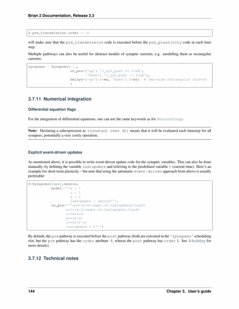
Brian 2 Documentation, Release 2.3
S.pre_transmission.order = -2
will make sure that the pre_transmission code is executed before the pre_plasticity code in each timestep.
Multiple pathways can also be useful for abstract models of synaptic currents, e.g. modelling them as rectangularcurrents:
synapses = Synapses(...,on_pre={'up': 'I_syn_post += 1*nA',
'down': 'I_syn_post -= 1*nA'},delays={'up': 0*ms, 'down': 5*ms} # 5ms-wide rectangular current)
3.7.11 Numerical integration
Differential equation flags
For the integration of differential equations, one can use the same keywords as for NeuronGroup.
Note: Declaring a subexpression as (constant over dt) means that it will be evaluated each timestep for allsynapses, potentially a very costly operation.
Explicit event-driven updates
As mentioned above, it is possible to write event-driven update code for the synaptic variables. This can also be donemanually, by defining the variable lastupdate and referring to the predefined variable t (current time). Here’s anexample for short-term plasticity – but note that using the automatic event-driven approach from above is usuallypreferable:
S=Synapses(input,neuron,model='''x : 1
u : 1w : 1lastupdate : second''',
on_pre='''u=U+(u-U)*exp(-(t-lastupdate)/tauf)x=1+(x-1)*exp(-(t-lastupdate)/taud)i+=w*u*xx*=(1-u)u+=U*(1-u)lastupdate = t''')
By default, the pre pathway is executed before the post pathway (both are executed in the 'synapses' schedulingslot, but the pre pathway has the order attribute -1, wheras the post pathway has order 1. See Scheduling formore details).
3.7.12 Technical notes
144 Chapter 3. User’s guide
Brian 2 Documentation, Release 2.3
How connection arguments are interpreted
If conditions for connecting neurons are combined with both the n (number of synapses to create) and the p (probabilityof a synapse) keywords, they are interpreted in the following way:
For every pair i, j:if condition(i, j) is fulfilled:
Evaluate p(i, j)If uniform random number between 0 and 1 < p(i, j):
Create n(i, j) synapses for (i, j)
With the generator syntax j='EXPR for VAR in RANGE if COND', the interpretation is:
For every i:for every VAR in RANGE:
j = EXPRif COND:
Create n(i, j) synapses for (i, j)
Note that the arguments in RANGE can only depend on i and the values of presynaptic variables. Similarly, theexpression for j, EXPR can depend on i, presynaptic variables, and on the iteration variable VAR. The conditionCOND can depend on anything (presynaptic and postsynaptic variables).
With the 1-to-1 mapping syntax j='EXPR' the interpretation is:
For every i:j = EXPRCreate n(i, j) synapses for (i, j)
Efficiency considerations
If you are connecting a single pair of neurons, the direct form connect(i=5, j=10) is the most efficient. How-ever, if you are connecting a number of neurons, it will usually be more efficient to construct an array of i and jvalues and have a single connect(i=i, j=j) call.
For large connections, you should use one of the string based syntaxes where possible as this will generate compiledlow-level code that will be typically much faster than equivalent Python code.
If you are expecting a majority of pairs of neurons to be connected, then using the condition-based syntax is op-timal, e.g. connect(condition='i!=j'). However, if relatively few neurons are being connected then the1-to-1 mapping or generator syntax will be better. For 1-to-1, connect(j='i') will always be faster thanconnect(condition='i==j') because the latter has to evaluate all N**2 pairs (i, j) and check if thecondition is true, whereas the former only has to do O(N) operations.
One tricky problem is how to efficiently generate connectivity with a probability p(i, j) that depends on both i andj, since this requires N*N computations even if the expected number of synapses is proportional to N. Some tricks forgetting around this are shown in Example: efficient_gaussian_connectivity.
3.8 Input stimuli
For Brian 1 users
See the document Inputs (Brian 1 –> 2 conversion) for details how to convert Brian 1 code.
3.8. Input stimuli 145
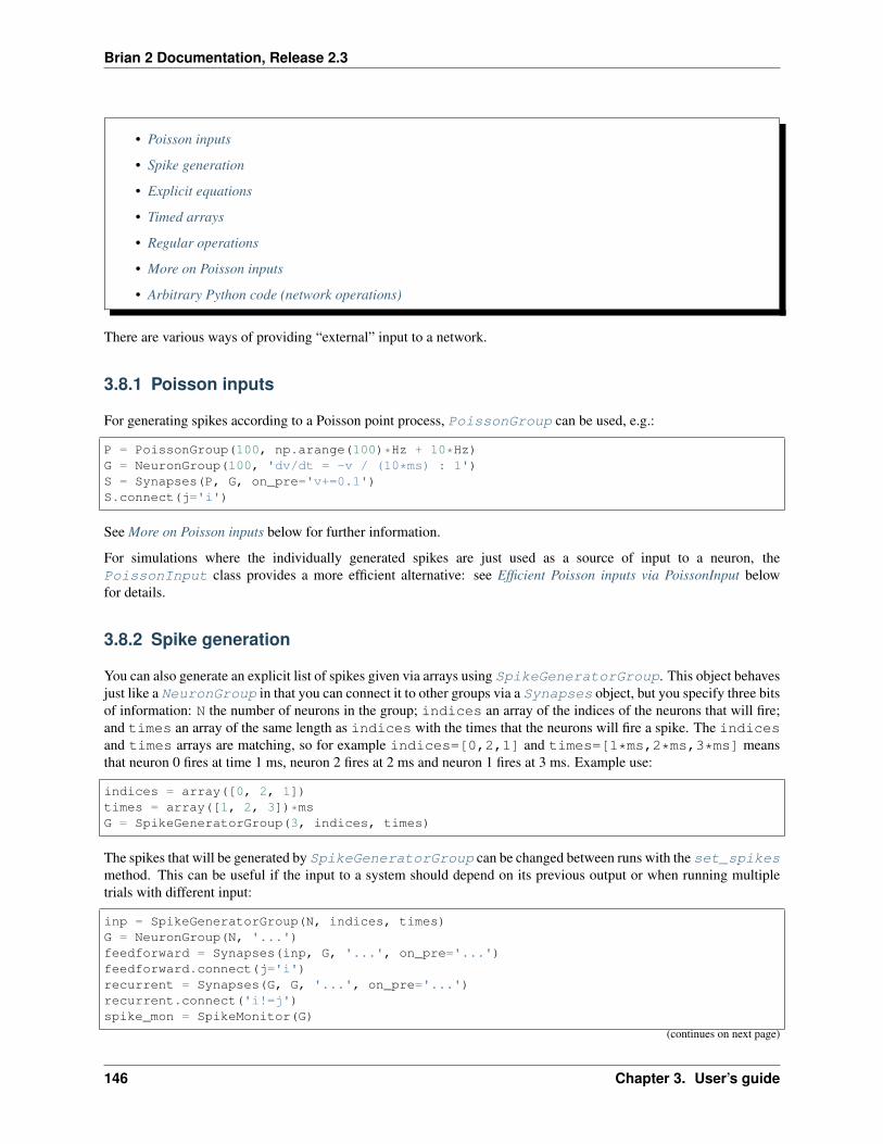
Brian 2 Documentation, Release 2.3
• Poisson inputs
• Spike generation
• Explicit equations
• Timed arrays
• Regular operations
• More on Poisson inputs
• Arbitrary Python code (network operations)
There are various ways of providing “external” input to a network.
3.8.1 Poisson inputs
For generating spikes according to a Poisson point process, PoissonGroup can be used, e.g.:
P = PoissonGroup(100, np.arange(100)*Hz + 10*Hz)G = NeuronGroup(100, 'dv/dt = -v / (10*ms) : 1')S = Synapses(P, G, on_pre='v+=0.1')S.connect(j='i')
See More on Poisson inputs below for further information.
For simulations where the individually generated spikes are just used as a source of input to a neuron, thePoissonInput class provides a more efficient alternative: see Efficient Poisson inputs via PoissonInput belowfor details.
3.8.2 Spike generation
You can also generate an explicit list of spikes given via arrays using SpikeGeneratorGroup. This object behavesjust like a NeuronGroup in that you can connect it to other groups via a Synapses object, but you specify three bitsof information: N the number of neurons in the group; indices an array of the indices of the neurons that will fire;and times an array of the same length as indices with the times that the neurons will fire a spike. The indicesand times arrays are matching, so for example indices=[0,2,1] and times=[1*ms,2*ms,3*ms] meansthat neuron 0 fires at time 1 ms, neuron 2 fires at 2 ms and neuron 1 fires at 3 ms. Example use:
indices = array([0, 2, 1])times = array([1, 2, 3])*msG = SpikeGeneratorGroup(3, indices, times)
The spikes that will be generated by SpikeGeneratorGroup can be changed between runs with the set_spikesmethod. This can be useful if the input to a system should depend on its previous output or when running multipletrials with different input:
inp = SpikeGeneratorGroup(N, indices, times)G = NeuronGroup(N, '...')feedforward = Synapses(inp, G, '...', on_pre='...')feedforward.connect(j='i')recurrent = Synapses(G, G, '...', on_pre='...')recurrent.connect('i!=j')spike_mon = SpikeMonitor(G)
(continues on next page)
146 Chapter 3. User’s guide

Brian 2 Documentation, Release 2.3
(continued from previous page)
# ...run(runtime)# Replay the previous output of group G as input into the groupinp.set_spikes(spike_mon.i, spike_mon.t + runtime)run(runtime)
3.8.3 Explicit equations
If the input can be explicitly expressed as a function of time (e.g. a sinusoidal input current), then its description canbe directly included in the equations of the respective group:
G = NeuronGroup(100, '''dv/dt = (-v + I)/(10*ms) : 1rates : Hz # each neuron's input has a different ratesize : 1 # and a different amplitudeI = size*sin(2*pi*rates*t) : 1''')
G.rates = '10*Hz + i*Hz'G.size = '(100-i)/100. + 0.1'
3.8.4 Timed arrays
If the time dependence of the input cannot be expressed in the equations in the way shown above, it is possible tocreate a TimedArray . This acts as a function of time where the values at given time points are given explicitly.This can be especially useful to describe non-continuous stimulation. For example, the following code defines aTimedArray where stimulus blocks consist of a constant current of random strength for 30ms, followed by nostimulus for 20ms. Note that in this particular example, numerical integration can use exact methods, since it canassume that the TimedArray is a constant function of time during a single integration time step.
Note: The semantics of TimedArray changed slightly compared to Brian 1: for TimedArray([x1, x2, ...], dt=my_dt), the value x1 will be returned for all 0<=t<my_dt, x2 for my_dt<=t<2*my_dt etc., whereasBrian1 returned x1 for 0<=t<0.5*my_dt, x2 for 0.5*my_dt<=t<1.5*my_dt, etc.
stimulus = TimedArray(np.hstack([[c, c, c, 0, 0]for c in np.random.rand(1000)]),
dt=10*ms)G = NeuronGroup(100, 'dv/dt = (-v + stimulus(t))/(10*ms) : 1',
threshold='v>1', reset='v=0')G.v = '0.5*rand()' # different initial values for the neurons
TimedArray can take a one-dimensional value array (as above) and therefore return the same value for all neuronsor it can take a two-dimensional array with time as the first and (neuron/synapse/. . . -)index as the second dimension.
In the following, this is used to implement shared noise between neurons, all the “even neurons” get the first noiseinstantiation, all the “odd neurons” get the second:
runtime = 1*secondstimulus = TimedArray(np.random.rand(int(runtime/defaultclock.dt), 2),
dt=defaultclock.dt)G = NeuronGroup(100, 'dv/dt = (-v + stimulus(t, i % 2))/(10*ms) : 1',
threshold='v>1', reset='v=0')
3.8. Input stimuli 147
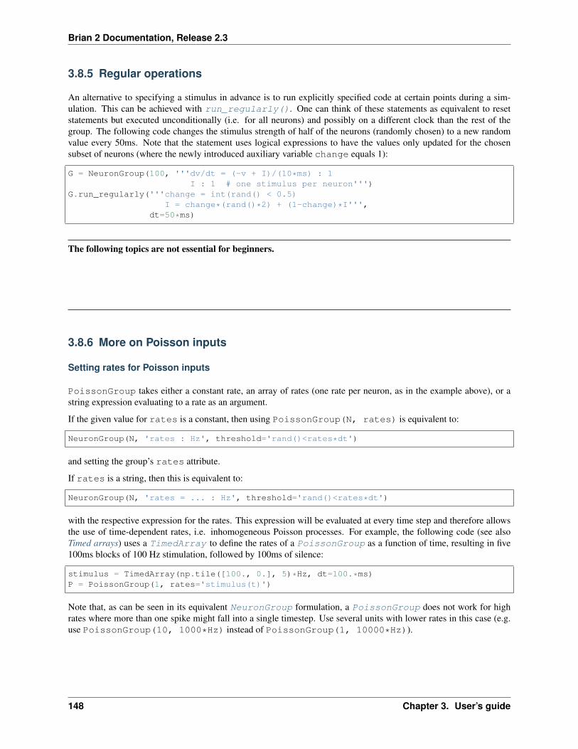
Brian 2 Documentation, Release 2.3
3.8.5 Regular operations
An alternative to specifying a stimulus in advance is to run explicitly specified code at certain points during a sim-ulation. This can be achieved with run_regularly(). One can think of these statements as equivalent to resetstatements but executed unconditionally (i.e. for all neurons) and possibly on a different clock than the rest of thegroup. The following code changes the stimulus strength of half of the neurons (randomly chosen) to a new randomvalue every 50ms. Note that the statement uses logical expressions to have the values only updated for the chosensubset of neurons (where the newly introduced auxiliary variable change equals 1):
G = NeuronGroup(100, '''dv/dt = (-v + I)/(10*ms) : 1I : 1 # one stimulus per neuron''')
G.run_regularly('''change = int(rand() < 0.5)I = change*(rand()*2) + (1-change)*I''',
dt=50*ms)
The following topics are not essential for beginners.
3.8.6 More on Poisson inputs
Setting rates for Poisson inputs
PoissonGroup takes either a constant rate, an array of rates (one rate per neuron, as in the example above), or astring expression evaluating to a rate as an argument.
If the given value for rates is a constant, then using PoissonGroup(N, rates) is equivalent to:
NeuronGroup(N, 'rates : Hz', threshold='rand()<rates*dt')
and setting the group’s rates attribute.
If rates is a string, then this is equivalent to:
NeuronGroup(N, 'rates = ... : Hz', threshold='rand()<rates*dt')
with the respective expression for the rates. This expression will be evaluated at every time step and therefore allowsthe use of time-dependent rates, i.e. inhomogeneous Poisson processes. For example, the following code (see alsoTimed arrays) uses a TimedArray to define the rates of a PoissonGroup as a function of time, resulting in five100ms blocks of 100 Hz stimulation, followed by 100ms of silence:
stimulus = TimedArray(np.tile([100., 0.], 5)*Hz, dt=100.*ms)P = PoissonGroup(1, rates='stimulus(t)')
Note that, as can be seen in its equivalent NeuronGroup formulation, a PoissonGroup does not work for highrates where more than one spike might fall into a single timestep. Use several units with lower rates in this case (e.g.use PoissonGroup(10, 1000*Hz) instead of PoissonGroup(1, 10000*Hz)).
148 Chapter 3. User’s guide
Brian 2 Documentation, Release 2.3
Efficient Poisson inputs via PoissonInput
For simulations where the PoissonGroup is just used as a source of input to a neuron (i.e., the individually generatedspikes are not important, just their impact on the target cell), the PoissonInput class provides a more efficientalternative: instead of generating spikes, PoissonInput directly updates a target variable based on the sum ofindependent Poisson processes:
G = NeuronGroup(100, 'dv/dt = -v / (10*ms) : 1')P = PoissonInput(G, 'v', 100, 100*Hz, weight=0.1)
The PoissonInput class is however more restrictive than PoissonGroup, it only allows for a constant rateacross all neurons (but you can create several PoissonInput objects, targeting different subgroups). It internallyuses BinomialFunction which will draw a random number each time step, either from a binomial distribution orfrom a normal distribution as an approximation to the binomial distribution if 𝑛𝑝 > 5 ∧ 𝑛(1− 𝑝) > 5, where 𝑛 is thenumber of inputs and 𝑝 = 𝑑𝑡 · 𝑟𝑎𝑡𝑒 the spiking probability for a single input.
3.8.7 Arbitrary Python code (network operations)
If none of the above techniques is general enough to fulfill the requirements of a simulation, Brian allows you to writea NetworkOperation, an arbitrary Python function that is executed every time step (possible on a different clockthan the rest of the simulation). This function can do arbitrary operations, use conditional statements etc. and it will beexecuted as it is (i.e. as pure Python code even if weave code generation is active). Note that one cannot use networkoperations in combination with the C++ standalone mode. Network operations are particularly useful when somecondition or calculation depends on operations across neurons, which is currently not possible to express in abstractcode. The following code switches input on for a randomly chosen single neuron every 50 ms:
G = NeuronGroup(10, '''dv/dt = (-v + active*I)/(10*ms) : 1I = sin(2*pi*100*Hz*t) : 1 (shared) #single inputactive : 1 # will be set in the network operation''')
@network_operation(dt=50*ms)def update_active():
index = np.random.randint(10) # index for the active neuronG.active_ = 0 # the underscore switches off unit checkingG.active_[index] = 1
Note that the network operation (in the above example: update_active) has to be included in the Network objectif one is constructed explicitly.
Only functions with zero or one arguments can be used as a NetworkOperation. If the function has one argumentthen it will be passed the current time t:
@network_operation(dt=1*ms)def update_input(t):
if t>50*ms and t<100*ms:pass # do something
Note that this is preferable to accessing defaultclock.t from within the function – if the network operation isnot running on the defaultclock itself, then that value is not guaranteed to be correct.
Instance methods can be used as network operations as well, however in this case they have to be constructed explicitly,the network_operation() decorator cannot be used:
class Simulation(object):def __init__(self, data):
self.data = data
(continues on next page)
3.8. Input stimuli 149
Brian 2 Documentation, Release 2.3
(continued from previous page)
self.group = NeuronGroup(...)self.network_op = NetworkOperation(self.update_func, dt=10*ms)self.network = Network(self.group, self.network_op)
def update_func(self):pass # do something
def run(self, runtime):self.network.run(runtime)
3.9 Recording during a simulation
For Brian 1 users
See the document Monitors (Brian 1 –> 2 conversion) for details how to convert Brian 1 code.
• Recording spikes
• Recording variables at spike time
• Recording variables continuously
• Recording population rates
• Getting all data
• Recording values for a subset of the run
• Freeing up memory in long recordings
• Recording random subsets of neurons
Recording variables during a simulation is done with “monitor” objects. Specifically, spikes are recorded withSpikeMonitor, the time evolution of variables with StateMonitor and the firing rate of a population of neuronswith PopulationRateMonitor.
3.9.1 Recording spikes
To record spikes from a group G simply create a SpikeMonitor via SpikeMonitor(G). After the simulation,you can access the attributes i, t, num_spikes and count of the monitor. The i and t attributes give the array ofneuron indices and times of the spikes. For example, if M.i==[0, 2, 1] and M.t==[1*ms, 2*ms, 3*ms]it means that neuron 0 fired a spike at 1 ms, neuron 2 fired a spike at 2 ms, and neuron 1 fired a spike at 3 ms.Alternatively, you can also call the spike_trains method to get a dictionary mapping neuron indices to arrays ofspike times, i.e. in the above example, spike_trains = M.spike_trains(); spike_trains[1] wouldreturn array([ 3.]) * msecond. The num_spikes attribute gives the total number of spikes recorded, andcount is an array of the length of the recorded group giving the total number of spikes recorded from each neuron.
Example:
G = NeuronGroup(N, model='...')M = SpikeMonitor(G)
(continues on next page)
150 Chapter 3. User’s guide
Brian 2 Documentation, Release 2.3
(continued from previous page)
run(runtime)plot(M.t/ms, M.i, '.')
If you are only interested in summary statistics but not the individual spikes, you can set the record argument toFalse. You will then not have access to i and t but you can still get the count and the total number of spikes(num_spikes).
3.9.2 Recording variables at spike time
By default, a SpikeMonitor only records the time of the spike and the index of the neuron that spiked. Sometimesit can be useful to addtionaly record other variables, e.g. the membrane potential for models where the threshold isnot at a fixed value. This can be done by providing an extra variables argument, the recorded variable can then beaccessed as an attribute of the SpikeMonitor, e.g.:
G = NeuronGroup(10, 'v : 1', threshold='rand()<100*Hz*dt')G.run_regularly('v = rand()')M = SpikeMonitor(G, variables=['v'])run(100*ms)plot(M.t/ms, M.v, '.')
To conveniently access the values of a recorded variable for a single neuron, the SpikeMonitor.values()method can be used that returns a dictionary with the values for each neuron.:
G = NeuronGroup(N, '''dv/dt = (1-v)/(10*ms) : 1v_th : 1''',
threshold='v > v_th',# randomly change the threshold after a spike:reset='''v=0
v_th = clip(v_th + rand()*0.2 - 0.1, 0.1, 0.9)''')G.v_th = 0.5spike_mon = SpikeMonitor(G, variables='v')run(1*second)v_values = spike_mon.values('v')print('Threshold crossing values for neuron 0: {}'.format(v_values[0]))hist(spike_mon.v, np.arange(0, 1, .1))show()
Note: Spikes are not the only events that can trigger recordings, see Custom events.
3.9.3 Recording variables continuously
To record how a variable evolves over time, use a StateMonitor, e.g. to record the variable v at every time stepand plot it for neuron 0:
G = NeuronGroup(...)M = StateMonitor(G, 'v', record=True)run(...)plot(M.t/ms, M.v[0]/mV)
In general, you specify the group, variables and indices you want to record from. You specify the variables with astring or list of strings, and the indices either as an array of indices or True to record all indices (but beware becausethis may take a lot of memory).
3.9. Recording during a simulation 151

Brian 2 Documentation, Release 2.3
After the simulation, you can access these variables as attributes of the monitor. They are 2D arrays with shape(num_indices, num_times). The special attribute t is an array of length num_times with the correspondingtimes at which the values were recorded.
Note that you can also use StateMonitor to record from Synapses where the indices are the synapse indicesrather than neuron indices.
In this example, we record two variables v and u, and record from indices 0, 10 and 100. Afterwards, we plot therecorded values of v and u from neuron 0:
G = NeuronGroup(...)M = StateMonitor(G, ('v', 'u'), record=[0, 10, 100])run(...)plot(M.t/ms, M.v[0]/mV, label='v')plot(M.t/ms, M.u[0]/mV, label='u')
There are two subtly different ways to get the values for specific neurons: you can either index the 2D array stored inthe attribute with the variable name (as in the example above) or you can index the monitor itself. The former will usean index relative to the recorded neurons (e.g. M.v[1] will return the values for the second recorded neuron which isthe neuron with the index 10 whereas M.v[10] would raise an error because only three neurons have been recorded),whereas the latter will use an absolute index corresponding to the recorded group (e.g. M[1].v will raise an errorbecause the neuron with the index 1 has not been recorded and M[10].v will return the values for the neuron withthe index 10). If all neurons have been recorded (e.g. with record=True) then both forms give the same result.
Note that for plotting all recorded values at once, you have to transpose the variable values:
plot(M.t/ms, M.v.T/mV)
Note: In contrast to Brian 1, the values are recorded at the beginning of a time step and not at the end (you can setthe when argument when creating a StateMonitor, details about scheduling can be found here: Custom progressreporting).
3.9.4 Recording population rates
To record the time-varying firing rate of a population of neurons use PopulationRateMonitor. After the simu-lation the monitor will have two attributes t and rate, the latter giving the firing rate at each time step correspondingto the time in t. For example:
G = NeuronGroup(...)M = PopulationRateMonitor(G)run(...)plot(M.t/ms, M.rate/Hz)
To get a smoother version of the rate, use PopulationRateMonitor.smooth_rate().
The following topics are not essential for beginners.
152 Chapter 3. User’s guide

Brian 2 Documentation, Release 2.3
3.9.5 Getting all data
Note that all monitors are implement as “groups”, so you can get all the stored values in a monitor with theget_states method, which can be useful to dump all recorded data to disk, for example:
import picklegroup = NeuronGroup(...)state_mon = StateMonitor(group, 'v', record=...)run(...)data = state_mon.get_states(['t', 'v'])with open('state_mon.pickle', 'w') as f:
pickle.dump(data, f)
3.9.6 Recording values for a subset of the run
Monitors can be created and deleted between runs, e.g. to ignore the first second of your simulation in your recordingsyou can do:
# Set up network without monitorrun(1*second)state_mon = StateMonitor(....)run(...) # Continue run and record with the StateMonitor
Alternatively, you can set the monitor’s active attribute as explained in the Scheduling section.
3.9.7 Freeing up memory in long recordings
Creating and deleting monitors can also be useful to free memory during a long recording. The following will do asimulation run, dump the monitor data to disk, delete the monitor and finally continue the run with a new monitor:
import pickle# Set up networkstate_mon = StateMonitor(...)run(...) # a long rundata = state_mon.get_states(...)with open('first_part.data', 'w') as f:
pickle.dump(data, f)del state_mondel datastate_mon = StateMonitor(...)run(...) # another long run
Note that this technique cannot be applied in standalone mode.
3.9.8 Recording random subsets of neurons
In large networks, you might only be interested in the activity of a random subset of neurons. While you can specifya record argument for a StateMonitor that allows you to select a subset of neurons, this is not possible forSpikeMonitor/EventMonitor and PopulationRateMonitor. However, Brian allows you to record withthese monitors from a subset of neurons by using a subgroup:
group = NeuronGroup(1000, ...)spike_mon = SpikeMonitor(group[:100]) # only record first 100 neurons
3.9. Recording during a simulation 153
Brian 2 Documentation, Release 2.3
It might seem like a restriction that such a subgroup has to be contiguous, but the order of neurons in a group doesnot have any meaning as such; in a randomly ordered group of neurons, any contiguous group of neurons can beconsidered a random subset. If some aspects of your model do depend on the position of the neuron in a group (e.g.a ring model, where neurons are connected based on their distance in the ring, or a model where initial values orparameters span a range of values in a regular fashion), then this requires an extra step: instead of using the order ofneurons in the group directly, or depending on the neuron index i, create a new, shuffled, index variable as part of themodel definition and then depend on this index instead:
group = NeuronGroup(10000, '''....index : integer (constant)''')
indices = group.i[:]np.random.shuffle(indices)group.index = indices# Then use 'index' in string expressions or use it as an index array# for initial values/parameters defined as numpy arrays
If this solution is not feasible for some reason, there is another approach that works for aSpikeMonitor/EventMonitor. You can add an additional flag to each neuron, stating whether it shouldbe recorded or not. Then, you define a new custom event that is identical to the event you are interested in, butadditionally requires the flag to be set. E.g. to only record the spikes of neurons with the to_record attribute set:
group = NeuronGroup(..., '''...to_record : boolean (constant)''',
threshold='...', reset='...',events={'recorded_spike': '... and to_record'})
group.to_record = ...mon_events = EventMonitor(group, 'recorded_spike')
Note that this solution will evaluate the threshold condition for each neuron twice, and is therefore slightly less ef-ficient. There’s one additional caveat: you’ll have to manually include and not_refractory in your eventsdefinition if your neuron uses refractoriness. This is done automatically for the threshold condition, but not forany user-defined events.
3.10 Running a simulation
For Brian 1 users
See the document Networks and clocks (Brian 1 –> 2 conversion) for details how to convert Brian 1 code.
• Networks
• Setting the simulation time step
• Progress reporting
• Continuing/repeating simulations
• Multiple magic runs
• Changing the simulation time step
• Profiling
• Scheduling
154 Chapter 3. User’s guide
Brian 2 Documentation, Release 2.3
• Store/restore
To run a simulation, one either constructs a new Network object and calls its Network.run() method, or uses the“magic” system and a plain run() call, collecting all the objects in the current namespace.
Note that Brian has several different ways of running the actual computations, and choosing the right one can makeorders of magnitude of difference in terms of simplicity and efficiency. See Computational methods and efficiency formore details.
3.10.1 Networks
In most straightforward simulations, you do not have to explicitly create a Network object but instead can simplycall run() to run a simulation. This is what is called the “magic” system, because Brian figures out automaticallywhat you want to do.
When calling run(), Brian runs the collect() function to gather all the objects in the current context. It willinclude all the objects that are “visible”, i.e. that you could refer to with an explicit name:
G = NeuronGroup(10, 'dv/dt = -v / tau : volt')S = Synapses(G, G, model='w:1', on_pre='v+=w')S.connect('i!=j')mon = SpikeMonitor(G)
run(10*ms) # will include G, S, mon
Note that it will not automatically include objects that are “hidden” in containers, e.g. if you store several monitorsin a list. Use an explicit Network object in this case. It might be convenient to use the collect() function whencreating the Network object in that case:
G = NeuronGroup(10, 'dv/dt = -v / tau : volt')S = Synapses(G, G, model='w:1', on_pre='v+=w')S.connect('i!=j')monitors = [SpikeMonitor(G), StateMonitor(G, 'v', record=True)]
# a simple run would not include the monitorsnet = Network(collect()) # automatically include G and Snet.add(monitors) # manually add the monitors
net.run(10*ms)
3.10.2 Setting the simulation time step
To set the simulation time step for every simulated object, set the dt attribute of the defaultclock which is usedby all objects that do not explicitly specify a clock or dt value during construction:
defaultclock.dt = 0.05*ms
If some objects should use a different clock (e.g. to record values with a StateMonitor not at every time step in along running simulation), you can provide a dt argument to the respective object:
s_mon = StateMonitor(group, 'v', record=True, dt=1*ms)
To sum up:
• Set defaultclock.dt to the time step that should be used by most (or all) of your objects.
3.10. Running a simulation 155
Brian 2 Documentation, Release 2.3
• Set dt explicitly when creating objects that should use a different time step.
Behind the scenes, a new Clock object will be created for each object that defines its own dt value.
3.10.3 Progress reporting
Especially for long simulations it is useful to get some feedback about the progress of the simulation. Brian offers afew built-in options and an extensible system to report the progress of the simulation. In the Network.run() orrun() call, two arguments determine the output: report and report_period. When report is set to 'text'or 'stdout', the progress will be printed to the standard output, when it is set to 'stderr', it will be printed to“standard error”. There will be output at the start and the end of the run, and during the run in report_periodintervals. It is also possible to do custom progress reporting.
3.10.4 Continuing/repeating simulations
To store the current state of the simulation, call store() (use the Network.store() method for a Network).You can store more than one snapshot of a system by providing a name for the snapshot; if store() is called withouta specified name, 'default' is used as the name. To restore the state, use restore().
The following simple example shows how this system can be used to run several trials of an experiment:
# set up the networkG = NeuronGroup(...)...spike_monitor = SpikeMonitor(G)
# Snapshot the statestore()
# Run the trialsspike_counts = []for trial in range(3):
restore() # Restore the initial staterun(...)# store the resultsspike_counts.append(spike_monitor.count)
The following schematic shows how multiple snapshots can be used to run a network with a separate “train” and “test”phase. After training, the test is run several times based on the trained network. The whole process of training andtesting is repeated several times as well:
# set up the networkG = NeuronGroup(..., '''...
test_input : amp...''')
S = Synapses(..., '''...plastic : boolean (shared)...''')
G.v = ...S.connect(...)S.w = ...
# First snapshot at t=0store('initialized')
(continues on next page)
156 Chapter 3. User’s guide
Brian 2 Documentation, Release 2.3
(continued from previous page)
# Run 3 complete trialsfor trial in range(3):
# Simulate training phaserestore('initialized')S.plastic = Truerun(...)
# Snapshot after learningstore('after_learning')
# Run 5 tests after the trainingfor test_number in range(5):
restore('after_learning')S.plastic = False # switch plasticity offG.test_input = test_inputs[test_number]# monitor the activity nowspike_mon = SpikeMonitor(G)run(...)# Do something with the result# ...
The following topics are not essential for beginners.
3.10.5 Multiple magic runs
When you use more than a single run() statement, the magic system tries to detect which of the following twosituations applies:
1. You want to continue a previous simulation
2. You want to start a new simulation
For this, it uses the following heuristic: if a simulation consists only of objects that have not been run, it will starta new simulation starting at time 0 (corresponding to the creation of a new Network object). If a simulation onlyconsists of objects that have been simulated in the previous run() call, it will continue that simulation at the previoustime.
If neither of these two situations apply, i.e., the network consists of a mix of previously run objects and new objects,an error will be raised. If this is not a mistake but intended (e.g. when a new input source and synapses should beadded to a network at a later stage), use an explicit Network object.
In these checks, “non-invalidating” objects (i.e. objects that have BrianObject.invalidates_magic_network set to False) are ignored, e.g. creating new monitors is always possible.
Note that if you do not want to run an object for the complete duration of your simulation, you can create the object inthe beginning of your simulation and then set its active attribute. For details, see the Scheduling section below.
3.10. Running a simulation 157

Brian 2 Documentation, Release 2.3
3.10.6 Changing the simulation time step
You can change the simulation time step after objects have been created or even after a simulation has been run:
defaultclock.dt = 0.1*ms# Set the network# ...run(initial_time)defaultclock.dt = 0.01*msrun(full_time - initial_time)
To change the time step between runs for objects that do not use the defaultclock, you cannot directly change theirdt attribute (which is read-only) but instead you have to change the dt of the clock attribute. If you want to changethe dt value of several objects at the same time (but not for all of them, i.e. when you cannot use defaultclock.dt) then you might consider creating a Clock object explicitly and then passing this clock to each object with theclock keyword argument (instead of dt). This way, you can later change the dt for several objects at once byassigning a new value to Clock.dt.
Note that a change of dt has to be compatible with the internal representation of clocks as an integer value (the numberof elapsed time steps). For example, you can simulate an object for 100ms with a time step of 0.1ms (i.e. for 1000steps) and then switch to a dt of 0.5ms, the time will then be internally represented as 200 steps. You cannot, however,switch to a dt of 0.3ms, because 100ms are not an integer multiple of 0.3ms.
3.10.7 Profiling
To get an idea which parts of a simulation take the most time, Brian offers a basic profiling mechanism. If a simulationis run with the profile=True keyword argument, it will collect information about the total simulation time foreach CodeObject. This information can then be retrieved from Network.profiling_info, which containsa list of (name, time) tuples or a string summary can be obtained by calling profiling_summary(). Thefollowing example shows profiling output after running the CUBA example (where the neuronal state updates take upthe most time):
>>> profiling_summary(show=5) # show the 5 objects that took the longestProfiling summary=================neurongroup_stateupdater 5.54 s 61.32 %synapses_pre 1.39 s 15.39 %synapses_1_pre 1.03 s 11.37 %spikemonitor 0.59 s 6.55 %neurongroup_thresholder 0.33 s 3.66 %
3.10.8 Scheduling
Every simulated object in Brian has three attributes that can be specified at object creation time: dt, when, andorder. The time step of the simulation is determined by dt, if it is specified, or otherwise by defaultclock.dt.Changing this will therefore change the dt of all objects that don’t specify one. Alternatively, a clock object can bespecified directly, this can be useful if a clock should be shared between several objects – under most circumstances,however, a user should not have to deal with the creation of Clock objects and just define dt.
During a single time step, objects are updated in an order according first to their when argument’s position inthe schedule. This schedule is determined by Network.schedule which is a list of strings, determining “ex-ecution slots” and their order. It defaults to: ['start', 'groups', 'thresholds', 'synapses','resets', 'end']. In addition to the names provided in the schedule, names such as before_thresholdsor after_synapses can be used that are understood as slots in the respective positions. The default for the when
158 Chapter 3. User’s guide

Brian 2 Documentation, Release 2.3
attribute is a sensible value for most objects (resets will happen in the reset slot, etc.) but sometimes it make senseto change it, e.g. if one would like a StateMonitor, which by default records in the start slot, to record themembrane potential before a reset is applied (otherwise no threshold crossings will be observed in the membranepotential traces).
Finally, if during a time step two objects fall in the same execution slot, they will be updated in ascending orderaccording to their order attribute, an integer number defaulting to 0. If two objects have the same when and orderattribute then they will be updated in an arbitrary but reproducible order (based on the lexicographical order of theirnames).
Note that objects that don’t do any computation by themselves but only act as a container for other objects (e.g. aNeuronGroup which contains a StateUpdater, a Resetter and a Thresholder), don’t have any value forwhen, but pass on the given values for dt and order to their containing objects.
If you want your simulation object to run only for a particular time period of the whole simulation, you can use theactive attribute. For example, this can be useful when you want a monitor to be active only for some time out of along simulation:
# Set up the network# ...monitor = SpikeMonitor(...)monitor.active = Falserun(long_time*seconds) # not recordingmonitor.active = Truerun(required_time*seconds) # recording
To see how the objects in a network are scheduled, you can use the scheduling_summary() function:
>>> group = NeuronGroup(10, 'dv/dt = -v/(10*ms) : 1', threshold='v > 1',... reset='v = 0')>>> mon = StateMonitor(group, 'v', record=True, dt=1*ms)>>> scheduling_summary()
object | part of | Clock→˓dt | when | order | active----------------------------------------+-----------------------------+---------------→˓---------+------------+-------+-------statemonitor (StateMonitor) | statemonitor (StateMonitor) | 1. ms (every→˓10 steps) | start | 0 | yesneurongroup_stateupdater (StateUpdater) | neurongroup (NeuronGroup) | 100. us→˓(every step) | groups | 0 | yesneurongroup_thresholder (Thresholder) | neurongroup (NeuronGroup) | 100. us→˓(every step) | thresholds | 0 | yesneurongroup_resetter (Resetter) | neurongroup (NeuronGroup) | 100. us→˓(every step) | resets | 0 | yes
As you can see in the output above, the StateMonitor will only record the membrane potential every 10 time steps,but when it does, it will do it at the start of the time step, before the numerical integration, the thresholding, and thereset operation takes place.
Every new Network starts a simulation at time 0; Network.t is a read-only attribute, to go back to a previousmoment in time (e.g. to do another trial of a simulation with a new noise instantiation) use the mechanism describedbelow.
3.10.9 Store/restore
Note that Network.run(), Network.store() and Network.restore() (or run(), store(),restore()) are the only way of affecting the time of the clocks. In contrast to Brian1, it is no longer necessary (norpossible) to directly set the time of the clocks or call a reinit function.
3.10. Running a simulation 159
Brian 2 Documentation, Release 2.3
The state of a network can also be stored on disk with the optional filename argument of Network.store()/store(). This way, you can run the initial part of a simulation once, store it to disk, and then continuefrom this state later. Note that the store()/restore()mechanism does not re-create the network as such, you stillneed to construct all the NeuronGroup, Synapses, StateMonitor, . . . objects, restoring will only restore allthe state variable values (membrane potential, conductances, synaptic connections/weights/delays, . . . ). This restora-tion does however restore the internal state of the objects as well, e.g. spikes that have not been delivered yet becauseof synaptic delays will be delivered correctly.
3.11 Multicompartment models
For Brian 1 users
See the document Multicompartmental models (Brian 1 –> 2 conversion) for details how to convert Brian 1 code.
It is possible to create neuron models with a spatially extended morphology, using the SpatialNeuron class. ASpatialNeuron is a single neuron with many compartments. Essentially, it works as a NeuronGroup whereelements are compartments instead of neurons.
A SpatialNeuron is specified by a morphology (see Creating a neuron morphology) and a set of equations fortransmembrane currents (see Creating a spatially extended neuron).
3.11.1 Creating a neuron morphology
Schematic morphologies
Morphologies can be created combining geometrical objects:
soma = Soma(diameter=30*um)cylinder = Cylinder(diameter=1*um, length=100*um, n=10)
The first statement creates a single iso-potential compartment (i.e. with no axial resistance within the compartment),with its area calculated as the area of a sphere with the given diameter. The second one specifies a cylinder consistingof 10 compartments with identical diameter and the given total length.
For more precise control over the geometry, you can specify the length and diameter of each individual compartment,including the diameter at the start of the section (i.e. for n compartments: n length and n+1 diameter values) in aSection object:
section = Section(diameter=[6, 5, 4, 3, 2, 1]*um, length=[10, 10, 10, 5, 5]*um, n=5)
The individual compartments are modeled as truncated cones, changing the diameter linearly between the given diam-eters over the length of the compartment. Note that the diameter argument specifies the values at the nodes betweenthe compartments, but accessing the diameter attribute of a Morphology object will return the diameter at thecenter of the compartment (see the note below).
The following table summarizes the different options to create schematic morphologies (the black compartment beforethe start of the section represents the parent compartment with diameter 15 𝜇m, not specified in the code below):
160 Chapter 3. User’s guide

Brian 2 Documentation, Release 2.3
ExampleSoma
# Soma always has a single→˓compartmentSoma(diameter=30*um)
Cylinder# Each compartment has fixed→˓length and diameterCylinder(n=5, diameter=10*um,→˓length=50*um)
Section# Length and diameter→˓individually defined for→˓each compartment (at start# and end)Section(n=5, diameter=[15, 5,→˓10, 5, 10, 5]*um,
length=[10, 20, 5, 5,→˓10]*um)
Note: For a Section, the diameter argument specifies the diameter between the compartments (and atthe beginning/end of the first/last compartment). the corresponding values can therefore be later retrieved fromthe Morphology via the start_diameter and end_diameter attributes. The diameter attribute ofa Morphology does correspond to the diameter at the midpoint of the compartment. For a Cylinder,start_diameter, diameter, and end_diameter are of course all identical.
The tree structure of a morphology is created by attaching Morphology objects together:
morpho = Soma(diameter=30*um)morpho.axon = Cylinder(length=100*um, diameter=1*um, n=10)morpho.dendrite = Cylinder(length=50*um, diameter=2*um, n=5)
These statements create a morphology consisting of a cylindrical axon and a dendrite attached to a spherical soma.Note that the names axon and dendrite are arbitrary and chosen by the user. For example, the same morphologycan be created as follows:
morpho = Soma(diameter=30*um)morpho.output_process = Cylinder(length=100*um, diameter=1*um, n=10)morpho.input_process = Cylinder(length=50*um, diameter=2*um, n=5)
The syntax is recursive, for example two sections can be added at the end of the dendrite as follows:
morpho.dendrite.branch1 = Cylinder(length=50*um, diameter=1*um, n=3)morpho.dendrite.branch2 = Cylinder(length=50*um, diameter=1*um, n=3)
Equivalently, one can use an indexing syntax:
morpho['dendrite']['branch1'] = Cylinder(length=50*um, diameter=1*um, n=3)morpho['dendrite']['branch2'] = Cylinder(length=50*um, diameter=1*um, n=3)
3.11. Multicompartment models 161
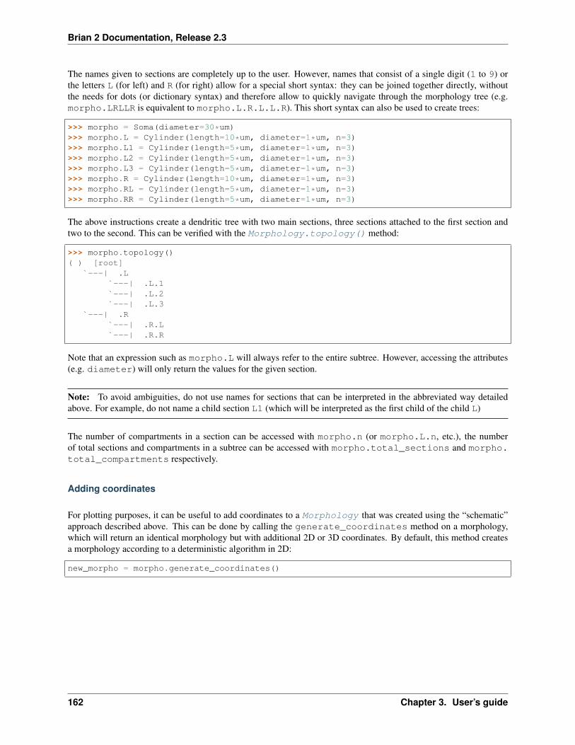
Brian 2 Documentation, Release 2.3
The names given to sections are completely up to the user. However, names that consist of a single digit (1 to 9) orthe letters L (for left) and R (for right) allow for a special short syntax: they can be joined together directly, withoutthe needs for dots (or dictionary syntax) and therefore allow to quickly navigate through the morphology tree (e.g.morpho.LRLLR is equivalent to morpho.L.R.L.L.R). This short syntax can also be used to create trees:
>>> morpho = Soma(diameter=30*um)>>> morpho.L = Cylinder(length=10*um, diameter=1*um, n=3)>>> morpho.L1 = Cylinder(length=5*um, diameter=1*um, n=3)>>> morpho.L2 = Cylinder(length=5*um, diameter=1*um, n=3)>>> morpho.L3 = Cylinder(length=5*um, diameter=1*um, n=3)>>> morpho.R = Cylinder(length=10*um, diameter=1*um, n=3)>>> morpho.RL = Cylinder(length=5*um, diameter=1*um, n=3)>>> morpho.RR = Cylinder(length=5*um, diameter=1*um, n=3)
The above instructions create a dendritic tree with two main sections, three sections attached to the first section andtwo to the second. This can be verified with the Morphology.topology() method:
>>> morpho.topology()( ) [root]
`---| .L`---| .L.1`---| .L.2`---| .L.3
`---| .R`---| .R.L`---| .R.R
Note that an expression such as morpho.L will always refer to the entire subtree. However, accessing the attributes(e.g. diameter) will only return the values for the given section.
Note: To avoid ambiguities, do not use names for sections that can be interpreted in the abbreviated way detailedabove. For example, do not name a child section L1 (which will be interpreted as the first child of the child L)
The number of compartments in a section can be accessed with morpho.n (or morpho.L.n, etc.), the numberof total sections and compartments in a subtree can be accessed with morpho.total_sections and morpho.total_compartments respectively.
Adding coordinates
For plotting purposes, it can be useful to add coordinates to a Morphology that was created using the “schematic”approach described above. This can be done by calling the generate_coordinates method on a morphology,which will return an identical morphology but with additional 2D or 3D coordinates. By default, this method createsa morphology according to a deterministic algorithm in 2D:
new_morpho = morpho.generate_coordinates()
162 Chapter 3. User’s guide
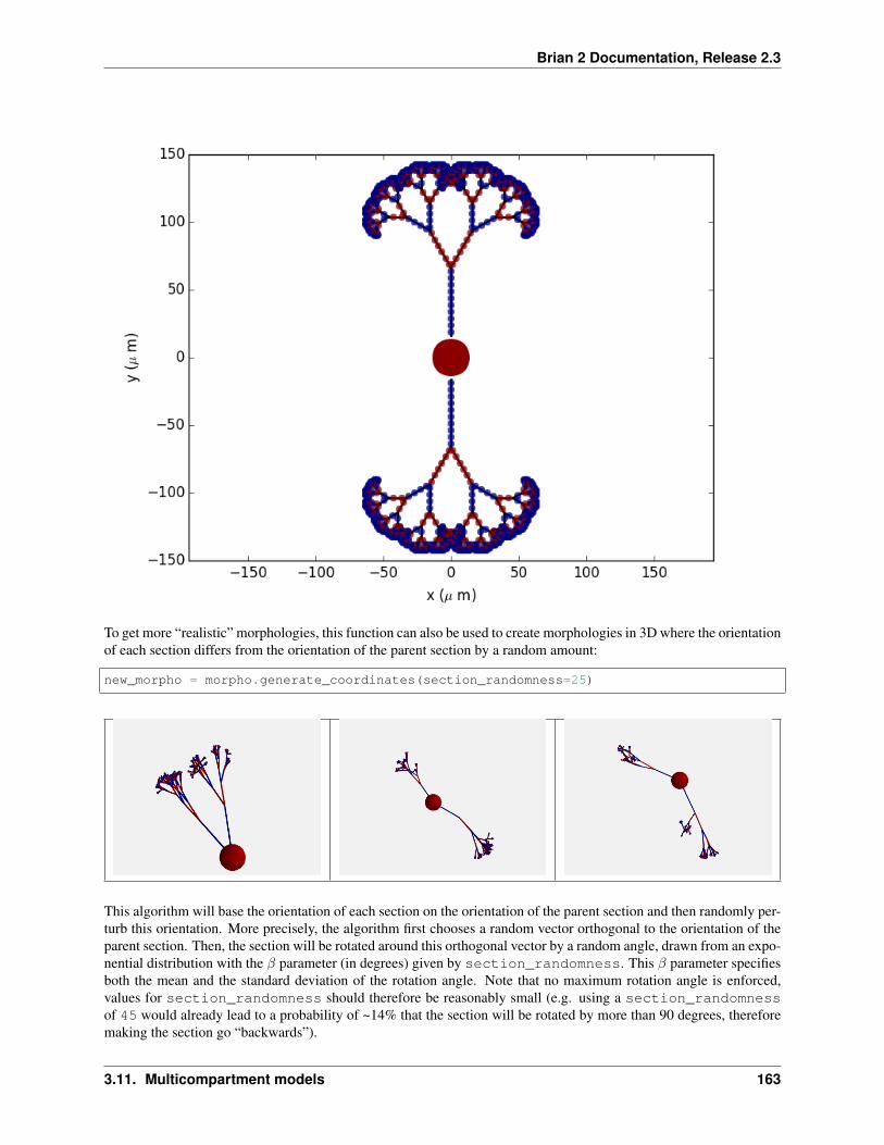
Brian 2 Documentation, Release 2.3
To get more “realistic” morphologies, this function can also be used to create morphologies in 3D where the orientationof each section differs from the orientation of the parent section by a random amount:
new_morpho = morpho.generate_coordinates(section_randomness=25)
This algorithm will base the orientation of each section on the orientation of the parent section and then randomly per-turb this orientation. More precisely, the algorithm first chooses a random vector orthogonal to the orientation of theparent section. Then, the section will be rotated around this orthogonal vector by a random angle, drawn from an expo-nential distribution with the 𝛽 parameter (in degrees) given by section_randomness. This 𝛽 parameter specifiesboth the mean and the standard deviation of the rotation angle. Note that no maximum rotation angle is enforced,values for section_randomness should therefore be reasonably small (e.g. using a section_randomnessof 45 would already lead to a probability of ~14% that the section will be rotated by more than 90 degrees, thereforemaking the section go “backwards”).
3.11. Multicompartment models 163
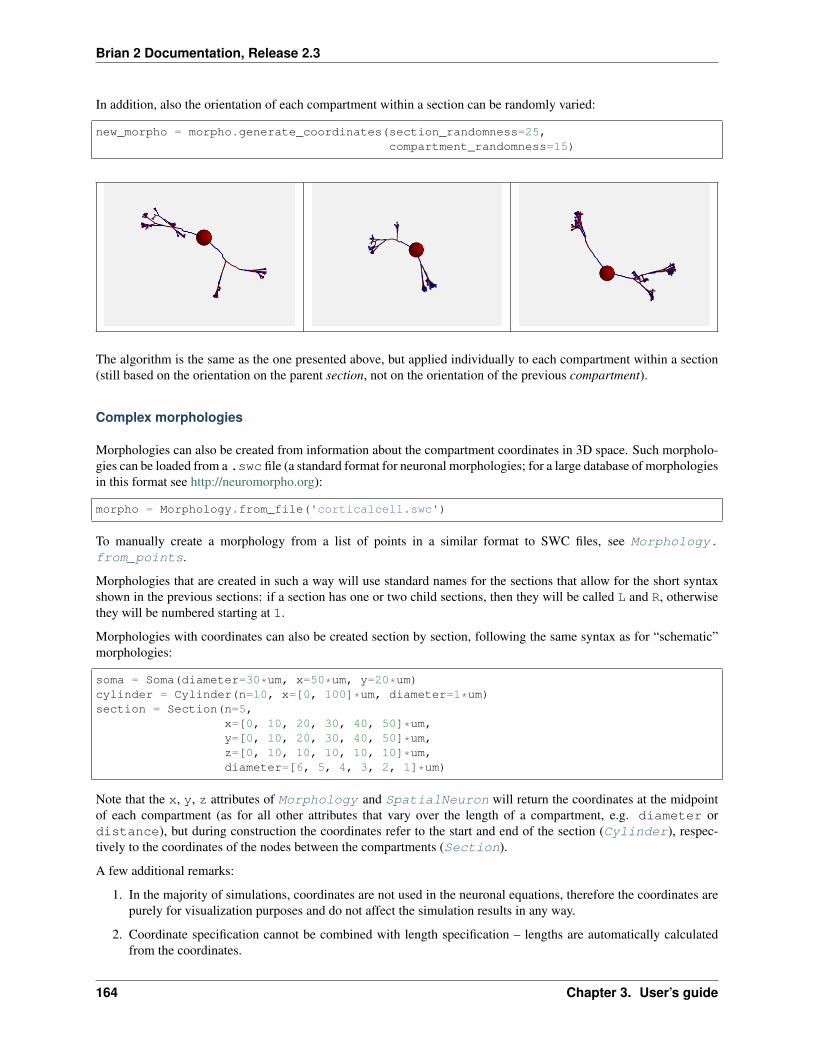
Brian 2 Documentation, Release 2.3
In addition, also the orientation of each compartment within a section can be randomly varied:
new_morpho = morpho.generate_coordinates(section_randomness=25,compartment_randomness=15)
The algorithm is the same as the one presented above, but applied individually to each compartment within a section(still based on the orientation on the parent section, not on the orientation of the previous compartment).
Complex morphologies
Morphologies can also be created from information about the compartment coordinates in 3D space. Such morpholo-gies can be loaded from a .swc file (a standard format for neuronal morphologies; for a large database of morphologiesin this format see http://neuromorpho.org):
morpho = Morphology.from_file('corticalcell.swc')
To manually create a morphology from a list of points in a similar format to SWC files, see Morphology.from_points.
Morphologies that are created in such a way will use standard names for the sections that allow for the short syntaxshown in the previous sections: if a section has one or two child sections, then they will be called L and R, otherwisethey will be numbered starting at 1.
Morphologies with coordinates can also be created section by section, following the same syntax as for “schematic”morphologies:
soma = Soma(diameter=30*um, x=50*um, y=20*um)cylinder = Cylinder(n=10, x=[0, 100]*um, diameter=1*um)section = Section(n=5,
x=[0, 10, 20, 30, 40, 50]*um,y=[0, 10, 20, 30, 40, 50]*um,z=[0, 10, 10, 10, 10, 10]*um,diameter=[6, 5, 4, 3, 2, 1]*um)
Note that the x, y, z attributes of Morphology and SpatialNeuron will return the coordinates at the midpointof each compartment (as for all other attributes that vary over the length of a compartment, e.g. diameter ordistance), but during construction the coordinates refer to the start and end of the section (Cylinder), respec-tively to the coordinates of the nodes between the compartments (Section).
A few additional remarks:
1. In the majority of simulations, coordinates are not used in the neuronal equations, therefore the coordinates arepurely for visualization purposes and do not affect the simulation results in any way.
2. Coordinate specification cannot be combined with length specification – lengths are automatically calculatedfrom the coordinates.
164 Chapter 3. User’s guide

Brian 2 Documentation, Release 2.3
3. The coordinate specification can also be 1- or 2-dimensional (as in the first two examples above), the unspecifiedcoordinate will use 0 𝜇m.
4. All coordinates are interpreted relative to the parent compartment, i.e. the point (0 𝜇m, 0 𝜇m, 0 𝜇m) refers tothe end point of the previous compartment. Most of the time, the first element of the coordinate specificationis therefore 0 𝜇m, to continue a section where the previous one ended. However, it can be convenient to use avalue different from 0 𝜇m for sections connecting to the Soma to make them (visually) connect to a point onthe sphere surface instead of the center of the sphere.
3.11.2 Creating a spatially extended neuron
A SpatialNeuron is a spatially extended neuron. It is created by specifying the morphology as a Morphologyobject, the equations for transmembrane currents, and optionally the specific membrane capacitance Cm and intracel-lular resistivity Ri:
gL = 1e-4*siemens/cm**2EL = -70*mVeqs = '''Im=gL * (EL - v) : amp/meter**2I : amp (point current)'''neuron = SpatialNeuron(morphology=morpho, model=eqs, Cm=1*uF/cm**2, Ri=100*ohm*cm)neuron.v = EL + 10*mV
Several state variables are created automatically: the SpatialNeuron inherits all the geometrical variables of thecompartments (length, diameter, area, volume), as well as the distance variable that gives the distance tothe soma. For morphologies that use coordinates, the x, y and z variables are provided as well. Additionally, a statevariable Cm is created. It is initialized with the value given at construction, but it can be modified on a compartment percompartment basis (which is useful to model myelinated axons). The membrane potential is stored in state variable v.
Note that for all variable values that vary across a compartment (e.g. distance, x, y, z, v), the value that is reportedis the value at the midpoint of the compartment.
The key state variable, which must be specified at construction, is Im. It is the total transmembrane current, expressedin units of current per area. This is a mandatory line in the definition of the model. The rest of the string description mayinclude other state variables (differential equations or subexpressions) or parameters, exactly as in NeuronGroup.At every timestep, Brian integrates the state variables, calculates the transmembrane current at every point on theneuronal morphology, and updates v using the transmembrane current and the diffusion current, which is calculatedbased on the morphology and the intracellular resistivity. Note that the transmembrane current is a surfacic current,not the total current in the compartement. This choice means that the model equations are independent of the numberof compartments chosen for the simulation. The space and time constants can obtained for any point of the neuronwith the space_constant respectively time_constant attributes:
l = neuron.space_constant[0]tau = neuron.time_constant[0]
The calculation is based on the local total conductance (not just the leak conductance), therefore, it can potentially varyduring a simulation (e.g. decrease during an action potential). The reported value is only correct for compartments witha cylindrical geometry, though, it does not give reasonable values for compartments with strongly varying diameter.
To inject a current I at a particular point (e.g. through an electrode or a synapse), this current must be divided by thearea of the compartment when inserted in the transmembrane current equation. This is done automatically when theflag point current is specified, as in the example above. This flag can apply only to subexpressions or parameterswith amp units. Internally, the expression of the transmembrane current Im is simply augmented with +I/area. Acurrent can then be injected in the first compartment of the neuron (generally the soma) as follows:
3.11. Multicompartment models 165

Brian 2 Documentation, Release 2.3
neuron.I[0] = 1*nA
State variables of the SpatialNeuron include all the compartments of that neuron (including subtrees). Therefore,the statement neuron.v = EL + 10*mV sets the membrane potential of the entire neuron at -60 mV.
Subtrees can be accessed by attribute (in the same way as in Morphology objects):
neuron.axon.gNa = 10*gL
Note that the state variables correspond to the entire subtree, not just the main section. That is, if the axon had branches,then the above statement would change gNa on the main section and all the sections in the subtree. To access the mainsection only, use the attribute main:
neuron.axon.main.gNa = 10*gL
A typical use case is when one wants to change parameter values at the soma only. For example, inserting an electrodecurrent at the soma is done as follows:
neuron.main.I = 1*nA
A part of a section can be accessed as follows:
initial_segment = neuron.axon[10*um:50*um]
Finally, similar to the way that you can refer to a subset of neurons of a NeuronGroup, you can also index theSpatialNeuron object itself, e.g. to get a group representing only the first compartment of a cell (typically thesoma), you can use:
soma = neuron[0]
In the same way as for sections, you can also use slices, either with the indices of compartments, or with the distancefrom the root:
first_compartments = neurons[:3]first_compartments = neurons[0*um:30*um]
However, note that this is restricted to contiguous indices which most of the time means that all compartments indexedin this way have to be part of the same section. Such indices can be acquired directly from the morphology:
axon = neurons[morpho.axon.indices[:]]
or, more concisely:
axon = neurons[morpho.axon]
Synaptic inputs
There are two methods to have synapses on SpatialNeuron. The first one to insert synaptic equations directly inthe neuron equations:
eqs='''Im = gL * (EL - v) : amp/meter**2Is = gs * (Es - v) : amp (point current)dgs/dt = -gs/taus : siemens'''neuron = SpatialNeuron(morphology=morpho, model=eqs, Cm=1*uF/cm**2, Ri=100*ohm*cm)
166 Chapter 3. User’s guide

Brian 2 Documentation, Release 2.3
Note that, as for electrode stimulation, the synaptic current must be defined as a point current. Then we use aSynapses object to connect a spike source to the neuron:
S = Synapses(stimulation, neuron, on_pre='gs += w')S.connect(i=0, j=50)S.connect(i=1, j=100)
This creates two synapses, on compartments 50 and 100. One can specify the compartment number with its spatialposition by indexing the morphology:
S.connect(i=0, j=morpho[25*um])S.connect(i=1, j=morpho.axon[30*um])
In this method for creating synapses, there is a single value for the synaptic conductance in any compartment. Thismeans that it will fail if there are several synapses onto the same compartment and synaptic equations are nonlinear.The second method, which works in such cases, is to have synaptic equations in the Synapses object:
eqs='''Im = gL * (EL - v) : amp/meter**2Is = gs * (Es - v) : amp (point current)gs : siemens'''neuron = SpatialNeuron(morphology=morpho, model=eqs, Cm=1 * uF / cm ** 2, Ri=100 *→˓ohm * cm)S = Synapses(stimulation, neuron, model='''dg/dt = -g/taus : siemens
gs_post = g : siemens (summed)''',on_pre='g += w')
Here each synapse (instead of each compartment) has an associated value g, and all values of g for each compartment(i.e., all synapses targeting that compartment) are collected into the compartmental variable gs.
Detecting spikes
To detect and record spikes, we must specify a threshold condition, essentially in the same way as for aNeuronGroup:
neuron = SpatialNeuron(morphology=morpho, model=eqs, threshold='v > 0*mV', refractory=→˓'v > -10*mV')
Here spikes are detected when the membrane potential v reaches 0 mV. Because there is generally no explicit reset inthis type of model (although it is possible to specify one), v remains above 0 mV for some time. To avoid detectingspikes during this entire time, we specify a refractory period. In this case no spike is detected as long as v is greaterthan -10 mV. Another possibility could be:
neuron = SpatialNeuron(morphology=morpho, model=eqs, threshold='m > 0.5', refractory=→˓'m > 0.4')
where m is the state variable for sodium channel activation (assuming this has been defined in the model). Here a spikeis detected when half of the sodium channels are open.
With the syntax above, spikes are detected in all compartments of the neuron. To detect them in a single compartment,use the threshold_location keyword:
neuron = SpatialNeuron(morphology=morpho, model=eqs, threshold='m > 0.5', threshold_→˓location=30,
refractory='m > 0.4')
3.11. Multicompartment models 167
Brian 2 Documentation, Release 2.3
In this case, spikes are only detecting in compartment number 30. Reset then applies locally to that compartment (if areset statement is defined). Again the location of the threshold can be specified with spatial position:
neuron = SpatialNeuron(morphology=morpho, model=eqs, threshold='m > 0.5',threshold_location=morpho.axon[30*um],refractory='m > 0.4')
Subgroups
In the same way that you can refer to a subset of neurons in a NeuronGroup, you can also refer to a subset ofcompartments in a SpatialNeuron
3.12 Computational methods and efficiency
• Runtime code generation
• Standalone code generation
• Compiler settings
Brian has several different methods for running the computations in a simulation. The default mode is Runtimecode generation, which runs the simulation loop in Python but compiles and executes the modules doing the actualsimulation work (numerical integration, synaptic propagation, etc.) in a defined target language. Brian will select thebest available target language automatically. On Windows, to ensure that you get the advantages of compiled code,read the instructions on installing a suitable compiler in Windows. Runtime mode has the advantage that you cancombine the computations performed by Brian with arbitrary Python code specified as NetworkOperation.
The fact that the simulation is run in Python means that there is a (potentially big) overhead for each simulated timestep. An alternative is to run Brian in with Standalone code generation – this is in general faster (for certain types ofsimulations much faster) but cannot be used for all kinds of simulations. To enable this mode, add the following lineafter your Brian import, but before your simulation code:
set_device('cpp_standalone')
For detailed control over the compilation process (both for runtime and standalone code generation), you can changethe Cleaning up after a run that are used.
The following topics are not essential for beginners.
3.12.1 Runtime code generation
Code generation means that Brian takes the Python code and strings in your model and generates code in one of severalpossible different languages and actually executes that. The target language for this code generation process is set inthe codegen.target preference. By default, this preference is set to 'auto', meaning that it will chose a compiledlanguage target if possible and fall back to Python otherwise (it will also raise a warning in this case, set codegen.target
168 Chapter 3. User’s guide

Brian 2 Documentation, Release 2.3
to 'numpy' explicitly to avoid this warning). There are two compiled language targets for Python 2.x, 'weave'(needing a working installation of a C++ compiler) and 'cython' (needing the Cython package in addition); forPython 3.x, only 'cython' is available. If you want to chose a code generation target explicitly (e.g. because youwant to get rid of the warning that only the Python fallback is available), set the preference to 'numpy', 'weave'or 'cython' at the beginning of your script:
from brian2 import *prefs.codegen.target = 'numpy' # use the Python fallback
See Preferences for different ways of setting preferences.
Warning:
Do not use the weave code generation targets when running multiple simulations in parallel. SeeKnown issues for more details.
Caching
When you run code with weave or cython for the first time, it will take some time to compile the code. For shortsimulations, this can make these targets to appear slow compared to the numpy target where such compilation is notnecessary. However, the compiled code is stored on disk and will be re-used for later runs, making these simulationsstart faster. If you run many simulations with different code (e.g. Brian’s test suite), this code can take quite a bit ofspace on the disk. During the import of the brian2 package, we check whether the size of the disk cache exceeds thevalue set by the codegen.max_cache_dir_size preference (by default, 1GB) and display a message if this is the case.You can clear the disk cache manually, or use the clear_cache function, e.g. clear_cache('cython').
3.12.2 Standalone code generation
Brian supports generating standalone code for multiple devices. In this mode, running a Brian script generates sourcecode in a project tree for the target device/language. This code can then be compiled and run on the device, andmodified if needed. At the moment, the only “device” supported is standalone C++ code. In some cases, the speedgains can be impressive, in particular for smaller networks with complicated spike propagation rules (such as STDP).
To use the C++ standalone mode, you only have to make very small changes to your script. The exact change dependson whether your script has only a single run() (or Network.run()) call, or several of them:
Single run call
At the beginning of the script, i.e. after the import statements, add:
set_device('cpp_standalone')
The CPPStandaloneDevice.build function will be automatically called with default arguments right after therun() call. If you need non-standard arguments then you can specify them as part of the set_device() call:
set_device('cpp_standalone', directory='my_directory', debug=True)
Multiple run calls
At the beginning of the script, i.e. after the import statements, add:
3.12. Computational methods and efficiency 169
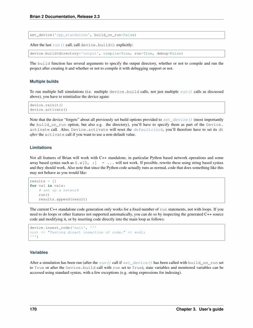
Brian 2 Documentation, Release 2.3
set_device('cpp_standalone', build_on_run=False)
After the last run() call, call device.build() explicitly:
device.build(directory='output', compile=True, run=True, debug=False)
The build function has several arguments to specify the output directory, whether or not to compile and run theproject after creating it and whether or not to compile it with debugging support or not.
Multiple builds
To run multiple full simulations (i.e. multiple device.build calls, not just multiple run() calls as discussedabove), you have to reinitialize the device again:
device.reinit()device.activate()
Note that the device “forgets” about all previously set build options provided to set_device() (most importantlythe build_on_run option, but also e.g. the directory), you’ll have to specify them as part of the Device.activate call. Also, Device.activate will reset the defaultclock, you’ll therefore have to set its dtafter the activate call if you want to use a non-default value.
Limitations
Not all features of Brian will work with C++ standalone, in particular Python based network operations and somearray based syntax such as S.w[0, :] = ... will not work. If possible, rewrite these using string based syntaxand they should work. Also note that since the Python code actually runs as normal, code that does something like thismay not behave as you would like:
results = []for val in vals:
# set up a networkrun()results.append(result)
The current C++ standalone code generation only works for a fixed number of run statements, not with loops. If youneed to do loops or other features not supported automatically, you can do so by inspecting the generated C++ sourcecode and modifying it, or by inserting code directly into the main loop as follows:
device.insert_code('main', '''cout << "Testing direct insertion of code." << endl;''')
Variables
After a simulation has been run (after the run() call if set_device() has been called with build_on_run setto True or after the Device.build call with run set to True), state variables and monitored variables can beaccessed using standard syntax, with a few exceptions (e.g. string expressions for indexing).
170 Chapter 3. User’s guide

Brian 2 Documentation, Release 2.3
Multi-threading with OpenMP
Warning: OpenMP code has not yet been well tested and so may be inaccurate.
When using the C++ standalone mode, you have the opportunity to turn on multi-threading, if your C++ compiler iscompatible with OpenMP. By default, this option is turned off and only one thread is used. However, by changing thepreferences of the codegen.cpp_standalone object, you can turn it on. To do so, just add the following line in yourpython script:
prefs.devices.cpp_standalone.openmp_threads = XX
XX should be a positive value representing the number of threads that will be used during the simulation. Note thatthe speedup will strongly depend on the network, so there is no guarantee that the speedup will be linear as a functionof the number of threads. However, this is working fine for networks with not too small timestep (dt > 0.1ms), andresults do not depend on the number of threads used in the simulation.
Customizing the build process
In standalone mode, a standard “make file” is used to orchestrate the compilation and linking. To pro-vide additional arguments to the make command (respectively nmake on Windows), you can use the de-vices.cpp_standalone.extra_make_args_unix or devices.cpp_standalone.extra_make_args_windows preference. OnLinux, this preference is by default set to ['-j'] to enable parallel compilation. Note that you can also use thesearguments to overwrite variables in the make file, e.g. to use clang instead of the default gcc compiler:
prefs.devices.cpp_standalone.extra_make_args_unix += ['CC=clang++']
Cleaning up after a run
Standalone simulations store all results of a simulation (final state variable values and values stored in monitors) todisk. These results can take up quite significant amount of space, and you might therefore want to delete these resultswhen you do not need them anymore. You can do this by using the device’s delete method:
device.delete()
Be aware that deleting the data will make all access to state variables fail, including the access to values in monitors.You should therefore only delete the data after doing all analysis/plotting that you are interested in.
By default, this function will delete both the generated code and the data, i.e. the full project directory. If you want tokeep the code (which typically takes up little space compared to the results), exclude it from the deletion:
device.delete(code=False)
If you added any additional files to the project directory manually, these will not be deleted by default. To delete thefull directory regardless of its content, use the force option:
device.delete(force=True)
Note: When you initialize state variables with concrete values (and not with a string expression), they will be storedto disk from your Python script and loaded from disk at the beginning of the standalone run. Since these values
3.12. Computational methods and efficiency 171
Brian 2 Documentation, Release 2.3
are necessary for the compiled binary file to run, they are considered “code” from the point of view of the deletefunction.
3.12.3 Compiler settings
If using C++ code generation (either via weave, cython or standalone), the compiler settings can make a big differencefor the speed of the simulation. By default, Brian uses a set of compiler settings that switches on various optimizationsand compiles for running on the same architecture where the code is compiled. This allows the compiler to make useof as many advanced instructions as possible, but reduces portability of the generated executable (which is not usuallyan issue).
If there are any issues with these compiler settings, for example because you are using an older version of the C++compiler or because you want to run the generated code on a different architecture, you can change the settings by man-ually specifying the codegen.cpp.extra_compile_args preference (or by using codegen.cpp.extra_compile_args_gcc orcodegen.cpp.extra_compile_args_msvc if you want to specify the settings for either compiler only).
3.13 Converting from integrated form to ODEs
Brian requires models to be expressed as systems of first order ordinary differential equations, and the effect of spikesto be expressed as (possibly delayed) one-off changes. However, many neuron models are given in integrated form.For example, one form of the Spike Response Model (SRM; Gerstner and Kistler 2002) is defined as
𝑉 (𝑡) =∑𝑖
𝑤𝑖
∑𝑡𝑖
PSP(𝑡− 𝑡𝑖) + 𝑉rest
where 𝑉 (𝑡) is the membrane potential, 𝑉rest is the rest potential, 𝑤𝑖 is the synaptic weight of synapse 𝑖, and 𝑡𝑖 are thetimings of the spikes coming from synapse 𝑖, and PSP is a postsynaptic potential function.
An example PSP is the 𝛼-function PSP(𝑡) = (𝑡/𝜏)𝑒−𝑡/𝜏 . For this function, we could rewrite the equation above inthe following ODE form:
𝜏d𝑉
d𝑡= 𝑉rest − 𝑉 + 𝑔
𝜏d𝑔
d𝑡= −𝑔
𝑔 ← 𝑔 + 𝑤𝑖 upon spike from synapse 𝑖
This could then be written in Brian as:
eqs = '''dV/dt = (V_rest-V+g)/tau : 1dg/dt = -g/tau : 1'''G = NeuronGroup(N, eqs, ...)...S = Synapses(G, G, 'w : 1', on_pre='g += w')
To see that these two formulations are the same, you first solve the problem for the case of a single synapse and asingle spike at time 0. The initial conditions at 𝑡 = 0 will be 𝑉 (0) = 𝑉rest, 𝑔(0) = 𝑤.
To solve these equations, let’s substitute 𝑠 = 𝑡/𝜏 and take derivatives with respect to 𝑠 instead of 𝑡, set 𝑢 = 𝑉 − 𝑉rest,and assume 𝑤 = 1. This gives us the equations 𝑢′ = 𝑔 − 𝑢, 𝑔′ = −𝑔 with initial conditions 𝑢(0) = 0, 𝑔(0) = 1. Atthis point, you can either consult a textbook on solving linear systems of differential equations, or just plug this intoWolfram Alpha to get the solution 𝑔(𝑠) = 𝑒−𝑠, 𝑢(𝑠) = 𝑠𝑒−𝑠 which is equal to the PSP given above.
172 Chapter 3. User’s guide
Brian 2 Documentation, Release 2.3
Now we use the linearity of these differential equations to see that it also works when 𝑤 = 0 and for summing overmultiple spikes at different times.
In general, to convert from integrated form to ODE form, see Köhn and Wörgötter (1998), Sánchez-Montañás (2001),and Jahnke et al. (1999). However, for some simple and widely used types of synapses, use the list below. In thislist, we assume synapses are postsynaptic potentials, but you can replace 𝑉 (𝑡) with a current or conductance forpostsynaptic currents or conductances. In each case, we give the Brian code with unitless variables, where eqs is thedifferential equations for the target NeuronGroup, and on_pre is the argument to Synapses.
Exponential synapse 𝑉 (𝑡) = 𝑒−𝑡/𝜏 :
eqs = '''dV/dt = -V/tau : 1'''on_pre = 'V += w'
Alpha synapse 𝑉 (𝑡) = (𝑡/𝜏)𝑒−𝑡/𝜏 :
eqs = '''dV/dt = (x-V)/tau : 1dx/dt = -x/tau : 1'''on_pre = 'x += w'
𝑉 (𝑡) reaches a maximum value of 𝑤/𝑒 at time 𝑡 = 𝜏 .
Biexponential synapse 𝑉 (𝑡) = 𝜏2𝜏2−𝜏1
(𝑒−𝑡/𝜏1 − 𝑒−𝑡/𝜏2
):
eqs = '''dV/dt = ((tau_2 / tau_1) ** (tau_1 / (tau_2 - tau_1))*x-V)/tau_1 : 1dx/dt = -x/tau_2 : 1'''on_pre = 'x += w'
𝑉 (𝑡) reaches a maximum value of 𝑤 at time 𝑡 = 𝜏1𝜏2𝜏2−𝜏1
log(
𝜏2𝜏1
).
STDP
The weight update equation of the standard STDP is also often stated in an integrated form and can be converted to anODE form. This is covered in Tutorial 2.
3.13. Converting from integrated form to ODEs 173

Brian 2 Documentation, Release 2.3
174 Chapter 3. User’s guide

CHAPTER 4
Advanced guide
This section has additional information on details not covered in the User’s guide.
4.1 Functions
• Default functions
• User-provided functions
– Python code generation
– Other code generation targets
– Dependencies between functions
– Additional compiler arguments
– Arrays vs. scalar values in user-provided functions
– Functions with context-dependent return values
– Additional namespace
– Data types
– External source files
All equations, expressions and statements in Brian can make use of mathematical functions. However, functions haveto be prepared for use with Brian for two reasons: 1) Brian is strict about checking the consistency of units, thereforeevery function has to specify how it deals with units; 2) functions need to be implemented differently for differentcode generation targets.
Brian provides a number of default functions that are already prepared for use with numpy and C++ and also providesa mechanism for preparing new functions for use (see below).
175
Brian 2 Documentation, Release 2.3
4.1.1 Default functions
The following functions (stored in the DEFAULT_FUNCTIONS dictionary) are ready for use:
• Random numbers: rand (random numbers drawn from a uniform distribution between 0 and 1), randn (ran-dom numbers drawn from the standard normal distribution, i.e. with mean 0 and standard deviation 1), andpoisson (discrete random numbers from a Poisson distribution with rate parameter 𝜆)
• Elementary functions: sqrt, exp, log, log10, abs, sign
• Trigonometric functions: sin, cos, tan, sinh, cosh, tanh, arcsin, arccos, arctan
• Functions for improved numerical accuracy: expm1 (calculates exp(x) - 1, more accurate for x close to0), log1p (calculates log(1 + x), more accurate for x close to 0), and exprel (calculates (exp(x) -1)/x, more accurate for x close to 0, and returning 1.0 instead of NaN for x == 0
• General utility functions: clip, floor, ceil
Brian also provides a special purpose function int, which can be used to convert an expression or variable into aninteger value. This is especially useful for boolean values (which will be converted into 0 or 1), for example to havea conditional evaluation as part of an equation or statement which sometimes allows to circumvent the lack of an ifstatement. For example, the following reset statement resets the variable v to either v_r1 or v_r2, depending on thevalue of w: 'v = v_r1 * int(w <= 0.5) + v_r2 * int(w > 0.5)'
Finally, the function timestep is a function that takes a time and the length of a time step as an input and returns aninteger corresponding to the respective time step. The advantage of using this function over a simple division is that itslightly shifts the time before dividing to avoid floating point issues. This function is used as part of the Refractorinessmechanism.
4.1.2 User-provided functions
Python code generation
If a function is only used in contexts that use Python code generation, preparing a function for use with Brian onlymeans specifying its units. The simplest way to do this is to use the check_units() decorator:
@check_units(x1=meter, y1=meter, x2=meter, y2=meter, result=meter)def distance(x1, y1, x2, y2):
return sqrt((x1 - x2)**2 + (y1 - y2)**2)
Another option is to wrap the function in a Function object:
def distance(x1, y1, x2, y2):return sqrt((x1 - x2)**2 + (y1 - y2)**2)
# wrap the distance functiondistance = Function(distance, arg_units=[meter, meter, meter, meter],
return_unit=meter)
The use of Brian’s unit system has the benefit of checking the consistency of units for every operation but at theexpense of performance. Consider the following function, for example:
@check_units(I=amp, result=Hz)def piecewise_linear(I):
return clip((I-1*nA) * 50*Hz/nA, 0*Hz, 100*Hz)
When Brian runs a simulation, the state variables are stored and passed around without units for performance reasons.If the above function is used, however, Brian adds units to its input argument so that the operations inside the functiondo not fail with dimension mismatches. Accordingly, units are removed from the return value so that the function
176 Chapter 4. Advanced guide
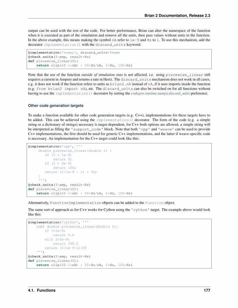
Brian 2 Documentation, Release 2.3
output can be used with the rest of the code. For better performance, Brian can alter the namespace of the functionwhen it is executed as part of the simulation and remove all the units, then pass values without units to the function.In the above example, this means making the symbol nA refer to 1e-9 and Hz to 1. To use this mechanism, add thedecorator implementation() with the discard_units keyword:
@implementation('numpy', discard_units=True)@check_units(I=amp, result=Hz)def piecewise_linear(I):
return clip((I-1*nA) * 50*Hz/nA, 0*Hz, 100*Hz)
Note that the use of the function outside of simulation runs is not affected, i.e. using piecewise_linear stillrequires a current in Ampere and returns a rate in Hertz. The discard_unitsmechanism does not work in all cases,e.g. it does not work if the function refers to units as brian2.nA instead of nA, if it uses imports inside the function(e.g. from brian2 import nA), etc. The discard_units can also be switched on for all functions withouthaving to use the implementation() decorator by setting the codegen.runtime.numpy.discard_units preference.
Other code generation targets
To make a function available for other code generation targets (e.g. C++), implementations for these targets have tobe added. This can be achieved using the implementation() decorator. The form of the code (e.g. a simplestring or a dictionary of strings) necessary is target-dependent, for C++ both options are allowed, a simple string willbe interpreted as filling the 'support_code' block. Note that both 'cpp' and 'weave' can be used to provideC++ implementations, the first should be used for generic C++ implementations, and the latter if weave-specific codeis necessary. An implementation for the C++ target could look like this:
@implementation('cpp', '''double piecewise_linear(double I) {
if (I < 1e-9)return 0;
if (I > 3e-9)return 100;
return (I/1e-9 - 1) * 50;}''')
@check_units(I=amp, result=Hz)def piecewise_linear(I):
return clip((I-1*nA) * 50*Hz/nA, 0*Hz, 100*Hz)
Alternatively, FunctionImplementation objects can be added to the Function object.
The same sort of approach as for C++ works for Cython using the 'cython' target. The example above would looklike this:
@implementation('cython', '''cdef double piecewise_linear(double I):
if I<1e-9:return 0.0
elif I>3e-9:return 100.0
return (I/1e-9-1)*50''')
@check_units(I=amp, result=Hz)def piecewise_linear(I):
return clip((I-1*nA) * 50*Hz/nA, 0*Hz, 100*Hz)
4.1. Functions 177
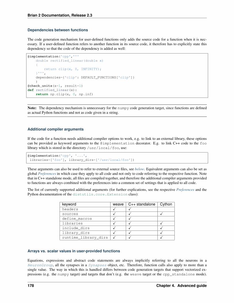
Brian 2 Documentation, Release 2.3
Dependencies between functions
The code generation mechanism for user-defined functions only adds the source code for a function when it is nec-essary. If a user-defined function refers to another function in its source code, it therefore has to explicitly state thisdependency so that the code of the dependency is added as well:
@implementation('cpp','''double rectified_linear(double x){
return clip(x, 0, INFINITY);}''',dependencies={'clip': DEFAULT_FUNCTIONS['clip']})
@check_units(x=1, result=1)def rectified_linear(x):
return np.clip(x, 0, np.inf)
Note: The dependency mechanism is unnecessary for the numpy code generation target, since functions are definedas actual Python functions and not as code given in a string.
Additional compiler arguments
If the code for a function needs additional compiler options to work, e.g. to link to an external library, these optionscan be provided as keyword arguments to the @implementation decorator. E.g. to link C++ code to the foolibrary which is stored in the directory /usr/local/foo, use:
@implementation('cpp', '...',libraries=['foo'], library_dirs=['/usr/local/foo'])
These arguments can also be used to refer to external source files, see below. Equivalent arguments can also be set asglobal Preferences in which case they apply to all code and not only to code referring to the respective function. Notethat in C++ standalone mode, all files are compiled together, and therefore the additional compiler arguments providedto functions are always combined with the preferences into a common set of settings that is applied to all code.
The list of currently supported additional arguments (for further explications, see the respective Preferences and thePython documentation of the distutils.core.Extension class):
keyword weave C++ standalone Cythonheaders X Xsources X X Xdefine_macros X Xlibraries X X Xinclude_dirs X X Xlibrary_dirs X X Xruntime_library_dirs X X X
Arrays vs. scalar values in user-provided functions
Equations, expressions and abstract code statements are always implicitly referring to all the neurons in aNeuronGroup, all the synapses in a Synapses object, etc. Therefore, function calls also apply to more than asingle value. The way in which this is handled differs between code generation targets that support vectorized ex-pressions (e.g. the numpy target) and targets that don’t (e.g. the weave target or the cpp_standalone mode).
178 Chapter 4. Advanced guide
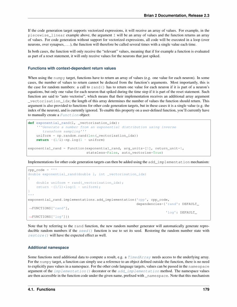
Brian 2 Documentation, Release 2.3
If the code generation target supports vectorized expressions, it will receive an array of values. For example, in thepiecewise_linear example above, the argument I will be an array of values and the function returns an arrayof values. For code generation without support for vectorized expressions, all code will be executed in a loop (overneurons, over synapses, . . . ), the function will therefore be called several times with a single value each time.
In both cases, the function will only receive the “relevant” values, meaning that if for example a function is evaluatedas part of a reset statement, it will only receive values for the neurons that just spiked.
Functions with context-dependent return values
When using the numpy target, functions have to return an array of values (e.g. one value for each neuron). In somecases, the number of values to return cannot be deduced from the function’s arguments. Most importantly, this isthe case for random numbers: a call to rand() has to return one value for each neuron if it is part of a neuron’sequations, but only one value for each neuron that spiked during the time step if it is part of the reset statement. Suchfunction are said to “auto vectorise”, which means that their implementation receives an additional array argument_vectorisation_idx; the length of this array determines the number of values the function should return. Thisargument is also provided to functions for other code generation targets, but in these cases it is a single value (e.g. theindex of the neuron), and is currently ignored. To enable this property on a user-defined function, you’ll currently haveto manually create a Function object:
def exponential_rand(l, _vectorisation_idx):'''Generate a number from an exponential distribution using inverse
transform sampling'''uniform = np.random.rand(len(_vectorisation_idx))return -(1/l)*np.log(1 - uniform)
exponential_rand = Function(exponential_rand, arg_units=[1], return_unit=1,stateless=False, auto_vectorise=True)
Implementations for other code generation targets can then be added using the add_implementation mechanism:
cpp_code = '''double exponential_rand(double l, int _vectorisation_idx){
double uniform = rand(_vectorisation_idx);return -(1/l)*log(1 - uniform);
}'''exponential_rand.implementations.add_implementation('cpp', cpp_code,
dependencies={'rand': DEFAULT_→˓FUNCTIONS['rand'],
'log': DEFAULT_→˓FUNCTIONS['log']})
Note that by referring to the rand function, the new random number generator will automatically generate repro-ducible random numbers if the seed() function is use to set its seed. Restoring the random number state withrestore() will have the expected effect as well.
Additional namespace
Some functions need additional data to compute a result, e.g. a TimedArray needs access to the underlying array.For the numpy target, a function can simply use a reference to an object defined outside the function, there is no needto explicitly pass values in a namespace. For the other code language targets, values can be passed in the namespaceargument of the implementation() decorator or the add_implementation method. The namespace valuesare then accessible in the function code under the given name, prefixed with _namespace. Note that this mechanism
4.1. Functions 179

Brian 2 Documentation, Release 2.3
should only be used for numpy arrays or general objects (e.g. function references to call Python functions from weaveor Cython code). Scalar values should be directly included in the function code, by using a “dynamic implemention”(see add_dynamic_implementation).
See TimedArray and BinomialFunction for examples that use this mechanism.
Data types
By default, functions are assumed to take any type of argument, and return a floating point value. If you want to puta restriction on the type of an argument, or specify that the return type should be something other than float, eitherdeclare it as a Function (and see its documentation on specifying types) or use the declare_types() decorator,e.g.:
@check_units(a=1, b=1, result=1)@declare_types(a='integer', result='highest')def f(a, b):
return a*b
This is potentially important if you have functions that return integer or boolean values, because Brian’s code genera-tion optimisation step will make some potentially incorrect simplifications if it assumes that the return type is floatingpoint.
External source files
Code for functions can also be provided via external files in the target language. This can be especially useful forlinking to existing code without having to include it a second time in the Python script. For C++-based code generationtargets (i.e. weave and the C++ standalone mode), the external code should be in a file that is provided as anargument to the sources keyword, together with a header file whose name is provided to headers (see the notefor the codegen.cpp.headers preference about the necessary format). Since the main simulation code is compiledand executed in a different directory, you should also point the compiler towards the directory of the header file viathe include_dirs keyword. For the same reason, use an absolute path for the source file. For example, thepiecewise_linear function from above can be implemented with external files as follows:
//file: piecewise_linear.hdouble piecewise_linear(double);
//file: piecewise_linear.cppdouble piecewise_linear(double I) {
if (I < 1e-9)return 0;
if (I > 3e-9)return 100;
return (I/1e-9 - 1) * 50;}
# Python script
# Get the absolute directory of this Python script, the C++ files are# expected to be stored alongside of itimport oscurrent_dir = os.path.abspath(os.path.dirname(__file__))
@implementation('cpp', '// all code in piecewise_linear.cpp',sources=[os.path.join(current_dir,
(continues on next page)
180 Chapter 4. Advanced guide

Brian 2 Documentation, Release 2.3
(continued from previous page)
'piecewise_linear.cpp')],headers=['"piecewise_linear.h"'],include_dirs=[current_dir])
@check_units(I=amp, result=Hz)def piecewise_linear(I):
return clip((I-1*nA) * 50*Hz/nA, 0*Hz, 100*Hz)
For Cython, the process is very similar (see the Cython documentation for general information). The name of theheader file does not need to be specified, it is expected to have the same name as the source file (except for the .pxdextension). The source and header files will be automatically copied to the cache directory where Cython files arecompiled, they therefore have to be imported as top-level modules, regardless of whether the executed Python code isitself in a package or module.
A Cython equivalent of above’s C++ example can be written as:
# file: piecewise_linear.pxdcdef double piecewise_linear(double)
# file: piecewise_linear.pyxcdef double piecewise_linear(double I):
if I<1e-9:return 0.0
elif I>3e-9:return 100.0
return (I/1e-9-1)*50
# Python script
# Get the absolute directory of this Python script, the Cython files# are expected to be stored alongside of itimport oscurrent_dir = os.path.abspath(os.path.dirname(__file__))
@implementation('cython','from piecewise_linear cimport piecewise_linear',sources=[os.path.join(current_dir,
'piecewise_linear.pyx')])@check_units(I=amp, result=Hz)def piecewise_linear(I):
return clip((I-1*nA) * 50*Hz/nA, 0*Hz, 100*Hz)
4.2 Preferences
Brian has a system of global preferences that affect how certain objects behave. These can be set either in scripts byusing the prefs object or in a file. Each preference looks like codegen.c.compiler, i.e. dotted names.
4.2.1 Accessing and setting preferences
Preferences can be accessed and set either keyword-based or attribute-based. The following are equivalent:
prefs['codegen.c.compiler'] = 'gcc'prefs.codegen.c.compiler = 'gcc'
4.2. Preferences 181

Brian 2 Documentation, Release 2.3
Using the attribute-based form can be particulary useful for interactive work, e.g. in ipython, as it offers autocom-pletion and documentation. In ipython, prefs.codegen.c? would display a docstring with all the preferencesavailable in the codegen.c category.
4.2.2 Preference files
Preferences are stored in a hierarchy of files, with the following order (each step overrides the values in the previousstep but no error is raised if one is missing):
• The global defaults are stored in the installation directory.
• The user default are stored in ~/.brian/user_preferences (which works on Windows as well as Linux).The ~ symbol refers to the user directory.
• The file brian_preferences in the current directory.
The preference files are of the following form:
a.b.c = 1# Comment line[a]b.d = 2[a.b]b.e = 3
This would set preferences a.b.c=1, a.b.d=2 and a.b.e=3.
4.2.3 List of preferences
Brian itself defines the following preferences (including their default values):
GSL
Directory containing GSL code
GSL.directory = None Set path to directory containing GSL header files (gsl_odeiv2.h etc.) If this directory isalready in Python’s include (e.g. because of conda installation), this path can be set to None.
codegen
Code generation preferences
codegen.loop_invariant_optimisations = True
Whether to pull out scalar expressions out of the statements, so that they are only evaluated once insteadof once for every neuron/synapse/. . . Can be switched off, e.g. because it complicates the code (and thesame optimisation is already performed by the compiler) or because the code generation target does notdeal well with it. Defaults to True.
codegen.max_cache_dir_size = 1000
The size of a directory (in MB) with cached code for weave or Cython that triggers a warning. Set to 0 tonever get a warning.
codegen.string_expression_target = 'numpy'
182 Chapter 4. Advanced guide

Brian 2 Documentation, Release 2.3
Default target for the evaluation of string expressions (e.g. when indexing state variables). Should nor-mally not be changed from the default numpy target, because the overhead of compiling code is not worththe speed gain for simple expressions.
Accepts the same arguments as codegen.target, except for 'auto'
codegen.target = 'auto'
Default target for code generation.
Can be a string, in which case it should be one of:
• 'auto' the default, automatically chose the best code generation target available.
• 'weave' uses scipy.weave to generate and compile C++ code, should work anywhere wheregcc is installed and available at the command line.
• 'cython', uses the Cython package to generate C++ code. Needs a working installation of Cythonand a C++ compiler.
• 'numpy' works on all platforms and doesn’t need a C compiler but is often less efficient.
Or it can be a CodeObject class.
codegen.cpp
C++ compilation preferences
codegen.cpp.compiler = ''
Compiler to use (uses default if empty)
Should be gcc or msvc.
codegen.cpp.define_macros = []
List of macros to define; each macro is defined using a 2-tuple, where ‘value’ is either the string to defineit to or None to define it without a particular value (equivalent of “#define FOO” in source or -DFOO onUnix C compiler command line).
codegen.cpp.extra_compile_args = None
Extra arguments to pass to compiler (if None, use either extra_compile_args_gcc orextra_compile_args_msvc).
codegen.cpp.extra_compile_args_gcc = ['-w', '-O3', '-ffast-math','-fno-finite-math-only', '-march=native']
Extra compile arguments to pass to GCC compiler
codegen.cpp.extra_compile_args_msvc = ['/Ox', '/w', '', '/MP']
Extra compile arguments to pass to MSVC compiler (the default /arch: flag is determined based on theprocessor architecture)
codegen.cpp.extra_link_args = []
Any extra platform- and compiler-specific information to use when linking object files together.
codegen.cpp.headers = []
A list of strings specifying header files to use when compiling the code. The list might look like [“<vec-tor>”,“‘my_header’”]. Note that the header strings need to be in a form than can be pasted at the end of a#include statement in the C++ code.
codegen.cpp.include_dirs = []
4.2. Preferences 183

Brian 2 Documentation, Release 2.3
Include directories to use. Note that $prefix/include will be appended to the end automatically,where $prefix is Python’s site-specific directory prefix as returned by sys.prefix.
codegen.cpp.libraries = []
List of library names (not filenames or paths) to link against.
codegen.cpp.library_dirs = []
List of directories to search for C/C++ libraries at link time. Note that $prefix/lib will be appendedto the end automatically, where $prefix is Python’s site-specific directory prefix as returned by sys.prefix.
codegen.cpp.msvc_architecture = ''
MSVC architecture name (or use system architectue by default).
Could take values such as x86, amd64, etc.
codegen.cpp.msvc_vars_location = ''
Location of the MSVC command line tool (or search for best by default).
codegen.cpp.runtime_library_dirs = []
List of directories to search for C/C++ libraries at run time.
codegen.generators
Codegen generator preferences (see subcategories for individual languages)
codegen.generators.cpp
C++ codegen preferences
codegen.generators.cpp.flush_denormals = False
Adds code to flush denormals to zero.
The code is gcc and architecture specific, so may not compile on all platforms. The code, for reference is:
#define CSR_FLUSH_TO_ZERO (1 << 15)unsigned csr = __builtin_ia32_stmxcsr();csr |= CSR_FLUSH_TO_ZERO;__builtin_ia32_ldmxcsr(csr);
Found at http://stackoverflow.com/questions/2487653/avoiding-denormal-values-in-c.
codegen.generators.cpp.restrict_keyword = '__restrict'
The keyword used for the given compiler to declare pointers as restricted.
This keyword is different on different compilers, the default works for gcc and MSVS.
codegen.runtime
Runtime codegen preferences (see subcategories for individual targets)
codegen.runtime.cython
Cython runtime codegen preferences
codegen.runtime.cython.cache_dir = None
Location of the cache directory for Cython files. By default, will be stored in abrian_extensions subdirectory where Cython inline stores its temporary files (the result ofget_cython_cache_dir()).
184 Chapter 4. Advanced guide

Brian 2 Documentation, Release 2.3
codegen.runtime.cython.delete_source_files = True
Whether to delete source files after compiling. The Cython source files can take a significant amount ofdisk space, and are not used anymore when the compiled library file exists. They are therefore deleted bydefault, but keeping them around can be useful for debugging.
codegen.runtime.cython.multiprocess_safe = True
Whether to use a lock file to prevent simultaneous write access to cython .pyx and .so files.
codegen.runtime.numpy
Numpy runtime codegen preferences
codegen.runtime.numpy.discard_units = False
Whether to change the namespace of user-specifed functions to remove units.
core
Core Brian preferences
core.default_float_dtype = float64
Default dtype for all arrays of scalars (state variables, weights, etc.).
core.default_integer_dtype = int32
Default dtype for all arrays of integer scalars.
core.outdated_dependency_error = True
Whether to raise an error for outdated dependencies (True) or just a warning (False).
core.network
Network preferences
core.network.default_schedule = ['start', 'groups', 'thresholds', 'synapses','resets', 'end']
Default schedule used for networks that don’t specify a schedule.
devices
Device preferences
devices.cpp_standalone
C++ standalone preferences
devices.cpp_standalone.extra_make_args_unix = ['-j']
Additional flags to pass to the GNU make command on Linux/OS-X. Defaults to “-j” for parallel compi-lation.
devices.cpp_standalone.extra_make_args_windows = []
Additional flags to pass to the nmake command on Windows. By default, no additional flags are passed.
devices.cpp_standalone.openmp_spatialneuron_strategy = None
DEPRECATED. Previously used to chose the strategy to parallelize the solution of the three tridiagonalsystems for multicompartmental neurons. Now, its value is ignored.
devices.cpp_standalone.openmp_threads = 0
4.2. Preferences 185
Brian 2 Documentation, Release 2.3
The number of threads to use if OpenMP is turned on. By default, this value is set to 0 and the C++ code isgenerated without any reference to OpenMP. If greater than 0, then the corresponding number of threadsare used to launch the simulation.
devices.cpp_standalone.run_environment_variables = {'LD_BIND_NOW': '1'}
Dictionary of environment variables and their values that will be set during the execution of the standalonecode.
legacy
Preferences to enable legacy behaviour
legacy.refractory_timing = False
Whether to use the semantics for checking the refractoriness condition that were in place up until (in-cluding) version 2.1.2. In that implementation, refractory periods that were multiples of dt could lead toa varying number of refractory timesteps due to the nature of floating point comparisons). This prefer-ence is only provided for exact reproducibility of previously obtained results, new simulations should usethe improved mechanism which uses a more robust mechanism to convert refractoriness into timesteps.Defaults to False.
logging
Logging system preferences
logging.console_log_level = 'INFO'
What log level to use for the log written to the console.
Has to be one of CRITICAL, ERROR, WARNING, INFO, DEBUG or DIAGNOSTIC.
logging.delete_log_on_exit = True
Whether to delete the log and script file on exit.
If set to True (the default), log files (and the copy of the main script) will be deleted after the brianprocess has exited, unless an uncaught exception occured. If set to False, all log files will be kept.
logging.file_log = True
Whether to log to a file or not.
If set to True (the default), logging information will be written to a file. The log level can be set via thelogging.file_log_level preference.
logging.file_log_level = 'DIAGNOSTIC'
What log level to use for the log written to the log file.
In case file logging is activated (see logging.file_log), which log level should be used for logging. Has tobe one of CRITICAL, ERROR, WARNING, INFO, DEBUG or DIAGNOSTIC.
logging.save_script = True
Whether to save a copy of the script that is run.
If set to True (the default), a copy of the currently run script is saved to a temporary location. It isdeleted after a successful run (unless logging.delete_log_on_exit is False) but is kept after an uncaughtexception occured. This can be helpful for debugging, in particular when several simulations are runningin parallel.
logging.std_redirection = True
186 Chapter 4. Advanced guide
Brian 2 Documentation, Release 2.3
Whether or not to redirect stdout/stderr to null at certain places.
This silences a lot of annoying compiler output, but will also hide error messages making it harder to debugproblems. You can always temporarily switch it off when debugging. If logging.std_redirection_to_file isset to True as well, then the output is saved to a file and if an error occurs the name of this file will beprinted.
logging.std_redirection_to_file = True
Whether to redirect stdout/stderr to a file.
If both logging.std_redirection and this preference are set to True, all standard output/error(most importantly output from the compiler) will be stored in files and if an error occurs the name of thisfile will be printed. If logging.std_redirection is True and this preference is False, then all standardoutput/error will be completely suppressed, i.e. neither be displayed nor stored in a file.
The value of this preference is ignore if logging.std_redirection is set to False.
4.3 Logging
Brian uses a logging system to display warnings and general information messages to the user, as well as writing themto a file with more detailed information, useful for debugging. Each log message has one of the following “log levels”:
ERROR Only used when an exception is raised, i.e. an error occurs and the current operation is interrupted. Example:You use a variable name in an equation that Brian does not recognize.
WARNING Brian thinks that something is most likely a bug, but it cannot be sure. Example: You use a Synapsesobject without any synapses in your simulation.
INFO Brian wants to make the user aware of some automatic choice that it did for the user. Example: You did notspecify an integration method for a NeuronGroup and therefore Brian chose an appropriate method for you.
DEBUG Additional information that might be useful when a simulation is not working as expected. Example: Theintegration timestep used during the simulation.
DIAGNOSTIC Additional information useful when tracking down bugs in Brian itself. Example: The generated codefor a CodeObject.
By default, all messages are written to the log file and all messages of level INFO and above are displayed on theconsole. To change what messages are displayed, see below.
Note: By default, the log file is deleted after a successful simulation run, i.e. when the simulation exited without anerror. To keep the log around, set the logging.delete_log_on_exit preference to False.
4.3.1 Showing/hiding log messages
If you want to change what messages are displayed on the console, you can call a method of the method ofBrianLogger:
BrianLogger.log_level_debug() # now also display debug messages
It is also possible to suppress messages for certain sub-hierarchies by using BrianLogger.suppress_hierarchy:
4.3. Logging 187
Brian 2 Documentation, Release 2.3
# Suppress code generation messages on the consoleBrianLogger.suppress_hierarchy('brian2.codegen')# Suppress preference messages even in the log fileBrianLogger.suppress_hierarchy('brian2.core.preferences',
filter_log_file=True)
Similarly, messages ending in a certain name can be suppressed with BrianLogger.suppress_name:
# Suppress resolution conflict warningsBrianLogger.suppress_name('resolution_conflict')
These functions should be used with care, as they suppresses messages independent of the level, i.e. even warning anderror messages.
4.3.2 Preferences
You can also change details of the logging system via Brian’s Preferences system. With this mechanism, you canswitch the logging to a file off completely (by setting logging.file_log to False) or have it log less messages (by settinglogging.file_log_level to a level higher than DIAGNOSTIC) – this can be important for long-running simulations wherethe log might otherwise take up a lot of disk space. For a list of all preferences related to logging, see the documentationof the brian2.utils.logger module.
Warning: Most of the logging preferences are only taken into account during the initialization of the logging sys-tem which takes place as soon as brian2 is imported. Therefore, if you use e.g. prefs.logging.file_log= False in your script, this will not have the intended effect! Instead, set these preferences in a file (see Prefer-ences).
4.4 Namespaces
Equations can contain references to external parameters or functions. During the initialisation of a NeuronGroupor a Synapses object, this namespace can be provided as an argument. This is a group-specific namespace that willonly be used for names in the context of the respective group. Note that units and a set of standard functions arealways provided and should not be given explicitly. This namespace does not necessarily need to be exhaustive at thetime of the creation of the NeuronGroup/Synapses, entries can be added (or modified) at a later stage via thenamespace attribute (e.g. G.namespace['tau'] = 10*ms).
At the point of the call to the Network.run() namespace, any group-specific namespace will be augmented by the“run namespace”. This namespace can be either given explicitly as an argument to the run method or it will be takenfrom the locals and globals surrounding the call. A warning will be emitted if a name is defined in more than onenamespace.
To summarize: an external identifier will be looked up in the context of an object such as NeuronGroup orSynapses. It will follow the following resolution hierarchy:
1. Default unit and function names.
2. Names defined in the explicit group-specific namespace.
3. Names in the run namespace which is either explicitly given or the implicit namespace surrounding the run call.
Note that if you completely specify your namespaces at the Group level, you should probably pass an empty dictionaryas the namespace argument to the run call – this will completely switch off the “implicit namespace” mechanism.
188 Chapter 4. Advanced guide
Brian 2 Documentation, Release 2.3
The following three examples show the different ways of providing external variable values, all having the same effectin this case:
# Explicit argument to the NeuronGroupG = NeuronGroup(1, 'dv/dt = -v / tau : 1', namespace={'tau': 10*ms})net = Network(G)net.run(10*ms)
# Explicit argument to the run functionG = NeuronGroup(1, 'dv/dt = -v / tau : 1')net = Network(G)net.run(10*ms, namespace={'tau': 10*ms})
# Implicit namespace from the contextG = NeuronGroup(1, 'dv/dt = -v / tau : 1')net = Network(G)tau = 10*msnet.run(10*ms)
External variables are free to change between runs (but not during one run), the value at the time of the run() call isused in the simulation.
4.5 Custom progress reporting
4.5.1 Progress reporting
For custom progress reporting (e.g. graphical output, writing to a file, etc.), the report keyword accepts a callable(i.e. a function or an object with a __call__ method) that will be called with four parameters:
• elapsed: the total (real) time since the start of the run
• completed: the fraction of the total simulation that is completed, i.e. a value between 0 and 1
• start: The start of the simulation (in biological time)
• duration: the total duration (in biological time) of the simulation
The function will be called every report_period during the simulation, but also at the beginning and end withcompleted equal to 0.0 and 1.0, respectively.
For the C++ standalone mode, the same standard options are available. It is also possible to implement custom progressreporting by directly passing the code (as a multi-line string) to the report argument. This code will be filled intoa progress report function template, it should therefore only contain a function body. The simplest use of this mightlook like:
net.run(duration, report='std::cout << (int)(completed*100.) << "% completed" <<→˓std::endl;')
Examples of custom reporting
Progress printed to a file
from brian2.core.network import TextReportreport_file = open('report.txt', 'w')file_reporter = TextReport(report_file)
(continues on next page)
4.5. Custom progress reporting 189
Brian 2 Documentation, Release 2.3
(continued from previous page)
net.run(duration, report=file_reporter)report_file.close()
“Graphical” output on the console
This needs a “normal” Linux console, i.e. it might not work in an integrated console in an IDE.
Adapted from http://stackoverflow.com/questions/3160699/python-progress-bar
import sys
class ProgressBar(object):def __init__(self, toolbar_width=40):
self.toolbar_width = toolbar_widthself.ticks = 0
def __call__(self, elapsed, complete, start, duration):if complete == 0.0:
# setup toolbarsys.stdout.write("[%s]" % (" " * self.toolbar_width))sys.stdout.flush()sys.stdout.write("\b" * (self.toolbar_width + 1)) # return to start of
→˓line, after '['else:
ticks_needed = int(round(complete * self.toolbar_width))if self.ticks < ticks_needed:
sys.stdout.write("-" * (ticks_needed-self.ticks))sys.stdout.flush()self.ticks = ticks_needed
if complete == 1.0:sys.stdout.write("\n")
net.run(duration, report=ProgressBar(), report_period=1*second)
4.6 Random numbers
Brian provides two basic functions to generate random numbers that can be used in model code and equations:rand(), to generate uniformly generated random numbers between 0 and 1, and randn(), to generate randomnumbers from a standard normal distribution (i.e. normally distributed numbers with a mean of 0 and a standarddeviation of 1). All other stochastic elements of a simulation (probabilistic connections, Poisson-distributed inputgenerated by PoissonGroup or PoissonInput, differential equations using the noise term xi, . . . ) will inter-nally make use of these two basic functions.
For Runtime code generation, random numbers are generated by numpy.random.rand and numpy.random.randn respectively, which uses a Mersenne-Twister pseudorandom number generator. When the numpy code gen-eration target is used, these functions are called directly, but for weave and cython, Brian uses a internal buffersfor uniformly and normally distributed random numbers and calls the numpy functions whenever all numbers fromthis buffer have been used. This avoids the overhead of switching between C code and Python code for each ran-dom number. For Standalone code generation, the random number generation is based on “randomkit”, the sameMersenne-Twister implementation that is used by numpy. The source code of this implementation will be included inevery generated standalone project.
4.6.1 Seeding and reproducibility
190 Chapter 4. Advanced guide

Brian 2 Documentation, Release 2.3
Runtime mode
As explained above, Runtime code generation makes use of numpy’s random number generator. In principle, us-ing numpy.random.seed therefore permits reproducing a stream of random numbers. However, for weave andcython, Brian’s buffer complicates the matter a bit: if a simulation sets numpy’s seed, uses 10000 random numbers,and then resets the seed, the following 10000 random numbers (assuming the current size of the buffer) will comeout of the pre-generated buffer before numpy’s random number generation functions are called again and take intoaccount the seed set by the user. Instead, users should use the seed() function provided by Brian 2 itself, this willtake care of setting numpy’s random seed and empty Brian’s internal buffers. This function also has the advantagethat it will continue to work when the simulation is switched to standalone code generation (see below). Note thatrandom numbers are not guaranteed to be reproducible across different code generation targets or different versions ofBrian, especially if several sources of randomness are used in the same CodeObject (e.g. two noise variables in theequations of a NeuronGroup). This is because Brian does not guarantee the order of certain operations (e.g. shouldit first generate all random numbers for the first noise variable for all neurons, followed by the random numbers forthe second noise variable for all neurons or rather first the random numbers for all noice variables of the first neuron,then for the second neuron, etc.) Since all random numbers are coming from the same stream of random numbers, theorder of getting the numbers out of this stream matter.
Standalone mode
For Standalone code generation, Brian’s seed() function will insert code to set the random number generator seedinto the generated code. The code will be generated at the position where the seed() call was made, allowingdetailed control over the seeding. For example the following code would generate identical initial conditions everytime it is run, but the noise generated by the xi variable would differ:
G = NeuronGroup(10, 'dv/dt = -v/(10*ms) + 0.1*xi/sqrt(ms) : 1')seed(4321)G.v = 'rand()'seed()run(100*ms)
Note: In standalone mode, seed() will not set numpy’s random number generator. If you use random numbersin the Python script itself (e.g. to generate a list of synaptic connections that will be passed to the standalone codeas a pre-calculated array), then you have to explicitly call numpy.random.seed yourself to make these randomnumbers reproducible.
Note: Seeding should lead to reproducible random numbers even when using OpenMP with multiple threads (forrepeated simulations with the same number of threads), but this has not been rigorously tested. Use at your own risk.
4.7 Custom events
4.7.1 Overview
In most simulations, a NeuronGroup defines a threshold on its membrane potential that triggers a spike event. Thisevent can be monitored by a SpikeMonitor, it is used in synaptic interactions, and in integrate-and-fire models italso leads to the execution of one or more reset statements.
Sometimes, it can be useful to define additional events, e.g. when an ion concentration in the cell crosses a certainthreshold. This can be done with the custom events system in Brian, which is illustrated in this diagram.
4.7. Custom events 191
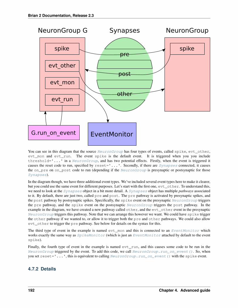
Brian 2 Documentation, Release 2.3
spike
evt_other
evt_mon
evt_run
NeuronGroup G
spike
NeuronGroupSynapses
pre
post
other
EventMonitorG.run_on_event
You can see in this diagram that the source NeuronGroup has four types of events, called spike, evt_other,evt_mon and evt_run. The event spike is the default event. It is triggered when you you includethreshold='...' in a NeuronGroup, and has two potential effects. Firstly, when the event is triggered itcauses the reset code to run, specified by reset='...'. Secondly, if there are Synapses connected, it causesthe on_pre on on_post code to run (depending if the NeuronGroup is presynaptic or postsynaptic for thoseSynapses).
In the diagram though, we have three additional event types. We’ve included several event types here to make it clearer,but you could use the same event for different purposes. Let’s start with the first one, evt_other. To understand this,we need to look at the Synapses object in a bit more detail. A Synapses object has multiple pathways associatedto it. By default, there are just two, called pre and post. The pre pathway is activated by presynaptic spikes, andthe post pathway by postsynaptic spikes. Specifically, the spike event on the presynaptic NeuronGroup triggersthe pre pathway, and the spike event on the postsynaptic NeuronGroup triggers the post pathway. In theexample in the diagram, we have created a new pathway called other, and the evt_other event in the presynapticNeuronGroup triggers this pathway. Note that we can arrange this however we want. We could have spike triggerthe other pathway if we wanted to, or allow it to trigger both the pre and other pathways. We could also allowevt_other to trigger the pre pathway. See below for details on the syntax for this.
The third type of event in the example is named evt_mon and this is connected to an EventMonitor whichworks exactly the same way as SpikeMonitor (which is just an EventMonitor attached by default to the eventspike).
Finally, the fourth type of event in the example is named evt_run, and this causes some code to be run in theNeuronGroup triggered by the event. To add this code, we call NeuronGroup.run_on_event(). So, whenyou set reset='...', this is equivalent to calling NeuronGroup.run_on_event() with the spike event.
4.7.2 Details
192 Chapter 4. Advanced guide
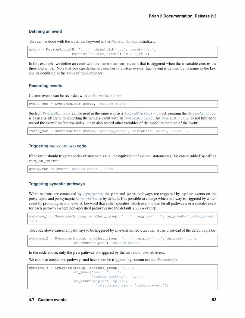
Brian 2 Documentation, Release 2.3
Defining an event
This can be done with the events keyword in the NeuronGroup initializer:
group = NeuronGroup(N, '...', threshold='...', reset='...',events={'custom_event': 'x > x_th'})
In this example, we define an event with the name custom_event that is triggered when the x variable crosses thethreshold x_th. Note that you can define any number of custom events. Each event is defined by its name as the key,and its condition as the value of the dictionary.
Recording events
Custom events can be recorded with an EventMonitor:
event_mon = EventMonitor(group, 'custom_event')
Such an EventMonitor can be used in the same way as a SpikeMonitor – in fact, creating the SpikeMonitoris basically identical to recording the spike event with an EventMonitor. An EventMonitor is not limited torecord the event time/neuron index, it can also record other variables of the model at the time of the event:
event_mon = EventMonitor(group, 'custom_event', variables['var1', 'var2'])
Triggering NeuronGroup code
If the event should trigger a series of statements (i.e. the equivalent of reset statements), this can be added by callingrun_on_event:
group.run_on_event('custom_event', 'x=0')
Triggering synaptic pathways
When neurons are connected by Synapses, the pre and post pathways are triggered by spike events on thepresynaptic and postsynaptic NeuronGroup by default. It is possible to change which pathway is triggered by whichevent by providing an on_event keyword that either specifies which event to use for all pathways, or a specific eventfor each pathway (where non-specified pathways use the default spike event):
synapse_1 = Synapses(group, another_group, '...', on_pre='...', on_event='custom_event→˓')
The code above causes all pathways to be triggered by an event named custom_event instead of the default spike.
synapse_2 = Synapses(group, another_group, '...', on_pre='...', on_post='...',on_event={'pre': 'custom_event'})
In the code above, only the pre pathway is triggered by the custom_event event.
We can also create new pathways and have them be triggered by custom events. For example:
synapse_3 = Synapses(group, another_group, '...',on_pre={'pre': '....',
'custom_pathway': '...'},on_event={'pre': 'spike',
'custom_pathway': 'custom_event'})
4.7. Custom events 193
Brian 2 Documentation, Release 2.3
In this code, the default pre pathway is still triggered by the spike event, but there is a new pathway calledcustom_pathway that is triggered by the custom_event event.
Scheduling
By default, custom events are checked after the spiking threshold (in the after_thresholds slots) and statementsare executed after the reset (in the after_resets slots). The slot for the execution of custom event-triggeredstatements can be changed when it is added with the usual when and order keyword arguments (see Scheduling fordetails). To change the time when the condition is checked, use NeuronGroup.set_event_schedule().
4.8 State update
In Brian, a state updater transforms a set of equations into an abstract state update code (and therefore is automaticallytarget-independent). In general, any function (or callable object) that takes an Equations object and returns abstractcode (as a string) can be used as a state updater and passed to the NeuronGroup constructor as a method argument.
The more common use case is to specify no state updater at all or chose one by name, see Choice of state updatersbelow.
4.8.1 Explicit state update
Explicit state update schemes can be specified in mathematical notation, using the ExplicitStateUpdater class.A state updater scheme contains a series of statements, defining temporary variables and a final line (starting withx_new =), giving the updated value for the state variable. The description can make reference to t (the current time),dt (the size of the time step), x (value of the state variable), and f(x, t) (the definition of the state variable x,assuming dx/dt = f(x, t). In addition, state updaters supporting stochastic equations additionally make useof dW (a normal distributed random variable with variance dt) and g(x, t), the factor multiplied with the noisevariable, assuming dx/dt = f(x, t) + g(x, t) * xi.
Using this notation, simple forward Euler integration is specified as:
x_new = x + dt * f(x, t)
A Runge-Kutta 2 (midpoint) method is specified as:
k = dt * f(x,t)x_new = x + dt * f(x + k/2, t + dt/2)
When creating a new state updater using ExplicitStateUpdater, you can specify the stochastickeyword argument, determining whether this state updater does not support any stochastic equations (None,the default), stochastic equations with additive noise only ('additive'), or arbitrary stochastic equations('multiplicative'). The provided state updaters use the Stratonovich interpretation for stochastic equations(which is the correct interpretation if the white noise source is seen as the limit of a coloured noise source with ashort time constant). As a result of this, the simple Euler-Maruyama scheme (x_new = x + dt*f(x, t) +dW*g(x, t)) will only be used for additive noise.
An example for a general state updater that handles arbitrary multiplicative noise (under Stratonovich interpretation)is the derivative-free Milstein method:
x_support = x + dt*f(x, t) + dt**.5 * g(x, t)g_support = g(x_support, t)k = 1/(2*dt**.5)*(g_support - g(x, t))*(dW**2)x_new = x + dt*f(x,t) + g(x, t) * dW + k
194 Chapter 4. Advanced guide

Brian 2 Documentation, Release 2.3
Note that a single line in these descriptions is only allowed to mention g(x, t), respectively f(x, t) only once(and you are not allowed to write, for example, g(f(x, t), t)). You can work around these restrictions by usingintermediate steps, defining temporary variables, as in the above examples for milstein and rk2.
4.8.2 Choice of state updaters
As mentioned in the beginning, you can pass arbitrary callables to the method argument of a NeuronGroup, as longas this callable converts an Equations object into abstract code. The best way to add a new state updater, however,is to register it with brian and provide a method to determine whether it is appropriate for a given set of equations.This way, it can be automatically chosen when no method is specified and it can be referred to with a name (i.e. youcan pass a string like 'euler' to the method argument instead of importing euler and passing a reference to theobject itself).
If you create a new state updater using the ExplicitStateUpdater class, you have to specify what kind ofstochastic equations it supports. The keyword argument stochastic takes the values None (no stochastic equationsupport, the default), 'additive' (support for stochastic equations with additive noise), 'multiplicative'(support for arbitrary stochastic equations).
After creating the state updater, it has to be registered with StateUpdateMethod:
new_state_updater = ExplicitStateUpdater('...', stochastic='additive')StateUpdateMethod.register('mymethod', new_state_updater)
The preferred way to do write new general state updaters (i.e. state updaters that cannot be described using the explicitsyntax described above) is to extend the StateUpdateMethod class (but this is not strictly necessary, all that isneeded is an object that implements a __call__ method that operates on an Equations object and a dictionary ofvariables). Optionally, the state updater can be registered with StateUpdateMethod as shown above.
4.8.3 Implicit state updates
Note: All of the following is just here for future reference, it’s not implemented yet.
Implicit schemes often use Newton-Raphson or fixed point iterations. These can also be defined by mathematicalstatements, but the number of iterations is dynamic and therefore not easily vectorised. However, this might not be abig issue in C, GPU or even with Numba.
Backward Euler
Backward Euler is defined as follows:
x(t+dt)=x(t)+dt*f(x(t+dt),t+dt)
This is not a executable statement because the RHS depends on the future. A simple way is to perform fixed pointiterations:
x(t+dt)=x(t)x(t+dt)=x(t)+dt*dx=f(x(t+dt),t+dt) until increment<tolerance
This includes a loop with a different number of iterations depending on the neuron.
4.8. State update 195

Brian 2 Documentation, Release 2.3
4.9 How Brian works
In this section we will briefly cover some of the internals of how Brian works. This is included here to understand thegeneral process that Brian goes through in running a simulation, but it will not be sufficient to understand the sourcecode of Brian itself or to extend it to do new things. For a more detailed view of this, see the documentation in theDeveloper’s guide.
4.9.1 Clock-driven versus event-driven
Brian is a clock-driven simulator. This means that the simulation time is broken into an equally spaced time grid, 0,dt, 2*dt, 3*dt, . . . . At each time step t, the differential equations specifying the models are first integrated giving thevalues at time t+dt. Spikes are generated when a condition such as v>vt is satisfied, and spikes can only occur on thetime grid.
The advantage of clock driven simulation is that it is very flexible (arbitrary differential equations can be used) andcomputationally efficient. However, the time grid approximation can lead to an overestimate of the amount of syn-chrony that is present in a network. This is usually not a problem, and can be managed by reducing the time step dt,but it can be an issue for some models.
Note that the inaccuracy introduced by the spike time approximation is of order O(dt), so the total accuracy of thesimulation is of order O(dt) per time step. This means that in many cases, there is no need to use a higher ordernumerical integration method than forward Euler, as it will not improve the order of the error beyond O(dt). See Stateupdate for more details of numerical integration methods.
Some simulators use an event-driven method. With this method, spikes can occur at arbitrary times instead of juston the grid. This method can be more accurate than a clock-driven simulation, but it is usually substantially morecomputationally expensive (especially for larger networks). In addition, they are usually more restrictive in terms ofthe class of differential equations that can be solved.
For a review of some of the simulation strategies that have been used, see Brette et al. 2007.
4.9.2 Code overview
The user-visible part of Brian consists of a number of objects such as NeuronGroup, Synapses, Network, etc.These are all written in pure Python and essentially work to translate the user specified model into the computationalengine. The end state of this translation is a collection of short blocks of code operating on a namespace, which arecalled in a sequence by the Network. Examples of these short blocks of code are the “state updaters” which performnumerical integration, or the synaptic propagation step. The namespaces consist of a mapping from names to values,where the possible values can be scalar values, fixed-length or dynamically sized arrays, and functions.
4.9.3 Syntax layer
The syntax layer consists of everything that is independent of the way the final simulation is computed (i.e. the lan-guage and device it is running on). This includes things like NeuronGroup, Synapses, Network, Equations,etc.
The user-visible part of this is documented fully in the User’s guide and the Advanced guide. In particular, things suchas the analysis of equations and assignment of numerical integrators. The end result of this process, which is passedto the computational engine, is a specification of the simulation consisting of the following data:
• A collection of variables which are scalar values, fixed-length arrays, dynamically sized arrays, and functions.These are handled by Variable objects detailed in Variables and indices. Examples: each state variable ofa NeuronGroup is assigned an ArrayVariable; the list of spike indices stored by a SpikeMonitor isassigned a DynamicArrayVariable; etc.
196 Chapter 4. Advanced guide

Brian 2 Documentation, Release 2.3
• A collection of code blocks specified via an “abstract code block” and a template name. The “abstract codeblock” is a sequence of statements such as v = vr which are to be executed. In the case that say, v and vrare arrays, then the statement is to be executed for each element of the array. These abstract code blocks areeither given directly by the user (in the case of neuron threshold and reset, and synaptic pre and post codes),or generated from differential equations combined with a numerical integrator. The template name is one of asmall set (around 20 total) which give additional context. For example, the code block a = b when consideredas part of a “state update” means execute that for each neuron index. In the context of a reset statement, it meansexecute it for each neuron index of a neuron that has spiked. Internally, these templates need to be implementedfor each target language/device, but there are relatively few of them.
• The order of execution of these code blocks, as defined by the Network.
4.9.4 Computational engine
The computational engine covers everything from generating to running code in a particular language or on a particulardevice. It starts with the abstract definition of the simulation resulting from the syntax layer described above.
The computational engine is described by a Device object. This is used for allocating memory, generating andrunning code. There are two types of device, “runtime” and “standalone”. In runtime mode, everything is managedby Python, even if individual code blocks are in a different language. Memory is managed using numpy arrays (whichcan be passed as pointers to use in other languages). In standalone mode, the output of the process (after callingDevice.build) is a complete source code project that handles everything, including memory management, and isindependent of Python.
For both types of device, one of the key steps that works in the same way is code generation, the creation of acompilable and runnable block of code from an abstract code block and a collection of variables. This happens in twostages: first of all, the abstract code block is converted into a code snippet, which is a syntactically correct block ofcode in the target language, but not one that can run on its own (it doesn’t handle accessing the variables from memory,etc.). This code snippet typically represents the inner loop code. This step is handled by a CodeGenerator object.In some cases it will involve a syntax translation (e.g. the Python syntax x**y in C++ should be pow(x, y)).The next step is to insert this code snippet into a template to form a compilable code block. This code block is thenpassed to a runtime CodeObject. In the case of standalone mode, this doesn’t do anything, but for runtime devicesit handles compiling the code and then running the compiled code block in the given namespace.
4.10 Interfacing with external code
Some neural simulations benefit from a direct connections to external libraries, e.g. to support real-time input froma sensor (but note that Brian currently does not offer facilities to assure real-time processing) or to perform complexcalculations during a simulation run.
If the external library is written in Python (or is a library with Python bindings), then the connection can be madeeither using the mechanism for User-provided functions, or using a network operation.
In case of C/C++ libraries, only the User-provided functions mechanism can be used. On the other hand, such simu-lations can use the same user-provided C++ code to run both with the runtime weave target and with the Standalonecode generation mode. In addition to that code, one generally needs to include additional header files and use com-piler/linker options to interface with the external code. For this, several preferences can be used that will be taken intoaccount for weave, cython and the cpp_standalone device. These preferences are mostly equivalent to therespective keyword arguments for Python’s distutils.core.Extension class, see the documentation of thecpp_prefs module for more details.
4.10. Interfacing with external code 197

Brian 2 Documentation, Release 2.3
198 Chapter 4. Advanced guide
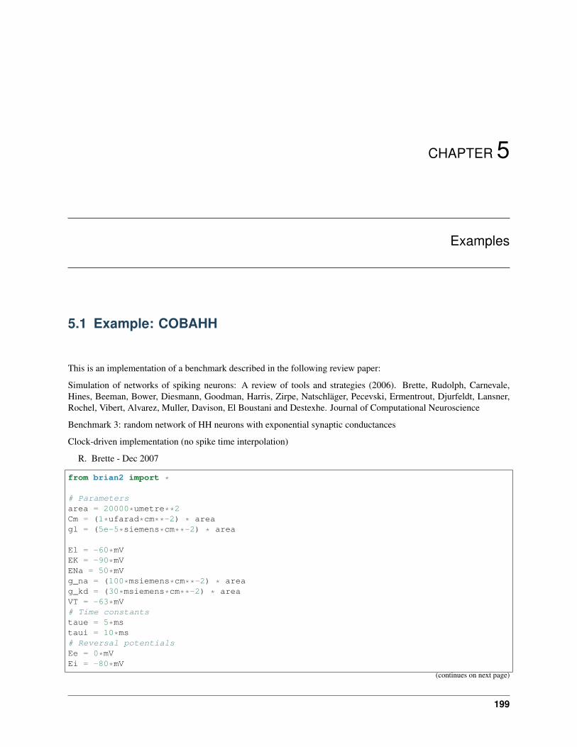
CHAPTER 5
Examples
5.1 Example: COBAHH
This is an implementation of a benchmark described in the following review paper:
Simulation of networks of spiking neurons: A review of tools and strategies (2006). Brette, Rudolph, Carnevale,Hines, Beeman, Bower, Diesmann, Goodman, Harris, Zirpe, Natschläger, Pecevski, Ermentrout, Djurfeldt, Lansner,Rochel, Vibert, Alvarez, Muller, Davison, El Boustani and Destexhe. Journal of Computational Neuroscience
Benchmark 3: random network of HH neurons with exponential synaptic conductances
Clock-driven implementation (no spike time interpolation)
R. Brette - Dec 2007
from brian2 import *
# Parametersarea = 20000*umetre**2Cm = (1*ufarad*cm**-2) * areagl = (5e-5*siemens*cm**-2) * area
El = -60*mVEK = -90*mVENa = 50*mVg_na = (100*msiemens*cm**-2) * areag_kd = (30*msiemens*cm**-2) * areaVT = -63*mV# Time constantstaue = 5*mstaui = 10*ms# Reversal potentialsEe = 0*mVEi = -80*mV
(continues on next page)
199

Brian 2 Documentation, Release 2.3
(continued from previous page)
we = 6*nS # excitatory synaptic weightwi = 67*nS # inhibitory synaptic weight
# The modeleqs = Equations('''dv/dt = (gl*(El-v)+ge*(Ee-v)+gi*(Ei-v)-
g_na*(m*m*m)*h*(v-ENa)-g_kd*(n*n*n*n)*(v-EK))/Cm : volt
dm/dt = alpha_m*(1-m)-beta_m*m : 1dn/dt = alpha_n*(1-n)-beta_n*n : 1dh/dt = alpha_h*(1-h)-beta_h*h : 1dge/dt = -ge*(1./taue) : siemensdgi/dt = -gi*(1./taui) : siemensalpha_m = 0.32*(mV**-1)*4*mV/exprel((13*mV-v+VT)/(4*mV))/ms : Hzbeta_m = 0.28*(mV**-1)*5*mV/exprel((v-VT-40*mV)/(5*mV))/ms : Hzalpha_h = 0.128*exp((17*mV-v+VT)/(18*mV))/ms : Hzbeta_h = 4./(1+exp((40*mV-v+VT)/(5*mV)))/ms : Hzalpha_n = 0.032*(mV**-1)*5*mV/exprel((15*mV-v+VT)/(5*mV))/ms : Hzbeta_n = .5*exp((10*mV-v+VT)/(40*mV))/ms : Hz''')
P = NeuronGroup(4000, model=eqs, threshold='v>-20*mV', refractory=3*ms,method='exponential_euler')
Pe = P[:3200]Pi = P[3200:]Ce = Synapses(Pe, P, on_pre='ge+=we')Ci = Synapses(Pi, P, on_pre='gi+=wi')Ce.connect(p=0.02)Ci.connect(p=0.02)
# InitializationP.v = 'El + (randn() * 5 - 5)*mV'P.ge = '(randn() * 1.5 + 4) * 10.*nS'P.gi = '(randn() * 12 + 20) * 10.*nS'
# Record a few tracestrace = StateMonitor(P, 'v', record=[1, 10, 100])run(1 * second, report='text')plot(trace.t/ms, trace[1].v/mV)plot(trace.t/ms, trace[10].v/mV)plot(trace.t/ms, trace[100].v/mV)xlabel('t (ms)')ylabel('v (mV)')show()
200 Chapter 5. Examples

Brian 2 Documentation, Release 2.3
5.2 Example: CUBA
This is a Brian script implementing a benchmark described in the following review paper:
Simulation of networks of spiking neurons: A review of tools and strategies (2007). Brette, Rudolph, Carnevale, Hines,Beeman, Bower, Diesmann, Goodman, Harris, Zirpe, Natschlager, Pecevski, Ermentrout, Djurfeldt, Lansner, Rochel,Vibert, Alvarez, Muller, Davison, El Boustani and Destexhe. Journal of Computational Neuroscience 23(3):349-98
Benchmark 2: random network of integrate-and-fire neurons with exponential synaptic currents.
Clock-driven implementation with exact subthreshold integration (but spike times are aligned to the grid).
from brian2 import *
taum = 20*mstaue = 5*mstaui = 10*msVt = -50*mVVr = -60*mVEl = -49*mV
eqs = '''dv/dt = (ge+gi-(v-El))/taum : volt (unless refractory)
(continues on next page)
5.2. Example: CUBA 201

Brian 2 Documentation, Release 2.3
(continued from previous page)
dge/dt = -ge/taue : voltdgi/dt = -gi/taui : volt'''
P = NeuronGroup(4000, eqs, threshold='v>Vt', reset='v = Vr', refractory=5*ms,method='exact')
P.v = 'Vr + rand() * (Vt - Vr)'P.ge = 0*mVP.gi = 0*mV
we = (60*0.27/10)*mV # excitatory synaptic weight (voltage)wi = (-20*4.5/10)*mV # inhibitory synaptic weightCe = Synapses(P, P, on_pre='ge += we')Ci = Synapses(P, P, on_pre='gi += wi')Ce.connect('i<3200', p=0.02)Ci.connect('i>=3200', p=0.02)
s_mon = SpikeMonitor(P)
run(1 * second)
plot(s_mon.t/ms, s_mon.i, ',k')xlabel('Time (ms)')ylabel('Neuron index')show()
202 Chapter 5. Examples
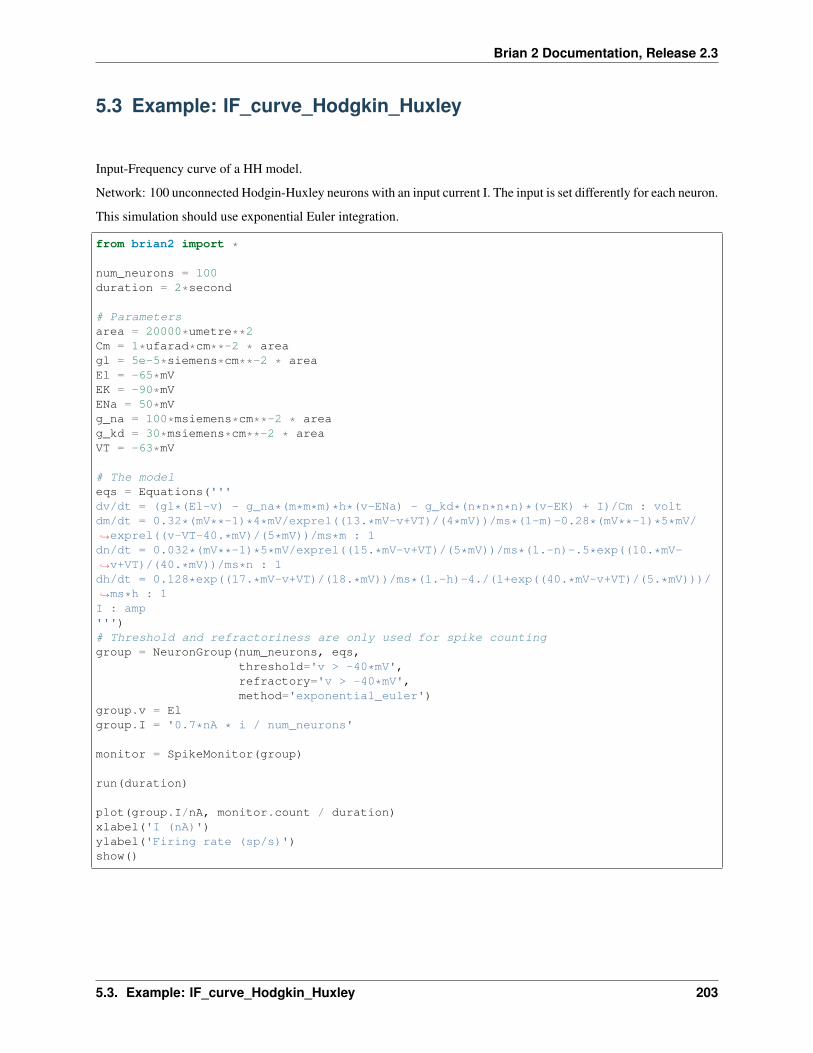
Brian 2 Documentation, Release 2.3
5.3 Example: IF_curve_Hodgkin_Huxley
Input-Frequency curve of a HH model.
Network: 100 unconnected Hodgin-Huxley neurons with an input current I. The input is set differently for each neuron.
This simulation should use exponential Euler integration.
from brian2 import *
num_neurons = 100duration = 2*second
# Parametersarea = 20000*umetre**2Cm = 1*ufarad*cm**-2 * areagl = 5e-5*siemens*cm**-2 * areaEl = -65*mVEK = -90*mVENa = 50*mVg_na = 100*msiemens*cm**-2 * areag_kd = 30*msiemens*cm**-2 * areaVT = -63*mV
# The modeleqs = Equations('''dv/dt = (gl*(El-v) - g_na*(m*m*m)*h*(v-ENa) - g_kd*(n*n*n*n)*(v-EK) + I)/Cm : voltdm/dt = 0.32*(mV**-1)*4*mV/exprel((13.*mV-v+VT)/(4*mV))/ms*(1-m)-0.28*(mV**-1)*5*mV/→˓exprel((v-VT-40.*mV)/(5*mV))/ms*m : 1dn/dt = 0.032*(mV**-1)*5*mV/exprel((15.*mV-v+VT)/(5*mV))/ms*(1.-n)-.5*exp((10.*mV-→˓v+VT)/(40.*mV))/ms*n : 1dh/dt = 0.128*exp((17.*mV-v+VT)/(18.*mV))/ms*(1.-h)-4./(1+exp((40.*mV-v+VT)/(5.*mV)))/→˓ms*h : 1I : amp''')# Threshold and refractoriness are only used for spike countinggroup = NeuronGroup(num_neurons, eqs,
threshold='v > -40*mV',refractory='v > -40*mV',method='exponential_euler')
group.v = Elgroup.I = '0.7*nA * i / num_neurons'
monitor = SpikeMonitor(group)
run(duration)
plot(group.I/nA, monitor.count / duration)xlabel('I (nA)')ylabel('Firing rate (sp/s)')show()
5.3. Example: IF_curve_Hodgkin_Huxley 203

Brian 2 Documentation, Release 2.3
5.4 Example: IF_curve_LIF
Input-Frequency curve of a IF model.
Network: 1000 unconnected integrate-and-fire neurons (leaky IF) with an input parameter v0. The input is set differ-ently for each neuron.
from brian2 import *
n = 1000duration = 1*secondtau = 10*mseqs = '''dv/dt = (v0 - v) / tau : volt (unless refractory)v0 : volt'''group = NeuronGroup(n, eqs, threshold='v > 10*mV', reset='v = 0*mV',
refractory=5*ms, method='exact')group.v = 0*mVgroup.v0 = '20*mV * i / (n-1)'
monitor = SpikeMonitor(group)
(continues on next page)
204 Chapter 5. Examples
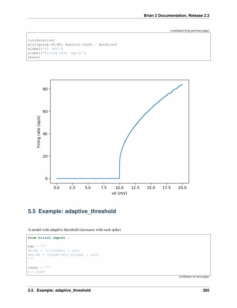
Brian 2 Documentation, Release 2.3
(continued from previous page)
run(duration)plot(group.v0/mV, monitor.count / duration)xlabel('v0 (mV)')ylabel('Firing rate (sp/s)')show()
5.5 Example: adaptive_threshold
A model with adaptive threshold (increases with each spike)
from brian2 import *
eqs = '''dv/dt = -v/(10*ms) : voltdvt/dt = (10*mV-vt)/(15*ms) : volt'''
reset = '''v = 0*mV
(continues on next page)
5.5. Example: adaptive_threshold 205
Brian 2 Documentation, Release 2.3
(continued from previous page)
vt += 3*mV'''
IF = NeuronGroup(1, model=eqs, reset=reset, threshold='v>vt',method='exact')
IF.vt = 10*mVPG = PoissonGroup(1, 500 * Hz)
C = Synapses(PG, IF, on_pre='v += 3*mV')C.connect()
Mv = StateMonitor(IF, 'v', record=True)Mvt = StateMonitor(IF, 'vt', record=True)# Record the value of v when the threshold is crossedM_crossings = SpikeMonitor(IF, variables='v')run(2*second, report='text')
subplot(1, 2, 1)plot(Mv.t / ms, Mv[0].v / mV)plot(Mvt.t / ms, Mvt[0].vt / mV)ylabel('v (mV)')xlabel('t (ms)')# zoom in on the first 100msxlim(0, 100)subplot(1, 2, 2)hist(M_crossings.v / mV, bins=np.arange(10, 20, 0.5))xlabel('v at threshold crossing (mV)')show()
206 Chapter 5. Examples

Brian 2 Documentation, Release 2.3
5.6 Example: non_reliability
Reliability of spike timing.
See e.g. Mainen & Sejnowski (1995) for experimental results in vitro.
Here: a constant current is injected in all trials.
from brian2 import *
N = 25tau = 20*mssigma = .015eqs_neurons = '''dx/dt = (1.1 - x) / tau + sigma * (2 / tau)**.5 * xi : 1 (unless refractory)'''neurons = NeuronGroup(N, model=eqs_neurons, threshold='x > 1', reset='x = 0',
refractory=5*ms, method='euler')spikes = SpikeMonitor(neurons)
run(500*ms)plot(spikes.t/ms, spikes.i, '.k')
(continues on next page)
5.6. Example: non_reliability 207
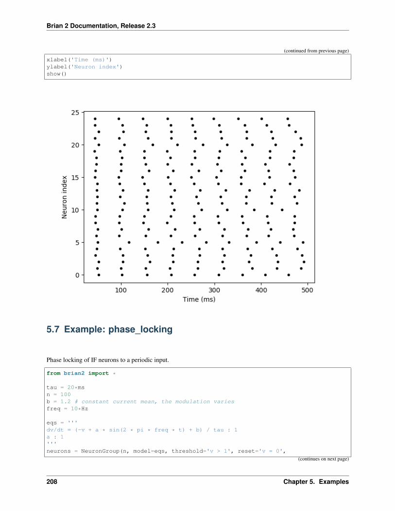
Brian 2 Documentation, Release 2.3
(continued from previous page)
xlabel('Time (ms)')ylabel('Neuron index')show()
5.7 Example: phase_locking
Phase locking of IF neurons to a periodic input.
from brian2 import *
tau = 20*msn = 100b = 1.2 # constant current mean, the modulation variesfreq = 10*Hz
eqs = '''dv/dt = (-v + a * sin(2 * pi * freq * t) + b) / tau : 1a : 1'''neurons = NeuronGroup(n, model=eqs, threshold='v > 1', reset='v = 0',
(continues on next page)
208 Chapter 5. Examples
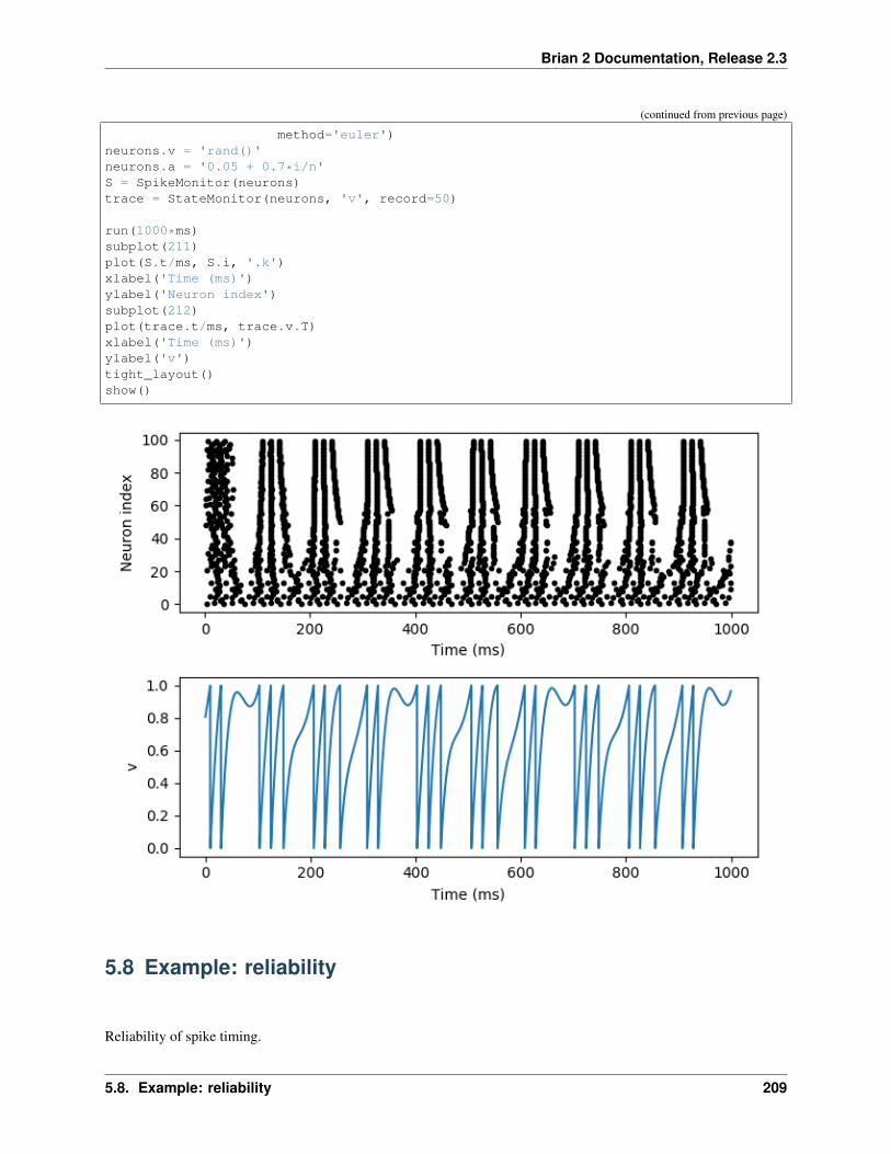
Brian 2 Documentation, Release 2.3
(continued from previous page)
method='euler')neurons.v = 'rand()'neurons.a = '0.05 + 0.7*i/n'S = SpikeMonitor(neurons)trace = StateMonitor(neurons, 'v', record=50)
run(1000*ms)subplot(211)plot(S.t/ms, S.i, '.k')xlabel('Time (ms)')ylabel('Neuron index')subplot(212)plot(trace.t/ms, trace.v.T)xlabel('Time (ms)')ylabel('v')tight_layout()show()
5.8 Example: reliability
Reliability of spike timing.
5.8. Example: reliability 209
Brian 2 Documentation, Release 2.3
See e.g. Mainen & Sejnowski (1995) for experimental results in vitro.
from brian2 import *
# The common noisy inputN = 25tau_input = 5*msinput = NeuronGroup(1, 'dx/dt = -x / tau_input + (2 /tau_input)**.5 * xi : 1')
# The noisy neurons receiving the same inputtau = 10*mssigma = .015eqs_neurons = '''dx/dt = (0.9 + .5 * I - x) / tau + sigma * (2 / tau)**.5 * xi : 1I : 1 (linked)'''neurons = NeuronGroup(N, model=eqs_neurons, threshold='x > 1',
reset='x = 0', refractory=5*ms, method='euler')neurons.x = 'rand()'neurons.I = linked_var(input, 'x') # input.x is continuously fed into neurons.Ispikes = SpikeMonitor(neurons)
run(500*ms)plt.plot(spikes.t/ms, spikes.i, '.k')xlabel('Time (ms)')ylabel('Neuron index')show()
210 Chapter 5. Examples
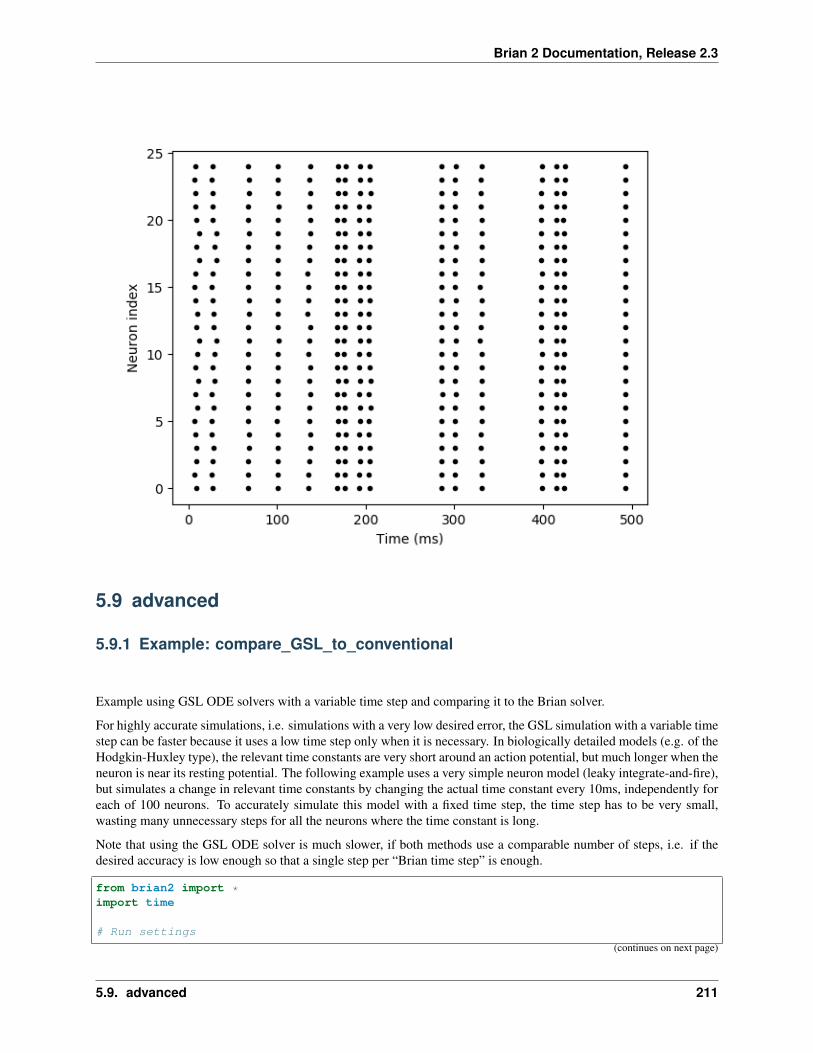
Brian 2 Documentation, Release 2.3
5.9 advanced
5.9.1 Example: compare_GSL_to_conventional
Example using GSL ODE solvers with a variable time step and comparing it to the Brian solver.
For highly accurate simulations, i.e. simulations with a very low desired error, the GSL simulation with a variable timestep can be faster because it uses a low time step only when it is necessary. In biologically detailed models (e.g. of theHodgkin-Huxley type), the relevant time constants are very short around an action potential, but much longer when theneuron is near its resting potential. The following example uses a very simple neuron model (leaky integrate-and-fire),but simulates a change in relevant time constants by changing the actual time constant every 10ms, independently foreach of 100 neurons. To accurately simulate this model with a fixed time step, the time step has to be very small,wasting many unnecessary steps for all the neurons where the time constant is long.
Note that using the GSL ODE solver is much slower, if both methods use a comparable number of steps, i.e. if thedesired accuracy is low enough so that a single step per “Brian time step” is enough.
from brian2 import *import time
# Run settings
(continues on next page)
5.9. advanced 211
Brian 2 Documentation, Release 2.3
(continued from previous page)
start_dt = .1 * msmethod = 'rk2'error = 1.e-6 # requested accuracy
def runner(method, dt, options=None):seed(0)I = 5group = NeuronGroup(100, '''dv/dt = (-v + I)/tau : 1
tau : second''',method=method,method_options=options,dt=dt)
group.run_regularly('''v = rand()tau = 0.1*ms + rand()*9.9*ms''', dt=10*ms)
rec_vars = ['v', 'tau']if 'gsl' in method:
rec_vars += ['_step_count']net = Network(group)net.run(0 * ms)mon = StateMonitor(group, rec_vars, record=True, dt=start_dt)net.add(mon)start = time.time()net.run(1 * second)mon.add_attribute('run_time')mon.run_time = time.time() - startreturn mon
lin = runner('linear', start_dt)method_options = {'save_step_count': True,
'absolute_error': error,'max_steps': 10000}
gsl = runner('gsl_%s' % method, start_dt, options=method_options)
print("Running with GSL integrator and variable time step:")print('Run time: %.3fs' % gsl.run_time)
# check gsl errorassert np.max(np.abs(
lin.v - gsl.v)) < error, "Maximum error gsl integration too large: %f" % np.max(np.abs(lin.v - gsl.v))
print("average step count: %.1f" % np.mean(gsl._step_count))print("average absolute error: %g" % np.mean(np.abs(gsl.v - lin.v)))
print("\nRunning with exact integration and fixed time step:")dt = start_dtcount = 0dts = []avg_errors = []max_errors = []runtimes = []while True:
print('Using dt: %s' % str(dt))brian = runner(method, dt)print('\tRun time: %.3fs' % brian.run_time)
(continues on next page)
212 Chapter 5. Examples
Brian 2 Documentation, Release 2.3
(continued from previous page)
avg_errors.append(np.mean(np.abs(brian.v - lin.v)))max_errors.append(np.max(np.abs(brian.v - lin.v)))dts.append(dt)runtimes.append(brian.run_time)if np.max(np.abs(brian.v - lin.v)) > error:
print('\tError too high (%g), decreasing dt' % np.max(np.abs(brian.v - lin.v)))
dt *= .5count += 1
else:break
print("Desired error level achieved:")print("average step count: %.2fs" % (start_dt / dt))print("average absolute error: %g" % np.mean(np.abs(brian.v - lin.v)))
print('Run time: %.3fs' % brian.run_time)if brian.run_time > gsl.run_time:
print("This is %.1f times slower than the simulation with GSL's variable ""time step method." % (brian.run_time / gsl.run_time))
else:print("This is %.1f times faster than the simulation with GSL's variable "
"time step method." % (gsl.run_time / brian.run_time))
fig, (ax1, ax2) = plt.subplots(1, 2)ax2.axvline(1e-6, color='gray')for label, gsl_error, std_errors, ax in [('average absolute error', np.mean(np.→˓abs(gsl.v - lin.v)), avg_errors, ax1),
('maximum absolute error', np.max(np.abs(gsl.→˓v - lin.v)), max_errors, ax2)]:
ax.set(xscale='log', yscale='log')ax.plot([], [], 'o', color='C0', label='fixed time step') # for the legend entryfor (error, runtime, dt) in zip(std_errors, runtimes, dts):
ax.plot(error, runtime, 'o', color='C0')ax.annotate('%s' % str(dt), xy=(error, runtime), xytext=(2.5, 5),
textcoords='offset points', color='C0')ax.plot(gsl_error, gsl.run_time, 'o', color='C1', label='variable time step (GSL)
→˓')ax.set(xlabel=label, xlim=(10**-10, 10**1))
ax1.set_ylabel('runtime (s)')ax2.legend(loc='lower left')
plt.show()
5.9. advanced 213
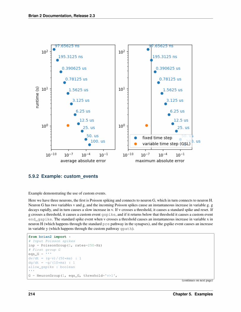
Brian 2 Documentation, Release 2.3
5.9.2 Example: custom_events
Example demonstrating the use of custom events.
Here we have three neurons, the first is Poisson spiking and connects to neuron G, which in turn connects to neuron H.Neuron G has two variables v and g, and the incoming Poisson spikes cause an instantaneous increase in variable g. gdecays rapidly, and in turn causes a slow increase in v. If v crosses a threshold, it causes a standard spike and reset. Ifg crosses a threshold, it causes a custom event gspike, and if it returns below that threshold it causes a custom eventend_gspike. The standard spike event when v crosses a threshold causes an instantaneous increase in variable x inneuron H (which happens through the standard pre pathway in the synapses), and the gspike event causes an increasein variable y (which happens through the custom pathway gpath).
from brian2 import *# Input Poisson spikesinp = PoissonGroup(1, rates=250*Hz)# First group Geqs_G = '''dv/dt = (g-v)/(50*ms) : 1dg/dt = -g/(10*ms) : 1allow_gspike : boolean'''G = NeuronGroup(1, eqs_G, threshold='v>1',
(continues on next page)
214 Chapter 5. Examples
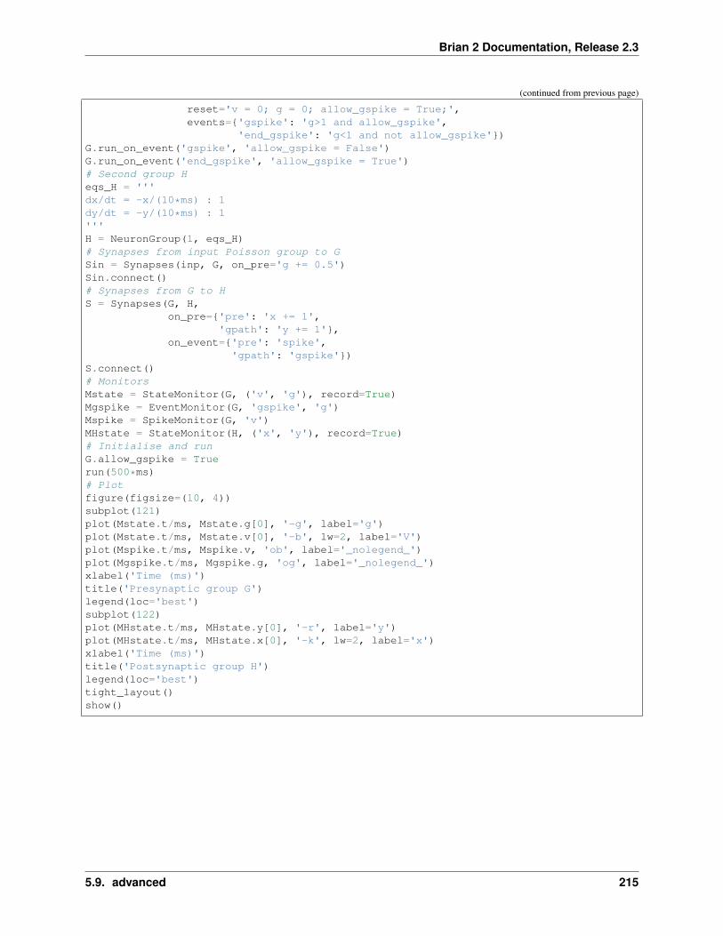
Brian 2 Documentation, Release 2.3
(continued from previous page)
reset='v = 0; g = 0; allow_gspike = True;',events={'gspike': 'g>1 and allow_gspike',
'end_gspike': 'g<1 and not allow_gspike'})G.run_on_event('gspike', 'allow_gspike = False')G.run_on_event('end_gspike', 'allow_gspike = True')# Second group Heqs_H = '''dx/dt = -x/(10*ms) : 1dy/dt = -y/(10*ms) : 1'''H = NeuronGroup(1, eqs_H)# Synapses from input Poisson group to GSin = Synapses(inp, G, on_pre='g += 0.5')Sin.connect()# Synapses from G to HS = Synapses(G, H,
on_pre={'pre': 'x += 1','gpath': 'y += 1'},
on_event={'pre': 'spike','gpath': 'gspike'})
S.connect()# MonitorsMstate = StateMonitor(G, ('v', 'g'), record=True)Mgspike = EventMonitor(G, 'gspike', 'g')Mspike = SpikeMonitor(G, 'v')MHstate = StateMonitor(H, ('x', 'y'), record=True)# Initialise and runG.allow_gspike = Truerun(500*ms)# Plotfigure(figsize=(10, 4))subplot(121)plot(Mstate.t/ms, Mstate.g[0], '-g', label='g')plot(Mstate.t/ms, Mstate.v[0], '-b', lw=2, label='V')plot(Mspike.t/ms, Mspike.v, 'ob', label='_nolegend_')plot(Mgspike.t/ms, Mgspike.g, 'og', label='_nolegend_')xlabel('Time (ms)')title('Presynaptic group G')legend(loc='best')subplot(122)plot(MHstate.t/ms, MHstate.y[0], '-r', label='y')plot(MHstate.t/ms, MHstate.x[0], '-k', lw=2, label='x')xlabel('Time (ms)')title('Postsynaptic group H')legend(loc='best')tight_layout()show()
5.9. advanced 215
Brian 2 Documentation, Release 2.3
5.9.3 Example: exprel_function
Show the improved numerical accuracy when using the exprel() function in rate equations.
Rate equations for channel opening/closing rates often include a term of the form 𝑥exp(𝑥)−1 . This term is problematic
for two reasons:
• It is not defined for 𝑥 = 0 (where it should equal to 1 for continuity);
• For values 𝑥 ≈ 0, there is a loss of accuracy.
For better accuracy, and to avoid issues at 𝑥 = 0, Brian provides the function exprel(), which is equivalent toexp(𝑥)−1
𝑥 , but with better accuracy and the expected result at 𝑥 = 0. In this example, we demonstrate the advantage ofexpressing a typical rate equation from the HH model with exprel().
from brian2 import *
# Dummy group to evaluate the rate equation at various pointseqs = '''v : volt
# opening rate from the HH modelalpha_simple = 0.32*(mV**-1)*(-50*mV-v)/
(exp((-50*mV-v)/(4*mV))-1.)/ms : Hzalpha_improved = 0.32*(mV**-1)*4*mV/exprel((-50*mV-v)/(4*mV))/ms : Hz'''
neuron = NeuronGroup(1000, eqs)
# Use voltage values around the problematic pointneuron.v = np.linspace(-50 - .5e-6, -50 + .5e-6, len(neuron))*mV
fig, ax = plt.subplots()ax.plot((neuron.v + 50*mV)/nvolt, neuron.alpha_simple,
'.', label=r'$\alpha_\mathrm{simple}$')ax.plot((neuron.v + 50*mV)/nvolt, neuron.alpha_improved,
'k', label=r'$\alpha_\mathrm{improved}$')ax.legend()ax.set(xlabel='$v$ relative to -50mV (nV)', ylabel=r'$\alpha$ (Hz)')ax.ticklabel_format(useOffset=False)plt.tight_layout()plt.show()
216 Chapter 5. Examples
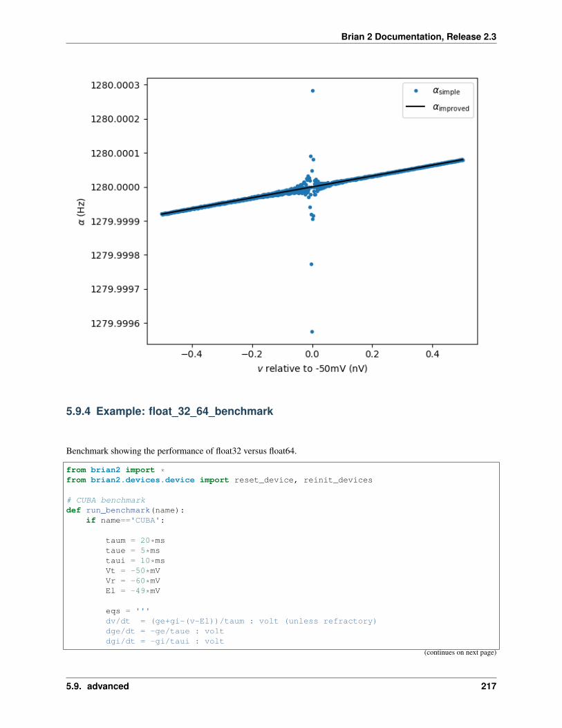
Brian 2 Documentation, Release 2.3
5.9.4 Example: float_32_64_benchmark
Benchmark showing the performance of float32 versus float64.
from brian2 import *from brian2.devices.device import reset_device, reinit_devices
# CUBA benchmarkdef run_benchmark(name):
if name=='CUBA':
taum = 20*mstaue = 5*mstaui = 10*msVt = -50*mVVr = -60*mVEl = -49*mV
eqs = '''dv/dt = (ge+gi-(v-El))/taum : volt (unless refractory)dge/dt = -ge/taue : voltdgi/dt = -gi/taui : volt
(continues on next page)
5.9. advanced 217
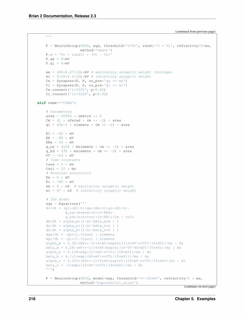
Brian 2 Documentation, Release 2.3
(continued from previous page)
'''
P = NeuronGroup(4000, eqs, threshold='v>Vt', reset='v = Vr', refractory=5*ms,method='exact')
P.v = 'Vr + rand() * (Vt - Vr)'P.ge = 0*mVP.gi = 0*mV
we = (60*0.27/10)*mV # excitatory synaptic weight (voltage)wi = (-20*4.5/10)*mV # inhibitory synaptic weightCe = Synapses(P, P, on_pre='ge += we')Ci = Synapses(P, P, on_pre='gi += wi')Ce.connect('i<3200', p=0.02)Ci.connect('i>=3200', p=0.02)
elif name=='COBA':
# Parametersarea = 20000 * umetre ** 2Cm = (1 * ufarad * cm ** -2) * areagl = (5e-5 * siemens * cm ** -2) * area
El = -60 * mVEK = -90 * mVENa = 50 * mVg_na = (100 * msiemens * cm ** -2) * areag_kd = (30 * msiemens * cm ** -2) * areaVT = -63 * mV# Time constantstaue = 5 * mstaui = 10 * ms# Reversal potentialsEe = 0 * mVEi = -80 * mVwe = 6 * nS # excitatory synaptic weightwi = 67 * nS # inhibitory synaptic weight
# The modeleqs = Equations('''dv/dt = (gl*(El-v)+ge*(Ee-v)+gi*(Ei-v)-
g_na*(m*m*m)*h*(v-ENa)-g_kd*(n*n*n*n)*(v-EK))/Cm : volt
dm/dt = alpha_m*(1-m)-beta_m*m : 1dn/dt = alpha_n*(1-n)-beta_n*n : 1dh/dt = alpha_h*(1-h)-beta_h*h : 1dge/dt = -ge*(1./taue) : siemensdgi/dt = -gi*(1./taui) : siemensalpha_m = 0.32*(mV**-1)*4*mV/exprel((13*mV-v+VT)/(4*mV))/ms : Hzbeta_m = 0.28*(mV**-1)*5*mV/exprel((v-VT-40*mV)/(5*mV))/ms : Hzalpha_h = 0.128*exp((17*mV-v+VT)/(18*mV))/ms : Hzbeta_h = 4./(1+exp((40*mV-v+VT)/(5*mV)))/ms : Hzalpha_n = 0.032*(mV**-1)*5*mV/exprel((15*mV-v+VT)/(5*mV))/ms : Hzbeta_n = .5*exp((10*mV-v+VT)/(40*mV))/ms : Hz''')
P = NeuronGroup(4000, model=eqs, threshold='v>-20*mV', refractory=3 * ms,method='exponential_euler')
(continues on next page)
218 Chapter 5. Examples

Brian 2 Documentation, Release 2.3
(continued from previous page)
Pe = P[:3200]Pi = P[3200:]Ce = Synapses(Pe, P, on_pre='ge+=we')Ci = Synapses(Pi, P, on_pre='gi+=wi')Ce.connect(p=0.02)Ci.connect(p=0.02)
# InitializationP.v = 'El + (randn() * 5 - 5)*mV'P.ge = '(randn() * 1.5 + 4) * 10.*nS'P.gi = '(randn() * 12 + 20) * 10.*nS'
run(1 * second, profile=True)
return sum(t for name, t in magic_network.profiling_info)
def generate_results(num_repeats):results = {}
for name in ['CUBA', 'COBA']:for target in ['numpy', 'cython', 'weave']:
for dtype in [float32, float64]:prefs.codegen.target = targetprefs.core.default_float_dtype = dtypetimes = [run_benchmark(name) for repeat in range(num_repeats)]results[name, target, dtype.__name__] = amin(times)
for name in ['CUBA', 'COBA']:for dtype in [float32, float64]:
times = []for _ in range(num_repeats):
reset_device()reinit_devices()set_device('cpp_standalone', directory=None, with_output=False)prefs.core.default_float_dtype = dtypetimes.append(run_benchmark(name))
results[name, 'cpp_standalone', dtype.__name__] = amin(times)
return results
results = generate_results(3)
bar_width = 0.9names = ['CUBA', 'COBA']targets = ['numpy', 'cython', 'weave', 'cpp_standalone']precisions = ['float32', 'float64']
figure(figsize=(8, 8))for j, name in enumerate(names):
subplot(2, 2, 1+2*j)title(name)index = arange(len(targets))for i, precision in enumerate(precisions):
bar(index+i*bar_width/len(precisions),[results[name, target, precision] for target in targets],bar_width/len(precisions), label=precision, align='edge')
ylabel('Time (s)')(continues on next page)
5.9. advanced 219

Brian 2 Documentation, Release 2.3
(continued from previous page)
if j:xticks(index+0.5*bar_width, targets, rotation=45)
else:xticks(index+0.5*bar_width, ('',)*len(targets))legend(loc='best')
subplot(2, 2, 2+2*j)index = arange(len(precisions))for i, target in enumerate(targets):
bar(index+i*bar_width/len(targets),[results[name, target, precision] for precision in precisions],bar_width/len(targets), label=target, align='edge')
ylabel('Time (s)')if j:
xticks(index+0.5*bar_width, precisions, rotation=45)else:
xticks(index+0.5*bar_width, ('',)*len(precisions))legend(loc='best')
tight_layout()show()
5.9.5 Example: opencv_movie
An example that uses a function from external C library (OpenCV in this case). Works for all C-based code generationtargets (i.e. for weave and cpp_standalone device) and for numpy (using the Python bindings).
This example needs a working installation of OpenCV 3.x and its Python bindings. It has been tested on 64 bit Linux ina conda environment with packages from the conda-forge channels (opencv 3.4.4, x264 1!152.20180717, ffmpeg4.1).
import osimport urllib2import cv2 # Import OpenCV2
from brian2 import *
defaultclock.dt = 1*msprefs.codegen.target = 'weave'prefs.logging.std_redirection = Falseset_device('cpp_standalone', clean=True)filename = os.path.abspath('Megamind.avi')
if not os.path.exists(filename):print('Downloading the example video file')response = urllib2.urlopen('http://docs.opencv.org/2.4/_downloads/Megamind.avi')data = response.read()with open(filename, 'wb') as f:
f.write(data)
video = cv2.VideoCapture(filename)width, height, frame_count = (int(video.get(cv2.CAP_PROP_FRAME_WIDTH)),
int(video.get(cv2.CAP_PROP_FRAME_HEIGHT)),
(continues on next page)
220 Chapter 5. Examples
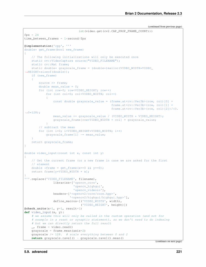
Brian 2 Documentation, Release 2.3
(continued from previous page)
int(video.get(cv2.CAP_PROP_FRAME_COUNT)))fps = 24time_between_frames = 1*second/fps
@implementation('cpp', '''double* get_frame(bool new_frame){
// The following initializations will only be executed oncestatic cv::VideoCapture source("VIDEO_FILENAME");static cv::Mat frame;static double* grayscale_frame = (double*)malloc(VIDEO_WIDTH*VIDEO_
→˓HEIGHT*sizeof(double));if (new_frame){
source >> frame;double mean_value = 0;for (int row=0; row<VIDEO_HEIGHT; row++)
for (int col=0; col<VIDEO_WIDTH; col++){
const double grayscale_value = (frame.at<cv::Vec3b>(row, col)[0] +frame.at<cv::Vec3b>(row, col)[1] +frame.at<cv::Vec3b>(row, col)[2])/(3.
→˓0*128);mean_value += grayscale_value / (VIDEO_WIDTH * VIDEO_HEIGHT);grayscale_frame[row*VIDEO_WIDTH + col] = grayscale_value;
}// subtract the meanfor (int i=0; i<VIDEO_HEIGHT*VIDEO_WIDTH; i++)
grayscale_frame[i] -= mean_value;}return grayscale_frame;
}
double video_input(const int x, const int y){
// Get the current frame (or a new frame in case we are asked for the first// elementdouble *frame = get_frame(x==0 && y==0);return frame[y*VIDEO_WIDTH + x];
}'''.replace('VIDEO_FILENAME', filename),
libraries=['opencv_core','opencv_highgui','opencv_videoio'],
headers=['<opencv2/core/core.hpp>','<opencv2/highgui/highgui.hpp>'],
define_macros=[('VIDEO_WIDTH', width),('VIDEO_HEIGHT', height)])
@check_units(x=1, y=1, result=1)def video_input(x, y):
# we assume this will only be called in the custom operation (and not for# example in a reset or synaptic statement), so we don't need to do indexing# but we can directly return the full result_, frame = video.read()grayscale = frame.mean(axis=2)grayscale /= 128. # scale everything between 0 and 2return grayscale.ravel() - grayscale.ravel().mean()
(continues on next page)
5.9. advanced 221

Brian 2 Documentation, Release 2.3
(continued from previous page)
N = width * heighttau, tau_th = 10*ms, time_between_framesG = NeuronGroup(N, '''dv/dt = (-v + I)/tau : 1
dv_th/dt = -v_th/tau_th : 1row : integer (constant)column : integer (constant)I : 1 # input current''',
threshold='v>v_th', reset='v=0; v_th = 3*v_th + 1.0',method='exact')
G.v_th = 1G.row = 'i//width'G.column = 'i%width'
G.run_regularly('I = video_input(column, row)',dt=time_between_frames)
mon = SpikeMonitor(G)runtime = frame_count*time_between_framesrun(runtime, report='text')
# Avoid going through the whole Brian2 indexing machinery too muchi, t, row, column = mon.i[:], mon.t[:], G.row[:], G.column[:]
import matplotlib.animation as animation
# TODO: Use overlapping windowsstepsize = 100*msdef next_spikes():
step = next_spikes.stepif step*stepsize > runtime:
next_spikes.step=0raise StopIteration()
spikes = i[(t>=step*stepsize) & (t<(step+1)*stepsize)]next_spikes.step += 1yield column[spikes], row[spikes]
next_spikes.step = 0
fig, ax = plt.subplots()dots, = ax.plot([], [], 'k.', markersize=2, alpha=.25)ax.set_xlim(0, width)ax.set_ylim(0, height)ax.invert_yaxis()def run(data):
x, y = datadots.set_data(x, y)
ani = animation.FuncAnimation(fig, run, next_spikes, blit=False, repeat=True,repeat_delay=1000)
plt.show()
5.9.6 Example: stochastic_odes
Demonstrate the correctness of the “derivative-free Milstein method” for multiplicative noise.
222 Chapter 5. Examples
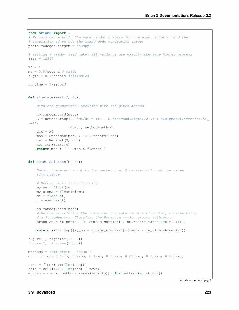
Brian 2 Documentation, Release 2.3
from brian2 import *# We only get exactly the same random numbers for the exact solution and the# simulation if we use the numpy code generation targetprefs.codegen.target = 'numpy'
# setting a random seed makes all variants use exactly the same Wiener processseed = 12347
X0 = 1mu = 0.5/second # driftsigma = 0.1/second #diffusion
runtime = 1*second
def simulate(method, dt):'''simulate geometrical Brownian with the given method'''np.random.seed(seed)G = NeuronGroup(1, 'dX/dt = (mu - 0.5*second*sigma**2)*X + X*sigma*xi*second**.5:
→˓1',dt=dt, method=method)
G.X = X0mon = StateMonitor(G, 'X', record=True)net = Network(G, mon)net.run(runtime)return mon.t_[:], mon.X.flatten()
def exact_solution(t, dt):'''Return the exact solution for geometrical Brownian motion at the giventime points'''# Remove units for simplicitymy_mu = float(mu)my_sigma = float(sigma)dt = float(dt)t = asarray(t)
np.random.seed(seed)# We are calculating the values at the *start* of a time step, as when using# a StateMonitor. Therefore the Brownian motion starts with zerobrownian = np.hstack([0, cumsum(sqrt(dt) * np.random.randn(len(t)-1))])
return (X0 * exp((my_mu - 0.5*my_sigma**2)*(t+dt) + my_sigma*brownian))
figure(1, figsize=(16, 7))figure(2, figsize=(16, 7))
methods = ['milstein', 'heun']dts = [1*ms, 0.5*ms, 0.2*ms, 0.1*ms, 0.05*ms, 0.025*ms, 0.01*ms, 0.005*ms]
rows = floor(sqrt(len(dts)))cols = ceil(1.0 * len(dts) / rows)errors = dict([(method, zeros(len(dts))) for method in methods])
(continues on next page)
5.9. advanced 223

Brian 2 Documentation, Release 2.3
(continued from previous page)
for dt_idx, dt in enumerate(dts):print('dt: %s' % dt)trajectories = {}# Test the numerical methodsfor method in methods:
t, trajectories[method] = simulate(method, dt)# Calculate the exact solutionexact = exact_solution(t, dt)
for method in methods:# plot the trajectoriesfigure(1)subplot(rows, cols, dt_idx+1)plot(t, trajectories[method], label=method, alpha=0.75)
# determine the mean absolute errorerrors[method][dt_idx] = mean(abs(trajectories[method] - exact))# plot the difference to the real trajectoryfigure(2)subplot(rows, cols, dt_idx+1)plot(t, trajectories[method] - exact, label=method, alpha=0.75)
figure(1)plot(t, exact, color='gray', lw=2, label='exact', alpha=0.75)title('dt = %s' % str(dt))xticks([])
figure(1)legend(frameon=False, loc='best')tight_layout()
figure(2)legend(frameon=False, loc='best')tight_layout()
figure(3)for method in methods:
plot(array(dts) / ms, errors[method], 'o', label=method)legend(frameon=False, loc='best')xscale('log')yscale('log')xlabel('dt (ms)')ylabel('Mean absolute error')tight_layout()
show()
224 Chapter 5. Examples
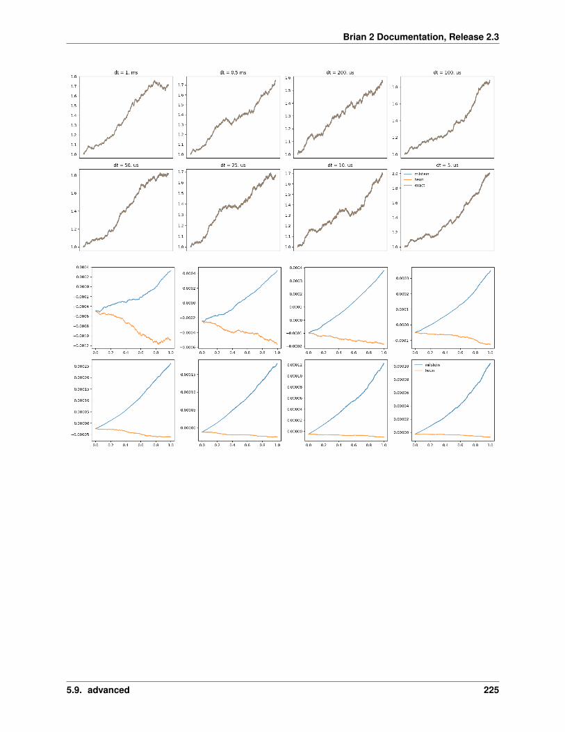
Brian 2 Documentation, Release 2.3
5.9. advanced 225
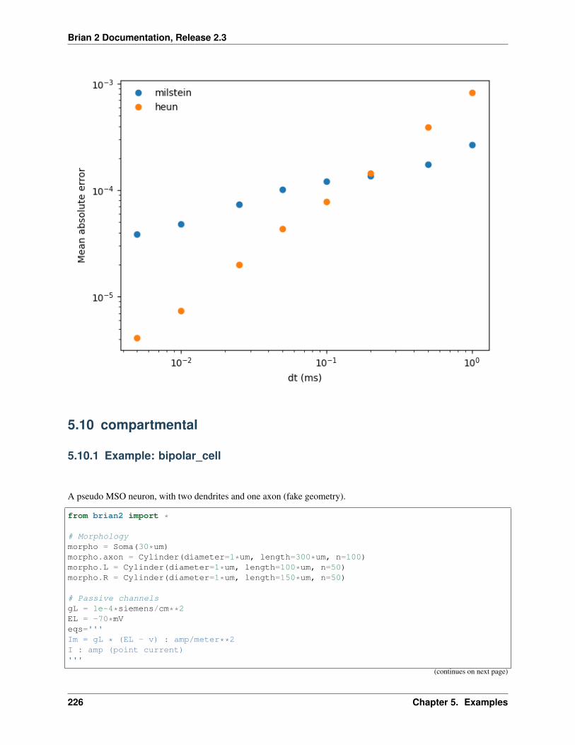
Brian 2 Documentation, Release 2.3
5.10 compartmental
5.10.1 Example: bipolar_cell
A pseudo MSO neuron, with two dendrites and one axon (fake geometry).
from brian2 import *
# Morphologymorpho = Soma(30*um)morpho.axon = Cylinder(diameter=1*um, length=300*um, n=100)morpho.L = Cylinder(diameter=1*um, length=100*um, n=50)morpho.R = Cylinder(diameter=1*um, length=150*um, n=50)
# Passive channelsgL = 1e-4*siemens/cm**2EL = -70*mVeqs='''Im = gL * (EL - v) : amp/meter**2I : amp (point current)'''
(continues on next page)
226 Chapter 5. Examples

Brian 2 Documentation, Release 2.3
(continued from previous page)
neuron = SpatialNeuron(morphology=morpho, model=eqs,Cm=1*uF/cm**2, Ri=100*ohm*cm, method='exponential_euler')
neuron.v = ELneuron.I = 0*amp
# Monitorsmon_soma = StateMonitor(neuron, 'v', record=[0])mon_L = StateMonitor(neuron.L, 'v', record=True)mon_R = StateMonitor(neuron, 'v', record=morpho.R[75*um])
run(1*ms)neuron.I[morpho.L[50*um]] = 0.2*nA # injecting in the left dendriterun(5*ms)neuron.I = 0*amprun(50*ms, report='text')
subplot(211)plot(mon_L.t/ms, mon_soma[0].v/mV, 'k')plot(mon_L.t/ms, mon_L[morpho.L[50*um]].v/mV, 'r')plot(mon_L.t/ms, mon_R[morpho.R[75*um]].v/mV, 'b')ylabel('v (mV)')subplot(212)for x in linspace(0*um, 100*um, 10, endpoint=False):
plot(mon_L.t/ms, mon_L[morpho.L[x]].v/mV)xlabel('Time (ms)')ylabel('v (mV)')show()
5.10. compartmental 227
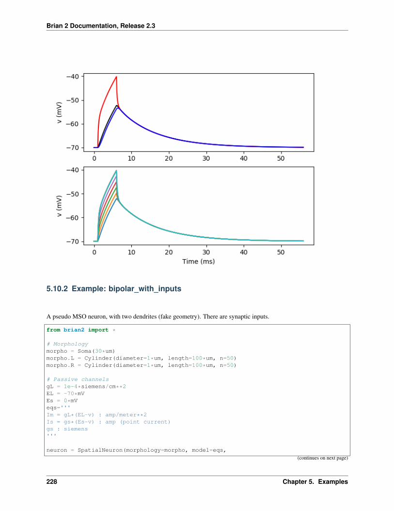
Brian 2 Documentation, Release 2.3
5.10.2 Example: bipolar_with_inputs
A pseudo MSO neuron, with two dendrites (fake geometry). There are synaptic inputs.
from brian2 import *
# Morphologymorpho = Soma(30*um)morpho.L = Cylinder(diameter=1*um, length=100*um, n=50)morpho.R = Cylinder(diameter=1*um, length=100*um, n=50)
# Passive channelsgL = 1e-4*siemens/cm**2EL = -70*mVEs = 0*mVeqs='''Im = gL*(EL-v) : amp/meter**2Is = gs*(Es-v) : amp (point current)gs : siemens'''
neuron = SpatialNeuron(morphology=morpho, model=eqs,
(continues on next page)
228 Chapter 5. Examples
Brian 2 Documentation, Release 2.3
(continued from previous page)
Cm=1*uF/cm**2, Ri=100*ohm*cm, method='exponential_euler')neuron.v = EL
# Regular inputsstimulation = NeuronGroup(2, 'dx/dt = 300*Hz : 1', threshold='x>1', reset='x=0',
method='euler')stimulation.x = [0, 0.5] # Asynchronous
# Synapsestaus = 1*msw = 20*nSS = Synapses(stimulation, neuron, model='''dg/dt = -g/taus : siemens (clock-driven)
gs_post = g : siemens (summed)''',on_pre='g += w', method='exact')
S.connect(i=0, j=morpho.L[-1])S.connect(i=1, j=morpho.R[-1])
# Monitorsmon_soma = StateMonitor(neuron, 'v', record=[0])mon_L = StateMonitor(neuron.L, 'v', record=True)mon_R = StateMonitor(neuron.R, 'v',
record=morpho.R[-1])
run(50*ms, report='text')
subplot(211)plot(mon_L.t/ms, mon_soma[0].v/mV, 'k')plot(mon_L.t/ms, mon_L[morpho.L[-1]].v/mV, 'r')plot(mon_L.t/ms, mon_R[morpho.R[-1]].v/mV, 'b')ylabel('v (mV)')subplot(212)for x in linspace(0*um, 100*um, 10, endpoint=False):
plot(mon_L.t/ms, mon_L[morpho.L[x]].v/mV)xlabel('Time (ms)')ylabel('v (mV)')show()
5.10. compartmental 229

Brian 2 Documentation, Release 2.3
5.10.3 Example: bipolar_with_inputs2
A pseudo MSO neuron, with two dendrites (fake geometry). There are synaptic inputs.
Second method.
from brian2 import *
# Morphologymorpho = Soma(30*um)morpho.L = Cylinder(diameter=1*um, length=100*um, n=50)morpho.R = Cylinder(diameter=1*um, length=100*um, n=50)
# Passive channelsgL = 1e-4*siemens/cm**2EL = -70*mVEs = 0*mVtaus = 1*mseqs='''Im = gL*(EL-v) : amp/meter**2Is = gs*(Es-v) : amp (point current)dgs/dt = -gs/taus : siemens'''
(continues on next page)
230 Chapter 5. Examples

Brian 2 Documentation, Release 2.3
(continued from previous page)
neuron = SpatialNeuron(morphology=morpho, model=eqs,Cm=1*uF/cm**2, Ri=100*ohm*cm, method='exponential_euler')
neuron.v = EL
# Regular inputsstimulation = NeuronGroup(2, 'dx/dt = 300*Hz : 1', threshold='x>1', reset='x=0',
method='euler')stimulation.x = [0, 0.5] # Asynchronous
# Synapsesw = 20*nSS = Synapses(stimulation, neuron,on_pre='gs += w')S.connect(i=0, j=morpho.L[99.9*um])S.connect(i=1, j=morpho.R[99.9*um])
# Monitorsmon_soma = StateMonitor(neuron, 'v', record=[0])mon_L = StateMonitor(neuron.L, 'v', record=True)mon_R = StateMonitor(neuron, 'v', record=morpho.R[99.9*um])
run(50*ms, report='text')
subplot(211)plot(mon_L.t/ms, mon_soma[0].v/mV, 'k')plot(mon_L.t/ms, mon_L[morpho.L[99.9*um]].v/mV, 'r')plot(mon_L.t/ms, mon_R[morpho.R[99.9*um]].v/mV, 'b')ylabel('v (mV)')subplot(212)for i in [0, 5, 10, 15, 20, 25, 30, 35, 40, 45]:
plot(mon_L.t/ms, mon_L.v[i, :]/mV)xlabel('Time (ms)')ylabel('v (mV)')show()
5.10. compartmental 231
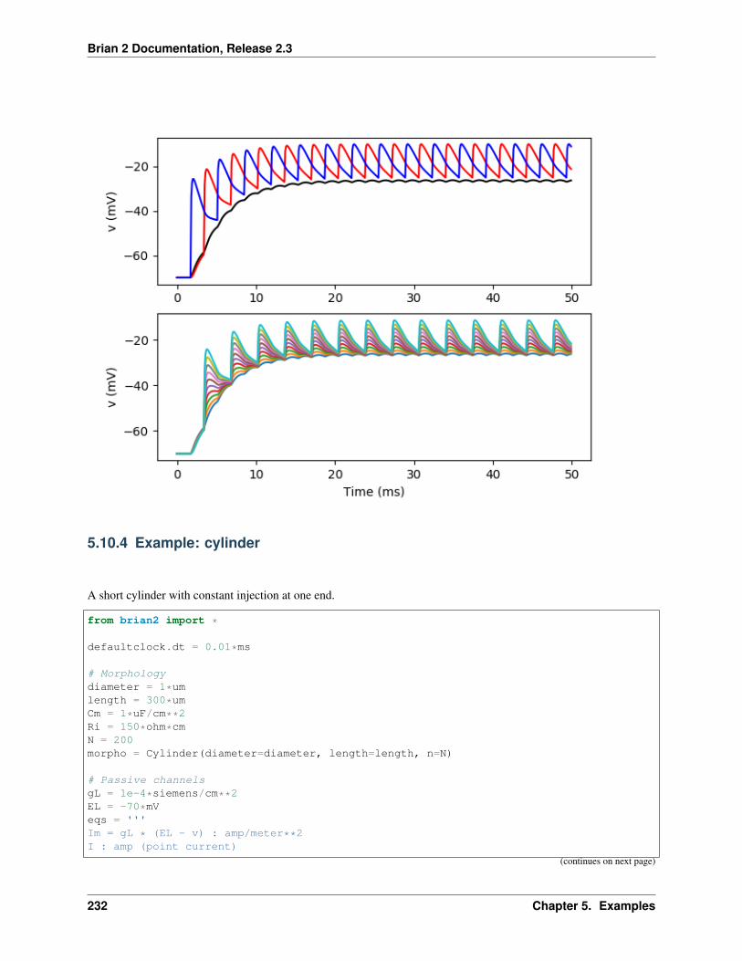
Brian 2 Documentation, Release 2.3
5.10.4 Example: cylinder
A short cylinder with constant injection at one end.
from brian2 import *
defaultclock.dt = 0.01*ms
# Morphologydiameter = 1*umlength = 300*umCm = 1*uF/cm**2Ri = 150*ohm*cmN = 200morpho = Cylinder(diameter=diameter, length=length, n=N)
# Passive channelsgL = 1e-4*siemens/cm**2EL = -70*mVeqs = '''Im = gL * (EL - v) : amp/meter**2I : amp (point current)
(continues on next page)
232 Chapter 5. Examples

Brian 2 Documentation, Release 2.3
(continued from previous page)
'''
neuron = SpatialNeuron(morphology=morpho, model=eqs, Cm=Cm, Ri=Ri,method='exponential_euler')
neuron.v = EL
la = neuron.space_constant[0]print("Electrotonic length: %s" % la)
neuron.I[0] = 0.02*nA # injecting at the left endrun(100*ms, report='text')
plot(neuron.distance/um, neuron.v/mV, 'kx')# Theoryx = neuron.distancera = la * 4 * Ri / (pi * diameter**2)theory = EL + ra * neuron.I[0] * cosh((length - x) / la) / sinh(length / la)plot(x/um, theory/mV, 'r')xlabel('x (um)')ylabel('v (mV)')show()
5.10. compartmental 233
Brian 2 Documentation, Release 2.3
5.10.5 Example: hh_with_spikes
Hodgkin-Huxley equations (1952).
Spikes are recorded along the axon, and then velocity is calculated.
from brian2 import *from scipy import stats
defaultclock.dt = 0.01*ms
morpho = Cylinder(length=10*cm, diameter=2*238*um, n=1000, type='axon')
El = 10.613*mVENa = 115*mVEK = -12*mVgl = 0.3*msiemens/cm**2gNa0 = 120*msiemens/cm**2gK = 36*msiemens/cm**2
# Typical equationseqs = '''# The same equations for the whole neuron, but possibly different parameter values# distributed transmembrane currentIm = gl * (El-v) + gNa * m**3 * h * (ENa-v) + gK * n**4 * (EK-v) : amp/meter**2I : amp (point current) # applied currentdm/dt = alpham * (1-m) - betam * m : 1dn/dt = alphan * (1-n) - betan * n : 1dh/dt = alphah * (1-h) - betah * h : 1alpham = (0.1/mV) * 10*mV/exprel((-v+25*mV)/(10*mV))/ms : Hzbetam = 4 * exp(-v/(18*mV))/ms : Hzalphah = 0.07 * exp(-v/(20*mV))/ms : Hzbetah = 1/(exp((-v+30*mV) / (10*mV)) + 1)/ms : Hzalphan = (0.01/mV) * 10*mV/exprel((-v+10*mV)/(10*mV))/ms : Hzbetan = 0.125*exp(-v/(80*mV))/ms : HzgNa : siemens/meter**2'''
neuron = SpatialNeuron(morphology=morpho, model=eqs, method="exponential_euler",refractory="m > 0.4", threshold="m > 0.5",Cm=1*uF/cm**2, Ri=35.4*ohm*cm)
neuron.v = 0*mVneuron.h = 1neuron.m = 0neuron.n = .5neuron.I = 0*ampneuron.gNa = gNa0M = StateMonitor(neuron, 'v', record=True)spikes = SpikeMonitor(neuron)
run(50*ms, report='text')neuron.I[0] = 1*uA # current injection at one endrun(3*ms)neuron.I = 0*amprun(50*ms, report='text')
# Calculation of velocity(continues on next page)
234 Chapter 5. Examples

Brian 2 Documentation, Release 2.3
(continued from previous page)
slope, intercept, r_value, p_value, std_err = stats.linregress(spikes.t/second,neuron.distance[spikes.i]/meter)
print("Velocity = %.2f m/s" % slope)
subplot(211)for i in range(10):
plot(M.t/ms, M.v.T[:, i*100]/mV)ylabel('v')subplot(212)plot(spikes.t/ms, spikes.i*neuron.length[0]/cm, '.k')plot(spikes.t/ms, (intercept+slope*(spikes.t/second))/cm, 'r')xlabel('Time (ms)')ylabel('Position (cm)')show()
5.10.6 Example: hodgkin_huxley_1952
Hodgkin-Huxley equations (1952).
from brian2 import *
(continues on next page)
5.10. compartmental 235

Brian 2 Documentation, Release 2.3
(continued from previous page)
morpho = Cylinder(length=10*cm, diameter=2*238*um, n=1000, type='axon')
El = 10.613*mVENa = 115*mVEK = -12*mVgl = 0.3*msiemens/cm**2gNa0 = 120*msiemens/cm**2gK = 36*msiemens/cm**2
# Typical equationseqs = '''# The same equations for the whole neuron, but possibly different parameter values# distributed transmembrane currentIm = gl * (El-v) + gNa * m**3 * h * (ENa-v) + gK * n**4 * (EK-v) : amp/meter**2I : amp (point current) # applied currentdm/dt = alpham * (1-m) - betam * m : 1dn/dt = alphan * (1-n) - betan * n : 1dh/dt = alphah * (1-h) - betah * h : 1alpham = (0.1/mV) * 10*mV/exprel((-v+25*mV)/(10*mV))/ms : Hzbetam = 4 * exp(-v/(18*mV))/ms : Hzalphah = 0.07 * exp(-v/(20*mV))/ms : Hzbetah = 1/(exp((-v+30*mV) / (10*mV)) + 1)/ms : Hzalphan = (0.01/mV) * 10*mV/exprel((-v+10*mV)/(10*mV))/ms : Hzbetan = 0.125*exp(-v/(80*mV))/ms : HzgNa : siemens/meter**2'''
neuron = SpatialNeuron(morphology=morpho, model=eqs, Cm=1*uF/cm**2,Ri=35.4*ohm*cm, method="exponential_euler")
neuron.v = 0*mVneuron.h = 1neuron.m = 0neuron.n = .5neuron.I = 0neuron.gNa = gNa0neuron[5*cm:10*cm].gNa = 0*siemens/cm**2M = StateMonitor(neuron, 'v', record=True)
run(50*ms, report='text')neuron.I[0] = 1*uA # current injection at one endrun(3*ms)neuron.I = 0*amprun(100*ms, report='text')for i in range(75, 125, 1):
plot(cumsum(neuron.length)/cm, i+(1./60)*M.v[:, i*5]/mV, 'k')yticks([])ylabel('Time [major] v (mV) [minor]')xlabel('Position (cm)')axis('tight')show()
236 Chapter 5. Examples

Brian 2 Documentation, Release 2.3
5.10.7 Example: infinite_cable
An (almost) infinite cable with pulse injection in the middle.
from brian2 import *
defaultclock.dt = 0.001*ms
# Morphologydiameter = 1*umCm = 1*uF/cm**2Ri = 100*ohm*cmN = 500morpho = Cylinder(diameter=diameter, length=3*mm, n=N)
# Passive channelsgL = 1e-4*siemens/cm**2EL = -70*mVeqs = '''Im = gL * (EL-v) : amp/meter**2I : amp (point current)'''
(continues on next page)
5.10. compartmental 237
Brian 2 Documentation, Release 2.3
(continued from previous page)
neuron = SpatialNeuron(morphology=morpho, model=eqs, Cm=Cm, Ri=Ri,method = 'exponential_euler')
neuron.v = EL
taum = Cm /gL # membrane time constantprint("Time constant: %s" % taum)la = neuron.space_constant[0]print("Characteristic length: %s" % la)
# Monitorsmon = StateMonitor(neuron, 'v', record=range(0, N//2, 20))
neuron.I[len(neuron) // 2] = 1*nA # injecting in the middlerun(0.02*ms)neuron.I = 0*amprun(10*ms, report='text')
t = mon.tplot(t/ms, mon.v.T/mV, 'k')# Theory (incorrect near cable ends)for i in range(0, len(neuron)//2, 20):
x = (len(neuron)/2 - i) * morpho.length[0]theory = (1/(la*Cm*pi*diameter) * sqrt(taum / (4*pi*(t + defaultclock.dt))) *
exp(-(t+defaultclock.dt)/taum -taum / (4*(t+defaultclock.dt))*(x/la)**2))
theory = EL + theory * 1*nA * 0.02*msplot(t/ms, theory/mV, 'r')
xlabel('Time (ms)')ylabel('v (mV')show()
238 Chapter 5. Examples

Brian 2 Documentation, Release 2.3
5.10.8 Example: lfp
Hodgkin-Huxley equations (1952)
We calculate the extracellular field potential at various places.
from brian2 import *defaultclock.dt = 0.01*msmorpho = Cylinder(x=[0, 10]*cm, diameter=2*238*um, n=1000, type='axon')
El = 10.613* mVENa = 115*mVEK = -12*mVgl = 0.3*msiemens/cm**2gNa0 = 120*msiemens/cm**2gK = 36*msiemens/cm**2
# Typical equationseqs = '''# The same equations for the whole neuron, but possibly different parameter values# distributed transmembrane currentIm = gl * (El-v) + gNa * m**3 * h * (ENa-v) + gK * n**4 * (EK-v) : amp/meter**2I : amp (point current) # applied current
(continues on next page)
5.10. compartmental 239
Brian 2 Documentation, Release 2.3
(continued from previous page)
dm/dt = alpham * (1-m) - betam * m : 1dn/dt = alphan * (1-n) - betan * n : 1dh/dt = alphah * (1-h) - betah * h : 1alpham = (0.1/mV) * 10*mV/exprel((-v+25*mV)/(10*mV))/ms : Hzbetam = 4 * exp(-v/(18*mV))/ms : Hzalphah = 0.07 * exp(-v/(20*mV))/ms : Hzbetah = 1/(exp((-v+30*mV) / (10*mV)) + 1)/ms : Hzalphan = (0.01/mV) * 10*mV/exprel((-v+10*mV)/(10*mV))/ms : Hzbetan = 0.125*exp(-v/(80*mV))/ms : HzgNa : siemens/meter**2'''
neuron = SpatialNeuron(morphology=morpho, model=eqs, Cm=1*uF/cm**2,Ri=35.4*ohm*cm, method="exponential_euler")
neuron.v = 0*mVneuron.h = 1neuron.m = 0neuron.n = .5neuron.I = 0neuron.gNa = gNa0neuron[5*cm:10*cm].gNa = 0*siemens/cm**2M = StateMonitor(neuron, 'v', record=True)
# LFP recorderNe = 5 # Number of electrodessigma = 0.3*siemens/meter # Resistivity of extracellular field (0.3-0.4 S/m)lfp = NeuronGroup(Ne,model='''v : volt
x : metery : meterz : meter''')
lfp.x = 7*cm # Off center (to be far from stimulating electrode)lfp.y = [1*mm, 2*mm, 4*mm, 8*mm, 16*mm]S = Synapses(neuron,lfp,model='''w : ohm*meter**2 (constant) # Weight in the LFP→˓calculation
v_post = w*(Ic_pre-Im_pre) : volt (summed)''')S.summed_updaters['v_post'].when = 'after_groups' # otherwise Ic has not yet been→˓updated for the current time step.S.connect()S.w = 'area_pre/(4*pi*sigma)/((x_pre-x_post)**2+(y_pre-y_post)**2+(z_pre-z_→˓post)**2)**.5'
Mlfp = StateMonitor(lfp,'v',record=True)
run(50*ms, report='text')neuron.I[0] = 1*uA # current injection at one endrun(3*ms)neuron.I = 0*amprun(100*ms, report='text')
subplot(211)for i in range(10):
plot(M.t/ms,M.v[i*100]/mV)ylabel('$V_m$ (mV)')subplot(212)for i in range(5):
plot(M.t/ms,Mlfp.v[i]/mV)ylabel('LFP (mV)')
(continues on next page)
240 Chapter 5. Examples
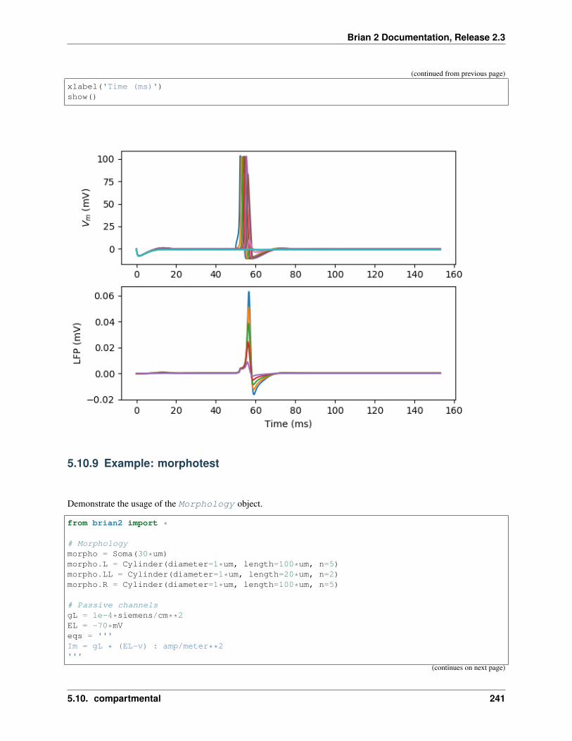
Brian 2 Documentation, Release 2.3
(continued from previous page)
xlabel('Time (ms)')show()
5.10.9 Example: morphotest
Demonstrate the usage of the Morphology object.
from brian2 import *
# Morphologymorpho = Soma(30*um)morpho.L = Cylinder(diameter=1*um, length=100*um, n=5)morpho.LL = Cylinder(diameter=1*um, length=20*um, n=2)morpho.R = Cylinder(diameter=1*um, length=100*um, n=5)
# Passive channelsgL = 1e-4*siemens/cm**2EL = -70*mVeqs = '''Im = gL * (EL-v) : amp/meter**2'''
(continues on next page)
5.10. compartmental 241

Brian 2 Documentation, Release 2.3
(continued from previous page)
neuron = SpatialNeuron(morphology=morpho, model=eqs,Cm=1*uF/cm**2, Ri=100*ohm*cm, method='exponential_euler')
neuron.v = arange(0, 13)*volt
print(neuron.v)print(neuron.L.v)print(neuron.LL.v)print(neuron.L.main.v)
5.10.10 Example: rall
A cylinder plus two branches, with diameters according to Rall’s formula
from brian2 import *
defaultclock.dt = 0.01*ms
# Passive channelsgL = 1e-4*siemens/cm**2EL = -70*mV
# Morphologydiameter = 1*umlength = 300*umCm = 1*uF/cm**2Ri = 150*ohm*cmN = 500rm = 1 / (gL * pi * diameter) # membrane resistance per unit lengthra = (4 * Ri)/(pi * diameter**2) # axial resistance per unit lengthla = sqrt(rm / ra) # space lengthmorpho = Cylinder(diameter=diameter, length=length, n=N)d1 = 0.5*umL1 = 200*umrm = 1 / (gL * pi * d1) # membrane resistance per unit lengthra = (4 * Ri) / (pi * d1**2) # axial resistance per unit lengthl1 = sqrt(rm / ra) # space lengthmorpho.L = Cylinder(diameter=d1, length=L1, n=N)d2 = (diameter**1.5 - d1**1.5)**(1. / 1.5)rm = 1/(gL * pi * d2) # membrane resistance per unit lengthra = (4 * Ri) / (pi * d2**2) # axial resistance per unit lengthl2 = sqrt(rm / ra) # space lengthL2 = (L1 / l1) * l2morpho.R = Cylinder(diameter=d2, length=L2, n=N)
eqs='''Im = gL * (EL-v) : amp/meter**2I : amp (point current)'''
neuron = SpatialNeuron(morphology=morpho, model=eqs, Cm=Cm, Ri=Ri,method='exponential_euler')
neuron.v = EL
(continues on next page)
242 Chapter 5. Examples
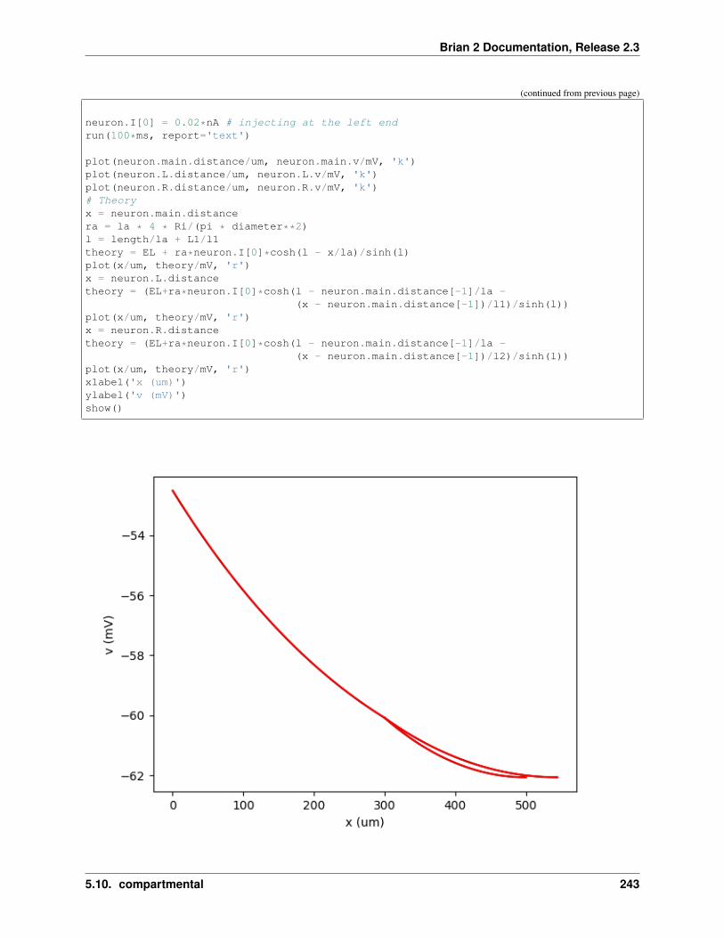
Brian 2 Documentation, Release 2.3
(continued from previous page)
neuron.I[0] = 0.02*nA # injecting at the left endrun(100*ms, report='text')
plot(neuron.main.distance/um, neuron.main.v/mV, 'k')plot(neuron.L.distance/um, neuron.L.v/mV, 'k')plot(neuron.R.distance/um, neuron.R.v/mV, 'k')# Theoryx = neuron.main.distancera = la * 4 * Ri/(pi * diameter**2)l = length/la + L1/l1theory = EL + ra*neuron.I[0]*cosh(l - x/la)/sinh(l)plot(x/um, theory/mV, 'r')x = neuron.L.distancetheory = (EL+ra*neuron.I[0]*cosh(l - neuron.main.distance[-1]/la -
(x - neuron.main.distance[-1])/l1)/sinh(l))plot(x/um, theory/mV, 'r')x = neuron.R.distancetheory = (EL+ra*neuron.I[0]*cosh(l - neuron.main.distance[-1]/la -
(x - neuron.main.distance[-1])/l2)/sinh(l))plot(x/um, theory/mV, 'r')xlabel('x (um)')ylabel('v (mV)')show()
5.10. compartmental 243
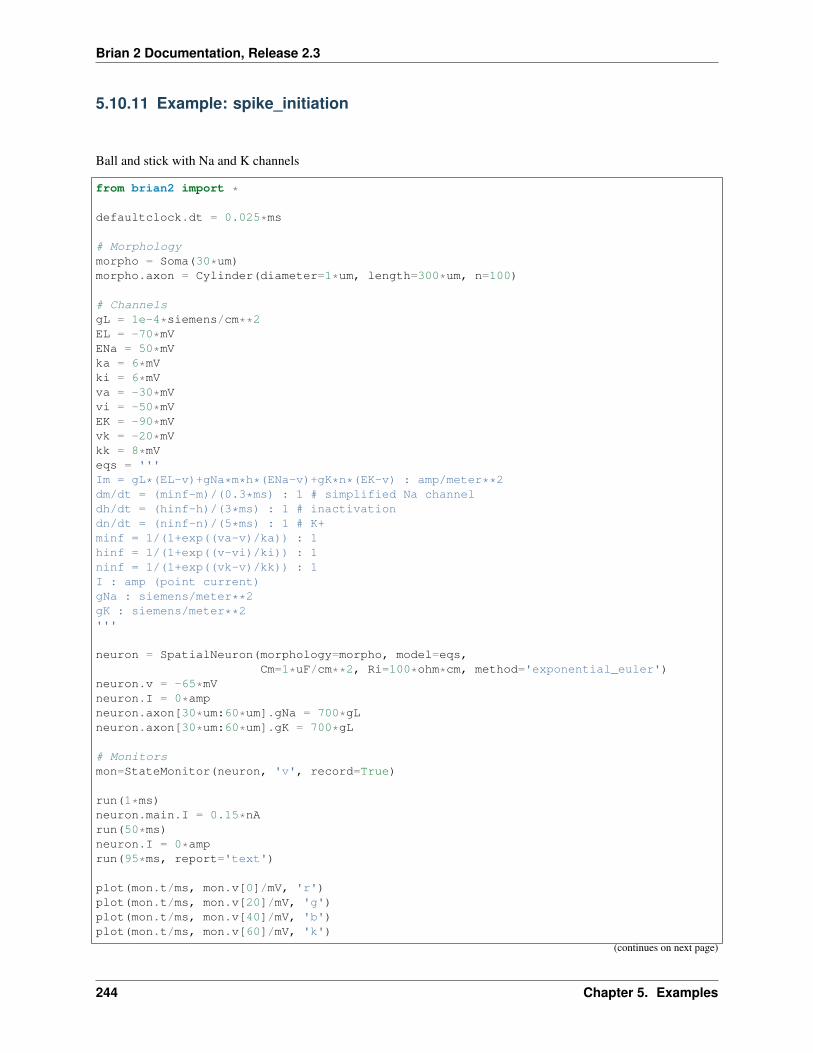
Brian 2 Documentation, Release 2.3
5.10.11 Example: spike_initiation
Ball and stick with Na and K channels
from brian2 import *
defaultclock.dt = 0.025*ms
# Morphologymorpho = Soma(30*um)morpho.axon = Cylinder(diameter=1*um, length=300*um, n=100)
# ChannelsgL = 1e-4*siemens/cm**2EL = -70*mVENa = 50*mVka = 6*mVki = 6*mVva = -30*mVvi = -50*mVEK = -90*mVvk = -20*mVkk = 8*mVeqs = '''Im = gL*(EL-v)+gNa*m*h*(ENa-v)+gK*n*(EK-v) : amp/meter**2dm/dt = (minf-m)/(0.3*ms) : 1 # simplified Na channeldh/dt = (hinf-h)/(3*ms) : 1 # inactivationdn/dt = (ninf-n)/(5*ms) : 1 # K+minf = 1/(1+exp((va-v)/ka)) : 1hinf = 1/(1+exp((v-vi)/ki)) : 1ninf = 1/(1+exp((vk-v)/kk)) : 1I : amp (point current)gNa : siemens/meter**2gK : siemens/meter**2'''
neuron = SpatialNeuron(morphology=morpho, model=eqs,Cm=1*uF/cm**2, Ri=100*ohm*cm, method='exponential_euler')
neuron.v = -65*mVneuron.I = 0*ampneuron.axon[30*um:60*um].gNa = 700*gLneuron.axon[30*um:60*um].gK = 700*gL
# Monitorsmon=StateMonitor(neuron, 'v', record=True)
run(1*ms)neuron.main.I = 0.15*nArun(50*ms)neuron.I = 0*amprun(95*ms, report='text')
plot(mon.t/ms, mon.v[0]/mV, 'r')plot(mon.t/ms, mon.v[20]/mV, 'g')plot(mon.t/ms, mon.v[40]/mV, 'b')plot(mon.t/ms, mon.v[60]/mV, 'k')
(continues on next page)
244 Chapter 5. Examples
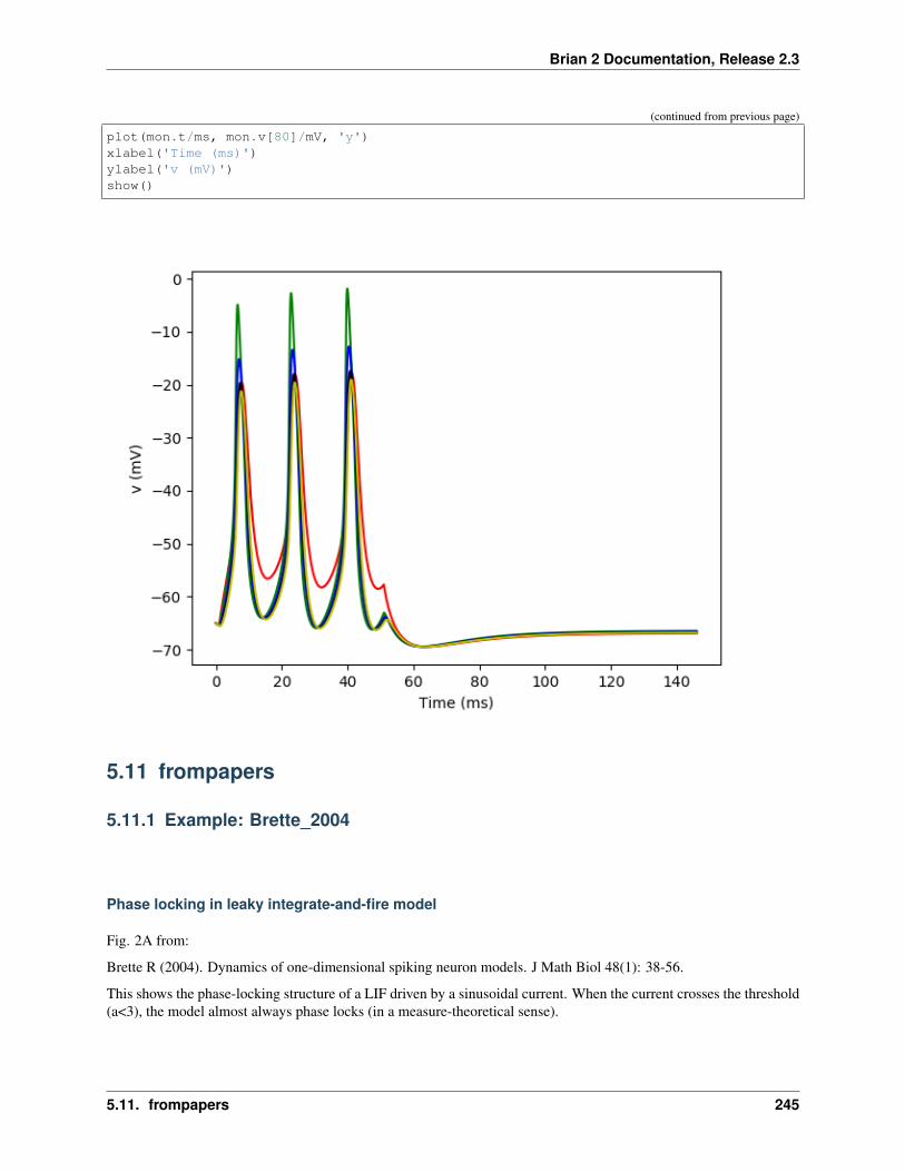
Brian 2 Documentation, Release 2.3
(continued from previous page)
plot(mon.t/ms, mon.v[80]/mV, 'y')xlabel('Time (ms)')ylabel('v (mV)')show()
5.11 frompapers
5.11.1 Example: Brette_2004
Phase locking in leaky integrate-and-fire model
Fig. 2A from:
Brette R (2004). Dynamics of one-dimensional spiking neuron models. J Math Biol 48(1): 38-56.
This shows the phase-locking structure of a LIF driven by a sinusoidal current. When the current crosses the threshold(a<3), the model almost always phase locks (in a measure-theoretical sense).
5.11. frompapers 245
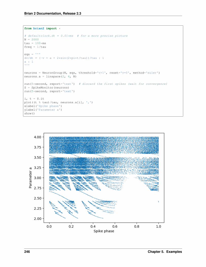
Brian 2 Documentation, Release 2.3
from brian2 import *
# defaultclock.dt = 0.01*ms # for a more precise pictureN = 2000tau = 100*msfreq = 1/tau
eqs = '''dv/dt = (-v + a + 2*sin(2*pi*t/tau))/tau : 1a : 1'''
neurons = NeuronGroup(N, eqs, threshold='v>1', reset='v=0', method='euler')neurons.a = linspace(2, 4, N)
run(5*second, report='text') # discard the first spikes (wait for convergence)S = SpikeMonitor(neurons)run(5*second, report='text')
i, t = S.itplot((t % tau)/tau, neurons.a[i], ',')xlabel('Spike phase')ylabel('Parameter a')show()
246 Chapter 5. Examples

Brian 2 Documentation, Release 2.3
5.11.2 Example: Brette_Gerstner_2005
Adaptive exponential integrate-and-fire model.
http://www.scholarpedia.org/article/Adaptive_exponential_integrate-and-fire_model
Introduced in Brette R. and Gerstner W. (2005), Adaptive Exponential Integrate-and-Fire Model as an Effective De-scription of Neuronal Activity, J. Neurophysiol. 94: 3637 - 3642.
from brian2 import *
# ParametersC = 281 * pFgL = 30 * nStaum = C / gLEL = -70.6 * mVVT = -50.4 * mVDeltaT = 2 * mVVcut = VT + 5 * DeltaT
# Pick an electrophysiological behaviourtauw, a, b, Vr = 144*ms, 4*nS, 0.0805*nA, -70.6*mV # Regular spiking (as in the paper)#tauw,a,b,Vr=20*ms,4*nS,0.5*nA,VT+5*mV # Bursting#tauw,a,b,Vr=144*ms,2*C/(144*ms),0*nA,-70.6*mV # Fast spiking
eqs = """dvm/dt = (gL*(EL - vm) + gL*DeltaT*exp((vm - VT)/DeltaT) + I - w)/C : voltdw/dt = (a*(vm - EL) - w)/tauw : ampI : amp"""
neuron = NeuronGroup(1, model=eqs, threshold='vm>Vcut',reset="vm=Vr; w+=b", method='euler')
neuron.vm = ELtrace = StateMonitor(neuron, 'vm', record=0)spikes = SpikeMonitor(neuron)
run(20 * ms)neuron.I = 1*nArun(100 * ms)neuron.I = 0*nArun(20 * ms)
# We draw nicer spikesvm = trace[0].vm[:]for t in spikes.t:
i = int(t / defaultclock.dt)vm[i] = 20*mV
plot(trace.t / ms, vm / mV)xlabel('time (ms)')ylabel('membrane potential (mV)')show()
5.11. frompapers 247
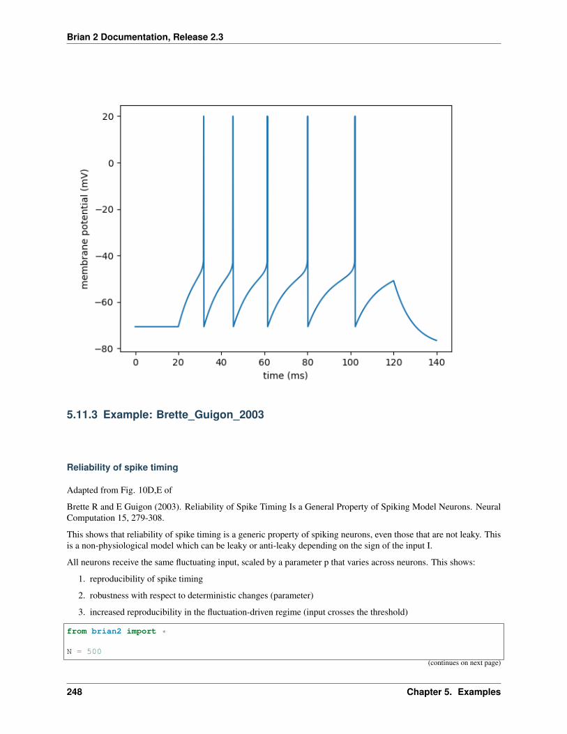
Brian 2 Documentation, Release 2.3
5.11.3 Example: Brette_Guigon_2003
Reliability of spike timing
Adapted from Fig. 10D,E of
Brette R and E Guigon (2003). Reliability of Spike Timing Is a General Property of Spiking Model Neurons. NeuralComputation 15, 279-308.
This shows that reliability of spike timing is a generic property of spiking neurons, even those that are not leaky. Thisis a non-physiological model which can be leaky or anti-leaky depending on the sign of the input I.
All neurons receive the same fluctuating input, scaled by a parameter p that varies across neurons. This shows:
1. reproducibility of spike timing
2. robustness with respect to deterministic changes (parameter)
3. increased reproducibility in the fluctuation-driven regime (input crosses the threshold)
from brian2 import *
N = 500
(continues on next page)
248 Chapter 5. Examples

Brian 2 Documentation, Release 2.3
(continued from previous page)
tau = 33*mstaux = 20*mssigma = 0.02
eqs_input = '''dx/dt = -x/taux + (2/taux)**.5*xi : 1'''
eqs = '''dv/dt = (v*I + 1)/tau + sigma*(2/tau)**.5*xi : 1I = 0.5 + 3*p*B : 1B = 2./(1 + exp(-2*x)) - 1 : 1 (shared)p : 1x : 1 (linked)'''
input = NeuronGroup(1, eqs_input, method='euler')neurons = NeuronGroup(N, eqs, threshold='v>1', reset='v=0', method='euler')neurons.p = '1.0*i/N'neurons.v = 'rand()'neurons.x = linked_var(input, 'x')
M = StateMonitor(neurons, 'B', record=0)S = SpikeMonitor(neurons)
run(1000*ms, report='text')
subplot(211) # The inputplot(M.t/ms, M[0].B)xticks([])title('shared input')subplot(212)plot(S.t/ms, neurons.p[S.i], ',')plot([0, 1000], [.5, .5], color='C1')xlabel('time (ms)')ylabel('p')title('spiking activity')show()
5.11. frompapers 249

Brian 2 Documentation, Release 2.3
5.11.4 Example: Brunel_Hakim_1999
Dynamics of a network of sparsely connected inhibitory current-based integrate-and-fire neurons. Individual neu-rons fire irregularly at low rate but the network is in an oscillatory global activity regime where neurons are weaklysynchronized.
Reference: “Fast Global Oscillations in Networks of Integrate-and-Fire Neurons with Low Firing Rates” NicolasBrunel & Vincent Hakim Neural Computation 11, 1621-1671 (1999)
from brian2 import *
N = 5000Vr = 10*mVtheta = 20*mVtau = 20*msdelta = 2*mstaurefr = 2*msduration = .1*secondC = 1000sparseness = float(C)/NJ = .1*mVmuext = 25*mVsigmaext = 1*mV
(continues on next page)
250 Chapter 5. Examples
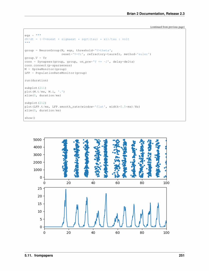
Brian 2 Documentation, Release 2.3
(continued from previous page)
eqs = """dV/dt = (-V+muext + sigmaext * sqrt(tau) * xi)/tau : volt"""
group = NeuronGroup(N, eqs, threshold='V>theta',reset='V=Vr', refractory=taurefr, method='euler')
group.V = Vrconn = Synapses(group, group, on_pre='V += -J', delay=delta)conn.connect(p=sparseness)M = SpikeMonitor(group)LFP = PopulationRateMonitor(group)
run(duration)
subplot(211)plot(M.t/ms, M.i, '.')xlim(0, duration/ms)
subplot(212)plot(LFP.t/ms, LFP.smooth_rate(window='flat', width=0.5*ms)/Hz)xlim(0, duration/ms)
show()
5.11. frompapers 251

Brian 2 Documentation, Release 2.3
5.11.5 Example: Brunel_Wang_2001
Sample-specific persistent activity
Five subpopulations with three selective and one reset stimuli example. Analog to figure 6b in the paper.
BRUNEL, Nicolas et WANG, Xiao-Jing. Effects of neuromodulation in a cortical network model of object workingmemory dominated by recurrent inhibition. Journal of computational neuroscience, 2001, vol. 11, no 1, p. 63-85.
from brian2 import *
# populationsN = 1000N_E = int(N * 0.8) # pyramidal neuronsN_I = int(N * 0.2) # interneurons
# voltageV_L = -70. * mVV_thr = -50. * mVV_reset = -55. * mVV_E = 0. * mVV_I = -70. * mV
# membrane capacitanceC_m_E = 0.5 * nFC_m_I = 0.2 * nF
# membrane leakg_m_E = 25. * nSg_m_I = 20. * nS
# refractory periodtau_rp_E = 2. * mstau_rp_I = 1. * ms
# external stimulirate = 3 * HzC_ext = 800
# synapsesC_E = N_EC_I = N_I
# AMPA (excitatory)g_AMPA_ext_E = 2.08 * nSg_AMPA_rec_E = 0.104 * nS * 800. / N_Eg_AMPA_ext_I = 1.62 * nSg_AMPA_rec_I = 0.081 * nS * 800. / N_Etau_AMPA = 2. * ms
# NMDA (excitatory)g_NMDA_E = 0.327 * nS * 800. / N_Eg_NMDA_I = 0.258 * nS * 800. / N_Etau_NMDA_rise = 2. * mstau_NMDA_decay = 100. * ms
(continues on next page)
252 Chapter 5. Examples

Brian 2 Documentation, Release 2.3
(continued from previous page)
alpha = 0.5 / msMg2 = 1.
# GABAergic (inhibitory)g_GABA_E = 1.25 * nS * 200. / N_Ig_GABA_I = 0.973 * nS * 200. / N_Itau_GABA = 10. * ms
# subpopulationsf = 0.1p = 5N_sub = int(N_E * f)N_non = int(N_E * (1. - f * p))w_plus = 2.1w_minus = 1. - f * (w_plus - 1.) / (1. - f)
# modelingeqs_E = '''dv / dt = (- g_m_E * (v - V_L) - I_syn) / C_m_E : volt (unless refractory)
I_syn = I_AMPA_ext + I_AMPA_rec + I_NMDA_rec + I_GABA_rec : amp
I_AMPA_ext = g_AMPA_ext_E * (v - V_E) * s_AMPA_ext : ampI_AMPA_rec = g_AMPA_rec_E * (v - V_E) * 1 * s_AMPA : ampds_AMPA_ext / dt = - s_AMPA_ext / tau_AMPA : 1ds_AMPA / dt = - s_AMPA / tau_AMPA : 1
I_NMDA_rec = g_NMDA_E * (v - V_E) / (1 + Mg2 * exp(-0.062 * v / mV) / 3.57) * s_NMDA_→˓tot : amps_NMDA_tot : 1
I_GABA_rec = g_GABA_E * (v - V_I) * s_GABA : ampds_GABA / dt = - s_GABA / tau_GABA : 1'''
eqs_I = '''dv / dt = (- g_m_I * (v - V_L) - I_syn) / C_m_I : volt (unless refractory)
I_syn = I_AMPA_ext + I_AMPA_rec + I_NMDA_rec + I_GABA_rec : amp
I_AMPA_ext = g_AMPA_ext_I * (v - V_E) * s_AMPA_ext : ampI_AMPA_rec = g_AMPA_rec_I * (v - V_E) * 1 * s_AMPA : ampds_AMPA_ext / dt = - s_AMPA_ext / tau_AMPA : 1ds_AMPA / dt = - s_AMPA / tau_AMPA : 1
I_NMDA_rec = g_NMDA_I * (v - V_E) / (1 + Mg2 * exp(-0.062 * v / mV) / 3.57) * s_NMDA_→˓tot : amps_NMDA_tot : 1
I_GABA_rec = g_GABA_I * (v - V_I) * s_GABA : ampds_GABA / dt = - s_GABA / tau_GABA : 1'''
P_E = NeuronGroup(N_E, eqs_E, threshold='v > V_thr', reset='v = V_reset',→˓refractory=tau_rp_E, method='euler')P_E.v = V_LP_I = NeuronGroup(N_I, eqs_I, threshold='v > V_thr', reset='v = V_reset',→˓refractory=tau_rp_I, method='euler') (continues on next page)
5.11. frompapers 253

Brian 2 Documentation, Release 2.3
(continued from previous page)
P_I.v = V_L
eqs_glut = '''s_NMDA_tot_post = w * s_NMDA : 1 (summed)ds_NMDA / dt = - s_NMDA / tau_NMDA_decay + alpha * x * (1 - s_NMDA) : 1 (clock-driven)dx / dt = - x / tau_NMDA_rise : 1 (clock-driven)w : 1'''
eqs_pre_glut = '''s_AMPA += wx += 1'''
eqs_pre_gaba = '''s_GABA += 1'''
eqs_pre_ext = '''s_AMPA_ext += 1'''
# E to EC_E_E = Synapses(P_E, P_E, model=eqs_glut, on_pre=eqs_pre_glut, method='euler')C_E_E.connect('i != j')C_E_E.w[:] = 1
for pi in range(N_non, N_non + p * N_sub, N_sub):
# internal other subpopulation to current nonselectiveC_E_E.w[C_E_E.indices[:, pi:pi + N_sub]] = w_minus
# internal current subpopulation to current subpopulationC_E_E.w[C_E_E.indices[pi:pi + N_sub, pi:pi + N_sub]] = w_plus
# E to IC_E_I = Synapses(P_E, P_I, model=eqs_glut, on_pre=eqs_pre_glut, method='euler')C_E_I.connect()C_E_I.w[:] = 1
# I to IC_I_I = Synapses(P_I, P_I, on_pre=eqs_pre_gaba, method='euler')C_I_I.connect('i != j')
# I to EC_I_E = Synapses(P_I, P_E, on_pre=eqs_pre_gaba, method='euler')C_I_E.connect()
# external noiseC_P_E = PoissonInput(P_E, 's_AMPA_ext', C_ext, rate, '1')C_P_I = PoissonInput(P_I, 's_AMPA_ext', C_ext, rate, '1')
# at 1s, select population 1C_selection = int(f * C_ext)rate_selection = 25 * Hzstimuli1 = TimedArray(np.r_[np.zeros(40), np.ones(2), np.zeros(100)], dt=25 * ms)input1 = PoissonInput(P_E[N_non:N_non + N_sub], 's_AMPA_ext', C_selection, rate_→˓selection, 'stimuli1(t)') (continues on next page)
254 Chapter 5. Examples

Brian 2 Documentation, Release 2.3
(continued from previous page)
# at 2s, select population 2stimuli2 = TimedArray(np.r_[np.zeros(80), np.ones(2), np.zeros(100)], dt=25 * ms)input2 = PoissonInput(P_E[N_non + N_sub:N_non + 2 * N_sub], 's_AMPA_ext', C_selection,→˓ rate_selection, 'stimuli2(t)')
# at 4s, reset selectionstimuli_reset = TimedArray(np.r_[np.zeros(120), np.ones(2), np.zeros(100)], dt=25 *→˓ms)input_reset_I = PoissonInput(P_E, 's_AMPA_ext', C_ext, rate_selection, 'stimuli_→˓reset(t)')input_reset_E = PoissonInput(P_I, 's_AMPA_ext', C_ext, rate_selection, 'stimuli_→˓reset(t)')
# monitorsN_activity_plot = 15sp_E_sels = [SpikeMonitor(P_E[pi:pi + N_activity_plot]) for pi in range(N_non, N_non→˓+ p * N_sub, N_sub)]sp_E = SpikeMonitor(P_E[:N_activity_plot])sp_I = SpikeMonitor(P_I[:N_activity_plot])
r_E_sels = [PopulationRateMonitor(P_E[pi:pi + N_sub]) for pi in range(N_non, N_non +→˓p * N_sub, N_sub)]r_E = PopulationRateMonitor(P_E[:N_non])r_I = PopulationRateMonitor(P_I)
# simulate, can be long >120snet = Network(collect())net.add(sp_E_sels)net.add(r_E_sels)net.run(4 * second, report='stdout')
# plottingtitle('Population rates')xlabel('ms')ylabel('Hz')
plot(r_E.t / ms, r_E.smooth_rate(width=25 * ms) / Hz, label='nonselective')plot(r_I.t / ms, r_I.smooth_rate(width=25 * ms) / Hz, label='inhibitory')
for i, r_E_sel in enumerate(r_E_sels[::-1]):plot(r_E_sel.t / ms, r_E_sel.smooth_rate(width=25 * ms) / Hz, label='selective {}
→˓'.format(p - i))
legend()figure()
title('Population activities ({} neurons/pop)'.format(N_activity_plot))xlabel('ms')yticks([])
plot(sp_E.t / ms, sp_E.i + (p + 1) * N_activity_plot, '.', markersize=2, label=→˓'nonselective')plot(sp_I.t / ms, sp_I.i + p * N_activity_plot, '.', markersize=2, label='inhibitory')
for i, sp_E_sel in enumerate(sp_E_sels[::-1]):plot(sp_E_sel.t / ms, sp_E_sel.i + (p - i - 1) * N_activity_plot, '.',
→˓markersize=2, label='selective {}'.format(p - i)) (continues on next page)
5.11. frompapers 255
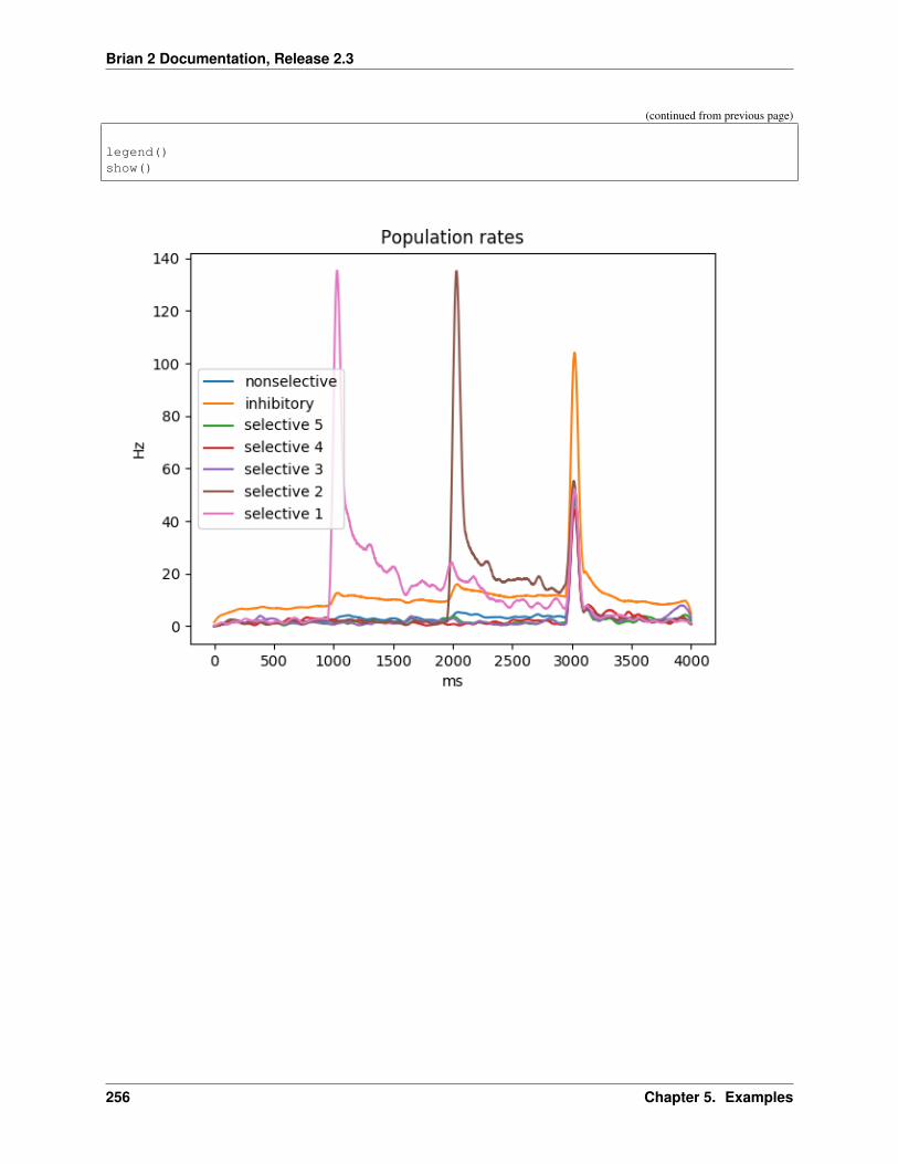
Brian 2 Documentation, Release 2.3
(continued from previous page)
legend()show()
256 Chapter 5. Examples
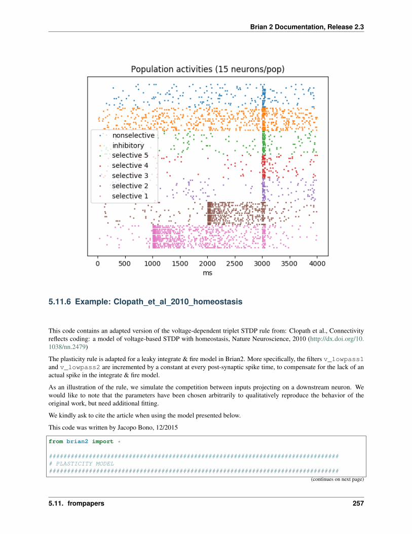
Brian 2 Documentation, Release 2.3
5.11.6 Example: Clopath_et_al_2010_homeostasis
This code contains an adapted version of the voltage-dependent triplet STDP rule from: Clopath et al., Connectivityreflects coding: a model of voltage-based STDP with homeostasis, Nature Neuroscience, 2010 (http://dx.doi.org/10.1038/nn.2479)
The plasticity rule is adapted for a leaky integrate & fire model in Brian2. More specifically, the filters v_lowpass1and v_lowpass2 are incremented by a constant at every post-synaptic spike time, to compensate for the lack of anactual spike in the integrate & fire model.
As an illustration of the rule, we simulate the competition between inputs projecting on a downstream neuron. Wewould like to note that the parameters have been chosen arbitrarily to qualitatively reproduce the behavior of theoriginal work, but need additional fitting.
We kindly ask to cite the article when using the model presented below.
This code was written by Jacopo Bono, 12/2015
from brian2 import *
################################################################################# PLASTICITY MODEL################################################################################
(continues on next page)
5.11. frompapers 257

Brian 2 Documentation, Release 2.3
(continued from previous page)
#### Plasticity Parameters
V_rest = -70.*mV # resting potentialV_thresh = -55.*mV # spiking thresholdTheta_low = V_rest # depolarization threshold for plasticityx_reset = 1. # spike trace reset valuetaux = 15.*ms # spike trace time constantA_LTD = 1.5e-4 # depression amplitudeA_LTP = 1.5e-2 # potentiation amplitudetau_lowpass1 = 40*ms # timeconstant for low-pass filtered voltagetau_lowpass2 = 30*ms # timeconstant for low-pass filtered voltagetau_homeo = 1000*ms # homeostatic timeconstantv_target = 12*mV**2 # target depolarisation
#### Plasticity Equations
# equations executed at every timestepCSyn_model = ('''
w_ampa:1 # synaptic weight (ampa synapse)''')
# equations executed only when a presynaptic spike occursPre_eq = ('''
g_ampa_post += w_ampa*ampa_max_cond→˓ # increment synaptic conductance
A_LTD_u = A_LTD*(v_homeo**2/v_target)→˓ # metaplasticity
w_minus = A_LTD_u*(v_lowpass1_post/mV - Theta_low/mV)*int(v_lowpass1_post/→˓mV - Theta_low/mV > 0) # synaptic depression
w_ampa = clip(w_ampa-w_minus, 0, w_max)→˓ # hard bounds
''' )
# equations executed only when a postsynaptic spike occursPost_eq = ('''
v_lowpass1 += 10*mV→˓ # mimics the depolarisation effect due to a spike
v_lowpass2 += 10*mV→˓ # mimics the depolarisation effect due to a spike
v_homeo += 0.1*mV→˓ # mimics the depolarisation effect due to a spike
w_plus = A_LTP*x_trace_pre*(v_lowpass2_post/mV - Theta_low/mV)*int(v_→˓lowpass2_post/mV - Theta_low/mV > 0) # synaptic potentiation
w_ampa = clip(w_ampa+w_plus, 0, w_max)→˓ # hard bounds
''' )
################################################################################# I&F Parameters and equations################################################################################
#### Neuron parameters
gleak = 30.*nS # leak conductanceC = 300.*pF # membrane capacitancetau_AMPA = 2.*ms # AMPA synaptic timeconstant
(continues on next page)
258 Chapter 5. Examples

Brian 2 Documentation, Release 2.3
(continued from previous page)
E_AMPA = 0.*mV # reversal potential AMPA
ampa_max_cond = 5.e-8*siemens # Ampa maximal conductancew_max = 1. # maximal ampa weight
#### Neuron Equations
# We connect 10 presynaptic neurons to 1 downstream neuron
# downstream neuroneqs_neurons = '''dv/dt = (gleak*(V_rest-v) + I_ext + I_syn)/C: volt # voltagedv_lowpass1/dt = (v-v_lowpass1)/tau_lowpass1 : volt # low-pass filter of the→˓voltagedv_lowpass2/dt = (v-v_lowpass2)/tau_lowpass2 : volt # low-pass filter of the→˓voltagedv_homeo/dt = (v-V_rest-v_homeo)/tau_homeo : volt # low-pass filter of the→˓voltageI_ext : amp # external currentI_syn = g_ampa*(E_AMPA-v): amp # synaptic currentdg_ampa/dt = -g_ampa/tau_AMPA : siemens # synaptic conductancedx_trace/dt = -x_trace/taux :1 # spike trace'''
# input neuronseqs_inputs = '''dv/dt = gleak*(V_rest-v)/C: volt # voltagedx_trace/dt = -x_trace/taux :1 # spike tracerates : Hz # input ratesselected_index : integer (shared) # active neuron'''
################################################################################# Simulation################################################################################
#### Parameters
defaultclock.dt = 500.*us # timestepNr_neurons = 1 # Number of downstream neuronsNr_inputs = 5 # Number of input neuronsinput_rate = 35*Hz # Ratesinit_weight = 0.5 # initial synaptic weightfinal_t = 20.*second # end of simulationinput_time = 100.*ms # duration of an input
#### Create neuron objects
Nrn_downstream = NeuronGroup(Nr_neurons, eqs_neurons, threshold='v>V_thresh',reset='v=V_rest;x_trace+=x_reset/(taux/ms)',method='euler')
Nrns_input = NeuronGroup(Nr_inputs, eqs_inputs, threshold='rand()<rates*dt',reset='v=V_rest;x_trace+=x_reset/(taux/ms)',method='exact')
#### create Synapses
(continues on next page)
5.11. frompapers 259

Brian 2 Documentation, Release 2.3
(continued from previous page)
Syn = Synapses(Nrns_input, Nrn_downstream,model=Syn_model,on_pre=Pre_eq,on_post=Post_eq)
Syn.connect(i=numpy.arange(Nr_inputs), j=0)
#### Monitors and storageW_evolution = StateMonitor(Syn, 'w_ampa', record=True)
#### Run
# Initial valuesNrn_downstream.v = V_restNrn_downstream.v_lowpass1 = V_restNrn_downstream.v_lowpass2 = V_restNrn_downstream.v_homeo = 0Nrn_downstream.I_ext = 0.*ampNrn_downstream.x_trace = 0.Nrns_input.v = V_restNrns_input.x_trace = 0.Syn.w_ampa = init_weight
# Switch on a different input every 100msNrns_input.run_regularly('''
selected_index = int(floor(rand()*Nr_inputs))rates = input_rate * int(selected_index == i) # All rates
→˓are zero except for the selected neuron''', dt=input_time)
run(final_t, report='text')
################################################################################# Plots################################################################################stitle = 'Synaptic Competition'
fig = figure(figsize=(8, 5))for kk in range(Nr_inputs):
plt.plot(W_evolution.t, W_evolution.w_ampa[kk], '-', linewidth=2)xlabel('Time [ms]', fontsize=22)ylabel('Weight [a.u.]', fontsize=22)plt.subplots_adjust(bottom=0.2, left=0.15, right=0.95, top=0.85)title(stitle, fontsize=22)plt.show()
260 Chapter 5. Examples
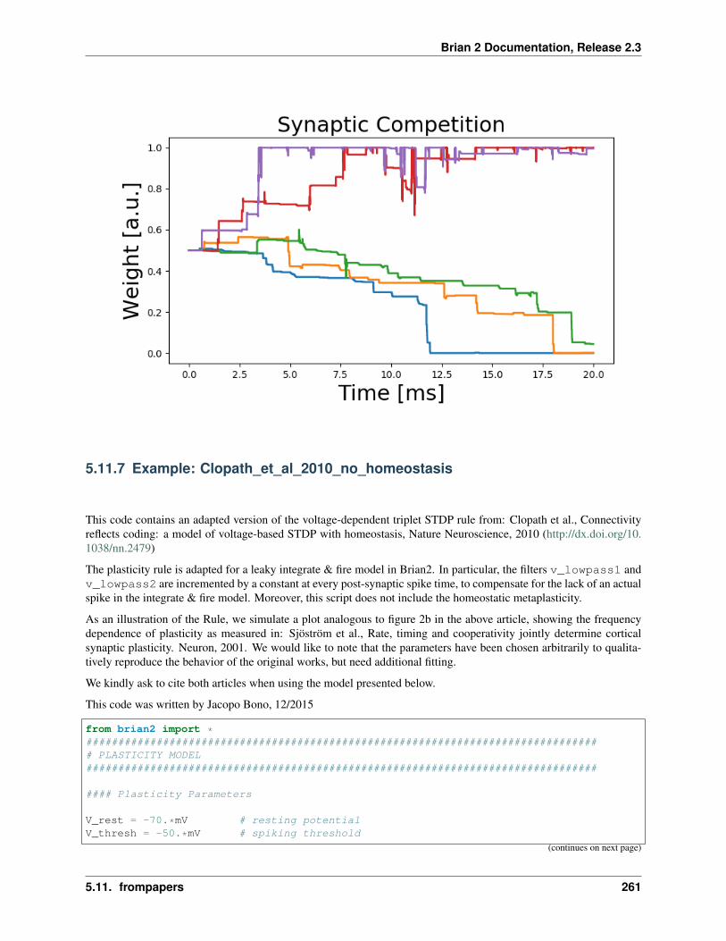
Brian 2 Documentation, Release 2.3
5.11.7 Example: Clopath_et_al_2010_no_homeostasis
This code contains an adapted version of the voltage-dependent triplet STDP rule from: Clopath et al., Connectivityreflects coding: a model of voltage-based STDP with homeostasis, Nature Neuroscience, 2010 (http://dx.doi.org/10.1038/nn.2479)
The plasticity rule is adapted for a leaky integrate & fire model in Brian2. In particular, the filters v_lowpass1 andv_lowpass2 are incremented by a constant at every post-synaptic spike time, to compensate for the lack of an actualspike in the integrate & fire model. Moreover, this script does not include the homeostatic metaplasticity.
As an illustration of the Rule, we simulate a plot analogous to figure 2b in the above article, showing the frequencydependence of plasticity as measured in: Sjöström et al., Rate, timing and cooperativity jointly determine corticalsynaptic plasticity. Neuron, 2001. We would like to note that the parameters have been chosen arbitrarily to qualita-tively reproduce the behavior of the original works, but need additional fitting.
We kindly ask to cite both articles when using the model presented below.
This code was written by Jacopo Bono, 12/2015
from brian2 import *################################################################################# PLASTICITY MODEL################################################################################
#### Plasticity Parameters
V_rest = -70.*mV # resting potentialV_thresh = -50.*mV # spiking threshold
(continues on next page)
5.11. frompapers 261

Brian 2 Documentation, Release 2.3
(continued from previous page)
Theta_low = V_rest # depolarization threshold for plasticityx_reset = 1. # spike trace reset valuetaux = 15.*ms # spike trace time constantA_LTD = 1.5e-4 # depression amplitudeA_LTP = 1.5e-2 # potentiation amplitudetau_lowpass1 = 40*ms # timeconstant for low-pass filtered voltagetau_lowpass2 = 30*ms # timeconstant for low-pass filtered voltage
#### Plasticity Equations
# equations executed at every timestepSyn_model = '''
w_ampa:1 # synaptic weight (ampa synapse)'''
# equations executed only when a presynaptic spike occursPre_eq = '''
g_ampa_post += w_ampa*ampa_max_cond→˓ # increment synaptic conductance
w_minus = A_LTD*(v_lowpass1_post/mV - Theta_low/mV)*int(v_lowpass1_post/mV -→˓Theta_low/mV > 0) # synaptic depression
w_ampa = clip(w_ampa-w_minus,0,w_max)→˓ # hard bounds
'''
# equations executed only when a postsynaptic spike occursPost_eq = '''
v_lowpass1 += 10*mV→˓ # mimics the depolarisation by a spike
v_lowpass2 += 10*mV→˓ # mimics the depolarisation by a spike
w_plus = A_LTP*x_trace_pre*(v_lowpass2_post/mV - Theta_low/mV)*int(v_→˓lowpass2_post/mV - Theta_low/mV > 0) # synaptic potentiation
w_ampa = clip(w_ampa+w_plus,0,w_max)→˓ # hard bounds
'''
################################################################################# I&F Parameters and equations################################################################################
#### Neuron parameters
gleak = 30.*nS # leak conductanceC = 300.*pF # membrane capacitancetau_AMPA = 2.*ms # AMPA synaptic timeconstantE_AMPA = 0.*mV # reversal potential AMPA
ampa_max_cond = 5.e-10*siemens # Ampa maximal conductancew_max = 1. # maximal ampa weight
#### Neuron Equations
(continues on next page)
262 Chapter 5. Examples
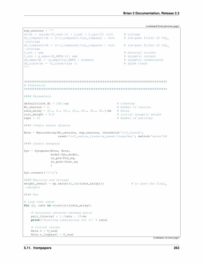
Brian 2 Documentation, Release 2.3
(continued from previous page)
eqs_neurons = '''dv/dt = (gleak*(V_rest-v) + I_ext + I_syn)/C: volt # voltagedv_lowpass1/dt = (v-v_lowpass1)/tau_lowpass1 : volt # low-pass filter of the→˓voltagedv_lowpass2/dt = (v-v_lowpass2)/tau_lowpass2 : volt # low-pass filter of the→˓voltageI_ext : amp # external currentI_syn = g_ampa*(E_AMPA-v): amp # synaptic currentdg_ampa/dt = -g_ampa/tau_AMPA : siemens # synaptic conductancedx_trace/dt = -x_trace/taux :1 # spike trace'''
################################################################################# Simulation################################################################################
#### Parameters
defaultclock.dt = 100.*us # timestepNr_neurons = 2 # Number of neuronsrate_array = [1., 5., 10., 15., 20., 30., 50.]*Hz # Ratesinit_weight = 0.5 # initial synaptic weightreps = 15 # Number of pairings
#### Create neuron objects
Nrns = NeuronGroup(Nr_neurons, eqs_neurons, threshold='v>V_thresh',reset='v=V_rest;x_trace+=x_reset/(taux/ms)', method='euler')#
#### create Synapses
Syn = Synapses(Nrns, Nrns,model=Syn_model,on_pre=Pre_eq,on_post=Post_eq)
Syn.connect('i!=j')
#### Monitors and storageweight_result = np.zeros((2,len(rate_array))) # to save the final→˓weights
#### Run
# loop over ratesfor jj, rate in enumerate(rate_array):
# Calculate interval between pairspair_interval = 1./rate - 10*msprint('Starting simulations for %s' % rate)
# Initial valuesNrns.v = V_restNrns.v_lowpass1 = V_rest
(continues on next page)
5.11. frompapers 263

Brian 2 Documentation, Release 2.3
(continued from previous page)
Nrns.v_lowpass2 = V_restNrns.I_ext = 0*ampNrns.x_trace = 0.Syn.w_ampa = init_weight
# loop over pairingsfor ii in range(reps):
# 1st SPIKENrns.v[0] = V_thresh + 1*mV# 2nd SPIKErun(10*ms)Nrns.v[1] = V_thresh + 1*mV# runrun(pair_interval)print('Pair %d out of %d' % (ii+1, reps))
#store weight changesweight_result[0, jj] = 100.*Syn.w_ampa[0]/init_weightweight_result[1, jj] = 100.*Syn.w_ampa[1]/init_weight
################################################################################# Plots################################################################################
stitle = 'Pairings'scolor = 'k'
figure(figsize=(8, 5))plot(rate_array,weight_result[0, :], '-', linewidth=2, color=scolor)plot(rate_array,weight_result[1, :], ':', linewidth=2, color=scolor)xlabel('Pairing frequency [Hz]', fontsize=22)ylabel('Normalised Weight [%]', fontsize=22)legend(['Pre-Post', 'Post-Pre'], loc='best')subplots_adjust(bottom=0.2, left=0.15, right=0.95, top=0.85)title(stitle)show()
264 Chapter 5. Examples
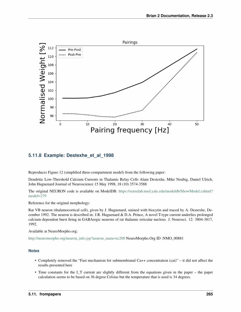
Brian 2 Documentation, Release 2.3
5.11.8 Example: Destexhe_et_al_1998
Reproduces Figure 12 (simplified three-compartment model) from the following paper:
Dendritic Low-Threshold Calcium Currents in Thalamic Relay Cells Alain Destexhe, Mike Neubig, Daniel Ulrich,John Huguenard Journal of Neuroscience 15 May 1998, 18 (10) 3574-3588
The original NEURON code is available on ModelDB: https://senselab.med.yale.edu/modeldb/ShowModel.cshtml?model=279
Reference for the original morphology:
Rat VB neuron (thalamocortical cell), given by J. Huguenard, stained with biocytin and traced by A. Destexhe, De-cember 1992. The neuron is described in: J.R. Huguenard & D.A. Prince, A novel T-type current underlies prolongedcalcium-dependent burst firing in GABAergic neurons of rat thalamic reticular nucleus. J. Neurosci. 12: 3804-3817,1992.
Available at NeuroMorpho.org:
http://neuromorpho.org/neuron_info.jsp?neuron_name=tc200 NeuroMorpho.Org ID :NMO_00881
Notes
• Completely removed the “Fast mechanism for submembranal Ca++ concentration (cai)” – it did not affect theresults presented here
• Time constants for the I_T current are slightly different from the equations given in the paper – the papercalculation seems to be based on 36 degree Celsius but the temperature that is used is 34 degrees.
5.11. frompapers 265

Brian 2 Documentation, Release 2.3
• To reproduce Figure 12C, the “presence of dendritic shunt conductances” meant setting g_L to 0.15 mS/cm^2for the whole neuron.
• Other small discrepancies with the paper – values from the NEURON code were used whenever different fromthe values stated in the paper
from __future__ import print_functionfrom brian2 import *from brian2.units.constants import (zero_celsius, faraday_constant as F,
gas_constant as R)
defaultclock.dt = 0.01*ms
VT = -52*mVEl = -76.5*mV # from code, text says: -69.85*mV
E_Na = 50*mVE_K = -100*mVC_d = 7.954 # dendritic correction factor
T = 34*kelvin + zero_celsius # 34 degC (current-clamp experiments)tadj_HH = 3.0**((34-36)/10.0) # temperature adjustment for Na & K (original→˓recordings at 36 degC)tadj_m_T = 2.5**((34-24)/10.0)tadj_h_T = 2.5**((34-24)/10.0)
shift_I_T = -1*mV
gamma = F/(R*T) # R=gas constant, F=Faraday constantZ_Ca = 2 # Valence of Calcium ionsCa_i = 240*nM # intracellular Calcium concentrationCa_o = 2*mM # extracellular Calcium concentration
eqs = Equations('''Im = gl*(El-v) - I_Na - I_K - I_T: amp/meter**2I_inj : amp (point current)gl : siemens/meter**2
# HH-type currents for spike initiationg_Na : siemens/meter**2g_K : siemens/meter**2I_Na = g_Na * m**3 * h * (v-E_Na) : amp/meter**2I_K = g_K * n**4 * (v-E_K) : amp/meter**2v2 = v - VT : volt # shifted membrane potential (Traub convention)dm/dt = (0.32*(mV**-1)*(13.*mV-v2)/
(exp((13.*mV-v2)/(4.*mV))-1.)*(1-m)-0.28*(mV**-1)*(v2-40.*mV)/(exp((v2-40.*mV)/(5.*mV))-1.)*m) / ms * tadj_HH: 1
dn/dt = (0.032*(mV**-1)*(15.*mV-v2)/(exp((15.*mV-v2)/(5.*mV))-1.)*(1.-n)-.5*exp((10.*mV-v2)/(40.*mV))*n) / ms *
→˓tadj_HH: 1dh/dt = (0.128*exp((17.*mV-v2)/(18.*mV))*(1.-h)-4./(1+exp((40.*mV-v2)/(5.*mV)))*h) /→˓ms * tadj_HH: 1
# Low-threshold Calcium current (I_T) -- nonlinear function of voltageI_T = P_Ca * m_T**2*h_T * G_Ca : amp/meter**2P_Ca : meter/second # maximum Permeability to CalciumG_Ca = Z_Ca**2*F*v*gamma*(Ca_i - Ca_o*exp(-Z_Ca*gamma*v))/(1 - exp(-Z_Ca*gamma*v)) :→˓coulomb/meter**3
(continues on next page)
266 Chapter 5. Examples

Brian 2 Documentation, Release 2.3
(continued from previous page)
dm_T/dt = -(m_T - m_T_inf)/tau_m_T : 1dh_T/dt = -(h_T - h_T_inf)/tau_h_T : 1m_T_inf = 1/(1 + exp(-(v/mV + 56)/6.2)) : 1h_T_inf = 1/(1 + exp((v/mV + 80)/4)) : 1tau_m_T = (0.612 + 1.0/(exp(-(v/mV + 131)/16.7) + exp((v/mV + 15.8)/18.2))) * ms /→˓tadj_m_T: secondtau_h_T = (int(v<-81*mV) * exp((v/mV + 466)/66.6) +
int(v>=-81*mV) * (28 + exp(-(v/mV + 21)/10.5))) * ms / tadj_h_T: second''')
# Simplified three-compartment morphologymorpho = Cylinder(x=[0, 38.42]*um, diameter=26*um)morpho.dend = Cylinder(x=[0, 12.49]*um, diameter=10.28*um)morpho.dend.distal = Cylinder(x=[0, 84.67]*um, diameter=8.5*um)neuron = SpatialNeuron(morpho, eqs, Cm=0.88*uF/cm**2, Ri=173*ohm*cm,
method='exponential_euler')
neuron.v = -74*mV# Only the soma has Na/K channelsneuron.main.g_Na = 100*msiemens/cm**2neuron.main.g_K = 100*msiemens/cm**2# Apply the correction factor to the dendrites
neuron.dend.Cm *= C_dneuron.m_T = 'm_T_inf'neuron.h_T = 'h_T_inf'
mon = StateMonitor(neuron, ['v'], record=True)
store('initial state')
def do_experiment(currents, somatic_density, dendritic_density,dendritic_conductance=0.0379*msiemens/cm**2,HH_currents=True):
restore('initial state')voltages = []neuron.P_Ca = somatic_densityneuron.dend.distal.P_Ca = dendritic_density * C_d# dendritic conductance (shunting conductance used for Fig 12C)neuron.gl = dendritic_conductanceneuron.dend.gl = dendritic_conductance * C_dif not HH_currents:
# Shut off spiking (for Figures 12B and 12C)neuron.g_Na = 0*msiemens/cm**2neuron.g_K = 0*msiemens/cm**2
run(180*ms)store('before current')for current in currents:
restore('before current')neuron.main.I_inj = currentprint('.', end='')run(320*ms)voltages.append(mon[morpho].v[:]) # somatic voltage
return voltages
(continues on next page)
5.11. frompapers 267
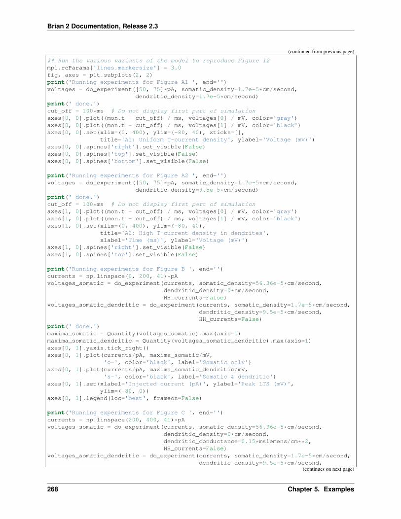
Brian 2 Documentation, Release 2.3
(continued from previous page)
## Run the various variants of the model to reproduce Figure 12mpl.rcParams['lines.markersize'] = 3.0fig, axes = plt.subplots(2, 2)print('Running experiments for Figure A1 ', end='')voltages = do_experiment([50, 75]*pA, somatic_density=1.7e-5*cm/second,
dendritic_density=1.7e-5*cm/second)print(' done.')cut_off = 100*ms # Do not display first part of simulationaxes[0, 0].plot((mon.t - cut_off) / ms, voltages[0] / mV, color='gray')axes[0, 0].plot((mon.t - cut_off) / ms, voltages[1] / mV, color='black')axes[0, 0].set(xlim=(0, 400), ylim=(-80, 40), xticks=[],
title='A1: Uniform T-current density', ylabel='Voltage (mV)')axes[0, 0].spines['right'].set_visible(False)axes[0, 0].spines['top'].set_visible(False)axes[0, 0].spines['bottom'].set_visible(False)
print('Running experiments for Figure A2 ', end='')voltages = do_experiment([50, 75]*pA, somatic_density=1.7e-5*cm/second,
dendritic_density=9.5e-5*cm/second)print(' done.')cut_off = 100*ms # Do not display first part of simulationaxes[1, 0].plot((mon.t - cut_off) / ms, voltages[0] / mV, color='gray')axes[1, 0].plot((mon.t - cut_off) / ms, voltages[1] / mV, color='black')axes[1, 0].set(xlim=(0, 400), ylim=(-80, 40),
title='A2: High T-current density in dendrites',xlabel='Time (ms)', ylabel='Voltage (mV)')
axes[1, 0].spines['right'].set_visible(False)axes[1, 0].spines['top'].set_visible(False)
print('Running experiments for Figure B ', end='')currents = np.linspace(0, 200, 41)*pAvoltages_somatic = do_experiment(currents, somatic_density=56.36e-5*cm/second,
dendritic_density=0*cm/second,HH_currents=False)
voltages_somatic_dendritic = do_experiment(currents, somatic_density=1.7e-5*cm/second,dendritic_density=9.5e-5*cm/second,HH_currents=False)
print(' done.')maxima_somatic = Quantity(voltages_somatic).max(axis=1)maxima_somatic_dendritic = Quantity(voltages_somatic_dendritic).max(axis=1)axes[0, 1].yaxis.tick_right()axes[0, 1].plot(currents/pA, maxima_somatic/mV,
'o-', color='black', label='Somatic only')axes[0, 1].plot(currents/pA, maxima_somatic_dendritic/mV,
's-', color='black', label='Somatic & dendritic')axes[0, 1].set(xlabel='Injected current (pA)', ylabel='Peak LTS (mV)',
ylim=(-80, 0))axes[0, 1].legend(loc='best', frameon=False)
print('Running experiments for Figure C ', end='')currents = np.linspace(200, 400, 41)*pAvoltages_somatic = do_experiment(currents, somatic_density=56.36e-5*cm/second,
dendritic_density=0*cm/second,dendritic_conductance=0.15*msiemens/cm**2,HH_currents=False)
voltages_somatic_dendritic = do_experiment(currents, somatic_density=1.7e-5*cm/second,dendritic_density=9.5e-5*cm/second,
(continues on next page)
268 Chapter 5. Examples
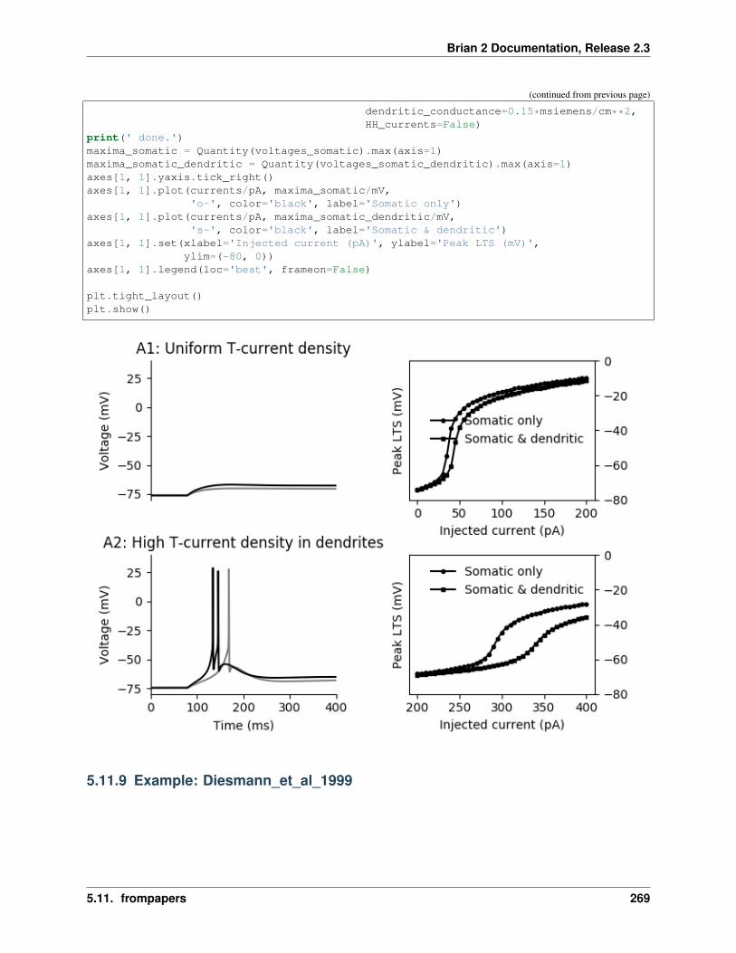
Brian 2 Documentation, Release 2.3
(continued from previous page)
dendritic_conductance=0.15*msiemens/cm**2,HH_currents=False)
print(' done.')maxima_somatic = Quantity(voltages_somatic).max(axis=1)maxima_somatic_dendritic = Quantity(voltages_somatic_dendritic).max(axis=1)axes[1, 1].yaxis.tick_right()axes[1, 1].plot(currents/pA, maxima_somatic/mV,
'o-', color='black', label='Somatic only')axes[1, 1].plot(currents/pA, maxima_somatic_dendritic/mV,
's-', color='black', label='Somatic & dendritic')axes[1, 1].set(xlabel='Injected current (pA)', ylabel='Peak LTS (mV)',
ylim=(-80, 0))axes[1, 1].legend(loc='best', frameon=False)
plt.tight_layout()plt.show()
5.11.9 Example: Diesmann_et_al_1999
5.11. frompapers 269

Brian 2 Documentation, Release 2.3
Synfire chains
M. Diesmann et al. (1999). Stable propagation of synchronous spiking in cortical neural networks. Nature 402,529-533.
from brian2 import *
duration = 100*ms
# Neuron model parametersVr = -70*mVVt = -55*mVtaum = 10*mstaupsp = 0.325*msweight = 4.86*mV# Neuron modeleqs = Equations('''dV/dt = (-(V-Vr)+x)*(1./taum) : voltdx/dt = (-x+y)*(1./taupsp) : voltdy/dt = -y*(1./taupsp)+25.27*mV/ms+
(39.24*mV/ms**0.5)*xi : volt''')
# Neuron groupsn_groups = 10group_size = 100P = NeuronGroup(N=n_groups*group_size, model=eqs,
threshold='V>Vt', reset='V=Vr', refractory=1*ms,method='euler')
Pinput = SpikeGeneratorGroup(85, np.arange(85),np.random.randn(85)*1*ms + 50*ms)
# The network structureS = Synapses(P, P, on_pre='y+=weight')S.connect(j='k for k in range((int(i/group_size)+1)*group_size, (int(i/group_→˓size)+2)*group_size) '
'if i<N_pre-group_size')Sinput = Synapses(Pinput, P[:group_size], on_pre='y+=weight')Sinput.connect()
# Record the spikesMgp = SpikeMonitor(P)Minput = SpikeMonitor(Pinput)# Setup the network, and run itP.V = 'Vr + rand() * (Vt - Vr)'run(duration)
plot(Mgp.t/ms, 1.0*Mgp.i/group_size, '.')plot([0, duration/ms], np.arange(n_groups).repeat(2).reshape(-1, 2).T, 'k-')ylabel('group number')yticks(np.arange(n_groups))xlabel('time (ms)')show()
270 Chapter 5. Examples
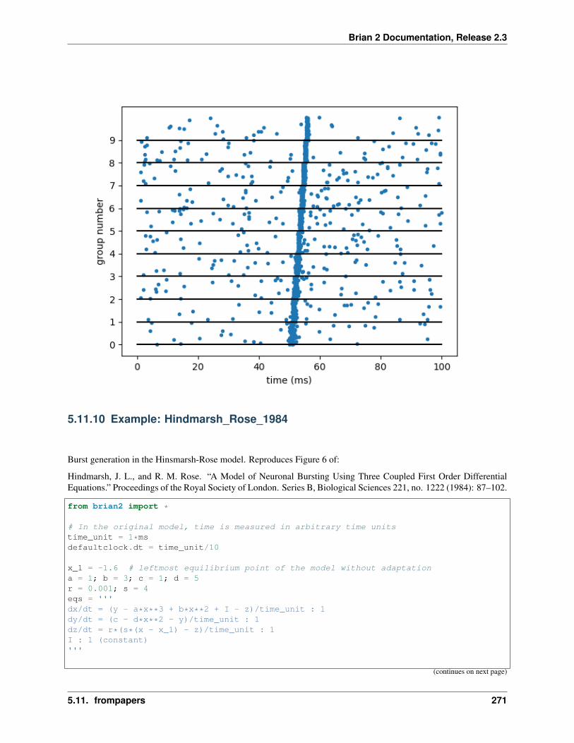
Brian 2 Documentation, Release 2.3
5.11.10 Example: Hindmarsh_Rose_1984
Burst generation in the Hinsmarsh-Rose model. Reproduces Figure 6 of:
Hindmarsh, J. L., and R. M. Rose. “A Model of Neuronal Bursting Using Three Coupled First Order DifferentialEquations.” Proceedings of the Royal Society of London. Series B, Biological Sciences 221, no. 1222 (1984): 87–102.
from brian2 import *
# In the original model, time is measured in arbitrary time unitstime_unit = 1*msdefaultclock.dt = time_unit/10
x_1 = -1.6 # leftmost equilibrium point of the model without adaptationa = 1; b = 3; c = 1; d = 5r = 0.001; s = 4eqs = '''dx/dt = (y - a*x**3 + b*x**2 + I - z)/time_unit : 1dy/dt = (c - d*x**2 - y)/time_unit : 1dz/dt = r*(s*(x - x_1) - z)/time_unit : 1I : 1 (constant)'''
(continues on next page)
5.11. frompapers 271

Brian 2 Documentation, Release 2.3
(continued from previous page)
# We run the model with three different currentsneuron = NeuronGroup(3, eqs, method='rk4')
# Set all variables to their equilibrium pointneuron.x = x_1neuron.y = 'c - d*x**2'neuron.z = 'r*(s*(x - x_1))'
# Set the constant current inputneuron.I = [0.4, 2, 4]
# Record the "membrane potential"mon = StateMonitor(neuron, 'x', record=True)
run(2100*time_unit)
ax_top = plt.subplot2grid((2, 3), (0, 0), colspan=3)ax_bottom_l = plt.subplot2grid((2, 3), (1, 0), colspan=2)ax_bottom_r = plt.subplot2grid((2, 3), (1, 2))for ax in [ax_top, ax_bottom_l, ax_bottom_r]:
ax.spines['top'].set_visible(False)ax.spines['right'].set_visible(False)ax.set(ylim=(-2, 2), yticks=[-2, 0, 2])
ax_top.plot(mon.t/time_unit, mon.x[0])
ax_bottom_l.plot(mon.t/time_unit, mon.x[1])ax_bottom_l.set_xlim(700, 2100)
ax_bottom_r.plot(mon.t/time_unit, mon.x[2])ax_bottom_r.set_xlim(1400, 2100)ax_bottom_r.set_yticks([])
plt.show()
272 Chapter 5. Examples
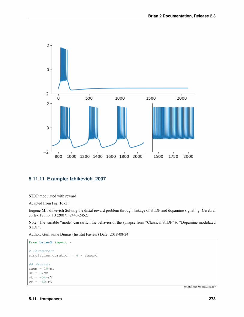
Brian 2 Documentation, Release 2.3
5.11.11 Example: Izhikevich_2007
STDP modulated with reward
Adapted from Fig. 1c of:
Eugene M. Izhikevich Solving the distal reward problem through linkage of STDP and dopamine signaling. Cerebralcortex 17, no. 10 (2007): 2443-2452.
Note: The variable “mode” can switch the behavior of the synapse from “Classical STDP” to “Dopamine modulatedSTDP”.
Author: Guillaume Dumas (Institut Pasteur) Date: 2018-08-24
from brian2 import *
# Parameterssimulation_duration = 6 * second
## Neuronstaum = 10*msEe = 0*mVvt = -54*mVvr = -60*mV
(continues on next page)
5.11. frompapers 273

Brian 2 Documentation, Release 2.3
(continued from previous page)
El = -74*mVtaue = 5*ms
## STDPtaupre = 20*mstaupost = taupregmax = .01dApre = .01dApost = -dApre * taupre / taupost * 1.05dApost *= gmaxdApre *= gmax
## Dopamine signalingtauc = 1000*mstaud = 200*mstaus = 1*msepsilon_dopa = 5e-3
# Setting the stage
## Stimuli sectioninput_indices = array([0, 1, 0, 1, 1, 0,
0, 1, 0, 1, 1, 0])input_times = array([ 500, 550, 1000, 1010, 1500, 1510,
3500, 3550, 4000, 4010, 4500, 4510])*msinput = SpikeGeneratorGroup(2, input_indices, input_times)
neurons = NeuronGroup(2, '''dv/dt = (ge * (Ee-vr) + El - v) / taum : voltdge/dt = -ge / taue : 1''',
threshold='v>vt', reset='v = vr',method='exact')
neurons.v = vrneurons_monitor = SpikeMonitor(neurons)
synapse = Synapses(input, neurons,model='''s: volt''',on_pre='v += s')
synapse.connect(i=[0, 1], j=[0, 1])synapse.s = 100. * mV
## STDP sectionsynapse_stdp = Synapses(neurons, neurons,
model='''mode: 1dc/dt = -c / tauc : 1 (clock-driven)dd/dt = -d / taud : 1 (clock-driven)ds/dt = mode * c * d / taus : 1 (clock-driven)dApre/dt = -Apre / taupre : 1 (event-driven)dApost/dt = -Apost / taupost : 1 (event-driven)''',
on_pre='''ge += sApre += dAprec = clip(c + mode * Apost, -gmax, gmax)s = clip(s + (1-mode) * Apost, -gmax, gmax)''',
on_post='''Apost += dApostc = clip(c + mode * Apre, -gmax, gmax)s = clip(s + (1-mode) * Apre, -gmax, gmax)''',
(continues on next page)
274 Chapter 5. Examples

Brian 2 Documentation, Release 2.3
(continued from previous page)
method='euler')
synapse_stdp.connect(i=0, j=1)synapse_stdp.mode = 0synapse_stdp.s = 1e-10synapse_stdp.c = 1e-10synapse_stdp.d = 0synapse_stdp_monitor = StateMonitor(synapse_stdp, ['s', 'c', 'd'], record=[0])
## Dopamine signaling sectiondopamine_indices = array([0, 0, 0])dopamine_times = array([3520, 4020, 4520])*msdopamine = SpikeGeneratorGroup(1, dopamine_indices, dopamine_times)dopamine_monitor = SpikeMonitor(dopamine)reward = Synapses(dopamine, synapse_stdp, model='''''',
on_pre='''d_post += epsilon_dopa''',method='exact')
reward.connect()
# Simulation## Classical STDPsynapse_stdp.mode = 0run(simulation_duration/2)## Dopamine modulated STDPsynapse_stdp.mode = 1run(simulation_duration/2)
# Visualisationdopamine_indices, dopamine_times = dopamine_monitor.itneurons_indices, neurons_times = neurons_monitor.itfigure(figsize=(12,6))subplot(411)plot([0.05, 2.95], [2.7, 2.7], linewidth=5, color='k')text(1.5, 3, 'Classical STDP', horizontalalignment='center', fontsize=20)plot([3.05, 5.95], [2.7, 2.7], linewidth=5, color='k')text(4.5, 3, 'Dopamine modulated STDP', horizontalalignment='center', fontsize=20)plot(neurons_times, neurons_indices, 'ob')plot(dopamine_times, dopamine_indices + 2, 'or')xlim([0, simulation_duration/second])ylim([-0.5, 4])yticks([0, 1, 2], ['Pre-neuron', 'Post-neuron', 'Reward'])xticks([])subplot(412)plot(synapse_stdp_monitor.t/second, synapse_stdp_monitor.d.T/gmax, 'r-')xlim([0, simulation_duration/second])ylabel('Extracellular\ndopamine d(t)')xticks([])subplot(413)plot(synapse_stdp_monitor.t/second, synapse_stdp_monitor.c.T/gmax, 'b-')xlim([0, simulation_duration/second])ylabel('Eligibility\ntrace c(t)')xticks([])subplot(414)plot(synapse_stdp_monitor.t/second, synapse_stdp_monitor.s.T/gmax, 'g-')xlim([0, simulation_duration/second])ylabel('Synaptic\nstrength s(t)')xlabel('Time (s)')
(continues on next page)
5.11. frompapers 275
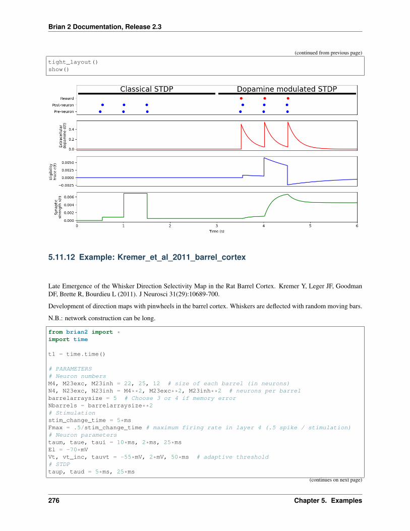
Brian 2 Documentation, Release 2.3
(continued from previous page)
tight_layout()show()
5.11.12 Example: Kremer_et_al_2011_barrel_cortex
Late Emergence of the Whisker Direction Selectivity Map in the Rat Barrel Cortex. Kremer Y, Leger JF, GoodmanDF, Brette R, Bourdieu L (2011). J Neurosci 31(29):10689-700.
Development of direction maps with pinwheels in the barrel cortex. Whiskers are deflected with random moving bars.
N.B.: network construction can be long.
from brian2 import *import time
t1 = time.time()
# PARAMETERS# Neuron numbersM4, M23exc, M23inh = 22, 25, 12 # size of each barrel (in neurons)N4, N23exc, N23inh = M4**2, M23exc**2, M23inh**2 # neurons per barrelbarrelarraysize = 5 # Choose 3 or 4 if memory errorNbarrels = barrelarraysize**2# Stimulationstim_change_time = 5*msFmax = .5/stim_change_time # maximum firing rate in layer 4 (.5 spike / stimulation)# Neuron parameterstaum, taue, taui = 10*ms, 2*ms, 25*msEl = -70*mVVt, vt_inc, tauvt = -55*mV, 2*mV, 50*ms # adaptive threshold# STDPtaup, taud = 5*ms, 25*ms
(continues on next page)
276 Chapter 5. Examples

Brian 2 Documentation, Release 2.3
(continued from previous page)
Ap, Ad= .05, -.04# EPSPs/IPSPsEPSP, IPSP = 1*mV, -1*mVEPSC = EPSP * (taue/taum)**(taum/(taue-taum))IPSC = IPSP * (taui/taum)**(taum/(taui-taum))Ap, Ad = Ap*EPSC, Ad*EPSC
# Layer 4, models the input stimuluseqs_layer4 = '''rate = int(is_active)*clip(cos(direction - selectivity), 0, inf)*Fmax: Hzis_active = abs((barrel_x + 0.5 - bar_x) * cos(direction) + (barrel_y + 0.5 - bar_y)→˓* sin(direction)) < 0.5: booleanbarrel_x : integer # The x index of the barrelbarrel_y : integer # The y index of the barrelselectivity : 1# Stimulus parameters (same for all neurons)bar_x = cos(direction)*(t - stim_start_time)/(5*ms) + stim_start_x : 1 (shared)bar_y = sin(direction)*(t - stim_start_time)/(5*ms) + stim_start_y : 1 (shared)direction : 1 (shared) # direction of the current stimulusstim_start_time : second (shared) # start time of the current stimulusstim_start_x : 1 (shared) # start position of the stimulusstim_start_y : 1 (shared) # start position of the stimulus'''layer4 = NeuronGroup(N4*Nbarrels, eqs_layer4, threshold='rand() < rate*dt',
method='euler', name='layer4')layer4.barrel_x = '(i // N4) % barrelarraysize + 0.5'layer4.barrel_y = 'i // (barrelarraysize*N4) + 0.5'layer4.selectivity = '(i%N4)/(1.0*N4)*2*pi' # for each barrel, selectivity between 0→˓and 2*pi
stimradius = (11+1)*.5
# Chose a new randomly oriented bar every 60msrunner_code = '''direction = rand()*2*pistim_start_x = barrelarraysize / 2.0 - cos(direction)*stimradiusstim_start_y = barrelarraysize / 2.0 - sin(direction)*stimradiusstim_start_time = t'''layer4.run_regularly(runner_code, dt=60*ms, when='start')
# Layer 2/3# Model: IF with adaptive thresholdeqs_layer23 = '''dv/dt=(ge+gi+El-v)/taum : voltdge/dt=-ge/taue : voltdgi/dt=-gi/taui : voltdvt/dt=(Vt-vt)/tauvt : volt # adaptationbarrel_idx : integerx : 1 # in "barrel width" unitsy : 1 # in "barrel width" units'''layer23 = NeuronGroup(Nbarrels*(N23exc+N23inh), eqs_layer23,
threshold='v>vt', reset='v = El; vt += vt_inc',refractory=2*ms, method='euler', name='layer23')
layer23.v = Ellayer23.vt = Vt
(continues on next page)
5.11. frompapers 277

Brian 2 Documentation, Release 2.3
(continued from previous page)
# Subgroups for excitatory and inhibitory neurons in layer 2/3layer23exc = layer23[:Nbarrels*N23exc]layer23inh = layer23[Nbarrels*N23exc:]
# Layer 2/3 excitatory# The units for x and y are the width/height of a single barrellayer23exc.x = '(i % (barrelarraysize*M23exc)) * (1.0/M23exc)'layer23exc.y = '(i // (barrelarraysize*M23exc)) * (1.0/M23exc)'layer23exc.barrel_idx = 'floor(x) + floor(y)*barrelarraysize'
# Layer 2/3 inhibitorylayer23inh.x = 'i % (barrelarraysize*M23inh) * (1.0/M23inh)'layer23inh.y = 'i // (barrelarraysize*M23inh) * (1.0/M23inh)'layer23inh.barrel_idx = 'floor(x) + floor(y)*barrelarraysize'
print("Building synapses, please wait...")# Feedforward connections (plastic)feedforward = Synapses(layer4, layer23exc,
model='''w:voltdA_source/dt = -A_source/taup : volt (event-driven)dA_target/dt = -A_target/taud : volt (event-driven)''
→˓',on_pre='''ge+=w
A_source += Apw = clip(w+A_target, 0, EPSC)''',
on_post='''A_target += Adw = clip(w+A_source, 0, EPSC)''',
name='feedforward')# Connect neurons in the same barrel with 50% probabilityfeedforward.connect('(barrel_x_pre + barrelarraysize*barrel_y_pre) == barrel_idx_post→˓',
p=0.5)feedforward.w = EPSC*.5
print('excitatory lateral')# Excitatory lateral connectionsrecurrent_exc = Synapses(layer23exc, layer23, model='w:volt', on_pre='ge+=w',
name='recurrent_exc')recurrent_exc.connect(p='.15*exp(-.5*(((x_pre-x_post)/.4)**2+((y_pre-y_post)/.4)**2))→˓')recurrent_exc.w['j<Nbarrels*N23exc'] = EPSC*.3 # excitatory->excitatoryrecurrent_exc.w['j>=Nbarrels*N23exc'] = EPSC # excitatory->inhibitory
# Inhibitory lateral connectionsprint('inhibitory lateral')recurrent_inh = Synapses(layer23inh, layer23exc, on_pre='gi+=IPSC',
name='recurrent_inh')recurrent_inh.connect(p='exp(-.5*(((x_pre-x_post)/.2)**2+((y_pre-y_post)/.2)**2))')
if get_device().__class__.__name__=='RuntimeDevice':print('Total number of connections')print('feedforward: %d' % len(feedforward))print('recurrent exc: %d' % len(recurrent_exc))print('recurrent inh: %d' % len(recurrent_inh))
(continues on next page)
278 Chapter 5. Examples

Brian 2 Documentation, Release 2.3
(continued from previous page)
t2 = time.time()print("Construction time: %.1fs" % (t2 - t1))
run(5*second, report='text')
# Calculate the preferred direction of each cell in layer23 by doing a# vector average of the selectivity of the projecting layer4 cells, weighted# by the synaptic weight._r = bincount(feedforward.j,
weights=feedforward.w * cos(feedforward.selectivity_pre)/feedforward.N_→˓incoming,
minlength=len(layer23exc))_i = bincount(feedforward.j,
weights=feedforward.w * sin(feedforward.selectivity_pre)/feedforward.N_→˓incoming,
minlength=len(layer23exc))selectivity_exc = (arctan2(_r, _i) % (2*pi))*180./pi
scatter(layer23.x[:Nbarrels*N23exc], layer23.y[:Nbarrels*N23exc],c=selectivity_exc[:Nbarrels*N23exc],edgecolors='none', marker='s', cmap='hsv')
vlines(np.arange(barrelarraysize), 0, barrelarraysize, 'k')hlines(np.arange(barrelarraysize), 0, barrelarraysize, 'k')clim(0, 360)colorbar()show()
5.11. frompapers 279
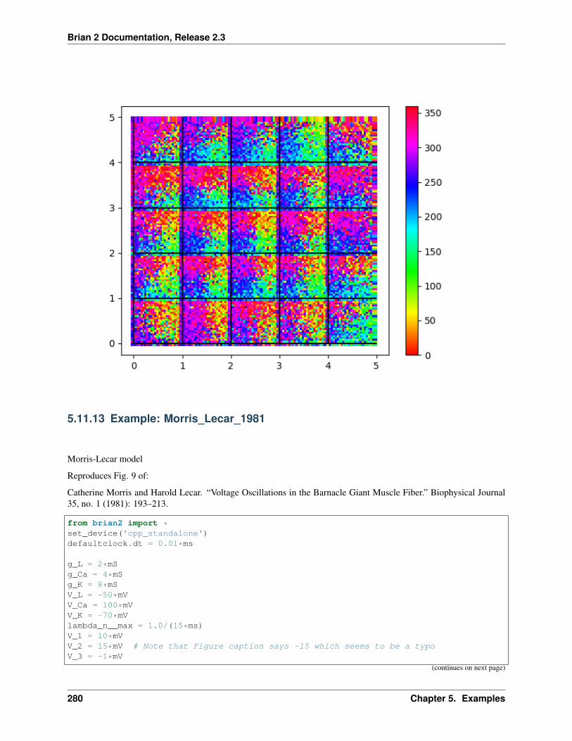
Brian 2 Documentation, Release 2.3
5.11.13 Example: Morris_Lecar_1981
Morris-Lecar model
Reproduces Fig. 9 of:
Catherine Morris and Harold Lecar. “Voltage Oscillations in the Barnacle Giant Muscle Fiber.” Biophysical Journal35, no. 1 (1981): 193–213.
from brian2 import *set_device('cpp_standalone')defaultclock.dt = 0.01*ms
g_L = 2*mSg_Ca = 4*mSg_K = 8*mSV_L = -50*mVV_Ca = 100*mVV_K = -70*mVlambda_n__max = 1.0/(15*ms)V_1 = 10*mVV_2 = 15*mV # Note that Figure caption says -15 which seems to be a typoV_3 = -1*mV
(continues on next page)
280 Chapter 5. Examples
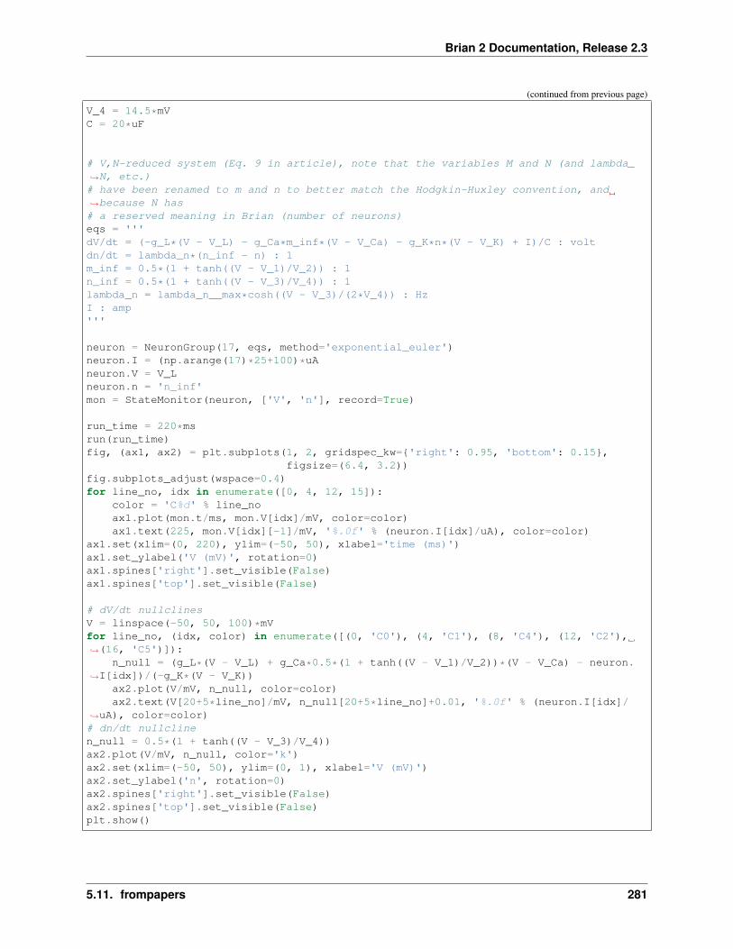
Brian 2 Documentation, Release 2.3
(continued from previous page)
V_4 = 14.5*mVC = 20*uF
# V,N-reduced system (Eq. 9 in article), note that the variables M and N (and lambda_→˓N, etc.)# have been renamed to m and n to better match the Hodgkin-Huxley convention, and→˓because N has# a reserved meaning in Brian (number of neurons)eqs = '''dV/dt = (-g_L*(V - V_L) - g_Ca*m_inf*(V - V_Ca) - g_K*n*(V - V_K) + I)/C : voltdn/dt = lambda_n*(n_inf - n) : 1m_inf = 0.5*(1 + tanh((V - V_1)/V_2)) : 1n_inf = 0.5*(1 + tanh((V - V_3)/V_4)) : 1lambda_n = lambda_n__max*cosh((V - V_3)/(2*V_4)) : HzI : amp'''
neuron = NeuronGroup(17, eqs, method='exponential_euler')neuron.I = (np.arange(17)*25+100)*uAneuron.V = V_Lneuron.n = 'n_inf'mon = StateMonitor(neuron, ['V', 'n'], record=True)
run_time = 220*msrun(run_time)fig, (ax1, ax2) = plt.subplots(1, 2, gridspec_kw={'right': 0.95, 'bottom': 0.15},
figsize=(6.4, 3.2))fig.subplots_adjust(wspace=0.4)for line_no, idx in enumerate([0, 4, 12, 15]):
color = 'C%d' % line_noax1.plot(mon.t/ms, mon.V[idx]/mV, color=color)ax1.text(225, mon.V[idx][-1]/mV, '%.0f' % (neuron.I[idx]/uA), color=color)
ax1.set(xlim=(0, 220), ylim=(-50, 50), xlabel='time (ms)')ax1.set_ylabel('V (mV)', rotation=0)ax1.spines['right'].set_visible(False)ax1.spines['top'].set_visible(False)
# dV/dt nullclinesV = linspace(-50, 50, 100)*mVfor line_no, (idx, color) in enumerate([(0, 'C0'), (4, 'C1'), (8, 'C4'), (12, 'C2'),→˓(16, 'C5')]):
n_null = (g_L*(V - V_L) + g_Ca*0.5*(1 + tanh((V - V_1)/V_2))*(V - V_Ca) - neuron.→˓I[idx])/(-g_K*(V - V_K))
ax2.plot(V/mV, n_null, color=color)ax2.text(V[20+5*line_no]/mV, n_null[20+5*line_no]+0.01, '%.0f' % (neuron.I[idx]/
→˓uA), color=color)# dn/dt nullclinen_null = 0.5*(1 + tanh((V - V_3)/V_4))ax2.plot(V/mV, n_null, color='k')ax2.set(xlim=(-50, 50), ylim=(0, 1), xlabel='V (mV)')ax2.set_ylabel('n', rotation=0)ax2.spines['right'].set_visible(False)ax2.spines['top'].set_visible(False)plt.show()
5.11. frompapers 281
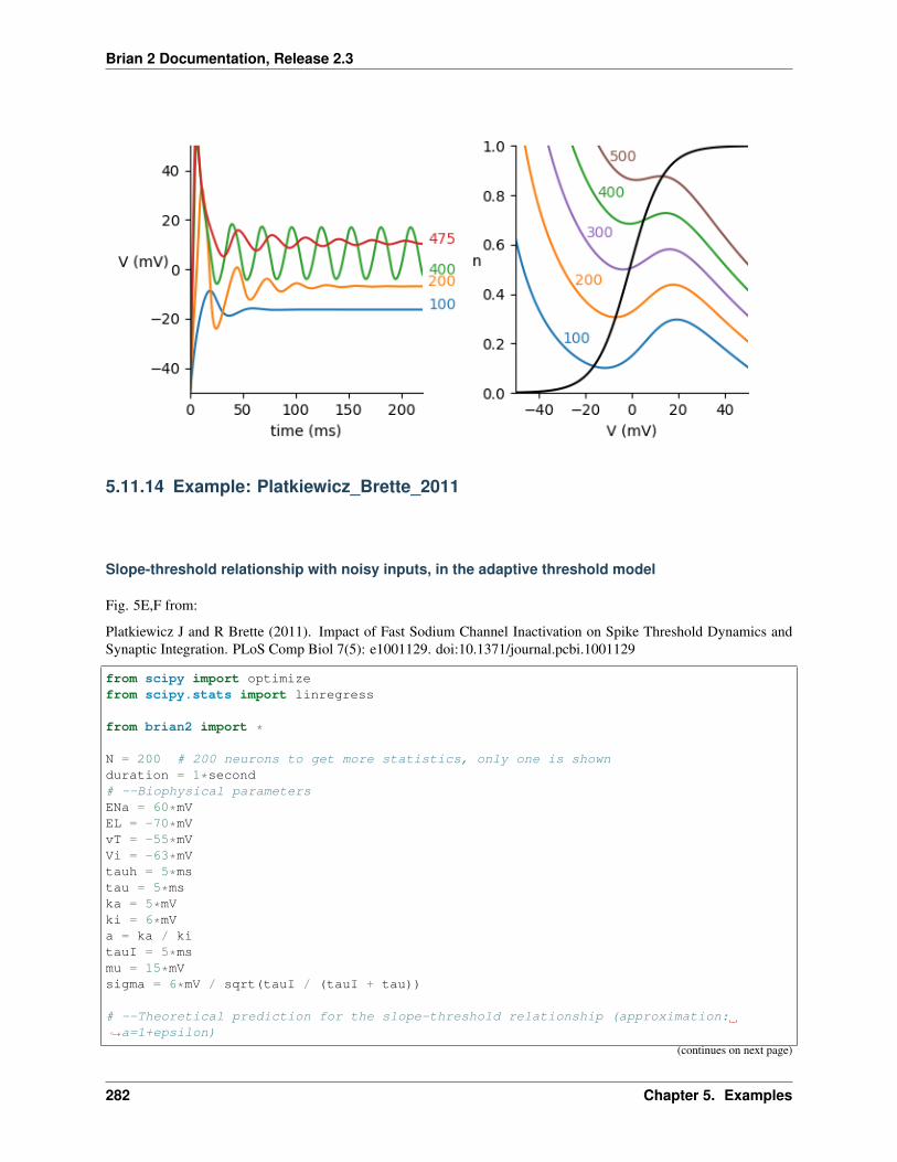
Brian 2 Documentation, Release 2.3
5.11.14 Example: Platkiewicz_Brette_2011
Slope-threshold relationship with noisy inputs, in the adaptive threshold model
Fig. 5E,F from:
Platkiewicz J and R Brette (2011). Impact of Fast Sodium Channel Inactivation on Spike Threshold Dynamics andSynaptic Integration. PLoS Comp Biol 7(5): e1001129. doi:10.1371/journal.pcbi.1001129
from scipy import optimizefrom scipy.stats import linregress
from brian2 import *
N = 200 # 200 neurons to get more statistics, only one is shownduration = 1*second# --Biophysical parametersENa = 60*mVEL = -70*mVvT = -55*mVVi = -63*mVtauh = 5*mstau = 5*mska = 5*mVki = 6*mVa = ka / kitauI = 5*msmu = 15*mVsigma = 6*mV / sqrt(tauI / (tauI + tau))
# --Theoretical prediction for the slope-threshold relationship (approximation:→˓a=1+epsilon)
(continues on next page)
282 Chapter 5. Examples
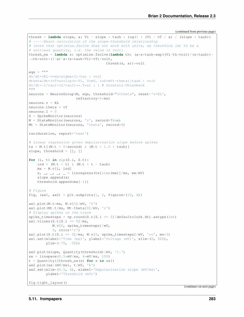
Brian 2 Documentation, Release 2.3
(continued from previous page)
thresh = lambda slope, a: Vi - slope * tauh * log(1 + (Vi - vT / a) / (slope * tauh))# -----Exact calculation of the slope-threshold relationship# (note that optimize.fsolve does not work with units, we therefore let th be a# unitless quantity, i.e. the value in volt).thresh_ex = lambda s: optimize.fsolve(lambda th: (a*s*tauh*exp((Vi-th*volt)/(s*tauh))-→˓th*volt*(1-a)-a*(s*tauh+Vi)+vT)/volt,
thresh(s, a))*volt
eqs = """dv/dt=(EL-v+mu+sigma*I)/tau : voltdtheta/dt=(vT+a*clip(v-Vi, 0*mV, inf*mV)-theta)/tauh : voltdI/dt=-I/tauI+(2/tauI)**.5*xi : 1 # Ornstein-Uhlenbeck"""neurons = NeuronGroup(N, eqs, threshold="v>theta", reset='v=EL',
refractory=5*ms)neurons.v = ELneurons.theta = vTneurons.I = 0S = SpikeMonitor(neurons)M = StateMonitor(neurons, 'v', record=True)Mt = StateMonitor(neurons, 'theta', record=0)
run(duration, report='text')
# Linear regression gives depolarization slope before spikestx = M.t[(M.t > 0*second) & (M.t < 1.5 * tauh)]slope, threshold = [], []
for (i, t) in zip(S.i, S.t):ind = (M.t < t) & (M.t > t - tauh)mx = M.v[i, ind]s, _, _, _, _ = linregress(tx[:len(mx)]/ms, mx/mV)slope.append(s)threshold.append(mx[-1])
# Figurefig, (ax1, ax2) = plt.subplots(1, 2, figsize=(10, 4))
ax1.plot(M.t/ms, M.v[0]/mV, 'k')ax1.plot(Mt.t/ms, Mt.theta[0]/mV, 'r')# Display spikes on the tracespike_timesteps = np.round(S.t[S.i == 0]/defaultclock.dt).astype(int)ax1.vlines(S.t[S.i == 0]/ms,
M.v[0, spike_timesteps]/mV,0, color='r')
ax1.plot(S.t[S.i == 0]/ms, M.v[0, spike_timesteps]/mV, 'ro', ms=3)ax1.set(xlabel='Time (ms)', ylabel='Voltage (mV)', xlim=(0, 500),
ylim=(-75, -35))
ax2.plot(slope, Quantity(threshold)/mV, 'r.')sx = linspace(0.5*mV/ms, 4*mV/ms, 100)t = Quantity([thresh_ex(s) for s in sx])ax2.plot(sx/(mV/ms), t/mV, 'k')ax2.set(xlim=(0.5, 4), xlabel='Depolarization slope (mV/ms)',
ylabel='Threshold (mV)')
fig.tight_layout()(continues on next page)
5.11. frompapers 283
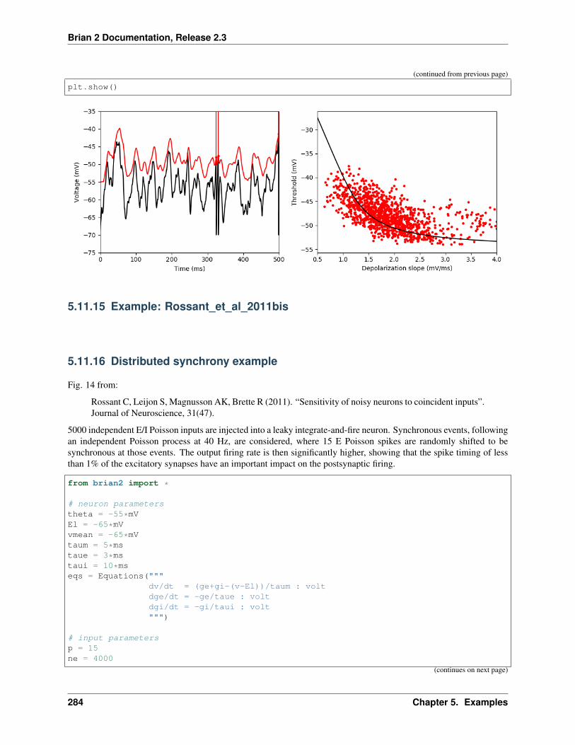
Brian 2 Documentation, Release 2.3
(continued from previous page)
plt.show()
5.11.15 Example: Rossant_et_al_2011bis
5.11.16 Distributed synchrony example
Fig. 14 from:
Rossant C, Leijon S, Magnusson AK, Brette R (2011). “Sensitivity of noisy neurons to coincident inputs”.Journal of Neuroscience, 31(47).
5000 independent E/I Poisson inputs are injected into a leaky integrate-and-fire neuron. Synchronous events, followingan independent Poisson process at 40 Hz, are considered, where 15 E Poisson spikes are randomly shifted to besynchronous at those events. The output firing rate is then significantly higher, showing that the spike timing of lessthan 1% of the excitatory synapses have an important impact on the postsynaptic firing.
from brian2 import *
# neuron parameterstheta = -55*mVEl = -65*mVvmean = -65*mVtaum = 5*mstaue = 3*mstaui = 10*mseqs = Equations("""
dv/dt = (ge+gi-(v-El))/taum : voltdge/dt = -ge/taue : voltdgi/dt = -gi/taui : volt""")
# input parametersp = 15ne = 4000
(continues on next page)
284 Chapter 5. Examples

Brian 2 Documentation, Release 2.3
(continued from previous page)
ni = 1000lambdac = 40*Hzlambdae = lambdai = 1*Hz
# synapse parameterswe = .5*mV/(taum/taue)**(taum/(taue-taum))wi = (vmean-El-lambdae*ne*we*taue)/(lambdae*ni*taui)
# NeuronGroup definitiongroup = NeuronGroup(N=2, model=eqs, reset='v = El',
threshold='v>theta',refractory=5*ms, method='exact')
group.v = Elgroup.ge = group.gi = 0
# independent E/I Poisson inputsp1 = PoissonInput(group[0:1], 'ge', N=ne, rate=lambdae, weight=we)p2 = PoissonInput(group[0:1], 'gi', N=ni, rate=lambdai, weight=wi)
# independent E/I Poisson inputs + synchronous E eventsp3 = PoissonInput(group[1:], 'ge', N=ne, rate=lambdae-(p*1.0/ne)*lambdac, weight=we)p4 = PoissonInput(group[1:], 'gi', N=ni, rate=lambdai, weight=wi)p5 = PoissonInput(group[1:], 'ge', N=1, rate=lambdac, weight=p*we)
# run the simulationM = SpikeMonitor(group)SM = StateMonitor(group, 'v', record=True)BrianLogger.log_level_info()run(1*second)# plot trace and spikesfor i in [0, 1]:
spikes = (M.t[M.i == i] - defaultclock.dt)/msval = SM[i].vsubplot(2,1,i+1)plot(SM.t/ms, val)plot(tile(spikes, (2,1)),
vstack((val[array(spikes, dtype=int)],zeros(len(spikes)))), 'C0')
title("%s: %d spikes/second" % (["uncorrelated inputs", "correlated inputs"][i],M.count[i]))
tight_layout()show()
5.11. frompapers 285
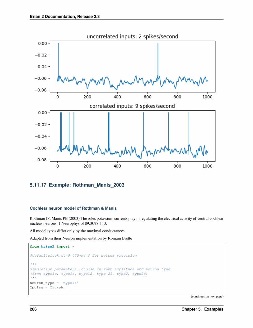
Brian 2 Documentation, Release 2.3
5.11.17 Example: Rothman_Manis_2003
Cochlear neuron model of Rothman & Manis
Rothman JS, Manis PB (2003) The roles potassium currents play in regulating the electrical activity of ventral cochlearnucleus neurons. J Neurophysiol 89:3097-113.
All model types differ only by the maximal conductances.
Adapted from their Neuron implementation by Romain Brette
from brian2 import *
#defaultclock.dt=0.025*ms # for better precision
'''Simulation parameters: choose current amplitude and neuron type(from type1c, type1t, type12, type 21, type2, type2o)'''neuron_type = 'type1c'Ipulse = 250*pA
(continues on next page)
286 Chapter 5. Examples
Brian 2 Documentation, Release 2.3
(continued from previous page)
C = 12*pFEh = -43*mVEK = -70*mV # -77*mV in mod fileEl = -65*mVENa = 50*mVnf = 0.85 # proportion of n vs p kineticszss = 0.5 # steady state inactivation of glttemp = 22. # temperature in degree celciusq10 = 3. ** ((temp - 22) / 10.)# hcno current (octopus cell)frac = 0.0qt = 4.5 ** ((temp - 33.) / 10.)
# Maximal conductances of different cell types in nSmaximal_conductances = dict(type1c=(1000, 150, 0, 0, 0.5, 0, 2),type1t=(1000, 80, 0, 65, 0.5, 0, 2),type12=(1000, 150, 20, 0, 2, 0, 2),type21=(1000, 150, 35, 0, 3.5, 0, 2),type2=(1000, 150, 200, 0, 20, 0, 2),type2o=(1000, 150, 600, 0, 0, 40, 2) # octopus cell)gnabar, gkhtbar, gkltbar, gkabar, ghbar, gbarno, gl = [x * nS for x in maximal_→˓conductances[neuron_type]]
# Classical Na channeleqs_na = """ina = gnabar*m**3*h*(ENa-v) : ampdm/dt=q10*(minf-m)/mtau : 1dh/dt=q10*(hinf-h)/htau : 1minf = 1./(1+exp(-(vu + 38.) / 7.)) : 1hinf = 1./(1+exp((vu + 65.) / 6.)) : 1mtau = ((10. / (5*exp((vu+60.) / 18.) + 36.*exp(-(vu+60.) / 25.))) + 0.04)*ms :→˓secondhtau = ((100. / (7*exp((vu+60.) / 11.) + 10.*exp(-(vu+60.) / 25.))) + 0.6)*ms :→˓second"""
# KHT channel (delayed-rectifier K+)eqs_kht = """ikht = gkhtbar*(nf*n**2 + (1-nf)*p)*(EK-v) : ampdn/dt=q10*(ninf-n)/ntau : 1dp/dt=q10*(pinf-p)/ptau : 1ninf = (1 + exp(-(vu + 15) / 5.))**-0.5 : 1pinf = 1. / (1 + exp(-(vu + 23) / 6.)) : 1ntau = ((100. / (11*exp((vu+60) / 24.) + 21*exp(-(vu+60) / 23.))) + 0.7)*ms : secondptau = ((100. / (4*exp((vu+60) / 32.) + 5*exp(-(vu+60) / 22.))) + 5)*ms : second"""
# Ih channel (subthreshold adaptive, non-inactivating)eqs_ih = """ih = ghbar*r*(Eh-v) : ampdr/dt=q10*(rinf-r)/rtau : 1rinf = 1. / (1+exp((vu + 76.) / 7.)) : 1rtau = ((100000. / (237.*exp((vu+60.) / 12.) + 17.*exp(-(vu+60.) / 14.))) + 25.)*ms :→˓second"""
(continues on next page)
5.11. frompapers 287

Brian 2 Documentation, Release 2.3
(continued from previous page)
# KLT channel (low threshold K+)eqs_klt = """iklt = gkltbar*w**4*z*(EK-v) : ampdw/dt=q10*(winf-w)/wtau : 1dz/dt=q10*(zinf-z)/ztau : 1winf = (1. / (1 + exp(-(vu + 48.) / 6.)))**0.25 : 1zinf = zss + ((1.-zss) / (1 + exp((vu + 71.) / 10.))) : 1wtau = ((100. / (6.*exp((vu+60.) / 6.) + 16.*exp(-(vu+60.) / 45.))) + 1.5)*ms : secondztau = ((1000. / (exp((vu+60.) / 20.) + exp(-(vu+60.) / 8.))) + 50)*ms : second"""
# Ka channel (transient K+)eqs_ka = """ika = gkabar*a**4*b*c*(EK-v): ampda/dt=q10*(ainf-a)/atau : 1db/dt=q10*(binf-b)/btau : 1dc/dt=q10*(cinf-c)/ctau : 1ainf = (1. / (1 + exp(-(vu + 31) / 6.)))**0.25 : 1binf = 1. / (1 + exp((vu + 66) / 7.))**0.5 : 1cinf = 1. / (1 + exp((vu + 66) / 7.))**0.5 : 1atau = ((100. / (7*exp((vu+60) / 14.) + 29*exp(-(vu+60) / 24.))) + 0.1)*ms : secondbtau = ((1000. / (14*exp((vu+60) / 27.) + 29*exp(-(vu+60) / 24.))) + 1)*ms : secondctau = ((90. / (1 + exp((-66-vu) / 17.))) + 10)*ms : second"""
# Leakeqs_leak = """ileak = gl*(El-v) : amp"""
# h current for octopus cellseqs_hcno = """ihcno = gbarno*(h1*frac + h2*(1-frac))*(Eh-v) : ampdh1/dt=(hinfno-h1)/tau1 : 1dh2/dt=(hinfno-h2)/tau2 : 1hinfno = 1./(1+exp((vu+66.)/7.)) : 1tau1 = bet1/(qt*0.008*(1+alp1))*ms : secondtau2 = bet2/(qt*0.0029*(1+alp2))*ms : secondalp1 = exp(1e-3*3*(vu+50)*9.648e4/(8.315*(273.16+temp))) : 1bet1 = exp(1e-3*3*0.3*(vu+50)*9.648e4/(8.315*(273.16+temp))) : 1alp2 = exp(1e-3*3*(vu+84)*9.648e4/(8.315*(273.16+temp))) : 1bet2 = exp(1e-3*3*0.6*(vu+84)*9.648e4/(8.315*(273.16+temp))) : 1"""
eqs = """dv/dt = (ileak + ina + ikht + iklt + ika + ih + ihcno + I)/C : voltvu = v/mV : 1 # unitless vI : amp"""eqs += eqs_leak + eqs_ka + eqs_na + eqs_ih + eqs_klt + eqs_kht + eqs_hcno
neuron = NeuronGroup(1, eqs, method='exponential_euler')neuron.v = El
run(50*ms, report='text') # Go to rest
(continues on next page)
288 Chapter 5. Examples

Brian 2 Documentation, Release 2.3
(continued from previous page)
M = StateMonitor(neuron, 'v', record=0)neuron.I = Ipulse
run(100*ms, report='text')
plot(M.t / ms, M[0].v / mV)xlabel('t (ms)')ylabel('v (mV)')show()
5.11.18 Example: Sturzl_et_al_2000
Adapted from Theory of Arachnid Prey Localization W. Sturzl, R. Kempter, and J. L. van Hemmen PRL 2000
Poisson inputs are replaced by integrate-and-fire neurons
Romain Brette
from brian2 import *
# Parametersdegree = 2 * pi / 360.
(continues on next page)
5.11. frompapers 289

Brian 2 Documentation, Release 2.3
(continued from previous page)
duration = 500*msR = 2.5*cm # radius of scorpionvr = 50*meter/second # Rayleigh wave speedphi = 144*degree # angle of preyA = 250*HzdeltaI = .7*ms # inhibitory delaygamma = (22.5 + 45 * arange(8)) * degree # leg angledelay = R / vr * (1 - cos(phi - gamma)) # wave delay
# Wave (vector w)time = arange(int(duration / defaultclock.dt) + 1) * defaultclock.dtDtot = 0.w = 0.for f in arange(150, 451)*Hz:
D = exp(-(f/Hz - 300) ** 2 / (2 * (50 ** 2)))rand_angle = 2 * pi * rand()w += 100 * D * cos(2 * pi * f * time + rand_angle)Dtot += D
w = .01 * w / Dtot
# Rates from the waverates = TimedArray(w, dt=defaultclock.dt)
# Leg mechanical receptorstau_legs = 1 * mssigma = .01eqs_legs = """dv/dt = (1 + rates(t - d) - v)/tau_legs + sigma*(2./tau_legs)**.5*xi:1d : second"""legs = NeuronGroup(8, model=eqs_legs, threshold='v > 1', reset='v = 0',
refractory=1*ms, method='euler')legs.d = delayspikes_legs = SpikeMonitor(legs)
# Command neuronstau = 1 * mstaus = 1.001 * mswex = 7winh = -2eqs_neuron = '''dv/dt = (x - v)/tau : 1dx/dt = (y - x)/taus : 1 # alpha currentsdy/dt = -y/taus : 1'''neurons = NeuronGroup(8, model=eqs_neuron, threshold='v>1', reset='v=0',
method='exact')synapses_ex = Synapses(legs, neurons, on_pre='y+=wex')synapses_ex.connect(j='i')synapses_inh = Synapses(legs, neurons, on_pre='y+=winh', delay=deltaI)synapses_inh.connect('abs(((j - i) % N_post) - N_post/2) <= 1')spikes = SpikeMonitor(neurons)
run(duration, report='text')
nspikes = spikes.countphi_est = imag(log(sum(nspikes * exp(gamma * 1j))))
(continues on next page)
290 Chapter 5. Examples
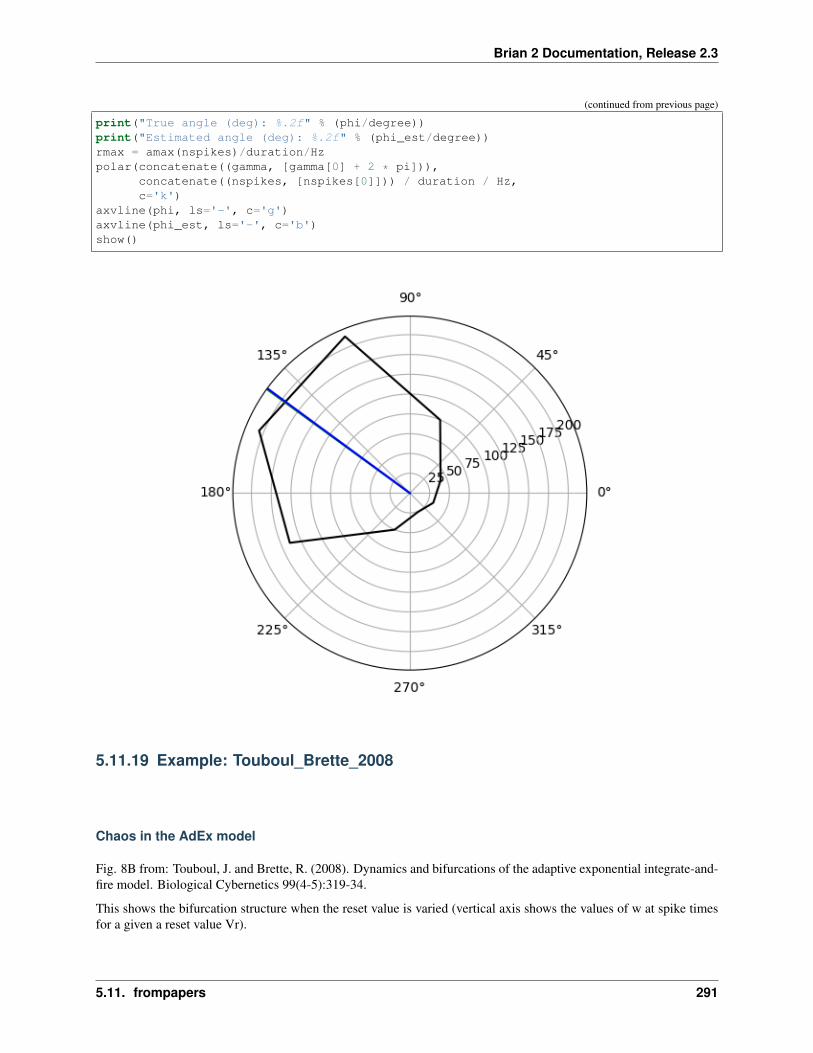
Brian 2 Documentation, Release 2.3
(continued from previous page)
print("True angle (deg): %.2f" % (phi/degree))print("Estimated angle (deg): %.2f" % (phi_est/degree))rmax = amax(nspikes)/duration/Hzpolar(concatenate((gamma, [gamma[0] + 2 * pi])),
concatenate((nspikes, [nspikes[0]])) / duration / Hz,c='k')
axvline(phi, ls='-', c='g')axvline(phi_est, ls='-', c='b')show()
5.11.19 Example: Touboul_Brette_2008
Chaos in the AdEx model
Fig. 8B from: Touboul, J. and Brette, R. (2008). Dynamics and bifurcations of the adaptive exponential integrate-and-fire model. Biological Cybernetics 99(4-5):319-34.
This shows the bifurcation structure when the reset value is varied (vertical axis shows the values of w at spike timesfor a given a reset value Vr).
5.11. frompapers 291
Brian 2 Documentation, Release 2.3
from brian2 import *
defaultclock.dt = 0.01*ms
C = 281*pFgL = 30*nSEL = -70.6*mVVT = -50.4*mVDeltaT = 2*mVtauw = 40*msa = 4*nSb = 0.08*nAI = .8*nAVcut = VT + 5 * DeltaT # practical threshold conditionN = 200
eqs = """dvm/dt=(gL*(EL-vm)+gL*DeltaT*exp((vm-VT)/DeltaT)+I-w)/C : voltdw/dt=(a*(vm-EL)-w)/tauw : ampVr:volt"""
neuron = NeuronGroup(N, model=eqs, threshold='vm > Vcut',reset="vm = Vr; w += b", method='euler')
neuron.vm = ELneuron.w = a * (neuron.vm - EL)neuron.Vr = linspace(-48.3 * mV, -47.7 * mV, N) # bifurcation parameter
init_time = 3*secondrun(init_time, report='text') # we discard the first spikes
states = StateMonitor(neuron, "w", record=True, when='start')spikes = SpikeMonitor(neuron)run(1 * second, report='text')
# Get the values of Vr and w for each spikeVr = neuron.Vr[spikes.i]w = states.w[spikes.i, int_((spikes.t-init_time)/defaultclock.dt)]
figure()plot(Vr / mV, w / nA, '.k')xlabel('Vr (mV)')ylabel('w (nA)')show()
292 Chapter 5. Examples

Brian 2 Documentation, Release 2.3
5.11.20 Example: Vogels_et_al_2011
Inhibitory synaptic plasticity in a recurrent network model
(F. Zenke, 2011) (from the 2012 Brian twister)
Adapted from:
Vogels, T. P., H. Sprekeler, F. Zenke, C. Clopath, and W. Gerstner. Inhibitory Plasticity Balances Excitation andInhibition in Sensory Pathways and Memory Networks. Science (November 10, 2011).
from brian2 import *
# ############################################ Defining network model parameters# ###########################################
NE = 8000 # Number of excitatory cellsNI = NE/4 # Number of inhibitory cells
tau_ampa = 5.0*ms # Glutamatergic synaptic time constanttau_gaba = 10.0*ms # GABAergic synaptic time constant
(continues on next page)
5.11. frompapers 293
Brian 2 Documentation, Release 2.3
(continued from previous page)
epsilon = 0.02 # Sparseness of synaptic connections
tau_stdp = 20*ms # STDP time constant
simtime = 10*second # Simulation time
# ############################################ Neuron model# ###########################################
gl = 10.0*nsiemens # Leak conductanceel = -60*mV # Resting potentialer = -80*mV # Inhibitory reversal potentialvt = -50.*mV # Spiking thresholdmemc = 200.0*pfarad # Membrane capacitancebgcurrent = 200*pA # External current
eqs_neurons='''dv/dt=(-gl*(v-el)-(g_ampa*v+g_gaba*(v-er))+bgcurrent)/memc : volt (unless refractory)dg_ampa/dt = -g_ampa/tau_ampa : siemensdg_gaba/dt = -g_gaba/tau_gaba : siemens'''
# ############################################ Initialize neuron group# ###########################################
neurons = NeuronGroup(NE+NI, model=eqs_neurons, threshold='v > vt',reset='v=el', refractory=5*ms, method='euler')
Pe = neurons[:NE]Pi = neurons[NE:]
# ############################################ Connecting the network# ###########################################
con_e = Synapses(Pe, neurons, on_pre='g_ampa += 0.3*nS')con_e.connect(p=epsilon)con_ii = Synapses(Pi, Pi, on_pre='g_gaba += 3*nS')con_ii.connect(p=epsilon)
# ############################################ Inhibitory Plasticity# ###########################################
eqs_stdp_inhib = '''w : 1dApre/dt=-Apre/tau_stdp : 1 (event-driven)dApost/dt=-Apost/tau_stdp : 1 (event-driven)'''alpha = 3*Hz*tau_stdp*2 # Target rate parametergmax = 100 # Maximum inhibitory weight
con_ie = Synapses(Pi, Pe, model=eqs_stdp_inhib,on_pre='''Apre += 1.
w = clip(w+(Apost-alpha)*eta, 0, gmax)g_gaba += w*nS''',
(continues on next page)
294 Chapter 5. Examples

Brian 2 Documentation, Release 2.3
(continued from previous page)
on_post='''Apost += 1.w = clip(w+Apre*eta, 0, gmax)
''')con_ie.connect(p=epsilon)con_ie.w = 1e-10
# ############################################ Setting up monitors# ###########################################
sm = SpikeMonitor(Pe)
# ############################################ Run without plasticity# ###########################################eta = 0 # Learning raterun(1*second)
# ############################################ Run with plasticity# ###########################################eta = 1e-2 # Learning raterun(simtime-1*second, report='text')
# ############################################ Make plots# ###########################################
i, t = sm.itsubplot(211)plot(t/ms, i, 'k.', ms=0.25)title("Before")xlabel("")yticks([])xlim(0.8*1e3, 1*1e3)subplot(212)plot(t/ms, i, 'k.', ms=0.25)xlabel("time (ms)")yticks([])title("After")xlim((simtime-0.2*second)/ms, simtime/ms)show()
5.11. frompapers 295

Brian 2 Documentation, Release 2.3
5.11.21 Example: Wang_Buszaki_1996
Wang-Buszaki model
J Neurosci. 1996 Oct 15;16(20):6402-13. Gamma oscillation by synaptic inhibition in a hippocampal interneuronalnetwork model. Wang XJ, Buzsaki G.
Note that implicit integration (exponential Euler) cannot be used, and therefore simulation is rather slow.
from brian2 import *
defaultclock.dt = 0.01*ms
Cm = 1*uF # /cm**2Iapp = 2*uAgL = 0.1*msiemensEL = -65*mVENa = 55*mVEK = -90*mVgNa = 35*msiemensgK = 9*msiemens
(continues on next page)
296 Chapter 5. Examples
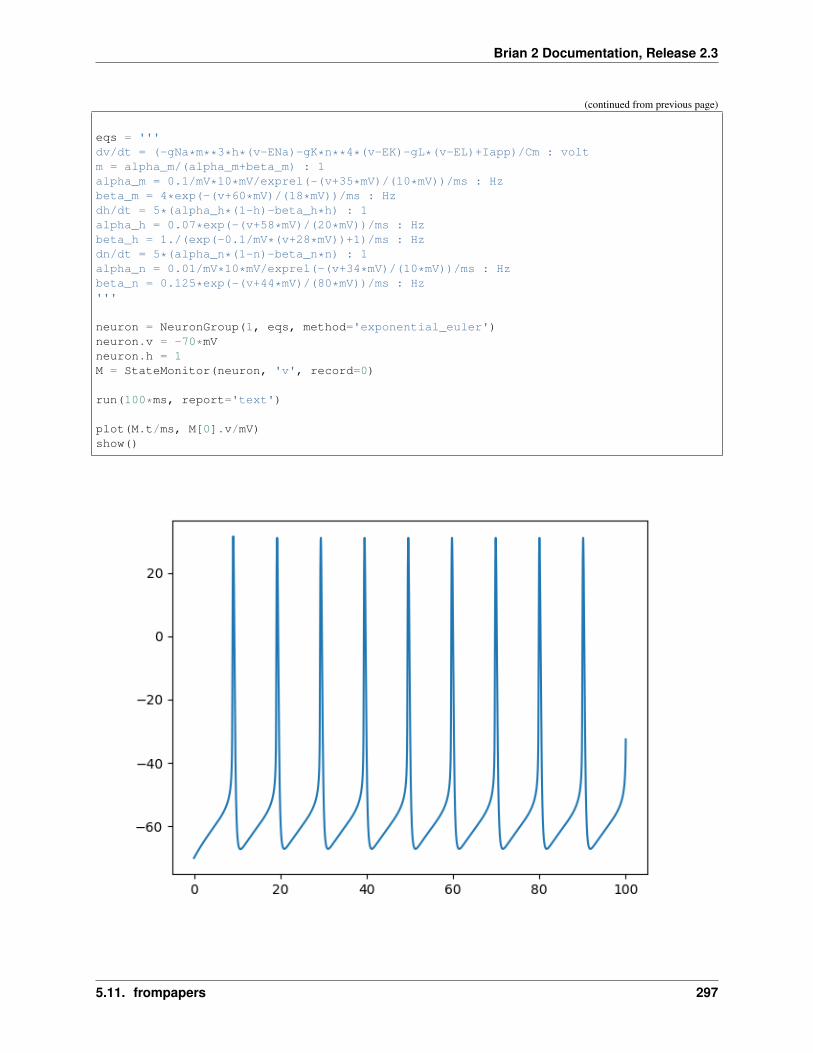
Brian 2 Documentation, Release 2.3
(continued from previous page)
eqs = '''dv/dt = (-gNa*m**3*h*(v-ENa)-gK*n**4*(v-EK)-gL*(v-EL)+Iapp)/Cm : voltm = alpha_m/(alpha_m+beta_m) : 1alpha_m = 0.1/mV*10*mV/exprel(-(v+35*mV)/(10*mV))/ms : Hzbeta_m = 4*exp(-(v+60*mV)/(18*mV))/ms : Hzdh/dt = 5*(alpha_h*(1-h)-beta_h*h) : 1alpha_h = 0.07*exp(-(v+58*mV)/(20*mV))/ms : Hzbeta_h = 1./(exp(-0.1/mV*(v+28*mV))+1)/ms : Hzdn/dt = 5*(alpha_n*(1-n)-beta_n*n) : 1alpha_n = 0.01/mV*10*mV/exprel(-(v+34*mV)/(10*mV))/ms : Hzbeta_n = 0.125*exp(-(v+44*mV)/(80*mV))/ms : Hz'''
neuron = NeuronGroup(1, eqs, method='exponential_euler')neuron.v = -70*mVneuron.h = 1M = StateMonitor(neuron, 'v', record=0)
run(100*ms, report='text')
plot(M.t/ms, M[0].v/mV)show()
5.11. frompapers 297
Brian 2 Documentation, Release 2.3
5.12 frompapers/Brette_2012
5.12.1 Example: Fig1
Brette R (2013). Sharpness of spike initiation in neurons explained by compartmentalization. PLoS Comp Biol, doi:10.1371/journal.pcbi.1003338.
Fig 1C-E. Somatic voltage-clamp in a ball-and-stick model with Na channels at a particular location.
from brian2 import *from params import *
defaultclock.dt = 0.025*ms
# Morphologymorpho = Soma(50*um) # chosen for a target Rmmorpho.axon = Cylinder(diameter=1*um, length=300*um, n=300)
location = 40*um # where Na channels are placedduration = 500*ms
# Channelseqs='''Im = gL*(EL - v) + gclamp*(vc - v) + gNa*m*(ENa - v) : amp/meter**2dm/dt = (minf - m) / taum: 1 # simplified Na channelminf = 1 / (1 + exp((va - v) / ka)) : 1gclamp : siemens/meter**2gNa : siemens/meter**2vc = EL + 50*mV * t/duration : volt (shared) # Voltage clamp with a ramping voltage→˓command'''
neuron = SpatialNeuron(morphology=morpho, model=eqs, Cm=Cm, Ri=Ri)compartment = morpho.axon[location]neuron.v = ELneuron.gclamp[0] = gL*500neuron.gNa[compartment] = gNa_0/neuron.area[compartment]
# Monitorsmon = StateMonitor(neuron, ['v', 'vc', 'm'], record=True)
run(duration, report='text')
subplot(221)plot(mon[0].vc/mV,
-((mon[0].vc - mon[0].v)*(neuron.gclamp[0]))*neuron.area[0]/nA, 'k')xlabel('V (mV)')ylabel('I (nA)')xlim(-75, -45)title('I-V curve')
subplot(222)plot(mon[0].vc/mV, mon[compartment].m, 'k')xlabel('V (mV)')ylabel('m')
(continues on next page)
298 Chapter 5. Examples

Brian 2 Documentation, Release 2.3
(continued from previous page)
title('Activation curve (m(V))')
subplot(223)# Number of simulation time steps for each volt increment in the voltage-clampdt_per_volt = len(mon.t)/(50*mV)for v in [-64*mV, -61*mV, -58*mV, -55*mV]:
plot(mon.v[:100 ,int(dt_per_volt*(v - EL))]/mV, 'k')xlabel('Distance from soma (um)')ylabel('V (mV)')title('Voltage across axon')
subplot(224)plot(mon[compartment].v/mV, mon[compartment].v/mV, 'k--') # Diagonalplot(mon[0].v/mV, mon[compartment].v/mV, 'k')xlabel('Vs (mV)')ylabel('Va (mV)')tight_layout()show()
5.12.2 Example: Fig3AB
Brette R (2013). Sharpness of spike initiation in neurons explained by compartmentalization. PLoS Comp Biol, doi:
5.12. frompapers/Brette_2012 299
Brian 2 Documentation, Release 2.3
10.1371/journal.pcbi.1003338.
Fig. 3. A, B. Kink with only Nav1.6 channels
from brian2 import *from params import *
codegen.target='numpy'
defaultclock.dt = 0.025*ms
# Morphologymorpho = Soma(50*um) # chosen for a target Rmmorpho.axon = Cylinder(diameter=1*um, length=300*um, n=300)
location = 40*um # where Na channels are placed
# Channelseqs='''Im = gL*(EL - v) + gNa*m*(ENa - v) : amp/meter**2dm/dt = (minf - m) / taum : 1 # simplified Na channelminf = 1 / (1 + exp((va - v) / ka)) : 1gNa : siemens/meter**2Iin : amp (point current)'''
neuron = SpatialNeuron(morphology=morpho, model=eqs, Cm=Cm, Ri=Ri,method="exponential_euler")
compartment = morpho.axon[location]neuron.v = ELneuron.gNa[compartment] = gNa_0/neuron.area[compartment]M = StateMonitor(neuron, ['v', 'm'], record=True)
run(20*ms, report='text')neuron.Iin[0] = gL * 20*mV * neuron.area[0]run(80*ms, report='text')
subplot(121)plot(M.t/ms, M[0].v/mV, 'r')plot(M.t/ms, M[compartment].v/mV, 'k')plot(M.t/ms, M[compartment].m*(80+60)-80, 'k--') # open channelsylim(-80, 60)xlabel('Time (ms)')ylabel('V (mV)')title('Voltage traces')
subplot(122)dm = diff(M[0].v) / defaultclock.dtdm40 = diff(M[compartment].v) / defaultclock.dtplot((M[0].v/mV)[1:], dm/(volt/second), 'r')plot((M[compartment].v/mV)[1:], dm40/(volt/second), 'k')xlim(-80, 40)xlabel('V (mV)')ylabel('dV/dt (V/s)')title('Phase plot')tight_layout()show()
300 Chapter 5. Examples
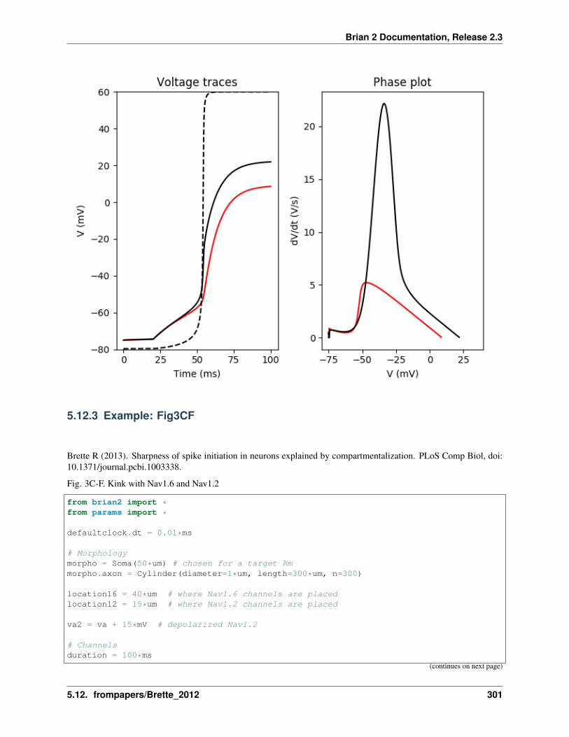
Brian 2 Documentation, Release 2.3
5.12.3 Example: Fig3CF
Brette R (2013). Sharpness of spike initiation in neurons explained by compartmentalization. PLoS Comp Biol, doi:10.1371/journal.pcbi.1003338.
Fig. 3C-F. Kink with Nav1.6 and Nav1.2
from brian2 import *from params import *
defaultclock.dt = 0.01*ms
# Morphologymorpho = Soma(50*um) # chosen for a target Rmmorpho.axon = Cylinder(diameter=1*um, length=300*um, n=300)
location16 = 40*um # where Nav1.6 channels are placedlocation12 = 15*um # where Nav1.2 channels are placed
va2 = va + 15*mV # depolarized Nav1.2
# Channelsduration = 100*ms
(continues on next page)
5.12. frompapers/Brette_2012 301
Brian 2 Documentation, Release 2.3
(continued from previous page)
eqs='''Im = gL * (EL - v) + gNa*m*(ENa - v) + gNa2*m2*(ENa - v) : amp/meter**2dm/dt = (minf - m) / taum : 1 # simplified Na channelminf = 1 / (1 + exp((va - v) / ka)) : 1dm2/dt = (minf2 - m2) / taum : 1 # simplified Na channel, Nav1.2minf2 = 1/(1 + exp((va2 - v) / ka)) : 1gNa : siemens/meter**2gNa2 : siemens/meter**2 # Nav1.2Iin : amp (point current)'''
neuron = SpatialNeuron(morphology=morpho, model=eqs, Cm=Cm, Ri=Ri,method="exponential_euler")
compartment16 = morpho.axon[location16]compartment12 = morpho.axon[location12]neuron.v = ELneuron.gNa[compartment16] = gNa_0/neuron.area[compartment16]neuron.gNa2[compartment12] = 20*gNa_0/neuron.area[compartment12]# MonitorsM = StateMonitor(neuron, ['v', 'm', 'm2'], record=True)
run(20*ms, report='text')neuron.Iin[0] = gL * 20*mV * neuron.area[0]run(80*ms, report='text')
subplot(221)plot(M.t/ms, M[0].v/mV, 'r')plot(M.t/ms, M[compartment16].v/mV, 'k')plot(M.t/ms, M[compartment16].m*(80+60)-80, 'k--') # open channelsylim(-80, 60)xlabel('Time (ms)')ylabel('V (mV)')title('Voltage traces')
subplot(222)plot(M[0].v/mV, M[compartment16].m,'k')plot(M[0].v/mV, 1 / (1 + exp((va - M[0].v) / ka)), 'k--')plot(M[0].v/mV, M[compartment12].m2, 'r')plot(M[0].v/mV, 1 / (1 + exp((va2 - M[0].v) / ka)), 'r--')xlim(-70, 0)xlabel('V (mV)')ylabel('m')title('Activation curves')
subplot(223)dm = diff(M[0].v) / defaultclock.dtdm40 = diff(M[compartment16].v) / defaultclock.dtplot((M[0].v/mV)[1:], dm/(volt/second), 'r')plot((M[compartment16].v/mV)[1:], dm40/(volt/second), 'k')xlim(-80, 40)xlabel('V (mV)')ylabel('dV/dt (V/s)')title('Phase plot')
subplot(224)plot((M[0].v/mV)[1:], dm/(volt/second), 'r')plot((M[compartment16].v/mV)[1:], dm40/(volt/second), 'k')
(continues on next page)
302 Chapter 5. Examples

Brian 2 Documentation, Release 2.3
(continued from previous page)
plot((M[0].v/mV)[1:], 10 + 0*dm/(volt/second), 'k--')xlim(-70, -40)ylim(0, 20)xlabel('V (mV)')ylabel('dV/dt (V/s)')title('Phase plot(zoom)')tight_layout()show()
5.12.4 Example: Fig4
Brette R (2013). Sharpness of spike initiation in neurons explained by compartmentalization. PLoS Comp Biol, doi:10.1371/journal.pcbi.1003338.
Fig. 4E-F. Spatial distribution of Na channels. Tapering axon near soma.
from brian2 import *from params import *
defaultclock.dt = 0.025*ms
(continues on next page)
5.12. frompapers/Brette_2012 303
Brian 2 Documentation, Release 2.3
(continued from previous page)
# Morphologymorpho = Soma(50*um) # chosen for a target Rm# Tapering (change this for the other figure panels)diameters = hstack([linspace(4, 1, 11), ones(290)])*ummorpho.axon = Section(diameter=diameters, length=ones(300)*um, n=300)
# Na channelsNa_start = (25 + 10)*umNa_end = (40 + 10)*umlinear_distribution = True # True is F, False is E
duration = 500*ms
# Channelseqs='''Im = gL*(EL - v) + gclamp*(vc - v) + gNa*m*(ENa - v) : amp/meter**2dm/dt = (minf - m) / taum: 1 # simplified Na channelminf = 1 / (1 + exp((va - v) / ka)) : 1gclamp : siemens/meter**2gNa : siemens/meter**2vc = EL + 50*mV * t / duration : volt (shared) # Voltage clamp with a ramping→˓voltage command'''
neuron = SpatialNeuron(morphology=morpho, model=eqs, Cm=Cm, Ri=Ri,method="exponential_euler")
compartments = morpho.axon[Na_start:Na_end]neuron.v = ELneuron.gclamp[0] = gL*500
if linear_distribution:profile = linspace(1, 0, len(compartments))
else:profile = ones(len(compartments))
profile = profile / sum(profile) # normalization
neuron.gNa[compartments] = gNa_0 * profile / neuron.area[compartments]
# Monitorsmon = StateMonitor(neuron, 'v', record=True)
run(duration, report='text')
dt_per_volt = len(mon.t) / (50*mV)for v in [-64*mV, -61*mV, -58*mV, -55*mV, -52*mV]:
plot(mon.v[:100, int(dt_per_volt * (v - EL))]/mV, 'k')xlim(0, 50+10)ylim(-65, -25)ylabel('V (mV)')xlabel('Location (um)')title('Voltage across axon')tight_layout()show()
304 Chapter 5. Examples
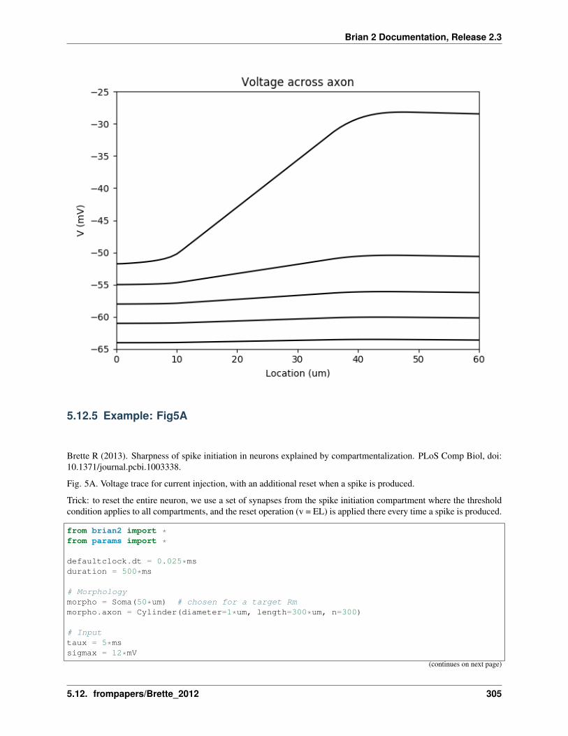
Brian 2 Documentation, Release 2.3
5.12.5 Example: Fig5A
Brette R (2013). Sharpness of spike initiation in neurons explained by compartmentalization. PLoS Comp Biol, doi:10.1371/journal.pcbi.1003338.
Fig. 5A. Voltage trace for current injection, with an additional reset when a spike is produced.
Trick: to reset the entire neuron, we use a set of synapses from the spike initiation compartment where the thresholdcondition applies to all compartments, and the reset operation (v = EL) is applied there every time a spike is produced.
from brian2 import *from params import *
defaultclock.dt = 0.025*msduration = 500*ms
# Morphologymorpho = Soma(50*um) # chosen for a target Rmmorpho.axon = Cylinder(diameter=1*um, length=300*um, n=300)
# Inputtaux = 5*mssigmax = 12*mV
(continues on next page)
5.12. frompapers/Brette_2012 305
Brian 2 Documentation, Release 2.3
(continued from previous page)
xx0 = 7*mV
compartment = 40
# Channelseqs = '''Im = gL * (EL - v) + gNa * m * (ENa - v) + gLx * (xx0 + xx) : amp/meter**2dm/dt = (minf - m) / taum : 1 # simplified Na channelminf = 1 / (1 + exp((va - v) / ka)) : 1gNa : siemens/meter**2gLx : siemens/meter**2dxx/dt = -xx / taux + sigmax * (2 / taux)**.5 *xi : volt'''
neuron = SpatialNeuron(morphology=morpho, model=eqs, Cm=Cm, Ri=Ri,threshold='m>0.5', threshold_location=compartment,refractory=5*ms)
neuron.v = ELneuron.gLx[0] = gLneuron.gNa[compartment] = gNa_0 / neuron.area[compartment]
# Reset the entire neuron when there is a spikereset = Synapses(neuron, neuron, on_pre='v = EL')reset.connect('i == compartment') # Connects the spike initiation compartment to all→˓compartments
# MonitorsS = SpikeMonitor(neuron)M = StateMonitor(neuron, 'v', record=0)run(duration, report='text')
# Add spikes for displayv = M[0].vfor t in S.t:
v[int(t / defaultclock.dt)] = 50*mV
plot(M.t/ms, v/mV, 'k')tight_layout()show()
306 Chapter 5. Examples

Brian 2 Documentation, Release 2.3
5.12.6 Example: params
Parameters for spike initiation simulations.
from brian2.units import *
# Passive parametersEL = -75*mVS = 7.85e-9*meter**2 # area (sphere of 50 um diameter)Cm = 0.75*uF/cm**2gL = 1. / (30000*ohm*cm**2)Ri = 150*ohm*cm
# Na channelsENa = 60*mVka = 6*mVva = -40*mVgNa_0 = gL * 2*Staum = 0.1*ms
5.12. frompapers/Brette_2012 307

Brian 2 Documentation, Release 2.3
5.13 frompapers/Stimberg_et_al_2018
5.13.1 Example: example_1_COBA
Modeling neuron-glia interactions with the Brian 2 simulator Marcel Stimberg, Dan F. M. Goodman, Romain Brette,Maurizio De Pittà bioRxiv 198366; doi: https://doi.org/10.1101/198366
Figure 1: Modeling of neurons and synapses.
Randomly connected networks with conductance-based synapses (COBA; see Brunel, 2000). Synapses exhibit short-time plasticity (Tsodyks, 2005; Tsodyks et al., 1998).
from brian2 import *import sympy
import plot_utils as pu
seed(11922) # to get identical figures for repeated runs
################################################################################# Model parameters################################################################################### General parametersduration = 1.0*second # Total simulation timesim_dt = 0.1*ms # Integrator/sampling stepN_e = 3200 # Number of excitatory neuronsN_i = 800 # Number of inhibitory neurons
### Neuron parametersE_l = -60*mV # Leak reversal potentialg_l = 9.99*nS # Leak conductanceE_e = 0*mV # Excitatory synaptic reversal potentialE_i = -80*mV # Inhibitory synaptic reversal potentialC_m = 198*pF # Membrane capacitancetau_e = 5*ms # Excitatory synaptic time constanttau_i = 10*ms # Inhibitory synaptic time constanttau_r = 5*ms # Refractory periodI_ex = 150*pA # External currentV_th = -50*mV # Firing thresholdV_r = E_l # Reset potential
### Synapse parametersw_e = 0.05*nS # Excitatory synaptic conductancew_i = 1.0*nS # Inhibitory synaptic conductanceU_0 = 0.6 # Synaptic release probability at restOmega_d = 2.0/second # Synaptic depression rateOmega_f = 3.33/second # Synaptic facilitation rate
################################################################################# Model definition################################################################################# Set the integration time (in this case not strictly necessary, since we are# using the default value)defaultclock.dt = sim_dt
### Neurons(continues on next page)
308 Chapter 5. Examples
Brian 2 Documentation, Release 2.3
(continued from previous page)
neuron_eqs = '''dv/dt = (g_l*(E_l-v) + g_e*(E_e-v) + g_i*(E_i-v) +
I_ex)/C_m : volt (unless refractory)dg_e/dt = -g_e/tau_e : siemens # post-synaptic exc. conductancedg_i/dt = -g_i/tau_i : siemens # post-synaptic inh. conductance'''neurons = NeuronGroup(N_e + N_i, model=neuron_eqs,
threshold='v>V_th', reset='v=V_r',refractory='tau_r', method='euler')
# Random initial membrane potential values and conductancesneurons.v = 'E_l + rand()*(V_th-E_l)'neurons.g_e = 'rand()*w_e'neurons.g_i = 'rand()*w_i'exc_neurons = neurons[:N_e]inh_neurons = neurons[N_e:]
### Synapsessynapses_eqs = '''# Usage of releasable neurotransmitter per single action potential:du_S/dt = -Omega_f * u_S : 1 (event-driven)# Fraction of synaptic neurotransmitter resources available:dx_S/dt = Omega_d *(1 - x_S) : 1 (event-driven)'''synapses_action = '''u_S += U_0 * (1 - u_S)r_S = u_S * x_Sx_S -= r_S'''exc_syn = Synapses(exc_neurons, neurons, model=synapses_eqs,
on_pre=synapses_action+'g_e_post += w_e*r_S')inh_syn = Synapses(inh_neurons, neurons, model=synapses_eqs,
on_pre=synapses_action+'g_i_post += w_i*r_S')
exc_syn.connect(p=0.05)inh_syn.connect(p=0.2)# Start from "resting" condition: all synapses have fully-replenished# neurotransmitter resourcesexc_syn.x_S = 1inh_syn.x_S = 1
# ############################################################################### # Monitors# ############################################################################### Note that we could use a single monitor for all neurons instead, but in this# way plotting is a bit easier in the endexc_mon = SpikeMonitor(exc_neurons)inh_mon = SpikeMonitor(inh_neurons)
### We record some additional data from a single excitatory neuronni = 50# Record conductances and membrane potential of neuron nistate_mon = StateMonitor(exc_neurons, ['v', 'g_e', 'g_i'], record=ni)# We make sure to monitor synaptic variables after synapse are updated in order# to use simple recurrence relations to reconstruct them. Record all synapses# originating from neuron nisynapse_mon = StateMonitor(exc_syn, ['u_S', 'x_S'],
record=exc_syn[ni, :], when='after_synapses')(continues on next page)
5.13. frompapers/Stimberg_et_al_2018 309
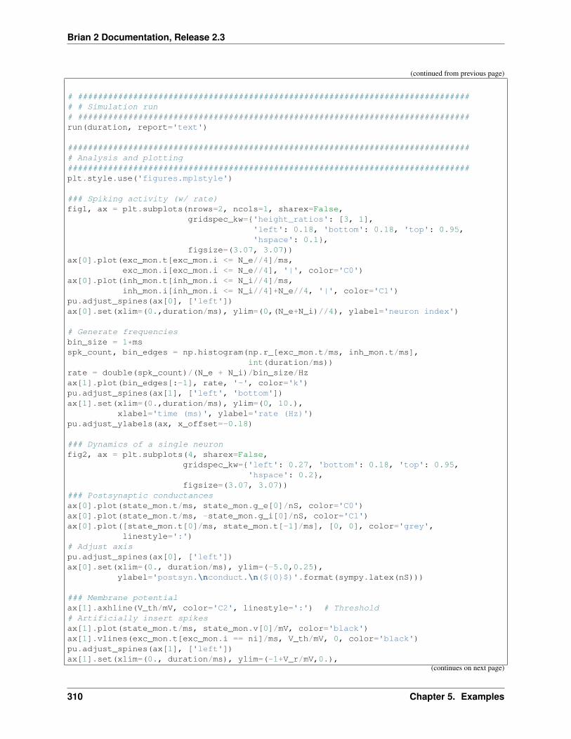
Brian 2 Documentation, Release 2.3
(continued from previous page)
# ############################################################################### # Simulation run# ##############################################################################run(duration, report='text')
################################################################################# Analysis and plotting################################################################################plt.style.use('figures.mplstyle')
### Spiking activity (w/ rate)fig1, ax = plt.subplots(nrows=2, ncols=1, sharex=False,
gridspec_kw={'height_ratios': [3, 1],'left': 0.18, 'bottom': 0.18, 'top': 0.95,'hspace': 0.1},
figsize=(3.07, 3.07))ax[0].plot(exc_mon.t[exc_mon.i <= N_e//4]/ms,
exc_mon.i[exc_mon.i <= N_e//4], '|', color='C0')ax[0].plot(inh_mon.t[inh_mon.i <= N_i//4]/ms,
inh_mon.i[inh_mon.i <= N_i//4]+N_e//4, '|', color='C1')pu.adjust_spines(ax[0], ['left'])ax[0].set(xlim=(0.,duration/ms), ylim=(0,(N_e+N_i)//4), ylabel='neuron index')
# Generate frequenciesbin_size = 1*msspk_count, bin_edges = np.histogram(np.r_[exc_mon.t/ms, inh_mon.t/ms],
int(duration/ms))rate = double(spk_count)/(N_e + N_i)/bin_size/Hzax[1].plot(bin_edges[:-1], rate, '-', color='k')pu.adjust_spines(ax[1], ['left', 'bottom'])ax[1].set(xlim=(0.,duration/ms), ylim=(0, 10.),
xlabel='time (ms)', ylabel='rate (Hz)')pu.adjust_ylabels(ax, x_offset=-0.18)
### Dynamics of a single neuronfig2, ax = plt.subplots(4, sharex=False,
gridspec_kw={'left': 0.27, 'bottom': 0.18, 'top': 0.95,'hspace': 0.2},
figsize=(3.07, 3.07))### Postsynaptic conductancesax[0].plot(state_mon.t/ms, state_mon.g_e[0]/nS, color='C0')ax[0].plot(state_mon.t/ms, -state_mon.g_i[0]/nS, color='C1')ax[0].plot([state_mon.t[0]/ms, state_mon.t[-1]/ms], [0, 0], color='grey',
linestyle=':')# Adjust axispu.adjust_spines(ax[0], ['left'])ax[0].set(xlim=(0., duration/ms), ylim=(-5.0,0.25),
ylabel='postsyn.\nconduct.\n(${0}$)'.format(sympy.latex(nS)))
### Membrane potentialax[1].axhline(V_th/mV, color='C2', linestyle=':') # Threshold# Artificially insert spikesax[1].plot(state_mon.t/ms, state_mon.v[0]/mV, color='black')ax[1].vlines(exc_mon.t[exc_mon.i == ni]/ms, V_th/mV, 0, color='black')pu.adjust_spines(ax[1], ['left'])ax[1].set(xlim=(0., duration/ms), ylim=(-1+V_r/mV,0.),
(continues on next page)
310 Chapter 5. Examples

Brian 2 Documentation, Release 2.3
(continued from previous page)
ylabel='membrane\npotential\n(${0}$)'.format(sympy.latex(mV)))
### Synaptic variables# Retrieves indexes of spikes in the synaptic monitor using the fact that we# are sampling spikes and synaptic variables by the same dtspk_index = np.in1d(synapse_mon.t, exc_mon.t[exc_mon.i == ni])ax[2].plot(synapse_mon.t[spk_index]/ms, synapse_mon.x_S[0][spk_index], '.',
ms=4, color='C3')ax[2].plot(synapse_mon.t[spk_index]/ms, synapse_mon.u_S[0][spk_index], '.',
ms=4, color='C4')# Super-impose reconstructed solutionstime = synapse_mon.t # time vectortspk = Quantity(synapse_mon.t, copy=True) # Spike timesfor ts in exc_mon.t[exc_mon.i == ni]:
tspk[time >= ts] = tsax[2].plot(synapse_mon.t/ms, 1 + (synapse_mon.x_S[0]-1)*exp(-(time-tspk)*Omega_d),
'-', color='C3')ax[2].plot(synapse_mon.t/ms, synapse_mon.u_S[0]*exp(-(time-tspk)*Omega_f),
'-', color='C4')# Adjust axispu.adjust_spines(ax[2], ['left'])ax[2].set(xlim=(0., duration/ms), ylim=(-0.05, 1.05),
ylabel='synaptic\nvariables\n$u_S,\,x_S$')
nspikes = np.sum(spk_index)x_S_spike = synapse_mon.x_S[0][spk_index]u_S_spike = synapse_mon.u_S[0][spk_index]ax[3].vlines(synapse_mon.t[spk_index]/ms, np.zeros(nspikes),
x_S_spike*u_S_spike/(1-u_S_spike))pu.adjust_spines(ax[3], ['left', 'bottom'])ax[3].set(xlim=(0., duration/ms), ylim=(-0.01, 0.62),
yticks=np.arange(0, 0.62, 0.2), xlabel='time (ms)', ylabel='$r_S$')
pu.adjust_ylabels(ax, x_offset=-0.20)
plt.show()
5.13. frompapers/Stimberg_et_al_2018 311

Brian 2 Documentation, Release 2.3
5.13.2 Example: example_2_gchi_astrocyte
Modeling neuron-glia interactions with the Brian 2 simulator Marcel Stimberg, Dan F. M. Goodman, Romain Brette,Maurizio De Pittà bioRxiv 198366; doi: https://doi.org/10.1101/198366
Figure 2: Modeling of synaptically-activated astrocytes
Two astrocytes (one stochastic and the other deterministic) activated by synapses (connecting “dummy” groups ofneurons) (see De Pitta’ et al., 2009)
from brian2 import *
import plot_utils as pu
(continues on next page)
312 Chapter 5. Examples

Brian 2 Documentation, Release 2.3
(continued from previous page)
set_device('cpp_standalone', directory=None) # Use fast "C++ standalone mode"seed(790824) # to get identical figures for repeated runs
################################################################################# Model parameters################################################################################### General parametersduration = 30*second # Total simulation timesim_dt = 1*ms # Integrator/sampling step
### Neuron parametersf_0 = 0.5*Hz # Spike rate of the "source" neurons
### Synapse parametersrho_c = 0.001 # Synaptic vesicle-to-extracellular space volume ratioY_T = 500*mmolar # Total vesicular neurotransmitter concentrationOmega_c = 40/second # Neurotransmitter clearance rate
### Astrocyte parameters# --- Calcium fluxesO_P = 0.9*umolar/second # Maximal Ca^2+ uptake rate by SERCAsK_P = 0.1 * umolar # Ca2+ affinity of SERCAsC_T = 2*umolar # Total cell free Ca^2+ contentrho_A = 0.18 # ER-to-cytoplasm volume ratioOmega_C = 6/second # Maximal rate of Ca^2+ release by IP_3RsOmega_L = 0.1/second # Maximal rate of Ca^2+ leak from the ER# --- IP_3R kinecticsd_1 = 0.13*umolar # IP_3 binding affinityd_2 = 1.05*umolar # Ca^2+ inactivation dissociation constantO_2 = 0.2/umolar/second # IP_3R binding rate for Ca^2+ inhibitiond_3 = 0.9434*umolar # IP_3 dissociation constantd_5 = 0.08*umolar # Ca^2+ activation dissociation constant# --- Agonist-dependent IP_3 productionO_beta = 5*umolar/second # Maximal rate of IP_3 production by PLCbetaO_N = 0.3/umolar/second # Agonist binding rateOmega_N = 0.5/second # Maximal inactivation rateK_KC = 0.5*umolar # Ca^2+ affinity of PKCzeta = 10 # Maximal reduction of receptor affinity by PKC# --- IP_3 productionO_delta = 0.2 *umolar/second # Maximal rate of IP_3 production by PLCdeltakappa_delta = 1.5 * umolar # Inhibition constant of PLC_delta by IP_3K_delta = 0.3*umolar # Ca^2+ affinity of PLCdelta# --- IP_3 degradationOmega_5P = 0.1/second # Maximal rate of IP_3 degradation by IP-5PK_D = 0.5*umolar # Ca^2+ affinity of IP3-3KK_3K = 1*umolar # IP_3 affinity of IP_3-3KO_3K = 4.5*umolar/second # Maximal rate of IP_3 degradation by IP_3-3K# --- IP_3 external productionF_ex = 0.09*umolar/second # Maximal exogenous IP3 flowI_Theta = 0.3*umolar # Threshold gradient for IP_3 diffusionomega_I = 0.05*umolar # Scaling factor of diffusion
################################################################################# Model definition################################################################################defaultclock.dt = sim_dt # Set the integration time
(continues on next page)
5.13. frompapers/Stimberg_et_al_2018 313
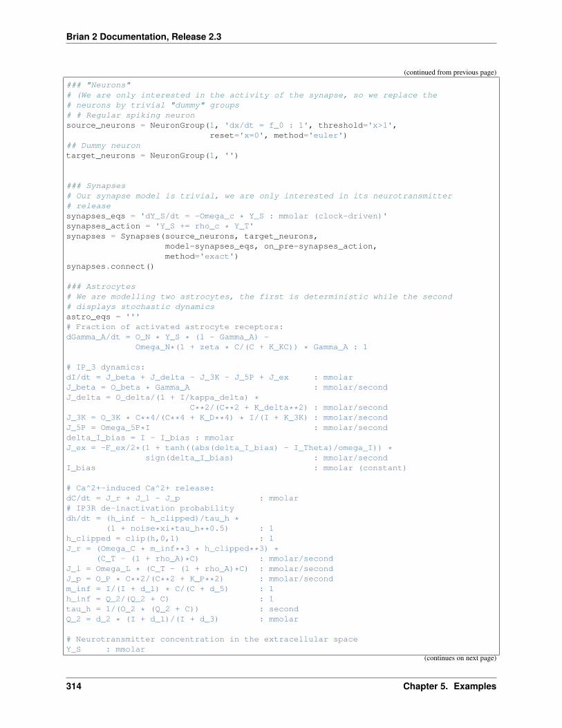
Brian 2 Documentation, Release 2.3
(continued from previous page)
### "Neurons"# (We are only interested in the activity of the synapse, so we replace the# neurons by trivial "dummy" groups# # Regular spiking neuronsource_neurons = NeuronGroup(1, 'dx/dt = f_0 : 1', threshold='x>1',
reset='x=0', method='euler')## Dummy neurontarget_neurons = NeuronGroup(1, '')
### Synapses# Our synapse model is trivial, we are only interested in its neurotransmitter# releasesynapses_eqs = 'dY_S/dt = -Omega_c * Y_S : mmolar (clock-driven)'synapses_action = 'Y_S += rho_c * Y_T'synapses = Synapses(source_neurons, target_neurons,
model=synapses_eqs, on_pre=synapses_action,method='exact')
synapses.connect()
### Astrocytes# We are modelling two astrocytes, the first is deterministic while the second# displays stochastic dynamicsastro_eqs = '''# Fraction of activated astrocyte receptors:dGamma_A/dt = O_N * Y_S * (1 - Gamma_A) -
Omega_N*(1 + zeta * C/(C + K_KC)) * Gamma_A : 1
# IP_3 dynamics:dI/dt = J_beta + J_delta - J_3K - J_5P + J_ex : mmolarJ_beta = O_beta * Gamma_A : mmolar/secondJ_delta = O_delta/(1 + I/kappa_delta) *
C**2/(C**2 + K_delta**2) : mmolar/secondJ_3K = O_3K * C**4/(C**4 + K_D**4) * I/(I + K_3K) : mmolar/secondJ_5P = Omega_5P*I : mmolar/seconddelta_I_bias = I - I_bias : mmolarJ_ex = -F_ex/2*(1 + tanh((abs(delta_I_bias) - I_Theta)/omega_I)) *
sign(delta_I_bias) : mmolar/secondI_bias : mmolar (constant)
# Ca^2+-induced Ca^2+ release:dC/dt = J_r + J_l - J_p : mmolar# IP3R de-inactivation probabilitydh/dt = (h_inf - h_clipped)/tau_h *
(1 + noise*xi*tau_h**0.5) : 1h_clipped = clip(h,0,1) : 1J_r = (Omega_C * m_inf**3 * h_clipped**3) *
(C_T - (1 + rho_A)*C) : mmolar/secondJ_l = Omega_L * (C_T - (1 + rho_A)*C) : mmolar/secondJ_p = O_P * C**2/(C**2 + K_P**2) : mmolar/secondm_inf = I/(I + d_1) * C/(C + d_5) : 1h_inf = Q_2/(Q_2 + C) : 1tau_h = 1/(O_2 * (Q_2 + C)) : secondQ_2 = d_2 * (I + d_1)/(I + d_3) : mmolar
# Neurotransmitter concentration in the extracellular spaceY_S : mmolar
(continues on next page)
314 Chapter 5. Examples
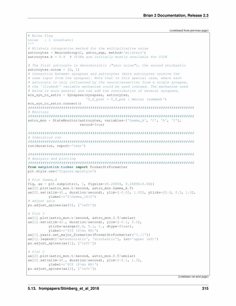
Brian 2 Documentation, Release 2.3
(continued from previous page)
# Noise flagnoise : 1 (constant)'''# Milstein integration method for the multiplicative noiseastrocytes = NeuronGroup(2, astro_eqs, method='milstein')astrocytes.h = 0.9 # IP3Rs are initially mostly available for CICR
# The first astrocyte is deterministic ("zero noise"), the second stochasticastrocytes.noise = [0, 1]# Connection between synapses and astrocytes (both astrocytes receive the# same input from the synapse). Note that in this special case, where each# astrocyte is only influenced by the neurotransmitter from a single synapse,# the '(linked)' variable mechanism could be used instead. The mechanism used# below is more general and can add the contribution of several synapses.ecs_syn_to_astro = Synapses(synapses, astrocytes,
'Y_S_post = Y_S_pre : mmolar (summed)')ecs_syn_to_astro.connect()################################################################################# Monitors################################################################################astro_mon = StateMonitor(astrocytes, variables=['Gamma_A', 'C', 'h', 'I'],
record=True)
################################################################################# Simulation run################################################################################run(duration, report='text')
################################################################################# Analysis and plotting################################################################################from matplotlib.ticker import FormatStrFormatterplt.style.use('figures.mplstyle')
# Plot Gamma_Afig, ax = plt.subplots(4, 1, figsize=(6.26894, 6.26894*0.66))ax[0].plot(astro_mon.t/second, astro_mon.Gamma_A.T)ax[0].set(xlim=(0., duration/second), ylim=[-0.05, 1.02], yticks=[0.0, 0.5, 1.0],
ylabel=r'$\Gamma_{A}$')# Adjust axispu.adjust_spines(ax[0], ['left'])
# Plot Iax[1].plot(astro_mon.t/second, astro_mon.I.T/umolar)ax[1].set(xlim=(0., duration/second), ylim=[-0.1, 5.0],
yticks=arange(0.0, 5.1, 1., dtype=float),ylabel=r'$I$ ($\mu M$)')
ax[1].yaxis.set_major_formatter(FormatStrFormatter('%.1f'))ax[1].legend(['deterministic', 'stochastic'], loc='upper left')pu.adjust_spines(ax[1], ['left'])
# Plot Cax[2].plot(astro_mon.t/second, astro_mon.C.T/umolar)ax[2].set(xlim=(0., duration/second), ylim=[-0.1, 1.3],
ylabel=r'$C$ ($\mu M$)')pu.adjust_spines(ax[2], ['left'])
(continues on next page)
5.13. frompapers/Stimberg_et_al_2018 315

Brian 2 Documentation, Release 2.3
(continued from previous page)
# Plot hax[3].plot(astro_mon.t/second, astro_mon.h.T)ax[3].set(xlim=(0., duration/second),
ylim=[0.4, 1.02],ylabel='h', xlabel='time ($s$)')
pu.adjust_spines(ax[3], ['left', 'bottom'])
pu.adjust_ylabels(ax, x_offset=-0.1)
plt.show()
5.13.3 Example: example_3_io_synapse
Modeling neuron-glia interactions with the Brian 2 simulator Marcel Stimberg, Dan F. M. Goodman, Romain Brette,Maurizio De Pittà bioRxiv 198366; doi: https://doi.org/10.1101/198366
Figure 3: Modeling of modulation of synaptic release by gliotransmission.
Three synapses: the first one without astrocyte, the remaining two respectively with open-loop and close-loop glio-transmission (see De Pitta’ et al., 2011, 2016)
from brian2 import *
import plot_utils as pu
set_device('cpp_standalone', directory=None) # Use fast "C++ standalone mode"
(continues on next page)
316 Chapter 5. Examples
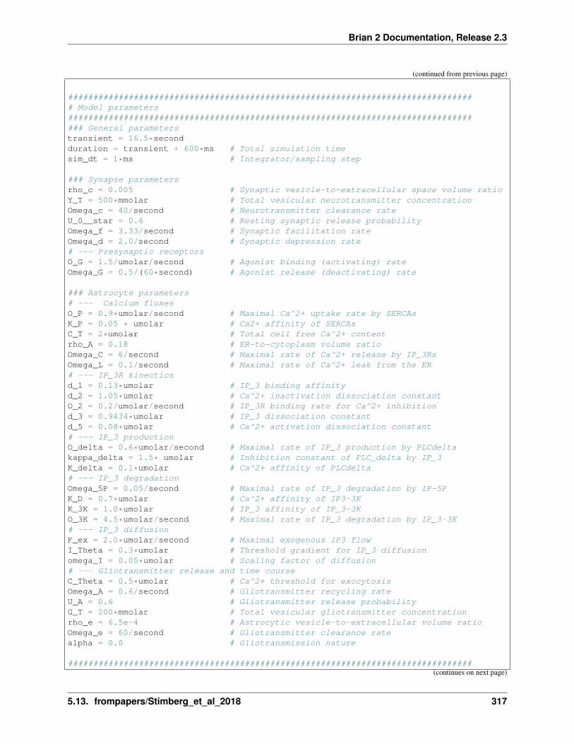
Brian 2 Documentation, Release 2.3
(continued from previous page)
################################################################################# Model parameters################################################################################### General parameterstransient = 16.5*secondduration = transient + 600*ms # Total simulation timesim_dt = 1*ms # Integrator/sampling step
### Synapse parametersrho_c = 0.005 # Synaptic vesicle-to-extracellular space volume ratioY_T = 500*mmolar # Total vesicular neurotransmitter concentrationOmega_c = 40/second # Neurotransmitter clearance rateU_0__star = 0.6 # Resting synaptic release probabilityOmega_f = 3.33/second # Synaptic facilitation rateOmega_d = 2.0/second # Synaptic depression rate# --- Presynaptic receptorsO_G = 1.5/umolar/second # Agonist binding (activating) rateOmega_G = 0.5/(60*second) # Agonist release (deactivating) rate
### Astrocyte parameters# --- Calcium fluxesO_P = 0.9*umolar/second # Maximal Ca^2+ uptake rate by SERCAsK_P = 0.05 * umolar # Ca2+ affinity of SERCAsC_T = 2*umolar # Total cell free Ca^2+ contentrho_A = 0.18 # ER-to-cytoplasm volume ratioOmega_C = 6/second # Maximal rate of Ca^2+ release by IP_3RsOmega_L = 0.1/second # Maximal rate of Ca^2+ leak from the ER# --- IP_3R kinecticsd_1 = 0.13*umolar # IP_3 binding affinityd_2 = 1.05*umolar # Ca^2+ inactivation dissociation constantO_2 = 0.2/umolar/second # IP_3R binding rate for Ca^2+ inhibitiond_3 = 0.9434*umolar # IP_3 dissociation constantd_5 = 0.08*umolar # Ca^2+ activation dissociation constant# --- IP_3 productionO_delta = 0.6*umolar/second # Maximal rate of IP_3 production by PLCdeltakappa_delta = 1.5* umolar # Inhibition constant of PLC_delta by IP_3K_delta = 0.1*umolar # Ca^2+ affinity of PLCdelta# --- IP_3 degradationOmega_5P = 0.05/second # Maximal rate of IP_3 degradation by IP-5PK_D = 0.7*umolar # Ca^2+ affinity of IP3-3KK_3K = 1.0*umolar # IP_3 affinity of IP_3-3KO_3K = 4.5*umolar/second # Maximal rate of IP_3 degradation by IP_3-3K# --- IP_3 diffusionF_ex = 2.0*umolar/second # Maximal exogenous IP3 flowI_Theta = 0.3*umolar # Threshold gradient for IP_3 diffusionomega_I = 0.05*umolar # Scaling factor of diffusion# --- Gliotransmitter release and time courseC_Theta = 0.5*umolar # Ca^2+ threshold for exocytosisOmega_A = 0.6/second # Gliotransmitter recycling rateU_A = 0.6 # Gliotransmitter release probabilityG_T = 200*mmolar # Total vesicular gliotransmitter concentrationrho_e = 6.5e-4 # Astrocytic vesicle-to-extracellular volume ratioOmega_e = 60/second # Gliotransmitter clearance ratealpha = 0.0 # Gliotransmission nature
################################################################################(continues on next page)
5.13. frompapers/Stimberg_et_al_2018 317

Brian 2 Documentation, Release 2.3
(continued from previous page)
# Model definition################################################################################defaultclock.dt = sim_dt # Set the integration time
### "Neurons"# We are only interested in the activity of the synapse, so we replace the# neurons by trivial "dummy" groupsspikes = [0, 50, 100, 150, 200,
300, 310, 320, 330, 340, 350, 360, 370, 380, 390, 400]*msspikes += transient # allow for some initial transientsource_neurons = SpikeGeneratorGroup(1, np.zeros(len(spikes)), spikes)target_neurons = NeuronGroup(1, '')
### Synapses# Note that the synapse does not actually have any effect on the post-synaptic# target# Also note that for easier plotting we do not use the "event-driven" flag here,# even though the value of u_S and x_S only needs to be updated on the arrival# of a spikesynapses_eqs = '''# NeurotransmitterdY_S/dt = -Omega_c * Y_S : mmolar (clock-driven)# Fraction of activated presynaptic receptorsdGamma_S/dt = O_G * G_A * (1 - Gamma_S) -
Omega_G * Gamma_S : 1 (clock-driven)# Usage of releasable neurotransmitter per single action potential:du_S/dt = -Omega_f * u_S : 1 (clock-driven)# Fraction of synaptic neurotransmitter resources available:dx_S/dt = Omega_d *(1 - x_S) : 1 (clock-driven)# released synaptic neurotransmitter resources:r_S : 1# gliotransmitter concentration in the extracellular space:G_A : mmolar'''synapses_action = '''U_0 = (1 - Gamma_S) * U_0__star + alpha * Gamma_Su_S += U_0 * (1 - u_S)r_S = u_S * x_Sx_S -= r_SY_S += rho_c * Y_T * r_S'''synapses = Synapses(source_neurons, target_neurons,
model=synapses_eqs, on_pre=synapses_action,method='exact')
# We create three synapses, only the second and third ones are modulated by astrocytessynapses.connect(True, n=3)
### Astrocytes# The astrocyte emits gliotransmitter when its Ca^2+ concentration crosses# a thresholdastro_eqs = '''# IP_3 dynamics:dI/dt = J_delta - J_3K - J_5P + J_ex : mmolarJ_delta = O_delta/(1 + I/kappa_delta) * C**2/(C**2 + K_delta**2) : mmolar/secondJ_3K = O_3K * C**4/(C**4 + K_D**4) * I/(I + K_3K) : mmolar/secondJ_5P = Omega_5P*I : mmolar/second# Exogenous stimulation
(continues on next page)
318 Chapter 5. Examples
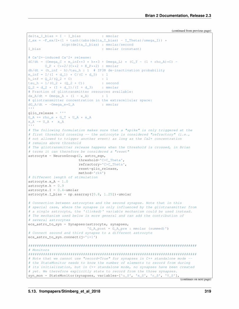
Brian 2 Documentation, Release 2.3
(continued from previous page)
delta_I_bias = I - I_bias : mmolarJ_ex = -F_ex/2*(1 + tanh((abs(delta_I_bias) - I_Theta)/omega_I)) *
sign(delta_I_bias) : mmolar/secondI_bias : mmolar (constant)
# Ca^2+-induced Ca^2+ release:dC/dt = (Omega_C * m_inf**3 * h**3 + Omega_L) * (C_T - (1 + rho_A)*C) -
O_P * C**2/(C**2 + K_P**2) : mmolardh/dt = (h_inf - h)/tau_h : 1 # IP3R de-inactivation probabilitym_inf = I/(I + d_1) * C/(C + d_5) : 1h_inf = Q_2/(Q_2 + C) : 1tau_h = 1/(O_2 * (Q_2 + C)) : secondQ_2 = d_2 * (I + d_1)/(I + d_3) : mmolar# Fraction of gliotransmitter resources available:dx_A/dt = Omega_A * (1 - x_A) : 1# gliotransmitter concentration in the extracellular space:dG_A/dt = -Omega_e*G_A : mmolar'''glio_release = '''G_A += rho_e * G_T * U_A * x_Ax_A -= U_A * x_A'''# The following formulation makes sure that a "spike" is only triggered at the# first threshold crossing -- the astrocyte is considered "refractory" (i.e.,# not allowed to trigger another event) as long as the Ca2+ concentration# remains above threshold# The gliotransmitter release happens when the threshold is crossed, in Brian# terms it can therefore be considered a "reset"astrocyte = NeuronGroup(2, astro_eqs,
threshold='C>C_Theta',refractory='C>C_Theta',reset=glio_release,method='rk4')
# Different length of stimulationastrocyte.x_A = 1.0astrocyte.h = 0.9astrocyte.I = 0.4*umolarastrocyte.I_bias = np.asarray([0.8, 1.25])*umolar
# Connection between astrocytes and the second synapse. Note that in this# special case, where the synapse is only influenced by the gliotransmitter from# a single astrocyte, the '(linked)' variable mechanism could be used instead.# The mechanism used below is more general and can add the contribution of# several astrocytesecs_astro_to_syn = Synapses(astrocyte, synapses,
'G_A_post = G_A_pre : mmolar (summed)')# Connect second and third synapse to a different astrocyteecs_astro_to_syn.connect(j='i+1')
################################################################################# Monitors################################################################################# Note that we cannot use "record=True" for synapses in C++ standalone mode --# the StateMonitor needs to know the number of elements to record from during# its initialization, but in C++ standalone mode, no synapses have been created# yet. We therefore explicitly state to record from the three synapses.syn_mon = StateMonitor(synapses, variables=['u_S', 'x_S', 'r_S', 'Y_S'],
(continues on next page)
5.13. frompapers/Stimberg_et_al_2018 319
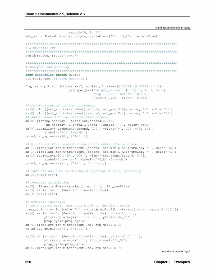
Brian 2 Documentation, Release 2.3
(continued from previous page)
record=[0, 1, 2])ast_mon = StateMonitor(astrocyte, variables=['C', 'G_A'], record=True)
################################################################################# Simulation run################################################################################run(duration, report='text')
################################################################################# Analysis and plotting################################################################################from matplotlib import cyclerplt.style.use('figures.mplstyle')
fig, ax = plt.subplots(nrows=7, ncols=1,figsize=(6.26894, 6.26894 * 1.2),gridspec_kw={'height_ratios': [3, 2, 1, 1, 3, 3, 3],
'top': 0.98, 'bottom': 0.08,'left': 0.15, 'right': 0.95})
## Ca^2+ traces of the two astrocytesax[0].plot((ast_mon.t-transient)/second, ast_mon.C[0]/umolar, '-', color='C2')ax[0].plot((ast_mon.t-transient)/second, ast_mon.C[1]/umolar, '-', color='C3')## Add threshold for gliotransmitter releaseax[0].plot(np.asarray([-transient/second,0.0]),
np.asarray([C_Theta,C_Theta])/umolar, ':', color='gray')ax[0].set(xlim=[-transient/second, 0.0], yticks=[0., 0.4, 0.8, 1.2],
ylabel=r'$C$ ($\mu$M)')pu.adjust_spines(ax[0], ['left'])
## Gliotransmitter concentration in the extracellular spaceax[1].plot((ast_mon.t-transient)/second, ast_mon.G_A[0]/umolar, '-', color='C2')ax[1].plot((ast_mon.t-transient)/second, ast_mon.G_A[1]/umolar, '-', color='C3')ax[1].set(yticks=[0., 50., 100.], xlim=[-transient/second, 0.0],
xlabel='time (s)', ylabel=r'$G_A$ ($\mu$M)')pu.adjust_spines(ax[1], ['left', 'bottom'])
## Turn off one axis to display x-labeling of ax[1] correctlyax[2].axis('off')
## Synaptic stimulationax[3].vlines((spikes-transient)/ms, 0, 1, clip_on=False)ax[3].set(xlim=(0, (duration-transient)/ms))ax[3].axis('off')
## Synaptic variables# Use a custom cycle that uses black as the first colorprop_cycle = cycler(color='k').concat(matplotlib.rcParams['axes.prop_cycle'][2:])ax[4].set(xlim=(0, (duration-transient)/ms), ylim=[0., 1.],
yticks=np.arange(0, 1.1, .25), ylabel='$u_S$',prop_cycle=prop_cycle)
ax[4].plot((syn_mon.t-transient)/ms, syn_mon.u_S.T)pu.adjust_spines(ax[4], ['left'])
ax[5].set(xlim=(0, (duration-transient)/ms), ylim=[-0.05, 1.],yticks=np.arange(0,1.1,.25), ylabel='$x_S$',prop_cycle=prop_cycle)
ax[5].plot((syn_mon.t-transient)/ms, syn_mon.x_S.T)(continues on next page)
320 Chapter 5. Examples
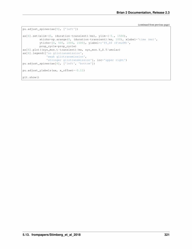
Brian 2 Documentation, Release 2.3
(continued from previous page)
pu.adjust_spines(ax[5], ['left'])
ax[6].set(xlim=(0, (duration-transient)/ms), ylim=(-5., 1500),xticks=np.arange(0, (duration-transient)/ms, 100), xlabel='time (ms)',yticks=[0, 500, 1000, 1500], ylabel=r'$Y_S$ ($\mu$M)',prop_cycle=prop_cycle)
ax[6].plot((syn_mon.t-transient)/ms, syn_mon.Y_S.T/umolar)ax[6].legend(['no gliotransmission',
'weak gliotransmission','stronger gliotransmission'], loc='upper right')
pu.adjust_spines(ax[6], ['left', 'bottom'])
pu.adjust_ylabels(ax, x_offset=-0.11)
plt.show()
5.13. frompapers/Stimberg_et_al_2018 321

Brian 2 Documentation, Release 2.3
5.13.4 Example: example_4_rsmean
Modeling neuron-glia interactions with the Brian 2 simulator Marcel Stimberg, Dan F. M. Goodman, Romain Brette,Maurizio De Pittà bioRxiv 198366; doi: https://doi.org/10.1101/198366
Figure 4C: Closed-loop gliotransmission.
322 Chapter 5. Examples
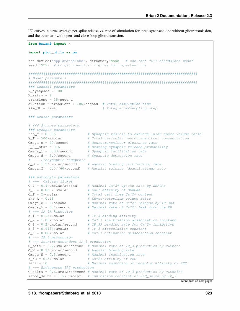
Brian 2 Documentation, Release 2.3
I/O curves in terms average per-spike release vs. rate of stimulation for three synapses: one without gliotransmission,and the other two with open- and close-loop gliotransmssion.
from brian2 import *
import plot_utils as pu
set_device('cpp_standalone', directory=None) # Use fast "C++ standalone mode"seed(1929) # to get identical figures for repeated runs
################################################################################# Model parameters################################################################################### General parametersN_synapses = 100N_astro = 2transient = 15*secondduration = transient + 180*second # Total simulation timesim_dt = 1*ms # Integrator/sampling step
### Neuron parameters
# ### Synapse parameters### Synapse parametersrho_c = 0.005 # Synaptic vesicle-to-extracellular space volume ratioY_T = 500*mmolar # Total vesicular neurotransmitter concentrationOmega_c = 40/second # Neurotransmitter clearance rateU_0__star = 0.6 # Resting synaptic release probabilityOmega_f = 3.33/second # Synaptic facilitation rateOmega_d = 2.0/second # Synaptic depression rate# --- Presynaptic receptorsO_G = 1.5/umolar/second # Agonist binding (activating) rateOmega_G = 0.5/(60*second) # Agonist release (deactivating) rate
### Astrocyte parameters# --- Calcium fluxesO_P = 0.9*umolar/second # Maximal Ca^2+ uptake rate by SERCAsK_P = 0.05 * umolar # Ca2+ affinity of SERCAsC_T = 2*umolar # Total cell free Ca^2+ contentrho_A = 0.18 # ER-to-cytoplasm volume ratioOmega_C = 6/second # Maximal rate of Ca^2+ release by IP_3RsOmega_L = 0.1/second # Maximal rate of Ca^2+ leak from the ER# --- IP_3R kinecticsd_1 = 0.13*umolar # IP_3 binding affinityd_2 = 1.05*umolar # Ca^2+ inactivation dissociation constantO_2 = 0.2/umolar/second # IP_3R binding rate for Ca^2+ inhibitiond_3 = 0.9434*umolar # IP_3 dissociation constantd_5 = 0.08*umolar # Ca^2+ activation dissociation constant# --- IP_3 production# --- Agonist-dependent IP_3 productionO_beta = 3.2*umolar/second # Maximal rate of IP_3 production by PLCbetaO_N = 0.3/umolar/second # Agonist binding rateOmega_N = 0.5/second # Maximal inactivation rateK_KC = 0.5*umolar # Ca^2+ affinity of PKCzeta = 10 # Maximal reduction of receptor affinity by PKC# --- Endogenous IP3 productionO_delta = 0.6*umolar/second # Maximal rate of IP_3 production by PLCdeltakappa_delta = 1.5* umolar # Inhibition constant of PLC_delta by IP_3
(continues on next page)
5.13. frompapers/Stimberg_et_al_2018 323
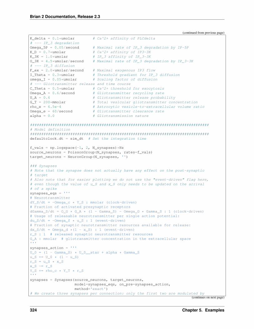
Brian 2 Documentation, Release 2.3
(continued from previous page)
K_delta = 0.1*umolar # Ca^2+ affinity of PLCdelta# --- IP_3 degradationOmega_5P = 0.05/second # Maximal rate of IP_3 degradation by IP-5PK_D = 0.7*umolar # Ca^2+ affinity of IP3-3KK_3K = 1.0*umolar # IP_3 affinity of IP_3-3KO_3K = 4.5*umolar/second # Maximal rate of IP_3 degradation by IP_3-3K# --- IP_3 diffusionF_ex = 2.0*umolar/second # Maximal exogenous IP3 flowI_Theta = 0.3*umolar # Threshold gradient for IP_3 diffusionomega_I = 0.05*umolar # Scaling factor of diffusion# --- Gliotransmitter release and time courseC_Theta = 0.5*umolar # Ca^2+ threshold for exocytosisOmega_A = 0.6/second # Gliotransmitter recycling rateU_A = 0.6 # Gliotransmitter release probabilityG_T = 200*mmolar # Total vesicular gliotransmitter concentrationrho_e = 6.5e-4 # Astrocytic vesicle-to-extracellular volume ratioOmega_e = 60/second # Gliotransmitter clearance ratealpha = 0.0 # Gliotransmission nature
################################################################################# Model definition################################################################################defaultclock.dt = sim_dt # Set the integration time
f_vals = np.logspace(-1, 2, N_synapses)*Hzsource_neurons = PoissonGroup(N_synapses, rates=f_vals)target_neurons = NeuronGroup(N_synapses, '')
### Synapses# Note that the synapse does not actually have any effect on the post-synaptic# target# Also note that for easier plotting we do not use the "event-driven" flag here,# even though the value of u_S and x_S only needs to be updated on the arrival# of a spikesynapses_eqs = '''# NeurotransmitterdY_S/dt = -Omega_c * Y_S : mmolar (clock-driven)# Fraction of activated presynaptic receptorsdGamma_S/dt = O_G * G_A * (1 - Gamma_S) - Omega_G * Gamma_S : 1 (clock-driven)# Usage of releasable neurotransmitter per single action potential:du_S/dt = -Omega_f * u_S : 1 (event-driven)# Fraction of synaptic neurotransmitter resources available for release:dx_S/dt = Omega_d *(1 - x_S) : 1 (event-driven)r_S : 1 # released synaptic neurotransmitter resourcesG_A : mmolar # gliotransmitter concentration in the extracellular space'''synapses_action = '''U_0 = (1 - Gamma_S) * U_0__star + alpha * Gamma_Su_S += U_0 * (1 - u_S)r_S = u_S * x_Sx_S -= r_SY_S += rho_c * Y_T * r_S'''synapses = Synapses(source_neurons, target_neurons,
model=synapses_eqs, on_pre=synapses_action,method='exact')
# We create three synapses per connection: only the first two are modulated by(continues on next page)
324 Chapter 5. Examples
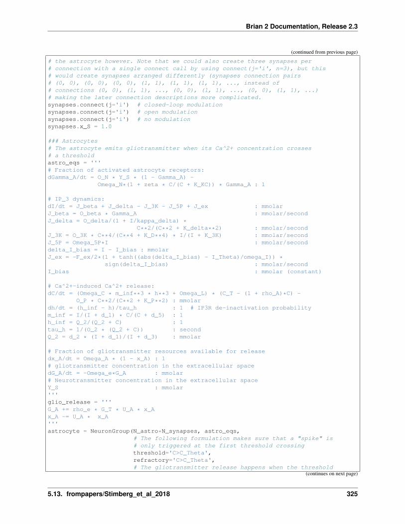
Brian 2 Documentation, Release 2.3
(continued from previous page)
# the astrocyte however. Note that we could also create three synapses per# connection with a single connect call by using connect(j='i', n=3), but this# would create synapses arranged differently (synapses connection pairs# (0, 0), (0, 0), (0, 0), (1, 1), (1, 1), (1, 1), ..., instead of# connections (0, 0), (1, 1), ..., (0, 0), (1, 1), ..., (0, 0), (1, 1), ...)# making the later connection descriptions more complicated.synapses.connect(j='i') # closed-loop modulationsynapses.connect(j='i') # open modulationsynapses.connect(j='i') # no modulationsynapses.x_S = 1.0
### Astrocytes# The astrocyte emits gliotransmitter when its Ca^2+ concentration crosses# a thresholdastro_eqs = '''# Fraction of activated astrocyte receptors:dGamma_A/dt = O_N * Y_S * (1 - Gamma_A) -
Omega_N*(1 + zeta * C/(C + K_KC)) * Gamma_A : 1
# IP_3 dynamics:dI/dt = J_beta + J_delta - J_3K - J_5P + J_ex : mmolarJ_beta = O_beta * Gamma_A : mmolar/secondJ_delta = O_delta/(1 + I/kappa_delta) *
C**2/(C**2 + K_delta**2) : mmolar/secondJ_3K = O_3K * C**4/(C**4 + K_D**4) * I/(I + K_3K) : mmolar/secondJ_5P = Omega_5P*I : mmolar/seconddelta_I_bias = I - I_bias : mmolarJ_ex = -F_ex/2*(1 + tanh((abs(delta_I_bias) - I_Theta)/omega_I)) *
sign(delta_I_bias) : mmolar/secondI_bias : mmolar (constant)
# Ca^2+-induced Ca^2+ release:dC/dt = (Omega_C * m_inf**3 * h**3 + Omega_L) * (C_T - (1 + rho_A)*C) -
O_P * C**2/(C**2 + K_P**2) : mmolardh/dt = (h_inf - h)/tau_h : 1 # IP3R de-inactivation probabilitym_inf = I/(I + d_1) * C/(C + d_5) : 1h_inf = Q_2/(Q_2 + C) : 1tau_h = 1/(O_2 * (Q_2 + C)) : secondQ_2 = d_2 * (I + d_1)/(I + d_3) : mmolar
# Fraction of gliotransmitter resources available for releasedx_A/dt = Omega_A * (1 - x_A) : 1# gliotransmitter concentration in the extracellular spacedG_A/dt = -Omega_e*G_A : mmolar# Neurotransmitter concentration in the extracellular spaceY_S : mmolar'''glio_release = '''G_A += rho_e * G_T * U_A * x_Ax_A -= U_A * x_A'''astrocyte = NeuronGroup(N_astro*N_synapses, astro_eqs,
# The following formulation makes sure that a "spike" is# only triggered at the first threshold crossingthreshold='C>C_Theta',refractory='C>C_Theta',# The gliotransmitter release happens when the threshold
(continues on next page)
5.13. frompapers/Stimberg_et_al_2018 325
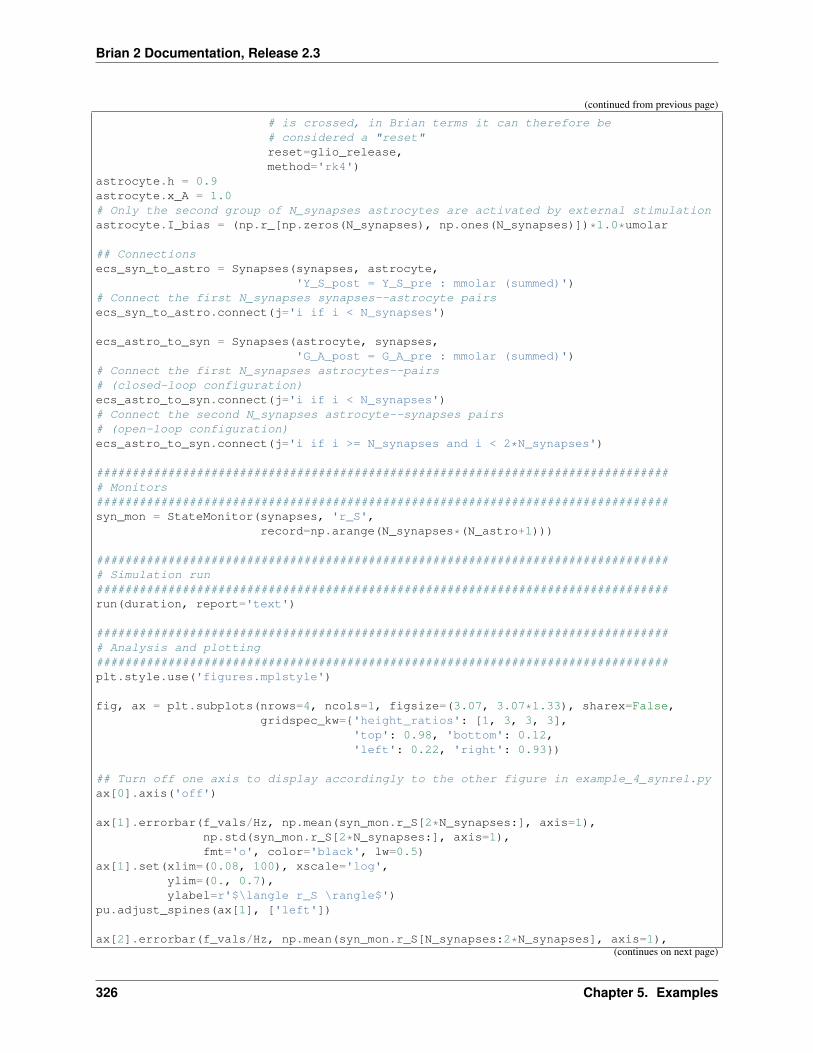
Brian 2 Documentation, Release 2.3
(continued from previous page)
# is crossed, in Brian terms it can therefore be# considered a "reset"reset=glio_release,method='rk4')
astrocyte.h = 0.9astrocyte.x_A = 1.0# Only the second group of N_synapses astrocytes are activated by external stimulationastrocyte.I_bias = (np.r_[np.zeros(N_synapses), np.ones(N_synapses)])*1.0*umolar
## Connectionsecs_syn_to_astro = Synapses(synapses, astrocyte,
'Y_S_post = Y_S_pre : mmolar (summed)')# Connect the first N_synapses synapses--astrocyte pairsecs_syn_to_astro.connect(j='i if i < N_synapses')
ecs_astro_to_syn = Synapses(astrocyte, synapses,'G_A_post = G_A_pre : mmolar (summed)')
# Connect the first N_synapses astrocytes--pairs# (closed-loop configuration)ecs_astro_to_syn.connect(j='i if i < N_synapses')# Connect the second N_synapses astrocyte--synapses pairs# (open-loop configuration)ecs_astro_to_syn.connect(j='i if i >= N_synapses and i < 2*N_synapses')
################################################################################# Monitors################################################################################syn_mon = StateMonitor(synapses, 'r_S',
record=np.arange(N_synapses*(N_astro+1)))
################################################################################# Simulation run################################################################################run(duration, report='text')
################################################################################# Analysis and plotting################################################################################plt.style.use('figures.mplstyle')
fig, ax = plt.subplots(nrows=4, ncols=1, figsize=(3.07, 3.07*1.33), sharex=False,gridspec_kw={'height_ratios': [1, 3, 3, 3],
'top': 0.98, 'bottom': 0.12,'left': 0.22, 'right': 0.93})
## Turn off one axis to display accordingly to the other figure in example_4_synrel.pyax[0].axis('off')
ax[1].errorbar(f_vals/Hz, np.mean(syn_mon.r_S[2*N_synapses:], axis=1),np.std(syn_mon.r_S[2*N_synapses:], axis=1),fmt='o', color='black', lw=0.5)
ax[1].set(xlim=(0.08, 100), xscale='log',ylim=(0., 0.7),ylabel=r'$\langle r_S \rangle$')
pu.adjust_spines(ax[1], ['left'])
ax[2].errorbar(f_vals/Hz, np.mean(syn_mon.r_S[N_synapses:2*N_synapses], axis=1),(continues on next page)
326 Chapter 5. Examples

Brian 2 Documentation, Release 2.3
(continued from previous page)
np.std(syn_mon.r_S[N_synapses:2*N_synapses], axis=1),fmt='o', color='C2', lw=0.5)
ax[2].set(xlim=(0.08, 100), xscale='log',ylim=(0., 0.2), ylabel=r'$\langle r_S \rangle$')
pu.adjust_spines(ax[2], ['left'])
ax[3].errorbar(f_vals/Hz, np.mean(syn_mon.r_S[:N_synapses], axis=1),np.std(syn_mon.r_S[:N_synapses], axis=1),fmt='o', color='C3', lw=0.5)
ax[3].set(xlim=(0.08, 100), xticks=np.logspace(-1, 2, 4), xscale='log',ylim=(0., 0.7), xlabel='input frequency (Hz)',ylabel=r'$\langle r_S \rangle$')
ax[3].xaxis.set_major_formatter(ScalarFormatter())pu.adjust_spines(ax[3], ['left', 'bottom'])
pu.adjust_ylabels(ax, x_offset=-0.2)
plt.show()
5.13.5 Example: example_4_synrel
Modeling neuron-glia interactions with the Brian 2 simulator Marcel Stimberg, Dan F. M. Goodman, Romain Brette,Maurizio De Pittà bioRxiv 198366; doi: https://doi.org/10.1101/198366
Figure 4B: Closed-loop gliotransmission.
Extracellular neurotransmitter concentration (averaged across 500 synapses) for three step increases of the presynaptic
5.13. frompapers/Stimberg_et_al_2018 327

Brian 2 Documentation, Release 2.3
rate, for three synapses: one without gliotransmission, and the other two with open- and close-loop gliotransmssion.
from brian2 import *
import plot_utils as pu
set_device('cpp_standalone', directory=None) # Use fast "C++ standalone mode"seed(16283) # to get identical figures for repeated runs
################################################################################# Model parameters################################################################################### General parametersN_synapses = 500N_astro = 2duration = 20*second # Total simulation timesim_dt = 1*ms # Integrator/sampling step
### Neuron parameters
# ### Synapse parameters### Synapse parametersrho_c = 0.005 # Synaptic vesicle-to-extracellular space volume ratioY_T = 500*mmolar # Total vesicular neurotransmitter concentrationOmega_c = 40/second # Neurotransmitter clearance rateU_0__star = 0.6 # Resting synaptic release probabilityOmega_f = 3.33/second # Synaptic facilitation rateOmega_d = 2.0/second # Synaptic depression rate# --- Presynaptic receptorsO_G = 1.5/umolar/second # Agonist binding (activating) rateOmega_G = 0.5/(60*second) # Agonist release (deactivating) rate
### Astrocyte parameters# --- Calcium fluxesO_P = 0.9*umolar/second # Maximal Ca^2+ uptake rate by SERCAsK_P = 0.05 * umolar # Ca2+ affinity of SERCAsC_T = 2*umolar # Total cell free Ca^2+ contentrho_A = 0.18 # ER-to-cytoplasm volume ratioOmega_C = 6/second # Maximal rate of Ca^2+ release by IP_3RsOmega_L = 0.1/second # Maximal rate of Ca^2+ leak from the ER# --- IP_3R kinecticsd_1 = 0.13*umolar # IP_3 binding affinityd_2 = 1.05*umolar # Ca^2+ inactivation dissociation constantO_2 = 0.2/umolar/second # IP_3R binding rate for Ca^2+ inhibitiond_3 = 0.9434*umolar # IP_3 dissociation constantd_5 = 0.08*umolar # Ca^2+ activation dissociation constant# --- IP_3 production# --- Agonist-dependent IP_3 productionO_beta = 3.2*umolar/second # Maximal rate of IP_3 production by PLCbetaO_N = 0.3/umolar/second # Agonist binding rateOmega_N = 0.5/second # Maximal inactivation rateK_KC = 0.5*umolar # Ca^2+ affinity of PKCzeta = 10 # Maximal reduction of receptor affinity by PKC# --- Endogenous IP3 productionO_delta = 0.6*umolar/second # Maximal rate of IP_3 production by PLCdeltakappa_delta = 1.5* umolar # Inhibition constant of PLC_delta by IP_3K_delta = 0.1*umolar # Ca^2+ affinity of PLCdelta# --- IP_3 diffusion
(continues on next page)
328 Chapter 5. Examples

Brian 2 Documentation, Release 2.3
(continued from previous page)
F = 2*umolar/second # GJC IP_3 permeabilityI_Theta = 0.3*umolar # Threshold gradient for IP_3 diffusionomega_I = 0.05*umolar # Scaling factor of diffusion# --- IP_3 degradationOmega_5P = 0.05/second # Maximal rate of IP_3 degradation by IP-5PK_D = 0.7*umolar # Ca^2+ affinity of IP3-3KK_3K = 1.0*umolar # IP_3 affinity of IP_3-3KO_3K = 4.5*umolar/second # Maximal rate of IP_3 degradation by IP_3-3K# --- IP_3 diffusionF_ex = 2.0*umolar/second # Maximal exogenous IP3 flowI_Theta = 0.3*umolar # Threshold gradient for IP_3 diffusionomega_I = 0.05*umolar # Scaling factor of diffusion# --- Gliotransmitter release and time courseC_Theta = 0.5*umolar # Ca^2+ threshold for exocytosisOmega_A = 0.6/second # Gliotransmitter recycling rateU_A = 0.6 # Gliotransmitter release probabilityG_T = 200*mmolar # Total vesicular gliotransmitter concentrationrho_e = 6.5e-4 # Astrocytic vesicle-to-extracellular volume ratioOmega_e = 60/second # Gliotransmitter clearance ratealpha = 0.0 # Gliotransmission nature
################################################################################# Model definition################################################################################defaultclock.dt = sim_dt # Set the integration time
# ### "Neurons"rate_in = TimedArray([0.011, 0.11, 1.1, 11] * Hz, dt=5*second)source_neurons = PoissonGroup(N_synapses, rates='rate_in(t)')target_neurons = NeuronGroup(N_synapses, '')
### Synapses# Note that the synapse does not actually have any effect on the post-synaptic# target# Also note that for easier plotting we do not use the "event-driven" flag here,# even though the value of u_S and x_S only needs to be updated on the arrival# of a spikesynapses_eqs = '''# NeurotransmitterdY_S/dt = -Omega_c * Y_S : mmolar (clock-driven)# Fraction of activated presynaptic receptorsdGamma_S/dt = O_G * G_A * (1 - Gamma_S) - Omega_G * Gamma_S : 1 (clock-driven)# Usage of releasable neurotransmitter per single action potential:du_S/dt = -Omega_f * u_S : 1 (event-driven)# Fraction of synaptic neurotransmitter resources available for release:dx_S/dt = Omega_d *(1 - x_S) : 1 (event-driven)r_S : 1 # released synaptic neurotransmitter resourcesG_A : mmolar # gliotransmitter concentration in the extracellular space'''synapses_action = '''U_0 = (1 - Gamma_S) * U_0__star + alpha * Gamma_Su_S += U_0 * (1 - u_S)r_S = u_S * x_Sx_S -= r_SY_S += rho_c * Y_T * r_S'''synapses = Synapses(source_neurons, target_neurons,
(continues on next page)
5.13. frompapers/Stimberg_et_al_2018 329
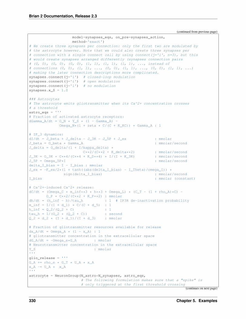
Brian 2 Documentation, Release 2.3
(continued from previous page)
model=synapses_eqs, on_pre=synapses_action,method='exact')
# We create three synapses per connection: only the first two are modulated by# the astrocyte however. Note that we could also create three synapses per# connection with a single connect call by using connect(j='i', n=3), but this# would create synapses arranged differently (synapses connection pairs# (0, 0), (0, 0), (0, 0), (1, 1), (1, 1), (1, 1), ..., instead of# connections (0, 0), (1, 1), ..., (0, 0), (1, 1), ..., (0, 0), (1, 1), ...)# making the later connection descriptions more complicated.synapses.connect(j='i') # closed-loop modulationsynapses.connect(j='i') # open modulationsynapses.connect(j='i') # no modulationsynapses.x_S = 1.0
### Astrocytes# The astrocyte emits gliotransmitter when its Ca^2+ concentration crosses# a thresholdastro_eqs = '''# Fraction of activated astrocyte receptors:dGamma_A/dt = O_N * Y_S * (1 - Gamma_A) -
Omega_N*(1 + zeta * C/(C + K_KC)) * Gamma_A : 1
# IP_3 dynamics:dI/dt = J_beta + J_delta - J_3K - J_5P + J_ex : mmolarJ_beta = O_beta * Gamma_A : mmolar/secondJ_delta = O_delta/(1 + I/kappa_delta) *
C**2/(C**2 + K_delta**2) : mmolar/secondJ_3K = O_3K * C**4/(C**4 + K_D**4) * I/(I + K_3K) : mmolar/secondJ_5P = Omega_5P*I : mmolar/seconddelta_I_bias = I - I_bias : mmolarJ_ex = -F_ex/2*(1 + tanh((abs(delta_I_bias) - I_Theta)/omega_I)) *
sign(delta_I_bias) : mmolar/secondI_bias : mmolar (constant)
# Ca^2+-induced Ca^2+ release:dC/dt = (Omega_C * m_inf**3 * h**3 + Omega_L) * (C_T - (1 + rho_A)*C) -
O_P * C**2/(C**2 + K_P**2) : mmolardh/dt = (h_inf - h)/tau_h : 1 # IP3R de-inactivation probabilitym_inf = I/(I + d_1) * C/(C + d_5) : 1h_inf = Q_2/(Q_2 + C) : 1tau_h = 1/(O_2 * (Q_2 + C)) : secondQ_2 = d_2 * (I + d_1)/(I + d_3) : mmolar
# Fraction of gliotransmitter resources available for releasedx_A/dt = Omega_A * (1 - x_A) : 1# gliotransmitter concentration in the extracellular spacedG_A/dt = -Omega_e*G_A : mmolar# Neurotransmitter concentration in the extracellular spaceY_S : mmolar'''glio_release = '''G_A += rho_e * G_T * U_A * x_Ax_A -= U_A * x_A'''astrocyte = NeuronGroup(N_astro*N_synapses, astro_eqs,
# The following formulation makes sure that a "spike" is# only triggered at the first threshold crossing
(continues on next page)
330 Chapter 5. Examples
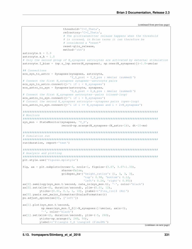
Brian 2 Documentation, Release 2.3
(continued from previous page)
threshold='C>C_Theta',refractory='C>C_Theta',# The gliotransmitter release happens when the threshold# is crossed, in Brian terms it can therefore be# considered a "reset"reset=glio_release,method='rk4')
astrocyte.h = 0.9astrocyte.x_A = 1.0# Only the second group of N_synapses astrocytes are activated by external stimulationastrocyte.I_bias = (np.r_[np.zeros(N_synapses), np.ones(N_synapses)])*1.0*umolar
## Connectionsecs_syn_to_astro = Synapses(synapses, astrocyte,
'Y_S_post = Y_S_pre : mmolar (summed)')# Connect the first N_synapses synapses--astrocyte pairsecs_syn_to_astro.connect(j='i if i < N_synapses')ecs_astro_to_syn = Synapses(astrocyte, synapses,
'G_A_post = G_A_pre : mmolar (summed)')# Connect the first N_synapses astrocytes--pairs (closed-loop)ecs_astro_to_syn.connect(j='i if i < N_synapses')# Connect the second N_synapses astrocyte--synapses pairs (open-loop)ecs_astro_to_syn.connect(j='i if i >= N_synapses and i < 2*N_synapses')
################################################################################# Monitors################################################################################syn_mon = StateMonitor(synapses, 'Y_S',
record=np.arange(N_synapses*(N_astro+1)), dt=10*ms)
################################################################################# Simulation run################################################################################run(duration, report='text')
################################################################################# Analysis and plotting################################################################################plt.style.use('figures.mplstyle')
fig, ax = plt.subplots(nrows=4, ncols=1, figsize=(3.07, 3.07*1.33),sharex=False,gridspec_kw={'height_ratios': [1, 3, 3, 3],
'top': 0.98, 'bottom': 0.12,'left': 0.24, 'right': 0.95})
ax[0].semilogy(syn_mon.t/second, rate_in(syn_mon.t), '-', color='black')ax[0].set(xlim=(0, duration/second), ylim=(0.01, 12),
yticks=[0.01, 0.1, 1, 10], ylabel=r'$\nu_{in}$ (Hz)')ax[0].yaxis.set_major_formatter(ScalarFormatter())pu.adjust_spines(ax[0], ['left'])
ax[1].plot(syn_mon.t/second,np.mean(syn_mon.Y_S[2*N_synapses:]/umolar, axis=0),'-', color='black')
ax[1].set(xlim=(0, duration/second), ylim=(-5, 260),yticks=np.arange(0, 260, 50),ylabel=r'$\langle Y_S \rangle$ ($\mu$M)')
(continues on next page)
5.13. frompapers/Stimberg_et_al_2018 331
Brian 2 Documentation, Release 2.3
(continued from previous page)
ax[1].legend(['no gliotransmission'], loc='upper left')pu.adjust_spines(ax[1], ['left'])
ax[2].plot(syn_mon.t/second,np.mean(syn_mon.Y_S[N_synapses:2*N_synapses]/umolar, axis=0),'-', color='C2')
ax[2].set(xlim=(0, duration/second), ylim=(-3, 150),yticks=np.arange(0, 151, 25),ylabel=r'$\langle Y_S \rangle$ ($\mu$M)')
ax[2].legend(['open-loop gliotransmission'], loc='upper left')pu.adjust_spines(ax[2], ['left'])
ax[3].plot(syn_mon.t/second,np.mean(syn_mon.Y_S[:N_synapses]/umolar, axis=0),'-', color='C3')
ax[3].set(xlim=(0, duration/second), ylim=(-2, 150),xticks=np.arange(0., duration/second+1, 5.0),yticks=np.arange(0, 151, 25),xlabel='time (s)', ylabel=r'$\langle Y_S \rangle$ ($\mu$M)')
ax[3].legend(['closed-loop gliotransmission'], loc='upper left')pu.adjust_spines(ax[3], ['left', 'bottom'])
pu.adjust_ylabels(ax, x_offset=-0.22)
plt.show()
332 Chapter 5. Examples
Brian 2 Documentation, Release 2.3
5.13.6 Example: example_5_astro_ring
Modeling neuron-glia interactions with the Brian 2 simulator Marcel Stimberg, Dan F. M. Goodman, Romain Brette,Maurizio De Pittà bioRxiv 198366; doi: https://doi.org/10.1101/198366
Figure 5: Astrocytes connected in a network.
Intercellular calcium wave propagation in a ring of 50 astrocytes connected by bidirectional gap junctions (see Gold-berg et al., 2010)
from brian2 import *
import plot_utils as pu
set_device('cpp_standalone', directory=None) # Use fast "C++ standalone mode"
################################################################################# Model parameters################################################################################### General parametersduration = 4000*second # Total simulation timesim_dt = 50*ms # Integrator/sampling step
### Astrocyte parameters# --- Calcium fluxesO_P = 0.9*umolar/second # Maximal Ca^2+ uptake rate by SERCAsK_P = 0.05 * umolar # Ca2+ affinity of SERCAsC_T = 2*umolar # Total cell free Ca^2+ contentrho_A = 0.18 # ER-to-cytoplasm volume ratioOmega_C = 6/second # Maximal rate of Ca^2+ release by IP_3RsOmega_L = 0.1/second # Maximal rate of Ca^2+ leak from the ER# --- IP_3R kinecticsd_1 = 0.13*umolar # IP_3 binding affinityd_2 = 1.05*umolar # Ca^2+ inactivation dissociation constantO_2 = 0.2/umolar/second # IP_3R binding rate for Ca^2+ inhibitiond_3 = 0.9434*umolar # IP_3 dissociation constantd_5 = 0.08*umolar # Ca^2+ activation dissociation constant# --- IP_3 productionO_delta = 0.6*umolar/second # Maximal rate of IP_3 production by PLCdeltakappa_delta = 1.5* umolar # Inhibition constant of PLC_delta by IP_3K_delta = 0.1*umolar # Ca^2+ affinity of PLCdelta# --- IP_3 degradationOmega_5P = 0.05/second # Maximal rate of IP_3 degradation by IP-5PK_D = 0.7*umolar # Ca^2+ affinity of IP3-3KK_3K = 1.0*umolar # IP_3 affinity of IP_3-3KO_3K = 4.5*umolar/second # Maximal rate of IP_3 degradation by IP_3-3K# --- IP_3 diffusionF_ex = 0.09*umolar/second # Maximal exogenous IP3 flowF = 0.09*umolar/second # GJC IP_3 permeabilityI_Theta = 0.3*umolar # Threshold gradient for IP_3 diffusionomega_I = 0.05*umolar # Scaling factor of diffusion
################################################################################# Model definition################################################################################defaultclock.dt = sim_dt # Set the integration time
(continues on next page)
5.13. frompapers/Stimberg_et_al_2018 333

Brian 2 Documentation, Release 2.3
(continued from previous page)
### Astrocytesastro_eqs = '''dI/dt = J_delta - J_3K - J_5P + J_ex + J_coupling : mmolarJ_delta = O_delta/(1 + I/kappa_delta) * C**2/(C**2 + K_delta**2) : mmolar/secondJ_3K = O_3K * C**4/(C**4 + K_D**4) * I/(I + K_3K) : mmolar/secondJ_5P = Omega_5P*I : mmolar/second# Exogenous stimulation (rectangular wave with period of 50s and duty factor 0.4)stimulus = int((t % (50*second))<20*second) : 1delta_I_bias = I - I_bias*stimulus : mmolarJ_ex = -F_ex/2*(1 + tanh((abs(delta_I_bias) - I_Theta)/omega_I)) *
sign(delta_I_bias) : mmolar/second# Diffusion between astrocytesJ_coupling : mmolar/second
# Ca^2+-induced Ca^2+ release:dC/dt = J_r + J_l - J_p : mmolardh/dt = (h_inf - h)/tau_h : 1J_r = (Omega_C * m_inf**3 * h**3) * (C_T - (1 + rho_A)*C) : mmolar/secondJ_l = Omega_L * (C_T - (1 + rho_A)*C) : mmolar/secondJ_p = O_P * C**2/(C**2 + K_P**2) : mmolar/secondm_inf = I/(I + d_1) * C/(C + d_5) : 1h_inf = Q_2/(Q_2 + C) : 1tau_h = 1/(O_2 * (Q_2 + C)) : secondQ_2 = d_2 * (I + d_1)/(I + d_3) : mmolar
# External IP_3 driveI_bias : mmolar (constant)'''
N_astro = 50 # Total number of astrocytes in the networkastrocytes = NeuronGroup(N_astro, astro_eqs, method='rk4')# Asymmetric stimulation on the 50th cell to get some nice chaotic patternsastrocytes.I_bias[N_astro//2] = 1.0*umolarastrocytes.h = 0.9# Diffusion between astrocytesastro_to_astro_eqs = '''delta_I = I_post - I_pre : mmolarJ_coupling_post = -F/2 * (1 + tanh((abs(delta_I) - I_Theta)/omega_I)) *
sign(delta_I) : mmolar/second (summed)'''astro_to_astro = Synapses(astrocytes, astrocytes,
model=astro_to_astro_eqs)# Couple neighboring astrocytes: two connections per astrocyte pair, as# the above formulation will only update the I_coupling term of one of the# astrocytesastro_to_astro.connect('j == (i + 1) % N_pre or '
'j == (i + N_pre - 1) % N_pre')
################################################################################# Monitors################################################################################astro_mon = StateMonitor(astrocytes, variables=['C'], record=True)
################################################################################# Simulation run################################################################################run(duration, report='text')
(continues on next page)
334 Chapter 5. Examples

Brian 2 Documentation, Release 2.3
(continued from previous page)
################################################################################# Analysis and plotting################################################################################plt.style.use('figures.mplstyle')
fig, ax = plt.subplots(nrows=1, ncols=1, figsize=(6.26894, 6.26894 * 0.66),gridspec_kw={'left': 0.1, 'bottom': 0.12})
scaling = 1.2step = 10ax.plot(astro_mon.t/second,
(astro_mon.C[0:N_astro//2-1].T/astro_mon.C.max() +np.arange(N_astro//2-1)*scaling), color='black')
ax.plot(astro_mon.t/second, (astro_mon.C[N_astro//2:].T/astro_mon.C.max() +np.arange(N_astro//2, N_astro)*scaling),
color='black')ax.plot(astro_mon.t/second, (astro_mon.C[N_astro//2-1].T/astro_mon.C.max() +
np.arange(N_astro//2-1, N_astro//2)*scaling),color='C0')
ax.set(xlim=(0., duration/second), ylim=(0, (N_astro+1.5)*scaling),xticks=np.arange(0., duration/second, 500), xlabel='time (s)',yticks=np.arange(0.5*scaling, (N_astro + 1.5)*scaling, step*scaling),yticklabels=[str(yt) for yt in np.arange(0, N_astro + 1, step)],ylabel='$C/C_{max}$ (cell index)')
pu.adjust_spines(ax, ['left', 'bottom'])
pu.adjust_ylabels([ax], x_offset=-0.08)
plt.show()
5.13. frompapers/Stimberg_et_al_2018 335

Brian 2 Documentation, Release 2.3
5.13.7 Example: example_6_COBA_with_astro
Modeling neuron-glia interactions with the Brian 2 simulator Marcel Stimberg, Dan F. M. Goodman, Romain Brette,Maurizio De Pittà bioRxiv 198366; doi: https://doi.org/10.1101/198366
Figure 6: Recurrent neuron-glial network.
Randomly connected COBA network (see Brunel, 2000) with excitatory synapses modulated by release-increasinggliotransmission from a randomly connected network of astrocytes.
from brian2 import *
import plot_utils as pu
set_device('cpp_standalone', directory=None) # Use fast "C++ standalone mode"seed(28371) # to get identical figures for repeated runs
################################################################################# Model parameters################################################################################### General parametersN_e = 3200 # Number of excitatory neuronsN_i = 800 # Number of inhibitory neuronsN_a = 3200 # Number of astrocytes
## Some metrics parameters needed to establish proper connectionssize = 3.75*mmeter # Length and width of the square latticedistance = 50*umeter # Distance between neurons
### Neuron parametersE_l = -60*mV # Leak reversal potentialg_l = 9.99*nS # Leak conductanceE_e = 0*mV # Excitatory synaptic reversal potentialE_i = -80*mV # Inhibitory synaptic reversal potentialC_m = 198*pF # Membrane capacitancetau_e = 5*ms # Excitatory synaptic time constanttau_i = 10*ms # Inhibitory synaptic time constanttau_r = 5*ms # Refractory periodI_ex = 100*pA # External currentV_th = -50*mV # Firing thresholdV_r = E_l # Reset potential
### Synapse parametersrho_c = 0.005 # Synaptic vesicle-to-extracellular space volume ratioY_T = 500.*mmolar # Total vesicular neurotransmitter concentrationOmega_c = 40/second # Neurotransmitter clearance rateU_0__star = 0.6 # Resting synaptic release probabilityOmega_f = 3.33/second # Synaptic facilitation rateOmega_d = 2.0/second # Synaptic depression ratew_e = 0.05*nS # Excitatory synaptic conductancew_i = 1.0*nS # Inhibitory synaptic conductance# --- Presynaptic receptorsO_G = 1.5/umolar/second # Agonist binding (activating) rateOmega_G = 0.5/(60*second) # Agonist release (deactivating) rate
### Astrocyte parameters# --- Calcium fluxes
(continues on next page)
336 Chapter 5. Examples

Brian 2 Documentation, Release 2.3
(continued from previous page)
O_P = 0.9*umolar/second # Maximal Ca^2+ uptake rate by SERCAsK_P = 0.05*umolar # Ca2+ affinity of SERCAsC_T = 2*umolar # Total cell free Ca^2+ contentrho_A = 0.18 # ER-to-cytoplasm volume ratioOmega_C = 6/second # Maximal rate of Ca^2+ release by IP_3RsOmega_L = 0.1/second # Maximal rate of Ca^2+ leak from the ER# --- IP_3R kinecticsd_1 = 0.13*umolar # IP_3 binding affinityd_2 = 1.05*umolar # Ca^2+ inactivation dissociation constantO_2 = 0.2/umolar/second # IP_3R binding rate for Ca^2+ inhibitiond_3 = 0.9434*umolar # IP_3 dissociation constantd_5 = 0.08*umolar # Ca^2+ activation dissociation constant# --- IP_3 production# --- Agonist-dependent IP_3 productionO_beta = 0.5*umolar/second # Maximal rate of IP_3 production by PLCbetaO_N = 0.3/umolar/second # Agonist binding rateOmega_N = 0.5/second # Maximal inactivation rateK_KC = 0.5*umolar # Ca^2+ affinity of PKCzeta = 10 # Maximal reduction of receptor affinity by PKC# --- Endogenous IP3 productionO_delta = 1.2*umolar/second # Maximal rate of IP_3 production by PLCdeltakappa_delta = 1.5*umolar # Inhibition constant of PLC_delta by IP_3K_delta = 0.1*umolar # Ca^2+ affinity of PLCdelta# --- IP_3 degradationOmega_5P = 0.05/second # Maximal rate of IP_3 degradation by IP-5PK_D = 0.7*umolar # Ca^2+ affinity of IP3-3KK_3K = 1.0*umolar # IP_3 affinity of IP_3-3KO_3K = 4.5*umolar/second # Maximal rate of IP_3 degradation by IP_3-3K# --- IP_3 diffusionF = 0.09*umolar/second # GJC IP_3 permeabilityI_Theta = 0.3*umolar # Threshold gradient for IP_3 diffusionomega_I = 0.05*umolar # Scaling factor of diffusion# --- Gliotransmitter release and time courseC_Theta = 0.5*umolar # Ca^2+ threshold for exocytosisOmega_A = 0.6/second # Gliotransmitter recycling rateU_A = 0.6 # Gliotransmitter release probabilityG_T = 200*mmolar # Total vesicular gliotransmitter concentrationrho_e = 6.5e-4 # Astrocytic vesicle-to-extracellular volume ratioOmega_e = 60/second # Gliotransmitter clearance ratealpha = 0.0 # Gliotransmission nature
################################################################################# Define HF stimulus################################################################################stimulus = TimedArray([1.0, 1.2, 1.0, 1.0], dt=2*second)
################################################################################# Simulation time (based on the stimulus)################################################################################duration = 8*second # Total simulation time
################################################################################# Model definition################################################################################### Neuronsneuron_eqs = '''dv/dt = (g_l*(E_l-v) + g_e*(E_e-v) + g_i*(E_i-v) + I_ex*stimulus(t))/C_m : volt→˓(unless refractory) (continues on next page)
5.13. frompapers/Stimberg_et_al_2018 337
Brian 2 Documentation, Release 2.3
(continued from previous page)
dg_e/dt = -g_e/tau_e : siemens # post-synaptic excitatory conductancedg_i/dt = -g_i/tau_i : siemens # post-synaptic inhibitory conductance# Neuron position in spacex : meter (constant)y : meter (constant)'''neurons = NeuronGroup(N_e + N_i, model=neuron_eqs,
threshold='v>V_th', reset='v=V_r',refractory='tau_r', method='euler')
exc_neurons = neurons[:N_e]inh_neurons = neurons[N_e:]# Arrange excitatory neurons in a gridN_rows = int(sqrt(N_e))N_cols = N_e//N_rowsgrid_dist = (size / N_cols)exc_neurons.x = '(i // N_rows)*grid_dist - N_rows/2.0*grid_dist'exc_neurons.y = '(i % N_rows)*grid_dist - N_cols/2.0*grid_dist'# Random initial membrane potential values and conductancesneurons.v = 'E_l + rand()*(V_th-E_l)'neurons.g_e = 'rand()*w_e'neurons.g_i = 'rand()*w_i'
### Synapsessynapses_eqs = '''# NeurotransmitterdY_S/dt = -Omega_c * Y_S : mmolar (clock-driven)# Fraction of activated presynaptic receptorsdGamma_S/dt = O_G * G_A * (1 - Gamma_S) - Omega_G * Gamma_S : 1 (clock-driven)# Usage of releasable neurotransmitter per single action potential:du_S/dt = -Omega_f * u_S : 1 (event-driven)# Fraction of synaptic neurotransmitter resources available for release:dx_S/dt = Omega_d *(1 - x_S) : 1 (event-driven)U_0 : 1# released synaptic neurotransmitter resources:r_S : 1# gliotransmitter concentration in the extracellular space:G_A : mmolar# which astrocyte covers this synapse ?astrocyte_index : integer (constant)'''synapses_action = '''U_0 = (1 - Gamma_S) * U_0__star + alpha * Gamma_Su_S += U_0 * (1 - u_S)r_S = u_S * x_Sx_S -= r_SY_S += rho_c * Y_T * r_S'''exc_syn = Synapses(exc_neurons, neurons, model=synapses_eqs,
on_pre=synapses_action+'g_e_post += w_e*r_S',method='exact')
exc_syn.connect(True, p=0.05)exc_syn.x_S = 1.0inh_syn = Synapses(inh_neurons, neurons, model=synapses_eqs,
on_pre=synapses_action+'g_i_post += w_i*r_S',method='exact')
inh_syn.connect(True, p=0.2)inh_syn.x_S = 1.0
(continues on next page)
338 Chapter 5. Examples
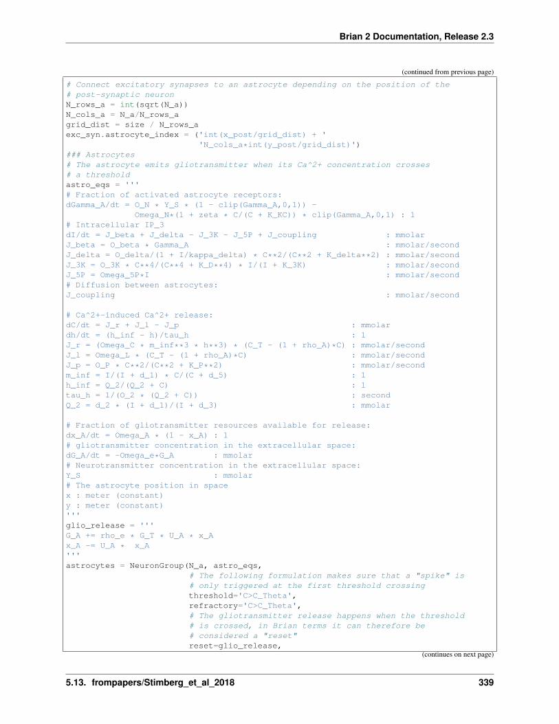
Brian 2 Documentation, Release 2.3
(continued from previous page)
# Connect excitatory synapses to an astrocyte depending on the position of the# post-synaptic neuronN_rows_a = int(sqrt(N_a))N_cols_a = N_a/N_rows_agrid_dist = size / N_rows_aexc_syn.astrocyte_index = ('int(x_post/grid_dist) + '
'N_cols_a*int(y_post/grid_dist)')### Astrocytes# The astrocyte emits gliotransmitter when its Ca^2+ concentration crosses# a thresholdastro_eqs = '''# Fraction of activated astrocyte receptors:dGamma_A/dt = O_N * Y_S * (1 - clip(Gamma_A,0,1)) -
Omega_N*(1 + zeta * C/(C + K_KC)) * clip(Gamma_A,0,1) : 1# Intracellular IP_3dI/dt = J_beta + J_delta - J_3K - J_5P + J_coupling : mmolarJ_beta = O_beta * Gamma_A : mmolar/secondJ_delta = O_delta/(1 + I/kappa_delta) * C**2/(C**2 + K_delta**2) : mmolar/secondJ_3K = O_3K * C**4/(C**4 + K_D**4) * I/(I + K_3K) : mmolar/secondJ_5P = Omega_5P*I : mmolar/second# Diffusion between astrocytes:J_coupling : mmolar/second
# Ca^2+-induced Ca^2+ release:dC/dt = J_r + J_l - J_p : mmolardh/dt = (h_inf - h)/tau_h : 1J_r = (Omega_C * m_inf**3 * h**3) * (C_T - (1 + rho_A)*C) : mmolar/secondJ_l = Omega_L * (C_T - (1 + rho_A)*C) : mmolar/secondJ_p = O_P * C**2/(C**2 + K_P**2) : mmolar/secondm_inf = I/(I + d_1) * C/(C + d_5) : 1h_inf = Q_2/(Q_2 + C) : 1tau_h = 1/(O_2 * (Q_2 + C)) : secondQ_2 = d_2 * (I + d_1)/(I + d_3) : mmolar
# Fraction of gliotransmitter resources available for release:dx_A/dt = Omega_A * (1 - x_A) : 1# gliotransmitter concentration in the extracellular space:dG_A/dt = -Omega_e*G_A : mmolar# Neurotransmitter concentration in the extracellular space:Y_S : mmolar# The astrocyte position in spacex : meter (constant)y : meter (constant)'''glio_release = '''G_A += rho_e * G_T * U_A * x_Ax_A -= U_A * x_A'''astrocytes = NeuronGroup(N_a, astro_eqs,
# The following formulation makes sure that a "spike" is# only triggered at the first threshold crossingthreshold='C>C_Theta',refractory='C>C_Theta',# The gliotransmitter release happens when the threshold# is crossed, in Brian terms it can therefore be# considered a "reset"reset=glio_release,
(continues on next page)
5.13. frompapers/Stimberg_et_al_2018 339

Brian 2 Documentation, Release 2.3
(continued from previous page)
method='rk4',dt=1e-2*second)
# Arrange astrocytes in a gridastrocytes.x = '(i // N_rows_a)*grid_dist - N_rows_a/2.0*grid_dist'astrocytes.y = '(i % N_rows_a)*grid_dist - N_cols_a/2.0*grid_dist'# Add random initializationastrocytes.C = 0.01*umolarastrocytes.h = 0.9astrocytes.I = 0.01*umolarastrocytes.x_A = 1.0
ecs_astro_to_syn = Synapses(astrocytes, exc_syn,'G_A_post = G_A_pre : mmolar (summed)')
ecs_astro_to_syn.connect('i == astrocyte_index_post')ecs_syn_to_astro = Synapses(exc_syn, astrocytes,
'Y_S_post = Y_S_pre/N_incoming : mmolar (summed)')ecs_syn_to_astro.connect('astrocyte_index_pre == j')# Diffusion between astrocytesastro_to_astro_eqs = '''delta_I = I_post - I_pre : mmolarJ_coupling_post = -(1 + tanh((abs(delta_I) - I_Theta)/omega_I))*
sign(delta_I)*F/2 : mmolar/second (summed)'''astro_to_astro = Synapses(astrocytes, astrocytes,
model=astro_to_astro_eqs)# Connect to all astrocytes less than 75um away# (about 4 connections per astrocyte)astro_to_astro.connect('i != j and '
'sqrt((x_pre-x_post)**2 +'' (y_pre-y_post)**2) < 75*um')
################################################################################# Monitors################################################################################# Note that we could use a single monitor for all neurons instead, but this# way plotting is a bit easier in the endexc_mon = SpikeMonitor(exc_neurons)inh_mon = SpikeMonitor(inh_neurons)ast_mon = SpikeMonitor(astrocytes)
################################################################################# Simulation run################################################################################run(duration, report='text')
################################################################################# Plot of Spiking activity################################################################################plt.style.use('figures.mplstyle')
fig, ax = plt.subplots(nrows=3, ncols=1, sharex=True, figsize=(6.26894, 6.26894*0.8),gridspec_kw={'height_ratios': [1, 6, 2],
'left': 0.12, 'top': 0.97})time_range = np.linspace(0, duration/second, duration/second*100)*secondax[0].plot(time_range, I_ex*stimulus(time_range)/pA, 'k')ax[0].set(xlim=(0, duration/second), ylim=(98, 122),
yticks=[100, 120], ylabel='$I_{ex}$ (pA)')(continues on next page)
340 Chapter 5. Examples
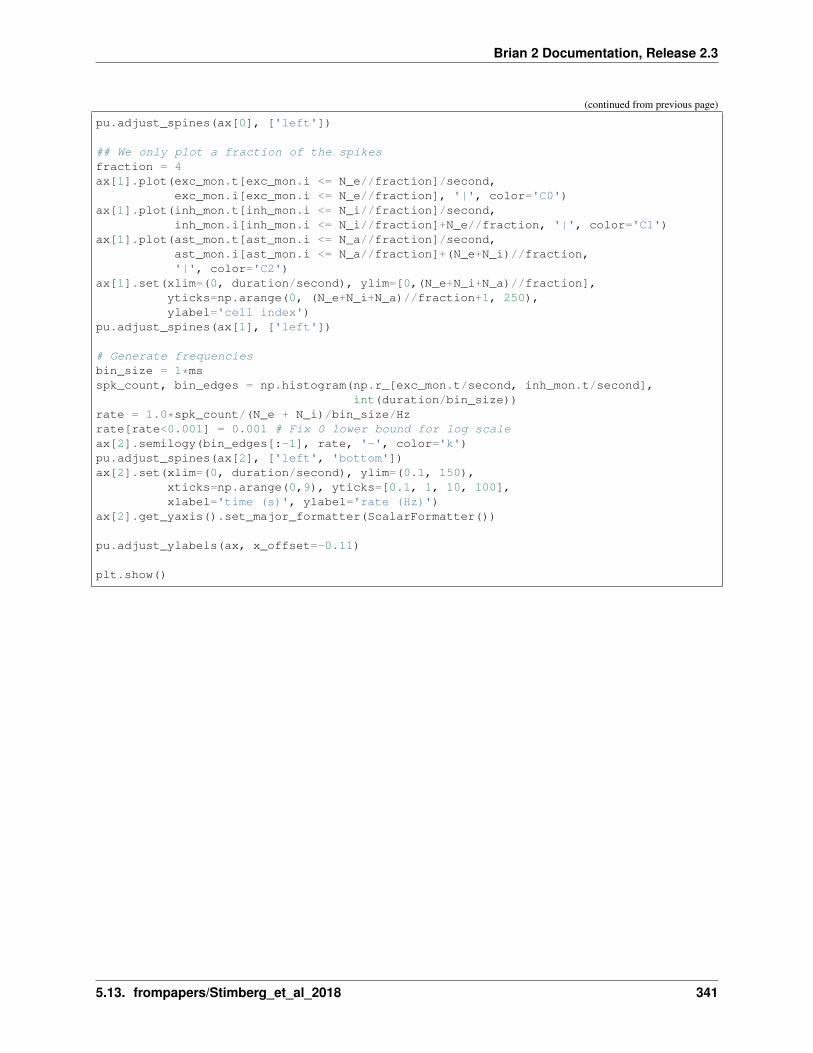
Brian 2 Documentation, Release 2.3
(continued from previous page)
pu.adjust_spines(ax[0], ['left'])
## We only plot a fraction of the spikesfraction = 4ax[1].plot(exc_mon.t[exc_mon.i <= N_e//fraction]/second,
exc_mon.i[exc_mon.i <= N_e//fraction], '|', color='C0')ax[1].plot(inh_mon.t[inh_mon.i <= N_i//fraction]/second,
inh_mon.i[inh_mon.i <= N_i//fraction]+N_e//fraction, '|', color='C1')ax[1].plot(ast_mon.t[ast_mon.i <= N_a//fraction]/second,
ast_mon.i[ast_mon.i <= N_a//fraction]+(N_e+N_i)//fraction,'|', color='C2')
ax[1].set(xlim=(0, duration/second), ylim=[0,(N_e+N_i+N_a)//fraction],yticks=np.arange(0, (N_e+N_i+N_a)//fraction+1, 250),ylabel='cell index')
pu.adjust_spines(ax[1], ['left'])
# Generate frequenciesbin_size = 1*msspk_count, bin_edges = np.histogram(np.r_[exc_mon.t/second, inh_mon.t/second],
int(duration/bin_size))rate = 1.0*spk_count/(N_e + N_i)/bin_size/Hzrate[rate<0.001] = 0.001 # Fix 0 lower bound for log scaleax[2].semilogy(bin_edges[:-1], rate, '-', color='k')pu.adjust_spines(ax[2], ['left', 'bottom'])ax[2].set(xlim=(0, duration/second), ylim=(0.1, 150),
xticks=np.arange(0,9), yticks=[0.1, 1, 10, 100],xlabel='time (s)', ylabel='rate (Hz)')
ax[2].get_yaxis().set_major_formatter(ScalarFormatter())
pu.adjust_ylabels(ax, x_offset=-0.11)
plt.show()
5.13. frompapers/Stimberg_et_al_2018 341

Brian 2 Documentation, Release 2.3
5.13.8 Example: plot_utils
Module with useful functions for making publication-ready plots.
def adjust_spines(ax, spines, position=5, smart_bounds=False):"""Set custom visibility and position of axes
ax : AxesAxes handle
spines : ListString list of 'left', 'bottom', 'right', 'top' spines to show
position : IntegerNumber of points for position of axis
"""for loc, spine in ax.spines.items():
if loc in spines:spine.set_position(('outward', position))spine.set_smart_bounds(smart_bounds)
else:spine.set_color('none') # don't draw spine
(continues on next page)
342 Chapter 5. Examples
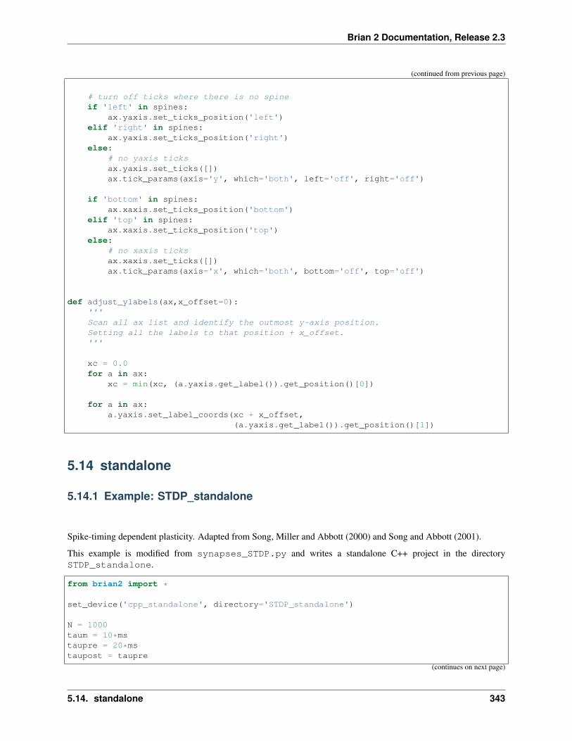
Brian 2 Documentation, Release 2.3
(continued from previous page)
# turn off ticks where there is no spineif 'left' in spines:
ax.yaxis.set_ticks_position('left')elif 'right' in spines:
ax.yaxis.set_ticks_position('right')else:
# no yaxis ticksax.yaxis.set_ticks([])ax.tick_params(axis='y', which='both', left='off', right='off')
if 'bottom' in spines:ax.xaxis.set_ticks_position('bottom')
elif 'top' in spines:ax.xaxis.set_ticks_position('top')
else:# no xaxis ticksax.xaxis.set_ticks([])ax.tick_params(axis='x', which='both', bottom='off', top='off')
def adjust_ylabels(ax,x_offset=0):'''Scan all ax list and identify the outmost y-axis position.Setting all the labels to that position + x_offset.'''
xc = 0.0for a in ax:
xc = min(xc, (a.yaxis.get_label()).get_position()[0])
for a in ax:a.yaxis.set_label_coords(xc + x_offset,
(a.yaxis.get_label()).get_position()[1])
5.14 standalone
5.14.1 Example: STDP_standalone
Spike-timing dependent plasticity. Adapted from Song, Miller and Abbott (2000) and Song and Abbott (2001).
This example is modified from synapses_STDP.py and writes a standalone C++ project in the directorySTDP_standalone.
from brian2 import *
set_device('cpp_standalone', directory='STDP_standalone')
N = 1000taum = 10*mstaupre = 20*mstaupost = taupre
(continues on next page)
5.14. standalone 343
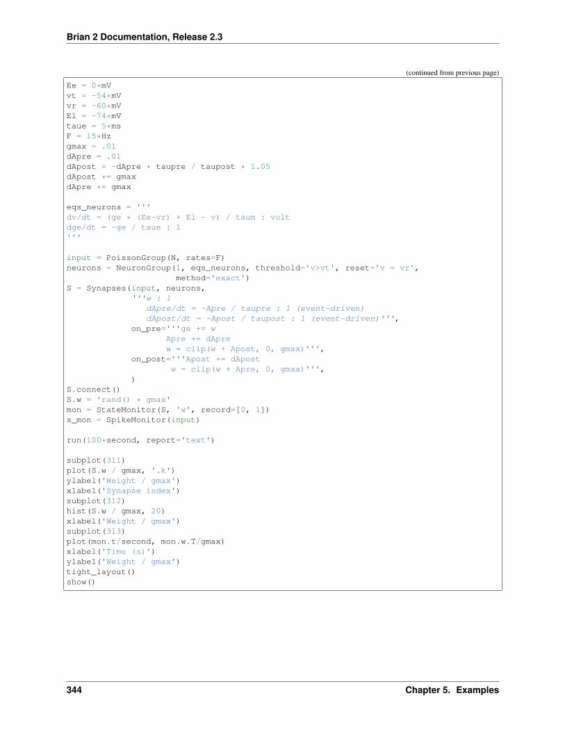
Brian 2 Documentation, Release 2.3
(continued from previous page)
Ee = 0*mVvt = -54*mVvr = -60*mVEl = -74*mVtaue = 5*msF = 15*Hzgmax = .01dApre = .01dApost = -dApre * taupre / taupost * 1.05dApost *= gmaxdApre *= gmax
eqs_neurons = '''dv/dt = (ge * (Ee-vr) + El - v) / taum : voltdge/dt = -ge / taue : 1'''
input = PoissonGroup(N, rates=F)neurons = NeuronGroup(1, eqs_neurons, threshold='v>vt', reset='v = vr',
method='exact')S = Synapses(input, neurons,
'''w : 1dApre/dt = -Apre / taupre : 1 (event-driven)dApost/dt = -Apost / taupost : 1 (event-driven)''',
on_pre='''ge += wApre += dAprew = clip(w + Apost, 0, gmax)''',
on_post='''Apost += dApostw = clip(w + Apre, 0, gmax)''',
)S.connect()S.w = 'rand() * gmax'mon = StateMonitor(S, 'w', record=[0, 1])s_mon = SpikeMonitor(input)
run(100*second, report='text')
subplot(311)plot(S.w / gmax, '.k')ylabel('Weight / gmax')xlabel('Synapse index')subplot(312)hist(S.w / gmax, 20)xlabel('Weight / gmax')subplot(313)plot(mon.t/second, mon.w.T/gmax)xlabel('Time (s)')ylabel('Weight / gmax')tight_layout()show()
344 Chapter 5. Examples
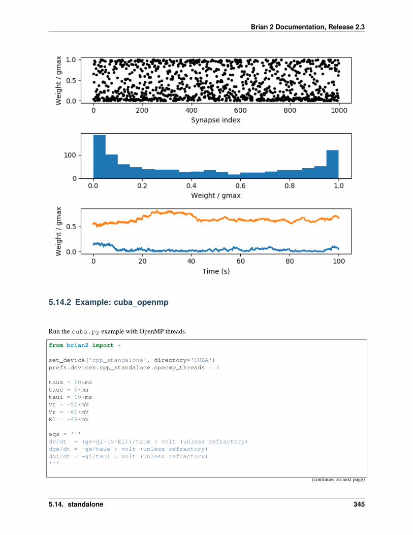
Brian 2 Documentation, Release 2.3
5.14.2 Example: cuba_openmp
Run the cuba.py example with OpenMP threads.
from brian2 import *
set_device('cpp_standalone', directory='CUBA')prefs.devices.cpp_standalone.openmp_threads = 4
taum = 20*mstaue = 5*mstaui = 10*msVt = -50*mVVr = -60*mVEl = -49*mV
eqs = '''dv/dt = (ge+gi-(v-El))/taum : volt (unless refractory)dge/dt = -ge/taue : volt (unless refractory)dgi/dt = -gi/taui : volt (unless refractory)'''
(continues on next page)
5.14. standalone 345
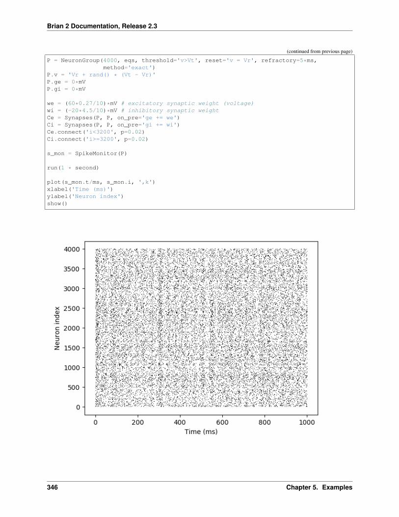
Brian 2 Documentation, Release 2.3
(continued from previous page)
P = NeuronGroup(4000, eqs, threshold='v>Vt', reset='v = Vr', refractory=5*ms,method='exact')
P.v = 'Vr + rand() * (Vt - Vr)'P.ge = 0*mVP.gi = 0*mV
we = (60*0.27/10)*mV # excitatory synaptic weight (voltage)wi = (-20*4.5/10)*mV # inhibitory synaptic weightCe = Synapses(P, P, on_pre='ge += we')Ci = Synapses(P, P, on_pre='gi += wi')Ce.connect('i<3200', p=0.02)Ci.connect('i>=3200', p=0.02)
s_mon = SpikeMonitor(P)
run(1 * second)
plot(s_mon.t/ms, s_mon.i, ',k')xlabel('Time (ms)')ylabel('Neuron index')show()
346 Chapter 5. Examples
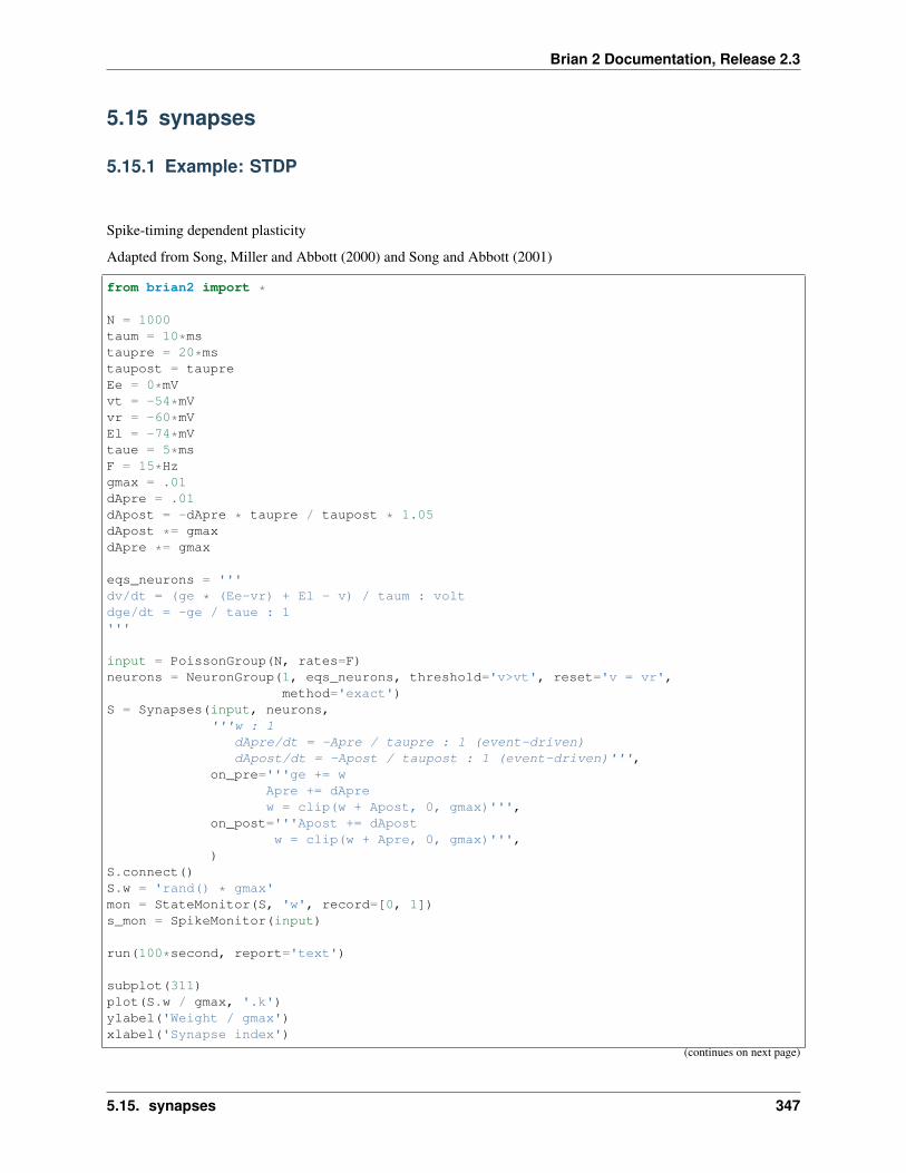
Brian 2 Documentation, Release 2.3
5.15 synapses
5.15.1 Example: STDP
Spike-timing dependent plasticity
Adapted from Song, Miller and Abbott (2000) and Song and Abbott (2001)
from brian2 import *
N = 1000taum = 10*mstaupre = 20*mstaupost = taupreEe = 0*mVvt = -54*mVvr = -60*mVEl = -74*mVtaue = 5*msF = 15*Hzgmax = .01dApre = .01dApost = -dApre * taupre / taupost * 1.05dApost *= gmaxdApre *= gmax
eqs_neurons = '''dv/dt = (ge * (Ee-vr) + El - v) / taum : voltdge/dt = -ge / taue : 1'''
input = PoissonGroup(N, rates=F)neurons = NeuronGroup(1, eqs_neurons, threshold='v>vt', reset='v = vr',
method='exact')S = Synapses(input, neurons,
'''w : 1dApre/dt = -Apre / taupre : 1 (event-driven)dApost/dt = -Apost / taupost : 1 (event-driven)''',
on_pre='''ge += wApre += dAprew = clip(w + Apost, 0, gmax)''',
on_post='''Apost += dApostw = clip(w + Apre, 0, gmax)''',
)S.connect()S.w = 'rand() * gmax'mon = StateMonitor(S, 'w', record=[0, 1])s_mon = SpikeMonitor(input)
run(100*second, report='text')
subplot(311)plot(S.w / gmax, '.k')ylabel('Weight / gmax')xlabel('Synapse index')
(continues on next page)
5.15. synapses 347

Brian 2 Documentation, Release 2.3
(continued from previous page)
subplot(312)hist(S.w / gmax, 20)xlabel('Weight / gmax')subplot(313)plot(mon.t/second, mon.w.T/gmax)xlabel('Time (s)')ylabel('Weight / gmax')tight_layout()show()
5.15.2 Example: efficient_gaussian_connectivity
An example of turning an expensive Synapses.connect() operation into three cheap ones using a mathematicaltrick.
Consider the connection probability between neurons i and j given by the Gaussian function 𝑝 = 𝑒−𝛼(𝑖−𝑗)2 (for someconstant 𝛼). If we want to connect neurons with this probability, we can very simply do:
S.connect(p='exp(-alpha*(i-j)**2)')
However, this has a problem. Although we know that this will create 𝑂(𝑁) synapses if N is the number of neurons,because we have specified p as a function of i and j, we have to evaluate p(i, j) for every pair (i, j), and
348 Chapter 5. Examples

Brian 2 Documentation, Release 2.3
therefore it takes 𝑂(𝑁2) operations.
Our first option is to take a cutoff, and say that if 𝑝 < 𝑞 for some small 𝑞, then we assume that 𝑝 ≈ 0. We can work outwhich j values are compatible with a given value of i by solving 𝑒−𝛼(𝑖−𝑗)2 < 𝑞 which gives |𝑖−𝑗| <
√− log(𝑞)/𝛼) =
𝑤. Now we implement the rule using the generator syntax to only search for values between i-w and i+w, exceptthat some of these values will be outside the valid range of values for j so we set skip_if_invalid=True. Theconnection code is then:
S.connect(j='k for k in range(i-w, i+w) if rand()<exp(-alpha*(i-j)**2)',skip_if_invalid=True)
This is a lot faster (see graph labelled “Limited” for this algorithm).
However, it may be a problem that we have to specify a cutoff and so we will lose some synapses doing this: it won’t bemathematically exact. This isn’t a problem for the Gaussian because w grows very slowly with the cutoff probabilityq, but for other probability distributions with more weight in the tails, it could be an issue.
If we want to be exact, we can still do a big improvement. For the case 𝑖−𝑤 ≤ 𝑗 ≤ 𝑖+𝑤 we use the same connectioncode, but we also handle the case |𝑖 − 𝑗| > 𝑤. This time, we note that we want to create a synapse with probability𝑝(𝑖 − 𝑗) and we can rewrite this as 𝑝(𝑖 − 𝑗)/𝑝(𝑤) · 𝑝(𝑤). If |𝑖 − 𝑗| > 𝑤 then this is a product of two probabilities𝑝(𝑖− 𝑗)/𝑝(𝑤) and 𝑝(𝑤). So in the region |𝑖− 𝑗| > 𝑤 a synapse will be created if two random events both occur, withthese two probabilities. This might seem a little strange until you notice that one of the two probabilities 𝑝(𝑤) doesn’tdepend on i or j. This lets us use the much more efficient sample algorithm to generate a set of candidate j values,and then add the additional test rand()<p(i-j)/p(w). Here’s the code for that:
w = int(ceil(sqrt(log(q)/-0.1)))S.connect(j='k for k in range(i-w, i+w) if rand()<exp(-alpha*(i-j)**2)',
skip_if_invalid=True)pmax = exp(-0.1*w**2)S.connect(j='k for k in sample(0, i-w, p=pmax) if rand()<exp(-alpha*(i-j)**2)/pmax',
skip_if_invalid=True)S.connect(j='k for k in sample(i+w, N_post, p=pmax) if rand()<exp(-alpha*(i-j)**2)/→˓pmax',
skip_if_invalid=True)
This “Divided” method is also much faster than the naive method, and is mathematically correct. Note though thatthis method is still 𝑂(𝑁2) but the constants are much, much smaller and this will usually be sufficient. It is possibleto take the ideas developed here even further and get even better scaling, but in most cases it’s unlikely to be worth theeffort.
The code below shows these examples written out, along with some timing code and plots for different values of N.
from brian2 import *import time
def naive(N):G = NeuronGroup(N, 'v:1', threshold='v>1', name='G')S = Synapses(G, G, on_pre='v += 1', name='S')S.connect(p='exp(-0.1*(i-j)**2)')
def limited(N, q=0.001):G = NeuronGroup(N, 'v:1', threshold='v>1', name='G')S = Synapses(G, G, on_pre='v += 1', name='S')w = int(ceil(sqrt(log(q)/-0.1)))S.connect(j='k for k in range(i-w, i+w) if rand()<exp(-0.1*(i-j)**2)', skip_if_
→˓invalid=True)
def divided(N, q=0.001):
(continues on next page)
5.15. synapses 349
Brian 2 Documentation, Release 2.3
(continued from previous page)
G = NeuronGroup(N, 'v:1', threshold='v>1', name='G')S = Synapses(G, G, on_pre='v += 1', name='S')w = int(ceil(sqrt(log(q)/-0.1)))S.connect(j='k for k in range(i-w, i+w) if rand()<exp(-0.1*(i-j)**2)', skip_if_
→˓invalid=True)pmax = exp(-0.1*w**2)S.connect(j='k for k in sample(0, i-w, p=pmax) if rand()<exp(-0.1*(i-j)**2)/pmax',
→˓ skip_if_invalid=True)S.connect(j='k for k in sample(i+w, N_post, p=pmax) if rand()<exp(-0.1*(i-j)**2)/
→˓pmax', skip_if_invalid=True)
def repeated_run(f, N, repeats):start_time = time.time()for _ in range(repeats):
f(N)end_time = time.time()return (end_time-start_time)/repeats
N = array([100, 500, 1000, 5000, 10000, 20000])repeats = array([100, 10, 10, 1, 1, 1])*3naive(10)limited(10)divided(10)print 'Starting naive'loglog(N, [repeated_run(naive, n, r) for n, r in zip(N, repeats)],
label='Naive', lw=2)print 'Starting limit'loglog(N, [repeated_run(limited, n, r) for n, r in zip(N, repeats)],
label='Limited', lw=2)print 'Starting divided'loglog(N, [repeated_run(divided, n, r) for n, r in zip(N, repeats)],
label='Divided', lw=2)xlabel('N')ylabel('Time (s)')legend(loc='best', frameon=False)show()
350 Chapter 5. Examples

Brian 2 Documentation, Release 2.3
5.15.3 Example: gapjunctions
Neurons with gap junctions.
from brian2 import *
n = 10v0 = 1.05tau = 10*ms
eqs = '''dv/dt = (v0 - v + Igap) / tau : 1Igap : 1 # gap junction current'''
neurons = NeuronGroup(n, eqs, threshold='v > 1', reset='v = 0',method='exact')
neurons.v = 'i * 1.0 / (n-1)'trace = StateMonitor(neurons, 'v', record=[0, 5])
S = Synapses(neurons, neurons, '''w : 1 # gap junction conductance
(continues on next page)
5.15. synapses 351
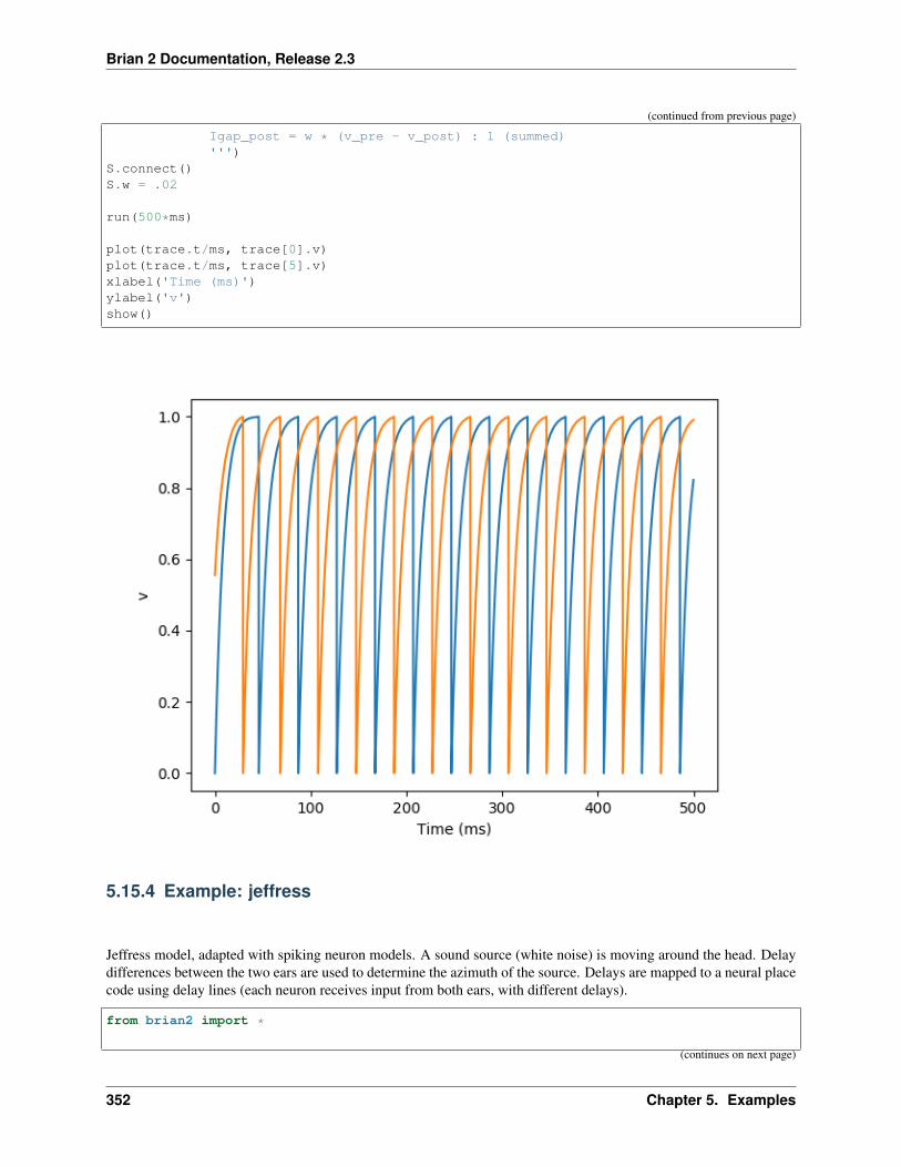
Brian 2 Documentation, Release 2.3
(continued from previous page)
Igap_post = w * (v_pre - v_post) : 1 (summed)''')
S.connect()S.w = .02
run(500*ms)
plot(trace.t/ms, trace[0].v)plot(trace.t/ms, trace[5].v)xlabel('Time (ms)')ylabel('v')show()
5.15.4 Example: jeffress
Jeffress model, adapted with spiking neuron models. A sound source (white noise) is moving around the head. Delaydifferences between the two ears are used to determine the azimuth of the source. Delays are mapped to a neural placecode using delay lines (each neuron receives input from both ears, with different delays).
from brian2 import *
(continues on next page)
352 Chapter 5. Examples

Brian 2 Documentation, Release 2.3
(continued from previous page)
defaultclock.dt = .02*ms
# Soundsound = TimedArray(10 * randn(50000), dt=defaultclock.dt) # white noise
# Ears and sound motion around the head (constant angular speed)sound_speed = 300*metre/secondinteraural_distance = 20*cm # big head!max_delay = interaural_distance / sound_speedprint("Maximum interaural delay: %s" % max_delay)angular_speed = 2 * pi / second # 1 turn/secondtau_ear = 1*mssigma_ear = .1eqs_ears = '''dx/dt = (sound(t-delay)-x)/tau_ear+sigma_ear*(2./tau_ear)**.5*xi : 1 (unless→˓refractory)delay = distance*sin(theta) : seconddistance : second # distance to the centre of the head in time unitsdtheta/dt = angular_speed : radian'''ears = NeuronGroup(2, eqs_ears, threshold='x>1', reset='x = 0',
refractory=2.5*ms, name='ears', method='euler')ears.distance = [-.5 * max_delay, .5 * max_delay]traces = StateMonitor(ears, 'delay', record=True)# Coincidence detectorsnum_neurons = 30tau = 1*mssigma = .1eqs_neurons = '''dv/dt = -v / tau + sigma * (2 / tau)**.5 * xi : 1'''neurons = NeuronGroup(num_neurons, eqs_neurons, threshold='v>1',
reset='v = 0', name='neurons', method='euler')
synapses = Synapses(ears, neurons, on_pre='v += .5')synapses.connect()
synapses.delay['i==0'] = '(1.0*j)/(num_neurons-1)*1.1*max_delay'synapses.delay['i==1'] = '(1.0*(num_neurons-j-1))/(num_neurons-1)*1.1*max_delay'
spikes = SpikeMonitor(neurons)
run(1000*ms)
# Plot the resultsi, t = spikes.itsubplot(2, 1, 1)plot(t/ms, i, '.')xlabel('Time (ms)')ylabel('Neuron index')xlim(0, 1000)subplot(2, 1, 2)plot(traces.t/ms, traces.delay.T/ms)xlabel('Time (ms)')ylabel('Input delay (ms)')xlim(0, 1000)tight_layout()
(continues on next page)
5.15. synapses 353

Brian 2 Documentation, Release 2.3
(continued from previous page)
show()
5.15.5 Example: licklider
Spike-based adaptation of Licklider’s model of pitch processing (autocorrelation with delay lines) with phase locking.
from brian2 import *
defaultclock.dt = .02 * ms
# Ear and soundmax_delay = 20*ms # 50 Hztau_ear = 1*mssigma_ear = 0.0eqs_ear = '''dx/dt = (sound-x)/tau_ear+0.1*(2./tau_ear)**.5*xi : 1 (unless refractory)sound = 5*sin(2*pi*frequency*t)**3 : 1 # nonlinear distortion#sound = 5*(sin(4*pi*frequency*t)+.5*sin(6*pi*frequency*t)) : 1 # missing fundamentalfrequency = (200+200*t*Hz)*Hz : Hz # increasing pitch'''receptors = NeuronGroup(2, eqs_ear, threshold='x>1', reset='x=0',
(continues on next page)
354 Chapter 5. Examples
Brian 2 Documentation, Release 2.3
(continued from previous page)
refractory=2*ms, method='euler')# Coincidence detectorsmin_freq = 50*Hzmax_freq = 1000*Hznum_neurons = 300tau = 1*mssigma = .1eqs_neurons = '''dv/dt = -v/tau+sigma*(2./tau)**.5*xi : 1'''
neurons = NeuronGroup(num_neurons, eqs_neurons, threshold='v>1', reset='v=0',method='euler')
synapses = Synapses(receptors, neurons, on_pre='v += 0.5')synapses.connect()synapses.delay = 'i*1.0/exp(log(min_freq/Hz)+(j*1.0/(num_neurons-1))*log(max_freq/min_→˓freq))*second'
spikes = SpikeMonitor(neurons)
run(500*ms)plot(spikes.t/ms, spikes.i, '.k')xlabel('Time (ms)')ylabel('Frequency')yticks([0, 99, 199, 299],
array(1. / synapses.delay[1, [0, 99, 199, 299]], dtype=int))show()
5.15. synapses 355
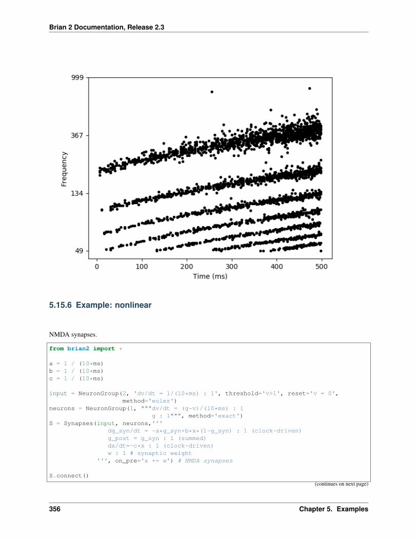
Brian 2 Documentation, Release 2.3
5.15.6 Example: nonlinear
NMDA synapses.
from brian2 import *
a = 1 / (10*ms)b = 1 / (10*ms)c = 1 / (10*ms)
input = NeuronGroup(2, 'dv/dt = 1/(10*ms) : 1', threshold='v>1', reset='v = 0',method='euler')
neurons = NeuronGroup(1, """dv/dt = (g-v)/(10*ms) : 1g : 1""", method='exact')
S = Synapses(input, neurons,'''dg_syn/dt = -a*g_syn+b*x*(1-g_syn) : 1 (clock-driven)g_post = g_syn : 1 (summed)dx/dt=-c*x : 1 (clock-driven)w : 1 # synaptic weight
''', on_pre='x += w') # NMDA synapses
S.connect()
(continues on next page)
356 Chapter 5. Examples

Brian 2 Documentation, Release 2.3
(continued from previous page)
S.w = [1., 10.]input.v = [0., 0.5]
M = StateMonitor(S, 'g',# If not using standalone mode, this could also simply be# record=Truerecord=np.arange(len(input)*len(neurons)))
Mn = StateMonitor(neurons, 'g', record=0)
run(1000*ms)
subplot(2, 1, 1)plot(M.t/ms, M.g.T)xlabel('Time (ms)')ylabel('g_syn')subplot(2, 1, 2)plot(Mn.t/ms, Mn[0].g)ylabel('Time (ms)')ylabel('g')tight_layout()show()
5.15. synapses 357

Brian 2 Documentation, Release 2.3
5.15.7 Example: spatial_connections
A simple example showing how string expressions can be used to implement spatial (deterministic or stochastic)connection patterns.
from brian2 import *
rows, cols = 20, 20G = NeuronGroup(rows * cols, '''x : meter
y : meter''')# initialize the grid positionsgrid_dist = 25*umeterG.x = '(i // rows) * grid_dist - rows/2.0 * grid_dist'G.y = '(i % rows) * grid_dist - cols/2.0 * grid_dist'
# Deterministic connectionsdistance = 120*umeterS_deterministic = Synapses(G, G)S_deterministic.connect('sqrt((x_pre - x_post)**2 + (y_pre - y_post)**2) < distance')
# Random connections (no self-connections)S_stochastic = Synapses(G, G)S_stochastic.connect('i != j',
p='1.5 * exp(-((x_pre-x_post)**2 + (y_pre-y_post)**2)/→˓(2*(60*umeter)**2))')
figure(figsize=(12, 6))
# Show the connections for some neurons in different colorsfor color in ['g', 'b', 'm']:
subplot(1, 2, 1)neuron_idx = np.random.randint(0, rows*cols)plot(G.x[neuron_idx] / umeter, G.y[neuron_idx] / umeter, 'o', mec=color,
mfc='none')plot(G.x[S_deterministic.j[neuron_idx, :]] / umeter,
G.y[S_deterministic.j[neuron_idx, :]] / umeter, color + '.')subplot(1, 2, 2)plot(G.x[neuron_idx] / umeter, G.y[neuron_idx] / umeter, 'o', mec=color,
mfc='none')plot(G.x[S_stochastic.j[neuron_idx, :]] / umeter,
G.y[S_stochastic.j[neuron_idx, :]] / umeter, color + '.')
for idx, t in enumerate(['determininstic connections','random connections']):
subplot(1, 2, idx + 1)xlim((-rows/2.0 * grid_dist) / umeter, (rows/2.0 * grid_dist) / umeter)ylim((-cols/2.0 * grid_dist) / umeter, (cols/2.0 * grid_dist) / umeter)title(t)xlabel('x')ylabel('y', rotation='horizontal')axis('equal')
tight_layout()show()
358 Chapter 5. Examples

Brian 2 Documentation, Release 2.3
5.15.8 Example: state_variables
Set state variable values with a string (using code generation).
from brian2 import *
G = NeuronGroup(100, 'v:volt', threshold='v>-50*mV')G.v = '(sin(2*pi*i/N) - 70 + 0.25*randn()) * mV'S = Synapses(G, G, 'w : volt', on_pre='v += w')S.connect()
space_constant = 200.0S.w['i > j'] = 'exp(-(i - j)**2/space_constant) * mV'
# Generate a matrix for displayw_matrix = np.zeros((len(G), len(G)))w_matrix[S.i[:], S.j[:]] = S.w[:]
subplot(1, 2, 1)plot(G.v[:] / mV)xlabel('Neuron index')ylabel('v')subplot(1, 2, 2)imshow(w_matrix)xlabel('i')ylabel('j')title('Synaptic weight')tight_layout()show()
5.15. synapses 359
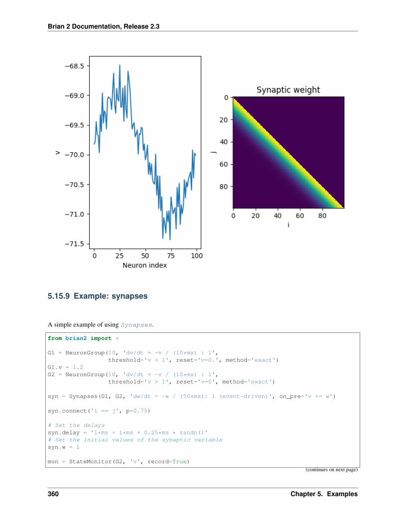
Brian 2 Documentation, Release 2.3
5.15.9 Example: synapses
A simple example of using Synapses.
from brian2 import *
G1 = NeuronGroup(10, 'dv/dt = -v / (10*ms) : 1',threshold='v > 1', reset='v=0.', method='exact')
G1.v = 1.2G2 = NeuronGroup(10, 'dv/dt = -v / (10*ms) : 1',
threshold='v > 1', reset='v=0', method='exact')
syn = Synapses(G1, G2, 'dw/dt = -w / (50*ms): 1 (event-driven)', on_pre='v += w')
syn.connect('i == j', p=0.75)
# Set the delayssyn.delay = '1*ms + i*ms + 0.25*ms * randn()'# Set the initial values of the synaptic variablesyn.w = 1
mon = StateMonitor(G2, 'v', record=True)
(continues on next page)
360 Chapter 5. Examples

Brian 2 Documentation, Release 2.3
(continued from previous page)
run(20*ms)plot(mon.t/ms, mon.v.T)xlabel('Time (ms)')ylabel('v')show()
5.15. synapses 361

Brian 2 Documentation, Release 2.3
362 Chapter 5. Examples
CHAPTER 6
brian2 package
Brian 2
Functions
check_cache(target)
6.1 check_cache function
(Shortest import: from brian2.__init__ import check_cache)
brian2.__init__.check_cache(target)
clear_cache(target) Clears the on-disk cache with the compiled files for agiven code generation target.
6.2 clear_cache function
(Shortest import: from brian2.__init__ import clear_cache)
brian2.__init__.clear_cache(target)Clears the on-disk cache with the compiled files for a given code generation target.
Parameters target : str
The code generation target (e.g. 'weave' or 'cython')
Raises
ValueError If the given code generation target does not have an on-disk cache
363
Brian 2 Documentation, Release 2.3
IOError If the cache directory contains unexpected files, suggesting that deleting it would also delete filesunrelated to the cache.
6.3 hears module
This is only a bridge for using Brian 1 hears with Brian 2.
Deprecated since version 2.2.2.2: Use the brian2hears package instead.
NOTES:
• Slicing sounds with Brian 2 units doesn’t work, you need to either use Brian 1 units or replace calls tosound[:20*ms] with sound.slice(None, 20*ms), etc.
TODO: handle properties (e.g. sound.duration)
Not working examples:
• time_varying_filter1 (care with units)
Exported members: convert_unit_b1_to_b2, convert_unit_b2_to_b1
Classes
BridgeSound We add a new method slice because slicing with unitscan’t work with Brian 2 units.
6.3.1 BridgeSound class
(Shortest import: from brian2.hears import BridgeSound)
class brian2.hears.BridgeSoundBases: brian2.hears.new_class
We add a new method slice because slicing with units can’t work with Brian 2 units.
Methods
slice(*args)
Details
slice(*args)
FilterbankGroup(filterbank, targetvar, . . . )
Methods
6.3.2 FilterbankGroup class
(Shortest import: from brian2.hears import FilterbankGroup)
364 Chapter 6. brian2 package
Brian 2 Documentation, Release 2.3
class brian2.hears.FilterbankGroup(filterbank, targetvar, *args, **kwds)Bases: brian2.groups.neurongroup.NeuronGroup
Methods
reinit()
Details
reinit()
Sound alias of brian2.hears.BridgeSound
6.3.3 Sound class
(Shortest import: from brian2.hears import Sound)
brian2.hears.Soundalias of brian2.hears.BridgeSound
WrappedSound alias of brian2.hears.new_class
6.3.4 WrappedSound class
(Shortest import: from brian2.hears import WrappedSound)
brian2.hears.WrappedSoundalias of brian2.hears.new_class
Functions
convert_unit_b1_to_b2(val)
6.3.5 convert_unit_b1_to_b2 function
(Shortest import: from brian2.hears import convert_unit_b1_to_b2)
brian2.hears.convert_unit_b1_to_b2(val)
convert_unit_b2_to_b1(val)
6.3.6 convert_unit_b2_to_b1 function
(Shortest import: from brian2.hears import convert_unit_b2_to_b1)
brian2.hears.convert_unit_b2_to_b1(val)
6.3. hears module 365

Brian 2 Documentation, Release 2.3
modify_arg(arg) Modify arguments to make them compatible with Brian1.
6.3.7 modify_arg function
(Shortest import: from brian2.hears import modify_arg)
brian2.hears.modify_arg(arg)Modify arguments to make them compatible with Brian 1.
• Arrays of units are replaced with straight arrays
• Single values are replaced with Brian 1 equivalents
• Slices are handled so we can use e.g. sound[:20*ms]
The second part was necessary because some functions/classes test if an object is an array or not to see if it is asequence, but because brian2.Quantity derives from ndarray this was causing problems.
wrap_units(f) Wrap a function to convert units into a form that Brian1 can handle.
6.3.8 wrap_units function
(Shortest import: from brian2.hears import wrap_units)
brian2.hears.wrap_units(f)Wrap a function to convert units into a form that Brian 1 can handle. Also, check the output argument, if it is ab1h.Sound wrap it.
wrap_units_class(_C) Wrap a class to convert units into a form that Brian 1can handle in all methods
6.3.9 wrap_units_class function
(Shortest import: from brian2.hears import wrap_units_class)
brian2.hears.wrap_units_class(_C)Wrap a class to convert units into a form that Brian 1 can handle in all methods
wrap_units_property(p)
6.3.10 wrap_units_property function
(Shortest import: from brian2.hears import wrap_units_property)
brian2.hears.wrap_units_property(p)
366 Chapter 6. brian2 package
Brian 2 Documentation, Release 2.3
6.4 numpy_ module
A dummy package to allow importing numpy and the unit-aware replacements of numpy functions without having toknow which functions are overwritten.
This can be used for example as import brian2.numpy_ as np
Exported members: ModuleDeprecationWarning, VisibleDeprecationWarning, __version__,show_config(), char, rec, memmap, newaxis, ndarray, flatiter, nditer, nested_iters, ufunc,arange(), array, zeros, count_nonzero(), empty, broadcast, dtype, fromstring, fromfile,frombuffer, int_asbuffer, where() . . . (628 more members)
6.5 only module
A dummy package to allow wildcard import from brian2 without also importing the pylab (numpy + matplotlib)namespace.
Usage: from brian2.only import *
Exported members: get_logger(), BrianLogger, std_silent, Trackable, Nameable,SpikeSource, linked_var(), DEFAULT_FUNCTIONS, Function, implementation(),declare_types(), PreferenceError, BrianPreference, prefs, brian_prefs, Clock,defaultclock, Equations, Expression, Statements, BrianObject, BrianObjectException,Network, profiling_summary(), scheduling_summary() . . . (304 more members)
Functions
restore_initial_state() Restores internal Brian variables to the state they are inwhen Brian is imported
6.5.1 restore_initial_state function
(Shortest import: from brian2 import restore_initial_state)
brian2.only.restore_initial_state()Restores internal Brian variables to the state they are in when Brian is imported
Resets defaultclock.dt = 0.1*ms, BrianGlobalPreferences._restore preferences, and setBrianObject._scope_current_key back to 0.
6.6 Subpackages
6.6.1 codegen package
Package providing the code generation framework.
Exported members: NumpyCodeObject, WeaveCodeObject, CythonCodeObject
_prefs module
6.6. Subpackages 367
Brian 2 Documentation, Release 2.3
codeobject module
Module providing the base CodeObject and related functions.
Exported members: CodeObject, constant_or_scalar
Classes
CodeObject(owner, code, variables, . . . [, name]) Executable code object.
CodeObject class
(Shortest import: from brian2.codegen.codeobject import CodeObject)
class brian2.codegen.codeobject.CodeObject(owner, code, variables, variable_indices, tem-plate_name, template_source, compiler_kwds,name=’codeobject*’)
Bases: brian2.core.names.Nameable
Executable code object.
The code can either be a string or a brian2.codegen.templates.MultiTemplate.
After initialisation, the code is compiled with the given namespace using code.compile(namespace).
Calling code(key1=val1, key2=val2) executes the code with the given variables inserted into thenamespace.
Attributes
class_name A short name for this type of CodeObjectgenerator_class The CodeGenerator class used by this
CodeObject
Methods
__call__(. . . ) <==> x(. . . )compile()is_available() Whether this target for code generation is available.run() Runs the code in the namespace.update_namespace() Update the namespace for this timestep.
Details
class_nameA short name for this type of CodeObject
generator_classThe CodeGenerator class used by this CodeObject
__call__(...) <==> x(...)
compile()
classmethod is_available()
368 Chapter 6. brian2 package
Brian 2 Documentation, Release 2.3
Whether this target for code generation is available. Should use a minimal example to check whether codegeneration works in general.
run()Runs the code in the namespace.
Returns return_value : dict
A dictionary with the keys corresponding to the output_variables defined duringthe call of CodeGenerator.code_object.
update_namespace()Update the namespace for this timestep. Should only deal with variables where the reference changesevery timestep, i.e. where the current reference in namespace is not correct.
Functions
check_compiler_kwds(compiler_kwds, . . . ) Internal function to check the provided compiler key-words against the list of understood keywords.
check_compiler_kwds function
(Shortest import: from brian2.codegen.codeobject import check_compiler_kwds)
brian2.codegen.codeobject.check_compiler_kwds(compiler_kwds, accepted_kwds, target)Internal function to check the provided compiler keywords against the list of understood keywords.
Parameters compiler_kwds : dict
Dictionary of compiler keywords and respective list of values.
accepted_kwds : list of str
The compiler keywords understood by the code generation target
target : str
The name of the code generation target (used for the error message).
Raises
ValueError If a compiler keyword is not understood
constant_or_scalar(varname, variable) Convenience function to generate code to access thevalue of a variable.
constant_or_scalar function
(Shortest import: from brian2.codegen.codeobject import constant_or_scalar)
brian2.codegen.codeobject.constant_or_scalar(varname, variable)Convenience function to generate code to access the value of a variable. Will return 'varname' if thevariable is a constant, and array_name[0] if it is a scalar array.
6.6. Subpackages 369
Brian 2 Documentation, Release 2.3
create_runner_codeobj(group, code, . . . [, . . . ]) Create a CodeObject for the execution of code in thecontext of a Group.
create_runner_codeobj function
(Shortest import: from brian2.codegen.codeobject import create_runner_codeobj)
brian2.codegen.codeobject.create_runner_codeobj(group, code, template_name,run_namespace, user_code=None,variable_indices=None,name=None, check_units=True,needed_variables=None, ad-ditional_variables=None,template_kwds=None, over-ride_conditional_write=None,codeobj_class=None)
Create a CodeObject for the execution of code in the context of a Group.
Parameters group : Group
The group where the code is to be run
code : str or dict of str
The code to be executed.
template_name : str
The name of the template to use for the code.
run_namespace : dict-like
An additional namespace that is used for variable lookup (either an explicitly definednamespace or one taken from the local context).
user_code : str, optional
The code that had been specified by the user before other code was added automatically.If not specified, will be assumed to be identical to code.
variable_indices : dict-like, optional
A mapping from Variable objects to index names (strings). If none is given, uses thecorresponding attribute of group.
name : str, optional
A name for this code object, will use group + '_codeobject*' if none is given.
check_units : bool, optional
Whether to check units in the statement. Defaults to True.
needed_variables: list of str, optional :
A list of variables that are neither present in the abstract code, nor in theUSES_VARIABLES statement in the template. This is only rarely necessary, an ex-ample being a StateMonitor where the names of the variables are neither known tothe template nor included in the abstract code statements.
additional_variables : dict-like, optional
370 Chapter 6. brian2 package
Brian 2 Documentation, Release 2.3
A mapping of names to Variable objects, used in addition to the variables saved ingroup.
template_kwds : dict, optional
A dictionary of additional information that is passed to the template.
override_conditional_write: list of str, optional :
A list of variable names which are used as conditions (e.g. for refractoriness) whichshould be ignored.
codeobj_class : class, optional
The CodeObject class to run code with. If not specified, defaults to the group’scodeobj_class attribute.
cpp_prefs module
Preferences related to C++ compilation
Preferences
C++ compilation preferences
codegen.cpp.compiler = ''
Compiler to use (uses default if empty)
Should be gcc or msvc.
codegen.cpp.define_macros = []
List of macros to define; each macro is defined using a 2-tuple, where ‘value’ is either the string to defineit to or None to define it without a particular value (equivalent of “#define FOO” in source or -DFOO onUnix C compiler command line).
codegen.cpp.extra_compile_args = None
Extra arguments to pass to compiler (if None, use either extra_compile_args_gcc orextra_compile_args_msvc).
codegen.cpp.extra_compile_args_gcc = ['-w', '-O3', '-ffast-math','-fno-finite-math-only', '-march=native']
Extra compile arguments to pass to GCC compiler
codegen.cpp.extra_compile_args_msvc = ['/Ox', '/w', '', '/MP']
Extra compile arguments to pass to MSVC compiler (the default /arch: flag is determined based on theprocessor architecture)
codegen.cpp.extra_link_args = []
Any extra platform- and compiler-specific information to use when linking object files together.
codegen.cpp.headers = []
A list of strings specifying header files to use when compiling the code. The list might look like [“<vec-tor>”,“‘my_header’”]. Note that the header strings need to be in a form than can be pasted at the end of a#include statement in the C++ code.
codegen.cpp.include_dirs = []
6.6. Subpackages 371

Brian 2 Documentation, Release 2.3
Include directories to use. Note that $prefix/include will be appended to the end automatically,where $prefix is Python’s site-specific directory prefix as returned by sys.prefix.
codegen.cpp.libraries = []
List of library names (not filenames or paths) to link against.
codegen.cpp.library_dirs = []
List of directories to search for C/C++ libraries at link time. Note that $prefix/lib will be appendedto the end automatically, where $prefix is Python’s site-specific directory prefix as returned by sys.prefix.
codegen.cpp.msvc_architecture = ''
MSVC architecture name (or use system architectue by default).
Could take values such as x86, amd64, etc.
codegen.cpp.msvc_vars_location = ''
Location of the MSVC command line tool (or search for best by default).
codegen.cpp.runtime_library_dirs = []
List of directories to search for C/C++ libraries at run time.
Exported members: get_compiler_and_args, get_msvc_env , compiler_supports_c99, C99Check
Classes
C99Check(name) Helper class to create objects that can bepassed as an availability_check to aFunctionImplementation.
C99Check class
(Shortest import: from brian2.codegen.cpp_prefs import C99Check)
class brian2.codegen.cpp_prefs.C99Check(name)Bases: object
Helper class to create objects that can be passed as an availability_check to aFunctionImplementation.
Methods
__call__(. . . ) <==> x(. . . )
Details
__call__(...) <==> x(...)
Functions
compiler_supports_c99()
372 Chapter 6. brian2 package

Brian 2 Documentation, Release 2.3
compiler_supports_c99 function
(Shortest import: from brian2.codegen.cpp_prefs import compiler_supports_c99)
brian2.codegen.cpp_prefs.compiler_supports_c99()
get_compiler_and_args() Returns the computed compiler and compilation flags
get_compiler_and_args function
(Shortest import: from brian2.codegen.cpp_prefs import get_compiler_and_args)
brian2.codegen.cpp_prefs.get_compiler_and_args()Returns the computed compiler and compilation flags
get_msvc_env()
get_msvc_env function
(Shortest import: from brian2.codegen.cpp_prefs import get_msvc_env)
brian2.codegen.cpp_prefs.get_msvc_env()
update_for_cross_compilation(library_dirs,. . . )
Update the compiler arguments to allow cross-compilation for 32bit on a 64bit Linux system.
update_for_cross_compilation function
(Shortest import: from brian2.codegen.cpp_prefs import update_for_cross_compilation)
brian2.codegen.cpp_prefs.update_for_cross_compilation(library_dirs, ex-tra_compile_args, ex-tra_link_args, logger=None)
Update the compiler arguments to allow cross-compilation for 32bit on a 64bit Linux system. Uses the providedlogger to print an INFO message and modifies the provided lists in-place.
Parameters library_dirs : list
List of library directories (will be modified in-place).
extra_compile_args : list
List of extra compile args (will be modified in-place).
extra_link_args : list
List of extra link args (will be modified in-place).
logger : BrianLogger, optional
The logger to use for the INFO message. Defaults to None (no message).
6.6. Subpackages 373

Brian 2 Documentation, Release 2.3
get_cpu_flags module
This script is used to ask for the CPU flags on Windows. We use this instead of importing the cpuinfo package,because recent versions of py-cpuinfo use the multiprocessing module, and any import of cpuinfo that is not within aif __name__ == '__main__': block will lead to the script being executed twice.
The CPU flags are printed to stdout encoded as JSON.
optimisation module
Simplify and optimise sequences of statements by rewriting and pulling out loop invariants.
Exported members: optimise_statements, ArithmeticSimplifier, Simplifier
Classes
ArithmeticSimplifier(variables) Carries out the following arithmetic simplifications:
ArithmeticSimplifier class
(Shortest import: from brian2.codegen.optimisation import ArithmeticSimplifier)
class brian2.codegen.optimisation.ArithmeticSimplifier(variables)Bases: brian2.parsing.bast.BrianASTRenderer
Carries out the following arithmetic simplifications:
1. Constant evaluation (e.g. exp(0)=1) by attempting to evaluate the expression in an “assumptions names-pace”
2. Binary operators, e.g. 0*x=0, 1*x=x, etc. You have to take care that the dtypes match here, e.g. if x is aninteger, then 1.0*x shouldn’t be replaced with x but left as 1.0*x.
Parameters variables : dict of (str, Variable)
Usual definition of variables.
assumptions : sequence of str
Additional assumptions that can be used in simplification, each assumption is a stringstatement. These might be the scalar statements for example.
Methods
render_BinOp(node)render_node(node) Assumes that the node has already been fully pro-
cessed by BrianASTRenderer
Details
render_BinOp(node)
render_node(node)Assumes that the node has already been fully processed by BrianASTRenderer
374 Chapter 6. brian2 package
Brian 2 Documentation, Release 2.3
Simplifier(variables, scalar_statements[, . . . ]) Carry out arithmetic simplifications (seeArithmeticSimplifier) and loop invariants
Simplifier class
(Shortest import: from brian2.codegen.optimisation import Simplifier)
class brian2.codegen.optimisation.Simplifier(variables, scalar_statements, ex-tra_lio_prefix=”)
Bases: brian2.parsing.bast.BrianASTRenderer
Carry out arithmetic simplifications (see ArithmeticSimplifier) and loop invariants
Parameters variables : dict of (str, Variable)
Usual definition of variables.
scalar_statements : sequence of Statement
Predefined scalar statements that can be used as part of simplification
Notes
After calling render_expr on a sequence of expressions (coming from vector statements typically), thisobject will have some new attributes:
loop_invariants [OrderedDict of (expression, varname)] varname will be of the form _lio_N where Nis some integer, and the expressions will be strings that correspond to scalar-only expressions that can beevaluated outside of the vector block.
loop_invariant_dtypes [dict of (varname, dtypename)] dtypename will be one of 'boolean','integer', 'float'.
Methods
render_expr(expr)render_node(node) Assumes that the node has already been fully pro-
cessed by BrianASTRenderer
Details
render_expr(expr)
render_node(node)Assumes that the node has already been fully processed by BrianASTRenderer
Functions
cancel_identical_terms(primary, inverted) Cancel terms in a collection, e.g.
cancel_identical_terms function
(Shortest import: from brian2.codegen.optimisation import cancel_identical_terms)
6.6. Subpackages 375

Brian 2 Documentation, Release 2.3
brian2.codegen.optimisation.cancel_identical_terms(primary, inverted)Cancel terms in a collection, e.g. a+b-a should be cancelled to b
Simply renders the nodes into expressions and removes whenever there is a common expression in primary andinverted.
Parameters primary : list of AST nodes
These are the nodes that are positive with respect to the operator, e.g. in x*y/z it wouldbe [x, y].
inverted : list of AST nodes
These are the nodes that are inverted with respect to the operator, e.g. in x*y/z it wouldbe [z].
Returns primary : list of AST nodes
Primary nodes after cancellation
inverted : list of AST nodes
Inverted nodes after cancellation
collect(node) Attempts to collect commutative operations into oneand simplifies them.
collect function
(Shortest import: from brian2.codegen.optimisation import collect)
brian2.codegen.optimisation.collect(node)Attempts to collect commutative operations into one and simplifies them.
For example, if x and y are scalars, and z is a vector, then (x*z)*y should be rewritten as (x*y)*z to minimisethe number of vector operations. Similarly, ((x*2)*3)*4 should be rewritten as x*24.
Works for either multiplication/division or addition/subtraction nodes.
The final output is a subexpression of the following maximal form:
(((numerical_value*(product of scalars))/(product of scalars))*(product of vectors))/(product of vec-tors)
Any possible cancellations will have been done.
Parameters node : Brian AST node
The node to be collected/simplified.
Returns node : Brian AST node
Simplified node.
collect_commutative(node, primary, inverted,. . . )
collect_commutative function
(Shortest import: from brian2.codegen.optimisation import collect_commutative)
376 Chapter 6. brian2 package
Brian 2 Documentation, Release 2.3
brian2.codegen.optimisation.collect_commutative(node, primary, inverted,terms_primary, terms_inverted,add_to_inverted=False)
evaluate_expr(expr, ns) Try to evaluate the expression in the given namespace
evaluate_expr function
(Shortest import: from brian2.codegen.optimisation import evaluate_expr)
brian2.codegen.optimisation.evaluate_expr(expr, ns)Try to evaluate the expression in the given namespace
Returns either (value, True) if successful, or (expr, False) otherwise.
expression_complexity(expr, variables)
expression_complexity function
(Shortest import: from brian2.codegen.optimisation import expression_complexity)
brian2.codegen.optimisation.expression_complexity(expr, variables)
optimise_statements(scalar_statements, . . . ) Optimise a sequence of scalar and vector statements
optimise_statements function
(Shortest import: from brian2.codegen.optimisation import optimise_statements)
brian2.codegen.optimisation.optimise_statements(scalar_statements, vector_statements,variables, blockname=”)
Optimise a sequence of scalar and vector statements
Performs the following optimisations:
1. Constant evaluations (e.g. exp(0) to 1). See evaluate_expr.
2. Arithmetic simplifications (e.g. 0*x to 0). See ArithmeticSimplifier, collect().
3. Pulling out loop invariants (e.g. v*exp(-dt/tau) to a=exp(-dt/tau) outside the loop and v*a inside). SeeSimplifier.
4. Boolean simplifications (allowing the replacement of expressions with booleans with a sequence ofif/thens). See Simplifier.
Parameters scalar_statements : sequence of Statement
Statements that only involve scalar values and should be evaluated in the scalar block.
vector_statements : sequence of Statement
Statements that involve vector values and should be evaluated in the vector block.
variables : dict of (str, Variable)
Definition of the types of the variables.
blockname : str, optional
6.6. Subpackages 377
Brian 2 Documentation, Release 2.3
Name of the block (used for LIO constant prefixes to avoid name clashes)
Returns new_scalar_statements : sequence of Statement
As above but with loop invariants pulled out from vector statements
new_vector_statements : sequence of Statement
Simplified/optimised versions of statements
reduced_node(terms, op) Reduce a sequence of terms with the given operator
reduced_node function
(Shortest import: from brian2.codegen.optimisation import reduced_node)
brian2.codegen.optimisation.reduced_node(terms, op)Reduce a sequence of terms with the given operator
For examples, if terms were [a, b, c] and op was multiplication then the reduction would be (a*b)*c.
Parameters terms : list
AST nodes.
op : AST node
Could be ast.Mult or ast.Add.
Examples
>>> import ast>>> nodes = [ast.Name(id='x'), ast.Name(id='y'), ast.Name(id='z')]>>> ast.dump(reduced_node(nodes, ast.Mult), annotate_fields=False)"BinOp(BinOp(Name('x'), Mult(), Name('y')), Mult(), Name('z'))">>> nodes = [ast.Name(id='x')]>>> ast.dump(reduced_node(nodes, ast.Add), annotate_fields=False)"Name('x')"
permutation_analysis module
Module for analysing synaptic pre and post code for synapse order independence.
Exported members: OrderDependenceError, check_for_order_independence
Classes
OrderDependenceError
OrderDependenceError class
(Shortest import: from brian2.codegen.permutation_analysis importOrderDependenceError)
class brian2.codegen.permutation_analysis.OrderDependenceError
378 Chapter 6. brian2 package

Brian 2 Documentation, Release 2.3
Bases: exceptions.Exception
Functions
check_for_order_independence(statements,. . . )
Check that the sequence of statements doesn’t dependon the order in which the indices are iterated through.
check_for_order_independence function
(Shortest import: from brian2.codegen.permutation_analysis importcheck_for_order_independence)
brian2.codegen.permutation_analysis.check_for_order_independence(statements,variables,indices)
Check that the sequence of statements doesn’t depend on the order in which the indices are iterated through.
statements module
Module providing the Statement class.
Classes
Statement(var, op, expr, comment, dtype[, . . . ]) A single line mathematical statement.
Statement class
(Shortest import: from brian2.codegen.statements import Statement)
class brian2.codegen.statements.Statement(var, op, expr, comment, dtype, constant=False,subexpression=False, scalar=False)
Bases: object
A single line mathematical statement.
The structure is var op expr.
Parameters var : str
The left hand side of the statement, the value being written to.
op : str
The operation, can be any of the standard Python operators (including += etc.) or aspecial operator := which means you are defining a new symbol (whereas = means youare setting the value of an existing symbol).
expr : str, Expression
The right hand side of the statement.
dtype : dtype
The numpy dtype of the value or array var().
constant : bool, optional
Set this flag to True if the value will not change (only applies for op==':='.
6.6. Subpackages 379

Brian 2 Documentation, Release 2.3
subexpression : bool, optional
Set this flag to True if the variable is a subexpression. In some languages (e.g. Python)you can use this to save a memory copy, because you don’t need to do lhs[:] =rhs but a redefinition lhs = rhs.
scalar : bool, optional
Set this flag to True if var() and expr are scalar.
Notes
Will compute the following attribute:
inplace True or False depending if the operation is in-place or not.
Boolean simplification notes:
Will initially set the attribute used_boolean_variables to None. This is set byoptimise_statements when it is called on a sequence of statements to the list of boolean vari-ables that are used in this expression. In addition, the attribute boolean_simplified_expressionsis set to a dictionary with keys consisting of a tuple of pairs (var, value) where var is the name of theboolean variable (will be in used_boolean_variables) and var is True or False. The values of thedictionary are strings representing the simplified version of the expression if each var=value substitution ismade for that key. The keys will range over all possible values of the set of boolean variables. The complexityof the original statement is set as the attribute complexity_std, and the complexity of the simplifiedversions are in the dictionary complexities (with the same keys).
This information can be used to generate code that replaces a complex expression that varies depending on thevalue of one or more boolean variables with an if/then sequence where each subexpression is simplified. Itis optional to use this (e.g. the numpy codegen does not, but the weave and cython ones do).
targets module
Module that stores all known code generation targets as codegen_targets.
Exported members: codegen_targets
templates module
Exported members: Templater
Classes
CodeObjectTemplate(template, template_source) Single template object returned by Templater andused for final code generation
CodeObjectTemplate class
(Shortest import: from brian2.codegen.templates import CodeObjectTemplate)
class brian2.codegen.templates.CodeObjectTemplate(template, template_source)Bases: object
Single template object returned by Templater and used for final code generation
380 Chapter 6. brian2 package
Brian 2 Documentation, Release 2.3
Should not be instantiated by the user, but only directly by Templater.
Notes
The final code is obtained from this by calling the template (see __call__).
Attributes
allows_scalar_write Does this template allow writing to scalar variables?iterate_all The indices over which the template iterates com-
pletelyvariables The set of variables in this templatewrites_read_only Read-only variables that are changed by this tem-
plate
Methods
__call__(scalar_code, vector_code, **kwds) Return a usable code block or blocks from this tem-plate.
Details
allows_scalar_writeDoes this template allow writing to scalar variables?
iterate_allThe indices over which the template iterates completely
variablesThe set of variables in this template
writes_read_onlyRead-only variables that are changed by this template
__call__(scalar_code, vector_code, **kwds)Return a usable code block or blocks from this template.
Parameters scalar_code : dict
Dictionary of scalar code blocks.
vector_code : dict
Dictionary of vector code blocks
**kwds :
Additional parameters to pass to the template
Notes
Returns either a string (if macros were not used in the template), or a MultiTemplate (if macros wereused).
6.6. Subpackages 381

Brian 2 Documentation, Release 2.3
LazyTemplateLoader(environment, extension) Helper object to load templates only when they areneeded.
LazyTemplateLoader class
(Shortest import: from brian2.codegen.templates import LazyTemplateLoader)
class brian2.codegen.templates.LazyTemplateLoader(environment, extension)Bases: object
Helper object to load templates only when they are needed.
Methods
get_template(name)
Details
get_template(name)
MultiTemplate(module) Code generated by a CodeObjectTemplate withmultiple blocks
MultiTemplate class
(Shortest import: from brian2.codegen.templates import MultiTemplate)
class brian2.codegen.templates.MultiTemplate(module)Bases: _abcoll.Mapping
Code generated by a CodeObjectTemplate with multiple blocks
Each block is a string stored as an attribute with the block name. The object can also be accessed as a dictionary.
Templater(package_name, extension[, env_globals]) Class to load and return all the templates aCodeObject defines.
Templater class
(Shortest import: from brian2.codegen.templates import Templater)
class brian2.codegen.templates.Templater(package_name, extension, env_globals=None)Bases: object
Class to load and return all the templates a CodeObject defines.
Parameters package_name : str, tuple of str
The package where the templates are saved. If this is a tuple then each template will besearched in order starting from the first package in the tuple until the template is found.This allows for derived templates to be used. See also derive.
382 Chapter 6. brian2 package
Brian 2 Documentation, Release 2.3
env_globals : dict (optional)
A dictionary of global values accessible by the templates. Can be used for providingutility functions. In all cases, the filter ‘autoindent’ is available (see existing templatesfor example usage).
Notes
Templates are accessed using templater.template_base_name (the base name is without the file ex-tension). This returns a CodeObjectTemplate.
Methods
derive(package_name[, extension, env_globals]) Return a new Templater derived from this one, wherethe new package name and globals overwrite the old.
Details
derive(package_name, extension=None, env_globals=None)Return a new Templater derived from this one, where the new package name and globals overwrite the old.
Functions
autoindent(code)
autoindent function
(Shortest import: from brian2.codegen.templates import autoindent)
brian2.codegen.templates.autoindent(code)
autoindent_postfilter(code)
autoindent_postfilter function
(Shortest import: from brian2.codegen.templates import autoindent_postfilter)
brian2.codegen.templates.autoindent_postfilter(code)
variables_to_array_names(variables[, . . . ])
variables_to_array_names function
(Shortest import: from brian2.codegen.templates import variables_to_array_names)
brian2.codegen.templates.variables_to_array_names(variables, access_data=True)
6.6. Subpackages 383
Brian 2 Documentation, Release 2.3
translation module
This module translates a series of statements into a language-specific syntactically correct code block that can beinserted into a template.
It infers whether or not a variable can be declared as constant, etc. It should handle common subexpressions, and soforth.
The input information needed:
• The sequence of statements (a multiline string) in standard mathematical form
• The list of known variables, common subexpressions and functions, and for each variable whether or not it is avalue or an array, and if an array what the dtype is.
• The dtype to use for newly created variables
• The language to translate to
Exported members: analyse_identifiers, get_identifiers_recursively
Classes
LineInfo(**kwds) A helper class, just used to store attributes.
LineInfo class
(Shortest import: from brian2.codegen.translation import LineInfo)
class brian2.codegen.translation.LineInfo(**kwds)Bases: object
A helper class, just used to store attributes.
Functions
analyse_identifiers(code, variables[, recur-sive])
Analyses a code string (sequence of statements) to findall identifiers by type.
analyse_identifiers function
(Shortest import: from brian2.codegen.translation import analyse_identifiers)
brian2.codegen.translation.analyse_identifiers(code, variables, recursive=False)Analyses a code string (sequence of statements) to find all identifiers by type.
In a given code block, some variable names (identifiers) must be given as inputs to the code block, and some arecreated by the code block. For example, the line:
a = b+c
This could mean to create a new variable a from b and c, or it could mean modify the existing value of a from bor c, depending on whether a was previously known.
Parameters code : str
The code string, a sequence of statements one per line.
variables : dict of Variable, set of names
384 Chapter 6. brian2 package
Brian 2 Documentation, Release 2.3
Specifiers for the model variables or a set of known names
recursive : bool, optional
Whether to recurse down into subexpressions (defaults to False).
Returns newly_defined : set
A set of variables that are created by the code block.
used_known : set
A set of variables that are used and already known, a subset of the known parameter.
unknown : set
A set of variables which are used by the code block but not defined by it and not previ-ously known. Should correspond to variables in the external namespace.
get_identifiers_recursively(expressions,. . . )
Gets all the identifiers in a list of expressions, recursingdown into subexpressions.
get_identifiers_recursively function
(Shortest import: from brian2.codegen.translation import get_identifiers_recursively)
brian2.codegen.translation.get_identifiers_recursively(expressions, variables, in-clude_numbers=False)
Gets all the identifiers in a list of expressions, recursing down into subexpressions.
Parameters expressions : list of str
List of expressions to check.
variables : dict-like
Dictionary of Variable objects
include_numbers : bool, optional
Whether to include number literals in the output. Defaults to False.
is_scalar_expression(expr, variables) Whether the given expression is scalar.
is_scalar_expression function
(Shortest import: from brian2.codegen.translation import is_scalar_expression)
brian2.codegen.translation.is_scalar_expression(expr, variables)Whether the given expression is scalar.
Parameters expr : str
The expression to check
variables : dict-like
Variable and Function object for all the identifiers used in expr
Returns scalar : bool
6.6. Subpackages 385
Brian 2 Documentation, Release 2.3
Whether expr is a scalar expression
make_statements(code, variables, dtype[, . . . ]) Turn a series of abstract code statements into Statementobjects, inferring whether each line is a set/declare op-eration, whether the variables are constant or not, andhandling the cacheing of subexpressions.
make_statements function
(Shortest import: from brian2.codegen.translation import make_statements)
brian2.codegen.translation.make_statements(code, variables, dtype, optimise=True, block-name=”)
Turn a series of abstract code statements into Statement objects, inferring whether each line is a set/declareoperation, whether the variables are constant or not, and handling the cacheing of subexpressions.
Parameters code : str
A (multi-line) string of statements.
variables : dict-like
A dictionary of with Variable and Function objects for every identifier used inthe code.
dtype : dtype
The data type to use for temporary variables
optimise : bool, optional
Whether to optimise expressions, including pulling out loop invariant expressions andputting them in new scalar constants. Defaults to False, since this function is alsoused just to in contexts where we are not interested by this kind of optimisation. For themain code generation stage, its value is set by the codegen.loop_invariant_optimisationspreference.
blockname : str, optional
A name for the block (used to name intermediate variables to avoid name clashes whenmultiple blocks are used together)
Returns :
——- :
scalar_statements, vector_statements : (list of Statement, list of Statement)
Lists with statements that are to be executed once and statements that are to be executedonce for every neuron/synapse/. . . (or in a vectorised way)
Notes
If optimise is True, then the scalar_statements may include newly introduced scalar constants thathave been identified as loop-invariant and have therefore been pulled out of the vector statements. The resultingstatements will also use augmented assignments where possible, i.e. a statement such as w = w + 1 will bereplaced by w += 1. Also, statements involving booleans will have additional information added to them (seeStatement for details) describing how the statement can be reformulated as a sequence of if/then statements.Calls optimise_statements.
386 Chapter 6. brian2 package

Brian 2 Documentation, Release 2.3
Subpackages
generators package
GSL_generator module
GSLCodeGenerators for code that uses the ODE solver provided by the GNU Scientific Library (GSL)
Exported members: GSLCodeGenerator, GSLWeaveCodeGenerator, GSLCythonCodeGenerator
Classes
GSLCodeGenerator(variables, . . . [, . . . ]) GSL code generator.
GSLCodeGenerator class
(Shortest import: from brian2.codegen.generators import GSLCodeGenerator)
class brian2.codegen.generators.GSL_generator.GSLCodeGenerator(variables, vari-able_indices,owner, it-erate_all,codeobj_class,name, tem-plate_name,over-ride_conditional_write=None,al-lows_scalar_write=False)
Bases: object
GSL code generator.
Notes
Approach is to first let the already existing code generator for a target language do the bulk of the translatingfrom abstract_code to actual code. This generated code is slightly adapted to render it GSL compatible. Themost critical part here is that the vector_code that is normally contained in a loop in the `main()` is moved tothe function `_GSL_func` that is sent to the GSL integrator. The variables used in the vector_code are addedto a struct named `dataholder` and their values are set from the Brian namespace just before the scalarcode block.
Methods
add_gsl_variables_as_non_scalar(diff_vars)Add _gsl variables as non-scalar.add_meta_variables(options)c_data_type(dtype) Get string version of object dtype that is attached to
Brian variables.diff_var_to_replace(diff_vars) Add differential variable-related strings that need to
be replaced to go from normal brian to GSL codeContinued on next page
6.6. Subpackages 387

Brian 2 Documentation, Release 2.3
Table 59 – continued from previous pagefind_differential_variables(code) Find the variables that were tagged
_gsl_{var}_f{ind} and return var, ind pairs.find_function_names() Return a list of used function names in the
self.variables dictionaryfind_undefined_variables(statements) Find identifiers that are not in self.variables
dictionary.find_used_variables(statements,other_variables)
Find all the variables used in the right hand side ofthe given expressions.
get_dimension_code(diff_num) Generate code for function that sets the dimension ofthe ODE system.
initialize_array(varname, values) Initialize a static array with given floating point val-ues.
is_constant_and_cpp_standalone(var_obj) Check whether self.cpp_standalone and variable isConstant.
is_cpp_standalone() Check whether we’re running with cpp_standalone.make_function_code(lines) Add lines of GSL translated vector code to ‘non-
changing’ _GSL_func code.scale_array_code(diff_vars, method_options) Return code for definition of
_GSL_scale_array in generated code.to_replace_vector_vars(variables_in_vector) Create dictionary containing key, value pairs with to
be replaced text to translate from conventional Brianto GSL.
translate(code, dtype) Translates an abstract code block into the target lan-guage.
translate_scalar_code(code_lines, . . . ) Translate scalar code: if calculated variables are usedin the vector_code their value is added to the variablein the _dataholder.
translate_vector_code(code_lines,to_replace)
Translate vector code to GSL compatible code bysubstituting fragments of code.
unpack_namespace(variables_in_vector, . . . [,. . . ])
Write code that unpacks Brian namespace tocython/cpp namespace.
unpack_namespace_single(var_obj,in_vector, . . . )
Writes the code necessary to pull single variable outof the Brian namespace into the generated code.
var_init_lhs(var, type) Get string version of the left hand side of an initial-izing expression
write_dataholder(variables_in_vector) Return string with full code for _dataholder struct.write_dataholder_single(var_obj) Return string declaring a single variable in the
_dataholder struct.yvector_code(diff_vars) Generate code for function dealing with GSLs y vec-
tor.
Details
add_gsl_variables_as_non_scalar(diff_vars)Add _gsl variables as non-scalar.
In GSLStateUpdater the differential equation variables are substituted with GSL tags that describe theinformation needed to translate the conventional Brian code to GSL compatible code. This function tellsBrian that the variables that contain these tags should always be vector variables. If we don’t do this, Brianrenders the tag-variables as scalar if no vector variables are used in the right hand side of the expression.
Parameters diff_vars : dict
dictionary with variables as keys and differential equation index as value
388 Chapter 6. brian2 package
Brian 2 Documentation, Release 2.3
add_meta_variables(options)
c_data_type(dtype)Get string version of object dtype that is attached to Brian variables. c pp_generator already has thisfunction, but the Cython generator does not, but we need it for GSL code generation.
diff_var_to_replace(diff_vars)Add differential variable-related strings that need to be replaced to go from normal brian to GSL code
From the code generated by Brian’s ‘normal’ generators (cpp_generator or cython_generator a few bitsof text need to be replaced to get GSL compatible code. The bits of text related to differential equationvariables are put in the replacer dictionary in this function.
Parameters diff_vars : dict
dictionary with variables as keys and differential equation index as value
Returns to_replace : dict
dictionary with strings that need to be replaced as keys and the strings that will replacethem as values
find_differential_variables(code)Find the variables that were tagged _gsl_{var}_f{ind} and return var, ind pairs.
GSLStateUpdater tagged differential variables and here we extract the information given in these tags.
Parameters code : list of strings
A list of strings containing gsl tagged variables
Returns diff_vars : dict
A dictionary with variable names as keys and differential equation index as value
find_function_names()Return a list of used function names in the self.variables dictionary
Functions need to be ignored in the GSL translation process, because the brian generator already suffi-ciently dealt with them. However, the brian generator also removes them from the variables dict, so thereis no way to check whether an identifier is a function after the brian translation process. This functionis called before this translation process and the list of function names is stored to be used in the GSLtranslation.
Returns function_names : list
list of strings that are function names used in the code
find_undefined_variables(statements)Find identifiers that are not in self.variables dictionary.
Brian does not save the _lio_ variables it uses anywhere. This is problematic for our GSL implementa-tion because we save the lio variables in the _dataholder struct (for which we need the datatype of thevariables). This function adds the left hand side variables that are used in the vector code to the variabledictionary as AuxiliaryVariables (all we need later is the datatype).
Parameters statements : list
list of statement objects (need to have the dtype attribute)
Notes
I keep self.variables and other_variables separate so I can distinguish what variables are inthe Brian namespace and which ones are defined in the code itself.
6.6. Subpackages 389

Brian 2 Documentation, Release 2.3
find_used_variables(statements, other_variables)Find all the variables used in the right hand side of the given expressions.
Parameters statements : list
list of statement objects
Returns used_variables : dict
dictionary of variables that are used as variable name (str), Variable pairs.
get_dimension_code(diff_num)Generate code for function that sets the dimension of the ODE system.
GSL needs to know how many differential variables there are in the ODE system. Since the currentapproach is to have the code in the vector loop the same for all simulations, this dimension is set by anexternal function. The code for this set_dimension functon is written here. It is assumed the code will bethe same for each target language with the exception of some syntactical differences
Parameters diff_num : int
Number of differential variables that describe the ODE system
Returns set_dimension_code : str
The code describing the target language function in a single string
initialize_array(varname, values)Initialize a static array with given floating point values. E.g. in C++, when called with arguments arrayand [1.0, 3.0, 2.0], this method should return double array[] = {1.0, 3.0, 2.0}.
Parameters varname : str
The name of the array variable that should be initialized
values : list of float
The values that should be assigned to the array
Returns code : str
One or more lines of array initialization code.
is_constant_and_cpp_standalone(var_obj)Check whether self.cpp_standalone and variable is Constant.
This check is needed because in the case of using the cpp_standalone device we do not want to applyour GSL variable conversion (var –> _GSL_dataholder.var), because the cpp_standalone code generationprocess involves replacing constants with their actual value (‘freezing’). This results in code that looks like(if for example var = 1.2): _GSL_dataholder.1.2 = 1.2 and _GSL_dataholder->1.2. To prevent repetitivecalls to get_device() etc. the outcome of is_cpp_standalone is saved.
Parameters var_obj : Variable
instance of brian Variable class describing the variable
Returns is_cpp_standalone : bool
whether the used device is cpp_standalone and the given variable is an instance of Con-stant
is_cpp_standalone()Check whether we’re running with cpp_standalone.
Test if get_device() is instance CPPStandaloneDevice.
Returns is_cpp_standalone : bool
390 Chapter 6. brian2 package
Brian 2 Documentation, Release 2.3
whether currently using cpp_standalone device
See also:
is_constant_and_cpp_standalone uses the returned value
make_function_code(lines)Add lines of GSL translated vector code to ‘non-changing’ _GSL_func code.
Adds nonchanging aspects of GSL _GSL_func code to lines of code written somewhere else(translate_vector_code). Here these lines are put between the non-changing parts of the codeand the target-language specific syntax is added.
Parameters lines : str
Code containing GSL version of equations
Returns function_code : str
code describing _GSL_func that is sent to GSL integrator.
scale_array_code(diff_vars, method_options)Return code for definition of _GSL_scale_array in generated code.
Parameters diff_vars : dict
dictionary with variable name (str) as key and differential variable index (int) as value
method_options : dict
dictionary containing integrator settings
Returns code : str
full code describing a function returning a array containing doubles with the absoluteerrors for each differential variable (according to their assigned index in the GSL State-Updater)
to_replace_vector_vars(variables_in_vector, ignore=frozenset([]))Create dictionary containing key, value pairs with to be replaced text to translate from conventional Brianto GSL.
Parameters variables_in_vector : dict
dictionary with variable name (str), Variable pairs of variables occurring in vectorcode
ignore : set, optional
set of strings with variable names that should be ignored
Returns to_replace : dict
dictionary with strings that need to be replaced i.e. _lio_1 will be_GSL_dataholder._lio_1 (in cython) or _GSL_dataholder->_lio_1 (cpp)
Notes
t will always be added because GSL defines its own t. i.e. for cpp: {‘const t =_ptr_array_defaultclock_t[0];’ : ‘’}
translate(code, dtype)Translates an abstract code block into the target language.
6.6. Subpackages 391

Brian 2 Documentation, Release 2.3
translate_scalar_code(code_lines, variables_in_scalar, variables_in_vector)Translate scalar code: if calculated variables are used in the vector_code their value is added to the variablein the _dataholder.
Parameters code_lines : list
list of strings containing scalar code
variables_in_vector : dict
dictionary with variable name (str), Variable pairs of variables occurring in vectorcode
variables_in_scalar : dict
dictionary with variable name (str), Variable pairs of variables occurring in scalarcode
Returns scalar_code : str
code fragment that should be injected in the main before the loop
translate_vector_code(code_lines, to_replace)Translate vector code to GSL compatible code by substituting fragments of code.
Parameters code_lines : list
list of strings describing the vector_code
to_replace: dict :
dictionary with to be replaced strings (see to_replace_vector_vars andto_replace_diff_vars)
Returns vector_code : str
New code that is now to be added to the function that is sent to the GSL integrator
unpack_namespace(variables_in_vector, variables_in_scalar, ignore=frozenset([]))Write code that unpacks Brian namespace to cython/cpp namespace.
For vector code this means putting variables in _dataholder (i.e. _GSL_dataholder->var or_GSL_dataholder.var = . . . ) Note that code is written so a variable could occur both in scalar and vec-tor code
Parameters variables_in_vector : dict
dictionary with variable name (str), Variable pairs of variables occurring in vectorcode
variables_in_scalar : dict
dictionary with variable name (str), Variable pairs of variables occurring inscalar code
ignore : set, optional
set of string names of variables that should be ignored
Returns unpack_namespace_code : str
code fragment unpacking the Brian namespace (setting variables in the _dataholderstruct in case of vector)
unpack_namespace_single(var_obj, in_vector, in_scalar)Writes the code necessary to pull single variable out of the Brian namespace into the generated code.
392 Chapter 6. brian2 package

Brian 2 Documentation, Release 2.3
The code created is significantly different between cpp and cython, so I decided to not make this func-tion general over all target languages (i.e. in contrast to most other functions that only have syntacticaldifferences)
var_init_lhs(var, type)Get string version of the left hand side of an initializing expression
Parameters var : str
type : str
Returns code : str
For cpp returns type + var, while for cython just var
write_dataholder(variables_in_vector)Return string with full code for _dataholder struct.
Parameters variables_in_vector : dict
dictionary containing variable name as key and Variable as value
Returns code : str
code for _dataholder struct
write_dataholder_single(var_obj)Return string declaring a single variable in the _dataholder struct.
Parameters var_obj : Variable
Returns code : str
string describing this variable object as required for the _dataholder struct (e.g.double* _array_neurongroup_v)
yvector_code(diff_vars)Generate code for function dealing with GSLs y vector.
The values of differential variables have to be transferred from Brian’s namespace to a vector that is givento GSL. The transferring from Brian –> y and back from y –> Brian after integration happens in separatefunctions. The code for these is written here.
Parameters diff_vars : dictionary
Dictionary containing variable names as keys (str) and differential variable index asvalue
Returns yvector_code : str
The code for the two functions (_fill_y_vector and _empty_y_vector) assingle string.
GSLCythonCodeGenerator(variables, . . . [, . . . ])
Methods
GSLCythonCodeGenerator class
(Shortest import: from brian2.codegen.generators import GSLCythonCodeGenerator)
6.6. Subpackages 393
Brian 2 Documentation, Release 2.3
class brian2.codegen.generators.GSL_generator.GSLCythonCodeGenerator(variables,vari-able_indices,owner,iter-ate_all,codeobj_class,name,tem-plate_name,over-ride_conditional_write=None,al-lows_scalar_write=False)
Bases: brian2.codegen.generators.GSL_generator.GSLCodeGenerator
Methods
c_data_type(dtype) Get string version of object dtype that is attached toBrian variables.
get_array_name(var[, access_data])initialize_array(varname, values) Initialize a static array with given floating point val-
ues.unpack_namespace_single(var_obj,in_vector, . . . )
Writes the code necessary to pull single variable outof the Brian namespace into the generated code.
var_init_lhs(var, type) Get string version of the left hand side of an initial-izing expression
var_replace_diff_var_lhs(var, ind)
Details
c_data_type(dtype)Get string version of object dtype that is attached to Brian variables. c pp_generator already has thisfunction, but the Cython generator does not, but we need it for GSL code generation.
static get_array_name(var, access_data=True)
initialize_array(varname, values)Initialize a static array with given floating point values. E.g. in C++, when called with arguments arrayand [1.0, 3.0, 2.0], this method should return double array[] = {1.0, 3.0, 2.0}.
Parameters varname : str
The name of the array variable that should be initialized
values : list of float
The values that should be assigned to the array
Returns code : str
One or more lines of array initialization code.
unpack_namespace_single(var_obj, in_vector, in_scalar)Writes the code necessary to pull single variable out of the Brian namespace into the generated code.
394 Chapter 6. brian2 package

Brian 2 Documentation, Release 2.3
The code created is significantly different between cpp and cython, so I decided to not make this func-tion general over all target languages (i.e. in contrast to most other functions that only have syntacticaldifferences)
var_init_lhs(var, type)Get string version of the left hand side of an initializing expression
Parameters var : str
type : str
Returns code : str
For cpp returns type + var, while for cython just var
var_replace_diff_var_lhs(var, ind)
GSLWeaveCodeGenerator(variables, . . . [, . . . ])
Methods
GSLWeaveCodeGenerator class
(Shortest import: from brian2.codegen.generators import GSLWeaveCodeGenerator)
class brian2.codegen.generators.GSL_generator.GSLWeaveCodeGenerator(variables,vari-able_indices,owner,iter-ate_all,codeobj_class,name,tem-plate_name,over-ride_conditional_write=None,al-lows_scalar_write=False)
Bases: brian2.codegen.generators.GSL_generator.GSLCodeGenerator
Methods
c_data_type(dtype) Get string version of object dtype that is attached toBrian variables.
get_array_name(var[, access_data])initialize_array(varname, values) Initialize a static array with given floating point val-
ues.unpack_namespace_single(var_obj,in_vector, . . . )
Writes the code necessary to pull single variable outof the Brian namespace into the generated code.
var_init_lhs(var, type) Get string version of the left hand side of an initial-izing expression
Continued on next page
6.6. Subpackages 395

Brian 2 Documentation, Release 2.3
Table 63 – continued from previous pagevar_replace_diff_var_lhs(var, ind)
Details
c_data_type(dtype)Get string version of object dtype that is attached to Brian variables. c pp_generator already has thisfunction, but the Cython generator does not, but we need it for GSL code generation.
static get_array_name(var, access_data=True)
initialize_array(varname, values)Initialize a static array with given floating point values. E.g. in C++, when called with arguments arrayand [1.0, 3.0, 2.0], this method should return double array[] = {1.0, 3.0, 2.0}.
Parameters varname : str
The name of the array variable that should be initialized
values : list of float
The values that should be assigned to the array
Returns code : str
One or more lines of array initialization code.
unpack_namespace_single(var_obj, in_vector, in_scalar)Writes the code necessary to pull single variable out of the Brian namespace into the generated code.
The code created is significantly different between cpp and cython, so I decided to not make this func-tion general over all target languages (i.e. in contrast to most other functions that only have syntacticaldifferences)
var_init_lhs(var, type)Get string version of the left hand side of an initializing expression
Parameters var : str
type : str
Returns code : str
For cpp returns type + var, while for cython just var
var_replace_diff_var_lhs(var, ind)
Functions
valid_gsl_dir(val) Validate given string to be path containing required GSLfiles.
valid_gsl_dir function
(Shortest import: from brian2.codegen.generators.GSL_generator import valid_gsl_dir)
brian2.codegen.generators.GSL_generator.valid_gsl_dir(val)Validate given string to be path containing required GSL files.
396 Chapter 6. brian2 package
Brian 2 Documentation, Release 2.3
base module
Base class for generating code in different programming languages, gives the methods which should be overridden toimplement a new language.
Exported members: CodeGenerator
Classes
CodeGenerator(variables, variable_indices, . . . ) Base class for all languages.
CodeGenerator class
(Shortest import: from brian2.codegen.generators import CodeGenerator)
class brian2.codegen.generators.base.CodeGenerator(variables, variable_indices,owner, iterate_all, codeobj_class,name, template_name, over-ride_conditional_write=None,allows_scalar_write=False)
Bases: object
Base class for all languages.
See definition of methods below.
TODO: more details here
Methods
array_read_write(statements) Helper function, gives the set of ArrayVariables thatare read from and written to in the series of state-ments.
arrays_helper(statements) Combines the two helper func-tions array_read_write andget_conditional_write_vars, and up-dates the read set.
determine_keywords() A dictionary of values that is made available to thetemplated.
get_array_name(var[, access_data]) Get a globally unique name for aArrayVariable.
get_conditional_write_vars() Helper function, returns a dict of mappings(varname, condition_var_name) indicat-ing that when varname is written to, it should onlybe when condition_var_name is True.
has_repeated_indices(statements) Whether any of the statements potentially uses re-peated indices (e.g.
translate(code, dtype) Translates an abstract code block into the target lan-guage.
translate_expression(expr) Translate the given expression string into a string inthe target language, returns a string.
translate_one_statement_sequence(statements)Continued on next page
6.6. Subpackages 397
Brian 2 Documentation, Release 2.3
Table 66 – continued from previous pagetranslate_statement(statement) Translate a single line Statement into the target
language, returns a string.translate_statement_sequence(. . . ) Translate a sequence of Statement into the target
language, taking care to declare variables, etc.
Details
array_read_write(statements)Helper function, gives the set of ArrayVariables that are read from and written to in the series of statements.Returns the pair read, write of sets of variable names.
arrays_helper(statements)Combines the two helper functions array_read_write and get_conditional_write_vars,and updates the read set.
determine_keywords()A dictionary of values that is made available to the templated. This is used for example by theCPPCodeGenerator to set up all the supporting code
static get_array_name(var, access_data=True)Get a globally unique name for a ArrayVariable.
Parameters var : ArrayVariable
The variable for which a name should be found.
access_data : bool, optional
For DynamicArrayVariable objects, specifying True here means the name forthe underlying data is returned. If specifying False, the name of object itself is re-turned (e.g. to allow resizing).
Returns :
——- :
name : str
A uniqe name for var().
get_conditional_write_vars()Helper function, returns a dict of mappings (varname, condition_var_name) indicating thatwhen varname is written to, it should only be when condition_var_name is True.
has_repeated_indices(statements)Whether any of the statements potentially uses repeated indices (e.g. pre- or postsynaptic indices).
translate(code, dtype)Translates an abstract code block into the target language.
translate_expression(expr)Translate the given expression string into a string in the target language, returns a string.
translate_one_statement_sequence(statements, scalar=False)
translate_statement(statement)Translate a single line Statement into the target language, returns a string.
translate_statement_sequence(scalar_statements, vector_statements)Translate a sequence of Statement into the target language, taking care to declare variables, etc. ifnecessary.
398 Chapter 6. brian2 package
Brian 2 Documentation, Release 2.3
Returns a tuple (scalar_code, vector_code, kwds)where scalar_code is a list of the linesof code executed before the inner loop, vector_code is a list of the lines of code in the inner loop, andkwds is a dictionary of values that is made available to the template.
cpp_generator module
Exported members: CPPCodeGenerator, c_data_type
Classes
CPPCodeGenerator(*args, **kwds) C++ language
CPPCodeGenerator class
(Shortest import: from brian2.codegen.generators import CPPCodeGenerator)
class brian2.codegen.generators.cpp_generator.CPPCodeGenerator(*args, **kwds)Bases: brian2.codegen.generators.base.CodeGenerator
C++ language
C++ code templates should provide Jinja2 macros with the following names:
main The main loop.
support_code The support code (function definitions, etc.), compiled in a separate file.
For user-defined functions, there are two keys to provide:
support_code The function definition which will be added to the support code.
hashdefine_code The #define code added to the main loop.
See TimedArray for an example of these keys.
Attributes
flush_denormalsrestrict
Methods
denormals_to_zero_code()determine_keywords() A dictionary of values that is made available to the
templated.get_array_name(var[, access_data])translate_expression(expr) Translate the given expression string into a string in
the target language, returns a string.translate_one_statement_sequence(statements)translate_statement(statement) Translate a single line Statement into the target
language, returns a string.translate_statement_sequence(sc_statements,. . . )
Translate a sequence of Statement into the targetlanguage, taking care to declare variables, etc.
Continued on next page
6.6. Subpackages 399

Brian 2 Documentation, Release 2.3
Table 69 – continued from previous pagetranslate_to_declarations(read, write,indices)translate_to_read_arrays(read, write, in-dices)translate_to_statements(statements, . . . )translate_to_write_arrays(write)
Details
flush_denormals
restrict
denormals_to_zero_code()
determine_keywords()A dictionary of values that is made available to the templated. This is used for example by theCPPCodeGenerator to set up all the supporting code
static get_array_name(var, access_data=True)
translate_expression(expr)Translate the given expression string into a string in the target language, returns a string.
translate_one_statement_sequence(statements, scalar=False)
translate_statement(statement)Translate a single line Statement into the target language, returns a string.
translate_statement_sequence(sc_statements, ve_statements)Translate a sequence of Statement into the target language, taking care to declare variables, etc. ifnecessary.
Returns a tuple (scalar_code, vector_code, kwds)where scalar_code is a list of the linesof code executed before the inner loop, vector_code is a list of the lines of code in the inner loop, andkwds is a dictionary of values that is made available to the template.
translate_to_declarations(read, write, indices)
translate_to_read_arrays(read, write, indices)
translate_to_statements(statements, conditional_write_vars)
translate_to_write_arrays(write)
Functions
c_data_type(dtype) Gives the C language specifier for numpy data types.
c_data_type function
(Shortest import: from brian2.codegen.generators import c_data_type)
brian2.codegen.generators.cpp_generator.c_data_type(dtype)Gives the C language specifier for numpy data types. For example, numpy.int32 maps to int32_t in C.
400 Chapter 6. brian2 package
Brian 2 Documentation, Release 2.3
cython_generator module
Exported members: CythonCodeGenerator
Classes
CythonCodeGenerator(*args, **kwds) Cython code generator
CythonCodeGenerator class
(Shortest import: from brian2.codegen.generators.cython_generator importCythonCodeGenerator)
class brian2.codegen.generators.cython_generator.CythonCodeGenerator(*args,**kwds)
Bases: brian2.codegen.generators.base.CodeGenerator
Cython code generator
Methods
determine_keywords() A dictionary of values that is made available to thetemplated.
translate_expression(expr) Translate the given expression string into a string inthe target language, returns a string.
translate_one_statement_sequence(statements)translate_statement(statement) Translate a single line Statement into the target
language, returns a string.translate_statement_sequence(sc_statements,. . . )
Translate a sequence of Statement into the targetlanguage, taking care to declare variables, etc.
translate_to_read_arrays(read, indices)translate_to_statements(statements, . . . )translate_to_write_arrays(write)
Details
determine_keywords()A dictionary of values that is made available to the templated. This is used for example by theCPPCodeGenerator to set up all the supporting code
translate_expression(expr)Translate the given expression string into a string in the target language, returns a string.
translate_one_statement_sequence(statements, scalar=False)
translate_statement(statement)Translate a single line Statement into the target language, returns a string.
translate_statement_sequence(sc_statements, ve_statements)Translate a sequence of Statement into the target language, taking care to declare variables, etc. ifnecessary.
Returns a tuple (scalar_code, vector_code, kwds)where scalar_code is a list of the linesof code executed before the inner loop, vector_code is a list of the lines of code in the inner loop, and
6.6. Subpackages 401
Brian 2 Documentation, Release 2.3
kwds is a dictionary of values that is made available to the template.
translate_to_read_arrays(read, indices)
translate_to_statements(statements, conditional_write_vars)
translate_to_write_arrays(write)
CythonNodeRenderer([auto_vectorise])
Methods
CythonNodeRenderer class
(Shortest import: from brian2.codegen.generators.cython_generator importCythonNodeRenderer)
class brian2.codegen.generators.cython_generator.CythonNodeRenderer(auto_vectorise=None)Bases: brian2.parsing.rendering.NodeRenderer
Methods
render_BinOp(node)render_Name(node)render_NameConstant(node)
Details
render_BinOp(node)
render_Name(node)
render_NameConstant(node)
Functions
get_cpp_dtype(obj)
get_cpp_dtype function
(Shortest import: from brian2.codegen.generators.cython_generator importget_cpp_dtype)
brian2.codegen.generators.cython_generator.get_cpp_dtype(obj)
get_numpy_dtype(obj)
402 Chapter 6. brian2 package

Brian 2 Documentation, Release 2.3
get_numpy_dtype function
(Shortest import: from brian2.codegen.generators.cython_generator importget_numpy_dtype)
brian2.codegen.generators.cython_generator.get_numpy_dtype(obj)
numpy_generator module
Exported members: NumpyCodeGenerator
Classes
NumpyCodeGenerator(variables, . . . [, . . . ]) Numpy language
NumpyCodeGenerator class
(Shortest import: from brian2.codegen.generators import NumpyCodeGenerator)
class brian2.codegen.generators.numpy_generator.NumpyCodeGenerator(variables,vari-able_indices,owner, it-erate_all,codeobj_class,name,tem-plate_name,over-ride_conditional_write=None,al-lows_scalar_write=False)
Bases: brian2.codegen.generators.base.CodeGenerator
Numpy language
Essentially Python but vectorised.
Methods
conditional_write(line, stmt, variables, . . . )determine_keywords() A dictionary of values that is made available to the
templated.read_arrays(read, write, indices, variables, . . . )translate_expression(expr) Translate the given expression string into a string in
the target language, returns a string.translate_one_statement_sequence(statements)translate_statement(statement) Translate a single line Statement into the target
language, returns a string.ufunc_at_vectorisation(statement, vari-ables, . . . )
Continued on next page
6.6. Subpackages 403
Brian 2 Documentation, Release 2.3
Table 78 – continued from previous pagevectorise_code(statements, variables, . . . [,. . . ])write_arrays(statements, read, write, . . . )
Details
conditional_write(line, stmt, variables, conditional_write_vars, created_vars)
determine_keywords()A dictionary of values that is made available to the templated. This is used for example by theCPPCodeGenerator to set up all the supporting code
read_arrays(read, write, indices, variables, variable_indices)
translate_expression(expr)Translate the given expression string into a string in the target language, returns a string.
translate_one_statement_sequence(statements, scalar=False)
translate_statement(statement)Translate a single line Statement into the target language, returns a string.
ufunc_at_vectorisation(statement, variables, indices, conditional_write_vars, created_vars,used_variables)
vectorise_code(statements, variables, variable_indices, index=’_idx’)
write_arrays(statements, read, write, variables, variable_indices)
VectorisationError
VectorisationError class
(Shortest import: from brian2.codegen.generators.numpy_generator importVectorisationError)
class brian2.codegen.generators.numpy_generator.VectorisationErrorBases: exceptions.Exception
Functions
ceil_func(value)
ceil_func function
(Shortest import: from brian2.codegen.generators.numpy_generator import ceil_func)
brian2.codegen.generators.numpy_generator.ceil_func(value)
clip_func(array, a_min, a_max)
clip_func function
(Shortest import: from brian2.codegen.generators.numpy_generator import clip_func)
404 Chapter 6. brian2 package
Brian 2 Documentation, Release 2.3
brian2.codegen.generators.numpy_generator.clip_func(array, a_min, a_max)
floor_func(value)
floor_func function
(Shortest import: from brian2.codegen.generators.numpy_generator import floor_func)
brian2.codegen.generators.numpy_generator.floor_func(value)
int_func(value)
int_func function
(Shortest import: from brian2.codegen.generators.numpy_generator import int_func)
brian2.codegen.generators.numpy_generator.int_func(value)
poisson_func(lam, vectorisation_idx)
poisson_func function
(Shortest import: from brian2.codegen.generators.numpy_generator importpoisson_func)
brian2.codegen.generators.numpy_generator.poisson_func(lam, vectorisation_idx)
rand_func(vectorisation_idx)
rand_func function
(Shortest import: from brian2.codegen.generators.numpy_generator import rand_func)
brian2.codegen.generators.numpy_generator.rand_func(vectorisation_idx)
randn_func(vectorisation_idx)
randn_func function
(Shortest import: from brian2.codegen.generators.numpy_generator import randn_func)
brian2.codegen.generators.numpy_generator.randn_func(vectorisation_idx)
runtime package
Runtime targets for code generation.
6.6. Subpackages 405
Brian 2 Documentation, Release 2.3
Subpackages
GSLcython_rt package
GSLcython_rt module
Module containing the Cython CodeObject for code generation for integration using the ODE solver provided in theGNU Scientific Library (GSL)
Exported members: GSLCythonCodeObject, IntegrationError
Classes
GSLCompileError
GSLCompileError class
(Shortest import: from brian2.codegen.runtime.GSLcython_rt.GSLcython_rt importGSLCompileError)
class brian2.codegen.runtime.GSLcython_rt.GSLcython_rt.GSLCompileErrorBases: exceptions.Exception
GSLCythonCodeObject(owner, code, variables,. . . )
Methods
GSLCythonCodeObject class
(Shortest import: from brian2.codegen import GSLCythonCodeObject)
class brian2.codegen.runtime.GSLcython_rt.GSLcython_rt.GSLCythonCodeObject(owner,code,vari-ables,vari-able_indices,tem-plate_name,tem-plate_source,com-piler_kwds,name=’cython_code_object*’)
Bases: brian2.codegen.runtime.cython_rt.cython_rt.CythonCodeObject
Methods
406 Chapter 6. brian2 package

Brian 2 Documentation, Release 2.3
compile()
Details
compile()
IntegrationError Error used to signify that GSL was unable to completeintegration (only works for cython)
IntegrationError class
(Shortest import: from brian2.codegen import IntegrationError)
class brian2.codegen.runtime.GSLcython_rt.GSLcython_rt.IntegrationErrorBases: exceptions.Exception
Error used to signify that GSL was unable to complete integration (only works for cython)
GSLweave_rt package
GSLweave_rt module
Module containing the Weave CodeObject for code generation for integration using the ODE solver provided in theGNU Scientific Library (GSL)
Exported members: GSLWeaveCodeObject
Classes
GSLCompileError
GSLCompileError class
(Shortest import: from brian2.codegen.runtime.GSLweave_rt.GSLweave_rt importGSLCompileError)
class brian2.codegen.runtime.GSLweave_rt.GSLweave_rt.GSLCompileErrorBases: exceptions.Exception
GSLWeaveCodeObject(owner, code, variables, . . . )
Methods
GSLWeaveCodeObject class
(Shortest import: from brian2.codegen import GSLWeaveCodeObject)
6.6. Subpackages 407
Brian 2 Documentation, Release 2.3
class brian2.codegen.runtime.GSLweave_rt.GSLweave_rt.GSLWeaveCodeObject(owner,code,vari-ables,vari-able_indices,tem-plate_name,tem-plate_source,com-piler_kwds,name=’weave_code_object*’)
Bases: brian2.codegen.runtime.weave_rt.weave_rt.WeaveCodeObject
Methods
run() Runs the code in the namespace.
Details
run()Runs the code in the namespace.
Returns return_value : dict
A dictionary with the keys corresponding to the output_variables defined duringthe call of CodeGenerator.code_object.
cython_rt package
cython_rt module
Exported members: CythonCodeObject
Classes
CythonCodeObject(owner, code, variables, . . . ) Execute code using Cython.
CythonCodeObject class
(Shortest import: from brian2 import CythonCodeObject)
408 Chapter 6. brian2 package
Brian 2 Documentation, Release 2.3
class brian2.codegen.runtime.cython_rt.cython_rt.CythonCodeObject(owner,code, vari-ables, vari-able_indices,tem-plate_name,tem-plate_source,com-piler_kwds,name=’cython_code_object*’)
Bases: brian2.codegen.runtime.numpy_rt.numpy_rt.NumpyCodeObject
Execute code using Cython.
Methods
compile()is_available() Whether this target for code generation is available.run() Runs the code in the namespace.update_namespace() Update the namespace for this timestep.variables_to_namespace()
Details
compile()
classmethod is_available()Whether this target for code generation is available. Should use a minimal example to check whether codegeneration works in general.
run()Runs the code in the namespace.
Returns return_value : dict
A dictionary with the keys corresponding to the output_variables defined duringthe call of CodeGenerator.code_object.
update_namespace()Update the namespace for this timestep. Should only deal with variables where the reference changesevery timestep, i.e. where the current reference in namespace is not correct.
variables_to_namespace()
extension_manager module
Cython automatic extension builder/manager
Inspired by IPython’s Cython cell magics, see: https://github.com/ipython/ipython/blob/master/IPython/extensions/cythonmagic.py
Exported members: cython_extension_manager
Classes
6.6. Subpackages 409

Brian 2 Documentation, Release 2.3
CythonExtensionManager()
Attributes
CythonExtensionManager class
(Shortest import: from brian2.codegen.runtime.cython_rt.extension_manager importCythonExtensionManager)
class brian2.codegen.runtime.cython_rt.extension_manager.CythonExtensionManagerBases: object
Attributes
so_ext The extension suffix for compiled modules.
Methods
create_extension(code[, force, name, . . . ])
Details
so_extThe extension suffix for compiled modules.
create_extension(code, force=False, name=None, define_macros=None, include_dirs=None,library_dirs=None, runtime_library_dirs=None, extra_compile_args=None,extra_link_args=None, libraries=None, compiler=None, sources=None,owner_name=”)
Functions
get_cython_cache_dir()
get_cython_cache_dir function
(Shortest import: from brian2.codegen.runtime.cython_rt.extension_manager importget_cython_cache_dir)
brian2.codegen.runtime.cython_rt.extension_manager.get_cython_cache_dir()
get_cython_extensions()
get_cython_extensions function
(Shortest import: from brian2.codegen.runtime.cython_rt.extension_manager importget_cython_extensions)
410 Chapter 6. brian2 package

Brian 2 Documentation, Release 2.3
brian2.codegen.runtime.cython_rt.extension_manager.get_cython_extensions()
simplify_path_env_var(path)
simplify_path_env_var function
(Shortest import: from brian2.codegen.runtime.cython_rt.extension_manager importsimplify_path_env_var)
brian2.codegen.runtime.cython_rt.extension_manager.simplify_path_env_var(path)
Objects
cython_extension_manager
cython_extension_manager object
(Shortest import: from brian2.codegen.runtime.cython_rt.extension_manager importcython_extension_manager)
brian2.codegen.runtime.cython_rt.extension_manager.cython_extension_manager = <brian2.codegen.runtime.cython_rt.extension_manager.CythonExtensionManager object>
numpy_rt package
Numpy runtime implementation.
Preferences
Numpy runtime codegen preferences
codegen.runtime.numpy.discard_units = False
Whether to change the namespace of user-specifed functions to remove units.
numpy_rt module
Module providing NumpyCodeObject.
Exported members: NumpyCodeObject
Classes
LazyArange(stop[, start, indices]) A class that can be used as a arange replacement (withan implied step size of 1) but does not actually create anarray of values until necessary.
LazyArange class
(Shortest import: from brian2.codegen.runtime.numpy_rt.numpy_rt import LazyArange)
6.6. Subpackages 411
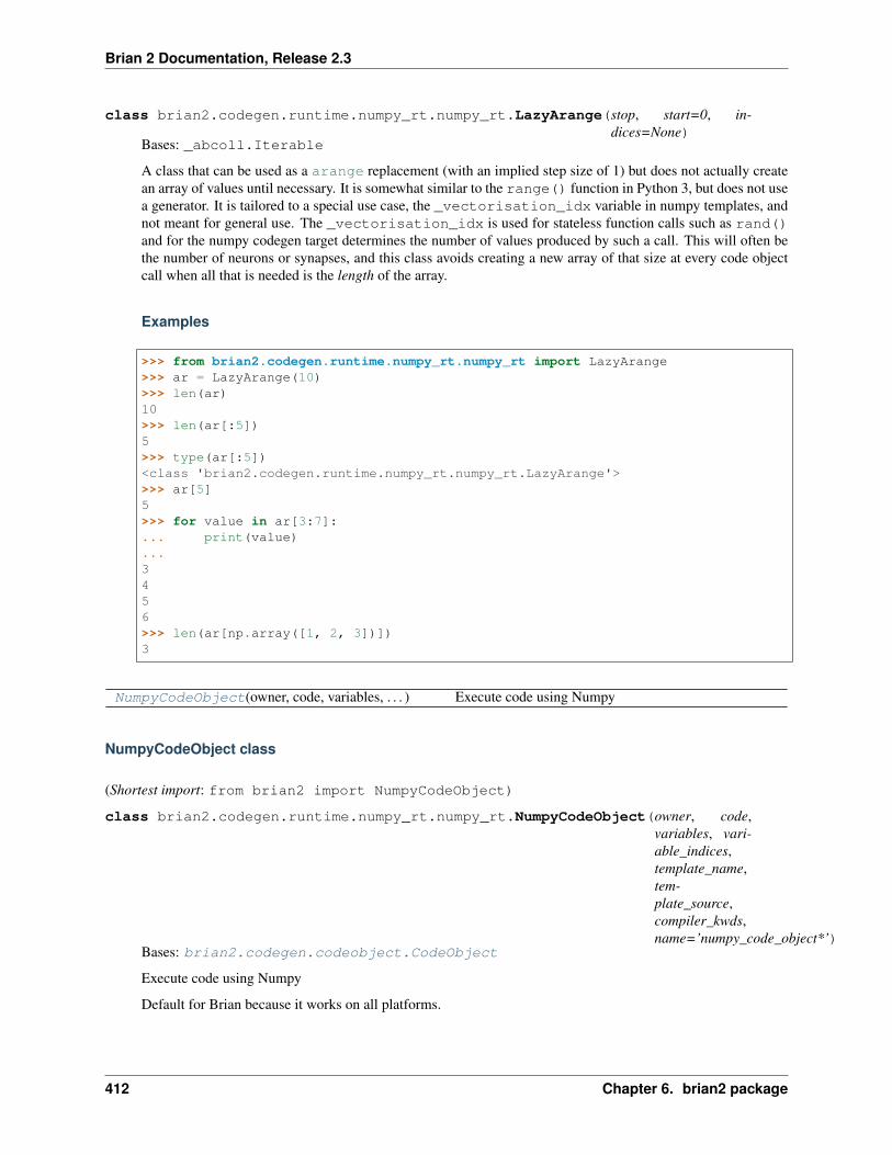
Brian 2 Documentation, Release 2.3
class brian2.codegen.runtime.numpy_rt.numpy_rt.LazyArange(stop, start=0, in-dices=None)
Bases: _abcoll.Iterable
A class that can be used as a arange replacement (with an implied step size of 1) but does not actually createan array of values until necessary. It is somewhat similar to the range() function in Python 3, but does not usea generator. It is tailored to a special use case, the _vectorisation_idx variable in numpy templates, andnot meant for general use. The _vectorisation_idx is used for stateless function calls such as rand()and for the numpy codegen target determines the number of values produced by such a call. This will often bethe number of neurons or synapses, and this class avoids creating a new array of that size at every code objectcall when all that is needed is the length of the array.
Examples
>>> from brian2.codegen.runtime.numpy_rt.numpy_rt import LazyArange>>> ar = LazyArange(10)>>> len(ar)10>>> len(ar[:5])5>>> type(ar[:5])<class 'brian2.codegen.runtime.numpy_rt.numpy_rt.LazyArange'>>>> ar[5]5>>> for value in ar[3:7]:... print(value)...3456>>> len(ar[np.array([1, 2, 3])])3
NumpyCodeObject(owner, code, variables, . . . ) Execute code using Numpy
NumpyCodeObject class
(Shortest import: from brian2 import NumpyCodeObject)
class brian2.codegen.runtime.numpy_rt.numpy_rt.NumpyCodeObject(owner, code,variables, vari-able_indices,template_name,tem-plate_source,compiler_kwds,name=’numpy_code_object*’)
Bases: brian2.codegen.codeobject.CodeObject
Execute code using Numpy
Default for Brian because it works on all platforms.
412 Chapter 6. brian2 package
Brian 2 Documentation, Release 2.3
Methods
compile()is_available() Whether this target for code generation is available.run() Runs the code in the namespace.update_namespace() Update the namespace for this timestep.variables_to_namespace()
Details
compile()
classmethod is_available()Whether this target for code generation is available. Should use a minimal example to check whether codegeneration works in general.
run()Runs the code in the namespace.
Returns return_value : dict
A dictionary with the keys corresponding to the output_variables defined duringthe call of CodeGenerator.code_object.
update_namespace()Update the namespace for this timestep. Should only deal with variables where the reference changesevery timestep, i.e. where the current reference in namespace is not correct.
variables_to_namespace()
weave_rt package
Runtime C++ code generation via weave.
weave_rt module
Module providing WeaveCodeObject.
Exported members: WeaveCodeObject, WeaveCodeGenerator
Classes
WeaveCodeGenerator(*args, **kwds)
WeaveCodeGenerator class
(Shortest import: from brian2.codegen import WeaveCodeGenerator)
class brian2.codegen.runtime.weave_rt.weave_rt.WeaveCodeGenerator(*args,**kwds)
Bases: brian2.codegen.generators.cpp_generator.CPPCodeGenerator
6.6. Subpackages 413

Brian 2 Documentation, Release 2.3
WeaveCodeObject(owner, code, variables, . . . ) Weave code object
WeaveCodeObject class
(Shortest import: from brian2 import WeaveCodeObject)
class brian2.codegen.runtime.weave_rt.weave_rt.WeaveCodeObject(owner, code,variables, vari-able_indices,template_name,tem-plate_source,compiler_kwds,name=’weave_code_object*’)
Bases: brian2.codegen.codeobject.CodeObject
Weave code object
The code should be a MultiTemplate object with two macros defined, main (for the main loop code) andsupport_code for any support code (e.g. function definitions).
Methods
compile()is_available() Whether this target for code generation is available.run() Runs the code in the namespace.update_namespace() Update the namespace for this timestep.variables_to_namespace()
Details
compile()
classmethod is_available()Whether this target for code generation is available. Should use a minimal example to check whether codegeneration works in general.
run()Runs the code in the namespace.
Returns return_value : dict
A dictionary with the keys corresponding to the output_variables defined duringthe call of CodeGenerator.code_object.
update_namespace()Update the namespace for this timestep. Should only deal with variables where the reference changesevery timestep, i.e. where the current reference in namespace is not correct.
variables_to_namespace()
Functions
414 Chapter 6. brian2 package
Brian 2 Documentation, Release 2.3
get_weave_cache_dir()
get_weave_cache_dir function
(Shortest import: from brian2.codegen.runtime.weave_rt.weave_rt importget_weave_cache_dir)
brian2.codegen.runtime.weave_rt.weave_rt.get_weave_cache_dir()
get_weave_extensions()
get_weave_extensions function
(Shortest import: from brian2.codegen.runtime.weave_rt.weave_rt importget_weave_extensions)
brian2.codegen.runtime.weave_rt.weave_rt.get_weave_extensions()
weave_data_type(dtype) Gives the C language specifier for numpy data types us-ing weave.
weave_data_type function
(Shortest import: from brian2.codegen.runtime.weave_rt.weave_rt importweave_data_type)
brian2.codegen.runtime.weave_rt.weave_rt.weave_data_type(dtype)Gives the C language specifier for numpy data types using weave. For example, numpy.int32 maps to longin C.
6.6.2 core package
Essential Brian modules, in particular base classes for all kinds of brian objects.
Built-in preferences
Core Brian preferences
core.default_float_dtype = float64
Default dtype for all arrays of scalars (state variables, weights, etc.).
core.default_integer_dtype = int32
Default dtype for all arrays of integer scalars.
core.outdated_dependency_error = True
Whether to raise an error for outdated dependencies (True) or just a warning (False).
6.6. Subpackages 415
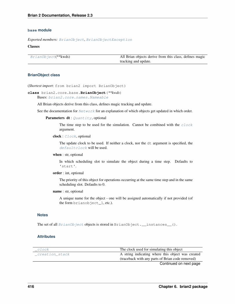
Brian 2 Documentation, Release 2.3
base module
Exported members: BrianObject, BrianObjectException
Classes
BrianObject(**kwds) All Brian objects derive from this class, defines magictracking and update.
BrianObject class
(Shortest import: from brian2 import BrianObject)
class brian2.core.base.BrianObject(**kwds)Bases: brian2.core.names.Nameable
All Brian objects derive from this class, defines magic tracking and update.
See the documentation for Network for an explanation of which objects get updated in which order.
Parameters dt : Quantity , optional
The time step to be used for the simulation. Cannot be combined with the clockargument.
clock : Clock, optional
The update clock to be used. If neither a clock, nor the dt argument is specified, thedefaultclock will be used.
when : str, optional
In which scheduling slot to simulate the object during a time step. Defaults to'start'.
order : int, optional
The priority of this object for operations occurring at the same time step and in the samescheduling slot. Defaults to 0.
name : str, optional
A unique name for the object - one will be assigned automatically if not provided (ofthe form brianobject_1, etc.).
Notes
The set of all BrianObject objects is stored in BrianObject.__instances__().
Attributes
_clock The clock used for simulating this object_creation_stack A string indicating where this object was created
(traceback with any parts of Brian code removed)Continued on next page
416 Chapter 6. brian2 package
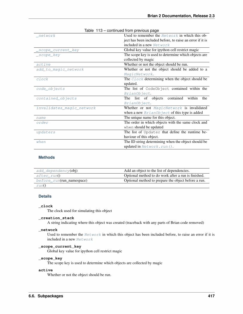
Brian 2 Documentation, Release 2.3
Table 113 – continued from previous page_network Used to remember the Network in which this ob-
ject has been included before, to raise an error if it isincluded in a new Network
_scope_current_key Global key value for ipython cell restrict magic_scope_key The scope key is used to determine which objects are
collected by magicactive Whether or not the object should be run.add_to_magic_network Whether or not the object should be added to a
MagicNetwork.clock The Clock determining when the object should be
updated.code_objects The list of CodeObject contained within the
BrianObject.contained_objects The list of objects contained within the
BrianObject.invalidates_magic_network Whether or not MagicNetwork is invalidated
when a new BrianObject of this type is addedname The unique name for this object.order The order in which objects with the same clock and
when should be updatedupdaters The list of Updater that define the runtime be-
haviour of this object.when The ID string determining when the object should be
updated in Network.run().
Methods
add_dependency(obj) Add an object to the list of dependencies.after_run() Optional method to do work after a run is finished.before_run(run_namespace) Optional method to prepare the object before a run.run()
Details
_clockThe clock used for simulating this object
_creation_stackA string indicating where this object was created (traceback with any parts of Brian code removed)
_networkUsed to remember the Network in which this object has been included before, to raise an error if it isincluded in a new Network
_scope_current_keyGlobal key value for ipython cell restrict magic
_scope_keyThe scope key is used to determine which objects are collected by magic
activeWhether or not the object should be run.
6.6. Subpackages 417
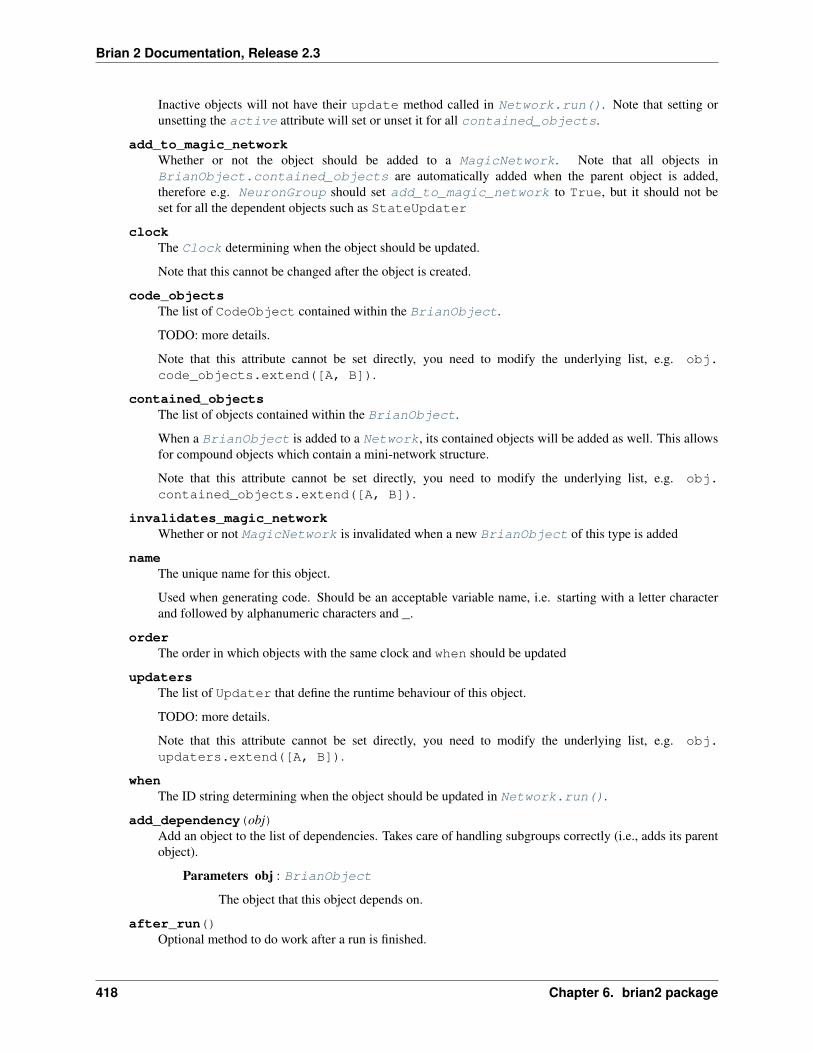
Brian 2 Documentation, Release 2.3
Inactive objects will not have their update method called in Network.run(). Note that setting orunsetting the active attribute will set or unset it for all contained_objects.
add_to_magic_networkWhether or not the object should be added to a MagicNetwork. Note that all objects inBrianObject.contained_objects are automatically added when the parent object is added,therefore e.g. NeuronGroup should set add_to_magic_network to True, but it should not beset for all the dependent objects such as StateUpdater
clockThe Clock determining when the object should be updated.
Note that this cannot be changed after the object is created.
code_objectsThe list of CodeObject contained within the BrianObject.
TODO: more details.
Note that this attribute cannot be set directly, you need to modify the underlying list, e.g. obj.code_objects.extend([A, B]).
contained_objectsThe list of objects contained within the BrianObject.
When a BrianObject is added to a Network, its contained objects will be added as well. This allowsfor compound objects which contain a mini-network structure.
Note that this attribute cannot be set directly, you need to modify the underlying list, e.g. obj.contained_objects.extend([A, B]).
invalidates_magic_networkWhether or not MagicNetwork is invalidated when a new BrianObject of this type is added
nameThe unique name for this object.
Used when generating code. Should be an acceptable variable name, i.e. starting with a letter characterand followed by alphanumeric characters and _.
orderThe order in which objects with the same clock and when should be updated
updatersThe list of Updater that define the runtime behaviour of this object.
TODO: more details.
Note that this attribute cannot be set directly, you need to modify the underlying list, e.g. obj.updaters.extend([A, B]).
whenThe ID string determining when the object should be updated in Network.run().
add_dependency(obj)Add an object to the list of dependencies. Takes care of handling subgroups correctly (i.e., adds its parentobject).
Parameters obj : BrianObject
The object that this object depends on.
after_run()Optional method to do work after a run is finished.
418 Chapter 6. brian2 package

Brian 2 Documentation, Release 2.3
Called by Network.after_run() after the main simulation loop terminated.
before_run(run_namespace)Optional method to prepare the object before a run.
TODO
run()
BrianObjectException(message, brianobj, . . . ) High level exception that adds extra Brian-specific in-formation to exceptions
BrianObjectException class
(Shortest import: from brian2 import BrianObjectException)
class brian2.core.base.BrianObjectException(message, brianobj, original_exception)Bases: exceptions.Exception
High level exception that adds extra Brian-specific information to exceptions
This exception should only be raised at a fairly high level in Brian code to pass information back to the user. Itadds extra information about where a BrianObject was defined to better enable users to locate the source ofproblems.
You should use the brian_object_exception function to raise this, and it should only be raised in anexcept block handling a prior exception.
Parameters message : str
Additional error information to add to the original exception.
brianobj : BrianObject
The object that caused the error to happen.
original_exception : Exception
The original exception that was raised.
Functions
brian_object_exception(message, brianobj,. . . )
Returns a BrianObjectException derived fromthe original exception.
brian_object_exception function
(Shortest import: from brian2.core.base import brian_object_exception)
brian2.core.base.brian_object_exception(message, brianobj, original_exception)Returns a BrianObjectException derived from the original exception.
Creates a new class derived from the class of the original exception and BrianObjectException. This al-lows exception handling code to respond both to the original exception class and BrianObjectException.
See BrianObjectException for arguments and notes.
6.6. Subpackages 419

Brian 2 Documentation, Release 2.3
device_override(name) Decorates a function/method to allow it to be overriddenby the current Device.
device_override function
(Shortest import: from brian2.core.base import device_override)
brian2.core.base.device_override(name)Decorates a function/method to allow it to be overridden by the current Device.
The name is the function name in the Device to use as an override if it exists.
The returned function has an additional attribute original_function which is a reference to the original,undecorated function.
weakproxy_with_fallback(obj) Attempts to create a weakproxy to the object, but fallsback to the object if not possible.
weakproxy_with_fallback function
(Shortest import: from brian2.core.base import weakproxy_with_fallback)
brian2.core.base.weakproxy_with_fallback(obj)Attempts to create a weakproxy to the object, but falls back to the object if not possible.
clocks module
Clocks for the simulator.
Exported members: Clock, defaultclock
Classes
Clock(dt[, name]) An object that holds the simulation time and the timestep.
Clock class
(Shortest import: from brian2 import Clock)
class brian2.core.clocks.Clock(dt, name=’clock*’)Bases: brian2.groups.group.VariableOwner
An object that holds the simulation time and the time step.
Parameters dt : float
The time step of the simulation as a float
name : str, optional
An explicit name, if not specified gives an automatically generated name
420 Chapter 6. brian2 package
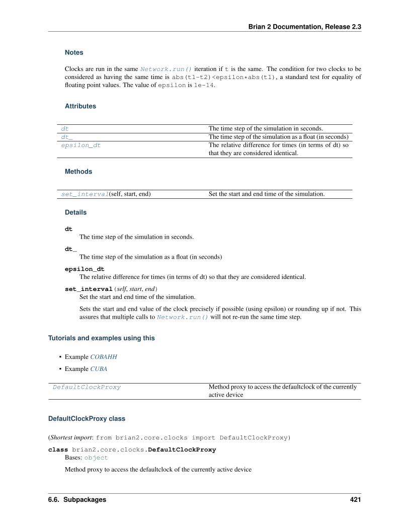
Brian 2 Documentation, Release 2.3
Notes
Clocks are run in the same Network.run() iteration if t is the same. The condition for two clocks to beconsidered as having the same time is abs(t1-t2)<epsilon*abs(t1), a standard test for equality offloating point values. The value of epsilon is 1e-14.
Attributes
dt The time step of the simulation in seconds.dt_ The time step of the simulation as a float (in seconds)epsilon_dt The relative difference for times (in terms of dt) so
that they are considered identical.
Methods
set_interval(self, start, end) Set the start and end time of the simulation.
Details
dtThe time step of the simulation in seconds.
dt_The time step of the simulation as a float (in seconds)
epsilon_dtThe relative difference for times (in terms of dt) so that they are considered identical.
set_interval(self, start, end)Set the start and end time of the simulation.
Sets the start and end value of the clock precisely if possible (using epsilon) or rounding up if not. Thisassures that multiple calls to Network.run() will not re-run the same time step.
Tutorials and examples using this
• Example COBAHH
• Example CUBA
DefaultClockProxy Method proxy to access the defaultclock of the currentlyactive device
DefaultClockProxy class
(Shortest import: from brian2.core.clocks import DefaultClockProxy)
class brian2.core.clocks.DefaultClockProxyBases: object
Method proxy to access the defaultclock of the currently active device
6.6. Subpackages 421
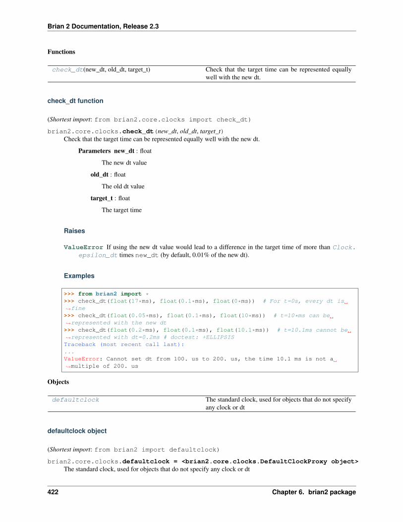
Brian 2 Documentation, Release 2.3
Functions
check_dt(new_dt, old_dt, target_t) Check that the target time can be represented equallywell with the new dt.
check_dt function
(Shortest import: from brian2.core.clocks import check_dt)
brian2.core.clocks.check_dt(new_dt, old_dt, target_t)Check that the target time can be represented equally well with the new dt.
Parameters new_dt : float
The new dt value
old_dt : float
The old dt value
target_t : float
The target time
Raises
ValueError If using the new dt value would lead to a difference in the target time of more than Clock.epsilon_dt times new_dt (by default, 0.01% of the new dt).
Examples
>>> from brian2 import *>>> check_dt(float(17*ms), float(0.1*ms), float(0*ms)) # For t=0s, every dt is→˓fine>>> check_dt(float(0.05*ms), float(0.1*ms), float(10*ms)) # t=10*ms can be→˓represented with the new dt>>> check_dt(float(0.2*ms), float(0.1*ms), float(10.1*ms)) # t=10.1ms cannot be→˓represented with dt=0.2ms # doctest: +ELLIPSISTraceback (most recent call last):...ValueError: Cannot set dt from 100. us to 200. us, the time 10.1 ms is not a→˓multiple of 200. us
Objects
defaultclock The standard clock, used for objects that do not specifyany clock or dt
defaultclock object
(Shortest import: from brian2 import defaultclock)
brian2.core.clocks.defaultclock = <brian2.core.clocks.DefaultClockProxy object>The standard clock, used for objects that do not specify any clock or dt
422 Chapter 6. brian2 package
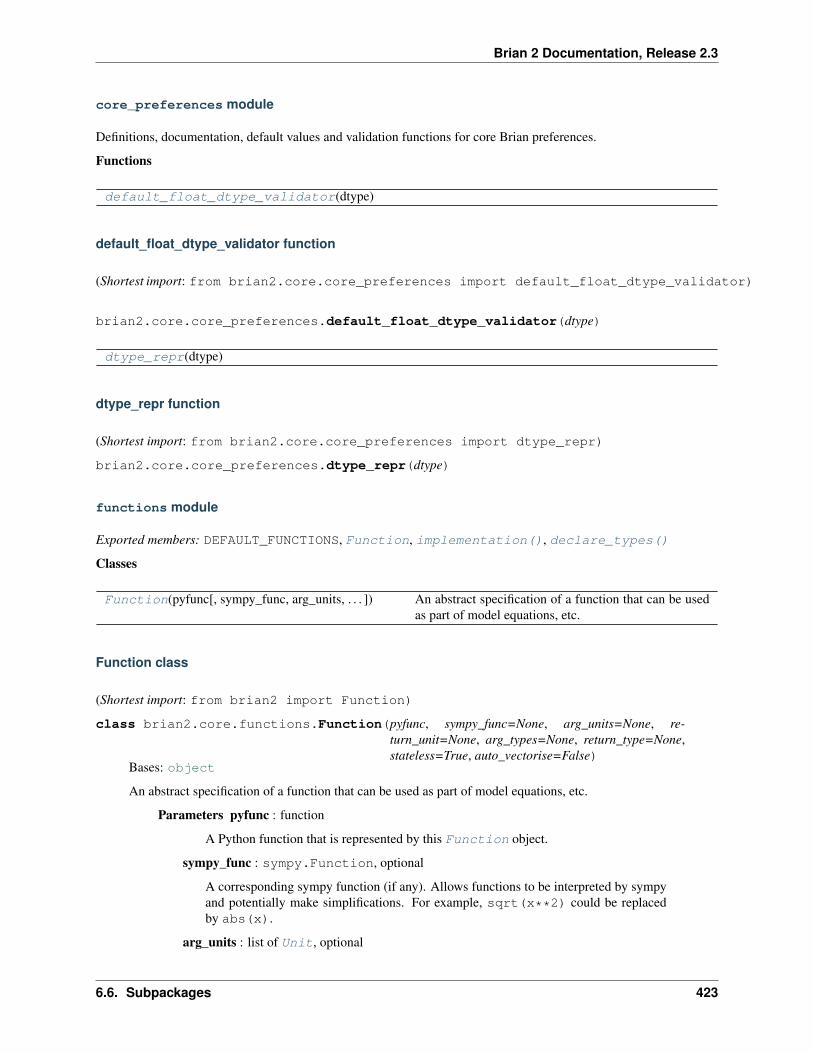
Brian 2 Documentation, Release 2.3
core_preferences module
Definitions, documentation, default values and validation functions for core Brian preferences.
Functions
default_float_dtype_validator(dtype)
default_float_dtype_validator function
(Shortest import: from brian2.core.core_preferences import default_float_dtype_validator)
brian2.core.core_preferences.default_float_dtype_validator(dtype)
dtype_repr(dtype)
dtype_repr function
(Shortest import: from brian2.core.core_preferences import dtype_repr)
brian2.core.core_preferences.dtype_repr(dtype)
functions module
Exported members: DEFAULT_FUNCTIONS, Function, implementation(), declare_types()
Classes
Function(pyfunc[, sympy_func, arg_units, . . . ]) An abstract specification of a function that can be usedas part of model equations, etc.
Function class
(Shortest import: from brian2 import Function)
class brian2.core.functions.Function(pyfunc, sympy_func=None, arg_units=None, re-turn_unit=None, arg_types=None, return_type=None,stateless=True, auto_vectorise=False)
Bases: object
An abstract specification of a function that can be used as part of model equations, etc.
Parameters pyfunc : function
A Python function that is represented by this Function object.
sympy_func : sympy.Function, optional
A corresponding sympy function (if any). Allows functions to be interpreted by sympyand potentially make simplifications. For example, sqrt(x**2) could be replacedby abs(x).
arg_units : list of Unit, optional
6.6. Subpackages 423

Brian 2 Documentation, Release 2.3
If pyfunc does not provide unit information (which typically means that it was not an-notated with a check_units() decorator), the units of the arguments have to speci-fied explicitly using this parameter.
return_unit : Unit or callable, optional
Same as for arg_units: if pyfunc does not provide unit information, this informa-tion has to be provided explictly here. return_unit can either be a specific Unit,if the function always returns the same unit, or a function of the input units, e.g. a“square” function would return the square of its input units, i.e. return_unit couldbe specified as lambda u: u**2.
arg_types : list of str, optional
Similar to arg_units, but gives the type of the argument rather than its unit. Inthe current version of Brian arguments are specified by one of the following strings:‘boolean’, ‘integer’, ‘float’, ‘any’. If arg_types is not specified, ‘any’ will be as-sumed. In future versions, a more refined specification may be possible. Note that anyargument with a type other than float should have no units. If
return_type : str, optional
Similar to return_unit and arg_types. In addition to ‘boolean’, ‘integer’ and‘float’ you can also use ‘highest’ which will return the highest type of its arguments.You can also give a function, as for return_unit. If the return type is not specified,it is assumed to be ‘float’.
stateless : bool, optional
Whether this function does not have an internal state, i.e. if it always returns the sameoutput when called with the same arguments. This is true for mathematical functionsbut not true for rand(), for example. Defaults to True.
auto_vectorise : bool, optional
Whether the implementations of this function should get an additional argument (notspecified in abstract code) that can be used to determine the number of values thatshould be returned (for the numpy target), or an index potentially useful for generatingdeterministic values independent of the order of vectorisation (for all other targets).The main use case are random number functions, e.g. equations refer to rand(), butthe generate code will actually call rand(_vectorisation_idx). Defaults toFalse.
Notes
If a function should be usable for code generation targets other than Python/numpy, implementationsfor these target languages have to be added using the implementation decorator or using theadd_implementations function.
Attributes
implementations Stores implementations for this function in aFunctionImplementationContainer
Methods
424 Chapter 6. brian2 package

Brian 2 Documentation, Release 2.3
__call__(. . . ) <==> x(. . . )is_locally_constant(dt) Return whether this function (if interpreted as a func-
tion of time) should be considered constant over atimestep.
Details
implementationsStores implementations for this function in a FunctionImplementationContainer
__call__(...) <==> x(...)
is_locally_constant(dt)Return whether this function (if interpreted as a function of time) should be considered constant over atimestep. This is most importantly used by TimedArray so that linear integration can be used. In itsstandard implementation, always returns False.
Parameters dt : float
The length of a timestep (without units).
Returns constant : bool
Whether the results of this function can be considered constant over one timestep oflength dt.
FunctionImplementation([name, code, . . . ]) A simple container object for function implementations.
FunctionImplementation class
(Shortest import: from brian2.core.functions import FunctionImplementation)
class brian2.core.functions.FunctionImplementation(name=None, code=None,namespace=None, depen-dencies=None, availabil-ity_check=None, dynamic=False,compiler_kwds=None)
Bases: object
A simple container object for function implementations.
Parameters name : str, optional
The name of the function in the target language. Should only be specified if the functionhas to be renamed for the target language.
code : language-dependent, optional
A language dependent argument specifying the implementation in the target language,e.g. a code string or a dictionary of code strings.
namespace : dict-like, optional
A dictionary of mappings from names to values that should be added to the namespaceof a CodeObject using the function.
dependencies : dict-like, optional
6.6. Subpackages 425
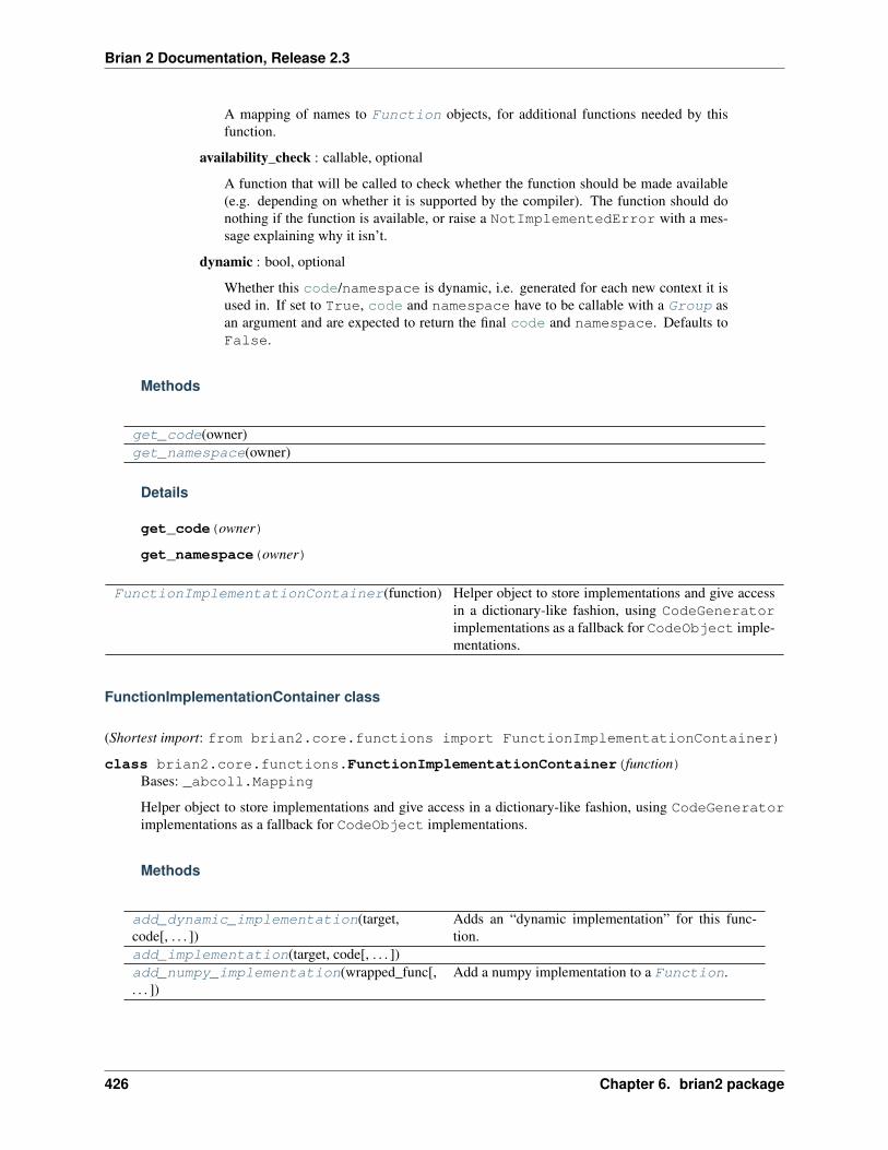
Brian 2 Documentation, Release 2.3
A mapping of names to Function objects, for additional functions needed by thisfunction.
availability_check : callable, optional
A function that will be called to check whether the function should be made available(e.g. depending on whether it is supported by the compiler). The function should donothing if the function is available, or raise a NotImplementedError with a mes-sage explaining why it isn’t.
dynamic : bool, optional
Whether this code/namespace is dynamic, i.e. generated for each new context it isused in. If set to True, code and namespace have to be callable with a Group asan argument and are expected to return the final code and namespace. Defaults toFalse.
Methods
get_code(owner)get_namespace(owner)
Details
get_code(owner)
get_namespace(owner)
FunctionImplementationContainer(function) Helper object to store implementations and give accessin a dictionary-like fashion, using CodeGeneratorimplementations as a fallback for CodeObject imple-mentations.
FunctionImplementationContainer class
(Shortest import: from brian2.core.functions import FunctionImplementationContainer)
class brian2.core.functions.FunctionImplementationContainer(function)Bases: _abcoll.Mapping
Helper object to store implementations and give access in a dictionary-like fashion, using CodeGeneratorimplementations as a fallback for CodeObject implementations.
Methods
add_dynamic_implementation(target,code[, . . . ])
Adds an “dynamic implementation” for this func-tion.
add_implementation(target, code[, . . . ])add_numpy_implementation(wrapped_func[,. . . ])
Add a numpy implementation to a Function.
426 Chapter 6. brian2 package

Brian 2 Documentation, Release 2.3
Details
add_dynamic_implementation(target, code, namespace=None, dependencies=None, availabil-ity_check=None, name=None, compiler_kwds=None)
Adds an “dynamic implementation” for this function. code and namespace arguments are expected tobe callables that will be called in Network.before_run() with the owner of the CodeObject asan argument. This allows to generate code that depends on details of the context it is run in, e.g. the dt ofa clock.
add_implementation(target, code, namespace=None, dependencies=None, availabil-ity_check=None, name=None, compiler_kwds=None)
add_numpy_implementation(wrapped_func, dependencies=None, discard_units=None, com-piler_kwds=None)
Add a numpy implementation to a Function.
Parameters function : Function
The function description for which an implementation should be added.
wrapped_func : callable
The original function (that will be used for the numpy implementation)
dependencies : list of Function, optional
A list of functions this function needs.
discard_units : bool, optional
See implementation().
SymbolicConstant(name, sympy_obj, value) Class for representing constants (e.g.
SymbolicConstant class
(Shortest import: from brian2.core.functions import SymbolicConstant)
class brian2.core.functions.SymbolicConstant(name, sympy_obj, value)Bases: brian2.core.variables.Constant
Class for representing constants (e.g. pi) that are understood by sympy.
exprel Represents (exp(x) - 1)/x.
exprel class
(Shortest import: from brian2.core.functions import exprel)
class brian2.core.functions.exprelBases: sympy.core.function.Function
Represents (exp(x) - 1)/x.
The benefit of using exprel(x) over (exp(x) - 1)/x is that the latter is prone to cancellation under finiteprecision arithmetic when x is close to zero, and cannot be evaluated when x is equal to zero.
6.6. Subpackages 427

Brian 2 Documentation, Release 2.3
Methods
eval(arg) Returns a canonical form of cls applied to argumentsargs.
fdiff([argindex]) Returns the first derivative of this function.
Details
classmethod eval(arg)Returns a canonical form of cls applied to arguments args.
The eval() method is called when the class cls is about to be instantiated and it should return either somesimplified instance (possible of some other class), or if the class cls should be unmodified, return None.
fdiff(argindex=1)Returns the first derivative of this function.
Tutorials and examples using this
• Example COBAHH
• Example IF_curve_Hodgkin_Huxley
• Example compartmental/hh_with_spikes
• Example compartmental/hodgkin_huxley_1952
• Example compartmental/lfp
• Example advanced/float_32_64_benchmark
• Example advanced/exprel_function
• Example frompapers/Wang_Buszaki_1996
Functions
declare_types(**types) Decorator to declare argument and result types for afunction
declare_types function
(Shortest import: from brian2 import declare_types)
brian2.core.functions.declare_types(**types)Decorator to declare argument and result types for a function
Usage is similar to check_units() except that types must be one of {VALID_ARG_TYPES} and the resulttype must be one of {VALID_RETURN_TYPES}. Unspecified argument types are assumed to be 'all' (i.e.anything is permitted), and an unspecified result type is assumed to be 'float'. Note that the 'highest'option for result type will give the highest type of its argument, e.g. if the arguments were boolean and integerthen the result would be integer, if the arguments were integer and float it would be float.
implementation(target[, code, namespace, . . . ]) A simple decorator to extend user-written Python func-tions to work with code generation in other languages.
428 Chapter 6. brian2 package
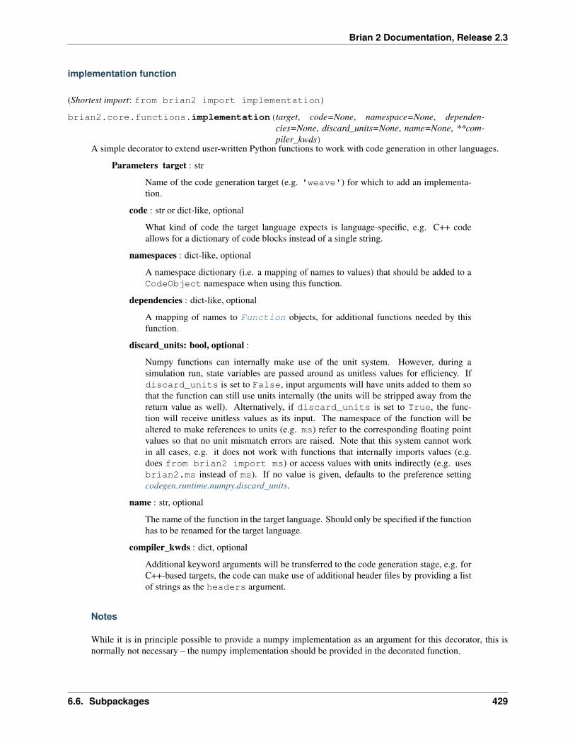
Brian 2 Documentation, Release 2.3
implementation function
(Shortest import: from brian2 import implementation)
brian2.core.functions.implementation(target, code=None, namespace=None, dependen-cies=None, discard_units=None, name=None, **com-piler_kwds)
A simple decorator to extend user-written Python functions to work with code generation in other languages.
Parameters target : str
Name of the code generation target (e.g. 'weave') for which to add an implementa-tion.
code : str or dict-like, optional
What kind of code the target language expects is language-specific, e.g. C++ codeallows for a dictionary of code blocks instead of a single string.
namespaces : dict-like, optional
A namespace dictionary (i.e. a mapping of names to values) that should be added to aCodeObject namespace when using this function.
dependencies : dict-like, optional
A mapping of names to Function objects, for additional functions needed by thisfunction.
discard_units: bool, optional :
Numpy functions can internally make use of the unit system. However, during asimulation run, state variables are passed around as unitless values for efficiency. Ifdiscard_units is set to False, input arguments will have units added to them sothat the function can still use units internally (the units will be stripped away from thereturn value as well). Alternatively, if discard_units is set to True, the func-tion will receive unitless values as its input. The namespace of the function will bealtered to make references to units (e.g. ms) refer to the corresponding floating pointvalues so that no unit mismatch errors are raised. Note that this system cannot workin all cases, e.g. it does not work with functions that internally imports values (e.g.does from brian2 import ms) or access values with units indirectly (e.g. usesbrian2.ms instead of ms). If no value is given, defaults to the preference settingcodegen.runtime.numpy.discard_units.
name : str, optional
The name of the function in the target language. Should only be specified if the functionhas to be renamed for the target language.
compiler_kwds : dict, optional
Additional keyword arguments will be transferred to the code generation stage, e.g. forC++-based targets, the code can make use of additional header files by providing a listof strings as the headers argument.
Notes
While it is in principle possible to provide a numpy implementation as an argument for this decorator, this isnormally not necessary – the numpy implementation should be provided in the decorated function.
6.6. Subpackages 429
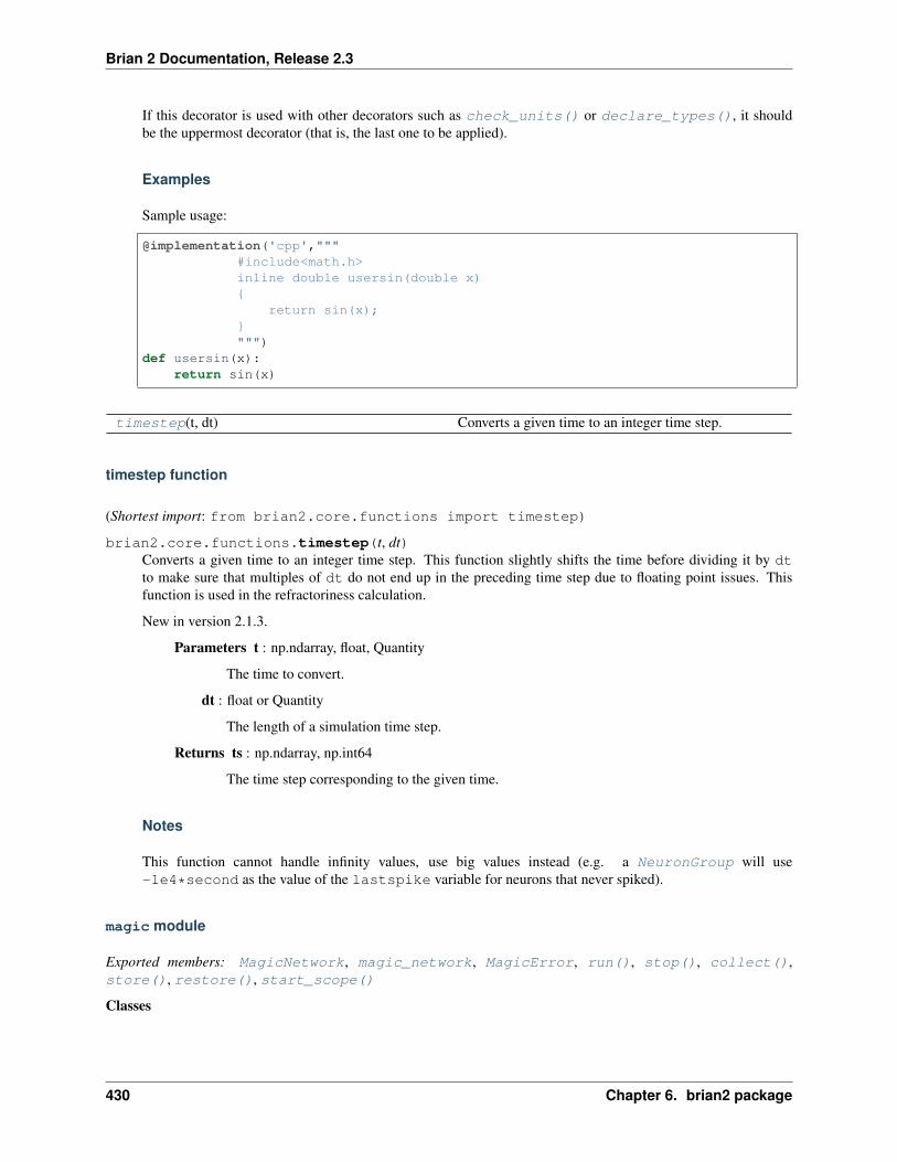
Brian 2 Documentation, Release 2.3
If this decorator is used with other decorators such as check_units() or declare_types(), it shouldbe the uppermost decorator (that is, the last one to be applied).
Examples
Sample usage:
@implementation('cpp',"""#include<math.h>inline double usersin(double x){
return sin(x);}""")
def usersin(x):return sin(x)
timestep(t, dt) Converts a given time to an integer time step.
timestep function
(Shortest import: from brian2.core.functions import timestep)
brian2.core.functions.timestep(t, dt)Converts a given time to an integer time step. This function slightly shifts the time before dividing it by dtto make sure that multiples of dt do not end up in the preceding time step due to floating point issues. Thisfunction is used in the refractoriness calculation.
New in version 2.1.3.
Parameters t : np.ndarray, float, Quantity
The time to convert.
dt : float or Quantity
The length of a simulation time step.
Returns ts : np.ndarray, np.int64
The time step corresponding to the given time.
Notes
This function cannot handle infinity values, use big values instead (e.g. a NeuronGroup will use-1e4*second as the value of the lastspike variable for neurons that never spiked).
magic module
Exported members: MagicNetwork, magic_network, MagicError, run(), stop(), collect(),store(), restore(), start_scope()
Classes
430 Chapter 6. brian2 package
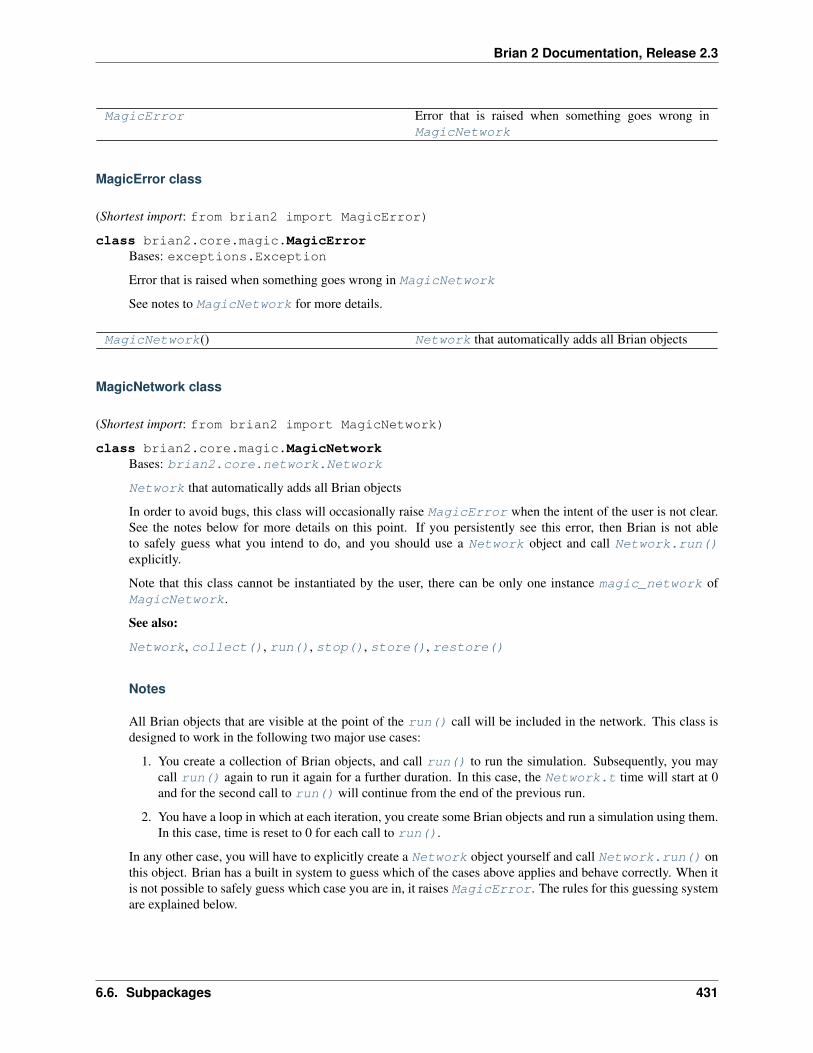
Brian 2 Documentation, Release 2.3
MagicError Error that is raised when something goes wrong inMagicNetwork
MagicError class
(Shortest import: from brian2 import MagicError)
class brian2.core.magic.MagicErrorBases: exceptions.Exception
Error that is raised when something goes wrong in MagicNetwork
See notes to MagicNetwork for more details.
MagicNetwork() Network that automatically adds all Brian objects
MagicNetwork class
(Shortest import: from brian2 import MagicNetwork)
class brian2.core.magic.MagicNetworkBases: brian2.core.network.Network
Network that automatically adds all Brian objects
In order to avoid bugs, this class will occasionally raise MagicError when the intent of the user is not clear.See the notes below for more details on this point. If you persistently see this error, then Brian is not ableto safely guess what you intend to do, and you should use a Network object and call Network.run()explicitly.
Note that this class cannot be instantiated by the user, there can be only one instance magic_network ofMagicNetwork.
See also:
Network, collect(), run(), stop(), store(), restore()
Notes
All Brian objects that are visible at the point of the run() call will be included in the network. This class isdesigned to work in the following two major use cases:
1. You create a collection of Brian objects, and call run() to run the simulation. Subsequently, you maycall run() again to run it again for a further duration. In this case, the Network.t time will start at 0and for the second call to run() will continue from the end of the previous run.
2. You have a loop in which at each iteration, you create some Brian objects and run a simulation using them.In this case, time is reset to 0 for each call to run().
In any other case, you will have to explicitly create a Network object yourself and call Network.run() onthis object. Brian has a built in system to guess which of the cases above applies and behave correctly. When itis not possible to safely guess which case you are in, it raises MagicError. The rules for this guessing systemare explained below.
6.6. Subpackages 431

Brian 2 Documentation, Release 2.3
If a simulation consists only of objects that have not been run, it will assume that you want to start a newsimulation. If a simulation only consists of objects that have been simulated in the previous run() call, it willcontinue that simulation at the previous time.
If neither of these two situations apply, i.e., the network consists of a mix of previously run objects and newobjects, an error will be raised.
In these checks, “non-invalidating” objects (i.e. objects that have BrianObject.invalidates_magic_network set to False) are ignored, e.g. creating new monitors is alwayspossible.
Methods
add(*objs) You cannot add objects directly to MagicNetworkafter_run()check_dependencies()get_states([units, format, subexpressions, . . . ]) See Network.get_states().remove(*objs) You cannot remove objects directly from
MagicNetworkrestore([name, filename, . . . ]) See Network.restore().run(duration[, report, report_period, . . . ]) Runs the simulation for the given duration.set_states(values[, units, format, level]) See Network.set_states().store([name, filename, level]) See Network.store().
Details
add(*objs)You cannot add objects directly to MagicNetwork
after_run()
check_dependencies()
get_states(units=True, format=’dict’, subexpressions=False, level=0)See Network.get_states().
remove(*objs)You cannot remove objects directly from MagicNetwork
restore(name=’default’, filename=None, restore_random_state=False, level=0)See Network.restore().
run(duration, report=None, report_period=60*second, namespace=None, level=0)Runs the simulation for the given duration.
Parameters duration : Quantity
The amount of simulation time to run for.
report : {None, ‘text’, ‘stdout’, ‘stderr’, function}, optional
How to report the progress of the simulation. If None, do not report progress. If'text' or 'stdout' is specified, print the progress to stdout. If 'stderr'is specified, print the progress to stderr. Alternatively, you can specify a call-back callable(elapsed, complete, duration) which will be passed theamount of time elapsed as a Quantity , the fraction complete from 0.0 to 1.0 andthe total duration of the simulation (in biological time). The function will always be
432 Chapter 6. brian2 package
Brian 2 Documentation, Release 2.3
called at the beginning and the end (i.e. for fractions 0.0 and 1.0), regardless of thereport_period.
report_period : Quantity
How frequently (in real time) to report progress.
namespace : dict-like, optional
A namespace that will be used in addition to the group-specific namespaces (if defined).If not specified, the locals and globals around the run function will be used.
profile : bool, optional
Whether to record profiling information (see Network.profiling_info). De-faults to False.
level : int, optional
How deep to go up the stack frame to look for the locals/global (see namespace argu-ment). Only used by run functions that call this run function, e.g. MagicNetwork.run() to adjust for the additional nesting.
Notes
The simulation can be stopped by calling Network.stop() or the global stop() function.
set_states(values, units=True, format=’dict’, level=0)See Network.set_states().
store(name=’default’, filename=None, level=0)See Network.store().
Functions
collect([level]) Return the list of BrianObjects that will be simu-lated if run() is called.
collect function
(Shortest import: from brian2 import collect)
brian2.core.magic.collect(level=0)Return the list of BrianObjects that will be simulated if run() is called.
Parameters level : int, optional
How much further up to go in the stack to find the objects. Needs only to be specified ifcollect() is called as part of a function and should be increased by 1 for every levelof nesting. Defaults to 0.
Returns objects : set of BrianObject
The objects that will be simulated.
get_objects_in_namespace(level) Get all the objects in the current namespace that derivefrom BrianObject.
6.6. Subpackages 433
Brian 2 Documentation, Release 2.3
get_objects_in_namespace function
(Shortest import: from brian2.core.magic import get_objects_in_namespace)
brian2.core.magic.get_objects_in_namespace(level)Get all the objects in the current namespace that derive from BrianObject. Used to determine the objects forthe MagicNetwork.
Parameters level : int, optional
How far to go back to get the locals/globals. Each function/method call should add 1 tothis argument, functions/method with a decorator have to add 2.
Returns objects : set
A set with weak references to the BrianObjects in the namespace.
restore([name, filename, restore_random_state]) Restore the state of the network and all included objects.
restore function
(Shortest import: from brian2 import restore)
brian2.core.magic.restore(name=’default’, filename=None, restore_random_state=False)Restore the state of the network and all included objects.
Parameters name : str, optional
The name of the snapshot to restore, if not specified uses 'default'.
filename : str, optional
The name of the file from where the state should be restored. If not specified, it is ex-pected that the state exist in memory (i.e. Network.store() was previously calledwithout the filename argument).
restore_random_state : bool, optional
Whether to restore the state of the random number generator. If set to True, goingback to an earlier state of the simulation will continue exactly where it left off, even ifthe simulation is stochastic. If set to False (the default), random numbers are inde-pendent between runs (except for explicitly set random seeds), regardless of whetherstore()/restore() has been used or not. Note that this also restores numpy’srandom number generator (since it is used internally by Brian), but it does not restorePython’s builtin random number generator in the random module.
See Also :
——– :
Network.restore :
run(duration[, report, report_period, . . . ]) Runs a simulation with all “visible” Brian objects forthe given duration.
run function
(Shortest import: from brian2 import run)
434 Chapter 6. brian2 package
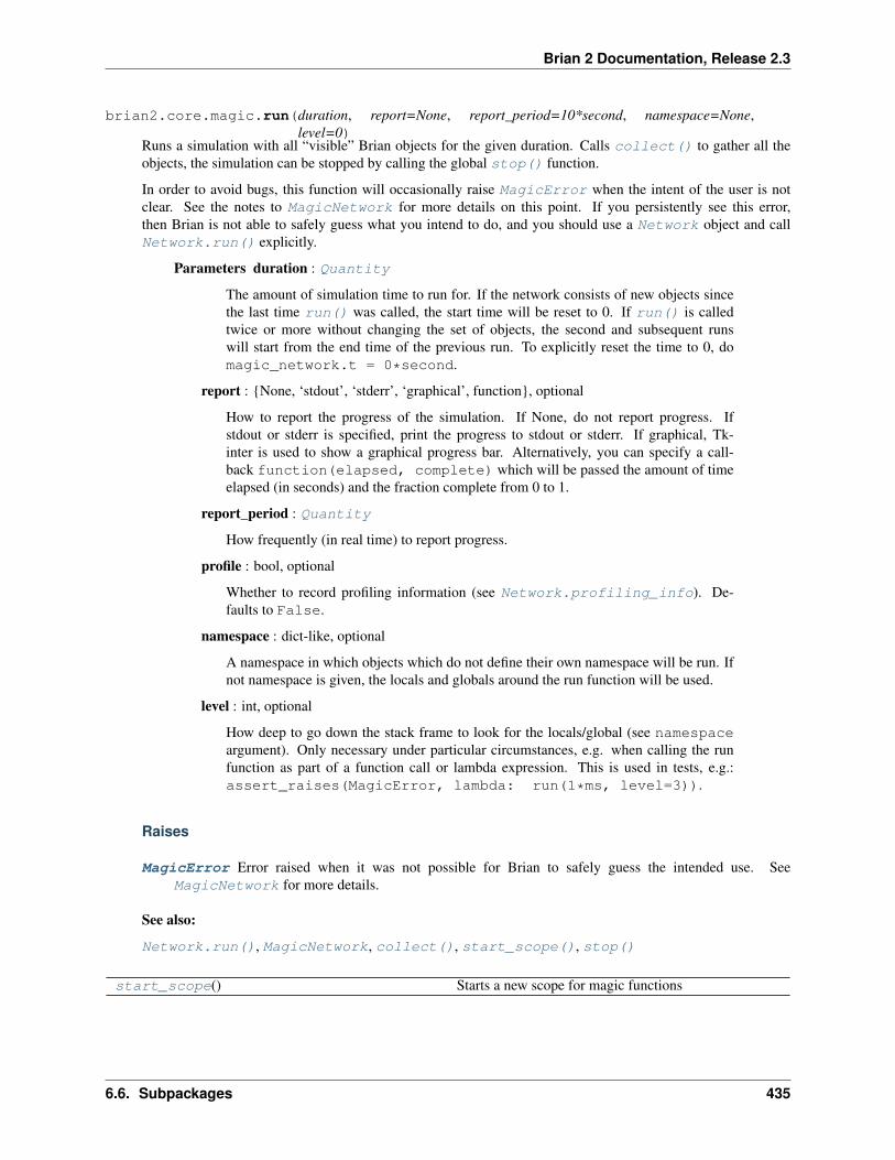
Brian 2 Documentation, Release 2.3
brian2.core.magic.run(duration, report=None, report_period=10*second, namespace=None,level=0)
Runs a simulation with all “visible” Brian objects for the given duration. Calls collect() to gather all theobjects, the simulation can be stopped by calling the global stop() function.
In order to avoid bugs, this function will occasionally raise MagicError when the intent of the user is notclear. See the notes to MagicNetwork for more details on this point. If you persistently see this error,then Brian is not able to safely guess what you intend to do, and you should use a Network object and callNetwork.run() explicitly.
Parameters duration : Quantity
The amount of simulation time to run for. If the network consists of new objects sincethe last time run() was called, the start time will be reset to 0. If run() is calledtwice or more without changing the set of objects, the second and subsequent runswill start from the end time of the previous run. To explicitly reset the time to 0, domagic_network.t = 0*second.
report : {None, ‘stdout’, ‘stderr’, ‘graphical’, function}, optional
How to report the progress of the simulation. If None, do not report progress. Ifstdout or stderr is specified, print the progress to stdout or stderr. If graphical, Tk-inter is used to show a graphical progress bar. Alternatively, you can specify a call-back function(elapsed, complete) which will be passed the amount of timeelapsed (in seconds) and the fraction complete from 0 to 1.
report_period : Quantity
How frequently (in real time) to report progress.
profile : bool, optional
Whether to record profiling information (see Network.profiling_info). De-faults to False.
namespace : dict-like, optional
A namespace in which objects which do not define their own namespace will be run. Ifnot namespace is given, the locals and globals around the run function will be used.
level : int, optional
How deep to go down the stack frame to look for the locals/global (see namespaceargument). Only necessary under particular circumstances, e.g. when calling the runfunction as part of a function call or lambda expression. This is used in tests, e.g.:assert_raises(MagicError, lambda: run(1*ms, level=3)).
Raises
MagicError Error raised when it was not possible for Brian to safely guess the intended use. SeeMagicNetwork for more details.
See also:
Network.run(), MagicNetwork, collect(), start_scope(), stop()
start_scope() Starts a new scope for magic functions
6.6. Subpackages 435

Brian 2 Documentation, Release 2.3
start_scope function
(Shortest import: from brian2 import start_scope)
brian2.core.magic.start_scope()Starts a new scope for magic functions
All objects created before this call will no longer be automatically included by the magic functions such asrun().
stop() Stops all running simulations.
stop function
(Shortest import: from brian2 import stop)
brian2.core.magic.stop()Stops all running simulations.
See also:
Network.stop(), run(), reinit
store([name, filename]) Store the state of the network and all included objects.
store function
(Shortest import: from brian2 import store)
brian2.core.magic.store(name=’default’, filename=None)Store the state of the network and all included objects.
Parameters name : str, optional
A name for the snapshot, if not specified uses 'default'.
filename : str, optional
A filename where the state should be stored. If not specified, the state will be stored inmemory.
See also:
Network.store()
Objects
magic_network Automatically constructed MagicNetwork of allBrian objects
magic_network object
(Shortest import: from brian2 import magic_network)
brian2.core.magic.magic_network = MagicNetwork()Automatically constructed MagicNetwork of all Brian objects
436 Chapter 6. brian2 package

Brian 2 Documentation, Release 2.3
names module
Exported members: Nameable
Classes
Nameable(name) Base class to find a unique name for an object
Nameable class
(Shortest import: from brian2 import Nameable)
class brian2.core.names.Nameable(name)Bases: brian2.core.tracking.Trackable
Base class to find a unique name for an object
If you specify a name explicitly, and it has already been taken, a ValueError is raised. You can also specifya name with a wildcard asterisk in the end, i.e. in the form 'name*'. It will then try name first but if this isalready specified, it will try name_1, name__2`, etc. This is the default mechanism used by most core objectsin Brian, e.g. NeuronGroup uses a default name of 'neurongroup*'.
Parameters name : str
An name for the object, possibly ending in * to specify that variants of this name shouldbe tried if the name (without the asterisk) is already taken. If (and only if) the name forthis object has already been set, it is also possible to call the initialiser with None forthe name argument. This situation can arise when a class derives from multiple classesthat derive themselves from Nameable (e.g. Group and CodeRunner) and theirinitialisers are called explicitely.
Raises
ValueError If the name is already taken.
Attributes
id A unique id for this object.name The unique name for this object.
Methods
assign_id() Assign a new id to this object.
Details
idA unique id for this object.
In contrast to names, which may be reused, the id stays unique. This is used in the dependency checkingto not have to deal with the chore of comparing weak references, weak proxies and strong references.
name
6.6. Subpackages 437
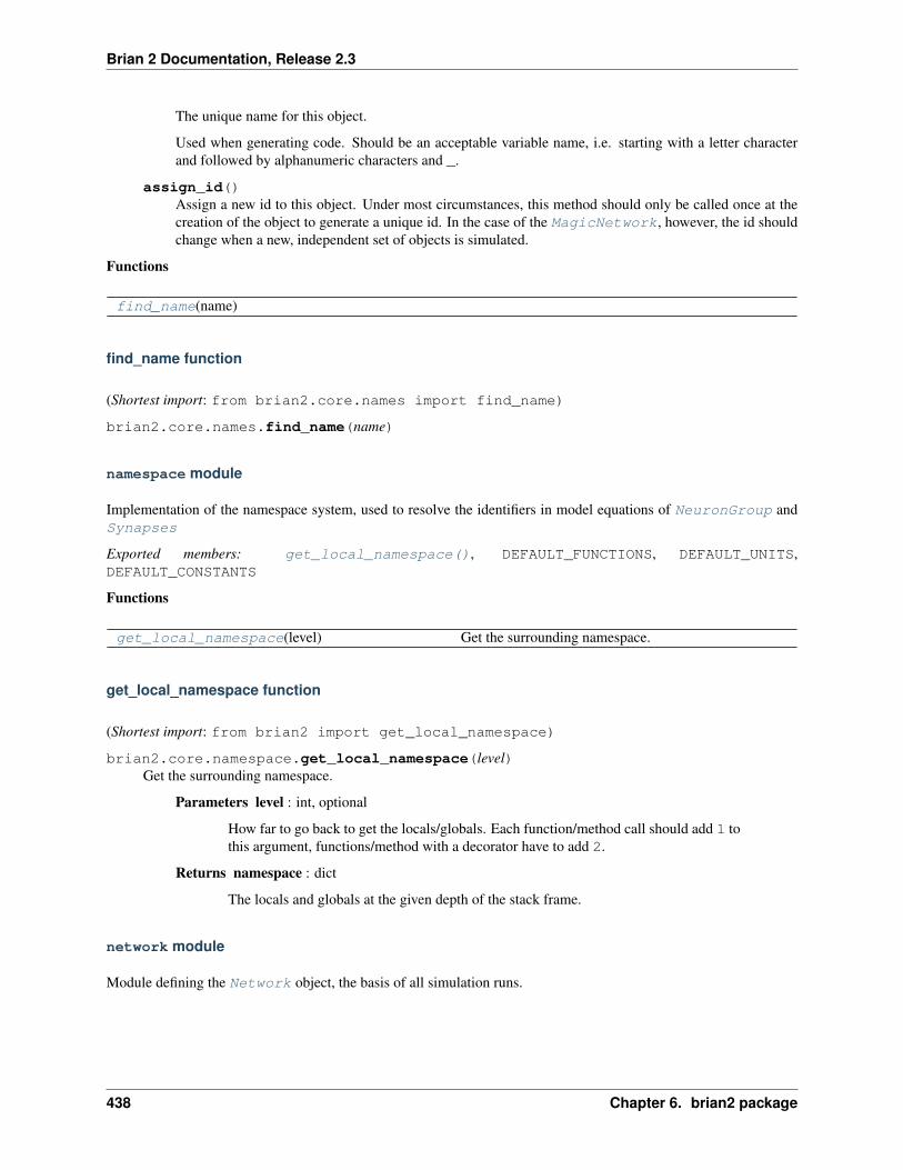
Brian 2 Documentation, Release 2.3
The unique name for this object.
Used when generating code. Should be an acceptable variable name, i.e. starting with a letter characterand followed by alphanumeric characters and _.
assign_id()Assign a new id to this object. Under most circumstances, this method should only be called once at thecreation of the object to generate a unique id. In the case of the MagicNetwork, however, the id shouldchange when a new, independent set of objects is simulated.
Functions
find_name(name)
find_name function
(Shortest import: from brian2.core.names import find_name)
brian2.core.names.find_name(name)
namespace module
Implementation of the namespace system, used to resolve the identifiers in model equations of NeuronGroup andSynapses
Exported members: get_local_namespace(), DEFAULT_FUNCTIONS, DEFAULT_UNITS,DEFAULT_CONSTANTS
Functions
get_local_namespace(level) Get the surrounding namespace.
get_local_namespace function
(Shortest import: from brian2 import get_local_namespace)
brian2.core.namespace.get_local_namespace(level)Get the surrounding namespace.
Parameters level : int, optional
How far to go back to get the locals/globals. Each function/method call should add 1 tothis argument, functions/method with a decorator have to add 2.
Returns namespace : dict
The locals and globals at the given depth of the stack frame.
network module
Module defining the Network object, the basis of all simulation runs.
438 Chapter 6. brian2 package

Brian 2 Documentation, Release 2.3
Preferences
Network preferences
core.network.default_schedule = ['start', 'groups', 'thresholds', 'synapses','resets', 'end']
Default schedule used for networks that don’t specify a schedule.
Exported members: Network, profiling_summary(), scheduling_summary()
Classes
Network(*objs[, name]) The main simulation controller in Brian
Network class
(Shortest import: from brian2 import Network)
class brian2.core.network.Network(*objs, name=’network*’)Bases: brian2.core.names.Nameable
The main simulation controller in Brian
Network handles the running of a simulation. It contains a set of Brian objects that are added with add. Therun method actually runs the simulation. The main run loop, determining which objects get called in whatorder is described in detail in the notes below. The objects in the Network are accesible via their names, e.g.net['neurongroup'] would return the NeuronGroup with this name.
Parameters objs : (BrianObject, container), optional
A list of objects to be added to the Network immediately, see add.
name : str, optional
An explicit name, if not specified gives an automatically generated name
See also:
MagicNetwork, run(), stop()
Notes
The main run loop performs the following steps:
1. Prepare the objects if necessary, see prepare.
2. Determine the end time of the simulation as t`+``duration`.
3. Determine which set of clocks to update. This will be the clock with the smallest value of t. If there areseveral with the same value, then all objects with these clocks will be updated simultaneously. Set t to theclock time.
4. If the t value of these clocks is past the end time of the simulation, stop running. If the Network.stop() method or the stop() function have been called, stop running. Set t to the end time of thesimulation.
5. For each object whose clock is set to one of the clocks from the previous steps, call the update method.This method will not be called if the active flag is set to False. The order in which the objects arecalled is described below.
6.6. Subpackages 439
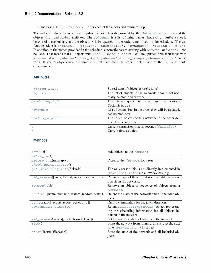
Brian 2 Documentation, Release 2.3
6. Increase Clock.t by Clock.dt for each of the clocks and return to step 2.
The order in which the objects are updated in step 4 is determined by the Network.schedule and theobjects when and order attributes. The schedule is a list of string names. Each when attribute shouldbe one of these strings, and the objects will be updated in the order determined by the schedule. The de-fault schedule is ['start', 'groups', 'thresholds', 'synapses', 'resets', 'end'].In addition to the names provided in the schedule, automatic names starting with before_ and after_ canbe used. That means that all objects with when=='before_start' will be updated first, then those withwhen=='start', when=='after_start', when=='before_groups', when=='groups' and soforth. If several objects have the same when attribute, then the order is determined by the order attribute(lower first).
Attributes
_stored_state Stored state of objects (store/restore)objects The set of objects in the Network, should not nor-
mally be modified directly.profiling_info The time spent in executing the various
CodeObject s.schedule List of when slots in the order they will be updated,
can be modified.sorted_objects The sorted objects of this network in the order de-
fined by the schedule.t Current simulation time in seconds (Quantity)t_ Current time as a float
Methods
add(*objs) Add objects to the Networkafter_run()before_run(namespace) Prepares the Network for a run.check_dependencies()get_profiling_info(**kwds) The only reason this is not directly implemented in
profiling_info is to allow devices (e.g.get_states([units, format, subexpressions, . . . ]) Return a copy of the current state variable values of
objects in the network..remove(*objs) Remove an object or sequence of objects from a
Network.restore([name, filename, restore_random_state]) Retore the state of the network and all included ob-
jects.run(duration[, report, report_period, . . . ]) Runs the simulation for the given duration.scheduling_summary() Return a SchedulingSummary object, represent-
ing the scheduling information for all objects in-cluded in the network.
set_states(values[, units, format, level]) Set the state variables of objects in the network.stop() Stops the network from running, this is reset the next
time Network.run() is called.store([name, filename]) Store the state of the network and all included ob-
jects.
440 Chapter 6. brian2 package
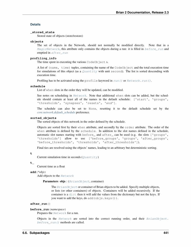
Brian 2 Documentation, Release 2.3
Details
_stored_stateStored state of objects (store/restore)
objectsThe set of objects in the Network, should not normally be modified directly. Note that in aMagicNetwork, this attribute only contains the objects during a run: it is filled in before_run andemptied in after_run
profiling_infoThe time spent in executing the various CodeObject s.
A list of (name, time) tuples, containing the name of the CodeObject and the total execution timefor simulations of this object (as a Quantity with unit second). The list is sorted descending withexecution time.
Profiling has to be activated using the profile keyword in run() or Network.run().
scheduleList of when slots in the order they will be updated, can be modified.
See notes on scheduling in Network. Note that additional when slots can be added, but the sched-ule should contain at least all of the names in the default schedule: ['start', 'groups','thresholds', 'synapses', 'resets', 'end'].
The schedule can also be set to None, resetting it to the default schedule set by thecore.network.default_schedule preference.
sorted_objectsThe sorted objects of this network in the order defined by the schedule.
Objects are sorted first by their when attribute, and secondly by the order attribute. The order of thewhen attribute is defined by the schedule. In addition to the slot names defined in the schedule,automatic slot names starting with before_ and after_ can be used (e.g. the slots ['groups','thresholds'] allow to use ['before_groups', 'groups', 'after_groups','before_thresholds', 'thresholds', 'after_thresholds']).
Final ties are resolved using the objects’ names, leading to an arbitrary but deterministic sorting.
tCurrent simulation time in seconds (Quantity)
t_Current time as a float
add(*objs)Add objects to the Network
Parameters objs : (BrianObject, container)
The BrianObject or container of Brian objects to be added. Specify multiple objects,or lists (or other containers) of objects. Containers will be added recursively. If thecontainer is a dict then it will add the values from the dictionary but not the keys. Ifyou want to add the keys, do add(objs.keys()).
after_run()
before_run(namespace)Prepares the Network for a run.
Objects in the Network are sorted into the correct running order, and their BrianObject.before_run() methods are called.
6.6. Subpackages 441
Brian 2 Documentation, Release 2.3
Parameters run_namespace : dict-like, optional
A namespace in which objects which do not define their own namespace will be run.
check_dependencies()
get_profiling_info(**kwds)The only reason this is not directly implemented in profiling_info is to allow devices (e.g.CPPStandaloneDevice) to overwrite this.
get_states(units=True, format=’dict’, subexpressions=False, read_only_variables=True, level=0)Return a copy of the current state variable values of objects in the network.. The returned arrays arecopies of the actual arrays that store the state variable values, therefore changing the values in the returneddictionary will not affect the state variables.
Parameters vars : list of str, optional
The names of the variables to extract. If not specified, extract all state variables (ex-cept for internal variables, i.e. names that start with '_'). If the subexpressionsargument is True, the current values of all subexpressions are returned as well.
units : bool, optional
Whether to include the physical units in the return value. Defaults to True.
format : str, optional
The output format. Defaults to 'dict'.
subexpressions: bool, optional :
Whether to return subexpressions when no list of variable names is given. Defaults toFalse. This argument is ignored if an explicit list of variable names is given in vars.
read_only_variables : bool, optional
Whether to return read-only variables (e.g. the number of neurons, the time, etc.). Set-ting it to Falsewill assure that the returned state can later be used with set_states.Defaults to True.
level : int, optional
How much higher to go up the stack to resolve external variables. Only relevant ifextracting subexpressions that refer to external variables.
Returns values : dict
A dictionary mapping object names to the state variables of that object, in the specifiedformat.
See also:
VariableOwner.get_states()
remove(*objs)Remove an object or sequence of objects from a Network.
Parameters objs : (BrianObject, container)
The BrianObject or container of Brian objects to be removed. Specify multipleobjects, or lists (or other containers) of objects. Containers will be removed recursively.
restore(name=’default’, filename=None, restore_random_state=False)Retore the state of the network and all included objects.
Parameters name : str, optional
442 Chapter 6. brian2 package

Brian 2 Documentation, Release 2.3
The name of the snapshot to restore, if not specified uses 'default'.
filename : str, optional
The name of the file from where the state should be restored. If not specified, it is ex-pected that the state exist in memory (i.e. Network.store() was previously calledwithout the filename argument).
restore_random_state : bool, optional
Whether to restore the state of the random number generator. If set to True, goingback to an earlier state of the simulation will continue exactly where it left off, evenif the simulation is stochastic. If set to False (the default), random numbers are in-dependent between runs (except for explicitly set random seeds), regardless of whetherstore()/restore() has been used or not. Note that this also restores numpy’srandom number generator (since it is used internally by Brian), but it does not restorePython’s builtin random number generator in the random module.
run(duration, report=None, report_period=60*second, namespace=None, level=0)Runs the simulation for the given duration.
Parameters duration : Quantity
The amount of simulation time to run for.
report : {None, ‘text’, ‘stdout’, ‘stderr’, function}, optional
How to report the progress of the simulation. If None, do not report progress. If'text' or 'stdout' is specified, print the progress to stdout. If 'stderr'is specified, print the progress to stderr. Alternatively, you can specify a call-back callable(elapsed, complete, duration) which will be passed theamount of time elapsed as a Quantity , the fraction complete from 0.0 to 1.0 andthe total duration of the simulation (in biological time). The function will always becalled at the beginning and the end (i.e. for fractions 0.0 and 1.0), regardless of thereport_period.
report_period : Quantity
How frequently (in real time) to report progress.
namespace : dict-like, optional
A namespace that will be used in addition to the group-specific namespaces (if defined).If not specified, the locals and globals around the run function will be used.
profile : bool, optional
Whether to record profiling information (see Network.profiling_info). De-faults to False.
level : int, optional
How deep to go up the stack frame to look for the locals/global (see namespace argu-ment). Only used by run functions that call this run function, e.g. MagicNetwork.run() to adjust for the additional nesting.
Notes
The simulation can be stopped by calling Network.stop() or the global stop() function.
6.6. Subpackages 443

Brian 2 Documentation, Release 2.3
scheduling_summary()Return a SchedulingSummary object, representing the scheduling information for all objects includedin the network.
Returns summary : SchedulingSummary
Object representing the scheduling information.
set_states(values, units=True, format=’dict’, level=0)Set the state variables of objects in the network.
Parameters values : dict
A dictionary mapping object names to objects of format, setting the states of thisobject.
units : bool, optional
Whether the values include physical units. Defaults to True.
format : str, optional
The format of values. Defaults to 'dict'
level : int, optional
How much higher to go up the stack to _resolve external variables. Only relevant whenusing string expressions to set values.
See also:
Group.set_states()
stop()Stops the network from running, this is reset the next time Network.run() is called.
store(name=’default’, filename=None)Store the state of the network and all included objects.
Parameters name : str, optional
A name for the snapshot, if not specified uses 'default'.
filename : str, optional
A filename where the state should be stored. If not specified, the state will be stored inmemory.
Notes
The state stored to disk can be restored with the Network.restore() function. Note that it will onlyrestore the internal state of all the objects (including undelivered spikes) – the objects have to exist alreadyand they need to have the same name as when they were stored. Equations, thresholds, etc. are not stored– this is therefore not a general mechanism for object serialization. Also, the format of the file is notguaranteed to work across platforms or versions. If you are interested in storing the state of a network fordocumentation or analysis purposes use Network.get_states() instead.
Tutorials and examples using this
• Tutorial 3-intro-to-brian-simulations
• Example IF_curve_LIF
444 Chapter 6. brian2 package
Brian 2 Documentation, Release 2.3
• Example IF_curve_Hodgkin_Huxley
• Example advanced/stochastic_odes
• Example advanced/compare_GSL_to_conventional
• Example frompapers/Brunel_Wang_2001
ProfilingSummary(net[, show]) Class to nicely display the results of profiling.
ProfilingSummary class
(Shortest import: from brian2.core.network import ProfilingSummary)
class brian2.core.network.ProfilingSummary(net, show=None)Bases: object
Class to nicely display the results of profiling. Objects of this class are returned by profiling_summary().
Parameters net : Network
The Network object to profile.
show : int, optional
The number of results to show (the longest results will be shown). If not specified, allresults will be shown.
See also:
Network.profiling_info
SchedulingSummary(objects) Object representing the schedule that is used to simulatethe objects in a network.
SchedulingSummary class
(Shortest import: from brian2.core.network import SchedulingSummary)
class brian2.core.network.SchedulingSummary(objects)Bases: object
Object representing the schedule that is used to simulate the objects in a network. Objects of this type arereturned by scheduling_summary(), they should not be created manually by the user.
Parameters objects : list of BrianObject
The sorted list of objects that are simulated by the network.
TextReport(stream) Helper object to report simulation progress inNetwork.run().
TextReport class
(Shortest import: from brian2.core.network import TextReport)
class brian2.core.network.TextReport(stream)
6.6. Subpackages 445
Brian 2 Documentation, Release 2.3
Bases: object
Helper object to report simulation progress in Network.run().
Parameters stream : file
The stream to write to, commonly sys.stdout or sys.stderr.
Methods
__call__(. . . ) <==> x(. . . )
Details
__call__(...) <==> x(...)
Functions
profiling_summary([net, show]) Returns a ProfilingSummary of the profiling infofor a run.
profiling_summary function
(Shortest import: from brian2 import profiling_summary)
brian2.core.network.profiling_summary(net=None, show=None)Returns a ProfilingSummary of the profiling info for a run. This object can be transformed to a stringexplicitly but on an interactive console simply calling profiling_summary() is enough since it will auto-matically convert the ProfilingSummary object.
Parameters net : {Network, None} optional
The Network object to profile, or magic_network if not specified.
show : int
The number of results to show (the longest results will be shown). If not specified, allresults will be shown.
schedule_propagation_offset([net]) Returns the minimal time difference for a post-synapticeffect after a spike.
schedule_propagation_offset function
(Shortest import: from brian2.core.network import schedule_propagation_offset)
brian2.core.network.schedule_propagation_offset(net=None)Returns the minimal time difference for a post-synaptic effect after a spike. With the default schedule, this timedifference is 0, since the thresholds slot precedes the synapses slot. For the GeNN device, however, apost-synaptic effect will occur in the following time step, this function therefore returns one dt.
Parameters net : Network
The network to check (uses the magic network if not specified).
446 Chapter 6. brian2 package

Brian 2 Documentation, Release 2.3
Returns offset : Quantity
The minimum spike propagation delay: 0*ms for the standard schedule but dt forschedules where synapses precedes thresholds.
Notes
This function always returns 0*ms or defaultclock.dt – no attempt is made to deal with other clocks.
scheduling_summary([net]) Returns a SchedulingSummary object, represent-ing the scheduling information for all objects includedin the given Network (or the “magic” network, if noneis specified).
scheduling_summary function
(Shortest import: from brian2 import scheduling_summary)
brian2.core.network.scheduling_summary(net=None)Returns a SchedulingSummary object, representing the scheduling information for all objects included inthe given Network (or the “magic” network, if none is specified). The returned objects can be printed orconverted to a string to give an ASCII table representation of the schedule. In a Jupyter notebook, the outputcan be displayed as a HTML table.
Parameters net : Network, optional
The network for which the scheduling information should be displayed. Defaults to the“magic” network.
Returns summary : SchedulingSummary
An object that represents the scheduling information.
operations module
Exported members: NetworkOperation, network_operation()
Classes
NetworkOperation(function[, dt, clock, . . . ]) Object with function that is called every time step.
NetworkOperation class
(Shortest import: from brian2 import NetworkOperation)
class brian2.core.operations.NetworkOperation(function, dt=None, clock=None,when=’start’, order=0,name=’networkoperation*’)
Bases: brian2.core.base.BrianObject
Object with function that is called every time step.
Parameters function : function
The function to call every time step, should take either no arguments in which case it
6.6. Subpackages 447
Brian 2 Documentation, Release 2.3
is called as function() or one argument, in which case it is called with the currentClock time (Quantity).
dt : Quantity , optional
The time step to be used for the simulation. Cannot be combined with the clockargument.
clock : Clock, optional
The update clock to be used. If neither a clock, nor the dt argument is specified, thedefaultclock will be used.
when : str, optional
In which scheduling slot to execute the operation during a time step. Defaults to'start'.
order : int, optional
The priority of this operation for operations occurring at the same time step and in thesame scheduling slot. Defaults to 0.
See also:
network_operation(), Network, BrianObject
Attributes
function The function to be called each time step
Methods
run()
Details
functionThe function to be called each time step
run()
Functions
network_operation([when]) Decorator to make a function get called every time stepof a simulation.
network_operation function
(Shortest import: from brian2 import network_operation)
brian2.core.operations.network_operation(when=None)Decorator to make a function get called every time step of a simulation.
The function being decorated should either have no arguments, or a single argument which will be called withthe current time t.
448 Chapter 6. brian2 package

Brian 2 Documentation, Release 2.3
Parameters dt : Quantity , optional
The time step to be used for the simulation. Cannot be combined with the clockargument.
clock : Clock, optional
The update clock to be used. If neither a clock, nor the dt argument is specified, thedefaultclock will be used.
when : str, optional
In which scheduling slot to execute the operation during a time step. Defaults to'start'.
order : int, optional
The priority of this operation for operations occurring at the same time step and in thesame scheduling slot. Defaults to 0.
See also:
NetworkOperation, Network, BrianObject
Notes
Converts the function into a NetworkOperation.
If using the form:
@network_operations(when='end')def f():
...
Then the arguments to network_operation must be keyword arguments.
Examples
Print something each time step: >>> from brian2 import * >>> @network_operation . . . def f(): . . .print(‘something’) . . . >>> net = Network(f)
Print the time each time step:
>>> @network_operation... def f(t):... print('The time is', t)...>>> net = Network(f)
Specify a dt, etc.:
>>> @network_operation(dt=0.5*ms, when='end')... def f():... print('This will happen at the end of each timestep.')...>>> net = Network(f)
6.6. Subpackages 449
Brian 2 Documentation, Release 2.3
preferences module
Brian global preferences are stored as attributes of a BrianGlobalPreferences object prefs.
Exported members: PreferenceError, BrianPreference, prefs, brian_prefs
Classes
BrianGlobalPreferences() Class of the prefs object.
BrianGlobalPreferences class
(Shortest import: from brian2.core.preferences import BrianGlobalPreferences)
class brian2.core.preferences.BrianGlobalPreferencesBases: _abcoll.MutableMapping
Class of the prefs object.
Used for getting/setting/validating/registering preference values. All preferences must be registered viaregister_preferences. To get or set a preference, you can either use a dictionary-based or an attribute-based interface:
prefs['core.default_float_dtype'] = float32prefs.core.default_float_dtype = float32
Preferences can be read from files, see load_preferences and read_preference_file. Note thatload_preferences is called automatically when Brian has finished importing.
Attributes
as_file Get a Brian preference doc file format string for thecurrent preferences
defaults_as_file Get a Brian preference doc file format string for thedefault preferences
toplevel_categories The toplevel preference categories
Methods
check_all_validated() Checks that all preferences that have been set havebeen validated.
do_validation() Validates preferences that have not yet been vali-dated.
eval_pref(value) Evaluate a string preference in the units namespaceget_documentation([basename, link_targets]) Generates a string documenting all preferences with
the given basename.load_preferences() Load all the preference files, but do not validate
them.read_preference_file(file) Reads a Brian preferences fileregister_preferences(prefbasename, . . . ) Registers a set of preference names, docs and valida-
tion functions.Continued on next page
450 Chapter 6. brian2 package

Brian 2 Documentation, Release 2.3
Table 172 – continued from previous pagereset_to_defaults() Resets the parameters to their default values.
Details
as_fileGet a Brian preference doc file format string for the current preferences
defaults_as_fileGet a Brian preference doc file format string for the default preferences
toplevel_categoriesThe toplevel preference categories
check_all_validated()Checks that all preferences that have been set have been validated.
Logs a warning if not. Should be called by Network.run() or other key Brian functions.
do_validation()Validates preferences that have not yet been validated.
eval_pref(value)Evaluate a string preference in the units namespace
get_documentation(basename=None, link_targets=True)Generates a string documenting all preferences with the given basename. If no basename is given, allpreferences are documented.
load_preferences()Load all the preference files, but do not validate them.
Preference files are read in the following order:
1. brian2/default_preferences from the Brian installation directory.
2. ~/.brian/user_preferences from the user’s home directory
3. ./brian_preferences from the current directory
Files that are missing are ignored. Preferences read at each step override preferences from previous steps.
See also:
read_preference_file
read_preference_file(file)Reads a Brian preferences file
The file format for Brian preferences is a plain text file of the form:
a.b.c = 1# Comment line[a]b.d = 2[a.b]e = 3
Blank and comment lines are ignored, all others should be of one of the following two forms:
key = value[section]
6.6. Subpackages 451
Brian 2 Documentation, Release 2.3
eval is called on the values, so strings should be written as, e.g. '3' rather than 3. The eval is calledwith all unit names available. Within a section, the section name is prepended to the key. So in the aboveexample, it would give the following unvalidated dictionary:
{'a.b.c': 1,'a.b.d': 2,'a.b.e': 3,}
Parameters file : file, str
The file object or filename of the preference file.
register_preferences(prefbasename, prefbasedoc, **prefs)Registers a set of preference names, docs and validation functions.
Parameters prefbasename : str
The base name of the preference.
prefbasedoc : str
Documentation for this base name
**prefs : dict of (name, BrianPreference) pairs
The preference names to be defined. The full preference name will beprefbasename.name, and the BrianPreference value is used to define thedefault value, docs, and validation function.
Raises
PreferenceError If the base name is already registered.
See also:
BrianPreference
reset_to_defaults()Resets the parameters to their default values.
BrianGlobalPreferencesView(basename,all_prefs)
A class allowing for accessing preferences in a subcate-gory.
BrianGlobalPreferencesView class
(Shortest import: from brian2.core.preferences import BrianGlobalPreferencesView)
class brian2.core.preferences.BrianGlobalPreferencesView(basename, all_prefs)Bases: _abcoll.MutableMapping
A class allowing for accessing preferences in a subcategory. It forwards requests toBrianGlobalPreferences and provides documentation and autocompletion support for all prefer-ences in the given category. This object is used to allow accessing preferences via attributes of the prefsobject.
Parameters basename : str
452 Chapter 6. brian2 package

Brian 2 Documentation, Release 2.3
The name of the preference category. Has to correspond to a key inBrianGlobalPreferences.pref_register.
all_prefs : BrianGlobalPreferences
A reference to the main object storing the preferences.
BrianPreference(default, docs[, validator, . . . ]) Used for defining a Brian preference.
BrianPreference class
(Shortest import: from brian2 import BrianPreference)
class brian2.core.preferences.BrianPreference(default, docs, validator=None,representor=<built-in function repr>)
Bases: object
Used for defining a Brian preference.
Parameters default : object
The default value.
docs : str
Documentation for the preference value.
validator : func
A function that True or False depending on whether the preference value is valid or not.If not specified, uses the DefaultValidator for the default value provided (checkif the class is the same, and for Quantity objects, whether the units are consistent).
representor : func
A function that returns a string representation of a valid preference value that can bepassed to eval. By default, uses repr which works in almost all cases.
DefaultValidator(value) Default preference validator
DefaultValidator class
(Shortest import: from brian2.core.preferences import DefaultValidator)
class brian2.core.preferences.DefaultValidator(value)Bases: object
Default preference validator
Used by BrianPreference as the default validator if none is given. First checks if the provided value is ofthe same class as the default value, and then if the default is a Quantity , checks that the units match.
Methods
__call__(. . . ) <==> x(. . . )
6.6. Subpackages 453
Brian 2 Documentation, Release 2.3
Details
__call__(...) <==> x(...)
ErrorRaiser
ErrorRaiser class
(Shortest import: from brian2.core.preferences import ErrorRaiser)
class brian2.core.preferences.ErrorRaiserBases: object
PreferenceError Exception relating to the Brian preferences system.
PreferenceError class
(Shortest import: from brian2 import PreferenceError)
class brian2.core.preferences.PreferenceErrorBases: exceptions.Exception
Exception relating to the Brian preferences system.
Functions
check_preference_name(name) Make sure that a preference name is valid.
check_preference_name function
(Shortest import: from brian2.core.preferences import check_preference_name)
brian2.core.preferences.check_preference_name(name)Make sure that a preference name is valid. This currently checks that the name does not contain illegal charactersand does not clash with method names such as “keys” or “items”.
Parameters name : str
The name to check.
Raises
PreferenceError In case the name is invalid.
parse_preference_name(name) Split a preference name into a base and end name.
parse_preference_name function
(Shortest import: from brian2.core.preferences import parse_preference_name)
454 Chapter 6. brian2 package

Brian 2 Documentation, Release 2.3
brian2.core.preferences.parse_preference_name(name)Split a preference name into a base and end name.
Parameters name : str
The full name of the preference.
Returns basename : str
The first part of the name up to the final ..
endname : str
The last part of the name from the final . onwards.
Examples
>>> parse_preference_name('core.weave_compiler')('core', 'weave_compiler')>>> parse_preference_name('codegen.cpp.compiler')('codegen.cpp', 'compiler')
Objects
brian_prefs
brian_prefs object
(Shortest import: from brian2 import brian_prefs)
brian2.core.preferences.brian_prefs = <brian2.core.preferences.ErrorRaiser object>
prefs Preference categories:
prefs object
(Shortest import: from brian2 import prefs)
brian2.core.preferences.prefs = <BrianGlobalPreferences with top-level categories: "core", "logging", "devices", "codegen", "legacy", "GSL">Preference categories:
** core ** Core Brian preferences
** logging ** Logging system preferences
** devices ** Device preferences
** codegen ** Code generation preferences
** legacy ** Preferences to enable legacy behaviour
** GSL ** Directory containing GSL code
spikesource module
Exported members: SpikeSource
6.6. Subpackages 455
Brian 2 Documentation, Release 2.3
Classes
SpikeSource A source of spikes.
SpikeSource class
(Shortest import: from brian2 import SpikeSource)
class brian2.core.spikesource.SpikeSourceBases: object
A source of spikes.
An object that can be used as a source of spikes for objects such as SpikeMonitor, Synapses, etc.
The defining properties of SpikeSource are that it should have:
• A length that can be extracted with len(obj), where the maximum spike index possible islen(obj)-1.
• An attribute spikes, an array of ints each from 0 to len(obj)-1 with no repeats (but possibly not insorted order). This should be updated each time step.
• A clock attribute, this will be used as the default clock for objects with this as a source.
spikesAn array of ints, each from 0 to len(obj)-1 with no repeats (but possibly not in sorted order). Updatedeach time step.
clockThe clock on which the spikes will be updated.
tracking module
Exported members: Trackable
Classes
InstanceFollower Keep track of all instances of classes derived fromTrackable
InstanceFollower class
(Shortest import: from brian2.core.tracking import InstanceFollower)
class brian2.core.tracking.InstanceFollowerBases: object
Keep track of all instances of classes derived from Trackable
The variable __instancesets__ is a dictionary with keys which are class objects, and values which areInstanceTrackerSet, so __instanceset__[cls] is a set tracking all of the instances of class cls(or a subclass).
456 Chapter 6. brian2 package

Brian 2 Documentation, Release 2.3
Methods
add(value)get(cls)
Details
add(value)
get(cls)
InstanceTrackerSet A set of weakref.ref to all existing objects of acertain class.
InstanceTrackerSet class
(Shortest import: from brian2.core.tracking import InstanceTrackerSet)
class brian2.core.tracking.InstanceTrackerSetBases: set
A set of weakref.ref to all existing objects of a certain class.
Should not normally be directly used.
Methods
add(value) Adds a weakref.ref to the valueremove(value) Removes the value (which should be a weakref) if
it is in the set
Details
add(value)Adds a weakref.ref to the value
remove(value)Removes the value (which should be a weakref) if it is in the set
Sometimes the value will have been removed from the set by clear, so we ignore KeyError in thiscase.
Trackable Classes derived from this will have their instancestracked.
Trackable class
(Shortest import: from brian2 import Trackable)
class brian2.core.tracking.TrackableBases: object
6.6. Subpackages 457
Brian 2 Documentation, Release 2.3
Classes derived from this will have their instances tracked.
The classmethod __instances__() will return an InstanceTrackerSet of the instances of thatclass, and its subclasses.
variables module
Exported members: Variable, Constant, ArrayVariable, DynamicArrayVariable,Subexpression, AuxiliaryVariable, VariableView , Variables, LinkedVariable,linked_var()
Classes
ArrayVariable(name, owner, size, device[, . . . ]) An object providing information about a model variablestored in an array (for example, all state variables).
ArrayVariable class
(Shortest import: from brian2.core.variables import ArrayVariable)
class brian2.core.variables.ArrayVariable(name, owner, size, device, dimen-sions=Dimension(), dtype=None, con-stant=False, scalar=False, read_only=False,dynamic=False, unique=False)
Bases: brian2.core.variables.Variable
An object providing information about a model variable stored in an array (for example, all state variables).Most of the time Variables.add_array should be used instead of instantiating this class directly.
Parameters name : ‘str’
The name of the variable. Note that this refers to the original name in the owning group.The same variable may be known under other names in other groups (e.g. the variablev of a NeuronGroup is known as v_post in a Synapse connecting to the group).
dimensions : Dimension, optional
The physical dimensions of the variable
owner : Nameable
The object that “owns” this variable, e.g. the NeuronGroup or Synapses objectthat declares the variable in its model equations.
size : int
The size of the array
device : Device
The device responsible for the memory access.
dtype : dtype, optional
The dtype used for storing the variable. If none is given, defaults tocore.default_float_dtype.
constant : bool, optional
Whether the variable’s value is constant during a run. Defaults to False.
458 Chapter 6. brian2 package
Brian 2 Documentation, Release 2.3
scalar : bool, optional
Whether this array is a 1-element array that should be treated like a scalar (e.g. for asingle delay value across synapses). Defaults to False.
read_only : bool, optional
Whether this is a read-only variable, i.e. a variable that is set internally and cannot bechanged by the user. Defaults to False.
unique : bool, optional
Whether the values in this array are all unique. This information is only important forvariables used as indices and does not have to reflect the actual contents of the array butonly the possibility of non-uniqueness (e.g. synaptic indices are always unique but thecorresponding pre- and post-synaptic indices are not). Defaults to False.
Attributes
conditional_write Another variable, on which the write is conditioned(e.g.
device The Device responsible for memory access.size The size of this variable.unique Wether all values in this arrays are necessarily unique
(only relevant for index variables).
Methods
get_addressable_value(name, group) Get the value (without units) of this variable in aform that can be indexed in the context of a group.
get_addressable_value_with_unit(name,group)
Get the value (with units) of this variable in a formthat can be indexed in the context of a group.
get_len() Get the length of the value associated with the vari-able or 0 for a scalar variable.
get_value() Return the value associated with the variable (with-out units).
set_conditional_write(var)set_value(value) Set the value associated with the variable.
Details
conditional_writeAnother variable, on which the write is conditioned (e.g. a variable denoting the absence of refractoriness)
deviceThe Device responsible for memory access.
sizeThe size of this variable.
uniqueWether all values in this arrays are necessarily unique (only relevant for index variables).
get_addressable_value(name, group)Get the value (without units) of this variable in a form that can be indexed in the context of a group. For
6.6. Subpackages 459
Brian 2 Documentation, Release 2.3
example, if a postsynaptic variable x is accessed in a synapse S as S.x_post, the synaptic indexingscheme can be used.
Parameters name : str
The name of the variable
group : Group
The group providing the context for the indexing. Note that this group is not neces-sarily the same as Variable.owner: a variable owned by a NeuronGroup can beindexed in a different way if accessed via a Synapses object.
Returns variable : object
The variable in an indexable form (without units).
get_addressable_value_with_unit(name, group)Get the value (with units) of this variable in a form that can be indexed in the context of a group. Forexample, if a postsynaptic variable x is accessed in a synapse S as S.x_post, the synaptic indexingscheme can be used.
Parameters name : str
The name of the variable
group : Group
The group providing the context for the indexing. Note that this group is not neces-sarily the same as Variable.owner: a variable owned by a NeuronGroup can beindexed in a different way if accessed via a Synapses object.
Returns variable : object
The variable in an indexable form (with units).
get_len()Get the length of the value associated with the variable or 0 for a scalar variable.
get_value()Return the value associated with the variable (without units). This is the way variables are accessed ingenerated code.
set_conditional_write(var)
set_value(value)Set the value associated with the variable.
AuxiliaryVariable(name[, dimensions, dtype,. . . ])
Variable description for an auxiliary variable (mostlikely one that is added automatically to abstract code,e.g.
AuxiliaryVariable class
(Shortest import: from brian2.core.variables import AuxiliaryVariable)
class brian2.core.variables.AuxiliaryVariable(name, dimensions=Dimension(),dtype=None, scalar=False)
Bases: brian2.core.variables.Variable
Variable description for an auxiliary variable (most likely one that is added automatically to abstract code,e.g. _cond for a threshold condition), specifying its type and unit for code generation. Most of the time
460 Chapter 6. brian2 package

Brian 2 Documentation, Release 2.3
Variables.add_auxiliary_variable should be used instead of instantiating this class directly.
Parameters name : str
The name of the variable
dimensions : Dimension, optional
The physical dimensions of the variable.
dtype : dtype, optional
The dtype used for storing the variable. If none is given, defaults tocore.default_float_dtype.
scalar : bool, optional
Whether the variable is a scalar value (True) or vector-valued, e.g. defined for everyneuron (False). Defaults to False.
Methods
get_value() Return the value associated with the variable (with-out units).
Details
get_value()Return the value associated with the variable (without units). This is the way variables are accessed ingenerated code.
Constant(name, value[, dimensions, owner]) A scalar constant (e.g.
Constant class
(Shortest import: from brian2.core.variables import Constant)
class brian2.core.variables.Constant(name, value, dimensions=Dimension(), owner=None)Bases: brian2.core.variables.Variable
A scalar constant (e.g. the number of neurons N). Information such as the dtype or whether this variable is aboolean are directly derived from the value. Most of the time Variables.add_constant should be usedinstead of instantiating this class directly.
Parameters name : str
The name of the variable
dimensions : Dimension, optional
The physical dimensions of the variable. Note that the variable itself (as referenced byvalue) should never have units attached.
value: reference to the variable value :
The value of the constant.
owner : Nameable, optional
6.6. Subpackages 461
Brian 2 Documentation, Release 2.3
The object that “owns” this variable, for constants that belong to a specific group, e.g.the N constant for a NeuronGroup. External constants will have None (the defaultvalue).
Attributes
value The constant’s value
Methods
get_value() Return the value associated with the variable (with-out units).
Details
valueThe constant’s value
get_value()Return the value associated with the variable (without units). This is the way variables are accessed ingenerated code.
DynamicArrayVariable(name, owner, size, de-vice)
An object providing information about a model variablestored in a dynamic array (used in Synapses).
DynamicArrayVariable class
(Shortest import: from brian2.core.variables import DynamicArrayVariable)
class brian2.core.variables.DynamicArrayVariable(name, owner, size, device,dimensions=Dimension(),dtype=None, constant=False,needs_reference_update=False,resize_along_first=False,scalar=False, read_only=False,unique=False)
Bases: brian2.core.variables.ArrayVariable
An object providing information about a model variable stored in a dynamic array (used in Synapses). Mostof the time Variables.add_dynamic_array should be used instead of instantiating this class directly.
Parameters name : ‘str’
The name of the variable. Note that this refers to the original name in the owning group.The same variable may be known under other names in other groups (e.g. the variablev of a NeuronGroup is known as v_post in a Synapse connecting to the group).
dimensions : Dimension, optional
The physical dimensions of the variable.
owner : Nameable
462 Chapter 6. brian2 package
Brian 2 Documentation, Release 2.3
The object that “owns” this variable, e.g. the NeuronGroup or Synapses objectthat declares the variable in its model equations.
size : int or tuple of int
The (initial) size of the variable.
device : Device
The device responsible for the memory access.
dtype : dtype, optional
The dtype used for storing the variable. If none is given, defaults tocore.default_float_dtype.
constant : bool, optional
Whether the variable’s value is constant during a run. Defaults to False.
needs_reference_update : bool, optional
Whether the code objects need a new reference to the underlying data at every time step.This should be set if the size of the array can be changed by other code objects. Defaultsto False.
scalar : bool, optional
Whether this array is a 1-element array that should be treated like a scalar (e.g. for asingle delay value across synapses). Defaults to False.
read_only : bool, optional
Whether this is a read-only variable, i.e. a variable that is set internally and cannot bechanged by the user. Defaults to False.
unique : bool, optional
Whether the values in this array are all unique. This information is only important forvariables used as indices and does not have to reflect the actual contents of the array butonly the possibility of non-uniqueness (e.g. synaptic indices are always unique but thecorresponding pre- and post-synaptic indices are not). Defaults to False.
Attributes
dimensionsndim The number of dimensionsneeds_reference_update Whether this variable needs an update of the refer-
ence to the underlying data whenever it is passed toa code object
resize_along_first Whether this array will be only resized along the firstdimension
Methods
resize(new_size) Resize the dynamic array.
6.6. Subpackages 463

Brian 2 Documentation, Release 2.3
Details
dimensions
ndimThe number of dimensions
needs_reference_updateWhether this variable needs an update of the reference to the underlying data whenever it is passed to acode object
resize_along_firstWhether this array will be only resized along the first dimension
resize(new_size)Resize the dynamic array. Calls self.device.resize to do the actual resizing.
Parameters new_size : int or tuple of int
The new size.
LinkedVariable(group, name, variable[, index]) A simple helper class to make linking variables explicit.
LinkedVariable class
(Shortest import: from brian2.core.variables import LinkedVariable)
class brian2.core.variables.LinkedVariable(group, name, variable, index=None)Bases: object
A simple helper class to make linking variables explicit. Users should use linked_var() instead.
Parameters group : Group
The group through which the variable is accessed (not necessarily the same asvariable.owner.
name : str
The name of variable in group (not necessarily the same as variable.name).
variable : Variable
The variable that should be linked.
index : str or ndarray, optional
An indexing array (or the name of a state variable), providing a mapping from the entriesin the link source to the link target.
Subexpression(name, owner, expr, device[, . . . ]) An object providing information about a named subex-pression in a model.
Subexpression class
(Shortest import: from brian2.core.variables import Subexpression)
464 Chapter 6. brian2 package

Brian 2 Documentation, Release 2.3
class brian2.core.variables.Subexpression(name, owner, expr, device, dimen-sions=Dimension(), dtype=None,scalar=False)
Bases: brian2.core.variables.Variable
An object providing information about a named subexpression in a model. Most of the time Variables.add_subexpression should be used instead of instantiating this class directly.
Parameters name : str
The name of the subexpression.
dimensions : Dimension, optional
The physical dimensions of the subexpression.
owner : Group
The group to which the expression refers.
expr : str
The subexpression itself.
device : Device
The device responsible for the memory access.
dtype : dtype, optional
The dtype used for the expression. Defaults to core.default_float_dtype.
scalar: bool, optional :
Whether this is an expression only referring to scalar variables. Defaults to False
Attributes
device The Device responsible for memory accessexpr The expression defining the subexpressionidentifiers The identifiers used in the expression
Methods
get_addressable_value(name, group) Get the value (without units) of this variable in aform that can be indexed in the context of a group.
get_addressable_value_with_unit(name,group)
Get the value (with units) of this variable in a formthat can be indexed in the context of a group.
Details
deviceThe Device responsible for memory access
exprThe expression defining the subexpression
identifiersThe identifiers used in the expression
6.6. Subpackages 465
Brian 2 Documentation, Release 2.3
get_addressable_value(name, group)Get the value (without units) of this variable in a form that can be indexed in the context of a group. Forexample, if a postsynaptic variable x is accessed in a synapse S as S.x_post, the synaptic indexingscheme can be used.
Parameters name : str
The name of the variable
group : Group
The group providing the context for the indexing. Note that this group is not neces-sarily the same as Variable.owner: a variable owned by a NeuronGroup can beindexed in a different way if accessed via a Synapses object.
Returns variable : object
The variable in an indexable form (without units).
get_addressable_value_with_unit(name, group)Get the value (with units) of this variable in a form that can be indexed in the context of a group. Forexample, if a postsynaptic variable x is accessed in a synapse S as S.x_post, the synaptic indexingscheme can be used.
Parameters name : str
The name of the variable
group : Group
The group providing the context for the indexing. Note that this group is not neces-sarily the same as Variable.owner: a variable owned by a NeuronGroup can beindexed in a different way if accessed via a Synapses object.
Returns variable : object
The variable in an indexable form (with units).
Variable(name[, dimensions, owner, dtype, . . . ]) An object providing information about model variables(including implicit variables such as t or xi).
Variable class
(Shortest import: from brian2.core.variables import Variable)
class brian2.core.variables.Variable(name, dimensions=Dimension(), owner=None,dtype=None, scalar=False, constant=False,read_only=False, dynamic=False, array=False)
Bases: brian2.utils.caching.CacheKey
An object providing information about model variables (including implicit variables such as t or xi). This classshould never be instantiated outside of testing code, use one of its subclasses instead.
Parameters name : ‘str’
The name of the variable. Note that this refers to the original name in the owning group.The same variable may be known under other names in other groups (e.g. the variablev of a NeuronGroup is known as v_post in a Synapse connecting to the group).
dimensions : Dimension, optional
The physical dimensions of the variable.
466 Chapter 6. brian2 package
Brian 2 Documentation, Release 2.3
owner : Nameable, optional
The object that “owns” this variable, e.g. the NeuronGroup or Synapses objectthat declares the variable in its model equations. Defaults to None (the value used forVariable objects without an owner, e.g. external Constants).
dtype : dtype, optional
The dtype used for storing the variable. Defaults to the preference core.default_scalar.dtype.
scalar : bool, optional
Whether the variable is a scalar value (True) or vector-valued, e.g. defined for everyneuron (False). Defaults to False.
constant: bool, optional :
Whether the value of this variable can change during a run. Defaults to False.
read_only : bool, optional
Whether this is a read-only variable, i.e. a variable that is set internally and cannot bechanged by the user (this is used for example for the variable N, the number of neuronsin a group). Defaults to False.
array : bool, optional
Whether this variable is an array. Allows for simpler check than testingisinstance(var, ArrayVariable). Defaults to False.
Attributes
array Whether the variable is an arrayconstant Whether the variable is constant during a rundim The variable’s dimensions.dtype The dtype used for storing the variable.dtype_str String representation of the numpy dtypedynamic Whether the variable is dynamically sized (only for
non-scalars)is_booleanis_integername The variable’s name.owner The Group to which this variable belongs.read_only Whether the variable is read-onlyscalar Whether the variable is a scalarunit The Unit of this variable
Methods
get_addressable_value(name, group) Get the value (without units) of this variable in aform that can be indexed in the context of a group.
get_addressable_value_with_unit(name,group)
Get the value (with units) of this variable in a formthat can be indexed in the context of a group.
Continued on next page
6.6. Subpackages 467
Brian 2 Documentation, Release 2.3
Table 206 – continued from previous pageget_len() Get the length of the value associated with the vari-
able or 0 for a scalar variable.get_value() Return the value associated with the variable (with-
out units).get_value_with_unit() Return the value associated with the variable (with
units).set_value(value) Set the value associated with the variable.
Details
arrayWhether the variable is an array
constantWhether the variable is constant during a run
dimThe variable’s dimensions.
dtypeThe dtype used for storing the variable.
dtype_strString representation of the numpy dtype
dynamicWhether the variable is dynamically sized (only for non-scalars)
is_boolean
is_integer
nameThe variable’s name.
ownerThe Group to which this variable belongs.
read_onlyWhether the variable is read-only
scalarWhether the variable is a scalar
unitThe Unit of this variable
get_addressable_value(name, group)Get the value (without units) of this variable in a form that can be indexed in the context of a group. Forexample, if a postsynaptic variable x is accessed in a synapse S as S.x_post, the synaptic indexingscheme can be used.
Parameters name : str
The name of the variable
group : Group
The group providing the context for the indexing. Note that this group is not neces-sarily the same as Variable.owner: a variable owned by a NeuronGroup can beindexed in a different way if accessed via a Synapses object.
468 Chapter 6. brian2 package
Brian 2 Documentation, Release 2.3
Returns variable : object
The variable in an indexable form (without units).
get_addressable_value_with_unit(name, group)Get the value (with units) of this variable in a form that can be indexed in the context of a group. Forexample, if a postsynaptic variable x is accessed in a synapse S as S.x_post, the synaptic indexingscheme can be used.
Parameters name : str
The name of the variable
group : Group
The group providing the context for the indexing. Note that this group is not neces-sarily the same as Variable.owner: a variable owned by a NeuronGroup can beindexed in a different way if accessed via a Synapses object.
Returns variable : object
The variable in an indexable form (with units).
get_len()Get the length of the value associated with the variable or 0 for a scalar variable.
get_value()Return the value associated with the variable (without units). This is the way variables are accessed ingenerated code.
get_value_with_unit()Return the value associated with the variable (with units).
set_value(value)Set the value associated with the variable.
VariableView(name, variable, group[, dimen-sions])
A view on a variable that allows to treat it as an numpyarray while allowing special indexing (e.g.
VariableView class
(Shortest import: from brian2.core.variables import VariableView)
class brian2.core.variables.VariableView(name, variable, group, dimensions=None)Bases: object
A view on a variable that allows to treat it as an numpy array while allowing special indexing (e.g. with strings)in the context of a Group.
Parameters name : str
The name of the variable (not necessarily the same as variable.name).
variable : Variable
The variable description.
group : Group
The group through which the variable is accessed (not necessarily the same asvariable.owner).
dimensions : Dimension, optional
6.6. Subpackages 469

Brian 2 Documentation, Release 2.3
The physical dimensions to be used for the variable, should be None when a variable isaccessed without units (e.g. when accessing G.var_).
Attributes
dtypeshapeunit The Unit of this variable
Methods
get_item(item[, level, namespace]) Get the value of this variable.get_subexpression_with_index_array(**kwds)get_with_expression(**kwds) Gets a variable using a string expression.get_with_index_array(**kwds)set_item(item, value[, level, namespace]) Set this variable.set_with_expression(**kwds) Sets a variable using a string expression.set_with_expression_conditional(**kwds)Sets a variable using a string expression and string
condition.set_with_index_array(**kwds)
Details
dtype
shape
unitThe Unit of this variable
get_item(item, level=0, namespace=None)Get the value of this variable. Called by __getitem__.
Parameters item : slice, ndarray or string
The index for the setting operation
level : int, optional
How much farther to go up in the stack to find the implicit namespace (if used, seerun_namespace).
namespace : dict-like, optional
An additional namespace that is used for variable lookup (if not defined, the implicitnamespace of local variables is used).
get_subexpression_with_index_array(**kwds)
get_with_expression(**kwds)Gets a variable using a string expression. Is called by VariableView.get_item for statements suchas print(G.v['g_syn > 0']).
Parameters code : str
470 Chapter 6. brian2 package
Brian 2 Documentation, Release 2.3
An expression that states a condition for elements that should be selected. Can containreferences to indices, such as i or j and to state variables. For example: 'i>3 andv>0*mV'.
run_namespace : dict-like
An additional namespace that is used for variable lookup (either an explicitly definednamespace or one taken from the local context).
get_with_index_array(**kwds)
set_item(item, value, level=0, namespace=None)Set this variable. This function is called by __setitem__ but there is also a situation where it should becalled directly: if the context for string-based expressions is higher up in the stack, this function allows toset the level argument accordingly.
Parameters item : slice, ndarray or string
The index for the setting operation
value : Quantity , ndarray or number
The value for the setting operation
level : int, optional
How much farther to go up in the stack to find the implicit namespace (if used, seerun_namespace).
namespace : dict-like, optional
An additional namespace that is used for variable lookup (if not defined, the implicitnamespace of local variables is used).
set_with_expression(**kwds)Sets a variable using a string expression. Is called by VariableView.set_item for statements suchas S.var[:, :] = 'exp(-abs(i-j)/space_constant)*nS'
Parameters item : ndarray
The indices for the variable (in the context of this group).
code : str
The code that should be executed to set the variable values. Can contain references toindices, such as i or j
run_namespace : dict-like, optional
An additional namespace that is used for variable lookup (if not defined, the implicitnamespace of local variables is used).
check_units : bool, optional
Whether to check the units of the expression.
run_namespace : dict-like, optional
An additional namespace that is used for variable lookup (if not defined, the implicitnamespace of local variables is used).
set_with_expression_conditional(**kwds)Sets a variable using a string expression and string condition. Is called by VariableView.set_itemfor statements such as S.var['i!=j'] = 'exp(-abs(i-j)/space_constant)*nS'
Parameters cond : str
6.6. Subpackages 471

Brian 2 Documentation, Release 2.3
The string condition for which the variables should be set.
code : str
The code that should be executed to set the variable values.
run_namespace : dict-like, optional
An additional namespace that is used for variable lookup (if not defined, the implicitnamespace of local variables is used).
check_units : bool, optional
Whether to check the units of the expression.
set_with_index_array(**kwds)
Variables(owner[, default_index]) A container class for storing Variable objects.
Variables class
(Shortest import: from brian2.core.variables import Variables)
class brian2.core.variables.Variables(owner, default_index=’_idx’)Bases: _abcoll.Mapping
A container class for storing Variable objects. Instances of this class are used as the Group.variablesattribute and can be accessed as (read-only) dictionaries.
Parameters owner : Nameable
The object (typically a Group) “owning” the variables.
default_index : str, optional
The index to use for the variables (only relevant for ArrayVariable andDynamicArrayVariable). Defaults to '_idx'.
Attributes
indices A dictionary given the index name for every arrayname
owner A reference to the Group owning these variables
Methods
add_arange(name, size[, start, dtype, . . . ]) Add an array, initialized with a range of integers.add_array(name, size[, dimensions, values, . . . ]) Add an array (initialized with zeros).add_arrays(names, size[, dimensions, dtype,. . . ])
Adds several arrays (initialized with zeros) with thesame attributes (size, units, etc.).
add_auxiliary_variable(name[, dimen-sions, . . . ])
Add an auxiliary variable (most likely one that isadded automatically to abstract code, e.g.
add_constant(name, value[, dimensions]) Add a scalar constant (e.g.add_dynamic_array(name, size[, dimensions,. . . ])
Add a dynamic array.
Continued on next page
472 Chapter 6. brian2 package
Brian 2 Documentation, Release 2.3
Table 212 – continued from previous pageadd_object(name, obj) Add an arbitrary Python object.add_reference(name, group[, varname, index]) Add a reference to a variable defined somewhere else
(possibly under a different name).add_references(group, varnames[, index]) Add all Variable objects from a name to
Variable mapping with the same name as in theoriginal mapping.
add_referred_subexpression(name,group, . . . )add_subexpression(name, expr[, dimensions,. . . ])
Add a named subexpression.
create_clock_variables(clock[, prefix]) Convenience function to add the t and dt attributesof a clock.
Details
indicesA dictionary given the index name for every array name
ownerA reference to the Group owning these variables
add_arange(name, size, start=0, dtype=<type ’numpy.int32’>, constant=True, read_only=True,unique=True, index=None)
Add an array, initialized with a range of integers.
Parameters name : str
The name of the variable.
size : int
The size of the array.
start : int
The start value of the range.
dtype : dtype, optional
The dtype used for storing the variable. If none is given, defaults to np.int32.
constant : bool, optional
Whether the variable’s value is constant during a run. Defaults to True.
read_only : bool, optional
Whether this is a read-only variable, i.e. a variable that is set internally and cannot bechanged by the user. Defaults to True.
index : str, optional
The index to use for this variable. Defaults to Variables.default_index.
unique : bool, optional
See ArrayVariable. Defaults to True here.
add_array(name, size, dimensions=Dimension(), values=None, dtype=None, constant=False,read_only=False, scalar=False, unique=False, index=None)
Add an array (initialized with zeros).
Parameters name : str
6.6. Subpackages 473
Brian 2 Documentation, Release 2.3
The name of the variable.
dimensions : Dimension, optional
The physical dimensions of the variable.
size : int
The size of the array.
values : ndarray, optional
The values to initalize the array with. If not specified, the array is initialized to zero.
dtype : dtype, optional
The dtype used for storing the variable. If none is given, defaults tocore.default_float_dtype.
constant : bool, optional
Whether the variable’s value is constant during a run. Defaults to False.
scalar : bool, optional
Whether this is a scalar variable. Defaults to False, if set to True, also implies thatsize() equals 1.
read_only : bool, optional
Whether this is a read-only variable, i.e. a variable that is set internally and cannot bechanged by the user. Defaults to False.
index : str, optional
The index to use for this variable. Defaults to Variables.default_index.
unique : bool, optional
See ArrayVariable. Defaults to False.
add_arrays(names, size, dimensions=Dimension(), dtype=None, constant=False, read_only=False,scalar=False, unique=False, index=None)
Adds several arrays (initialized with zeros) with the same attributes (size, units, etc.).
Parameters names : list of str
The names of the variable.
dimensions : Dimension, optional
The physical dimensions of the variable.
size : int
The sizes of the arrays.
dtype : dtype, optional
The dtype used for storing the variables. If none is given, defaults tocore.default_float_dtype.
constant : bool, optional
Whether the variables’ values are constant during a run. Defaults to False.
scalar : bool, optional
Whether these are scalar variables. Defaults to False, if set to True, also implies thatsize() equals 1.
474 Chapter 6. brian2 package

Brian 2 Documentation, Release 2.3
read_only : bool, optional
Whether these are read-only variables, i.e. variables that are set internally and cannotbe changed by the user. Defaults to False.
index : str, optional
The index to use for these variables. Defaults to Variables.default_index.
unique : bool, optional
See ArrayVariable. Defaults to False.
add_auxiliary_variable(name, dimensions=Dimension(), dtype=None, scalar=False)Add an auxiliary variable (most likely one that is added automatically to abstract code, e.g. _cond for athreshold condition), specifying its type and unit for code generation.
Parameters name : str
The name of the variable
dimensions : Dimension
The physical dimensions of the variable.
dtype : dtype, optional
The dtype used for storing the variable. If none is given, defaults tocore.default_float_dtype.
scalar : bool, optional
Whether the variable is a scalar value (True) or vector-valued, e.g. defined for everyneuron (False). Defaults to False.
add_constant(name, value, dimensions=Dimension())Add a scalar constant (e.g. the number of neurons N).
Parameters name : str
The name of the variable
value: reference to the variable value :
The value of the constant.
dimensions : Dimension, optional
The physical dimensions of the variable. Note that the variable itself (as referenced byvalue) should never have units attached.
add_dynamic_array(name, size, dimensions=Dimension(), values=None, dtype=None, con-stant=False, needs_reference_update=False, resize_along_first=False,read_only=False, unique=False, scalar=False, index=None)
Add a dynamic array.
Parameters name : str
The name of the variable.
dimensions : Dimension, optional
The physical dimensions of the variable.
size : int or tuple of int
The (initital) size of the array.
values : ndarray, optional
6.6. Subpackages 475
Brian 2 Documentation, Release 2.3
The values to initalize the array with. If not specified, the array is initialized to zero.
dtype : dtype, optional
The dtype used for storing the variable. If none is given, defaults tocore.default_float_dtype.
constant : bool, optional
Whether the variable’s value is constant during a run. Defaults to False.
needs_reference_update : bool, optional
Whether the code objects need a new reference to the underlying data at every time step.This should be set if the size of the array can be changed by other code objects. Defaultsto False.
scalar : bool, optional
Whether this is a scalar variable. Defaults to False, if set to True, also implies thatsize() equals 1.
read_only : bool, optional
Whether this is a read-only variable, i.e. a variable that is set internally and cannot bechanged by the user. Defaults to False.
index : str, optional
The index to use for this variable. Defaults to Variables.default_index.
unique : bool, optional
See DynamicArrayVariable. Defaults to False.
add_object(name, obj)Add an arbitrary Python object. This is only meant for internal use and therefore only names starting withan underscore are allowed.
Parameters name : str
The name used for this object (has to start with an underscore).
obj : object
An arbitrary Python object that needs to be accessed directly from a CodeObject.
add_reference(name, group, varname=None, index=None)Add a reference to a variable defined somewhere else (possibly under a different name). This is for exampleused in Subgroup and Synapses to refer to variables in the respective NeuronGroup.
Parameters name : str
The name of the variable (in this group, possibly a different name from var.name).
group : Group
The group from which var() is referenced
varname : str, optional
The variable to refer to. If not given, defaults to name.
index : str, optional
The index that should be used for this variable (defaults to Variables.default_index).
476 Chapter 6. brian2 package
Brian 2 Documentation, Release 2.3
add_references(group, varnames, index=None)Add all Variable objects from a name to Variable mapping with the same name as in the originalmapping.
Parameters group : Group
The group from which the variables are referenced
varnames : iterable of str
The variables that should be referred to in the current group
index : str, optional
The index to use for all the variables (defaults to Variables.default_index)
add_referred_subexpression(name, group, subexpr, index)
add_subexpression(name, expr, dimensions=Dimension(), dtype=None, scalar=False, in-dex=None)
Add a named subexpression.
Parameters name : str
The name of the subexpression.
dimensions : Dimension
The physical dimensions of the subexpression.
expr : str
The subexpression itself.
dtype : dtype, optional
The dtype used for the expression. Defaults to core.default_float_dtype.
scalar : bool, optional
Whether this is an expression only referring to scalar variables. Defaults to False
index : str, optional
The index to use for this variable. Defaults to Variables.default_index.
create_clock_variables(clock, prefix=”)Convenience function to add the t and dt attributes of a clock.
Parameters clock : Clock
The clock that should be used for t and dt.
prefix : str, optional
A prefix for the variable names. Used for example in monitors to not confuse the dy-namic array of recorded times with the current time in the recorded group.
Functions
get_dtype(obj) Helper function to return the numpy.dtype of an ar-bitrary object.
6.6. Subpackages 477
Brian 2 Documentation, Release 2.3
get_dtype function
(Shortest import: from brian2.core.variables import get_dtype)
brian2.core.variables.get_dtype(obj)Helper function to return the numpy.dtype of an arbitrary object.
Parameters obj : object
Any object (but typically some kind of number or array).
Returns dtype : numpy.dtype
The type of the given object.
get_dtype_str(val) Returns canonical string representation of the dtype of avalue or dtype
get_dtype_str function
(Shortest import: from brian2.core.variables import get_dtype_str)
brian2.core.variables.get_dtype_str(val)Returns canonical string representation of the dtype of a value or dtype
Returns dtype_str : str
The numpy dtype name
linked_var(group_or_variable[, name, index]) Represents a link target for setting a linked variable.
linked_var function
(Shortest import: from brian2 import linked_var)
brian2.core.variables.linked_var(group_or_variable, name=None, index=None)Represents a link target for setting a linked variable.
Parameters group_or_variable : NeuronGroup or VariableView
Either a reference to the target NeuronGroup (e.g. G) or a direct reference to aVariableView object (e.g. G.v). In case only the group is specified, name hasto be specified as well.
name : str, optional
The name of the target variable, necessary if group_or_variable is aNeuronGroup.
index : str or ndarray, optional
An indexing array (or the name of a state variable), providing a mapping from the entriesin the link source to the link target.
478 Chapter 6. brian2 package
Brian 2 Documentation, Release 2.3
Examples
>>> from brian2 import *>>> G1 = NeuronGroup(10, 'dv/dt = -v / (10*ms) : volt')>>> G2 = NeuronGroup(10, 'v : volt (linked)')>>> G2.v = linked_var(G1, 'v')>>> G2.v = linked_var(G1.v) # equivalent
variables_by_owner(variables, owner)
variables_by_owner function
(Shortest import: from brian2.core.variables import variables_by_owner)
brian2.core.variables.variables_by_owner(variables, owner)
6.6.3 devices package
Package providing the “devices” infrastructure.
device module
Module containing the Device base class as well as the RuntimeDevice implementation and some helper func-tions to access/set devices.
Exported members: Device, RuntimeDevice, get_device(), set_device(), all_devices,reinit_devices, reinit_and_delete, reset_device, device, seed()
Classes
CurrentDeviceProxy Method proxy for access to the currently active device
CurrentDeviceProxy class
(Shortest import: from brian2.devices.device import CurrentDeviceProxy)
class brian2.devices.device.CurrentDeviceProxyBases: object
Method proxy for access to the currently active device
Device() Base Device object.
Device class
(Shortest import: from brian2.devices import Device)
class brian2.devices.device.DeviceBases: object
Base Device object.
6.6. Subpackages 479
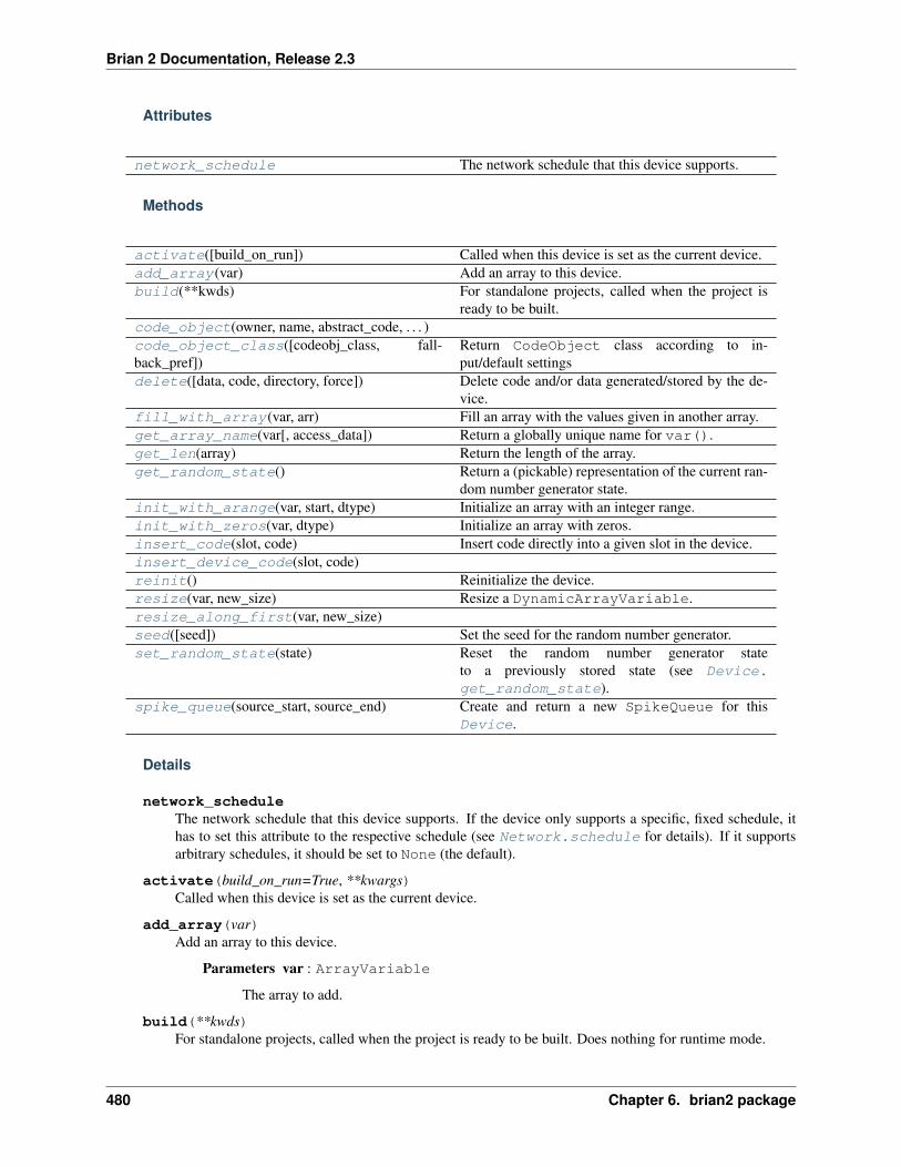
Brian 2 Documentation, Release 2.3
Attributes
network_schedule The network schedule that this device supports.
Methods
activate([build_on_run]) Called when this device is set as the current device.add_array(var) Add an array to this device.build(**kwds) For standalone projects, called when the project is
ready to be built.code_object(owner, name, abstract_code, . . . )code_object_class([codeobj_class, fall-back_pref])
Return CodeObject class according to in-put/default settings
delete([data, code, directory, force]) Delete code and/or data generated/stored by the de-vice.
fill_with_array(var, arr) Fill an array with the values given in another array.get_array_name(var[, access_data]) Return a globally unique name for var().get_len(array) Return the length of the array.get_random_state() Return a (pickable) representation of the current ran-
dom number generator state.init_with_arange(var, start, dtype) Initialize an array with an integer range.init_with_zeros(var, dtype) Initialize an array with zeros.insert_code(slot, code) Insert code directly into a given slot in the device.insert_device_code(slot, code)reinit() Reinitialize the device.resize(var, new_size) Resize a DynamicArrayVariable.resize_along_first(var, new_size)seed([seed]) Set the seed for the random number generator.set_random_state(state) Reset the random number generator state
to a previously stored state (see Device.get_random_state).
spike_queue(source_start, source_end) Create and return a new SpikeQueue for thisDevice.
Details
network_scheduleThe network schedule that this device supports. If the device only supports a specific, fixed schedule, ithas to set this attribute to the respective schedule (see Network.schedule for details). If it supportsarbitrary schedules, it should be set to None (the default).
activate(build_on_run=True, **kwargs)Called when this device is set as the current device.
add_array(var)Add an array to this device.
Parameters var : ArrayVariable
The array to add.
build(**kwds)For standalone projects, called when the project is ready to be built. Does nothing for runtime mode.
480 Chapter 6. brian2 package

Brian 2 Documentation, Release 2.3
code_object(owner, name, abstract_code, variables, template_name, variable_indices,codeobj_class=None, template_kwds=None, override_conditional_write=None,compiler_kwds=None)
code_object_class(codeobj_class=None, fallback_pref=’codegen.target’)Return CodeObject class according to input/default settings
Parameters codeobj_class : a CodeObject class, optional
If this is keyword is set to None or no arguments are given, this method will return thedefault.
fallback_pref : str, optional
String describing which attribute of prefs to access to retrieve the ‘default’ target. Usu-ally this is codegen.target, but in some cases we want to use object-specific targets suchas codegen.string_expression_target.
Returns codeobj_class : class
The CodeObject class that should be used
delete(data=True, code=True, directory=True, force=False)Delete code and/or data generated/stored by the device.
Parameters data : bool, optional
Whether to delete the data generated by the simulation (final values of state variables,data stored in monitors, etc.). Defaults to True.
code : bool, optional
Whether to delete the code generated by the simulation. Includes the numerical valuesused for initialization of state variables in assignments not using strings. Defaults toTrue.
directory : bool, optional
Whether to delete the project directory generated by the simulation. Will not deletedirectories that contain files not created by Brian unless the force option is specfied.Defaults to True.
force : bool, optional
Whether to delete the project directory with all its content, even if it contains files thatwere not created by Brian. Useful only when the directory option is set to True aswell. Defaults to False.
fill_with_array(var, arr)Fill an array with the values given in another array.
Parameters var : ArrayVariable
The array to fill.
arr : ndarray
The array values that should be copied to var().
get_array_name(var, access_data=True)Return a globally unique name for var().
Parameters access_data : bool, optional
6.6. Subpackages 481

Brian 2 Documentation, Release 2.3
For DynamicArrayVariable objects, specifying True here means the name forthe underlying data is returned. If specifying False, the name of object itself is re-turned (e.g. to allow resizing).
Returns name : str
The name for var().
get_len(array)Return the length of the array.
Parameters array : ArrayVariable
The array for which the length is requested.
Returns l : int
The length of the array.
get_random_state()Return a (pickable) representation of the current random number generator state. Providing the returnedobject (e.g. a dict) to Device.set_random_state should restore the random number generator state.
Returns state :
The state of the random number generator in a representation that can be passed as anargument to Device.set_random_state.
init_with_arange(var, start, dtype)Initialize an array with an integer range.
Parameters var : ArrayVariable
The array to fill with the integer range.
start : int
The start value for the integer range
dtype : dtype
The data type to use for the array.
init_with_zeros(var, dtype)Initialize an array with zeros.
Parameters var : ArrayVariable
The array to initialize with zeros.
dtype : dtype
The data type to use for the array.
insert_code(slot, code)Insert code directly into a given slot in the device. By default does nothing.
insert_device_code(slot, code)
reinit()Reinitialize the device. For standalone devices, clears all the internal state of the device.
resize(var, new_size)Resize a DynamicArrayVariable.
Parameters var : DynamicArrayVariable
The variable that should be resized.
482 Chapter 6. brian2 package
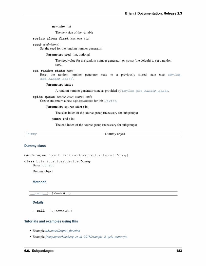
Brian 2 Documentation, Release 2.3
new_size : int
The new size of the variable
resize_along_first(var, new_size)
seed(seed=None)Set the seed for the random number generator.
Parameters seed : int, optional
The seed value for the random number generator, or None (the default) to set a randomseed.
set_random_state(state)Reset the random number generator state to a previously stored state (see Device.get_random_state).
Parameters state :
A random number generator state as provided by Device.get_random_state.
spike_queue(source_start, source_end)Create and return a new SpikeQueue for this Device.
Parameters source_start : int
The start index of the source group (necessary for subgroups)
source_end : int
The end index of the source group (necessary for subgroups)
Dummy Dummy object
Dummy class
(Shortest import: from brian2.devices.device import Dummy)
class brian2.devices.device.DummyBases: object
Dummy object
Methods
__call__(. . . ) <==> x(. . . )
Details
__call__(...) <==> x(...)
Tutorials and examples using this
• Example advanced/exprel_function
• Example frompapers/Stimberg_et_al_2018/example_2_gchi_astrocyte
6.6. Subpackages 483
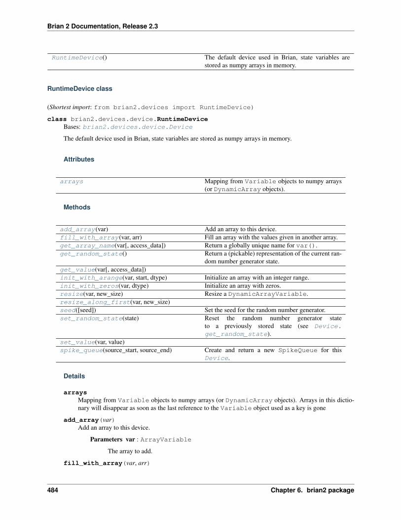
Brian 2 Documentation, Release 2.3
RuntimeDevice() The default device used in Brian, state variables arestored as numpy arrays in memory.
RuntimeDevice class
(Shortest import: from brian2.devices import RuntimeDevice)
class brian2.devices.device.RuntimeDeviceBases: brian2.devices.device.Device
The default device used in Brian, state variables are stored as numpy arrays in memory.
Attributes
arrays Mapping from Variable objects to numpy arrays(or DynamicArray objects).
Methods
add_array(var) Add an array to this device.fill_with_array(var, arr) Fill an array with the values given in another array.get_array_name(var[, access_data]) Return a globally unique name for var().get_random_state() Return a (pickable) representation of the current ran-
dom number generator state.get_value(var[, access_data])init_with_arange(var, start, dtype) Initialize an array with an integer range.init_with_zeros(var, dtype) Initialize an array with zeros.resize(var, new_size) Resize a DynamicArrayVariable.resize_along_first(var, new_size)seed([seed]) Set the seed for the random number generator.set_random_state(state) Reset the random number generator state
to a previously stored state (see Device.get_random_state).
set_value(var, value)spike_queue(source_start, source_end) Create and return a new SpikeQueue for this
Device.
Details
arraysMapping from Variable objects to numpy arrays (or DynamicArray objects). Arrays in this dictio-nary will disappear as soon as the last reference to the Variable object used as a key is gone
add_array(var)Add an array to this device.
Parameters var : ArrayVariable
The array to add.
fill_with_array(var, arr)
484 Chapter 6. brian2 package

Brian 2 Documentation, Release 2.3
Fill an array with the values given in another array.
Parameters var : ArrayVariable
The array to fill.
arr : ndarray
The array values that should be copied to var().
get_array_name(var, access_data=True)Return a globally unique name for var().
Parameters access_data : bool, optional
For DynamicArrayVariable objects, specifying True here means the name forthe underlying data is returned. If specifying False, the name of object itself is re-turned (e.g. to allow resizing).
Returns name : str
The name for var().
get_random_state()Return a (pickable) representation of the current random number generator state. Providing the returnedobject (e.g. a dict) to Device.set_random_state should restore the random number generator state.
Returns state :
The state of the random number generator in a representation that can be passed as anargument to Device.set_random_state.
get_value(var, access_data=True)
init_with_arange(var, start, dtype)Initialize an array with an integer range.
Parameters var : ArrayVariable
The array to fill with the integer range.
start : int
The start value for the integer range
dtype : dtype
The data type to use for the array.
init_with_zeros(var, dtype)Initialize an array with zeros.
Parameters var : ArrayVariable
The array to initialize with zeros.
dtype : dtype
The data type to use for the array.
resize(var, new_size)Resize a DynamicArrayVariable.
Parameters var : DynamicArrayVariable
The variable that should be resized.
new_size : int
6.6. Subpackages 485

Brian 2 Documentation, Release 2.3
The new size of the variable
resize_along_first(var, new_size)
seed(seed=None)Set the seed for the random number generator.
Parameters seed : int, optional
The seed value for the random number generator, or None (the default) to set a randomseed.
set_random_state(state)Reset the random number generator state to a previously stored state (see Device.get_random_state).
Parameters state :
A random number generator state as provided by Device.get_random_state.
set_value(var, value)
spike_queue(source_start, source_end)Create and return a new SpikeQueue for this Device.
Parameters source_start : int
The start index of the source group (necessary for subgroups)
source_end : int
The end index of the source group (necessary for subgroups)
Tutorials and examples using this
• Example frompapers/Kremer_et_al_2011_barrel_cortex
Functions
auto_target() Automatically chose a code generation target (invokedwhen the codegen.target preference is set to 'auto'.
auto_target function
(Shortest import: from brian2.devices.device import auto_target)
brian2.devices.device.auto_target()Automatically chose a code generation target (invoked when the codegen.target preference is set to 'auto'.Caches its result so it only does the check once. Prefers weave > cython > numpy.
Returns target : class derived from CodeObject
The target to use
get_device() Gets the actve Device object
486 Chapter 6. brian2 package

Brian 2 Documentation, Release 2.3
get_device function
(Shortest import: from brian2 import get_device)
brian2.devices.device.get_device()Gets the actve Device object
reinit_and_delete() Calls reinit_devices and additionally deletes thefiles left behind by the standalone mode in the tempo-rary directory.
reinit_and_delete function
(Shortest import: from brian2.devices import reinit_and_delete)
brian2.devices.device.reinit_and_delete()Calls reinit_devices and additionally deletes the files left behind by the standalone mode in the temporarydirectory. Silently suppresses errors that occur while deleting the directory.
reinit_devices() Reinitialize all devices, call Device.activateagain on the current device and reset the preferences.
reinit_devices function
(Shortest import: from brian2.devices import reinit_devices)
brian2.devices.device.reinit_devices()Reinitialize all devices, call Device.activate again on the current device and reset the preferences. Used asa “teardown” function in testing, if users want to reset their device (e.g. for multiple standalone runs in a singlescript), calling device.reinit() followed by device.activate() should normally be sufficient.
Notes
This also resets the defaultclock, i.e. a non-standard dt has to be set again.
reset_device([device]) Reset to a previously used device.
reset_device function
(Shortest import: from brian2.devices import reset_device)
brian2.devices.device.reset_device(device=None)Reset to a previously used device. Restores also the previously specified build options (see set_device())for the device. Mostly useful for internal Brian code and testing on various devices.
Parameters device : Device or str, optional
The device to go back to. If none is specified, go back to the device chosen withset_device() before the current one.
6.6. Subpackages 487

Brian 2 Documentation, Release 2.3
seed([seed]) Set the seed for the random number generator.
seed function
(Shortest import: from brian2 import seed)
brian2.devices.device.seed(seed=None)Set the seed for the random number generator.
Parameters seed : int, optional
The seed value for the random number generator, or None (the default) to set a randomseed.
Notes
This function delegates the call to Device.seed of the current device.
set_device(device[, build_on_run]) Set the device used for simulations.
set_device function
(Shortest import: from brian2 import set_device)
brian2.devices.device.set_device(device, build_on_run=True, **kwargs)Set the device used for simulations.
Parameters device : Device or str
The Device object or the name of the device.
build_on_run : bool, optional
Whether a call to run() (or Network.run()) should directly trigger a Device.build. This is only relevant for standalone devices and means that a run call directlytriggers the start of a simulation. If the simulation consists of multiple run calls, setbuild_on_run to False and call Device.build explicitly. Defaults to True.
kwargs : dict, optional
Only relevant when build_on_run is True: additional arguments that will be givento the Device.build call.
Objects
active_device The currently active device (set with set_device())
active_device object
(Shortest import: from brian2.devices.device import active_device)
brian2.devices.device.active_device = <brian2.devices.device.RuntimeDevice object>The currently active device (set with set_device())
488 Chapter 6. brian2 package

Brian 2 Documentation, Release 2.3
device Proxy object to access methods of the current device
device object
(Shortest import: from brian2 import device)
brian2.devices.device.device = <brian2.devices.device.CurrentDeviceProxy object>Proxy object to access methods of the current device
runtime_device The default device used in Brian, state variables arestored as numpy arrays in memory.
runtime_device object
(Shortest import: from brian2.devices.device import runtime_device)
brian2.devices.device.runtime_device = <brian2.devices.device.RuntimeDevice object>The default device used in Brian, state variables are stored as numpy arrays in memory.
Subpackages
cpp_standalone package
Package implementing the C++ “standalone” Device and CodeObject.
GSLcodeobject module
Module containing CPPStandalone CodeObject for code generation for integration using the ODE solver provided inthe GNU Scientific Library
Classes
GSLCPPStandaloneCodeObject(owner, code,. . . )
GSLCPPStandaloneCodeObject class
(Shortest import: from brian2.devices.cpp_standalone import GSLCPPStandaloneCodeObject)
6.6. Subpackages 489
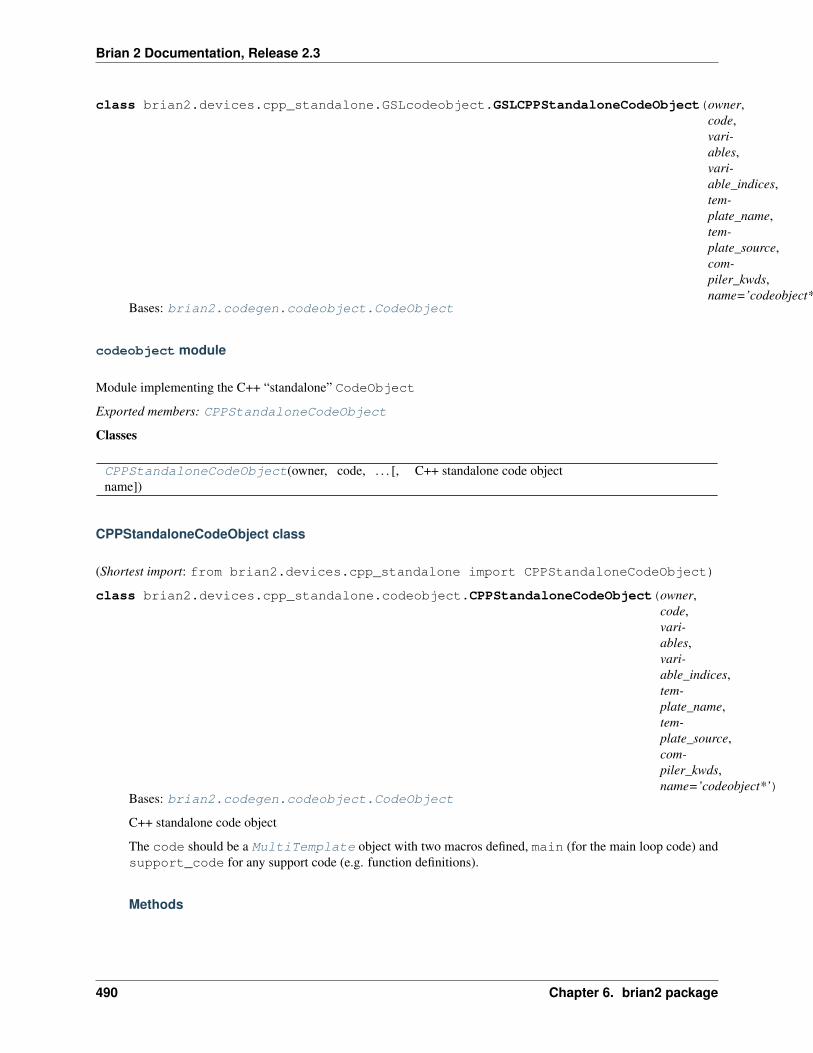
Brian 2 Documentation, Release 2.3
class brian2.devices.cpp_standalone.GSLcodeobject.GSLCPPStandaloneCodeObject(owner,code,vari-ables,vari-able_indices,tem-plate_name,tem-plate_source,com-piler_kwds,name=’codeobject*’)
Bases: brian2.codegen.codeobject.CodeObject
codeobject module
Module implementing the C++ “standalone” CodeObject
Exported members: CPPStandaloneCodeObject
Classes
CPPStandaloneCodeObject(owner, code, . . . [,name])
C++ standalone code object
CPPStandaloneCodeObject class
(Shortest import: from brian2.devices.cpp_standalone import CPPStandaloneCodeObject)
class brian2.devices.cpp_standalone.codeobject.CPPStandaloneCodeObject(owner,code,vari-ables,vari-able_indices,tem-plate_name,tem-plate_source,com-piler_kwds,name=’codeobject*’)
Bases: brian2.codegen.codeobject.CodeObject
C++ standalone code object
The code should be a MultiTemplate object with two macros defined, main (for the main loop code) andsupport_code for any support code (e.g. function definitions).
Methods
490 Chapter 6. brian2 package

Brian 2 Documentation, Release 2.3
__call__(. . . ) <==> x(. . . )run() Runs the code in the namespace.
Details
__call__(...) <==> x(...)
run()Runs the code in the namespace.
Returns return_value : dict
A dictionary with the keys corresponding to the output_variables defined duringthe call of CodeGenerator.code_object.
Functions
generate_rand_code(rand_func, owner)
generate_rand_code function
(Shortest import: from brian2.devices.cpp_standalone.codeobject importgenerate_rand_code)
brian2.devices.cpp_standalone.codeobject.generate_rand_code(rand_func, owner)
openmp_pragma(pragma_type)
openmp_pragma function
(Shortest import: from brian2.devices.cpp_standalone.codeobject importopenmp_pragma)
brian2.devices.cpp_standalone.codeobject.openmp_pragma(pragma_type)
device module
Classes
CPPStandaloneDevice() The Device used for C++ standalone simulations.
CPPStandaloneDevice class
(Shortest import: from brian2.devices.cpp_standalone.device importCPPStandaloneDevice)
class brian2.devices.cpp_standalone.device.CPPStandaloneDeviceBases: brian2.devices.device.Device
The Device used for C++ standalone simulations.
6.6. Subpackages 491

Brian 2 Documentation, Release 2.3
Attributes
arange_arrays List of all arrays to be filled with numbers (list of(var, varname, start) tuples
array_cache Dictionary mapping ArrayVariable objects totheir value or to None if the value (potentially) de-pends on executed code.
arrays Dictionary mapping ArrayVariable objects totheir globally unique name
build_on_run Whether a run should trigger a buildbuild_options build optionscode_lines Code lines that have been manually added with
device.insert_code() Dictionary mappingslot names to lists of lines.
dynamic_arrays List of all dynamic arrays Dictionary mappingDynamicArrayVariable objects with 1 dimen-sion to their globally unique name
dynamic_arrays_2d Dictionary mapping DynamicArrayVariableobjects with 2 dimensions to their globally uniquename
enable_profiling Whether to generate profiling information (stored inan instance variable to be accessible during CodeOb-ject generation)
has_been_run Whether the simulation has been runmsvc_env cached environment variables for MSVCprofiled_codeobjects CodeObjects that use profiling (users can potentially
enable profiling only for a subset of runs)project_dir The directory which contains the generated code and
resultsstatic_arrays Dict of all static saved arrayszero_arrays List of all arrays to be filled with zeros (list of (var,
varname) )
Methods
add_array(var) Add an array to this device.build([directory, compile, run, debug, . . . ]) Build the projectcheck_openmp_compatible(nb_threads)code_object(owner, name, abstract_code, . . . )code_object_class([codeobj_class, fall-back_pref])
Return CodeObject class (eitherCPPStandaloneCodeObject class or in-put)
compile_source(directory, compiler, debug,clean)copy_source_files(writer, directory)delete([code, data, directory, force]) Delete code and/or data generated/stored by the de-
vice.fill_with_array(var, arr) Fill an array with the values given in another array.find_synapses()freeze(code, ns)
Continued on next page
492 Chapter 6. brian2 package
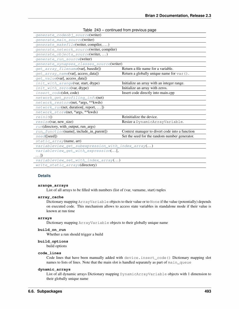
Brian 2 Documentation, Release 2.3
Table 243 – continued from previous pagegenerate_codeobj_source(writer)generate_main_source(writer)generate_makefile(writer, compiler, . . . )generate_network_source(writer, compiler)generate_objects_source(writer, . . . )generate_run_source(writer)generate_synapses_classes_source(writer)get_array_filename(var[, basedir]) Return a file name for a variable.get_array_name(var[, access_data]) Return a globally unique name for var().get_value(var[, access_data])init_with_arange(var, start, dtype) Initialize an array with an integer range.init_with_zeros(var, dtype) Initialize an array with zeros.insert_code(slot, code) Insert code directly into main.cppnetwork_get_profiling_info(net)network_restore(net, *args, **kwds)network_run(net, duration[, report, . . . ])network_store(net, *args, **kwds)reinit() Reinitialize the device.resize(var, new_size) Resize a DynamicArrayVariable.run(directory, with_output, run_args)run_function(name[, include_in_parent]) Context manager to divert code into a functionseed([seed]) Set the seed for the random number generator.static_array(name, arr)variableview_get_subexpression_with_index_array(. . . )variableview_get_with_expression(. . . [,. . . ])variableview_set_with_index_array(. . . )write_static_arrays(directory)
Details
arange_arraysList of all arrays to be filled with numbers (list of (var, varname, start) tuples
array_cacheDictionary mapping ArrayVariable objects to their value or to None if the value (potentially) dependson executed code. This mechanism allows to access state variables in standalone mode if their value isknown at run time
arraysDictionary mapping ArrayVariable objects to their globally unique name
build_on_runWhether a run should trigger a build
build_optionsbuild options
code_linesCode lines that have been manually added with device.insert_code() Dictionary mapping slotnames to lists of lines. Note that the main slot is handled separately as part of main_queue
dynamic_arraysList of all dynamic arrays Dictionary mapping DynamicArrayVariable objects with 1 dimension totheir globally unique name
6.6. Subpackages 493

Brian 2 Documentation, Release 2.3
dynamic_arrays_2dDictionary mapping DynamicArrayVariable objects with 2 dimensions to their globally uniquename
enable_profilingWhether to generate profiling information (stored in an instance variable to be accessible during CodeOb-ject generation)
has_been_runWhether the simulation has been run
msvc_envcached environment variables for MSVC
profiled_codeobjectsCodeObjects that use profiling (users can potentially enable profiling only for a subset of runs)
project_dirThe directory which contains the generated code and results
static_arraysDict of all static saved arrays
zero_arraysList of all arrays to be filled with zeros (list of (var, varname) )
add_array(var)Add an array to this device.
Parameters var : ArrayVariable
The array to add.
build(directory=’output’, compile=True, run=True, debug=False, clean=False, with_output=True, ad-ditional_source_files=None, run_args=None, direct_call=True, **kwds)
Build the project
TODO: more details
Parameters directory : str, optional
The output directory to write the project to, any existing files will be overwritten. If thegiven directory name is None, then a temporary directory will be used (used in the testsuite to avoid problems when running several tests in parallel). Defaults to 'output'.
compile : bool, optional
Whether or not to attempt to compile the project. Defaults to True.
run : bool, optional
Whether or not to attempt to run the built project if it successfully builds. Defaults toTrue.
debug : bool, optional
Whether to compile in debug mode. Defaults to False.
with_output : bool, optional
Whether or not to show the stdout of the built program when run. Output will beshown in case of compilation or runtime error. Defaults to True.
clean : bool, optional
Whether or not to clean the project before building. Defaults to False.
494 Chapter 6. brian2 package
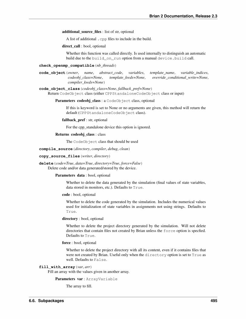
Brian 2 Documentation, Release 2.3
additional_source_files : list of str, optional
A list of additional .cpp files to include in the build.
direct_call : bool, optional
Whether this function was called directly. Is used internally to distinguish an automaticbuild due to the build_on_run option from a manual device.build call.
check_openmp_compatible(nb_threads)
code_object(owner, name, abstract_code, variables, template_name, variable_indices,codeobj_class=None, template_kwds=None, override_conditional_write=None,compiler_kwds=None)
code_object_class(codeobj_class=None, fallback_pref=None)Return CodeObject class (either CPPStandaloneCodeObject class or input)
Parameters codeobj_class : a CodeObject class, optional
If this is keyword is set to None or no arguments are given, this method will return thedefault (CPPStandaloneCodeObject class).
fallback_pref : str, optional
For the cpp_standalone device this option is ignored.
Returns codeobj_class : class
The CodeObject class that should be used
compile_source(directory, compiler, debug, clean)
copy_source_files(writer, directory)
delete(code=True, data=True, directory=True, force=False)Delete code and/or data generated/stored by the device.
Parameters data : bool, optional
Whether to delete the data generated by the simulation (final values of state variables,data stored in monitors, etc.). Defaults to True.
code : bool, optional
Whether to delete the code generated by the simulation. Includes the numerical valuesused for initialization of state variables in assignments not using strings. Defaults toTrue.
directory : bool, optional
Whether to delete the project directory generated by the simulation. Will not deletedirectories that contain files not created by Brian unless the force option is specfied.Defaults to True.
force : bool, optional
Whether to delete the project directory with all its content, even if it contains files thatwere not created by Brian. Useful only when the directory option is set to True aswell. Defaults to False.
fill_with_array(var, arr)Fill an array with the values given in another array.
Parameters var : ArrayVariable
The array to fill.
6.6. Subpackages 495

Brian 2 Documentation, Release 2.3
arr : ndarray
The array values that should be copied to var().
find_synapses()
freeze(code, ns)
generate_codeobj_source(writer)
generate_main_source(writer)
generate_makefile(writer, compiler, compiler_flags, linker_flags, nb_threads, debug)
generate_network_source(writer, compiler)
generate_objects_source(writer, arange_arrays, synapses, static_array_specs, networks)
generate_run_source(writer)
generate_synapses_classes_source(writer)
get_array_filename(var, basedir=’results’)Return a file name for a variable.
Parameters var : ArrayVariable
The variable to get a filename for.
basedir : str
The base directory for the filename, defaults to 'results'.
Returns :
——- :
filename : str
A filename of the form 'results/'+varname+'_'+str(hash(varname)),where varname is the name returned by get_array_name.
Notes
The reason that the filename is not simply 'results/' + varname is that this could lead to file namesthat are not unique in file systems that are not case sensitive (e.g. on Windows).
get_array_name(var, access_data=True)Return a globally unique name for var().
Parameters access_data : bool, optional
For DynamicArrayVariable objects, specifying True here means the name forthe underlying data is returned. If specifying False, the name of object itself is re-turned (e.g. to allow resizing).
get_value(var, access_data=True)
init_with_arange(var, start, dtype)Initialize an array with an integer range.
Parameters var : ArrayVariable
The array to fill with the integer range.
start : int
496 Chapter 6. brian2 package
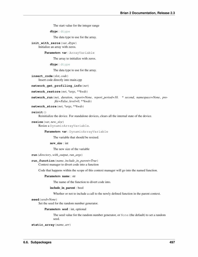
Brian 2 Documentation, Release 2.3
The start value for the integer range
dtype : dtype
The data type to use for the array.
init_with_zeros(var, dtype)Initialize an array with zeros.
Parameters var : ArrayVariable
The array to initialize with zeros.
dtype : dtype
The data type to use for the array.
insert_code(slot, code)Insert code directly into main.cpp
network_get_profiling_info(net)
network_restore(net, *args, **kwds)
network_run(net, duration, report=None, report_period=10. * second, namespace=None, pro-file=False, level=0, **kwds)
network_store(net, *args, **kwds)
reinit()Reinitialize the device. For standalone devices, clears all the internal state of the device.
resize(var, new_size)Resize a DynamicArrayVariable.
Parameters var : DynamicArrayVariable
The variable that should be resized.
new_size : int
The new size of the variable
run(directory, with_output, run_args)
run_function(name, include_in_parent=True)Context manager to divert code into a function
Code that happens within the scope of this context manager will go into the named function.
Parameters name : str
The name of the function to divert code into.
include_in_parent : bool
Whether or not to include a call to the newly defined function in the parent context.
seed(seed=None)Set the seed for the random number generator.
Parameters seed : int, optional
The seed value for the random number generator, or None (the default) to set a randomseed.
static_array(name, arr)
6.6. Subpackages 497

Brian 2 Documentation, Release 2.3
variableview_get_subexpression_with_index_array(variableview, item,run_namespace=None)
variableview_get_with_expression(variableview, code, run_namespace=None)
variableview_set_with_index_array(variableview, item, value, check_units)
write_static_arrays(directory)
CPPWriter(project_dir)
Methods
CPPWriter class
(Shortest import: from brian2.devices.cpp_standalone.device import CPPWriter)
class brian2.devices.cpp_standalone.device.CPPWriter(project_dir)Bases: object
Methods
write(filename, contents)
Details
write(filename, contents)
RunFunctionContext(name, include_in_parent)
RunFunctionContext class
(Shortest import: from brian2.devices.cpp_standalone.device importRunFunctionContext)
class brian2.devices.cpp_standalone.device.RunFunctionContext(name, in-clude_in_parent)
Bases: object
Functions
invert_dict(x)
invert_dict function
(Shortest import: from brian2.devices.cpp_standalone.device import invert_dict)
brian2.devices.cpp_standalone.device.invert_dict(x)
Objects
498 Chapter 6. brian2 package

Brian 2 Documentation, Release 2.3
cpp_standalone_device The Device used for C++ standalone simulations.
cpp_standalone_device object
(Shortest import: from brian2.devices.cpp_standalone import cpp_standalone_device)
brian2.devices.cpp_standalone.device.cpp_standalone_device = <brian2.devices.cpp_standalone.device.CPPStandaloneDevice object>The Device used for C++ standalone simulations.
6.6.4 equations package
Module handling equations and “code strings”, expressions or statements, used for example for the reset and thresholddefinition of a neuron.
Exported members: Equations, Expression, Statements
codestrings module
Module defining CodeString, a class for a string of code together with information about its namespace. Onlyserves as a parent class, its subclasses Expression and Statements are the ones that are actually used.
Exported members: Expression, Statements
Classes
CodeString(code) A class for representing “code strings”, i.e.
CodeString class
(Shortest import: from brian2.equations.codestrings import CodeString)
class brian2.equations.codestrings.CodeString(code)Bases: _abcoll.Hashable
A class for representing “code strings”, i.e. a single Python expression or a sequence of Python statements.
Parameters code : str
The code string, may be an expression or a statement(s) (possibly multi-line).
Attributes
code The code string
Details
codeThe code string
6.6. Subpackages 499
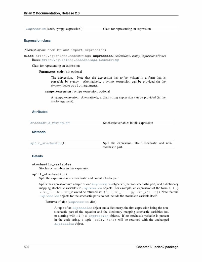
Brian 2 Documentation, Release 2.3
Expression([code, sympy_expression]) Class for representing an expression.
Expression class
(Shortest import: from brian2 import Expression)
class brian2.equations.codestrings.Expression(code=None, sympy_expression=None)Bases: brian2.equations.codestrings.CodeString
Class for representing an expression.
Parameters code : str, optional
The expression. Note that the expression has to be written in a form that isparseable by sympy. Alternatively, a sympy expression can be provided (in thesympy_expression argument).
sympy_expression : sympy expression, optional
A sympy expression. Alternatively, a plain string expression can be provided (in thecode argument).
Attributes
stochastic_variables Stochastic variables in this expression
Methods
split_stochastic() Split the expression into a stochastic and non-stochastic part.
Details
stochastic_variablesStochastic variables in this expression
split_stochastic()Split the expression into a stochastic and non-stochastic part.
Splits the expression into a tuple of one Expression objects f (the non-stochastic part) and a dictionarymapping stochastic variables to Expression objects. For example, an expression of the form f + g
* xi_1 + h * xi_2 would be returned as: (f, {'xi_1': g, 'xi_2': h}) Note that theExpression objects for the stochastic parts do not include the stochastic variable itself.
Returns (f, d) : (Expression, dict)
A tuple of an Expression object and a dictionary, the first expression being the non-stochastic part of the equation and the dictionary mapping stochastic variables (xior starting with xi_) to Expression objects. If no stochastic variable is presentin the code string, a tuple (self, None) will be returned with the unchangedExpression object.
500 Chapter 6. brian2 package

Brian 2 Documentation, Release 2.3
Statements(code) Class for representing statements.
Statements class
(Shortest import: from brian2 import Statements)
class brian2.equations.codestrings.Statements(code)Bases: brian2.equations.codestrings.CodeString
Class for representing statements.
Parameters code : str
The statement or statements. Several statements can be given as a multi-line string orseparated by semicolons.
Notes
Currently, the implementation of this class does not add anything to CodeString, but it should be usedinstead of that class for clarity and to allow for future functionality that is only relevant to statements and not toexpressions.
Functions
is_constant_over_dt(expression, variables, . . . ) Check whether an expression can be considered as con-stant over a time step.
is_constant_over_dt function
(Shortest import: from brian2.equations.codestrings import is_constant_over_dt)
brian2.equations.codestrings.is_constant_over_dt(expression, variables, dt_value)Check whether an expression can be considered as constant over a time step. This is not the case when theexpression either:
1. contains the variable t (except as the argument of a function that can be considered as constant over a timestep, e.g. a TimedArray with a dt equal to or greater than the dt used to evaluate this expression)
2. refers to a stateful function such as rand().
Parameters expression : sympy.Expr
The (sympy) expression to analyze
variables : dict
The variables dictionary.
dt_value : float or None
The length of a timestep (without units), can be None if the time step is not yet known.
Returns is_constant : bool
Whether the expression can be considered to be constant over a time step.
6.6. Subpackages 501

Brian 2 Documentation, Release 2.3
equations module
Exported members: Equations
Classes
EquationError Exception type related to errors in an equation defini-tion.
EquationError class
(Shortest import: from brian2.equations.equations import EquationError)
class brian2.equations.equations.EquationErrorBases: exceptions.Exception
Exception type related to errors in an equation definition.
Equations(eqns, **kwds) Container that stores equations from which models canbe created.
Equations class
(Shortest import: from brian2 import Equations)
class brian2.equations.equations.Equations(eqns, **kwds)Bases: _abcoll.Hashable, _abcoll.Mapping
Container that stores equations from which models can be created.
String equations can be of any of the following forms:
1. dx/dt = f : unit (flags) (differential equation)
2. x = f : unit (flags) (equation)
3. x : unit (flags) (parameter)
String equations can span several lines and contain Python-style comments starting with #
Parameters eqs : str or list of SingleEquation objects
A multiline string of equations (see above) – for internal purposes also a list ofSingleEquation objects can be given. This is done for example when adding newequations to implement the refractory mechanism. Note that in this case the variablenames are not checked to allow for “internal names”, starting with an underscore.
kwds: keyword arguments :
Keyword arguments can be used to replace variables in the equation string. Argumentshave to be of the form varname=replacement, where varname has to correspondto a variable name in the given equation. The replacement can be either a string (replac-ing a name with a new name, e.g. tau='tau_e') or a value (replacing the variablename with the value, e.g. tau=tau_e or tau=10*ms).
502 Chapter 6. brian2 package
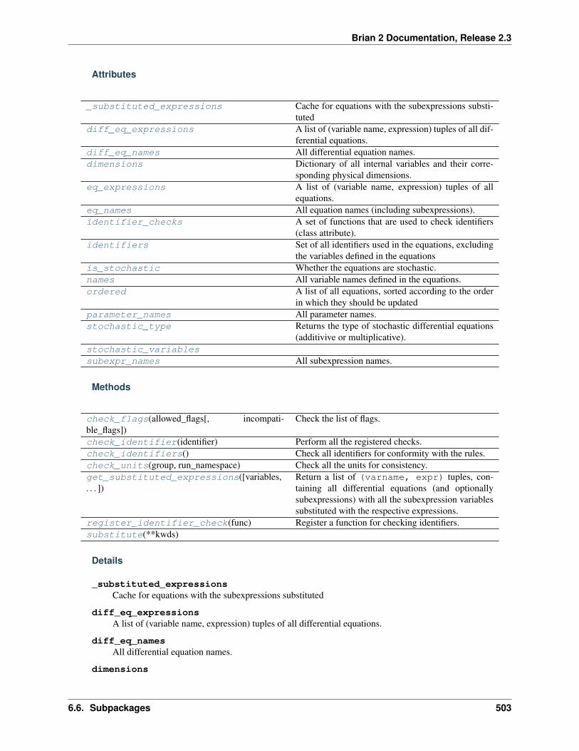
Brian 2 Documentation, Release 2.3
Attributes
_substituted_expressions Cache for equations with the subexpressions substi-tuted
diff_eq_expressions A list of (variable name, expression) tuples of all dif-ferential equations.
diff_eq_names All differential equation names.dimensions Dictionary of all internal variables and their corre-
sponding physical dimensions.eq_expressions A list of (variable name, expression) tuples of all
equations.eq_names All equation names (including subexpressions).identifier_checks A set of functions that are used to check identifiers
(class attribute).identifiers Set of all identifiers used in the equations, excluding
the variables defined in the equationsis_stochastic Whether the equations are stochastic.names All variable names defined in the equations.ordered A list of all equations, sorted according to the order
in which they should be updatedparameter_names All parameter names.stochastic_type Returns the type of stochastic differential equations
(additivive or multiplicative).stochastic_variablessubexpr_names All subexpression names.
Methods
check_flags(allowed_flags[, incompati-ble_flags])
Check the list of flags.
check_identifier(identifier) Perform all the registered checks.check_identifiers() Check all identifiers for conformity with the rules.check_units(group, run_namespace) Check all the units for consistency.get_substituted_expressions([variables,. . . ])
Return a list of (varname, expr) tuples, con-taining all differential equations (and optionallysubexpressions) with all the subexpression variablessubstituted with the respective expressions.
register_identifier_check(func) Register a function for checking identifiers.substitute(**kwds)
Details
_substituted_expressionsCache for equations with the subexpressions substituted
diff_eq_expressionsA list of (variable name, expression) tuples of all differential equations.
diff_eq_namesAll differential equation names.
dimensions
6.6. Subpackages 503

Brian 2 Documentation, Release 2.3
Dictionary of all internal variables and their corresponding physical dimensions.
eq_expressionsA list of (variable name, expression) tuples of all equations.
eq_namesAll equation names (including subexpressions).
identifier_checksA set of functions that are used to check identifiers (class attribute). Functions can be registered with thestatic method Equations.register_identifier_check and will be automatically used whenchecking identifiers
identifiersSet of all identifiers used in the equations, excluding the variables defined in the equations
is_stochasticWhether the equations are stochastic.
namesAll variable names defined in the equations.
orderedA list of all equations, sorted according to the order in which they should be updated
parameter_namesAll parameter names.
stochastic_typeReturns the type of stochastic differential equations (additivive or multiplicative). The system is onlyclassified as additive if all equations have only additive noise (or no noise).
Returns type : str
Either None (no noise variables), 'additive' (factors for all noise variables areindependent of other state variables or time), 'multiplicative' (at least one ofthe noise factors depends on other state variables and/or time).
stochastic_variables
subexpr_namesAll subexpression names.
check_flags(allowed_flags, incompatible_flags=None)Check the list of flags.
Parameters allowed_flags : dict
A dictionary mapping equation types (PARAMETER, DIFFERENTIAL_EQUATION,SUBEXPRESSION) to a list of strings (the allowed flags for that equation type)
incompatible_flags : list of tuple
A list of flag combinations that are not allowed for the same equation.
Notes :
—– :
Not specifying allowed flags for an equation type is the same as :
specifying an empty list for it. :
504 Chapter 6. brian2 package

Brian 2 Documentation, Release 2.3
Raises
ValueError If any flags are used that are not allowed.
static check_identifier(identifier)Perform all the registered checks. Checks can be registered via Equations.register_identifier_check.
Parameters identifier : str
The identifier that should be checked
Raises
ValueError If any of the registered checks fails.
check_identifiers()Check all identifiers for conformity with the rules.
Raises
ValueError If an identifier does not conform to the rules.
See also:
Equations.check_identifier The function that is called for each identifier.
check_units(group, run_namespace)Check all the units for consistency.
Parameters group : Group
The group providing the context
run_namespace : dict-like, optional
An additional namespace that is used for variable lookup (if not defined, the implicitnamespace of local variables is used).
level : int, optional
How much further to go up in the stack to find the calling frame
Raises
DimensionMismatchError In case of any inconsistencies.
get_substituted_expressions(variables=None, include_subexpressions=False)Return a list of (varname, expr) tuples, containing all differential equations (and optionally subex-pressions) with all the subexpression variables substituted with the respective expressions.
Parameters variables : dict, optional
A mapping of variable names to Variable/Function objects.
include_subexpressions : bool
Whether also to return substituted subexpressions. Defaults to False.
6.6. Subpackages 505
Brian 2 Documentation, Release 2.3
Returns expr_tuples : list of (str, CodeString)
A list of (varname, expr) tuples, where expr is a CodeString object with allsubexpression variables substituted with the respective expression.
static register_identifier_check(func)Register a function for checking identifiers.
Parameters func : callable
The function has to receive a single argument, the name of the identifier to check, andraise a ValueError if the identifier violates any rule.
substitute(**kwds)
Tutorials and examples using this
• Example COBAHH
• Example IF_curve_Hodgkin_Huxley
• Example advanced/float_32_64_benchmark
• Example frompapers/Rossant_et_al_2011bis
• Example frompapers/Diesmann_et_al_1999
• Example frompapers/Hindmarsh_Rose_1984
• Example frompapers/Clopath_et_al_2010_homeostasis
• Example frompapers/Clopath_et_al_2010_no_homeostasis
• Example frompapers/Destexhe_et_al_1998
SingleEquation(type, varname, dimensions[, . . . ]) Class for internal use, encapsulates a single equation orparameter.
SingleEquation class
(Shortest import: from brian2.equations.equations import SingleEquation)
class brian2.equations.equations.SingleEquation(type, varname, dimensions,var_type=’float’, expr=None,flags=None)
Bases: _abcoll.Hashable, brian2.utils.caching.CacheKey
Class for internal use, encapsulates a single equation or parameter.
Note: This class should never be used directly, it is only useful as part of the Equations class.
Parameters type : {PARAMETER, DIFFERENTIAL_EQUATION, SUBEXPRESSION}
The type of the equation.
varname : str
The variable that is defined by this equation.
dimensions : Dimension
506 Chapter 6. brian2 package
Brian 2 Documentation, Release 2.3
The physical dimensions of the variable
var_type : {FLOAT, INTEGER, BOOLEAN}
The type of the variable (floating point value or boolean).
expr : Expression, optional
The expression defining the variable (or None for parameters).
flags: list of str, optional :
A list of flags that give additional information about this equation. What flags are pos-sible depends on the type of the equation and the context.
Attributes
identifiers All identifiers in the RHS of this equation.stochastic_variables Stochastic variables in the RHS of this equationunit The Unit of this equation.
Details
identifiersAll identifiers in the RHS of this equation.
stochastic_variablesStochastic variables in the RHS of this equation
unitThe Unit of this equation.
Functions
check_identifier_basic(identifier) Check an identifier (usually resulting from an equationstring provided by the user) for conformity with therules.
check_identifier_basic function
(Shortest import: from brian2.equations.equations import check_identifier_basic)
brian2.equations.equations.check_identifier_basic(identifier)Check an identifier (usually resulting from an equation string provided by the user) for conformity with therules. The rules are:
1. Only ASCII characters
2. Starts with a character, then mix of alphanumerical characters and underscore
3. Is not a reserved keyword of Python
Parameters identifier : str
The identifier that should be checked
6.6. Subpackages 507

Brian 2 Documentation, Release 2.3
Raises
SyntaxError If the identifier does not conform to the above rules.
check_identifier_constants(identifier) Make sure that identifier names do not clash with func-tion names.
check_identifier_constants function
(Shortest import: from brian2.equations.equations import check_identifier_constants)
brian2.equations.equations.check_identifier_constants(identifier)Make sure that identifier names do not clash with function names.
check_identifier_functions(identifier) Make sure that identifier names do not clash with func-tion names.
check_identifier_functions function
(Shortest import: from brian2.equations.equations import check_identifier_functions)
brian2.equations.equations.check_identifier_functions(identifier)Make sure that identifier names do not clash with function names.
check_identifier_reserved(identifier) Check that an identifier is not using a reserved specialvariable name.
check_identifier_reserved function
(Shortest import: from brian2.equations.equations import check_identifier_reserved)
brian2.equations.equations.check_identifier_reserved(identifier)Check that an identifier is not using a reserved special variable name. The special variables are: ‘t’, ‘dt’, and‘xi’, as well as everything starting with xi_.
Parameters identifier: str :
The identifier that should be checked
Raises
SyntaxError If the identifier is a special variable name.
check_identifier_units(identifier) Make sure that identifier names do not clash with unitnames.
508 Chapter 6. brian2 package
Brian 2 Documentation, Release 2.3
check_identifier_units function
(Shortest import: from brian2.equations.equations import check_identifier_units)
brian2.equations.equations.check_identifier_units(identifier)Make sure that identifier names do not clash with unit names.
check_subexpressions(group, equations, . . . ) Checks the subexpressions in the equations and raisesan error if a subexpression refers to stateful functionswithout being marked as “constant over dt”.
check_subexpressions function
(Shortest import: from brian2.equations.equations import check_subexpressions)
brian2.equations.equations.check_subexpressions(group, equations, run_namespace)Checks the subexpressions in the equations and raises an error if a subexpression refers to stateful functionswithout being marked as “constant over dt”.
Parameters group : Group
The group providing the context.
equations : Equations
The equations to check.
run_namespace : dict
The run namespace for resolving variables.
Raises
SyntaxError For subexpressions not marked as “constant over dt” that refer to stateful functions.
dimensions_and_type_from_string(unit_string)Returns the physical dimensions that results from eval-uating a string like “siemens / metre ** 2”, allowing forthe special string “1” to signify dimensionless units, thestring “boolean” for a boolean and “integer” for an inte-ger variable.
dimensions_and_type_from_string function
(Shortest import: from brian2.equations.equations import dimensions_and_type_from_string)
brian2.equations.equations.dimensions_and_type_from_string(unit_string)Returns the physical dimensions that results from evaluating a string like “siemens / metre ** 2”, allowing forthe special string “1” to signify dimensionless units, the string “boolean” for a boolean and “integer” for aninteger variable.
Parameters unit_string : str
The string that should evaluate to a unit
6.6. Subpackages 509

Brian 2 Documentation, Release 2.3
Returns d, type : (Dimension, {FLOAT, INTEGER or BOOL})
The resulting physical dimensions and the type of the variable.
Raises
ValueError If the string cannot be evaluated to a unit.
extract_constant_subexpressions(eqs)
extract_constant_subexpressions function
(Shortest import: from brian2.equations.equations import extract_constant_subexpressions)
brian2.equations.equations.extract_constant_subexpressions(eqs)
is_stateful(expression, variables) Whether the given expression refers to stateful functions(and is therefore not guaranteed to give the same resultif called repetively).
is_stateful function
(Shortest import: from brian2.equations.equations import is_stateful)
brian2.equations.equations.is_stateful(expression, variables)Whether the given expression refers to stateful functions (and is therefore not guaranteed to give the same resultif called repetively).
Parameters expression : sympy.Expression
The sympy expression to check.
variables : dict
The dictionary mapping variable names to Variable or Function objects.
Returns stateful : bool
True, if the given expression refers to a stateful function like rand() and Falseotherwise.
parse_string_equations(eqns) Parse a string defining equations.
parse_string_equations function
(Shortest import: from brian2.equations.equations import parse_string_equations)
brian2.equations.equations.parse_string_equations(eqns)Parse a string defining equations.
Parameters eqns : str
The (possibly multi-line) string defining the equations. See the documentation of the
510 Chapter 6. brian2 package
Brian 2 Documentation, Release 2.3
Equations class for details.
Returns equations : dict
A dictionary mapping variable names to Equations objects
refractory module
Module implementing Brian’s refractory mechanism.
Exported members: add_refractoriness
Functions
add_refractoriness(eqs) Extends a given set of equations with the refractorymechanism.
add_refractoriness function
(Shortest import: from brian2.equations.refractory import add_refractoriness)
brian2.equations.refractory.add_refractoriness(eqs)Extends a given set of equations with the refractory mechanism. New parameters are added and differentialequations with the “unless refractory” flag are changed so that their right-hand side is 0 when the neuron isrefractory (by multiplication with the not_refractory variable).
Parameters eqs : Equations
The equations without refractory mechanism.
Returns new_eqs : Equations
New equations, with added parameters and changed differential equations having the“unless refractory” flag.
check_identifier_refractory(identifier) Check that the identifier is not using a name reserved forthe refractory mechanism.
check_identifier_refractory function
(Shortest import: from brian2.equations.refractory import check_identifier_refractory)
brian2.equations.refractory.check_identifier_refractory(identifier)Check that the identifier is not using a name reserved for the refractory mechanism. The reserved names arenot_refractory, refractory, refractory_until.
Parameters identifier : str
The identifier to check.
Raises
ValueError If the identifier is a variable name used for the refractory mechanism.
6.6. Subpackages 511

Brian 2 Documentation, Release 2.3
unitcheck module
Utility functions for handling the units in Equations.
Exported members: unit_from_expression, check_dimensions, check_units_statements
Functions
check_dimensions(expression, dimensions, . . . ) Compares the physical dimensions of an expression toexpected dimensions in a given namespace.
check_dimensions function
(Shortest import: from brian2.equations.unitcheck import check_dimensions)
brian2.equations.unitcheck.check_dimensions(expression, dimensions, variables)Compares the physical dimensions of an expression to expected dimensions in a given namespace.
Parameters expression : str
The expression to evaluate.
dimensions : Dimension
The expected physical dimensions for the expression.
variables : dict
Dictionary of all variables (including external constants) used in the expression.
Raises
KeyError In case on of the identifiers cannot be resolved.
DimensionMismatchError If an unit mismatch occurs during the evaluation.
check_units_statements(code, variables) Check the units for a series of statements.
check_units_statements function
(Shortest import: from brian2.equations.unitcheck import check_units_statements)
brian2.equations.unitcheck.check_units_statements(code, variables)Check the units for a series of statements. Setting a model variable has to use the correct unit. For newlyintroduced temporary variables, the unit is determined and used to check the following statements to ensureconsistency.
Parameters code : str
The statements as a (multi-line) string
variables : dict of Variable objects
The information about all variables used in code (including Constant objects forexternal variables)
512 Chapter 6. brian2 package

Brian 2 Documentation, Release 2.3
Raises
KeyError In case on of the identifiers cannot be resolved.
DimensionMismatchError If an unit mismatch occurs during the evaluation.
6.6.5 groups package
Package providing groups such as NeuronGroup or PoissonGroup.
Exported members: CodeRunner, Group, VariableOwner, NeuronGroup
group module
Exported members: Group, VariableOwner, CodeRunner
Classes
CodeRunner(group, template[, code, . . . ]) A “code runner” that runs a CodeObject everytimestep and keeps a reference to the Group.
CodeRunner class
(Shortest import: from brian2 import CodeRunner)
class brian2.groups.group.CodeRunner(group, template, code=”, user_code=None,dt=None, clock=None, when=’start’, order=0,name=’coderunner*’, check_units=True, tem-plate_kwds=None, needed_variables=None, over-ride_conditional_write=None, codeobj_class=None,generate_empty_code=True)
Bases: brian2.core.base.BrianObject
A “code runner” that runs a CodeObject every timestep and keeps a reference to the Group. Used inNeuronGroup for Thresholder, Resetter and StateUpdater.
On creation, we try to run the before_run method with an empty additional namespace (see Network.before_run()). If the namespace is already complete this might catch unit mismatches.
Parameters group : Group
The group to which this object belongs.
template : Template
The template that should be used for code generation
code : str, optional
The abstract code that should be executed every time step. Theupdate_abstract_code method might generate this code dynamically be-fore every run instead.
dt : Quantity , optional
The time step to be used for the simulation. Cannot be combined with the clockargument.
6.6. Subpackages 513

Brian 2 Documentation, Release 2.3
user_code : str, optional
The abstract code as specified by the user, i.e. without any additions of internal codethat the user not necessarily knows about. This will be used for warnings and errormessages.
clock : Clock, optional
The update clock to be used. If neither a clock, nor the dt argument is specified, thedefaultclock will be used.
when : str, optional
In which scheduling slot to execute the operation during a time step. Defaults to'start'.
order : int, optional
The priority of this operation for operations occurring at the same time step and in thesame scheduling slot. Defaults to 0.
name : str, optional
The name for this object.
check_units : bool, optional
Whether the units should be checked for consistency before a run. Is activated (True)by default but should be switched off for state updaters (units are already checked forthe equations and the generated abstract code might have already replaced variableswith their unit-less values)
template_kwds : dict, optional
A dictionary of additional information that is passed to the template.
needed_variables: list of str, optional :
A list of variables that are neither present in the abstract code, nor in theUSES_VARIABLES statement in the template. This is only rarely necessary, an ex-ample being a StateMonitor where the names of the variables are neither known tothe template nor included in the abstract code statements.
override_conditional_write: list of str, optional :
A list of variable names which are used as conditions (e.g. for refractoriness) whichshould be ignored.
codeobj_class : class, optional
The CodeObject class to run code with. If not specified, defaults to the group’scodeobj_class attribute.
generate_empty_code : bool, optional
Whether to generate a CodeObject if there is no abstract code to execute. Defaultsto True but should be switched off e.g. for a StateUpdater when there is nothingto do.
Methods
before_run(run_namespace) Optional method to prepare the object before a run.Continued on next page
514 Chapter 6. brian2 package
Brian 2 Documentation, Release 2.3
Table 277 – continued from previous pageupdate_abstract_code(run_namespace) Update the abstract code for the code object.
Details
before_run(run_namespace)Optional method to prepare the object before a run.
TODO
update_abstract_code(run_namespace)Update the abstract code for the code object. Will be called in before_run and should update theCodeRunner.abstract_code attribute.
Does nothing by default.
Group(**kwds)
Methods
Group class
(Shortest import: from brian2 import Group)
class brian2.groups.group.Group(**kwds)Bases: brian2.groups.group.VariableOwner, brian2.core.base.BrianObject
Methods
custom_operation(*args, **kwds)resolve_all(identifiers, run_namespace[, . . . ]) Resolve a list of identifiers.run_regularly(code[, dt, clock, when, . . . ]) Run abstract code in the group’s namespace.runner(*args, **kwds)
Details
custom_operation(*args, **kwds)
resolve_all(identifiers, run_namespace, user_identifiers=None, additional_variables=None)Resolve a list of identifiers. Calls Group._resolve() for each identifier.
Parameters identifiers : iterable of str
The names to look up.
run_namespace : dict-like, optional
An additional namespace that is used for variable lookup (if not defined, the implicitnamespace of local variables is used).
user_identifiers : iterable of str, optional
The names in identifiers that were provided by the user (i.e. are part of user-specified equations, abstract code, etc.). Will be used to determine when to issue
6.6. Subpackages 515
Brian 2 Documentation, Release 2.3
namespace conflict warnings. If not specified, will be assumed to be identical toidentifiers.
additional_variables : dict-like, optional
An additional mapping of names to Variable objects that will be checked beforeGroup.variables.
Returns variables : dict of Variable or Function
A mapping from name to Variable/Function object for each of the names givenin identifiers
Raises
KeyError If one of the names in identifier cannot be resolved
run_regularly(code, dt=None, clock=None, when=’start’, order=0, name=None,codeobj_class=None)
Run abstract code in the group’s namespace. The created CodeRunner object will be automaticallyadded to the group, it therefore does not need to be added to the network manually. However, a referenceto the object will be returned, which can be used to later remove it from the group or to set it to inactive.
Parameters code : str
The abstract code to run.
dt : Quantity , optional
The time step to use for this custom operation. Cannot be combined with the clockargument.
clock : Clock, optional
The update clock to use for this operation. If neither a clock nor the dt argument isspecified, defaults to the clock of the group.
when : str, optional
When to run within a time step, defaults to the 'start' slot.
name : str, optional
A unique name, if non is given the name of the group appended with ‘run_regularly’,‘run_regularly_1’, etc. will be used. If a name is given explicitly, it will be used asgiven (i.e. the group name will not be prepended automatically).
codeobj_class : class, optional
The CodeObject class to run code with. If not specified, defaults to the group’scodeobj_class attribute.
Returns obj : CodeRunner
A reference to the object that will be run.
runner(*args, **kwds)
IndexWrapper(group) Convenience class to allow access to the indices via in-dexing syntax.
516 Chapter 6. brian2 package

Brian 2 Documentation, Release 2.3
IndexWrapper class
(Shortest import: from brian2.groups.group import IndexWrapper)
class brian2.groups.group.IndexWrapper(group)Bases: object
Convenience class to allow access to the indices via indexing syntax. This allows for example to get all indicesfor synapses originating from neuron 10 by writing synapses.indices[10, :] instead of synapses._indices.((10, slice(None)).
Indexing(group[, default_index]) Object responsible for calculating flat index arrays fromarbitrary group- specific indices.
Indexing class
(Shortest import: from brian2.groups.group import Indexing)
class brian2.groups.group.Indexing(group, default_index=’_idx’)Bases: object
Object responsible for calculating flat index arrays from arbitrary group- specific indices. Stores strong refer-ences to the necessary variables so that basic indexing (i.e. slicing, integer arrays/values, . . . ) works even whenthe respective VariableOwner no longer exists. Note that this object does not handle string indexing.
Methods
__call__([item, index_var]) Return flat indices to index into state variables fromarbitrary group specific indices.
Details
__call__(item=slice(None, None, None), index_var=None)Return flat indices to index into state variables from arbitrary group specific indices. In the default imple-mentation, raises an error for multidimensional indices and transforms slices into arrays.
Parameters item : slice, array, int
The indices to translate.
Returns indices : numpy.ndarray
The flat indices corresponding to the indices given in item.
See also:
SynapticIndexing
VariableOwner(name) Mix-in class for accessing arrays by attribute.
VariableOwner class
(Shortest import: from brian2 import VariableOwner)
6.6. Subpackages 517
Brian 2 Documentation, Release 2.3
class brian2.groups.group.VariableOwner(name)Bases: brian2.core.names.Nameable
Mix-in class for accessing arrays by attribute.
# TODO: Overwrite the __dir__ method to return the state variables # (should make autocompletion work)
Methods
add_attribute(name) Add a new attribute to this group.check_variable_write(variable) Function that can be overwritten to raise an error if
writing to a variable should not be allowed.get_states([vars, units, format, . . . ]) Return a copy of the current state variable values.set_states(values[, units, format, level]) Set the state variables.state(name[, use_units, level]) Return the state variable in a way that properly sup-
ports indexing in the context of this group
Details
add_attribute(name)Add a new attribute to this group. Using this method instead of simply assigning to the new attribute nameis necessary because Brian will raise an error in that case, to avoid bugs passing unnoticed (misspelledstate variable name, un-declared state variable, . . . ).
Parameters name : str
The name of the new attribute
Raises
AttributeError If the name already exists as an attribute or a state variable.
check_variable_write(variable)Function that can be overwritten to raise an error if writing to a variable should not be allowed. Note thatthis does not deal with incorrect writes that are general to all kind of variables (incorrect units, writing toa read-only variable, etc.). This function is only used for type-specific rules, e.g. for raising an error inSynapses when writing to a synaptic variable before any connect call.
By default this function does nothing.
Parameters variable : Variable
The variable that the user attempts to set.
get_states(vars=None, units=True, format=’dict’, subexpressions=False,read_only_variables=True, level=0)
Return a copy of the current state variable values. The returned arrays are copies of the actual arrays thatstore the state variable values, therefore changing the values in the returned dictionary will not affect thestate variables.
Parameters vars : list of str, optional
The names of the variables to extract. If not specified, extract all state variables (ex-cept for internal variables, i.e. names that start with '_'). If the subexpressionsargument is True, the current values of all subexpressions are returned as well.
units : bool, optional
518 Chapter 6. brian2 package

Brian 2 Documentation, Release 2.3
Whether to include the physical units in the return value. Defaults to True.
format : str, optional
The output format. Defaults to 'dict'.
subexpressions: bool, optional :
Whether to return subexpressions when no list of variable names is given. Defaults toFalse. This argument is ignored if an explicit list of variable names is given in vars.
read_only_variables : bool, optional
Whether to return read-only variables (e.g. the number of neurons, the time, etc.). Set-ting it to Falsewill assure that the returned state can later be used with set_states.Defaults to True.
level : int, optional
How much higher to go up the stack to resolve external variables. Only relevant ifextracting subexpressions that refer to external variables.
Returns values : dict or specified format
The variables specified in vars, in the specified format.
set_states(values, units=True, format=’dict’, level=0)Set the state variables.
Parameters values : depends on format
The values according to format.
units : bool, optional
Whether the values include physical units. Defaults to True.
format : str, optional
The format of values. Defaults to 'dict'
level : int, optional
How much higher to go up the stack to resolve external variables. Only relevant whenusing string expressions to set values.
state(name, use_units=True, level=0)Return the state variable in a way that properly supports indexing in the context of this group
Parameters name : str
The name of the state variable
use_units : bool, optional
Whether to use the state variable’s unit.
level : int, optional
How much farther to go down in the stack to find the namespace.
Returns :
——- :
var : VariableView or scalar value
The state variable’s value that can be indexed (for non-scalar values).
6.6. Subpackages 519

Brian 2 Documentation, Release 2.3
Functions
get_dtype(equation[, dtype]) Helper function to interpret the dtype keyword argu-ment in NeuronGroup etc.
get_dtype function
(Shortest import: from brian2.groups.group import get_dtype)
brian2.groups.group.get_dtype(equation, dtype=None)Helper function to interpret the dtype keyword argument in NeuronGroup etc.
Parameters equation : SingleEquation
The equation for which a dtype should be returned
dtype : dtype or dict, optional
Either the dtype to be used as a default dtype for all float variables (instead of thecore.default_float_dtype preference) or a dictionary stating the dtype for some vari-ables; all other variables will use the preference default
Returns d : dtype
The dtype for the variable defined in equation
neurongroup module
Exported members: NeuronGroup
Classes
NeuronGroup(N, model[, method, . . . ]) A group of neurons.
NeuronGroup class
(Shortest import: from brian2 import NeuronGroup)
class brian2.groups.neurongroup.NeuronGroup(N, model, method=(’exact’, ’euler’,’heun’), method_options=None, thresh-old=None, reset=None, refractory=False,events=None, namespace=None,dtype=None, dt=None, clock=None,order=0, name=’neurongroup*’,codeobj_class=None)
Bases: brian2.groups.group.Group, brian2.core.spikesource.SpikeSource
A group of neurons.
Parameters N : int
Number of neurons in the group.
model : (str, Equations)
The differential equations defining the group
method : (str, function), optional
520 Chapter 6. brian2 package

Brian 2 Documentation, Release 2.3
The numerical integration method. Either a string with the name of a registered method(e.g. “euler”) or a function that receives an Equations object and returns the cor-responding abstract code. If no method is specified, a suitable method will be chosenautomatically.
threshold : str, optional
The condition which produces spikes. Should be a single line boolean expression.
reset : str, optional
The (possibly multi-line) string with the code to execute on reset.
refractory : {str, Quantity}, optional
Either the length of the refractory period (e.g. 2*ms), a string expression that evaluatesto the length of the refractory period after each spike (e.g. '(1 + rand())*ms'),or a string expression evaluating to a boolean value, given the condition under whichthe neuron stays refractory after a spike (e.g. 'v > -20*mV')
events : dict, optional
User-defined events in addition to the “spike” event defined by the threshold. Has tobe a mapping of strings (the event name) to strings (the condition) that will be checked.
namespace: dict, optional :
A dictionary mapping identifier names to objects. If not given, the namespace will befilled in at the time of the call of Network.run(), with either the values from thenamespace argument of the Network.run() method or from the local context, ifno such argument is given.
dtype : (dtype, dict), optional
The numpy.dtype that will be used to store the values, or a dictionary specifying thetype for variable names. If a value is not provided for a variable (or no value is providedat all), the preference setting core.default_float_dtype is used.
codeobj_class : class, optional
The CodeObject class to run code with.
dt : Quantity , optional
The time step to be used for the simulation. Cannot be combined with the clockargument.
clock : Clock, optional
The update clock to be used. If neither a clock, nor the dt argument is specified, thedefaultclock will be used.
order : int, optional
The priority of of this group for operations occurring at the same time step and in thesame scheduling slot. Defaults to 0.
name : str, optional
A unique name for the group, otherwise use neurongroup_0, etc.
6.6. Subpackages 521

Brian 2 Documentation, Release 2.3
Notes
NeuronGroup contains a StateUpdater, Thresholder and Resetter, and these are run at the‘groups’, ‘thresholds’ and ‘resets’ slots (i.e. the values of their when attribute take these values). The orderattribute will be passed down to the contained objects but can be set individually by setting the order attributeof the state_updater, thresholder and resetter attributes, respectively.
Attributes
_refractory The refractory condition or timespanevent_codes Code that is triggered on events (e.g.events Events supported by this groupmethod_choice The state update method selected by the usernamespace The group-specific namespaceresetter Reset neurons which have spiked (or perform arbi-
trary actions for user-defined events)spikes The spikes returned by the most recent thresholding
operation.state_updater Performs numerical integration stepsubexpression_updater Update the “constant over a time step” subexpres-
sionsthresholder Checks the spike threshold (or abitrary user-defined
events)user_equations The original equations as specified by the user (i.e.
Methods
before_run([run_namespace]) Optional method to prepare the object before a run.run_on_event(event, code[, when, order]) Run code triggered by a custom-defined event (see
NeuronGroup documentation for the specificationof events).The created Resetter object will be au-tomatically added to the group, it therefore does notneed to be added to the network manually.
set_event_schedule(event[, when, order]) Change the scheduling slot for checking the condi-tion of an event.
state(name[, use_units, level]) Return the state variable in a way that properly sup-ports indexing in the context of this group
Details
_refractoryThe refractory condition or timespan
event_codesCode that is triggered on events (e.g. reset)
eventsEvents supported by this group
method_choiceThe state update method selected by the user
522 Chapter 6. brian2 package

Brian 2 Documentation, Release 2.3
namespaceThe group-specific namespace
resetterReset neurons which have spiked (or perform arbitrary actions for user-defined events)
spikesThe spikes returned by the most recent thresholding operation.
state_updaterPerforms numerical integration step
subexpression_updaterUpdate the “constant over a time step” subexpressions
thresholderChecks the spike threshold (or abitrary user-defined events)
user_equationsThe original equations as specified by the user (i.e. without the multiplied int(not_refractory)term for equations marked as (unless refractory))
before_run(run_namespace=None)Optional method to prepare the object before a run.
TODO
run_on_event(event, code, when=’after_resets’, order=None)Run code triggered by a custom-defined event (see NeuronGroup documentation for the specificationof events).The created Resetter object will be automatically added to the group, it therefore does notneed to be added to the network manually. However, a reference to the object will be returned, which canbe used to later remove it from the group or to set it to inactive.
Parameters event : str
The name of the event that should trigger the code
code : str
The code that should be executed
when : str, optional
The scheduling slot that should be used to execute the code. Defaults to'after_resets'.
order : int, optional
The order for operations in the same scheduling slot. Defaults to the order of theNeuronGroup.
Returns obj : Resetter
A reference to the object that will be run.
set_event_schedule(event, when=’after_thresholds’, order=None)Change the scheduling slot for checking the condition of an event.
Parameters event : str
The name of the event for which the scheduling should be changed
when : str, optional
The scheduling slot that should be used to check the condition. Defaults to'after_thresholds'.
6.6. Subpackages 523
Brian 2 Documentation, Release 2.3
order : int, optional
The order for operations in the same scheduling slot. Defaults to the order of theNeuronGroup.
state(name, use_units=True, level=0)Return the state variable in a way that properly supports indexing in the context of this group
Parameters name : str
The name of the state variable
use_units : bool, optional
Whether to use the state variable’s unit.
level : int, optional
How much farther to go down in the stack to find the namespace.
Returns :
——- :
var : VariableView or scalar value
The state variable’s value that can be indexed (for non-scalar values).
Tutorials and examples using this
• Tutorial 2-intro-to-brian-synapses
• Tutorial 3-intro-to-brian-simulations
• Tutorial 1-intro-to-brian-neurons
• Example reliability
• Example IF_curve_LIF
• Example phase_locking
• Example COBAHH
• Example non_reliability
• Example IF_curve_Hodgkin_Huxley
• Example CUBA
• Example adaptive_threshold
• Example compartmental/bipolar_with_inputs
• Example compartmental/bipolar_with_inputs2
• Example compartmental/lfp
• Example advanced/stochastic_odes
• Example advanced/compare_GSL_to_conventional
• Example advanced/float_32_64_benchmark
• Example advanced/exprel_function
• Example advanced/custom_events
524 Chapter 6. brian2 package

Brian 2 Documentation, Release 2.3
• Example advanced/opencv_movie
• Example synapses/licklider
• Example synapses/efficient_gaussian_connectivity
• Example synapses/gapjunctions
• Example synapses/nonlinear
• Example synapses/synapses
• Example synapses/state_variables
• Example synapses/jeffress
• Example synapses/spatial_connections
• Example synapses/STDP
• Example standalone/cuba_openmp
• Example standalone/STDP_standalone
• Example frompapers/Rossant_et_al_2011bis
• Example frompapers/Diesmann_et_al_1999
• Example frompapers/Hindmarsh_Rose_1984
• Example frompapers/Clopath_et_al_2010_homeostasis
• Example frompapers/Wang_Buszaki_1996
• Example frompapers/Morris_Lecar_1981
• Example frompapers/Izhikevich_2007
• Example frompapers/Vogels_et_al_2011
• Example frompapers/Brette_Gerstner_2005
• Example frompapers/Brette_Guigon_2003
• Example frompapers/Kremer_et_al_2011_barrel_cortex
• Example frompapers/Rothman_Manis_2003
• Example frompapers/Brunel_Hakim_1999
• Example frompapers/Clopath_et_al_2010_no_homeostasis
• Example frompapers/Touboul_Brette_2008
• Example frompapers/Sturzl_et_al_2000
• Example frompapers/Platkiewicz_Brette_2011
• Example frompapers/Brette_2004
• Example frompapers/Brunel_Wang_2001
• Example frompapers/Stimberg_et_al_2018/example_6_COBA_with_astro
• Example frompapers/Stimberg_et_al_2018/example_1_COBA
• Example frompapers/Stimberg_et_al_2018/example_5_astro_ring
• Example frompapers/Stimberg_et_al_2018/example_2_gchi_astrocyte
• Example frompapers/Stimberg_et_al_2018/example_4_synrel
6.6. Subpackages 525

Brian 2 Documentation, Release 2.3
• Example frompapers/Stimberg_et_al_2018/example_4_rsmean
• Example frompapers/Stimberg_et_al_2018/example_3_io_synapse
Resetter(group[, when, order, event]) The CodeRunner that applies the reset statement(s)to the state variables of neurons that have spiked in thistimestep.
Resetter class
(Shortest import: from brian2.groups.neurongroup import Resetter)
class brian2.groups.neurongroup.Resetter(group, when=’resets’, order=None,event=’spike’)
Bases: brian2.groups.group.CodeRunner
The CodeRunner that applies the reset statement(s) to the state variables of neurons that have spiked in thistimestep.
Methods
update_abstract_code(run_namespace) Update the abstract code for the code object.
Details
update_abstract_code(run_namespace)Update the abstract code for the code object. Will be called in before_run and should update theCodeRunner.abstract_code attribute.
Does nothing by default.
StateUpdater(group, method[, method_options]) The CodeRunner that updates the state variables of aNeuronGroup at every timestep.
StateUpdater class
(Shortest import: from brian2.groups.neurongroup import StateUpdater)
class brian2.groups.neurongroup.StateUpdater(group, method, method_options=None)Bases: brian2.groups.group.CodeRunner
The CodeRunner that updates the state variables of a NeuronGroup at every timestep.
Methods
update_abstract_code(run_namespace) Update the abstract code for the code object.
526 Chapter 6. brian2 package
Brian 2 Documentation, Release 2.3
Details
update_abstract_code(run_namespace)Update the abstract code for the code object. Will be called in before_run and should update theCodeRunner.abstract_code attribute.
Does nothing by default.
SubexpressionUpdater(group, subexpressions) The CodeRunner that updates the state variables stor-ing the values of subexpressions that have been markedas “constant over dt”.
SubexpressionUpdater class
(Shortest import: from brian2.groups.neurongroup import SubexpressionUpdater)
class brian2.groups.neurongroup.SubexpressionUpdater(group, subexpressions,when=’before_start’)
Bases: brian2.groups.group.CodeRunner
The CodeRunner that updates the state variables storing the values of subexpressions that have been markedas “constant over dt”.
Thresholder(group[, when, event]) The CodeRunner that applies the threshold con-dition to the state variables of a NeuronGroupat every timestep and sets its spikes andrefractory_until attributes.
Thresholder class
(Shortest import: from brian2.groups.neurongroup import Thresholder)
class brian2.groups.neurongroup.Thresholder(group, when=’thresholds’, event=’spike’)Bases: brian2.groups.group.CodeRunner
The CodeRunner that applies the threshold condition to the state variables of a NeuronGroup at everytimestep and sets its spikes and refractory_until attributes.
Methods
update_abstract_code(run_namespace) Update the abstract code for the code object.
Details
update_abstract_code(run_namespace)Update the abstract code for the code object. Will be called in before_run and should update theCodeRunner.abstract_code attribute.
Does nothing by default.
Functions
6.6. Subpackages 527
Brian 2 Documentation, Release 2.3
check_identifier_pre_post(identifier) Do not allow names ending in _pre or _post to avoidconfusion.
check_identifier_pre_post function
(Shortest import: from brian2.groups.neurongroup import check_identifier_pre_post)
brian2.groups.neurongroup.check_identifier_pre_post(identifier)Do not allow names ending in _pre or _post to avoid confusion.
to_start_stop(item, N) Helper function to transform a single number, a slice oran array of contiguous indices to a start and stop value.
to_start_stop function
(Shortest import: from brian2.groups.neurongroup import to_start_stop)
brian2.groups.neurongroup.to_start_stop(item, N)Helper function to transform a single number, a slice or an array of contiguous indices to a start and stopvalue. This is used to allow for some flexibility in the syntax of specifying subgroups in NeuronGroup andSpatialNeuron.
Parameters item : slice, int or sequence
The slice, index, or sequence of indices to use. Note that a sequence of indices has tobe a sorted ascending sequence of subsequent integers.
N : int
The total number of elements in the group.
Returns start : int
The start value of the slice.
stop : int
The stop value of the slice.
Examples
>>> from brian2.groups.neurongroup import to_start_stop>>> to_start_stop(slice(3, 6), 10)(3, 6)>>> to_start_stop(slice(3, None), 10)(3, 10)>>> to_start_stop(5, 10)(5, 6)>>> to_start_stop([3, 4, 5], 10)(3, 6)>>> to_start_stop([3, 5, 7], 10)Traceback (most recent call last):
...IndexError: Subgroups can only be constructed using contiguous indices.
528 Chapter 6. brian2 package

Brian 2 Documentation, Release 2.3
subgroup module
Exported members: Subgroup
Classes
Subgroup(source, start, stop[, name]) Subgroup of any Group
Subgroup class
(Shortest import: from brian2 import Subgroup)
class brian2.groups.subgroup.Subgroup(source, start, stop, name=None)Bases: brian2.groups.group.Group, brian2.core.spikesource.SpikeSource
Subgroup of any Group
Parameters source : SpikeSource
The source object to subgroup.
start, stop : int
Select only spikes with indices from start to stop-1.
name : str, optional
A unique name for the group, or use source.name+'_subgroup_0', etc.
Attributes
spikes
Details
spikes
6.6.6 importexport package
Package providing import/export support.
Exported members: ImportExport
dictlike module
Module providing DictImportExport and PandasImportExport (requiring a working installation of pan-das).
Classes
DictImportExport An importer/exporter for variables in format of dict ofnumpy arrays.
6.6. Subpackages 529
Brian 2 Documentation, Release 2.3
DictImportExport class
(Shortest import: from brian2.importexport import DictImportExport)
class brian2.importexport.dictlike.DictImportExportBases: brian2.importexport.importexport.ImportExport
An importer/exporter for variables in format of dict of numpy arrays.
Attributes
name
Methods
export_data(group, variables[, units, level])import_data(group, data[, units, level])
Details
name
static export_data(group, variables, units=True, level=0)
static import_data(group, data, units=True, level=0)
PandasImportExport An importer/exporter for variables in pandas DataFrameformat.
PandasImportExport class
(Shortest import: from brian2.importexport import PandasImportExport)
class brian2.importexport.dictlike.PandasImportExportBases: brian2.importexport.importexport.ImportExport
An importer/exporter for variables in pandas DataFrame format.
Attributes
name
Methods
export_data(group, variables[, units, level])import_data(group, data[, units, level])
530 Chapter 6. brian2 package

Brian 2 Documentation, Release 2.3
Details
name
static export_data(group, variables, units=True, level=0)
static import_data(group, data, units=True, level=0)
importexport module
Module defining the ImportExport class that enables getting state variable data in and out of groups in variousformats (see Group.get_states() and Group.set_states()).
Classes
ImportExport Class for registering new import/export methods (viastatic methods).
ImportExport class
(Shortest import: from brian2 import ImportExport)
class brian2.importexport.importexport.ImportExportBases: object
Class for registering new import/export methods (via static methods). Also the base class that shouldbe extended for such methods (ImportExport.export_data, ImportExport.import_data, andImportExport.name have to be overwritten).
See also:
VariableOwner.get_states(), VariableOwner.set_states()
Attributes
methods A dictionary mapping import/export methods namesto ImportExport objects
name Abstract property giving a method name.
Methods
export_data(group, variables) Asbtract static export data method with two obliga-tory parameters.
import_data(group, data) Import and set state variables.register(importerexporter) Register a import/export method.
Details
methodsA dictionary mapping import/export methods names to ImportExport objects
nameAbstract property giving a method name.
6.6. Subpackages 531

Brian 2 Documentation, Release 2.3
static export_data(group, variables)Asbtract static export data method with two obligatory parameters. It should return a copy of the currentstate variable values. The returned arrays are copies of the actual arrays that store the state variable values,therefore changing the values in the returned dictionary will not affect the state variables.
Parameters group : Group
Group object.
variables : list of str
The names of the variables to extract.
static import_data(group, data)Import and set state variables.
Parameters group : Group
Group object.
data : dict_like
Data to import with variable names.
static register(importerexporter)Register a import/export method. Registered methods can be referred to via their name.
Parameters importerexporter : ImportExport
The importerexporter object, e.g. an DictImportExport.
6.6.7 input package
Classes for providing external input to a network.
Exported members: BinomialFunction, PoissonGroup, PoissonInput, SpikeGeneratorGroup,TimedArray
binomial module
Implementation of BinomialFunction
Exported members: BinomialFunction
Classes
BinomialFunction(n, p[, approximate, name]) A function that generates samples from a binomial dis-tribution.
BinomialFunction class
(Shortest import: from brian2 import BinomialFunction)
class brian2.input.binomial.BinomialFunction(n, p, approximate=True,name=’_binomial*’)
Bases: brian2.core.functions.Function, brian2.core.names.Nameable
A function that generates samples from a binomial distribution.
Parameters n : int
532 Chapter 6. brian2 package
Brian 2 Documentation, Release 2.3
Number of samples
p : float
Probablility
approximate : bool, optional
Whether to approximate the binomial with a normal distribution if 𝑛𝑝 > 5∧𝑛(1−𝑝) >5. Defaults to True.
Attributes
implementations Container for implementing functions for differenttargets This container can be extended by other code-generation targets/devices The key has to be thename of the target, the value a function that takesthree parameters (n, p, use_normal) and returns a tu-ple of (code, dependencies)
Details
implementationsContainer for implementing functions for different targets This container can be extended by other code-generation targets/devices The key has to be the name of the target, the value a function that takes threeparameters (n, p, use_normal) and returns a tuple of (code, dependencies)
poissongroup module
Exported members: PoissonGroup
Classes
PoissonGroup(**kwds) Poisson spike source
PoissonGroup class
(Shortest import: from brian2 import PoissonGroup)
class brian2.input.poissongroup.PoissonGroup(**kwds)Bases: brian2.groups.group.Group, brian2.core.spikesource.SpikeSource
Poisson spike source
Parameters N : int
Number of neurons
rates : Quantity , str
Single rate, array of rates of length N, or a string expression evaluating to a rate. Thisstring expression will be evaluated at every time step, it can therefore be time-dependent(e.g. refer to a TimedArray).
dt : Quantity , optional
6.6. Subpackages 533
Brian 2 Documentation, Release 2.3
The time step to be used for the simulation. Cannot be combined with the clockargument.
clock : Clock, optional
The update clock to be used. If neither a clock, nor the dt argument is specified, thedefaultclock will be used.
when : str, optional
When to run within a time step, defaults to the 'thresholds' slot.
order : int, optional
The priority of of this group for operations occurring at the same time step and in thesame scheduling slot. Defaults to 0.
name : str, optional
Unique name, or use poissongroup, poissongroup_1, etc.
Attributes
namespace The group-specific namespacespikes The spikes returned by the most recent thresholding
operation.
Methods
before_run([run_namespace]) Optional method to prepare the object before a run.
Details
namespaceThe group-specific namespace
spikesThe spikes returned by the most recent thresholding operation.
before_run(run_namespace=None)Optional method to prepare the object before a run.
TODO
Tutorials and examples using this
• Tutorial 3-intro-to-brian-simulations
• Example adaptive_threshold
• Example advanced/custom_events
• Example synapses/STDP
• Example standalone/STDP_standalone
• Example frompapers/Stimberg_et_al_2018/example_4_synrel
534 Chapter 6. brian2 package

Brian 2 Documentation, Release 2.3
• Example frompapers/Stimberg_et_al_2018/example_4_rsmean
poissoninput module
Exported members: PoissonInput
Classes
PoissonInput(target, target_var, N, rate, weight) Adds independent Poisson input to a target variable of aGroup.
PoissonInput class
(Shortest import: from brian2 import PoissonInput)
class brian2.input.poissoninput.PoissonInput(target, target_var, N, rate, weight,when=’synapses’, order=0)
Bases: brian2.groups.group.CodeRunner
Adds independent Poisson input to a target variable of a Group. For large numbers of inputs, this is much moreefficient than creating a PoissonGroup. The synaptic events are generated randomly during the simulationand are not preloaded and stored in memory. All the inputs must target the same variable, have the samefrequency and same synaptic weight. All neurons in the target Group receive independent realizations ofPoisson spike trains.
Parameters target : Group
The group that is targeted by this input.
target_var : str
The variable of target that is targeted by this input.
N : int
The number of inputs
rate : Quantity
The rate of each of the inputs
weight : str or Quantity
Either a string expression (that can be interpreted in the context of target) or aQuantity that will be added for every event to the target_var of target. Theunit has to match the unit of target_var
when : str, optional
When to update the target variable during a time step. Defaults to the synapsesscheduling slot.
order : int, optional
The priority of of the update compared to other operations occurring at the same timestep and in the same scheduling slot. Defaults to 0.
Attributes
6.6. Subpackages 535
Brian 2 Documentation, Release 2.3
N The number of inputsrate The rate of each input
Methods
before_run(run_namespace) Optional method to prepare the object before a run.
Details
NThe number of inputs
rateThe rate of each input
before_run(run_namespace)Optional method to prepare the object before a run.
TODO
Tutorials and examples using this
• Example frompapers/Rossant_et_al_2011bis
• Example frompapers/Brunel_Wang_2001
spikegeneratorgroup module
Module defining SpikeGeneratorGroup.
Exported members: SpikeGeneratorGroup
Classes
SpikeGeneratorGroup(N, indices, times[, dt,. . . ])
A group emitting spikes at given times.
SpikeGeneratorGroup class
(Shortest import: from brian2 import SpikeGeneratorGroup)
class brian2.input.spikegeneratorgroup.SpikeGeneratorGroup(N, indices,times, dt=None,clock=None, pe-riod=0*second,when=’thresholds’,order=0,sorted=False,name=’spikegeneratorgroup*’,codeobj_class=None)
Bases: brian2.groups.group.Group, brian2.groups.group.CodeRunner, brian2.core.spikesource.SpikeSource
536 Chapter 6. brian2 package
Brian 2 Documentation, Release 2.3
A group emitting spikes at given times.
Parameters N : int
The number of “neurons” in this group
indices : array of integers
The indices of the spiking cells
times : Quantity
The spike times for the cells given in indices. Has to have the same length asindices.
period : Quantity , optional
If this is specified, it will repeat spikes with this period. A period of 0s means notrepeating spikes.
dt : Quantity , optional
The time step to be used for the simulation. Cannot be combined with the clockargument.
clock : Clock, optional
The update clock to be used. If neither a clock, nor the dt argument is specified, thedefaultclock will be used.
when : str, optional
When to run within a time step, defaults to the 'thresholds' slot.
order : int, optional
The priority of of this group for operations occurring at the same time step and in thesame scheduling slot. Defaults to 0.
sorted : bool, optional
Whether the given indices and times are already sorted. Set to True if your eventsare already sorted (first by spike time, then by index), this can save significant time atconstruction if your arrays contain large numbers of spikes. Defaults to False.
Notes
• If sorted is set to True, the given arrays will not be copied (only affects runtime mode)..
Attributes
_neuron_index Array of spiking neuron indices._previous_dt Remember the dt we used the last time when we
checked the spike bins to not repeat the work for mul-tiple runs with the same dt
_spike_time Array of spiking neuron times._spikes_changed “Dirty flag” that will be set when spikes are changed
after the before_run checkspikes The spikes returned by the most recent thresholding
operation.
6.6. Subpackages 537
Brian 2 Documentation, Release 2.3
Methods
before_run(run_namespace) Optional method to prepare the object before a run.set_spikes(indices, times[, period, sorted]) Change the spikes that this group will generate.
Details
_neuron_indexArray of spiking neuron indices.
_previous_dtRemember the dt we used the last time when we checked the spike bins to not repeat the work for multipleruns with the same dt
_spike_timeArray of spiking neuron times.
_spikes_changed“Dirty flag” that will be set when spikes are changed after the before_run check
spikesThe spikes returned by the most recent thresholding operation.
before_run(run_namespace)Optional method to prepare the object before a run.
TODO
set_spikes(indices, times, period=0*second, sorted=False)Change the spikes that this group will generate.
This can be used to set the input for a second run of a model based on the output of a first run (if the inputfor the second run is already known before the first run, then all the information should simply be includedin the initial SpikeGeneratorGroup initializer call, instead).
Parameters indices : array of integers
The indices of the spiking cells
times : Quantity
The spike times for the cells given in indices. Has to have the same length asindices.
period : Quantity , optional
If this is specified, it will repeat spikes with this period. A period of 0s means notrepeating spikes.
sorted : bool, optional
Whether the given indices and times are already sorted. Set to True if your eventsare already sorted (first by spike time, then by index), this can save significant time atconstruction if your arrays contain large numbers of spikes. Defaults to False.
Tutorials and examples using this
• Tutorial 3-intro-to-brian-simulations
• Example frompapers/Diesmann_et_al_1999
538 Chapter 6. brian2 package

Brian 2 Documentation, Release 2.3
• Example frompapers/Izhikevich_2007
• Example frompapers/Stimberg_et_al_2018/example_3_io_synapse
timedarray module
Implementation of TimedArray .
Exported members: TimedArray
Classes
TimedArray(values, dt[, name]) A function of time built from an array of values.
TimedArray class
(Shortest import: from brian2 import TimedArray)
class brian2.input.timedarray.TimedArray(values, dt, name=None)Bases: brian2.core.functions.Function, brian2.core.names.Nameable, brian2.utils.caching.CacheKey
A function of time built from an array of values. The returned object can be used as a function, including inmodel equations etc. The resulting function has to be called as funcion_name(t) if the provided value arrayis one-dimensional and as function_name(t, i) if it is two-dimensional.
Parameters values : ndarray or Quantity
An array of values providing the values at various points in time. This array can eitherbe one- or two-dimensional. If it is two-dimensional it’s first dimension should be thetime.
dt : Quantity
The time distance between values in the values array.
name : str, optional
A unique name for this object, see Nameable for details. Defaults to'_timedarray*'.
Notes
For time values corresponding to elements outside of the range of values provided, the first respectively lastelement is returned.
Examples
>>> from brian2 import *>>> ta = TimedArray([1, 2, 3, 4] * mV, dt=0.1*ms)>>> print(ta(0.3*ms))4. mV>>> G = NeuronGroup(1, 'v = ta(t) : volt')>>> mon = StateMonitor(G, 'v', record=True)>>> net = Network(G, mon)
(continues on next page)
6.6. Subpackages 539
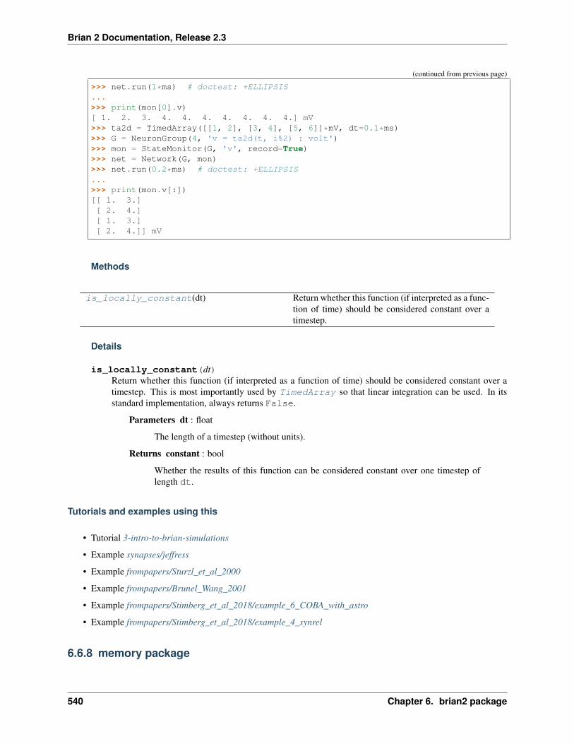
Brian 2 Documentation, Release 2.3
(continued from previous page)
>>> net.run(1*ms) # doctest: +ELLIPSIS...>>> print(mon[0].v)[ 1. 2. 3. 4. 4. 4. 4. 4. 4. 4.] mV>>> ta2d = TimedArray([[1, 2], [3, 4], [5, 6]]*mV, dt=0.1*ms)>>> G = NeuronGroup(4, 'v = ta2d(t, i%2) : volt')>>> mon = StateMonitor(G, 'v', record=True)>>> net = Network(G, mon)>>> net.run(0.2*ms) # doctest: +ELLIPSIS...>>> print(mon.v[:])[[ 1. 3.][ 2. 4.][ 1. 3.][ 2. 4.]] mV
Methods
is_locally_constant(dt) Return whether this function (if interpreted as a func-tion of time) should be considered constant over atimestep.
Details
is_locally_constant(dt)Return whether this function (if interpreted as a function of time) should be considered constant over atimestep. This is most importantly used by TimedArray so that linear integration can be used. In itsstandard implementation, always returns False.
Parameters dt : float
The length of a timestep (without units).
Returns constant : bool
Whether the results of this function can be considered constant over one timestep oflength dt.
Tutorials and examples using this
• Tutorial 3-intro-to-brian-simulations
• Example synapses/jeffress
• Example frompapers/Sturzl_et_al_2000
• Example frompapers/Brunel_Wang_2001
• Example frompapers/Stimberg_et_al_2018/example_6_COBA_with_astro
• Example frompapers/Stimberg_et_al_2018/example_4_synrel
6.6.8 memory package
540 Chapter 6. brian2 package

Brian 2 Documentation, Release 2.3
dynamicarray module
TODO: rewrite this (verbatim from Brian 1.x), more efficiency
Exported members: DynamicArray , DynamicArray1D
Classes
DynamicArray(shape[, dtype, factor, . . . ]) An N-dimensional dynamic array class
DynamicArray class
(Shortest import: from brian2.memory.dynamicarray import DynamicArray)
class brian2.memory.dynamicarray.DynamicArray(shape, dtype=<type ’float’>, fac-tor=2, use_numpy_resize=False, re-fcheck=True)
Bases: object
An N-dimensional dynamic array class
The array can be resized in any dimension, and the class will handle allocating a new block of data and copyingwhen necessary.
Warning: The data will NOT be contiguous for >1D arrays. To ensure this, you will either need to use 1Darrays, or to copy the data, or use the shrink method with the current size (although note that in both casesyou negate the memory and efficiency benefits of the dynamic array).
Initialisation arguments:
shape, dtype The shape and dtype of the array to initialise, as in Numpy. For 1D arrays, shape can be asingle int, for ND arrays it should be a tuple.
factor The resizing factor (see notes below). Larger values tend to lead to more wasted memory, but morecomputationally efficient code.
use_numpy_resize, refcheck Normally, when you resize the array it creates a new array and copies thedata. Sometimes, it is possible to resize an array without a copy, and if this option is set it will attempt todo this. However, this can cause memory problems if you are not careful so the option is off by default.You need to ensure that you do not create slices of the array so that no references to the memory exist otherthan the main array object. If you are sure you know what you’re doing, you can switch this referencecheck off. Note that resizing in this way is only done if you resize in the first dimension.
The array is initialised with zeros. The data is stored in the attribute data which is a Numpy array.
Some numpy methods are implemented and can work directly on the array object, including len(arr),arr[...] and arr[...]=.... In other cases, use the data attribute.
Notes
The dynamic array returns a data attribute which is a view on the larger _data attribute. When a resizeoperation is performed, and a specific dimension is enlarged beyond the size in the _data attribute, the size isincreased to the larger of cursize*factor and newsize. This ensures that the amortized cost of increasingthe size of the array is O(1).
6.6. Subpackages 541
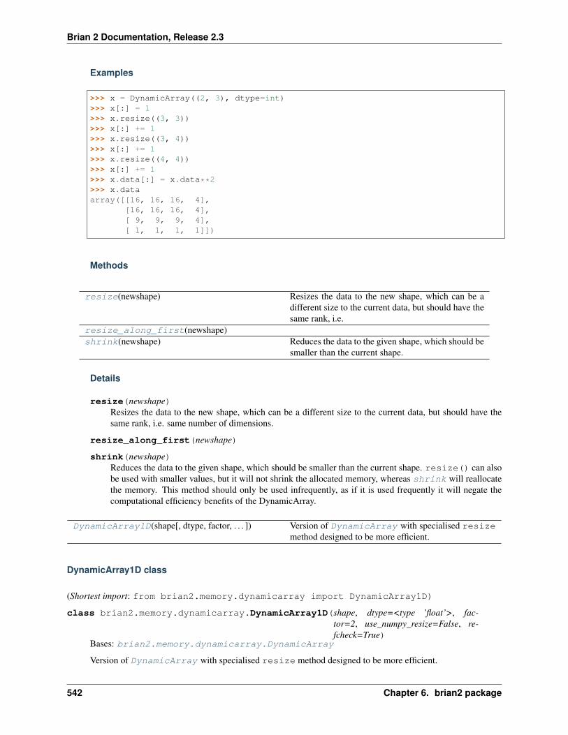
Brian 2 Documentation, Release 2.3
Examples
>>> x = DynamicArray((2, 3), dtype=int)>>> x[:] = 1>>> x.resize((3, 3))>>> x[:] += 1>>> x.resize((3, 4))>>> x[:] += 1>>> x.resize((4, 4))>>> x[:] += 1>>> x.data[:] = x.data**2>>> x.dataarray([[16, 16, 16, 4],
[16, 16, 16, 4],[ 9, 9, 9, 4],[ 1, 1, 1, 1]])
Methods
resize(newshape) Resizes the data to the new shape, which can be adifferent size to the current data, but should have thesame rank, i.e.
resize_along_first(newshape)shrink(newshape) Reduces the data to the given shape, which should be
smaller than the current shape.
Details
resize(newshape)Resizes the data to the new shape, which can be a different size to the current data, but should have thesame rank, i.e. same number of dimensions.
resize_along_first(newshape)
shrink(newshape)Reduces the data to the given shape, which should be smaller than the current shape. resize() can alsobe used with smaller values, but it will not shrink the allocated memory, whereas shrink will reallocatethe memory. This method should only be used infrequently, as if it is used frequently it will negate thecomputational efficiency benefits of the DynamicArray.
DynamicArray1D(shape[, dtype, factor, . . . ]) Version of DynamicArray with specialised resizemethod designed to be more efficient.
DynamicArray1D class
(Shortest import: from brian2.memory.dynamicarray import DynamicArray1D)
class brian2.memory.dynamicarray.DynamicArray1D(shape, dtype=<type ’float’>, fac-tor=2, use_numpy_resize=False, re-fcheck=True)
Bases: brian2.memory.dynamicarray.DynamicArray
Version of DynamicArray with specialised resize method designed to be more efficient.
542 Chapter 6. brian2 package

Brian 2 Documentation, Release 2.3
Methods
resize(newshape) Resizes the data to the new shape, which can be adifferent size to the current data, but should have thesame rank, i.e.
Details
resize(newshape)Resizes the data to the new shape, which can be a different size to the current data, but should have thesame rank, i.e. same number of dimensions.
Functions
getslices(shape[, from_start])
getslices function
(Shortest import: from brian2.memory.dynamicarray import getslices)
brian2.memory.dynamicarray.getslices(shape, from_start=True)
6.6.9 monitors package
Base package for all monitors, i.e. objects to record activity during a simulation run.
Exported members: SpikeMonitor, EventMonitor, StateMonitor, PopulationRateMonitor
ratemonitor module
Exported members: PopulationRateMonitor
Classes
PopulationRateMonitor(source[, name, . . . ]) Record instantaneous firing rates, averaged across neu-rons from a NeuronGroup or other spike source.
PopulationRateMonitor class
(Shortest import: from brian2 import PopulationRateMonitor)
class brian2.monitors.ratemonitor.PopulationRateMonitor(source,name=’ratemonitor*’,codeobj_class=None,dtype=<type’numpy.float64’>)
Bases: brian2.groups.group.Group, brian2.groups.group.CodeRunner
Record instantaneous firing rates, averaged across neurons from a NeuronGroup or other spike source.
Parameters source : (NeuronGroup, SpikeSource)
6.6. Subpackages 543
Brian 2 Documentation, Release 2.3
The source of spikes to record.
name : str, optional
A unique name for the object, otherwise will use source.name+'_ratemonitor_0', etc.
codeobj_class : class, optional
The CodeObject class to run code with.
dtype : dtype, optional
The dtype to use to store the rate variable. Defaults to float64, i.e. double preci-sion.
Notes :
—– :
Currently, this monitor can only monitor the instantaneous firing rates at :
each time step of the source clock. Any binning/smoothing of the firing :
rates has to be done manually afterwards. :
Attributes
source The group we are recording from
Methods
reinit() Clears all recorded ratesresize(new_size)smooth_rate(self[, window, width]) Return a smooth version of the population rate.
Details
sourceThe group we are recording from
reinit()Clears all recorded rates
resize(new_size)
smooth_rate(self, window=’gaussian’, width=None)Return a smooth version of the population rate.
Parameters window : str, ndarray
The window to use for smoothing. Can be a string to chose a predefined win-dow('flat' for a rectangular, and 'gaussian' for a Gaussian-shaped window).In this case the width of the window is determined by the width argument. Note thatfor the Gaussian window, the width parameter specifies the standard deviation of theGaussian, the width of the actual window is 4*width + dt (rounded to the nearestdt). For the flat window, the width is rounded to the nearest odd multiple of dt to avoidshifting the rate in time. Alternatively, an arbitrary window can be given as a numpy
544 Chapter 6. brian2 package

Brian 2 Documentation, Release 2.3
array (with an odd number of elements). In this case, the width in units of time de-pends on the dt of the simulation, and no width argument can be specified. The givenwindow will be automatically normalized to a sum of 1.
width : Quantity , optional
The width of the window in seconds (for a predefined window).
Returns rate : Quantity
The population rate in Hz, smoothed with the given window. Note that the rates aresmoothed and not re-binned, i.e. the length of the returned array is the same as the lengthof the rate attribute and can be plotted against the PopulationRateMonitor ‘st attribute.
Tutorials and examples using this
• Example frompapers/Brunel_Hakim_1999
• Example frompapers/Brunel_Wang_2001
spikemonitor module
Exported members: EventMonitor, SpikeMonitor
Classes
EventMonitor(source, event[, variables, . . . ]) Record events from a NeuronGroup or another eventsource.
EventMonitor class
(Shortest import: from brian2 import EventMonitor)
class brian2.monitors.spikemonitor.EventMonitor(source, event, variables=None,record=True, when=None, or-der=None, name=’eventmonitor*’,codeobj_class=None)
Bases: brian2.groups.group.Group, brian2.groups.group.CodeRunner
Record events from a NeuronGroup or another event source.
The recorded events can be accessed in various ways: the attributes i and t store all the indices and eventtimes, respectively. Alternatively, you can get a dictionary mapping neuron indices to event trains, by callingthe event_trains method.
Parameters source : NeuronGroup, SpikeSource
The source of events to record.
event : str
The name of the event to record
variables : str or sequence of str, optional
Which variables to record at the time of the event (in addition to the index of the neuron).Can be the name of a variable or a list of names.
6.6. Subpackages 545
Brian 2 Documentation, Release 2.3
record : bool, optional
Whether or not to record each event in i and t (the count will always be recorded).Defaults to True.
when : str, optional
When to record the events, by default records events in the same slot where the event isemitted.
order : int, optional
The priority of of this group for operations occurring at the same time step and in thesame scheduling slot. Defaults to the order where the event is emitted + 1, i.e. it will berecorded directly afterwards.
name : str, optional
A unique name for the object, otherwise will use source.name+'_eventmonitor_0', etc.
codeobj_class : class, optional
The CodeObject class to run code with.
See also:
SpikeMonitor
Attributes
count The array of event counts (length = size of targetgroup)
event The event that we are listening toit Returns the pair (i, t).it_ Returns the pair (i, t_).num_events Returns the total number of recorded events.record Whether to record times and indices of eventsrecord_variables The additional variables that will be recordedsource The source we are recording from
Methods
all_values() Return a dictionary mapping recorded variablenames (including t) to a dictionary mapping neuronindices to arrays of variable values at the time of theevents (sorted by time).
event_trains() Return a dictionary mapping event indices to arraysof event times.
reinit() Clears all recorded spikesresize(new_size)values(var) Return a dictionary mapping neuron indices to arrays
of variable values at the time of the events (sorted bytime).
546 Chapter 6. brian2 package

Brian 2 Documentation, Release 2.3
Details
countThe array of event counts (length = size of target group)
eventThe event that we are listening to
itReturns the pair (i, t).
it_Returns the pair (i, t_).
num_eventsReturns the total number of recorded events.
recordWhether to record times and indices of events
record_variablesThe additional variables that will be recorded
sourceThe source we are recording from
all_values()Return a dictionary mapping recorded variable names (including t) to a dictionary mapping neuron indicesto arrays of variable values at the time of the events (sorted by time). This is equivalent to (but moreefficient than) calling values for each variable and storing the result in a dictionary.
Returns all_values : dict
Dictionary mapping variable names to dictionaries which themselves are mapping neu-ron indicies to arrays of variable values at the time of the events.
Examples
>>> from brian2 import *>>> G = NeuronGroup(2, """counter1 : integer... counter2 : integer... max_value : integer""",... threshold='counter1 >= max_value',... reset='counter1 = 0')>>> G.run_regularly('counter1 += 1; counter2 += 1') # doctest: +ELLIPSISCodeRunner(...)>>> G.max_value = [50, 100]>>> mon = EventMonitor(G, event='spike', variables='counter2')>>> run(10*ms)>>> all_values = mon.all_values()>>> print(all_values['counter2'][0])[ 50 100]>>> print(all_values['t'][1])[ 9.9] ms
event_trains()Return a dictionary mapping event indices to arrays of event times. Equivalent to calling values('t').
Returns event_trains : dict
6.6. Subpackages 547

Brian 2 Documentation, Release 2.3
Dictionary that stores an array with the event times for each neuron index.
See also:
SpikeMonitor.spike_trains()
reinit()Clears all recorded spikes
resize(new_size)
values(var)Return a dictionary mapping neuron indices to arrays of variable values at the time of the events (sortedby time).
Parameters var : str
The name of the variable.
Returns values : dict
Dictionary mapping each neuron index to an array of variable values at the time of theevents
Examples
>>> from brian2 import *>>> G = NeuronGroup(2, """counter1 : integer... counter2 : integer... max_value : integer""",... threshold='counter1 >= max_value',... reset='counter1 = 0')>>> G.run_regularly('counter1 += 1; counter2 += 1') # doctest: +ELLIPSISCodeRunner(...)>>> G.max_value = [50, 100]>>> mon = EventMonitor(G, event='spike', variables='counter2')>>> run(10*ms)>>> counter2_values = mon.values('counter2')>>> print(counter2_values[0])[ 50 100]>>> print(counter2_values[1])[100]
Tutorials and examples using this
• Example advanced/custom_events
SpikeMonitor(source[, variables, record, . . . ]) Record spikes from a NeuronGroup or other spikesource.
SpikeMonitor class
(Shortest import: from brian2 import SpikeMonitor)
548 Chapter 6. brian2 package
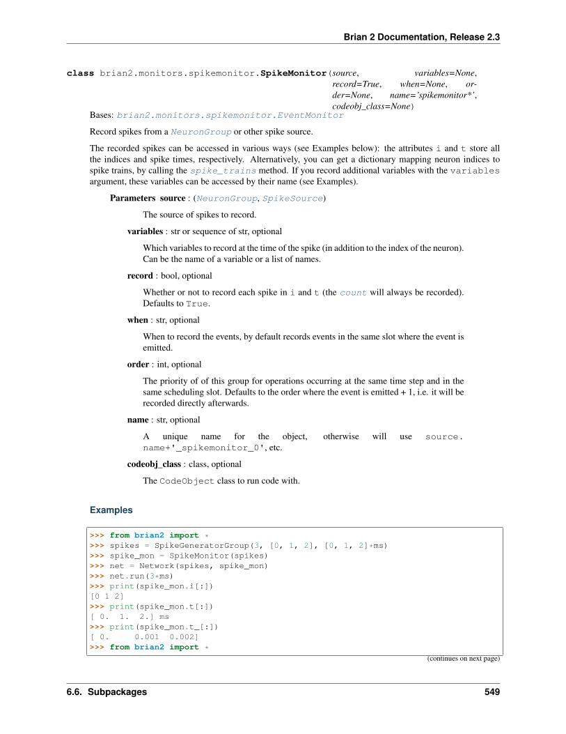
Brian 2 Documentation, Release 2.3
class brian2.monitors.spikemonitor.SpikeMonitor(source, variables=None,record=True, when=None, or-der=None, name=’spikemonitor*’,codeobj_class=None)
Bases: brian2.monitors.spikemonitor.EventMonitor
Record spikes from a NeuronGroup or other spike source.
The recorded spikes can be accessed in various ways (see Examples below): the attributes i and t store allthe indices and spike times, respectively. Alternatively, you can get a dictionary mapping neuron indices tospike trains, by calling the spike_trains method. If you record additional variables with the variablesargument, these variables can be accessed by their name (see Examples).
Parameters source : (NeuronGroup, SpikeSource)
The source of spikes to record.
variables : str or sequence of str, optional
Which variables to record at the time of the spike (in addition to the index of the neuron).Can be the name of a variable or a list of names.
record : bool, optional
Whether or not to record each spike in i and t (the count will always be recorded).Defaults to True.
when : str, optional
When to record the events, by default records events in the same slot where the event isemitted.
order : int, optional
The priority of of this group for operations occurring at the same time step and in thesame scheduling slot. Defaults to the order where the event is emitted + 1, i.e. it will berecorded directly afterwards.
name : str, optional
A unique name for the object, otherwise will use source.name+'_spikemonitor_0', etc.
codeobj_class : class, optional
The CodeObject class to run code with.
Examples
>>> from brian2 import *>>> spikes = SpikeGeneratorGroup(3, [0, 1, 2], [0, 1, 2]*ms)>>> spike_mon = SpikeMonitor(spikes)>>> net = Network(spikes, spike_mon)>>> net.run(3*ms)>>> print(spike_mon.i[:])[0 1 2]>>> print(spike_mon.t[:])[ 0. 1. 2.] ms>>> print(spike_mon.t_[:])[ 0. 0.001 0.002]>>> from brian2 import *
(continues on next page)
6.6. Subpackages 549
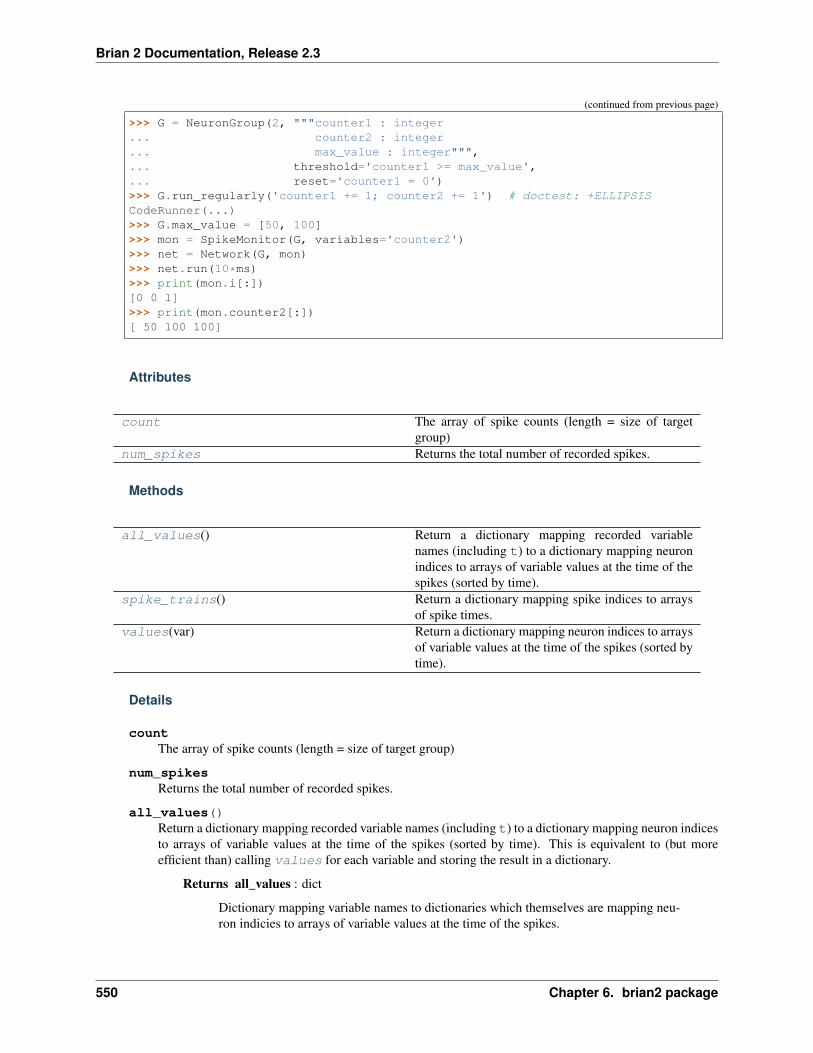
Brian 2 Documentation, Release 2.3
(continued from previous page)
>>> G = NeuronGroup(2, """counter1 : integer... counter2 : integer... max_value : integer""",... threshold='counter1 >= max_value',... reset='counter1 = 0')>>> G.run_regularly('counter1 += 1; counter2 += 1') # doctest: +ELLIPSISCodeRunner(...)>>> G.max_value = [50, 100]>>> mon = SpikeMonitor(G, variables='counter2')>>> net = Network(G, mon)>>> net.run(10*ms)>>> print(mon.i[:])[0 0 1]>>> print(mon.counter2[:])[ 50 100 100]
Attributes
count The array of spike counts (length = size of targetgroup)
num_spikes Returns the total number of recorded spikes.
Methods
all_values() Return a dictionary mapping recorded variablenames (including t) to a dictionary mapping neuronindices to arrays of variable values at the time of thespikes (sorted by time).
spike_trains() Return a dictionary mapping spike indices to arraysof spike times.
values(var) Return a dictionary mapping neuron indices to arraysof variable values at the time of the spikes (sorted bytime).
Details
countThe array of spike counts (length = size of target group)
num_spikesReturns the total number of recorded spikes.
all_values()Return a dictionary mapping recorded variable names (including t) to a dictionary mapping neuron indicesto arrays of variable values at the time of the spikes (sorted by time). This is equivalent to (but moreefficient than) calling values for each variable and storing the result in a dictionary.
Returns all_values : dict
Dictionary mapping variable names to dictionaries which themselves are mapping neu-ron indicies to arrays of variable values at the time of the spikes.
550 Chapter 6. brian2 package

Brian 2 Documentation, Release 2.3
Examples
>>> from brian2 import *>>> G = NeuronGroup(2, """counter1 : integer... counter2 : integer... max_value : integer""",... threshold='counter1 >= max_value',... reset='counter1 = 0')>>> G.run_regularly('counter1 += 1; counter2 += 1') # doctest: +ELLIPSISCodeRunner(...)>>> G.max_value = [50, 100]>>> mon = SpikeMonitor(G, variables='counter2')>>> run(10*ms)>>> all_values = mon.all_values()>>> print(all_values['counter2'][0])[ 50 100]>>> print(all_values['t'][1])[ 9.9] ms
spike_trains()Return a dictionary mapping spike indices to arrays of spike times.
Returns spike_trains : dict
Dictionary that stores an array with the spike times for each neuron index.
Examples
>>> from brian2 import *>>> spikes = SpikeGeneratorGroup(3, [0, 1, 2], [0, 1, 2]*ms)>>> spike_mon = SpikeMonitor(spikes)>>> run(3*ms)>>> spike_trains = spike_mon.spike_trains()>>> spike_trains[1]array([ 1.]) * msecond
values(var)Return a dictionary mapping neuron indices to arrays of variable values at the time of the spikes (sorted bytime).
Parameters var : str
The name of the variable.
Returns values : dict
Dictionary mapping each neuron index to an array of variable values at the time of thespikes.
Examples
>>> from brian2 import *>>> G = NeuronGroup(2, """counter1 : integer... counter2 : integer... max_value : integer""",... threshold='counter1 >= max_value',
(continues on next page)
6.6. Subpackages 551
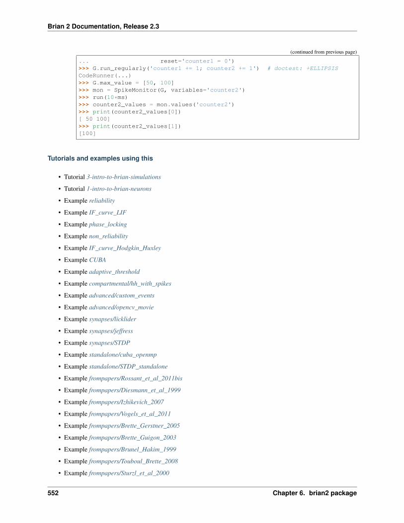
Brian 2 Documentation, Release 2.3
(continued from previous page)
... reset='counter1 = 0')>>> G.run_regularly('counter1 += 1; counter2 += 1') # doctest: +ELLIPSISCodeRunner(...)>>> G.max_value = [50, 100]>>> mon = SpikeMonitor(G, variables='counter2')>>> run(10*ms)>>> counter2_values = mon.values('counter2')>>> print(counter2_values[0])[ 50 100]>>> print(counter2_values[1])[100]
Tutorials and examples using this
• Tutorial 3-intro-to-brian-simulations
• Tutorial 1-intro-to-brian-neurons
• Example reliability
• Example IF_curve_LIF
• Example phase_locking
• Example non_reliability
• Example IF_curve_Hodgkin_Huxley
• Example CUBA
• Example adaptive_threshold
• Example compartmental/hh_with_spikes
• Example advanced/custom_events
• Example advanced/opencv_movie
• Example synapses/licklider
• Example synapses/jeffress
• Example synapses/STDP
• Example standalone/cuba_openmp
• Example standalone/STDP_standalone
• Example frompapers/Rossant_et_al_2011bis
• Example frompapers/Diesmann_et_al_1999
• Example frompapers/Izhikevich_2007
• Example frompapers/Vogels_et_al_2011
• Example frompapers/Brette_Gerstner_2005
• Example frompapers/Brette_Guigon_2003
• Example frompapers/Brunel_Hakim_1999
• Example frompapers/Touboul_Brette_2008
• Example frompapers/Sturzl_et_al_2000
552 Chapter 6. brian2 package
Brian 2 Documentation, Release 2.3
• Example frompapers/Platkiewicz_Brette_2011
• Example frompapers/Brette_2004
• Example frompapers/Brunel_Wang_2001
• Example frompapers/Brette_2012/Fig5A
• Example frompapers/Stimberg_et_al_2018/example_6_COBA_with_astro
• Example frompapers/Stimberg_et_al_2018/example_1_COBA
statemonitor module
Exported members: StateMonitor
Classes
StateMonitor(source, variables, record[, . . . ]) Record values of state variables during a run
StateMonitor class
(Shortest import: from brian2 import StateMonitor)
class brian2.monitors.statemonitor.StateMonitor(source, variables, record, dt=None,clock=None, when=’start’, or-der=0, name=’statemonitor*’,codeobj_class=None)
Bases: brian2.groups.group.Group, brian2.groups.group.CodeRunner
Record values of state variables during a run
To extract recorded values after a run, use the t attribute for the array of times at which values were recorded,and variable name attribute for the values. The values will have shape (len(indices), len(t)), whereindices are the array indices which were recorded. When indexing the StateMonitor directly, the re-turned object can be used to get the recorded values for the specified indices, i.e. the indexing semantic refers tothe indices in source, not to the relative indices of the recorded values. For example, when recording only neu-rons with even numbers, mon[[0, 2]].v will return the values for neurons 0 and 2, whereas mon.v[[0,2]] will return the values for the first and third recorded neurons, i.e. for neurons 0 and 4.
Parameters source : Group
Which object to record values from.
variables : str, sequence of str, True
Which variables to record, or True to record all variables (note that this may use agreat deal of memory).
record : bool, sequence of ints
Which indices to record, nothing is recorded for False, everything is recorded forTrue (warning: may use a great deal of memory), or a specified subset of indices.
dt : Quantity , optional
The time step to be used for the monitor. Cannot be combined with the clock argu-ment.
clock : Clock, optional
6.6. Subpackages 553

Brian 2 Documentation, Release 2.3
The update clock to be used. If neither a clock, nor the dt argument is specified, theclock of the source() will be used.
when : str, optional
At which point during a time step the values should be recorded. Defaults to 'start'.
order : int, optional
The priority of of this group for operations occurring at the same time step and in thesame scheduling slot. Defaults to 0.
name : str, optional
A unique name for the object, otherwise will use source.name+'statemonitor_0', etc.
codeobj_class : CodeObject, optional
The CodeObject class to create.
Notes
Since this monitor by default records in the 'start' time slot, recordings of the membrane potential inintegrate-and-fire models may look unexpected: the recorded membrane potential trace will never be abovethreshold in an integrate-and-fire model, because the reset statement will have been applied already. Set thewhen keyword to a different value if this is not what you want.
Note that record=True only works in runtime mode for synaptic variables. This is because the actual arrayof indices has to be calculated and this is not possible in standalone mode, where the synapses have not beencreated yet at this stage. Consider using an explicit array of indices instead, i.e. something like record=np.arange(n_synapses).
Examples
Record all variables, first 5 indices:
eqs = """dV/dt = (2-V)/(10*ms) : 1"""threshold = 'V>1'reset = 'V = 0'G = NeuronGroup(100, eqs, threshold=threshold, reset=reset)G.V = rand(len(G))M = StateMonitor(G, True, record=range(5))run(100*ms)plot(M.t, M.V.T)show()
Attributes
record The array of recorded indicesrecord_variables The variables to record
554 Chapter 6. brian2 package

Brian 2 Documentation, Release 2.3
Methods
record_single_timestep() Records a single time step.reinit()resize(new_size)
Details
recordThe array of recorded indices
record_variablesThe variables to record
record_single_timestep()Records a single time step. Useful for recording the values at the end of the simulation – otherwise aStateMonitor will not record the last simulated values since its when attribute defaults to 'start',i.e. the last recording is at the beginning of the last time step.
Notes
This function will only work if the StateMonitor has been already run, but a run with a length of 0*msdoes suffice.
Examples
>>> from brian2 import *>>> G = NeuronGroup(1, 'dv/dt = -v/(5*ms) : 1')>>> G.v = 1>>> mon = StateMonitor(G, 'v', record=True)>>> run(0.5*ms)>>> print(np.array_str(mon.v[:], precision=3))[[ 1. 0.98 0.961 0.942 0.923]]>>> print(mon.t[:])[ 0. 100. 200. 300. 400.] us>>> print(np.array_str(G.v[:], precision=3)) # last value had not been→˓recorded[ 0.905]>>> mon.record_single_timestep()>>> print(mon.t[:])[ 0. 100. 200. 300. 400. 500.] us>>> print(np.array_str(mon.v[:], precision=3))[[ 1. 0.98 0.961 0.942 0.923 0.905]]
reinit()
resize(new_size)
Tutorials and examples using this
• Tutorial 2-intro-to-brian-synapses
• Tutorial 3-intro-to-brian-simulations
6.6. Subpackages 555
Brian 2 Documentation, Release 2.3
• Tutorial 1-intro-to-brian-neurons
• Example phase_locking
• Example COBAHH
• Example adaptive_threshold
• Example compartmental/spike_initiation
• Example compartmental/bipolar_with_inputs
• Example compartmental/bipolar_with_inputs2
• Example compartmental/hh_with_spikes
• Example compartmental/infinite_cable
• Example compartmental/hodgkin_huxley_1952
• Example compartmental/bipolar_cell
• Example compartmental/lfp
• Example advanced/stochastic_odes
• Example advanced/compare_GSL_to_conventional
• Example advanced/custom_events
• Example synapses/gapjunctions
• Example synapses/nonlinear
• Example synapses/synapses
• Example synapses/jeffress
• Example synapses/STDP
• Example standalone/STDP_standalone
• Example frompapers/Rossant_et_al_2011bis
• Example frompapers/Hindmarsh_Rose_1984
• Example frompapers/Clopath_et_al_2010_homeostasis
• Example frompapers/Wang_Buszaki_1996
• Example frompapers/Morris_Lecar_1981
• Example frompapers/Izhikevich_2007
• Example frompapers/Brette_Gerstner_2005
• Example frompapers/Brette_Guigon_2003
• Example frompapers/Rothman_Manis_2003
• Example frompapers/Destexhe_et_al_1998
• Example frompapers/Touboul_Brette_2008
• Example frompapers/Platkiewicz_Brette_2011
• Example frompapers/Brette_2012/Fig3CF
• Example frompapers/Brette_2012/Fig3AB
• Example frompapers/Brette_2012/Fig5A
556 Chapter 6. brian2 package
Brian 2 Documentation, Release 2.3
• Example frompapers/Brette_2012/Fig1
• Example frompapers/Brette_2012/Fig4
• Example frompapers/Stimberg_et_al_2018/example_1_COBA
• Example frompapers/Stimberg_et_al_2018/example_5_astro_ring
• Example frompapers/Stimberg_et_al_2018/example_2_gchi_astrocyte
• Example frompapers/Stimberg_et_al_2018/example_4_synrel
• Example frompapers/Stimberg_et_al_2018/example_4_rsmean
• Example frompapers/Stimberg_et_al_2018/example_3_io_synapse
StateMonitorView(monitor, item)
StateMonitorView class
(Shortest import: from brian2.monitors.statemonitor import StateMonitorView)
class brian2.monitors.statemonitor.StateMonitorView(monitor, item)Bases: object
6.6.10 parsing package
bast module
Brian AST representation
This is a standard Python AST representation with additional information added.
Exported members: brian_ast, BrianASTRenderer, dtype_hierarchy
Classes
BrianASTRenderer(variables[, copy_variables]) This class is modelled after NodeRenderer - seethere for details.
BrianASTRenderer class
(Shortest import: from brian2.parsing.bast import BrianASTRenderer)
class brian2.parsing.bast.BrianASTRenderer(variables, copy_variables=True)Bases: object
This class is modelled after NodeRenderer - see there for details.
Methods
render_BinOp(node)render_BoolOp(node)render_Call(node)
Continued on next page
6.6. Subpackages 557

Brian 2 Documentation, Release 2.3
Table 341 – continued from previous pagerender_Compare(node)render_Constant(node)render_Name(node)render_NameConstant(node)render_Num(node)render_UnaryOp(node)render_node(node)
Details
render_BinOp(node)
render_BoolOp(node)
render_Call(node)
render_Compare(node)
render_Constant(node)
render_Name(node)
render_NameConstant(node)
render_Num(node)
render_UnaryOp(node)
render_node(node)
Functions
brian_ast(expr, variables) Returns an AST tree representation with additional in-formation
brian_ast function
(Shortest import: from brian2.parsing.bast import brian_ast)
brian2.parsing.bast.brian_ast(expr, variables)Returns an AST tree representation with additional information
Each node will be a standard Python ast node with the following additional attributes:
dtype One of 'boolean', 'integer' or 'float', referring to the data type of the value of this node.
scalar Either True or False if the node uses any vector-valued variables.
complexity An integer representation of the computational complexity of the node. This is a very rough rep-resentation used for things like 2*(x+y) is less complex than 2*x+2*y and exp(x) is more complexthan 2*x but shouldn’t be relied on for fine distinctions between expressions.
Parameters expr : str
The expression to convert into an AST representation
variables : dict
The dictionary of Variable objects used in the expression.
558 Chapter 6. brian2 package
Brian 2 Documentation, Release 2.3
brian_dtype_from_dtype(dtype) Returns ‘boolean’, ‘integer’ or ‘float’
brian_dtype_from_dtype function
(Shortest import: from brian2.parsing.bast import brian_dtype_from_dtype)
brian2.parsing.bast.brian_dtype_from_dtype(dtype)Returns ‘boolean’, ‘integer’ or ‘float’
brian_dtype_from_value(value) Returns ‘boolean’, ‘integer’ or ‘float’
brian_dtype_from_value function
(Shortest import: from brian2.parsing.bast import brian_dtype_from_value)
brian2.parsing.bast.brian_dtype_from_value(value)Returns ‘boolean’, ‘integer’ or ‘float’
is_boolean(value)
is_boolean function
(Shortest import: from brian2.parsing.bast import is_boolean)
brian2.parsing.bast.is_boolean(value)
is_boolean_dtype(obj)
is_boolean_dtype function
(Shortest import: from brian2.parsing.bast import is_boolean_dtype)
brian2.parsing.bast.is_boolean_dtype(obj)
is_float(value)
is_float function
(Shortest import: from brian2.parsing.bast import is_float)
brian2.parsing.bast.is_float(value)
is_float_dtype(obj)
6.6. Subpackages 559

Brian 2 Documentation, Release 2.3
is_float_dtype function
(Shortest import: from brian2.parsing.bast import is_float_dtype)
brian2.parsing.bast.is_float_dtype(obj)
is_integer(value)
is_integer function
(Shortest import: from brian2.parsing.bast import is_integer)
brian2.parsing.bast.is_integer(value)
is_integer_dtype(obj)
is_integer_dtype function
(Shortest import: from brian2.parsing.bast import is_integer_dtype)
brian2.parsing.bast.is_integer_dtype(obj)
dependencies module
Exported members: abstract_code_dependencies
Functions
abstract_code_dependencies(code[, . . . ]) Analyses identifiers used in abstract code blocks
abstract_code_dependencies function
(Shortest import: from brian2.parsing.dependencies import abstract_code_dependencies)
brian2.parsing.dependencies.abstract_code_dependencies(code, known_vars=None,known_funcs=None)
Analyses identifiers used in abstract code blocks
Parameters code : str
The abstract code block.
known_vars : set
The set of known variable names.
known_funcs : set
The set of known function names.
Returns results : namedtuple with the following fields
all The set of all identifiers that appear in this code block, including functions.
560 Chapter 6. brian2 package

Brian 2 Documentation, Release 2.3
read The set of values that are read, excluding functions.
write The set of all values that are written to.
funcs The set of all function names.
known_all The set of all identifiers that appear in this code block and are known.
known_read The set of known values that are read, excluding functions.
known_write The set of known values that are written to.
known_funcs The set of known functions that are used.
unknown_read The set of all unknown variables whose values are read. Equal toread-known_vars.
unknown_write The set of all unknown variables written to. Equal towrite-known_vars.
unknown_funcs The set of all unknown function names, equal tofuncs-known_funcs.
undefined_read The set of all unknown variables whose values are read beforethey are written to. If this set is nonempty it usually indicates an error, since a variablethat is read should either have been defined in the code block (in which case it willappear in newly_defined) or already be known.
newly_defined The set of all variable names which are newly defined in this ab-stract code block.
get_read_write_funcs(parsed_code)
get_read_write_funcs function
(Shortest import: from brian2.parsing.dependencies import get_read_write_funcs)
brian2.parsing.dependencies.get_read_write_funcs(parsed_code)
expressions module
Exported members: parse_expression_dimensions
Functions
is_boolean_expression(expr, variables) Determines if an expression is of boolean type or not
is_boolean_expression function
(Shortest import: from brian2.parsing.expressions import is_boolean_expression)
brian2.parsing.expressions.is_boolean_expression(expr, variables)Determines if an expression is of boolean type or not
Parameters expr : str
The expression to test
variables : dict-like of Variable
6.6. Subpackages 561
Brian 2 Documentation, Release 2.3
The variables used in the expression.
Returns isbool : bool
Whether or not the expression is boolean.
Raises
SyntaxError If the expression ought to be boolean but is not, for example x<y and z where z is not aboolean variable.
Notes
We test the following cases recursively on the abstract syntax tree:
• The node is a boolean operation. If all the subnodes are boolean expressions we return True, otherwisewe raise the SyntaxError.
• The node is a function call, we return True or False depending on whether the function description hasthe _returns_bool attribute set.
• The node is a variable name, we return True or False depending on whether is_boolean attribute isset or if the name is True or False.
• The node is a comparison, we return True.
• The node is a unary operation, we return True if the operation is not, otherwise False.
• Otherwise we return False.
parse_expression_dimensions(expr, vari-ables)
Returns the unit value of an expression, and checks itsvalidity
parse_expression_dimensions function
(Shortest import: from brian2.parsing.expressions import parse_expression_dimensions)
brian2.parsing.expressions.parse_expression_dimensions(expr, variables)Returns the unit value of an expression, and checks its validity
Parameters expr : str
The expression to check.
variables : dict
Dictionary of all variables used in the expr (including Constant objects for externalvariables)
Returns unit : Quantity
The output unit of the expression
Raises
SyntaxError If the expression cannot be parsed, or if it uses a**b for b anything other than a constantnumber.
562 Chapter 6. brian2 package

Brian 2 Documentation, Release 2.3
DimensionMismatchError If any part of the expression is dimensionally inconsistent.
functions module
Exported members: AbstractCodeFunction, abstract_code_from_function,extract_abstract_code_functions, substitute_abstract_code_functions
Classes
AbstractCodeFunction(name, args, code, . . . ) The information defining an abstract code function
AbstractCodeFunction class
(Shortest import: from brian2.parsing.functions import AbstractCodeFunction)
class brian2.parsing.functions.AbstractCodeFunction(name, args, code, return_expr)Bases: object
The information defining an abstract code function
Has attributes corresponding to initialisation parameters
Parameters name : str
The function name.
args : list of str
The arguments to the function.
code : str
The abstract code string consisting of the body of the function less the return statement.
return_expr : str or None
The expression returned, or None if there is nothing returned.
FunctionRewriter(func[, numcalls]) Inlines a function call using temporary variables
FunctionRewriter class
(Shortest import: from brian2.parsing.functions import FunctionRewriter)
class brian2.parsing.functions.FunctionRewriter(func, numcalls=0)Bases: ast.NodeTransformer
Inlines a function call using temporary variables
numcalls is the number of times the function rewriter has been called so far, this is used to make sure that whenrecursively inlining there is no name aliasing. The substitute_abstract_code_functions ensures that this is keptup to date between recursive runs.
The pre attribute is the set of lines to be inserted above the currently being processed line, i.e. the inline code.
The visit method returns the current line processed so that the function call is replaced with the output of theinlining.
6.6. Subpackages 563

Brian 2 Documentation, Release 2.3
Methods
visit_Call(node)
Details
visit_Call(node)
VarRewriter(pre) Rewrites all variable names in names by prepending pre
VarRewriter class
(Shortest import: from brian2.parsing.functions import VarRewriter)
class brian2.parsing.functions.VarRewriter(pre)Bases: ast.NodeTransformer
Rewrites all variable names in names by prepending pre
Methods
visit_Call(node)visit_Name(node)
Details
visit_Call(node)
visit_Name(node)
Functions
abstract_code_from_function(func) Converts the body of the function to abstract code
abstract_code_from_function function
(Shortest import: from brian2.parsing.functions import abstract_code_from_function)
brian2.parsing.functions.abstract_code_from_function(func)Converts the body of the function to abstract code
Parameters func : function, str or ast.FunctionDef
The function object to convert. Note that the arguments to the function are ignored.
Returns func : AbstractCodeFunction
The corresponding abstract code function
Raises
SyntaxError If unsupported features are used such as if statements or indexing.
564 Chapter 6. brian2 package

Brian 2 Documentation, Release 2.3
extract_abstract_code_functions(code) Returns a set of abstract code functions from functiondefinitions.
extract_abstract_code_functions function
(Shortest import: from brian2.parsing.functions import extract_abstract_code_functions)
brian2.parsing.functions.extract_abstract_code_functions(code)Returns a set of abstract code functions from function definitions.
Returns all functions defined at the top level and ignores any other code in the string.
Parameters code : str
The code string defining some functions.
Returns funcs : dict
A mapping (name, func) for func an AbstractCodeFunction.
substitute_abstract_code_functions(code,funcs)
Performs inline substitution of all the functions in thecode
substitute_abstract_code_functions function
(Shortest import: from brian2.parsing.functions import substitute_abstract_code_functions)
brian2.parsing.functions.substitute_abstract_code_functions(code, funcs)Performs inline substitution of all the functions in the code
Parameters code : str
The abstract code to make inline substitutions into.
funcs : list, dict or set of AbstractCodeFunction
The function substitutions to use, note in the case of a dict, the keys are ignored and thefunction name is used.
Returns code : str
The code with inline substitutions performed.
rendering module
Exported members: NodeRenderer, NumpyNodeRenderer, CPPNodeRenderer, SympyNodeRenderer,get_node_value
Classes
6.6. Subpackages 565

Brian 2 Documentation, Release 2.3
CPPNodeRenderer([auto_vectorise])
Methods
CPPNodeRenderer class
(Shortest import: from brian2.parsing.rendering import CPPNodeRenderer)
class brian2.parsing.rendering.CPPNodeRenderer(auto_vectorise=None)Bases: brian2.parsing.rendering.NodeRenderer
Methods
render_Assign(node)render_BinOp(node)render_Name(node)render_NameConstant(node)
Details
render_Assign(node)
render_BinOp(node)
render_Name(node)
render_NameConstant(node)
NodeRenderer([auto_vectorise])
Methods
NodeRenderer class
(Shortest import: from brian2.parsing.rendering import NodeRenderer)
class brian2.parsing.rendering.NodeRenderer(auto_vectorise=None)Bases: object
Methods
render_Assign(node)render_AugAssign(node)render_BinOp(node)render_BinOp_parentheses(left, right, op)render_BoolOp(node)
Continued on next page
566 Chapter 6. brian2 package

Brian 2 Documentation, Release 2.3
Table 366 – continued from previous pagerender_Call(node)render_Compare(node)render_Constant(node)render_Name(node)render_NameConstant(node)render_Num(node)render_UnaryOp(node)render_code(code)render_element_parentheses(node) Render an element with parentheses around it or
leave them away for numbers, names and functioncalls.
render_expr(expr[, strip])render_func(node)render_node(node)
Details
render_Assign(node)
render_AugAssign(node)
render_BinOp(node)
render_BinOp_parentheses(left, right, op)
render_BoolOp(node)
render_Call(node)
render_Compare(node)
render_Constant(node)
render_Name(node)
render_NameConstant(node)
render_Num(node)
render_UnaryOp(node)
render_code(code)
render_element_parentheses(node)Render an element with parentheses around it or leave them away for numbers, names and function calls.
render_expr(expr, strip=True)
render_func(node)
render_node(node)
NumpyNodeRenderer([auto_vectorise])
Methods
6.6. Subpackages 567
Brian 2 Documentation, Release 2.3
NumpyNodeRenderer class
(Shortest import: from brian2.parsing.rendering import NumpyNodeRenderer)
class brian2.parsing.rendering.NumpyNodeRenderer(auto_vectorise=None)Bases: brian2.parsing.rendering.NodeRenderer
Methods
render_UnaryOp(node)
Details
render_UnaryOp(node)
SympyNodeRenderer([auto_vectorise])
Methods
SympyNodeRenderer class
(Shortest import: from brian2.parsing.rendering import SympyNodeRenderer)
class brian2.parsing.rendering.SympyNodeRenderer(auto_vectorise=None)Bases: brian2.parsing.rendering.NodeRenderer
Methods
render_BinOp(node)render_BoolOp(node)render_Call(node)render_Compare(node)render_Name(node)render_NameConstant(node)render_Num(node)render_UnaryOp(node)render_func(node)
Details
render_BinOp(node)
render_BoolOp(node)
render_Call(node)
render_Compare(node)
render_Name(node)
568 Chapter 6. brian2 package
Brian 2 Documentation, Release 2.3
render_NameConstant(node)
render_Num(node)
render_UnaryOp(node)
render_func(node)
Functions
get_node_value(node) Helper function to mask differences between Pythonversions
get_node_value function
(Shortest import: from brian2.parsing.rendering import get_node_value)
brian2.parsing.rendering.get_node_value(node)Helper function to mask differences between Python versions
statements module
Functions
parse_statement(code) Parses a single line of code into “var op expr”.
parse_statement function
(Shortest import: from brian2.parsing.statements import parse_statement)
brian2.parsing.statements.parse_statement(code)Parses a single line of code into “var op expr”.
Parameters code : str
A string containing a single statement of the form var op expr # comment,where the # comment part is optional.
Returns var, op, expr, comment : str, str, str, str
The four parts of the statement.
Examples
>>> parse_statement('v = -65*mV # reset the membrane potential')('v', '=', '-65*mV', 'reset the membrane potential')>>> parse_statement('v += dt*(-v/tau)')('v', '+=', 'dt*(-v/tau)', '')
sympytools module
Utility functions for parsing expressions and statements.
Classes
6.6. Subpackages 569

Brian 2 Documentation, Release 2.3
CustomSympyPrinter([settings]) Printer that overrides the printing of some basic sympyobjects.
CustomSympyPrinter class
(Shortest import: from brian2.parsing.sympytools import CustomSympyPrinter)
class brian2.parsing.sympytools.CustomSympyPrinter(settings=None)Bases: sympy.printing.str.StrPrinter
Printer that overrides the printing of some basic sympy objects. E.g. print “a and b” instead of “And(a, b)”.
Functions
check_expression_for_multiple_stateful_functions(. . . )
check_expression_for_multiple_stateful_functions function
(Shortest import: from brian2.parsing.sympytools import check_expression_for_multiple_stateful_functions)
brian2.parsing.sympytools.check_expression_for_multiple_stateful_functions(expr,vari-ables)
expression_complexity(expr[, complexity]) Returns the complexity of an expression (either stringor sympy)
expression_complexity function
(Shortest import: from brian2.parsing.sympytools import expression_complexity)
brian2.parsing.sympytools.expression_complexity(expr, complexity=None)Returns the complexity of an expression (either string or sympy)
The complexity is defined as 1 for each arithmetic operation except divide which is 2, and all other operationsare 20. This can be overridden using the complexity argument.
Note: calling this on a statement rather than an expression is likely to lead to errors.
Parameters expr: ‘sympy.Expr‘ or str :
The expression.
complexity: None or dict (optional) :
A dictionary mapping expression names to their complexity, to overwrite default be-haviour.
Returns complexity: int :
The complexity of the expression.
str_to_sympy(expr[, variables]) Parses a string into a sympy expression.
570 Chapter 6. brian2 package
Brian 2 Documentation, Release 2.3
str_to_sympy function
(Shortest import: from brian2.parsing.sympytools import str_to_sympy)
brian2.parsing.sympytools.str_to_sympy(expr, variables=None)Parses a string into a sympy expression. There are two reasons for not using sympify directly: 1) sympifydoes a from sympy import *, adding all functions to its namespace. This leads to issues when trying touse sympy function names as variable names. For example, both beta and factor – quite reasonable namesfor variables – are sympy functions, using them as variables would lead to a parsing error. 2) We want to use acommon syntax across expressions and statements, e.g. we want to allow to use and (instead of &) and functionnames like ceil (instead of ceiling).
Parameters expr : str
The string expression to parse.
variables : dict, optional
Dictionary mapping variable/function names in the expr to their respectiveVariable/Function objects.
Returns s_expr :
A sympy expression
Raises
SyntaxError In case of any problems during parsing.
sympy_to_str(sympy_expr) Converts a sympy expression into a string.
sympy_to_str function
(Shortest import: from brian2.parsing.sympytools import sympy_to_str)
brian2.parsing.sympytools.sympy_to_str(sympy_expr)Converts a sympy expression into a string. This could be as easy as str(sympy_exp) but it is possiblethat the sympy expression contains functions like Abs (for example, if an expression such as sqrt(x**2)appeared somewhere). We do want to re-translate Abs into abs in this case.
Parameters sympy_expr : sympy.core.expr.Expr
The expression that should be converted to a string.
Returns :
str_expr : str
A string representing the sympy expression.
Objects
PRINTER Printer that overrides the printing of some basic sympyobjects.
6.6. Subpackages 571
Brian 2 Documentation, Release 2.3
PRINTER object
(Shortest import: from brian2.parsing.sympytools import PRINTER)
brian2.parsing.sympytools.PRINTER = <brian2.parsing.sympytools.CustomSympyPrinter object>Printer that overrides the printing of some basic sympy objects. E.g. print “a and b” instead of “And(a, b)”.
6.6.11 random package
6.6.12 spatialneuron package
Exported members: Morphology , Soma, Cylinder, Section, SpatialNeuron
morphology module
Exported members: Morphology , Section, Cylinder, Soma
Classes
Children(owner) Helper class to represent the children (sub trees) of asection.
Children class
(Shortest import: from brian2.spatialneuron.morphology import Children)
class brian2.spatialneuron.morphology.Children(owner)Bases: object
Helper class to represent the children (sub trees) of a section. Can be used like a dictionary (mapping names toMorphology objects), but iterates over the values (sub trees) instead of over the keys (names).
Methods
add(name, subtree[, automatic_name]) Add a new child to the morphology.name(child) Return the given name (i.e.remove(name) Remove a subtree from this morphology.
Details
add(name, subtree, automatic_name=False)Add a new child to the morphology.
Parameters name : str
The name (e.g. "axon", "soma") to use for this sub tree.
subtree : Morphology
The subtree to link as a child.
automatic_name : bool, optional
572 Chapter 6. brian2 package

Brian 2 Documentation, Release 2.3
Whether to chose a new name automatically, if a subtree of the same name alreadyexists (uses e.g. "dend2" instead "dend"). Defaults to False and will raise anerror instead.
name(child)Return the given name (i.e. not the automatic name such as 1) for a child subtree.
Parameters child : Morphology
Returns name : str
The given name for the child.
remove(name)Remove a subtree from this morphology.
Parameters name : str
The name of the sub tree to remove.
Cylinder(**kwds) A cylindrical section.
Cylinder class
(Shortest import: from brian2 import Cylinder)
class brian2.spatialneuron.morphology.Cylinder(**kwds)Bases: brian2.spatialneuron.morphology.Section
A cylindrical section. For sections with more complex geometry (varying length and/or diameter of each com-partment), use the Section class.
Parameters diameter : Quantity
The diameter of the cylinder.
n : int, optional
The number of compartments in this section. Defaults to 1.
length : Quantity , optional
The length of the cylinder. Cannot be combined with the specification of coordinates.
x : Quantity , optional
A sequence of two values, the start and the end point of the cylinder. The coordinatesare interpreted as relative to the end point of the parent compartment (if any), so in mostcases the start point should be 0*um. The common exception is a cylinder connectingto a Soma, here the start point can be used to make the cylinder start at the surface of thesphere instead of at its center. You can specify all of x, y, or z to specify a morphologyin 3D, or only one or two out of them to specify a morphology in 1D or 2D.
y : Quantity , optional
See x
z : Quantity , optional
See x
type : str, optional
The type (e.g. "axon") of this Cylinder.
6.6. Subpackages 573
Brian 2 Documentation, Release 2.3
Attributes
area The membrane surface area of each compartment inthis section.
diameter The diameter at the middle of each compartment inthis section.
end_diameter The diameter at the end of each compartment in thissection.
r_length_1 The geometry-dependent term to calculate the con-ductance between the start and the midpoint of eachcompartment.
r_length_2 The geometry-dependent term to calculate the con-ductance between the midpoint and the end of eachcompartment.
start_diameter The diameter at the start of each compartment in thissection.
volume The volume of each compartment in this section.
Methods
copy_section() Create a copy of the current section (attributes of thissection only, not re-creating the parent/children rela-tion)
Details
areaThe membrane surface area of each compartment in this section. The surface area of each compartment iscalculated as 𝜋𝑑𝑙, where 𝑙 is the length of the compartment, and 𝑑 is its diameter. Note that this surfacearea does not contain the area of the two disks at the two sides of the cylinder.
diameterThe diameter at the middle of each compartment in this section.
end_diameterThe diameter at the end of each compartment in this section.
r_length_1The geometry-dependent term to calculate the conductance between the start and the midpoint of eachcompartment. Dividing this value by the Intracellular resistivity gives the conductance.
r_length_2The geometry-dependent term to calculate the conductance between the midpoint and the end of eachcompartment. Dividing this value by the Intracellular resistivity gives the conductance.
start_diameterThe diameter at the start of each compartment in this section.
volumeThe volume of each compartment in this section. The volume of each compartment is calculated as 𝜋 𝑑
2
2𝑙 ,
where 𝑙 is the length of the compartment, and 𝑑 is its diameter.
copy_section()Create a copy of the current section (attributes of this section only, not re-creating the parent/childrenrelation)
574 Chapter 6. brian2 package

Brian 2 Documentation, Release 2.3
Returns copy : Morphology
A copy of this section (without the links to the parent/children)
Tutorials and examples using this
• Example compartmental/spike_initiation
• Example compartmental/morphotest
• Example compartmental/bipolar_with_inputs
• Example compartmental/bipolar_with_inputs2
• Example compartmental/hh_with_spikes
• Example compartmental/infinite_cable
• Example compartmental/cylinder
• Example compartmental/hodgkin_huxley_1952
• Example compartmental/bipolar_cell
• Example compartmental/lfp
• Example compartmental/rall
• Example frompapers/Destexhe_et_al_1998
• Example frompapers/Brette_2012/Fig3CF
• Example frompapers/Brette_2012/Fig3AB
• Example frompapers/Brette_2012/Fig5A
• Example frompapers/Brette_2012/Fig1
Morphology(**kwds) Neuronal morphology (tree structure).
Morphology class
(Shortest import: from brian2 import Morphology)
class brian2.spatialneuron.morphology.Morphology(**kwds)Bases: object
Neuronal morphology (tree structure).
The data structure is a tree where each node is an un-branched section consisting of a number of connectedcompartments, each one defined by its geometrical properties (length, area, diameter, position).
Notes
You cannot create objects of this class, create a Soma, a Section, or a Cylinder instead.
Attributes
6.6. Subpackages 575
Brian 2 Documentation, Release 2.3
area The membrane surface area of each compartment inthis section.
children The children (as a Children object) of this section.coordinates Array with all coordinates at the start- and end-points
of each compartment in this section.coordinates_ Array with all coordinates (as unitless floating point
numbers) at the start- and end-points of each com-partment in this section.
diameter The diameter at the middle of each compartment inthis section.
distance The total distance between the midpoint of eachcompartment and the root of the morphology.
end_distance The distance to the root of the morphology at the endof this section.
end_x The x coordinate at the end of each compartment.end_x_ The x coordinate (as a unitless floating point number)
at the end of each compartment.end_y The y coordinate at the end of each compartment.end_y_ The y coordinate (as a unitless floating point number)
at the end of each compartment.end_z The z coordinate at the end of each compartment.end_z_ The z coordinate (as a unitless floating point number)
at the end of each compartment.length The length of each compartment in this section.n The number of compartments in this section.parent The parent section of this section.r_length_1 The geometry-dependent term to calculate the con-
ductance between the start and the midpoint of eachcompartment.
r_length_2 The geometry-dependent term to calculate the con-ductance between the midpoint and the end of eachcompartment.
start_x The x coordinate at the beginning of each compart-ment.
start_x_ The x coordinate (as a unitless floating point number)at the beginning of each compartment.
start_y The y coordinate at the beginning of each compart-ment.
start_y_ The y coordinate (as a unitless floating point number)at the beginning of each compartment.
start_z The z coordinate at the beginning of each compart-ment.
start_z_ The z coordinate (as a unitless floating point number)at the beginning of each compartment.
total_compartments The total number of compartments in this subtree(i.e.
total_sections The total number of sections in this subtree.volume The volume of each compartment in this section.x The x coordinate at the midpoint of each compart-
ment.Continued on next page
576 Chapter 6. brian2 package

Brian 2 Documentation, Release 2.3
Table 385 – continued from previous pagex_ The x coordinate (as a unitless floating point number)
at the midpoint of each compartment.y The y coordinate at the midpoint of each compart-
ment.y_ The y coordinate (as a unitless floating point number)
at the midpoint of each compartment.z The y coordinate at the midpoint of each compart-
ment.z_ The z coordinate (as a unitless floating point number)
at the midpoint of each compartment.
Methods
copy_section() Create a copy of the current section (attributes of thissection only, not re-creating the parent/children rela-tion)
from_file(filename[, spherical_soma]) Convencience method to load a morphology from agiven file.
from_points(points[, spherical_soma]) Create a morphology from a sequence of points(similar to the SWC format, see Morphology.from_swc_file).
from_swc_file(filename[, spherical_soma]) Load a morphology from a SWC file.generate_coordinates([section_randomness,. . . ])
Create a new Morphology , with coordinates filledin place where the previous morphology did not haveany.
topology() Return a representation of the topology
Details
areaThe membrane surface area of each compartment in this section.
childrenThe children (as a Children object) of this section.
coordinatesArray with all coordinates at the start- and end-points of each compartment in this section. The array hassize (𝑛 + 1) × 3, where 𝑛 is the number of compartments in this section. Each row is one point (startpoint of first compartment, end point of first compartment, end point of second compartment, . . . ), withthe columns being the x, y, and z coordinates. Returns None for morphologies without coordinates.
coordinates_Array with all coordinates (as unitless floating point numbers) at the start- and end-points of each compart-ment in this section. The array has size (𝑛+1)×3, where 𝑛 is the number of compartments in this section.Each row is one point (start point of first compartment, end point of first compartment, end point of secondcompartment, . . . ), with the columns being the x, y, and z coordinates. Returns None for morphologieswithout coordinates.
diameterThe diameter at the middle of each compartment in this section.
distanceThe total distance between the midpoint of each compartment and the root of the morphology.
6.6. Subpackages 577
Brian 2 Documentation, Release 2.3
end_distanceThe distance to the root of the morphology at the end of this section.
end_xThe x coordinate at the end of each compartment. Returns None for morphologies without coordinates.
end_x_The x coordinate (as a unitless floating point number) at the end of each compartment. Returns None formorphologies without coordinates.
end_yThe y coordinate at the end of each compartment. Returns None for morphologies without coordinates.
end_y_The y coordinate (as a unitless floating point number) at the end of each compartment. Returns None formorphologies without coordinates.
end_zThe z coordinate at the end of each compartment. Returns None for morphologies without coordinates.
end_z_The z coordinate (as a unitless floating point number) at the end of each compartment. Returns None formorphologies without coordinates.
lengthThe length of each compartment in this section.
nThe number of compartments in this section.
parentThe parent section of this section.
r_length_1The geometry-dependent term to calculate the conductance between the start and the midpoint of eachcompartment. Dividing this value by the Intracellular resistivity gives the conductance.
r_length_2The geometry-dependent term to calculate the conductance between the midpoint and the end of eachcompartment. Dividing this value by the Intracellular resistivity gives the conductance.
start_xThe x coordinate at the beginning of each compartment. Returns None for morphologies without coordi-nates.
start_x_The x coordinate (as a unitless floating point number) at the beginning of each compartment. ReturnsNone for morphologies without coordinates.
start_yThe y coordinate at the beginning of each compartment. Returns None for morphologies without coordi-nates.
start_y_The y coordinate (as a unitless floating point number) at the beginning of each compartment. ReturnsNone for morphologies without coordinates.
start_zThe z coordinate at the beginning of each compartment. Returns None for morphologies without coordi-nates.
578 Chapter 6. brian2 package
Brian 2 Documentation, Release 2.3
start_z_The z coordinate (as a unitless floating point number) at the beginning of each compartment. ReturnsNone for morphologies without coordinates.
total_compartmentsThe total number of compartments in this subtree (i.e. the number of compartments in this section plus allthe compartments in the sections deeper in the tree).
total_sectionsThe total number of sections in this subtree.
volumeThe volume of each compartment in this section.
xThe x coordinate at the midpoint of each compartment. Returns None for morphologies without coordi-nates.
x_The x coordinate (as a unitless floating point number) at the midpoint of each compartment. Returns Nonefor morphologies without coordinates.
yThe y coordinate at the midpoint of each compartment. Returns None for morphologies without coordi-nates.
y_The y coordinate (as a unitless floating point number) at the midpoint of each compartment. Returns Nonefor morphologies without coordinates.
zThe y coordinate at the midpoint of each compartment. Returns None for morphologies without coordi-nates.
z_The z coordinate (as a unitless floating point number) at the midpoint of each compartment. Returns Nonefor morphologies without coordinates.
copy_section()Create a copy of the current section (attributes of this section only, not re-creating the parent/childrenrelation)
Returns copy : Morphology
A copy of this section (without the links to the parent/children)
static from_file(filename, spherical_soma=True)Convencience method to load a morphology from a given file. At the moment, only SWC files are sup-ported, calling this function is therefore equivalent to calling Morphology.from_swc_file directly.
Parameters filename : str
The name of a file storing a morphology.
spherical_soma : bool, optional
Whether to model the soma as a sphere.
Returns :
——- :
morphology : Morphology
6.6. Subpackages 579
Brian 2 Documentation, Release 2.3
The morphology stored in the given file.
static from_points(points, spherical_soma=True)Create a morphology from a sequence of points (similar to the SWC format, see Morphology.from_swc_file). Each point has to be a 7-tuple: (index, name, x, y, z, diameter,parent)
Note that the values should not use units, but are instead all taken to be in micrometers.
Parameters points : sequence of 7-tuples
The points of the morphology.
spherical_soma : bool, optional
Whether to model a soma as a sphere.
Returns :
——- :
morphology : Morphology
Notes
This format closely follows the SWC format (see Morphology.from_swc_file) with two differ-ences: the type should be a string (e.g. 'soma') instead of an integer and the 6-th element should bethe diameter and not the radius.
static from_swc_file(filename, spherical_soma=True)Load a morphology from a SWC file. A large database of morphologies in this format can be found athttp://neuromorpho.org
The format consists of an optional header of lines starting with # (ignored), followed by a sequence ofpoints, each described in a line following the format:
index type x y z radius parent
index is an integer label (starting at 1) that identifies the current point and increases by one each line.type is an integer representing the type of the neural segment. The only type that changes the interpreta-tion by Brian is the type 1 which signals a soma. Types 2 (axon), 3 (dendrite), and 4 (apical dendrite) areused to give corresponding names to the respective sections. All other types are ignored. x, y, and z arethe cartesian coordinates at each point and r is its radius. parent refers to the index of the parent pointor is -1 for the root point.
Parameters filename : str
The name of the SWC file.
spherical_soma : bool, optional
Whether to model the soma as a sphere.
Returns morpho : Morphology
The morphology stored in the given file.
generate_coordinates(section_randomness=0.0, compartment_randomness=0.0, over-write_existing=False)
Create a new Morphology , with coordinates filled in place where the previous morphology did not haveany. This is mostly useful for plotting a morphology, it does not affect its electrical properties.
Parameters section_randomness : float, optional
580 Chapter 6. brian2 package
Brian 2 Documentation, Release 2.3
The randomness when deciding the direction vector for each new section. The givennumber is the 𝛽 parameter of an exponential distribution (in degrees) which will beused to determine the deviation from the direction of the parent section. If the givenvalue equals 0 (the default), then a deterministic algorithm will be used instead.
compartment_randomness : float, optional
The randomness when deciding the direction vector for each compartment within asection. The given number is the 𝛽 parameter of an exponential distribution (in degrees)which will be used to determine the deviation from the main direction of the currentsection. If the given value equals 0 (the default), then all compartments will be along astraight line.
overwrite_existing : bool, optional
Whether to overwrite existing coordinates in the morphology. This is by default setto False, meaning that only sections that do not currently have any coordinates setwill get new coordinates. This allows to conveniently generate a morphology thatcan be plotted for a morphology that is based on points but also has artificially addedsections (the most common case: an axon added to a reconstructed morphology). Ifset to True, all sections will get new coordinates. This can be useful to either geta schematic representation of the morphology (with section_randomness andcompartment_randomness both 0) or to simply generate a new random variationof a morphology (which will still be electrically equivalent, of course).
Returns morpho_with_coordinates : Morphology
The same morphology, but with coordinates
topology()Return a representation of the topology
Returns topology : Topology
An object representing the topology (can be converted to a string by using str(...)or simply by printing it with print.)
Tutorials and examples using this
• Example compartmental/spike_initiation
• Example compartmental/morphotest
• Example compartmental/bipolar_with_inputs
• Example compartmental/bipolar_with_inputs2
• Example compartmental/infinite_cable
• Example compartmental/cylinder
• Example compartmental/bipolar_cell
• Example compartmental/rall
• Example frompapers/Brette_2012/Fig3CF
• Example frompapers/Brette_2012/Fig3AB
• Example frompapers/Brette_2012/Fig5A
• Example frompapers/Brette_2012/Fig1
6.6. Subpackages 581

Brian 2 Documentation, Release 2.3
• Example frompapers/Brette_2012/Fig4
MorphologyIndexWrapper(morphology) A simpler version of IndexWrapper, not allowingfor string indexing (Morphology is not a Group).
MorphologyIndexWrapper class
(Shortest import: from brian2.spatialneuron.morphology importMorphologyIndexWrapper)
class brian2.spatialneuron.morphology.MorphologyIndexWrapper(morphology)Bases: object
A simpler version of IndexWrapper, not allowing for string indexing (Morphology is not a Group). Itallows to use morphology.indices[...] instead of morphology[...]._indices().
Node
Attributes
Node class
(Shortest import: from brian2.spatialneuron.morphology import Node)
class brian2.spatialneuron.morphology.NodeBases: tuple
Attributes
children Alias for field number 7comp_name Alias for field number 1diameter Alias for field number 5index Alias for field number 0parent Alias for field number 6x Alias for field number 2y Alias for field number 3z Alias for field number 4
Details
childrenAlias for field number 7
comp_nameAlias for field number 1
diameterAlias for field number 5
indexAlias for field number 0
582 Chapter 6. brian2 package
Brian 2 Documentation, Release 2.3
parentAlias for field number 6
xAlias for field number 2
yAlias for field number 3
zAlias for field number 4
Section(**kwds) A section (unbranched structure), described as a se-quence of truncated cones with potentially varying di-ameters and lengths per compartment.
Section class
(Shortest import: from brian2 import Section)
class brian2.spatialneuron.morphology.Section(**kwds)Bases: brian2.spatialneuron.morphology.Morphology
A section (unbranched structure), described as a sequence of truncated cones with potentially varying diametersand lengths per compartment.
Parameters diameter : Quantity
Either a single value (the constant diameter along the whole section), or a value of lengthn+1. When n+1 values are given, they will be interpreted as the diameters at the startof the first compartment and the diameters at the end of each compartment (which isequivalent to: the diameter at the start of each compartment and the diameter at the endof the last compartment.
n : int, optional
The number of compartments in this section. Defaults to 1.
length : Quantity , optional
Either a single value (the total length of the section), or a value of length n, the lengthof each individual compartment. Cannot be combined with the specification of coordi-nates.
x : Quantity , optional
n+1 values, specifying the x coordinates of the start point of the first compartment andthe end-points of all compartments (which is equivalent to: the start point of all com-partments and the end point of the last compartment). The coordinates are interpretedas relative to the end point of the parent compartment (if any), so in most cases the startpoint should be 0*um. The common exception is a cylinder connecting to a Soma, herethe start point can be used to make the cylinder start at the surface of the sphere insteadof at its center. You can specify all of x, y, or z to specify a morphology in 3D, or onlyone or two out of them to specify a morphology in 1D or 2D.
y : Quantity , optional
See x
z : Quantity , optional
6.6. Subpackages 583

Brian 2 Documentation, Release 2.3
See x
type : str, optional
The type (e.g. "axon") of this Section.
Attributes
area The membrane surface area of each compartment inthis section.
diameter The diameter at the middle of each compartment inthis section.
distance The total distance between the midpoint of eachcompartment and the root of the morphology.
end_diameter The diameter at the end of each compartment in thissection.
end_distance The distance to the root of the morphology at the endof this section.
end_x_ The x coordinate (as a unitless floating point number)at the end of each compartment.
end_y_ The y coordinate (as a unitless floating point number)at the end of each compartment.
end_z_ The z coordinate (as a unitless floating point number)at the end of each compartment.
length The length of each compartment in this section.r_length_1 The geometry-dependent term to calculate the con-
ductance between the start and the midpoint of eachcompartment.
r_length_2 The geometry-dependent term to calculate the con-ductance between the midpoint and the end of eachcompartment.
start_diameter The diameter at the start of each compartment in thissection.
start_x_ The x coordinate (as a unitless floating point number)at the beginning of each compartment.
start_y_ The y coordinate (as a unitless floating point number)at the beginning of each compartment.
start_z_ The z coordinate (as a unitless floating point number)at the beginning of each compartment.
volume The volume of each compartment in this section.x_ The x coordinate (as a unitless floating point number)
at the midpoint of each compartment.y_ The y coordinate (as a unitless floating point number)
at the midpoint of each compartment.z_ The z coordinate (as a unitless floating point number)
at the midpoint of each compartment.
Methods
584 Chapter 6. brian2 package
Brian 2 Documentation, Release 2.3
copy_section() Create a copy of the current section (attributes of thissection only, not re-creating the parent/children rela-tion)
Details
areaThe membrane surface area of each compartment in this section. The surface area of each compartment is
calculated as 𝜋2 (𝑑1 + 𝑑2)
√(𝑑1−𝑑2)2
4 + 𝑙2), where 𝑙 is the length of the compartment, and 𝑑1 and 𝑑2 are thediameter at the start and end of the compartment, respectively. Note that this surface area does not containthe area of the two disks at the two sides of the truncated cone.
diameterThe diameter at the middle of each compartment in this section.
distanceThe total distance between the midpoint of each compartment and the root of the morphology.
end_diameterThe diameter at the end of each compartment in this section.
end_distanceThe distance to the root of the morphology at the end of this section.
end_x_The x coordinate (as a unitless floating point number) at the end of each compartment. Returns None formorphologies without coordinates.
end_y_The y coordinate (as a unitless floating point number) at the end of each compartment. Returns None formorphologies without coordinates.
end_z_The z coordinate (as a unitless floating point number) at the end of each compartment. Returns None formorphologies without coordinates.
lengthThe length of each compartment in this section.
r_length_1The geometry-dependent term to calculate the conductance between the start and the midpoint of eachcompartment. Dividing this value by the Intracellular resistivity gives the conductance.
r_length_2The geometry-dependent term to calculate the conductance between the midpoint and the end of eachcompartment. Dividing this value by the Intracellular resistivity gives the conductance.
start_diameterThe diameter at the start of each compartment in this section.
start_x_The x coordinate (as a unitless floating point number) at the beginning of each compartment. ReturnsNone for morphologies without coordinates.
start_y_The y coordinate (as a unitless floating point number) at the beginning of each compartment. ReturnsNone for morphologies without coordinates.
6.6. Subpackages 585
Brian 2 Documentation, Release 2.3
start_z_The z coordinate (as a unitless floating point number) at the beginning of each compartment. ReturnsNone for morphologies without coordinates.
volumeThe volume of each compartment in this section. The volume of each compartment is calculated as𝜋12 𝑙(𝑑
21 + 𝑑1𝑑2 + 𝑑22), where 𝑙 is the length of the compartment, and 𝑑1 and 𝑑2 are the diameter at the
start and end of the compartment, respectively.
x_The x coordinate (as a unitless floating point number) at the midpoint of each compartment. Returns Nonefor morphologies without coordinates.
y_The y coordinate (as a unitless floating point number) at the midpoint of each compartment. Returns Nonefor morphologies without coordinates.
z_The z coordinate (as a unitless floating point number) at the midpoint of each compartment. Returns Nonefor morphologies without coordinates.
copy_section()Create a copy of the current section (attributes of this section only, not re-creating the parent/childrenrelation)
Returns copy : Morphology
A copy of this section (without the links to the parent/children)
Tutorials and examples using this
• Example frompapers/Brette_2012/Fig4
Soma(**kwds) A spherical, iso-potential soma.
Soma class
(Shortest import: from brian2 import Soma)
class brian2.spatialneuron.morphology.Soma(**kwds)Bases: brian2.spatialneuron.morphology.Morphology
A spherical, iso-potential soma.
Parameters diameter : Quantity
Diameter of the sphere.
x : Quantity , optional
The x coordinate of the position of the soma.
y : Quantity , optional
The y coordinate of the position of the soma.
z : Quantity , optional
The z coordinate of the position of the soma.
586 Chapter 6. brian2 package

Brian 2 Documentation, Release 2.3
type : str, optional
The type of this section, defaults to 'soma'.
Attributes
area The membrane surface area of this section (as an ar-ray of length 1).
diameter The diameter of this section (as an array of length 1).distance The total distance between the midpoint of this sec-
tion and the root of the morphology.end_distance The distance to the root of the morphology at the end
of this section.end_x_ The x-coordinate of the current section (as an array
of length 1).end_y_ The y-coordinate of the current section (as an array
of length 1).end_z_ The z-coordinate of the current section (as an array
of length 1).length The “length” (equal to diameter) of this section
(as an array of length 1).r_length_1 The geometry-dependent term to calculate the con-
ductance between the start and the midpoint of eachcompartment.
r_length_2 The geometry-dependent term to calculate the con-ductance between the midpoint and the end of eachcompartment.
start_x_ The x-coordinate of the current section (as an arrayof length 1).
start_y_ The y-coordinate of the current section (as an arrayof length 1).
start_z_ The z-coordinate of the current section (as an arrayof length 1).
volume The volume of this section (as an array of length 1).x_ The x-coordinate of the current section (as an array
of length 1).y_ The y-coordinate of the current section (as an array
of length 1).z_ The z-coordinate of the current section (as an array
of length 1).
Methods
copy_section() Create a copy of the current section (attributes of thissection only, not re-creating the parent/children rela-tion)
Details
areaThe membrane surface area of this section (as an array of length 1).
6.6. Subpackages 587
Brian 2 Documentation, Release 2.3
diameterThe diameter of this section (as an array of length 1).
distanceThe total distance between the midpoint of this section and the root of the morphology. The Soma is mostlikely the root of the morphology, and therefore the distance is 0.
end_distanceThe distance to the root of the morphology at the end of this section. Note that since a Soma is modeledas a point (see docs of x, etc.), it does not add anything to the total distance, e.g. a section connecting to aSoma has a distance of 0 um at its start.
end_x_The x-coordinate of the current section (as an array of length 1). Note that a Soma is modelled as a “point”with finite surface/volume, equivalent to that of a sphere with the given diameter. It’s start-, midpoint-,and end-coordinates are therefore identical.
end_y_The y-coordinate of the current section (as an array of length 1). Note that a Soma is modelled as a “point”with finite surface/volume, equivalent to that of a sphere with the given diameter. It’s start-, midpoint-,and end-coordinates are therefore identical.
end_z_The z-coordinate of the current section (as an array of length 1). Note that a Soma is modelled as a “point”with finite surface/volume, equivalent to that of a sphere with the given diameter. It’s start-, midpoint-,and end-coordinates are therefore identical.
lengthThe “length” (equal to diameter) of this section (as an array of length 1).
r_length_1The geometry-dependent term to calculate the conductance between the start and the midpoint of eachcompartment. Returns a fixed (high) value for a Soma, corresponding to a section with very low intracel-lular resistance.
r_length_2The geometry-dependent term to calculate the conductance between the midpoint and the end of each com-partment. Returns a fixed (high) value for a Soma, corresponding to a section with very low intracellularresistance.
start_x_The x-coordinate of the current section (as an array of length 1). Note that a Soma is modelled as a “point”with finite surface/volume, equivalent to that of a sphere with the given diameter. It’s start-, midpoint-,and end-coordinates are therefore identical.
start_y_The y-coordinate of the current section (as an array of length 1). Note that a Soma is modelled as a “point”with finite surface/volume, equivalent to that of a sphere with the given diameter. It’s start-, midpoint-,and end-coordinates are therefore identical.
start_z_The z-coordinate of the current section (as an array of length 1). Note that a Soma is modelled as a “point”with finite surface/volume, equivalent to that of a sphere with the given diameter. It’s start-, midpoint-,and end-coordinates are therefore identical.
volumeThe volume of this section (as an array of length 1).
x_The x-coordinate of the current section (as an array of length 1). Note that a Soma is modelled as a “point”
588 Chapter 6. brian2 package
Brian 2 Documentation, Release 2.3
with finite surface/volume, equivalent to that of a sphere with the given diameter. It’s start-, midpoint-,and end-coordinates are therefore identical.
y_The y-coordinate of the current section (as an array of length 1). Note that a Soma is modelled as a “point”with finite surface/volume, equivalent to that of a sphere with the given diameter. It’s start-, midpoint-,and end-coordinates are therefore identical.
z_The z-coordinate of the current section (as an array of length 1). Note that a Soma is modelled as a “point”with finite surface/volume, equivalent to that of a sphere with the given diameter. It’s start-, midpoint-,and end-coordinates are therefore identical.
copy_section()Create a copy of the current section (attributes of this section only, not re-creating the parent/childrenrelation)
Returns copy : Morphology
A copy of this section (without the links to the parent/children)
Tutorials and examples using this
• Example compartmental/spike_initiation
• Example compartmental/morphotest
• Example compartmental/bipolar_with_inputs
• Example compartmental/bipolar_with_inputs2
• Example compartmental/bipolar_cell
• Example frompapers/Brette_2012/Fig3CF
• Example frompapers/Brette_2012/Fig3AB
• Example frompapers/Brette_2012/Fig5A
• Example frompapers/Brette_2012/Fig1
• Example frompapers/Brette_2012/Fig4
SubMorphology(morphology, i, j) A view on a subset of a section in a morphology.
SubMorphology class
(Shortest import: from brian2.spatialneuron.morphology import SubMorphology)
class brian2.spatialneuron.morphology.SubMorphology(morphology, i, j)Bases: object
A view on a subset of a section in a morphology.
Attributes
6.6. Subpackages 589

Brian 2 Documentation, Release 2.3
area The membrane surface area of each compartment inthis sub-section.
diameter The diameter at the middle of each compartment inthis sub-section.
distance The total distance between the midpoint of eachcompartment in this sub-section and the root of themorphology.
end_x The x coordinate at the end of each compartment inthis sub-section.
end_x_ The x coordinate (as a unitless floating point number)at the end of each compartment in this sub-section.
end_y The y coordinate at the end of each compartment inthis sub-section.
end_y_ The y coordinate (as a unitless floating point number)at the end of each compartment in this sub-section.
end_z The z coordinate at the end of each compartment inthis sub-section.
end_z_ The z coordinate (as a unitless floating point number)at the end of each compartment in this sub-section.
length The length of each compartment in this sub-section.n The number of compartments in this sub-section.n_sections The number of sections in this sub-section (always
1).r_length_1 The geometry-dependent term to calculate the con-
ductance between the start and the midpoint of eachcompartment in this sub-section.
r_length_2 The geometry-dependent term to calculate the con-ductance between the midpoint and the end of eachcompartment in this sub-section.
start_x The x coordinate at the beginning of each compart-ment in this sub-section.
start_x_ The x coordinate (as a unitless floating point number)at the beginning of each compartment in this sub-section.
start_y The y coordinate at the beginning of each compart-ment in this sub-section.
start_y_ The y coordinate (as a unitless floating point number)at the beginning of each compartment in this sub-section.
start_z The x coordinate at the beginning of each compart-ment in this sub-section.
start_z_ The z coordinate (as a unitless floating point number)at the beginning of each compartment in this sub-section.
volume The volume of each compartment in this sub-section.x The x coordinate at the midpoint of each compart-
ment in this sub-section.x_ The x coordinate (as a unitless floating point num-
ber) at the midpoint of each compartment in this sub-section.
Continued on next page
590 Chapter 6. brian2 package

Brian 2 Documentation, Release 2.3
Table 397 – continued from previous pagey The y coordinate at the midpoint of each compart-
ment in this sub-section.y_ The y coordinate (as a unitless floating point num-
ber) at the midpoint of each compartment in this sub-section.
z The z coordinate at the midpoint of each compart-ment in this sub-section.
z_ The z coordinate (as a unitless floating point num-ber) at the midpoint of each compartment in this sub-section.
Details
areaThe membrane surface area of each compartment in this sub-section.
diameterThe diameter at the middle of each compartment in this sub-section.
distanceThe total distance between the midpoint of each compartment in this sub-section and the root of the mor-phology.
end_xThe x coordinate at the end of each compartment in this sub-section. Returns None for morphologieswithout coordinates.
end_x_The x coordinate (as a unitless floating point number) at the end of each compartment in this sub-section.Returns None for morphologies without coordinates.
end_yThe y coordinate at the end of each compartment in this sub-section. Returns None for morphologieswithout coordinates.
end_y_The y coordinate (as a unitless floating point number) at the end of each compartment in this sub-section.Returns None for morphologies without coordinates.
end_zThe z coordinate at the end of each compartment in this sub-section. Returns None for morphologieswithout coordinates.
end_z_The z coordinate (as a unitless floating point number) at the end of each compartment in this sub-section.Returns None for morphologies without coordinates.
lengthThe length of each compartment in this sub-section.
nThe number of compartments in this sub-section.
n_sectionsThe number of sections in this sub-section (always 1).
r_length_1The geometry-dependent term to calculate the conductance between the start and the midpoint of eachcompartment in this sub-section. Dividing this value by the Intracellular resistivity gives the conductance.
6.6. Subpackages 591

Brian 2 Documentation, Release 2.3
r_length_2The geometry-dependent term to calculate the conductance between the midpoint and the end of eachcompartment in this sub-section. Dividing this value by the Intracellular resistivity gives the conductance.
start_xThe x coordinate at the beginning of each compartment in this sub-section. Returns None for morpholo-gies without coordinates.
start_x_The x coordinate (as a unitless floating point number) at the beginning of each compartment in this sub-section. Returns None for morphologies without coordinates.
start_yThe y coordinate at the beginning of each compartment in this sub-section. Returns None for morpholo-gies without coordinates.
start_y_The y coordinate (as a unitless floating point number) at the beginning of each compartment in this sub-section. Returns None for morphologies without coordinates.
start_zThe x coordinate at the beginning of each compartment in this sub-section. Returns None for morpholo-gies without coordinates.
start_z_The z coordinate (as a unitless floating point number) at the beginning of each compartment in this sub-section. Returns None for morphologies without coordinates.
volumeThe volume of each compartment in this sub-section.
xThe x coordinate at the midpoint of each compartment in this sub-section. Returns None for morphologieswithout coordinates.
x_The x coordinate (as a unitless floating point number) at the midpoint of each compartment in this sub-section. Returns None for morphologies without coordinates.
yThe y coordinate at the midpoint of each compartment in this sub-section. Returns None for morphologieswithout coordinates.
y_The y coordinate (as a unitless floating point number) at the midpoint of each compartment in this sub-section. Returns None for morphologies without coordinates.
zThe z coordinate at the midpoint of each compartment in this sub-section. Returns None for morphologieswithout coordinates.
z_The z coordinate (as a unitless floating point number) at the midpoint of each compartment in this sub-section. Returns None for morphologies without coordinates.
Topology(morphology) A representation of the topology of a Morphology .
592 Chapter 6. brian2 package

Brian 2 Documentation, Release 2.3
Topology class
(Shortest import: from brian2.spatialneuron.morphology import Topology)
class brian2.spatialneuron.morphology.Topology(morphology)Bases: object
A representation of the topology of a Morphology . Has a useful string representation, inspired by NEURON’stopology function.
spatialneuron module
Exported members: SpatialNeuron
Classes
FlatMorphology(morphology) Container object to store the flattened representation ofa morphology.
FlatMorphology class
(Shortest import: from brian2.spatialneuron.spatialneuron import FlatMorphology)
class brian2.spatialneuron.spatialneuron.FlatMorphology(morphology)Bases: object
Container object to store the flattened representation of a morphology. Note that all values are stored as numpyarrays without unit information (i.e. in base units).
SpatialNeuron([morphology, model, . . . ]) A single neuron with a morphology and possibly manycompartments.
SpatialNeuron class
(Shortest import: from brian2 import SpatialNeuron)
6.6. Subpackages 593
Brian 2 Documentation, Release 2.3
class brian2.spatialneuron.spatialneuron.SpatialNeuron(morphology=None,model=None, thresh-old=None, refrac-tory=False, reset=None,events=None, thresh-old_location=None,dt=None, clock=None,order=0, Cm=0.009 * metre** -4 * kilogram ** -1 * sec-ond ** 4 * amp ** 2, Ri=1.5* metre ** 3 * kilogram *second ** -3 * amp ** -2,name=’spatialneuron*’,dtype=None,namespace=None,method=(’exact’, ’exponen-tial_euler’, ’rk2’, ’heun’),method_options=None)
Bases: brian2.groups.neurongroup.NeuronGroup
A single neuron with a morphology and possibly many compartments.
Parameters morphology : Morphology
The morphology of the neuron.
model : (str, Equations)
The equations defining the group.
method : (str, function), optional
The numerical integration method. Either a string with the name of a registered method(e.g. “euler”) or a function that receives an Equations object and returns the cor-responding abstract code. If no method is specified, a suitable method will be chosenautomatically.
threshold : str, optional
The condition which produces spikes. Should be a single line boolean expression.
threshold_location : (int, Morphology), optional
Compartment where the threshold condition applies, specified as an integer (com-partment index) or a Morphology object corresponding to the compartment (e.g.morpho.axon[10*um]). If unspecified, the threshold condition applies at all com-partments.
Cm : Quantity , optional
Specific capacitance in uF/cm**2 (default 0.9). It can be accessed and modified later asa state variable. In particular, its value can differ in different compartments.
Ri : Quantity , optional
Intracellular resistivity in ohm.cm (default 150). It can be accessed as a shared statevariable, but modified only before the first run. It is uniform across the neuron.
reset : str, optional
The (possibly multi-line) string with the code to execute on reset.
events : dict, optional
594 Chapter 6. brian2 package
Brian 2 Documentation, Release 2.3
User-defined events in addition to the “spike” event defined by the threshold. Has tobe a mapping of strings (the event name) to strings (the condition) that will be checked.
refractory : {str, Quantity}, optional
Either the length of the refractory period (e.g. 2*ms), a string expression that evaluatesto the length of the refractory period after each spike (e.g. '(1 + rand())*ms'),or a string expression evaluating to a boolean value, given the condition under whichthe neuron stays refractory after a spike (e.g. 'v > -20*mV')
namespace : dict, optional
A dictionary mapping identifier names to objects. If not given, the namespace will befilled in at the time of the call of Network.run(), with either the values from thenamespace argument of the Network.run() method or from the local context, ifno such argument is given.
dtype : (dtype, dict), optional
The numpy.dtype that will be used to store the values, or a dictionary specifying thetype for variable names. If a value is not provided for a variable (or no value is providedat all), the preference setting core.default_float_dtype is used.
dt : Quantity , optional
The time step to be used for the simulation. Cannot be combined with the clockargument.
clock : Clock, optional
The update clock to be used. If neither a clock, nor the dt argument is specified, thedefaultclock will be used.
order : int, optional
The priority of of this group for operations occurring at the same time step and in thesame scheduling slot. Defaults to 0.
name : str, optional
A unique name for the group, otherwise use spatialneuron_0, etc.
Attributes
user_equations The original equations as specified by the user (i.e.
Methods
spatialneuron_attribute(neuron, name) Selects a subtree from SpatialNeuron neuronand returns a SpatialSubgroup.
spatialneuron_segment(neuron, item) Selects a segment from SpatialNeuron neuron,where item is a slice of either compartment indexesor distances.
Details
user_equationsThe original equations as specified by the user (i.e. before inserting point-currents into the membrane
6.6. Subpackages 595

Brian 2 Documentation, Release 2.3
equation, before adding all the internally used variables and constants, etc.).
static spatialneuron_attribute(neuron, name)Selects a subtree from SpatialNeuron neuron and returns a SpatialSubgroup. If it does not exist,returns the Group attribute.
static spatialneuron_segment(neuron, item)Selects a segment from SpatialNeuron neuron, where item is a slice of either compartment indexes ordistances. Note a: segment is not a SpatialNeuron, only a Group.
Tutorials and examples using this
• Example compartmental/spike_initiation
• Example compartmental/morphotest
• Example compartmental/bipolar_with_inputs
• Example compartmental/bipolar_with_inputs2
• Example compartmental/hh_with_spikes
• Example compartmental/infinite_cable
• Example compartmental/cylinder
• Example compartmental/hodgkin_huxley_1952
• Example compartmental/bipolar_cell
• Example compartmental/lfp
• Example compartmental/rall
• Example frompapers/Destexhe_et_al_1998
• Example frompapers/Brette_2012/Fig3CF
• Example frompapers/Brette_2012/Fig3AB
• Example frompapers/Brette_2012/Fig5A
• Example frompapers/Brette_2012/Fig1
• Example frompapers/Brette_2012/Fig4
SpatialStateUpdater(group, method, clock[,. . . ])
The CodeRunner that updates the state variables of aSpatialNeuron at every timestep.
SpatialStateUpdater class
(Shortest import: from brian2.spatialneuron.spatialneuron importSpatialStateUpdater)
class brian2.spatialneuron.spatialneuron.SpatialStateUpdater(group, method,clock, order=0)
Bases: brian2.groups.group.CodeRunner, brian2.groups.group.Group
The CodeRunner that updates the state variables of a SpatialNeuron at every timestep.
596 Chapter 6. brian2 package
Brian 2 Documentation, Release 2.3
Methods
before_run(run_namespace) Optional method to prepare the object before a run.
Details
before_run(run_namespace)Optional method to prepare the object before a run.
TODO
SpatialSubgroup(source, start, stop, morphology) A subgroup of a SpatialNeuron.
SpatialSubgroup class
(Shortest import: from brian2.spatialneuron.spatialneuron import SpatialSubgroup)
class brian2.spatialneuron.spatialneuron.SpatialSubgroup(source, start, stop, mor-phology, name=None)
Bases: brian2.groups.subgroup.Subgroup
A subgroup of a SpatialNeuron.
Parameters source : int
First compartment.
stop : int
Ending compartment, not included (as in slices).
morphology : Morphology
Morphology corresponding to the subgroup (not the full morphology).
name : str, optional
Name of the subgroup.
6.6.13 stateupdaters package
Module for transforming model equations into “abstract code” that can be then be further translated into executablecode by the codegen module.
Exported members: StateUpdateMethod, linear, exact, independent, milstein, heun, euler,rk2, rk4, ExplicitStateUpdater, exponential_euler, gsl_rk2, gsl_rk4, gsl_rkf45,gsl_rkck, gsl_rk8pd
GSL module
Module containg the StateUpdateMethod for integration using the ODE solver provided in the GNU Scientific Library(GSL)
Exported members: gsl_rk2, gsl_rk4, gsl_rkf45, gsl_rkck, gsl_rk8pd
Classes
6.6. Subpackages 597

Brian 2 Documentation, Release 2.3
GSLContainer(method_options, integrator[, . . . ]) Class that contains information (equation- or integrator-related) required for later code generation
GSLContainer class
(Shortest import: from brian2.stateupdaters.GSL import GSLContainer)
class brian2.stateupdaters.GSL.GSLContainer(method_options, integrator, ab-stract_code=None, needed_variables=[],variable_flags=[])
Bases: object
Class that contains information (equation- or integrator-related) required for later code generation
Methods
__call__(obj) Transfer the code object class saved in self to the ob-ject sent as an argument.
get_codeobj_class() Return codeobject class based on target language anddevice.
Details
__call__(obj)Transfer the code object class saved in self to the object sent as an argument.
This method is returned when calling GSLStateUpdater. This class inherits fromStateUpdateMethod which orignally only returns abstract code. However, with GSL this re-turns a method because more is needed than just the abstract code: the state updater requires its ownCodeObject that is different from the other NeuronGroup objects. This method adds this CodeObjectto the StateUpdater object (and also adds the variables ‘t’, ‘dt’, and other variables that are needed inthe GSLCodeGenerator.
Parameters obj : GSLStateUpdater
the object that the codeobj_class and other variables need to be transferred to
Returns abstract_code : str
The abstract code (translated equations), that is returned conventionally by brian andused for later code generation in the CodeGenerator.translate method.
get_codeobj_class()Return codeobject class based on target language and device.
Choose which version of the GSL CodeObject to use. If `isinstance(device,CPPStandaloneDevice)`, then we want the GSLCPPStandaloneCodeObject. Otherwise thereturn value is based on prefs.codegen.target.
Returns code_object : class
The respective CodeObject class (i.e. either GSLWeaveCodeObject,GSLCythonCodeObject, or GSLCPPStandaloneCodeObject).
598 Chapter 6. brian2 package

Brian 2 Documentation, Release 2.3
GSLStateUpdater(integrator) A statupdater that rewrites the differential equations sothat the GSL generator knows how to write the code inthe target language.
GSLStateUpdater class
(Shortest import: from brian2.stateupdaters.GSL import GSLStateUpdater)
class brian2.stateupdaters.GSL.GSLStateUpdater(integrator)Bases: brian2.stateupdaters.base.StateUpdateMethod
A statupdater that rewrites the differential equations so that the GSL generator knows how to write the code inthe target language.
New in version 2.1.
Methods
__call__(equations[, variables, method_options]) Translate equations to abstract_code.
Details
__call__(equations, variables=None, method_options=None)Translate equations to abstract_code.
Parameters equations : Equations
object containing the equations that describe the ODE systemTransferClass(self)
variables : dict
dictionary containing str, Variable pairs
Returns method : callable
Method that needs to be called with StateUpdater to add CodeObject class andsome other variables so these can be sent to the CodeGenerator
Objects
gsl_rk2 A statupdater that rewrites the differential equations sothat the GSL generator knows how to write the code inthe target language.
gsl_rk2 object
(Shortest import: from brian2 import gsl_rk2)
brian2.stateupdaters.GSL.gsl_rk2 = <brian2.stateupdaters.GSL.GSLStateUpdater object>A statupdater that rewrites the differential equations so that the GSL generator knows how to write the code inthe target language.
New in version 2.1.
6.6. Subpackages 599

Brian 2 Documentation, Release 2.3
gsl_rk4 A statupdater that rewrites the differential equations sothat the GSL generator knows how to write the code inthe target language.
gsl_rk4 object
(Shortest import: from brian2 import gsl_rk4)
brian2.stateupdaters.GSL.gsl_rk4 = <brian2.stateupdaters.GSL.GSLStateUpdater object>A statupdater that rewrites the differential equations so that the GSL generator knows how to write the code inthe target language.
New in version 2.1.
gsl_rk8pd A statupdater that rewrites the differential equations sothat the GSL generator knows how to write the code inthe target language.
gsl_rk8pd object
(Shortest import: from brian2 import gsl_rk8pd)
brian2.stateupdaters.GSL.gsl_rk8pd = <brian2.stateupdaters.GSL.GSLStateUpdater object>A statupdater that rewrites the differential equations so that the GSL generator knows how to write the code inthe target language.
New in version 2.1.
gsl_rkck A statupdater that rewrites the differential equations sothat the GSL generator knows how to write the code inthe target language.
gsl_rkck object
(Shortest import: from brian2 import gsl_rkck)
brian2.stateupdaters.GSL.gsl_rkck = <brian2.stateupdaters.GSL.GSLStateUpdater object>A statupdater that rewrites the differential equations so that the GSL generator knows how to write the code inthe target language.
New in version 2.1.
gsl_rkf45 A statupdater that rewrites the differential equations sothat the GSL generator knows how to write the code inthe target language.
gsl_rkf45 object
(Shortest import: from brian2 import gsl_rkf45)
brian2.stateupdaters.GSL.gsl_rkf45 = <brian2.stateupdaters.GSL.GSLStateUpdater object>
600 Chapter 6. brian2 package

Brian 2 Documentation, Release 2.3
A statupdater that rewrites the differential equations so that the GSL generator knows how to write the code inthe target language.
New in version 2.1.
base module
Exported members: StateUpdateMethod
Classes
StateUpdateMethod
Attributes
StateUpdateMethod class
(Shortest import: from brian2 import StateUpdateMethod)
class brian2.stateupdaters.base.StateUpdateMethodBases: object
Attributes
stateupdaters A dictionary mapping state updater names toStateUpdateMethod objects
Methods
__call__(equations[, variables, method_options]) Generate abstract code from equations.apply_stateupdater(equations, variables,method)
Applies a given state updater to equations.
register(name, stateupdater) Register a state updater.
Details
stateupdatersA dictionary mapping state updater names to StateUpdateMethod objects
__call__(equations, variables=None, method_options=None)Generate abstract code from equations. The method also gets the the variables because some state updatershave to check whether variable names reflect other state variables (which can change from timestep totimestep) or are external values (which stay constant during a run) For convenience, this arguments areoptional – this allows to directly see what code a state updater generates for a set of equations by simplywriting euler(eqs), for example.
Parameters equations : Equations
The model equations.
variables : dict, optional
6.6. Subpackages 601
Brian 2 Documentation, Release 2.3
The Variable objects for the model variables.
method_options : dict, optional
Additional options specific to the state updater.
Returns :
——- :
code : str
The abstract code performing a state update step.
static apply_stateupdater(equations, variables, method, method_options=None,group_name=None)
Applies a given state updater to equations. If a method is given, the state updater with the given name isused or if is a callable, then it is used directly. If a method is a list of names, all the methods will be trieduntil one that doesn’t raise an UnsupportedEquationsException is found.
Parameters equations : Equations
The model equations.
variables : dict
The dictionary of Variable objects, describing the internal model variables.
method : {callable, str, list of str}
A callable usable as a state updater, the name of a registered state updater or a list ofnames of state updaters.
Returns abstract_code : str
The code integrating the given equations.
static register(name, stateupdater)Register a state updater. Registered state updaters can be referred to via their name.
Parameters name : str
A short name for the state updater (e.g. 'euler')
stateupdater : StateUpdaterMethod
The state updater object, e.g. an ExplicitStateUpdater.
UnsupportedEquationsException
UnsupportedEquationsException class
(Shortest import: from brian2.stateupdaters.base import UnsupportedEquationsException)
class brian2.stateupdaters.base.UnsupportedEquationsExceptionBases: exceptions.Exception
Functions
602 Chapter 6. brian2 package
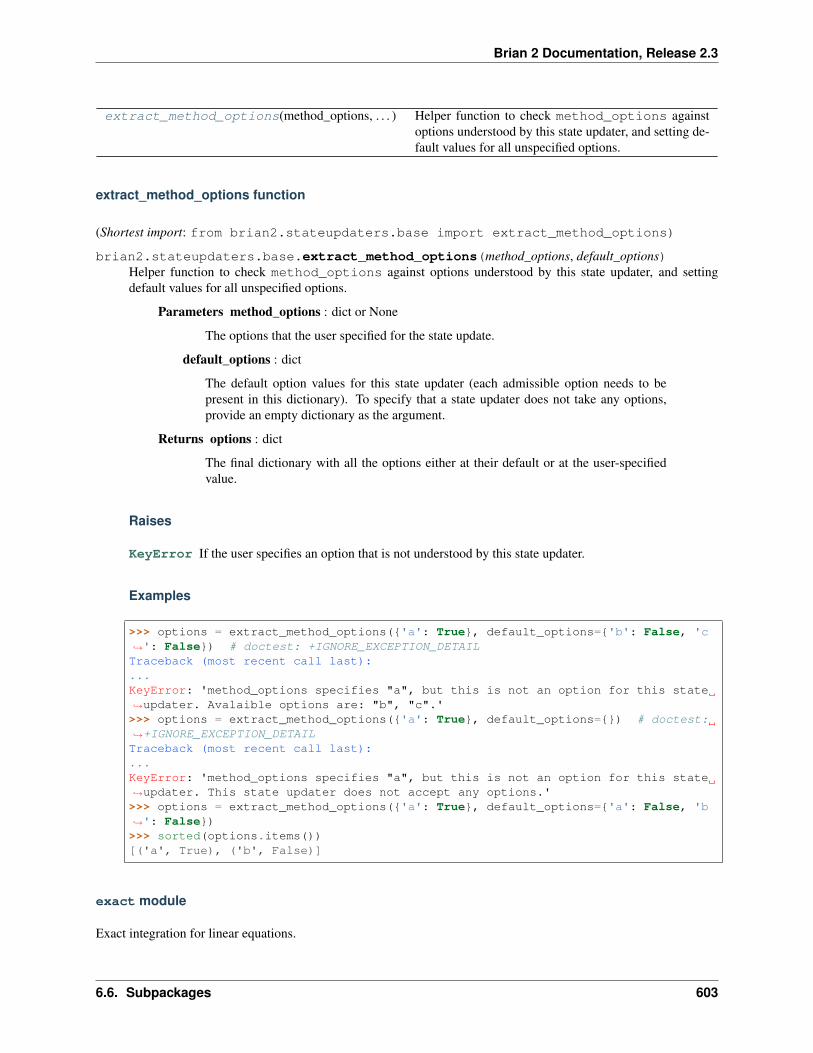
Brian 2 Documentation, Release 2.3
extract_method_options(method_options, . . . ) Helper function to check method_options againstoptions understood by this state updater, and setting de-fault values for all unspecified options.
extract_method_options function
(Shortest import: from brian2.stateupdaters.base import extract_method_options)
brian2.stateupdaters.base.extract_method_options(method_options, default_options)Helper function to check method_options against options understood by this state updater, and settingdefault values for all unspecified options.
Parameters method_options : dict or None
The options that the user specified for the state update.
default_options : dict
The default option values for this state updater (each admissible option needs to bepresent in this dictionary). To specify that a state updater does not take any options,provide an empty dictionary as the argument.
Returns options : dict
The final dictionary with all the options either at their default or at the user-specifiedvalue.
Raises
KeyError If the user specifies an option that is not understood by this state updater.
Examples
>>> options = extract_method_options({'a': True}, default_options={'b': False, 'c→˓': False}) # doctest: +IGNORE_EXCEPTION_DETAILTraceback (most recent call last):...KeyError: 'method_options specifies "a", but this is not an option for this state→˓updater. Avalaible options are: "b", "c".'>>> options = extract_method_options({'a': True}, default_options={}) # doctest:→˓+IGNORE_EXCEPTION_DETAILTraceback (most recent call last):...KeyError: 'method_options specifies "a", but this is not an option for this state→˓updater. This state updater does not accept any options.'>>> options = extract_method_options({'a': True}, default_options={'a': False, 'b→˓': False})>>> sorted(options.items())[('a', True), ('b', False)]
exact module
Exact integration for linear equations.
6.6. Subpackages 603
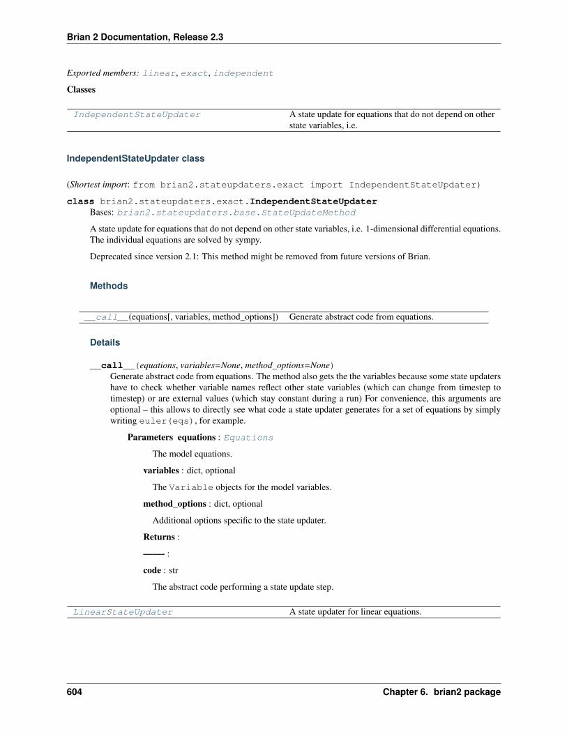
Brian 2 Documentation, Release 2.3
Exported members: linear, exact, independent
Classes
IndependentStateUpdater A state update for equations that do not depend on otherstate variables, i.e.
IndependentStateUpdater class
(Shortest import: from brian2.stateupdaters.exact import IndependentStateUpdater)
class brian2.stateupdaters.exact.IndependentStateUpdaterBases: brian2.stateupdaters.base.StateUpdateMethod
A state update for equations that do not depend on other state variables, i.e. 1-dimensional differential equations.The individual equations are solved by sympy.
Deprecated since version 2.1: This method might be removed from future versions of Brian.
Methods
__call__(equations[, variables, method_options]) Generate abstract code from equations.
Details
__call__(equations, variables=None, method_options=None)Generate abstract code from equations. The method also gets the the variables because some state updatershave to check whether variable names reflect other state variables (which can change from timestep totimestep) or are external values (which stay constant during a run) For convenience, this arguments areoptional – this allows to directly see what code a state updater generates for a set of equations by simplywriting euler(eqs), for example.
Parameters equations : Equations
The model equations.
variables : dict, optional
The Variable objects for the model variables.
method_options : dict, optional
Additional options specific to the state updater.
Returns :
——- :
code : str
The abstract code performing a state update step.
LinearStateUpdater A state updater for linear equations.
604 Chapter 6. brian2 package
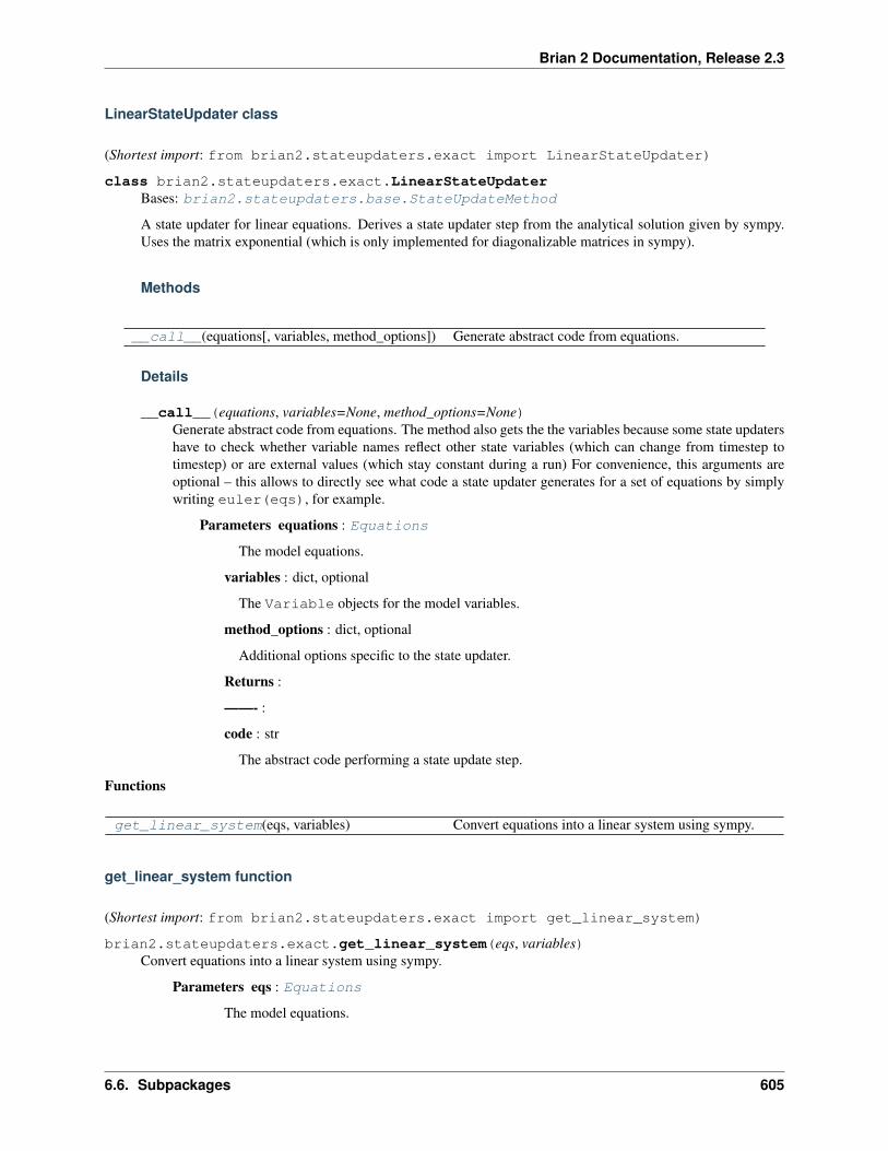
Brian 2 Documentation, Release 2.3
LinearStateUpdater class
(Shortest import: from brian2.stateupdaters.exact import LinearStateUpdater)
class brian2.stateupdaters.exact.LinearStateUpdaterBases: brian2.stateupdaters.base.StateUpdateMethod
A state updater for linear equations. Derives a state updater step from the analytical solution given by sympy.Uses the matrix exponential (which is only implemented for diagonalizable matrices in sympy).
Methods
__call__(equations[, variables, method_options]) Generate abstract code from equations.
Details
__call__(equations, variables=None, method_options=None)Generate abstract code from equations. The method also gets the the variables because some state updatershave to check whether variable names reflect other state variables (which can change from timestep totimestep) or are external values (which stay constant during a run) For convenience, this arguments areoptional – this allows to directly see what code a state updater generates for a set of equations by simplywriting euler(eqs), for example.
Parameters equations : Equations
The model equations.
variables : dict, optional
The Variable objects for the model variables.
method_options : dict, optional
Additional options specific to the state updater.
Returns :
——- :
code : str
The abstract code performing a state update step.
Functions
get_linear_system(eqs, variables) Convert equations into a linear system using sympy.
get_linear_system function
(Shortest import: from brian2.stateupdaters.exact import get_linear_system)
brian2.stateupdaters.exact.get_linear_system(eqs, variables)Convert equations into a linear system using sympy.
Parameters eqs : Equations
The model equations.
6.6. Subpackages 605
Brian 2 Documentation, Release 2.3
Returns (diff_eq_names, coefficients, constants) : (list of str, sympy.Matrix, sympy.Matrix)
A tuple containing the variable names (diff_eq_names) corresponding to the rowsof the matrix coefficients and the vector constants, representing the systemof equations in the form M * X + B
Raises
ValueError If the equations cannot be converted into an M * X + B form.
Objects
exact A state updater for linear equations.
exact object
(Shortest import: from brian2 import exact)
brian2.stateupdaters.exact.exact = LinearStateUpdater()A state updater for linear equations. Derives a state updater step from the analytical solution given by sympy.Uses the matrix exponential (which is only implemented for diagonalizable matrices in sympy).
independent A state update for equations that do not depend on otherstate variables, i.e.
independent object
(Shortest import: from brian2 import independent)
brian2.stateupdaters.exact.independent = <brian2.stateupdaters.exact.IndependentStateUpdater object>A state update for equations that do not depend on other state variables, i.e. 1-dimensional differential equations.The individual equations are solved by sympy.
Deprecated since version 2.1: This method might be removed from future versions of Brian.
linear A state updater for linear equations.
linear object
(Shortest import: from brian2 import linear)
brian2.stateupdaters.exact.linear = LinearStateUpdater()A state updater for linear equations. Derives a state updater step from the analytical solution given by sympy.Uses the matrix exponential (which is only implemented for diagonalizable matrices in sympy).
explicit module
Exported members: milstein, heun, euler, rk2, rk4, ExplicitStateUpdater
Classes
606 Chapter 6. brian2 package
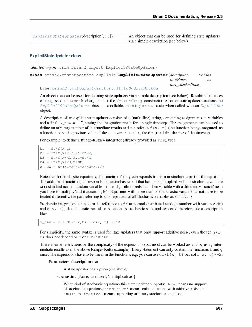
Brian 2 Documentation, Release 2.3
ExplicitStateUpdater(description[, . . . ]) An object that can be used for defining state updatersvia a simple description (see below).
ExplicitStateUpdater class
(Shortest import: from brian2 import ExplicitStateUpdater)
class brian2.stateupdaters.explicit.ExplicitStateUpdater(description, stochas-tic=None, cus-tom_check=None)
Bases: brian2.stateupdaters.base.StateUpdateMethod
An object that can be used for defining state updaters via a simple description (see below). Resulting instancescan be passed to the method argument of the NeuronGroup constructor. As other state updater functions theExplicitStateUpdater objects are callable, returning abstract code when called with an Equationsobject.
A description of an explicit state updater consists of a (multi-line) string, containing assignments to variablesand a final “x_new = . . . ”, stating the integration result for a single timestep. The assignments can be used todefine an arbitrary number of intermediate results and can refer to f(x, t) (the function being integrated, asa function of x, the previous value of the state variable and t, the time) and dt, the size of the timestep.
For example, to define a Runge-Kutta 4 integrator (already provided as rk4), use:
k1 = dt*f(x,t)k2 = dt*f(x+k1/2,t+dt/2)k3 = dt*f(x+k2/2,t+dt/2)k4 = dt*f(x+k3,t+dt)x_new = x+(k1+2*k2+2*k3+k4)/6
Note that for stochastic equations, the function f only corresponds to the non-stochastic part of the equation.The additional function g corresponds to the stochastic part that has to be multiplied with the stochastic variablexi (a standard normal random variable – if the algorithm needs a random variable with a different variance/meanyou have to multiply/add it accordingly). Equations with more than one stochastic variable do not have to betreated differently, the part referring to g is repeated for all stochastic variables automatically.
Stochastic integrators can also make reference to dW (a normal distributed random number with variance dt)and g(x, t), the stochastic part of an equation. A stochastic state updater could therefore use a descriptionlike:
x_new = x + dt*f(x,t) + g(x, t) * dW
For simplicity, the same syntax is used for state updaters that only support additive noise, even though g(x,t) does not depend on x or t in that case.
There a some restrictions on the complexity of the expressions (but most can be worked around by using inter-mediate results as in the above Runge- Kutta example): Every statement can only contain the functions f and gonce; The expressions have to be linear in the functions, e.g. you can use dt*f(x, t) but not f(x, t)**2.
Parameters description : str
A state updater description (see above).
stochastic : {None, ‘additive’, ‘multiplicative’}
What kind of stochastic equations this state updater supports: None means no supportof stochastic equations, 'additive' means only equations with additive noise and'multiplicative' means supporting arbitrary stochastic equations.
6.6. Subpackages 607

Brian 2 Documentation, Release 2.3
Raises
ValueError If the parsing of the description failed.
See also:
euler, rk2, rk4, milstein
Notes
Since clocks are updated after the state update, the time t used in the state update step is still at its previousvalue. Enumerating the states and discrete times, x_new = x + dt*f(x, t) is therefore understood as𝑥𝑖+1 = 𝑥𝑖 + 𝑑𝑡𝑓(𝑥𝑖, 𝑡𝑖), yielding the correct forward Euler integration. If the integrator has to refer to the timeat the end of the timestep, simply use t + dt instead of t.
Attributes
DESCRIPTION A complete state updater descriptionEXPRESSION A single expressionOUTPUT The last line of a state updater descriptionSTATEMENT An assignment statementTEMP_VAR Legal names for temporary variables
Methods
DESCRIPTION A complete state updater descriptionEXPRESSION A single expressionOUTPUT The last line of a state updater descriptionSTATEMENT An assignment statementTEMP_VAR Legal names for temporary variables__call__(eqs[, variables, method_options]) Apply a state updater description to model equations.replace_func(x, t, expr, temp_vars,eq_symbols)
Used to replace a single occurance of f(x, t) org(x, t): expr is the non-stochastic (in the caseof f) or stochastic part (g) of the expression defin-ing the right-hand-side of the differential equationdescribing var().
Details
DESCRIPTION = {[Group:({~{"x_new"} W:(abcd..., abcd...) Suppress:("=") rest of line})]... Group:({Suppress:("x_new") Suppress:("=") rest of line})}A complete state updater description
EXPRESSION = rest of lineA single expression
OUTPUT = Group:({Suppress:("x_new") Suppress:("=") rest of line})The last line of a state updater description
STATEMENT = Group:({~{"x_new"} W:(abcd..., abcd...) Suppress:("=") rest of line})An assignment statement
TEMP_VAR = {~{"x_new"} W:(abcd..., abcd...)}
608 Chapter 6. brian2 package
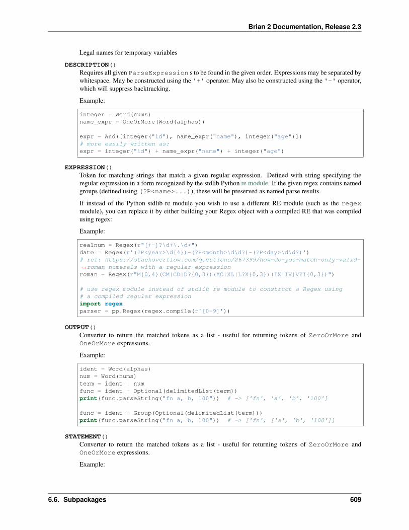
Brian 2 Documentation, Release 2.3
Legal names for temporary variables
DESCRIPTION()Requires all given ParseExpression s to be found in the given order. Expressions may be separated bywhitespace. May be constructed using the '+' operator. May also be constructed using the '-' operator,which will suppress backtracking.
Example:
integer = Word(nums)name_expr = OneOrMore(Word(alphas))
expr = And([integer("id"), name_expr("name"), integer("age")])# more easily written as:expr = integer("id") + name_expr("name") + integer("age")
EXPRESSION()Token for matching strings that match a given regular expression. Defined with string specifying theregular expression in a form recognized by the stdlib Python re module. If the given regex contains namedgroups (defined using (?P<name>...)), these will be preserved as named parse results.
If instead of the Python stdlib re module you wish to use a different RE module (such as the regexmodule), you can replace it by either building your Regex object with a compiled RE that was compiledusing regex:
Example:
realnum = Regex(r"[+-]?\d+\.\d*")date = Regex(r'(?P<year>\d{4})-(?P<month>\d\d?)-(?P<day>\d\d?)')# ref: https://stackoverflow.com/questions/267399/how-do-you-match-only-valid-→˓roman-numerals-with-a-regular-expressionroman = Regex(r"M{0,4}(CM|CD|D?{0,3})(XC|XL|L?X{0,3})(IX|IV|V?I{0,3})")
# use regex module instead of stdlib re module to construct a Regex using# a compiled regular expressionimport regexparser = pp.Regex(regex.compile(r'[0-9]'))
OUTPUT()Converter to return the matched tokens as a list - useful for returning tokens of ZeroOrMore andOneOrMore expressions.
Example:
ident = Word(alphas)num = Word(nums)term = ident | numfunc = ident + Optional(delimitedList(term))print(func.parseString("fn a, b, 100")) # -> ['fn', 'a', 'b', '100']
func = ident + Group(Optional(delimitedList(term)))print(func.parseString("fn a, b, 100")) # -> ['fn', ['a', 'b', '100']]
STATEMENT()Converter to return the matched tokens as a list - useful for returning tokens of ZeroOrMore andOneOrMore expressions.
Example:
6.6. Subpackages 609

Brian 2 Documentation, Release 2.3
ident = Word(alphas)num = Word(nums)term = ident | numfunc = ident + Optional(delimitedList(term))print(func.parseString("fn a, b, 100")) # -> ['fn', 'a', 'b', '100']
func = ident + Group(Optional(delimitedList(term)))print(func.parseString("fn a, b, 100")) # -> ['fn', ['a', 'b', '100']]
TEMP_VAR()Requires all given ParseExpression s to be found in the given order. Expressions may be separated bywhitespace. May be constructed using the '+' operator. May also be constructed using the '-' operator,which will suppress backtracking.
Example:
integer = Word(nums)name_expr = OneOrMore(Word(alphas))
expr = And([integer("id"), name_expr("name"), integer("age")])# more easily written as:expr = integer("id") + name_expr("name") + integer("age")
__call__(eqs, variables=None, method_options=None)Apply a state updater description to model equations.
Parameters eqs : Equations
The equations describing the model
variables: dict-like, optional :
The Variable objects for the model. Ignored by the explicit state updater.
method_options : dict, optional
Additional options to the state updater (not used at the moment for the explicit stateupdaters).
Examples
>>> from brian2 import *>>> eqs = Equations('dv/dt = -v / tau : volt')>>> print(euler(eqs))_v = -dt*v/tau + vv = _v>>> print(rk4(eqs))__k_1_v = -dt*v/tau__k_2_v = -dt*(0.5*__k_1_v + v)/tau__k_3_v = -dt*(0.5*__k_2_v + v)/tau__k_4_v = -dt*(__k_3_v + v)/tau_v = 0.166666666666667*__k_1_v + 0.333333333333333*__k_2_v + 0.→˓333333333333333*__k_3_v + 0.166666666666667*__k_4_v + vv = _v
replace_func(x, t, expr, temp_vars, eq_symbols, stochastic_variable=None)Used to replace a single occurance of f(x, t) or g(x, t): expr is the non-stochastic (in the case
610 Chapter 6. brian2 package

Brian 2 Documentation, Release 2.3
of f) or stochastic part (g) of the expression defining the right-hand-side of the differential equation de-scribing var(). It replaces the variable var() with the value given as x and t by the value given for t.Intermediate variables will be replaced with the appropriate replacements as well.
For example, in the rk2 integrator, the second step involves the calculation of f(k/2 + x, dt/2 +t). If var() is v and expr is -v / tau, this will result in -(_k_v/2 + v)/tau.
Note that this deals with only one state variable var(), given as an argument to the surrounding_generate_RHS function.
Functions
diagonal_noise(equations, variables) Checks whether we deal with diagonal noise, i.e.
diagonal_noise function
(Shortest import: from brian2.stateupdaters.explicit import diagonal_noise)
brian2.stateupdaters.explicit.diagonal_noise(equations, variables)Checks whether we deal with diagonal noise, i.e. one independent noise variable per variable.
Raises
UnsupportedEquationsException If the noise is not diagonal.
split_expression(expr) Split an expression into a part containing the function fand another one containing the function g.
split_expression function
(Shortest import: from brian2.stateupdaters.explicit import split_expression)
brian2.stateupdaters.explicit.split_expression(expr)Split an expression into a part containing the function f and another one containing the function g. Returns atuple of the two expressions (as sympy expressions).
Parameters expr : str
An expression containing references to functions f and g.
Returns (non_stochastic, stochastic) : tuple of sympy expressions
A pair of expressions representing the non-stochastic (containing function-independentterms and terms involving f) and the stochastic part of the expression (terms involvingg and/or dW).
Examples
>>> split_expression('dt * __f(__x, __t)')(dt*__f(__x, __t), None)>>> split_expression('dt * __f(__x, __t) + __dW * __g(__x, __t)')(dt*__f(__x, __t), __dW*__g(__x, __t))
(continues on next page)
6.6. Subpackages 611

Brian 2 Documentation, Release 2.3
(continued from previous page)
>>> split_expression('1/(2*dt**.5)*(__g_support - __g(__x, __t))*(__dW**2)')(0, __dW**2*__g_support*dt**(-0.5)/2 - __dW**2*dt**(-0.5)*__g(__x, __t)/2)
Objects
euler Forward Euler state updater
euler object
(Shortest import: from brian2 import euler)
brian2.stateupdaters.explicit.euler = ExplicitStateUpdater('''x_new = __dW*__g(__x, __t) + __x + dt*__f(__x, __t)''', stochastic='additive')Forward Euler state updater
heun Stochastic Heun method (for multiplicative StratonovicSDEs with non-diagonal diffusion matrix)
heun object
(Shortest import: from brian2 import heun)
brian2.stateupdaters.explicit.heun = ExplicitStateUpdater('''__x_support = __dW*__g(__x, __t) + __x __g_support = __g(__x_support, __t + dt) x_new = 0.5*__dW*(__g_support + __g(__x, __t)) + __x + dt*__f(__x, __t)''', stochastic='multiplicative')Stochastic Heun method (for multiplicative Stratonovic SDEs with non-diagonal diffusion matrix)
milstein Derivative-free Milstein method
milstein object
(Shortest import: from brian2 import milstein)
brian2.stateupdaters.explicit.milstein = ExplicitStateUpdater('''__x_support = __x + dt**0.5*__g(__x, __t) + dt*__f(__x, __t) __g_support = __g(__x_support, __t) __k = 0.5*__dW**2.0*dt**(-0.5)*(__g_support - __g(__x, __t)) x_new = __dW*__g(__x, __t) + __k + __x + dt*__f(__x, __t)''', stochastic='multiplicative')Derivative-free Milstein method
rk2 Second order Runge-Kutta method (midpoint method)
rk2 object
(Shortest import: from brian2 import rk2)
brian2.stateupdaters.explicit.rk2 = ExplicitStateUpdater('''__k = dt*__f(__x, __t) x_new = __x + dt*__f(0.5*__k + __x, __t + 0.5*dt)''', stochastic=None)Second order Runge-Kutta method (midpoint method)
rk4 Classical Runge-Kutta method (RK4)
rk4 object
(Shortest import: from brian2 import rk4)
612 Chapter 6. brian2 package
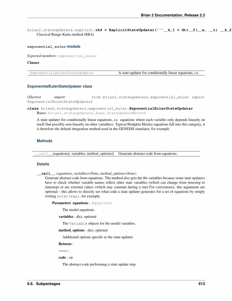
Brian 2 Documentation, Release 2.3
brian2.stateupdaters.explicit.rk4 = ExplicitStateUpdater('''__k_1 = dt*__f(__x, __t) __k_2 = dt*__f(0.5*__k_1 + __x, __t + 0.5*dt) __k_3 = dt*__f(0.5*__k_2 + __x, __t + 0.5*dt) __k_4 = dt*__f(__k_3 + __x, __t + dt) x_new = 0.166666666666667*__k_1 + 0.333333333333333*__k_2 + 0.333333333333333*__k_3 + 0.166666666666667*__k_4 + __x''', stochastic=None)Classical Runge-Kutta method (RK4)
exponential_euler module
Exported members: exponential_euler
Classes
ExponentialEulerStateUpdater A state updater for conditionally linear equations, i.e.
ExponentialEulerStateUpdater class
(Shortest import: from brian2.stateupdaters.exponential_euler importExponentialEulerStateUpdater)
class brian2.stateupdaters.exponential_euler.ExponentialEulerStateUpdaterBases: brian2.stateupdaters.base.StateUpdateMethod
A state updater for conditionally linear equations, i.e. equations where each variable only depends linearly onitself (but possibly non-linearly on other variables). Typical Hodgkin-Huxley equations fall into this category, itis therefore the default integration method used in the GENESIS simulator, for example.
Methods
__call__(equations[, variables, method_options]) Generate abstract code from equations.
Details
__call__(equations, variables=None, method_options=None)Generate abstract code from equations. The method also gets the the variables because some state updatershave to check whether variable names reflect other state variables (which can change from timestep totimestep) or are external values (which stay constant during a run) For convenience, this arguments areoptional – this allows to directly see what code a state updater generates for a set of equations by simplywriting euler(eqs), for example.
Parameters equations : Equations
The model equations.
variables : dict, optional
The Variable objects for the model variables.
method_options : dict, optional
Additional options specific to the state updater.
Returns :
——- :
code : str
The abstract code performing a state update step.
6.6. Subpackages 613

Brian 2 Documentation, Release 2.3
Functions
get_conditionally_linear_system(eqs[,variables])
Convert equations into a linear system using sympy.
get_conditionally_linear_system function
(Shortest import: from brian2.stateupdaters.exponential_euler importget_conditionally_linear_system)
brian2.stateupdaters.exponential_euler.get_conditionally_linear_system(eqs,vari-ables=None)
Convert equations into a linear system using sympy.
Parameters eqs : Equations
The model equations.
Returns coefficients : dict of (sympy expression, sympy expression) tuples
For every variable x, a tuple (M, B) containing the coefficients M and B (as sympyexpressions) for M * x + B
Raises
ValueError If one of the equations cannot be converted into a M * x + B form.
Examples
>>> from brian2 import Equations>>> eqs = Equations("""... dv/dt = (-v + w**2) / tau : 1... dw/dt = -w / tau : 1... """)>>> system = get_conditionally_linear_system(eqs)>>> print(system['v'])(-1/tau, w**2.0/tau)>>> print(system['w'])(-1/tau, 0)
Objects
exponential_euler A state updater for conditionally linear equations, i.e.
exponential_euler object
(Shortest import: from brian2 import exponential_euler)
brian2.stateupdaters.exponential_euler.exponential_euler = <brian2.stateupdaters.exponential_euler.ExponentialEulerStateUpdater object>A state updater for conditionally linear equations, i.e. equations where each variable only depends linearly onitself (but possibly non-linearly on other variables). Typical Hodgkin-Huxley equations fall into this category, itis therefore the default integration method used in the GENESIS simulator, for example.
614 Chapter 6. brian2 package

Brian 2 Documentation, Release 2.3
6.6.14 synapses package
Package providing synapse support.
Exported members: Synapses
parse_synaptic_generator_syntax module
Exported members: parse_synapse_generator
Functions
handle_range(*args, **kwds) Checks the arguments/keywords for the range iterator
handle_range function
(Shortest import: from brian2.synapses.parse_synaptic_generator_syntax importhandle_range)
brian2.synapses.parse_synaptic_generator_syntax.handle_range(*args, **kwds)Checks the arguments/keywords for the range iterator
Should have 1-3 positional arguments.
Returns a dict with keys low, high, step. Default values are low=0, step=1.
handle_sample(*args, **kwds) Checks the arguments/keywords for the sample iterator
handle_sample function
(Shortest import: from brian2.synapses.parse_synaptic_generator_syntax importhandle_sample)
brian2.synapses.parse_synaptic_generator_syntax.handle_sample(*args, **kwds)Checks the arguments/keywords for the sample iterator
Should have 1-3 positional arguments and 1 keyword argument (either p or size).
Returns a dict with keys low, high, step, sample_size, p, size. Default values are low=0,step=1`. Sample size will be either ``'random' or 'fixed'. In the first case, pwill havea value and size will be None (and vice versa for the second case).
parse_synapse_generator(expr) Returns a parsed form of a synapse generator expres-sion.
parse_synapse_generator function
(Shortest import: from brian2.synapses.parse_synaptic_generator_syntax importparse_synapse_generator)
brian2.synapses.parse_synaptic_generator_syntax.parse_synapse_generator(expr)Returns a parsed form of a synapse generator expression.
6.6. Subpackages 615
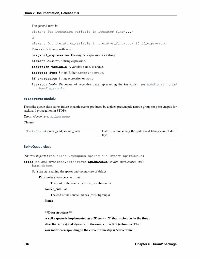
Brian 2 Documentation, Release 2.3
The general form is:
element for iteration_variable in iterator_func(...)
or
element for iteration_variable in iterator_func(...) if if_expression
Returns a dictionary with keys:
original_expression The original expression as a string.
element As above, a string expression.
iteration_variable A variable name, as above.
iterator_func String. Either range or sample.
if_expression String expression or None.
iterator_kwds Dictionary of key/value pairs representing the keywords. See handle_range andhandle_sample.
spikequeue module
The spike queue class stores future synaptic events produced by a given presynaptic neuron group (or postsynaptic forbackward propagation in STDP).
Exported members: SpikeQueue
Classes
SpikeQueue(source_start, source_end) Data structure saving the spikes and taking care of de-lays.
SpikeQueue class
(Shortest import: from brian2.synapses.spikequeue import SpikeQueue)
class brian2.synapses.spikequeue.SpikeQueue(source_start, source_end)Bases: object
Data structure saving the spikes and taking care of delays.
Parameters source_start : int
The start of the source indices (for subgroups)
source_end : int
The end of the source indices (for subgroups)
Notes :
—– :
**Data structure** :
A spike queue is implemented as a 2D array ‘X‘ that is circular in the time :
direction (rows) and dynamic in the events direction (columns). The :
row index corresponding to the current timestep is ‘currentime‘. :
616 Chapter 6. brian2 package
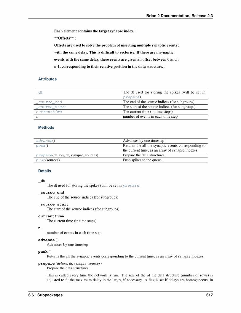
Brian 2 Documentation, Release 2.3
Each element contains the target synapse index. :
**Offsets** :
Offsets are used to solve the problem of inserting multiple synaptic events :
with the same delay. This is difficult to vectorise. If there are n synaptic :
events with the same delay, these events are given an offset between 0 and :
n-1, corresponding to their relative position in the data structure. :
Attributes
_dt The dt used for storing the spikes (will be set inprepare)
_source_end The end of the source indices (for subgroups)_source_start The start of the source indices (for subgroups)currenttime The current time (in time steps)n number of events in each time step
Methods
advance() Advances by one timesteppeek() Returns the all the synaptic events corresponding to
the current time, as an array of synapse indexes.prepare(delays, dt, synapse_sources) Prepare the data structurespush(sources) Push spikes to the queue.
Details
_dtThe dt used for storing the spikes (will be set in prepare)
_source_endThe end of the source indices (for subgroups)
_source_startThe start of the source indices (for subgroups)
currenttimeThe current time (in time steps)
nnumber of events in each time step
advance()Advances by one timestep
peek()Returns the all the synaptic events corresponding to the current time, as an array of synapse indexes.
prepare(delays, dt, synapse_sources)Prepare the data structures
This is called every time the network is run. The size of the of the data structure (number of rows) isadjusted to fit the maximum delay in delays, if necessary. A flag is set if delays are homogeneous, in
6.6. Subpackages 617
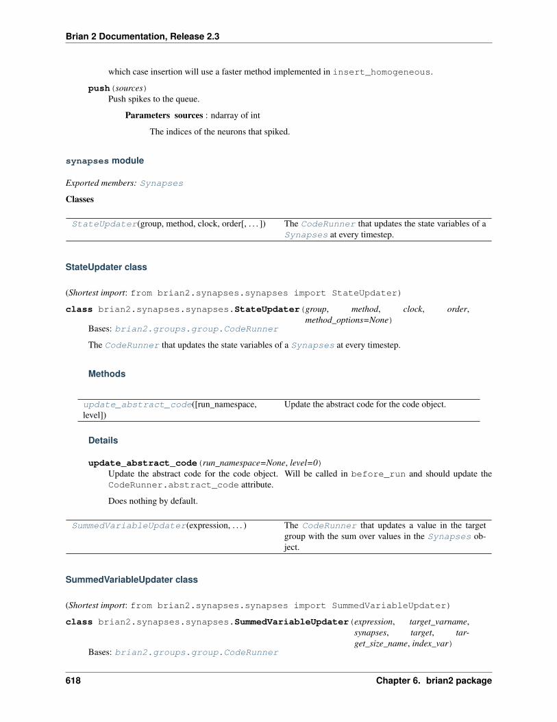
Brian 2 Documentation, Release 2.3
which case insertion will use a faster method implemented in insert_homogeneous.
push(sources)Push spikes to the queue.
Parameters sources : ndarray of int
The indices of the neurons that spiked.
synapses module
Exported members: Synapses
Classes
StateUpdater(group, method, clock, order[, . . . ]) The CodeRunner that updates the state variables of aSynapses at every timestep.
StateUpdater class
(Shortest import: from brian2.synapses.synapses import StateUpdater)
class brian2.synapses.synapses.StateUpdater(group, method, clock, order,method_options=None)
Bases: brian2.groups.group.CodeRunner
The CodeRunner that updates the state variables of a Synapses at every timestep.
Methods
update_abstract_code([run_namespace,level])
Update the abstract code for the code object.
Details
update_abstract_code(run_namespace=None, level=0)Update the abstract code for the code object. Will be called in before_run and should update theCodeRunner.abstract_code attribute.
Does nothing by default.
SummedVariableUpdater(expression, . . . ) The CodeRunner that updates a value in the targetgroup with the sum over values in the Synapses ob-ject.
SummedVariableUpdater class
(Shortest import: from brian2.synapses.synapses import SummedVariableUpdater)
class brian2.synapses.synapses.SummedVariableUpdater(expression, target_varname,synapses, target, tar-get_size_name, index_var)
Bases: brian2.groups.group.CodeRunner
618 Chapter 6. brian2 package
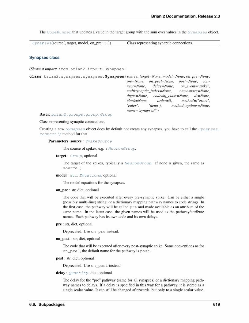
Brian 2 Documentation, Release 2.3
The CodeRunner that updates a value in the target group with the sum over values in the Synapses object.
Synapses(source[, target, model, on_pre, . . . ]) Class representing synaptic connections.
Synapses class
(Shortest import: from brian2 import Synapses)
class brian2.synapses.synapses.Synapses(source, target=None, model=None, on_pre=None,pre=None, on_post=None, post=None, con-nect=None, delay=None, on_event=’spike’,multisynaptic_index=None, namespace=None,dtype=None, codeobj_class=None, dt=None,clock=None, order=0, method=(’exact’,’euler’, ’heun’), method_options=None,name=’synapses*’)
Bases: brian2.groups.group.Group
Class representing synaptic connections.
Creating a new Synapses object does by default not create any synapses, you have to call the Synapses.connect() method for that.
Parameters source : SpikeSource
The source of spikes, e.g. a NeuronGroup.
target : Group, optional
The target of the spikes, typically a NeuronGroup. If none is given, the same assource()
model : str, Equations, optional
The model equations for the synapses.
on_pre : str, dict, optional
The code that will be executed after every pre-synaptic spike. Can be either a single(possibly multi-line) string, or a dictionary mapping pathway names to code strings. Inthe first case, the pathway will be called pre and made available as an attribute of thesame name. In the latter case, the given names will be used as the pathway/attributenames. Each pathway has its own code and its own delays.
pre : str, dict, optional
Deprecated. Use on_pre instead.
on_post : str, dict, optional
The code that will be executed after every post-synaptic spike. Same conventions as foron_pre`, the default name for the pathway is post.
post : str, dict, optional
Deprecated. Use on_post instead.
delay : Quantity , dict, optional
The delay for the “pre” pathway (same for all synapses) or a dictionary mapping path-way names to delays. If a delay is specified in this way for a pathway, it is stored as asingle scalar value. It can still be changed afterwards, but only to a single scalar value.
6.6. Subpackages 619
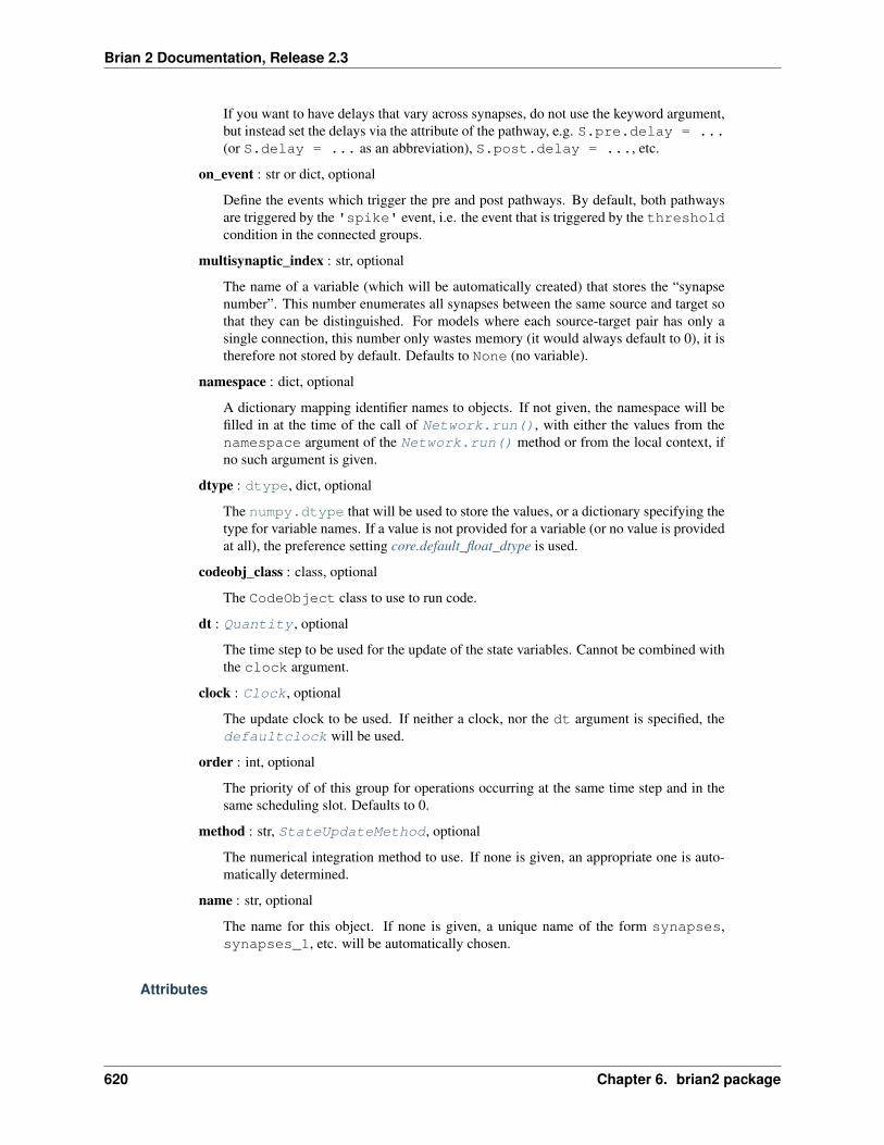
Brian 2 Documentation, Release 2.3
If you want to have delays that vary across synapses, do not use the keyword argument,but instead set the delays via the attribute of the pathway, e.g. S.pre.delay = ...(or S.delay = ... as an abbreviation), S.post.delay = ..., etc.
on_event : str or dict, optional
Define the events which trigger the pre and post pathways. By default, both pathwaysare triggered by the 'spike' event, i.e. the event that is triggered by the thresholdcondition in the connected groups.
multisynaptic_index : str, optional
The name of a variable (which will be automatically created) that stores the “synapsenumber”. This number enumerates all synapses between the same source and target sothat they can be distinguished. For models where each source-target pair has only asingle connection, this number only wastes memory (it would always default to 0), it istherefore not stored by default. Defaults to None (no variable).
namespace : dict, optional
A dictionary mapping identifier names to objects. If not given, the namespace will befilled in at the time of the call of Network.run(), with either the values from thenamespace argument of the Network.run() method or from the local context, ifno such argument is given.
dtype : dtype, dict, optional
The numpy.dtype that will be used to store the values, or a dictionary specifying thetype for variable names. If a value is not provided for a variable (or no value is providedat all), the preference setting core.default_float_dtype is used.
codeobj_class : class, optional
The CodeObject class to use to run code.
dt : Quantity , optional
The time step to be used for the update of the state variables. Cannot be combined withthe clock argument.
clock : Clock, optional
The update clock to be used. If neither a clock, nor the dt argument is specified, thedefaultclock will be used.
order : int, optional
The priority of of this group for operations occurring at the same time step and in thesame scheduling slot. Defaults to 0.
method : str, StateUpdateMethod, optional
The numerical integration method to use. If none is given, an appropriate one is auto-matically determined.
name : str, optional
The name for this object. If none is given, a unique name of the form synapses,synapses_1, etc. will be automatically chosen.
Attributes
620 Chapter 6. brian2 package
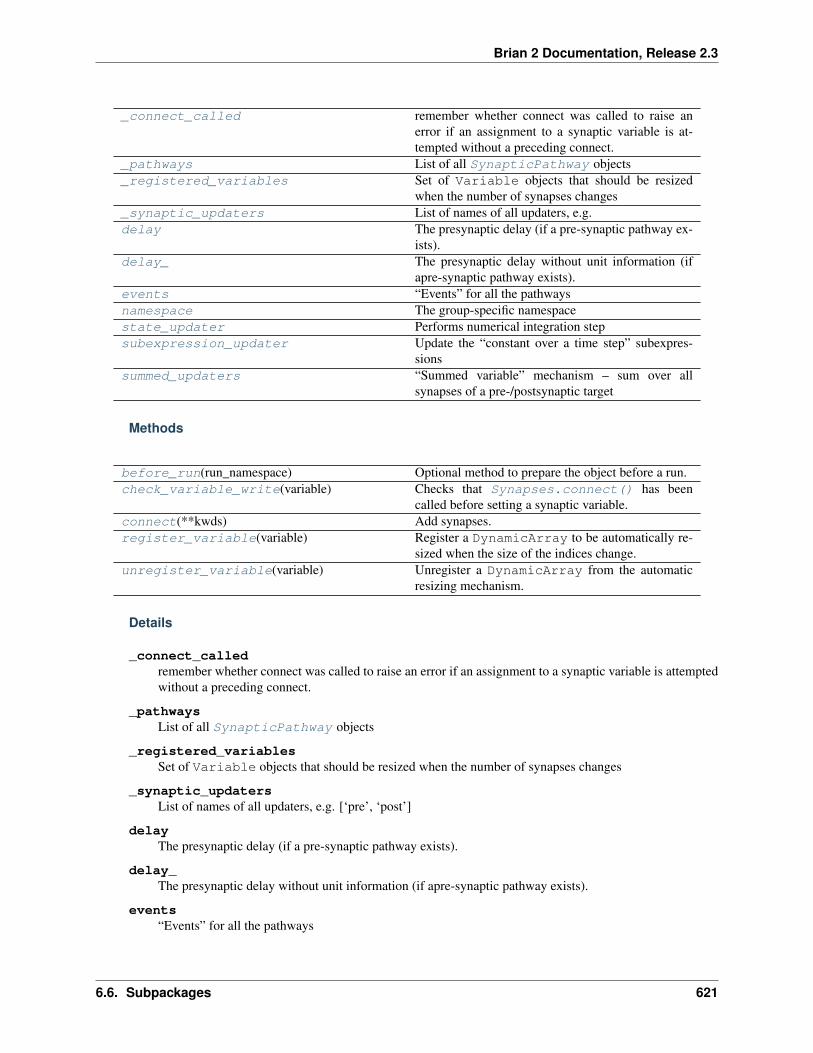
Brian 2 Documentation, Release 2.3
_connect_called remember whether connect was called to raise anerror if an assignment to a synaptic variable is at-tempted without a preceding connect.
_pathways List of all SynapticPathway objects_registered_variables Set of Variable objects that should be resized
when the number of synapses changes_synaptic_updaters List of names of all updaters, e.g.delay The presynaptic delay (if a pre-synaptic pathway ex-
ists).delay_ The presynaptic delay without unit information (if
apre-synaptic pathway exists).events “Events” for all the pathwaysnamespace The group-specific namespacestate_updater Performs numerical integration stepsubexpression_updater Update the “constant over a time step” subexpres-
sionssummed_updaters “Summed variable” mechanism – sum over all
synapses of a pre-/postsynaptic target
Methods
before_run(run_namespace) Optional method to prepare the object before a run.check_variable_write(variable) Checks that Synapses.connect() has been
called before setting a synaptic variable.connect(**kwds) Add synapses.register_variable(variable) Register a DynamicArray to be automatically re-
sized when the size of the indices change.unregister_variable(variable) Unregister a DynamicArray from the automatic
resizing mechanism.
Details
_connect_calledremember whether connect was called to raise an error if an assignment to a synaptic variable is attemptedwithout a preceding connect.
_pathwaysList of all SynapticPathway objects
_registered_variablesSet of Variable objects that should be resized when the number of synapses changes
_synaptic_updatersList of names of all updaters, e.g. [‘pre’, ‘post’]
delayThe presynaptic delay (if a pre-synaptic pathway exists).
delay_The presynaptic delay without unit information (if apre-synaptic pathway exists).
events“Events” for all the pathways
6.6. Subpackages 621
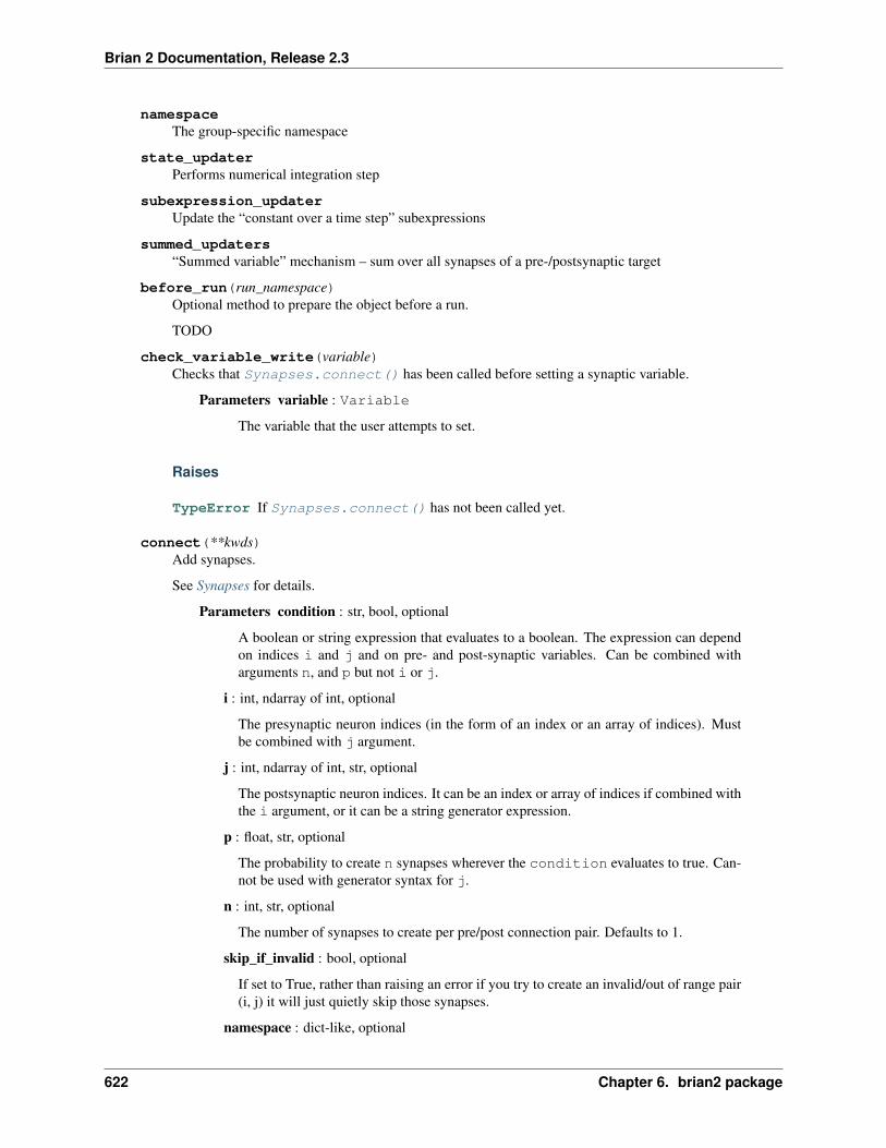
Brian 2 Documentation, Release 2.3
namespaceThe group-specific namespace
state_updaterPerforms numerical integration step
subexpression_updaterUpdate the “constant over a time step” subexpressions
summed_updaters“Summed variable” mechanism – sum over all synapses of a pre-/postsynaptic target
before_run(run_namespace)Optional method to prepare the object before a run.
TODO
check_variable_write(variable)Checks that Synapses.connect() has been called before setting a synaptic variable.
Parameters variable : Variable
The variable that the user attempts to set.
Raises
TypeError If Synapses.connect() has not been called yet.
connect(**kwds)Add synapses.
See Synapses for details.
Parameters condition : str, bool, optional
A boolean or string expression that evaluates to a boolean. The expression can dependon indices i and j and on pre- and post-synaptic variables. Can be combined witharguments n, and p but not i or j.
i : int, ndarray of int, optional
The presynaptic neuron indices (in the form of an index or an array of indices). Mustbe combined with j argument.
j : int, ndarray of int, str, optional
The postsynaptic neuron indices. It can be an index or array of indices if combined withthe i argument, or it can be a string generator expression.
p : float, str, optional
The probability to create n synapses wherever the condition evaluates to true. Can-not be used with generator syntax for j.
n : int, str, optional
The number of synapses to create per pre/post connection pair. Defaults to 1.
skip_if_invalid : bool, optional
If set to True, rather than raising an error if you try to create an invalid/out of range pair(i, j) it will just quietly skip those synapses.
namespace : dict-like, optional
622 Chapter 6. brian2 package
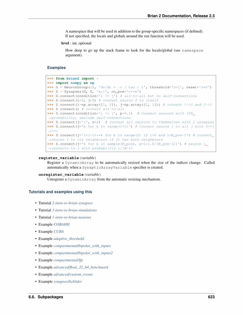
Brian 2 Documentation, Release 2.3
A namespace that will be used in addition to the group-specific namespaces (if defined).If not specified, the locals and globals around the run function will be used.
level : int, optional
How deep to go up the stack frame to look for the locals/global (see namespaceargument).
Examples
>>> from brian2 import *>>> import numpy as np>>> G = NeuronGroup(10, 'dv/dt = -v / tau : 1', threshold='v>1', reset='v=0')>>> S = Synapses(G, G, 'w:1', on_pre='v+=w')>>> S.connect(condition='i != j') # all-to-all but no self-connections>>> S.connect(i=0, j=0) # connect neuron 0 to itself>>> S.connect(i=np.array([1, 2]), j=np.array([2, 1])) # connect 1->2 and 2->1>>> S.connect() # connect all-to-all>>> S.connect(condition='i != j', p=0.1) # Connect neurons with 10%→˓probability, exclude self-connections>>> S.connect(j='i', n=2) # Connect all neurons to themselves with 2 synapses>>> S.connect(j='k for k in range(i+1)') # Connect neuron i to all j with 0<=j→˓<=i>>> S.connect(j='i+(-1)**k for k in range(2) if i>0 and i<N_pre-1') # connect→˓neuron i to its neighbours if it has both neighbours>>> S.connect(j='k for k in sample(N_post, p=i*1.0/(N_pre-1))') # neuron i→˓connects to j with probability i/(N-1)
register_variable(variable)Register a DynamicArray to be automatically resized when the size of the indices change. Calledautomatically when a SynapticArrayVariable specifier is created.
unregister_variable(variable)Unregister a DynamicArray from the automatic resizing mechanism.
Tutorials and examples using this
• Tutorial 2-intro-to-brian-synapses
• Tutorial 3-intro-to-brian-simulations
• Tutorial 1-intro-to-brian-neurons
• Example COBAHH
• Example CUBA
• Example adaptive_threshold
• Example compartmental/bipolar_with_inputs
• Example compartmental/bipolar_with_inputs2
• Example compartmental/lfp
• Example advanced/float_32_64_benchmark
• Example advanced/custom_events
• Example synapses/licklider
6.6. Subpackages 623
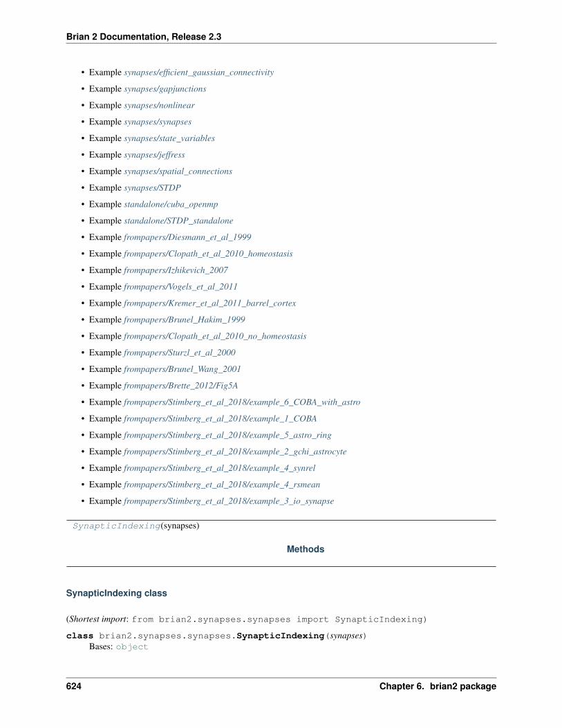
Brian 2 Documentation, Release 2.3
• Example synapses/efficient_gaussian_connectivity
• Example synapses/gapjunctions
• Example synapses/nonlinear
• Example synapses/synapses
• Example synapses/state_variables
• Example synapses/jeffress
• Example synapses/spatial_connections
• Example synapses/STDP
• Example standalone/cuba_openmp
• Example standalone/STDP_standalone
• Example frompapers/Diesmann_et_al_1999
• Example frompapers/Clopath_et_al_2010_homeostasis
• Example frompapers/Izhikevich_2007
• Example frompapers/Vogels_et_al_2011
• Example frompapers/Kremer_et_al_2011_barrel_cortex
• Example frompapers/Brunel_Hakim_1999
• Example frompapers/Clopath_et_al_2010_no_homeostasis
• Example frompapers/Sturzl_et_al_2000
• Example frompapers/Brunel_Wang_2001
• Example frompapers/Brette_2012/Fig5A
• Example frompapers/Stimberg_et_al_2018/example_6_COBA_with_astro
• Example frompapers/Stimberg_et_al_2018/example_1_COBA
• Example frompapers/Stimberg_et_al_2018/example_5_astro_ring
• Example frompapers/Stimberg_et_al_2018/example_2_gchi_astrocyte
• Example frompapers/Stimberg_et_al_2018/example_4_synrel
• Example frompapers/Stimberg_et_al_2018/example_4_rsmean
• Example frompapers/Stimberg_et_al_2018/example_3_io_synapse
SynapticIndexing(synapses)
Methods
SynapticIndexing class
(Shortest import: from brian2.synapses.synapses import SynapticIndexing)
class brian2.synapses.synapses.SynapticIndexing(synapses)Bases: object
624 Chapter 6. brian2 package
Brian 2 Documentation, Release 2.3
Methods
__call__([index, index_var]) Returns synaptic indices for index, which can be atuple of indices (including arrays and slices), a singleindex or a string.
Details
__call__(index=None, index_var=’_idx’)Returns synaptic indices for index, which can be a tuple of indices (including arrays and slices), a singleindex or a string.
SynapticPathway(synapses, code, prepost[, . . . ]) The CodeRunner that applies the pre/post state-ment(s) to the state variables of synapses where the pre-/postsynaptic group spiked in this time step.
SynapticPathway class
(Shortest import: from brian2.synapses.synapses import SynapticPathway)
class brian2.synapses.synapses.SynapticPathway(synapses, code, prepost, objname=None,delay=None, event=’spike’)
Bases: brian2.groups.group.CodeRunner, brian2.groups.group.Group
The CodeRunner that applies the pre/post statement(s) to the state variables of synapses where the pre-/postsynaptic group spiked in this time step.
Parameters synapses : Synapses
Reference to the main Synapses object
prepost : {‘pre’, ‘post’}
Whether this object should react to pre- or postsynaptic spikes
objname : str, optional
The name to use for the object, will be appendend to the name of synapses to createa name in the sense of Nameable. If None is provided (the default), prepost willbe used.
delay : Quantity , optional
A scalar delay (same delay for all synapses) for this pathway. If not given, delays areexpected to vary between synapses.
Attributes
_initialise_queue_codeobj The CodeObject initalising the SpikeQueue atthe begin of a run
queue The SpikeQueue
Methods
6.6. Subpackages 625

Brian 2 Documentation, Release 2.3
before_run(**kwds)check_variable_write(variable) Function that can be overwritten to raise an error if
writing to a variable should not be allowed.initialise_queue()push_spikes()update_abstract_code(**kwds)
Details
_initialise_queue_codeobjThe CodeObject initalising the SpikeQueue at the begin of a run
queueThe SpikeQueue
before_run(**kwds)
check_variable_write(variable)Function that can be overwritten to raise an error if writing to a variable should not be allowed. Note thatthis does not deal with incorrect writes that are general to all kind of variables (incorrect units, writing toa read-only variable, etc.). This function is only used for type-specific rules, e.g. for raising an error inSynapses when writing to a synaptic variable before any connect call.
By default this function does nothing.
Parameters variable : Variable
The variable that the user attempts to set.
initialise_queue()
push_spikes()
update_abstract_code(**kwds)
SynapticSubgroup(synapses, indices) A simple subgroup of Synapses that can be used forindexing.
SynapticSubgroup class
(Shortest import: from brian2.synapses.synapses import SynapticSubgroup)
class brian2.synapses.synapses.SynapticSubgroup(synapses, indices)Bases: object
A simple subgroup of Synapses that can be used for indexing.
Parameters indices : ndarray of int
The synaptic indices represented by this subgroup.
synaptic_pre : DynamicArrayVariable
References to all pre-synaptic indices. Only used to throw an error when new synapseswhere added after creating this object.
Functions
626 Chapter 6. brian2 package

Brian 2 Documentation, Release 2.3
find_synapses(index, synaptic_neuron)
find_synapses function
(Shortest import: from brian2.synapses.synapses import find_synapses)
brian2.synapses.synapses.find_synapses(index, synaptic_neuron)
slice_to_test(x) Returns a testing function corresponding to whether anindex is in slice x.
slice_to_test function
(Shortest import: from brian2.synapses.synapses import slice_to_test)
brian2.synapses.synapses.slice_to_test(x)Returns a testing function corresponding to whether an index is in slice x. x can also be an int.
6.6.15 units package
The unit system.
Exported members: pamp, namp, uamp, mamp, amp, kamp, Mamp, Gamp, Tamp, kelvin, kilogram, pmetre,nmetre, umetre, mmetre, metre, kmetre, Mmetre, Gmetre, Tmetre, pmeter, nmeter, umeter,mmeter, meter . . . (218 more members)
allunits module
THIS FILE IS AUTOMATICALLY GENERATED BY A STATIC CODE GENERATION TOOL DO NOT EDIT BYHAND
Instead edit the template:
dev/tools/static_codegen/units_template.py
Exported members: metre, meter, kilogram, second, amp, ampere, kelvin, mole, mol, candle,kilogramme, gram, gramme, molar, radian, steradian, hertz, newton, pascal, joule, watt,coulomb, volt, farad, ohm . . . (2045 more members)
Objects
celsius A dummy object to raise errors when celsius is used.
celsius object
(Shortest import: from brian2.units.allunits import celsius)
brian2.units.allunits.celsius = <brian2.units.allunits._Celsius object>A dummy object to raise errors when celsius is used. The use of celsius can lead to ambiguities whenmixed with temperatures in kelvin, so its use is no longer supported. See github issue #817 for details.
6.6. Subpackages 627
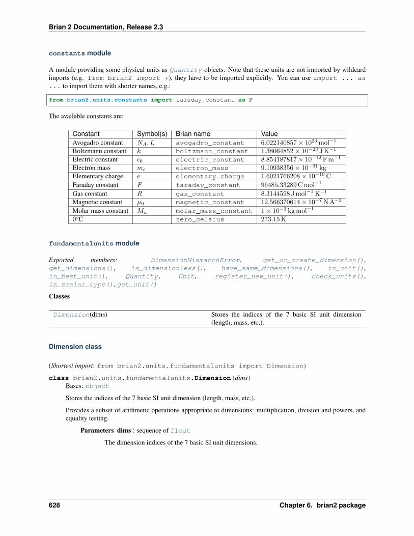
Brian 2 Documentation, Release 2.3
constants module
A module providing some physical units as Quantity objects. Note that these units are not imported by wildcardimports (e.g. from brian2 import *), they have to be imported explicitly. You can use import ... as... to import them with shorter names, e.g.:
from brian2.units.constants import faraday_constant as F
The available constants are:
Constant Symbol(s) Brian name ValueAvogadro constant 𝑁𝐴, 𝐿 avogadro_constant 6.022140857× 10²³ mol−1
Boltzmann constant 𝑘 boltzmann_constant 1.38064852× 10⁻²³ J K−1
Electric constant 𝜖0 electric_constant 8.854187817× 10⁻¹² F m−1
Electron mass 𝑚𝑒 electron_mass 9.10938356× 10⁻³¹ kgElementary charge 𝑒 elementary_charge 1.6021766208× 10⁻¹⁹ C
Faraday constant 𝐹 faraday_constant 96485.33289 C mol−1
Gas constant 𝑅 gas_constant 8.3144598 J mol−1 K−1
Magnetic constant 𝜇0 magnetic_constant 12.566370614× 10⁻⁷ N A−2
Molar mass constant 𝑀𝑢 molar_mass_constant 1× 10⁻³ kg mol−1
0°C zero_celsius 273.15 K
fundamentalunits module
Exported members: DimensionMismatchError, get_or_create_dimension(),get_dimensions(), is_dimensionless(), have_same_dimensions(), in_unit(),in_best_unit(), Quantity , Unit, register_new_unit(), check_units(),is_scalar_type(), get_unit()
Classes
Dimension(dims) Stores the indices of the 7 basic SI unit dimension(length, mass, etc.).
Dimension class
(Shortest import: from brian2.units.fundamentalunits import Dimension)
class brian2.units.fundamentalunits.Dimension(dims)Bases: object
Stores the indices of the 7 basic SI unit dimension (length, mass, etc.).
Provides a subset of arithmetic operations appropriate to dimensions: multiplication, division and powers, andequality testing.
Parameters dims : sequence of float
The dimension indices of the 7 basic SI unit dimensions.
628 Chapter 6. brian2 package
Brian 2 Documentation, Release 2.3
Notes
Users shouldn’t use this class directly, it is used internally in Quantity and Unit. Even internally, never useDimension(...) to create a new instance, use get_or_create_dimension() instead. This functionmakes sure that only one Dimension instance exists for every combination of indices, allowing for a very fastdimensionality check with is.
Attributes
dim Returns the Dimension object itself.is_dimensionless Whether this Dimension is dimensionless.
Methods
get_dimension(d) Return a specific dimension.
Details
dimReturns the Dimension object itself. This can be useful, because it allows to check for the dimension ofan object by checking its dim attribute – this will return a Dimension object for Quantity , Unit andDimension.
is_dimensionlessWhether this Dimension is dimensionless.
Notes
Normally, instead one should check dimension for being identical to DIMENSIONLESS.
get_dimension(d)Return a specific dimension.
Parameters d : str
A string identifying the SI basic unit dimension. Can be either a description like“length” or a basic unit like “m” or “metre”.
Returns dim : float
The dimensionality of the dimension d.
DimensionMismatchError(description, *dims) Exception class for attempted operations with inconsis-tent dimensions.
DimensionMismatchError class
(Shortest import: from brian2 import DimensionMismatchError)
class brian2.units.fundamentalunits.DimensionMismatchError(description, *dims)Bases: exceptions.Exception
Exception class for attempted operations with inconsistent dimensions.
6.6. Subpackages 629

Brian 2 Documentation, Release 2.3
For example, 3*mvolt + 2*amp raises this exception. The purpose of this class is to help catch errors basedon incorrect units. The exception will print a representation of the dimensions of the two inconsistent objectsthat were operated on.
Parameters description : str
A description of the type of operation being performed, e.g. Addition, Multiplication,etc.
dims : Dimension
The physical dimensions of the objects involved in the operation, any number of themis possible
Tutorials and examples using this
• Tutorial 1-intro-to-brian-neurons
Quantity A number with an associated physical dimension.
Quantity class
(Shortest import: from brian2 import Quantity)
class brian2.units.fundamentalunits.QuantityBases: numpy.ndarray, object
A number with an associated physical dimension. In most cases, it is not necessary to create a Quantity objectby hand, instead use multiplication and division of numbers with the constant unit names second, kilogram,etc.
See also:
Unit
Notes
The Quantity class defines arithmetic operations which check for consistency of dimensions and raise theDimensionMismatchError exception if they are inconsistent. It also defines default and other representations fora number for printing purposes.
See the documentation on the Unit class for more details about the available unit names like mvolt, etc.
Casting rules
The rules that define the casting operations for Quantity object are:
1. Quantity op Quantity = Quantity Performs dimension checking if appropriate
2. (Scalar or Array) op Quantity = Quantity Assumes that the scalar or array is dimensionless
There is one exception to the above rule, the number 0 is interpreted as having “any dimension”.
Examples
630 Chapter 6. brian2 package

Brian 2 Documentation, Release 2.3
>>> from brian2 import *>>> I = 3 * amp # I is a Quantity object>>> R = 2 * ohm # same for R>>> I * R6. * volt>>> (I * R).in_unit(mvolt)'6000. mV'>>> (I * R) / mvolt6000.0>>> X = I + R # doctest: +IGNORE_EXCEPTION_DETAILTraceback (most recent call last):
...DimensionMismatchError: Addition, dimensions were (A) (m^2 kg s^-3 A^-2)>>> Is = np.array([1, 2, 3]) * amp>>> Is * Rarray([ 2., 4., 6.]) * volt>>> np.asarray(Is * R) # gets rid of unitsarray([ 2., 4., 6.])
Attributes
dimensions The physical dimensions of this quantity.is_dimensionless Whether this is a dimensionless quantity.dim The physical dimensions of this quantity.
Methods
with_dimensions(value, *args, **keywords) Create a Quantity object with dim.has_same_dimensions(other) Return whether this object has the same dimensions
as another.in_unit(u[, precision, python_code]) Represent the quantity in a given unit.in_best_unit([precision, python_code]) Represent the quantity in the “best” unit.
Details
dimensionsThe physical dimensions of this quantity.
is_dimensionlessWhether this is a dimensionless quantity.
dimThe physical dimensions of this quantity.
static with_dimensions(value, *args, **keywords)Create a Quantity object with dim.
Parameters value : {array_like, number}
The value of the dimension
args : {Dimension, sequence of float}
Either a single argument (a Dimension) or a sequence of 7 values.
6.6. Subpackages 631

Brian 2 Documentation, Release 2.3
kwds :
Keywords defining the dim, see Dimension for details.
Returns q : Quantity
A Quantity object with the given dim
Examples
All of these define an equivalent Quantity object:
>>> from brian2 import *>>> Quantity.with_dimensions(2, get_or_create_dimension(length=1))2. * metre>>> Quantity.with_dimensions(2, length=1)2. * metre>>> 2 * metre2. * metre
has_same_dimensions(other)Return whether this object has the same dimensions as another.
Parameters other : {Quantity , array-like, number}
The object to compare the dimensions against.
Returns same : bool
True if other has the same dimensions.
in_unit(u, precision=None, python_code=False)Represent the quantity in a given unit. If python_code is True, this will return valid python code, i.e.a string like 5.0 * um ** 2 instead of 5.0 um^2
Parameters u : {Quantity , Unit}
The unit in which to show the quantity.
precision : int, optional
The number of digits of precision (in the given unit, see Examples). If no value is given,numpy’s get_printoptions() value is used.
python_code : bool, optional
Whether to return valid python code (True) or a human readable string (False, thedefault).
Returns s : str
String representation of the object in unit u.
See also:
in_unit()
Examples
632 Chapter 6. brian2 package

Brian 2 Documentation, Release 2.3
>>> from brian2.units import *>>> from brian2.units.stdunits import *>>> x = 25.123456 * mV>>> x.in_unit(volt)'0.02512346 V'>>> x.in_unit(volt, 3)'0.025 V'>>> x.in_unit(mV, 3)'25.123 mV'
in_best_unit(precision=None, python_code=False, *regs)Represent the quantity in the “best” unit.
Parameters python_code : bool, optional
If set to False (the default), will return a string like 5.0 um^2 which is not a validPython expression. If set to True, it will return 5.0 * um ** 2 instead.
precision : int, optional
The number of digits of precision (in the best unit, see Examples). If no value is given,numpy’s get_printoptions() value is used.
regs : UnitRegistry objects
The registries where to search for units. If none are given, the standard, user-definedand additional registries are searched in that order.
Returns representation : str
A string representation of this Quantity .
See also:
in_best_unit()
Examples
>>> from brian2.units import *
>>> x = 0.00123456 * volt
>>> x.in_best_unit()'1.23456 mV'
>>> x.in_best_unit(3)'1.235 mV'
Tutorials and examples using this
• Example frompapers/Destexhe_et_al_1998
• Example frompapers/Platkiewicz_Brette_2011
• Example frompapers/Stimberg_et_al_2018/example_1_COBA
6.6. Subpackages 633
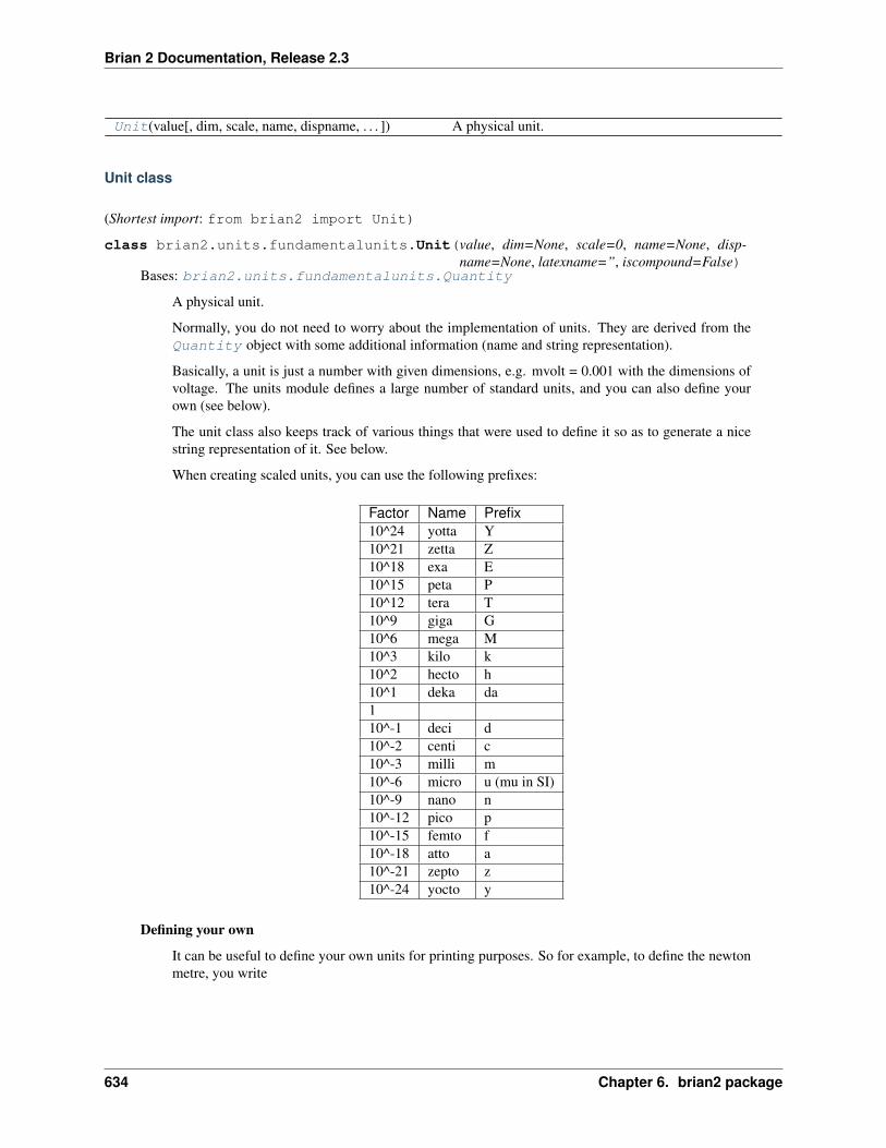
Brian 2 Documentation, Release 2.3
Unit(value[, dim, scale, name, dispname, . . . ]) A physical unit.
Unit class
(Shortest import: from brian2 import Unit)
class brian2.units.fundamentalunits.Unit(value, dim=None, scale=0, name=None, disp-name=None, latexname=”, iscompound=False)
Bases: brian2.units.fundamentalunits.Quantity
A physical unit.
Normally, you do not need to worry about the implementation of units. They are derived from theQuantity object with some additional information (name and string representation).
Basically, a unit is just a number with given dimensions, e.g. mvolt = 0.001 with the dimensions ofvoltage. The units module defines a large number of standard units, and you can also define yourown (see below).
The unit class also keeps track of various things that were used to define it so as to generate a nicestring representation of it. See below.
When creating scaled units, you can use the following prefixes:
Factor Name Prefix10^24 yotta Y10^21 zetta Z10^18 exa E10^15 peta P10^12 tera T10^9 giga G10^6 mega M10^3 kilo k10^2 hecto h10^1 deka da110^-1 deci d10^-2 centi c10^-3 milli m10^-6 micro u (mu in SI)10^-9 nano n10^-12 pico p10^-15 femto f10^-18 atto a10^-21 zepto z10^-24 yocto y
Defining your own
It can be useful to define your own units for printing purposes. So for example, to define the newtonmetre, you write
634 Chapter 6. brian2 package
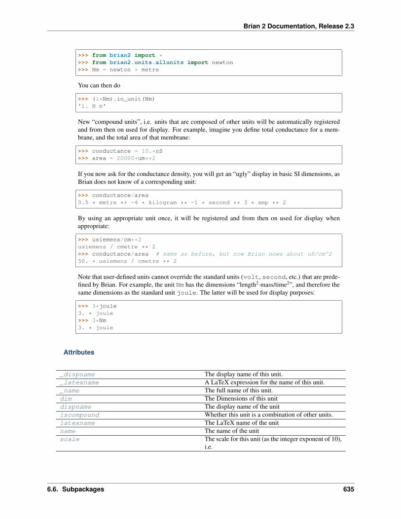
Brian 2 Documentation, Release 2.3
>>> from brian2 import *>>> from brian2.units.allunits import newton>>> Nm = newton * metre
You can then do
>>> (1*Nm).in_unit(Nm)'1. N m'
New “compound units”, i.e. units that are composed of other units will be automatically registeredand from then on used for display. For example, imagine you define total conductance for a mem-brane, and the total area of that membrane:
>>> conductance = 10.*nS>>> area = 20000*um**2
If you now ask for the conductance density, you will get an “ugly” display in basic SI dimensions, asBrian does not know of a corresponding unit:
>>> conductance/area0.5 * metre ** -4 * kilogram ** -1 * second ** 3 * amp ** 2
By using an appropriate unit once, it will be registered and from then on used for display whenappropriate:
>>> usiemens/cm**2usiemens / cmetre ** 2>>> conductance/area # same as before, but now Brian nows about uS/cm^250. * usiemens / cmetre ** 2
Note that user-defined units cannot override the standard units (volt, second, etc.) that are prede-fined by Brian. For example, the unit Nm has the dimensions “length2·mass/time2”, and therefore thesame dimensions as the standard unit joule. The latter will be used for display purposes:
>>> 3*joule3. * joule>>> 3*Nm3. * joule
Attributes
_dispname The display name of this unit._latexname A LaTeX expression for the name of this unit._name The full name of this unit.dim The Dimensions of this unitdispname The display name of the unitiscompound Whether this unit is a combination of other units.latexname The LaTeX name of the unitname The name of the unitscale The scale for this unit (as the integer exponent of 10),
i.e.
6.6. Subpackages 635

Brian 2 Documentation, Release 2.3
Methods
create(dim, name, dispname[, latexname, scale]) Create a new named unit.create_scaled_unit(baseunit, scalefactor) Create a scaled unit from a base unit.set_display_name(name) Sets the display name for the unit.set_latex_name(name) Sets the LaTeX name for the unit.set_name(name) Sets the name for the unit.
Details
_dispnameThe display name of this unit.
_latexnameA LaTeX expression for the name of this unit.
_nameThe full name of this unit.
dimThe Dimensions of this unit
dispnameThe display name of the unit
iscompoundWhether this unit is a combination of other units.
latexnameThe LaTeX name of the unit
nameThe name of the unit
scaleThe scale for this unit (as the integer exponent of 10), i.e. a scale of 3 means 10^3, e.g. for a “k” prefix.
static create(dim, name, dispname, latexname=None, scale=0)Create a new named unit.
Parameters dim : Dimension
The dimensions of the unit.
name : str
The full name of the unit, e.g. 'volt'
dispname : str
The display name, e.g. 'V'
latexname : str, optional
The name as a LaTeX expression (math mode is assumed, do not add $ signs or similar),e.g. '\omega'. If no latexname is specified, dispname will be used.
scale : int, optional
The scale of this unit as an exponent of 10, e.g. -3 for a unit that is 1/1000 of the basescale. Defaults to 0 (i.e. a base unit).
Returns u : Unit
636 Chapter 6. brian2 package

Brian 2 Documentation, Release 2.3
The new unit.
static create_scaled_unit(baseunit, scalefactor)Create a scaled unit from a base unit.
Parameters baseunit : Unit
The unit of which to create a scaled version, e.g. volt, amp.
scalefactor : str
The scaling factor, e.g. "m" for mvolt, mamp
Returns u : Unit
The new unit.
set_display_name(name)Sets the display name for the unit.
Deprecated since version 2.1: Create a new unit with Unit.create instead.
set_latex_name(name)Sets the LaTeX name for the unit.
Deprecated since version 2.1: Create a new unit with Unit.create instead.
set_name(name)Sets the name for the unit.
Deprecated since version 2.1: Create a new unit with Unit.create instead.
UnitRegistry() Stores known units for printing in best units.
UnitRegistry class
(Shortest import: from brian2.units.fundamentalunits import UnitRegistry)
class brian2.units.fundamentalunits.UnitRegistryBases: object
Stores known units for printing in best units.
All a user needs to do is to use the register_new_unit() function.
Default registries:
The units module defines three registries, the standard units, user units, and additional units. Finding bestunits is done by first checking standard, then user, then additional. New user units are added by using theregister_new_unit() function.
Standard units includes all the basic non-compound unit names built in to the module, including volt, amp, etc.Additional units defines some compound units like newton metre (Nm) etc.
Methods
add(u) Add a unit to the registry__getitem__(x) Returns the best unit for quantity x
6.6. Subpackages 637

Brian 2 Documentation, Release 2.3
Details
add(u)Add a unit to the registry
__getitem__(x)Returns the best unit for quantity x
The algorithm is to consider the value:
m=abs(x/u)
for all matching units u. We select the unit where this ratio is the closest to 10 (if it is an array with severalvalues, we select the unit where the deviations from that are the smallest. More precisely, the unit thatminimizes the sum of (log10(m)-1)**2 over all entries).
Functions
check_units(**au) Decorator to check units of arguments passed to a func-tion
check_units function
(Shortest import: from brian2 import check_units)
brian2.units.fundamentalunits.check_units(**au)Decorator to check units of arguments passed to a function
Raises
DimensionMismatchError In case the input arguments or the return value do not have the expected di-mensions.
TypeError If an input argument or return value was expected to be a boolean but is not.
Notes
This decorator will destroy the signature of the original function, and replace it with the signature (*args,**kwds). Other decorators will do the same thing, and this decorator critically needs to know the signature ofthe function it is acting on, so it is important that it is the first decorator to act on a function. It cannot be usedin combination with another decorator that also needs to know the signature of the function.
Note that the bool type is “strict”, i.e. it expects a proper boolean value and does not accept 0 or 1. This is notthe case the other way round, declaring an argument or return value as “1” does allow for a True or Falsevalue.
Examples
>>> from brian2.units import *>>> @check_units(I=amp, R=ohm, wibble=metre, result=volt)... def getvoltage(I, R, **k):... return I*R
638 Chapter 6. brian2 package
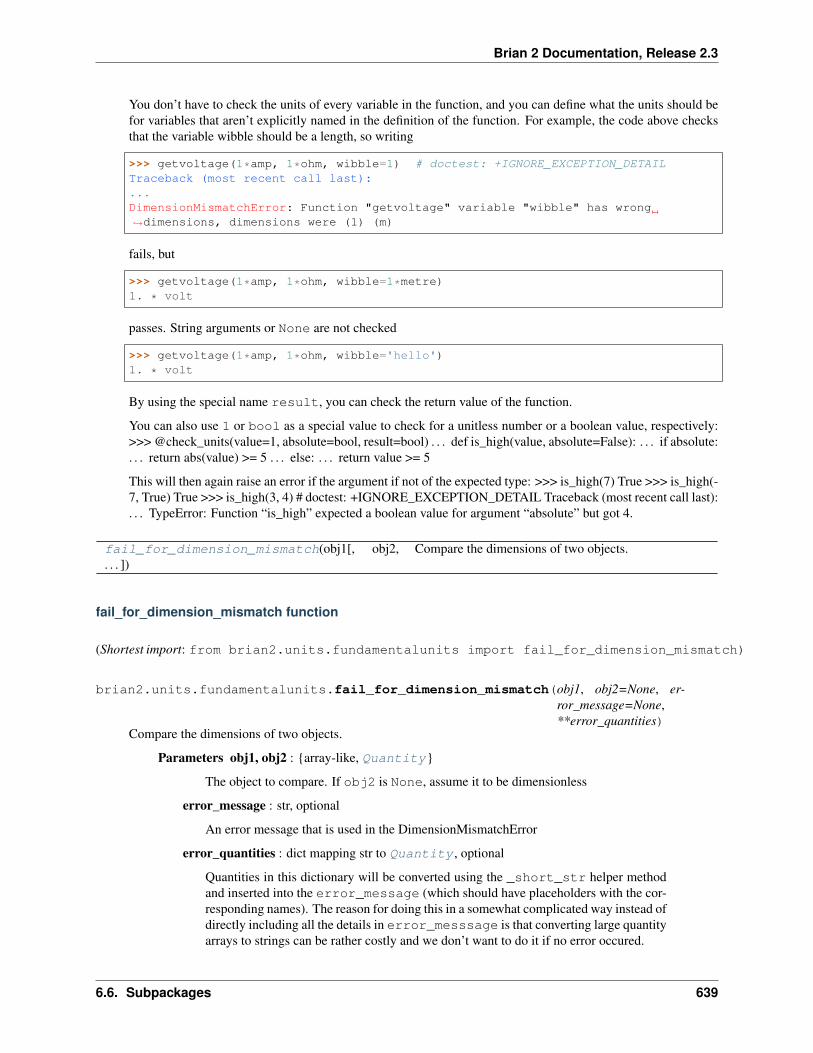
Brian 2 Documentation, Release 2.3
You don’t have to check the units of every variable in the function, and you can define what the units should befor variables that aren’t explicitly named in the definition of the function. For example, the code above checksthat the variable wibble should be a length, so writing
>>> getvoltage(1*amp, 1*ohm, wibble=1) # doctest: +IGNORE_EXCEPTION_DETAILTraceback (most recent call last):...DimensionMismatchError: Function "getvoltage" variable "wibble" has wrong→˓dimensions, dimensions were (1) (m)
fails, but
>>> getvoltage(1*amp, 1*ohm, wibble=1*metre)1. * volt
passes. String arguments or None are not checked
>>> getvoltage(1*amp, 1*ohm, wibble='hello')1. * volt
By using the special name result, you can check the return value of the function.
You can also use 1 or bool as a special value to check for a unitless number or a boolean value, respectively:>>> @check_units(value=1, absolute=bool, result=bool) . . . def is_high(value, absolute=False): . . . if absolute:. . . return abs(value) >= 5 . . . else: . . . return value >= 5
This will then again raise an error if the argument if not of the expected type: >>> is_high(7) True >>> is_high(-7, True) True >>> is_high(3, 4) # doctest: +IGNORE_EXCEPTION_DETAIL Traceback (most recent call last):. . . TypeError: Function “is_high” expected a boolean value for argument “absolute” but got 4.
fail_for_dimension_mismatch(obj1[, obj2,. . . ])
Compare the dimensions of two objects.
fail_for_dimension_mismatch function
(Shortest import: from brian2.units.fundamentalunits import fail_for_dimension_mismatch)
brian2.units.fundamentalunits.fail_for_dimension_mismatch(obj1, obj2=None, er-ror_message=None,**error_quantities)
Compare the dimensions of two objects.
Parameters obj1, obj2 : {array-like, Quantity}
The object to compare. If obj2 is None, assume it to be dimensionless
error_message : str, optional
An error message that is used in the DimensionMismatchError
error_quantities : dict mapping str to Quantity , optional
Quantities in this dictionary will be converted using the _short_str helper methodand inserted into the error_message (which should have placeholders with the cor-responding names). The reason for doing this in a somewhat complicated way instead ofdirectly including all the details in error_messsage is that converting large quantityarrays to strings can be rather costly and we don’t want to do it if no error occured.
6.6. Subpackages 639
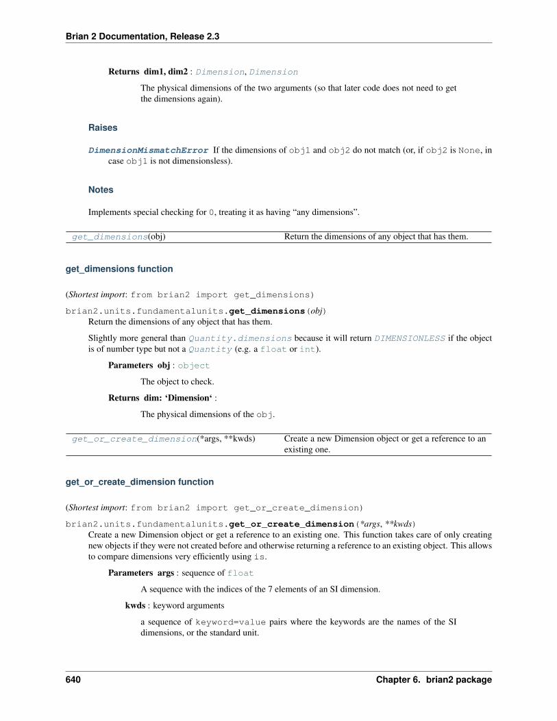
Brian 2 Documentation, Release 2.3
Returns dim1, dim2 : Dimension, Dimension
The physical dimensions of the two arguments (so that later code does not need to getthe dimensions again).
Raises
DimensionMismatchError If the dimensions of obj1 and obj2 do not match (or, if obj2 is None, incase obj1 is not dimensionsless).
Notes
Implements special checking for 0, treating it as having “any dimensions”.
get_dimensions(obj) Return the dimensions of any object that has them.
get_dimensions function
(Shortest import: from brian2 import get_dimensions)
brian2.units.fundamentalunits.get_dimensions(obj)Return the dimensions of any object that has them.
Slightly more general than Quantity.dimensions because it will return DIMENSIONLESS if the objectis of number type but not a Quantity (e.g. a float or int).
Parameters obj : object
The object to check.
Returns dim: ‘Dimension‘ :
The physical dimensions of the obj.
get_or_create_dimension(*args, **kwds) Create a new Dimension object or get a reference to anexisting one.
get_or_create_dimension function
(Shortest import: from brian2 import get_or_create_dimension)
brian2.units.fundamentalunits.get_or_create_dimension(*args, **kwds)Create a new Dimension object or get a reference to an existing one. This function takes care of only creatingnew objects if they were not created before and otherwise returning a reference to an existing object. This allowsto compare dimensions very efficiently using is.
Parameters args : sequence of float
A sequence with the indices of the 7 elements of an SI dimension.
kwds : keyword arguments
a sequence of keyword=value pairs where the keywords are the names of the SIdimensions, or the standard unit.
640 Chapter 6. brian2 package

Brian 2 Documentation, Release 2.3
Notes
The 7 units are (in order):
Length, Mass, Time, Electric Current, Temperature, Quantity of Substance, Luminosity
and can be referred to either by these names or their SI unit names, e.g. length, metre, and m all refer to thesame thing here.
Examples
The following are all definitions of the dimensions of force
>>> from brian2 import *>>> get_or_create_dimension(length=1, mass=1, time=-2)metre * kilogram * second ** -2>>> get_or_create_dimension(m=1, kg=1, s=-2)metre * kilogram * second ** -2>>> get_or_create_dimension([1, 1, -2, 0, 0, 0, 0])metre * kilogram * second ** -2
get_unit(d) Find an unscaled unit (e.g.
get_unit function
(Shortest import: from brian2 import get_unit)
brian2.units.fundamentalunits.get_unit(d)Find an unscaled unit (e.g. volt but not mvolt) for a Dimension.
Parameters d : Dimension
The dimension to find a unit for.
Returns u : Unit
A registered unscaled Unit for the dimensions d, or a new Unit if no unit was found.
get_unit_for_display(d) Return a string representation of an appropriate un-scaled unit or '1' for a dimensionless quantity.
get_unit_for_display function
(Shortest import: from brian2.units.fundamentalunits import get_unit_for_display)
brian2.units.fundamentalunits.get_unit_for_display(d)Return a string representation of an appropriate unscaled unit or '1' for a dimensionless quantity.
Parameters d : Dimension
The dimension to find a unit for.
Returns s : str
A string representation of the respective unit or the string '1'.
6.6. Subpackages 641

Brian 2 Documentation, Release 2.3
have_same_dimensions(obj1, obj2) Test if two values have the same dimensions.
have_same_dimensions function
(Shortest import: from brian2 import have_same_dimensions)
brian2.units.fundamentalunits.have_same_dimensions(obj1, obj2)Test if two values have the same dimensions.
Parameters obj1, obj2 : {Quantity , array-like, number}
The values of which to compare the dimensions.
Returns same : bool
True if obj1 and obj2 have the same dimensions.
in_best_unit(x[, precision]) Represent the value in the “best” unit.
in_best_unit function
(Shortest import: from brian2 import in_best_unit)
brian2.units.fundamentalunits.in_best_unit(x, precision=None)Represent the value in the “best” unit.
Parameters x : {Quantity , array-like, number}
The value to display
precision : int, optional
The number of digits of precision (in the best unit, see Examples). If no value is given,numpy’s get_printoptions() value is used.
Returns representation : str
A string representation of this Quantity .
See also:
Quantity.in_best_unit()
Examples
>>> from brian2.units import *>>> in_best_unit(0.00123456 * volt)'1.23456 mV'>>> in_best_unit(0.00123456 * volt, 2)'1.23 mV'>>> in_best_unit(0.123456)'0.123456'>>> in_best_unit(0.123456, 2)'0.12'
642 Chapter 6. brian2 package
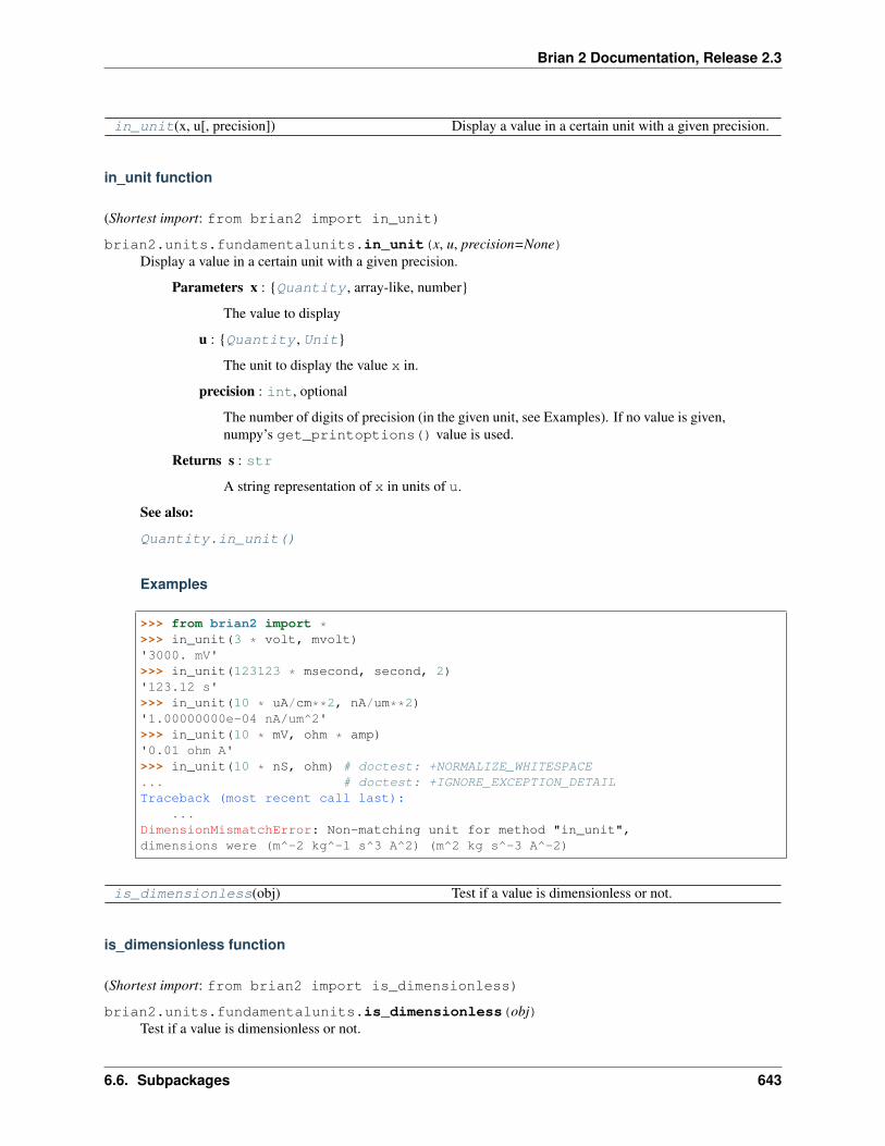
Brian 2 Documentation, Release 2.3
in_unit(x, u[, precision]) Display a value in a certain unit with a given precision.
in_unit function
(Shortest import: from brian2 import in_unit)
brian2.units.fundamentalunits.in_unit(x, u, precision=None)Display a value in a certain unit with a given precision.
Parameters x : {Quantity , array-like, number}
The value to display
u : {Quantity , Unit}
The unit to display the value x in.
precision : int, optional
The number of digits of precision (in the given unit, see Examples). If no value is given,numpy’s get_printoptions() value is used.
Returns s : str
A string representation of x in units of u.
See also:
Quantity.in_unit()
Examples
>>> from brian2 import *>>> in_unit(3 * volt, mvolt)'3000. mV'>>> in_unit(123123 * msecond, second, 2)'123.12 s'>>> in_unit(10 * uA/cm**2, nA/um**2)'1.00000000e-04 nA/um^2'>>> in_unit(10 * mV, ohm * amp)'0.01 ohm A'>>> in_unit(10 * nS, ohm) # doctest: +NORMALIZE_WHITESPACE... # doctest: +IGNORE_EXCEPTION_DETAILTraceback (most recent call last):
...DimensionMismatchError: Non-matching unit for method "in_unit",dimensions were (m^-2 kg^-1 s^3 A^2) (m^2 kg s^-3 A^-2)
is_dimensionless(obj) Test if a value is dimensionless or not.
is_dimensionless function
(Shortest import: from brian2 import is_dimensionless)
brian2.units.fundamentalunits.is_dimensionless(obj)Test if a value is dimensionless or not.
6.6. Subpackages 643
Brian 2 Documentation, Release 2.3
Parameters obj : object
The object to check.
Returns dimensionless : bool
True if obj is dimensionless.
is_scalar_type(obj) Tells you if the object is a 1d number type.
is_scalar_type function
(Shortest import: from brian2 import is_scalar_type)
brian2.units.fundamentalunits.is_scalar_type(obj)Tells you if the object is a 1d number type.
Parameters obj : object
The object to check.
Returns scalar : bool
True if obj is a scalar that can be interpreted as a dimensionless Quantity .
quantity_with_dimensions(floatval, dims) Create a new Quantity with the given dimensions.
quantity_with_dimensions function
(Shortest import: from brian2.units.fundamentalunits import quantity_with_dimensions)
brian2.units.fundamentalunits.quantity_with_dimensions(floatval, dims)Create a new Quantity with the given dimensions. Calls get_or_create_dimensionswith the dimen-sion tuple of the dims argument to make sure that unpickling (which calls this function) does not accidentallycreate new Dimension objects which should instead refer to existing ones.
Parameters floatval : float
The floating point value of the quantity.
dims : Dimension
The physical dimensions of the quantity.
Returns q : Quantity
A quantity with the given dimensions.
See also:
get_or_create_dimensions
Examples
>>> from brian2 import *>>> quantity_with_dimensions(0.001, volt.dim)1. * mvolt
644 Chapter 6. brian2 package
Brian 2 Documentation, Release 2.3
register_new_unit(u) Register a new unit for automatic displaying of quanti-ties
register_new_unit function
(Shortest import: from brian2 import register_new_unit)
brian2.units.fundamentalunits.register_new_unit(u)Register a new unit for automatic displaying of quantities
Parameters u : Unit
The unit that should be registered.
Examples
>>> from brian2 import *>>> 2.0*farad/metre**22. * metre ** -4 * kilogram ** -1 * second ** 4 * amp ** 2>>> register_new_unit(pfarad / mmetre**2)>>> 2.0*farad/metre**22000000. * pfarad / mmetre ** 2
wrap_function_change_dimensions(func,. . . )
Returns a new function that wraps the given functionfunc so that it changes the dimensions of its input.
wrap_function_change_dimensions function
(Shortest import: from brian2.units.fundamentalunits import wrap_function_change_dimensions)
brian2.units.fundamentalunits.wrap_function_change_dimensions(func,change_dim_func)
Returns a new function that wraps the given function func so that it changes the dimensions of its input.Quantities are transformed to unitless numpy arrays before calling func, the output is a quantity with theoriginal dimensions passed through the function change_dim_func. A typical use would be a sqrt functionthat uses lambda d: d ** 0.5 as change_dim_func.
These transformations apply only to the very first argument, all other arguments are ignored/untouched.
wrap_function_dimensionless(func) Returns a new function that wraps the given functionfunc so that it raises a DimensionMismatchError if thefunction is called on a quantity with dimensions (ex-cluding dimensionless quantities).
wrap_function_dimensionless function
(Shortest import: from brian2.units.fundamentalunits import wrap_function_dimensionless)
brian2.units.fundamentalunits.wrap_function_dimensionless(func)
6.6. Subpackages 645
Brian 2 Documentation, Release 2.3
Returns a new function that wraps the given function func so that it raises a DimensionMismatchError if thefunction is called on a quantity with dimensions (excluding dimensionless quantities). Quantities are trans-formed to unitless numpy arrays before calling func.
These checks/transformations apply only to the very first argument, all other arguments are ignored/untouched.
wrap_function_keep_dimensions(func) Returns a new function that wraps the given functionfunc so that it keeps the dimensions of its input.
wrap_function_keep_dimensions function
(Shortest import: from brian2.units.fundamentalunits import wrap_function_keep_dimensions)
brian2.units.fundamentalunits.wrap_function_keep_dimensions(func)Returns a new function that wraps the given function func so that it keeps the dimensions of its input. Quan-tities are transformed to unitless numpy arrays before calling func, the output is a quantity with the originaldimensions re-attached.
These transformations apply only to the very first argument, all other arguments are ignored/untouched, allowingto work functions like sum to work as expected with additional axis etc. arguments.
wrap_function_remove_dimensions(func) Returns a new function that wraps the given functionfunc so that it removes any dimensions from its input.
wrap_function_remove_dimensions function
(Shortest import: from brian2.units.fundamentalunits import wrap_function_remove_dimensions)
brian2.units.fundamentalunits.wrap_function_remove_dimensions(func)Returns a new function that wraps the given function func so that it removes any dimensions from its input.Useful for functions that are returning integers (indices) or booleans, irrespective of the datatype contained inthe array.
These transformations apply only to the very first argument, all other arguments are ignored/untouched.
Objects
DIMENSIONLESS The singleton object for dimensionless Dimensions.
DIMENSIONLESS object
(Shortest import: from brian2.units.fundamentalunits import DIMENSIONLESS)
brian2.units.fundamentalunits.DIMENSIONLESS = Dimension()The singleton object for dimensionless Dimensions.
additional_unit_register UnitRegistry containing additional units (new-ton*metre, farad / metre, . . . )
646 Chapter 6. brian2 package
Brian 2 Documentation, Release 2.3
additional_unit_register object
(Shortest import: from brian2.units.fundamentalunits import additional_unit_register)
brian2.units.fundamentalunits.additional_unit_register = <brian2.units.fundamentalunits.UnitRegistry object>UnitRegistry containing additional units (newton*metre, farad / metre, . . . )
standard_unit_register UnitRegistry containing all the standard units (me-tre, kilogram, um2. . . )
standard_unit_register object
(Shortest import: from brian2.units.fundamentalunits import standard_unit_register)
brian2.units.fundamentalunits.standard_unit_register = <brian2.units.fundamentalunits.UnitRegistry object>UnitRegistry containing all the standard units (metre, kilogram, um2. . . )
user_unit_register UnitRegistry containing all units defined by theuser
user_unit_register object
(Shortest import: from brian2.units.fundamentalunits import user_unit_register)
brian2.units.fundamentalunits.user_unit_register = <brian2.units.fundamentalunits.UnitRegistry object>UnitRegistry containing all units defined by the user
stdunits module
Optional short unit names
This module defines the following short unit names:
mV, mA, uA (micro_amp), nA, pA, mF, uF, nF, nS, mS, uS, ms, Hz, kHz, MHz, cm, cm2, cm3, mm, mm2, mm3, um,um2, um3
Exported members: mV, mA, uA, nA, pA, pF, uF, nF, nS, uS, mS, ms, us, Hz, kHz, MHz, cm, cm2, cm3, mm, mm2,mm3, um, um2, um3 . . . (3 more members)
unitsafefunctions module
Unit-aware replacements for numpy functions.
Exported members: log(), log10(), exp(), expm1(), log1p(), exprel(), sin(), cos(), tan(),arcsin(), arccos(), arctan(), sinh(), cosh(), tanh(), arcsinh(), arccosh(), arctanh(),diagonal(), ravel(), trace(), dot(), where(), ones_like(), zeros_like() . . . (2 more mem-bers)
Functions
6.6. Subpackages 647

Brian 2 Documentation, Release 2.3
arange([start,] stop[, step,][, dtype]) Return evenly spaced values within a given interval.
arange function
(Shortest import: from brian2 import arange)
brian2.units.unitsafefunctions.arange([start ], stop[, step], dtype=None)Return evenly spaced values within a given interval.
Values are generated within the half-open interval [start, stop) (in other words, the interval includingstart but excluding stop()). For integer arguments the function is equivalent to the Python built-in rangefunction, but returns an ndarray rather than a list.
When using a non-integer step, such as 0.1, the results will often not be consistent. It is better to use numpy.linspace for these cases.
Parameters start : number, optional
Start of interval. The interval includes this value. The default start value is 0.
stop : number
End of interval. The interval does not include this value, except in some cases wherestep() is not an integer and floating point round-off affects the length of out.
step : number, optional
Spacing between values. For any output out, this is the distance between two adjacentvalues, out[i+1] - out[i]. The default step size is 1. If step() is specified asa position argument, start must also be given.
dtype : dtype
The type of the output array. If dtype is not given, infer the data type from the otherinput arguments.
Returns arange : ndarray
Array of evenly spaced values.
For floating point arguments, the length of the result is ceil((stop - start)/step). Because of floating point overflow, this rule may result in the last element ofout being greater than stop().
See also:
linspace() Evenly spaced numbers with careful handling of endpoints.
ogrid Arrays of evenly spaced numbers in N-dimensions.
mgrid Grid-shaped arrays of evenly spaced numbers in N-dimensions.
Examples
>>> np.arange(3)array([0, 1, 2])>>> np.arange(3.0)array([ 0., 1., 2.])>>> np.arange(3,7)
(continues on next page)
648 Chapter 6. brian2 package

Brian 2 Documentation, Release 2.3
(continued from previous page)
array([3, 4, 5, 6])>>> np.arange(3,7,2)array([3, 5])
arccos(x, /[, out, where, casting, order, . . . ]) Trigonometric inverse cosine, element-wise.
arccos function
(Shortest import: from brian2 import arccos)
brian2.units.unitsafefunctions.arccos(x, /, out=None, *, where=True, casting=’same_kind’,order=’K’, dtype=None, subok=True[, signature, ex-tobj])
Trigonometric inverse cosine, element-wise.
The inverse of cos() so that, if y = cos(x), then x = arccos(y).
Parameters x : array_like
x-coordinate on the unit circle. For real arguments, the domain is [-1, 1].
out : ndarray, None, or tuple of ndarray and None, optional
A location into which the result is stored. If provided, it must have a shape that theinputs broadcast to. If not provided or None, a freshly-allocated array is returned. Atuple (possible only as a keyword argument) must have length equal to the number ofoutputs.
where : array_like, optional
Values of True indicate to calculate the ufunc at that position, values of False indicateto leave the value in the output alone.
**kwargs :
For other keyword-only arguments, see the ufunc docs.
Returns angle : ndarray
The angle of the ray intersecting the unit circle at the given x-coordinate in radians [0,pi]. This is a scalar if x is a scalar.
See also:
cos(), arctan(), arcsin(), emath.arccos
Notes
arccos() is a multivalued function: for each x there are infinitely many numbers z such that cos(z) = x.The convention is to return the angle z whose real part lies in [0, pi].
For real-valued input data types, arccos() always returns real output. For each value that cannot be expressedas a real number or infinity, it yields nan and sets the invalid floating point error flag.
For complex-valued input, arccos() is a complex analytic function that has branch cuts [-inf, -1] and[1, inf] and is continuous from above on the former and from below on the latter.
The inverse cos() is also known as acos or cos^-1.
6.6. Subpackages 649
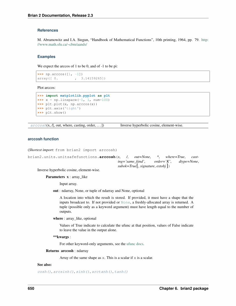
Brian 2 Documentation, Release 2.3
References
M. Abramowitz and I.A. Stegun, “Handbook of Mathematical Functions”, 10th printing, 1964, pp. 79. http://www.math.sfu.ca/~cbm/aands/
Examples
We expect the arccos of 1 to be 0, and of -1 to be pi:
>>> np.arccos([1, -1])array([ 0. , 3.14159265])
Plot arccos:
>>> import matplotlib.pyplot as plt>>> x = np.linspace(-1, 1, num=100)>>> plt.plot(x, np.arccos(x))>>> plt.axis('tight')>>> plt.show()
arccosh(x, /[, out, where, casting, order, . . . ]) Inverse hyperbolic cosine, element-wise.
arccosh function
(Shortest import: from brian2 import arccosh)
brian2.units.unitsafefunctions.arccosh(x, /, out=None, *, where=True, cast-ing=’same_kind’, order=’K’, dtype=None,subok=True[, signature, extobj])
Inverse hyperbolic cosine, element-wise.
Parameters x : array_like
Input array.
out : ndarray, None, or tuple of ndarray and None, optional
A location into which the result is stored. If provided, it must have a shape that theinputs broadcast to. If not provided or None, a freshly-allocated array is returned. Atuple (possible only as a keyword argument) must have length equal to the number ofoutputs.
where : array_like, optional
Values of True indicate to calculate the ufunc at that position, values of False indicateto leave the value in the output alone.
**kwargs :
For other keyword-only arguments, see the ufunc docs.
Returns arccosh : ndarray
Array of the same shape as x. This is a scalar if x is a scalar.
See also:
cosh(), arcsinh(), sinh(), arctanh(), tanh()
650 Chapter 6. brian2 package
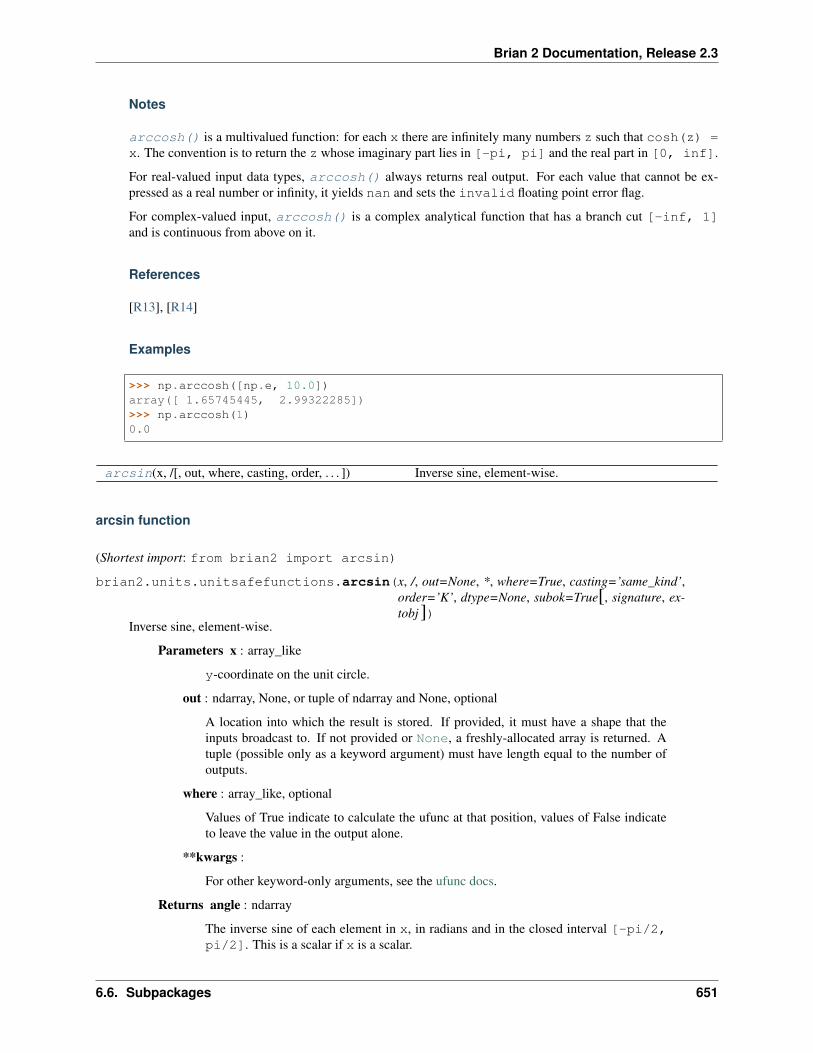
Brian 2 Documentation, Release 2.3
Notes
arccosh() is a multivalued function: for each x there are infinitely many numbers z such that cosh(z) =x. The convention is to return the z whose imaginary part lies in [-pi, pi] and the real part in [0, inf].
For real-valued input data types, arccosh() always returns real output. For each value that cannot be ex-pressed as a real number or infinity, it yields nan and sets the invalid floating point error flag.
For complex-valued input, arccosh() is a complex analytical function that has a branch cut [-inf, 1]and is continuous from above on it.
References
[R13], [R14]
Examples
>>> np.arccosh([np.e, 10.0])array([ 1.65745445, 2.99322285])>>> np.arccosh(1)0.0
arcsin(x, /[, out, where, casting, order, . . . ]) Inverse sine, element-wise.
arcsin function
(Shortest import: from brian2 import arcsin)
brian2.units.unitsafefunctions.arcsin(x, /, out=None, *, where=True, casting=’same_kind’,order=’K’, dtype=None, subok=True[, signature, ex-tobj])
Inverse sine, element-wise.
Parameters x : array_like
y-coordinate on the unit circle.
out : ndarray, None, or tuple of ndarray and None, optional
A location into which the result is stored. If provided, it must have a shape that theinputs broadcast to. If not provided or None, a freshly-allocated array is returned. Atuple (possible only as a keyword argument) must have length equal to the number ofoutputs.
where : array_like, optional
Values of True indicate to calculate the ufunc at that position, values of False indicateto leave the value in the output alone.
**kwargs :
For other keyword-only arguments, see the ufunc docs.
Returns angle : ndarray
The inverse sine of each element in x, in radians and in the closed interval [-pi/2,pi/2]. This is a scalar if x is a scalar.
6.6. Subpackages 651
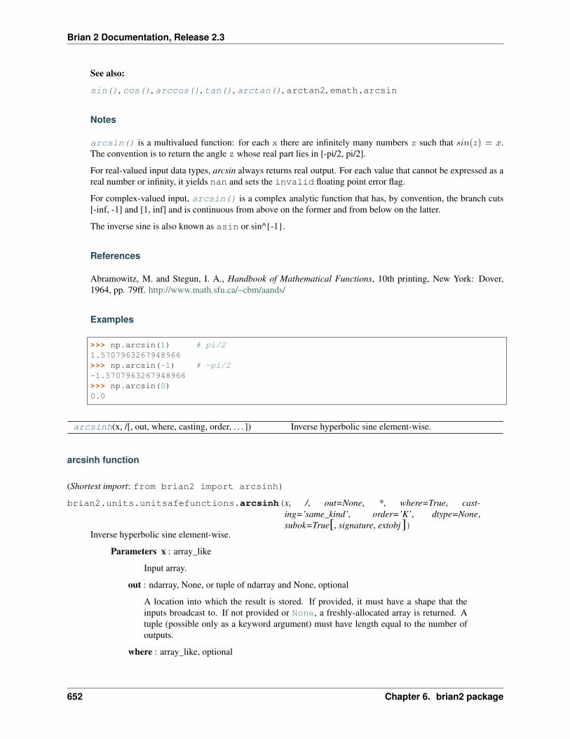
Brian 2 Documentation, Release 2.3
See also:
sin(), cos(), arccos(), tan(), arctan(), arctan2, emath.arcsin
Notes
arcsin() is a multivalued function: for each x there are infinitely many numbers z such that 𝑠𝑖𝑛(𝑧) = 𝑥.The convention is to return the angle z whose real part lies in [-pi/2, pi/2].
For real-valued input data types, arcsin always returns real output. For each value that cannot be expressed as areal number or infinity, it yields nan and sets the invalid floating point error flag.
For complex-valued input, arcsin() is a complex analytic function that has, by convention, the branch cuts[-inf, -1] and [1, inf] and is continuous from above on the former and from below on the latter.
The inverse sine is also known as asin or sin^{-1}.
References
Abramowitz, M. and Stegun, I. A., Handbook of Mathematical Functions, 10th printing, New York: Dover,1964, pp. 79ff. http://www.math.sfu.ca/~cbm/aands/
Examples
>>> np.arcsin(1) # pi/21.5707963267948966>>> np.arcsin(-1) # -pi/2-1.5707963267948966>>> np.arcsin(0)0.0
arcsinh(x, /[, out, where, casting, order, . . . ]) Inverse hyperbolic sine element-wise.
arcsinh function
(Shortest import: from brian2 import arcsinh)
brian2.units.unitsafefunctions.arcsinh(x, /, out=None, *, where=True, cast-ing=’same_kind’, order=’K’, dtype=None,subok=True[, signature, extobj])
Inverse hyperbolic sine element-wise.
Parameters x : array_like
Input array.
out : ndarray, None, or tuple of ndarray and None, optional
A location into which the result is stored. If provided, it must have a shape that theinputs broadcast to. If not provided or None, a freshly-allocated array is returned. Atuple (possible only as a keyword argument) must have length equal to the number ofoutputs.
where : array_like, optional
652 Chapter 6. brian2 package

Brian 2 Documentation, Release 2.3
Values of True indicate to calculate the ufunc at that position, values of False indicateto leave the value in the output alone.
**kwargs :
For other keyword-only arguments, see the ufunc docs.
Returns out : ndarray or scalar
Array of the same shape as x. This is a scalar if x is a scalar.
Notes
arcsinh() is a multivalued function: for each x there are infinitely many numbers z such that sinh(z) =x. The convention is to return the z whose imaginary part lies in [-pi/2, pi/2].
For real-valued input data types, arcsinh() always returns real output. For each value that cannot be ex-pressed as a real number or infinity, it returns nan and sets the invalid floating point error flag.
For complex-valued input, arccos() is a complex analytical function that has branch cuts [1j, infj] and[-1j, -infj] and is continuous from the right on the former and from the left on the latter.
The inverse hyperbolic sine is also known as asinh or sinh^-1.
References
[R15], [R16]
Examples
>>> np.arcsinh(np.array([np.e, 10.0]))array([ 1.72538256, 2.99822295])
arctan(x, /[, out, where, casting, order, . . . ]) Trigonometric inverse tangent, element-wise.
arctan function
(Shortest import: from brian2 import arctan)
brian2.units.unitsafefunctions.arctan(x, /, out=None, *, where=True, casting=’same_kind’,order=’K’, dtype=None, subok=True[, signature, ex-tobj])
Trigonometric inverse tangent, element-wise.
The inverse of tan, so that if y = tan(x) then x = arctan(y).
Parameters x : array_like
out : ndarray, None, or tuple of ndarray and None, optional
A location into which the result is stored. If provided, it must have a shape that theinputs broadcast to. If not provided or None, a freshly-allocated array is returned. Atuple (possible only as a keyword argument) must have length equal to the number ofoutputs.
where : array_like, optional
6.6. Subpackages 653
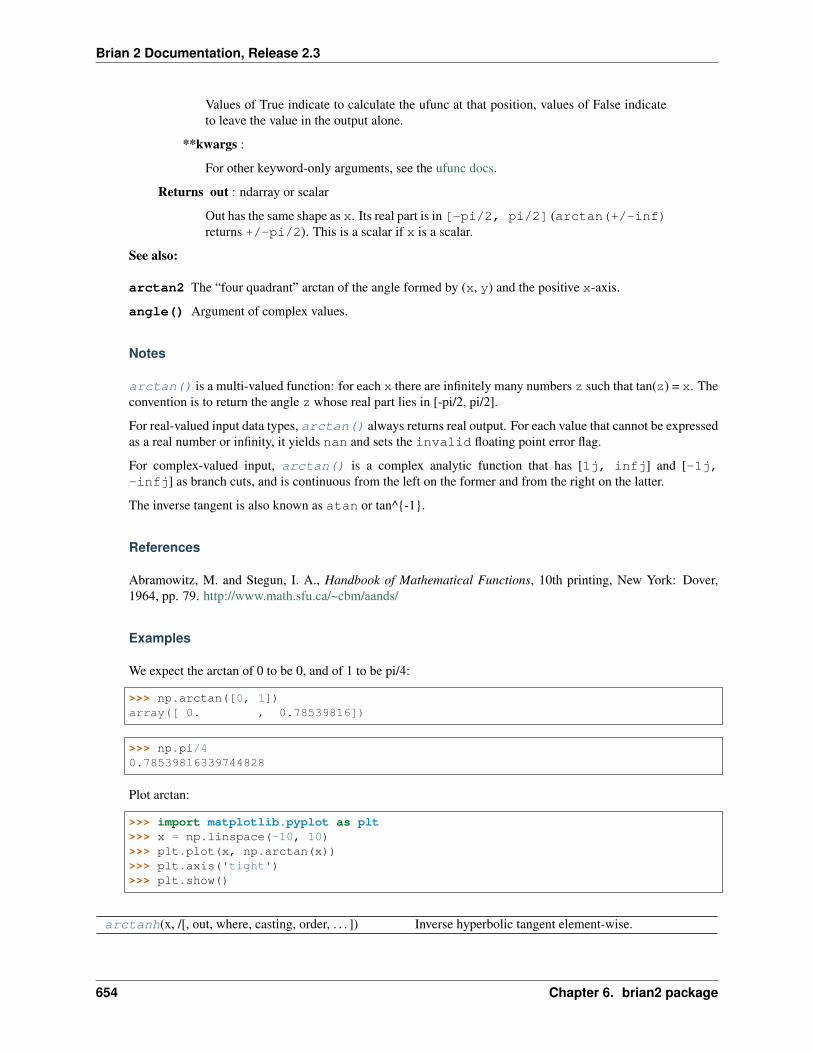
Brian 2 Documentation, Release 2.3
Values of True indicate to calculate the ufunc at that position, values of False indicateto leave the value in the output alone.
**kwargs :
For other keyword-only arguments, see the ufunc docs.
Returns out : ndarray or scalar
Out has the same shape as x. Its real part is in [-pi/2, pi/2] (arctan(+/-inf)returns +/-pi/2). This is a scalar if x is a scalar.
See also:
arctan2 The “four quadrant” arctan of the angle formed by (x, y) and the positive x-axis.
angle() Argument of complex values.
Notes
arctan() is a multi-valued function: for each x there are infinitely many numbers z such that tan(z) = x. Theconvention is to return the angle z whose real part lies in [-pi/2, pi/2].
For real-valued input data types, arctan() always returns real output. For each value that cannot be expressedas a real number or infinity, it yields nan and sets the invalid floating point error flag.
For complex-valued input, arctan() is a complex analytic function that has [1j, infj] and [-1j,-infj] as branch cuts, and is continuous from the left on the former and from the right on the latter.
The inverse tangent is also known as atan or tan^{-1}.
References
Abramowitz, M. and Stegun, I. A., Handbook of Mathematical Functions, 10th printing, New York: Dover,1964, pp. 79. http://www.math.sfu.ca/~cbm/aands/
Examples
We expect the arctan of 0 to be 0, and of 1 to be pi/4:
>>> np.arctan([0, 1])array([ 0. , 0.78539816])
>>> np.pi/40.78539816339744828
Plot arctan:
>>> import matplotlib.pyplot as plt>>> x = np.linspace(-10, 10)>>> plt.plot(x, np.arctan(x))>>> plt.axis('tight')>>> plt.show()
arctanh(x, /[, out, where, casting, order, . . . ]) Inverse hyperbolic tangent element-wise.
654 Chapter 6. brian2 package

Brian 2 Documentation, Release 2.3
arctanh function
(Shortest import: from brian2 import arctanh)
brian2.units.unitsafefunctions.arctanh(x, /, out=None, *, where=True, cast-ing=’same_kind’, order=’K’, dtype=None,subok=True[, signature, extobj])
Inverse hyperbolic tangent element-wise.
Parameters x : array_like
Input array.
out : ndarray, None, or tuple of ndarray and None, optional
A location into which the result is stored. If provided, it must have a shape that theinputs broadcast to. If not provided or None, a freshly-allocated array is returned. Atuple (possible only as a keyword argument) must have length equal to the number ofoutputs.
where : array_like, optional
Values of True indicate to calculate the ufunc at that position, values of False indicateto leave the value in the output alone.
**kwargs :
For other keyword-only arguments, see the ufunc docs.
Returns out : ndarray or scalar
Array of the same shape as x. This is a scalar if x is a scalar.
See also:
emath.arctanh
Notes
arctanh() is a multivalued function: for each x there are infinitely many numbers z such that tanh(z) =x. The convention is to return the z whose imaginary part lies in [-pi/2, pi/2].
For real-valued input data types, arctanh() always returns real output. For each value that cannot be ex-pressed as a real number or infinity, it yields nan and sets the invalid floating point error flag.
For complex-valued input, arctanh() is a complex analytical function that has branch cuts [-1, -inf]and [1, inf] and is continuous from above on the former and from below on the latter.
The inverse hyperbolic tangent is also known as atanh or tanh^-1.
References
[R17], [R18]
Examples
>>> np.arctanh([0, -0.5])array([ 0. , -0.54930614])
6.6. Subpackages 655
Brian 2 Documentation, Release 2.3
cos(x, /[, out, where, casting, order, . . . ]) Cosine element-wise.
cos function
(Shortest import: from brian2 import cos)
brian2.units.unitsafefunctions.cos(x, /, out=None, *, where=True, casting=’same_kind’, or-der=’K’, dtype=None, subok=True[, signature, extobj])
Cosine element-wise.
Parameters x : array_like
Input array in radians.
out : ndarray, None, or tuple of ndarray and None, optional
A location into which the result is stored. If provided, it must have a shape that theinputs broadcast to. If not provided or None, a freshly-allocated array is returned. Atuple (possible only as a keyword argument) must have length equal to the number ofoutputs.
where : array_like, optional
Values of True indicate to calculate the ufunc at that position, values of False indicateto leave the value in the output alone.
**kwargs :
For other keyword-only arguments, see the ufunc docs.
Returns y : ndarray
The corresponding cosine values. This is a scalar if x is a scalar.
Notes
If out is provided, the function writes the result into it, and returns a reference to out. (See Examples)
References
M. Abramowitz and I. A. Stegun, Handbook of Mathematical Functions. New York, NY: Dover, 1972.
Examples
>>> np.cos(np.array([0, np.pi/2, np.pi]))array([ 1.00000000e+00, 6.12303177e-17, -1.00000000e+00])>>>>>> # Example of providing the optional output parameter>>> out2 = np.cos([0.1], out1)>>> out2 is out1True>>>>>> # Example of ValueError due to provision of shape mis-matched `out`>>> np.cos(np.zeros((3,3)),np.zeros((2,2)))Traceback (most recent call last):
(continues on next page)
656 Chapter 6. brian2 package

Brian 2 Documentation, Release 2.3
(continued from previous page)
File "<stdin>", line 1, in <module>ValueError: operands could not be broadcast together with shapes (3,3) (2,2)
cosh(x, /[, out, where, casting, order, . . . ]) Hyperbolic cosine, element-wise.
cosh function
(Shortest import: from brian2 import cosh)
brian2.units.unitsafefunctions.cosh(x, /, out=None, *, where=True, casting=’same_kind’, or-der=’K’, dtype=None, subok=True[, signature, extobj])
Hyperbolic cosine, element-wise.
Equivalent to 1/2 * (np.exp(x) + np.exp(-x)) and np.cos(1j*x).
Parameters x : array_like
Input array.
out : ndarray, None, or tuple of ndarray and None, optional
A location into which the result is stored. If provided, it must have a shape that theinputs broadcast to. If not provided or None, a freshly-allocated array is returned. Atuple (possible only as a keyword argument) must have length equal to the number ofoutputs.
where : array_like, optional
Values of True indicate to calculate the ufunc at that position, values of False indicateto leave the value in the output alone.
**kwargs :
For other keyword-only arguments, see the ufunc docs.
Returns out : ndarray or scalar
Output array of same shape as x. This is a scalar if x is a scalar.
Examples
>>> np.cosh(0)1.0
The hyperbolic cosine describes the shape of a hanging cable:
>>> import matplotlib.pyplot as plt>>> x = np.linspace(-4, 4, 1000)>>> plt.plot(x, np.cosh(x))>>> plt.show()
diagonal(x, *args, **kwds) Return specified diagonals.
6.6. Subpackages 657
Brian 2 Documentation, Release 2.3
diagonal function
(Shortest import: from brian2 import diagonal)
brian2.units.unitsafefunctions.diagonal(x, *args, **kwds)Return specified diagonals.
If a is 2-D, returns the diagonal of a with the given offset, i.e., the collection of elements of the form a[i,i+offset]. If a has more than two dimensions, then the axes specified by axis1 and axis2 are used todetermine the 2-D sub-array whose diagonal is returned. The shape of the resulting array can be determined byremoving axis1 and axis2 and appending an index to the right equal to the size of the resulting diagonals.
In versions of NumPy prior to 1.7, this function always returned a new, independent array containing a copy ofthe values in the diagonal.
In NumPy 1.7 and 1.8, it continues to return a copy of the diagonal, but depending on this fact is deprecated.Writing to the resulting array continues to work as it used to, but a FutureWarning is issued.
Starting in NumPy 1.9 it returns a read-only view on the original array. Attempting to write to the resultingarray will produce an error.
In some future release, it will return a read/write view and writing to the returned array will alter your originalarray. The returned array will have the same type as the input array.
If you don’t write to the array returned by this function, then you can just ignore all of the above.
If you depend on the current behavior, then we suggest copying the returned array explicitly, i.e., use np.diagonal(a).copy() instead of just np.diagonal(a). This will work with both past and future ver-sions of NumPy.
Parameters a : array_like
Array from which the diagonals are taken.
offset : int, optional
Offset of the diagonal from the main diagonal. Can be positive or negative. Defaults tomain diagonal (0).
axis1 : int, optional
Axis to be used as the first axis of the 2-D sub-arrays from which the diagonals shouldbe taken. Defaults to first axis (0).
axis2 : int, optional
Axis to be used as the second axis of the 2-D sub-arrays from which the diagonalsshould be taken. Defaults to second axis (1).
Returns array_of_diagonals : ndarray
If a is 2-D, then a 1-D array containing the diagonal and of the same type as a isreturned unless a is a matrix, in which case a 1-D array rather than a (2-D) matrixis returned in order to maintain backward compatibility.
If a.ndim > 2, then the dimensions specified by axis1 and axis2 are removed,and a new axis inserted at the end corresponding to the diagonal.
Raises
ValueError If the dimension of a is less than 2.
658 Chapter 6. brian2 package

Brian 2 Documentation, Release 2.3
See also:
diag() MATLAB work-a-like for 1-D and 2-D arrays.
diagflat() Create diagonal arrays.
trace() Sum along diagonals.
Examples
>>> a = np.arange(4).reshape(2,2)>>> aarray([[0, 1],
[2, 3]])>>> a.diagonal()array([0, 3])>>> a.diagonal(1)array([1])
A 3-D example:
>>> a = np.arange(8).reshape(2,2,2); aarray([[[0, 1],
[2, 3]],[[4, 5],[6, 7]]])
>>> a.diagonal(0, # Main diagonals of two arrays created by skipping... 0, # across the outer(left)-most axis last and... 1) # the "middle" (row) axis first.array([[0, 6],
[1, 7]])
The sub-arrays whose main diagonals we just obtained; note that each corresponds to fixing the right-most(column) axis, and that the diagonals are “packed” in rows.
>>> a[:,:,0] # main diagonal is [0 6]array([[0, 2],
[4, 6]])>>> a[:,:,1] # main diagonal is [1 7]array([[1, 3],
[5, 7]])
dot(a, b[, out]) Dot product of two arrays.
dot function
(Shortest import: from brian2 import dot)
brian2.units.unitsafefunctions.dot(a, b, out=None)Dot product of two arrays. Specifically,
• If both a and b are 1-D arrays, it is inner product of vectors (without complex conjugation).
• If both a and b are 2-D arrays, it is matrix multiplication, but using matmul() or a @ b is preferred.
• If either a or b is 0-D (scalar), it is equivalent to multiply() and using numpy.multiply(a, b)
6.6. Subpackages 659

Brian 2 Documentation, Release 2.3
or a * b is preferred.
• If a is an N-D array and b is a 1-D array, it is a sum product over the last axis of a and b.
• If a is an N-D array and b is an M-D array (where M>=2), it is a sum product over the last axis of a andthe second-to-last axis of b:
dot(a, b)[i,j,k,m] = sum(a[i,j,:] * b[k,:,m])
Parameters a : array_like
First argument.
b : array_like
Second argument.
out : ndarray, optional
Output argument. This must have the exact kind that would be returned if it was notused. In particular, it must have the right type, must be C-contiguous, and its dtypemust be the dtype that would be returned for dot(a,b). This is a performance feature.Therefore, if these conditions are not met, an exception is raised, instead of attemptingto be flexible.
Returns output : ndarray
Returns the dot product of a and b. If a and b are both scalars or both 1-D arrays thena scalar is returned; otherwise an array is returned. If out is given, then it is returned.
Raises
ValueError If the last dimension of a is not the same size as the second-to-last dimension of b.
See also:
vdot Complex-conjugating dot product.
tensordot() Sum products over arbitrary axes.
einsum() Einstein summation convention.
matmul ‘@’ operator as method with out parameter.
Examples
>>> np.dot(3, 4)12
Neither argument is complex-conjugated:
>>> np.dot([2j, 3j], [2j, 3j])(-13+0j)
For 2-D arrays it is the matrix product:
660 Chapter 6. brian2 package

Brian 2 Documentation, Release 2.3
>>> a = [[1, 0], [0, 1]]>>> b = [[4, 1], [2, 2]]>>> np.dot(a, b)array([[4, 1],
[2, 2]])
>>> a = np.arange(3*4*5*6).reshape((3,4,5,6))>>> b = np.arange(3*4*5*6)[::-1].reshape((5,4,6,3))>>> np.dot(a, b)[2,3,2,1,2,2]499128>>> sum(a[2,3,2,:] * b[1,2,:,2])499128
exp(x, /[, out, where, casting, order, . . . ]) Calculate the exponential of all elements in the inputarray.
exp function
(Shortest import: from brian2 import exp)
brian2.units.unitsafefunctions.exp(x, /, out=None, *, where=True, casting=’same_kind’, or-der=’K’, dtype=None, subok=True[, signature, extobj])
Calculate the exponential of all elements in the input array.
Parameters x : array_like
Input values.
out : ndarray, None, or tuple of ndarray and None, optional
A location into which the result is stored. If provided, it must have a shape that theinputs broadcast to. If not provided or None, a freshly-allocated array is returned. Atuple (possible only as a keyword argument) must have length equal to the number ofoutputs.
where : array_like, optional
Values of True indicate to calculate the ufunc at that position, values of False indicateto leave the value in the output alone.
**kwargs :
For other keyword-only arguments, see the ufunc docs.
Returns out : ndarray or scalar
Output array, element-wise exponential of x. This is a scalar if x is a scalar.
See also:
expm1() Calculate exp(x) - 1 for all elements in the array.
exp2 Calculate 2**x for all elements in the array.
Notes
The irrational number e is also known as Euler’s number. It is approximately 2.718281, and is the base of thenatural logarithm, ln (this means that, if 𝑥 = ln 𝑦 = log𝑒 𝑦, then 𝑒𝑥 = 𝑦. For real input, exp(x) is always
6.6. Subpackages 661
Brian 2 Documentation, Release 2.3
positive.
For complex arguments, x = a + ib, we can write 𝑒𝑥 = 𝑒𝑎𝑒𝑖𝑏. The first term, 𝑒𝑎, is already known (it isthe real argument, described above). The second term, 𝑒𝑖𝑏, is cos 𝑏 + 𝑖 sin 𝑏, a function with magnitude 1 and aperiodic phase.
References
[R19], [R20]
Examples
Plot the magnitude and phase of exp(x) in the complex plane:
>>> import matplotlib.pyplot as plt
>>> x = np.linspace(-2*np.pi, 2*np.pi, 100)>>> xx = x + 1j * x[:, np.newaxis] # a + ib over complex plane>>> out = np.exp(xx)
>>> plt.subplot(121)>>> plt.imshow(np.abs(out),... extent=[-2*np.pi, 2*np.pi, -2*np.pi, 2*np.pi], cmap='gray')>>> plt.title('Magnitude of exp(x)')
>>> plt.subplot(122)>>> plt.imshow(np.angle(out),... extent=[-2*np.pi, 2*np.pi, -2*np.pi, 2*np.pi], cmap='hsv')>>> plt.title('Phase (angle) of exp(x)')>>> plt.show()
linspace(start, stop[, num, endpoint, . . . ]) Return evenly spaced numbers over a specified interval.
linspace function
(Shortest import: from brian2 import linspace)
brian2.units.unitsafefunctions.linspace(start, stop, num=50, endpoint=True, retstep=False,dtype=None)
Return evenly spaced numbers over a specified interval.
Returns num evenly spaced samples, calculated over the interval [start, stop()].
The endpoint of the interval can optionally be excluded.
Changed in version 1.16.0: Non-scalar start and stop() are now supported.
Parameters start : array_like
The starting value of the sequence.
stop : array_like
The end value of the sequence, unless endpoint is set to False. In that case, the se-quence consists of all but the last of num + 1 evenly spaced samples, so that stop()
662 Chapter 6. brian2 package
Brian 2 Documentation, Release 2.3
is excluded. Note that the step size changes when endpoint is False.
num : int, optional
Number of samples to generate. Default is 50. Must be non-negative.
endpoint : bool, optional
If True, stop() is the last sample. Otherwise, it is not included. Default is True.
retstep : bool, optional
If True, return (samples, step()), where step() is the spacing between samples.
dtype : dtype, optional
The type of the output array. If dtype is not given, infer the data type from the otherinput arguments.
New in version 1.9.0.
axis : int, optional
The axis in the result to store the samples. Relevant only if start or stop are array-like.By default (0), the samples will be along a new axis inserted at the beginning. Use -1 toget an axis at the end.
New in version 1.16.0.
Returns samples : ndarray
There are num equally spaced samples in the closed interval [start, stop] or thehalf-open interval [start, stop) (depending on whether endpoint is True orFalse).
step : float, optional
Only returned if retstep is True
Size of spacing between samples.
See also:
arange() Similar to linspace(), but uses a step size (instead of the number of samples).
geomspace() Similar to linspace(), but with numbers spaced evenly on a log scale (a geometric pro-gression).
logspace() Similar to geomspace(), but with the end points specified as logarithms.
Examples
>>> np.linspace(2.0, 3.0, num=5)array([ 2. , 2.25, 2.5 , 2.75, 3. ])>>> np.linspace(2.0, 3.0, num=5, endpoint=False)array([ 2. , 2.2, 2.4, 2.6, 2.8])>>> np.linspace(2.0, 3.0, num=5, retstep=True)(array([ 2. , 2.25, 2.5 , 2.75, 3. ]), 0.25)
Graphical illustration:
6.6. Subpackages 663
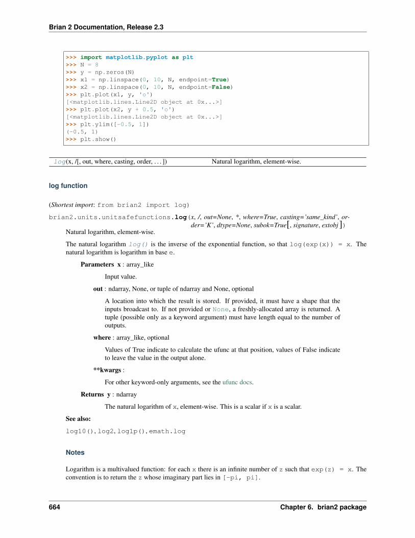
Brian 2 Documentation, Release 2.3
>>> import matplotlib.pyplot as plt>>> N = 8>>> y = np.zeros(N)>>> x1 = np.linspace(0, 10, N, endpoint=True)>>> x2 = np.linspace(0, 10, N, endpoint=False)>>> plt.plot(x1, y, 'o')[<matplotlib.lines.Line2D object at 0x...>]>>> plt.plot(x2, y + 0.5, 'o')[<matplotlib.lines.Line2D object at 0x...>]>>> plt.ylim([-0.5, 1])(-0.5, 1)>>> plt.show()
log(x, /[, out, where, casting, order, . . . ]) Natural logarithm, element-wise.
log function
(Shortest import: from brian2 import log)
brian2.units.unitsafefunctions.log(x, /, out=None, *, where=True, casting=’same_kind’, or-der=’K’, dtype=None, subok=True[, signature, extobj])
Natural logarithm, element-wise.
The natural logarithm log() is the inverse of the exponential function, so that log(exp(x)) = x. Thenatural logarithm is logarithm in base e.
Parameters x : array_like
Input value.
out : ndarray, None, or tuple of ndarray and None, optional
A location into which the result is stored. If provided, it must have a shape that theinputs broadcast to. If not provided or None, a freshly-allocated array is returned. Atuple (possible only as a keyword argument) must have length equal to the number ofoutputs.
where : array_like, optional
Values of True indicate to calculate the ufunc at that position, values of False indicateto leave the value in the output alone.
**kwargs :
For other keyword-only arguments, see the ufunc docs.
Returns y : ndarray
The natural logarithm of x, element-wise. This is a scalar if x is a scalar.
See also:
log10(), log2, log1p(), emath.log
Notes
Logarithm is a multivalued function: for each x there is an infinite number of z such that exp(z) = x. Theconvention is to return the z whose imaginary part lies in [-pi, pi].
664 Chapter 6. brian2 package
Brian 2 Documentation, Release 2.3
For real-valued input data types, log() always returns real output. For each value that cannot be expressed asa real number or infinity, it yields nan and sets the invalid floating point error flag.
For complex-valued input, log() is a complex analytical function that has a branch cut [-inf, 0] andis continuous from above on it. log() handles the floating-point negative zero as an infinitesimal negativenumber, conforming to the C99 standard.
References
[R21], [R22]
Examples
>>> np.log([1, np.e, np.e**2, 0])array([ 0., 1., 2., -Inf])
ravel(x, *args, **kwds) Return a contiguous flattened array.
ravel function
(Shortest import: from brian2 import ravel)
brian2.units.unitsafefunctions.ravel(x, *args, **kwds)Return a contiguous flattened array.
A 1-D array, containing the elements of the input, is returned. A copy is made only if needed.
As of NumPy 1.10, the returned array will have the same type as the input array. (for example, a masked arraywill be returned for a masked array input)
Parameters a : array_like
Input array. The elements in a are read in the order specified by order, and packed asa 1-D array.
order : {‘C’,’F’, ‘A’, ‘K’}, optional
The elements of a are read using this index order. ‘C’ means to index the elements inrow-major, C-style order, with the last axis index changing fastest, back to the first axisindex changing slowest. ‘F’ means to index the elements in column-major, Fortran-styleorder, with the first index changing fastest, and the last index changing slowest. Notethat the ‘C’ and ‘F’ options take no account of the memory layout of the underlyingarray, and only refer to the order of axis indexing. ‘A’ means to read the elements inFortran-like index order if a is Fortran contiguous in memory, C-like order otherwise.‘K’ means to read the elements in the order they occur in memory, except for reversingthe data when strides are negative. By default, ‘C’ index order is used.
Returns y : array_like
y is an array of the same subtype as a, with shape (a.size,). Note that matrices arespecial cased for backward compatibility, if a is a matrix, then y is a 1-D ndarray.
See also:
ndarray.flat 1-D iterator over an array.
6.6. Subpackages 665

Brian 2 Documentation, Release 2.3
ndarray.flatten 1-D array copy of the elements of an array in row-major order.
ndarray.reshape Change the shape of an array without changing its data.
Notes
In row-major, C-style order, in two dimensions, the row index varies the slowest, and the column index thequickest. This can be generalized to multiple dimensions, where row-major order implies that the index alongthe first axis varies slowest, and the index along the last quickest. The opposite holds for column-major, Fortran-style index ordering.
When a view is desired in as many cases as possible, arr.reshape(-1) may be preferable.
Examples
It is equivalent to reshape(-1, order=order).
>>> x = np.array([[1, 2, 3], [4, 5, 6]])>>> print(np.ravel(x))[1 2 3 4 5 6]
>>> print(x.reshape(-1))[1 2 3 4 5 6]
>>> print(np.ravel(x, order='F'))[1 4 2 5 3 6]
When order is ‘A’, it will preserve the array’s ‘C’ or ‘F’ ordering:
>>> print(np.ravel(x.T))[1 4 2 5 3 6]>>> print(np.ravel(x.T, order='A'))[1 2 3 4 5 6]
When order is ‘K’, it will preserve orderings that are neither ‘C’ nor ‘F’, but won’t reverse axes:
>>> a = np.arange(3)[::-1]; aarray([2, 1, 0])>>> a.ravel(order='C')array([2, 1, 0])>>> a.ravel(order='K')array([2, 1, 0])
>>> a = np.arange(12).reshape(2,3,2).swapaxes(1,2); aarray([[[ 0, 2, 4],
[ 1, 3, 5]],[[ 6, 8, 10],[ 7, 9, 11]]])
>>> a.ravel(order='C')array([ 0, 2, 4, 1, 3, 5, 6, 8, 10, 7, 9, 11])>>> a.ravel(order='K')array([ 0, 1, 2, 3, 4, 5, 6, 7, 8, 9, 10, 11])
666 Chapter 6. brian2 package

Brian 2 Documentation, Release 2.3
sin(x, /[, out, where, casting, order, . . . ]) Trigonometric sine, element-wise.
sin function
(Shortest import: from brian2 import sin)
brian2.units.unitsafefunctions.sin(x, /, out=None, *, where=True, casting=’same_kind’, or-der=’K’, dtype=None, subok=True[, signature, extobj])
Trigonometric sine, element-wise.
Parameters x : array_like
Angle, in radians (2𝜋 rad equals 360 degrees).
out : ndarray, None, or tuple of ndarray and None, optional
A location into which the result is stored. If provided, it must have a shape that theinputs broadcast to. If not provided or None, a freshly-allocated array is returned. Atuple (possible only as a keyword argument) must have length equal to the number ofoutputs.
where : array_like, optional
Values of True indicate to calculate the ufunc at that position, values of False indicateto leave the value in the output alone.
**kwargs :
For other keyword-only arguments, see the ufunc docs.
Returns y : array_like
The sine of each element of x. This is a scalar if x is a scalar.
See also:
arcsin(), sinh(), cos()
Notes
The sine is one of the fundamental functions of trigonometry (the mathematical study of triangles). Considera circle of radius 1 centered on the origin. A ray comes in from the +𝑥 axis, makes an angle at the origin(measured counter-clockwise from that axis), and departs from the origin. The 𝑦 coordinate of the outgoingray’s intersection with the unit circle is the sine of that angle. It ranges from -1 for 𝑥 = 3𝜋/2 to +1 for 𝜋/2.The function has zeroes where the angle is a multiple of 𝜋. Sines of angles between 𝜋 and 2𝜋 are negative. Thenumerous properties of the sine and related functions are included in any standard trigonometry text.
Examples
Print sine of one angle:
>>> np.sin(np.pi/2.)1.0
Print sines of an array of angles given in degrees:
>>> np.sin(np.array((0., 30., 45., 60., 90.)) * np.pi / 180. )array([ 0. , 0.5 , 0.70710678, 0.8660254 , 1. ])
6.6. Subpackages 667
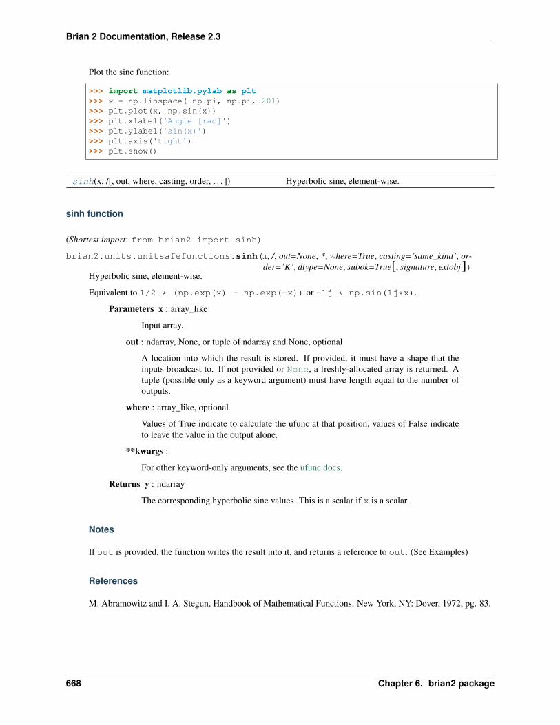
Brian 2 Documentation, Release 2.3
Plot the sine function:
>>> import matplotlib.pylab as plt>>> x = np.linspace(-np.pi, np.pi, 201)>>> plt.plot(x, np.sin(x))>>> plt.xlabel('Angle [rad]')>>> plt.ylabel('sin(x)')>>> plt.axis('tight')>>> plt.show()
sinh(x, /[, out, where, casting, order, . . . ]) Hyperbolic sine, element-wise.
sinh function
(Shortest import: from brian2 import sinh)
brian2.units.unitsafefunctions.sinh(x, /, out=None, *, where=True, casting=’same_kind’, or-der=’K’, dtype=None, subok=True[, signature, extobj])
Hyperbolic sine, element-wise.
Equivalent to 1/2 * (np.exp(x) - np.exp(-x)) or -1j * np.sin(1j*x).
Parameters x : array_like
Input array.
out : ndarray, None, or tuple of ndarray and None, optional
A location into which the result is stored. If provided, it must have a shape that theinputs broadcast to. If not provided or None, a freshly-allocated array is returned. Atuple (possible only as a keyword argument) must have length equal to the number ofoutputs.
where : array_like, optional
Values of True indicate to calculate the ufunc at that position, values of False indicateto leave the value in the output alone.
**kwargs :
For other keyword-only arguments, see the ufunc docs.
Returns y : ndarray
The corresponding hyperbolic sine values. This is a scalar if x is a scalar.
Notes
If out is provided, the function writes the result into it, and returns a reference to out. (See Examples)
References
M. Abramowitz and I. A. Stegun, Handbook of Mathematical Functions. New York, NY: Dover, 1972, pg. 83.
668 Chapter 6. brian2 package
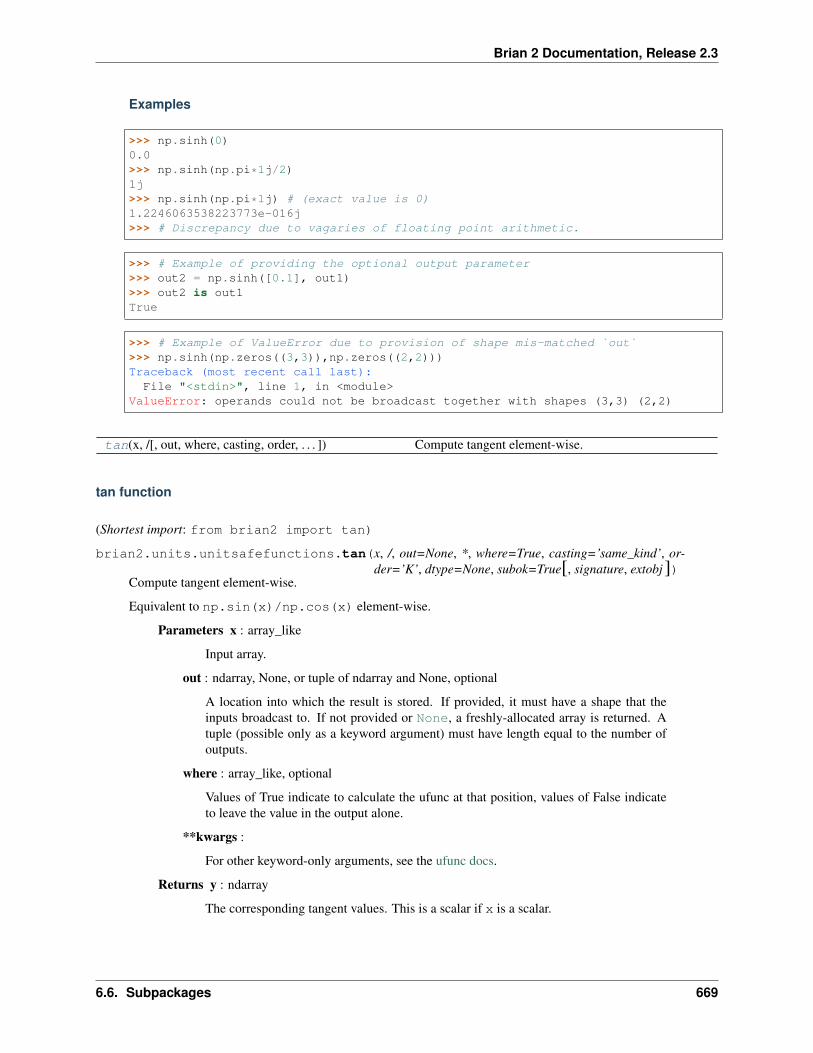
Brian 2 Documentation, Release 2.3
Examples
>>> np.sinh(0)0.0>>> np.sinh(np.pi*1j/2)1j>>> np.sinh(np.pi*1j) # (exact value is 0)1.2246063538223773e-016j>>> # Discrepancy due to vagaries of floating point arithmetic.
>>> # Example of providing the optional output parameter>>> out2 = np.sinh([0.1], out1)>>> out2 is out1True
>>> # Example of ValueError due to provision of shape mis-matched `out`>>> np.sinh(np.zeros((3,3)),np.zeros((2,2)))Traceback (most recent call last):File "<stdin>", line 1, in <module>
ValueError: operands could not be broadcast together with shapes (3,3) (2,2)
tan(x, /[, out, where, casting, order, . . . ]) Compute tangent element-wise.
tan function
(Shortest import: from brian2 import tan)
brian2.units.unitsafefunctions.tan(x, /, out=None, *, where=True, casting=’same_kind’, or-der=’K’, dtype=None, subok=True[, signature, extobj])
Compute tangent element-wise.
Equivalent to np.sin(x)/np.cos(x) element-wise.
Parameters x : array_like
Input array.
out : ndarray, None, or tuple of ndarray and None, optional
A location into which the result is stored. If provided, it must have a shape that theinputs broadcast to. If not provided or None, a freshly-allocated array is returned. Atuple (possible only as a keyword argument) must have length equal to the number ofoutputs.
where : array_like, optional
Values of True indicate to calculate the ufunc at that position, values of False indicateto leave the value in the output alone.
**kwargs :
For other keyword-only arguments, see the ufunc docs.
Returns y : ndarray
The corresponding tangent values. This is a scalar if x is a scalar.
6.6. Subpackages 669
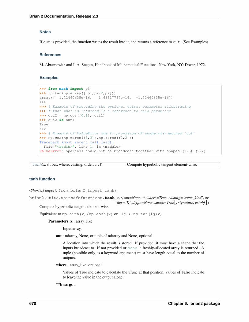
Brian 2 Documentation, Release 2.3
Notes
If out is provided, the function writes the result into it, and returns a reference to out. (See Examples)
References
M. Abramowitz and I. A. Stegun, Handbook of Mathematical Functions. New York, NY: Dover, 1972.
Examples
>>> from math import pi>>> np.tan(np.array([-pi,pi/2,pi]))array([ 1.22460635e-16, 1.63317787e+16, -1.22460635e-16])>>>>>> # Example of providing the optional output parameter illustrating>>> # that what is returned is a reference to said parameter>>> out2 = np.cos([0.1], out1)>>> out2 is out1True>>>>>> # Example of ValueError due to provision of shape mis-matched `out`>>> np.cos(np.zeros((3,3)),np.zeros((2,2)))Traceback (most recent call last):File "<stdin>", line 1, in <module>
ValueError: operands could not be broadcast together with shapes (3,3) (2,2)
tanh(x, /[, out, where, casting, order, . . . ]) Compute hyperbolic tangent element-wise.
tanh function
(Shortest import: from brian2 import tanh)
brian2.units.unitsafefunctions.tanh(x, /, out=None, *, where=True, casting=’same_kind’, or-der=’K’, dtype=None, subok=True[, signature, extobj])
Compute hyperbolic tangent element-wise.
Equivalent to np.sinh(x)/np.cosh(x) or -1j * np.tan(1j*x).
Parameters x : array_like
Input array.
out : ndarray, None, or tuple of ndarray and None, optional
A location into which the result is stored. If provided, it must have a shape that theinputs broadcast to. If not provided or None, a freshly-allocated array is returned. Atuple (possible only as a keyword argument) must have length equal to the number ofoutputs.
where : array_like, optional
Values of True indicate to calculate the ufunc at that position, values of False indicateto leave the value in the output alone.
**kwargs :
670 Chapter 6. brian2 package
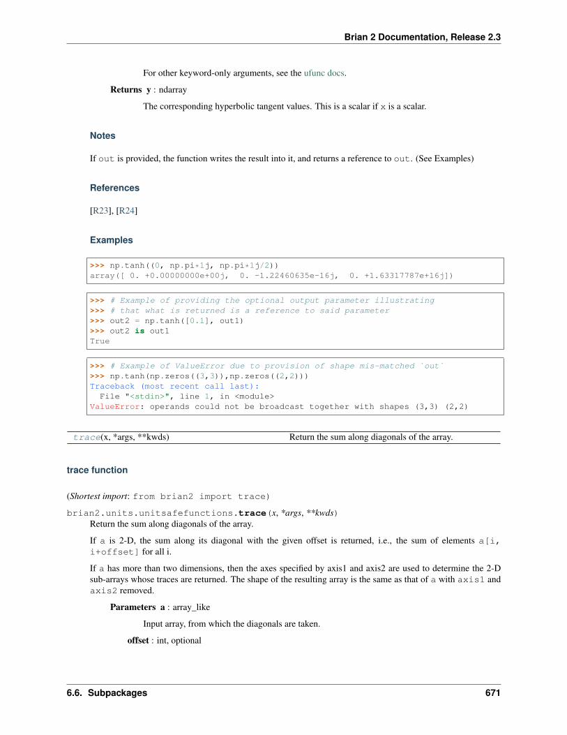
Brian 2 Documentation, Release 2.3
For other keyword-only arguments, see the ufunc docs.
Returns y : ndarray
The corresponding hyperbolic tangent values. This is a scalar if x is a scalar.
Notes
If out is provided, the function writes the result into it, and returns a reference to out. (See Examples)
References
[R23], [R24]
Examples
>>> np.tanh((0, np.pi*1j, np.pi*1j/2))array([ 0. +0.00000000e+00j, 0. -1.22460635e-16j, 0. +1.63317787e+16j])
>>> # Example of providing the optional output parameter illustrating>>> # that what is returned is a reference to said parameter>>> out2 = np.tanh([0.1], out1)>>> out2 is out1True
>>> # Example of ValueError due to provision of shape mis-matched `out`>>> np.tanh(np.zeros((3,3)),np.zeros((2,2)))Traceback (most recent call last):File "<stdin>", line 1, in <module>
ValueError: operands could not be broadcast together with shapes (3,3) (2,2)
trace(x, *args, **kwds) Return the sum along diagonals of the array.
trace function
(Shortest import: from brian2 import trace)
brian2.units.unitsafefunctions.trace(x, *args, **kwds)Return the sum along diagonals of the array.
If a is 2-D, the sum along its diagonal with the given offset is returned, i.e., the sum of elements a[i,i+offset] for all i.
If a has more than two dimensions, then the axes specified by axis1 and axis2 are used to determine the 2-Dsub-arrays whose traces are returned. The shape of the resulting array is the same as that of a with axis1 andaxis2 removed.
Parameters a : array_like
Input array, from which the diagonals are taken.
offset : int, optional
6.6. Subpackages 671
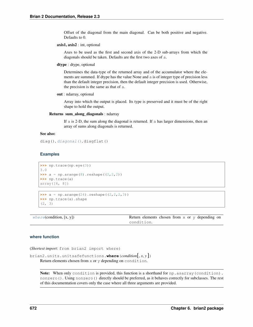
Brian 2 Documentation, Release 2.3
Offset of the diagonal from the main diagonal. Can be both positive and negative.Defaults to 0.
axis1, axis2 : int, optional
Axes to be used as the first and second axis of the 2-D sub-arrays from which thediagonals should be taken. Defaults are the first two axes of a.
dtype : dtype, optional
Determines the data-type of the returned array and of the accumulator where the ele-ments are summed. If dtype has the value None and a is of integer type of precision lessthan the default integer precision, then the default integer precision is used. Otherwise,the precision is the same as that of a.
out : ndarray, optional
Array into which the output is placed. Its type is preserved and it must be of the rightshape to hold the output.
Returns sum_along_diagonals : ndarray
If a is 2-D, the sum along the diagonal is returned. If a has larger dimensions, then anarray of sums along diagonals is returned.
See also:
diag(), diagonal(), diagflat()
Examples
>>> np.trace(np.eye(3))3.0>>> a = np.arange(8).reshape((2,2,2))>>> np.trace(a)array([6, 8])
>>> a = np.arange(24).reshape((2,2,2,3))>>> np.trace(a).shape(2, 3)
where(condition, [x, y]) Return elements chosen from x or y depending oncondition.
where function
(Shortest import: from brian2 import where)
brian2.units.unitsafefunctions.where(condition[, x, y])Return elements chosen from x or y depending on condition.
Note: When only condition is provided, this function is a shorthand for np.asarray(condition).nonzero(). Using nonzero() directly should be preferred, as it behaves correctly for subclasses. The restof this documentation covers only the case where all three arguments are provided.
672 Chapter 6. brian2 package

Brian 2 Documentation, Release 2.3
Parameters condition : array_like, bool
Where True, yield x, otherwise yield y.
x, y : array_like
Values from which to choose. x, y and condition need to be broadcastable to someshape.
Returns out : ndarray
An array with elements from x where condition is True, and elements from y else-where.
See also:
choose()
nonzero() The function that is called when x and y are omitted
Notes
If all the arrays are 1-D, where() is equivalent to:
[xv if c else yvfor c, xv, yv in zip(condition, x, y)]
Examples
>>> a = np.arange(10)>>> aarray([0, 1, 2, 3, 4, 5, 6, 7, 8, 9])>>> np.where(a < 5, a, 10*a)array([ 0, 1, 2, 3, 4, 50, 60, 70, 80, 90])
This can be used on multidimensional arrays too:
>>> np.where([[True, False], [True, True]],... [[1, 2], [3, 4]],... [[9, 8], [7, 6]])array([[1, 8],
[3, 4]])
The shapes of x, y, and the condition are broadcast together:
>>> x, y = np.ogrid[:3, :4]>>> np.where(x < y, x, 10 + y) # both x and 10+y are broadcastarray([[10, 0, 0, 0],
[10, 11, 1, 1],[10, 11, 12, 2]])
>>> a = np.array([[0, 1, 2],... [0, 2, 4],... [0, 3, 6]])>>> np.where(a < 4, a, -1) # -1 is broadcastarray([[ 0, 1, 2],
(continues on next page)
6.6. Subpackages 673

Brian 2 Documentation, Release 2.3
(continued from previous page)
[ 0, 2, -1],[ 0, 3, -1]])
wrap_function_to_method(func) Wraps a function so that it calls the correspondingmethod on the Quantities object (if called with a Quan-tities object as the first argument).
wrap_function_to_method function
(Shortest import: from brian2.units.unitsafefunctions importwrap_function_to_method)
brian2.units.unitsafefunctions.wrap_function_to_method(func)Wraps a function so that it calls the corresponding method on the Quantities object (if called with a Quantitiesobject as the first argument). All other arguments are left untouched.
6.6.16 utils package
Utility functions for Brian.
Exported members: get_logger(), BrianLogger, std_silent
arrays module
Helper module containing functions that operate on numpy arrays.
Functions
calc_repeats(delay) Calculates offsets corresponding to an array, where re-peated values are subsequently numbered, i.e.
calc_repeats function
(Shortest import: from brian2.utils.arrays import calc_repeats)
brian2.utils.arrays.calc_repeats(delay)Calculates offsets corresponding to an array, where repeated values are subsequently numbered, i.e. if theren identical values, the returned array will have values from 0 to n-1 at their positions. The code is complexbecause tricks are needed for vectorisation.
This function is used in the Python SpikeQueue to calculate the offset array for the insertion of spikes withtheir respective delays into the queue and in the numpy code for synapse creation to calculate how many synapsesfor each source-target pair exist.
Examples
>>> import numpy as np>>> print(calc_repeats(np.array([7, 5, 7, 3, 7, 5])))[0 0 1 0 2 1]
674 Chapter 6. brian2 package
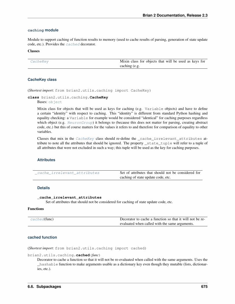
Brian 2 Documentation, Release 2.3
caching module
Module to support caching of function results to memory (used to cache results of parsing, generation of state updatecode, etc.). Provides the cached decorator.
Classes
CacheKey Mixin class for objects that will be used as keys forcaching (e.g.
CacheKey class
(Shortest import: from brian2.utils.caching import CacheKey)
class brian2.utils.caching.CacheKeyBases: object
Mixin class for objects that will be used as keys for caching (e.g. Variable objects) and have to definea certain “identity” with respect to caching. This “identity” is different from standard Python hashing andequality checking: a Variable for example would be considered “identical” for caching purposes regardlesswhich object (e.g. NeuronGroup) it belongs to (because this does not matter for parsing, creating abstractcode, etc.) but this of course matters for the values it refers to and therefore for comparison of equality to othervariables.
Classes that mix in the CacheKey class should re-define the _cache_irrelevant_attributes at-tribute to note all the attributes that should be ignored. The property _state_tuple will refer to a tuple ofall attributes that were not excluded in such a way; this tuple will be used as the key for caching purposes.
Attributes
_cache_irrelevant_attributes Set of attributes that should not be considered forcaching of state update code, etc.
Details
_cache_irrelevant_attributesSet of attributes that should not be considered for caching of state update code, etc.
Functions
cached(func) Decorator to cache a function so that it will not be re-evaluated when called with the same arguments.
cached function
(Shortest import: from brian2.utils.caching import cached)
brian2.utils.caching.cached(func)Decorator to cache a function so that it will not be re-evaluated when called with the same arguments. Uses the_hashable function to make arguments usable as a dictionary key even though they mutable (lists, dictionar-ies, etc.).
6.6. Subpackages 675
Brian 2 Documentation, Release 2.3
Parameters func : function
The function to decorate.
Returns decorated : function
The decorated function.
Notes
This is not a general-purpose caching decorator in any way comparable to functools.lru_cache orjoblib’s caching functions. It is very simplistic (no maximum cache size, no normalization of calls, e.g. foo(3)and foo(x=3) are not considered equivalent function calls) and makes very specific assumptions for our usecase. Most importantly, Variable objects are considered to be identical when they refer to the same object,even though the actually stored values might have changed.
environment module
Functions
running_from_ipython() Check whether we are currently running under ipython.
running_from_ipython function
(Shortest import: from brian2.utils.environment import running_from_ipython)
brian2.utils.environment.running_from_ipython()Check whether we are currently running under ipython.
Returns ipython : bool
Whether running under ipython or not.
filetools module
File system tools
Exported members: ensure_directory , ensure_directory_of_file, in_directory ,copy_directory
Classes
in_directory(new_dir) Safely temporarily work in a subdirectory
in_directory class
(Shortest import: from brian2.utils.filetools import in_directory)
class brian2.utils.filetools.in_directory(new_dir)Bases: object
Safely temporarily work in a subdirectory
Usage:
676 Chapter 6. brian2 package
Brian 2 Documentation, Release 2.3
with in_directory(directory):... do stuff here
Guarantees that the code in the with block will be executed in directory, and that after the block is completedwe return to the original directory.
Functions
copy_directory(source, target) Copies directory source to target.
copy_directory function
(Shortest import: from brian2.utils.filetools import copy_directory)
brian2.utils.filetools.copy_directory(source, target)Copies directory source to target.
ensure_directory(d) Ensures that a given directory exists (creates it if neces-sary)
ensure_directory function
(Shortest import: from brian2.utils.filetools import ensure_directory)
brian2.utils.filetools.ensure_directory(d)Ensures that a given directory exists (creates it if necessary)
ensure_directory_of_file(f) Ensures that a directory exists for filename to go in (cre-ates if necessary), and returns the directory path.
ensure_directory_of_file function
(Shortest import: from brian2.utils.filetools import ensure_directory_of_file)
brian2.utils.filetools.ensure_directory_of_file(f)Ensures that a directory exists for filename to go in (creates if necessary), and returns the directory path.
logger module
Brian’s logging module.
Preferences
Logging system preferences
logging.console_log_level = 'INFO'
What log level to use for the log written to the console.
Has to be one of CRITICAL, ERROR, WARNING, INFO, DEBUG or DIAGNOSTIC.
6.6. Subpackages 677
Brian 2 Documentation, Release 2.3
logging.delete_log_on_exit = True
Whether to delete the log and script file on exit.
If set to True (the default), log files (and the copy of the main script) will be deleted after the brianprocess has exited, unless an uncaught exception occured. If set to False, all log files will be kept.
logging.file_log = True
Whether to log to a file or not.
If set to True (the default), logging information will be written to a file. The log level can be set via thelogging.file_log_level preference.
logging.file_log_level = 'DIAGNOSTIC'
What log level to use for the log written to the log file.
In case file logging is activated (see logging.file_log), which log level should be used for logging. Has tobe one of CRITICAL, ERROR, WARNING, INFO, DEBUG or DIAGNOSTIC.
logging.save_script = True
Whether to save a copy of the script that is run.
If set to True (the default), a copy of the currently run script is saved to a temporary location. It isdeleted after a successful run (unless logging.delete_log_on_exit is False) but is kept after an uncaughtexception occured. This can be helpful for debugging, in particular when several simulations are runningin parallel.
logging.std_redirection = True
Whether or not to redirect stdout/stderr to null at certain places.
This silences a lot of annoying compiler output, but will also hide error messages making it harder to debugproblems. You can always temporarily switch it off when debugging. If logging.std_redirection_to_file isset to True as well, then the output is saved to a file and if an error occurs the name of this file will beprinted.
logging.std_redirection_to_file = True
Whether to redirect stdout/stderr to a file.
If both logging.std_redirection and this preference are set to True, all standard output/error(most importantly output from the compiler) will be stored in files and if an error occurs the name of thisfile will be printed. If logging.std_redirection is True and this preference is False, then all standardoutput/error will be completely suppressed, i.e. neither be displayed nor stored in a file.
The value of this preference is ignore if logging.std_redirection is set to False.
Exported members: get_logger(), BrianLogger, std_silent
Classes
BrianLogger(name) Convenience object for logging.
BrianLogger class
(Shortest import: from brian2 import BrianLogger)
class brian2.utils.logger.BrianLogger(name)Bases: object
678 Chapter 6. brian2 package

Brian 2 Documentation, Release 2.3
Convenience object for logging. Call get_logger() to get an instance of this class.
Parameters name : str
The name used for logging, normally the name of the module.
Attributes
_log_messages Class attribute for remembering log messages thatshould only be displayed once
exception_occured Class attribute to remember whether any exceptionoccured
file_handler The logging.FileHandler responsible forlogging to the temporary log file
tmp_log The name of the temporary log file (by defaultdeleted after the run if no exception occurred), if any
tmp_script The name of the temporary copy of the main scriptfile (by default deleted after the run if no exceptionoccurred), if any
Methods
debug(msg[, name_suffix, once]) Log a debug message.diagnostic(msg[, name_suffix, once]) Log a diagnostic message.error(msg[, name_suffix, once]) Log an error message.info(msg[, name_suffix, once]) Log an info message.initialize() Initialize Brian’s logging system.log_level_debug() Set the log level to “debug”.log_level_diagnostic() Set the log level to “diagnostic”.log_level_error() Set the log level to “error”.log_level_info() Set the log level to “info”.log_level_warn() Set the log level to “warn”.suppress_hierarchy(name[, filter_log_file]) Suppress all log messages in a given hiearchy.suppress_name(name[, filter_log_file]) Suppress all log messages with a given name.warn(msg[, name_suffix, once]) Log a warn message.
Details
_log_messagesClass attribute for remembering log messages that should only be displayed once
exception_occuredClass attribute to remember whether any exception occured
file_handlerThe logging.FileHandler responsible for logging to the temporary log file
tmp_logThe name of the temporary log file (by default deleted after the run if no exception occurred), if any
tmp_scriptThe name of the temporary copy of the main script file (by default deleted after the run if no exceptionoccurred), if any
6.6. Subpackages 679
Brian 2 Documentation, Release 2.3
debug(msg, name_suffix=None, once=False)Log a debug message.
Parameters msg : str
The message to log.
name_suffix : str, optional
A suffix to add to the name, e.g. a class or function name.
once : bool, optional
Whether this message should be logged only once and not repeated if sent another time.
diagnostic(msg, name_suffix=None, once=False)Log a diagnostic message.
Parameters msg : str
The message to log.
name_suffix : str, optional
A suffix to add to the name, e.g. a class or function name.
once : bool, optional
Whether this message should be logged only once and not repeated if sent another time.
error(msg, name_suffix=None, once=False)Log an error message.
Parameters msg : str
The message to log.
name_suffix : str, optional
A suffix to add to the name, e.g. a class or function name.
once : bool, optional
Whether this message should be logged only once and not repeated if sent another time.
info(msg, name_suffix=None, once=False)Log an info message.
Parameters msg : str
The message to log.
name_suffix : str, optional
A suffix to add to the name, e.g. a class or function name.
once : bool, optional
Whether this message should be logged only once and not repeated if sent another time.
static initialize()Initialize Brian’s logging system. This function will be called automatically when Brian is imported.
static log_level_debug()Set the log level to “debug”.
static log_level_diagnostic()Set the log level to “diagnostic”.
680 Chapter 6. brian2 package
Brian 2 Documentation, Release 2.3
static log_level_error()Set the log level to “error”.
static log_level_info()Set the log level to “info”.
static log_level_warn()Set the log level to “warn”.
static suppress_hierarchy(name, filter_log_file=False)Suppress all log messages in a given hiearchy.
Parameters name : str
Suppress all log messages in the given name hierarchy. For example, specify-ing 'brian2' suppresses all messages logged by Brian, specifying 'brian2.codegen' suppresses all messages generated by the code generation modules.
filter_log_file : bool, optional
Whether to suppress the messages also in the log file. Defaults to False meaning thatsuppressed messages are not displayed on the console but are still saved to the log file.
static suppress_name(name, filter_log_file=False)Suppress all log messages with a given name.
Parameters name : str
Suppress all log messages ending in the given name. For example,specifying 'resolution_conflict' would suppress messages withnames such as brian2.equations.codestrings.CodeString.resolution_conflict or brian2.equations.equations.Equations.resolution_conflict.
filter_log_file : bool, optional
Whether to suppress the messages also in the log file. Defaults to False meaning thatsuppressed messages are not displayed on the console but are still saved to the log file.
warn(msg, name_suffix=None, once=False)Log a warn message.
Parameters msg : str
The message to log.
name_suffix : str, optional
A suffix to add to the name, e.g. a class or function name.
once : bool, optional
Whether this message should be logged only once and not repeated if sent another time.
Tutorials and examples using this
• Example frompapers/Rossant_et_al_2011bis
HierarchyFilter(name) A class for suppressing all log messages in a subtree ofthe name hierarchy.
6.6. Subpackages 681
Brian 2 Documentation, Release 2.3
HierarchyFilter class
(Shortest import: from brian2.utils.logger import HierarchyFilter)
class brian2.utils.logger.HierarchyFilter(name)Bases: object
A class for suppressing all log messages in a subtree of the name hierarchy. Does exactly the opposite as thelogging.Filter class, which allows messages in a certain name hierarchy to pass.
Parameters name : str
The name hiearchy to suppress. See BrianLogger.suppress_hierarchy fordetails.
Methods
filter(record) Filter out all messages in a subtree of the name hier-archy.
Details
filter(record)Filter out all messages in a subtree of the name hierarchy.
LogCapture(log_list[, log_level]) A class for capturing log warnings.
LogCapture class
(Shortest import: from brian2.utils.logger import LogCapture)
class brian2.utils.logger.LogCapture(log_list, log_level=30)Bases: logging.Handler
A class for capturing log warnings. This class is used by catch_logs to allow testing in a similar way as withwarnings.catch_warnings.
Methods
emit(record) Do whatever it takes to actually log the specified log-ging record.
install() Install this handler to catch all warnings.uninstall() Uninstall this handler and re-connect the previously
installed handlers.
Details
emit(record)Do whatever it takes to actually log the specified logging record.
This version is intended to be implemented by subclasses and so raises a NotImplementedError.
682 Chapter 6. brian2 package

Brian 2 Documentation, Release 2.3
install()Install this handler to catch all warnings. Temporarily disconnect all other handlers.
uninstall()Uninstall this handler and re-connect the previously installed handlers.
NameFilter(name) A class for suppressing log messages ending with a cer-tain name.
NameFilter class
(Shortest import: from brian2.utils.logger import NameFilter)
class brian2.utils.logger.NameFilter(name)Bases: object
A class for suppressing log messages ending with a certain name.
Parameters name : str
The name to suppress. See BrianLogger.suppress_name for details.
Methods
filter(record) Filter out all messages ending with a certain name.
Details
filter(record)Filter out all messages ending with a certain name.
catch_logs([log_level]) A context manager for catching log messages.
catch_logs class
(Shortest import: from brian2.utils.logger import catch_logs)
class brian2.utils.logger.catch_logs(log_level=30)Bases: object
A context manager for catching log messages. Use this for testing the messages that are logged. Defaults tocatching warning/error messages and this is probably the only real use case for testing. Note that while thiscontext manager is active, all log messages are suppressed. Using this context manager returns a list of (loglevel, name, message) tuples.
Parameters log_level : int or str, optional
The log level above which messages are caught.
6.6. Subpackages 683

Brian 2 Documentation, Release 2.3
Examples
>>> logger = get_logger('brian2.logtest')>>> logger.warn('An uncaught warning') # doctest: +SKIPWARNING brian2.logtest: An uncaught warning>>> with catch_logs() as l:... logger.warn('a caught warning')... print('l contains: %s' % l)...l contains: [('WARNING', 'brian2.logtest', 'a caught warning')]
std_silent([alwaysprint]) Context manager that temporarily silences stdout andstderr but keeps the output saved in a temporary file andwrites it if an exception is raised.
std_silent class
(Shortest import: from brian2 import std_silent)
class brian2.utils.logger.std_silent(alwaysprint=False)Bases: object
Context manager that temporarily silences stdout and stderr but keeps the output saved in a temporary file andwrites it if an exception is raised.
Attributes
dest_stderrdest_stdout
Methods
close()
Details
dest_stderr = None
dest_stdout = None
classmethod close()
Functions
brian_excepthook(exc_type, exc_obj, exc_tb) Display a message mentioning the debug log in case ofan uncaught exception.
brian_excepthook function
(Shortest import: from brian2.utils.logger import brian_excepthook)
684 Chapter 6. brian2 package

Brian 2 Documentation, Release 2.3
brian2.utils.logger.brian_excepthook(exc_type, exc_obj, exc_tb)Display a message mentioning the debug log in case of an uncaught exception.
clean_up_logging() Shutdown the logging system and delete the debug logfile if no error occured.
clean_up_logging function
(Shortest import: from brian2.utils.logger import clean_up_logging)
brian2.utils.logger.clean_up_logging()Shutdown the logging system and delete the debug log file if no error occured.
get_logger([module_name]) Get an object that can be used for logging.
get_logger function
(Shortest import: from brian2 import get_logger)
brian2.utils.logger.get_logger(module_name=’brian2’)Get an object that can be used for logging.
Parameters module_name : str
The name used for logging, should normally be the module name as returned by__name__.
Returns logger : BrianLogger
log_level_validator(log_level)
log_level_validator function
(Shortest import: from brian2.utils.logger import log_level_validator)
brian2.utils.logger.log_level_validator(log_level)
stringtools module
Exported members: indent, deindent, word_substitute, replace,get_identifiers, strip_empty_lines, stripped_deindented_lines,strip_empty_leading_and_trailing_lines, code_representation, SpellChecker
Classes
SpellChecker(words[, alphabet]) A simple spell checker that will be used to suggest thecorrect name if the user made a typo (e.g.
6.6. Subpackages 685
Brian 2 Documentation, Release 2.3
SpellChecker class
(Shortest import: from brian2.utils.stringtools import SpellChecker)
class brian2.utils.stringtools.SpellChecker(words, alpha-bet=’abcdefghijklmnopqrstuvwxyz0123456789_’)
Bases: object
A simple spell checker that will be used to suggest the correct name if the user made a typo (e.g. for statevariable names).
Parameters words : iterable of str
The known words
alphabet : iterable of str, optional
The allowed characters. Defaults to the characters allowed for identifiers, i.e. asciicharacters, digits and the underscore.
Methods
edits1(word)known(words)known_edits2(word)suggest(word)
Details
edits1(word)
known(words)
known_edits2(word)
suggest(word)
Functions
code_representation(code) Returns a string representation for several different for-mats of code
code_representation function
(Shortest import: from brian2.utils.stringtools import code_representation)
brian2.utils.stringtools.code_representation(code)Returns a string representation for several different formats of code
Formats covered include: - A single string - A list of statements/strings - A dict of strings - A dict of lists ofstatements/strings
deindent(text[, numtabs, spacespertab, . . . ]) Returns a copy of the string with the common indenta-tion removed.
686 Chapter 6. brian2 package
Brian 2 Documentation, Release 2.3
deindent function
(Shortest import: from brian2.utils.stringtools import deindent)
brian2.utils.stringtools.deindent(text, numtabs=None, spacespertab=4, docstring=False)Returns a copy of the string with the common indentation removed.
Note that all tab characters are replaced with spacespertab spaces.
If the docstring flag is set, the first line is treated differently and is assumed to be already correctly tabulated.
If the numtabs option is given, the amount of indentation to remove is given explicitly and not the commonindentation.
Examples
Normal strings, e.g. function definitions:
>>> multiline = """ def f(x):... return x**2""">>> print(multiline)
def f(x):return x**2
>>> print(deindent(multiline))def f(x):
return x**2>>> print(deindent(multiline, docstring=True))
def f(x):return x**2>>> print(deindent(multiline, numtabs=1, spacespertab=2))def f(x):
return x**2
Docstrings:
>>> docstring = """First docstring line.... This line determines the indentation.""">>> print(docstring)First docstring line.
This line determines the indentation.>>> print(deindent(docstring, docstring=True))First docstring line.This line determines the indentation.
get_identifiers(expr[, include_numbers]) Return all the identifiers in a given string expr, that iseverything that matches a programming language vari-able like expression, which is here implemented as theregexp \b[A-Za-z_][A-Za-z0-9_]*\b.
get_identifiers function
(Shortest import: from brian2.utils.stringtools import get_identifiers)
brian2.utils.stringtools.get_identifiers(expr, include_numbers=False)Return all the identifiers in a given string expr, that is everything that matches a programming language variable
6.6. Subpackages 687
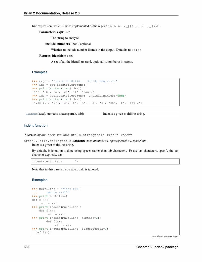
Brian 2 Documentation, Release 2.3
like expression, which is here implemented as the regexp \b[A-Za-z_][A-Za-z0-9_]*\b.
Parameters expr : str
The string to analyze
include_numbers : bool, optional
Whether to include number literals in the output. Defaults to False.
Returns identifiers : set
A set of all the identifiers (and, optionally, numbers) in expr.
Examples
>>> expr = '3-a*_b+c5+8+f(A - .3e-10, tau_2)*17'>>> ids = get_identifiers(expr)>>> print(sorted(list(ids)))['A', '_b', 'a', 'c5', 'f', 'tau_2']>>> ids = get_identifiers(expr, include_numbers=True)>>> print(sorted(list(ids)))['.3e-10', '17', '3', '8', 'A', '_b', 'a', 'c5', 'f', 'tau_2']
indent(text[, numtabs, spacespertab, tab]) Indents a given multiline string.
indent function
(Shortest import: from brian2.utils.stringtools import indent)
brian2.utils.stringtools.indent(text, numtabs=1, spacespertab=4, tab=None)Indents a given multiline string.
By default, indentation is done using spaces rather than tab characters. To use tab characters, specify the tabcharacter explictly, e.g.:
indent(text, tab=' ')
Note that in this case spacespertab is ignored.
Examples
>>> multiline = """def f(x):... return x*x""">>> print(multiline)def f(x):
return x*x>>> print(indent(multiline))
def f(x):return x*x
>>> print(indent(multiline, numtabs=2))def f(x):
return x*x>>> print(indent(multiline, spacespertab=2))def f(x):
(continues on next page)
688 Chapter 6. brian2 package
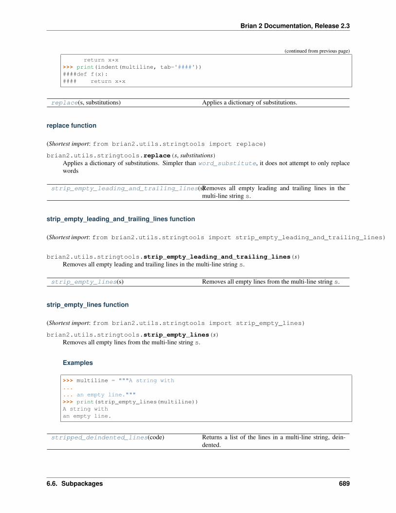
Brian 2 Documentation, Release 2.3
(continued from previous page)
return x*x>>> print(indent(multiline, tab='####'))####def f(x):#### return x*x
replace(s, substitutions) Applies a dictionary of substitutions.
replace function
(Shortest import: from brian2.utils.stringtools import replace)
brian2.utils.stringtools.replace(s, substitutions)Applies a dictionary of substitutions. Simpler than word_substitute, it does not attempt to only replacewords
strip_empty_leading_and_trailing_lines(s)Removes all empty leading and trailing lines in themulti-line string s.
strip_empty_leading_and_trailing_lines function
(Shortest import: from brian2.utils.stringtools import strip_empty_leading_and_trailing_lines)
brian2.utils.stringtools.strip_empty_leading_and_trailing_lines(s)Removes all empty leading and trailing lines in the multi-line string s.
strip_empty_lines(s) Removes all empty lines from the multi-line string s.
strip_empty_lines function
(Shortest import: from brian2.utils.stringtools import strip_empty_lines)
brian2.utils.stringtools.strip_empty_lines(s)Removes all empty lines from the multi-line string s.
Examples
>>> multiline = """A string with...... an empty line.""">>> print(strip_empty_lines(multiline))A string withan empty line.
stripped_deindented_lines(code) Returns a list of the lines in a multi-line string, dein-dented.
6.6. Subpackages 689

Brian 2 Documentation, Release 2.3
stripped_deindented_lines function
(Shortest import: from brian2.utils.stringtools import stripped_deindented_lines)
brian2.utils.stringtools.stripped_deindented_lines(code)Returns a list of the lines in a multi-line string, deindented.
word_substitute(expr, substitutions) Applies a dict of word substitutions.
word_substitute function
(Shortest import: from brian2.utils.stringtools import word_substitute)
brian2.utils.stringtools.word_substitute(expr, substitutions)Applies a dict of word substitutions.
The dict substitutions consists of pairs (word, rep) where each word word appearing in expr isreplaced by rep. Here a ‘word’ means anything matching the regexp \bword\b.
Examples
>>> expr = 'a*_b+c5+8+f(A)'>>> print(word_substitute(expr, {'a':'banana', 'f':'func'}))banana*_b+c5+8+func(A)
topsort module
Exported members: topsort
Functions
topsort(graph) Topologically sort a graph
topsort function
(Shortest import: from brian2.utils.topsort import topsort)
brian2.utils.topsort.topsort(graph)Topologically sort a graph
The graph should be of the form {node: [list of nodes], ...}.
690 Chapter 6. brian2 package
CHAPTER 7
Developer’s guide
This section is intended as a guide to how Brian functions internally for people developing Brian itself, or extensionsto Brian. It may also be of some interest to others wishing to better understand how Brian works internally.
7.1 Coding guidelines
The basic principles of developing Brian are:
1. For the user, the emphasis is on making the package flexible, readable and easy to use. See the paper “The Briansimulator” in Frontiers in Neuroscience for more details.
2. For the developer, the emphasis is on keeping the package maintainable by a small number of people. To thisend, we use stable, well maintained, existing open source packages whenever possible, rather than writing ourown code.
7.1.1 Development workflow
Brian development is done in a git repository on github. Continuous integration testing is provided by travis CI, codecoverage is measured with coveralls.io.
The repository structure
Brian’s repository structure is very simple, as we are normally not supporting older versions with bugfixes or othercomplicated things. The master branch of the repository is the basis for releases, a release is nothing more than addinga tag to the branch, creating the tarball, etc. The master branch should always be in a deployable state, i.e. one shouldbe able to use it as the base for everyday work without worrying about random breakages due to updates. To ensurethis, no commit ever goes into the master branch without passing the test suite before (see below). The only exceptionto this rule is if a commit not touches any code files, e.g. additions to the README file or to the documentation (buteven in this case, care should be taken that the documentation is still built correctly).
For every feature that a developer works on, a new branch should be opened (normally based on the master branch),with a descriptive name (e.g. add-numba-support). For developers that are members of “brian-team”, the branch
691

Brian 2 Documentation, Release 2.3
should ideally be created in the main repository. This way, one can easily get an overview over what the “core team”is currently working on. Developers who are not members of the team should fork the repository and work in theirown repository (if working on multiple issues/features, also using branches).
Implementing a feature/fixing a bug
Every new feature or bug fix should be done in a dedicated branch and have an issue in the issue database. For bugs,it is important to not only fix the bug but also to introduce a new test case (see Testing) that makes sure that the bugwill not ever be reintroduced by other changes. It is often a good idea to first define the test cases (that should fail)and then work on the fix so that the tests pass. As soon as the feature/fix is complete or as soon as specific feedbackon the code is needed, open a “pull request” to merge the changes from your branch into master. In this pull request,others can comment on the code and make suggestions for improvements. New commits to the respective branchautomatically appear in the pull request which makes it a great tool for iterative code review. Even more useful, traviswill automatically run the test suite on the result of the merge. As a reviewer, always wait for the result of this test (itcan take up to 30 minutes or so until it appears) before doing the merge and never merge when a test fails. As soonas the reviewer (someone from the core team and not the author of the feature/fix) decides that the branch is readyto merge, he/she can merge the pull request and optionally delete the corresponding branch (but it will be hidden bydefault, anyway).
Useful links
• The Brian repository: https://github.com/brian-team/brian2
• Travis testing for Brian: https://travis-ci.org/brian-team/brian2
• Code Coverage for Brian: https://coveralls.io/github/brian-team/brian2
• The Pro Git book: https://git-scm.com/book/en/v2
• github’s documentation on pull requests: https://help.github.com/articles/using-pull-requests
7.1.2 Coding conventions
General recommendations
Syntax is chosen as much as possible from the user point of view, to reflect the concepts as directly as possible. Ideally,a Brian script should be readable by someone who doesn’t know Python or Brian, although this isn’t always possible.Function, class and keyword argument names should be explicit rather than abbreviated and consistent across Brian.See Romain’s paper On the design of script languages for neural simulators for a discussion.
We use the PEP-8 coding conventions for our code. This in particular includes the following conventions:
• Use 4 spaces instead of tabs per indentation level
• Use spaces after commas and around the following binary operators: assignment (=), augmented assignment(+=, -= etc.), comparisons (==, <, >, !=, <>, <=, >=, in, not in, is, is not), Booleans (and, or, not).
• Do not use spaces around the equals sign in keyword arguments or when specifying default values. Neither putspaces immediately inside parentheses, brackets or braces, immediately before the open parenthesis that startsthe argument list of a function call, or immediately before the open parenthesis that starts an indexing or slicing.
• Avoid using a backslash for continuing lines whenever possible, instead use Python’s implicit line joining insideparentheses, brackets and braces.
• The core code should only contain ASCII characters, no encoding has to be declared
692 Chapter 7. Developer’s guide
Brian 2 Documentation, Release 2.3
• imports should be on different lines (e.g. do not use import sys, os) and should be grouped in the follow-ing order, using blank lines between each group:
1. standard library imports
2. third-party library imports (e.g. numpy, scipy, sympy, . . . )
3. brian imports
• Use absolute imports for everything outside of “your” package, e.g. if you are working in brian2.equations, import functions from the stringtools modules via from brian2.utils.stringtoolsimport .... Use the full path when importing, e.g. do from brian2.units.fundamentalunitsimport seconds instead of from brian2 import seconds.
• Use “new-style” relative imports for everything in “your” package, e.g. in brian2.codegen.functions.py import the Function class as from .specifiers import Function.
• Do not use wildcard imports (from brian2 import *), instead import only the identifiers you need, e.g.from brian2 import NeuronGroup, Synapses. For packages like numpy that are used a lot, useimport numpy as np. But note that the user should still be able to do something like from brian2import * (and this style can also be freely used in examples and tests, for example). Modules always have touse the __all__ mechanism to specify what is being made available with a wildcard import. As an exceptionfrom this rule, the main brian2/__init__.py may use wildcard imports.
Python 2 vs. Python 3
Brian is written in Python 2 but runs on Python 3 using the 2to3 conversion tool (which is automatically applied ifBrian is installed using the standard python setup.py install mechanism). To make this possible withouttoo much effort, Brian no longer supports Python 2.5 and can therefore make use of a couple of forward-compatible(but backward-incompatible) idioms introduced in Python 2.6. The Porting to Python 3 book is available online andhas a lot of information on these topics. Here are some things to keep in mind when developing Brian:
• If you are working with integers and using division, consider using // for flooring division (default behaviourfor / in python 2) and switch the behaviour of / to floating point division by using from __future__import division .
• If importing modules from the standard library (which have changed quite a bit from Python 2 to Python 3), onlyuse simple import statements like import itertools instead of from itertools import izip –2to3 is otherwise unable to make the correct conversion.
• If you are using the print statement (which should only occur in tests, in particular doctests – always use theLogging framework if you want to present messages to the user otherwise), try “cheating” and use the functionalstyle in Python 2, i.e. write print('some text') instead of print 'some text'. More complicatedprint statements should be avoided, e.g instead of print >>sys.stderr, 'Error message use sys.stderr.write('Error message\n') (or, again, use logging).
• Exception stacktraces look a bit different in Python 2 and 3: For non-standard exceptions, Python 2 only printsthe Exception class name (e.g. DimensionMismatchError) whereas Python 3 prints the name includ-ing the module name (e.g. brian2.units.fundamentalunits.DimensionMismatchError). Thiswill make doctests fail that match the exception message. In this case, write the doctest in the style of Python2 but add the doctest directive #doctest: +IGNORE_EXCEPTION_DETAIL to the statement leading tothe exception. This unfortunately has the side effect of also ignoring the text of the exception, but it will still failfor an incorrect exception type.
• If you write code reading and writing strings to files, make sure you make the distinction between bytes andunicode (see “separate binary data and strings” ) In general, strings within Brian are unicode strings and onlyconverted to bytes when reading from or writing to a file (or something like a network stream, for example).
• If you are sorting lists or dictionaries, have a look at “when sorting, use key instead of cmp”
7.1. Coding guidelines 693

Brian 2 Documentation, Release 2.3
• Make sure to define a __hash__ function for objects that define an __eq__ function (and to define it consis-tently). Python 3 is more strict about this, an object with __eq__ but without __hash__ is unhashable.
7.1.3 Representing Brian objects
__repr__ and __str__
Every class should specify or inherit useful __repr__ and __str__ methods. The __repr__ method shouldgive the “official” representation of the object; if possible, this should be a valid Python expression, ideally allowingfor eval(repr(x)) == x. The __str__ method on the other hand, gives an “informal” representation of theobject. This can be anything that is helpful but does not have to be Python code. For example:
>>> import numpy as np>>> ar = np.array([1, 2, 3]) * mV>>> print(ar) # uses __str__[ 1. 2. 3.] mV>>> ar # uses __repr__array([ 1., 2., 3.]) * mvolt
If the representation returned by __repr__ is not Python code, it should be enclosed in <...>, e.g. a Synapsesrepresentation might be <Synapses object with 64 synapses>.
If you don’t want to make the distinction between __repr__ and __str__, simply define only a __repr__function, it will be used instead of __str__ automatically (no need to write __str__ = __repr__). Finally,if you include the class name in the representation (which you should in most cases), use self.__class__.__name__ instead of spelling out the name explicitly – this way it will automatically work correctly for subclasses.It will also prevent you from forgetting to update the class name in the representation if you decide to rename the class.
LaTeX representations with sympy
Brian objects dealing with mathematical expressions and equations often internally use sympy. Sympy’s latexfunction does a nice job of converting expressions into LaTeX code, using fractions, root symbols, etc. as well asconverting greek variable names into corresponding symbols and handling sub- and superscripts. For the conversionof variable names to work, they should use an underscore for subscripts and two underscores for superscripts:
>>> from sympy import latex, Symbol>>> tau_1__e = Symbol('tau_1__e')>>> print(latex(tau_1__e))\tau^{e}_{1}
Sympy’s printer supports formatting arbitrary objects, all they have to do is to implement a _latex method (notrailing underscore). For most Brian objects, this is unnecessary as they will never be formatted with sympy’s LaTeXprinter. For some core objects, in particular the units, is is useful, however, as it can be reused in LaTeX representationsfor ipython (see below). Note that the _latex method should not return $ or \begin{equation} (sympy’smethod includes a mode argument that wraps the output automatically).
Representations for ipython
“Old” ipython console
In particular for representations involing arrays or lists, it can be useful to break up the representation into chunks, orindent parts of the representation. This is supported by the ipython console’s “pretty printer”. To make this work for
694 Chapter 7. Developer’s guide

Brian 2 Documentation, Release 2.3
a class, add a _repr_pretty_(self, p, cycle) (note the single underscores) method. You can find moreinformation in the ipython documentation .
“New” ipython console (qtconsole and notebook)
The new ipython consoles, the qtconsole and the ipython notebook support a much richer set of representationsfor objects. As Brian deals a lot with mathematical objects, in particular the LaTeX and to a lesser extent theHTML formatting capabilities of the ipython notebook are interesting. To support LaTeX representation, implementa _repr_latex_ method returning the LaTeX code (including $, \begin{equation} or similar). If the objectalready has a _latex method (see LaTeX representations with sympy above), this can be as simple as:
def _repr_latex_(self):return sympy.latex(self, mode='inline') # wraps the expression in $ .. $
The LaTeX rendering only supports a single mathematical block. For complex objects, e.g. NeuronGroup it mightbe useful to have a richer representation. This can be achieved by returning HTML code from _repr_html_ – thisHTML code is processed by MathJax so it can include literal LaTeX code that will be transformed before it is renderedas HTML. An object containing two equations could therefore be represented with a method like this:
def _repr_html_(self):return '''<h3> Equation 1 </h3>{eq_1}<h3> Equation 2 </h3>{eq_2}'''.format(eq_1=sympy.latex(self.eq_1, mode='equation'),
eq_2=sympy.latex(self.eq_2, mode='equation'))
7.1.4 Defensive programming
One idea for Brian 2 is to make it so that it’s more likely that errors are raised rather than silently causing weird bugs.Some ideas in this line:
Synapses.source should be stored internally as a weakref Synapses._source, and Synapses.source should be a com-puted attribute that dereferences this weakref. Like this, if the source object isn’t kept by the user, Synapses won’tstore a reference to it, and so won’t stop it from being deallocated.
We should write an automated test that takes a piece of correct code like:
NeuronGroup(N, eqs, reset='V>Vt')
and tries replacing all arguments by nonsense arguments, it should always raise an error in this case (forcing us towrite code to validate the inputs). For example, you could create a new NonsenseObject class, and do this:
nonsense = NonsenseObject()NeuronGroup(nonsense, eqs, reset='V>Vt')NeuronGroup(N, nonsense, reset='V>Vt')NeuronGroup(N, eqs, nonsense)
In general, the idea should be to make it hard for something incorrect to run without raising an error, preferably at thepoint where the user makes the error and not in some obscure way several lines later.
The preferred way to validate inputs is one that handles types in a Pythonic way. For example, instead of doingsomething like:
7.1. Coding guidelines 695
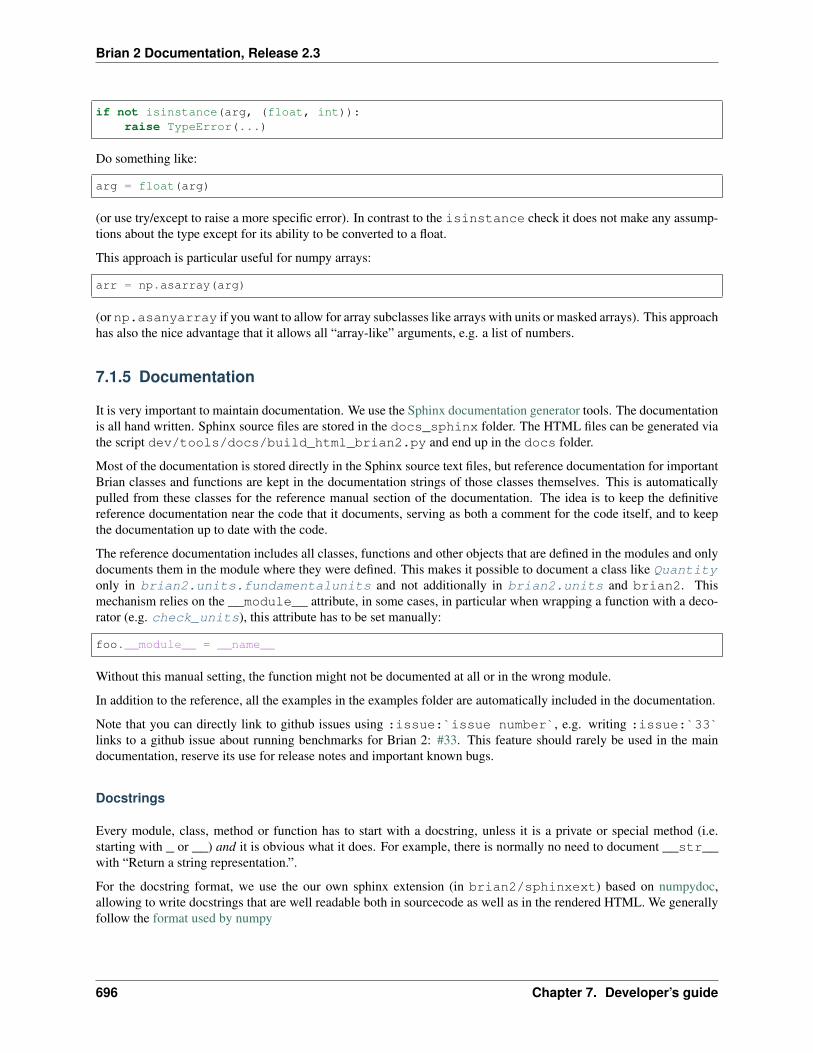
Brian 2 Documentation, Release 2.3
if not isinstance(arg, (float, int)):raise TypeError(...)
Do something like:
arg = float(arg)
(or use try/except to raise a more specific error). In contrast to the isinstance check it does not make any assump-tions about the type except for its ability to be converted to a float.
This approach is particular useful for numpy arrays:
arr = np.asarray(arg)
(or np.asanyarray if you want to allow for array subclasses like arrays with units or masked arrays). This approachhas also the nice advantage that it allows all “array-like” arguments, e.g. a list of numbers.
7.1.5 Documentation
It is very important to maintain documentation. We use the Sphinx documentation generator tools. The documentationis all hand written. Sphinx source files are stored in the docs_sphinx folder. The HTML files can be generated viathe script dev/tools/docs/build_html_brian2.py and end up in the docs folder.
Most of the documentation is stored directly in the Sphinx source text files, but reference documentation for importantBrian classes and functions are kept in the documentation strings of those classes themselves. This is automaticallypulled from these classes for the reference manual section of the documentation. The idea is to keep the definitivereference documentation near the code that it documents, serving as both a comment for the code itself, and to keepthe documentation up to date with the code.
The reference documentation includes all classes, functions and other objects that are defined in the modules and onlydocuments them in the module where they were defined. This makes it possible to document a class like Quantityonly in brian2.units.fundamentalunits and not additionally in brian2.units and brian2. Thismechanism relies on the __module__ attribute, in some cases, in particular when wrapping a function with a deco-rator (e.g. check_units), this attribute has to be set manually:
foo.__module__ = __name__
Without this manual setting, the function might not be documented at all or in the wrong module.
In addition to the reference, all the examples in the examples folder are automatically included in the documentation.
Note that you can directly link to github issues using :issue:`issue number`, e.g. writing :issue:`33`links to a github issue about running benchmarks for Brian 2: #33. This feature should rarely be used in the maindocumentation, reserve its use for release notes and important known bugs.
Docstrings
Every module, class, method or function has to start with a docstring, unless it is a private or special method (i.e.starting with _ or __) and it is obvious what it does. For example, there is normally no need to document __str__with “Return a string representation.”.
For the docstring format, we use the our own sphinx extension (in brian2/sphinxext) based on numpydoc,allowing to write docstrings that are well readable both in sourcecode as well as in the rendered HTML. We generallyfollow the format used by numpy
696 Chapter 7. Developer’s guide

Brian 2 Documentation, Release 2.3
When the docstring uses variable, class or function names, these should be enclosed in single backticks. Class andfunction/method names will be automatically linked to the corresponding documentation. For classes imported inthe main brian2 package, you do not have to add the package name, e.g. writing `NeuronGroup` is enough. Forother classes, you have to give the full path, e.g. `brian2.units.fundamentalunits.UnitRegistry`.If it is clear from the context where the class is (e.g. within the documentation of UnitRegistry), consider usingthe ~ abbreviation: `~brian2.units.fundamentalunits.UnitRegistry` displays only the class name:UnitRegistry . Note that you do not have to enclose the exception name in a “Raises” or “Warns” section, or theclass/method/function name in a “See Also” section in backticks, they will be automatically linked (putting backticksthere will lead to incorrect display or an error message),
Inline source fragments should be enclosed in double backticks.
Class docstrings follow the same conventions as method docstrings and should document the __init__ method, the__init__ method itself does not need a docstring.
Documenting functions and methods
The docstring for a function/method should start with a one-line description of what the function does, without re-ferring to the function name or the names of variables. Use a “command style” for this summary, e.g. “Return theresult.” instead of “Returns the result.” If the signature of the function cannot be automatically extracted because ofan decorator (e.g. check_units()), place a signature in the very first row of the docstring, before the one-linedescription.
For methods, do not document the self parameter, nor give information about the method being static or a classmethod (this information will be automatically added to the documentation).
Documenting classes
Class docstrings should use the same “Parameters” and “Returns” sections as method and function docstrings fordocumenting the __init__ constructor. If a class docstring does not have any “Attributes” or “Methods” section,these sections will be automatically generated with all documented (i.e. having a docstring), public (i.e. not startingwith _) attributes respectively methods of the class. Alternatively, you can provide these sections manually. This isuseful for example in the Quantity class, which would otherwise include the documentation of many ndarraymethods, or when you want to include documentation for functions like __getitem__ which would otherwise notbe documented. When specifying these sections, you only have to state the names of documented methods/attributesbut you can also provide direct documentation. For example:
Attributes----------foobarbaz
This is a description.
This can be used for example for class or instance attributes which do not have “classical” docstrings. However, youcan also use a special syntax: When defining class attributes in the class body or instance attributes in __init__ youcan use the following variants (here shown for instance attributes):
def __init__(a, b, c):#: The docstring for the instance attribute a.#: Can also span multiple linesself.a = a
self.b = b #: The docstring for self.b (only one line).
(continues on next page)
7.1. Coding guidelines 697

Brian 2 Documentation, Release 2.3
(continued from previous page)
self.c = c'The docstring for self.c, directly *after* its definition'
Long example of a function docstring
This is a very long docstring, showing all the possible sections. Most of the time no See Also, Notes or Referencessection is needed:
def foo(var1, var2, long_var_name='hi') :"""A one-line summary that does not use variable names or the function name.
Several sentences providing an extended description. Refer tovariables using back-ticks, e.g. `var1`.
Parameters----------var1 : array_like
Array_like means all those objects -- lists, nested lists, etc. --that can be converted to an array. We can also refer tovariables like `var1`.
var2 : intThe type above can either refer to an actual Python type(e.g. ``int``), or describe the type of the variable in moredetail, e.g. ``(N,) ndarray`` or ``array_like``.
Long_variable_name : {'hi', 'ho'}, optionalChoices in brackets, default first when optional.
Returns-------describe : type
Explanationoutput : type
Explanationtuple : type
Explanationitems : type
even more explaining
Raises------BadException
Because you shouldn't have done that.
See Also--------otherfunc : relationship (optional)newfunc : Relationship (optional), which could be fairly long, in which
case the line wraps here.thirdfunc, fourthfunc, fifthfunc
Notes-----Notes about the implementation algorithm (if needed).
(continues on next page)
698 Chapter 7. Developer’s guide

Brian 2 Documentation, Release 2.3
(continued from previous page)
This can have multiple paragraphs.
You may include some math:
.. math:: X(e^{j\omega } ) = x(n)e^{ - j\omega n}
And even use a greek symbol like :math:`omega` inline.
References----------Cite the relevant literature, e.g. [1]_. You may also cite thesereferences in the notes section above.
.. [1] O. McNoleg, "The integration of GIS, remote sensing,expert systems and adaptive co-kriging for environmental habitatmodelling of the Highland Haggis using object-oriented, fuzzy-logicand neural-network techniques," Computers & Geosciences, vol. 22,pp. 585-588, 1996.
Examples--------These are written in doctest format, and should illustrate how touse the function.
>>> a=[1,2,3]>>> print([x + 3 for x in a])[4, 5, 6]>>> print("a\nb")ab
"""
pass
7.1.6 Logging
For a description of logging from the users point of view, see Logging.
Logging in Brian is based on the logging module in Python’s standard library.
Every brian module that needs logging should start with the following line, using the get_logger() function toget an instance of BrianLogger:
logger = get_logger(__name__)
In the code, logging can then be done via:
logger.diagnostic('A diagnostic message')logger.debug('A debug message')logger.info('An info message')logger.warn('A warning message')logger.error('An error message')
If a module logs similar messages in different places or if it might be useful to be able to suppress a subset of messages
7.1. Coding guidelines 699

Brian 2 Documentation, Release 2.3
in a module, add an additional specifier to the logging command, specifying the class or function name, or a methodname including the class name (do not include the module name, it will be automatically added as a prefix):
logger.debug('A debug message', 'CodeString')logger.debug('A debug message', 'NeuronGroup.update')logger.debug('A debug message', 'reinit')
If you want to log a message only once, e.g. in a function that is called repeatedly, set the optional once keyword toTrue:
logger.debug('Will only be shown once', once=True)logger.debug('Will only be shown once', once=True)
The output of debugging looks like this in the log file:
2012-10-02 14:41:41,484 DEBUG brian2.equations.equations.CodeString: A debug→˓message
and like this on the console (if the log level is set to “debug”):
DEBUG A debug message [brian2.equations.equations.CodeString]
Log level recommendations
diagnostic Low-level messages that are not of any interest to the normal user but useful for debugging Brian itself. Atypical example is the source code generated by the code generation module.
debug Messages that are possibly helpful for debugging the user’s code. For example, this shows which objects wereincluded in the network, which clocks the network uses and when simulations start and stop.
info Messages which are not strictly necessary, but are potentially helpful for the user. In particular, this will showmessages about the chosen state updater and other information that might help the user to achieve better per-formance and/or accuracy in the simulations (e.g. using (event-driven) in synaptic equations, avoidingincompatible dt values between TimedArray and the NeuronGroup using it, . . . )
warn Messages that alert the user to a potential mistake in the code, e.g. two possible solutions for an identifier in anequation. It can also be used to make the user aware that he/she is using an experimental feature, an unsupportedcompiler or similar. In this case, normally the once=True option should be used to raise this warning onlyonce. As a rule of thumb, “common” scripts like the examples provided in the examples folder should normallynot lead to any warnings.
error This log level is not used currently in Brian, an exception should be raised instead. It might be useful in“meta-code”, running scripts and catching any errors that occur.
The default log level shown to the user is info. As a general rule, all messages that the user sees in the de-fault configuration (i.e., info and warn level) should be avoidable by simple changes in the user code, e.g. therenaming of variables, explicitly specifying a state updater instead of relying on the automatic system, adding(clock-driven)/(event-driven) to synaptic equations, etc.
Testing log messages
It is possible to test whether code emits an expected log message using the catch_logs context manager. Thisis normally not necessary for debug and info messages, but should be part of the unit tests for warning messages(catch_logs by default only catches warning and error messages):
700 Chapter 7. Developer’s guide
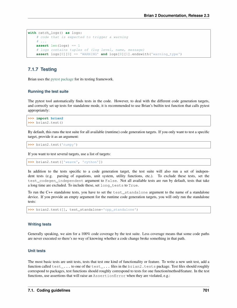
Brian 2 Documentation, Release 2.3
with catch_logs() as logs:# code that is expected to trigger a warning# ...assert len(logs) == 1# logs contains tuples of (log level, name, message)assert logs[0][0] == 'WARNING' and logs[0][1].endswith('warning_type')
7.1.7 Testing
Brian uses the pytest package for its testing framework.
Running the test suite
The pytest tool automatically finds tests in the code. However, to deal with the different code generation targets,and correctly set up tests for standalone mode, it is recommended to use Brian’s builtin test function that calls pytestappropriately:
>>> import brian2>>> brian2.test()
By default, this runs the test suite for all available (runtime) code generation targets. If you only want to test a specifictarget, provide it as an argument:
>>> brian2.test('numpy')
If you want to test several targets, use a list of targets:
>>> brian2.test(['weave', 'cython'])
In addition to the tests specific to a code generation target, the test suite will also run a set of indepen-dent tests (e.g. parsing of equations, unit system, utility functions, etc.). To exclude these tests, set thetest_codegen_independent argument to False. Not all available tests are run by default, tests that takea long time are excluded. To include these, set long_tests to True.
To run the C++ standalone tests, you have to set the test_standalone argument to the name of a standalonedevice. If you provide an empty argument for the runtime code generation targets, you will only run the standalonetests:
>>> brian2.test([], test_standalone='cpp_standalone')
Writing tests
Generally speaking, we aim for a 100% code coverage by the test suite. Less coverage means that some code pathsare never executed so there’s no way of knowing whether a code change broke something in that path.
Unit tests
The most basic tests are unit tests, tests that test one kind of functionality or feature. To write a new unit test, add afunction called test_... to one of the test_... files in the brian2.tests package. Test files should roughlycorrespond to packages, test functions should roughly correspond to tests for one function/method/feature. In the testfunctions, use assertions that will raise an AssertionError when they are violated, e.g.:
7.1. Coding guidelines 701

Brian 2 Documentation, Release 2.3
G = NeuronGroup(42, model='dv/dt = -v / (10*ms) : 1')assert len(G) == 42
When comparing arrays, use the array_equal() function from numpy.testing.utils which takes care ofcomparing types, shapes and content and gives a nicer error message in case the assertion fails. Never make testsdepend on external factors like random numbers – tests should always give the same result when run on the samecodebase. You should not only test the expected outcome for the correct use of functions and classes but also thaterrors are raised when expected. For that you can use pytest’s raises function with which you can define a block ofcode that should raise an exception of a certain type:
with pytest.raises(DimensionMismatchError):3*volt + 5*second
You can also check whether expected warnings are raised, see the documentation of the logging mechanism for details
For simple functions, doctests (see below) are a great alternative to writing classical unit tests.
By default, all tests are executed for all selected runtime code generation targets (see Running the test suite above).This is not useful for all tests, some basic tests that for example test equation syntax or the use of physical units donot depend on code generation and need therefore not to be repeated. To execute such tests only once, they can beannotated with a codegen_independent marker, using the mark decorator:
import pytestfrom brian2 import NeuronGroup
@pytest.mark.codegen_independentdef test_simple():
# Test that the length of a NeuronGroup is correctgroup = NeuronGroup(5, '')assert len(group) == 5
Tests that are not “codegen-independent” are by default only executed for the runtimes device, i.e. not for thecpp_standalone device, for example. However, many of those tests follow a common pattern that is com-patible with standalone devices as well: they set up a network, run it, and check the state of the network after-wards. Such tests can be marked as standalone_compatible, using the mark decorator in the same way as forcodegen_independent tests.:
import pytestfrom numpy.testing.utils import assert_equalfrom brian2 import *
@pytest.mark.standalone_compatibledef test_simple_run():
# Check that parameter values of a neuron don't change after a rungroup = NeuronGroup(5, 'v : volt')group.v = 'i*mV'run(1*ms)assert_equal(group.v[:], np.arange(5)*mV)
Tests that have more than a single run function but are otherwise compatible with standalone mode (e.g. they don’tneed access to the number of synapses or results of the simulation before the end of the simulation), can be marked asstandalone_compatible and multiple_runs. They then have to use an explicit device.build(...)call of the form shown below:
import pytestfrom numpy.testing.utils import assert_equalfrom brian2 import *
(continues on next page)
702 Chapter 7. Developer’s guide
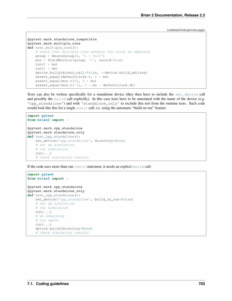
Brian 2 Documentation, Release 2.3
(continued from previous page)
@[email protected]_runsdef test_multiple_runs():
# Check that multiple runs advance the clock as expectedgroup = NeuronGroup(5, 'v : volt')mon = StateMonitor(group, 'v', record=True)run(1 * ms)run(1 * ms)device.build(direct_call=False, **device.build_options)assert_equal(defaultclock.t, 2 * ms)assert_equal(mon.t[0], 0 * ms)assert_equal(mon.t[-1], 2 * ms - defaultclock.dt)
Tests can also be written specifically for a standalone device (they then have to include the set_device calland possibly the build call explicitly). In this case tests have to be annotated with the name of the device (e.g.'cpp_standalone') and with 'standalone_only' to exclude this test from the runtime tests. Such codewould look like this for a single run() call, i.e. using the automatic “build on run” feature:
import pytestfrom brian2 import *
@[email protected]_onlydef test_cpp_standalone():
set_device('cpp_standalone', directory=None)# set up simulation# run simulationrun(...)# check simulation results
If the code uses more than one run() statement, it needs an explicit build call:
import pytestfrom brian2 import *
@[email protected]_onlydef test_cpp_standalone():
set_device('cpp_standalone', build_on_run=False)# set up simulation# run simulationrun(...)# do something# run againrun(...)device.build(directory=None)# check simulation results
7.1. Coding guidelines 703

Brian 2 Documentation, Release 2.3
Summary
@pytest.mark marker Executed fordevices
explicit use of device
codegen_independent independent ofdevices
none
none Runtime tar-gets
none
standalone_compatible Runtime andstandalone
none
standalone_compatible,multiple_runs
Runtime andstandalone
device.build(direct_call=False,
**device.build_options)cpp_standalone,standalone_only
C++ stan-dalone device
set_device('cpp_standalone') ...device.build(directory=None)
my_device,standalone_only
“My device” set_device('my_device') ... device.build(directory=None)
Doctests
Doctests are executable documentation. In the Examples block of a class or function documentation, simply writecode copied from an interactive Python session (to do this from ipython, use %doctestmode), e.g.:
>>> from brian2.utils.stringtools import word_substitute>>> expr = 'a*_b+c5+8+f(A)'>>> print(word_substitute(expr, {'a':'banana', 'f':'func'}))banana*_b+c5+8+func(A)
During testing, the actual output will be compared to the expected output and an error will be raised if they don’tmatch. Note that this comparison is strict, e.g. trailing whitespace is not ignored. There are various ways of workingaround some problems that arise because of this expected exactness (e.g. the stacktrace of a raised exception willnever be identical because it contains file names), see the doctest documentation for details.
Doctests can (and should) not only be used in docstrings, but also in the hand-written documentation, making sure thatthe examples actually work. To turn a code example into a doc test, use the .. doctest:: directive, see Equationsfor examples written as doctests. For all doctests, everything that is available after from brian2 import * canbe used directly. For everything else, add import statements to the doctest code or – if you do not want the importstatements to appear in the document – add them in a .. testsetup:: block. See the documentation for Sphinx’sdoctest extension for more details.
Doctests are a great way of testing things as they not only make sure that the code does what it is supposed to do butalso that the documentation is up to date!
Correctness tests
[These do not exist yet for brian2]. Unit tests test a specific function or feature in isolation. In addition, we want tohave tests where a complex piece of code (e.g. a complete simulation) is tested. Even if it is sometimes impossibleto really check whether the result is correct (e.g. in the case of the spiking activity of a complex network), a usefulcheck is also whether the result is consistent. For example, the spiking activity should be the same when using codegeneration for Python or C++. Or, a network could be pickled before running and then the result of the run could becompared to a second run that starts from the unpickled network.
704 Chapter 7. Developer’s guide
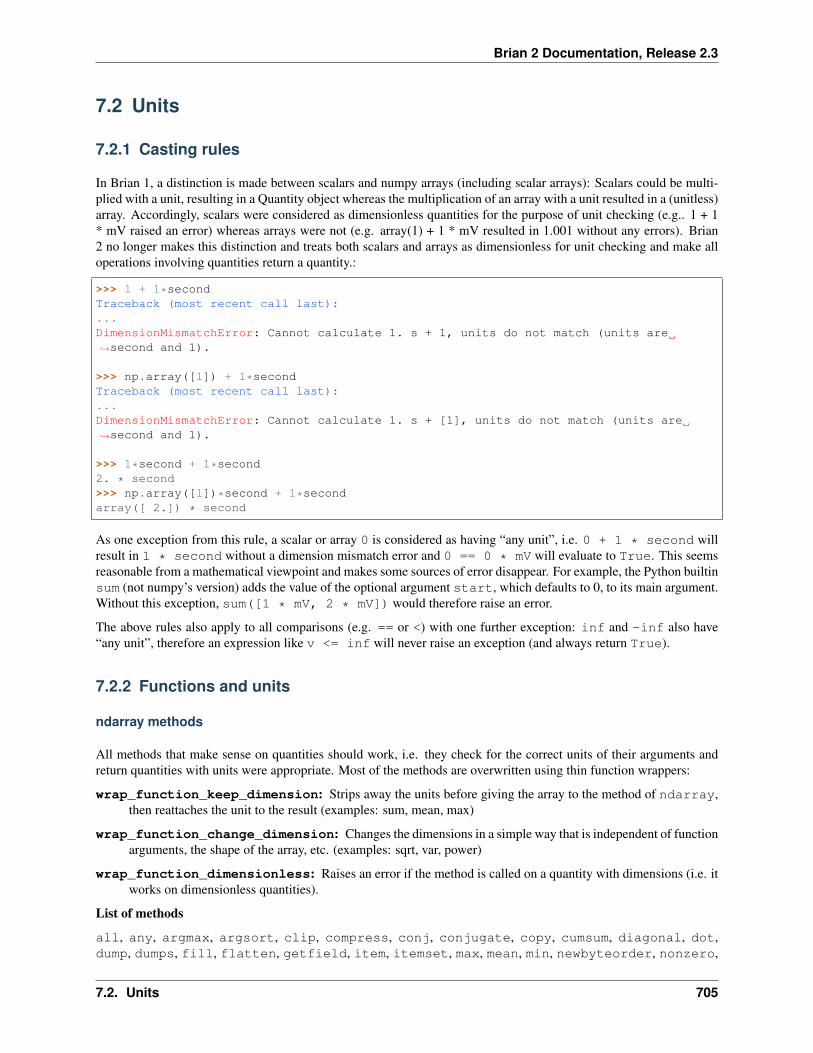
Brian 2 Documentation, Release 2.3
7.2 Units
7.2.1 Casting rules
In Brian 1, a distinction is made between scalars and numpy arrays (including scalar arrays): Scalars could be multi-plied with a unit, resulting in a Quantity object whereas the multiplication of an array with a unit resulted in a (unitless)array. Accordingly, scalars were considered as dimensionless quantities for the purpose of unit checking (e.g.. 1 + 1* mV raised an error) whereas arrays were not (e.g. array(1) + 1 * mV resulted in 1.001 without any errors). Brian2 no longer makes this distinction and treats both scalars and arrays as dimensionless for unit checking and make alloperations involving quantities return a quantity.:
>>> 1 + 1*secondTraceback (most recent call last):...DimensionMismatchError: Cannot calculate 1. s + 1, units do not match (units are→˓second and 1).
>>> np.array([1]) + 1*secondTraceback (most recent call last):...DimensionMismatchError: Cannot calculate 1. s + [1], units do not match (units are→˓second and 1).
>>> 1*second + 1*second2. * second>>> np.array([1])*second + 1*secondarray([ 2.]) * second
As one exception from this rule, a scalar or array 0 is considered as having “any unit”, i.e. 0 + 1 * second willresult in 1 * second without a dimension mismatch error and 0 == 0 * mV will evaluate to True. This seemsreasonable from a mathematical viewpoint and makes some sources of error disappear. For example, the Python builtinsum (not numpy’s version) adds the value of the optional argument start, which defaults to 0, to its main argument.Without this exception, sum([1 * mV, 2 * mV]) would therefore raise an error.
The above rules also apply to all comparisons (e.g. == or <) with one further exception: inf and -inf also have“any unit”, therefore an expression like v <= inf will never raise an exception (and always return True).
7.2.2 Functions and units
ndarray methods
All methods that make sense on quantities should work, i.e. they check for the correct units of their arguments andreturn quantities with units were appropriate. Most of the methods are overwritten using thin function wrappers:
wrap_function_keep_dimension: Strips away the units before giving the array to the method of ndarray,then reattaches the unit to the result (examples: sum, mean, max)
wrap_function_change_dimension: Changes the dimensions in a simple way that is independent of functionarguments, the shape of the array, etc. (examples: sqrt, var, power)
wrap_function_dimensionless: Raises an error if the method is called on a quantity with dimensions (i.e. itworks on dimensionless quantities).
List of methods
all, any, argmax, argsort, clip, compress, conj, conjugate, copy, cumsum, diagonal, dot,dump, dumps, fill, flatten, getfield, item, itemset, max, mean, min, newbyteorder, nonzero,
7.2. Units 705
Brian 2 Documentation, Release 2.3
prod, ptp, put, ravel, repeat, reshape, round, searchsorted, setasflat, setfield, setflags,sort, squeeze, std, sum, take, tolist, trace, transpose, var, view
Notes
• Methods directly working on the internal data buffer (setfield, getfield, newbyteorder) ignore thedimensions of the quantity.
• The type of a quantity cannot be int, therefore astype does not quite work when trying to convert the arrayinto integers.
• choose is only defined for integer arrays and therefore does not work
• tostring and tofile only return/save the pure array data without the unit (but you can use dump or dumpsto pickle a quantity array)
• resize does not work: ValueError: cannot resize this array: it does not ownits data
• cumprod would result in different dimensions for different elements and is therefore forbidden
• item returns a pure Python float by definition
• itemset does not check for units
Numpy ufuncs
All of the standard numpy ufuncs (functions that operate element-wise on numpy arrays) are supported, meaning thatthey check for correct units and return appropriate arrays. These functions are often called implicitly, for examplewhen using operators like < or **.
Math operations: add, subtract, multiply, divide, logaddexp, logaddexp2, true_divide,floor_divide, negative, power, remainder, mod, fmod, absolute, rint, sign, conj,conjugate, exp, exp2, log, log2, log10, expm1, log1p, sqrt, square, reciprocal,ones_like
Trigonometric functions: sin, cos, tan, arcsin, arccos, arctan, arctan2, hypot, sinh, cosh, tanh,arcsinh, arccosh, arctanh, deg2rad, rad2deg
Bitwise functions: bitwise_and, bitwise_or, bitwise_xor, invert, left_shift, right_shift
Comparison functions: greater, greater_equal, less, less_equal, not_equal, equal,logical_and, logical_or, logical_xor, logical_not, maximum, minimum
Floating functions: isreal, iscomplex, isfinite, isinf, isnan, floor, ceil, trunc, fmod
Not taken care of yet: signbit, copysign, nextafter, modf, ldexp, frexp
Notes
• Everything involving log or exp, as well as trigonometric functions only works on dimensionless array (forarctan2 and hypot this is questionable, though)
• Unit arrays can only be raised to a scalar power, not to an array of exponents as this would lead to differingdimensions across entries. For simplicity, this is enforced even for dimensionless quantities.
• Bitwise functions never works on quantities (numpy will by itself throw a TypeError because they are floatsnot integers).
• All comparisons only work for matching dimensions (with the exception of always allowing comparisons to 0)and return a pure boolean array.
• All logical functions treat quantities as boolean values in the same way as floats are treated as boolean: Anynon-zero value is True.
706 Chapter 7. Developer’s guide

Brian 2 Documentation, Release 2.3
Numpy functions
Many numpy functions are functional versions of ndarray methods (e.g. mean, sum, clip). They therefore workautomatically when called on quantities, as numpy propagates the call to the respective method.
There are some functions in numpy that do not propagate their call to the corresponding method (because they usenp.asarray instead of np.asanyarray, which might actually be a bug in numpy): trace, diagonal, ravel, dot.For these, wrapped functions in unitsafefunctions.py are provided.
Wrapped numpy functions in unitsafefunctions.py
These functions are thin wrappers around the numpy functions to correctly check for units and return quantities whenappropriate:
log, exp, sin, cos, tan, arcsin, arccos, arctan, sinh, cosh, tanh, arcsinh, arccosh, arctanh,diagonal, ravel, trace, dot
numpy functions that work unchanged
This includes all functional counterparts of the methods mentioned above (with the exceptions mentioned above).Some other functions also work correctly, as they are only using functions/methods that work with quantities:
• linspace, diff, digitize1
• trim_zeros, fliplr, flipud, roll, rot90, shuffle
• corrcoeff1
numpy functions that return a pure numpy array instead of quantities
• arange
• cov
• random.permutation
• histogram, histogram2d
• cross, inner, outer
• where
numpy functions that do something wrong
• insert, delete (return a quantity array but without units)
• correlate (returns a quantity with wrong units)
• histogramdd (raises a DimensionMismatchError)
User-defined functions and units
For performance and simplicity reasons, code within the Brian core does not use Quantity objects but unitless numpyarrays instead. See Adding support for new functions for details on how to make use user-defined functions withBrian’s unit system.
1 But does not care about the units of its input.
7.2. Units 707

Brian 2 Documentation, Release 2.3
7.3 Equations and namespaces
7.3.1 Equation parsing
Parsing is done via pyparsing, for now find the grammar at the top of the brian2.equations.equations file.
7.3.2 Variables
Each Brian object that saves state variables (e.g. NeuronGroup, Synapses, StateMonitor) has a variablesattribute, a dictionary mapping variable names to Variable objects (in fact a Variables object, not a simpledictionary). Variable objects contain information about the variable (name, dtype, units) as well as access to thevariable’s value via a get_value method. Some will also allow setting the values via a corresponding set_valuemethod. These objects can therefore act as proxies to the variables’ “contents”.
Variable objects provide the “abstract namespace” corresponding to a chunk of “abstract code”, they are all that isneeded to check for syntactic correctness, unit consistency, etc.
7.3.3 Namespaces
The namespace attribute of a group can contain information about the external (variable or function) names usedin the equations. It specifies a group-specific namespace used for resolving names in that group. At run time, thisnamespace is combined with a “run namespace”. This namespace is either explicitly provided to the Network.run() method, or the implicit namespace consisting of the locals and globals around the point where the run functionis called is used. This namespace is then passed down to all the objects via Network.before_fun which calls allthe individual BrianObject.before_run() methods with this namespace.
7.4 Variables and indices
7.4.1 Introduction
To be able to generate the proper code out of abstract code statements, the code generation process has to have accessto information about the variables (their type, size, etc.) as well as to the indices that should be used for indexingarrays (e.g. a state variable of a NeuronGroup will be indexed differently in the NeuronGroup state updater andin synaptic propagation code). Most of this information is stored in the variables attribute of a VariableOwner(this includes NeuronGroup, Synapses, PoissonGroup and everything else that has state variables). Thevariables attribute can be accessed as a (read-only) dictionary, mapping variable names to Variable objectsstoring the information about the respective variable. However, it is not a simple dictionary but an instance of theVariables class. Let’s have a look at its content for a simple example:
>>> tau = 10*ms>>> G = NeuronGroup(10, 'dv/dt = -v / tau : volt')>>> for name, var in sorted(G.variables.items()):... print('%s : %s' % (name, var))...N : <Constant(dimensions=Dimension(), dtype=int64, scalar=True, constant=True, read_→˓only=True)>dt : <ArrayVariable(dimensions=second, dtype=float, scalar=True, constant=True, read_→˓only=True)>i : <ArrayVariable(dimensions=Dimension(), dtype=int32, scalar=False, constant=True,→˓read_only=True)>
(continues on next page)
708 Chapter 7. Developer’s guide
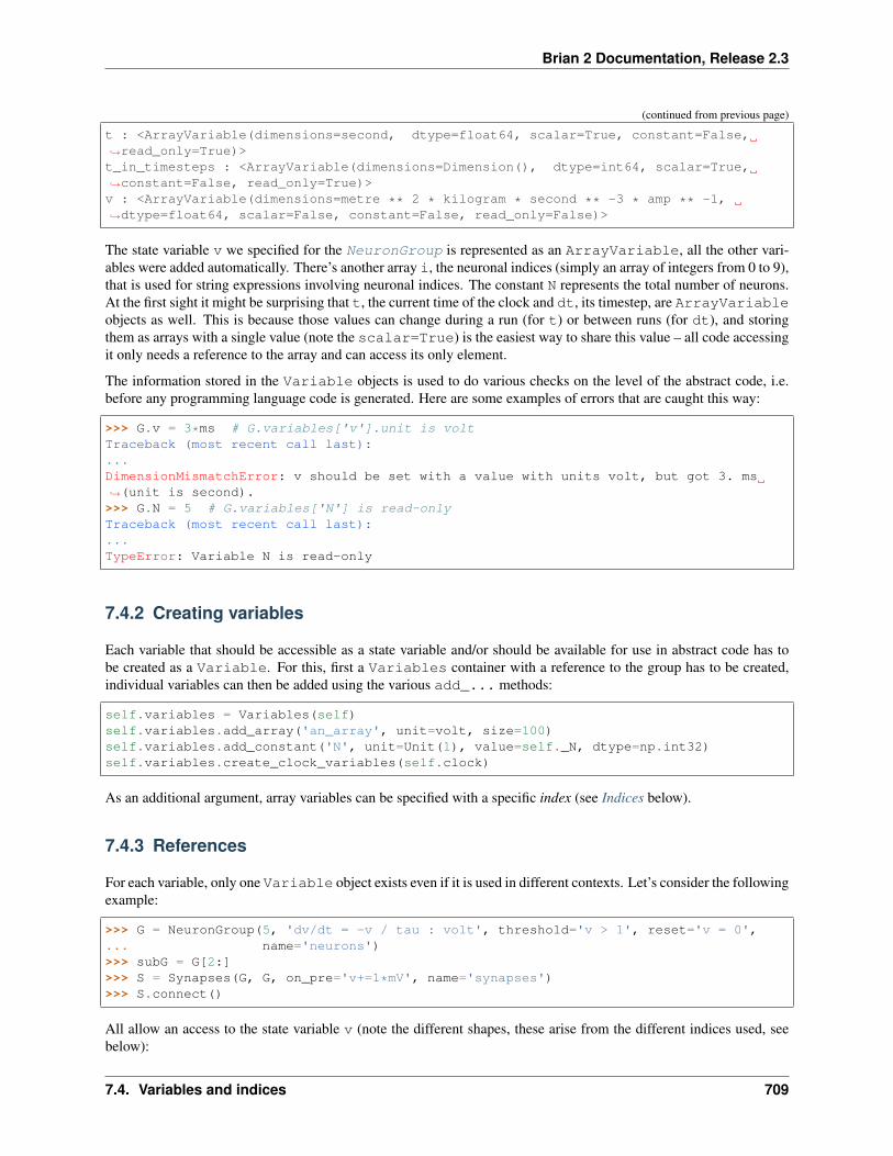
Brian 2 Documentation, Release 2.3
(continued from previous page)
t : <ArrayVariable(dimensions=second, dtype=float64, scalar=True, constant=False,→˓read_only=True)>t_in_timesteps : <ArrayVariable(dimensions=Dimension(), dtype=int64, scalar=True,→˓constant=False, read_only=True)>v : <ArrayVariable(dimensions=metre ** 2 * kilogram * second ** -3 * amp ** -1,→˓dtype=float64, scalar=False, constant=False, read_only=False)>
The state variable v we specified for the NeuronGroup is represented as an ArrayVariable, all the other vari-ables were added automatically. There’s another array i, the neuronal indices (simply an array of integers from 0 to 9),that is used for string expressions involving neuronal indices. The constant N represents the total number of neurons.At the first sight it might be surprising that t, the current time of the clock and dt, its timestep, are ArrayVariableobjects as well. This is because those values can change during a run (for t) or between runs (for dt), and storingthem as arrays with a single value (note the scalar=True) is the easiest way to share this value – all code accessingit only needs a reference to the array and can access its only element.
The information stored in the Variable objects is used to do various checks on the level of the abstract code, i.e.before any programming language code is generated. Here are some examples of errors that are caught this way:
>>> G.v = 3*ms # G.variables['v'].unit is voltTraceback (most recent call last):...DimensionMismatchError: v should be set with a value with units volt, but got 3. ms→˓(unit is second).>>> G.N = 5 # G.variables['N'] is read-onlyTraceback (most recent call last):...TypeError: Variable N is read-only
7.4.2 Creating variables
Each variable that should be accessible as a state variable and/or should be available for use in abstract code has tobe created as a Variable. For this, first a Variables container with a reference to the group has to be created,individual variables can then be added using the various add_... methods:
self.variables = Variables(self)self.variables.add_array('an_array', unit=volt, size=100)self.variables.add_constant('N', unit=Unit(1), value=self._N, dtype=np.int32)self.variables.create_clock_variables(self.clock)
As an additional argument, array variables can be specified with a specific index (see Indices below).
7.4.3 References
For each variable, only one Variable object exists even if it is used in different contexts. Let’s consider the followingexample:
>>> G = NeuronGroup(5, 'dv/dt = -v / tau : volt', threshold='v > 1', reset='v = 0',... name='neurons')>>> subG = G[2:]>>> S = Synapses(G, G, on_pre='v+=1*mV', name='synapses')>>> S.connect()
All allow an access to the state variable v (note the different shapes, these arise from the different indices used, seebelow):
7.4. Variables and indices 709

Brian 2 Documentation, Release 2.3
>>> G.v<neurons.v: array([ 0., 0., 0., 0., 0.]) * volt>>>> subG.v<neurons_subgroup.v: array([ 0., 0., 0.]) * volt>>>> S.v<synapses.v: array([ 0., 0., 0., 0., 0., 0., 0., 0., 0., 0., 0., 0., 0.,
0., 0., 0., 0., 0., 0., 0., 0., 0., 0., 0., 0.]) * volt>
In all of these cases, the Variables object stores references to the same ArrayVariable object:
>>> id(G.variables['v'])108610960>>> id(subG.variables['v'])108610960>>> id(S.variables['v'])108610960
Such a reference can be added using Variables.add_reference, note that the name used for the reference isnot necessarily the same as in the original group, e.g. in the above example S.variables also stores references tov under the names v_pre and v_post.
7.4.4 Indices
In subgroups and especially in synapses, the transformation of abstract code into executable code is not straightforwardbecause it can involve variables from different contexts. Here is a simple example:
>>> G = NeuronGroup(5, 'dv/dt = -v / tau : volt', threshold='v > 1', reset='v = 0')>>> S = Synapses(G, G, 'w : volt', on_pre='v+=w')
The seemingly trivial operation v+=w involves the variable v of the NeuronGroup and the variable w of theSynapses object which have to be indexed in the appropriate way. Since this statement is executed in the con-text of S, the variable indices stored there are relevant:
>>> S.variables.indices['w']'_idx'>>> S.variables.indices['v']'_postsynaptic_idx'
The index _idx has a special meaning and always refers to the “natural” index for a group (e.g. all neurons for aNeuronGroup, all synapses for a Synapses object, etc.). All other indices have to refer to existing arrays:
>>> S.variables['_postsynaptic_idx']<DynamicArrayVariable(dimensions=Dimension(), dtype=<class 'numpy.int32'>,→˓scalar=False, constant=True, read_only=True)>
In this case, _postsynaptic_idx refers to a dynamic array that stores the postsynaptic targets for each synapse(since it is an array itself, it also has an index. It is defined for each synapse so its index is _idx – in fact there iscurrently no support for an additional level of indirection in Brian: a variable representing an index has to have _idxas its own index). Using this index information, the following C++ code (slightly simplified) is generated:
for(int _spiking_synapse_idx=0;_spiking_synapse_idx<_num_spiking_synapses;_spiking_synapse_idx++)
{const int _idx = _spiking_synapses[_spiking_synapse_idx];
(continues on next page)
710 Chapter 7. Developer’s guide

Brian 2 Documentation, Release 2.3
(continued from previous page)
const int _postsynaptic_idx = _ptr_array_synapses__synaptic_post[_idx];const double w = _ptr_array_synapses_w[_idx];double v = _ptr_array_neurongroup_v[_postsynaptic_idx];v += w;_ptr_array_neurongroup_v[_postsynaptic_idx] = v;
}
In this case, the “natural” index _idx iterates over all the synapses that received a spike (this is defined in the template)and _postsynaptic_idx refers to the postsynaptic targets for these synapses. The variables w and v are thenpulled out of their respective arrays with these indices so that the statement v += w; does the right thing.
7.4.5 Getting and setting state variables
When a state variable is accessed (e.g. using G.v), the group does not return a reference to the underlying array itselfbut instead to a VariableView object. This is because a state variable can be accessed in different contexts andindexing it with a number/array (e.g. obj.v[0]) or a string (e.g. obj.v['i>3']) can refer to different values inthe underlying array depending on whether the object is the NeuronGroup, a Subgroup or a Synapses object.
The __setitem__ and __getitem__ methods in VariableView delegate to VariableView.set_itemand VariableView.get_item respectively (which can also be called directly under special circumstances). Theyanalyze the arguments (is the index a number, a slice or a string? Is the target value an array or a string expression?)and delegate the actual retrieval/setting of the values to a specific method:
• Getting with a numerical (or slice) index (e.g. G.v[0]): VariableView.get_with_index_array
• Getting with a string index (e.g. G.v['i>3']): VariableView.get_with_expression
• Setting with a numerical (or slice) index and a numerical target value (e.g. G.v[5:] = -70*mV):VariableView.set_with_index_array
• Setting with a numerical (or slice) index and a string expression value (e.g. G.v[5:] = (-70+i)*mV):VariableView.set_with_expression
• Setting with a string index and a string expression value (e.g. G.v['i>5'] = (-70+i)*mV):VariableView.set_with_expression_conditional
These methods are annotated with the device_override decorator and can therefore be implemented in a differentway in certain devices. The standalone device, for example, overrides the all the getting functions and the setting withindex arrays. Note that for standalone devices, the “setter” methods do not actually set the values but only note themdown for later code generation.
7.4.6 Additional variables and indices
The variables stored in the variables attribute of a VariableOwner can be used everywhere (e.g. in the stateupdater, in the threshold, the reset, etc.). Objects that depend on these variables, e.g. the Thresholder of aNeuronGroup add additional variables, in particular AuxiliaryVariables that are automatically added to theabstract code: a threshold condition v > 1 is converted into the statement _cond = v > 1; to specify the meaningof the variable _cond for the code generation stage (in particular, C++ code generation needs to know the data type)an AuxiliaryVariable object is created.
In some rare cases, a specific variable_indices dictionary is provided that overrides the indices for variablesstored in the variables attribute. This is necessary for synapse creation because the meaning of the variableschanges in this context: an expression v>0 does not refer to the v variable of all the connected postsynaptic variables,as it does under other circumstances in the context of a Synapses object, but to the v variable of all possible targets.
7.4. Variables and indices 711

Brian 2 Documentation, Release 2.3
7.5 Preferences system
Each preference looks like codegen.c.compiler, i.e. dotted names. Each preference has to be registered andvalidated. The idea is that registering all preferences ensures that misspellings of a preference value by a user causesan error, e.g. if they wrote codgen.c.compiler it would raise an error. Validation means that the value is checkedfor validity, so codegen.c.compiler = 'gcc' would be allowed, but codegen.c.compiler = 'hcc'would cause an error.
An additional requirement is that the preferences system allows for extension modules to define their own preferences,including extending the existing core brian preferences. For example, an extension might want to define extension.* but it might also want to define a new language for codegen, e.g. codegen.lisp.*. However, extensions cannotadd preferences to an existing category.
7.5.1 Accessing and setting preferences
Preferences can be accessed and set either keyword-based or attribute-based. To set/get the value for the preferenceexample mentioned before, the following are equivalent:
prefs['codegen.c.compiler'] = 'gcc'prefs.codegen.c.compiler = 'gcc'
if prefs['codegen.c.compiler'] == 'gcc':...
if prefs.codegen.c.compiler == 'gcc':...
Using the attribute-based form can be particulary useful for interactive work, e.g. in ipython, as it offers autocom-pletion and documentation. In ipython, prefs.codegen.c? would display a docstring with all the preferencesavailable in the codegen.c category.
7.5.2 Preference files
Preferences are stored in a hierarchy of files, with the following order (each step overrides the values in the previousstep but no error is raised if one is missing):
• The global defaults are stored in the installation directory.
• The user default are stored in ~/.brian/preferences (which works on Windows as well as Linux).
• The file brian_preferences in the current directory.
7.5.3 Registration
Registration of preferences is performed by a call to BrianGlobalPreferences.register_preferences,e.g.:
register_preferences('codegen.c','Code generation preferences for the C language','compiler'= BrianPreference(
validator=is_compiler,docs='...',default='gcc'),
(continues on next page)
712 Chapter 7. Developer’s guide

Brian 2 Documentation, Release 2.3
(continued from previous page)
...)
The first argument 'codegen.c' is the base name, and every preference of the form codegen.c.* has to be regis-tered by this function (preferences in subcategories such as codegen.c.somethingelse.* have to be specifiedseparately). In other words, by calling register_preferences, a module takes ownership of all the preferenceswith one particular base name. The second argument is a descriptive text explaining what this category is about. Thepreferences themselves are provided as keyword arguments, each set to a BrianPreference object.
7.5.4 Validation functions
A validation function takes a value for the preference and returns True (if the value is a valid value) or False. Ifno validation function is specified, a default validator is used that compares the value against the default value: Bothshould belong to the same class (e.g. int or str) and, in the case of a Quantity have the same unit.
7.5.5 Validation
Setting the value of a preference with a registered base name instantly triggers validation. Trying to set an unregisteredpreference using keyword or attribute access raises an error. The only exception from this rule is when the preferencesare read from configuration files (see below). Since this happens before the user has the chance to import extensionsthat potentially define new preferences, this uses a special function (_set_preference). In this case,for basenames that are not yet registered, validation occurs when the base name is registered. If, at the time that Network.run() is called, there are unregistered preferences set, a PreferenceError is raised.
7.5.6 File format
The preference files are of the following form:
a.b.c = 1# Comment line[a]b.d = 2[a.b]b.e = 3
This would set preferences a.b.c=1, a.b.d=2 and a.b.e=3.
7.5.7 Built-in preferences
Brian itself defines the following preferences:
GSL
Directory containing GSL code
GSL.directory = None Set path to directory containing GSL header files (gsl_odeiv2.h etc.) If this directory isalready in Python’s include (e.g. because of conda installation), this path can be set to None.
7.5. Preferences system 713
Brian 2 Documentation, Release 2.3
codegen
Code generation preferences
codegen.loop_invariant_optimisations = True
Whether to pull out scalar expressions out of the statements, so that they are only evaluated once insteadof once for every neuron/synapse/. . . Can be switched off, e.g. because it complicates the code (and thesame optimisation is already performed by the compiler) or because the code generation target does notdeal well with it. Defaults to True.
codegen.max_cache_dir_size = 1000
The size of a directory (in MB) with cached code for weave or Cython that triggers a warning. Set to 0 tonever get a warning.
codegen.string_expression_target = 'numpy'
Default target for the evaluation of string expressions (e.g. when indexing state variables). Should nor-mally not be changed from the default numpy target, because the overhead of compiling code is not worththe speed gain for simple expressions.
Accepts the same arguments as codegen.target, except for 'auto'
codegen.target = 'auto'
Default target for code generation.
Can be a string, in which case it should be one of:
• 'auto' the default, automatically chose the best code generation target available.
• 'weave' uses scipy.weave to generate and compile C++ code, should work anywhere wheregcc is installed and available at the command line.
• 'cython', uses the Cython package to generate C++ code. Needs a working installation of Cythonand a C++ compiler.
• 'numpy' works on all platforms and doesn’t need a C compiler but is often less efficient.
Or it can be a CodeObject class.
codegen.cpp
C++ compilation preferences
codegen.cpp.compiler = ''
Compiler to use (uses default if empty)
Should be gcc or msvc.
codegen.cpp.define_macros = []
List of macros to define; each macro is defined using a 2-tuple, where ‘value’ is either the string to defineit to or None to define it without a particular value (equivalent of “#define FOO” in source or -DFOO onUnix C compiler command line).
codegen.cpp.extra_compile_args = None
Extra arguments to pass to compiler (if None, use either extra_compile_args_gcc orextra_compile_args_msvc).
codegen.cpp.extra_compile_args_gcc = ['-w', '-O3', '-ffast-math','-fno-finite-math-only', '-march=native']
Extra compile arguments to pass to GCC compiler
714 Chapter 7. Developer’s guide

Brian 2 Documentation, Release 2.3
codegen.cpp.extra_compile_args_msvc = ['/Ox', '/w', '', '/MP']
Extra compile arguments to pass to MSVC compiler (the default /arch: flag is determined based on theprocessor architecture)
codegen.cpp.extra_link_args = []
Any extra platform- and compiler-specific information to use when linking object files together.
codegen.cpp.headers = []
A list of strings specifying header files to use when compiling the code. The list might look like [“<vec-tor>”,“‘my_header’”]. Note that the header strings need to be in a form than can be pasted at the end of a#include statement in the C++ code.
codegen.cpp.include_dirs = []
Include directories to use. Note that $prefix/include will be appended to the end automatically,where $prefix is Python’s site-specific directory prefix as returned by sys.prefix.
codegen.cpp.libraries = []
List of library names (not filenames or paths) to link against.
codegen.cpp.library_dirs = []
List of directories to search for C/C++ libraries at link time. Note that $prefix/lib will be appendedto the end automatically, where $prefix is Python’s site-specific directory prefix as returned by sys.prefix.
codegen.cpp.msvc_architecture = ''
MSVC architecture name (or use system architectue by default).
Could take values such as x86, amd64, etc.
codegen.cpp.msvc_vars_location = ''
Location of the MSVC command line tool (or search for best by default).
codegen.cpp.runtime_library_dirs = []
List of directories to search for C/C++ libraries at run time.
codegen.generators
Codegen generator preferences (see subcategories for individual languages)
codegen.generators.cpp
C++ codegen preferences
codegen.generators.cpp.flush_denormals = False
Adds code to flush denormals to zero.
The code is gcc and architecture specific, so may not compile on all platforms. The code, for reference is:
#define CSR_FLUSH_TO_ZERO (1 << 15)unsigned csr = __builtin_ia32_stmxcsr();csr |= CSR_FLUSH_TO_ZERO;__builtin_ia32_ldmxcsr(csr);
Found at http://stackoverflow.com/questions/2487653/avoiding-denormal-values-in-c.
codegen.generators.cpp.restrict_keyword = '__restrict'
7.5. Preferences system 715
Brian 2 Documentation, Release 2.3
The keyword used for the given compiler to declare pointers as restricted.
This keyword is different on different compilers, the default works for gcc and MSVS.
codegen.runtime
Runtime codegen preferences (see subcategories for individual targets)
codegen.runtime.cython
Cython runtime codegen preferences
codegen.runtime.cython.cache_dir = None
Location of the cache directory for Cython files. By default, will be stored in abrian_extensions subdirectory where Cython inline stores its temporary files (the result ofget_cython_cache_dir()).
codegen.runtime.cython.delete_source_files = True
Whether to delete source files after compiling. The Cython source files can take a significant amount ofdisk space, and are not used anymore when the compiled library file exists. They are therefore deleted bydefault, but keeping them around can be useful for debugging.
codegen.runtime.cython.multiprocess_safe = True
Whether to use a lock file to prevent simultaneous write access to cython .pyx and .so files.
codegen.runtime.numpy
Numpy runtime codegen preferences
codegen.runtime.numpy.discard_units = False
Whether to change the namespace of user-specifed functions to remove units.
core
Core Brian preferences
core.default_float_dtype = float64
Default dtype for all arrays of scalars (state variables, weights, etc.).
core.default_integer_dtype = int32
Default dtype for all arrays of integer scalars.
core.outdated_dependency_error = True
Whether to raise an error for outdated dependencies (True) or just a warning (False).
core.network
Network preferences
core.network.default_schedule = ['start', 'groups', 'thresholds', 'synapses','resets', 'end']
Default schedule used for networks that don’t specify a schedule.
716 Chapter 7. Developer’s guide

Brian 2 Documentation, Release 2.3
devices
Device preferences
devices.cpp_standalone
C++ standalone preferences
devices.cpp_standalone.extra_make_args_unix = ['-j']
Additional flags to pass to the GNU make command on Linux/OS-X. Defaults to “-j” for parallel compi-lation.
devices.cpp_standalone.extra_make_args_windows = []
Additional flags to pass to the nmake command on Windows. By default, no additional flags are passed.
devices.cpp_standalone.openmp_spatialneuron_strategy = None
DEPRECATED. Previously used to chose the strategy to parallelize the solution of the three tridiagonalsystems for multicompartmental neurons. Now, its value is ignored.
devices.cpp_standalone.openmp_threads = 0
The number of threads to use if OpenMP is turned on. By default, this value is set to 0 and the C++ code isgenerated without any reference to OpenMP. If greater than 0, then the corresponding number of threadsare used to launch the simulation.
devices.cpp_standalone.run_environment_variables = {'LD_BIND_NOW': '1'}
Dictionary of environment variables and their values that will be set during the execution of the standalonecode.
legacy
Preferences to enable legacy behaviour
legacy.refractory_timing = False
Whether to use the semantics for checking the refractoriness condition that were in place up until (in-cluding) version 2.1.2. In that implementation, refractory periods that were multiples of dt could lead toa varying number of refractory timesteps due to the nature of floating point comparisons). This prefer-ence is only provided for exact reproducibility of previously obtained results, new simulations should usethe improved mechanism which uses a more robust mechanism to convert refractoriness into timesteps.Defaults to False.
logging
Logging system preferences
logging.console_log_level = 'INFO'
What log level to use for the log written to the console.
Has to be one of CRITICAL, ERROR, WARNING, INFO, DEBUG or DIAGNOSTIC.
logging.delete_log_on_exit = True
Whether to delete the log and script file on exit.
If set to True (the default), log files (and the copy of the main script) will be deleted after the brianprocess has exited, unless an uncaught exception occured. If set to False, all log files will be kept.
7.5. Preferences system 717

Brian 2 Documentation, Release 2.3
logging.file_log = True
Whether to log to a file or not.
If set to True (the default), logging information will be written to a file. The log level can be set via thelogging.file_log_level preference.
logging.file_log_level = 'DIAGNOSTIC'
What log level to use for the log written to the log file.
In case file logging is activated (see logging.file_log), which log level should be used for logging. Has tobe one of CRITICAL, ERROR, WARNING, INFO, DEBUG or DIAGNOSTIC.
logging.save_script = True
Whether to save a copy of the script that is run.
If set to True (the default), a copy of the currently run script is saved to a temporary location. It isdeleted after a successful run (unless logging.delete_log_on_exit is False) but is kept after an uncaughtexception occured. This can be helpful for debugging, in particular when several simulations are runningin parallel.
logging.std_redirection = True
Whether or not to redirect stdout/stderr to null at certain places.
This silences a lot of annoying compiler output, but will also hide error messages making it harder to debugproblems. You can always temporarily switch it off when debugging. If logging.std_redirection_to_file isset to True as well, then the output is saved to a file and if an error occurs the name of this file will beprinted.
logging.std_redirection_to_file = True
Whether to redirect stdout/stderr to a file.
If both logging.std_redirection and this preference are set to True, all standard output/error(most importantly output from the compiler) will be stored in files and if an error occurs the name of thisfile will be printed. If logging.std_redirection is True and this preference is False, then all standardoutput/error will be completely suppressed, i.e. neither be displayed nor stored in a file.
The value of this preference is ignore if logging.std_redirection is set to False.
7.6 Adding support for new functions
For a description of Brian’s function system from the user point of view, see Functions.
The default functions available in Brian are stored in the DEFAULT_FUNCTIONS dictionary. New Function objectscan be added to this dictionary to make them available to all Brian code, independent of its namespace.
To add a new implementation for a code generation target, a FunctionImplementation can be added to theFunction.implementations dictionary. The key for this dictionary has to be either a CodeGenerator classobject, or a CodeObject class object. The CodeGenerator of a CodeObject (e.g. CPPCodeGenerator forWeaveCodeObject) is used as a fallback if no implementation specific to the CodeObject class exists.
If a function is already provided for the target language (e.g. it is part of a library imported by default), using thesame name, all that is needed is to add an empty FunctionImplementation object to mark the function asimplemented. For example, exp is a standard function in C++:
DEFAULT_FUNCTIONS['exp'].implementations[CPPCodeGenerator] = FunctionImplementation()
718 Chapter 7. Developer’s guide

Brian 2 Documentation, Release 2.3
Some functions are implemented but have a different name in the target language. In this case, theFunctionImplementation object only has to specify the new name:
DEFAULT_FUNCTIONS['arcsin'].implementations[CPPCodeGenerator] =→˓FunctionImplementation('asin')
Finally, the function might not exist in the target language at all, in this case the code for the function has to beprovided, the exact form of this code is language-specific. In the case of C++, it’s a dictionary of code blocks:
clip_code = {'support_code': '''double _clip(const float value, const float a_min, const float a_max){
if (value < a_min)return a_min;
if (value > a_max)return a_max;
return value;}'''}
DEFAULT_FUNCTIONS['clip'].implementations[CPPCodeGenerator] = FunctionImplementation(→˓'_clip',
→˓code=clip_code)
7.7 Code generation
The generation of a code snippet is done by a CodeGenerator class. The templates are stored in theCodeObject.templater attribute, which is typically implemented as a subdirectory of templates. The com-pilation and running of code is done by a CodeObject. See the sections below for each of these.
7.7.1 Code path
The following gives an outline of the key steps that happen for the code generation associated to a NeuronGroupStateUpdater. The items in grey are Brian core functions and methods and do not need to be implemented tocreate a new code generation target or device. The parts in yellow are used when creating a new device. The parts ingreen relate to generating code snippets from abstract code blocks. The parts in blue relate to creating new templateswhich these snippets are inserted into. The parts in red relate to creating new runtime behaviour (compiling andrunning generated code).
7.7. Code generation 719
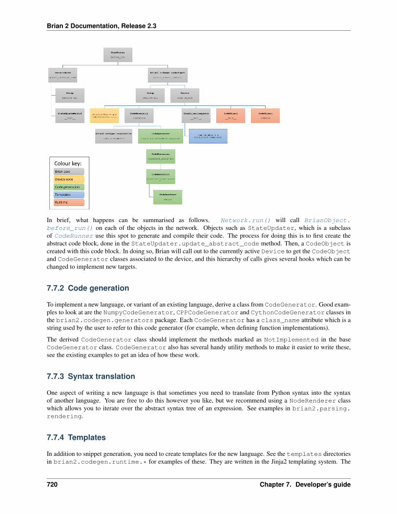
Brian 2 Documentation, Release 2.3
In brief, what happens can be summarised as follows. Network.run() will call BrianObject.before_run() on each of the objects in the network. Objects such as StateUpdater, which is a subclassof CodeRunner use this spot to generate and compile their code. The process for doing this is to first create theabstract code block, done in the StateUpdater.update_abstract_code method. Then, a CodeObject iscreated with this code block. In doing so, Brian will call out to the currently active Device to get the CodeObjectand CodeGenerator classes associated to the device, and this hierarchy of calls gives several hooks which can bechanged to implement new targets.
7.7.2 Code generation
To implement a new language, or variant of an existing language, derive a class from CodeGenerator. Good exam-ples to look at are the NumpyCodeGenerator, CPPCodeGenerator and CythonCodeGenerator classes inthe brian2.codegen.generators package. Each CodeGenerator has a class_name attribute which is astring used by the user to refer to this code generator (for example, when defining function implementations).
The derived CodeGenerator class should implement the methods marked as NotImplemented in the baseCodeGenerator class. CodeGenerator also has several handy utility methods to make it easier to write these,see the existing examples to get an idea of how these work.
7.7.3 Syntax translation
One aspect of writing a new language is that sometimes you need to translate from Python syntax into the syntaxof another language. You are free to do this however you like, but we recommend using a NodeRenderer classwhich allows you to iterate over the abstract syntax tree of an expression. See examples in brian2.parsing.rendering.
7.7.4 Templates
In addition to snippet generation, you need to create templates for the new language. See the templates directoriesin brian2.codegen.runtime.* for examples of these. They are written in the Jinja2 templating system. The
720 Chapter 7. Developer’s guide
Brian 2 Documentation, Release 2.3
location of these templates is set as the CodeObject.templater attribute. Examples such as CPPCodeObjectshow how this is done.
7.7.5 Code objects
To allow the final code block to be compiled and run, derive a class from CodeObject. This class should implementthe placeholder methods defined in the base class. The class should also have attributes templater (which should bea Templater object pointing to the directory where the templates are stored) generator_class (which shouldbe the CodeGenerator class), and class_name (which should be a string the user can use to refer to this codegeneration target.
7.7.6 Default functions
You will typically want to implement the default functions such as the trigonometric, exponential and rand functions.We usually put these implementations either in the same module as the CodeGenerator class or the CodeObjectclass depending on whether they are language-specific or runtime target specific. See those modules for examples ofimplementing these functions.
7.7.7 Code guide
• brian2.codegen: everything related to code generation
• brian2.codegen.generators: snippet generation, including the CodeGenerator classes and defaultfunction implementations.
• brian2.codegen.runtime: templates, compilation and running of code, including CodeObject anddefault function implementations.
• brian2.core.functions, brian2.core.variables: these define the values that variable namescan have.
• brian2.parsing: tools for parsing expressions, etc.
• brian2.parsing.rendering: AST tools for rendering expressions in Python into different languages.
• brian2.utils: various tools for string manipulation, file management, etc.
7.7.8 Additional information
For some additional (older, but still accurate) notes on code generation:
Older notes on code generation
The following is an outline of how the Brian 2 code generation system works, with indicators as to which packages tolook at and which bits of code to read for a clearer understanding.
We illustrate the global process with an example, the creation and running of a single NeuronGroup object:
• Parse the equations, add refractoriness to them: this isn’t really part of code generation.
• Allocate memory for the state variables.
• Create Thresholder, Resetter and StateUpdater objects.
– Determine all the variable and function names used in the respective abstract code blocks and templates
7.7. Code generation 721

Brian 2 Documentation, Release 2.3
– Determine the abstract namespace, i.e. determine a Variable or Function object for each name.
– Create a CodeObject based on the abstract code, template and abstract namespace. This will generatecode in the target language and the namespace in which the code will be executed.
• At runtime, each object calls CodeObject.__call__ to execute the code.
Stages of code generation
Equations to abstract code
In the case of Equations, the set of equations are combined with a numerical integration method to generate anabstract code block (see below) which represents the integration code for a single time step.
An example of this would be converting the following equations:
eqs = '''dv/dt = (v0-v)/tau : volt (unless refractory)v0 : volt'''group = NeuronGroup(N, eqs, threshold='v>10*mV',
reset='v=0*mV', refractory=5*ms)
into the following abstract code using the exponential_euler method (which is selected automatically):
not_refractory = 1*((t - lastspike) > 0.005000)_BA_v = -v0_v = -_BA_v + (_BA_v + v)*exp(-dt*not_refractory/tau)v = _v
The code for this stage can be seen in NeuronGroup.__init__(), StateUpdater.__init__,and StateUpdater.update_abstract_code (in brian2.groups.neurongroup), and theStateUpdateMethod classes defined in the brian2.stateupdaters package.
For more details, see State update.
Abstract code
‘Abstract code’ is just a multi-line string representing a block of code which should be executed for each item (e.g.each neuron, each synapse). Each item is independent of the others in abstract code. This allows us to later generatecode either for vectorised languages (like numpy in Python) or using loops (e.g. in C++).
Abstract code is parsed according to Python syntax, with certain language constructs excluded. For example, therecannot be any conditional or looping statements at the moment, although support for this is in principle possibleand may be added later. Essentially, all that is allowed at the moment is a sequence of arithmetical a = b*c stylestatements.
Abstract code is provided directly by the user for threshold and reset statements in NeuronGroup and for pre/postspiking events in Synapses.
Abstract code to snippet
We convert abstract code into a ‘snippet’, which is a small segment of code which is syntactically correct in thetarget language, although it may not be runnable on its own (that’s handled by insertion into a ‘template’ later). Thisis handled by the CodeGenerator object in brian2.codegen.generators. In the case of converting into
722 Chapter 7. Developer’s guide
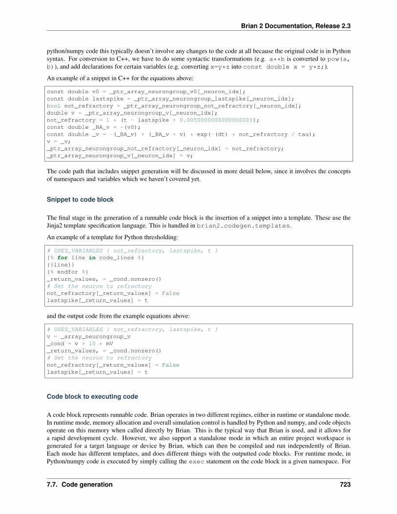
Brian 2 Documentation, Release 2.3
python/numpy code this typically doesn’t involve any changes to the code at all because the original code is in Pythonsyntax. For conversion to C++, we have to do some syntactic transformations (e.g. a**b is converted to pow(a,b)), and add declarations for certain variables (e.g. converting x=y*z into const double x = y*z;).
An example of a snippet in C++ for the equations above:
const double v0 = _ptr_array_neurongroup_v0[_neuron_idx];const double lastspike = _ptr_array_neurongroup_lastspike[_neuron_idx];bool not_refractory = _ptr_array_neurongroup_not_refractory[_neuron_idx];double v = _ptr_array_neurongroup_v[_neuron_idx];not_refractory = 1 * (t - lastspike > 0.0050000000000000001);const double _BA_v = -(v0);const double _v = -(_BA_v) + (_BA_v + v) * exp(-(dt) * not_refractory / tau);v = _v;_ptr_array_neurongroup_not_refractory[_neuron_idx] = not_refractory;_ptr_array_neurongroup_v[_neuron_idx] = v;
The code path that includes snippet generation will be discussed in more detail below, since it involves the conceptsof namespaces and variables which we haven’t covered yet.
Snippet to code block
The final stage in the generation of a runnable code block is the insertion of a snippet into a template. These use theJinja2 template specification language. This is handled in brian2.codegen.templates.
An example of a template for Python thresholding:
# USES_VARIABLES { not_refractory, lastspike, t }{% for line in code_lines %}{{line}}{% endfor %}_return_values, = _cond.nonzero()# Set the neuron to refractorynot_refractory[_return_values] = Falselastspike[_return_values] = t
and the output code from the example equations above:
# USES_VARIABLES { not_refractory, lastspike, t }v = _array_neurongroup_v_cond = v > 10 * mV_return_values, = _cond.nonzero()# Set the neuron to refractorynot_refractory[_return_values] = Falselastspike[_return_values] = t
Code block to executing code
A code block represents runnable code. Brian operates in two different regimes, either in runtime or standalone mode.In runtime mode, memory allocation and overall simulation control is handled by Python and numpy, and code objectsoperate on this memory when called directly by Brian. This is the typical way that Brian is used, and it allows fora rapid development cycle. However, we also support a standalone mode in which an entire project workspace isgenerated for a target language or device by Brian, which can then be compiled and run independently of Brian.Each mode has different templates, and does different things with the outputted code blocks. For runtime mode, inPython/numpy code is executed by simply calling the exec statement on the code block in a given namespace. For
7.7. Code generation 723
Brian 2 Documentation, Release 2.3
C++/weave code, the scipy.weave.inline function is used. In standalone mode, the templates will typicallyeach be saved into different files.
Key concepts
Namespaces
In general, a namespace is simply a mapping/dict from names to values. In Brian we use the term ‘namespace’ in twoways: the high level “abstract namespace” maps names to objects based on the Variables or Function class. Inthe above example, v maps to an ArrayVariable object, tau to a Constant object, etc. This namespace hasall the information that is needed for checking the consistency of units, to determine which variables are boolean orscalar, etc. During the CodeObject creation, this abstract namespace is converted into the final namespace in whichthe code will be executed. In this namespace, v maps to the numpy array storing the state variable values (withoutunits) and tau maps to a concrete value (again, without units). See Equations and namespaces for more details.
Variable
Variable objects contain information about the variable they correspond to, including details like the data type,whether it is a single value or an array, etc.
See brian2.core.variables and, e.g. Group._create_variables, NeuronGroup._create_variables().
Templates
Templates are stored in Jinja2 format. They come in one of two forms, either they are a single template if codegeneration only needs to output a single block of code, or they define multiple Jinja macros, each of which is aseparate code block. The CodeObject should define what type of template it wants, and the names of the macrosto define. For examples, see the templates in the directories in brian2/codegen/runtime. See brian2.codegen.templates for more details.
Code guide
This section includes a guide to the various relevant packages and subpackages involved in the code generation process.
codegen Stores the majority of all code generation related code.
codegen.functions Code related to including functions - built-in and user-defined - in generated code.
codegen.generators Each CodeGenerator is defined in a module here.
codegen.runtime Each runtime CodeObject and its templates are defined in a package here.
core
core.variables The Variable types are defined here.
equations Everything related to Equations.
groups All Group related stuff is in here. The Group.resolve methods are responsible for determining theabstract namespace.
parsing Various tools using Python’s ast module to parse user-specified code. Includes syntax translation tovarious languages in parsing.rendering.
724 Chapter 7. Developer’s guide
Brian 2 Documentation, Release 2.3
stateupdaters Everything related to generating abstract code blocks from integration methods is here.
7.8 Devices
This document describes how to implement a new Device for Brian. This is a somewhat complicated process, andyou should first be familiar with devices from the user point of view (Computational methods and efficiency) as wellas the code generation system (Code generation).
We wrote Brian’s devices system to allow for two major use cases, although it can potentially be extended beyond this.The two use cases are:
1. Runtime mode. In this mode, everything is managed by Python, including memory management (using numpyby default) and running the simulation. Actual computational work can be carried out in several different ways,including numpy, weave or Cython.
2. Standalone mode. In this mode, running a Brian script leads to generating an entire source code project treewhich can be compiled and run independently of Brian or Python.
Runtime mode is handled by RuntimeDevice and is already implemented, so here I will mainly discuss standalonedevices. A good way to understand these devices is to look at the implementation of CPPStandaloneDevice (theonly one implemented in the core of Brian). In many cases, the simplest way to implement a new standalone devicewould be to derive a class from CPPStandaloneDevice and overwrite just a few methods.
7.8.1 Memory management
Memory is managed primarily via the Device.add_array, Device.get_value and Device.set_valuemethods. When a new array is created, the add_array method is called, and when trying to access this memory theother two are called. The RuntimeDevice uses numpy to manage the memory and returns the underlying arraysin these methods. The CPPStandaloneDevice just stores a dictionary of array names but doesn’t allocate anymemory. This information is later used to generate code that will allocate the memory, etc.
7.8.2 Code objects
As in the case of runtime code generation, computational work is done by a collection of CodeObject s. InCPPtandaloneDevice, each code object is converted into a pair of .cpp and .h files, and this is probably afairly typical way to do it. For this device, it just uses the same code generation routines as for the runtime C++ deviceweave.
7.8.3 Building
The method Device.build is used to generate the project. This can be implemented any way you like, althoughlooking at CPPStandaloneDevice.build is probably a good way to get an idea of how to do it.
7.8.4 Device override methods
Several functions and methods in Brian are decorated with the device_override decorator. This mechanismallows a standalone device to override the behaviour of any of these functions by implementing a method with the nameprovided to device_override. For example, the CPPStandaloneDevice uses this to override Network.run() as CPPStandaloneDevice.network_run.
7.8. Devices 725
Brian 2 Documentation, Release 2.3
7.8.5 Other methods
There are some other methods to implement, including initialising arrays, creating spike queues for synaptic propaga-tion. Take a look at the source code for these.
7.9 Multi-threading with OpenMP
The following is an outline of how to make C++ standalone templates compatible with OpenMP, and therefore makethem work in a multi-threaded environment. This should be considered as an extension to Code generation, that hasto be read first. The C++ standalone mode of Brian is compatible with OpenMP, and therefore simulations can belaunched by users with one or with multiple threads. Therefore, when adding new templates, the developers need tomake sure that those templates are properly handling the situation if launched with OpenMP.
7.9.1 Key concepts
All the simulations performed with the C++ standalone mode can be launched with multi-threading, and make use ofmultiple cores on the same machine. Basically, all the Brian operations that can easily be performed in parallel, suchas computing the equations for NeuronGroup, Synapses, and so on can and should be split among several threads.The network construction, so far, is still performed only by one single thread, and all created objects are shared by allthe threads.
7.9.2 Use of #pragma flags
In OpenMP, all the parallelism is handled thanks to extra comments, added in the main C++ code, under the form:
#pragma omp ...
But to avoid any dependencies in the code that is generated by Brian when OpenMP is not activated, we are usingfunctions that will only add those comments, during code generation, when such a multi-threading mode is turned on.By default, nothing will be inserted.
Translations of the #pragma commands
All the translations from openmp_pragma() calls in the C++ templates are handled in the file devices/cpp_standalone/codeobject.py In this function, you can see that all calls with various string inputs willgenerate #pragma statements inserted into the C++ templates during code generation. For example:
{{ openmp_pragma('static') }}
will be transformed, during code generation, into:
#pragma omp for schedule(static)
You can find the list of all the translations in the core of the openmp_pragma() function, and if some extra transla-tions are needed, they should be added here.
Execution of the OpenMP code
In this section, we are explaining the main ideas behind the OpenMP mode of Brian, and how the simulation isexecuted in such a parallel context. As can be seen in devices/cpp_standalone/templates/main.cpp,
726 Chapter 7. Developer’s guide

Brian 2 Documentation, Release 2.3
the appropriate number of threads, defined by the user, is fixed at the beginning of the main function in the C++ codewith:
{{ openmp_pragma('set_num_threads') }}
equivalent to (thanks to the openmp_pragam() function defined above): nothing if OpenMP is turned off (default),and to:
omp_set_dynamic(0);omp_set_num_threads(nb_threads);
otherwise. When OpenMP creates a parallel context, this is the number of threads that will be used. As said, networkcreation is performed without any calls to OpenMP, on one single thread. Each template that wants to use parallelismhas to add {{ openmp_pragma{('parallel')}} to create a general block that will be executed in parallel or{{ openmp_pragma{('parallel-static')}} to execute a single loop in parallel.
7.9.3 How to make your template use OpenMP parallelism
To design a parallel template, such as for example devices/cpp_standalone/templates/common_group.cpp, you can see that as soon as you have loops that can safely be split across nodes, youjust need to add an openmp command in front of those loops:
{{openmp_pragma('parallel-static')}}for(int _idx=0; _idx<N; _idx++){
...}
By doing so, OpenMP will take care of splitting the indices and each thread will loop only on a subset of indices,sharing the load. By default, the scheduling use for splitting the indices is static, meaning that each node will getthe same number of indices: this is the faster scheduling in OpenMP, and it makes sense for NeuronGroup orSynapses because operations are the same for all indices. By having a look at examples of templates such asdevices/cpp_standalone/templates/statemonitor.cpp, you can see that you can merge portions ofcode executed by only one node and portions executed in parallel. In this template, for example, only one node isrecording the time and extending the size of the arrays to store the recorded values:
{{_dynamic_t}}.push_back(_clock_t);
// Resize the dynamic arrays{{_recorded}}.resize(_new_size, _num_indices);
But then, values are written in the arrays by all the nodes:
{{ openmp_pragma('parallel-static') }}for (int _i = 0; _i < _num_indices; _i++){
....}
In general, operations that manipulate global data structures, e.g. that use push_back for a std::vector, shouldonly be executed by a single thread.
7.9.4 Synaptic propagation in parallel
7.9. Multi-threading with OpenMP 727

Brian 2 Documentation, Release 2.3
General ideas
With OpenMP, synaptic propagation is also multi-threaded. Therefore, we have to modify the SynapticPathwayobjects, handling spike propagation. As can be seen in devices/cpp_standalone/templates/synapses_classes.cpp, such an object, created during run time, will be able to get the number of threadsdecided by the user:
_nb_threads = {{ openmp_pragma('get_num_threads') }};
By doing so, a SynapticPathway, instead of handling only one SpikeQueue, will be divided into_nb_threads SpikeQueues, each of them handling a subset of the total number of connections. Allthe calls to SynapticPathway object are performed from within parallel blocks in the synapses andsynapses_push_spikes template, we have to take this parallel context into account. This is why all the functionof the SynapticPathway object are taking care of the node number:
void push(int *spikes, unsigned int nspikes){
queue[{{ openmp_pragma('get_thread_num') }}]->push(spikes, nspikes);}
Such a method for the SynapticPathway will make sure that when spikes are propagated, all the threads willpropagate them to their connections. By default, again, if OpenMP is turned off, the queue vector has size 1.
Preparation of the SynapticPathway
Here we are explaining the implementation of the prepare() method for SynapticPathway:
{{ openmp_pragma('parallel') }}{
unsigned int length;if ({{ openmp_pragma('get_thread_num') }} == _nb_threads - 1)
length = n_synapses - (unsigned int) {{ openmp_pragma('get_thread_num') }}*n_→˓synapses/_nb_threads;
elselength = (unsigned int) n_synapses/_nb_threads;
unsigned int padding = {{ openmp_pragma('get_thread_num') }}*(n_synapses/_nb_→˓threads);
queue[{{ openmp_pragma('get_thread_num') }}]->openmp_padding = padding;queue[{{ openmp_pragma('get_thread_num') }}]->prepare(&real_delays[padding], &
→˓sources[padding], length, _dt);}
Basically, each threads is getting an equal number of synapses (except the last one, that will get the remaining ones, ifthe number is not a multiple of n_threads), and the queues are receiving a padding integer telling them what partof the synapses belongs to each queue. After that, the parallel context is destroyed, and network creation can continue.Note that this could have been done without a parallel context, in a sequential manner, but this is just speeding upeverything.
Selection of the spikes
Here we are explaining the implementation of the peek() method for SynapticPathway. This is an example ofconcurrent access to data structures that are not well handled in parallel, such as std::vector. When peek() iscalled, we need to return a vector of all the neuron spiking at that particular time. Therefore, we need to ask every
728 Chapter 7. Developer’s guide
Brian 2 Documentation, Release 2.3
queue of the SynapticPathway what are the id of the spiking neurons, and concatenate them. Because those idsare stored in vectors with various shapes, we need to loop over nodes to perform this concatenate, in a sequentialmanner:
{{ openmp_pragma('static-ordered') }}for(int _thread=0; _thread < {{ openmp_pragma('get_num_threads') }}; _thread++){
{{ openmp_pragma('ordered') }}{
if (_thread == 0)all_peek.clear();
all_peek.insert(all_peek.end(), queue[_thread]->peek()->begin(), queue[_→˓thread]->peek()->end());
}}
The loop, with the keyword ‘static-ordered’, is therefore performed such that node 0 enters it first, then node 1, and soon. Only one node at a time is executing the block statement. This is needed because vector manipulations can not beperformed in a multi-threaded manner. At the end of the loop, all_peek is now a vector where all sub queues havewritten the id of spiking cells, and therefore this is the list of all spiking cells within the SynapticPathway.
7.9.5 Compilation of the code
One extra file needs to be modified, in order for OpenMP implementation to work. This is the makefile devices/cpp_standalone/templates/makefile. As one can simply see, the CFLAGS are dynamically modifiedduring code generation thanks to:
{{ openmp_pragma('compilation') }}
If OpenMP is activated, this will add the following dependencies:
-fopenmp
such that if OpenMP is turned off, nothing, in the generated code, does depend on it.
7.10 Solving differential equations with the GNU Scientific Library
Conventionally, Brian generates its own code performing Numerical integration according to the chosen algorithm(see the section on Code generation). Another option is to let the differential equation solvers defined in the GNUScientific Library (GSL) solve the given equations. In addition to offering a few extra integration methods, the GSLintegrator comes with the option of having an adaptable timestep. The latter functionality can have benefits for thespeed with which large simulations can be run. This is because it allows the use of larger timesteps for the overheadloops in Python, without losing the accuracy of the numerical integration at points where small timesteps are necessary.In addition, a major benefit of using the ODE solvers from GSL is that an estimation is performed on how wrong thecurrent solution is, so that simulations can be performed with some confidence on accuracy. (Note however that theconfidence of accuracy is based on estimation!)
7.10.1 StateUpdateMethod
7.10. Solving differential equations with the GNU Scientific Library 729
Brian 2 Documentation, Release 2.3
Translation of equations to abstract code
The first part of Brian’s code generation is the translation of equations to what we call ‘abstract code’. In the caseof Brian’s stateupdaters so far, this abstract code describes the calculations that need to be done to update differentialvariables depending on their equations as is explained in the section on State update. In the case of preparing theequations for GSL integration this is a bit different. Instead of writing down the computations that have to be done toreach the new value of the variable after a time step, the equations have to be described in a way that GSL understands.The differential equations have to be defined in a function and the function is given to GSL. This is best explainedwith an example. If we have the following equations (taken from the adaptive threshold example):
dv/dt = -v/(10*ms) : voltdvt/dt = (10*mV - vt)/(15*ms) : volt
We would describe the equations to GSL as follows:
v = y[0]vt = y[1]f[0] = -v/(10e-3)f[1] = (10e-3 - vt)
Each differential variable gets an index. Its value at any time is saved in the y-array and the derivatives are savedin the f-array. However, doing this translation in the stateupdater would mean that Brian has to deal with variabledescriptions that contain array accessing: something that for example sympy doesn’t do. Because we still want to useBrian’s existing parsing and checking mechanisms, we needed to find a way to describe the abstract code with only‘normal’ variable names. Our solution is to replace the y[0], f[0], etc. with a ‘normal’ variable name that is laterreplaced just before the final code generation (in the GSLCodeGenerator). It has a tag and all the informationneeded to write the final code. As an example, the GSL abstract code for the above equations would be:
v = _gsl_y0vt = _gsl_y1_gsl_f0 = -v/(10e-3)_gsl_f1 = (10e-3 - vt)
In the GSLCodeGenerator these tags get replaced by the actual accessing of the arrays.
Return value of the StateUpdateMethod
So far, for each each code generation language (numpy, weave, cython) there was just one set of rules of howto translate abstract code to real code, described in its respective CodeObject and CodeGenerator. If thetarget language is set to weave, the stateupdater will use the WeaveCodeObject, just like other objects suchas the StateMonitor. However, to achieve the above decribed translations of the abstract code generated bythe StateUpdateMethod, we need a special WeaveCodeObject for the stateupdater alone (which at itsturn can contain the special CodeGenerator), and this CodeObject should be selected based on the chosenStateUpdateMethod.
In order to achieve CodeObject selection based on the chosen stateupdater, the StateUpdateMethod returns aclass that can be called with an object, and the appropriate CodeObject is added as an attribute to the given object.The return value of this callable is the abstract code describing the equations in a language that makes sense to theGSLCodeGenerator.
7.10.2 GSLCodeObject
Each target language has its own GSLCodeObject that is derived from the already existing code object of its lan-guage. There are only minimal changes to the already existing code object:
730 Chapter 7. Developer’s guide

Brian 2 Documentation, Release 2.3
• Overwrite stateupate template: a new version of the stateupdate template is given (stateupdate.cpp for weave/C++ standalone and stateupdate.pyx for cython).
• Have a GSL specific generator_class: GSLWeaveCodeGenerator or GSLCythonCodeGenerator
• Add the attribute original_generator_class: the conventional target-language generator is used to dothe bulk of the translation to get from abstract code to language-specific code.
This defining of GSL-specific code objects also allowed us to catch compilation errors so we can give the user someinformation on that it might be GSL-related (overwriting the compile()method in the case of cython and the run()method for weave). In the case of the C++ CodeObject such overriding wasn’t really possible so compilation errorsin this case might be quite undescriptive.
7.10.3 GSLCodeGenerator
This is where the magic happens. Roughly 1000 lines of code define the translation of abstract code to code that usesthe GNU Scientific Library’s ODE solvers to achieve state updates.
Upon a call to run(), the code objects necessary for the simulation get made. The code for this is described in thedevice. Part of making the code objects is generating the code that describes the code objects. This starts with a callto translate, which in the case of GSL brings us to the GSLCodeGenerator.translate(). This method isbuilt up as follows:
• Some GSL-specific preparatory work:
– Check whether the equations contain variable names that are reserved for the GSL code.
– Add the ‘gsl tags’ (see section on StateUpdateMethod) to the variables known to Brian as non-scalars.This is necessary to ensure that all equations containing ‘gsl tags’ are considered vector equations, andthus added to Brian’s vector code.
– Add GSL integrator meta variables as official Brian variables, so these are also taken into account upontranslation. The meta variables that are possible are described in the user manual (e.g. GSL’s step taken ina single overhead step ‘_step_count’).
– Save function names. The original generators delete the function names from the variables dictionary oncethey are processed. However, we need to know later in the GSL part of the code generation whether acertain encountered variable name refers to a function or not.
• Brian’s general preparatory work. This piece of code is directly copied from the base CodeGenerator and is thussimilar to what is done normally.
• A call to original_generator.translate() to get the abstract code translated into code that is target-language specific.
• A lot of statements to translate the target-language specific code to GSL-target-language specific code, describedin more detail below.
The biggest difference between conventional Brian code and GSL code is that the stateupdate-decribing lines arecontained directly in the main() or in a separate function, respectively. In both cases, the equations describing thesystem refer to parameters that are in the Brian namespace (e.g. “dv/dt = -v/tau” needs access to “tau”). How can weaccess Brian’s namespace in this separate function that is needed with GSL?
To explain the solution we first need some background information on this ‘separate function’ that is given to the GSLintegrators: _GSL_func. This function always gets three arguments:
• double t: the current time. This is relevant when the equations are dependent on time.
• const double _GSL_y[]’: an array containing the current values of the differential variables (const be-cause the cannot be changed by _GSL_func itself).
7.10. Solving differential equations with the GNU Scientific Library 731
Brian 2 Documentation, Release 2.3
• double f[]: an array containing the derivatives of the differential variables (i.e. the equations describing thedifferential system).
• void * params: a pointer.
The pointer can be a pointer to whatever you want, and can thus point to a data structure containing the systemparameters (such as tau). To achieve a structure containing all the parameters of the system, a considerable amount ofcode has to be added/changed to that generated by conventional Brian:
• The data structure, _GSL_dataholder, has to be defined with all variables needed in the vector code. For thisreason, also the datatype of each variable is required.
– This is done in the method GSLCodeGenerator.write_dataholder
• Instead of referring to the variables by their name only (e.g. dv/dt = -v/tau), the variables have tobe accessed as part of the data structure (e .g. dv/dt = -v/_GSL_dataholder->tau in the case ofweave/cpp). Also, as mentioned earlier, we want to translate the ‘gsl tags’ to what they should be in the finalcode (e.g. _gsl_f0 to f[0]).
– This is done in the method GSLCodeGenerator.translate_vector_code. It works based onthe to_replace dictionary (generated in the methods GSLCodeGenerator.diff_var_to_replaceand GSLCodeGenerator.to_replace_vector_vars) that simply contains the old variables askeys and new variables as values, and is given to the word_replace function.
• The values of the variables in the data structure have to be set to the values of the variables in the Brian names-pace.
– This is done in the method GSLCodeGenerator.unpack_namespace, and for the‘scalar’ variables that require calculation first it is done in the method GSLCodeGenerator.translate_scalar_code.
In addition, a few more ‘support’ functions are generated for the GSL script:
• int _set_dimension(size_t * dimension): sets the dimension of the system. Required for GSL.
• double* _assign_memory_y(): allocates the right amount of memory for the y array (also according tothe dimension of the system).
• int _fill_y_vector(_dataholder* _GSL_dataholder, double* _GSL_y, int_idx): pulls out the values for each differential variable out of the ‘Brian’ array into the y-vector. This happensin the vector loop (e.g. y[0] = _GSL_dataholder->_ptr_array_neurongroup_v[_idx]; forweave/C++).
• int _empty_y_vector(_dataholder* _GSL_dataholder, double* _GSL_y, int_idx): the opposite of _fill_y_vector. Pulls final numerical solutions from the y array and gives itback to Brian’s namespace.
• double* _set_GSL_scale_array(): sets the array bound for each differential vari-able, for which the values are based on method_options['absolute_error'] andmethod_options['absolute_error_per_variable'].
All of this is written in support functions so that the vector code in the main() can stay almost constant for anysimulation.
7.10.4 Stateupdate templates
There is many extra things that need to be done for each simulation when using GSL compared to conventional Brianstateupdaters. These are summarized in this section.
Things that need to be done for every type of simulation (either before, in or after main()):
732 Chapter 7. Developer’s guide

Brian 2 Documentation, Release 2.3
• Cython-only: define the structs and functions that we will be using in cython language (for weave these defini-tions already sit in GSL’s own header files that are included).
• Prepare the gsl_odeiv2_system: give function pointer, set dimension, give pointer to_GSL_dataholder as params.
• Allocate the driver (name for the struct that contains the info necessary to perform GSL integration)
• Define dt.
Things that need to be done every loop iteration for every type of simulation:
• Define t and t1 (t + dt).
• Transfer the values in the Brian arrays to the y-array that will be given to GSL.
• Set _GSL_dataholder._idx (in case we need to access array variables in _GSL_func).
• Initialize the driver (reset counters, set dt_start).
• Apply driver (either with adaptable- or fixed time step).
• Optionally save certain meta-variables
• Transfer values from GSL’s y-vector to Brian arrays
7.10. Solving differential equations with the GNU Scientific Library 733

Brian 2 Documentation, Release 2.3
734 Chapter 7. Developer’s guide

CHAPTER 8
Indices and tables
• genindex
• modindex
• search
735

Brian 2 Documentation, Release 2.3
736 Chapter 8. Indices and tables

Bibliography
[R13] M. Abramowitz and I.A. Stegun, “Handbook of Mathematical Functions”, 10th printing, 1964, pp. 86. http://www.math.sfu.ca/~cbm/aands/
[R14] Wikipedia, “Inverse hyperbolic function”, https://en.wikipedia.org/wiki/Arccosh
[R15] M. Abramowitz and I.A. Stegun, “Handbook of Mathematical Functions”, 10th printing, 1964, pp. 86. http://www.math.sfu.ca/~cbm/aands/
[R16] Wikipedia, “Inverse hyperbolic function”, https://en.wikipedia.org/wiki/Arcsinh
[R17] M. Abramowitz and I.A. Stegun, “Handbook of Mathematical Functions”, 10th printing, 1964, pp. 86. http://www.math.sfu.ca/~cbm/aands/
[R18] Wikipedia, “Inverse hyperbolic function”, https://en.wikipedia.org/wiki/Arctanh
[R19] Wikipedia, “Exponential function”, https://en.wikipedia.org/wiki/Exponential_function
[R20] M. Abramovitz and I. A. Stegun, “Handbook of Mathematical Functions with Formulas, Graphs, and Mathe-matical Tables,” Dover, 1964, p. 69, http://www.math.sfu.ca/~cbm/aands/page_69.htm
[R21] M. Abramowitz and I.A. Stegun, “Handbook of Mathematical Functions”, 10th printing, 1964, pp. 67. http://www.math.sfu.ca/~cbm/aands/
[R22] Wikipedia, “Logarithm”. https://en.wikipedia.org/wiki/Logarithm
[R23] M. Abramowitz and I. A. Stegun, Handbook of Mathematical Functions. New York, NY: Dover, 1972, pg. 83.http://www.math.sfu.ca/~cbm/aands/
[R24] Wikipedia, “Hyperbolic function”, https://en.wikipedia.org/wiki/Hyperbolic_function
737

Brian 2 Documentation, Release 2.3
738 Bibliography

Python Module Index
_brian2.__init__, 363
cbrian2.codegen, 367brian2.codegen._prefs, 367brian2.codegen.codeobject, 368brian2.codegen.cpp_prefs, 371brian2.codegen.generators, 387brian2.codegen.generators.base, 397brian2.codegen.generators.cpp_generator,
399brian2.codegen.generators.cython_generator,
401brian2.codegen.generators.GSL_generator,
387brian2.codegen.generators.numpy_generator,
403brian2.codegen.get_cpu_flags, 374brian2.codegen.optimisation, 374brian2.codegen.permutation_analysis, 378brian2.codegen.runtime, 405brian2.codegen.runtime.cython_rt, 408brian2.codegen.runtime.cython_rt.cython_rt,
408brian2.codegen.runtime.cython_rt.extension_manager,
409brian2.codegen.runtime.GSLcython_rt, 406brian2.codegen.runtime.GSLcython_rt.GSLcython_rt,
406brian2.codegen.runtime.GSLweave_rt, 407brian2.codegen.runtime.GSLweave_rt.GSLweave_rt,
407brian2.codegen.runtime.numpy_rt, 411brian2.codegen.runtime.numpy_rt.numpy_rt,
411brian2.codegen.runtime.weave_rt, 413brian2.codegen.runtime.weave_rt.weave_rt,
413
brian2.codegen.statements, 379brian2.codegen.targets, 380brian2.codegen.templates, 380brian2.codegen.translation, 384brian2.core, 415brian2.core.base, 416brian2.core.clocks, 420brian2.core.core_preferences, 423brian2.core.functions, 423brian2.core.magic, 430brian2.core.names, 437brian2.core.namespace, 438brian2.core.network, 438brian2.core.operations, 447brian2.core.preferences, 450brian2.core.spikesource, 455brian2.core.tracking, 456brian2.core.variables, 458
dbrian2.devices, 479brian2.devices.cpp_standalone, 489brian2.devices.cpp_standalone.codeobject,
490brian2.devices.cpp_standalone.device,
491brian2.devices.cpp_standalone.GSLcodeobject,
489brian2.devices.device, 479
ebrian2.equations, 499brian2.equations.codestrings, 499brian2.equations.equations, 502brian2.equations.refractory, 511brian2.equations.unitcheck, 512
gbrian2.groups, 513brian2.groups.group, 513
739

Brian 2 Documentation, Release 2.3
brian2.groups.neurongroup, 520brian2.groups.subgroup, 529
hbrian2.hears, 364
ibrian2.importexport, 529brian2.importexport.dictlike, 529brian2.importexport.importexport, 531brian2.input, 532brian2.input.binomial, 532brian2.input.poissongroup, 533brian2.input.poissoninput, 535brian2.input.spikegeneratorgroup, 536brian2.input.timedarray, 539
mbrian2.memory.dynamicarray, 541brian2.monitors, 543brian2.monitors.ratemonitor, 543brian2.monitors.spikemonitor, 545brian2.monitors.statemonitor, 553
nbrian2.numpy_, 367
obrian2.only, 367
pbrian2.parsing.bast, 557brian2.parsing.dependencies, 560brian2.parsing.expressions, 561brian2.parsing.functions, 563brian2.parsing.rendering, 565brian2.parsing.statements, 569brian2.parsing.sympytools, 569
sbrian2.spatialneuron, 572brian2.spatialneuron.morphology, 572brian2.spatialneuron.spatialneuron, 593brian2.stateupdaters, 597brian2.stateupdaters.base, 601brian2.stateupdaters.exact, 603brian2.stateupdaters.explicit, 606brian2.stateupdaters.exponential_euler,
613brian2.stateupdaters.GSL, 597brian2.synapses, 615brian2.synapses.parse_synaptic_generator_syntax,
615brian2.synapses.spikequeue, 616
brian2.synapses.synapses, 618
ubrian2.units, 627brian2.units.allunits, 627brian2.units.constants, 628brian2.units.fundamentalunits, 628brian2.units.stdunits, 647brian2.units.unitsafefunctions, 647brian2.utils, 674brian2.utils.arrays, 674brian2.utils.caching, 675brian2.utils.environment, 676brian2.utils.filetools, 676brian2.utils.logger, 677brian2.utils.stringtools, 685brian2.utils.topsort, 690
740 Python Module Index
Index
Symbols__call__() (brian2.codegen.codeobject.CodeObject
method), 368__call__() (brian2.codegen.cpp_prefs.C99Check
method), 372__call__() (brian2.codegen.templates.CodeObjectTemplate
method), 381__call__() (brian2.core.functions.Function method),
425__call__() (brian2.core.network.TextReport method),
446__call__() (brian2.core.preferences.DefaultValidator
method), 454__call__() (brian2.devices.cpp_standalone.codeobject.CPPStandaloneCodeObject
method), 491__call__() (brian2.devices.device.Dummy method),
483__call__() (brian2.groups.group.Indexing method),
517__call__() (brian2.stateupdaters.GSL.GSLContainer
method), 598__call__() (brian2.stateupdaters.GSL.GSLStateUpdater
method), 599__call__() (brian2.stateupdaters.base.StateUpdateMethod
method), 601__call__() (brian2.stateupdaters.exact.IndependentStateUpdater
method), 604__call__() (brian2.stateupdaters.exact.LinearStateUpdater
method), 605__call__() (brian2.stateupdaters.explicit.ExplicitStateUpdater
method), 610__call__() (brian2.stateupdaters.exponential_euler.ExponentialEulerStateUpdater
method), 613__call__() (brian2.synapses.synapses.SynapticIndexing
method), 625__getitem__() (brian2.units.fundamentalunits.UnitRegistry
method), 638_cache_irrelevant_attributes
(brian2.utils.caching.CacheKey attribute),
675_clock (brian2.core.base.BrianObject attribute), 417_connect_called (brian2.synapses.synapses.Synapses
attribute), 621_creation_stack (brian2.core.base.BrianObject at-
tribute), 417_dispname (brian2.units.fundamentalunits.Unit at-
tribute), 636_dt (brian2.synapses.spikequeue.SpikeQueue attribute),
617_initialise_queue_codeobj
(brian2.synapses.synapses.SynapticPathwayattribute), 626
_latexname (brian2.units.fundamentalunits.Unit at-tribute), 636
_log_messages (brian2.utils.logger.BrianLogger at-tribute), 679
_name (brian2.units.fundamentalunits.Unit attribute),636
_network (brian2.core.base.BrianObject attribute),417
_neuron_index (brian2.input.spikegeneratorgroup.SpikeGeneratorGroupattribute), 538
_pathways (brian2.synapses.synapses.Synapsesattribute), 621
_previous_dt (brian2.input.spikegeneratorgroup.SpikeGeneratorGroupattribute), 538
_refractory (brian2.groups.neurongroup.NeuronGroupattribute), 522
_registered_variables(brian2.synapses.synapses.Synapses attribute),621
_scope_current_key(brian2.core.base.BrianObject attribute),417
_scope_key (brian2.core.base.BrianObject attribute),417
_source_end (brian2.synapses.spikequeue.SpikeQueueattribute), 617
_source_start (brian2.synapses.spikequeue.SpikeQueue
741
Brian 2 Documentation, Release 2.3
attribute), 617_spike_time (brian2.input.spikegeneratorgroup.SpikeGeneratorGroup
attribute), 538_spikes_changed (brian2.input.spikegeneratorgroup.SpikeGeneratorGroup
attribute), 538_stored_state (brian2.core.network.Network
attribute), 441_substituted_expressions
(brian2.equations.equations.Equations at-tribute), 503
_synaptic_updaters(brian2.synapses.synapses.Synapses attribute),621
Aabstract_code_dependencies() (in module
brian2.parsing.dependencies), 560abstract_code_from_function() (in module
brian2.parsing.functions), 564AbstractCodeFunction (class in
brian2.parsing.functions), 563activate() (brian2.devices.device.Device method),
480active (brian2.core.base.BrianObject attribute), 417active_device (in module brian2.devices.device),
488add() (brian2.core.magic.MagicNetwork method), 432add() (brian2.core.network.Network method), 441add() (brian2.core.tracking.InstanceFollower method),
457add() (brian2.core.tracking.InstanceTrackerSet
method), 457add() (brian2.spatialneuron.morphology.Children
method), 572add() (brian2.units.fundamentalunits.UnitRegistry
method), 638add_arange() (brian2.core.variables.Variables
method), 473add_array() (brian2.core.variables.Variables
method), 473add_array() (brian2.devices.cpp_standalone.device.CPPStandaloneDevice
method), 494add_array() (brian2.devices.device.Device method),
480add_array() (brian2.devices.device.RuntimeDevice
method), 484add_arrays() (brian2.core.variables.Variables
method), 474add_attribute() (brian2.groups.group.VariableOwner
method), 518add_auxiliary_variable()
(brian2.core.variables.Variables method),475
add_constant() (brian2.core.variables.Variablesmethod), 475
add_dependency() (brian2.core.base.BrianObjectmethod), 418
add_dynamic_array()(brian2.core.variables.Variables method),475
add_dynamic_implementation()(brian2.core.functions.FunctionImplementationContainermethod), 427
add_gsl_variables_as_non_scalar()(brian2.codegen.generators.GSL_generator.GSLCodeGeneratormethod), 388
add_implementation()(brian2.core.functions.FunctionImplementationContainermethod), 427
add_meta_variables()(brian2.codegen.generators.GSL_generator.GSLCodeGeneratormethod), 389
add_numpy_implementation()(brian2.core.functions.FunctionImplementationContainermethod), 427
add_object() (brian2.core.variables.Variablesmethod), 476
add_reference() (brian2.core.variables.Variablesmethod), 476
add_references() (brian2.core.variables.Variablesmethod), 476
add_referred_subexpression()(brian2.core.variables.Variables method),477
add_refractoriness() (in modulebrian2.equations.refractory), 511
add_subexpression()(brian2.core.variables.Variables method),477
add_to_magic_network(brian2.core.base.BrianObject attribute),418
additional_unit_register (in modulebrian2.units.fundamentalunits), 647
advance() (brian2.synapses.spikequeue.SpikeQueuemethod), 617
after_run() (brian2.core.base.BrianObject method),418
after_run() (brian2.core.magic.MagicNetworkmethod), 432
after_run() (brian2.core.network.Network method),441
all_values() (brian2.monitors.spikemonitor.EventMonitormethod), 547
all_values() (brian2.monitors.spikemonitor.SpikeMonitormethod), 550
allows_scalar_write
742 Index

Brian 2 Documentation, Release 2.3
(brian2.codegen.templates.CodeObjectTemplateattribute), 381
analyse_identifiers() (in modulebrian2.codegen.translation), 384
apply_stateupdater()(brian2.stateupdaters.base.StateUpdateMethodstatic method), 602
arange() (in module brian2.units.unitsafefunctions),648
arange_arrays (brian2.devices.cpp_standalone.device.CPPStandaloneDeviceattribute), 493
arccos() (in module brian2.units.unitsafefunctions),649
arccosh() (in module brian2.units.unitsafefunctions),650
arcsin() (in module brian2.units.unitsafefunctions),651
arcsinh() (in module brian2.units.unitsafefunctions),652
arctan() (in module brian2.units.unitsafefunctions),653
arctanh() (in module brian2.units.unitsafefunctions),655
area (brian2.spatialneuron.morphology.Cylinderattribute), 574
area (brian2.spatialneuron.morphology.Morphology at-tribute), 577
area (brian2.spatialneuron.morphology.Section at-tribute), 585
area (brian2.spatialneuron.morphology.Soma at-tribute), 587
area (brian2.spatialneuron.morphology.SubMorphologyattribute), 591
ArithmeticSimplifier (class inbrian2.codegen.optimisation), 374
array (brian2.core.variables.Variable attribute), 468array_cache (brian2.devices.cpp_standalone.device.CPPStandaloneDevice
attribute), 493array_read_write()
(brian2.codegen.generators.base.CodeGeneratormethod), 398
arrays (brian2.devices.cpp_standalone.device.CPPStandaloneDeviceattribute), 493
arrays (brian2.devices.device.RuntimeDevice at-tribute), 484
arrays_helper() (brian2.codegen.generators.base.CodeGeneratormethod), 398
ArrayVariable (class in brian2.core.variables), 458as_file (brian2.core.preferences.BrianGlobalPreferences
attribute), 451assign_id() (brian2.core.names.Nameable method),
438auto_target() (in module brian2.devices.device),
486
autoindent() (in module brian2.codegen.templates),383
autoindent_postfilter() (in modulebrian2.codegen.templates), 383
AuxiliaryVariable (class inbrian2.core.variables), 460
Bbefore_run() (brian2.core.base.BrianObject
method), 419before_run() (brian2.core.network.Network
method), 441before_run() (brian2.groups.group.CodeRunner
method), 515before_run() (brian2.groups.neurongroup.NeuronGroup
method), 523before_run() (brian2.input.poissongroup.PoissonGroup
method), 534before_run() (brian2.input.poissoninput.PoissonInput
method), 536before_run() (brian2.input.spikegeneratorgroup.SpikeGeneratorGroup
method), 538before_run() (brian2.spatialneuron.spatialneuron.SpatialStateUpdater
method), 597before_run() (brian2.synapses.synapses.Synapses
method), 622before_run() (brian2.synapses.synapses.SynapticPathway
method), 626BinomialFunction (class in brian2.input.binomial),
532brian2.__init__ (module), 363brian2.codegen (module), 367brian2.codegen._prefs (module), 367brian2.codegen.codeobject (module), 368brian2.codegen.cpp_prefs (module), 371brian2.codegen.generators (module), 387brian2.codegen.generators.base (module),
397brian2.codegen.generators.cpp_generator
(module), 399brian2.codegen.generators.cython_generator
(module), 401brian2.codegen.generators.GSL_generator
(module), 387brian2.codegen.generators.numpy_generator
(module), 403brian2.codegen.get_cpu_flags (module), 374brian2.codegen.optimisation (module), 374brian2.codegen.permutation_analysis
(module), 378brian2.codegen.runtime (module), 405brian2.codegen.runtime.cython_rt (mod-
ule), 408
Index 743

Brian 2 Documentation, Release 2.3
brian2.codegen.runtime.cython_rt.cython_rt(module), 408
brian2.codegen.runtime.cython_rt.extension_manager(module), 409
brian2.codegen.runtime.GSLcython_rt(module), 406
brian2.codegen.runtime.GSLcython_rt.GSLcython_rt(module), 406
brian2.codegen.runtime.GSLweave_rt (mod-ule), 407
brian2.codegen.runtime.GSLweave_rt.GSLweave_rt(module), 407
brian2.codegen.runtime.numpy_rt (module),411
brian2.codegen.runtime.numpy_rt.numpy_rt(module), 411
brian2.codegen.runtime.weave_rt (module),413
brian2.codegen.runtime.weave_rt.weave_rt(module), 413
brian2.codegen.statements (module), 379brian2.codegen.targets (module), 380brian2.codegen.templates (module), 380brian2.codegen.translation (module), 384brian2.core (module), 415brian2.core.base (module), 416brian2.core.clocks (module), 420brian2.core.core_preferences (module), 423brian2.core.functions (module), 423brian2.core.magic (module), 430brian2.core.names (module), 437brian2.core.namespace (module), 438brian2.core.network (module), 438brian2.core.operations (module), 447brian2.core.preferences (module), 450brian2.core.spikesource (module), 455brian2.core.tracking (module), 456brian2.core.variables (module), 458brian2.devices (module), 479brian2.devices.cpp_standalone (module),
489brian2.devices.cpp_standalone.codeobject
(module), 490brian2.devices.cpp_standalone.device
(module), 491brian2.devices.cpp_standalone.GSLcodeobject
(module), 489brian2.devices.device (module), 479brian2.equations (module), 499brian2.equations.codestrings (module), 499brian2.equations.equations (module), 502brian2.equations.refractory (module), 511brian2.equations.unitcheck (module), 512brian2.groups (module), 513
brian2.groups.group (module), 513brian2.groups.neurongroup (module), 520brian2.groups.subgroup (module), 529brian2.hears (module), 364brian2.importexport (module), 529brian2.importexport.dictlike (module), 529brian2.importexport.importexport (mod-
ule), 531brian2.input (module), 532brian2.input.binomial (module), 532brian2.input.poissongroup (module), 533brian2.input.poissoninput (module), 535brian2.input.spikegeneratorgroup (mod-
ule), 536brian2.input.timedarray (module), 539brian2.memory.dynamicarray (module), 541brian2.monitors (module), 543brian2.monitors.ratemonitor (module), 543brian2.monitors.spikemonitor (module), 545brian2.monitors.statemonitor (module), 553brian2.numpy_ (module), 367brian2.only (module), 367brian2.parsing.bast (module), 557brian2.parsing.dependencies (module), 560brian2.parsing.expressions (module), 561brian2.parsing.functions (module), 563brian2.parsing.rendering (module), 565brian2.parsing.statements (module), 569brian2.parsing.sympytools (module), 569brian2.spatialneuron (module), 572brian2.spatialneuron.morphology (module),
572brian2.spatialneuron.spatialneuron (mod-
ule), 593brian2.stateupdaters (module), 597brian2.stateupdaters.base (module), 601brian2.stateupdaters.exact (module), 603brian2.stateupdaters.explicit (module),
606brian2.stateupdaters.exponential_euler
(module), 613brian2.stateupdaters.GSL (module), 597brian2.synapses (module), 615brian2.synapses.parse_synaptic_generator_syntax
(module), 615brian2.synapses.spikequeue (module), 616brian2.synapses.synapses (module), 618brian2.units (module), 627brian2.units.allunits (module), 627brian2.units.constants (module), 628brian2.units.fundamentalunits (module),
628brian2.units.stdunits (module), 647
744 Index
Brian 2 Documentation, Release 2.3
brian2.units.unitsafefunctions (module),647
brian2.utils (module), 674brian2.utils.arrays (module), 674brian2.utils.caching (module), 675brian2.utils.environment (module), 676brian2.utils.filetools (module), 676brian2.utils.logger (module), 677brian2.utils.stringtools (module), 685brian2.utils.topsort (module), 690brian_ast() (in module brian2.parsing.bast), 558brian_dtype_from_dtype() (in module
brian2.parsing.bast), 559brian_dtype_from_value() (in module
brian2.parsing.bast), 559brian_excepthook() (in module
brian2.utils.logger), 684brian_object_exception() (in module
brian2.core.base), 419brian_prefs (in module brian2.core.preferences),
455BrianASTRenderer (class in brian2.parsing.bast),
557BrianGlobalPreferences (class in
brian2.core.preferences), 450BrianGlobalPreferencesView (class in
brian2.core.preferences), 452BrianLogger (class in brian2.utils.logger), 678BrianObject (class in brian2.core.base), 416BrianObjectException (class in
brian2.core.base), 419BrianPreference (class in brian2.core.preferences),
453BridgeSound (class in brian2.hears), 364build() (brian2.devices.cpp_standalone.device.CPPStandaloneDevice
method), 494build() (brian2.devices.device.Device method), 480build_on_run (brian2.devices.cpp_standalone.device.CPPStandaloneDevice
attribute), 493build_options (brian2.devices.cpp_standalone.device.CPPStandaloneDevice
attribute), 493
CC99Check (class in brian2.codegen.cpp_prefs), 372c_data_type() (brian2.codegen.generators.GSL_generator.GSLCodeGenerator
method), 389c_data_type() (brian2.codegen.generators.GSL_generator.GSLCythonCodeGenerator
method), 394c_data_type() (brian2.codegen.generators.GSL_generator.GSLWeaveCodeGenerator
method), 396c_data_type() (in module
brian2.codegen.generators.cpp_generator),400
cached() (in module brian2.utils.caching), 675
CacheKey (class in brian2.utils.caching), 675calc_repeats() (in module brian2.utils.arrays), 674cancel_identical_terms() (in module
brian2.codegen.optimisation), 375catch_logs (class in brian2.utils.logger), 683ceil_func() (in module
brian2.codegen.generators.numpy_generator),404
celsius (in module brian2.units.allunits), 627check_all_validated()
(brian2.core.preferences.BrianGlobalPreferencesmethod), 451
check_cache() (in module brian2.__init__), 363check_compiler_kwds() (in module
brian2.codegen.codeobject), 369check_dependencies()
(brian2.core.magic.MagicNetwork method),432
check_dependencies()(brian2.core.network.Network method), 442
check_dimensions() (in modulebrian2.equations.unitcheck), 512
check_dt() (in module brian2.core.clocks), 422check_expression_for_multiple_stateful_functions()
(in module brian2.parsing.sympytools), 570check_flags() (brian2.equations.equations.Equations
method), 504check_for_order_independence() (in module
brian2.codegen.permutation_analysis), 379check_identifier()
(brian2.equations.equations.Equations staticmethod), 505
check_identifier_basic() (in modulebrian2.equations.equations), 507
check_identifier_constants() (in modulebrian2.equations.equations), 508
check_identifier_functions() (in modulebrian2.equations.equations), 508
check_identifier_pre_post() (in modulebrian2.groups.neurongroup), 528
check_identifier_refractory() (in modulebrian2.equations.refractory), 511
check_identifier_reserved() (in modulebrian2.equations.equations), 508
check_identifier_units() (in modulebrian2.equations.equations), 509
check_identifiers()(brian2.equations.equations.Equationsmethod), 505
check_openmp_compatible()(brian2.devices.cpp_standalone.device.CPPStandaloneDevicemethod), 495
check_preference_name() (in modulebrian2.core.preferences), 454
Index 745

Brian 2 Documentation, Release 2.3
check_subexpressions() (in modulebrian2.equations.equations), 509
check_units() (brian2.equations.equations.Equationsmethod), 505
check_units() (in modulebrian2.units.fundamentalunits), 638
check_units_statements() (in modulebrian2.equations.unitcheck), 512
check_variable_write()(brian2.groups.group.VariableOwner method),518
check_variable_write()(brian2.synapses.synapses.Synapses method),622
check_variable_write()(brian2.synapses.synapses.SynapticPathwaymethod), 626
children (brian2.spatialneuron.morphology.Morphologyattribute), 577
children (brian2.spatialneuron.morphology.Node at-tribute), 582
Children (class in brian2.spatialneuron.morphology),572
class_name (brian2.codegen.codeobject.CodeObjectattribute), 368
clean_up_logging() (in modulebrian2.utils.logger), 685
clear_cache() (in module brian2.__init__), 363clip_func() (in module
brian2.codegen.generators.numpy_generator),404
clock (brian2.core.base.BrianObject attribute), 418clock (brian2.core.spikesource.SpikeSource attribute),
456Clock (class in brian2.core.clocks), 420close() (brian2.utils.logger.std_silent class method),
684code (brian2.equations.codestrings.CodeString at-
tribute), 499code_lines (brian2.devices.cpp_standalone.device.CPPStandaloneDevice
attribute), 493code_object() (brian2.devices.cpp_standalone.device.CPPStandaloneDevice
method), 495code_object() (brian2.devices.device.Device
method), 480code_object_class()
(brian2.devices.cpp_standalone.device.CPPStandaloneDevicemethod), 495
code_object_class()(brian2.devices.device.Device method), 481
code_objects (brian2.core.base.BrianObject at-tribute), 418
code_representation() (in modulebrian2.utils.stringtools), 686
CodeGenerator (class inbrian2.codegen.generators.base), 397
CodeObject (class in brian2.codegen.codeobject), 368CodeObjectTemplate (class in
brian2.codegen.templates), 380CodeRunner (class in brian2.groups.group), 513CodeString (class in brian2.equations.codestrings),
499collect() (in module brian2.codegen.optimisation),
376collect() (in module brian2.core.magic), 433collect_commutative() (in module
brian2.codegen.optimisation), 376comp_name (brian2.spatialneuron.morphology.Node
attribute), 582compile() (brian2.codegen.codeobject.CodeObject
method), 368compile() (brian2.codegen.runtime.cython_rt.cython_rt.CythonCodeObject
method), 409compile() (brian2.codegen.runtime.GSLcython_rt.GSLcython_rt.GSLCythonCodeObject
method), 407compile() (brian2.codegen.runtime.numpy_rt.numpy_rt.NumpyCodeObject
method), 413compile() (brian2.codegen.runtime.weave_rt.weave_rt.WeaveCodeObject
method), 414compile_source() (brian2.devices.cpp_standalone.device.CPPStandaloneDevice
method), 495compiler_supports_c99() (in module
brian2.codegen.cpp_prefs), 373conditional_write
(brian2.core.variables.ArrayVariable at-tribute), 459
conditional_write()(brian2.codegen.generators.numpy_generator.NumpyCodeGeneratormethod), 404
connect() (brian2.synapses.synapses.Synapsesmethod), 622
constant (brian2.core.variables.Variable attribute),468
Constant (class in brian2.core.variables), 461constant_or_scalar() (in module
brian2.codegen.codeobject), 369contained_objects (brian2.core.base.BrianObject
attribute), 418convert_unit_b1_to_b2() (in module
brian2.hears), 365convert_unit_b2_to_b1() (in module
brian2.hears), 365coordinates (brian2.spatialneuron.morphology.Morphology
attribute), 577coordinates_ (brian2.spatialneuron.morphology.Morphology
attribute), 577copy_directory() (in module brian2.utils.filetools),
677
746 Index
Brian 2 Documentation, Release 2.3
copy_section() (brian2.spatialneuron.morphology.Cylindermethod), 574
copy_section() (brian2.spatialneuron.morphology.Morphologymethod), 579
copy_section() (brian2.spatialneuron.morphology.Sectionmethod), 586
copy_section() (brian2.spatialneuron.morphology.Somamethod), 589
copy_source_files()(brian2.devices.cpp_standalone.device.CPPStandaloneDevicemethod), 495
cos() (in module brian2.units.unitsafefunctions), 656cosh() (in module brian2.units.unitsafefunctions), 657count (brian2.monitors.spikemonitor.EventMonitor at-
tribute), 547count (brian2.monitors.spikemonitor.SpikeMonitor at-
tribute), 550cpp_standalone_device (in module
brian2.devices.cpp_standalone.device), 499CPPCodeGenerator (class in
brian2.codegen.generators.cpp_generator),399
CPPNodeRenderer (class inbrian2.parsing.rendering), 566
CPPStandaloneCodeObject (class inbrian2.devices.cpp_standalone.codeobject),490
CPPStandaloneDevice (class inbrian2.devices.cpp_standalone.device), 491
CPPWriter (class inbrian2.devices.cpp_standalone.device), 498
create() (brian2.units.fundamentalunits.Unit staticmethod), 636
create_clock_variables()(brian2.core.variables.Variables method),477
create_extension()(brian2.codegen.runtime.cython_rt.extension_manager.CythonExtensionManagermethod), 410
create_runner_codeobj() (in modulebrian2.codegen.codeobject), 370
create_scaled_unit()(brian2.units.fundamentalunits.Unit staticmethod), 637
CurrentDeviceProxy (class inbrian2.devices.device), 479
currenttime (brian2.synapses.spikequeue.SpikeQueueattribute), 617
custom_operation() (brian2.groups.group.Groupmethod), 515
CustomSympyPrinter (class inbrian2.parsing.sympytools), 570
Cylinder (class in brian2.spatialneuron.morphology),573
cython_extension_manager (in modulebrian2.codegen.runtime.cython_rt.extension_manager),411
CythonCodeGenerator (class inbrian2.codegen.generators.cython_generator),401
CythonCodeObject (class inbrian2.codegen.runtime.cython_rt.cython_rt),408
CythonExtensionManager (class inbrian2.codegen.runtime.cython_rt.extension_manager),410
CythonNodeRenderer (class inbrian2.codegen.generators.cython_generator),402
Ddebug() (brian2.utils.logger.BrianLogger method), 679declare_types() (in module brian2.core.functions),
428default_float_dtype_validator() (in mod-
ule brian2.core.core_preferences), 423defaultclock (in module brian2.core.clocks), 422DefaultClockProxy (class in brian2.core.clocks),
421defaults_as_file (brian2.core.preferences.BrianGlobalPreferences
attribute), 451DefaultValidator (class in
brian2.core.preferences), 453deindent() (in module brian2.utils.stringtools), 687delay (brian2.synapses.synapses.Synapses attribute),
621delay_ (brian2.synapses.synapses.Synapses attribute),
621delete() (brian2.devices.cpp_standalone.device.CPPStandaloneDevice
method), 495delete() (brian2.devices.device.Device method), 481denormals_to_zero_code()
(brian2.codegen.generators.cpp_generator.CPPCodeGeneratormethod), 400
derive() (brian2.codegen.templates.Templatermethod), 383
DESCRIPTION (brian2.stateupdaters.explicit.ExplicitStateUpdaterattribute), 608
DESCRIPTION() (brian2.stateupdaters.explicit.ExplicitStateUpdatermethod), 609
dest_stderr (brian2.utils.logger.std_silent attribute),684
dest_stdout (brian2.utils.logger.std_silent attribute),684
determine_keywords()(brian2.codegen.generators.base.CodeGeneratormethod), 398
determine_keywords()
Index 747

Brian 2 Documentation, Release 2.3
(brian2.codegen.generators.cpp_generator.CPPCodeGeneratormethod), 400
determine_keywords()(brian2.codegen.generators.cython_generator.CythonCodeGeneratormethod), 401
determine_keywords()(brian2.codegen.generators.numpy_generator.NumpyCodeGeneratormethod), 404
device (brian2.core.variables.ArrayVariable attribute),459
device (brian2.core.variables.Subexpression attribute),465
Device (class in brian2.devices.device), 479device (in module brian2.devices.device), 489device_override() (in module brian2.core.base),
420diagnostic() (brian2.utils.logger.BrianLogger
method), 680diagonal() (in module
brian2.units.unitsafefunctions), 658diagonal_noise() (in module
brian2.stateupdaters.explicit), 611diameter (brian2.spatialneuron.morphology.Cylinder
attribute), 574diameter (brian2.spatialneuron.morphology.Morphology
attribute), 577diameter (brian2.spatialneuron.morphology.Node at-
tribute), 582diameter (brian2.spatialneuron.morphology.Section
attribute), 585diameter (brian2.spatialneuron.morphology.Soma at-
tribute), 587diameter (brian2.spatialneuron.morphology.SubMorphology
attribute), 591DictImportExport (class in
brian2.importexport.dictlike), 530diff_eq_expressions
(brian2.equations.equations.Equations at-tribute), 503
diff_eq_names (brian2.equations.equations.Equationsattribute), 503
diff_var_to_replace()(brian2.codegen.generators.GSL_generator.GSLCodeGeneratormethod), 389
dim (brian2.core.variables.Variable attribute), 468dim (brian2.units.fundamentalunits.Dimension at-
tribute), 629dim (brian2.units.fundamentalunits.Quantity attribute),
631dim (brian2.units.fundamentalunits.Unit attribute), 636Dimension (class in brian2.units.fundamentalunits),
628DIMENSIONLESS (in module
brian2.units.fundamentalunits), 646
DimensionMismatchError (class inbrian2.units.fundamentalunits), 629
dimensions (brian2.core.variables.DynamicArrayVariableattribute), 464
dimensions (brian2.equations.equations.Equationsattribute), 503
dimensions (brian2.units.fundamentalunits.Quantityattribute), 631
dimensions_and_type_from_string() (inmodule brian2.equations.equations), 509
dispname (brian2.units.fundamentalunits.Unit at-tribute), 636
distance (brian2.spatialneuron.morphology.Morphologyattribute), 577
distance (brian2.spatialneuron.morphology.Sectionattribute), 585
distance (brian2.spatialneuron.morphology.Soma at-tribute), 588
distance (brian2.spatialneuron.morphology.SubMorphologyattribute), 591
do_validation() (brian2.core.preferences.BrianGlobalPreferencesmethod), 451
dot() (in module brian2.units.unitsafefunctions), 659dt (brian2.core.clocks.Clock attribute), 421dt_ (brian2.core.clocks.Clock attribute), 421dtype (brian2.core.variables.Variable attribute), 468dtype (brian2.core.variables.VariableView attribute),
470dtype_repr() (in module
brian2.core.core_preferences), 423dtype_str (brian2.core.variables.Variable attribute),
468Dummy (class in brian2.devices.device), 483dynamic (brian2.core.variables.Variable attribute), 468dynamic_arrays (brian2.devices.cpp_standalone.device.CPPStandaloneDevice
attribute), 493dynamic_arrays_2d
(brian2.devices.cpp_standalone.device.CPPStandaloneDeviceattribute), 493
DynamicArray (class inbrian2.memory.dynamicarray), 541
DynamicArray1D (class inbrian2.memory.dynamicarray), 542
DynamicArrayVariable (class inbrian2.core.variables), 462
Eedits1() (brian2.utils.stringtools.SpellChecker
method), 686emit() (brian2.utils.logger.LogCapture method), 682enable_profiling (brian2.devices.cpp_standalone.device.CPPStandaloneDevice
attribute), 494end_diameter (brian2.spatialneuron.morphology.Cylinder
attribute), 574
748 Index
Brian 2 Documentation, Release 2.3
end_diameter (brian2.spatialneuron.morphology.Sectionattribute), 585
end_distance (brian2.spatialneuron.morphology.Morphologyattribute), 577
end_distance (brian2.spatialneuron.morphology.Sectionattribute), 585
end_distance (brian2.spatialneuron.morphology.Somaattribute), 588
end_x (brian2.spatialneuron.morphology.Morphologyattribute), 578
end_x (brian2.spatialneuron.morphology.SubMorphologyattribute), 591
end_x_ (brian2.spatialneuron.morphology.Morphologyattribute), 578
end_x_ (brian2.spatialneuron.morphology.Section at-tribute), 585
end_x_ (brian2.spatialneuron.morphology.Somaattribute), 588
end_x_ (brian2.spatialneuron.morphology.SubMorphologyattribute), 591
end_y (brian2.spatialneuron.morphology.Morphologyattribute), 578
end_y (brian2.spatialneuron.morphology.SubMorphologyattribute), 591
end_y_ (brian2.spatialneuron.morphology.Morphologyattribute), 578
end_y_ (brian2.spatialneuron.morphology.Section at-tribute), 585
end_y_ (brian2.spatialneuron.morphology.Somaattribute), 588
end_y_ (brian2.spatialneuron.morphology.SubMorphologyattribute), 591
end_z (brian2.spatialneuron.morphology.Morphologyattribute), 578
end_z (brian2.spatialneuron.morphology.SubMorphologyattribute), 591
end_z_ (brian2.spatialneuron.morphology.Morphologyattribute), 578
end_z_ (brian2.spatialneuron.morphology.Section at-tribute), 585
end_z_ (brian2.spatialneuron.morphology.Somaattribute), 588
end_z_ (brian2.spatialneuron.morphology.SubMorphologyattribute), 591
ensure_directory() (in modulebrian2.utils.filetools), 677
ensure_directory_of_file() (in modulebrian2.utils.filetools), 677
epsilon_dt (brian2.core.clocks.Clock attribute), 421eq_expressions (brian2.equations.equations.Equations
attribute), 504eq_names (brian2.equations.equations.Equations at-
tribute), 504EquationError (class in
brian2.equations.equations), 502Equations (class in brian2.equations.equations), 502error() (brian2.utils.logger.BrianLogger method), 680ErrorRaiser (class in brian2.core.preferences), 454euler (in module brian2.stateupdaters.explicit), 612eval() (brian2.core.functions.exprel class method),
428eval_pref() (brian2.core.preferences.BrianGlobalPreferences
method), 451evaluate_expr() (in module
brian2.codegen.optimisation), 377event (brian2.monitors.spikemonitor.EventMonitor at-
tribute), 547event_codes (brian2.groups.neurongroup.NeuronGroup
attribute), 522event_trains() (brian2.monitors.spikemonitor.EventMonitor
method), 547EventMonitor (class in
brian2.monitors.spikemonitor), 545events (brian2.groups.neurongroup.NeuronGroup at-
tribute), 522events (brian2.synapses.synapses.Synapses attribute),
621exact (in module brian2.stateupdaters.exact), 606exception_occured
(brian2.utils.logger.BrianLogger attribute),679
exp() (in module brian2.units.unitsafefunctions), 661ExplicitStateUpdater (class in
brian2.stateupdaters.explicit), 607exponential_euler (in module
brian2.stateupdaters.exponential_euler),614
ExponentialEulerStateUpdater (class inbrian2.stateupdaters.exponential_euler), 613
export_data() (brian2.importexport.dictlike.DictImportExportstatic method), 530
export_data() (brian2.importexport.dictlike.PandasImportExportstatic method), 531
export_data() (brian2.importexport.importexport.ImportExportstatic method), 531
expr (brian2.core.variables.Subexpression attribute),465
exprel (class in brian2.core.functions), 427EXPRESSION (brian2.stateupdaters.explicit.ExplicitStateUpdater
attribute), 608Expression (class in brian2.equations.codestrings),
500EXPRESSION() (brian2.stateupdaters.explicit.ExplicitStateUpdater
method), 609expression_complexity() (in module
brian2.codegen.optimisation), 377expression_complexity() (in module
brian2.parsing.sympytools), 570
Index 749
Brian 2 Documentation, Release 2.3
extract_abstract_code_functions() (inmodule brian2.parsing.functions), 565
extract_constant_subexpressions() (inmodule brian2.equations.equations), 510
extract_method_options() (in modulebrian2.stateupdaters.base), 603
Ffail_for_dimension_mismatch() (in module
brian2.units.fundamentalunits), 639fdiff() (brian2.core.functions.exprel method), 428file_handler (brian2.utils.logger.BrianLogger at-
tribute), 679fill_with_array()
(brian2.devices.cpp_standalone.device.CPPStandaloneDevicemethod), 495
fill_with_array() (brian2.devices.device.Devicemethod), 481
fill_with_array()(brian2.devices.device.RuntimeDevicemethod), 484
filter() (brian2.utils.logger.HierarchyFilter method),682
filter() (brian2.utils.logger.NameFilter method), 683FilterbankGroup (class in brian2.hears), 364find_differential_variables()
(brian2.codegen.generators.GSL_generator.GSLCodeGeneratormethod), 389
find_function_names()(brian2.codegen.generators.GSL_generator.GSLCodeGeneratormethod), 389
find_name() (in module brian2.core.names), 438find_synapses() (brian2.devices.cpp_standalone.device.CPPStandaloneDevice
method), 496find_synapses() (in module
brian2.synapses.synapses), 627find_undefined_variables()
(brian2.codegen.generators.GSL_generator.GSLCodeGeneratormethod), 389
find_used_variables()(brian2.codegen.generators.GSL_generator.GSLCodeGeneratormethod), 390
FlatMorphology (class inbrian2.spatialneuron.spatialneuron), 593
floor_func() (in modulebrian2.codegen.generators.numpy_generator),405
flush_denormals (brian2.codegen.generators.cpp_generator.CPPCodeGeneratorattribute), 400
freeze() (brian2.devices.cpp_standalone.device.CPPStandaloneDevicemethod), 496
from_file() (brian2.spatialneuron.morphology.Morphologystatic method), 579
from_points() (brian2.spatialneuron.morphology.Morphologystatic method), 580
from_swc_file() (brian2.spatialneuron.morphology.Morphologystatic method), 580
function (brian2.core.operations.NetworkOperationattribute), 448
Function (class in brian2.core.functions), 423FunctionImplementation (class in
brian2.core.functions), 425FunctionImplementationContainer (class in
brian2.core.functions), 426FunctionRewriter (class in
brian2.parsing.functions), 563
Ggenerate_codeobj_source()
(brian2.devices.cpp_standalone.device.CPPStandaloneDevicemethod), 496
generate_coordinates()(brian2.spatialneuron.morphology.Morphologymethod), 580
generate_main_source()(brian2.devices.cpp_standalone.device.CPPStandaloneDevicemethod), 496
generate_makefile()(brian2.devices.cpp_standalone.device.CPPStandaloneDevicemethod), 496
generate_network_source()(brian2.devices.cpp_standalone.device.CPPStandaloneDevicemethod), 496
generate_objects_source()(brian2.devices.cpp_standalone.device.CPPStandaloneDevicemethod), 496
generate_rand_code() (in modulebrian2.devices.cpp_standalone.codeobject),491
generate_run_source()(brian2.devices.cpp_standalone.device.CPPStandaloneDevicemethod), 496
generate_synapses_classes_source()(brian2.devices.cpp_standalone.device.CPPStandaloneDevicemethod), 496
generator_class (brian2.codegen.codeobject.CodeObjectattribute), 368
get() (brian2.core.tracking.InstanceFollower method),457
get_addressable_value()(brian2.core.variables.ArrayVariable method),459
get_addressable_value()(brian2.core.variables.Subexpression method),465
get_addressable_value()(brian2.core.variables.Variable method),
750 Index
Brian 2 Documentation, Release 2.3
468get_addressable_value_with_unit()
(brian2.core.variables.ArrayVariable method),460
get_addressable_value_with_unit()(brian2.core.variables.Subexpression method),466
get_addressable_value_with_unit()(brian2.core.variables.Variable method),469
get_array_filename()(brian2.devices.cpp_standalone.device.CPPStandaloneDevicemethod), 496
get_array_name() (brian2.codegen.generators.base.CodeGeneratorstatic method), 398
get_array_name() (brian2.codegen.generators.cpp_generator.CPPCodeGeneratorstatic method), 400
get_array_name() (brian2.codegen.generators.GSL_generator.GSLCythonCodeGeneratorstatic method), 394
get_array_name() (brian2.codegen.generators.GSL_generator.GSLWeaveCodeGeneratorstatic method), 396
get_array_name() (brian2.devices.cpp_standalone.device.CPPStandaloneDevicemethod), 496
get_array_name() (brian2.devices.device.Devicemethod), 481
get_array_name() (brian2.devices.device.RuntimeDevicemethod), 485
get_code() (brian2.core.functions.FunctionImplementationmethod), 426
get_codeobj_class()(brian2.stateupdaters.GSL.GSLContainermethod), 598
get_compiler_and_args() (in modulebrian2.codegen.cpp_prefs), 373
get_conditional_write_vars()(brian2.codegen.generators.base.CodeGeneratormethod), 398
get_conditionally_linear_system() (inmodule brian2.stateupdaters.exponential_euler),614
get_cpp_dtype() (in modulebrian2.codegen.generators.cython_generator),402
get_cython_cache_dir() (in modulebrian2.codegen.runtime.cython_rt.extension_manager),410
get_cython_extensions() (in modulebrian2.codegen.runtime.cython_rt.extension_manager),410
get_device() (in module brian2.devices.device), 487get_dimension() (brian2.units.fundamentalunits.Dimension
method), 629get_dimension_code()
(brian2.codegen.generators.GSL_generator.GSLCodeGenerator
method), 390get_dimensions() (in module
brian2.units.fundamentalunits), 640get_documentation()
(brian2.core.preferences.BrianGlobalPreferencesmethod), 451
get_dtype() (in module brian2.core.variables), 478get_dtype() (in module brian2.groups.group), 520get_dtype_str() (in module brian2.core.variables),
478get_identifiers() (in module
brian2.utils.stringtools), 687get_identifiers_recursively() (in module
brian2.codegen.translation), 385get_item() (brian2.core.variables.VariableView
method), 470get_len() (brian2.core.variables.ArrayVariable
method), 460get_len() (brian2.core.variables.Variable method),
469get_len() (brian2.devices.device.Device method),
482get_linear_system() (in module
brian2.stateupdaters.exact), 605get_local_namespace() (in module
brian2.core.namespace), 438get_logger() (in module brian2.utils.logger), 685get_msvc_env() (in module
brian2.codegen.cpp_prefs), 373get_namespace() (brian2.core.functions.FunctionImplementation
method), 426get_node_value() (in module
brian2.parsing.rendering), 569get_numpy_dtype() (in module
brian2.codegen.generators.cython_generator),403
get_objects_in_namespace() (in modulebrian2.core.magic), 434
get_or_create_dimension() (in modulebrian2.units.fundamentalunits), 640
get_profiling_info()(brian2.core.network.Network method), 442
get_random_state() (brian2.devices.device.Devicemethod), 482
get_random_state()(brian2.devices.device.RuntimeDevicemethod), 485
get_read_write_funcs() (in modulebrian2.parsing.dependencies), 561
get_states() (brian2.core.magic.MagicNetworkmethod), 432
get_states() (brian2.core.network.Networkmethod), 442
get_states() (brian2.groups.group.VariableOwner
Index 751
Brian 2 Documentation, Release 2.3
method), 518get_subexpression_with_index_array()
(brian2.core.variables.VariableView method),470
get_substituted_expressions()(brian2.equations.equations.Equationsmethod), 505
get_template() (brian2.codegen.templates.LazyTemplateLoadermethod), 382
get_unit() (in modulebrian2.units.fundamentalunits), 641
get_unit_for_display() (in modulebrian2.units.fundamentalunits), 641
get_value() (brian2.core.variables.ArrayVariablemethod), 460
get_value() (brian2.core.variables.AuxiliaryVariablemethod), 461
get_value() (brian2.core.variables.Constantmethod), 462
get_value() (brian2.core.variables.Variablemethod), 469
get_value() (brian2.devices.cpp_standalone.device.CPPStandaloneDevicemethod), 496
get_value() (brian2.devices.device.RuntimeDevicemethod), 485
get_value_with_unit()(brian2.core.variables.Variable method),469
get_weave_cache_dir() (in modulebrian2.codegen.runtime.weave_rt.weave_rt),415
get_weave_extensions() (in modulebrian2.codegen.runtime.weave_rt.weave_rt),415
get_with_expression()(brian2.core.variables.VariableView method),470
get_with_index_array()(brian2.core.variables.VariableView method),471
getslices() (in modulebrian2.memory.dynamicarray), 543
Group (class in brian2.groups.group), 515gsl_rk2 (in module brian2.stateupdaters.GSL), 599gsl_rk4 (in module brian2.stateupdaters.GSL), 600gsl_rk8pd (in module brian2.stateupdaters.GSL), 600gsl_rkck (in module brian2.stateupdaters.GSL), 600gsl_rkf45 (in module brian2.stateupdaters.GSL), 600GSLCodeGenerator (class in
brian2.codegen.generators.GSL_generator),387
GSLCompileError (class inbrian2.codegen.runtime.GSLcython_rt.GSLcython_rt),406
GSLCompileError (class inbrian2.codegen.runtime.GSLweave_rt.GSLweave_rt),407
GSLContainer (class in brian2.stateupdaters.GSL),598
GSLCPPStandaloneCodeObject (class inbrian2.devices.cpp_standalone.GSLcodeobject),489
GSLCythonCodeGenerator (class inbrian2.codegen.generators.GSL_generator),393
GSLCythonCodeObject (class inbrian2.codegen.runtime.GSLcython_rt.GSLcython_rt),406
GSLStateUpdater (class inbrian2.stateupdaters.GSL), 599
GSLWeaveCodeGenerator (class inbrian2.codegen.generators.GSL_generator),395
GSLWeaveCodeObject (class inbrian2.codegen.runtime.GSLweave_rt.GSLweave_rt),407
Hhandle_range() (in module
brian2.synapses.parse_synaptic_generator_syntax),615
handle_sample() (in modulebrian2.synapses.parse_synaptic_generator_syntax),615
has_been_run (brian2.devices.cpp_standalone.device.CPPStandaloneDeviceattribute), 494
has_repeated_indices()(brian2.codegen.generators.base.CodeGeneratormethod), 398
has_same_dimensions()(brian2.units.fundamentalunits.Quantitymethod), 632
have_same_dimensions() (in modulebrian2.units.fundamentalunits), 642
heun (in module brian2.stateupdaters.explicit), 612HierarchyFilter (class in brian2.utils.logger), 682
Iid (brian2.core.names.Nameable attribute), 437identifier_checks
(brian2.equations.equations.Equations at-tribute), 504
identifiers (brian2.core.variables.Subexpressionattribute), 465
identifiers (brian2.equations.equations.Equationsattribute), 504
identifiers (brian2.equations.equations.SingleEquationattribute), 507
752 Index
Brian 2 Documentation, Release 2.3
implementation() (in modulebrian2.core.functions), 429
implementations (brian2.core.functions.Functionattribute), 425
implementations (brian2.input.binomial.BinomialFunctionattribute), 533
import_data() (brian2.importexport.dictlike.DictImportExportstatic method), 530
import_data() (brian2.importexport.dictlike.PandasImportExportstatic method), 531
import_data() (brian2.importexport.importexport.ImportExportstatic method), 532
ImportExport (class inbrian2.importexport.importexport), 531
in_best_unit() (brian2.units.fundamentalunits.Quantitymethod), 633
in_best_unit() (in modulebrian2.units.fundamentalunits), 642
in_directory (class in brian2.utils.filetools), 676in_unit() (brian2.units.fundamentalunits.Quantity
method), 632in_unit() (in module brian2.units.fundamentalunits),
643indent() (in module brian2.utils.stringtools), 688independent (in module brian2.stateupdaters.exact),
606IndependentStateUpdater (class in
brian2.stateupdaters.exact), 604index (brian2.spatialneuron.morphology.Node at-
tribute), 582Indexing (class in brian2.groups.group), 517IndexWrapper (class in brian2.groups.group), 517indices (brian2.core.variables.Variables attribute),
473info() (brian2.utils.logger.BrianLogger method), 680init_with_arange()
(brian2.devices.cpp_standalone.device.CPPStandaloneDevicemethod), 496
init_with_arange() (brian2.devices.device.Devicemethod), 482
init_with_arange()(brian2.devices.device.RuntimeDevicemethod), 485
init_with_zeros()(brian2.devices.cpp_standalone.device.CPPStandaloneDevicemethod), 497
init_with_zeros() (brian2.devices.device.Devicemethod), 482
init_with_zeros()(brian2.devices.device.RuntimeDevicemethod), 485
initialise_queue()(brian2.synapses.synapses.SynapticPathwaymethod), 626
initialize() (brian2.utils.logger.BrianLogger staticmethod), 680
initialize_array()(brian2.codegen.generators.GSL_generator.GSLCodeGeneratormethod), 390
initialize_array()(brian2.codegen.generators.GSL_generator.GSLCythonCodeGeneratormethod), 394
initialize_array()(brian2.codegen.generators.GSL_generator.GSLWeaveCodeGeneratormethod), 396
insert_code() (brian2.devices.cpp_standalone.device.CPPStandaloneDevicemethod), 497
insert_code() (brian2.devices.device.Devicemethod), 482
insert_device_code()(brian2.devices.device.Device method), 482
install() (brian2.utils.logger.LogCapture method),682
InstanceFollower (class in brian2.core.tracking),456
InstanceTrackerSet (class inbrian2.core.tracking), 457
int_func() (in modulebrian2.codegen.generators.numpy_generator),405
IntegrationError (class inbrian2.codegen.runtime.GSLcython_rt.GSLcython_rt),407
invalidates_magic_network(brian2.core.base.BrianObject attribute),418
invert_dict() (in modulebrian2.devices.cpp_standalone.device), 498
is_available() (brian2.codegen.codeobject.CodeObjectclass method), 368
is_available() (brian2.codegen.runtime.cython_rt.cython_rt.CythonCodeObjectclass method), 409
is_available() (brian2.codegen.runtime.numpy_rt.numpy_rt.NumpyCodeObjectclass method), 413
is_available() (brian2.codegen.runtime.weave_rt.weave_rt.WeaveCodeObjectclass method), 414
is_boolean (brian2.core.variables.Variable attribute),468
is_boolean() (in module brian2.parsing.bast), 559is_boolean_dtype() (in module
brian2.parsing.bast), 559is_boolean_expression() (in module
brian2.parsing.expressions), 561is_constant_and_cpp_standalone()
(brian2.codegen.generators.GSL_generator.GSLCodeGeneratormethod), 390
is_constant_over_dt() (in modulebrian2.equations.codestrings), 501
Index 753
Brian 2 Documentation, Release 2.3
is_cpp_standalone()(brian2.codegen.generators.GSL_generator.GSLCodeGeneratormethod), 390
is_dimensionless (brian2.units.fundamentalunits.Dimensionattribute), 629
is_dimensionless (brian2.units.fundamentalunits.Quantityattribute), 631
is_dimensionless() (in modulebrian2.units.fundamentalunits), 643
is_float() (in module brian2.parsing.bast), 559is_float_dtype() (in module brian2.parsing.bast),
560is_integer (brian2.core.variables.Variable attribute),
468is_integer() (in module brian2.parsing.bast), 560is_integer_dtype() (in module
brian2.parsing.bast), 560is_locally_constant()
(brian2.core.functions.Function method),425
is_locally_constant()(brian2.input.timedarray.TimedArray method),540
is_scalar_expression() (in modulebrian2.codegen.translation), 385
is_scalar_type() (in modulebrian2.units.fundamentalunits), 644
is_stateful() (in modulebrian2.equations.equations), 510
is_stochastic (brian2.equations.equations.Equationsattribute), 504
iscompound (brian2.units.fundamentalunits.Unit at-tribute), 636
it (brian2.monitors.spikemonitor.EventMonitor at-tribute), 547
it_ (brian2.monitors.spikemonitor.EventMonitor at-tribute), 547
iterate_all (brian2.codegen.templates.CodeObjectTemplateattribute), 381
Kknown() (brian2.utils.stringtools.SpellChecker
method), 686known_edits2() (brian2.utils.stringtools.SpellChecker
method), 686
Llatexname (brian2.units.fundamentalunits.Unit at-
tribute), 636LazyArange (class in
brian2.codegen.runtime.numpy_rt.numpy_rt),411
LazyTemplateLoader (class inbrian2.codegen.templates), 382
length (brian2.spatialneuron.morphology.Morphologyattribute), 578
length (brian2.spatialneuron.morphology.Section at-tribute), 585
length (brian2.spatialneuron.morphology.Somaattribute), 588
length (brian2.spatialneuron.morphology.SubMorphologyattribute), 591
linear (in module brian2.stateupdaters.exact), 606LinearStateUpdater (class in
brian2.stateupdaters.exact), 605LineInfo (class in brian2.codegen.translation), 384linked_var() (in module brian2.core.variables), 478LinkedVariable (class in brian2.core.variables), 464linspace() (in module
brian2.units.unitsafefunctions), 662load_preferences()
(brian2.core.preferences.BrianGlobalPreferencesmethod), 451
log() (in module brian2.units.unitsafefunctions), 664log_level_debug()
(brian2.utils.logger.BrianLogger staticmethod), 680
log_level_diagnostic()(brian2.utils.logger.BrianLogger staticmethod), 680
log_level_error()(brian2.utils.logger.BrianLogger staticmethod), 680
log_level_info() (brian2.utils.logger.BrianLoggerstatic method), 681
log_level_validator() (in modulebrian2.utils.logger), 685
log_level_warn() (brian2.utils.logger.BrianLoggerstatic method), 681
LogCapture (class in brian2.utils.logger), 682
Mmagic_network (in module brian2.core.magic), 436MagicError (class in brian2.core.magic), 431MagicNetwork (class in brian2.core.magic), 431make_function_code()
(brian2.codegen.generators.GSL_generator.GSLCodeGeneratormethod), 391
make_statements() (in modulebrian2.codegen.translation), 386
method_choice (brian2.groups.neurongroup.NeuronGroupattribute), 522
methods (brian2.importexport.importexport.ImportExportattribute), 531
milstein (in module brian2.stateupdaters.explicit),612
modify_arg() (in module brian2.hears), 366
754 Index

Brian 2 Documentation, Release 2.3
Morphology (class inbrian2.spatialneuron.morphology), 575
MorphologyIndexWrapper (class inbrian2.spatialneuron.morphology), 582
msvc_env (brian2.devices.cpp_standalone.device.CPPStandaloneDeviceattribute), 494
MultiTemplate (class in brian2.codegen.templates),382
NN (brian2.input.poissoninput.PoissonInput attribute), 536n (brian2.spatialneuron.morphology.Morphology at-
tribute), 578n (brian2.spatialneuron.morphology.SubMorphology at-
tribute), 591n (brian2.synapses.spikequeue.SpikeQueue attribute),
617n_sections (brian2.spatialneuron.morphology.SubMorphology
attribute), 591name (brian2.core.base.BrianObject attribute), 418name (brian2.core.names.Nameable attribute), 437name (brian2.core.variables.Variable attribute), 468name (brian2.importexport.dictlike.DictImportExport at-
tribute), 530name (brian2.importexport.dictlike.PandasImportExport
attribute), 531name (brian2.importexport.importexport.ImportExport
attribute), 531name (brian2.units.fundamentalunits.Unit attribute), 636name() (brian2.spatialneuron.morphology.Children
method), 573Nameable (class in brian2.core.names), 437NameFilter (class in brian2.utils.logger), 683names (brian2.equations.equations.Equations attribute),
504namespace (brian2.groups.neurongroup.NeuronGroup
attribute), 522namespace (brian2.input.poissongroup.PoissonGroup
attribute), 534namespace (brian2.synapses.synapses.Synapses
attribute), 621ndim (brian2.core.variables.DynamicArrayVariable at-
tribute), 464needs_reference_update
(brian2.core.variables.DynamicArrayVariableattribute), 464
Network (class in brian2.core.network), 439network_get_profiling_info()
(brian2.devices.cpp_standalone.device.CPPStandaloneDevicemethod), 497
network_operation() (in modulebrian2.core.operations), 448
network_restore()(brian2.devices.cpp_standalone.device.CPPStandaloneDevice
method), 497network_run() (brian2.devices.cpp_standalone.device.CPPStandaloneDevice
method), 497network_schedule (brian2.devices.device.Device
attribute), 480network_store() (brian2.devices.cpp_standalone.device.CPPStandaloneDevice
method), 497NetworkOperation (class in
brian2.core.operations), 447NeuronGroup (class in brian2.groups.neurongroup),
520Node (class in brian2.spatialneuron.morphology), 582NodeRenderer (class in brian2.parsing.rendering),
566num_events (brian2.monitors.spikemonitor.EventMonitor
attribute), 547num_spikes (brian2.monitors.spikemonitor.SpikeMonitor
attribute), 550NumpyCodeGenerator (class in
brian2.codegen.generators.numpy_generator),403
NumpyCodeObject (class inbrian2.codegen.runtime.numpy_rt.numpy_rt),412
NumpyNodeRenderer (class inbrian2.parsing.rendering), 568
Oobjects (brian2.core.network.Network attribute), 441openmp_pragma() (in module
brian2.devices.cpp_standalone.codeobject),491
optimise_statements() (in modulebrian2.codegen.optimisation), 377
order (brian2.core.base.BrianObject attribute), 418OrderDependenceError (class in
brian2.codegen.permutation_analysis), 378ordered (brian2.equations.equations.Equations at-
tribute), 504OUTPUT (brian2.stateupdaters.explicit.ExplicitStateUpdater
attribute), 608OUTPUT() (brian2.stateupdaters.explicit.ExplicitStateUpdater
method), 609owner (brian2.core.variables.Variable attribute), 468owner (brian2.core.variables.Variables attribute), 473
PPandasImportExport (class in
brian2.importexport.dictlike), 530parameter_names (brian2.equations.equations.Equations
attribute), 504parent (brian2.spatialneuron.morphology.Morphology
attribute), 578
Index 755

Brian 2 Documentation, Release 2.3
parent (brian2.spatialneuron.morphology.Node at-tribute), 582
parse_expression_dimensions() (in modulebrian2.parsing.expressions), 562
parse_preference_name() (in modulebrian2.core.preferences), 454
parse_statement() (in modulebrian2.parsing.statements), 569
parse_string_equations() (in modulebrian2.equations.equations), 510
parse_synapse_generator() (in modulebrian2.synapses.parse_synaptic_generator_syntax),615
peek() (brian2.synapses.spikequeue.SpikeQueuemethod), 617
poisson_func() (in modulebrian2.codegen.generators.numpy_generator),405
PoissonGroup (class in brian2.input.poissongroup),533
PoissonInput (class in brian2.input.poissoninput),535
PopulationRateMonitor (class inbrian2.monitors.ratemonitor), 543
PreferenceError (class in brian2.core.preferences),454
prefs (in module brian2.core.preferences), 455prepare() (brian2.synapses.spikequeue.SpikeQueue
method), 617PRINTER (in module brian2.parsing.sympytools), 572profiled_codeobjects
(brian2.devices.cpp_standalone.device.CPPStandaloneDeviceattribute), 494
profiling_info (brian2.core.network.Network at-tribute), 441
profiling_summary() (in modulebrian2.core.network), 446
ProfilingSummary (class in brian2.core.network),445
project_dir (brian2.devices.cpp_standalone.device.CPPStandaloneDeviceattribute), 494
push() (brian2.synapses.spikequeue.SpikeQueuemethod), 618
push_spikes() (brian2.synapses.synapses.SynapticPathwaymethod), 626
QQuantity (class in brian2.units.fundamentalunits), 630quantity_with_dimensions() (in module
brian2.units.fundamentalunits), 644queue (brian2.synapses.synapses.SynapticPathway at-
tribute), 626
Rr_length_1 (brian2.spatialneuron.morphology.Cylinder
attribute), 574r_length_1 (brian2.spatialneuron.morphology.Morphology
attribute), 578r_length_1 (brian2.spatialneuron.morphology.Section
attribute), 585r_length_1 (brian2.spatialneuron.morphology.Soma
attribute), 588r_length_1 (brian2.spatialneuron.morphology.SubMorphology
attribute), 591r_length_2 (brian2.spatialneuron.morphology.Cylinder
attribute), 574r_length_2 (brian2.spatialneuron.morphology.Morphology
attribute), 578r_length_2 (brian2.spatialneuron.morphology.Section
attribute), 585r_length_2 (brian2.spatialneuron.morphology.Soma
attribute), 588r_length_2 (brian2.spatialneuron.morphology.SubMorphology
attribute), 592rand_func() (in module
brian2.codegen.generators.numpy_generator),405
randn_func() (in modulebrian2.codegen.generators.numpy_generator),405
rate (brian2.input.poissoninput.PoissonInput attribute),536
ravel() (in module brian2.units.unitsafefunctions),665
read_arrays() (brian2.codegen.generators.numpy_generator.NumpyCodeGeneratormethod), 404
read_only (brian2.core.variables.Variable attribute),468
read_preference_file()(brian2.core.preferences.BrianGlobalPreferencesmethod), 451
record (brian2.monitors.spikemonitor.EventMonitorattribute), 547
record (brian2.monitors.statemonitor.StateMonitor at-tribute), 555
record_single_timestep()(brian2.monitors.statemonitor.StateMonitormethod), 555
record_variables (brian2.monitors.spikemonitor.EventMonitorattribute), 547
record_variables (brian2.monitors.statemonitor.StateMonitorattribute), 555
reduced_node() (in modulebrian2.codegen.optimisation), 378
register() (brian2.importexport.importexport.ImportExportstatic method), 532
register() (brian2.stateupdaters.base.StateUpdateMethod
756 Index
Brian 2 Documentation, Release 2.3
static method), 602register_identifier_check()
(brian2.equations.equations.Equations staticmethod), 506
register_new_unit() (in modulebrian2.units.fundamentalunits), 645
register_preferences()(brian2.core.preferences.BrianGlobalPreferencesmethod), 452
register_variable()(brian2.synapses.synapses.Synapses method),623
reinit() (brian2.devices.cpp_standalone.device.CPPStandaloneDevicemethod), 497
reinit() (brian2.devices.device.Device method), 482reinit() (brian2.hears.FilterbankGroup method), 365reinit() (brian2.monitors.ratemonitor.PopulationRateMonitor
method), 544reinit() (brian2.monitors.spikemonitor.EventMonitor
method), 548reinit() (brian2.monitors.statemonitor.StateMonitor
method), 555reinit_and_delete() (in module
brian2.devices.device), 487reinit_devices() (in module
brian2.devices.device), 487remove() (brian2.core.magic.MagicNetwork method),
432remove() (brian2.core.network.Network method), 442remove() (brian2.core.tracking.InstanceTrackerSet
method), 457remove() (brian2.spatialneuron.morphology.Children
method), 573render_Assign() (brian2.parsing.rendering.CPPNodeRenderer
method), 566render_Assign() (brian2.parsing.rendering.NodeRenderer
method), 567render_AugAssign()
(brian2.parsing.rendering.NodeRenderermethod), 567
render_BinOp() (brian2.codegen.generators.cython_generator.CythonNodeRenderermethod), 402
render_BinOp() (brian2.codegen.optimisation.ArithmeticSimplifiermethod), 374
render_BinOp() (brian2.parsing.bast.BrianASTRenderermethod), 558
render_BinOp() (brian2.parsing.rendering.CPPNodeRenderermethod), 566
render_BinOp() (brian2.parsing.rendering.NodeRenderermethod), 567
render_BinOp() (brian2.parsing.rendering.SympyNodeRenderermethod), 568
render_BinOp_parentheses()(brian2.parsing.rendering.NodeRenderer
method), 567render_BoolOp() (brian2.parsing.bast.BrianASTRenderer
method), 558render_BoolOp() (brian2.parsing.rendering.NodeRenderer
method), 567render_BoolOp() (brian2.parsing.rendering.SympyNodeRenderer
method), 568render_Call() (brian2.parsing.bast.BrianASTRenderer
method), 558render_Call() (brian2.parsing.rendering.NodeRenderer
method), 567render_Call() (brian2.parsing.rendering.SympyNodeRenderer
method), 568render_code() (brian2.parsing.rendering.NodeRenderer
method), 567render_Compare() (brian2.parsing.bast.BrianASTRenderer
method), 558render_Compare() (brian2.parsing.rendering.NodeRenderer
method), 567render_Compare() (brian2.parsing.rendering.SympyNodeRenderer
method), 568render_Constant()
(brian2.parsing.bast.BrianASTRenderermethod), 558
render_Constant()(brian2.parsing.rendering.NodeRenderermethod), 567
render_element_parentheses()(brian2.parsing.rendering.NodeRenderermethod), 567
render_expr() (brian2.codegen.optimisation.Simplifiermethod), 375
render_expr() (brian2.parsing.rendering.NodeRenderermethod), 567
render_func() (brian2.parsing.rendering.NodeRenderermethod), 567
render_func() (brian2.parsing.rendering.SympyNodeRenderermethod), 569
render_Name() (brian2.codegen.generators.cython_generator.CythonNodeRenderermethod), 402
render_Name() (brian2.parsing.bast.BrianASTRenderermethod), 558
render_Name() (brian2.parsing.rendering.CPPNodeRenderermethod), 566
render_Name() (brian2.parsing.rendering.NodeRenderermethod), 567
render_Name() (brian2.parsing.rendering.SympyNodeRenderermethod), 568
render_NameConstant()(brian2.codegen.generators.cython_generator.CythonNodeRenderermethod), 402
render_NameConstant()(brian2.parsing.bast.BrianASTRenderermethod), 558
Index 757
Brian 2 Documentation, Release 2.3
render_NameConstant()(brian2.parsing.rendering.CPPNodeRenderermethod), 566
render_NameConstant()(brian2.parsing.rendering.NodeRenderermethod), 567
render_NameConstant()(brian2.parsing.rendering.SympyNodeRenderermethod), 568
render_node() (brian2.codegen.optimisation.ArithmeticSimplifiermethod), 374
render_node() (brian2.codegen.optimisation.Simplifiermethod), 375
render_node() (brian2.parsing.bast.BrianASTRenderermethod), 558
render_node() (brian2.parsing.rendering.NodeRenderermethod), 567
render_Num() (brian2.parsing.bast.BrianASTRenderermethod), 558
render_Num() (brian2.parsing.rendering.NodeRenderermethod), 567
render_Num() (brian2.parsing.rendering.SympyNodeRenderermethod), 569
render_UnaryOp() (brian2.parsing.bast.BrianASTRenderermethod), 558
render_UnaryOp() (brian2.parsing.rendering.NodeRenderermethod), 567
render_UnaryOp() (brian2.parsing.rendering.NumpyNodeRenderermethod), 568
render_UnaryOp() (brian2.parsing.rendering.SympyNodeRenderermethod), 569
replace() (in module brian2.utils.stringtools), 689replace_func() (brian2.stateupdaters.explicit.ExplicitStateUpdater
method), 610reset_device() (in module brian2.devices.device),
487reset_to_defaults()
(brian2.core.preferences.BrianGlobalPreferencesmethod), 452
resetter (brian2.groups.neurongroup.NeuronGroupattribute), 523
Resetter (class in brian2.groups.neurongroup), 526resize() (brian2.core.variables.DynamicArrayVariable
method), 464resize() (brian2.devices.cpp_standalone.device.CPPStandaloneDevice
method), 497resize() (brian2.devices.device.Device method), 482resize() (brian2.devices.device.RuntimeDevice
method), 485resize() (brian2.memory.dynamicarray.DynamicArray
method), 542resize() (brian2.memory.dynamicarray.DynamicArray1D
method), 543resize() (brian2.monitors.ratemonitor.PopulationRateMonitor
method), 544resize() (brian2.monitors.spikemonitor.EventMonitor
method), 548resize() (brian2.monitors.statemonitor.StateMonitor
method), 555resize_along_first
(brian2.core.variables.DynamicArrayVariableattribute), 464
resize_along_first()(brian2.devices.device.Device method), 483
resize_along_first()(brian2.devices.device.RuntimeDevicemethod), 486
resize_along_first()(brian2.memory.dynamicarray.DynamicArraymethod), 542
resolve_all() (brian2.groups.group.Groupmethod), 515
restore() (brian2.core.magic.MagicNetworkmethod), 432
restore() (brian2.core.network.Network method),442
restore() (in module brian2.core.magic), 434restore_initial_state() (in module
brian2.only), 367restrict (brian2.codegen.generators.cpp_generator.CPPCodeGenerator
attribute), 400rk2 (in module brian2.stateupdaters.explicit), 612rk4 (in module brian2.stateupdaters.explicit), 612run() (brian2.codegen.codeobject.CodeObject
method), 369run() (brian2.codegen.runtime.cython_rt.cython_rt.CythonCodeObject
method), 409run() (brian2.codegen.runtime.GSLweave_rt.GSLweave_rt.GSLWeaveCodeObject
method), 408run() (brian2.codegen.runtime.numpy_rt.numpy_rt.NumpyCodeObject
method), 413run() (brian2.codegen.runtime.weave_rt.weave_rt.WeaveCodeObject
method), 414run() (brian2.core.base.BrianObject method), 419run() (brian2.core.magic.MagicNetwork method), 432run() (brian2.core.network.Network method), 443run() (brian2.core.operations.NetworkOperation
method), 448run() (brian2.devices.cpp_standalone.codeobject.CPPStandaloneCodeObject
method), 491run() (brian2.devices.cpp_standalone.device.CPPStandaloneDevice
method), 497run() (in module brian2.core.magic), 434run_function() (brian2.devices.cpp_standalone.device.CPPStandaloneDevice
method), 497run_on_event() (brian2.groups.neurongroup.NeuronGroup
method), 523run_regularly() (brian2.groups.group.Group
758 Index

Brian 2 Documentation, Release 2.3
method), 516RunFunctionContext (class in
brian2.devices.cpp_standalone.device), 498runner() (brian2.groups.group.Group method), 516running_from_ipython() (in module
brian2.utils.environment), 676runtime_device (in module brian2.devices.device),
489RuntimeDevice (class in brian2.devices.device), 484
Sscalar (brian2.core.variables.Variable attribute), 468scale (brian2.units.fundamentalunits.Unit attribute),
636scale_array_code()
(brian2.codegen.generators.GSL_generator.GSLCodeGeneratormethod), 391
schedule (brian2.core.network.Network attribute), 441schedule_propagation_offset() (in module
brian2.core.network), 446scheduling_summary()
(brian2.core.network.Network method), 443scheduling_summary() (in module
brian2.core.network), 447SchedulingSummary (class in brian2.core.network),
445Section (class in brian2.spatialneuron.morphology),
583seed() (brian2.devices.cpp_standalone.device.CPPStandaloneDevice
method), 497seed() (brian2.devices.device.Device method), 483seed() (brian2.devices.device.RuntimeDevice method),
486seed() (in module brian2.devices.device), 488set_conditional_write()
(brian2.core.variables.ArrayVariable method),460
set_device() (in module brian2.devices.device), 488set_display_name()
(brian2.units.fundamentalunits.Unit method),637
set_event_schedule()(brian2.groups.neurongroup.NeuronGroupmethod), 523
set_interval() (brian2.core.clocks.Clock method),421
set_item() (brian2.core.variables.VariableViewmethod), 471
set_latex_name() (brian2.units.fundamentalunits.Unitmethod), 637
set_name() (brian2.units.fundamentalunits.Unitmethod), 637
set_random_state() (brian2.devices.device.Devicemethod), 483
set_random_state()(brian2.devices.device.RuntimeDevicemethod), 486
set_spikes() (brian2.input.spikegeneratorgroup.SpikeGeneratorGroupmethod), 538
set_states() (brian2.core.magic.MagicNetworkmethod), 433
set_states() (brian2.core.network.Networkmethod), 444
set_states() (brian2.groups.group.VariableOwnermethod), 519
set_value() (brian2.core.variables.ArrayVariablemethod), 460
set_value() (brian2.core.variables.Variablemethod), 469
set_value() (brian2.devices.device.RuntimeDevicemethod), 486
set_with_expression()(brian2.core.variables.VariableView method),471
set_with_expression_conditional()(brian2.core.variables.VariableView method),471
set_with_index_array()(brian2.core.variables.VariableView method),472
shape (brian2.core.variables.VariableView attribute),470
shrink() (brian2.memory.dynamicarray.DynamicArraymethod), 542
Simplifier (class in brian2.codegen.optimisation),375
simplify_path_env_var() (in modulebrian2.codegen.runtime.cython_rt.extension_manager),411
sin() (in module brian2.units.unitsafefunctions), 667SingleEquation (class in
brian2.equations.equations), 506sinh() (in module brian2.units.unitsafefunctions), 668size (brian2.core.variables.ArrayVariable attribute),
459slice() (brian2.hears.BridgeSound method), 364slice_to_test() (in module
brian2.synapses.synapses), 627smooth_rate() (brian2.monitors.ratemonitor.PopulationRateMonitor
method), 544so_ext (brian2.codegen.runtime.cython_rt.extension_manager.CythonExtensionManager
attribute), 410Soma (class in brian2.spatialneuron.morphology), 586sorted_objects (brian2.core.network.Network at-
tribute), 441Sound (in module brian2.hears), 365source (brian2.monitors.ratemonitor.PopulationRateMonitor
attribute), 544
Index 759

Brian 2 Documentation, Release 2.3
source (brian2.monitors.spikemonitor.EventMonitorattribute), 547
SpatialNeuron (class inbrian2.spatialneuron.spatialneuron), 593
spatialneuron_attribute()(brian2.spatialneuron.spatialneuron.SpatialNeuronstatic method), 596
spatialneuron_segment()(brian2.spatialneuron.spatialneuron.SpatialNeuronstatic method), 596
SpatialStateUpdater (class inbrian2.spatialneuron.spatialneuron), 596
SpatialSubgroup (class inbrian2.spatialneuron.spatialneuron), 597
SpellChecker (class in brian2.utils.stringtools), 686spike_queue() (brian2.devices.device.Device
method), 483spike_queue() (brian2.devices.device.RuntimeDevice
method), 486spike_trains() (brian2.monitors.spikemonitor.SpikeMonitor
method), 551SpikeGeneratorGroup (class in
brian2.input.spikegeneratorgroup), 536SpikeMonitor (class in
brian2.monitors.spikemonitor), 548SpikeQueue (class in brian2.synapses.spikequeue),
616spikes (brian2.core.spikesource.SpikeSource at-
tribute), 456spikes (brian2.groups.neurongroup.NeuronGroup at-
tribute), 523spikes (brian2.groups.subgroup.Subgroup attribute),
529spikes (brian2.input.poissongroup.PoissonGroup at-
tribute), 534spikes (brian2.input.spikegeneratorgroup.SpikeGeneratorGroup
attribute), 538SpikeSource (class in brian2.core.spikesource), 456split_expression() (in module
brian2.stateupdaters.explicit), 611split_stochastic()
(brian2.equations.codestrings.Expressionmethod), 500
standard_unit_register (in modulebrian2.units.fundamentalunits), 647
start_diameter (brian2.spatialneuron.morphology.Cylinderattribute), 574
start_diameter (brian2.spatialneuron.morphology.Sectionattribute), 585
start_scope() (in module brian2.core.magic), 436start_x (brian2.spatialneuron.morphology.Morphology
attribute), 578start_x (brian2.spatialneuron.morphology.SubMorphology
attribute), 592
start_x_ (brian2.spatialneuron.morphology.Morphologyattribute), 578
start_x_ (brian2.spatialneuron.morphology.Sectionattribute), 585
start_x_ (brian2.spatialneuron.morphology.Soma at-tribute), 588
start_x_ (brian2.spatialneuron.morphology.SubMorphologyattribute), 592
start_y (brian2.spatialneuron.morphology.Morphologyattribute), 578
start_y (brian2.spatialneuron.morphology.SubMorphologyattribute), 592
start_y_ (brian2.spatialneuron.morphology.Morphologyattribute), 578
start_y_ (brian2.spatialneuron.morphology.Sectionattribute), 585
start_y_ (brian2.spatialneuron.morphology.Soma at-tribute), 588
start_y_ (brian2.spatialneuron.morphology.SubMorphologyattribute), 592
start_z (brian2.spatialneuron.morphology.Morphologyattribute), 578
start_z (brian2.spatialneuron.morphology.SubMorphologyattribute), 592
start_z_ (brian2.spatialneuron.morphology.Morphologyattribute), 578
start_z_ (brian2.spatialneuron.morphology.Sectionattribute), 585
start_z_ (brian2.spatialneuron.morphology.Soma at-tribute), 588
start_z_ (brian2.spatialneuron.morphology.SubMorphologyattribute), 592
state() (brian2.groups.group.VariableOwnermethod), 519
state() (brian2.groups.neurongroup.NeuronGroupmethod), 524
state_updater (brian2.groups.neurongroup.NeuronGroupattribute), 523
state_updater (brian2.synapses.synapses.Synapsesattribute), 622
STATEMENT (brian2.stateupdaters.explicit.ExplicitStateUpdaterattribute), 608
Statement (class in brian2.codegen.statements), 379STATEMENT() (brian2.stateupdaters.explicit.ExplicitStateUpdater
method), 609Statements (class in brian2.equations.codestrings),
501StateMonitor (class in
brian2.monitors.statemonitor), 553StateMonitorView (class in
brian2.monitors.statemonitor), 557StateUpdateMethod (class in
brian2.stateupdaters.base), 601StateUpdater (class in brian2.groups.neurongroup),
760 Index

Brian 2 Documentation, Release 2.3
526StateUpdater (class in brian2.synapses.synapses),
618stateupdaters (brian2.stateupdaters.base.StateUpdateMethod
attribute), 601static_array() (brian2.devices.cpp_standalone.device.CPPStandaloneDevice
method), 497static_arrays (brian2.devices.cpp_standalone.device.CPPStandaloneDevice
attribute), 494std_silent (class in brian2.utils.logger), 684stochastic_type (brian2.equations.equations.Equations
attribute), 504stochastic_variables
(brian2.equations.codestrings.Expressionattribute), 500
stochastic_variables(brian2.equations.equations.Equations at-tribute), 504
stochastic_variables(brian2.equations.equations.SingleEquationattribute), 507
stop() (brian2.core.network.Network method), 444stop() (in module brian2.core.magic), 436store() (brian2.core.magic.MagicNetwork method),
433store() (brian2.core.network.Network method), 444store() (in module brian2.core.magic), 436str_to_sympy() (in module
brian2.parsing.sympytools), 571strip_empty_leading_and_trailing_lines()
(in module brian2.utils.stringtools), 689strip_empty_lines() (in module
brian2.utils.stringtools), 689stripped_deindented_lines() (in module
brian2.utils.stringtools), 690subexpr_names (brian2.equations.equations.Equations
attribute), 504Subexpression (class in brian2.core.variables), 464subexpression_updater
(brian2.groups.neurongroup.NeuronGroupattribute), 523
subexpression_updater(brian2.synapses.synapses.Synapses attribute),622
SubexpressionUpdater (class inbrian2.groups.neurongroup), 527
Subgroup (class in brian2.groups.subgroup), 529SubMorphology (class in
brian2.spatialneuron.morphology), 589substitute() (brian2.equations.equations.Equations
method), 506substitute_abstract_code_functions() (in
module brian2.parsing.functions), 565suggest() (brian2.utils.stringtools.SpellChecker
method), 686summed_updaters (brian2.synapses.synapses.Synapses
attribute), 622SummedVariableUpdater (class in
brian2.synapses.synapses), 618suppress_hierarchy()
(brian2.utils.logger.BrianLogger staticmethod), 681
suppress_name() (brian2.utils.logger.BrianLoggerstatic method), 681
SymbolicConstant (class in brian2.core.functions),427
sympy_to_str() (in modulebrian2.parsing.sympytools), 571
SympyNodeRenderer (class inbrian2.parsing.rendering), 568
Synapses (class in brian2.synapses.synapses), 619SynapticIndexing (class in
brian2.synapses.synapses), 624SynapticPathway (class in
brian2.synapses.synapses), 625SynapticSubgroup (class in
brian2.synapses.synapses), 626
Tt (brian2.core.network.Network attribute), 441t_ (brian2.core.network.Network attribute), 441tan() (in module brian2.units.unitsafefunctions), 669tanh() (in module brian2.units.unitsafefunctions), 670TEMP_VAR (brian2.stateupdaters.explicit.ExplicitStateUpdater
attribute), 608TEMP_VAR() (brian2.stateupdaters.explicit.ExplicitStateUpdater
method), 610Templater (class in brian2.codegen.templates), 382TextReport (class in brian2.core.network), 445thresholder (brian2.groups.neurongroup.NeuronGroup
attribute), 523Thresholder (class in brian2.groups.neurongroup),
527TimedArray (class in brian2.input.timedarray), 539timestep() (in module brian2.core.functions), 430tmp_log (brian2.utils.logger.BrianLogger attribute),
679tmp_script (brian2.utils.logger.BrianLogger at-
tribute), 679to_replace_vector_vars()
(brian2.codegen.generators.GSL_generator.GSLCodeGeneratormethod), 391
to_start_stop() (in modulebrian2.groups.neurongroup), 528
toplevel_categories(brian2.core.preferences.BrianGlobalPreferencesattribute), 451
Index 761
Brian 2 Documentation, Release 2.3
Topology (class in brian2.spatialneuron.morphology),593
topology() (brian2.spatialneuron.morphology.Morphologymethod), 581
topsort() (in module brian2.utils.topsort), 690total_compartments
(brian2.spatialneuron.morphology.Morphologyattribute), 579
total_sections (brian2.spatialneuron.morphology.Morphologyattribute), 579
trace() (in module brian2.units.unitsafefunctions),671
Trackable (class in brian2.core.tracking), 457translate() (brian2.codegen.generators.base.CodeGenerator
method), 398translate() (brian2.codegen.generators.GSL_generator.GSLCodeGenerator
method), 391translate_expression()
(brian2.codegen.generators.base.CodeGeneratormethod), 398
translate_expression()(brian2.codegen.generators.cpp_generator.CPPCodeGeneratormethod), 400
translate_expression()(brian2.codegen.generators.cython_generator.CythonCodeGeneratormethod), 401
translate_expression()(brian2.codegen.generators.numpy_generator.NumpyCodeGeneratormethod), 404
translate_one_statement_sequence()(brian2.codegen.generators.base.CodeGeneratormethod), 398
translate_one_statement_sequence()(brian2.codegen.generators.cpp_generator.CPPCodeGeneratormethod), 400
translate_one_statement_sequence()(brian2.codegen.generators.cython_generator.CythonCodeGeneratormethod), 401
translate_one_statement_sequence()(brian2.codegen.generators.numpy_generator.NumpyCodeGeneratormethod), 404
translate_scalar_code()(brian2.codegen.generators.GSL_generator.GSLCodeGeneratormethod), 391
translate_statement()(brian2.codegen.generators.base.CodeGeneratormethod), 398
translate_statement()(brian2.codegen.generators.cpp_generator.CPPCodeGeneratormethod), 400
translate_statement()(brian2.codegen.generators.cython_generator.CythonCodeGeneratormethod), 401
translate_statement()
(brian2.codegen.generators.numpy_generator.NumpyCodeGeneratormethod), 404
translate_statement_sequence()(brian2.codegen.generators.base.CodeGeneratormethod), 398
translate_statement_sequence()(brian2.codegen.generators.cpp_generator.CPPCodeGeneratormethod), 400
translate_statement_sequence()(brian2.codegen.generators.cython_generator.CythonCodeGeneratormethod), 401
translate_to_declarations()(brian2.codegen.generators.cpp_generator.CPPCodeGeneratormethod), 400
translate_to_read_arrays()(brian2.codegen.generators.cpp_generator.CPPCodeGeneratormethod), 400
translate_to_read_arrays()(brian2.codegen.generators.cython_generator.CythonCodeGeneratormethod), 402
translate_to_statements()(brian2.codegen.generators.cpp_generator.CPPCodeGeneratormethod), 400
translate_to_statements()(brian2.codegen.generators.cython_generator.CythonCodeGeneratormethod), 402
translate_to_write_arrays()(brian2.codegen.generators.cpp_generator.CPPCodeGeneratormethod), 400
translate_to_write_arrays()(brian2.codegen.generators.cython_generator.CythonCodeGeneratormethod), 402
translate_vector_code()(brian2.codegen.generators.GSL_generator.GSLCodeGeneratormethod), 392
Uufunc_at_vectorisation()
(brian2.codegen.generators.numpy_generator.NumpyCodeGeneratormethod), 404
uninstall() (brian2.utils.logger.LogCapturemethod), 683
unique (brian2.core.variables.ArrayVariable attribute),459
unit (brian2.core.variables.Variable attribute), 468unit (brian2.core.variables.VariableView attribute), 470unit (brian2.equations.equations.SingleEquation at-
tribute), 507Unit (class in brian2.units.fundamentalunits), 634UnitRegistry (class in
brian2.units.fundamentalunits), 637unpack_namespace()
(brian2.codegen.generators.GSL_generator.GSLCodeGeneratormethod), 392
762 Index

Brian 2 Documentation, Release 2.3
unpack_namespace_single()(brian2.codegen.generators.GSL_generator.GSLCodeGeneratormethod), 392
unpack_namespace_single()(brian2.codegen.generators.GSL_generator.GSLCythonCodeGeneratormethod), 394
unpack_namespace_single()(brian2.codegen.generators.GSL_generator.GSLWeaveCodeGeneratormethod), 396
unregister_variable()(brian2.synapses.synapses.Synapses method),623
UnsupportedEquationsException (class inbrian2.stateupdaters.base), 602
update_abstract_code()(brian2.groups.group.CodeRunner method),515
update_abstract_code()(brian2.groups.neurongroup.Resetter method),526
update_abstract_code()(brian2.groups.neurongroup.StateUpdatermethod), 527
update_abstract_code()(brian2.groups.neurongroup.Thresholdermethod), 527
update_abstract_code()(brian2.synapses.synapses.StateUpdatermethod), 618
update_abstract_code()(brian2.synapses.synapses.SynapticPathwaymethod), 626
update_for_cross_compilation() (in modulebrian2.codegen.cpp_prefs), 373
update_namespace()(brian2.codegen.codeobject.CodeObjectmethod), 369
update_namespace()(brian2.codegen.runtime.cython_rt.cython_rt.CythonCodeObjectmethod), 409
update_namespace()(brian2.codegen.runtime.numpy_rt.numpy_rt.NumpyCodeObjectmethod), 413
update_namespace()(brian2.codegen.runtime.weave_rt.weave_rt.WeaveCodeObjectmethod), 414
updaters (brian2.core.base.BrianObject attribute),418
user_equations (brian2.groups.neurongroup.NeuronGroupattribute), 523
user_equations (brian2.spatialneuron.spatialneuron.SpatialNeuronattribute), 595
user_unit_register (in modulebrian2.units.fundamentalunits), 647
Vvalid_gsl_dir() (in module
brian2.codegen.generators.GSL_generator),396
value (brian2.core.variables.Constant attribute), 462values() (brian2.monitors.spikemonitor.EventMonitor
method), 548values() (brian2.monitors.spikemonitor.SpikeMonitor
method), 551var_init_lhs() (brian2.codegen.generators.GSL_generator.GSLCodeGenerator
method), 393var_init_lhs() (brian2.codegen.generators.GSL_generator.GSLCythonCodeGenerator
method), 395var_init_lhs() (brian2.codegen.generators.GSL_generator.GSLWeaveCodeGenerator
method), 396var_replace_diff_var_lhs()
(brian2.codegen.generators.GSL_generator.GSLCythonCodeGeneratormethod), 395
var_replace_diff_var_lhs()(brian2.codegen.generators.GSL_generator.GSLWeaveCodeGeneratormethod), 396
Variable (class in brian2.core.variables), 466VariableOwner (class in brian2.groups.group), 517variables (brian2.codegen.templates.CodeObjectTemplate
attribute), 381Variables (class in brian2.core.variables), 472variables_by_owner() (in module
brian2.core.variables), 479variables_to_array_names() (in module
brian2.codegen.templates), 383variables_to_namespace()
(brian2.codegen.runtime.cython_rt.cython_rt.CythonCodeObjectmethod), 409
variables_to_namespace()(brian2.codegen.runtime.numpy_rt.numpy_rt.NumpyCodeObjectmethod), 413
variables_to_namespace()(brian2.codegen.runtime.weave_rt.weave_rt.WeaveCodeObjectmethod), 414
VariableView (class in brian2.core.variables), 469variableview_get_subexpression_with_index_array()
(brian2.devices.cpp_standalone.device.CPPStandaloneDevicemethod), 497
variableview_get_with_expression()(brian2.devices.cpp_standalone.device.CPPStandaloneDevicemethod), 498
variableview_set_with_index_array()(brian2.devices.cpp_standalone.device.CPPStandaloneDevicemethod), 498
VarRewriter (class in brian2.parsing.functions), 564VectorisationError (class in
brian2.codegen.generators.numpy_generator),404
vectorise_code() (brian2.codegen.generators.numpy_generator.NumpyCodeGenerator
Index 763

Brian 2 Documentation, Release 2.3
method), 404visit_Call() (brian2.parsing.functions.FunctionRewriter
method), 564visit_Call() (brian2.parsing.functions.VarRewriter
method), 564visit_Name() (brian2.parsing.functions.VarRewriter
method), 564volume (brian2.spatialneuron.morphology.Cylinder at-
tribute), 574volume (brian2.spatialneuron.morphology.Morphology
attribute), 579volume (brian2.spatialneuron.morphology.Section at-
tribute), 586volume (brian2.spatialneuron.morphology.Soma
attribute), 588volume (brian2.spatialneuron.morphology.SubMorphology
attribute), 592
Wwarn() (brian2.utils.logger.BrianLogger method), 681weakproxy_with_fallback() (in module
brian2.core.base), 420weave_data_type() (in module
brian2.codegen.runtime.weave_rt.weave_rt),415
WeaveCodeGenerator (class inbrian2.codegen.runtime.weave_rt.weave_rt),413
WeaveCodeObject (class inbrian2.codegen.runtime.weave_rt.weave_rt),414
when (brian2.core.base.BrianObject attribute), 418where() (in module brian2.units.unitsafefunctions),
672with_dimensions()
(brian2.units.fundamentalunits.Quantitystatic method), 631
word_substitute() (in modulebrian2.utils.stringtools), 690
wrap_function_change_dimensions() (inmodule brian2.units.fundamentalunits), 645
wrap_function_dimensionless() (in modulebrian2.units.fundamentalunits), 645
wrap_function_keep_dimensions() (in mod-ule brian2.units.fundamentalunits), 646
wrap_function_remove_dimensions() (inmodule brian2.units.fundamentalunits), 646
wrap_function_to_method() (in modulebrian2.units.unitsafefunctions), 674
wrap_units() (in module brian2.hears), 366wrap_units_class() (in module brian2.hears), 366wrap_units_property() (in module brian2.hears),
366WrappedSound (in module brian2.hears), 365
write() (brian2.devices.cpp_standalone.device.CPPWritermethod), 498
write_arrays() (brian2.codegen.generators.numpy_generator.NumpyCodeGeneratormethod), 404
write_dataholder()(brian2.codegen.generators.GSL_generator.GSLCodeGeneratormethod), 393
write_dataholder_single()(brian2.codegen.generators.GSL_generator.GSLCodeGeneratormethod), 393
write_static_arrays()(brian2.devices.cpp_standalone.device.CPPStandaloneDevicemethod), 498
writes_read_only (brian2.codegen.templates.CodeObjectTemplateattribute), 381
Xx (brian2.spatialneuron.morphology.Morphology at-
tribute), 579x (brian2.spatialneuron.morphology.Node attribute), 583x (brian2.spatialneuron.morphology.SubMorphology at-
tribute), 592x_ (brian2.spatialneuron.morphology.Morphology at-
tribute), 579x_ (brian2.spatialneuron.morphology.Section attribute),
586x_ (brian2.spatialneuron.morphology.Soma attribute),
588x_ (brian2.spatialneuron.morphology.SubMorphology
attribute), 592
Yy (brian2.spatialneuron.morphology.Morphology at-
tribute), 579y (brian2.spatialneuron.morphology.Node attribute), 583y (brian2.spatialneuron.morphology.SubMorphology at-
tribute), 592y_ (brian2.spatialneuron.morphology.Morphology at-
tribute), 579y_ (brian2.spatialneuron.morphology.Section attribute),
586y_ (brian2.spatialneuron.morphology.Soma attribute),
589y_ (brian2.spatialneuron.morphology.SubMorphology
attribute), 592yvector_code() (brian2.codegen.generators.GSL_generator.GSLCodeGenerator
method), 393
Zz (brian2.spatialneuron.morphology.Morphology at-
tribute), 579z (brian2.spatialneuron.morphology.Node attribute), 583z (brian2.spatialneuron.morphology.SubMorphology at-
tribute), 592
764 Index
Brian 2 Documentation, Release 2.3
z_ (brian2.spatialneuron.morphology.Morphology at-tribute), 579
z_ (brian2.spatialneuron.morphology.Section attribute),586
z_ (brian2.spatialneuron.morphology.Soma attribute),589
z_ (brian2.spatialneuron.morphology.SubMorphologyattribute), 592
zero_arrays (brian2.devices.cpp_standalone.device.CPPStandaloneDeviceattribute), 494
Index 765