11 Series Impedance of Distribution Lines and Feeders Part II

Electrical Distribution System AnalysisDr. Ganesh Kumbhar

Department of Electrical EngineeringIndian Institute of Technology, Roorkee

Lecture – 11Series Impedance of Distribution Lines and Feeders Part II

In the last lecture, we were discussing about Series Impedance of Distribution Lines and

Feeders. We have seen that if the lines are transposed, the impedances of all the 3 phases

they are equal and they can be easily calculated we have discussed those formulae in the

last class.

We also discussed if the lines are un transposed, then it will be matrix of 3 by 3 size. So,

series impedance of the distribution line will be represented using 3 3 by 3 size

impedance matrix. And then at the end of the lecture we were discussing about if there

are unbalanced ground current which are flowing through the ground and we have seen

that these currents affect the series impedance of the line. And in the last class basically

we have seen that how they affect.

(Refer Slide Time: 01:21)

So, in this case if you remember in the last class we have discussed about this circuit

here and in this circuit we have considered 2 conductors this is conductor i and this is

conductor j. And there are currents which are flowing I i and I j and unbalanced current

means I i minus I j will be flowing through the ground or you can say I i plus I j which

will be flowing through the ground.

Now, because of this current the self impedance of the conductor i as well as conductor j

will get modified as well as mutual impedances between the conductors they will get

modified. And in the last class we have derived those modified expressions of

impedances those are Z ii cap and Z ij cap. So, mutual impedance of between i and j will

get modified like this and self impedance of the conductor i will get modified like this.

And if you see this equation here we have seen that this ri is nothing, but resistance of

the conductor which is available up to us from the data sheet. This term which is natural

log of 1 divided by GMR GMR i which is depend upon your GMR of the conductor i

which can be easily estimated. However, if you observe these 2 terms one is rd which is

resistance of your ground path and this, another term natural log of D id multiplied by D

di divided by GMR d. So, this is nothing, but GMR of your ground conductor this is

nothing, but distance between conductor i to the ground conductor and this is nothing,

but distance between again conductor i to the ground conductor.

And we have seen that when these currents flow through the ground, there is we are not

having definite path for this particular currents. And because of that it is very difficult to

get all these distances as well as GMRs of ground conductors. Now when this ground

currents are flowing as we have seen that there will be mutual impedance between

ground current at to the conductor j which is represented by Z jd, there will be mutual

impedance between ground current and i conductor which will be represented by Z id

and there will be self impedance of ground path which will be given by Z dd where this

is resistive part which is rd.

So, getting this rd as well as all these distances of ground conductor is tricky thing. Also

if you see in mutual impedance part there is rd term here again it is difficult to get.

Similarly we are getting this term here which is depend on the distances with respect to

ground conductor; as well as GMR of your ground conductor ah.

However, this distance is available; so we can get this term. So, this term is not available

this term is not available, this term is not available and this term this 4 terms are not

available. Anyway this 2 terms are this term is not available. So, I will just erase this

available; so rd is not available here.


So, this is because as I explained you the earth is consisting of many layers of we can say

they can be represented by various types of conductor ah. We can say that top layer will

be represented by small conductor layer, then there will be some bigger conductors at

below that and then there will be conductor size will go on increasing as you go inside

the your earth surface.


And this earth surface is easily considered using your Carson’s equations.

So, as we discuss since a distribution feeder is inherently unbalanced. So, many times

your ground path will be having currents flowing through it and because of that yourself

as well as mutual impedances will get altered. Then you have seen the earth is conductor

of enormous dimension and non uniform conductivity. The earth current distribution is

not uniform; so, when the currents are flowing through the earth surface they will be non

uniform.

Therefore, it becomes very difficult to calculate the impedance of the conductor with

earth return. Because for that we need to know the distribution of current returning to the

earth and which is not available because your earth is very very non uniform resistivity

and because of that earth currents will not get uniformly distributors. So, getting the

impedance with earth return is quite difficult thing.

However, this problems this problem is attacked by many engineers and they have made

many assumptions while deriving that one of them is very famous which is derived by

Carson in 1926. And this is applicable to power system study which will give us the self

and mutual impedances of any arbitrary number of conductors, when there is earth return

current flowing.

However, actual Carson’s equations they consist of infinite series which will be difficult

to calculate. So, in due course of the time many people have modified these equations so

that we can easily use them for power system studies or distribution system studies. So,

for that one of the modifications to the Carson’s equation is used using equivalent depth

of earth return.


So, using equivalent depth of earth return the Carson’s equations are modified.

So, in this case what they do if there is; if there are 2 conductors say this is conductor 1,

this is conductor 2 at say some height h 1 and h 2 and to calculate the inductance; we

consider images of those conductor. So, image of conductor 1 is this one image of

conductor 2 is this one; however, we are not considering these images at exactly h one

distance below the ground.

However, we consider these images at distance De from the earth surface or you can say

distance between the 2 conductor; we consider them as distance De and this distance is

called as equivalent depth of earth return. And using this equivalent depth of earth return

we can modify our Carson’s equations. And here this equivalent depth of earth return is

given by this formula here, which is 2160 in the square root this is nothing, but resistivity

of earth and this is nothing, but your frequency of operation.

So, if the frequency increases your equivalent depth of earth return goes down ah. This

formula is given in unit as a feet; however, many times we use meter as unit to measure

distance between the conductors. So, in that case this formula can be converted into

meters by multiplying this convergent factor which is converting meters feeds to meter.

Now, let us see what are these modified equations? So modified equations given by

Carson’s are shown here.


So, this gives us self impedance of the conductor and this gives us mutual impedance

between the conductors. And if you compare the equations with our equations which we

have derived in case of if there are earth currents. So, we can see that this term was not

available to us as well as this 2 terms were not available to us and Carson has given this

2 terms in terms of frequency. So, this rd is represented by this term here that is 9.86 into

10 raised to minus 7 multiplied by frequency of operation.

And this natural log multiplied by these distances and GMRs can be represented by

equivalent depth of earth return. So, we can replace this whole natural log term in using

natural log of De here similarly this term can be also replaced using natural log of De.

So, you have got the required quantities which were unknown to us and those are given

by natural log of De and this rd term is given by this 9.86 into 10 raised to minus 7 into

frequency. And as we discussed your equivalent depth of earth return which is De is

given by this expression.


Now, let us see how we can get this equation for 50 hertz and if we if your unit of

measurement of transmission line length is in kilometer. So, 50 hertz is your operating

frequency of your distribution system and lengths of feeder we are giving in kilometers.

One more thing we are considering it here that is conductor distances means distance

between the conductors, we are considering in meters. So, in that case the formula

formulae which were given by Carson’s or expression given by Carson’s can be modified

like this.

So, in this case this is your Carson’s equation for self impedance and in this case; this

term will get modified, we can put the frequency is equal to 50 hertz. So, instead of

frequency I put 50 hertz here also this omega will get modified and this omega will

become 2 pi into 50. Now if you are multiply this term by 1000 here because here we are

taking 1000 because we are considering this formula was in ohms per meter and if we

want to convert into ohms per kilometer, we need to multiplied by 1000. So, this term

here multiplied by 1000 will get this term here and this term here multiplied by 1000 will

get this term here.

So, the formula for self impedance is given by this expression here; I can say this is 1

and the formula for mutual impedance is given by this here sees again it is in ohms per

meter. So, we need to multiply it by 1000 to get ohms per kilometer. So, we need to

multiplied this expression by 1000 and then we need to put this frequency is equal to 50

hertz and here also it will be 2 pi into 50 and so, if you put these values I will get

expression for mutual impedance.

So, this is expression 2; this is expression for self impedance and this is expression for

mutual impedance. When the frequency is 50 hertz and your distances in kilometer and

distance between the conductor distances between the conductor if they are giving in

given in meters.

And in this case this De is calculated using this formula here. So, De is 2160 into

resistivity divided by frequency and square root of it this formula is in feet, but here we

are considering distances in meter; so, we need to convert this formula into meters. So,

this is your feet to meter convergence and resistivity of earth. So, depending upon type of

earth your resistivity of the earth will change. So, here for damp earth resistivity is 100,

for dry earth it is around 1000 and for sea water it is around 1.

So, depending upon the area where we are distribution system is existing you can choose

your resistivity of earth, you can put it here. So, this in this particular formula I have

considered damp earth which is in general case. So, I put the resistivity of damp earth

here frequency is 50 hertz and then we can get the equivalent depth of earth return and if

I take the natural log of 8; I will get this term here.

So, this is how we get modified Carson’s equations of self impedance and mutual

impedance let us see unit of your system.


Our frequency is in 60 hertz or frequency of your distribution system is 60 hertz, units of

measurement of distances of the feeder is in miles and your distances between the

conductors if they are given in feet.

Then we can easily modify these expressions for self impedance and mutual impedance

by putting 50 hertz or 60 hertz frequency here. And here also this will become 2 pi into

60. So, here it is 2 pi into 60 and this f will be replace by 60 and here this meter need to

be converted into miles. So, this convergence factor is 1609.34 mile number of meters in

mile. And if you simplify this using this, I will get this expression here which gives me

self impedance of the conductor at 60 hertz and mile as a unit; so, Ohm per mile.

Similarly, the mutual impedance between the conductor will be calculated by putting

frequency in this 2 terms and multiplying it by 1609.34 to convert into miles. So, I will

get this expression here which will give me mutual impedance between the conductor. In

this case since distances are considered in feets; those are distances between the

conductors. So, in that case you can use directly this formula here and I can put the

resistivity of damp earth which will give me De and this De; I put into this expression to

get this term here.

So, here when you are using this formula this GMR should be in feet as well as the

distance D ij should be in feet because your De we are considering in feets. So, whenever

we are considering De in feet you have to use D ij distance in feet itself. So, this is how

we can get the expressions for self and mutual impedances of distribution lines at 60

hertz and mile unit. So, if you see the summary of these impedances of distribution line.


So, you are you are seen that in case of transposed line; the impedances of all the 3

phases they are same. So, in this case Z a is equal to Z b is equal to Z c; they will be

given by this expression here and which will be having only one term; however, if the

line is un transposed, but the ground currents if you are not considering, then your

expression is in terms of matrix here; which will give me matrix of 3 by 3 size. And

usually consisting of all the impedances and all these impedances will be calculated

using this self and mutual impedance formula.

So, diagonal entries of this matrix will be calculated using this expression here and non

diagonal entries will be calculating using this expression. Then just now we have derived

the expressions for self and mutual impedances; if the line is un transposed and if there

are ground return current present. So, we have seen that the impedances will get altered

because of this ground currents and basically it is because of mutual coupling between

ground currents and your phase conductors, these impedances are getting altered.

And in that case if there is ground return current present your expression for self

impedance is given by this which is in ohms per kilometer where the distances of GMR i

and D ij; they are taken in terms of meters and this is your expression for mutual

impedance.


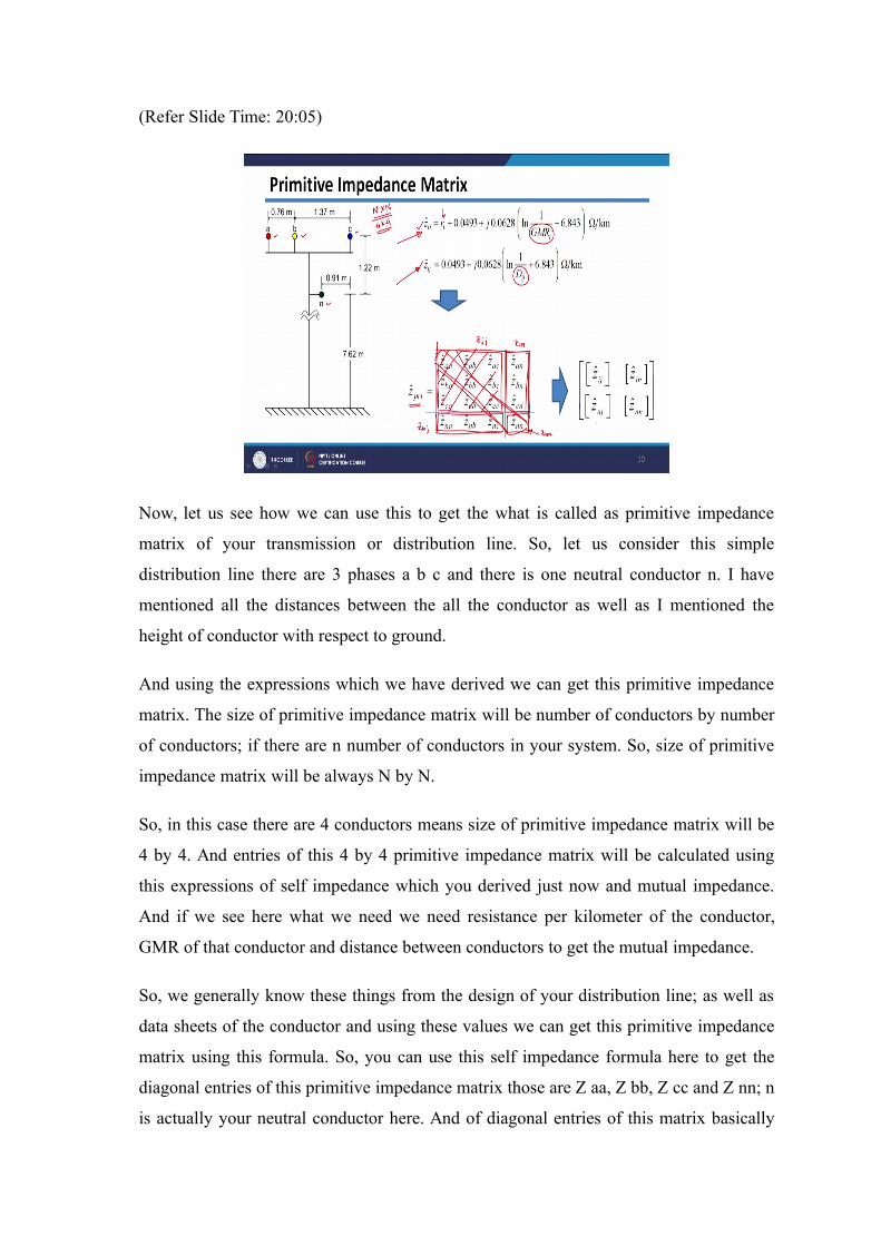
Now, let us see how we can use this to get the what is called as primitive impedance

matrix of your transmission or distribution line. So, let us consider this simple

distribution line there are 3 phases a b c and there is one neutral conductor n. I have

mentioned all the distances between the all the conductor as well as I mentioned the

height of conductor with respect to ground.

And using the expressions which we have derived we can get this primitive impedance

matrix. The size of primitive impedance matrix will be number of conductors by number

of conductors; if there are n number of conductors in your system. So, size of primitive

impedance matrix will be always N by N.

So, in this case there are 4 conductors means size of primitive impedance matrix will be

4 by 4. And entries of this 4 by 4 primitive impedance matrix will be calculated using

this expressions of self impedance which you derived just now and mutual impedance.

And if we see here what we need we need resistance per kilometer of the conductor,

GMR of that conductor and distance between conductors to get the mutual impedance.

So, we generally know these things from the design of your distribution line; as well as

data sheets of the conductor and using these values we can get this primitive impedance

matrix using this formula. So, you can use this self impedance formula here to get the

diagonal entries of this primitive impedance matrix those are Z aa, Z bb, Z cc and Z nn; n

is actually your neutral conductor here. And of diagonal entries of this matrix basically

all these entries we can get it from this expression 2. Again this is symmetric matrix; so,

on the entries of lower half of lower triangular half of this matrix can be easily calculated

or directly we can take it from upper triangular of part of the matrix.

Then we are going to divide this matrix into 4 parts; the parts corresponding to phase

conductors we want to separate from parts corresponding to neutral conductors. So, if

you see this part of the matrix is having only the phase conductors and this is actually

represented by Z ij. So, this part of the matrix I am representing it by Z ij. So, where i j I

am considering corresponding to your phase conductors this part which consisting of Z

in.

So, this I am representing by Z in because it is between impedances between your phase

conductors and neutral conductors which we want to separate out. Here also this part if

you see this consist of phase conductors as well as neutral conductors. So, I am

representing by Z nj and this part is only the neutral conductor part; so, this is

represented by Z nn.

So, if you write these 4 parts in short form I will get expression like this.


Again let us see for bigger matrix if there are 3 phase conductors and 3 neutral our earth

conductors ah; in that case you will be having say this l m n. So, a b c I am considering

phase conductors and l m n are your ground or neutral conductors.

So, in this case again we can divide this part is consisting of only terms related to phase

conductors. So, this will be represented by Z ij this is representing your phase as well as

neutral conductors. So, this will be represented by Z in; this is again representing phase

as well as neutral conductors. So, this will be Z nj and this is depending only the neutral

conductors. So, this is Z nn this this now we can divide this matrix into 4 parts.

Now, let us see what is a meaning of this 4 parts. So, here I have shown one typical case

where are there are 3 phase conductors and one neutral conductor and this neutral

conductor is having multi ground system.


So, it is this neutral conductor is grounded at various location along its path; so, here it is

grounded as well as here it is grounded. So, this system of equations we can write it like

this. So, voltages at this terminal of all the 3 conductor with respect to ground.

So, V ag with this voltage V bg and V cg and V ng all the 3 all the 4 conductor voltages

will be represented like this; they will be voltages of these conductors at these terminal

plus the drop which is happening in this part of the feeder.

So, in this case; so the voltages at the secondary end they are represented by dash term

here. So, V dash ag V dash bg V dash cg and V dash ng; they are thus this we end

voltages plus the drop along the feeder will be represented by this term here and this

system of equation. So, these 3 terms I can write in short form as V abc this term as it is

V ng here; these 3 terms I can write in short form as V dash abc, this term here and this

term is V dash ng as it is.

These 3 currents which are basically phase currents I can write using I abc notation and

this is your neutral current which is I n notation here therefore, this matrix will get again

divided into 4 part similar to those. So, this is corresponding to your phase conductors

and remaining parts are phase conductor to neutral conductor and only the neutral

conductor part. So, again this matrix is divided into 4 parts and these are the 4 parts. So,

this part is only related to your phase conductors, this is phase and neutral this is this is

again phase and neutral and this part is only related to your neutral conductor.


So, therefore, this equation from this slide I can take it on next slide. So, if you see this

equation here what I can do; I can write this equation number 1 say into form of 2

equation. So, this is your first equation which is first row of this and second equation is

which is second row; I can write them separately.

So, V abc will be equal to V dash abc plus Z ij into I abc plus Z in to I n. So, this is your

first equation here first row and the second equation corresponding to second row is V ng

which will be equal to V dash ng plus your Z nj into I abc plus Z nn into I n. So, this is

your second equation I can say third equation this is your second equation.

Now, if you observe this V ng and V dash ng term here. So, if you go to the previous

slide and if you observe here as I told you this ng and this n V dash ng. So, V ng and V

dash ng since they are grounded it at multiple location; the voltages V ng and V dash ng

they will be 0. So, we can see that this V ng voltage and V dash ng because of multiple

grounding they will be 0.

So, from this equation number 3; so, from this equation number 3 I can write V ng which

is 0 V dash ng is 0 and then the remaining terms are Z nj multiplied by I abc and Z nn

multiplied by I n. And then this expression I can write in terms of I n by taking other

terms on left hand side. So, I I can write I n will be equal to this term here which is

minus Z nn inverse multiplied by Z nj into I abc.

Then we can put these into expression 2 here; so, if we put this value into expression 2

ah. So, this term will get replaced by this term here. So, after replacing that I n with this

term here I will get this term here. And in this case I can take this I abc common out; so

the overall term in the bracket will be Z ij plus this term here which is Z in multiplied by

Z nn inverse multiplied by Z nj.

And this bracketed term calling Z abc and on this side it is V abc and V dash abc, Z abc

and I abc. So, if you observe this expression here which consist of only phase related

voltages and phase or or line currents only. So, nowhere there is terms related to neutral

conductor voltages or neutral conductor currents. So, we have eliminated your neutral

conductor using this expression here where your Z abc is represented by this term.

So, basically Z abc is given by this term by separating your primitive impedance matrix

into 4 parts. So, this is called as Kron reduction where we are eliminating the ground as

well as neutral conductors.


So, basically what we did the system which is having 4 conductors, we have converted

that system into only 3 phase conductors by eliminating your ground conductor here. So,

this but it is just directly not eliminated; however, we have taken the effect of those

conductor current on the phase conductor by doing Kron reduction. And using the Kron

reduction we have seen that your 4 by 4 primitive impedance matrix. So, this was your

primitive impedance matrix which is basically conductor size by conductor size.

So, in this case it is 4 by 4 because we are we are considering 4 conductors here. We

have divided into 4 parts and using Kron reduction which is given by this expression

here; we have got your phase impedance matrix, so this is called as phase impedance

matrix which will be number of phases by number of charges generally there are 3

phases; so, it will be 3 by 3 in size. So, primitive impedance matrix which was 4 by 4 in

size we have converted then into 3 by 3 size using Kron reduction.


So, let us take one example with actual dimensions. So, here we have seen there are 4

conductors and for these 4 conductors; you are having this primitive impedance matrix

huge entries will be calculated using these expressions of self and mutual impedances.

And we have discussed that these diagonal entries of this matrix will be calculated using

self impedance formula which is formula number 1.

And the half diagonal entries will be calculated using this mutual impedance formula and

you have seen that it only needs your resistance per kilometer of your feeder, conductor

and your GMR of conductor. And to get the mutual impedance we need distances

between the 2 conductor for which we are interested in calculating mutual impedance.

And once you get primitive impedance matrix using this you have to do the Kron

reduction to get phase impedance matrix which is 3 by 3 in size.


So, in this example I have considered these distances and GMRs and resistance per

kilometer required will be taken from the data sheets because we know which conductors

we have used for this system. So, for phase conductors we have used this 336 comma

400 which is having 26 by 7 means 26 aluminum conductor and 7 steel conductor.

So, which is ACSR conductor here and for neutral conductor we have used this 4 by 0

which is having 4 by 1 ACSR means there are 4, 6 aluminum strands and 1 steel strand.

So, for these 2 conductors from the data sheets we can get GMR GMRs of those

conductors. So, GMRs GMR of phase conductor is given by this and GMR of neutral

conductor is this, resistance of phase conductor per kilometer and this is your resistance

of neutral conductor per kilometer.

So, basically this 2 things are required in Carson’s equations and you can easily get the

distances between various conductors. So, dab 0.76 meter D bc 1.37 meter, D ca 2.13

meter, D an 1.72 meter, D bn 1.3 meter and D cn 1.52 meter. You can easily calculate

them from the design sheet of your distribution line and once you get those distances and

GMRs of the conductor you can get the self impedance of say conductor a that that can

be calculated using this self impedance formula here.


Resistance we can take it from resistance of the phase conductor a and GMR of

conductor a will be taken from GMR of the phase conductor. And if you put these values

into this expressions; I will get Z aa impedance which is having this value here which is

Ohm per kilometer.


Similarly, we can get mutual impedance between a and b conductor. So, mutual

impedance between these 2 conductors again if you are using this mutual impedance

formula given by Carson. And in this case we need distance between the 2 conductor D

ab which is 0 point it is 0.762 meter and D ab I am putting it here and after putting D ab;

I will get this mutual impedance between conductor a and b.


Similarly, we can get the mutual impedances as well as self impedances of all the

conductors and mutual impedances between all the pairs of the conductors. And if you do

this I will get this primitive impedance matrix which is 4 by 4 because there is in 4

conductors in this system. So, this is your primitive impedance matrix which is 4 by 4

size calculated using this self and mutual impedance formulae given by Carson.


So, after getting primitive impedance matrix we need to use Kron reduction technique to

get the phase impedance matrix. So we need to divide this primitive impedance matrix

into 4 parts separating phase conductors and neutral conductors; so in this case these are

related to phase conductors and this is neutral conductors. Similarly these rows are

corresponding to phase conductors see and this is neutral conductor.

So, this is nothing, but matrix which is related to only the phase conductor which is

represented by Z ij; this is related to neutral and phase conductors. So, this is Z in here

this is again related to phase and neutral conductors. So, this is Z nj here and this is

related only neutral conductors; so, this is your Z nn. So, from these 4 parts and using the

expression of the Kron reduction; which you have obtained; so, these are the 4 parts into

we can put into this Kron reduction equation.

And if you do that I will get the phase impedance matrix which is given by this. So, this

how we can get the series impedance matrix of your distribution line or feeder.


So, in summary of today’s lecture we have seen calculation of series impedance of

distribution lines and feeders. Specifically, we have seen this calculation for the systems

which consisting of earth return current. So, if there are earth return current we have seen

that we can use Carson’s equations and we have derived this Carson’s equations and the

modified form of Carson’s equations.

And we have seen that it can be used to calculate the impedances of the distribution line

with earth return. And then we have seen Kron reduction basically this Kron reduction

converts your primitive impedance matrix to the phase impedance matrix. Primitive

impedance matrix we have seen it is number of conductor by number of conductor size

which convert into phase impedance matrix which is 3 by 3 in size.

And finally, you are taken one typical example of distribution feeder and for that feeder;

we have calculated primitive impedance matrix and then we have converted that

primitive impedance matrix into phase impedance matrix.

Thank you.

11 Series Impedance of Distribution Lines and Feeders Part II

Documents

Transcript of 11 Series Impedance of Distribution Lines and Feeders Part II