1 | sampling and data - WebAssign

1 | SAMPLING AND DATA

Figure 1.1 We encounter statistics in our daily lives more often than we probably realize and from many differentsources, like the news. (credit: David Sim)

Introduction

Chapter Objectives

By the end of this chapter, the student should be able to:

• Recognize and differentiate between key terms.• Apply various types of sampling methods to data collection.• Create and interpret frequency tables.

You are probably asking yourself the question, "When and where will I use statistics?" If you read any newspaper, watchtelevision, or use the Internet, you will see statistical information. There are statistics about crime, sports, education,politics, and real estate. Typically, when you read a newspaper article or watch a television news program, you are givensample information. With this information, you may make a decision about the correctness of a statement, claim, or "fact."Statistical methods can help you make the "best educated guess."

Since you will undoubtedly be given statistical information at some point in your life, you need to know some techniquesfor analyzing the information thoughtfully. Think about buying a house or managing a budget. Think about your chosenprofession. The fields of economics, business, psychology, education, biology, law, computer science, police science, andearly childhood development require at least one course in statistics.

Included in this chapter are the basic ideas and words of probability and statistics. You will soon understand that statisticsand probability work together. You will also learn how data are gathered and what "good" data can be distinguished from"bad."

1.1 | Definitions of Statistics, Probability, and Key TermsThe science of statistics deals with the collection, analysis, interpretation, and presentation of data. We see and use data inour everyday lives.

CHAPTER 1 | SAMPLING AND DATA 9

In your classroom, try this exercise. Have class members write down the average time (in hours, to the nearest half-hour) they sleep per night. Your instructor will record the data. Then create a simple graph (called a dot plot) of thedata. A dot plot consists of a number line and dots (or points) positioned above the number line. For example, considerthe following data:

5; 5.5; 6; 6; 6; 6.5; 6.5; 6.5; 6.5; 7; 7; 8; 8; 9

The dot plot for this data would be as follows:

Figure 1.2

Does your dot plot look the same as or different from the example? Why? If you did the same example in an Englishclass with the same number of students, do you think the results would be the same? Why or why not?

Where do your data appear to cluster? How might you interpret the clustering?

The questions above ask you to analyze and interpret your data. With this example, you have begun your study ofstatistics.

In this course, you will learn how to organize and summarize data. Organizing and summarizing data is called descriptivestatistics. Two ways to summarize data are by graphing and by using numbers (for example, finding an average). After youhave studied probability and probability distributions, you will use formal methods for drawing conclusions from "good"data. The formal methods are called inferential statistics. Statistical inference uses probability to determine how confidentwe can be that our conclusions are correct.

Effective interpretation of data (inference) is based on good procedures for producing data and thoughtful examinationof the data. You will encounter what will seem to be too many mathematical formulas for interpreting data. The goalof statistics is not to perform numerous calculations using the formulas, but to gain an understanding of your data. Thecalculations can be done using a calculator or a computer. The understanding must come from you. If you can thoroughlygrasp the basics of statistics, you can be more confident in the decisions you make in life.

ProbabilityProbability is a mathematical tool used to study randomness. It deals with the chance (the likelihood) of an event occurring.For example, if you toss a fair coin four times, the outcomes may not be two heads and two tails. However, if you tossthe same coin 4,000 times, the outcomes will be close to half heads and half tails. The expected theoretical probability ofheads in any one toss is 1

2 or 0.5. Even though the outcomes of a few repetitions are uncertain, there is a regular pattern

of outcomes when there are many repetitions. After reading about the English statistician Karl Pearson who tossed a coin24,000 times with a result of 12,012 heads, one of the authors tossed a coin 2,000 times. The results were 996 heads. Thefraction 996

2000 is equal to 0.498 which is very close to 0.5, the expected probability.

The theory of probability began with the study of games of chance such as poker. Predictions take the form of probabilities.To predict the likelihood of an earthquake, of rain, or whether you will get an A in this course, we use probabilities. Doctorsuse probability to determine the chance of a vaccination causing the disease the vaccination is supposed to prevent. Astockbroker uses probability to determine the rate of return on a client's investments. You might use probability to decide tobuy a lottery ticket or not. In your study of statistics, you will use the power of mathematics through probability calculationsto analyze and interpret your data.

10 CHAPTER 1 | SAMPLING AND DATA

This content is available for free at http://cnx.org/content/col11562/1.16

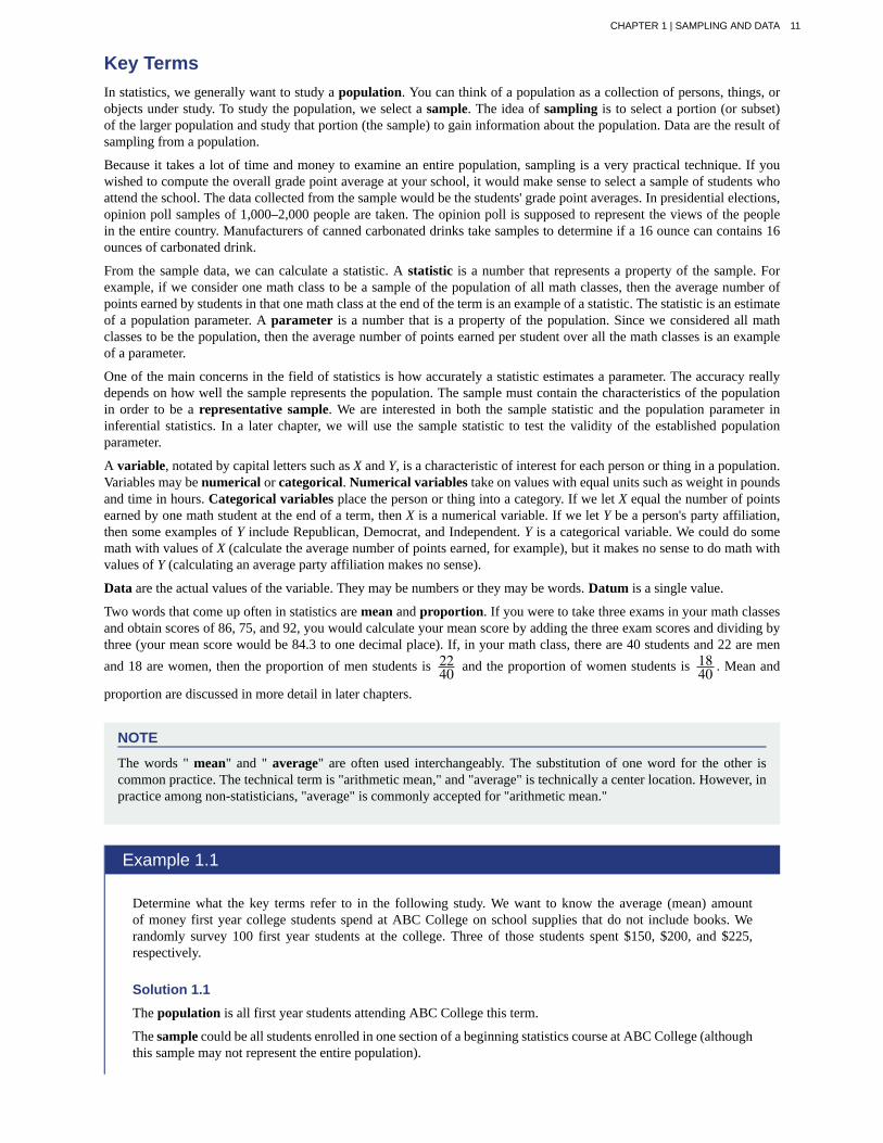
Key TermsIn statistics, we generally want to study a population. You can think of a population as a collection of persons, things, orobjects under study. To study the population, we select a sample. The idea of sampling is to select a portion (or subset)of the larger population and study that portion (the sample) to gain information about the population. Data are the result ofsampling from a population.

Because it takes a lot of time and money to examine an entire population, sampling is a very practical technique. If youwished to compute the overall grade point average at your school, it would make sense to select a sample of students whoattend the school. The data collected from the sample would be the students' grade point averages. In presidential elections,opinion poll samples of 1,000–2,000 people are taken. The opinion poll is supposed to represent the views of the peoplein the entire country. Manufacturers of canned carbonated drinks take samples to determine if a 16 ounce can contains 16ounces of carbonated drink.

From the sample data, we can calculate a statistic. A statistic is a number that represents a property of the sample. Forexample, if we consider one math class to be a sample of the population of all math classes, then the average number ofpoints earned by students in that one math class at the end of the term is an example of a statistic. The statistic is an estimateof a population parameter. A parameter is a number that is a property of the population. Since we considered all mathclasses to be the population, then the average number of points earned per student over all the math classes is an exampleof a parameter.

One of the main concerns in the field of statistics is how accurately a statistic estimates a parameter. The accuracy reallydepends on how well the sample represents the population. The sample must contain the characteristics of the populationin order to be a representative sample. We are interested in both the sample statistic and the population parameter ininferential statistics. In a later chapter, we will use the sample statistic to test the validity of the established populationparameter.

A variable, notated by capital letters such as X and Y, is a characteristic of interest for each person or thing in a population.Variables may be numerical or categorical. Numerical variables take on values with equal units such as weight in poundsand time in hours. Categorical variables place the person or thing into a category. If we let X equal the number of pointsearned by one math student at the end of a term, then X is a numerical variable. If we let Y be a person's party affiliation,then some examples of Y include Republican, Democrat, and Independent. Y is a categorical variable. We could do somemath with values of X (calculate the average number of points earned, for example), but it makes no sense to do math withvalues of Y (calculating an average party affiliation makes no sense).

Data are the actual values of the variable. They may be numbers or they may be words. Datum is a single value.

Two words that come up often in statistics are mean and proportion. If you were to take three exams in your math classesand obtain scores of 86, 75, and 92, you would calculate your mean score by adding the three exam scores and dividing bythree (your mean score would be 84.3 to one decimal place). If, in your math class, there are 40 students and 22 are menand 18 are women, then the proportion of men students is 22

40 and the proportion of women students is 1840 . Mean and

proportion are discussed in more detail in later chapters.

NOTE

The words " mean" and " average" are often used interchangeably. The substitution of one word for the other iscommon practice. The technical term is "arithmetic mean," and "average" is technically a center location. However, inpractice among non-statisticians, "average" is commonly accepted for "arithmetic mean."

Example 1.1

Determine what the key terms refer to in the following study. We want to know the average (mean) amountof money first year college students spend at ABC College on school supplies that do not include books. Werandomly survey 100 first year students at the college. Three of those students spent $150, $200, and $225,respectively.

Solution 1.1

The population is all first year students attending ABC College this term.

The sample could be all students enrolled in one section of a beginning statistics course at ABC College (althoughthis sample may not represent the entire population).


The parameter is the average (mean) amount of money spent (excluding books) by first year college students atABC College this term.

The statistic is the average (mean) amount of money spent (excluding books) by first year college students in thesample.

The variable could be the amount of money spent (excluding books) by one first year student. Let X = the amountof money spent (excluding books) by one first year student attending ABC College.

The data are the dollar amounts spent by the first year students. Examples of the data are $150, $200, and $225.

1.1 Determine what the key terms refer to in the following study. We want to know the average (mean) amount ofmoney spent on school uniforms each year by families with children at Knoll Academy. We randomly survey 100families with children in the school. Three of the families spent $65, $75, and $95, respectively.

Example 1.2

Determine what the key terms refer to in the following study.

A study was conducted at a local college to analyze the average cumulative GPA’s of students who graduated lastyear. Fill in the letter of the phrase that best describes each of the items below.

1._____ Population 2._____ Statistic 3._____ Parameter 4._____ Sample 5._____ Variable 6._____ Data

a) all students who attended the college last yearb) the cumulative GPA of one student who graduated from the college last yearc) 3.65, 2.80, 1.50, 3.90d) a group of students who graduated from the college last year, randomly selectede) the average cumulative GPA of students who graduated from the college last yearf) all students who graduated from the college last yearg) the average cumulative GPA of students in the study who graduated from the college last year

Solution 1.21. f; 2. g; 3. e; 4. d; 5. b; 6. c

Example 1.3


As part of a study designed to test the safety of automobiles, the National Transportation Safety Board collectedand reviewed data about the effects of an automobile crash on test dummies. Here is the criterion they used:

Speed at which Cars Crashed Location of “drive” (i.e. dummies)

35 miles/hour Front Seat

Table 1.1

Cars with dummies in the front seats were crashed into a wall at a speed of 35 miles per hour. We want to knowthe proportion of dummies in the driver’s seat that would have had head injuries, if they had been actual drivers.We start with a simple random sample of 75 cars.

Solution 1.3



The population is all cars containing dummies in the front seat.

The sample is the 75 cars, selected by a simple random sample.

The parameter is the proportion of driver dummies (if they had been real people) who would have suffered headinjuries in the population.

The statistic is proportion of driver dummies (if they had been real people) who would have suffered head injuriesin the sample.

The variable X = the number of driver dummies (if they had been real people) who would have suffered headinjuries.

The data are either: yes, had head injury, or no, did not.

Example 1.4


An insurance company would like to determine the proportion of all medical doctors who have been involved inone or more malpractice lawsuits. The company selects 500 doctors at random from a professional directory anddetermines the number in the sample who have been involved in a malpractice lawsuit.

Solution 1.4

The population is all medical doctors listed in the professional directory.

The parameter is the proportion of medical doctors who have been involved in one or more malpractice suits inthe population.

The sample is the 500 doctors selected at random from the professional directory.

The statistic is the proportion of medical doctors who have been involved in one or more malpractice suits in thesample.

The variable X = the number of medical doctors who have been involved in one or more malpractice suits.

The data are either: yes, was involved in one or more malpractice lawsuits, or no, was not.

Do the following exercise collaboratively with up to four people per group. Find a population, a sample, the parameter,the statistic, a variable, and data for the following study: You want to determine the average (mean) number of glassesof milk college students drink per day. Suppose yesterday, in your English class, you asked five students how manyglasses of milk they drank the day before. The answers were 1, 0, 1, 3, and 4 glasses of milk.

1.2 | Data, Sampling, and Variation in Data and SamplingData may come from a population or from a sample. Small letters like x or y generally are used to represent data values.

Most data can be put into the following categories:

• Qualitative

• Quantitative

Qualitative data are the result of categorizing or describing attributes of a population. Hair color, blood type, ethnic group,the car a person drives, and the street a person lives on are examples of qualitative data. Qualitative data are generallydescribed by words or letters. For instance, hair color might be black, dark brown, light brown, blonde, gray, or red. Bloodtype might be AB+, O-, or B+. Researchers often prefer to use quantitative data over qualitative data because it lends itselfmore easily to mathematical analysis. For example, it does not make sense to find an average hair color or blood type.


Quantitative data are always numbers. Quantitative data are the result of counting or measuring attributes of a population.Amount of money, pulse rate, weight, number of people living in your town, and number of students who take statistics areexamples of quantitative data. Quantitative data may be either discrete or continuous.

All data that are the result of counting are called quantitative discrete data. These data take on only certain numericalvalues. If you count the number of phone calls you receive for each day of the week, you might get values such as zero, one,two, or three.

All data that are the result of measuring are quantitative continuous data assuming that we can measure accurately.Measuring angles in radians might result in such numbers as π

6 , π3 , π

2 , π , 3π4 , and so on. If you and your friends carry

backpacks with books in them to school, the numbers of books in the backpacks are discrete data and the weights of thebackpacks are continuous data.

Example 1.5 Data Sample of Quantitative Discrete Data

The data are the number of books students carry in their backpacks. You sample five students. Two students carrythree books, one student carries four books, one student carries two books, and one student carries one book. Thenumbers of books (three, four, two, and one) are the quantitative discrete data.

1.5 The data are the number of machines in a gym. You sample five gyms. One gym has 12 machines, one gym has15 machines, one gym has ten machines, one gym has 22 machines, and the other gym has 20 machines. What type ofdata is this?

Example 1.6 Data Sample of Quantitative Continuous Data

The data are the weights of backpacks with books in them. You sample the same five students. The weights (inpounds) of their backpacks are 6.2, 7, 6.8, 9.1, 4.3. Notice that backpacks carrying three books can have differentweights. Weights are quantitative continuous data because weights are measured.

1.6 The data are the areas of lawns in square feet. You sample five houses. The areas of the lawns are 144 sq. feet,160 sq. feet, 190 sq. feet, 180 sq. feet, and 210 sq. feet. What type of data is this?

Example 1.7

You go to the supermarket and purchase three cans of soup (19 ounces) tomato bisque, 14.1 ounces lentil, and 19ounces Italian wedding), two packages of nuts (walnuts and peanuts), four different kinds of vegetable (broccoli,cauliflower, spinach, and carrots), and two desserts (16 ounces Cherry Garcia ice cream and two pounds (32ounces chocolate chip cookies).

Name data sets that are quantitative discrete, quantitative continuous, and qualitative.

Solution 1.7

One Possible Solution:

• The three cans of soup, two packages of nuts, four kinds of vegetables and two desserts are quantitativediscrete data because you count them.



• The weights of the soups (19 ounces, 14.1 ounces, 19 ounces) are quantitative continuous data because youmeasure weights as precisely as possible.

• Types of soups, nuts, vegetables and desserts are qualitative data because they are categorical.

Try to identify additional data sets in this example.

Example 1.8

The data are the colors of backpacks. Again, you sample the same five students. One student has a red backpack,two students have black backpacks, one student has a green backpack, and one student has a gray backpack. Thecolors red, black, black, green, and gray are qualitative data.

1.8 The data are the colors of houses. You sample five houses. The colors of the houses are white, yellow, white, red,and white. What type of data is this?

NOTE

You may collect data as numbers and report it categorically. For example, the quiz scores for each student are recordedthroughout the term. At the end of the term, the quiz scores are reported as A, B, C, D, or F.

Example 1.9

Work collaboratively to determine the correct data type (quantitative or qualitative). Indicate whether quantitativedata are continuous or discrete. Hint: Data that are discrete often start with the words "the number of."

a. the number of pairs of shoes you own

b. the type of car you drive

c. where you go on vacation

d. the distance it is from your home to the nearest grocery store

e. the number of classes you take per school year.

f. the tuition for your classes

g. the type of calculator you use

h. movie ratings

i. political party preferences

j. weights of sumo wrestlers

k. amount of money (in dollars) won playing poker

l. number of correct answers on a quiz

m. peoples’ attitudes toward the government

n. IQ scores (This may cause some discussion.)

Solution 1.9Items a, e, f, k, and l are quantitative discrete; items d, j, and n are quantitative continuous; items b, c, g, h, i, andm are qualitative.


1.9 Determine the correct data type (quantitative or qualitative) for the number of cars in a parking lot. Indicatewhether quantitative data are continuous or discrete.

Example 1.10

A statistics professor collects information about the classification of her students as freshmen, sophomores,juniors, or seniors. The data she collects are summarized in the pie chart Figure 1.2. What type of data does thisgraph show?

Figure 1.3

Solution 1.10This pie chart shows the students in each year, which is qualitative data.

1.10 The registrar at State University keeps records of the number of credit hours students complete each semester.The data he collects are summarized in the histogram. The class boundaries are 10 to less than 13, 13 to less than 16,16 to less than 19, 19 to less than 22, and 22 to less than 25.



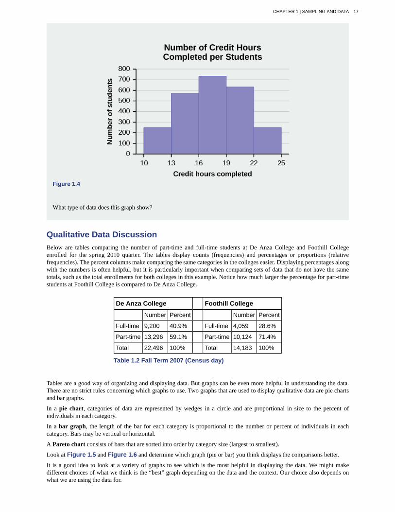
Figure 1.4

What type of data does this graph show?

Qualitative Data DiscussionBelow are tables comparing the number of part-time and full-time students at De Anza College and Foothill Collegeenrolled for the spring 2010 quarter. The tables display counts (frequencies) and percentages or proportions (relativefrequencies). The percent columns make comparing the same categories in the colleges easier. Displaying percentages alongwith the numbers is often helpful, but it is particularly important when comparing sets of data that do not have the sametotals, such as the total enrollments for both colleges in this example. Notice how much larger the percentage for part-timestudents at Foothill College is compared to De Anza College.

De Anza College Foothill College

Number Percent Number Percent

Full-time 9,200 40.9% Full-time 4,059 28.6%

Part-time 13,296 59.1% Part-time 10,124 71.4%

Total 22,496 100% Total 14,183 100%

Table 1.2 Fall Term 2007 (Census day)

Tables are a good way of organizing and displaying data. But graphs can be even more helpful in understanding the data.There are no strict rules concerning which graphs to use. Two graphs that are used to display qualitative data are pie chartsand bar graphs.

In a pie chart, categories of data are represented by wedges in a circle and are proportional in size to the percent ofindividuals in each category.

In a bar graph, the length of the bar for each category is proportional to the number or percent of individuals in eachcategory. Bars may be vertical or horizontal.

A Pareto chart consists of bars that are sorted into order by category size (largest to smallest).

Look at Figure 1.5 and Figure 1.6 and determine which graph (pie or bar) you think displays the comparisons better.

It is a good idea to look at a variety of graphs to see which is the most helpful in displaying the data. We might makedifferent choices of what we think is the “best” graph depending on the data and the context. Our choice also depends onwhat we are using the data for.


(a) (b)Figure 1.5

Figure 1.6

Percentages That Add to More (or Less) Than 100%Sometimes percentages add up to be more than 100% (or less than 100%). In the graph, the percentages add to more than100% because students can be in more than one category. A bar graph is appropriate to compare the relative size of thecategories. A pie chart cannot be used. It also could not be used if the percentages added to less than 100%.

Characteristic/Category Percent

Full-Time Students 40.9%

Students who intend to transfer to a 4-year educational institution 48.6%

Students under age 25 61.0%

TOTAL 150.5%

Table 1.3 De Anza College Spring 2010



Figure 1.7

Omitting Categories/Missing DataThe table displays Ethnicity of Students but is missing the "Other/Unknown" category. This category contains people whodid not feel they fit into any of the ethnicity categories or declined to respond. Notice that the frequencies do not add up tothe total number of students. In this situation, create a bar graph and not a pie chart.

Frequency Percent

Asian 8,794 36.1%

Black 1,412 5.8%

Filipino 1,298 5.3%

Hispanic 4,180 17.1%

Native American 146 0.6%

Pacific Islander 236 1.0%

White 5,978 24.5%

TOTAL 22,044 out of 24,382 90.4% out of 100%

Table 1.4 Ethnicity of Students at De Anza College FallTerm 2007 (Census Day)

Figure 1.8


The following graph is the same as the previous graph but the “Other/Unknown” percent (9.6%) has been included. The“Other/Unknown” category is large compared to some of the other categories (Native American, 0.6%, Pacific Islander1.0%). This is important to know when we think about what the data are telling us.

This particular bar graph in Figure 1.9 can be difficult to understand visually. The graph in Figure 1.10 is a Pareto chart.The Pareto chart has the bars sorted from largest to smallest and is easier to read and interpret.

Figure 1.9 Bar Graph with Other/Unknown Category

Figure 1.10 Pareto Chart With Bars Sorted by Size

Pie Charts: No Missing DataThe following pie charts have the “Other/Unknown” category included (since the percentages must add to 100%). Thechart in Figure 1.11b is organized by the size of each wedge, which makes it a more visually informative graph than theunsorted, alphabetical graph in Figure 1.11a.



(a)(b)

Figure 1.11

SamplingGathering information about an entire population often costs too much or is virtually impossible. Instead, we use a sampleof the population. A sample should have the same characteristics as the population it is representing. Most statisticiansuse various methods of random sampling in an attempt to achieve this goal. This section will describe a few of the mostcommon methods. There are several different methods of random sampling. In each form of random sampling, eachmember of a population initially has an equal chance of being selected for the sample. Each method has pros and cons. Theeasiest method to describe is called a simple random sample. Any group of n individuals is equally likely to be chosen byany other group of n individuals if the simple random sampling technique is used. In other words, each sample of the samesize has an equal chance of being selected. For example, suppose Lisa wants to form a four-person study group (herselfand three other people) from her pre-calculus class, which has 31 members not including Lisa. To choose a simple randomsample of size three from the other members of her class, Lisa could put all 31 names in a hat, shake the hat, close hereyes, and pick out three names. A more technological way is for Lisa to first list the last names of the members of her classtogether with a two-digit number, as in Table 1.5:

ID Name ID Name ID Name

00 Anselmo 11 King 21 Roquero

01 Bautista 12 Legeny 22 Roth

02 Bayani 13 Lundquist 23 Rowell

03 Cheng 14 Macierz 24 Salangsang

04 Cuarismo 15 Motogawa 25 Slade

05 Cuningham 16 Okimoto 26 Stratcher

06 Fontecha 17 Patel 27 Tallai

07 Hong 18 Price 28 Tran

08 Hoobler 19 Quizon 29 Wai

09 Jiao 20 Reyes 30 Wood

10 Khan

Table 1.5 Class Roster

Lisa can use a table of random numbers (found in many statistics books and mathematical handbooks), a calculator, ora computer to generate random numbers. For this example, suppose Lisa chooses to generate random numbers from acalculator. The numbers generated are as follows:

0.94360; 0.99832; 0.14669; 0.51470; 0.40581; 0.73381; 0.04399


Lisa reads two-digit groups until she has chosen three class members (that is, she reads 0.94360 as the groups 94, 43, 36,60). Each random number may only contribute one class member. If she needed to, Lisa could have generated more randomnumbers.

The random numbers 0.94360 and 0.99832 do not contain appropriate two digit numbers. However the third randomnumber, 0.14669, contains 14 (the fourth random number also contains 14), the fifth random number contains 05, and theseventh random number contains 04. The two-digit number 14 corresponds to Macierz, 05 corresponds to Cuningham, and04 corresponds to Cuarismo. Besides herself, Lisa’s group will consist of Marcierz, Cuningham, and Cuarismo.

To generate random numbers:

• Press MATH.

• Arrow over to PRB.

• Press 5:randInt(. Enter 0, 30).

• Press ENTER for the first random number.

• Press ENTER two more times for the other 2 random numbers. If there is a repeat press ENTER again.

Note: randInt(0, 30, 3) will generate 3 random numbers.

Figure 1.12

Besides simple random sampling, there are other forms of sampling that involve a chance process for getting the sample.Other well-known random sampling methods are the stratified sample, the cluster sample, and the systematicsample.

To choose a stratified sample, divide the population into groups called strata and then take a proportionate numberfrom each stratum. For example, you could stratify (group) your college population by department and then choose aproportionate simple random sample from each stratum (each department) to get a stratified random sample. To choosea simple random sample from each department, number each member of the first department, number each member ofthe second department, and do the same for the remaining departments. Then use simple random sampling to chooseproportionate numbers from the first department and do the same for each of the remaining departments. Those numberspicked from the first department, picked from the second department, and so on represent the members who make up thestratified sample.

To choose a cluster sample, divide the population into clusters (groups) and then randomly select some of the clusters.All the members from these clusters are in the cluster sample. For example, if you randomly sample four departmentsfrom your college population, the four departments make up the cluster sample. Divide your college faculty by department.The departments are the clusters. Number each department, and then choose four different numbers using simple randomsampling. All members of the four departments with those numbers are the cluster sample.

To choose a systematic sample, randomly select a starting point and take every nth piece of data from a listing of thepopulation. For example, suppose you have to do a phone survey. Your phone book contains 20,000 residence listings. Youmust choose 400 names for the sample. Number the population 1–20,000 and then use a simple random sample to pick anumber that represents the first name in the sample. Then choose every fiftieth name thereafter until you have a total of 400names (you might have to go back to the beginning of your phone list). Systematic sampling is frequently chosen becauseit is a simple method.

A type of sampling that is non-random is convenience sampling. Convenience sampling involves using results that arereadily available. For example, a computer software store conducts a marketing study by interviewing potential customers



who happen to be in the store browsing through the available software. The results of convenience sampling may be verygood in some cases and highly biased (favor certain outcomes) in others.

Sampling data should be done very carefully. Collecting data carelessly can have devastating results. Surveys mailed tohouseholds and then returned may be very biased (they may favor a certain group). It is better for the person conducting thesurvey to select the sample respondents.

True random sampling is done with replacement. That is, once a member is picked, that member goes back into thepopulation and thus may be chosen more than once. However for practical reasons, in most populations, simple randomsampling is done without replacement. Surveys are typically done without replacement. That is, a member of thepopulation may be chosen only once. Most samples are taken from large populations and the sample tends to be small incomparison to the population. Since this is the case, sampling without replacement is approximately the same as samplingwith replacement because the chance of picking the same individual more than once with replacement is very low.

In a college population of 10,000 people, suppose you want to pick a sample of 1,000 randomly for a survey. For anyparticular sample of 1,000, if you are sampling with replacement,

• the chance of picking the first person is 1,000 out of 10,000 (0.1000);

• the chance of picking a different second person for this sample is 999 out of 10,000 (0.0999);

• the chance of picking the same person again is 1 out of 10,000 (very low).

If you are sampling without replacement,

• the chance of picking the first person for any particular sample is 1000 out of 10,000 (0.1000);

• the chance of picking a different second person is 999 out of 9,999 (0.0999);

• you do not replace the first person before picking the next person.

Compare the fractions 999/10,000 and 999/9,999. For accuracy, carry the decimal answers to four decimal places. To fourdecimal places, these numbers are equivalent (0.0999).

Sampling without replacement instead of sampling with replacement becomes a mathematical issue only when thepopulation is small. For example, if the population is 25 people, the sample is ten, and you are sampling with replacementfor any particular sample, then the chance of picking the first person is ten out of 25, and the chance of picking a differentsecond person is nine out of 25 (you replace the first person).

If you sample without replacement, then the chance of picking the first person is ten out of 25, and then the chance ofpicking the second person (who is different) is nine out of 24 (you do not replace the first person).

Compare the fractions 9/25 and 9/24. To four decimal places, 9/25 = 0.3600 and 9/24 = 0.3750. To four decimal places,these numbers are not equivalent.

When you analyze data, it is important to be aware of sampling errors and nonsampling errors. The actual process ofsampling causes sampling errors. For example, the sample may not be large enough. Factors not related to the samplingprocess cause nonsampling errors. A defective counting device can cause a nonsampling error.

In reality, a sample will never be exactly representative of the population so there will always be some sampling error. As arule, the larger the sample, the smaller the sampling error.

In statistics, a sampling bias is created when a sample is collected from a population and some members of the populationare not as likely to be chosen as others (remember, each member of the population should have an equally likely chance ofbeing chosen). When a sampling bias happens, there can be incorrect conclusions drawn about the population that is beingstudied.

Example 1.11

A study is done to determine the average tuition that San Jose State undergraduate students pay per semester.Each student in the following samples is asked how much tuition he or she paid for the Fall semester. What is thetype of sampling in each case?

a. A sample of 100 undergraduate San Jose State students is taken by organizing the students’ names byclassification (freshman, sophomore, junior, or senior), and then selecting 25 students from each.

b. A random number generator is used to select a student from the alphabetical listing of all undergraduatestudents in the Fall semester. Starting with that student, every 50th student is chosen until 75 students areincluded in the sample.

c. A completely random method is used to select 75 students. Each undergraduate student in the fall semesterhas the same probability of being chosen at any stage of the sampling process.


d. The freshman, sophomore, junior, and senior years are numbered one, two, three, and four, respectively.A random number generator is used to pick two of those years. All students in those two years are in thesample.

e. An administrative assistant is asked to stand in front of the library one Wednesday and to ask the first 100undergraduate students he encounters what they paid for tuition the Fall semester. Those 100 students arethe sample.

Solution 1.11a. stratified; b. systematic; c. simple random; d. cluster; e. convenience

1.11 You are going to use the random number generator to generate different types of samples from the data.

This table displays six sets of quiz scores (each quiz counts 10 points) for an elementary statistics class.

#1 #2 #3 #4 #5 #6

5 7 10 9 8 3

10 5 9 8 7 6

9 10 8 6 7 9

9 10 10 9 8 9

7 8 9 5 7 4

9 9 9 10 8 7

7 7 10 9 8 8

8 8 9 10 8 8

9 7 8 7 7 8

8 8 10 9 8 7

Table 1.6

Instructions: Use the Random Number Generator to pick samples.

1. Create a stratified sample by column. Pick three quiz scores randomly from each column.

◦ Number each row one through ten.

◦ On your calculator, press Math and arrow over to PRB.

◦ For column 1, Press 5:randInt( and enter 1,10). Press ENTER. Record the number. Press ENTER 2 moretimes (even the repeats). Record these numbers. Record the three quiz scores in column one that correspondto these three numbers.

◦ Repeat for columns two through six.

◦ These 18 quiz scores are a stratified sample.

2. Create a cluster sample by picking two of the columns. Use the column numbers: one through six.

◦ Press MATH and arrow over to PRB.

◦ Press 5:randInt( and enter 1,6). Press ENTER. Record the number. Press ENTER and record that number.

◦ The two numbers are for two of the columns.

◦ The quiz scores (20 of them) in these 2 columns are the cluster sample.

3. Create a simple random sample of 15 quiz scores.

◦ Use the numbering one through 60.

◦ Press MATH. Arrow over to PRB. Press 5:randInt( and enter 1, 60).



◦ Press ENTER 15 times and record the numbers.

◦ Record the quiz scores that correspond to these numbers.

◦ These 15 quiz scores are the systematic sample.

4. Create a systematic sample of 12 quiz scores.

◦ Use the numbering one through 60.

◦ Press MATH. Arrow over to PRB. Press 5:randInt( and enter 1, 60).

◦ Press ENTER. Record the number and the first quiz score. From that number, count ten quiz scores andrecord that quiz score. Keep counting ten quiz scores and recording the quiz score until you have a sampleof 12 quiz scores. You may wrap around (go back to the beginning).

Example 1.12

Determine the type of sampling used (simple random, stratified, systematic, cluster, or convenience).

a. A soccer coach selects six players from a group of boys aged eight to ten, seven players from a group ofboys aged 11 to 12, and three players from a group of boys aged 13 to 14 to form a recreational soccer team.

b. A pollster interviews all human resource personnel in five different high tech companies.

c. A high school educational researcher interviews 50 high school female teachers and 50 high school maleteachers.

d. A medical researcher interviews every third cancer patient from a list of cancer patients at a local hospital.

e. A high school counselor uses a computer to generate 50 random numbers and then picks students whosenames correspond to the numbers.

f. A student interviews classmates in his algebra class to determine how many pairs of jeans a student owns,on the average.

Solution 1.12a. stratified; b. cluster; c. stratified; d. systematic; e. simple random; f.convenience

1.12 Determine the type of sampling used (simple random, stratified, systematic, cluster, or convenience).

A high school principal polls 50 freshmen, 50 sophomores, 50 juniors, and 50 seniors regarding policy changes forafter school activities.

If we were to examine two samples representing the same population, even if we used random sampling methods for thesamples, they would not be exactly the same. Just as there is variation in data, there is variation in samples. As you becomeaccustomed to sampling, the variability will begin to seem natural.

Example 1.13

Suppose ABC College has 10,000 part-time students (the population). We are interested in the average amount ofmoney a part-time student spends on books in the fall term. Asking all 10,000 students is an almost impossibletask.

Suppose we take two different samples.

First, we use convenience sampling and survey ten students from a first term organic chemistry class. Many ofthese students are taking first term calculus in addition to the organic chemistry class. The amount of money theyspend on books is as follows:

$128; $87; $173; $116; $130; $204; $147; $189; $93; $153


The second sample is taken using a list of senior citizens who take P.E. classes and taking every fifth senior citizenon the list, for a total of ten senior citizens. They spend:

$50; $40; $36; $15; $50; $100; $40; $53; $22; $22

It is unlikely that any student is in both samples.

a. Do you think that either of these samples is representative of (or is characteristic of) the entire 10,000 part-timestudent population?

Solution 1.13a. No. The first sample probably consists of science-oriented students. Besides the chemistry course, some ofthem are also taking first-term calculus. Books for these classes tend to be expensive. Most of these students are,more than likely, paying more than the average part-time student for their books. The second sample is a group ofsenior citizens who are, more than likely, taking courses for health and interest. The amount of money they spendon books is probably much less than the average parttime student. Both samples are biased. Also, in both cases,not all students have a chance to be in either sample.

b. Since these samples are not representative of the entire population, is it wise to use the results to describe theentire population?

Solution 1.13b. No. For these samples, each member of the population did not have an equally likely chance of being chosen.

Now, suppose we take a third sample. We choose ten different part-time students from the disciplines ofchemistry, math, English, psychology, sociology, history, nursing, physical education, art, and early childhooddevelopment. (We assume that these are the only disciplines in which part-time students at ABC College areenrolled and that an equal number of part-time students are enrolled in each of the disciplines.) Each student ischosen using simple random sampling. Using a calculator, random numbers are generated and a student froma particular discipline is selected if he or she has a corresponding number. The students spend the followingamounts:

$180; $50; $150; $85; $260; $75; $180; $200; $200; $150

c. Is the sample biased?

Solution 1.13c. The sample is unbiased, but a larger sample would be recommended to increase the likelihood that the samplewill be close to representative of the population. However, for a biased sampling technique, even a large sampleruns the risk of not being representative of the population.

Students often ask if it is "good enough" to take a sample, instead of surveying the entire population. If the surveyis done well, the answer is yes.

1.13 A local radio station has a fan base of 20,000 listeners. The station wants to know if its audience would prefermore music or more talk shows. Asking all 20,000 listeners is an almost impossible task.

The station uses convenience sampling and surveys the first 200 people they meet at one of the station’s music concertevents. 24 people said they’d prefer more talk shows, and 176 people said they’d prefer more music.

Do you think that this sample is representative of (or is characteristic of) the entire 20,000 listener population?

As a class, determine whether or not the following samples are representative. If they are not, discuss the reasons.

1. To find the average GPA of all students in a university, use all honor students at the university as the sample.



2. To find out the most popular cereal among young people under the age of ten, stand outside a large supermarketfor three hours and speak to every twentieth child under age ten who enters the supermarket.

3. To find the average annual income of all adults in the United States, sample U.S. congressmen. Create a clustersample by considering each state as a stratum (group). By using simple random sampling, select states to be partof the cluster. Then survey every U.S. congressman in the cluster.

4. To determine the proportion of people taking public transportation to work, survey 20 people in New York City.Conduct the survey by sitting in Central Park on a bench and interviewing every person who sits next to you.

5. To determine the average cost of a two-day stay in a hospital in Massachusetts, survey 100 hospitals across thestate using simple random sampling.

Variation in DataVariation is present in any set of data. For example, 16-ounce cans of beverage may contain more or less than 16 ounces ofliquid. In one study, eight 16 ounce cans were measured and produced the following amount (in ounces) of beverage:

15.8; 16.1; 15.2; 14.8; 15.8; 15.9; 16.0; 15.5

Measurements of the amount of beverage in a 16-ounce can may vary because different people make the measurements orbecause the exact amount, 16 ounces of liquid, was not put into the cans. Manufacturers regularly run tests to determine ifthe amount of beverage in a 16-ounce can falls within the desired range.

Be aware that as you take data, your data may vary somewhat from the data someone else is taking for the same purpose.This is completely natural. However, if two or more of you are taking the same data and get very different results, it is timefor you and the others to reevaluate your data-taking methods and your accuracy.

Variation in SamplesIt was mentioned previously that two or more samples from the same population, taken randomly, and having close tothe same characteristics of the population will likely be different from each other. Suppose Doreen and Jung both decideto study the average amount of time students at their college sleep each night. Doreen and Jung each take samples of 500students. Doreen uses systematic sampling and Jung uses cluster sampling. Doreen's sample will be different from Jung'ssample. Even if Doreen and Jung used the same sampling method, in all likelihood their samples would be different. Neitherwould be wrong, however.

Think about what contributes to making Doreen’s and Jung’s samples different.

If Doreen and Jung took larger samples (i.e. the number of data values is increased), their sample results (the averageamount of time a student sleeps) might be closer to the actual population average. But still, their samples would be, in alllikelihood, different from each other. This variability in samples cannot be stressed enough.

Size of a SampleThe size of a sample (often called the number of observations) is important. The examples you have seen in this book so farhave been small. Samples of only a few hundred observations, or even smaller, are sufficient for many purposes. In polling,samples that are from 1,200 to 1,500 observations are considered large enough and good enough if the survey is randomand is well done. You will learn why when you study confidence intervals.

Be aware that many large samples are biased. For example, call-in surveys are invariably biased, because people choose torespond or not.

Divide into groups of two, three, or four. Your instructor will give each group one six-sided die. Try this experimenttwice. Roll one fair die (six-sided) 20 times. Record the number of ones, twos, threes, fours, fives, and sixes you get inTable 1.7 and Table 1.8 (“frequency” is the number of times a particular face of the die occurs):


Face on Die Frequency

1

2

3

4

5

6

Table 1.7 First Experiment (20rolls)

Face on Die Frequency

1

2

3

4

5

6

Table 1.8 Second Experiment(20 rolls)

Did the two experiments have the same results? Probably not. If you did the experiment a third time, do you expect theresults to be identical to the first or second experiment? Why or why not?

Which experiment had the correct results? They both did. The job of the statistician is to see through the variabilityand draw appropriate conclusions.

Critical EvaluationWe need to evaluate the statistical studies we read about critically and analyze them before accepting the results of thestudies. Common problems to be aware of include

• Problems with samples: A sample must be representative of the population. A sample that is not representative of thepopulation is biased. Biased samples that are not representative of the population give results that are inaccurate andnot valid.

• Self-selected samples: Responses only by people who choose to respond, such as call-in surveys, are often unreliable.

• Sample size issues: Samples that are too small may be unreliable. Larger samples are better, if possible. In somesituations, having small samples is unavoidable and can still be used to draw conclusions. Examples: crash testing carsor medical testing for rare conditions

• Undue influence: collecting data or asking questions in a way that influences the response

• Non-response or refusal of subject to participate: The collected responses may no longer be representative of thepopulation. Often, people with strong positive or negative opinions may answer surveys, which can affect the results.

• Causality: A relationship between two variables does not mean that one causes the other to occur. They may be related(correlated) because of their relationship through a different variable.

• Self-funded or self-interest studies: A study performed by a person or organization in order to support their claim. Isthe study impartial? Read the study carefully to evaluate the work. Do not automatically assume that the study is good,but do not automatically assume the study is bad either. Evaluate it on its merits and the work done.

• Misleading use of data: improperly displayed graphs, incomplete data, or lack of context



• Confounding: When the effects of multiple factors on a response cannot be separated. Confounding makes it difficultor impossible to draw valid conclusions about the effect of each factor.

1.3 | Frequency, Frequency Tables, and Levels ofMeasurementOnce you have a set of data, you will need to organize it so that you can analyze how frequently each datum occurs in theset. However, when calculating the frequency, you may need to round your answers so that they are as precise as possible.

Answers and Rounding OffA simple way to round off answers is to carry your final answer one more decimal place than was present in the originaldata. Round off only the final answer. Do not round off any intermediate results, if possible. If it becomes necessary to roundoff intermediate results, carry them to at least twice as many decimal places as the final answer. For example, the averageof the three quiz scores four, six, and nine is 6.3, rounded off to the nearest tenth, because the data are whole numbers. Mostanswers will be rounded off in this manner.

It is not necessary to reduce most fractions in this course. Especially in Probability Topics, the chapter on probability, itis more helpful to leave an answer as an unreduced fraction.

Levels of MeasurementThe way a set of data is measured is called its level of measurement. Correct statistical procedures depend on a researcherbeing familiar with levels of measurement. Not every statistical operation can be used with every set of data. Data can beclassified into four levels of measurement. They are (from lowest to highest level):

• Nominal scale level

• Ordinal scale level

• Interval scale level

• Ratio scale level

Data that is measured using a nominal scale is qualitative. Categories, colors, names, labels and favorite foods along withyes or no responses are examples of nominal level data. Nominal scale data are not ordered. For example, trying to classifypeople according to their favorite food does not make any sense. Putting pizza first and sushi second is not meaningful.

Smartphone companies are another example of nominal scale data. Some examples are Sony, Motorola, Nokia, Samsungand Apple. This is just a list and there is no agreed upon order. Some people may favor Apple but that is a matter of opinion.Nominal scale data cannot be used in calculations.

Data that is measured using an ordinal scale is similar to nominal scale data but there is a big difference. The ordinal scaledata can be ordered. An example of ordinal scale data is a list of the top five national parks in the United States. The topfive national parks in the United States can be ranked from one to five but we cannot measure differences between the data.

Another example of using the ordinal scale is a cruise survey where the responses to questions about the cruise are“excellent,” “good,” “satisfactory,” and “unsatisfactory.” These responses are ordered from the most desired response to theleast desired. But the differences between two pieces of data cannot be measured. Like the nominal scale data, ordinal scaledata cannot be used in calculations.

Data that is measured using the interval scale is similar to ordinal level data because it has a definite ordering but thereis a difference between data. The differences between interval scale data can be measured though the data does not have astarting point.

Temperature scales like Celsius (C) and Fahrenheit (F) are measured by using the interval scale. In both temperaturemeasurements, 40° is equal to 100° minus 60°. Differences make sense. But 0 degrees does not because, in both scales, 0 isnot the absolute lowest temperature. Temperatures like -10° F and -15° C exist and are colder than 0.

Interval level data can be used in calculations, but one type of comparison cannot be done. 80° C is not four times as hot as20° C (nor is 80° F four times as hot as 20° F). There is no meaning to the ratio of 80 to 20 (or four to one).

Data that is measured using the ratio scale takes care of the ratio problem and gives you the most information. Ratio scaledata is like interval scale data, but it has a 0 point and ratios can be calculated. For example, four multiple choice statisticsfinal exam scores are 80, 68, 20 and 92 (out of a possible 100 points). The exams are machine-graded.

The data can be put in order from lowest to highest: 20, 68, 80, 92.

The differences between the data have meaning. The score 92 is more than the score 68 by 24 points. Ratios can becalculated. The smallest score is 0. So 80 is four times 20. The score of 80 is four times better than the score of 20.


FrequencyTwenty students were asked how many hours they worked per day. Their responses, in hours, are as follows: 5; 6; 3; 3; 2;4; 7; 5; 2; 3; 5; 6; 5; 4; 4; 3; 5; 2; 5; 3.

Table 1.9 lists the different data values in ascending order and their frequencies.

DATA VALUE FREQUENCY

2 3

3 5

4 3

5 6

6 2

7 1

Table 1.9 Frequency Table ofStudent Work Hours

A frequency is the number of times a value of the data occurs. According to Table 1.9, there are three students who worktwo hours, five students who work three hours, and so on. The sum of the values in the frequency column, 20, representsthe total number of students included in the sample.

A relative frequency is the ratio (fraction or proportion) of the number of times a value of the data occurs in the set of alloutcomes to the total number of outcomes. To find the relative frequencies, divide each frequency by the total number ofstudents in the sample–in this case, 20. Relative frequencies can be written as fractions, percents, or decimals.

DATA VALUE FREQUENCY RELATIVE FREQUENCY

2 3320 or 0.15

3 5520 or 0.25

4 3320 or 0.15

5 6620 or 0.30

6 2220 or 0.10

7 1120 or 0.05

Table 1.10 Frequency Table of Student Work Hours withRelative Frequencies

The sum of the values in the relative frequency column of Table 1.10 is 2020 , or 1.

Cumulative relative frequency is the accumulation of the previous relative frequencies. To find the cumulative relativefrequencies, add all the previous relative frequencies to the relative frequency for the current row, as shown in Table 1.11.



DATA VALUE FREQUENCY RELATIVEFREQUENCY

CUMULATIVE RELATIVEFREQUENCY

2 3320 or 0.15 0.15

3 5520 or 0.25 0.15 + 0.25 = 0.40

4 3320 or 0.15 0.40 + 0.15 = 0.55

5 6620 or 0.30 0.55 + 0.30 = 0.85

6 2220 or 0.10 0.85 + 0.10 = 0.95

7 1120 or 0.05 0.95 + 0.05 = 1.00

Table 1.11 Frequency Table of Student Work Hours with Relative andCumulative Relative Frequencies

The last entry of the cumulative relative frequency column is one, indicating that one hundred percent of the data has beenaccumulated.

NOTE

Because of rounding, the relative frequency column may not always sum to one, and the last entry in the cumulativerelative frequency column may not be one. However, they each should be close to one.

Table 1.12 represents the heights, in inches, of a sample of 100 male semiprofessional soccer players.

HEIGHTS(INCHES) FREQUENCY RELATIVE

FREQUENCY

CUMULATIVERELATIVEFREQUENCY

59.95–61.95 55

100 = 0.05 0.05

61.95–63.95 33

100 = 0.03 0.05 + 0.03 = 0.08

63.95–65.95 1515100 = 0.15 0.08 + 0.15 = 0.23

65.95–67.95 4040100 = 0.40 0.23 + 0.40 = 0.63

67.95–69.95 1717100 = 0.17 0.63 + 0.17 = 0.80

69.95–71.95 1212100 = 0.12 0.80 + 0.12 = 0.92

71.95–73.95 77

100 = 0.07 0.92 + 0.07 = 0.99

73.95–75.95 11

100 = 0.01 0.99 + 0.01 = 1.00

Total = 100 Total = 1.00

Table 1.12 Frequency Table of Soccer Player Height


The data in this table have been grouped into the following intervals:

• 59.95 to 61.95 inches

• 61.95 to 63.95 inches

• 63.95 to 65.95 inches

• 65.95 to 67.95 inches

• 67.95 to 69.95 inches

• 69.95 to 71.95 inches

• 71.95 to 73.95 inches

• 73.95 to 75.95 inches

NOTE

This example is used again in the Descriptive Statistics (http://cnx.org/content/col11562/latest/#m46925)chapter, where the method used to compute the intervals will be explained.

In this sample, there are five players whose heights fall within the interval 59.95–61.95 inches, three players whose heightsfall within the interval 61.95–63.95 inches, 15 players whose heights fall within the interval 63.95–65.95 inches, 40 playerswhose heights fall within the interval 65.95–67.95 inches, 17 players whose heights fall within the interval 67.95–69.95inches, 12 players whose heights fall within the interval 69.95–71.95, seven players whose heights fall within the interval71.95–73.95, and one player whose heights fall within the interval 73.95–75.95. All heights fall between the endpoints ofan interval and not at the endpoints.

Example 1.14

From Table 1.12, find the percentage of heights that are less than 65.95 inches.

Solution 1.14If you look at the first, second, and third rows, the heights are all less than 65.95 inches. There are 5 + 3 + 15 = 23players whose heights are less than 65.95 inches. The percentage of heights less than 65.95 inches is then 23

100or 23%. This percentage is the cumulative relative frequency entry in the third row.



http://cnx.org/content/col11562/latest/#m46925

1.14 Table 1.13 shows the amount, in inches, of annual rainfall in a sample of towns.

Rainfall (Inches) Frequency Relative Frequency Cumulative Relative Frequency

2.95–4.97 6650 = 0.12 0.12

4.97–6.99 7750 = 0.14 0.12 + 0.14 = 0.26

6.99–9.01 151550 = 0.30 0.26 + 0.30 = 0.56

9.01–11.03 8850 = 0.16 0.56 + 0.16 = 0.72

11.03–13.05 9950 = 0.18 0.72 + 0.18 = 0.90

13.05–15.07 5550 = 0.10 0.90 + 0.10 = 1.00

Total = 50 Total = 1.00

Table 1.13

From Table 1.13, find the percentage of rainfall that is less than 9.01 inches.

Example 1.15

From Table 1.12, find the percentage of heights that fall between 61.95 and 65.95 inches.

Solution 1.15Add the relative frequencies in the second and third rows: 0.03 + 0.15 = 0.18 or 18%.

1.15 From Table 1.13, find the percentage of rainfall that is between 6.99 and 13.05 inches.

Example 1.16

Use the heights of the 100 male semiprofessional soccer players in Table 1.12. Fill in the blanks and check youranswers.

a. The percentage of heights that are from 67.95 to 71.95 inches is: ____.

b. The percentage of heights that are from 67.95 to 73.95 inches is: ____.

c. The percentage of heights that are more than 65.95 inches is: ____.

d. The number of players in the sample who are between 61.95 and 71.95 inches tall is: ____.

e. What kind of data are the heights?

f. Describe how you could gather this data (the heights) so that the data are characteristic of all malesemiprofessional soccer players.


Remember, you count frequencies. To find the relative frequency, divide the frequency by the total number ofdata values. To find the cumulative relative frequency, add all of the previous relative frequencies to the relativefrequency for the current row.

Solution 1.16a. 29%

b. 36%

c. 77%

d. 87

e. quantitative continuous

f. get rosters from each team and choose a simple random sample from each

1.16 From Table 1.13, find the number of towns that have rainfall between 2.95 and 9.01 inches.

In your class, have someone conduct a survey of the number of siblings (brothers and sisters) each student has. Createa frequency table. Add to it a relative frequency column and a cumulative relative frequency column. Answer thefollowing questions:

1. What percentage of the students in your class have no siblings?

2. What percentage of the students have from one to three siblings?

3. What percentage of the students have fewer than three siblings?



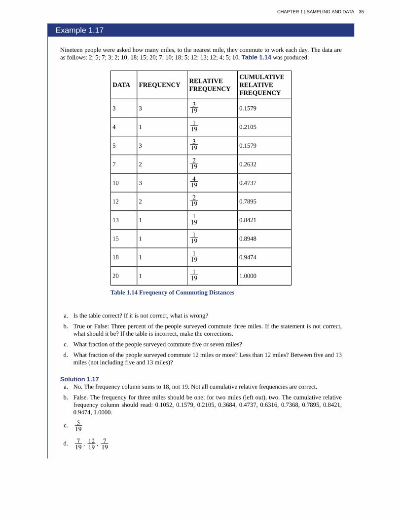
Example 1.17

Nineteen people were asked how many miles, to the nearest mile, they commute to work each day. The data areas follows: 2; 5; 7; 3; 2; 10; 18; 15; 20; 7; 10; 18; 5; 12; 13; 12; 4; 5; 10. Table 1.14 was produced:

DATA FREQUENCY RELATIVEFREQUENCY

CUMULATIVERELATIVEFREQUENCY

3 3 319 0.1579

4 1 119 0.2105

5 3 319 0.1579

7 2 219 0.2632

10 3 419 0.4737

12 2 219 0.7895

13 1 119 0.8421

15 1 119 0.8948

18 1 119 0.9474

20 1 119 1.0000

Table 1.14 Frequency of Commuting Distances

a. Is the table correct? If it is not correct, what is wrong?

b. True or False: Three percent of the people surveyed commute three miles. If the statement is not correct,what should it be? If the table is incorrect, make the corrections.

c. What fraction of the people surveyed commute five or seven miles?

d. What fraction of the people surveyed commute 12 miles or more? Less than 12 miles? Between five and 13miles (not including five and 13 miles)?

Solution 1.17a. No. The frequency column sums to 18, not 19. Not all cumulative relative frequencies are correct.

b. False. The frequency for three miles should be one; for two miles (left out), two. The cumulative relativefrequency column should read: 0.1052, 0.1579, 0.2105, 0.3684, 0.4737, 0.6316, 0.7368, 0.7895, 0.8421,0.9474, 1.0000.

c. 519

d. 719 , 12

19 , 719


1.17 Table 1.13 represents the amount, in inches, of annual rainfall in a sample of towns. What fraction of townssurveyed get between 11.03 and 13.05 inches of rainfall each year?

Example 1.18

Table 1.15 contains the total number of deaths worldwide as a result of earthquakes for the period from 2000 to2012.

Year Total Number of Deaths

2000 231

2001 21,357

2002 11,685

2003 33,819

2004 228,802

2005 88,003

2006 6,605

2007 712

2008 88,011

2009 1,790

2010 320,120

2011 21,953

2012 768

Total 823,356

Table 1.15

Answer the following questions.

a. What is the frequency of deaths measured from 2006 through 2009?

b. What percentage of deaths occurred after 2009?

c. What is the relative frequency of deaths that occurred in 2003 or earlier?

d. What is the percentage of deaths that occurred in 2004?

e. What kind of data are the numbers of deaths?

f. The Richter scale is used to quantify the energy produced by an earthquake. Examples of Richter scalenumbers are 2.3, 4.0, 6.1, and 7.0. What kind of data are these numbers?

Solution 1.18a. 97,118 (11.8%)

b. 41.6%

c. 67,092/823,356 or 0.081 or 8.1 %

d. 27.8%

e. Quantitative discrete

f. Quantitative continuous



1.18 Table 1.16 contains the total number of fatal motor vehicle traffic crashes in the United States for the periodfrom 1994 to 2011.

Year Total Number of Crashes Year Total Number of Crashes

1994 36,254 2004 38,444

1995 37,241 2005 39,252

1996 37,494 2006 38,648

1997 37,324 2007 37,435

1998 37,107 2008 34,172

1999 37,140 2009 30,862

2000 37,526 2010 30,296

2001 37,862 2011 29,757

2002 38,491 Total 653,782

2003 38,477

Table 1.16

Answer the following questions.

a. What is the frequency of deaths measured from 2000 through 2004?

b. What percentage of deaths occurred after 2006?

c. What is the relative frequency of deaths that occurred in 2000 or before?

d. What is the percentage of deaths that occurred in 2011?

e. What is the cumulative relative frequency for 2006? Explain what this number tells you about the data.

1.4 | Experimental Design and EthicsDoes aspirin reduce the risk of heart attacks? Is one brand of fertilizer more effective at growing roses than another?Is fatigue as dangerous to a driver as the influence of alcohol? Questions like these are answered using randomizedexperiments. In this module, you will learn important aspects of experimental design. Proper study design ensures theproduction of reliable, accurate data.

The purpose of an experiment is to investigate the relationship between two variables. When one variable causes changein another, we call the first variable the explanatory variable. The affected variable is called the response variable. In arandomized experiment, the researcher manipulates values of the explanatory variable and measures the resulting changesin the response variable. The different values of the explanatory variable are called treatments. An experimental unit is asingle object or individual to be measured.

You want to investigate the effectiveness of vitamin E in preventing disease. You recruit a group of subjects and ask themif they regularly take vitamin E. You notice that the subjects who take vitamin E exhibit better health on average thanthose who do not. Does this prove that vitamin E is effective in disease prevention? It does not. There are many differencesbetween the two groups compared in addition to vitamin E consumption. People who take vitamin E regularly often takeother steps to improve their health: exercise, diet, other vitamin supplements, choosing not to smoke. Any one of thesefactors could be influencing health. As described, this study does not prove that vitamin E is the key to disease prevention.

Additional variables that can cloud a study are called lurking variables. In order to prove that the explanatory variable iscausing a change in the response variable, it is necessary to isolate the explanatory variable. The researcher must design herexperiment in such a way that there is only one difference between groups being compared: the planned treatments. This isaccomplished by the random assignment of experimental units to treatment groups. When subjects are assigned treatmentsrandomly, all of the potential lurking variables are spread equally among the groups. At this point the only differencebetween groups is the one imposed by the researcher. Different outcomes measured in the response variable, therefore, must


be a direct result of the different treatments. In this way, an experiment can prove a cause-and-effect connection betweenthe explanatory and response variables.

The power of suggestion can have an important influence on the outcome of an experiment. Studies have shown that theexpectation of the study participant can be as important as the actual medication. In one study of performance-enhancingdrugs, researchers noted:

Results showed that believing one had taken the substance resulted in [performance] times almost as fast as those associatedwith consuming the drug itself. In contrast, taking the drug without knowledge yielded no significant performanceincrement.[1]

When participation in a study prompts a physical response from a participant, it is difficult to isolate the effects of theexplanatory variable. To counter the power of suggestion, researchers set aside one treatment group as a control group.This group is given a placebo treatment–a treatment that cannot influence the response variable. The control group helpsresearchers balance the effects of being in an experiment with the effects of the active treatments. Of course, if you areparticipating in a study and you know that you are receiving a pill which contains no actual medication, then the power ofsuggestion is no longer a factor. Blinding in a randomized experiment preserves the power of suggestion. When a personinvolved in a research study is blinded, he does not know who is receiving the active treatment(s) and who is receivingthe placebo treatment. A double-blind experiment is one in which both the subjects and the researchers involved with thesubjects are blinded.

Example 1.19

Researchers want to investigate whether taking aspirin regularly reduces the risk of heart attack. Four hundredmen between the ages of 50 and 84 are recruited as participants. The men are divided randomly into two groups:one group will take aspirin, and the other group will take a placebo. Each man takes one pill each day for threeyears, but he does not know whether he is taking aspirin or the placebo. At the end of the study, researchers countthe number of men in each group who have had heart attacks.

Identify the following values for this study: population, sample, experimental units, explanatory variable,response variable, treatments.

Solution 1.19The population is men aged 50 to 84.The sample is the 400 men who participated.The experimental units are the individual men in the study.The explanatory variable is oral medication.The treatments are aspirin and a placebo.The response variable is whether a subject had a heart attack.

Example 1.20

The Smell & Taste Treatment and Research Foundation conducted a study to investigate whether smell canaffect learning. Subjects completed mazes multiple times while wearing masks. They completed the pencil andpaper mazes three times wearing floral-scented masks, and three times with unscented masks. Participants wereassigned at random to wear the floral mask during the first three trials or during the last three trials. For eachtrial, researchers recorded the time it took to complete the maze and the subject’s impression of the mask’s scent:positive, negative, or neutral.

a. Describe the explanatory and response variables in this study.

b. What are the treatments?

c. Identify any lurking variables that could interfere with this study.

d. Is it possible to use blinding in this study?

Solution 1.20a. The explanatory variable is scent, and the response variable is the time it takes to complete the maze.

b. There are two treatments: a floral-scented mask and an unscented mask.

1. McClung, M. Collins, D. “Because I know it will!”: placebo effects of an ergogenic aid on athletic performance. Journal ofSport & Exercise Psychology. 2007 Jun. 29(3):382-94. Web. April 30, 2013.



c. All subjects experienced both treatments. The order of treatments was randomly assigned so there were nodifferences between the treatment groups. Random assignment eliminates the problem of lurking variables.

d. Subjects will clearly know whether they can smell flowers or not, so subjects cannot be blinded in this study.Researchers timing the mazes can be blinded, though. The researcher who is observing a subject will notknow which mask is being worn.

Example 1.21

A researcher wants to study the effects of birth order on personality. Explain why this study could not beconducted as a randomized experiment. What is the main problem in a study that cannot be designed as arandomized experiment?

Solution 1.21The explanatory variable is birth order. You cannot randomly assign a person’s birth order. Random assignmenteliminates the impact of lurking variables. When you cannot assign subjects to treatment groups at random, therewill be differences between the groups other than the explanatory variable.

1.21 You are concerned about the effects of texting on driving performance. Design a study to test the response timeof drivers while texting and while driving only. How many seconds does it take for a driver to respond when a leadingcar hits the brakes?

a. Describe the explanatory and response variables in the study.

b. What are the treatments?

c. What should you consider when selecting participants?

d. Your research partner wants to divide participants randomly into two groups: one to drive without distraction andone to text and drive simultaneously. Is this a good idea? Why or why not?

e. Identify any lurking variables that could interfere with this study.

f. How can blinding be used in this study?

EthicsThe widespread misuse and misrepresentation of statistical information often gives the field a bad name. Some say that“numbers don’t lie,” but the people who use numbers to support their claims often do.

A recent investigation of famous social psychologist, Diederik Stapel, has led to the retraction of his articles from someof the world’s top journals including Journal of Experimental Social Psychology, Social Psychology, Basic and AppliedSocial Psychology, British Journal of Social Psychology, and the magazine Science. Diederik Stapel is a former professorat Tilburg University in the Netherlands. Over the past two years, an extensive investigation involving three universitieswhere Stapel has worked concluded that the psychologist is guilty of fraud on a colossal scale. Falsified data taints over 55papers he authored and 10 Ph.D. dissertations that he supervised.

Stapel did not deny that his deceit was driven by ambition. But it was more complicated than that, he told me. He insistedthat he loved social psychology but had been frustrated by the messiness of experimental data, which rarely led to clearconclusions. His lifelong obsession with elegance and order, he said, led him to concoct sexy results that journals foundattractive. “It was a quest for aesthetics, for beauty—instead of the truth,” he said. He described his behavior as anaddiction that drove him to carry out acts of increasingly daring fraud, like a junkie seeking a bigger and better high.[2]

The committee investigating Stapel concluded that he is guilty of several practices including:

• creating datasets, which largely confirmed the prior expectations,

2. Yudhijit Bhattacharjee, “The Mind of a Con Man,” Magazine, New York Times, April 26, 2013. Available online at:http://www.nytimes.com/2013/04/28/magazine/diederik-stapels-audacious-academic-fraud.html?src=dayp&_r=2&(accessed May 1, 2013).


• altering data in existing datasets,

• changing measuring instruments without reporting the change, and

• misrepresenting the number of experimental subjects.

Clearly, it is never acceptable to falsify data the way this researcher did. Sometimes, however, violations of ethics are notas easy to spot.

Researchers have a responsibility to verify that proper methods are being followed. The report describing the investigationof Stapel’s fraud states that, “statistical flaws frequently revealed a lack of familiarity with elementary statistics.”[3] Manyof Stapel’s co-authors should have spotted irregularities in his data. Unfortunately, they did not know very much aboutstatistical analysis, and they simply trusted that he was collecting and reporting data properly.

Many types of statistical fraud are difficult to spot. Some researchers simply stop collecting data once they have just enoughto prove what they had hoped to prove. They don’t want to take the chance that a more extensive study would complicatetheir lives by producing data contradicting their hypothesis.

Professional organizations, like the American Statistical Association, clearly define expectations for researchers. There areeven laws in the federal code about the use of research data.

When a statistical study uses human participants, as in medical studies, both ethics and the law dictate that researchersshould be mindful of the safety of their research subjects. The U.S. Department of Health and Human Services overseesfederal regulations of research studies with the aim of protecting participants. When a university or other research institutionengages in research, it must ensure the safety of all human subjects. For this reason, research institutions establish oversightcommittees known as Institutional Review Boards (IRB). All planned studies must be approved in advance by the IRB.Key protections that are mandated by law include the following:

• Risks to participants must be minimized and reasonable with respect to projected benefits.

• Participants must give informed consent. This means that the risks of participation must be clearly explained to thesubjects of the study. Subjects must consent in writing, and researchers are required to keep documentation of theirconsent.

• Data collected from individuals must be guarded carefully to protect their privacy.

These ideas may seem fundamental, but they can be very difficult to verify in practice. Is removing a participant’s namefrom the data record sufficient to protect privacy? Perhaps the person’s identity could be discovered from the data thatremains. What happens if the study does not proceed as planned and risks arise that were not anticipated? When is informedconsent really necessary? Suppose your doctor wants a blood sample to check your cholesterol level. Once the sample hasbeen tested, you expect the lab to dispose of the remaining blood. At that point the blood becomes biological waste. Does aresearcher have the right to take it for use in a study?

It is important that students of statistics take time to consider the ethical questions that arise in statistical studies.How prevalent is fraud in statistical studies? You might be surprised—and disappointed. There is a website(www.retractionwatch.com) (http://cnx.org/content/m46919/1.6/www.retractionwatch.com) dedicated tocataloging retractions of study articles that have been proven fraudulent. A quick glance will show that the misuse ofstatistics is a bigger problem than most people realize.

Vigilance against fraud requires knowledge. Learning the basic theory of statistics will empower you to analyze statisticalstudies critically.

Example 1.22

Describe the unethical behavior in each example and describe how it could impact the reliability of the resultingdata. Explain how the problem should be corrected.

A researcher is collecting data in a community.

a. She selects a block where she is comfortable walking because she knows many of the people living on thestreet.

b. No one seems to be home at four houses on her route. She does not record the addresses and does not returnat a later time to try to find residents at home.

c. She skips four houses on her route because she is running late for an appointment. When she gets home, shefills in the forms by selecting random answers from other residents in the neighborhood.

3. “Flawed Science: The Fraudulent Research Practices of Social Psychologist Diederik Stapel,” Tillburg University,November 28, 2012, http://www.tilburguniversity.edu/upload/064a10cd-bce5-4385-b9ff-05b840caeae6_120695_Rapp_nov_2012_UK_web.pdf (accessed May 1, 2013).



http://cnx.org/content/m46919/1.6/www.retractionwatch.com

Solution 1.22a. By selecting a convenient sample, the researcher is intentionally selecting a sample that could be biased.

Claiming that this sample represents the community is misleading. The researcher needs to select areas inthe community at random.

b. Intentionally omitting relevant data will create bias in the sample. Suppose the researcher is gatheringinformation about jobs and child care. By ignoring people who are not home, she may be missing data fromworking families that are relevant to her study. She needs to make every effort to interview all members ofthe target sample.

c. It is never acceptable to fake data. Even though the responses she uses are “real” responses provided byother participants, the duplication is fraudulent and can create bias in the data. She needs to work diligentlyto interview everyone on her route.

1.22 Describe the unethical behavior, if any, in each example and describe how it could impact the reliability of theresulting data. Explain how the problem should be corrected.

A study is commissioned to determine the favorite brand of fruit juice among teens in California.

a. The survey is commissioned by the seller of a popular brand of apple juice.

b. There are only two types of juice included in the study: apple juice and cranberry juice.

c. Researchers allow participants to see the brand of juice as samples are poured for a taste test.

d. Twenty-five percent of participants prefer Brand X, 33% prefer Brand Y and 42% have no preference betweenthe two brands. Brand X references the study in a commercial saying “Most teens like Brand X as much as ormore than Brand Y.”


1.1 Data Collection ExperimentClass Time:

Names:

Student Learning Outcomes• The student will demonstrate the systematic sampling technique.

• The student will construct relative frequency tables.

• The student will interpret results and their differences from different data groupings.

Movie SurveyAsk five classmates from a different class how many movies they saw at the theater last month. Do not include rentedmovies.

1. Record the data.

2. In class, randomly pick one person. On the class list, mark that person’s name. Move down four names on theclass list. Mark that person’s name. Continue doing this until you have marked 12 names. You may need to goback to the start of the list. For each marked name record the five data values. You now have a total of 60 datavalues.

3. For each name marked, record the data.

______ ______ ______ ______ ______ ______ ______ ______

______ ______ ______ ______ ______ ______ ______ ______

______ ______ ______ ______ ______ ______ ______ ______

______ ______ ______ ______ ______ ______ ______ ______

______ ______ ______ ______ ______ ______ ______ ______

______ ______ ______ ______ ______ ______ ______ ______

______ ______ ______ ______ ______ ______ ______ ______

Table 1.17

Order the DataComplete the two relative frequency tables below using your class data.

Number of Movies Frequency Relative Frequency Cumulative Relative Frequency

0

1

2

3

4

5

6




7+

Table 1.18 Frequency of Number of Movies Viewed


0–1

2–3

4–5

6–7+

Table 1.19 Frequency of Number of Movies Viewed

1. Using the tables, find the percent of data that is at most two. Which table did you use and why?

2. Using the tables, find the percent of data that is at most three. Which table did you use and why?

3. Using the tables, find the percent of data that is more than two. Which table did you use and why?

4. Using the tables, find the percent of data that is more than three. Which table did you use and why?

Discussion Questions1. Is one of the tables “more correct” than the other? Why or why not?

2. In general, how could you group the data differently? Are there any advantages to either way of grouping thedata?

3. Why did you switch between tables, if you did, when answering the question above?


1.2 Sampling ExperimentClass Time:

Names:

Student Learning Outcomes• The student will demonstrate the simple random, systematic, stratified, and cluster sampling techniques.

• The student will explain the details of each procedure used.

In this lab, you will be asked to pick several random samples of restaurants. In each case, describe your procedurebriefly, including how you might have used the random number generator, and then list the restaurants in the sampleyou obtained.

NOTE

The following section contains restaurants stratified by city into columns and grouped horizontally by entree cost(clusters).

Restaurants Stratified by City and Entree Cost

EntreeCost Under $10 $10 to under $15 $15 to under

$20 Over $20

San JoseEl Abuelo Taq, PastaMia, Emma’s Express,Bamboo Hut

Emperor’s Guard,Creekside Inn

Agenda, Gervais,Miro’s

Blake’s, Eulipia,Hayes Mansion,Germania

Palo Alto Senor Taco, OliveGarden, Taxi’s

Ming’s, P.A. Joe’s,Stickney’s

Scott’s Seafood,Poolside Grill,Fish Market

Sundance Mine,Maddalena’s,Spago’s

Los GatosMary’s Patio, MountEverest, Sweet Pea’s,Andele Taqueria

Lindsey’s, Willow Street Toll HouseCharter House,La Maison DuCafe

MountainView

Maharaja, New Ma’s,Thai-Rific, Garden Fresh

Amber Indian, La Fiesta,Fiesta del Mar, Dawit

Austin’s, Shiva’s,Mazeh Le Petit Bistro

Cupertino Hobees, Hung Fu,Samrat, Panda Express

Santa Barb. Grill, Mand.Gourmet, Bombay Oven,Kathmandu West

Fontana’s, BluePheasant

Hamasushi,Helios

SunnyvaleChekijababi, Taj India,Full Throttle, Tia Juana,Lemon Grass

Pacific Fresh, CharleyBrown’s, Cafe Cameroon,Faz, Aruba’s

Lion & Compass,The Palace,Beau Sejour

SantaClara

Rangoli, ArmadilloWilly’s, Thai Pepper,Pasand

Arthur’s, Katie’s Cafe,Pedro’s, La Galleria

Birk’s, TruyaSushi, ValleyPlaza

Lakeside,Mariani’s

Table 1.20 Restaurants Used in Sample

A Simple Random Sample



Pick a simple random sample of 15 restaurants.

1. Describe your procedure.

2. Complete the table with your sample.

1. __________ 6. __________ 11. __________

2. __________ 7. __________ 12. __________

3. __________ 8. __________ 13. __________

4. __________ 9. __________ 14. __________

5. __________ 10. __________ 15. __________

Table 1.21

A Systematic SamplePick a systematic sample of 15 restaurants.



1. __________ 6. __________ 11. __________

2. __________ 7. __________ 12. __________

3. __________ 8. __________ 13. __________

4. __________ 9. __________ 14. __________

5. __________ 10. __________ 15. __________

Table 1.22

A Stratified SamplePick a stratified sample, by city, of 20 restaurants. Use 25% of the restaurants from each stratum. Round to the nearestwhole number.



1. __________ 6. __________ 11. __________ 16. __________

2. __________ 7. __________ 12. __________ 17. __________

3. __________ 8. __________ 13. __________ 18. __________

4. __________ 9. __________ 14. __________ 19. __________

5. __________ 10. __________ 15. __________ 20. __________

Table 1.23

A Stratified SamplePick a stratified sample, by entree cost, of 21 restaurants. Use 25% of the restaurants from each stratum. Round to thenearest whole number.




1. __________ 6. __________ 11. __________ 16. __________

2. __________ 7. __________ 12. __________ 17. __________

3. __________ 8. __________ 13. __________ 18. __________

4. __________ 9. __________ 14. __________ 19. __________

5. __________ 10. __________ 15. __________ 20. __________

21. __________

Table 1.24

A Cluster SamplePick a cluster sample of restaurants from two cities. The number of restaurants will vary.



1. ________ 6. ________ 11. ________ 16. ________ 21. ________

2. ________ 7. ________ 12. ________ 17. ________ 22. ________

3. ________ 8. ________ 13. ________ 18. ________ 23. ________

4. ________ 9. ________ 14. ________ 19. ________ 24. ________

5. ________ 10. ________ 15. ________ 20. ________ 25. ________

Table 1.25



Average

Blinding

Categorical Variable

Cluster Sampling

Continuous Random Variable

Control Group

Convenience Sampling

Cumulative Relative Frequency

Data

Discrete Random Variable

Double-blinding

Experimental Unit

Explanatory Variable

Frequency

Informed Consent

Institutional Review Board

Lurking Variable

Nonsampling Error

Numerical Variable

Parameter

Placebo

Population

Probability

Proportion

KEY TERMSalso called mean; a number that describes the central tendency of the data

not telling participants which treatment a subject is receiving

variables that take on values that are names or labels

a method for selecting a random sample and dividing the population into groups (clusters); usesimple random sampling to select a set of clusters. Every individual in the chosen clusters is included in the sample.

a random variable (RV) whose outcomes are measured; the height of trees in theforest is a continuous RV.

a group in a randomized experiment that receives an inactive treatment but is otherwise managedexactly as the other groups

a nonrandom method of selecting a sample; this method selects individuals that are easilyaccessible and may result in biased data.

The term applies to an ordered set of observations from smallest to largest. Thecumulative relative frequency is the sum of the relative frequencies for all values that are less than or equal to thegiven value.

a set of observations (a set of possible outcomes); most data can be put into two groups: qualitative (an attributewhose value is indicated by a label) or quantitative (an attribute whose value is indicated by a number).Quantitative data can be separated into two subgroups: discrete and continuous. Data is discrete if it is the result ofcounting (such as the number of students of a given ethnic group in a class or the number of books on a shelf). Datais continuous if it is the result of measuring (such as distance traveled or weight of luggage)

a random variable (RV) whose outcomes are counted

the act of blinding both the subjects of an experiment and the researchers who work with the subjects

any individual or object to be measured

the independent variable in an experiment; the value controlled by researchers

the number of times a value of the data occurs

Any human subject in a research study must be cognizant of any risks or costs associated with thestudy. The subject has the right to know the nature of the treatments included in the study, their potential risks, andtheir potential benefits. Consent must be given freely by an informed, fit participant.

a committee tasked with oversight of research programs that involve human subjects

a variable that has an effect on a study even though it is neither an explanatory variable nor aresponse variable

an issue that affects the reliability of sampling data other than natural variation; it includes avariety of human errors including poor study design, biased sampling methods, inaccurate information provided bystudy participants, data entry errors, and poor analysis.

variables that take on values that are indicated by numbers

a number that is used to represent a population characteristic and that generally cannot be determined easily

an inactive treatment that has no real effect on the explanatory variable

all individuals, objects, or measurements whose properties are being studied

a number between zero and one, inclusive, that gives the likelihood that a specific event will occur

the number of successes divided by the total number in the sample


Qualitative Data

Quantitative Data

Random Assignment

Random Sampling

Relative Frequency

Representative Sample

Response Variable

Sample

Sampling Bias

Sampling Error

Sampling with Replacement

Sampling without Replacement

Simple Random Sampling

Statistic

Stratified Sampling

Systematic Sampling

Treatments

Variable

See Data.

See Data.

the act of organizing experimental units into treatment groups using random methods

a method of selecting a sample that gives every member of the population an equal chance ofbeing selected.

the ratio of the number of times a value of the data occurs in the set of all outcomes to the numberof all outcomes to the total number of outcomes

a subset of the population that has the same characteristics as the population

the dependent variable in an experiment; the value that is measured for change at the end of anexperiment

a subset of the population studied

not all members of the population are equally likely to be selected

the natural variation that results from selecting a sample to represent a larger population; this variationdecreases as the sample size increases, so selecting larger samples reduces sampling error.

Once a member of the population is selected for inclusion in a sample, that member isreturned to the population for the selection of the next individual.

A member of the population may be chosen for inclusion in a sample only once. Ifchosen, the member is not returned to the population before the next selection.

a straightforward method for selecting a random sample; give each member of thepopulation a number. Use a random number generator to select a set of labels. These randomly selected labelsidentify the members of your sample.

a numerical characteristic of the sample; a statistic estimates the corresponding population parameter.

a method for selecting a random sample used to ensure that subgroups of the population arerepresented adequately; divide the population into groups (strata). Use simple random sampling to identify aproportionate number of individuals from each stratum.

a method for selecting a random sample; list the members of the population. Use simplerandom sampling to select a starting point in the population. Let k = (number of individuals in thepopulation)/(number of individuals needed in the sample). Choose every kth individual in the list starting with theone that was randomly selected. If necessary, return to the beginning of the population list to complete your sample.

different values or components of the explanatory variable applied in an experiment

a characteristic of interest for each person or object in a population

CHAPTER REVIEW

1.1 Definitions of Statistics, Probability, and Key Terms

The mathematical theory of statistics is easier to learn when you know the language. This module presents important termsthat will be used throughout the text.

1.2 Data, Sampling, and Variation in Data and Sampling

Data are individual items of information that come from a population or sample. Data may be classified as qualitative,quantitative continuous, or quantitative discrete.

Because it is not practical to measure the entire population in a study, researchers use samples to represent the population.A random sample is a representative group from the population chosen by using a method that gives each individual in thepopulation an equal chance of being included in the sample. Random sampling methods include simple random sampling,



stratified sampling, cluster sampling, and systematic sampling. Convenience sampling is a nonrandom method of choosinga sample that often produces biased data.

Samples that contain different individuals result in different data. This is true even when the samples are well-chosen andrepresentative of the population. When properly selected, larger samples model the population more closely than smallersamples. There are many different potential problems that can affect the reliability of a sample. Statistical data needs to becritically analyzed, not simply accepted.

1.3 Frequency, Frequency Tables, and Levels of Measurement

Some calculations generate numbers that are artificially precise. It is not necessary to report a value to eight decimal placeswhen the measures that generated that value were only accurate to the nearest tenth. Round off your final answer to onemore decimal place than was present in the original data. This means that if you have data measured to the nearest tenth ofa unit, report the final statistic to the nearest hundredth.

In addition to rounding your answers, you can measure your data using the following four levels of measurement.

• Nominal scale level: data that cannot be ordered nor can it be used in calculations

• Ordinal scale level: data that can be ordered; the differences cannot be measured

• Interval scale level: data with a definite ordering but no starting point; the differences can be measured, but there isno such thing as a ratio.

• Ratio scale level: data with a starting point that can be ordered; the differences have meaning and ratios can becalculated.

When organizing data, it is important to know how many times a value appears. How many statistics students study fivehours or more for an exam? What percent of families on our block own two pets? Frequency, relative frequency, andcumulative relative frequency are measures that answer questions like these.

1.4 Experimental Design and Ethics

A poorly designed study will not produce reliable data. There are certain key components that must be included in everyexperiment. To eliminate lurking variables, subjects must be assigned randomly to different treatment groups. One of thegroups must act as a control group, demonstrating what happens when the active treatment is not applied. Participants inthe control group receive a placebo treatment that looks exactly like the active treatments but cannot influence the responsevariable. To preserve the integrity of the placebo, both researchers and subjects may be blinded. When a study is designedproperly, the only difference between treatment groups is the one imposed by the researcher. Therefore, when groupsrespond differently to different treatments, the difference must be due to the influence of the explanatory variable.

“An ethics problem arises when you are considering an action that benefits you or some cause you support, hurts orreduces benefits to others, and violates some rule.”[4] Ethical violations in statistics are not always easy to spot. Professionalassociations and federal agencies post guidelines for proper conduct. It is important that you learn basic statisticalprocedures so that you can recognize proper data analysis.

PRACTICE

1.1 Definitions of Statistics, Probability, and Key Terms

Use the following information to answer the next five exercises. Studies are often done by pharmaceutical companies todetermine the effectiveness of a treatment program. Suppose that a new AIDS antibody drug is currently under study. It isgiven to patients once the AIDS symptoms have revealed themselves. Of interest is the average (mean) length of time inmonths patients live once they start the treatment. Two researchers each follow a different set of 40 patients with AIDS fromthe start of treatment until their deaths. The following data (in months) are collected.

Researcher A:

3; 4; 11; 15; 16; 17; 22; 44; 37; 16; 14; 24; 25; 15; 26; 27; 33; 29; 35; 44; 13; 21; 22; 10; 12; 8; 40; 32; 26; 27; 31; 34; 29;17; 8; 24; 18; 47; 33; 34

Researcher B:

4. Andrew Gelman, “Open Data and Open Methods,” Ethics and Statistics, http://www.stat.columbia.edu/~gelman/research/published/ChanceEthics1.pdf (accessed May 1, 2013).


3; 14; 11; 5; 16; 17; 28; 41; 31; 18; 14; 14; 26; 25; 21; 22; 31; 2; 35; 44; 23; 21; 21; 16; 12; 18; 41; 22; 16; 25; 33; 34; 29;13; 18; 24; 23; 42; 33; 29

Determine what the key terms refer to in the example for Researcher A.

1. population

2. sample

3. parameter

4. statistic

5. variable

1.2 Data, Sampling, and Variation in Data and Sampling6. “Number of times per week” is what type of data?

a. qualitative; b. quantitative discrete; c. quantitative continuous

Use the following information to answer the next four exercises: A study was done to determine the age, number of timesper week, and the duration (amount of time) of residents using a local park in San Antonio, Texas. The first house in theneighborhood around the park was selected randomly, and then the resident of every eighth house in the neighborhoodaround the park was interviewed.

7. The sampling method was

a. simple random; b. systematic; c. stratified; d. cluster

8. “Duration (amount of time)” is what type of data?


9. The colors of the houses around the park are what kind of data?


10. The population is ______________________

11. Table 1.26 contains the total number of deaths worldwide as a result of earthquakes from 2000 to 2012.

Year Total Number of Deaths

2000 231

2001 21,357

2002 11,685

2003 33,819

2004 228,802

2005 88,003

2006 6,605

2007 712

2008 88,011

2009 1,790

2010 320,120

2011 21,953

2012 768

Total 823,856

Table 1.26

Use Table 1.26 to answer the following questions.

a. What is the proportion of deaths between 2007 and 2012?b. What percent of deaths occurred before 2001?



c. What is the percent of deaths that occurred in 2003 or after 2010?d. What is the fraction of deaths that happened before 2012?e. What kind of data is the number of deaths?f. Earthquakes are quantified according to the amount of energy they produce (examples are 2.1, 5.0, 6.7). What

type of data is that?g. What contributed to the large number of deaths in 2010? In 2004? Explain.

For the following four exercises, determine the type of sampling used (simple random, stratified, systematic, cluster, orconvenience).

12. A group of test subjects is divided into twelve groups; then four of the groups are chosen at random.

13. A market researcher polls every tenth person who walks into a store.

14. The first 50 people who walk into a sporting event are polled on their television preferences.

15. A computer generates 100 random numbers, and 100 people whose names correspond with the numbers on the list arechosen.

Use the following information to answer the next seven exercises: Studies are often done by pharmaceutical companies todetermine the effectiveness of a treatment program. Suppose that a new AIDS antibody drug is currently under study. It isgiven to patients once the AIDS symptoms have revealed themselves. Of interest is the average (mean) length of time inmonths patients live once starting the treatment. Two researchers each follow a different set of 40 AIDS patients from thestart of treatment until their deaths. The following data (in months) are collected.

Researcher A: 3; 4; 11; 15; 16; 17; 22; 44; 37; 16; 14; 24; 25; 15; 26; 27; 33; 29; 35; 44; 13; 21; 22; 10; 12; 8; 40; 32; 26;27; 31; 34; 29; 17; 8; 24; 18; 47; 33; 34

Researcher B: 3; 14; 11; 5; 16; 17; 28; 41; 31; 18; 14; 14; 26; 25; 21; 22; 31; 2; 35; 44; 23; 21; 21; 16; 12; 18; 41; 22; 16;25; 33; 34; 29; 13; 18; 24; 23; 42; 33; 29

16. Complete the tables using the data provided:

Survival Length (inmonths) Frequency Relative

FrequencyCumulative RelativeFrequency

0.5–6.5

6.5–12.5

12.5–18.5

18.5–24.5

24.5–30.5

30.5–36.5

36.5–42.5

42.5–48.5

Table 1.27 Researcher A

Survival Length (inmonths) Frequency Relative

FrequencyCumulative RelativeFrequency

0.5–6.5

6.5–12.5

12.5–18.5

18.5–24.5

24.5–30.5

30.5–36.5

36.5-45.5

Table 1.28 Researcher B


17. Determine what the key term data refers to in the above example for Researcher A.

18. List two reasons why the data may differ.

19. Can you tell if one researcher is correct and the other one is incorrect? Why?

20. Would you expect the data to be identical? Why or why not?

21. How might the researchers gather random data?

22. Suppose that the first researcher conducted his survey by randomly choosing one state in the nation and then randomlypicking 40 patients from that state. What sampling method would that researcher have used?

23. Suppose that the second researcher conducted his survey by choosing 40 patients he knew. What sampling methodwould that researcher have used? What concerns would you have about this data set, based upon the data collection method?

Use the following data to answer the next five exercises: Two researchers are gathering data on hours of video games playedby school-aged children and young adults. They each randomly sample different groups of 150 students from the sameschool. They collect the following data.

Hours Played per Week Frequency Relative Frequency Cumulative Relative Frequency

0–2 26 0.17 0.17

2–4 30 0.20 0.37

4–6 49 0.33 0.70

6–8 25 0.17 0.87

8–10 12 0.08 0.95

10–12 8 0.05 1

Table 1.29 Researcher A

Hours Played per Week Frequency Relative Frequency Cumulative Relative Frequency

0–2 48 0.32 0.32

2–4 51 0.34 0.66

4–6 24 0.16 0.82

6–8 12 0.08 0.90

8–10 11 0.07 0.97

10–12 4 0.03 1

Table 1.30 Researcher B

24. Give a reason why the data may differ.

25. Would the sample size be large enough if the population is the students in the school?

26. Would the sample size be large enough if the population is school-aged children and young adults in the United States?

27. Researcher A concludes that most students play video games between four and six hours each week. Researcher Bconcludes that most students play video games between two and four hours each week. Who is correct?

28. As part of a way to reward students for participating in the survey, the researchers gave each student a gift card to avideo game store. Would this affect the data if students knew about the award before the study?

Use the following data to answer the next five exercises: A pair of studies was performed to measure the effectiveness ofa new software program designed to help stroke patients regain their problem-solving skills. Patients were asked to usethe software program twice a day, once in the morning and once in the evening. The studies observed 200 stroke patientsrecovering over a period of several weeks. The first study collected the data in Table 1.31. The second study collected thedata in Table 1.32.



Group Showed improvement No improvement Deterioration

Used program 142 43 15

Did not use program 72 110 18

Table 1.31

Group Showed improvement No improvement Deterioration

Used program 105 74 19

Did not use program 89 99 12

Table 1.32

29. Given what you know, which study is correct?

30. The first study was performed by the company that designed the software program. The second study was performedby the American Medical Association. Which study is more reliable?

31. Both groups that performed the study concluded that the software works. Is this accurate?

32. The company takes the two studies as proof that their software causes mental improvement in stroke patients. Is this afair statement?

33. Patients who used the software were also a part of an exercise program whereas patients who did not use the softwarewere not. Does this change the validity of the conclusions from Exercise 1.31?

34. Is a sample size of 1,000 a reliable measure for a population of 5,000?

35. Is a sample of 500 volunteers a reliable measure for a population of 2,500?

36. A question on a survey reads: "Do you prefer the delicious taste of Brand X or the taste of Brand Y?" Is this a fairquestion?

37. Is a sample size of two representative of a population of five?

38. Is it possible for two experiments to be well run with similar sample sizes to get different data?

1.3 Frequency, Frequency Tables, and Levels of Measurement39. What type of measure scale is being used? Nominal, ordinal, interval or ratio.

a. High school soccer players classified by their athletic ability: Superior, Average, Above averageb. Baking temperatures for various main dishes: 350, 400, 325, 250, 300c. The colors of crayons in a 24-crayon boxd. Social security numberse. Incomes measured in dollarsf. A satisfaction survey of a social website by number: 1 = very satisfied, 2 = somewhat satisfied, 3 = not satisfied

g. Political outlook: extreme left, left-of-center, right-of-center, extreme righth. Time of day on an analog watchi. The distance in miles to the closest grocery storej. The dates 1066, 1492, 1644, 1947, and 1944

k. The heights of 21–65 year-old womenl. Common letter grades: A, B, C, D, and F

1.4 Experimental Design and Ethics40. Design an experiment. Identify the explanatory and response variables. Describe the population being studied andthe experimental units. Explain the treatments that will be used and how they will be assigned to the experimental units.Describe how blinding and placebos may be used to counter the power of suggestion.

41. Discuss potential violations of the rule requiring informed consent.a. Inmates in a correctional facility are offered good behavior credit in return for participation in a study.b. A research study is designed to investigate a new children’s allergy medication.c. Participants in a study are told that the new medication being tested is highly promising, but they are not told that

only a small portion of participants will receive the new medication. Others will receive placebo treatments andtraditional treatments.


HOMEWORK

1.1 Definitions of Statistics, Probability, and Key TermsFor each of the following eight exercises, identify: a. the population, b. the sample, c. the parameter, d. the statistic, e. thevariable, and f. the data. Give examples where appropriate.

42. A fitness center is interested in the mean amount of time a client exercises in the center each week.

43. Ski resorts are interested in the mean age that children take their first ski and snowboard lessons. They need thisinformation to plan their ski classes optimally.

44. A cardiologist is interested in the mean recovery period of her patients who have had heart attacks.

45. Insurance companies are interested in the mean health costs each year of their clients, so that they can determine thecosts of health insurance.

46. A politician is interested in the proportion of voters in his district who think he is doing a good job.

47. A marriage counselor is interested in the proportion of clients she counsels who stay married.

48. Political pollsters may be interested in the proportion of people who will vote for a particular cause.

49. A marketing company is interested in the proportion of people who will buy a particular product.

Use the following information to answer the next three exercises: A Lake Tahoe Community College instructor is interestedin the mean number of days Lake Tahoe Community College math students are absent from class during a quarter.

50. What is the population she is interested in?a. all Lake Tahoe Community College studentsb. all Lake Tahoe Community College English studentsc. all Lake Tahoe Community College students in her classesd. all Lake Tahoe Community College math students

51. Consider the following:

X = number of days a Lake Tahoe Community College math student is absent

In this case, X is an example of a:

a. variable.b. population.c. statistic.d. data.

52. The instructor’s sample produces a mean number of days absent of 3.5 days. This value is an example of a:a. parameter.b. data.c. statistic.d. variable.

1.2 Data, Sampling, and Variation in Data and SamplingFor the following exercises, identify the type of data that would be used to describe a response (quantitative discrete,quantitative continuous, or qualitative), and give an example of the data.

53. number of tickets sold to a concert

54. percent of body fat

55. favorite baseball team

56. time in line to buy groceries

57. number of students enrolled at Evergreen Valley College

58. most-watched television show

59. brand of toothpaste

60. distance to the closest movie theatre

61. age of executives in Fortune 500 companies

62. number of competing computer spreadsheet software packages



Use the following information to answer the next two exercises: A study was done to determine the age, number of timesper week, and the duration (amount of time) of resident use of a local park in San Jose. The first house in the neighborhoodaround the park was selected randomly and then every 8th house in the neighborhood around the park was interviewed.

63. “Number of times per week” is what type of data?a. qualitativeb. quantitative discretec. quantitative continuous

64. “Duration (amount of time)” is what type of data?a. qualitativeb. quantitative discretec. quantitative continuous

65. Airline companies are interested in the consistency of the number of babies on each flight, so that they have adequatesafety equipment. Suppose an airline conducts a survey. Over Thanksgiving weekend, it surveys six flights from Boston toSalt Lake City to determine the number of babies on the flights. It determines the amount of safety equipment needed bythe result of that study.

a. Using complete sentences, list three things wrong with the way the survey was conducted.b. Using complete sentences, list three ways that you would improve the survey if it were to be repeated.

66. Suppose you want to determine the mean number of students per statistics class in your state. Describe a possiblesampling method in three to five complete sentences. Make the description detailed.

67. Suppose you want to determine the mean number of cans of soda drunk each month by students in their twenties at yourschool. Describe a possible sampling method in three to five complete sentences. Make the description detailed.

68. List some practical difficulties involved in getting accurate results from a telephone survey.

69. List some practical difficulties involved in getting accurate results from a mailed survey.

70. With your classmates, brainstorm some ways you could overcome these problems if you needed to conduct a phone ormail survey.

71. The instructor takes her sample by gathering data on five randomly selected students from each Lake Tahoe CommunityCollege math class. The type of sampling she used is

a. cluster samplingb. stratified samplingc. simple random samplingd. convenience sampling

72. A study was done to determine the age, number of times per week, and the duration (amount of time) of residents usinga local park in San Jose. The first house in the neighborhood around the park was selected randomly and then every eighthhouse in the neighborhood around the park was interviewed. The sampling method was:

a. simple randomb. systematicc. stratifiedd. cluster

73. Name the sampling method used in each of the following situations:a. A woman in the airport is handing out questionnaires to travelers asking them to evaluate the airport’s service.

She does not ask travelers who are hurrying through the airport with their hands full of luggage, but instead asksall travelers who are sitting near gates and not taking naps while they wait.

b. A teacher wants to know if her students are doing homework, so she randomly selects rows two and five and thencalls on all students in row two and all students in row five to present the solutions to homework problems to theclass.

c. The marketing manager for an electronics chain store wants information about the ages of its customers. Overthe next two weeks, at each store location, 100 randomly selected customers are given questionnaires to fill outasking for information about age, as well as about other variables of interest.

d. The librarian at a public library wants to determine what proportion of the library users are children. The librarianhas a tally sheet on which she marks whether books are checked out by an adult or a child. She records this datafor every fourth patron who checks out books.

e. A political party wants to know the reaction of voters to a debate between the candidates. The day after the debate,the party’s polling staff calls 1,200 randomly selected phone numbers. If a registered voter answers the phone oris available to come to the phone, that registered voter is asked whom he or she intends to vote for and whetherthe debate changed his or her opinion of the candidates.

74. A “random survey” was conducted of 3,274 people of the “microprocessor generation” (people born since 1971, theyear the microprocessor was invented). It was reported that 48% of those individuals surveyed stated that if they had $2,000


to spend, they would use it for computer equipment. Also, 66% of those surveyed considered themselves relatively savvycomputer users.

a. Do you consider the sample size large enough for a study of this type? Why or why not?b. Based on your “gut feeling,” do you believe the percents accurately reflect the U.S. population for those

individuals born since 1971? If not, do you think the percents of the population are actually higher orlower than the sample statistics? Why? Additional information: The survey, reported by Intel Corporation,was filled out by individuals who visited the Los Angeles Convention Center to see the Smithsonian Institute'sroad show called “America’s Smithsonian.”

c. With this additional information, do you feel that all demographic and ethnic groups were equally represented atthe event? Why or why not?

d. With the additional information, comment on how accurately you think the sample statistics reflect the populationparameters.

75. The Gallup-Healthways Well-Being Index is a survey that follows trends of U.S. residents on a regular basis. Thereare six areas of health and wellness covered in the survey: Life Evaluation, Emotional Health, Physical Health, HealthyBehavior, Work Environment, and Basic Access. Some of the questions used to measure the Index are listed below.

Identify the type of data obtained from each question used in this survey: qualitative, quantitative discrete, or quantitativecontinuous.

a. Do you have any health problems that prevent you from doing any of the things people your age can normally do?b. During the past 30 days, for about how many days did poor health keep you from doing your usual activities?c. In the last seven days, on how many days did you exercise for 30 minutes or more?d. Do you have health insurance coverage?

76. In advance of the 1936 Presidential Election, a magazine titled Literary Digest released the results of an opinionpoll predicting that the republican candidate Alf Landon would win by a large margin. The magazine sent post cardsto approximately 10,000,000 prospective voters. These prospective voters were selected from the subscription list of themagazine, from automobile registration lists, from phone lists, and from club membership lists. Approximately 2,300,000people returned the postcards.

a. Think about the state of the United States in 1936. Explain why a sample chosen from magazine subscription lists,automobile registration lists, phone books, and club membership lists was not representative of the population ofthe United States at that time.

b. What effect does the low response rate have on the reliability of the sample?c. Are these problems examples of sampling error or nonsampling error?d. During the same year, George Gallup conducted his own poll of 30,000 prospective voters. His researchers used

a method they called "quota sampling" to obtain survey answers from specific subsets of the population. Quotasampling is an example of which sampling method described in this module?

77. Crime-related and demographic statistics for 47 US states in 1960 were collected from government agencies, includingthe FBI's Uniform Crime Report. One analysis of this data found a strong connection between education and crimeindicating that higher levels of education in a community correspond to higher crime rates.

Which of the potential problems with samples discussed in Section 1.2 could explain this connection?

78. YouPolls is a website that allows anyone to create and respond to polls. One question posted April 15 asks:

“Do you feel happy paying your taxes when members of the Obama administration are allowed to ignore their taxliabilities?”[5]

As of April 25, 11 people responded to this question. Each participant answered “NO!”

Which of the potential problems with samples discussed in this module could explain this connection?

79. A scholarly article about response rates begins with the following quote:

“Declining contact and cooperation rates in random digit dial (RDD) national telephone surveys raise serious concernsabout the validity of estimates drawn from such research.”[6]

The Pew Research Center for People and the Press admits:

“The percentage of people we interview – out of all we try to interview – has been declining over the past decade ormore.”[7]

5. lastbaldeagle. 2013. On Tax Day, House to Call for Firing Federal Workers Who Owe Back Taxes. Opinion poll postedonline at: http://www.youpolls.com/details.aspx?id=12328 (accessed May 1, 2013).

6. Scott Keeter et al., “Gauging the Impact of Growing Nonresponse on Estimates from a National RDD Telephone Survey,”Public Opinion Quarterly 70 no. 5 (2006), http://poq.oxfordjournals.org/content/70/5/759.full(http://poq.oxfordjournals.org/content/70/5/759.full) (accessed May 1, 2013).



http://poq.oxfordjournals.org/content/70/5/759.full

http://poq.oxfordjournals.org/content/70/5/759.full

a. What are some reasons for the decline in response rate over the past decade?b. Explain why researchers are concerned with the impact of the declining response rate on public opinion polls.

1.3 Frequency, Frequency Tables, and Levels of Measurement80. Fifty part-time students were asked how many courses they were taking this term. The (incomplete) results are shownbelow:

# of Courses Frequency Relative Frequency Cumulative Relative Frequency

1 30 0.6

2 15

3

Table 1.33 Part-time Student Course Loads

a. Fill in the blanks in Table 1.33.b. What percent of students take exactly two courses?c. What percent of students take one or two courses?

81. Sixty adults with gum disease were asked the number of times per week they used to floss before their diagnosis. The(incomplete) results are shown in Table 1.34.

# Flossing per Week Frequency Relative Frequency Cumulative Relative Freq.

0 27 0.4500

1 18

3 0.9333

6 3 0.0500

7 1 0.0167

Table 1.34 Flossing Frequency for Adults with Gum Disease

a. Fill in the blanks in Table 1.34.b. What percent of adults flossed six times per week?c. What percent flossed at most three times per week?

82. Nineteen immigrants to the U.S were asked how many years, to the nearest year, they have lived in the U.S. The dataare as follows: 2; 5; 7; 2; 2; 10; 20; 15; 0; 7; 0; 20; 5; 12; 15; 12; 4; 5; 10.

Table 1.35 was produced.

Data Frequency Relative Frequency Cumulative Relative Frequency

0 2219 0.1053

2 3319 0.2632

4 1119 0.3158

Table 1.35 Frequency of Immigrant Survey Responses

7. Frequently Asked Questions, Pew Research Center for the People & the Press, http://www.people-press.org/methodology/frequently-asked-questions/#dont-you-have-trouble-getting-people-to-answer-your-polls (accessed May 1, 2013).


Data Frequency Relative Frequency Cumulative Relative Frequency

5 3319 0.4737

7 2219 0.5789

10 2219 0.6842

12 2219 0.7895

15 1119 0.8421

20 1119 1.0000

Table 1.35 Frequency of Immigrant Survey Responses

a. Fix the errors in Table 1.35. Also, explain how someone might have arrived at the incorrect number(s).b. Explain what is wrong with this statement: “47 percent of the people surveyed have lived in the U.S. for 5 years.”c. Fix the statement in b to make it correct.d. What fraction of the people surveyed have lived in the U.S. five or seven years?e. What fraction of the people surveyed have lived in the U.S. at most 12 years?f. What fraction of the people surveyed have lived in the U.S. fewer than 12 years?

g. What fraction of the people surveyed have lived in the U.S. from five to 20 years, inclusive?

83. How much time does it take to travel to work? Table 1.36 shows the mean commute time by state for workers at least16 years old who are not working at home. Find the mean travel time, and round off the answer properly.

24.0 24.3 25.9 18.9 27.5 17.9 21.8 20.9 16.7 27.3

18.2 24.7 20.0 22.6 23.9 18.0 31.4 22.3 24.0 25.5

24.7 24.6 28.1 24.9 22.6 23.6 23.4 25.7 24.8 25.5

21.2 25.7 23.1 23.0 23.9 26.0 16.3 23.1 21.4 21.5

27.0 27.0 18.6 31.7 23.3 30.1 22.9 23.3 21.7 18.6

Table 1.36

84. Forbes magazine published data on the best small firms in 2012. These were firms which had been publicly traded forat least a year, have a stock price of at least $5 per share, and have reported annual revenue between $5 million and $1billion. Table 1.37 shows the ages of the chief executive officers for the first 60 ranked firms.

Age Frequency Relative Frequency Cumulative Relative Frequency

40–44 3

45–49 11

50–54 13

55–59 16

60–64 10

65–69 6

70–74 1

Table 1.37



a. What is the frequency for CEO ages between 54 and 65?b. What percentage of CEOs are 65 years or older?c. What is the relative frequency of ages under 50?d. What is the cumulative relative frequency for CEOs younger than 55?e. Which graph shows the relative frequency and which shows the cumulative relative frequency?

(a) (b)

Figure 1.13

Use the following information to answer the next two exercises: Table 1.38 contains data on hurricanes that have madedirect hits on the U.S. Between 1851 and 2004. A hurricane is given a strength category rating based on the minimum windspeed generated by the storm.

Category Number of Direct Hits Relative Frequency Cumulative Frequency

1 109 0.3993 0.3993

2 72 0.2637 0.6630

3 71 0.2601

4 18 0.9890

5 3 0.0110 1.0000

Total = 273

Table 1.38 Frequency of Hurricane Direct Hits

85. What is the relative frequency of direct hits that were category 4 hurricanes?a. 0.0768b. 0.0659c. 0.2601d. Not enough information to calculate

86. What is the relative frequency of direct hits that were AT MOST a category 3 storm?a. 0.3480b. 0.9231c. 0.2601d. 0.3370

1.4 Experimental Design and Ethics87. How does sleep deprivation affect your ability to drive? A recent study measured the effects on 19 professionaldrivers. Each driver participated in two experimental sessions: one after normal sleep and one after 27 hours of total sleepdeprivation. The treatments were assigned in random order. In each session, performance was measured on a variety of tasksincluding a driving simulation.

Use key terms from this module to describe the design of this experiment.


88. An advertisement for Acme Investments displays the two graphs in Figure 1.14 to show the value of Acme’s productin comparison with the Other Guy’s product. Describe the potentially misleading visual effect of these comparison graphs.How can this be corrected?

(a) (b)

Figure 1.14 As the graphs show, Acme consistently outperforms the Other Guys!

89. The graph in Figure 1.15 shows the number of complaints for six different airlines as reported to the US Department ofTransportation in February 2013. Alaska, Pinnacle, and Airtran Airlines have far fewer complaints reported than American,Delta, and United. Can we conclude that American, Delta, and United are the worst airline carriers since they have the mostcomplaints?

Figure 1.15

BRINGING IT TOGETHER: HOMEWORK90. Seven hundred and seventy-one distance learning students at Long Beach City College responded to surveys in the2010-11 academic year. Highlights of the summary report are listed in Table 1.39.

Have computer at home 96%

Unable to come to campus for classes 65%

Age 41 or over 24%

Would like LBCC to offer more DL courses 95%

Table 1.39 LBCC Distance Learning SurveyResults



Took DL classes due to a disability 17%

Live at least 16 miles from campus 13%

Took DL courses to fulfill transfer requirements 71%

Table 1.39 LBCC Distance Learning SurveyResults

a. What percent of the students surveyed do not have a computer at home?b. About how many students in the survey live at least 16 miles from campus?c. If the same survey were done at Great Basin College in Elko, Nevada, do you think the percentages would be the

same? Why?

91. Several online textbook retailers advertise that they have lower prices than on-campus bookstores. However, animportant factor is whether the Internet retailers actually have the textbooks that students need in stock. Students need to beable to get textbooks promptly at the beginning of the college term. If the book is not available, then a student would not beable to get the textbook at all, or might get a delayed delivery if the book is back ordered.

A college newspaper reporter is investigating textbook availability at online retailers. He decides to investigate one textbookfor each of the following seven subjects: calculus, biology, chemistry, physics, statistics, geology, and general engineering.He consults textbook industry sales data and selects the most popular nationally used textbook in each of these subjects.He visits websites for a random sample of major online textbook sellers and looks up each of these seven textbooks to seeif they are available in stock for quick delivery through these retailers. Based on his investigation, he writes an article inwhich he draws conclusions about the overall availability of all college textbooks through online textbook retailers.

Write an analysis of his study that addresses the following issues: Is his sample representative of the population of all collegetextbooks? Explain why or why not. Describe some possible sources of bias in this study, and how it might affect the resultsof the study. Give some suggestions about what could be done to improve the study.

REFERENCES

1.1 Definitions of Statistics, Probability, and Key TermsThe Data and Story Library, http://lib.stat.cmu.edu/DASL/Stories/CrashTestDummies.html (accessed May 1, 2013).

1.2 Data, Sampling, and Variation in Data and SamplingGallup-Healthways Well-Being Index. http://www.well-beingindex.com/default.asp (accessed May 1, 2013).

Gallup-Healthways Well-Being Index. http://www.well-beingindex.com/methodology.asp (accessed May 1, 2013).

Gallup-Healthways Well-Being Index. http://www.gallup.com/poll/146822/gallup-healthways-index-questions.aspx(accessed May 1, 2013).

Data from http://www.bookofodds.com/Relationships-Society/Articles/A0374-How-George-Gallup-Picked-the-President

Dominic Lusinchi, “’President’ Landon and the 1936 Literary Digest Poll: Were Automobile and Telephone Owners toBlame?” Social Science History 36, no. 1: 23-54 (2012), http://ssh.dukejournals.org/content/36/1/23.abstract (accessed May1, 2013).

“The Literary Digest Poll,” Virtual Laboratories in Probability and Statistics http://www.math.uah.edu/stat/data/LiteraryDigest.html (accessed May 1, 2013).

“Gallup Presidential Election Trial-Heat Trends, 1936–2008,” Gallup Politics http://www.gallup.com/poll/110548/gallup-presidential-election-trialheat-trends-19362004.aspx#4 (accessed May 1, 2013).

The Data and Story Library, http://lib.stat.cmu.edu/DASL/Datafiles/USCrime.html (accessed May 1, 2013).

LBCC Distance Learning (DL) program data in 2010-2011, http://de.lbcc.edu/reports/2010-11/future/highlights.html#focus(accessed May 1, 2013).

Data from San Jose Mercury News

1.3 Frequency, Frequency Tables, and Levels of Measurement“State & County QuickFacts,” U.S. Census Bureau. http://quickfacts.census.gov/qfd/download_data.html (accessed May 1,2013).


“State & County QuickFacts: Quick, easy access to facts about people, business, and geography,” U.S. Census Bureau.http://quickfacts.census.gov/qfd/index.html (accessed May 1, 2013).

“Table 5: Direct hits by mainland United States Hurricanes (1851-2004),” National Hurricane Center,http://www.nhc.noaa.gov/gifs/table5.gif (accessed May 1, 2013).

“Levels of Measurement,” http://infinity.cos.edu/faculty/woodbury/stats/tutorial/Data_Levels.htm (accessed May 1, 2013).

Courtney Taylor, “Levels of Measurement,” about.com, http://statistics.about.com/od/HelpandTutorials/a/Levels-Of-Measurement.htm (accessed May 1, 2013).

David Lane. “Levels of Measurement,” Connexions, http://cnx.org/content/m10809/latest/ (accessed May 1, 2013).

1.4 Experimental Design and Ethics“Vitamin E and Health,” Nutrition Source, Harvard School of Public Health, http://www.hsph.harvard.edu/nutritionsource/vitamin-e/ (accessed May 1, 2013).

Stan Reents. “Don’t Underestimate the Power of Suggestion,” athleteinme.com, http://www.athleteinme.com/ArticleView.aspx?id=1053 (accessed May 1, 2013).

Ankita Mehta. “Daily Dose of Aspiring Helps Reduce Heart Attacks: Study,” International Business Times, July 21, 2011.Also available online at http://www.ibtimes.com/daily-dose-aspirin-helps-reduce-heart-attacks-study-300443 (accessedMay 1, 2013).

The Data and Story Library, http://lib.stat.cmu.edu/DASL/Stories/ScentsandLearning.html (accessed May 1, 2013).

M.L. Jacskon et al., “Cognitive Components of Simulated Driving Performance: Sleep Loss effect and Predictors,” AccidentAnalysis and Prevention Journal, Jan no. 50 (2013), http://www.ncbi.nlm.nih.gov/pubmed/22721550 (accessed May 1,2013).

“Earthquake Information by Year,” U.S. Geological Survey. http://earthquake.usgs.gov/earthquakes/eqarchives/year/(accessed May 1, 2013).

“Fatality Analysis Report Systems (FARS) Encyclopedia,” National Highway Traffic and Safety Administration.http://www-fars.nhtsa.dot.gov/Main/index.aspx (accessed May 1, 2013).

Data from www.businessweek.com (accessed May 1, 2013).

Data from www.forbes.com (accessed May 1, 2013).

“America’s Best Small Companies,” http://www.forbes.com/best-small-companies/list/ (accessed May 1, 2013).

U.S. Department of Health and Human Services, Code of Federal Regulations Title 45 Public Welfare Department of Healthand Human Services Part 46 Protection of Human Subjects revised January 15, 2009. Section 46.111:Criteria for IRBApproval of Research.

“April 2013 Air Travel Consumer Report,” U.S. Department of Transportation, April 11 (2013), http://www.dot.gov/airconsumer/april-2013-air-travel-consumer-report (accessed May 1, 2013).

Lori Alden, “Statistics can be Misleading,” econoclass.com, http://www.econoclass.com/misleadingstats.html (accessedMay 1, 2013).

Maria de los A. Medina, “Ethics in Statistics,” Based on “Building an Ethics Module for Business, Science, and EngineeringStudents” by Jose A. Cruz-Cruz and William Frey, Connexions, http://cnx.org/content/m15555/latest/ (accessed May 1,2013).

SOLUTIONS

1 AIDS patients.

3 The average length of time (in months) AIDS patients live after treatment.

5 X = the length of time (in months) AIDS patients live after treatment

7 b

9 a

11a. 0.5242



b. 0.03%

c. 6.86%

d. 823,088823,856

e. quantitative discrete

f. quantitative continuous

g. In both years, underwater earthquakes produced massive tsunamis.

13 systematic

15 simple random

17 values for X, such as 3, 4, 11, and so on

19 No, we do not have enough information to make such a claim.

21 Take a simple random sample from each group. One way is by assigning a number to each patient and using a randomnumber generator to randomly select patients.

23 This would be convenience sampling and is not random.

25 Yes, the sample size of 150 would be large enough to reflect a population of one school.

27 Even though the specific data support each researcher’s conclusions, the different results suggest that more data need tobe collected before the researchers can reach a conclusion.

29 There is not enough information given to judge if either one is correct or incorrect.

31 The software program seems to work because the second study shows that more patients improve while using thesoftware than not. Even though the difference is not as large as that in the first study, the results from the second study arelikely more reliable and still show improvement.

33 Yes, because we cannot tell if the improvement was due to the software or the exercise; the data is confounded, and areliable conclusion cannot be drawn. New studies should be performed.

35 No, even though the sample is large enough, the fact that the sample consists of volunteers makes it a self-selectedsample, which is not reliable.

37 No, even though the sample is a large portion of the population, two responses are not enough to justify any conclusions.Because the population is so small, it would be better to include everyone in the population to get the most accurate data.

39a. ordinal

b. interval

c. nominal

d. nominal

e. ratio

f. ordinal

g. nominal

h. interval

i. ratio

j. interval

k. ratio

l. ordinal


41a. Inmates may not feel comfortable refusing participation, or may feel obligated to take advantage of the promised

benefits. They may not feel truly free to refuse participation.

b. Parents can provide consent on behalf of their children, but children are not competent to provide consent forthemselves.

c. All risks and benefits must be clearly outlined. Study participants must be informed of relevant aspects of the study inorder to give appropriate consent.

43a. all children who take ski or snowboard lessons

b. a group of these children

c. the population mean age of children who take their first snowboard lesson

d. the sample mean age of children who take their first snowboard lesson

e. X = the age of one child who takes his or her first ski or snowboard lesson

f. values for X, such as 3, 7, and so on

45a. the clients of the insurance companies

b. a group of the clients

c. the mean health costs of the clients

d. the mean health costs of the sample

e. X = the health costs of one client

f. values for X, such as 34, 9, 82, and so on

47a. all the clients of this counselor

b. a group of clients of this marriage counselor

c. the proportion of all her clients who stay married

d. the proportion of the sample of the counselor’s clients who stay married

e. X = the number of couples who stay married

f. yes, no

49a. all people (maybe in a certain geographic area, such as the United States)

b. a group of the people

c. the proportion of all people who will buy the product

d. the proportion of the sample who will buy the product

e. X = the number of people who will buy it

f. buy, not buy

51 a

53 quantitative discrete, 150

55 qualitative, Oakland A’s

57 quantitative discrete, 11,234 students

59 qualitative, Crest

61 quantitative continuous, 47.3 years



63 b

65a. The survey was conducted using six similar flights.

The survey would not be a true representation of the entire population of air travelers.Conducting the survey on a holiday weekend will not produce representative results.

b. Conduct the survey during different times of the year.Conduct the survey using flights to and from various locations.Conduct the survey on different days of the week.

67 Answers will vary. Sample Answer: You could use a systematic sampling method. Stop the tenth person as they leaveone of the buildings on campus at 9:50 in the morning. Then stop the tenth person as they leave a different building oncampus at 1:50 in the afternoon.

69 Answers will vary. Sample Answer: Many people will not respond to mail surveys. If they do respond to the surveys,you can’t be sure who is responding. In addition, mailing lists can be incomplete.

71 b

73 convenience; cluster; stratified ; systematic; simple random

75a. qualitative

b. quantitative discrete

c. quantitative discrete

d. qualitative

77 Causality: The fact that two variables are related does not guarantee that one variable is influencing the other. Wecannot assume that crime rate impacts education level or that education level impacts crime rate. Confounding: There aremany factors that define a community other than education level and crime rate. Communities with high crime rates andhigh education levels may have other lurking variables that distinguish them from communities with lower crime ratesand lower education levels. Because we cannot isolate these variables of interest, we cannot draw valid conclusions aboutthe connection between education and crime. Possible lurking variables include police expenditures, unemployment levels,region, average age, and size.

79a. Possible reasons: increased use of caller id, decreased use of landlines, increased use of private numbers, voice mail,

privacy managers, hectic nature of personal schedules, decreased willingness to be interviewed

b. When a large number of people refuse to participate, then the sample may not have the same characteristics of thepopulation. Perhaps the majority of people willing to participate are doing so because they feel strongly about thesubject of the survey.

81a.

# Flossing per Week Frequency Relative Frequency Cumulative Relative Frequency

0 27 0.4500 0.4500

1 18 0.3000 0.7500

3 11 0.1833 0.9333

6 3 0.0500 0.9833

7 1 0.0167 1

Table 1.40


b. 5.00%

c. 93.33%

83 The sum of the travel times is 1,173.1. Divide the sum by 50 to calculate the mean value: 23.462. Because each state’stravel time was measured to the nearest tenth, round this calculation to the nearest hundredth: 23.46.

85 b

87 Explanatory variable: amount of sleepResponse variable: performance measured in assigned tasksTreatments: normal sleep and 27 hours of total sleep deprivationExperimental Units: 19 professional driversLurking variables: none – all drivers participated in both treatmentsRandom assignment: treatments were assigned in random order; this eliminated the effect of any “learning” that may takeplace during the first experimental sessionControl/Placebo: completing the experimental session under normal sleep conditionsBlinding: researchers evaluating subjects’ performance must not know which treatment is being applied at the time

89 You cannot assume that the numbers of complaints reflect the quality of the airlines. The airlines shown with thegreatest number of complaints are the ones with the most passengers. You must consider the appropriateness of methods forpresenting data; in this case displaying totals is misleading.

91 Answers will vary. Sample answer: The sample is not representative of the population of all college textbooks. Tworeasons why it is not representative are that he only sampled seven subjects and he only investigated one textbook in eachsubject. There are several possible sources of bias in the study. The seven subjects that he investigated are all in mathematicsand the sciences; there are many subjects in the humanities, social sciences, and other subject areas, (for example: literature,art, history, psychology, sociology, business) that he did not investigate at all. It may be that different subject areas exhibitdifferent patterns of textbook availability, but his sample would not detect such results. He also looked only at the mostpopular textbook in each of the subjects he investigated. The availability of the most popular textbooks may differ from theavailability of other textbooks in one of two ways:

• the most popular textbooks may be more readily available online, because more new copies are printed, and morestudents nationwide are selling back their used copies OR

• the most popular textbooks may be harder to find available online, because more student demand exhausts the supplymore quickly.

In reality, many college students do not use the most popular textbook in their subject, and this study gives no usefulinformation about the situation for those less popular textbooks. He could improve this study by:

• expanding the selection of subjects he investigates so that it is more representative of all subjects studied by collegestudents, and

• expanding the selection of textbooks he investigates within each subject to include a mixed representation of both themost popular and less popular textbooks.



1 | sampling and data - WebAssign

Documents

Transcript of 1 | sampling and data - WebAssign