Joint Data Streaming and Sampling

Techniques for Detection of Super

Sources and Destinations

Qi Zhao Abhishek Kumar Jun (Jim) Xu

College of Computing

Georgia Institute of Technology

1

Definitions and Problem

• Fan-out/Fan-in: the number of distinct destinations/sources

a source/destination communicates during a small time in-

terval.

• Super Source and Destination: the sources/destinations hav-

ing a large fan-out/fan-in.

• Problem: How to detect super sources and destinations in

near real-time at a high speed link (e.g., 10 Gbps or 40 Gbps).

2

Example Motivating Applications

• Detection of port-scans: a port-scan launcher is a super

source.

• Detecting DDoS attacks: the victim is a super destination.

• Internet worms: an infected host is a super source.

• ”hot spots” in P2P or CDN networks: a busy server/peer is

a super destination.

3

Previous Approaches

• Maintaining per-flow state (Snort and FlowScan): prohibitive

fast memory consumption

• Triggered Bitmap scheme [Estan et al. IMC’03]: not com-

plete

• Hash-based flow sampling [Venkataraman et al. NDSS’05]:

not accurate

4

Our Tools to attack the problem

• Network data streaming: process each and every packet pass-

ing through to glean the most important information for an-

swering a class of query using a small yet well-organized data

structure.

• Sampling: classical technique to reduce the processing load

• Close collaboration between them

5

Our Schemes

• The simple scheme: filtering after sampling

• The advanced scheme: separating identity gathering and

counting

6

Our Schemes

• The simple scheme: filtering after sampling

• The advanced scheme: separating identity gathering and

counting

7

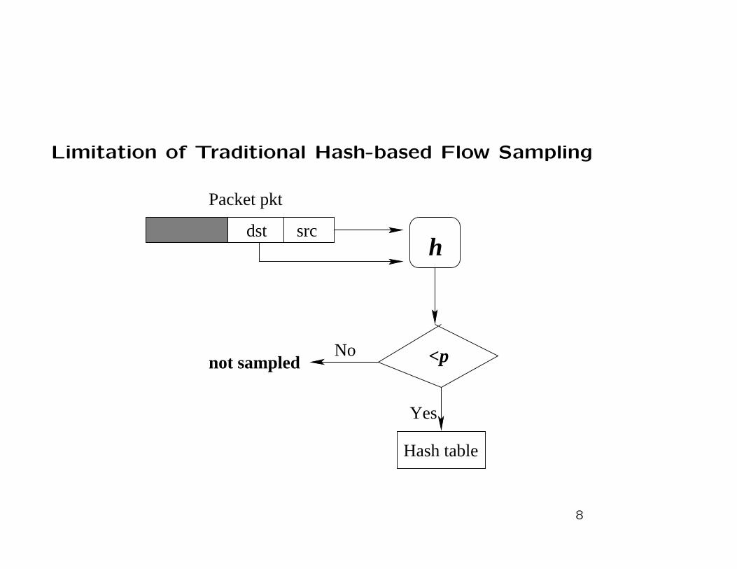
Limitation of Traditional Hash-based Flow Sampling

srcdst

Packet pkt

h

Yes

Nonot sampled

Hash table

<p

8

Limitation of Traditional Hash-based Flow Sampling

• If a flow is sampled (i.e., hash value < p), all packets belong-

ing to it need to be processed by the hash table.

• p has to be much smaller than the ratio between the op-

erating speed of the hash table and the arrival rate of the

traffic.

• small sampling rate leads to large estimation error.

9

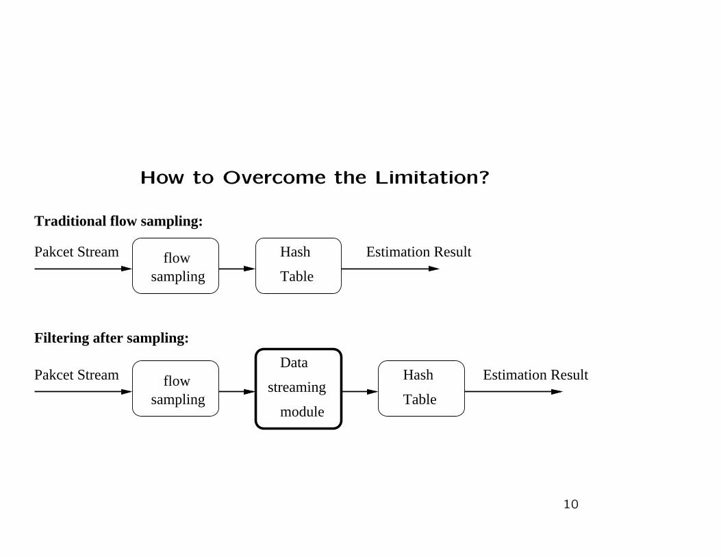
How to Overcome the Limitation?

Pakcet Stream

samplingflow

Traditional flow sampling:

Filtering after sampling:

Pakcet Stream

samplingflow Hash Estimation Result

Data

module

streamingHash Estimation Result

Table

Table

10

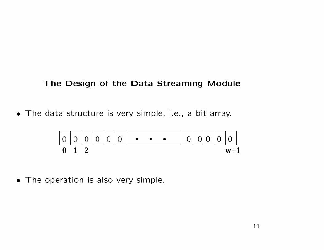
The Design of the Data Streaming Module

• The data structure is very simple, i.e., a bit array.

0 0 0 0 0 0 0 0 0 0 0w−11 20

• The operation is also very simple.

11

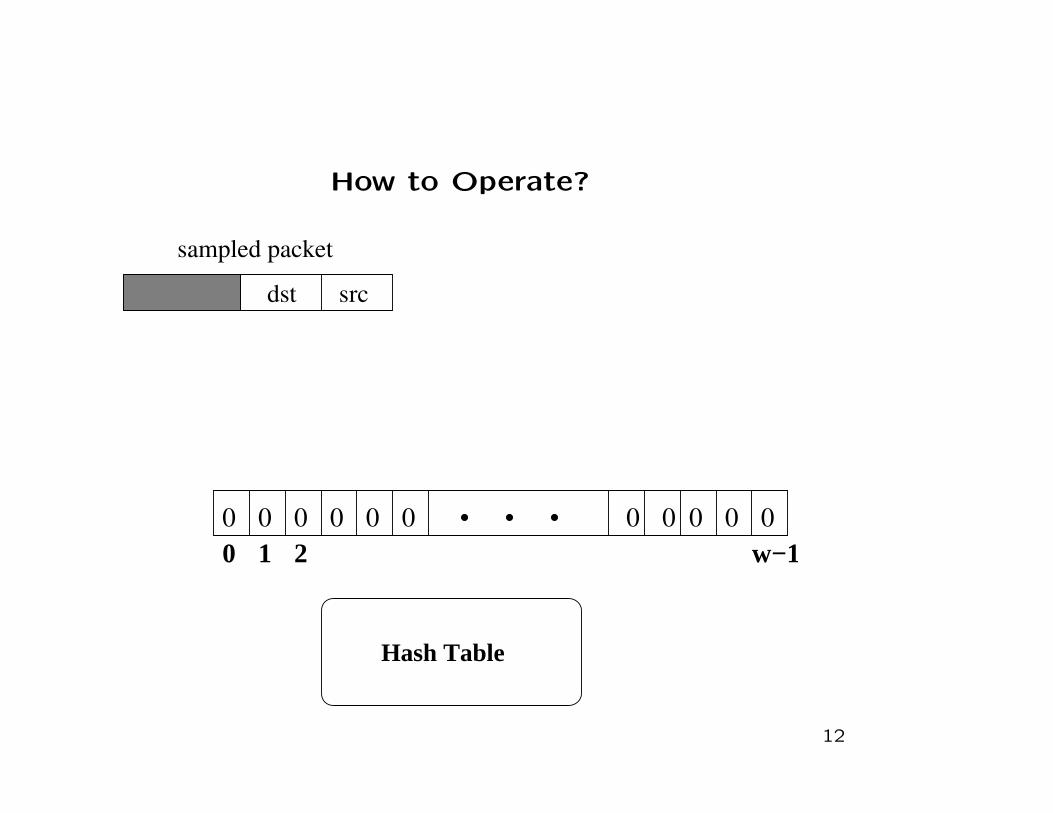
How to Operate?

0 0 0 0 0 0 0 0 0 0 0

srcdst

w−11 20

Hash Table

sampled packet

12

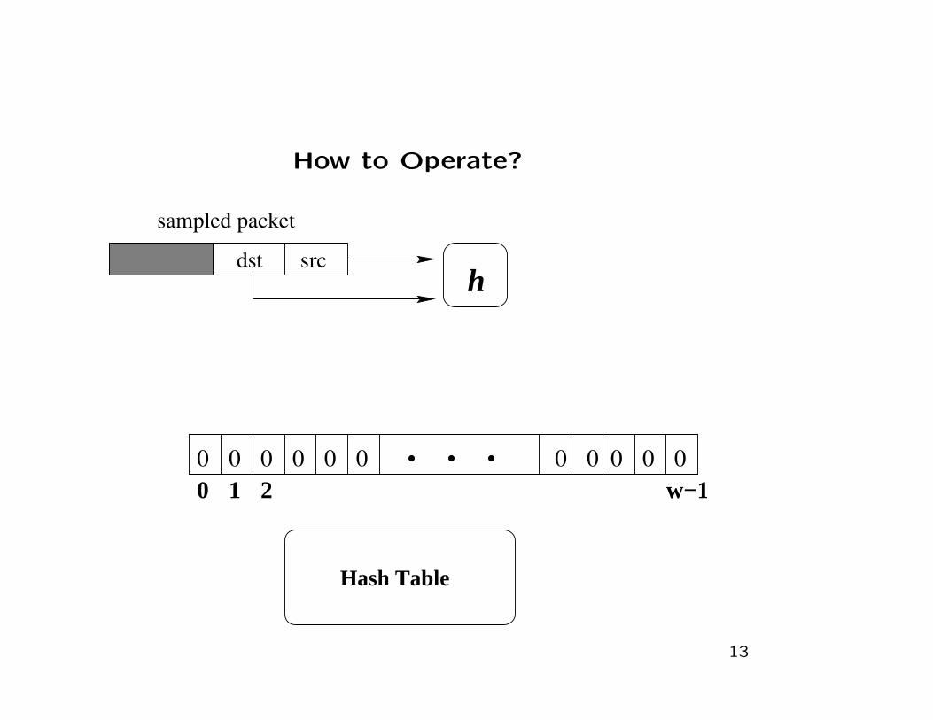
How to Operate?

0 0 0 0 0 0 0 0 0 0 0

srcdsth

w−11 20

Hash Table

sampled packet

13

How to Operate?

0 0 0 0 0 0 0 0 0 0 0

srcdsth

w−11 20

Hash Table

sampled packet

14

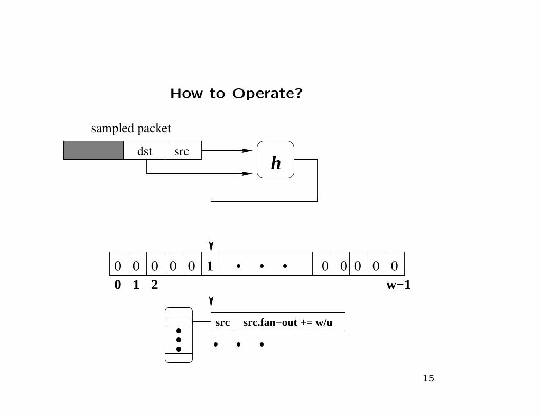
How to Operate?

0 0 0 0 0 1 0 0 0 0 0

srcdsth

w−11 20

src src.fan−out += w/u

sampled packet

15

Accuracy

• unbiased estimator

• its approximate variance is given by

V ar[F̂s] ≈

∑pFsj=1

w−uj

uj

p2+

Fs(1 − p)

p

16

Our Schemes

• The simple scheme: filtering after sampling

• The advanced scheme: separating identity gathering and

counting

17

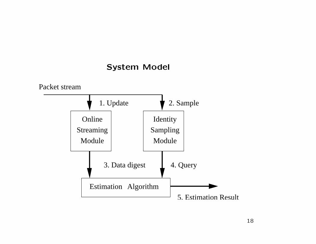
System Model

Streaming

Online

Module Module

1. Update 2. Sample

Packet stream

Identity

AlgorithmEstimation

5. Estimation Result

Sampling

4. Query3. Data digest

18

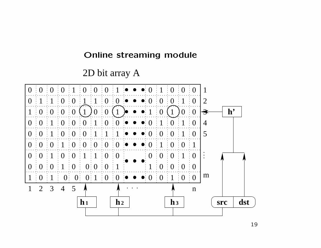
Online streaming module

3 4 521 . . . n

...

1 1 1

1

1

1

1

1 1 1

1

1

1

1

1

2

3

5

4

m

1

1

1

1

1 1

111

11

11

111

11

1 1 1

src dst

h’

h hh 2 31

2D bit array A

0

0 0 0 0 0 0 0 0 00 0

0

0

0

0

0

0 0 0 0 0 0 0 0 0 0

0

0

0

0

0

00000000

0

0

0

0

0

0 0 0 0 0 0 0 0 0

0000

0

0

0

0

0

0

0

0

0

0

0

0

00 0

0

00

0 0

0

0 1

0

0

0

0

0

0

0

0

0

0

19

Identity sampling module

• The purpose is to capture the identities of potential super

sources that will be used to look up the previous 2D bit array

to obtain their fan-out estimations.

• Use aforementioned filtering after sampling technique

• Use different recording strategy: only record the sampled

source identities sequentially in DRAM instead of construct-

ing a hash table.

20

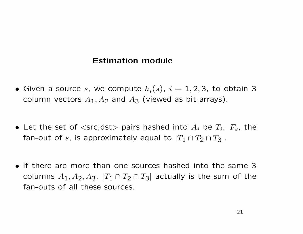
Estimation module

• Given a source s, we compute hi(s), i = 1,2,3, to obtain 3

column vectors A1, A2 and A3 (viewed as bit arrays).

• Let the set of <src,dst> pairs hashed into Ai be Ti. Fs, the

fan-out of s, is approximately equal to |T1 ∩ T2 ∩ T3|.

• if there are more than one sources hashed into the same 3

columns A1, A2, A3, |T1 ∩ T2 ∩ T3| actually is the sum of the

fan-outs of all these sources.

21

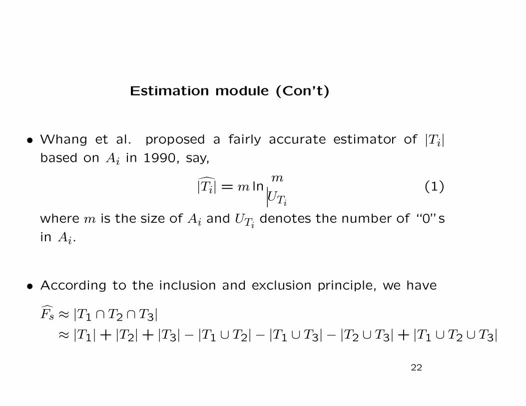
Estimation module (Con’t)

• Whang et al. proposed a fairly accurate estimator of |Ti|

based on Ai in 1990, say,

|̂Ti| = m lnm

UTi

(1)

where m is the size of Ai and UTidenotes the number of “0”s

in Ai.

• According to the inclusion and exclusion principle, we have

F̂s ≈ |T1 ∩ T2 ∩ T3|

≈ |T1| + |T2| + |T3| − |T1 ∪ T2| − |T1 ∪ T3| − |T2 ∪ T3| + |T1 ∪ T2 ∪ T3|

22

Accuracy

• almost unbiased

• its approximate variance is given by

V ar[F̂s] ≈ −m3∑

i=1

f(tTi) − m

∑

1≤i1<i2≤3

f(tTi1∪Ti2

)

+ 2m(f(tT1∪(T2∩T3)) + f(tT2∪(T1∩T3)

) + f(tT3∪(T2∩T1)))

+ 2m∑

1≤i1<i2≤3

f(tTi1∩Ti2

)

− 2m(f(tT1∩(T2∪T3)) + f(tT2∩(T1∪T3)

) + f(tT3∩(T2∪T1)))

+ mf(tT1∪T2∪T3)

where f(t) = et − t − 1.

23

Evaluation

• Traces from USC, UNC and NLANR

• simulate our schemes running on a fully utilized OC-192 (10

Gbps) using 128KB SRAM.

• For the simple scheme we set a flow sampling rate of 25%

which is required to fit in 128KB SRAM.

• Both online streaming model and identity sampling module

of the advanced scheme have enough speed to process the

incoming traffic with 100% sampling.

24

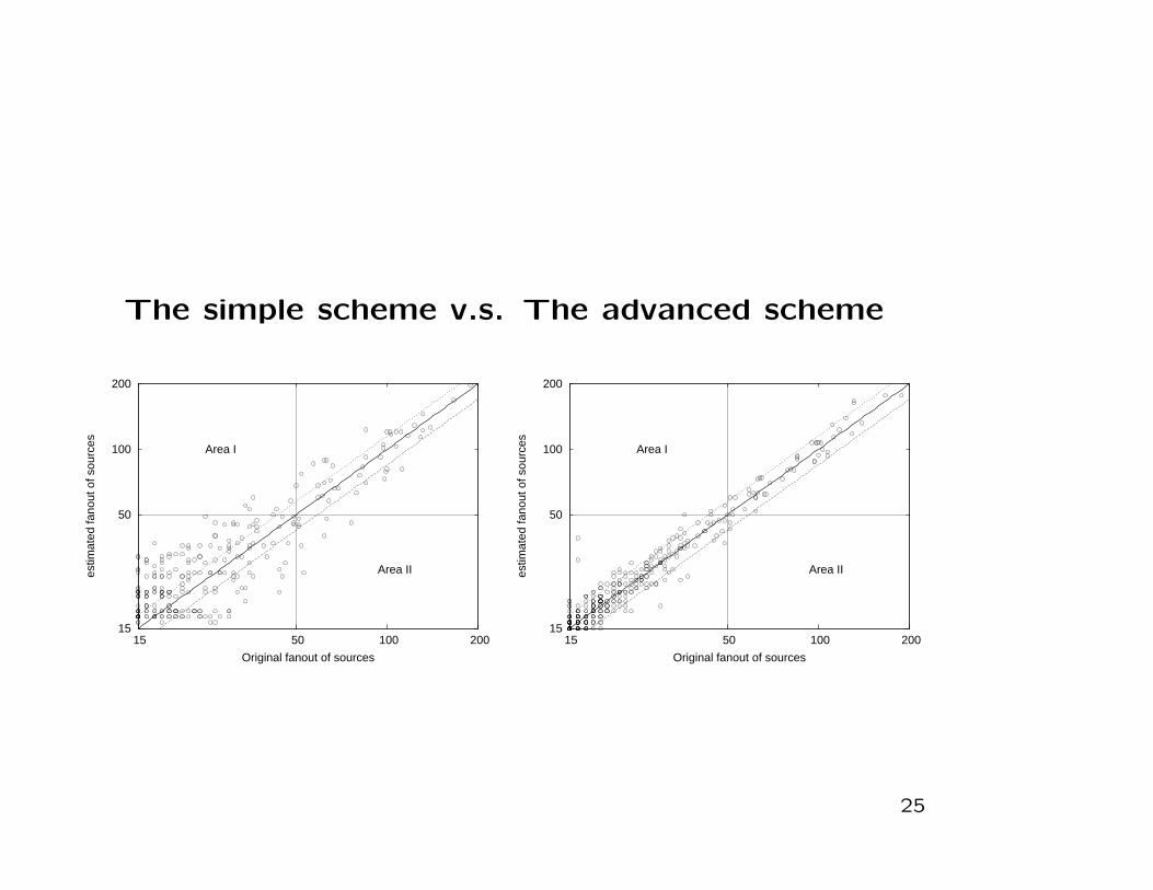
The simple scheme v.s. The advanced scheme

15

50

100

200

15 50 100 200

estim

ated

fano

ut o

f sou

rces

Original fanout of sources

Area I

Area II

15

50

100

200

15 50 100 200

estim

ated

fano

ut o

f sou

rces

Original fanout of sources

Area I

Area II

25

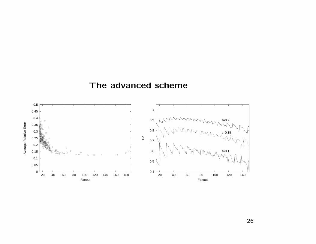
The advanced scheme

0

0.05

0.1

0.15

0.2

0.25

0.3

0.35

0.4

0.45

0.5

20 40 60 80 100 120 140 160 180

Ave

rage

Rel

ativ

e E

rror

Fanout

0.4

0.5

0.6

0.7

0.8

0.9

1

20 40 60 80 100 120 140

1-δ

Fanout

ε=0.2

ε=0.1

ε=0.15

26

Conclusion

• filtering after sampling: the simple scheme

• separating identity gathering and counting: the advanced

scheme

27

Thank you!

• We thank to IMC and GTISC for supporting our travel.

• Questions?

28