1-s2 0-S0094114X1000203X-main

Mechanism and Machine Theory 46 (2011) 1016–1035

Contents lists available at ScienceDirect

Mechanism and Machine Theory

j ourna l homepage: www.e lsev ie r.com/ locate /mechmt

Modelling and dynamics of a servo-valve controlled hydraulic motorby bondgraph

K. Dasgupta a,⁎, H. Murrenhoff b

a Dept. of Mechanical Engg. & Mining Machinery Engg., Indian School of Mines University, Dhanbad, 826004, Indiab Institute of Fluid Power Transmission and Control, University of Technology, Aachen, RWTH, Steinbachstrasse 53, D-52074 Aachen, Germany

a r t i c l e i n f o

⁎ Corresponding author. Tel.: +91 326 2296551x54E-mail address: [email protected] (K. D

0094-114X/$ – see front matter © 2010 Elsevier Ltd.doi:10.1016/j.mechmachtheory.2010.11.006

a b s t r a c t

Article history:Received 1 December 2008Received in revised form 24 October 2010Accepted 16 November 2010Available online 21 March 2011

A comprehensive model of a closed-loop servo-valve controlled hydro-motor drive system hasbeen made using Bondgraph simulation technique (Thoma, 1990) [17]. The validation of theservo-valve model is obtained first by the established results of Gordic et al., 2004 [10]. Thedynamic performance of the complete system has been studied with respect to the variation ofthe parameters of the PI controller that drives the servo-valve.

© 2010 Elsevier Ltd. All rights reserved.
Keywords:Servo-valveClosed-loop controlledBondgraphSimulationModellingHydro-motor
1. Introduction

Electro-hydraulic servo-drives are widely used in industrial applications like machine tools, testing equipment andautonomous manufacturing systems. Many articles regarding various aspects of servo-valve have appeared alongside theirdevelopment. In this respect, the most significant reference book is of Meritt [1] where a general description of the servo-valve,along with the design of its spindle, flapper-nozzle valve, torque motor, etc. are explained. In recent years Dimarogoans [2] hasaddressed on the evaluation in design theory and control mechanism where CAD design of control system is well presented.

Generally servo-valve dynamics are described by first and second order transfer functions, depending on the dynamiccharacteristics of the system. The data obtained from the manufacturers' catalogue are used for the estimation of time constants,natural frequencies and damping ratio of the valve [3]. Such model can give the preliminary insight of its operation, may not beable to explain the phenomenon in wide operating range. Thereby, researchers have proposed higher order models [4–7] to takeinto account the effects of some non-linearities in the form of transfer functions or state-space equations. The published articles byUrata [8,9] have givenmore detail analysis of the torquemotor and elastic structure dynamics of the flapper. However, most of theabove articles include the experimental validation of already establishedmodels. More recently, Gordic et al. [10] have establisheda comprehensive mathematical model of the commonly used electro-hydraulic two-stage flow control with a spindle positionfeedback servo-valve. They have also studied the effects of the variation of torque motor parameters on the servo-valveperformance [11] using MATLAB-SIMULINK environment.

The servo-valve coupled with a hydraulic motor in closed-loop control system is used to achieve accurate torque, velocity andposition control. In most of the industrial drives, where very high performance is not the requirement, the simple classical controltechnique is adopted. Using non-dimensional approach, Watton [12] has analysed optimum steady state performance of the

43; fax: +91 326 2296563.asgupta).

All rights reserved.

http://dx.doi.org/10.1016/j.mechmachtheory.2010.11.006

mailto:[email protected]

http://dx.doi.org/10.1016/j.mechmachtheory.2010.11.006

http://www.sciencedirect.com/science/journal/0094114X

1017K. Dasgupta, H. Murrenhoff / Mechanism and Machine Theory 46 (2011) 1016–1035

proportional valve controlled axial piston motor drive and established the effects of flow and torque losses of the motor on theefficiency of the system. Most of the available literatures are concerned with the open-loop servo-valve controlled hydro-motordrive systems [13,14]. More recently, the influence of the actuator leakage on the dynamic behavior of the flapper-nozzle valvecontrolled electro-hydraulic servo system is studied by Attila [15]. However, considering the detailed model of the valve and theactuator, the performance of the closed-loop system has not yet been studied.

The transfer functionmethod is a powerful tool for analyzing hydraulic control system. It is, however, limited in that non-linearterms that frequently appear in the describing equations, which must be linearized in one form or other, usually about anoperating point. Consequently, other analytical approach such as Bondgraph technique [16,17], which does not considerlinearization found to be more desirable in the present study. It is a powerful tool for modelling complex systems even withinteraction of several energy domains.

The objective of the present article is to create a comprehensive dynamic model of a closed-loop servo-valve controlled hydro-motor drive system by using Bondgraph. The servo-valve analysed by Gordic et.al [10] is considered in the present investigation.The model proposed in the present article is validated by the established results [10]. The influences of various parameters of theProportional–Integral (PI) controller that drives the servo-valve on the response of the system are studied. The model relating tothe various control parameters on the performance of the system can be used to predict and improve the physical design of thesystem and its associated components.

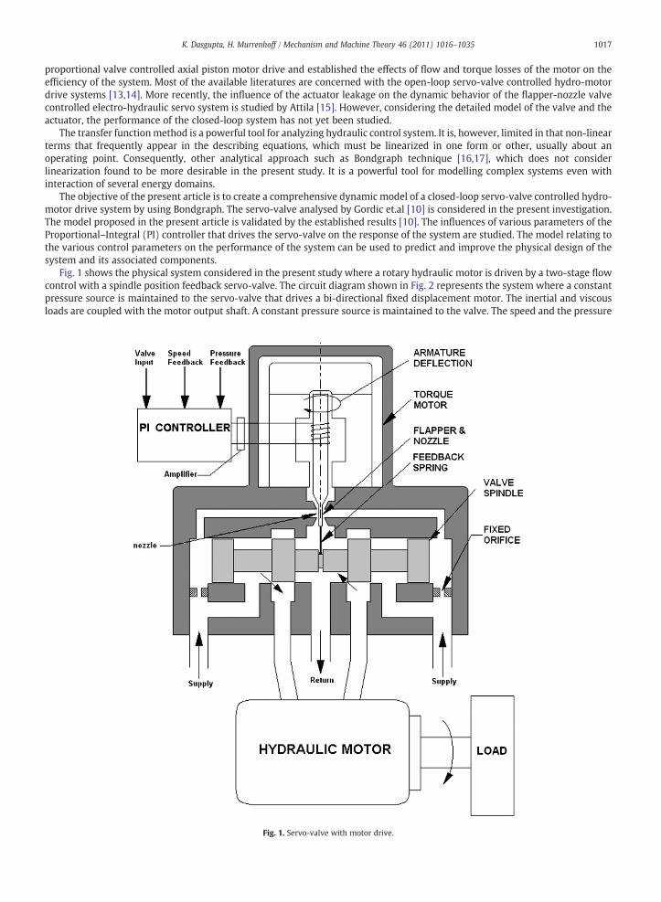
Fig. 1 shows the physical system considered in the present study where a rotary hydraulic motor is driven by a two-stage flowcontrol with a spindle position feedback servo-valve. The circuit diagram shown in Fig. 2 represents the system where a constantpressure source is maintained to the servo-valve that drives a bi-directional fixed displacement motor. The inertial and viscousloads are coupled with the motor output shaft. A constant pressure source is maintained to the valve. The speed and the pressure

Fig. 1. Servo-valve with motor drive.

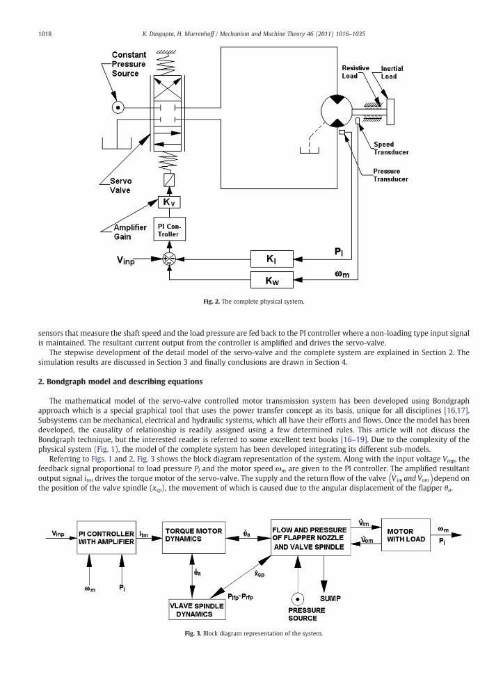
Fig. 2. The complete physical system.

Fig. 3. Block diagram representation of the system.

1018 K. Dasgupta, H. Murrenhoff / Mechanism and Machine Theory 46 (2011) 1016–1035

sensors that measure the shaft speed and the load pressure are fed back to the PI controller where a non-loading type input signalis maintained. The resultant current output from the controller is amplified and drives the servo-valve.

The stepwise development of the detail model of the servo-valve and the complete system are explained in Section 2. Thesimulation results are discussed in Section 3 and finally conclusions are drawn in Section 4.

2. Bondgraph model and describing equations

The mathematical model of the servo-valve controlled motor transmission system has been developed using Bondgraphapproach which is a special graphical tool that uses the power transfer concept as its basis, unique for all disciplines [16,17].Subsystems can be mechanical, electrical and hydraulic systems, which all have their efforts and flows. Once the model has beendeveloped, the causality of relationship is readily assigned using a few determined rules. This article will not discuss theBondgraph technique, but the interested reader is referred to some excellent text books [16–19]. Due to the complexity of thephysical system (Fig. 1), the model of the complete system has been developed integrating its different sub-models.

Referring to Figs. 1 and 2, Fig. 3 shows the block diagram representation of the system. Along with the input voltage Vinp, thefeedback signal proportional to load pressure Pl and the motor speed ωm are given to the PI controller. The amplified resultantoutput signal itm drives the torque motor of the servo-valve. The supply and the return flow of the valve V im and Vom

� �depend on

the position of the valve spindle (xsp), the movement of which is caused due to the angular displacement of the flapper θa.

image of Fig.�2

image of Fig.�3


The sub-models of the complete system are as follows:

a. Sub-model of the torque motor and the valve spindleb. Sub-model of the flow and pressures through the flapper-nozzle and the valve spindlec. Sub-model of the hydro-motor drive systemd. Sub-model of the PI controller

The following assumptions are made in developing the models:

• A constant pressure source to the inlet port of the valve is considered,• The fluid considered in the analysis has Newtonian characteristics,• Resistive and capacitive effects are lumped wherever appropriate. All springs are assumed to be linear,• Sump pressure is assumed to be zero,• The masses of the feedback spring, flapper and the flexure tube lumped into one inertial element, as are the damping forces.Similar considerations are made for the main valve spindle,

• The steady state flow forces that act on the valve spindle and the flapper are considered, while the dynamic flow forces areneglected.

2.1. Model of the torque motor and the spool position feedback

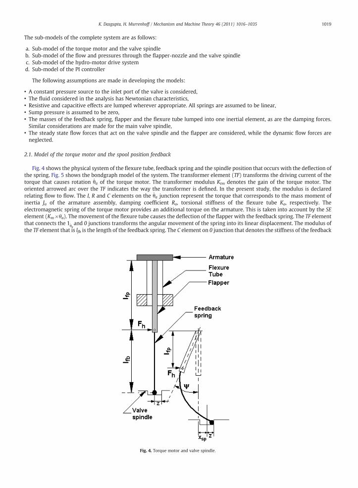
Fig. 4 shows the physical system of the flexure tube, feedback spring and the spindle position that occurs with the deflection ofthe spring. Fig. 5 shows the bondgraph model of the system. The transformer element (TF) transforms the driving current of thetorque that causes rotation θa of the torque motor. The transformer modulus Ktm denotes the gain of the torque motor. Theoriented arrowed arc over the TF indicates the way the transformer is defined. In the present study, the modulus is declaredrelating flow to flow. The I, R and C elements on the θa junction represent the torque that corresponds to the mass moment ofinertia Ja of the armature assembly, damping coefficient Ra, torsional stiffness of the flexure tube Ka, respectively. Theelectromagnetic spring of the torque motor provides an additional torque on the armature. This is taken into account by the SEelement (Km×θa). The movement of the flexure tube causes the deflection of the flapper with the feedback spring. The TF elementthat connects the 1θaand 0 junctions transforms the angular movement of the spring into its linear displacement. The modulus ofthe TF element that is lfb is the length of the feedback spring. The C element on 0 junction that denotes the stiffness of the feedback

Fig. 4. Torque motor and valve spindle.

image of Fig.�4

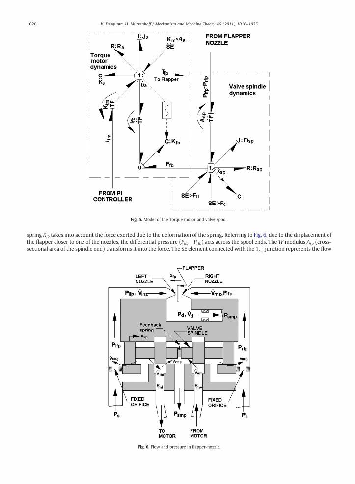
Fig. 5. Model of the Torque motor and valve spool.

Fig. 6. Flow and pressure in flapper-nozzle.


spring Kfb takes into account the force exerted due to the deformation of the spring. Referring to Fig. 6, due to the displacement ofthe flapper closer to one of the nozzles, the differential pressure (Plfb−Prfb) acts across the spool ends. The TFmodulus Asp (cross-sectional area of the spindle end) transforms it into the force. The SE element connected with the 1xsp junction represents the flow

image of Fig.�5

image of Fig.�6


force Fff that acts on the valve spindle. Similarly I, R and SE elements on the 1xsp represent the inertia force due to spindle massmsp,the resistive force due to the viscous damping coefficient Rsp and the Coulomb friction force Fc that exists at the very low speed ofthe valve spindle, respectively. The activated C element on the same junction records the valve displacement xsp.

The system equations derived from themodel are based on the lumped elements (I and C) with integral causality present in thesystem. They are as follows:

In the model, 1 θajunction in the mechanical part of the torque motor comes from a force balance, resulting from the constitutive

equations of each element. Referring to the Fig. 5, the inertia torque on the torque motor armature is expressed as:

where

pa = Ktm itm+Km θa−Ffb lfb−Tfp−θa Ra−Ka θa ð1Þ

The first term of the above equation indicates the inertia torque of the torque motor, the second term is the driving torque, thethird term is the electro-magnetic spring torque, fourth term is the torque due to the deformation of the feedback spring, fifth termis the torque due to the deformation of the flapper, the sixth term indicates the viscous friction torque of the armature with theflexure tube and the seventh term is the torque due to the bending of the flexure tube, respectively.

The force Ffb caused due to the deformation of the feedback spring is expressed as:

Ffb = Kfbxfb ð2Þ

the deformation of the spring xfb is given by

xfb = θa lfb−xsp

The angular velocity of the flapper is given by

θa = pa = Ja ð3Þ

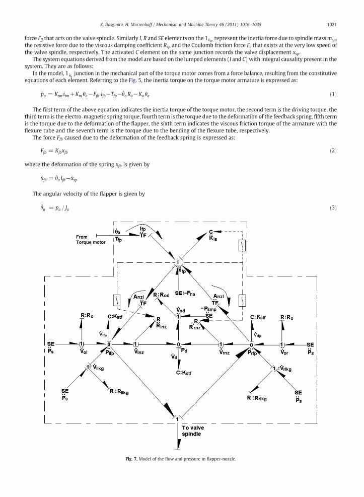
Fig. 7. Model of the flow and pressure in flapper-nozzle.

image of Fig.�7


The torque Tfp=Fh lfp causes deformation of the flapper, expression of which is given by Eq. (9) in Section 2.2.The valve dynamics due to the mechanical part of the valve spindle is expressed as:

psp = Plfp−Prfp� �

Asp−Kfb xfb−Rsp xsp−Fc−Fff ð4Þ

In the above equation, Fc is the dry friction force that acts on the spindle given by [20]:

Fc =Fcn sign xsp

� �; xsp ≠ 0

Z; Zj j b FcoFco sign Zð Þ; Zj j≥ Fco; xsp =0

8><>:

Z=(Plfp−Prfp) Asp−Ffb−Fff.
whereThe flow force that acts on the valve spindle in the event of opening of valve is given by [21]: Fff=0.43 π dsp (Ps−Pl) xsp.After complete opening of the valve port, i.e., xsp≥xspm, to arrest the spindle motion, high damping has been considered for
the valve seat. In Fig. 5, it has been considered by changing the value of the damping coefficient of the valve spindle Rsp

accordingly.The velocity of the valve spindle is expressed as:

xsp = psp =msp ð5Þ

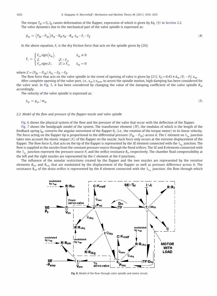
2.2. Model of the flow and pressure of the flapper-nozzle and valve spindle

Fig. 6 shows the physical system of the flow and the pressure of the valve that occur with the deflection of the flapper.Fig. 7 shows the bondgraph model of the system. The transformer element (TF), the modulus of which is the length of the

feedback spring lfp, converts the angular movement of the flapper θa (i.e., the rotation of the torque motor) to its linear velocity.The force acting on the flapper tip is proportional to the differential pressure (Plfp−Prfp) across it. The C element on 1xfp junctiontakes into account the elastic impact (Fi) of the flapper on the nozzle. Such force only occurs at the extreme displacement of theflapper. The flow force Fh that acts on the tip of the flapper is represented by the SE element connected with the 1xfp junction. Theflow is supplied to the nozzles from the constant pressure source through the fixed orifices. The SE and R elements connected withthe 1Vo

junction represent the pressure source Ps and the orifice resistance Ro, respectively. The chamber fluid compressibility atthe left and the right nozzles are represented by the C element at the 0 junctions.

The influence of the annular restrictions created by the flapper and the two nozzles are represented by the resistiveelements Rlnz and Rrnz that are modulated by the displacement of the flapper as well as pressure difference across it. Theresistance Rod of the drain orifice is represented by the R element connected with the 1vod junction; the flow through which

Fig. 8. Model of the flow through valve spindle and motor circuit.

image of Fig.�8


depends on the pressure difference (Pd−Psmp) across it. The force acting on the valve spool is proportional to the differentialpressure (Plfp−Prfp). In the above model, the flow through the orifices and the nozzles are represented by their correspondingresistive elements. Since the resistances are in conductive causalities, while deriving the system equations they are consideredas modulated flow sources, the flow through which depend on the port opening areas and the pressure difference across it.Similarly, the leakage flow to the nozzle chamber through the valve spindle depends on the pressure difference across theleakage path. The following system equations are derived from the model:

Considering the compressibility of the fluid in the chambers connecting the spool ends with the nozzles, with the deflection ofthe flapper towards the left nozzle, the flow balance equations become:

where

where

V lfp = Vol + xfp Anzl + V llkg−V lnz−xsp Asp ð6Þ

V rfp = Vor−xfp Anzl + V rlkg−V rnz + xsp Asp ð7Þ

In Eqs. (6) and (7), the first terms represent the compressibility flow loss of the fluid, the second terms indicate the flowthrough their respective orifice, the third terms are the flow due to the displacement of the flapper, the fourth terms are theleakage flow through the valve spindle to the nozzle chamber that depend on the length of the leakage paths and pressuredifference across it, the fifth terms indicate the flow to the discharge chamber from the nozzle and the sixth terms representthe flow due to the displacement of the valve spindle. Similarly, the flow to the discharge chamber from the nozzles Vod isgiven by:

Vod = V lnz + V rnz−Vd ð8Þ

Vd is the compressibility flow loss of the fluid in the discharge chamber.
whereThe expressions of the flow through the orifices and nozzles considered in Eqs. (6), (7) and (8) are given in Section 2.5.The 1xfp junction that represents the flapper displacement xfp comes from the torque balance, which is expressed as:
Tfp = Prfp–Plfp� �

Anzl + Fha + Fin o

lfp ð9Þ

In the above equation the flow force that acts on the tip of the flapper and the elastic impact force of the flapper on the nozzleare given by [1]:

Fha = 8π K2nl xo−xfp� �2

Plfp−Pd� �

−K2nr xo + xfp� �2

Prfp−Pd� ��

Knl and Knr are the flow coefficients of the nozzle orifices.

Fi = Kis jxfp j–xo� �

sign xfp� �

lfp;when xfp�� ≥ xo

Kis, xfp and xo are the impact stiffness, the displacement of the flapper and the distance of the flapper tip from each nozzle atnull position, respectively.

The pressure at the nozzles and the discharge chamber are expressed as:

Plfp = Kstf Vlfp; Prfp = Kstf Vrfp and Pd = Kstf1Vd; respectively:

Fig. 9. Model of the controller.

image of Fig.�9


The velocity of the flapper tip is given by

xfp = θa lfp ð10Þ

2.3. Model of the hydro-motor drive system

Referring to Fig. 2, the flow supplied from the servo-valve drives the motor connected with the viscous and the inertial loads.Fig. 8 shows the model of the system. A constant supply pressure (Ps) is maintained at the inlet port of the servo-valve. It isrepresented by the SE element on 1 junction. The outlet flow from the motor through the valve port goes to the sump at zeropressure. The servo-valve ports are considered as variable resistances Rim and Rom, the flow through which depends on therespective port opening area that depends on the displacement of the valve spindle xsp and the pressure difference across it. Thevalve spindle is considered to be of rectangular ports, symmetrical spindle with critically lapped lands. The 0 junctions representthe pressures Pmi and Pmo correspond to the pressures at the inlet and outlet port of the motor, respectively. The C elements onthese junctions take into account the compressibility loss of the fluid. The leakage resistance Rilkg represents the internal leakageflow Vilkg that occurs due to the pressure difference (Pmi−Pmo) across the motor ports. The valve leakage resistance Rvlkg dependson the displacement of the valve spindle. The flow resistances are in conductivity, therefore, they are considered as modulatedflow sources.

Fig. 10. Model of the complete system.

image of Fig.�10


The TF element that connects the 0Pm and the 1ωmjunctions transforms the hydraulic power to mechanical power or vice-versa,

where the modulus Dm indicates the volume displacement rate of the motor. The 1ωmjunction representing the mechanical part of

the load corresponds to the speed of the motor output shaft ωm. The I, R and SE elements represent the load inertia Jl, speeddependent friction load Rl and the slip torque Tsl, respectively. They are with the 1ωm

junction that constitutes the load dynamics.The activated C element on the same junction records the output speed of the motor ωm.

The system equations derived from the model are as follows:With the compressibility of the fluid, the flow balance at the inlet and the outlet ports of the motor are given by

V imc = V im−Vvlkg−V ilkg−ωmDm ð11Þ

Vomc = −Vom + V ilkg + ωmDm−Vvlkg ð12Þ

The pressures at the inlet and outlet ports of the motor are expressed as:

Pmi = Kmstf Vmi and Pmo = Kmstf Vmo; respectively:

The 1 junction in the mechanical part of the motor comes from the torque balance, which is expressed by the followingequation, resulting from the constitutive equation of each element:

pl = Pmi−Pmoð ÞDm−ωm Rl−Tsl ð13Þ

the first term of the above equation is the torque due to the inertia load Jl, the second term indicates the torque equivalent to
wherethe differential pressure across the motor, the third term is the torque loss due to viscous friction coefficient Rl and the fourth termis the slip torque.
The motor speed is given by:

ωm = pl = Jl ð14Þ

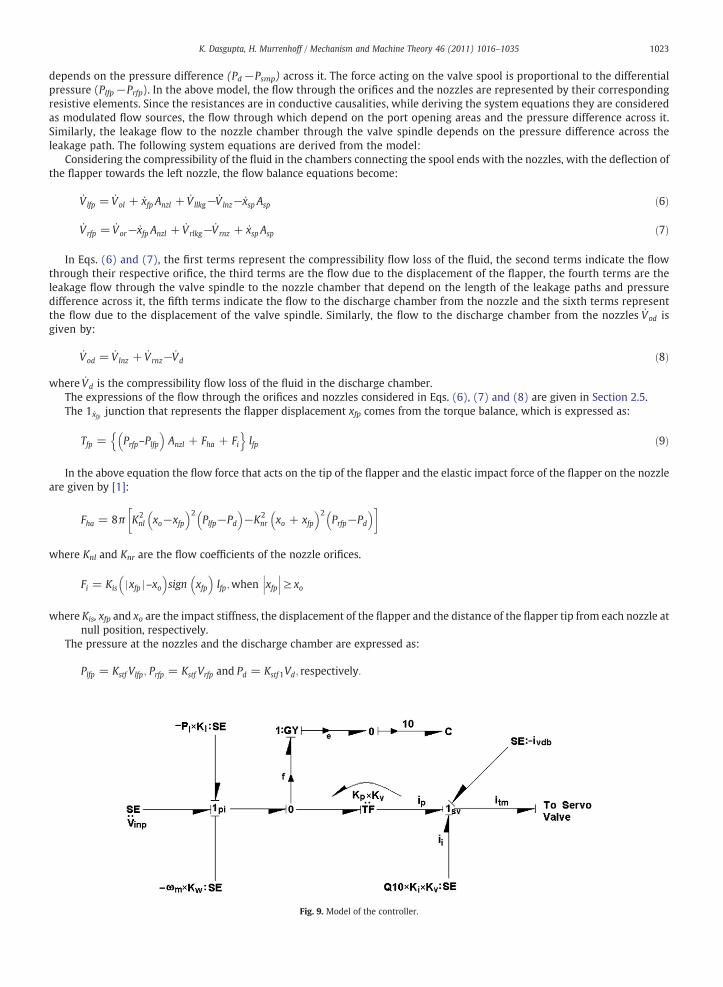
2.4. Model of the controller

A feedback control system is used to control the motor speed. Referring to Fig. 2, the feedback strategy is achieved by adoptingthe motor speed ωm and load pressure (Pl=Pmi−Pmo) and feeding both the signals back and subtracted from the reference inputvoltage Vinp. The resultant voltage is supplied to the PI controller. The current output of the controller is multiplied by the amplifiergain Kv that drives the torque motor. The bondgraph model of the control unit is shown in Fig. 9.

The SE elements on the 1pi junction correspond to the input voltage Vinp, the pressure and speed feedback signals multipliedby their respective gain values (Kl and Kw). The proportional control action is being implemented by multiplying the resultantvoltage by the proportional gain Kp×Kv. Also, the resultant signal from 1pi junction is integrated at bond C10. The integralcontrol action is adopted by multiplying the signal obtained at bond C10 by the gain Ki×Kv. The two feedback signals

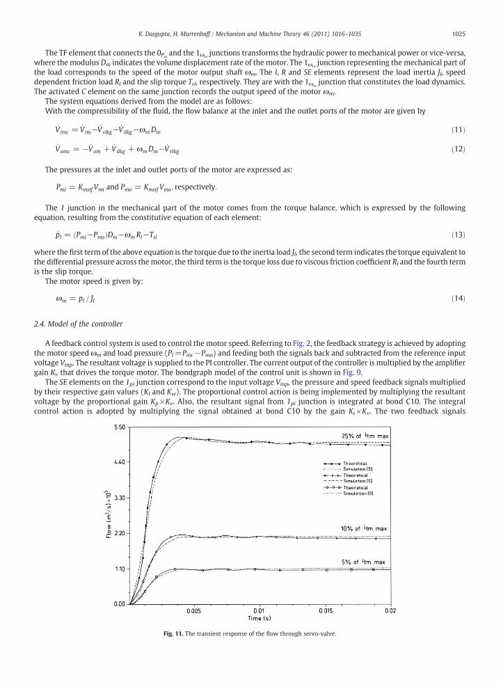
Fig. 11. The transient response of the flow through servo-valve.

image of Fig.�11

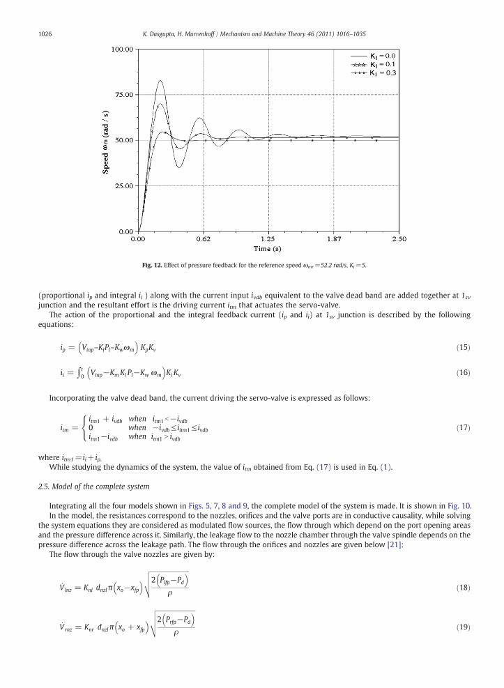
Fig. 12. Effect of pressure feedback for the reference speed ωmr=52.2 rad/s, Ki=5.


(proportional ip and integral ii ) along with the current input ivdb equivalent to the valve dead band are added together at 1svjunction and the resultant effort is the driving current itm that actuates the servo-valve.

The action of the proportional and the integral feedback current (ip and ii) at 1sv junction is described by the followingequations:

ip = Vinp–KlPl–Kwωm

� �KpKv ð15Þ

ii = ∫t0

Vinp−Km Kl Pl−Kw ωm

� �Ki Kv ð16Þ

Incorporating the valve dead band, the current driving the servo-valve is expressed as follows:

itm =itm1 + ivdb when itm1b−ivdb0 when −ivdb≤ iitm1≤ ivdbitm1−ivdb when itm1 N ivdb

8<: ð17Þ

itm1=ii+ ip.
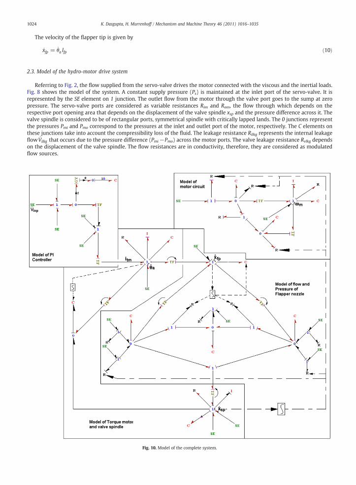
whereWhile studying the dynamics of the system, the value of itm obtained from Eq. (17) is used in Eq. (1).
2.5. Model of the complete system

Integrating all the four models shown in Figs. 5, 7, 8 and 9, the complete model of the system is made. It is shown in Fig. 10.In the model, the resistances correspond to the nozzles, orifices and the valve ports are in conductive causality, while solving

the system equations they are considered as modulated flow sources, the flow through which depend on the port opening areasand the pressure difference across it. Similarly, the leakage flow to the nozzle chamber through the valve spindle depends on thepressure difference across the leakage path. The flow through the orifices and nozzles are given below [21]:

The flow through the valve nozzles are given by:

V lnz = Knl dnzl π xo−xfp� � ffiffiffiffiffiffiffiffiffiffiffiffiffiffiffiffiffiffiffiffiffiffiffiffiffi

2 Plfp−Pd� �

ρ

vuut ð18Þ

V rnz = Knr dnzl π xo + xfp� � ffiffiffiffiffiffiffiffiffiffiffiffiffiffiffiffiffiffiffiffiffiffiffiffiffi

2 Prfp−Pd� �

ρ

vuut ð19Þ

image of Fig.�12

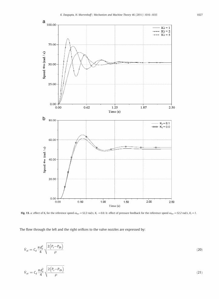
Fig. 13. a: effect of Ki for the reference speed ωmr=52.2 rad/s, Kl =0.0. b: effect of pressure feedback for the reference speed ωmr=52.2 rad/s, Ki=1.


The flow through the left and the right orifices to the valve nozzles are expressed by:

Vol = Cdπd2o4

ffiffiffiffiffiffiffiffiffiffiffiffiffiffiffiffiffiffiffiffiffiffiffiffi2 Ps−Plfb� �

ρ

vuut ð20Þ

Vor = Cdπd2o4

ffiffiffiffiffiffiffiffiffiffiffiffiffiffiffiffiffiffiffiffiffiffiffiffiffi2 Ps−Prfb� �

ρ

vuut ð21Þ

image of Fig.�13

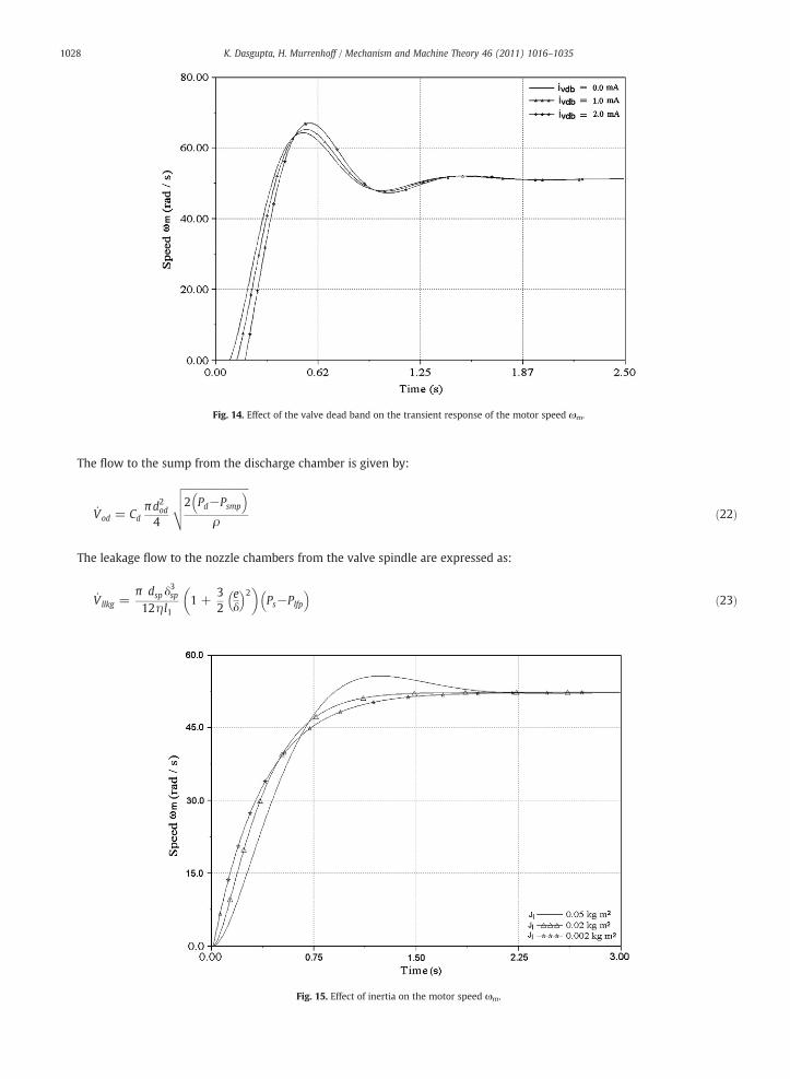
Fig. 14. Effect of the valve dead band on the transient response of the motor speed ωm.

Fig. 15. Effect of inertia on the motor speed ωm.


The flow to the sump from the discharge chamber is given by:

Vod = Cdπd2od4

ffiffiffiffiffiffiffiffiffiffiffiffiffiffiffiffiffiffiffiffiffiffiffiffiffiffiffi2 Pd−Psmp

� �ρ

vuut ð22Þ

The leakage flow to the nozzle chambers from the valve spindle are expressed as:

V llkg =π dsp δ

3sp

12η l11 +

32

eδ

� �2�

Ps−Plfp� �

ð23Þ

image of Fig.�14

image of Fig.�15

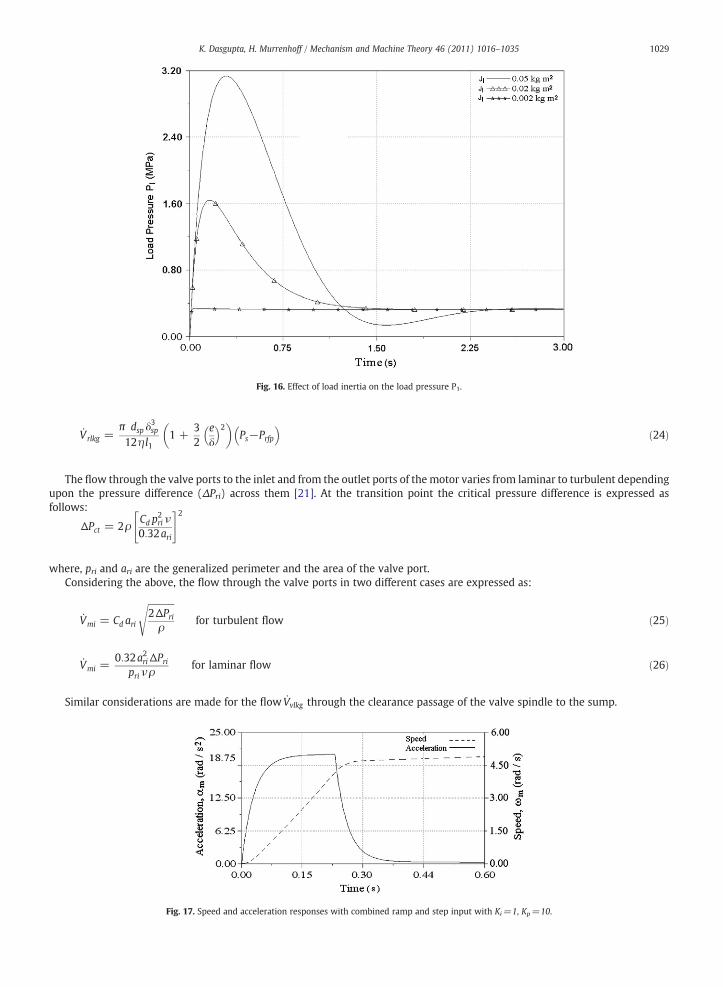
Fig. 16. Effect of load inertia on the load pressure P1.

Fig. 17. Speed and acceleration responses with combined ramp and step input with Ki=1, Kp=10.


V rlkg =π dsp δ

3sp

12η l11 +

32

eδ

� �2�

Ps−Prfp� �

ð24Þ

The flow through the valve ports to the inlet and from the outlet ports of the motor varies from laminar to turbulent dependingupon the pressure difference (ΔPri) across them [21]. At the transition point the critical pressure difference is expressed asfollows:

2" #2

ΔPct = 2ρCd pri ν0:32ari

ð24Þ

, pri and ari are the generalized perimeter and the area of the valve port.
whereConsidering the above, the flow through the valve ports in two different cases are expressed as:
Vmi = Cd ari

ffiffiffiffiffiffiffiffiffiffiffiffi2ΔPriρ

sfor turbulent flow ð25Þ

Vmi =0:32a2riΔPri

pri νρfor laminar flow ð26Þ

Similar considerations are made for the flow Vvlkg through the clearance passage of the valve spindle to the sump.

image of Fig.�16

image of Fig.�17


3. Simulation results and discussion

The simulation results are discussed in the following steps:

• In the first step, the servo-valve model in no-load condition is validated by comparing with the results obtained by Gordic etal. [10].

• In the next step, with the PI controller, the closed-loop performances of the complete system are studied.

The system equations obtained in Section 2 are solved numerically with the help of Symbols, 2000 [22]. This particular packageruns on as self-styled multi-tasking environment through different modules including control system analysis. The pictorialrepresentation of the bondgraph model of any physical system can be made and subsequently, the state equations are developed,which are solved numerically along with their graphical representation. It can also take various non-linearities of the system. Byusing the software, the observer states can be created additionally by activated bonds which do not change the dynamics of thesystem.

3.1. Servo-valve model verification

In validating the servo-valve model in no-load condition, in the complete model shown in Fig. 10, the sub-model of the PIcontroller is not considered. A constant source of current (itm) in Eq. (1) for driving the torque motor has been assumed. Thesystem equations given in Section 2.1 through 2.3 along with the Eq. (18) through (26) of Section 2.5 are solved numericallyusing the parametric values given in Appendix A. Additional parameters of the motor are suitably assumed. Fig. 11 comparesthe simulation results of the present study with that of Gordic. et.al [10]. The results are presented for the three differentvalues of itm.

The deviations of the simulated response which is nearly about 5%, when compared with the established results [10], may bedue to the following reasons:

• The flow coefficients are assumed for the orifices and the flapper-nozzle in the present study.• The flow force on the valve spindle indicated in Eq. (9) is considered to be of the usual form [1,21].• The leakages through the clearance passage of the valve spindle as well as the inlet and outlet flow of the valve are considered tobe either turbulent or laminar (Eqs. (25) and (26)) depending upon the pressure difference across the flow path.

However, the close agreement between the simulation and experimental results validates the proposed model.

3.2. Dynamic performance of the system

The parametric studies of the dynamic performance of the complete system have been made, by solving all the equationsderived in Sections 2.1 through 2.5. Applying integral control strategy, the effects of pressure feedback on the system's responses

Fig. 18. Speed response with combined ramp and step input with Ki=1, Kp=100.

image of Fig.�18


are investigated. The influences of the slip torque Tsl, dead band ivdb of the servo-valve and the load inertia on the system'sperformance are studied. The effects of the parameters of the Proportional–Integral (PI) on the performance of the system are alsodiscussed.

3.2.1. Effect of pressure feedbackWith integral control action (Ki=5), using step input (Vinp) to the servo-valve, the effects of the pressure feedback (Kl) on the

speed response of the system is shown in Fig. 12. The results show that the response is improved by increasing the value of Kl,while oscillations of the transient part of the response are considerably reduced in the maximum overshoot with correspondingdecrease in settling time. It is seen that perceptible damping effectmay be introduced by applying the pressure feedback; however,there exists steady state error. Comparing the speed response with the pressure feedback Kl=0.0 with that of Kl=0.1, it is seenthat for Ki=5 the steady state error is about 3%. However, by increasing Kl to 0.3 where steady state error is increased by 6%,further damping is obtained.

The results shown in Fig. 13a indicates that the dynamic response of the system can be improved by decreasing the value of Ki

even without pressure feedback Kl=0.0. The maximum overshoot is reduced from 58.5% to 25.5% and the settling time alsoreduces from 1.5 s to 1.3 s with the decrease in Ki=5 to Ki=1.

The response shown in Fig. 13b indicates that further improvement of the response may be achieved by introducing a value ofKl=0.1 with Ki=1.0 that decreases the maximum overshoot by 6.7%. However, this leads to a small steady state error of 5%. Theresults shown in Fig. 13b is with the torque load Tsl=0.5 Nm. that corresponds to the steady state speed of 50.6 rad/s with Kl=0.1.With the reduction of friction torque to Tsl=0.225 Nm, the speed can be further increased to 51.35 rad/s with the same value ofKl=0.1. The corresponding results are not shown here for clarity.

3.2.2. Influence of valve dead bandThe influence of the valve dead band on the system's response is exhibited in Fig. 14. While modelling, it is considered as

equivalent current input (ivdb) to the servo-valve as explained in Section 2.4. The results are obtained with the dead bands ofivdb=1 mA, 2 mA and without dead band ivdb=0.0 mA. Comparing the results obtained at the reference speed of 52.2 rad/s, itindicates that the valve dead band has a delay characteristics and it also has the influence on the maximum overshoot of theresponse. With the increase in the valve dead band from 0.0 to 2.0 mA, the starting time ts, the delay time td and the rise time tr areincreased from 0.06 s to 0.08 s, 0.10 s to 0.15 s and 0.50 s to 0.58 s, respectively.

3.2.3. Influence of load inertiaThe effect of load inertia on the dynamics of the speed and the load pressure are shown in Figs. 15 and 16, respectively. With

increase in inertia, the speed and the pressure responses become more oscillatory.The speed characteristics presented in Fig. 15 indicate that the delay time, defined at 50% of the final steady state speed,

decreases with decrease in load inertia Jl from 0.05 kgm2 to 0.02 kg m2 and the corresponding overshoot of the speed at the higherinertia is about 15%. It is also clear that with the increase in the load inertia, the settling time of the system response increases(Fig. 16).

Fig. 19. Speed response with combined ramp and step input with Ki=10, Kp=100.

image of Fig.�19


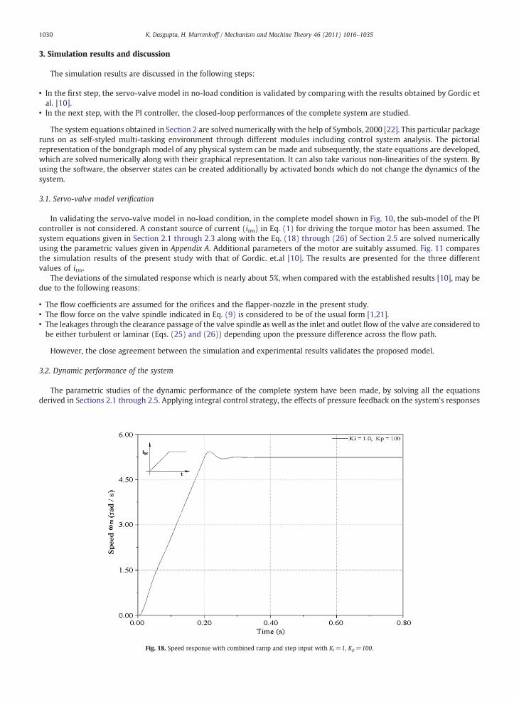
3.2.4. Effect of combined ramp and step inputMany applications require the servo-drive to accelerate a load to a constant velocity such as in cutting tool. In the present

analysis, the speed control is achieved with Proportional-Integral control action to obtain the zero error in the desired constantspeed 5.22 rad/s at the end of acceleration (t1=0.23 s) as indicated in Fig. 17.

The simulation results also show that when the proportional controller gain is set at Kp=10, there is an error of about 13% inthe speed (not shown in the present article) at the end of acceleration (t1=0.23 s). However, the response becomes moreoscillatory when the proportional controller gain is increased to Kp=100 as shown in Fig. 18.

By setting Kp=10 and Ki=100 yields a smooth response with minor overshoot, that almost satisfies the performancespecification shown in Fig. 19.

4. Conclusion

The article presents a significant aspect of an integrated study of modelling and simulation of a closed-loop servo-valvecontrolled hydro-motor drive system. The bondgraph model of the complete system has been developed. Comparing thesimulation results with that of Gordic et al. [10], the servo-valve model is validated in Fig. 11, with reasonable accuracy. The servo-valve model presented in this article may be useful for modelling all similar types of valve. The model includes phenomena andquantities of influence on analysed servo-drive, so it can predict its performance in a wider range of expected working regime.Combining the servo-valve with a motor circuit, the dynamic response of the closed-loop system is analysed. The effects of variouscontrol parameters on the overall response of the system are discussed. Justifiably many plausible parameters like inertia of theworking fluid in the conduit and the valve, elasticity of the conduit etc. are not incorporated in the details of the modelling. Still,model contains several critical parameters those substantially influence the performance of the system within the range ofoperation considered. The following conclusions are derived from the simulation results:

• Increasing the pressure feedback with constant integral gain improves the transient response of the system (Fig. 12).• Without pressure feedback, with the decrease in the integral coefficient, the system's oscillations reduces (Fig. 13).• The valve dead band has a delay characteristics and it also increases the maximum overshoot of the system (Fig. 14).• With the increase in inertia load, the speed and the pressure responses become more oscillatory with considerable increase inthe maximum overshoot (Figs. 15 and 16).

• With the combined ramp and step input, the response becomes more oscillatory with the increase in speed (Fig. 18). However,with the proper adjustment of integral and proportional gain, the desired performance may be achieved (Fig. 19).

Attention should be paid to the applicability of the proposedmodel at very high load pressure, where current driving the servo-valve saturates and the assumed flow equations are not applicable.

Authors believe that the integrated model of the servo-valve with the motor transmission system proposed here would beuseful to study the control theoretical aspects of the plant, where such system is an integral part and it provides insights forimproving the design of the system. Further study can be made by incorporating more sophisticated controller for the motortransmission system.

NomenclatureAsp Cross-sectional area of the spindle endAnzl Area of the nozzlear Area of the valve portCd Discharge coefficient of the orificeCq Valve flow coefficientdsp Diameter of the valve spindlednzl Diameter of the nozzledo Diameter of the orificedod Diameter of the sump orificeDm Volume displacement rate of the hydro-motore Spool eccentricityFfb Force due to the deformation of feedback springFc Dry friction force on the valve spindleFcn Nominal dry friction force on the valve spindleFco Initial dry friction force on the valve spindleFff Flow force on the valve spindleFh Flow force on the flapperFi Elastic impact force on the flapperii Integral feedback current of the controllerip Proportional feedback current of the controlleritm Driving current of the torque motorivdb Valve dead bandJa Mass moment of inertia of the armature assembly


Jl Mass moment of inertia of the load connected with the motorKtm Torque motor gainKm Torque motor electromagnetic spring constantKi Proportional controller gainKp Integral controller gainKl Pressure feedback gainKw Speed feedback gainkis Impact stiffnessKv Servo-valve amplifier gainKa Stiffness of the flexure tubeKfb Stiffness of the feedback springKstf Compressibility of the fluid in the nozzle chamberKstf1 Compressibility of the fluid in the discharge chamberKmstf Compressibility of the fluid at the inlet and the outlet ports of the motorKfb Stiffness of the feedback springKnl, Knr Flow coefficients of the left and the right orifices of the servo-valvelfp Length of the flapperlfb Length of the feedback springlpr Perimeter of the valve portl1 Length between the supply and the actuator port of the servo-valvemsp Mass of the valve spindlepa Angular momentum of the armature assemblypl Angular momentum of the hydraulic motor shaftpsp Momentum of the valve spindlePmi, Pmo Pressure at the inlet and the outlet ports of the motorPlfp Pressure acting at the left end area of the spindlePrfp Pressure acting on the right end area of the spindlePl Load pressurePs Supply pressurePsmp Sump pressurePlfp and Prfp Pressures at the left and the right nozzle chambersPd Pressure at the discharge chamberRim and Rom Resistances of the inlet and outlet port of the valve spindleRilkg Internal leakage resistance of the motorRa Viscous resistance coefficient of the torque motorRl Viscous load coefficient on the hydro-motorRvlkg and Rllkg Leakage resistance of the valve spindleRlnz and Rrnz Nozzle port resistancesRsp Viscous friction coefficient of the valve spindleRo, Rod Resistance of the valve and the drain orifices, respectively.Tfp Torque caused due to the deformation of the flapperTf Stiction load with motorTsl Slip torque applied to the motorVinp Servo-valve input voltageV im and Vom Flow through the inlet and the outlet ports of the hydro-motor, respectively.V lnz and Vrnz Flow through the valve nozzles to the discharge chamberVod Flow through the discharge port of the servo-valveV llkg and Vrlkg Leakage flow through the valve spindle to the nozzle chambersVvlkg Leakage flow through the valve spindle to the return portVmi Generalized flow through the valve spindle that goes/comes out to/from the motor port.Vol and Vor Flow through the left and the right orifices to the nozzle chambers, respectivelyV lfp;V rfp Compressibility flow loss of the fluid in the left and right side of the flapperV ilkg Internal leakage flow of the hydro-motorVd Compressibility flow loss of the fluid in the discharge chamberx0 Distance of the flapper tip to each nozzle at nullxfp Displacement of the flapperxfb Deformation of the feedback springxsp Displacement of the valve spindlexspm Maximum displacement of the valve spindleρ Density of the fluidν Kinematic viscosity of the fluid


η Dynamic viscosity of the fluidδsp Radial clearance between the valve spindle and the bushingωm The motor speed.ωmr Reference speed of the motorΔPct Critical pressure difference across the valve portθfp Displacement of the flapperθa Angular displacement of the torque motor• It indicates the time derivative of the parameter

Acknowledgement

The first author gratefully acknowledges the fellowship and facilities provided to him by the Indian National Science Academy(INSA), India and the DFG/Germany, and the kind cooperation of the University staff during his 2 months work in the Institute ofFluid Power Transmission and Control, University of Technology Aachen, Germany. The authors are thankful to Dr. S. Pan for thetechnical discussion on the paper.

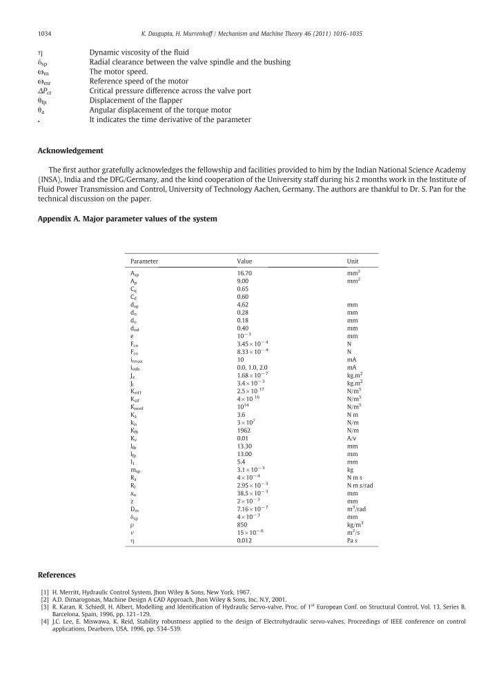
Appendix A. Major parameter values of the system

Parameter Value Unit

Asp 16.70 mm2

Ap 9.00 mm2

Cq 0.65Cd 0.60dsp 4.62 mmdn 0.28 mmdo 0.18 mmdod 0.40 mme 10−3 mmFcn 3.45×10−4 NFco 8.33×10−4 Nitmax 10 mAivdb 0.0, 1.0, 2.0 mAJa 1.68×10−7 kg.m2

Jl 3.4×10−3 kg.m2

Kstf1 2.5×10 17 N/m5

Kstf 4×10 16 N/m5

Kmstf 1014 N/m5

Ka 3.6 N mkis 3×107 N/mKfb 1962 N/mKv 0.01 A/vlfb 13.30 mmlfp 13.00 mml1 5.4 mmmsp 3.1×10−3 kgRa 4×10−4 N m sRl 2.95×10−3 N m s/radxo 38.5×10−3 mmz 2×10−3 mmDm 7.16×10−7 m3/radδsp 4×10−3 mmρ 850 kg/m3

ν 15×10−6 m2/sη 0.012 Pa s

References

[1] H. Merritt, Hydraulic Control System, Jhon Wiley & Sons, New York, 1967.[2] A.D. Dimarogonas, Machine Design A CAD Approach, Jhon Wiley & Sons, Inc, N.Y, 2001.[3] R. Karan, R. Schiedl, H. Albert, Modelling and Identification of Hydraulic Servo-valve, Proc. of 1st European Conf. on Structural Control, Vol. 13, Series B,

Barcelona, Spain, 1996, pp. 121–129.[4] J.C. Lee, E. Miswawa, K. Reid, Stability robustness applied to the design of Electrohydraulic servo-valves, Proceedings of IEEE conference on control

applications, Dearborn, USA, 1996, pp. 534–539.


[5] Van Schothrost. G., Modelling of long-stroke hydraulic servo-systems for flight simulator motion control and system design, PhD. Thesis, 1997, TechnischeUniversiteit Delft, Netherlands.

[6] Tawfik. M., Model based control of an Electro-hydraulic servo-valve, PhD. Thesis, 1999, University of Akron, Ohio, USA.[7] D. Wang, R. Dolid, M. Donath, J. Albright, Development and verification of a two-stage flow control servo-valve model, ASME, The Fluid Power and System

Technology Division (FPST) 2 (1995) 121–129.[8] E. Urata, M. Shinoda, Influence of Amplifier and Feedback on the Dynamics of Water Hydraulic Servo-valve, Proceedings of the forth JHPS International

Symposium on Fluid Power, Tokyo, Japan, 1999, pp. 567–572.[9] E. Urata, Study of Magnetic Circuits for Servo-valve TorqueMotors, BathWorkshop on Power Transmission and Control (PTMC), Bath, U.K, 2000, pp. 269–282.

[10] D. Gordic, M. Babic, N. Jovicic, Modelling of spool position feedback servo-valves, International Journal of Fluid power 5 (1) (2004) 37–50.[11] D. Gordic, M. Babic, N. Jovicic and D. Milovanovic., Effects of the variation of Torque Motor Parameters on Servo-valve Performance, Stronjniski vestnik—

Journal of Mechanical Engineering, 54 (2208) 12, pp. 866–873.[12] J. Watton, An Explicit Design Approach to Determine the Optimum Steady-state Performance of Axial Piston Motor Drives, Proc. I.MechE, Vol. 220, Part I, J.

Systems and Control Engg, 2006, pp. 131–143.[13] J. Watton, The dynamic performance of an electro-hydraulic servo-valve / motor system with transmission line effects, ASME Journal of Dynamic Systems

Measurements and Control 109 (1987) 14–18.[14] K. Dasgupta, J. Watton, S. Pan, Open-loop dynamic performance of a servo-valve controlled motor transmission systemwith pump loading using steady-state

characteristics, Mechanism and Machine Theory, 41, Elsevier, 2006, pp. 262–282.[15] KOVARI Attila, Influence of Cylinder Leakage on Dynamic Behavior of Electro-hydraulic Servo System, 7th International Symposium on Intelligent system and

informaticsSISY'09, 25–26 Sept. 2009, Subotica, Hungary, 2009, pp. 375–379.[16] D.C. Karnopp, R.C. Rosenburg, System Dynamics: a Unified Approach, Wiley Intersciences, 1975.[17] J.U. Thoma, Simulation by Bondgraph, Springer-Verlag, Germany, 1990.[18] A. Mukherjee, R. Karmakar, Modelling and Simulation of Engineering Systems through Bondgraph, Narosa Publishing House, New Delhi, India, 2000.[19] M. Verge, D. Jaume, Modelisation Structure des Systems avec les Bondgraphs, 20038 Edition Tecnip.[20] S.C. Southward, C.J. Radcliffe, C.R. MacCluer, Robust nonlinear stick-slip friction compensation, ASME Journal of Dynamic Systems, Measurement, and Control

113 (1991) 639–6448 Dec.[21] D. McCloy, H.R. Martin, The control of Fluid Power, Longman, London, 1973.[22] Symbols 2000, High Tech Consultants, STEP, IIT, Kharagpur, India, www.symbols2000.com.

http://www.symbols2000.com

1-s2 0-S0094114X1000203X-main

Documents

Transcript of 1-s2 0-S0094114X1000203X-main