اللجنة العلمية - جامعة الموصل
223
ية الهندسةكل الذهبي ليوبيلللثاني ل المؤتمر الهندسي ا– لفترة من لموصلمعة ال جا91 - 19 / 99 / 1192 علميةجنة الل الليلةحمد طيب ال أ.د. م رئيسا عضوحمد جميل أ.د. صباح م أ.د.د يسف حاجم أحم عضو أ.د.لطعاند علي ا سع عضو أ.د.يل خلد مرعين سي حس عضو أ.د.د أحمد حام عبد الحكيم عضو أ.د.حمد سعيد باسل م عضو أ.د.لجبارحمد عبد ا م جاسم عضو أ.د.حمود باسل شكر م عضو أ.د.عليحمود ال برهان م عضو أ. م. د. عجميل حيدر سعد ال لي عضو أ. م. د.حمدي الدين أ قصي كمال عضو أ. م. د.يل رافد أحمد خل عضواد إعدد أحمد حام. عبد الحكيم أ.د
-
Upload
khangminh22 -
Category
Documents
-
view
3 -
download
0
Transcript of اللجنة العلمية - جامعة الموصل

19/99/1192-91جامعة الموصل للفترة من –المؤتمر الهندسي الثاني لليوبيل الذهبي لكلية الهندسة
اللجنة العلمية
رئيسا أ.د. محمد طيب الليلة
أ.د. صباح محمد جميل عضو
عضو أحمد يسف حاجم أ.د.
عضو سعد علي الطعان أ.د.
عضو حسن سيد مرعي خليل أ.د.
عضو عبد الحكيم حامد أحمد أ.د.
عضو باسل محمد سعيد أ.د.
عضو جاسم محمد عبد الجبار أ.د.
عضو باسل شكر محمود أ.د.
عضو برهان محمود العلي أ.د.
عضو لي حيدر سعد الجميلع د.م.أ.
عضو قصي كمال الدين أألحمدي د.م.أ.
عضو رافد أحمد خليل د.م.أ.
إعداد
أ.د. عبد الحكيم حامد أحمد

Computers Engineering Department
حاسوبالقسم هندسة
19/99/1192-91جامعة الموصل للفترة من –مؤتمر الهندسي الثاني لليوبيل الذهبي لكلية الهندسة لحاسوبا هندسة قسم
المحتوياترقم
ألصفحة
تسلسل ألعنوان
لنظام مراقبة فيدوي Horprasertتصميم وتنفيذ وحدة ذكية مخصصة لخوارزمية 1
بالبوابات القابلة للبرمجة حقليا
لمى أكرم حمدي د. أحالم فاضل محمود
1.
المصفوفات بطريقة المصفوفة اإلنقباضية وتنفيذها باستخدام تصميم عملية ضرب 15
البوبات القابلة للبرمجة حقليا
ذكوان محمد سليم فرح نزار إبراهيم
2.
التقسيم التلقائي لألنسجة الطبيعية والمرضية في صور الرنين المغناطيسي 26
العنقدةللدماغ على أساس التصنيف وطرق
أمين محمد عبد السالم سالمي د. أحالم فاضل محمود
3.
خوارزمية لتشفير الصورة الملونة باستخدام ترميز الحامض النووي 04
ونظرية الفوضى
فخر الدين حامد علي مها بشير حسين
0.
خوارزمية تشفير انسيابية للصورة الملونة باستخدام النظرية الفوضوية 22
مها بشير حسين فخرالدين حامد علي
2.
للعنقدة في البرنامج التوضيحي في الماتالب K-Means طريقتان لتعديل خوارزمية 52
R2012a الوارد باإلصدار
د. جاسم محمد عبد الجبار هشام ياسين عباس
5.
باستخدام تقنية المايكروكونترولر -مستخدم ضد االلة -لعبة تك تاك 04
عالء الدين يوسف العمري /استاذ مشارك
7.
معايير أداء الشبكة لبروتوكوالت الوصول الى الوسط في الشبكات الالسلكية المتشابكة 11
د. محمد بشير عبد هللا الصميدعيكرم عنان عبد الغني الغضنفري
0.
باستخدام مصفوفة البوابات المنطقية القابلة للبرمجة TCP/UDPإختيار بروتوكول 101
د. عبد الستار محمد خضر خالد فزع محمود
1.
FPGA معمارية لنظام معالجة الرأس بإستخدام 112
عمر زياد طارق د. فخر الدين حامد علي
14.
تشفير البيانات عالي األداء لخوارزمية معيار التشفير المتقدم باستخدام شريحة البوابات 125
القـــابلة للبرمجة
إسراء غانم محمد د. شفاء عبد الرحمن داؤد
11.
لهيكلية معالج البحث عن المسار األقصر نوع FPGAالتصميم والتنفيذ باعتماد رقاقة 135
المتوازي -خط األنابيب
محمد عبد علي العبادي ,د.ماجد عبد النبي علوان ,د. جاسم محمد عبد الجبار
12.
المستخدمة في الالسلكية ) Ad Hoc) تقييم أداء بروتوكوالت التوجيه في شبكات 153
OPNET أنظمة سكادا باستخدام برنامج المحاكاة
د. قتيبة ابراهيم علي فجر فهر فاضل
13.
دراسة باسلوب المحاكاة النماط بروتوكول التحكم بالنقل في االنظمة المطمورة 165
ضحى عبد الجبار عبدد. قتيبة ابراهيم علي
10.
فحص آليات األنتقال من اإلصدار الرابع الى اإلصدار السادس لشبكة جامعة الموصل 180
د. عبد الباري رؤوف سليمان فادي أحمد جاسم
12.
تحويل مويجي كسوري لمتحسسات الوسائط المتعددة الالسلكية مع تقليل آثار الحدود 191
جاسم محمد عبد الجبارد. علياء قصي أحمد تقي
15.
دراسة أداء شبكة المتحسس الالسلكي في تطبيقات نقل الصوت 201
أكرم عبد الموجود داود د. قتيبة ابراهيم علي
17.
تقنية الكلونة إلخفاء الرسالة السريةاستخدام 212
سعدون حسين عبدهللا
10.
Hamdai: An FPGA Design and Implementation of Custom IP Core…
1
An FPGA Design and Implementation of Custom IP Core for
Efficient Horprasert Video Surveillance System
Abstract:
The video surveillance system is considered as a complex system because it requires
intensive computations. This paper presents an embedded custom IP architecture on
FPGA which is able to detect a new object from training background. The purpose of
designing custom IP core is to reduce computational complexity of Horprasert model,
which it is an intensive task with a high computational cost and processing time. The
proposed custom core has been designed using an Embedded Development Kit (EDK)
for hardware-software co-design which is able to extract the background on resource-
limited environments and offers low degradation. The developed Horprasert video
model structure can operate at an estimated frequency of 189.322MHz by utilizing 9
multipliers and 60 LUTS of target FPGA device to provide cost effective solution for
video Surveillance systems. The system is capable to process stereo video streams of
resolutions up to 1,920 × 1,080 at 30 frames per second (1080p30). The co-design
strategy shows how to move non-real-time constrained operations to software running
on the processor in order to decrease the hardware resources required for only detection
IP unit.
Keywords: video surveillance; Horprasert Model; EDK, Co-Design ; FPGA.
لنظام مراقبة فيدوي Horprasertرزمية تصميم وتنفيذ وحدة ذكية مخصصة لخوا
بالبوابات القابلة للبرمجة حقليا
لمى أكرم حمدي د. أحالم فاضل محمود
-الملخص:
يقدم هذا البحث بتصميم معمارية كتلة فكرية يعتبر نظام المراقبة الفيديوي نظام معقد ألنه يتطلب حسابات مكثفة.
لة للبرمجة التي تكون قادرة على كشف الكائن الجديد من الخلفية المدربة. الهدف من باستخدام البوابات المنطقية القاب
أن عملية كشف الكائن الجديد ، حيث Horprasertمن أجل الحد من التعقيد الحسابي لنموذج تصميم كتلة فكرية هو
الورقة بنية لبنة ذكية مخصصة . تعرض هذه عمليات حسابية معقدة بتكلفة عالية ويتطلب وقت كبير للتجهيزتحتاج الى
لهذا الغرض مبنية على البوابات القابلة للبرمجة حقليا لها القدرة على الكشف عن األجسام الجديدة بعد التدريب على
( التي تتيح EDKخلفية مكان المراقبة. وقد تم تصميم جوهر البنية المقترحة باستخدام العدة المطورة للنظام المطمور )
لماديات والمعالج البرمجي الستخراج المعلومات األساسية لمعالجة خلفية نظام المراقبة ببيئة ذات موارد الدمج بين ا
من خالل االستفادة MHz 223.911موديل الفيديو المقترح يعمل في تردد المقدرة Horprasertمحدودة. أن هيكل
ة حقليا لتوفير حل فعال من ناحية الكلفة ألنظمة جدول من جداول طرفيات البوابة القابلة للبرمج 06ضوارب و 3من
إطارا في الثانية 96بمعدل 1,080 × 1,920المراقبة بالفيديو. النظام قادر على معالجة سلسلة ستيريو فيديو تصل إلى
(2626p30 أن إستراتيجية التصميم المشترك أوضحت فائدة تجزئة المنظومة المقترحة لعمليات غير مقيدة في .) الوقت
الحقيقي يمكن تنفيذها من قبل المعالج البرمجي إلبقاء الموارد المادية حصرا لوحدة الكشف عن األجسام الجديدة.
Luma Akram Hamdai Dr. Ahlam Fadhil Mahmood Computer Engineering Department Computer Engineering Department
University of Mosul University of Mosul
19/99/1192-91جامعة الموصل للفترة من –ليوبيل الذهبي لكلية الهندسة ا – العلمي الهندسي الثانيالمؤتمر
2
1. Introduction: Visual surveillance is a very active research area in computer vision, thanks to the
rapidly increasing number of surveillance cameras that lead to a strong demand for automatic
processing methods for their output. The scientific challenge is to devise and implement
automatic systems able to detect and track moving objects, and interpret their activities and
behaviors. The need is strongly felt world-wide, not only by private companies, but also by
governments and public institutions, with the aim of increasing people safety and services
efficiency[1]. It is indeed a key technology for fight against terrorism and crime, public safety
(e.g., in transport networks, town centers, schools, and hospitals), and efficient management
of transport networks and public facilities (e.g., traffic lights, railroad crossings).
The main tasks in visual surveillance systems include motion detection, object
classification, tracking, activity understanding, and semantic description. This paper focus on
the detection phase of a general visual surveillance system using static camera. The detection
of moving objects in video streams is the first relevant step of information extraction in many
computer vision applications. The most usual approach to segment moving objects is known
as background subtraction, and is considered as a key first stage in video surveillance
systems. This technique consists of building a reference model which represents the static
background of the scene during a certain period of time. Multiple factors and events may
affect the scene, making this first background subtraction a non-trivial task; sudden and
gradual illumination changes, presence of shadows, or background repetitive movements
(such as waving trees), among many others[2].
The idea of background subtraction is to subtract the current image from a reference
image, which is acquired from a static background during a period of time. The subtraction
leaves only non-stationary or new objects, which include the objects' entire silhouette region.
There are different methods described in the literature in order to obtain this background
model for a scene captured by a still camera: MOG (Mixture of Gaussians), Horprasert model,
Bayesian decision rules, Codebook-based model, or Component Analysis (PCA and ICA). In
spite of the differences between existing algorithms, background subtraction techniques are
computationally expensive in general, especially when they are considered only the first stage
in a multi-level video analytics system. For that reason, efficient implementation for
background subtraction technique is a key to the development of real-time video surveillance
systems.
2. Literature Review The goal of video surveillance systems is to monitor the activity in a specified, indoor
or outdoor area. Since the cameras used in surveillance are typically stationary, a
straightforward way to detect moving objects is to compare each new frame with a reference
frame, representing in the best possible way the scene background. By subtracting the
background from the current frame in all regions where the current frame matches the
reference frame, a segmentation of the moving objects is readily achieved. The results of this
process, called background subtraction, are used by the higher level processing modules for
object tracking, event detection and scene understanding purposes. Successful background
subtraction plays a key role in obtaining reliable results in the higher level processing tasks.
This is why many researchers considered carefully the problem of background modeling.
Many background subtraction methods have been proposed in the past decades including:
Gaussian Mixture Model: In 2007[3], Zhen Tang and Zhenjiang Miao simplify the original
GMM to improve its performance(save time and space) with shadow detection and noise
Hamdai: An FPGA Design and Implementation of Custom IP Core…
3
removing. A new matching function is presented in [4,5], that allows for better treatment
of shadows and noise and reduces block artifacts.
Codebook Model: Ref [6] presents a real-time algorithm for foreground-background
segmentation. Extracts structure of background and models it in layered codebook.
Layered codebook is a simple data structure containing two codebooks that is defined per
pixel. The first layer is main codebook, other is cache codebook, and both contain some
codewords relative to a pixel. Main codebook models the current background images and
cache codebook is used to model new background images during input sequence. During
input sequence, foreground-background is segmented and two-layered codebook is
updated. So this algorithm can model moving backgrounds, multi backgrounds and
illumination changes and this is efficient in both memory and computational complexity.
Rectgauss-Tex Method: It presents a region-based method for background subtraction. It
relies on color histograms, texture information, and successive division of candidate
rectangular image regions to model the background and detect motion. This method
integrates texture and the Gaussian Mixture model. It is a multi scale rectangular region
based motion detection and background subtraction algorithm. It filters noise during image
differentiation. The choice of the coarsest rectangle size should be selected to be small
enough to detect the object of interest. Thus, balancing the rectangle size for the detection
of small objects might be incompatible for very small objects while filtering noise[7].
Texture based method: [8] presents a novel and efficient texture-based method for
modeling the background and detecting moving objects from a video sequence. Each pixel
is modeled as a group of adaptive local binary pattern histograms that are calculated over a
circular region around the pixel. This method is tolerant to the multimodality of the
background, and the introduction/removal of background objects. The method requires a
non-moving camera, which restricts its usage in certain applications.
A Bayes decision rule: Liyuan et.al.[9] A Bayes decision rule is derived for background
and foreground classification based on the statistics of principal features. Principal feature
representation for both the static and dynamic background pixels is investigated. A novel
learning method is proposed to adapt to both gradual and sudden “once-off” background
changes. The convergence of the learning process is analyzed and a formula to select a
proper learning rate is derived. Under the proposed framework, a novel algorithm for
detecting foreground objects from complex environments is then established. It consists of
change detection, change classification, foreground segmentation, and background
maintenance.
In spite of the differences between existing algorithms, background subtraction
techniques are computationally expensive in general, especially when they consider only the
first stage in a multi-level video analytics system. For that reason, efficient implementation is
key to the development of real-time video surveillance systems. In the framework of
embedded systems implementations, characterized by power consumption and real-time
constraints, several of these techniques have been implemented using FPGAs [1,10,11] or
DSPs [12]. There also are other real-time approaches using GPUs [13].
This paper proposes an FPGA architecture based on the method described by
Horprasert. Thus, the use of FPGAs is justified by requirements of scalability, size and low
power consumption which are key features that other technologies are not able to
achieve. The Horprasert method has been selected since it requires less memory to store
the model while keeping fairly good accuracy, hence being more suitable for
implementation in low cost FPGAs. Add to Horprasert model builds a static background
model, which means that the model is obtained at an initial training phase. Therefore, the
19/99/1192-91جامعة الموصل للفترة من –ليوبيل الذهبي لكلية الهندسة ا – العلمي الهندسي الثانيالمؤتمر
4
proposed architecture has been designed with the development environment for System-on-
Programmable Chip (SoPC) design, EDK of Xilinx [14], and includes the Microblaze
processor, which will be used to build the reference background model and can be used for
updating over time. While the next stages of subtraction and pixel by pixel classification will
be performed by a specific hardware module.
The paper is organized as follows. Section 3 briefly describe the background model by
Horprasert et al. [1], including the notation required in order to be able to follow the rest of
the paper. Section 4 shows the developed hardware architecture, including a study of the fixed
point arithmetic, the background subtraction stage on FPGA. In Section 5 results are shown
and analyzed, regarding system performance. Finally, conclusions is presented in Section 6.
3. Horprasert background Subtraction Method As previously mentioned, FPGA implementation is based on the algorithm proposed by
Horprasert et al. [1]. This algorithm basically obtains a reference image to model the
background
of the scene so that it can perform automatic threshold selection, subtraction operation and,
finally, pixel-wise classification.
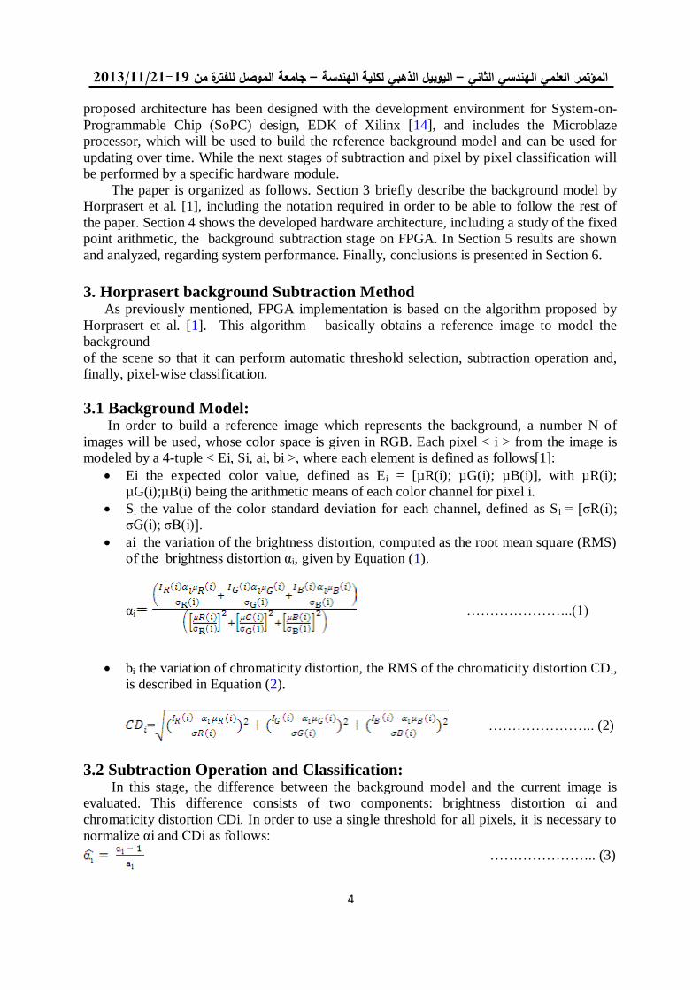
3.1 Background Model: In order to build a reference image which represents the background, a number N of
images will be used, whose color space is given in RGB. Each pixel < i > from the image is
modeled by a 4-tuple < Ei, Si, ai, bi >, where each element is defined as follows[1]:
Ei the expected color value, defined as Ei = [µR(i); µG(i); µB(i)], with µR(i);
µG(i);µB(i) being the arithmetic means of each color channel for pixel i.
Si the value of the color standard deviation for each channel, defined as Si = [σR(i);
σG(i); σB(i)].
ai the variation of the brightness distortion, computed as the root mean square (RMS)
of the brightness distortion αi, given by Equation (1).
αi …………………..(1)
bi the variation of chromaticity distortion, the RMS of the chromaticity distortion CDi,
is described in Equation (2).
= ………………….. (2)
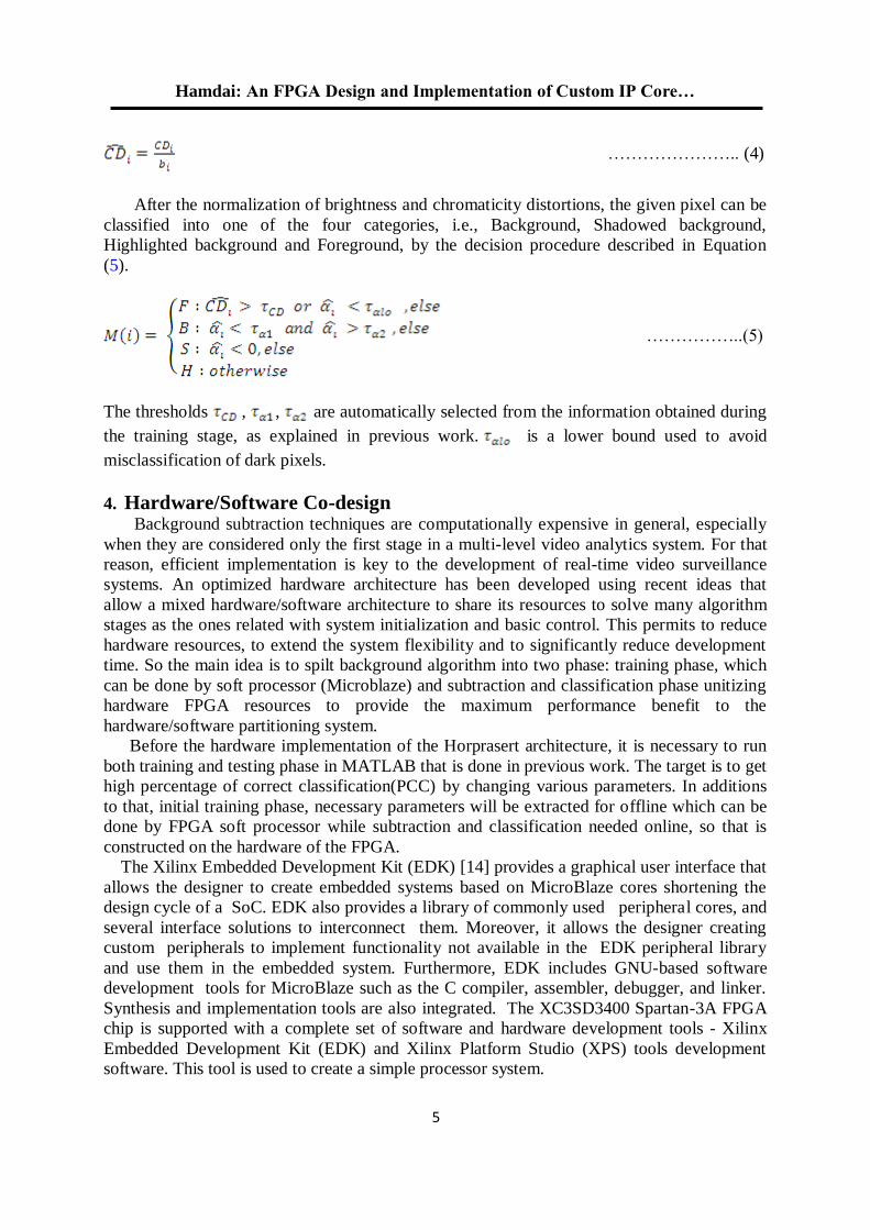
3.2 Subtraction Operation and Classification: In this stage, the difference between the background model and the current image is
evaluated. This difference consists of two components: brightness distortion αi and
chromaticity distortion CDi. In order to use a single threshold for all pixels, it is necessary to
normalize αi and CDi as follows:
………………….. (3)
Hamdai: An FPGA Design and Implementation of Custom IP Core…
5
………………….. (4)
After the normalization of brightness and chromaticity distortions, the given pixel can be
classified into one of the four categories, i.e., Background, Shadowed background,
Highlighted background and Foreground, by the decision procedure described in Equation
(5).
……………..(5)
The thresholds , , are automatically selected from the information obtained during
the training stage, as explained in previous work. is a lower bound used to avoid
misclassification of dark pixels.
4. Hardware/Software Co-design
Background subtraction techniques are computationally expensive in general, especially
when they are considered only the first stage in a multi-level video analytics system. For that
reason, efficient implementation is key to the development of real-time video surveillance
systems. An optimized hardware architecture has been developed using recent ideas that
allow a mixed hardware/software architecture to share its resources to solve many algorithm
stages as the ones related with system initialization and basic control. This permits to reduce
hardware resources, to extend the system flexibility and to significantly reduce development
time. So the main idea is to spilt background algorithm into two phase: training phase, which
can be done by soft processor (Microblaze) and subtraction and classification phase unitizing
hardware FPGA resources to provide the maximum performance benefit to the
hardware/software partitioning system.
Before the hardware implementation of the Horprasert architecture, it is necessary to run
both training and testing phase in MATLAB that is done in previous work. The target is to get
high percentage of correct classification(PCC) by changing various parameters. In additions
to that, initial training phase, necessary parameters will be extracted for offline which can be
done by FPGA soft processor while subtraction and classification needed online, so that is
constructed on the hardware of the FPGA.
The Xilinx Embedded Development Kit (EDK) [14] provides a graphical user interface that
allows the designer to create embedded systems based on MicroBlaze cores shortening the
design cycle of a SoC. EDK also provides a library of commonly used peripheral cores, and
several interface solutions to interconnect them. Moreover, it allows the designer creating
custom peripherals to implement functionality not available in the EDK peripheral library
and use them in the embedded system. Furthermore, EDK includes GNU-based software
development tools for MicroBlaze such as the C compiler, assembler, debugger, and linker.
Synthesis and implementation tools are also integrated. The XC3SD3400 Spartan-3A FPGA
chip is supported with a complete set of software and hardware development tools - Xilinx
Embedded Development Kit (EDK) and Xilinx Platform Studio (XPS) tools development
software. This tool is used to create a simple processor system.
19/99/1192-91جامعة الموصل للفترة من –ليوبيل الذهبي لكلية الهندسة ا – العلمي الهندسي الثانيالمؤتمر
6
The first step is partitioning the system into hardware and software components. The
software is written in C and it runs into the MicroBlaze. The hardware (custom IP) has been
described in VHDL and is connected to the MicroBlaze through the PLB (Peripheral Local
Bus).
4.1 Microblaze Soft-Core Processor MicroBlaze soft core is highly simplified embedded processor soft core with relatively
high performance developed by Xilinx Company.[14] This soft core enjoys high
configurability and allows designer to make proper choice based on his own design
requirements to build his own hardware platform. The processor architecture includes thirty-
two 32-bit general-purpose registers and the soft core adopts RISC instruction set and
Harvard architecture and has the following performance characteristics:
32-bit general-purpose registers.
32-bit instruction word length.
Separated 32-bit instruction and data bus.
A 32-bit version of the PLB V4.6 interface.
LMB provides simple synchronous protocol for efficient block RAM transfers.
Local Memory Bus (LMB) enables direct access to on-chip block memory (BRAM), it
provides high-speed instructions and data caching and features three-stage pipelined
architecture; Hardware debugging module (MDM) and eight input/output fast link interfaces (FSL) are
available.
The software component on the FPGA Horprasert model consists of the C code that runs on
the MicroBlaze to obtain an initial training phase.
4.2 Hardware Architecture The foreground/background segmentation is executed by a hardware module, where the
current image and the background model are stored. Considerable reduction of the hardware
complexity of the architecture is achieved through precalculating and storing several
constants and avoiding division operations by substituting them for multiplications, which
require less hardware resources. In the case of brightness distortion αi, these constants are
computed according to Equation(6):
…..……….(6)
, ,
The brightness distortion αi will remain as in Equation (7), making use of the constants Ri,
Gi, Bi.
αi = Ri IR(i) + Gi IG(i) + Bi IB(i) …………….(7)
In order to remove the divisions in the computation of the chromaticity distortion CDi, then
store , and instead of Si, ai and bi.
Hamdai: An FPGA Design and Implementation of Custom IP Core…
7
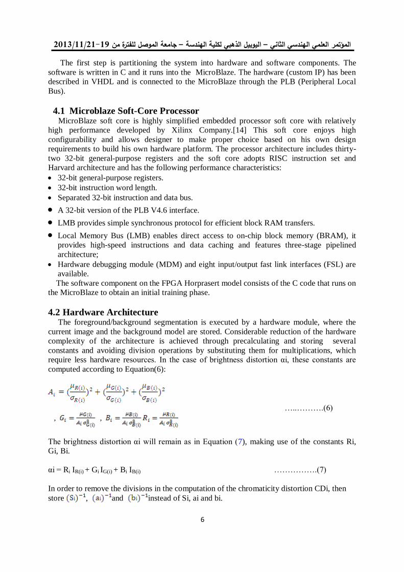
The main idea is to use Microblaze processor for the background model, the subtraction
and pixel-wise classification stages, will be performed by an IP core connected to the MPMC
interface (MultiPort Memory Controller provide access to external memory via multiport:
PLB, SDMA, XCL, VFBC and NPI) . This module has been designed with the high level of
abstraction hardware description language VHDL, VHDL has two input streams (background
model BM(i) and current image I(i)) and two output stream , . Figure 1 shows in more
detail the pipelined datapath for Horprasert testing hardware module.
The square root computation is generally grouped into two distinct categories. The
estimation methods, which includes algorithms such as Rough estimation and Newton-
Raphson method (and also its derivations: CORDIC, DeLugish's and Chen's), whereby the
second category is called digit-by-digit method. The restoring algorithm has a big limitation at
restoring step in the regular flow. Primarily for this
Figure 1. Hardware Architecture of Intellectual-Property (IP) core for background subtraction
stage.
reason, although initially having led the way for all the other methods, it has been declined in
importance and nowadays it is no longer used [15]. The non restoring algorithm does not
restore the remainder, which can be implemented with least hardware resource usage, a
strategy to implement a modified non restoring square root algorithm based on FPGA which
adopt fully pipelined architecture will be used to calculate CDi. The main principle of the
method is only uses subtract operation and append 01 which is implemented in register
transfer level (RTL) abstraction, but add operation and append 11 are not used. This strategy
will needs fewer pipeline stages.
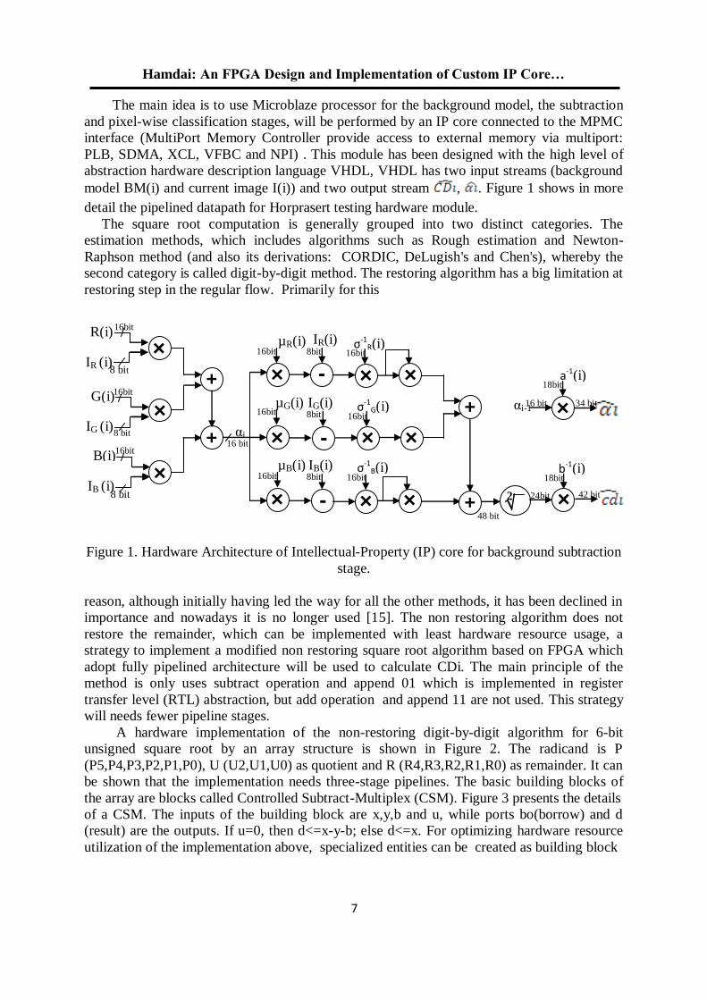
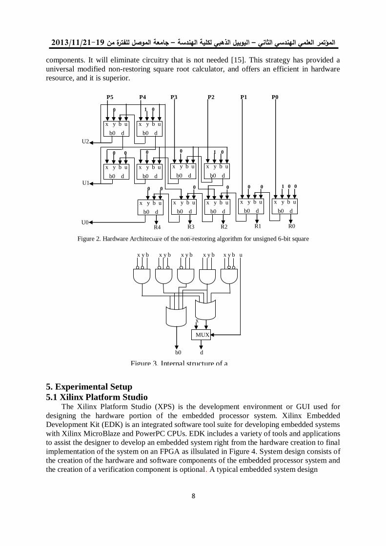
A hardware implementation of the non-restoring digit-by-digit algorithm for 6-bit
unsigned square root by an array structure is shown in Figure 2. The radicand is P
(P5,P4,P3,P2,P1,P0), U (U2,U1,U0) as quotient and R (R4,R3,R2,R1,R0) as remainder. It can
be shown that the implementation needs three-stage pipelines. The basic building blocks of
the array are blocks called Controlled Subtract-Multiplex (CSM). Figure 3 presents the details
of a CSM. The inputs of the building block are x,y,b and u, while ports bo(borrow) and d
(result) are the outputs. If u=0, then d<=x-y-b; else d<=x. For optimizing hardware resource
utilization of the implementation above, specialized entities can be created as building block
8 bit
8 bit
8 bit
16 bit
+
R(i)
IR (i)
G(i)
IG (i)
B(i)
IB (i)
+ αi
µR(i)
µG(i)
µB(i)
IR(i)
IG(i)
IB(i)
σ-1R(i)
σ-1G(i)
-
-
-
σ-1B(i)
+
+ √ 2
b-1(i)
×
×
×
× ×
×
× ×
×
×
×
×
×
a-1(i)
αi-1 ×
16bit
16bit
16bit
16bit
16bit
16bit
8bit
8bit
8bit
24bit
18bit
18bit
16bit
16bit
16bit
48 bit
16 bit 34 bit
42 bit
19/99/1192-91جامعة الموصل للفترة من –ليوبيل الذهبي لكلية الهندسة ا – العلمي الهندسي الثانيالمؤتمر
8
components. It will eliminate circuitry that is not needed [15]. This strategy has provided a
universal modified non-restoring square root calculator, and offers an efficient in hardware
resource, and it is superior.
5. Experimental Setup
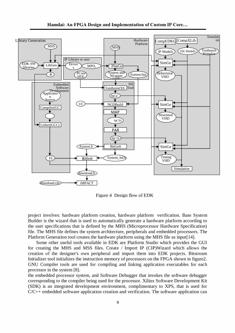
5.1 Xilinx Platform Studio The Xilinx Platform Studio (XPS) is the development environment or GUI used for
designing the hardware portion of the embedded processor system. Xilinx Embedded
Development Kit (EDK) is an integrated software tool suite for developing embedded systems
with Xilinx MicroBlaze and PowerPC CPUs. EDK includes a variety of tools and applications
to assist the designer to develop an embedded system right from the hardware creation to final
implementation of the system on an FPGA as illsulated in Figure 4. System design consists of
the creation of the hardware and software components of the embedded processor system and
the creation of a verification component is optional. A typical embedded system design
Figure 2. Hardware Architecture of the non-restoring algorithm for unsigned 6-bit square
root
0 0
x y b u
b0 d
1 0 0
x y b u
R2
b0 d
x y b u
b0 d
x y b u
R3
b0 d
x y b u
R4
b0 d
x y b u
R0
b0 d
x y b u
b0 d
x y b u
b0 d
x y b u
b0 d
x y b u
b0 d
x y b u
R1
b0 d
0 0 0 0
0 0
U1
1 0 0
0 1 0
U2
q
U0
P5 P4 P3 P2 P1 P0
0
x y b x y b x y b x y b x y b u
MUX
x
b0 d
Figure 3. Internal structure of a
CSM block
Hamdai: An FPGA Design and Implementation of Custom IP Core…
9
project involves: hardware platform creation, hardware platform verification. Base System
Builder is the wizard that is used to automatically generate a hardware platform according to
the user specifications that is defined by the MHS (Microprocessor Hardware Specification)
file. The MHS file defines the system architecture, peripherals and embedded processors. The
Platform Generation tool creates the hardware platform using the MHS file as input[14].
Some other useful tools available in EDK are Platform Studio which provides the GUI
for creating the MHS and MSS files. Create / Import IP (CIP)Wizard which allows the
creation of the designer's own peripheral and import them into EDK projects. Bitstream
Initializer tool initializes the instruction memory of processors on the FPGA shown in figure2.
GNU Compiler tools are used for compiling and linking application executables for each
processor in the system [8].
the embedded processor system, and Software Debugger that invokes the software debugger
corresponding to the compiler being used for the processor. Xilinx Software Development Kit
(SDK) is an integrated development environment, complimentary to XPS, that is used for
C/C++ embedded software application creation and verification. The software application can
NGC
Synthesis(XST)
NGDBuild
MAP
NCD, PCF
PAR
NCD
BitGen
System_bd.b
mm
System.b
it
Bitlnit
UC
F
download.b
it
ISE Tool
s
PlatGe
n
LibGen EDK SW libraries
MSS
Library Generation
Drivers
MDD
IP Library or user
Repository
PCore HDL
MPD, PAQ
MHS
System and Wrapper
VHD
System.bm
m
Behavioral VHD Model
SimGe
n
IP Models
ISE Models
CompXLib CompEDKL
ib
Structural VHD Model
SimGe
n
Timing VHD Model
SimGe
n
Testbench Stimulus
Simulation
Simulation
Generator
.a
Hardware Platform
Generation
Application
Source c,.h,.s
Compiler(GC
C)
Linker(GCC)
EL
F
iMPACT download.cm
d
Embedded Software
Development
Figure 4 Design flow of EDK
19/99/1192-91جامعة الموصل للفترة من –ليوبيل الذهبي لكلية الهندسة ا – العلمي الهندسي الثانيالمؤتمر
11
be written in a "C or C++" then the complete embedded processor system for user application
will be completed, else debug & download the bit file into FPGA. Then FPGA behaves like
processor implemented on it in a Xilinx Field Programmable Gate Array (FPGA) device.
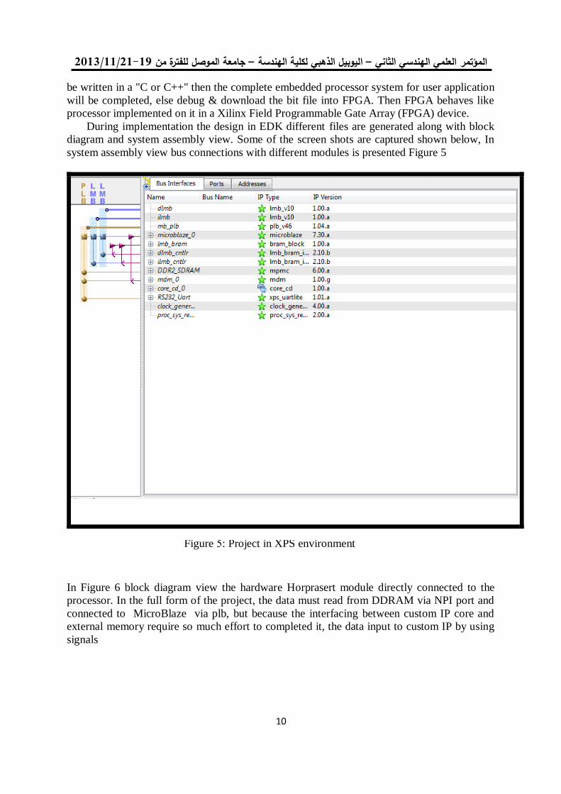
During implementation the design in EDK different files are generated along with block
diagram and system assembly view. Some of the screen shots are captured shown below, In
system assembly view bus connections with different modules is presented Figure 5
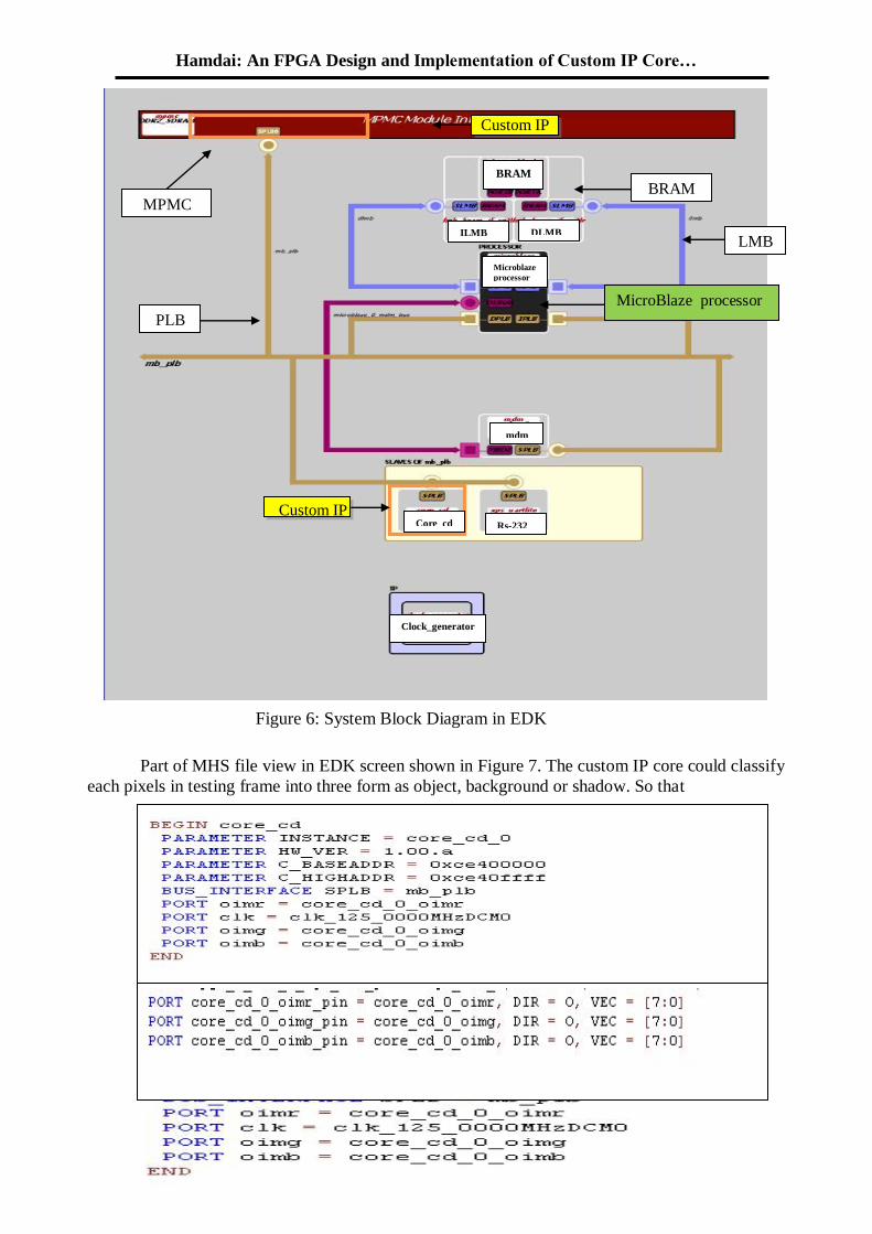
In Figure 6 block diagram view the hardware Horprasert module directly connected to the
processor. In the full form of the project, the data must read from DDRAM via NPI port and
connected to MicroBlaze via plb, but because the interfacing between custom IP core and
external memory require so much effort to completed it, the data input to custom IP by using
signals
Figure 5: Project in XPS environment
Hamdai: An FPGA Design and Implementation of Custom IP Core…
11
Part of MHS file view in EDK screen shown in Figure 7. The custom IP core could classify
each pixels in testing frame into three form as object, background or shadow. So that
Figure 7: part of MHS file view in EDK
Figure 6: System Block Diagram in EDK
Custom IP
MicroBlaze processor
BRAM
LMB
MPMC
PLB
Custom IP Core_cd Rs-232
Clock_generator
mdm
Microblaze
processor
BRAM
ILMB DLMB
19/99/1192-91جامعة الموصل للفترة من –ليوبيل الذهبي لكلية الهندسة ا – العلمي الهندسي الثانيالمؤتمر
12
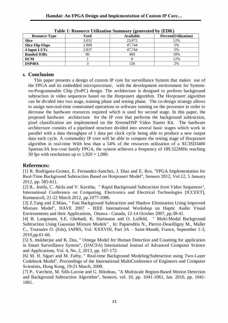
5.2. Experimental Results The architecture has been designed and implemented on XC3SD3400 Spartan-3A FPGAs
by Xilinx, the simulation result and Synthesis Report are shown in Figure 9 and table1 respectively. The simulation of the architecture designed (as showed above in figure(1)), where the input signal is (r,g,b :that perform the equation in eq.(7), Ir,Ig,Ib: represent the colored pixel, invs: represent the standard deviation, inva, invb : represent variation computed by take the RMS of brightness and color distortion, the thresholds for classification input (maxta1,maxt2,maxcd,talo) and the oimr,oimg,oimb are the pixels output (in figure 9 shown the first output present red pixels that is mean the pixel is forground (new object present). The hardware architecture consists of a pipelined structure divided into several basic stages which work in parallel with a data throughput of 1 data per clock cycle being able to produce a new output data each cycle. The processing time of pixel is equal to 5.282 ns, which is enough to complete operations of 30 color frames with 1,920 × 1,080 resolution.
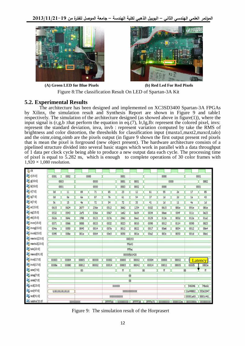
Figure 8:The classification Result On LED of Spartan-3A Kit
Figure 9: The simulation result of the Horprasert
IP Core
Latency
(A) Green LED for Blue Pixels (b) Red Led For Red Pixels
Hamdai: An FPGA Design and Implementation of Custom IP Core…
13
Table 1: Resource Utilization Summary (generated by (EDK) Resource Type Used Available Percent(Utilization)
Slice 3,032 23,872 12%
Slice Flip Flops 2.808 47,744 5%
4 Input LUTs 2.837 47,744 5%
Bonded IOBs 86 469 18%
DCM 1 8 12%
DSP48A 3 126 2%
6. Conclusion This paper presents a design of custom IP core for surveillance System that makes use of
the FPGA and its embedded microprocessor, with the development environment for System-
on-Programmable Chip (SoPC) design. The architecture is designed to perform background
subtraction in video sequences based on the Horprasert algorithm. The Horprasert algorithm
can be divided into two stage, training phase and testing phase. The co-design strategy allows
to assign non-real-time constrained operations to software running on the processor in order to
decrease the hardware resources required which is used for second stage. In this paper, the
proposed hardware architecture for the IP core that performs the background subtraction,
pixel classification are implemented on the XtremeDSP Video Starter Kit. The hardware
architecture consists of a pipelined structure divided into several basic stages which work in
parallel with a data throughput of 1 data per clock cycle being able to produce a new output
data each cycle. A commodity IP core will be able to compute the testing stage of Horprasert
algorithm in real-time With less than a 54% of the resources utilization of a XC3SD3400
Spartan-3A low-cost family FPGA, the system achieves a frequency of 189.322MHz reaching
30 fps with resolutions up to 1,920 × 1,080.
References: [1] R. Rodriguez-Gomez, E. Fernandez-Sanchez, J. Diaz and E. Ros, "FPGA Implementation for
Real-Time Background Subtraction Based on Horprasert Model", Sensors 2012, Vol.12, 5 January
2012, pp. 585-611.
[2] R.. Jenifa, C. Akila and V. Kavitha, " Rapid Background Subtraction from Video Sequences",
International Conference on Computing, Electronics and Electrical Technologies [ICCEET],
Kumaracoil, 21-22 March 2012, pp.1077-1086.
[3] Z.Tang and Z.Miao, " Fast Background Subtraction and Shadow Elimination Using Improved
Mixture Model", HAVE 2007 - IEEE International Workshop on Haptic Audio Visual
Environments and their Applications, Ottawa - Canada, 12-14 October 2007, pp.38-41.
[4] B. Langmann, S.E. Ghobadi, K. Hartmann and O. Loffeld, " Multi-Modal Background
Subtraction Using Gaussian Mixture Models" , In: Paparoditis N., Pierrot-Deseilligny M., Mallet
C., Tournaire O. (Eds), IAPRS, Vol. XXXVIII, Part 3A – Saint-Mandé, France, September 1-3,
2010,pp.61-66.
[5] S. mukherjee and K. Das, " Omega Model for Human Detection and Counting for application
in Smart Surveillance System", (IJACSA) International Journal of Advanced Computer Science
and Applications, Vol. 4, No. 2, 2013, pp. 167-172.
[6] M. H. Sigari and M. Fathy, " Real-time Background Modeling/Subtraction using Two-Layer
Codebook Model", Proceedings of the International MultiConference of Engineers and Computer
Scientists, Hong Kong, 19-21 March, 2008.
[7] P.. Varcheie, M. Sills-Lavoie and G. Bilodeau, "A Multiscale Region-Based Motion Detection
and Background Subtraction Algorithm", Sensors, vol. 10, pp. 1041-1061, Jan. 2010, pp. 1041-
1061.

19/99/1192-91جامعة الموصل للفترة من –ليوبيل الذهبي لكلية الهندسة ا – العلمي الهندسي الثانيالمؤتمر
14
[8] M. Heikkilä , M. Pietikäinen , S. Member,IEEE, "A Texture-Based Method for Modeling the
Background and Detecting Moving Objects", IEEE Transactions on Pattern Analysis and Machine
Intelligence, Vol 28, April 2006,pp 657-662.
[9] L. Li, Member, IEEE, W. Huang, Member, IEEE, I. Yu-Hua Gu, Senior Member, IEEE, and
Q. Tian, Senior Member, IEEE, "Statistical Modeling of Complex Backgrounds for Foreground
Object Detection", IEEE Transactions On Image Processing, Vol. 13, No. 11, November 2004, pp.
1459- 1472.
[10] Jiang, H., Ardo, H., Owall, V., “Hardware Accelerator Design for Video Segmentation with
Multi-Modal Background Modelling”, In Proceedings of the IEEE International Symposium on
Circuits and Systems (ISCAS ’05), Kobe, Japan, 23–26 May 2005; Volume 2, pp. 1142–1145.
[11] M. Genovese, E. Napoli, D. Caro, N. Petra, and A. Strollo, " FPGA Implementation of
Gaussian Mixture Model Algorithm for 47fps Segmentation of 1080p Video", Hindawi Publishing
Corporation Journal of Electrical and Computer Engineering Volume 2013, Article ID 129589,
Accepted 7 January 2013, 8 pages.
[12] M. Basavaiah, "Development of Optical Flow Based Moving Object Detection and
Tracking System on an Embedded DSP Processor", Journal of Advances in Computational
Research: An International Journal Vol. 1 No. 1-2 (January-December, 2012), pp.15-25.
[13] V. Pham, P. Vo, V.T. Hung, L.H. Bac , “GPU Implementation of Extended Gaussian Mixture
Model for Background Subtraction” In Proceedings of the IEEE RIVF International Conference
on Computing and Communication Technologies, Research, Innovation, and Vision for the Future
(RIVF), Hanoi, Vietnam, 1–4 November 2010, pp. 1–4.
[14] Xilinx, Inc., " Embedded System Tools Reference Manual", UG111 EDK 12.2, July 23, 2010,
pp 1-292.
[15] T. Sutikno, A. Jidin, A. Jidin and N. driIs, " Simplified VHDL Coding of Modified Non-
Restoring Square Root Calculator", International Journal of Reconfigurable and Embedded
Systems (IJRES), Vol. 1, No. 1, March 2012, pp. 37-42.
Saleem: Design and FPGA Implementation of Systolic Array Architecture …..
51
Design and FPGA Implementation of Systolic Array
Architecture for Matrix Multiplication Thakwan Mohammad Saleem Farah Nazar Ibraheem Computer Engineering Department, College of Engineering, University of Mosul.
Abstract The evolution of computer and Internet has brought demand for powerful and
high speed data processing, but in such complex environment, fewer methods can
provide perfect solution. To handle above addressed issue, parallel computing is
proposed as a solution to the contradiction. This paper provides solution for the
addressed issues of demand for high speed data processing and demonstrates an
effective design for the Matrix Multiplication using Systolic Architecture on
Reconfigurable Systems (RS) like Field Programmable Gate Arrays (FPGAs).Here, the
systolic architecture increases the computing speed by combining the concept of parallel
processing and pipelining into a single concept. The RTL code is written for matrix
multiplication with both systolic architecture and conventional(sequential) method in
VHDL , Synthesized by using Xilinx ISE 14.2 and targeted to the device xc3s500e-4fg320
, then finally the designs are compared to each other to evaluate the performance of
proposed architecture. The proposed Matrix Multiplication with systolic architecture
has given the core speed 210.2MHz ,it enhances the speed of matrix multiplication by
twice of conventional method which is 101.7MHz.
Keywords: FPGA, Matrix Multiplication, Parallel Computing, Systolic Array, VHDL.
تصميم عملية ضرب المصفوفات بطريقة المصفوفة اإلنقباضية وتنفيذها باستخدام البوبات القابلة
للبرمجة حقليا
اهيمذكوان محمد سليم فرح نزار إبر
جامعة الموصل -كلية الهندسة -قسم هندسة الحاسوب
الملخصفي ظل التطور الحاصل في علم الحاسوب وشبكة المعلوماتية ظهرت الحاجة لضرورة معالجة البيانات بسرعة
اباتها ودقة عالية , مما ادى الى ظهور مفهوم المعالجة المتوازية لحل الكثير من المشاكل الحسابية والتي تتضمن حس
الكثير من الزمن , واحدى اهم الحسابات والتي تدخل في كثير من التطبيقات مثل تطبيقات معالجة االشارة الرقمية
ومعالجة الصور والفيديو هي عملية ضرب المصفوفات , في هذا البحث تم تصميم معمارية مصفوفة انقباضية تقوم
ستخدام اسلوب المعالجة المتوازية واسلوب خ االنابي في نف بعملية ضرب المصفوفات بكفاءة وسرعة عالية نظرا ال
الوقت , المعمارية المصممة تم تنفيذها على شريحة البوابات المنطقية القابلة للبرمجة حقليا", وتمت مقارنة نتائج
ث تم التوصل الى المعمارية المصممة مع المعمارية التقليدية لضرب المصفوفات وقياس كفاءة المعمارية المصممة, حي
ان استخدام المصفوفة االنقباضية ادى الى زيادة مقدار السرعة تقريبا بمقدار الضعف مقارنة مع استخدام الطريقة
ميكاهرتز في حالة استخدام المصفوفة االنقباضية في عملية الضرب ,بينما 2.012التقليدية ,حيث كانت السرعة تساوي
استخدام المصفوفة التقليدية 1 ميكاهرتز عند 0.11.كانت تساوي
19/99/1192-91جامعة الموصل للفترة من –ليوبيل الذهبي لكلية الهندسة ا –الهندسي الثاني العلمي المؤتمر
51
1-Introduction
In the sphere of information processing , matrix computations are amongst the most
frequently required and computationally intensive tasks, Their computation forms the basis of
many important applications, such as digital signal, image and video processing, numerical
analysis, computer graphics and vision, etc. The nature of matrix multiplication algorithms is
such that they are perfectly suited to parallel exploitation
Systolic networks are a class of pipelined array architectures which rhythmically
compute and pass data through the complex, these arrays are suited for processing repetitive
computations. Although this kind of computation usually involves a great deal of computing
power, such computations are parallelizable and highly regular[1]. The systolic array
architecture exploits this parallelism and regularity to deliver the required computational
speed. In computer architecture, a systolic architecture is a pipelined network arrangement of
Processing Elements (PEs) called cells, each cell shares the information with its neighbors
immediately after processing, all systolic cells perform computations concurrently, while
data, such as initial inputs, partial results, and final outputs, is being passed from cell to cell.
When partial results are moved between cells, they are computed over these cells in a pipeline
manner. In this case the computation of each single output is separated over these cells. This
contrasts to other parallel architectures based on data partitioning, for which the computation
of each output is computed solely on one single processor [3-4]. When a systolic array is in
operation, computing at cells, communication between cells and input from and output to the
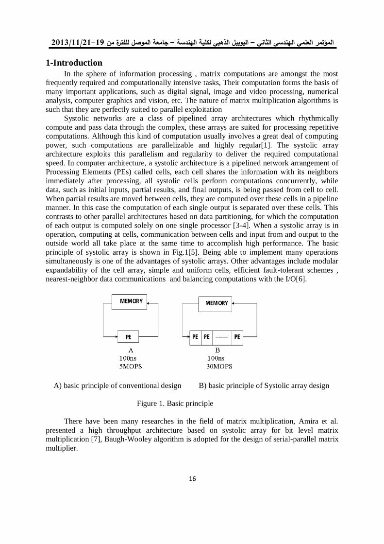
outside world all take place at the same time to accomplish high performance. The basic
principle of systolic array is shown in Fig.1[5]. Being able to implement many operations
simultaneously is one of the advantages of systolic arrays. Other advantages include modular
expandability of the cell array, simple and uniform cells, efficient fault-tolerant schemes ,
nearest-neighbor data communications and balancing computations with the I/O[6].
A) basic principle of conventional design B) basic principle of Systolic array design
Figure 1. Basic principle
There have been many researches in the field of matrix multiplication, Amira et al.
presented a high throughput architecture based on systolic array for bit level matrix
multiplication [7], Baugh-Wooley algorithm is adopted for the design of serial-parallel matrix
multiplier.
Saleem: Design and FPGA Implementation of Systolic Array Architecture …..
51
Amira et al. designed a parameterizable system for 8-bit fixed point matrix
multiplication using FPGA [8], Their design used both systolic architecture and distributed
arithmetic design methodology for the implementation of matrix multiplication .
In[9], Mencer et al. implemented the matrix multiplication on Xilinx XC4000E FPGA, Their
designs employ bit serial multipliers using Booth encoding. They focused on tradeoffs
between area and maximum running frequency with parameterized circuit generators. Their
design was improved by Amira et al. in [10] using modified booth encoder multiplicat ion
along with Wallace tree addition.
Jang et al. improved the design in [11] and [12] in terms of area, speed [11] and energy
[12] by taking advantage of data reuse. They reduced the latency for computing matrix
product by employing internal storage registers in the processing element (PE). Their
algorithms need n multipliers, n adders,and total storage of size n2 words.
Kung et. al. have proposed a unified systolic architecture for the implementation of
neural network models [13]. It has been shown that the proper ordering of the elements of the
weight matrix makes it possible to design a cascaded dependency graph for consecutive
matrix multiplication, which requires the directions of data movement at both the input and
the output of the dependency graph to be identical, iterations of a back-propagation algorithm
have been mapped onto a ring systolic array.
Choi et al. developed novel designs and architectures for FPGAs which minimized the
power consumption along with latency and area [14]-[15]. They used linear systolic
architecture to develop energy efficient designs. For linear systolic array, the amount of
storage per processing element affects the system wide energy. Thus, they used maximum
amount of storage per processing element and minimum number of multipliers to obtain
energy-efficient matrix multiplier.
A large number of systolic array designs have been developed and used to perform a
broad range of computations. In fact, recent advances in theory and software have allowed
some of these systolic arrays to be derived automatically [16]. There are numerous
computations for which systolic designs exist such as signal and image processing,
polynomial and multiple precision integer arithmetic, matrix arithmetic and nonnumeric
applications [17].
The rest of this paper is organized as follows. In section 2 the methods and materials of
the architectural design is presented. Section 3 shows the hardware Implementation details.
The Experimental result are given in section 4. Section 5 concludes this paper.
2- Background And Theory
2.1 Basic concepts of systolic systems The designation systolic follows from the operational principle of the systolic
architecture. The systolic style is characterized by an intensive application of both pipelining
and parallelism, controlled by a global and completely synchronous clock. Data streams
pulsate rhythmically through the communication network, Here, pipelining is not constrained
to a single space axis but concerns all data streams possibly moving in different directions and
intersecting in the cells of the systolic array[18].
A systolic system typically consists of a host computer, and the actual systolic array.
Conceptionally, the host computer is of minor importance, just controlling the operation of
the systolic array and supplying the data. The systolic array can be understood as a specialized
19/99/1192-91جامعة الموصل للفترة من –ليوبيل الذهبي لكلية الهندسة ا –الهندسي الثاني العلمي المؤتمر
51
network of cells rapidly performing data-intensive computations, supported by massive
parallelism.
A systolic algorithm is the program collaboratively executed by the cells of a systolic
array.
Systolic arrays may appear very differently, but usually share many of key features:
Modularity ( the array consists of modular processing units , Regularity (the modular units are
interconnected with homogeneously),Spatial Locality ( the cells has a local communication
interconnection), Temporal locality(the cells transmits the signals from one cell to other
which require at least one unit time delay)
There are three types of systolic array based on its topology, One dimensional systolic
array (Linear Array), Two dimensional systolic array (Mesh-connected Array), Three
dimensional systolic array.
In this paper ,the tow dimensional systolic array was chosen as a proposed architecture
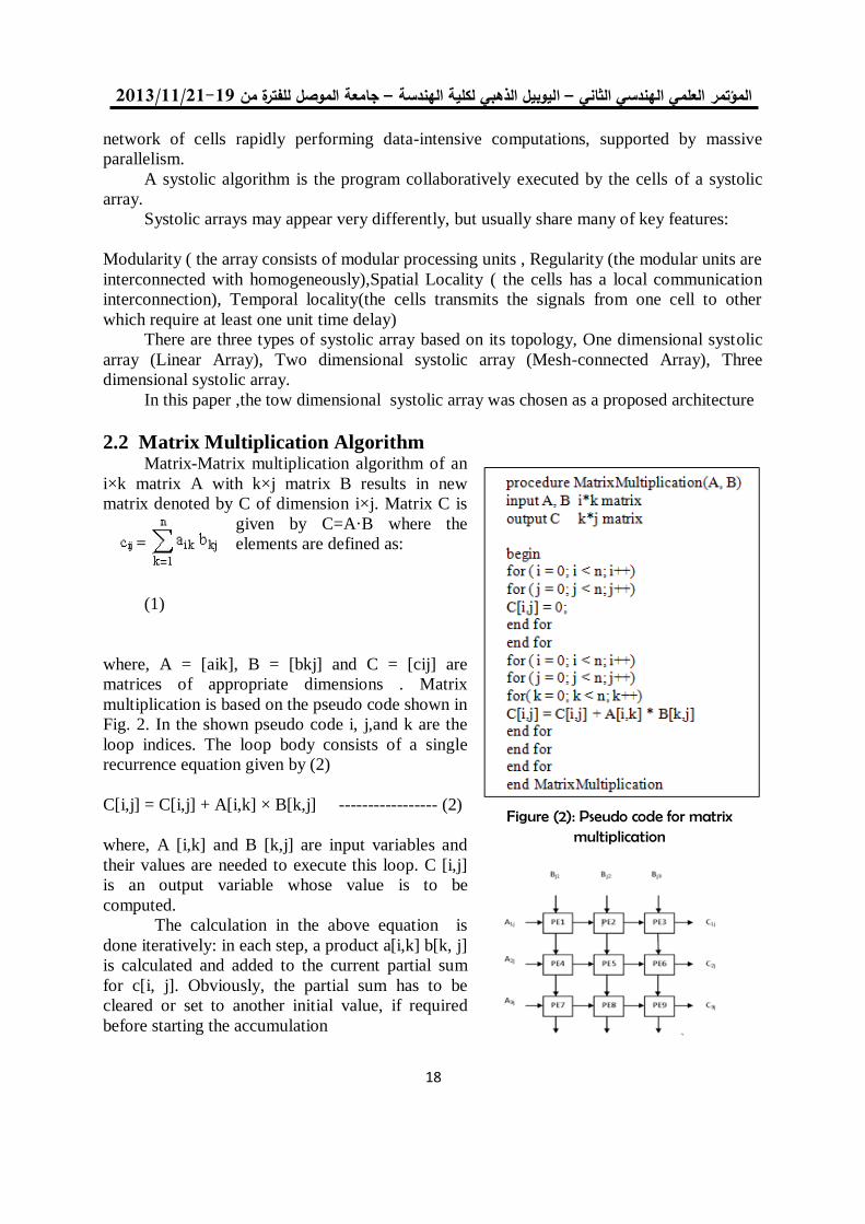
2.2 Matrix Multiplication Algorithm Matrix-Matrix multiplication algorithm of an
i×k matrix A with k×j matrix B results in new
matrix denoted by C of dimension i×j. Matrix C is
given by C=A·B where the
elements are defined as:
(1)
where, A = [aik], B = [bkj] and C = [cij] are
matrices of appropriate dimensions . Matrix
multiplication is based on the pseudo code shown in
Fig. 2. In the shown pseudo code i, j,and k are the
loop indices. The loop body consists of a single
recurrence equation given by (2)
C[i,j] = C[i,j] + A[i,k] × B[k,j] ----------------- (2)
where, A [i,k] and B [k,j] are input variables and
their values are needed to execute this loop. C [i,j]
is an output variable whose value is to be
computed.
The calculation in the above equation is
done iteratively: in each step, a product a[i,k] b[k, j]
is calculated and added to the current partial sum
for c[i, j]. Obviously, the partial sum has to be
cleared or set to another initial value, if required
before starting the accumulation
Figure (2): Pseudo code for matrix multiplication
Saleem: Design and FPGA Implementation of Systolic Array Architecture …..
51
Now ,in the Pseudo code shown above , If i = j = k = N, we have to perform N³
multiplications, additions, and assignments, each. Hence the running time of this algorithm is
of order O(N³) for any sequential processor.
The above equation can also be realized with the array of processors(systolic array) of
dimension i×j, as shown in Fig. 3. The connections are realized in horizontal and in vertical
directions. Therefore the mesh connections of Linear processor Array structure is convenient
for this operation where the data stream of matrix A is flowing to the right and the data stream
of matrix B is flowing top down. The elements of matrix C are stored in the appropriate
processors of the array . In this case the expected speedup is
3-Hardware Implementation Details
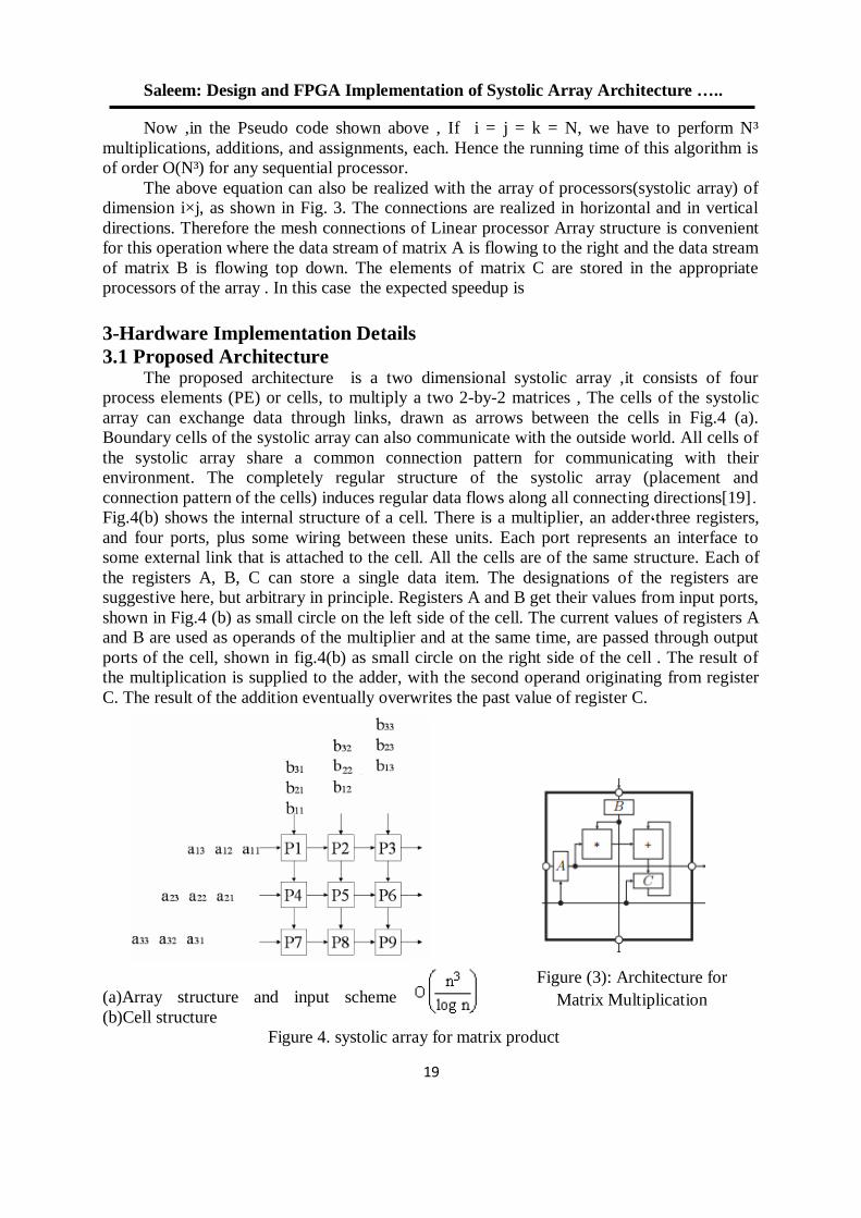
3.1 Proposed Architecture The proposed architecture is a two dimensional systolic array ,it consists of four
process elements (PE) or cells, to multiply a two 2-by-2 matrices , The cells of the systolic
array can exchange data through links, drawn as arrows between the cells in Fig.4 (a).
Boundary cells of the systolic array can also communicate with the outside world. All cells of
the systolic array share a common connection pattern for communicating with their
environment. The completely regular structure of the systolic array (placement and
connection pattern of the cells) induces regular data flows along all connecting directions[19] .
Fig.4(b) shows the internal structure of a cell. There is a multiplier, an adder,three registers,
and four ports, plus some wiring between these units. Each port represents an interface to
some external link that is attached to the cell. All the cells are of the same structure. Each of
the registers A, B, C can store a single data item. The designations of the registers are
suggestive here, but arbitrary in principle. Registers A and B get their values from input ports,
shown in Fig.4 (b) as small circle on the left side of the cell. The current values of registers A
and B are used as operands of the multiplier and at the same time, are passed through output
ports of the cell, shown in fig.4(b) as small circle on the right side of the cell . The result of
the multiplication is supplied to the adder, with the second operand originating from register
C. The result of the addition eventually overwrites the past value of register C.
(a)Array structure and input scheme
(b)Cell structure
Figure 4. systolic array for matrix product
Figure (3): Architecture for
Matrix Multiplication
19/99/1192-91جامعة الموصل للفترة من –ليوبيل الذهبي لكلية الهندسة ا –الهندسي الثاني العلمي المؤتمر
02
3.2 Implementation of the Algorithm There are five steps of mapping algorithm to systolic architecture:
1. Buffer all the variables.
2. Determine the PEs functions by collecting the assignment statements in the
loop bodies into m input and n output functions {Determine dependence matrix}
3-Find transformation matrix (T).
4. Apply a linear reindexing transformation matrix (T).
5. Find connections between processors and the direction of data flow.
these steps will be implemented to the algorithm of multiplication of 2-by-2 matrices.
First, consider the following algorithm which represents multiplication of two -2 by 2
matrices A and B :
for (k 1= ;k<=2 ;k++)
for (i=1 ;i<=2 ;i++)
for (j=1 ;j<=2 ;j++)
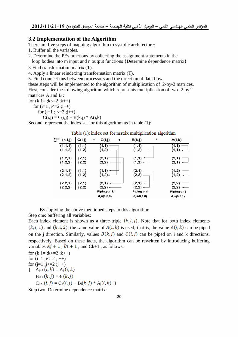
C(i,j) = C(i,j) + B(k,j) * A(i,k) Second, represent the index set for this algorithm as in table (1):
By applying the above mentioned steps to this algorithm:
Step one: buffering all variables:
Each index element is shown as a three-triple . Note that for both index elements
and , the same value of is used; that is, the value can be piped
on the j direction. Similarly, values and can be piped on i and k directions,
respectively. Based on these facts, the algorithm can be rewritten by introducing buffering
variables , , and Ck+1 , as follows:
for (k 1= ;k<=2 ;k++)
for (i=1 ;i<=2 ;i++)
for (j=1 ;j<=2 ;j++)
{ Aj+1 = Aj
Bi+1 =Bi
Ck+1 = Ck + Bi * Aj }
Step two: Determine dependence matrix:
Saleem: Design and FPGA Implementation of Systolic Array Architecture …..
05
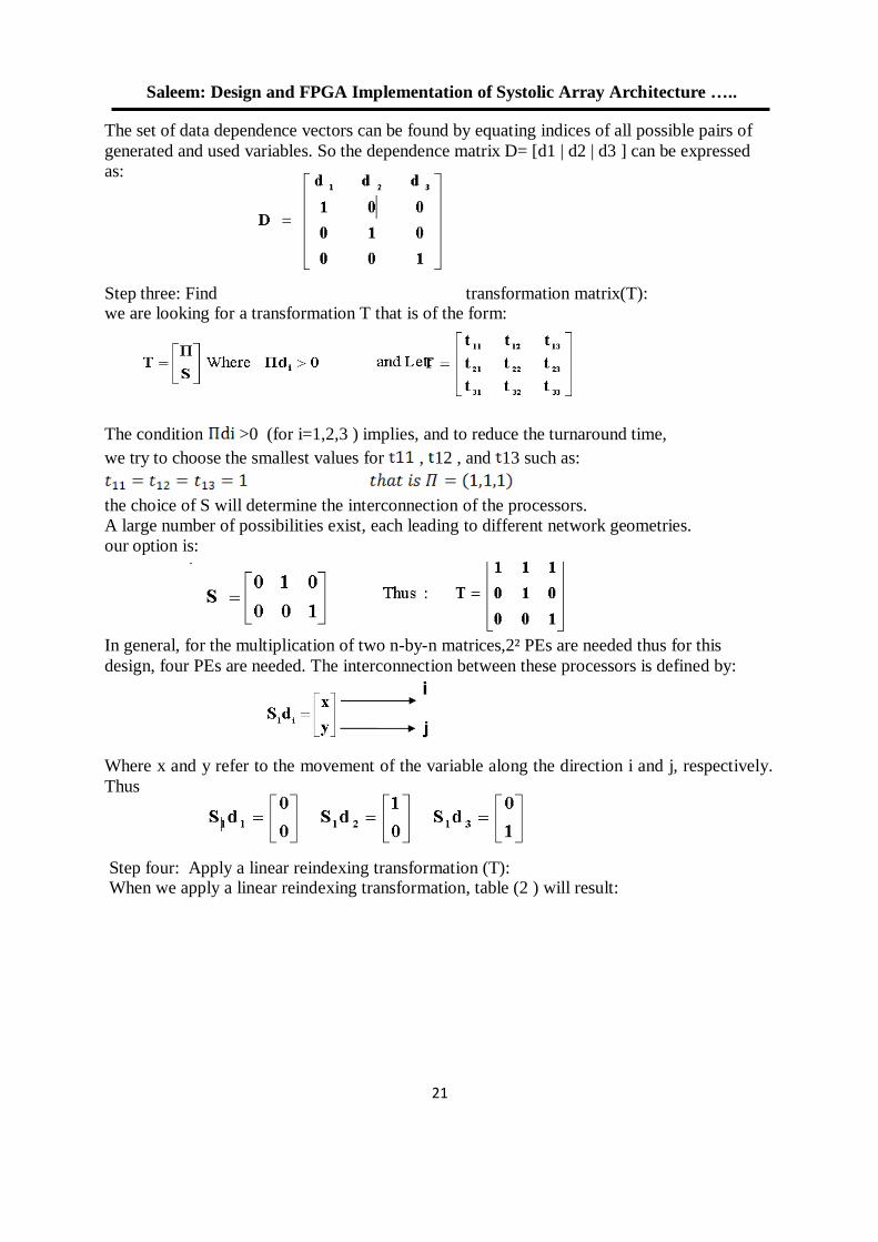
The set of data dependence vectors can be found by equating indices of all possible pairs of
generated and used variables. So the dependence matrix D= [d1 | d2 | d3 ] can be expressed
as:
Step three: Find transformation matrix(T): we are looking for a transformation T that is of the form:
The condition >0 (for i=1,2,3 ) implies, and to reduce the turnaround time,
we try to choose the smallest values for , 12 , and 13 such as:
the choice of S will determine the interconnection of the processors.
A large number of possibilities exist, each leading to different network geometries.
our option is:
In general, for the multiplication of two n-by-n matrices,2² PEs are needed thus for this
design, four PEs are needed. The interconnection between these processors is defined by:
Where x and y refer to the movement of the variable along the direction i and j, respectively.
Thus
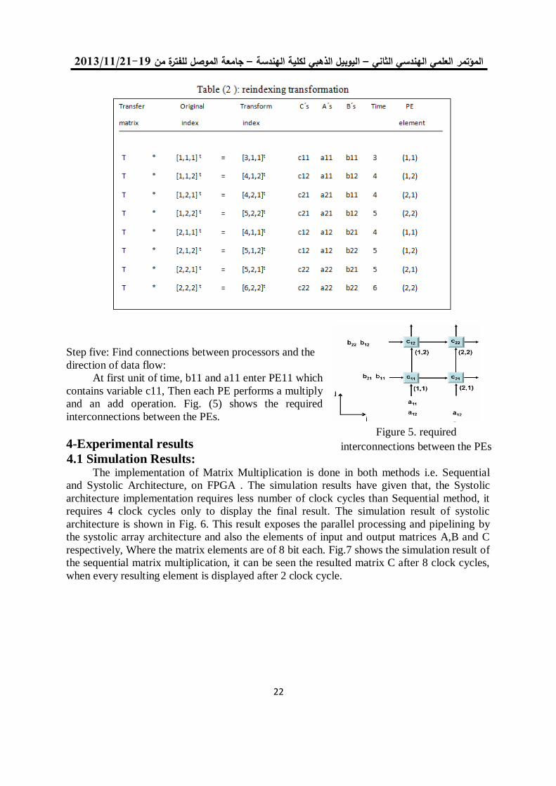
Step four: Apply a linear reindexing transformation (T): When we apply a linear reindexing transformation, table (2 ) will result:
19/99/1192-91جامعة الموصل للفترة من –ليوبيل الذهبي لكلية الهندسة ا –الهندسي الثاني العلمي المؤتمر
00
Step five: Find connections between processors and the
direction of data flow:
At first unit of time, b11 and a11 enter PE11 which
contains variable c11, Then each PE performs a multiply
and an add operation. Fig. (5) shows the required
interconnections between the PEs.
4-Experimental results
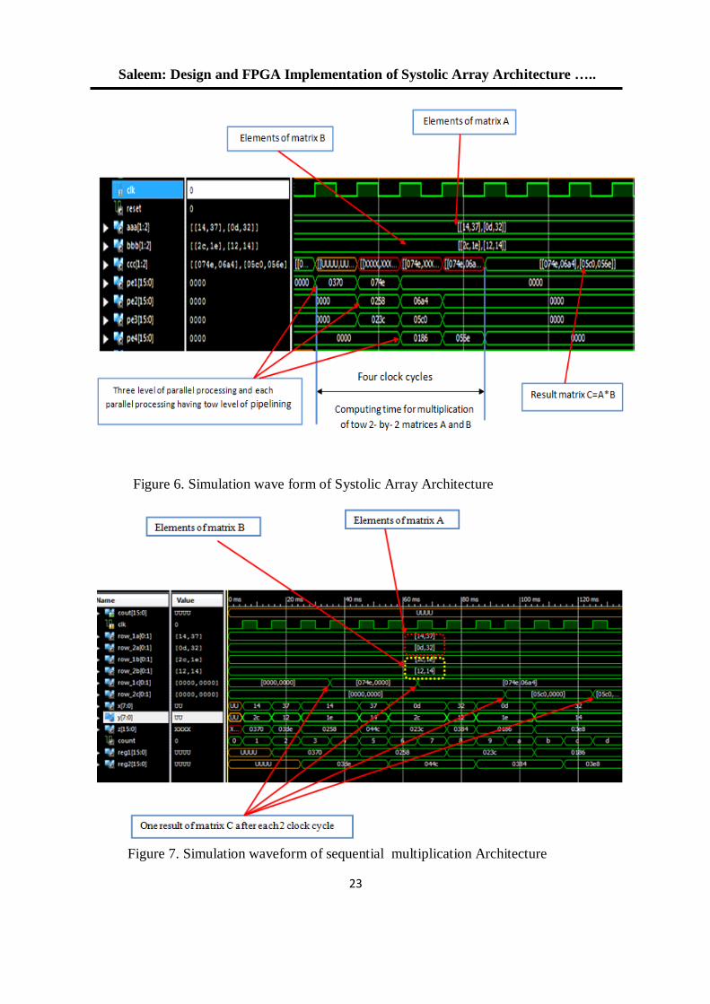
4.1 Simulation Results: The implementation of Matrix Multiplication is done in both methods i.e. Sequential
and Systolic Architecture, on FPGA . The simulation results have given that, the Systolic
architecture implementation requires less number of clock cycles than Sequential method, it
requires 4 clock cycles only to display the final result. The simulation result of systolic
architecture is shown in Fig. 6. This result exposes the parallel processing and pipelining by
the systolic array architecture and also the elements of input and output matrices A,B and C
respectively, Where the matrix elements are of 8 bit each. Fig.7 shows the simulation result of
the sequential matrix multiplication, it can be seen the resulted matrix C after 8 clock cycles,
when every resulting element is displayed after 2 clock cycle.
Figure 5. required
interconnections between the PEs
Saleem: Design and FPGA Implementation of Systolic Array Architecture …..
02
Figure 6. Simulation wave form of Systolic Array Architecture
Figure 7. Simulation waveform of sequential multiplication Architecture
19/99/1192-91جامعة الموصل للفترة من –ليوبيل الذهبي لكلية الهندسة ا –الهندسي الثاني العلمي المؤتمر
02
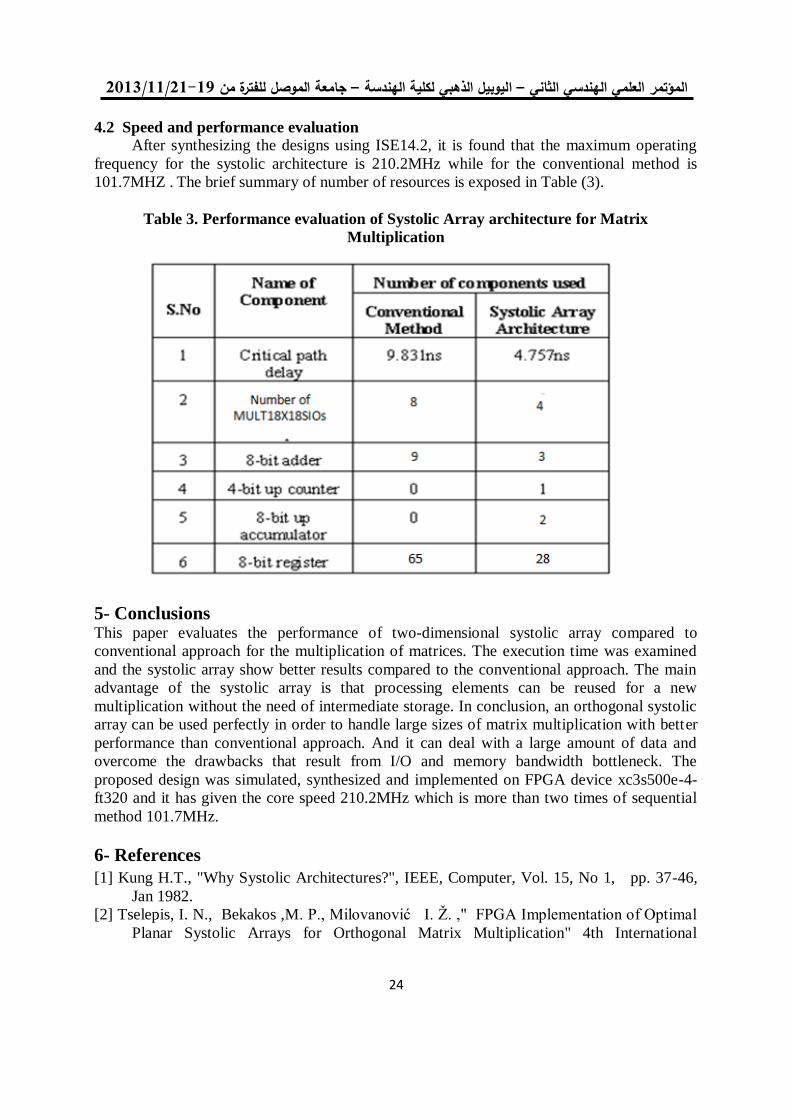
4.2 Speed and performance evaluation
After synthesizing the designs using ISE14.2, it is found that the maximum operating
frequency for the systolic architecture is 210.2MHz while for the conventional method is
101.7MHZ . The brief summary of number of resources is exposed in Table (3).
Table 3. Performance evaluation of Systolic Array architecture for Matrix
Multiplication
5- Conclusions This paper evaluates the performance of two-dimensional systolic array compared to
conventional approach for the multiplication of matrices. The execution time was examined
and the systolic array show better results compared to the conventional approach. The main
advantage of the systolic array is that processing elements can be reused for a new
multiplication without the need of intermediate storage. In conclusion, an orthogonal systolic
array can be used perfectly in order to handle large sizes of matrix multiplication with better
performance than conventional approach. And it can deal with a large amount of data and
overcome the drawbacks that result from I/O and memory bandwidth bottleneck. The
proposed design was simulated, synthesized and implemented on FPGA device xc3s500e-4-
ft320 and it has given the core speed 210.2MHz which is more than two times of sequential
method 101.7MHz.
6- References
[1] Kung H.T., "Why Systolic Architectures?", IEEE, Computer, Vol. 15, No 1, pp. 37-46,
Jan 1982.
[2] Tselepis, I. N., Bekakos ,M. P., Milovanović I. Ž. ," FPGA Implementation of Optimal
Planar Systolic Arrays for Orthogonal Matrix Multiplication" 4th International

Saleem: Design and FPGA Implementation of Systolic Array Architecture …..
01
Conference: Sciences of Electronic, Technologies of Information and
Telecommunications March 25-29, 2007 – TUNISIA
[3] Chung, J. H., Yoon, H. S., Maeng, S. R., "A Systolic Array Exploiting the Inherent
Parallelisms Artificial Neural Networks", Micro-processing and Microprogramming.
Elsevier Science Publishers B. V., Vol. 33, No.6, (1992),pp.145-159.
[4]. Kane, A. J., Evans, D. J., "An instruction systolic array architecture for neural networks.
International Journal of Computer Mathematics", Vol. 61,No.2, (1996),pp63-89
[5]. Juan, A."Field-programmable gate aray implementation of a scalable integral image
architecture based on systolic arrays ",Phd Thesis ,.utah state university,2011, pp.8
[6] Shapri ,A.H.M. , Rahman,N.A.Z., "Performance Analysis of Two-Dimensional Systolic
Array Matrix Multiplication with Orthogonal Interconnections", International Journal
on New Computer Architectures and Their Applications (IJNCAA),Vol
1,No.3,pp.1066-1075, The Society of Digital Information and Wireless
Communications, (ISSN),2011,pp. 2220-9085)
[7] Amira ,A. , Bouridane, A., Rahman, Milligan, P. , and Sage P., “A High hroughput FPGA
Implementation of a Bit-Level Matrix Product”, Proc. of IEEE Workshop on Signal
Processing Systems, Oct. 2000, pp. 356–364.
[8] Amira A. , Bensaali, F. ,“An FPGA based parameterizable system for matrix product
implementation,” Proc. of IEEE Workshop on Signal Processing Systems, Oct 2002,
pp. 75-79.
[9] Mencer, O., Morf, M., and Flynn, M. J. “PAM-Blox:" High performance FPGA design
for adaptive computing," Proc. of IEEE Symp. on FPGAs for Custom Computing
Machines, April 1998, pp. 167–174.
[10] Amira, A. , Bouridane, A. and Milligan, P. “Accelerating Matrix Product on
Reconfigurable Hardware for Signal Processing,” Proc. of 11th Int. Conf. on Field
[11] J. Jang, S. Choi, and V. K. Prasanna, “Area and Time Efficient Implementations of
Matrix Multiplication on FPGAs,” Proc. of IEEE Int. Conf. on Field Programmable
Technology, Dec. 2002, pp. 93–100.
[12] Jan,J. , Choi,S. and V. K. Prasanna, “Energy and Time Efficient Matrix Multiplication on
FPGAs,” IEEE Trans. on VLSI Systems, Vol.13, No. 11, Nov. 2005, pp. 1305–1319,
[13] Kung, S. Y., Hwang, J. N.," A unified systolic architecture for artificial neural networks".
J. Journal of Parallel and Distributed Computing , vol. 6,No.2,1989pp. 358—387.
[14] S. Choi, V. K. Prasanna, and J. Jang, “Minimizing energy dissipation of matrix
multiplication kernel on Virtex-II,” Proc. of SPIE, Vol. 4867, July 2002, pp.98–106
[15] S. Choi, R. Scrofano, V. K. Prasanna, and J. Jang, “Energy efficient signal processing
using FPGAs,” Proceedings of the 2003 ACM/SIGDA eleventh international
symposium on Field programmable gate arrays, Feb. 2003, pp. 225–234,
[16] M. P. Bekakos, “Highly Parallel Computations-Algorithms and Applications,”
Democritus University of Thrace, Greece, 2001,pp. 139-209.
[17] M.A. Frumkin , Systolic Computations, Scripps Research Institute, La Jolla, California,
U.S.A., 1992.
[18]A. Darte, Y.Robert, F. Vivien. Scheduling and Automatic Parallelization.
BirkhäuserBoston, 2000. 562
[19] ZARGHAM, M. R. computer Architecture "single and parallel systems". Prentice–Hall
International, Inc, .
19/99/1192-91جامعة الموصل للفترة من –ليوبيل الذهبي لكلية الهندسة ا –الثاني لهندسي االعلمي المؤتمر
62
Automatic Segmentation of Normal and Pathological Tissues in MRI Brain Images based on Classifier and Clustering Methods
Abstract Segmentation of brain magnetic resonance images is a crucial step in surgical and
treatment planning. In this paper, a fully automatic technique is proposed for a precise segmentation of normal and pathological tissues in MRI brain images. The normal tissues such as WM (White Matter), GM (Gray Matter) and CSF (Cerebrospinal Fluid) are segmented from the normal MRI images and the pathological tissues such as tumors are extracted from the abnormal images. The abnormal segmentation technique can detect tumors, extract them from MRI images, find their position and finally calculate their area. All these could be done based on combining neural classifier with clustering methods. The abnormal MRI slices are divided into equal sized blocks then five features are extracted from each block of abnormal slice. They are the two dynamic statistical features (mean and variance) and the three 2D wavelet decomposition features (horizontal , vertical and diagonal) which are used as inputs to the neural network units for tumor blocks detection. Then Otsu or K-mean clustering methods are used to extract tumors from detected tumor blocks. The segmentation based on Otsu's clustering or K-mean's clustering is implemented using MATLAB 7.12.0.635 on 572 magnetic resonance images having brain tumors to extract them and also on images without any abnormality to segment the White matter, Gray matter and Cerebrospinal Fluid on different MRI cases. A hybrid technique provides a good quality results for clustering healthy tissue structures and pathology tissues. The requirement for a surgical planning or even image-guided surgery now could be performed more accurate. Keywords: Brain Segmentation; Clustering; White Matter (WM), Cerebrospinal fluid(CSF), Gray matter(GM); K-mean.
في صور الرسنين المغناطيسيالطبيعي والمرضي سنسة ألالتلقائي ل التقسيم وطرق العنقدةلتصنيف للدماغ على أساس ا
الملخص اقترحت، بحثال هذا والعالج. في لدماغ خطوة حاسم في أجراء العمليات الةراحيليعتبر تقسيم صور الرسنين المغناطيسي
األسنسة صور أ. حيث تةزتقني أوتوماتيكي لتةزئ دقيق لألسنسة الطبيعي والمرضي في صور الدماغ بالرسنين المغناطيسيصور األورام والىلتشخيص اطبيعي باعتبارها سائل النخاع صور الرمادي وصور المادة إلى صور المادة البيضاء و الطبيعي
تقني تقسيم الحاالت الغير طبيعي يمكنها الكشف عن األورام، واستخراجها من صور حاالت مرضي .ب مصاب صور باعتبارها العصبي مع أساليب الشبك تصنيفات، من خالل الةمع بين ساحتها وأخيرا حساب م اهعالرسنين المغناطيسي، والعثور على موق
ثم استخراج خمس ميزات لكل كتل بعاد إلى كتل متساوي األ غير طبيعياللرسنين المغناطيسي ا صور م شرائحيبتقسيتم ذلك العنقدة. )األفقي ي ثنائي البعد ل المويةيلتحللميزات ثالث والتباين( و المعدلمالمح اإلحصائي الحيوي )ال، هما مصاب ائح الشرال صور من
. ثم يتم استخدام العنقدةالورمفي الشرائح المصاب بالعصبي للكتل اتوحدات الشبكلتستخدم كمدخالت حيثقطري( الوالرأسي و الستخراج األورام فقط من الكتل التي تحوي الورم. تم تنفيذ المقترح باستخدام K-meansو Otsu التةميع تيبخوارزمي المتمثل أألوراما مرضي تم استخراج شريح من صور الرسنين المغناطيسي منه 275على 7.12.0.635اإلصدار ب MATLABبرسنامج
مختلف . المزج بين أكثر من المادة الرمادي والسائل النخاعي لحاالتومادة البيضاء الصور إلى أجرى تصنيفهاطبيعي منها و منهاين اتخاذ تساعد كثيرا في تحس سنوعي جيدة من تقسيم هياكل األسنسة السليم واألسنسة المرضي . الطريق المقترح سنتج عنه طريق
أكثر. دق ب األورام الستئصالالقرار للتدخل الةراحي إضاف إلى الةراح المعتمدة على الصور وذلك
Ameen M. Abd-Alsalam Selami Dr. Ahlam F. Mahmood Computer Engineering Department
[email protected] [email protected]
أمين محمد عبد السالم سالمي د. أحالم فاضل محمود
جامع الموصل -كلي الهندس -بوساقسم هندس الح
Selami: Automatic Segmentation of Normal and Pathological Tissues in …..
62
1. Introduction In the last two decades medical science has seen a revolutionary development in the
field of biomedical diagnostic imaging. The current advancement in the field of artificial
intelligence and computer vision technologies was very effectively put into practice in
applications such as diagnosis of diseases like cancer through medical imaging. This
intelligent system uses medical images as an input to analyze normal and pathological tissues
from MRI brain images, which is generally recognized as key to better diagnosis and patient
care. Although patient scans can be obtained using different imaging modalities, Magnetic
Resonance Imaging (MRI) system has been commonly preferred for brain imaging over other
modalities because of its non-invasive and non-ionizing nature, and also because it allows for
direct multi-plane imaging. MR images of the brain and other cranial structures are clearer
and more detailed than with other imaging methods. This detail makes MRI an invaluable tool
in early diagnosis and evaluation of many conditions, normal or including tumors.
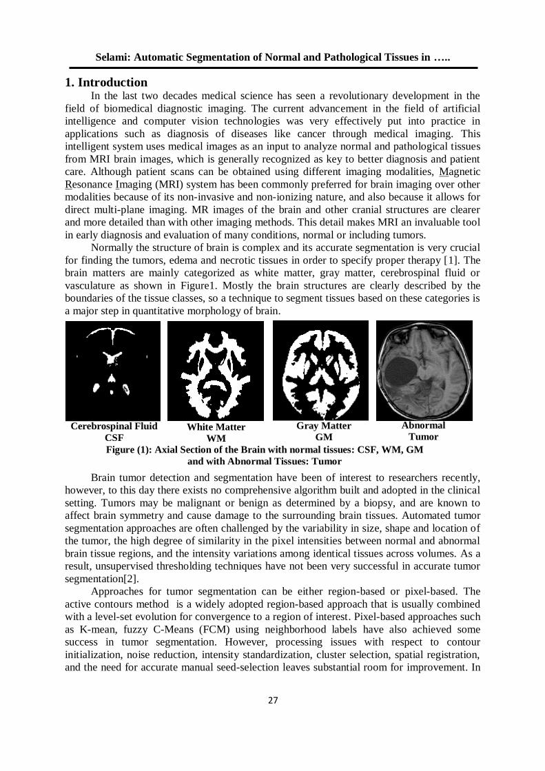
Normally the structure of brain is complex and its accurate segmentation is very crucial
for finding the tumors, edema and necrotic tissues in order to specify proper therapy [1]. The
brain matters are mainly categorized as white matter, gray matter, cerebrospinal fluid or
vasculature as shown in Figure1. Mostly the brain structures are clearly described by the
boundaries of the tissue classes, so a technique to segment tissues based on these categories is
a major step in quantitative morphology of brain.
Brain tumor detection and segmentation have been of interest to researchers recently,
however, to this day there exists no comprehensive algorithm built and adopted in the clinical
setting. Tumors may be malignant or benign as determined by a biopsy, and are known to
affect brain symmetry and cause damage to the surrounding brain tissues. Automated tumor
segmentation approaches are often challenged by the variability in size, shape and location of
the tumor, the high degree of similarity in the pixel intensities between normal and abnormal
brain tissue regions, and the intensity variations among identical tissues across volumes. As a
result, unsupervised thresholding techniques have not been very successful in accurate tumor
segmentation[2].
Approaches for tumor segmentation can be either region-based or pixel-based. The
active contours method is a widely adopted region-based approach that is usually combined
with a level-set evolution for convergence to a region of interest. Pixel-based approaches such
as K-mean, fuzzy C-Means (FCM) using neighborhood labels have also achieved some
success in tumor segmentation. However, processing issues with respect to contour
initialization, noise reduction, intensity standardization, cluster selection, spatial registration,
and the need for accurate manual seed-selection leaves substantial room for improvement. In
Cerebrospinal Fluid
CSF White Matter
WM
Gray Matter
GM Abnormal
Tumor
Figure (1): Axial Section of the Brain with normal tissues: CSF, WM, GM
and with Abnormal Tissues: Tumor
19/99/1192-91جامعة الموصل للفترة من –ليوبيل الذهبي لكلية الهندسة ا –الثاني لهندسي االعلمي المؤتمر
62
addition, building a robust automated approach that does not require user intervention is very
important, particularly for processing large data sets.
2. Literature Review In this section, review some of the primary techniques available in literature for brain
MR image segmentation. In the recent years various schemes for processing medical images
appeared in literature. Researchers have developed many schemes and techniques for
segmenting and characterizing the medical images.
Jingxin et al. [3], suggest employing the Hidden Markov Random Field (HMRF) model
for segmenting a multi-channel brain MR images by using Spatial accuracy-weighted Hidden
Markov random field and Expectation maximization (SHE) approach. Authors integrating the
SHE method into a computerized system to aid the diagnosis and follow-up of glioblastoma
multiforme patients. Although this method does not completely eliminate the problem of
inaccuracy resulting from registration of low-resolution image data to high-resolution data,
the algorithm presented suggests a promising research direction for automated segmentation
of clinical brain tumor images.
Dipak Kumar Kole et.al[4] proposed a new medical diagnosis system for image
segmentation. They proposes an automatic brain tumor detection and isolation of tumor cells
from MRI images using genetic algorithm (GA) based clustering method, intensity based
asymmetric map and region growing technique.
B. Vijayakumar [5],[6] highlight that segmentation results will not be accurate if the
tumor edges are not sharp, and this case occurs during the initial stage of tumor. Texture-
based method is proposed in this paper. In first phase classify brain images into tumor and
non-tumors using Feed Forwarded Artificial neural network based classifier. After
classification tumor region is extracted from those images which are classified as malignant
using two stage segmentation process. Along with brain tumor detection, segmentation is also
done automatically using consists of first order and second order GLCM (Gray level Co-
occurrence Matrix) based features extraction from segmented brain MR images. Experiments
have revealed that the technique was more robust to initialization, faster, and precise but this
method is little complicated.
S. Javeed Hussain et.al[1],[7],[8] implements a neuro-fuzzy segmentation process of the
MRI data to detect various tissues like WM, GM, CSF and tumor. To detect brain tumor a
neuro fuzzy segmentation technique initially performs classification process by utilizing dual
FFBNN networks. In terms of features that are extracted in two ways from the MRI brain
images. Then compare the results with the existing ones. This attains a higher value of
detected tumor pixels than any other segmentation techniques. features that are extracted in
two ways from the MRI brain images. A Seed Region Growing[9] is used to segment a
color image. Seeds is automatically selected depending on calculating the pixel intensity
difference of pixel in the Luv color space and relative Euclidean distances. Initial regions are
developed by applying SRG to selected seeds and classified based on the region distance
defined by the color spatial and adjacent information. A combined segmentation and
histogram thresholding technique [10] has been presented for analyzing MRI brain images.
Ajala Funmilola et.al [11],[12] discussed various image segmentation algorithms. They
compare the outputs and check which type of segmentation technique is better for a particular
format. Their work is mainly focused on clustering methods, specifically k-means and fuzzy
c-means clustering algorithms. They combine these algorithms together to form another
method called fuzzy k-c-means clustering algorithm, which results better in terms of time
utilization. The algorithms have been implemented and tested with MRI images of human
brain. Results have been analyzed and recorded.
Selami: Automatic Segmentation of Normal and Pathological Tissues in …..
62
Li et al. [13] report that edge detection, image segmentation and matching are not easy
to achieve in optical lenses that have long focal lengths. Previously, researchers have
proposed many techniques for this mechanism, one of which is wavelet-based image fusion.
The wavelet function can be improved by applying discrete wavelet frame transform (DWFT)
and support vector machine (SVM). In [14],[15] study evaluates various techniques that play
a vital role within the domain of segmentation brain MRI images. A few data mining
techniques are also used for segmenting medical image. Data mining is the method of
discovering meaningful global patterns and relationships that lie hidden within very huge
databases containing vast amount of data. Similar type of data is classified by using
classification or clustering method, which is the elementary task of segmentation and pattern
matching. Various techniques like neural networks, bayesian networks, decision tree and rule-
based algorithms are used to get the desired data mining outcomes in segmentation.
This paper proposes a simple automatic segmentation method which separates brain
tumors from healthy tissues in an MRI image to aid in the task of tracking tumor size over
time. An initial classification process is done using dynamic neuro-fuzzy technique to
classify input MRI of tumorous and normal. In Segmentation, the normal tissues such as
White Matter (WM), Gray Matter (GM) and Cerebrospinal Fluid (CSF) are segmented from
the normal MRI images and pathological tissues such as Tumor is segmented from the
abnormal images.
The rest of this paper is organized as follows: In section 2, the overview of the proposed
method is provided. Section 3 gives the concepts of segmentation algorithm and describes
Ostus, k-mean based clustering approach. The experimental results are presented in section 4
and section 5 concludes the paper.
3. Proposed Brain Tissue Segmentation This paper proposes an efficient method to segment the normal and pathological tissues in the
MRI brain images. Two major stages are involved in segmentation methodology:
Classification
Segmentation
3.1 Classification Initially, the classification process is done on the given MRI brain images. In
classification, the feature extraction process is performed then these extracted features are
given to the Fuzzy Inference System (FIS) and Feed Forward Neural Network (FFNN) for
classifying MRI brain slices, that is done in the previous work [16]. In this way, the brain
MRI images are classified into normal and abnormal. Next, the segmentation process is
performed for these classified images.
3.2 Segmentation Segmentation process is performed in both normal and abnormal images. In normal
images, the normal tissues such as WM, GM and CSF are segmented and in abnormal images,
tumor tissues are extracted and determined some properties like the size and position of the
tumor. Following are the two steps involved in the segmentation process: 1) normal tissue
segmentation 2) Pathological tissue Segmentation.
3.2.1 Normal Tissue Segmentation
In MRI brain images, the normal tissues such as WM, GM and CSF are segmented as
shown in Figure 2. The detail description about this segmentation process is given in [1],[17].
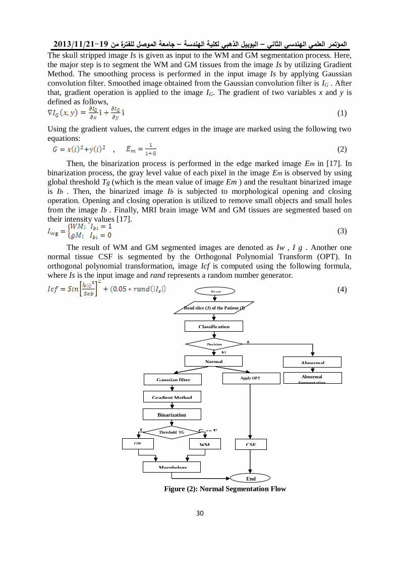
19/99/1192-91جامعة الموصل للفترة من –ليوبيل الذهبي لكلية الهندسة ا –الثاني لهندسي االعلمي المؤتمر
03
The skull stripped image Is is given as input to the WM and GM segmentation process. Here,
the major step is to segment the WM and GM tissues from the image Is by utilizing Gradient
Method. The smoothing process is performed in the input image Is by applying Gaussian
convolution filter. Smoothed image obtained from the Gaussian convolution filter is IG . After
that, gradient operation is applied to the image IG. The gradient of two variables x and y is
defined as follows,
(1)
Using the gradient values, the current edges in the image are marked using the following two
equations:
, (2)
Then, the binarization process is performed in the edge marked image Em in [17]. In
binarization process, the gray level value of each pixel in the image Em is observed by using
global threshold Tg (which is the mean value of image Em ) and the resultant binarized image
is Ib . Then, the binarized image Ib is subjected to morphological opening and closing
operation. Opening and closing operation is utilized to remove small objects and small holes
from the image Ib . Finally, MRI brain image WM and GM tissues are segmented based on
their intensity values [17].
(3)
The result of WM and GM segmented images are denoted as Iw , I g . Another one
normal tissue CSF is segmented by the Orthogonal Polynomial Transform (OPT). In
orthogonal polynomial transformation, image Icf is computed using the following formula,
where Is is the input image and rand represents a random number generator.
(4)
Figure (2): Normal Segmentation Flow
Chart
A
N
Start
Decision
L G or E
End
Read slice (J) of the Patient (I)
Classification
Normal
Gaussian filter Apply OPT
Abnormal
Abnormal
Segmentation
Gradient Method
Binarization
GM WM CSF
Morphology
Threshold TG
Selami: Automatic Segmentation of Normal and Pathological Tissues in …..
03
Sob represents the sum of the pixels that are greater than or equal to a threshold value
(100 is considered in this paper because the pixels minimum values are zeros and most of
their maximum values do not exceed 200, as 100 lies in the mid, therefore it is selected as a
threshold value), and the Icf represents the image that contains the CSF as a black color.
3.2.2 Pathological Tissue Segmentation
Pathological tissues such as tumor is segmented from the classified abnormal images by
combined two different methods:
Feed forward neural network (FFNN) as a classifier.
Otsu and K-mean clustering algorithms.
As first, the proposed hybrid method investigate a feed forward neural network as the
classifier to discriminate the tumor blocks from the non-tumor regions. In the selected brain
tumor slice, each of the slices of the subject dataset to be segmented is divided into non
overlapping equal sized square blocks of size 32*32 pixels. The features vector for each block
is calculated. The trained FFNN for the corresponding brain view is used to predict the
class labels for all the non-overlapping blocks. Particularly in each block, 5 features are
extracted namely, statistical features such as mean and variance, and multilevel 2D wavelet
decomposition features such as horizontal, vertical, diagonal bands of wavelet transform. The
feature vector of each block is.
Fb={Mb, Eb, Hb, Vb, Db} (5)
Mean and Variance features are extracted directly from each block, as below
Mb = (6)
Eb = 2 (7)
Where B is the 32*32 block in MRI abnormal image slices, N and M are number of
pixels available in rows and columns in blocks respectively.
To obtain the wavelet features, here "Haar" wavelet is applied to the block and
performed two levels of wavelet transform. After preformed the second level of wavelet
transform, three features are extracted (HL, LH and HH) from the result image. The
computation of these three features are described in the following equations:
Hb= (8)
Vb= (9)
Db= (10)
These feature values are used as the input vectors to the classifier. The output of the
classifier suggests presence/absence of tumor in a given block. Specifically, a classifier output
that is close to ‘one’ suggests a tumor block while the output that is close to ‘zero’ suggests
non-tumor block. The second stage of the proposed hybrid method is to extract tumor from a
detected tumor blocks. For this goal two segmentation algorithm are used:
1. The Otsu’s thresholding method: Otsu’s thresholding is viewed as a statistical decision
theory concept. The main goal of this method is to minimize the average error incurred in
assigning pixels to classes. This segmentation is based on the probability density function of
19/99/1192-91جامعة الموصل للفترة من –ليوبيل الذهبي لكلية الهندسة ا –الثاني لهندسي االعلمي المؤتمر
06
grey-levels of each class occurring in a given problem. The Otsu’s method aims at
maximizing the between-class variance. The basic idea is that well-thresholded classes should
be distinct with respect to the grey-level values of their pixels, and, conversely, that a
threshold giving the best separation between classes in terms of their intensity values would
be the optimum. The steps of the Otsu’s thresholding method as stated in [18] are as follows:
1. Compute the normalized histogram of the input image.
2. Compute the cumulative sums P(k) for k=0,1,2,...,L-1
3. Compute the cumulative means M(k) for k=0,1,2,...,L-1
4. Compute the global intensity mean MG
5. Compute the between-class variance for k=0,1,2,..., L-1
6. Obtain Otsu’s threshold k* as the value of k for which is maximum. If the
maximum is not unique, obtain k* by averaging the values of k corresponding to
the various maxima detected.
2. K-Means Clustering Algorithm: It is one of the simplest unsupervised learning
algorithms that solve the well known clustering problem. The procedure follows a simple and
easy way to classify a given data set through a certain number of clusters (assume k clusters)
fixed a priori. The main idea is to define k centroids, one for each cluster. These centroids are
placed at different location to cause different results. So, the better choice is to place them as
much as possible far away from each other. The next step is to take each point belonging to a
given data set and associate it to the nearest centroid [18]. When no point is pending, the first
step is completed and an early grouping is done. At this point we need to re-calculate k new
centroids as bar centre of the clusters resulting from the previous step. After we have these k
new centroids, a new binding has to be done between the same data set points and the nearest
new centroids. A loop has been generated. As a result of this loop we may notice that the k
centroids change their location step by step until no more changes are done. In other words
centroids do not move any more. Finally, this algorithm aims at minimizing an objective
function, in this case a squared error function.
(11)
Where is a chosen distance measure between a data point and the cluster centre
cj; an indicator of the distance of the N data points from their respective cluster centres. The
generalized algorithm is composed of the following steps:
1. Pick K cluster centres, either randomly or based on some trial and error.
2. Assign each pixel in the image to the cluster that minimizes the distance, pixel color
difference, intensity, texture, and location between the pixel and the cluster centre
3. Re-compute the cluster centres by averaging all of the pixels in the cluster.
4. Repeat steps 2 and 3 until convergence is attained (e.g. no pixels change clusters) A
drawback of the k-means algorithm is that the number of clusters k is an input
parameter. An inappropriate choice of k may yield poor results.
As shown in figure 2 and figure 3, the last stage in flow charts are morphological
operations that are useful in the representation and description of region shape, such as
boundaries, skeletons, etc. The basic idea in morphology is to convolve an image with a given
mask (known as the structuring element), and to binarize the result of the convolution using a
given function choices of convolution mask and binarization function that depends on a
particular morphological operator.
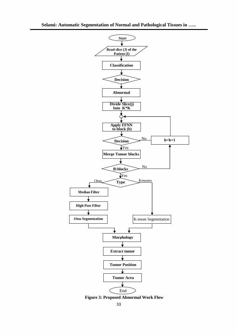
Selami: Automatic Segmentation of Normal and Pathological Tissues in …..
00
Figure 3: Proposed Abnormal Work Flow
Start
Decision
B:blocks
End
Read slice (J) of the
Patient (I)
Classification
Abnormal
Divide Slice(j) Into K*K
blocks
Morphology
Apply FFNN to block (b)
Decision
Yes
b=b+1 No
Merge Tumor blocks
Yes
No
Type
Median Filter
High Pass Filter
Otsu Segmentation
Otsu Kmeans
K-mean Segmentation
Extract tumor
Tumor Position
Tumor Area
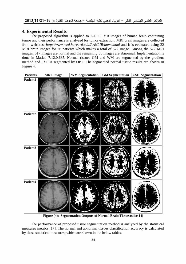
19/99/1192-91جامعة الموصل للفترة من –ليوبيل الذهبي لكلية الهندسة ا –الثاني لهندسي االعلمي المؤتمر
03
4. Experimental Results The proposed algorithm is applied to 2-D T1 MR images of human brain containing
tumor and their performance is analyzed for tumor extraction. MRI brain images are collected
from websites: http://www.med.harvard.edu/AANLIB/home.html and it is evaluated using 22
MRI brain images for 26 patients which makes a total of 572 image. Among the 572 MRI
images, 517 images are normal and the remaining 55 images are abnormal. Implementation is
done in Matlab 7.12.0.635. Normal tissues GM and WM are segmented by the gradient
method and CSF is segmented by OPT. The segmented normal tissue results are shown in
Figure 4.
Patients MRI image WM Segmentation GM Segmentation CSF Segmentation
Patient1
Patient2
Patient3
Patient4
Figure (4): Segmentation Outputs of Normal Brain Tissues(slice 14)
The performance of proposed tissue segmentation method is analyzed by the statistical
measures metrics [17]. The normal and abnormal tissues classification accuracy is calculated
by these statistical measures, which are shown in the below tables.
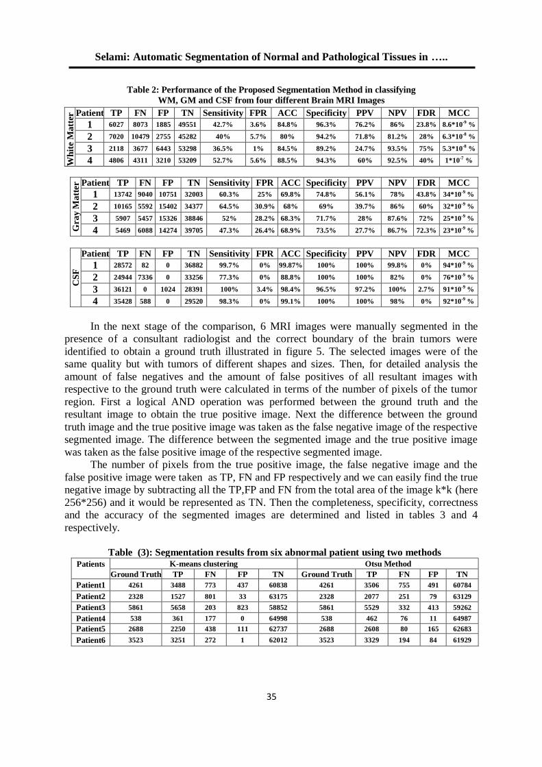
Selami: Automatic Segmentation of Normal and Pathological Tissues in …..
03
Gray M
att
er Patient TP FN FP TN Sensitivity FPR ACC Specificity PPV NPV FDR MCC
1 13742 9040 10751 32003 60.3% 25% 69.8% 74.8% 56.1% 78% 43.8% 34*10-9
%
2 10165 5592 15402 34377 64.5% 30.9% 68% 69% 39.7% 86% 60% 32*10-9
%
3 5907 5457 15326 38846 52% 28.2% 68.3% 71.7% 28% 87.6% 72% 25*10-9
%
4 5469 6088 14274 39705 47.3% 26.4% 68.9% 73.5% 27.7% 86.7% 72.3% 23*10-9
%
CS
F
Patient TP FN FP TN Sensitivity FPR ACC Specificity PPV NPV FDR MCC
1 28572 82 0 36882 99.7% 0% 99.87% 100% 100% 99.8% 0% 94*10-9
%
2 24944 7336 0 33256 77.3% 0% 88.8% 100% 100% 82% 0% 76*10-9
%
3 36121 0 1024 28391 100% 3.4% 98.4% 96.5% 97.2% 100% 2.7% 91*10-9
%
4 35428 588 0 29520 98.3% 0% 99.1% 100% 100% 98% 0% 92*10-9
%
In the next stage of the comparison, 6 MRI images were manually segmented in the
presence of a consultant radiologist and the correct boundary of the brain tumors were
identified to obtain a ground truth illustrated in figure 5. The selected images were of the
same quality but with tumors of different shapes and sizes. Then, for detailed analysis the
amount of false negatives and the amount of false positives of all resultant images with
respective to the ground truth were calculated in terms of the number of pixels of the tumor
region. First a logical AND operation was performed between the ground truth and the
resultant image to obtain the true positive image. Next the difference between the ground
truth image and the true positive image was taken as the false negative image of the respective
segmented image. The difference between the segmented image and the true positive image
was taken as the false positive image of the respective segmented image.
The number of pixels from the true positive image, the false negative image and the
false positive image were taken as TP, FN and FP respectively and we can easily find the true
negative image by subtracting all the TP,FP and FN from the total area of the image k*k (here
256*256) and it would be represented as TN. Then the completeness, specificity, correctness
and the accuracy of the segmented images are determined and listed in tables 3 and 4
respectively.
Table (3): Segmentation results from six abnormal patient using two methods
Patients
K-means clustering Otsu Method
Ground Truth TP FN FP TN Ground Truth TP FN FP TN
Patient1 4261 3488 773 437 60838 4261 3506 755 491 60784
Patient2 2328 1527 801 33 63175 2328 2077 251 79 63129
Patient3 5861 5658 203 823 58852 5861 5529 332 413 59262
Patient4 538 361 177 0 64998 538 462 76 11 64987
Patient5 2688 2250 438 111 62737 2688 2608 80 165 62683
Patient6 3523 3251 272 1 62012 3523 3329 194 84 61929
Table 2: Performance of the Proposed Segmentation Method in classifying
WM, GM and CSF from four different Brain MRI Images
Wh
ite
Matt
er Patient TP FN FP TN Sensitivity FPR ACC Specificity PPV NPV FDR MCC
1 6027 8073 1885 49551 42.7% 3.6% 84.8% 96.3% 76.2% 86% 23.8% 8.6*10-9
%
2 7020 10479 2755 45282 40% 5.7% 80% 94.2% 71.8% 81.2% 28% 6.3*10-8
%
3 2118 3677 6443 53298 36.5% 1% 84.5% 89.2% 24.7% 93.5% 75% 5.3*10-8
%
4 4806 4311 3210 53209 52.7% 5.6% 88.5% 94.3% 60% 92.5% 40% 1*10-7
%
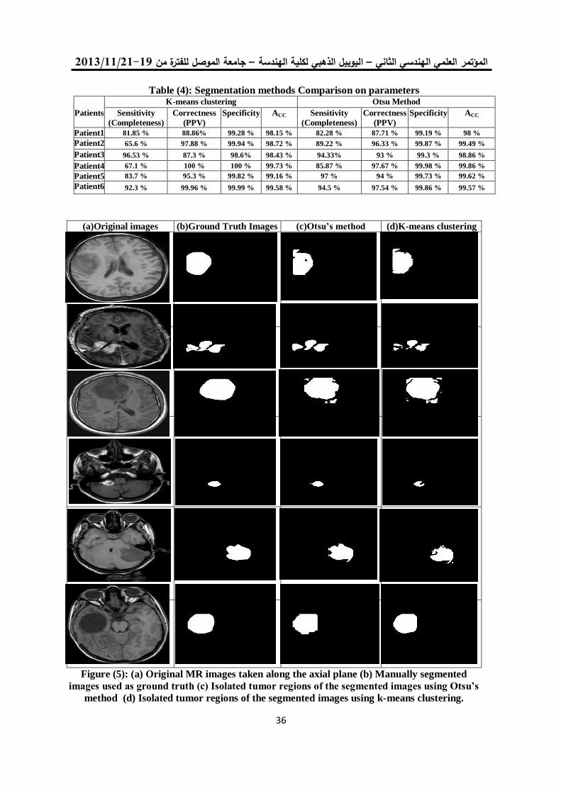
19/99/1192-91جامعة الموصل للفترة من –ليوبيل الذهبي لكلية الهندسة ا –الثاني لهندسي االعلمي المؤتمر
02
Table (4): Segmentation methods Comparison on parameters
Patients
K-means clustering Otsu Method
Sensitivity
(Completeness)
Correctness
(PPV)
Specificity ACC Sensitivity
(Completeness)
Correctness
(PPV)
Specificity ACC
Patient1 81.85 % 88.86% 99.28 % 98.15 % 82.28 % 87.71 % 99.19 % 98 %
Patient2 65.6 % 97.88 % 99.94 % 98.72 % 89.22 % 96.33 % 99.87 % 99.49 %
Patient3 96.53 % 87.3 % 98.6% 98.43 % 94.33% 93 % 99.3 % 98.86 %
Patient4 67.1 % 100 % 100 % 99.73 % 85.87 % 97.67 % 99.98 % 99.86 %
Patient5 83.7 % 95.3 % 99.82 % 99.16 % 97 % 94 % 99.73 % 99.62 %
Patient6 92.3 % 99.96 % 99.99 % 99.58 % 94.5 % 97.54 % 99.86 % 99.57 %
(a)Original images (b)Ground Truth Images (c)Otsu’s method (d)K-means clustering
Figure (5): (a) Original MR images taken along the axial plane (b) Manually segmented
images used as ground truth (c) Isolated tumor regions of the segmented images using Otsu’s
method (d) Isolated tumor regions of the segmented images using k-means clustering.
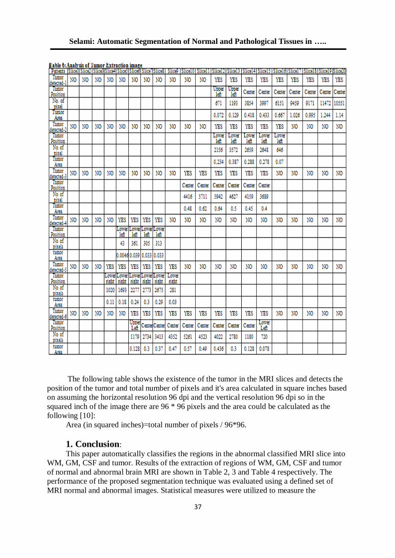
Selami: Automatic Segmentation of Normal and Pathological Tissues in …..
02
The following table shows the existence of the tumor in the MRI slices and detects the
position of the tumor and total number of pixels and it's area calculated in square inches based
on assuming the horizontal resolution 96 dpi and the vertical resolution 96 dpi so in the
squared inch of the image there are 96 * 96 pixels and the area could be calculated as the
following [10]:
Area (in squared inches)=total number of pixels / 96*96.
1. Conclusion:
This paper automatically classifies the regions in the abnormal classified MRI slice into
WM, GM, CSF and tumor. Results of the extraction of regions of WM, GM, CSF and tumor
of normal and abnormal brain MRI are shown in Table 2, 3 and Table 4 respectively. The
performance of the proposed segmentation technique was evaluated using a defined set of
MRI normal and abnormal images. Statistical measures were utilized to measure the
19/99/1192-91جامعة الموصل للفترة من –ليوبيل الذهبي لكلية الهندسة ا –الثاني لهندسي االعلمي المؤتمر
02
efficiency of the proposed tissue segmentation technique. Then, the performance of the
proposed segmentation technique was analyzed and compared with the traditional approach.
The comparative results have shown that the proposed technique has outperformed the
existing hybrid approach in terms of accuracy, specificity and sensitivity. Thus, the
performance of the proposed technique was clearly proved and understood from the
experimental results and analysis.
As the segmentation is applied based on both Otsu and K-Mean methods, results
designates that segmentation based on Otsu method gives better outcomes than working with
K-Mean, especially while working with normal tissues, but it needs and additional Median
and High pass filtering steps before it starts. Another conclusion was obvious while working
with normal tissues that is: CSF segmentation gives better results than the other two normal
tissues segmentation: WM and GM.
It is worth noting that working on T1 MRI images with high contrast makes it easier to
classify the image into normal and abnormal and then to detect the normal tissues and
abnormal tissues in the segmentation step, and that is way Otsu's method gives better results,
it is because of using high pass filter before starting. Also in WM and GM segmentation,
gradient operation is used, which enhances the contrast, to make the edges of different tissues
more obvious and thus better separation could be achieved.
References:
[1] S.J. Hussain, T. S. Savithri and P.V. Devi, "Segmentation of Tissues in Brain MRI
Images using Dynamic Neuro-Fuzzy Technique", International Journal of Soft Computing
and Engineering (IJSCE), ISSN: 2231-2307, Vol.1, No. 6, PP. 416-423, January 2012.
[2] J. J. Thiagarajan, K. N. ramamurthy, D. Jayaraman, J. thiagarajan, and Deepta,
"Kernel Sparse Models For Automated Tumor Segmentation", International Journal on
Artificial Intelligence Tools, Vol. 1, PP. 1:12 WSPC/Instruction File, March 12, 2013.
[3] J. Niea, Z. Xuea, T. Liua, G. S. Youngb, K. Setayeshb, L. Guoc and S. T. C. Wong,
"Automated brain tumor segmentation using spatial accuracy-weighted hidden Markov
Random Field", Computerized Medical Imaging and Graphics, Vol. 33, PP. 431–441, 2009.
[4] D. K. Kole and A. Halder "Automatic Brain Tumor Detection and Isolation of
Tumor Cells from MRI Images", International Journal of Computer Applications (0975 –
8887), Vol. 39, No.16, PP.26-30, February 2012..
[5] B. Vijayakumar, A. Chaturvedi, "Tumor Cut-Segmentation and Classification of
MR Images using Texture Features and Feed Forward Neural Networks", European Journal of
Scientific Research, ISSN 1450-216X, Vol. 85, No. 3, PP. 363 – 372, September, 2012.
[6] K. M. Iftekharuddin, S. Ahmed and J. Hossen, "Multiresolution texture models for
brain tumor segmentation in MRI", 33rd Annual International Conference of the IEEE EMBS,
Boston, Massachusetts USA, PP. 6985- 6988, August 30 - September 3, 2011.
[7] S. J. Hussain, C. Venkatesh, S. Asif hussain, L. Chetana and V. Gireesha,
"Segmentation of Normal and Pathological Tissues in MRI Brain Images Using Dual
Classifier", International Conference on Advancements in Information Technology with
workshop of ICBMG, IPCSIT, Chennai, Vol. 20, PP. 165-169, 8-9 December, 2011.
[8] S. A. Hussain and M. P. Raju, "Neuro-Fuzzy System for Medical Image
Processing", Proceedings of the International Conference on Communication and
Computational Intelligence – 2010, Kongu Engineering College, Perundurai, Erode, T.N.,
India, PP.382-385, 27 – 29 December,2010.
[9] W. Li, H. Huang, D. Zhang, H. Tang and C. Wang, "A Color Image Segmentation
Method Based on Automatic Seeded Region Growing", Proceedings of the IEEE International
Conference on Automation and Logistics, Jinan, China, PP. 1925-1929, August 18 - 21, 2007.
Selami: Automatic Segmentation of Normal and Pathological Tissues in …..
02
[10] M. K Kowar and S. Yadav, "Brain Tumor Detection and Segmentation Using
Histogram Thresholding", International Journal of Engineering and Advanced Technology
(IJEAT) ISSN: 2249 – 8958, Vol. 1, No. 4, PP.16-20, April 2012.
[11] F. Ajala, O. A. Oke, T. O. Adedeji, O.M. Alade and E.A. Adewusi, "Fuzzy k-c-
means Clustering Algorithm for Medical Image Segmentation", Journal of Information
Engineering and Applications, Vol. 2, No. 6, PP. 21-33, 2012.
[12] A. V. Gawand, P. Lokhande, S. daware and U. Kulkarni, "Image Segmentation for
Nature Images using K-Mean and Fuzzy C-Mean", International Conference on Recent
Trends in Information Technology and Computer Science (ICRTITCS), Proceedings
published in International Journal of Computer Applications (IJCA), PP.37- 40, 2011.
[13] C. Dwith, V. Angoth and A. Singh, "Wavelet Based Image Fusion for Detection of
Brain Tumor", Image, Graphics and Signal Processing, Vol. 1, PP. 25-31, 2013.
[14] A. H. Gondal, M. A. Khan, "A Review of Fully Automated Techniques for Brain
Tumor Detection From MR Images", Modern Education and Computer Science, Vol. 2,
PP.55-61, 2013.
[15] A. Ahirwar, "Study of Techniques used for Medical Image Segmentation and
Computation of Statistical Test for Region Classification of Brain MRI", Information
Technology and Computer Science, Vol. 5, PP.44-53, 2013.
[16] A.F. Mahmood and A. M. Abd-Alsalam, "Automatic Brian MRI Slices
Classification Using Hybrid Technique", accepted in Rafidain Engineering Journal.
[17] V. Sheejakumari and B. S. Gomathi, "Healthy and Pathological Tissues
Classification in MRI Brain Images using Hybrid Genetic Algorithm-Neural Network
(HGANN) Approach", European Journal of Scientific Research, Vol. 87, No. 2, PP. 212-226,
September, 2012.
[18] R. C. Gonzalez, R. E. Woods, "Digital Image Processing", Edn. 3, Pearson
Education. Prentice Hall, PP. 742-747, 2008.
19/99/1192-91جامعة الموصل للفترة من –اليوبيل الذهبي لكلية الهندسة –المؤتمر العلمي الهندسي الثاني
04
خوارزمية لتشفير الصورة الملونة باستخدام ترميز الحامض النووي
ونظرية الفوضىالدين حامد علي فخر
*مها بشير حسين
**
[email protected] [email protected]
لعراق.ا –* قسم هندسة الحاسوب/ كلية الهندسة / جامعة الموصل
العراق. –** قسم الهندسة الكهربائية/ كلية الهندسة/ جامعة الموصل
المستخلصيعد التشفير باستخدام الحامض النووي ونظرية الفوضى من االتجاهات الحديثة الواعدة في علم التعمية في الوقت
لما توفره حوسبة الحامض النووي من الحاضر, والتي تزايد استخدامها بشكل ملحوظ في السنوات القليلة الماضية وذلك
مزايا تجعلها مناسبة جدا الستخدامها في علم التعمية, ولالرتباط الوثيق الذي تم اكتشافه مؤخرا بين نظرية الفوضى وعلم
التعمية. في هذا البحث تم تقديم خوارزمية تشفير انسيابية للصورة الملونة باستخدام الخرائط الفوضوية لتغيير مواقع
يم النقاط الصورية ومن ثم استخدام سالسل الحامض النووي لتغيير قيم النقاط الصورية باستخدام تشفير سجل المرة وق
( والذي يعتبر غير قابل للكسر نظريا. تم تنفيذ الخوارزمية واجراء عدة تحليالت لقياس كفاءة وامنية OTPالواحدة )
بتت نتائج التجارب والتحليالت األمنية التي تم اجراؤها بأن (. اثMatLab R2011bالخوارزمية باستخدام برنامج )
الخوارزمية تمتلك كفاءة عالية وطول مفتاح وحساسية للتغيير فيه كافيين جدا لمقاومة هجوم القوة الوحشية, وامتالكها
ضلية.ألمنية تامة نتيجة الستخدام سجل المرة الواحدة وقابلية جيدة لمقاومة الهجمات االحصائية والتفا
الكلمات الدالة: التشفير االنسيابي, تشفير الحامض النووي, التشفير المتناظر, الدالة اللوجستية, سجل المرة الواحدة
(OTP.نظرية الفوضى ,)
Colored Image Encryption Algorithm Using DNA Code and Chaos Theory
Fakhrulddin H. Ali
* Maha Basher Hussein
**
[email protected] [email protected] * Dept. of Computer Engineering/ College of Engineering/ University of Mosul – IRAQ.
** Dept. of Electrical Engineering/ College of Engineering/ University of Mosul – IRAQ.
Abstract At recent time, Encryption using DNA computing and Chaos theory are from
modern promising research areas at the field of Cryptography. They are increasingly
used in the past few years, because of advantages of DNA computing that make it very
suitable for being used in Cryptography, and because of the close relationship between
Chaos theory and cryptography. In this paper a stream cipher algorithm for Image
Encryption has been proposed. The chaotic logistic map is used for confusing and
diffusing the Image pixels, and then a DNA sequence used as an OTP to change pixel
values. The algorithm has been implemented and several analysis has been done using
(MatLab R2011b) program, the analysis results proved that the proposed algorithm has
high efficiency, very sufficient key sensitivity and length to resist brute force attacks,
perfect security as a result of using OTP and good ability to resist statistical and
differential attacks.
Keywords: Chaos theory, DNA cryptography, Image Encryption, Logistic map, stream
cipher, symmetrical encryption, one time pad OTP.
م ترميز الحامض النووي ونظرية الفوضىخوارزمية لتشفير الصورة الملونة باستخداعلي:
04
المقدمة: -1
وزيادة تبادل رسائل الوسائط المتعددة إن التطور في شبكات الحاسوب وزيادة استخدام االنترنت في الوقت الحاضر
أدى الى االعتماد على هذه التقنيات في مختلف امور الحياة, إن توفير األمنية للمعلومات والصور الرقمية بشكل ملحوظ
المتبادلة متطلب ضروري لكل االستخدامات سواء كانت لألغراض السياسية أو الطبية او االقتصادية وحتى االستخدامات
حة واسعة لبحوث وخوارزميات تشفير الشخصية. ولكون الصور الرقمية تدخل في كل هذه المجاالت, تم توفير مسا
ية عن المعلومات النصية مثل كمية البيانات العالية الصورة الرقمية. نظرا للخواص التي تتميز بها معلومات الصورة الرقم
والترابط الوثيق بين معلومات الصورة وغيرها من الخواص التي تنفرد بها الصور الرقمية عن البيانات النصية باإلضافة
ى حاجة التطبيقات الصورية في بعض االحيان الى متطلبات اخرى مثل المعالجة في الزمن الحقيقي والدقة والحفاظ على ال
تنسيق الصورة مما يجعل طرق التشفير التقليدية صعبة التطبيق وبطيئة المعالجة بالنسبة للصور وصعوبة تحقيق هذه
فإن خوارزميات التشفير التقليدية غير مناسبة لتشفير الصور الرقمية, الية المطاليب مع تحقيق االمنية العالية والجودة الع
لذلك كان االتجاه الى نظريات وخوارزميات اخرى لتوفير مواصفات تشفير وأمنية عالية للصورة الرقمية. في السنوات
قتها الوثيقة مع علم التعمية, الماضية تم التوجه الى استخدام نظرية الفوضى في مجال التشفير لمزايا هذه النظرية وعال
حيث تمتاز بحساسيتها العالية للتغيير في القيم االبتدائية وسهولة توليد قيمها, والحصول على قيم عشوائية مشابهة
. منذ أن قامت العالمة جيسيكا فردريك باقتراح نظام تشفير للصور باستخدام النظرية الفوضوية عام [1]للضوضاء منها
حوث تتوالى في مجال تشفير الصورة باستخدام نظرية الفوضى. ومنذ بضع سنين يتم دمج هذه النظرية مع والب[2] 7991
للحصول على انظمة ( DNA Computingاستخدام تشفير الحامض النووي المعتمد على حوسبة الحامض النووي )
والذي 7991عالم ليونارد ادلمان عام وخوارزميات تشفير فعالة. كانت البداية لعلم حوسبة الحامض النووي مع بحث ال
استطاع فيه باستخدام شرائط الحامض النووي والعمليات البيولوجية الجزيئية بحل مشكلة الرجل الرحالة بين سبعة مدن
وبعمله هذا فتح آفاقا جديدة لعلم الحوسبة فائقة السرعة وهائلة التوازي وبمستوى عال جدا من التعقيد نظرا للخواص [3]
ي تمتلكها سالسل الحامض النووي, تم استخدام حوسبة الحامض النووي في مجاالت عديدة منها حل المسائل الصعبة الت
والتي ال يمكن حلها نظرا لمحدودية الوقت او الموارد, فقد استخدمت هذه النظرية في مجال خزن المعلومات نظرا لسعة
واستخدمت ايضا في جميع مجاالت علم التعمية كاإلخفاء والتشفير الخزن الهائلة التي تمتلكها شرائط الحامض النووي,
بتقديم [4]قام الباحثون في المصدر 7991وتوليد المفاتيح وادارتها وتحليل خوارزميات التشفير وكسرها , ففي عام
عمليات تم استخدام ال 0222( المعروفة باستخدام حوسبة الحامض النووي, وفي عام DESطريقة لكسر خوارزمية )
باستخدام تشفير الحامض النووي وتم اقتراح طريقتين لتشفير الصورة فضال عن طريقة إلخفاء البيولوجية لتشفير الصور
فقد قدموا خوارزميات لتشفير [6 – 13]. أما الباحثون في المصادر [5]المعلومات ضمن شرائط الحامض النووي
وذلك بدمج النظرية الفوضوية مع التشفير باستخدام الحامض النووي, وذلك باستخدام خرائط فوضوية مختلفة الصورة
وخواص وعمليات مختلفة للحامض النووي , كاستخدام طريقة جمع وطرح القواعد النيتروجينية, او استخدام دالة أو
خرى معتمدة على اسس العمليات البيولوجية, ومن ( بين هذه القواعد, او استخدام خواص اXOR Functionالحصرية )
ثم قاموا بتحليل خواص الخوارزميات المقترحة ومدى مناعتها لعدة انواع من الهجمات والتحليالت. في هذا البحث قــ دمت
(OTP: One Time Pad Cipherخوارزمية تشفير انسيابية للصورة الملونة باالعتماد على شفرة سجل المرة الواحدة )
والذي يعتبر غير قابل للكسر نظريا وذلك باستخدام سالسل الحامض النووي والخرائط الفوضوية.
:الجزء النظري-1المرة التفاصيل عن الحامض النووي وتشفير الحامض النووي, وعن التشفير باستخدام سجل هذا القسم يحوي بعض
.الواحدة والدالة الفوضوية المستخدمة في الخوارزمية المقترحة
تتكون سلسلة الحامض النووي من سلسلتين متممتين ألحدهما اآلخر, وتتكون هذه :ترميز الحامض النووي .2-1
Guanine(, الكوانين )Cytosine C( , السايتوسين )Adenine Aالسالسل من اربع قواعد نيتروجينية هي : االدنين )
G( الثايمين ,)Thymine T يرتبط األدنين في أحد الشريطين مع الثايمين في الشريط اآلخر, أي يكون االدنين متمما .)
. (1كما في الشكل ) للثايمين, وكذلك الحال بالنسبة للسايتوسين والكوانين
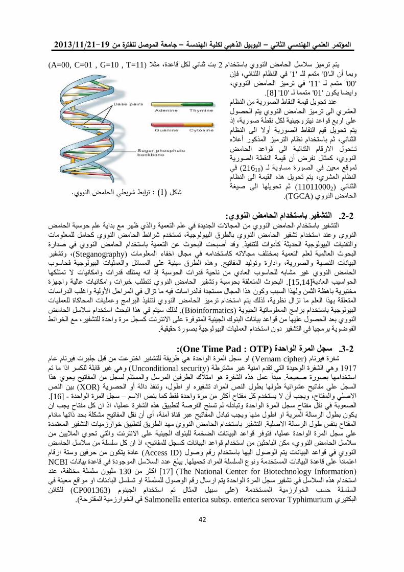
19/99/1192-91جامعة الموصل للفترة من –اليوبيل الذهبي لكلية الهندسة –المؤتمر العلمي الهندسي الثاني
04
(A=00, C=01 , G=10 , T=11بت ثنائي لكل قاعدة, مثال ) 0النووي باستخدام يتم ترميز سالسل الحامض
في النظام الثنائي, فإن '1'متمم للـ '0'وبما أن الـ
في ترميز الحامض النووي, '11'متمم لـ '00'
.[8] '10'متمما لـ '01'وايضا يكون
عند تحويل قيمة النقاط الصورية من النظام
العشري الى ترميز الحامض النووي يتم الحصول
على اربع قواعد نيتروجينية لكل نقطة صورية, إذ
يتم تحويل قيم النقاط الصورية أوال الى النظام
الثنائي, ثم باستخدام نظام الترميز المذكور أعاله
الحامض تــ حول االرقام الثنائية الى قواعد
النووي, كمثال نفرض أن قيمة النقطة الصورية
( في 21610لموقع معين في الصورة مساوية لـ )
النظام العشري, يتم تحويل هذه القيمة الى النظام
ثم تحويلها الى صيغة (110110002الثنائي )
(.TGCAالحامض النووي )
التشفير باستخدام الحامض النووي: .2-2التشفير باستخدام الحامض النووي من المجاالت الجديدة في علم التعمية والذي ظهر مع بداية علم حوسبة الحامض
كحامل للمعلومات شرائط الحامض النووي وعند استخدام تشفير الحامض النووي بالطرق البيولوجية, تستخدمالنووي
حت البحوث عن التعمية باستخدام الحامض النووي في صدارة والتقنيات البيولوجية الحديثة كأدوات للتنفيذ. وقد أصب
(, وتشفير Steganographyاخفاء المعلومات )ختلف مجاالته كاستخدامه في مجال البحوث العالمية لعلم التعمية بم
حاسوب وتوليد المفاتيح. وهذه الطرق مبنية على المسائل والعمليات البيولوجية فالبيانات النصية والصورية, وادارة
الحامض النووي غير مشابه للحاسوب العادي من ناحية قدرات الحوسبة إذ انه يمتلك قدرات وامكانيات ال تمتلكها
. البحوث المتعلقة بحوسبة وتشفير الحامض النووي تتطلب خبرات وامكانيات عالية واجهزة [15,14]الحواسيب العادية
مختبرية باهظة الثمن ولهذا السبب وكون هذا المجال مستجدا فالدراسات فيه ما تزال في المراحل األولية واغلب الدراسات
النووي لتنفيذ البرامج وعمليات المحاكاة للعمليات يتم استخدام ترميز الحامضالمتعلقة بهذا العلم ما تزال نظرية, لذلك
(. لذلك سيتم في هذا البحث استخدام سالسل الحامض Bioinformaticsالبيولوجية باستخدام برامج المعلوماتية الحيوية )
, مع الخرائط النووي بعد الحصول عليها من قواعد بيانات البنوك الجينية المتوفرة على االنترنت كسجل مرة واحدة للتشفير
الفوضوية برمجيا في التشفير دون استخدام العمليات البيولوجية بصورة حقيقية.
(:One Time Pad : OTPسجل المرة الواحدة ) .2-3عام سجل المرة الواحدة هي طريقة للتشفير اخترعت من قبل جلبرت فيرنام ( او Vernam cipherشفرة فيرنام )
( وهي غير قابلة للكسر اذا ما تم Unconditional securityم امنية غير مشترطة )وهي الشفرة الوحيدة التي تقد 7971
استخدامها بصورة صحيحة. مبدأ عمل هذه الشفرة هو امتالك الطرفين المرسل والمستلم لسجل من المفاتيح يحوي هذا
بين النص ((XORوتنفذ دالة أو الحصرية السجل على مفاتيح عشوائية طولها بطول النص المراد تشفيره او اطول,
. [16] -سجل المرة الواحدة – مرة واحدة فقط كما ينص االسمأكثر من كل مفتاح االصلي والمفتاح, ويجب أن ال يستخدم
عمليا, اذ ان كل مفتاح يجب ان ادله لم تسنح الفرصة لتطبيق هذه الشفرة الصعوبة في نقل مفتاح سجل المرة الواحدة وتب
كون بطول الرسالة السرية او اطول منها ويجب تبادل المفاتيح عبر قناة آمنة, أي أن نقل المفاتيح مشكلة بحد ذاتها مادام ي
التشفير المعتمدة خوارزمياتالمفتاح بنفس طول الرسالة االصلية. التشفير باستخدام الحامض النووي مهد الطريق لتطبيق
ر قواعد البيانات الضخمة للبنوك الجينية على االنترنت والتي تحوي الماليين من عمليا, فتوفعلى سجل المرة الواحدة
سالسل الحامض النووي, مكن الباحثين من استخدام قواعد البيانات كسجل للمفاتيح, اذ ان كل سلسلة من سالسل الحامض
ة يتكون من حرفين وستة ارقام ( عادAccess IDالنووي في قواعد البيانات يتم الوصول اليها باستخدام رقم وصول )
NCBI اعتمادا على قاعدة البيانات المستخدمة ونوع السلسلة المراد تحميلها. يبلغ عدد السالسل الموجودة في قاعدة بيانات
(The National Center for Biotechnology Information )[17] مليون سلسلة مختلفة, عند 130اكثر من
او تسلسل البادئات او مواقع معينة في ي تشفير سجل المرة الواحدة يتم ارسال رقم الوصول للسلسلةاستخدام هذه السالسل ف
للكائن ((CP001363 الجينوم)على سبيل المثال تم استخدام السلسلة حسب الخوارزمية المستخدمة
في الخوارزمية المقترحة(. Salmonella enterica subsp. enterica serovar Typhimuriumالبكتيري
ترابط شريطي الحامض النووي.: ( 1شكل )
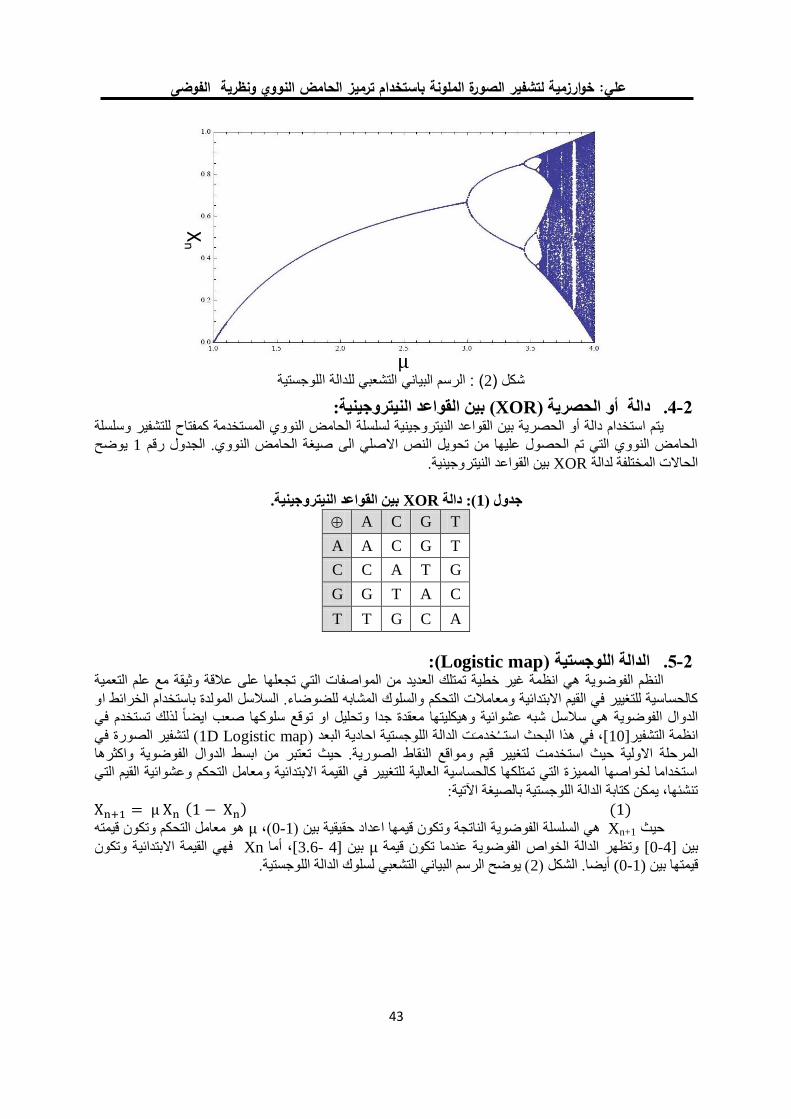
م ترميز الحامض النووي ونظرية الفوضىخوارزمية لتشفير الصورة الملونة باستخداعلي:
04
:النيتروجينيةبين القواعد (XORأو الحصرية ) دالة .2-4يتم استخدام دالة أو الحصرية بين القواعد النيتروجينية لسلسلة الحامض النووي المستخدمة كمفتاح للتشفير وسلسلة
يوضح 1الحامض النووي التي تم الحصول عليها من تحويل النص االصلي الى صيغة الحامض النووي. الجدول رقم
.بين القواعد النيتروجينية XORالحاالت المختلفة لدالة
بين القواعد النيتروجينية. XORدالة (:1)جدول
T G C A
T G C A A
G T A C C
C A T G G
A C G T T
(:Logistic mapالدالة اللوجستية ) .2-5النظم الفوضوية هي انظمة غير خطية تمتلك العديد من المواصفات التي تجعلها على عالقة وثيقة مع علم التعمية
والسلوك المشابه للضوضاء. السالسل المولدة باستخدام الخرائط او كالحساسية للتغيير في القيم االبتدائية ومعامالت التحكم
وهيكليتها معقدة جدا وتحليل او توقع سلوكها صعب ايضا لذلك تستخدم في عشوائية الدوال الفوضوية هي سالسل شبه
( لتشفير الصورة في 1D Logistic map , في هذا البحث استــ خدمـ ت الدالة اللوجستية احادية البعد )[10]انظمة التشفير
الدوال الفوضوية واكثرها خدمت لتغيير قيم ومواقع النقاط الصورية. حيث تعتبر من ابسطالمرحلة االولية حيث است
استخداما لخواصها المميزة التي تمتلكها كالحساسية العالية للتغيير في القيمة االبتدائية ومعامل التحكم وعشوائية القيم التي
تنشئها, يمكن كتابة الدالة اللوجستية بالصيغة اآلتية:
( ) ( ) هو معامل التحكم وتكون قيمته (, 1-0هي السلسلة الفوضوية الناتجة وتكون قيمها اعداد حقيقية بين ) Xn+1حيث
وتكون فهي القيمة االبتدائية Xn , أما [4 -3.6]بين وتظهر الدالة الخواص الفوضوية عندما تكون قيمة [4-0]بين
( يوضح الرسم البياني التشعبي لسلوك الدالة اللوجستية.2أيضا. الشكل ) (1-0) قيمتها بين
μ
Xn
اللوجستية للدالة التشعبي البياني الرسم: ( 2) شكل
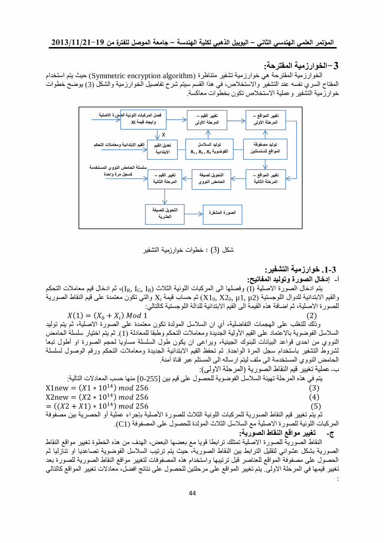
19/99/1192-91جامعة الموصل للفترة من –اليوبيل الذهبي لكلية الهندسة –المؤتمر العلمي الهندسي الثاني
00
الخوارزمية المقترحة:-2( حيث يتم استخدام Symmetric encryption algorithmالخوارزمية المقترحة هي خوارزمية تشفير متناظرة )
( يوضح خطوات 3المفتاح السري نفسه عند التشفير واالستخالص, في هذا القسم سيتم شرح تفاصيل الخوارزمية والشكل )
خوارزمية التشفير وعملية االستخالص تكون بخطوات معاكسة.
. خوارزمية التشفير:3-1 :الصورة وتوليد المفاتيحإدخال -أ
(, ثم ادخال قيم معامالت التحكم IR, IG, IB( وفصلها الى المركبات اللونية الثالث )Iيتم ادخال الصورة االصلية )
والتي تكون معتمدة على قيم النقاط الصورية Xi( ثم حساب قيمة X10, X20, µ1, µ2يم االبتدائية للدوال اللوجستية )والق
للصورة االصلية, ثم اضافة هذه القيمة الى القيم االبتدائية للدالة اللوجستية كالتالي:
( ) ( ) ( ) التفاضلية, أي ان السالسل المولدة تكون معتمدة على الصورة االصلية, ثم يتم توليد الهجماتوذلك للتغلب على
سلسلة الحامض (. ثم يتم اختيار 1السالسل الفوضوية باالعتماد على القيم األولية الجديدة ومعامالت التحكم وطبقا للمعادلة )
الجينية, ويراعى ان يكون طول السلسلة مساويا لحجم الصورة او أطول تبعا النووي من احدى قواعد البيانات للبنوك
لشروط التشفير باستخدام سجل المرة الواحدة. ثم تحفظ القيم االبتدائية الجديدة ومعامالت التحكم ورقم الوصول لسلسلة
الحامض النووي المستخدمة الى ملف ليتم ارساله الى المستلم عبر قناة آمنة.
غيير قيم النقاط الصورية )المرحلة االولى(:عملية ت -ب
منها حسب المعادالت التالية: [255-0]يتم في هذه المرحلة تهيئة السالسل الفوضوية للحصول على قيم بين
( ) ( ) ( ) ( ) (( ) ) ( )
رة األصلية بإجراء عملية أو الحصرية بين مصفوفة ثم يتم تغيير قيم النقاط الصورية للمركبات اللونية الثالث للصو
.C1)للحصول على المصفوفة ) لمولدةالمركبات اللونية للصورة االصلية مع السالسل الثالث ا
تغيير مواقع النقاط الصورية: -جالنقاط الصورية للصورة االصلية تمتلك ترابطا قويا مع بعضها البعض, الهدف من هذه الخطوة تغيير مواقع النقاط
تصاعديا او تنازليا ثم الصورية بشكل عشوائي لتقليل الترابط بين النقاط الصورية, حيث يتم ترتيب السالسل الفوضوية
الحصول على مصفوفة المواقع للعناصر قبل ترتيبها واستخدام هذه المصفوفات لتغيير مواقع النقاط الصورية للصورة بعد
. يتم تغيير المواقع على مرحلتين للحصول على نتائج افضل, معادالت تغيير المواقع كالتالي تغيير قيمها في المرحلة االولى
:
X
Xi
–
X1 , X2 , X3
X1 , X2
–
–
–
طوا وار مي التش ير : (3شكل )
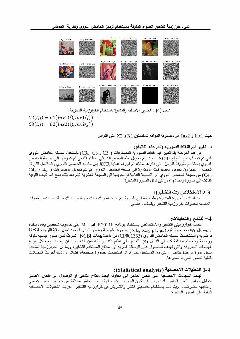
م ترميز الحامض النووي ونظرية الفوضىخوارزمية لتشفير الصورة الملونة باستخداعلي:
04
( ) ( ( ) ( ))
( ) ( ( ) ( ))
على التوالي. X2و X1هي مصفوفة المواقع للسلسلتين Inx2و Inx1حيث
تغيير قيم النقاط الصورية )المرحلة الثانية(: -د
لة الحامض النووي باستخدام سلس (C3R, C3G, C3Bفي هذه المرحلة يتم تغيير قيم النقاط الصورية للمصفوفات )
, حيث يتم تحويل هذه المصفوفات الى النظام الثنائي ثم تحويلها الى صيغة الحامض NCBIالتي تم تحميلها من الموقع
بين سلسلة الحامض النووي والسالسل التي تم XORالنووي باستخدام طريقة الترميز التي ذكرها سابقا, ثم اجراء عملية
,C4R, C4Gثم يتم تحويل المصفوفات )لمذكورة الى صيغة الحامض النووي. من تحويل المصفوفات ا الحصول عليها
C4B من صيغة الحامض النووي الى الصيغة الثنائية ثم تحويلها الى الصيغة العشرية ليتم بعد ذلك دمج المركبات اللونية )
( والتي تمثل الصورة المشفرة.Cالثالث الى صورة واحدة )
االستخالص )فك التشفير(: 3-2بعد استالم الصورة المشفرة وملف المفاتيح السرية يتم استخدامها الستخالص الصورة االصلية باستخدام العمليات
.وبتسلسل عكسي العكسية لخطوات خوارزمية التشفير
النتائج والتحليالت:-4يعمل بنظام على حاسوب شخصي MatLab R2011b نـ فذت خوارزميتي التشفير واالستخالص باستخدام برنامج
Windows 7( تم اختيار قيم ,X10, X20, µ1, µ2 بصورة عشوائية وضمن المدى المحدد لعمل الدالة اللوجستية كدالة )
شفرت ثمان صور قياسية ملونة . NCBI من قاعدة بيانات (CP001363سلسلة الحامض النووي ) واستــ خد مت فوضوية
للحكم على نظام التشفير بأنه آمن فإنه يجب ان يصمد بوجه كل انواع (.4مختلفة كما في الشكل ) ورمادية وبأحجام
الهجمات المعروفة والتي تهدف للحصول على الرسالة السرية او المفتاح المستخدم للتشفير, وبما أن الخوارزمية تستخدم
دمت بصورة صحيحة, فضال عن ذلك أجريت التحليالت سجل المرة الواحدة للتشفير والتي من المستحيل كسرها اذا استخ
التالية للصور التي تم تشفيرها.
(:Statistical analysis) التحليالت االحصائية 4-1ايجاد مفتاح التشفير او الوصول الى النص االصلي تهدف الهجمات االحصائية على النص المشفر الى محاولة
بتحليل خواص النص المشفر, لذلك يجب أن تكون الخواص االحصائية للنص المشفر مختلفة عن خواص النص االصلي
ومشابهة للضوضاء, ويتم ذلك باستخدام خاصيتي النشر والتشويش في خوارزمية التشفير. أجريت التحليالت االحصائية
على الصور المشفرة:التالية
الصور األصلي والمش رة باست دام ال وار مي المقترح .: ( 4شكل )
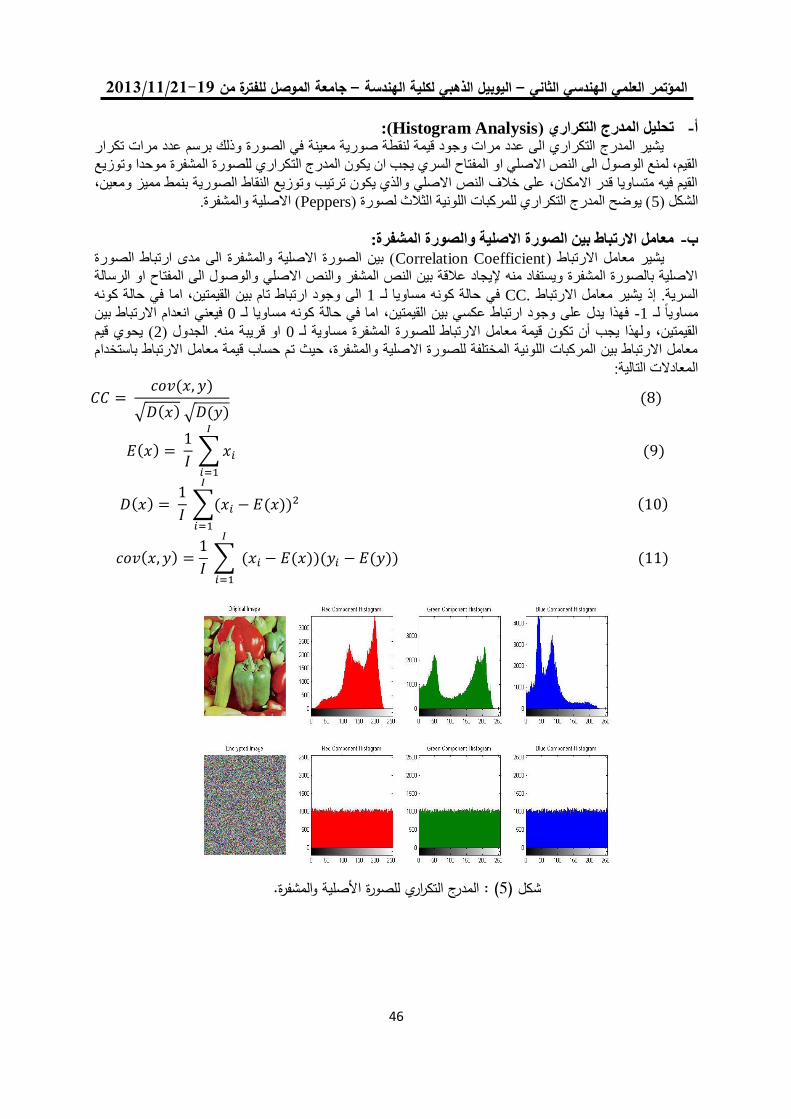
19/99/1192-91جامعة الموصل للفترة من –اليوبيل الذهبي لكلية الهندسة –المؤتمر العلمي الهندسي الثاني
04
(:Histogram Analysis) تحليل المدرج التكراري -أفي الصورة وذلك برسم عدد مرات تكرار يشير المدرج التكراري الى عدد مرات وجود قيمة لنقطة صورية معينة
موحدا وتوزيع القيم, لمنع الوصول الى النص االصلي او المفتاح السري يجب ان يكون المدرج التكراري للصورة المشفرة
القيم فيه متساويا قدر االمكان, على خالف النص االصلي والذي يكون ترتيب وتوزيع النقاط الصورية بنمط مميز ومعين,
( االصلية والمشفرة.Peppers( يوضح المدرج التكراري للمركبات اللونية الثالث لصورة )5الشكل )
معامل االرتباط بين الصورة االصلية والصورة المشفرة: -ب( بين الصورة االصلية والمشفرة الى مدى ارتباط الصورة Correlation Coefficientيشير معامل االرتباط )
االصلية بالصورة المشفرة ويستفاد منه إليجاد عالقة بين النص المشفر والنص االصلي والوصول الى المفتاح او الرسالة
في حالة كونه الى وجود ارتباط تام بين القيمتين, اما 1في حالة كونه مساويا لـ .CCالسرية. إذ يشير معامل االرتباط
فيعني انعدام االرتباط بين 0فهذا يدل على وجود ارتباط عكسي بين القيمتين, اما في حالة كونه مساويا لـ 1- مساويا لـ
( يحوي قيم 2جدول )الاو قريبة منه. 0القيمتين, ولهذا يجب أن تكون قيمة معامل االرتباط للصورة المشفرة مساوية لـ
م حساب قيمة معامل االرتباط باستخدام تمعامل االرتباط بين المركبات اللونية المختلفة للصورة االصلية والمشفرة, حيث
المعادالت التالية:
( )
√ ( ) √ ( ) ( )
( )
∑
( )
( )
∑( ( ))
( )
( )
∑ ( ( ))( ( )) ( )
والمش رة.المدرج التكراري للصورة األصلي : ( 5شكل )
م ترميز الحامض النووي ونظرية الفوضىخوارزمية لتشفير الصورة الملونة باستخداعلي:
04
المركبات اللونية المختلفة للصور االصلية والمشفرة.قيم معامل االرتباط بين (:2)جدول
تشير النتائج الى أن قيمة معامل االرتباط بين الصورة األصلية والمشفرة قليلة جدا )مساوية للصفر تقريبا( وهذا يدل
أو استنتاج عالقة بين على انعدام االرتباط بين الصورتين , أي صعوبة الوصول الى الصورة األصلية من الصورة المشفرة االرتباط بين الصورة األصلية والمشفرة. تحليل باستخدام الهجمات االحصائية المعتمدة علىالصورتين
االرتباط بين النقاط الصورية المتجاورة: -جتمتلك الصورة الرقمية ارتباطا وثيقا بين قيم نقاطها الصورية المتجاورة افقيا وعموديا وقطريا, ويجب تقليل وفك هذا االرتباط لمنع استنتاج عالقة بين النقاط الصورية المتجاورة وكيفية ترتيبها, لذلك يجب ان تكون قيمة معامل االرتباط بين
زوج عشوائي من النقاط 5000( يبين قيم معامل االرتباط لـ 3. الجدول )0و قريبة من النقاط الصورية المتجاورة مساوية ا( يوضح كيفية توزيع النقاط الصورية للـ 6الصورية المتجاورة افقيا وعموديا وقطريا للصورة االصلية والمشفرة. والشكل )
ألصلية والمشفرة.( اCameramanزوج من النقاط الصورية المختارة بشكل عشوائي لصورة ) 5000
قيم معامل االرتباط بين النقاط الصورية المتجاورة للصورة االصلية والمشفرة. (:3)جدول
الحجم الصورةCRR
* 10-3
CRG
* 10-3
CRB
* 10-3
CGR
* 10-3
CGG
* 10-3
CGB
* 10-3
CBR
* 10-3
CBG
* 10-3
CBB
* 10-3
الصورة
*كاملة
10-3
Girl
.Bmp
720*576
*3 -0.234 0.562 1.414 1.137 0.924 0.380 1.858 0.408 0.035 0.138
Pepper
.Bmp
512*512
*3 -0.068 0.636 1.370 -1.232 2.104 0.442 -0.381 1.237 1.860 1.871
Fruits
.Bmp
512*480
*3 -3.124 0.316 0.862 -2.915 -0.010 -0.106 -2.558 0.286 -0.358 -1.834
Flowers
.Bmp
500*362
*3 -0.444 -0.091 3.624 -1.202 -1.084 6.135 -1.155 -1.870 2.081 0.137
Lenna
.Tif
256*256
*3 -3.531 2.671 5.662 -1.932 3.762 2.625 -1.590 1.814 0.038 1.343
Airplane.Bmp 1024
*1024 -- -- -- -- -- -- -- -- -- 0.266
Boats
.Bmp
720
*576 -- -- -- -- -- -- -- -- -- 2.304
Cameraman.tif 512
*512 -- -- -- -- -- -- -- -- -- -1.420
Girl Pepper Fruits Flowers Lenna Airplane Boats Cameraman
رحم
ألي ا
ونب الل
ركالم
ةصلي
ألرة ا
وص
ال
0.9822 0.9687 0.9642 0.9582 0.9758 0.9936 0.9624 0.9811 أفقي
0.9902 0.9737 0.9477 0.9771 0.9726 0.9928 0.9678 0.9885 عمودي
0.9750 0.9474 0.9446 0.9332 0.9545 0.9862 0.9587 0.9724 قطري
رة وص
ال
رةشف
الم 0.00001 0.0074 0.0021- 0.0013- 0.0043 0.0017 0.0070- 0.0016 أفقي
0.0054 0.0067 0.0015- 0.0012- 0.0124- 0.0098 0.0041 0.0069 عمودي
0.0073- 0.0016 0.00008- 0.0073- 0.0085- 0.0120- 0.0039- 0.0117 قطري
رض
خأل
ي اون
ب اللرك
المرة
وص
ال
ةصلي
ألا
-- -- -- 0.9420 0.9574 0.9859 0.9821 0.9833 أفقي
-- -- -- 0.9688 0.9504 0.9841 0.9835 0.9907 عمودي
-- -- -- 0.9179 0.9204 0.9666 0.9709 0.9770 قطري
رة وص
ال
رةشف
الم -- -- -- 0.0088 0.0025- 0.0039- 0.0092- 0.0062 أفقي
-- -- -- 0.0106 0.0009 0.0045 0.0030 0.0039- عمودي
-- -- -- 0.0068 0.0095- 0.0220- 0.0012- 0.0031 قطري
قرزألي ا
ونب الل
ركالم
رة وص
ال
ةصلي
ألا
-- -- -- 0.9213 0.9564 0.9308 0.9687 0.9841 أفقي
-- -- -- 0.9493 0.9510 0.9195 0.9686 0.9907 عمودي
-- -- -- 0.8946 0.9221 0.8479 0.9510 0.9783 قطري
رة وص
ال
رةشف
الم
-- -- -- 0.0115 0.0009- 0.0064 0.0142- 0.0038- أفقي
-- -- -- 0.0058- 0.0115- 0.0011- 0.0007 0.0045- عمودي
-- -- -- 0.0012- 0.0097 0.0004- 0.0092 0.0003 قطري
19/99/1192-91جامعة الموصل للفترة من –اليوبيل الذهبي لكلية الهندسة –المؤتمر العلمي الهندسي الثاني
04
انتروبية المعلومات: -دانتروبية المعلومات للصورة يحدد كيفية توزيع قيم النقاط الصورية, أي احتمالية وجود كل قيمة, وبمعنى آخر
العشوائي يكون توزيع القيم باحتماليات متساوية. يمكن حساب انتروبية المعلومات مقياس لعشوائية النظام, في النظام
انتروبية المعلومات من المعادلة التالية:
( ) ∑ ( ) [ ( )]
( )
, اذا فرضنا ان النظام عشوائي كليا, فستكون قيمة انتروبية miهي احتمالية وجود العنصر ( ) حيث أن
وهي القيمة المثالية. لذلك يجب ان تكون قيمة انتروبية المعلومات للصورة المشفرة قريبة من القيمة 8المعلومات مساوية لـ
االصلية والمشفرة نالحظ ان انتروبية المعلومات للصور المشفرة ( قيم انتروبية المعلومات للصور 4المثالية, في الجدول )
قريبة جدا من القيمة المثالية.
.قيم انتروبية المعلومات للصورة االصلية والمشفرة (:4)جدول
(:Key space analysis. تحليل مساحة المفتاح )4-2فإن امنية نظام التشفير يجب ان يكون معتمدا على المفتاح بصورة رئيسية, [18]حسب قوانين كيركوف في التشفير
(, وحسب Brute Force Attacksلذلك يجب أن يكون طول مفتاح التشفير كافيا لمنع نجاح هجمات القوة الوحشية )
2سرعة الحواسيب الموجودة في الوقت الحالي يجب ان ال يكون طول المفتاح اقل من 100
((100 bit لتوفير األمنية ضد
, مساحة المفتاح للخوارزمية هو العدد الكلي للمفاتيح المستخدمة للتشفير, في الخوارزمية [19]هجمات القوة الوحشية
المقترحة توجد خمس مفاتيح, اربعة منها تابعة للقيم االبتدائية ومعامالت التحكم للدوال اللوجستية, اما الخامس فهو سلسلة
10لى فرض أن دقة كل مفتاح من المفاتيح االربعة االولى مساوي لـ الحامض النووي. ع-14
سلسلة الحامض فضال عن
2النووي والتي يبلغ طولها )n
يمثل حاصل ضرب بعدي الصورة nهو طول الرسالة االصلية وبالنسبة للصورة n( حيث
ل المفتاح النهائي مساويا لـ:للصورة الملونة, فيكون طو 3للصورة الرمادية, وحاصل ضرب بعدي الصورة *
(:Key Sensitivity analysis. تحليل حساسية المفتاح )4-3اضافة الى امتالك المفتاح لمساحة واسعة لمقاومة هجوم القوة الوحشية , يجب أن تكون الخوارزمية حساسة للتغيير
ان تغيير صغير جدا في المفتاح يولد نص مشفر مختلف عن النص الذي تم توليده قبل تغيير الصغير في قيمة المفتاح, أي
المفتاح او التغيير الصغير في المفتاح يؤدي الى فشل استرجاع الصورة. أجريت التحليالت التالية إلثبات حساسية
الخوارزمية للتغيير الصغير في قيمة المفاتيح السرية:
( وتم µ1=3.9, µ2=3.75 ( باستخدام القيم االبتدائية )3*512*512( بحجم )Peppers ش فرت صورة ) -أ
(.B .7الحصول على الصورة في الشكل )
10 - 3.9الى ) µ1تم تغيير قيمة -ب-14
( مع ثبوت قيم المفاتيح االخرى, وتم الحصول على الصورة المشفرة في
(.D .7الشكل )( وتم ايجاد الفرق بين الصورتين في C .7الشكل )
تم استخالص الصورة االصلية من الصورة المشفرة باستخدام المفتاح الصحيح والحصول على الصورة في -ج
( وهي مطابقة للصورة االصلية تماما.E .7الشكل )
( باستخدام قيم المفاتيح نفسها ماعدا B .7( من الصورة المشفرة الشكل )F .7تم استخالص الصورة في الشكل ) -د
µ2 10ضافة تم ا-14
اليها. وهذا يظهر مدى حساسية الخوارزمية للتغيير في المفاتيح.
انتروبية المعلومات للصورة المشفرة انتروبية المعلومات للصورة االصلية الحجم الصورة
Girl.Bmp 720*576 *3 7.469677 7.999861
Pepper.Bmp 512*512 *3 7.669826 7.999755
Fruits.Bmp 512*480 *3 7.518966 7.999722
Flowers.Bmp 500*362 *3 7.537226 7.999677
Lenna.Tif 256 *256 *3 7.730098 7.999242
Airplane.Bmp 1024 *1024 5.641454 7.999807
Boats.Bmp 720 *576 7.088124 7.999551
Cameraman.tif 512 *512 7.047955 7.999259
م ترميز الحامض النووي ونظرية الفوضىخوارزمية لتشفير الصورة الملونة باستخداعلي:
04
(:PSNR & MSE. مقياس متوسط مربع الخطأ وذروة نسبة االشارة الى الضوضاء )4-4من اكثر المقاييس المستخدمة لمعرفة مدى ابتعاد قيم الصورة المشفرة عن قيم الصورة االصلية, او معرفة نسبة
كالتالي: MSEو PSNRالتشويش التي تعرضت لها الصورة االصلية عند تشفيرها, يتم قياس نسب
(
√ ) ( ) ( )
∑ ∑ [ ( ) ( )]
( )
بين الصورة PSNRن تكون قيمة بما ان الغاية من التشفير هو الحصول على صورة مشابهة للضوضاء لذلك يجب ا
للمركبات اللونية MSEو PSNR( قيم 5اعلى ما يمكن. في الجدول ) MSEاالصلية والمشفرة اقل ما يمكن, وقيمة
المختلفة بين الصورة االصلية والمشفرة.
بين الصورة االصلية والمشفرة. MSEو PSNRقيم (:(5جدول
الحجم الصورةMSE
Image
MSE
Red
MSE
Green
MSE
Blue
PSNR
Image
PSNR
Red
PSNR
Green
PSNR
Blue
Girl.
Bmp
720*576
*3 8825.5 9285.4 8457.7 8733.5 8.6733 8.4527 8.8582 8.7188
Pepper.
Bmp
512*512
*3 10111 8014.6 11206 11114 8.0825 9.0919 7.6361 7.6720
Fruits.
Bmp
512*480
*3 10559 8823.1 9475.7 13378 7.8944 8.6745 8.3646 6.8665
Flowers.
Bmp
500*362
*3 11098 11995 11151 10149 7.6780 7.3407 7.6575 8.0661
Lenna.
Tif
256*256
*3 8879.6 10605 8995.6 7037.6 8.6468 7.8754 8.5904 9.6565
Airplane.
Bmp
1024
*1024 15124 -- -- -- 6.3339 -- -- --
Boats.
Bmp
720
*576 7934.9 -- -- -- 9.1353 -- -- --
Cameraman.
tif
512
*512 9416.8 -- -- -- 8.3917 -- -- --
(:Differential Attacks. التحليالت التفاضلية )4-5الهدف من هذه الهجمات هو الوصول الى المفتاح السري, لتنفيذ هذه الهجمات يقوم المهاجم بتشفير صورة معينة ثم
احداث تغيير بسيط فيها كتغيير قيمة نقطة صورية معينة, ثم تشفير الصورة بعد تغييرها ومالحظة التغييرات التي تطرأ
على الصورة المشفرة, فإذا كان التغيير كبيرا فإن الهجمات التفاضلية ال تكون ناجحة, تم اجراء التحليالت التالية لمعرفة
التفاضلية:مدى استجابة الخوارزمية للتحليالت
Number of) النقاط الصوريةعدد معدل تغيير NPCRيقصد ب : UACIو NPCRتحليل نسبتي -
Pixel Change Ratio وبـ )UACI ( معدل التغيير الموحد للكثافة اللونيةUnified Average Color
Intensity الصورة االصلية على (, وتستخدم هذه النسب لمعرفة تأثير تغيير قيمة نقطة صورية واحدة من
الصورة المشفرة الناتجة. يمكن حساب هذه النسب من المعادالت التالية:
∑ ( )
( )
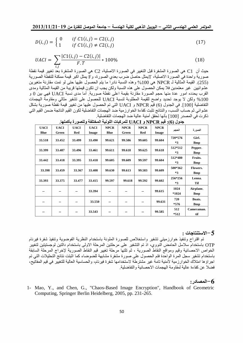
19/99/1192-91جامعة الموصل للفترة من –اليوبيل الذهبي لكلية الهندسة –المؤتمر العلمي الهندسي الثاني
44
( ) { ( ) ( )
( ) ( ) ( )
∑| ( ) ( )|
( )
هي الصورة المشفرة بعد تغيير قيمة نقطة C2هي الصورة المشفرة قبل التغيير في الصورة االصلية, C1حيث أن
يمثل اكبر قيمة ممكنة للنقطة الصورية Fيمثل حاصل ضرب بعدي الصورة, وTصورية واحدة في الصورة االصلية,
ول عليها حتى لو تمت مقارنة متغيرين % وهذه النسبة نادرا ما يتم الحص100هي NPCRالقيمة المثالية لـ (. 255)
عشوائيين غير معتمدين فال يمكن الحصول على هذه النسبة ولكن يجب ان تكون قيمتها قريبة من القيمة المثالية ومدى
و 0فهي بين UACIالقرب يحدده امور عدة منها حجم الصورة مقارنة بقيمة اعلى نقطة صورية. أما مدى نسبة
للحصول على تشفير مثالي ومقاومة الهجمات UACIتحديد واضح للقيمة المطلوبة لنسبة ولكن ال يوجد %100
التي تم الحصول عليها من تغيير قيمة نقطة صورية بشكل UACIو NPCR( قيم 6. في الجدول )[100]التفاضلية
لقيم الناتجة ضمن القيم التي عشوائي ثم حساب النسب, والنتائج تثبت كفاءة الخوارزمية ضد الهجمات التفاضلية لكون ا
بأنها تحقق أمنية عالية ضد الهجمات التفاضلية. [100]ذكرت في المصدر
للمركبات اللونية المختلفة وللصورة بأكملها. UACIو NPCRقيم (:6)جدول
الحجم الصورةNPCR
Image
NPCR
Red
NPCR
Green
NPCR
Blue
UACI
Image
UACI
Red
UACI
Green
UACI
Blue
Girl.
Bmp
720*576
*3 99.604 99.605 99.586 99.621 33.490 33.499 33.452 33.518
Pepper.
Bmp
512*512
*3 99.618 99.625 99.618 99.611 33.461 33.496 33.487 33.399
Fruits.
Bmp
512*480
*3 99.604 99.597 99.609 99.605 33.418 33.395 33.418 33.442
Flowers.
Bmp
500*362
*3 99.609 99.583 99.613 99.630 33.408 33.367 33.459 33.398
Lenna.
Tif
256*256
*3 99.602 99.592 99.618 99.597 33.415 33.477 33.375 33.393
Airplane.
Bmp
1024
*1024 99.615 -- -- -- 33.394 -- -- --
Boats.
Bmp
720
*576 99.631 -- -- -- 33.550 -- -- --
Cameraman.
tif
512
*512 99.585 -- -- -- 33.543 -- -- --
: االستنتاجات-5تم اقتراح وتنفيذ خوارزميتي تشفير واستخالص للصورة الملونة باستخدام النظرية الفوضوية وتنفيذ شفرة فيرنام
OTP باستخدام سالسل الحامض النووي, اذ تم التشفير على مرحلتين المرحلة االولى باستخدام دالتين لوجستيتين لتغيير
الخواص االحصائية وقيم ومواقع النقاط الصورية , ثم تلتها مرحلة تغيير قيم النقاط الصورية إلخراج المرحلة السابقة
اثبتت نتائج التحليالت التي تم ل على صورة مشفرة مشابهة للضوضاء كمافتم الحصو باستخدام تشفير سجل المرة الواحدة
شفرة فيرنام, والحساسية العالية للتغيير في قيم المفاتيح, الستخدامهااجراؤها امتالك الخوارزمية ألمنية تامة غير مشترطة
ة الهجمات االحصائية والتفاضلية.فضال عن كفاءة عالية لمقاوم
المصادر:-61- Mao, Y., and Chen, G., "Chaos-Based Image Encryption", Handbook of Geometric
Computing, Springer Berlin Heidelberg, 2005, pp. 231-265.
م ترميز الحامض النووي ونظرية الفوضىخوارزمية لتشفير الصورة الملونة باستخداعلي:
44
2- Fridrich, J., "Image Encryption Based On Chaotic Maps", Systems, Man And Cybernetics,
IEEE International Conference On Computational Cybernetics And Simulation, Vol. 2,
No.1, 1997, pp. 1105-1110.
3- Adleman, L.M. "Molecular computation of solution to combinatorial problems", Science
266, 1994, pp. 1021–1024.
4- D. Boneh, C. Dunworth, and R. Lipton, "Breaking DES using a molecular computer", In
Proceedings of DIMACS workshop on DNA computing, 1995, pp. 37-65.
5- A. Gehani, T.H LaBean, J.H. Reif, DNA-based cryptography, In: 5th DIMACS Series in
Discrete Mathematics and Theoretical Computer Science, MIT, Vol. 54, 1999, pp. 233-
249.
6- Wang,Q., Zhang, Q., Zhou, Ch., "A Multilevel Image Encryption Algorithm Based on
Chaos and DNA Coding", Bio-Inspired Computing BIC-TA'09., Fourth International
Conference on IEEE, 2009, pp. 1-5.
7- Zhou, Sh., Zhang, Q., Wei, X., "Image Encryption Algorithm Based on DNA Sequences for
the Big Image", Multimedia Information Networking and Security (MINES) International
Conference on IEEE, 2010, pp. 884-888.
8- Zhang, Q., Ling G., and Wei, X., "Image encryption using DNA addition combining with
chaotic maps", Mathematical and Computer Modeling Vol. 52, No.11, 2010, pp. 2028-
2035.
9- Saberi Kamarposhti, M., AlBedawi, I., Mohamad, D., "A New Hybrid Method for Image
Encryption using DNA Sequence and Chaotic Logistic Map", Australian Journal of Basic
and Applied Sciences, Vol. 6, No.3, 2012, pp. 371-380.
10- Zhang, Q., Xue, X., & Wei, X., "A Novel Image Encryption Algorithm Based on DNA
Subsequence Operation", The Scientific World Journal, 2012.
11- Babaei, M., "A novel text and image encryption method based on chaos theory and DNA
computing", Natural Computing, 2012, pp. 1-7.
12- Soni, A., Acharya, A.,"A Novel Image Encryption Approach using an Index based Chaos
and DNA Encoding and its Performance Analysis", International Journal of Computer
Applications, Vol. 47, No.23, June 2012.
13- Wang, Q., Zhang, Q., Wei, X., "Image encryption algorithm based on DNA biological
properties and chaotic systems", IEEE Fifth International Conference on Bio-Inspired
Computing: Theories and Applications (BIC-TA), 2010, pp. 132-136.
14- Zhang, Y., & Fu, L. H. B. "Research on DNA Cryptography, Applied Cryptography and
Network Security", Dr. Jaydip Sen (Ed.), ISBN: 978-953-51-0218-2, In Tech, 2012.
15- Popovici, C., "Aspects of DNA Cryptography", Annals of the University of Craiova-
Mathematics and Computer Science Series, Vol. 37, No.3, 2010, pp. 147-151.
16- Borda, M., "Fundamentals in information theory and coding", Springer, verlag/
Berlin/Heidelberg, 2011, pp. 512.
17- http://www.ncbi.nlm.nih.gov/, The National Center for Biotechnology Information.
18- Kerckhoffs, A., "La Cryptographie Militaire", Journal Des Sciences Militaires,
Vol. IX, (Electronic Version And English Translation Of "La Cryptographie Militaire" By
Peticolas, Fabien), Jan. 1883, pp. 5-38.
19- Alvarez, G., And Li, Sh., "Some Basic Cryptographic Requirements For Chaos-Based
Cryptosystems", International Journal Of Bifurcation And Chaos, Vol. 16, No. 08, 2006,
pp. 2129-2151.
20- Wu, Y., Noonan, J. P., And Agaian, S., "NPCR and UACI Randomness Tests for Image
Encryption", Cyber Journals: Multidisciplinary Journals in Science and Technology,
Journal of Selected Areas in Telecommunications (JSAT), April Edition 2011, pp. 31-38.
19/99/1192-91جامعة الموصل للفترة من –اليوبيل الذهبي لكلية الهندسة –المؤتمر العلمي الهندسي الثاني
25
خوارزمية تشفير انسيابية للصورة الملونة باستخدام النظرية الفوضوية
فخرالدين حامد علي*
[email protected] مها بشير حسين
العراق. –** قسم الهندسة الكهربائية/ كلية الهندسة/ جامعة الموصل العراق. –الحاسوب/ كلية الهندسة / جامعة الموصل * قسم هندسة
المستخلص
عند الرغبة في الحفاظ على أمنية وخصوصية نقلها. تعتبر نظرية الفوضى إن تشفير الصور الرقمية ضروري
من النظريات الواعدة حديثة االستخدام في هذا المجال, حيث أجريت العديد من البحوث في نهاية التسعينات ولحد اآلن
الدالة اللوجستية لتوليد حول الموضوع. في هذا البحث تم تقديم خوارزمية تشفير انسيابية للصورة الملونة باستخدام
سلسلتين من االعداد الفوضوية, تم استخدام االعداد المولدة من السالسل لتغيير قيم النقاط الصورية, واست خد مت
مصفوفة المواقع لألعداد المولدة من السالسل بعد ترتيبها تصاعديا أو تنازليا لتغيير مواقع النقاط الصورية. تم تحليل
كفاءة التشفير, وتحليل طول المفتاح وقياسبإجراء التحليالت التفاضلية والتحليالت االحصائية اداء الخوارزمية
وحساسيته وايجاد سرعة اداء الخوارزمية, اثبتت النتائج امتالك الخوارزمية المقترحة للصفات المطلوبة لصد الهجمات
رجاع التام للصورة عند المستلم وتقديم آلية عند , مع امكانية االست االحصائية والتفاضلية وهجمات القوة الوحشية
أ ستـ خد م باإلضافة لسرعة التشفير واالسترجاع. لصورة المشفرة للتغيير اثناء نقلهالمعرفة اذا ما تعرضت ا المستلم
لتنفيذ الخوارزمية واجراء التحليالت. Matlab R2011bبرنامج نظرية الفوضى . ,الدالة اللوجستية ,ر المتناظرالتشفي ,لمات الدالة: التشفير االنسيابي الك
An Image Encryption Stream Cipher Algorithm Based on Chaos
Theory
Fakhrulddin H. Ali* Maha Basher Hussein
**
[email protected] [email protected] * Dept. of Computer Engineering/ College of Engineering/ University of Mosul – IRAQ.
** Dept. of Electrical Engineering/ College of Engineering/ University of Mosul – IRAQ.
Abstract Image Encryption is important for protecting image information. Chaos theory is
a promising modern method for Image Encryption which has been adopted since the
beginning of the last decade and the end of the decade before. In this paper A chaos
based stream cipher has been proposed to encrypt color Images, two of logistic maps
have been used to generate two sequences of Chaos numbers, the sequence from first
map is used to modify pixel values, where the Index array for the second sequence after
sorting it has been used to scramble pixel locations, the performance of the algorithm has
been analyzed and results show that the algorithm has a very long key space, and high
sensitivity for small changes in key which makes the algorithm Immune to Brute force
attacks, and it can resist the differential and statistical attacks, in addition to having very
high encryption and decryption speed, the receiver can detect any changes to the
encrypted image during transmission. the algorithm has been implemented and analysis
done by using MatLab R2011b software.
Keywords: Chaos theory, Image Encryption, Logistic map, stream cipher, symmetrical
encryption.
يةخوارزمية تشفير انسيابية للصورة الملونة باستخدام النظرية الفوضو : علي
25
المقدمة: .1نية معالجة االشارة الرقمية وظهور المزيد من خدمات المستهلكين االلكترونية مع شيوع استخدام االنترنت وتطور تق
طبيقات الصور الرقمية في واالجهزة االلكترونية والتي تقوم بتزويد خواص اضافية لحفظ وتبادل الوسائط المتعددة, فإن ت
. انتشار تقنية الوسائط المتعددة في المجتمع ادت الى ان تلعب الصور الرقمية وملفات الفيديو دورا اهم من تزايد مستمر
الرسائل النصية التقليدية, مما يتطلب حماية حقيقية لخصوصية المستخدمين. لتحقيق حماية مماثلة فإن الحل األمثل هو
الوصول الى البيانات من األطراف غير المعنية, من الخوارزميات تشفير البيانات الرقمية إلحباط الهجمات او محاوالت
وعلى الرغم من ذلك فإن خوارزميات التشفير هذه ليست DES ,RSA, IDEAالمستخدمة لتشفير الصور خوارزمية
علومات مثالية لتشفير الصور وذلك لبعض الخواص الجوهرية للصور مثل كمية البيانات العالية والترابط الوثيق بين م
الصورة وغيرها من الخواص التي تنفرد بها الصور الرقمية عن البيانات النصية باإلضافة الى حاجة التطبيقات الصورية
في بعض االحيان الى متطلبات اخرى مثل المعالجة في الزمن الحقيقي والدقة والحفاظ على تنسيق الصورة مما يجعل طرق
طيئة المعالجة بالنسبة للصور وصعوبة تحقيق هذه المطاليب مع تحقيق االمنية العالية التشفير التقليدية صعبة التطبيق وب
والجودة العالية. في السنوات االخيرة ونظرا للعالقة الوثيقة بين نظرية الفوضى وعلم التعمية , علم التعمية باستخدام
و, تشفير الصور باستخدام االسلوب الفوضوي االسلوب الفوضوي تم استغالله لتصميم انظمة تشفير الصور وملفات الفيدي
لن يستطيع حل جميع المشاكل الموجودة في مجال تشفير الصور ولكن على الرغم من ذلك هذه النظرية تستطيع تزويدنا
بطرق واعدة جدا والتي تستطيع جزئيا تحقيق كثير من متطلبات تشفير الصورة واثبات تفوقها على طرق التشفير التقليدية
سيما مع امكانية جمعها لمواصفات السرعة واالمان والمرونة من خالل التصميم الجيد, وبصورة عامة فإن الشفرات ال
. منذ قيام العالم [3-1] المعتمدة على االسلوب الفوضوي بإمكانها التفوق على طرق التشفير التقليدية وتحقيق اداء جيد جدا
, والبحوث تتوالى في مجال تشفير الصور باالعتماد 7991صور في عام فريدريك باقتراح اول نظام فوضوي لتشفير ال
. تم في هذا البحث اقتراح خوارزمية تشفير للصور معتمدة على االسلوب الفوضوي باستخدام [4]على االسلوب الفوضوي
حيث تم 6002في سنة , ومن الدراسات المشابهة في هذا المجال ما قام به الباحثون Logistic map)الخريطة اللوجستية)
ولزيادة متانة الخوارزمية بت 80اقتراح نظام تشفير كتلي للصورة باستخدام الخريطة اللوجستية بمفتاح خارجي بطول
تم 6002. وفي سنة [5]نقطة صورية 72ضد الهجمات فانه يتم تعديل المفاتيح بعد تشفير كل كتلة من البيانات بحجم
80ستخدام الخريطة اللوجستية لتغيير قيم النقاط الصورية ومواقعها واستخدام مفتاح بطول عرض طريقة لتشفير الصور با
تم استخدام الخريطة اللوجستية وخريطة هينون 6070, وفي سنة [6] بت ايضا مع تحليل اداء الخوارزمية واثبات كفاءتها
التصاميم الصناعية ,وتم استخدام هذه لتوليد سلسلة من االرقام الفوضوية لتشفير صور (Henon map)الفوضوية
تم ة المولدة إذ السالسل لتغير قيم النقاط الصدرية للصورة باستخدام عملية او االستثنائية بين معلومات الصورة والسلسل
تم توظيف سلوك الفوضى لتصميم نظام تشفير للصورة باستخدام مفتاح . وفي السنة نفسها [7] تحليل أداء الخوارزمية
تحليل مواصفات النظام والحصول على خواص و الدالة اللوجستية لتشفير الصورة بت واستخدام701رجي مكون من خا
مماثلة للتشفير بالطرق التقليدية ومن الممكن توظيف هذه الخوارزمية لنقل المعلومات السرية عبر االنترنيت باإلضافة الى
قتراح نظام تشفير للصور الملونة بأحجام مختلفة باستخدام الدالة قاموا با [9]. اما الباحثون في المصدر [8]الصور
, حيث تم استخدام دالة لوجستية لعملية النشر ودالة اخرى لتغيير مواقع النقاط الصورية باستخدام 6070اللوجستية في سنة
تم تقديم طريقة 6077 بت وتم تحليل مواصفات النظام وادائه وتحمله للهجمات المعروفة. وفي سنة 35مفتاح بمساحة
لتشفير الصور باستخدام الدالة اللوجستية ايضا مع تبديل مواقع النقاط الصورية وتغيير قيمها وتحليل خواص واداء
.[10]الخوارزمية وكذلك اثبات امكانية استرجاع الصورة بعد تعرضها الى التشويش اثناء النقل
الخلفية النظرية: .2المعلومات االساسية عن التشفير وتشفير الصورة والنظرية الفوضوية وعالقتها مع علم سيتم في هذا الجزء ذكر بعض
التعمية مع شرح للدالة الفوضوية المستخدمة في الخوارزمية.
تشفير الصورة: 2-1الفكرة األساسية للتشفير هو تحوير الرسالة المنقولة بطريقة معينة بحيث ال يمكن اعادة محتويات الرسالة الى
وضعها االصلي اال من قبل المستلم المعني بالرسالة, عادة تكون أمنية أي نظام تشفير معتمدة على المفتاح فقط بصورة
رئيسية, أي بعبارة اخرى من المفترض ان يكون الخصم على علم بهيكلية نظام التشفير ويملك خوارزمية التشفير وأيضا
, فحسب مبادئ كيرشوف في التشفير [1]ة للحصول على البيانات المشفرةيستطيع الوصول الى قناة نقل البيانات المشفر
فإن نظام التشفير المثالي يجب أن يعتمد على المفتاح فقط لتأمين المعلومات وتكون [11] 7225والتي قدمها في سنة
افه بخالف الخوارزمية الخوارزمية المستخدمة وهيكلية النظام مكشوفة نظرا لكون المفتاح سهل التغيير اذا ما تم اكتش
وهيكلية النظام والتي من الصعوبة تغييرها اذا افترضنا انها كانت سرية.
19/99/1192-91جامعة الموصل للفترة من –اليوبيل الذهبي لكلية الهندسة –المؤتمر العلمي الهندسي الثاني
25
وذلك بتحويل الصورة االصلية الى صورة اخرى مشفرة وصعبة التمييز تشفير الصورة هي تقنية توفير الحماية للصورة
,يمكن تقسيم خوارزميات تشفير الصور الى ثالثة مجاميع رئيسية:
(.Pixel Scramblingرزمية تبديل المواقع )خوا -7
(.Pixel Replacementخوارزمية تحويل القيم ) -6
Combination between Pixel Scrambling and Pixelخوارزمية تبديل المواقع مع تحويل القيم ) -5
Replacement.)
وهناك نوعان رئيسيان للتشفير:
(: ويعرف أيضا بالتشفير المتناظر, وفي هذا النوع يكون Private key Cryptographyتشفير المفتاح السري ) -7
المفتاح المستخدم للتشفير هو نفسه المفتاح المستخدم لفك الشفرة.
(: ويعرف ايضا بالتشفير بالمفتاح غير المتناظر, وفي Public key Cryptographyتشفير المفتاح العمومي ) -6
.[12,13]لتشفير ومفتاح خاص لفك التشفيرهذه الطريقة يتم استخدام مفتاحين , مفتاح عام ل
نظرية الفوضى: 2-2يقصد بنظرية الفوضى او األسلوب الفوضوي سلوك بعض األنظمة الحركية غير الخطية والتي تحت شروط معينة
تظهر حركات حساسة بالنسبة للقيم االبتدائية, هناك صفتان اساسيتان لألنظمة الفوضوية هي الحساسية للتغيير في القيم
(. والفوضى هي ظاهرة موجودة في االنظمة غير الخطية المحددة mixing propertyاالبتدائية وخاصية الخلط او الدمج )
والتي تظهر حساسية عالية للقيم االولية وتملك سلوك مشابه للعشوائية, تم اكتشاف النظرية الفوضوية من قبل العالم ادوارد
قت اصبحت هذ النظرية فرعا من فروع الدراسات العلمية وفي الوقت الحاضر ومنذ ذلك الو [14] 7925لورنز في عام
تم . [1,15]يتم تكريس اهتمام متزايد الستخدام االنظمة الحركية الفوضوية غير المستمرة )او الخرائط( في انظمة التشفير
[4] قام العالم فريدريك 7991وفي عام [16] 7929استخدام النظرية الفوضوية في مجال التشفير ألول مرة عام
باستخدام هذه النظرية لتشفير الصورة ألول مرة. الفائدة الرئيسية الستخدام هذه النظرية تتمثل بأن االشارة الفوضوية تبدو
كالضوضاء للمستخدمين غير المعنيين بغض النظر عن آلية توليد هذه االشارة, وأيضا فإن االشارة المولدة تعتمد بصورة
معامالت التحكم والقيم االبتدائية للدوال او الخرائط المولدة لها, وأي تغيير طفيف على هذه القيم يتم توليد اشارة قوية على
مختلفة كليا, بعبارة أخرى فإنه من الممكن استخدام معامالت التحكم والقيم االبتدائية بصورة فعالة كمفاتيح في نظام التشفير
كلفة مما يجعلها مناسبة لتشفير البيانات كبيرة توليد االشارة الفوضوية هي عملية منخفضة الوباإلضافة الى ذلك فإن عملية ت
.[18,17]الحجم
العالقة بين نظرية الفوضى وعلم التعمية : 2-3منذ التسعينات والعديد من الباحثين الحظوا وجود عالقة مثيرة لالهتمام بين نظرية الفوضى وعلم التعمية, معظم
ة الفوضوية لها خواص مقابلة في انظمة التشفير, واالنظمة الفوضوية غير المستمرة تمتلك العديد من خواص االنظم
الخواص المطلوبة في علم التعمية واهمها الحساسية للقيم االبتدائية وقيم معامالت التحكم والمسارات غير المحددة, أول
ي علم التعمية, اما الخاصية الثالثة فمتعلقة بخاصية ( فDiffusionخاصيتين مقابلتين لخاصية النشر او التوزيع)
بالنسبة لعلم التعمية, خاصية التشويش يعنى بها جعل العالقة بين النص الواضح والنص المشفر (Confusion)التشويش
غير معتمدة على بعضها البعض احصائيا, اما النشر فيقصد به نشر تأثير رقم منفرد من النص الواضح على عدة ارقام من
رية والرقمية األمينة, والمثير لالنتباه أن العالم النص المشفر وهذه الخواص هي االساس لتطوير انظمة التشفير التناظ
بذكر خواص النشر والتشويش الواجب توفرها في أنظمة -أي قبل اكتشاف نظرية الفوضى – 7919شانون قام في سنة
. الخرائط الفوضوية وخوارزميات التشفير تمتلك عديدا من الخواص المتشابهة, كال منهما [21-19]االتصاالت السرية
اسين للتغييرات الصغيرة جدا على القيم االبتدائية والمتغيرات والتي تقابلها المفاتيح في انظمة التشفير, كال منهما يسلكان حس
( من التشفير, Roundsسلوكا مشابها للعشوائية, تقوم خوارزميات التعمية بخلط ونشر البيانات عن طريق عدة جوالت )
(, Iterationجزء صغير من البيانات عبر فضاء الطور بأكمله من خالل التكرار)في حين تقوم الخرائط الفوضوية بنشر
الفرق الوحيد هو ان عمليات التشفير يتم تعريفها ضمن مجموعات محددة من االعداد الصحيحة بينما تعرف األرقام
ة او رقمية, والتماثلية منها تكون . يمكن ألنظمة التشفير الفوضوية أن تكون تماثلي[1]الفوضوية باستخدام األعداد الحقيقية
( stream ciphersمستندة على تقنية التزامن الفوضوية, اما الرقمية منها فيمكن ان تقسم الى قسمين : شفرات انسيابية )
( التي تستخدم PRNG( ,وتستخدم الشفرات االنسيابية لتوليد االعداد العشوائية المزيفة )Block ciphersوشفرات كتلية )
اء النص االصلي وتشفيره, اما الشفرات الكتلية فتستخدم النص االصلي و/أو المفاتيح السرية عدة مرات للحصول على إلخف
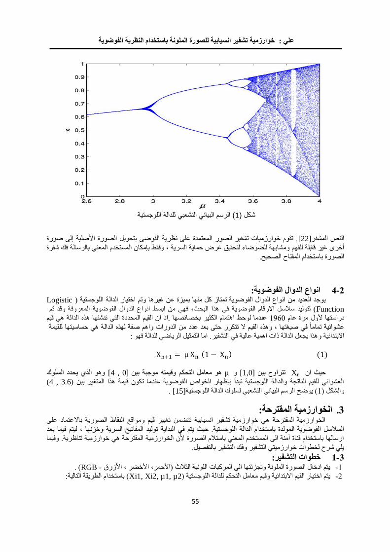
يةخوارزمية تشفير انسيابية للصورة الملونة باستخدام النظرية الفوضو : علي
22
. تقوم خوارزميات تشفير الصور المعتمدة على نظرية الفوضى بتحويل الصورة األصلية إلى صورة [22]النص المشفر
اية السرية , وفقط بإمكان المستخدم المعني بالرسالة فك شفرة أخرى غير قابلة للفهم ومشابهة للضوضاء لتحقيق غرض حم
الصورة باستخدام المفتاح الصحيح.
انواع الدوال الفوضوية: 2-4 Logisticاللوجستية ) وتم اختيار الدالة غيرها عن بميزة منها كل تمتاز الفوضوية الدوال انواع من العديد يوجد
Functionتم وقد المعروفة الفوضوية الدوال انواع ابسط من ة في هذا البحث, فهي( لتوليد سالسل االرقام الفوضوي
قيم هي الدالة هذه تنشئها التي المحددة القيم ان اذ .بخصائصها الكثير اهتمام لوحظ عندما 7920دراستها ألول مرة عام
للقيمة حساسيتها هي الدالة لهذه صفة الدورات واهم من عدد بعد حتى ال تتكرر القيم وهذه , صيغتها في تماما عشوائية
التشفير. اما التمثيل الرياضي للدالة فهو : في عالية اهمية ذات الدالة يجعل وهذا االبتدائية
( ) ( )
وهو الذي يحدد السلوك [0 , 4]هو معامل التحكم وقيمته موجبة بين و [1,0]تتراوح بين Xnحيث ان
( 3.6 , 4العشوائي للقيم الناتجة والدالة اللوجستية تبدأ بإظهار الخواص الفوضوية عندما تكون قيمة هذا المتغير بين )
. [15] ة( يوضح الرسم البياني التشعبي لسلوك الدالة اللوجستي7والشكل )
الخوارزمية المقترحة: .3
الخوارزمية المقترحة هي خوارزمية تشفير انسيابية تتضمن تغيير قيم ومواقع النقاط الصورية باالعتماد على
توليد المفاتيح السرية وخزنها , ليتم فيما بعد السالسل الفوضوية المولدة باستخدام الدالة اللوجستية. حيث يتم في البداية
ارسالها باستخدام قناة آمنة الى المستخدم المعني باستالم الصورة ألن الخوارزمية المقترحة هي خوارزمية تناظرية. وفيما
يلي شرح لخطوات خوارزميتي التشفير وفك التشفير بالتفصيل.
خطوات التشفير: 3-1 ( .RGB -يتم ادخال الصورة الملونة وتجزئتها الى المركبات اللونية الثالث )األحمر, األخضر , األزرق -7
( باستخدام الطريقة التالية:Xi1, Xi2, µ1, µ2يتم اختيار القيم االبتدائية وقيم معامل التحكم للدالة اللوجستية ) -6
اللوجستية للدالة التشعبي البياني الرسم( 1) شكل
19/99/1192-91جامعة الموصل للفترة من –اليوبيل الذهبي لكلية الهندسة –المؤتمر العلمي الهندسي الثاني
25
رة عشوائية وضمن المدى المحدد لعمل الدالة اللوجستية ( بصوXin1, Xin2يتم اختيار القيم االبتدائية االولية ) -أ
كدالة فوضوية.
( :2, من المعادلة رقم ) k0يتم حساب -ب
∑∑∑
( )
( )
(.i,j,kهي قيمة النقطة الصورية في الموقع ) P(i,j,k)هو حاصل ضرب بعدي الصورة , و M * Nحيث أن
يتم اختيار قيم معامالت التحكم بصورة عشوائية وضمن المدى المحدد لعمل الدالة كدالة فوضوية ويتم حساب -ج
تمثل المفاتيح السرية للتشفير:القيم االبتدائية الجديدة التي سيتم اعتمادها لتوليد السالسل الفوضوية وهذه القيم
( ) ( )
( ) ( )
يتم حفظ المفاتيح السرية الى ملف ألرساله فيما بعد الى الشخص المعني باستالم الصورة عبر قناة آمنة. - د
يتم توليد سالسل األرقام الفوضوية األولى والثانية باستخدام القيم االبتدائية ومعامالت التحكم التي تم تحديدها في -5
( .1) (, وحسب المعادلة6الخطوة )
بالطريقة التالية:السلسلة األولى يتم تعديل عناصر -1
( ( ) ) ( )
X1newيتم تنفيذ عملية أو الحصرية بين عناصر مصفوفة المركبات اللونية الثالث للصورة االصلية مع المصفوفة -3
على المصفوفات: للحصول, وذلك لتغيير قيم النقاط الصورية للصورة االصلية
( )
( )
( )
Indexتبة )يتم ترتيب عناصر السلسلة الفوضوية الثانية تصاعديا والحصول على مصفوفة المواقع للمصفوفة المر -2
Array أي يتم البحث عن اصغر عنصر وحين يتم ايجاده يتم خزن موقعه والبحث عن العنصر الذي يليه ثم خزن ,)
موقعه وهكذا لحين االنتهاء من ترتيب المصفوفة بأكملها.
فة لكل مركب لوني وذلك حسب مصفو C1يتم تبديل مواقع النقاط الصورية للمركبات اللونية الثالث للمصفوفة -1
لكل مركب لوني: C( للحصول على المصفوفة 2المواقع التي اوجدناها في الخطوة )
( ) ( ( )) ( )
( ) ( ( )) ( )
( ) ( ( )) ( )
للحصول على الصورة المشفرة. Cيتم دمج المركبات اللونية الثالث للمصفوفة -2
خطوات فك التشفير: 3-2 يتم ادخال الصورة المشفرة وتجزئتها الى المركبات اللونية الثالث. -7
( والتي تم استالمها بطريقة اتصال آمنة.Xi1, Xi2, µ1, µ2يتم إدخال مفاتيح التشفير) -6
يةخوارزمية تشفير انسيابية للصورة الملونة باستخدام النظرية الفوضو : علي
25
بتعويض القيم االبتدائية ومعامالت التحكم التي تم يتم توليد سلسلتين من االرقام الفوضوية باستخدام الدالة اللوجستية -5
(.6ادخالها في الخطوة )
( من خطوات التشفير.3يتم تعديل عناصر السلسلة االولى كما في الخطوة ) -1
من خطوات التشفير. 1يتم ترتيب عناصر السلسلة الثانية والحصول على مصفوفة المواقع كما في الخطوة -3
مركبات اللونية الثالث الى مواقعها االصلية باستخدام مصفوفة المواقع التي تم الحصول تتم اعادة عناصر مصفوفة ال -2
( ويتم الحصول على المصفوفات معدلة القيم في هذه الخطوة.3عليها في الخطوة )
يتم استرجاع القيم االصلية للنقاط الصورية بالقيام بعملية أو الحصرية بين عناصر السلسلة الفوضوية االولى -1
عناصر المصفوفات معدلة القيم للحصول على المصفوفات التي تحوي قيم النقاط الصورية للصورة االصلية و
للمركبات اللونية الثالث.
تتم اعادة دمج المركبات اللونية الثالث للحصول على الصورة االصلية. -2
كانت الصورة المستلمة قد تم التالعب للكشف عن التغييرات التي قد تطرأ على الصورة المشفرة أثناء نقلها وفيما اذا -9
للصورة االصلية k0للصورة المستخلصة واذا لم تكن مساوية لقيمة k0بها اثناء النقل او وصلت كما هي يتم حساب
فهذا يشير الى أن الصورة المستلمة قد تم التالعب بقيمها, باإلمكان االستفادة من هذه اآللية عند تشفير ونقل الصور
لتغيير الدقيق فيها كصور الخرائط والتصاميم الصناعية.الحساسة ل
تحليالت األمان واالداء : .4, (Cryptanalytic)التشفير المثالي للصورة يجب أن يقاوم كل انواع الهجمات المعروفة مثل : الهجمات التحليلية
. في هذا القسم ستتم [23]( Brute force attackالهجمات االحصائية , الهجمات التفاضلية , وهجوم القوة الوحشية )
ش ف رت أربع صور قياسية دراسة امنية الخوارزمية وادائها بإجراء عدة تحليالت لخواص الصورة قبل وبعد تشفيرها ,
للتشفير وفك التشفير واجراء التحليالت, وتم تنفيذ التحليالت التالية:R2011b Matlabاستخدام برنامج ب
(:Key space analysisتحليل مساحة المفتاح ) 4-1 المفتاح المستخدم لعملية التشفير يجب أن ال يكون طويال جدا او قصيرا جدا , المفتاح القصير يمكن الحصول عليه
سابقا بأن أمنية نظام التشفير الجيد يكون معتمدا ذكرهبسهولة عند تطبيق هجوم القوة الوحشية والهجمات التحليلية, وكما تم
صورة أساسية تبعا لقوانين كيرشوف في التشفير, اما المفتاح الطويل جدا فيقلل من سرعة أداء النظام وهذا على المفتاح ب
غير مرغوب فيه ألن سرعة التشفير من المواصفات المهمة ألنظمة التشفير والتي تأتي اهميتها بعد تحقيق األمنية .يجب أن
2المفتاح عن مساحة تقلال 100
, في الخوارزمية المقترحة تم استخدام سلسلتين من [23]من األمانلتوفير مستوى عال
االرقام الفوضوية تم توليدها باستخدام الدالة اللوجستية, وكل سلسلة تتطلب قيمة ابتدائية ومتغير التحكم بالدالة اللوجستية
10ائية بدقة حيث يتم استخدامهم كمفاتيح للتشفير, اذا تم استخدام متغيرات التحكم والقيم االبتد14
للمفتاح ةالكلي المساحةفإن
: ستكون
1014
* 1014
*1014
* 1014
=1056
=2186
وهذا الطول مالئم جدا لمقاومة هجوم القوة الوحشية., bit 186أي بطول
( :Key sensitivity analysisتحليل حساسية المفتاح ) 4-2باإلضافة الى كون طول المفتاح كافيا لمنح األمان للنظام , فإن نظام التشفير المثالي يجب ان يكون حساسا جدا ألي
تغيير طفيف في المفتاح السري, وأي تغيير طفيف في المفتاح المستخدم يجب أن يؤدي الى توليد صورة مشفرة مختلفة كليا
ريت , وهذا يضمن مقاومة النظام لهجوم القوة الوحشية, عن الصورة المشفرة قبل التغيير في المفتاح عدة تجارب الختبار أ ج
مدى حساسية النظام للتغيير في المفتاح كالتالي:
كمفتاح لتوليد السلسلة االولى من االرقام الفوضوية , وتم الحصول على الصورة X10القيمة االبتدائية أ س تخدمت -أ
. أ ( .6ة األصلية )الشكل . ب( من الصور6المشفرة )الشكل
X10= X10 + 10المفتاح نفسه مع فرق قليل بمقدار أستخدم -ب-13
. ج( 6وتم الحصول على الصورة المشفرة )الشكل
الصورة المشفرة في هذه الخطوة مع الصورة المشفرة في الخطوة وقورنت , . أ (6فس الصورة االصلية )الشكل من ن
. د( .6)أ( والفرق بين الصورتين موضح في )الشكل
. ب( باستخدام نفس المفتاح المستخدم للتشفير وتم الحصول 6الصورة األصلية من الصورة المشفرة )الشكل أ ستخلصت -ج
األصلية في الخطوة )أ( , والفرق بين الصورة المستخلصة . هـ( والتي هي نفس الصورة 6على الصورة )الشكل
. و(.6والصورة األصلية موضح في )الشكل
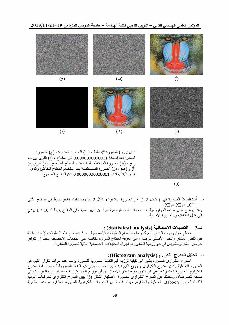
19/99/1192-91جامعة الموصل للفترة من –اليوبيل الذهبي لكلية الهندسة –المؤتمر العلمي الهندسي الثاني
25
. ب( باستخدام تغيير بسيط في المفتاح الثاني 6. ز( من الصورة المشفرة )الشكل 6الصورة في )الشكل أ ستخلصت -د
X20= X20+ 10-14
.
10 * 1مناعة الخوارزمية ضد هجمات القوة الوحشية حيث ان تغيير طفيف في المفتاح بقيمة وهذا يوضح مدى-14
يؤدي
الى فشل استخالص الصورة األصلية.
( :Statistical analysisالتحليالت االحصائية ) 4-3إليجاد عالقة معظم خوارزميات التشفير يتم كسرها باستخدام التحليالت االحصائية, حيث تستخدم هذه التحليالت
بين النص المشفر والنص األصلي للوصول الى معرفة المفتاح السري, للتغلب على الهجمات االحصائية يجب ان تتوافر
خواص النشر والتشويش في خوارزمية التشفير. تم اجراء التحليالت االحصائية التالية للصورة المشفرة:
(:Histogram analysisتحليل المدرج التكراري) -أمدرج التكراري للصورة يشير الى كيفية توزيع قيم النقاط الصورية للصورة برسم عدد مرات تكرار القيم, في ال
الصورة األصلية يكون المدرج التكراري وتوزيع القيم فيه متباينا حسب توزيع قيم النقاط الصورية للصورة, أما المدرج
االمكان أي أن توزيع القيم يكون فيه متساويا وبمظهر عشوائي التكراري للصورة المشفرة فينبغي ان يكون موحدا قدر
( يبين المدرج التكراري للمركبات اللونية 3مشابه للضوضاء, ومختلفا عن المدرج التكراري للصورة األصلية. الشكل )
شابهة األصلية والمشفرة. حيث نالحظ ان المدرجات التكرارية للصورة المشفرة موحدة وم Baboon الثالث لصورة
)ج( )ب( )أ(
)و( )هـ( )د(
)ز(
. )أ( الصورة األصلية , )ب( الصورة المشفرة , )ج( الصورة 2 شكل
الى المفتاح , )د( الفرق بين ب 0.0000000000001المشفرة بعد إضافة
و ج , )هـ( الصورة المستخلصة باستخدام المفتاح الصحيح , )و( الفرق بين )أ( و )هـ( , )ز( الصورة المستخلصة بعد استخدام المفتاح الخاطئ والذي
عن المفتاح الصحيح . 0.00000000000001رق قليال بمقدار يف
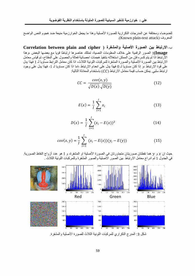
يةخوارزمية تشفير انسيابية للصورة الملونة باستخدام النظرية الفوضو : علي
25
عن المدرجات التكرارية للصورة األصلية وهذا ما يجعل الخوارزمية منيعة ضد هجوم النص الواضح للضوضاء ومختلفة
(.Known plain-text attackالمعروف )
Correlation between plain and cipherاالرتباط بين الصورة األصلية والمشفرة ) -ب
Image:) الصور الرقمية على خالف المعلومات النصية, تمتلك عناصرها ارتباطا قويا مع بعضها البعض ,وهذا
االرتباط اذا لم يتم كسره فإن من الممكن استغالله بتنفيذ هجمات احصائية فعالة والحصول على المفتاح, تم قياس معامل
فهذا يدل 1نية الثالث, اذا كان معامل الترابط مساويا لـ االرتباط بين الصورة األصلية والصورة المشفرة للمركبات اللو
فهذا يدل على وجود 1-فهذا يدل على انعدام االرتباط ,اما اذا كان مساويا لـ 0على قوة االرتباط ,و إذا كان مساويا لـ
( باستخدام المعادلة التالية: ارتباط سلبي. يمكن حساب قيمة معامل االرتباط )
( )
√ ( ) √ ( ) ( )
( )
∑
( )
( )
∑( ( ))
( )
( )
∑ ( ( ))( ( )) ( )
هو عدد أزواج النقاط الصورية. Iو في الصورة األصلية او المشفرة, هما نقطتان صوريتان متجاورتان و حيث ان
للمركبات اللونية الثالث .والمشفرة ادراج معامل االرتباط بين الصور االصلية والصورتم 1في الجدول
Red Green Blue
: المدرج التكراري للمركبات اللونية الثالث للصورة األصلية والمشفرة.3 شكل
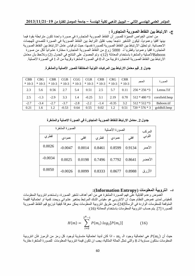
19/99/1192-91جامعة الموصل للفترة من –اليوبيل الذهبي لكلية الهندسة –المؤتمر العلمي الهندسي الثاني
56
االرتباط بين النقاط الصورية المتجاورة : -جمن احدى الخواص المميزة للصور أن النقاط الصورية المتجاورة في صورة واحدة تكون مترابطة بقوة فيما
بينها أفقيا وعموديا , ليكون التشفير ناجحا يجب تقليل الترابط بين النقاط الصورية في الصورة للتصدي للهجمات
سها, حيث تم قياس عامل االرتباط بين النقاط الصورية االحصائية. تم تحليل االرتباط بين النقاط الصورية للصورة نف
صورة تجاورة مختارة عشوائيا لكل من زوج من النقاط الصورية الم 5000المتجاورة افقيا وعموديا وقطريا لـ
Baboon ( ونالحظ بأن معامل 2(, وتم الحصول على النتائج في الجدول )12المشفرة باستخدام المعادلة )واألصلية
في الصورة االصلية. 1في الصورة المشفرة وقريبة من الـ 0االرتباط بين النقاط الصورية المتجاورة قريبة من الـ
.األصلية والمشفرة اللونية المختلفة للصور. قيم معامل االرتباط بين المركبات 1جدول
. معامل االرتباط للنقاط الصورية المتجاورة في الصورة االصلية والمشفرة2جدول
المركب
اللوني
الصورة المشفرة الصورة األصلية
قطري عمودي افقي قطري عمودي افقي
0.0026 0.0047- 0.0014 0.8461 0.8599 0.9134 األحمر
0.0034- 0.0025 0.0198 0.7496 0.7792 0.8641 األخضر
0.0050 0.0026- 0.0099 0.8333 0.8677 0.8988 األزرق
(:Information Entropyانتروبية المعلومات ) -دوتستخدم انتروبية المعلومات الغموض وعدم القابلية على فهم الصورة المشفرة هي من أهم أهداف تشفير الصورة,
كمقياس لمدى غموض النظام حيث ان االنتروبي هو مقياس الشك المرتبط بمتغير عشوائي ويحدد كمية او احتمالية القيمة
معرفة كيفية توزيع قيم النقاط الصورية ن طريق انتروبية المعلومات يمكن,ع[24]المتوقعة للمعلومات الواردة في الرسالة
(:16يتم حساب انتروبية المعلومات باستخدام المعادلة ) .[7]للصورة
( ) ∑ ( ) [ ( )]
( )
, اذا كان لدينا احتمالية متساوية لوجود كل رمز من الرموز فأن انتروبية هي احتمالية وجود الـ ( ) حيث أن
والتي تمثل الحالة المثالية, يجب ان تكون قيمة انتروبية المعلومات للصورة المشفرة مقاربة 8المعلومات ستكون مساوية لـ
الحجم الصورةCRR
* 10-3
CRG
* 10-3
CRB
* 10-3
CGR
* 10-3
CGG
* 10-3
CGB
* 10-3
CBR
* 10-3
CBG
* 10-3
CBB
* 10-3
Lenna.Tif 256 * 256 *3 0.11 5.7 2.5 0.51 5.4 2.7 0.56 5.6 2.3
cornfield.bmp 512 * 480 *3 0.70 2.19 3.1 -0.25 1.4 3.3 -2.9 -1.3 2.5
Baboon.tif 512 * 512 *3 3.2 -0.35 -1.4 -2.2 -2.8 -3.7 -2.7 -3.4 -2.7
goldhill.bmp 720 * 576 * 3 0.51 1.2 0.02 0.55 0.64 -0.53 1.2 1.6 0.21
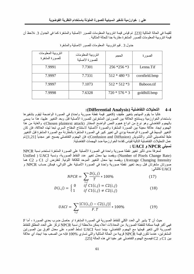
يةخوارزمية تشفير انسيابية للصورة الملونة باستخدام النظرية الفوضو : علي
51
ن . نالحظ أ3ألصلية والمشفرة كما في الجدول ا س قيمة انتروبية المعلومات للصور. تم قيا[23]للقيمة في الحالة المثالية
المشفرة مقاربة جدا للحالة المثالية . قيمة انتروبية المعلومات للصور
االصلية والمشفرة قيم انتروبية المعلومات للصور. 3جدول
انتروبية المعلومات الحجم الصورة
للصورة االصلية
انتروبية المعلومات
للصورة المشفرة
Lenna.Tif 256 *256 *3 7.7301 7.9991
cornfield.bmp 512 * 480 *3 7.7331 7.9997
Baboon.tif 512 * 512 *3 7.1073 7.9997
goldhill.bmp 720 * 576 * 3 7.6328 7.9998
(:Differential Analysisالتحليالت التفاضلية ) 4-4غالبا ما يقوم المهاجم بتغيير طفيف )كتغيير قيمة نقطة صورية واحدة( في الصورة الواضحة ليقوم بتشفيرها
باستخدام الخوارزمية ويستنتج العالقة بين الصورتين المشفرتين للصورة األصلية قبل وبعد التغيير عليها, هذا ما يسمى
(, والغاية من هذا Chosen plaintext attackاضح المختار )بالهجوم التفاضلي وهو نوع من انواع هجوم النص الو
الهجوم ايجاد عالقة معينة بين الصورة المشفرة والصورة األصلية الستنتاج المفتاح السري تبعا لهذه العالقة, فإن كان
لمشفرة قبل التغيير التغيير البسيط في الصورة الواضحة يؤدي الى تغيير كبير في الصورة المشفرة بالمقارنة مع الصورة ا
.تم [1,21] (, فإن الهجوم التفاضلي يصبح غير مجديا Confusion and Diffusionطبقا لخاصيتي النشر والتشويش )
عمل التحليالت التفاضلية التالية لقياس كفاءة الخوارزمية ضد الهجمات التفاضلية:
: UACIو NPCRنسبتي NPCRلمعرفة مدى تأثير تغيير نقطة صورية واحدة في الصورة األصلية على الصورة المشفرة تستخدم نسبة
(Number of Pixels Change Rate ويقصد بها معدل تغيير عدد النقاط الصورية, ونسبة )UACI (Unified
Average Changing Intensityونية. لنفترض أن ( ويقصد بها معدل التغيير الموحد للكثافة اللC1 وC2 هما
و NPCRصورتان مشفرتان قبل وبعد تغيير نقطة صورية واحدة في الصورة األصلية على التوالي, فيمكن حساب
UACI :كالتالي
∑ ( )
( )
( ) { ( ) ( )
( ) ( ) ( )
∑| ( ) ( )|
( )
يشير الى العدد الكلي للنقاط الصورية في الصورة المشفرة او حاصل ضرب بعدي الصورة , أما حيث أن تركز على العدد المطلق للنقاط NPCRفهي أكبر قيمة ممكنة للنقطة الصورية. من المعادالت اعاله يمكن مالحظة أن نسبة
تسلط الضوء على معدل الفرق بين الصورتين UACIنسبة الصورية التي تتغير قيمتها مع الهجوم التفاضلي, بينما
فإنه من الصعب جدا ايجاد أي عالقة %100قريبة من الحالة المثالية والتي تساوي NPCRالمشفرتين, عندما تكون قيمة
.[25]فيصبح الهجوم التفاضلي غير مفيدا في هذه الحالة C2و C1بين
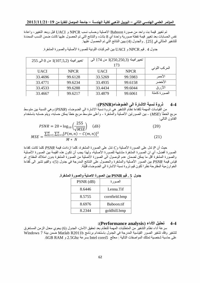
19/99/1192-91جامعة الموصل للفترة من –اليوبيل الذهبي لكلية الهندسة –المؤتمر العلمي الهندسي الثاني
55
قبل وبعد التغيير, واعادة UACIو NPCRاالصلية وحساب نسب Baboon صورةتم تغيير قيمة بت واحد من
بتات, والنتائج التي تم الحصول عليها كانت ضمن النسب المحددة 8نفس الحسابات بعد تغيير قيمة نقطة صورية واحدة أي
( يبين النتائج التي تم الحصول عليها.4. والجدول ) [25]للتشفير المثالي في
.لصورة األصلية والصورة المشفرةل المركبات اللونية بين UACIو NPCR. قيم 4جدول
(:PSNRذروة نسبة االشارة الى الضوضاء) 4-4( وهي النسبة بين متوسط PSNRمن القياسات المهمة لكفاءة نظام التشفير هي ذروة نسبة االشارة الى الضوضاء )
حسابه باستخدام وأعلى متوسط مربع خطأ يمكن حسابه, ويتم -األصلية والمشفرة بين الصورتين -( MSEمربع الخطأ )
القانون التالي:
(
√ ) ( ) ( )
∑ ∑ [ ( ) ( )]
( )
كلما كانت كفاءة PSNRتدل على الصورة المشفرة, كلما ازدادت قيمة Cتدل على الصورة األصلية و Pحيث أن
صورة األصلية الصورة أفضل, أي ان الصورة المشفرة مشابهة للصورة األصلية, ولهذا يجب أن تكون هذه القيمة بين ال
والصورة المشفرة أقل ما يمكن لضمان عدم الوصول الى الصورة األصلية من الصورة المشفرة بدون امتالك المفتاح. تم
(, والقيم تشير الى كفاءة 5والحصول على النتائج المدرجة في جدول )بين الصور األصلية والمشفرة PSNRقياس قيمة
قيم ذروة نسبة االشارة الى الضوضاء قليلة.الخوارزمية المقترحة نظرا لكون
صورة االصلية والصورة المشفرة.بين ال PSNR. قيم 5جدول
(:Performance analysisتحليل األداء ) 4-4المستغرق ( يحوي معدل الزمن6التشفير من المتطلبات المهمة للنظام بعد تحقيق األمان, الجدول ) سرعة أداء نظام
Windows 7ضمن بيئة Matlab R2011bباستخدام برنامج ور القياسية المدرجة في الجدوللتشفير وفك تشفير الص
.6GB RAMو 2.5Ghz بسرعة Intel corei5 على حاسبة شخصية تمتلك المواصفات التالية : معالج
المركب اللوني
الى 174من I(250,250,3)تغيير قيمة
173 255 الى 0من I(107,5,2)تغيير قيمة
NPCR UACI NPCR UACI
33.4696 99.6128 33.5269 99.5983 األحمر
33.4771 99.6234 33.4935 99.6158 األخضر
33.4533 99.6288 33.4434 99.6044 األزرق
33.4667 99.6217 33.4879 99.6061 الصورة كاملة
PSNR (dB) الصورة
Lenna.Tif 8.6446
cornfield.bmp 8.5755
Baboon.tif 8.6976
goldhill.bmp 8.2344
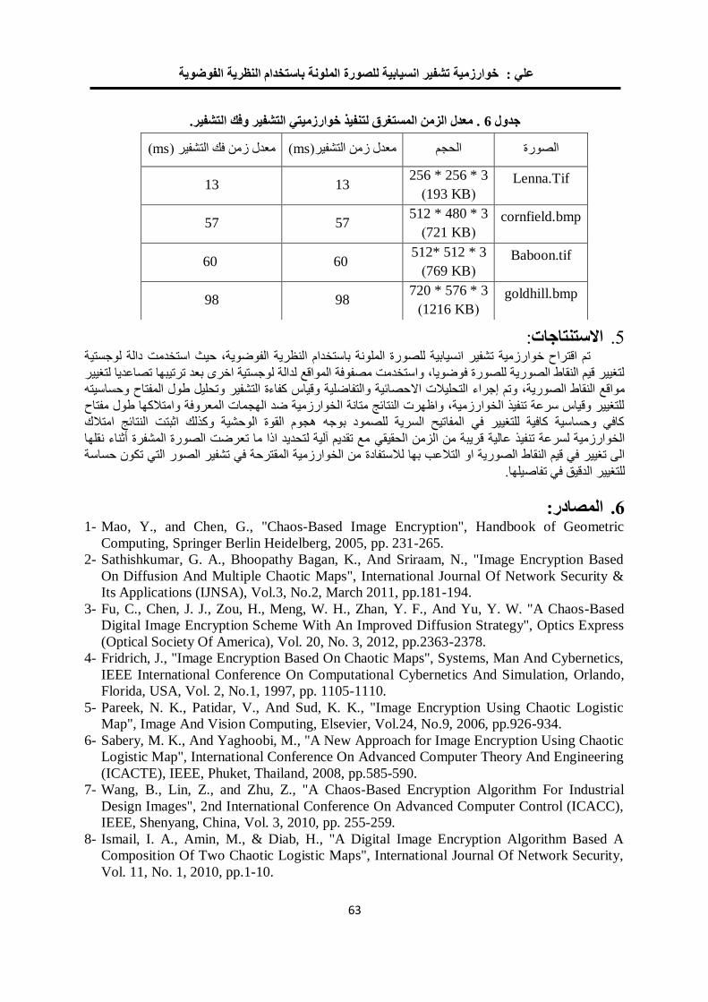
يةخوارزمية تشفير انسيابية للصورة الملونة باستخدام النظرية الفوضو : علي
55
. معدل الزمن المستغرق لتنفيذ خوارزميتي التشفير وفك التشفير. 6جدول
:االستنتاجات .3تم اقتراح خوارزمية تشفير انسيابية للصورة الملونة باستخدام النظرية الفوضوية, حيث استخدمت دالة لوجستية
لتغيير قيم النقاط الصورية للصورة فوضويا, واستخدمت مصفوفة المواقع لدالة لوجستية اخرى بعد ترتيبها تصاعديا لتغيير
حصائية والتفاضلية وقياس كفاءة التشفير وتحليل طول المفتاح وحساسيته التحليالت اال إجراءمواقع النقاط الصورية, وتم
للتغيير وقياس سرعة تنفيذ الخوارزمية, واظهرت النتائج متانة الخوارزمية ضد الهجمات المعروفة وامتالكها طول مفتاح
لك اثبتت النتائج امتالك كافي وحساسية كافية للتغيير في المفاتيح السرية للصمود بوجه هجوم القوة الوحشية وكذ
مع تقديم آلية لتحديد اذا ما تعرضت الصورة المشفرة أثناء نقلها قريبة من الزمن الحقيقي الخوارزمية لسرعة تنفيذ عالية
من الخوارزمية المقترحة في تشفير الصور التي تكون حساسة لالستفادةالى تغيير في قيم النقاط الصورية او التالعب بها
الدقيق في تفاصيلها.للتغيير
المصادر: .61- Mao, Y., and Chen, G., "Chaos-Based Image Encryption", Handbook of Geometric
Computing, Springer Berlin Heidelberg, 2005, pp. 231-265.
2- Sathishkumar, G. A., Bhoopathy Bagan, K., And Sriraam, N., "Image Encryption Based
On Diffusion And Multiple Chaotic Maps", International Journal Of Network Security &
Its Applications (IJNSA), Vol.3, No.2, March 2011, pp.181-194.
3- Fu, C., Chen, J. J., Zou, H., Meng, W. H., Zhan, Y. F., And Yu, Y. W. "A Chaos-Based
Digital Image Encryption Scheme With An Improved Diffusion Strategy", Optics Express
(Optical Society Of America), Vol. 20, No. 3, 2012, pp.2363-2378.
4- Fridrich, J., "Image Encryption Based On Chaotic Maps", Systems, Man And Cybernetics,
IEEE International Conference On Computational Cybernetics And Simulation, Orlando,
Florida, USA, Vol. 2, No.1, 1997, pp. 1105-1110.
5- Pareek, N. K., Patidar, V., And Sud, K. K., "Image Encryption Using Chaotic Logistic
Map", Image And Vision Computing, Elsevier, Vol.24, No.9, 2006, pp.926-934.
6- Sabery, M. K., And Yaghoobi, M., "A New Approach for Image Encryption Using Chaotic
Logistic Map", International Conference On Advanced Computer Theory And Engineering
(ICACTE), IEEE, Phuket, Thailand, 2008, pp.585-590.
7- Wang, B., Lin, Z., and Zhu, Z., "A Chaos-Based Encryption Algorithm For Industrial
Design Images", 2nd International Conference On Advanced Computer Control (ICACC),
IEEE, Shenyang, China, Vol. 3, 2010, pp. 255-259.
8- Ismail, I. A., Amin, M., & Diab, H., "A Digital Image Encryption Algorithm Based A
Composition Of Two Chaotic Logistic Maps", International Journal Of Network Security,
Vol. 11, No. 1, 2010, pp.1-10.
(ms) رمعدل زمن فك التشفي (msمعدل زمن التشفير) الحجم الصورة
Lenna.Tif 256 * 256 * 3
(193 KB) 13 13
cornfield.bmp 512 * 480 * 3
(721 KB) 57 57
Baboon.tif 512* 512 * 3
(769 KB) 60 60
goldhill.bmp 720 * 576 * 3
(1216 KB) 98 98
19/99/1192-91جامعة الموصل للفترة من –اليوبيل الذهبي لكلية الهندسة –المؤتمر العلمي الهندسي الثاني
55
9- Rodriguez-Sahagun, M. T., Mercado-Sánchez, J.B., López-Mancilla, D., Jaimes-Reátegui,
R., García-López, J.H., "Image Encryption Based On Logistic Chaotic Map For Secure
Communications", Electronics, Robotics And Automotive Mechanics Conference
(CERMA), IEEE, Cuernavaca, Morelos, México, 2010, pp. 319-324.
10- Bo, L., Na, L., Jianxia, L., & Wei, L. "Research Of Image Encryption Algorithm Based
On Chaos Theory", The 6th International Forum On Strategic Technology (IFOST), Vol.
2, IEEE, Harbin, China, August 2011, pp. 1096-1098.
11- Kerckhoffs, A., "La Cryptographie Militaire" Journal Des Sciences Militaires, Vol. IX,
(Electronic Version And English Translation Of "La Cryptographie Militaire" By
Peticolas, Fabien), Jan. 1883, pp. 5–38.
12- sharma, P., Godara, M., and Singh, R., "Digital Image Encryption Techniques: A
Review", International Journal of Computing & Business Research ISSN:2229 – 6166,
2012.
13- Patel, K. D., and Belani, S., "Image Encryption Using different Techniques: A Review",
International Journal of Emerging Technology and advanced Engineering, Vol. 1, No. 1,
November 2011, pp.30-34.
14- Lorenz EN, "The Essence of Chaos", University of Washington Press, Seattle, WA, 1993.
ايالف اسامة, "التشفير الفوضوي باستخدام المقياس الحيوي", مجلة الرافدين لعلوم سجى جاسم, ميالد جادر, -15
نوفمبر 50 -69الحاسبات والرياضيات , عدد خاص بوقائع المؤتمر العلمي الثالث في تقانة المعلومات,
,6070 pp.183-197.
16- Matthews, R., "On The Derivation Of A "Chaotic" Encryption Algorithm", Cryptologia,
Vol. 13, No. 1, 1989, pp.29-42.
17- Su, Z., Zhang, G., And Jiang, J., "Multimedia Security: A Survey Of Chaos-Based
Encryption Technology", Multimedia – A Multidisciplinary Approach To Complex
Issues, Dr. Ioannis Karydis (Ed.), ISBN: 978-953-51-0216-8, Intech, 2012.
18- Zhou, S., Zhang, Q., Wei, X., Zhou, Ch., "A Summarization On Image Encryption",
IETE Technical Review Vol. 27 No. 6, Nov. – Dec. 2010, pp.503-510.
19- Shannon, C. E., "Communication Theory Of Secrecy Systems", Bell System Technical
Journal, Vol.28, No. 4, Oct. 1949, pp.656-715.
20- Hasimoto Beltrán, R., "Low-Complexity Chaotic Encryption System", Revista Mexicana
De Física, Vol. 53 No. 1, Feb. 2007, pp.58-65.
21- Alvarez, G., And Li, Sh., "Some Basic Cryptographic Requirements For Chaos-Based
Cryptosystems", International Journal Of Bifurcation And Chaos, Vol. 16, No. 08, 2006,
pp.2129-2151.
22- Hussein, S. H., "Proposal Of A Cryptosystem Based On Chaos Theory And Fuzzy
Logic", Tishreen University Journal For Research And Scientific Studies- Engineering
Science Series, Vol. 31, No. 1, 2009, pp.83-97.
23- Pareek, N. K., "Design And Analysis Of A Novel Digital Image Encryption Scheme",
International Journal Of Network Security & Its Applications (IJNSA), Vol.4, No.2,
March 2012, pp. 95-108.
24- Ihara, Sh., "Information Theory For Continuous Systems", World Scientific Publishing
Company Incorporated, Vol. 2, 1993.
25- Wu, Y., Noonan, J. P., And Agaian, S., "NPCR and UACI Randomness Tests for Image
Encryption", Cyber Journals: Multidisciplinary Journals in Science and Technology,
Journal of Selected Areas in Telecommunications (JSAT), April Edition 2011, pp.31-38.
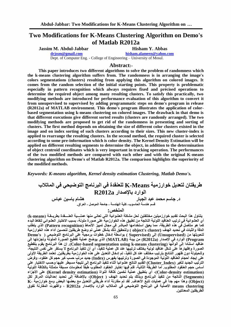
Abdul-Jabbar: Two Modifications for K-Means Clustering Algorithm on …
56
Two Modifications for K-Means Clustering Algorithm on Demo's
of Matlab R2012a Hisham Y. Abbas
[email protected] Jassim M. Abdul-Jabbar
[email protected] Dept. of Computer Eng. - College of Engineering – University of Mosul.
Abstract:- This paper introduces two different algorithms to solve the problem of randomness which
the k-means clustering algorithm suffers from. The randomness is in arranging the image's colors segmentations (clusters) resulting from applying this algorithm on colored images. It comes from the random selection of the initial starting points. This property is problematic especially in pattern recognition which always requires fixed and précised operations to determine the required object among many resulting clusters. To satisfy this practically, two modifying methods are introduced for performance evaluation of this algorithm to convert it from unsupervised to supervised by adding programmatic steps on demo's program in release (R2012a) of MATLAB environment. This demo's program illustrates the application of color-based segmentation using k-means clustering on colored images. The drawback in that demo is that different executions give different sorted results (clusters are randomly arranged). The two modifying methods are proposed to get rid of the randomness in presenting and sorting of clusters. The first method depends on obtaining the size of different color clusters existed in the image and on index sorting of such clusters according to their sizes. This new cluster-index is applied to rearrange the resulting clusters. In the second method, the required cluster is selected according to some pre-information which is color density. The Kernel Density Estimation will be applied on different resulting segments to determine the object, in addition to the determination of object centroid coordinates which is very important in tracking operation. The performances of the two modified methods are compared with each other and with the original K-means clustering algorithm on Demo's of Matlab R2012a. The comparison highlights the superiority of the modified methods.
Keywords: K-means algorithm, Kernel density estimation Clustering, Matlab Demo's.
لماتالبفي اللعنقدة في البرنامج التوضيحي K-Meansلتعديل خوارزمية طريقتان
R2012aباإلصدار الوارد هشام ياسين عباس د. جاسم محمد عبد الجبار العراق. -جامعة الموصل -كلية الهندسة -قسم هندسة الحاسوب
:الملخص( k-meansة )ـقــقدة بطريــــية العنــــيتناول هذا البحث تقديم خوارزميتين مختلفتين لحل مشكلة العشوائية التي تعاني منها عمل
بدء بسبب االختيار العشوائي لنقاط ال ،صورة ملونةه الخوارزمية على تطبيق هذ منالعناقيد اللونية الناتجة العشوائية في ترتيب أيالذي يتطلب ( Pattern recognition) األنماط، مما يعيق استخدامها المباشر في مجال تمييز كما هو متأصل في هذه الطريقة
هذه الخوارزمية أداءبشكل عملي تم وضع طريقتين لتحسين ( ولتحقيق ذلك (object's cluster والثبات في تحديد الهدفالدقة Demo'sالتوضيحي ) خطوات برمجية على البرنامج إدخالبواسطة ( Supervised) إلى( Unsupervisedلتحويلها من )
Program اإلصدار( الوارد في (R2012a )من بيئة (MATLAB الذي يوضح عملية تقطيع الصورة الملونة وتجزئتها )إلى يقوم بتقطيع هذا البرنامج إن .(Color-based segmentation using k-means clustering) ألوانها إلىعناقيد استنادا
،أن تنفيذ البرنامج ال يستقر على نفس النتيجة أي ،ختلف ترتيبها عند كل عملية تنفيذعلى شكل عناقيد لونية ي وإظهارهاالصورة األولىتعتمد الطريقة . طريقتينب الخوارزمية هذه على عديلالتإدخال تميذ، عند كل تنف بترتيب مختلفحيلولة دون ظهور النتائج ولل وفرض ،عنقود كل حجم كبر حسب مرتب جديد (Index) بفهرس وترتيبها الصورة في الموجودة اللونية العناقيدإيجاد أحجام على
على االختيار وحسب عليهامسيطر نتيجةإلى البرنامج تنفيذأثناء عشوائيا الناتج القديم Cluster_Index)) لتغير الجديد الترتيب اللونية بالكثافة ةمتمثل مسبقة لمعلومات طبقا المطلوب العنقود ختيارها إفي تمف ،الثانيةالطريقة أما المطلوب. العنقود حجمأساس
(Color-density estimation)، النواة كثافة تخمين عملية بتطبيقأي ((Kernel density estimation األجزاء على((Segments الهدف تحديد يتم وبذلك البرنامج تنفيذ من الناتجة ((Object ،لكل المركز إحداثيات تحديد إلى باإلضافة(Object) لقد تم مقارنة أداء طريقتي التعديل مع بعضها البعض ومع خوارزمية .في عمليات تتبع األهداف مهم جدا وهذاK-
means clustering األصلية في البرنامج التوضيحي في الماتالب الوارد باإلصدارR2012a وأظهرت المقارنة تفوق ، الطريقتين المعدلتين.
19/99/1192-91جامعة الموصل للفترة من –ليوبيل الذهبي لكلية الهندسة ا –الهندسي الثاني العلمي المؤتمر
55
1. Introduction Machine learning is now a central to many areas of interest in computer science and
related large-scale information processing domains. Broadly speaking the main two subfields
of machine learning are supervised learning and unsupervised learning. In supervised learning
the focus is on accurate prediction, whereas in unsupervised learning the aim is to find
compact descriptions of the data [1-4].
Clustering is an unsupervised classification mechanism where a set of patterns (data),
usually multidimensional, is classified into groups (clusters) such that members of one group
are similar according to a predefined criterion. Clustering of a set forms a partition of its
elements chosen to minimize some measure of dissimilarity between members of the same
cluster. Clustering algorithms are often applied in various information and control fields like
data mining, pattern recognition, learning theory, etc.
The k-means is the most commonly-used clustering algorithm. It is most effective for
relatively smaller data sets. The k-means finds a locally optimal solution by minimizing a
distance measure between each data and its nearest cluster center [1-7].
Suppose a data set, D, contains n objects in Euclidean space. Partitioning methods
distribute the objects in D into k clusters, C1, C2… Ck, that is, Ci D and Ci ∩ Cj= Ø for (1 ≤
i, j ≤ k). An objective function is used to assess the partitioning quality so that objects within a
cluster are similar to one another but dissimilar to objects in other clusters. Accordingly, the
objective function aims for high intracluster similarity and low intercluster similarity.
A centroid-based partitioning technique uses the centroid of a cluster, Ci, to represent
that cluster. Conceptually, the centroid of a cluster is its center point. The centroid can be
defined in various ways such as by the mean or medoid of the objects (or points) assigned to
the cluster. The difference between an object p Ci and ci, the representative of the cluster, is
measured by dist(p, ci), where dist(x,y) is the Euclidean distance between two points x and y.
The quality of cluster Ci can be measured by the "within- cluster variation", which is the sum
of squared error between all objects in Ci and the centroid ci, defined as [4]
∑ ∑
(1)
where E is the sum of the squared error for all objects in the data set; p is the point in space
representing a given object; and ci is the centroid of cluster Ci (both p and ci are
multidimensional). If the items are simple points in a n-dimensional space, then a simple
metric will be the Euclidean distance. If we consider p, q as two points, then the Euclidean
distance is given by
√∑ (2)
In the following, the k-means clustering algorithm is presented:
Algorithm: (k-means). k-means algorithm for partitioning, where each cluster’s center is
represented by the mean value of the objects in the cluster [4].
Input:
k: the number of clusters,
D: a data set containing n objects.
Output: A set of k clusters.
Method:
(1) Arbitrarily choose k objects from D as the initial cluster centers;
(2) Repeat
Abdul-Jabbar: Two Modifications for K-Means Clustering Algorithm on …
56
(3) (Re)assign each object to the cluster to which the object is the most similar, based on the
mean value of the objects in the cluster;
(4) Update the cluster means, that is, calculate the mean value of the objects for each cluster;
(5) Until no change;
In this paper, two modified methods are proposed for k-means clustering algorithm on
Demo's of Matlab R2012a. It is proved that such modifications can solve the problem of
randomness of the resulting clusters and can reorder them according to sum predefined rules.
This paper is organized as follows: besides this introductory section, section 2 presents
the previous works. Section 3 contains the kernel density estimation. The conversion of the
RGB images to Lab color space is described in section 4. Section 5 highlights the color-based
segmentation using the original k-means clustering. Section 6 contains two modified
algorithms for k-means clustering with no problem of randomness. Experimental results with
some discussions are included in section 7. Finally, Section 8 gives the conclusions.
2. Previous Works The k-means clustering algorithm faces two major problems. One is the problem of
obtaining non-optimal solutions [5] and the randomness in arranging the image's colors
segmentations (clusters), resulting from applying such algorithm on colored images. The
second problem is that of empty cluster generation. Such problem is also referred to as the
singularity problem. Singularity in clustering is obtained when one or more clusters become
empty. Both problems are caused by bad initialization [5].
Over the last several years different approaches were proposed to improve global
search properties of k-means algorithm and its performance on large data sets. Different
algorithms for clustering modification of k-means were proposed. Mu-Chun Su and Chien-
Hsing Chou [8] introduced in 2001 a modified version of the k-means algorithm to cluster
data. The adopted some nonmetric distance measure based on the idea of "point symmetry".
The point symmetry distance was applied in data clustering and human face detection. The
effectiveness of such modified version was verified via several data sets. In 2006, A. M.
Bagirov and K. Mardaneh [9] proposed many algorithms for the challenging problem of
clustering in gene expression data sets. However, due to the large number of genes, only a few
algorithms (including k-means) were applied for the clustering of samples. Such algorithms in
general converged only to local minima and those local minima were significantly different
form global solutions as the number of clusters increases [9]. To improve global search
properties of k-means algorithm and its performance on large data sets, a new version of the
k-means algorithm was developed. Such version was proved to be effective for solving
clustering problems in gene expression data sets.
Recently, in 2009, another modified k-means algorithm was presented by M. K.
Pakhira [5] to eliminate the production of empty clusters. Such empty clusters problem can
produce anomalous behavior of the system leading to significant performance degradation.
Also in 2009, Lin Zhu, et al. [10] presented a generalized fuzzy C-means clustering
algorithm with improved fuzzy partitions.
More recently, B. F. Momin and P. M. Yelmar [11] in 2012, introduced modifications
in hard K-means algorithm such that algorithm can be used for clustering data with
categorical attributes.
3. Kernel Density Estimation Kernel density estimation [4], [7] is a nonparametric density estimation approach from
statistics. The general idea behind kernel density estimation is simple. An observed object is
19/99/1192-91جامعة الموصل للفترة من –ليوبيل الذهبي لكلية الهندسة ا –الهندسي الثاني العلمي المؤتمر
56
treated as an indicator of high-probability density in the surrounding region. The probability
density at a point depends on the distances from this point to the observed objects. If we let x1,
x2,… xn, be an independent and identically distributed sample of a random variable f . The
kernel density approximation of the probability density function is given by
∑ (
)
(3)
where K(.) is a kernel and h is the bandwidth serving as a smoothing parameter. A kernel can
be regarded as a function modeling the influence of a sample point within its neighborhood.
The kernel K(.) is a non-negative real-valued integrable function that should satisfy the
following two requirements: ∫
(u) du =1 and K(-u) = K(u) for all values of u. A
frequently used kernel is the standards zero mean Gaussian function with unit variance which
can be given as
(
)
√
( )
(4)
The Gaussian kernel is used to estimate density based on the given set of objects to be
clustered.
4. L a b- Color Space In this paper, the RGB images are converted to the L*a*b*, or CIELab, color space. It
is an International Standard for color measurements, adopted by the Commission
Internationale d’Eclairage (CIE) in 1976. For a given object, the observed light intensity
depends on both the intensity and the spectral distribution of the illuminating light, and the
spectral distribution of the object reflectivity. Therefore, CIE defined the spectral properties
of several standard illuminants. The most common one is standard illuminant D65,
corresponding to the radiation of a black body at 6500°C, which is intended to represent
average daylight [12].
The L*a*b* color space can be derived from the CIE XYZ tristimulus values. The
L*a*b* space consists of a luminosity layer 'L*', chromaticity-layer 'a*' which indicates
where color falls along the red-green axis, and chromaticity-layer 'b*' which indicates where
the color falls along the blue-yellow axis. All of the color information is in the 'a*' and 'b*'
layers. A measurement method with reduce complexity can be achieved by measuring the
difference between the two color components a & b using the Euclidean distance metric [13].
The chromaticity coordinates are denoted by r, g, b and x, y, z. The transformation
from R, G, and B to X, Y, and Z can be shown as follows:
X = 0.4124 r + 0.3576 g + 0.1805 b (5)
Y = 0.2126 r + 0.7152 g + 0.0722 b (6)
Z = 0.0193 r + 0.1192 g + 0.9505 b (7)
The general definitions of the chromaticies x, y, z are:
x = X / (X + Y + Z) (8)
y = Y / (X + Y + Z) (9)
z = Z / (X + Y + Z) (10)
where x + y + z = 1.
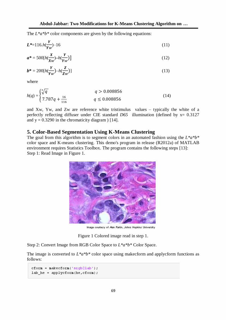
Abdul-Jabbar: Two Modifications for K-Means Clustering Algorithm on …
56
The L*a*b* color components are given by the following equations:
L*=116.h(
)–16 (11)
a* = 500[h(
)–h(
(12)
b* = 200[h(
–h(
] (13)
where
h(q) = {√
(14)
and Xw, Yw, and Zw are reference white tristimulus values – typically the white of a
perfectly reflecting diffuser under CIE standard D65 illumination (defined by x= 0.3127
and y = 0.3290 in the chromaticity diagram ) [14].
5. Color-Based Segmentation Using K-Means Clustering The goal from this algorithm is to segment colors in an automated fashion using the L*a*b*
color space and K-means clustering. This demo's program in release (R2012a) of MATLAB
environment requires Statistics Toolbox. The program contains the following steps [13]:
Step 1: Read Image in Figure 1.
Figure 1 Colored image read in step 1.
Step 2: Convert Image from RGB Color Space to L*a*b* Color Space.
The image is converted to L*a*b* color space using makecform and applycform functions as
follows:
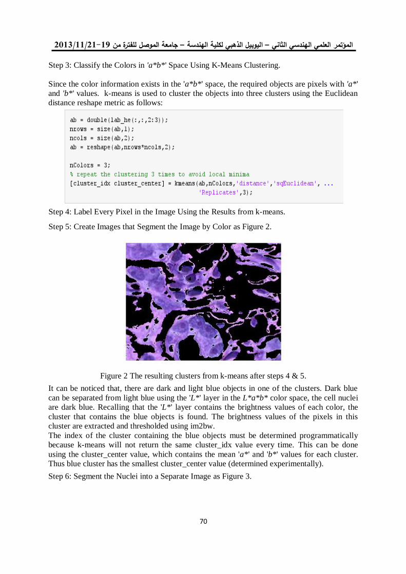
19/99/1192-91جامعة الموصل للفترة من –ليوبيل الذهبي لكلية الهندسة ا –الهندسي الثاني العلمي المؤتمر
67
Step 3: Classify the Colors in 'a*b*' Space Using K-Means Clustering.
Since the color information exists in the 'a*b*' space, the required objects are pixels with 'a*'
and 'b*' values. k-means is used to cluster the objects into three clusters using the Euclidean
distance reshape metric as follows:
Step 4: Label Every Pixel in the Image Using the Results from k-means.
Step 5: Create Images that Segment the Image by Color as Figure 2.
Figure 2 The resulting clusters from k-means after steps 4 & 5.
It can be noticed that, there are dark and light blue objects in one of the clusters. Dark blue
can be separated from light blue using the 'L*' layer in the L*a*b* color space, the cell nuclei
are dark blue. Recalling that the 'L*' layer contains the brightness values of each color, the
cluster that contains the blue objects is found. The brightness values of the pixels in this
cluster are extracted and thresholded using im2bw.
The index of the cluster containing the blue objects must be determined programmatically
because k-means will not return the same cluster_idx value every time. This can be done
using the cluster_center value, which contains the mean 'a*' and 'b*' values for each cluster.
Thus blue cluster has the smallest cluster_center value (determined experimentally).
Step 6: Segment the Nuclei into a Separate Image as Figure 3.
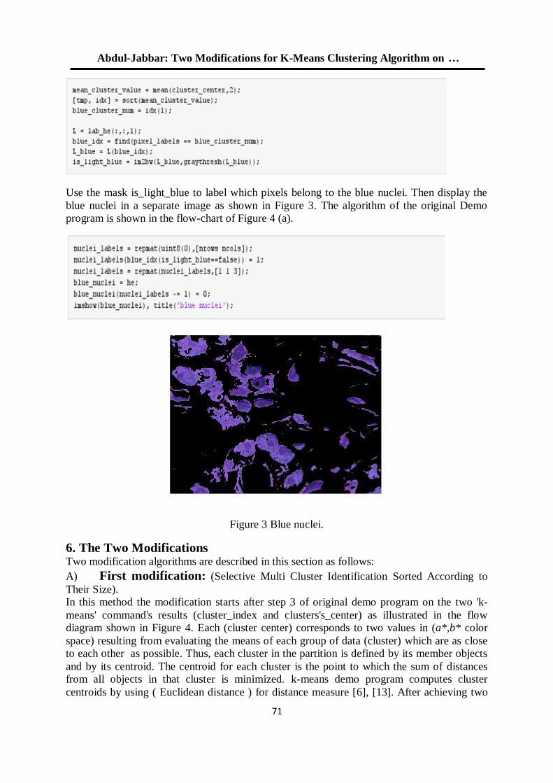
Abdul-Jabbar: Two Modifications for K-Means Clustering Algorithm on …
67
Use the mask is_light_blue to label which pixels belong to the blue nuclei. Then display the
blue nuclei in a separate image as shown in Figure 3. The algorithm of the original Demo
program is shown in the flow-chart of Figure 4 (a).
Figure 3 Blue nuclei.
6. The Two Modifications Two modification algorithms are described in this section as follows:
A) First modification: (Selective Multi Cluster Identification Sorted According to
Their Size).
In this method the modification starts after step 3 of original demo program on the two 'k-
means' command's results (cluster_index and clusters's_center) as illustrated in the flow
diagram shown in Figure 4. Each (cluster center) corresponds to two values in (a*,b* color
space) resulting from evaluating the means of each group of data (cluster) which are as close
to each other as possible. Thus, each cluster in the partition is defined by its member objects
and by its centroid. The centroid for each cluster is the point to which the sum of distances
from all objects in that cluster is minimized. k-means demo program computes cluster
centroids by using ( Euclidean distance ) for distance measure [6], [13]. After achieving two
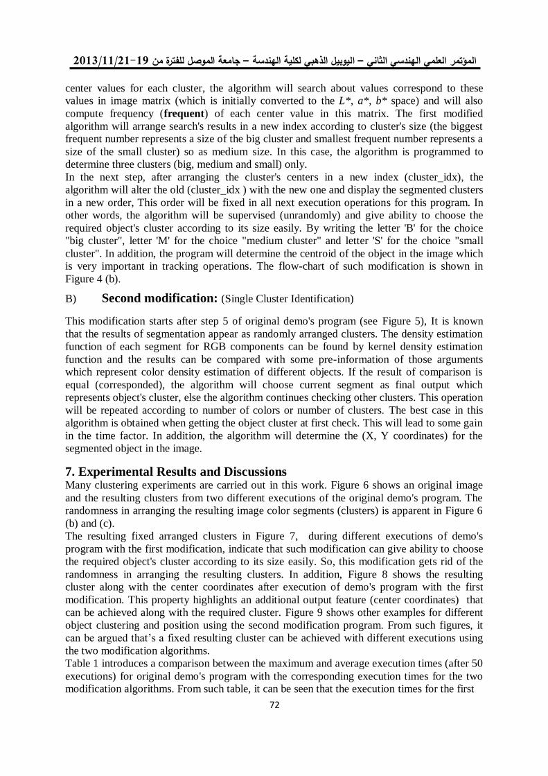
19/99/1192-91جامعة الموصل للفترة من –ليوبيل الذهبي لكلية الهندسة ا –الهندسي الثاني العلمي المؤتمر
67
center values for each cluster, the algorithm will search about values correspond to these
values in image matrix (which is initially converted to the L*, a*, b* space) and will also
compute frequency (frequent) of each center value in this matrix. The first modified
algorithm will arrange search's results in a new index according to cluster's size (the biggest
frequent number represents a size of the big cluster and smallest frequent number represents a
size of the small cluster) so as medium size. In this case, the algorithm is programmed to
determine three clusters (big, medium and small) only.
In the next step, after arranging the cluster's centers in a new index (cluster_idx), the
algorithm will alter the old (cluster_idx ) with the new one and display the segmented clusters
in a new order, This order will be fixed in all next execution operations for this program. In
other words, the algorithm will be supervised (unrandomly) and give ability to choose the
required object's cluster according to its size easily. By writing the letter 'B' for the choice
"big cluster", letter 'M' for the choice "medium cluster" and letter 'S' for the choice "small
cluster". In addition, the program will determine the centroid of the object in the image which
is very important in tracking operations. The flow-chart of such modification is shown in
Figure 4 (b).
B) Second modification: (Single Cluster Identification)
This modification starts after step 5 of original demo's program (see Figure 5), It is known
that the results of segmentation appear as randomly arranged clusters. The density estimation
function of each segment for RGB components can be found by kernel density estimation
function and the results can be compared with some pre-information of those arguments
which represent color density estimation of different objects. If the result of comparison is
equal (corresponded), the algorithm will choose current segment as final output which
represents object's cluster, else the algorithm continues checking other clusters. This operation
will be repeated according to number of colors or number of clusters. The best case in this
algorithm is obtained when getting the object cluster at first check. This will lead to some gain
in the time factor. In addition, the algorithm will determine the (X, Y coordinates) for the
segmented object in the image.
7. Experimental Results and Discussions Many clustering experiments are carried out in this work. Figure 6 shows an original image
and the resulting clusters from two different executions of the original demo's program. The
randomness in arranging the resulting image color segments (clusters) is apparent in Figure 6
(b) and (c).
The resulting fixed arranged clusters in Figure 7, during different executions of demo's
program with the first modification, indicate that such modification can give ability to choose
the required object's cluster according to its size easily. So, this modification gets rid of the
randomness in arranging the resulting clusters. In addition, Figure 8 shows the resulting
cluster along with the center coordinates after execution of demo's program with the first
modification. This property highlights an additional output feature (center coordinates) that
can be achieved along with the required cluster. Figure 9 shows other examples for different
object clustering and position using the second modification program. From such figures, it
can be argued that’s a fixed resulting cluster can be achieved with different executions using
the two modification algorithms.
Table 1 introduces a comparison between the maximum and average execution times (after 50
executions) for original demo's program with the corresponding execution times for the two
modification algorithms. From such table, it can be seen that the execution times for the first
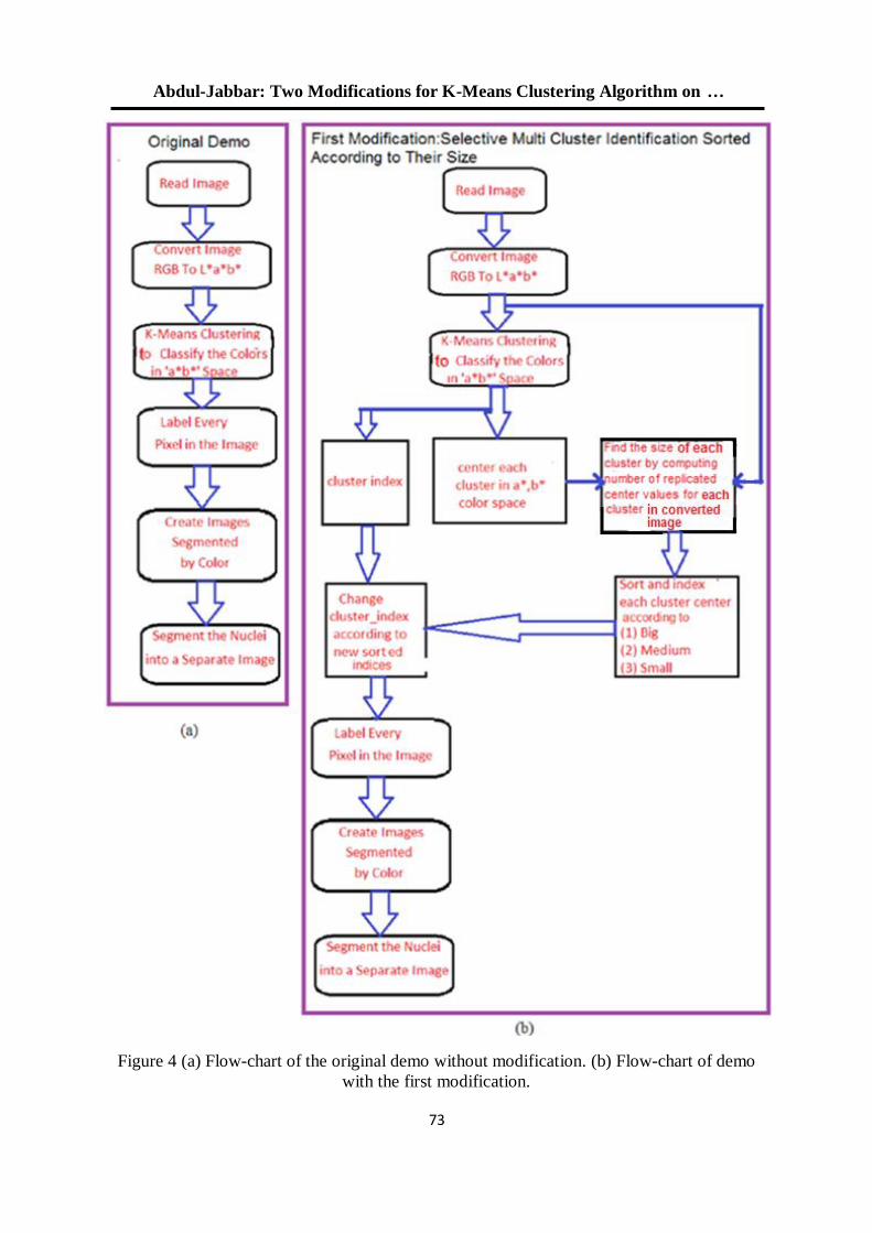
Abdul-Jabbar: Two Modifications for K-Means Clustering Algorithm on …
67
Figure 4 (a) Flow-chart of the original demo without modification. (b) Flow-chart of demo
with the first modification.
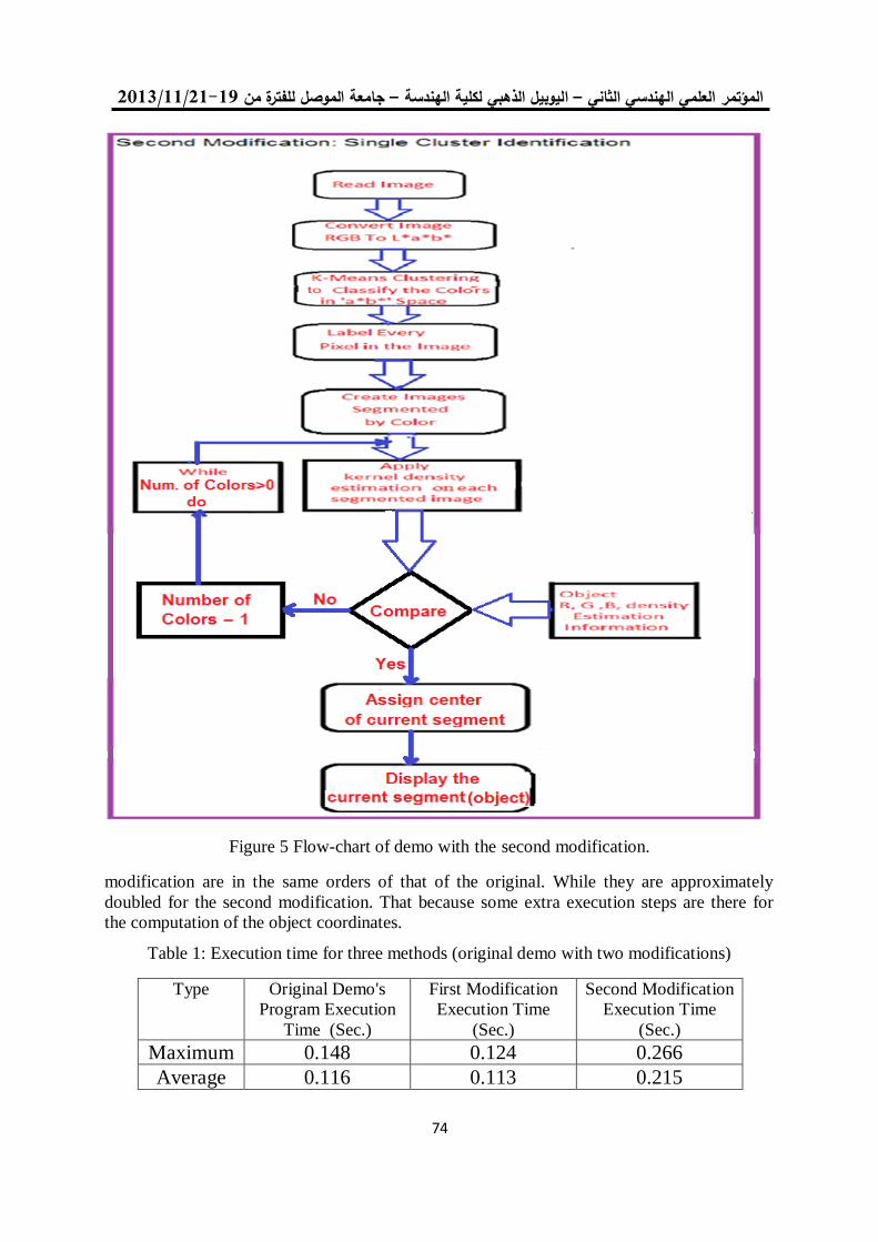
19/99/1192-91جامعة الموصل للفترة من –ليوبيل الذهبي لكلية الهندسة ا –الهندسي الثاني العلمي المؤتمر
67
Figure 5 Flow-chart of demo with the second modification.
modification are in the same orders of that of the original. While they are approximately
doubled for the second modification. That because some extra execution steps are there for
the computation of the object coordinates.
Table 1: Execution time for three methods (original demo with two modifications)
Type Original Demo's
Program Execution
Time (Sec.)
First Modification
Execution Time
(Sec.)
Second Modification
Execution Time
(Sec.)
Maximum 0.148 0.124 0.266
Average 0.116 0.113 0.215
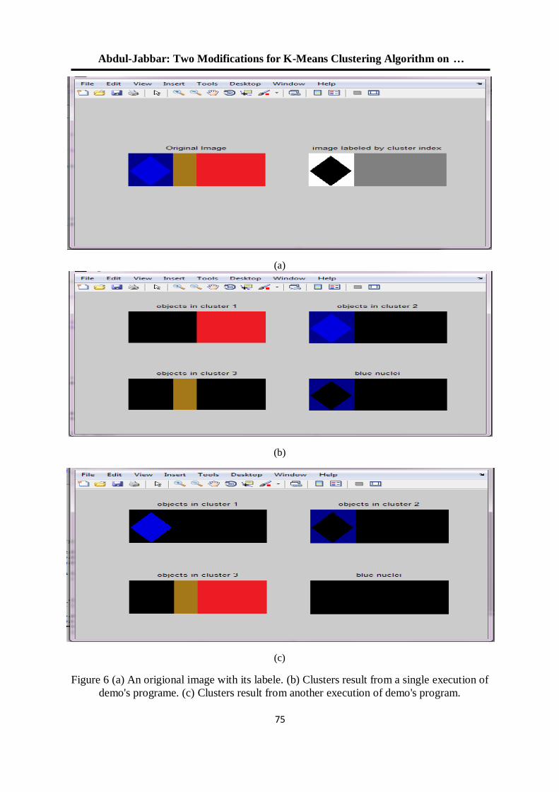
Abdul-Jabbar: Two Modifications for K-Means Clustering Algorithm on …
66
(a)
(b)
(c)
Figure 6 (a) An origional image with its labele. (b) Clusters result from a single execution of
demo's programe. (c) Clusters result from another execution of demo's program.
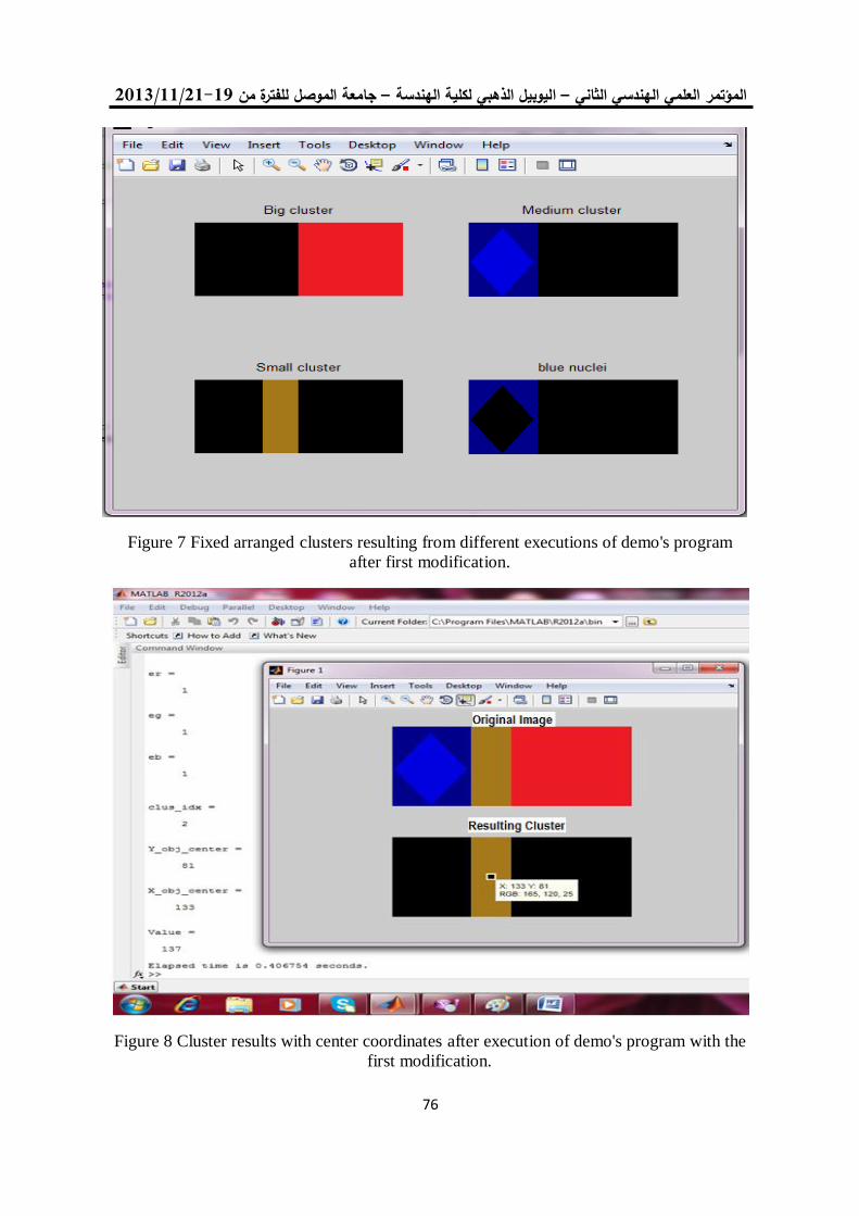
19/99/1192-91جامعة الموصل للفترة من –ليوبيل الذهبي لكلية الهندسة ا –الهندسي الثاني العلمي المؤتمر
65
Figure 7 Fixed arranged clusters resulting from different executions of demo's program
after first modification.
Figure 8 Cluster results with center coordinates after execution of demo's program with the
first modification.
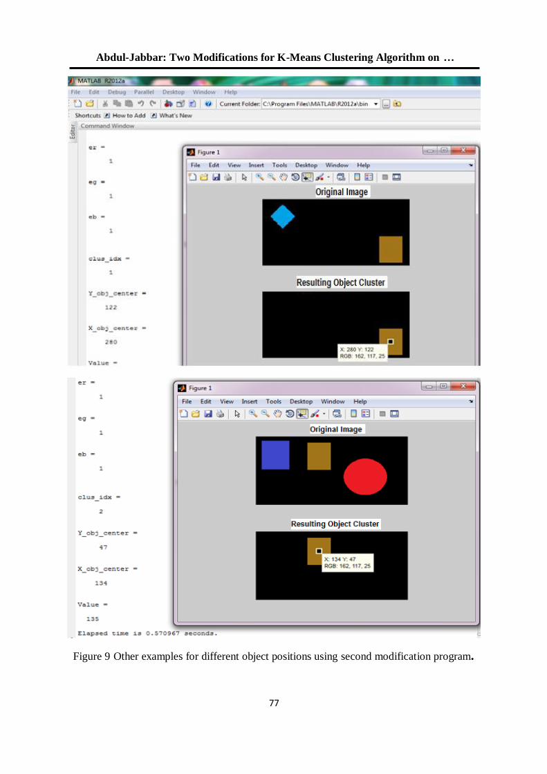
Abdul-Jabbar: Two Modifications for K-Means Clustering Algorithm on …
66
Figure 9 Other examples for different object positions using second modification program.
19/99/1192-91جامعة الموصل للفترة من –ليوبيل الذهبي لكلية الهندسة ا –الهندسي الثاني العلمي المؤتمر
66
8. Conclusions Two different modified algorithms have been introduced to solve the problem of randomness
in arranging clusters of the different executions in the k-means clustering algorithm of the
demo's program in MATLAB R2012a. The two modifications have been examined using
different clusters to illustrate their fixed resulting cluster for different executions. Execution times of the first modification have appeared in the same orders of the
corresponding execution times of original Demo's program, while in the second modification,
execution times have been doubled.
It can be recommended that it is best to use the first modification for fast identification and
control purposes, while the second is preferred for color-based clustering without specifying
the size of the required cluster.
References [1] D. Barber, "Bayesian Reasoning and Machine Learning", Cambridge University Press,
ISBN/ASIN: 0521518148, 2011 .
[2] M. Jordan, J. Kleinberg, B. Scholkopf and C. M. Bishop, "Pattern Recognition and
Machine Learning", Springer Science +Business Media, LLC, 2006.
[3] M. N. Murty and V. S. Devi, "Pattern Recognition an Algorithmic Approach", Springer
Science + Business Media, Universities Press (India) Pvt. Ltd, 2011.
[4] J. Han, M. Kamber and J. Pei, "Data Mining Concepts and Techniques", 3rd
Edition,
Elsevier Inc, 2012.
[5] M. K. Pakhira, "A Modified k-means Algorithm to Avoid Empty Clusters", International
Journal of Recent Trends in Engineering, Vol. 1, No. 1, May 2009, 220-226 pp.
[6] MathWorks, Help of MATLAB-R2012a,"Introduction to k- Means Clustering"
http://www.mathworks.com/help/stats/k-meansclustering.html?searchHighlight=K-
Means+Clustering
[7] R. Szeliski, "Computer Vision: Algorithms and Applications", Microsoft Research,
Springer, ISBN 978-1-84882-935-0, 2010.
[8] Mu-Chun Su, Member, IEEE, and Chien-Hsing Chou, Student Member, IEEE, "A
Modified Version of the k-means Algorithm with a Distance Based on Cluster Symmetry",
IEEE Transactions on Pattern Analysis and Machine Intelligence, Vol. 23, No, 6, June 2001,
674-434 pp.
[9] A. M. Bagirov, and K. Mardaneh, "Modified Global K-Means Algorithm For Clustering in
Gene Expression Data Sets", Centre for Informatics and Applied Optimization, School of
Information Technology and Mathematical Sciences, University of Ballarat, Victoria,
Australian Computer Society, Inc., 2006.
[10] Lin Zhu, Fu-Lai Chung, and Shitong Wang,” Generalized Fuzzy C-Means Clustering
Algorithm With Improved Fuzzy Partitions”, IEEE Trans. Syst. Man. Vol. 39, No. 3, 2009,
PP.578-591.

Abdul-Jabbar: Two Modifications for K-Means Clustering Algorithm on …
66
[11] B. F. Momin and P. M. Yelmar, "Modifications in K-Means Clustering Algorithm",
International Journal of Soft Computing and Engineering (IJSCE) ISSN: 2231-2307, Vol. 2,
Issue-3, July 2012, pp. 349-354.
[12] N. A. Baykan, N. Yılmaz and G. Kansun,"Case Study in Effects of Color Spaces for
Mineral Identification", Scientific Research and Essays Vol. 5(11), 2010,1243-1253pp.
[13] MathWorks, Help of MATLAB-R2012a,"Color-Based-Segmentation-Using-k-Means-
Clustering", on http://www.mathworks.com/help/images/examples/color-based-
segmentation-using-k-means-clustering.html
[14] R. C. Gonzalez and R. E. Woods, "Digital Image Processing", 3rd
Ed, Pearson Education,
Inc., 2008.
19/99/1192-91جامعة الموصل للفترة من –ليوبيل الذهبي لكلية الهندسة ا – الهندسي الثانيالعلمي المؤتمر
08
Human vs. Machine Tic-Tac Game Based on Microcontroller
Technology
Alauddin Al-Omary / Associate Professor College of Information Technology
University of Bahrain
Abstract In this paper the hardware implementation of intelligent Tic-Tac toy is presented. The
implementation uses Graphical LCD (GLCD) touch screen and microcontroller. The
microcontroller receives the player move from GLCD (displayed as X) and uses
intelligent algorithm to analyze the move and choose the best counter move. The
microcontroller displays the counter move on the screen as circle (O). The algorithm
decides the winner when game is finished according to the Tic-Tac playing rule. The
system is implemented using cheap available off-the-shelf electronic components so it has
the advantage of cheap implementation. The system is tested and proved to be working
fast and efficiently. The prototype test shows that the system fulfills the game
requirement in term of playability and fast response time which is about (0.25ms) on
average.
Keywords: Tic-Tac Game, AI, Microcontroller, Zero-sum assumption algorithm.
باستخدام تقنية المايكروكونترولر -مستخدم ضد االلة -لعبة تك تاك
عالء الدين يوسف العمري /استاذ مشارك
كلية تقنية المعلومات / جامعة البحرين
الخالصة
لعبة التك تاك باستخدام خوارزمية ذكية تمت برمجتها داخل معالج مايكروكونترولر. تم في هذا البحث تم تنفيذ
الدخال خطوات اللعبة ومن قبل مستخدم وتقوم االلة بحساب الرد االمثل وارساله GLCDاستخدام شاشة لمس نوع
اكمال احدهما خطا طوليا او الى الشاشة. يكون الفائز في اللعبة الشخص الالعب أو االلة حسب شروط اللعبة وعند
(. off-the-shelf electronic componentsعرضيا او قطريا. تم تنفيذ اللعبة باستخدام مواد متوفرة رخيصة )
تمتاز اللعبة باستخدام خوارزمية ذكية ومواد رخيصة واداء جيد قياسا لما تم تنفيذه من قبل الباحثين. تم فحص االلة
ملي ثانية. 0.25ية التي برمجت بها مع سرعة استجابة مقدارها وتبين صحة عمل الخوارزم
.: لعبة التك تاك ، الذكاء الصناعي، المعالج المايكروي ، خوارزمية المجموع الصفري االفتراضي كلمات دالة
Al-Omary: Human vs. Machine Tic-Tac Game Based on Microcontroller …..
08
I. INTRODUCTION Games provide a real source of enjoyment in daily life. Games also are helpful in
improving the physical and mental health of human. Apart from daily life physical games,
people also play computer games. These games are different than those of physical games in a
sense that they do not involve much physical activity rather mental and emotional activities.
I.I TYPES OF GAME Perfect Information Game: In which player knows all the possible moves of himself and
opponent and their results e.g. Chess, Tic-Tac, etc.
Imperfect Information Game: In which player does not know all the possible moves of the
opponent e.g. Bridge since all the cards are not visible to player.
I.II TIC-TAC GAME Among many game available, the Tic-Tac toy seems to be popular since it has very
simple rules and can be played by kids as well as adults.
Tic-tac game is a pencil-and-paper game for two players, X and O, who take turns marking
the spaces in a 3×3 grid. The X player usually goes first. The player who succeeds in placing
three respective marks in a horizontal, vertical, or diagonal row wins the game. In this paper
the X player is a Man and the O player is the machine.
I.III RELATED WORK Many software implementations of Tic Tac game had been reported and recently it
became available for smart phone such as the one for Apple iPhone [1], and the other for
Android environment [2]. However few hardware implementations were reported.
In Cornell University [3] hardware based game system with touch screen interfaces based
on Atmel ATmega644 microcontroller was reported. The system implements Tic-Tac game
and other two games.
A system where two players can play Tic Tac Toe with each other using their respective
PC by the help of microcontroller is introduced in [4]. The objectives of the work includes
developing an algorithm for Tic Tac Toe, interfacing hardware with the two PCs and to design
a real world setup for Tic- Tac toe game using LED array / robotic arms. The algorithm
proposed in this paper is fuzzy based and tested for the game. The researchers in [5] took
advantage of earcons [6] fundamental characteristics, such as spatialization usually employed
for concurrent/parallel reproduction, in order to implement a tic-tac-toe audio game prototype.
The proposed sonic design is transparently integrated with a user control/interaction
mechanism that can be easily implemented in mobile devices incorporating movement sensors
(i.e. accelerometers and gyroscope).
In [7] a design of a parallel digital circuit that performs neural network (NN) calculations
to evaluate Tic-Tac-Toe position was introduced. FPGA’s are programmed to implement
custom digital designs by physically mapping paths between the logic gates on each device.
Using an FPGA allows the structure of the NN to be reprogrammed without any monetary
cost. The author claims that NN implementation has better performance than traditional
software implementations, because it takes advantage of the NN's inherent parallel structure.
Another NN application is implemented by [8] extend the game by adding two additional
rows, two additional columns, and has been extended to the 3rd dimension. The paper
calculate the optimum position using the idea of creating a neural network that uses
19/99/1192-91جامعة الموصل للفترة من –ليوبيل الذهبي لكلية الهندسة ا – الهندسي الثانيالعلمي المؤتمر
08
backpropagation coupled with elements of a genetic algorithm to improve the likelihood that
the most optimal solution is obtained and outline our methodology at the implementation level.
However, some these implementations are expensive and some are slow and lacking the
speed required by real time game response. Also getting the optimum counter move is another
issue in some of these hardware implementations.
I.IV SCOPE OF THE WORK
People generally play computer games by using the common input devices like
keyboard, mouse and joystick. A real sensation is not always achieved by playing these games
with these traditional devices. This is due to the fact that the buttons on the keyboard and
joystick do not truly reflect the mapping between game elements and their directional
movements.
In this paper the implementation of portable player Tic-Tac game machine is presented.
In order to make a real sensation for player who plays the game a GLCD is used. The GLCD
serves as input and output for the game. The machine is designed to be portable inexpensive
and fast. To make a cheap machine, the presented Tic-Tac game uses off-the shelf cheap
components such as PIC microcontroller and GLCD. The microcontroller is programmed using
intelligent algorithm that implements the Tic-Tac game rules and responds to the player move
fast.
There are different options for tic-tac-toe game. We can create either two human players
game or AI (micro-controller) verses human player. We realized that creating AI verses human
will be a challenging one, and we kept in mind AI part as the goal of our work.
II. GAME THEORY Games [9], [10], [11] are represented in the form of trees wherein nodes represent all the
possible states of a game and edges represent moves between them. Initial state of the game is
represented by root and terminal states by leaves of the tree. In a normal search problem, the
optimal solution would be a sequence of moves leading to a goal state that is a win. Even for a
simple game like tic-tac-toe is too complex to draw the entire game tree
II.I DEFINITION
Game playing is a search problem defined by the following components [9]:
Initial state: This defines initial configuration of the game and identifies first player to move.
Successor function: This identifies which are the possible states that can be achieved from the
current state. This function returns a list of (move, state) pairs, each indicating a legal move
and the resulting state.
Goal test: Which checks whether a given state is a goal state or not. States where the game
ends are called as terminal states.
Path cost / utility / payoff function: This gives a numeric value for the terminal states. In chess,
the outcome is winning, losing or draw, with values +1, -1, or 0. Some games have wider range
of possible outcomes.
II.II THE TIC-TAC GAME CHARACTERISTICS [11]
1- It is two players game
2- It is a deterministic game which means that when you provide it a specific set of inputs you
will get the exact same set of outputs [9].
3- It is a perfect information game where perfect information is available for all move [10].
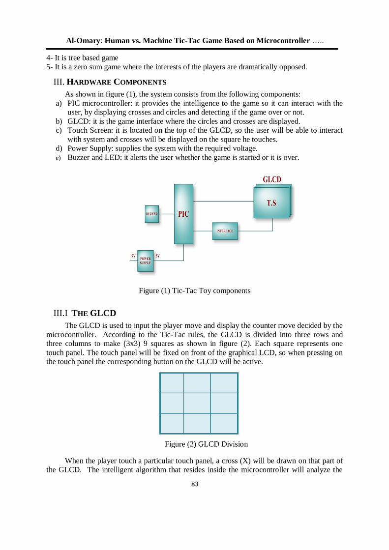
Al-Omary: Human vs. Machine Tic-Tac Game Based on Microcontroller …..
08
4- It is tree based game
5- It is a zero sum game where the interests of the players are dramatically opposed.
III. HARDWARE COMPONENTS
As shown in figure (1), the system consists from the following components:
a) PIC microcontroller: it provides the intelligence to the game so it can interact with the
user, by displaying crosses and circles and detecting if the game over or not.
b) GLCD: it is the game interface where the circles and crosses are displayed.
c) Touch Screen: it is located on the top of the GLCD, so the user will be able to interact
with system and crosses will be displayed on the square he touches.
d) Power Supply: supplies the system with the required voltage.
e) Buzzer and LED: it alerts the user whether the game is started or it is over.
Figure (1) Tic-Tac Toy components
III.I THE GLCD
The GLCD is used to input the player move and display the counter move decided by the
microcontroller. According to the Tic-Tac rules, the GLCD is divided into three rows and
three columns to make (3x3) 9 squares as shown in figure (2). Each square represents one
touch panel. The touch panel will be fixed on front of the graphical LCD, so when pressing on
the touch panel the corresponding button on the GLCD will be active.
Figure (2) GLCD Division
When the player touch a particular touch panel, a cross (X) will be drawn on that part of
the GLCD. The intelligent algorithm that resides inside the microcontroller will analyze the
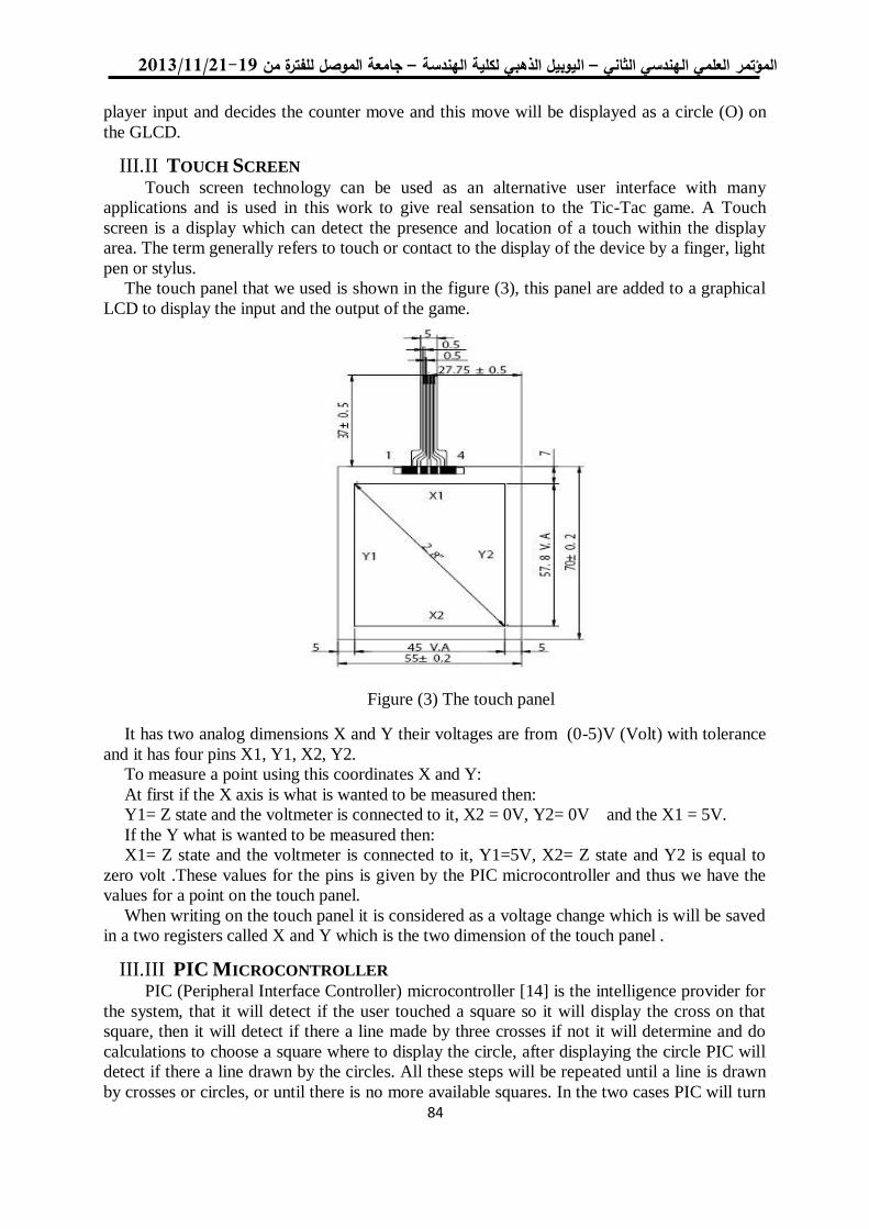
19/99/1192-91جامعة الموصل للفترة من –ليوبيل الذهبي لكلية الهندسة ا – الهندسي الثانيالعلمي المؤتمر
08
player input and decides the counter move and this move will be displayed as a circle (O) on
the GLCD.
III.II TOUCH SCREEN Touch screen technology can be used as an alternative user interface with many
applications and is used in this work to give real sensation to the Tic-Tac game. A Touch
screen is a display which can detect the presence and location of a touch within the display
area. The term generally refers to touch or contact to the display of the device by a finger, light
pen or stylus.
The touch panel that we used is shown in the figure (3), this panel are added to a graphical
LCD to display the input and the output of the game.
Figure (3) The touch panel
It has two analog dimensions X and Y their voltages are from (0-5)V (Volt) with tolerance
and it has four pins X1, Y1, X2, Y2.
To measure a point using this coordinates X and Y:
At first if the X axis is what is wanted to be measured then:
Y1= Z state and the voltmeter is connected to it, X2 = 0V, Y2= 0V and the X1 = 5V.
If the Y what is wanted to be measured then:
X1= Z state and the voltmeter is connected to it, Y1=5V, X2= Z state and Y2 is equal to
zero volt .These values for the pins is given by the PIC microcontroller and thus we have the
values for a point on the touch panel.
When writing on the touch panel it is considered as a voltage change which is will be saved
in a two registers called X and Y which is the two dimension of the touch panel .
III.III PIC MICROCONTROLLER PIC (Peripheral Interface Controller) microcontroller [14] is the intelligence provider for
the system, that it will detect if the user touched a square so it will display the cross on that
square, then it will detect if there a line made by three crosses if not it will determine and do
calculations to choose a square where to display the circle, after displaying the circle PIC will
detect if there a line drawn by the circles. All these steps will be repeated until a line is drawn
by crosses or circles, or until there is no more available squares. In the two cases PIC will turn
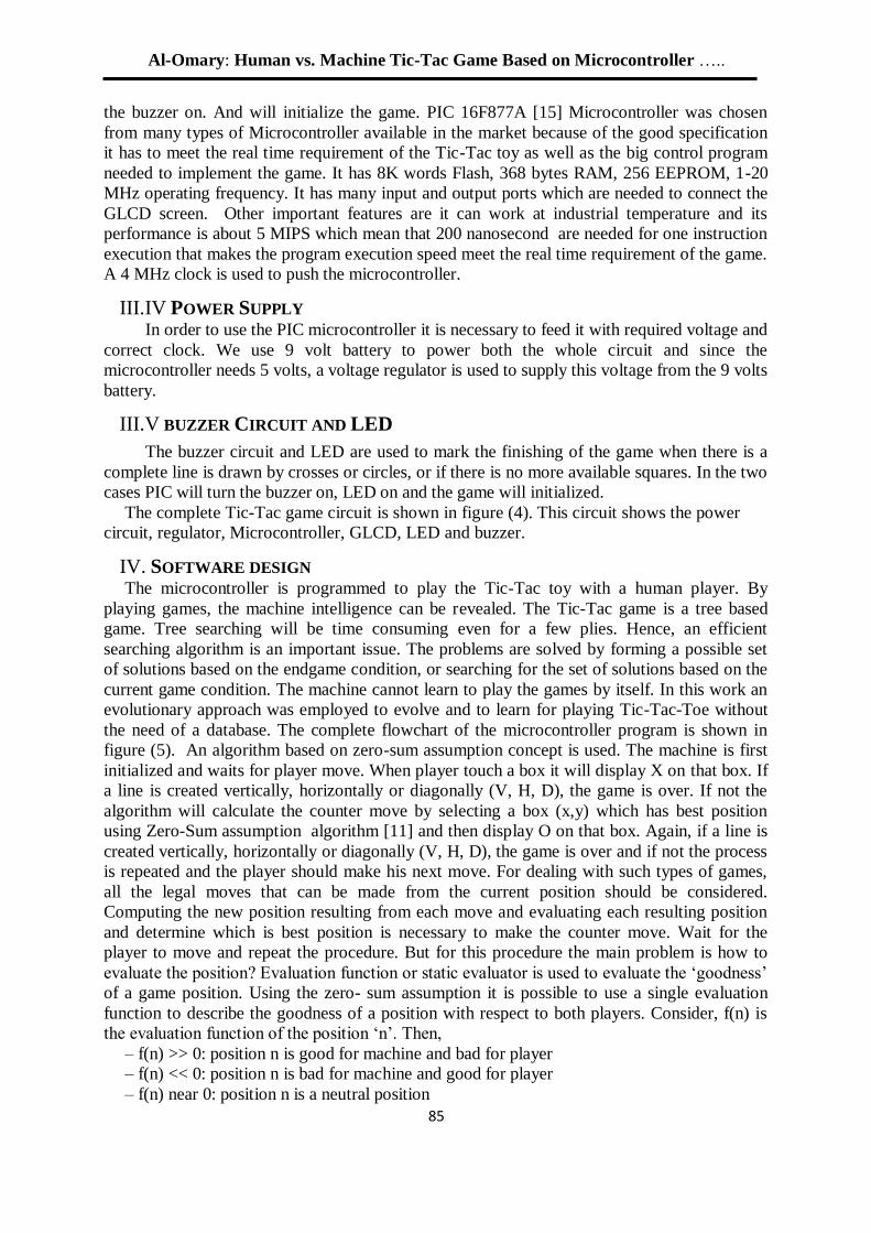
Al-Omary: Human vs. Machine Tic-Tac Game Based on Microcontroller …..
08
the buzzer on. And will initialize the game. PIC 16F877A [15] Microcontroller was chosen
from many types of Microcontroller available in the market because of the good specification
it has to meet the real time requirement of the Tic-Tac toy as well as the big control program
needed to implement the game. It has 8K words Flash, 368 bytes RAM, 256 EEPROM, 1-20
MHz operating frequency. It has many input and output ports which are needed to connect the
GLCD screen. Other important features are it can work at industrial temperature and its
performance is about 5 MIPS which mean that 200 nanosecond are needed for one instruction
execution that makes the program execution speed meet the real time requirement of the game.
A 4 MHz clock is used to push the microcontroller.
III.IV POWER SUPPLY In order to use the PIC microcontroller it is necessary to feed it with required voltage and
correct clock. We use 9 volt battery to power both the whole circuit and since the
microcontroller needs 5 volts, a voltage regulator is used to supply this voltage from the 9 volts
battery.
III.V BUZZER CIRCUIT AND LED
The buzzer circuit and LED are used to mark the finishing of the game when there is a
complete line is drawn by crosses or circles, or if there is no more available squares. In the two
cases PIC will turn the buzzer on, LED on and the game will initialized.
The complete Tic-Tac game circuit is shown in figure (4). This circuit shows the power
circuit, regulator, Microcontroller, GLCD, LED and buzzer.
IV. SOFTWARE DESIGN The microcontroller is programmed to play the Tic-Tac toy with a human player. By
playing games, the machine intelligence can be revealed. The Tic-Tac game is a tree based
game. Tree searching will be time consuming even for a few plies. Hence, an efficient
searching algorithm is an important issue. The problems are solved by forming a possible set
of solutions based on the endgame condition, or searching for the set of solutions based on the
current game condition. The machine cannot learn to play the games by itself. In this work an
evolutionary approach was employed to evolve and to learn for playing Tic-Tac-Toe without
the need of a database. The complete flowchart of the microcontroller program is shown in
figure (5). An algorithm based on zero-sum assumption concept is used. The machine is first
initialized and waits for player move. When player touch a box it will display X on that box. If
a line is created vertically, horizontally or diagonally (V, H, D), the game is over. If not the
algorithm will calculate the counter move by selecting a box (x,y) which has best position
using Zero-Sum assumption algorithm [11] and then display O on that box. Again, if a line is
created vertically, horizontally or diagonally (V, H, D), the game is over and if not the process
is repeated and the player should make his next move. For dealing with such types of games,
all the legal moves that can be made from the current position should be considered.
Computing the new position resulting from each move and evaluating each resulting position
and determine which is best position is necessary to make the counter move. Wait for the
player to move and repeat the procedure. But for this procedure the main problem is how to
evaluate the position? Evaluation function or static evaluator is used to evaluate the ‘goodness’
of a game position. Using the zero- sum assumption it is possible to use a single evaluation
function to describe the goodness of a position with respect to both players. Consider, f(n) is
the evaluation function of the position ‘n’. Then,
– f(n) >> 0: position n is good for machine and bad for player
– f(n) << 0: position n is bad for machine and good for player
– f(n) near 0: position n is a neutral position
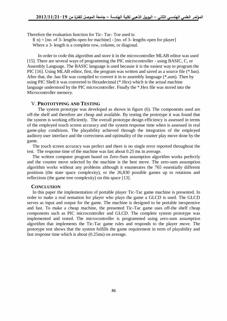
19/99/1192-91جامعة الموصل للفترة من –ليوبيل الذهبي لكلية الهندسة ا – الهندسي الثانيالعلمي المؤتمر
08
Therefore the evaluation function for Tic- Tac- Toe used is:
f( n) = [no. of 3- lengths open for machine] - [no. of 3- lengths open for player]
Where a 3- length is a complete row, column, or diagonal.
In order to code this algorithm and store it in the microcontroller MLAB editor was used
[15]. There are several ways of programming the PIC microcontroller - using BASIC, C, or
Assembly Language. The BASIC language is used because it is the easiest way to program the
PIC [16]. Using MLAB editor, first, the program was written and saved as a source file (*.bas).
After that, the .bas file was compiled to convert it in to assembly language (*.asm). Then by
using PIC Shell it was converted to Hexadecimal (*.Hex) which is the actual machine
language understood by the PIC microcontroller. Finally the *.Hex file was stored into the
Microcontroller memory.
V. PROTOTYPING AND TESTING The system prototype was developed as shown in figure (6). The components used are
off-the shelf and therefore are cheap and available. By testing the prototype it was found that
the system is working efficiently. The overall prototype design efficiency is assessed in terms
of the employed touch screen accuracy and the system response time when is assessed in real
game-play conditions. The playability achieved through the integration of the employed
auditory user interface and the correctness and optimality of the counter play move done by the
game.
The touch screen accuracy was perfect and there is no single error reported throughout the
test. The response time of the machine was fast about 0.25 ms in average.
The written computer program based on Zero-Sum assumption algorithm works perfectly
and the counter move selected by the machine is the best move. The zero-sum assumption
algorithm works without any problems although it enumerates the 765 essentially different
positions (the state space complexity), or the 26,830 possible games up to rotations and
reflections (the game tree complexity) on this space [13].
CONCLUSION In this paper the implementation of portable player Tic-Tac game machine is presented. In
order to make a real sensation for player who plays the game a GLCD is used. The GLCD
serves as input and output for the game. The machine is designed to be portable inexpensive
and fast. To make a cheap machine, the presented Tic-Tac game uses off-the shelf cheap
components such as PIC microcontroller and GLCD. The complete system prototype was
implemented and tested. The microcontroller is programmed using zero-sum assumption
algorithm that implements the Tic-Tac game rules and responds to the player move. The
prototype test shows that the system fulfills the game requirement in term of playability and
fast response time which is about (0.25ms) on average.
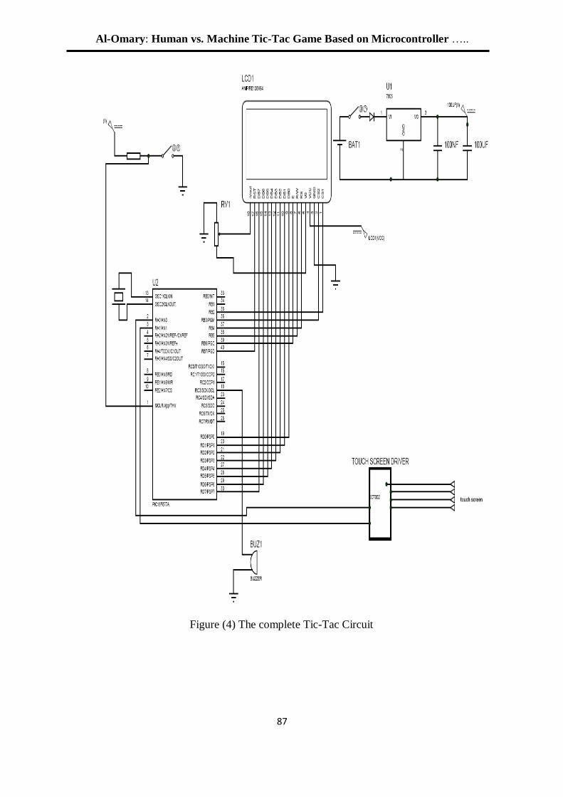
Al-Omary: Human vs. Machine Tic-Tac Game Based on Microcontroller …..
08
Figure (4) The complete Tic-Tac Circuit
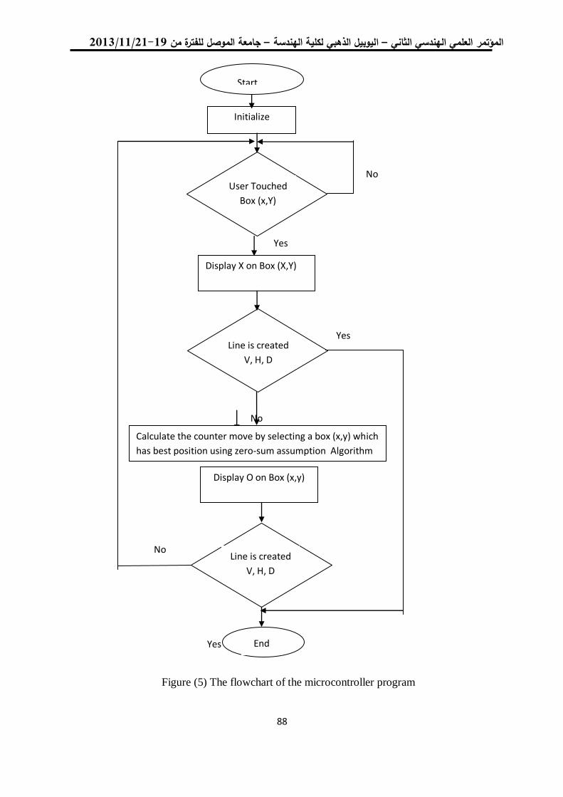
19/99/1192-91جامعة الموصل للفترة من –ليوبيل الذهبي لكلية الهندسة ا – الهندسي الثانيالعلمي المؤتمر
00
Figure (5) The flowchart of the microcontroller program
No
Yes
Start
Initialize
User Touched
Box (x,Y)
Display X on Box (X,Y)
Line is created
V, H, D
Yes
Yes
No
Calculate the counter move by selecting a box (x,y) which
has best position using zero-sum assumption Algorithm
Display O on Box (x,y)
Line is created
V, H, D
End
No
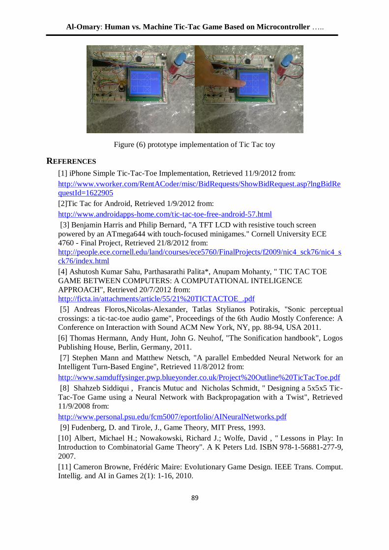
Al-Omary: Human vs. Machine Tic-Tac Game Based on Microcontroller …..
08
Figure (6) prototype implementation of Tic Tac toy
REFERENCES
[1] iPhone Simple Tic-Tac-Toe Implementation, Retrieved 11/9/2012 from:
http://www.vworker.com/RentACoder/misc/BidRequests/ShowBidRequest.asp?lngBidRe
questId=1622905
[2]Tic Tac for Android, Retrieved 1/9/2012 from:
http://www.androidapps-home.com/tic-tac-toe-free-android-57.html
[3] Benjamin Harris and Philip Bernard, "A TFT LCD with resistive touch screen
powered by an ATmega644 with touch-focused minigames." Cornell University ECE
4760 - Final Project, Retrieved 21/8/2012 from:
http://people.ece.cornell.edu/land/courses/ece5760/FinalProjects/f2009/nic4_sck76/nic4_s
ck76/index.html
[4] Ashutosh Kumar Sahu, Parthasarathi Palita*, Anupam Mohanty, " TIC TAC TOE
GAME BETWEEN COMPUTERS: A COMPUTATIONAL INTELIGENCE
APPROACH", Retrieved 20/7/2012 from:
http://ficta.in/attachments/article/55/21%20TICTACTOE_.pdf
[5] Andreas Floros,Nicolas-Alexander, Tatlas Stylianos Potirakis, "Sonic perceptual
crossings: a tic-tac-toe audio game", Proceedings of the 6th Audio Mostly Conference: A
Conference on Interaction with Sound ACM New York, NY, pp. 88-94, USA 2011.
[6] Thomas Hermann, Andy Hunt, John G. Neuhof, "The Sonification handbook", Logos
Publishing House, Berlin, Germany, 2011.
[7] Stephen Mann and Matthew Netsch, "A parallel Embedded Neural Network for an
Intelligent Turn-Based Engine", Retrieved 11/8/2012 from:
http://www.samduffysinger.pwp.blueyonder.co.uk/Project%20Outline%20TicTacToe.pdf
[8] Shahzeb Siddiqui , Francis Mutuc and Nicholas Schmidt, " Designing a 5x5x5 Tic-
Tac-Toe Game using a Neural Network with Backpropagation with a Twist", Retrieved
11/9/2008 from:
http://www.personal.psu.edu/fcm5007/eportfolio/AINeuralNetworks.pdf
[9] Fudenberg, D. and Tirole, J., Game Theory, MIT Press, 1993.
[10] Albert, Michael H.; Nowakowski, Richard J.; Wolfe, David , " Lessons in Play: In
Introduction to Combinatorial Game Theory". A K Peters Ltd. ISBN 978-1-56881-277-9,
2007.
[11] Cameron Browne, Frédéric Maire: Evolutionary Game Design. IEEE Trans. Comput.
Intellig. and AI in Games 2(1): 1-16, 2010.

19/99/1192-91جامعة الموصل للفترة من –ليوبيل الذهبي لكلية الهندسة ا – الهندسي الثانيالعلمي المؤتمر
88
[12] Beck, József, Combinatorial games: tic-tac-toe theory. Cambridge University
Press. ISBN 978-0-521-46100-9, 2008..
[13] Prajit K. Dutta, Strategies andGames: Theory and Practice, MIT Press, 1999.
[14] Programming PIC MCUs in BASIC. Retrieved 11/9/2011 from:
http://www.mikroe.com/en/books/picbasicbook/01.htm
[15] PIC programming tools. Retrieved 1/6/2011 from:
http://www.geocities.com/nozomsite/pic1.htm
[16] PIC microcontroller tutorial. Retrieved 8/7/2012 from:
http://www.voti.nl/picfaq/index.html
AL-Ghadanfary: Network Performance Metrics for Mac Protocols in Wireless …
19
Network Performance Metrics for Mac Protocols
in Wireless Mesh Networks
Dr. Mohammed Basheer Al-Somaidai Karam Anan Al-Ghadanfary Department of Electrical Engineering, College of Engineering, University of Mosul- Iraq.
[email protected] [email protected]
Abstract
The topic of Wireless Mesh Networks (WMN) is getting wide spread interest
among researchers in recent years. MAC sub-layer in WMN could be implemented
using different protocols depending on the coordination function. This paper simulates a
WMN project that runs under two IEEE 802.11 standards (a and g) with two MAC sub-
layer protocols Distributed Coordination Function (DCF) and Enhanced Distributed
coordination function Channel Access (EDCA). The results confirmed the outstanding
performance of EDCA protocol over the DCF protocol especially for real time
applications such as voice and video.
Key words: DCF, EDCA, MAC protocols, OPNET, simulation, WMN.
معايير أداء الشبكة لبروتوكوالت الوصول الى الوسط في الشبكات الالسلكية المتشابكة
كرم عنان عبد الغني الغضنفري
د. محمد بشير عبد هللا الصميدعي
العراق. –جامعة الموصل قسم الهندسة الكهربائية/ كلية الهندسة/
المستخلص
أنيمكن الكثير من الباحثين في السنوات األخيرة. على اهتمام موضوع الشبكات الالسلكية المتشابكة يستحوذ
جة ذا البحث نمذالوسط الفرعية بعدة بروتوكوالت اعتمادا على دالة التنسيق الموزعة. يتناول ه إلىطبقة الوصول ذتنف
لكترونيكالوامعهد المهندسين الكهربائيين ابكة تعمل ضمن معيارين من معايير شبكة السلكية متشلمشروع ومحاكاة
أكدت. EDCAو DCFالوسط فيهما على احد بروتوكولين هما إلى. تعتمد طبقة الوصول 802.11gو 802.11aوهما
تطبيقات الحساسة الفي كافة مقاييس أداء الشبكة خصوصا في DCFعلى بروتوكول EDCAالنتائج تفوق بروتوكول
.والفيديوللزمن مثل الصوت
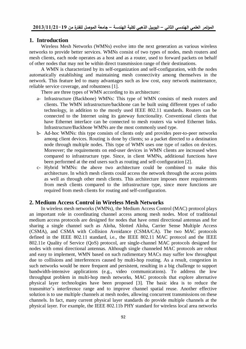
19/99/1192-91جامعة الموصل للفترة من –ليوبيل الذهبي لكلية الهندسة ا –العلمي الهندسي الثاني المؤتمر
19
1. Introduction Wireless Mesh Networks (WMNs) evolve into the next generation as various wireless
networks to provide better services. WMNs consist of two types of nodes, mesh routers and
mesh clients, each node operates as a host and as a router, used to forward packets on behalf
of other nodes that may not be within direct transmission range of their destinations.
A WMN is characterized by its self-organization and self-configuration, with the nodes
automatically establishing and maintaining mesh connectivity among themselves in the
network. This feature led to many advantages such as low cost, easy network maintenance,
reliable service coverage, and robustness [1].
There are three types of WMN according to its architecture:
a- Infrastructure (Backbone) WMNs: This type of WMN consists of mesh routers and
clients. The WMN infrastructure/backbone can be built using different types of radio
technology, in addition to the mostly used IEEE 802.11 standards. Routers can be
connected to the Internet using its gateway functionality. Conventional clients that
have Ethernet interface can be connected to mesh routers via wired Ethernet links.
Infrastructure/Backbone WMNs are the most commonly used type.
b- Ad-hoc WMNs: this type consists of clients only and provides peer-to-peer networks
among client devices. Routing is done by clients; so a packet directed to a destination
node through multiple nodes. This type of WMN uses one type of radios on devices.
Moreover; the requirements on end-user devices in WMN clients are increased when
compared to infrastructure type. Since, in client WMNs, additional functions have
been performed at the end users such as routing and self-configuration [2].
c- Hybrid WMNs: the above two architecture could be combined to make this
architecture. In which mesh clients could access the network through the access points
as well as through other mesh clients. This architecture imposes more requirements
from mesh clients compared to the infrastructure type, since more functions are
required from mesh clients for routing and self-configuration.
2. Medium Access Control in Wireless Mesh Networks In wireless mesh networks (WMNs), the Medium Access Control (MAC) protocol plays
an important role in coordinating channel access among mesh nodes. Most of traditional
medium access protocols are designed for nodes that have omni directional antennas and for
sharing a single channel such as Aloha, Slotted Aloha, Carrier Sense Multiple Access
(CSMA), and CSMA with Collision Avoidance (CSMA/CA). The two MAC protocols
defined in the IEEE 802.11 standard, i.e., the IEEE 802.11 MAC protocol and the IEEE
802.11e Quality of Service (QoS) protocol, are single-channel MAC protocols designed for
nodes with omni directional antennas. Although single channeled MAC protocols are robust
and easy to implement, WMN based on such rudimentary MACs may suffer low throughput
due to collisions and interferences caused by multi-hop routing. As a result, congestion in
such networks would be more frequent and persistent, resulting in a big challenge to support
bandwidth-intensive applications (e.g., video communications). To address the low
throughput problem in multi-hop mesh networks, MAC protocols that explore alternative
physical layer technologies have been proposed [3]. The basic idea is to reduce the
transmitter’s interference range and to improve channel spatial reuse. Another effective
solution is to use multiple channels at mesh nodes, allowing concurrent transmissions on these
channels. In fact, many current physical layer standards do provide multiple channels at the
physical layer. For example, the IEEE 802.11b PHY standard for wireless local area networks
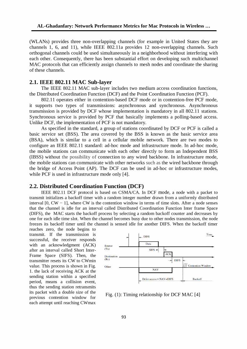
AL-Ghadanfary: Network Performance Metrics for Mac Protocols in Wireless …
19
(WLANs) provides three non-overlapping channels (for example in United States they are
channels 1, 6, and 11), while IEEE 802.11a provides 12 non-overlapping channels. Such
orthogonal channels could be used simultaneously in a neighborhood without interfering with
each other. Consequently, there has been substantial effort on developing such multichannel
MAC protocols that can efficiently assign channels to mesh nodes and coordinate the sharing
of these channels.
2.1. IEEE 802.11 MAC Sub-layer The IEEE 802.11 MAC sub-layer includes two medium access coordination functions,
the Distributed Coordination Function (DCF) and the Point Coordination Function (PCF).
802.11 operates either in contention-based DCF mode or in contention-free PCF mode,
it supports two types of transmissions: asynchronous and synchronous. Asynchronous
transmission is provided by DCF whose implementation is mandatory in all 802.11 stations.
Synchronous service is provided by PCF that basically implements a polling-based access.
Unlike DCF, the implementation of PCF is not mandatory.
As specified in the standard, a group of stations coordinated by DCF or PCF is called a
basic service set (BSS). The area covered by the BSS is known as the basic service area
(BSA), which is similar to a cell in a cellular mobile network. There are two modes to
configure an IEEE 802.11 standard: ad-hoc mode and infrastructure mode. In ad-hoc mode,
the mobile stations can communicate with each other directly to form an Independent BSS
(IBSS) without the possibility of connection to any wired backbone. In infrastructure mode,
the mobile stations can communicate with other networks such as the wired backbone through
the bridge of Access Point (AP). The DCF can be used in ad-hoc or infrastructure modes,
while PCF is used in infrastructure mode only [4].
2.2. Distributed Coordination Function (DCF) IEEE 802.11 DCF protocol is based on CSMA/CA. In DCF mode, a node with a packet to
transmit initializes a backoff timer with a random integer number drawn from a uniformly distributed
interval [0, CW − 1], where CW is the contention window in terms of time slots. After a node senses
that the channel is idle for an interval called Distributed Coordination Function Inter frame Space
(DIFS), the MAC starts the backoff process by selecting a random backoff counter and decreases by one for each idle time slot. When the channel becomes busy due to other nodes transmission, the node
freezes its backoff timer until the channel is sensed idle for another DIFS. When the backoff timer
reaches zero, the node begins to transmit. If the transmission is
successful, the receiver responds
with an acknowledgment (ACK) after an interval called Short Inter-
Frame Space (SIFS). Then, the
transmitter resets its CW to CWmin
value. This process is shown in Fig. 1. the lack of receiving ACK at the
sending station within a specified
period, means a collision event, thus the sending station retransmits
its packet with a double size of the
previous contention window for
each attempt until reaching CWmax
Fig. (1): Timing relationship for DCF MAC [4]
protocol
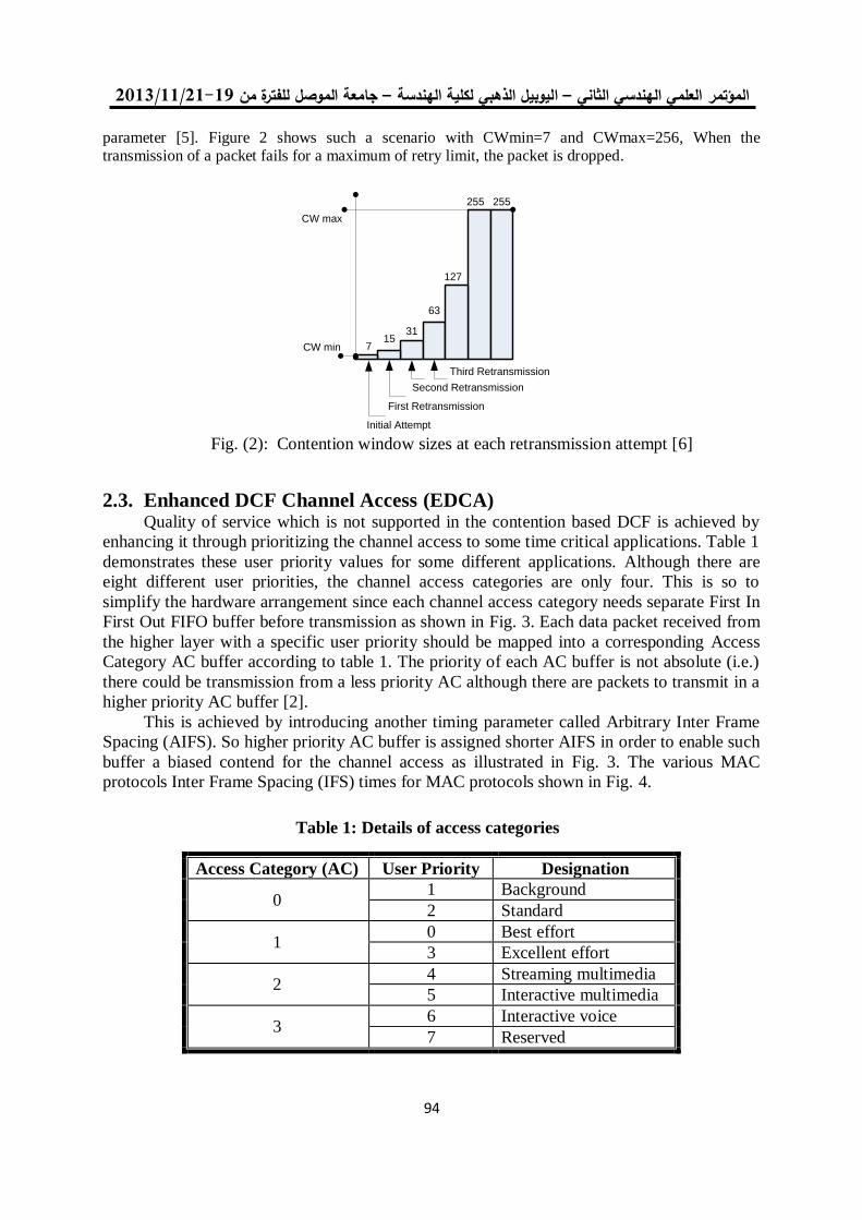
19/99/1192-91جامعة الموصل للفترة من –ليوبيل الذهبي لكلية الهندسة ا –العلمي الهندسي الثاني المؤتمر
19
parameter [5]. Figure 2 shows such a scenario with CWmin=7 and CWmax=256, When the transmission of a packet fails for a maximum of retry limit, the packet is dropped.
715
31
63
127
255 255
CW max
CW min
Initial Attempt
First Retransmission
Third Retransmission
Second Retransmission
2.3. Enhanced DCF Channel Access (EDCA) Quality of service which is not supported in the contention based DCF is achieved by
enhancing it through prioritizing the channel access to some time critical applications. Table 1
demonstrates these user priority values for some different applications. Although there are
eight different user priorities, the channel access categories are only four. This is so to
simplify the hardware arrangement since each channel access category needs separate First In
First Out FIFO buffer before transmission as shown in Fig. 3. Each data packet received from
the higher layer with a specific user priority should be mapped into a corresponding Access
Category AC buffer according to table 1. The priority of each AC buffer is not absolute (i.e.)
there could be transmission from a less priority AC although there are packets to transmit in a
higher priority AC buffer [2].
This is achieved by introducing another timing parameter called Arbitrary Inter Frame
Spacing (AIFS). So higher priority AC buffer is assigned shorter AIFS in order to enable such
buffer a biased contend for the channel access as illustrated in Fig. 3. The various MAC
protocols Inter Frame Spacing (IFS) times for MAC protocols shown in Fig. 4.
Access Category (AC) User Priority Designation
0 1 Background
2 Standard
1 0 Best effort
3 Excellent effort
2 4 Streaming multimedia
5 Interactive multimedia
3 6 Interactive voice
7 Reserved
Fig. (2): Contention window sizes at each retransmission attempt [6]
Table 1: Details of access categories
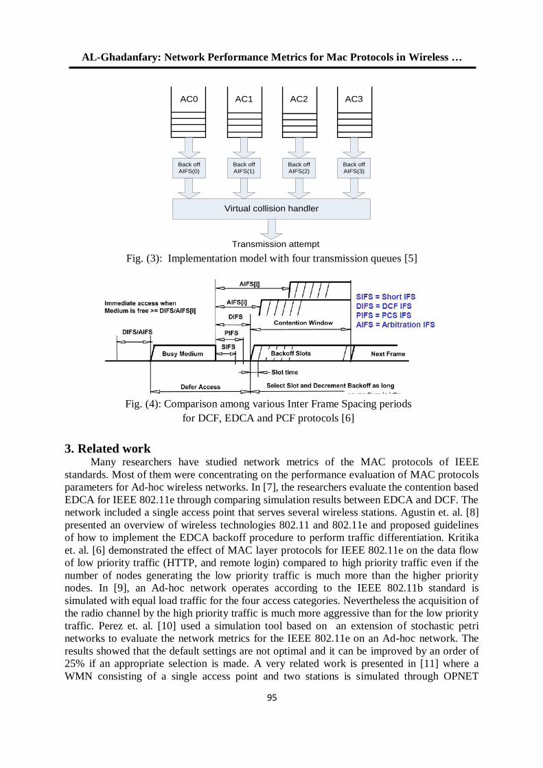
AL-Ghadanfary: Network Performance Metrics for Mac Protocols in Wireless …
19
AC0 AC1 AC2 AC3
Back off
AIFS(0)
Back off
AIFS(1)
Back off
AIFS(2)
Back off
AIFS(3)
Virtual collision handler
Transmission attempt
3. Related work Many researchers have studied network metrics of the MAC protocols of IEEE
standards. Most of them were concentrating on the performance evaluation of MAC protocols
parameters for Ad-hoc wireless networks. In [7], the researchers evaluate the contention based
EDCA for IEEE 802.11e through comparing simulation results between EDCA and DCF. The
network included a single access point that serves several wireless stations. Agustin et. al. [8]
presented an overview of wireless technologies 802.11 and 802.11e and proposed guidelines
of how to implement the EDCA backoff procedure to perform traffic differentiation. Kritika
et. al. [6] demonstrated the effect of MAC layer protocols for IEEE 802.11e on the data flow
of low priority traffic (HTTP, and remote login) compared to high priority traffic even if the
number of nodes generating the low priority traffic is much more than the higher priority
nodes. In [9], an Ad-hoc network operates according to the IEEE 802.11b standard is
simulated with equal load traffic for the four access categories. Nevertheless the acquisition of
the radio channel by the high priority traffic is much more aggressive than for the low priority
traffic. Perez et. al. [10] used a simulation tool based on an extension of stochastic petri
networks to evaluate the network metrics for the IEEE 802.11e on an Ad-hoc network. The
results showed that the default settings are not optimal and it can be improved by an order of
25% if an appropriate selection is made. A very related work is presented in [11] where a
WMN consisting of a single access point and two stations is simulated through OPNET
Fig. (3): Implementation model with four transmission queues [5]
Fig. (4): Comparison among various Inter Frame Spacing periods
for DCF, EDCA and PCF protocols [6]
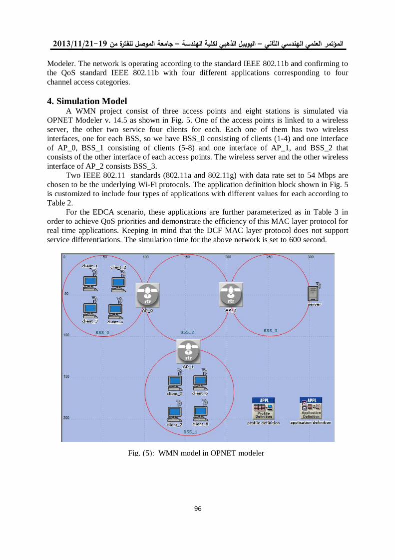
19/99/1192-91جامعة الموصل للفترة من –ليوبيل الذهبي لكلية الهندسة ا –العلمي الهندسي الثاني المؤتمر
19
Modeler. The network is operating according to the standard IEEE 802.11b and confirming to
the QoS standard IEEE 802.11b with four different applications corresponding to four
channel access categories.
4. Simulation Model A WMN project consist of three access points and eight stations is simulated via
OPNET Modeler v. 14.5 as shown in Fig. 5. One of the access points is linked to a wireless
server, the other two service four clients for each. Each one of them has two wireless
interfaces, one for each BSS, so we have BSS_0 consisting of clients (1-4) and one interface
of AP_0, BSS_1 consisting of clients (5-8) and one interface of AP_1, and BSS_2 that
consists of the other interface of each access points. The wireless server and the other wireless
interface of AP_2 consists BSS_3.
Two IEEE 802.11 standards (802.11a and 802.11g) with data rate set to 54 Mbps are
chosen to be the underlying Wi-Fi protocols. The application definition block shown in Fig. 5
is customized to include four types of applications with different values for each according to
Table 2.
For the EDCA scenario, these applications are further parameterized as in Table 3 in
order to achieve QoS priorities and demonstrate the efficiency of this MAC layer protocol for
real time applications. Keeping in mind that the DCF MAC layer protocol does not support
service differentiations. The simulation time for the above network is set to 600 second.
Fig. (5): WMN model in OPNET modeler
simulation
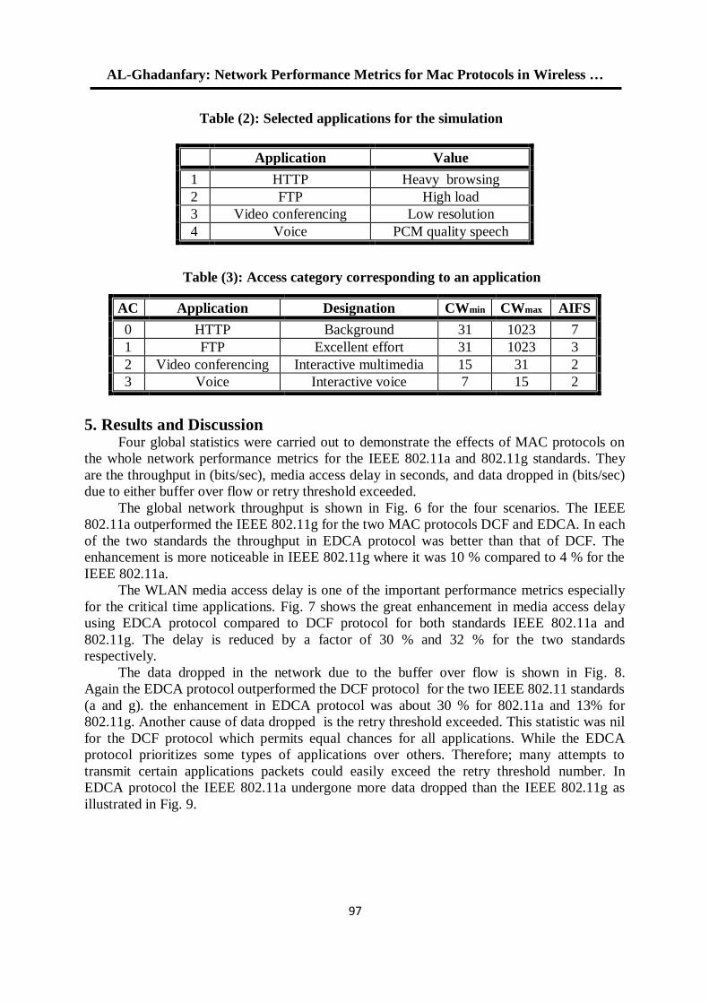
AL-Ghadanfary: Network Performance Metrics for Mac Protocols in Wireless …
19
Application Value
1 HTTP Heavy browsing
2 FTP High load
3 Video conferencing Low resolution
4 Voice PCM quality speech
AC Application Designation CWmin CWmax AIFS
0 HTTP Background 31 1023 7
1 FTP Excellent effort 31 1023 3
2 Video conferencing Interactive multimedia 15 31 2
3 Voice Interactive voice 7 15 2
5. Results and Discussion Four global statistics were carried out to demonstrate the effects of MAC protocols on
the whole network performance metrics for the IEEE 802.11a and 802.11g standards. They
are the throughput in (bits/sec), media access delay in seconds, and data dropped in (bits/sec)
due to either buffer over flow or retry threshold exceeded.
The global network throughput is shown in Fig. 6 for the four scenarios. The IEEE
802.11a outperformed the IEEE 802.11g for the two MAC protocols DCF and EDCA. In each
of the two standards the throughput in EDCA protocol was better than that of DCF. The
enhancement is more noticeable in IEEE 802.11g where it was 10 % compared to 4 % for the
IEEE 802.11a.
The WLAN media access delay is one of the important performance metrics especially
for the critical time applications. Fig. 7 shows the great enhancement in media access delay
using EDCA protocol compared to DCF protocol for both standards IEEE 802.11a and
802.11g. The delay is reduced by a factor of 30 % and 32 % for the two standards
respectively.
The data dropped in the network due to the buffer over flow is shown in Fig. 8.
Again the EDCA protocol outperformed the DCF protocol for the two IEEE 802.11 standards
(a and g). the enhancement in EDCA protocol was about 30 % for 802.11a and 13% for
802.11g. Another cause of data dropped is the retry threshold exceeded. This statistic was nil
for the DCF protocol which permits equal chances for all applications. While the EDCA
protocol prioritizes some types of applications over others. Therefore; many attempts to
transmit certain applications packets could easily exceed the retry threshold number. In
EDCA protocol the IEEE 802.11a undergone more data dropped than the IEEE 802.11g as
illustrated in Fig. 9.
Table (2): Selected applications for the simulation
Table (3): Access category corresponding to an application
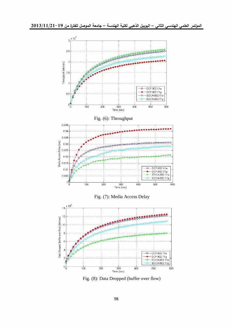
19/99/1192-91جامعة الموصل للفترة من –ليوبيل الذهبي لكلية الهندسة ا –العلمي الهندسي الثاني المؤتمر
19
Fig. (6): Throughput
Fig. (7): Media Access Delay
Fig. (8): Data Dropped (buffer over flow)
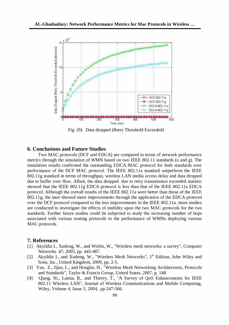
AL-Ghadanfary: Network Performance Metrics for Mac Protocols in Wireless …
11
6. Conclusions and Future Studies Two MAC protocols (DCF and EDCA) are compared in terms of network performance
metrics through the simulation of WMN based on two IEEE 802.11 standards (a and g). The
simulation results confirmed the outstanding EDCA MAC protocol for both standards over
performance of the DCF MAC protocol. The IEEE 802.11a standard outperform the IEEE
802.11g standard in terms of throughput, wireless LAN media access delay and data dropped
due to buffer over flow. Albeit, the data dropped due to retry transmission exceeded statistic
showed that the IEEE 802.11g EDCA protocol is less than that of the IEEE 802.11a EDCA
protocol. Although the overall results of the IEEE 802.11a were better than those of the IEEE
802.11g; the later showed more improvements through the application of the EDCA protocol
over the DCF protocol compared to the less improvements in the IEEE 802.11a. more studies
are conducted to investigate the effects of mobility upon the two MAC protocols for the two
standards. Further future studies could be subjected to study the increasing number of hops
associated with various routing protocols to the performance of WMNs deploying various
MAC protocols.
7. References [1] Akyildiz I., Xudong, W., and Weilin, W., "Wireless mesh networks: a survey", Computer
Networks 47, 2005, pp. 445-487.
[2] Akyildiz I., and Xudong, W., "Wireless Mesh Networks", 1st Edition, John Wiley and
Sons, Inc., United Kingdom, 2009, pp. 2-5.
[3] Yan, Z., Jijun, L., and Honglin, H., "Wireless Mesh Networking Architectures, Protocols
and Standards", Taylor & Francis Group, United States, 2007, p. 148.
[4] Qiang, Ni., Lamia, R., and Thierry, T., "A Survey of QoS Enhancements for IEEE
802.11 Wireless LAN", Journal of Wireless Communications and Mobile Computing,
Wiley, Volume 4, Issue 5, 2004, pp.547-566.
Fig. (9): Data dropped (Retry Threshold Exceeded)
19/99/1192-91جامعة الموصل للفترة من –ليوبيل الذهبي لكلية الهندسة ا –العلمي الهندسي الثاني المؤتمر
911
[5] Dorothy, R., Mjumo, M., and Karim, D., "Improving the Performance of 802.11
Wireless LANs with MAC Adaptation", Southern Africa Telecommunication Networks
and Applications Conference (SATNAC), Spier Estate, Stellenbosch, Southern Africa,
September 2010.
[6] Kritika, S., Nitin, B., and Namarta, K., "Performance Evaluation of 802.11
WLAN Scenarios in OPNET Modeler", International Journal of Computer Applications
Vol. 22, No.9, May 2011, pp. 30-35.
[7] Chung-Sheng, L., Tak-Goa, T., and Han-Chieh, C., " Evaluation of Contention-Based
EDCA for IEEE 802.11e Wireless LAN", Journal of Internet Technology Volume 5,
No.4, 2004, pp. 429-434.
[8] Agustin, Z., Guiomar, C., Josep, M., and Carlos, S., "Developing a QoS 802.11e Model
in a Wireless Environment", OPNETWORK conference, Washington D.C. August
2005, pp. 1-6.
[9] Sandeep, K., and Jyotsna, S., "Performance Evaluation of IEEE 802.11e", International
Journal of Computer Science & Technology (IJCST), Vol. 2 Issue 4, Oct.-Dec. 2011,
pp. 40-44.
[10] Santiago, P., Higinio, F., Gustavo, M., and Luis, B., "Throughput Quantitative Analysis
of EDCA 802.11e in Different Scenarios", Journal of Computer Science & Technology
(JCS&T), Vol. 13 No. 1, April 2013, pp. 16-24.
[11] Felix, D., Luminita, S. and Ion, B., "Mac Level Based Quality of Service Management in
IEEE 802.11 Networks", Bulletin of The Polytechnic Institute of IAŞI, Tome 57 (LXI),
Fasc. 4, 2011, pp. 77-84.
باستخدام مصفوفة البوابات البوابات ..... TCP/UDPمحمود: إختيار بروتوكول
101
مصفوفة البوابات باستخدام TCP/UDPبروتوكول ختيارإ المنطقية القابلة للبرمجة
الستار محمد خضر عبد د. خالد فزع محمود األلكترونيات هندسة قسم -قدمأمهندس
جامعة الموصل -كلية هندسة االلكترونيات هيئة التعليم التقني - ستاذ مساعدأ
الموصل -المعهد التقني [email protected] [email protected]
مستخلصال تكمن في تصميم المنظومات التي تعمل على تحليل الرزم UDPعن رزم TCPان اهمية فصل رزم
(Packet analysier) المنتقلة بين االجهزة داخل الشبكة عن طريق اجراء سلسلة من العمليات والتي تتضمن( خارج انظمة الحاسبات باالعتماد على مصفوفة Encapculation /Decapculationالتغليف وفك التغليف )
الوظائف وتحديد , للتعرف على مجموعة البروتوكوالت التي تؤدي هذه FPGAالبوابات المنطقية القابلة للبرمجة نوع البروتوكول المستخدم في كل ارسال ليتسنى لنا التحري عن اهمية هذه البيانات من نوع البروتوكول المستخدم ,
ومن ثم التعامل مع هذه البيانات من Headerكما تفيد هذه العملية بالوصول الى البيانات الحقيقية لكل طبقة بعد ازالة وتستعمل هذه العملية في ربط االجهزة التي تعمل على طبقات مختلفة من طبقات النظام خالل تغييرها او تشفيرها ,
الى باإلضافةلتوزيع تلك الرزم على اجهزة , Getway, عن طريق تصميم جهاز يعمل عمل بوابة OSIالمفتوح و كفاءة افضل واخيرا تطوير ( منذ ارسال الرزم الى استالمها مما يودي الى تطوير نظام ذDelay) التأخيرقياس كمية
FPGA kit Spartan 3E XC3S500E) )باإلضافة Multiport LAN بعد ان كان يحتوي علىPort LAN .واحد
,حقليا المبرمجة البوابات مصفوفة, المستخدم بينات برتوكول رزم, النقل على السيطرة بروتوكول رزمالكلمات الدالة: .الموسع المادي الكيان وصف لغة
TCP/UDP Selector Based on FPGA
AbdulSattar M. Khidhir Khalid F. Mhmoed
Assistant Prof.- Foundation of Technical Education
Mosul Technical Institute Electronic Engineer- Electronic Engineering Department
College of Electronic Engineering [email protected] [email protected]
Abstract Separation of TCP packets from UDP packets is an important task in design of
systems that analyze packets transported in networks. This is accomplished using a
series of tasks that include encapsulation and decapsulation . In this work this is
performed outside the computer nodes, using FPGA to know protocol groups that
perform these functions and identify the protocol used in each packet. The extraction of
actual data can make use of this process and then uses the data. This process can be used
in connection of devices that works at different OSI layers by the design of a gateway to
dispatch these packets to other devices. This work includes measurement of delay inside
the FPGA which leads to better design. The result of the work can be used as an
expansion to multi LAN ports in SPARTAN 3E XC3S500E FPGA kit which includes
only one LAN port.
Keywords: TCP Packets , UDP Packets, FPGA, VHDL.
19/99/1192-91جامعة الموصل للفترة من –ليوبيل الذهبي لكلية الهندسة ا –العلمي الهندسي الثاني المؤتمر
101
المقدمة .1له اهمية خاصة وذلك بسبب اهمية نوع UDPاو TCPان الختيار نوع البروتوكول من الطبقة الرابعة اما
اذا process to process connection عن الوثوقية في االرسال المسؤولةالبيانات المراد ارسالها, ان هذه الطبقة هي اي اتصال Connection orientedمن نوع TCPبروتوكول االرسال يستخدمكانت البيانات من النوع المهم سوف
بعد ارسال كل رزمة حسب نوع االرسال المستخدم مع ذلك االتصال ACKوصول بسبب استالم موجه وموثوق ال("stop and wait" or "pipeline" ) وهناك عدة انواع من البروتوكوالت التي تتعامل مع هذا النوع في الطبقات
. اما اذا كانت البيانات من ان فقدان اي جزء من تلك الرزمة يؤدي الى خسارة كل الرزمة HTTP ,FTPاالعلى والسبب انه من النوع UDPالنوع االقل اهمية وعامل السرعة هو المطلوب يجب استخدام بروتوكول االرسال
Connection Less استالم ال يتمايACK على سالمتها ال يؤثربعد ارسال الرزمة , ان فقدان جزء من البياناتوهناك عدة انواع من البروتوكوالت تتعامل معه من Real Timeتي تفيد في تطبيقات المهم هو سرعة استالم البيانات وال
headerيحتوي على TCPأن ,كما يمكن توضيح بعض الفروق االساسية بيت البروتوكولين VOIPو DNSضمنها
20byte وتكون سرعته اقل بسبب استخدام تقنية لحماية البيانات من الضياعCongestion control and flow
control لكل رزمة اكثر ,أما بروتوكول المحملةوكمية البياناتUDP يحتوي علىheader 8byte وسرعته اعلى [2][1].وكمية البيانات المحملة اقل بتلك التقنيتين ال يعملألنه
الدراسات السابقة: .2
تواكب التطور السريع ألنظمة االتصاالت نظمةالذين يحاولون ايجاد تقنيات جديدة في أ العديد من الباحثين اليزال , delayولتقليل األضرار الناتجة عن تلكم العمليات مثل , االستفادة قدر المستطاع من الحزمة المخصصة لهمالحاسوب ب
كفاءة االرسال وعرض الحزمة منهم من استطاع تقليل حجم الحزمة عن طريق كبسها او تقطيعها الى اجزاء اصغرهم من حاول تطوير تلك ومن Steganographyاول حماية تلك الحزمة عن طريق التشفير او االخفاء ومنهم من يح [3].ما يليهذه البحوث نسرد الشبكات من
.port noلتخصيص رقم المنفذ Linux التشغيل خوارزمية تستخدم في قلب نظام باقتراحقام احد الباحثين ان رقم المنفذ مهم جدا في االتصاالت عبر االنترنت , Linuxوذلك لتحسين اداء نظام UDPو TCP للبروتكولبالنسبة
[4] وقد اعطت الدراسة اداء عالي في تطبيقات الشبكات والتي تتعامل مع عدد كبير من نقاط االتصال .بدراسة كاملة عن هيكل نظام االيثرنت والتحديات التي تحول دون تطوير هذا النظام اخر في نفس السنة قام باحث
,أن هذه البرمجيات متطورة جدا من CAN to ethernet converterوامكانية معالجتها ,هذا النظام تم بناءه بواسطة
ع السلك الغير قياسي في االتصال واستخدام ناحية المتانة وزيادة الوثوقية ,ان التقييم استند الى استخدام السلك القياسي مللحصول على جميع الخصائص بالنسبة للشبكة لمقارنتها مع تلك الخصائص Topologiesعدة انواع من الربط
[5] الموضوعة للشبكة القياسية .ه الدراسه عبر االيثرنت في هذTDMAباقتراح انماط التحزيم لمحول نظام احد الباحثين السنة قام نفس ايضا في
النشط TDMAالعام ونمط شق البيانات TDMAتم فحص ثالث انماط للمعالجة والتي اطلق عليها نمط شق البيانات ,كفاءة االطار delayالصامت ثم استخدم مجموعة من العوامل )تاخير المعالجة TDMAونمط اخماد شق البيانات
frame واخيرا عرض الحزمة المستخدمةBW افضل نتائج حصل عليها عند استخدام النمط الفعال لحالة (وقد اوضح ان [6] .لمتعدد ولجميع انواع المعلوماتاالطار ا
The OSL Modelاالتصال المعتمد على الطبقات .3
المفتوح هو مجموعة بروتوكوالت تقوم بتنظيم العمل بين نظامين مختلفين لتامين االتصال باالعتماد النظامان على البروتكوالت االقل مستوى لتهيئة البيانات بحيث كل نوع من تلك االنواع تعمل بطبقة معينة واشهر هذه االنظمة
اجة امين االتصال بين نظامين مختلفين دون الحوالمستخدم في ت 0791( وضع هذا النموذج نهاية سنة OSIنموذج ) ليس بروتوكول وانما نموذج يظم مجموعة بروتوكوالت تعمل OSI. ان نموذج الى تغيير االجزاء المادية والبرمجية
على حسب اتجاه في طبقات مختلفة وتقوم باستالم البيانات التي تحتاجها من البروتوكول االدنى منه في الطبقة او اال. يظم النموذج سبعة طبقات بتحويل البيانات من شكل الى اخر . يتميز النموذج بكونه مرن في التعامل وموثوقاالتصال
كل واحدة تقوم باداء جزء من المهام في عملية االتصال لكي يتسنى له التعامل مع جميع انظمة الحاسبات والمبين في [7] [1] .(0) الشكل
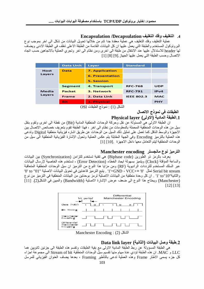
باستخدام مصفوفة البوابات البوابات ..... TCP/UDPمحمود: إختيار بروتوكول
101
Encapsulation /Decapsulation التغليف وفك التغليف .4
عملية التغليف وفك التغليف هي عملية معقدة جدا تتم من خاللها تحويل البيانات من شكل الى اخر بموجب نوع ويضافالبروتوكول المستخدم والطبقة التي يعمل عليها ان كل البيانات القادمة من الطبقة االعلى تغلف في الطبقة االدنى
وتجري العملية باالتجاهين حسب اتجاه عليها عند االنتقال من طبقة الى اخرى ومن نظام الى اخر دالللالست headerلها [9] [8] [1]االتصال وحسب الطبقة التي يعمل عليها الجهاز.
OSI نموذج الطبقات: (0) الشكل
الطبقات في نموذج االتصال Physical layer.الطبقة المادية )االولى( 1
( من نقطة الى اخرى وتقوم بنقل Bitالطبقة االولى هي المسئولة عن نقل وحركة الوحدات المنطقية المادية )ان
بالمعلومات من نظام الى اخر , فهذا الطبقة تقوم بتعريف خصائص االتصال بين المحملةسيل من هذه الوحدات المنطقية وتدعى Digitalمن الوحدات عن طريق اشاره فيزيائية منطقية االجهزة والوسط الناقل كما تعمل على تمثيل ذلك السيل
الفيزيائية المنطقية الى سيل من اإلشارةوفي الجهة المقابلة يتم عكس العملية وتحول Encodingهذه العملية بالترميز [10] [1] . الوحدات المنطقية ليتم التعامل معها داخل االجهزة
Manchester encodingالترميز نوع مانجستر ( بين البيانات Synchronization( هي تقنية تستخدم للتزامن )Biphase codeيعرف بالرمز ذو الطورين )
البيانات إلرسال( , تستخدم هذه الخاصية Error Detection( ويتميز بسهولة ايجاد الخطاء )Clockوالساعة المؤقتة )( ومن مزايا هذا النوع من الترميز ان سيل الوحدات المنطقية المتعاقبة RFعبر السلك المستخدم للترددات الراديوية )
Serial bit stream 0'تمثل' =VCC+ ,'1'=GND 01". يتبع الترميز قاعدتين في تحويل البيانات االصلية" to '0' المنطقية في الترميز من نوع . ان كل وحدة منطقية من البيانات االصلية ترمز بوحدتين من البيانات "to"10 '1'والثانية
(Manchesterويحتاج هذا ال ) االصلية اإلشارةنوع الى ضعف عرض (Bandwidthوالمبين في الشكل )(2).[11]
[12] [13]
Manchester Encoding( : 2الشكل )
Data link layer.طبقة وصل البيانات )الثانية( 2عن ربط الطبقة المادية االولى مع بقية الطبقات وتقسم هذه الطبقة الى جزئين ثانويين هما المسؤولةهي الطبقة
LLC وMAC ان هذه الطبقة تؤدي عدة مهام منها تقسيم سيل الوحدات المنطقية .Stream of bit الى مجموعة اجزاءالعنوان الفيزيائي للمرسل يضاف, بعدها Framing بالتأطيروهذه العملية تدعى Frameكل جزء يسمى االطار

19/99/1192-91جامعة الموصل للفترة من –ليوبيل الذهبي لكلية الهندسة ا –العلمي الهندسي الثاني المؤتمر
101
عند االنتقال بالشبكة بواسطة Frameعن ايجاد االخطاء التي تحدث في مسؤولةكما انها Frameوالمستقبل لكل لكي CRCمخزونة في حيز القيمةوتكون هذه Standard Ethernetالمعتمدة في CRC – 32احتساب عملية منطقية CRC.[1] [14]مستلم ثم مقارنته مع القيمة الموضوع داخل حيز Frameكل ل CRCيستطيع المستقبل حساب
Ethernet Frame Format Standardشكل االطار القياسي لاليثرنت (preamble = 7 byte( ومؤشر بداية االطار )SFD = 1 byte يستخدمان للتزامن بين المرسل والمستقبل هذا ). ان هذه الكمية من البايت تقوم بتنبيه المستقبل لوجود بيانات قادمة والتي تضاف من الطبقة االولى وتعلم 8byteالحيز
إليجاد Frameبايت يضاف في الطبقة الثانية يساعد 6حيز يتكون من New frame .DAالمستقبل بوجوب استالم حيز الطول الثانية يساعد المستقبل بمعرفة المرسل. بايت يضاف في الطبقة 6حيز يتكون من SAالمستقبل المطلوب .
( هذا الحيز يعرف بحيز النوع او الطول باالعتماد على القيمة التي بداخلة ,في نظام length or type=2byteاو النوع ),ويستخدم هذا MAC frame باستخدامكول في الطبقات االعلى ويعتبر حيز نوع ليتم تعريف البروت القديمااليثرنت
والنوعين 802.3في نظام االيثرنت القياسي Data and padding البيانات الحيز لتعريف طول المعلومات في حيزويمثل البيانات القادمة من الطبقة Frameحسب طول 1500الى 46يكون متغير منحيز البيانات حاليا . يستخدمان CRCالخطاء بعد االستالم ويتبع في الحل خوارزمية إليجاد, يستخدم Frameحاصل الجمع المنطقي CRCالثالثة .
[15] [14] (.3)والمبين في الشكل 32 –
شكل االطار: (3) الشكل
FPGAمصفوفة البوابات المنطقية القابلة للبرمجة .5اسوبية والمنطقية من العالم, أدت الحاجة الى اختصار احجام االجهزة الح يشهدهالذي الكبير نظرا للتطور
من مجموعة بلوكات منطقية FPGAالى استخدام شريحة واحدة لتقوم بعدة مهام , يتألف باإلضافةالذواكر , المعالجات وتطبيقات متعددة , ومن هنا جاء لتأديةلتأليف مصفوفة Switchوالتي ترتبط مع بعضها عن طريق قواطع االلكترونية
لهذا يمكن اعادة برمجته والنوع الثاني Switchesالذي يستخدم القواطع االلكترونية FPGAالفرق بين النوع االول CPLD تنصهر عند البرمجة لمرة واحدة , ومن اشهر الشركات المصنعة لشريحة اإللكترونيةالذي يستخدم فواصمFPGA هي شركةXilinx الرائدة في هذا المجال وشركةAltera المستخدمة في برمجة لغةالبالترتيب الثاني , أن VHDL .[16][17][18]لغة وصف الماديات ذات السرعة العالية FPGAشريحة
المقترح النظام تصميم .6كما موضح في OSIمن طبقات النظام المفتوح والثالثة تم تصميم المنظومة لتعمل على الطبقة االولى والثانية
(4) الشكل
التصميم المقترح : (4) الشكل
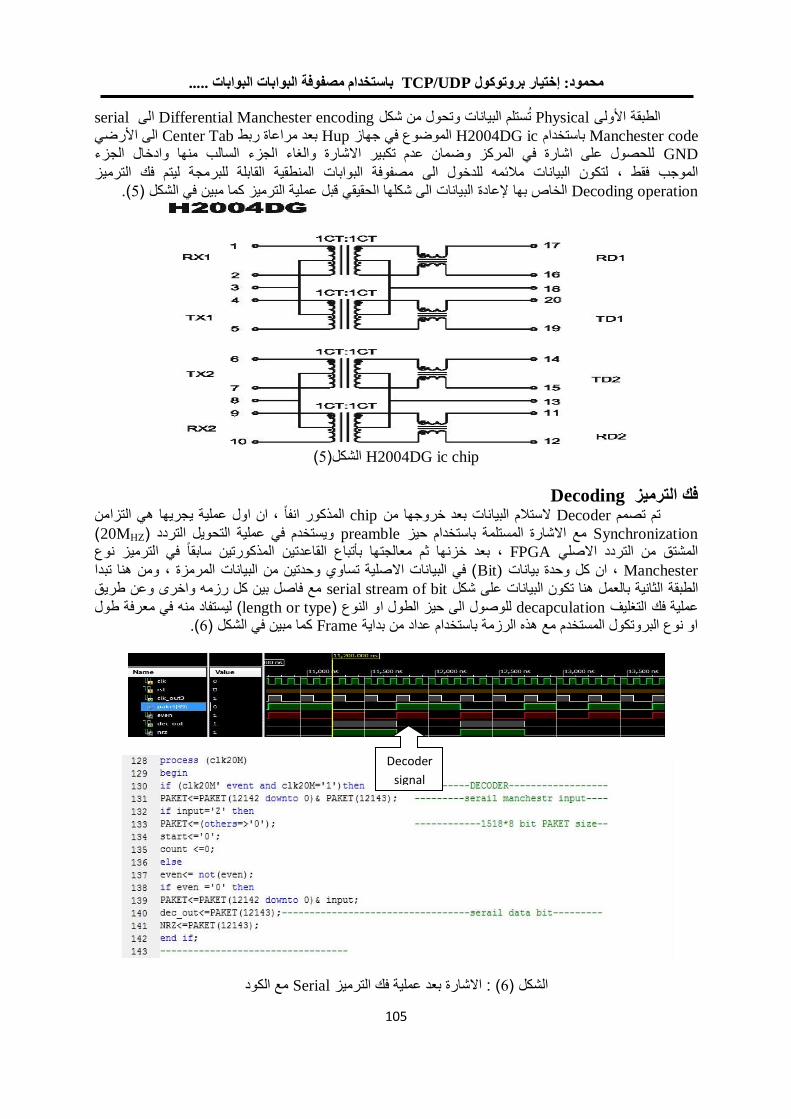
باستخدام مصفوفة البوابات البوابات ..... TCP/UDPمحمود: إختيار بروتوكول
101
serialالى Differential Manchester encoding ت ستلم البيانات وتحول من شكل Physicalاألولى الطبقة
Manchester code باستخدام H2004DG ic في جهاز الموضوعHup بعد مراعاة ربطCenter Tab الى األرضيGND للحصول على اشارة في المركز وضمان عدم تكبير االشارة والغاء الجزء السالب منها وادخال الجزء
المنطقية القابلة للبرمجة ليتم فك الترميز البواباتللدخول الى مصفوفة مالئمهلتكون البيانات ,الموجب فقط Decoding operation (5) ي قبل عملية الترميز كما مبين في الشكلالبيانات الى شكلها الحقيق ةدإلعاالخاص بها .
H2004DG ic chip (5الشكل)
Decodingفك الترميز , ان اول عملية يجريها هي التزامن المذكور انفا chipالبيانات بعد خروجها من الستالم Decoderصمم تم ت
Synchronization حيز باستخداممع االشارة المستلمةpreamble ( 20ويستخدم في عملية التحويل الترددMHZ ) بعد خزنها ثم معالجتها بأتباع القاعدتين المذكورتين سابقا في الترميز نوع ,FPGA المشتق من التردد االصلي
Manchester , ان كل وحدة بياناتBit)ومن هنا تبدا , ( في البيانات االصلية تساوي وحدتين من البيانات المرمزةمع فاصل بين كل رزمه واخرى وعن طريق serial stream of bitالثانية بالعمل هنا تكون البيانات على شكل الطبقة
ليستفاد منه في معرفة طول (length or typeللوصول الى حيز الطول او النوع ) decapculation التغليفعملية فك .(6) كما مبين في الشكل Frameاو نوع البروتكول المستخدم مع هذه الرزمة باستخدام عداد من بداية
مع الكود Serialاالشارة بعد عملية فك الترميز : (6) الشكل
Decoder
signal
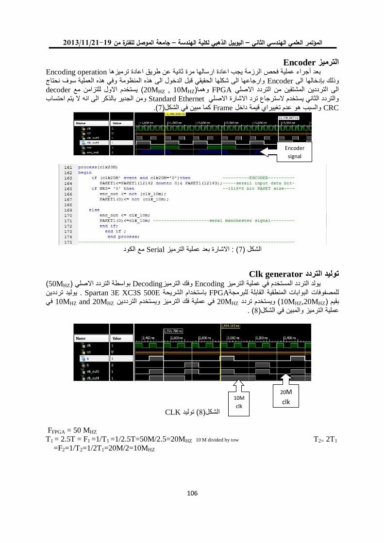
19/99/1192-91جامعة الموصل للفترة من –ليوبيل الذهبي لكلية الهندسة ا –العلمي الهندسي الثاني المؤتمر
101
Encoderالترميز Encoding operationجراء عملية فحص الرزمة يجب اعادة ارسالها مرة ثانية عن طريق اعادة ترميزها بعد أ
وفي هذه العملية سوف نحتاج المنظومةوارجاعها الى شكلها الحقيقي قبل الدخول الى هذه Encoderالى بإدخالهاوذلك decoderيستخدم االول للتزامن مع (20MHZ , 10MHZوهما) FPGAالى الترددين المشتقين من التردد االصلي
احتساب ال يتمومن الجدير بالذكر الى انه Standard Ethernetوالتردد الثاني يستخدم السترجاع ترد االشارة االصلي CRC والسبب هو عدم تغييراي قيمة داخلFrame (9)كما مبين في الشكل.
مع الكود Serialاالشارة بعد عملية الترميز : (9) الشكل
Clk generatorتوليد التردد
( 50MHZبواسطة التردد االصلي ) Decodingوفك الترميز Encodingيولد التردد المستخدم في عملية الترميز يوليد ترددين . Spartan 3E XC3S 500E باستخدام الشريحة FPGAللمصفوفات البوابات المنطقية القابلة للبرمجة
في 10MHZ and 20MHZفي عملية فك الترميز ويستخدم الترددين 20MHZ( ويستخدم تردد 10MHZ,20MHZ) بقيم .( 8)عملية الترميز والمبين في الشكل
CLKتوليد (8الشكل)
FFPGA = 50 MHZ T1 = 2.5T = F1 =1/T1 =1/2.5T=50M/2.5=20MHZ 10 M divided by tow T2= 2T1
=F2=1/T2=1/2T1=20M/2=10MHZ
Encoder
signal
10M
clk
20M
clk
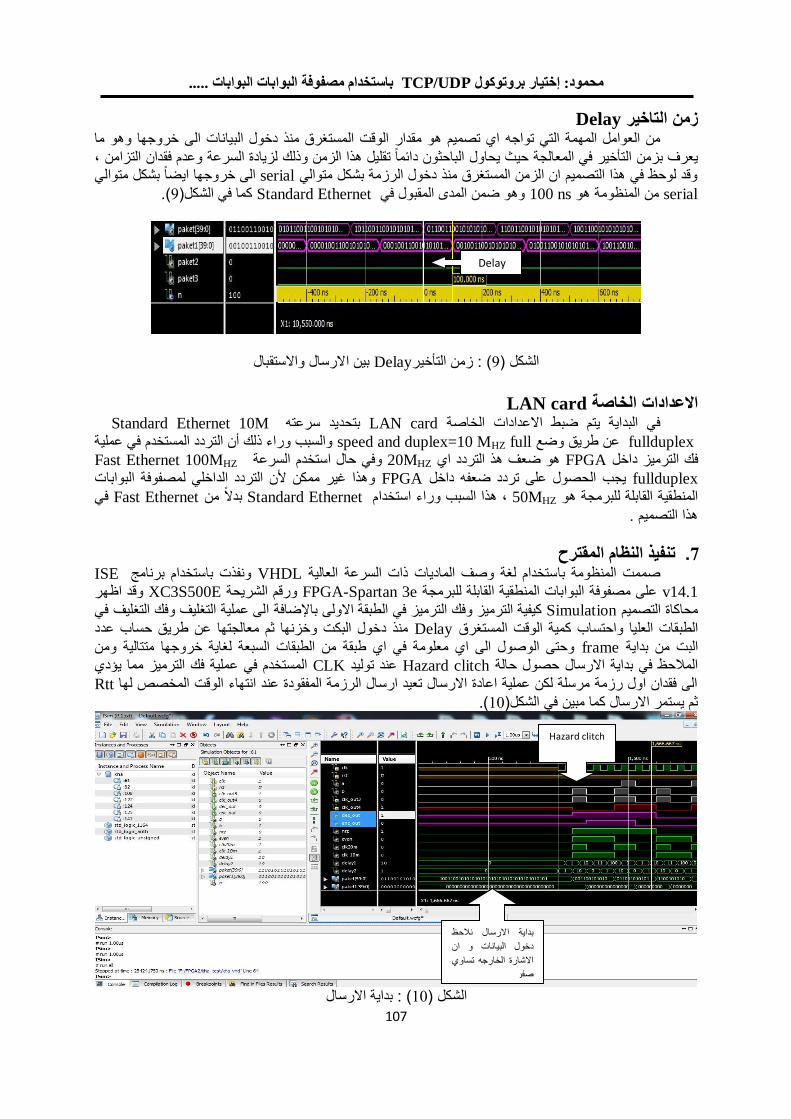
باستخدام مصفوفة البوابات البوابات ..... TCP/UDPمحمود: إختيار بروتوكول
101
Delayزمن التاخير خروجها وهو ماغرق منذ دخول البيانات الى تالوقت المس مقداراي تصميم هو هالتي تواج ةمن العوامل المهم
, يعرف بزمن التأخير في المعالجة حيث يحاول الباحثون دائما تقليل هذا الزمن وذلك لزيادة السرعة وعدم فقدان التزامن ا بشكل متوالي ضالى خروجها اي serialوقد لوحظ في هذا التصميم ان الزمن المستغرق منذ دخول الرزمة بشكل متوالي
serial 100من المنظومة هو ns وهو ضمن المدى المقبول فيStandard Ethernet (7كما في الشكل).
بين االرسال واالستقبال Delayزمن التأخير: (7) الشكل
LAN card ةعدادات الخاصالا
Standard Ethernet 10M بتحديد سرعته LAN cardفي البداية يتم ضبط االعدادات الخاصة
fullduplex عن طريق وضعspeed and duplex=10 MHZ full والسبب وراء ذلك أن التردد المستخدم في عملية Fast Ethernet 100MHZوفي حال استخدم السرعة 20MHZهو ضعف هذ التردد اي FPGAالترميز داخل فك
fullduplex يجب الحصول على تردد ضعفه داخلFPGA وهذا غير ممكن ألن التردد الداخلي لمصفوفة البواباتفي Fast Ethernet بدال من Standard Ethernet, هذا السبب وراء استخدام 50MHZ المنطقية القابلة للبرمجة هو
هذا التصميم .
المقترح النظام نفيذت .7 ISEستخدام برنامج اونفذت ب VHDLستخدام لغة وصف الماديات ذات السرعة العالية اصممت المنظومة ب
v14.1 على مصفوفة البوابات المنطقية القابلة للبرمجةFPGA-Spartan 3e ةورقم الشريح XC3S500E وقد اظهرالى عملية التغليف وفك التغليف في ةضافإلكيفية الترميز وفك الترميز في الطبقة االولى با Simulationمحاكاة التصميم
منذ دخول البكت وخزنها ثم معالجتها عن طريق حساب عدد Delayاب كمية الوقت المستغرق الطبقات العليا واحتسوحتى الوصول الى اي معلومة في اي طبقة من الطبقات السبعة لغاية خروجها متتالية ومن frameالبت من بداية
ملية فك الترميز مما يؤدي المستخدم في ع CLKعند توليد Hazard clitchالمالحظ في بداية االرسال حصول حالة Rttالى فقدان اول رزمة مرسلة لكن عملية اعادة االرسال تعيد ارسال الرزمة المفقودة عند انتهاء الوقت المخصص لها
.(01)ثم يستمر االرسال كما مبين في الشكل
بداية االرسال: (01) الشكل
Delay
Hazard clitch
بداية االرسال نالحظ
دخول البيانات و ان
االشارة الخارجه تساوي
صفر
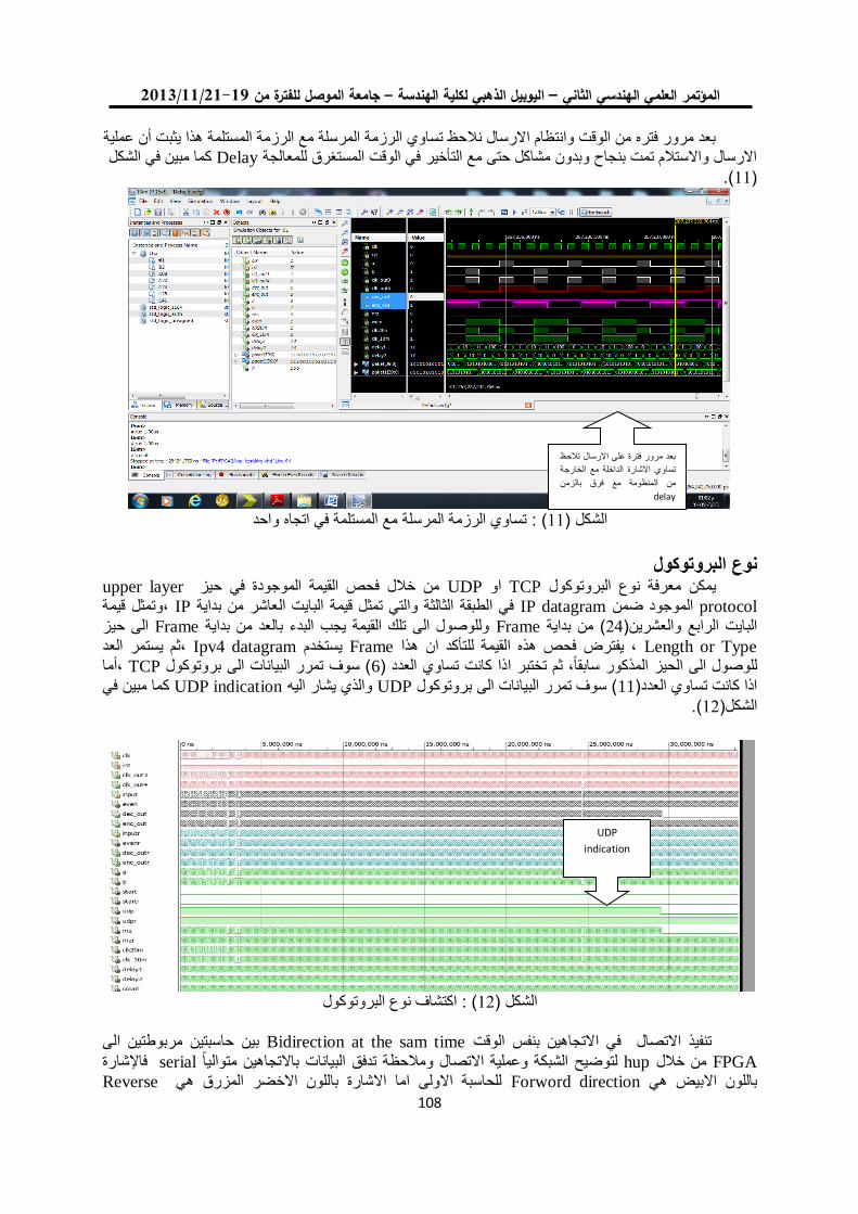
19/99/1192-91جامعة الموصل للفترة من –ليوبيل الذهبي لكلية الهندسة ا –العلمي الهندسي الثاني المؤتمر
101
بعد مرور فتره من الوقت وانتظام االرسال نالحظ تساوي الرزمة المرسلة مع الرزمة المستلمة هذا يثبت أن عملية كما مبين في الشكل Delayاالرسال واالستالم تمت بنجاح وبدون مشاكل حتى مع التأخير في الوقت المستغرق للمعالجة
(00) .
تساوي الرزمة المرسلة مع المستلمة في اتجاه واحد : (00) الشكل
نوع البروتوكول
upper layerمن خالل فحص القيمة الموجودة في حيز UDPاو TCPيمكن معرفة نوع البروتوكول
protocol الموجود ضمنIP datagram من بداية في الطبقة الثالثة والتي تمثل قيمة البايت العاشرIP وتمثل قيمة,الى حيز Frameوللوصول الى تلك القيمة يجب البدء بالعد من بداية Frame( من بداية 24البايت الرابع والعشرين)
Length or Type يفترض فحص هذه القيمة للتأكد ان هذا ,Frame يستخدمIpv4 datagram ثم يستمر العد,,أما TCP( سوف تمرر البيانات الى بروتوكول 6 المذكور سابقا , ثم تختبر اذا كانت تساوي العدد ) للوصول الى الحيز
كما مبين في UDP indicationوالذي يشار اليه UDP( سوف تمرر البيانات الى بروتوكول 11اذا كانت تساوي العدد) . (02)الشكل
اكتشاف نوع البروتوكول : (02) الشكل
بين حاسبتين مربوطتين الى Bidirection at the sam timeفي االتجاهين بنفس الوقت االتصال تنفيذ FPGA من خاللhup لتوضيح الشبكة وعملية االتصال ومالحظة تدفق البيانات باالتجاهين متواليا serial فاإلشارة
Reverseللحاسبة االولى اما االشارة باللون االخضر المزرق هي Forword directionباللون االبيض هي
UDP
indication
بعد مرور فترة على االرسال نالحظ
ي االشارة الداخلة مع الخارجة تساو
من المنظومة مع فرق بالزمن
delay
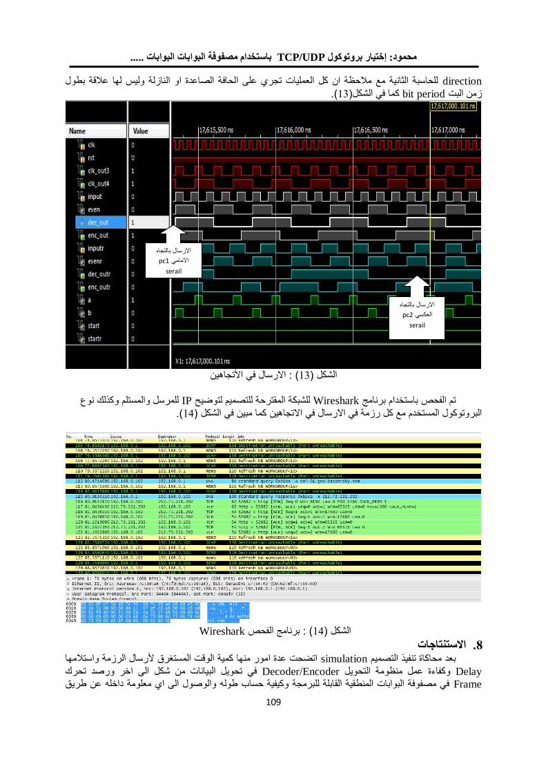
باستخدام مصفوفة البوابات البوابات ..... TCP/UDPمحمود: إختيار بروتوكول
101
direction للحاسبة الثانية مع مالحظة ان كل العمليات تجري على الحافة الصاعدة او النازلة وليس لها عالقة بطول .(03كما في الشكل) bit periodزمن البت
االرسال في األتجاهين : (03) الشكل
للمرسل والمستلم وكذلك نوع IPللشبكة المقترحة للتصميم لتوضيح Wiresharkتم الفحص باستخدام برنامج
.(04) في الشكلكما مبين رزمة في االرسال في االتجاهين البروتوكول المستخدم مع كل
Wireshark برنامج الفحص : (04) الشكل
االستنتاجات .8اتضحت عدة امور منها كمية الوقت المستغرق ألرسال الرزمة واستالمها simulationبعد محاكاة تنفيذ التصميم
Delay وكفاءة عمل منظومة التحويلDecoder/Encoder في تحويل البيانات من شكل الى اخر ورصد تحركFrame في مصفوفة البوابات المنطقية القابلة للبرمجة وكيفية حساب طوله والوصول الى اي معلومة داخله عن طريق
ه االرسال بالتجا
pc1االمامي
serail
االرسال بالتجاه
pc2العكسي
serail
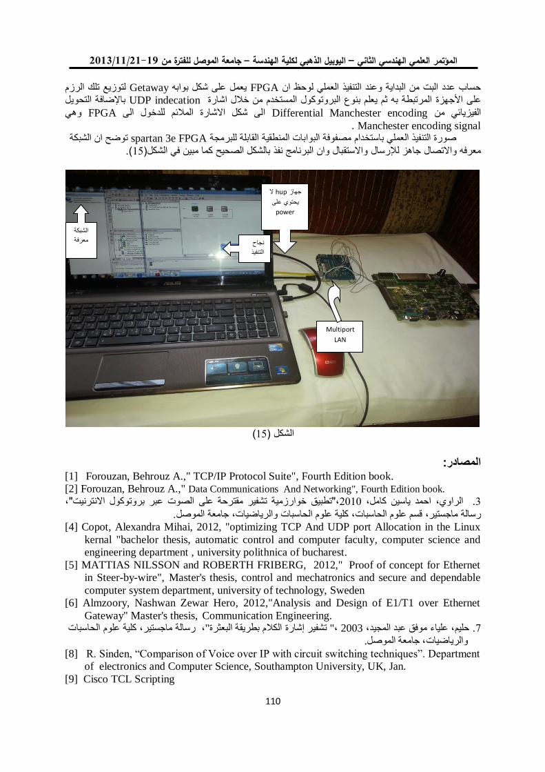
19/99/1192-91جامعة الموصل للفترة من –ليوبيل الذهبي لكلية الهندسة ا –العلمي الهندسي الثاني المؤتمر
110
لتوزيع تلك الرزم Getawayيعمل على شكل بوابه FPGAحساب عدد البت من البداية وعند التنفيذ العملي لوحظ ان التحويل باإلضافة UDP indecationكول المستخدم من خالل اشارة والمرتبطة به ثم يعلم بنوع البروت جهزةاألعلى
وهي FPGAالى شكل االشارة المالئم للدخول الى Differential Manchester encodingالفيزيائي من Manchester encoding signal .
توضح ان الشبكة spartan 3e FPGAمصفوفة البوابات المنطقية القابلة للبرمجة صورة التنفيذ العملي باستخدام .(05)كما مبين في الشكلواالستقبال وان البرنامج نفذ بالشكل الصحيح لإلرسالمعرفه واالتصال جاهز
(05) لشكلا
المصادر:
[1] Forouzan, Behrouz A.," TCP/IP Protocol Suite", Fourth Edition book.
[2] Forouzan, Behrouz A.," Data Communications And Networking", Fourth Edition book.
بروتوكول االنترنيت",,"تطبيق خوارزمية تشفير مقترحة على الصوت عبر 2101, احمد ياسين كامل, الراوي .3
جامعة الموصل. الرياضيات,, كلية علوم الحاسبات والحاسبات قسم علوم ,رسالة ماجستير[4] Copot, Alexandra Mihai, 2012, "optimizing TCP And UDP port Allocation in the Linux
kernal "bachelor thesis, automatic control and computer faculty, computer science and
engineering department , university polithnica of bucharest.
[5] MATTIAS NILSSON and ROBERTH FRIBERG, 2012," Proof of concept for Ethernet
in Steer-by-wire", Master's thesis, control and mechatronics and secure and dependable
computer system department, university of technology, Sweden
[6] Almzoory, Nashwan Zewar Hero, 2012,"Analysis and Design of E1/T1 over Ethernet
Gateway" Master's thesis, Communication Engineering.
علوم الحاسبات ةكلي ر,ماجستي رسالة ,"البعثرة قةبطري إشارة الكالم رتشفي" , 2003 د,المجي عبد موفق اءليع م,حلي .9
.الموصل جامعة ات,والرياضي[8] R. Sinden, “Comparison of Voice over IP with circuit switching techniques”. Department
of electronics and Computer Science, Southampton University, UK, Jan.
[9] Cisco TCL Scripting
Multiport
LAN
الشبكة
معرفة
ال hupجهاز
يحتوي على
power
نجاح
التنفيذ
باستخدام مصفوفة البوابات البوابات ..... TCP/UDPمحمود: إختيار بروتوكول
111
http://www.cisco.com/en/US/products/sw/iosswrel/ps5207/products_feature_guide09186a008
01a75a7.html
[10] "10/100 BASE-T signal port " http://www.mnc-tek. com , white paper.
[11] Pedroni, Volnei A. ," Circuit Design with VHDL ", book, London , England.
[12] Mills, Adrian, 2009, "Manchester encoding using RS-232 ".
[13] Benthien, Dr.George W. "Digital Encoding And Decoding", 2007 , thesis.
[14] Cisco IP-to-IP Gateway Configuration http://www.cisco.com/univercd/cc/td/doc/product/software/ios123/123cgcr/vvfax_c/callc_c/h
323_c/ipipgw/ipgw.htm
[15] Christophoros Kachris, 2010 ,"Design and Implementation of aTCP/IP core for
reconfigurable logic", Master's thesis, Electronic and Computer Engineering Department, Technical University, Crete102002.
[16] Frank Vahid, John Wiley and Sons Publishers, "Digital Design", First Edition 2007
book.
[17] . www.xilinx.com , Spartan-3E Start Kit Board User Guide white paper.
[18] http://opencores.org/ for implementation core.
19/99/1192-91جامعة الموصل للفترة من –ليوبيل الذهبي لكلية الهندسة ا –العلمي الهندسي الثاني المؤتمر
111
FPGA Based Architectures for Vertex Processing System
Fakhrulddin H. Ali Omar Z. Tarik [email protected] [email protected]
Dept. of Computer Engineering/ College of Engineering/ University of Mosul – IRAQ.
Abstract
The three dimensional0 (3D) transformations are considered one of the basic
operations required to translate , rotate, or scale the objects in 3D space. The
continuous evolution in computer graphics and its applications requires more objects
and therefore more vertices to model them. As a result of that the transformations
consume more processing time since they are applied to each of the vertices
individually. In this paper a vertex processing system is proposed and implemented to
increase the performance speed when the execution of the transformation operations
are performed. The system consists of two main units. The transformation matrix unit
that computes variety types of individual and composite transformations. The second
unit is the vertex processing unit which is implemented with three proposed
architectures. The performance of the three architectures are tested and compared.
FPGA ( Field Programmable Gates Array ) is used to implement the system.
Keywords: FPGA, Concatenation Matrix, Vertices, Pipelining.
FPGAمعمارية لنظام معالجة الرأس بإستخدام
عمر زياد طارق الدين حامد علي فخرد.
[email protected] [email protected]
العراق. –قسم هندسة الحاسوب/ كلية الهندسة / جامعة الموصل
الخالصة
ت عد عمليات التحويالت الهندسية من العمليات األساسية في علم الرسوم الحاسوبية، عن طريقها يمكن
ر في علم الرسوم الحاسوبية حيث تحريك، أو تدوير، أو تكبير، أو تصغير الكائنات في فضاء ثالثي األبعاد. ومع التطو
أصبحت المشاهد أكثر تعقيدا من حيث عدد الكائنات وعدد الرؤوس التي تمثل هذه الكائنات لذلك أصبحت عملية تطبيق
التحويالت على المشاهد تأخذ وقت تنفيذ كبير حيث كل رأس من الرؤوس المكونة للمشهد يتطلب تطبيق التحويل
في هذا البحث تم تنفيذ نظام لمعالجة الرؤوس من أجل زيادة سرعة االداء. النظام يتكون المطلوب عليه بشكل منفصل.
من وحديتين وحدة تكوين مصفوفة التحويل حيث بواسطة هذه الوحدة يمكن تكوين التحويالت االساسية او مجموعة
الث معماريات وتم مقارنة االداء من التحويالت المركبة ، والوحدة الثانية هي وحدة معالجة الرؤوس حيث تم تقديم ث
فيما بينهم من حيث سرعة التنفيذ والموارد المحجوزة. تم تنفيذ النظام باستعمال البوابات القابلة للبرمجة حقليا
(FPGA).
Ali: FPGA Based Architectures for Vertex Processing …..
111
1- Introduction
The science of computer graphics has become very sophisticated and its applications
entered in everyday life such as Computer Aided Design, Medical diagnoses, Video
Gaming, Computer Simulation and Others. Real time applications of computer graphics
require high speed processing therefore several means are considered to increase
performance and speed up the calculations. GPU ( Graphics Processing Unit ) which is used
in Personal Computers is one of the well-known examples to accomplish this. In 3D
computer graphics the major transformations used are translation, rotation and scaling of the
objects. Each object commonly consists of hundreds of vertices so the processing time of the
transformation consumes considerable time. To transform an object each of its vertices is
transformed first then it is further processed to compute its new image. In three dimensional
applications such transformations have to be carried out in the object space before projection
to the image space which requires more processing time due to the third dimension. This is
why a hardware support is necessary in such a condition. So many papers are devoted to this
area of research and a review of some of the recent ones are listed next.
In 2006 the researchers F.Bensaali and A.Amira proposed an article which investigates the
suitability of field programmable gate array devices as an accelerator for implementing 3D
affine transformations. The proposed solution is based on processing large matrix
multiplication implemented for large 3D models on the RC1000 Celoxica board based
development platform using Handel-C[1]. In 2007 Faycal Bensaali , Abbes Amira and Reza
Sotudeh described field-programmable gate arrays in implementing floating-point
arithmetic. The performance in terms of area/speed of the proposed architectures has been
assessed and has shown that they require less area and can run with a higher frequency,
according to them, when compared with existing systems [2].In 2010, Sahen presented a
paper, where a 32-bit floating-point based hardware module was designed to speed-up 3D
graphic transformations using field programmable gate array (FPGA). Module’s data
processing speed was compared to various PCs. The results showed that, 3D graphic
transformations can be speeded-up by a factor (up to 11.47) employing the designed module,
as claimed by him [3]. In 2012 F.H. Ali tends to construct a general form of a single matrix
representation for multiple geometric transformations for three dimensional objects. This
way, a speed up factor of 1 to 5, according to his paper, can be gained. An architecture is
designed and implemented as a hardware unit and then tested for single matrix
transformation using Field Programmable Gate Array (FPGA) [4]. However, this paper
introduces a vertex processing system based on FPGA . The system has two units,
transformation matrix unit that creates the transformation matrix and the processing unit.
Two Patterns for the transformation matrix has been proposed, each one can form variety
types of unique or composite transformations. Since the rotation requires trigonometric
functions, a Look-Up Table method has been used to evaluate it. The vertex processing unit
has been designed using three architectures , serial processing , parallel coordinates
processing and parallel vertices processing.
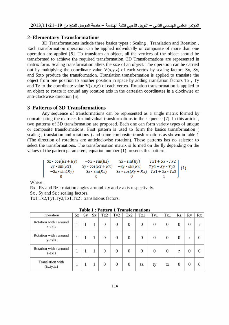
19/99/1192-91جامعة الموصل للفترة من –ليوبيل الذهبي لكلية الهندسة ا –العلمي الهندسي الثاني المؤتمر
111
2- Elementary Transformations 3D Transformations include three basics types : Scaling , Translation and Rotation .
Each transformation operation can be applied individually or composite of more than one
operation are applied [5]. To transform an object, all the vertices of the object should be
transformed to achieve the required transformation. 3D Transformations are represented in
matrix form. Scaling transformation alters the size of an object. The operation can be carried
out by multiplying the coordinate value V(x,y,z) of each vertex by scaling factors Sx, Sy,
and Szto produce the transformation. Translation transformation is applied to translate the
object from one position to another position in space by adding translation factors Tx , Ty
and Tz to the coordinate value V(x,y,z) of each vertex. Rotation transformation is applied to
an object to rotate it around any rotation axis in the cartesian coordinates in a clockwise or
anti-clockwise direction [6].
3- Patterns of 3D Transformations Any sequence of transformations can be represented as a single matrix formed by
concatenating the matrices for individual transformations in the sequence [7]. In this article ,
two patterns of 3D transformation are proposed. Each one can form variety types of unique
or composite transformations. First pattern is used to form the basics transformation (
scaling , translation and rotations ) and some composite transformations as shown in table 1
(The direction of rotations are anticlockwise rotation). These patterns has no selector to
select the transformations. The transformation matrix is formed on the fly depending on the
values of the pattern parameters, equation number (1) presents this pattern.
Where :
Rx , Ry and Rz : rotation angles around x,y and z axis respectively.
Sx , Sy and Sz : scaling factors.
Tx1,Tx2,Ty1,Ty2,Tz1,Tz2 : translations factors.
Table 1 : Pattern 1 Transformations
Rx Ry Rz Tx1 Ty1 Tz1 Tx2 Ty2 Tz2 Sx Sy Sz Operation
r 0 0 0 0 0 0 0 0 1 1 1 Rotation with r around
x-axis
0 r 0 0 0 0 0 0 0 1 1 1 Rotation with r around
y-axis
0 0 r 0 0 0 0 0 0 1 1 1 Rotation with r around
z-axis
0 0 0 tx ty tz 0 0 0 1 1 1 Translation with
(tx,ty,tz)
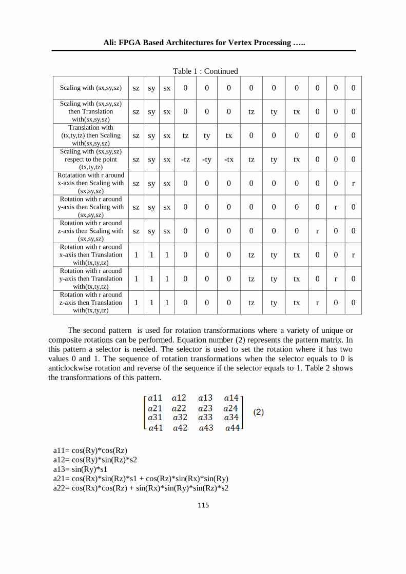
Ali: FPGA Based Architectures for Vertex Processing …..
111
Table 1 : Continued
0 0 0 0 0 0 0 0 0 sx sy sz Scaling with (sx,sy,sz)
0 0 0 tx ty tz 0 0 0 sx sy sz Scaling with (sx,sy,sz)
then Translation
with(sx,sy,sz)
0 0 0 0 0 0 tx ty tz sx sy sz Translation with
(tx,ty,tz) then Scaling
with(sx,sy,sz)
0 0 0 tx ty tz -tx -ty -tz sx sy sz Scaling with (sx,sy,sz)
respect to the point (tx,ty,tz)
r 0 0 0 0 0 0 0 0 sx sy sz Rotatation with r around
x-axis then Scaling with
(sx,sy,sz)
0 r 0 0 0 0 0 0 0 sx sy sz Rotation with r around
y-axis then Scaling with
(sx,sy,sz)
0 0 r 0 0 0 0 0 0 sx sy sz Rotation with r around
z-axis then Scaling with
(sx,sy,sz)
r 0 0 tx ty tz 0 0 0 1 1 1 Rotation with r around
x-axis then Translation
with(tx,ty,tz)
0 r 0 tx ty tz 0 0 0 1 1 1 Rotation with r around
y-axis then Translation
with(tx,ty,tz)
0 0 r tx ty tz 0 0 0 1 1 1 Rotation with r around
z-axis then Translation with(tx,ty,tz)
The second pattern is used for rotation transformations where a variety of unique or
composite rotations can be performed. Equation number (2) represents the pattern matrix. In
this pattern a selector is needed. The selector is used to set the rotation where it has two
values 0 and 1. The sequence of rotation transformations when the selector equals to 0 is
anticlockwise rotation and reverse of the sequence if the selector equals to 1. Table 2 shows
the transformations of this pattern.
a11= cos(Ry)*cos(Rz)
a12= cos(Ry)*sin(Rz)*s2
a13= sin(Ry)*s1
a21= cos(Rx)*sin(Rz)*s1 + cos(Rz)*sin(Rx)*sin(Ry)
a22= cos(Rx)*cos(Rz) + sin(Rx)*sin(Ry)*sin(Rz)*s2
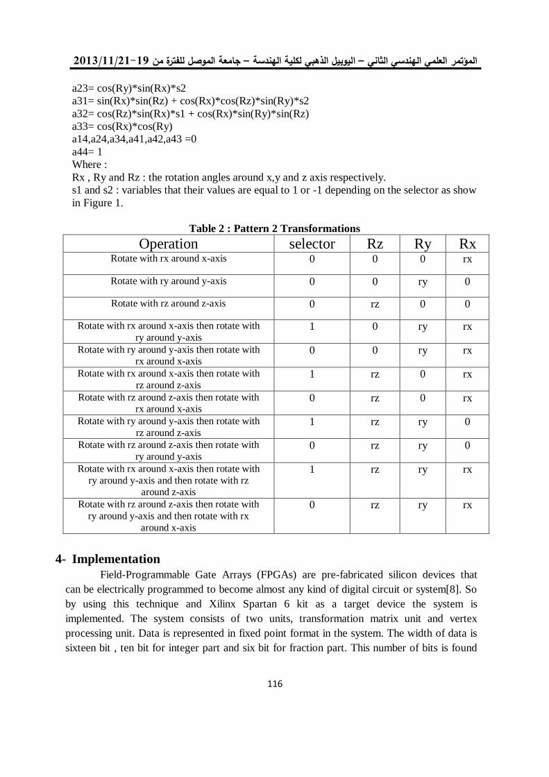
19/99/1192-91جامعة الموصل للفترة من –ليوبيل الذهبي لكلية الهندسة ا –العلمي الهندسي الثاني المؤتمر
111
a23= cos(Ry)*sin(Rx)*s2
a31= sin(Rx)*sin(Rz) + cos(Rx)*cos(Rz)*sin(Ry)*s2
a32= cos(Rz)*sin(Rx)*s1 + cos(Rx)*sin(Ry)*sin(Rz)
a33= cos(Rx)*cos(Ry)
a14,a24,a34,a41,a42,a43 =0
a44= 1
Where :
Rx , Ry and Rz : the rotation angles around x,y and z axis respectively.
s1 and s2 : variables that their values are equal to 1 or -1 depending on the selector as show
in Figure 1.
Table 2 : Pattern 2 Transformations
Rx Ry Rz selector Operation rx 0 0 0 Rotate with rx around x-axis
0 ry 0 0 Rotate with ry around y-axis
0 0 rz 0 Rotate with rz around z-axis
rx ry 0 1 Rotate with rx around x-axis then rotate with
ry around y-axis
rx ry 0 0 Rotate with ry around y-axis then rotate with rx around x-axis
rx 0 rz 1 Rotate with rx around x-axis then rotate with
rz around z-axis
rx 0 rz 0 Rotate with rz around z-axis then rotate with rx around x-axis
0 ry rz 1 Rotate with ry around y-axis then rotate with
rz around z-axis
0 ry rz 0 Rotate with rz around z-axis then rotate with
ry around y-axis
rx ry rz 1 Rotate with rx around x-axis then rotate with
ry around y-axis and then rotate with rz around z-axis
rx ry rz 0 Rotate with rz around z-axis then rotate with
ry around y-axis and then rotate with rx
around x-axis
4- Implementation
Field-Programmable Gate Arrays (FPGAs) are pre-fabricated silicon devices that
can be electrically programmed to become almost any kind of digital circuit or system[8]. So
by using this technique and Xilinx Spartan 6 kit as a target device the system is
implemented. The system consists of two units, transformation matrix unit and vertex
processing unit. Data is represented in fixed point format in the system. The width of data is
sixteen bit , ten bit for integer part and six bit for fraction part. This number of bits is found
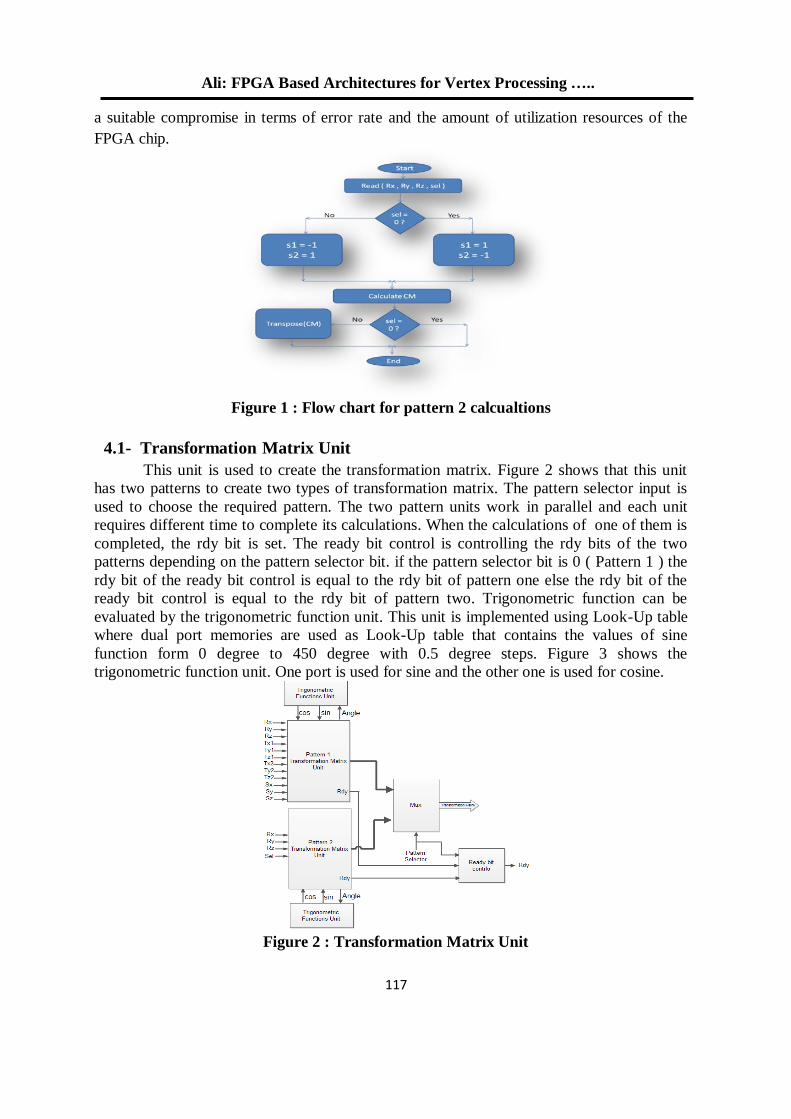
Ali: FPGA Based Architectures for Vertex Processing …..
111
a suitable compromise in terms of error rate and the amount of utilization resources of the
FPGA chip.
Figure 1 : Flow chart for pattern 2 calcualtions
4.1- Transformation Matrix Unit
This unit is used to create the transformation matrix. Figure 2 shows that this unit
has two patterns to create two types of transformation matrix. The pattern selector input is
used to choose the required pattern. The two pattern units work in parallel and each unit
requires different time to complete its calculations. When the calculations of one of them is
completed, the rdy bit is set. The ready bit control is controlling the rdy bits of the two
patterns depending on the pattern selector bit. if the pattern selector bit is 0 ( Pattern 1 ) the
rdy bit of the ready bit control is equal to the rdy bit of pattern one else the rdy bit of the
ready bit control is equal to the rdy bit of pattern two. Trigonometric function can be
evaluated by the trigonometric function unit. This unit is implemented using Look-Up table
where dual port memories are used as Look-Up table that contains the values of sine
function form 0 degree to 450 degree with 0.5 degree steps. Figure 3 shows the
trigonometric function unit. One port is used for sine and the other one is used for cosine.
Figure 2 : Transformation Matrix Unit
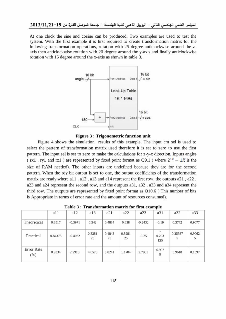
19/99/1192-91جامعة الموصل للفترة من –ليوبيل الذهبي لكلية الهندسة ا –العلمي الهندسي الثاني المؤتمر
111
At one clock the sine and cosine can be produced. Two examples are used to test the
system. With the first example it is first required to create transformation matrix for the
following transformation operations, rotation with 25 degree anticlockwise around the z-
axis then anticlockwise rotation with 20 degree around the y-axis and finally anticlockwise
rotation with 15 degree around the x-axis as shown in table 3.
Figure 3 : Trigonometric function unit
Figure 4 shows the simulation results of this example. The input cm_sel is used to
select the pattern of transformation matrix used therefore it is set to zero to use the first
pattern. The input sel is set to zero to make the calculations for z-y-x direction. Inputs angles
( rx1 , ry1 and rz1 ) are represented by fixed point format as Q9.1 ( where is the
size of RAM needed). The other inputs are undefined because they are for the second
pattern. When the rdy bit output is set to one, the output coefficients of the transformation
matrix are ready where a11 , a12 , a13 and a14 represent the first row, the outputs a21 , a22 ,
a23 and a24 represent the second row, and the outputs a31, a32 , a33 and a34 represent the
third row. The outputs are represented by fixed point format as Q10.6 ( This number of bits
is Appropriate in terms of error rate and the amount of resources consumed).
Table 3 : Transformation matrix for first example
a11 a12 a13 a21 a22 a23 a31 a32 a33
Theoretical 0.8517 -0.3971 0.342 0.4884 0.838 -0.2432 -0.19 0.3742 0.9077
Practical 0.84375 -0.4062 0.3281
25
0.4843
75
0.8281
25 -0.25
-
0.203
125
0.35937
5
0.9062
5
Error Rate
(%) 0.9334 2.2916 4.0570 0.8241 1.1784 2.7961
6.907
9 3.9618 0.1597
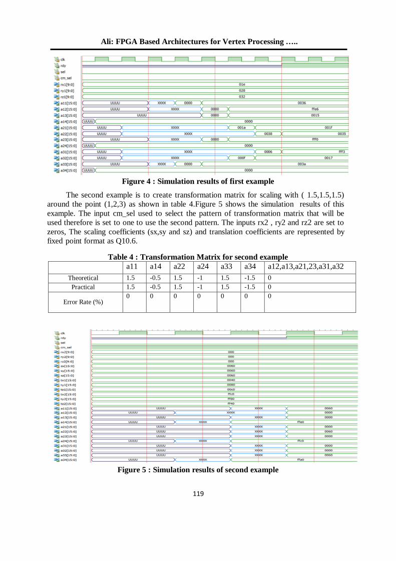
Ali: FPGA Based Architectures for Vertex Processing …..
111
Figure 4 : Simulation results of first example
The second example is to create transformation matrix for scaling with ( 1.5,1.5,1.5)
around the point (1,2,3) as shown in table 4.Figure 5 shows the simulation results of this
example. The input cm_sel used to select the pattern of transformation matrix that will be
used therefore is set to one to use the second pattern. The inputs rx2 , ry2 and rz2 are set to
zeros, The scaling coefficients (sx,sy and sz) and translation coefficients are represented by
fixed point format as Q10.6.
Table 4 : Transformation Matrix for second example
a11 a14 a22 a24 a33 a34 a12,a13,a21,23,a31,a32
Theoretical 1.5 -0.5 1.5 -1 1.5 -1.5 0
Practical 1.5 -0.5 1.5 -1 1.5 -1.5 0
Error Rate (%) 0 0 0 0 0 0 0
Figure 5 : Simulation results of second example
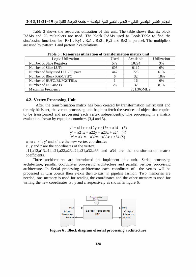
19/99/1192-91جامعة الموصل للفترة من –ليوبيل الذهبي لكلية الهندسة ا –العلمي الهندسي الثاني المؤتمر
111
Table 3 shows the resources utilization of this unit. The table shows that six block
RAMs and 26 multipliers are used. The block RAMs used as Look-Table to find the
sine/cosine functions for Rx1 , Ry1 , Rz1 , Rx2 , Ry2 and Rz2 in parallel. The multipliers
are used by pattern 1 and pattern 2 calculations.
Table 5 : Resources utilization of transformation matrix unit
Logic Utilization Used Available Utilization Number of Slice Registers 572 18224 3%
Number of Slice LUTs 603 9112 6%
Number of fully used LUT-FF pairs 447 728 61%
Number of Block RAM/FIFO 6 32 18%
Number of BUFG/BUFGCTRLs 1 16 6%
Number of DSP48A1s 26 32 81%
Maximum Frequency 281.365MHz
4.2- Vertex Processing Unit
After the transformation matrix has been created by transformation matrix unit and
the rdy bit is set, the vertex processing unit begin to fetch the vertices of object that require
to be transformed and processing each vertex independently. The processing is a matrix
evaluation shown by equations numbers (3,4 and 5).
x’ = a11x + a12y + a13z + a14 (3)
y’ = a21x + a22y + a23z + a24 (4)
z’ = a31x + a32y + a33z + a34 (5)
where: x’ , y’ and z’ are the new vertex coordinates
x , y and z are the coordinates of the vertex
a11,a12,a13,a14,a21,a22,a23,a24,a31,a32,a33 and a34 are the transformation matrix
coefficients.
Three architectures are introduced to implement this unit. Serial processing
architecture, parallel coordinates processing architecture and parallel vertices processing
architecture. In Serial processing architecture each coordinate of the vertex will be
processed in turn ,x-axis then y-axis then z-axis, in pipeline fashion. Two memories are
needed, one memory is used for reading the coordinates and the other memory is used for
writing the new coordinates x , y and z respectively as shown in figure 6.
Figure 6 : Block diagram ofserial processing architecture
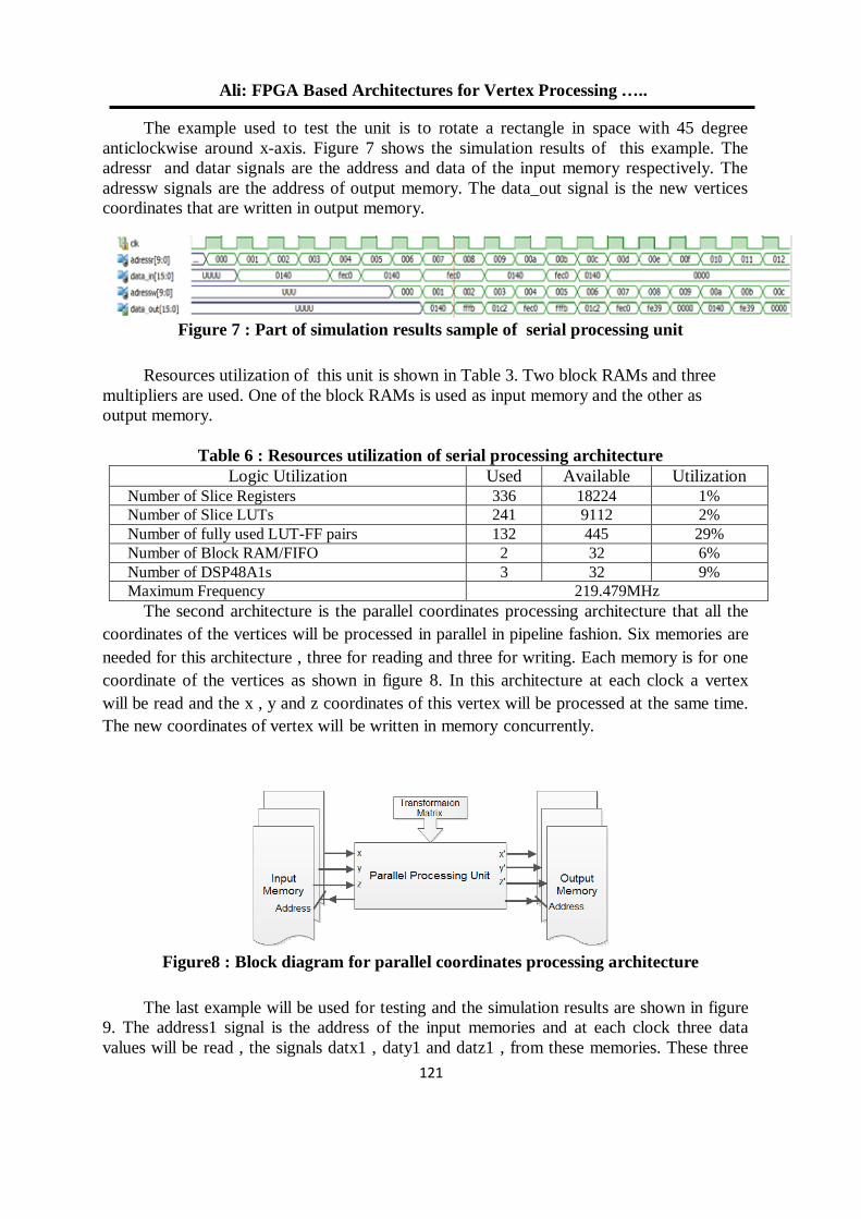
Ali: FPGA Based Architectures for Vertex Processing …..
111
The example used to test the unit is to rotate a rectangle in space with 45 degree
anticlockwise around x-axis. Figure 7 shows the simulation results of this example. The
adressr and datar signals are the address and data of the input memory respectively. The
adressw signals are the address of output memory. The data_out signal is the new vertices
coordinates that are written in output memory.
Figure 7 : Part of simulation results sample of serial processing unit
Resources utilization of this unit is shown in Table 3. Two block RAMs and three
multipliers are used. One of the block RAMs is used as input memory and the other as
output memory.
Table 6 : Resources utilization of serial processing architecture
Logic Utilization Used Available Utilization Number of Slice Registers 336 18224 1%
Number of Slice LUTs 241 9112 2%
Number of fully used LUT-FF pairs 132 445 29%
Number of Block RAM/FIFO 2 32 6%
Number of DSP48A1s 3 32 9%
Maximum Frequency 219.479MHz
The second architecture is the parallel coordinates processing architecture that all the
coordinates of the vertices will be processed in parallel in pipeline fashion. Six memories are
needed for this architecture , three for reading and three for writing. Each memory is for one
coordinate of the vertices as shown in figure 8. In this architecture at each clock a vertex
will be read and the x , y and z coordinates of this vertex will be processed at the same time.
The new coordinates of vertex will be written in memory concurrently.
Figure8 : Block diagram for parallel coordinates processing architecture
The last example will be used for testing and the simulation results are shown in figure
9. The address1 signal is the address of the input memories and at each clock three data
values will be read , the signals datx1 , daty1 and datz1 , from these memories. These three
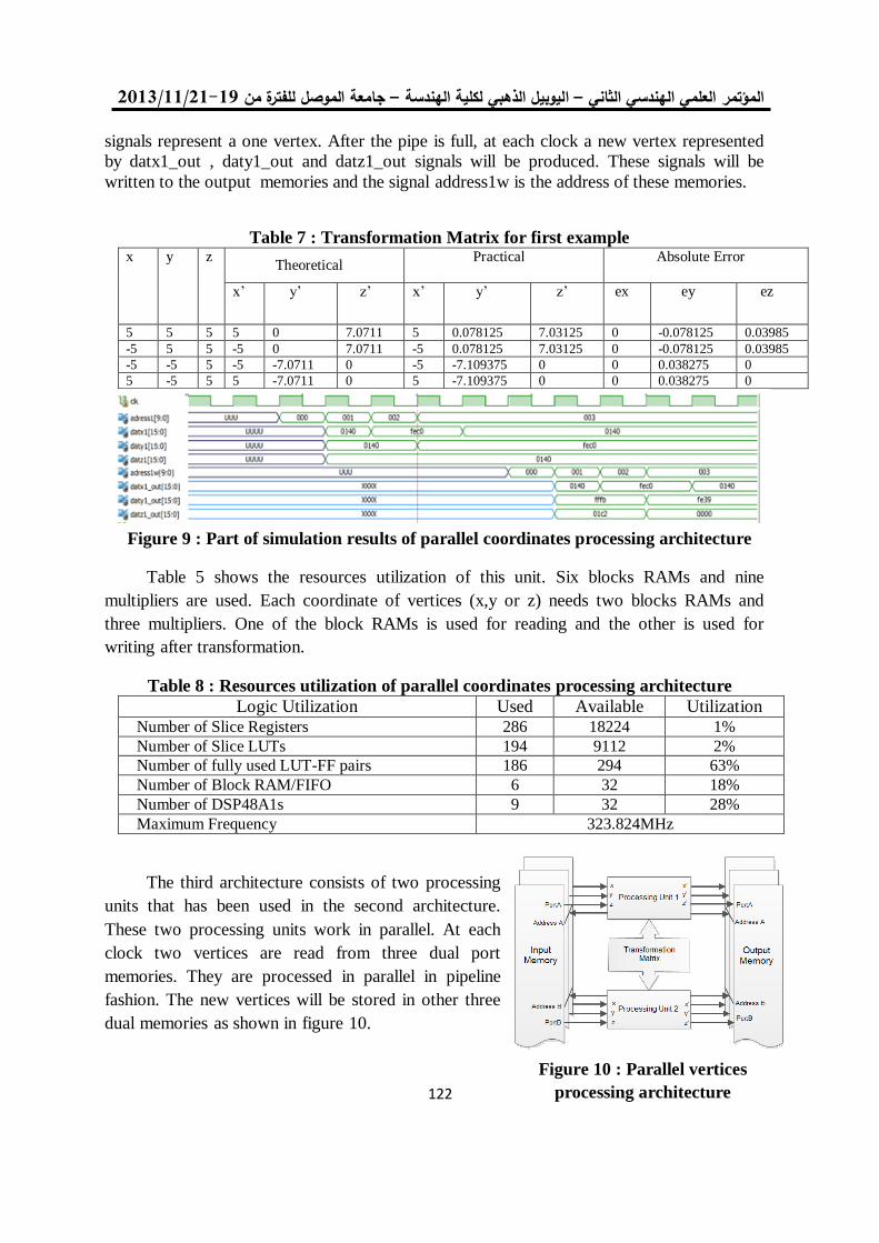
19/99/1192-91جامعة الموصل للفترة من –ليوبيل الذهبي لكلية الهندسة ا –العلمي الهندسي الثاني المؤتمر
111
signals represent a one vertex. After the pipe is full, at each clock a new vertex represented
by datx1_out , daty1_out and datz1_out signals will be produced. These signals will be
written to the output memories and the signal address1w is the address of these memories.
Table 7 : Transformation Matrix for first example x y z
Theoretical Practical Absolute Error
x’ y’ z’ x’ y’ z’ ex ey ez
5 5 5 5 0 7.0711 5 0.078125 7.03125 0 -0.078125 0.03985
-5 5 5 -5 0 7.0711 -5 0.078125 7.03125 0 -0.078125 0.03985
-5 -5 5 -5 -7.0711 0 -5 -7.109375 0 0 0.038275 0
5 -5 5 5 -7.0711 0 5 -7.109375 0 0 0.038275 0
Figure 9 : Part of simulation results of parallel coordinates processing architecture
Table 5 shows the resources utilization of this unit. Six blocks RAMs and nine
multipliers are used. Each coordinate of vertices (x,y or z) needs two blocks RAMs and
three multipliers. One of the block RAMs is used for reading and the other is used for
writing after transformation.
Table 8 : Resources utilization of parallel coordinates processing architecture
Logic Utilization Used Available Utilization Number of Slice Registers 286 18224 1%
Number of Slice LUTs 194 9112 2%
Number of fully used LUT-FF pairs 186 294 63%
Number of Block RAM/FIFO 6 32 18%
Number of DSP48A1s 9 32 28%
Maximum Frequency 323.824MHz
The third architecture consists of two processing
units that has been used in the second architecture.
These two processing units work in parallel. At each
clock two vertices are read from three dual port
memories. They are processed in parallel in pipeline
fashion. The new vertices will be stored in other three
dual memories as shown in figure 10.
Figure 10 : Parallel vertices
processing architecture
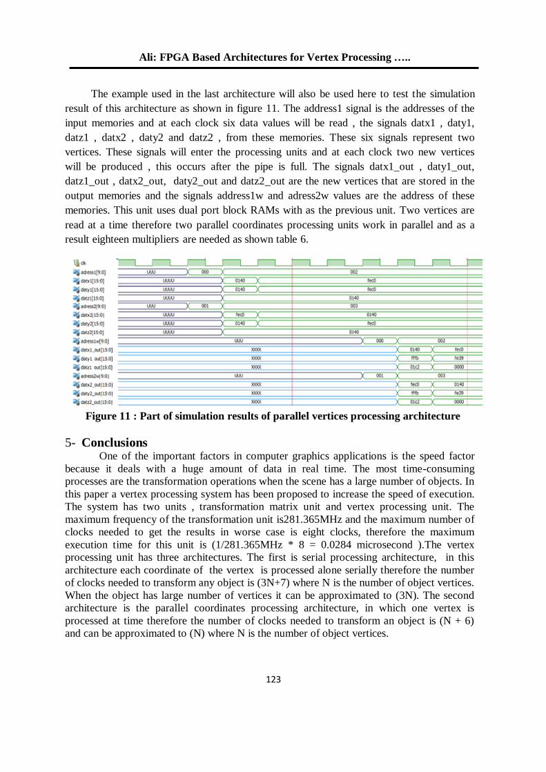
Ali: FPGA Based Architectures for Vertex Processing …..
111
The example used in the last architecture will also be used here to test the simulation
result of this architecture as shown in figure 11. The address1 signal is the addresses of the
input memories and at each clock six data values will be read , the signals datx1 , daty1,
datz1 , datx2 , daty2 and datz2 , from these memories. These six signals represent two
vertices. These signals will enter the processing units and at each clock two new vertices
will be produced , this occurs after the pipe is full. The signals datx1_out , daty1_out,
datz1_out , datx2_out, daty2_out and datz2_out are the new vertices that are stored in the
output memories and the signals address1w and adress2w values are the address of these
memories. This unit uses dual port block RAMs with as the previous unit. Two vertices are
read at a time therefore two parallel coordinates processing units work in parallel and as a
result eighteen multipliers are needed as shown table 6.
Figure 11 : Part of simulation results of parallel vertices processing architecture
5- Conclusions
One of the important factors in computer graphics applications is the speed factor
because it deals with a huge amount of data in real time. The most time-consuming
processes are the transformation operations when the scene has a large number of objects. In
this paper a vertex processing system has been proposed to increase the speed of execution.
The system has two units , transformation matrix unit and vertex processing unit. The
maximum frequency of the transformation unit is281.365MHz and the maximum number of
clocks needed to get the results in worse case is eight clocks, therefore the maximum
execution time for this unit is (1/281.365MHz * 8 = 0.0284 microsecond ).The vertex
processing unit has three architectures. The first is serial processing architecture, in this
architecture each coordinate of the vertex is processed alone serially therefore the number
of clocks needed to transform any object is (3N+7) where N is the number of object vertices.
When the object has large number of vertices it can be approximated to (3N). The second
architecture is the parallel coordinates processing architecture, in which one vertex is
processed at time therefore the number of clocks needed to transform an object is (N + 6)
and can be approximated to (N) where N is the number of object vertices.
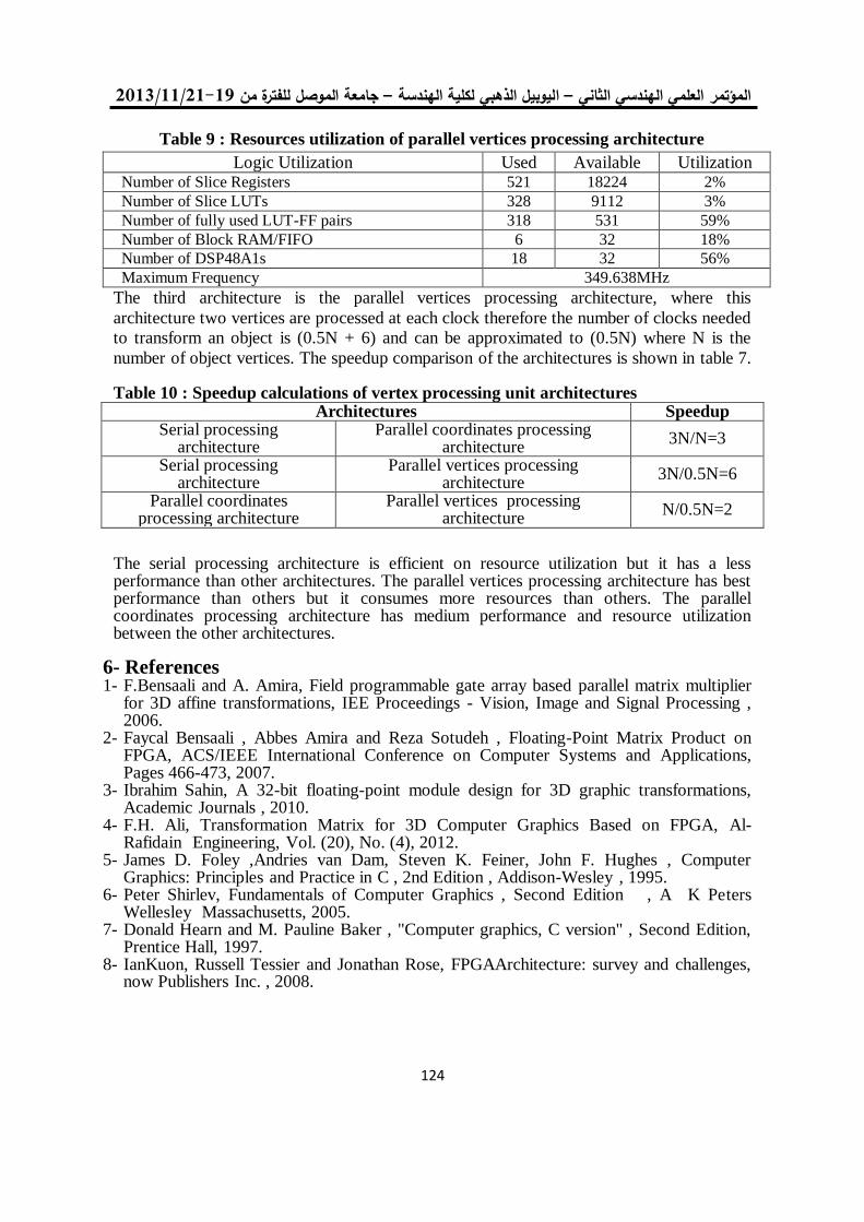
19/99/1192-91جامعة الموصل للفترة من –ليوبيل الذهبي لكلية الهندسة ا –العلمي الهندسي الثاني المؤتمر
111
Table 9 : Resources utilization of parallel vertices processing architecture
Logic Utilization Used Available Utilization Number of Slice Registers 521 18224 2%
Number of Slice LUTs 328 9112 3%
Number of fully used LUT-FF pairs 318 531 59%
Number of Block RAM/FIFO 6 32 18%
Number of DSP48A1s 18 32 56%
Maximum Frequency 349.638MHz
The third architecture is the parallel vertices processing architecture, where this
architecture two vertices are processed at each clock therefore the number of clocks needed
to transform an object is (0.5N + 6) and can be approximated to (0.5N) where N is the
number of object vertices. The speedup comparison of the architectures is shown in table 7.
Table 10 : Speedup calculations of vertex processing unit architectures Architectures Speedup
Serial processing architecture
Parallel coordinates processing architecture
3N/N=3
Serial processing architecture
Parallel vertices processing architecture
3N/0.5N=6
Parallel coordinates processing architecture
Parallel vertices processing architecture
N/0.5N=2
The serial processing architecture is efficient on resource utilization but it has a less performance than other architectures. The parallel vertices processing architecture has best performance than others but it consumes more resources than others. The parallel coordinates processing architecture has medium performance and resource utilization between the other architectures.
6- References 1- F.Bensaali and A. Amira, Field programmable gate array based parallel matrix multiplier
for 3D affine transformations, IEE Proceedings - Vision, Image and Signal Processing , 2006.
2- Faycal Bensaali , Abbes Amira and Reza Sotudeh , Floating-Point Matrix Product on FPGA, ACS/IEEE International Conference on Computer Systems and Applications, Pages 466-473, 2007.
3- Ibrahim Sahin, A 32-bit floating-point module design for 3D graphic transformations, Academic Journals , 2010.
4- F.H. Ali, Transformation Matrix for 3D Computer Graphics Based on FPGA, Al-Rafidain Engineering, Vol. (20), No. (4), 2012.
5- James D. Foley ,Andries van Dam, Steven K. Feiner, John F. Hughes , Computer Graphics: Principles and Practice in C , 2nd Edition , Addison-Wesley , 1995.
6- Peter Shirlev, Fundamentals of Computer Graphics , Second Edition , A K Peters Wellesley Massachusetts, 2005.
7- Donald Hearn and M. Pauline Baker , "Computer graphics, C version" , Second Edition, Prentice Hall, 1997.
8- IanKuon, Russell Tessier and Jonathan Rose, FPGAArchitecture: survey and challenges, now Publishers Inc. , 2008.
. . . . تشفير البيانات عالي األداء لخوارزمية معيار التشفير المتقدم : داؤد
521
تشفير البيانات عالي األداء لخوارزمية معيار التشفير المتقدم باستخدام شريحة البوابات
القـــابلة للبرمجة
شفاء عبد الرحمن داؤدد. *
إسراء غانم محمد **
العراق. –جامعة الموصل * قسم هندسة الحاسوب/ كلية الهندسة /
العراق. –** قسم الهندسة الكهربائية/ كلية الهندسة/ جامعة الموصل
الملخصالتصوير وأنظمةالكثير من الخدمات الرقمية مثل مؤتمرات الفيديو, وتطبيقات الصور الطبية والعسكرية
الحقيقي, في هذا البحث تم التنفيذ المتوازي وتشفير في الوقت نظام امني موثوق والتقدم السريع لالنترنيت , تتطلب
استخدام مبدأ توليد التسلسل إضافةتقنية خط االنابيب المقترحة, باستخدام( AESلخوارزمية معيار التشفير المتقدم )
العشوائي لزيادة قوة التشفير والذي يعمل بدوره على تقليل الترابط الموجود في البيانات . ان الهدف من البحث هو
التي يتم استخدامها AESتحقيق سرعة عالية لنظام امني موثوق يستخدم في تطبيقات الوسائط المتعددة . خوارزمية
يمكن تطبيقها على انواع أخرى من البيانات التي تستخدم في تطبيقات الوسائط المتعددة مثل في البيانات النصية
Spartan 6 ( XC6SLX16نوع FPGAعلى شريحة ال الصورة , الصوت او الفيديو . تم تنفيذ معمارية التوازي
ذج للدراسة لهذا النوع من التشفير .سيتم اخذ الصورة كنمو (VHDL) السرعة عالية المادي الوصف لغة باستخدام (
( ثانية وبذلك فان هذا الزمن 0.00053في زمن مقداره ) 256*256بحجم . هذا النظام له القدرة على معالجة صورة
. يلبي متطلبات الزمن الحقيقي
High Performance Data Encryption based on Advanced
Encryption Standard using FPGA
Esraa Gh. Mohammad**
Dr. Shefa A. Dawwd*
* Dept. of Computer Engineering/ College of Engineering/ University of Mosul – IRAQ.
** Dept. of Electrical Engineering/ College of Engineering/ University of Mosul – IRAQ.
Abstract Many digital services , such as confidential video conferencing , medical , military
imaging systems and the rapid progress of Internet require reliable security and
encryption in real time to store and transmit these digital images/videos .In this paper a
parallel implementation of the advanced encryption standard (AES) using pipelining
technique is proposed . for more security a pseudo random sequence generator (PRSG)
is used in advance .The goal is to achieve a high speed reliable security system for real
time application . The available AES that is used for text data can be applied to other
types of data that is used in multimedia application like image , speech or video .The
parallel architecture is implemented on Field Programmable Gate Arrays
(FPGA)family of Spartan _ 6 ( XC6SLX16 ) using Very high speed Hardware
Description Language (VHDL) . an image encryption is taken as a case study . the
system is capable to process image (256*256)in (0.00053) second .consequentially the
real time requirement is achieved .
Keywords: Image encryption, FPGA, Pipeline design, AES.
19/99/1192-91جامعة الموصل للفترة من –اليوبيل الذهبي لكلية الهندسة –المؤتمر العلمي الهندسي الثاني
521
المقدمة -1أدى النمو المتطور في تقنيات الحاسوب واالتصاالت الى زيادة الحاجة لتوفير حماية امنية عالية للملفات
والمعلومات المخزونة والمنقولة من التالعب بها , ومن هنا ظهرت الحاجة الملحة اليجاد علم يعمل على توفير حماية امنية
المفتاح السري الذي يحول النص باستخداميلها الى شكل غير مفهوم للمعلومات عن طريق تغيير محتوى هذه البيانات وتحو
كانت الحكومة االمريكية على علم بأن خوارزمية 1993قراءته .في عام اآلخرونالعادي الى نص مشفر ال يستطيع
كانت على وشك االختراق بسبب استخدامها عدد أنها إلى إضافة( لم تكن تعمل بأداء عالي DESمقياس تشفير البيانات )
بت فقط لحجم المفتاح المستخدم في التشفير والذي يعد بدوره عرضة لالختراق , لذلك فأنه في 56قليل من البتات يبلغ
ر كمعيار للتشفي Rijndael( أن خوارزمية NISTاعلن المعهد الوطني للمعايير والتكنولوجيا ) 2001/تشرين االول
على الرغم DES, والتي تستخدم لحماية المعلومات الحساسة وبذلك فانه تم استبدالها بخوارزمية ال (AES) [6] المتقدم
هذا النوع من التشفير عبارة عن تشفير مفتاح متماثل اي ان المفتاح متماثل في عملية من انتشارها في ذلك الوقت .
منذ اعتماد وارزمية على اسلوب تشفير الكتل اي تفوم بتشفير مجموعة من البتات . التشفير وفك التشفير وتعتمد هذه الخ
المعهد الوطني للمعايير والتكنولوجيا, توالت البحوث في استخدام الخوارزمية في خوارزمية معيار التشفير المتقدم من قبل
مثلة بحصانتها ضد الهجمات, فضال عن مرونتها قوة في التشفير والمتتشفير مختلف أنواع البيانات, وذلك لما تمتلكه من
2009في عام في التعامل مع أحجام مختلفة من البيانات, ومن اهم األفكار واألعمال التي تم العمل بها في السنوات السابقة ,
ه وتسبق عملية التشفير هذ RC4 و AES بعملية تشفير لنوعين من الخوارزميات Fatimah S.Aقامت الباحثة
عملية بعثرة لعناصر الصورة لتقليل الترابط بين العناصر المتجاورة وذلك بأستخدام مبدأ توليد التسلسل العشوائي, ثم يليها
تطبيق واحدة من الخوارزميات المذكورة للحصول على الصورة المشفرة النهائية وقد قللت هذه الطريقة من الترابط بشكل
بقياس كفاءة االداء لثالث انواع Hanna R.Iقامت الباحثة 2010.في عام [1] ة كبير للعناصر المتجاورة للصور
ومن المعروف ان هذه االنواع تشترك بنفس طول حجم البيانات Towfish و AES , Serpentمن الخوارزميات وهي
وكذلك المفتاح , اضافة الى ان هذا البحث تم فيه دراسة سرعة االداء لهذه الخوارزميات وتم مقارنة النتائج وتبين ان
Dr. N. Nagarajanو H.K. Reshmaقام كل من الباحثان 2012.في عام [2]هي االكثر كفاءة AESخوارزمية
وذلك AES ,لتقليل المساحة الالزمة لتنفيذ معمارية FPGAال على Mix Columnلتنفيذ ال , بأقتراح تقنية مثالية
. تم 9و 2في عملية التشفير , اما في عملية فك التشفير فتقتصر على عملية الضرب في 2باعتمادها على الضرب بالرقم
.في عام ISE 8.1[3]باستخدام برنامج Xilinx Spartan3E (XC3S100E) رقاقةتنفيذ المعمارية المصممة على
لخوارزمية ال Mix Column بأقتراح ثالث معماريات لتنفيذ ال Sliman A , et alقام كل من الباحثون 2012
AES ثالثة فكانت معتمدة على وكانت االولى عبارة عن طريقة رياضية و الثانية اعتمدت على استخدام الجداول اما ال
خصائص النظام الثنائي وقد اثبتت المعمارية الثالثة كفاءتها من ناحية تقليل المساحة وزيادة السرعة مقارنة بالبقية
-S بأقتراح معمارية جديدة للـ .Bahman Rو .Bahram Rقام الباحثان 2013. في عام [4]بالخوارزميات االخرى
box ـــ لخوارزمية ال. AES عمل الباحثان على تصميم معمارية تعتمد على البوابات المنطقيةAND ,OR ,NAT
,XOR وذلك لتقليل المساحة الالزمة وكذلك لغرض تحسين اداء النظام تم استخدام تقنية خط االنابيب والتي تكونت من
) Xc4vf100 Xilinx Virtex IVقاقة , وتم تطبيق المعمارية المصممة على ر S-boxاربع مراحل لتكوين ال
Xc4vf100 ) بأستخدام برنامجISE V 7.1[5] اعتمادا على خواص نظام ال.AES من ناحية السرعة والوثوقية , تم
مع التشفير المــتدفق لتشفير المعلومات ) الصورة كحالة دراسة ( AESلنظام ال هجينةفي هذا البحث اقتراح معمارية
يتم استخدمها على نطاق واسع في AESمنذ ذلك الحين فأن خوارزمية في الزمن الحقيقي وبمساحة سليكونية مقبولة .
يقات الوسائط المتعددة , والبطاقات الذكية و في تطب اآلمنةمجموعة متنوعة من التطبيقات المهمة مثل انظمة االتصال
كتشفير الصور والفيديو والصوت الخ ... في السنوات االخيرة بدأت المزيد من الخدمات والتطبيقات بالظهور والتي تحتاج
الى امان عالي لتلبية متطلبات المستخدم مثل الهواتف المحمولة والمساعد الشخصي اللذان يوفران وظائف اضافية من
رسائل الوسائط المتعددة , ان انتشار هذا النوع من تكنولوجيا الوسائط المتعددة عزز اهمية هذا النوع من اهمها توفير تبادل
المعلومات التي تتطلب امان عالي لتلبية خصوصية المستخدم . هذه التطبيقات اضافة الى احتياجها الى االمان العالي فأنها
امل السرعة سيكون محور البحث الرئيسي في هذه الورقة .تحتاج الى تشفير في الزمن الحقيقي لهذا فأن ع
سيعرض نبذ مختصرة عن علم التشفير , 2ما تبقى من هذا البحث سيتم تقسيمه وفق االجزاء التالية , الجزء
خط تقنيةيستعرض مفهوم 4مبدأ توليد التسلسل العشــوائي والتشفير المتدفق ما الجزء سيتم فيه عرض مفهوم 3الجزء
مناقشة النتائج التي تم التوصل اليها في هذا فيه سيتمالمعمارية المقترحة , ماتبقى 5االنابيب بينما يعرض الجزء
البحــــــث.
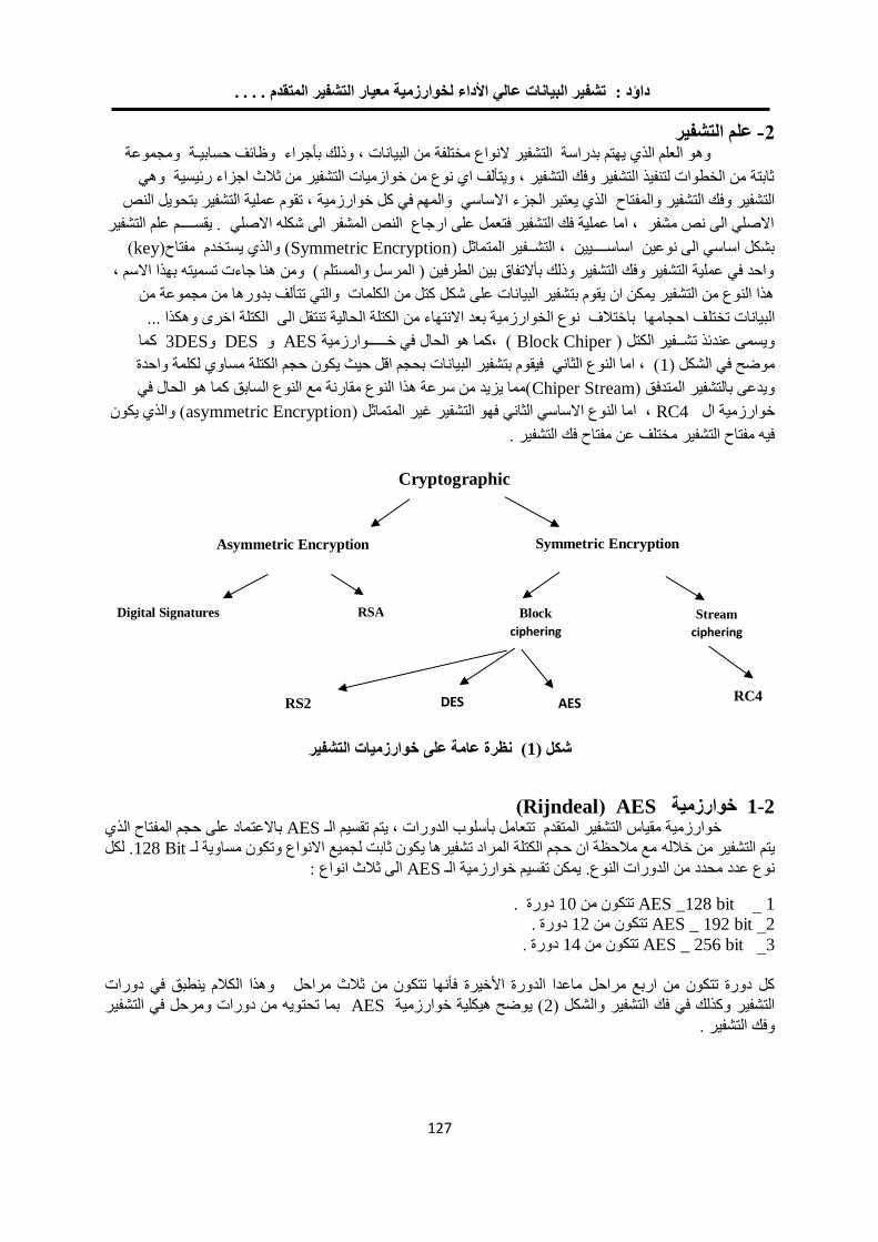
. . . . تشفير البيانات عالي األداء لخوارزمية معيار التشفير المتقدم : داؤد
521
علم التشفير -2وهو العلم الذي يهتم بدراسة التشفير النواع مختلفة من البيانات , وذلك بأجراء وظائف حسابيـة ومجموعة
ثابتة من الخطوات لتنفيذ التشفير وفك التشفير , ويتألف اي نوع من خوازميات التشفير من ثالث اجزاء رئيسية وهي
الساسي والمهم في كل خوارزمية , تقوم عملية التشفير بتحويل النص التشفير وفك التشفير والمفتاح الذي يعتبر الجزء ا
االصلي الى نص مشفر , اما عملية فك التشفير فتعمل على ارجاع النص المشفر الى شكله االصلي . يقســــم علم التشفير
( keyلذي يستخدم مفتاح)( واSymmetric Encryptionبشكل اساسي الى نوعين اساســــيين , التشــفير المتماثل )
واحد في عملية التشفير وفك التشفير وذلك بأالتفاق بين الطرفين ) المرسل والمستلم ( ومن هنا جاءت تسميته بهذا االسم ,
هذا النوع من التشفير يمكن ان يقوم بتشفير البيانات على شكل كتل من الكلمات والتي تتألف بدورها من مجموعة من
ف احجامها باختالف نوع الخوارزمية بعد االنتهاء من الكتلة الحالية تنتقل الى الكتلة اخرى وهكذا ... البيانات تختل
كما 3DES وDES و AES ( ,كما هو الحال في خـــــوارزمية Block Chiperويسمى عندئذ تشــفير الكتل )
ات بحجم اقل حيث يكون حجم الكتلة مساوي لكلمة واحدة ( , اما النوع الثاني فيقوم بتشفير البيان1موضح في الشكل )
(مما يزيد من سرعة هذا النوع مقارنة مع النوع السابق كما هو الحال في Chiper Streamويدعى بالتشفير المتدفق )
كون ( والذي يasymmetric Encryption, اما النوع االساسي الثاني فهو التشفير غير المتماثل ) RC4خوارزمية ال
فيه مفتاح التشفير مختلف عن مفتاح فك التشفير .
خوارزميات التشفير نظرة عامة على( 1شكل )
AES (Rijndeal) خوارزمية 1-2باالعتماد على حجم المفتاح الذي AES ـتقسيم ال يتمخوارزمية مقياس التشفير المتقدم تتعامل بأسلوب الدورات ,
. لكل Bit 128يع االنواع وتكون مساوية لـ ممع مالحظة ان حجم الكتلة المراد تشفيرها يكون ثابت لج خاللهيتم التشفير من
الى ثالث انواع : AESـيمكن تقسيم خوارزمية ال نوع عدد محدد من الدورات النوع.
1 _AES _128 bit دورة . 10تتكون من
2 _AES _ 192 bit دورة . 12تتكون من
3 _AES _ 256 bit دورة . 14تتكون من
فأنها تتكون من ثالث مراحل وهذا الكالم ينطبق في دورات األخيرةكل دورة تتكون من اربع مراحل ماعدا الدورة
بما تحتويه من دورات ومرحل في التشفير AES( يوضح هيكلية خوارزمية 2التشفير وكذلك في فك التشفير والشكل )
وفك التشفير .
Asymmetric Encryption Symmetric Encryption
RS2 DES AES RC4
Block
ciphering
Stream
ciphering
Digital Signatures RSA
Cryptographic
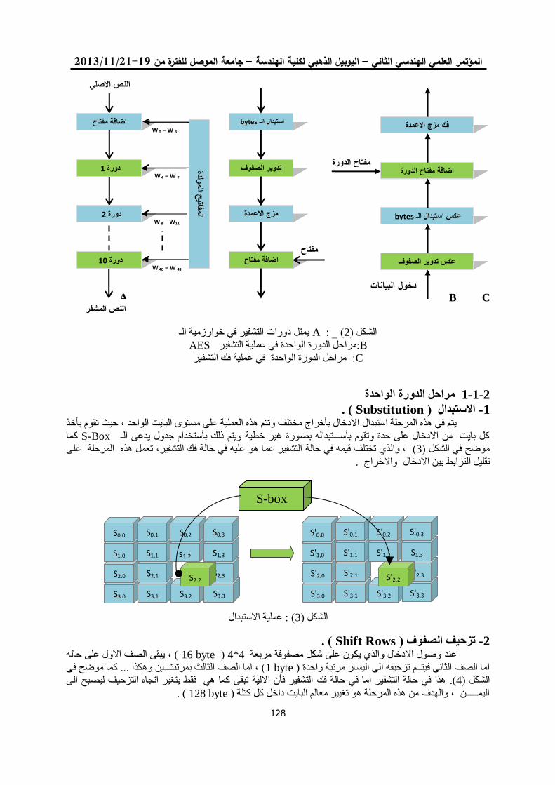
19/99/1192-91جامعة الموصل للفترة من –اليوبيل الذهبي لكلية الهندسة –المؤتمر العلمي الهندسي الثاني
521
B C A
يمثل دورات التشفير في خوارزمية الـ : A( _ 2الشكل )
B مراحل الدورة الواحدة في عملية التشفير:AES
Cمراحل الدورة الواحدة في عملية فك التشفير :
مراحل الدورة الواحدة 1-2-1
. (Substitution االستبدال ) -1يتم في هذه المرحلة استبدال االدخال بأخراج مختلف وتتم هذه العملية على مستوى البايت الواحد , حيث تقوم بأخذ
كما S-Boxكل بايت من االدخال على حدة وتقوم بأســـتبداله بصورة غير خطية ويتم ذلك بأستخدام جدول يدعى الـ
التشفير عما هو عليه في حالة فك التشفير, تعمل هذه المرحلة على , والذي تختلف قيمه في حالة (3موضح في الشكل )
واالخراج . تقليل الترابط بين االدخال
( : عملية االستبدال3الشكل )
( . Shift Rowsتزحيف الصفوف ) -2( , يبقى الصف االول على حاله byte 16 ) 4*4عند وصول االدخال والذي يكون على شكل مصفوفة مربعة
كما موضح في ( , اما الصف الثالث بمرتبتـــين وهكذا ... byte 1اما الصف الثاني فيتــم تزحيفه الى اليسار مرتبة واحدة )
التشفير فأن االلية تبقى كما هي فقط يتغير اتجاه التزحيف ليصبح الى هذا في حالة التشفير اما في حالة فك (. 4الشكل )
( . byte 128اليمـــــن , والهدف من هذه المرحلة هو تغيير معالم البايت داخل كل كتلة )
bytes استبدال الـ
مزج االعمدة
تدوير الصفوف
مفتاح
اضافة مفتاح الدورة
الدورة
المشفرالنص
االصليالنص
W 4 – W 7
W 8 – W11
W 40 – W 43
W 0 – W 3
ح المولدةالمفاتي
اضافة مفتاح
الدورة
2 دورة
10 دورة
1 دورة مفتاح الدورة
فك مزج االعمدة
bytes عكس استبدال الـ
عكس تدوير الصفوف
اضافة مفتاح الدورة
دخول البيانات
S'3,0 S'3,1 S'3,2 S'3,3
S'2,0 S'2,1 S'2,3
S'1,0 S'1,1 S'1,2 S1,3
S'0,0 S'0,1 S'0,2 S'0,3
S'2,2
S3,0 S3,1 S3,2 S3,3
S2,0 S2,1 S2,3
S1,0 S1,1 s1,2 S1,3
S0,0 S0,1 S0,2 S0,3
S2,2
S-box
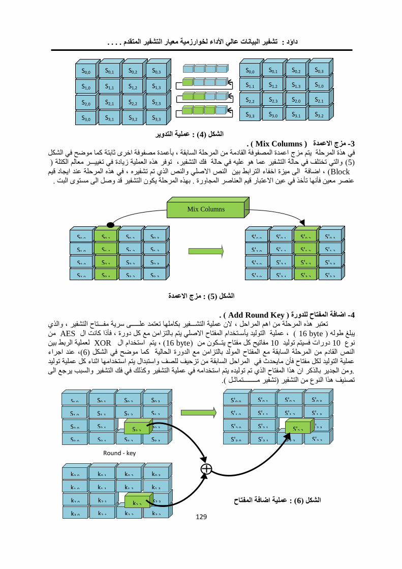
. . . . تشفير البيانات عالي األداء لخوارزمية معيار التشفير المتقدم : داؤد
521
( : عملية التدوير4الشكل )
( . ( Mix Columnsمزج االعمدة -3
كما موضح في الشكل اعمدة المصفوفة القادمة من المرحلة السابقة , بأعمدة مصفوفة اخرى ثابتة في هذة المرحلة يتم مزج
والتي تختلف في حالة التشفير عما هو عليه في حالة فك التشفير, توفر هذه العملية زيادة في تغييـــر معالم الكتلة ) (5)
Block الصلي والنص الذي تم تشفيره , في هذه المرحلة عند ايجاد قيم ( , اضافة الى ميزة اخفاء الترابط بين النص ا
عنصر معين فأنها تأخذ في عين االعتبار قيم العناصر المجاورة . بهذه المرحلة يكون التشفير قد وصل الى مستوى البت .
( : مزج االعمدة5الشكل )
( . Add Round Key اضافة المفتاح للدورة ) -4
الن عملية التشـــفير بكاملها تعتمد علـــــى سرية مفـــتاح التشفير , والذي تعتبر هذه المرحلة من اهم المراحل ,
من AES( , عملية التوليد يأسـتخدام المفتاح االصلي يتم بالتزامن مع كل دورة , فأذا كانت ال byte 16يبلغ طوله )
لعملية الربط بين XOR ( , يتم استخدام ال byte 16مفاتيح كل مفتاح يتــكون من ) 10دورات فسيتم توليد 10نوع
, عند اجراء (6كما موضح في الشكل ) النص القادم من المرحلة السابقة مع المفتاح المولد بالتزامن مع الدورة الحالية
ملية توليد عملية التوليد لكل مفتاح فأن مايحدث في المراحل السابقة من تزحيف للصف واستبدال يتم استخدامها اثناء كل ع
.ومن الجدير بالذكر ان هذا المفتاح الذي تم توليده يتم استخدامه في عملية التشفير وكذلك في فك التشفير والسبب يرجع الى
تصنيف هذا النوع من التشفير )تشفير مــــــــتماثـل (.
S3,0 S3,1 S3,2 S3,3
S2,0 S2,1 S2,2 S2,3
S1,0 S1,1 S1,2 S1,3
S0,0 S0,1 S0,2 S0,3
S3,3 S3,0 S3,1 S3,2
S2,2 S2,3 S2,0 S2,1
S1,1 S1,2 S1,3 S1,0
S0,0 S0,1 S0,2 S0,3
Mix Columns
S3,0 S3,1 S3,2 S3,3
S2,0 S2,1 S2,2 S2,3
S1,0 S1,1 S1,2 S1,3
S0,0 S0,1 S0,2 S0,3
S'3,0 S'3,1 S'3,2 S'3,3
S'2,0 S'2,1 S'2,2 S'2,3
S'1,0 S'1,1 S'1,2 S'1,3
S'0,0 S'0,1 S'0,2 S'0,3
Round - key
S'3,0 S'3,1 S'3,2 S'3,3
S'2,0 S'2,1 S'2,3
S'1,0 S'1,1 S'1,2 S'1,3
S'0,0 S'0,1 S'0,2 S'0,3
S'2,2
S3,0 S3,1 S3,2 S3,3
S2,0 S2,1 S2,3
S1,0 S1,1 S1,2 S1,3
S0,0 S0,1 S0,2 S0,3
S2,2
k3,0 k3,1 k3,2 k3,3
k2,0 k2,1 k2,3
k1,0 k1,1 k1,2 k1,3
k0,0 k0,1 k0,2 k0,3
k2,2 ( عملية اضافة المفتاح6الشكل : )
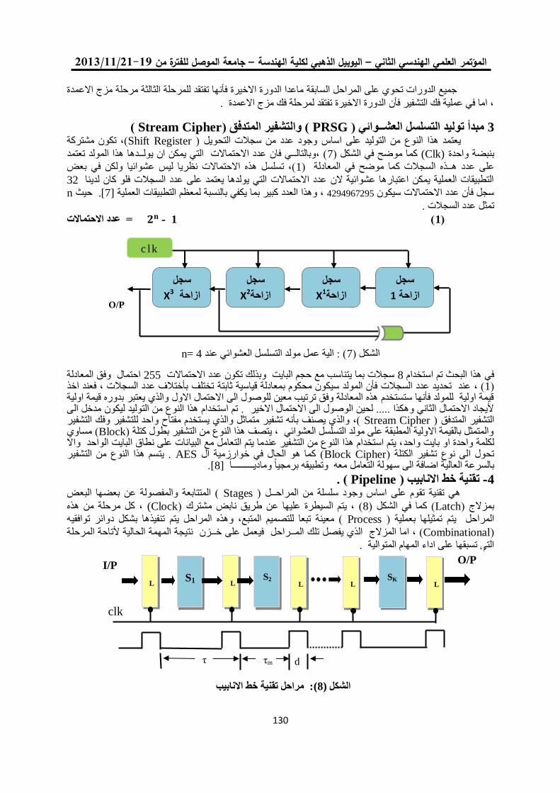
19/99/1192-91جامعة الموصل للفترة من –اليوبيل الذهبي لكلية الهندسة –المؤتمر العلمي الهندسي الثاني
531
جميع الدورات تحوي على المراحل السابقة ماعدا الدورة االخيرة فأنها تفتقد للمرحلة الثالثة مرحلة مزج االعمدة
, اما في عملية فك التشفير فأن الدورة االخيرة تفتقد لمرحلة فك مزج االعمدة .
(Stream Cipher ( والتشفير المتدفق ) PRSGمبدأ توليد التسلسل العشــوائي ) 3(, تكون مشتركة Shift Registerيعتمد هذا النوع من التوليد على اساس وجود عدد من سجالت التحويل )
( ,وبالتالــي فان عدد االحتماالت التي يمكن ان يولــدها هذا المولد تعتمد 7كما موضح في الشكل )(Clk) بنبضة واحدة
(, تسلسل هذه االحتماالت نظريا ليس عشوائيا ولكن في بعض 1المعادلة )على عدد هــذه السجالت كما موضح في
32التطبيقات العملية يمكن اعتبارها عشوائية الن عدد االحتماالت التي يولدها يعتمد على عدد السجالت فلو كان لدينا
nحيث .[7]ظم التطبيقات العملية , وهذا العدد كبير بما يكفي بالنسبة لمع 4294967295سجل فأن عدد االحتماالت سيكون
عدد السجالت . تمثل
= عدد االحتماالت - 1( 1)
n= 4( : الية عمل مولد التسلسل العشوائي عند 7الشكل )
احتمال وفق المعادلة 255سجالت بما يتناسب مع حجم البايت وبذلك تكون عدد االحتماالت 8في هذا البحث تم استخدام تختلف بأختالف عدد السجالت , فعند اخذ فأن المولد سيكون محكوم بمعادلة قياسية ثابتة ( , عند تحديد عدد السجالت 1)
قيمة اولية للمولد فأنها ستستخدم هذه المعادلة وفق ترتيب معين للوصول الى االحتمال االول والذي يعتبر بدوره قيمة اولية يكون مدخل الى أليجاد االحتمال الثاني وهكذا ..... لحين الوصول الى االحتمال االخير . تم استخدام هذا النوع من التوليد ل
(, والذي يصنف بأنه تشفير متماثل والذي يستخدم مفتاح واحد للتشفير وفك التشفير Stream Cipher التشفير المتدفق )( مساوي Blockوالمتمثل بالقيمة االولية المطبقة على مولد التسلسل العشوائي , يتصف هذا النوع من التشفير بطول كتلة )
, يتم استخدام هذا النوع من التشفير عندما يتم التعامل مع البيانات على نطاق البايت الواحد واال حدلكلمة واحدة او بايت وا. يتسم هذا النوع من التشفير AES( كما هو الحال في خوارزمية ال Block Cipherتحول الى نوع تشفير الكتلة )
. [8] بالسرعة العالية اضافة الى سهولة التعامل معه وتطبيقه برمجيا وماديـــــــــا ( . Pipelineتقنية خط االنابيب ) -4
( المتتابعة والمفصولة عن بعضها البعض Stagesاساس وجود سلسلة من المراحــل ) هي تقنية تقوم على
, كل مرحلة من هذه Clock)( , يتم السيطرة عليها عن طريق نابض مشترك )8( كما في الشكل )Latch) بمزالج
تنفيذها بشكل دوائر توافقيه , وهذه المراحل يتم( معينة تبعا للتصميم المتبع Process المراحل يتم تمثيلها بعملية )
(Combinational اما , )عمل على خــزن نتيجة المهمة الحالية ألتاحة المرحلة المزالج الذي يفصل تلك المــراحل في
التي تسبقها على اداء المهام المتوالية .
c lk
سجل
X3ازاحة
سجل
X2ازاحة
سجل
X1ازاحة
سجل
1ازاحة O/P
clk
d
O/P I/P
S1
L
L
S2
L
L
SK
L
τm τ
الشكل (8): مراحل تقنية خط االنابيب
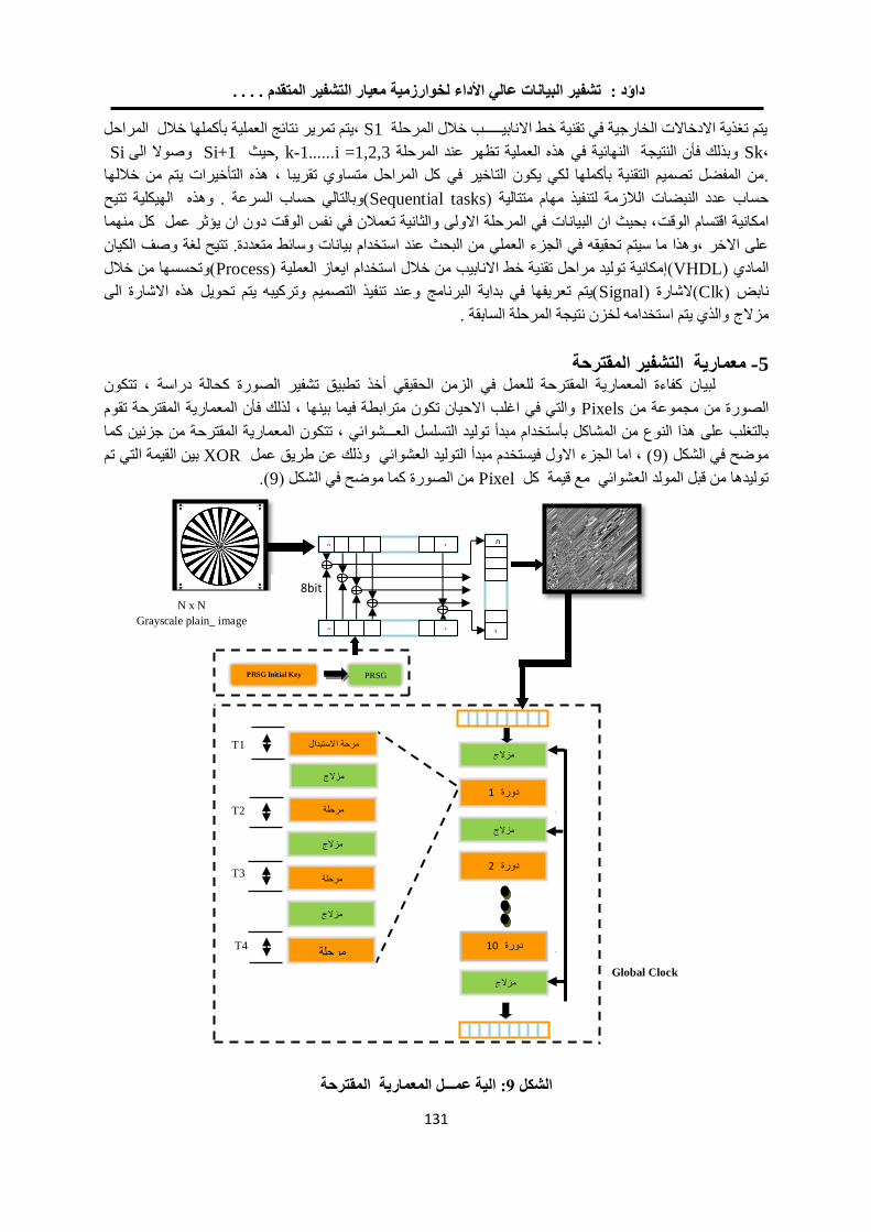
. . . . تشفير البيانات عالي األداء لخوارزمية معيار التشفير المتقدم : داؤد
535
Global Clock
ذ
T4
T3
T2
T1
8bit
0 1
0 1
1
0
N x N
Grayscale plain_ image
PRSG PRSG Initial Key
1دورة
مزالج
مزالج
2دورة
10دورة
مزالج
مزالج
االستبدال ةمرح
مرحلة
مرحلة
مزالج
مزالج
مرحلة
بأكملها خالل المراحل,يتم تمرير نتائج العملية S1 يتم تغذية االدخاالت الخارجية في تقنية خط االنابيـــــب خالل المرحلة
,Sk وبذلك فأن النتيجة النهائية في هذه العملية تظهر عند المرحلةi =1,2,3......, k-1 حيث Si+1 وصوال الى Si
كل المراحل متساوي تقريبا , هذه التأخيرات يتم من خاللها من المفضل تصميم التقنية بأكملها لكي يكون التاخير في .
يكلية تتيح (وبالتالي حساب السرعة . وهذه الهSequential tasksحساب عدد النبضات الالزمة لتنفيذ مهام متتالية )
ثر عمل كل منهما , بحيث ان البيانات في المرحلة االولى والثانية تعمالن في نفس الوقت دون ان يؤامكانية اقتسام الوقت
تتيح لغة وصف الكيان على االخر ,وهذا ما سيتم تحقيقه في الجزء العملي من البحث عند استخدام بيانات وسائط متعددة.
(وتحسسها من خالل Processإمكانية توليد مراحل تقنية خط االنابيب من خالل استخدام ايعاز العملية )(VHDL)المادي
(يتم تعريفها في بداية البرنامج وعند تنفيذ التصميم وتركيبه يتم تحويل هذه االشارة الى Signal)(الشارة Clkنابض )
. والذي يتم استخدامه لخزن نتيجة المرحلة السابقة مزالج
معمارية التشفير المقترحة -5تتكون لبيان كفاءة المعمارية المقترحة للعمل في الزمن الحقيقي أخذ تطبيق تشفير الصورة كحالة دراسة ,
والتي في اغلب االحيان تكون مترابطة فيما بينها , لذلك فأن المعمارية المقترحة تقوم Pixels جموعة منالصورة من م
د التسلسل العـــشوائي , تتكون المعمارية المقترحة من جزئين كما بالتغلب على هذا النوع من المشاكل بأستخدام مبدأ تولي
قيمة التي تم بين ال XOR( , اما الجزء االول فيستخدم مبدأ التوليد العشوائي وذلك عن طريق عمل 9موضح في الشكل )
(. 9من الصورة كما موضح في الشكل ) Pixelتوليدها من قبل المولد العشوائي مع قيمة كل
لية عمـــل المعمارية المقترحة ا: 9الشكل
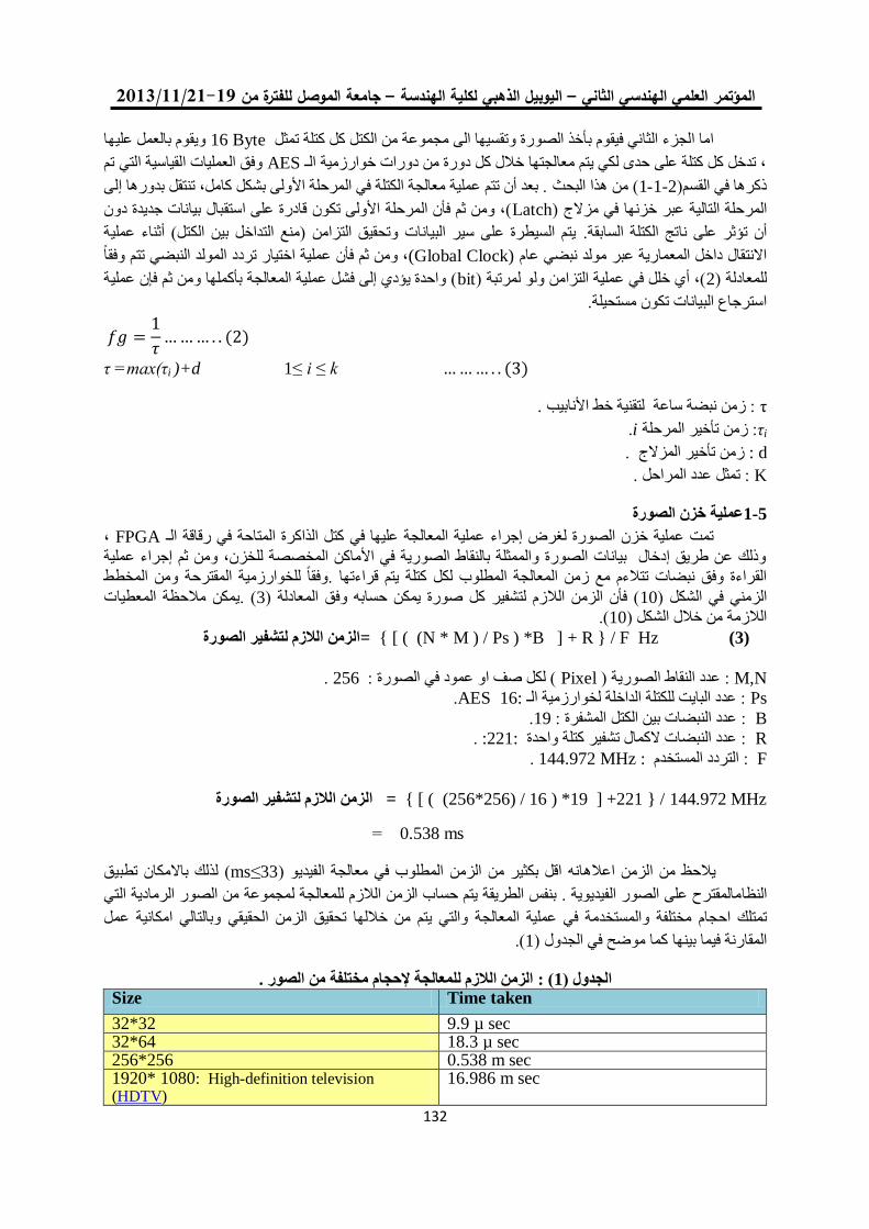
19/99/1192-91جامعة الموصل للفترة من –اليوبيل الذهبي لكلية الهندسة –المؤتمر العلمي الهندسي الثاني
532
ويقوم بالعمل عليها Byte 16اما الجزء الثاني فيقوم بأخذ الصورة وتقسيها الى مجموعة من الكتل كل كتلة تمثل
وفق العمليات القياسية التي تم AES, تدخل كل كتلة على حدى لكي يتم معالجتها خالل كل دورة من دورات خوارزمية الـ
. بعد أن تتم عملية معالجة الكتلة في المرحلة األولى بشكل كامل, تنتقل بدورها إلى ( من هذا البحث 1-2-1ذكرها في القسم)
(, ومن ثم فأن المرحلة األولى تكون قادرة على استقبال بيانات جديدة دون Latchية عبر خزنها في مزالج )المرحلة التال
يتم السيطرة على سير البيانات وتحقيق التزامن )منع التداخل بين الكتل( أثناء عملية . أن تؤثر على ناتج الكتلة السابقة
, ومن ثم فأن عملية اختيار تردد المولد النبضي تتم وفقا (Global Clock)االنتقال داخل المعمارية عبر مولد نبضي عام
( واحدة يؤدي إلى فشل عملية المعالجة بأكملها ومن ثم فإن عملية bit(, أي خلل في عملية التزامن ولو لمرتبة )2للمعادلة )
استرجاع البيانات تكون مستحيلة.
τ =max(τi )+d 1≤ i ≤ k
τ . زمن نبضة ساعة لتقنية خط األنابيب :
τi زمن تأخير المرحلة :i.
: d. زمن تأخير المزالج
K . تمثل عدد المراحل :
عملية خزن الصورة 1-5
, FPGAتمت عملية خزن الصورة لغرض إجراء عملية المعالجة عليها في كتل الذاكرة المتاحة في رقاقة الـ
وذلك عن طريق إدخال بيانات الصورة والممثلة بالنقاط الصورية في األماكن المخصصة للخزن, ومن ثم إجراء عملية
وفقا للخوارزمية المقترحة ومن المخطط ة يتم قراءتها .القراءة وفق نبضات تتالءم مع زمن المعالجة المطلوب لكل كتل
يمكن مالحظة المعطيات .( 3المعادلة ) وفق( فأن الزمن الالزم لتشفير كل صورة يمكن حسابه 10الزمني في الشكل )
(.10الالزمة من خالل الشكل )
= { [ ( (N * M ) / Ps ) *B ] + R } / F Hz (3) الزمن الالزم لتشفير الصورة
M,N ( عدد النقاط الصورية : Pixel : لكل صف او عمود في الصورة ) 256.
Ps عدد البايت للكتلة الداخلة لخوارزمية الـ :AES 16: .
B : 19: عدد النبضات بين الكتل المشفرة .
R 221:: عدد النبضات الكمال تشفير كتلة واحدة: .
F : 144.972التردد المستخدم MHz : .
= { [ ( (256*256) / 16 ) *19 ] +221 } / 144.972 MHzالزمن الالزم لتشفير الصورة
= 0.538 ms
لذلك باالمكان تطبيق (ms≤33)انه اقل بكثير من الزمن المطلوب في معالجة الفيديو يالحظ من الزمن اعاله
التي الرمادية مجموعة من الصور لالالزم للمعالجة اب الزمن سح يتمبنفس الطريقة المقترح على الصور الفيديوية . النظام
وبالتالي امكانية عمل الزمن الحقيقي والتي يتم من خاللها تحقيق الجةالمستخدمة في عملية المعومختلفة احجام تمتلك
(. 1كما موضح في الجدول ) المقارنة فيما بينها
مختلفة من الصور . إلحجامالزمن الالزم للمعالجة ( : 1الجدول )Time taken Size
9.9 µ sec 32*32 18.3 µ sec 32*64 0.538 m sec 256*256 16.986 m sec 1920* 1080: High-definition television
)HDTV(
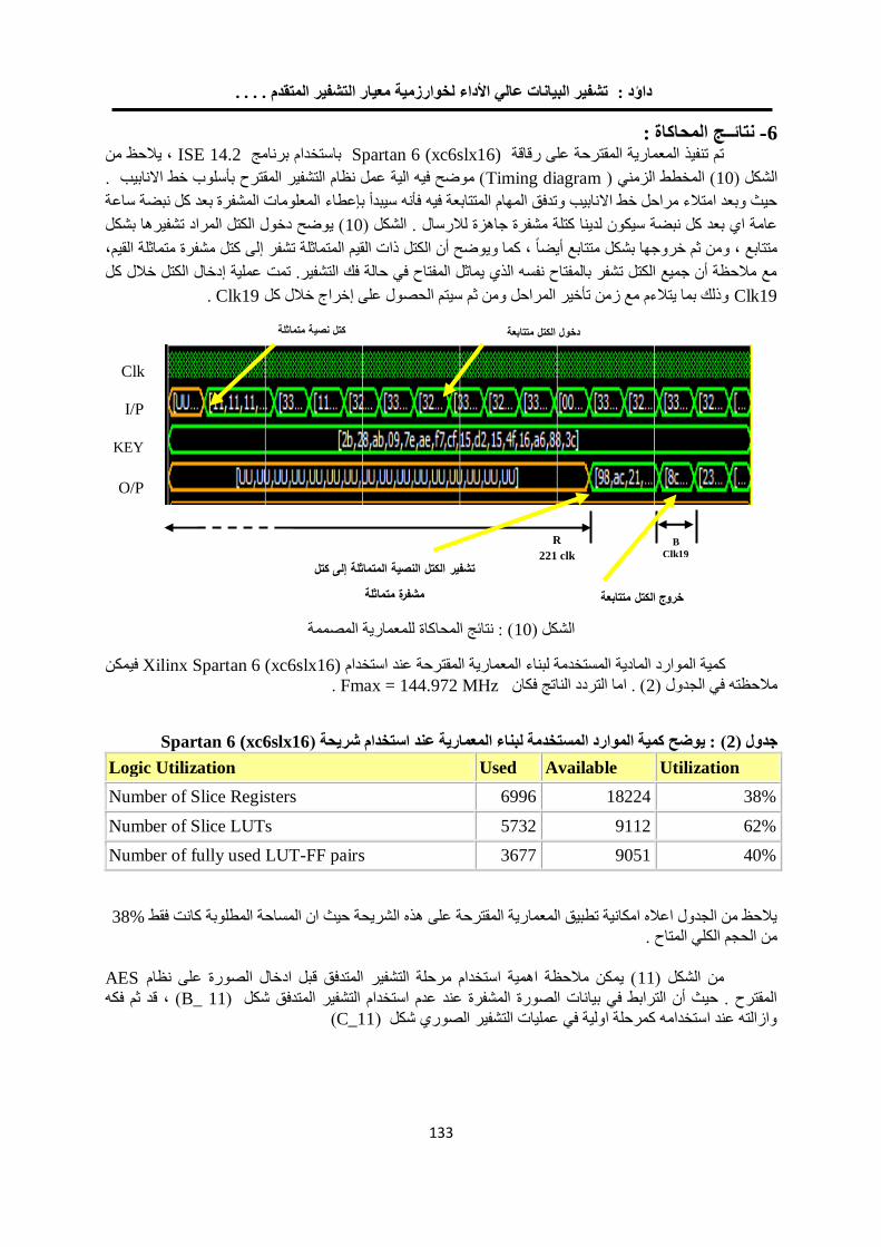
. . . . تشفير البيانات عالي األداء لخوارزمية معيار التشفير المتقدم : داؤد
533
نتائــج المحاكاة : -6, يالحظ من ISE 14.2برنامج باستخدام Spartan 6 (xc6slx16) تم تنفيذ المعمارية المقترحة على رقاقة
( موضح فيه الية عمل نظام التشفير المقترح بأسلوب خط االنابيب . Timing diagram( المخطط الزمني )10الشكل )
المعلومات المشفرة بعد كل نبضة ساعة بإعطاءحيث وبعد امتالء مراحل خط االنابيب وتدفق المهام المتتابعة فيه فأنه سيبدأ
( يوضح دخول الكتل المراد تشفيرها بشكل 10) الشكلعامة اي بعد كل نبضة سيكون لدينا كتلة مشفرة جاهزة لالرسال .
متتابع , ومن ثم خروجها بشكل متتابع أيضا , كما ويوضح أن الكتل ذات القيم المتماثلة تشفر إلى كتل مشفرة متماثلة القيم,
الكتل خالل كل مع مالحظة أن جميع الكتل تشفر بالمفتاح نفسه الذي يماثل المفتاح في حالة فك التشفير. تمت عملية إدخال
Clk19 وذلك بما يتالءم مع زمن تأخير المراحل ومن ثم سيتم الحصول على إخراج خالل كلClk19 .
( : نتائج المحاكاة للمعمارية المصممة 10)الشكل
فيمكن Xilinx Spartan 6 (xc6slx16)عند استخدام المقترحة معماريةال لبناء المستخدمة المادية الموارد كمية
. Fmax = 144.972 MHz( . اما التردد الناتج فكان 2الجدول ) فيمالحظته
Spartan 6 (xc6slx16: يوضح كمية الموارد المستخدمة لبناء المعمارية عند استخدام شريحة )( 2جدول )
Logic Utilization Used Available Utilization
Number of Slice Registers 6996 18224 38%
Number of Slice LUTs 5732 9112 62%
Number of fully used LUT-FF pairs 3677 9051 40%
%38ة المطلوبة كانت فقط حيالحظ من الجدول اعاله امكانية تطبيق المعمارية المقترحة على هذه الشريحة حيث ان المسا
من الحجم الكلي المتاح .
AES( يمكن مالحظة اهمية استخدام مرحلة التشفير المتدفق قبل ادخال الصورة على نظام 11من الشكل )
( , قد ثم فكه B_ 11المقترح . حيث أن الترابط في بيانات الصورة المشفرة عند عدم استخدام التشفير المتدفق شكل )
(C_11وازالته عند استخدامه كمرحلة اولية في عمليات التشفير الصوري شكل )
كتل نصية متماثلة دخول الكتل متتابعة
خروج الكتل متتابعة
كتل إلىتشفير الكتل النصية المتماثلة مشفرة متماثلة
Clk
I/P
KEY
O/P
R
221 clk
B
Clk19
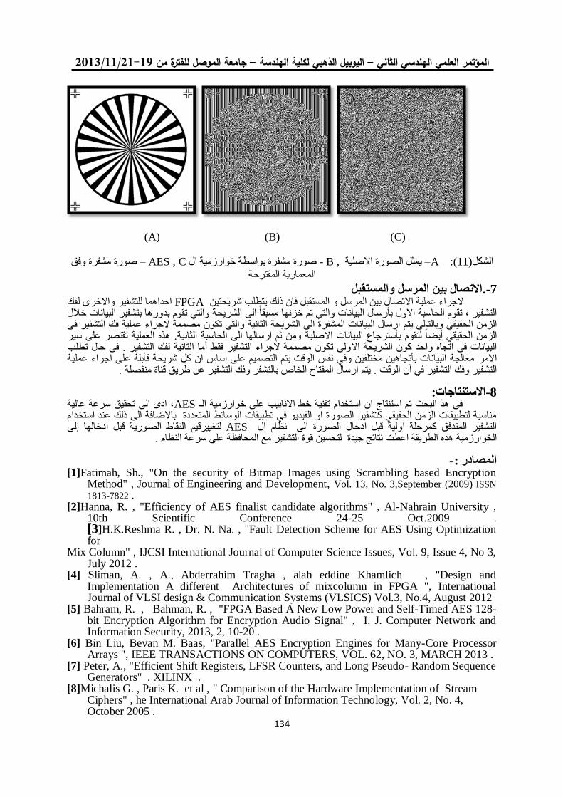
19/99/1192-91جامعة الموصل للفترة من –اليوبيل الذهبي لكلية الهندسة –المؤتمر العلمي الهندسي الثاني
531
(A) (B) (C)
صورة مشفرة وفق – AES , Cصورة مشفرة بواسطة خوارزمية ال , B - يمثل الصورة االصلية – A: (11)الشكل
المعمارية المقترحة
االتصال بين المرسل والمستقبل 7-.احداهما للتشفير واالخرى لفك FPGAالجراء عملية االتصال بين المرسل و المستقبل فان ذلك يتطلب شريحتين
التشفير , تقوم الحاسبة االول بأرسال البيانات والتي تم خزنها مسبقأ الى الشريحة والتي تقوم بدورها بتشفير البيانات خالل في مصممة الجراء عملية فك التشفير قيقي وبالتالي يتم ارسال البيانات المشفرة الى الشريحة الثانية والتي تكونالزمن الح
. هذه العملية تقتصر على سير ومن ثم ارسالها الى الحاسبة الثانية االصلية بياناتال بأسترجاع الزمن الحقيقي أيضا لتقوم لفك التشفير . في حال تطلب ولى تكون مصممة الجراء التشفير فقط أما الثانية البيانات في اتجاه واحد كون الشريحة اال
معالجة البيانات بأتجاهين مختلفين وفي نفس الوقت يتم التصميم على اساس ان كل شريحة قأبلة على اجراء عملية االمر . قناة منفصلة عن طريقيتم ارسال المفتاح الخاص بالتشفر وفك التشفير .الوقت آنالتشفير وفك التشفير في
االستنتاجات:8-
, ادى الى تحقيق سرعة عالية AESـفي هذ البحث تم استنتاج ان استخدام تقنية خط االنابيب على خوارزمية المناسبة لتطبيقات الزمن الحقيقي كتشفير الصورة او الفيديو في تطبيقات الوسائط المتعددة باالضافة الى ذلك عند استخدام
إلى ادخالها النقاط الصورية قبل لتغييرقيم AES التشفير المتدفق كمرحلة اولية قبل ادخال الصورة الى نظام ال . فير مع المحافظة على سرعة النظامهذه الطريقة اعطت نتائج جيدة لتحسين قوة التش الخوارزمية
-المصادر :
[1]Fatimah, Sh., "On the security of Bitmap Images using Scrambling based Encryption Method" , Journal of Engineering and Development, Vol. 13, No. 3,September (2009) ISSN
1813-7822 . [2]Hanna, R. , "Efficiency of AES finalist candidate algorithms" , Al-Nahrain University ,
10th Scientific Conference 24-25 Oct.2009 . [3]H.K.Reshma R. , Dr. N. Na. , "Fault Detection Scheme for AES Using Optimization for
Mix Column" , IJCSI International Journal of Computer Science Issues, Vol. 9, Issue 4, No 3, July 2012 .
[4] Sliman, A. , A., Abderrahim Tragha , alah eddine Khamlich , "Design and Implementation A different Architectures of mixcolumn in FPGA ", International Journal of VLSI design & Communication Systems (VLSICS) Vol.3, No.4, August 2012
[5] Bahram, R. , Bahman, R. , "FPGA Based A New Low Power and Self-Timed AES 128-bit Encryption Algorithm for Encryption Audio Signal" , I. J. Computer Network and Information Security, 2013, 2, 10-20 .
[6] Bin Liu, Bevan M. Baas, "Parallel AES Encryption Engines for Many-Core Processor Arrays ", IEEE TRANSACTIONS ON COMPUTERS, VOL. 62, NO. 3, MARCH 2013 .
[7] Peter, A., "Efficient Shift Registers, LFSR Counters, and Long Pseudo- Random Sequence Generators" , XILINX .
[8]Michalis G. , Paris K. et al , " Comparison of the Hardware Implementation of Stream Ciphers" , he International Arab Journal of Information Technology, Vol. 2, No. 4, October 2005 .
Abdul-Jabbar: Design and Implementation of A Novel FPGA-Based …..
531
Design and Implementation of A Novel FPGA-Based Pipelined-
Parallel Processor Architecture for Shortest Path Search
Abstract In this paper, a pipelined-parallel hardware architecture to compute the shortest
paths of OSPF networks is proposed based on parallel shortest path searching
algorithm. OSPF protocol uses the software version of the sequential Dijkstra
algorithm for computing and constructing the routing table for each router in an
autonomous system area. The proposed Pipelined-Parallel Shortest Path Searching
(PPSPS) processor overcomes the time delay of executing the sequential Dijkstra
algorithm by conventional processors by reducing the execution time from to
, where is the number of nodes. The design is targeted to Xilinx Virtex 7
FPGA chip, and in order to make the parallel processor capable to handle an OSPF
area with 256 nodes, a pipelining feature is adopted and successfully implemented
within chip resources availability. Very large speed up factors (approximately within
the range of 20 – 280) have been achieved by the proposed ultra-high performance
PPSPS processor when compared with the conventional software Dijkstra algorithm.
Keywords:- Pipelined-Parallel Hardware Architecture, OSPF Networks, Dijkstra
Algorithm, Pipelined-Parallel Shortest Path Searching (PPSPS) Processor, FPGA,
Speed Up Factor.
هيكلية معالج البحث عن المسار األقصر ل FPGAرقاقة التصميم والتنفيذ باعتماد
المتوازي -نوع خط األنابيب
الخالصة
الخالصة:
OSPF شبكات مسارات أقصر لحساب وازيةالمت خطوط األنابيبب معمارية مادية، تم إقتراح في هذه البحث
من الخوارزمية صدار البرميياإل OSPF بروتوكول يستخدم أقصر مسار.عن للبحث بإعتماد خوارزمية متوازية
خطوط معالج البحث المقترح نوع . ذاتية التحكم في منطقة م و ج ه لكل جدول التوجيهبناء و لحساب متتابعةال جيكسترا
لياتالمعا في متتابعةال جيكسترا خوارزمية تنفيذ وقت تأخير يتغلب على( PPSPS) مسار قصرأل الموازياألنابيب
التصميم على وتم تنفيذ. تمثل عدد العقد حيث أن إلى من وقت تنفيذ عن طريق تقليل التقليدية
تم ، عقدة 256 بـ OSPF منطقة قادر على التعامل مع المعالج الموازي ليعل، وسعيا Xilinx Virtex 7 FPGAرقاقة
فائقال من خالل األداء. ورقاقةبال المتوفرة الموارد بإستخدام ونفذت بنياح سطة خطوط األنابيبالنقل بوا ميزة اعتماد
جدا )تقريبا ضمن كبيرة سريعت تحققت معامالت يكسترا التقليديةجمع خوارزمية بالمقارنة المقترح PPSPS للمعالج
.(280الى 20 المدى من
Jassim M. Abdul-Jabbar Computer Engineering
Department, College of
Engineering,
University of Mosul, Mosul, Iraq.
Majid A. Alwan Computer Engineering
Department, College of
Engineering,
University of Basra, Basra, Iraq. .comaltimimee@yahoo
اليبار عبد محمد جاسمد. كلية الهندسة -قسم هندسة الحاسوب
العراق -الموصل -الموصلجامعة
علوان النبي عبد ماجدد. كلية الهندسة -قسم هندسة الحاسبات
العراق -البصرة -جامعة البصرة
Mohammed A. Ali Al-Ebadi Computer Engineering
Department, College of
Engineering,
University of Basra, Basra, Iraq. o.commohammed.alebadi@yaho
العبادي جودة علي عبد محمد كلية الهندسة -قسم هندسة الحاسبات
العراق -البصرة -جامعة البصرة
o.commohammed.alebadi@yaho
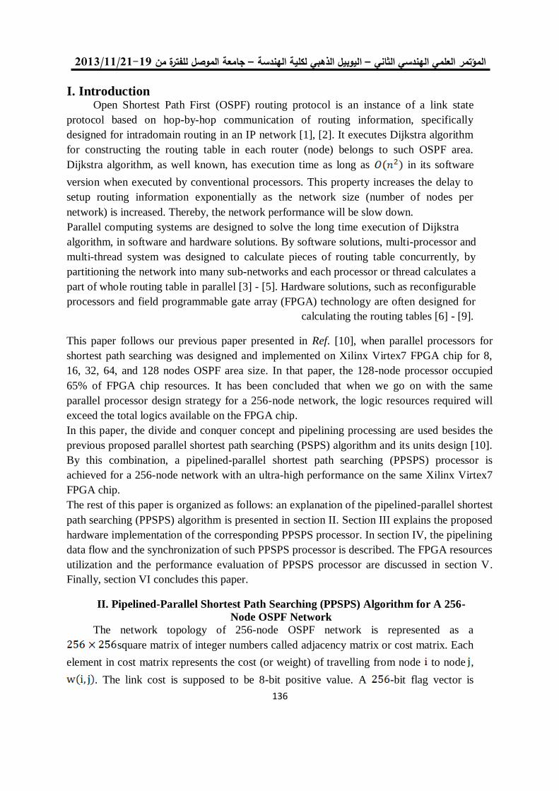
19/99/1192-91جامعة الموصل للفترة من –ليوبيل الذهبي لكلية الهندسة ا –العلمي الهندسي الثاني المؤتمر
531
I. Introduction Open Shortest Path First (OSPF) routing protocol is an instance of a link state
protocol based on hop-by-hop communication of routing information, specifically
designed for intradomain routing in an IP network [1], [2]. It executes Dijkstra algorithm
for constructing the routing table in each router (node) belongs to such OSPF area.
Dijkstra algorithm, as well known, has execution time as long as in its software
version when executed by conventional processors. This property increases the delay to
setup routing information exponentially as the network size (number of nodes per
network) is increased. Thereby, the network performance will be slow down.
Parallel computing systems are designed to solve the long time execution of Dijkstra
algorithm, in software and hardware solutions. By software solutions, multi-processor and
multi-thread system was designed to calculate pieces of routing table concurrently, by
partitioning the network into many sub-networks and each processor or thread calculates a
part of whole routing table in parallel [3] - [5]. Hardware solutions, such as reconfigurable
processors and field programmable gate array (FPGA) technology are often designed for
calculating the routing tables [6] - [9].
This paper follows our previous paper presented in Ref. [10], when parallel processors for
shortest path searching was designed and implemented on Xilinx Virtex7 FPGA chip for 8,
16, 32, 64, and 128 nodes OSPF area size. In that paper, the 128-node processor occupied
65% of FPGA chip resources. It has been concluded that when we go on with the same
parallel processor design strategy for a 256-node network, the logic resources required will
exceed the total logics available on the FPGA chip.
In this paper, the divide and conquer concept and pipelining processing are used besides the
previous proposed parallel shortest path searching (PSPS) algorithm and its units design [10].
By this combination, a pipelined-parallel shortest path searching (PPSPS) processor is
achieved for a 256-node network with an ultra-high performance on the same Xilinx Virtex7
FPGA chip.
The rest of this paper is organized as follows: an explanation of the pipelined-parallel shortest
path searching (PPSPS) algorithm is presented in section II. Section III explains the proposed
hardware implementation of the corresponding PPSPS processor. In section IV, the pipelining
data flow and the synchronization of such PPSPS processor is described. The FPGA resources
utilization and the performance evaluation of PPSPS processor are discussed in section V.
Finally, section VI concludes this paper.
II. Pipelined-Parallel Shortest Path Searching (PPSPS) Algorithm for A 256-
Node OSPF Network
The network topology of 256-node OSPF network is represented as a
square matrix of integer numbers called adjacency matrix or cost matrix. Each
element in cost matrix represents the cost (or weight) of travelling from node to node ,
. The link cost is supposed to be 8-bit positive value. A -bit flag vector is
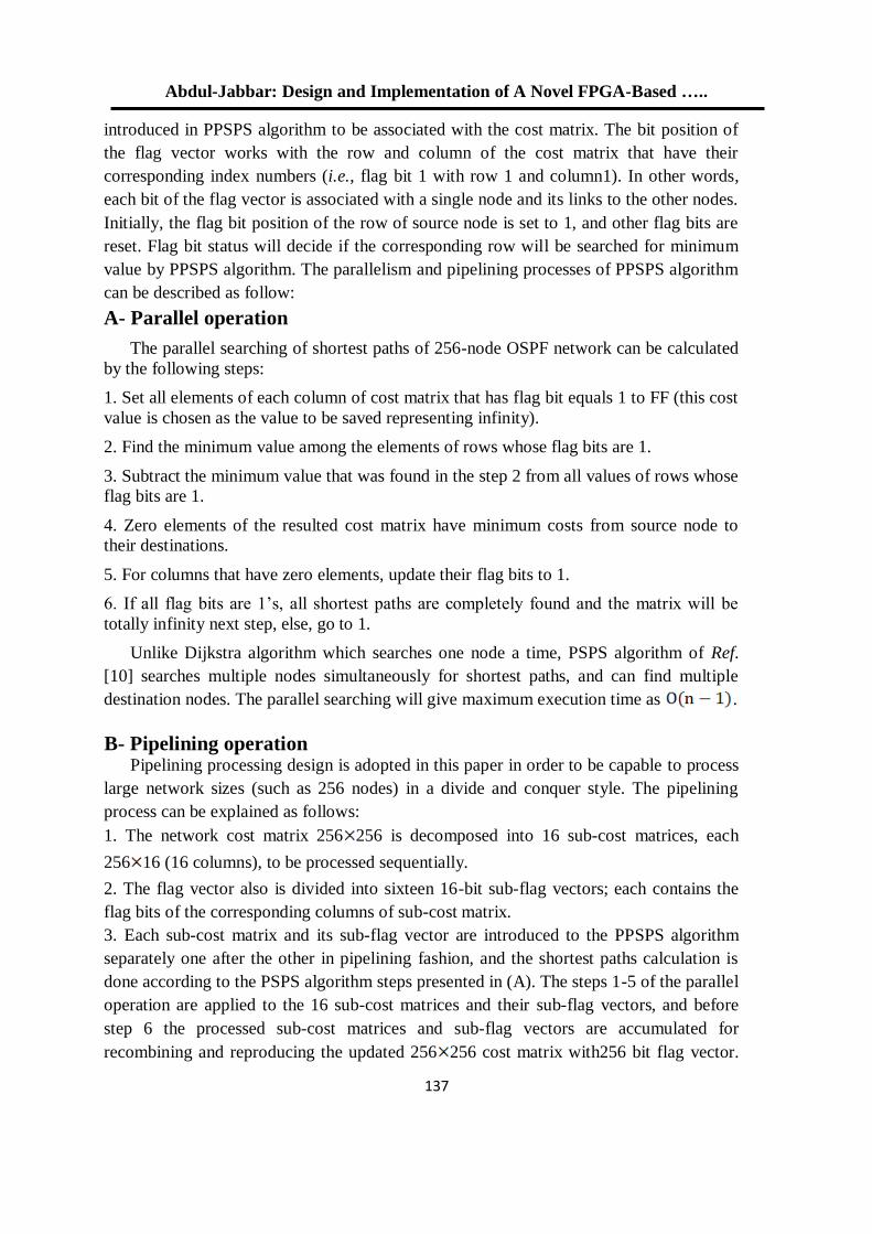
Abdul-Jabbar: Design and Implementation of A Novel FPGA-Based …..
531
introduced in PPSPS algorithm to be associated with the cost matrix. The bit position of
the flag vector works with the row and column of the cost matrix that have their
corresponding index numbers (i.e., flag bit 1 with row 1 and column1). In other words,
each bit of the flag vector is associated with a single node and its links to the other nodes.
Initially, the flag bit position of the row of source node is set to 1, and other flag bits are
reset. Flag bit status will decide if the corresponding row will be searched for minimum
value by PPSPS algorithm. The parallelism and pipelining processes of PPSPS algorithm
can be described as follow:
A- Parallel operation
The parallel searching of shortest paths of 256-node OSPF network can be calculated
by the following steps:
1. Set all elements of each column of cost matrix that has flag bit equals 1 to FF (this cost
value is chosen as the value to be saved representing infinity).
2. Find the minimum value among the elements of rows whose flag bits are 1.
3. Subtract the minimum value that was found in the step 2 from all values of rows whose
flag bits are 1.
4. Zero elements of the resulted cost matrix have minimum costs from source node to
their destinations.
5. For columns that have zero elements, update their flag bits to 1.
6. If all flag bits are 1’s, all shortest paths are completely found and the matrix will be
totally infinity next step, else, go to 1.
Unlike Dijkstra algorithm which searches one node a time, PSPS algorithm of Ref.
[10] searches multiple nodes simultaneously for shortest paths, and can find multiple
destination nodes. The parallel searching will give maximum execution time as .
B- Pipelining operation Pipelining processing design is adopted in this paper in order to be capable to process
large network sizes (such as 256 nodes) in a divide and conquer style. The pipelining
process can be explained as follows:
1. The network cost matrix 256 256 is decomposed into 16 sub-cost matrices, each
256 16 (16 columns), to be processed sequentially.
2. The flag vector also is divided into sixteen 16-bit sub-flag vectors; each contains the
flag bits of the corresponding columns of sub-cost matrix.
3. Each sub-cost matrix and its sub-flag vector are introduced to the PPSPS algorithm
separately one after the other in pipelining fashion, and the shortest paths calculation is
done according to the PSPS algorithm steps presented in (A). The steps 1-5 of the parallel
operation are applied to the 16 sub-cost matrices and their sub-flag vectors, and before
step 6 the processed sub-cost matrices and sub-flag vectors are accumulated for
recombining and reproducing the updated 256 256 cost matrix with256 bit flag vector.
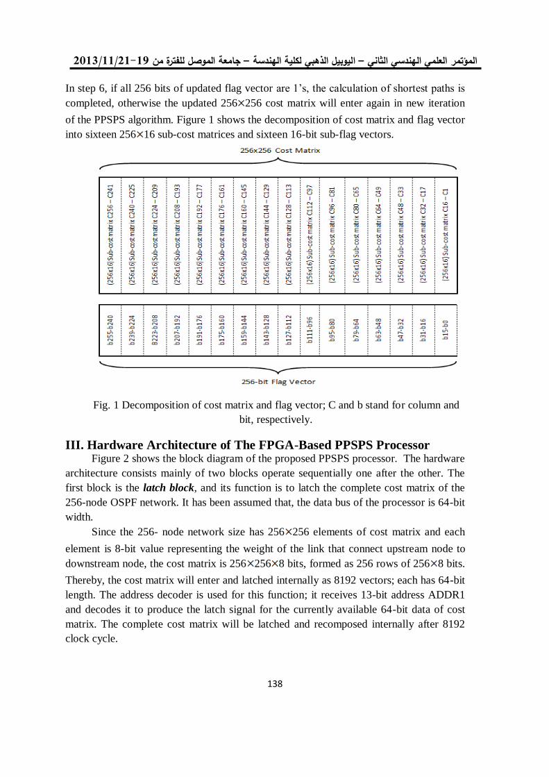
19/99/1192-91جامعة الموصل للفترة من –ليوبيل الذهبي لكلية الهندسة ا –العلمي الهندسي الثاني المؤتمر
531
In step 6, if all 256 bits of updated flag vector are 1’s, the calculation of shortest paths is
completed, otherwise the updated 256 256 cost matrix will enter again in new iteration
of the PPSPS algorithm. Figure 1 shows the decomposition of cost matrix and flag vector
into sixteen 256 16 sub-cost matrices and sixteen 16-bit sub-flag vectors.
Fig. 1 Decomposition of cost matrix and flag vector; C and b stand for column and
bit, respectively.
III. Hardware Architecture of The FPGA-Based PPSPS Processor Figure 2 shows the block diagram of the proposed PPSPS processor. The hardware
architecture consists mainly of two blocks operate sequentially one after the other. The
first block is the latch block, and its function is to latch the complete cost matrix of the
256-node OSPF network. It has been assumed that, the data bus of the processor is 64-bit
width.
Since the 256- node network size has 256 256 elements of cost matrix and each
element is 8-bit value representing the weight of the link that connect upstream node to
downstream node, the cost matrix is 256 256 8 bits, formed as 256 rows of 256 8 bits.
Thereby, the cost matrix will enter and latched internally as 8192 vectors; each has 64-bit
length. The address decoder is used for this function; it receives 13-bit address ADDR1
and decodes it to produce the latch signal for the currently available 64-bit data of cost
matrix. The complete cost matrix will be latched and recomposed internally after 8192
clock cycle.
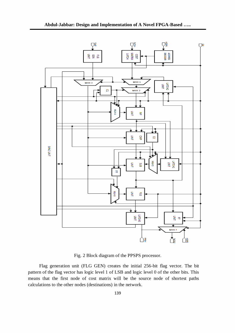
Abdul-Jabbar: Design and Implementation of A Novel FPGA-Based …..
531
Fig. 2 Block diagram of the PPSPS processor.
Flag generation unit (FLG GEN) creates the initial 256-bit flag vector. The bit
pattern of the flag vector has logic level 1 of LSB and logic level 0 of the other bits. This
means that the first node of cost matrix will be the source node of shortest paths
calculations to the other nodes (destinations) in the network.
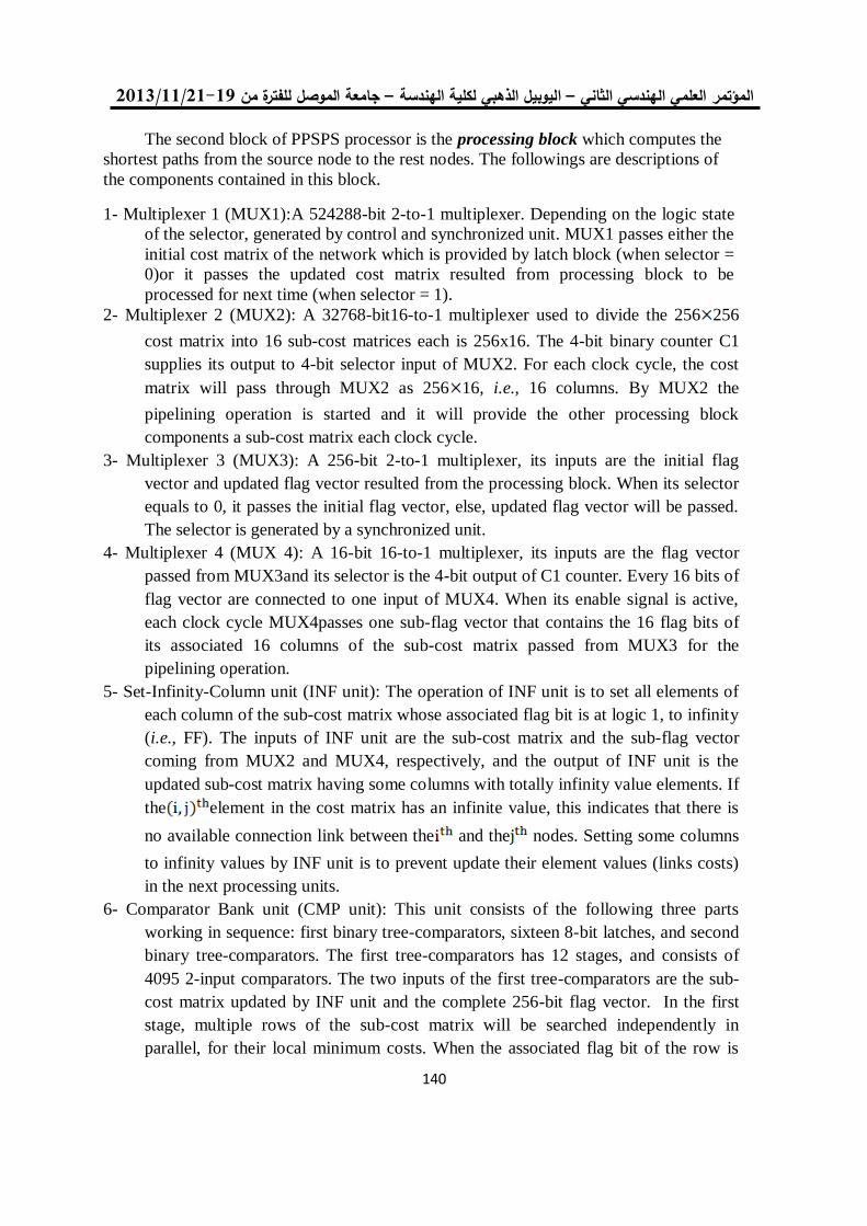
19/99/1192-91جامعة الموصل للفترة من –ليوبيل الذهبي لكلية الهندسة ا –العلمي الهندسي الثاني المؤتمر
541
The second block of PPSPS processor is the processing block which computes the
shortest paths from the source node to the rest nodes. The followings are descriptions of
the components contained in this block.
1- Multiplexer 1 (MUX1):A 524288-bit 2-to-1 multiplexer. Depending on the logic state
of the selector, generated by control and synchronized unit. MUX1 passes either the
initial cost matrix of the network which is provided by latch block (when selector =
0)or it passes the updated cost matrix resulted from processing block to be
processed for next time (when selector = 1).
2- Multiplexer 2 (MUX2): A 32768-bit16-to-1 multiplexer used to divide the 256 256
cost matrix into 16 sub-cost matrices each is 256x16. The 4-bit binary counter C1
supplies its output to 4-bit selector input of MUX2. For each clock cycle, the cost
matrix will pass through MUX2 as 256 16, i.e., 16 columns. By MUX2 the
pipelining operation is started and it will provide the other processing block
components a sub-cost matrix each clock cycle.
3- Multiplexer 3 (MUX3): A 256-bit 2-to-1 multiplexer, its inputs are the initial flag
vector and updated flag vector resulted from the processing block. When its selector
equals to 0, it passes the initial flag vector, else, updated flag vector will be passed.
The selector is generated by a synchronized unit.
4- Multiplexer 4 (MUX 4): A 16-bit 16-to-1 multiplexer, its inputs are the flag vector
passed from MUX3and its selector is the 4-bit output of C1 counter. Every 16 bits of
flag vector are connected to one input of MUX4. When its enable signal is active,
each clock cycle MUX4passes one sub-flag vector that contains the 16 flag bits of
its associated 16 columns of the sub-cost matrix passed from MUX3 for the
pipelining operation.
5- Set-Infinity-Column unit (INF unit): The operation of INF unit is to set all elements of
each column of the sub-cost matrix whose associated flag bit is at logic 1, to infinity
(i.e., FF). The inputs of INF unit are the sub-cost matrix and the sub-flag vector
coming from MUX2 and MUX4, respectively, and the output of INF unit is the
updated sub-cost matrix having some columns with totally infinity value elements. If
the element in the cost matrix has an infinite value, this indicates that there is
no available connection link between the and the nodes. Setting some columns
to infinity values by INF unit is to prevent update their element values (links costs)
in the next processing units.
6- Comparator Bank unit (CMP unit): This unit consists of the following three parts
working in sequence: first binary tree-comparators, sixteen 8-bit latches, and second
binary tree-comparators. The first tree-comparators has 12 stages, and consists of
4095 2-input comparators. The two inputs of the first tree-comparators are the sub-
cost matrix updated by INF unit and the complete 256-bit flag vector. In the first
stage, multiple rows of the sub-cost matrix will be searched independently in
parallel, for their local minimum costs. When the associated flag bit of the row is
Abdul-Jabbar: Design and Implementation of A Novel FPGA-Based …..
545
set, its local minimum cost will pass to the next stages, else an infinity value will be
placed instead. The rest stages of the first comparators tree will search the global
minimum among the local minimums of the first stage. Finally, the output of this
part is the minimum link cost of the participated links. This minimum value of the
sub-cost matrix will be latched, waiting for all other minimum values of the rest sub-
cost matrices. By the pipelining operation, 16 different minimum values are latched
in the second part of the comparator bank unit. The third part is another tree-
comparators, having 4 stages with fifteen 2-input comparators. The operation of this
part is to find the final minimum cost from the 16 latched minimum values of the
previous two parts.
7- Latch 1unit (LATCH1): This unit is to latch all sub-cost matrices after processing by
INF unit. LATCH1 basically consists of 65536 8-bit latches, distributed as 16
groups; each with 4096 8-bit latches, and each group will latch a single sub-cost
matrix. The output of this unit is the complete 256 256 cost matrix.
8- Multiplexer 5 (MUX5): MUX5 is similar toMUX2 in its construction and operation.
MUX5 receives the output of LATCH1 and reforms it as 16 groups of sub-cost
matrices to be passed in sequence according to the selector bits status that generated
by C2 4-bit binary counter. In other word, MUX5 divides the 256 256 cost matrix
into 16 sub-cost matrices each with 256 16.
9- Subtractor Matrix unit (SUB unit):The subtractor matrix unit is a two-dimensional
array of simple subtractors. The inputs of SUB unit are the 256 16 sub-
cost matrixpassed from MUX5, the minimum cost produced by CMP unit and the
256-bit flag. The subtractor of a specific position in the subtractors array will
subtract the minimum cost from the non-infinity cost value at the same position of
the sub-cost matrix. This is done only for the rows of the sub-cost matrix which have
flag bits equal to 1, other rows will remain unchanged. All subtractors will operate
simultaneously, and as a result the updated sub-cost matrix will have zero values.
10- Latch 2 unit (LATCH2): This unit accumulates the sub-cost matrices processed by
SUB unit to reform the updated 256 256 cost matrix. The output of this unit is
supplied to MUX1 for the next iteration of shortest path calculations.
11- Multiplexer 6 (MUX6): The same as MUX4 in its operation. The 4-bit selector is the
output of counter C2 but delayed by one clock cycle for synchronization.
12- Flag Update unit (FLG unit): FLG unit receives the updated sub-cost matrix produced
by SUB unit and the sub-flag vector passed from MUX6. The function of this unit is
that, when a zero value is found in each column of the sub-cost matrix, the
corresponding flag bit will be set to 1. All 16 columns will be searched in parallel
and all affected bits of sub-flag vector will be updated at the same time.
19/99/1192-91جامعة الموصل للفترة من –ليوبيل الذهبي لكلية الهندسة ا –العلمي الهندسي الثاني المؤتمر
541
13- Latch 3 unit (LATCH3): Because of FLG unit produces only 16 bits updated sub-flag
vector for one time, the 16 sub-flag vectors will be latched by LATCH3 unit to
reproduce the complete new 256-bit flag vector that will be used for the next
iteration of the processing block. This unit consists of two levels of 256-bit latches,
the first level is to latch the sub-flag vectors one after the other, and the second level
to release all 256 bits of the complete new flag vector. Also, a signal RTRDY will
produce if all 256 bits of the flag vector are 1’s to indicate that all shortest paths are
found and the routing table information of the network can be downloaded from the
hardware. It is generated by ANDing all new 256 bits of flag vector.
14- Routing Table unit (RT unit): The RT unit will have the final information of the
shortest paths of the network routs. It consists of bits array viewed as 16
partitions; each partition is 256 16 bits sub-array. The input of this unit is the sub-
cost matrix resulted from SUB unit. The zero values of sub-cost matrix elements
will set the corresponding bits positions in a sub-array of RT unit. Each sub-cost
matrix process a sub-array of RT unit, and the 16 sub-cost matrices covers the
256 256 bit array. At the end of the shortest path computations, when bit is
set, this means that the link from node to node is participated in the shortest
path because of its minimum cost.
15- Multiplexer 7 (MUX7): Finally, the routing table can be read out from the RT unit
using a MUX7. This multiplexer has 1024 inputs and one output; each is of 64-bit
wide. Its selector is 10-bit address bus ADDR2 for reading the 256 256 bits of RT
units as 64 bits each click cycle. MUX7 will be enabled if RTRDY signal of
LATCH3 unit is logic 1.
16- Synchronization unit (SYNC unit): The synchronization and control the flow of the
data from one unit to the other in PPSPS processor is done by SYNC unit. It controls
the cost matrix processing steps by releasing signals for enabling/disabling each
component of the processor hardware. SYNC unit consists of two53-bit rotation
registers (SRR1 and SRR2) and one256-bit inputs OR-gate. The function of OR-gate
is to produce the selector of MUX1 and MUX3 by ORing the 256 bits of the new
flag vector generated by FLG – LATCH3 units. Initially, all these 256 bits are set to
logic 0, so the initial selector state is logic 0, that will cause MUX1 and MUX3 pass
the origin cost matrix and flag vector, respectively. After the first iteration of the
processing block, the 256 bits of the new flag vector will contain at least one bit
with logic 1 level, resulting the selector will change its state to logic 1 and
accordingly MUX1 and MUX3 will pass the updated cost matrix and flag vector,
respectively. The selector will remain at logic 1 till the computation of shortest paths
is completed. The two synchronization rotation registers of SYNC unit are
described in the next section.
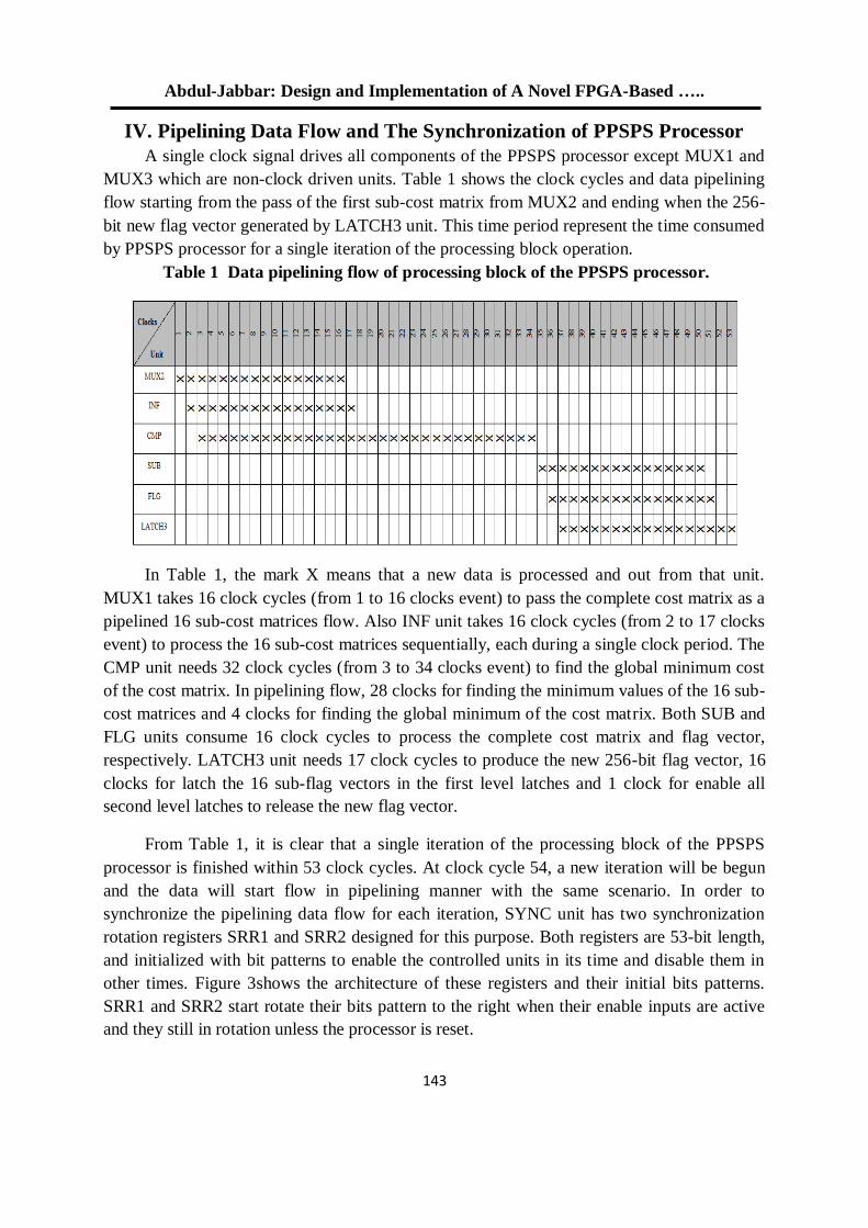
Abdul-Jabbar: Design and Implementation of A Novel FPGA-Based …..
543
IV. Pipelining Data Flow and The Synchronization of PPSPS Processor
A single clock signal drives all components of the PPSPS processor except MUX1 and
MUX3 which are non-clock driven units. Table 1 shows the clock cycles and data pipelining
flow starting from the pass of the first sub-cost matrix from MUX2 and ending when the 256-
bit new flag vector generated by LATCH3 unit. This time period represent the time consumed
by PPSPS processor for a single iteration of the processing block operation.
Table 1 Data pipelining flow of processing block of the PPSPS processor.
In Table 1, the mark X means that a new data is processed and out from that unit.
MUX1 takes 16 clock cycles (from 1 to 16 clocks event) to pass the complete cost matrix as a
pipelined 16 sub-cost matrices flow. Also INF unit takes 16 clock cycles (from 2 to 17 clocks
event) to process the 16 sub-cost matrices sequentially, each during a single clock period. The
CMP unit needs 32 clock cycles (from 3 to 34 clocks event) to find the global minimum cost
of the cost matrix. In pipelining flow, 28 clocks for finding the minimum values of the 16 sub-
cost matrices and 4 clocks for finding the global minimum of the cost matrix. Both SUB and
FLG units consume 16 clock cycles to process the complete cost matrix and flag vector,
respectively. LATCH3 unit needs 17 clock cycles to produce the new 256-bit flag vector, 16
clocks for latch the 16 sub-flag vectors in the first level latches and 1 clock for enable all
second level latches to release the new flag vector.
From Table 1, it is clear that a single iteration of the processing block of the PPSPS
processor is finished within 53 clock cycles. At clock cycle 54, a new iteration will be begun
and the data will start flow in pipelining manner with the same scenario. In order to
synchronize the pipelining data flow for each iteration, SYNC unit has two synchronization
rotation registers SRR1 and SRR2 designed for this purpose. Both registers are 53-bit length,
and initialized with bit patterns to enable the controlled units in its time and disable them in
other times. Figure 3shows the architecture of these registers and their initial bits patterns.
SRR1 and SRR2 start rotate their bits pattern to the right when their enable inputs are active
and they still in rotation unless the processor is reset.
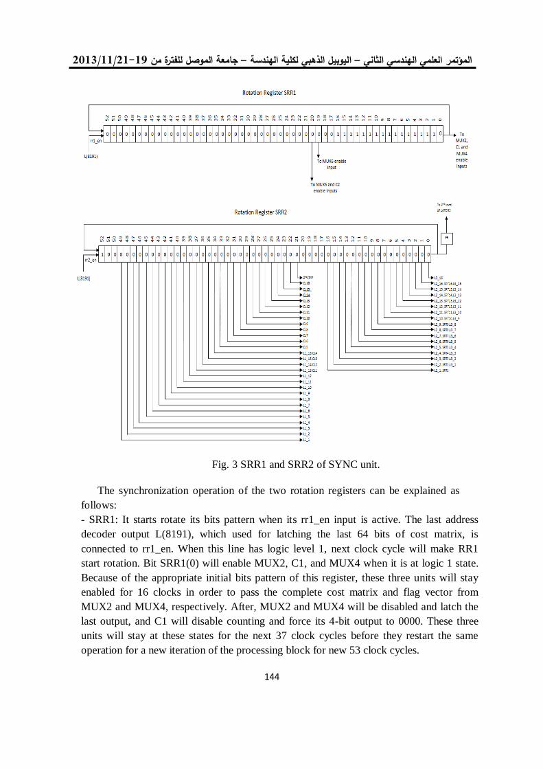
19/99/1192-91جامعة الموصل للفترة من –ليوبيل الذهبي لكلية الهندسة ا –العلمي الهندسي الثاني المؤتمر
544
The synchronization operation of the two rotation registers can be explained as
follows:
- SRR1: It starts rotate its bits pattern when its rr1_en input is active. The last address
decoder output L(8191), which used for latching the last 64 bits of cost matrix, is
connected to rr1_en. When this line has logic level 1, next clock cycle will make RR1
start rotation. Bit SRR1(0) will enable MUX2, C1, and MUX4 when it is at logic 1 state.
Because of the appropriate initial bits pattern of this register, these three units will stay
enabled for 16 clocks in order to pass the complete cost matrix and flag vector from
MUX2 and MUX4, respectively. After, MUX2 and MUX4 will be disabled and latch the
last output, and C1 will disable counting and force its 4-bit output to 0000. These three
units will stay at these states for the next 37 clock cycles before they restart the same
operation for a new iteration of the processing block for new 53 clock cycles.
Fig. 3 SRR1 and SRR2 of SYNC unit.
Abdul-Jabbar: Design and Implementation of A Novel FPGA-Based …..
541
The SRR1(20) bit is connected to C2 and MUX5 enable inputs. When its logic state is
1, these two units will start working in next clock cycle. The 4-bit output of counter C2 is pre-
set to 0000. So, if MUX5 is enabled, it will pass the first sub-cost matrix toward the SUB unit.
In the same clock cycle, C2 will increment its output by 1 to prepare the selector of MUX5to
select the second sub-cost matrix in the next clock cycle. This operation will continue for 16
clock cycles in order to complete passing all the 16 sub-cost matrices which stored in
LATCH1 unit. SRR4(20) bit will be at logic 1 level after 34 clocks from enabling the register,
and stay at this level for a 16 clocks, then return to 0 for 37 clocks. By this way, SUB unit will
process the 16 sub-cost matrices in a pipelining manner during each iteration of the
processing block. On the other hand, SRR4(19) bit enables MUX6 when its logic level is 1,
i.e., after one clock cycle from C2 and MUX5 enabled, for 16 clock cycles.
- SRR2: Latch 1 unit stores the 16 sub-costs matrices after updating by INF unit in
pipelining manner. The 16 enable signals of this unit are provided by SRR2. After 3 clocks
from the time of L(8191) signal is set to logic 1, the first sub-cost matrix is arrived to
LATCH1 unit, and the rest matrices will come consequently during the next 15 clocks. The
initial bits pattern of SRR2 is set so that SRR2(49) will be at logic 1 at the same time of the
arrival of the first sub-cost matrix to LATCH1, and because of connecting this bit to the first
latch enable, L1_1, next clock cycle will save this sub-cost matrix in its latches. The other
sub-cost matrices will be also stored in LATCH1 unit by logic 1 state of SRR2(48) to
SRR2(34) bits which represent the enable signals of the other 15 latches L1_2 to L1_16.
The second function of SRR2 register is that to enable the intermediate stage of CMP
unit, which is the latch part. The logic states of bits SRR2(37) through SRR2(22) are used to
enable the sixteen 8-bit latches CL1 through CL16, respectively, in sequence and one latch
per a clock cycle. The result of this operation is the latching of the 16 minimum values of the
sub-cost matrices processed by first comparator of CMP unit. It is required 15 clock cycles,
from the time of L8191 is logic 1, to find the minimum cost of the first sub-cost matrix. The
other 15 minimums of the rest sub-cost matrices will be found during the next 15 clock
cycles. When all the 16 minimum values are found and latched, the second comparator will be
enabled at the next clock by SRR2(21) bit to find the global minimum during 4 clock cycles,
and the CMP unit finishes its work for this iteration and will repeat the same operation next
iteration.
The other function of this rotation register is to provide latch signals for three units,
LATCH2, RT, and LATCH3. SRR2(16) will be at logic 1after 36 clocks from SRR2 starts
rotating. During the next clock cycle, SRR2(16) will latch the first updated sub-cost matrix
produced by SUB unit in LATCH2 unit, and also will enable first 16 columns of the bits array
of RT unit for updating its bits from logic level 0 to 1 if the corresponding costs of the
updated sub-cost matrix have zero values. In the same manner, SRR2(15) to SRR2(1) will be
used for the rest parts of LATCH2 unit and RT unit. On the other hand and by the same way,
SRR2(15) through SRR2(0) will be used to latch the 16 sub-flag vectors resulting from FLG
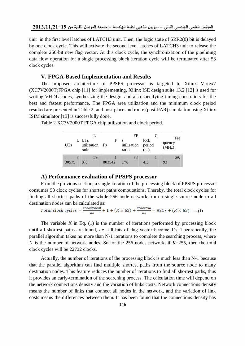
19/99/1192-91جامعة الموصل للفترة من –ليوبيل الذهبي لكلية الهندسة ا –العلمي الهندسي الثاني المؤتمر
541
unit in the first level latches of LATCH3 unit. Then, the logic state of SRR2(0) bit is delayed
by one clock cycle. This will activate the second level latches of LATCH3 unit to release the
complete 256-bit new flag vector. At this clock cycle, the synchronization of the pipelining
data flow operation for a single processing block iteration cycle will be terminated after 53
clock cycles.
V. FPGA-Based Implementation and Results
The proposed architecture of PPSPS processor is targeted to Xilinx Virtex7
(XC7V2000T)FPGA chip [11] for implementing. Xilinx ISE design suite 13.2 [12] is used for
writing VHDL codes, synthesizing the design, and also specifying timing constraints for the
best and fastest performance. The FPGA area utilization and the minimum clock period
resulted are presented in Table 2, and post place and route (post-PAR) simulation using Xilinx
ISIM simulator [13] is successfully done.
Table 2 XC7V2000T FPGA chip utilization and clock period.
A) Performance evaluation of PPSPS processor
From the previous section, a single iteration of the processing block of PPSPS processor
consumes 53 clock cycles for shortest paths computations. Thereby, the total clock cycles for
finding all shortest paths of the whole 256-node network from a single source node to all
destination nodes can be calculated as:
... (1)
The variable K in Eq. (1) is the number of iterations performed by processing block
until all shortest paths are found, i.e., all bits of flag vector become 1’s. Theoretically, the
parallel algorithm takes no more than N-1 iterations to complete the searching process, where
N is the number of network nodes. So for the 256-nodes network, if K=255, then the total
clock cycles will be 22732 clocks.
Actually, the number of iterations of the processing block is much less than N-1 because
that the parallel algorithm can find multiple shortest paths from the source node to many
destination nodes. This feature reduces the number of iterations to find all shortest paths, thus
it provides an early-termination of the searching process. The calculation time will depend on
the network connections density and the variation of links costs. Network connections density
means the number of links that connect all nodes in the network, and the variation of link
costs means the differences between them. It has been found that the connections density has
L
UTs
LUTs
utilization
ratio
F
Fs
FFs
utilization
ratio
Clock
period
(ns)
Frequency
(MHz)
7
30575
59.
8%
1
803542
73
.7%
1
4.3
69.
93
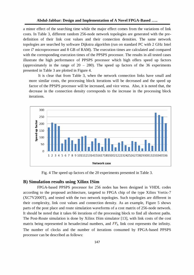
Abdul-Jabbar: Design and Implementation of A Novel FPGA-Based …..
541
a minor effect of the searching time while the major effect comes from the variations of link
costs. In Table 3, different random 256-node network topologies are generated with the pre-
definition of their link cost values and their connection densities. The same network
topologies are searched by software Dijkstra algorithm (run on standard PC with 2 GHz Intel
core i7 microprocessor and 8 GB of RAM). The execution times are calculated and compared
with the corresponding execution times of the PPSPS processor. The results in all tested cases
illustrate the high performance of PPSPS processor which high offers speed up factors
(approximately in the range of 20 – 280). The speed up factors of the 36 experiments
presented in Table 3 are plotted in Figure 4.
It is clear that from Table 3, when the network connection links have small and
more similar costs, the processing block iterations will be decreased and the speed up
factor of the PPSPS processor will be increased, and vice versa. Also, it is noted that, the
decrease in the connection density corresponds to the increase in the processing block
iterations.
Fig. 4 The speed up factors of the 20 experiments presented in Table 3.
B) Simulation results using Xilinx ISim
FPGA-based PPSPS processor for 256 nodes has been designed in VHDL codes
according to the proposed architecture, targeted to FPGA chip of the type Xilinx Vertix-7
(XC7V2000T), and tested with the two network topologies. Such topologies are different in
their complexity, link cost values and connection density. As an example, Figure 5 shows
parts of the post place and route simulation waveforms of a cost matrix of 256-node network.
It should be noted that it takes 66 iterations of the processing block to find all shortest paths.
The Post-Route simulation is done by Xilinx ISim simulator [13], with link costs of the cost
matrix being represented in hexadecimal numbers, and link cost represents the infinity.
The number of clocks and the number of iterations consumed by FPGA-based PPSPS
processor can be described as follows:
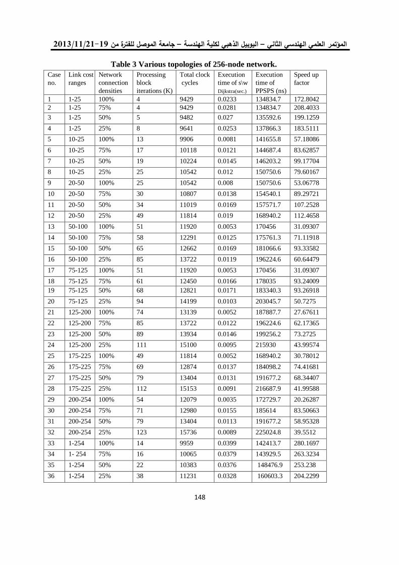
19/99/1192-91جامعة الموصل للفترة من –ليوبيل الذهبي لكلية الهندسة ا –العلمي الهندسي الثاني المؤتمر
541
Table 3 Various topologies of 256-node network.
Case
no.
Link cost
ranges
Network
connection
densities
Processing
block
iterations (K)
Total clock
cycles
Execution
time of s\w
Dijkstra(sec.)
Execution
time of
PPSPS (ns)
Speed up
factor
1 1-25 100% 4 9429 0.0233 134834.7 172.8042
2 1-25 75% 4 9429 0.0281 134834.7 208.4033
3 1-25 50% 5 9482 0.027 135592.6 199.1259
4 1-25 25% 8 9641 0.0253 137866.3 183.5111
5 10-25 100% 13 9906 0.0081 141655.8 57.18086
6 10-25 75% 17 10118 0.0121 144687.4 83.62857
7 10-25 50% 19 10224 0.0145 146203.2 99.17704
8 10-25 25% 25 10542 0.012 150750.6 79.60167
9 20-50 100% 25 10542 0.008 150750.6 53.06778
10 20-50 75% 30 10807 0.0138 154540.1 89.29721
11 20-50 50% 34 11019 0.0169 157571.7 107.2528
12 20-50 25% 49 11814 0.019 168940.2 112.4658
13 50-100 100% 51 11920 0.0053 170456 31.09307
14 50-100 75% 58 12291 0.0125 175761.3 71.11918
15 50-100 50% 65 12662 0.0169 181066.6 93.33582
16 50-100 25% 85 13722 0.0119 196224.6 60.64479
17 75-125 100% 51 11920 0.0053 170456 31.09307
18 75-125 75% 61 12450 0.0166 178035 93.24009
19 75-125 50% 68 12821 0.0171 183340.3 93.26918
20 75-125 25% 94 14199 0.0103 203045.7 50.7275
21 125-200 100% 74 13139 0.0052 187887.7 27.67611
22 125-200 75% 85 13722 0.0122 196224.6 62.17365
23 125-200 50% 89 13934 0.0146 199256.2 73.2725
24 125-200 25% 111 15100 0.0095 215930 43.99574
25 175-225 100% 49 11814 0.0052 168940.2 30.78012
26 175-225 75% 69 12874 0.0137 184098.2 74.41681
27 175-225 50% 79 13404 0.0131 191677.2 68.34407
28 175-225 25% 112 15153 0.0091 216687.9 41.99588
29 200-254 100% 54 12079 0.0035 172729.7 20.26287
30 200-254 75% 71 12980 0.0155 185614 83.50663
31 200-254 50% 79 13404 0.0113 191677.2 58.95328
32 200-254 25% 123 15736 0.0089 225024.8 39.5512
33 1-254 100% 14 9959 0.0399 142413.7 280.1697
34 1- 254 75% 16 10065 0.0379 143929.5 263.3234
35 1-254 50% 22 10383 0.0376 148476.9 253.238
36 1-254 25% 38 11231 0.0328 160603.3 204.2299
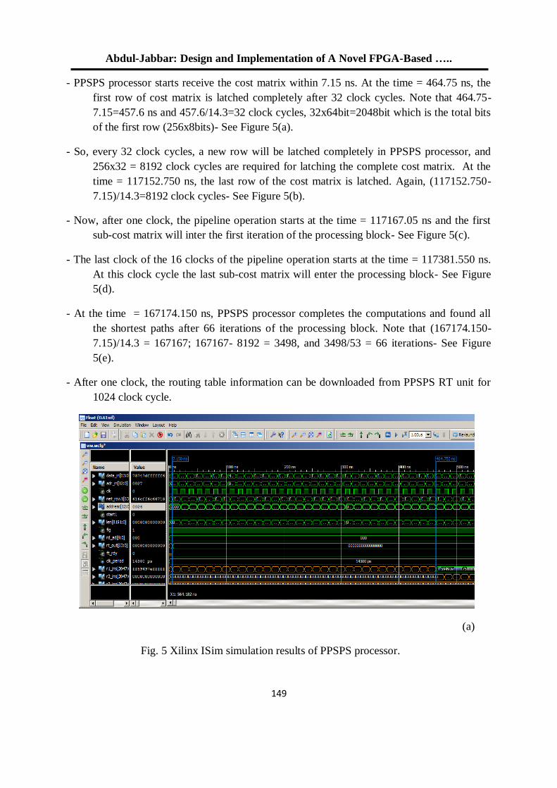
Abdul-Jabbar: Design and Implementation of A Novel FPGA-Based …..
541
- PPSPS processor starts receive the cost matrix within 7.15 ns. At the time = 464.75 ns, the
first row of cost matrix is latched completely after 32 clock cycles. Note that 464.75-
7.15=457.6 ns and 457.6/14.3=32 clock cycles, 32x64bit=2048bit which is the total bits
of the first row (256x8bits)- See Figure 5(a).
- So, every 32 clock cycles, a new row will be latched completely in PPSPS processor, and
256x32 = 8192 clock cycles are required for latching the complete cost matrix. At the
time = 117152.750 ns, the last row of the cost matrix is latched. Again, (117152.750-
7.15)/14.3=8192 clock cycles- See Figure 5(b).
- Now, after one clock, the pipeline operation starts at the time = 117167.05 ns and the first
sub-cost matrix will inter the first iteration of the processing block- See Figure 5(c).
- The last clock of the 16 clocks of the pipeline operation starts at the time = 117381.550 ns.
At this clock cycle the last sub-cost matrix will enter the processing block- See Figure
5(d).
- At the time = 167174.150 ns, PPSPS processor completes the computations and found all
the shortest paths after 66 iterations of the processing block. Note that (167174.150-
7.15)/14.3 = 167167; 167167- 8192 = 3498, and 3498/53 = 66 iterations- See Figure
5(e).
- After one clock, the routing table information can be downloaded from PPSPS RT unit for
1024 clock cycle.
(a)
Fig. 5 Xilinx ISim simulation results of PPSPS processor.
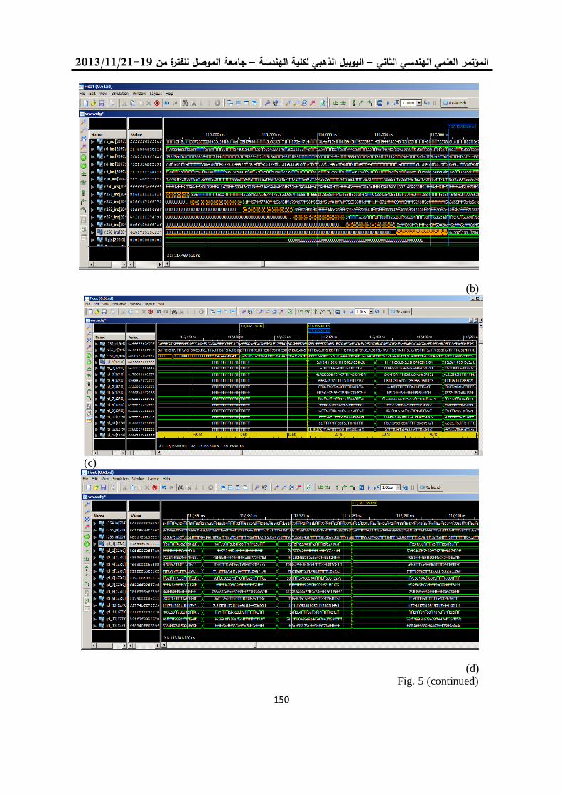
19/99/1192-91جامعة الموصل للفترة من –ليوبيل الذهبي لكلية الهندسة ا –العلمي الهندسي الثاني المؤتمر
511
(b)
(c)
(d) Fig. 5 (continued)
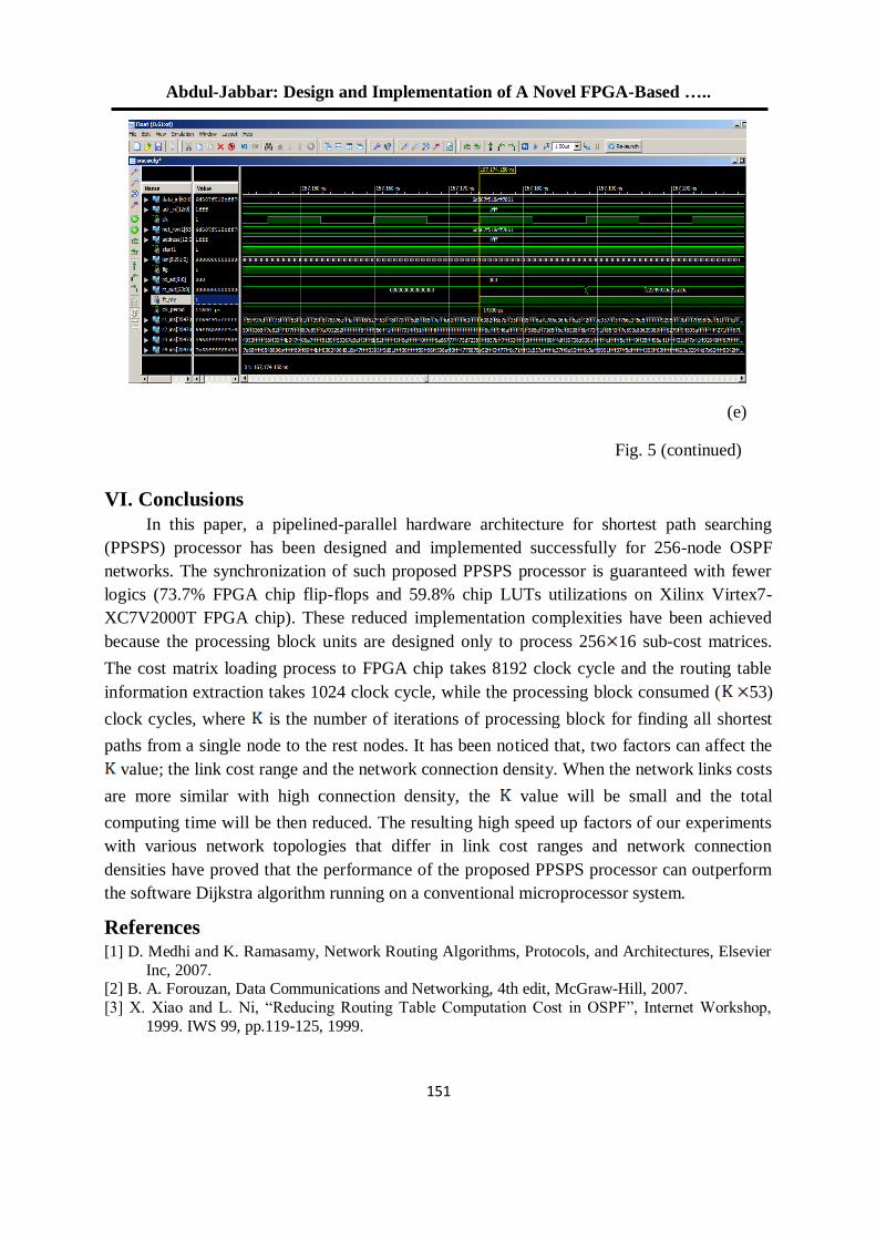
Abdul-Jabbar: Design and Implementation of A Novel FPGA-Based …..
515
(e)
Fig. 5 (continued)
VI. Conclusions
In this paper, a pipelined-parallel hardware architecture for shortest path searching
(PPSPS) processor has been designed and implemented successfully for 256-node OSPF
networks. The synchronization of such proposed PPSPS processor is guaranteed with fewer
logics (73.7% FPGA chip flip-flops and 59.8% chip LUTs utilizations on Xilinx Virtex7-
XC7V2000T FPGA chip). These reduced implementation complexities have been achieved
because the processing block units are designed only to process 256 16 sub-cost matrices.
The cost matrix loading process to FPGA chip takes 8192 clock cycle and the routing table
information extraction takes 1024 clock cycle, while the processing block consumed ( 53)
clock cycles, where is the number of iterations of processing block for finding all shortest
paths from a single node to the rest nodes. It has been noticed that, two factors can affect the
value; the link cost range and the network connection density. When the network links costs
are more similar with high connection density, the value will be small and the total
computing time will be then reduced. The resulting high speed up factors of our experiments
with various network topologies that differ in link cost ranges and network connection
densities have proved that the performance of the proposed PPSPS processor can outperform
the software Dijkstra algorithm running on a conventional microprocessor system.
References [1] D. Medhi and K. Ramasamy, Network Routing Algorithms, Protocols, and Architectures, Elsevier
Inc, 2007. [2] B. A. Forouzan, Data Communications and Networking, 4th edit, McGraw-Hill, 2007.
[3] X. Xiao and L. Ni, “Reducing Routing Table Computation Cost in OSPF”, Internet Workshop,
1999. IWS 99, pp.119-125, 1999.
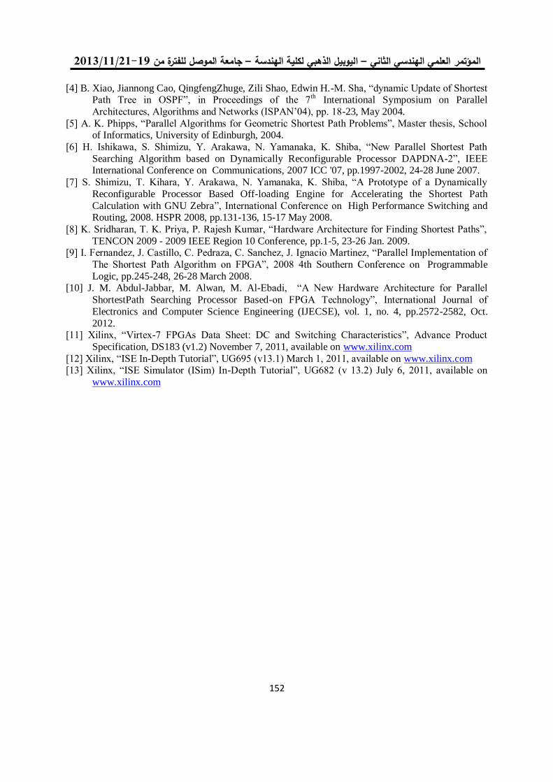
19/99/1192-91جامعة الموصل للفترة من –ليوبيل الذهبي لكلية الهندسة ا –العلمي الهندسي الثاني المؤتمر
511
[4] B. Xiao, Jiannong Cao, QingfengZhuge, Zili Shao, Edwin H.-M. Sha, “dynamic Update of Shortest Path Tree in OSPF”, in Proceedings of the 7
th International Symposium on Parallel
Architectures, Algorithms and Networks (ISPAN’04), pp. 18-23, May 2004.
[5] A. K. Phipps, “Parallel Algorithms for Geometric Shortest Path Problems”, Master thesis, School of Informatics, University of Edinburgh, 2004.
[6] H. Ishikawa, S. Shimizu, Y. Arakawa, N. Yamanaka, K. Shiba, “New Parallel Shortest Path
Searching Algorithm based on Dynamically Reconfigurable Processor DAPDNA-2”, IEEE International Conference on Communications, 2007 ICC '07, pp.1997-2002, 24-28 June 2007.
[7] S. Shimizu, T. Kihara, Y. Arakawa, N. Yamanaka, K. Shiba, “A Prototype of a Dynamically
Reconfigurable Processor Based Off-loading Engine for Accelerating the Shortest Path
Calculation with GNU Zebra”, International Conference on High Performance Switching and Routing, 2008. HSPR 2008, pp.131-136, 15-17 May 2008.
[8] K. Sridharan, T. K. Priya, P. Rajesh Kumar, “Hardware Architecture for Finding Shortest Paths”,
TENCON 2009 - 2009 IEEE Region 10 Conference, pp.1-5, 23-26 Jan. 2009. [9] I. Fernandez, J. Castillo, C. Pedraza, C. Sanchez, J. Ignacio Martinez, “Parallel Implementation of
The Shortest Path Algorithm on FPGA”, 2008 4th Southern Conference on Programmable
Logic, pp.245-248, 26-28 March 2008. [10] J. M. Abdul-Jabbar, M. Alwan, M. Al-Ebadi, “A New Hardware Architecture for Parallel
ShortestPath Searching Processor Based-on FPGA Technology”, International Journal of
Electronics and Computer Science Engineering (IJECSE), vol. 1, no. 4, pp.2572-2582, Oct.
2012. [11] Xilinx, “Virtex-7 FPGAs Data Sheet: DC and Switching Characteristics”, Advance Product
Specification, DS183 (v1.2) November 7, 2011, available on www.xilinx.com
[12] Xilinx, “ISE In-Depth Tutorial”, UG695 (v13.1) March 1, 2011, available on www.xilinx.com [13] Xilinx, “ISE Simulator (ISim) In-Depth Tutorial”, UG682 (v 13.2) July 6, 2011, available on
www.xilinx.com
Ali: Evaluation of Routing Protocols of Wireless Ad Hoc for SCADA Systems….
351
Evaluation of Routing Protocols of Wireless Ad Hoc for SCADA
Systems Using OPNET Simulator
Qutaiba I. Ali Fajer Fehr Fadhel Computer Eng. Dept. Computer and Internet Center
Mosul University, Mosul, Iraq.
[email protected] [email protected]
Abstract Many mechanisms were used to improve reliability of wire links in SCADA
systems. This paper suggests enhancing the reliability of SCADA system links using
wireless Ad hoc Network technology or MANET. Our SCADA system emulates a real
SCADA system connecting 20 electrical substations with their central control in Mosul
city/Iraq. We suggest the use of a standby wireless network which is activated to carry
the data of the SCADA system in the event of wired network failure. MANET
performance was evaluated by comparing four of its most important routing protocols
(DSR, AODV, OLSR, and TORA ).
Keywords- SCADA; Reliability; MANET; DSR; AODV; OLSR; TORA.
الالسلكية المستخدمة في أنظمة ) Ad Hocتقييم أداء بروتوكوالت التوجيه في شبكات )
OPNETسكادا باستخدام برنامج المحاكاة
فجر فهر فاضل قتيبة ابراهيم علي د. كلية الهندسة -قسم هندسة الحاسوب مركز الحاسوب واإلنترنت
العراق –الموصل -صلجامعة المو
الخالصةتستخدم العديد من اآلليات لتحسين حالة الوثوقية في أنظمة التحكم اإلشرافي وجلب البيانات )السكادا( ذات
Ad االرتباط السلكي, تم في هذا البحث اقتراح تحسين وثوقية ارتباط نظام السكادا الذي يستخدم االرتباط الالسلكي)
hoc( أو تقنية )MANET) محطة 02. يحاكي النظام الذي تم استخدامه في هذا البحث نظام سكادا حقيقي يقوم بربط
( لنقل MANET Protocolكهربائية بمركز للتحكم في مدينة الموصل/ العراق باستخدام شبكة السلكية تستخدم )
نة للكشف عن أداء أربع من أهم بيانات النظام في حالة حدوث أي فشل في الشبكة السلكية للنظام. بعد ذلك تم عمل مقار
الالسلكية. (MANETبرتوكوالت التوجيه في تقنية )
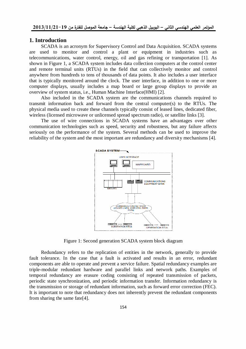
19/99/1192-91جامعة الموصل للفترة من –ليوبيل الذهبي لكلية الهندسة ا –العلمي الهندسي الثاني المؤتمر
351
1. Introduction SCADA is an acronym for Supervisory Control and Data Acquisition. SCADA systems
are used to monitor and control a plant or equipment in industries such as
telecommunications, water control, energy, oil and gas refining or transportation [1]. As
shown in Figure 1, a SCADA system includes data collection computers at the control center
and remote terminal units (RTUs) in the field that can collectively monitor and control
anywhere from hundreds to tens of thousands of data points. It also includes a user interface
that is typically monitored around the clock. The user interface, in addition to one or more
computer displays, usually includes a map board or large group displays to provide an
overview of system status, i.e., Human Machine Interface(HMI) [2].
Also included in the SCADA system are the communications channels required to
transmit information back and forward from the central computer(s) to the RTUs. The
physical media used to create these channels typically consist of leased lines, dedicated fiber,
wireless (licensed microwave or unlicensed spread spectrum radio), or satellite links [3].
The use of wire connections in SCADA systems have an advantages over other
communication technologies such as speed, security and robustness, but any failure affects
seriously on the performance of the system. Several methods can be used to improve the
reliability of the system and the most important are redundancy and diversity mechanisms [4].
Figure 1: Second generation SCADA system block diagram
Redundancy refers to the replication of entities in the network, generally to provide
fault tolerance. In the case that a fault is activated and results in an error, redundant
components are able to operate and prevent a service failure. Spatial redundancy examples are
triple-modular redundant hardware and parallel links and network paths. Examples of
temporal redundancy are erasure coding consisting of repeated transmission of packets,
periodic state synchronization, and periodic information transfer. Information redundancy is
the transmission or storage of redundant information, such as forward error correction (FEC).
It is important to note that redundancy does not inherently prevent the redundant components
from sharing the same fate[4].
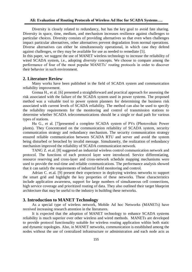
Ali: Evaluation of Routing Protocols of Wireless Ad Hoc for SCADA Systems….
355
Diversity is closely related to redundancy, but has the key goal to avoid fate sharing.
Diversity in space, time, medium, and mechanism increases resilience against challenges to
particular choices. Diversity consists of providing alternatives so that even when challenges
impact particular alternatives, other alternatives prevent degradation from normal operations.
Diverse alternatives can either be simultaneously operational, in which case they defend
against challenges, or they may be available for use as needed to remediate [5].
In this paper, we suggest the use of MANET wireless technology to increase the reliability of
wired SCADA system, i.e., adopting diversity concepts. We choose to compare among the
performance of four of the most popular MANETs’ routing protocols in order to discover
their behavior in such environment.
2. Literature Review Many works have been published in the field of SCADA system and communication
reliability improvement.
Gomaa H., et al. [6] presented a straightforward and practical approach for assessing the
risk associated with the failure of the SCADA system used in power systems. The proposed
method was a valuable tool to power system planners for determining the business risk
associated with current levels of SCADA reliability. The method can also be used to specify
the reliability requirements for the monitoring and control of transmission stations to
determine whether SCADA telecommunications should be a single or dual path for various
types of stations.
Hu G., et al. [7]presented a complete SCADA system of PVs (Photovoltaic Power
plants). They Concentrated on the communication reliability of SCADA system, security
communication strategy and redundancy mechanism. The security communication strategy
ensured reliable communication between SCADA RTU and server and avoid the system
being disturbed or breached by invalid message. Simultaneity, the realization of redundancy
mechanism improved the reliability of SCADA communication network.
TANG Z. et.al. [8] suggested an industrial wireless control communication network and
protocol. The functions of each protocol layer were introduced. Service differentiating,
resource reserving and cross-layer and cross-network schedule mapping mechanisms were
used to provide the real-time and reliable communications. The performance analysis showed
that it can satisfy the requirements of industrial field monitoring and control.
Adrian C. et.al. [9] present their experience in deploying wireless networks to support
the smart grid and highlight the key properties of these networks. These characteristics
include application awareness, support for large numbers of simultaneous cell connections,
high service coverage and prioritized routing of data. They also outlined their target blueprint
architecture that may be useful to the industry in building these networks.
3. Introduction to MANET Technology As a special type of wireless network, Mobile Ad hoc Networks (MANETs) have
received increasing research attention in the literatures.
It is expected that the adoption of MANET technology to enhance SCADA systems
reliability is much superior over other wireless and wired methods. MANETs are developed
to provide protocol functionality suitable for wireless routing application within both static
and dynamic topologies. Also, in MANET networks, communication is established among the
nodes without the use of centralized infrastructure or administration and each node acts as
19/99/1192-91جامعة الموصل للفترة من –ليوبيل الذهبي لكلية الهندسة ا –العلمي الهندسي الثاني المؤتمر
351
both an end-host and as a router due to limited propagation range of each node’s wireless
transmission [10]. In addition, the cost of ownership, installation and maintenance is very low
comparing to other redundancy methods. However, the performance of such system depends
mainly on the network’s topology, dimension, number of nodes and the selected routing
protocol.
Such routing protocols can be described according to their characteristics and are
divided into two main categories: Table-driven routing protocols and source-initiated on-
demand driven routing protocols [11]. Figure (2) illustrate routing protocol categories. The
table-driven routing protocols maintain consistent and up-to-date routing information from
each node to the remaining nodes in the network in one or more routing tables regardless of
the need of such routes. Source initiated on-demand routing, initiates routing activities only
when data packets are present and needs routing which reduces routing load [12].
Figure 2.Routing protocol classification
A. Dynamic Source Routing (DSR) DSR is an entirely on-demand ad hoc network routing protocol composed of two parts:
Route Discovery and Route Maintenance [13]. DSR is a reactive protocol that discovers and
maintains routes between nodes on demand [14]. In order to discover a route between two
nodes, DSR floods the network with a Route Request packet. This packet is forwarded only
once by each node after concatenating its own address to the path. When the targeted node
receives the Route Request, it piggybacks a Route Reply to the sender and a route is
established. Each time a packet follows an established route, each node has to ensure that the
link is reliable between itself and the next node. DSR provides three successive steps to
perform this maintenance: link layer acknowledgment, passive acknowledgment and network
layer acknowledgment. If a route is broken, then the node which detects the failure sends (by
piggybacking) a Route Error packet to the original sender [14].
B. Ad Hoc on-Demand Distance Vector Routing (AODV) AODV provides on-demand route discovery in mobile ad hoc networks [15]. Like most
reactive routing protocols, route finding is based on a route discovery cycle involving a
broadcast network search and a uncast reply containing discovered paths. AODV relies on
per-node sequence numbers for loop freedom and for ensuring selection of the most recent
routing path. AODV nodes maintain a route table in which next-hop routing information for
destination nodes is stored. Each routing table entry has an associated lifetime value. If a
route is not utilized within the lifetime period, the route expires. Otherwise, each time the
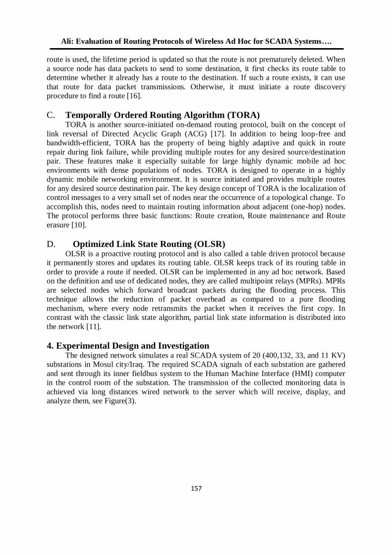
Ali: Evaluation of Routing Protocols of Wireless Ad Hoc for SCADA Systems….
351
route is used, the lifetime period is updated so that the route is not prematurely deleted. When
a source node has data packets to send to some destination, it first checks its route table to
determine whether it already has a route to the destination. If such a route exists, it can use
that route for data packet transmissions. Otherwise, it must initiate a route discovery
procedure to find a route [16].
C. Temporally Ordered Routing Algorithm (TORA) TORA is another source-initiated on-demand routing protocol, built on the concept of
link reversal of Directed Acyclic Graph (ACG) [17]. In addition to being loop-free and
bandwidth-efficient, TORA has the property of being highly adaptive and quick in route
repair during link failure, while providing multiple routes for any desired source/destination
pair. These features make it especially suitable for large highly dynamic mobile ad hoc
environments with dense populations of nodes. TORA is designed to operate in a highly
dynamic mobile networking environment. It is source initiated and provides multiple routes
for any desired source destination pair. The key design concept of TORA is the localization of
control messages to a very small set of nodes near the occurrence of a topological change. To
accomplish this, nodes need to maintain routing information about adjacent (one-hop) nodes.
The protocol performs three basic functions: Route creation, Route maintenance and Route
erasure [10].
D. Optimized Link State Routing (OLSR) OLSR is a proactive routing protocol and is also called a table driven protocol because
it permanently stores and updates its routing table. OLSR keeps track of its routing table in
order to provide a route if needed. OLSR can be implemented in any ad hoc network. Based
on the definition and use of dedicated nodes, they are called multipoint relays (MPRs). MPRs
are selected nodes which forward broadcast packets during the flooding process. This
technique allows the reduction of packet overhead as compared to a pure flooding
mechanism, where every node retransmits the packet when it receives the first copy. In
contrast with the classic link state algorithm, partial link state information is distributed into
the network [11].
4. Experimental Design and Investigation The designed network simulates a real SCADA system of 20 (400,132, 33, and 11 KV)
substations in Mosul city/Iraq. The required SCADA signals of each substation are gathered
and sent through its inner fieldbus system to the Human Machine Interface (HMI) computer
in the control room of the substation. The transmission of the collected monitoring data is
achieved via long distances wired network to the server which will receive, display, and
analyze them, see Figure(3).
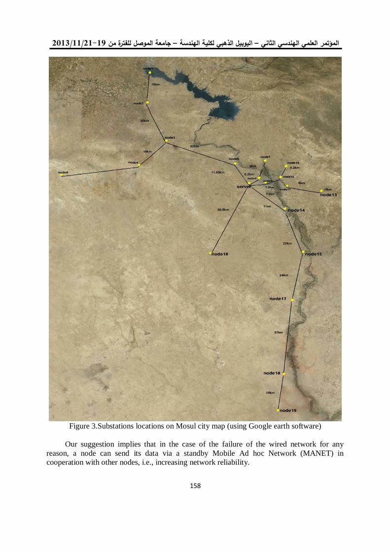
19/99/1192-91جامعة الموصل للفترة من –ليوبيل الذهبي لكلية الهندسة ا –العلمي الهندسي الثاني المؤتمر
351
Figure 3.Substations locations on Mosul city map (using Google earth software)
Our suggestion implies that in the case of the failure of the wired network for any
reason, a node can send its data via a standby Mobile Ad hoc Network (MANET) in
cooperation with other nodes, i.e., increasing network reliability.

Ali: Evaluation of Routing Protocols of Wireless Ad Hoc for SCADA Systems….
351
In our network, due to its power & performance efficiency over conventional IEEE
802.11 WLAN, IEEE 802.11g is the network standard used. Each node in this network has
more than one neighbor, so the transmission power used depends on the longest neighbor
distance except for central station (Server), which needs more adjustments to avoid extra load.
Each node transmits a report of its important digital and analog alarm and status signals
to the central server for displaying and processing, where each signal is represented by a
number of bits ending on its type. For example, status signals (we called digital signals) are
represented by one bit and other measured values (we called analog signals) are represented
by 12 bits for more accuracy, see table(1), i.e., the number of bits for each feeder or
transformer is 52bits. These bits were collected and arranged as an File Transfer Protocol
(FTP) file where each substation uploads different file sizes depending on the number of
feeders and transformers, see Table(2).
Table 1: signals name, type and numbers of bits represented for each substation feeder Signal name Signal type NO. of bits
Feeder control digital 1
Fire alarm digital 1
Feeder status(ON/OFF) digital 1
Feeder tripping status digital 1
Feeder current value Analog 12
Oil temperature Analog 12
Feeder voltage value Analog 12
Transformer coils thermal Analog 12
Table 2: Number of Feeders and Transformers, and length of transmitted data bits from
each substation
Initial data without overload
(control data)(bit) Number of Feeders and Transformers Node
1664 32 1
1196 23 2
1196 23 3
1404 27 4
1196 23 5
468 9 6
780 15 7
1040 20 8
832 16 9
114 2 10
884 17 11
364 7 12
1768 34 13
936 18 14
104 2 15
988 19 16
1092 21 17
780 15 18
780 15 19
1300 25 20
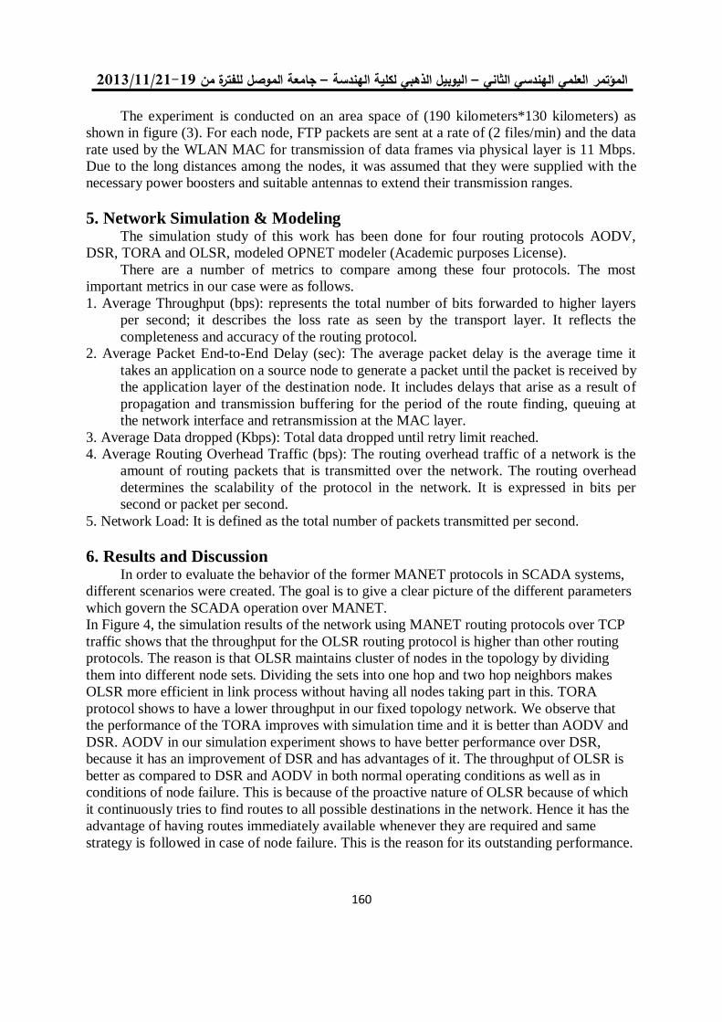
19/99/1192-91جامعة الموصل للفترة من –ليوبيل الذهبي لكلية الهندسة ا –العلمي الهندسي الثاني المؤتمر
311
The experiment is conducted on an area space of (190 kilometers*130 kilometers) as
shown in figure (3). For each node, FTP packets are sent at a rate of (2 files/min) and the data
rate used by the WLAN MAC for transmission of data frames via physical layer is 11 Mbps.
Due to the long distances among the nodes, it was assumed that they were supplied with the
necessary power boosters and suitable antennas to extend their transmission ranges.
5. Network Simulation & Modeling The simulation study of this work has been done for four routing protocols AODV,
DSR, TORA and OLSR, modeled OPNET modeler (Academic purposes License).
There are a number of metrics to compare among these four protocols. The most
important metrics in our case were as follows.
1. Average Throughput (bps): represents the total number of bits forwarded to higher layers
per second; it describes the loss rate as seen by the transport layer. It reflects the
completeness and accuracy of the routing protocol.
2. Average Packet End-to-End Delay (sec): The average packet delay is the average time it
takes an application on a source node to generate a packet until the packet is received by
the application layer of the destination node. It includes delays that arise as a result of
propagation and transmission buffering for the period of the route finding, queuing at
the network interface and retransmission at the MAC layer.
3. Average Data dropped (Kbps): Total data dropped until retry limit reached.
4. Average Routing Overhead Traffic (bps): The routing overhead traffic of a network is the
amount of routing packets that is transmitted over the network. The routing overhead
determines the scalability of the protocol in the network. It is expressed in bits per
second or packet per second.
5. Network Load: It is defined as the total number of packets transmitted per second.
6. Results and Discussion In order to evaluate the behavior of the former MANET protocols in SCADA systems,
different scenarios were created. The goal is to give a clear picture of the different parameters
which govern the SCADA operation over MANET.
In Figure 4, the simulation results of the network using MANET routing protocols over TCP
traffic shows that the throughput for the OLSR routing protocol is higher than other routing
protocols. The reason is that OLSR maintains cluster of nodes in the topology by dividing
them into different node sets. Dividing the sets into one hop and two hop neighbors makes
OLSR more efficient in link process without having all nodes taking part in this. TORA
protocol shows to have a lower throughput in our fixed topology network. We observe that
the performance of the TORA improves with simulation time and it is better than AODV and
DSR. AODV in our simulation experiment shows to have better performance over DSR,
because it has an improvement of DSR and has advantages of it. The throughput of OLSR is
better as compared to DSR and AODV in both normal operating conditions as well as in
conditions of node failure. This is because of the proactive nature of OLSR because of which
it continuously tries to find routes to all possible destinations in the network. Hence it has the
advantage of having routes immediately available whenever they are required and same
strategy is followed in case of node failure. This is the reason for its outstanding performance.
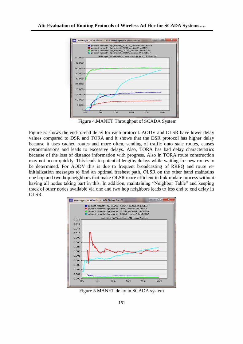
Ali: Evaluation of Routing Protocols of Wireless Ad Hoc for SCADA Systems….
313
Figure 4.MANET Throughput of SCADA System
Figure 5. shows the end-to-end delay for each protocol. AODV and OLSR have lower delay
values compared to DSR and TORA and it shows that the DSR protocol has higher delay
because it uses cached routes and more often, sending of traffic onto stale routes, causes
retransmissions and leads to excessive delays. Also, TORA has bad delay characteristics
because of the loss of distance information with progress. Also in TORA route construction
may not occur quickly. This leads to potential lengthy delays while waiting for new routes to
be determined. For AODV this is due to frequent broadcasting of RREQ and route re-
initialization messages to find an optimal freshest path. OLSR on the other hand maintains
one hop and two hop neighbors that make OLSR more efficient in link update process without
having all nodes taking part in this. In addition, maintaining “Neighbor Table” and keeping
track of other nodes available via one and two hop neighbors leads to less end to end delay in
OLSR.
Figure 5.MANET delay in SCADA system
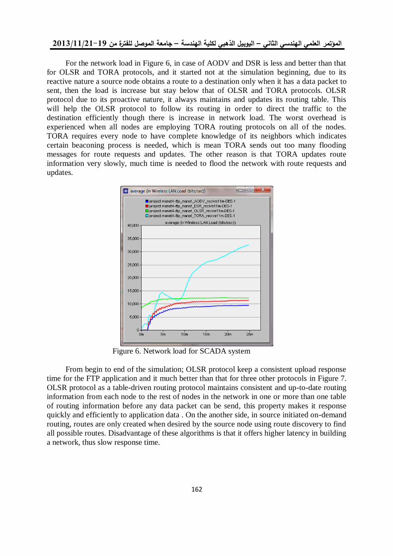
19/99/1192-91جامعة الموصل للفترة من –ليوبيل الذهبي لكلية الهندسة ا –العلمي الهندسي الثاني المؤتمر
311
For the network load in Figure 6, in case of AODV and DSR is less and better than that
for OLSR and TORA protocols, and it started not at the simulation beginning, due to its
reactive nature a source node obtains a route to a destination only when it has a data packet to
sent, then the load is increase but stay below that of OLSR and TORA protocols. OLSR
protocol due to its proactive nature, it always maintains and updates its routing table. This
will help the OLSR protocol to follow its routing in order to direct the traffic to the
destination efficiently though there is increase in network load. The worst overhead is
experienced when all nodes are employing TORA routing protocols on all of the nodes.
TORA requires every node to have complete knowledge of its neighbors which indicates
certain beaconing process is needed, which is mean TORA sends out too many flooding
messages for route requests and updates. The other reason is that TORA updates route
information very slowly, much time is needed to flood the network with route requests and
updates.
Figure 6. Network load for SCADA system
From begin to end of the simulation; OLSR protocol keep a consistent upload response
time for the FTP application and it much better than that for three other protocols in Figure 7.
OLSR protocol as a table-driven routing protocol maintains consistent and up-to-date routing
information from each node to the rest of nodes in the network in one or more than one table
of routing information before any data packet can be send, this property makes it response
quickly and efficiently to application data . On the another side, in source initiated on-demand
routing, routes are only created when desired by the source node using route discovery to find
all possible routes. Disadvantage of these algorithms is that it offers higher latency in building
a network, thus slow response time.
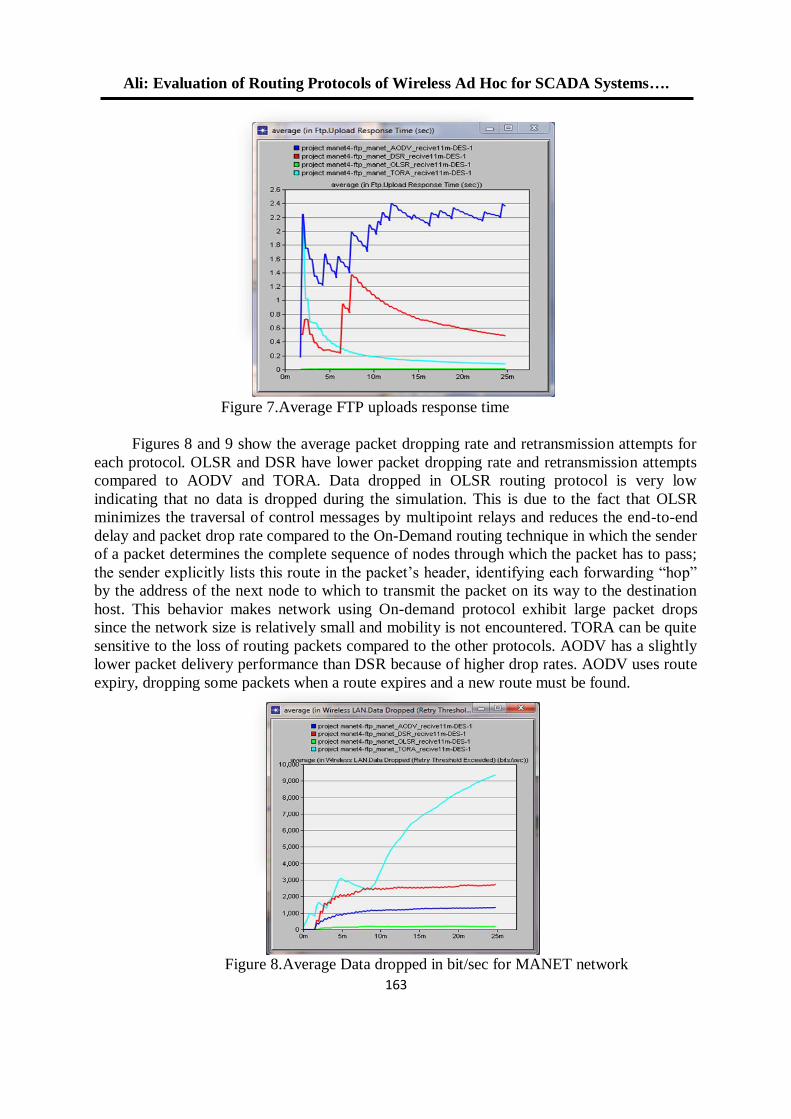
Ali: Evaluation of Routing Protocols of Wireless Ad Hoc for SCADA Systems….
311
Figure 7.Average FTP uploads response time
Figures 8 and 9 show the average packet dropping rate and retransmission attempts for
each protocol. OLSR and DSR have lower packet dropping rate and retransmission attempts
compared to AODV and TORA. Data dropped in OLSR routing protocol is very low
indicating that no data is dropped during the simulation. This is due to the fact that OLSR
minimizes the traversal of control messages by multipoint relays and reduces the end-to-end
delay and packet drop rate compared to the On-Demand routing technique in which the sender
of a packet determines the complete sequence of nodes through which the packet has to pass;
the sender explicitly lists this route in the packet’s header, identifying each forwarding “hop”
by the address of the next node to which to transmit the packet on its way to the destination
host. This behavior makes network using On-demand protocol exhibit large packet drops
since the network size is relatively small and mobility is not encountered. TORA can be quite
sensitive to the loss of routing packets compared to the other protocols. AODV has a slightly
lower packet delivery performance than DSR because of higher drop rates. AODV uses route
expiry, dropping some packets when a route expires and a new route must be found.
Figure 8.Average Data dropped in bit/sec for MANET network
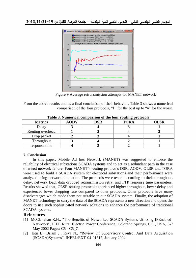
19/99/1192-91جامعة الموصل للفترة من –ليوبيل الذهبي لكلية الهندسة ا –العلمي الهندسي الثاني المؤتمر
311
Figure 9.Average retransmission attempts for MANET network
From the above results and as a final conclusion of their behavior, Table 3 shows a numerical
comparison of the four protocols, “1” for the best up to “4” for the worst.
Table 3. Numerical comparison of the four routing protocols
Metrics AODV DSR TORA OLSR
Delay 3 4 3 1
Routing overhead 1 2 4 3
Drop packet 2 3 4 1
Throughput 3 4 2 1
response time 4 3 2 1
7. Conclusion
In this paper, Mobile Ad hoc Network (MANET) was suggested to enforce the
reliability of electrical substations SCADA systems and to act as a redundant path in the case
of wired network failure. Four MANET’s routing protocols DSR, AODV, OLSR and TORA
were used to build a SCADA system for electrical substations and their performance were
analyzed using network simulation. The protocols were tested according to their throughput,
delay, network load; data dropped retransmission retry, and FTP response time parameters.
Results showed that, OLSR routing protocol experienced higher throughput, lower delay and
experienced lower dropping rate compared to other protocols. Other protocols have many
disadvantages which made them not suitable in our SCADA system. Finally, the adoption of
MANET technology to carry the data of the SCADA represents a new direction and opens the
doors to use such sophisticated network solutions to enhance the performance of traditional
SCADA systems.
References [1] McClanahan R.H., "The Benefits of Networked SCADA Systems Utilizing IPEnabled
Networks", IEEE Rural Electric Power Conference, Colorado Springs, CO , USA, 5-7
May 2002 Pages: C5 - C5_7.
[2] Ken B., Briam J., Reva N., “Review Of Supervisory Control And Data Acquisition
(SCADA)Systems”, INEEL/EXT-04-01517, January 2004.
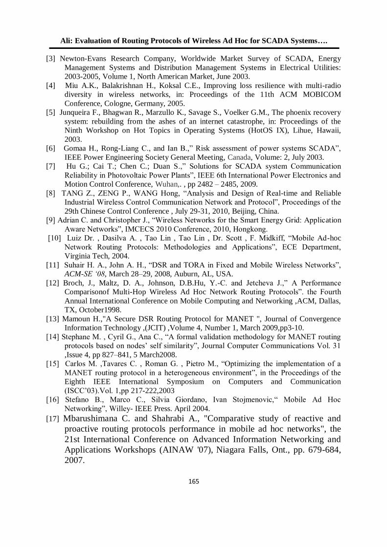
Ali: Evaluation of Routing Protocols of Wireless Ad Hoc for SCADA Systems….
315
[3] Newton-Evans Research Company, Worldwide Market Survey of SCADA, Energy
Management Systems and Distribution Management Systems in Electrical Utilities:
2003-2005, Volume 1, North American Market, June 2003.
[4] Miu A.K., Balakrishnan H., Koksal C.E., Improving loss resilience with multi-radio
diversity in wireless networks, in: Proceedings of the 11th ACM MOBICOM
Conference, Cologne, Germany, 2005.
[5] Junqueira F., Bhagwan R., Marzullo K., Savage S., Voelker G.M., The phoenix recovery
system: rebuilding from the ashes of an internet catastrophe, in: Proceedings of the
Ninth Workshop on Hot Topics in Operating Systems (HotOS IX), Lihue, Hawaii,
2003.
[6] Gomaa H., Rong-Liang C., and Ian B.,” Risk assessment of power systems SCADA”,
IEEE Power Engineering Society General Meeting, Canada, Volume: 2, July 2003.
[7] Hu G.; Cai T.; Chen C.; Duan S.,” Solutions for SCADA system Communication
Reliability in Photovoltaic Power Plants”, IEEE 6th International Power Electronics and
Motion Control Conference, Wuhan,. , pp 2482 – 2485, 2009.
[8] TANG Z., ZENG P., WANG Hong, “Analysis and Design of Real-time and Reliable
Industrial Wireless Control Communication Network and Protocol”, Proceedings of the
29th Chinese Control Conference , July 29-31, 2010, Beijing, China.
[9] Adrian C. and Christopher J., “Wireless Networks for the Smart Energy Grid: Application
Aware Networks”, IMCECS 2010 Conference, 2010, Hongkong.
[10] Luiz Dr. , Dasilva A. , Tao Lin , Tao Lin , Dr. Scott , F. Midkiff, “Mobile Ad-hoc
Network Routing Protocols: Methodologies and Applications”, ECE Department,
Virginia Tech, 2004.
[11] Suhair H. A., John A. H., “DSR and TORA in Fixed and Mobile Wireless Networks”,
ACM-SE ‘08, March 28–29, 2008, Auburn, AL, USA.
[12] Broch, J., Maltz, D. A., Johnson, D.B.Hu, Y.-C. and Jetcheva J.,” A Performance
Comparisonof Multi-Hop Wireless Ad Hoc Network Routing Protocols”. the Fourth
Annual International Conference on Mobile Computing and Networking ,ACM, Dallas,
TX, October1998.
[13] Mamoun H.,"A Secure DSR Routing Protocol for MANET ", Journal of Convergence
Information Technology ,(JCIT) ,Volume 4, Number 1, March 2009,pp3-10.
[14] Stephane M. , Cyril G., Ana C., “A formal validation methodology for MANET routing
protocols based on nodes’ self similarity”, Journal Computer Communications Vol. 31
,Issue 4, pp 827–841, 5 March2008.
[15] Carlos M. ,Tavares C. , Roman G. , Pietro M., “Optimizing the implementation of a
MANET routing protocol in a heterogeneous environment”, in the Proceedings of the
Eighth IEEE International Symposium on Computers and Communication
(ISCC’03).Vol. 1,pp 217-222,2003
[16] Stefano B., Marco C., Silvia Giordano, Ivan Stojmenovic,“ Mobile Ad Hoc
Networking”, Willey- IEEE Press. April 2004.
[17] Mbarushimana C. and Shahrabi A., "Comparative study of reactive and
proactive routing protocols performance in mobile ad hoc networks", the
21st International Conference on Advanced Information Networking and
Applications Workshops (AINAW '07), Niagara Falls, Ont., pp. 679-684,
2007.
19/99/1192-91جامعة الموصل للفترة من –ليوبيل الذهبي لكلية الهندسة ا –العلمي الهندسي الثاني المؤتمر
611
A Simulation Study of Different TCP Flavors in Embedded
Systems Qutaiba Ibrahem Ali Duha Abduljabbar Abed
[email protected] [email protected]
Computer Engineering Department, Collage of Engineering, University of Mosul, Iraq.
Abstract TCP is the most used transport protocol in Internet. Algorithms like Slow Start,
Congestion Avoidance, Fast Retransmit and Fast Recovery are the basis for different
TCP flavors. Tahoe, SACK ,Reno and New Reno are TCP versions that use these
algorithms. With the rapid growth of the Internet, the interest for connecting small
devices such as embedded system appliances into an existing network infrastructure has
increased, where the embedded system is a federation structure of computer hardware
with software infrastructure, and perhaps find some mechanical parts and other
additives .Any embedded system consists of the following units (CPU, memory, the
timing units, analog signals to digital signals converter units, Units show results, The
units send and receive information). Such devices often have very limited CPU and
memory resources. This paper focuses on different TCP flavors which are used in
embedded systems and choose which of them given faster response and best CPU
utilization. Several simulations have been run with OPNET in order to acquire a better
understanding of these flavors and the way they perform their functions.
Key words: embedded system, Ftp, New Reno, Opnet, SACK Tahoe, TCP.
المطمورة دراسة باسلوب المحاكاة النماط بروتوكول التحكم بالنقل في االنظمة
عبد جبارالضحى عبد قتيبة ابراهيم عليد.
العراق. –قسم هندسة الحاسوب/ كلية الهندسة / جامعة الموصل
المستخلص
الخوارزمييا مثيل البدا ية البطي يةن تجنيد االزدويا و , هواألكثر استخداما فيي اننترني TCP بروتوكول التحكم بالنقل
Tahoe, SACK ,New مختلفية. TCP رسال السير عة واوارزميية االنتعياس السير عة هيي سيات لنكهيا إعادة إال
Reno إصيدارا TCP مي النميو السير لرنترني ن ازداد االهتميا ليربز األجهي ة . التيي تسيتخد هيال الخوارزمييا
ويي تكيوه هياا النظيا مين اتحياد البنيية الصغيرة مثل جه ة نظا مضمن)مطمور( إلى البنية التحتيية للبيبكة الحالييةن
العتاد ة للحاسد م البنية البرمجية ن واودة من اهم اصائص هال النظم هي تخ نها على ذاكرة ثابتة والقييا بوييفية
واودة في الغالد. تكوه ي نظا مطمور من الوودا التالية )وودة المعالجة المرك ةن والااكرةن ووويدا اار((هيال
في نظا TCP رك هاا البح على مختلف النكها لبروتوكول التحكم بالنقل . جه ة االبا ماتكوه ذا موارد محددة األ
بوق قليل نسبيا و تحقق االستغالل االمثل لوودة المعالجة المرك ة. نج عملية نقل الملفا مضمن وااتيار التي سوف ت
من جل الحصول على فهم فضل لهال النكها والطر قة التي تؤدي OPNET تم تبغيل العد د من عمليا المحاكاة م
ويائفها.
Ali: A Simulation Study of Different TCP Flavors in Embedded Systems
611
1-Introduction
Unlike personal computers that run a variety of applications, embedded systems are designed
for performing specific tasks. An embedded system used in a device (for instance the
embedded system in washing machine that is used to cycle through the various states of the
washing machine) is programmed by the designers of the system and generally cannot be
programmed by the end user. Embedded systems possess the following distinguishing
One qualities Reliability, Responsiveness ,Specialized Hardware, Low cost, Robustness [1].
of the characteristics of embedded systems they are stored on the memory fixed and doing
g units(CPU, memory, The one job mostly . Any embedded system consists of the followin
Units show results, The units analog signals to digital signals converter units,timing units,
based -Microcontroller Examples of Embedded systems are[2]. send and receive information)
single or multi-display digital panel meter (for voltage, current, resistance).,Robots,
Peripheral controllers, Biomedical systems, industrial process controller ,Mobile Smart
Phones and Computing systems , Embedded systems for wireless LAN and convergent
technology devices[3].
2-TCP/IP stack
TCP is the embodiment of reliable end-to-end transmission functionality in the overall
Internet architecture. All the functionality required to take a simple base of IP datagram
delivery and build upon this a control model that implements reliability, sequencing, flow
control, and data streaming is embedded within TCP [4]. TCP provides a communication
channel between processes on each host system . The channel is reliable, full-duplex, and
streaming. To achieve this functionality, the TCP drivers break up the session data stream into
discrete segments, and attach a TCP header to each segment. An IP header is attached to this
TCP packet, and the composite packet is then passed to the network for delivery. This TCP
header has numerous fields that are used to support the intended TCP functionality. TCP has
the following functional characteristics[5]:
Unicast protocol : TCP does not support broadcast or multicast network models. Connection
state : Rather than impose a state within the network to support the connection, TCP uses
synchronized state between the two endpoints.
Reliable : Reliability implies that the stream of octets passed to the TCP driver at one
end of the connection will be transmitted across the network so that the stream is presented to
the remote process as the same sequence of octets, in the same order as that generated by the
sender.
Full duplex : TCP is a full-duplex protocol; it allows both parties to send and receive
data within the context of the single TCP connection.
Streaming : Although TCP uses a packet structure for network transmission, TCP is a
true streaming protocol, and application-level network operations are not transparent. Some
protocols explicitly encapsulate each application transaction; for every write , there must be a
matching read . In this manner, the application-derived segmentation of the data stream into a
logical record structure is preserved across the network. TCP does not preserve such an
implicit structure imposed on the data stream, so that there is no pairing between write and
read operations within the network protocol.
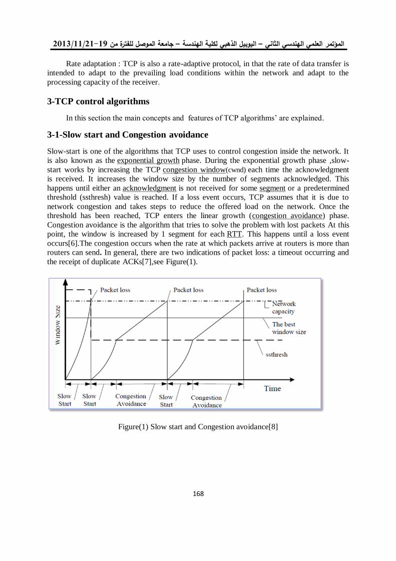
19/99/1192-91جامعة الموصل للفترة من –ليوبيل الذهبي لكلية الهندسة ا –العلمي الهندسي الثاني المؤتمر
611
Rate adaptation : TCP is also a rate-adaptive protocol, in that the rate of data transfer is
intended to adapt to the prevailing load conditions within the network and adapt to the
processing capacity of the receiver.
3-TCP control algorithms
In this section the main concepts and features of TCP algorithms’ are explained.
3-1-Slow start and Congestion avoidance
Slow-start is one of the algorithms that TCP uses to control congestion inside the network. It
is also known as the exponential growth phase. During the exponential growth phase ,slow-
start works by increasing the TCP congestion window(cwnd) each time the acknowledgment
is received. It increases the window size by the number of segments acknowledged. This
happens until either an acknowledgment is not received for some segment or a predetermined
threshold (ssthresh) value is reached. If a loss event occurs, TCP assumes that it is due to
network congestion and takes steps to reduce the offered load on the network. Once the
threshold has been reached, TCP enters the linear growth (congestion avoidance) phase.
Congestion avoidance is the algorithm that tries to solve the problem with lost packets At this
point, the window is increased by 1 segment for each RTT. This happens until a loss event
occurs[6].The congestion occurs when the rate at which packets arrive at routers is more than
routers can send. In general, there are two indications of packet loss: a timeout occurring and
the receipt of duplicate ACKs[7],see Figure(1).
Figure(1) Slow start and Congestion avoidance[8]
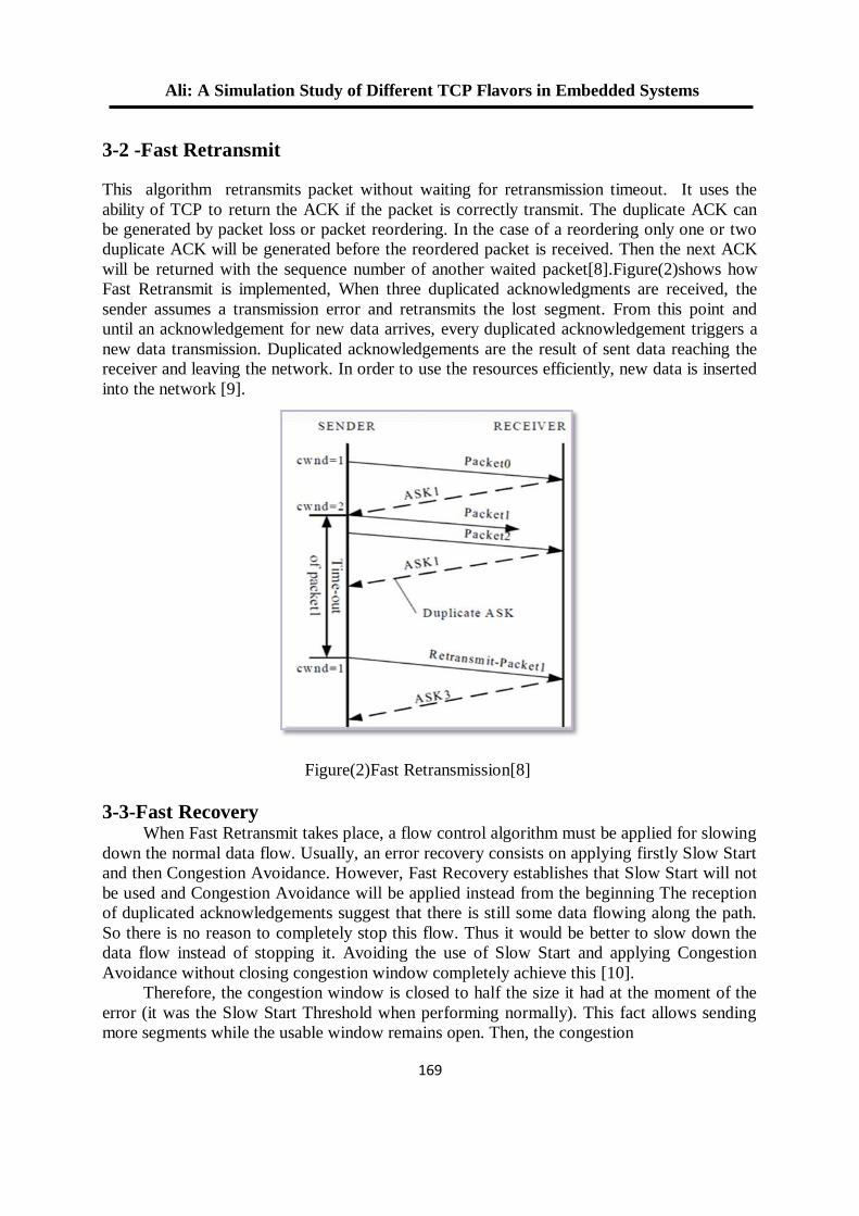
Ali: A Simulation Study of Different TCP Flavors in Embedded Systems
611
3-2 -Fast Retransmit
This algorithm retransmits packet without waiting for retransmission timeout. It uses the
ability of TCP to return the ACK if the packet is correctly transmit. The duplicate ACK can
be generated by packet loss or packet reordering. In the case of a reordering only one or two
duplicate ACK will be generated before the reordered packet is received. Then the next ACK
will be returned with the sequence number of another waited packet[8].Figure(2)shows how
Fast Retransmit is implemented, When three duplicated acknowledgments are received, the
sender assumes a transmission error and retransmits the lost segment. From this point and
until an acknowledgement for new data arrives, every duplicated acknowledgement triggers a
new data transmission. Duplicated acknowledgements are the result of sent data reaching the
receiver and leaving the network. In order to use the resources efficiently, new data is inserted
into the network [9].
Figure(2)Fast Retransmission[8]
3-3-Fast Recovery When Fast Retransmit takes place, a flow control algorithm must be applied for slowing
down the normal data flow. Usually, an error recovery consists on applying firstly Slow Start
and then Congestion Avoidance. However, Fast Recovery establishes that Slow Start will not
be used and Congestion Avoidance will be applied instead from the beginning The reception
of duplicated acknowledgements suggest that there is still some data flowing along the path.
So there is no reason to completely stop this flow. Thus it would be better to slow down the
data flow instead of stopping it. Avoiding the use of Slow Start and applying Congestion
Avoidance without closing congestion window completely achieve this [10].
Therefore, the congestion window is closed to half the size it had at the moment of the
error (it was the Slow Start Threshold when performing normally). This fact allows sending
more segments while the usable window remains open. Then, the congestion
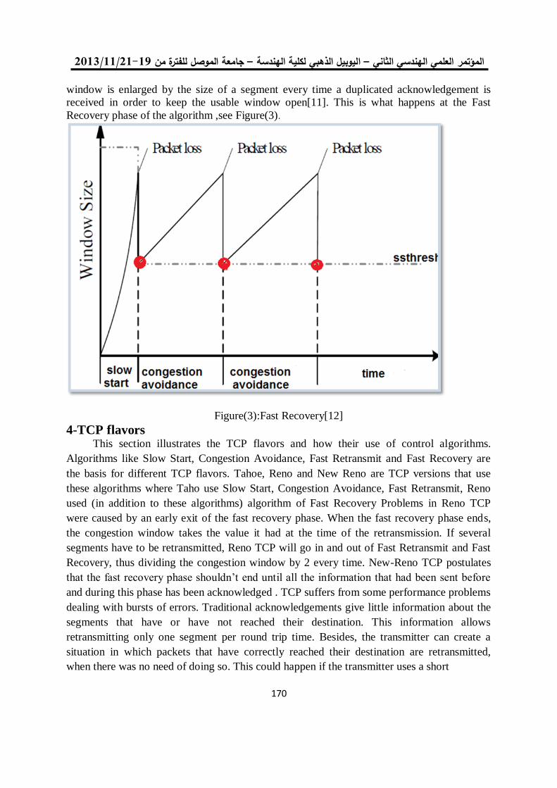
19/99/1192-91جامعة الموصل للفترة من –ليوبيل الذهبي لكلية الهندسة ا –العلمي الهندسي الثاني المؤتمر
611
window is enlarged by the size of a segment every time a duplicated acknowledgement is
received in order to keep the usable window open[11]. This is what happens at the Fast
Recovery phase of the algorithm ,see Figure(3).
Figure(3):Fast Recovery[12]
4-TCP flavors This section illustrates the TCP flavors and how their use of control algorithms.
Algorithms like Slow Start, Congestion Avoidance, Fast Retransmit and Fast Recovery are
the basis for different TCP flavors. Tahoe, Reno and New Reno are TCP versions that use
these algorithms where Taho use Slow Start, Congestion Avoidance, Fast Retransmit, Reno
used (in addition to these algorithms) algorithm of Fast Recovery Problems in Reno TCP
were caused by an early exit of the fast recovery phase. When the fast recovery phase ends,
the congestion window takes the value it had at the time of the retransmission. If several
segments have to be retransmitted, Reno TCP will go in and out of Fast Retransmit and Fast
Recovery, thus dividing the congestion window by 2 every time. New-Reno TCP postulates
that the fast recovery phase shouldn’t end until all the information that had been sent before
and during this phase has been acknowledged . TCP suffers from some performance problems
dealing with bursts of errors. Traditional acknowledgements give little information about the
segments that have or have not reached their destination. This information allows
retransmitting only one segment per round trip time. Besides, the transmitter can create a
situation in which packets that have correctly reached their destination are retransmitted,
when there was no need of doing so. This could happen if the transmitter uses a short
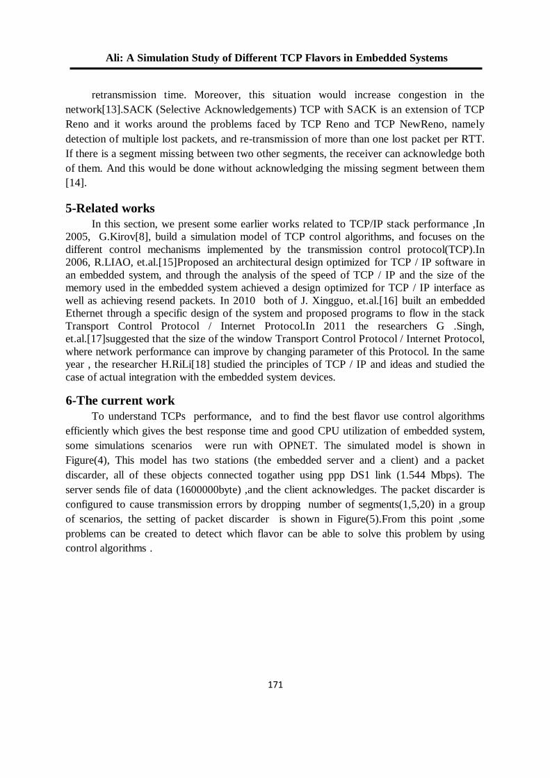
Ali: A Simulation Study of Different TCP Flavors in Embedded Systems
616
retransmission time. Moreover, this situation would increase congestion in the
network[13].SACK (Selective Acknowledgements) TCP with SACK is an extension of TCP
Reno and it works around the problems faced by TCP Reno and TCP NewReno, namely
detection of multiple lost packets, and re-transmission of more than one lost packet per RTT.
If there is a segment missing between two other segments, the receiver can acknowledge both
of them. And this would be done without acknowledging the missing segment between them
[14].
5-Related works
In this section, we present some earlier works related to TCP/IP stack performance ,In
2005, G.Kirov[8], build a simulation model of TCP control algorithms, and focuses on the
different control mechanisms implemented by the transmission control protocol(TCP).In
2006, R.LIAO, et.al.[15]Proposed an architectural design optimized for TCP / IP software in
an embedded system, and through the analysis of the speed of TCP / IP and the size of the
memory used in the embedded system achieved a design optimized for TCP / IP interface as
well as achieving resend packets. In 2010 both of J. Xingguo, et.al.[16] built an embedded
Ethernet through a specific design of the system and proposed programs to flow in the stack
Transport Control Protocol / Internet Protocol.In 2011 the researchers G .Singh,
et.al.[17]suggested that the size of the window Transport Control Protocol / Internet Protocol,
where network performance can improve by changing parameter of this Protocol. In the same
year , the researcher H.RiLi[18] studied the principles of TCP / IP and ideas and studied the
case of actual integration with the embedded system devices.
6-The current work
To understand TCPs performance, and to find the best flavor use control algorithms
efficiently which gives the best response time and good CPU utilization of embedded system,
some simulations scenarios were run with OPNET. The simulated model is shown in
Figure(4), This model has two stations (the embedded server and a client) and a packet
discarder, all of these objects connected togather using ppp DS1 link (1.544 Mbps). The
server sends file of data (1600000byte) ,and the client acknowledges. The packet discarder is
configured to cause transmission errors by dropping number of segments(1,5,20) in a group
of scenarios, the setting of packet discarder is shown in Figure(5).From this point ,some
problems can be created to detect which flavor can be able to solve this problem by using
control algorithms .
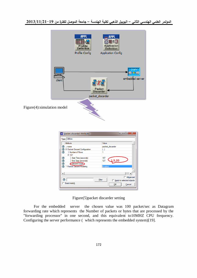
19/99/1192-91جامعة الموصل للفترة من –ليوبيل الذهبي لكلية الهندسة ا –العلمي الهندسي الثاني المؤتمر
611
Figure(4):simulation model
Figure(5)packet discarder setting
For the embedded server the chosen value was 100 packet/sec as Datagram
forwarding rate which represents the Number of packets or bytes that are processed by the
"forwarding processor" in one second, and this equivalent to10MHZ CPU frequency.
Configuring the server performance ( which represents the embedded system)[19].
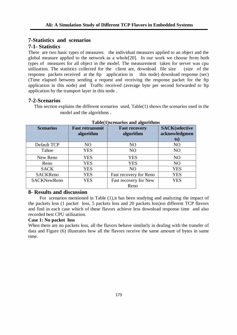
Ali: A Simulation Study of Different TCP Flavors in Embedded Systems
611
7-Statistics and scenarios
7-1- Statistics There are two basic types of measures: the individual measures applied to an object and the
global measure applied to the network as a whole[20]. In our work we choose from both
types of measures for all object in the model. The measurement taken for server was cpu
utilization. The statistics collected for the client are, download file size (size of the
response packets received at the ftp application in this node) download response (sec)
(Time elapsed between sending a request and receiving the response packet for the ftp
application in this node) and Traffic received (average byte per second forwarded to ftp
application by the transport layer in this node .
7-2-Scenarios This section explains the different scenarios used, Table(1) shows the scenarios used in the
model and the algorithms .
Table(1)scenarios and algorithms
Scenarios Fast retransmit
algorithm
Fast recovery
algorithm
SACK(selective
acknowledgmen
ts)
Default TCP NO NO NO
Tahoe YES NO NO
New Reno YES YES NO
Reno YES YES NO
SACK YES NO YES
SACKReno YES Fast recovery for Reno YES
SACKNewReno YES Fast recovery for New
Reno
YES
8- Results and discussion For scenarios mentioned in Table (1),it has been studying and analyzing the impact of
the packets loss (1 packet loss, 5 packets loss and 20 packets loss)on different TCP flavors
and find in each case which of these flavors achieve less download response time and also
recorded best CPU utilization.
Case 1: No packet loss
When there are no packets loss, all the flavors behave similarly in dealing with the transfer of
data and Figure (6) illustrates how all the flavors receive the same amount of bytes in same
time.
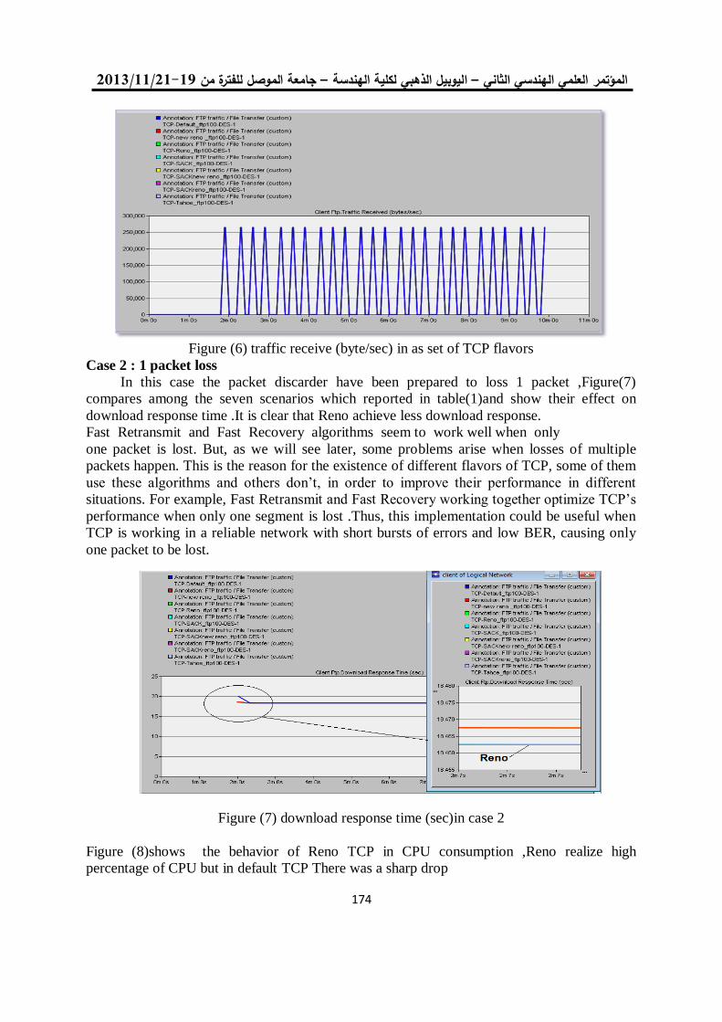
19/99/1192-91جامعة الموصل للفترة من –ليوبيل الذهبي لكلية الهندسة ا –العلمي الهندسي الثاني المؤتمر
611
Figure (6) traffic receive (byte/sec) in as set of TCP flavors
Case 2 : 1 packet loss
In this case the packet discarder have been prepared to loss 1 packet ,Figure(7)
compares among the seven scenarios which reported in table(1)and show their effect on
download response time .It is clear that Reno achieve less download response.
Fast Retransmit and Fast Recovery algorithms seem to work well when only
one packet is lost. But, as we will see later, some problems arise when losses of multiple
packets happen. This is the reason for the existence of different flavors of TCP, some of them
use these algorithms and others don’t, in order to improve their performance in different
situations. For example, Fast Retransmit and Fast Recovery working together optimize TCP’s
performance when only one segment is lost .Thus, this implementation could be useful when
TCP is working in a reliable network with short bursts of errors and low BER, causing only
one packet to be lost.
Figure (7) download response time (sec)in case 2
Figure (8)shows the behavior of Reno TCP in CPU consumption ,Reno realize high
percentage of CPU but in default TCP There was a sharp drop
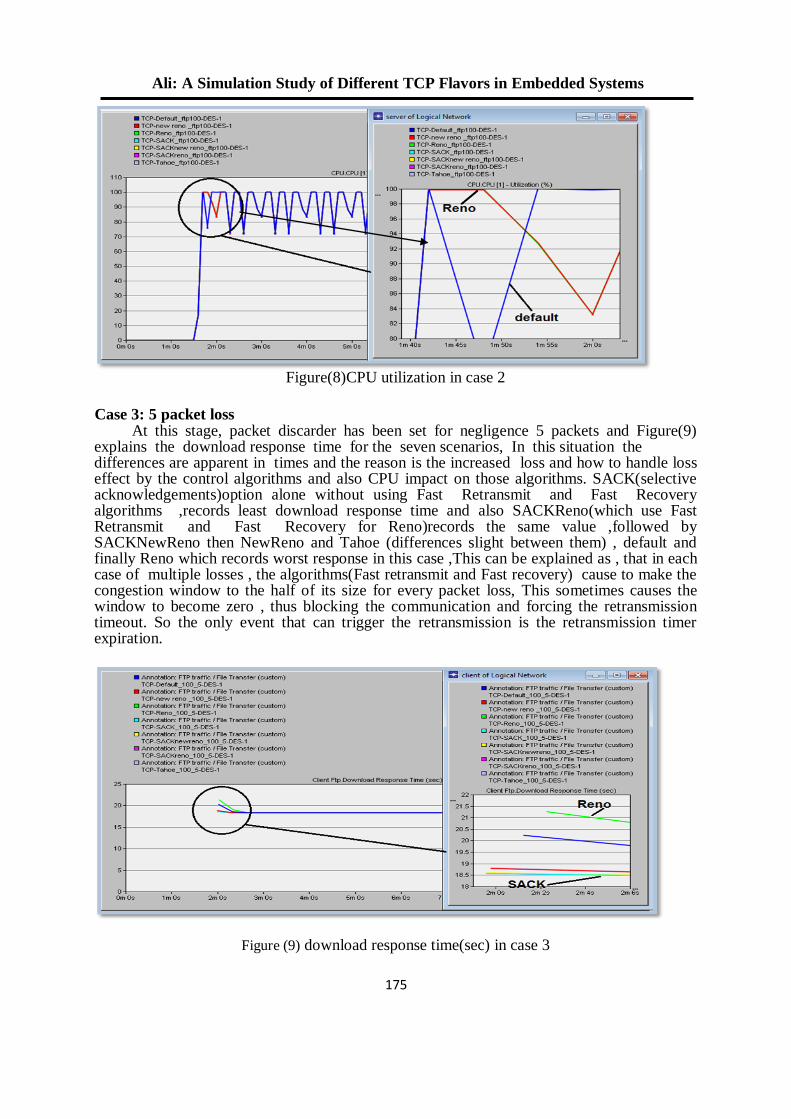
Ali: A Simulation Study of Different TCP Flavors in Embedded Systems
611
Figure(8)CPU utilization in case 2
Case 3: 5 packet loss At this stage, packet discarder has been set for negligence 5 packets and Figure(9)
explains the download response time for the seven scenarios, In this situation the differences are apparent in times and the reason is the increased loss and how to handle loss effect by the control algorithms and also CPU impact on those algorithms. SACK(selective acknowledgements)option alone without using Fast Retransmit and Fast Recovery algorithms ,records least download response time and also SACKReno(which use Fast Retransmit and Fast Recovery for Reno)records the same value ,followed by SACKNewReno then NewReno and Tahoe (differences slight between them) , default and finally Reno which records worst response in this case ,This can be explained as , that in each case of multiple losses , the algorithms(Fast retransmit and Fast recovery) cause to make the congestion window to the half of its size for every packet loss, This sometimes causes the window to become zero , thus blocking the communication and forcing the retransmission timeout. So the only event that can trigger the retransmission is the retransmission timer expiration.
Figure (9) download response time(sec) in case 3
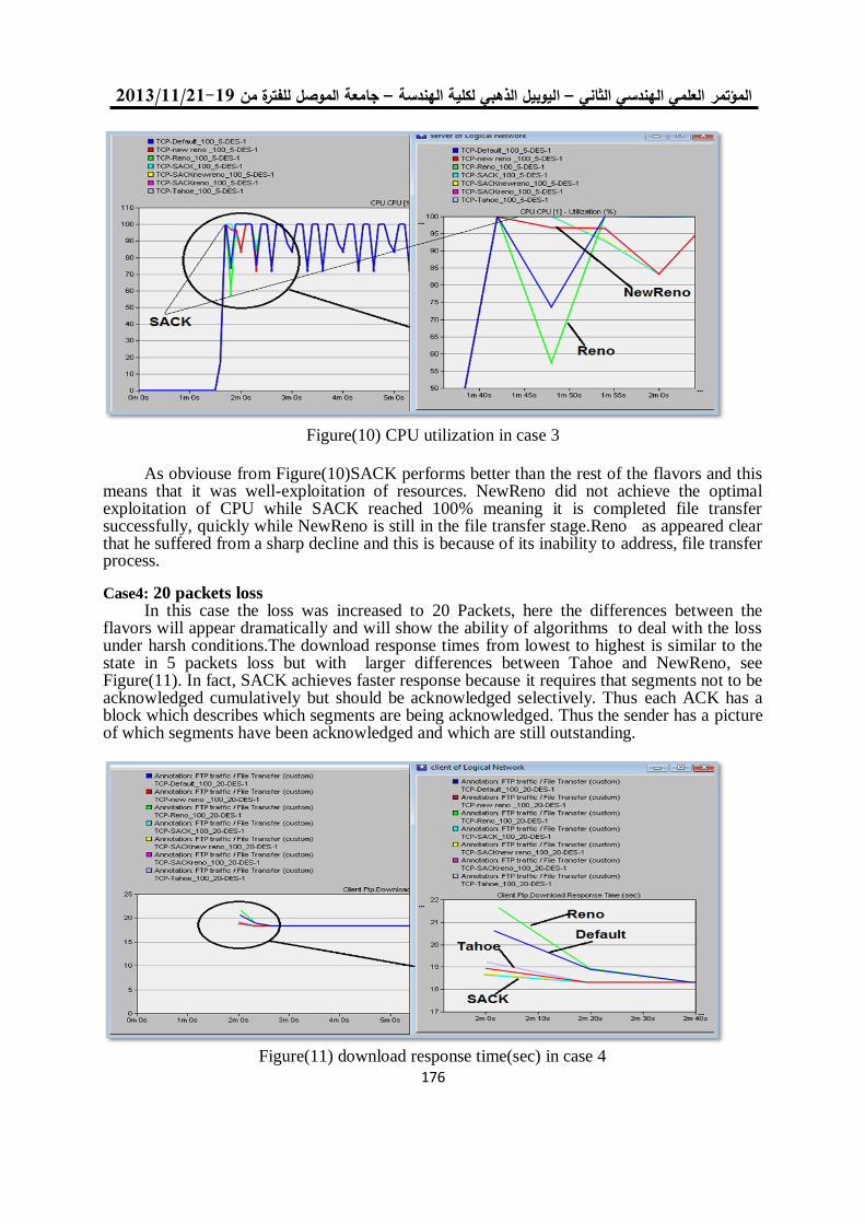
19/99/1192-91جامعة الموصل للفترة من –ليوبيل الذهبي لكلية الهندسة ا –العلمي الهندسي الثاني المؤتمر
611
Figure(10) CPU utilization in case 3
As obviouse from Figure(10)SACK performs better than the rest of the flavors and this
means that it was well-exploitation of resources. NewReno did not achieve the optimal exploitation of CPU while SACK reached 100% meaning it is completed file transfer successfully, quickly while NewReno is still in the file transfer stage.Reno as appeared clear that he suffered from a sharp decline and this is because of its inability to address, file transfer process.
Case4: 20 packets loss In this case the loss was increased to 20 Packets, here the differences between the
flavors will appear dramatically and will show the ability of algorithms to deal with the loss under harsh conditions.The download response times from lowest to highest is similar to the state in 5 packets loss but with larger differences between Tahoe and NewReno, see Figure(11). In fact, SACK achieves faster response because it requires that segments not to be acknowledged cumulatively but should be acknowledged selectively. Thus each ACK has a block which describes which segments are being acknowledged. Thus the sender has a picture of which segments have been acknowledged and which are still outstanding.
Figure(11) download response time(sec) in case 4
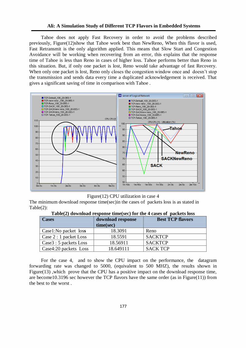
Ali: A Simulation Study of Different TCP Flavors in Embedded Systems
611
Tahoe does not apply Fast Recovery in order to avoid the problems described
previously, Figure(12)show that Tahoe work best than NewReno, When this flavor is used,
Fast Retransmit is the only algorithm applied. This means that Slow Start and Congestion
Avoidance will be working when recovering from an error, this explains that the response
time of Tahoe is less than Reno in cases of higher loss. Tahoe performs better than Reno in
this situation. But, if only one packet is lost, Reno would take advantage of fast Recovery.
When only one packet is lost, Reno only closes the congestion window once and doesn’t stop
the transmission and sends data every time a duplicated acknowledgement is received. That
gives a significant saving of time in comparison with Tahoe .
Figure(12) CPU utilization in case 4
The minimum download response time(sec)in the cases of packets loss is as stated in
Table(2):
Table(2) download response time(sec) for the 4 cases of packets loss
Cases download response
time(sec)
Best TCP flavors
Case1:No packet loss 18.3091 Reno
Case 2 : 1 packet Loss 18.5591 SACKTCP
Case3 : 5 packets Loss 18.56911 SACKTCP
Case4:20 packets Loss 18.649111 SACK TCP
For the case 4, and to show the CPU impact on the performance, the datagram
forwarding rate was changed to 5000, (equivalent to 500 MHZ), the results shown in
Figure(13) ,which prove that the CPU has a positive impact on the download response time,
are become10.3196 sec however the TCP flavors have the same order (as in Figure(11)) from
the best to the worst .
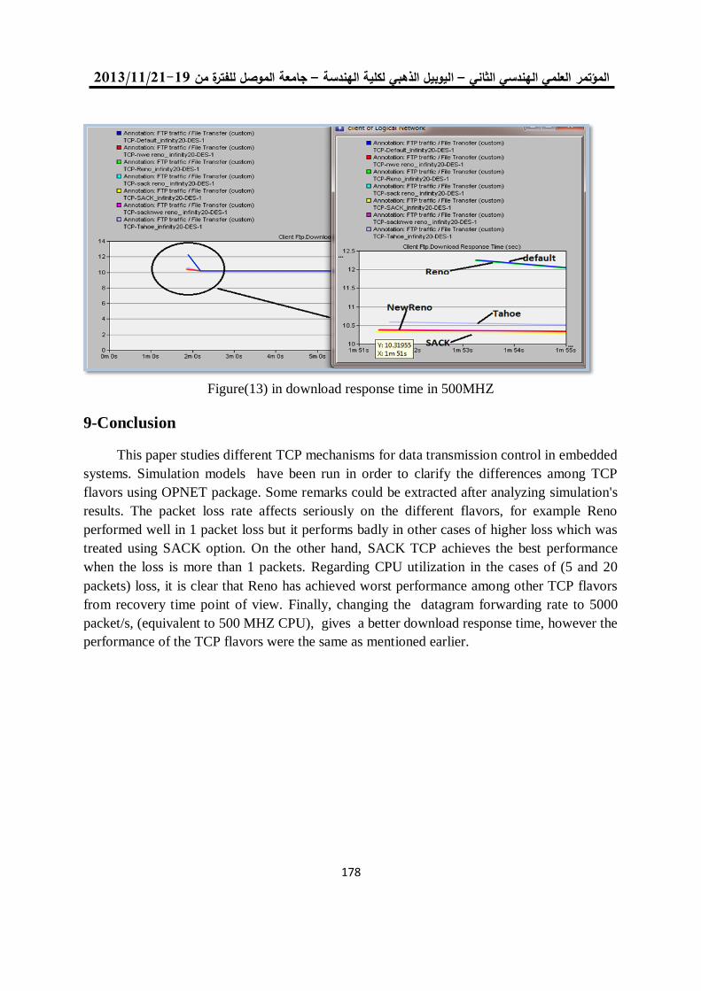
19/99/1192-91جامعة الموصل للفترة من –ليوبيل الذهبي لكلية الهندسة ا –العلمي الهندسي الثاني المؤتمر
611
Figure(13) in download response time in 500MHZ
9-Conclusion
This paper studies different TCP mechanisms for data transmission control in embedded
systems. Simulation models have been run in order to clarify the differences among TCP
flavors using OPNET package. Some remarks could be extracted after analyzing simulation's
results. The packet loss rate affects seriously on the different flavors, for example Reno
performed well in 1 packet loss but it performs badly in other cases of higher loss which was
treated using SACK option. On the other hand, SACK TCP achieves the best performance
when the loss is more than 1 packets. Regarding CPU utilization in the cases of (5 and 20
packets) loss, it is clear that Reno has achieved worst performance among other TCP flavors
from recovery time point of view. Finally, changing the datagram forwarding rate to 5000
packet/s, (equivalent to 500 MHZ CPU), gives a better download response time, however the
performance of the TCP flavors were the same as mentioned earlier.
Ali: A Simulation Study of Different TCP Flavors in Embedded Systems
611
10-References
1-P. Reddy," Embedded Systems", Resonance Inc., December 2002, pp. 20-23.
2-I.Ahmad," Fuzzy logic for embedded systems applications" ,Newnes Inc., 2003,pp.2-3.
3- K.Raj ,"Embedded Systems - Architecture, Programming and Design" ,Tata McGraw-Hill
Education,2008,pp.27-30.
4- G. Huston, Telstra," TCP Performance", The Internet Protocol Journal, Volume 3, No. 2,
2000.
5-L.parziale,J.forrester,"TCP/IP tutorial and technical overview",IBM Inc,2006,pp.150-152.
6- M. Borden, "A study of active queue management for congestion control," in Proc. IEEE
INFOCOM, March 2000.
7-V.Jacobson, "Congestion Avoidance and Control", SIGCOMM conf(ACM),vol 18,no 4
,1988,pp.314-329.
8-G. Kirov," A Simulation Analysis of the TCP Control Algorithms", International
Conference on Computer Systems and Technologies – Comp Sys Tech’, 2005.
9- W. Stevens ,“TCP Slow Start, Congestion Avoidance, Fast Retransmit and Fast Recovery
Algorithms”, 1997, [RFC2001].
10-G. Corral, A. Zaballos," Simulation-based study of TCP flow control mechanisms
using OPNET Modeler", algorithms journal, vol 2,2005,pp.4-7.
11-F.Copaciu,B.moraru,"Practical analysis of TCP implementations: Tahoe, Reno,
NewReno",RoEduNet International Conference ,vol 1,2003,pp.125-138.
12- L. Subedi, M.Najiminaini, L.Trajkovi" , Performance Evaluation of TCP Tahoe, Reno,
Reno with SACK, and NewReno Using OPNET Modeler", OPNET Technologies Inc, 2008.
13-M. Mathis, J. Mahdavi, S. Floyd, " TCP Selective Acknowledgement
Options", RFC 2018, IETF, October 1996.
14-S. Floyd, "Issues of TCP with SACK", citeseer Inc. , Mar. 1996.
15-R.Liao, Y.Ji, H.Li," Optimized design and implementation of TCP/IP software
architecture based on embedded system", International Conference on Machine Learning and
Cybernetics ,2006.
16- J. Xingguo, Q.Yulin, Y. Jiancheng,"A method to streamline the TCP/IP Protocol Stack at
embedded systems", Information Science and Management Engineering (ISME),vol 1,2010.
17-G.Singh , J.Singh," Performance Evaluation and Optimization of TCP Parameters over
Frame Relay", International Journal on Computer Science and Engineering (IJCSE), Vol. 3
No. 10 October 2011
18- H.RiLi ," Research and Application of TCP/IP Protocol in Embedded System",
Communication Software and Networks (ICCSN) Conference ,2011,pp.584-587.
19- Q. I. Ali,” An Efficient Simulation Methodology Of Networked Industrial Devices” ,IEEE
SSD08 Conference, Jordan, 2008.
20-Q.ibrahim,I.khudher,"network simulation guide",Lap Inc,2011.
.
19/99/1192-91جامعة الموصل للفترة من –ليوبيل الذهبي لكلية الهندسة ا –العلمي الهندسي الثاني المؤتمر
081
Investigation of Ipv4 to Ipv6 Transition Mechanisms for Mosul
University Network
Abdul-Bary Raouf Suleiman Fadi Ahmed Jassim Assistant Professor MSc Student
College of Electronics Eng. College of Engineering
University of Mosul University of Mosul
[email protected] [email protected]
Abstract Due to the rapid growth of the Internet, the IPv4 address space will be depleted in
the end of 2013. To overcome this limitation, a new alternative version of Internet
Protocol has been invented that is called the Next Generation of Internet Protocol or
simply (IPv6). In order to solve the packet header incompatibility problem between IPv4
and IPv6 at the migration time, RFC defines the following types of transition
mechanisms: Dual Stack, Tunneling, and Translation. As a higher educational
environment, the University of Mosul network have to be transited to the new version in
the near future. In this paper, the dual stack and the tunneling mechanism have been
investigated to be applied for Mosul university network. The study is carried out using
OPNET Modeler simulator and applying services such as internet connectivity, internal
HTTP and E-mail browsing, database access, and video conference. The best mechanism
to be used is selected by considering the topology of the university network and by
evaluating the end to end delay, throughput, video delay, video delay variation, and
CPU utilization. The results give preference to the dual stack to be used when it is
possible and 6-to-4 tunnel when it is necessary.
Keywords: 6-to-4, Dual Stack, IPv4, IPv6, OPNET, Simulation, Tunnel.
فحص آليات األنتقال من اإلصدار الرابع الى اإلصدار السادس لشبكة جامعة الموصل
عبد الباري رؤوف سليماند. *
فادي أحمد جاسم **
العراق. –/ جامعة الموصل األلكترونيات هندسة/ كلية والمعلوماتية * قسم هندسة الحاسوب
العراق. –امعة الموصل / كلية الهندسة/ جحاسوبهندسة ال** قسم
الملخص
على الرغم من العدد الكبير من العناوين التي يدعمها بروتوكول االنترنت االصدار الرابع، اال ان هذا العدد قد ينفذ
نتيجة للعدد المتزايد من االجهزة على االنترنت. ذلك ما ادى الى ايجاد بروتوكول بديل 3102بحلول نهاية هذا العام
وكول االنترنت االصدار السادس. حيث ان عملية التحول الى االصدار الجديد لن تكون مباشرة نتيجة لعدم عـرف ببروت
التوافق بين صيغ الحزم لهذين االصدارين، لذلك تم تحديد عدد من الطرق التي من شأنها تسهيل عملية االنتقال والتي
شبكة جامعة الموصل باعتبارها بيئة تعليم وذلك يحتم علىTranslation. و Tunnelingو Dual Stackتشمل
و Dual Stackعالي التحول الى االصدار الجديد في المستقبل القريب. في هذا البحث قمنا بتطبيق طريقتي
Tunneling على شبكة جامعة الموصل باستخدام برنامج المحاكاةOPNET Modeler مع تفعيل الخدمات التي
نت وخدمة منتدى الجامعة الداخلي والبريد االلكتروني الداخلي وقواعد البيانات والمؤتمرات تقدمها الشبكة كخدمات االنتر
الفيديوية، ومن ثم ايجاد افضل الية للتطبيق اعتمادا على طوبولوجية شبكة الجامعة اضافة الى عدة معطيات. وقد ادت
كأنسب بديل. 6to4كون متاحة والية كأفضل الية للتطبيق عندما ت Dual Stackاالختبارات الى ترشيح طريقة
Suleiman: Investigation of Ipv4 to Ipv6 Transition Mechanisms …..
080
I. Introduction With the rapid growth of the Internet, the 4.2 billion address space of 32-bit IPv4 has
been exhausted due to the increasing in the number of devices on the internet. To overcome
this problem of depletion, a number of solutions are suggested. One of the solutions was the
Classless Inter-Domain Routing (CIDR) which is a method to decrease the growth of routing
tables within the internet and the exhaustion of IPv4 addresses consequently. Another solution
was the using of Network Address Translation (NAT) in which one network device assigns a
public address to computers inside a private network. The third solution is the using of
automatic addressing (DHCP). These three techniques did not solve the address exhaustion
problem, but only delayed it [1]. Unfortunately, in February 2011, IANA's pool of IPv4
addresses was depleted [2], and the expected depletion date for IPv4 address is the end of
2013. Hence, the IPv6 addresses will have to be assigned [3]. IPv6 has 128-bit address length
which provides up to 2128
or 3 x 1038
IP addresses. Moreover, there are many other
advantages of IPv6 compared to IPv4 such as auto-configuration and renumbering, new
datagram format, better support for quality of service, better security support, mobility
features, and modernized routing support [4]. Generally, the transition to IPv6 for Mosul
University network will permit to make use of all services and advantages involved in this
version for this network.
With this trend, major Internet Service Providers (ISPs), networking equipment
manufacturers (Cisco, D-link, ...etc.), and web companies (Google, Yahoo, ... etc.) around the
world enabled IPv6 for their products and services on the 6th of June 2012, which is called
World IPv6 Launch Day [5]. After enabling IPv6, some networks will be using IPv4 and
others using IPv6. For communication to be successful, a mechanism needs to be defined in
order to solve the packet header incompatibility problem between IPv4 and IPv6 at the
migration time. So that, the following types of transition mechanisms are defined: Dual Stack,
Tunneling, and Translation [6].
II. Related Work Number of papers have been published in this field. Yao-Chung Chang, Reen-Cheng
Wang, Han-Chieh Chao, and Jiann-Liang Chen determined the data delivery efficiency of 6to4 tunnel, configured tunnel, and tunnel broker mechanisms in a real network [7]. V. Visoottiviseth and N. Bureenok, performed a comparison between different popular operating systems such as Windows 2003, FreeBSD 5.3, and RedHat 9.0 when the ISATAP tunneling mechanism is applied. The test results gave preference to RedHat 9.0 followed by FreeBSD 5.3 and then Windows 2003 [8]. D. Shalini Punithavathani and K. Sankaranarayanan presented configured tunnels, 6to4 tunneling, and tunnel broker transition mechanisms in different networks. The 6to4 showed better performance in latency and throughput than those of the configured tunnel and tunnel broker mechanisms. In the contrary, 6to4 mechanism had greater overhead, than the other two mechanisms, which required higher CPU utilization in the border router [6]. Sh. Narayan, S. Tauch measured the performance of configured tunnel and 6to4 tunneling in MS Windows Server 2003 and MS Windows Server 2008 [9]. The researchers M. Aazam, I. Khan, M. Alam, and A. Qayyum implemented two tunneling mechanisms; Teredo and ISATAP on real testbed consisting of five to six devices running Microsoft Windows (MS Windows XP and MS Windows Server 2003) and Linux operating systems [10]. M. Adeel, M. Syed, S. Hussain Shah, I. Khan, and M. Alam, addressed 6to4 and ISATAP tunneling mechanisms [11]. N. Bahaman, Anton Satria Prabuwono, R. Alsaqour, and M. Zaki Mas`ud experimented the performance of Tunneling Mechanism and then compared them with native IPv4 and IPv6 [12]. Se-Joon Yoon, Jong-Tak Park, Dae-In Choi, and Hyun K. Kahng wrote a paper concentrated on an experimental work based on Linux
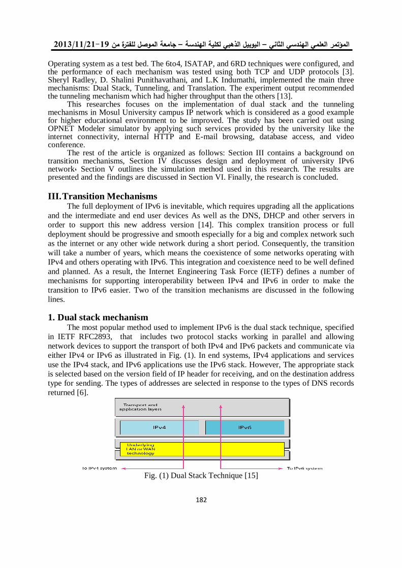
19/99/1192-91جامعة الموصل للفترة من –ليوبيل الذهبي لكلية الهندسة ا –العلمي الهندسي الثاني المؤتمر
081
Operating system as a test bed. The 6to4, ISATAP, and 6RD techniques were configured, and the performance of each mechanism was tested using both TCP and UDP protocols [3]. Sheryl Radley, D. Shalini Punithavathani, and L.K Indumathi, implemented the main three mechanisms: Dual Stack, Tunneling, and Translation. The experiment output recommended the tunneling mechanism which had higher throughput than the others [13].
This researches focuses on the implementation of dual stack and the tunneling mechanisms in Mosul University campus IP network which is considered as a good example for higher educational environment to be improved. The study has been carried out using OPNET Modeler simulator by applying such services provided by the university like the internet connectivity, internal HTTP and E-mail browsing, database access, and video conference.
The rest of the article is organized as follows: Section III contains a background on transition mechanisms, Section IV discusses design and deployment of university IPv6 network, Section V outlines the simulation method used in this research. The results are presented and the findings are discussed in Section VI. Finally, the research is concluded.
III. Transition Mechanisms The full deployment of IPv6 is inevitable, which requires upgrading all the applications
and the intermediate and end user devices As well as the DNS, DHCP and other servers in
order to support this new address version [14]. This complex transition process or full
deployment should be progressive and smooth especially for a big and complex network such
as the internet or any other wide network during a short period. Consequently, the transition
will take a number of years, which means the coexistence of some networks operating with
IPv4 and others operating with IPv6. This integration and coexistence need to be well defined
and planned. As a result, the Internet Engineering Task Force (IETF) defines a number of
mechanisms for supporting interoperability between IPv4 and IPv6 in order to make the
transition to IPv6 easier. Two of the transition mechanisms are discussed in the following
lines.
1. Dual stack mechanism The most popular method used to implement IPv6 is the dual stack technique, specified
in IETF RFC2893, that includes two protocol stacks working in parallel and allowing
network devices to support the transport of both IPv4 and IPv6 packets and communicate via
either IPv4 or IPv6 as illustrated in Fig. (1). In end systems, IPv4 applications and services
use the IPv4 stack, and IPv6 applications use the IPv6 stack. However, The appropriate stack
is selected based on the version field of IP header for receiving, and on the destination address
type for sending. The types of addresses are selected in response to the types of DNS records
returned [6].
Fig. (1) Dual Stack Technique [15]
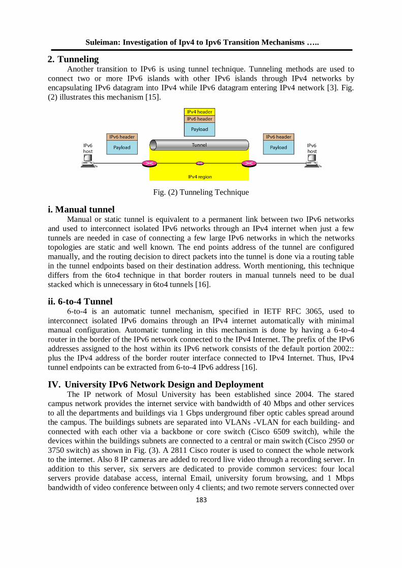
Suleiman: Investigation of Ipv4 to Ipv6 Transition Mechanisms …..
081
2. Tunneling Another transition to IPv6 is using tunnel technique. Tunneling methods are used to
connect two or more IPv6 islands with other IPv6 islands through IPv4 networks by
encapsulating IPv6 datagram into IPv4 while IPv6 datagram entering IPv4 network [3]. Fig.
(2) illustrates this mechanism [15].
Fig. (2) Tunneling Technique
i. Manual tunnel Manual or static tunnel is equivalent to a permanent link between two IPv6 networks
and used to interconnect isolated IPv6 networks through an IPv4 internet when just a few
tunnels are needed in case of connecting a few large IPv6 networks in which the networks
topologies are static and well known. The end points address of the tunnel are configured
manually, and the routing decision to direct packets into the tunnel is done via a routing table
in the tunnel endpoints based on their destination address. Worth mentioning, this technique
differs from the 6to4 technique in that border routers in manual tunnels need to be dual
stacked which is unnecessary in 6to4 tunnels [16].
ii. 6-to-4 Tunnel 6-to-4 is an automatic tunnel mechanism, specified in IETF RFC 3065, used to
interconnect isolated IPv6 domains through an IPv4 internet automatically with minimal
manual configuration. Automatic tunneling in this mechanism is done by having a 6-to-4
router in the border of the IPv6 network connected to the IPv4 Internet. The prefix of the IPv6
addresses assigned to the host within its IPv6 network consists of the default portion 2002::
plus the IPv4 address of the border router interface connected to IPv4 Internet. Thus, IPv4
tunnel endpoints can be extracted from 6-to-4 IPv6 address [16].
IV. University IPv6 Network Design and Deployment The IP network of Mosul University has been established since 2004. The stared
campus network provides the internet service with bandwidth of 40 Mbps and other services
to all the departments and buildings via 1 Gbps underground fiber optic cables spread around
the campus. The buildings subnets are separated into VLANs -VLAN for each building- and
connected with each other via a backbone or core switch (Cisco 6509 switch), while the
devices within the buildings subnets are connected to a central or main switch (Cisco 2950 or
3750 switch) as shown in Fig. (3). A 2811 Cisco router is used to connect the whole network
to the internet. Also 8 IP cameras are added to record live video through a recording server. In
addition to this server, six servers are dedicated to provide common services: four local
servers provide database access, internal Email, university forum browsing, and 1 Mbps
bandwidth of video conference between only 4 clients; and two remote servers connected over
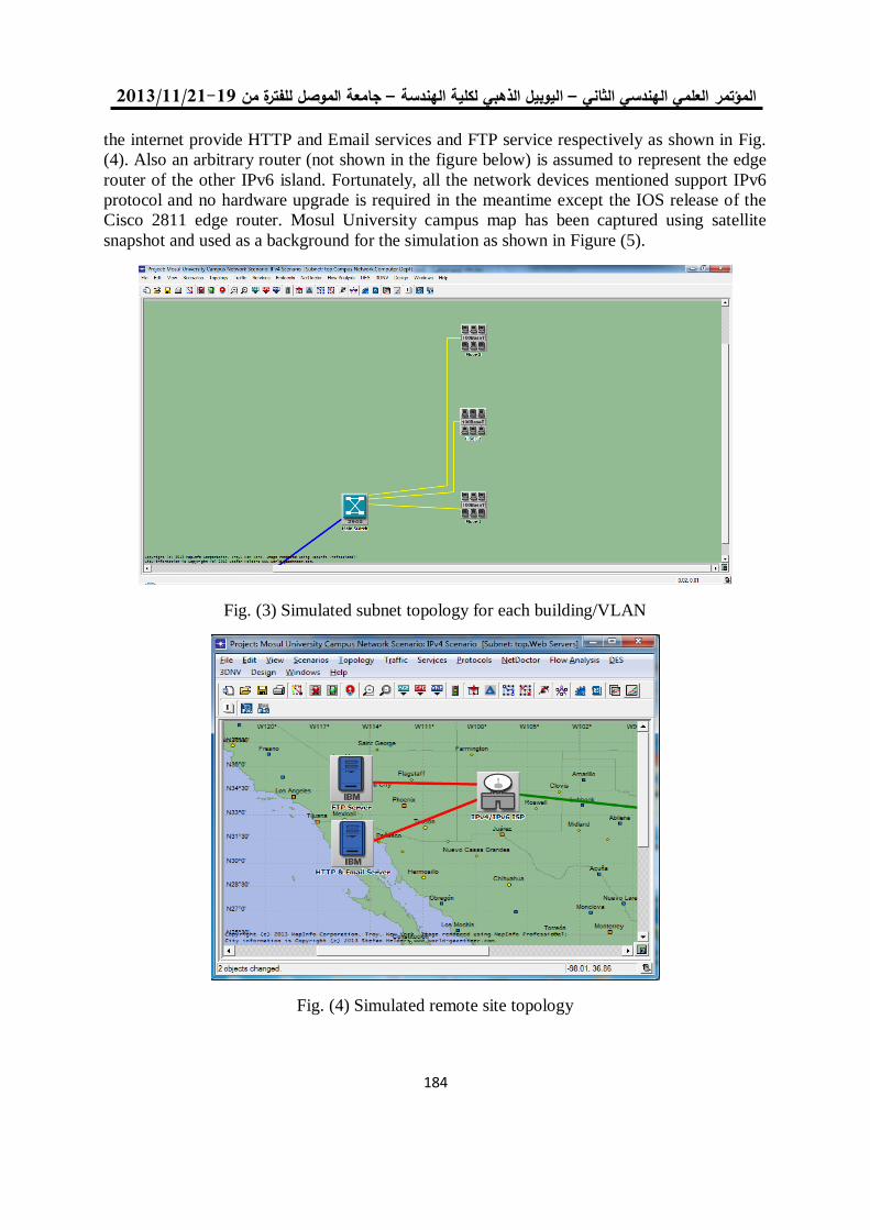
19/99/1192-91جامعة الموصل للفترة من –ليوبيل الذهبي لكلية الهندسة ا –العلمي الهندسي الثاني المؤتمر
081
the internet provide HTTP and Email services and FTP service respectively as shown in Fig.
(4). Also an arbitrary router (not shown in the figure below) is assumed to represent the edge
router of the other IPv6 island. Fortunately, all the network devices mentioned support IPv6
protocol and no hardware upgrade is required in the meantime except the IOS release of the
Cisco 2811 edge router. Mosul University campus map has been captured using satellite
snapshot and used as a background for the simulation as shown in Figure (5).
Fig. (3) Simulated subnet topology for each building/VLAN
Fig. (4) Simulated remote site topology
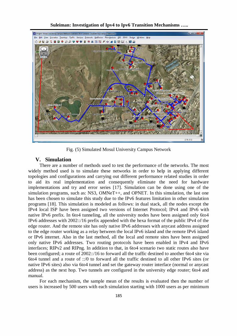
Suleiman: Investigation of Ipv4 to Ipv6 Transition Mechanisms …..
081
Fig. (5) Simulated Mosul University Campus Network
V. Simulation There are a number of methods used to test the performance of the networks. The most
widely method used is to simulate these networks in order to help in applying different
topologies and configurations and carrying out different performance related studies in order
to aid its real implementation and consequently eliminate the need for hardware
implementations and try and error series [17]. Simulation can be done using one of the
simulation programs, such as: NS3, OMNeT++, and OPNET. In this simulation, the last one
has been chosen to simulate this study due to the IPv6 features limitation in other simulation
programs [18]. This simulation is modeled as follows: in dual stack, all the nodes except the
IPv4 local ISP have been assigned two versions of Internet Protocol; IPv4 and IPv6 with
native IPv6 prefix. In 6to4 tunneling, all the university nodes have been assigned only 6to4
IPv6 addresses with 2002::/16 prefix appended with the hexa format of the public IPv4 of the
edge router. And the remote site has only native IPv6 addresses with anycast address assigned
to the edge router working as a relay between the local IPv6 island and the remote IPv6 island
or IPv6 internet. Also in the last method, all the local and remote sites have been assigned
only native IPv6 addresses. Two routing protocols have been enabled in IPv4 and IPv6
interfaces; RIPv2 and RIPng. In addition to that, in 6to4 scenario two static routes also have
been configured; a route of 2002::/16 to forward all the traffic destined to another 6to4 site via
6to4 tunnel and a route of ::/0 to forward all the traffic destined to all other IPv6 sites (or
native IPv6 sites) also via 6to4 tunnel and set the gateway router interface (normal or anycast
address) as the next hop. Two tunnels are configured in the university edge router; 6to4 and
manual.
For each mechanism, the sample mean of the results is evaluated then the number of
users is increased by 500 users with each simulation starting with 1000 users as per minimum
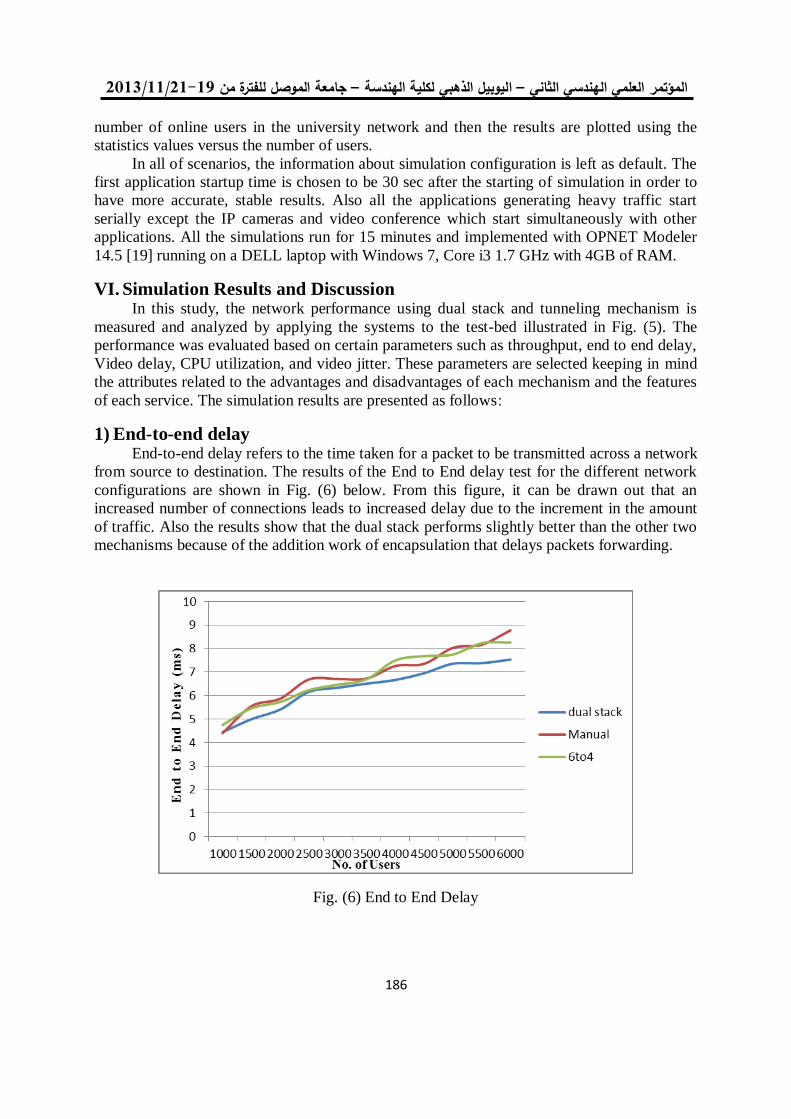
19/99/1192-91جامعة الموصل للفترة من –ليوبيل الذهبي لكلية الهندسة ا –العلمي الهندسي الثاني المؤتمر
081
number of online users in the university network and then the results are plotted using the
statistics values versus the number of users.
In all of scenarios, the information about simulation configuration is left as default. The
first application startup time is chosen to be 30 sec after the starting of simulation in order to
have more accurate, stable results. Also all the applications generating heavy traffic start
serially except the IP cameras and video conference which start simultaneously with other
applications. All the simulations run for 15 minutes and implemented with OPNET Modeler
14.5 [19] running on a DELL laptop with Windows 7, Core i3 1.7 GHz with 4GB of RAM.
VI. Simulation Results and Discussion In this study, the network performance using dual stack and tunneling mechanism is
measured and analyzed by applying the systems to the test-bed illustrated in Fig. (5). The
performance was evaluated based on certain parameters such as throughput, end to end delay,
Video delay, CPU utilization, and video jitter. These parameters are selected keeping in mind
the attributes related to the advantages and disadvantages of each mechanism and the features
of each service. The simulation results are presented as follows:
1) End-to-end delay End-to-end delay refers to the time taken for a packet to be transmitted across a network
from source to destination. The results of the End to End delay test for the different network
configurations are shown in Fig. (6) below. From this figure, it can be drawn out that an
increased number of connections leads to increased delay due to the increment in the amount
of traffic. Also the results show that the dual stack performs slightly better than the other two
mechanisms because of the addition work of encapsulation that delays packets forwarding.
Fig. (6) End to End Delay
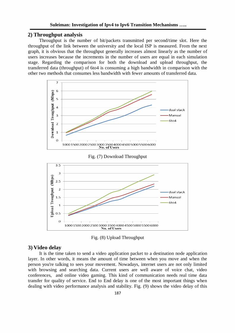
Suleiman: Investigation of Ipv4 to Ipv6 Transition Mechanisms …..
081
2) Throughput analysis Throughput is the number of bit/packets transmitted per second/time slot. Here the
throughput of the link between the university and the local ISP is measured. From the next
graph, it is obvious that the throughput generally increases almost linearly as the number of
users increases because the increments in the number of users are equal in each simulation
stage. Regarding the comparison for both the download and upload throughput, the
transferred data (throughput) of 6to4 is consuming a high bandwidth in comparison with the
other two methods that consumes less bandwidth with fewer amounts of transferred data.
Fig. (7) Download Throughput
Fig. (8) Upload Throughput
3) Video delay It is the time taken to send a video application packet to a destination node application
layer. In other words, it means the amount of time between when you move and when the
person you're talking to sees your movement. Nowadays, internet users are not only limited
with browsing and searching data. Current users are well aware of voice chat, video
conferences, and online video gaming. This kind of communication needs real time data
transfer for quality of service. End to End delay is one of the most important things when
dealing with video performance analysis and stability. Fig. (9) shows the video delay of this
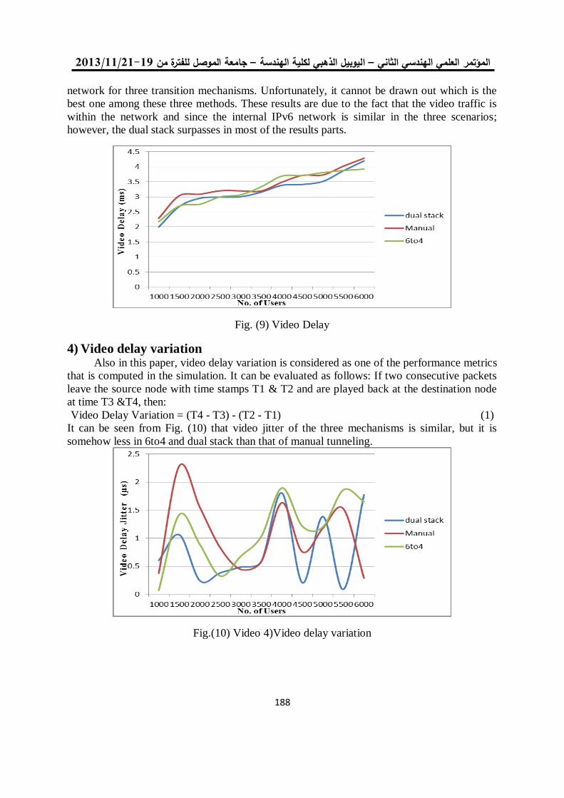
19/99/1192-91جامعة الموصل للفترة من –ليوبيل الذهبي لكلية الهندسة ا –العلمي الهندسي الثاني المؤتمر
088
network for three transition mechanisms. Unfortunately, it cannot be drawn out which is the
best one among these three methods. These results are due to the fact that the video traffic is
within the network and since the internal IPv6 network is similar in the three scenarios;
however, the dual stack surpasses in most of the results parts.
Fig. (9) Video Delay
4) Video delay variation Also in this paper, video delay variation is considered as one of the performance metrics
that is computed in the simulation. It can be evaluated as follows: If two consecutive packets
leave the source node with time stamps T1 & T2 and are played back at the destination node
at time T3 &T4, then:
Video Delay Variation = (T4 - T3) - (T2 - T1) (1)
It can be seen from Fig. (10) that video jitter of the three mechanisms is similar, but it is
somehow less in 6to4 and dual stack than that of manual tunneling.
Fig.(10) Video 4)Video delay variation
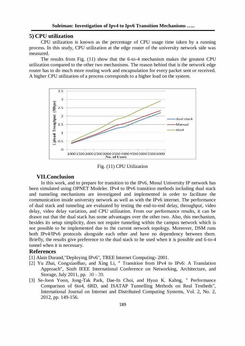
Suleiman: Investigation of Ipv4 to Ipv6 Transition Mechanisms …..
081
5) CPU utilization CPU utilization is known as the percentage of CPU usage time taken by a running
process. In this study, CPU utilization at the edge router of the university network side was
measured.
The results from Fig. (11) show that the 6-to-4 mechanism makes the greatest CPU
utilization compared to the other two mechanisms. The reason behind that is the network edge
router has to do much more routing work and encapsulation for every packet sent or received.
A higher CPU utilization of a process corresponds to a higher load on the system.
Fig. (11) CPU Utilization
VII.Conclusion In this work, and to prepare for transition to the IPv6, Mosul University IP network has
been simulated using OPNET Modeler. IPv4 to IPv6 transition methods including dual stack
and tunneling mechanisms are investigated and implemented in order to facilitate the
communication inside university network as well as with the IPv6 internet. The performance
of dual stack and tunneling are evaluated by testing the end-to-end delay, throughput, video
delay, video delay variation, and CPU utilization. From our performance results, it can be
drawn out that the dual stack has some advantages over the other two. Also, this mechanism,
besides its setup simplicity, does not require tunneling within the campus network which is
not possible to be implemented due to the current network topology. Moreover, DSM runs
both IPv4/IPv6 protocols alongside each other and have no dependency between them.
Briefly, the results give preference to the dual stack to be used when it is possible and 6-to-4
tunnel when it is necessary.
References [1] Alain Durand,"Deploying IPv6", TREE Internet Computing, 2001.
[2] Yu Zhai, CongxiaoBao, and Xing Li, " Transition from IPv4 to IPv6: A Translation
Approach", Sixth IEEE International Conference on Networking, Architecture, and
Storage, July 2011, pp. 30 - 39.
[3] Se-Joon Yoon, Jong-Tak Park, Dae-In Choi, and Hyun K. Kahng, " Performance
Comparison of 6to4, 6RD, and ISATAP Tunnelling Methods on Real Testbeds",
International Journal on Internet and Distributed Computing Systems, Vol. 2, No. 2,
2012, pp. 149-156.
19/99/1192-91جامعة الموصل للفترة من –ليوبيل الذهبي لكلية الهندسة ا –العلمي الهندسي الثاني المؤتمر
011
[4] Aris, Cahyadi, Risdianto, and R. Rumani, "IPv6 Tunnel Broker Implementation and
Analysis for IPv6 and IPv4 Interconnection", The 6th International Conference on
Telecommunication Systems, Services, and Applications, Oct. 2011, pp. 139-144.
[5] World IPv6 Launch, http://www.worldipv6launch.org.
[6] D. Shalini, Punithavathani, K. Sankaranarayanan, "IPv4/IPv6 Transition Mechanisms",
European Journal of Scientific Research, Vol. 34, No. 1, 2009, pp.110-124.
[7] Yao-Chung Chang, Reen-Cheng Wang, Han-Chieh Chao, and Jiann-Liang Chen,
“Performance Investigation of IPv4/IPv6 Transition Mechanisms”, Journal of Internet
Technology, Vol. 5, No. 2, 2004, pp. 163-170.
[8] Vasaka Visoottiviseth and Niwat Bureenok, “Performance Comparison of ISATAP
Implementations on FreeBSD, RedHat, and Windows 2003”, 22nd International
Conference on Advanced Information Networking and Applications, 2008, pp. 547-552.
[9] Shaneel Narayan, Sotharith Tauch, “Network Performance Evaluation of IPv4-v6
Configured Tunnel and 6to4 Transition Mechanisms on Windows Server Operating
Systems”, International Conference On Computer Design And Applications, Vol. 5,
2010, pp. 435-440.
[10] Mohammad Aazam, Imran Khan, Mohammad Alam and Amir Qayyum, "Comparison of
IPv6 Tunneled Traffic of Teredo and ISATAP over Test-bed Setup", IEEE International
Conference of Information and Emerging Technologies, 2010, pp. 1-4.
[11] Mohammad Aazam, Adeel M. Syed, Syed Atif Hussain Shah, Imran Khan, and
Muhammad Alam, “Evaluation of 6to4 and ISATAP on a Test LAN”, IEEE
Symposium on Computers & Informatics, 2011, pp. 46-50.
[12] Nazrulazhar Bahaman, Anton Satria Prabuwono, Raed Alsaqour and Mohd Zaki Mas`ud,
“Network Performance Evaluation of Tunneling Mechanism”, Journal of Applied
Sciences, Vol. 12, No. 5, 2012, pp. 459-465.
[13] Sheryl Radley, D. Shalini Punithavathani, and L.K Indumathi, “Evaluation and Study of
Transition Techniques Addressed on IPv4-IPv6”, International Journal of Computer
Applications, Vol. 66, No. 5, 2013, pp 1-6.
[14] Tim Chown, "IPv6 Campus Transition Experiences", the International Conference on
Software Engineering, 2005, pp. 46-49.
[15] B. A. Forouzan, " Data Communications and Networking ," McGraw-Hill, Fourth
Edition, 2007, pp. 604.
[16] John J. Amoss and Daniel Minoli, "Handbook of IPv4 to IPv6 Transition Methodologies
for Institutional and Corporate Networks", Taylor & Francis Group, LLC, 2008, pp 124
& 129.
[17] Mohammed Basheer and A.I. A. Jabbar, "Towards the Improvement of the Computer
Network of Mosul University Using (OPNET) Software", Al-Rafidain Engineering
Journal, Vol. 15, No. 1, 2007, pp.16-26.
[18] Brittany Clore, Matthew Dunlop, Randolph Marchany, and Joseph Tront,"An Evaluation
of IPv6 in Simulation using OPNET Modeler", The Eighth Advanced International
Conference on Telecommunications, 2012, pp. 111-115.
[19] "OPNET Modeler” [Online] Available: http://www.opnet.com /solutions/ network_rd /
modeler.html.
Abdul-Jabbar: A Fractional Wavelet Transform for Wireless Multimedia …..
191
A Fractional Wavelet Transform for Wireless Multimedia Sensors
With Reduced Boundary Artifacts
Jassim M. Abdul-Jabbar Alyaa Q. Ahmed Taqi Computer Engineering Department Software Engineering Department
College of Engineering College of Computer and arithmetic science
University of Mosul, Mosul, Iraq.
[email protected] [email protected]
Abstract Wavelet-based algorithms are increasingly used for satellite, communication and
network transmission of images. Although wireless multimedia sensors are widely used
to deliver multimedia content, their computational and memory resources are still
limited to perform a multi-level wavelet transform. Recently, fractional wavelet filter
technique became an interesting solution to reduce communication energy and wireless
bandwidth, for resource-constrained devices (e.g. digital cameras), but that is achieved
at the expense of the image quality. In this paper, a modified fractional wavelet
transform is proposed to reduce boundary artifacts caused by fractional segmentations.
The average of the last and first rows of any two overlapped successive fractions is
obtained and located in a single row (first row of the next fraction) at the fraction
boarder. This technique produced a better image quality after image reconstruction.
Applying such technique on different types of images using 9/7 and 5/3 wavelet filters,
results in a promising performance.
Keywords: 2D-DWT, Fractional wavelet, CDF 9/7, VSNs, Blocking artifact.
تحويل مويجي كسوري لمتحسسات الوسائط المتعددة الالسلكية مع تقليل آثار الحدود جاسم محمد عبد الجبارد. علياء قصي أحمد تقي
قسم هندسة الحاسوب قسم هندسة البرامجيات كلية الهندسة كلية علوم الحاسوب والرياضيات
العراق-الموصل-جامعة الموصل[email protected] [email protected]
الخالصةاستخدمت الخوارزميات المعتمدة على التحويل المويجي بشكل كبير في مجال االتصاالت ونقل الصور عبر
ط المتعددة الالسلكية تستخدم بشكل واسع لنقل مكونات الوسائط وبالرغم من أن متحسسات الوسائ شبكات االتصاالت.أصبح التحويل .ة التحويل المويجي بعدة مستوياتالمتعددة، اإل أن لها مصادر ذاكرة وقدرات معالجة محدودة لتنفيذ عملي
سلكية ،لجأجهزة ذات الال الالزمة للحسابات ومدى التردداتلكسوري مؤخرا من الحلول المفيدة لتقليل القدرة االمويجي في هذا البحث اقترحت طريقة . ولكن ذلك سيكون على حساب جودة الصورة،المحدودة مثل الكاميرات الرقمية المصادر
لكسوري لتقليل التأثير ظهور الحافات في مقاطع الصورة الناتج عن عملية التقطيع الكسورية، التحسين للتحويل المويجي .ي أول سطر من إطار المقطع التاليوأول سطر لكل مقطعين متتاليين وتوضع النتيجة فوذلك بحساب معدل آخر سطر
هذه التقنية أدت إلى توليد صورة ذات جودة أفضل للصورة الناتجة من عملية االسترجاع.تائج أدت إلى ن 5/3و 9/7إن تطبيق هذه التقنية على صور بمختلف األنواع وباستخدام مرشحي التحويل المويجي
واعدة.
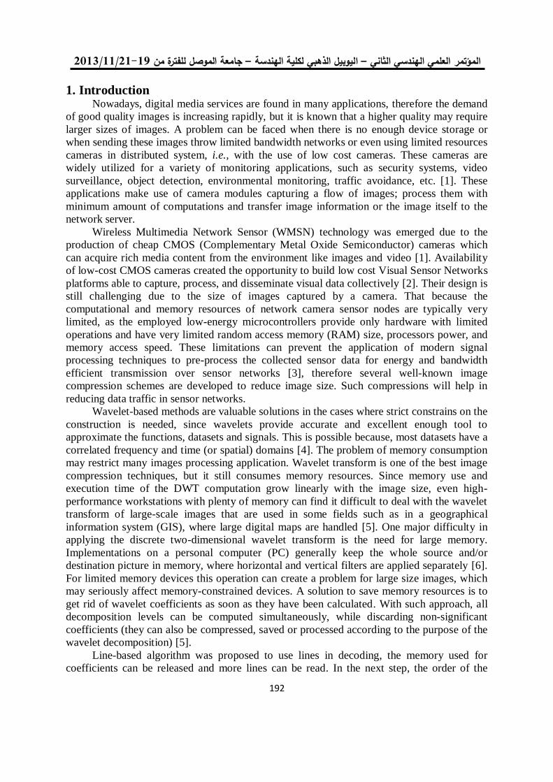
19/99/1192-91جامعة الموصل للفترة من –ليوبيل الذهبي لكلية الهندسة ا –العلمي الهندسي الثاني المؤتمر
191
1. Introduction Nowadays, digital media services are found in many applications, therefore the demand
of good quality images is increasing rapidly, but it is known that a higher quality may require
larger sizes of images. A problem can be faced when there is no enough device storage or
when sending these images throw limited bandwidth networks or even using limited resources
cameras in distributed system, i.e., with the use of low cost cameras. These cameras are
widely utilized for a variety of monitoring applications, such as security systems, video
surveillance, object detection, environmental monitoring, traffic avoidance, etc. [1]. These
applications make use of camera modules capturing a flow of images; process them with
minimum amount of computations and transfer image information or the image itself to the
network server.
Wireless Multimedia Network Sensor (WMSN) technology was emerged due to the
production of cheap CMOS (Complementary Metal Oxide Semiconductor) cameras which
can acquire rich media content from the environment like images and video [1]. Availability
of low-cost CMOS cameras created the opportunity to build low cost Visual Sensor Networks
platforms able to capture, process, and disseminate visual data collectively [2]. Their design is
still challenging due to the size of images captured by a camera. That because the
computational and memory resources of network camera sensor nodes are typically very
limited, as the employed low-energy microcontrollers provide only hardware with limited
operations and have very limited random access memory (RAM) size, processors power, and
memory access speed. These limitations can prevent the application of modern signal
processing techniques to pre-process the collected sensor data for energy and bandwidth
efficient transmission over sensor networks [3], therefore several well-known image
compression schemes are developed to reduce image size. Such compressions will help in
reducing data traffic in sensor networks.
Wavelet-based methods are valuable solutions in the cases where strict constrains on the
construction is needed, since wavelets provide accurate and excellent enough tool to
approximate the functions, datasets and signals. This is possible because, most datasets have a
correlated frequency and time (or spatial) domains [4]. The problem of memory consumption
may restrict many images processing application. Wavelet transform is one of the best image
compression techniques, but it still consumes memory resources. Since memory use and
execution time of the DWT computation grow linearly with the image size, even high-
performance workstations with plenty of memory can find it difficult to deal with the wavelet
transform of large-scale images that are used in some fields such as in a geographical
information system (GIS), where large digital maps are handled [5]. One major difficulty in
applying the discrete two-dimensional wavelet transform is the need for large memory.
Implementations on a personal computer (PC) generally keep the whole source and/or
destination picture in memory, where horizontal and vertical filters are applied separately [6].
For limited memory devices this operation can create a problem for large size images, which
may seriously affect memory-constrained devices. A solution to save memory resources is to
get rid of wavelet coefficients as soon as they have been calculated. With such approach, all
decomposition levels can be computed simultaneously, while discarding non-significant
coefficients (they can also be compressed, saved or processed according to the purpose of the
wavelet decomposition) [5].
Line-based algorithm was proposed to use lines in decoding, the memory used for
coefficients can be released and more lines can be read. In the next step, the order of the
Abdul-Jabbar: A Fractional Wavelet Transform for Wireless Multimedia …..
191
coefficients is rearranged with some extra buffers to allow efficient use of memory in both
encoders [7]. A block-based implementation of the DWT was also used in order to match with
block-based encoders and to reduce the memory usage of the wavelet transform [8]. A general
recursive algorithm was proposed on PC computers in [5] to compute the DWT in a line-
based fashion to reduce memory and cache sizes.
Recently, the fractional wavelet filter was presented by S. Rein and M. Reisslein [3].
Bio 9/7 Wavelet transforms in convolution form and lifting scheme were used on a low-
memory digital sensor. They explained how to compute a fractional wavelet transform with
fixed-point arithmetic. They treated such fractional transform as the basis for its efficient
integer-based computation on a microcontroller.
In this paper, two implementations of three wavelet algorithms (traditional, fractional
and modified fractional) are presented by means of a simple filter bank, using wavelet 9/7 and
5/3 filters. The rest of this paper is arranged as follows: Section 2 contains a brief review of
discrete wavelet transform. Section 3 describes image boundaries problems. In Section 4,
fractional wavelet transform is presented, while Section 5 describes the proposed modified
fractional wavelet transform. In Section 6, some results and discussions are given. Finally,
Section 7 concludes this paper.
2. Discrete Wavelet Transform Discrete Wavelet Transform (DWT) can be viewed as a multi-resolution decomposition
of a signal. In general to perform forward DWT which also called the (analysis) operation, the
set of signal samples is passed through low-pass and high-pass filters by convolution
operation. The output is then down-sampled by factor of two. The down-sampled low-pass
output represents a low-resolution version of the original set that contains its half resolution.
Such down-sampled output will be used to construct the next level. On other hand, the down-
sampled high-pass output represents a residual version of the original set that is needed for the
perfect reconstruction (synthesis) of the original set [9]. Both analysis and synthesis structures
are shown in Figure 1 with L and H as Low pass and High pass decomposing filters,
respectively, L' and H
' as Low pass and High pass reconstructing filters, respectively, S as the
original signal and S' as the reconstructed signal. In this paper, wavelet 9/7 and 5/3 filters are
examined, since they are usually selected as inclusion in the JPEG2000 standard [10]. In the
following two subsections, explanations of these filters are given.
Figure (1): DWT decomposition and reconstruction.
reconstruction
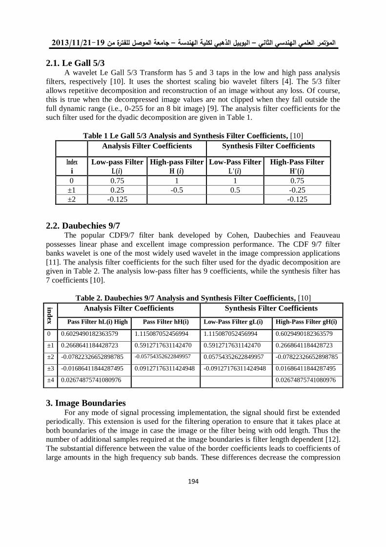
19/99/1192-91جامعة الموصل للفترة من –ليوبيل الذهبي لكلية الهندسة ا –العلمي الهندسي الثاني المؤتمر
191
2.1. Le Gall 5/3 A wavelet Le Gall 5/3 Transform has 5 and 3 taps in the low and high pass analysis
filters, respectively [10]. It uses the shortest scaling bio wavelet filters [4]. The 5/3 filter
allows repetitive decomposition and reconstruction of an image without any loss. Of course,
this is true when the decompressed image values are not clipped when they fall outside the
full dynamic range (i.e., 0-255 for an 8 bit image) [9]. The analysis filter coefficients for the
such filter used for the dyadic decomposition are given in Table 1.
2.2. Daubechies 9/7 The popular CDF9/7 filter bank developed by Cohen, Daubechies and Feauveau
possesses linear phase and excellent image compression performance. The CDF 9/7 filter
banks wavelet is one of the most widely used wavelet in the image compression applications
[11]. The analysis filter coefficients for the such filter used for the dyadic decomposition are
given in Table 2. The analysis low-pass filter has 9 coefficients, while the synthesis filter has
7 coefficients [10].
Table 2. Daubechies 9/7 Analysis and Synthesis Filter Coefficients, [10]
3. Image Boundaries For any mode of signal processing implementation, the signal should first be extended
periodically. This extension is used for the filtering operation to ensure that it takes place at
both boundaries of the image in case the image or the filter being with odd length. Thus the
number of additional samples required at the image boundaries is filter length dependent [12].
The substantial difference between the value of the border coefficients leads to coefficients of
large amounts in the high frequency sub bands. These differences decrease the compression
Table 1 Le Gall 5/3 Analysis and Synthesis Filter Coefficients, [10]
Analysis Filter Coefficients Synthesis Filter Coefficients
Index
i
Low-pass Filter
L( i)
High-pass Filter
H (i)
Low-Pass Filter
L'( i)
High-Pass Filter
H'(i)
0 0.75 1 1 0.75
±1 0.25 -0.5 0.5 -0.25
±2 -0.125 -0.125
ind
ex
Analysis Filter Coefficients Synthesis Filter Coefficients
Pass Filter hL(i) High Pass Filter hH(i) Low-Pass Filter gL(i) High-Pass Filter gH(i)
0 0.6029490182363579 1.115087052456994 1.115087052456994 0.6029490182363579
±1 0.2668641184428723 0.5912717631142470 0.5912717631142470 0.2668641184428723
±2 -0.07822326652898785 -0.05754352622849957 0.05754352622849957 -0.07822326652898785
±3 -0.01686411844287495 0.09127176311424948 -0.09127176311424948 0.01686411844287495
±4 0.02674875741080976 0.02674875741080976
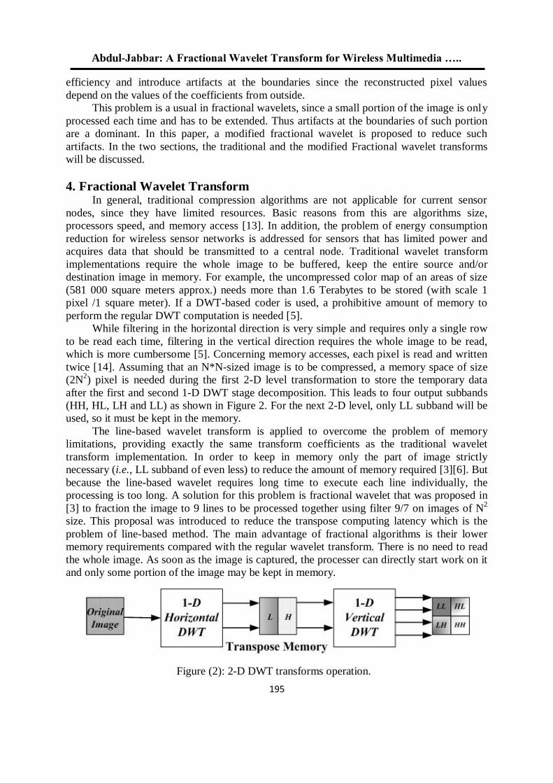
Abdul-Jabbar: A Fractional Wavelet Transform for Wireless Multimedia …..
191
efficiency and introduce artifacts at the boundaries since the reconstructed pixel values
depend on the values of the coefficients from outside.
This problem is a usual in fractional wavelets, since a small portion of the image is only
processed each time and has to be extended. Thus artifacts at the boundaries of such portion
are a dominant. In this paper, a modified fractional wavelet is proposed to reduce such
artifacts. In the two sections, the traditional and the modified Fractional wavelet transforms
will be discussed.
4. Fractional Wavelet Transform In general, traditional compression algorithms are not applicable for current sensor
nodes, since they have limited resources. Basic reasons from this are algorithms size,
processors speed, and memory access [13]. In addition, the problem of energy consumption
reduction for wireless sensor networks is addressed for sensors that has limited power and
acquires data that should be transmitted to a central node. Traditional wavelet transform
implementations require the whole image to be buffered, keep the entire source and/or
destination image in memory. For example, the uncompressed color map of an areas of size
(581 000 square meters approx.) needs more than 1.6 Terabytes to be stored (with scale 1
pixel /1 square meter). If a DWT-based coder is used, a prohibitive amount of memory to
perform the regular DWT computation is needed [5].
While filtering in the horizontal direction is very simple and requires only a single row
to be read each time, filtering in the vertical direction requires the whole image to be read,
which is more cumbersome [5]. Concerning memory accesses, each pixel is read and written
twice [14]. Assuming that an N*N-sized image is to be compressed, a memory space of size
(2N2) pixel is needed during the first 2-D level transformation to store the temporary data
after the first and second 1-D DWT stage decomposition. This leads to four output subbands
(HH, HL, LH and LL) as shown in Figure 2. For the next 2-D level, only LL subband will be
used, so it must be kept in the memory.
The line-based wavelet transform is applied to overcome the problem of memory
limitations, providing exactly the same transform coefficients as the traditional wavelet
transform implementation. In order to keep in memory only the part of image strictly
necessary (i.e., LL subband of even less) to reduce the amount of memory required [3][6]. But
because the line-based wavelet requires long time to execute each line individually, the
processing is too long. A solution for this problem is fractional wavelet that was proposed in
[3] to fraction the image to 9 lines to be processed together using filter 9/7 on images of N2
size. This proposal was introduced to reduce the transpose computing latency which is the
problem of line-based method. The main advantage of fractional algorithms is their lower
memory requirements compared with the regular wavelet transform. There is no need to read
the whole image. As soon as the image is captured, the processer can directly start work on it
and only some portion of the image may be kept in memory.
Figure (2): 2-D DWT transforms operation.
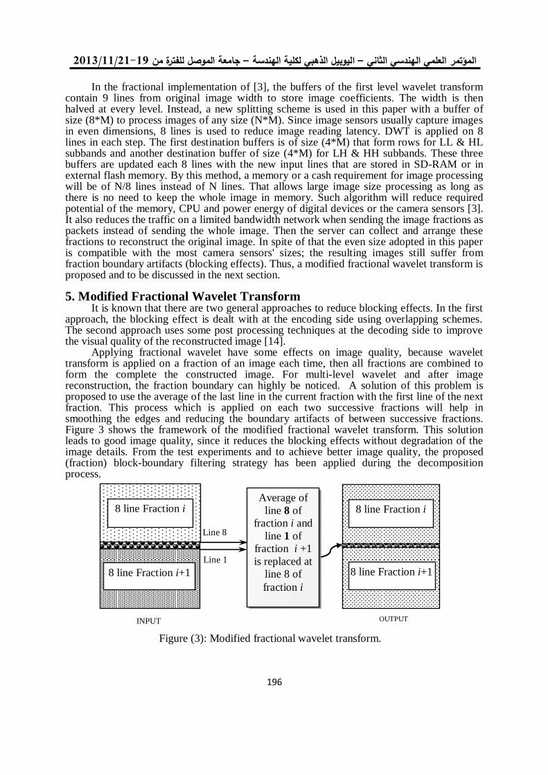
19/99/1192-91جامعة الموصل للفترة من –ليوبيل الذهبي لكلية الهندسة ا –العلمي الهندسي الثاني المؤتمر
191
In the fractional implementation of [3], the buffers of the first level wavelet transform contain 9 lines from original image width to store image coefficients. The width is then halved at every level. Instead, a new splitting scheme is used in this paper with a buffer of size (8*M) to process images of any size (N*M). Since image sensors usually capture images in even dimensions, 8 lines is used to reduce image reading latency. DWT is applied on 8 lines in each step. The first destination buffers is of size (4*M) that form rows for LL & HL subbands and another destination buffer of size (4*M) for LH & HH subbands. These three buffers are updated each 8 lines with the new input lines that are stored in SD-RAM or in external flash memory. By this method, a memory or a cash requirement for image processing will be of N/8 lines instead of N lines. That allows large image size processing as long as there is no need to keep the whole image in memory. Such algorithm will reduce required potential of the memory, CPU and power energy of digital devices or the camera sensors [3]. It also reduces the traffic on a limited bandwidth network when sending the image fractions as packets instead of sending the whole image. Then the server can collect and arrange these fractions to reconstruct the original image. In spite of that the even size adopted in this paper is compatible with the most camera sensors' sizes; the resulting images still suffer from fraction boundary artifacts (blocking effects). Thus, a modified fractional wavelet transform is proposed and to be discussed in the next section.
5. Modified Fractional Wavelet Transform
It is known that there are two general approaches to reduce blocking effects. In the first approach, the blocking effect is dealt with at the encoding side using overlapping schemes. The second approach uses some post processing techniques at the decoding side to improve the visual quality of the reconstructed image [14].
Applying fractional wavelet have some effects on image quality, because wavelet transform is applied on a fraction of an image each time, then all fractions are combined to form the complete the constructed image. For multi-level wavelet and after image reconstruction, the fraction boundary can highly be noticed. A solution of this problem is proposed to use the average of the last line in the current fraction with the first line of the next fraction. This process which is applied on each two successive fractions will help in smoothing the edges and reducing the boundary artifacts of between successive fractions. Figure 3 shows the framework of the modified fractional wavelet transform. This solution leads to good image quality, since it reduces the blocking effects without degradation of the image details. From the test experiments and to achieve better image quality, the proposed (fraction) block-boundary filtering strategy has been applied during the decomposition process.
Figure (3): Modified fractional wavelet transform.
OUTPUT
8 line Fraction i
8 line Fraction i+1
INPUT
Line 8
Line 1
8 line Fraction i+1
Average of
line 8 of
fraction i and
line 1 of
fraction i +1
is replaced at
line 8 of
fraction i
8 line Fraction i
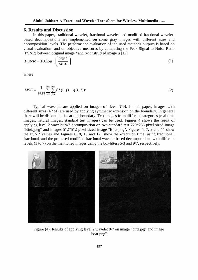
Abdul-Jabbar: A Fractional Wavelet Transform for Wireless Multimedia …..
191
6. Results and Discussion In this paper, traditional wavelet, fractional wavelet and modified fractional wavelet-
based decompositions are implemented on some gray images with different sizes and
decomposition levels. The performance evaluation of the used methods outputs is based on
visual evaluation and on objective measures by computing the Peak Signal to Noise Ratio
(PSNR) between original image f and reconstructed image g [12].
MSEPSNR
2
10
255log.10 (1)
where
1N
0
1N
0
2)),(),((N.N
1
i j
jigjifMSE (2)
Typical wavelets are applied on images of sizes N*N. In this paper, images with
different sizes (N*M) are used by applying symmetric extension on the boundary. In general
there will be discontinuities at this boundary. Test images from different categories (real time
images, natural images, standard test images) can be used. Figures 4 shows the result of
applying level 2 wavelet 9/7 decomposition on two standard test 229*255 pixel sized image
"Bird.jpeg" and images 512*512 pixel-sized image "Boat.png". Figures 5, 7, 9 and 11 show
the PSNR values and Figures 6, 8, 10 and 12 show the execution time, using traditional,
fractional, and the proposed modified fractional wavelet-based decompositions with different
levels (1 to 7) on the mentioned images using the boi-filters 5/3 and 9/7, respectively.
Figure (4): Results of applying level 2 wavelet 9/7 on image "bird.jpg" and image
"boat.png".
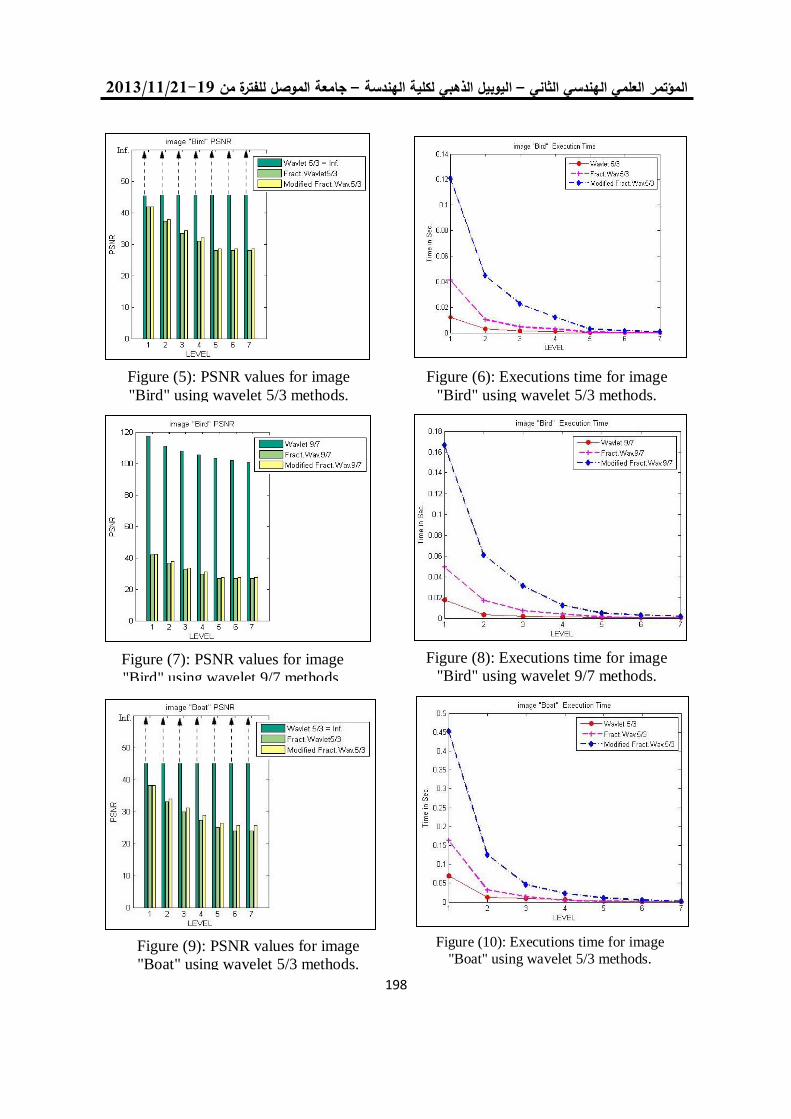
19/99/1192-91جامعة الموصل للفترة من –ليوبيل الذهبي لكلية الهندسة ا –العلمي الهندسي الثاني المؤتمر
191
Figure (7): PSNR values for image
"Bird" using wavelet 9/7 methods.
Figure (6): Executions time for image
"Bird" using wavelet 5/3 methods.
Figure (9): PSNR values for image
"Boat" using wavelet 5/3 methods.
Figure (10): Executions time for image
"Boat" using wavelet 5/3 methods.
Figure (8): Executions time for image
"Bird" using wavelet 9/7 methods.
Figure (5): PSNR values for image
"Bird" using wavelet 5/3 methods.
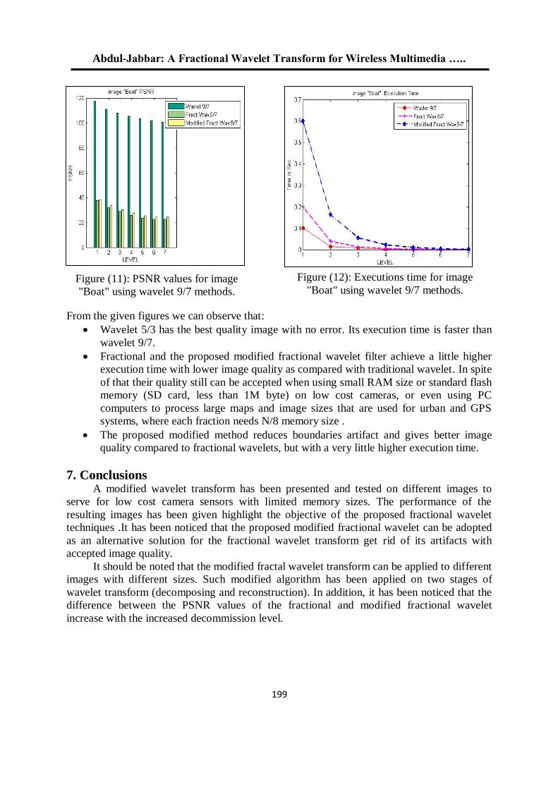
Abdul-Jabbar: A Fractional Wavelet Transform for Wireless Multimedia …..
199
From the given figures we can observe that:
Wavelet 5/3 has the best quality image with no error. Its execution time is faster than
wavelet 9/7.
Fractional and the proposed modified fractional wavelet filter achieve a little higher
execution time with lower image quality as compared with traditional wavelet. In spite
of that their quality still can be accepted when using small RAM size or standard flash
memory (SD card, less than 1M byte) on low cost cameras, or even using PC
computers to process large maps and image sizes that are used for urban and GPS
systems, where each fraction needs N/8 memory size .
The proposed modified method reduces boundaries artifact and gives better image
quality compared to fractional wavelets, but with a very little higher execution time.
7. Conclusions A modified wavelet transform has been presented and tested on different images to
serve for low cost camera sensors with limited memory sizes. The performance of the
resulting images has been given highlight the objective of the proposed fractional wavelet
techniques .It has been noticed that the proposed modified fractional wavelet can be adopted
as an alternative solution for the fractional wavelet transform get rid of its artifacts with
accepted image quality.
It should be noted that the modified fractal wavelet transform can be applied to different
images with different sizes. Such modified algorithm has been applied on two stages of
wavelet transform (decomposing and reconstruction). In addition, it has been noticed that the
difference between the PSNR values of the fractional and modified fractional wavelet
increase with the increased decommission level.
Figure (11): PSNR values for image
"Boat" using wavelet 9/7 methods.
Figure (12): Executions time for image
"Boat" using wavelet 9/7 methods.
19/99/1192-91جامعة الموصل للفترة من –ليوبيل الذهبي لكلية الهندسة ا –العلمي الهندسي الثاني المؤتمر
122
References: 1. AlNuaimi, M., Sallabi, F. and Shuaib, K., “A Survey of Wireless Multimedia Sensor
Networks Challenges and Solutions”, International Conference on Innovations in
Information Technology, Abu Dhabi, 25-27 April 2011, pp. 191-196.
2. Tavli, B., Bicakci, K., Zilan, R. and Barcelo-Ordinas, J. M., “A survey of Visual Sensor
Network Platforms ", Multimedia Tools and Applications, Vol. 60 No. 3, Oct. 2012,
pp. 689-726.
3. Rein, S., and Reisslein, M., “Low-Memory Wavelet Transforms for Wireless Sensor
Networks: A Tutorial”, IEEE Communications Surveys & Tutorials, Vol. 13, No.2, 2011,
pp. 291-307.
4. Babu, P. A., and Prasad,, K. V. S. V. R., “Image Interpolation using 5/3 Lifting Scheme
Approach”, Signal & Image Processing: An International Journal (SIPIJ) Vol.2, No.1,
March 2011, pp.71-80.
5. Oliver, J. and Malumbres, M. P., “On the Design of Fast Wavelet Transform Algorithms
with Low Memory Requirements”, IEEE Trans. Circuits Systems. Video Technol, Vol.
18, No. 2, 2008, pp. 237–248.
6. Rein, S., Lehmann, S. and Gühmann, C., “Fractional Wavelet Filter for Camera Sensor
Node with External Flash and Extremely Little RAM”, MobiMedia’08, July 7-9, 2008,
Oulu, Finland, pp.252-261,
7. Chrysafis, C. and Ortega, A., “Line-Based, Reduced Memory, Wavelet Image
Compression”, IEEE Trans. Image Process, Vol. 9, No. 3, 2000, pp. 378–389.
8. Bao, Y. and Kuo, C., “Design of Wavelet-Based Image Codec in Memory Constrained
Environment”, IEEE Trans. Circuits Systems. Video Technol., Vol.11, No. 5. 2001, pp.
642-650.
9. Singh, R., Verma, R. and Kumar, S., “JPEG2000: Wavelet Based Image Compression”,
EE678 Wavelets Application Assignment 1. http://www.ee.iitb.ac.in
10. Taubman, D. S. and Marcellin, M. W., “JPEG2000: Standard for Interactive Imaging”, Proceedings of the IEEE, Vol. 90, No. 8, Aug. 2002, pp. 1336-1357.
11. Yang, G. and Guo, S., “A New Wavelet Lifting Scheme for Image Compression
Applications”, IWICPAS 2006, LNCS 4153, 2006, pp. 465–474.
12. Acharya, T. and Ray, A. k., “Image Processing Principles and Applications” John Wiley
and Sons, Inc., USA, 2005, pp.370.
13. Lecuire, V., Duran- Faundez, C. and Krommenacker, N., “Energy-Efficient Transmission
of Wavelet-Based Images in Wireless Sensor Networks”, EURASIP Journal on Image and
Video Processing, Vol. 2, 2007, pp. 15-15.
14. Gandam, A. and Sidhu, J. S., “A Post-Processing Algorithm for Detection & Removal of
Corner Outlier”, International Journal of Computer Applications (0975 –8887), Vol.4,
No.2, July 2010, pp. 9-16.
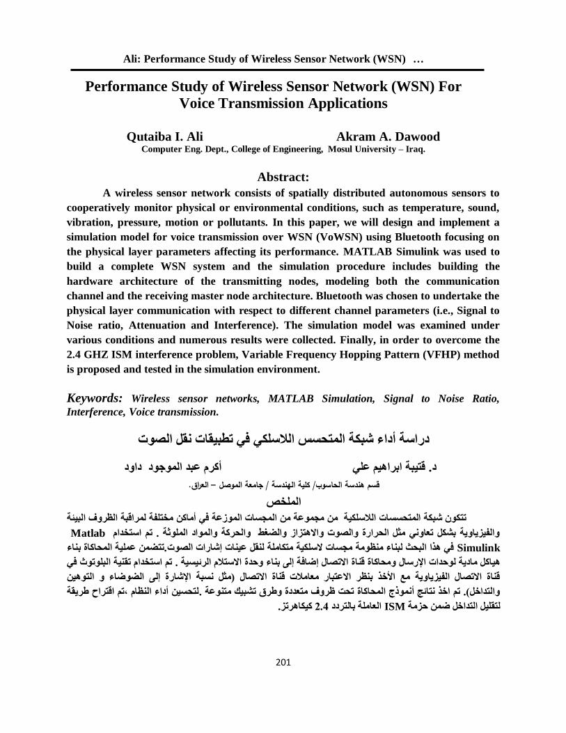
Ali: Performance Study of Wireless Sensor Network (WSN) …
201
Performance Study of Wireless Sensor Network (WSN) For
Voice Transmission Applications
Qutaiba I. Ali Akram A. Dawood
Computer Eng. Dept., College of Engineering, Mosul University – Iraq.
Abstract:
A wireless sensor network consists of spatially distributed autonomous sensors to
cooperatively monitor physical or environmental conditions, such as temperature, sound,
vibration, pressure, motion or pollutants. In this paper, we will design and implement a
simulation model for voice transmission over WSN (VoWSN) using Bluetooth focusing on
the physical layer parameters affecting its performance. MATLAB Simulink was used to
build a complete WSN system and the simulation procedure includes building the
hardware architecture of the transmitting nodes, modeling both the communication
channel and the receiving master node architecture. Bluetooth was chosen to undertake the
physical layer communication with respect to different channel parameters (i.e., Signal to
Noise ratio, Attenuation and Interference). The simulation model was examined under
various conditions and numerous results were collected. Finally, in order to overcome the
2.4 GHZ ISM interference problem, Variable Frequency Hopping Pattern (VFHP) method
is proposed and tested in the simulation environment.
Keywords: Wireless sensor networks, MATLAB Simulation, Signal to Noise Ratio,
Interference, Voice transmission.
في تطبيقات نقل الصوتالمتحسس الالسلكي ةشبك أداءدراسة
داود الموجود أكرم عبد قتيبة ابراهيم عليد. العراق. –قسم هندسة الحاسوب/ كلية الهندسة / جامعة الموصل
الملخص
لبيئة تتكون شبكة المتحسسات الالسلكية من مجموعة من المجسات الموزعة في أماكن مختلفة لمراقبة الظروف ا
Matlab والفيزياوية بشكل تعاوني مثل الحرارة والصوت واالهتزاز والضغط والحركة والمواد الملوثة . تم استخدام
Simulink تتضمن عملية المحاكاة بناء لنقل عينات إشارات الصوت في هذا البحث لبناء منظومة مجسات السلكية متكاملة.
م تقنية البلوتوث في ااستخدتم اة االتصال إضافة إلى بناء وحدة االستالم الرئيسية . هياكل مادية لوحدات اإلرسال ومحاكاة قن
التوهين قناة االتصال الفيزياوية مع األخذ بنظر االعتبار معامالت قناة االتصال )مثل نسبة اإلشارة إلى الضوضاء و
لتحسين أداء النظام ,تم اقتراح طريقة تنوعة .والتداخل(. تم اخذ نتائج أنموذج المحاكاة تحت ظروف متعددة وطرق تشبيك م
كيكاهرتز. 4.2العاملة بالتردد ISMلتقليل التداخل ضمن حزمة
19/99/1192-91جامعة الموصل للفترة من –ليوبيل الذهبي لكلية الهندسة ا –العلمي الهندسي الثاني المؤتمر
202
1. Introduction
Traditional wireless sensor network (WSN) has focused on sensing and reporting
physical phenomenon or environmental parameters, such as temperature, sound and pressure etc.
Currently, using WSN for emergency response has gained significant attention due to the
development of WSN technology. The data types transmitted over WSN becomes diversity.
There are many hazard scenarios, such as emergency response, rescue, and disaster during
mountain climbing, which need to support voice transmission over WSN (VoWSN). Several
standards are currently under developed for WSN. The Institute of Electrical and Electronics
Engineers (IEEE) approved the 802.15.4 Standard [1] to define the physical and Media Access
Control (MAC) for Low-Rate Wireless Personal Area Network (LR-WPAN). Upper layer are
defined by Zigbee Alliance [2,3]. The features of Zigbee include the standard specified operation
in the unlicensed 2.4 GHz worldwide, low power consumption, low transfer rate (default rate:
250kbps), short range communication capability, (maximum: 300m), limited computational
capacity and memories[3].
In general, Wireless multimedia sensor networks have the potential to enable many new
applications. These can be classified as follows [4, 5]:
Multimedia Surveillance Sensor Networks. Surveillance sensor networks will be used to
enhance and complement existing surveillance systems to prevent crime and terrorist
attacks. Multimedia content, such as video streams and still images, as well as computer
vision techniques, can be used to locate missing persons, identify criminals or terrorists, or
infer and record other potentially relevant activities (thefts, car accidents, traffic violations).
Traffic Avoidance, Enforcement, and Control Systems. It will be possible to monitor car
traffic in big cities or on highways and deploy services that offer traffic routing advice to
avoid congestion or identify violations. In addition, smart parking advice systems based on
WMSNs will detect available parking spaces and provide drivers with automated parking
advice.
Advanced Health Care Delivery. Telemedicine sensor networks can be integrated with third
and fourth generation (3G/4G) cellular networks to provide ubiquitous health care services.
Patients will carry medical sensors to monitor parameters such as body temperature, blood
pressure, pulse oximetry, ECG, and breathing activity. Remote medical centers will monitor
the condition of their patients to infer emergency situations.
Environmental and Structural Monitoring. Arrays of video sensors already are used by
oceanographers to determine the evolution of sandbars using image processing techniques.
Video and imaging sensors also are used to monitor the structural health of bridges or other
civil structures.
Industrial Process Control. Multimedia content such as imaging, temperature, or pressure,
can be used for time-critical, industrial, process control. In automated manufacturing
processes, the integration of machine vision systems with WMSNs can simplify and add
flexibility to systems for visual inspections and automated actions.
The usage of Bluetooth as the direct access of voice transmission has been prevalent.
Therefore, transmitting voice data via Bluetooth is very attractive for many applications. In this
paper, we will design and implement a simulation model for Voice transmission over WSN
(VoWSN) using Bluetooth focusing on the physical layer parameters affecting its performance.
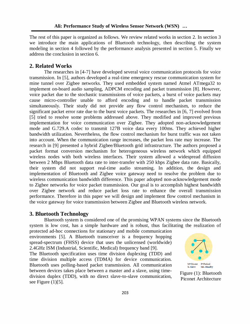
Ali: Performance Study of Wireless Sensor Network (WSN) …
203
The rest of this paper is organized as follows. We review related works in section 2. In section 3
we introduce the main applications of Bluetooth technology, then describing the system
modeling in section 4 followed by the performance analysis presented in section 5. Finally we
address the conclusion in section 6.
2. Related Works The researches in [4-7] have developed several voice communication protocols for voice
transmission. In [5], authors developed a real-time emergency rescue communication system for
mine tunnel over Zigbee networks. They used embedded system named Atmel ATmega32 to
implement on-board audio sampling, ADPCM encoding and packet transmission [8]. However,
voice packet due to the stochastic transmissions of voice packets, a burst of voice packets may
cause micro-controller unable to afford encoding and to handle packet transmission
simultaneously. Their study did not provide any flow control mechanism, to reduce the
significant packet error rate due to the burst voice packets. The researches in [6, 7] evolved from
[5] tried to resolve some problems addressed above. They modified and improved previous
implementation for voice communication over Zigbee. They adopted non-acknowledgement
mode and G.729.A codec to transmit 127B voice data every 100ms. They achieved higher
bandwidth utilization. Nevertheless, the flow control mechanism for burst traffic was not taken
into account. When the communication range increases, the packet loss rate may increase. The
research in [9] presented a hybrid Zigbee/Bluetooth grid infrastructure. The authors proposed a
packet format conversion mechanism for heterogeneous wireless network which equipped
wireless nodes with both wireless interfaces. Their system allowed a widespread diffusion
between 2 Mbps Bluetooth data rate to inter-transfer with 250 kbps Zigbee data rate. Basically,
their system did not support real-time audio streaming. In addition, the design and
implementation of Bluetooth and Zigbee voice gateway need to resolve the problem due to
wireless communication bandwidth difference. This paper adopted non-acknowledgement mode
to Zigbee networks for voice packet transmission. Our goal is to accomplish highest bandwidth
over Zigbee network and reduce packet loss rate to enhance the overall transmission
performance. Therefore in this paper we will design and implement flow control mechanism in
the voice gateway for voice transmission between Zigbee and Bluetooth wireless network.
3. Bluetooth Technology Bluetooth system is considered one of the promising WPAN systems since the Bluetooth
system is low cost, has a simple hardware and is robust, thus facilitating the realization of
protected ad-hoc connections for stationary and mobile communication
environments [5]. A Bluetooth transceiver is a frequency hopping
spread-spectrum (FHSS) device that uses the unlicensed (worldwide)
2.4GHz ISM (Industrial, Scientific, Medical) frequency band [9].
The Bluetooth specification uses time division duplexing (TDD) and
time division multiple access (TDMA) for device communication.
Bluetooth uses polling-based packet transmission. All communication
between devices takes place between a master and a slave, using time-
division duplex (TDD), with no direct slave-to-slave communication,
see Figure (1)[5].
Figure (1): Bluetooth
Piconet Architecture
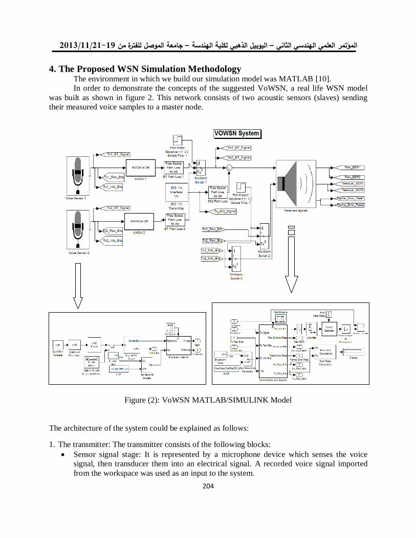
19/99/1192-91جامعة الموصل للفترة من –ليوبيل الذهبي لكلية الهندسة ا –العلمي الهندسي الثاني المؤتمر
204
4. The Proposed WSN Simulation Methodology The environment in which we build our simulation model was MATLAB [10].
In order to demonstrate the concepts of the suggested VoWSN, a real life WSN model
was built as shown in figure 2. This network consists of two acoustic sensors (slaves) sending
their measured voice samples to a master node.
Figure (2): VoWSN MATLAB/SIMULINK Model
The architecture of the system could be explained as follows:
1. The transmitter: The transmitter consists of the following blocks:
Sensor signal stage: It is represented by a microphone device which senses the voice
signal, then transducer them into an electrical signal. A recorded voice signal imported
from the workspace was used as an input to the system.
Ali: Performance Study of Wireless Sensor Network (WSN) …
205
Up-sample to 64ksamples/s: Up-samples the input to a higher rate by inserting zeros
between samples.
CVSD Encoder: Encode a 64 K samples per sec speech signal into a 64Kbps bit stream.
Bluetooth Clock: Each Bluetooth device has a free-running 28-bit Bluetooth clock. The
clock ticks 3,200 times per second or once every 312.5 µsec, representing a clock rate of
3.2 KHz.
Hop Sequence Generator: For devices to communicate with each other, they must
transmit and receive on the same frequency at the same time. The hop sequence generator
generates a sequence of hop frequencies in the range 0 to 78.
Encode and modulate: The 366 data bits are transmitted at 1 Mbps and modulated using
Gaussian frequency shift keying (GFSK). GFSK effectively transmits +150 kHz signal
relative to the carrier for a 1bit, and a 150 kHz signal for a 0 bit. The carrier signal is
generated in the Simulink model by a baseband MFSK block set to 79 symbols and a
separation of 1MHz. If a hop frequency value 0 is input, a -39MHz complex sinusoid is
generated. If a 1 is entered, a -38 MHz complex sinusoid is generated and so on. In the
model, the hop sequences are generated by a simple random number generator, not using
the actual method specified in the standard. The transmitter is turned off after 366 bits
using a Gain block to multiply the frame with a mask of 36600 ones and 26500 zeros.
The medium consists of the following blocks:
AWGN Channel: The AWGN Channel block adds white Gaussian noise to a real or
complex input signal. When the input signal is real, this block adds real Gaussian noise
and produces a real output signal. When the input signal is complex, this block adds
complex Gaussian noise and produces a complex output signal.
Path Loss: Reduce the amplitude of the input signal by the amount specified. The loss can
be specified directly using the “Decibels” mode, or indirectly using the “Distance and
Frequency” mode. The reciprocal of the loss is applied as a gain, e.g., a loss of +20 dB,
which reduces the signal by a factor of 10 corresponds to a gain value of 0.1.
802.11b interferer: Add signals that have the same frequency of the data signal to make
interference between the data signal and other signals.
Multiport Switch: The Multiport Switch block chooses between a number of inputs. The
first input is called the control input, while the rest of the inputs are called data inputs.
The value of the control input determines which data input is passed through to the output
port. This switch allows the simulator to emulate contention behavior among different
nodes.
The receiver consists of the following blocks:
Hop Sequence Generator: same as mentioned earlier.
Demodulate and decode: This block is used to extract the original information-bearing
signal from a modulated carrier wave, and to recover the information contends in it.
Zero-Order Hold: The block samples and holds its input for the specified sample period.
The block accepts one input and generates one output, both of which can be scalar or
vector. If the input is a vector, all elements of the vector are held for the same sample
period.
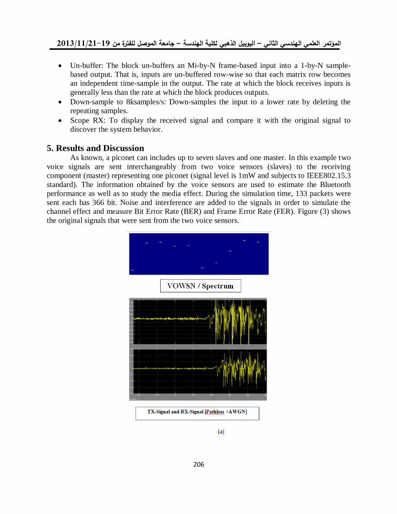
19/99/1192-91جامعة الموصل للفترة من –ليوبيل الذهبي لكلية الهندسة ا –العلمي الهندسي الثاني المؤتمر
206
Un-buffer: The block un-buffers an Mi-by-N frame-based input into a 1-by-N sample-
based output. That is, inputs are un-buffered row-wise so that each matrix row becomes
an independent time-sample in the output. The rate at which the block receives inputs is
generally less than the rate at which the block produces outputs.
Down-sample to 8ksamples/s: Down-samples the input to a lower rate by deleting the
repeating samples.
Scope RX: To display the received signal and compare it with the original signal to
discover the system behavior.
5. Results and Discussion As known, a piconet can includes up to seven slaves and one master. In this example two
voice signals are sent interchangeably from two voice sensors (slaves) to the receiving
component (master) representing one piconet (signal level is 1mW and subjects to IEEE802.15.3
standard). The information obtained by the voice sensors are used to estimate the Bluetooth
performance as well as to study the media effect. During the simulation time, 133 packets were
sent each has 366 bit. Noise and interference are added to the signals in order to simulate the
channel effect and measure Bit Error Rate (BER) and Frame Error Rate (FER). Figure (3) shows
the original signals that were sent from the two voice sensors.
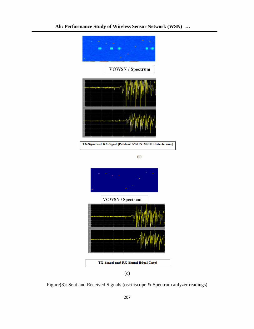
Ali: Performance Study of Wireless Sensor Network (WSN) …
207
(c)
Figure(3): Sent and Received Signals (osciliscope & Spectrum anlyzer readings)
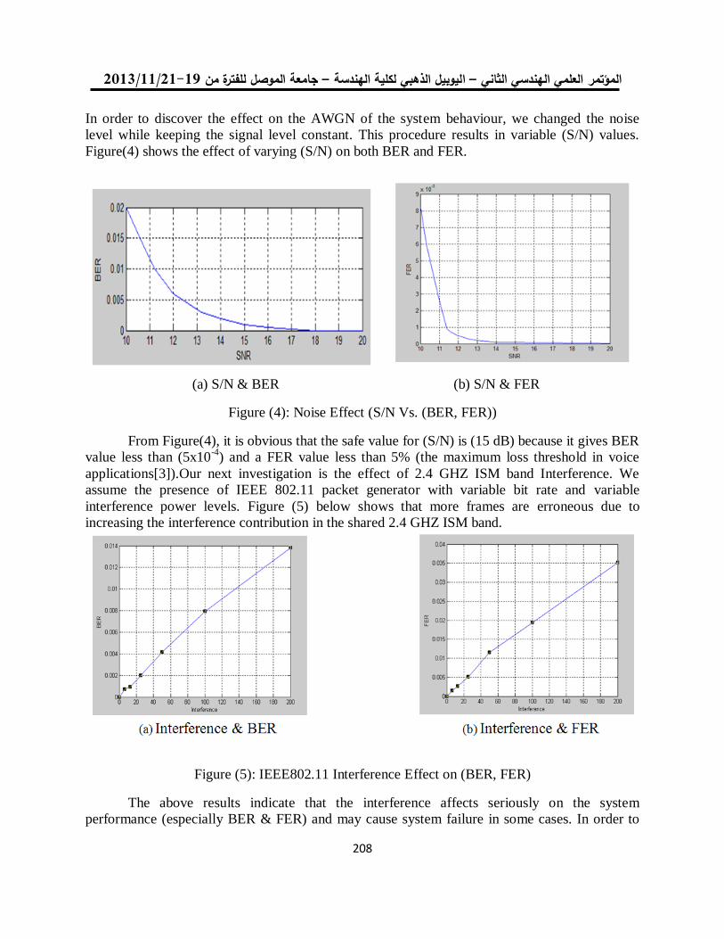
19/99/1192-91جامعة الموصل للفترة من –ليوبيل الذهبي لكلية الهندسة ا –العلمي الهندسي الثاني المؤتمر
208
In order to discover the effect on the AWGN of the system behaviour, we changed the noise
level while keeping the signal level constant. This procedure results in variable (S/N) values.
Figure(4) shows the effect of varying (S/N) on both BER and FER.
(a) S/N & BER (b) S/N & FER
Figure (4): Noise Effect (S/N Vs. (BER, FER))
From Figure(4), it is obvious that the safe value for (S/N) is (15 dB) because it gives BER
value less than (5x10⁻⁴
) and a FER value less than 5% (the maximum loss threshold in voice
applications[3]).Our next investigation is the effect of 2.4 GHZ ISM band Interference. We
assume the presence of IEEE 802.11 packet generator with variable bit rate and variable
interference power levels. Figure (5) below shows that more frames are erroneous due to
increasing the interference contribution in the shared 2.4 GHZ ISM band.
Figure (5): IEEE802.11 Interference Effect on (BER, FER)
The above results indicate that the interference affects seriously on the system
performance (especially BER & FER) and may cause system failure in some cases. In order to
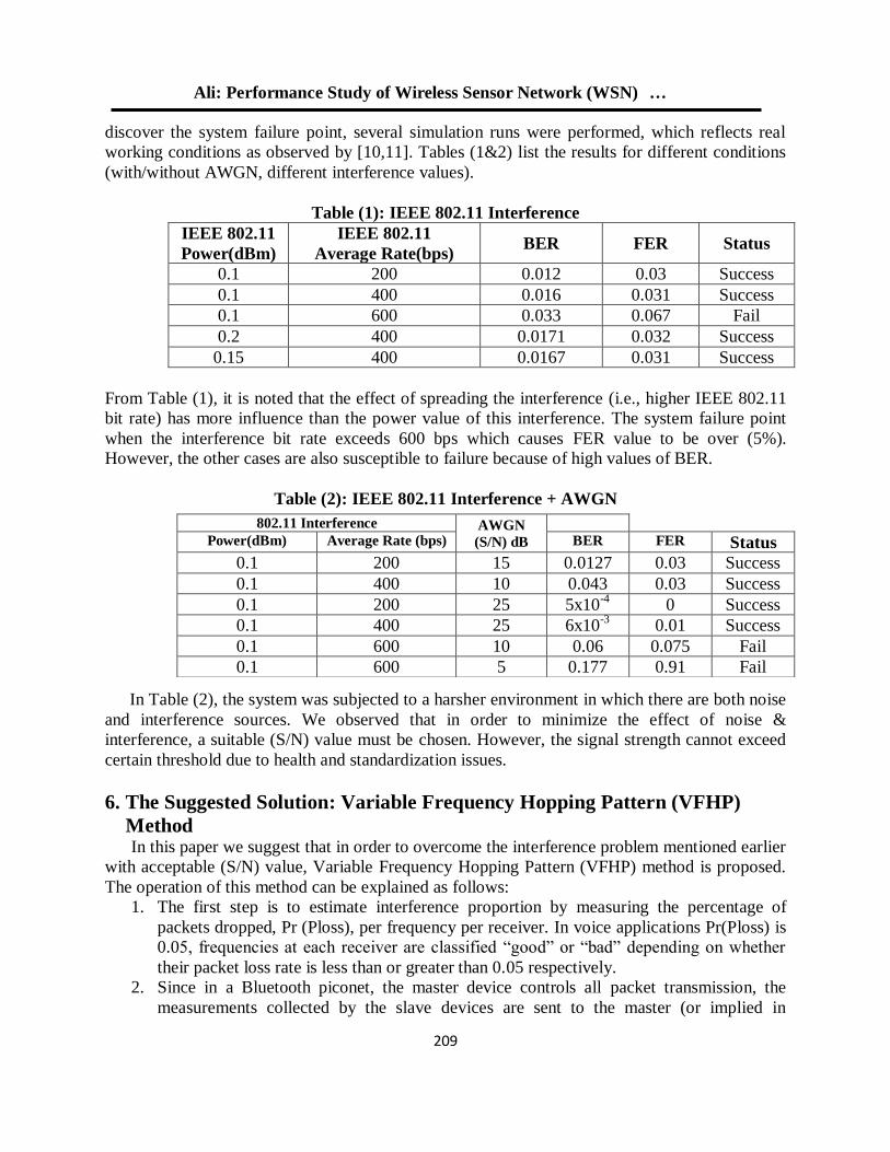
Ali: Performance Study of Wireless Sensor Network (WSN) …
209
discover the system failure point, several simulation runs were performed, which reflects real
working conditions as observed by [10,11]. Tables (1&2) list the results for different conditions
(with/without AWGN, different interference values).
Table (1): IEEE 802.11 Interference
IEEE 802.11
Power(dBm)
IEEE 802.11
Average Rate(bps) BER FER Status
0.1 200 0.012 0.03 Success
0.1 400 0.016 0.031 Success
0.1 600 0.033 0.067 Fail
0.2 400 0.0171 0.032 Success
0.15 400 0.0167 0.031 Success
From Table (1), it is noted that the effect of spreading the interference (i.e., higher IEEE 802.11
bit rate) has more influence than the power value of this interference. The system failure point
when the interference bit rate exceeds 600 bps which causes FER value to be over (5%).
However, the other cases are also susceptible to failure because of high values of BER.
Table (2): IEEE 802.11 Interference + AWGN
In Table (2), the system was subjected to a harsher environment in which there are both noise
and interference sources. We observed that in order to minimize the effect of noise &
interference, a suitable (S/N) value must be chosen. However, the signal strength cannot exceed
certain threshold due to health and standardization issues.
6. The Suggested Solution: Variable Frequency Hopping Pattern (VFHP)
Method In this paper we suggest that in order to overcome the interference problem mentioned earlier
with acceptable (S/N) value, Variable Frequency Hopping Pattern (VFHP) method is proposed.
The operation of this method can be explained as follows:
1. The first step is to estimate interference proportion by measuring the percentage of
packets dropped, Pr (Ploss), per frequency per receiver. In voice applications Pr(Ploss) is
0.05, frequencies at each receiver are classified “good” or “bad” depending on whether
their packet loss rate is less than or greater than 0.05 respectively.
2. Since in a Bluetooth piconet, the master device controls all packet transmission, the
measurements collected by the slave devices are sent to the master (or implied in
802.11 Interference AWGN
(S/N) dB
Power(dBm) Average Rate (bps) BER FER Status
0.1 200 15 0.0127 0.03 Success
0.1 400 10 0.043 0.03 Success
0.1 200 25 5x10⁻⁴
0 Success
0.1 400 25 6x10⁻³
0.01 Success
0.1 600 10 0.06 0.075 Fail
0.1 600 5 0.177 0.91 Fail
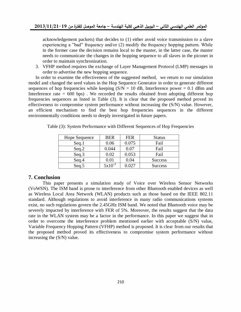
19/99/1192-91جامعة الموصل للفترة من –ليوبيل الذهبي لكلية الهندسة ا –العلمي الهندسي الثاني المؤتمر
210
acknowledgement packets) that decides to (1) either avoid voice transmission to a slave
experiencing a ”bad” frequency and/or (2) modify the frequency hopping pattern. While
in the former case the decision remains local to the master, in the latter case, the master
needs to communicate the changes in the hopping sequence to all slaves in the piconet in
order to maintain synchronization.
3. VFHP method requires the exchange of Layer Management Protocol (LMP) messages in
order to advertise the new hopping sequence.
In order to examine the effectiveness of the suggested method, we return to our simulation
model and changed the seed values in the Hop Sequence Generator in order to generate different
sequences of hop frequencies while keeping (S/N = 10 dB, Interference power = 0.1 dBm and
Interference rate = 600 bps) . We recorded the results obtained from adopting different hop
frequencies sequences as listed in Table (3). It is clear that the proposed method proved its
effectiveness to compromise system performance without increasing the (S/N) value. However,
an efficient mechanism to find the best hop frequencies sequences in the different
environmentally conditions needs to deeply investigated in future papers.
Table (3): System Performance with Different Sequences of Hop Frequencies
Hope Sequence BER FER Status
Seq.1 0.06 0.075 Fail
Seq.2 0.044 0.07 Fail
Seq.3 0.02 0.053 Fail
Seq.4 0.01 0.04 Success
Seq.5 5x10⁻³
0.027 Success
7. Conclusion This paper presents a simulation study of Voice over Wireless Sensor Networks
(VoWSN). The ISM band is prone to interference from other Bluetooth enabled devices as well
as Wireless Local Area Network (WLAN) products such as those based on the IEEE 802.11
standard. Although regulations to avoid interference in many radio communications systems
exist, no such regulations govern the 2.45GHz ISM band. We noted that Bluetooth voice may be
severely impacted by interference with FER of 5%. Moreover, the results suggest that the data
rate in the WLAN system may be a factor in the performance. In this paper we suggest that in
order to overcome the interference problem mentioned earlier with acceptable (S/N) value,
Variable Frequency Hopping Pattern (VFHP) method is proposed. It is clear from our results that
the proposed method proved its effectiveness to compromise system performance without
increasing the (S/N) value.
Ali: Performance Study of Wireless Sensor Network (WSN) …
211
References
1. IEEE 802.15.4 standard: Wireless Medium Access Control (MAC) and Physical Layer (PHY)
Specification for Low-Rate Wireless Personal Area Networks (LR-WPAN), Oct.2003.
2. ZigBee Alliance: ZigBee Specification. ZigBee Alliance. 053474r17 edn. (Jan. 17 2008).
3. D. Brunelli, M. Maggiorotti, L. Benini, and F. L. Bellifemine, "Analysis of audio streaming
capability of zigbee networks," In Proceedings of Fifth European Workshop on Wireless Sensor
Network , VOL. 4913, pp.198-204, 2008.
4. L. Luo, W. Cao, C. Huang, T. Abdelzaher, J. A. Stankovic, and M. Ward, “Enviromic:
Towards cooperative storage and retrieval in audio sensor networks,” 27th International
Conference on Distributed Computing Systems, pp. 34-34, 2007.
5. R. Mangharam, A. Rowe, R. Rajkumar, and R. Suzuki, “Voice over Sensor Networks,”27th
IEEE International of Real-Time Systems Symposium, pp. 291-302, 2006.
6. H. Y. Song, and S. H. Cho, “Performances of IEEE 802.15.4 Unslotted CSMA-CA for Voice
Communications,” The 17th Asia-Pacific Conference on Communications, 2011.
7. H.Y. Song, H.C.Yoon, and S.H.Cho, “Implementation and analysis of IEEE 802.15.4 MAC
for Voice Communications,” The 4th Joint Workshop between HYU and BUPT, 2009.
8. Atmel Corporation, atmega32 data sheet, 2005.
9. M. Ruta, F. Scioscia, T. D. Noia, and E. D. Sciascio, “A hybrid ZigBee/Bluetooth approach to
mobile semantic grids,” International Journal of Computer Systems Science & Engineering, Vol.
25, No. 3, pp. 49-63, 2010.
10. A. Mathew, N. Chandrababu, K. Elleithy, S. Rizvi, "IEEE 802.11 & Bluetooth interference:
simulation and coexistence", 7th Annual Conference on Communication Networks and Services
Research, pp. 217 – 223, 2009.
11. B. Matthew, "Wi-Fi (IEEE 802.11b) and Bluetooth coexistence issues and solutions for the
2.4 GHz ISM band", Texas Instruments Technical Report, 2009.

19/99/1192-91جامعة الموصل للفترة من –ليوبيل الذهبي لكلية الهندسة ا –العلمي الهندسي الثاني المؤتمر
212
استخدام تقنية الكلونة إلخفاء الرسالة السرية سعدون حسين عبدهللا
مدرس مساعد علوم حاسوب/
قسم علوم الحياة كلية العلوم/ جامعة الموصل/
المستخلصالسرية باالستفادة من تقنية الكلونة والتي تعتبر من إحدى إلخفاء المعلومات خالل هذا البحث تم اقتراح طريقة
احدث الطرائق التي تستخدم إلخفاء المعلومات عن طريق ترميز الرسالة )النصية,الصوتية,الصورية,الفديوية( إلى ما
باستخدام E.coliالناتجة إلى بالزميد )ناقل( مأخوذ من بكتيريا DNA, ثم يتم إدخال سلسلةDNA يقابلها من سلسلة
)الغريب( إلى طرف المستلم وهو بدوره يستخدم طريقة تقنية الكلونة وإرسال البالزميد الحاوي على السلسلة السرية
وية للرسالة, ثم يستخدم خوارزمية إلعادة ( لمعرفة السلسلة السرية الحاLocal Alignmentاالصطفاف الموضعي )
إلى الرسالة السرية )النصية,الصوتية,الصورية,الفديوية(, وهذه الطريقة يندرج ضمن علم جديد DNAترميز سلسلة
( , كانت Bioinformaticsيجمع بين علوم الحاسوب وعلم البيولوجي الجزيئي والذي يختصر بـالمعلوماتية الحياتية )
لطريقة جيدة جدا من ناحية قوتها في اخفاء المعلومات وبأطوال مختلفة من الرسالة السرية وبوقت اقل نتائج هذه ا
%.011واسترجاع للرسالة السرية بنسبة
، تقنية الكلونة ، بالزميد ، معلوماتية الحياتية. DNA: اخفاء المعلومات، سلسلة الكلمات المفتاحية
Using Cloning Technique for Hiding Secret Message
Abstract During this research was suggest a method to hide secret information by using
Cloning Technique, This method regarded as one of the resent method that is used to
hide information by encoded message (text,sound,image,video) to sequence of DNA,
Then resulting sequence was inserted to plasmid (taken from bacteria E.coli ) using
Cloning Technique , The plasmid that containing secret sequence was sent to recipient.
The recipient used local alignment method to discover the secret sequence and use an
algorithm to Re-encoding DNA sequence to secret massage(text, sound, image, video),
This method is a new science combined between computer science and molecular
biology which is called bioinformatics, The results of this method is very good of its
Robust to information hiding and different lengths of the secret message and less time
and retrieve the secret message by 100%.
Sadoon H. Abdullah
University of Mosul/ Collage of Science/ Biology Dept.

استخدام تقنية الكلونة إلخفاء الرسالة السرية: عبدهللا
213
خلفية عن اخفاء المعلوماتالرقمية وشبكة االنترنيت واالتصاالت أصبحت الخصوصية الشخصية عرضة التقنيات نظرا للتطور الهائل في مجال
ين من لالنتهاك بسهولة أكبر من ذي قبل، فكان البد من طرائق ت حفظ بها سرية البيانات الشخصية عند تناقلها لمنع المتطفل
وجدت تقنية الكتابة المخفية الرقمية، شهدت بدايات العقد األخير من القرن الماضي ظهور االطالع عليها، لهذا لغرض
، على الرغم من أن الكتابة المخفية عموما لها جذور موغلة في عمق التاريخ ، إذ اخفاء الرسالةحوث حول طليعة الب
.[1]لمخفية بعضها بدائياستخدمت طرائق مختلفة إلنجاز الكتابة ا
إخفاء البيانات وي عنى به فن إخفاء رسالة في وسط Information Hidingأو إخفاء المعلومات Data Hidingإخفاء البيانات
.[2,1]مضيف مثل تسجيل صوتي أو فيديو أو الصور الثابتة أو الوثائق النصية دون أي تشويه في الوسط المضيف
الطرائق األكثر استخداما لالتصال اآلمن هو الكتابة المخفية. والكتابة المخفية لها تاريخ قديم يعود إلى عهد اليونانيين أحد
وارسالهم الى الطرف القدماء إذ كانوا يمارسون هذا الفن عبر توشيم الرسالة السرية على رؤوس المراسلين المحلوقة
. واستخدمت طرائق أخرى مخفية في أيامها األولى ؤوسهم لمعرفة الرسالة السريةبدوره يحلق رالمستلم بعد نمو شعرهم
الحاضر الكتابة المخفية أخذت . في الوقت سري داخل نص مبهم غير مثير للشبههمثل استخدام الحبر السري أو إخفاء نص
ة مثل الصور والفيديو والملفات الصوتية جديدا ، إذ باتت التقنية الرقمية تستخدم إلخفاء الرسائل في الوسائط الرقمي منحا
. [1]وباقي أنواع ملفات الحاسوب وكذلك في بروتوكوالت االنترنيت
Steganographyالكتابة المغطاة وتتألف من مقطعين (جاءت من الكلمة اإلغريقية ) Steganographyكلمة
( ويعني الكتابة أو الرسم، وهما معا يعنيان مصطلح graphicسرية والثاني )يعني مغطاة أو ( وهوSteganosاألول )
البيانات خالل بأنها فن اإلخفاء Steganography، ويمكن تعريف الكتابة المغطاة Covered writingالكتابة المغطاة
بطريقة ال تدعو ،أو الحامل، والبيانات المحمولة غير مؤذية للمضيف Carrierأو حاملة لها Hostبيانات أخرى مضيفة
[3,4]احتمالية وجودها في إلى الشك
Conflicting Propertiesخصائص متعارضة ثمة خصائص يجب األخذ بها عند تطبيق إحدى تقنيات إخفاء المعلومات، وهي:
خاصييية عييدم تغيييير الغطيياء بصييورة ملحوظيية ميين قبييل حييواس : (Imperceptibility ) القدددرة علددى عدددم االدرا . 0
االنسان البصرية والسمعية.
ت المخفيية أو تيدميرها وتعني مدى قوة تقنية إخفاء المعلومات أمام الهجمات واكتشاف البيانا (:Robustness القوة ) . 2
و تشويشها.
كمية البيانات المراد إخفاؤها داخل وسط مضيف لها من دون كشفها. (:Capacity السعة ) . 3
وهذه الخاصية تعني إن البيانات المخفية تكيون غيير قابلية للكشيف (:Undetectability القدرة على عدم االكتشاف ) . 4
من قبل المهاجمين.
ي وقت واحد، ومثال ذلك إن نخفي إن الخصائص السابقة تكون متعارضة فيما بينها وال يمكن تحقيقها جميعا ف
معلومات كبيرة داخل صورة، فعند ذلك النحقق القوة المطلوبة ويكون من السهل اكتشاف إن ثمة بيانات مخفية من قبل
المهاجمين )تعارض خاصية السعة وقدرة عدم االكتشاف(، وفي الغالب إذا كانت التقنية قوية ضد الهجمات والتشويش عليها
)كتقنيات العالمة يانات المخفية ستكون قليلة، وغالبا ما يجب توفير خاصية القوة في تقنيات إثبات الملكيةفان كمية الب
الن تلك التقنيات تتطلب القوة ضد الهجمات ويقابل ذلك إخفاء بيانات قليلة نسبيا )تعارض خاصية القوة مع السعة( المائية(
[3 ,5,6].
Biological Background خلفية البايولوجيةال
Deoxyribonucleic Acid (DNA)الحامض النووي الرايبي منقوص األوكسجين يمكييين تعريفيييه بأنيييه التركيبييية الكاملييية للتعليميييات الخاصييية بتكيييوين الكيييائن الحيييي، ويحتيييوي عليييى البصيييمات التيييي
العواميييل الوراثيييية موجيييودة عليييى أشيييرطة مييين تحيييدد كيييل مكونيييات الخليييية وأنشيييطتها طيييوال حيييياة الكيييائن الحيييي، وهيييذه
يكونييييان وحييييدات تسييييمى ( الحلزونييييية الشييييكل، فضييييال عيييين جزيمييييات البييييروتين، وهمييييا معييييا DNA الحييييامن النييييووي )
( وهيييي التيييي تحيييدد كيييل صيييفات Genes الكروموسيييومات، وعليييى هيييذه الكروموسيييومات توجيييد المورثيييات أو الجينيييات )
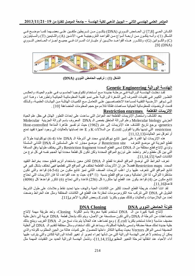
19/99/1192-91جامعة الموصل للفترة من –ليوبيل الذهبي لكلية الهندسة ا –العلمي الهندسي الثاني المؤتمر
214
( يتكييييون ميييين شييييريطين ملتفييييين علييييى بعضييييهما كمييييا موضييييح فييييي DNA إن الحييييامن النييييووي ) [7,8] الكييييائن الحييييي
( والسيييايتوزين T ( والثيييايمين )A (، وأنيييه يتكيييون مييين أربعييية أنيييواع مييين القواعيييد النتروجينيييية هيييي، األدنيييين ) 1 ) الشيييكل
( C( والكيييييوانين ) G وتتكيييييرر هيييييذه القواعيييييد مالييييييين أو ملييييييارات الميييييرات فيييييي جمييييييع أجيييييزاء الحيييييامن النيييييووي ،)
( DNA ) [9].
(DNA( : تركيب الحامض النووي )0الشكل )
Genetic Engineeringالهندسة الوراثية ميييع أسيييتخدام تكنولوجييييا الحاسيييوب فيييي عليييوم الحيييياة، وانعكييي دة جديييي الوراثيييية فيييي مرحلييية لقيييد دخليييت الهندسييية
الحياتيييية وتطورهيييا ، وهيييذا أدى التطيييور الكبيييير فيييي تقنييييات التعيييرف إليييى الشيييفرة الوراثيييية عليييى نميييو تقنيييية المعلوماتيييية
إليييى تيييوفير األرضيييية التقنيييية لمسييياعدة االختصاصييييين عليييى التعاميييل ميييع الكمييييات الهائلييية مييين البيانيييات العلميييية، وكيييذلك
قدمت الرياضيات للمعلوماتية الحياتية مساهمات فعالة تتالءم مع حجم المعلو [ . 11 ] مات المتضاعفة
enzymesRestriction اإلنزيمات القاطعةيعد اكتشاف واستعمال اإلنزيمات القاطعة احد العوامل التي ساعدت على إحداث التطور الهائل في حقل علم الحياة
Molecularالمعروف باسم الوراثة الجزيمية DNAالوراثة المتعلق بفحص الـ وعلم Molecular biologyالجزيمي
genetics ( حيث تم تفسير ظاهرة المناعة1691إلى عام )، يرجع تاريخ اكتشاف هذه اإلنزيماتHost-controlled
restriction التي تبديها بكتريا القولونE.coli من السالالتK وE عند إصابتها بالعاثيات إلى وجود أجهزة تقييد تمنع
[11,12,13]أو تعرقل نمو العاثيات
( نيوكلوتيدة طوال ثم 9-4عادة ) DNAهذه اإلنزيمات لها القدرة على تمييز تتابع نيوكلوتيدي محدد في أشرطة الـ
الثنائي السلسلة DNA أو موضع مجاور له على السلسلتين للـ Restriction siteتقطع الجريمة في موضع التعرف
المسافة والتي يختلف طولها وفق Restriction fragment تسمى القطع المحددة DNAوتؤدي إلنتاج قطع مختلفة من الـ
عتمد على توزيع المواقع المحددة ولكن تكون كل قطعة محددة لها الحجم نفسه في كل نوع من التي بين كل مقطع وآخر وت
[11,14,15].الكائنات الحية
لكائن معين باستخدام أنزيم قاطع محدد بخرائط التقييد DNA تعرف الخرائط التي توضح المواقع المنفردة لقطع الـ
ففضال عن إن األنزيمات القاطعة تختلف في المواقع التي تقطعها فهي تختلف بشكل كبير في Restriction mapsالمحدد
عد والتي تكون ( قوا4،5،9تتابع المواقع التي تتعرف عليها وان اغلب أنزيمات الصنف الثاني تميز تتابع مكون من )
عدد القواعد، لذا فان األنزيمات التي تحتاج n(، حيث /1متناظرة التوالي، لذا فان احتمالية وجود مواقع القطع بنسبة )
( 4169( تتكرر قواعدها كل )9( قاعدة والتي تحتاج )159( قواعد يكون عدد القطع لها متكررة كل )4تتابع مكون من )
[11,16].قاعدة
انشأ العلماء خريطة القطع المحدد لكثير من الكائنات الحية والهدف منها تحديد نقاط وعالمات على طول الشريط لقد
التي تتركب منه الكروموسومات لمقارنة هذه القطع في الكائنات المختلفة ومثل هذه الخرائط وضعت DNAالطويل في
.[11]البكتريا األخرى وبعن E.coliلعدد من البالزميدات والعاثيات وكذلك جينوم بكتريا
DNA DNA Cloningكلونة الحامض النووي
، وتعد طريقة مهمة إلنتاج Cloningتستخدم تقنية معروفة باسم الكلونة DNAإلنتاج كمية كبيرة من الـ
غريبة إلى داخل خلية DNAوالتي تكون مستنسخة عن األصل، ويتم ذلك بإدخال قطعة DNAمتضاعفات من أشرطة الـ
الغريب وينتج بذلك DNA( ومع تضاعف هذه الخاليا يتم بناء نسخ من الـ E.coliمضيف مناسبة )عادة تستخدم بكتريا
إلى الخلية DNAخلية جديدة تملك صفة مضافة وتسمى بالخلية المكلونة، ويساعد في ذلك استخدام وسائل مختلفة لتقديم الـ
بحيث يمكنها التكاثر داخلها للحصول على كميات هائلة من الجين المطلوب كلونته والذي Vectorsالمضيفة تسمى النواقل
غراض الهندسة الوراثية التي من شأنها إجراء تحوير أو تغيير للمادة الوراثية للكائن والتي يترتب عليها يمكن أن يستخدم أل
، وتشمل الهندسة الوراثية العديد من التقنيات المهمة مثل [11,14,15]ظهريأداء األحياء عند انتقالها لمرحلة التعبير الم
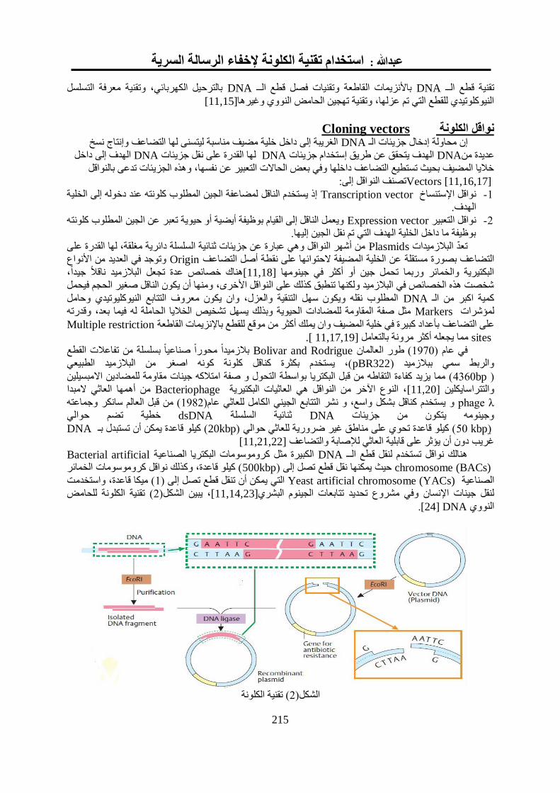
استخدام تقنية الكلونة إلخفاء الرسالة السرية: عبدهللا
215
بالترحيل الكهربائي، وتقنية معرفة التسلسل DNAت فصل قطع الــباألنزيمات القاطعة وتقنيا DNAتقنية قطع الــ
[11,15]رهاالنيوكلوتيدي للقطع التي تم عزلها، وتقنية تهجين الحامن النووي وغي
Cloning vectors نواقل الكلونة الغريبة إلى داخل خلية مضيف مناسبة ليتسنى لها التضاعف وإنتاج نسخ DNAإن محاولة إدخال جزيمات الـ
الهدف إلى داخل DNA لها القدرة على نقل جزيمات DNA الهدف يتحقق عن طريق إستخدام جزيمات DNAعديدة من
النواقل خاليا المضيف بحيث تستطيع التضاعف داخلها وفي بعن الحاالت التعبير عن نفسها، وهذه الجزيمات تدعى ب
Vectors [11,16,17] :تصنف النواقل إلى
إذ يستخدم الناقل لمضاعفة الجين المطلوب كلونته عند دخوله إلى الخلية Transcription vectorنواقل اإلستنساخ -1
الهدف.
ويعمل الناقل إلى القيام بوظيفة أيضية أو حيوية تعبر عن الجين المطلوب كلونته Expression vectorنواقل التعبير -1
بوظيفة ما داخل الخلية الهدف التي تم نقل الجين إليها.
تعد البالزميدات Plasmids من أشهر النواقل وهي عبارة عن جزيمات ثنائية السلسلة دائرية مغلقة، لها القدرة على
وتوجد في العديد من األنواع Originعن الخلية المضيفة الحتوائها على نقطة أصل التضاعف التضاعف بصورة مستقلة
هناك خصائص عدة تجعل البالزميد ناقال جيدا ، [11,18]البكتيرية والخمائر وربما تحمل جين أو أكثر في جينومها
ومنها أن يكون الناقل صغير الحجم فيحمل شخصت هذه الخصائص في البالزميد ولكنها تنطبق كذلك على النواقل األخرى،
المطلوب نقله ويكون سهل التنقية والعزل، وان يكون معروف التتابع النيوكليوتيدي وحامل DNA كمية اكبر من الـ
ملة له فيما بعد، وقدرتهمثل صفة المقاومة للمضادات الحيوية وبذلك يسهل تشخيص الخاليا الحا Markersلمؤشرات
Multiple restrictionبأعداد كبيرة في خلية المضيف وان يملك أكثر من موقع للقطع باإلنزيمات القاطعة على التضاعف
sites [11,17,19 ].مما يجعله أكثر مرونة بالتعامل
بالزميدا محورا صناعيا بسلسلة من تفاعالت القطع Bolivar and Rodrigue( طور العالمان 1691في عام )
(، يستخدم بكثرة كناقل كلونة كونه اصغر من البالزميد الطبيعيpBR322والربط سمي ببالزميد )
(bp 4691 مما يزيد كفاءة التقاطه من قبل البكتريا بواسطة التحول و صفة امتالكه جينات مقاومة للمضادين االمبسيلين )
من أهمها العاثي المبدا Bacteriophage، النوع اآلخر من النواقل هي العاثيات البكتيرية [11,20]كلين والتتراساي
phage λ (من قبل العالم سانكر وجماعته 1691و يستخدم كناقل بشكل واسع، و نشر التتابع الجيني الكامل للعاثي عام )
ة تضم حواليخطي dsDNAثنائية السلسلة DNAوجينومه يتكون من جزيمات
(kbp 51( كيلو قاعدة تحوي على مناطق غير ضرورية للعاثي حوالي )20kbp كيلو قاعدة يمكن أن تستبدل بـ )DNA
[11,21,22]غريب دون أن يؤثر على قابلية العاثي لإلصابة والتضاعف
Bacterial artificialالكبيرة مثل كروموسومات البكتريا الصناعية DNAهنالك نواقل تستخدم لنقل قطع الــ
chromosome (BACs) ( 500حيث يمكنها نقل قطع تصل إلىkbp كيلو قاعدة، وكذلك نواقل كروموسومات الخمائر )
( ميكا قاعدة، واستخدمت 1التي يمكن أن تنقل قطع تصل إلى ) Yeast artificial chromosome (YACs)الصناعية
( تقنية الكلونة للحامن 1، يبين الشكل)[11,14,23]ابعات الجينوم البشريلنقل جينات اإلنسان وفي مشروع تحديد تت
.DNA [24]النووي
( تقنية الكلونة1الشكل)
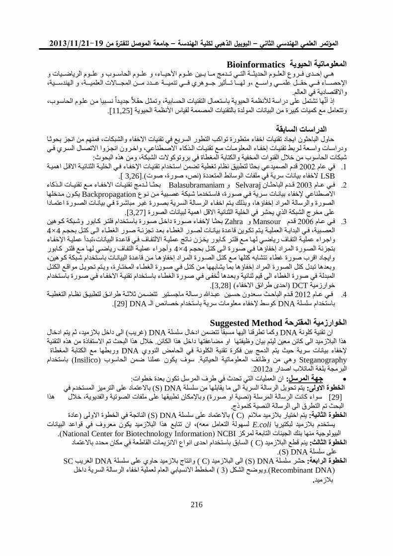
19/99/1192-91جامعة الموصل للفترة من –ليوبيل الذهبي لكلية الهندسة ا –العلمي الهندسي الثاني المؤتمر
216
Bioinformaticsالمعلوماتية الحيوية و و عليييوم الرياضييييات وم الحاسيييوب م األحيييياء، و علييي و هيييي إحيييدى فيييروع العليييوم الحديثييية التيييي تيييدمج ميييا بيييين علييي
و لهييييا تييييأثير جييييوهري فييييي تنمييييية عييييدد ميييين المجيييياالت العلمييييية، و الهندسييييية، ، واسييييع علمييييي اإلحصيييياء فييييي حقييييل
واالقتصادية في العالم.
، الحاسيوب إذ أنها تشتمل على دراسة لألنظمة الحيوية باستعمال التقنيات الحسابية، وتمثيل حقيال جدييدا نسيبيا مين عليوم
[.11,25 ] ن البيانات المولدة بالتقنيات المصممة لقياس األنظمة الحيوية وتتعامل مع كميات كبيرة م
الدراسات السابقة حاول الباحثون ايجاد تقنيات اخفاء متطورة تواكب التطور السريع في تقنيات االخفاء والشبكات، فمنهم من انجز بحوثيا
االصييطناعي، واخييرون انجييزوا االتصييال السييري فييي ودراسييات واسييعة لييربط تقنيييات إخفيياء المعلومييات مييع تقنيييات الييذكاء
كتابة المغطاة في بروتوكوالت الشبكة، ومن هذه البحوث: شبكات الحاسوب من خالل القنوات المخفية وال
بحثا لتطبيق نظام تغطية تضمن اسيتخدام تقنييات اإلخفياء فيي الخليية الثنائيية االقيل اهميية قدم الصميدعي 1111 في عام . 1
LSB .)[3,26 ] الخفاء بيانات سرية في ملفات الوسائط المتعددة )نص، صورة، صوت.
بحثييا لييدمج تقنيييات االخفيياء مييع تقنيييات الييذكاء Balasubramaniam و Selvaraj ن قييدم الباحثييا 1116 فييي عييام . 1
يكيون ميدخلها Backpropagation بيانيات سيرية فيي صيورة، فاسيتخدما شيبكة عصيبية مين نيوع إلخفاء االصطناعي
الصورة والرسالة المراد إخفاؤها، وبذلك ييتم اخفياء الرسيالة السيرية بصيورة غيير مباشيرة فيي بيانيات الصيورة اعتميادا
.[3,27] على مخرج الشبكة الذي يحشر في الخلية الثنائية االقل اهمية لبيانات الصورة
ة باسيتخدام فلتيير كيابور وشييبكة كييوهين صييورة داخيل صييور إلخفياء بحثييا Zahra و Mansour قيدم 1119 فيي عييام . 6
4×4 ييتم تكييوين قاعيدة بيانييات لصيور الغطيياء بعيد تجزئيية صيور الغطيياء اليى كتييل بحجييم العملييية العصيبية، فييي البدايية
تبيدأ عمليية اإلخفيياء يية االلتفيياف فيي قاعيدة البيانات، يخيزن نياتج عمل التفياف رياضيي لهيا مييع فلتير كيابور واجيراء عمليية
التفياف رياضيي لهيا ميع فلتير كيابور وأجيراء عمليية 4×4 الميراد إخفاؤهيا فيي صيورة اليى كتيل بحجيم بتجزئة الصيورة
وايجاد اقرب صورة غطاء تتشابه كتلها ميع كتيل الصيورة الميراد إخفاؤهيا مين قاعيدة البيانيات باسيتخدام شيبكة كيوهين،
اء المختيارة، وييتم تحوييل مواقيع الكتيل وبعدها تبدل كتل الصورة المراد إخفاؤها بما يشابهها مين كتيل فيي صيورة الغطي
المبدلة في صورة الغطاء الى قيم ثنائية وبعيدها ت خفيى فيي صيورة الغطياء باسيتخدام تقنيية االخفياء فيي صيورة باسيتخدام
.[3,28] )احدى طرائق االخفاء( DCT خوارزمية
ضييمن ثالثيية طرائييق لتطبيييق نظييام التغطييية حسييين عبييدا رسييالة ماجسييتير تت قييدم الباحييث سييعدون 1111 فييي عييام . 4
DNA .[29] كوسط إلخفاء معلومات سرية باستخدام خصائص الـ DNA باستخدام سلسلة
Suggested Method الخوارزمية المقترحةيتم ادخال ثم)غريب( الى داخل بالزميد، DNAادخال سلسلة تتضمن وكما تطرقنا اليها مسبقا DNAان تقنية كلونة
داخل هذا الكائن. خالل هذا البحث تم االستفاذة من هذه التقنية او مضاعفتها هذا البالزميد الى كائن معين ليتم بيان وظيفتها
مع الكتابة المغطاةوربطها DNA ي الحامن النوويدمج بين فكرة تقنية الكلونة فالحيث يتم إلخفاء بيانات سرية
Steganography الحياتيةوهي من وظائف المعلوماتية. ( سوف يكون عملنا ضمن الحاسوبInsilico) باستخدام
. a1111لغة الماتالب اصدار ب البرمجة
ان العمليات التي تحدث في طرف المرسل تكون بعدة خطوات:: جهة المرسل
ترميز المستخدم في ال( باالعتماد على S) DNAمن سلسلة ما يقابلهايتم تحويل الرسالة السرية الى الخطوة االولى:
هذا والفديوية، خاللسواء كانت الرسالة المرسلة )نصية او صورة( وباإلمكان تطبيقها على ملفات الصوتية [29]
التطرق الى الرسالة النصية كنموذج. تمالبحث
)عادة ( الناتجة في الخطوة االولىS) DNAباالعتماد على سلسلة C )) مالئم يتم اختيار بالزميد الخطوة الثانية:
في قواعد البيانات تتابع هذا البالزميد يكون معروف ان ،معه(لسهولة التعامل E.coliيستخدم بالزميد لبكتيريا
NCBI (National Center for Biotechnology Information.) منها بنك الجينات التابعة لمركز البيولوجية
اطعة في مكان محدد باالعتماد السابق باستخدام احدى انواع االنزيمات الق C )ينم قطع البالزميد ) الخطوة الثالث:
DNA (S.)سلسلة على
SCالغريب DNAوانتاج بالزميد حاوي على سلسلة C )) ( الى البالزميدS)DNA حشر سلسلة الخطوة الرابعة:
(Recombinant DNA.)( 6ويوضح الشكل ) لعملية اخفاء الرسالة السرية داخل العام يالمخطط االنسياب
.بالزميد
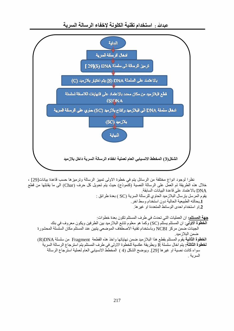
استخدام تقنية الكلونة إلخفاء الرسالة السرية: عبدهللا
217
، [29]يز الرسالة وترميزها حسب قاعدة بياناتينظرا لوجود انواع مختلفة من الرسائل يتم في خطوة االولى تم
الى ما يقابلها من قطع (Char) حيث يتم تحويل كل حرف )كنموذج( النصيةخالل هذه الطريقة تم العمل على الرسالة
DNA السابقة باالعتماد على قاعدة البيانات.
: طرائقبعدة ( SC)يقوم المرسل بإرسال البالزميد الحاوي للرسالة السرية
الطبيعية الحالية دون استخدام وسط اخر.بحالته .0
المتعددة او غيرها. الوسائطاو استخدام احدى .2
ان العمليات التي تحدث في طرف المستلم تكون بعدة خطوات:: جهة المستلم
بنكمعروف في ويكونالبالزميد بين الطرفين تتابع وكما هو معلوم (SC): ان المستلم يستلم الخطوة االولى
السلسلة المحشورة عند المستلم مكان وباستخدام تقنية االصطفاف الموضعي يتبين NCBIالجينات ضمن مركز
.ضمن البالزميد
DNA(R)من سلسلة Fragmentنهاياتها واخذ هذه القطعة البالزميد ضمن هذايقوم المستلم بقطع الخطوة الثانية
وبطريقة عكسية للخطوة االولى في طرف المستلم يتم استرجاع الرسالة السرية R يتم اخال سلسلة لخطوة الثالثة:
استرجاع الرسالة لعملية العام ( المخطط االنسيابي 4. ويوضح الشكل )[29] سواء كانت نصية او غيرها
.السرية
( المخطط االنسيابي العام لعملية اخفاء الرسالة السرية داخل بالزميد3الشكل)
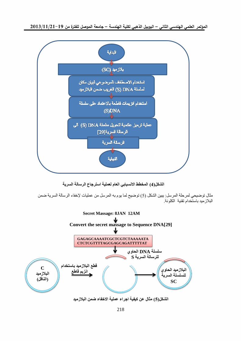
19/99/1192-91جامعة الموصل للفترة من –ليوبيل الذهبي لكلية الهندسة ا –العلمي الهندسي الثاني المؤتمر
218
المخطط االنسيابي العام لعملية استرجاع الرسالة السرية (4الشكل)
الرسالة السرية ضمن إلخفاء( توضيح لما يوم به المرسل من عمليات 5ن الشكل )ييب :لمرحلة المرسل توضيحيمثال
البالزميد باستخدام تقنية الكلونة.
Convert the secret massage to Sequence DNA[29]
( مثال عن كيفية اجراء عملية االخفاء ضمن البالزميد5لشكل)ا
Secret Massage: 8JAN 12AM
GAGAGCAAAATCGCTCGTCTAAAAATA
CTCTCGTTTTAGCGAGCAGATTTTTAT
C
البالزميد
)الناقل(
البالزميد الحاوي
ةللسلسلة السري
SC
البالزميد باستخدام قطع
قاطع انزيم
الحاوي DNAسلسلة
S للرسالة السرية
استخدام تقنية الكلونة إلخفاء الرسالة السرية: عبدهللا
219
Result and Discussionالنتائج والمناقشة بهذه الطريقة تتضمن مجموعة من النتائج باالعتماد من المقايي DNAان العمل على اخفاء الرسالة السرية ضمن وسط
منها:
:ان هذه الطريقة اثبتت استيعابها اطوال مختلفة من الرسالة السرية بعد ترميزها. طول الرسالة السرية
:ان العمل على تقنية الكلونة لباحثي العلوم الطبية اصبحت مسالة طبيعية فان العملية تكون الشكوك سرية الوسط الناقل
فيها قليلة. :الى البالزميد )الغطاء( تتكيف معها وال ان الرسالة السرية بعد ادخالها سرية نقل الرسالة السرية
يوحي وجود الرسالة السرية
:ثواني اما زمن استرجاع 5كانت زمن اخفاء الرسالة السرية زمن اخفاء واسترجاع الرسالة السرية
ثواني . 11الرسالة السرية عند الشخص المخول كانت
ان العمل على سلسلة االخرى للطريقة:من نقاط القوةDNA يتطلب معرفة كاملة وخلفية نظرية وعملية بالبيولوجي
من والمأخوذة بين الطرفين عليها والمتفق السرية DNA لسلسلة المحلل كشف الصعوبة منالجزيمي، كذلك
.مختلفة لكائنات DNA سلسلة مليون163 من ما يقارب على تحتوي كونها بسرعة NCBI البيانات قاعدة
Conclusionsاالستنتاجات : اآلتية االستنتاجات إلى التوصل تم البحث وباالعتماد على النتائج هذا في المقترحة تطبيق الطريقة خالل من
الجزيمي اعطت اهمية عالية البيولوجيان استخدام الطرائق الحديثة وخاصة بدمج تقنيات علوم الحاسوب وعلم
في اخفاء المعلومات. .تعتبر هذه الطريقة المقترحة من الطرائق الحديثة إلخفاء المعلومات واتثبت جدارتها باالعتماد على المقايي السابقة
ان العمل على تقنية الكلونة تتطلب معرفة كاملة عن التقنية وانواع االنزيمات القاطعة واختيار مكان الحشر لسلسلة الحاوية
للرسالة السرية.
باإلمكان ( العمل على التقنية طبيعيا Invitro.ضمن انبوب اختبار في مختبرات علوم الحياة ضمن شروط معينة )
References المصادر اكتشاف المعلومات المخفية في الصور واستخالصها باستخدام الشبكات العصبية"، ،"فرهاد محي الدين خليفة -1
.1ص،1111جامعة الموصل،العراق،،علوم حاسوب رسالة ماجستير
2- Sabeti Vajiheh,and et al., "Steganalysis of Embedding in Difference of Image Pixel Pairs
by Neural Network". ISC, vol. 1, no. 1, January 2009, pp. 17-26.
" تقصي تقنيات اخفاء المعلومات باستخدام الشبكات العصبية وبروتوكوالت الشبكة"،اميرة بيبو سلو، -6
.4ص،1116،جامعة الموصل،العراق،علوم حاسوبرسالة ماجستير
4- Buchanan, Joshua Michael,"Creating a Robust Form of Steganography", Unpublished
M. Sc. Thesis, Wake Forest University, North Carolina, , 2004.
5- Dujan Basheer Taha, "Digital Image Watermarking Techniques for Copyright Protection",
Unpublished D. Ph. Thesis ,Computer Science, University of Mosul,
Iraq,2004
6- Hovaneak, Rastislav, Foris, Peter and Levicky, Dusan,"Steganography Based on DWT
Transform", Technical University of Kosice, Slovak Republic. ,2002.
جامعة ،علوم الرياضيات اطروحة دكتورا المعلوماتية الحياتية"، عمر صابر قاسم،" تطبيق التقنيات الذكائية في -9
.9-5،ص1111 ، العراق،الموصل
، "استخدام الهندسة الوراثية في التحقيق الجنائي : أساليب وتطبيقات"، المركز القومي للبحوث السواحوجدي عبد الفتاح -9
.1111، القاهرة،
9- Calvino, M., Gomez, N. and Mingo, L.F., “DNA Simulation of Genetic Algorithms:
Fitness Computation”, International Journal ,Information Theories & Applications,
Vol.14, 2007,pp.45-46.
علوم رسالة ماجستير تمييز الصور الطبية للدماغ باستخدام تقنيات البايومعلوماتية"، اسامة ياسين محمد،" -11
.1،ص1111الموصل،العراق،،جامعة حاسوب
19/99/1192-91جامعة الموصل للفترة من –ليوبيل الذهبي لكلية الهندسة ا –العلمي الهندسي الثاني المؤتمر
220
تكسيره بعد Escherichia coliلبكتريا DNAالتغيرات الحيوية في خصائص الـ " رغد رياض شفيق العباسي، -11
.14 -16،ص1119العراق،،جامعة الموصل،علوم الحياة "، رسالة ماجستيرواستخدامه في الكلونة
12- Arber, W. and Morse, M.L. “Host specificity of DNA produced by Escherichia coli.
Genetics”, 1965,pp. 137-148.
13- Dussoix. D. and Arber, W. “Host specificity of DNA produce by Escherichia coli.
II",Control over acceptance of DNA from infecting phage . J. Mol. Biol., 1962.5: pp.
37-49.
14- Karp, G. "Cell and Molecular Biology". 4th ed., John Wiley & Sons, Inc., New
York.,2005.
15- Tamarin, R. H. "Principles of Genetics". 5th ed., McGraw-Hill Companies, Inc., USA,
1996.
16- Brown, T.A. "Gene Cloning". 3rd
ed., Chapman & Hall, Inc., London ,1997.
17- Streips, U.N. and Yasbin, R.E. "Modern Microbial Genetics". 2nd
ed., John Wiley &
Sons, Inc., New York, 2002.
18- Old, R.W. and Primrose, S.B. "Principles of Gene Manipulation an Introduction to
Genetic Engineering". 5th
ed., Blackwell Science, Ltd., Oxford,1998.
19- Sofer, W.H. (1991). "Introduction to Genetic Engineering". Boston, Butterworth, cited by:
Paolella, P. (1998). "Introduction to Molecular Biology". McGraw-Hill Companies, Inc.,
New York.
20- Bolivar, F.and et al. ,Construction and characterization of new cloning vehicles.
Gene,1977, 2: pp. 95-113.
21- Sanger, F. and et al.,Nucleotide sequence of bacteriophage lambda DNA. J. Mol.
Biol.,1982, 162: pp.729-773.
22- Darnell, J. and et al., "Molecular Cell Biology". Scientific American Books, Inc., New York,
1986.
. 1119 ، جامعة بغداد، العراق ، التقنية الحيوية الميكروبية )توجيهات جزيمية( " زهرة محمود الخفاجي، - 16
24-Jan Koolman and et al.,”Color Atlas of Biochemistry”, 2nd Ed, Philipps University
Marburg, Institute of Physiologic Chemistry,Marburg, Germany,2005.
25- International Journal of Bioinformatics Research and Applications,e-mail:
[email protected] or At the website: http://www.inderscience.com ,
Switzerland.2004.
.1111،جامعة الموصل،العراق،علوم حاسوب "، رسالة ماجستيرعامر تحسين سهيل، "تطبيق نظام التغطية"، -26
27- Selvaraj, J. and Balasubramaniam, R.,"Neural Network Based Camouflaging in Still
Image", University of Tamilnadu, India, 2003, [email protected]
28- Shi, Yun Q., "Transactions on Data Hiding and Multimedia Security", Springer- Verlag,
New Jersey Institute of Technology Newark, USA,2008.
،جامعة عليييوم حاسييييوب رسييييالة ماجسيييتير طا إلخفييياء المعلوميييات"،وسيييي DNAسيييعدون حسيييين عبدا،"تسلسيييالت -29
. 65- 64 ،ص 1111 الموصل،العراق،