ARTICLE IN PRESS

0022-0248/$ - se

doi:10.1016/j.jc

�CorrespondE-mail addr

Journal of Crystal Growth 291 (2006) 272–289

www.elsevier.com/locate/jcrysgro

Second order sharp-interface and thin-interface asymptotic analysesand error minimization for phase-field descriptions of two-sided

dilute binary alloy solidification

Arvind Gopinatha,�, Robert C. Armstrongb, Robert A. Brownb

aDivision of Engineering and Applied Sciences, Harvard University, Cambridge, MA 02138, USAbDepartment of Chemical Engineering, Massachusetts Institute of Technology, Cambridge, MA 02139, USA

Received 16 August 2004; accepted 1 March 2006

Communicated by G.B. McFadden

Abstract

Sharp-interface and thin-interface asymptotic analyses are presented for a generalization of the Beckermann–Karma phase-field model

for solidification of a dilute binary alloy when the interface curvature is macroscopic. The ratio of diffusivities, Rm � D0s=D0m, in the solid

and melt is arbitrary with 0pRmp1. Discrepancies between this diffuse-interface model and the classical, two sided solutal model (TSM)

description are quantified up to second order in the small parameter � that controls the interface thickness. We uncover extra terms in the

interface species flux balance and in the Gibbs–Thomson equilibrium condition introduced by the finite width of the interface.

Asymptotic results in the limit of rapid-interfacial kinetics are presented for both finite phase-field mobility and a quasi-steady state

approximation for the phase-field wherein the phase-field responds passively to the concentration field. The possibility of adding

additional terms to the phase-field version of the species conservation equation is explored as a means of achieving Oð�2Þ consistency withthe classical model. Our results naturally lead to a generalization of the anti-trapping solutal flux suggested by Karma [Phase-field-

formulation for quantitative modeling of alloy solidification, Phys. Rev. Lett. 87(11) (2001) 115701] for the limit Rm ¼ 0. Achieving

second order accuracy for arbitrary Rm requires judicious choices for the interpolating functions; these are calculated a posteriori using

the functional forms of the error terms as a guide.

r 2006 Elsevier B.V. All rights reserved.

PACS: 81.30.Fb

Keywords: A1. Anti-trapping solutal flux; A1. Directional solidification; A2. Phase-field models; A3. Two-sided model; B1. Dilute binary alloys

1. Introduction

Phase-field models [1–6] (PFM) for alloy solidificationare attractive alternatives to the classical sharp-interfacedescriptions of interfacial phenomena embodied in theframework of Gibbs thermodynamic description of aninterface as a mathematical surface. The appeal of thephase-field description comes from the mathematical andcomputational simplicity of replacing the moving bound-ary problem with coupled nonlinear reaction–diffusionequations and the considerable methodology that is

e front matter r 2006 Elsevier B.V. All rights reserved.

rysgro.2006.03.001

ing author. Tel.: +1617 253 6545; fax: +1 617 258 8992.

ess: arvind.gopinath@gmail.com (A. Gopinath).

available for this latter class of problems. A key step tothe use of phenomenologically based phase-field models iscareful computation and analysis for understanding thedifferences between these and classical sharp-interfacedescriptions. Towards this end, we present a formal secondorder asymptotic analysis of a generalized version of theBeckermann–Karma [1,4] phase-field model applicable forstudying dilute, binary alloy solidification processes witharbitrary solid and melt component diffusivities. TheBeckermann–Karma model has been used to studyphenomena ranging from dentritic growth to the develop-ment of microstructure in a mushy alloy and is typical ofmodels that are derived from geometrical principles [1,4].The set of equations can be formulated to explicitly

ARTICLE IN PRESS

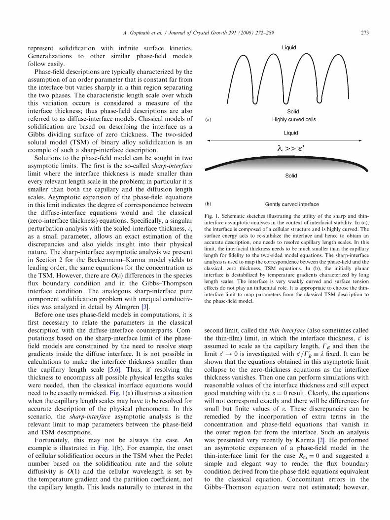
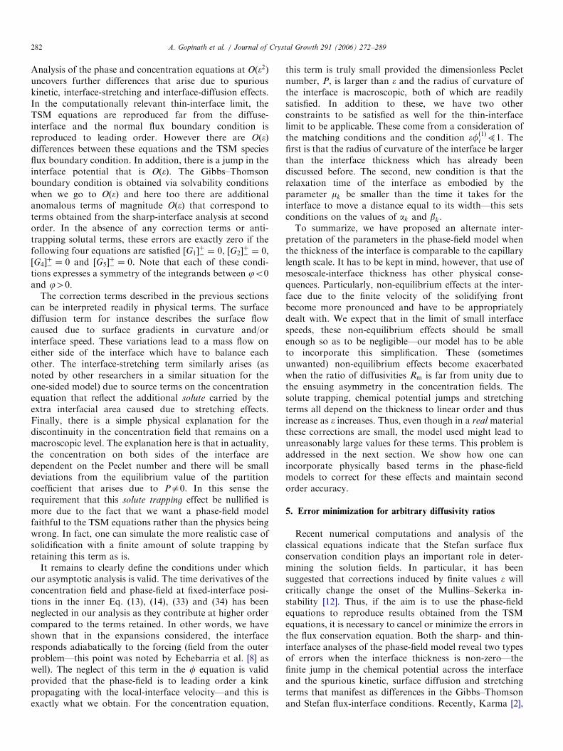
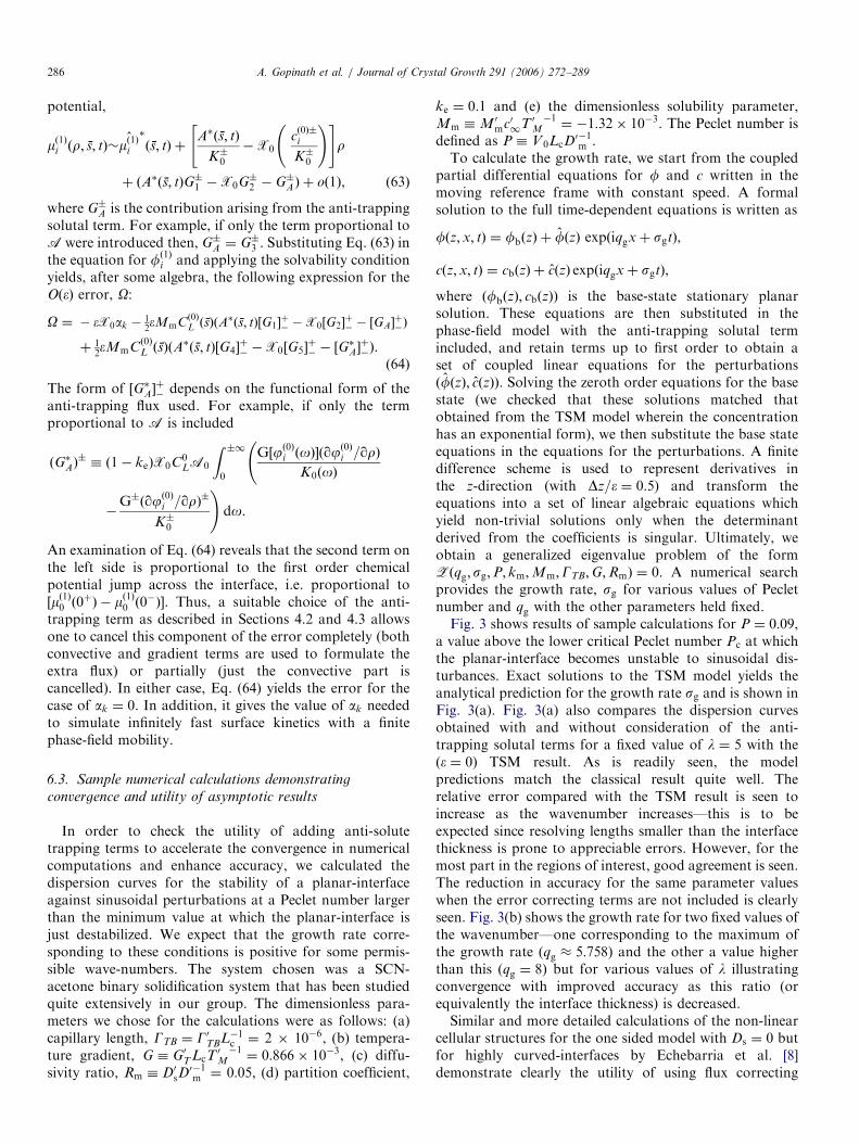
Fig. 1. Schematic sketches illustrating the utility of the sharp and thin-

interface asymptotic analyses in the context of interfacial stability. In (a),

the interface is composed of a cellular structure and is highly curved. The

surface energy acts to re-stabilize the interface and hence to obtain an

accurate description, one needs to resolve capillary length scales. In this

limit, the interfacial thickness needs to be much smaller than the capillary

length for fidelity to the two-sided model equations. The sharp-interface

analysis is used to map the correspondence between the phase-field and the

classical, zero thickness, TSM equations. In (b), the initially planar

interface is destabilized by temperature gradients characterized by long

length scales. The interface is very weakly curved and surface tension

effects do not play an influential role. It is appropriate to choose the thin-

interface limit to map parameters from the classical TSM description to

the phase-field model.

A. Gopinath et al. / Journal of Crystal Growth 291 (2006) 272–289 273

represent solidification with infinite surface kinetics.Generalizations to other similar phase-field modelsfollow easily.

Phase-field descriptions are typically characterized by theassumption of an order parameter that is constant far fromthe interface but varies sharply in a thin region separatingthe two phases. The characteristic length scale over whichthis variation occurs is considered a measure of theinterface thickness; thus phase-field descriptions are alsoreferred to as diffuse-interface models. Classical models ofsolidification are based on describing the interface as aGibbs dividing surface of zero thickness. The two-sidedsolutal model (TSM) of binary alloy solidification is anexample of such a sharp-interface description.

Solutions to the phase-field model can be sought in twoasymptotic limits. The first is the so-called sharp-interface

limit where the interface thickness is made smaller thanevery relevant length scale in the problem; in particular it issmaller than both the capillary and the diffusion lengthscales. Asymptotic expansion of the phase-field equationsin this limit indicates the degree of correspondence betweenthe diffuse-interface equations would and the classical(zero-interface thickness) equations. Specifically, a singularperturbation analysis with the scaled-interface thickness, �,as a small parameter, allows an exact estimation of thediscrepancies and also yields insight into their physicalnature. The sharp-interface asymptotic analysis we presentin Section 2 for the Beckermann–Karma model yields toleading order, the same equations for the concentration asthe TSM. However, there are Oð�Þ differences in the speciesflux boundary condition and in the Gibbs–Thompsoninterface condition. The analogous sharp-interface purecomponent solidification problem with unequal conductiv-ities was analyzed in detail by Almgren [3].

Before one uses phase-field models in computations, it isfirst necessary to relate the parameters in the classicaldescription with the diffuse-interface counterparts. Com-putations based on the sharp-interface limit of the phase-field models are constrained by the need to resolve steepgradients inside the diffuse interface. It is not possible incalculations to make the interface thickness smaller thanthe capillary length scale [5,6]. Thus, if resolving thethickness to encompass all possible physical lengths scaleswere needed, then the classical interface equations wouldneed to be exactly mimicked. Fig. 1(a) illustrates a situationwhen the capillary length scales may have to be resolved foraccurate description of the physical phenomena. In thisscenario, the sharp-interface asymptotic analysis is therelevant limit to map parameters between the phase-fieldand TSM descriptions.

Fortunately, this may not be always the case. Anexample is illustrated in Fig. 1(b). For example, the onsetof cellular solidification occurs in the TSM when the Pecletnumber based on the solidification rate and the solutediffusivity is Oð1Þ and the cellular wavelength is set bythe temperature gradient and the partition coefficient, notthe capillary length. This leads naturally to interest in the

second limit, called the thin-interface (also sometimes calledthe thin-film) limit, in which the interface thickness, �0 isassumed to scale as the capillary length, GB and then thelimit �0 ! 0 is investigated with �0=G0B � l fixed. It can beshown that the equations obtained in this asymptotic limitcollapse to the zero-thickness equations as the interfacethickness vanishes. Then one can perform simulations withreasonable values of the interface thickness and still expectgood matching with the � ¼ 0 result. Clearly, the equationswill not correspond exactly and there will be differences forsmall but finite values of �. These discrepancies can beremedied by the incorporation of extra terms in theconcentration and phase-field equations that vanish inthe outer region far from the interface. Such an analysiswas presented very recently by Karma [2]. He performedan asymptotic expansion of a phase-field model in thethin-interface limit for the case Rm ¼ 0 and suggested asimple and elegant way to render the flux boundarycondition derived from the phase-field equations equivalentto the classical equation. Concomitant errors in theGibbs–Thomson equation were not estimated; however,

ARTICLE IN PRESSA. Gopinath et al. / Journal of Crystal Growth 291 (2006) 272–289274

computations with the modified equations for a dentriticgrowth problem demonstrated good convergence proper-ties. The analysis for the one-sided model is relevant foralloys that are substitutional with Rm�Oð10�4Þ. In somecases however, we can have Rm�Oð10�3 � 10�2Þ andeffects of non-zero Rm must be considered, especially when�0=Lc�Rm, Lc being a characteristic macroscopic lengthscale. Ideally we could like to cancel anomalous terms inorder to obtain both the classical Gibbs–Thomsonequilibrium interface condition and flux conservationboundary conditions for the general case 0oRmo1.

A very recent paper by Ramirez et al. [5] presents thethin-interface analysis, up to first order, of a thermo-dynamically motivated phase-field model with coupledheat and solute diffusion with Rm ¼ 0. Solute trappingwas eliminated to leading order by incorporatingan anti-trapping flux term in the species conservationequation. One feature of this analysis was that the phase-field equation was intrinsically time-dependent with aconcentration-dependent time scale t�1 that could beappropriately chosen to simulate infinitely fast surfacekinetics. We will show in this article that the form of thistime scale follows naturally for arbitrary Rm. In addition,more than one form of this time scale is physicallypermissible.

The phase-field equations are compared to the classicalTSM equations for directional solidification of a dilutebinary alloy in an imposed temperature field that translateswith speed V0 in the z0 direction. The binary alloycomprises of an impurity B in a pure component A. Letc0m and c0s be the melt and solid concentrations of theimpurity (mole fractions) and D0m and D0s be thediffusivities of the impurity in the melt and solid,respectively. The far field impurity concentrations satisfythe mass conservation statement limz0!1 c0m ¼ c01 andlimz0!�1 c0s ¼ c01. Non-dimensional lengths are scaled bya characteristic length Lc, time by L2

cD0m�1 and concentra-

tions by the far field concentration c01. This yields thedimensionless equations

qcm

qt¼ r2cm þ P

qcm

qz;

qcs

qt¼ Rmr

2cs þ Pqcs

qz,

with the conditions limz!1 cm ¼ 1 and limz!�1 cs ¼ 1,where Rm � D0s=D0m and P � V 0LcD

0m�1.

An important equilibrium assumption made in the twosided model is that all non-equilibrium kinetic effectsexcept for a non-zero solidification rate are ignored. At theinterface the concentrations satisfy equilibrium and con-servation of species criteria. The first criteria yields theequation

ðcsÞI ¼ keðcmÞI , (1)

where ke being the equilibrium partition coefficient fromthe equilibrium phase plots. The flux of the impurity iscontinuous across the interface as trapping effects are notconsidered in the model. Parameterizing the interface, I,

as F ðx; z; tÞ � z� Bðx; tÞ � 0 yields the second equation

½Rmðn � =csÞ � ðn � =cmÞ�I ¼ ez � nð1� keÞcm PþqBqt

� �� �I

,

(2)

where we have assumed the mean interface motion to be inthe direction of ez. A second interface criteria is obtainedfrom near equilibrium thermodynamic considerations. Themelt/solid interface is assumed to be a Gibbs dividinginterface near equilibrium. The T–c curves of the solid andliquid phases are linearized about the melting temperatureof the pure melt T 0M , to yield approximate expressions ofthe melting temperature as a function of concentration,T 0 ¼ T 0M þM 0

sc0s and T 0 ¼ T 0M þM 0

mc0m. The parameters,M 0

m and the M 0s are the slopes of the linearized liquidus and

solidus curves, respectively. The assumption of equilibriumat the interface implies that the interface curvature,temperature and concentration satisfy the Gibbs–Thomp-son condition (GTC). In the two sided model equations,the temperature field is assumed to be prescribed. This isapplicable due to the wide separation in time scales overwhich heat and mass diffusion occur. Consequently, thetemperature of the interface is determined by its position—experimentally, one might envisage obtaining this bymoving the sample continually at constant velocity in atemperature field (see for example, Karma [2] and Ungarand Brown [7] and references therein). The imposedtemperature field is given in dimensionless form byT � T0 þ Gz, where T � T 0=T 0M and G � G0T LcT

0M�1 is

the dimensionless temperature gradient. The GTC thensimplifies to

ðT0 � 1Þ þ GzI ¼MmðcmÞI þ GTBð2@ÞI , (3)

where @ is the mean curvature of the interface, GTB is thedimensionless capillary length (scaled with Lc) [7] andMm �M 0

mc01T 0M�1. Note that in the above equation, the

intrinsic kinetics of the interface are assumed to beinstantaneous. The temperature field we have assumedcorresponds to the frozen (fixed) temperature assumptionfor solidification with a constant specified speed in atemperature gradient of magnitude G directed along thez-axis.In the following sections, we present the original and

generalized versions of the Beckermann–Karma phase-fieldmodel. Second order sharp and thin-interface asymptoticresults are presented for arbitrary diffusivity ratios, Rm. Tomaintain generality, we show our results using functionsthat are left as free and adjustable in order to providefreedom for subsequent error cancellation. This approachalso allows our results to be easily applied to other modelsas well. After a draft of this manuscript was submitted, theauthors became aware of very recent, related work byEchebarria et al. [8] on the thin-interface analysis of aphase-field model for the one-sided, binary solidificationproblems. Their work is a detailed exposition of resultspublished previously by Karma [2] for Rm ¼ 0. The workpresented in this paper is related to their work but more

ARTICLE IN PRESSA. Gopinath et al. / Journal of Crystal Growth 291 (2006) 272–289 275

general as we analyze the relationship between the sharpand thin-interface limits of phase-field models for Rm.However, we also show in Appendix that the equations weobtain reduce to results obtained by Karma’s [2] andEchebarria et al. [8]—thus, our analysis is consistent withthe published results for the one-sided models. Finally, inorder to illustrate the utility of the formalism, we presentsome numerical calculations of the dispersion curve for aset of sample parameters with and without the errorcorrecting terms. The curves obtained compare well to theclassical, zero-thickness limit with faster convergenceexhibited by the equations that include the anti-trappingcorrection terms.

2. The Beckermann–Karma phase-field model and

generalizations

Phase-field models for alloy solidification fall into twocategories. The first comprises of models derived viathermodynamic formulations like the WBM model [4]. Inthis approach, the interfacial region is assumed to be amixture of solid and liquid with the same composition.Principles from irreversible thermodynamics applied toentropy or energy production are invoked to formulateconstitutive equations for the concentration and the phase-field. The field parameters are determined by connectingthe model to the analogous classical equations via a sharpor thin-interface asymptotic analysis. The second class ofmodels treat the interface region as a mixture of solid andliquid with different compositions but equal chemicalpotentials. Examples are the models described in Tiadenet al. [9] and Beckermann et al. [1].

We use the Beckermann–Karma model to illustrate ouranalyses. Details of the derivation can be found in theoriginal papers by Beckermann and co-workers [1]. Theequations comprising this model are derived phenomen-ologically from the classical equations, hence theseequations take on physical meaning only in the sharp-interface limit. In this respect, there seems no clearadvantage to restricting analyses to purely thermodynamicmodels. In fact, the Beckermann–Karma model offersflexibility in simulating growth without kinetic effects orsolute trapping as demonstrated by Ramirez et al. [5]. Wefollow a notation wherein the phase field variable has thevalues f ¼ 0 in the liquid (melt) and f ¼ 1 in the solidphases. Let z be the coordinate along which the tempera-ture gradient acts, as well as being the direction ofsolidification. The evolution equation for the non-con-served field, f in a coordinate frame moving with constantvelocity V 00ez is given by

1

m0k

qfqt0¼

1

m0kV 00ðez � =

0fÞ þ G0B r02f�

1

j=0fjð=0f=0Þj=0fj

� �þ ðT 0M � T 0 þM 0

mc0mÞj=0fj.

Using the approximations ðj=0fjÞ�1ð=0f=0Þj=0fj � fð1�fÞð1� 2fÞ�0�2 and j=0fj � fð1� fÞ�0�1, the final form of

the equation for f becomes

1

m0k

qfqt0¼

1

m0kV 00ðez � =

0fÞ þ G0B r02f�

fð1� fÞð1� 2fÞ�2

� �

þ ðT 0M � T 0 þM 0mc0mÞ

fð1� fÞ�0

,

where m0k;V00; �0 and G0B are interpreted as the kinetic

coefficient, solidification rate, characteristic interface thick-ness and the Gibbs–Thompson coefficient, respectively,and M 0

m is the slope of the liquidus curve. A compositemixture concentration is defined as c � fcs þ ð1� fÞcmwhere c=cm � 1� fþ kef. The ratio cs=cm ¼ ke is con-strained to remain constant and equal to the equilibriumpartition coefficient. Summing the averaged species equa-tions for the impurity and using Fick’s law yields thespecies equation

qc0

qt0¼ V 00ðez � =

0c0Þ þ =0 � ðfD0s=0c0s þ ð1� fÞD0m=0c0mÞ.

We choose Lc, as a characteristic length, the meltdiffusivity as a characteristic diffusivity and defineRm � D0s=D0m. The equations for c � c0=c01 and f are then,

qc

qt¼ Pðez � =cÞ þ = � DðfÞ =cþ

ð1� keÞc

1� fþ kef=f

� �� �,

(4)

qfqt¼ Pðez � =fÞ þ mkGB r

2f�fð1� fÞð1� 2fÞ

�2

� �

þ mkð1� T þMmcmÞfð1� fÞ

�, ð5Þ

where P � V 00Lc=D0m is the Peclet number andDðfÞ � Rm þ ð1� RmÞð1� fÞð1� fþ kefÞ

�1. The para-meters mk � m0kT 0MLc=D0m and GB � G0B=ðT

0MLcÞ are the

scaled kinetic coefficient and the Gibbs–Thompsoncoefficient, respectively. The temperature has been scaledwith T 0M .We now make a simple but important substitution that

proves useful in the asymptotic analyses. Recognizing thatmk is strictly the kinetic rate coefficient in the limit of zero-interface thickness (since the derivation starts from theclassical-interface model), we write

m�1k � ðbk þ ak�Þ. (6)

This transformation is motivated by the results ofAlmgren’s analysis for the pure melt case and also by theexpectation that time-dependent simulations may be usedto study the limit of infinite surface kinetics. Furthermore,this transformation enables us to investigate the limits bk ¼

0 and m�1k ¼ 0, independently. We note that this also allowsus a degree of freedom whereby we can model not onlyconditions wherein Eq. (3) holds, but more generalsituations where intrinsic interfacial dynamics takes placeon time scales comparable to convective time scales. Thiscompletes the formulation of the model for the directional

ARTICLE IN PRESSA. Gopinath et al. / Journal of Crystal Growth 291 (2006) 272–289276

solidification problem (see Refs. [10,11] for details of theTSM equations).

z

e

es

0 (ε)

Melt

Solid

φ = 0

φ = 1

φ = 0.5

Πs

Outer region

Outer region

1/2 << φ < 1

0 < φ << 1/2

ρ

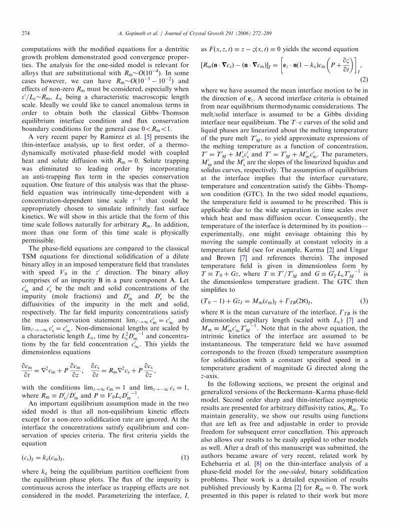
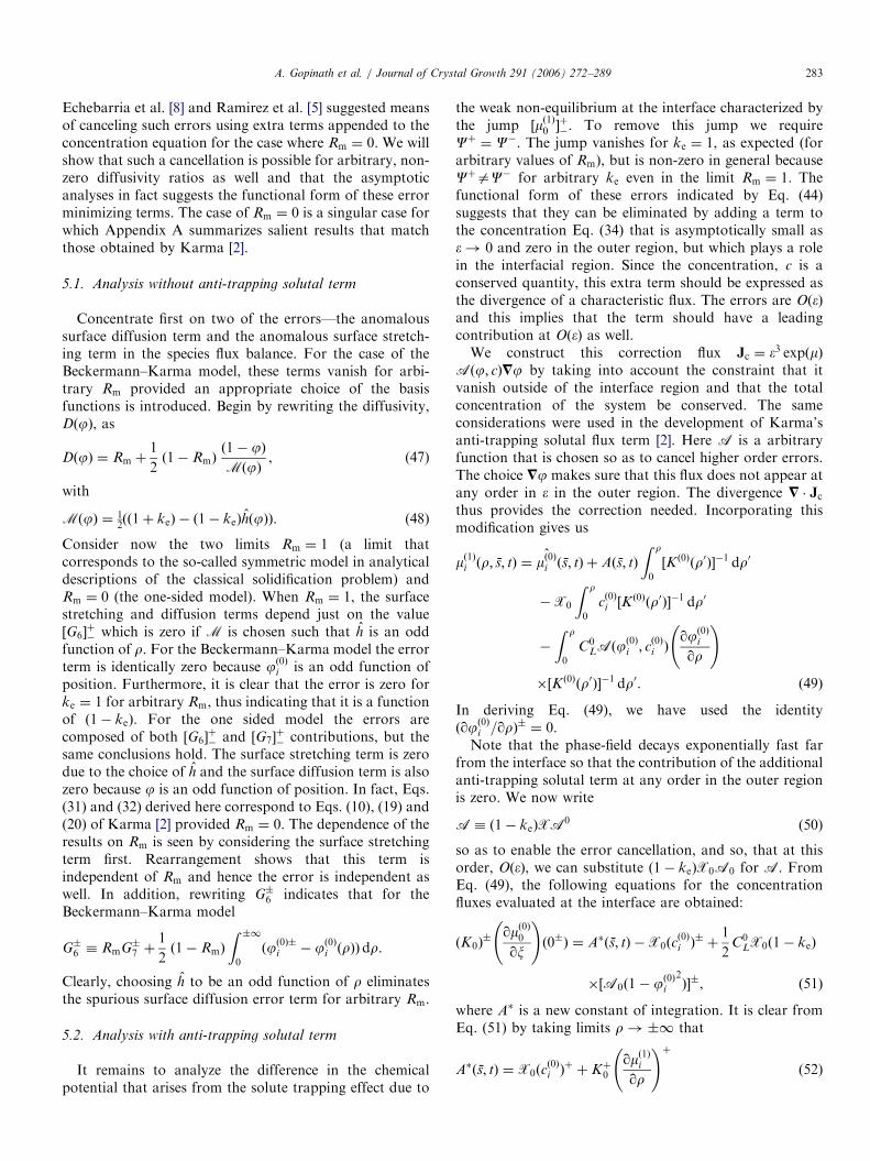
Fig. 2. Definition sketch of the inner and outer regions and the local

curvilinear co-ordinate system we employ.

2.1. Solutions for the isothermal problem with a planar

interface

It is valuable to note the equilibrium, isothermal, planarinterface (1D) solution to the Beckermann–Karma model.Setting P ¼ 0, G ¼ 0 yields the steady state equations for c

and f.

0 ¼ = � DðfÞ =cþð1� keÞc

1� fþ kef=f

� �� �, (7)

0 ¼ GB r2f�

fð1� fÞð1� 2fÞ�2

� �

þ ð1� T0 þMmcmÞfð1� fÞ

�. ð8Þ

where T0 is the isothermal temperature. We choose z as thecoordinate normal to the interface defined by f ¼ 1

2and x

as the coordinate tangential to the interface. Far from thediffuse interface jzjb�, and f ¼ 1 or f ¼ 0 depending onthe phase. The phase field equation is trivially satisfied andthe concentration equation reduces to the simple formD�= � ð=c�Þ ¼ 0 where Dþ ¼ 1 and D� ¼ Rm and cþ ¼ cmand c� ¼ cs. These equations are solved subject to theboundary conditions cmðz!1Þ ¼ 1 and ðdcs=dyÞz¼�1 ¼

0. The solutions that satisfy these and also the conditionke ¼ ðcs=cmÞI are cm ¼ 1 and cs ¼ ke. These are thesolutions to the solid and melt concentrations in the outerregion away from the region separating the two phases. Inorder to study the variation of c and f in the region close tof ¼ 1

2, we combine Eqs. (7) and (8) and integrate once with

respect to z to give d½lnðcÞ�=df ¼ ðke � 1Þð1� fþ kefÞ�1.

This yields the equilibrium solution ce ¼ feke þ 1� fe.This solution is valid both in the inner and outer regionsfor all z. Using this solution, the equation for the phasefield in the inner region reduces to

�2r2f ¼ fð1� fÞð1� 2fÞ ��

GB

ð1� T0 þMmÞfð1� fÞ.

Seeking a 1D field, we multiply both sides by df=dz andintegrate over z. Evaluating the resulting integrals andusing boundary conditions far from the interface yields 1�T0 þMm ¼ 0 which is the GTC at the interface atequilibrium. Thus, the diffuse interface formulation repro-duces both the correct concentration fields and the correctinterface condition at equilibrium. We are now in aposition to calculate the equilibrium phase-field feðzÞ.The phase field Eq. (7) reduces to the simple form �2r2f ¼fð1� fÞð1� 2fÞ which has the solution

feðzÞ ¼1

21� tanh

z

2�

� �� �(9)

satisfying the boundary conditions. Eq. (9) clearly indicatesthat the phase field decays exponentially fast for jzjb�.

3. Sharp-interface asymptotic analysis of the equations

The main aim in the following sections is to relate theboundary-less phase-field problem to the classical free-boundary problem. More specifically, we want to see howthe equations describing the concentration field in thephase-field model compare to the classical model as thewidth of the interface goes to zero. As mentioned in theintroduction, sharp-interface analysis fixes the interfacethickness (defined in a suitable way) to be smaller thanevery relevant physical length scale in the problem. Thisdisparity in scales allows us to define a small parameterthat enables a singular perturbation expansion to beperformed. For a given outer field and concomitantinterface velocities and interface curvature, the inner fieldcan be calculated with matching providing boundaryconditions that have to be satisfied for a self-consistentsolution to emerge. These consistency conditions corre-spond to the interface conditions in the classical free-boundary problem. It has to be also emphasized that theinterface can have an arbitrary but finite, macroscopiccurvature (the radius of curvature being larger than theinterface thickness). Otherwise the idea of an inner–outerexpansion loses meaning (Fig. 2).We begin with a sharp-interface analysis of the original

Beckermann–Karma equations for general finite surfacekinetics up to second order, for direct comparison with

ARTICLE IN PRESSA. Gopinath et al. / Journal of Crystal Growth 291 (2006) 272–289 277

Almgren’s work for the pure component problem and tosuggest connections to Karma’s analysis for Rm ¼ 0. Forsmall interface thicknesses, �0, solutions consist of a largebulk region (outer region) in which f is equal to either 0 or1 at z ¼ �1. Near the interface (which has a macroscopiccurvature defined more precisely later in the paper), there isan inner region of width Oð�Þ in which f varies rapidlybetween 0 and 1. We will first introduce coordinatetransformations for expressing the equations in thevariables appropriate for both the outer regions far fromthe interface and the inner interfacial region. Theseexpressions will also be utilized in the thin-film asymptoticanalysis.

3.1. Co-ordinate transformations in terms of local

curvilinear co-ordinates

Define the interface by Pðt : �Þ for �40 as the locus ofpoints satisfying f ¼ 1

2. Parameterize the curve by acoordinate s which is the arc-length along the 2D interface.Near Pðt : �Þ a signed function xðr; t : �Þ is defined with thesign of ð1

2� fÞ. A local curvilinear coordinate system ðx; sÞ

is proposed with coordinates such that j=xj ¼ 1 and=x � =s ¼ 0. This is done by appropriately extending s tothe neighborhood of Pðt : �Þ via a suitably uniqueformulation such that for each point r a unique set ðx; sÞis assigned. As long as Pðt : �Þ tends towards Pðt : 0Þsmoothly as �! 0, this coordinate transformation remainswell posed. One may then verify that the followingexpressions are true:

r2 ¼ qxx þ ðDxÞqx þ ðDsÞqs þ j=sj2qss,

ðqtÞr ¼ ðqtÞðx;sÞ � vnqx þqs

qtqs,

= � ½DðfÞ=f � ¼ qx DðfÞqf

qx

� �þ ðDxÞDðfÞ

qf

qxþ ðDsÞDðfÞ

qf

qs

þ j=sj2qs DðfÞqf

qs

� �,

ðDxÞðx; s; t : �Þ�k0 þ �ðk1 � xðk20 � 2X0ÞÞ þOð�2Þ,

= � a ¼ qxðn � aÞ þ qsðes � aÞ þ k0ðn � aÞ þOð�Þ,

where vn is the normal velocity of the surface, n ¼ er is thelocal normal to the surface, es is the local tangent, k is themean (macroscopic) curvature and X is the (macroscopic)Gaussian curvature. Note that vn ¼ vð0Þn þ �v

ð1Þn þ �

2vð2Þn þ

Oð�3Þ. Similarly, define X � ½vn þ Pðez � nfÞ� and writeX ¼ X0 þ �X1 þ �2X2 þOð�3Þ. Thus, we have obtainedtransformations to recast our equations in terms of acurvilinear co-ordinate system attached to the movinginterface. At the same time, we have not suppressed theintrinsic time-dependence of the fields.

3.1.1. Time-dependent equations in the outer-region far from

curved interface

Postulate the expansions

fouter ¼ f0 ¼ fð0Þ0 þ �fð1Þ0 þ �

2fð2Þ0 þOð�3Þ

and

couter ¼ c0 ¼ cð0Þ0 þ �c

ð1Þ0 þ �

2cð2Þ0 þOð�3Þ,

where fðkÞ0 and cðkÞ0 are of order k and are functions of

ðx; s; t : �Þ. The interface is given by the locus x ¼ 0. Theouter region is characterized in the re-scaled coordinatesðr ¼ x=�; s ¼ sÞ. In the outer region where f is zero or one,the equation for f is trivially satisfied and can bedisregarded. The equation for c

ðkÞ0 at each order in � has

the simple form

qcðkÞ0

qt

!�r

¼ Pðez � =cðkÞ0 Þ�þ = � ½D�c

ðkÞ0 =mðkÞ0 �, (10)

where D� � Dðx ¼ 0�Þ, so that D� � Rm, Dþ � 1 and=ðmðkÞ0 Þ

�¼ = lnðc

ðkÞ0 Þ�. Note that the outer problem is in

general time-dependent—we have not assumed stationarystate profiles. One may seek steady traveling wave solutionsby rewriting Eq. (10) in a reference frame moving with themean interface speed.

3.1.2. Equations in the inner region in the vicinity of the

curved interface and matching criteria

In the inner region, jxjpOð�Þ, we write

finner ¼ fiðr; s; tÞ ¼ fð0Þi þ �fð1Þi þ �

2fð2Þi þOð�3Þ

and

cinner ¼ ciðr; s; tÞ ¼ cð0Þi þ �c

ð1Þi þ �

2cð2Þi þOð�3Þ.

The matching region is given by 15jrj5��1 and �5jxj51.Define the function m � lnðc=ð1� fþ kefÞÞ, which may beinterpreted as a chemical potential. The matching condi-tions for the phase field variable, f, are limr!�1 fð0Þi ¼ 0or 1 and limr!�1 fðkÞi ¼ 0 for kX1. For the chemicalpotential the matching conditions are

limr!�1

mð0Þinner ¼ limr!�1

mð0Þi ¼ mð0Þouterðx! 0�Þ ¼ mð0Þ0 ð0�Þ (11)

and

mð1Þi �½qxmð0Þ0 ð0

�Þ�rþ mð1Þ0 ð0�Þ þ oð1Þ; r!�1. (12)

Using the transformations and re-scaled coordinates onegets for the phase-field f ¼ fi, the equation

�2

mkGB

qfqt

� �ðr;sÞ�

1

�vn

qfqrþ st

qfqs

" #

¼�

mkGB

Pðez � nfÞqfqr�

qFðfÞqf

þ �2r2f

þ�

GB

ð1� TÞqGðfÞqfþ

�

GB

Mmðexp mÞqGðfÞqf

. ð13Þ

The functions in the above equation are chosen to satisfyqFðfÞ=qf ¼ fð1� fÞð1� 2fÞ and qGðfÞ=qf ¼ fð1� fÞ.

ARTICLE IN PRESSA. Gopinath et al. / Journal of Crystal Growth 291 (2006) 272–289278

The equation for the concentration is now written as

�2qc

qt

� �ðr;sÞ�

1

�vn

qc

qrþ st

qc

qs

" #

¼ �Pðez � nfÞqc

qrþ �2Pðez � =sÞ

qc

qsþ �2= � ½DðfÞc=m�.

ð14Þ

Substituting the expansions for f and c into Eqs. (12) and(13), gives at Oð�0Þ,

�qFqfðf ¼ fð0Þi Þ þ

q2fð0Þi

qr2¼ 0,

qqr

Dðfð0Þi Þcð0Þi

qmð0Þi

qr

!¼ 0, ð15Þ

where fð0Þi ¼ fð0Þi ðrÞ. The translational invariance is re-moved by specifying that fð0Þi ð0Þ ¼

12. The unique solution

for the phase-field satisfying the boundary conditions is

fð0Þi ðr; s; tÞ ¼12ð1� tanhð1

2rÞÞ. (16)

The concentration field has the form

cð0Þi ¼ C

ð0ÞL ðsÞð1� fð0Þi þ kef

ð0Þi Þ (17)

or equivalently, mð0Þi ¼ lnCð0ÞL ðsÞ. Matching this inner

solution to the outer solution yields equations for the meltconcentration in the TSM viz, ðc

ð0Þ0 Þþ¼ ðcmÞI ¼ C

ð0ÞL ðsÞ and

ðcð0Þ0 Þ�¼ ðcsÞI ¼ keC

ð0ÞL ðsÞ as required.

3.2. Analysis at Oð�Þ

The concentration and phase-field variations at Oð�Þ cannow be easily obtained. The equation for the phase field atOð�Þ is

Lfð1Þi þbk

GB

qfð0Þi

qr

!X0 þ

Lc

Rc

� �k�0

qfð0Þi

qr

þ1

GB

ð1� TÞG0ðfð0Þi Þ þ1

GB

MmCð0ÞL ðsÞG

0ðfð0Þi Þ ¼ 0, ð18Þ

where the operator Lfð1Þi � ðq2fð1Þi =qr

2 � fð1Þi F00ðfð0Þi ÞÞ andRc is a characteristic curvature scale. BecauseLðqfð0Þi =qrÞ ¼ 0, for a bounded solution to exist, thefollowing solvability criterion must be satisfied:

Lfð1Þi ;qfð0Þi

qr

* +¼

Z þ1�1

Lfð1Þi

qfð0Þi

qrdr ¼ 0

or

�bk

GB

X0 �Lc

Rc

� �k�0 þ

1

GB

ð1� Tð0; sÞ þMmCð0ÞL ðsÞÞ ¼ 0.

(19)

This equation is identical to the Gibbs–Thomson equili-brium condition in the TSM with an additional term due tointerface kinetics. Using Eq. (19), shows that the leadingOð�Þ correction to the phase-field in the inner region isidentically zero; that is fð1Þi ¼ 0. Thus the Gibbs–Thomson

condition is accurately reproduced with Oð�Þ errors in thesharp-interface limit.The equation for the concentration field, c

ð1Þi ðr; s; tÞ, is

X0qcð0Þi

qrþ

Lc

Rc

� �k�0cð0Þi Dðfð0Þi Þ

qmð0Þi

qr

þqqr

cð0Þi Dðfð0Þi Þ

qmð1Þi

qrþ cð1Þi Dðfð0Þi Þ

qmð0Þi

qr

"

þcð0Þi fð1Þi D0ðfð0Þi Þ

qmð0Þi

qr

#¼ 0. ð20Þ

Integrating Eq. (20) twice yields the general solution

mð1Þi ðr; s; tÞ ¼^mð0Þi ðs; tÞ þ Aðs; tÞ

Z r

0

½K ð0Þðr0Þ��1 dr0

�X0

Z r

0

cð0Þi ½K

ð0Þðr0Þ��1 dr0. ð21Þ

Expanding Eq. (21) in the limits r!�1, gives theexpressions,

mð1Þi ðr; s; tÞ�^mð1Þi ðs; tÞ þ

Aðs; tÞ

K�0�X0

cð0Þ�i

K�0

( ) !" #r

þ ðCÞ� þ oð1Þ,

where K0 � cð0Þi Dðjð0Þi Þ and � indicates the limiting value as

r!�1. The functions C� are given by

C�ðs; tÞ ¼ Aðs; tÞ

Z �10

1

K0ðoÞ�

1

K�0

� �do

�X0

Z �10

cð0Þi ðoÞ

K0ðoÞ�

cð0Þ�i

K�0

!do. ð22Þ

Matching Eq. (21) to the outer solution for the concentra-tion using Eqs. (10) and (11) yields the criterion

K0qmð0Þ0qx

!ð0�Þ ¼ Aðs; tÞ �X0ðc

ð0Þi Þ�. (23)

The � on the left side refers to the limit r!�1 while the0� on the right side refers to the limit x! 0�. EliminatingAðs; tÞ from Eq. (23) yields the condition

X0ðke � 1ÞCð0ÞL ðsÞ ¼ Dþ c

ð0Þ0

qmð0Þ0qx

!ð0þÞ �D� c

ð0Þ0

qmð0Þ0qx

!ð0�Þ,

(24)

which upon simplification is seen to be identical to the fluxbalance equation in the TSM at Oð�Þ. It is important tonote that for the surface to be in quasi-equilibrium, it isalso required that ½mð1Þ0 �

þ� � mð1Þ0 ð0

þÞ � mð1Þ0 ð0�Þ ¼ 0. For this

condition we requireCþ ¼ C�. We will return to this pointlater in the discussion of the thin-film analysis. Aninteresting fact that emerges is that to leading order, thekink like profile fð0Þi is convected along with the interfacevelocity—the interface velocity is itself not prescribed fromthis set of equations!

ARTICLE IN PRESSA. Gopinath et al. / Journal of Crystal Growth 291 (2006) 272–289 279

3.3. Analysis at Oð�2Þ

The phase-field and concentration equations are nowsequentially analyzed at Oð�2Þ. Expanding the phase-fieldequation and using previous results, yields

Lfð2Þi ¼ �X0ak

GB

qfð0Þi

qr

!�X1

bk

GB

qfð0Þi

qr

!

�Lc

Rc

� �k�1

qfð0Þi

qr�

1

GB

ð1� TÞ1G0ðfð0Þi Þ

þ rLc

Rc

� �2

ðk20 � 2X0Þqfð0Þi

qr

!

þ1

GB

MmCð0ÞL ðsÞm

ð1Þi

qfð0Þi

qr

!. ð25Þ

The solvability condition is used to estimate the GTC atthis order of approximation. Note that the curvature termðk20 � 2X0Þ yields a contribution that is identically zerosince ðqfð0Þi =qrÞ is an odd function of r. Application of thesolvability condition gives

ð1� TÞ1 � GB

Lc

Rc

� �k�1 � bkX1 � akX0

þ3

2MmC

ð0ÞL ðsÞ

Z þ1�1

mð1Þi

qfð0Þi

qr

!2

dr ¼ 0. ð26Þ

Comparison with the GTC in the TSM shows that thephase-field model yields the same result at Oð�2Þ with anextra term given by

O ¼ ��X0ak þ �MmCð0ÞL ðsÞ½D� mð1Þ0 ð0

þÞ�

arising due to the diffuse nature of the interface, with

D ¼ mð1Þ0 ð0þÞ þ 1

2Aðs; tÞðG4 � G1Þ

þ� þ

12X0ðG2 � G5Þ

þ�.

The terms G�4 and G�5 are defined as

G�4 �

Z �10

G½fð0Þi ðoÞ�K0ðoÞ

�G�

K�0

!do,

G�5 �

Z �10

G½fð0Þi ðoÞ�cð0Þi ðoÞ

K0ðoÞ�

G�cð0Þ�i

K�0

!do.

We conclude this section by analyzing the concentrationequation at Oð�2Þ. Note that fð1Þi ¼ 0, m ¼ lnðc=ð1� fþkefÞÞ � lnðc=MÞ and mð1Þi ¼ c

ð1Þi =c

ð0Þi . Defining a surface

diffusion operator as

Dsð:Þ ¼ j=sj2qssð:Þ þ ðDsÞqqsð:Þ (27)

and combining this expression in conjunction with resultsof the previous section yields the following equation for the

concentration field at Oð�2Þ:

K0qmð2Þi

qr

!¼ B�X0c

ð1Þi �X1c

ð0Þi

� DsðC0LÞ

Z r

0

D0Mð0Þ dr� mð1Þi ðA�X0c

ð0Þi Þ

�Lc

Rc

� �k�0

Z r

0

ðA�X0cð0Þi Þdr

þ ½st � Pðez � =sÞ�dC0

L

ds

� �Z r

0

Mð0Þ dr, ð28Þ

where B is a constant of integration and Mð0Þ ¼Mðfð0Þi Þ.Taking the limits of Eq. (28) as r!�1, and matching tothe outer solution using,

qmð2Þi

qr

!�rðqxxðm

ð0Þ0 ÞÞð0

�Þ þ qxðmð1Þ0 Þð0

�Þ þ oð1Þ; r!�1

(29)

gives expressions for the jump in the gradient of thepotential across the interface and the error in the mass fluxcondition across the interface. The Oð1Þ term inK0ðqm

ð2Þi =qrÞ as r!�1 is

B�X1ðcð0Þi Þ�� Að

^mð1Þi þC�Þ � DsðC0LÞG

�6

þ ½st � Pðez � =sÞ�dC0

L

ds

� �G�7 þ

Lc

Rc

� �k�0X0C0

LG�7 , ð30Þ

where

G�6 �

Z �10

ðD0Mð0Þ � ðD0M

ð0ÞÞ�Þdr (31)

and

G�7 �

Z �10

ðMð0Þ � ðMð0ÞÞ�Þdr. (32)

The term G6 characterizes the error due to surface diffusionwhile G7 is the error due to interface stretching andcurvature. Comparison of Eq. (30) with the correspondingTSM expression at second order indicates that for the Oð�Þerrors in the flux to be zero, the first order flux andchemical potential must be continuous across the interfaceand in addition, require Cþ ¼ C�, ½G6�

þ� ¼ 0 and ½G7�

þ� ¼

0 individually or in a suitable combination.

4. Thin-interface asymptotic analysis of the

Beckermann–Karma model

A thin-interface analysis of the Beckermann–Karmamodel is presented in this section. In other words, theinterface thickness is assumed to be small but not muchsmaller than the capillary length. To facilitate comparisonwith the previous work by Karma, we redefine our phase-field variable using the re-definition, j ¼ 2f� 1, so that inthe solid phase (f ¼ 1, j ¼ 1) and in the melt (f ¼ 0,j ¼ �1). An additional interpolating function is nowincorporated in the equations for the Beckermann–Karma

ARTICLE IN PRESSA. Gopinath et al. / Journal of Crystal Growth 291 (2006) 272–289280

model; in the original Eqs. (4) and (5), this function, $ðfÞ,was set to equal f. In what follows, we will leave thisinterpolating function unspecified—the motivation will beto use this, if needed as an adjustable function to enableexact reduction of the diffuse interface model to the TSMas �! 0. The parameter mk is retained, but the scalingðmkGBÞ

�1� lðbk þ akÞ is applied. The equation for the

phase-field variable is then rewritten as

l�2ðbk þ akÞqjqt

� �þ st

qjqs

� �� l�ðbk þ akÞX

qjqr

¼ �F0BðjÞ þ �2r2jþ l

G0ðjÞ3ð1� T þ expðmÞMmÞ,

ð33Þ

where the concentration, cðr; s; tÞ is related to cm bycm � c=MðjÞ. We define cs � kecm so that the modifiedmodel is strictly valid only for dilute alloys at nearequilibrium situations. The variable m is defined as m �lnðc=MðjÞÞ and the functional M½$ðjÞ� � 1�$ðjÞ þke$ðjÞ with$ðjÞ ¼ ð1þ jÞ=2 for the Beckermann–Karmaformulation. The forms for terms F0BðjÞ ¼ �jð1� j2Þ=2and G0ðjÞ ¼ 3ð1� j2Þ=2 are used (where the primes denotederivatives with respect to j), and are identical to theBeckermann–Karma model and satisfy thermodynamicconstraints. In order to derive the modified concentrationequation, we redefine the diffusivity DðjÞ as DðjÞ �Rm þ ð1� RmÞð1� jÞð2MÞ�1. Note that if $ðjÞ ¼ð1þ jÞ=2, the diffusivity in the Beckermann–Karma modelis obtained. The concentration equation reads

�2qc

qt

� �ðr;sÞ�

1

�vn

qc

qrþ st

qc

qs

" #

¼ �Pðez � nfÞqc

qrþ �2Pðez � =sÞ

qc

qsþ �2= � ðDðjÞc=mÞ.

ð34Þ

Note again, that the equations in the inner and outerregion are time-dependent and valid provided the curva-ture is macroscopic with respect to the interface thickness.

As before, the variables (j; c and m) are expanded inpowers of � both in the inner and outer regions. In theouter region, far from the interface, j ¼ �1 for all �.Expanding j in the inner region as

jinner ¼ jiðr; s; tÞ ¼ jð0Þi þ �jð1Þi þ �

2jð2Þi þOð�3Þ, (35)

yields the boundary conditions

jð0Þi ðr!�1Þ ¼ �1; jðkÞi ðr!�1Þ ¼ 0 (36)

for kX1. At leading order Oð�ð0ÞÞ, the concentrationequation in the inner region is

qqr

cð0Þi Dðjð0Þi Þ

qmð0Þi

qr

!¼ 0, (37)

with

� F0Bðjð0Þi Þ þ

q2jð0Þi

qr2þ l

G0ðjð0Þi Þ

3

ð1� Tð� ¼ 0Þ þ expðmð0Þi ÞMmÞ ¼ 0. ð38Þ

The concentration equation is easily solved to yield mð0Þi ¼

lnðCð0ÞL ðs; tÞÞ and c

ð0Þi ¼ C

ð0ÞL Mðjð0Þi Þ. Note that c

ð0Þi ¼ 0 also

solves the concentration equation, but is not a physicallyvalid solution since it does not satisfy the requiredboundary conditions. The phase-field equation is satisfiedby

jð0Þi ðrÞ ¼ � tanhðr=2Þ (39)

provided that the solvability condition

12lð1� ðjð0Þi Þ

2Þ½ð1� Tð� ¼ 0ÞÞ þ expðmð0Þi ÞMm� ¼ 0

is satisfied. To leading order, the boundary condition is

ð1� Tð� ¼ 0ÞÞ þ expðmð0Þi ÞMm ¼ 0, (40)

so that the base state is a locally planar, equilibriuminterface, where curvature does not enter at lowest order.This result makes physical sense since l is held fixed and�! 0 implies that surface energy effects also vanish in thislimit. However, this is a very ill-posed problem inmathematical terms as we are neglecting the highest orderderivatives in the GTC. At Oð�0Þ, the Gibbs–Thomsonequation without surface energy is obtained. It should bepointed out that the phase-field variable satisfies thefollowing consistency condition imposed in order toremove the translational invariance of the base state:

fki ðr ¼ 0; s; tÞ ¼ 0 8kX0.

4.1. Analysis at Oð�Þ

Proceeding to Oð�1Þ, yields the following equationfor mð1Þi :

qcð0Þi

qrX0 þ

qqr

cð0Þi Dðjð0Þi Þ

qmð1Þi

qr

!¼ 0. (41)

Integrating Eq. (41) twice yields the equation (identical atthis order to that obtained in the sharp interface analysis)

mð1Þi ðr; s; tÞ ¼^mð1Þi ðs; tÞ þ Aðs; tÞ

Z r

0

K�10 ðnÞdn

�X0

Z r

0

cð0Þi K�10 ðnÞdn, ð42Þ

which on expanding in the limits r!�1 and subsequentsimplification along the lines of that followed in the sharp-interface analysis yields the same flux conservationequation (24), at the interface. Additionally, the followingexpression for the constant Aðs; tÞ is obtained:

Aðs; tÞ ¼ X0C0LðsÞ þ c

ð0Þ0

qmð0Þ0qx

!ð0þÞ, (43)

ARTICLE IN PRESSA. Gopinath et al. / Journal of Crystal Growth 291 (2006) 272–289 281

indicating that A depends on gradients of the concentrationfield evaluated at the interface for Rm40. The singular caseRm ¼ 0 is analyzed later in the Appendix. In addition,for the surface to be in quasi-equilibrium, the equation½mð1Þ0 �

þ� � mð1Þ0 ð0

þÞ � mð1Þ0 ð0�Þ ¼ 0 must hold. Using

Eq. (22), this condition is written in the more compactform as

½mð1Þ0 �þ� ¼ X0C0

LðsÞ½G1�þ� þ c

ð0Þ0

qmð0Þ0qx

!ð0þÞ½G1�

þ� �X0½G2�

þ�.

(44)

Clearly there are three contributions to the jump in thechemical potential that need to be set to zero for Oð�2Þaccuracy; a term proportional to the interface speed, a termproportional to the convective flux of solute dragged due tothe interface, and a term proportional to the gradient inconcentration at the interface. These conditions may ormay not be satisfied depending on the functional formsused for the potential well terms and the interpolatingfunctions hðjÞ and DðjÞ.

Unlike the result from the analysis in the sharp interfacelimit, fð1Þi is now in general non-zero. Writing the phase-field equation at Oð�Þ and then applying solvabilityconditions, gives the Gibbs–Thomson relationship validup to Oð�Þ. Combining the two solvability conditions, atorders Oð�0Þ and Oð�1Þ yields

½1� TðsÞ� þMmCð0ÞL ðsÞ½1þ �m

ð1Þ0 ð0

þÞ�

� GB

Lc

Rc

� �k�0 � bkX0 þ O ¼ 0, ð45Þ

with the term O ¼ Oð�Þ. Thus the phase-field model in thislimit yields equations that vary from the TSM equations byquantities of Oð�Þ. We note that this derivation retainsmuch of the form of the Oð�2Þ sharp-interface analysisbecause of the similarities in the expression for theconcentration field. The sequence of steps in the analysisdiffers; note that in obtaining the solvability condition atsecond order for the sharp interface limit, the equationfð1Þi ¼ 0 is used. We also had to demonstrate explicitly thatthe anomalous curvature terms do not contribute toadditional terms. Although the errors in Eq. (45) havethe same form, they arise at different orders in the twoanalyses. The GTC at Oð�Þ in the thin-interface limitinvolves the zeroth order curvature and normal velocityterms. But the sharp-interface analogue involves the firstorder curvature and normal velocity terms. As derived isSection 3, this error in the GTC is

O ¼ � �X0ak þ �MmCð0ÞL ðsÞ

12Aðs; tÞðG4 � G1Þ

þ�

�þ1

2X0ðG2 � G5Þ

þ�

�.

Note the dependence of the error terms on ak, A and X0—each represents Oð�Þ spurious kinetic effects and arediscussed in the next section.

4.2. Analysis of the phase-field and concentration equations

at Oð�2Þ

Proceeding now to the concentration equation at Oð�2Þ,and integrating once with respect to r yields

K0qmð2Þi

qr

!þ cð0Þ0 fð1Þi D0ðjð0Þi Þ

qmð1Þi

qr

!

¼ B�X0cð1Þi �X1c

ð0Þi � DsðC

0LÞ

Z r

0

D0Mð0Þ dr

�cð1Þi

cð0Þi

!ðA�X0c

ð0Þi Þ

�Lc

Rc

� �k�0

Z r

0

ðA�X0cð0Þi Þdr

þ ½st � Pðez � =sÞ�dC0

L

ds

� �Z r

0

Mð0Þ dr. ð46Þ

In deriving Eq. (46) the conditions qmð0Þi =qr ¼ 0 and mð0Þi ¼

lnC0L have been used. Eq. (46) is almost the same as Eq.

(28) obtained in the sharp-interface analysis, except for anadditional term proportional to fð1Þi on the left side of theequation and the term ðc

ð1Þi =c

ð0Þi Þ instead of mð1Þi . In the

sharp-interface limit, fð1Þi ¼ 0 and so mð1Þi ¼ ðcð1Þi =c

ð0Þi Þ. In

the thin-interface limit,

mð1Þi ¼cð1Þi

cð0Þi

!�

Mð1Þ

Mð0Þ

� �,

where Mð1Þ ¼ �ð1� keÞjð1Þi =2 for the Beckermann–Karma

model. Note that fð1Þi and its gradient decays as r!�1.Indeed, matching with the outer solution indicates that itdecays exponentially with distance from the interfacialregion. Hence while evaluating Eq. (46) for jrjb1, both theadditional terms drop out leaving an expression identical tothat obtained in the sharp-interface limit. The Oð�Þ surfacediffusion and surface stretching terms also are identical.It remains to estimate the errors at Oð�2Þ to the GTC.

The equation for fð2Þi is expanded and the solvabilityrequirement is applied. As before, the anomalous curvatureterms drop out on integration. Unfortunately, terms thatare proportional to mð2Þi are encountered and cannot beevaluated from the expressions we have. Thus, we areunable to obtain any further information about higherorder corrections to the GTC.

4.3. Summary of asymptotic results and physical

interpretations

Let us summarize the results from the asymptoticanalyses and focus on the discrepancies between the sharp-and thin-interface limits of the diffuse-interface model andthe TSM equivalents. In the sharp-interface limit, theBeckermann–Karma model reproduces both the fluxboundary condition and the Gibbs–Thomson equilibriumcondition to leading order. There are Oð�Þ errors in thepotential across the interface which have to be cancelled.

ARTICLE IN PRESSA. Gopinath et al. / Journal of Crystal Growth 291 (2006) 272–289282

Analysis of the phase and concentration equations at Oð�2Þuncovers further differences that arise due to spuriouskinetic, interface-stretching and interface-diffusion effects.In the computationally relevant thin-interface limit, theTSM equations are reproduced far from the diffuse-interface and the normal flux boundary condition isreproduced to leading order. However there are Oð�Þdifferences between these equations and the TSM speciesflux boundary condition. In addition, there is a jump in theinterface potential that is Oð�Þ. The Gibbs–Thomsonboundary condition is obtained via solvability conditionswhen we go to Oð�Þ and here too there are additionalanomalous terms of magnitude Oð�Þ that correspond toterms obtained from the sharp-interface analysis at secondorder. In the absence of any correction terms or anti-trapping solutal terms, these errors are exactly zero if thefollowing four equations are satisfied ½G1�

þ� ¼ 0, ½G2�

þ� ¼ 0;

½G4�þ� ¼ 0 and ½G5�

þ� ¼ 0. Note that each of these condi-

tions expresses a symmetry of the integrands between jo0and j40.

The correction terms described in the previous sectionscan be interpreted readily in physical terms. The surfacediffusion term for instance describes the surface flowcaused due to surface gradients in curvature and/orinterface speed. These variations lead to a mass flow oneither side of the interface which have to balance eachother. The interface-stretching term similarly arises (asnoted by other researchers in a similar situation for theone-sided model) due to source terms on the concentrationequation that reflect the additional solute carried by theextra interfacial area caused due to stretching effects.Finally, there is a simple physical explanation for thediscontinuity in the concentration field that remains on amacroscopic level. The explanation here is that in actuality,the concentration on both sides of the interface aredependent on the Peclet number and there will be smalldeviations from the equilibrium value of the partitioncoefficient that arises due to Pa0. In this sense therequirement that this solute trapping effect be nullified ismore due to the fact that we want a phase-field modelfaithful to the TSM equations rather than the physics beingwrong. In fact, one can simulate the more realistic case ofsolidification with a finite amount of solute trapping byretaining this term as is.

It remains to clearly define the conditions under whichour asymptotic analysis is valid. The time derivatives of theconcentration field and phase-field at fixed-interface posi-tions in the inner Eq. (13), (14), (33) and (34) has beenneglected in our analysis as they contribute at higher ordercompared to the terms retained. In other words, we haveshown that in the expansions considered, the interfaceresponds adiabatically to the forcing (field from the outerproblem—this point was noted by Echebarria et al. [8] aswell). The neglect of this term in the f equation is validprovided that the phase-field is to leading order a kinkpropagating with the local-interface velocity—and this isexactly what we obtain. For the concentration equation,

this term is truly small provided the dimensionless Pecletnumber, P, is larger than � and the radius of curvature ofthe interface is macroscopic, both of which are readilysatisfied. In addition to these, we have two otherconstraints to be satisfied as well for the thin-interfacelimit to be applicable. These come from a consideration ofthe matching conditions and the condition �fð1Þi 51. Thefirst is that the radius of curvature of the interface be largerthan the interface thickness which has already beendiscussed before. The second, new condition is that therelaxation time of the interface as embodied by theparameter mk be smaller than the time it takes for theinterface to move a distance equal to its width—this setsconditions on the values of ak and bk.To summarize, we have proposed an alternate inter-

pretation of the parameters in the phase-field model whenthe thickness of the interface is comparable to the capillarylength scale. It has to be kept in mind, however, that use ofmesoscale-interface thickness has other physical conse-quences. Particularly, non-equilibrium effects at the inter-face due to the finite velocity of the solidifying frontbecome more pronounced and have to be appropriatelydealt with. We expect that in the limit of small interfacespeeds, these non-equilibrium effects should be smallenough so as to be negligible—our model has to be ableto incorporate this simplification. These (sometimesunwanted) non-equilibrium effects become exacerbatedwhen the ratio of diffusivities Rm is far from unity due tothe ensuing asymmetry in the concentration fields. Thesolute trapping, chemical potential jumps and stretchingterms all depend on the thickness to linear order and thusincrease as � increases. Thus, even though in a real materialthese corrections are small, the model used might lead tounreasonably large values for these terms. This problem isaddressed in the next section. We show how one canincorporate physically based terms in the phase-fieldmodels to correct for these effects and maintain secondorder accuracy.

5. Error minimization for arbitrary diffusivity ratios

Recent numerical computations and analysis of theclassical equations indicate that the Stefan surface fluxconservation condition plays an important role in deter-mining the solution fields. In particular, it has beensuggested that corrections induced by finite values � willcritically change the onset of the Mullins–Sekerka in-stability [12]. Thus, if the aim is to use the phase-fieldequations to reproduce results obtained from the TSMequations, it is necessary to cancel or minimize the errors inthe flux conservation equation. Both the sharp- and thin-interface analyses of the phase-field model reveal two typesof errors when the interface thickness is non-zero—thefinite jump in the chemical potential across the interfaceand the spurious kinetic, surface diffusion and stretchingterms that manifest as differences in the Gibbs–Thomsonand Stefan flux-interface conditions. Recently, Karma [2],

ARTICLE IN PRESSA. Gopinath et al. / Journal of Crystal Growth 291 (2006) 272–289 283

Echebarria et al. [8] and Ramirez et al. [5] suggested meansof canceling such errors using extra terms appended to theconcentration equation for the case where Rm ¼ 0. We willshow that such a cancellation is possible for arbitrary, non-zero diffusivity ratios as well and that the asymptoticanalyses in fact suggests the functional form of these errorminimizing terms. The case of Rm ¼ 0 is a singular case forwhich Appendix A summarizes salient results that matchthose obtained by Karma [2].

5.1. Analysis without anti-trapping solutal term

Concentrate first on two of the errors—the anomaloussurface diffusion term and the anomalous surface stretch-ing term in the species flux balance. For the case of theBeckermann–Karma model, these terms vanish for arbi-trary Rm provided an appropriate choice of the basisfunctions is introduced. Begin by rewriting the diffusivity,DðjÞ, as

DðjÞ ¼ Rm þ1

2ð1� RmÞ

ð1� jÞMðjÞ

, (47)

with

MðjÞ ¼ 12ðð1þ keÞ � ð1� keÞhðjÞÞ. (48)

Consider now the two limits Rm ¼ 1 (a limit thatcorresponds to the so-called symmetric model in analyticaldescriptions of the classical solidification problem) andRm ¼ 0 (the one-sided model). When Rm ¼ 1, the surfacestretching and diffusion terms depend just on the value½G6�

þ� which is zero if M is chosen such that h is an odd

function of r. For the Beckermann–Karma model the errorterm is identically zero because jð0Þi is an odd function ofposition. Furthermore, it is clear that the error is zero forke ¼ 1 for arbitrary Rm, thus indicating that it is a functionof ð1� keÞ. For the one sided model the errors arecomposed of both ½G6�

þ� and ½G7�

þ� contributions, but the

same conclusions hold. The surface stretching term is zerodue to the choice of h and the surface diffusion term is alsozero because j is an odd function of position. In fact, Eqs.(31) and (32) derived here correspond to Eqs. (10), (19) and(20) of Karma [2] provided Rm ¼ 0. The dependence of theresults on Rm is seen by considering the surface stretchingterm first. Rearrangement shows that this term isindependent of Rm and hence the error is independent aswell. In addition, rewriting G�6 indicates that for theBeckermann–Karma model

G�6 � RmG�7 þ1

2ð1� RmÞ

Z �10

ðjð0Þ�i � jð0Þi ðrÞÞdr.

Clearly, choosing h to be an odd function of r eliminatesthe spurious surface diffusion error term for arbitrary Rm.

5.2. Analysis with anti-trapping solutal term

It remains to analyze the difference in the chemicalpotential that arises from the solute trapping effect due to

the weak non-equilibrium at the interface characterized bythe jump ½mð1Þ0 �

þ�. To remove this jump we require

Cþ ¼ C�. The jump vanishes for ke ¼ 1, as expected (forarbitrary values of Rm), but is non-zero in general becauseCþaC� for arbitrary ke even in the limit Rm ¼ 1. Thefunctional form of these errors indicated by Eq. (44)suggests that they can be eliminated by adding a term tothe concentration Eq. (34) that is asymptotically small as�! 0 and zero in the outer region, but which plays a rolein the interfacial region. Since the concentration, c is aconserved quantity, this extra term should be expressed asthe divergence of a characteristic flux. The errors are Oð�Þand this implies that the term should have a leadingcontribution at Oð�Þ as well.We construct this correction flux Jc ¼ �3 expðmÞ

Aðj; cÞ=j by taking into account the constraint that itvanish outside of the interface region and that the totalconcentration of the system be conserved. The sameconsiderations were used in the development of Karma’santi-trapping solutal flux term [2]. Here A is a arbitraryfunction that is chosen so as to cancel higher order errors.The choice =j makes sure that this flux does not appear atany order in � in the outer region. The divergence = � Jcthus provides the correction needed. Incorporating thismodification gives us

mð1Þi ðr; s; tÞ ¼^mð0Þi ðs; tÞ þ Aðs; tÞ

Z r

0

½K ð0Þðr0Þ��1 dr0

�X0

Z r

0

cð0Þi ½K

ð0Þðr0Þ��1 dr0

�

Z r

0

C0LAðj

ð0Þi ; c

ð0Þi Þ

qjð0Þi

qr

!

½K ð0Þðr0Þ��1 dr0. ð49Þ

In deriving Eq. (49), we have used the identityðqjð0Þi =qrÞ

�¼ 0.

Note that the phase-field decays exponentially fast farfrom the interface so that the contribution of the additionalanti-trapping solutal term at any order in the outer regionis zero. We now write

A � ð1� keÞXA0 (50)

so as to enable the error cancellation, and so, that at thisorder, Oð�Þ, we can substitute ð1� keÞX0A0 for A. FromEq. (49), the following equations for the concentrationfluxes evaluated at the interface are obtained:

ðK0Þ� qmð0Þ0

qx

!ð0�Þ ¼ A�ðs; tÞ �X0ðc

ð0Þi Þ�þ

1

2C0

LX0ð1� keÞ

½A0ð1� jð0Þi

2Þ��, ð51Þ

where A� is a new constant of integration. It is clear fromEq. (51) by taking limits r!�1 that

A�ðs; tÞ ¼ X0ðcð0Þi Þþþ Kþ0

qmð1Þi

qr

!þ(52)

ARTICLE IN PRESSA. Gopinath et al. / Journal of Crystal Growth 291 (2006) 272–289284

provided that A is a non-singular regular function of r. Asimple form is a constant, we shall show that this indeedprovides a degree of freedom that enables cancellation ofthe chemical potential jump.

Using ðcð0Þi Þþ¼ C0

L, ðcð0Þi Þ�¼ keC

0L, ðc

ð0Þi Þþ¼ ðc

ð0Þ0 Þð0

þÞ,ðcð0Þi Þ�¼ ðc

ð0Þ0 Þð0

�Þ and ðqmð0Þ0 =qxÞ ¼ ðcð0Þ0 Þ�1ðqcð0Þ0 =qxÞ, gives

the balance equation for the concentration flux as

X0ðke � 1ÞCð0ÞL ðsÞ �

1

2C0

Lð1� keÞX0A0½ðjð0Þi Þ

2�þ�

¼ Dqcð0Þ0

qx

!ð0þÞ � D

qcð0Þ0

qx

!ð0�Þ. ð53Þ

Since the term that includes ½ðjð0Þi Þ2�þ� is zero, the extra anti-

trapping solutal term does not change the flux balance atOð�Þ. Evaluating the contribution of this term to thepotential jump yields the modified expression for ½mð1Þ0 �

þ� as

½mð1Þ0 �þ� ¼ X0C0

LðsÞ½G1�þ� þ c

ð0Þ0

qmð0Þ0qx

!ð0þÞ½G1�

þ�

�X0½G2�þ� � ½G3�

þ�, ð54Þ

with

G�3 � �1

2ð1� keÞX0

Z �10

C0LA0ð1� ðj

ð0Þi Þ

2Þ½K ð0Þðr0Þ��1 dr0.

(55)

Considering only terms that are linear in X0, the net jumpin the potential proportional to the mean-interface velocity(convective motion) is found to be X0½G8�

þ� where

G�8 ¼

Z �10

ðL� L�Þdr0,

Lðjð0Þi Þ ¼1�Mð0Þ þ ð1=2ÞA0ð1� keÞð1� jð0Þi Þð1þ jð0Þi Þ

Mð0ÞDð0Þ.

ð56Þ

Eq. (56) is a generalization of Eqs. (7) and (8) obtained byKarma [2] for arbitrary nonzero values of the diffusivityratio. Note that we cannot set Rm ¼ 0 in (56) because thedenominator in the integrand becomes singular. In theAppendix, we show how a rederivation explicitly valid forRm ¼ 0 recovers Karma’s results. The pre-factor, X0,which follows naturally from Eqs. (50) and (54), is identicalto the pre-factor suggested by Karma, the Oð�0Þ componentof j=jj�1ðqj=qtÞ. Algebraic manipulations indicate that asrequired, G�8 ¼ 0 for arbitrary Rm, if ke ¼ 1. For generalvalues of Rm, choosing hðjÞ ¼ j and A0 ¼ ð1�RmkeÞð2RmkeÞ

�1 reduces Eq. (56) to the simple form

G�8 ¼ a

Z �10

ðjð0Þi � ðjð0Þi Þ�Þdr0,

where a is a constant. The error identically zero since thezeroth order phase-field is an odd function of r. Thus, thischoice of the anti-solutal term cancels the spuriousconvective contributions to the first order chemicalpotential jump. Analysis of the concentration equation atOð�2Þ with the anti-trapping solutal flux indicates that

Eq. (46) is modified as

K0qmð2Þi

qr

!þ cð0Þ0 fð1Þi D0ðfð0Þi Þ

qmð1Þi

qr

!

¼ B�ðs; tÞ �X0cð1Þi �X1c

ð0Þi � DsðC

0LÞ

Z r

0

D0Mð0Þ dr

�cð1Þi

cð0Þi

cð0Þi D0

qmð1Þi

qr

!þ ½st � Pðez � =sÞ�

dC0L

ds

� �Z r

0

Mð0Þ dr

�Lc

Rc

� �k�0

Z r

0

cð0Þi D0

qmð1Þi

qr

!dr

� ð1� keÞ X1A0C0L

qjð0Þi

qr

!� ð1� keÞ X0A0C0

L

qjð1Þi

qr

!

� ð1� keÞ X0A0C0Lmð1Þi

qjð0Þi

qr

!

�ð1� keÞLc

Rc

� �k�0X0C

0L

Z r

0

A0qjð0Þi

qr

!dr. (57)

Note that

K0qmð1Þi

qr

!¼ A�ðs; tÞ �X0c

ð0Þi � ð1� keÞC

0LX0A0

qjð0Þi

qr

!.

(58)

From the expressions derived at lower orders we knowthat jð1Þi , ðqjð0Þi =qrÞ and ðqj

ð1Þi =qrÞ all decay exponentially

with jrj. Thus, terms that involve these vanish in the limitsr!�1. Substitution of Eq. (58) into Eq. (46) andanalyzing the resulting equation in the limits r!�1shows that the Oð1Þ terms in K0ðqm

ð2Þi =qrÞ as r!�1 are

B�ðs; tÞ �X1ðcð0Þi Þ��

cð1Þi

cð0Þi

!A�ðs; tÞ � DsðC

0LÞG

�6

þ ½st � Pðez � =sÞ�dC0

L

ds

� �G�7

þLc

Rc

� �k�0X0C

0LG�7 . ð59Þ

For jrjb1, we also have mð1Þi ¼ ðcð1Þi =c

ð0Þi Þ to leading order.

If the anti-trapping solute term is included, the additionalterms in the flux balance at the interface vanish providedthe surface diffusion and surface stretching terms vanish asbefore and the chemical potential jump across the interfaceis nullified. Note that the surface diffusion and stretchingterms are not modified by the inclusion of the anti-trappingsolute flux. From Eq. (59), it follows that the Stefan fluxcondition is satisfied to Oð�2Þ provided the Oð�Þ errorsvanish.In addition, from the previous discussion it is clear that it

is possible to cancel the remaining error in the chemicalpotential jump that is proportional to the gradient of the

ARTICLE IN PRESSA. Gopinath et al. / Journal of Crystal Growth 291 (2006) 272–289 285

zeroth order potential evaluated at the interface. Thisquantity is not known from our analysis and has to beobtained by solving for the concentration field in the outerregion separately with appropriate boundary and initialconditions. For computational purposes, however, as onecan assume that this quantity is known at the beginning ofeach solution step. Formulating a similar flux correctinganti-trapping solutal term of the form ½B�3 expðmÞ�ð=jÞðqmð0Þ0 =qxÞð0

þÞ and repeating the analysis, we find thatchoosing a value of B ¼ ð1� keÞXBð0Þ given by

Bð0Þ

2þBð0Þ¼

1� Rmke

1þ Rmke

� �2

allows the elimination of all Oð�Þ errors in the fluxconservation equation arising from finite � for 0oRmp1.

6. Approaches to simulations of solidification with infinitely

fast surface kinetics

The asymptotic analysis described in Sections 3 and 4give a framework for discussing simulations of solidifica-tion with infinitely fast surface kinetics in the zero-interfacethickness limit which is particularly relevant for low speedsolidification processes. The TSM equations are usuallyformulated with instantaneous-interface relaxation. Al-most all current phase-field simulations however utilizetime-dependent simulations to solve for the set ðf; cÞ so thatthe phase-field mobility is set to a finite value. This isbecause the set of equations for the phase-field andconcentration may then be solved using standard explicittime integrators with steady states accessed by integratingto long time.

It is interesting to consider two cases that correspond toinfinitely fast surface kinetics; the first where the phase-fieldkinetics is set to be instantaneous (m�1k ¼ 0) and the secondwhen a finite value of the phase-field mobility is used withbk ¼ 0 and aka0. This second approach has beeninvestigated by Karma [2] and by Almgren [3] as well.

6.1. Infinitely fast surface kinetics without anti-trapping

solutal flux

Consider Eq. (26) in the sharp-interface analysis and Eq.(45) in the thin-interface analysis, both with m�1k ¼ 0 so thatbk ¼ 0 and ak ¼ 0. This implies that the equation for thephase-field is a quasi-stationary reaction–diffusion equation

that is coupled to time-independent concentration equation.In this approximation, the Oð�Þ error to GTC isð12Þ�MmC0

L½AðG4 � G1Þþ� þX0ðG2 � G5Þ

þ�� and A has con-

tributions arising from concentration gradients at theinterface, as well as the local-interface velocity, X0. Inprinciple, one could consider adding carefully chosenadditional terms to the phase-field equation to cancel theseerrors: the form of these terms is suggested by Eq. (45).Accordingly, in simulations with m�1k ¼ 0, cancellation of

Oð�Þ errors in the GTC will require either ðG4 � G1Þþ� and

ðG2 � G5Þþ� or the incorporation of extra terms in Eq. (33).

An alternate method of obtaining infinitely fast surfacekinetics has been investigated in some detail by Karma andco-workers [2,4,5]. Eq. (45) indicates that can obtain aneffective-interface kinetic coefficient which is independentof the value of the phase-field thickness, � and then set thisto zero, and still have a finite value of the overall phase-field mobility. This process corresponds to setting bk ¼ 0while keeping aka0. Alternately, a specified value of thekinetic coefficient in the sharp-interface limit, is obtainedby choosing the appropriate value of bk a priori. In bothcases, the value of ak may be chosen arbitrarily and is atour disposal to cancel possible discrepancies with the TSMequations. Consider the expression

D ¼ mð1Þ0 ð0þÞ þ

1

2Aðs; tÞðG4 � G1Þ

þ� þ

1

2X0ðG2 � G5Þ

þ� (60)

arising from the expression for the error in the GTC. Asmentioned earlier and as also noted by Almgren [3] forpure component solidification, terms involving A should beindependently cancelled since these involve gradients of theconcentration at the interface. The other terms in Eq. (60)are proportional to the interface speed and constitutespurious effective kinetic coefficients. These are eliminatedby choosing ak to be

½akðC0LÞ�1 ¼

12MmC0

LðG2 � G5Þþ�. (61)

A closer examination shows that we have obtained ageneralization of Karma’s result for the case of non-zeroRm. Note, however, that this special choice of the kineticcoefficient is not a constant as found in Almgren’s analysis[3] or as suggested by Karma [2] but is in fact a function ofthe interfacial concentration. For the case of isothermalsolidification, this kinetic coefficient is a constant as theinterfacial concentration is known from equilibrium con-ditions. Thus, one may adjust the value of the phase-fieldmobility as the simulation progresses to get an effective(classical) kinetic coefficient that is independent of theinterface thickness. In case one is unable to cancel out theterms proportional to A completely, we can redefine ak as afunction of C0

L to minimize as much of the errors aspossible. This leads to the alternate value for the kineticconstant

½akðC0LÞ�2 ¼

12MmC0

L½ðG2 � G5Þþ� þ C0

LðG4 � G1Þþ��. (62)

These equations give the Oð�Þ discrepancies between thediffuse-interface and TSM equations insofar as theGibbs–Thomson boundary condition is concerned for theBeckermann–Karma model.

6.2. Infinitely fast surface kinetics with anti-trapping solutal

flux

We now investigate the effects the anti-trapping soluteterm has on the Gibbs–Thomson equation at Oð�Þ.Repeating the analysis of Section 3.2, we get for the

ARTICLE IN PRESSA. Gopinath et al. / Journal of Crystal Growth 291 (2006) 272–289286

potential,

mð1Þi ðr; s; tÞ�^mð1Þi

�

ðs; tÞ þA�ðs; tÞ

K�0�X0

cð0Þ�i

K�0

!" #r

þ ðA�ðs; tÞG�1 �X0G�2 � G�AÞ þ oð1Þ, ð63Þ

where G�A is the contribution arising from the anti-trappingsolutal term. For example, if only the term proportional toA were introduced then, G�A ¼ G�3 . Substituting Eq. (63) inthe equation for fð1Þi and applying the solvability conditionyields, after some algebra, the following expression for theOð�Þ error, O:

O ¼ � �X0ak �12�MmC

ð0ÞL ðsÞðA

�ðs; tÞ½G1�þ� �X0½G2�

þ� � ½GA�

þ�Þ

þ 12�MmC

ð0ÞL ðsÞðA

�ðs; tÞ½G4�þ� �X0½G5�

þ� � ½G

�A�þ�Þ.ð64Þ

The form of ½G�A�þ� depends on the functional form of the

anti-trapping flux used. For example, if only the termproportional to A is included

ðG�AÞ�� ð1� keÞX0C

0LA0

Z �10

G½jð0Þi ðoÞ�ðqjð0Þi =qrÞ

K0ðoÞ

�G�ðqjð0Þi =qrÞ

�

K�0

!do.

An examination of Eq. (64) reveals that the second term onthe left side is proportional to the first order chemicalpotential jump across the interface, i.e. proportional to½mð1Þ0 ð0

þÞ � mð1Þ0 ð0�Þ�. Thus, a suitable choice of the anti-

trapping term as described in Sections 4.2 and 4.3 allowsone to cancel this component of the error completely (bothconvective and gradient terms are used to formulate theextra flux) or partially (just the convective part iscancelled). In either case, Eq. (64) yields the error for thecase of ak ¼ 0. In addition, it gives the value of ak neededto simulate infinitely fast surface kinetics with a finitephase-field mobility.

6.3. Sample numerical calculations demonstrating

convergence and utility of asymptotic results

In order to check the utility of adding anti-solutetrapping terms to accelerate the convergence in numericalcomputations and enhance accuracy, we calculated thedispersion curves for the stability of a planar-interfaceagainst sinusoidal perturbations at a Peclet number largerthan the minimum value at which the planar-interface isjust destabilized. We expect that the growth rate corre-sponding to these conditions is positive for some permis-sible wave-numbers. The system chosen was a SCN-acetone binary solidification system that has been studiedquite extensively in our group. The dimensionless para-meters we chose for the calculations were as follows: (a)capillary length, GTB ¼ G0TBL�1c ¼ 2 10�6, (b) tempera-ture gradient, G � G0T LcT

0M�1¼ 0:866 10�3, (c) diffu-

sivity ratio, Rm � D0sD0�1m ¼ 0:05, (d) partition coefficient,

ke ¼ 0:1 and (e) the dimensionless solubility parameter,Mm �M 0

mc01T 0M�1¼ �1:32 10�3. The Peclet number is

defined as P � V 0LcD0�1m .

To calculate the growth rate, we start from the coupledpartial differential equations for f and c written in themoving reference frame with constant speed. A formalsolution to the full time-dependent equations is written as

fðz;x; tÞ ¼ fbðzÞ þ fðzÞ expðiqgxþ sgtÞ,

cðz; x; tÞ ¼ cbðzÞ þ cðzÞ expðiqgxþ sgtÞ,

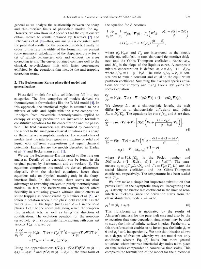
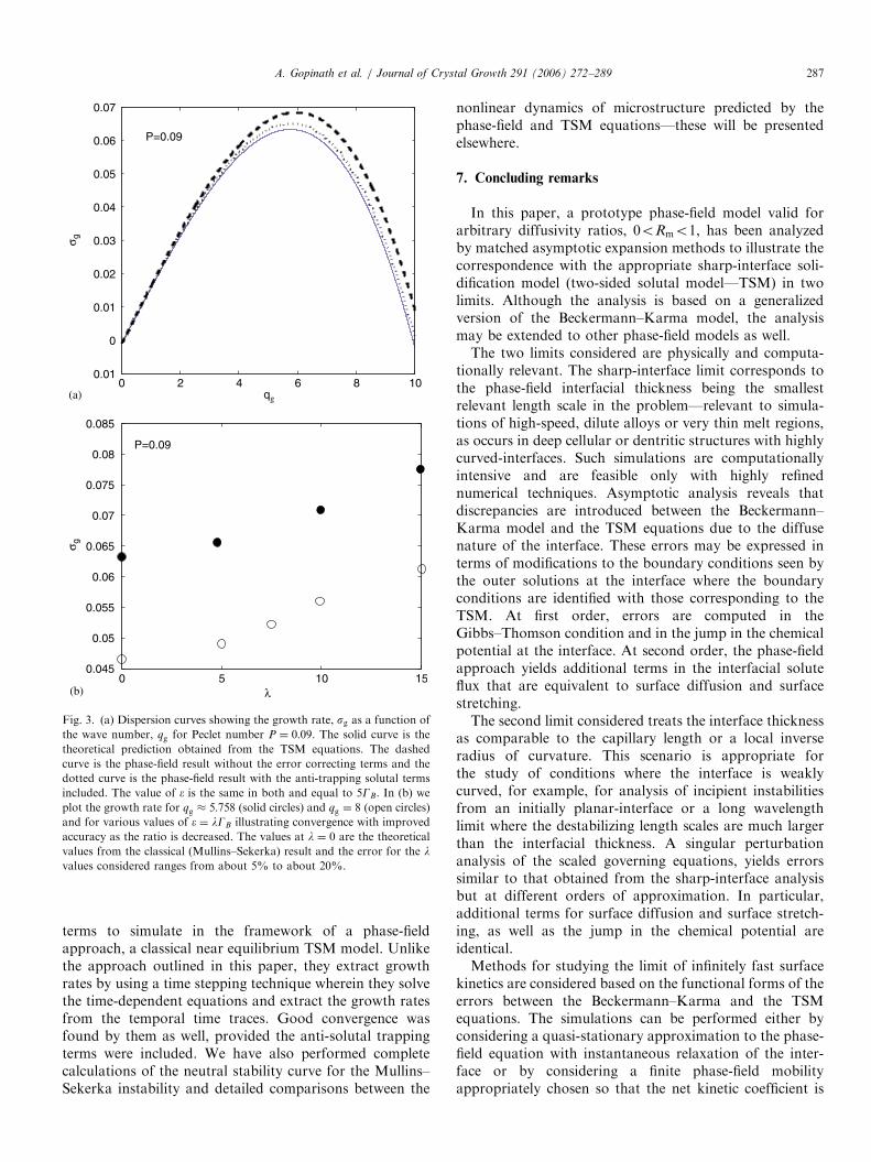
where ðfbðzÞ; cbðzÞÞ is the base-state stationary planarsolution. These equations are then substituted in thephase-field model with the anti-trapping solutal termincluded, and retain terms up to first order to obtain aset of coupled linear equations for the perturbationsðfðzÞ; cðzÞÞ. Solving the zeroth order equations for the basestate (we checked that these solutions matched thatobtained from the TSM model wherein the concentrationhas an exponential form), we then substitute the base stateequations in the equations for the perturbations. A finitedifference scheme is used to represent derivatives inthe z-direction (with Dz=� ¼ 0:5) and transform theequations into a set of linear algebraic equations whichyield non-trivial solutions only when the determinantderived from the coefficients is singular. Ultimately, weobtain a generalized eigenvalue problem of the formZðqg;sg;P; km;Mm;GTB;G;RmÞ ¼ 0. A numerical searchprovides the growth rate, sg for various values of Pecletnumber and qg with the other parameters held fixed.Fig. 3 shows results of sample calculations for P ¼ 0:09,

a value above the lower critical Peclet number Pc at whichthe planar-interface becomes unstable to sinusoidal dis-turbances. Exact solutions to the TSM model yields theanalytical prediction for the growth rate sg and is shown inFig. 3(a). Fig. 3(a) also compares the dispersion curvesobtained with and without consideration of the anti-trapping solutal terms for a fixed value of l ¼ 5 with the(� ¼ 0) TSM result. As is readily seen, the modelpredictions match the classical result quite well. Therelative error compared with the TSM result is seen toincrease as the wavenumber increases—this is to beexpected since resolving lengths smaller than the interfacethickness is prone to appreciable errors. However, for themost part in the regions of interest, good agreement is seen.The reduction in accuracy for the same parameter valueswhen the error correcting terms are not included is clearlyseen. Fig. 3(b) shows the growth rate for two fixed values ofthe wavenumber—one corresponding to the maximum ofthe growth rate (qg � 5:758) and the other a value higherthan this (qg ¼ 8) but for various values of l illustratingconvergence with improved accuracy as this ratio (orequivalently the interface thickness) is decreased.Similar and more detailed calculations of the non-linear

cellular structures for the one sided model with Ds ¼ 0 butfor highly curved-interfaces by Echebarria et al. [8]demonstrate clearly the utility of using flux correcting

ARTICLE IN PRESS

0 2 4 6 8 100.01

0

0.01

0.02

0.03

0.04

0.05

0.06

0.07

qg

σ gσ g

P=0.09

0 5 10 150.045

0.05

0.055

0.06

0.065

0.07

0.075

0.08

0.085

P=0.09

λ

(b)

(a)

Fig. 3. (a) Dispersion curves showing the growth rate, sg as a function of

the wave number, qg for Peclet number P ¼ 0:09. The solid curve is the

theoretical prediction obtained from the TSM equations. The dashed

curve is the phase-field result without the error correcting terms and the

dotted curve is the phase-field result with the anti-trapping solutal terms

included. The value of � is the same in both and equal to 5GB. In (b) we

plot the growth rate for qg � 5:758 (solid circles) and qg ¼ 8 (open circles)

and for various values of � ¼ lGB illustrating convergence with improved

accuracy as the ratio is decreased. The values at l ¼ 0 are the theoretical

values from the classical (Mullins–Sekerka) result and the error for the lvalues considered ranges from about 5% to about 20%.

A. Gopinath et al. / Journal of Crystal Growth 291 (2006) 272–289 287

terms to simulate in the framework of a phase-fieldapproach, a classical near equilibrium TSM model. Unlikethe approach outlined in this paper, they extract growthrates by using a time stepping technique wherein they solvethe time-dependent equations and extract the growth ratesfrom the temporal time traces. Good convergence wasfound by them as well, provided the anti-solutal trappingterms were included. We have also performed completecalculations of the neutral stability curve for the Mullins–Sekerka instability and detailed comparisons between the

nonlinear dynamics of microstructure predicted by thephase-field and TSM equations—these will be presentedelsewhere.

7. Concluding remarks

In this paper, a prototype phase-field model valid forarbitrary diffusivity ratios, 0oRmo1, has been analyzedby matched asymptotic expansion methods to illustrate thecorrespondence with the appropriate sharp-interface soli-dification model (two-sided solutal model—TSM) in twolimits. Although the analysis is based on a generalizedversion of the Beckermann–Karma model, the analysismay be extended to other phase-field models as well.The two limits considered are physically and computa-

tionally relevant. The sharp-interface limit corresponds tothe phase-field interfacial thickness being the smallestrelevant length scale in the problem—relevant to simula-tions of high-speed, dilute alloys or very thin melt regions,as occurs in deep cellular or dentritic structures with highlycurved-interfaces. Such simulations are computationallyintensive and are feasible only with highly refinednumerical techniques. Asymptotic analysis reveals thatdiscrepancies are introduced between the Beckermann–Karma model and the TSM equations due to the diffusenature of the interface. These errors may be expressed interms of modifications to the boundary conditions seen bythe outer solutions at the interface where the boundaryconditions are identified with those corresponding to theTSM. At first order, errors are computed in theGibbs–Thomson condition and in the jump in the chemicalpotential at the interface. At second order, the phase-fieldapproach yields additional terms in the interfacial soluteflux that are equivalent to surface diffusion and surfacestretching.The second limit considered treats the interface thickness

as comparable to the capillary length or a local inverseradius of curvature. This scenario is appropriate forthe study of conditions where the interface is weaklycurved, for example, for analysis of incipient instabilitiesfrom an initially planar-interface or a long wavelengthlimit where the destabilizing length scales are much largerthan the interfacial thickness. A singular perturbationanalysis of the scaled governing equations, yields errorssimilar to that obtained from the sharp-interface analysisbut at different orders of approximation. In particular,additional terms for surface diffusion and surface stretch-ing, as well as the jump in the chemical potential areidentical.Methods for studying the limit of infinitely fast surface

kinetics are considered based on the functional forms of theerrors between the Beckermann–Karma and the TSMequations. The simulations can be performed either byconsidering a quasi-stationary approximation to the phase-field equation with instantaneous relaxation of the inter-face or by considering a finite phase-field mobilityappropriately chosen so that the net kinetic coefficient is

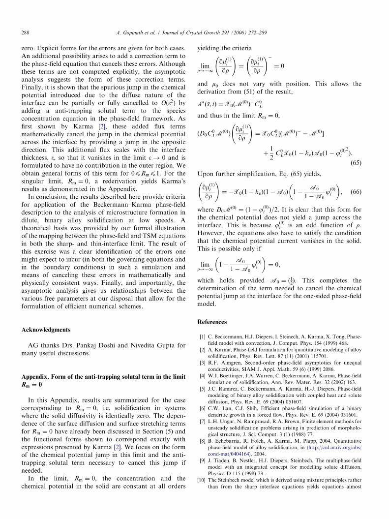
ARTICLE IN PRESSA. Gopinath et al. / Journal of Crystal Growth 291 (2006) 272–289288

zero. Explicit forms for the errors are given for both cases.An additional possibility arises to add a correction term tothe phase-field equation that cancels these errors. Althoughthese terms are not computed explicitly, the asymptoticanalysis suggests the form of these correction terms.Finally, it is shown that the spurious jump in the chemicalpotential introduced due to the diffuse nature of theinterface can be partially or fully cancelled to Oð�2Þ byadding a anti-trapping solutal term to the speciesconcentration equation in the phase-field framework. Asfirst shown by Karma [2], these added flux termsmathematically cancel the jump in the chemical potentialacross the interface by providing a jump in the oppositedirection. This additional flux scales with the interfacethickness, �, so that it vanishes in the limit �! 0 and isformulated to have no contribution in the outer region. Weobtain general forms of this term for 0pRmp1. For thesingular limit, Rm ¼ 0, a rederivation yields Karma’sresults as demonstrated in the Appendix.

In conclusion, the results described here provide criteriafor application of the Beckermann–Karma phase-fielddescription to the analysis of microstructure formation indilute, binary alloy solidification at low speeds. Atheoretical basis was provided by our formal illustrationof the mapping between the phase-field and TSM equationsin both the sharp- and thin-interface limit. The result ofthis exercise was a clear identification of the errors onemight expect to incur (in both the governing equations andin the boundary conditions) in such a simulation andmeans of canceling these errors in mathematically andphysically consistent ways. Finally, and importantly, theasymptotic analysis gives us relationships between thevarious free parameters at our disposal that allow for theformulation of efficient numerical schemes.

Acknowledgments

AG thanks Drs. Pankaj Doshi and Nivedita Gupta formany useful discussions.

Appendix. Form of the anti-trapping solutal term in the limit

Rm ¼ 0

In this Appendix, results are summarized for the casecorresponding to Rm ¼ 0, i.e, solidification in systemswhere the solid diffusivity is identically zero. The depen-dence of the surface diffusion and surface stretching termsfor Rm ¼ 0 have already been discussed in Section (5) andthe functional forms shown to correspond exactly withexpressions presented by Karma [2]. We focus on the formof the chemical potential jump in this limit and the anti-trapping solutal term necessary to cancel this jump ifneeded.

In the limit, Rm ¼ 0, the concentration and thechemical potential in the solid are constant at all orders

yielding the criteria

limr!�1

qmð1Þi

qr

!¼

qmð1Þi

qr

!�¼ 0

and m0 does not vary with position. This allows thederivation from (51) of the result,

A�ðs; tÞ ¼ X0ðMð0ÞÞ�C0

L

and thus in the limit Rm ¼ 0,

ðD0C0LM

ð0ÞÞqmð1Þi

qr

!¼ X0C

0L½ðM

ð0ÞÞ��Mð0Þ�

þ1

2C0

LX0ð1� keÞA0ð1� jð0Þi

2Þ.

ð65Þ

Upon further simplification, Eq. (65) yields,

qmð1Þi

qr

!¼ �X0ð1� keÞð1�A0Þ 1�

A0

1�A0jð0Þi

� �, (66)

where D0Mð0Þ ¼ ð1� jð0Þi Þ=2. It is clear that this form for

the chemical potential does not yield a jump across theinterface. This is because jð0Þi is an odd function of r.However, the equations also have to satisfy the conditionthat the chemical potential current vanishes in the solid.This is possible only if

limr!�1

1�A0

1�A0jð0Þi

� �¼ 0,

which holds provided A0 ¼ ð12Þ. This completes the

determination of the term needed to cancel the chemicalpotential jump at the interface for the one-sided phase-fieldmodel.

References

[1] C. Beckermann, H.J. Diepers, I. Steinech, A. Karma, X. Tong, Phase-

field model with convection, J. Comput. Phys. 154 (1999) 468.

[2] A. Karma, Phase-field formulation for quantitative modeling of alloy

solidification, Phys. Rev. Lett. 87 (11) (2001) 115701.

[3] R.F. Almgren, Second-order phase-field asymptotics for unequal

conductivities, SIAM J. Appl. Math. 59 (6) (1999) 2086.

[4] W.J. Boettinger, J.A. Warren, C. Beckermann, A. Karma, Phase-field

simulation of solidification, Ann. Rev. Mater. Res. 32 (2002) 163.

[5] J.C. Ramirez, C. Beckermann, A. Karma, H.-J. Diepers, Phase-field

modeling of binary alloy solidification with coupled heat and solute

diffusion, Phys. Rev. E. 69 (2004) 051607.

[6] C.W. Lan, C.J. Shih, Efficient phase-field simulation of a binary

dendritic growth in a forced flow, Phys. Rev. E. 69 (2004) 031601.

[7] L.H. Ungar, N. Ramprasad, R.A. Brown, Finite element methods for

unsteady solidification problems arising in prediction of morpholo-

gical structure, J. Sci. Comput. 3 (1) (1988) 77.

[8] B. Echebarria, R. Folch, A. Karma, M. Plapp, 2004. Quantitative

phase-field model of alloy solidification, in hhttp://cul.arxiv.org/abs/

cond-mat/0404164i, 2004.

[9] J. Tiaden, B. Nestler, H.J. Diepers, Steinbech, The multiphase-field

model with an integrated concept for modelling solute diffusion,

Physica D 115 (1998) 73.

[10] The Steinbech model which is derived using mixture principles rather

than from the sharp interface equations yields equations almost

ARTICLE IN PRESSA. Gopinath et al. / Journal of Crystal Growth 291 (2006) 272–289 289

identical to the Beckermann model. Thus, the asymptotic analysis

presented here is more generally applicable.

[11] Many numerical and analytical studies on directional solidification

employ models like the WBM model—see Ref. [9] for example—

derived using entropy functionals. In the isothermal limit, the

concentration field for the WBM model follows the equation:

qc0=qt0 ¼ V 00ðez � =0c0Þ þ =0 � M 0

c

RT 0

vm=0c0 þM 0

cMðc0;fÞ=0f

� �,

where M 0c is a mobility related to impurity diffusion and is a function

of f, and Mðc0;fÞ ¼ c0ð1� c0Þðq=qfÞðF 0B � F 0AÞ with F 0A and F 0B being

suitable free energies densities. For dilute solutions and in near

equilibrium conditions Mðc0;fÞ � ðc0s � c0mÞ. The models of Beck-

ermann [1] and Tiaden et al. [9] explicitly incorporate this

approximation and hence are appropriate for dilute solutions while

the WBM model reduces to this approximation for dilute alloys. It

may be shown that this term represents segregation flux due to

gradients in the phase field and in non-dilute solutions leads to solute

trapping. The evolution of the phase field in the WBM model for

constant temperature has the general form [9]

qf=qt0 ¼ V 00ðez � =0fÞ þM 0

f=0 � ð�02=0fÞ �M 0fW 0ðfÞ þM 0

fG0ðfÞðc0 � c0�Þ,

where the equations have been rewritten in terms of a potential,

W 0ðfÞ, coupling function, G0ðfÞ and a mean interface concentration

c0�. Comparison of this formulation to the analogous equation from

the Beckermann model indicates that even in near equilibrium

conditions, the last term is not small and varies significantly over the

phase boundary. This term contributes to an effective flux that

influences the form of the Gibbs–Thompson condition.

[12] W.W. Mullins, R.F. Sekerka, Stability of a planar interface during

solidification of a dilute binary alloy, J. Appl. Phys. 35 (1964) 444.