Trans. Nonferrous Met. Soc. China 25(2015) 2797−2806

New interpretation of experimental data on

Si−As alloy solidification with planar interface

S. L. SOBOLEV

Institute of Problems of Chemical Physics, Academy of Sciences of Russia, Chernogolovka, Moscow Region 142432, Russia

Received 14 October 2014; accepted 12 December 2014

Abstract: An analytical model was developed to describe Si−As alloy solidification in the whole range of measured interface velocity. It is demonstrated that at low interface velocity, the solidification occurs in the initial transient regime. The model leads to good comparison with the experimental data taking both local nonequilibrium effects at high interface velocity and steady state effects at low interface velocity into account. The local nonequilibrium diffusion effects shrink the initial transient period and lead to diffusionless solidification at high interface velocity. Key words: alloy solidification; initial transient; local-nonequilibrium diffusion; hyperbolic diffusion equation; Si−As alloys; diffusionless solidification; complete solute trapping 1 Introduction

Due to the relationship between the complex microstructures and the mechanical properties of welded, soldered, and cast components, solidification of alloys is one of the most researched subjects in materials science [1−17]. At high interface velocity, the solidification process involves extremely fast heat and mass transfer at very small time and length scales, which implies that the process occurs under far from equilibrium conditions [3−17]. The compositions, structure and properties of multi-component materials produced by phase transformation depend on the degree of deviation from local diffusion equilibrium, which is characterized by the ratio of the interface velocity v to the characteristic diffusion velocity vD [9−11]. Therefore, the development of capability to predict alloy solidification phenomena in the wide range of interface velocity observed in solidification experiments is an important task in designing new materials and new processes. For the sake of mathematical simplicity, theoretical modeling of the rapid alloy solidification usually assumes that the process occurs under steady- state condition, which implies that the solid−liquid interface moves with constant interface velocity v and

the initial transient stage can be ignored, which, in many cases, is proved to be a good assumption [1−17]. However, large discrepancies exist in the experimental results and the theoretical modeling of the Si−As systems [6−17], especially at low interface velocity when the non-steady-state effects are very important. In this work, new interpretation of the Si−As experiments is given [6−8], paying particular attention to the question whether the steady-state is really reached or not during the experimental measurements. The interpretation takes into account both the deviation from local diffusion equilibrium in the bulk liquid at high interface velocity, which is described by the local nonequilibrium diffusion model (LNDM) [9−11], and non-steady-state effects at low interface velocity [1].

2 Formulation of LNDM 2.1 Classical equation

The LNDM [9−11] takes into account the deviation from local diffusion equilibrium in the bulk liquid during rapid alloy solidification. At high interface velocity, the solute diffusion ahead of the moving interface cannot be described by classical diffusion equation of parabolic type which is based on the local equilibrium assumption, because the local equilibrium assumption is valid only

Corresponding author: S. L. SOBOLEV; Tel: +79-032478152; E-mail: sobolev@icp.ac.ru DOI: 10.1016/S1003-6326(15)63905-X

S. L. SOBOLEV/Trans. Nonferrous Met. Soc. China 25(2015) 2797−2806

2798

for relatively low interface velocity (v<<vD). The characteristic velocity vD is the so-called diffusion velocity, i.e., the velocity of propagation of diffusive disturbances in liquid phase, which is of the order of 1/30 m/s. When v∝vD, the local equilibrium assumption is not longer valid and the local nonequilibrium theory should be used [9−17]. The most popular version of the local-nonequilibrium thermodynamics is the so-called extended irreversible thermodynamics (EIT) [19], which includes dissipative fluxes in the set of independent variables. Reviews of some other local nonequilibrium approaches can be found in Refs. [20−25]. It is remarkable that all the extended approaches lead to the hyperbolic diffusion equation in the form

2

2

2

2

xCD

tC

tC

∂∂

=∂∂

+∂∂ τ (1)

which is the simplest generalization of the classical diffusion equation of parabolic type to the local nonequilibrium case, where C is the solute concentration, τ is the relaxation time of diffusion field to local equilibrium, and D is the solute diffusion coefficient. Hyperbolic Eq. (1) results in a finite diffusion speed vD=(D/τ)1/2. The classical diffusion equation of parabolic type, which can be obtained from Eq. (1) at τ=0, leads to a paradox of an infinite diffusion velocity [19−25]. The Galilean transformation of the coordinate X=x−vt transforms Eq. (1) to Eq. (2) provided that the solid–liquid interface itself travels at the same constant speed v.

2

2

2

22

2

2

XCD

XCv

tC

XCv

tC

∂∂

=∂∂

+∂∂

+∂∂

−∂∂

ττ (2)

Thus, the local nonequilibrium diffusion model (LNDM) for rapid solidification of binary alloys is based on the modified (hyperbolic) diffusion form Eq. (1) or its another form, Eq. (2).

2.2 Steady-state approximation

The exact mathematical treatment of the solute diffusion problem may be found by solving the time- dependent diffusion equation (Eq. (1)), subject to appropriate initial and boundary conditions in both the solid and the melt. But to avoid mathematical difficulties, the steady-state approximation is usually used. The steady-state assumption assumes that after a short initial transient period, the solid−liquid interface begins to move with constant velocity and the solute concentration is time-independent in the reference frame attached to the interface. The steady-state assumption significantly simplifies the mathematical formulation of the problem. Strictly speaking, the mathematical analysis shows that the steady-state solidification takes an ‘infinite’ amount of time and distance to be achieved [1]. But for many practical situations, the reasonable limits can be

established where the departure from the true steady- state may be ignored.

When the system achieves steady-state regime, i.e., the solute concentration is time-independent in the moving reference frame attached to the interface, Eq. (2) reduces to [9−11]

0dd

dd)/1( 2

22D

2 =+−XCv

XCvvD (3)

Thus, the steady-state assumption ‘hides” the time

dependence expressed in the solute diffusion equation (Eq. (2)) transforming it to an ordinary second-order differential equation (Eq. (3)). For analytic simplicity and ease of application, the steady-state solute diffusion equation (Eq. (3)) were solved first for semi-infinite solidifying systems [9−11]

( ) ( )⎪⎩

⎪⎨⎧

><+−−−

=D

DDi

vvCvvCvvDvXCC

XC ,

,)]/1(/exp[

0

022

0

(4) where C0 and Ci are the solute concentration in the liquid far from (X→∞) and at the interface (X=0), respectively. Equation (4) clearly demonstrates that the solute diffusion field ahead of the solid−liquid interface moving with velocity v≥vD remains undisturbed due to the local nonequilibrium diffusion effects. This implies that when the interface velocity v passes through the critical point, v=vD, an abrupt transition to diffusionless solidification occurs [9−11,25]. Equation (4) defines the local nonequilibrium characteristic diffusing length δLNDM as [9−11,25]

⎪⎩

⎪⎨⎧

><−

=D

D22

LNDM

,0 ,/)/1(

vvvvvvvD Dδ (5)

For every additional unit of the characteristic

diffusion length δLNDM, the solute concentration in the liquid phase at that distance from the interface decreases by an additional factor of 1/e, e is the base of the natural logarithm. The characteristic diffusion length δLNDM shrinks more rapidly with increasing the interface velocity v than expected from the local equilibrium approach, which gives the characteristic diffusion length as δ=D/v [1]. When the interface velocity v exceeds the critical point vD, the diffusion layer ahead of the interface does not form at all (δLNDM=0) due to the transition to diffusionless solidification [9−11,25]. The corresponding effective diffusion coefficient in the bulk liquid takes the following form [9−11]

⎪⎩

⎪⎨⎧

><−

=D

D2D

2LNDM

,0 ,)/1(

vvvvvvDD (6)

The effective diffusion coefficient, Eq. (6), can be

used to transform results of the classical local

S. L. SOBOLEV/Trans. Nonferrous Met. Soc. China 25(2015) 2797−2806

2799

equilibrium theory to the local nonequilibrium case by substitution of D for DLNDM. The effective diffusion coefficient depends on the ratio of v/vD, which characterizes the extent of deviation from local equilibrium. At low interface velocity (v/vD<<1), the diffusion occurs under local equilibrium condition and the effective diffusion coefficient reduces to the usual diffusion coefficient D. As the interface velocity v increases, the diffusion process begins to deviate from local equilibrium, which is manifested by the reduced effective diffusion coefficient DLNDM<D. When the interface velocity v passes through the critical point v=vD, a sharp transition from diffusion controlled growth with DLNDM>0 at v<vD to diffusionless growth with DLNDM=0 at v≥vD occurs [9−11]. The effective diffusion coefficient has been successfully used in the extended solute trapping models [9−11], the generalized solute drag model [12,13], proposed as an extension of Hillert– Sundman theory, the application of the maximal entropy production principle to rapid solidification of binary alloys [14], etc. Moreover, the concept of the effective diffusion coefficient has been extended for the space nonlocal situations [4,26].

Equation (4) implies that mathematically at v<vD, the thickness of the diffusion boundary layer is infinite. Instead of dealing with an exponential distribution of solute, spread over an infinite distance, at least in principle, one may usefully approximate the diffusion field by an equivalent finite boundary layer of thickness δb. Boundary layers are constructs used in many engineering applications as controlled approximations that capture special features of exact, but perhaps awkward, mathematical descriptions. In local equilibrium solidification theory, the effective boundary is defined as δb=2δ=2D/v [1,27]. The boundary layer δb is equal to the base-length of a right-angled triangle having a height which is equal to the excess solute concentration at the interface, and an area which is the same as that under the exponential curve [1,27]. The corresponding local nonequilibrium boundary layer can be written as .2 LNDMLNDM

b δδ = The local non- equilibrium diffusion boundary layer LNDM

bδ shrinks more rapidly with increasing the interface velocity than the local equilibrium diffusion boundary layer and equals zero in the diffusionless regime v≥vD.

As the solid−liquid interface position advances at very fast rates, there is substantial aberration from the equilibrium concentrations at the interface in both the solid and liquid phases. This deviation can be characterized through the segregation coefficient K, which is defined as the ratio of the solid concentration CS to the liquid concentration CL at the interface. The increase in the segregation coefficient with increasing the interface velocity v is known as solute trapping and a

complete understanding of the trapping process requires the dependence K(v) on the kinetic and thermodynamic properties of the alloy. The main prediction of LNDM [9−11,25] is that due to an abrupt transition to diffusionless solidification at a well-defined interface velocity v=vD, the complete solute trapping K(v)=1 occurs at the same velocity. This result is consistent with the experimental data [7,8,28], molecular dynamic simulations [29], and phase-field-crystal model [30]. A phenomenon closely related to solute trapping occurs during the solidification of a congruently melting ordered intermetallic compound and is known as disorder trapping [31], where the local nonequilibrium diffusion effects can also play an important role. The latest version of LNDM gives the effective partition coefficient in the following form [11]

⎪⎩

⎪⎨⎧

><

=−+

D

D))/(1/(1

ELNDM

,1 ,D

vvvvKK

vvAv (7)

where KE is the equilibrium partition coefficient, A is a constant such as vD/(A+1) representing the characteristic velocities above which K deviates strongly from KE [32]. 3 Initial transient effects

A steady-state described above, however, requires the development of the solute boundary layer δb, implying the prior occurrence of an initial transient solidification period. The solute boundary layer builds up gradually, precisely because the rejection of solute atoms from the interface occurs initially at a greater rate than the flux of atoms diffusing away from the interface through the increasingly steeper concentration gradient being established in the adjacent melt. Within this transient, the concentration of the liquid at the interface increases from C0 to C0/K. With respect to the phase diagram, this means that the first solid to solidify has the composition C0K, and reaches the composition C0, and the interface temperature TS corresponding to the composition C0 at steady-state [1,27]. The exact mathematical treatment of the initial transient solidification problem may be found by solving the time-dependent diffusion equation, subject to appropriate initial and boundary conditions in both the solid and the melt. Following the study of GLICKSMAN [1], one can use the boundary layer concept to estimate the characteristic time tst and length lst, which are necessary to develop steady-state conditions. The procedure starts with evaluating the gradient in the liquid phase at the solid−liquid interface, which was considered to be the ratio of the concentration difference at the interface ∆CL=(CL(t)−C0) to the characteristic diffusion length δ=D/v [1]. Strictly speaking, the mass-equivalent

S. L. SOBOLEV/Trans. Nonferrous Met. Soc. China 25(2015) 2797−2806

2800

triangular boundary layer δb, which is just twice the characteristic diffusion length δ, is more accurate to use for this estimate. To take both possible approximations into account, the solute concentration gradient in the liquid phase at X=0 is estimated as follows:

LNDML

0dd

γδC

XC

X

Δ−=⎟

⎠⎞

⎜⎝⎛

=

where the local nonequilibrium diffusion characteristic length δLNDM is defined by Eq. (5), and γ is 1/2. Using the same procedure described by GLICKSMAN [1], after a few steps of algebra, one gets

( )⎪⎩

⎪⎨

⎧

>

<⎟⎟⎠

⎞⎜⎜⎝

⎛

−−−−

=

D

D2D

2

2

0L

,1

,)/1(

exp)1(1

vv

vvtvvD

KvKKCtC γ (8)

where CL(t) is the time-dependent solute concentrations at the moving planar solid–liquid interface with allowance for the local equilibrium diffusion effects. Equation (8) can define the characteristic time tst and length lst to achieve steady-state as follows:

D2

2D

2LNDMst ,)/1( vv

KvvvDt <

−=γ (9)

D

2D

2LNDMst ,)/1( vv

vKvvDl <

−=γ (10)

When v≥vD, alloy solidification occurs in the diffusionless regime, which implies that 0LNDM

st =t and 0LNDM

st =l . Note that K in these equations is velocity- dependent (Section 2). For low velocity regimes v<<vD, these equations reduce to the local equilibrium results tst=γD/v2KE and lst=γD/vKE [1]. Note that KURZ and FISHER [27] suggested even more stronger condition reach steady-state as lst=4D/vKE, using γ=4. These equations clearly demonstrate that small values of partition coefficient K and interface velocity v cause the initial transient to stretch out, and take longer to achieve steady-state conditions. The local nonequilibrium diffusion effects lead to reduced diffusion boundary layer and increased partition coefficient, which reduces the time and length needed to reach the steady-state at high interface velocity. The characteristic nondimensional time )/( 2

DLNDMst

LNDMst γτ DKvt= and length =LNDM

sth )/( D

LNDMst γDKvl as functions of the nondimensional

interface velocity v/vD are shown in Fig. 1. It should be stressed here that in the slow velocity

regime v→0 (Fig. 1), the transient time tst and length hst may be very long. It implies that in modeling solidification experiments, it is important to ensure that the steady-state conditions have been really reached. If the characteristic time of an experiment tex significantly exceeds the initial transient characteristic time tst, then

there is enough time for the interface to reach steady-state conditions and the stead-state assumption can be used. The opposite inequality tex<tst implies that the steady-state is not established yet and the initial transient period should be taken into account during modeling the process.

Fig. 1 Nondimensional characteristic time and length to reach steady state vs nondimensional interface velocity using Eqs. (9) and (10), respectively (Curves 1 for characteristic length, curves 2 for characteristic time, dashed curves for local equilibrium case, solid curves for local nonequilibrium case) 4 Interface temperature 4.1 General formulation

The driving force for solidification of ideal solution has the well-known form [33]

+−−=Δ ))(1(/ eqLLE CCKRTG

)/ln()( ELEL KKKCKKC +− (11) where ∆G is the free energy change for the formation of one mole of solid from a liquid of composition CL, and

eqLC is the equilibrium liquid composition. To obtain the

interface temperature T as a function of the interface velocity v, this expression should be combined with kinetic law [2,30]

)]}/(exp[1{0 RTGvv Δ−−= (12) where at ∞→Δ )]/([ RTG . Combining Eqs. (11) and (12) and taking into account that the interface temperature

eqLLA CmTT += [33], where TA is the melting

temperature of the major component and mL is the equilibrium liquidus slope, one can get

⎟⎟⎠

⎞⎜⎜⎝

⎛−

−−⎟⎟⎠

⎞⎜⎜⎝

⎛⎟⎟⎠

⎞⎜⎜⎝

⎛−−

−+=

0E

L

EE

LLA 1ln

1ln11

1 vv

Km

KKK

KCmTT

(13) When v ≥ vD, the transition to complete solute

trapping (K=1) occurs (Eqs. (6) and (7)), and Eq. (13) reduces to

S. L. SOBOLEV/Trans. Nonferrous Met. Soc. China 25(2015) 2797−2806

2801

⎟⎟⎠

⎞⎜⎜⎝

⎛−

−−

−+=

0E

L

E

E0LA 1ln

1)1(ln

vv

Km

KKCmTT (14)

The so-called T0 temperature, i.e., the temperature of equal free energy of two phases, can be expressed as [33]

)1(ln

E

E0LA0 −+=

KKCm

TT where C0 is the initial solute concentration. Now it can rewrite Eq. (14) for the interface temperature at v≥vD in terms of T0 as

⎟⎟⎠

⎞⎜⎜⎝

⎛−

−−=

0E

L0 1ln

1 vv

KmTT (15)

It implies that, when the interface velocity v exceeds

the critical value vD, the alloy solidifies completely diffusionless and partitionless, i.e., behaviors as a “pure metal” with melting temperature T0. For relatively low interface velocity (v<<v0), the kinetic undercooling

)]/(1ln[)1( 01

ELK vvKmT −−=Δ − in Eqs. (13)−(15) reduces to the more familiar form kK / μvT =Δ , where

LE0k /)1( mKv −=μ is the interface kinetic coefficient [33].

Thus, Eq. (13) in combination with Eq. (7) gives the interface temperature as a function of two unknown parameters: the interface velocity v and the solute concentration at the interface CL. To get the interface temperature as a function of the interface velocity v, some additional assumption about CL should be made.

4.2 Steady-state regime

The mass conservation law applied to the steady-state solidification with planar interface implies that when the steady-state conditions are finally achieved, the solid freezing from the melt must also have established a steady solute concentration exactly equal to that of the initial melt concentration, C0. The steady-state solute concentration at the interface in the liquid phase is CL=C0/K. In such a case, Eq. (13) for the steady-state interface temperature takes the form

−⎟⎟⎠

⎞⎜⎜⎝

⎛ −−−+=

E

E0AA1 ln

)/ln(1(1)(KK

KKKTTTT

D0E

L ,1ln1

vvvv

Km

<⎟⎟⎠

⎞⎜⎜⎝

⎛−

− (16)

D0E

L01 ,1ln

1vv

vv

KmTT =⎟⎟

⎠

⎞⎜⎜⎝

⎛−

−−= (17)

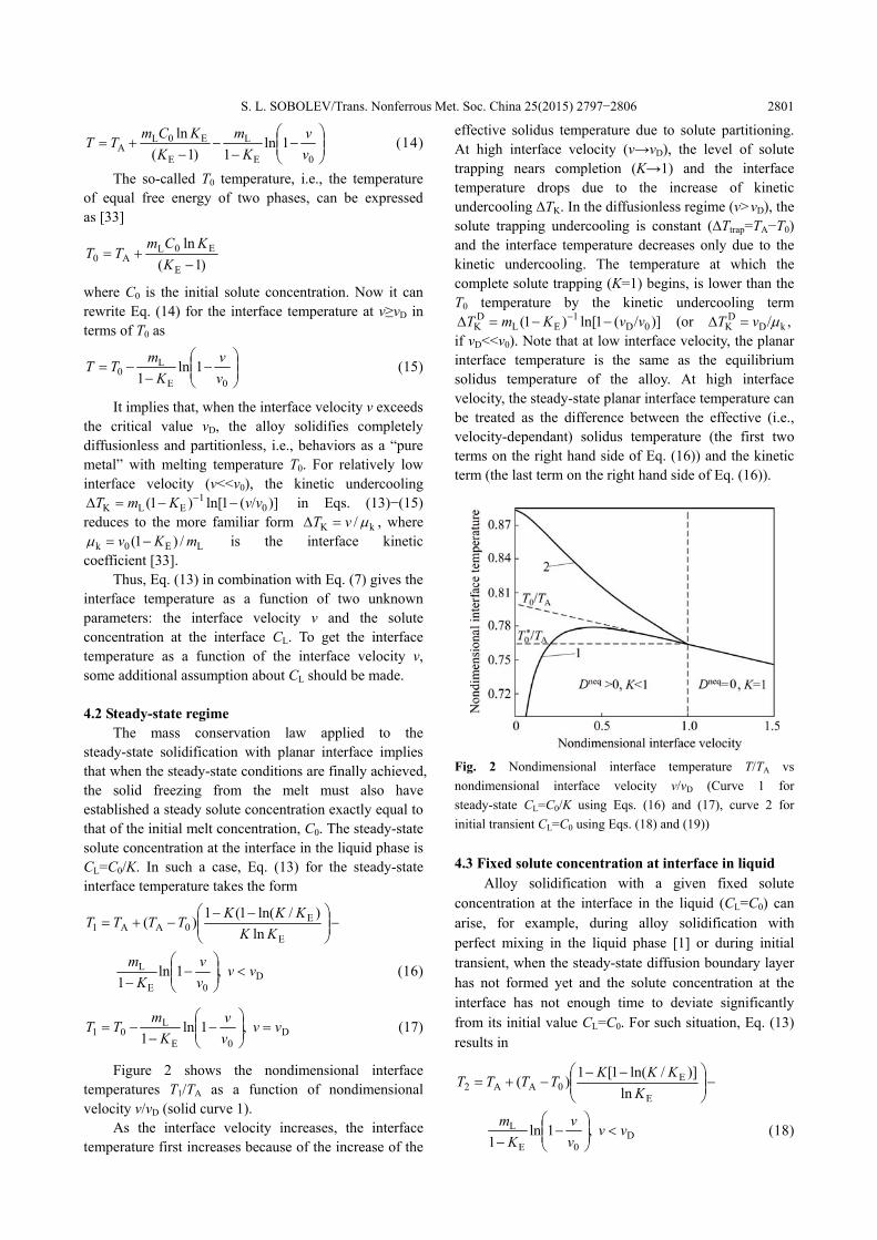
Figure 2 shows the nondimensional interface

temperatures T1/TA as a function of nondimensional velocity v/vD (solid curve 1).

As the interface velocity increases, the interface temperature first increases because of the increase of the

effective solidus temperature due to solute partitioning. At high interface velocity (v→vD), the level of solute trapping nears completion (K→1) and the interface temperature drops due to the increase of kinetic undercooling ∆TK. In the diffusionless regime (v>vD), the solute trapping undercooling is constant (∆Ttrap=TA−T0) and the interface temperature decreases only due to the kinetic undercooling. The temperature at which the complete solute trapping (K=1) begins, is lower than the T0 temperature by the kinetic undercooling term

)]/(1ln[)1( 0D1

ELD

K vvKmT −−=Δ − (or ,/ kDD

K μvT =Δ if vD<<v0). Note that at low interface velocity, the planar interface temperature is the same as the equilibrium solidus temperature of the alloy. At high interface velocity, the steady-state planar interface temperature can be treated as the difference between the effective (i.e., velocity-dependant) solidus temperature (the first two terms on the right hand side of Eq. (16)) and the kinetic term (the last term on the right hand side of Eq. (16)).

Fig. 2 Nondimensional interface temperature T/TA vs nondimensional interface velocity v/vD (Curve 1 for steady-state CL=C0/K using Eqs. (16) and (17), curve 2 for initial transient CL=C0 using Eqs. (18) and (19)) 4.3 Fixed solute concentration at interface in liquid

Alloy solidification with a given fixed solute concentration at the interface in the liquid (CL=C0) can arise, for example, during alloy solidification with perfect mixing in the liquid phase [1] or during initial transient, when the steady-state diffusion boundary layer has not formed yet and the solute concentration at the interface has not enough time to deviate significantly from its initial value CL=C0. For such situation, Eq. (13) results in

−⎟⎟⎠

⎞⎜⎜⎝

⎛ −−−+=

E

E0AA2 ln

)]/ln(1[1)(K

KKKTTTT

D0E

L ,1ln1

vvvv

Km

<⎟⎟⎠

⎞⎜⎜⎝

⎛−

− (18)

S. L. SOBOLEV/Trans. Nonferrous Met. Soc. China 25(2015) 2797−2806

2802

D0E

L02 ,1ln

1vv

vv

KmTT =⎟⎟

⎠

⎞⎜⎜⎝

⎛−

−−= (19)

In this case, the interface temperature always

decreases with increasing the interface velocity v (curve 2 in Fig. 2). The temperature decrease at v<vD is more pronounced than that at v>vD because of the solute trapping effects. When v<vD, the temperature decreases due to both the decrease of the effective liquidus temperature and the increase of the kinetic undercooling, whereas at v>vD, the diffusionless regime occurs and the interface temperature decreases only due to the kinetic undercooling. The difference between the initial transient interface temperature and the steady-state interface temperature (T2−T1)∝(1−K)/K decreases with increasing the interface velocity in the diffusionless and partitionless regime, i.e., at v>vD, these temperatures are coincide (Fig. 2). The first two terms on the right hand side of Eq. (18) can be treated as effective liquidus temperature. 5 Application to Si−As alloy solidification

In resent years, rapid solidification of Si−As alloys is one of the most important subjects of great practical and scientific interest [6−17]. The Si−As systems have been studied extensively, but large discrepancies still exist in the experimental results and theoretical modeling. Rapid solidification of polycrystalline Si−4.5%As (mole fraction) and Si−9%As (mole fraction) alloys at velocity ranging from 0.25 to 2 m/s was studied by KITTL et al [6−8] using the pulsed laser melting technique. The congruent melting temperature T0 [6], the solute partition coefficient [7,8], and the interface temperature [8] were measured as functions of the interface velocity under steady-state conditions. The theoretical description of KITTL et al’s experimental data is under an extensive discussion [10−17]. Both local equilibrium [6−8,15,17] and local nonequilibrium [9−14,16] approaches have been used, but all of them assume under steady-state condition, which leads to some difficulties in describing the experimental data at low interface velocity. To avoid these difficulties, the experimental conditions are first analyzed here at which the experimental measurements were performed [6−8]. The key question is whether the steady-state conditions in the KITTL et al’s experiments have been really reached as it was stated by the authors of the experiment [6−8]. To answer this question, the characteristic time of the experiment, tex, with the characteristic time needed for the interface to reach the steady-state conditions, tst, is compared. The characteristic time of the experiment is the ratio of the interface depth, d, at which the interface temperature was measured [8] and the interface velocity, v, i.e., lex=d/v.

The characteristic time needed for the interface to approach steady-state condition, tst, is given by Eq. (9). The interface temperature versus interface velocity relation was measured by KITTL et al [8] for an interface depth d=30 nm from the surface, which was expected to be sufficiently far from the beginning of solidification for the steady-state to be established. The parameters for the calculation of tst are D=(1.5±0.5)×10−8 m2/s and KE=0.3 [8]. Note that there is some uncertainty in KE, whose value falls within the range from KE=7×10−4 to KE=0.3 [8]. For further calculations, the commonly accepted value of KE=0.3 [8] is used here, keeping in mind that KE=7×10−4 would give high value of tst. The characteristic time tex and tst for KITTL et al’s experiments [8] are shown in Fig. 3 as functions of the interface velocity (v).

Fig. 3 Characteristic time vs interface velocity for Si−As alloy solidification [8] (Dashed curve for characteristic time of experimental measurements, tex=d/v; solid curves for characteristic time to reach steady-state, tst, using Eq. (9))

Figure 3 demonstrates that at v<v1≈1.1 m/s for γ=1 and at v<v2≈2.2 m/s for γ=2, the characteristic time of the experiment tex is less than the characteristic time tst to achieve steady-state conditions. This implies that the interface depth d, at which the interface temperature was measured in KITTL et al’s experiments [8], was not kept high enough to ensure the steady-state conditions in the whole range of the measured interface velocity. In other words, the interface temperature in KITTL et al’s experiments was measured under non-steady-state conditions in the low velocity regime (v<1 m/s). Thus, the analysis demonstrates that at relatively low interface velocity (v<1 m/s), the steady-state was not reached in the experiments of KITTL et al [8] and non-steady-state approaches are needed to theoretically describe the experimental data. In order to describe the KITTL et al’s experiments in the whole range of the measured interface velocity, two T are calculated versus v functions: T1, which corresponds to the steady-state conditions (tex>tst),

S. L. SOBOLEV/Trans. Nonferrous Met. Soc. China 25(2015) 2797−2806

2803

and T2, which corresponds to the non-steady-state conditions (tex<tst). In the equilibrium v=0, the solute concentration at the interface (CL) equals to the initial solute concentration C0. It means that during initial stage of solidification, i.e., during initial transient, when tex<tst , the solute concentration at the interface has not enough time to change significantly from its initial value, i.e., CL≈C0. Therefore, the interface temperature during the initial transient period (tex<tst) can be calculated using Eqs. (18) and (19), which assumes fixed solute concentration at the interface (CL≈C0). The steady-state interface temperature is described by Eqs. (16) and (17), which assumes CS=C0. The interface temperatures (T) as functions of interface velocity (v), calculated for the steady-state (curve 1) and the initial transient (curve 2), is shown in Fig. 4.

Fig. 4 Interface temperature vs interface velocity (Curve 1 for steady-state using Eqs. (16) and (17), curve 2 for initial transient using Eqs. (18) and (19); thick gray line for transition between initial transient and steady-state, spheres for experimental points [8]; parameters: KE=0.3, T0=1423 K, vD=2.5 m/s, ε=1.25)

The best fit of the steady-state interface temperature T1 (curve 1 in Fig. 4) to experimental date was obtained with fitting parameter T0=1423 K. This value is in good agreement with T0=(1423±25) K determined by KITTL et al’s experiments [6]. The initial transient temperature T2 (curve 2 in Fig. 4) was calculate using Eq. (18) with the same value of T0 and the average solute concentration at the interface 0L CC ε= with ε=1.25. The correction coefficient ε was introduced to take the increase of solute concentration at the interface into account during the initial transient from CL=C0 at t=0 to CL=C0/K at t≈tst. The main feature observed when comparing the model predictions with the experimental data is the increase of the calculated initial transient temperature (T2) with decreasing the interface velocity (v), which corresponds to the experimental data in the whole range of the measured interface velocity (Fig. 4), whereas the

steady-state interface temperature (T1) decreases with decreasing the interface velocity v in the low velocity regime, which contradicts the experimental data at v<1 m/s. This is allowed to treat the low velocity regime in the KITTL et al’s experiments [8] as non-steady-state one, which corresponds to the estimate of the characteristic times tst and tex (Fig. 3) for these velocities. The gray line in Fig. 4 approximates intermediate regime between the initial transient and the steady-state regime, which occurs between v1≈0.8 m/s and v2≈1.7 m/s. This corresponds to the condition of tex≈tst, which holds within the range between v1 and v2 (Fig. 3). Thus the experimental data of KITTL et al [8] for rapid solidification of Si−As alloy can be interpreted as follows: 1) in the low velocity regime (v<v1), the characteristic time of the experiment tex is less than the characteristic time needed to reach the steady-state tst, which means that this regime of solidification can be treated as initial transient; 2) at high interface velocity (v>v2), the inverse inequality holds (tex>tst), i.e., the solidification occurs in steady-state; 3) in the range of v1<v<v2, the characteristic time is of the same order (tex≈tst) and the transition from initial transient to steady-state regime occurs (the thick gray line in Fig. 4). 6 Comparison with other models and

discussion

LI et al [12] proposed thermodynamic approach for Si−As alloy with non-straight liquidus and solidus curves. The model is consistent with the available experimental data if significant solute drag effects are introduced. They also investigated the differences between their model and other typical models for Si−As alloy solidification by using the site fraction f as a fitting parameter to obtain a better description of the experimental data for each model [12]. In another paper, they considered a generalized solute drag model for binary alloy solidification with a planar phase interface proposed as an extension of Hillert–Sundman model [13]. Using a new thermodynamic parameter set of the Si−As system, the model can, with the introduction of three new adjustable parameters, fit the available experimental data. Note that the difference between LI et al’s model and other discussed models [12,13] is of the order of the error of the experiment (Figs. 2 and 3 in Ref. [12] and Fig. 2 in Ref. [13]), that makes it difficult to judge which model provides more realistic description of the experiment. The model calculation of the interface thickness based on steady-state assumption gave unphysically large values at low interface velocity, which led to conclusion that the steady-state condition in KITTL et al’s experiments may not be achieved at these velocities [13]. To correct their steady-state model, LI et al approximated the solute

S. L. SOBOLEV/Trans. Nonferrous Met. Soc. China 25(2015) 2797−2806

2804

concentration in the solid phase at the interface by velocity dependant function for v<0.8 m/s [12,13]. This corresponds to the present prediction that solidification in the KITTL et al’s experiments occurs in non-steady-state regime at v≤0.8 m/s. Note that the effective partition coefficients K(v) predicted by the generalized solute drag model of LI et al [13] and the previous LNDM [9−11] (Eq. (7)) are nearly indistinguishable.

WANG et al [14] described the steady-state planar solidification of Si−As alloy using a maximal entropy production principle. They analyzed the phase diagram of the Si−As system and concluded that the steady-state planar solidification with CS=C0 is not possible for Si−9%As (mole fraction) alloy if v is not sufficiently high. They also noticed that their prediction of the interface temperature T based on the steady state approach is good for v>0.8 m/s but that is not good for v<0.8 m/s for any sets of parameters (Figs. 7(b) and 9(b) in Ref. [14]). These conclusions correspond to the present model, which predicts the non-steady-state regime at low interface velocity v<v0≈0.8 m/s (Figs. 3 and 4). The prediction of the effective partition coefficient K(v) based on the maximal entropy production principle [14] is indistinguishable from the prediction of LNDM [9−11] (Eq. (7)).

Thus, the extended models [12−14] with allowance for solute drags, non-straight liquidus−solidus lines and maximal entropy production principle, may give more realistic solution at high interface velocity, but still have difficulties in describing low velocity regimes of Si−As alloy solidification due to steady-state assumption. The non-steady-state effects qualitatively change the behavior of the interface temperature versus the interface velocity function in the low velocity regime. The combination of the non-steady-state approach with the extended Si−As solidification models [12−14] is an interesting topic for future work and will be presented elsewhere. More experimental work and direct measurements of interface response functions and phase diagrams of Si−As alloys are required to confirm the results of theoretical modeling and distinguish between different physical effects.

It has been demonstrated in the previous sections that, despite the fact that the steady-state concept provides a useful tool for modeling alloy solidification [1−17], there are some difficulties in describing the low velocity regime with planar interface. Strictly speaking, from purely mathematical point of view, the steady-state takes an ‘infinite’ amount of time and distance to be achieved [1], but for many practically important applications, the finite characteristic time tst and length lst

to reach steady-state, Eqs. (9) and (10), respectively, are proved to be very useful approximation. But still in the low velocity limit v→0, both characteristic scales tend to infinity. This also confirms that in the low velocity regime, the steady-state is difficult to achieve and the initial transient effects should be taken into account for successful modeling of low velocity alloy solidification.

The steady-state solute concentration in the solid is C0 for any value of interface velocity, whereas the steady-state concentration in the liquid at the interface depends on v as CL(v)=C0/K(v). For low interface velocity (v→0), the steady-state solute concentration at the interface is CL=C0/KE. The corresponding interface temperature for planar interface is equal to the solidus temperature Ti=Tsol(C0). In the equilibrium state, when the interface does not move (v=0), the equilibrium liquid and solid solute concentrations are 0

eqL CC = and

,0EeqS CKC = respectively. The corresponding

equilibrium temperature eq)0( TT = is determined by the phase diagram of the alloy as the liquidus temperature for 0

eqL CC = or the solidus temperature for

0EeqS CKC = , i.e., )()( 0E

sol0

liqeq CKTCTT == . Thus, the steady-state planar interface temperature Ti is not formally continuous in the limit v → 0 because

).0(lim i0TT

v≠

→ The difference between Ti and Teq is

equal to ./)1( EE0L KKCm − The discontinuity seemingly arise because τst→∞ and lst→∞ at v→0 (Eqs. (9) and (10)), which implies that the steady-state solidification is practically impossible to achieve in the low velocity regime. Thus, in the low velocity regime, the steady-state approximation is not good enough for planar interface solidification, and one should use either an exact time-dependant mathematical formulation of the solute diffusion problem, or its appropriate approximation with allowance for the non-steady-state effects. 7 Conclusions

The steady-state approximation is a good tool for modeling alloy solidification with planar interface in many practically important situations. However, it requires the development of the solute boundary layer, implying the prior occurrence of an initial transient period. The smaller the values of the equilibrium partition coefficient and the interface velocity are, the slower the steady-state reaches, and the longer the transient period lasts. This is an important factor to bear in mind when applying steady-state theory to experiments involving low equilibrium partition coefficient and slow moving planar interface. In particular, it concerns the KITTL et al’s Si−As alloy solidification experiments [6−8], which is better

S. L. SOBOLEV/Trans. Nonferrous Met. Soc. China 25(2015) 2797−2806

2805

described by the non-steady state approximation at relatively low interface velocity when the initial transient effects play an important role. The local nonequilibrium diffusion effects shrink the initial transient period due to the decreased effective diffusion coefficient.

Acknowledgments

The reported study was partially supported by RFBR, research project No. 14-48-03535.

References [1] GLICKSMAN M E. Principles of solidification [M]. New York:

Springer, 2011: 520. [2] ASTA M, BECKERMANN C, KARMA A, KURZ W,

NAPOLITANO R, PLAPP M, PURDY G, RAPPAZ M, TRIVEDI R. Solidification microstructures and solid-state parallels: Recent developments, future directions [J]. Acta Materialia, 2009, 57: 941−971.

[3] LIU F, YANG G C. Rapid solidification of highly undercooled bulk liquid superalloy: Recent developments, future directions [J]. International Materials Reviews, 2006, 51: 145−170.

[4] SERDYUKOV S I. Higher order heat and mass transfer equations and their justification in extended irreversible thermodynamics [J]. Theoretical Foundations of Chemical Engineering, 2013, 47: 89−103.

[5] WANG G X, PRASAD V. Microscale heat and mass transfer and non-equilibrium phase change in rapid solidification [J]. Material Science and Engineering A, 2000, 292: 142−148.

[6] KITTL J A, REITANO R, AZIZ M J, BRUNCO D P, THOMPSON M O. Time-resolved temperature measurements during rapid solidification of Si−As alloys induced by pulsed-laser melting [J]. Journal of Applied Physics, 1993, 73: 3725−3733.

[7] KITTL J A, AZIZ M J, BRUNCO D P, THOMPSON M O. Nonequilibrium partitioning during rapid solidification of Si−As alloys [J]. Journal of Crystal Growth, 1995, 148: 172−182.

[8] KITTL J A, SANDERS P G, AZIZ M J, BRUNCO D P, THOMPSON M O. Complete experimental test of kinetic model for rapid alloy solidification [J]. Acta Materialia, 2000, 48: 4797−4811.

[9] SOBOLEV S L. Local-nonequilibrium model for rapid solidification of undercooled melts [J]. Physics Letters A, 1995, 199: 383−386.

[10] SOBOLEV S L. Local non-equilibrium diffusion model for solute trapping during rapid solidification [J]. Acta Materialia, 2012, 60: 2711−2718.

[11] SOBOLEV S L. An analytical model for complete solute trapping during rapid solidificationof binary alloys [J]. Materials Letters, 2012, 89: 191−194.

[12] LI Shu, ZHANG Jiong, WU Ping. A comparative study on migration of a planar interface during solidification of non-dilute alloys [J]. Journal of Crystal Growth, 2010, 312: 982−988.

[13] LI Shu, ZHANG Jiong, WU Ping. Numerical solution and comparison to experiment of solute drag models for binary alloy solidification with a planar phase interface [J]. Scripta Materialia, 2010, 62: 716−719.

[14] WANG Haifeng, LIU Feng, ZHAI Haimin, WANG Kang. Application of the maximal entropy production principle to rapid solidification: A sharp interface model [J]. Acta Materialia, 2012, 60: 1444−1454.

[15] DANILOV D, NESTLER B. Phase-field modelling of solute trapping during rapid solidification of a Si−As alloy [J]. Acta Materialia, 2006, 54: 4659−4664.

[16] WANG Hai-feng, LIU Feng, YANG Wei, CHEN Zheng, YANG Gencang, ZHOU Yao-he. Solute trapping model incorporating diffusive interface [J]. Acta Materialia, 2008, 56: 746−753.

[17] WANG Hai-feng, LIU Feng, CHEN Zheng, YANG Wei. Solute trapping model based on solute drag treatment [J]. Transaction of nonferrous metals society of China, 2010, 20: 877−811.

[18] SOBOLEV S L. An analytical model for local-nonequilibrium solute trapping during rapid solidification [J]. Transaction of nonferrous metals society of China, 2012, 22: 2749−2755.

[19] JOU D, CASAS-VAZQUEZ J, LEBON G. Extended irreversible thermodynamics [M]. Berlin: Springer, 1996: 383.

[20] SOBOLEV S L. Transport processes and travelling waves in systems with local nonequilibrium [J]. Soviet Physics – Uspekhi, 1991, 34(3): 217−229.

[21] NETTLETON R E, SOBOLEV S L. Application of extended thermodynamics to chemical, rheological, and transport processes: A special survey. Part I. Approaches and scalar rate processes [J]. Journal of Non-equilibrium Thermodynamics, 1995, 20: 205−229.

[22] NETTLETON R E, SOBOLEV S L. Application of extended thermodynamics to chemical, rheological, and transport processes: a special survey. Part II. Vector transport processes, shear relaxation and rheology [J]. Journal of non-equilibrium thermodynamics, 1995, 20: 297−331.

[23] NETTLETON R E, SOBOLEV S L. Application of extended thermodynamics to chemical, rheological, and transport processes: A special survey. Part III. Wave phenomena [J]. Journal of Non-equilibrium Thermodynamics, 1996, 21: 1−16.

[24] SOBOLEV S L. Space-time nonlocal model for heat conduction [J]. Physical Review E, 1994, 50: 3255−3258.

[25] SOBOLEV S L. On the transition from diffusion-limited to kinetic-limited regimes of alloy solidification [J]. Acta Materialia, 2013, 61, 7881−7888.

[26] SOBOLEV S L. Nonlocal diffusion models: Application to rapid solidification of binary mixtures [J]. International Journal of Heat and Mass Transfer, 2014, 71: 295−302.

[27] KURZ W, FISHER D J. Fundamentals of solidification [M]. Switzerland-Germany-UK-USA: Trans Tech Publications, 1986: 242.

[28] WALDER S. Dendritic growth rate in undercooled, dilute Ti−Ni melts [J]. Materials Science and Engineering A, 1997, 229(1−2): 156−162.

[29] YANG Y, HUMADI H, BUTA D, LAIRD B B, SUN D, HOYT J J, ASTA M. Atomistic simulations of nonequilibrium crystal-growth kinetics from alloy melts [J]. Physical Review Letters, 2011, 107(2): 025505.

[30] HUMADI H, HOYT J J, PROVATAS N. Phase-field-crystal study of solute trapping [J]. Physical Review E, 2013, 87: 022404.

[31] ZHENG X Q, YANG Y, GAO Y F, HOYT J J, ASTA M, SUN D. Disorder trapping during crystallization of the B2-ordered NiAl compound [J]. Physical Review E, 2012, 85: 041601.

[32] JACKSON K A, KIRK M. BEATTY K M, GUDGEL K A. An analytical model for non-equilibrium segregation during crystallization [J]. Journal of Crystal Growth, 2004, 271: 481−494.

[33] BOETTINGGER W J, CORIEL S R. Microstructure formation in rapidly solidified alloys [C]//Science and technology of the undercooled melt 1986. Dordrecht: Martinus Nijhoff Publishers, 1986: 81−108.

S. L. SOBOLEV/Trans. Nonferrous Met. Soc. China 25(2015) 2797−2806

2806

Si−As 合金平界面凝固过程实验数据的新阐释

S. L. SOBOLEV

Institute of Problems of Chemical Physics, Academy of Sciences of Russia,

Chernogolovka, Moscow Region 142432, Russia

摘 要：建立一个分析模型来描述 Si−As 合金在测得的界面速率范围内的凝固过程。分析表明：在低界面速率下，

凝固发生在初始瞬态。因考虑了在高界面速率下的局部非平衡效应和在低界面速率下的稳态效应，这个模型与实

验数据吻合较好。局部非平衡扩散效应缩小了初始瞬态过程，并导致了高界面速率下的无扩散凝固。

关键词：合金凝固；初始瞬态；局部非平衡扩散；双曲线扩散方程；Si−As 合金；无扩散固化；完全溶质截留

(Edited by Mu-lan QIN)