Yarn Manufacture I: Principal of Carding & Drawing

Yarn Manufacture I: Principal of Carding & DrawingProf. R. Chattopadhyay

Department of Textile TechnologyIndian Institute of Technology, Delhi

Lecture – 09Fibre Configuration & Neps in Card Sliver

Today’s discussion topic is Fibre Configuration and Neps in Card Sliver.

(Refer Slide Time: 00:25)

Let us look at the shapes of fibres in card sliver. Now, certain steps are depicted in the

slide. What we see here that, the configuration or the shape of the fibres are many. We

can see that some fibres are straight in nature; like, the fibre shown here. Some fibre ends

are bent in the form of a hook, we call them hook fibre. Some fibres are bent and the 2

links of the hook are almost similar in length, we call them U shape hook fibre.

Some fibres are forming a loop. So, we call it loop fibre. Some fibres are entangled in

nature like this fibre so, this is entangled fibre. And there are fibres which are more or

less straight like this fibre also as told earlier. So, there are enumerable shapes which are

available in the card sliver. Now, if we want to visualize these shapes, then what

technique is available with us so that we can see the shape of the fibres. If I take a fibre

sliver and then see it under microscope, then we will find that there are many fibres what

will be very difficult to know exact shape of those fibres because, all the fibres are of

same color.


So, there is a technique known as tracer fibre technique, which can be employed to study

the shape of fibres in a sliver. So, what is this technique that we are going to discuss? In

this technique, first of all a small quantity of fibre is dyed with any commercial

whitening agent, like Tinopal BVN. After dying this we dry the fibres in room

temperature. And once it is completely dried, we have to open it by hand using our

fingers. Once the fibres are separated from each other, now these tracer fibres are mixed

with normal fibres is not dyed fibre, these are tracer fibres on a Finisher Scutcher lattice.

And then we have to form a lap so that all these tracer fibres get mixed up with the rest

of the fibres and then a lap is produced.

So, this one is tracer fibres not dyed fibres. The next step: now we process the lap on a

card and collect the web samples from the card or we can also collect this sliver. And

then place this web or this sliver on a blackboard. So, you can collect number of samples

and put them on blackboards. Next, the direction of the delivered web or the sliver is to

be marked on the black board so, that we can find out later on in which directions the

fibres were delivered. So, which is the forward directions, and which is the backward

directions.

Now, these collected samples have to be seen under UV light source in a darkroom. The

configuration of the tracer fibres would be distinctly visible as they will all glow under

UV light. So, once they are visible it becomes easy for us to note down the configuration.

We can trace the configuration on piece of paper. Or we can take photograph and later on

we can see the photographs and study the configuration. So, this is the technique known

as tracer fibre technique. This technique has been used by many people to study the

configuration of fibres.


Now, here is a table where the fibres have been classified according to their

configurations. And if we look at this table, what we see here that there are fibres having

hook in the leading directions. We call them leading hook fibres. There are fibres with a

hook in the trailing part of the fibre. We call them trailing hook fibre. There are fibres or

both the ends are hooked we call it both end hook fibre. Then there are fibres some of

them are straight, we call them straight fibres. And there are fibres which do not fall into

these categories, and therefore, we put them into another separate category called others.

So, there are 1, 2, 3, 4, 5 different categories. And what we see here is this that generally

trading hook fibres are more in numbers than leading hooks. This is one important

observations, which has been shown by many people. Around 50 to 60 percent of the

fibres are trailing hook fibres. And 20 to 30 percents are leading hook fibres. This is also

the typical distribution of the hooks fibre in a sliver. Straight fibres are not really many,

but there are definitely some straight fibres as well. And we can also see the doffer speed

can affect the pattern of hook formations.

That is, in this case for 2 different doffer speeds 10 rpm and 18 rpm. We can see the

configurations and; obviously, the configurations are different in terms of numbers of the

hook fibres in different categories. So, we can also say that doffer speed plays a role in

deciding the number of hooks in different categories. From here we go to the next slide.


That is, mechanisms of trailing hook formations. That why these hooks get formed? Why

trailing hooks are more in number than leading hooks? So, in the diagram we see that is

a cylinder and there is a doffer. And let us concentrate on a fibre A B as shown in the

diagram. Now as the fibre is carried forward by the cylinder, and the fibre approaches the

doffer surface, the leading end of the fibre A B comes into contact with the doffer. And

then it keeps on traveling at the speed of doffer. Like the fibre original position is A 0 B

0. Position 2; let us say this is position 1 where the leading end has landed on the doffer

surface. But the trailing end is still in contact with the cylinder.

Now, in this situation what will happen? The leading end is a contact with the doffer. So,

this end will move at the speed of doffer. The trailing end is in contact with the cylinder.

So, this will move at the speed of cylinder. Therefore, the 2 ends of the same fibre will

move at two different velocities. We all know that the velocity of the cylinder is much

more than the velocity of the doffer. See V c is the velocity of cylinder, and V d is a

velocity of deep doffer, then we all know that V c is much greater than V d.

So, what will happen? During the process of transfer the end B will quick quickly pass

through the transferred zone. So, the end A which is in contact with the doffer still

remains on the doffer, but the other end B now moves forward and takes the position A 2

B 2. Now what happens in this situation? That as a result of this the fibre turns, that is B

comes in front of A. So, earlier the end A was in front of B. Now while going through the

transferred zone, the entire fibre reverses and B moves forward than A, because end B is

in contact with the cylinder.

After this fibre get transferred and this will appear like this; say, this will be A 3 B 3. And

we see that the fibre will appear from the doffer as a trailing hook fibre. End B gets

combed by the cylinder wire points or cylinder teeth. Hence the end B may not have a

hooked end. Whereas, end A which latched on the doffer surface, remains caught there in

the form of a hook. And therefore, finally, when this fibre emerges from the doffer, it is

in the configuration of a trailing hook. This is the mechanism of trailing hook formation.

From there we can say that fibre situated on the surface of cylinder fibre layer, are

positively controlled by doffer and their front ends form mostly trailing hooks.


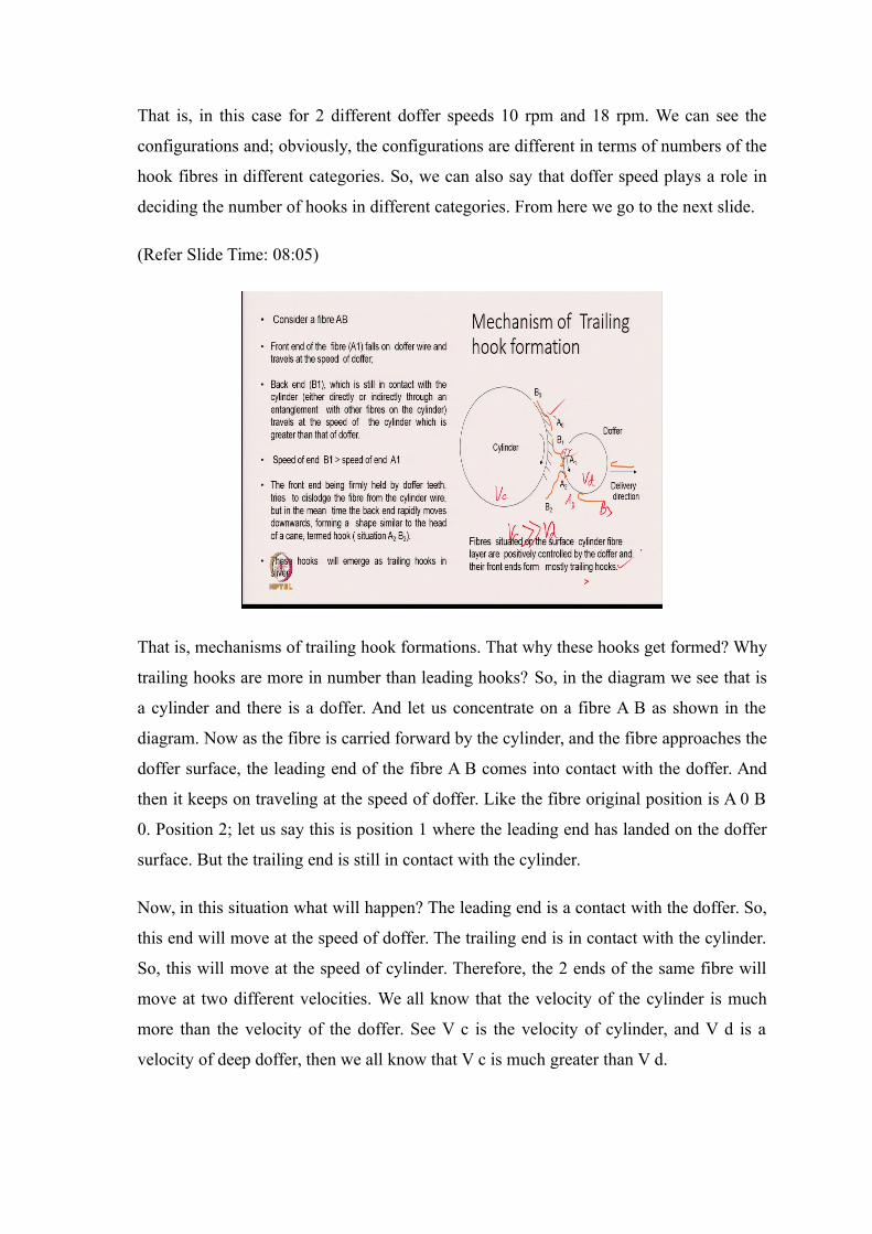
From here we go to the next slide in order to understand the mechanism of leading hook

formations. The diagram is shown here and let us consider another fibre A B the different

positions of the fibres are also shown in the diagram. Now what we see here that the

fibre situated in the lower fibre layer on the cylinders are peeled off by the doffer only

through it is contact with the top layer. On the cylinder we have a thick layer of fibre.

So, some fibres are directly in contact with the doffer wire in the cylinder wire points.

Similarly, there are fibres which are lying on the cylinder, but may not be positively

gripped by the wire points of the cylinder. They are in contact with other fibres which are

in turn in contact with the cylinder wire points. So, these fibres are basically on the top

layer of the cylinder. So, in the process of peeling off what happens? The trailing end of

the fibres which are embedded in the cylinder wires after losing contact with the cylinder

gets whipped up due to sudden relaxation and form a leading hook. Let us look at the

fibre here now. Fibre A B approaches the doffer.

So, what happens? The end comes here into contact with the doffer like here. And then as

the doffer cylinder wire points are combing the end point of the same fibre, these fibres

looses contact they are peeled off from the surface of the cylinder and then suddenly

whipped up due to relaxation of stress as shown in the diagram as A 2 B 2. With the

formation of thicker fibre layer the proportion of indirectly controlled fibre increases and

therefore, this proportion of leading hook. So, when this fibre gets whipped up, then we

see that fibre comes as leading hook from the surface of the doffer ok. This is how the

leading hooks are getting formed.


Then from there we go to the mechanism of another theory for the formation of leading

hooks. And it shows that that the front end of a fibre moving with the velocity of the

cylinder comes into contact with the relatively slower moving doffer surface. And when

the end hits the doffer surface, the front part of the fibre moves at a slower speed.

Whereas, the back part is moving at a higher speed because the back part of the fibre is

in contact with the cylinder and the front part is in contact with the doffer.

And as a result of this the fibres get buckled in the form of the hook. And in the same

way they get transferred to the doffer. If the fibre is loosely held by the cylinder is

depends largely on the nature and extent of positive control exercised by the cylinder and

the rest of the fibre it get transferred without reversal and hence form a leading hook. So,

what we see here? The fibre initial position is 1 the next position is coming over here, A

1 B 1 this is position 2, and the third position is 3.

So, therefore here these fibres mostly on the top layer of the cylinder; they come and hit

the doffer surface. The end gets buckle and the fibre as a whole get transferred to the

doffer. And these fibre therefore, will emerge as leading hook fibre ok. This is A 3 B 3

and the same way the fibre will move out and we call them leading hook fibres. So, these

are the 2 mechanism of the formation of leading hook and we have already discussed the

formation of trailing hooks.


But there are so many different configuration of fibres. So, if we look at the

characteristics of a card sliver. Then we can write the fibres take a variety of innumerable

shapes. Shapes are so many that actually is difficult sometimes to categorize them into

only 5 categories, there could be many more categories. But broadly people have tried to

classify them into 5 categories. Most of the fibres are not straight and neither parallel to

each other not to the axis of this silver.

The another point is fibres are entangled with each other. And a card sliver therefore is

springy in nature. So, if you take a card sliver, either cotton card sliver or polyester card

sliver. And if you pull it little bit you will find it acts like a spring. The reason behind the

spring is that the fibres are entangled with each other. They are bent and they are crimped

and they are missing each other, and hence the nature of the card sliver is very, very

springy in nature.


Now, we will be interested to know to how can we measure the degree of disorder of

fibres in a sliver. So, if I change certain possible parameters and see there are some times

of some types of hooks are more in number than the other type, or overall paralization or

orientation of the fibres whether they are different or not. We need a measurement

technique by which we will be able to tell whether a change in process parameter or fibre

parameter or machine parameter has made any difference on the degree of disorder of

fibres within the sliver or not.

The direct technique based on actually looking at the configuration of the fibre is very,

very time consuming and very, very laborious. Therefore, we have to find out a simple

way to measure the degree of disorder in fibres in a sliver. This is the technique which

has been shown by some people. So, we try to understand this technique first. Let us take

a sliver. Consider a section whose length is less than the fibre length. So, this is the

sliver, let us take this section whose length is less than the fibre length.

Now, let the fibre be straightened out by repeated combing and sorted out according to

length. From this zone let us say we take out this zone as f, and then we see the fibres

within this zone are having different configurations. Let us comb out these portions of

the fibres. And after combing now let us arrange the fibres in order of decreasing length

as shown in this diagram. Now, within this any fibre whose length is greater than the

section length, like this is the section length from here to there which is equal to this

section length.

Any fibre greater than this must have been either bent that mean these fibres, they are

either bent in the form of a hook within this section, or there may be twisted or they

must, be lining lying in inclined fashion within this. And therefore, when you comb them

out, they get straightened out, and their length exceeds the length of the section. So, this

part of the fibre indicates in a way the number of fibres which are in a bend shape or a

hook shape within the section that we have considered.

So, we can get some indications regarding the extent of departure from orientations from

the number of those fibres which extended beyond the section length. So, if we get more

number of fibres in this category; which are greater than the section length we can say

more and more fibres where not oriented along the axis of the sliver. So, number of these

fibres or one can also find out the weight of these fibres can give us some idea about the

degree of disorder of fibres in the sliver.


From here a technique was developed by a person called Lindsey which is very simple

technique very easy to operate also. So, in this technique what is that there is a base plate

here which is B. And on the base plate that are 3 plates P Q 1 and Q 2. And the base plate

and the plates P Q 1 Q 2, they can be screwed together by these fly nuts. So, these are fly

nuts so, there are holes here which passes through this plate and goes further down the

base plate.

So, I phi if I using the fly nut we can remove these plates or we can tighten the plate

against the base plate, the width of the plate P is around 1 inch. The width of the plate Q

is around half an inch. So, what we do? We first remove the plates top plates and place a

sliver. Once the sliver is put there even put 2 slivers or 3 sliver side by side. If we feel

that one sliver is too thin, we can have 2 slivers or 3 slivers and place them side by side.

While placing them we have to make sure that which side is the leading side of the sliver

and which side is the trailing side of sliver; that means, if whether this is the direction of

delivery from the machine, then we should must mark this side.

So, that it indicates that this is the direction in which these slivers were delivered. Now

what we do ? We remove one of these plates. Let us say we remove plate Q 2, but before

removing we will cut this sliver along the edge of the plate Q 2. After cutting, you

remove this part of the sliver from here, and then we remove the plate Q 2. And let us say

after removal of the plate, we will see something like this in front of the clam P.

So, you see the fibres here this is the cutting edge. And there are fibres projecting out

from the clam. Many of those fibres are not straight and they are having different

configurations. Now we would use a comb and we will start combing this part

repeatedly. While combing we have to be little careful. So, that in the sense that the

fibres should not break so, you comb them gently and repeatedly. After some time what

we find, while most of the fibres will be stated out like this. And the fibres which are

within this zone from here to there, but they are not held by the clam, they all will be

removed.

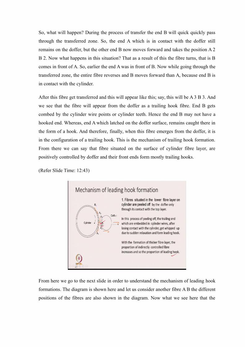
And this is the part shown as C here. That is combed out portion; fibres which are loose

in this zone. And these are the portions fibres which are extending beyond the cutting

line. Now what we do? We put this plate Q 2 back again and cut these portions. The

portion which is extending beyond the plate Q 2 so, if we cut this along this line, this is

the portion we call it E. So, E is indicating let us say the weight of fibre extended portion

beyond the cutting line. And the part which is here is the weight of fibres in between

cutting line and the plate.


So, you see that the fibre which was here, now they have been classified into 3 groups.

Fibre C, which are loose and combed out; fibre E which extended beyond the cutting

edge and fibres N which are in between the cutting edge and the clamp. These 3

quantities gives us some idea about the degree of disorder of fibres in a sliver. The

indices which have been proposed are 2. One is combing ratio which is C by E plus N

and the other one is orientation index 1 minus E by N into 100. These 2 indices gives us

an idea about the degree of disorder of fibres in a sliver and also the level of their

orientations. There are many more indices proposed by many people, but we are not

taking them, but we are not discussing them right now. Let us concentrate on these 2

indices.


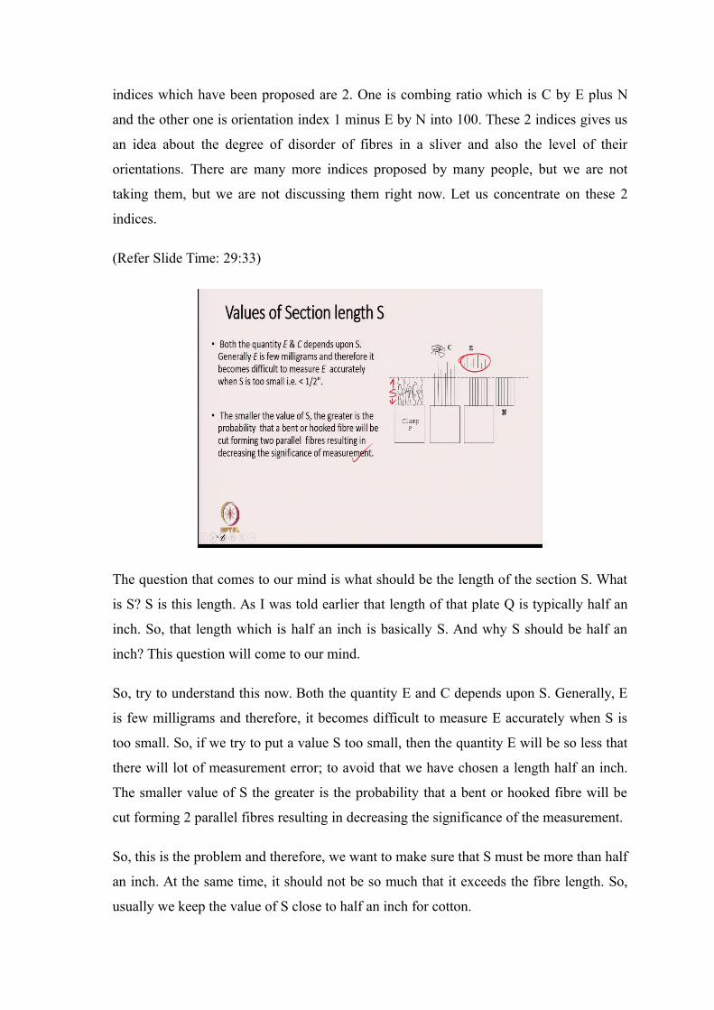
The question that comes to our mind is what should be the length of the section S. What

is S? S is this length. As I was told earlier that length of that plate Q is typically half an

inch. So, that length which is half an inch is basically S. And why S should be half an

inch? This question will come to our mind.

So, try to understand this now. Both the quantity E and C depends upon S. Generally, E

is few milligrams and therefore, it becomes difficult to measure E accurately when S is

too small. So, if we try to put a value S too small, then the quantity E will be so less that

there will lot of measurement error; to avoid that we have chosen a length half an inch.

The smaller value of S the greater is the probability that a bent or hooked fibre will be

cut forming 2 parallel fibres resulting in decreasing the significance of the measurement.

So, this is the problem and therefore, we want to make sure that S must be more than half

an inch. At the same time, it should not be so much that it exceeds the fibre length. So,

usually we keep the value of S close to half an inch for cotton.


Some values of fibre disorder and orientation. Like see in this case we see here: what is

the influence of section width or section length S. As a section width increased from half

an inch to 5 by 8 of an inch to 6 by 8 of an inch, we see the combing ratio keeps

increasing the orientation on also keeps on increasing. So, this is how the 2 indices

changes with increase in section width typically the values which are chosen for section

width is generally half an inch.


Now, the comparison between these two indices, combing ratio and orientation index; let

us say consider a sample in which 80 percent of fibres are parallel and extend across the

section whereas, just 20 percent are perpendicular to it. Let us say there is a sliver in

which 80 percent of fibres are parallel to each other. And these fibres extending across

the section and only 20 percent fibres are perpendicular to it.

So, C R and orientation index will be in this case 0.25 C R, orientation index will be 100

since E will be almost 0. So, orientation index indicates complete parallelism even

though 20 percent fibres are completely out of line. So, orientation index may not be able

to make a proper judgment in a hypothetical situation like this that is one of the difficulty

with the orientation index. Though, this is an extreme case the same difficulty will be

met in varying degrees with orientation index.

If there is an appreciable proportion of crisscross fibres in the sample so, that is the

difficulty that we faced with orientation index. And therefore, other indices have been

proposed by others, but they are beyond the scope of this course. Combing ratio should

not be much greater than 1, except when the fibres are very, very short. If C R goes

beyond 1.5 orientation index should be regarded as having dubious significance. This is

also you have to keep in mind.


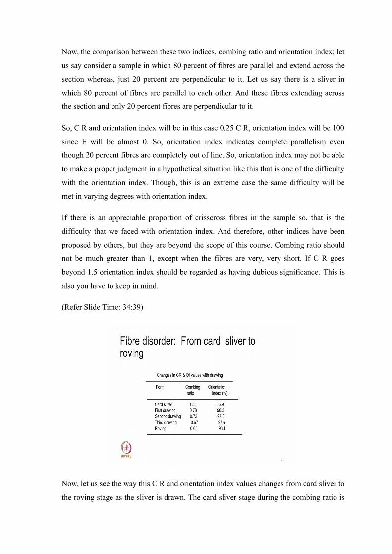
Now, let us see the way this C R and orientation index values changes from card sliver to

the roving stage as the sliver is drawn. The card sliver stage during the combing ratio is

1.55. And as we stretch the sliver go through the process of drawing and go up to roving

what we find here? That the ratio goes down and down. So, you will learn later on that

drawing is a process through which we reduce the number of hooks, and at the same time

we improve the orientation of fibres. And therefore, we expect combing ratio to go down

which is reflected in this data.

And also we can see that the orientation index also gradually is improving, that basically

gives an indication that fibres are becoming more and more oriented towards the axis of

the sliver or doffing whatever the product is.


Now, come to the next important part of the discussion that is Neps. Discussion on card

carding machine is not complete without discussion on neps. So, neps are tiny entangle

mass of fibres they spoil the appearance of the yarn and the fabrics. The lesser they are

the better in a yarn. And therefore, we are very much concerned about neps.


And carding is a process by which neps can be removed, we can eliminate many neps. At

the same time, we must know that carding can also generate neps. So, carding is a

machine which can generate neps, which can remove neps or eliminate neps, see if there

is a generation and the removal, then one may ask the question and whether we should

whether there is a benefit in the carding process as far as neps are concerned, the benefit

is there because the removal of neps are more in number than the creation of neps by the

same machine.

If the process is maintained perfectly, if the machine parameters are chosen properly, and

if we maintain the machine correctly, then you will always find a reduction in neps in the

card sliver in comparison to what was fed to the machines. But if the machine is not

maintained properly, the machine the process is not set properly, then we may find

tremendous increase in neps also. So, you have to keep in mind both the facts. Let us see

how the machines generate neps. Nep formation is because of buckling of fibre during

processing and sudden release of stored elastic energy a result of stretching during

carding action ok.


It has been shown that the frequency of nep formation is related to Euler’s parameters,

but N is proportional to f l square divided by E into I. Where N is the number of neps, f

is the stress on fibre, E is the elastic modulus of the fibre, and I is the fibre cross

sectional moment of inertia, l is the fibre length. What is I considering a fibre to be

cylinder? I can be written as pi d square by 64. Where d is the fibre diameter. In case of

cotton if the micronaire value is mu, we can write mu l equal to weight of fibres, we can

relate it to the volume and density of the fibres by these equations. And from here we can

find out the value of d square.

So, putting the value of d in 2 we get I to be like this. And when I put I in equation one

we get n in terms of fibre parameters; that is, n is proportional to f stress level on fibre, l

fibre length gamma which is density of fibre. E as stated elastic modulus and mu is the

micronaire value of cotton in the case of cotton. So, what we see here that the number of

neps that gets formed is a function of stress level. And it increases with length of the

fibres. So, you have to be very careful when a given fibre. What is the length of it? And

what is the level of stress that is acting on the fibres during processing of the fibres on

the machine.


Factors which affect nep formations; fibre factors or fineness of the fibre, the maturity

value in the case of cotton. The length parameter of the fibre what is the length in the

case of cotton, another parameters which come is impurities in cotton. The other thing is

the magnitude of tensile stress development on the fibre can also affect nep formation

especially in the carding zone.

So, any process parameter that increases carding force is likely to enhance generation of

neps. So, we can try to analyze the various factors which can affect carding force. With

the fibres if we see maturity plays a very important role and fineness also plays a very

important role. The fibres as finer or the fibres will be in mature in the case of cotton.

Then they can easily form neps because, their bending legatee is also very low. They can

easily get bent and take the configuration of the neps easily and therefore, fineness and

maturity both comes into picture. Length also basically facilitates.

The buckling or bending of the fibres within the carding zone and hence, length also

becomes very important. And the other thing in the case of cotton is impurities in cotton.

See many of these impurities also gets counted as neps many instrument. The other thing

which could be problematic is that the impurities are there in the cotton the impurities.

Sometimes they get lost between the wire points of cylinder. And therefore, the cylinder

looses it is opening capability. And hence the fibres which are coming from the licker

inside they are not getting separated or opened out properly by the teeth of the cylinder.

Because impurities have completely filled up may be the spaces between the wire points.

And therefore, all those wire points will do is that opening capability. The fibres will be

there on the tip of the surface of the teeth and they are not getting penetrated by the teeth

properly. And hence there were difficulty in separation. So, therefore, these parameters of

the fibres are very, very important from the point of view of nep formations. The other

thing is the stress level. So, this stress level during carding especially the level of stress

which acts on the fibres between flat and cylinder is very important.

So, there what matters is the this the space between flat and cylinder. If the fibres are

long there will be lot of force development on them, because there will be lot of

entanglement between the fibres, a lot of friction between the fibres and the wire points

of the cylinder and flat and hence carding force will rise with the length of fibres.

Similarly, if the fibres if the space is too narrow between cylinder and flat, then also the

carding force will increase and if we increase the cylinder speed, also this carding force

will increase.

So, all these parameters cylinder speed the setting between cylinder and flat the length of

fibres are important from the point of view of caring force also. So, we have to ensure

that the carding force do not go too high. In that case also some neps may be formed.

Why these neps are forming because of the carding force? The fibres get stressed by the

force, and when these fibres are released suddenly, then the internal stress which is there

in the fibre. That stress will cause the fibres to buckle. It was sudden release of the

energy which is within the fibre.

Since, they are all stretched and therefore, when they try to buckle because of sudden

release of the energy, they themselves will get bent and also they may bring some other

fibres which are close to it and put them together and create a knot like you know fibres

which we call neps. So, the more the force is created, the more will be the internal space

on the fibres and more will be the energy within the fibres. And hence, possibilities of

buckling when due to the sudden release of the force will be tremendous. So, this is what

is therefore, important the next point.


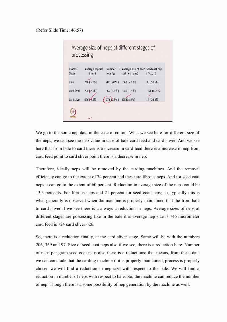
We go to the some nep data in the case of cotton. What we see here for different size of

the neps, we can see the nep value in case of bale card feed and card sliver. And we see

here that from bale to card there is a increase in card feed there is a increase in nep from

card feed point to card sliver point there is a decrease in nep.

Therefore, ideally neps will be removed by the carding machines. And the removal

efficiency can go to the extent of 74 percent and these are fibrous neps. And for seed coat

neps it can go to the extent of 60 percent. Reduction in average size of the neps could be

13.5 percents. For fibrous neps and 21 percent for seed coat neps; so, typically this is

what generally is observed when the machine is properly maintained that the from bale

to card sliver if we see there is a always a reduction in neps. Average sizes of neps at

different stages are possessing like in the bale it is average nep size is 746 micrometer

card feed is 724 card sliver 626.

So, there is a reduction finally, at the card sliver stage. Same will be with the numbers

206, 369 and 97. Size of seed coat neps also if we see, there is a reduction here. Number

of neps per gram seed coat neps also there is a reductions; that means, from these data

we can conclude that the carding machine if it is properly maintained, process is properly

chosen we will find a reduction in nep size with respect to the bale. We will find a

reduction in number of neps with respect to bale. So, the machine can reduce the number

of nep. Though there is a some possibility of nep generation by the machine as well.


This diagram gives us an idea about the nep reduction as a function of size of the neps.

Now if you look at this data, then we will see that very, very small size neps if we

classify the data in 2 groups in terms of size of the neps. Any size that this side there is a

increase in neps. Whereas, on the lower side this side the values are decreasing, as the

size of the neps are increasing there is a decrease in size from with respect to feed.

So, what we feed to the machine, and what we see in the card sliver there is a reduction.

And this ratio of reduction is shown here by this particular plot. It basically means from

here that bigger sized neps are reduced to very large extent. But there is a increase in

small size neps. Now, why there is a increase the small size neps? The possibilities are

two, one is it is difficult for the machine to remove the small size neps which are 200

micron 300 micron and 400 micron in size.

The other thing could be that big size neps are broken into pieces. And part of those big

neps becomes small sized neps now. So, their numbers though reduces, but small size

names increase in number, because these bigger ones get splitted into smaller ones now.

And hence you may find the net increase in the number of small size neps. So, that is the

reason why we find increase in neps in this region whereas, we find the decrease in neps

in this region. With that we close today’s discussion.

And thanks.

Yarn Manufacture I: Principal of Carding & Drawing

Documents

Transcript of Yarn Manufacture I: Principal of Carding & Drawing