What Comes Beyond the Standard Models - Inspire HEP

ii

“proc16” — 2016/12/12 — 10:17 — page I — #1 ii

ii

ii

BLEJSKE DELAVNICE IZ FIZIKE LETNIK 17, ST. 2BLED WORKSHOPS IN PHYSICS VOL. 17, NO. 2

ISSN 1580-4992

Proceedings to the 19th Workshop

What Comes Beyond theStandard Models

Bled, July 11–19, 2016

Edited by

Norma Susana Mankoc BorstnikHolger Bech Nielsen

Dragan Lukman

DMFA – ZALOZNISTVO

LJUBLJANA, DECEMBER 2016

ii

“proc16” — 2016/12/12 — 10:17 — page II — #2 ii

ii

ii

The 19th Workshop What Comes Beyond the Standard Models,11.– 19. July 2016, Bled

was organized by

Society of Mathematicians, Physicists and Astronomers of Slovenia

and sponsored by

Department of Physics, Faculty of Mathematics and Physics, University of Ljubljana

Society of Mathematicians, Physicists and Astronomers of Slovenia

Beyond Semiconductor (Matjaz Breskvar)

Scientific Committee

John Ellis, CERNRoman Jackiw, MIT

Masao Ninomiya, Okayama Institute for Quantum Physics

Organizing Committee

Norma Susana Mankoc BorstnikHolger Bech NielsenMaxim Yu. Khlopov

The Members of the Organizing Committee of the International Workshop “WhatComes Beyond the Standard Models”, Bled, Slovenia, state that the articles

published in the Proceedings to the 19th Workshop “What Comes Beyond theStandard Models”, Bled, Slovenia are refereed at the Workshop in intense

in-depth discussions.

ii

“proc16” — 2016/12/12 — 10:17 — page III — #3 ii

ii

ii

Workshops organized at Bled

. What Comes Beyond the Standard Models(June 29–July 9, 1998), Vol. 0 (1999) No. 1(July 22–31, 1999)(July 17–31, 2000)(July 16–28, 2001), Vol. 2 (2001) No. 2(July 14–25, 2002), Vol. 3 (2002) No. 4(July 18–28, 2003) Vol. 4 (2003) Nos. 2-3(July 19–31, 2004), Vol. 5 (2004) No. 2(July 19–29, 2005) , Vol. 6 (2005) No. 2(September 16–26, 2006), Vol. 7 (2006) No. 2(July 17–27, 2007), Vol. 8 (2007) No. 2(July 15–25, 2008), Vol. 9 (2008) No. 2(July 14–24, 2009), Vol. 10 (2009) No. 2(July 12–22, 2010), Vol. 11 (2010) No. 2(July 11–21, 2011), Vol. 12 (2011) No. 2(July 9–19, 2012), Vol. 13 (2012) No. 2(July 14–21, 2013), Vol. 14 (2013) No. 2(July 20–28, 2014), Vol. 15 (2014) No. 2(July 11–19, 2015), Vol. 16 (2015) No. 2(July 11–19, 2016), Vol. 17 (2016) No. 2

. Hadrons as Solitons (July 6–17, 1999)

. Few-Quark Problems (July 8–15, 2000), Vol. 1 (2000) No. 1

. Selected Few-Body Problems in Hadronic and Atomic Physics (July 7–14, 2001),Vol. 2 (2001) No. 1

. Quarks and Hadrons (July 6–13, 2002), Vol. 3 (2002) No. 3

. Effective Quark-Quark Interaction (July 7–14, 2003), Vol. 4 (2003) No. 1

. Quark Dynamics (July 12–19, 2004), Vol. 5 (2004) No. 1

. Exciting Hadrons (July 11–18, 2005), Vol. 6 (2005) No. 1

. Progress in Quark Models (July 10–17, 2006), Vol. 7 (2006) No. 1

. Hadron Structure and Lattice QCD (July 9–16, 2007), Vol. 8 (2007) No. 1

. Few-Quark States and the Continuum (September 15–22, 2008),Vol. 9 (2008) No. 1

. Problems in Multi-Quark States (June 29–July 6, 2009), Vol. 10 (2009) No. 1

. Dressing Hadrons (July 4–11, 2010), Vol. 11 (2010) No. 1

. Understanding hadronic spectra (July 3–10, 2011), Vol. 12 (2011) No. 1

. Hadronic Resonances (July 1–8, 2012), Vol. 13 (2012) No. 1

. Looking into Hadrons (July 7–14, 2013), Vol. 14 (2013) No. 1

. Quark Masses and Hadron Spectra (July 6–13, 2014), Vol. 15 (2014) No. 1

. Exploring Hadron Resonances (July 5–11, 2015), Vol. 16 (2015) No. 1

. Quarks, Hadrons, Matter (July 3–10, 2016), Vol. 17 (2016) No. 1

.

Statistical Mechanics of Complex Systems (August 27–September 2, 2000) Studies of Elementary Steps of Radical Reactions in Atmospheric Chemistry

(August 25–28, 2001)

ii

“proc16” — 2016/12/12 — 10:17 — page IV — #4 ii

ii

ii

ii

“proc16” — 2016/12/12 — 10:17 — page V — #5 ii

ii

ii

Contents

Preface in English and Slovenian Language . . . . . . . . . . . . . . . . . . . . . . . . . . . . VII

Talk Section . . . . . . . . . . . . . . . . . . . . . . . . . . . . . . . . . . . . . . . . . . . . . . . . . . . . . . . . 1

1 DAMA/LIBRA Results and PerspectivesR. Bernabei et al. . . . . . . . . . . . . . . . . . . . . . . . . . . . . . . . . . . . . . . . . . . . . . . . . . . . . . 1

2 Experience in Modeling Properties of Fundamental Particles UsingBinary CodesE.G. Dmitrieff . . . . . . . . . . . . . . . . . . . . . . . . . . . . . . . . . . . . . . . . . . . . . . . . . . . . . . . 8

3 Quark and Lepton Masses and Mixing From a Gauged SU(3)F FamilySymmetry With a Light O(eV) Sterile Dirac NeutrinoA. Hernandez-Galeana . . . . . . . . . . . . . . . . . . . . . . . . . . . . . . . . . . . . . . . . . . . . . . . 36

4 Nonstandard Cosmologies From Physics Beyond the Standard ModelM.Yu. Khlopov . . . . . . . . . . . . . . . . . . . . . . . . . . . . . . . . . . . . . . . . . . . . . . . . . . . . . . 52

5 Gauge Fields With Respect to d = (3+1) in the Kaluza-Klein Theoriesand in the Spin-charge-family TheoryD. Lukman and N.S. Mankoc Borstnik . . . . . . . . . . . . . . . . . . . . . . . . . . . . . . . . . . 66

6 Spin-charge-family Theory is Offering Next Step in UnderstandingElementary Particles and Fields and Correspondingly UniverseN.S. Mankoc Borstnik . . . . . . . . . . . . . . . . . . . . . . . . . . . . . . . . . . . . . . . . . . . . . . . . 77

7 Do Present Experiments Exclude the Fourth Family Quarks as Well asthe Existence of More Than One Scalar?N.S. Mankoc Borstnik and H.B.F. Nielsen . . . . . . . . . . . . . . . . . . . . . . . . . . . . . . . 128

8 The Spin-charge-family Theory Offers Understanding of the TriangleAnomalies Cancellation in the Standard ModelN.S. Mankoc Borstnik and H.B.F. Nielsen . . . . . . . . . . . . . . . . . . . . . . . . . . . . . . . 147

9 The New LHC-Peak is a Bound State of 6 Top + 6 Anti topH.B. Nielsen . . . . . . . . . . . . . . . . . . . . . . . . . . . . . . . . . . . . . . . . . . . . . . . . . . . . . . . . 157

10 Progressing Beyond the Standard ModelsB.A. Robson . . . . . . . . . . . . . . . . . . . . . . . . . . . . . . . . . . . . . . . . . . . . . . . . . . . . . . . . . 177

ii

“proc16” — 2016/12/12 — 10:17 — page VI — #6 ii

ii

ii

VI Contents

Discussion Section . . . . . . . . . . . . . . . . . . . . . . . . . . . . . . . . . . . . . . . . . . . . . . . . . . 189

11 Discreteness of Point Charge in Nonlinear ElectrodynamicsA.I. Breev and A.E. Shabad . . . . . . . . . . . . . . . . . . . . . . . . . . . . . . . . . . . . . . . . . . . . 191

12 The Hypothesis of Unity of the Higgs Field With the Coulomb FieldE.G. Dmitrieff . . . . . . . . . . . . . . . . . . . . . . . . . . . . . . . . . . . . . . . . . . . . . . . . . . . . . . . 201

13 What Cosmology Can Come From the Broken SU(3) Symmetry of theThree Known Families?A. Hernandez Galeana and M.Yu. Khlopov . . . . . . . . . . . . . . . . . . . . . . . . . . . . . 204

14 Phenomenological Mass Matrices With a Democratic WarpA. Kleppe . . . . . . . . . . . . . . . . . . . . . . . . . . . . . . . . . . . . . . . . . . . . . . . . . . . . . . . . . . . 210

Virtual Institute of Astroparticle Physics Presentation . . . . . . . . . . . . . . . . . . . 219

15 Virtual Institute of Astroparticle Physics — Scientific-EducationalPlatform for Physics Beyond the Standard ModelM.Yu. Khlopov . . . . . . . . . . . . . . . . . . . . . . . . . . . . . . . . . . . . . . . . . . . . . . . . . . . . . . 221

ii

“proc16” — 2016/12/12 — 10:17 — page VII — #7 ii

ii

ii

Preface

The series of workshops on ”What Comes Beyond the Standard Models?” startedin 1998 with the idea of Norma and Holger for organizing a real workshop, inwhich participants would spend most of the time in discussions, confrontingdifferent approaches and ideas. It is the nineteenth workshop which took placethis year in the picturesque town of Bled by the lake of the same name, surroundedby beautiful mountains and offering pleasant walks and mountaineering.In our very open minded, friendly, cooperative, long, tough and demanding dis-cussions several physicists and even some mathematicians have contributed. Mostof topics presented and discussed in our Bled workshops concern the proposalshow to explain physics beyond the so far accepted and experimentally confirmedboth standard models - in elementary particle physics and cosmology. Althoughmost of participants are theoretical physicists, many of them with their own sug-gestions how to make the next step beyond the accepted models and theories,experts from experimental laboratories were very appreciated, helping a lot tounderstand what do measurements really tell and which kinds of predictions canbest be tested.The (long) presentations (with breaks and continuations over several days), fol-lowed by very detailed discussions, have been extremely useful, at least for theorganizers. We hope and believe, however, that this is the case also for most ofparticipants, including students. Many a time, namely, talks turned into very ped-agogical presentations in order to clarify the assumptions and the detailed steps,analyzing the ideas, statements, proofs of statements and possible predictions,confronting participants’ proposals with the proposals in the literature or withproposals of the other participants, so that all possible weak points of the propos-als showed up very clearly. The ideas therefore seem to develop in these yearsconsiderably much faster than they would without our workshops.This year experiments have not brought much new, although a lot of work andeffort has been put in, but the news will come when the analyses of the datagathered with 13 TeV on the LHC will be done. The analyses might show whetherthere are the new family and the new scalar fields (both predicted by the spin-charge-family theory and discussed in this proceedings), as well as whether thetwo events, the ≈ 750 GeV resonance decaying into two photons (predicted byMultiple-Point-Principle) and the ≈ 1.8 TeV resonance decaying into severalproducts, are nontheless real, manifesting new scalar fields. They may see the darkmatter constituents, or rather not since they are much heavier neutral baryons.

ii

“proc16” — 2016/12/12 — 10:17 — page VIII — #8 ii

ii

ii

The new data might answer the question, whether laws of nature are elegant (aspredicted by the spin-charge-family theory and also — up to the families — otherKaluza-Klein-like theories and the string theories) or she is “just using gaugegroups when needed” (what many models do).While the spin-charge-family theory predicts the fourth family members as well asseveral new scalar fields which determine the higgs and the Yukawa couplings, thehigh energy physicists do not expect the existence of the fourth family membersat all. Their expectation relies on the analyses of the experimental data groundedon the standard model assumptions with one scalar and the perturbativity, or onslight extensions of the standard model assumptions. These analyzes manifest thatthe results when only three families are included are in better agreement with theexperimental data than those, which include also the fourth family.The fact that the spin-charge-family theory offers the explanation for all the as-sumptions of the standard model, explaining also other phenomenas, like thedark matter existence and the matter/antimatter asymmetry (even ”miraculous”cancellation of the triangle anomaly in the standard model seems natural in thespin-charge-family theory as presented in this proceedings), and that the standardmodel assumptions are in this theory not acceptable for events which are not in thearea of low enough energies, it might very well be that there is the fourth family.New data on mixing matrices of quarks and leptons, when accurate enough, willhelp to determine in which interval can masses of the fourth family membersbe expected. There are several papers in this proceedings manifesting that themore work is put into the spin-charge-family theory the more explanations for theobserved phenomena and the better theoretical grounds for this theory offers.The Multiple Point Principle was able to predict the mass of the scalar higgs, whileassuming the existence of several degenerated vacuua (which all have the sameenergy densities, that is the same cosmological constants) and the validity of thestandard model almost up to the Planck scale. The spin-charge-family theory,which explains all the assumptions of the standard model, predicts on the otherhand several steps at least up to the scale of unification of the standard modelgauge fields - 1016 GeV. Although the two theories seems almost in contradiction,they still might both be right within some accuracy. Trying to understand whysome predictions of both models might agree, can help to better understand whythe standard model works so well so far and how will the next step beyondthe standard model, suggested by the spin-charge-family theory, manifest inexperiments.The old idea, that quarks and leptons are made up of (massless) constituents,is back, suggesting in this proceedings that quarks and leptons are composites,carrying only the SU(3) and U(1) charges and that the higgs is the resonance ofcomposites, while the weak vector bosons as well as gravity origin in these twogauge fields.However, while the spin-charge-family theory, assuming that fermions, carryingonly spin (describable with both kinds of the Clifford algebra objects), shouldexplain — to be accepted as an “elegant” theory — “how has nature decided”to come from ∞ (or from 0) to d = (13 + 1) and to the standard model stagethrough the phase transitions, must the theory, assuming constituents of quarks

ii

“proc16” — 2016/12/12 — 10:17 — page IX — #9 ii

ii

ii

and leptons, explain, “why nature started with these constituents” carrying besidesthe spin the SU(3) and U(1) charges.That the Clifford algebra manifests also in the by computers used binary code andthat one can built as a computer expert, recognizing degrees of freedom from thestandard model, a parallel model is also seen in the proceedings.How much and in which direction will future cosmological experiments helpto understand what are elementary constituents of matter? The DAMA/Libraexperiment, running for a decade in so far in three phases, each next phase moreaccurate than the previous one, reports that (of what ever origin are signals whichmanifest the dependence of the signal on the position of the earth with respectto the sun and of the sun position in the galaxy) their measurements are moreand more accurate, and the only so far acceptable explanation for the origin ofthe signals, which are they measuring for so many years, is the dark matter. Thediscussions at Bled lead to the conclusions that also other groups searching for thedark matter particles, will see these signals or some other types of signals, if thedark matter is composed of different particles.There is the contribution about how much will the theoretical models of theelementary fermions and bosons, as well as of the cosmology influence the cosmo-logical measurements and how might the measurements make a choice of the sofar proposed models, or help to find new.Finally the gravitational waves signal was measured, what is opening the door tofurther gravitational wave astronomy. This will help to understand better severalphase transitions which have brought our universe, after breaking the starting(whatever) symmetry to the today stage.As every year also this year there has been not enough time to mature the verydiscerning and inovative discussions, for which we have spent a lot of time, intothe written contributions.Since the time to prepare the proceedings is indeed very short, less than twomonths, authors did not have a time to polish their contributions carefully enough,but this is compensate by the fresh content of the contributions.Questions and answers as well as lectures enabled by M.Yu. Khlopov via VirtualInstitute of Astroparticle Physics (viavca.in2p3.fr/site.html) of APC have in amplediscussions helped to resolve many dilemmas.The reader can find the records of all the talks delivered by cosmovia since Bled2009 on viavca.in2p3.fr/site.html in Previous - Conferences. The three talks de-livered by: Holger Bech Nielsen (New Resonances/ Fluctuations? at LHC Boundstates of tops and anti tops), Norma Mankoc-Borstnik (Do no observations so far ofthe fourth family quarks speak against the spin-charge-family theory?) and MaximKhlopov (Nonstandard cosmologies from BSM physics), can be accessed directly at

http://viavca.in2p3.fr/what comes beyond the standard model xix.html

Most of the talks can be found on the workshop homepage

http://bsm.fmf.uni-lj.si/.

ii

“proc16” — 2016/12/12 — 10:17 — page X — #10 ii

ii

ii

Bled Workshops owe their success to participants who have at Bled in the heart ofSlovene Julian Alps enabled friendly and active sharing of information and ideas,yet their success was boosted by vidoeconferences.Let us conclude this preface by thanking cordially and warmly to all the partici-pants, present personally or through the teleconferences at the Bled workshop, fortheir excellent presentations and in particular for really fruitful discussions andthe good and friendly working atmosphere.The workshops take place in the house gifted to the Society of Mathematicians,Physicists and Astronomers of Slovenia by the Slovenian mathematician JosipPlemelj, well known to the participants by his work in complex algebra.

Norma Mankoc Borstnik, Holger Bech Nielsen, Maxim Y. Khlopov,(the Organizing comittee)

Norma Mankoc Borstnik, Holger Bech Nielsen, Dragan Lukman,(the Editors)

Ljubljana, December 2016

ii

“proc16” — 2016/12/12 — 10:17 — page XI — #11 ii

ii

ii

1 Predgovor (Preface in Slovenian Language)

Serija delavnic ,,Kako preseci oba standardna modela, kozmoloskega in elek-trosibkega” (”What Comes Beyond the Standard Models?”) se je zacela leta 1998 zidejo Norme in Holgerja, da bi organizirali delavnice, v katerih bi udelezenci vizcrpnih diskusijah kriticno soocili razlicne ideje in teorije. Letos smo imeli devet-najsto delavnico na Bledu ob slikovitem jezeru, kjer prijetni sprehodi in pohodina cudovite gore, ki kipijo nad mestom, ponujajo priloznosti in vzpodbudo zadiskusije.K nasim zelo odprtim, prijateljskim, dolgim in zahtevnim diskusijam, polnimiskrivega sodelovanja, je prispevalo veliko fizikov in celo nekaj matematikov.Vecina predlogov teorij in modelov, predstavljenih in diskutiranih na nasih Ble-jskih delavnicah, isce odgovore na vprasanja, ki jih v fizikalni skupnosti sprejetain s stevilnimi poskusi potrjena standardni model osnovnih fermionskih in bo-zonskih polj ter kozmoloski standardni model puscata odprta. Ceprav je vecinaudelezencev teoreticnih fizikov, mnogi z lastnimi idejami kako narediti naslednjikorak onkraj sprejetih modelov in teorij, so se posebej dobrodosli predstavnikieksperimentalnih laboratorijev, ki nam pomagajo v odprtih diskusijah razjasnitiresnicno sporocilo meritev in kaksne napovedi so potrebne, da jih lahko s poskusidovolj zanesljivo preverijo.Organizatorji moramo priznati, da smo se na blejskih delavnicah v (dolgih) pred-stavitvah (z odmori in nadaljevanji cez vec dni), ki so jim sledile zelo podrobnediskusije, naucili veliko, morda vec kot vecina udelezencev. Upamo in verjamemo,da so veliko odnesli tudi studentje in vecina udelezencev. Velikokrat so se pre-davanja spremenila v zelo pedagoske predstavitve, ki so pojasnile predpostavkein podrobne korake, soocile predstavljene predloge s predlogi v literaturi ali spredlogi ostalih udelezencev ter jasno pokazale, kje utegnejo ticati sibke tockepredlogov. Zdi se, da so se ideje v teh letih razvijale bistveno hitreje, zahvaljujocprav tem delavnicam.To leto poskusi niso prinesli veliko novega, cetudi je bilo v eksperimente vlozenegaogromno dela, idej in truda. Nove reultate in z njimi nova spoznanja je pricakovatisele, ko bodo narejene analize podatkov, pridobljenih na posodobljenem trkalniku(the Large Hadron Collider) pri 13 TeV. Tedaj bomo morda izvedeli ali obstajajonova druzina in nova skalarna polja (kar napoveduje teorija spinov-nabojev-druzinv zbornicnem prispevku). Izvedeli bodo tudi, ali sta dva dogodka, eden pri ≈ 750GeV, ki razpade v dva fotona (kot napove ’Multiple-Point-Principle’) in drugi pri≈ 1.8 TeV, ki razpade v vec produktov, resnicna in ju povzroca razpad vezanegastanja sestih kvarkov in sestih antikvarkov ali pa nova skalarna polja. Morda bodoizmerili tudi delce temne snovi, kar pa ni prav verjetno, ce temno snov gradijomnogo tezji nevtralni barioni.

ii

“proc16” — 2016/12/12 — 10:17 — page XII — #12 ii

ii

ii

Novi podatki bodo morda dali odgovor na vprasanje, ali so zakoni narave pre-prosti (kot napove teorija spinov-nabojev-druzin kakor tudi — razen druzin —ostale teorije Kaluza-Kleinovega tipa, pa tudi teorije strun), ali pa narava preprosto”uporabi umeritvene grupe, kadar jih potrebuje” (kar pocne veliko modelov).Teorija spinov-nabojev-druzin napove clane cetrte druzine in vec novih skalarnihpolj, ki dolocajo higgsov skalar in Yukawine sklopitve. Vendar vecina fizikov,ki so aktivni na tem podrocju, meni, da dosedanji poskusi cetrte druzine nedopuscajo. Cetudi je res, da se analize eksperimentalnih podatkov, ki vkljucujejocetrto druzino, slabse ujemajo z meritvami kot tiste, ki je ne, je res tudi, da analizetemeljijo na privzetkih standardnega modela, da je skalarno polje (higgs) enosamo in da so privzetki perturbativnosti sprejemljivi, ali pa na majhnih razsiritvahpredpostavk standardnega modela.Ker ponuja teorija spinov-nabojev-druzin, zgrajena na preprosti zacetni akciji,razlago za vse privzetke standardnega modela, ponuja pa se mnogo vec, den-imo pojasnilo za izvor temne snovi in za asimetrijo med snovjo in antisnovjo vopazljivem delu vesolja (celo ,,cudezno” krajsanje trikotniske anomalije v stan-dardnem modelu se zdi naravno v teoriji spinov-nabojev-druzin, kot je prikazanov tem zborniku) in ker predpostavkam standardnega modela ta teorija ne pritrjuje,kadar gre za dogodke, ki niso v obmocju dovolj nizkih energij, se zde napovedi,da cetrte druzine ni, preuranjena.Novi podatki o mesalnih matrikah kvarkov in leptonov bodo, ce bodo dovoljnatancni, pomagali dolociti interval pricakovanih mas za clane cetrte druzine. Vtem zborniku je nekaj prispevkov, ki kazejo, da z vec vlozenega dela v teorijospinov-nabojev-druzin le ta ponudi vec razlag za opazene pojave in boljse teo-reticne temelje teorije.Nacelo veckratnosti tock (,,Multiple Point Principle”) je omogocilo napoved masehiggsovega skalarja, ob predpostavki, da obstoja vec degeneriranih vakuumskihstanj (ki imajo vsa enako energijsko gostoto, to je enako kozmolosko konstanto)in da velja standardni model skoraj do Planckove skale. Nasprotno pa napoveteorija spinov-nabojev-druzin, vec stopenj vsaj do skale poenotenja umeritvenihpolj standardnega modela - 1016 GeV. Ceprav se ti dve teoriji zdita v nasprotju,sta vendarle lahko v znotraj dolocene natancnosti celo skladni. Razumevanjemorebitne skladnosti napovedi obeh modelov lahko pomaga bolje razumeti, zakajstandardni model dosedaj deluje tako dobro in kako se bodo naslednji korakionkraj standardnega modela, ki jih predlaga teorija spinov-nabojev-druzin, kazaliv poskusih.Stara ideja, da so kvarki in leptoni sestavljeni iz (brezmasnih) delcev, se vraca.Prispevek v tem zborniku predlaga, da so kvarki in leptoni sestavljeni delci, kiimajo samo naboje grup SU(3) in U(1), da je higgs resonanca teh sestavnih delcev,sibki bozoni in gravitacija pa so porojeni iz umeritvenih polj teh dveh vrst nabojev.Medtem, ko mora teorija spinov-nabojev-druzin, ki predpostavi, da fermioninosijo samo spin (ki ga opiseta obe vrsti Cliffordovih objektov) pojasniti — cenaj velja kot ”elegantna” teorija — kako se je ,,narava odlocila” da gre iz∞ (aliiz 0) v d = (13+ 1) ter do danasnjega stanja preko faznih prehodov, v katerih seje zacetna simetrija zlomila do danasnje, mora teorija, ki privzame, da so kvarki

ii

“proc16” — 2016/12/12 — 10:17 — page XIII — #13 ii

ii

ii

in leptoni sestavljeni delci, pojasniti ,,zakaj je narava zacela s temi poddelci”, kinosijo razen spina se naboje grup SU(3) in U(1) naboje.V zborniku je prispevek, ki kaze, da imajo Cliffordove algebre realizacijo tudi vbinarni kodi, ki jo uporabljajo racunalniki, in da lahko racunalniski strokovnjak vnjej prepozna prostostne stopnje standardnega modela in razvije vzporedni modelza delce.V kateri smeri in kako bodo bodoci kozmoloski poskusi pomagali razumeti, kajso osnovi delci snovi? Eksperiment DAMA/Libra, ki meri casovno odvisnostintenzitete signalov od lege Zemlje glede na Sonce in od lege Sonca v Galaksiji,tece ze desetletje. Zdaj tece ze tretja faza, vsaka naslednja faza je bolj natancnaod prejsnje. Meritve povedo, da je casovna odvisnost intenzitete signala izrazitain nedvoumna ne glede na to, kaksen je izvor signalov. Edina doslej sprejemljivarazlaga je, da je temna snov tista, ki prozi izmerjene signale. Diskusije na delavnicivodijo k zakljucku, da bodo slej ko prej tudi ostale skupine, ki iscejo delce temnesnovi, zaznale te signale ali kaksne druge tipe signalov, ce temno snov sestavljavec komponent.V zborniku je tudi prispevek na temo, kaksen utegne biti vpliv teoreticnih modelovza opis osnovnih fermionov in bozonov ter vpliv kozmoloskih modelov na koz-moloske meritve in kako lahko meritve podprejo ali izlocijo predlagane modele,ali pomagajo najti drugacno pot in razumevanje vesolja.Koncno je uspelo izmeriti gravitacijske valove, kar bo prav gotovo vzpodbudilonove eksperimente, ki bodo z merjenjem gravitacijskih valov pomagali boljerazumeti fazne prehode v zgodovini vesolja, ki so vodili do zlomitev (katerekolize) zacetetne simetrije in pripeljali vesolje v stanje, ki ga danes opazujemo.Kot vsako leto nam tudi letos ni uspelo predstaviti v zborniku kar nekaj zeloobetavnih diskusij, ki so tekle na delavnici in za katere smo porabili veliko casa.Premalo je bilo casa do zakljucka redakcije, manj kot dva meseca, zato avtorjiniso mogli povsem izpiliti prispevkov, vendar upamo, da to nadomesti svezinaprispevkov.Cetudi so k uspehu ,,Blejskih delavnic” najvec prispevali udelezenci, ki so naBledu omogocili prijateljsko in aktivno izmenjavo mnenj v osrcju slovenskihJulijcev, so k uspehu prispevale tudi videokonference, ki so povezale delavnice zlaboratoriji po svetu. Vprasanja in odgovori ter tudi predavanja, ki jih je v zadnjihletih omogocil M.Yu. Khlopov preko Virtual Institute of Astroparticle Physics(viavca.in2p3.fr/site.html, APC, Pariz), so v izcrpnih diskusijah pomagali razcistitimarsikatero dilemo.Bralec najde zapise vseh predavanj, objavljenih preko ”cosmovia” od leta 2009,na viavca.in2p3.fr/site.html v povezavi Previous - Conferences. Troje letosnjihpredavanj,Holger Bech Nielsen (New Resonances/ Fluctuations? at LHC Bound states oftops and anti tops), Norma Mankoc-Borstnik (Do no observations so far of thefourth family quarks speak against the spin-charge-family theory?) in MaximKhlopov (Nonstandard cosmologies from BSM physics), je dostopnih na

http://viavca.in2p3.fr/what comes beyond the standard model xix.html

ii

“proc16” — 2016/12/12 — 10:17 — page XIV — #14 ii

ii

ii

Vecino predavanj najde bralec na spletni strani delavnice na

http://bsm.fmf.uni-lj.si/.

Naj zakljucimo ta predgovor s prisrcno in toplo zahvalo vsem udelezencem,prisotnim na Bledu osebno ali preko videokonferenc, za njihova predavanja in seposebno za zelo plodne diskusije in odlicno vzdusje.Delavnica poteka v hisi, ki jo je Drustvu matematikov, fizikov in astronomovSlovenije zapustil v last slovenski matematik Josip Plemelj, udelezencem delavnic,ki prihajajo iz razlicnih koncev sveta, dobro poznan po svojem delu v kompleksnialgebri.

Norma Mankoc Borstnik, Holger Bech Nielsen, Maxim Y. Khlopov,(Organizacijski odbor)

Norma Mankoc Borstnik, Holger Bech Nielsen, Dragan Lukman,(uredniki)

Ljubljana, grudna (decembra) 2016

ii

“proc16” — 2016/12/12 — 10:17 — page 1 — #15 ii

ii

ii

Talk Section

All talk contributions are arranged alphabetically with respect to the authors’names.

ii

“proc16” — 2016/12/12 — 10:17 — page 2 — #16 ii

ii

ii

ii

“proc16” — 2016/12/12 — 10:17 — page 1 — #17 ii

ii

ii

BLED WORKSHOPSIN PHYSICSVOL. 17, NO. 2

Proceedings to the 19th WorkshopWhat Comes Beyond . . . (p. 1)Bled, Slovenia, July 11–19, 2016

1 DAMA/LIBRA Results and Perspectives

R. Bernabei1, P. Belli1, S. d’Angelo1, A. Di Marco1, F. Montecchia1†,F. Cappella1, A. d’Angelo1, A. Incicchitti1,V. Caracciolo3‡, R. Cerulli3,C.J. Dai4, H.L. He4, X.H. Ma4, X.D. Sheng4, R.G. Wang4, Z.P. Ye4§

1Dip. di Fisica, Univ. Tor Vergataand INFN-Roma Tor Vergata, I-00133 Rome, Italy2Dip. di Fisica, Univ. di Roma La Sapienzaand INFN-Roma, I-00185 Rome, Italy3Laboratori Nazionali del Gran Sasso, I.N.F.N., Assergi, Italy4Key Laboratory of Particle Astrophysics, Institute of High Energy Physics, ChineseAcademy of Sciences, P.O. Box 918/3, Beijing 100049, China

Abstract. The DAMA/LIBRA experiment (∼ 250 kg of highly radio-pure NaI(Tl)) is runningdeep underground at the Gran Sasso National Laboratory (LNGS) of the I.N.F.N. Herewe briefly recall the results obtained in its first phase of measurements (DAMA/LIBRA–phase1; total exposure: 1.04 ton × yr). DAMA/LIBRA–phase1 and the former DAMA/NaI(cumulative exposure: 1.33 ton × yr) give evidence at 9.3 σ C.L. for the presence of DMparticles in the galactic halo by exploiting the model-independent DM annual modulationsignature. No systematic or side reaction able to mimic the exploited DM signature has beenfound or suggested by anyone over more than a decade. At present DAMA/LIBRA–phase2is running with increased sensitivity.

Povzetek. Poskus DAMA/LIBRA, ki vsebuje ∼ 250 kg visoko radio cistegaNaI(Tl), potekagloboko v podzemlju v Gran Sasso National Laboratory (LNGS) v okviru institutov I.N.F.N.Avtorji na kratko predstavijo rezultate prve in druge skupine meritev, ki kazeta letno mod-ulacijo signala, (DAMA/LIBRA–faza 1; skupna ekspozicija: 1.04 ton× let). DAMA/LIBRA–faza 1 je skupaj s predhodnim poskusom DAMA/NaI (skupna ekspozicija 1.33 ton × let)potrdila prisotnost delcev v nasi galaksiji, ki utegnejo biti temna snov, z zanesljivostjo 9.3 σ.V obdobju vec kot desetih let ni njihova ali katerakoli druga skupina uspela najti nobenedruge razlage za reakcijo, ki bi povzrocila letno odvisnost signala. Trenutno poteka meritevs povecano obcutljivostjo, DAMA/LIBRA–faza 2.

1.1 Introduction

The DAMA project is based on the development and use of low backgroundscintillators. In particular, the second generation DAMA/LIBRA apparatus [1–21], as the former DAMA/NaI (see for example Ref. [8,22,23] and references† also Dip. di Ingegneria Civile e Ingegneria Informatica, Universita di Roma “Tor Vergata”,

I-00133 Rome, Italy‡ e-mail: [email protected]§ also University of Jing Gangshan, Ji’an, Jiangxi, China

ii

“proc16” — 2016/12/12 — 10:17 — page 2 — #18 ii

ii

ii

2 R. Bernabei et al.

therein), is further investigating the presence of DM particles in the galactic haloby exploiting the model independent DM annual modulation signature, originallysuggested in the mid 80’s[24]. At present DAMA/LIBRA is running in its phase2with increased sensitivity. The detailed description of the DAMA/LIBRA set-upduring the phase1 has been discussed in details in Ref. [1–4,8,17–21].

The signature exploited by DAMA/LIBRA (the model independent DMannual modulation) is a consequence of the Earth’s revolution around the Sun;in fact, the Earth should be crossed by a larger flux of DM particles around ' 2June (when the projection of the Earth orbital velocity on the Sun velocity withrespect to the Galaxy is maximum) and by a smaller one around ' 2 December(when the two velocities are opposite). This DM annual modulation signature isvery effective since the effect induced by DM particles must simultaneously satisfymany requirements: the rate must contain a component modulated according toa cosine function (1) with one year period (2) and a phase peaked roughly ' 2June (3); this modulation must only be found in a well-defined low energy range,where DM particle induced events can be present (4); it must apply only to thoseevents in which just one detector of many actually “fires” (single-hit events), sincethe DM particle multi-interaction probability is negligible (5); the modulationamplitude in the region of maximal sensitivity must be ' 7% for usually adoptedhalo distributions (6), but it can be larger (even up to ' 30%) in case of somepossible scenarios such as e.g. those in Ref. [25,26]. Thus this signature is modelindependent, very discriminating and, in addition, it allows the test of a largerange of cross sections and of halo densities. This DM signature might be mimickedonly by systematic effects or side reactions able to account for the whole observedmodulation amplitude and to simultaneously satisfy all the requirements givenabove. No one is available [1–4,7,8,14,27,22,23,12,13,15,16,19,21].

1.2 The results of DAMA/LIBRA–phase1and DAMA/NaI

The total exposure of DAMA/LIBRA–phase1 is 1.04 ton × yr in seven annualcycles; when including also that of the first generation DAMA/NaI experiment itis 1.33 ton × yr, corresponding to 14 annual cycles [2–4,8].

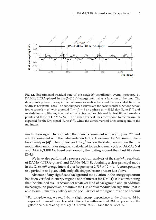
To point out the presence of the signal the time behaviour of the experi-mental residual rates of the single-hit scintillation events for DAMA/NaI andDAMA/LIBRA–phase1 in the (2–6) keV energy interval is plotted in Fig. 1.1. Theχ2 test excludes the hypothesis of absence of modulation in the data: χ2/d.o.f. =83.1/50 for the (2–6) keV energy interval (P-value = 2.2 × 10−3). When fitting thesingle-hit residual rate of DAMA/LIBRA–phase1 together with the DAMA/NaIones, with the function: A cosω(t− t0), considering a period T = 2π

ω= 1 yr and

a phase t0 = 152.5 day (June 2nd) as expected by the DM annual modulationsignature, the following modulation amplitude is obtained: A = (0.0110± 0.0012)cpd/kg/keV corresponding to 9.2 σ C.L.. When the period, and the phase arekept free in the fitting procedure, the modulation amplitude is (0.0112± 0.0012)cpd/kg/keV (9.3 σ C.L.), the period T = (0.998 ± 0.002) year and the phaset0 = (144± 7) day, values well in agreement with expectations for a DM annual

ii

“proc16” — 2016/12/12 — 10:17 — page 3 — #19 ii

ii

ii

1 DAMA/LIBRA Results and Perspectives 3

Fig. 1.1. Experimental residual rate of the single-hit scintillation events measured byDAMA/LIBRA–phase1 in the (2–6) keV energy interval as a function of the time. Thedata points present the experimental errors as vertical bars and the associated time binwidth as horizontal bars. The superimposed curves are the cosinusoidal functions behav-iors A cosω(t − t0) with a period T = 2π

ω= 1 yr, a phase t0 = 152.5 day (June 2nd) and

modulation amplitudes, A, equal to the central values obtained by best fit on these datapoints and those of DAMA/NaI. The dashed vertical lines correspond to the maximumexpected for the DM signal (June 2nd), while the dotted vertical lines correspond to theminimum.

modulation signal. In particular, the phase is consistent with about June 2nd andis fully consistent with the value independently determined by Maximum Likeli-hood analysis [4]1. The run test and the χ2 test on the data have shown that themodulation amplitudes singularly calculated for each annual cycle of DAMA/NaIand DAMA/LIBRA–phase1 are normally fluctuating around their best fit values[2–4,8].

We have also performed a power spectrum analysis of the single-hit residualsof DAMA/LIBRA–phase1 and DAMA/NaI [8], obtaining a clear principal modein the (2–6) keV energy interval at a frequency of 2.737× 10−3 d−1, correspondingto a period of ' 1 year, while only aliasing peaks are present just above.

Absence of any significant background modulation in the energy spectrumhas been verified in energy regions not of interest for DM [4]; it is worth notingthat the obtained results account of whatever kind of background and, in addition,no background process able to mimic the DM annual modulation signature (that isable to simultaneously satisfy all the peculiarities of the signature and to account

1 For completeness, we recall that a slight energy dependence of the phase could beexpected in case of possible contributions of non-thermalized DM components to thegalactic halo, such as e.g. the SagDEG stream [28,30,31] and the caustics [32].

ii

“proc16” — 2016/12/12 — 10:17 — page 4 — #20 ii

ii

ii


for the whole measured modulation amplitude) is available (see also discussionse.g. in Ref. [1–4,7,8,14,15]).

A further relevant investigation in the DAMA/LIBRA–phase1 data has beenperformed by applying the same hardware and software procedures, used toacquire and to analyse the single-hit residual rate, to the multiple-hit one. In fact,since the probability that a DM particle interacts in more than one detector isnegligible, a DM signal can be present just in the single-hit residual rate. Thus, thecomparison of the results of the single-hit events with those of the multiple-hit onescorresponds practically to compare between them the cases of DM particles beam-on and beam-off. This procedure also allows an additional test of the backgroundbehaviour in the same energy interval where the positive effect is observed. Inparticular, the residual rates of the single-hit events measured in the (2–6) keVenergy interval over the DAMA/LIBRA–phase1 annual cycles, as collected ina single cycle, are reported in Ref. [4] together with the residual rates of themultiple-hit events in the same energy interval. A clear modulation satisfying allthe peculiarities of the DM annual modulation signature is present in the single-hit events, while the fitted modulation amplitude for the multiple-hit residualrate is well compatible with zero: −(0.0005 ± 0.0004) cpd/kg/keV in the sameenergy region (2–6) keV. Thus, again evidence of annual modulation with thefeatures required by the DM annual modulation signature is present in the single-hit residuals (events class to which the DM particle induced events belong), whileit is absent in the multiple-hit residual rate (event class to which only backgroundevents belong). Similar results were also obtained for the last two annual cycles ofthe DAMA/NaI experiment [23]. Since the same identical hardware and the sameidentical software procedures have been used to analyse the two classes of events,the obtained result offers an additional strong support for the presence of a DMparticle component in the galactic halo.

By performing a maximum-likelihood analysis of the single-hit scintillationevents, it is possible to extract from the data the modulation amplitude, Sm, as afunction of the energy considering T =1 yr and t0 = 152.5 day. Again the resultshave shown that positive signal is present in the (2–6) keV energy interval, whileSm values compatible with zero are present just above; for details see Ref. [4].Moreover, as described in Ref. [2–4,8], the observed annual modulation effect iswell distributed in all the 25 detectors, the annual cycles and the energy bins at 95%C.L. Further analyses have been performed. All of them confirm the evidence forthe presence of an annual modulation in the data satisfying all the requirementsfor a DM signal.

Sometimes naive statements were put forwards as the fact that in natureseveral phenomena may show some kind of periodicity. The point is whether theymight mimic the annual modulation signature in DAMA/LIBRA (and formerDAMA/NaI), i.e. whether they might be not only quantitatively able to accountfor the observed modulation amplitude but also able to contemporaneously satisfyall the requirements of the DM annual modulation signature. The same is alsofor side reactions. This has already been deeply investigated in Ref. [1–4] andreferences therein; the arguments and the quantitative conclusions, presented

ii

“proc16” — 2016/12/12 — 10:17 — page 5 — #21 ii

ii

ii


there, also apply to the entire DAMA/LIBRA–phase1 data. Additional argumentscan be found in Ref. [7,8,14,15].

No modulation has been found in any possible source of systematics or side re-actions; thus, cautious upper limits on possible contributions to the DAMA/LIBRAmeasured modulation amplitude are summarized in Ref. [2–4]. It is worth notingthat they do not quantitatively account for the measured modulation amplitudes,and also are not able to simultaneously satisfy all the many requirements of thesignature. Similar analyses have also been done for the DAMA/NaI data [22,23].In particular, in Ref. [15] it is shone that, the muons and the solar neutrinos cannotgive any significant contribution to the DAMA annual modulation results.

In conclusion, DAMA give model-independent evidence (at 9.3σ C.L. over 14independent annual cycles) for the presence of DM particles in the galactic halo.

As regards comparisons, we recall that no direct model independent compari-son is possible in the field when different target materials and/or approaches areused; the same is for the strongly model dependent indirect searches. In particular,the DAMA model independent evidence is compatible with a wide set of scenariosregarding the nature of the DM candidate and related astrophysical, nuclear andparticle Physics; as examples some given scenarios and parameters are discussede.g. in Ref. [22,2,8] and references therein. Further large literature is available onthe topics. In conclusion, both negative results and possible positive hints arecompatible with the DAMA model-independent DM annual modulation resultsin various scenarios considering also the existing experimental and theoretical un-certainties; the same holds for the strongly model dependent indirect approaches(see e.g. arguments in Ref. [8] and references therein).

The single-hit low energy scintillation events collected byDAMA/LIBRA–phase1 have also been investigated in terms of possible diurnaleffects[14]. In particular, a diurnal effect with the sidereal time is expected for DMbecause of Earth rotation; this DM second-order effect is model-independent andhas several peculiar requirements as the DM annual modulation effect has. At thepresent level of sensitivity the presence of any significant diurnal variation andof diurnal time structures in the data can be excluded for both the cases of solarand sidereal time; in particular, the DM diurnal modulation amplitude expected,because of the Earth diurnal motion, on the basis of the DAMA DM annual modu-lation results is below the present sensitivity [14]. It will be possible to investigatesuch a diurnal effect with adequate sensitivity only when a much larger exposurewill be available; moreover better sensitivities can also be achieved by loweringthe software energy threshold as in the presently running DAMA/LIBRA–phase2.

The data of DAMA/LIBRA–phase1 have also been used to investigate theso-called Earth Shadow Effect which could be expected for DM candidate particlesinducing nuclear recoils; this effect would be induced by the variation duringthe day of the Earth thickness crossed by the DM particle in order to reach theexperimental set-up. It is worth noting that a similar effect can be pointed out onlyfor candidates with high cross-section with ordinary matter, which implies lowDM local density in order to fulfill the DAMA/LIBRA DM annual modulationresults. Such DM candidates could get trapped in substantial quantities in theEarths core; in this case they could annihilate and produce secondary particles (e.g.

ii

“proc16” — 2016/12/12 — 10:17 — page 6 — #22 ii

ii

ii


neutrinos) and/or they could carry thermal energy away from the core, givingpotentiality to further investigate them. The results, obtained by analysing in theframework of the Earth Shadow Effect the DAMA/LIBRA–phase1 (total exposure1.04 ton×yr) data are reported in Ref. [20].

For completeness we recall that other rare processes have also been searchedfor by DAMA/LIBRA-phase1; see for details Refs. [9–11].

1.3 DAMA/LIBRA–phase2 and perspectives

An important upgrade has started at end of 2010 replacing all the PMTs with newones having higher Quantum Efficiency; details on the developments and on thereached performances in the operative conditions are reported in Ref. [6]. Theyhave allowed us to lower the software energy threshold of the experiment to 1 keVand to improve also other features as e.g. the energy resolution [6].

Since the fulfillment of this upgrade and after some optimization periods,DAMA/LIBRA–phase2 is continuously running in order e.g.:

1. to increase the experimental sensitivity thanks to the lower software energythreshold;

2. to improve the corollary investigation on the nature of the DM particle andrelated astrophysical, nuclear and particle physics arguments;

3. to investigate other signal features and second order effects. This requires longand dedicated work for reliable collection and analysis of very large exposures.

In the future DAMA/LIBRA will also continue its study on several other rareprocesses as also the former DAMA/NaI apparatus did.

Moreover, the possibility of a pioneering experiment with anisotropic ZnWO4detectors to further investigate, with the directionality approach, those DM candi-dates that scatter off target nuclei is in progress [29].

Finally, future improvements of the DAMA/LIBRA set-up to further increasethe sensitivity (possible DAMA/LIBRA-phase3) and the developments towardsthe possible DAMA/1ton (1 ton full sensitive mass on the contrary of other kindof detectors), we proposed in 1996, are considered at some extent. For the first casedevelopments of new further radiopurer PMTs with high quantum efficiency areprogressed, while in the second case it would be necessary to overcome the presentproblems regarding: i) the supplying, selection and purifications of a large numberof high quality NaI and, mainly, TlI powders; ii) the availability of equipmentsand competence for reliable measurements of small trace contaminants in ppt orlower region; iii) the creation of updated protocols for growing, handling andmaintaining the crystals; iv) the availability of large Kyropoulos equipments withsuitable platinum crucibles; v) etc.. At present, due to the change of rules forprovisions of strategical materials, the large costs and the lost of some equipmentsand competence also at industry level, new developments of ultra-low-backgroundNaI(Tl) detectors appear to be quite difficult. On the other hand, generally largermasses do not imply a priori larger sensitivity; in case the DM annual modulationsignature is exploited, the improvement of other parameters of the experimentalset-up (as e.g. the energy threshold, the running time,...) plays an important roleas well.

ii

“proc16” — 2016/12/12 — 10:17 — page 7 — #23 ii

ii

ii


References

1. R. Bernabei et al., Nucl. Instr. and Meth. A 592 297 (2008).2. R. Bernabei et al., Eur. Phys. J. C 56 333 (2008).3. R. Bernabei et al., Eur. Phys. J. C 67 39 (2010).4. R. Bernabei et al., Eur. Phys. J. C 73 2648 (2013).5. P. Belli et al., Phys. Rev. D 84 055014 (2011).6. R. Bernabei et al., J. of Instr. 7 P03009 (2012).7. R. Bernabei et al., Eur. Phys. J. C 72 2064 (2012).8. R. Bernabei et al., Int. J. of Mod. Phys. A 28 1330022 (2013).9. R. Bernabei et al., Eur. Phys. J. C 62 327 (2009).

10. R. Bernabei et al., Eur. Phys. J. C 72 1920 (2012).11. R. Bernabei et al., Eur. Phys. J. A 49 64 (2013).12. R. Bernabei et al., Adv. High Energy Phys. Article ID:605659 (2014).13. R. Bernabei et al., Phys.Part.Nucl. 46 138–146 (2015).14. R. Bernabei et al., Eur. Phys. J. C 74 2827 (2014).15. R. Bernabei et al., Eur. Phys. J. C 74 3196 (2014).16. R. Bernabei et al., Int. J. Mod. Phys. A 31 1642006 (2016).17. R. Bernabei et al., Int. J. Mod. Phys. A 31 1642005 (2016).18. R. Bernabei et al., Int. J. Mod. Phys. A 31 1642004 (2016).19. R. Bernabei et al., Int. J. Mod. Phys. A 30 1545006 (2015).20. R. Bernabei et al., Eur. Phys. J. C 75 239 (2015).21. R. Bernabei et al., Phys. Part. Nucl. 46 138–146 (2015).22. R. Bernabei el al., La Rivista del Nuovo Cimento 26 n.1 1–73 (2003).23. R. Bernabei et al., Int. J. Mod. Phys. D 13 2127 (2004).24. K.A. Drukier et al., Phys. Rev. D 33 3495 (1986); K. Freese et al., Phys. Rev. D 373388

(1988).25. D. Smith and N. Weiner, Phys. Rev. D 64 043502 (2001); D. Tucker-Smith and N. Weiner,

Phys. Rev. D 72 063509 (2005); D. P. Finkbeiner et al, Phys. Rev. D 80 115008 (2009).26. K. Freese et al., Phys. Rev. D 71 043516 (2005); K. Freese et al., Phys. Rev. Lett. 92 11301

(2004).27. R. Bernabei et al., Eur. Phys. J. C 18 283 (2000).28. R. Bernabei et al., Eur. Phys. J. C 47 263 (2006).29. R. Bernabei et al., Eur. Phys. J. C 73 2276 (2013).30. K. Freese et al., Phys. Rev. D 71 043516 (2005); New Astr. Rev. 49 193 (2005); astro-

ph/0310334; astro-ph/0309279.31. G. Gelmini, P. Gondolo, Phys. Rev. D 64 023504 (2001).32. F.S. Ling, P. Sikivie and S. Wick, Phys. Rev. D 70 123503 (2004).

ii

“proc16” — 2016/12/12 — 10:17 — page 8 — #24 ii

ii

ii


Proceedings to the 19th WorkshopWhat Comes Beyond . . . (p. 8)Bled, Slovenia, July 11–19, 2016

2 Experience in Modeling Properties ofFundamental Particles Using Binary Codes

E.G. Dmitrieff ?

29 88 Postyshev bvd., Irkutsk, Russia

Abstract. This work summarizes our study in fundamental particles modeling, based onthe amount of information behind particular property. We had built our models firstly usinglinear binary sequences, then continued with cyclic and spatial arranged binary codes, andthen came to space tessellation, isomorphic with these codes.

We show that properties of particles and vacuum can be effectively represented inthese models, and some predictions can be made. In particular, we imply existence andpredict structure of new fundamental massless scalar boson, that forms vacuum condensate.

Povzetek. Avtor v prispevku predstavi svoj model za opis lastnosti osnovnih delcev, kitemelji na kolicini informacij, ki je potrebna za opis dolocenih lastnosti. Uporabi binarnazaporedja, nadaljuje s ciklicnimi in prostorsko razporejenimi binarnimi kodami in zakljucis teselacijami prostora, ki so izomorfne tem kodam.

Pokaze, da lahko s tem modelom preprosto opise lastnosti osnovnih delcev in vaku-uma in ponudi nekaj napovedi. Napove obstoj in strukturo novega fundamentalnegaskalarnega bozona, ki tvori vakuumski kondenzat.

2.1 Introduction

There are several approaches in building fundamental particle models. The main-stream one is based on the Quantun Field Theory [1].

In contrast, as structural elements for building our models, we chose Booleanalgebra objects, namely spatial binary codes, or bit graphs. They are extensions ofbit sequences used in computers (see Appendix 2.8). We needed to extend themto reflect the multi-valence – in the first place, of the color. Having counted thenumber of possible values for particular property, we chose the minimal sufficientnumber of bits [2]. Then, we tried to extract from the codes as much data aspossible.

We shall demonstrate how one can start, and how far one can go using codes.Also, we point out when the codes should be replaced with more relevant buildingblocks.

Since the Boolean codes, that we used, are the special case of Clifford algebraobjects [3], our models can be compared to other models based on the Cliffordalgebra (see [5] and other references appearing in this paper).

? [email protected]

ii

“proc16” — 2016/12/12 — 10:17 — page 9 — #25 ii

ii

ii

2 Experience in Modeling Properties of Fundamental Particles. . . 9

2.2 Models overview

Our work is an application of the approach mentioned above to the domain offundamental particles’ properties - first of all, to their quantum numbers. Theresult is a family of models, each representing a set of particle’s properties. Theyare shown in Table 2.1.

Binary code modelsProperties 3-bit 4-bit 6-bit 8-bit 8.1

Electric charge Q ⇓ + + + +Dirac neutrinos ⇓ + + + +Matter/antimatter + + - - -Baryon number B + - - - -Lepton number L + - - - -Weak isospin T3 + ⇓ ⇓ + +Weak hypercharge YW + + + + +Color charge - ⇓ ⇓ ⇓ ⇓Fermion flavor - - - ⇓ ⇓Spin states - - - ± ±Handedness - - - - ±Mass - - - - ±Interactions ± ± - - -Condensates - - - - ±Applied to fermions + + + + +Applied to bosons - + + + +Applied to vacuum - ± + + +

Table 2.1. Family of models representing particular properties. Arrow sign (⇓) means thatthe model is based on known values of this property; plus sign (+) means that values of thisproperty are derived from the model; ± sign means that in this model some approximationis discussed.

Models inherit derived properties from their ascenders, so they can skip deriv-ing some of them. properties derived in it., but, being based on other assumptions,does not inherit the added ”by hand” basement of it. Instead, it introduces itsown basement, allowing to derive the values, that have been used to build theascending model.This mechanism is also used to avoid direct deriving of all thedata in each model. So all the models are stand-alone, but ’help’ each other as ifthey were ’family members’.

In the first, simplest one, we allocate 3 bits for storing information aboutelectrical charge of each particle, and then express several quantum numbers (B,L, T3, YW) as combination (mostly linear) of these bits. Also, we consider somebitwise operations as symmetry and interaction representations.

To represent more properties, including color, flavor and spin states, weredesigned the model several times appended more bits when necessary, until wecame to 8-bit model.

ii

“proc16” — 2016/12/12 — 10:17 — page 10 — #26 ii

ii

ii

10 E.G. Dmitrieff

In advanced 8-bit model (8.1), the vacuum is considered as a condensed state,or the tessellation, of the multiple copies of new scalar particle. The code of thisparticle in this model was reserved for the singlet, or longitudinal, photon. Thevacuum particle is considered the same way as others. Also, other particles areconsidered regarding this background condensate – as a set of one or severalstructure defects of it. This approach also allows to obtain the first approximation ofparticles’ masses, based on the count of structure defects.

The following models are not included here in details since they are not builtusing codes.

Since we needed to take in account the interface between neighboring bits, in3D model, instead of bits, we used electrically charged polyhedra. We supposedthat they are organized into the Weaire-Phelan honeycomb structure [6] due toits minimal surface square among the structures formed by polyhedra of equalvolume. We assume that the default alternation of positive- and negative-chargedpolyhedra follows our 8.1 model of vacuum condensate, while the anti-structuredefects of this alternation represent particles. The square of the walls betweenoppositely-charged polyhedra, that is geometrically dependent on the defects’structure, is used as second approximation of particles’ masses.

The distortion of the structure, native to the vacuum condensate and causedby defects, is taken in account in 3D.1 model, allowing to consider the relativesmall influence of the curvature on the surface energy.

2.3 Electric charge: 3-bit one’s complement code model

2.3.1 Charge data analysis

The first property, that attracted our attention, was the particle’s electric chargeQ. Among 61 known fundamental particles [8], [9] there are only 7 differentvalues of electric charge (we do not take now any assumptions about the mattertype, counting both particles and antiparticles). The charges are symmetricallydistributed from −1 through 0 to +1 keeping the interval ∆Q = 1/3 (see Table 2.2).

Count of particles with electrical charge Q ofSet of particles total −1 −2/3 −1/3 0 +1/3 +2/3 +1

All particles 61 4 9 9 17 9 9 4All fermions 48 3 9 9 6 9 9 3Fermions of one family 12 1 3 3 2 3 3 1All bosons 13 1 - - 11 - - 1Vector bosons 12 1 - - 10 - - 1Scalar boson 1 - - - 1 - - -

Table 2.2. Distribution of known electrical charge values in different groups of fundamentalparticles. Each quark color state, and also particles with their antiparticles, including neu-trino, are counted separately. In contrast, different spin- and handedness states are countedas one particle. The 8 gluons, counted among 13 bosons, are the QCD combinations [7].

ii

“proc16” — 2016/12/12 — 10:17 — page 11 — #27 ii

ii

ii


Following the approach of counting minimal information needed to representthe experimental data, we should use at least 3 bits to represent seven values [2].

N = log2 7 ≈ 2.807 (2.1)

Moreover, all 7 values of Q are peculiar to fermions only. The known funda-mental bosons can have just 3 integer values of electrical charge: −1, 0 and +1.Also, each fermion family has the same distribution of Q values. So, the modelof electrical charge for one fermion family members, is the most complex case.Therefore, it should be appropriate for all the fundamental particles’ charge, andwe can keep focusing on one fermion family only.

Additionally, we assumed, that the neutrino and anti-neutrino are not justonly different, Dirac particles, but their zero electric charges are also not the samein their nature — but just coinciding. This assumption looks natural while takinginto account, that the electrical charge can be represented as the sum of weakisospin and the half of weak hyper-charge, and they have different signs for theparticle and anti-particle:

Q = T3 +YW

2;QνL =

1

2−1

2;QνR = −

1

2+1

2. (2.2)

So we consider they have different origins, but degenerated values, assuming+0 for neutrino and -0 for anti-neutrino.

2.3.2 Charge coding

After these assumptions, we have 8 different electrical charges (with two of themdegenerated), even and symmetrically distributed around zero. The number ofrequired bits become exactly 3 because 8 is the integer power of two:

N = log2 8 = 3. (2.3)

To get the integer numbers, we multiplied it by 3:

3Q ∈ −3,−2,−1,−0,+0, 1, 2, 3 (2.4)

We used then the code of N = 3 bits with ones’ complement convention (seeAppendix 2.9 for details) to obtain binary representations for charge values.

We chose this convention because it has exactly the same data range [−(2N−1−

1) . . . 2N−1 − 1] as the data to be coded (2.4), so all the possible code combinationsmap to existing particle charges without exceptions (see Table 2.3).

Having three bits qi of the 3Q representation, we always can retrieve thecharge value back (2.93):

3Q = −3q2 + 2q1 + q0 (2.5)

orQ =

2q1 + q03

− q2. (2.6)

ii

“proc16” — 2016/12/12 — 10:17 — page 12 — #28 ii

ii

ii

12 E.G. Dmitrieff

Electrical charge Q -1 -2/3 -1/3 -0 +0 +1/3 +2/3 +1Fermions l− u d ν ν d u l+

Integer charge 3Q -3 -2 -1 -0 +0 1 2 3Charge code q2q1q0 100 101 110 111 000 001 010 011

The least significant bit q0 0 1 0 1 0 1 0 1Ordinal matter + - + - + - + -Anti-matter - + - + - + - +Two lower bits q1q0 00 01 10 11 00 01 10 11Kind of fermions. . . leptons 00 - - - 00 - - -. . . anti-leptons - - - 11 - - - 11. . . quarks - - 10 - - - 10. . . anti-quarks - 01 - - - 01 - -Lepton numberL = 1 − q1 − q0 1 0 0 -1 1 0 0 -1Baryon numberB = (q1 − q0)/3 0 -1/3 1/3 0 0 -1/3 1/3 0Weak hypercharge:YwL = 4

3q1 + q0(

53− 2q2) − 1 -1 -4/3 1/3 (0) -1 2/3 1/3 2

YwR = 4q1−q03

− 2q2(1 − q0) -2 -1/3 -2/3 1 (0) -1/3 4/3 1Yw = 4

3q1 +

23q0 − 1 -1 -1/3 1/3 (1) -1 -1/3 1/3 1

Y∗w = 43q1 +

23q0 − 2q2 -2 -4/3 -2/3 0 (0) 2/3 4/3 2

The eldest bit q2 1 1 1 1 0 0 0 0Weak isospin:T3L = (1 − q0)(

12− q2) -1/2 0 -1/2 (0) 1/2 0 1/2 0

T3R = q0(12− q2) 0 -1/2 0 -1/2 (0) 1/2 0 1/2

T3 =12− q2 -1/2 -1/2 -1/2 (-1/2) 1/2 1/2 1/2 1/2

T∗3 = 0 0 0 0 0 (0) 0 0 0

Bosons W− Z0, H0 g? γ W+

Scalar / Singlet (S = 0)Yw = 4

3q1 +

23q0 − 1 (-1) 1 (-1) (1)

T3 =12− q2 (-1/2) -1/2 (1/2) (1/2)

Vector/ Triplet (S = ±1)Y∗w = 0 0 0 0 0T∗3 = 2

3q1 +

13q0 − q2 -1 0 0 1

Table 2.3. Electrical charge distribution, 3-bit charge codes and fermions’ quantum numbersas bit combinations. Symbols u, d, l, ν mean u- and d-type quarks, charged leptons andneutrinos regardless of their membership in families. The estimated values

2.3.3 Symmetries as bitwise operations

Two operations on bits qi appeared to be isomorphic with two particles’ symme-tries: isotopic symmetry and charge inversion.

• Since the bitwise inversion is the negation of value, it acts as charge symmetryoperation C over the representations, transforming code of any anti-particleinto the code of corresponding particle, and vice versa:

¬[u] = ¬101 = 010 = [u] (2.7)

ii

“proc16” — 2016/12/12 — 10:17 — page 13 — #29 ii

ii

ii


¬[l−] = ¬100 = 011 = [l+] (2.8)

(square brackets here mean obtaining the ones’ complement code, in form ofq2q1q0, that is shown in typewriter font).

• The q2-only inversion (i.e. bitwise exclusive or operation ⊕ between chargecode and 100) corresponds to the isotopic symmetry operation (marked hereas ′) between up and down particles:

[u ′] = [u]⊕ 100 = 101⊕ 100 = 001 = [d], (2.9)

[ν ′] = [ν]⊕ 100 = 000⊕ 100 = 100 = [l−] (2.10)

(we assume that antiparticles have reversed positions in isotopic doublets:anti-up quark is anti-up, i.e. down, and anti-down is up).Following (2.5), (2.90), for any particle with charge Q:

3Q ′ = 2q1 + q0 − 3(¬q2) = 2q1 + q0 + 3(q2 − 1) = (2.11)

= (2q1 + q0 − 3q2) + 6q2 − 3 = 3Q+ 3(2q2 − 1),

so3Q ′ = 3Q− 3 in case q2 = 0 (up particles); (2.12)

3Q ′ = 3Q+ 3 in case q2 = 1 (down particles). (2.13)

This allows to use addition1 operator + instead of exclusive or ⊕:

[u ′] = [u] + 3 = 101+ 011 = −2+ 3 = 1 = 001 = [d] (2.14)

[ν ′] = [ν] − 3 = 000+ 100 = +0+ (−3) = −3 = 100 = [l−]. (2.15)

Note that +3 and −3 coincide with charged weak bosons’ 3Q values:

+3 = 011 = [W+],−3 = 100 = [W−], (2.16)

so weak interactions can be expressed in code form, as charge conservingequation. For instance:

u→ d+W+;

2

3= −

1

3+ 1;

010 = 110+ 011;

[u] = [d] + [W+]. (2.17)

• The same way, we can express weak neutral-current, electromagnetic and alsostrong interactions, since [Z0], [γ], [g] ∈ 000;111:

[l−] = [l−] + [γ], (2.18)

[dr] + [grg] = [dg] (2.19)

(Color state is shown as upper index).In 3-bit model, all these interactions are considered as identity operation E,turning particles’ codes into themselves: up into ups’, downs’ into downs’,quarks’ into quarks’, leptons’ into leptons’. But, since codes are multivalent,color state or family membership may change.

1 Addition is performed according to rules for ones’ complement code operations [14].

ii

“proc16” — 2016/12/12 — 10:17 — page 14 — #30 ii

ii

ii

14 E.G. Dmitrieff

2.3.4 Quantum numbers as bit combinations

Filling the constructed codes of Q in a tabular form, we found that several linearcombinations of bits produce values, equal to fermion’s quantum numbers (seetable 2.3).

• The least significant bit q0 is equal to 1 for antiparticles and 0 for particles.• Two lower bits q1q0 form lepton number L, baryon number B and weak

hypercharge Yw:L = 1− q1 − q0, (2.20)

B =q1 − q03

; (2.21)

for left-handed particles (q0 = 0) and right-handed anti-particles (q0 = 1):

Yw = B− L =4

3q1 +

2

3q0 − 1, or (2.22)

Yw

2=2q1 + q0

3−1

2. (2.23)

• The eldest bit q2 defines the weak isospin of left-handed particles and right-handed anti-particles:

T3 =1

2− q2. (2.24)

Since for right-handed particles and left-handed anti-particles

Y∗w2

=2q1 + q0

3− q2 = Q, (2.25)

T∗3 = 0, (2.26)

we can express YwL and YwR separately, for both particles and anti-particles, asquadratic combinations:

YwL =4

3q1 + q0(

5

3− 2q2) − 1 (2.27)

YwR =4q1 − q0

3− 2q2(1− q0) (2.28)

T3L = (1− q0)(1

2− q2) (2.29)

T3R = q0(1

2− q2) (2.30)

For vector bosons, equations for weak isospin and weak hypercharge are reversed,comparing to right-handed fermions:

T∗3 =2q1 + q0

3− q2 = Q, (2.31)

Y∗w2

= 0, (2.32)

ii

“proc16” — 2016/12/12 — 10:17 — page 15 — #31 ii

ii

ii


and scalar Higgs boson has the same equations as (2.24, 2.22)Basing on the least significant bit q0, it is possible to give the term definitions

for ordinal matter and anti-matter, that do not rely on their cosmological distribution.Instead, they depend on the choice of positive or negative sign of electrical charge.In case the electron is considered negative-charged, as usual, the definitions arethe following:

The ordinal matter consist of one or more fundamental fermions having the valueof 0 in the least significant bit of ones’ complement codes of their electricalcharges, expressed in units of 1

3|e|;

The anti-matter consist of fermions having the value of 1 in this bit.The mixed matter consist of fermons of both types noted above (for instance,

mesons and the positronium).

2.4 Intermediate 4- and 6-bit code models

2.4.1 Fermions: 4-bit model

Color coding The 3-bit model, shown above, represents several properties offundamental particles, that do not depend on their color state. We could notsuggest any qi combination, that would reasonably express colors.

But, we notice the following facts:

• the color states of quarks (colors) differs from color states of anti-quarks (anti-colors) and also from colorless color states of leptons, so the count of differentcolor states is at least 7;

• there is neither red nor colorless anti-quark, neither colorless nor magentaquark, neither green nor yellow lepton, so the number of color states for theparticular kind of fermions is limited to 3 (quarks) or 1 (leptons);• the numerator in the expression (2.6) of electrical charge Q

N1 = 2q1 + q0 (2.33)

has a form of 2-bit decomposition into powers of two (2.86) of some positiveinteger number. Its value is 0 for leptons, 1 for anti-quarks, 2 for quarks and 3for anti-leptons (see table 2.4);

• for any code of N = 3 bits, containing N1 digits 1 (or 0, symmetrically), thecount of possible combinations is CN13 , i.e. 1, 3, 3, and 1, respectively. In caseall three bits have the same value, there is only one combination; but whenthey are different, the number of variants rises up to three;

• these counts of combinations coincide with the count of different color states.

Supposing that the ’colorless’ color of leptons also differs from the ’colorless’color of anti-leptons (like we did with neutrino’s and anti-neutrino’s charge), thenumber of known colors becomes 8, so the color requires 3 bits to be coded.

Following facts listed above, we allocated 3 bits to be the color representation,and assigned the combinations to fermion kinds accordingly to number of digit 1they contain (table 2.4) .

ii

“proc16” — 2016/12/12 — 10:17 — page 16 — #32 ii

ii

ii

16 E.G. Dmitrieff

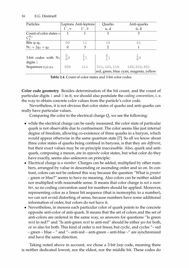
Particles Leptons Anti-leptons Quarks Anti-quarksl−, ν l+, ν u, d u, d

Count of color states =CN13

1 1 3 3

Bits q1q0 00 11 10 01N1 = 2q1 + q0 0 3 2 1

3-bit codes with N1digits 1

000

111

011

100

Sequences c2c1c0 000 111 011, 101, 110 100, 010, 001red, green, blue cyan, magenta, yellow

Table 2.4. Count of color states and 3-bit color codes.

Color code geometry Besides determination of the bit count, and the count ofparticular digits 1 and 0 in it, we should also postulate the coding convention, i. e.the way to obtain concrete color values from the particle’s color code.

Nevertheless, it is not obvious that color states of quarks and anti-quarks canreally have particular values.

Comparing the color to the electrical charge Q, we see the following:

• while the electrical charge can be easily measured, the color state of particularquark is not observable due to confinement. The color seems like just internaldegree of freedom, allowing co-existence of three quarks in a baryon, whichwould appear otherwise in the same quantum state [7]. So all we know aboutthree color states of quarks being confined in baryons, is that they are different,but their exact values may be on principle inaccessible. Also, quark and anti-quark, composing a meson, are in opposite color states, but what color do theyhave exactly, seems also unknown on principle;

• Electrical charge is a number. Charges can be added, multiplied by other num-bers, arranged by value in descending or ascending order and so on. In con-trast, colors can not be ordered this way because the question ”What is greater– green or blue?” seems to have no meaning. Also colors can be neither addednor multiplied with reasonable sense. It means that color charge is not a num-ber, so no coding convention used for numbers should be applied. Moreover,representing color as a linear bit sequence (that is isomorphic to a number),we can not avoid distorting of sense, because numbers have some additionalinformation of order, but colors do not have it.

• Nevertheless, in mesons each particular color of quark points to the concreteopposite anti-color of anti-quark. It means that the set of colors and the set ofanti-colors are ordered in the same way, so answers for questions ”Is greennext to red?” and ”Is anti-green next to anti-red” should be either yes for both,or no also for both. This kind of order is not linear, but cyclic, and cycles ”– red– green – blue – ” and ”– anti-red – anti-green – anti-blue –” are synchronizedand have the same direction.

Taking noted above in account, we chose a 3-bit loop code, meaning thereis neither dedicated lowest, nor the eldest, nor the middle bit. These codes do

ii

“proc16” — 2016/12/12 — 10:17 — page 17 — #33 ii

ii

ii


not look like c2c1c0 (that would assume some integer’s binary decomposition),but rather like cicjck, where i, j, k ∈ 0; 1; 2 and i 6= j 6= k. Writing bits this way,we emphasize that all three bits are peers, so their positions are as equivalent asvertices in equilateral triangle.

In order to read this code as a bit sequence (or as an integer number, that isisomorphic), it is necessary to choose the bit that will be accessed first, and thenthe clockwise or counterclockwise direction2.

This act of selection, in fact, puts additional information to the result andbreaks the triangular symmetry.

In case of random selection, each color code of quark or anti-quark, containingbits of both values, would produce three different sequences.

In contrast with quarks, lepton’s and anti-leptons’ color codes, containingequal bits, always produce the same fixed sequence regardless of starting point.

To get compatible with QCD color names, we associated them with serializedcolor codes as shown in Table 2.4.

For equilateral triangle codes, both cyclic directions produce coinciding 3-bitsequences, but in different order. Since order is significant (for instance, to keepentanglement), the color coding convention should be 3-bit directed loop.

Operations and properties The count of digit 1 in color code is equal to N1:

N1 =

2∑i=0

ci. (2.34)

Combining q2 with N1, we can calculate the electric charge

Q =

2∑i=0

ci

3− q2, (2.35)

weak hypercharge

Yw

2=

2∑i=0

ci

3−1

2(2.36)

and other properties listed in section 2.3.Additionally, now we have color representations. Codes for anti-colors of

anti-quarks have the only one bit with value of 1: anti-red or cyan (r), anti-green ormagenta (g) and anti-blue or yellow (b). Codes for quark colors – red (r), green (g)and blue (b) – have two digits 1. Following this analogue, leptons are white withcolor code of three zeros, and anti-leptons are black, with code of three digits 1.

Note that we utilize each of 24 = 16 code combination, and keep two of threesymmetries mentioned above.

2 Note that it is not trivial task to store non-sequential, particularly triangle-symmetricalcodes in computer memory. Computer architecture is designed to store and processinteger numbers as bit sequences with known dedicated (first) bit address. The trianglestructure can be realized, for instance, as a loop buffer with random current pointer.Codes of entangled particles should keep sharing the same pointer.

ii

“proc16” — 2016/12/12 — 10:17 — page 18 — #34 ii

ii

ii

18 E.G. Dmitrieff

• The all-bit inversion transforms the code of particle into the code of its anti-particle with the opposite color:

¬[l−]4 = ¬1(000) = 0(11

1) = [l+]4; (2.37)

¬[u]4 = ¬1(100) = 0(01

1) = [u]4, (2.38)

or, with particular color – for instance, with anti-red anti-up quark:

¬[ur]4 = ¬1(100) = 0(011) = [ur]4 (2.39)

(Square brackets with index 4 mean obtaining the 4-bit code, in native q2(cicjck)

or serialized q2(c2c1c0) form).• The q2 inversion does not affect q1q0, so it does not change ci, transforming

between up and down fermions with the same color.

2.4.2 Bosons: 6-bit model

Gluons Having the method of color representation, we applied it to obtain codesfor gluons. They have color and anti-color, so suitable codes for them should be6-bit combinations, containing two triangle color codes, of 3 bits each.

The problem is that gluons are not electrically-charged, but both color andanti-color codes, used in 4-bit fermion model, also carry the positive electricalcharge: it is the only q2 that has minus sign in equation (2.35) for Q. Counted forwhole 6-bit code, it would be

2∑i=0

cci3

+

2∑i=0

cci3

=2

3+1

3= +1 > Qg = 0, (2.40)

where cc, cc are codes of gluon’s color and anti-color.Nevertheless, we noticed that this problem does not arise in case we also

include terms −1/2 in the calculation, as we did with YwL2

(2.36). These terms shiftthe charge value of each bit down, so shifted values are symmetrical regarding 0,and therefore they can produce both positive and negative sums. It can mean thatwe should use more appropriate and more symmetrical values than 0 and 1.

Following this, we introduced new bit-like3 symbols bi that are just scaledand shifted ci:

bi =ci

3−1

6, i ∈ 0, 1, 2, bi ∈ −

1

6;1

6 = 0©; 1©. (2.41)

This substitutions puts the denominator 1/3 and also the shift −1/6 inside bitsbi, so their electrical charge values become symmetrical ±1/6. Further we usesymbols 0© = −1

6and 1© = +1

6as short form for values of bi.

3 Symbols bi are not true bits, i.e. binary digits. They are although binary (can be of one oftwo values), but not digits since they are shifted and scaled (while digits supposed tohave values in 0; 1). But they are isomorphic with ci that are digits. So we still use word’bit’ for bi, keeping that in mind.

ii

“proc16” — 2016/12/12 — 10:17 — page 19 — #35 ii

ii

ii


The gluon electrical charge expressed through bi is

Qg =

2∑i=0

bci +

2∑i=0

bci =∑ 1©

0© 1©+∑ 0©

0© 1© =1

6−1

6= 0, (2.42)

as supposed. The ’anti-gluons’, i.e. combinations of anti-color and color in reversedorder also can be coded this way with triangles exchanged. So these 18 codes can berepresentations of gluon states (grb and so on) forming the basis for combination,that produces eight QCD gluons.

Electroweak bosons Extending this approach to colorless color-anticolor pairs,i.e. white-black and black-white, we get just two possible codes for colorless zero-

charged bosons: 1©1© 1© 0©0© 0© and 0©

0© 0© 1©1© 1©.

In Standard Model there are three known particles with this set of properties:

• Z0, as usual boson, supposed to be either in singlet (S = 0) or in triplet (S = ±1)spin state;

• photon γ that is transversal, i.e. triplet-only (S = ±1);• scalar Higgs boson H0 with just one singlet spin state (S = 0).

So photon and Higgs boson together carry the same amount of informationabout spin – as would usual vector boson do – and may share one 6-bit double-color code4.

In this model it is still not clear, which of two codes should be assigned to γtogether with H0 and to Z0:

Qγ = QH0 = QZ0 =∑ 1©

1© 1©+∑ 0©

0© 0© =1

2−1

2= 0. (2.43)

We see that the order of primary and secondary triangle color codes is signifi-cant, so the 6-bit code should be treated as ordered.

Finally, combining codes of black with black, and also of white with white,

we get the only two codes with Q = ±1, which should representW+ (1©1© 1© 1©

1© 1©)

andW− (0©0© 0© 0©

0© 0©).

2.4.3 6-bit code model for fermions

After completing two-color 6-bit codes for bosons, we get back to fermions. Theidea is to express their 4-bit codes, i.e. one q2 and three ci bits, also through bisymbols, unifying them with bosons.

As we had scaled ci bits and shifted them down (2.41), we scale the q2 bitand shifted it up. Additionally, we split it into three symbols b2b1b0, repeating the

4 Positioning the Higgs boson in one cell with the photon is poorly correlated with knownvalues of its weak hyper-charge and weak isospin (see Table 2.3). We solve this problemin Advanced 8.1 model (section 2.6).

ii

“proc16” — 2016/12/12 — 10:17 — page 20 — #36 ii

ii

ii

20 E.G. Dmitrieff

White (1) Anti-colors (3) Colors (3) Black (1)0©0© 0© 0©

0© 1© 0©1© 1© 1©

1© 1©

Black (1) 1©1© 1© γ/H0 W+

Colors (3) 0©1© 1© gcc

Anti-colors (3) 0©0© 1© gcc

White (1) 0©0© 0© W− Z0

Table 2.5. 6-bit codes for bosons

same value three times. It is necessary because effective absolute value of q2 is 1,that is three times greater than effective value 1/3 of ci (2.35), so

bT3i =1

6−q2

3, i ∈ 0; 1; 2. (2.44)

These symbols bT3i have the same domain as bci and bci (2.41): bi ∈ 0©; 1©.Being of the same value, three bT3i always produce the same sequence regardlessof their symmetry.

Electroweak quantum numbers are expressed through bi in a more simpleway than through qi in (2.24, 2.23, 2.6), without additional constants:

T3 =1

2− q2 =

1

2−

2∑i=0

q2

3=

2∑i=0

(1

6−q2

3) =

2∑i=0

bT3i ; (2.45)

Yw

2=

2∑i=0

bci ; (2.46)

Q =

5∑i=0

bi (2.47)

(in last equation all six bits are summed).

Leptons (1) Anti- Quarks (3) Anti-quarks (3) leptons (1)

T3L bT30©0© 0© 0©

0© 1© 0©1© 1© 1©

1© 1©Up 1

21© 1© 1© ν d u l+

Down − 120© 0© 0© l− u d ν

Table 2.6. 6-bit codes for fermions

2.5 8-bit code model extending the 6-bit one with boson spinstates and fermion flavors

The unified 6-bit representations of fermions and bosons are multivalent. Threefermions of different families share the same code. Two states of bosons – singlet

ii

“proc16” — 2016/12/12 — 10:17 — page 21 — #37 ii

ii

ii


and triplet – do the same. Following the approach of building model with b-typesymbols only, we have to keep in mind the total sum of them, that must be equalto the particle’s electric charge.

Both family membership, and being in particular spin state do not affect theelectric charge. So, we can extend codes, keeping total charge intact, just with evennumber of b-type bits. Combinations of odd number of them are not electricallyneutral, since counts of positive and negative values in this case would never beequal:

2n∑i=0

bi 6= 0, n ∈ Z (2.48)

Adding n bit pairs, we would get Cn2n = (2n)!(n!)2

= 2, 6, 20, ... zero-chargedcombinations of them. We see that one additional pair is quite enough to representtwo boson’s states.

There is no suitable pair count to represent three fermion families with thisapproach. The nearest number of them, with two pairs added, would be six. So itis suitable to represent six flavors. The fermion code in this case would contain6+ 4 = 10 bit.

To represent three families, we could also use three-bit combinations withdifferent bits, since C13 = C

23 = 3, but we would then have extra charge of ±1/6.

We took in account, that, in contrast with bosons’ 6-bit codes, fermions’ oneshave T3 codes of three bi bits. These codes utilize only two of eight possiblecombinations: 0© 0© 0© and 1© 1© 1©, because just these codes have suitable values ofelectric charge to get T3 = ±1/2. Six other combinations containing both 0© and 1©are not in use since they have wrong charge values of ±1/6.

We found that these ’wrong’ combinations coincide with combinations re-quired to represent families, and their extra charge can be effectively compensatedby adding one equal-valued b-bit pair of opposite charge. The fermion code wouldbe of 8 bits, that is preferable than 10.

Thus, we added a pair of bpi symbols to both bosons’ and fermions’ codes,allocating four possible combinations of them in the following way:

• For bosons, we used two zero-charged combinations of different bits, 0© 1© and1© 0©. We associated one of them with singlet and another with triplet state byarbitrary choice .

• For fermions, firstly, we replaced bT3 code, that has two ’right’ combinations,with 3-bit bf code5, having six ’wrong’ ones, that carry ±1/6 instead of ±1/2.Secondly, compensating extra electrical charge of ∓1/3, we applied the pairwith both equal values: 1© 1© for up fermions and 0© 0© for down ones, withelectrical charge of ±1/3:

1© 1© 1©⇒1© 1© 0©1© 0© 1©+ 1© 1©;

0© 1© 1©0© 0© 0©⇒

0© 0© 1©0© 1© 0©+ 0© 0©1© 0© 0©

(2.49)

5 fmeans ’family’ or ’flavor’

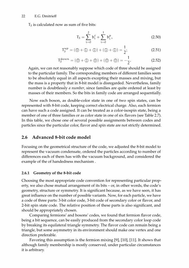
ii

“proc16” — 2016/12/12 — 10:17 — page 22 — #38 ii

ii

ii

22 E.G. Dmitrieff

T3 is calculated now as sum of five bits:

T3 =

2∑i=0

bfi +

1∑i=0

bpi , (2.50)

Tup3 = ( 0©+ 1©+ 1©) + ( 1©+ 1©) =1

2; (2.51)

Tdown3 = ( 0©+ 1©+ 0©) + ( 0©+ 0©) = −1

2. (2.52)

Again, we can not reasonably suppose which code of three should be assignedto the particular family. The corresponding members of different families seemto be absolutely equal in all aspects excepting their masses and mixing, butthe mass is a property that in 8-bit model is disregarded. Nevertheless, familynumber is doubtlessly a number, since families are quite ordered at least bymasses of their members. So the bits in family code are arranged sequentially.

Now each boson, as double-color state in one of two spin states, can berepresented with 8-bit code, keeping correct electrical charge. Also, each fermioncan have such a code assigned. It can be treated as a color-isospin state, being amember of one of three families or as color state in one of six flavors (see Table 2.7).In this table, we chose one of several possible assignments between codes andparticles since the particular color, flavor and spin state are not strictly determined.

2.6 Advanced 8-bit code model

Focusing on the geometrical structure of the code, we adjusted the 8-bit model torepresent the vacuum condensate, ordered the particles according to number ofdifferences each of them has with the vacuum background, and considered theexample of the of handedness mechanism .

2.6.1 Geometry of the 8-bit code

Choosing the most appropriate code convention for representing particular prop-erty, we also chose mutual arrangement of its bits – or, in other words, the code’sgeometry, structure or symmetry. It is significant because, as we have seen, it hasgreat influence on the number of possible variants. Now, for each particle, we havea code of three parts: 3-bit color code, 3-bit code of secondary color or flavor, and2-bit spin state code. The relative position of these parts is also significant, andshould be appropriately chosen.

Comparing fermions’ and bosons’ codes, we found that fermion flavor code,being a bit sequence, can be easily produced from the secondary color loop codeby breaking its equilateral triangle symmetry. The flavor code can remain being atriangle, but some asymmetry in its environment should make one vertex and onedirection preferable.

Favoring this assumption is the fermion mixing [9], [10], [11]. It shows thatalthough family membership is mostly conserved, under particular circumstancesit is arbitrary.

ii

“proc16” — 2016/12/12 — 10:17 — page 23 — #39 ii

ii

ii


Primary color codes bc1

White Anti-colors Colors Black0©0© 0© 0©

0© 1© (3)0©1© 1© (3)

1©1© 1©

Pair bp 3 bits charge − 12

− 16

16

12

FermionsIsotopic Flavor T3 Leptons Anti- Quarks Anti-state bf quarks leptons1© 1© 1© 1© 0© νe d u e+

Up 1© 0© 1© 12

νµ s c µ+

0© 1© 1© ντ b t τ+

0© 0© 0© 0© 1© e− u d νeDown 0© 1© 0© − 1

2µ− c s νµ

1© 0© 0© τ− t b ντ

BosonsSpin 2nd color charge Electro- Strong Electro-state bc2 weak (gluons) weak

0© 1© 1©1© 1© 1

2H0 W+↑↓

Singlet 0©1© 1© 1

6gcc↑↓

S = 00©0© 1© − 1

6gcc↑↓

0©0© 0© − 1

2W−↑↓ Z0↑↓

1© 0© 1©1© 1© 1

2γ W+

Triplet 0©1© 1© 1

6gcc

S = ±1 0©0© 1© − 1

6gcc

0©0© 0© − 1

2W−

Z0

Table 2.7. 8-bit codes associated with fundamental particles. The code for a particle is acombination of three parts from row and column: one bit pair and two 3-bit codes, 8 bitsaltogether. Bit 1© carries electrical charge 1/6 while 0© carries −1/6. Electrical charge Qis the sum of them all, and other quantum numbers can be retrieved from it using 3-bitmodel. Secondary color codes have the same meanings with primary ones. Color and anti-color triangle codes produce three individual sequential codes for particular colors each. Itcauses that there are 3 (anti)quarks of different color and 3× 3 = 9 gluon color-anticolorcombinations in their table cells. Since the particular color, flavor and spin state are notstrictly determined, one of several possible assignments between codes and particles ischosen.

Another possibility is to consider the flavor code and secondary color codeare two different codes. This would cause the bit number to be increased to 11.Taking in account the symmetry between secondary and primary color codes,and following the requirement of even total bit count, we would increase it upto 14. Keeping that in mind, in this section we are following the 8-bit model. Init, the asymmetrical flavor code appears just along with charged bit pair (twoequal-valued bits). This charged pair can be produced from zero-charged one, thatis inherent to bosons, by inversion of one of its bits. So this inverted bit can bethe factor that breaks triangle symmetry of color code, turning it into the code of

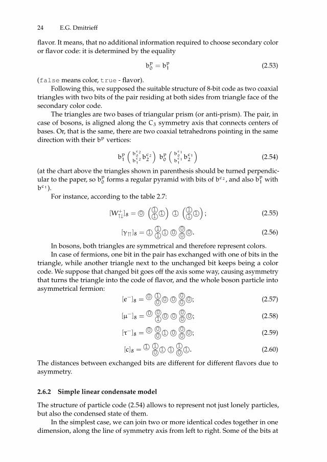
ii

“proc16” — 2016/12/12 — 10:17 — page 24 — #40 ii

ii

ii

24 E.G. Dmitrieff

flavor. It means, that no additional information required to choose secondary coloror flavor code: it is determined by the equality

bp0 = bp1 (2.53)

(false means color, true - flavor).Following this, we supposed the suitable structure of 8-bit code as two coaxial

triangles with two bits of the pair residing at both sides from triangle face of thesecondary color code.

The triangles are two bases of triangular prism (or anti-prism). The pair, incase of bosons, is aligned along the C3 symmetry axis that connects centers ofbases. Or, that is the same, there are two coaxial tetrahedrons pointing in the samedirection with their bp vertices:

bp1

(bc20

bc21

bc22

)bp0

(bc10

bc11

bc12

)(2.54)

(at the chart above the triangles shown in parenthesis should be turned perpendic-ular to the paper, so bp0 forms a regular pyramid with bits of bc2 , and also bp1 withbc1 ).

For instance, according to the table 2.7:

[W+↑↓]8 = 0©(1©1© 1©

)1©(1©1© 1©

); (2.55)

[γ]8 = 1© 1©1© 1© 0© 0©

0© 0©. (2.56)

In bosons, both triangles are symmetrical and therefore represent colors.In case of fermions, one bit in the pair has exchanged with one of bits in the

triangle, while another triangle next to the unchanged bit keeps being a colorcode. We suppose that changed bit goes off the axis some way, causing asymmetrythat turns the triangle into the code of flavor, and the whole boson particle intoasymmetrical fermion:

[e−]8 =0© 1©

0© 0© 0© 0©0© 0©; (2.57)

[µ−]8 =0© 0©

1© 0© 0© 0©0© 0©; (2.58)

[τ−]8 =0© 0©

0© 1© 0© 0©0© 0©; (2.59)

[c]8 =1© 1©

0© 1© 1© 1©0© 1©. (2.60)

The distances between exchanged bits are different for different flavors due toasymmetry.

2.6.2 Simple linear condensate model

The structure of particle code (2.54) allows to represent not just lonely particles,but also the condensed state of them.

In the simplest case, we can join two or more identical codes together in onedimension, along the line of symmetry axis from left to right. Some of the bits at

ii

“proc16” — 2016/12/12 — 10:17 — page 25 — #41 ii

ii

ii


the right side of the left particle code are in close proximity to bits at the left sideof the right particle codeIt causes ambivalence since we could treat right side ofleft code together with left side of right code also as a code of some particle.

Here we consider electrically neutral, colorless boson condensate codes, thatcan be formed by codes of H0, Z0 and γ.

The code assigned to the Higgs boson from Table 2.7, being repeated, formsthe following condensate code:

[. . . H0 . . . ]8 = . . . 0©1©1© 1© 1© 0©

0© 0© 0© 1©1© 1© 1© 0©

0© 0© 0© . . . (2.61)

It has an asymmetry: 0© is to the left from 1©1© 1©.

The photon condensate code is:

[. . . γ . . . ]8 = . . . 1©1©1© 1© 0© 0©

0© 0© 1© 1©1© 1© 0© 0©

0© 0© 1© . . . (2.62)

This condensate has 0© to the right of 1©1© 1©. In it, compared to [. . . H0 . . . ], bits inpairs are exchanged – or, globally shifted half-code size along the axis.

It looks like γ condensate code can be produced from (2.61) by axis-reversingand mirror-reflection. After reversing, to get the same results as before, the trianglesshould be processed in backward direction6. To keep the direction, one shouldperform mirroring after axis-reversing.

Z0 condensate codes are the following:

[. . . Z0 . . . ]8 = . . . 1©0©0© 0© 0© 1©

1© 1© 1© 0©0© 0© 0© 1©

1© 1© 1© . . . ; (2.63)

[. . . Z0↑↓ . . . ]8 = . . . 0© 0©0© 0© 1© 1©

1© 1© 0© 0©0© 0© 1© 1©

1© 1© 0© . . . . (2.64)

They can be produced from (2.61) and (2.62) with all-bit inversion C.We note that in case both primary and secondary code have the same cyclic

direction, the same result is produced by the shift on half-translation-unit, i.e. fourbits.

In case the directions are opposite, one should additionally perform the mirror-reflection P after shift to change back the direction. Therefore, sequential C and Papplied to any whole condensate code would produce almost original but shiftedstate.

The same way we can write simple linear gluon condensate code. For instance,a chain of diagonal gluon codes, joined together, should be the following:

[. . . gcc . . . ]8 = . . . 0©1©0© 1© 1© 0©

1© 0© 0© 1©0© 1© 1© 0©

1© 0© 0© . . . (2.65)

It is almost colorless, since each color triangle has two anti-color neighbors, andvice versa. On both ends of this chain there are ’bare’ color and anti-color triangles.The chain of ’anti-gluons’ looks like shifted gluon chain, excepting color andanti-color on ends are reversed:

[. . . gcc . . . ]8 = . . . 1©0©1© 0© 0© 1©

0© 1© 1© 0©1© 0© 0© 1©

0© 1© 0© . . . (2.66)

6 The triangle color codes are directed, since colors have strict-defined operation next (2.4.1)

ii

“proc16” — 2016/12/12 — 10:17 — page 26 — #42 ii

ii

ii

26 E.G. Dmitrieff

We suppose that these gluon code chains, joined to quark and anti-quarkcodes with opposite colors at ends, could be used to represent mesons.

We also suppose that non-diagonal gluon codes could produce more compli-cated (non-linear) condensate codes, useful in hadron modeling.

One of the possible ways to build the spatial condensate code is to join thelinear condensate codes as threads into bunches, producing the lattice. Thus,considering the linear condensate code as a thread among similar threads, wecould take in account the neighboring bits in other threads.

2.6.3 Particles as differences with background condensate and an example ofmass representation at electroweak scale

We found that vacuum condensate can be represented by any of four colorlesscodes shown above (2.61 – 2.64), so one of them should be chosen.

The particle forming the condensate ’vanishes’ because such a particle doesnot differ from the background7. One of three remaining zero-charged colorlessparticle codes differs from vacuum code by 2 bits (one bit pair); the second onediffers from it by both triangles, i.e. 6 bits, and last one differs by all 8 bits.

We noted that ratio of different bits for two latter particles, 6/8 = 0.75 is justslightly (2, 88%) higher than 0.729, that is experimental value of mZ/mH [12], [13].

Supposing that masses of particles somehow depend on the number of dif-ferences their codes have with the code of massless vacuum, we also checked theW±↑↑ code (2.55).

Comparing to the code of ’vanished’ longitudinal photon, that we used torepresent H0, [W±↑↑]8 has 5 different bits (three in triangle, two in pair) so this ratio5/8 = 0.625 is slightly less (2, 74%) than experimentalmW/mH ≈ 0.6426.

We supposed that these differences in ratios are connected to the differentcontribution in mass, caused by the change in the pair and in the triangle. Usingthe experimental values of mZ and mW as defining points, we estimated thesecontributions for the pair (m2) and the triangle (m3).

Dividing experimentalmZ by two, since its code supposed to consist of twochanged triangles, we get the estimated mass contribution of one changed triangle:

m3 =mZ

2=91.1876

2≈ 45.6(GeV). (2.67)

Subtracting it fromW mass, we get the estimated mass contribution of the changedpair 8:

m2 = mW −m3 = 80.385− 45.6 ≈ 34.8(GeV). (2.68)

So the mass of particle with the 8-bit-changed code should be

m8 = m3 +m3 +m2 ≈mZ

2+mW ≈ 126.0(GeV), (2.69)

7 The vacuum condensate particles are supposed to be observable individually on thebackground of other condensates, for instance, gluon condensate in hadrons.

8 Note that one changed bit in pair and one changed bit in triangle appear to have similarbut slightly different mass effects, about 17.4 and 15.2 GeV, respectively.

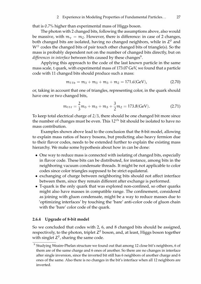
ii

“proc16” — 2016/12/12 — 10:17 — page 27 — #43 ii

ii

ii


that is 0.7% higher than experimental mass of Higgs boson.The photon with 2 changed bits, following the assumptions above, also would

be massive, with mγ = m2. However, there is difference: in case of 2 changes,both changed bits are isolated, having no changed neighbors, while in Z0 andW± codes the changed bits of pair touch other changed bits of triangle(s). So themass is probably dependent not on the number of changed bits directly, but ondifferences in interface between bits caused by these changes9.

Applying this approach to the code of the last known particle in the samemass scale, t quark, with experimental mass of 173.07 GeV, we found that a particlecode with 11 changed bits should produce such a mass:

m11b = m3 +m3 +m3 +m2 = 171.6(GeV), (2.70)

or, taking in account that one of triangles, representing color, in the quark shouldhave one or two changed bits,

m11f =2

3m3 +m3 +m3 +

3

2m2 = 173.8(GeV). (2.71)

To keep total electrical charge of 2/3, there should be one changed bit more sincethe number of changes must be even. This 12th bit should be isolated to have nomass contribution.

Examples shown above lead to the conclusion that the 8-bit model, allowingto explain mass ratios of heavy bosons, but predicting also heavy fermion dueto their flavor codes, needs to be extended further to explain the existing masshierarchy. We make some hypothesis about how in can be done:

• One way to reduce mass is connected with isolating of changed bits, especiallyin flavor code. These bits can be distributed, for instance, among bits in theneighboring vacuum condensate threads. It might be not applicable to colorcodes since color triangles supposed to be strict equilateral.

• exchanging of charge between neighboring bits should not affect interfacebetween them, since they remain different after exchange is performed.

• T-quark is the only quark that was explored non-confined, so other quarksmight also have masses in compatible range. The confinement, consideredas joining with gluon condensate, might be a way to reduce masses due to’optimizing interfaces’ by touching the ’bare’ anti-color code of gluon chainwith the ’bare’ color code of the quark.

2.6.4 Upgrade of 8-bit model

So we concluded that codes with 2, 6, and 8 changed bits should be assigned,respectively, to the photon, triplet Z0 boson, and, at least, Higgs boson togetherwith singlet Z0, sharing the same code.

9 Studying Weaire-Phelan structure we found out that among 12 close bit’s neighbors, 6 ofthem are of the same charge and 6 ones of another. So there are no changes in interfaceafter single inversion, since the inverted bit still has 6 neighbors of another charge and 6ones of the same. Also there is no changes in the bit’s interface when all 12 neighbors areinverted.

ii

“proc16” — 2016/12/12 — 10:17 — page 28 — #44 ii

ii

ii

28 E.G. Dmitrieff

Remembering that in simple 8-bit model we had assigned the codes of spinstates, and also the codes for H0, γ, and Z0 by arbitrary decision we adjusted themodel in the following way:

• We left the code for the photon intact.• So the vacuum condensate code should be the code reserved for longitudinal

photon. We marked it with symbol V0. As a singlet, or scalar particle, it issupposed to follow the equations (2.24, 2.22), having

T3 = 1/2, Yw/2 = −1/2. (2.72)

• We assigned the code, produced from code of vacuum condensate with all-8-bit inversion, to the Higgs boson H0. It might be the same particle with thesinglet Z0.

• We also adjusted the meaning of bit pair: it represents singlet state when it isopposite to the charge of triangles.

• The last code left we assigned to the triplet state of Z0.• We assumed that cyclic directions of primary and secondary color codes are

opposite, so CP = shift;

The result is shown in the Table 2.8.

2.6.5 Handedness

Both ’wrong’ right-handed fermions and left-handed anti-fermions are known tohave T∗3 = 0, so Y∗w/2 = Q.

Combining odd number of b bits, it is not possible to get integer value (2.48),so codes for them should have even bit count.

As we have shown (2.25, 2.26), the correct values can be produced by explicitlychanged formulas. Using b bits, it is done by including all the 8 bits in the equationfor Y∗w/2 and none for T3.

The known values for triplet states of vector bosons are produced in reversedway: all the 8 bits are summed in equation for T3 and none for Y∗w/2.

Since the effect of handedness on T3 and Yw/2 is always of ±1/2, the sameresult can be obtained by adding or subtracting the corresponding parts of thescalar vacuum particle (2.72), also making bit count even.

In the simple linear condensate model this can be shown, for instance, as shiftof the particle code on a half-length, so both T3 codes of vacuum and particle joinstogether, and both Yw/2 codes do the same.

We consider the particle, for instance, electron e−, surrounded by vacuumcondensate, with the following code:

[. . . V0e−V0 . . . ]8.1 = . . . 0©1©1© 1© 1©︸︷︷︸T3=+ 1

2

0©0© 0©︸︷︷︸

Yw2

=− 12︸︷︷︸

V0

0© 1©0© 0© 0©︸︷︷︸

T3=− 12

0©0© 0©︸︷︷︸Yw2

=− 12︸︷︷︸

e−L

0© 1©1© 1© 1© 0©

0© 0© . . .

(2.73)

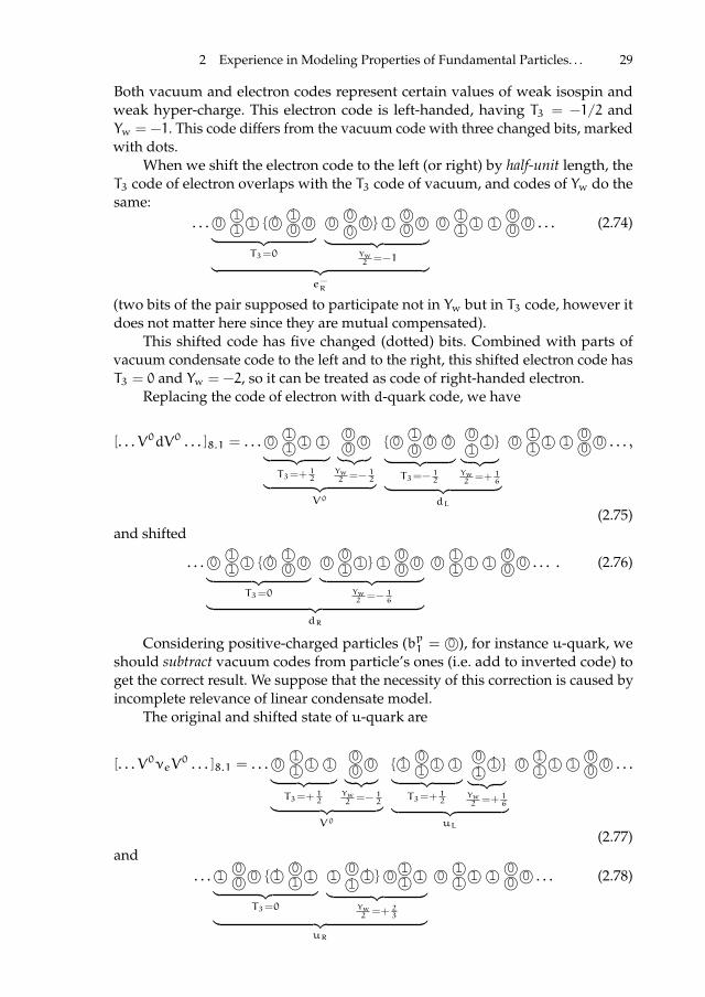
ii

“proc16” — 2016/12/12 — 10:17 — page 29 — #45 ii

ii

ii


Both vacuum and electron codes represent certain values of weak isospin andweak hyper-charge. This electron code is left-handed, having T3 = −1/2 andYw = −1. This code differs from the vacuum code with three changed bits, markedwith dots.

When we shift the electron code to the left (or right) by half-unit length, theT3 code of electron overlaps with the T3 code of vacuum, and codes of Yw do thesame:

. . . 0© 1©1© 1© 0© 1©

0© 0©︸︷︷︸T3=0

0© 0©0© 0© 1© 0©

0© 0©︸︷︷︸Yw2

=−1︸︷︷︸e−R

0© 1©1© 1© 1© 0©

0© 0© . . . (2.74)

(two bits of the pair supposed to participate not in Yw but in T3 code, however itdoes not matter here since they are mutual compensated).

This shifted code has five changed (dotted) bits. Combined with parts ofvacuum condensate code to the left and to the right, this shifted electron code hasT3 = 0 and Yw = −2, so it can be treated as code of right-handed electron.

Replacing the code of electron with d-quark code, we have

[. . . V0dV0 . . . ]8.1 = . . . 0©1©1© 1© 1©︸︷︷︸T3=+ 1

2

0©0© 0©︸︷︷︸

Yw2

=− 12︸︷︷︸

V0

0© 1©0© 0© 0©︸︷︷︸

T3=− 12

0©1© 1©︸︷︷︸Yw2

=+ 16︸︷︷︸

dL

0© 1©1© 1© 1© 0©

0© 0© . . . ,

(2.75)and shifted

. . . 0© 1©1© 1© 0© 1©

0© 0©︸︷︷︸T3=0

0© 0©1© 1© 1© 0©

0© 0©︸︷︷︸Yw2

=− 16︸︷︷︸

dR

0© 1©1© 1© 1© 0©

0© 0© . . . . (2.76)

Considering positive-charged particles (bp1 = 0©), for instance u-quark, weshould subtract vacuum codes from particle’s ones (i.e. add to inverted code) toget the correct result. We suppose that the necessity of this correction is caused byincomplete relevance of linear condensate model.

The original and shifted state of u-quark are

[. . . V0νeV0 . . . ]8.1 = . . . 0©

1©1© 1© 1©︸︷︷︸T3=+ 1

2

0©0© 0©︸︷︷︸

Yw2

=− 12︸︷︷︸

V0

1© 0©1© 1© 1©︸︷︷︸

T3=+ 12

0©1© 1©︸︷︷︸Yw2

=+ 16︸︷︷︸

uL

0© 1©1© 1© 1© 0©

0© 0© . . .

(2.77)and

. . . 1© 0©0© 0© 1© 0©

1© 1©︸︷︷︸T3=0

1© 0©1© 1© 0© 1©

1© 1©︸︷︷︸Yw2

=+ 23︸︷︷︸

uR

0© 1©1© 1© 1© 0©

0© 0© . . . (2.78)

ii

“proc16” — 2016/12/12 — 10:17 — page 30 — #46 ii

ii

ii

30 E.G. Dmitrieff

(here the parts of vacuum codes outside braces intended to be subtracted areinverted, or, what is the same, exchanged).

They both have 4 changed bits. Note that u-type quarks and u-type anti-quarks are the only fermions having similar color and flavor codes with the samecounts of 1 and 0. So, the fluctuation between them would be the most easy.

The left-handed neutrino has only two changed bits, like the photon:

[. . . V0νeV0 . . . ]8.1 = . . . 0©

1©1© 1© 1©︸︷︷︸T3=+ 1

2

0©0© 0©︸︷︷︸

Yw2

=− 12︸︷︷︸

V0

1© 0©1© 1© 1©︸︷︷︸

T3=+ 12

0©0© 0©︸︷︷︸Yw2

=− 12︸︷︷︸

νL

0© 1©1© 1© 1© 0©

0© 0© . . .

(2.79)In contrast, the right-handed neutrino would have 6 changed bits and zero valueof both weak hyper-charge and isospin:

. . . 1© 0©0© 0© 1© 0©

1© 1©︸︷︷︸T3=0

1© 0©0© 0© 0© 1©

1© 1©︸︷︷︸Yw2

=0︸︷︷︸νeR

0© 1©1© 1© 1© 0©

0© 0© . . . (2.80)

This large number of changed bits, as we have seen, may cause mass of the rightneutrino in the electroweak mass scale.

The model of the particle surrounded by the condensate, has another degreeof freedom: after shifting, the right and left parts of code could be exchanged.After that, the particle code has the same changed bit count, as before. So it can beused as representation of flipping the spin.

All the 28 = 256 codes possible in the 8.1 model are listed in the Table 2.8.Some of them are assigned to particles or particle components; others are vacant.Several vacant codes may be really in use because of shifting. Anyway, some ofthem can correspond to new particles, so they should be explored.

2.7 Summary

We considered several models of fundamental particles and condensates, based onbit graphs. We managed to represent all the particles of Standard Model. The bitcode approach seems to be relevant and efficient for modeling discrete properties.Nevertheless, such a properties like masses, require some improvements to takein account interfaces or relationships between neighboring bits.

2.8 Appendix: Bit graphs

Natural number a is usually represented in computers as a sequence of bits, thatare factors in the decomposition of a into powers of two:

a =

N−1∑i=0

2iai, (2.81)

ii

“proc16” — 2016/12/12 — 10:17 — page 31 — #47 ii

ii

ii

2 Experience in Modeling Properties of Fundamental Particles. . . 31bp 0→

01

bp 1bc2\bc1

000

100

010

001

011

101

110

111

000

100

010

001

011

101

110

111

(−11 3

)4(−1)5

(−2 3

)6(−

1 3)7

(−1)3

(−2 3

)4(−

1 3)5

(0)6

000

e− R

µ− R

τ− R

W− ↑↓

Z0

(−1)3

(−2 3

)4(−

1 3)5

(0)6

(−2 3

)2(−

1 3)3

(0)4

(1 3)5

100

e− L

ur R,ur Lcr R,ug Ltr R,ub Ldr Ldg Ldb L

νeL

grr ↑↓

grg ↑↓

grb ↑↓

010

µ− L

ug R,cr Lcg R,cg Ltg R,cb Lsr L

sg Lsb L

νµL

ggr ↑↓

ggg ↑↓

ggb ↑↓

000

1τ− L

ub R,tr Lcb R,tg Ltb R,tb Lbr Lbg Lbb L

ντL

gbr ↑↓

gbg ↑↓

gbb ↑↓

(−2 3

)2(−

1 3)3

(0)4

(1 3)5

(−1 3

)1(0

)2(1 3

)3(2 3

)401

1dr R

sr Rbr R

grr ↑↓grg ↑↓grb ↑↓

101

dg R

sg Rbg R

ggr ↑↓ggg ↑↓ggb ↑↓

110

db R

sb Rbb R

gbr

gbg

gbb

(−1 3

)1(0

)2(1 3

)3(2 3

)4(0

)0(1 3

)1(2 3

)2(1

)311

1νeR

νµR

ντR

V0(γ

↑↓)W

+ ↑↓(−1)5

(−2 3

)6(−

1 3)7

(0)8

(−2 3

)4(−

1 3)5

(0)6

(1 3)7

000

W−

H0,Z0 ↑↓

νeR

νµR

ντR

(−2 3

)4(−

1 3)5

(0)6

(1 3)7

(−1 3

)3(0

)4(1 3

)5(2 3

)610

0grr grg grb

dr R

sr Rbr R

010

ggr

ggg

ggb

dg R

sg Rbg R

100

1gbr

gbg

gbb

db R

sb Rbb R

(−1 3

)3(0

)4(1 3

)5(2 3

)6(0

)2(1 3

)3(2 3

)4(1

)501

1grr ↑↓

grg ↑↓

grb ↑↓

νeL

dr Ldg Ldb Lur R,ur Lcr R,ug Ltr R,ub L

e+ L

101

ggr ↑↓

ggg ↑↓

ggb ↑↓

νµL

sr Lsg L

sb Lug R,cr Lcg R,cg Ltg R,cb L

µ+ L

110

gbr ↑↓

gbg ↑↓

gbb ↑↓

ντL

br Lbg Lbb Lub R,tr Lcb R,tg Ltb R,tb L

τ+ L

(0)2

(1 3)3

(2 3)4

(1)5

(1 3)1

(2 3)2

(1)3

(11 3

)411

1γ

W+

e+ R

µ+ R

τ+ R

Tabl

e2.

8.C

ode

com

bina

tions

assi

gned

topa

rtic

les

in8.

1m

odel

.The

righ

t-ha

nded

code

sar

eth

esa

me

with

left

-han

ded,

butt

hey

are

plac

edin

shift

edpo

siti

onin

rela

tion

toth

eco

nden

sate

.In

top-

righ

tcor

ner

ofce

llsth

ere

are

the

elec

tric

alch

arge

(Q)a

ndth

enu

mbe

rof

chan

ged

bits

.

ii

“proc16” — 2016/12/12 — 10:17 — page 32 — #48 ii

ii

ii

32 E.G. Dmitrieff

where N is a number of bits required, determined by magnitude of a:

N > log2 a,N ∈ Z. (2.82)

In order to stop the processing properly, N should be known just after operatingon the last bit in a sequence.

In fact, due to logarithmic dependence,N can be prefixed, by choosing it largeenough, exceeding the logarithm of any value from the data domain.

The common way to express these sequences in paper writing is to write a textline of symbols 0 and 1, delimited with white spaces aside, implicitly assumingthat the rightmost digit represents the least significant bit, i.e. a factor a0 of 20.The leftmost bit is the highest-power non-zero (i.e. one) factor, so all bits to the leftare known to be 0 and therefore can be omitted. N in this case is the total count ofdigits 0 and 1, and i is the zero-based right-to-left index of digit10.

To represent these sequences explicitly, we use non-weighted directed graphswith bits in vertices. Each vertex in this case has the only outgoing directed edge,pointing to the next bit’s vertex: ai+1 ← ai. For instance, with prefixed N = 3

L99 1← 1← 0⇒ 1102 (2.83)

(the leftmost bit points to nothing); or, with self-determined N:

→ 0← 1← 1← 0⇒ 1102 (2.84)

(zero next to the rightmost 1 is pointing to itself, representing the infinite sequencesof zero factors of 2 in higher powers, and also, in fact, terminates the sequence).

To read the value, the graph is processed starting with the dedicated vertex(it is the leftmost one, that is not next to any vertex),then following with thenext one, repeating until either the prefixed count elapses, or nothing-pointed orself-pointing vertex is detected.

In case the vertices in graph are partially rearranged, the result value ofthis graph processing is changed. While the graph remains an open, non-circularsequence, values remain strict-defined:

1← 1← 0⇒ 1012 = 5. (2.85)

When the sequence is closed into a loop, the value becomes arbitrary since there isno more dedicated starting point:

( 11 ←− 0) ⇒ 1102,0112,1012 = 6, 3, 5

Some loop codes (namely, containing all the same digits) represent strictly definedvalues:

( 11 ←− 1) ⇒ 1112 = 7.

10 This is the same way, as usual decimal numbers are represented in writing, exceptingthe base of power, the base of logarithm, and the count of different digits, are equal to 2instead of 10.

ii

“proc16” — 2016/12/12 — 10:17 — page 33 — #49 ii

ii

ii


As we have seen, the linear graphs (sequences) can be written in text lineswith implicit (omitted) edges, since they do not contain loops. The same way,some containing loops graphs also can be shown with implicit edges, using flattessellations, for instance pie charts or square- or hexagonal matrices.

The more vertices contained in the graph, the more dimensions is requiredto represent its edges implicitly. For instance, 4-bit graph with vertices, coupledequally each-to-each, contains 4 loops, and its 6 equal edges can be implicitlyexpressed by placing bits in vertices of tetrahedron. 5 bits would require 4Dspace and placement in vertices of the simplex, and so on. The count of differentcombinations for these each-to-each coupled graphs is CN1N1+N0 (whereN0 andN1are counts of digits 0 and 1 in the graph).

Graphs with non-equal and/or not each-to-each coupling edges also canbe isomorphic to geometrical shapes: for instance, 8-bit graph with each-to-eachcoupled vertices having 12 edges of the first type, 12 of the second type, and 4 ofthe third type, can be implicitly represented as 3-dimensional cube, since it has 12edges, 12 face diagonals and 4 own diagonals.

Also, bit graps, implicit or explicit, can be continuous, (quasi)periodical,repeating the distribution of vertices and edges. They can be used, for instance, torepresent fields.

Bit graphs also can be nesting, meaning that vertices may contain either bitsor bit graphs. The edges also can be nested the same way. In this case, inner graphscan require more dimensions then outer ones to be implicitly coupled. So nestedgraphs can be a model for folded dimensions.

2.9 Appendix: Ones’ complement code convention

Briefly, in one’s complement coding convention, the negation is bitwise inversion,the eldest bit represents the sign, and there are two different zero representations,positive and negative [14].

The non-negative number a+ is coded in the general way: all binary digitsai (0 or 1) excepting the eldest aN−1 (which is equal to 0) are factors in thedecomposition of a+ into powers of two:

a+ =

N−2∑i=0

2iai. (2.86)

Bits ai could be obtained as remaining from sequential division by two:

d−1 = a+; (2.87)

di =

[di−1

2

];ai = di−1 − 2di (2.88)

(square brackets here mean the integer division).The representation of negative number is produced from representation of

its absolute value by inversion of all their bits. Thus, the eldest bit aN−1 takesthe value of 1. This bit does not act as a factor in the decomposition, but when it

ii

“proc16” — 2016/12/12 — 10:17 — page 34 — #50 ii

ii

ii

34 E.G. Dmitrieff

has the value of 1, it changes the composition formula, so it takes inverted binarydigits ai:

a− = −

N−2∑i=0

2i(¬ai). (2.89)

Taking into account¬ai = 1− ai, (2.90)

we have

a− =

N−2∑i=0

2i(ai − 1) =

N−2∑i=0

2iai −

N−2∑i=0

2i = a+ − (2N−1 − 1), (2.91)

so aN−1 is the factor of an extra negative term (1− 2N−1) in the decomposition:

a = (1− 2N−1)aN−1 +

N−2∑i=0

2iai. (2.92)

For code of N = 3 bits, the value of a is expressed through them as

a = −3a2 + 2a1 + a0. (2.93)

Acknowledgments

I’m grateful to Norma Susanna Mankoc Borstnik for the invitation and organiza-tion of the Workshop, and for suggestsions and discussions.

I thank my close relatives, Maya Ivanova and Arina Dmitrieva, for participat-ing in discussions, helpful suggestions and patience.

Also I’m grateful to Ekaterina Boyarskikh for assistance in text editing.

References

1. G.’t Hooft: The conceptual basis of Quantum Field Theory, Handbook of the Philosophy ofScience, Elsevier, December 23, 2004.

2. R.V.L. Hartley: Transmission of Information, Bell System Technical Journal, (July 1928),pp. 535–563.

3. V.Labunetz, E.Rundblad, and J.Astola: Is the Brain the Clifford Algebra QuantumComputer?, in: Leo Dorst, Chris Doran, Joan Lasenby: Applications of GeometricAlgebra in Computer Science and Engineering, Birkhauser, Boston 2002.

4. Va.B. Zel’dovich, I.Yu. Kobzarev, and L.B. Okun: Cosmological consequences of aspontaneous breakdown of a discrete symmetry, Zh. Eksp. Teor. Fiz. 67 3–11 (July 1974).

5. N.S. Mankoc Borstni,: The explanation for the origin of the higgs scalar and for theYukawa couplings by the spin-charge-family theory, J. of Mod. Physics 6 2244–2274 (2015),http://dx.doi.org/10.4236/jmp.2015.615230 [http://arxiv.org/abs/1409.4981].

6. D.Weaire, R.Phelan, A counter-example to Kelvin’s conjecture on minimal surfaces,Phil. Mag. Lett., 69 107-110 (1994), doi:10.1080/09500839408241577.

7. D. Griffiths, Introduction to Elementary Particles, John Wiley & Sons, ISBN 0-471-60386-4, (1987).

ii

“proc16” — 2016/12/12 — 10:17 — page 35 — #51 ii

ii

ii


8. L. B. Okun, Current status of elementary particle physics, UFN, 168 6 625-629, (1998).9. A. Pitch: The Standard Model of Electroweak Interactions, arXiv:1201.0537v1 [hep-ph].

10. Z. Maki, M. Nakagawa, S. Sakata, Remarks on the Unified Model of Elementary Parti-cles, Progress of Theoretical Physics 28 870 (1962). doi:10.1143/PTP.28.870.

11. M. Kobayashi, T. Maskawa; Maskawa, CP-Violation in the Renormalizable The-ory of Weak Interaction, Progress of Theoretical Physics 49 (2): 652-657 (1973).doi:10.1143/PTP.49.652.

12. K. Nakamura et al. (Particle Data Group), J. Phys. G 37 075021 (2010) (URL:http://pdg.lbl.gov).

13. Combined Measurement of the Higgs Boson Mass in pp Collisions at√s = 7 and

8 TeV with the ATLAS and CMS Experiments, Phys. Rev. Lett. 114 191803 (2015),doi:10.1103/PhysRevLett.114.191803 arXiv:1503.07589 [hep-ex].

14. D.E.Knuth: The Art of Computer Programming: Seminumerical algorithms, Addison-Wesley,Reading - Massachusetts, 1997.

ii

“proc16” — 2016/12/12 — 10:17 — page 36 — #52 ii

ii

ii


Proceedings to the 19th WorkshopWhat Comes Beyond . . . (p. 36)

Bled, Slovenia, July 11–19, 2016

3 Quark and Lepton Masses and Mixing From aGauged SU(3)F Family Symmetry With a LightO(eV) Sterile Dirac Neutrino

A. Hernandez-Galeana ??, ???

APC laboratory, Universite Paris Diderot, Batiment Condorcet,10, rue Alice Domon et Leonie Duquet 75205 Paris cedex 13, France

Abstract. In the framework of a complete vector-like and universal gauged SU(3)F familysymmetry, we report a global region in the parameter space where this approach canaccount for a realistic spectrum of quark masses and mixing in a 4× 4 non-unitary VCKM,as well as for the known charged lepton masses and the squared neutrino mass differencesreported from neutrino oscillation experiments. The SU(3)F family symmetry is brokenspontaneously in two stages by heavy SM singlet scalars, whose hierarchy of scales yieldand approximate SU(2)F global symmetry associated to the almost degenerate bosonmasses of the order of the lower scale of the SU(3)F SSB. The gauge symmetry, the fermioncontent, and the transformation of the scalar fields, all together, avoid Yukawa couplingsbetween SM fermions. Therefore, in this scenario ordinary heavy fermions, top and bottomquarks and tau lepton, become massive at tree level from Dirac See-saw mechanisms,while light fermions, including light neutrinos, obtain masses from radiative correctionsmediated by the massive gauge bosons of the SU(3)F family symmetry. The displayedfit parameter space region solution for fermion masses and mixing yield the vector-likefermion masses:MD ≈ 3.2TeV,MU ≈ 6.9TeV,ME ≈ 21.6TeV, SU(2)F family gauge bosonmasses ofO(2TeV), and the squared neutrino mass differences:m22 −m

21 ≈ 7.5× 10−5 eV2,

m23 −m22 ≈ 2.2× 10−3 eV2,m24 −m

21 ≈ 0.81 eV2.

Povzetek. Avtor ponudi razsiritev standardnega modela, ki k poznanim grupam doda sedruzinsko (umeritveno) grupo SU(3)F. Poisce obmocje v prostoru parametrov, ki ponudieksperimentalno sprejemljive lastnosti kvarkov in leptonov. Druzinsko simetrijo zlomiv dveh korakih. Tezki fermioni - kvarka t in b ter lepton tau - postanejo masivni nadrevesnem nivoju (z mehanizmom gugalnice, see-saw), ostali pa s popravki visjih re-dov. Mase fermionov, pri katerih so kvantna stevila levorocnih in desnorocnih fermionovenaka, so nekaj TeV ali vec: MD ≈ 3.2TeV, MU ≈ 6.9TeV, ME ≈ 21.6TeV. Mase bo-zonov z druzinskimi kvantnimi stevili so O(2TeV), razliki kvadratov nevtrinskih mass paso:m22 −m

21 ≈ 7.5× 10−5 eV2,m23 −m

22 ≈ 2.2× 10−3 eV2,m24 −m

21 ≈ 0.81 eV2.

?? On sabbatical leave from:Departamento de Fısica, ESFM - Instituto Politecnico NacionalU. P. ”Adolfo Lopez Mateos”. C. P. 07738, Ciudad de Mexico, Mexico.

??? e-mail: [email protected]

ii

“proc16” — 2016/12/12 — 10:17 — page 37 — #53 ii

ii

ii

3 Quark and Lepton Masses and Mixing From a Gauged SU(3)F Family. . . 37

3.1 Introduction

The origen of the hierarchy of fermion masses and mixing is one of the mostimportant open problems in particle physics. Any attempt to account for thishierarchy introduce a mass generation mechanism which distinguish among thedifferent Standard Model (SM) quarks and leptons.

After the discovery of the scalar Higgs boson on 2012, LHC has not found a conclu-sive evidence of new physics. However, there are theoretical motivations to lookfor new particles in order to answer some open questions like; neutrino ossccilla-tions, dark matter, stability of the Higgs mass against radiative corrections,,etc.

In this article, we address the problem of charged fermion masses and quarkmixing within the framework of an extension of the SM introduced by the author in[1]. This Beyond Standard Model (BSM) proposal include a vector gauged SU(3)Ffamily symmetry1 commuting with the SM group and introduce a hierarchicalmassgeneration mechanism in which the light fermions obtain masses throughloop radiative corrections, mediated by the massive bosons associated to theSU(3)F family symmetry that is spontaneously broken, while the masses of thetop and bottom quarks as well as for the tau lepton, are generated at tree levelfrom ”Dirac See-saw”[3] mechanisms implemented by the introduction of a newset of SU(2)L weak singlets U,D, E and N vector-like fermions. Due to the factthat these vector-like quarks do not couple to theW boson, the mixing of U andDvector-like quarks with the SM quarks gives rise to and extended 4×4 non-unitaryCKM quark mixing matrix [4].

3.2 Model with SU(3)F flavor symmetry

3.2.1 Fermion content

We define the gauge symmetry group

G ≡ SU(3)F ⊗ SU(3)C ⊗ SU(2)L ⊗U(1)Y (3.1)

where SU(3)F is a completely vector-like and universal gauged family symmetry.That is, the corresponding gauge bosons couple equally to Left and Right Handedordinary Quarks and Leptons, including right handed neutrinos.GSM = SU(3)C⊗SU(2)L ⊗U(1)Y is the ”Standard Model” (SM) gauge group, with gH, gs, g and g′

the coupling constants. The content of fermions assumes the ordinary quarks andleptons assigned under G as:

Ordinary Fermions: qoiL =

(uoiLdoiL

), loiL =

(νoiLeoiL

), Q = T3L +

12Y

Ψoq = (3, 3, 2,1

3)L =

qo1Lqo2Lqo3L

, Ψol = (3, 1, 2,−1)L =

lo1Llo2Llo3L

1 See [1,2] and references therein for some other SU(3)F family symmetry model proposals.

ii

“proc16” — 2016/12/12 — 10:17 — page 38 — #54 ii

ii

ii

38 A. Hernandez-Galeana

Ψou = (3, 3, 1,4

3)R =

uoRcoRtoR

, Ψod = (3, 3, 1,−2

3)R =

doRsoRboR

Ψoe = (3, 1, 1,−2)R =

eoRµoRτoR

where the last entry corresponds to the hypercharge Y, and the electric charge isdefined by Q = T3L +

12Y. The model also includes two types of extra fermions:

Right Handed Neutrinos: ΨoνR = (3, 1, 1, 0)R =

νeRνµRντR

,

and the SU(2)L weak singlet vector-like fermions

Sterile Neutrinos: NoL, NoR = (1, 1, 1, 0) ,

The Vector Like quarks:

UoL, UoR = (1, 3, 1,

4

3) , DoL, D

oR = (1, 3, 1,−

2

3) (3.2)

and

The Vector Like electrons: EoL, EoR = (1, 1, 1,−2)

The transformation of these vector-like fermions allows the mass invariant massterms

MU UoL U

oR + MD D

oL D

oR + ME E

oL E

oR + h.c. , (3.3)

and

mD NoLN

oR + mL N

oL (N

oL)c + mR N

oR (N

oR)c + h.c (3.4)

The above fermion content make the model anomaly free. After the definition of thegauge symmetry group and the assignment of the ordinary fermions in the usualform under the standard model group and in the fundamental 3-representationunder the SU(3)F family symmetry, the introduction of the right-handed neutrinosis required to cancel anomalies[5]. The SU(2)L weak singlets vector-like fermionshave been introduced to give masses at tree level only to the third family of knownfermions through Dirac See-saw mechanisms. These vector like fermions play acrucial role to implement a hierarchical spectrum for quarks and charged leptonmasses, together with the radiative corrections.

3.3 SU(3)F family symmetry breaking

We need to be consistent with low energy Standard Model (SM) and simultane-ously we would like to generate and account for the hierarchy of fermion masses

ii

“proc16” — 2016/12/12 — 10:17 — page 39 — #55 ii

ii

ii


and mixing after spontaneously symmetry breaking (SSB) down to SU(3)C×U(1)Q.Previous basic assumptions of this BSM define the required scalar fields andV.E.V’s to achieve the desired symmetry breaking.

To implement a hierarchical spectrum for charged fermion masses, and simul-taneously to achieve the SSB of SU(3)F, we introduce the flavon scalar fields:ηi, i = 2, 3,

ηi = (3, 1, 1, 0) =

ηoi1ηoi2ηoi3

, i = 2, 3

with the ”Vacuum ExpectationValues” (VEV’s):

〈η2〉T = (0,Λ2, 0) , 〈η3〉T = (0, 0,Λ3) . (3.5)

The above scalar fields and VEV’s break completely the SU(3)F flavor symmetry.The corresponding SU(3)F gauge bosons are defined in Eq.(3.17) through theircouplings to fermions. Thus, the contribution to the horizontal gauge boson massesfrom Eq.(3.5) read

• 〈η2〉 :g2H2

Λ222

(Y+1 Y−1 + Y+3 Y

−3 ) +

g2H2Λ224

(Z21 +Z223

− 2Z1Z2√3)

• 〈η3〉 :g2H3

Λ232

(Y+2 Y−2 + Y+3 Y

−3 ) + g

2H3Λ23

Z223

These two scalars in the fundamental representation is the minimal set of scalars to breakdown completely the SU(3)F family symmetry.

SU(3)F ×GSM〈η3〉,〈η2〉−−−−−−→ SU(2)F ?×GSM

〈η2〉,〈η3〉−−−−−−→ GSM

FCNC ?

Λ3(Λ2): 5 very heavy boson masses (≥ 100 TeV ′s)

Λ2(Λ3): 3 heavy boson masses (a few TeV ′s).

Notice that the hierarchy of scales Λ3 Λ2 define an ”approximate SU(2)Fglobal symmetry” in the spectrum of SU(3)F gauge boson masses. To suppressproperly the FCNC like, for instance PDG 2016 [9] : µ → eγ (Br < 5.7× 10−13) ,µ → e e e (Br < 1 × 10−12) , Ko − Ko, it is relevant which gauge bosons becomemassive at the lower scale of the SU(3)F symmetry breaking.

Therefore, neglecting tiny contributions from electroweak symmetry breaking,we obtain the gauge boson mass terms.

M22 Y

+1 Y

−1 +M2

3 Y+2 Y

−2 + (M2

2 +M23) Y

+3 Y

−3 +

1

2M22 Z

21

+1

2

M22 + 4M

23

3Z22 −

1

2(M2

2)2√3Z1 Z2 (3.6)

ii

“proc16” — 2016/12/12 — 10:17 — page 40 — #56 ii

ii

ii


M22 =

g2HΛ22

2, M2

3 =g2HΛ

23

2, y ≡ M3

M2=Λ3

Λ2(3.7)

Z1 Z2

Z1 M22 −

M22√3

Z2 −M22√3

M22+4M23

3

Table 3.1. Z1 − Z2 mixing mass matrix

Diagonalization of the Z1 − Z2 squared mass matrix yield the eigenvalues

M2− =

2

3

(M22 +M

23 −

√(M2

3 −M22)2 +M2

2M23

)−

(3.8)

M2+ =

2

3

(M22 +M

23 +

√(M2

3 −M22)2 +M2

2M23

)+

(3.9)

M22 Y

+1 Y

−1 +M2

3 Y+2 Y

−2 + (M2

2 +M23) Y

+3 Y

−3 +M2

−

Z2−2

+M2+

Z2+2

(3.10)

where (Z1Z2

)=

(cosφ − sinφsinφ cosφ

)(Z−

Z+

)(3.11)

cosφ sinφ =

√3

4

M22√

M42 +M

23(M

23 −M

22)

Due to the Z1 − Z2 mixing, we diagonalize the propagators involving Z1 andZ2 gauge bosons according to Eq.(3.11)

Z1 = cosφ Z− − sinφ Z+ , Z2 = sinφ Z− + cosφ Z+

3.4 Electroweak symmetry breaking

Recently ATLAS[6] and CMS[7] at the Large Hadron Collider announced thediscovery of a Higgs-like particle, whose properties, couplings to fermions andgauge bosons will determine whether it is the SM Higgs or a member of anextended Higgs sector associated to a BSM theory. For electroweak symmetrybreaking we introduction two triplets of SU(2)L Higgs doublets, namely;

ii

“proc16” — 2016/12/12 — 10:17 — page 41 — #57 ii

ii

ii


Φu = (3, 1, 2,−1) =

(φo

φ−

)u1(

φo

φ−

)u2(

φo

φ−

)u3

, Φd = (3, 1, 2,+1) =

(φ+

φo

)d1(

φ+

φo

)d2(

φ+

φo

)d3

,

and the VEV?s

Φu〉 =

〈Φu1 〉〈Φu2 〉〈Φu3 〉

, 〈Φd〉 =

〈Φd1 〉〈Φd2 〉〈Φd3 〉

,

where

Φui 〉 =1√2

(vui0

), 〈Φdi 〉 =

1√2

(0

vdi

).

The contributions from 〈Φu〉 and 〈Φd〉 yield the W and Z gauge boson massesand mixing with the SU(3)F gauge bosons

g2

4(v2u + v2d)W

+W− +(g2 + g′

2)

8(v2u + v2d)Z

2o

+14

√g2 + g′2 gH Zo

[(v21u − v22u − v21d + v22d)Z1

+(v21u + v22u − 2v23u − v21d − v22d + 2v23d)Z2√3

+2 (v1uv2u − v1dv2d)Y+1 +Y−

1√2

+ 2 (v1uv3u − v1dv3d)Y+2 +Y−

2√2

+2 (v2uv3u − v2dv3d)Y+3 +Y−

3√2

]+ tiny contributions to the SU(3) gauge boson masses ,

v2u = v21u+v22u+v

23u , v2d = v21d+v

22d+v

23d. Hence, if we define as usualMW = 1

2gv,

we may write v =√v2u + v2d ≈ 246 GeV.

Y1j =Y+j + Y−

j√2

, Y±j =Y1j ∓ iY2j√

2(3.12)

The mixing of Zo neutral gauge boson with the SU(3)F gauge bosons modify thecouplings of the standard model Z boson with the ordinary quarks and leptons

ii

“proc16” — 2016/12/12 — 10:17 — page 42 — #58 ii

ii

ii


3.5 Fermion masses

3.5.1 Dirac See-saw mechanisms

Now we describe briefly the procedure to get the masses for fermions. The analysisis presented explicitly for the charged lepton sector, with a completely analogousprocedure for the u and d quarks and Dirac neutrinos. With the fields of particlesintroduced in the model, we may write the gauge invariant Yukawa couplings, as

h ψol Φd EoR + h2 ψ

oe η2 E

oL + h3 ψ

oe η3 E

oL + M EoL E

oR + h.c (3.13)

where M is a free mass parameter ( because its mass term is gauge invariant)and h, h2 and h3 are Yukawa coupling constants. When the involved scalar fieldsacquire VEV’s we get, in the gauge basis ψoL,R

T = (eo, µo, τo, Eo)L,R, the massterms ψoLMoψoR + h.c, where

Mo =

0 0 0 h v10 0 0 h v20 0 0 h v30 h2Λ2 h3Λ3 M

≡0 0 0 a10 0 0 a20 0 0 a30 b2 b3 M

. (3.14)

Notice thatMo has the same structure of a See-saw mass matrix, here for Diracfermion masses. So, we callMo a ”Dirac See-saw” mass matrix.Mo is diagonal-ized by applying a biunitary transformation ψoL,R = VoL,R χL,R. The orthogonalmatrices VoL and VoR are obtained explicitly in the Appendix A. From VoL and VoR ,and using the relationships defined in this Appendix, one computes

VoLTMo VoR = Diag(0, 0,−λ3, λ4) (3.15)

VoLTMoMoT VoL = VoR

TMoTMo VoR = Diag(0, 0, λ23, λ24) . (3.16)

where λ23 and λ24 are the nonzero eigenvalues defined in Eqs.(3.50-3.51), λ4 beingthe fourth heavy fermion mass, and λ3 of the order of the top, bottom and taumass for u, d and e fermions, respectively. We see from Eqs.(3.15,3.16) that at treelevel the See-saw mechanism yields two massless eigenvalues associated to thelight fermions:

3.6 One loop contribution to fermion masses

Subsequently, the masses for the light fermions arise through one loop radiativecorrections. After the breakdown of the electroweak symmetry we can constructthe generic one loop mass diagram of Fig. 1. Internal fermion line in this diagramrepresent the Dirac see-saw mechanism implemented by the couplings in Eq.(3.13).The vertices read from the SU(3)F flavor symmetry interaction Lagrangian

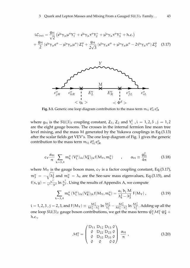
ii

“proc16” — 2016/12/12 — 10:17 — page 43 — #59 ii

ii

ii


iLint =gH√2

(eoγµµ

oY+1 + eoγµτoY+2 + µoγµτ

oY+3 + h.c.)

+gH

2(eoγµe

o − µoγµµo)Zµ1 +

gH

2√3(eoγµe

o + µoγµµo − 2τoγµτ

o)Zµ2 (3.17)

eojR eokR

Y

EoL Eo

R eofL eoiL

M

< ηk > < Φd >

Fig. 3.1. Generic one loop diagram contribution to the mass termmij eoiLe

ojR

where gH is the SU(3)F coupling constant, Z1, Z2 and Yji , i = 1, 2, 3 , j = 1, 2

are the eight gauge bosons. The crosses in the internal fermion line mean treelevel mixing, and the mass M generated by the Yukawa couplings in Eq.(3.13)after the scalar fields get VEV’s. The one loop diagram of Fig. 1 gives the genericcontribution to the mass termmij e

oiLe

ojR

cYαH

π

∑k=3,4

mok (VoL )ik(V

oR)jkf(MY ,m

ok) , αH ≡

g2H4π

(3.18)

where MY is the gauge boson mass, cY is a factor coupling constant, Eq.(3.17),

mo3 = −√λ23 and mo4 = λ4 are the See-saw mass eigenvalues, Eq.(3.15), and

f(x, y) = x2

x2−y2ln x2

y2. Using the results of Appendix A, we compute∑

k=3,4

mok (VoL )ik(V

oR)jkf(MY ,m

ok) =

ai bjM

λ24 − λ23

F(MY) , (3.19)

i = 1, 2, 3 , j = 2, 3, and F(MY) ≡ M2Y

M2Y−λ24

ln M2Y

λ24

−M2Y

M2Y−λ23

ln M2Y

λ23

. Adding up all the

one loop SU(3)F gauge boson contributions, we get the mass terms ψoLMo1 ψ

oR +

h.c.,

Mo1 =

D11 D12 D13 0

0 D22 D23 0

0 D32 D33 0

0 0 0 0

αH

π, (3.20)

ii

“proc16” — 2016/12/12 — 10:17 — page 44 — #60 ii

ii

ii


D11 = µ11(FZ14

+FZ212

+ Fm) +1

2(µ22F1 + µ33F2)

D12 = µ12(−FZ14

+FZ212

)

D13 = −µ13(FZ26

+ Fm)

D22 = µ22(FZ14

+FZ212

− Fm) +1

2(µ11F1 + µ33F3)

D23 = −µ23(FZ26

− Fm)

D32 = −µ32(FZ26

− Fm)

D33 = µ33FZ23

+1

2(µ11F2 + µ22F3) ,

Here,

F1 ≡ F(MY1) , F2 ≡ F(MY2) , F3 ≡ F(MY3)

FZ1 = cos2φF(M−) + sin2φF(M+) , FZ2 = sin2φF(M−) + cos2φF(M+)

M2Y1

=M22 , M2

Y2=M2

3 , M2Y3

=M22 +M

23

Fm =cosφ sinφ2√3

[ F(M−) − F(M+) ]

withM2,M3,M−,M+ the horizontal boson masses, Eqs.(3.7-3.9),

µij =ai bjM

λ24 − λ23

=ai bj

a bλ3 cα cβ , (3.21)

and cα ≡ cosα , cβ ≡ cosβ , sα ≡ sinα , sβ ≡ sinβ, as defined in the Appendix,Eq.(3.52). Therefore, up to one loop corrections we obtain the fermion masses

ψoLMo ψoR + ψoLMo1 ψ

oR = χLM χR , (3.22)

withM≡[Diag(0, 0,−λ3, λ4) + V

oLTMo

1 VoR

].

Using VoL , VoR from Eqs.(3.45-3.46) we get the mass matrix up to one loopradiative corrections:

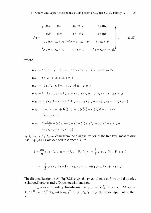
ii

“proc16” — 2016/12/12 — 10:17 — page 45 — #61 ii

ii

ii


M =

m11 m12 cβm13 sβm13

m21 m22 cβm23 sβm23

cαm31 cαm32 (−λ3 + cαcβm33) cαsβm33

sαm31 sαm32 sαcβm33 (λ4 + sαsβm33)

, (3.23)

where

m11 = δ c1 π1 , m21 = −δ s1 s2 π1 , m31 = δ c2 s1 π1

m12 = δ s1 sr (c1 c2 cr ∆+ π3)

m13 = −δ s1 (c1 c2 Fm− c1 c2 s2r ∆+ cr π3)

m22 = δ(−3 c2 cr s2 sr Fm + c21 c2 cr s2 sr ∆+ c2 cr π2 + c1 s2 sr π3)

m23 = δ(c2 s2 (1+ s21 − 3s

2r) Fm + c21 c2 s2 s

2r ∆+ c2 sr π2 − c1 cr s2 π3)

m32 = δ(−cr sr (−1+ 3s22) Fm + cr (c

22s21 + s

22) sr ∆+ cr s2 π2

−c1 c2 sr π3)

m33 = δ(−FZ26

− (c22 s21 − s

22 − s

2r + 3s

22 s2r) Fm + (c22 s

21 + s

22) s

2r ∆

+s2 sr π2 + c1 c2 cr π3).

s1, s2, sr, sα, sβ, λ3, λ4 come from the diagonalization of the tree level mass matrixMo, Eq. ( 3.14 ), are defined in Appendix 3.9.

δ =αH

πcα cβ λ3 , ∆ = 1

4(FZ2 − FZ1) , π1 =

1

2(c1 c2 cr F2 + F1 s2 sr)

π2 =1

2(c1 c2 cr F3 + FZ1 s2 sr) , π3 =

12(c1 c2 cr FZ2 + F3 s2 sr)

The diagonalization ofM, Eq.(3.23) gives the physical masses for u and d quarks,e charged leptons and ν Dirac neutrino masses.

Using a new biunitary transformation χL,R = V(1)L,R ΨL,R; χL M χR =

ΨL V(1)L

TM V

(1)R ΨR, with ΨL,RT = (f1, f2, f3, F)L,R the mass eigenfields, that

is

ii

“proc16” — 2016/12/12 — 10:17 — page 46 — #62 ii

ii

ii


V(1)L

TMMT V

(1)L = V

(1)R

TMTM V

(1)R = Diag(m21,m

22,m

23,M

2F) , (3.24)

m21 = m2e,m22 = m

2µ,m23 = m

2τ andM2

F =M2E for charged leptons. Therefore, the

transformation from massless to mass fermions eigenfields in this scenario reads

ψoL = VoL V(1)L ΨL and ψoR = VoR V

(1)R ΨR (3.25)

It is worth to comment here that neutrinos may also obtain left-handed andright-handed Majorana masses both from tree level and radiative corrections.

3.6.1 Quark (VCKM)4×4 and Lepton (UPMNS)4×8 mixing matrices

Within this SU(3)F family symmetry model, the transformation from massless tophysical mass fermion eigenfields for quarks and charged leptons is

ψoL = VoL V(1)L ΨL and ψoR = VoR V

(1)R ΨR ,

Recall now that vector like quarks, Eq.(3.2), are SU(2)L weak singlets, and hence,they do not couple toW boson in the interaction basis. In this way, the interactionof L-handed up and down quarks; fouL

T = (uo, co, to)L and fodLT = (do, so, bo)L,

to theW charged gauge boson is

g√2fouLγµf

odLW

+µ =

g√2ΨuL [(VouL V

(1)uL )3×4]

T (VodL V(1)dL )3×4 γµΨdL W

+µ , (3.26)

g is the SU(2)L gauge coupling. Hence, the non-unitary VCKM of dimension 4× 4is identified as

(VCKM)4×4 = [(VouL V(1)uL )3×4]

T (VodL V(1)dL )3×4 (3.27)

3.7 Numerical results

To illustrate the spectrum of masses and mixing from this scenario, let us consider thefollowing fit of space parameters at theMZ scale [8]

Using the input values for the SU(3)F family symmetry:

M2 = 2TeV , M3 = 2000TeV ,αH

π= 0.2 (3.28)

withM2,M3 horizontal boson masses, Eq.(3.7), and the coupling constant, respec-tively, and the tree level mixing angles

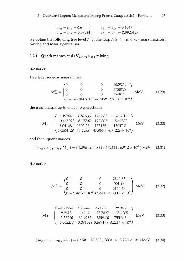
ii

“proc16” — 2016/12/12 — 10:17 — page 47 — #63 ii

ii

ii


s1d = s1e = 0.6 s2d = s2e = 0.1047

s1u = s1ν = 0.575341 s2u = s2ν = 0.0925127

we obtain the following tree levelMof , one loopMf, f = u, d, e, νmass matrices,

mixing and mass eigenvalues:

3.7.1 Quark masses and (VCKM)4×4 mixing

u-quarks:

Tree level see-saw mass matrix:

Mou =

0 0 0 108921.

0 0 0 17589.5

0 0 0 154844.

0 −6.42288× 106 462459. 2.5111× 106

MeV , (3.29)

the mass matrix up to one loop corrections:

Mu =

7.19764 −626.533 −1479.88 −3792.15

−0.468392 −81.7707 −197.807 −506.875

5.04103 1502.25 −172425. 12057.2

0.0504129 15.0233 47.0554 6.91226× 106

MeV (3.30)

and the u-quark masses

(mu , mc , mt , MU ) = ( 1.396 , 644.835 , 172438 , 6.912× 106 ) MeV (3.31)

d-quarks:

Mod =

0 0 0 2860.87

0 0 0 501.98

0 0 0 3814.49

0 −2.3645× 106 323661. 2.17117× 106

MeV (3.32)

Md =

−4.22954 3.26664 26.4239 29.045

19.9418 −41.6 −57.7027 −63.4265

−2.27726 −31.0285 −2859.26 755.343

−0.002277 −0.031028 0.687179 3.2264× 106

MeV (3.33)

(md , ms , mb , MD ) = ( 2.501 , 45.803 , 2860.14 , 3.226× 106 ) MeV (3.34)

ii

“proc16” — 2016/12/12 — 10:17 — page 48 — #64 ii

ii

ii


and the quark mixing

(VCKM)4×4 =

−0.97445 0.224576 −0.003514 −0.000021

−0.224523 −0.973562 0.042015 −0.000010

0.006011 0.041720 0.999041 −0.001233

−0.000219 −0.0011268 −0.011702 0.000014

(3.35)

3.7.2 Lepton masses and (UPMNS)4×4 mixing:

Charged leptons:

Moe =

0 0 0 129165.

0 0 0 22663.9

0 0 0 172220.

0 −337398. 32029.6 2.16401× 107

MeV (3.36)

Me =

2.2376 −66.4545 −394.792 −6.18239

−0.175708 −9.01417 −57.8818 −0.906422

1.66889 164.714 −1693.76 26.556

0.016689 1.64723 16.9589 2.16438× 107

MeV (3.37)

fit the charged lepton masses:

(me , mµ , mτ , ME) = (0.486 , 102.702 , 1746.17 , 2.164× 107 ) MeV (3.38)

Dirac neutrino masses:

Moν =

0 0 0 0.076760

0 0 0 0.012395

0 0 0 0.109124

0 −0.108392 −0.264395 0.854133

eV (3.39)

Mν =

0.015703 −0.004190 0.009713 0.003179

−0.001021 −0.01824 −0.005614 −0.001837

0.010890 0.004245 −0.048705 −0.002164

0.001539 0.000600 −0.000934 0.909297

eV (3.40)

fit the light neutrino masses:

(m1 , m2 , m3 , m4) = ( 0.017127 , 0.0192 , 0.050703 , 0.909309 ) eV (3.41)

the squared mass differences:

ii

“proc16” — 2016/12/12 — 10:17 — page 49 — #65 ii

ii

ii


m22 −m21 = 0.000075 eV2 , m23 −m

22 = 0.00220 eV2 (3.42)

and the lepton mixing

(UPMNS)4×4 =

0.610887 −0.786302 −0.092369 0.003816

−0.709911 −0.595411 0.374805 0.032066

−0.349473 −0.164968 −0.912482 −0.133926

0.001821 0.000257 0.009733 0.001377

(3.43)

3.8 Conclusions

Within the frame work of a gauged SU(3)F family symmetry model, we havereported in section 7 a global fit region of the parameter space where this scenariocan accommodate a realistic spectrum for the ordinary quark masses and mixing ina non-unitary (VCKM)4×4, for the charged lepton masses and the squared neutrinomass differences, within allowed values reported in PDG 2016 [9].

Simultaneously, some of extra particles introduced in this scenario; horizontalgauge bosons and vector-like fermions are predicted to lie within a few TeV’sregion, and hence, within current LHC energies.

It is worth to comment that the gauge symmetry G ≡ SU(3)F × GSM, thefermion content, and the transformation of the scalar fields, all together, avoidYukawa couplings between SM fermions. So, the scalar fields introduced to breakthe symmetries in the model: η2, η3, Φu and Φd couple ordinary fermions withtheir corresponding vector-like fermion U, D, E and N, through the tree levelYukawa couplings. Therefore, FCNC scalar couplings to ordinary fermions aresuppressed by light-heavy mixing angles, which may be small enough to suppressproperly the FCNC mediated by the scalar fields within this scenario.

3.9 Appendix: Diagonalization of the generic Dirac See-sawmass matrix

Mo =

0 0 0 a10 0 0 a20 0 0 a30 b2 b3 c

(3.44)

Using a biunitary transformation ψoL = VoL χL and ψoR = VoR χR to diagonalizeMo,the orthogonal matrices VoL and VoR may be written explicitly as

VoL =

c1 −s1 s2 s1 c2 cα s1 c2 sα0 c2 s2 cα s2 sα

−s1 −c1 s2 c1 c2 cα c1 c2 sα0 0 −sα cα

(3.45)

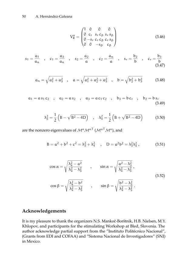
ii

“proc16” — 2016/12/12 — 10:17 — page 50 — #66 ii

ii

ii


VoR =

1 0 0 0

0 cr sr cβ sr sβ0 −sr cr cβ cr sβ0 0 −sβ cβ

(3.46)

s1 =a1

an, c1 =

a3

an, s2 =

a2

a, c2 =

an

a, sr =

b2

b, cr =

b3

b(3.47)

an =√a21 + a

23 , a =

√a21 + a

22 + a

23 , b =

√b22 + b

23 (3.48)

a1 = a s1 c2 , a2 = a s2 , a3 = a c1 c2 , b3 = b cr , b2 = b sr(3.49)

λ23 =1

2

(B−

√B2 − 4D

), λ24 =

1

2

(B+

√B2 − 4D

)(3.50)

are the nonzero eigenvalues ofMoMoT (MoTMo), and

B = a2 + b2 + c2 = λ23 + λ24 , D = a2b2 = λ23λ

24 , (3.51)

cosα =

√λ24 − a

2

λ24 − λ23

, sinα =

√a2 − λ23λ24 − λ

23

,

(3.52)

cosβ =

√λ24 − b

2

λ24 − λ23

, sinβ =

√b2 − λ23λ24 − λ

23

.

Acknowledgements

It is my pleasure to thank the organizers N.S. Mankoc-Borstnik, H.B. Nielsen, M.Y.Khlopov, and participants for the stimulating Workshop at Bled, Slovenia. Theauthor acknowledge partial support from the ”Instituto Politecnico Nacional”,(Grants from EDI and COFAA) and ”Sistema Nacional de Investigadores” (SNI)in Mexico.

ii

“proc16” — 2016/12/12 — 10:17 — page 51 — #67 ii

ii

ii


References

1. A. Hernandez-Galeana, Rev. Mex. Fis. Vol. 50(5), (2004) 522. hep-ph/0406315.2. A. Hernandez-Galeana, Bled Workshops in Physics, (ISSN:1580-4992), Vol. 16,

No. 2, (2015) Pag. 47; arXiv:1602.08212[hep-ph]; Vol. 15, No. 2, (2014) Pag. 93;arXiv:1412.6708[hep-ph]; Vol. 14, No. 2, (2013) Pag. 82; arXiv:1312.3403[hep-ph]; Vol.13, No. 2, (2012) Pag. 28; arXiv:1212.4571[hep-ph]; Vol. 12, No. 2, (2011) Pag. 41;arXiv:1111.7286[hep-ph]; Vol. 11, No. 2, (2010) Pag. 60; arXiv:1012.0224[hep-ph]; BledWorkshops in Physics,Vol. 10, No. 2, (2009) Pag. 67; arXiv:0912.4532[hep-ph];

3. Z.G.Berezhiani and M.Yu.Khlopov, Sov.J.Nucl.Phys. 51 (1990) 739; 935; Sov.J.Nucl.Phys.52 (1990) 60; Z.Phys.C- Particles and Fields 49 (1991) 73; Z.G.Berezhiani, M.Yu.Khlopovand R.R.Khomeriki, Sov.J.Nucl.Phys. 52 (1990) 344; A.S.Sakharov and M.Yu.KhlopovPhys.Atom.Nucl. 57 (1994) 651; M.Yu. Khlopov: Cosmoparticle physics, World Scientific,New York -London-Hong Kong - Singapore, 1999; M.Yu. Khlopov: Fundamentals ofCosmoparticle physics, CISP-Springer, Cambridge, 2011; Z.G. Berezhiani, J.K. Chkareuli,JETP Lett. 35 (612) 1982; JETP Lett. 37 (338) 1983; Z.G. Berezhiani, Phys. Lett. B 129 (99)1983.

4. J.A. Aguilar-Saavedra, R. Benbrik, S. Heinemeyer, and M. Perez-Victoria,arXiv:1306.0572; J.A. Aguilar-Saavedra, arXiv:1306.4432; Jonathan M. Arnold, BartoszFornal and Michael Trott, JHEP 1008:059, 2010, arXiv:1005.2185 and references therein.

5. T. Yanagida, Phys. Rev. D 20, 2986 (1979).6. G. Aad et. al., ATLAS Collaboration, Phys. Lett. B 716, 1(2012), arXiv: 1207.7214.7. S. Chatrchyan et. al., CMS Collaboration, Phys. Lett. B 716, 30(2012), arXiv: 1207.7235.8. Zhi-zhong Xing, He Zhang and Shun Zhou, Phys. Rev. D 86, 013013 (2012).9. The Review of Particle Physics (2016), C. Patrignani et al. (Particle Data Group), Chin.

Phys. C, 40, 100001 (2016).

ii

“proc16” — 2016/12/12 — 10:17 — page 52 — #68 ii

ii

ii




4 Nonstandard Cosmologies From Physics Beyondthe Standard Model

M.Yu. Khlopov1,2 ?

1National Research Nuclear University ”MEPHI” (Moscow Engineering Physics Institute),115409 Moscow, RussiaCentre for Cosmoparticle Physics “Cosmion” 115409 Moscow, Russia2APC laboratory 10, rue Alice Domon et Lonie Duquet 75205 Paris Cedex 13, France

Abstract. The modern cosmology is based on inflationary models with baryosynthesis anddark matter/energy. It implies extension of particle symmetry beyond the Standard model.Studies of physical basis of the modern cosmology combine direct searches for new physicsat accelerators with its indirect non-accelerator probes, in which cosmological consequencesof particle models play important role. The cosmological consequences of particle modelsinevitably go beyond the ’standard’ cosmological ΛCDM model and some possible featureof such ’nonstandard’cosmological scenarios is the subject of the present brief review.

Povzetek. Kozmoloski modeli gradijo na inflacijskih modelih, na bariogenezi in na ob-stoju temne snovi in temne energije. Vse to zahteva vec kot pa ponudi standardni modelosnovnih delcev. Kozmoloske meritve in meritve na pospesevalnikih skupaj preverjajokozmoloske modele in modele osnovnih delcev. V kratkem pregledu se avtor omeji nanekatere znacilnosti ’nestandardnih’ kozmoloskih modelov.

4.1 Introduction

The now standard ΛCDM cosmological model involving inflation, baryosynthesisand dark matter/energy implies physics beyond the Standard model (BSM) ofelementary particles. However, particle models, predicting new physics, can hardlyreduce their cosmological consequences to these basic elements of the Standardcosmological model. One can expect that they can give rise to additional modeldependent signatures of new physics and to corresponding non-Standard featuresof the cosmological scenario. Therefore any model that pretends to be a physicalbasis for the modern cosmology should be studied in more details in order toreveal such non-Standard cosmological features and we discuss in the presentbrief review some possible signatures for non-Standard cosmological scenarios.

The extension of the Standard model can be developed in either up-down orbottom-up direction. In the first case (as e.g. in the approach of [1]) the overwhelm-ing framework is proposed, which embeds the Standard model and involvesnew physics beyond it. To be realistic this new physics should provide inflation,

? [email protected]

ii

“proc16” — 2016/12/12 — 10:17 — page 53 — #69 ii

ii

ii

4 Nonstandard Cosmologies From Physics Beyond the Standard Model 53

baryosynthesis and dark matter. To be true it should be falsifiable, predictingmodel dependent signatures for its probe.

The bottom-up approach, motivated by internal problems and incompletenessof the Standard model, generally involves smaller number of parameters of newphysics, than it inevitably takes place in the up-down case. It makes possibleto study in more details such models and, in particular, their cosmological andastrophysical impact.

We’d like to consider physical motivations and effects of multi-componentdark matter (Section 4.2), as well as of primordial nonlinear structures from phasetransitions in early Universe and from nonhomogeneous baryosynthesis, reflectedin its extreme form in the existence of antimatter domains and antimatter objectsin the baryon asymmetric Universe (Section 4.3). The importance of the accountfor non-standard cosmological features of physics beyond the Standard model isstressed in the conclusive Section 4.4.

4.2 Multi-component dark matter

Stability of elementary constituents of matter reflects the fundamental symmetryof microworld, which prevents decays of the lightest particles that possess thissymmetry. So atoms are stable because electrons cannot decay owing to electriccharge conservation, while protons that can in principle decay are very longlivingdue to the conservation of the baryon number. Physics beyond the Standard model,extending particle symmetry, involves new conservation laws that leads to stabilityof new forms of matter that can play the role of dark matter candidates.

In the simplest case extension of particle symmetry can lead to only onenew conservation law corresponding to a single dark matter candidate. Mostpopular scenarios assume that this candidate is a Weakly Interacting MassiveParticle (WIMP) having strong motivation in the so called ”WIMP miracle”: thecalculated frozen out abundance of WIMPs with mass around several tens - severalhundreds GeV provides their contribution in the total density of the Universe thatcan explain observed dark matter density. The simplest WIMP scenario has anadvantage to be checked in the combination of cosmological, astrophysical andphysical effects. WIMP annihilation to ordinary particles not only determines theirfrozen out concentration but also should lead to contribution of energetic productsof this annihilation to the fluxes of cosmic rays and cosmic gamma radiation. Itsupports indirect searches for dark matter following the original idea of [2]. Thesame process viewed in t-channel corresponds to WIMP scattering on ordinarymatter, and viewed from the opposite side to creation of WIMPs in collisions ofmatter particles. The former motivates direct searches for dark matter, while thelatter challenges WIMP searches at accelerators and colliders. WIMP paradigmfound physical motivation in supersymmetric models that were considered as themainstream in studies of physics beyond the Standard model.

However, direct searches for dark matter have controversial results andthough their interpretation in the terms of WIMPs is still not ruled out [3], amore general approach to a possible solution of the dark matter problem is appeal-ing. Here we’ll discuss some possible nontrivial forms of cosmological dark matter

ii

“proc16” — 2016/12/12 — 10:17 — page 54 — #70 ii

ii

ii

54 M.Yu. Khlopov

that naturally follow from physics beyond the Standard Model. These examplesreflect various features of multi-component dark matter either by compositenessof its species or by co-existence of various dark matter candidates.

4.2.1 Composite dark matter and OHe cosmology

In the same way as the ordinary matter is composed by atoms, which consist ofelectrically charged electrons and nuclei, bound by Coulomb forces, new electri-cally charged stable particles may be bound by ordinary Coulomb field in the darkatoms of the dark matter. The electrically charged constituents of dark atoms maybe not only elementary particles, but can be composite objects, as are ordinary nu-clei and nucleons. The problem of stable electrically charged particles is that boundwith electrons, such particles with charges +1 and +2 form anomalous isotopesof hydrogen and helium. In particular, the idea of stable charged particles boundin neutral dark atoms put forward by Sheldon Glashow in his sinister model [4]found the unrecoverable problem of anomalous istotope overproduction, revealedin [5]. It is impossible to realize the dark atom scenario in any model predicting sta-ble +1 and -1 charged species. The former inevitably bind with electrons, forminganomalous hydrogen directly, while the latter bind first with primordial helium in+1 charged ions, which in turn form anomalous hydrogen.

Starting from 2006 the solutions of dark atom scenario were proposed [6–13],in which stable -2 charged species are bound with primordial helium in neutralOHe atoms, which play important catalyzing role in reduction of all the undesir-able positively charged heavy species that can give rise to anomalous isotopes.Moreover OHe atoms can be a candidate for composite dark matter, dominatingin the matter density of the Universe. Such candidates for dark matter shouldconsist of negatively doubly-charged heavy (with the mass ∼ 1 TeV) particles,which are called O−−, coupled to primordial helium. Lepton-like technibaryons,technileptons, AC-leptons or clusters of three heavy anti-U-quarks of 4th gener-ation with strongly suppressed hadronic interactions are examples of such O−−

particles (see [6–8,10–13] for a review and for references). Another direction ofcomposite dark matter scenario is to consider neutral stable heavy quark clustersas it is proposed in the approach of [1]. However, even in this approach heavystable -2 charged clusters (u5u5u5) of stable antiquarks u5 of 5th generation canalso find their physical basis [9].

As it was qualitatively shown earlier (see [14,15] for the latest review), thetransfer function of density perturbations of OHe dark matter has specific Warmer-than-Cold features, reflecting its composite nature and the nuclear cross sectionsfor OHe elastic collisions with nuclei.

The cosmological and astrophysical effects of such composite dark matter(dark atoms of OHe) are dominantly related to the helium shell of OHe and involveonly one parameter of new physics − the mass of O−−.

If dark matter can bind to normal matter, the observations could come from ra-diative capture of thermalized OHe and could depend on the detector compositionand temperature. In the matter of the underground detector local concentrationof OHe is determined by the equilibrium between the infalling cosmic OHe flux

ii

“proc16” — 2016/12/12 — 10:17 — page 55 — #71 ii

ii

ii


and its diffusion towards the center of Earth. Since the infalling flux experiencesannual changes due to Earth’s rotation around Sun, this local OHe concentrationpossess annual modulations.

The positive results of the DAMA/NaI and DAMA/LIBRA experiments arethen explained by the annual modulations of the rate of radiative capture of OHeby sodium nuclei. Such radiative capture to a low energy OHe-nucleus bound stateis possible only for intermediate-mass nuclei: this explains the negative results ofthe XENON100 and LUX experiments. The rate of this capture can be calculated bythe analogy with radiative capture of neutron by proton, taking into account thescalar and isoscalar nature of He nucleus, what makes possible only E1 transitionwith isospin violation in this process. In the result this rate is proportional to thetemperature (to the square of relative velocity in the absence of local thermalequilibrium): this leads to a suppression of this effect in cryogenic detectors, suchas CDMS.

The timescale of OHe collisions in the Galaxy exceeds the age of the Universe,what proves that the OHe gas is collisionless. However the rate of such collisionsis nonzero and grows in the regions of higher OHe density, particularly in thecentral part of the Galaxy, where these collisions lead to OHe excitations. De-excitations of OHe with pair production in E0 transitions can explain the excessof the positron-annihilation line, observed by INTEGRAL in the galactic bulge[12,13,16–20]. The calculated rate of collisions and OHe excitation in them stronglydepends on OHe density and relative velocity and the explanation of positronexcess was found to be very sensitive to the dark matter density in the centralpart of Galaxy, where baryonic matter dominates and theoretical estimations arevery uncertain. The latest analysis of dark matter distribution favors more modestvalues of dark matter central density, what fixes the explanation of the excess ofthe positron-annihilation line by OHe collisions and de-excitation in a very narrowrange of the mass of O−− near 1.25 TeV.

In a two-component dark atom model, based on Walking Technicolor, a sparseWIMP-like component of atom-like state, made of positive and negative doublycharged techniparticles, is present together with the dominant OHe dark atom andthe decays of doubly positive charged techniparticles to pairs of same-sign leptonscan explain the excess of high-energy cosmic-ray positrons, found in PAMELAand AMS02 experiments [21]. This explanation is possible for the mass of decaying+2 charged particle below 1 TeV and depends on the branching ratios of leptonicchannels. Since even pure lepton decay channels are inevitably accompaniedby gamma radiation the important constraint on this model follows from themeasurement of cosmic gamma ray background in FERMI/LAT experiment. Itmay be shown that the constraints on this background may be satisfied if thedecaying component is distributed in disc and not in halo, what implies moresophisticated self-interacting nature of this component. In fact, a serious problemfor any source of cosmic poitrons distributed in halo and not concentrated in thedisc.

The crucial problem of OHe scenario is the existence of a dipole barrier inOHe nuclear interaction. The scenario in which such a barrier does not appear was

ii

“proc16” — 2016/12/12 — 10:17 — page 56 — #72 ii

ii

ii

56 M.Yu. Khlopov

considered in [22] and The over-abundance of anomalous isotopes in terrestrialmatter seems to be unavoidable in this case..

This makes the full solution of OHe nuclear physics, started in [23], vital.The answer to the possibility of the creation of a dipole Coulomb barrier in OHeinteraction with nuclei is crucial. Indeed, the model cannot work if no repulsiveinteraction appears at some distance between

The problem of the Earth’s shadowing represents another potential problemfor OHe scenario. The terrestrial matter is opaque for OHe, what should inevitablylead to an effect of Earth matter shadowing for the OHe flux and correspondingdiurnal modulation, constrained in DAMA/LIBRA experiment [24]. The OHemodel involves only one parameter of new physics - mass of O−− and its cosmo-logical effects are related to nuclear and atomic physics, being within the Standardmodel, but even in this case many principal features of cosmological consequencesremain unclear.

4.2.2 Mirror atoms

Mirror particles, first proposed by T. D. Lee and C. N. Yang in Ref. [26] to restoreequivalence of left- and right-handed co-ordinate systems in the presence ofP- and C- violation in weak interactions, should be strictly symmetric by theirproperties to their ordinary twins. After discovery of CP-violation it was shownby I. Yu. Kobzarev, L. B. Okun and I. Ya. Pomeranchuk in Ref. [27] that mirrorpartners cannot be associated with antiparticles and should represent a new setof symmetric partners for ordinary quarks and leptons with their own strong,electromagnetic and weak mirror interactions. It means that there should existmirror quarks, bound in mirror nucleons by mirror QCD forces and mirror atoms,in which mirror nuclei are bound with mirror electrons by mirror electromagneticinteraction [28,29]. If gravity is the only common interaction for ordinary andmirror particles, mirror matter can be present in the Universe in the form ofelusive mirror objects, having symmetric properties with ordinary astronomicalobjects (gas, plasma, stars, planets...), but causing only gravitational effects on theordinary matter [30,31].

Even in the absence of any other common interaction except for gravity, theobservational data on primordial helium abundance and upper limits on thelocal dark matter seem to exclude mirror matter, evolving in the Universe in afully symmetric way in parallel with the ordinary baryonic matter[32,33]. Thesymmetry in cosmological evolution of mirror matter can be broken either byinitial conditions[34,35], or by breaking mirror symmetry in the sets of particlesand their interactions as it takes place in the shadow world[36,37], arising in theheterotic string model. We refer to Refs. [38–40] for current review of mirror matterand its cosmology.

Mirror matter in its fully symmetric implementation doesn’t involve newparameters of new physics, since all the parameters of mirror particles and theirinteractions are by construction strictly equal to the corresponding values of theirordinary partners. However, though there is no common interactions between or-dinary and mirror matter except for gravity, just the presence of mirror particles in

ii

“proc16” — 2016/12/12 — 10:17 — page 57 — #73 ii

ii

ii


the same space-time with ordinary matter causes contradictions with observationsin a strictly symmetric mirror matter cosmology.

4.2.3 Unstable particles

The next to lightest particle that possess a new conserved charge may be suffi-ciently longliving to retain some observable trace in the Universe.

Primordial unstable particles with the lifetime, less than the age of the Uni-verse, τ < tU, can not survive to the present time. But, if their lifetime is sufficientlylarge to satisfy the condition τ (mPl/m)·(1/m), their existence in early Universecan lead to direct or indirect traces[41].

Weakly interacting particles, decaying to invisible modes, can influence LargeScale Structure formation. Such decays prevent formation of the structure, ifthey take place before the structure is formed. Invisible products of decays afterthe structure is formed should contribute in the cosmological dark energy. TheUnstable Dark matter scenarios[42–50] implied weakly interacting particles thatform the structure on the matter dominated stage and then decay to invisiblemodes after the structure is formed.

Cosmological flux of decay products contributing into the cosmic and gammaray backgrounds represents the direct trace of unstable particles[41,51]. If thedecay products do not survive to the present time their interaction with matterand radiation can cause indirect trace in the light element abundance[52–55] or inthe fluctuations of thermal radiation[56].

If the particle lifetime is much less than 1s the multi-step indirect traces arepossible, provided that particles dominate in the Universe before their decay. Onthe dust-like stage of their dominance black hole formation takes place, and thespectrum of such primordial black holes traces the particle properties (mass, frozenconcentration, lifetime) [57–59]. The particle decay in the end of dust like stageinfluences the baryon asymmetry of the Universe. In any way cosmophenomeno-LOGICAL chains link the predicted properties of even unstable new particles tothe effects accessible in astronomical observations. Such effects may be importantin the analysis of the observational data.

4.3 Primordial cosmological structures

4.3.1 Relics of phase transitions in very early Universe

Parameters of new stable and metastable particles are also determined by a patternof particle symmetry breaking. This pattern is reflected in a succession of phasetransitions in the early Universe. First order phase transitions proceed throughbubble nucleation, which can result in black hole formation (see e.g. Refs. [60] and[61] for review and references). Phase transitions of the second order can lead toformation of topological defects, such as walls, string or monopoles. The obser-vational data put severe constraints on magnetic monopole [62] and cosmic wallproduction [63], as well as on the parameters of cosmic strings [64,65]. Structureof cosmological defects can be changed in succession of phase transitions. More

ii

“proc16” — 2016/12/12 — 10:17 — page 58 — #74 ii

ii

ii

58 M.Yu. Khlopov

complicated forms like walls-surrounded-by-strings can appear. Such structurescan be unstable, but their existence can leave a trace in nonhomogeneous distri-bution of dark matter and give rise to large scale structures of nonhomogeneousdark matter like archioles [66–68]. This effect should be taken into account in theanalysis of cosmological effects of weakly interacting slim particles (WISPs) (seeRef. [69] for current review) that can play the role of cold dark matter in spite oftheir small mass.

A wide class of particle models possesses a symmetry breaking pattern, whichcan be effectively described by pseudo-Nambu–Goldstone (PNG) field and whichcorresponds to formation of unstable topological defect structure in the earlyUniverse (see Ref. [61] for review and references). The Nambu–Goldstone naturein such an effective description reflects the spontaneous breaking of global U(1)symmetry, resulting in continuous degeneracy of vacua. The explicit symmetrybreaking at smaller energy scale changes this continuous degeneracy by discretevacuum degeneracy. The character of formed structures is different for phasetransitions, taking place on post-inflationary and inflationary stages.

4.3.2 Large scale correlations of axion field

At high temperatures such a symmetry breaking pattern implies the successionof second order phase transitions. In the first transition, continuous degeneracyof vacua leads, at scales exceeding the correlation length, to the formation oftopological defects in the form of a string network; in the second phase transition,continuous transitions in space between degenerated vacua form surfaces: domainwalls surrounded by strings. This last structure is unstable, but, as was shownin the example of the invisible axion [66–68], it is reflected in the large scaleinhomogeneity of distribution of energy density of coherent PNG (axion) fieldoscillations. This energy density is proportional to the initial value of phase, whichacquires dynamical meaning of amplitude of axion field, when axion mass isswitched on in the result of the second phase transition.

The value of phase changes by 2π around string. This strong nonhomogeneityof phase leads to corresponding nonhomogeneity of energy density of coherentPNG (axion) field oscillations. Usual argument (see e.g. Ref. [70] and referencestherein) is essential only on scales, corresponduing to mean distance betweenstrings. This distance is small, being of the order of the scale of cosmologicalhorizon in the period, when PNG field oscillations start. However, since the non-homogeneity of phase follows the pattern of axion string network this argumentmisses large scale correlations in the distribution of oscillations’ energy density.

Indeed, numerical analysis of string network (see review in the Ref. [71])indicates that large string loops are strongly suppressed and the fraction of about80% of string length, corresponding to long loops, remains virtually the same inall large scales. This property is the other side of the well known scale invariantcharacter of string network. Therefore the correlations of energy density shouldpersist on large scales, as it was revealed in Refs. [66–68].

The large scale correlations in topological defects and their imprints in pri-mordial inhomogeneities is the indirect effect of inflation, if phase transitions take

ii

“proc16” — 2016/12/12 — 10:17 — page 59 — #75 ii

ii

ii


place after reheating of the Universe. Inflation provides in this case the equalconditions of phase transition, taking place in causally disconnected regions.

4.3.3 Primordial seeds for Active Galactic Nuclei

If the phase transitions take place on inflational stage new forms of primordiallarge scale correlations appear. The example of global U(1) symmetry, brokenspontaneously in the period of inflation and successively broken explicitly afterreheating, was considered in Ref. [73]. In this model, spontaneous U(1) symmetrybreaking at inflational stage is induced by the vacuum expectation value 〈ψ〉 = fof a complex scalar field Ψ = ψ exp (iθ), having also explicit symmetry breakingterm in its potential Veb = Λ4(1 − cos θ). The latter is negligible in the periodof inflation, if f Λ, so that there appears a valley relative to values of phasein the field potential in this period. Fluctuations of the phase θ along this valley,being of the order of ∆θ ∼ H/(2πf) (here H is the Hubble parameter at inflationalstage) change in the course of inflation its initial value within the regions ofsmaller size. Owing to such fluctuations, for the fixed value of θ60 in the period ofinflation with e-foldingN = 60 corresponding to the part of the Universe within themodern cosmological horizon, strong deviations from this value appear at smallerscales, corresponding to later periods of inflation with N < 60. If θ60 < π, thefluctuations can move the value of θN to θN > π in some regions of the Universe.After reheating, when the Universe cools down to temperature T = Λ the phasetransition to the true vacuum states, corresponding to the minima of Veb takesplace. For θN < π the minimum of Veb is reached at θvac = 0, whereas in theregions with θN > π the true vacuum state corresponds to θvac = 2π. For θ60 < πin the bulk of the volume within the modern cosmological horizon θvac = 0.However, within this volume there appear regions with θvac = 2π. These regionsare surrounded by massive domain walls, formed at the border between the twovacua. Since regions with θvac = 2π are confined, the domain walls are closed.After their size equals the horizon, closed walls can collapse into black holes.The minimal mass of such black hole is determined by the condition that it’sSchwarzschild radius, rg = 2GM/c2 exceeds the width of the wall, l ∼ f/Λ2, andit is given byMmin ∼ f(mPl/Λ)

2. The maximal mass is determined by the massof the wall, corresponding to the earliest region θN > π, appeared at inflationalstage.

This mechanism can lead to formation of primordial black holes of a whateverlarge mass (up to the mass of AGNs [74,75], see for latest review Ref. [76]). Suchblack holes appear in the form of primordial black hole clusters, exhibiting fractaldistribution in space [72,77,61]. It can shed new light on the problem of galaxyformation [61,75].

The described mechanism of massive PBH clouds formation may be of specialinterest for the interpretation of the recently discovered gravitational wave signalsfrom coalescence of massive black hole (BH) binaries [79,80]. It naturally leads toformation of massive BH binaries within such a cloud, while the mass range ofPBHs, determined by f and Λ can naturally cover the values of tens of Solar mass.

ii

“proc16” — 2016/12/12 — 10:17 — page 60 — #76 ii

ii

ii

60 M.Yu. Khlopov

60

0

matter

matteranti

i

i 60

60

+

Fig. 4.1. The inflational evolution of the phase (taken from the Ref. [78]). The phase θ60sits in the range [π, 0] at the beginning of inflation and makes Brownian step δθeff =

Hinfl/(2πfeff) at each e–fold. The typical wavelength of the fluctuation δθ is equal to H−1infl.

The whole domainH−1infl, containing phase θN gets divided, after one e–fold, into e3 causally

disconnected domains of radius H−1infl. Each new domain contains almost homogeneous

phase value θN−1 = θN ± δθeff. Every successive e-fold this process repeats in everydomain.

4.3.4 Antimatter in Baryon asymmetric Universe?

Primordial strong inhomogeneities can also appear in the baryon charge distri-bution. The appearance of antibaryon domains in the baryon asymmetrical Uni-verse, reflecting the inhomogeneity of baryosynthesis, is the profound signatureof such strong inhomogeneity [81]. On the example of the model of spontaneousbaryosynthesis (see Ref. [82] for review) the possibility for existence of antimatterdomains, surviving to the present time in inflationary Universe with inhomoge-neous baryosynthesis was revealed in [83].

The mechanism of spontaneous baryogenesis [82] implies the existence of acomplex scalar field χ = (f/

√2) exp (θ) carrying the baryonic charge. The U(1)

symmetry, which corresponds to the baryon charge, is broken spontaneouslyand explicitly. The explicit breakdown of U(1) symmetry is caused by the phase-dependent term

V(θ) = Λ4(1− cos θ). (4.1)

The possible baryon and lepton number violating interaction of the field χwithmatter fields can have the following structure [82]

L = gχQL+ h.c., (4.2)

where fields Q and L represent a heavy quark and lepton, coupled to the ordinarymatter fields.

In the early Universe, at a time when the friction term, induced by the Hubbleconstant, becomes comparable with the angular mass mθ = Λ2

f, the phase θ starts

ii

“proc16” — 2016/12/12 — 10:17 — page 61 — #77 ii

ii

ii


to oscillate around the minima of the PNG potential and decays into matter fieldsaccording to (4.2). The coupling (4.2) gives rise to the following [82]: as the phasestarts to roll down in the clockwise direction (Fig. 4.1), it preferentially createsexcess of baryons over antibaryons, while the opposite is true as it starts to rolldown in the opposite direction.

The fate of such antimatter regions depends on their size. If the physicalsize of some of them is larger than the critical surviving size Lc = 8h2 kpc [83],they survive annihilation with surrounding matter. Evolution of sufficiently denseantimatter domains can lead to formation of antimatter globular clusters [84]. Theexistence of such cluster in the halo of our Galaxy should lead to the pollution ofthe galactic halo by antiprotons. Their annihilation can reproduce [85] the observedgalactic gamma background in the range tens-hundreds MeV. The prediction ofantihelium component of cosmic rays [86], accessible to future searches for cosmicray antinuclei in PAMELA and AMS II experiments, as well as of antimattermeteorites [87] provides the direct experimental test for this hypothesis.

So the primordial strong inhomogeneities in the distribution of total, darkmatter and baryon density in the Universe is the new important phenomenonof cosmological models, based on particle models with hierarchy of symmetrybreaking.

4.4 Conclusions

As soon as physics beyond the Standard model involves new symmetries andmechanisms of their breaking, new model dependent non-standard features ofthe cosmological scenario should inevitably appear. Even rather restricted listof possible examples of such features, presented here, gives the flavor of newcosmology that can come from the new physics.

The wider is the symmetry group embedding the symmetry of the Standardmodel of elementary particles, the larger is the list of cosmologically viable pre-dictions that provide various probes for the considered particle model. Enteringthe corresponding multi-dimensional space of parameters, we simultaneouslyincrease the set of their probes. It makes the set of equations for these parametersover-determined and provides a complete test for however extensive theoreticalmodel.

One can conclude that the account for non-Standard cosmological scenarios inthe analysis of the data of precision cosmology extends the space of cosmologicalparameters and provides nontrivial test for physics beyond the Standard model.

Acknowledgements

I express my gratitude to Jean-Ren Cudell for kind hospitality in the University ofLiege, where this contribution was completed. The work was performed within theframework of the Center FRPP supported by MEPhI Academic Excellence Project(contract 02.03.21.0005, 27.08.2013). The part on initial cosmological conditionswas supported by the Ministry of Education and Science of Russian Federation,project 3.472.2014/K and on the forms of dark matter by grant RFBR 14-22-03048.

ii

“proc16” — 2016/12/12 — 10:17 — page 62 — #78 ii

ii

ii

62 M.Yu. Khlopov

References

1. N.S. Mankoc-Borstnik: these proceedings.2. Ya.B. Zeldovich, A.A. Klypin, M.Yu. Khlopov, V.M. Chechetkin: Astrophysical bounds

on the mass of heavy stable neutral leptons. Sov.J.Nucl.Phys. 31 664 (1980).3. R.Bernabei, et al.: Dark Matter investigation by DAMA at Gran Sasso. Int. J. Mod. Phys.

A 28 1330022 [71 pages] (2013). DOI: 10.1142/S0217751X133002264. S. L. Glashow, “A sinister extension of the standard model to SU(3) x SU(2) x SU(2) x

U(1),” arXiv:hep-ph/0504287, 2005.5. D. Fargion and M. Khlopov: Tera-leptons shadows over sinister Universe. arXiv:hep-

ph/0507087; Gravitation and Cosmology 19 213 (2013).6. M.Y. Khlopov: Composite dark matter from 4th generation. Pisma Zh. Eksp. Teor. Fiz.

83 3 (2006); [JETP Lett. 83 (2006) 1] [astro-ph/0511796].7. M.Y. Khlopov and C. Kouvaris: Composite dark matter from a model with composite

Higgs boson. Phys. Rev. D 78 065040 (2008) [arXiv:0806.1191 [astro-ph]];8. D. Fargion, M.Y. Khlopov and C. A. Stephan: Cold dark matter by heavy double

charged leptons? Class. Quant. Grav. 23 7305 (2006) [astro-ph/0511789]; M.Y. Khlopovand C.A. Stephan: Composite dark matter with invisible light from almost-commutativegeometry. [astro-ph/0603187].

9. M.Y. Khlopov and N.S. Mankoc Borstnik: Bled Workshops in Physics 11, 177 (2010).10. M. Y. Khlopov, A. G. Mayorov and E. Y. .Soldatov: The dark atoms of dark matter.

Prespace. J. 1 1403 (2010) [arXiv:1012.0934 [astro-ph.CO]];11. M. Y. Khlopov: Physics of Dark Matter in the Light of Dark Atoms. Mod. Phys. Lett. A

26 2823 (2011) [arXiv:1111.2838 [astro-ph.CO]].12. M. Yu. Khlopov: Fundamental Particle Structure in the Cosmological Dark Matter Int.

J. Mod. Phys. A 28, 1330042 (2013).13. M. Yu. Khlopov: Dark Atoms and Puzzles of Dark Matter Searches. Int. J. Mod. Phys.

A 29, 1443002 (2014).14. M. Yu. Khlopov: Cosmological Reflection of Particle Symmetry. Symmetry, 8 81 (2016).15. M.Yu.Khlopov: 10 years of dark atoms of composite dark matter. Bled Workshops in

Physics 16 71 (2015).16. M.Yu. Khlopov: Composite dark matter from stable charged constituents. arXiv:

0806.3581 [astro-ph], 2008.17. M.Yu. Khlopov and C. Kouvaris: Strong Interactive Massive Particles from a Strong

Coupled Theory. Phys.Rev.D 77 065002 (18 pages),(2008); [arXiv:0710.2189].18. M.Yu. Khlopov, A.G. Mayorov and E.Yu. Soldatov: Composite Dark Matter and Puzzles

of Dark Matter Searches. Int. J. Mod. Phys.D 19 1385-1395, (2010) [arXiv:1003.1144].19. J.-R. Cudell, M.Yu. Khlopov and Q. Wallemacq: Dark atoms and the positron-

annihilation-line excess in the galactic bulge. Advances in High Energy Physics 2014Article ID 869425, (2014) [arXiv: 1401.5228].

20. J.-R. Cudell, M.Yu.Khlopov and Q.Wallemacq: Effects of dark atom excitations.Mod.Phys.Lett. A 29 (2014) 1440006, [arXiv:1411.1655].

21. K. Belotsky, M. Khlopov, C. Kouvaris and M. Laletin: Decaying Dark Atom constituentsand cosmic positron excess. Advances in High Energy Physics, 2014 Article ID 214258,(2014) [arXiv:1403.1212]; K. Belotsky, M. Khlopov and M. Laletin: Dark Atoms andtheir decaying constituents, Bled Workshops in Physics 15, 1 (2014) [arXiv: 1411.3657];K. Belotsky, M. Khlopov, C. Kouvaris and M. Laletin: High Energy Positrons andGamma Radiation from Decaying Constituents of a two-component Dark Atom Model.Int.J.Mod.Phys.D 24 1545004, (2015)[arXiv: 1508.02881].

22. J.-R. Cudell, M.Yu. Khlopov and Q. Wallemacq: Some Potential Problems of OHeComposite Dark Matter. Bled Workshops in Physics 15, 66 (2014)

ii

“proc16” — 2016/12/12 — 10:17 — page 63 — #79 ii

ii

ii


23. J.-R. Cudell, M.Yu. Khlopov and Q. Wallemacq, The nuclear physics of OHe. BledWorkshops in Physics 13, 10 (2012)

24. DAMA Collaboration (R.Bernabei et al): Model independent result on possible diurnaleffect in DAMA/LIBRA-phase1 Eur. Phys. J C 74 2827 (2014).

25. J.-R. Cudell and M.Yu. Khlopov: Dark atoms with nuclear shell: A status review.Int.J.Mod.Phys.D 24 1545007 (2015).

26. T. D. Lee and C. N. Yang: Question of Parity Conservation in Weak Interactions. Phys.Rev. 104 254 (1956).

27. I. Yu. Kobzarev, L. B. Okun and I. Ya. Pomeranchuk: On the possibility of experimentalobservation of mirror particles. Sov.J.Nucl.Phys. 3 837 (1966).

28. Ya. B. Zeldovich and M. Yu. Khlopov: The Neutrino Mass in Elementary Particle Physicsand in Big Bang Cosmology. Sov. Phys. Uspekhi 24 755 (1981).

29. R. Foot and R. R. Volkas: Neutrino physics and the mirror world: How exact paritysymmetry explains the solar neutrino deficit, the atmospheric neutrino anomaly andthe LSND experiment. Phys. Rev. D 52 6595 (1995).

30. S. I. Blinnikov, M. Yu. Khlopov: On possible effects of mirror particles. Sov.J.Nucl.Phys.36 472 (1982).

31. S. I. Blinnikov, M. Yu. Khlopov: Possible astronomical effects of mirror particles. Sov.Astron. J. 27 371 (1983).

32. E. D. Carlson and S.L.Glashow: Nucleosynthesis Versus the Mirror Universe. Phys. Lett.B 193 168 (1987).

33. R. Foot and R. R. Volkas: The Exact parity symmetric model and big bang nucleosyn-thesis. Astropart. Phys. 7 283 (1997).

34. Z. Berezhiani, D. Comelli and F. Villante: The Early mirror universe: Inflation, baryoge-nesis, nucleosynthesis and dark matter. Phys. Lett. B 503 362 (2001).

35. Z. Berezhiani: Mirror world and its cosmological consequences. Int. J. Mod. Phys. A 193775 (2004).

36. E. W. Kolb, D. Seckel and M. S. Turner: The shadow world. Nature 314 415 (1985).37. M. Yu. Khlopov et al.: Observational physics of mirror world. Sov. Astron. 35 21 (1991).38. Maxim Khlopov, Fundamentals of Cosmic Particle physics CISP-SPRINGER, Cambridge,

2012.39. L. B. Okun: Mirror particles and mirror matter: 50 years of speculations and search.

Phys. Usp. 50 380 (2007).40. P. Ciarcelluti: Cosmology with mirror dark matter. Int.J.Mod.Phys. D 19 2151 (2010)41. M. Yu. Khlopov and V. M. Chechetkin: Antiprotons in the Universe as a cosmological

test of Grand Unification. Sov. J. Part. Nucl. 18 267 (1987).42. A. G. Doroshkevich and M. Yu. Khlopov: On the physical nature of dark matter of the

Universe. Sov. J. Nucl. Phys. 39 551 (1984).43. A. G. Doroshkevich and M. Yu. Khlopov: Formation of structure in the Universe with

unstable neutrinos. Mon. Not. R. Astron. Soc. 211 279 (1984).44. A. G. Doroshkevich, A. A. Klypin and M. Yu. Khlopov: Cosmological Models with

Unstable Neutrinos. Sov. Astron. 32 127 (1988).45. A. G. Doroshkevich, A. A. Klypin and M. Yu. Khlopov: Large-scale structure formation

by decaying massive neutrinos. Mon. Not. R. Astron. Soc. 239 923 (1989).46. Z.G.Berezhiani and M.Yu.Khlopov: Physics of cosmological dark matter in the theory

of broken family symmetry. Sov.J.Nucl.Phys. 52 60 (1990).47. Z.G.Berezhiani and M.Yu.Khlopov: Cosmology of spontaneously broken gauge family

symmetry with axion solution of strong CP-problem. Z.Phys.C- Particles and Fields 4973 (1991).

48. M. S. Turner, G. Steigman and L. M. Krauss: Flatness of the universe - Reconcilingtheoretical prejudices with observational data. Phys.Rev.Lett. 52 2090 (1984).

ii

“proc16” — 2016/12/12 — 10:17 — page 64 — #80 ii

ii

ii

64 M.Yu. Khlopov

49. G. Gelmini, D. N. Schramm and J. W. F. Valle: Majorons: A simultaneous solution to thelarge and small scale dark matter problems. Phys.Lett. B 146 311 (1984).

50. A. S. Sakharov and M. Yu. Khlopov: Horizontal unification as the phenomenology ofthe theory of ”everything”. Phys.Atom.Nucl. 57 651 (1994).

51. E. V. Sedelnikov and M. Yu. Khlopov: Cosmic rays as an additional source of infor-mation about nonequilibrium processes in the Universe. Phys.Atom.Nucl. 59 1000(1996).

52. Yu. L. Levitan et al.: Production of light elements in cascades from energetic antiprotonsin early Universe and problems of nuclear cosmoarcheology. Sov.J.Nucl.Phys. 47 109(1988).

53. M. Yu. Khlopov et al.: Nonequilibrium cosmological nucleosynthesis of light elements:Calculations by the Monte Carlo method. Phys. Atom. Nucl. 57 1393 (1994).

54. E. V. Sedel’nikov, S. S. Filippov and M. Yu. Khlopov: Kinetic theory of nonequilibriumcosmological nucleosynthesis. Phys. Atom. Nucl. 58 235 (1995).

55. S. Dimopoulos et al.: Is the Universe Closed by Baryons? Nucleosynthesis With a LateDecaying Massive Particle. Astrophys.J. 330 545 (1988)

56. A. G. Doroshkevich and M. Yu. Khlopov: Fluctuations of the Cosmic BackgroundTemperature in Unstable-Particle Cosmologies. Sov. Astron. Lett 11 236 (1985).

57. A. G. Polnarev and M. Yu. Khlopov: Cosmology, Primordial Black Holes, And Super-massive Particles. Sov. Phys. Uspekhi 28 213 (1985).

58. M. Yu. Khlopov and A. G. Polnarev: Primordial Black Holes As A Cosmological Test OfGrand Unification. Phys.Lett. B 97 383 (1980).

59. A. G. Polnarev and M. Yu. Khlopov: Primordial Black Holes and the ERA of SuperheavyParticle Dominance in the Early Universe. Sov. Astron. 25 406 (1981).

60. R. V. Konoplich et al.: Formation of black holes in the first order phase transitions ascosmological test of mechanisms of symmetry breaking. Phys. Atom. Nucl. 62 1593(1999).

61. M. Yu. Khlopov and S. G. Rubin, Cosmological pattern of microphysics in inflationaryuniverse (Kluwer, Dordrecht, 2004).

62. Ya. B. Zeldovich and M. Yu. Khlopov: On the concentration of relic magnetic monopolesin the Universe. Phys. Lett. B 79 1134 (1978).

63. Ya. B. Zeldovich, I. Yu. Kobzarev and L. B. Okun: Cosmological Consequences of theSpontaneous Breakdown of Discrete Symmetry. JETP 40 1 (1975).

64. Ya. B. Zeldovich: Cosmological fluctuations produced near a singularity. MNRAS 192663 (1980).

65. A. Vilenkin: Cosmological density fluctuations produced by vacuum strings. Phys. Rev.Lett. 46 1169 (1981).

66. A. S. Sakharov and M. Yu. Khlopov: The nonhomogeneity problem for the primordialaxion field. Phys. Atom. Nucl. 57 485 (1994)

67. A. S. Sakharov and M. Yu. Khlopov and D. D. Sokoloff: Large scale modulation of thedistribution of coherent oscillations of a primordial axion field in the Universe Phys.Atom. Nucl. 59 1005 (1996)

68. A. S. Sakharov and M. Yu. Khlopov and D. D. Sokoloff: The nonlinear modulation ofthe density distribution in standard axionic CDM and its cosmological impact. Nucl.Phys. Proc. Suppl. 72 105 (1999)

69. J. Jaeckel and A. Ringwald: The Low-Energy Frontier of Particle Physics. Ann. Rev.Nucl. Part. Sci. 60 405 (2010).

70. J.E. Kim: Light Pseudoscalars, Particle Physics and Cosmology. Phys. Rept. 150 1 (1987).71. A. Vilenkin and E. P. S. Shellard, Cosmic Strings and other Topological Defects (Cambridge,

Cambridge University Press 1994).

ii

“proc16” — 2016/12/12 — 10:17 — page 65 — #81 ii

ii

ii


72. M. Yu. Khlopov, S. G. Rubin and A. S. Sakharov: Strong Primordial Nonhomogeneitiesand Galaxy Formation. Gravitation and Cosmology Suppl. 8 57 (2002).

73. S. G. Rubin, M. Yu. Khlopov and A. S. Sakharov: Primordial black holes from non-equilibrium second order phase transitions. Gravitation and Cosmology Suppl. 6 51(2000).

74. S. G. Rubin, A. S. Sakharov and M. Yu. Khlopov: Formation of primordial galacticnuclei at phase transitions in the early Universe JETP 92 921 (2001).

75. V. Dokuchaev, Y. Eroshenko and S. Rubin: Quasars formation around clusters of pri-mordial black holes. Gravitation and Cosmology 11 99 (2005).

76. M. Yu. Khlopov: Primordial black holes. Res.Astron.Astrophys.10 495 (2010).77. M. Yu. Khlopov, S. G. Rubin and A. S. Sakharov: Primordial Structure of Massive Black

Hole Clusters. Astropart. Phys. 23 265 (2005).78. M. Yu. Khlopov: Primordial nonlinear structures and massive black holes from early

Universe. Journal of Physics. Conference series. 66 P.012032 (2007).79. B. P. Abbott et al. [LIGO Scientific and Virgo Collaborations]: Observation of Gravi-

tational Waves from a Binary Black Hole Merger. Phys. Rev. Lett. 116 061102 (2016)[arXiv:1602.03837 [gr-qc]].

80. B. P. Abbott et al. [LIGO Scienti c and Virgo Collaborations]: GW151226: Observation ofGravitational Waves from a 22-Solar-Mass Binary Black Hole Coalescence. Phys. Rev.Lett. 116 241103 (2016) [arXiv:1606.04855 [gr-qc]].

81. V. M. Chechetkin et al.: Astrophysical aspects of antiproton interaction with He (Anti-matter in the Universe). Phys. Lett. B 118 329 (1982).

82. A. D. Dolgov: Matter and antimatter in the universe. Nucl. Phys. Proc. Suppl. 113 40(2002).

83. M. Yu. Khlopov, S. G. Rubin and A. S. Sakharov: Possible origin of antimatter regionsin the baryon dominated universe. Phys. Rev. D 62 0835051 (2000).

84. M. Yu. Khlopov: An antimatter globular cluster in our galaxy: A probe for the origin ofmatter. Gravitation and Cosmology 4 69 (1998).

85. Yu.A. Golubkov and M. Yu. Khlopov: Anti-protons annihilation in the galaxy as asource of diffuse gamma background. Phys.Atom.Nucl. 64 1821 (2001).

86. K. M. Belotsky et al.: Anti-helium flux as a signature for antimatter globular clusters inour galaxy. Phys. Atom.Nucl. 63 233 (2000).

87. D. Fargion and M.Yu. Khlopov: Antimatter bounds by anti-asteroids annihilations onplanets and sun. Astropart. Phys. 19 441 (2003).

ii

“proc16” — 2016/12/12 — 10:17 — page 66 — #82 ii

ii

ii




5 Gauge Fields With Respect to d = (3 + 1) in theKaluza-Klein Theories and in the Spin-charge-familyTheory ?

D. Lukman and N.S. Mankoc Borstnik

Department of Physics, FMF, University of Ljubljana, Jadranska 19, SI-1000 Ljubljana,Slovenia

Abstract. It is shown that in the spin-charge-family theory, as well as in all the Kaluza-Kleinlike theories, vielbeins and spin connections manifest in d = (3+ 1) space equivalent vectorgauge fields, when space d ≥ 5manifests large enough symmetry. The authors demonstratethis equivalence in spaces with the symmetry of metric tensor gστ = ηστ f, for any scalarfunction f of the coordinates xσ, where xσ denotes coordinates of space out of d = (3 + 1).Also the connection between vielbeins and scalar fields in d = (3 + 1) is discussed.

Povzetek. Avtorja pokazeta, da opis s tetradami in opis s spinskimi povezavami voditav d = (3 + 1) prostoru do ekvivalentnih vektorskih umeritvenih polj v primeru, ko imaprostor z d ≥ 5 dovolj veliko simetrijo. To ne velja samo za teorijo spinov-nabojev-druzin,ampak tudi za vse teorije Kaluza-Kleinovega tipa. Ekvivalenco pokazeta v prostorih, vkaterih velja za metricni tenzor gστ = ηστ f, kjer je f poljubna skalarna funkcija koordinatxσ, ki sezejo v prostor z dovolj veliko simetrijo. Avtorja obravnavata tudi povezavo medtetradami in skalarnimi polji v prostoru d = (3 + 1).

5.1 Introduction

We demonstrate in this paper that in spaces with the symmetry of metric tensorgστ = ηστ f

−2, where (xσ, xτ) determine the coordinates of the (almost [10])compactified space, ηστ is the diagonal matrix in this space and f is any scalarfunction of these coordinates, both procedures - the ordinary Kaluza-Klein onewith the vielbeins and the one with the spin connections (related to the vielbeibs,Eq.(5.4), used in the spin-charge-family theory ([1–5] and the references therein) -lead in d = (3+ 1) to the same gauge vector fields. That either the vielbeins or thespin connections represent in symmetric enough spaces in d = (3+ 1) the samevector gauge fields, is known for a long time [6–8]. This contribution is only toclarify this equivalence.

In the starting action of the spin-charge-family theory [2,5,3,4] fermions interactwith the vielbeins fαa and the two kinds of the spin-connection fields -ωabα andωabα - the gauge fields of Sab = i

4(γa γb − γb γa) and Sab = i

4(γa γb − γb γa),

? This is the improved version of the 2015 Bled contribution.

ii

“proc16” — 2016/12/12 — 10:17 — page 67 — #83 ii

ii

ii

5 Gauge Fields With Respect to d = (3 + 1) in the Kaluza-Klein Theories. . . 67

respectively:

A =

∫ddx E

1

2(ψ γap0aψ) + h.c.+∫

ddx E (αR+ α R) , (5.1)

here p0a = fαap0α + 12E

pα, Efαa−, p0α = pα − 1

2Sabωabα − 1

2Sabωabα, R =

12fα[afβb] (ωabα,β−ωcaαω

cbβ)+h.c., R = 1

2fα[afβb] (ωabα,β−ωcaα ω

cbβ)+

h.c.. The action introduces two kinds of the Clifford algebra objects, γa and γa,

γa, γb+ = 2ηab = γa, γb+ . (5.2)

fαa are vielbeins inverted to eaα, Latin letters (a, b, ..) denote flat indices, Greek let-ters (α,β, ..) are Einstein indices, (m,n, ..) and (µ, ν, ..) denote the correspondingindices in (0, 1, 2, 3), (s, t, ..) and (σ, τ, ..) denote corresponding indices in d ≥ 5:

eaαfβa = δβα , eaαf

αb = δab , (5.3)

E = det(eaα). The action A offers the explanation for the origin and all theproperties of the observed fermions (of the family members and families), ofthe observed vector gauge fields and the scalar higgs, of the Yukawa couplings,explaining the origin of the matter/anti-matter asymmetry, the appearance of thedark matter and predicts new scalars, new families and a new gauge field ([2,1]and references therein).

The spin connection fields and the vielbeins are related fields and - if thereare no spinor (fermion) sources - both kinds of the spin connection fields areexpressible with the vielbeins. In Ref. [5] (Eq. (C9)) the expressions relating thespin connection fields of both kinds with the vielbeins and the spinor sources arepresented.

We present below the relation among theωabα fields and the vielbeins ([8],Eq. (6.5), where the relation ea,α + ωabα ebβ − Γα

′βα e

aα ′ = 0 is used), ([3],

Eq. (C9)).

ωabe =

1

2Eeeα ∂β(Ef

α[afβb]) − eaα ∂β(Ef

α[bfβe])

− ebα∂β(Efα[efβa])

+1

4Ψ(γe Sab − γ[aSb]

e)Ψ

−1

d− 2δea[

1

Eedα∂β(Ef

α[dfβb]) + ΨγdS

db Ψ]

− δeb[1

Eedα∂β(Ef

α[dfβa]) + ΨγdS

da Ψ] . (5.4)

When the gauge vector and scalar fields in d = (3 + 1) are studied, originatingin (d− 4)-dimensional space, the denominator 1

d−2 must be replaced by 1(d−4)−2 .

One notices that if there are no spinor sources, carrying the spinor quantumnumbers Sab, then ωabc is completely determined by the vielbeins (and so isωabc). Eq. (5.4) manifests that the last terms with δea and δeb do not contribute

ii

“proc16” — 2016/12/12 — 10:17 — page 68 — #84 ii

ii

ii

68 D. Lukman and N.S. Mankoc Borstnik

when the vector gauge fields ωstm, (s, t) = (5, 6, . . . , d) and m = (0, 1, 2, 3), areunder consideration.

We demonstrate in this paper that in the spaces with the maximal numberof the Killing vectors ([6], p. (331–340)) and with no spinor sources present, thevielbeins fσm and the spin connections ωstm are in Kaluza-Klein theories [7,6]related. We find, Eq. 5.14: fσm = −1

2Eσstω

stm(xν) . When the vector gauge fields

are superposition of the spin connection fields (AAim =∑s,t c

Aistω

stm), the

relation among the vielbeins and spin connections are correspondingly: fσm =∑A ~τAσ ~AAm, as presented in Eq. (5.22).

Since the vielbeins fαa and inverted vielbeins eaα (Eq. (5.3)) appear in themetric tensor as a product (gαβ = fαaf

αa, gαβ = eaαeaα), also tensors of thevector gauge fields appear in d = (3 + 1) in the curvature R(d) as it is expected(Eqs. (5.24, 5.23)): R(d) = R(4) + R(d−4) − 1

4gστE

σstE

τs ′t ′ F

stµν F

s ′t ′µν, that is inproducts.

5.2 Proof that spin connections and vielbeins lead to the samevector gauge fields in (3 + 1)-dimensional space-time

We discuss relations between the spin connections and the vielbeins when thereare no spinor sources present and the space in (d− 4) demonstrates the desiredisometry (keeping the form of the metric in (d− 4) space unchanged) in order toprove that both ways, either using the vielbeins or the spin connections, lead toequivalent vector gauge fields in (3+ 1).

Let the (d − 4) space manifest the rotational symmetry, determined by theinfinitesimal coordinate transformations of the kind

x ′µ = xµ , x ′σ = xσ + εst(xµ)Eσst(xτ) = xσ − iεst(xµ)Mst x

σ , (5.5)

whereMst = Sst+Lst, Lst = xspt−xtps, Sst concern internal degrees of freedomof boson and fermion fields, Mst,Ms ′t ′ − = i(ηst

′Mts ′ +ηts

′Mst ′ −ηss

′Mtt ′ −

ηtt′Mss ′). From Eq. (5.5) it follows

−iMst xσ = Eσst = xs f

σt − xt f

σs ,

Eσst = (esτ fσt − etτ f

σs)x

τ ,

Mstσ : = iEσst , (5.6)

and correspondingly: Mst = Eσstpσ. One derives, when taking into accountEq. (5.6) and the commutation relations among generators of the infinitesimalrotations, the equation for the Killing vectors Eσst

EσstpσEτs ′t ′pτ − E

σs ′t ′pσE

τstpτ = −i(ηst ′E

τts ′ + ηts ′E

τst ′ − ηss ′E

τtt ′ − ηtt ′E

τss ′)pτ ,

(5.7)

and the Killing equation

DσEτst +DτEσst = 0 ,

DσEτst = ∂σEτst − Γτ ′

τσEτ ′st . (5.8)

ii

“proc16” — 2016/12/12 — 10:17 — page 69 — #85 ii

ii

ii


Let the corresponding background field (gαβ = eaα eaβ) be

eaα =

(δmµ e

mσ = 0

esµ esσ

), fαa =

(δµm fσm0 = fµs f

σs ,

), (5.9)

so that the background field in d = (3+ 1) is flat. From eaµfσa = δσµ = 0 it follows

esµ = −δmµ esσfσm . (5.10)

This leads to

gαβ =

(ηmn + fσmf

τnesσesτ −fτme

sτesσ

−fτnesτesσ esσesτ

), (5.11)

and

gαβ =

(ηmn fσmfσm fσsf

τs + fσmfτm

). (5.12)

We have: Γτ′

τσ = 12gτ′σ ′ (gσσ ′ ,τ+gτσ ′ ,σ−gστ,σ ′ ).

One can check properties of fσmδmµ under general coordinate transformations

x ′µ = x ′µ(xν), x ′σ = x ′σ(xτ)(g ′αβ = ∂xρ

∂x ′α∂xδ

∂x ′βgρδ

)f ′σmδ

mµ =

∂xν

∂x ′µ∂x ′σ

∂xτfτν . (5.13)

Let us introduce the field Ωstm(xν), which depend only on the coordinates ind = (3+ 1), as follows

fσm : = −1

2EσstΩ

stm(xν) , (5.14)

with Eσst = −iMstσ defined in Eq. (5.6). From Eqs. (5.13,5.14) follow the transfor-

mation properties ofΩstm under the coordinate transformations of Eq. (5.5).If we look for the transformation properties of the superpositions of the fields

Ωstm, let say AAim = cAistΩstm which are the gauge fields of τAi with thecommutation relations τAi, τBj− = iδAB f

AijkτAk, where τAi = cAistMst, underthe coordinate transformations of Eq. (5.5), one finds

δ0AAim = εAi,m + ifAijkAAjm εAk . (5.15)

Let us make a choice of fσs = fδσs , which solves the Killing equation (5.8) if fis the scalar function of the coordinates, and has for the inverse vielbeins esσ =

f−1δsσ. and let us put the expression for fσm, Eq. (5.14), into Eq. (5.4) to see therelation amongωstm and fσm. One finds

ωstm =1

2Efσm [etσ∂τ(Ef

τs) − esσ ∂τ(Ef

τt)]

+esσ∂τ[E(fσmfτt − f

τmfσt)] − etσ∂τ[E(f

σmfτs − f

τmfσs)] . (5.16)

Since we have assumed that there is no spinor sources present, the source termψ†γ0γmSstψ is left away.

ii

“proc16” — 2016/12/12 — 10:17 — page 70 — #86 ii

ii

ii


Using the inverse vielbeins esσ = f−1δsσ and det(esσ) = E = f−(d−4),Eq. (5.9), and taking Ωstm = Ωstm(xn), as assumed above, it follows (after usingEq. (5.14) and recognizing that fσm = −1

2(es ′τ ′f

σt ′ − et ′τ ′f

σs ′) x

τ ′ Ωs′t ′m)

ωstm =1

2(ηsσ δ

τt − ηtσ δ

τs)∂τf

σm ,

ωstm = Ωstm . (5.17)

It is therefore proven for the vielbeins fσm = −12Eσstω

stm(xν) , Eq. (5.14), where

in d ≥ 5 vielbeins solve the Killing equation (5.8), that the spin connectionsdetermine the gauge vector fields in d = (3+ 1).

Statement: Let the space with s ≥ 5 have the symmetry allowing the infinitesimaltransformations of the kind

x ′µ = xµ , x ′σ = xσ − i∑A,i,s,t

εAi(xµ) cAistMst x

σ , (5.18)

then the vielbeins fσm in Eq. (5.9) manifest in d = (3+ 1) the vector gauge fields AAim

fσm =∑A

~τAσ ~AAm , (5.19)

where

τAi =∑st

cAistMst ,

τAi, τBj− = ifAijkτAk δAB ,

~τA = ~τAσ pσ = ~τAστ xτ pσ

τAiσ =∑st

cAistMstσ =

∑st

cAist (esτ fσt − etτ f

σs)x

τ ,

AAim =∑st

cAistωstm . (5.20)

The relation betweenωstm and vielbeins is determined by Eq. (5.16), if there areno spinor sources present.

It is not difficult to see that, if using Eq. (5.4) to find the relation betweenAAim =

∑st c

Aistω

stm and fσm of Eq. (5.19), we end up with the relation

AAim = AAim , (5.21)

leading to the equation

fσm =∑A

~τAσ ~Am . (5.22)

The Lagrange function for these gauge vector fields follows from the curvaturein d dimensional space Rαβαγgβγ, after using Eqs. (5.12, 5.11) in the relation forΓαβγ = 1

2gαδ (gγδ,β+gβδ,γ− gβγ,δ ) and after taking into account this relation

in the Riemann tensor Rαβγδ = Γαβ[γ,δ] +Γαα ′[γΓ

α ′βδ], where ,δ denotes the

ii

“proc16” — 2016/12/12 — 10:17 — page 71 — #87 ii

ii

ii


derivative with respect to ∂∂xδ

and the parentheses require anti symmetrisation ofthe two indexes.

For a flat four dimensional space (R(4) = 0) it follows for the curvature

R(d) = R(d−4) −1

4gστE

σstE

τs ′t ′ F

stµν F

s ′t ′µν ,

Fstµν = ∂µAstν − ∂νA

stµ − f(st)(s ′t ′)(s"t")A

(s ′t ′)µ A(s ′′t")

ν ,

fσm = −1

2Eσ(st)ω

stµ fµm ,

Eσ(st) =Mstxσ = (esτf

σt − etτf

σs)x

τ , (5.23)

where R(d−4) determines the curvature in the (d − 4) dimensional space. fσmsimplifies when fσs = fδσs and d = (3+ 1) is a flat space to fσm = ωστm x

τ.When the space (d− 4) manifests the symmetry of Eq. (5.19)

fσm =∑A

~τAσ ~AAm

and d = (3+1) is a flat space, the curvature R(d) becomes equal to [6](Eq. (10.41)) 1

R(d) = R(d−4) −1

4gστE

σAiE

τA ′i ′ F

AimnFA ′i ′

mn ,

FAimn = ∂mAstn − ∂nA

stm − ifAijkAAjm AAkn ,

AAim =∑st

cAistωstm ,

τAi =∑st

cAistMst . (5.24)

The integration of the action∫Ed4xd(d−4)xR(d) over (d− 4) space (in which

only even functions of the coordinates xσ give nonzero contributions) leads tothe well known effective action for the vector gauge fields in d = (3 + 1) space:∫Ed4x −1

4FAiµν F

Aiµν . All the vector gauge fields are superposition of the spinconnection fields: AAim =

∑s,t c

Aistω

stm.

This completes the proof of the above statement, that the vielbeins fσm,σ = (5, 6, . . . , d), m = (0, 1, 2, 3), are expressible with the spin connection fieldsωstm, (s, t) = (5, 6, . . . , d): fσm =

∑A,i,s,t, τ

Aiσ cAistωstm.

In the subsection 5.2.1 we demonstrate the connection among the spin con-nection fields ωstm and the vielbeins fσm when (d − 4) space manifests theSU(2)× SU(2) symmetry. Generalization to any symmetry in a (d− 4) space goesin a similar way, leading to the corresponding expressions for the vector gaugefields in d = (3+ 1).

5.2.1 Vector gauge fields as the superposition of the spin connections

Let us demonstrate the statement that all the vector gauge fields are superpositionof the spin connection fields in the case, when the space SO(7, 1) breaks intoSO(3, 1)× SU(2)× SU(2).

1 Ref. [13], Sect. 5.3, deriving the Lagrange function for the gauge fields by using theClifford algebra space, allows both, the curvature R and its quadratic form R2, Eq. (240).

ii

“proc16” — 2016/12/12 — 10:17 — page 72 — #88 ii

ii

ii


One finds the coefficients cAist for the two SU(2) generators,

τ1i = c1istMst and τ2i = c2istMst

by requiring the commutation relations τAi, τBj− = δABεijk τAk

~τ1 =1

2(M58 −M67,M57 +M68,M56 −M78)

~τ2 =1

2(M58 +M67,M57 −M68,M56 +M78) , (5.25)

while one finds coefficients c1ist and c2ist for the corresponding gauge fields

~A1a =1

2(ω58a −ω67a,ω57a +ω68a,ω56a −ω78a)

~A2a =1

2(ω58a +ω67a,ω57a −ω68a,ω56a +ω78a) , (5.26)

from the relation

~τA~AAm =Mstωstm . (5.27)

Taking into account Eq. (5.5) (Ref. [5], Eq. (11)) one finds

~τ1 = ~τ1σ pσ = ~τ1στxτ pσ ,

~τ2 = ~τ2σ pσ = ~τ2στxτ pσ ,

~τ1στ =1

2(e5τf

σ8 − e8τfσ5 − e6τf

σ7 + e7τfσ6,

e5τfσ7 − e7τf

σ5 + e6τfσ8 − e8τf

σ6,

e5τfσ6 − e6τf

σ5 − e7τfσ8 + e8τf

σ7),

~τ2στ =1

2(e5τf


σ7 − e7τfσ6,

e5τfσ7 − e7τf


σ6,

e5τfσ6 − e6τf

σ5 + e7τfσ8 − e8τf

σ7) . (5.28)

The expressions for fσm are correspondingly

fσm = (~τ1στ ~A1m + ~τ2στ ~A2m) xτ . (5.29)

Expressing the two SU(2) gauge fields, ~A1m and ~A2m, with ωstm as it is requiredin Eqs. (5.26), then using for eachωstm the expression presented in Eq. (5.16), inwhich fσm is replaced by the relation in Eq. (5.29), then taking for fσs = fδσs , wheref is a scalar function of the coordinates xσ, σ = (5, 6, . . . , 8) (in this case esµ =

−δmµ esσfσm, Eq. (5.10)), it follows after a longer but straightforward calculation

that

~A1m = ~A1m ,~A2m = ~A2m . (5.30)

One obtains this result for any component of A1im and A2im, i = 1, 2, 3, separately.

ii

“proc16” — 2016/12/12 — 10:17 — page 73 — #89 ii

ii

ii


It is not difficult to see that the gauge fields, which are superposition ofωstm, s, t = (5, 6, . . . , d), demonstrate in d = (3+ 1) the isometry of the space ofSO(d− 4), Eq. (5.9), with

esσ = f−1

1 0 0 · · · 00 1 0 · · · 00 0 1 · · · 0

· · · 0· · · 0

0 0 · · · 1

, fσs = f

1 0 0 · · · 00 1 0 · · · 00 0 1 · · · 0

· · · 0· · · 0

0 0 · · · 1

. (5.31)

The space breaks into SO(3 + 1) × SO(d − 4) and f is any scalar field of thecoordinates:

f = f(

∑σ(x

σ)2

ρ20) , (5.32)

while ρ0 is the radius of the (d− 4) sphere and

fσm =∑A

~AAm ~τAστ xτ , (5.33)

where ~AAm are the superposition of ωstm, AAim =∑s,t c

Aistω

stm, demonstrating

the symmetry of the space with s ≥ 5. This completes the proof of the statement inthe section 5.2.

5.3 Relations between vielbeins and spin connections forscalars

We demonstrate in this section the relation between the vielbeins and the spinconnections for the scalar gauge fields, again for the case that the space (d − 4)

demonstrates the isometry presented in Eqs. (5.5 - 5.9) and we make a choice offσs = fδ

σs (which solves the Killing equation (5.8), if f is the scalar function of the

coordinates). We do not include fermion sources and we put fσm = 0.To find the relation among the vielbeins and spin connections we need to

express the curvature Rστστ ′gττ′

for the (d− 4) space, where the Riemann tensorand Γστσ ′ for this space are

Rστσ ′τ ′ = Γστ[τ ′,σ ′] + Γ

στ ′′[σ ′ Γ

τ ′′

ττ ′],

Γστσ ′ =1

2gστ

′(gσ ′τ ′ ,τ+gττ ′ ,σ ′ −gτσ ′ ,τ ′ ) , (5.34)

in terms of vielbeins gστ = fσs fτs, which is in our case gστ = f2 ηστ, while

gστ = f−2 ηστ (,δ again denotes the derivative with respect to ∂∂xδ

and [ ] theanti symmetrization with respect to particular two indexes) and compare thisexpression with the corresponding one for the spin connections

R =1

2fα[afβb] (ωabα,β −ωcaαω

cbβ)+ h.c. , (5.35)

ii

“proc16” — 2016/12/12 — 10:17 — page 74 — #90 ii

ii

ii


One finds that Γστσ ′ is for fσs = f δσs equal to

Γστσ ′ = f−1 (δσσ ′ f,τ+δ

στ f,σ ′ −η

σ ′τ f,σ),

while one finds for ωsts ′ = −(f,t δss ′ − f,s δts ′) and for ωstσ = ωsts ′ es ′σ =

−f−1(f,t δsσ − f,s δtσ).It then follows for Rστστ ′ gττ

′, Eq. (5.34), since Γστ[τ ′,σ ′] gττ

′= 2 (d − 4 −

1) (f,τ f,τ− f f,τ

,τ) and Γστ ′′[σ ′ Γτ′′ττ ′] g

ττ ′ = (−1+d− 4) (2−d− 4) f,τ f,τ, that

Rστστ ′gττ ′ = (d− 4− 1) [2− (d− 4− 2)] f,τ f

,τ − 2 · f f,τ ,τ . (5.36)

Taking into account Eq. (5.4) we also find the same expression, [namely (Eq. (5.35)),fσ[sfτt] ωstσ,τ = 2 (d − 4 − 1) (f,τ f

,τ − f f,τ,τ) and fσ[sfτt] (−)ωt ′sσω

t ′tτ =

(−1 + d − 4) (2 − d − 4) f,τ f,τ] for 1

2fσ[sfτt] (ωstσ,τ − ωt ′sσω

t ′tτ) + h.c. =

(d− 4− 1) [2− (d− 4− 2)] · f,τ f,τ − 2 · f f,,ττ .

We therefore conclude: If there are no spinor sources present and fσs = δσs f,where f = f(xτxτ), then

Rστστ ′gττ ′ =

1

2fσ[sfτt] (ωstτ,σ +ωst ′σω

t ′

tτ)+ h.c. , (5.37)

where

ωstσ = ωsts ′ es ′

σ = −f−1(f,t δsσ − f,s δtσ) . (5.38)

5.4 Conclusions

We presented the proof, that the vielbeins fσm (Einstein index σ ≥ 5,m = 0, 1, 2, 3)lead in d = (3+1) to the vector gauge fields, which are the superposition of the spinconnection fields ωstm: fσm =

∑A

~AAm ~τAστ xτ, with AAim =

∑s,t c

Aistω

stm,

when the metric in (d− 4), gστ, is invariant under the coordinate transformationsxσ′= xσ +

∑A,i,s,t ε

Ai (xm) cAist Eσst(xτ) and cAist Eσst = τAiσ, while τAiσ

solves the Killing equation (Eq. (5.8)):Dσ τAiτ +DττAiσ = 0 (Dσ τAiτ = ∂σ −Γτ

′

τστAiτ ′ ).

We demonstrated for the case when SO(7, 1) breaks into SO(3, 1)× SU(2)×SU(2) that

∑A,i τ

AiAAim =∑s,tM

stωstm and that the effective action in (3+ 1)

for the vector gauge fields is∫d4x −1

4FAiµν F

Aiµν , where FAimn = ∂mAstn −

∂nAstm − ifAijkAAjm AAkn .The generalization of the break of SO(13, 1) into SO(3, 1)× SU(2)× SU(2)×

SU(3)×U(1), used in the spin-charge-family theory, goes equivalently. In a generalcase one has

∑A,i τ

AiAAim =∑∗s,tM

stωstm, where ∗ means that the summationconcerns only those (s, t), which appear in τAi.

The proof is true for any f which is a scalar function of the coordinatesxσ, σ ≥ 5.

We also demonstrated that spin connections and vielbeins are related alsofor the scalar fields. However, while for the vector gauge fields the (effective)low energy action is in d = (3 + 1) equal to

∫Ed4x −1

4FAiµν F

Aiµν , whereFAimn = ∂mA

stn − ∂nA

stm − ifAijkAAjm AAkn , AAim =

∑st c

Aistω

stm and τAi =

ii

“proc16” — 2016/12/12 — 10:17 — page 75 — #91 ii

ii

ii

5 Gauge Fields With Respect to d = (3 + 1) in the Kaluza-Klein Theories. . . 75∑st c

AistMst, it follows for the scalar fields that Γστ[τ ′,σ] + Γστ ′′[σ Γτ′′ττ ′] g

ττ ′

= 12fσ[sfτt] (ωstτ,σ +ωst ′σω

t ′tτ)+ h.c. .

Similar relation follows also for the superposition of the spin connectionfields.

We indeed assume an almost (Ref. [11]) compactified space, which means thatthere are sources which force (d− 4) space to compactify 2.

5.5 Appendix: Derivation of the equality ~A1m = ~A1

m

We demonstrate for the case A11m , equal to (ω58m −ω67m), Eq. (5.26), that this A11mis equal to A11m , appearing in Eq. (5.29)

fσm =∑A,i

AAim τAiστxτ . (5.39)

When using Eq. (5.16) forA11m = ω58m−ω67m we end up with the expression

A11m =1

2E

fσm[e8σ∂τ(Ef

τ5) − e5σ∂τ(Efτ8)]

−fσm[e7σ∂τ(Efτ6) − e6σ∂τ(Ef

τ7)]

+e5σ∂τ[E(fσmfτ8) − fτmf

σ8] − e6σ∂τ[E(fσmfτ7) − fτmf

σ7]

−e8σ∂τ[E(fσmfτ5) − fτmf

σ5] + e7σ∂τ[E(fσmfτ6) − fτmf

σ6]

.

(5.40)

We must insert for fσm the expression from Eq. (5.39). We obtain when taking intoaccount Eq. (5.28)

A11m = ∂8(f5m) − ∂5(f8m) − ∂7(f6m) + ∂6(f7m) . (5.41)

Inserting Eq. (5.39), in which we take into account Eq. (5.28) as well as that esσ =

f−1δsσ and fσs = fδσs , into Eq. (5.41), we and up with

A11m =∑A,i

AAimδA1 δi1 . (5.42)

Similarly one obtains for the gauge fields of both subgroups SU(2)× SU(2) of thegroup SO(4)

AAim =∑B,j

ABjmδABδij . (5.43)

Similar derivations go for any SO(n).

2 We have shown in Ref. [12,11] that for f = (1 + ρ2

(2ρ0)2 ) the symmetry of the space with

the coordinate xσ, σ = (5), (6), is a surface S2,with one point missing.

ii

“proc16” — 2016/12/12 — 10:17 — page 76 — #92 ii

ii

ii


References

1. N.S. Mankoc Borstnik, ”Spin-charge-family theory is offering next step in understand-ing elementary particles and fields and correspondingly universe”, sent for publicationinto Proceedings to The 10th Biennial Conference on Classical and Quantum RelativisticDynamics of Particles and Fields, IARD conference, Ljubljana 6-9 of June 2016.

2. N.S. Mankoc Borstnik, ”Matter-antimatter asymmetry in the spin-charge-family theory”,Phys. Rev. D 91 065004 (2015) [arxiv:1409.7791].

3. N.S. Mankoc Borstnik, ”The explanation for the origin of the higgs scalar and for theYukawa couplings by the spin-charge-family theory”, J.of Mod. Physics 6 2244–2274 (2015),http://dx.doi.org./10.4236/jmp.2015.615230 [http://arxiv.org/abs/1409.4981].

4. N.S. Mankoc Borstnik, ”Thespin-charge-family theory is explaining the origin of fam-ilies, of the Higgs and the Yukawa Couplings”, J. of Modern Phys. 4 823 (2013)[arxiv:1312.1542].

5. N.S. Mankoc Borstnik, ”The spin-charge-family theory is offering an explanation for theorigin of the Higgs’s scalar and for the Yukawa couplings”, [arxiv:1409.4981].

6. M. Blagojevic, Gravitation and gauge symmetries, IoP Publishing, Bristol, 2002.7. The authors of the works presented in An introduction to Kaluza-Klein theories, Ed. by H.

C. Lee, World Scientific, Singapore 1983.8. Norma Mankoc Borstnik, Holger Bech Nielsen, Dragan Lukman, “An example of

Kaluza-Klein-like theories leading after compactification to massless spinors coupledto a gauge field-derivations and proofs”, in Proceedings to the 7th Workshop ”What ComesBeyond the Standard Models”, Bled, July 19–31, 2004, Ed. by Norma Mankoc Borstnik,Holger Bech Nielsen, Colin Froggatt, Dragan Lukman, DMFA Zaloznistvo, LjubljanaDecember 2004, p.64-84 [hep-ph/0412208].

9. D. Lukman, N.S. Mankoc Borstnik, ”Vector and scalar gauge fields with respect tod = (3+ 1) in Kaluza-Klein theories and in the spin-charge-family theory”, in Proceedingsto the 18th Workshop ”What Comes Beyond the Standard Models”, Bled, 11–19 of July, 2015,Ed. N.S. Mankoc Borstnik, H.B. Nielsen, D. Lukman, DMFA Zaloznistvo, LjubljanaDecember 2015, p. 158–164 [arXiv:1604.00675].

10. D. Lukman, N.S. Mankoc Borstnik, H.B. Nielsen, ”An effective two dimensionality”cases bring a new hope to the Kaluza-Klein-like theories”, New J. Phys. 13 103027 (2011),1–25 [arxiv1001.4679v5].

11. D. Lukman, N.S. Mankoc Borstnik, H.B. Nielsen, ”An effective two dimensionality”cases bring a new hope to the Kaluza-Klein-like theories”, New J. Phys. 13 103027 (2011).

12. N.S. Mankoc Borstnik, H.B. Nielsen, ”An example of Kaluza-Klein-like theory withboundary conditions, which lead to massless and mass protected spinors chirallycoupled to gauge fields”, Phys. Lett. B 644 198–202 (2007).

13. Matej Pavsic, ”Spin Gauge Theory of Gravity in Clifford Space: A Realization ofKaluza-Klein Theory in 4-Dimensional Spacetime”, Int.J.Mod.Phys. A21 5905–5956(2006) [arXiv:gr-qc/0507053].

ii

“proc16” — 2016/12/12 — 10:17 — page 77 — #93 ii

ii

ii




6 Spin-charge-family Theory is Offering Next Stepin Understanding Elementary Particles and Fields andCorrespondingly Universe

N.S. Mankoc Borstnik ?

Department of Physics, FMF, University of Ljubljana,Jadranska 19, SI-1000 Ljubljana, Slovenia

Abstract. More than 40 years ago the standard model made a successful new step in un-derstanding properties of fermion and boson fields. Now the next step is needed, whichwould explain what the standard model and the cosmological models just assume: a. Theorigin of quantum numbers of massless one family members. b. The origin of families. c.The origin of the vector gauge fields. d. The origin of the higgses and Yukawa couplings.e. The origin of the dark matter. f. The origin of the matter-antimatter asymmetry. g. Theorigin of the dark energy. h. And several other open problems. The spin-charge-family theory,a kind of the Kaluza-Klein theories in (d = (2n− 1) + 1)-space-time, with d = (13+ 1) andthe two kinds of the spin connection fields, which are the gauge fields of the two kinds ofthe Clifford algebra objects anti-commuting with one another, offers this very much needednext step. The talk presents: i. A short presentation of this theory. ii. The review over theachievements of this theory so far, with some not published yet achievements included. iii.Predictions for future experiments.

Povzetek. Pred vec kot 40 leti je standardni model omogocil uspesen nov korak v razumevanjulastnosti fermionskih in bozonskih polj. Zdaj pa je potreben nov korak, ki bo pojasnil pred-postavke, na katerih gradijo standardni model ter kozmoloski modeli. Pojasniti je potrebno:a. Izvor kvantnih stevil brezmasnih clanov posamezne druzine. b. Izvor druzin. c. Izvorvektorskih umeritvenih polj. d. Izvor higgsovega delca in Yukawinih sklopitev. e. Izvortemne snovi. f. Izvor asimetrije med snovjo in antisnovjo. g. Izvor temne energije. h. Odprtihvprasanj je se vec. Teorija spinov-nabojev-druzin, ki sodi deloma med Kaluza-Kleinove teorijev (d = (2n − 1) + 1)-prostor-casu, z d = (13 + 1), vendar gradi na dveh vrstah objektovCliffordove algebre, ki med saboj antikomutirajo, ponuja ta potreben korak. V predavanjuavtorica predstavi: i. Kratek pregled te teorije. ii. Pregled dosedanjih dosezkov, vkljucno znekaterimi se neobjavljenimi rezultati. iii. Napovedi za prihodnje poskuse.

6.1 Introduction

The standard model made a great step in understanding properties of fermion andboson fields by: i. Starting with massless fields. ii. Assuming quantum numbersof one family of massless quarks and leptons and relating the handedness with

? [email protected]

ii

“proc16” — 2016/12/12 — 10:17 — page 78 — #94 ii

ii

ii

78 N.S. Mankoc Borstnik

charges. iii. Postulating the existence of several families. iv. Postulating the exis-tence of the vector gauge fields of the charges of quarks and leptons. v. Postulatinga simple action for fermions and vector bosons under the requirement of the gaugeinvariance. vi. Postulating the existence of the scalar field, which breaks the weakand the hyper charges of the vacuum what makes fermions and heavy bosonsmassive. viii. Postulating the Yukawa couplings.

Properties of fermions and bosons in the standard model are presented andcommented in 6.7.

Although the assumptions from i.- v. are elegant, in particular the assumptionthat all the elementary fields are massless gaining masses through the interactionsonly, as well as the choice of simple actions for fermion and boson massless fields,yet these assumptions need the explanation, why has nature ”decided” to makethis particular choice of fermions and vector gauge fields and in what steps in theevolution.

The assumption vi. that there is the massive scalar field, carrying the chargesin the fundamental representations of the groups, while all the other bosons(vector bosons) carry charges in the adjoint representations of the groups, andthe assumption that the Yukawa couplings take care of the fermion properties,without explaining the origin of these couplings, do not seem either elegant orsimple.

The experiments have confirmed so far the existence of three families offermions with by the standard model required properties, of the vector fields, whichare the gauge fields of the charges SU(3), SU(2) and U(1), and of the higgs, all inaccordance with the standard model assumptions.

To be able to predict the outcome of future experiments the next step beyondthe standard model is needed.

Just adding several new fields by repeating ideas of the standard model, with-out explaining the assumptions of this so far so successful model, has to myunderstanding a little chance to be the right step.

The spin-charge-family theory [1–15] does explain all the assumptions of thestandard model: i. The charges of the left and of the right handed quarks and leptonsof one family - the right handed neutrinos are in this theory regular membersof each family - and of their antiquarks and antileptons. ii. The appearance andproperties of families. iii. The appearance and properties of the vector gaugefields of the family members charges. iv. The appearance and properties of scalarsfields, explaining the properties of the higgses carrying charges in the fundamentalrepresentations of the groups and the Yukawa couplings.

The spin-charge-family theory is offering also the explanation for the existenceof the phenomenas not explained by the standard model: a. For the dark matter [13].b. For the (ordinary) matter-antimatter asymmetry [2].

This theory predicts: a. At the low energy regime two decoupled groups offour families; a.i. The fourth [1,5,4,9,12] to the already observed three families ofquarks and leptons will be measured at the LHC [14]; a.ii. The lowest of the upperfour families constitutes the dark matter [13]. b. New scalar fields with the weakand the hyper charges of the higgs [1,4], some of them will be measured at theLHC. c. New SU(2) vector gauge fields, explaining the appearance of the hyper

ii

“proc16” — 2016/12/12 — 10:17 — page 79 — #95 ii

ii

ii

6 Spin-charge-family Theory is Offering Next Step. . . 79

charge and its U(1) gauge field. d. New scalar fields, which are in the fundamentalrepresentations of the colour charge (triplets), explaining the ordinary matter-antimatter asymmetry and causing the proton decay.

Within this theory many consequences of the standard model, like it is the”miraculous” cancellation of the triangle anomalies, can straightforwardly beexplained (Subsect. 6.4.3).

6.2 Short presentation of the spin-charge-family theory

This section follows a lot the similar one from Ref. [2]. It briefly presents the spin-charge-family theory ([1,2,4,5], and the references therein). The details of the theorywill follow in Sect. (6.3).

Let me start with the assumptions on which the theory is built. Comments,following the assumptions, will explain the meaning of each of the assumptions.

A i. Fermions (ψ) carry in d = (13 + 1) as the internal degrees of freedom onlytwo kinds of spins, no charges, determined by the two kinds of the Clifford objects 1,(γa and γa), and interact correspondingly with the two kinds of the spin connectionfields -ωabα and ωabα, (the gauge fields of Sab = i

4(γaγb−γbγa), the generators

of SO(13, 1) and Sab = i4

(γaγb − γbγa), the generators of SO(13, 1)), and thevielbeins fαa.

A =

∫ddx E Lf +∫ddx E (αR+ α R) ,

Lf =1

2(ψ γap0aψ) + h.c. ,

p0a = fαap0α +1

2Epα, Ef

αa− ,

p0α = pα −1

2Sabωabα −

1

2Sabωabα ,

R =1


cbβ)+ h.c. ,

R =1

2fα[afβb] (ωabα,β − ωcaα ω

cbβ)+ h.c. . (6.1)

Here 2 fα[afβb] = fαafβb − fαbfβa. R and R are the two scalars (R is a curvature).1 There exist only two kinds of the Clifford algebra objects, connected with the left and

right multiplication ([1], Sect. IV. Eq.(28)).2 fαa are inverted vielbeins to eaα with the properties eaαfαb = δab, e

aαfβa = δβα, E =

det(eaα). Latin indices a, b, ..,m, n, .., s, t, .. denote a tangent space (a flat index), whileGreek indices α, β, .., µ, ν, ..σ, τ, .. denote an Einstein index (a curved index). Letters fromthe beginning of both the alphabets indicate a general index (a, b, c, .. and α, β, γ, .. ),from the middle of both the alphabets the observed dimensions 0, 1, 2, 3 (m,n, .. andµ, ν, ..), indices from the bottom of the alphabets indicate the compactified dimensions(s, t, .. and σ, τ, ..). We assume the signature ηab = diag1,−1,−1, · · · ,−1.

ii

“proc16” — 2016/12/12 — 10:17 — page 80 — #96 ii

ii

ii


A ii. The manifold M(13+1) breaks first into M(7+1) ×M(6) (which manifestsas SO(7, 1) ×SU(3) ×U(1)), affecting both internal degrees of freedom - the onerepresented by γa and the one represented by γa. Since the left handed (withrespect to M(7+1)) spinors couple differently to scalar (with respect to M(7+1))fields than the right handed ones, the break can leave massless and mass protected2((7+1)/2−1) families [34]. The rest of families get heavy masses 3.

A iii. There are additional breaks of symmetry: The manifold M(7+1) breaksfurther intoM(3+1)×M(4).

A iv. There is a scalar condensate (Table 6.1) of two right handed neutrinos withthe family quantum numbers of the upper four families, bringing masses of thescale ∝ 1016 GeV to all the vector and scalar gauge fields, which interact with thecondensate [2].

A v. There are the scalar fields with the space index (7, 8) carrying the weak (τ1i)and the hyper charges (Y = τ23 + τ4, τ1i and τ2i are generators of the subgroupsof SO(4), τ4 and τ3i are the generators of U(1)2 and SU(3), respectively, which aresubgroups of SO(6)), which with their nonzero vacuum expectation values changethe properties of the vacuum and break the weak charge and the hyper charge.Interacting with fermions and with the weak and hyper bosons, they bring massesto heavy bosons and to twice four groups of families. Carrying no electromagnetic(Q = τ13 + Y) and colour (τ3i) charges and no SO(3, 1) spin, the scalar fields leavethe electromagnetic, colour and gravity fields in d = (3+ 1) massless.

Comments (C) on the assumptions (A):

C i. The simple starting action, Eq.(6.1), of the spin-charge-family theory leads inthe low energy regime - after the breaks of the starting symmetry - to the effectiveaction, which is the standard model action with the right handed neutrinos included,what offers the explanation for all the standard model assumptions, as well as forthe appearance of the families, of the higgs and of the Yukawa couplings:

C i.a. One Weyl (massless) representation of SO(13, 1) contains [5,3,4,9,1], ifanalyzed with respect to the subgroups SO(3, 1), SU(2)I, SU(2)II, SU(3) and U(1)(Eqs. (A1) - (A6) of Ref. [1]), all the family members and anti-members assumed bythe standard model, with the right handed neutrinos as the regular members of eachfamily in addition: It contains the left handed weak (SU(2)I) charged and SU(2)IIchargeless colour triplet quarks and colourless leptons and right handed weakchargeless and SU(2)II charged coloured quarks and colourless leptons, as well asthe right handed weak charged and SU(2)II chargeless anti-coloured (anti-triplet)antiquarks and (anti)colourless antileptons, and left handed weak chargeless andSU(2)II charged antiquarks and antileptons. (The anti-fermion states are reachable

3 A toy model [34,35] was studied in d = (5 + 1) with the same action as in Eq. (6.1).The break from d = (5 + 1) to d = (3 + 1)× an almost S2 was studied. For a particularchoice of vielbeins and for a class of spin connection fields the manifoldM(5+1) breaksinto M(3+1) times an almost S2, while 2((3+1)/2−1) families remain massless and massprotected. Equivalent assumption, although not yet proved how does it really work, ismade in the d = (13 + 1) case. This study is in progress.

ii

“proc16” — 2016/12/12 — 10:17 — page 81 — #97 ii

ii

ii


from the fermion states by the application of the discrete symmetry operator CNPN , presented in Ref. [36].)

C i.b. Before the electroweak break are all observable gauge fields massless:the gravity, the colour octet vector gauge fields (of the group SU(3) from SO(6)),the weak triplet vector gauge fields (of the group SU(2)I from SO(4)), and thehyper singlet vector gauge field (a superposition of U(1) from SO(6) and the thirdcomponent of SU(2)II triplet). All are the superposition of the fαc ωabα spinorgauge fields.

C i.c. There are before the electroweak break two decoupled massless groupsof four families of quarks and leptons, in the fundamental representations ofSU(2)

R,SO(3,1)× SU(2)

II,SO(4)and SU(2)

L,SO(3,1)× SU(2)

I,SO(4)groups, respec-

tively - the subgroups of SO(3, 1) and SO(4) (Table 6.4). These eight familiesremain massless up to the electroweak break due to the ”mass protection mecha-nism”, that is due to the fact that the right handed members have no left handedpartners with the same charges.

C i.d. There are scalar fields [2,1] with the space index (7, 8) and with respectto the space index with the weak charge and the hyper charge of the Higgs’s scalar(Eq. (6.21)). They have additional quantum numbers, belonging either to one ofthe two groups of two triplets or to three singlets.One group of the two triplets belong to the family groups SU(2)

R SO(3,1)and

SU(2)II SO(4)

and couple to the upper four families. The second group of the two

triplets belong to the family groups SU(2)L SO(3,1)

and SU(2)I SO(4)

and coupleto the lower four families. All these scalars are the superposition of fσs ωabσ 4.Scalars, belonging to three singlets, are the gauge fields of the charges (Q,Q ′, Y ′) 5

and couple to the family members of both groups of families.They are the super-position of fσs ωabσ 6. Both kinds of scalar fields determine the fermion masses(Eq. (6.31)), offering the explanation for the Yukawa couplings and the heavybosons masses.

C i.e. The starting action contains also additional SU(2)II (from SO(4),Eq. (6.68)) vector gauge fields (one of the components contributes to the hypercharge gauge fields as explained above), as well as the scalar fields with the spaceindex s ∈ (5, 6) and t ∈ (9, 10, . . . , 14). All these fields gain masses of the scale ofthe condensate (Table 6.1) with which they interact. They all are expressible assuperposition of fµm ωabµ. In the case of free fields (if no spinor source, carryingtheir quantum numbers, is present) both fµmωabµ and fµm ωabµ are expressible

4 ~A1s = (ω58s − ω67s, ω57s + ω68s, ω56s − ω78s) , ~ANLs = (ω23s + i ω01s, ω31s +

i ω02s, ω12s + i ω03s) , ~A2s = (ω58s + ω67s, ω57s − ω68s, ω56s + ω78s) and ~ANRs =

(ω23s − i ω01s, ω31s − i ω02s, ω12s − i ω03s) , where (s ∈ (7, 8)) (Ref. [1], Eq. (A8)).5 Q := τ13 + Y , Q ′ := −Y tan2 ϑ1 + τ13 , Q ′ := −Y tan2 ϑ1 + τ13 , Y := τ4 + τ23 , Y ′ :=−τ4 tan2 ϑ2 + τ23 , Q := τ13 + Y (Ref. [1], Eq. (A7).

6 A4s = gQQAQs + gQ′Q ′AQ

′s + gY

′Y ′AY

′s , A4s = −(ω9 10 s +ω11 12 s +ω13 14 s) , A13s =

(ω56s −ω78s) , A23s = (ω56s +ω78s) , AQs = sin ϑ1A13s + cos ϑ1AYs , AQ′

s = cos ϑ1A13s −

sin ϑ1AYs , AY′s = cos ϑ2A23s − sin ϑ2A4s , with (s ∈ (7, 8)) (Re. [1], Eq. (A9)).

ii

“proc16” — 2016/12/12 — 10:17 — page 82 — #98 ii

ii

ii


with vielbeins, Eq. (C9) in Ref. [1], correspondingly only one kind of the threegauge fields are the propagating fields.

C ii., C iii.: There are many ways of breaking symmetries from d = (13+ 1) tod = (3 + 1). The assumed breaks explain why the weak and the hyper chargesare connected with the handedness of spinors, manifesting correspondingly theproperties of the family members - the quarks and the leptons, left and righthanded (Table 6.2) - and of the vector gauge fields.Since the left handed members are weak charged while the right handed ones areweak chargeless, the family members remain massless and mass protected up tothe electroweak break, when the nonzero vacuum expectation values of the scalarfields with the space index (7, 8) break the weak and the hyper charge symmetry.Antiparticles are accessible from particles by the application of the operator CN·PN , as explained in Refs. [36,37]. This discrete symmetry operator does notcontain γa’s degrees of freedom. To each family member there corresponds theanti-member, with the same family quantum number.

C iv.: It is the condensate of two right handed neutrinos with the quantumnumbers of the upper four families (Table 6.1), which makes massive all the scalargauge fields (with the index (5, 6, 7, 8), as well as those with the index (9, . . . , 14))and the vector gauge fields, manifesting nonzero τ4, τ23, τ4, τ23, N3R

7. Only thevector gauge fields of Y, SU(3) and SU(2)I remain massless, since they do notinteract with the condensate, its corresponding quantum numbers are zero (Y = 0,τ3i = 0 and τ1i = 0).

C v.: At the electroweak break the scalar fields with the space index s = (7, 8) -originating in ωabs 8, as well as some superposition ofωs ′s"s with the quantumnumbers (Q,Q ′, Y ′) (footnotes in this paper and Ref. [1], Eq. (22)), conserving theelectromagnetic charge - change their mutual interaction, and gaining nonzerovacuum expectation values change correspondingly also their masses. They con-tribute to mass matrices of twice the four families, as well as to the masses of theheavy vector bosons (to the two members of the weak triplet and the superposi-tion of the third member of the weak triplet with the hyper vector field (Ref. ([1],Eqs. (17-20)).

All the rest scalar fields keep masses of the scale of the condensate and arecorrespondingly unobservable in the low energy regime.

7 ~τ1 := 12(S58− S67, S57+ S68, S56− S78) , ~τ2 := 1

2(S58+ S67, S57− S68, S56+ S78) , ~N±(=

~N(L,R)) :12(S23±iS01, S31±iS02, S12±iS03) , ~τ3 := 1

2S9 12−S10 11 , S9 11+S10 12, S9 10−

S11 12 , S9 14 − S10 13, S9 13 + S10 14 , S11 14 − S12 13 , S11 13 + S12 14 , 1√3(S9 10 + S11 12 −

2S13 14) , τ4 := − 13(S9 10 + S11 12 + S13 14) , ~τ1 := 1

2(S58 − S67, S57 + S68, S56 − S78) ,

~τ2 := 12(S58 + S67, S57 − S68, S56 + S78) , ~NL,R := 1

2(S23 ± iS01, S31 ± iS02, S12 ± iS03) ,

τ4 := − 13(S9 10 + S11 12 + S13 14) Ref. ([1], Eqs. (A1-A6)).

8 ANL±78(±)

= ANL178(±)

∓ i ANL278(±)

, ANL±78(±)

= (ω2378(±)

+ i ω0178(±)

) ∓ i (ω3178(±)

+ i ω0278(±)

) ,

ANL378(±)

= (ω1278(±)

+ i ω0378(±)

) , AQ78(±)

= ω5678(±)

− (ω9 10

78(±)

+ω11 12

78(±)

+ω13 14

78(±)

) , with

N3L ANL±78(±)

=± ANL±78(±)

, N3L ANL378(±)

= 0 and QAQ78(±)

= 0 (Ref. [1], Eq. (22)).

ii

“proc16” — 2016/12/12 — 10:17 — page 83 — #99 ii

ii

ii


state S03 S12 τ13 τ23 τ4 Y Q τ13 τ23 τ4 Y Q N3L N3R

(|νVIII1R >1 |νVIII

2R >2) 0 0 0 1 −1 0 0 0 1 −1 0 0 0 1

(|νVIII1R >1 |eVIII2R >2) 0 0 0 0 −1 −1 −1 0 1 −1 0 0 0 1

(|eVIII1R >1 |eVIII2R >2) 0 0 0 −1 −1 −2 −2 0 1 −1 0 0 0 1

Table 6.1. This table is taken from [2]. The condensate of the two right handed neutrinos νR,with the VIIIth family quantum numbers, coupled to spin zero and belonging to a tripletwith respect to the generators τ2i, is presented, together with its two partners. The righthanded neutrino has Q = 0 = Y. The triplet carries τ4 = −1, τ23 = 1, τ4 = −1, N3R = 1,N3L = 0, Y = 0, Q = 0. The family quantum numbers are presented in Table 6.4.

The fourth family to the observed three ones is predicted to be observed at theLHC. Its properties are under consideration [14,15]. The baryons of the stable familyof the upper four families offer the explanation for the dark matter [13]. The triplet and anti-triplet scalar fields contribute together with the condensate to the matter/anti-matterasymmetry [2].

6.3 Quarks, leptons and vector and scalar gauge fields in thespin-charge-family theory

I shall formally rewrite the part of the action in Eq.(6.1), which determines thespinor degrees of freedom, in the way that we can clearly see that the actiondoes manifest in the low energy regime by the standard model required degrees offreedom of the fermions (Table 6.9), of the vector gauge fields (Table 6.10) and ofthe scalar gauge fields (Table 6.11) [5,3,4,10,1,9,6–8,11–14].

Lf = ψγm(pm −∑A,i

gAiτAiAAim )ψ+

∑s=7,8

ψγsp0s ψ+

∑

t=5,6,9,...,14

ψγtp0t ψ , (6.2)

where p0s = ps − 12Ss′s"ωs ′s"s −

12Sabωabs, p0t = pt − 1

2St′t"ωt ′t"t −

12Sabωabt,

with m ∈ (0, 1, 2, 3), s ∈ (7, 8), (s ′, s") ∈ (5, 6, 7, 8), (a, b) (appearing in Sab)run within either (0, 1, 2, 3) or (5, 6, 7, 8), t runs ∈ (5, . . . , 14), (t ′, t") run either∈ (5, 6, 7, 8) or ∈ (9, 10, . . . , 14). The spinor function ψ represents all family mem-bers of all the 2

7+12

−1 = 8 families.The first line of Eq. (6.2) determines (in d = (3+1)) the kinematics and dynam-

ics of spinor (fermion) fields, coupled to the vector gauge fields. The generatorsτAi of the charge groups are expressible in terms of Sab through the complex

ii

“proc16” — 2016/12/12 — 10:17 — page 84 — #100 ii

ii

ii


coefficients cAiab 9,

τAi =∑a,b

cAiab Sab , (6.3)

fulfilling the commutation relations

τAi, τBj− = iδABfAijkτAk . (6.4)

They represent the colour (τ3i), the weak (τ1i) and the hyper (Y) charges (as wellas the SU(2)II (τ2i) and τ4 charges, the gauge fields of these last two groups gainmasses interacting with the condensate, Table 6.1. The condensate leaves massless,besides the colour and gravity gauge fields, only the weak and the hyper chargevector gauge fields). The corresponding vector gauge fields AAim are expressiblewith the spin connection fieldsωstm.

AAim =∑s,t

cAist ωstm , (6.5)

with (s, t) either in (5, 6, 7, 8) or in (9, . . . , 14), in agreement with the assumptionsA ii. and A iii.. I demonstrate [1,18] in Subsect. 6.3.2 the equivalence betweenthe usual Kaluza-Klein procedure leading to the vector gauge fields through thevielbeins and the procedure with the spin connections used by the spin-charge-family theory.

All the vector gauge fields, appearing in the first line of Eq. (6.2), except A2±mand AY

′

m (= cos ϑ2A23m − sin ϑ2A4m, Y ′ and τ4 are defined in the footnote 10), aremassless before the electroweak break. ~A3m carries the colour charge SU(3) (origi-nating in SO(6)), ~A1m carries the weak charge SU(2)I (SU(2)I and SU(2)II are thesubgroups of SO(4)) andAYm (= sin ϑ2A23m +cos ϑ2A4m ) carries the correspondingU(1) charge (Y = τ23 + τ4, τ4 originates in SO(6) and τ23 is the third componentof the second SU(2)II group, A4m and ~A2m are the corresponding vector gaugefields). The fields A2±m and AY

′

m get masses of the order of the condensate scalethrough the interaction with the condensate of the two right handed neutrinoswith the quantum numbers of one of the group of four families (the assumption Aiv., Table 6.1). (See Ref. [1].)

6.3.1 Quarks and leptons in the spin-charge-family theory

To offer the explanation for the origin of quantum numbers of one (anyone) familyof massless quarks and leptons, assumed by the standard model Table(6.9), the

9 ~τ1 := 12(S58 − S67, S57 + S68, S56 − S78) ,~τ2 := 1

2(S58 + S67, S57 − S68, S56 + S78),

~τ3 := 12S9 12−S10 11 , S9 11+S10 12, S9 10−S11 12 , S9 14−S10 13, S9 13+S10 14 , S11 14−

S12 13 , S11 13 + S12 14, 1√3(S9 10 + S11 12 − 2S13 14) , τ4 := − 1

3(S9 10 + S11 12 + S13 14).

After the electroweak break the nonconserved charges manifest Y := τ4 + τ23 , Y ′ :=−τ4 tan2 ϑ2 + τ23 ,Q ′ := −Y tan2 ϑ1 + τ13, θ1 is the electroweak angle, breaking the weakSU(2)I and the hyper charge, θ2 is the angle of the break of SU(2)II from SU(2)I×SU(2)II.Q := τ13 + Y remains the conserved charge.

10 Y ′ := −τ4 tan2 ϑ2 + τ23, τ4 = − 13(S9 10 + S11 12 + S13 14).

ii

“proc16” — 2016/12/12 — 10:17 — page 85 — #101 ii

ii

ii


spin-charge-family theory must answer the question, where do the standard modelcharges originate and why are the weak and the hyper charge connecting with thespin of quarks and leptons. The theory must answer also the question: Where dofamilies of quarks and leptons originate?

This section demonstrates that spinors, which carry in d = (13+1) nothing butspins of two kinds, determined by the two kinds of the Clifford algebra objects ([1],Sect. IV., App. B), explain the origin of spins and charges and of the families: Onekind of spins manifests in d− (3+ 1) at low energies the spin and all the charges,connecting the spin (the handedness) and the charges [6–8,11,31–33]. The secondkind explains the origin of families.

To explain the appearance of the electroweak break, which causes that all thefamilies become massive, the properties of the scalar fields must be explained.This is done in Subsects. 6.3.3, where also the appearance of the Yukawa couplingsis explained, while masses of the two groups of four families, predicted by thespin-charge-family theory, will be discussed in Subsect. 6.4.1.

In Table 6.2 one Weyl representation of spinors in d = (13+ 1) is presented.The technique [6,7,31,32], 6.6, is used, which makes that the states themselvesdemonstrate properties of spinors. Besides the states also the quantum numbers ofthe members are presented with respect to the groups SO(3, 1), SU(2)I, SU(2)II,U(1)II and SU(3), which are the subgroups of the group SO(13, 1). One easily seesthat the states of one Weyl representation include all the quarks and the leptons,and the antiquarks and the antileptons of one family of quarks and leptons, withjust the quantum as assumed by the standard model, Table 6.9.

Table 6.2 demonstrates that left handed quarks and leptons carry the weakcharge (SU(2)I with τ1i as generators) and the hyper charge (Y = τ23 + τ4, τ2i aregenerators of SU(2)II, which is a subgroup of SO(4), τ4 are generators of U(1)II,which is a subgroup of SO(6)) just as required by the standard model, Table 6.9,while the right handed quarks and leptons are weak chargeless, carrying theSU(2)II charge with τ2i as generators, determining the hyper charges of quarksand leptons, again in agreement with the standard model.

Quarks carry the colour charge in the fundamental representation and the”fermion charge” τ4 = 1

6, leptons are colourless carrying the ”fermion charge”

τ4 = −12

. Correspondingly is the hyper charge of either left handed or righthanded quarks and leptons in agreement with the standard model assumptions.

Table 6.2 demonstrates that left handed antiquarks and antileptons are weakchargeless and the right handed antiquarks and antileptons are weak charged.Antiquarks carry antitriplet charges, while leptons are anticolourless. Correspond-ingly fermions and anti-fermions carry opposite colour, hyper, electromagneticand ”fermion” charges than fermions.

Handedness is in the one Weyl representation of SO(13, 1) strongly related tothe weak charge and the hyper charge.

Left and right handed neutrinos (carrying nonzero Y ′ = −τ4 tan2 ϑ2 + τ23

quantum number) are the regular members of each family, and so are the antineu-trinos.

ii

“proc16” — 2016/12/12 — 10:17 — page 86 — #102 ii

ii

ii


i |aψi > Γ(3,1) S12 Γ(4) τ13 τ23 τ33 τ38 τ4 Y Q

(Anti)octet, Γ(1,7) = (−1) 1 , Γ(6) = (1) − 1

of (anti)quarks and (anti)leptons

1 uc1R

03(+i)

12(+) |

56(+)

78(+) ||

9 10(+)

11 12(−)

13 14(−) 1 1

21 0 1

212

12√3

16

23

23

2 uc1R

03[−i]

12[−] |

56(+)

78(+) ||

9 10(+)

11 12(−)

13 14(−) 1 − 1

21 0 1

212

12√3

16

23

23

3 dc1R

03(+i)

12(+) |

56[−]

78[−] ||

9 10(+)

11 12(−)

13 14(−) 1 1

21 0 − 1

212

12√3

16

− 13

− 13

4 dc1R

03[−i]

12[−] |

56[−]

78[−] ||

9 10(+)

11 12(−)

13 14(−) 1 − 1

21 0 − 1

212

12√3

16

− 13

− 13

5 dc1L

03[−i]

12(+) |

56[−]

78(+) ||

9 10(+)

11 12(−)

13 14(−) -1 1

2-1 − 1

20 1

212√3

16

16

− 13

6 dc1L

03(+i)

12[−] |

56[−]

78(+) ||

9 10(+)

11 12(−)

13 14(−) -1 − 1

2-1 − 1

20 1

212√3

16

16

− 13

7 uc1L

03[−i]

12(+) |

56(+)

78[−] ||

9 10(+)

11 12(−)

13 14(−) -1 1

2-1 1

20 1

212√3

16

16

23

8 uc1L

03(+i)

12[−] |

56(+)

78[−] ||

9 10(+)

11 12(−)

13 14(−) -1 − 1

2-1 1

20 1

212√3

16

16

23

9 uc2R

03(+i)

12(+) |

56(+)

78(+) ||

9 10[−]

11 12[+]

13 14(−) 1 1

21 0 1

2− 12

12√3

16

23

23

10 uc2R

03[−i]

12[−] |

56(+)

78(+) ||

9 10[−]

11 12[+]

13 14(−) 1 − 1

21 0 1

2− 12

12√3

16

23

23

· · ·

17 uc3R

03(+i)

12(+) |

56(+)

78(+) ||

9 10[−]

11 12(−)

13 14[+] 1 1

21 0 1

20 − 1√

316

23

23

18 uc3R

03[−i]

12[−] |

56(+)

78(+) ||

9 10[−]

11 12(−)

13 14[+] 1 − 1

21 0 1

20 − 1√

316

23

23

· · ·

25 νR

03(+i)

12(+) |

56(+)

78(+) ||

9 10(+)

11 12[+]

13 14[+] 1 1

21 0 1

20 0 − 1

20 0

26 νR

03[−i]

12[−] |

56(+)

78(+) ||

9 10(+)

11 12[+]

13 14[+] 1 − 1

21 0 1

20 0 − 1

20 0

27 eR

03(+i)

12(+) |

56[−]

78[−] ||

9 10(+)

11 12[+]

13 14[+] 1 1

21 0 − 1

20 0 − 1

2−1 −1

28 eR

03[−i]

12[−] |

56[−]

78[−] ||

9 10(+)

11 12[+]

13 14[+] 1 − 1

21 0 − 1

20 0 − 1

2−1 −1

29 eL

03[−i]

12(+) |

56[−]

78(+) ||

9 10(+)

11 12[+]

13 14[+] -1 1

2-1 − 1

20 0 0 − 1

2− 12

−1

30 eL

03(+i)

12[−] |

56[−]

78(+) ||

9 10(+)

11 12[+]

13 14[+] -1 − 1

2-1 − 1

20 0 0 − 1

2− 12

−1

31 νL

03[−i]

12(+) |

56(+)

78[−] ||

9 10(+)

11 12[+]

13 14[+] -1 1

2-1 1

20 0 0 − 1

2− 12

0

32 νL

03(+i)

12[−] |

56(+)

78[−] ||

9 10(+)

11 12[+]

13 14[+] -1 − 1

2-1 1

20 0 0 − 1

2− 12

0

Table 6.2. The left handed (Γ (13,1) = −1) (= Γ (7,1)× Γ (6)) multiplet of spinors - the membersof the SO(13, 1) group representation, manifesting the subgroup SO(7, 1) - of the colourcharged quarks and anti-quarks and the colourless leptons and antileptons, is presentedin the massless basis using the technique presented in 6.6. It contains the left handed(Γ (3,1) = −1) weak charged (τ13 = ± 1

2) and SU(2)II chargeless (τ23 = 0) quarks and the

right handed weak chargeless and SU(2)II charged (τ23 = ± 12

) quarks of three colours (ci

= (τ33, τ38)) with the ”spinor” charge (τ4 = 16

) and the colourless left handed weak chargedand right handed weak chargeless leptons with the ”spinor” charge (τ4 = − 1

2). S12 defines

the ordinary spin ± 12

. It contains also the corresponding anti-states with opposite charges,reachable from the particle states by the application of the discrete symmetry operator CNPN , presented in Refs. [36,37]. The vacuum state, on which the nilpotents and projectorsoperate, is not shown. The reader can find this Weyl representation also in Refs. [2,10,1].Table is separated into two parts.

Let me pay attention to the reader, that the term γ078

(−) τAi AAi78(−)

, where τAi

AAi78(−)

represent the superposition of either the scalar fieldsωabs or the scalar fields

ωabs, s ∈ (7, 8), as presented in Subsect. 6.3.3, Eq. (6.20), transforms the righthanded uc1R quark from the first line of Tables 6.2–6.3 into the left handed uc1L

ii

“proc16” — 2016/12/12 — 10:17 — page 87 — #103 ii

ii

ii


i |aψi > Γ(3,1) S12 Γ(4) τ13 τ23 τ33 τ38 τ4 Y Q

(Anti)octet, Γ(1,7) = (−1) 1 , Γ(6) = (1) − 1

of (anti)quarks and (anti)leptons

33 dc1L

03[−i]

12(+) |

56(+)

78(+) ||

9 10[−]

11 12[+]

13 14[+] -1 1

21 0 1

2− 12

− 12√3

− 16

13

13

34 dc1L

03(+i)

12[−] |

56(+)

78(+) ||

9 10[−]

11 12[+]

13 14[+] -1 − 1

21 0 1

2− 12

− 12√3

− 16

13

13

35 uc1L

03[−i]

12(+) |

56[−]

78[−] ||

9 10[−]

11 12[+]

13 14[+] -1 1

21 0 − 1

2− 12

− 12√3

− 16

− 23

− 23

36 uc1L

03(+i)

12[−] |

56[−]

78[−] ||

9 10[−]

11 12[+]

13 14[+] -1 − 1

21 0 − 1

2− 12

− 12√3

− 16

− 23

− 23

37 dc1R

03(+i)

12(+) |

56(+)

78[−] ||

9 10[−]

11 12[+]

13 14[+] 1 1

2-1 1

20 − 1

2− 12√3

− 16

− 16

13

38 dc1R

03[−i]

12[−] |

56(+)

78[−] ||

9 10[−]

11 12[+]

13 14[+] 1 − 1

2-1 1

20 − 1

2− 12√3

− 16

− 16

13

39 uc1R

03(+i)

12(+) |

56[−]

78(+) ||

9 10[−]

11 12[+]

13 14[+] 1 1

2-1 − 1

20 − 1

2− 12√3

− 16

− 16

− 23

40 uc1R

03[−i]

12[−] |

56[−]

78(+) ||

9 10[−]

11 12[+]

13 14[+] 1 − 1

2-1 − 1

20 − 1

2− 12√3

− 16

− 16

− 23

41 dc2L

03[−i]

12(+) |

56(+)

78(+) ||

9 10(+)

11 12(−)

13 14[+] -1 1

21 0 1

212

− 12√3

− 16

13

13

· · ·

49 dc3L

03[−i]

12(+) |

56(+)

78(+) ||

9 10(+)

11 12[+]

13 14(−) -1 1

21 0 1

20 1√

3− 16

13

13

· · ·

57 eL

03[−i]

12(+) |

56(+)

78(+) ||

9 10[−]

11 12(−)

13 14(−) -1 1

21 0 1

20 0 1

21 1

58 eL

03(+i)

12[−] |

56(+)

78(+) ||

9 10[−]

11 12(−)

13 14(−) -1 − 1

21 0 1

20 0 1

21 1

59 νL

03[−i]

12(+) |

56[−]

78[−] ||

9 10[−]

11 12(−)

13 14(−) -1 1

21 0 − 1

20 0 1

20 0

60 νL

03(+i)

12[−] |

56[−]

78[−] ||

9 10[−]

11 12(−)

13 14(−) -1 − 1

21 0 − 1

20 0 1

20 0

61 νR

03(+i)

12(+) |

56[−]

78(+) ||

9 10[−]

11 12(−)

13 14(−) 1 1

2-1 − 1

20 0 0 1

212

0

62 νR

03[−i]

12[−] |

56[−]

78(+) ||

9 10[−]

11 12(−)

13 14(−) 1 − 1

2-1 − 1

20 0 0 1

212

0

63 eR

03(+i)

12(+) |

56(+)

78[−] ||

9 10[−]

11 12(−)

13 14(−) 1 1

2-1 1

20 0 0 1

212

1

64 eR

03[−i]

12[−] |

56(+)

78[−] ||

9 10[−]

11 12(−)

13 14(−) 1 − 1

2-1 1

20 0 0 1

212

1

Table 6.3. Continuation of Table 6.2

quark from the seventh line of the same table 11, which can, due to the properties ofthe scalar fields (Eq. (6.21)), be interpreted also in the standard model way, namely,that AAi78

(−)

”dress” uc1R giving it the weak and the hyper charge of the left handed

uc1L quark, while γ0 changes handedness. Equivalently happens to νR from the

25th line, which transforms under the action of γ078

(−) τAi AAi78(−)

, into νL from the

31th line.

The operator γ078

(+) τAi AAi78(+)

transforms dc1R from the third line of Tables 6.2–

6.3 into dc1L from the fifth line of this table, or eR from the 27th line into eL fromthe 29th line, where AAi78

(+)

belong to the scalar fields from Eq. (6.19).

The operator τAi, if representing the first three operators in Eq. (6.19), (only)multiplies the right handed family member with its eigenvalue.

The term γ078

(∓) τAi AAi78(∓)

of the action (Eqs. (6.1, 6.2)) determines the Yukawa

couplings (6.3.3, 6.4.1).Since spinors (fermions) carry besides the family members quantum numbers

also the family quantum numbers, determined by Sab = i4(γaγb − γbγa), there

11 This transformation of the right handed family members into the corresponding lefthanded partners can easily be calculated by using Eqs. (6.59, 6.57, 6.73).

ii

“proc16” — 2016/12/12 — 10:17 — page 88 — #104 ii

ii

ii


are correspondingly 2(7+1)/2−1 = 8 families [1], which split into two groups offamilies, each manifesting the (SU(2)

SO(3,1)×SU(2)

SO(4)×U(1)) symmetry.

The eight families of the right handed u1R quark (the first member of theeight-plet of quarks from Tables 6.2 – 6.3) and of the right handed ν1R leptons (thefirst member of the eight-plet of leptons from Tables 6.2 – 6.3) are presented as anexample in Table 6.4 [4].

All the other members of any of the eight families of quarks or leptons followfrom any member of a particular family by the application of the operators N±R,Land τ(2,1)± on this particular member.

The eight families separate into two groups of four families: One groupcontains doublets with respect to ~NR and ~τ2, these families are singlets with respectto ~NL and ~τ1.Another group of four families contains doublets with respect to ~NL

and ~τ1, these families are singlets with respect to ~NR and ~τ2.If τAi represents the last four operators of Eq. (6.19) in Subsect. 6.3.3, the

operators γ078

(∓) τAi AAi78(∓)

((∓) for (uR, νR) and (dR, eR), respectively) transform

the right handed family member of one family into the left handed partner ofanother family within the same group of four families, since these four operatorsmanifest the symmetry twice (SU(2)

SO(3,1)× SU(2)

SO(4)). One group of four

families carries the family quantum numbers (~τ1, ~NL), the other group of fourfamilies carries the family quantum numbers (~τ2, ~NR).

The contribution of the scalar fields to masses of fermions and to the Yukawacouplings will be discussed in Subsects. (6.4.1, 6.3.3), respectively.

At each break of symmetry fermions can gain masses [38] of the order of thescale of the condensate. In the Refs. [34,35] we discuss possible conditions underwhich fermion remain massless at the break. This discussion concerns in our casethe break of d = (2(2n + 1) − 1, 1), for n = 9 or larger, down to d = (13 + 1)

and from d = (13 + 1) to d = (7 + 1) before the symmetry between spinors andantispinors is broken. After that the massless fermions are mass protected, sincethe left handed and right handed members differ in the weak and hyper charges,until the weak and the hyper charges are no longer conserved quantum numbers.

Let me point out here that there are scalar fields, the gauge scalars of ~NRand ~τ2, which couple only to the four families which are doublets with respect tothese two groups, while the scalar fields, which are the gauge scalars of ~NL and ~τ1,couple only to the four families which are doublets with respect to these last twogroups. Each of the two kinds of scalar contribute after the electroweak transitionto their own group of four families, while the scalar gauge fields of (Q,Q ′, Y ′)couple to family members of all eight families.

6.3.2 Vector gauge fields in the spin-charge-family theory

In the starting action of Eq. (6.1) of the spin-charge-family theory all the gaugefields are the gravitational ones: the vielbeins and the spin connections of twokinds. If there are no spinor sources present are both kinds of the spin connection

ii

“proc16” — 2016/12/12 — 10:17 — page 89 — #105 ii

ii

ii


τ13τ23N3 LN3 Rτ4

Iuc1R1

03

(+i)12

[+]|56

[+]78

(+)||910

(+)1112

(−)1314

(−)νR2

03

(+i)12

[+]|56

[+]78

(+)||910

(+)1112

[+]1314

[+]

−1 20

−1 20

−1 2

Iuc1R2

03

[+i]12

(+)|56

[+]78

(+)||910

(+)1112

(−)1314

(−)νR2

03

[+i]12

(+)|56

[+]78

(+)||910

(+)1112

[+]1314

[+]

−1 20

1 20

−1 2

Iuc1R3

03

(+i)12

[+]|56

(+)78

[+]||910

(+)1112

(−)1314

(−)νR3

03

(+i)12

[+]|56

(+)78

[+]||910

(+)1112

[+]1314

[+]

1 20

−1 20

−1 2

Iuc1R4

03

[+i]12

(+)|56

(+)78

[+]||910

(+)1112

(−)1314

(−)νR4

03

[+i]12

(+)|56

(+)78

[+]||910

(+)1112

[+]1314

[+]

1 20

1 20

−1 2

IIuc1R5

03

[+i]12

[+]|56

[+]78

[+]||910

(+)1112

(−)1314

(−)νR5

03

[+i]12

[+]|56

[+]78

[+]||910

(+)1112

[+]1314

[+]

0−1 20

−1 2−1 2

IIuc1R6

03

(+i)

12

(+)|56

[+]78

[+]||910

(+)1112

(−)1314

(−)νR6

03

(+i)

12

(+)|56

[+]78

[+]||910

(+)1112

[+]1314

[+]

0−1 20

1 2−1 2

IIuc1R7

03

[+i]12

[+]|56

(+)78

(+)||910

(+)1112

(−)1314

(−)νR7

03

[+i]12

[+]|56

(+)78

(+)||910

(+)1112

[+]1314

[+]

01 2

0−1 2−1 2

IIuc1R8

03

(+i)

12

(+)|56

(+)78

(+)||910

(+)1112

(−)1314

(−)νR8

03

(+i)

12

(+)|56

(+)78

(+)||910

(+)1112

[+]1314

[+]0

1 20

1 2−1 3

Tabl

e6.

4.Ei

ghtf

amili

esof

the

righ

than

deduc1R

(6.2

–6.3

)qua

rkw

ithsp

in1 2

,the

colo

urch

arge

(τ33=1/2

,τ38=1/(2√3),

and

ofth

eco

lour

less

righ

tha

nded

neu

trin

oνR

ofsp

in1 2

are

pre

sent

edin

the

left

and

inth

eri

ght

colu

mn,

resp

ecti

vely

.The

ybe

long

totw

ogr

oup

sof

fou

rfa

mili

es,o

ne(I

)

isa

dou

blet

wit

hre

spec

tto

(~ NL

and~ τ(1

))a

nda

sing

letw

ith

resp

ectt

o(~ NR

and~ τ(2

)),

the

othe

r(II)

isa

sing

letw

ith

resp

ectt

o(~ NL

and~ τ(1

))a

nda

doub

letw

ithw

ithre

spec

tto

(~ NR

and~ τ(2

)).

All

the

fam

ilies

ofea

chof

the

two

grou

psfo

llow

from

the

star

ting

one

byth

eap

plic

atio

nof

one

ofth

etw

oop

erat

ors

(N± R,L

,τ(2,1

)±),

Eq.(

6.73

),re

spec

tivel

y.Th

ege

nera

tors

(N± R,L

,τ(2,1

)±)(

Eq.(

6.73

))tr

ansf

ormu1R

ofon

efa

mily

toal

lthe

mem

bers

ofth

esa

me

fam

ilyof

the

sam

eco

lour

.The

sam

ege

nera

tors

tran

sfor

meq

uiva

lent

lyth

eri

ghth

ande

dne

utri

noν1R

toal

lthe

colo

urle

ssm

embe

rsof

the

sam

efa

mily

.

ii

“proc16” — 2016/12/12 — 10:17 — page 90 — #106 ii

ii

ii


fields uniquely determined by the vielbeins (Ref. [1], Eqs. ((30)-(32), (C9))). Spinors(fermions) interact with the vielbeins and the two kinds of the spin connectionfields. After the break of the starting symmetry SO(13, 1) the starting action mani-fests at low energies the effective action. Eq. (6.2) represents the effective actionfor fermions in d = (3 + 1) interacting with the vector gauge fields, which arethe superposition of the spin connection gauge fields with the vector index m(m = (0, 1, 2, 3)) - AAim =

∑s,t c

Aistωstm - and the scalar gauge fields, which arethe superposition of the spin connection gauge fields of both kinds ωabs’s andωabs’s with the scalar index s (s ≥ 5) - A(Q,Q ′,Y ′)

s =∑s,t c

(Q,Q",Y ′)stωstm (for(Q,Q ′, Y ′), respectively), AAi)s =

∑s,tc

Aist ωstm.I comment in this section that the vector gauge fields in the spin-charge-family

theory appear equivalently either from vielbeins fσm - like it is usually proceededin the Kaluza-Klein-like theories [40,39] (with which the spin-charge-family theoryhas many things in common) - or from the spin connection fields

∑s,t c

Aistω

stm.

This is indeed known for a long time [39–41].This section reviews Refs. [1,18,42], where this equivalence is demonstrated

when the spaces of d ≥ 5 have the metric tensor gστ = ηστ f−1, where (xσ, xτ)

determine the coordinates of the (almost [34]) compactified space, ηστ is thediagonal matrix in this space and f is any scalar function of these coordinates.

Let the space with s ≥ 5 have the symmetry allowing the infinitesimal trans-formations of the kind

x ′µ = xµ , x ′σ = xσ − i∑A,i,s,t

εAi(xµ)CAistMst x

σ , (6.6)

whereMst = Sst+Lst, Lst = xspt−xtps, Sst concern internal degrees of freedomof boson and fermion fields, Mst,Ms ′t ′ − = i(ηst

′Mts ′ +ηts

′Mst ′ −ηss

′Mtt ′ −

ηtt′Mss ′). From Eq. (6.6) it follows

−i∑s,t

CAistMst x

σ = EσAi =∑s,t

CAist (xs f

σt − xt f

σs) ,∑

s,t

CAistMst

σ : = iEσAi , (6.7)

and correspondingly: τAi = EσAipσ, where τAi =∑s,t CAi

stMst with the com-mutation relations τAi, τBj− = iδAB fAijk τAk, fAijk are the structure constantsof the symmetry group A. One derives, when taking into account Eq. (6.7) and thecommutation relations among generators of the infinitesimal transformations τAithe equation for the Killing vectors EσAi [39]

EσAipσEτBjpτ − E

σBjpσE

τAipτ = iδAB fAijk EτAkpτ , (6.8)

and the Killing equation

DσEτAi +DτEσBj = 0 ,

DσEτAi = ∂σEτAi − Γτ ′

τσEτ ′Ai . (6.9)

Let the corresponding background field (gαβ = eaα eaβ) be

eaα =

(δmµ e

mσ = 0

esµ esσ

), fαa =

(δµm fσm0 = fµs f

σs ,

), (6.10)

ii

“proc16” — 2016/12/12 — 10:17 — page 91 — #107 ii

ii

ii


so that the background field in d = (3+ 1) is flat. From eaµfσa = δσµ = 0 it follows

esµ = −δmµ esσfσm . (6.11)

This leads to

gαβ =

(ηmn + fσmf

τnesσesτ −fτme

sτesσ

−fτnesτesσ esσesτ

), (6.12)

and

gαβ =

(ηmn fσmfσm fσsf

τs + fσmfτm

). (6.13)

We have: Γτ′

τσ = 12gτ′σ ′(gσσ ′ ,τ+gτσ ′ ,σ−gστ,σ ′ ).

Let us make a choice for the vielbein

fσm =∑A

~τAσ ~AAm , (6.14)

where we expect ~AAm that they manifest in d = (3 + 1) as the gauge fields of thecharges τAi. To prove this we must compare the gauge fields AAm = CAi

stωstm,appearing in Eq. (6.2), with the gauge fields ~AAm.

If there are no fermions present then the vector gauge fields of the familymembers charges and of the family charges -ωabm and ωabm, respectively - areuniquely expressible with the vielbeins [2,1,42]. We are interested in the vectorgauge fields in d = (3+ 1), for which we find

ωstm =1

2Efσm [etσ∂τ(Ef

τs) − esσ ∂τ(Ef

τt)]

+esσ∂τ[E(fσmfτt − f

τmfσt)] − etσ∂τ[E(f

σmfτs − f

τmfσs)] . (6.15)

We must show that if we calculate CAistωstm by taking forωstm from Eq. (6.15)and we put on the right hand side of this equation the vielbeins fσm =

∑A ~τAσ ~AAm

from Eq. (6.14), we must end up with the equality relation

AAim = AAim . (6.16)

It is not difficult to check that Eq. (6.16) follows, if we take into account that esµ =

−δmµ and make a choice of the symmetry of space (d − 4): fσs = f δσs (Ref. [1],Sect. II.).

Calculating from Eqs. (6.12, 6.13) the Riemann curvature R(d) in d-dimensionalspace by taking into account that (d = (3+ 1)) space is flat, one obtains

R(d) = R(d−4) −1

4gστE

σAiE

τA ′i ′ F

AimnFA ′i ′

mn ,

FAimn = ∂mAstn − ∂nA

stm − ifAijkAAjm AAkn ,

AAim =∑st

cAistωstm ,

τAi =∑st

cAistMst . (6.17)

ii

“proc16” — 2016/12/12 — 10:17 — page 92 — #108 ii

ii

ii


The integration of the action∫Ed4xd(d−4)xR(d) over (d − 4) space (in which it

turns out that only even functions of coordinates xσ give nonzero contributions)leads to the well known effective action for the vector gauge fields in d = (3+ 1)

space:∫d4x −1

4FAiµν F

Aiµν .The quadratic form for the vector gauge fields, Eq. (6.17), in d = (3 + 1),

obtained from the curvature R(d) can be found in many text book [39]. In Ref. ([21],Sect. 5.3) the Lagrange function for the gauge vector fields is derived by using theClifford algebra space. The author allows besides the curvature R also its quadraticform R2 (Eq. (240)).

6.3.3 Scalar fields in the spin-charge-family theory explain the origin of thehiggs and Yukawa couplings

In the spin-charge-family theory the spin connection fields of both kinds, ωabs’sand ωabs’s, carrying the space index s = (7, 8), explain the higgs and the Yukawacouplings of the standard model. They all belong to the weak charge doublets ([1,2]and references therein), as will be demonstrated in this section.

After gaining nonzero vacuum expectation values these scalar fields break theweak and the hyper charges of the vacuum (the assumption A v. and comments Cv.) making all the fermions, due to the interaction with the vacuum, massive. Alsothe heavy bosons, interacting with the vacuum, gain masses.

The gauge scalar fields with the space index s > 8 contribute to the matter-antimatter asymmetry in the universe [2].

This section follows mainly the equivalent sections in Refs. [2,1].It turns out [2] that all scalars (the gauge fields with the space index s ≥ 5)

of the action (Eq. (6.1)) carry charges due to the space index in fundamentalrepresentations: They are either doublets (Table 6.5), s = (5, 6, 7, 8), or triplets(Table 6.8, also Ref. [2], Sect. II, Table I), s = (9, 10, .., 13, 14). Scalars with the spaceindices s ∈ (7, 8) and s ∈ (5, 6) are the SU(2) doublets (Table 6.5).

All scalars carry additional quantum numbers: Besides the quantum numbersdetermined by the space index s they carry also the quantum numbersAi, Eq. (6.3),the states of which belong to the adjoint representations. They originate in Sab

or Sab, Eq. (6.50), Sab = i4(γa γb − γb γa) , Sab = i

4(γa γb − γb γa), the gauge

fields of which areωabs and ωabs, respectively. Sab determine family membersspin and charges, Sab determine family charges.

The infinitesimal generators Sab, which apply on the spin connectionsωbde(= fαe ωbdα) and ωbde (= fαe ωbdα), on either the space index e or any of theindices (b, d, b, d), operates as follows

SabAd...e...g = i (ηaeAd...b...g − ηbeAd...a...g) , (6.18)

in accordance with the Eqs. (6.56, 6.57, 6.58). The expressions for the infinitesimaloperators of the subgroups of the starting group (presented in Eq. (6.3) and the foot-note before Eq. (6.3) and determined by the coefficients cAiab in Eq. (6.3)) are thesame for all three kinds of degrees of freedom, Sab, Sab or Sab. Correspondinglyare the same also the commutation relations

ii

“proc16” — 2016/12/12 — 10:17 — page 93 — #109 ii

ii

ii


At the electroweak break all the scalar fields with the space index (7, 8), thosewhich belong to one of twice two triplets carrying the family quantum numbers(τAi) and those which belong to one of the three singlets carrying the familymembers quantum numbers (Q,Q ′, Y ′), Eq. (6.19), start to self interact, gainingnonzero vacuum expectation values and breaking the weak charge, the hypercharge and the family charges.

Let me introduce a common notation AAis for all the scalar fields with s =

(7, 8), independently of whether they originate inωabs - in this caseAi= (Q,Q ′, Y ′)- or in ωabs - in this case all the family quantum numbers of all eight familiescontribute.

AAis represents (AQs , AQ ′

s , AY′

s ,~A1s ,

~ANLs , ~A2s ,

~ANRs ) ,

τAi represents (Q, Q ′, Y ′, ~τ1, ~NL, ~τ2, ~NR) . (6.19)

Here τAi represent all the operators, which apply on the spinor states. Thesescalars, the gauge scalar fields of the generators τAi and τAi, are expressible interms of the spin connection fields (Ref. [1], Eqs. (10,22,A8,A9)).

Let me demonstrate [1] that all the scalar fields with the space index (7, 8)

carry with respect to this space index the weak and the hyper charge (∓12

, ±12

),respectively. This means that all these scalars have properties as required for thehiggs in the standard model.

Let me make a choice of the superposition of the scalar fields so that theyare eigenstates of τ13 = 1

2(S56 − S78) (Eq (6.3) and footnotes at the same page). I

rewrite for this purpose the second line of Eq. (6.2) as follows (the momentum psis left out 12) ∑

s=(7,8),Ai

ψ γs (−τAiAAis )ψ =

−ψ 78

(+) τAi (AAi7 − iAAi8 )+78

(−) (τAi (AAi7 + iAAi8 ) ψ ,78

(±)= 1

2(γ7 ± i γ8 ) , AAi78

(±)

:= (AAi7 ∓ iAAi8 ) , (6.20)

with the summation over Ai performed, since AAis represent the scalar fields (AQs ,AQ

′

s , AY′

s , A4s , ~A1s , ~A2s , ~ANRs and ~ANLs ).The application of the operators Y (Y = τ23 + τ4, τ23 = 1

2(S56 + S78), τ4 =

−13(S9 10 + S11 12 + S13 14)),Q (Q = τ13 + Y and τ13 (τ13 = 1

2(S56 − S78)) on the

fields (AAi7 ∓ iAAi8 ) gives (Sab is defined in Eq. (6.18))

12 It is expected that solutions with nonzero momentum lead to higher masses of the fermionfields in d = (3 + 1) [34,35]. We correspondingly pay no attention to the momentumps , s ∈ (5, . . . , 8), when having in mind the lowest energy solutions, manifesting at lowenergies.

ii

“proc16” — 2016/12/12 — 10:17 — page 94 — #110 ii

ii

ii


τ13 (AAi7 ∓ iAAi8 ) = ± 12(AAi7 ∓ iAAi8 ) ,

Y (AAi7 ∓ iAAi8 ) = ∓ 12(AAi7 ∓ iAAi8 ) ,

Q (AAi7 ∓ iAAi8 ) = 0 . (6.21)

Since τ4, Y, τ13 and τ1+, τ1− give zero if applied on (AQs , AQ′

s and AY′

s ) withrespect to the quantum numbers (Q,Q ′, Y ′), and since Y and τ13 commute withthe family quantum numbers, one sees that the scalar fields AAis ( =(AQs , AYs , AY

′

s ,A4s , AQs , ~A1s , ~A2s , ~ANRs , ~ANLs )), rewritten as AAi78

(±)

= (AAi7 ∓ iAAi8 ) , are eigenstates

of τ13 and Y, having the quantum numbers of the standard model Higgs’ scalar.These superposition of AAi78

(±)

are presented in Table 6.5 as two doublets with

respect to the weak charge τ13, with the eigenvalue of τ23 (the second SU(2)IIcharge), equal to either −1

2or +1

2, respectively.

state τ13 τ23 spin τ4 QAAi78

(−)

AAi7 + iAAi8 + 12− 12

0 0 0

AAi56(−)

AAi5 + iAAi6 − 12− 12

0 0 -1

AAi78(+)

AAi7 − iAAi8 − 12+ 12

0 0 0

AAi56(+)

AAi5 − iAAi6 + 12+ 12

0 0 +1

Table 6.5. The two scalar weak doublets, one with τ23 = − 12

and the other with τ23 = + 12

,both with the ”spinor” quantum number τ4 = 0, are presented. In this table all the scalarfields carry besides the quantum numbers determined by the space index also the quantumnumbers Ai from Eq. (6.19).

The operators τ1± = τ11 ± iτ12

τ1±

=1

2[(S58 − S67) ∓ i (S57 + S68)] , (6.22)

transform one member of a doublet from Table 6.5 into another member of thesame doublet, keeping τ23 (= 1

2(S56 + S78)) unchanged, clarifying the above

statement.That the scalar fields AAi78

(±)

are either triplets as the gauge fields of the family

quantum numbers ( ~NR, ~NL, ~τ2, ~τ1); or they are singlets as the gauge fields of

Q = τ13 + Y, Q ′ = − tan2 ϑ1Y +τ13 and Y ′ = − tan2 ϑ2τ4 + τ23, is shown inRef. [1], Eq. (22).

One finds

N3L ANL±78(±)

= ± ANL±78(±)

, N3L ANL378(±)

= 0 ,

QAQ78(±)

= 0 . (6.23)

ii

“proc16” — 2016/12/12 — 10:17 — page 95 — #111 ii

ii

ii


with Q = S56 + τ4 = S56 − 13(S9 10 + S11 12 + S13 14), and with τ4 defined in the

footnote on the page of Eq. (6.3), if replacing Sab, Eq. (6.50), by Sab, Eq. (6.18).Similarly one finds properties with respect to the Ai quantum numbers for all

the scalar fields AAi78(±)

.

After the appearance of the condensate (Table 6.1), which breaks the SU(2)IIsymmetry (bringing masses to all the scalar fields), the weak charge ~τ1 and thehyper charge Y remain the conserved charges 13.

The nonzero vacuum expectation values of the scalar fields of Eq. (6.19) breakthe mass protection mechanism of quarks and leptons and determine correspond-ingly the mass matrices (Eq. (6.31)) of the two groups of quarks and leptons.

Obviously have the scalar fields in the spin-charge-family theory all the proper-ties of the higgs. I show below and in Subsect. 6.4.1 that these scalar fields explainalso the Yukawa couplings of the standard model.

All other scalar fields: AAis , s ∈ (5, 6) and AAit , t ∈ (9, . . . , 14) have massesof the order of the condensate scale and contribute to matter-antimatter asymme-try [2].

Effective action for scalar fields with the space index (7, 8)

Since all the scalar fields, as well as their Lagrange density, is included in thestarting action, Eq.(6.1), it would be possible, at least in principle, to derive thelow energy effective action for scalars by guessing the boundary conditions, underwhich the universe evolved. This is extremely demanding project.

In what follows the effective Lagrange density for the scalar fields is assumedthat it changes from the Lagrange density before the electroweak break Ls =

E (pmAAis )† (pmAAis ) − (m ′Ai)

2AAi†s AAis to

Lsg = E∑A,i

(pmAAis )† (pmAAis ) − (−λAi + (m ′Ai)

2))AAi†s AAis

+∑B,j

ΛAiBjAAi†s AAis ABj†s ABjs , (6.24)

where −λAi +m ′2Ai = m2Ai andmAi manifests as the mass of the AAis scalar.

The Lagrange density leads to the coupled equations of motion for manyscalar fields with, in this assumption, harmonic interactions. It requires a lot ofeffort to extract the dependence of the eigen modes on the parameters of theLagrange density to see the influence of the parameters on properties of fermions.This work has not yet been done. First attempts are in progress.

Yukawa couplings in the spin-charge-family theory

Let ψα(L,R) denote massless and Ψα(L,R) massive four vectors for each familymember α = (uL,R, dL,R, νL,R, eL,R), let say for the group of four families amongwhich there are the observed three families, after taking into account loop correc-

13 It is τ23 which determines the hyper charge Y (Y = S23 + τ4) of these scalar fields, sinceτ4, if applied on the scalar index of these scalar fields, gives zero, according to equationsin the footnote above Eq. (6.3).

ii

“proc16” — 2016/12/12 — 10:17 — page 96 — #112 ii

ii

ii


tions in all orders.

ψα(L,R) = Vα(L,R) Ψ

α(L,R) , (6.25)

and let (ψαk(L,R) , Ψαk(L,R)) be any component of the four vectors, massless and

massive, respectively. On the tree level we have ψα(L,R) = Vα(o) Ψ

α (o)(L,R) and

< ψαL |γ0Mα

(o) |ψαR >=< Ψ

α (o)L |γ0 Vα †(o)M

α(o) V

α(o) |Ψ

αR (o) >, (6.26)

withMα(o)kk ′ =

∑A,i (−g

Ai vAi∓) Cαkk ′ . g

Ai vAi∓ represents the nonzero vac-uum expactation values of the scalar fields. The coefficients Cαkk ′ are determinedby the mass matrices, Eq.(6.31), on the tree level in this case. It then follows

ΨαVα†(o)M

α(o) V

α(o) Ψ

α = Ψα

diag(mα(o)1 , · · · ,mα(o)4)Ψ

α ,

Vα†(o)Mα(o) V

α(o) = Φ

αΨ(o) . (6.27)

The coupling constantsmα(o)k (in some units) of the dynamical scalar fieldsΦαΨ(o)k,which are superposition of AAis , to the family member Ψαk belonging to the kth

family are on the tree level correspondingly equal to

(ΦαΨ(o))kk ′ Ψαk ′ = δkk ′m

α(o)k Ψ

αk . (6.28)

The superposition of scalar fields (ΦαΨ(o)), which couple to fermions anddepend on the quantum numbers α and k, are in general different from thesuperposition, which are their mass eigenstates. Each family member α of eachmassive family k couples in general to different superposition of scalar fields.

It turns out that mass matrices of both - quarks and leptons - behave in a verysimilar way. No additional neutrinos, offering a ”sea-saw” mechanism, are needed.All this is already included in the starting action.

6.3.4 The condensate in the spin-charge-family theory

The appearance of the condensate of two right handed neutrinos with propertiespresented in Table 6.1 is in this paper assumed, so that in the low energy regime thespin-charge-family theory lead to the effective action, explaining the assumptions ofthe standard model and consequently the observed phenomenas. The condensateshould appear during the expansion of the universe due to particular boundaryconditions and the conditions in the universe in the time of the appearance of thecondensate. This study has not yet been done.

The condensate, presented on Table 6.1, does not influence the colour, the weakand the hyper charges (~τ3, ~τ1, Y, respectively) of the corresponding gauge fields.Since the corresponding vector gauge fields don’t interact with the condensate,the colour, the weak and the hyper charges remain the conserved quantities up tothe electroweak phase transition.

The condensate changes the properties of the scalar fields, which are beforethe appearance of the condensate massless scalar gauge fields. Interaction withthe condensate makes all the scalar fields massive.

ii

“proc16” — 2016/12/12 — 10:17 — page 97 — #113 ii

ii

ii


After the electroweak break, when the scalar fields with the space indexs = (7, 8) - those with the family quantum numbers (Ni(L,R), τ

(1,2)i) and thosewith the family members quantum numbers (Q,Q ′, Y ′) - start to strongly selfinteract (Eq. (6.24)), gaining nonzero vacuum expectation values (Eq. (6.24)) andcorrespondingly changing the vacuum and their own masses, so that the weakcharge and the hyper charge are no longer conserved quantities. The only con-served charges are then the colour and the electromagnetic charges.

6.4 Summary of the spin-charge-family theory achievements so far

To understand better the history of our universe the explanation of the standardmodel assumptions is certainly needed. It is also needed to know the number offamilies in the low energy regime and to understand the appearance of phenome-nas like the existence of the dark matter, the matter-antimatter asymmetry and thedark energy.

I have demonstrated so far, that the spin-charge-family theory, starting with thesimple action in d = (13+ 1) for fermions - carrying only two kinds of spins (nocharges) - and for gauge fields - to which fermions are coupled, vielbeins and twokinds of spin connection fields - offers the explanation for all the assumptions ofthe standard model:a. The theory explains all the properties of the family members - quarks andleptons, left and right handed, relating handedness and charges, and their rightand left handed antiquarks and antileptons.b. It explains the appearance and properties of the families of family members.c. It explains the existence of the gauge vector fields of the family memberscharges.d. It explains the appearance and properties of the scalar field (the higgs) andthe Yukawa couplings.

The spin-charge-family theory predicts that there are at the low energy regimetwo decoupled groups of four families of quarks and leptons, what means thatbesides the observed three there is the fourth not yet observed family of quarksand leptons.

The existence of two decoupled groups of four families also means that thestable of the upper four families must also be observed. In Subsect. 6.4.4 [13] it ispresented that the stable of the upper four families constitute the dark matter.

In this section I present the spin-charge-family theory achievements, explaining:i. The properties of the lower four families, the three of which have alreadybeen observed, as they follow from the properties of the scalar fields of this theory,Subsect. 6.4.1,i. a. presenting the results of the calculations,i. b. discussing whether or not present experiments speak or not against theexistence of the fourth family, in particular I shall comment the contributionof the fourth family to the production of the higgs in the quark-fusion process,

ii

“proc16” — 2016/12/12 — 10:17 — page 98 — #114 ii

ii

ii


Subsect. 6.4.2, the topics which seems to speak the most against the existence ofthe fourth family.ii. The fact that this theory easily explains the ”miraculous” cancellation of thetriangle anomalies in the standard model, Subsect. 6.4.3.iii. The existence of the dark matter, Subsect. 6.4.4.iv. The explanation for the matter-antimatter asymmetry, Subsect. 6.4.5.

6.4.1 Masses of the lower four families of quarks and leptons in thespin-charge-family theory [12,14,15]

There are two groups of four families. The mass matrix of each family member ofeach of the group of four families demonstrates in the massless basis the U(1)×SU(2)× SU(2) symmetry (each of the two SU(2) is a subgroup, one of SO(3, 1)and the other of SO(4)).

The scalars with the family quantum numbers split the eight families intotwice four families. To the masses of the lower four families the scalar fields, whichare the gauge fields of ~NL and ~τ1 contribute. To the masses of the upper fourfamilies the gauge fields of ~NR and ~τ2 contribute. The scalars with the familymembers quantum numbers (Q,Q ′, Y ′) contribute to the masses of the lower andupper four families.

I discuss here properties of quarks and leptons of the lower four families,Eq. (6.31).

Letψi, i = (1, 2, 3, 4), denote the massless basis for a particular family memberα. And let us denote the two kinds of the operators, which transform the basisvectors into one another as

NiL , i = (1, 2, 3) , τiL , i = (1, 2, 3) . (6.29)

One finds

N3L (ψ1, ψ2, ψ3, ψ4) =1

2(−ψ1, ψ2,−ψ3, ψ4) ,

N+L (ψ1, ψ2, ψ3, ψ4) = (ψ2, 0, ψ4, 0) ,

N−L (ψ1, ψ2, ψ3, ψ4) = (0 , ψ1, 0, ψ3) ,

τ13 (ψ1, ψ2, ψ3, ψ4) =1

2(−ψ1,−ψ2, ψ3, ψ4) ,

τ1+ (ψ1, ψ2, ψ3, ψ4) = (ψ3, ψ4, 0, 0) ,

τ1− (ψ1, ψ2, ψ3, ψ4) = ( 0, 0, ψ1, ψ2) . (6.30)

This is indeed what the two SU(2) operators in the spin-charge-family theory do onthe lower four families. The gauge scalar fields AAi78

(±)

, Ai = [NiL, i = (±, 3), τ1i, i =(±, 3)], Eqs. (6.20, 6.19), of these operators determine (together with the operatorsand the corresponding coupling constants hidden in the scalar fields) the offdiagonal and diagonal matrix elements after the electroweak phase transition inwhich scalar fields gain nonzero vacuum expectation values.

ii

“proc16” — 2016/12/12 — 10:17 — page 99 — #115 ii

ii

ii


In addition to these two kinds of SU(2) scalars there are three U(1) scalars,which distinguish among the family members, contributing on the tree level thesame diagonal matrix elements for all the families.

In loop corrections in all orders the symmetry of mass matrices remainsunchanged, while the three U(1) scalars manifest in off diagonal elements as well.

All the scalars, the two three-plets and the three singlets, are doublets withrespect to the weak charge, contributing to the weak and the hyper charge of thefermions so that they transform the right handed members into the left handedonces with the phases presented in Table 6.2.

Mα =

−a1 − a e d b

e −a2 − a b d

d b a2 − a e

b d e a1 − a

α

. (6.31)

Although any accurate 3× 3 submatrix of the 4× 4 unitary matrix determinesthe 4 × 4 matrix uniquely, neither the quark nor (in particular) the lepton 3 ×3 mixing matrix are measured accurately enough that it would be possible todetermine three complex phases of the 4× 4mixing matrix as well as the mixingmatrix elements of the fourth family members to the lower three.

We therefore assumed in our calculations [12,14,15] that the mass matricesare symmetric and real. Correspondingly the mixing matrices are orthogonal. Wefitted the 6 free parameters of each quark mass matrix, Eq. (6.31), to twice three(6) measured quark masses, and to the 6 (from the experimental data extracted)parameters of the corresponding 4× 4mixing matrix.

While the experimental accuracy of the quark masses of the lower threefamilies does not influence the calculated mass matrices considerably, it turnedout that the experimental accuracy of the 3× 3 quark mixing matrix is not goodenough to trustworthy determine the mass intervals for the fourth family quarks.

Taking into account our calculations, in which we fit parameters of Eq. (6.31)to the experimental data for masses and mixing matrices for quarks and the mesondecays evaluations in the literature, as well as our own evaluations, we estimatedthat the fourth family quarks masses might be above 1 TeV. Choosing the masses ofthe fourth family quarks we were able not only to calculate the fourth family matrixelements to the lower three families, but also predict towards which values will thematrix elements of the 3× 3 submatrix move in more accurate experiments [15].

The two fitted mass matrices, Ref. ([15], Eqs. (23, 27)) lead to masses ofEq. (6.32) forMu4/MeV/c2 = 700 000 =Md4/MeV/c2

Mu/MeV/c2 = (1.3, 620.0, 172 000., 700 000.) ,

Md/MeV/c2 = (2.88508, 55.024, 2 899.99, 700 000.) , (6.32)

and to masses of Eq. (6.33) forMu4/MeV/c2 = 1 200 000 =Md4/MeV/c2

Mu/MeV/c2 = (1.3, 620.0, 172 000., 1 200 000.) ,

Md/MeV/c2 = (2.88508, 55.024, 2 899.99, 1 200 000.) . (6.33)

They lead to the 4× 4mixing matrix in which we fit two kinds of the experi-mental - the old data (expo) and the new data (expn) - each used in calculations

ii

“proc16” — 2016/12/12 — 10:17 — page 100 — #116 ii

ii

ii


for the choicemu4 = md4 = 700 GeV (old1, new1) andmu4 = md4 = 1 200 GeV(old2, new2), Eq. (6.34)

|V(ud)| =

expo 0.97425± 0.00022 0.2252± 0.0009 0.00415± 0.00049expn 0.97425± 0.00022 0.2253± 0.0008 0.00413± 0.00049old1 0.97423 0.22531 0.003

old2 0.97425 0.22536 0.00301

new1 0.97423 0.22531 0.00299

new2 0.97423 0.22538 0.00299

expo 0.230± 0.011 1.006± 0.023 0.0409± 0.0011expn 0.225± 0.008 0.986± 0.016 0.0411± 0.0013old1 0.22526 0.97338 0.042

old2 0.22534 0.97336 0.04239

new1 0.22534 0.97335 0.04245

new2 0.22531 0.97336 0.04248

expo 0.0084± 0.0006 0.0429± 0.0026 0.89± 0.07expn 0.0084± 0.0006 0.0400± 0.0027 1.021± 0.032old1 0.00663 0.04197 0.9991

old2 0.00663 0.04198 0.9991

new1 0.00667 0.04203 0.99909

new2 0.00667 0.04206 0.99909

.

(6.34)It was noticed [15] that the mass matrices of u and d quarks change by a factor of≈ 1.5 when the masses of the fourth family members grow from 700 GeV to 1 200GeV. The mixing matrix elements of the 3 × 3 sub matrix of the 4 × 4 matrix donot change a lot with the masses of the fourth family quarks, but they do changeso that they agree better with the newer [19] than with the older [20] experimentalvalues.

From the above results it follows:i. The predictionof the calculated mixing matrix elements, obtained by fittingthe symmetry of the mass matrices (Eq. (6.31)) to the experimental data [20], wasconfirmed by more accurate experimental data [19]. In all cases are the calculated3 × 3 matrix elements closer to the new experimental values than to the oldexperimental values.ii. The fourth family masses change the mass matrices considerably, while theirinfluence on the 3× 3 submatrix of the 4× 4mixing matrix is much weaker.i iii. We expect that more accurate experiments will bring a slightly smaller valuesfor (Vu1d1 , Vu1d3 , Vu3d3), smaller (Vu2d2 , Vu3d1), (Vu1d2 , Vu2d1) will slightlygrow and (Vu2d3 ) Vu3d2 will grow.iv. The matrix elements Vuid4 and Vu4di change considerably with the mass ofthe ourth family members, and they differ quite a lot also when using new insteadof the old experimental data for the mixing matrix.v. Fitting (twice 6) free parameters of the mass matrices to the new experimentaldata [19] gives smaller uncertainty in fitting procedure than when fitting to theold experimental data [20], while the masses of the fourth family members donot influence the uncertainty of the calculations considerably. Only very accurate

ii

“proc16” — 2016/12/12 — 10:17 — page 101 — #117 ii

ii

ii


mixing matrix elements would allow to determine fourth family quarks massesmore accurately.vi. Since the choice of the fourth family quark masses does not appreciablyinfluence either the fitting procedure or the obtained 3× 3mixing matrix, and alsonot the accuracy of the masses of the three lower families, it is difficult to predictthe interval for the masses of the fourth family members. For the masses of thefourth family quarks to be close or above 1 TeV speak more other experimentaldata, like decays of mesons.vii. If the masses of the fourth family members are above 1 TeV, the mass matricesare close to the democratic matrix: The matrix elements are closer to one anotherthe higher is the mass of the fourth family member. In such a case are the fourthfamily masses mostly determined by the scalars carrying the family quantumnumbers. Correspondingly are the masses of the u4-quarks closer to the masses ofthe d4-quarks.

The complex mass matrices would lead to unitary and not to orthogonalmixing matrices. The more accurate experimental data for quarks mixing matrixwould allow us to extract also the phases of the unitary mixing matrix, allowingus to predict the fourth family masses.

6.4.2 Is the existence of the fourth family in agreement with the presentexperiments?

This part is following equivalent part in my contribution to the Proceedings to theConference on New Physics at the Large Hadron Collider, 29 February – 4 March,2016, Nanyang Executive Centre, NTU, Singapore.

The spin-charge-family theory predicts the existence of the fourth family tothe observed three, while there has been no direct observation of the fourthfamily quarks with the masses below 1 TeV. The fourth family quarks with massesabove 1 TeV contribute according to the standard model (the standard model Yukawacouplings of quarks to the scalar higgs are proportional to mα4

v, wheremα4 is the

fourth family member (α = u, d) mass and v the vacuum expectation value of thescalar) to either the quark-gluon fusion production of the scalar field (the higgs)or to the scalar field decay into two photons ≈ 10 times too much in comparisonwith the observations. Correspondingly the high energy physicists do not expectthe existence of the fourth family members at all [26].

I am stressing [30] in this subsection that the ui-quarks and di-quarks of aith family, if they couple with the opposite sign (with respect to the ”±” degree offreedom) to the scalar fields, carrying the family Ai quantum numbers - AAi± (Ai =

(τ1i, NiL), (Eq. 6.19)) (they are the same for all the family members) - do notcontribute to either the quark-gluon fusion production of the scalar fields with thefamily quantum numbers or to the decay of these scalars into two photons, if theui-quarks and di-quarks have the same mass. Since the u4-quarks and d4-quarksmight have similar masses (Subsect. 6.4.1) and since their masses are formu4 > 1TeV and md4 > 1 TeV mostly determined by the scalars with the family quantumnumbers, the observations so far are consequently not in contradiction with the

ii

“proc16” — 2016/12/12 — 10:17 — page 102 — #118 ii

ii

ii


spin-charge-family theory prediction that there exists the fourth family coupled tothe observed three.

The couplings of ui and di to the scalars carrying the family members quan-tum numbers are determined besides by the corresponding couplings also by theeigenvalues of the operators (Q,Q ′, Y ′) on the quarks states (which do distinguishbetween ui and di).

The strong influence of the scalar fields carrying the family members quantumnumbers on the masses of the lower (observed) three families manifests in thehuge differences in the masses of ui and di, i = (1, 2, 3), among families (i) andfamily members (u, d). For the fourth family quarks, which are more and moredecoupled from the observed three families the higher are their masses [15,14],the influence of the scalar fields carrying the family members quantum numberson their masses is expected to be much weaker. Correspondingly the u4 and d4masses become closer to each other the higher are their masses and the weaker istheir couplings (the mixing matrix elements) to the lower three families.

If the masses of the fourth family quarks are close to each other, then u4 andd4 contribute in the quark-gluon fusion very little to the production of the scalarfield - the higgs - which is mostly superposition of the scalar fields with the familymembers quantum numbers, what is in agreement with the observation: In thequark-gluon fusion production of the higgs mostly the top (u3) contributes.

In Tables 6.2–6.3 the phases of all the states are chosen to be 1. Here I usedifferent phases, those which enable the usual presentation of fermions under thechange of spin and under CN ·PN .

In Table 6.6, the properties of u and d quarks, needed in Fig. 6.1, are presented.In Fig. 6.1 the properties of the u and d quarks, contributing to the production of

state τ13 Y Q

uRi 0 23

23

uLi12

16

23

dRi 0 − 13− 13

dLi − 12

16− 13

Table 6.6. The weak, hyper and electromagnetic charges for quarks in their massless basisare presented, the colour charge is not shown. These and other properties of quarks andleptons can be read from Tables 6.2–6.3.

the dynamical part of the scalar fields -ΦAi78

(±), Eq.(6.19), (AAi

78

(±)=ΦAi

78

(±)+vAi

78

(±)) - in the

quark-gluon fusion, are presented. One notices the opposite signs of the couplingsof ui with respect to di for etherΦ− or forΦ+: The fourth family quarks contributeto the production of the higgs little enough not to be in contradiction with theobservation. Correspondingly also the decay of the higgs, to the production ofwhich contribute mostly u3- quarks while the fourth family quarks are muchweaker coupled to this one, into two photons is in agreement with the observations.

The fourth family quarks can still contribute to the production of the scalarsof the masses of a few TeV, to which they couple stronger than to the higgs.

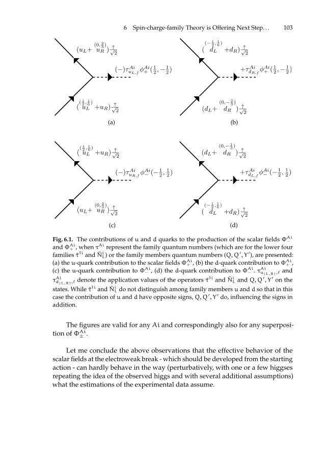
ii

“proc16” — 2016/12/12 — 10:17 — page 103 — #119 ii

ii

ii


(uL+(0, 23 )uR ) ↑√

2

(( 12 ,

16 )

uL +uR)↑√2

(−)τAiuL,f

φAi+ ( 12 ,−

12 )

(a)

((− 1

2 ,16 )

dL +dR)↑√2

(dL+(0,− 2

3 )

dR ) ↑√2

+τAidR,f

φAi+ ( 12 ,−

12 )

(b)

(( 12 ,

16 )

uL +uR)↑√2

(uL+(0, 23 )uR ) ↑√

2

(−)τAiuR,f

φAi− (− 1

2 ,12 )

(c)

(dL+(0,− 1

3 )

dR ) ↑√2

((− 1

2 ,16 )

dL +dR)↑√2

+τAidL,f

φAi− (− 1

2 ,12 )

(d)

Fig. 6.1. The contributions of u and d quarks to the production of the scalar fields ΦAi−

andΦAi+ , when τAi represent the family quantum numbers (which are for the lower fourfamilies τ1i and NiL) or the family members quantum numbers (Q,Q ′, Y ′), are presented:(a) the u-quark contribution to the scalar fields ΦAi+ , (b) the d-quark contribution to ΦAi+ ,(c) the u-quark contribution to ΦAi− , (d) the d-quark contribution to ΦAi− . τAiu(L,R),f

andτAid(L,R),f

denote the application values of the operators τ1i and NiL and Q,Q ′, Y ′ on thestates. While τ1i and NiL do not distinguish among family members u and d so that in thiscase the contribution of u and d have opposite signs, Q,Q ′, Y ′ do, influencing the signs inaddition.

The figures are valid for any Ai and correspondingly also for any superposi-tion of ΦAi± .

Let me conclude the above observations that the effective behavior of thescalar fields at the electroweak break - which should be developed from the startingaction - can hardly behave in the way (perturbatively, with one or a few higgsesrepeating the idea of the observed higgs and with several additional assumptions)what the estimations of the experimental data assume.

ii

“proc16” — 2016/12/12 — 10:17 — page 104 — #120 ii

ii

ii


6.4.3 Anomaly cancellation in the spin-charge-family theory

In the standard model triangle anomalies ”miraculously” disappear due to thefact that the sum of all possible traces Tr[τAiτBjτCk] (here τAi, τBi, τCk are thegenerators of one, of two or of three of the groups of SU(3), SU(2) and U(1)) overthe representations of one family of the left handed fermions and their antifermions(and separately of the right handed fermions and their antifermions), contributingto the triangle currents, are equal to zero [22–25].

Let me demonstrate that this cancellation of the standard model triangle anomalyfollows straightforwardly, if the SO(3, 1), SU(2), U(1) and SU(3) are the subgroupsof the orthogonal group SO(13, 1).

To the triangle anomaly the right-handed spinors (fermions) and antispinorscontribute with the opposite sign than the left handed spinors and their antispinors.Their common contribution to anomalies is proportional to [24]

(∑

(A,i,B,j,C,k)L L

Tr[τAi τBj τCk] −∑

(A,i,B,j,C,k)R R

Tr[τAi τBj τCk] ) , (6.35)

where τAi are in the standard model the generators of the infinitesimal transforma-tion of the groups SU(3)× SU(2)×U(1), while in the spin-charge-family theory τAi

are irreducible subgroups of the starting orthogonal group SO(2(2n+ 1) − 1, 1),n = 3. L L (R R) denote the left (right) handed spinors and their antispinors (right(left)), respectively.

In the first seven columns (up to to ||) of Table 6.7 the by the standard model as-sumed properties of the one family members, running in the triangle, are presented.The last two columns - taken from Table 6.2 - describe additional properties whichquarks and leptons (and antiquqrks and antileptons) would have, if the standardmodel groups SO(3, 1), SU(2), SU(3) and U(1) are embedded into the SO(13, 1)group. All the properties are needed to demonstrate that the ”miraculous” cancel-lation of the triangle anomalies is a ”trivial” one if one takes into account that thestandard model groups can easily be interpreted (unified) by making the next stepbeyond the standard model. The triangle anomaly of the standard model occurs if thetraces in Eq.(6.35) are not zero for either the left handed quarks and leptons andtheir antiparticles or the right handed quarks and leptons and their antiparticlesfor the Feynman triangle diagrams in which the gauge vector fields of the charges

U(1)×U(1)×U(1) ,SU(2)× SU(2)×U(1) ,SU(3)× SU(3)× SU(3) ,SU(3)× SU(3)×U(1) ,U(1)× gravitational (6.36)

contribute to the triangle anomaly.To see that embedding the standard model groups into the orthogonal group

SO(13, 1) makes the cancelltion of the triangle anomalies self evident, let us recog-nize: The subgroups of the SO(13, 1) group are SO(7, 1)×SO(6). The subgroups of

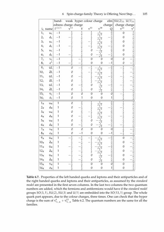
ii

“proc16” — 2016/12/12 — 10:17 — page 105 — #121 ii

ii

ii


hand- weak hyper colour charge elm SU(2)II U(1)IIedness charge charge charge charge charge

iL name Γ (3,1) τ13 Y τ33 τ38 Q τ23 τ4

1L uL −1 12

16

12

1

2√3

23

0 16

2L dL −1 − 12

16

12

1

2√3

− 13

0 16

3L uL −1 12

16

− 12

1

2√3

23

0 16

4L dL −1 − 12

16

− 12

1

2√3

− 13

0 16

5L uL −1 12

16

0 − 1√3

23

0 16

6L dL −1 − 12

16

0 − 1√3

− 13

0 16

7L νL −1 12

− 12

0 0 0 0 − 12

8L eL −1 − 12

− 12

0 0 −1 0 − 12

9L uL −1 0 − 23

− 12

− 1

2√3

− 23

− 12

− 16

10L dL −1 0 13

− 12

− 1

2√3

13

12

− 16

11L uL −1 0 − 23

12

− 1

2√3

− 23

− 12

− 16

12L dL −1 0 13

12

− 1

2√3

13

12

− 16

13L uL −1 0 − 23

0 1√3

− 23

− 12

− 16

14L dL −1 0 13

0 1√3

13

12

− 16

15L νL −1 0 0 0 0 0 − 12

12

16L eL −1 0 1 0 0 1 12

12

1R uR 1 0 23

12

1

2√3

23

12

16

2R dR 1 0 − 13

12

1

2√3

− 13

− 12

16

3R uR 1 0 23

− 12

1

2√3

23

12

16

4R dR 1 0 − 13

− 12

1

2√3

− 13

− 12

16

5R uR 1 0 23

0 − 1√3

23

12

16

6R dR 1 0 − 13

0 − 1√3

− 13

− 12

16

7R νR 1 0 0 0 0 0 12

− 12

8R eR 1 0 −1 0 0 −1 − 12

− 12

9R uR 1 − 12

− 16

− 12

− 1

2√3

− 23

0 − 16

10R dR 1 12

− 16

− 12

− 1

2√3

13

0 − 16

11R uR 1 − 12

− 16

12

− 1

2√3

− 23

0 − 16

12R dR 1 12

− 16

12

− 1

2√3

13

0 − 16

13R uR 1 − 12

− 16

0 1√3

− 23

0 − 16

14R dR 1 12

− 16

0 1√3

13

0 − 16

15R νR 1 − 12

12

0 0 0 0 12

16R eR 1 12

12

0 0 1 0 12

Table 6.7. Properties of the left handed quarks and leptons and their antiparticles and ofthe right handed quarks and leptons and their antiparticles, as assumed by the standardmodel are presented in the first seven columns. In the last two columns the two quantumnumbers are added, which the fermions and antifermions would have if the standard modelgroups SO(3, 1), SU(2), SU(3) and U(1) are embedded into the SO(13, 1) group. The wholequark part appears, due to the colour charges, three times. One can check that the hypercharge is the sum of τ4iL,R + τ23iL,R Table 6.2. The quantum numbers are the same for all thefamilies.

ii

“proc16” — 2016/12/12 — 10:17 — page 106 — #122 ii

ii

ii


SO(6) are the colour group SU(3) with the generators denoted by τ3i, i = 1, . . . , 8and the U(1) (we shall call it U(1)II) group with the generator τ4. One sees that allthe quarks have τ4 = 1

6, all the antiquarks have τ4 = −1

6, while the leptons have

τ4 = −12

and antileptons have τ4 = 12

. Correspondingly the trace of τ4 over all thefamily members is equal to zero.

The subgroups of the SO(7, 1), as seen in Table 6.2, have as subgroups SO(3, 1)×SU(2)I × SU2II, with the generators τ1i (representing the weak group operators)and τ2i (representing the generators of the additional SU(2) group), respectively.The left handed spinors are SU(2)I (weak) doublets and SU(2)II singlets, while theright handed spinors are the SU(2)I (weak) singlets and SU(2)II doublets. Corre-spondingly are the left handed antispinors the SU(2)I (weak) singlets and SU(2)IIdoublets, while the right handed antispinors are the SU(2)I (weak) doublets andthe SU(2)II singlets.

The hypercharge of the standard model corresponds to the sum of τ4 and τ23

Y = τ4 + τ23 . (6.37)

For the triangle Feynman diagram, to which three hyper U(1) boson fieldscontribute, we must evaluate

∑i Tr(Yi)

3, in which the sum runs over all themembers (i) of the left handed spinors and antispinors, and of the right handedspinors and antispinors separately. In the case of embedding the standard modelgroups into SO(13, 1) we have∑

iL,R

(YiL,R)3 =∑iL,R

(τ4iL,R + τ23iL,R)3

=∑iL,R

(τ4iL,R)3 +∑iL,R

(τ23iL,R)3

+∑iL,R

3.(τ4iL,R)2.τ23iL,R +

∑iL,R

3.τ4iL,R .(τ23iL,R

)2 , (6.38)

for either the left, iL, or the right, iR, handed members. Table 6.7 demonstratesclearly (last column) that

∑iL

(τ4iL)3 = 0, when the contribution of the left (right)

handed spinors and antispinors are taken into account.Table 6.7 also demonstrates (the last but one column) that

∑iL3.(τ4iL)

2.τ23iL =

0 even more trivially since the contribution of either spinors or antispinors - left orright handed - separately are equal to zero.

The easiest is to evaluate∑iL,R

(τ23iL )3 = 0 and

∑iL3.(τ4iL)

2.τ23iL = 0 since,as seen from Table 6.7, the summation separately within the quarks and leptonrepresentations give zero.

Since all the members belong to one spinor representation, it is straightfor-wardly that all the triangle traces are zero, if the standard model groups are thesubgroups of the orthogonal group SO(13, 1).

From only the standard model assumptions point of view the cancellation ofthe triangle anomalies does look miraculously. For our

∑iL,R

(YiL,R)3 one obtains

for the left handed members: [3.2.(16)3 + 2.(−1

2)3 + 3.((−2

3)3 + (1

3)3) + 13) ], and

for the right handed members: [3.((23)3 + (−1

3)3) + (−1)3) + 3.2.(−1

6)3 + 2.(1

2)3 ].

ii

“proc16” — 2016/12/12 — 10:17 — page 107 — #123 ii

ii

ii


6.4.4 Dark matter in the spin-charge-family theory

As discussed in Sect. 6.2 the spin-charge-family theory [5,3,6–10,4,11–17,2,1] predictsin the low energy region two decoupled groups of four families. In Ref. [13] thepossibility that the dark matter consists of clusters of the fifth family - the stableheavy family of quarks and leptons (with (amost) zero Yukawa couplings to thelower group of four families) - is discussed.

I presented here a very short overview through the estimation done in Ref. [13].In this reference we made a rough, but to our knowledge a reasonable, estimationof the properties of baryons of this fifth family members, following the behaviourof quarks during the evolution of the universe up to 1 GeV and through the colourphase transition. We also estimate the behaviour of the neutral clusters whenscattering among themselves and with the ordinary matter. We studied possiblelimitations on the family properties due to the cosmological evidences, the directexperimental evidences ([13], Sect. IV) and all others known properties of the darkmatter.

We used the simple hydrogen-like model to evaluate the properties of theseheavy baryons and their interaction among themselves and with the ordinarynuclei, taking into account that for masses of the order of 1 TeV or larger the onegluon exchange determines the force among the constituents of the fifth familybaryons ([13], Sect. II). Due to their very large masses ”the nuclear interaction”among these baryons has very interesting properties. We concluded that it is thefifth family neutron, which is very probably the most stable nucleon.

We followed the behaviour of the fifth family quarks and antiquarks in theplasma of the expanding universe, through the freezing out procedure solving theBoltzmann equations, through the colour phase transition, while forming neutrons,up to the present dark matter ([13], Sect. III).

The cosmological evolution suggested the limits for the masses of the fifthfamily quarks

10 TeV < mq5 c2 < a few · 102 TeV (6.39)

and for the scattering cross sections

10−8 fm2 < σc5 < 10−6 fm2 , (6.40)

while the measured density of the dark matter does not put much limitation onthe properties of heavy enough clusters.

The direct measurements limited the fifth family quark mass to ([13], Sect. IV.)

several 10TeV < mq5c2 < 105 TeV . (6.41)

We also find that our fifth family baryons of the mass of a few 10 TeV/c2 havefor a factor more than 100 times too small scattering amplitude with the ordinarymatter to cause a measurable heat flux on the Earth’s surface.

ii

“proc16” — 2016/12/12 — 10:17 — page 108 — #124 ii

ii

ii


6.4.5 Matter-antimatter in the spin-charge-family theory

I shortly overview in this section the properties, quantum numbers, and discretesymmetries of those scalar and vector gauge fields appearing in the starting action(Eqs. (6.1, 6.2) which cause transitions of antileptons into quarks and back, andantiquarks into quarks and back. The appearance of the condensate breaks thissymmetry making possible under non thermal conditions the ordinary (mostlymade of the first family members) matter-antimatter asymmetry. The reader canfind details in Ref. [2].

Scalar gauge fields, contributing to matter-antimatter asymmetry and causingalso the proton decay carry the triplet or antitriplet colour charges (see Table 6.8)and the fractional hyper and electromagnetic charge.

The Lagrange densities from Eqs. (6.1, 6.2) manifest CN · PN invariance. Allthe vector and the spinor gauge fields are before the appearance of the conden-sate (Subsect. 6.3.4) massless and reactions creating particles from antiparticlesand back go in both directions equivalently. Correspondingly there is no matter-antimatter asymmetry. It is the condensate, which breaks this symmetry

Let me analyse the Lagrange density of Eq. (6.2) before the appearance of thecondensate. The term γt 1

2Ss′s"ωs ′s"t can be rewritten as follows

γt1

2Ss′s"ωs ′s"t =

∑+,−

∑(t t ′)

tt ′

(±©)1

2Ss′s"ω

s"s"tt ′(±©)

,

ωs"s"

tt ′(±©)

: = ωs"s"

tt ′(±)

= (ωs ′s"t ∓ iωs ′s"t ′) ,

tt ′

(±©): =tt ′

(±)= 1

2(γt ± γt

′) ,

(t t ′) ∈ ((9 10), (11 12), (13 14)) . (6.42)

I introduced the notationstt ′

(±©) andωs"s"

tt ′(±©)

to distinguish among different super-

position of states in equations below.

The expressiontt ′

(±©) 12Ss′s" ω

s"s"tt ′(±©)

can be further rewritten as follows

tt ′

(±©)1

2Ss′s"ω

s"s"tt ′(±©)

=

tt ′

(±©) τ2+A2+tt ′(±©)

+ τ2−A2−tt ′(±©)

+ τ23A23tt ′(±©)

+ τ1+A1+tt ′(±©)

+ τ1−A1−tt ′(±©)

+ τ13A13tt ′(±©)

,

A2±tt ′(±©)

= (ω58tt ′(±©)

+ω67tt ′(±©)

) ∓ i(ω57tt ′(±©)

−ω68tt ′(±©)

) ,

A23tt ′(±©)

= (ω56tt ′(±©)

+ω78tt ′(±©)

) ,

A1±tt ′(±©)

= (ω58tt ′(±©)

−ω67tt ′(±©)

) ∓ i(ω57tt ′(±©)

+ω68tt ′(±©)

) ,

A13tt ′(±©)

= (ω56tt ′(±©)

−ω78tt ′(±©)

) .

(6.43)

ii

“proc16” — 2016/12/12 — 10:17 — page 109 — #125 ii

ii

ii


Equivalently one expresses the term γt 12Sab ωabt in Eq. (6.2) with Sab as the

infinitesimal generators of either SO(3, 1) or SO(4) and ωabt belonging to thecorresponding gauge fields with t = (9, . . . , 14), by using Eqs. (6.70 - 6.73), as

γt1

2Sab ωabt =

tt ′

(±©)1

2Sab ω

abtt ′(±©)

=

tt ′

(±©) τ2+ A2+tt ′(±©)

+ τ2− A2−tt ′(±©)

+ τ23 A23tt ′(±©)

+

τ1+ A1+tt ′(±©)

+ τ1− A1−tt ′(±©)

+ τ13 A13tt ′(±©)

+

N+R A

NR+tt ′(±©)

+ N−R A

NR−tt ′(±©)

+ N3R ANR3tt ′(±©)

+

N+L A

NL+tt ′(±©)

+ N−L A

NL−tt ′(±©)

+ N3L ANL3tt ′(±©)

,

ANR±tt ′(±©)

= (ω23tt ′(±©)

− i ω01tt ′(±©)

) ∓ i(ω31tt ′(±©)

− i ω02tt ′(±©)

) ,

ANR3tt ′(±©)

= (ω12tt ′(±©)

− i ω03tt ′(±©)

) ,

ANL±tt ′(±©)

= (ω23tt ′(±©)

+ i ω01tt ′(±©)

) ∓ i(ω31tt ′(±©)

+ i ω02tt ′(±©)

) ,

ANR3tt ′(±©)

= (ω12tt ′(±©)

+ i ω03tt ′(±©)

) .

(6.44)

The expressions for

A2±tt ′(±©)

, A23tt ′(±©)

, A1±tt ′(±©)

and A13tt ′(±©)

can easily be obtained from Eq.(6.43) by replacing in expressions for

A2±tt ′(±©)

, A23tt ′(±©)

, A1±tt ′(±©)

and A13tt ′(±©)

,

respectively,ωs ′s"

tt ′(±©)

by ωs ′s"

tt ′(±©)

.

The term γt 12St′t"ωt ′t"t in Eq. (6.2) can be rewritten with respect to the

generators St′t" and the corresponding gauge fields ωs ′s"t as one colour octet

scalar field and one U(1)II singlet scalar field (Eq. 6.69)

γt1

2St"t

′"ωt"t ′"t =∑+,−

∑(t t ′)

tt ′

(±©) ~τ3 · ~A3tt ′(±©)

+ τ4 ·A4tt ′(±©)

,

(t t ′) ∈ ((9 10), 11 12), 13 14)) . (6.45)

ii

“proc16” — 2016/12/12 — 10:17 — page 110 — #126 ii

ii

ii


Considering all the above equations (6.42 - 6.45), and leaving out p tt ′(±©)

since

in the low energy limit the momentum does not play any role, it follows

Lf" = ψ† γ0(−) ∑+,−

∑(t t ′)

tt ′

(±©) ·

[ τ2+A2+tt ′(±©)

+ τ2−A2−tt ′(±©)

+ τ23A23tt ′(±©)

+ τ1+A1+tt ′(±©)

+ τ1−A1−tt ′(±©)

+ τ13A13tt ′(±©)

+ τ2+ A2+tt ′(±©)

+ τ2− A2−tt ′(±©)

+ τ23 A23tt ′(±©)

+ τ1+ A1+tt ′(±©)

+ τ1− A1−tt ′(±©)

+ τ13 A13tt ′(±©)

+ N+R A

NR+tt ′(±©)

+ N−R A

NR−tt ′(±©)

+ N3R ANR3tt ′(±©)

+ N+L A

NL+tt ′(±©)

+ N−L A

NL−tt ′(±©)

+ N3L ANL3tt ′(±©)

+∑i

τ3iA3itt ′(±©)

+ τ4A4tt ′(±©)

+∑i

τ3i A3itt ′(±©)

+ τ4 A4tt ′(±©)

] ψ , (6.46)

where (t, t ′) run in pairs over [(9, 10), . . . (13, 14)] and the summation must goover + and − of tt ′

(±©)

.

On Table 6.8, taken from Ref. [2], the quantum numbers of the scalar andvector gauge fields, appearing in Eq. (6.2), are presented, where it is taken intoaccount that the spin of gauge fields is determined according to Eq. (6.47),

(Sab)ceAd...e...g = i (ηacδbe − η

bcδae )Ad...e...g , (6.47)

for each index (∈ (d . . . g)) of a bosonic field Ad...g separately. We must take intoaccount also the relation among Sab and the charges (the relations are, of course,the same for bosons and fermions), presented in Eqs. (6.67, 6.68, 6.69)). The scalarfields with the scalar index s = (9, 10, · · · , 14), presented in Table 6.8, carry one ofthe triplet colour charges and the ”spinor” charge equal to twice the quark ”spinor”charge, or the antitriplet colour charges and the anti ”spinor” charge. They carryin addition the quantum numbers of the adjoint representations originating in Sab

or in Sab 14.Let us choose the 57th line of Table 6.2, which represents in the spinor tech-

nique the left handed positron, e+L , to see what do the scalar fields, appearing inEq. (6.46) and in Table 6.8, do when applying on the left handed members of the

14 Although carrying the colour charge in one of the triplet or antitriplet states, these fieldscan not be interpreted as superpartners of the quarks since they do not have quantumnumbers as required by, let say, the N = 1 supersymmetry. The hyper charges and theelectromagnetic charges are namely not those required by the supersymmetric partnersto the family members.

ii

“proc16” — 2016/12/12 — 10:17 — page 111 — #127 ii

ii

ii


field prop. τ4 τ13 τ23 (τ33, τ38 ) Y Q τ4 τ13 τ23 N3LN3R

A1±

9 10(±©)

scalar ∓© 13± 1 0 (±© 1

2, ±© 1

2√3

) ∓© 13

∓© 13

+ ∓ 1 0 0 0 0 0

A139 10(±©)

scalar ∓© 13

0 0 (±© 12, ±© 1

2√3

) ∓© 13

∓© 13

0 0 0 0 0

A1±

11 12(±©)

scalar ∓© 13∓ 1 0 (∓© 1

2, ±© 1

2√3

) ∓© 13

∓© 13

+ ∓ 1 0 0 0 0 0

A1311 12(±©)

scalar ∓© 13

0 0 (∓© 12, ±© 1

2√3

) ∓© 13

∓© 13

0 0 0 0 0

A1±

13 14(±©)

scalar ∓© 13∓ 1 0 (0, ∓© 1√

3) ∓© 1

3∓© 13

+ ∓ 1 0 0 0 0 0

A1313 14(±©)

scalar ∓© 13

0 0 (0, ∓© 1√3

) ∓© 13

∓© 13

0 0 0 0 0

A2±

9 10(±©)

scalar ∓© 13

0 ± 1 (±© 12, ±© 1

2√3

) ∓© 13

+ ∓ 1 ∓© 13

+ ∓ 1 0 0 0 0 0

A239 10(±©)

scalar ∓© 13

0 0 (±© 12, ±© 1

2√3

) ∓© 13

∓© 13

0 0 0 0 0

· · ·

A1±

910(±©)

scalar ∓© 13

0 0 (±© 12, ±© 1

2√3

) ∓© 13

∓© 13

0 ± 1 0 0 0

A13910(±©)

scalar ∓© 13

0 0 (±© 12, ±© 1

2√3

) ∓© 13

∓© 13

0 0 0 0 0

· · ·

A2±

910(±©)

scalar ∓© 13

0 0 (±© 12, ±© 1

2√3

) ∓© 13

∓© 13

0 0 ± 1 0 0

A23910(±©)

scalar ∓© 13

0 0 (±© 12, ±© 1

2√3

) ∓© 13

∓© 13

0 0 0 0 0

· · ·

ANL±

910(±©)

scalar ∓© 13

0 0 (±© 12, ±© 1

2√3

) ∓© 13

∓© 13

0 0 0 ± 1 0

ANL3

910(±©)

scalar ∓© 13

0 0 (±© 12, ±© 1

2√3

) ∓© 13

∓© 13

0 0 0 0 0

· · ·

ANR±

910(±©)

scalar ∓© 13

0 0 (±© 12, ±© 1

2√3

) ∓© 13

∓© 13

0 0 0 0 ± 1

ANR3

910(±©)

scalar ∓© 13

0 0 (±© 12, ±© 1

2√3

) ∓© 13

∓© 13

0 0 0 0 0

· · ·

A3i9 10(±©)

scalar ∓© 13

0 0 (± 1+ ±© 12, ±© 1

2√3

) ∓© 13

∓© 13

0 0 0 0 0

· · ·A4910(±©)

scalar ∓© 13

0 0 (±© 12, ±© 1

2√3

) ∓© 13

∓© 13

0 0 0 0 0

· · ·~A3m vector 0 0 0 octet 0 0 0 0 0 0 0

A4m vector 0 0 0 0 0 0 0 0 0 0 0

Table 6.8. Quantum numbers of the scalar gauge fields carrying the space index t =

(9, 10, · · · , 14), appearing in Eq. (6.2), are presented. To the colour charge of all these scalarfields the space degrees of freedom contribute one of the triplets values. These scalars arewith respect to the two SU(2) charges, (τ13 and ~τ2), and the two SU(2) charges, (~τ1 and~τ2), triplets (that is in the adjoint representations of the corresponding groups), and theyall carry twice the ”spinor” number (τ4) of the quarks. The quantum numbers of the twovector gauge fields, the colour and the U(1)II ones, are added.

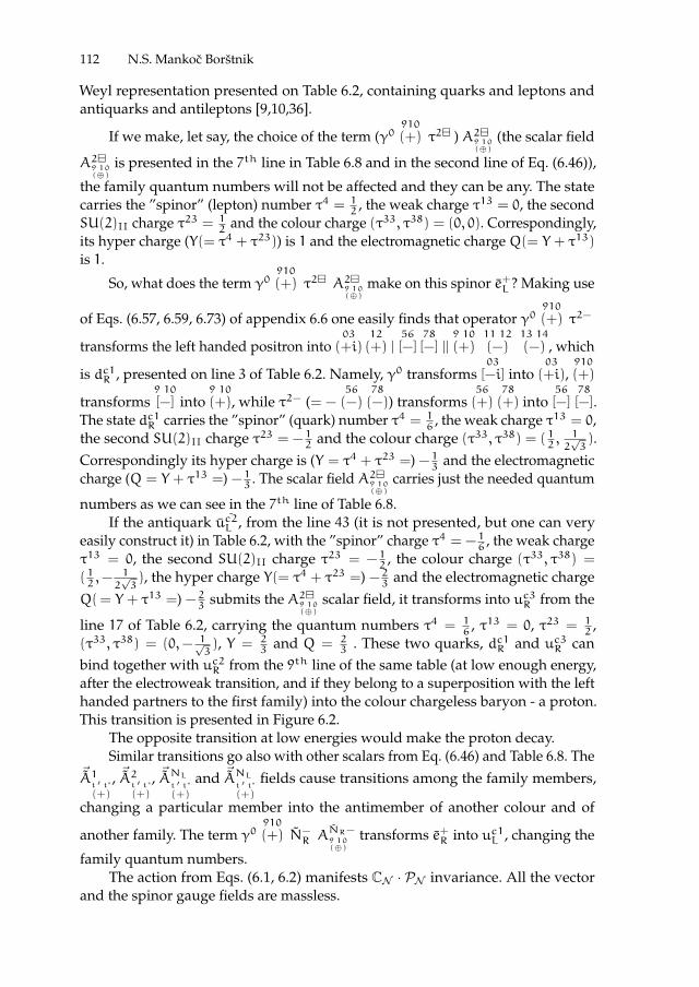
ii

“proc16” — 2016/12/12 — 10:17 — page 112 — #128 ii

ii

ii


Weyl representation presented on Table 6.2, containing quarks and leptons andantiquarks and antileptons [9,10,36].

If we make, let say, the choice of the term (γ0910

(+) τ2 ) A29 10(⊕)

(the scalar field

A29 10(⊕)

is presented in the 7th line in Table 6.8 and in the second line of Eq. (6.46)),

the family quantum numbers will not be affected and they can be any. The statecarries the ”spinor” (lepton) number τ4 = 1

2, the weak charge τ13 = 0, the second

SU(2)II charge τ23 = 12

and the colour charge (τ33, τ38) = (0, 0). Correspondingly,its hyper charge (Y(= τ4 + τ23)) is 1 and the electromagnetic charge Q(= Y + τ13)

is 1.

So, what does the term γ0910

(+) τ2 A29 10(⊕)

make on this spinor e+L ? Making use

of Eqs. (6.57, 6.59, 6.73) of appendix 6.6 one easily finds that operator γ0910

(+) τ2−

transforms the left handed positron into03

(+i)12

(+) |56

[−]78

[−] ||9 10

(+)11 12

(−)13 14

(−) , which

is dc1R , presented on line 3 of Table 6.2. Namely, γ0 transforms03

[−i] into03

(+i),910

(+)

transforms9 10

[−] into9 10

(+), while τ2− (= −56

(−)78

(−)) transforms56

(+)78

(+) into56

[−]78

[−].The state dc1R carries the ”spinor” (quark) number τ4 = 1

6, the weak charge τ13 = 0,

the second SU(2)II charge τ23 = −12

and the colour charge (τ33, τ38) = (12, 1

2√3).

Correspondingly its hyper charge is (Y = τ4 + τ23 =) −13

and the electromagneticcharge (Q = Y + τ13 =) −1

3. The scalar field A29 10

(⊕)

carries just the needed quantum

numbers as we can see in the 7th line of Table 6.8.If the antiquark uc2L , from the line 43 (it is not presented, but one can very

easily construct it) in Table 6.2, with the ”spinor” charge τ4 = −16

, the weak chargeτ13 = 0, the second SU(2)II charge τ23 = −1

2, the colour charge (τ33, τ38) =

(12,− 1

2√3), the hyper charge Y(= τ4 + τ23 =) −2

3and the electromagnetic charge

Q(= Y + τ13 =) −23

submits the A29 10(⊕)

scalar field, it transforms into uc3R from the

line 17 of Table 6.2, carrying the quantum numbers τ4 = 16

, τ13 = 0, τ23 = 12

,(τ33, τ38) = (0,− 1√

3), Y = 2

3and Q = 2

3. These two quarks, dc1R and uc3R can

bind together with uc2R from the 9th line of the same table (at low enough energy,after the electroweak transition, and if they belong to a superposition with the lefthanded partners to the first family) into the colour chargeless baryon - a proton.This transition is presented in Figure 6.2.

The opposite transition at low energies would make the proton decay.Similar transitions go also with other scalars from Eq. (6.46) and Table 6.8. The

~A1t ′ t"(+)

, ~A2t ′ t"(+)

, ~ANLt ′ t"(+)

and ~ANLt ′ t"(+)

fields cause transitions among the family members,

changing a particular member into the antimember of another colour and of

another family. The term γ0910

(+) N−R A

NR−9 10(⊕)

transforms e+R into uc1L , changing the

family quantum numbers.The action from Eqs. (6.1, 6.2) manifests CN · PN invariance. All the vector

and the spinor gauge fields are massless.

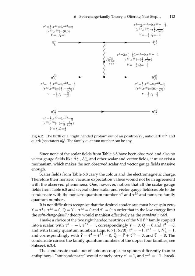
ii

“proc16” — 2016/12/12 — 10:17 — page 113 — #129 ii

ii

ii


uc2Rτ4= 1

6 ,τ13=0,τ23= 1

2

(τ33,τ38)=(− 12 ,

12√

3)

Y= 23 ,Q= 2

3

uc2R

uc2Lτ4=− 1

6 ,τ13=0,τ23=− 1

2

(τ33,τ38)=( 12 ,−1

2√

3)

Y=− 23 ,Q=− 2

3

uc3Rτ4= 1

6 ,τ13=0,τ23= 1

2

(τ33,τ38)=(0,− 1√3)

Y= 16 ,Q= 2

3

e+L

τ4= 12 ,τ

13=0,τ23= 12

(τ33,τ38)=(0,0)Y=1,Q=1

dc1R

τ4= 16 ,τ

13=0,τ23=− 12

(τ33,τ38)=( 12, 12√

3)

Y=− 13 ,Q=− 1

3

•

A2!9 10(+)

,τ4=2×(− 1

6 ),τ13=0,τ23=−1

(τ33,τ38)=( 12 ,1

2√

3)

Y=− 43 ,Q=− 4

3

•

Fig. 6.2. The birth of a ”right handed proton” out of an positron e+L , antiquark uc2L andquark (spectator) uc2R . The family quantum number can be any.

Since none of the scalar fields from Table 6.8 have been observed and also novector gauge fields like ~A2m, A4m and other scalar and vector fields, it must exist amechanism, which makes the non observed scalar and vector gauge fields massiveenough.

Scalar fields from Table 6.8 carry the colour and the electromagnetic charge.Therefore their nonzero vacuum expectation values would not be in agreementwith the observed phenomena. One, however, notices that all the scalar gaugefields from Table 6.8 and several other scalar and vector gauge fieldscouple to thecondensate with the nonzero quantum number τ4 and τ23 and nonzero familyquantum numbers.

It is not difficult to recognize that the desired condensate must have spin zero,Y = τ4+ τ23 = 0,Q = Y + τ13 = 0 and ~τ1 = 0 in order that in the low energy limitthe spin-charge-family theory would manifest effectively as the standard model.

I make a choice of the two right handed neutrinos of the VIIIth family coupledinto a scalar, with τ4 = −1, τ23 = 1, correspondingly Y = 0, Q = 0 and ~τ1 = 0,and with family quantum numbers (Eqs. (6.71, 6.70)) τ4 = −1, τ23 = 1, N3R = 1,and correspondingly with Y = τ4 + τ23 = 0, Q = Y + τ13 = 0, and ~τ1 = 0. Thecondensate carries the family quantum numbers of the upper four families, seeSubsect. 6.3.4.

The condensate made out of spinors couples to spinors differently than toantispinors - ”anticondensate” would namely carry τ4 = 1, and τ23 = −1 - break-

ii

“proc16” — 2016/12/12 — 10:17 — page 114 — #130 ii

ii

ii


ing correspondingly the CN · PN symmetry: The reactions creating particles fromantiparticles are not any longer symmetric to those creating antiparticle fromparticles.

Such a condensate leaves the hyper field AYm (= sin ϑ2A23m + cos ϑ2A4m) (forthe choice that sin ϑ2 = cos ϑ2 and g4 = g2, there is no justification for such achoice, AYm = 1√

2(A23m +A4m) follows) massless, while it gives masses to A2±m and

AY′

m (= 1√2(A4m−A23m ) for sin ϑ2 = cos ϑ2) and it gives masses also to all the scalar

gauge fields from Table 6.8, since they all couple to the condensate through τ4.The weak vector gauge fields, ~A1m, the hyper charge vector gauge fields, AYm,

and the colour vector gauge fields, ~A1m, remain massless.The scalar fields with the scalar space index s = (7, 8) (there are three singlets

which couple to all eight families, two triplets which couple only to the upper fourfamilies and another two triplets which couple only to the lower four families) -carrying the weak and the hyper charges of the Higgs’s scalar - wait for gainingnonzero vacuum expectation values to change their masses while causing theelectroweak break.

The condensate does what is needed so that in the low energy regime thespin-charge-family manifests as an effective theory which agrees with the standardmodel to such an extent that it is in agreement with the observed phenomena,explaining the standard model assumptions and predicting new fermion and bosonfields.

It also may hopefully explain the observed matter-antimatter asymmetry ifthe conditions in the expanding universe would be appropriate, Ref. ([2], Sect.VI.). The work needed to check these conditions in the expanding universe withinthe spin-charge-family theory is very demanding. Although we do have someexperience with following the history of the expanding universe [13], this studyneeds much more efforts, not only in calculations, but also in understanding themechanism of the condensate appearance, relations among the velocity of theexpansion, the temperature and the dimension of space-time in the period of theappearance of the condensate. This study has not yet been really started.

6.5 Conclusions

To better understand the history of the universe and also to make next step inunderstanding the dynamics of the elementary fermion fields and boson (vectorand scalar) gauge fields it is needed to explain the assumptions of the standardmodel, as well as the phenomena like the existence of the dark matter, matter-antimatter asymmetry and dark energy.

There must be understood the origin of: A. the family members quantumnumbers, B. the family quantum numbers, C. the origin of vector gauge fields, D.the origin of the higgs and Yukawa couplings.

One of the most urgent questions in the elementary particle physics is: Wheredo the families originate? Explaining the origin of families would answer the questionabout the number of families which are possibly observable at the low energy

ii

“proc16” — 2016/12/12 — 10:17 — page 115 — #131 ii

ii

ii


regime, about the origin of the scalar field(s) and the Yukawa couplings (thecouplings of fermions to the scalar field(s)), about the differences in the fermionsproperties - the differences in the masses and mixing matrices among familymembers – quarks and leptons, as well as about the hierarchy in quark and leptonmasses.

I demonstrated in this talk, that the spin-charge-family theory - starting withthe simple action in d = (13+ 1) for fermions and bosons - offers the explanationfor all the assumptions of the standard model:a. The theory explains all the properties of the family members - quarks andleptons, left and right handed, and their right and left handed antiquarks andantileptons 15, explaining why the left handed spinors carry the weak charge whilethe right handed do not (the right handed neutrino is the regular member of eachfamily).b. It explains the appearance and the properties of the families of family mem-bers.c. It explains the existence of the gauge vector fields of the family memberscharges.d. It explains the appearance and the properties of the scalar field (the higgs)and the Yukawa couplings.

All the gauge fields, vector and scalar in d = (3+ 1), origin in vielbeins andthe two kinds of spin connection fields in d = (13 + 1) - the gravity. If there areno spinors present, are the two spin connections expressible uniquely with thevielbeins [42].It also offers the explanation for the phenomena, which are not part of the standardmodel, like:e. It explains the existence of the dark matter.f. It explain the origin of the (ordinary) matter-antimatter asymmetry.

6.5.1 Predictions for the future experiments

The theory predicts:g. There are twice two groups of four families of quarks and leptons at lowenergies.g.i. The fourth family with masses above 1 TeV, weakly coupled to the observedthree families, will be measured at the LHC.g.ii. The quarks and leptons of the fifth family - that is of the stable one of theupper four families - form the dark matter. The family members, which formthe chargeless clusters, manifest, due to their very heavy masses, a ”new nuclearforce”.15 One Weyl representation of SO(13 + 1) contains, if analyzed with respect to the standard

model groups, all the members of one family, the coloured quarks and colourless leptons,and the anticoloured antiquarks and (anti)colourless antileptons, with the left handedleptons carrying the weak charge and the right handed ones weak chargeless, while theleft handed antispinors are weak chargeless and the right handed ones carry the weakcharge.

ii

“proc16” — 2016/12/12 — 10:17 — page 116 — #132 ii

ii

ii


h. The predicted scalar fields with the space index (7, 8) manifest in (d = (3+ 1))

as the weak and hyper charges doublets (as required by the standard model higgs)with respect to the space index. These scalars carry in addition:h.i. Either they carry one of the three family members quantum numbers, (Q,Q ′, Y ′)- belonging correspondingly to one of three singlets.h.ii. Or they carry family quantum numbers - belonging correspondingly to oneof the twice two triplets.h.iii. The three singlets and the two triplets determine mass matrices of the lowerfour families, contributing to masses of the heavy vector bosons.h.iv. These scalars determine the observed higgs and the Yukawa couplings.i. The predicted scalar fields with the space index (9, 10, .., 14) are triplets withrespect to the space index. They cause the transitions from antileptons into quarksand antiquarks into quarks and back.i.i. The condensate breaks the matter-antimatter symmetry, causing the asymme-try in the (ordinary) matter with respect to antimatter.i.ii. These condensate is responsible also for the proton decay.j. The condensate is a scalar of the two right handed neutrinos with the familyquantum numbers of the upper four families.k. The condensate gives masses to all the gauge fields with which it interacts.k.i. It gives masses to all scalar fields and to vector fields, leaving massless onlythe colour, the weak, the hyper vector gauge fields and the gravity in ((3+ 1)).l. There is the SU(2) (belonging together with the weak SU(2) to SO(4) gaugefields included in SO(7, 1)) vector gauge field, which gain masses of the order ofthe appearance of the condensate.m. At the electroweak break the scalar fields with the space index (7, 8) changetheir mutual interaction, and gaining nonzero vacuum expectation values, breakthe weak and the hyper charges and correspondingly the mass protection offermions, making them massive.n. The symmetry of mass matrices allow, in the case that the experimental datafor the mixing submatrix 3× 3 of the 4× 4mixing matrix would be accurate, todetermine the mixing matrix and the masses of the fourth family quarks. Theaccuracy, with which the masses of the six lower families are measured so far,does not influence the results appreciably. Due to uncertainty of the experimentaldata for the 3× 3mixing submatrix we are only able to determine the 4× 4 quarkmixing matrix for a chosen masses of the the fourth family quarks. However, wealso predict how will the 3× 3 submatrix of the mixing matrix change with moreaccurate measurements.n.i. The fourth family quarks mass matrices are for masses above 1 TeV closer andcloser to the democratic matrices. The less the scalars with the family membersquantum numbers contribute to masses of the fourth family quarks, the closer ismu4 tomd4 .n.ii. The large contribution of the scalars with the family members quantum num-bers (Q,Q ′, Y ′) to the masses of the lower four families manifests in the largedifferences of quarks masses of the lower four families.n.iii. Although we have done calculations also for leptons, must further analysesof their properties wait for more accurate experimental data.

ii

“proc16” — 2016/12/12 — 10:17 — page 117 — #133 ii

ii

ii


o. In the case that the u4 and d4 quarks have similar masses - determined mostlyby the scalar fields carrying the family quantum numbers - they contribute mostlyto the production of these scalars, while their contribution to the production ofthose scalars which carry the family members quantum numbers - to the higgs inparticular - is much weaker, which is in agreement with the experiment 16.p. All the degrees of freedom discussed in this talk are already a part of thesimple starting action Eq.(6.1).p.i. The way of breaking symmetries (ordered by the conditions determining thehistory of our universe) is assumed so that it leads in d = (3+ 1) to the observablesymmetries, although we could in principle derive it from the starting action andboundary conditions.p.ii. Also the effective interaction among scalar fields is assumed, although wecould derive it in principle from the starting action and the boundary conditions.r. The spin-charge-family theory easily explains what in the standard model seemslike a miracle: no triangle anomalies.s. A lot of efforts has been put in this theory to show that it could work as a nextstep below the standard model proving like:s.i. There is possibility in the Kaluza-Klein-like theory that breaking symmetriescan leave fermions massless.s.ii. That vielbeins in the Kaluza-Klein theories and spin-connections in the spin-charge-family theory represent the same vector gauge fields in d = (3+ 1).

6.5.2 Open questions in the spin-charge-family theory

There are several open problem in the spin-charge-family theory:t. Since this theory is, except that fermions carry two kinds of spins - one kindtaking care of spin and charges, the second one taking care of families - a kind ofthe Kaluza-Klein theories, it shares at very high energy with these theories thequantization problem.u. The dimension of space-time, d = (13+ 1), is in the spin-charge-family theorychosen, since SO(13, 1) contains all the members, assumed in the standard model.It contains also the right handed neutrino (which carries the Y ′ quantum number.)u.i. It should be shown, however, how has nature ”made the decision” in evolutionto go through this dimension and what is indeed the dimension of space-time(infinite?).v. There are many other open question, like:v.i. What is the reason for the (so small) dark energy?v.ii. At what energy the electroweak phase transition occurs? (Let me add thatthere is the answer within the spin-charge-family theory to this open problem.)v.iii. Why do we have fermions and bosons? [43]

It is encouraging that the more work is done on this theory the more answersto the open questions is found.

16 The coupling constants of the singlet scalar fields differ among themselves and also fromthe coupling constants of the two triplet scalar fields

ii

“proc16” — 2016/12/12 — 10:17 — page 118 — #134 ii

ii

ii


6.6 Appendix: Short presentation of spinor technique [1,7,31,32]

This appendix is a short review (taken from [4]) of the technique [7,33,31,32],initiated and developed in Ref. [7], while proposing the spin-charge-family the-ory [5,3,6–10,4,11–17,2,1]. All the internal degrees of freedom of spinors, with fam-ily quantum numbers included, are describable in the space of d-anticommuting(Grassmann) coordinates [7], if the dimension of ordinary space is also d. There aretwo kinds of operators in the Grassmann space fulfilling the Clifford algebra andanticommuting with one another Eq.(6.48). The technique was further developedin the present shape together with H.B. Nielsen [33,31,32].

In this last stage we rewrite a spinor basis, written in Ref. [7] as products ofpolynomials of Grassmann coordinates of odd and even Grassmann character,chosen to be eigenstates of the Cartan subalgebra defined by the two kinds of theClifford algebra objects, as products of nilpotents and projections, formed as oddand even objects of γa’s, respectively, and chosen to be eigenstates of a Cartansubalgebra of the Lorentz groups defined by γa’s and γa’s.

The technique can be used to construct a spinor basis for any dimension dand any signature in an easy and transparent way. Equipped with the graphicpresentation of basic states, the technique offers an elegant way to see all thequantum numbers of states with respect to the two Lorentz groups, as well astransformation properties of the states under any Clifford algebra object.

Ref. [1], App. B, briefly represents the starting point [7] of this technique.There are two kinds of the Clifford algebra objects, γa’s and γa’s.

These objects have properties,

γa, γb+ = 2ηab , γa, γb+ = 2ηab , , γa, γb+ = 0 . (6.48)

If B is a Clifford algebra object, let say a polynomial of γa, B = a0 + aa γa +

aab γaγb + · · ·+ aa1a2...ad γa1γa2 . . . γad , one finds

(γaB : = i(−)nB Bγa ) |ψ0 >,

B = a0 + aa0γa0 + aa1a2γ

a1γa2 + · · ·+ aa1···adγa1 · · ·γad , (6.49)

where |ψ0 > is a vacuum state, defined in Eq. (6.63) and (−)nB is equal to 1 for theterm in the polynomial which has an even number of γb’s, and to −1 for the termwith an odd number of γb’s, for any d, even or odd, and I is the unit element inthe Clifford algebra.

It follows from Eq. (6.49) that the two kinds of the Clifford algebra objects areconnected with the left and the right multiplication of any Clifford algebra objectsB (Eq. (6.49)).

The Clifford algebra objects Sab and Sab close the algebra of the Lorentzgroup

Sab : = (i/4)(γaγb − γbγa) ,

Sab : = (i/4)(γaγb − γbγa) , (6.50)

Sab, Scd− = 0 , Sab, Scd− = i(ηadSbc+ηbcSad−ηacSbd−ηbdSac) , Sab, Scd−= i(ηadSbc + ηbcSad − ηacSbd − ηbdSac) .

ii

“proc16” — 2016/12/12 — 10:17 — page 119 — #135 ii

ii

ii


We assume the “Hermiticity” property for γa’s

γa† = ηaaγa , (6.51)

in order that γa are compatible with (6.48) and formally unitary, i.e. γa † γa = I.One finds from Eq. (6.51) that (Sab)† = ηaaηbbSab.Recognizing from Eq.(6.50) that the two Clifford algebra objects Sab, Scd with

all indices different commute, and equivalently for Sab, Scd, we select the Cartansubalgebra of the algebra of the two groups, which form equivalent representationswith respect to one another

S03, S12, S56, · · · , Sd−1 d, if d = 2n ≥ 4,S03, S12, · · · , Sd−2 d−1, if d = (2n+ 1) > 4 ,

S03, S12, S56, · · · , Sd−1 d, if d = 2n ≥ 4 ,S03, S12, · · · , Sd−2 d−1, if d = (2n+ 1) > 4 . (6.52)

The choice for the Cartan subalgebra in d < 4 is straightforward. It is useful todefine one of the Casimirs of the Lorentz group - the handedness Γ (Γ, Sab− = 0)in any d

Γ (d) : = (i)d/2∏a

(√ηaaγa), if d = 2n,

Γ (d) : = (i)(d−1)/2∏a

(√ηaaγa), if d = 2n+ 1 . (6.53)

One proceeds equivalently for Γ (d), substituting γa’s by γa’s. We understand theproduct of γa’s in the ascending order with respect to the index a: γ0γ1 · · ·γd. Itfollows from Eq.(6.51) for any choice of the signature ηaa that Γ † = Γ, Γ2 = I.Wealso find that for d even the handedness anticommutes with the Clifford algebraobjects γa (γa, Γ + = 0) , while for d odd it commutes with γa (γa, Γ − = 0).

To make the technique simple we introduce the graphic presentation as fol-lows

ab

(k): =1

2(γa +

ηaa

ikγb) ,

ab

[k]:=1

2(1+

i

kγaγb) , (6.54)

where k2 = ηaaηbb. It follows then

γa =ab

(k) +ab

(−k) , γb = ikηaa (ab

(k) −ab

(−k)) ,

Sab =k

2(ab

[k] −ab

[−k]) . (6.55)

One can easily check by taking into account the Clifford algebra relation (Eq. (6.48))

and the definition of Sab and Sab (Eq. (6.50)) that the nilpotentab

(k) and the projectorab

[k] are ”eigenstates” of Sab and Sab

Sabab

(k)=1

2kab

(k) , Sabab

[k]=1

2kab

[k] ,

Sabab

(k)=1

2kab

(k) , Sabab

[k]= −1

2kab

[k] , (6.56)

ii

“proc16” — 2016/12/12 — 10:17 — page 120 — #136 ii

ii

ii


which means that we get the same objects back multiplied by the constant 12k in

the case of Sab, while Sab multiplyab

(k) by k andab

[k] by (−k) rather than (k). This

also means that whenab

(k) andab

[k] act from the left hand side on a vacuum state|ψ0〉 the obtained states are the eigenvectors of Sab. We further recognize that γa

transformab

(k) intoab

[−k], never toab

[k], while γa transformab

(k) intoab

[k], never toab

[−k]

γaab

(k)= ηaaab

[−k], γbab

(k)= −ikab

[−k], γaab

[k]=ab

(−k), γbab

[k]= −ikηaaab

(−k) ,

γaab

(k)= −iηaaab

[k], γbab

(k)= −kab

[k], γaab

[k]= iab

(k), γbab

[k]= −kηaaab

(k) .(6.57)

From Eq.(6.57) it follows

Sacab

(k)cd

(k) = −i

2ηaaηcc

ab

[−k]cd

[−k] , Sacab

(k)cd

(k)=i

2ηaaηcc

ab

[k]cd

[k] ,

Sacab

[k]cd

[k] =i

2

ab

(−k)cd

(−k) , Sacab

[k]cd

[k]= −i

2

ab

(k)cd

(k) ,

Sacab

(k)cd

[k] = −i

2ηaa

ab

[−k]cd

(−k) , Sacab

(k)cd

[k]= −i

2ηaa

ab

[k]cd

(k) ,

Sacab

[k]cd

(k) =i

2ηcc

ab

(−k)cd

[−k] , Sacab

[k]cd

(k)=i

2ηcc

ab

(k)cd

[k] . (6.58)

From Eq. (6.58) we conclude that Sab generate the equivalent representations withrespect to Sab and opposite.

Let us deduce some useful relations

ab

(k)ab

(k) = 0 ,ab

(k)ab

(−k)= ηaaab

[k] ,ab

(−k)ab

(k)= ηaaab

[−k] ,ab

(−k)ab

(−k)= 0 ,ab

[k]ab

[k] =ab

[k] ,ab

[k]ab

[−k]= 0 ,ab

[−k]ab

[k]= 0 ,ab

[−k]ab

[−k]=ab

[−k] ,ab

(k)ab

[k] = 0 ,ab

[k]ab

(k)=ab

(k) ,ab

(−k)ab

[k]=ab

(−k) ,ab

(−k)ab

[−k]= 0 ,ab

(k)ab

[−k] =ab

(k) ,ab

[k]ab

(−k)= 0,ab

[−k]ab

(k)= 0 ,ab

[−k]ab

(−k)=ab

(−k) .

(6.59)

We recognize in Eq. (6.59) the demonstration of the nilpotent and the projector

character of the Clifford algebra objectsab

(k) andab

[k], respectively. Defining

ab˜(±i)= 1

2(γa ∓ γb) ,

ab˜(±1)= 1

2(γa ± iγb) , (6.60)

one recognizes that

ab˜(k)ab

(k) = 0 ,ab˜(−k)

ab

(k)= −iηaaab

[k] ,ab˜(k)ab

[k]= iab

(k) ,ab˜(k)

ab

[−k]= 0 . (6.61)

Recognizing that

ab

(k)

†

= ηaaab

(−k) ,ab

[k]

†

=ab

[k] , (6.62)

ii

“proc16” — 2016/12/12 — 10:17 — page 121 — #137 ii

ii

ii


we define a vacuum state |ψ0 > so that one finds

<ab

(k)

†ab

(k) >= 1 ,

<ab

[k]

†ab

[k] >= 1 . (6.63)

Taking into account the above equations it is easy to find a Weyl spinorirreducible representation for d-dimensional space, with d even or odd.

For d even we simply make a starting state as a product of d/2, let us say,

only nilpotentsab

(k), one for each Sab of the Cartan subalgebra elements (Eq.(6.52)),applying it on an (unimportant) vacuum state. For d odd the basic states areproducts of (d − 1)/2 nilpotents and a factor (1 ± Γ). Then the generators Sab,which do not belong to the Cartan subalgebra, being applied on the starting statefrom the left, generate all the members of one Weyl spinor.

0d

(k0d)12

(k12)35

(k35) · · ·d−1 d−2

(kd−1 d−2) |ψ0 >0d

[−k0d]12

[−k12]35

(k35) · · ·d−1 d−2

(kd−1 d−2) |ψ0 >0d

[−k0d]12

(k12)35

[−k35] · · ·d−1 d−2

(kd−1 d−2) |ψ0 >

...0d

[−k0d]12

(k12)35

(k35) · · ·d−1 d−2

[−kd−1 d−2] |ψ0 >od

(k0d)12

[−k12]35

[−k35] · · ·d−1 d−2

(kd−1 d−2) |ψ0 >

... (6.64)

All the states have the same handedness Γ , since Γ, Sab− = 0. States, belongingto one multiplet with respect to the group SO(q, d− q), that is to one irreduciblerepresentation of spinors (one Weyl spinor), can have any phase. We made a choiceof the simplest one, taking all phases equal to one.

The above graphic representation demonstrates that for d even all the statesof one irreducible Weyl representation of a definite handedness follow from a

starting state, which is, for example, a product of nilpotentsab

(kab), by transforming

all possible pairs ofab

(kab)mn

(kmn) intoab

[−kab]mn

[−kmn]. There are Sam, San, Sbm, Sbn,which do this. The procedure gives 2(d/2−1) states. A Clifford algebra object γa

being applied from the left hand side, transforms a Weyl spinor of one handednessinto a Weyl spinor of the opposite handedness. Both Weyl spinors form a Diracspinor.

We shall speak about left handedness when Γ = −1 and about right handed-ness when Γ = 1 for either d even or odd.

While Sab which do not belong to the Cartan subalgebra (Eq. (6.52)) gener-ate all the states of one representation, Sab which do not belong to the Cartansubalgebra (Eq. (6.52)) generate the states of 2d/2−1 equivalent representations.

ii

“proc16” — 2016/12/12 — 10:17 — page 122 — #138 ii

ii

ii


Making a choice of the Cartan subalgebra set (Eq. (6.52)) of the algebra Sab andSab S03, S12, S56, S78, S9 10, S11 12, S13 14 , S03, S12, S56, S78, S9 10, S11 12, S13 14 , aleft handed (Γ (13,1) = −1) eigenstate of all the members of the Cartan subalgebra,representing a weak chargeless uR-quark with spin up, hyper charge (2/3) andcolour (1/2 , 1/(2

√3)), for example, can be written as

03

(+i)12

(+) |56

(+)78

(+) ||9 10

(+)11 12

(−)13 14

(−) |ψ0〉 =1

27(γ0 − γ3)(γ1 + iγ2)|(γ5 + iγ6)(γ7 + iγ8)||

(γ9 + iγ10)(γ11 − iγ12)(γ13 − iγ14)|ψ0〉 . (6.65)

This state is an eigenstate of all Sab and Sab which are members of the Cartansubalgebra (Eq. (6.52)).

The operators Sab, which do not belong to the Cartan subalgebra (Eq. (6.52)),generate families from the starting uR quark, transforming the uR quark fromEq. (6.65) to the uR of another family, keeping all of the properties with respectto Sab unchanged. In particular, S01 applied on a right handed uR-quark fromEq. (6.65) generates a state which is again a right handed uR-quark, weak charge-less, with spin up, hyper charge (2/3) and the colour charge (1/2 , 1/(2

√3))

S0103

(+i)12

(+) |56

(+)78

(+) ||910

(+)1112

(−)1314

(−)= −i

2

03

[ +i]12

[ + ] |56

(+)78

(+) ||910

(+)1112

(−)1314

(−) .

(6.66)

Below some useful relations [9] are presented

~N±(= ~N(L,R)) : =1

2(S23 ± iS01, S31 ± iS02, S12 ± iS03) , (6.67)

~τ1 : =1

2(S58 − S67, S57 + S68, S56 − S78) ,

~τ2 : =1

2(S58 + S67, S57 − S68, S56 + S78) , (6.68)

~τ3 :=1

2S9 12 − S10 11 , S9 11 + S10 12, S9 10 − S11 12,

S9 14 − S10 13, S9 13 + S10 14 , S11 14 − S12 13 ,

S11 13 + S12 14,1√3(S9 10 + S11 12 − 2S13 14) ,

τ4 := −1

3(S9 10 + S11 12 + S13 14) , (6.69)

~NL,R : =1

2(S23 ± iS01, S31 ± iS02, S12 ± iS03) , (6.70)

~τ1 : =1

2(S58 − S67, S57 + S68, S56 − S78) ,

~τ2 : =1

2(S58 + S67, S57 − S68, S56 + S78) , (6.71)

ii

“proc16” — 2016/12/12 — 10:17 — page 123 — #139 ii

ii

ii


τ4 := −1

3(S9 10 + S11 12 + S13 14) . (6.72)

N±+ = N1+ ± iN2+ = −03

(∓i)12

(±) , N±− = N1− ± iN2− =03

(±i)12

(±) ,

N±+ = −03˜(∓i)

12˜(±) , N±− =

03˜(±i)

12˜(±) ,

τ1± = (∓)56

(±)78

(∓) , τ2∓ = (∓)56

(∓)78

(∓) ,

τ1± = (∓)56˜(±)

78˜(∓) , τ2∓ = (∓)

56˜(∓)

78˜(∓) . (6.73)

6.7 Appendix: Standard model assumptions

α hand- weak hyper colour elmedness charge charge charge charge

name −4iS03S12 τ13 Y Q

uiL −1 1

216 colour triplet 2

3

diL −1 − 1

216 colour triplet − 1

3

νiL −1 1

2 − 12 colourless 0

eiL −1 − 1

2 − 12 colourless −1

uiR 1 weakless 2

3 colour triplet 23

diR 1 weakless − 1

3 colour triplet − 13

νiR 1 weakless 0 colourless 0

eiR 1 weakless −1 colourless −1

Table 6.9. Table represents the standard model assumptions for each of the three so farobserved (i = 1, 2, 3), before the electroweak break massless, families of quarks and leptons.Each family contains the left handed weak charged quarks and right handed weak charge-less quarks, each quark belonging to the colour triplet (1/2, 1/(2

√3)), (−1/2, 1/(2

√3)),

(0,−1/(√3)), and the left handed weak charged and right handed weak chargeless colour-

less leptons. τ13 defines the third component of the weak charge, Y is the hyper chargedetermining the electromagnetic charge Q = Y + τ13. The standard model assumes to eachfamily member of each family the corresponding anti-fermions.

More than 40 years ago the standard model offered an elegant new step inunderstanding the origin of fermions and bosons by postulating:

ii

“proc16” — 2016/12/12 — 10:17 — page 124 — #140 ii

ii

ii


name hand- weak hyper colour elmedness charge charge charge charge

hyper photon 0 0 0 colourless 0

weak bosons 0 triplet 0 colourless triplet

gluons 0 0 0 colour octet 0

Table 6.10. Vector fields, the gauge fields of the hyper, weak and colour charges, all masslessbefore the electroweak break. They all are vectors in the adjoint representations with respectto the weak, colour and hyper charges.

name hand- weak hyper colour elmedness charge charge charge charge

0· higgsu 0 12

12

colourless 1

<higgsd > 0 − 12

12

colourless 0

< higgsu > 0 12

− 12

colourless 0

0· higgsd 0 − 12

− 12

colourless −1

Table 6.11. Higgs is the scalar field with the weak charge and the hyper charge± 12

and∓ 12

,respectively. The 0. higgsd and 0. higgsu are not assumed. In Table these two are addedto manifest the fundamental representation of the charge groups. The two components,<higgsu > and<higgsd >, ”dress” in the standard model the right handed u-quarks andd-quarks, respectively, giving them the charges of the left partners.

• The existence of massless family members: coloured quarks and colourless lep-tons, both left and right handed, the left handed members distinguishing fromthe right handed ones in the weak and hyper charges and correspondinglymass protected, Table 6.9.

• The existence of - before the electroweak break - massless vector gauge fields tothe observed charges of the family members, Table 6.10.

• The existence of a massive scalar field carrying the weak charge (±12

) and thehyper charge (∓1

2), which by its ”nonzero vacuum expectation values” breaks

the weak and the hyper charge and correspondingly breaks the mass protec-tion of fermions and those vector bosons which interact with this vacuum,Table 6.11.• The existence of the Yukawa couplings of fermions, which together with (the glu-

ons and) the scalar take care of the properties of fermions after the electroweakbreak.

The standard model assumptions have been confirmed without offering sur-prises. The last unobserved field, the higgs, detected in June 2012, was confirmedin March 2013.

ii

“proc16” — 2016/12/12 — 10:17 — page 125 — #141 ii

ii

ii


References

1. N.S. Mankoc Borstnik, “The explanation for the origin of the higgs scalar and for theYukawa couplings by the spin-charge-family theory” J. of Mod. Phys. 6 2244 (2015.)

2. N.S. Mankoc Borstnik, “Can spin-charge-family theory explain baryon number nonconservation?” Phys. Rev. D 91 6 (2015) [arXiv:1409.7791, arXiv:1502.06786v1].

3. N.S. Mankoc Borstnik, “Do we have the explanation for the Higgs and Yukawa cou-plings of the standard model” in Proceedings to the 15 th Workshop ”What Comes Beyondthe Standard Models”, Bled, 9–19 of July, 2012, Ed. N.S. Mankoc Borstnik,H.B. Nielsen, D.Lukman, DMFA Zaloznistvo, Ljubljana, December 2012, p.56-71, [arxiv.1302.4305].

4. N.S. Mankoc Borstnik, “The spin-charge-family theory is explaining the originof families, of the Higgs and the Yukawa Couplings” J. of Modern Phys. 4 823(2013)[arXiv:1312.1542].

5. N.S. Mankoc Borstnik, “Spin-charge-family theory is explaining appearance of familiesof quarks and leptons, of Higgs and Yukawa couplings” in Proceedings to the 16 th Work-shop ”What Comes Beyond the Standard Models”, Bled, 14–21 of July, 2013, Ed. N.S. MankocBorstnik,H.B. Nielsen, and D. Lukman (DMFA Zaloznistvo, Ljubljana, December 2013)p.113–142, [arxiv:1312.1542].

6. N.S. Mankoc Borstnik,“Spin connection as a superpartner of a vielbein”, Phys. Lett. B292 25–29 (1992).

7. N.S. Mankoc Borstnik, “Spinor and vector representations in four dimensional Grass-mann space”, J. Math. Phys. 34 3731–3745 (1993).

8. N.S. Mankoc Borstnik, “Unification of spins and charges”, Int. J. Theor. Phys. 40 315–338(2001).

9. A. Borstnik Bracic and N.S. Mankoc Borstnik, “Origin of families of fermions and theirmass matrices”, Phys. Rev. D 74 073013 (2006) [hep-ph/0301029; hep-ph/9905357, p.52-57; hep-ph/0512062, p.17–31; hep-ph/0401043 ,p. 31-57].

10. A. Borstnik Bracic and N.S. Mankoc Borstnik, “The Approach Unifying Spins andCharges and Its Predictions” in Proceedings to the Euroconference on Symmetries Beyondthe Standard Model”, Portoroz, July 12–17, 2003, Ed. by N.S. Mankoc Borstnik, H.B.Nielsen, C. Froggatt, D. Lukman, DMFA Zaloznistvo, Ljubljana, December 2003, p.31–57 [hep-ph/0401043, hep-ph/0401055].

11. N.S. Mankoc Borstnik,“Unification of spins and charges in Grassmann space?”, ModernPhys. Lett. A 10 587–595 (1995).

12. G. Bregar, M. Breskvar, D. Lukman and N.S. Mankoc Borstnik, “On the origin of familiesof quarks and leptons — predictions for four families”, New J. Phys. 10 093002 (2008),[arXiv:0606159, arXiv:07082846, arXiv:0612250, p.25–50].

13. G. Bregar and N.S. Mankoc Borstnik, “Does dark matter consist of baryons of newstable family quarks?”, Phys. Rev. D 80, 083534 1–16 (2009).

14. G. Bregar and N.S. Mankoc Borstnik, “Can we predict the fourth family masses forquarks and leptons?” in Proceedings to the 16th Workshop ”What Comes Beyond the StandardModels”, Bled, 14–21 of July, 2013, Ed. N.S. Mankoc Borstnik, H.B. Nielsen, D. Lukman,DMFA Zaloznistvo, Ljubljana, December 2013, p. 31–51, [arxiv:1403.4441].

15. G. Bregar G and N.S. Mankoc Borstnik, “The new experimental data for the quarksmixing matrix are in better agreement with the spin-charge-family theory predictions”,in Proceedings to the 17th Workshop ”What Comes Beyond the Standard Models”, Bled, 20–28of July, 2014, Ed. N.S. Mankoc Borstnik, H.B. Nielsen, D. Lukman, DMFA Zaloznistvo,Ljubljana, December 2014, p.20–45 [ arXiv:1502.06786v1, arxiv:1412.5866]

16. N.S. Mankoc Borstnik, “Do we have the explanation for the Higgs and Yukawa cou-plings of the standard model”, [arxiv:1212.3184, arxiv:1011.5765].

ii

“proc16” — 2016/12/12 — 10:17 — page 126 — #142 ii

ii

ii


17. N.S. Mankoc Borstnik, “The spin-charge-family theory explains why the scalar Higgscarries the weak charge ± 1

2and the hyper charge ∓ 1

2”, in Proceedings to the 17th Work-

shop ”What Comes Beyond the Standard Models”, Bled, July 20–28, 2014, Ed. N.S. MankocBorstnik, H.B. Nielsen, D. Lukman, DMFA Zaloznistvo, Ljubljana, December 2014,p.163–182, [arxiv:1409.7791, arxiv:1212.4055].

18. D. Lukman D and N.S. Mankoc Borstnik, “Vector and Scalar Gauge Fields with Re-spect to d = (3 + 1) in Kaluza-Klein Theories and in the spin-charge-family theory”, inProceedings to the 18th Workshop ”What comes beyond the standard models”, Bled, 11–19 ofJuly, 2015, Ed. N.S. Mankoc Borstnik, H.B. Nielsen, D. Lukman, DMFA Zaloznistvo,Ljubljana, December 2015, p. 158–164 [arXiv:1604.00675].

19. A. Ceccucci (CERN), Z. Ligeti (LBNL), Y. Sakai (KEK), Particle Data Group, Aug. 29,2014, [http://pdg.lbl.gov/2014/reviews/rpp2014-rev-ckm-matrix.pdf].

20. K. Nakamuraet al, (Particle Data Group), J. Phys. G: 37 075021 (2010); Z.Z. Xing, H.Zhang, S. Zhou, Phys. Rev. D 77 113016 (2008) ; Beringer et al, Phys. Rev. D 86 010001(2012), Particle Physics booklet, July 2012, PDG, APS physics.

21. M. Pavsic, “Spin Gauge Theory of Gravity in Clifford Space: A Realization of Kaluza-Klein Theory in 4-Dimensional Spacetime”, Int.J.Mod.Phys. A 21 5905–5956 (2006),[arXiv:gr-qc/0507053].

22. L. Alvarez-Gaume, “An Introduction to Anomalies”, Erice School Math. Phys.1985:0093.

23. L. Alvarez-Gaume, E. Witten, “Gravitational Anomalies”, Nucl. Phys. B 234 269–330(1983).

24. A. Bilal, “Lectures on anomalies”, [arXiv:0802.0634].25. L. Alvarez-Gaume, J.M. Gracia-Bondıa, C.M. Martin, “Anomaly Cancellation and the

Gauge Group of the Standard Model in NCG”, [hep-th/9506115].26. Ali A and Neubert M 2016 private communication at the Singapore Conference on New

Physics at the Large Hadron Collider, 29 February – 4 March 2016.27. R. Franceschini, G.F. Giudice, J.F. Kamenik, M. McCullough, A. Pomarol, R. Rattazzi,

M. Redi, F. Riva, A. Strumia, R. Torre, [arXiv:1512.04933].28. CMS Collaboration 2012 CMS-PAS-EXO-12-045.29. CMS Collaboration, Phys. Rev. D 92 032004 (2015).30. N.S. Mankoc Borstnik, “Do present experiments exclude the fourth family quarks?”,

2016, to be sent to JHEP.31. N.S. Mankoc Borstnik and H.B. Nielsen, “How to generate spinor representations

in any dimension in terms of projection operators”, J. of Math. Phys. 43 5782 (2002)[hep-th/0111257].

32. N.S. Mankoc Borstnik and H.B.Nielsen, “How to generate families of spinors”, J. ofMath. Phys. 44 4817 (2003) [hep-th/0303224].

33. N.S. Mankoc Borstnik and H.B. Nielsen, “Dirac-Kahler approach connected to quantummechanics in Grassmann space”, Phys. Rev. D 62 044010 (2000 )[hep-th/9911032].

34. D. Lukman, N.S. Mankoc Borstnik and H.B. Nielsen, “An effective two dimensionalitycases bring a new hope to the Kaluza-Klein-like theories”, New J. Phys. 13 103027 (2011)[hep-th/1001.4679v5].

35. D. Lukman and N.S. Mankoc Borstnik, “Spinor states on a curved infinite disc with non-zero spin-connection fields”, J. Phys. A: Math. Theor. 45 465401 (2012) [arxiv:1205.1714,arxiv:1312.541, hep-ph/0412208 p.64-84].

36. N.S. Mankoc Borstnik and H.B. Nielsen, “Discrete symmetries in the Kaluza-Kleintheories”, J. High Energy Phys. JHEP04(2014)165 (2014) [arXiv:1212.2362]. 28

37. T. Troha, D. Lukman and N.S. Mankoc Borstnik, “Massless and massive representationsin the spinor technique” Int. J. of Mod. Phys. A 29 1450124 (2014) [arXiv:1312.1541].

ii

“proc16” — 2016/12/12 — 10:17 — page 127 — #143 ii

ii

ii


38. E. Witten, “Search for realistic Kaluza-Klein theory”, Nucl. Phys. B 186 412 (1981);Fermion quantum numbers in Kaluza-Klein theories Princeton Technical Rep. PRINT-83-1056, October 1983.

39. M. Blagojevic, Gravitation and gauge symmetries, Bristol, IoP Publishing, 2001.40. T. Appelquist, A. Chodos and P.G.O. Freund, An introduction to Kaluza-Klein theories, Ed

Lee H C, Singapore, World Scientific, 1983.41. N.S. Mankoc Borstnik, H.B. Nielsen and D. Lukman, “An example of Kaluza-Klein-

like theories leading after compactification to massless spinors coupled to a gaugefield-derivations and proofs”, in Proceedings to the 7th Workshop ”What Comes Beyond theStandard Models”, Bled, July 19 - 31, 2004, Ed. by Norma Mankoc Borstnik, Holger BechNielsen, Colin Froggatt, Dragan Lukman, DMFA Zaloznistvo, Ljubljana, December2004, p.64–84, [hep-ph/0412208].

42. N.S. Mankoc Borstnik and D. Lukman, “Vector and scalar gauge fields with respect tod = (3+1) in Kaluza-Klein theories and in the spin-charge-family theory”, in Proceedingsto the 18th Workshop ”What Comes Beyond the Standard Models”, Bled, 11–19 of July, 2015,Ed. N.S. Mankoc Borstnik, H.B. Nielsen, D. Lukman, DMFA Zaloznistvo, Ljubljana,December 2015, p. 158-164 [arXiv:1604.00675].

43. N.S. Mankoc Borstnik and H.B. Nielsen, “Fermionization in an arbitrary number of di-mensions”, in Proceedings to the 18th Workshop ”What Comes Beyond the Standard Models”,Bled, 11–19 of July, 2015, Ed. N.S. Mankoc Borstnik, H.B. Nielsen, D. Lukman,(DMFAZaloznistvo, Ljubljana, December 2015, p. 111–128 [arXiv:1602.03175].

ii

“proc16” — 2016/12/12 — 10:17 — page 128 — #144 ii

ii

ii




7 Do Present Experiments Exclude the Fourth FamilyQuarks as Well as the Existence of More Than OneScalar?

N.S. Mankoc Borstnik1 and H.B.F. Nielsen2

1University of Ljubljana,Jadranska 19, SI-1000 Ljubljana, Slovenia2The Niels Bohr Institute,Blegdamsvej 17 - 21, Copenhagen Ø; Denmark

Abstract. The spin-charge-family theory [1–17] predicts the existence of the fourth familyto the lower three. It also predicts several scalar fields (the mass eigenstates of the threesinglets with the family members quantum numbers and the two triplets with the familyquantum numbers) with the weak and the hyper charge of the standard model higgs field(± 1

2,∓ 1

2, respectively). There is so far no experimental evidence for either the existence of

the fourth family quarks with masses below 1 TeV or for the existence of more than onescalar field (however, the Yukawa couplings themselves are the signal that several scalarsmust exist). If the fourth family quarks have masses above 1 TeV then the experimentalevidences [18,19] require that they contribute negligible to either the quark-gluon fusionproduction of the observed scalar higgs or to the decay of this scalar. It is discussed inthis contribution why it is too early to say that the present experiments exclude the fourthfamily quarks predicted by the spin-charge-family theory.

Povzetek. Teorija spinov-nabojev-druzin [1–17] napove obstoj cetrte druzine k izmerjenimtrem. Napove tudi vec skalarnih polj (masnih lastnih stanj treh singletov s kvantnimistevili clanov druzin in dveh tripletov z druzinskimi kvantnimi stevili), ki imajo sibki inhiper naboj enak ustreznim nabojem higgsovega polja standardnega modela (± 1

2,∓ 1

2). Zdi

se, da dosedanji poskusi izkljucujejo obstoj kvarkov cetrte druzine, z maso pod 1 TeV, patudi novih skalarnih polj s tako maso. Ce pa naj imajo kvarki cetrte druzine maso nad 1TeV, mora biti njihov prispevek k nastanku izmerjenega (higsovega) skalarja, kakor tudik razpadu tega skalarja, zanemarljiv [18,19]. Prispevek pojasnjuje, zakaj je prezgodaj reci,da cetrte druzine, ki jo napove teorija spinov-nabojev-druzin ter novih skalarnih polj (njihovobstoj zagotavljajo ze Yukawine sklopitve), ni.

7.1 Introduction

The spin-charge-family theory [1–17] predicts before the electroweak break four -rather than the observed three - coupled massless families of quarks and leptons.The 4× 4 mass matrices of all the family members demonstrate in this theory thesame symmetry [14,15], determined by the scalar fields: the two SU(2) triplets- the gauge fields of the two family groups operating among families - and the

ii

“proc16” — 2016/12/12 — 10:17 — page 129 — #145 ii

ii

ii

7 Do Present Experiments Exclude the Fourth Family. . . 129

three singlets - the gauge fields of the three charges, (Q,Q ′ and Y ′), distinguishingamong family members [2,1]. All these scalar fields carry the weak and the hypercharge as does the scalar of the standard model: ±1

2and ∓1

2, respectively [17].

Since there is no direct observations of the fourth family quarks masses below1 TeV, while the fourth family quarks with masses above 1 TeV would contribute,according to the standard model (the standard model Yukawa couplings of the quarksto the scalar higgs is proportional to mα4

v, wheremα4 is the fourth family member

(α = u, d) mass and v the vacuum expectation value of the scalar), to either thequark-gluon fusion production of the scalar field (the higgs) or to the scalar fielddecay, too much in comparison with the observations, the high energy physicistsdo not expect the existence of the fourth family members at all [18,19].

Does this mean that there does not exist the fourth family coupled to theobserved three?

Before discussing the question to which extent can be the theoretical inter-pretations of the experimental data, grounded on the standard model assumptions,acceptable for four families, while they are obviously working well for three fami-lies, let be pointed out what supports the spin-charge-family theory to be the rightnext step beyond the standard model. This theory is only able not to explain - whilestarting from the very simple action in d ≥ (13 + 1), Eqs. (7.8, 7.9) of Sect. 7.4,with massless fermions with the spin of the two kinds (one kind taking care ofthe spin and of the charges of the family members the second kind taking care ofthe families (Eq. (6.50))), which couple only to the gravity (through the vielbeinsand the two kinds of the corresponding spin connections (Eqs. (7.8, 7.9))) - allthe assumptions of the standard model, but also to answer several open questionsbeyond the standard model. It offers the explanation for [1–17]:a. the appearance of all the charges of the left and right handed family membersand for their families and their properties,b. the appearance of all the corresponding vector and scalar gauge fields and theirproperties (explaining the appearance of the higgs and the Yukawa couplings),c. the appearance and properties of the dark matter,d. the appearance of the matter/antimatter asymmetry in the universe.

The theory predicts for the low energy regime:i. The existence of the fourth family to the observed three.ii. The existence of twice two triplets and three singlets of scalars, all with theproperties of the higgs with respect to the weak and hyper charges, explaining theexistence of the Yukawa couplings. Besides the higgs also a few of the others willbe observed at the LHC.iii. There are several other predictions.

Since the experimental accuracy of the (3× 3 submatrix of the 4× 4) mixingmatrices is not high enough, it is not yet possible to estimate masses of the fourthfamily members by fitting the experimental data to the parameters of mass ma-trices, determined by the symmetry as predicted by the spin-charge-family [15,14].While the fitting procedure is not influenced considerably by the accuracy of themeasured masses of the lower three families, the accuracy of the measured valuesof mixing matrices do influence, as expected the fitting results very much. The fact

ii

“proc16” — 2016/12/12 — 10:17 — page 130 — #146 ii

ii

ii

130 N.S. Mankoc Borstnik and H.B.F. Nielsen

that the fourth family quarks have not yet been observed - directly or indirectly -pushes the fourth family quarks masses to ≈ 2 TeV or higher.

The more effort and work is put into the spin-charge-family theory, the moreexplanations of the observed phenomena and the more predictions for the futureobservations follow out of it. Offering the explanation for so many observed phe-nomena - keeping in mind that all the explanations for the observed phenomenaoriginate in a simple starting action - qualifies the spin-charge-family theory as thecandidate for the next step beyond the standard model.

Since in the spin-charge-family theory all the low energy degrees of freedom ofelementary fields - fermions and vector and scalar bosons - follow from a simplestarting action, and since also the dynamics is determined in the starting action, itwould in principle be possible to calculate all the properties of the fields in the lowenergy regime, if we would know the boundary conditions. This is, of course, tooambitious program, not only because the boundary conditions are not known, butalso because of too many degrees of freedom of fermions and bosons, in particularat phase transitions (as teaches us physics of fluids and condensed matter).

This paper argues for the existence of the fourth family and of several scalarfields predicted by the spin-charge-family theory, discussing the arguments whythe contribution of the fourth family quarks to the quark-gluon fusion at LHC, aswell as the contribution of this family to the decay of the Higgs’s scalar might notdisagree with the observations, as long as the interpretations of the events relyon the standard model assumptions Ref. [20], which are not in agreement with thespin-charge-family theory.

Sect. 7.2 discusses the arguments why the fourth family might exist althoughhas not yet been observed - directly or indirectly.

The spin-charge-family theory is presented in the main talk of the author of thiscontribution.

7.2 The fourth family in the spin-charge-family theory and theexperimental constraints against it

The spin-charge-family theory predicts the fourth family to the observed three. Thecalculation of the fourth family properties to the observed three, when takinginto account the symmetry of mass matrices predicted by this theory and fittingthe consequently allowed parameters of mass matrices to the experimental data,shows [14,15], that the measured matrix elements of the 3 × 3 - submatrices ofthe 4× 4 - mixing matrices are far from being accurate enough even for quarks todetermine masses of the fourth family members. In Subsect. 7.2.3 a short reporton this calculation is presented. More can be found on Refs. [27,1,15] and thereferences cited there.

Since there has been no direct observation of the fourth family quarks with themasses below 1 TeV, while the standard model without the fourth family is in muchbetter agreement with the experiments than with the fourth family included, thehigh energy physicists do not expect the existence of the fourth family members atall [18,19].

ii

“proc16” — 2016/12/12 — 10:17 — page 131 — #147 ii

ii

ii


Should the explanation of the so far obtained experimental data by using thestandard model assumptions be accepted as the definite experimental evidence thatthere are only three families and that the fourth family of quarks and leptons doesnot exist?

Let us try to understand how far are the interpretations of the experimentaldata trustworthy, if following more or less the standard model assumptions:i. The standard model assumes one scalar doublet, the higgs (there are also modelsusing two scalar doublets or more, all more or less following the idea of the stan-dard model higgs [21,22]).ii. In calculations the validity of the Yukawa couplings in the perturbation calcula-tions are assumed.iii. Calculations have been done in the leading order, next to the leading order andeven some in one order more.iv. The 4×4mixing matrices elements of the fourth family members to the observedthree were just assumed (or neglected).

The review article [20] discusses, reporting on many papers (≈ 200), a possibil-ity of the existence of the fourth family due to the experimental data and theoreticalanalyses of the data, presenting also assumptions on which the theoretical analyseswere done. The author discusses the (non)existence of the fourth family quarksand leptons due to direct searches for the fourth family members, due to changesin mixing matrices if there exists the fourth family, due to measurements testingthe electroweak precision data with and without the existence of the fourth family,and in particular due to the analyzes of the higgs boson production and decay.The author concludes pointing out that if taking seriously that there exists onlyone scalar doublet and if assuming perturbativity of the Yukawa couplings andthe Dirac mass of the heavy neutrino, ”then the fourth family of fermions can notaccommodate the data for the higgs searches” and its decay.

This review article [20] appeared in 2013. The new data [24], reported alsoin the review talk [25], are not in contradiction with the conclusions of Ref. [20],while the measured mixing matrix elements for quarks - averaged over data ofseveral experimental groups - are still far from being accurate enough to allow thespin-charge-family theory to predict the fourth family quarks masses.

Although the assumptions, used to analyze the experimental data, might seemto most of high energy physicists acceptable, the assumptions do not appear sotrustworthy when looking at them from the point of view of the spin-charge-familytheory, what it will be done in this section.

Let us point out the differences between the generally used assumptions inthe analyses of the experimental data searching for new scalars and new familyand the properties of the fermions and scalar fields in the spin-charge-family theory.

Most commonly accepted assumptions [20,24]:A. There is only one Higgs doublet. If there are more, their properties (theirLagrange function) resemble the properties of the standard model higgs.B. The Yukawa couplings are used in the higher order corrections.C. The Dirac neutrino masses is used.D. The perturbativity of the theory is assumed.

ii

“proc16” — 2016/12/12 — 10:17 — page 132 — #148 ii

ii

ii


Arguments against these common assumptions:A’. Already the higgs enters into the standard model by ”hand”, with assumedLagrange function which couples the higgs to the weak bosons (W±m and Z0m) and”dresses” fermions with the (appropriate) weak and hyper charges. The higgs doesnot carry the family quantum numbers. To our understanding, just repeating the”game of the higgs” for several higges without a deeper understanding of theorigin of scalars can hardly be the right way beyond the standard model.B’. The Yukawa couplings are also put by ”hand” into the standard model to compen-sate the higgs independence of the family quantum numbers. Using the Yukawacouplings in perturbative way might have no theoretical support in calculationswith corrections next to leading and next to next to leading orders.C’. The Dirac neutrino masses seems natural, since all the other family membersdo have the Dirac masses, but either the Dirac or the Majorana mass of neutrinosmust be grounded in a deeper understanding of the origin of fermion masses.D’. The perturbativity of the theory, originating in effective Lagrange function, atand around the phase transition of the electroweak break, is also questionable,since the acceptance of the effective theory might easily break down.

Calculations done under the assumptions presented from A.-D. lead, due toRef. [20], to the conclusion:i. The ratio of the gluon-gluon fusion generating the higgs and decaying into twoZZ if taking into account the four families or only three is ≈ 5− 8.ii. The ratio of the gluon-gluon fusion generating higgs and decaying into bb iftaking into account the four families or only three is ≈ 5.iii.The most stringent is, due to Ref. Lenz, the predicted underproduction (for afactor of 5) in the two γ’s channel, if the fourth family is included into calculationswith respect to the calculations with only three families.The author of Ref. [20] reports also some additional drawbacks (calling them minor)of the theoretical interpretation of experiments, like: not taking into account thechange of the mixing matrix if there are four families instead of three, not allowinga large enough interval the masses of the fourth family, not taking into accountthe decays of higgs through the fourth family neutrinos if they appear to be lightenough (smaller than mH

2).

The spin-charge-family theory is disagrees with the assumptions A.- D.:A”. In the spin-charge-family theory there are three singlet and two triplet scalarfields originating like all the gauge fields (vectors, tenzors and scalars) in thestarting action (this can be read in Eqs. (7.8, 7.9) and in the talk of N.S.M.B. in thisProc., Eqs. (19,20)) as the gauge spin connection fields and manifesting in (3+ 1)

as scalars with the space index s = (7, 8), all carrying the weak and the hypercharges (determined by the space index s = (7, 8)) of the standard model higgs (inthe talk of N.S.M.B. in this Proc., Eq. (21)). The three singlets carry besides thehiggs quantum numbers also the family members quantum numbers (Q,Q ′, Y ′),the two triplets carry besides the higgs quantum numbers also the family quantumnumbers, Eq. (5) in the talk of N.S.M.B. in this Proc..B”. Scalars start as massless gauge fields, gaining masses when interacting withthe condensate (Table 1. in the talk of N.S.M.B. in this Proc.) and change their prop-erties when obtaining at the electroweak break the nonzero vacuum expectation

ii

“proc16” — 2016/12/12 — 10:17 — page 133 — #149 ii

ii

ii


values. Each family member of each family couples to a different superposition ofthe scalar mass eigenstates, what correspondingly determines the Yukawa cou-plings (Eqs. (25-28) in the talk of N.S.M.B. in this Proc.). Since it is not known atwhich scale does the electroweak break occur, the perturbativity of the Yukawacouplings might not be an acceptable assumption, in particular since at phasetransitions all the systems manifest the long range properties.C”. In the spin-charge-family theory all the family members have the Dirac masses.However, to the mass matrices of each family member besides the scalar fieldscarrying the family quantum numbers - the two triplets - also the scalars carryingthe family members quantum numbers - the three singlets (Q,Q ′, Y ′) - contribute.To neutrino masses besides the two triplets only the singlet - the gauge field of Y ′ -contribute. All these contributions are highly nonperturbative [12–15]. The threesinglets contribute to the off diagonal mass matrix elements only in the higherorder corrections, what makes masses of the family members so different.D”. Scalars with the space index s = (7, 8) (the two triplets and the three singlets)gain in a highly nonperturbative way nonzero vacuum expectation values, obeyingafter the electroweak break the approximate effective Lagrange function (Eq. (24)),for which one can’t expect that close to the phase transition the perturbativitywould work.

Let us look at the properties of the scalar fields contributing to the masses ofthe lower four families and of theW±m, Z0m in the spin-charge-family theory in moredetails.

7.2.1 Scalar fields contributing to the mass matrices of the lower fourfamilies in the spin-charge-family theory

The spin-charge-family theory predicts twice (almost) decoupled four families in thelow energy regime (Refs. [1,3,2,26]. We discuss here only properties of the lowerfour families.

To understand better how do in the spin-charge-family theory the scalar fieldsdetermine the properties of families of each family member - after the loop cor-rections are taken into account in all orders - the Lagrange density of the fermionmass term, Eq. (7.9) and Eq. (20) in the talk of N.S.M.B. in this Proc., the quarkspart in particular, is rewritten so that (massless) quark states, uk and dk, k is thefamily index, enter explicitly into expressions.

Lf=qm =

1

2[ψ†Lγ

0(∑

A,i,+,−

78

(±) τAigAiAAi± )ψR] + [ψ†Lγ0(∑

A,i,+,−

78

(±) τAigAiAAi± )ψR]† =

=1

2

∑k,l

[uk†L γ0(∑A,i

78

(−) τAigAiAAi− )ulR] + [uk†L γ0(∑A,i

78

(−) τAigAiAAi− )ulR]†+

[dk†L γ0(∑A,i

78

(+) τAigAiAAi+ )dlR] + [dk†L γ0(∑A,i

78

(+) τAigAiAAi+ )dlR]† . (7.1)

Operators τAi =∑s,t c

Aist S

st are defined in Eqs. (3,4) in the talk of N.S.M.B.in this Proc. and in Eqs. (7.10, 7.11), scalar fields AAi± =

∑s,t c

Aistω

st± and

ii

“proc16” — 2016/12/12 — 10:17 — page 134 — #150 ii

ii

ii


γ078

(±) are defined in Eqs. (19-21) in the talk of N.S.M.B. in this Proc.. The couplingconstants of the two triplets (A1i± , Ai

NL±) and three singlets (AQ± , AQ

′

± , AY′

± ) are inEq. (7.1) written explicitly.

Operators τAi and γ078

(±) are Hermitian. In what follows it is assumed that thescalar fieldsAAis are Hermitian as well and consequently it follows (AAi± )† = AAi∓ ).

While the family operators τ1i and NiL commute with γ078

(±), the three familymembers operators (Q,Q ′, Y ′) do not, but one sees that

(uk†L γ0∑

A,i,+,−

(Q,Q ′, Y ′)g(Q,Q′,Y ′)

78

(−) A(Q,Q ′,Y ′)− ulR)

† =

ul†R γ0 (Q,Q ′, Y ′)g(Q,Q

′Y ′)78

(+) A(Q,Q ′,Y ′)−

†ukL

= ul†R (QkR, Q′kR , Y

′kR )gQ,Q

′,Y ′ A(Q,Q ′,Y ′)+ ukR , (7.2)

where (QkR, Q′kR , Y

′kR ) denote the eigenvalues of the spinor state ukR.

The off diagonal matrix elements of mass matrices, Eq. (7.7), start to be depen-dent on the family members quantum numbers only in loop corrections, conse-quently the contributions of the loop corrections to all orders are indeed important.

Couplings of uk and dk to the scalars carrying the family members quantumnumbers are determined also by the eigenvalues of the operators (Q,Q ′, Y ′) onthe family members states. Strong influences of the scalar fields carrying the familymembers quantum numbers on the masses of the lower (observed) three familiesof quarks manifest in huge differences in masses of uk and dk, k = (1, 2, 3), amongfamily members (u, d). For the fourth family quarks, which are more and moredecoupled from the observed three families the higher are their masses [15,14],the influence of the scalar fields carrying the family members quantum numberson their masses is expected to be much weaker. Correspondingly might become theu4 and d4 masses closer to each other the higher are their masses and the weaker is theircouplings (the mixing matrix elements) to the lower three families.

The superposition of the scalar eigenstates which couple to the fourth family quarksmight therefore differ a lot from those which couple to the lower three families.

Although the gluons couple in the gluon-gluon fusion to all the quarks inan equivalent way, yet the family members with different family quantum numbercontribute to the production of different scalar mass eigenstates differently, which mightnot be in agreement with the simple standard model prediction, that the fourthfamily couples to the observed higgs proportionally to their masses (mi

v).

If the masses of the fourth family quarks are close to each other, then u4 and d4contribute in the quark-gluon fusion very little to the production of the observed scalarfield - the higgs - if the higgs is a superposition of different scalar fields mass eigenstatesthen the scalar, to which the fourth family quarks mostly couple, as it is expected.

The scalar fields from the starting action to the effective action Let us discussthe scalar fields, which contribute to the electroweak break with nonzero vacuum

ii

“proc16” — 2016/12/12 — 10:17 — page 135 — #151 ii

ii

ii


expectation values, from the point of view of the starting action (Eq. (7.8)) in orderto try to understand better their properties at the electroweak break.

The action (Eq. (7.8)) manifests that there are only ωmnσ, which are coupledto the vector gauge fields AAim ([27], Eqs. (19,20) in [28], as well as Subsect. 6.3.2,page 88, in the talk of N.S.M.B. in this Proc.) on the tree level.

The vector gauge fields AAim , namely, appear in the action, Eq. (7.8), as (Sub-sect. 3.2. in my talk in this Proc.)

fσm =∑A

~τAσ ~AAm , (7.3)

where τAi =∑st c

AistM

st,Mst = Sst + Lst, τAi, τBj− = ifAijkτAk δAB, ~τA =~τAσ pσ = ~τAστ x

τ pσ, τAiσ =∑st c

AistM

stσ =∑st c

Aist (esτ f

σt − etτ f

σs)x

τ,AAim =

∑st c

Aistω

stm. The relation betweenωstm and vielbeins is determined

by Eq. (7.4), if there are no spinor sources present.Correspondingly the vector gauge fields gain masses on the tree level through

fσmfτn (ωmn[σ,τ] − ωmm ′[τω

m ′nσ]) ([ ] means that the two indices must be

exchanged), when at the electroweak break the two triplets and the three singletsgain the nonzero vacuum expectation values. Indeed only one superposition -one triplet - is involved. Since only fσm represents the vector gauge fields (fµs =0 [1,28]) in the low energy regime, all the rest of scalar fields (the second tripletand the three singlets) contribute to masses ofW±m, Z0m only in loop corrections.

The action (Eq. (7.8)) leads to the equations of motion (Ref. [1], Eqs. (31,32))

0 = 2α

[fβb R

ba[βα] −

1

2eaα R

]+ 2α

[fβb R

ba[βα] −

1

2eaα R

]+ Ψγap0αΨ− fβbe

aα

(pβ(Ψγ

bΨ) − pα(ΨγaΨ)

),

p0α = pα −1

2Scdωcdα −

1

2Scd ωcdα ,

Rab[αβ] = ∂[αωabβ] +ω

ac[αω

cbβ] ,

Rab[αβ] = ∂[α ωabβ] + ω

ac[αω

cbβ] , (7.4)

fαcω[acb] + f

α[aωb]

cc =

1

E∂β(Ef

α[afβb]) +

1

2Ψ fαcγ

c Sabψ ,

fαc ω[acb] + f

α[a ωb]

cc =

1

E∂β(Ef

α[afβb]) +

1

2Ψ fαcγ

c Sabψ . (7.5)

One can read in Eqs. (7.4, 7.5) the interactions among the gauge fields and theinteractions of the gauge fields with the fermion fields (in particular we point outthe condensate [1] and Table 6.1 (on page 83) in the N.S.M.B. talk in this Proc.).

The appearing of the condensate, its interaction with the scalars and thebehavior of scalars at the electroweak phase transition are expected to be highlynonperturbative effects. It is assumed so far (estimating very roughly the degreesof freedom and the interactions among scalars and among scalars and fermions)

ii

“proc16” — 2016/12/12 — 10:17 — page 136 — #152 ii

ii

ii


that the effective Lagrange density of scalars, contributing to the electroweak break,might after the phase transition manifest the standard model assumptions, changingfrom the starting action Lagrange density Eq. (7.8) Ls = E (pmAAis )† (pmAAis ) −

(m ′Ai)2AAi†s AAis to

Lsg = E∑A,i

(pmAAis )† (pmAAis ) − (−λAi + (m ′Ai)

2))AAi†s AAis

+∑B,j

ΛAiBjAAi†s AAis ABj†s ABjs , (7.6)

where −λAi +m ′2Ai = m2Ai andmAi manifests as the mass of the AAis scalar.

Whether or not this is an acceptable effective Lagrange function or not remainsto be proved.

7.2.2 The contribution of the fourth family quarks of equal masses to theproduction of the scalar fields

In the N.S.M.B. talk in this proceedings, Subsect. 6.4.2 (page 101), a possibilityis discussed that if the fourth family quarks have approximately equal masses(the u4-quarks and d4-quarks might have similar masses, if their masses aremostly determined by the scalars with the family quantum numbers, as discussedin Subsect. 7.2.1), while u4 and d4 couple to the scalar fields determining theirmasses with the opposite phases, the contribution of the fourth family quarks tothe production of scalar fields in the gluon-gluon fusion can be negligible.

Since the family quantum numbers (τ1, NL) commute with the weak andthe hyper charges, the scalar fields carrying the family quantum numbers, ~A1,NL78

(±)

,

distinguish among u4 and d4 only due to the operator 78(±). Couplings of u4 and

d4 to those scalar fields, which carry in addition to the weak and the hyper chargethe family members quantum numbers - to the three singlets (AQ78

(±)

, AQ′

78(±)

, AY′

78(±)

) -

depend on the eigenvalues of (Q,Q ′, Y ′) on the quark states, which are differentfor ui and di quarks.

Since the masses of u4 and d4 are only approximately equal, the fourthfamily quarks can still weakly contribute to the production of the scalar fields, inparticular to those which mostly determine masses of the fourth family members.

7.2.3 Mass matrices of family members and the masses of the fourth familyquarks

The spin-charge-family theory [2,1,14,15] predicts the mass matrices of the familymembers α for each groups of four families, Eq. (7.7).

Mα =

−a1 − a e d b

e −a2 − a b d

d b a2 − a e

b d e a1 − a

α

. (7.7)

The mass matrices are determined at the electroweak break, when the scalar fieldswith the space index s = (7, 8) (the three singlets carrying the family members

ii

“proc16” — 2016/12/12 — 10:17 — page 137 — #153 ii

ii

ii


quantum numbers and the two triplets carrying the family quantum numbers,the two triplets and the three singlets interacting among themselves, Eq. (7.6) )get nonzero vacuum expectation values. In loop corrections the singlets influenceall the matrix elements of each mass matrix while keeping the SU

SO(3,1)(2) ×

SUSO(4)

(2) ×U(1) symmetry unchanged.In Refs. [14,15] the twice 6 parameters of the two mass matrices of the lower

group of four families of u and d quarks, in general non Hermitean, presented inEq. (7.7), were fitted to:i. twice three masses of the ui, i = 1, 2, 3 (u, c, t) and di, i = 1, 2, 3 (d, s, b) quarksandii. 3× 3 submatrix of the 4× 4 quark mixing matrix. Although the (n− 1)× (n− 1)

submatrix of the n× n unitary matrix, if accurately known, determines uniquelythe n×nmatrix for n ≥ 4, we were not able to determine the masses of the fourthfamilies, even not after assuming that the mass matrices are real, since the 3× 3submatrices are not known accurately enough. We only could tell the fourth familymatrix elements of the mixing matrix after assuming the masses of the fourthfamily quarks.

It turned out that for the masses of the fourth family quarks above 1 TeVthe mass matrices are more and more democratic and the fourth family quarksare more and more decoupled from the lower three families the larger are thefourth family masses. It correspondingly appears that the masses of u4 and d4 arecloser to each other the smaller is contribution of the scalar fields with the familymembers quantum numbers to their masses. The results are presented in Ref. [15].

7.3 Concluding remarks

In this contribution the arguments against the conclusions of most high energyphysicists that present experiments can hardly leave any room for the existence ofthe fourth family members is discussed.

The analysis of experiments, which are based on the assumptions of thestandard model - i. on the existence of one scalar doublet, if there are several theyfollow properties of the higgs, ii. on the perturbativity of the theory, iii. on guessingthe mixing matrices elements of the fourth family members to the observed three -might from the point of view of the spin-charge-family theory not be acceptable.

The main arguments against the standard model assumptions through the”eyes” of the spin-charge-family are:i. Assuming the existence of one scalar fields, or even several scalars repeating theidea of the standard model higgs, is too restrictive. In the spin-charge-family theorythere are three singlet and two triplet scalar fields, which all originate (like allthe gauge fields and the gravity in (3+ 1) do) in the starting action as the gaugespin connection fields and manifesting in (3+ 1) as scalars with the space indexs = (7, 8), all carrying the weak and the hyper charges (determined by the spaceindex s = (7, 8)) of the standard model higgs. The three singlets carry besides thehiggs quantum numbers also the family members quantum numbers (Q,Q ′, Y ′),the two triplets carry besides the higgs quantum numbers also the family quantum

ii

“proc16” — 2016/12/12 — 10:17 — page 138 — #154 ii

ii

ii


numbers.ii. Scalars start as massless gauge fields, gaining masses when interacting with thecondensate and changing their properties when at the electroweak break whengaining the nonzero vacuum expectation values. Each family member of eachfamily couples to a different superposition of the scalar mass eigenstates, whatcorrespondingly determines the Yukawa couplings. All these contributions arehighly nonperturbative.In addition, the three singlets contribute to the off diagonal mass matrix elementsonly in the higher order corrections, what makes masses of the family membersso different. Since it is also not known at which scale does the electroweak breakoccur, the perturbativity might not be an acceptable assumption even if at the lowenough energies the effective Lagrange density behaves perturbatively.iii. Also the mixing matrix elements from the fourth family members to the therest three might influence considerably the interpretation of the experimental data.Also since each family member couples to different superposition of the scalarmass eigenstates.Let us add that each family member can couple to the scalar fields with its ownphase. In the case that the fourth family quark u4 couples to the scalar fields withthe opposite phase than the d4 quark, and that their masses are closed to eachother, what seems to be the case in the spin-charge-family theory, then the fourthfamily quarks contribution to the production of higgs and its decay might be verysmall, also since the superposition of the scalar mass eigenstates which couple tothe fourth family quarks differ a lot from those which couple to the lower threefamilies.

Although the gluons couple in the gluon-gluon fusion to all the quarks in anequivalent way, yet the family members with different family quantum numbercontribute to the production of different scalar mass eigenstates differently, whatmeans that the simple standard model prediction, that the fourth family couples tothe observed higgs proportionally to their masses (mi

v), is not acceptable.

Let us point out at the end that the ability of the spin-charge-family theory,which starts with a simple action with fermions carrying two kinds of spins andno charges in d > (3 + 1) and interacting with only gravitational field, to offerthe explanation a.i. for all the assumptions of the standard model, a.ii. for theappearance of the family members and the families, a.iii. for the appearance ofthe gauge vector fields and their properties, a.iv. for the appearance of the scalarfields explaining the higgs and the Yukawa couplings, a.v. for the appearance ofthe dark matter, a.vi. for the appearance of the matter/antimatter asymmetry inthe universe, suggests that this theory must be taken as a candidate showing nextstep beyons the standard model. Correspondingly must the prediction of this theorythat there exists the fourth family coupled to the observed three and that thereexist several scalar fields, which explain besides the origin of the higgs also theYukawa couplings, be taken seriously.

ii

“proc16” — 2016/12/12 — 10:17 — page 139 — #155 ii

ii

ii


7.4 Appendix: Spin-charge-family theory, action andassumptions

I present in this appendix the assumptions of the spin-charge-family theory, on whichthe theory is built - following a lot the equivalent sections in Refs. [2,1] - startingwith the simple action for fermions and the gravity fields.

A i. In the action [2–4,1], Eq. (7.8), fermions ψ carry in d = (13+ 1) as the internaldegrees of freedom only two kinds of spins (no charges), which are determined by thetwo kinds of the Clifford algebra objects (there exist no additional Clifford algebraobjects (6.48)) - γa and γa - and interact correspondingly with the two kinds of the spinconnection fields -ωabα and ωabα, the gauge fields of Sab = i

4(γaγb − γbγa) (the

generators of SO(13, 1)) and Sab = i4(γaγb − γbγa) (the generators of SO(13, 1))

- and the vielbeins fαa.

A =

∫ddx E Lf +

∫ddx E (αR+ α R) ,

Lf =1

2(ψ γap0aψ) + h.c.,

p0a = fαap0α +1

2Epα, Ef

αa−, p0α = pα −

1

2Sabωabα −

1

2Sabωabα,

R =1


cbβ)+ h.c. ,

R =1

2fα[afβb] (ωabα,β − ωcaα ω

cbβ)+ h.c. . (7.8)

Here 1 fα[afβb] = fαafβb − fαbfβa. R and R are the two scalars (the two curva-tures) 2.

A ii. The manifold M(13+1) breaks first into M(7+1) times M(6) (manifestingas SO(7, 1) ×SU(3) ×U(1)), affecting both internal degrees of freedom - the onerepresented by (the superposition of) Sab and the one represented by (the super-position of) Sab. Since the left handed (with respect to M(7+1)) spinors coupledifferently to scalar (with respect to M(7+1)) fields than the right handed ones,the break can leave massless and mass protected 2((7+1)/2−1) massless families(which decouple into twice four families). The rest of families get heavy masses 3.

1 fαa are inverted vielbeins to eaα with the properties eaαfαb = δab, eaαfβa = δβα, E =

det(eaα). Latin indices a, b, ..,m, n, .., s, t, .. denote a tangent space (a flat index), whileGreek indices α, β, .., µ, ν, ..σ, τ, .. denote an Einstein index (a curved index). Letters fromthe beginning of both the alphabets indicate a general index (a, b, c, .. and α, β, γ, .. ),from the middle of both the alphabets the observed dimensions 0, 1, 2, 3 (m,n, .. andµ, ν, ..), indices from the bottom of the alphabets indicate the compactified dimensions(s, t, .. and σ, τ, ..). We assume the signature ηab = diag1,−1,−1, · · · ,−1.

2 R and R are expressible with vielbeins and their derivatives, when there are no fermionspresent [1,34].

3 A toy model [29,30] was studied in d = (5 + 1) with the same action as in Eq. (7.8).The break from d = (5 + 1) to d = (3 + 1)× an almost S2 was studied. For a particularchoice of vielbeins and for a class of spin connection fields the manifoldM(5+1) breaks

ii

“proc16” — 2016/12/12 — 10:17 — page 140 — #156 ii

ii

ii


A iii. The manifoldM(7+1) breaks further intoM(3+1)×M(4).

A iv. The scalar condensate (Table 7.1) of two right handed neutrinos with thefamily quantum numbers of one of the two groups of four families, brings massesof the scale of the unification (≈ 1016 GeV or higher) to all the vector and scalargauge fields, which interact with the condensate [2].

A v. There are nonzero vacuum expectation values of the scalar fields with thespace index s = (7, 8), conserving the electromagnetic and colour charge, whichcause the electroweak break and bring masses to all the fermions and to the heavybosons.

Comments on the assumptions:

C i. The starting action contains all degrees of freedom, either for fermionsor for bosons, needed to manifest at low energy regime in d = (3 + 1) all thevector and scalar gauge fields and the one family members as well as families ofquarks and leptons as assumed by the standard model: a. One representation ofSO(13, 1) contains, if analyzed with respect to the standard model groups (SO(3, 1)×SU(2)×U(1) ×SU(3)) all the members of one family (Table 6.4, page 89), left andright handed, quarks and leptons (the right handed neutrino is one of the familymembers), anti-quarks and anti-leptons, with the quantum numbers required bythe standard model 4. b. The action explains the appearance of families due tothe two kinds of the infinitesimal generators of groups: Sab and Sab 5. c. Theaction explains the appearance of the gauge fields of the standard model [2,1] 6.d. It explains the appearance of the scalar higgs and Yukawa couplings 7.

into M(3+1) times an almost S2, while 2((3+1)/2−1) families remain massless and massprotected. Equivalent assumption, its proof is in progress, is made in the d = (13 + 1)

case.4 It contains the left handed weak (SU(2)I) charged and SU(2)II chargeless colour triplet

quarks and colourless leptons (neutrinos and electrons), and the right handed weakchargeless and SU(2)II charged coloured quarks and colourless leptons, as well as theright handed weak charged and SU(2)II chargeless colour anti-triplet anti-quarks and(anti)colourless anti-leptons, and the left handed weak chargeless and SU(2)II chargedanti-quarks and anti-leptons. The anti-fermion states are reachable from the fermion statesby the application of the discrete symmetry operator CN PN , presented in Ref. [38,39].

5 There are before the electroweak break two decoupled groups of four massless families ofquarks and leptons, in the fundamental representations of SU(2)

R,SO(3,1)× SU(2)II,SO(4)

and SU(2)L,SO(3,1)× SU(2)I,SO(4) groups, respectively - the subgroups of SO(3, 1) and

SO(4) (Table 6.4, page 89). These eight families remain massless up to the electroweakbreak due to the ”mass protection mechanism”, that is due to the fact that the righthanded members have no left handed partners with the same charges.

6 Before the electroweak break are all observable gauge fields massless: the gravity, thecolour octet vector gauge fields (of the group SU(3) from SO(6)), the weak triplet vectorgauge field (of the group SU(2)I from SO(4)), and the hyper singlet vector gauge field (asuperposition of U(1) from SO(6) and the third component of SU(2)II triplet). All are thesuperposition of the fαc ωabα spinor gauge fields.

7 There are scalar fields with the space index (7, 8) and with respect to the space indexwith the weak and the hyper charge of the Higgs’s scalar. They belong with respect to

ii

“proc16” — 2016/12/12 — 10:17 — page 141 — #157 ii

ii

ii


e. The starting action contains also the additional SU(2)II (from SO(4)) vectorgauge triplet (one of the components contributes to the hyper charge gauge fielsas explained above in the footnote of d. of C.i.), as well as the scalar fields withthe space index s ∈ (5, 6) and t ∈ (9, 10, . . . , 14). All these fields gain massesof the scale of the condensate (Table 7.1), which they interact with. They all areexpressible with the superposition of fµmωabµ or of fµm ωabµ 8.

C ii., C iii. There are many ways of breaking symmetries from d = (13 + 1) tod = (3 + 1). The assumed breaks explain the connection between the weak andthe hyper charge and the handedness of spinors, manifesting correspondingly theobserved properties of the family members - the quarks and the leptons, left andright handed (Table 6.2, page 86) - and of the observed vector gauge fields. Afterthe break from SO(13, 1) to SO(3, 1) ×SU(2)×U(1)× SU(3) the anti-particles areaccessible from particles by the application of the operator CN ·PN , as explained 9

in Refs. [38].

C iv. It is the condensate (Table 7.1) of two right handed neutrinos with thequantum numbers of one group of four families, which makes massive all thescalar gauge fields (those with the space index s equal to (5, 6, 7, 8), as well asthose with the space indexs equal to (9, . . . , 14)) and those vector gauge fields,manifesting nonzero τ4, τ23, τ4, τ23, N3R [2,1]. Only the vector gauge fields of Y,SU(3) and SU(2) remain massless, since they do not interact with the condensate.

C v. At the electroweak break the scalar fields with the space index s = (7, 8)

- originating in ωabs, as well as some superposition of ωs ′s"s with the quan-tum numbers (Q,Q ′, Y ′), conserving the colour and the electromagnetic charge -change their mutual interaction, and gaining nonzero vacuum expectation valueschange correspondingly also their masses. They contribute to mass matrices oftwice the four families, as well as to the masses of the heavy vector bosons.

All the rest scalar fields keep masses of the scale of the condensate and arecorrespondingly unobservable in the low energy regime.

The fourth family to the observed three ones is predicted to be observed atthe LHC. Its properties are under consideration [14,15], the baryons of the stablefamily of the upper four families is offering the explanation for the dark matter [13]. The

additional quantum numbers either to one of the two groups of two triplets, (either toone of the two triplets of the groups SU(2)

R SO(3,1) and SU(2)II SO(4), or to one of the

two triplets of the groups SU(2)L SO(3,1) and SU(2)

I SO(4), respectively), which couplethrough the family quantum numbers to one (the first two triplets) or to another (thesecond two triplets) group of four families - all are the superposition of fσs ωabσ, or theybelong to three singlets, the scalar gauge fields of (Q,Q ′, Y ′), which couple to the familymembers of both groups of families - they are the superposition of fσs ωabσ. Both kindsof scalar fields determine the fermion masses (Eq. (7.7)), offering the explanation for thehiggs, the Yukawa couplings and the heavy bosons masses.

8 In the case of free fields (if no spinor source, carrying their quantum numbers, is present)both fµmωabµ and fµm ωabµ are expressible with vielbeins, correspondingly only onekind of the three gauge fields are the propagating fields.

9 The discrete symmetry operator CN ·PN , Refs. [38,39], does not contain γa’s degreesof freedom. To each family member there corresponds the anti-member, with the samefamily quantum number.

ii

“proc16” — 2016/12/12 — 10:17 — page 142 — #158 ii

ii

ii


triplet and anti-triplet scalar fields contribute together with the condensate to thematter/antimatter assymetry.

Let us (formally) rewrite that part of the action of Eq.(7.8), which determinesthe spinor degrees of freedom, in the way that we can clearly see that the actiondoes in the low energy regime manifest by the standard model required degrees offreedom of the fermions, vector and scalar gauge fields [4,5,3,1,9,6–8,11–14].

Lf = ψγm(pm −∑A,i

gAτAiAAim )ψ+

∑s=7,8

ψγsp0s ψ+

∑

t=5,6,9,...,14

ψγtp0t ψ , (7.9)

where

p0s = ps −1

2Ss′s"ωs ′s"s −

1

2Sabωabs,

p0t = pt −1

2St′t"ωt ′t"t −

1

2Sabωabt,

with m ∈ (0, 1, 2, 3), s ∈ (7, 8), (s ′, s") ∈ (5, 6, 7, 8), (a, b) (appearing in Sab)run within either (0, 1, 2, 3) or (5, 6, 7, 8), t runs ∈ (5, . . . , 14), (t ′, t") run either∈ (5, 6, 7, 8) or ∈ (9, 10, . . . , 14). The spinor function ψ represents all family mem-bers of all the 2

7+12

−1 = 8 families.The first line of Eq. (7.9) determines (in d = (3+1)) the kinematics and dynam-

ics of spinor (fermion) fields, coupled to the vector gauge fields. The generatorsτAi of the charge groups are expressible in terms of Sab through the complexcoefficients cAiab 10,

τAi =∑a,b

cAiab Sab , (7.10)

fulfilling the commutation relations

τAi, τBj− = iδABfAijkτAk . (7.11)

They represent the colour, the weak and the hyper charges (as well as the SU(2)IIand τ4 charges, the gauge fields of which gain masses interacting with the con-densate, Table 7.1, leaving massless only the hyper charge vector gauge field). Thecorresponding vector gauge fields AAim are expressible with the spin connectionfields ωstm, with (s, t) either ∈ (5, 6, 7, 8) or ∈ (9, . . . , 14), in agreement with the

10 ~τ1 := 12(S58 − S67, S57 + S68, S56 − S78) ,~τ2 := 1

2(S58 + S67, S57 − S68, S56 + S78),

~τ3 := 12S9 12−S10 11 , S9 11+S10 12, S9 10−S11 12 , S9 14−S10 13, S9 13+S10 14 , S11 14−

S12 13 , S11 13 + S12 14, 1√3(S9 10 + S11 12 − 2S13 14) , τ4 := − 1

3(S9 10 + S11 12 + S13 14).

After the electroweak break the charges Y := τ4 + τ23 , Y ′ := −τ4 tan2 ϑ2 + τ23 , Q :=

τ13 + Y ,Q ′ := −Y tan2 ϑ1 + τ13 manifest. θ1 is the electroweak angle, breaking SU(2)I,θ2 is the angle of the break of the SU(2)II from SU(2)I × SU(2)II.

ii

“proc16” — 2016/12/12 — 10:17 — page 143 — #159 ii

ii

ii


assumptions A ii. and A iii.. I demonstrate in Ref. [1] the equivalence betweenthe usual Kaluza-Klein procedure leading to the vector gauge fields through thevielbeins and the procedure with the spin connections proposed by the spin-charge-family theory.

All vector gauge fields, appearing in the first line of Eq. (7.9), except A2±m andAY

′

m (= cos ϑ2A23m − sin ϑ2A4m, Y ′ and τ4 are defined in 11), are massless beforethe electroweak break. ~A3m carries the colour charge SU(3) (originating in SO(6)),~A1m carries the weak charge SU(2)I (SU(2)I and SU(2)II are the subgroups ofSO(4)) and AYm (= sin ϑ2A23m + cos ϑ2A4m ) carries the corresponding U(1) charge(Y = τ23 + τ4, τ4 originates in SO(6) and τ23 is the third component of thesecond SU(2)II group, A4m and ~A2m are the corresponding vector gauge fields).The fields A2±m and AY

′

m get masses of the order of the condensate scale throughthe interaction with the condensate of the two right handed neutrinos with thequantum numbers of one - the upper one - of the two groups of four families (theassumption A iv., Table 7.1). (See Ref. [1].)

Since spinors (fermions) carry besides the family members quantum numbersalso the family quantum numbers, determined by Sab = i

4(γaγb − γbγa), there

are correspondingly 2(7+1)/2−1 = 8 families [1], which split into two groups offamilies, each manifesting the (SU(2)

SO(3,1)×SU(2)

SO(4)×U(1)) symmetry.

If there are no fermions present then the vector gauge fields of the familymembers and of the family charges -ωabm and ωabm, respectively - are uniquelyexpressible with the vielbeins [2,1].

The scalar fields, the gauge fields with the space index s = (7, 8), whichare either superposition of ωabs or of ωs ′ts, determine - after gaining nonzerovacuum expectation values (the assumption A v. and comments C v.) - masses offermions (belonging to two groups of four families of family members of spinors)and weak bosons.

The condensate (the assumption A iv.), Table 7.1, gives masses of the order ofthe scale of its appearance to all the scalar gauge fields, presented in the secondand the third line of Eq. (7.9).

The vector gauge fields of the (before the electroweak break) conserved thecolour, the weak and the hyper charges (~τ3, ~τ1, Y) do not interact with the con-densate and stay correspondingly massless. After the electroweak break - whenthe scalar fields (those with the family quantum numbers and those with the fam-ily members quantum numbers (Q,Q ′, Y ′)) with the space index s = (7, 8) startto strongly self interact, gaining nonzero vacuum expectation values - only thecharges ~τ3 and Q = Y + τ13 are the conserved charges. No family quantum num-bers are conserved, since all the scalar fields with the family quantum numbersand the space index s = (7, 8) gain nonzero vacuum expectation values.

Quarks and leptons have the ”spinor” quantum number (τ4, originating inSO(6)), presented in Table 6.2, page 86) equal to 1

6and −1

2, respectively.

11 Y ′ := −τ4 tan2 ϑ2 + τ23, τ4 = − 13(S9 10 + S11 12 + S13 14).

ii

“proc16” — 2016/12/12 — 10:17 — page 144 — #160 ii

ii

ii


state S03 S12 τ13 τ23 τ4 Y Q τ13 τ23 τ4 Y Q N3L N3R

(|νVIII1R >1 |νVIII

2R >2) 0 0 0 1 −1 0 0 0 1 −1 0 0 0 1

(|νVIII1R >1 |eVIII2R >2) 0 0 0 0 −1 −1 −1 0 1 −1 0 0 0 1

(|eVIII1R >1 |eVIII2R >2) 0 0 0 −1 −1 −2 −2 0 1 −1 0 0 0 1

Table 7.1. This table is taken from [2]. The condensate of the two right handed neutrinos νR,with the VIIIth family quantum numbers, coupled to spin zero and belonging to a tripletwith respect to the generators τ2i, is presented, together with its two partners. The righthanded neutrino has Q = 0 = Y. The triplet carries τ4 = −1, τ23 = 1, τ4 = −1, N3R = 1,N3L = 0, Y = 0, Q = 0. The family quantum numbers are presented in Table 6.4, page 89.

References

1. N.S. Mankoc Borstnik, ”The explanation for the origin of the higgs scalar and for theYukawa couplings by the spin-charge-family theory”, J. of Mod. Phys. 6 2244–2274 (2015).

2. N.S. Mankoc Borstnik, ”Can spin-charge-family theory explain baryon number non con-servation?”, Phys. Rev. D 91 6 (2015), 065004 ID: 0703013. doi:10.1103; [arxiv:1409.7791,arXiv:1502.06786v1].

3. N.S. Mankoc Borstnik, The spin-charge-family theory is explaining the origin of fam-ilies, of the Higgs and the Yukawa Couplings” J. of Modern Phys. 4 823–847 (2013)[arxiv:1312.1542].

4. N.S. Mankoc Borstnik, ”Spin-charge-family theory is explaining appearance of familiesof quarks and leptons, of Higgs and Yukawa couplings”, in Proceedings to the 16th Work-shop ”What comes beyond the standard models”, Bled, 14–21 of July, 2013, eds. N.S. MankocBorstnik, H.B. Nielsen and D. Lukman (DMFA Zaloznistvo, Ljubljana, December 2013,p.113–142, [arxiv:1312.1542].

5. N.S. Mankoc Borstnik, ”Do we have the explanation for the Higgs and Yukawa cou-plings of the standard model”, arXiv:1212.3184v2, (arXiv:1207.6233), in Proceedings to the15 th Workshop ”What comes beyond the standard models”, Bled, 9–19 of July, 2012, Ed. N.S.Mankoc Borstnik,H.B. Nielsen, D. Lukman, DMFA Zaloznistvo, Ljubljana, December2012, p.56–71, [arxiv.1302.4305].

6. N.S. Mankoc Borstnik, “Spin connection as a superpartner of a vielbein”, Phys. Lett. B292 25–29 (1992).

7. N.S. Mankoc Borstnik, “Spinor and vector representations in four dimensional Grass-mann space”, J. Math. Phys. 34 3731–3745 (1993).

8. N.S. Mankoc Borstnik, “Unification of spins and charges”, Int. J. Theor. Phys. 40 315–338(2001).

9. A. Borstnik Bracic and N.S. Mankoc Borstnik, “Origin of families of fermions and theirmass matrices”, Phys. Rev. D 74 073013 (2006) [hep-ph/0301029; hep-ph/9905357, p.52–57; hep-ph/0512062, p.17–31; hep-ph/0401043, p. 31–57].

10. A. Borstnik Bracic, N.S. Mankoc Borstnik,“The approach Unifying Spins and Chargesand Its Predictions”, in Proceedings to the Euroconference on Symmetries Beyond the StandardModel’, Portoroz, July 12–17, 2003, Ed. by N.S. Mankoc Borstnik, H.B. Nielsen, C. Froggatt,D. Lukman, DMFA Zaloznistvo, Ljubljana December 2003, p. 31–57, hep-ph/0401043,hep-ph/0401055.

11. N.S. Mankoc Borstnik, “Unification of spins and charges in Grassmann space?”, ModernPhys. Lett. A 10 587–595 (1995).

12. G. Bregar, M. Breskvar, D. Lukman and N.S. Mankoc Borstnik, “On the origin of familiesof quarks and leptons - predictions for four families”, New J. of Phys. 10 093002 (2008),[arXiv:0606159, aeXiv:07082846, arXiv:0612250, p.25–50].

ii

“proc16” — 2016/12/12 — 10:17 — page 145 — #161 ii

ii

ii


13. G. Bregar and N.S. Mankoc Borstnik, “Does dark matter consist of baryons of newstable family quarks?” Phys. Rev. D 80 083534 (2009) 1–16.

14. G. Bregar, N.S. Mankoc Borstnik, “Can we predict the fourth family masses for quarksand leptons?”, in Proceedings to the 16 th Workshop ”What comes beyond the standardmodels”, Bled, 14–21 of July, 2013, Ed. N.S. Mankoc Borstnik, H.B. Nielsen, D. Lukman,DMFA Zaloznistvo, Ljubljana December 2013, p. 31–51, [arxiv:1403.4441].

15. G. Bregar, N.S. Mankoc Borstnik, “The new experimental data for the quarks mixingmatrix are in better agreement with the spin-charge-family theory predictions”, in Pro-ceedings to the 17th Workshop ”What comes beyond the standard models”, Bled, 20–28 ofJuly, 2014, Ed. N.S. Mankoc Borstnik, H.B. Nielsen, D. Lukman, DMFA Zaloznistvo,Ljubljana December 2014, p.20–45 [ arXiv:1502.06786v1] [arxiv:1412.5866].

16. N.S. Mankoc Borstnik, “Do we have the explanation for the Higgs and Yukawa cou-plings of the standard model”, [arxiv:1212.3184, arxiv:1011.5765].

17. N.S. Mankoc Borstnik, “The spin-charge-family theory explains why the scalar Higgscarries the weak charge ± 1


2”, in Proceedings to the 17th

Workshop ”What Comes Beyond the Standard Models”, Bled, July 20–28, 2014, p.163–182,[arxiv:1409.7791, arxiv:1212.4055].

18. A. Ali in discussions and in private communication at the Singapore Conference onNew Physics at the Large Hadron Collider, 29 February - 4 March 2016.

19. M. Neubert, in duscussions at the Singapore20. A. Lenz, ”Constraints on a fourth generation of fermions from higgs boson searches”,

Advances in High Enery Physics 2013, ID 910275.21. T. P. Cheng and Marc Sher, “Mass-matrix ansatz and flavor nonconservation in models

with multiple Higgs doublets”, Phys. Rev. D 35 3484 (1987).22. F. Mahmoudi and O. Stal, “Flavor constraints on two-Higgs-doublet models with

general diagonal Yukawa couplings”, Phys. Rev. D 81 035016 (2010).23. C. Anastasioua, R. Boughezalb and F. Petrielloc, “Mixed QCD-electroweak corrections

to Higgs boson production in gluon fusion”, J. of High Energy Phys. 04 003 (2009).24. C. Patrignani et al. (Particle Data Group), Chin. Phys. C 40 100001 (2016) .25. A. Hoecker, “Physics at the LHC Run-2 and beyond”, [arXiv:1611v1[hep-ex]].26. N.S. Mankoc Borstnik, “The Spin-Charge-Family theory offers the explanation for all the

assumptions of the Standard model, for the Dark matter, for the Matter-antimatter asym-metry, making several predictions”, Proceedings to the Conference on New Physicsat the Large Hadron Collider, 29 Februar – 4March, 2016, Nanyang Executive Centre,NTU, Singapore, to be published.

27. N.S. Mankoc Borstnik, “Spin-charge-family theory is offering next step in understand-ing elementary particles and fields and correspondingly universe”, Proceedings tothe Conference on Cosmology, Gravitational Waves and Particles, IARD conferences,Ljubljana, 6-9 June 2016, The 10th Biennial Conference on Classical and QuantumRelativistic Dynamics of Particles and Fields, sent to the organizers in October 2016.

28. N.S. Mankoc Borstnik, D. Lukman, “Vector and scalar gauge fields with respect tod = (3 + 1) in Kaluza-Klein theories and in the spin-charge-family theory”, in Proceedingsto the 18th Workshop ”What comes beyond the standard models”, Bled, 11–19 of July, 2015,Ed. N.S. Mankoc Borstnik, H.B. Nielsen, D. Lukman, DMFA Zaloznistvo, LjubljanaDecember 2015, p. 158–164 [arXiv:1604.00675].

29. D. Lukman, N.S. Mankoc Borstnik, H.B. Nielsen, “An effective two dimensionalitycases bring a new hope to the Kaluza-Klein-like theories”, New J. Phys. 13 103027(2011), hep-th/1001.4679v5.

30. D. Lukman and N.S. Mankoc Borstnik, “Spinor states on a curved infinite disc with non-zero spin-connection fields”, J. Phys. A: Math. Theor. 45, 465401 (2012) [arxiv:1205.1714,arxiv:1312.541, hep-ph/0412208 p.64-84].

ii

“proc16” — 2016/12/12 — 10:17 — page 146 — #162 ii

ii

ii


31. R. Franceschini, G.F. Giudice, J.F. Kamenik, M. McCullough, A.Pomarol, R. Rattazzi, M.Redi, F. Riva, A. Strumia, R. Torre, arXiv:1512.04933.

32. CMS Collaboration, CMS-PAS-EXO-12-045.33. CMS Collaboration, Phys. Rev. D 92 032004 (2015) .34. N.S. Mankoc Borstnik, D. Lukman, “Vector and scalar gauge fields with respect to

d = (3 + 1) in Kaluza-Klein theories and in the spin-charge-family theory”, in Proceedingsto the 18th Workshop ”What comes beyond the standard models”, Bled, 11–19 of July, 2015,Ed. N.S. Mankoc Borstnik, H.B. Nielsen, D. Lukman, DMFA Zaloznistvo, LjubljanaDecember 2015, p. 158–164 [arXiv:1604.00675].

35. N.S. Mankoc Borstnik, H.B. Nielsen, “How to generate spinor representations in anydimension in terms of projection operators”, J. of Math. Phys. 43 5782 (2002), hep-th/0111257.

36. N.S. Mankoc Borstnik, H. B. Nielsen, “How to generate families of spinors”, J. of Math.Phys. 44 4817 (2003), hep-th/0303224.

37. N.S. Mankoc Borstnik, H. B. Nielsen, “Dirac-Kahler approach connected to quantummechanics in Grassmann space”, Phys. Rev. D 62 044010 (2000) 1–14, hep-th/9911032.

38. N.S. Mankoc Borstnik, H.B. Nielsen, “Discrete symmetries in the Kaluza-Klein-like theories”, doi:10.1007/ Jour. of High Energy Phys. 04 165–174 (2014)http://arxiv.org/abs/1212.2362v3.

39. T. Troha, D. Lukman and N.S. Mankoc Borstnik, “Massless and massive representationsin the spinor technique” Int. J. of Mod. Phys. A 29 1450124 (2014) [arXiv:1312.1541].

40. N.S. Mankoc Borstnik, H.B.F. Nielsen, “Fermionization in an arbitrary number ofdimensions”, in Proceedings to the 18th Workshop ”What comes beyond the standard models”,Bled, 11–19 of July, 2015, Ed. N.S. Mankoc Borstnik, H.B. Nielsen, D. Lukman, DMFAZaloznistvo, Ljubljana December 2015, p. 111–128 [http://arxiv.org/abs/1602.03175].

41. T. Kaluza, Sitzungsber. Preuss. Akad. Wiss. Berlin, Math. Phys. 96 69 (1921), O. Klein,Z.Phys. 37 895 (1926).

42. The authors of the works presented in An introduction to Kaluza-Klein theories, Ed. byH. C. Lee, World Scientific, Singapore 1983, T. Appelquist, A. Chodos, P.G.O. Freund(Eds.), Modern Kaluza-Klein Theories, Reading, USA: Addison Wesley, 1987.

43. D. Lukman, N. S. Mankoc Borstnik, H. B. Nielsen, New J. Phys. 13 10302 (2011)[arXiv:1001.4679v4].

ii

“proc16” — 2016/12/12 — 10:17 — page 147 — #163 ii

ii

ii




8 The Spin-charge-family Theory OffersUnderstanding of the Triangle AnomaliesCancellation in the Standard Model

N.S. Mankoc Borstnik1 and H.B.F. Nielsen2

1Department of Physics, FMF, University of Ljubljana,Jadranska 19, SI-1000 Ljubljana, Slovenia2The Niels Bohr Institute,Blegdamsvej 17 - 21, Copenhagen Ø; Denmark

Abstract. The standard model has for massless quarks and leptons “miraculously” no tri-angle anomalies due to the fact that the sum of all possible traces Tr[τAiτBjτCk] — whereτAi, τBi and τCk are the generators of one, of two or of three of the groups of SU(3), SU(2)and U(1) — over the representations of one family of the left handed fermions and theirantifermions (and separately of the right handed fermions and their antifermions), con-tributing to the triangle currents, are equal to zero [1–4]. It is demonstrated in this paperthat this cancellation of the standard model triangle anomaly follows straightforwardly if theSO(3, 1), SU(2), U(1) and SU(3) are the subgroups of the orthogonal group SO(13, 1), as itis assumed in the spin-charge-family [5,6,9–12,15–21].

Povzetek. V standardnem modelu za brezmasne kvarke in leptone anomalij kot po “cudezu”ni, ker je vsota vseh moznih sledi Tr[τAiτBjτCk] — kjer so τAi, τBi in τCk generatorjiene, dveh ali treh izmed grup SU(3), SU(2) in U(1) — po upodobitvah ene druzine lev-orocnih kvarkov in leptonov ter njihovih antidelcev (in loceno po upodobitvah ustreznihdesnorocnih delcev in antidelcev), ki prispevajo k tokovom v trikotniku, enaka nic [1–4].Prispevek pokaze, da to ”cudezno” iznicenje trikotniske anomalije standardnega modela pre-prosto sledi, ce obravnavamo (vlozimo) grupe SO(3, 1), SU(2), U(1) in SU(3) kot podgrupeortogonalne grupe SO(13, 1), tako kot to velja v teoriji spinov-nabojev-druzin [5,6,9–12,15–21].

8.1 Introduction

In d = (2n)-dimensional space-time massless fermions contribute through theone-loop (n + 1)-angle diagram an anomalous (infinite) function, which causesthe current non-conservation and contributes to the gauge non-invariance of theaction [1–4].

We discuss in this contribution anomalies in [d = (3+ 1)]-dimensional space-time, that is the triangle anomalies, from the point of view of the spin-charge-familytheory (which starts with a simple action in d = (13+ 1)−dimensional space-time)to demonstrate that embedding the standard model groups into the orthogonalgroup SO(13+ 1) explains elegantly the ”miraculous” cancellation of the triangle

ii

“proc16” — 2016/12/12 — 10:17 — page 148 — #164 ii

ii

ii


anomalies in the standard model. We add as an illustration the case when SO(13, 1)breaks into SO(1, 7)× SU(3)×U(1).

To the triangle anomaly the right-handed spinors (fermions) and anti-spinors(anti-fermions) contribute with the opposite sign than the left handed spinors andtheir anti-spinors. Their common contribution to anomalies is proportional to [3]

(∑

(A,i,B,j,C,k)L L

Tr[τAi τBj τCk] −∑

(A,i,B,j,C,k)R R

Tr[τAi τBj τCk] ) , (8.1)

where τAi are in the standard model the generators of the infinitesimal transforma-tion of the groups SU(3)× SU(2)×U(1), while in the spin-charge-family theory τAi

are irreducible subgroups of the starting orthogonal group SO(2(2n+ 1) − 1, 1),n = 3. L L (R R) denote the left (right) handed spinors and their antispinors (right(left)), respectively.

In d = (2n)-dimensional space-time one has summation over products of(n+ 1) products of generators.

We demonstrate that the triangle anomaly cancellation in d = (3 + 1) appearsnaturally, if the standard model groups - SO(3, 1) × SU(2) × SU(3) × U(1) - are em-bedded in the orthogonal group SO(13, 1), as it is assumed by the spin-charge-familytheory [5,6,9–12,15–21], while it appears in the standard model almost like a miracle.

One Weyl representation of spinors of SO(13, 1) (in the fourteen dimensionalspace-time) contains, if analyzed from the point of view of the standard modelgroups, all the left and the right handed quarks and leptons, and the right handedanti-partners of the left handed quarks and leptons and the left handed anti-partners of the right handed quarks and leptons of one family. This can be seen inTable 6.2 (see page 86), where the spinor part of quarks and leptons states (wavefunctions) and their quantum numbers are presented in the ”technique” withnilpotents and projectors [22]. Table 6.2 (see page 86) presents spinor handedness(Γ (3,1)), their spin (S12), weak charge (τ13), the second SU(2)II (τ23) (arisingtogether with SU(2)I from SO(4)), their colour charge (τ33, τ38) (arising togetherwith U(1)II from SO(6)), and the ”fermion” charge (τ4, the generator of U(1)II).The hyper charge is Y = (τ23 + τ4), the electromagnetic charge is Q = (τ13 + Y).

Let be pointed out that the spin-charge-family theory is able - while startingfrom a very simple action in d = (13 + 1) with massless fermions with the spinof the two kinds (one kind taking care of the spin and the charges of the familymembers in d = (3 + 1), the second kind taking care of the families and familycharges), coupling correspondingly only to the gravity (through the vielbeins andthe two kinds of the corresponding spin connections) - to explain not only allthe assumptions of the standard model, but answers also several open questionsbeyond the standard model [6,5,25].

In Sect. 8.2 the contribution to the triangle anomalies of the standard modelmassless fermions and anti-fermions are discussed from the point of view thatthe SO(3, 1), SU(2), SU(3) and U(1) are the subgroups of the orthogonal groupSO(13, 1).

We illustrate in Subsect. 8.2.2 the five-angle anomaly cancellation whenSO(13, 1) breaks into SO(7, 1)× SU(3)×U(1).

ii

“proc16” — 2016/12/12 — 10:17 — page 149 — #165 ii

ii

ii

8 The Spin-charge-family Theory Offers Understanding of the Triangle. . . 149

In App. 6.6 (page 118) the technique to represent spinors, used in this contri-bution, is explained.

8.2 Standard model triangle anomaly cancellation looks naturalif SO(3, 1), SU(2), SU(3) and U(1) are embedded inSO(13, 1)

The cancellation of the triangle anomalies of the massless quarks and leptons andtheir anti-particles looks from the point of view of the standard model ”miraculous”.

The triangle anomaly of the standard model occurs if the traces in Eq.(8.1) arenot zero for either the left handed quarks and leptons and their anti-particles or theright handed quarks and leptons and their anti-particles for the Feynman trianglediagrams in which the gauge vector fields of the type

U(1)×U(1)×U(1) ,SU(2)× SU(2)×U(1) ,SU(3)× SU(3)× SU(3) ,SU(3)× SU(3)×U(1) ,U(1)× gravitational (8.2)

contribute to the triangle anomaly.Let us first in Table 8.1 present by the standard model assumed properties

of a one family members, running in the triangle. The corresponding data arerepresented in the first seven columns (up to to ||). The last two columns describeadditional properties which quarks and leptons (and anti-quarks and anti-leptons)would have, if the standard model groups SO(3, 1), SU(2), SU(3) and U(1) areembedded into the SO(13, 1) group. The last two columns are taken from Table 6.2(see page 86). We shall comment these last two columns later. In the spin-charge-family theory are the family quantum numbers determined with the second kindof the Clifford algebra objects (Sab). Correspondingly are the spins and chargesthe same for all the families.

To calculate the traces required in Eq. (8.1) for the triangle anomalies ofEq. (8.2) the quantum numbers of the left handed spinors and antispinors, as wellas of the right handed spinors and antispinors, presented in Table 8.1 are needed.

Before demonstrating the well known results that the required traces are equalto zero, assuring the ”miraculous” anomaly free triangle diagrams, let us commentthe quantum numbers of the same spinors, if the standard model subgroups -SO(3, 1)× SU(2)× SU(3)×U(1) - are embedded into SO(13, 1). In this case eachof the standard model family members (of any family) have additional quantumnumbers, as one can see in Table 6.2 (page 86), where the quarks and leptons,left and right handed and the corresponding anti-quarks and anti-leptons arepresented.

The subgroups of the SO(13, 1) group are SO(7, 1)× SO(6). The subgroups ofSO(6) are the colour group SU(3) with the generators denoted by τ3i, i = 1, . . . , 8and the U(1) (we shall call it U(1)II) group with the generator τ4. One sees that

ii

“proc16” — 2016/12/12 — 10:17 — page 150 — #166 ii

ii

ii


hand- weak hyper colour charge elm SU(2)II U(1)IIedness charge charge charge charge charge

iL name Γ(3,1) τ13 Y τ33 τ38 Q τ23 τ4

1L uL −1 12

16

12

1

2√3

23

0 16

2L dL −1 − 12

16

12

1

2√3

− 13

0 16

3L uL −1 12

16

− 12

1

2√3

23

0 16

4L dL −1 − 12

16

− 12

1

2√3

− 13

0 16

5L uL −1 12

16

0 − 1√3

23

0 16

6L dL −1 − 12

16

0 − 1√3

− 13

0 16

7L νL −1 12

− 12

0 0 0 0 − 12

8L eL −1 − 12

− 12

0 0 −1 0 − 12

9L uL −1 0 − 23

− 12

− 1

2√3

− 23

− 12

− 16

10L dL −1 0 13

− 12

− 1

2√3

13

12

− 16

11L uL −1 0 − 23

12

− 1

2√3

− 23

− 12

− 16

12L dL −1 0 13

12

− 1

2√3

13

12

− 16

13L uL −1 0 − 23

0 1√3

− 23

− 12

− 16

14L dL −1 0 13

0 1√3

13

12

− 16

15L νL −1 0 0 0 0 0 − 12

12

16L eL −1 0 1 0 0 1 12

12

1R uR 1 0 23

12

1

2√3

23

12

16

2R dR 1 0 − 13

12

1

2√3

− 13

− 12

16

3R uR 1 0 23

− 12

1

2√3

23

12

16

4R dR 1 0 − 13

− 12

1

2√3

− 13

− 12

16

5R uR 1 0 23

0 − 1√3

23

12

16

6R dR 1 0 − 13

0 − 1√3

− 13

− 12

16

7R νR 1 0 0 0 0 0 12

− 12

8R eR 1 0 −1 0 0 −1 − 12

− 12

9R uR 1 − 12

− 16

− 12

− 1

2√3

− 23

0 − 16

10R dR 1 12

− 16

− 12

− 1

2√3

13

0 − 16

11R uR 1 − 12

− 16

12

− 1

2√3

− 23

0 − 16

12R dR 1 12

− 16

12

− 1

2√3

13

0 − 16

13R uR 1 − 12

− 16

0 1√3

− 23

0 − 16

14R dR 1 12

− 16

0 1√3

13

0 − 16

15R νR 1 − 12

12

0 0 0 0 12

16R eR 1 12

12

0 0 1 0 12

Table 8.1. Properties of the left handed quarks and leptons and their anti-particles and ofthe right handed quarks and leptons and their anti-particles, as assumed by the standardmodel, are presented in the first seven columns. In the last two columns the two quantumnumbers are added, which the fermions and anti-fermions would have if the standard modelgroups SO(3, 1), SU(2), SU(3) and U(1) are embedded into the SO(13, 1) group. The wholequark part appears, due to the colour charges, three times. One can check that the hypercharge is the sum of τ4iL,R + τ23iL,R Table 6.2 (see page 86). The quantum numbers are thesame for all the families also in the spin-charge-family theory.

all the quarks have τ4 = 16

, the anti-quarks have τ4 = −16

, while the leptons haveτ4 = −1

2and anti-leptons have τ4 = 1

2. Correspondingly the trace of τ4 over all the

family members is equal to zero. In one Weyl (spinor) representation of SO(13, 1)is the right handed neutrino (and correspondingly its anti-particle) the regularmember of the representation.

The subgroups of the SO(7, 1), as seen in Table 6.2 (on page 86), have assubgroups SO(3, 1)× SU(2)I × SU2II, with the generators τ1i (representing theweak group operators) and τ2i (representing the generators of the additional

ii

“proc16” — 2016/12/12 — 10:17 — page 151 — #167 ii

ii

ii


SU(2) group), respectively. The left handed spinors are SU(2)I (weak) doubletsand SU(2)II singlets, while the right handed spinors are the SU(2)I (weak) singletsand the SU(2)II doublets. Correspondingly are the left handed anti-spinors theSU(2)I (weak) singlets and the SU(2)II doublets, while the right handed anti-spinors are the SU(2)I (weak) doublets and the SU(2)II singlets.

The hyper charge of the standard model corresponds to the sum of τ4 and τ23

Y = τ4 + τ23 , (8.3)

which manifests after the SU(2)II symmetry is broken [5,6,9–12,15–21].A short presentation of the properties of the one family members, appearing

in a Weyl representation of SO(13, 1) (Table 6.2, see page 86), when the analyses ofthe members with respect to the subgroups SO(1, 3), SU(2)I, SU(2)II and U(1)IIis done, can be found in Table 8.1 when also the last two columns are taken intoaccount. Looking at this table one easily recognizes where does the ”miraculous”cancellation of the triangle anomalies emerges. Making a ”miraculous” cancella-tion of triangle anomalies a ”trivial” one, if one takes into account that the standardmodel groups have the origin in SO(13, 1), supports that the spin-charge-familytheory might be the right next step beyond the standard model.

It is worthwhile to point out that within the one Weyl representationof SO(13+1), Table 6.2 (see page 86), the handedness of the particles as well as of the anti-particles is uniquely connected with their charges, while in SO(10), for example,such a connection must be put by hand.

8.2.1 Traces of the left haded spinors and their antispinors and of the righthanded spinors and their antispinors of one family of quarks andleptons

Let us calculate the traces for possible anomalous triangle diagrams, presentedin Eq. (8.2). We must evaluate the trace of the product of three generators andsum the trace over all the representations of either the left handed members - thefirst part of the Table 8.1 - or the right handed members - the second part of theTable 8.1. Let us recognize again that in the case of embedding the standard modelgroups into SO(13, 1) we have Y = (τ4 + τ23).

For the triangle Feynman diagram, to which three hyper U(1) boson fieldscontribute, we must evaluate

∑i Tr(Yi)

3, in which the sum runs over all themembers (i) of the left handed spinors and antispinors, and of the right handedspinors and anti-spinors separately. In the case of embedding the standard modelgroups into SO(13, 1) we have∑

iL,R

(YiL,R)3 =∑iL,R

(τ4iL,R + τ23iL,R)3

=∑iL,R

(τ4iL,R)3 +∑iL,R

(τ23iL,R)3

+∑iL,R

3 · (τ4iL,R)2 · τ23iL,R +

∑iL,R

3 · τ4iL,R · (τ23iL,R

)2 , (8.4)

ii

“proc16” — 2016/12/12 — 10:17 — page 152 — #168 ii

ii

ii


for either the left, iL, or the right, iR, handed members. Table 8.1 demonstratesclearly that (YiL,R)

3 = 0without really make any algebraic evaluation. Namely, thelast column manifests that

∑iL

(τ4iL)3 = 0 [in details

∑iL

(τ4iL)3 = 0 = 2 ·3 · (1

6)3+

2 · 3 · (−16)3 + 2 · (−1

2)3 + 2 · (1

2)3] =

∑iR

(τ4iR)3 = 0. Table 8.1 also demonstrates

(the last but one column) that∑iL

(τ23iL )3 = 0 = [(3 + 1) · ((−1

2)3 + (1

2)3))], and

that also∑iR

(τ23iR )3 = 0 = [(3+ 1) · ((1

2)3 + (−1

2)3)].

From Table 8.1 one sees also that∑iL3 · (τ4iL)

2 · τ23iL = 0 = [3.((12)2 · (−1

2+

12) + 3 · (−1

6)2 · (−1

2+ 12)], as well as

∑iR3 · (τ4iR)

2.τ23iR = 0 = [3.((−12)2.(1

2+

(−12)) + 3 · (1

6)2 · (1

2+ (−1

2))].

That the last term in Eq. (8.4) is zero for either the left or the right handedspinors can also easily be seen:

∑iL3 · τ4iL · (τ

23iL)2 = 0 = [3 · (1

2((12)2 + (−1

2)2) +

3 · (−16)((1

2)2 + (−1

2)2))], as well as

∑iR3 · τ4iL · (τ

23iR)2 = 0 = [3 · (−1

2((12)2 +

(−12)2) + 3 · (1

6)((1

2)2 + (−1

2)2))].

Since all the members belong to one spinor representation, it is straightfor-wardly that all the triangle tracesare zero, if the standard model groups are thesubgroups of the orthogonal group SO(13, 1).

There is no need for a detailed calculations, since having a look on Table 8.1gives immediately the answer.

From only the standard model assumptions point of view the cancellation ofthe triangle anomalies does look miraculously. For our

∑iL,R

(YiL,R)3 one obtains

for the left handed members: [3 ·2 · (16)3+2 · (−1

2)3+3 · ((−2

3)3+(1

3)3)+13) ], and

for the right handed members: [3 · ((23)3+(−1

3)3)+ (−1)3)+3 ·2 · (−1

6)3+2 · (1

2)3].

8.2.2 Anomaly cancellation in case of SO(7, 1), SU(3), U(1) U(1) areembedded in SO(13, 1)

Let us add for an illustration the anomaly cancellation for the case when SO(13, 1)breaks into SO(7, 1)× SU(3)×U(1).

We should evaluate

(∑

(A,i,B,j,C,k,D,l,E,k)L L

Tr[τAi τBj τCk τDl τEK]

− (∑

(A,i,B,j,C,k,D,l,E,k)R R

Tr[τAi τBj τCk τDl τEK] ) . (8.5)

Let us treat the five-angle anomalies for the less trivial case

U(1)×U(1)×U(1)×U(1)×U(1) . (8.6)

Now only the last column of Table 8.1 is neeeded. Taking into account all the lefthanded partners and anti-partners one immediately sees that the correspondingtrace in Eq. (8.5) is zero [in details: 3 · 8 · ( (1

6

5+ (−1

6)5) + 8 · ( (−1

2)5 + (1

2)5) = 0.].

For all the rest possibilities is even easier to see that they are trivially zero as longas the coupling constants for particles and antiparticles are the same, as well as ofdoublets.

ii

“proc16” — 2016/12/12 — 10:17 — page 153 — #169 ii

ii

ii


8.3 Discussions and conclusions

Not only the assumptions of the standard model also the ”miraculous” cancella-tion of the triangle anomaly in the standard model calls for the explanation. Eachsuccessful model, offering the next step beyond the standard model, should offerall these explanations. Since the spin-charge-family theory does offer all these andmany others explanations of the phenomenas in the field of elementary fermionsand bosons, seems really promising to be the next step beyond the standard model.

In this work we demonstrate that the standard model triangle ”miraculous”anomaly cancellation can trivially be explained within the spin-charge-family theorysince one Weyl representation of SO(13, 1) (the model starts with the simple actionin d = (13 + 1), leading in the low energy regime to the standard model actionwith the right handed neutrino and his anti-neutrino included, explains also theappearance of the families, of the scalar field and the Yukawa couplings) contains,if analyzed from the point of view of the standard model groups SO(3, 1), SU(2),SU(3) and U(1), all the quarks and leptons and their anti-particles with the prop-erties assumed by the standard model (with the right handed neutrinos in addition).

In this theory the hyper charge Y appears as a sum of the two quantumnumbers: τ4 (a ”fermion” quantum number) and τ23 (the second SU(2) charge).Taking this into account and the fact that one Weyl representation has the traces ofall subgroups equal to zero, makes a simple explanation for the traceless productsof all contributions to the triangle anomalies of the standard model, with the U(1)×U(1)×U(1) included.

It should also be pointed out that embedding the standard model groupsinto SO(13, 1) makes the weak and hyper charges of particles and anti-particlesconnected with their handedness, which does not happen in the models whichrely on SO(10).

One Weyl representation of SO(13 + 1) contains left handed weak chargedand the second SU(2) chargeless coloured quarks and colourless leptons and righthanded weak chargeless and the second SU(2) charged quarks and leptons (elec-trons and neutrinos). It carries also the family quantum numbers, not mentionedin this table. The table is taken from Ref. [13].

The eight families of the first member of the eight-plet of quarks from Table 6.2(see page 86), for example, that is of the right handed u1R quark, are presented inthe left column of Table 8.2 [5]. In the right column of the same table the equivalenteight-plet of the right handed neutrinos ν1R are presented. All the other membersof any of the eight families of quarks or leptons follow from any member of aparticular family by the application of the operators N±R,L and τ(2,1)± on thisparticular member.

The eight-plets separate into two group of four families: One group containsdoublets with respect to ~NR and ~τ2, these families are singlets with respect to ~NL

and ~τ1. Another group of families contains doublets with respect to ~NL and ~τ1,these families are singlets with respect to ~NR and ~τ2.

The scalar fields which are the gauge scalars of ~NR and ~τ2 couple only to thefour families which are doublets with respect to these two groups. The scalar fields

ii

“proc16” — 2016/12/12 — 10:17 — page 154 — #170 ii

ii

ii


τ13τ23N3 LN3 Rτ4

Iuc1R1

03

(+i)12

[+]|56

[+]78

(+)||910

(+)1112

(−)1314

(−)νR2

03

(+i)12

[+]|56

[+]78

(+)||910

(+)1112

[+]1314

[+]

−1 2

0−1 2

0−1 2

Iuc1R2

03

[+i]12

(+)|56

[+]78

(+)||910

(+)1112

(−)1314

(−)νR2

03

[+i]12

(+)|56

[+]78

(+)||910

(+)1112

[+]1314

[+]

−1 2

01 2

0−1 2

Iuc1R3

03

(+i)12

[+]|56

(+)78

[+]||910

(+)1112

(−)1314

(−)νR3

03

(+i)12

[+]|56

(+)78

[+]||910

(+)1112

[+]1314

[+]

1 20−1 2

0−1 2

Iuc1R4

03

[+i]12

(+)|56

(+)78

[+]||910

(+)1112

(−)1314

(−)νR4

03

[+i]12

(+)|56

(+)78

[+]||910

(+)1112

[+]1314

[+]

1 20

1 20−1 2

IIuc1R5

03

[+i]12

[+]|56

[+]78

[+]||910

(+)1112

(−)1314

(−)νR5

03

[+i]12

[+]|56

[+]78

[+]||910

(+)1112

[+]1314

[+]

0−1 2

0−1 2−1 2

IIuc1R6

03

(+i)

12

(+)|56

[+]78

[+]||910

(+)1112

(−)1314

(−)νR6

03

(+i)

12

(+)|56

[+]78

[+]||910

(+)1112

[+]1314

[+]

0−1 2

01 2−1 2

IIuc1R7

03

[+i]12

[+]|56

(+)78

(+)||910

(+)1112

(−)1314

(−)νR7

03

[+i]12

[+]|56

(+)78

(+)||910

(+)1112

[+]1314

[+]

01 2

0−1 2−1 2

IIuc1R8

03

(+i)

12

(+)|56

(+)78

(+)||910

(+)1112

(−)1314

(−)νR8

03

(+i)

12

(+)|56

(+)78

(+)||910

(+)1112

[+]1314

[+]

01 2

01 2−1 3

Tabl

e8.

2.E

ight

fam

ilies

ofth

eri

ghth

and

educ1R

(Tab

le6.

2(s

eep

age

86))

quar

kw

ith

spin

1 2,t

heco

lou

rch

arge

(τ33=1/2,τ38=1/(2√3),

and

ofth

eco

lour

less

righ

than

ded

neut

rinoνR

ofsp

in1 2

are

pres

ente

din

the

left

and

inth

eri

ghtc

olum

n,re

spec

tive

ly.T

hey

belo

ngto

two

grou

psof

four

fam

ilies

,one

(II)

isa

dou

blet

wit

hre

spec

tto

(~ NL

and~ τ(1

))a

nda

sing

letw

ith

resp

ectt

o(~ NR

and~ τ(2

)),

the

othe

r(I

)is

asi

ngle

twit

hre

spec

tto

(~ NL

and~ τ(1

))a

nda

dou

blet

wit

hw

ith

resp

ectt

o(~ NR

and~ τ(2

)).

All

the

fam

ilies

follo

wfr

omth

est

arti

ngon

eby

the

app

licat

ion

ofth

eop

erat

ors

(N± R,L

,τ(2,1

)±),

Eq.(

6.73

).Th

ege

nera

tors

(N± R,L

,τ(2,1

)±)(

Eq.(

6.73

))tr

ansf

ormu1R

toal

lthe

mem

bers

ofon

efa

mily

ofth

esa

me

colo

ur.T

hesa

me

gene

rato

rstr

ansf

orm

equi

vale

ntly

the

righ

than

ded

neut

rinoν1R

toal

lthe

colo

urle

ssm

embe

rsof

the

sam

efa

mily

.

ii

“proc16” — 2016/12/12 — 10:17 — page 155 — #171 ii

ii

ii


which are the gauge scalars of ~NL and ~τ1 couple only to the four families whichare doublets with respect to these last two groups.

References

1. L. Alvarez-Gaume, ”An Introduction to Anomalies”, Erice School Math. Phys.1985:0093.

2. L. Alvarez-Gaume, E. Witten, ”Gravitational Anomalies”, Nucl. Phys. B 234 (1983)269–330.

3. A. Bilal, ”Lectures on anomalies”, [arXiv:0802.0634].4. L. Alvarez-Gaume, J.M. Gracia-Bondıa, C.M. Martin, ”Anomaly Cancellation and the

Gauge Group of the Standard Model in NCG”, [hep-th/9506115].5. N.S. Mankoc Borstnik, ”The explanation for the origin of the higgs scalar and for the

Yukawa couplings by the spin-charge-family theory”, J. of Mod. Phys. 6 2244–2274 (2015).6. N.S. Mankoc Borstnik, ”Can spin-charge-family theory explain baryon number non con-

servation?”, Phys. Rev. D 91 (2015) 6, 065004 ID: 0703013. doi:10.1103; [arxiv:1409.7791,arXiv:1502.06786v1].

7. N.S. Mankoc Borstnik, ”Spin-charge-family theory is explaining appearance of familiesof quarks and leptons, of Higgs and Yukawa couplings”, in Proceedings to the 16th Work-shop ”What Comes Beyond the Standard Models”, Bled, 14–21 of July, 2013, eds. N.S. MankocBorstnik, H.B. Nielsen and D. Lukman (DMFA Zaloznistvo, Ljubljana, December 2013)p.113–142, [arxiv:1312.1542].

8. N.S. Mankoc Borstnik, ”Do we have the explanation for the Higgs andYukawa couplings of the standard model”, http://arxiv.org/abs/1212.3184v2,(http://arxiv.org/abs/1207.6233), in Proceedings to the 15 th Workshop ”What Comes Be-yond the Standard Models”, Bled, 9–19 of July, 2012, Ed. N.S. Mankoc Borstnik,H.B. Nielsen,D. Lukman, DMFA Zaloznistvo, Ljubljana, December 2012, p.56–71, [arxiv.1302.4305].

9. N.S. Mankoc Borstnik, “Spin connection as a superpartner of a vielbein”, Phys. Lett. B292, 25–29 (1992).

10. N.S. Mankoc Borstnik, “Spinor and vector representations in four dimensional Grass-mann space”, J. Math. Phys. 34, 37310–3745 (1993).

11. N.S. Mankoc Borstnik, “Unification of spins and charges”, Int. J. Theor. Phys. 40, 315–338(2001).

12. A. Borstnik Bracic and N.S. Mankoc Borstnik, “Origin of families of fermions and theirmass matrices”, Phys. Rev. D 74, 073013 (2006), [hep-ph/0301029; hep-ph/9905357, p.52–57; hep-ph/0512062, p.17–31; hep-ph/0401043 ,p. 31-57].

13. A. Borstnik Bracic, N.S. Mankoc Borstnik,“The approach Unifying Spins and Chargesand Its Predictions”, in Proceedings to the Euroconference on Symmetries Beyond the Stan-dard Model”, Portoroz, July 12–17, 2003, Ed. by N.S. Mankoc Borstnik, H.B. Nielsen, C.Froggatt, D. Lukman, DMFA Zaloznistvo, Ljubljana December 2003, p. 31–57, hep-ph/0401043, hep-ph/0401055.

14. N.S. Mankoc Borstnik, “Unification of spins and charges in Grassmann space?”, ModernPhys. Lett. A 10, 587–595 (1995).

15. G. Bregar, M. Breskvar, D. Lukman and N.S. Mankoc Borstnik, ”On the origin of familiesof quarks and leptons - predictions for four families”, New J. of Phys. 10, 093002 (2008),[arXiv:0606159, aeXiv:07082846, arXiv:0612250, p.25–50].

16. G. Bregar and N.S. Mankoc Borstnik, ”Does dark matter consist of baryons of newstable family quarks?”, Phys. Rev. D 80, 083534 (2009) 1–16.

ii

“proc16” — 2016/12/12 — 10:17 — page 156 — #172 ii

ii

ii


17. G. Bregar, N.S. Mankoc Borstnik, ”Can we predict the fourth family masses for quarksand leptons?”, in Proceedings to the 16 th Workshop ”What Comes Beyond the StandardModels”, Bled, 14–21 of July, 2013, Ed. N.S. Mankoc Borstnik, H.B. Nielsen, D. Lukman,DMFA Zaloznistvo, Ljubljana December 2013, p. 31–51, [arxiv:1403.4441].

18. G. Bregar, N.S. Mankoc Borstnik, ”The new experimental data for the quarks mixingmatrix are in better agreement with the spin-charge-family theory predictions”, in Pro-ceedings to the 17th Workshop ”What Comes Beyond the Standard Models”, Bled, 20–28 ofJuly, 2014, Ed. N.S. Mankoc Borstnik, H.B. Nielsen, D. Lukman, DMFA Zaloznistvo,Ljubljana December 2014, p.20–45 [ arXiv:1502.06786v1, arxiv:1412.5866].

19. N.S. Mankoc Borstnik, ”Do we have the explanation for the Higgs and Yukawa cou-plings of the standard model”, [arxiv:1212.3184, arxiv:1011.5765].

20. N.S. Mankoc Borstnik, ”The spin-charge-family theory explains why the scalar Higgscarries the weak charge ± 1


2”, in Proceedings to the 17th Work-

shop ”What Comes Beyond the Standard Models”, Bled, July 20–28, 2014, Ed. N.S. MankocBorstnik, H.B. Nielsen, D. Lukman, DMFA Zaloznistvo, Ljubljana, December 2014,p.163–182, [arxiv:1409.7791, arxiv:1212.4055].

21. N.S. Mankoc Borstnik, ”Spin-charge-family theory is offering next step in understand-ing elementary particles and fields and correspondingly universe”, sent for publicationinto Proceedings to The 10th Biennial Conference on Classical and Quantum RelativisticDynamics of Particles and Fields, IARD conference, Ljubljana 6–9 of June 2016.

22. N.S. Mankoc Borstnik, H.B. Nielsen, “How to generate spinor representations in anydimension in terms of projection operators”, J. of Math. Phys. 43 5782 (2002) [hep-th/0111257].

23. D. Lukman, N.S. Mankoc Borstnik, H.B. Nielsen, ”An effective two dimensionality”cases bring a new hope to the Kaluza-Klein-like theories” New J. Phys. 13 103027 (2011)[hep-th/1001.4679v5].

24. D. Lukman and N.S. Mankoc Borstnik, ”Spinor states on a curved infinite disc with non-zero spin-connection fields”, J. Phys. A: Math. Theor. 45, 465401 (2012) [arxiv:1205.1714,arxiv:1312.541, hep-ph/0412208 p.64–84].

25. N.S. Mankoc Borstnik, ”The Spin-Charge-Family theory offers the explanation for all theassumptions of the Standard model, for the Dark matter, for the Matter-antimatter asym-metry, making several predictions”, Proceedings to the Conference on New Physicsat the Large Hadron Collider, 29 Februar - 4March, 2016, Nanyang Executive Centre,NTU, Singapore, to be published.

26. N.S. Mankoc Borstnik, D. Lukman, ”Vector and scalar gauge fields with respect tod = (3 + 1) in Kaluza-Klein theories and in the spin-charge-family theory”, in Proceedingsto the 18th Workshop ”What Comes Beyond the Standard Models”, Bled, 11–19 of July, 2015,Ed. N.S. Mankoc Borstnik, H.B. Nielsen, D. Lukman, DMFA Zaloznistvo, Ljubljana,December 2015, p. 158–164 [arXiv:1604.00675].

27. N.S. Mankoc Borstnik, H. B. Nielsen, “How to generate families of spinors”, J. of Math.Phys. 44 4817 (2003) [hep-th/0303224].

28. N.S. Mankoc Borstnik, H. B. Nielsen, “Dirac-Kahler approach connected to quantummechanics in Grassmann space”, Phys. Rev. D 62, 044010, (2000)1–14 [hep-th/9911032].

29. N.S. Mankoc Borstnik, H.B. Nielsen, ”Discrete symmetries in the Kaluza-Klein-liketheories”, doi:10.1007/ Jour. of High Energy Phys. 04 165–174 (2014), [arXiv:1212.2362v3]

30. T. Troha, D. Lukman and N.S. Mankoc Borstnik, ”Massless and massive representationsin the spinor technique” Int. J. of Mod. Phys. A 29 1450124 (2014).[arXiv:1312.1541].

ii

“proc16” — 2016/12/12 — 10:17 — page 157 — #173 ii

ii

ii




9 The New LHC-Peak is a Bound State of 6 Top + 6Anti top

H.B. Nielsen ?

Niels Bohr Institute, Blegdamsvej 15 -21DK 2100 Copenhagen Ø

Abstract. The point of the present talk was that the at the time of the talk still statisticallysignificant digamma resonance F(750) observed in ATLAS and CMS should be identifiedwith the bound state of 6 top and 6 anti top quarks, which we have long speculated to exist.Since then my calculations have suggested that the mass of the bound state is indeed in therange about 750 GeV[1,2]. If the story would be supported by there exisiting a resonanceinto one of our suggested channels γγ, pair of weak vector bosons, Higgs+ Higgs, or t +t, ...with a mass in the neighbourhood of 750 GeV, then it would be an indication of thetruth of our suggested new law of nature called “Multiple Point Principle”. As a proposal itis not really new since we used it even in the 90’s to PREdict the mass of the Higgs longbefore it were found to 135 ± 10 GeV. But it is “new” in the sense that yet nobody believesin it. It says that there are several vacua - in Standard Model case 3 - all having same energydensity.

Povzetek. Avtor pojasnjuje domnevno izmerjen dogodek resonance pri 750 GeV z raz-padom vezanega stanja dvanajstih kvarkov — 6 t in 6 t v dva fotona — ki ga je skupaj ssodelavci v modelu ”Multiple Point Principle” napovedal prav v tem energijskem obmocjuze dolgo pred meritvami [1,2]. Poleg razpada v dva fotona so napovedali razpade v paredveh tezkih in dveh skalarnih bozonov, v t in t,... Z modelom ”Multiple Point Principle” soze dolgo pred meritvijo mase higgsa napovedali njegovo maso pri (135 ± 10) GeV. Model”Multiple Point Principle” predpostavi, da eksistirajo razlicna vakuumska stanja, vsa z istoenergijsko gostoto, standardni model pa velja do Planckove energije. (V casu predavanjaso meritve veljale kot statisticno sprejemljive, nove meritve pa obstoja tega dogodka nisopotrdile.)

9.1 Introduction

The main point of the talk were, when I gave it in July 2016 that the - at that timestill statistically promising - New Diphoton Resonance F(750) of Mass 750 GeV shouldbe interpreted as a 6 Top + 6 Anti top Bound state is by now so much worth in asfar as the resonance F(750) now seem to have been washed out so that there is nomore statistical evidence for it.

We long worked on a picture based on the Standard Model alone, but involvinga bound state of 6 top + 6 antitop quarks bound by Higgs exchange and helped by

? [email protected]

ii

“proc16” — 2016/12/12 — 10:17 — page 158 — #174 ii

ii

ii

158 H.B. Nielsen

gluon exchange. Thus at first it would seem that the whole content of the articlebroke down when the statistics of the digamma-spectrum improved and turnedout no longer to support significantly any resonance any more.

However, let us immediately review that calculations[1,2] done partly after thefinishing of the Bled-workshop estimated in remarkable well coinciding methodsusing our multiple point principle to be discussed plus a kind of bag model, thata consistent mass just close to 770 GeV is called for. Let me also give the hope ofpointing to a newer statistical fluctuation[4] in the maas spectrum for two vectorboson ZV via two two hadron jets and a lepton pair, though only seen in CMS witha mass 650 GeV. (With the accuracy, with which we may so far estimate the massof our bound state of 6 top + 6 anti top, there is no difference between 750 GeV and650 GeV, but the experimental accuracy is good enough that the experimentallyyou can NOT identify 650 GeV with 750 GeV)

9.2 Plan for article

The Main Content of Talk on the Diphoton being the 6 top + 6 antitop Bound Stateis:

• In this scenario it is possible/natural, that the diphoton resonance of mass 750GeV has not yet been seen in other channels; but it is very close, and at the√s = 13TeV soon to be investigated it can no longer be hidden, if we are right!

• Laperashvili, Das and I calculated a little correction to the observed Higgsmass relative to the one connected to the effective Higgs potential Veff(φH). Byan appropriate mass (and radius) of this bound state “diphoton”- particle theobserved Higgs mass of 125 GeV could be just compatible with the high Higgs-field vacuum having just the same energy density as the present/physicalvacuum, in which we live. Fitting the mass of the bound state to this onlybarely instability of vacuum leads to a mass compatible with 750 GeV!

• We (thus) suggest that there is new law of nature the Multiple Point Principlesaying that there are several vacua with essentially zero energy density (to theaccuracy meant here the three quarters of the energy density of the universetoday is considered “zero”).

Plan of Talk on “New Resonance ?”:

• Intro: Introduction about main thesis: New Particle is Bound State of 6 top + 6antitop.

• New: Reviewing a bit doubtful peaks from recent LHC experiments.• 12 tops: Froggatt’s and mine crude estimates of the decay and production of

our speculated bound state.• MPP: Our long proposed new law of nature of several degenerate vacua.• MPP mass: Our calculations using MPP to get mass predictions for the new

peak, and for Higgs itself.• Conclusion: Conclude, that you ought to believe in our long proposed but

otherwise new law of nature, MPP (=“Multiple Point Principle”).

ii

“proc16” — 2016/12/12 — 10:17 — page 159 — #175 ii

ii

ii

9 The New LHC-Peak is a Bound State. . . 159

9.3 New Particle or Statistical Fluctuations?

The quite new particle - December 2015 - was a seemingly new particle , whichdecays into two photons and has a mass 750 GeV/c2 just found at ATLAS andalso seen by CMS. But which unfortunately got washed out in august 2016. Weshall interprete it as a bound state of 6 top + 6 anti top quark, but nobody knowsat present, what kind of particle it would be even, if it were not a statisticalfluctuation.

ii

“proc16” — 2016/12/12 — 10:17 — page 160 — #176 ii

ii

ii

160 H.B. Nielsen

9.3.1 There are a couple of further presumably fluctuations or resonances?

The newest and most trustworthy deviation from the Standard Model - but never-theless probably just a statistical fluctuation - is a little top/excess in the numberof pairs of photons that comes out of the LHC collisions, when this number isplotted versus the collected mass of the two photons.

The mass of the peak is 750 GeV/c2.

9.3.2 Has LHC shown anything in excess of the Standard Model ?

Not convincing, But there are Statistical Fluctuations, or is it New Physics ???A couple of may be new physics observations

• A Resonance with mass 1.8 TeV to 2 TeV ca. 3 σ• A Resonance (or something else) Decaying into e.g. two Higgs bosons of

W’s ... It is a single bin with an exceptional high number of events at a bitunder 0.3 TeV in mass. It is for decay to two particles that could be Higgs’s orW’s or Z’s This particle could easily be the particle which Colin Froggatt and Iimagined as a bound state consisting of 6 top + 6 antitop quarks. (but now weshifted our hope to the 750 GeV excess)

9.4 An early Deviation from Standard Model

• A excess of Higgs decay to γγ at ATLAS The first deviation found fromStandard Model was that ATLAS found a bit higher number of Higgs decaysto two photons than predicted from Standard Model But CMS did not confirmthat.

ii

“proc16” — 2016/12/12 — 10:17 — page 161 — #177 ii

ii

ii


• The very newest is a resonance→ γγwith mass 750 to 760 GeV.

This Atlas plot shows the mass spectrum for pairs of particles WW, WZ or ZZ.If the little relative increase in the number of events - i.e. of numbers of WW,

WZ, or ZZ pairs - at 1.8 TeV were statistically significant. But it is only 3 standard

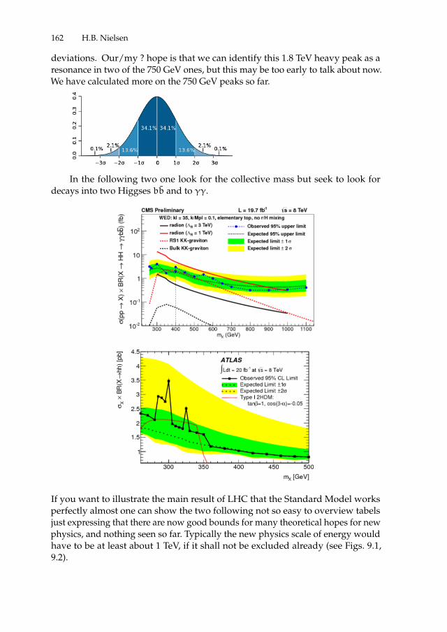
ii

“proc16” — 2016/12/12 — 10:17 — page 162 — #178 ii

ii

ii

162 H.B. Nielsen

deviations. Our/my ? hope is that we can identify this 1.8 TeV heavy peak as aresonance in two of the 750 GeV ones, but this may be too early to talk about now.We have calculated more on the 750 GeV peaks so far.

In the following two one look for the collective mass but seek to look fordecays into two Higgses bb and to γγ.

If you want to illustrate the main result of LHC that the Standard Model worksperfectly almost one can show the two following not so easy to overview tabelsjust expressing that there are now good bounds for many theoretical hopes for newphysics, and nothing seen so far. Typically the new physics scale of energy wouldhave to be at least about 1 TeV, if it shall not be excluded already (see Figs. 9.1,9.2).

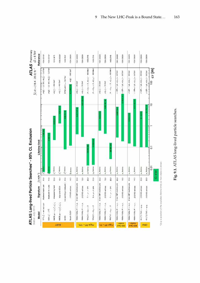
ii

“proc16” — 2016/12/12 — 10:17 — page 163 — #179 ii

ii

ii


Fig.

9.1.

ATL

AS

long

-liv

edpa

rtic

lese

arch

es.

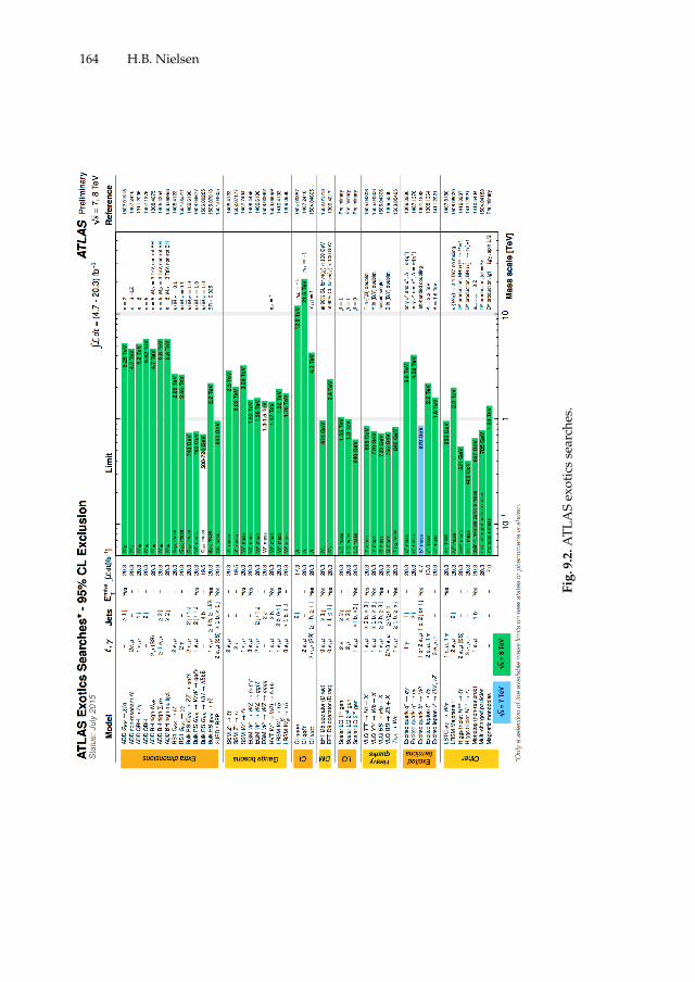
ii

“proc16” — 2016/12/12 — 10:17 — page 164 — #180 ii

ii

ii

164 H.B. Nielsen

Fig.

9.2.

ATL

AS

exot

ics

sear

ches

.

ii

“proc16” — 2016/12/12 — 10:17 — page 165 — #181 ii

ii

ii


9.5 12 tops

Colin Froggatt and I did an attempt to estimate the relative rates of decay of ourhypothesised bound state of the 6 top and 6 anti tops. We assume as reasonablethat the dominant decays are the two-particle decays because they have the bestphase space. 1 Nevertheless of course all the tops and anti tops have to annihilateaway before the bound state disappears. So with a low number, 2, of decay productparticles compared to the number 12 of constituents, most of the top anti top pairshave to annihilate into nothing so to speak. a major new point of Froggatts andmine work is the division of the decay amplitudes into two slightly differenttypes of decay: The two final state particles can come from the same top anti topannihilation, which we call “From same top-loop”, or they can be emitted fromtwo different annihilating top anti top pairs, and the latter we call “ From TWOdifferent loops of tops”. A major point to have in mind is, that, if the decay particleshave some quantum numbers, then that quantum number has to be transferedfrom one annihilation loop to another one. The difference between these two casesis illustrated by the figures with the “flowers” on. One effect that could have beenimportant is that e.g. weak gauge bosons W and the SU(2) coupling superpositionof the photon and the Z0 have a weak gauge charge, which is conserved as longas the Higgs vacuum expectation value is not included in the considered diagram.That means that the Higgs expectation value or some exchange of the quantumnumber from one annihilation loop to another one is required in order for sayWW decay occurring by use of the “From TWO different loops of tops” type ofdiagram. The major part of the photon which couples via the U(1) part, however,has no such “charge”. The main part of the γγ decay should therefore without anyproblem be possible with each photon coming from a different annihilation loop.Since there are 12/2 = 6 annihilation loops this a priori gives the main part of the(di)photon decay amplitude an extra factor 6; but it is even so that the numberof loops that must annihilate into quite nothing is 5 for both particles going fromone loop while only 4 in the case of the two decay particles coming from differentloops.

From same top-loop: From TWO different loops of tops:

Photon and transverse Z. The electric charge of the top quark is q = 2e/3 andthe effective coupling for of the photon to the tt loop is 4α/9.The corresponding effective coupling of Z to the tt loop is

α

2 sin2 θW cos2 θW

[(1

2−2

3sin2 θW

)2+

(−2

3sin2 θW

)2]=4α

9∗ 0.92.

(9.1)We take α = 1/129 and the Weinberg angle to be given by sin2 θW = 0.23.

1 I thank Li for discussions at CERN long time ago where we especially discussed that thetwo-particle decays at the end tended to dominate.

ii

“proc16” — 2016/12/12 — 10:17 — page 166 — #182 ii

ii

ii

166 H.B. Nielsen

Final st. f Bound Relative prediction Γ(S→f)Γ(S→γγ) Comt.

γγ < 0.8(r/5) (4α/9)2 = 1.2 ∗ 10−5 1gl + gl < 1300 · r

58αs/6)

2 = 2.3 ∗ 10−3 190H + H < 20(r/5) α2h/4 = 3 ∗ 10−4 25 Higgs

ZZ < 6(r/5) α2h/4 = 3 ∗ 10−4 25 longtl.WW < 20(r/5) α2h/2 = 6 ∗ 10−4 50 longtl.Zγ < 2(r/5) 2(4α/9)2 ∗ 0.92 1.8ZZ < 6(r/5) (4α/9)2 ∗ (0.92)2 0.8 tran.

WW < 20(r/5) 2(0.54α)2 = 3.5 ∗ 10−5 3 tran.t + t < 300(r/5) 3α2ttT2 = 6.5 ∗ 10−5 5

Γtotal(S)/Γ(S→ γγ): 302

Table 9.1. Assuming dominance of one top anti top pair giving the final state, relativepredictions are given for the partial decay widths of S and for the branching ratios relativeto the diphoton decay width compared to the experimental upper bounds.

Gluon. The vertex for a gluon of color i coupling to a top quark is gsλi/2. Aver-aging over the colors of the top quark, the effective coupling of the gluon tothe tt loop becomes

αs

3Tr

(λi

2

)2=αs

6. (9.2)

We take αs = 0.1 and then sum over the 8 color states of the gluon.

Higgs and longitudinalW± and Z0. According to the Goldstone Boson Equiva-lence Theorem in the high energy limit the couplings of the longitudinalW±

and Z0 become equal to those of the corresponding eaten Higgs fields. TheHiggs field coupling to the tt loop is

αh =g2t/2

4π= 0.035 (9.3)

where gt is the top quark Yukawa coupling constant.

TransverseW±. The W± gauge fields are formed from two real fields, W1 andW2, lying in the adjoint representation of SU(2). So their effective coupling tothe tt loop is

1

2∗ α

sin2 θW

((σi

2

)2)tLtL

=α

8 sin2 θW= 0.54α, (9.4)

where the extra factor of 1/2 is due toW± only interacting with left-handedtop quarks. The final sum over i = 1, 2 gives a factor of 2 in the decay rate.

Photon and transverse Z. The hypercharge coupled superposition of the photonand Z0 is described by the field Bµ = cos θWAµ − sin θWZµ. It couples withan average squared charge [(2/3)2+(1/6)2]/2 = 0.236 to a top quark. The twoloop diphoton decay is dominated by the production of this Bµ componentand so the effective coupling for the photon is 0.236α.The corresponding effective coupling of Z is 0.236α tan θW .

ii

“proc16” — 2016/12/12 — 10:17 — page 167 — #183 ii

ii

ii


Fin. f Bound Relative pred. Γ(S→f)Γ(S→γγ) Com.

γγ < 0.8(r/5) (0.236α)2 = 3.35 ∗ 10−6 1gl + gl < 1300 · r

58(αs/18)

2 = 2.5 ∗ 10−4 74H + H < 20(r/5) α4h/(4T2) = 3.4 ∗ 10−5 10 Higgs

ZZ < 6(r/5) α4h/(4T2) = 3.4 ∗ 10−5 10 longtn.WW < 20(r/5) α4h/(2T2) = 6.8 ∗ 10−5 20 longtn.Zγ < 2(r/5) 2(0.236α)2 tan2 θW 0.6ZZ < 6(r/5) (0.236α)2 tan2 θW 0.09 transv.

WW < 20(r/5) 2(0.54α)4/T2 = 6 ∗ 10−8 0.02 transv.t + t < 300(r/5) 3α4tt/T2 = 1.06 ∗ 10−3 316


Table 9.2. Assuming dominance of two top anti top pairs giving the final state, relativepredictions are given for the partial decay widths of S and for the branching ratios relativeto the diphoton decay width compared to the experimental upper bounds(Franceschini).

Gluon. Averaging over the colors of the two (anti)top pairs, the effective couplingof a gluon of color i for the ”crossed” diagram is

αs

9Tr

(λi

2

)2=αs

18. (9.5)

Higgs, longitudinal Z0,W±, top antitop. We use the same effective couplings asin the one loop case.

Final state f Bound Γ(S→f)Γ(S→γγ) Comment

γγ < 0.8(r/5) 1gluon + gluon < 1300(r/5) 117

Higgs + Higgs < 20(r/5) 15 Higgs-particlesZZ < 6(r/5) 15 longitudinal

WW < 20(r/5) 30 longitudinalZγ < 2(r/5) 1.0ZZ < 6(r/5) 0.3 transverse

WW < 20(r/5) 1.1 transversetop + anti top < 300(r/5) 208


Table 9.3. Benchmark model with ε2 = 0.15. Predictions are given for the decay branchingratios of S relative to the diphoton decay width and compared to the experimental upperbounds from ref. [5].

9.5.1 Production

We assume the production rate to be of an order calculated analogous to theproduction of a fourth family just taking into account that our bound state consistof 12 quarks. Using our decay ratio estimates the rate for S → γγ is order ofmagnitude o.k.

ii

“proc16” — 2016/12/12 — 10:17 — page 168 — #184 ii

ii

ii

168 H.B. Nielsen

9.6 MPP

Multiple Point Principle In general, a quantum field theory allows an existence ofseveral minima of the effective potential, which is a function of a scalar field.

If all vacua, corresponding to these minima, are degenerate, having zerocosmological constants, then we can speak about the existence of a multiple criticalpoint (MCP) in the phase diagram. See:[7].

We postulated a Multiple Point Principle (MPP) for many degenerate vacua.This principle should solve the finetuning problem by actually making a rule forfinetuning.

9.6.1 Multiple Point Principle

The Multiple Point Model (MPM) of the Universe evokes simply the StandardModel up to the scale ∼ 1018 GeV.

If the MPP is very accurate, we may have a new law of Nature, that can helpus to restrict coupling constants from theoretical principles.

Assuming the existence of two degenerate vacua in the SM:

1. the Electroweak vacuum at v = 246 GeV, and2. the Planck scale vacuum at v2 ' 1018 GeV,

See [8].We predicted the top-quark and Higgs boson masses:

Mt = 173± 5 GeV, MH = 135± 9 GeV.

Multiple Point Principle

Here it is shown the existence of the second (non-standard) minimum of theeffective potential of the pure SM at the Planck scale. Multiple Point Principle:The tree-level Higgs potential with the standard “Electroweak minimum” atφmin 1 = v is given by:

V1 =λ

4

(φ2 − v

)2+ C1.

ii

“proc16” — 2016/12/12 — 10:17 — page 169 — #185 ii

ii

ii


The new minimum at the Planck scale:

V2 = Veff(at Planck scale) =λrun

4

(φ2 − v2

)2+ C2,

can be higher or lower than the Electroweak one, showing a stable Electroweakvacuum (in the first case), or metastable one (in the second case).

In accordance with cosmological measurements, Froggatt and Nielsen as-sumed that cosmological constants C1 and C2 for both vacua are equal to zero (orapproximately zero): C1, 2 = 0, or C1, 2 ≈ 0.

This means that vacua v = v1 & v2, and they are degenerate. Multiple PointPrinciple The following requirements must be satisfied in order to, the effectivepotential have two degenerate minima:

Veff(φ2min 1) = Veff(φ

2min 2) = 0,

andV ′eff(φ

2min 1) = V

′eff(φ

2min 2) = 0,

where,

V ′(φ2) =∂V

∂φ2

[6]Multiple Point Principle postulates: There are many vacua with the same

energy density, or cosmological constant, and all cosmological constants are zero,or approximately zero.

ii

“proc16” — 2016/12/12 — 10:17 — page 170 — #186 ii

ii

ii

170 H.B. Nielsen

Multiple Point Principle If several vacua are degenerate, then the phase di-agram contains a special point – the Multiple Critical Point (MCP), at which thecorresponding phases assembly together.

ii

“proc16” — 2016/12/12 — 10:17 — page 171 — #187 ii

ii

ii


At the finetuned values of the variables pressure P and temperature T – wehave:

Tc ≈ 0.01oC, Pc ≈ 4.58 mm Hg,

giving the critical (triple) point O shown in the previous figure.

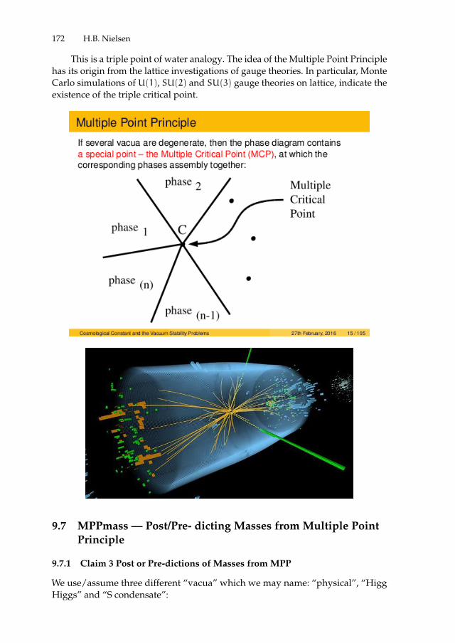
ii

“proc16” — 2016/12/12 — 10:17 — page 172 — #188 ii

ii

ii

172 H.B. Nielsen

This is a triple point of water analogy. The idea of the Multiple Point Principlehas its origin from the lattice investigations of gauge theories. In particular, MonteCarlo simulations of U(1), SU(2) and SU(3) gauge theories on lattice, indicate theexistence of the triple critical point.

9.7 MPPmass — Post/Pre- dicting Masses from Multiple PointPrinciple

9.7.1 Claim 3 Post or Pre-dictions of Masses from MPP

We use/assume three different “vacua” which we may name: “physical”, “HiggHiggs” and “S condensate”:

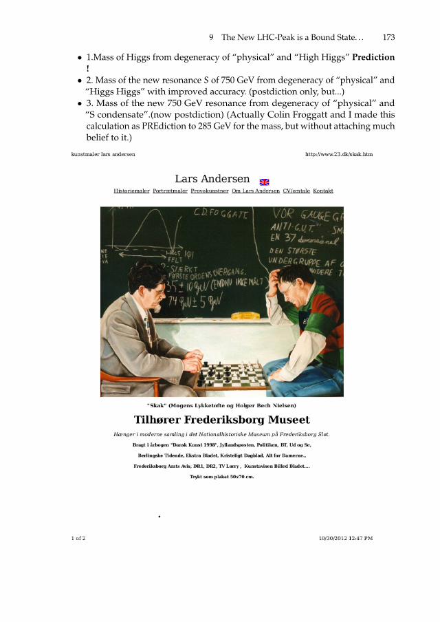
ii

“proc16” — 2016/12/12 — 10:17 — page 173 — #189 ii

ii

ii


• 1.Mass of Higgs from degeneracy of “physical” and “High Higgs” Prediction!

• 2. Mass of the new resonance S of 750 GeV from degeneracy of “physical” and“Higgs Higgs” with improved accuracy. (postdiction only, but...)• 3. Mass of the new 750 GeV resonance from degeneracy of “physical” and

“S condensate”.(now postdiction) (Actually Colin Froggatt and I made thiscalculation as PREdiction to 285 GeV for the mass, but without attaching muchbelief to it.)

ii

“proc16” — 2016/12/12 — 10:17 — page 174 — #190 ii

ii

ii

174 H.B. Nielsen

Higgs-Mass Correction:

9.8 Getting the Bound state S Mass from Requiring Degeneracyof Vacua “Physical” and “S Condensate” to 4 mt

With the right not so obvious approximations one gets in a very simple way thatthe bound state S shall have the massmS = 12mt/3 = 4mt. Thes assumptions:

• The “S condensate” vacuum is a lattice of same structure as diamond crystal.• We can count the binding energy as if the neighbouring S-states in the crystal

have there constituent top and anti tops in the n=2 level of the surrounded S.• We can ignore the effective Higgs mass for the exchange up to the n=2 level,

but from n=3 and on the Higgs mass may be taken infinite.• The MPP - degeneracy of “physical” and “S condensate” vacua - requires the

binding in the crystal to just cancel the Einstein masses of the S particles.• We can take the S’s in the “S condensate ” vacuum as at rest.

ii

“proc16” — 2016/12/12 — 10:17 — page 175 — #191 ii

ii

ii


9.8.1 Mass from MPP of S-condensate

We want to estimate the condition in a non-relativistic ansatz for the vacuum withthe S-condensate as a diamond-structure pattern of S-bound states. The bindingenergy between the neighbours in this pattern is estimated by assuming that thefour nearest neighbours S’s to a certain S have their top and anti tops effectivelyfilling up the 4 n = 2 states surrounding the S considered. Since n = 2 states inthe Bohr atom have a binding 1/n2 = 1/4 times that in the n = 1 states, we take itthat the binding per quark of a neighbouring S to a given one is in the Higgs masszero approximation just 1/4 times that binding of one of the constituent quarksinside its S. Thus the binding of an S to its neighbour must be with a potential 1/4of the binding energy of an S from its constituents.

In the assumed diamond lattice each carbon atom has 4 nearest neighbours,but each “binding-link” is attached to two carbon atoms. So the number of“binding-links” is twice as large as the number of carbon atoms. If we therefore asargued have one quarter of the binding energy in these “binding links” as in theS’s or the carbon atoms in the analogue, there will be 2/4 = 1/2 as much bindingin the “binding -links” as in the S’s themselves.

If the Einstein energy E = mc2 of a sample of bound states S consisting oftop and anti tops shall be just compensated by the binding energy between thesequarks, then the total binding energy per quark must add up to this Einsteinenergy numerically. Such compensation is required by our new law of nature“Multiple point principle”.

If the bindings in the “binding-links” make up 1/2 of the binding of theconstituents inside their respective S bound states, the latter must make up 2/3of the Einstein energy. The a priori Einstein energy of the twelve top or anti topquarks in an S bound state is of course 12 mt. The binding energy the S-boundstate should thus from MPP be 12mt * 2/3. Thus the left over mass of the S boundstate shall be 12mt - 2/3 *12mt = 12/3mt = 4mt, which is indeed very close tothe observed massmS = 750GeV . In fact 4mt = 4 ∗ 173GeV = 692GeV .

ii

“proc16” — 2016/12/12 — 10:17 — page 176 — #192 ii

ii

ii

176 H.B. Nielsen

9.9 Conclusion

Conclusion

• We have argued for that in our interpretation of the diphoton peak as a boundstate of 6t+ 6t bound state there are two arguments using the “multiple pointprinciple” that independently lead to the bound state having a mass near the750 GeV:

– A. The correction to the to be observed Higgs mass needed to make degen-eracy (MPP) of the physical and the high Higgs vacua is close to requiringthe bound state mass 760 GeV.

– B. To have the degeneracy (MPP) of the S-condensate vacuum with thephysical one an S mass of ∼ 4mt is needed.

• Even ignoring the little correction from the bound state S to the relationbetween the Higgs mass and the energy density of the high Higgs vacuum isso well approximately in correspondance with the MPP-required degeneracyof the physical and the high higgs vacua that we - Colin Froggatt and I -PREdited the Higgs mass correctly within 10 GeV!

• That the 750 GeV peak is so far only seen in the diphoton channel is so farbarely consistent with the bounds from LHC, because one has not yet analysedthe other relevant channels at 13 TeV.

• The production rate is in crude agreement with our estimate.

Acknowledgements

I would like to thank the Niels Bohr Institute for being allowed to stay as emeritusand even coming to Bled. Also I thank my collaborators Colin Froggatt, LarisaLaperashvili and Chitta Das for the work without which the information and

References

1. Holger Bech Nielsen,“Simple..” arXiv:1607.07907.2. Holger Bech Nielsen, “F(750), We miss you,...” arXiv:1610.00364.3. J. A. AguilarSaavedraa, J. H. Collins, S. Lombardod,“Traces of triboson resonance”,

arXiv:1607.08911v4 [hep-ph] 15 Sep 2016.4. The CMS Collaboration, Available on the CERN CDS information server CMS PAS

B2G-16-010, CMS Physics Analysis Summary Contact: [email protected]/07/17 “Search for diboson resonances in the semileptonic X→ ZV → l+l− + qq

final state at√s = 13 TeV with CMS”.

5. R. FRanceschini et al., “ What is the gamma gamma resonance at 750 GeV?”,arXiv:1512.04933.

6. C.D. Froggatt and H.B. Nielsen Phys. Lett. B368 96 (1996); arXiv:hep-ph/9607302.7. D.L. Bennett and H.B. Nielsen, Int. J. Mod. Phys. A9 5155 (1994); arXiv:hep-ph/931132.8. C.D. Froggatt and H.B. Nielsen, Phys. Lett. B368 96 (1996); arXiv:hep-ph/9511371.

ii

“proc16” — 2016/12/12 — 10:17 — page 177 — #193 ii

ii

ii




10 Progressing Beyond the Standard Models

B.A. Robson ?

The Australian National University, Canberra, ACT 2601, Australia

Abstract. The Standard Model of particle physics (SMPP) has enjoyed considerable successin describing a whole range of phenomena in particle physics. However, the model is con-sidered incomplete because it provides little understanding of other empirical observationssuch as the existence of three generations of leptons and quarks, which apart from masshave similar properties. This paper examines the basic assumptions upon which the SMPPis built and compares these with the assumptions of an alternative model, the GenerationModel (GM). The GM provides agreement with the SMPP for those phenomena which theSMPP is able to describe, but it is shown that the assumptions inherent in the GM allowprogress beyond the SMPP. In particular the GM leads to new paradigms for both massand gravity. The new theory for gravity provides an understanding of both dark matterand dark energy, representing progress beyond the Standard Model of Cosmology (SMC).

Povzetek. Standardni Model elektrosibke in barvne interakcije zelo uspesno opise velikopojavov v fiziki osnovnih delcev. Model imajo kljub temu za nepopoln, ker ne pojasnivrste empiricnih dejstev, kot je obstoj treh generacij leptonov in kvarkov, ki imajo, razenrazlicnih mas, zelo podobne lastnosti. V prispevku obravnavamo osnovne predpostavke,na katerih so zgradili ta model in jih primerjamo s predpostavkami alternativnega modela,generacijskega modela. Generacijski model se v napovedih ujema z napovedmi standard-nega modela za tiste pojave, ki jih slednji dobro opise. Drugacne predpostavke omogocijogeneracijskemu modelu napovedi, ki niso v dosegu standardnega modela: generacijskimodel ponudi drugacno paradigmo za maso in energijo. To vodi k novi teoriji gravitacije, kiponuja novo razumevanje problemov temne snovi in temne energije, ter s tem k razsiritvistandardnega modela kozmologije.

10.1 Introduction

The two models in the title are the Standard Model of Particle Physics (SMPP) andthe Standard Model of Cosmology (SMC).

In this paper the SMPP [1] will be briefly described, indicating its incomplete-ness and the need for an improved model such as the Generation Model (GM) [2]in which the elementary particles of the SMPP have a substructure. During the lastdecade an alternative model, the GM, has been developed, although the currentversion has not changed since 2011. This model allows the elementary particles ofthe SMPP to have a substructure, suggested by indirect evidence. This version ofthe GM leads to new paradigms for both mass [3] and gravity [4]. In particular

? [email protected]

ii

“proc16” — 2016/12/12 — 10:17 — page 178 — #194 ii

ii

ii

178 B.A. Robson

the new theory of gravity provides an understanding of both dark matter [5] anddark energy [6], and also solves the cosmological matter-antimatter asymmetryproblem [7]. These represent progress beyond both the SMPP and the SMC.

10.2 Standard Model of Particle Physics

The SMPP [1,2] was developed throughout the 20th century, although the currentformulation was essentially finalized in the mid-1970s following the experimentalconfirmation of the existence of quarks. The SMPP has enjoyed considerablesuccess in describing the interactions of leptons and the multitude of hadrons(baryons and mesons) with each other as well as the decay modes of the unstableleptons and hadrons. However, the model is considered to be incomplete in thesense that it provides little understanding of several empirical observations: itdoes not explain the occurrence of three generations of the elementary particles:the first generation comprising the up and down quarks, the electron and itsneutrino; the second generation comprising the charmed and strange quarks, themuon and its neutrino and the third generation comprising the top and bottomquarks, the tauon and its neutrino. Each generation behaves similarly except formass. Second, it does not provide a unified description of the origin of mass nordescribe the mass hierarchy of leptons and quarks. It also fails to describe thenature of gravity, dark matter, dark energy or the cosmological matter-antimatterasymmetry problem.

Because of the incompleteness of the SMPP, I have closely examined the basicassumptions upon which the SMPP has been erected [8]. There are three basicassumptions, which I consider to be dubious and also present major stumblingblocks preventing progress beyond the SMPP. These are (i) the assumption of adiverse complicated scheme of additive quantum numbers to classify its elemen-tary particles; (ii) the assumption of weak isospin doublets in the quark sector toaccommodate the universality of the charge-changing weak interactions and (iii)the assumption that the weak interactions are fundamental interactions describedby a local gauge theory.

The additive quantum numbers allotted in the SMPP to classify the six leptonsand the six quarks, which constitute the elementary matter particles of the SMPP,are charge Q, lepton number L, muon lepton number Lµ and tau lepton numberLτ for the leptons, and charge Q, baryon number A, strangeness S, charm C,bottomness B and topness T for the quarks. Antiparticles have opposite quantumnumbers to the corresponding particle.

It should be noted that except for charge, leptons and quarks have differentkinds of quantum numbers so that this classification is non-unified. Each of theadditive quantum numbers is conserved in any interaction, except for S, C, B andT , which may undergo a change of one unit in weak interactions.

I consider that the basic problem with the SMPP is this classification of its ele-mentary particles employing a diverse complicated scheme of additive quantumnumbers, some of which are not conserved in weak interaction processes; and atthe same time failing to provide any physical basis for this scheme.

ii

“proc16” — 2016/12/12 — 10:17 — page 179 — #195 ii

ii

ii

10 Progressing Beyond the Standard Models 179

Another problem with the SMPP concerns the method it employs to accommo-date the universality of the charge-changing (CC) weak interactions. The CC weakinteractions are mediated by the W bosons which have zero additive quantumnumbers apart from charge.

In the SMPP, the observed universality of the CC weak interactions in thelepton sector is described by assuming that the mass eigenstate leptons form weakisospin doublets. The leptons have weak isospin 1/2, whose third componentis related to both charge and lepton number. Restricting the discussion in thispaper to only the first two generations for simplicity, means that the two neutrinosinteract with their corresponding charged leptons with the full strength of the CCweak interaction and do not interact at all with the other charged lepton. This isguaranteed by the conservation of lepton numbers.

On the other hand the universality of the CC weak interactions in the quarksector is treated differently. It is assumed that the u and c quarks form weakisospin doublets with so-called weak eigenstate quarks d ′ and s ′, respectively,where

d ′ = d cos θ+ s sin θ,

and

s ′ = −d sin θ+ s cos θ,

and θ is a mixing angle introduced by Cabibbo in 1963 into the transition ampli-tudes prior to the development of the quark model in 1964. In the quark case thethird component of weak isospin is related to both charge and baryon number.

The SMPP assumes that the u and c quarks interact with d ′ and s ′, respec-tively, with the full strength of the CC weak interaction and that the u and c quarksdo not interact at all with s ′ and d ′, respectively. However, this latter assumption isdubious since, unlike the lepton sector, there are no conserved quantum numbersto guarantee this.

A third problem with the SMPP concerns the origin of mass. In the SMPP, themasses of hadrons arise mainly from the energy content of their constituent quarksand gluons, in agreement with Einstein’s 1905 conclusion. On the other hand themasses of the elementary particles, the leptons, the quarks and theW and Z bosonsare interpreted differently, arising from the existence of the so-called Higgs field[9,10]. The Higgs field was introduced mathematically to spontaneously breakthe U(1) x SU(2) local gauge symmetry of the electroweak interaction to generatethe masses of the W and Z bosons. The Higgs field also cured the associatedfermion mass problem: by coupling, with appropriate strength, originally masslessfermions to the scalar Higgs field, it is possible to produce the observed fermionmasses and to maintain local gauge invariance.

I consider that there are several problems with the SMPP’s interpretationof the origin of mass. First, there is no clear evidence for the existence of thehypothetical Higgs field. Second, the model provides no unified origin of mass.Third, the fermion-Higgs coupling strength is dependent upon the mass of thefermion so that a new parameter is introduced into the SMPP for each fermion

ii

“proc16” — 2016/12/12 — 10:17 — page 180 — #196 ii

ii

ii

180 B.A. Robson

mass. In fact fourteen new parameters are required, if one includes two moreparameters to describe the masses of the W boson and the Higgs particle. Fourth,the Higgs mechanism does not provide any physical explanation for the origin of themasses of the elementary particles.

The assumption that the weak interactions are fundamental interactions aris-ing from a local gauge theory, unlike both the electromagnetic and strong colourinteractions, is at variance with the experimental facts: both theW and Z particles,mediating the weak interactions, are massive, and this conflicts with the require-ment of a local gauge theory that the mediating particles should be massless inorder to guarantee the gauge invariance. I consider this assumption very dubious,especially since it leads to more problems than it solves. It also leaves severalquestions unanswered: How does the spontaneous symmetry breaking mechanism occurwithin the electroweak theory? What is the principle that determines the large range offermion masses exhibited by the leptons and quarks?

10.3 Generation Model of Particle Physics

The GM of particle physics [2,8] overcomes many of the problems inherent inthe SMPP. In the GM the three dubious assumptions of the SMPP discussedpreviously are replaced by three different and simpler assumptions. These are(i) the assumption of a simpler unified classification of leptons and quarks; (ii) theassumption that the mass eigenstate quarks form weak isospin doublets and thathadrons are composed of weak eigenstate quarks and (iii) the assumption that theweak interactions are not fundamental interactions.

Table 10.1 shows the additive quantum numbers allotted to both leptonsand quarks in the GM. This is a much simpler and unified classification schemeinvolving only three additive quantum numbers: chargeQ, particle number p andgeneration quantum number g. All three quantum numbers are conserved in allinteractions. In particular this classification scheme allows the development of acomposite model of leptons and quarks, which I consider a necessary conditionfor a simpler model.

particle Q p g particle Q p g

νe 0 −1 0 u + 23

13

0

e− −1 −1 0 d − 13

13

0

νµ 0 −1 ±1 c + 23

13±1

µ− −1 −1 ±1 s − 13

13±1

ντ 0 −1 0,±2 t + 23

130,±2

τ− −1 −1 0,±2 b − 13

130,±2

Table 10.1. GM additive quantum numbers for leptons and quarks.

The conservation of the generation quantum number in weak interactions wasonly achieved by making two postulates, which means that the GM differs funda-mentally from the SMPP in two more ways. First the GM postulates that it is the

ii

“proc16” — 2016/12/12 — 10:17 — page 181 — #197 ii

ii

ii


mass eigenstate quarks of the same generation, which form weak isospin doublets:(u, d) and (c, s). Thus the GM assumes, in the two generation approximation, thatthe u and c quarks interact with d and s, respectively, with the full strength of theCC weak interaction and that the u and c quarks do not interact at all with s andd, respectively. This is guaranteed by the conservation of the generation quantumnumber. Second, the GM postulates that hadrons are composed of weak eigenstatequarks such as d ′ and s ′ rather than the corresponding mass eigenstate quarks,d and s, as in the SMPP. Essentially, in the GM the roles of the mass eigenstatequarks and the weak eigenstate quarks are interchanged from that in the SMPP.These two postulates overcome the second dubious assumption of the SMPP.

The GM assumes that the leptons, quarks and theW and Z bosons are compos-ites. Consequently, the weak interactions are not fundamental interactions arisingfrom an SU(2) local gauge theory. They are residual interactions of the strongcolour interaction binding the constituents of the leptons, quarks and theW andZ bosons together. This strong colour interaction is completely analogous to thatof QCD in the SMPP. The composite nature of leptons, quarks and theW bosonsovercomes the dubious assumption of the SMPP that the weak interactions arefundamental.

10.4 Composite Generation Model

In 2005 I began construction of a GM in which the leptons and quarks are compositeparticles. This composite GM was based on the unified classification scheme andalso on early 1979 composite models of Harari [11] and Shupe [12]. The currentcomposite GM was proposed in 2011 and is described in detail in Chapter 1 ofthe book Particle Physics published by InTech in 2012 [2] and in a review paperpublished in Advances in High Energy Physics in 2013 [8]. Unfortunately, today Ihave only the time to indicate some of the features of the composite GM (CGM)that are relevant for today’s talk.

In the CGM the elementary particles of the SMPP have a substructure consist-ing of massless “rishons” bound together by strong colour interactions, mediatedby massless hypergluons. Each rishon carries a colour charge: red, green or bluelike a quark in the SMPP. This model is very similar to the SMPP in which hadronshave a substructure consisting of quarks bound together by strong colour interac-tions, mediated by massless gluons. Today I shall only have time to give a verybrief outline of the development of the CGM.

There are numerous models in the literature. However, the CGM is basedon the 1979 two-particle schematic models of Harari and Shupe, which are verysimilar and provide arguably the most economical and impressive description ofthe first generation of leptons and quarks. Both models treat leptons and quarksas composites of two kinds of spin-1/2 particles that Harari named “rishons”from the Hebrew for primary. The two kinds of rishons are labelled T with chargeQ = 1/3 and V with Q = 0.

Table 10.2 shows the structures given to the first generation of leptons andquarks. It should be noted that no composite particle involves mixtures of rishonsand antirishons. Also it should be noted that quarks contain mixtures of the two

ii

“proc16” — 2016/12/12 — 10:17 — page 182 — #198 ii

ii

ii

182 B.A. Robson

types of rishons, whereas leptons do not. Essentially, the Harari-Shupe model(HSM) describes the charge character of the first generation of particles.

particle structure Q

e+ TTT +1

u TTV, TVT, VTT + 23

d TVV, VTV, VVT + 13

νe VVV 0

νe VVV 0

d T VV, VT V, VVT − 13

u T T V, T V T , V T T − 23

e− T T T −1

Table 10.2. HSM of first generation of leptons and quarks.

The CGM is a major extension of the HSM: the introduction of a third kind ofrishon (U) and all three additive quantum numbers are allotted to each kind ofrishon (see Table 10.3).

rishon Q p g

T + 13

+ 13

0

V 0 + 13

0

U 0 + 13−1

Table 10.3. CGM additive quantum numbers for rishons.

Table 10.4 gives the structures of the first generation of leptons and quarks inthe CGM. Antiparticles are denoted in the usual manner by a “bar” placed abovethe particle identifier. The u-quark has p = 1/3 since it contains two T -rishons andone V-rishon. It is essential that the u-quark should contain an V-rishon ratherthan a V-rishon as in the HSM, since its particle number is required to agree withits baryon number 1/3. It should be noted that leptons are composed of threerishons, while quarks are composed of one rishon and one rishon-antirishon pair.Each lepton of the first generation is colourless, composed of three rishons carryingdifferent colours. Each quark of the first generation is coloured, composed of onerishon and one colourless rishon-antirishon pair. The first generation of particlesare all built out of T and V rishons and their antiparticles so that each particlehas g = 0. The second and third generations are identical to the first generationplus one and two colourless rishon-antirishon pair(s): UV or VU with Q = p = 0

but g = ±1 so that the second and third generations have g = ±1 and g = 0,±2,respectively. This gives three repeating patterns.

ii

“proc16” — 2016/12/12 — 10:17 — page 183 — #199 ii

ii

ii


particle structure Q p g

e+ TTT +1 +1 0

u TTV + 23

+ 130

d TVV + 13

− 130

νe VVV 0 −1 0

νe VVV 0 +1 0

d TVV − 13

+ 130

u T TV − 23

− 130

e− T T T −1 −1 0

Table 10.4. CGM of first generation of leptons and quarks.

10.5 Mass

Since the mass of a hadron arises mainly from the energy of its constituents, theCGM suggests that the mass of a lepton, quark or vector boson arises from acharacteristic energy E associated with its constituent rishons and hypergluons,according to m = E/c2. Thus the CGM provides a new paradigm and a unifieddescription for the origin of all mass: the mass of a body arises from the energycontent E of its constituents. The mass is given by m = E/c2 in agreement withEinstein’s 1905 conclusion, so that there is no need for the existence of a Higgsfield with its accompanying problems. A corollary of this idea is: If a particle hasmass, then it is composite.

The CGM suggests that the mass hierarchy of the three generations arisesfrom the substructures of the leptons and quarks. The mass of each compositeparticle is expected to be greater if the constituents are on average more widelyspaced: this is a consequence of the nature of the strong colour interactions, whichare stronger for larger separations of the colour charges, and higher generationparticles are more massive than lower generations. Particles with two or morecharged rishons will have larger structures due to electric repulsion.

Qualitatively, for the same generation, one expects that (i) a charged leptonwill have a greater mass than the corresponding neutral lepton; (ii) a Q = +2/3

quark will have a greater mass than the corresponding Q = −1/3 quark. Theseare both generally true: (i) the electron has a larger mass than its correspondingneutrino, and (ii) the top quark mass (175 GeV) is > the bottom quark mass (4.5GeV), the charmed quark mass (1.3 GeV) is > the strange quark mass (200 MeV),although the up quark mass (5 MeV) is < the down quark mass (10 MeV). The firstgeneration quarks seem to present an anomaly since the proton consists of twoup quarks and one down quark while the neutron consists of two down quarksand one up quark so that the proton is only stable if the down quark (Q = −1/3)is more massive than the up quark (Q = +2/3). In the CGM, this anomaly isaccounted for by the constituents of hadrons being weak-eigenstate quarks ratherthan mass-eigenstate quarks. The proton is stable since the weak eigenstate quarkd ′ has a larger mass than the up quark, containing about 5% of the strange quarkmass.

ii

“proc16” — 2016/12/12 — 10:17 — page 184 — #200 ii

ii

ii

184 B.A. Robson

10.6 Gravity

Let us now consider the nature of gravity within the framework of the GM. It isenvisaged that the rishons of each colourless lepton, i.e., a particle with total colourcharge zero, are very strongly localized since to date there is no direct evidencefor any substructure of these particles. The rishons are expected to be distributedaccording to quantum-mechanical wave functions, for which the product wavefunction is significant for only an extremely small volume of space so that thecorresponding colour fields are almost cancelled. It should be noted that the colourfields would only cancel completely if each of the rishons occupied the sameposition, but quantum mechanics prevents this. This raises a question: What is theresidual interaction arising from the incomplete cancellation of the strong interactions?

Between any two colourless leptons (electrons) there will be a very weakresidual interaction, arising from the colour interactions acting between the rishonsof one lepton and the rishons of the other lepton. In two papers [3,4] I suggestedthat this residual interaction gives rise to the usual gravitational interaction. Therewill be a similar residual interaction between any two colourless hadrons such asneutrons and protons, each containing three differently coloured quarks.

Gravity acts between bodies with mass. The mass of a body of ordinary matteris essentially the total mass of its constituent electrons, neutrons and protons. Inthe GM, each of these three particles is composite and colourless. Indeed, all threeparticles are in a three-colour antisymmetric state so that their behaviour withrespect to the colour interactions is basically the same. This suggests that theresidual colour interactions between electrons, neutrons and protons have severalproperties associated with the usual gravitational interaction: universality, veryweak strength and attraction.

In the GM gravity essentially arises from the residual colour forces betweenall electrons, neutrons and protons. This leads to a new law of gravity: the residualcolour interactions between any two bodies of masses m1 and m2, separatedby a distance r, leads to a universal law of gravitation, which closely resemblesNewton’s original law given by: F = H(r)m1m2/r2, where Newton’s gravitationalconstant (G) is replaced by a function of r, H(r).

The new gravitational interaction of the GM is based upon the residual colourinteractions acting between electrons, neutrons and protons. The GM assumes thatthe colour interactions acting between rishons have the same characteristics as thecolour interactions acting between quarks in the SMPP. These colour interactionshave two important properties that differ from the Newtonian interaction: (i)asymptotic freedom and (ii) colour confinement. These determine the nature ofthe function H(r).

Asymptotic freedom is rather a misnomer. A better term is antiscreening asused by Wilczek in his 2004 Nobel lecture. Antiscreening arises from the self-interactions of the hypergluons mediating the residual colour interactions. Theseantiscreening effects lead to an increase in the strength of the residual colourinteractions acting so thatH becomes an increasing function of r. The ‘flat’ rotationcurves observed for galaxies imply that H(r) = G(1+ kr).

ii

“proc16” — 2016/12/12 — 10:17 — page 185 — #201 ii

ii

ii


10.7 Galaxy Rotation Problem and Dark Matter

For galaxies there is a major gravitational problem [5], which has been aroundfor about forty years. It was found that the rotation curves for galaxies disagreedwith Newton’s gravitational law for large r: the stars and gas were rotating muchfaster than expected from Newton’s law and their orbital velocities were roughlyconstant. These observations implied that either Newton’s law was incorrect atlarge distances or some considerable mass was missing.

The rotation curve for a galaxy is the dependence of the orbital velocity ofthe visible matter in the galaxy on its radial distance from the centre of the galaxy.What the observations showed was that the rotation curves were essentially ‘flat’at the extremities of the visible matter, i.e., at large distances. This implies grossdisagreement with Newton’s universal law of gravitation, which predicts a fall-offas 1/

√r as in the solar system.

Two solutions, which have been very successful, are first the dark matterhypothesis that proposes that a galaxy is embedded within a giant halo of darkmatter. This matter is considered to be non-atomic but otherwise its nature isunknown and so far has not been detected. The second solution is the ModifiedNewtonian Dynamics (MOND) hypothesis: in 1983 Milgrom [13] proposed thatgravity varies from Newton’s law for low accelerations. This is an empiricalhypothesis without physical understanding.

It was found that the new law of gravity is essentially equivalent to the MONDhypothesis so that the GM gravitational interaction provides a physical basis forthe MOND hypothesis. In my opinion, the continuing success [14,15] of the MONDhypothesis is a strong argument against the existence of undetected dark matterhaloes, consisting of unknown matter embedding galaxies.

In the GMH(r) = G(1+kr) arises from the self-interactions of the hypergluonsmediating the gravitational interaction and explains the dark matter problem ofthe galaxy rotational curves: for small r, H(r) is approximately G and gravity isapproximately Newtonian; for large r, H(r) is approximately Gkr and gravity isapproximately 1/r rather than 1/r2, and the 1/r dependence gives the flat rotationcurves observed.

10.8 Dark Energy Problem

Colour confinement is the phenomenon that colour charged particles (e.g., quarksin the SMPP, rishons in the GM) cannot be isolated and consequently form colour-less composite particles (e.g., mesons and baryons in the SMPP and also leptonsin the GM). Colour confinement leads to another phenonmenon analogous to the‘hadronization process’, i.e., the formation of hadrons out of quarks and gluons inthe SMPP and implies H(r) = 0 for sufficiently large r in the GM.

In the GM, H(r) = 0 arises if the gravitational field energy is sufficient that itis energetically favourable to produce the mass of a particle-antiparticle colourlesspair rather than the colour field to extend further. This implies that gravity ceasesto exist for sufficiently large cosmological distances.

ii

“proc16” — 2016/12/12 — 10:17 — page 186 — #202 ii

ii

ii

186 B.A. Robson

The strong colour interaction is known to have a finite range of approximately10−15m. Gravity is about 10−41 times weaker at 10−15m [16] than the strong colourinteraction. This suggests that the ‘hadronization process’ for gravity occurs atabout 1026m, i.e., roughly ten billion light years.

The new law of gravity implies that gravity ceases to exist for cosmologicaldistances exceeding several billion light years, resulting in less slowing downof galaxies than expected from Newton’s law. This result agrees well with ob-servation [17,18] of distant Type Ia supernovae, which indicate the onset of anaccelerating expansion of the universe at about six billion light years.

10.9 Summary and Conclusion

The GM allows progress beyond the Standard Models of both particle physics andcosmology by the development of a composite model of the elementary particlesof the SMPP. This led to (i) a unified description of all mass and a qualitativeunderstanding of the mass hierarchy of the three generations of leptons andquarks and (ii) a new law of gravity and an understanding of both dark matterand dark energy.

References

1. K. Gottfried, V.F. Weisskopf, Concepts of Particle Physics Vol. 1, Oxford University Press,New York, 1984.

2. B. Robson, The generation model of particle physics in E. Kennedy, Particle Physics pp. 1-28,InTech Open Access Pub., Rijeka, 2012.

3. B.A. Robson, The generation model and the origin of mass, Int. J. Mod. Phys. E 18 1773(2009).

4. B.A. Robson, A quantum theory of gravity based on a composite model of leptons and quarks,Int. J. Mod. Phys. E 20 733 (2011).

5. B.A. Robson, The generation model of particle physics and galactic dark matter, Int. J. Mod.Phys. E 22 1350067 (2013).

6. B.A. Robson, Dark matter, dark energy and gravity, Int. J. Mod. Phys. E 24 1550012 (2015).7. B.A. Robson,The generation model of particle physics and the cosmological matter-antimatter

asymmetry problem, arXiv:1609.04034v1 [physics.gen-ph] 8 Sep 2016.8. B.A. Robson, Progressing beyond the standard model, Adv. High Energy Phys. 2013 341738

(2013).9. F. Englert, R. Brout, Broken symmetry and the mass of gauge bosons Phys. Rev. Lett. 13 321

(1964).10. P.W. Higgs, Broken symmetries and the masses of gauge bosons, Phys. Rev. Lett. 13 508

(1964).11. H. Harari, A schematic model of quarks and leptons, Phys. Lett. B 86 83 (1979).12. M.A. Shupe, A composite model of leptons and quarks, Phys. Lett. B 86 87 (1979).13. M. Milgrom, A modification of the Newtonian dynamics as a possible alternative to the hidden

mass hypothesis, Astrophysical J. 270 365 (1983).14. S.S. McGaugh, W.J.G. de Blok, Testing the hypothesis of modified dynamics with low surface

brightness galaxies and other evidence, Astrophys. J. 499 66 (1998).15. B. Famaey, S.S. McGaugh, Modified Newtonian Dynamics (MOND): Observational phe-

nomenology and relativistic extensions, Living Rev. in Relativity, 15 10 (2012).

ii

“proc16” — 2016/12/12 — 10:17 — page 187 — #203 ii

ii

ii


16. D. Lincoln, Understanding the Universe from Quarks to the Cosmos, rev. edn., WorldScientific, Singapore, 2012.

17. A.G. Riess et al., Observational evidence from supernovae for an accelerating universe and acosmological constant, Astronom. J. 116 1009 (1998).

18. S. Perlmutter et al. Measurements of Omega and Lambda from 42 high-redshift supernovae,Astrophys. J. 517 565 (1999).

ii

“proc16” — 2016/12/12 — 10:17 — page 188 — #204 ii

ii

ii

ii

“proc16” — 2016/12/12 — 10:17 — page 189 — #205 ii

ii

ii

Discussion Section

The discussion section is reserved for those open problems discussed duringthe workshop, that they might start new collaboration among participants or atleast stimulate participants to start to think about possible solutions of particularopen problems in a different way. Since the time between the workshop andthe deadline for contributions for the proceedings is very short and includes formost of participants also their holidays, it is not so easy to prepare besides theirpresentations at the workshop also the common contributions to the discussionsection. However, the discussions, even if not presented as a contribution to thissection, influenced participants’ contributions, published in the main section.

As it is happening every year also this year quite a lot of started discussionshave not succeeded to appear in this proceedings. Organizers hope that they willbe developed enough to appear among the next year talks, or will just stimulatethe works of the participants.

The author uses the old idea, that an appropriate parametrization of almostdemocratic mass matrices might help to better understand how fermions gainmasses, upgrading this idea by the appropriate rotations of mass matrices and aspecific parametrization of the Cabibbo-Kobayashi-Maskawa mixing matrix.

When studying the electrostatic interaction among two point charges in anonlinear model, taking into account QED, the authors find that the repulsionforce between two equal charges which are ∞ close to each other surprisinglydisappears, while it remains infinite if the charges are not equal.

Using the model based on the recognition that the binary code can well beused to clasify quarks and leptons of the standard model as well as the correspond-ing gauge fields, the authors try to evaluate the unification scale between the weakand the electromagnetic field.

A test is proposed which would show whether and how will the break ofthe SU(3) local gauge symmetry, originating in the family quantum number (themodel is described in the talk section), influence the cosmological observations.

All discussion contributions are arranged alphabetically with respect to theauthors’ names.

ii

“proc16” — 2016/12/12 — 10:17 — page 190 — #206 ii

ii

ii

Ta razdelek je namenjen odprtim vprasanjem, o katerih smo med delavnicoizcrpno razpravljali. Problemi, o katerih smo razpravljali, bodo morda privedli donovih sodelovanj med udelezenci, ali pa so pripravili udelezence, da razmislijo omoznih resitvah odprtih vprasanj na drugacne nacine. Ker je cas med delavnicoin rokom za oddajo prispevkov zelo kratek, vmes pa so poletne pocitnice, jezelo tezavno poleg prispevka, v katerem vsak udelezenec predstavi lastno delo,pripraviti se prispevek k temu razdelku.

Tako se velik del diskusij ne bo pojavil v letosnjem zborniku. So pa gotovovplivale na prispevek marsikaterega udelezenca. Organizatorji upamo, da bodote diskusije do prihodnje delavnice dozorele do oblike, da jih bo mogoce na njejpredstavit.

Avtorica prispevka uporabi dobro poznano idejo, da bi s primerno parametri-zacijo masnih matrik, ki so skoraj podobne edinkam, morda lahko razumeli, kakofermioni z maso postanejo masivni. Idejo nadgradi s primerno izbiro rotacijskihmatrik in parametrov mesalnih matrik.

Avtorji naletijo pri studiju electrostatske interacije med dvema tockastimanabojema, ko uporabijo nelinearni model ter upostevajo popravke kvantne elek-trodinamke, na presenetljiv rezultat: Odbojna sila, ki je med razlicnima nabojemaneskoncna, ko sta naboja tesno skupaj, postane med enakima nabojema enaka nic.

Avtor uporabi model z binarno kodo, ki ga pojani v predavanju, da ocenienergijsko skalo, pri kateri postaneta sibka in elektromagnetna sila enako mocni.

Avtorja predlagata kozmoske meritve, ki bodo pokazale, ce je model, kiuporabi grupo SU(3) za opis druzinskega kvantnega stevila (model je opisan venem od predavanj) smiselen. Zlomitev druzinskega kvantnega stevila vpliva nazgodovino razvoja vesolja in s predlaganimi meritvami ga je mogoce opaziti.

Prispevki v tej sekciji so, tako kot prispevki v glavnem delu, urejeni po abeced-nem redu priimkov avtorjev.

ii

“proc16” — 2016/12/12 — 10:17 — page 191 — #207 ii

ii

ii




11 Discreteness of Point Charge in NonlinearElectrodynamics

A.I. Breev1 ? and A.E. Shabad2,1 ??

1Tomsk State University, 36 Lenin Prospekt, 634050, Tomsk, Russia2P. N. Lebedev Physical Institute, 53 Leninskiy prospekt,119991, Moscow, Russia

Abstract. We consider two point charges in electrostatic interaction between them withinthe framework of a nonlinear model, associated with QED, that provides finiteness of theirfield energy. We argue that if the two charges are equal to each other the repulsion forcebetween them disappears when they are infinitely close to each other, but remains as usualinfinite if their values are different. This implies that within any system to which such amodel may be applicable the point charge is fractional, it may only be 2n-fold of a certainfundamental charge, n = 0, 1, 2....

We find the common field of the two charges in a dipole approximation, where theseparation between them is much smaller than the observation distance.

Povzetek. Avtorja obravnavata elekstrostaticno interakcijo med tockastima nabojema vokviru nelinearnega modela, pridruzenega kvantni elektrodinamiki, ki poskrbi, da je en-ergija polja koncna. V limiti, ko sta enaka tockasta neskoncno blizu, je odbojna sila mednjima koncna. Sila med razlicnima tockasima nabojema v isti limiti je sila neskoncna, takokot obicajno. Avtorja povzameta, da so v vsakem sistemu, ki mu tak model ustreza, tockastinaboji 2n-kratniki ustreznega osnovnega naboja, n = 0, 1, 2....

Poisceta skupno polje dveh nabojev v dipolnem priblizku z mnogo manjso medsebojnorazdaljo od razdalje opazovanja.

11.1 Introduction

Recently a class of nonlinear electrodynamic models was proposed [1] whereinthe electrostatic field of a point charge is, as usual, infinite in the point where thecharge is located, but this singularity is weaker than that of the Coulomb field, sothat the space integral for the energy stored in the field converges. In contrast tothe Born-Infeld model, the models from the class of Ref. [1] refer to nonsingularLagrangians that follow from the Euler-Heisenberg (E-H) effective Lagrangian[2] of QED truncated at any finite power of its Taylor expansion in the field. Thisallows us to identify the self-coupling constant of the electromagnetic field witha definite combination of the electron mass and charge and to propose that suchmodels may be used to extend QED to the extreme distances smaller than those for

? [email protected]?? [email protected]

ii

“proc16” — 2016/12/12 — 10:17 — page 192 — #208 ii

ii

ii

192 A.I. Breev and A.E. Shabad

which it may be thought of as a perfectly adequate theory. More general modelsbased on the Euler-Heisenberg Lagrangian, but fit also for considering non-staticnonlinear electromagnetic phenomena, where not-too-fast-varying in space andtime fields are involved, received attention as well. Among the nonlinear effectsstudied, there are the linear and quadratic electric and magnetic responses of thevacuum with a strong constant field in it to an applied electric field [3] , with theemphasis on the magneto-electric effect [4–6] and magnetic monopole formation[7]. Also self-interaction of electric and magnetic dipoles was considered withthe indication that the electric and magnetic moments of elementary particles aresubjected to a certain electromagnetic renormalization [8] after being calculatedfollowing a strong interaction theory, say, QCD or lattice simulations. Interactionof two laser beams against the background of a slow electromagnetic wave wasstudied along these lines, too [9].

In the present paper we are considering the electrostatic problem of two pointcharges that interact following nonlinear Maxwell equations stemming from theLagrangian of the above [1] type, their common field not being, of course, just alinear combination of the individual fields. The problem is outlined in the nextSection 11.2. Once the field energy is finite we are able to define the attraction orrepulsion force between charges as the derivative of the field energy with respectto the distance R between them. Contrary to the standard linear electrodynamics,this is evidently not the same as the product of one charge by the field strengthproduced by the other! Based on the permutational symmetry of the problem thattakes place in the special case where the values of the two charges are exactly thesame we establish that the repulsion force between equal charges disappears whenthe distance between them is zero. This may shed light to the ever-lasting puzzleof whether a point-like electric charge may exist without flying to pieces due tomutual repulsion of its charged constituents. The optional answer proposed bythe present consideration might be that after admitting that these exists a certainfundamental charge q, every other point charge should be fractional, equal to2nq,with n, being zero or positive integer. In Section 11.3 we are developing theprocedure of finding the solution to the above static two-body problem in theleading approximation with respect to the ratio of the distance R, to the coordinateof the observation point r, where this ratio is small – this makes the dipole-likeapproximation of Subsection 11.3.1. The simplifying circumstance that makes thisapproximation easy to handle is that it so happens that one needs, as a matter offact, to solve only the second Maxwell equation, the one following from the leastaction principle, while the first one, [∇× E] = 0, is trivially satisfied. The abovegeneral statement concerning the nullification of the repulsion force at R = 0 forequal charges is traced at the dynamical level of Subsection 11.3.1 1

1 Throughout the paper, Greek indices span Minkowski space-time, Roman indices spanits three-dimensional subspace. Boldfaced letters are three-dimensional vectors, sameletters without boldfacing and index designate their lengths, except the coordinate vectorx = r, whose length is denoted as r. The scalar product is (r · R) =xiRi, the vector productis C = [r× R] , Ci = εijkxiRk

ii

“proc16” — 2016/12/12 — 10:17 — page 193 — #209 ii

ii

ii

11 Discreteness of Point Charge in Nonlinear Electrodynamics 193

11.2 Nonlinear Maxwell equations

11.2.1 Nonlinear Maxwell equations as they originate from QED

It is known that QED is a nonlinear theory due to virtual electron-positron paircreation by a photon. The nonlinear Maxwell equation of QED for the electromag-netic field tensor Fνµ (x) = ∂µAν(x) − ∂νAµ(x) (Fτµ (x) designates its dual tensorFµν = (1/2) εµνρσFρσ ) produced by the classical source Jµ (x) may be written as,see e.g. [3].

∂νFνµ (x) − ∂τ

[δL (F,G)

δF (x)Fτµ (x) +

δL (F,G)

δG(x)Fτµ (x)

]= Jµ (x) . (11.1)

Here L (F,G) is the effective Lagrangian (a function of the two field invariantsF = 1

4FµνFµν and G = (1/4) FµνFµν), of which the generating functional of one-

particle-irreducible vertex functions, called effective action [10], is obtained bythe space-time integration as Γ [A] =

∫L (x)d4x. Eq. (11.1) is the realization of the

least action principle

δS [A]

δAµ (x)= ∂νFνµ (x) +

δΓ [A]

δAµ (x)= Jµ (x) , (11.2)

where the full action S [A] = SMax [A] + Γ [A] includes the standard classical,Maxwellian, electromagnetic action SMax [A] = −

∫F (x)d4xwith its Lagrangian

known as LMax = −F =12

(E2 − B2

)in terms of the electric and magnetic fields, E

and B.Eq. (11.1) is reliable only as long as its solutions vary but slowly in the space-

time variable xµ, because we do not include the space and time derivatives ofF and G as possible arguments of the functional Γ [A] treated approximately aslocal. This infrared, or local approximation shows itself as a rather productive tool[3]– [9]. The calculation of one electron-positron loop with the electron propagatortaken as solution to the Dirac equation in an arbitrary combination of constantelectric and magnetic fields of any magnitude supplies us with a useful exampleof Γ [A] known as the E-H effective action [2]. It is valid to the lowest order in thefine-structure constant α, but with no restriction imposed on the the backgroundfield, except that it has no nonzero space-time derivatives. Two-loop expression ofthis local functional is also available [11].

The dynamical Eq. (11.1), which makes the ”second pair” of Maxwell equa-tions, may be completed by postulating also their ”first pair”

∂νFνµ (x) = 0 , (11.3)

whose fulfillment allows using the 4-vector potential Aν(x) for representationof the fields: Fνµ (x) = ∂µAν(x) − ∂νAµ(x). This representation is important forformulating the least action principle and quantization of the electromagnetic field.From it Eq. (11.3) follows identically, unless the potential has singularity like theDirac string peculiar to magnetic monopole. In the present paper we keep to Eq.(11.3), although its denial is not meaningless, as discussed in Ref. [7], where amagnetic charge is produced in nonlinear electrodynamics.

ii

“proc16” — 2016/12/12 — 10:17 — page 194 — #210 ii

ii

ii


We want now to separate the electrostatic case. This may be possible if thereference frame exists where all the charges are at rest, J0 (x) = J0 (r) . (We denoter = x).Then in this ”rest frame” the spacial component of the current disappears,J (x) = 0, and the purely electric time-independent configuration Fij (r) = 0

would not contradict to equation (11.1). With the magnetic field equal to zero, theinvariant G = (E · B) disappears, too. In a theory even under the space reflection,to which class QED belongs, also we have ∂L(F,G)

∂G(x)

∣∣∣G=0

= 0, since the Lagrangianshould be an even function of the pseudoscalar G.Then we are left with theequation for a static electric field Ei = Fi0 (x)

∂iFi0 (r) − ∂iδL (F,0)δF (r)

Fi0(r) = J0 (r) . (11.4)

11.2.2 Model approach

Equation (11.4) is seen to be the equation of motion stemming directly from theLagrangian

L = −F+L (F,0) (11.5)

with the constant external charge J0 (r) . In the rest of the paper we shall be basingon this Lagrangian in understanding that it may originate from QED as describedabove or, alternatively, be given ad hoc to define a certain model. In the latter case,if treated seriously as applied to short distances near a point charge where the fieldcannot be considered as slowly varying, in other words, beyond the applicabilityof the infrared approximation of QED outlined above, the Lagrangian (11.5) maybe referred to as defining an extension of QED to short distances once L (F,0) isthe E-H Lagrangian (or else its multi-loop specification) restricted to G = 0.

It was shown in [1] that the important property of finiteness of the field energyof the point charge is guarantied if L (F,0) in (11.5) is a polynomial of any power,obtained, for instance, by truncating the Taylor expansion of the H-E Lagrangianat any integer power of F.On the other hand, it was indicated in [12] that a weakercondition is sufficient: if L (F,0) grows with -F as (−F)

w, the field energy is finiteprovided that w > 3

2. The derivation of this condition is given in [14] and in

[13]. As a matter of fact a more subtle condition suffices: L (F) ∼ (−F)32 lnu (−F) ,

u > 2. In what follows any of these sufficient conditions is meant to be fulfilled.In the present paper we confine ourselves to the simplest example of the

nonlinearity generated by keeping only quadratic terms in the Taylor expansionof the E-H Lagrangian in powers of the field invariant F

L (F((x),0) = 1

2

d2L (F,0)d2F

∣∣∣∣F=0

F2(x),

where the constant and linear terms are not kept, because their inclusion wouldcontradict the correspondance principle that does not admit changing the MaxwellLagrangian LMax = −F for small fields. The correspondance principle is laid intothe calculation of the E-H Lagrangian via the renormalization procedure.

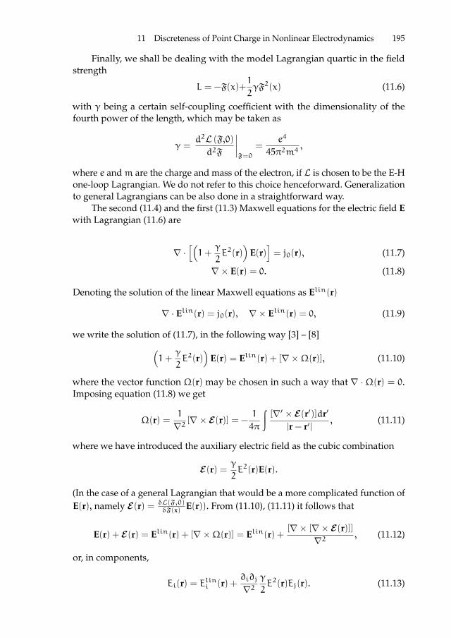
ii

“proc16” — 2016/12/12 — 10:17 — page 195 — #211 ii

ii

ii


Finally, we shall be dealing with the model Lagrangian quartic in the fieldstrength

L = −F(x)+1

2γF2(x) (11.6)

with γ being a certain self-coupling coefficient with the dimensionality of thefourth power of the length, which may be taken as

γ =d2L (F,0)d2F

∣∣∣∣F=0

=e4

45π2m4,

where e andm are the charge and mass of the electron, if L is chosen to be the E-Hone-loop Lagrangian. We do not refer to this choice henceforward. Generalizationto general Lagrangians can be also done in a straightforward way.

The second (11.4) and the first (11.3) Maxwell equations for the electric field Ewith Lagrangian (11.6) are

∇ ·[(1+

γ

2E2(r)

)E(r)

]= j0(r), (11.7)

∇× E(r) = 0. (11.8)

Denoting the solution of the linear Maxwell equations as Elin(r)

∇ · Elin(r) = j0(r), ∇× Elin(r) = 0, (11.9)

we write the solution of (11.7), in the following way [3] – [8](1+

γ

2E2(r)

)E(r) = Elin(r) + [∇×Ω(r)], (11.10)

where the vector function Ω(r) may be chosen in such a way that ∇ ·Ω(r) = 0.

Imposing equation (11.8) we get

Ω(r) =1

∇2[∇× E(r)] = −

1

4π

∫[∇′ × E(r′)]dr′

|r − r′|, (11.11)

where we have introduced the auxiliary electric field as the cubic combination

E(r) = γ

2E2(r)E(r).

(In the case of a general Lagrangian that would be a more complicated function ofE(r), namely E(r) = δL(F,0)

δF(x) E(r)). From (11.10), (11.11) it follows that

E(r) + E(r) = Elin(r) + [∇×Ω(r)] = Elin(r) +[∇× [∇× E(r)]]

∇2, (11.12)

or, in components,

Ei(r) = Elini (r) +∂i∂j

∇2γ

2E2(r)Ej(r). (11.13)

ii

“proc16” — 2016/12/12 — 10:17 — page 196 — #212 ii

ii

ii


In the centre-symmetric case of a single point charge considered in [1], [12], the pro-jection operator ∂i∂j∇2 in the latter equation is identity (Ω(r) = 0), and Eq. (11.13) isno longer an integral equation. The same will be the case in the cylindric-symmetricproblem of two point charges within the approximations to be considered in thenext Section. This simplification makes solution possible. In this case it is sufficientpresent the solution of the differential part of Eq. (11.7) in the form (11.10) settingΩ(r) = 0 in it, then the first Maxwell equation (11.8) is fulfilled automatically.

11.3 Two-body problem

By the two point charge problem we mean the one, where the current j0(r) in (11.7)is the sum of delta-functions centered in the positions r = ±R of two charges q1and q2 separated by the distance 2R (with the origin of coordinates xi placed inthe middle between the charges)

∇ ·[(1+

γ

2E2(r)

)E(r)

]= q1δ

3 (r − R) + q2δ3 (r + R) . (11.14)

In what follows we shall be addressing this equation accompanied by (11.8) forthe combined field of two charges.

We shall be separately interested in the force acting between them. The forceFi =

dP0

dRishould be defined as the derivative of the field energy P0 =

∫Θ00d3x

stored in the solution of Eqs. (11.14), (11.8) over the distance between them.The Noether energy-momentum tensor for the Lagrange density (11.5) is

Tρν = (1− γF (x))Fµν∂ρAµ − ηρνL(x). (11.15)

By subtracting the full derivative ∂µ [(1− γF (x) Fµν)Aρ] , equal to

[(1− γF (x) Fµν)∂µAρ]

due to the field equations (11.1) (without the source and with no dependence onG), the gauge-invariant and symmetric under the transposition ρ ν energy-momentum tensor

Θρν = (1− γF (x))FµνF ρµ − ηρνL(x) (11.16)

is obtained. This is the expression for the electromagnetic energy proper, withoutthe interaction energy with the source, the same as in the reference book [15].When there is electric field alone, the energy density is

Θ00 = (1+γE2

2)E2 −

E2

2

(1+

γE2

4

)=E2

2+3γE4

8. (11.17)

The integral for the full energy of two charges P0 =∫Θ00d3x converges since

it might diverge only when integrating over close vicinities of the charges. Butin each vicinity the field of the nearest charge dominates, and we know from theprevious publication [1] (also to be explained below) that the energy of a separate

ii

“proc16” — 2016/12/12 — 10:17 — page 197 — #213 ii

ii

ii


charge converges in the present model. When the charges are in the same point,R = 0, they make one charge q1 + q2,whose energy coverges, too.

The energy

P0 =

∫Θ00d3x (11.18)

is rotation-invariant. Hence it may only depend on the length R, in other words, bean even function of R. Then, in the point of coincidence R =0, the force Fi = dP0

dRi

must either disappear – if P0 is a differentiable function of R that point– orbe infinite – if not. Crucial to distinguish these cases is the value of the chargedifference δq = q2 − q1. If the two charges are equal, δq = 0, the solutionof equation (11.14) for the field is an even function of R, since this equation isinvariant under the reflection R→ −R. We shall see in the next subsection thatthe linear term in the expansion of the solution in powers of the small ratio R

ris

identical zero in this special case, and so is the linear term of P0.

11.3.1 Large distance case r R (dipole approximation)

We shall look for the solution in the form

E = E(0) + E(1) + ...

where E(0) and E(1) are contributions of the zeroth and first order with respect tothe ratio R

r, respectively.

The zero-order term is spherical-symmetric, because it corresponds to twocharges in the same point that make one charge,

E(0) =rr

E(0)(r). (11.19)

Eq. (11.8) is automatically fulfilled for this form.Let us write the first-order term E

(1)i in the following general cylindric-

symmetric form, linear in the ratio Rr

E(1) = r (R · r)a(r) + Rg(r), (11.20)

where a and g are functions of the only scalar r, and the cylindric axis is fixed asthe line passing through the two charges. Let us subject (11.20) to the equation(11.8) ∇× E(1) = 0. This results in the relation

a(r) =1

r

ddrg(r), (11.21)

provided that the vectors r,R are not parallel. We shall see that with the ansatzes(11.20) and (11.19) equation (11.10) can be satisfied with the choiceΩ(r) = 0 :(

1+γ

2E2(r)

)E(r) = Elin(r), (11.22)

namely, we shall find the coefficient functions a, g from Eq. (11.22) and thenascertain that the relation ( 11.21) is obeyed by the solution.

ii

“proc16” — 2016/12/12 — 10:17 — page 198 — #214 ii

ii

ii


The inhomogeneity in (11.22)

Elin(r) =q1

4π

r − R|r − R|3

+q2

4π

r + R|r + R|3

satisfies the linear (γ = 0) limit of equation (11.14)

∇ · Elin(r) = q1δ3 (r − R) + q2δ3 (r + R) (11.23)

and also (11.8). The inhomogeneity is expanded in Rr

as

Elin(r) =(q1 + q2)

4πr2rr+

(q2 − q1)

4πr2

(Rr− 3

rr

(R · r)r2

)+ ... =

=(q1 + q2)

4πr2rr+1

4π

(dr3

−3 (d · r)r5

r)+..., (11.24)

where d =(q2 − q1)R is the dipole moment, while the dots stand for the disre-garded quadrupole and higher multipole contributions.

The zero-order term satisfies the equation(1+

γ

2E(0)2(r)

)E(0)(r) =

(q1 + q2)

4πr2, (11.25)

with the first term of expansion (11.24) taken for inhomogeneity. This is an alge-braic (not differential) equation, cubic in the present model (11.6), solved explicitlyfor the field E(0) as a function of r in this case, but readily solved for the inversefunction r(E(0)) in any model,which is sufficient for many purposes. Even withoutsolving it we see that for small r γ

14 the second term in the bracket dominates

over the unity, therefore the asymptotic behavior in this region follows from (11.25)to be

E(0)(r) ∼

(q1 + q22πγ

) 13

r−23 .

This weakened – as compared to the Coulomb field q1+q24π

r−2 – singularity is notan obstacle for convergence of the both integrals in (11.18), (11.17) for the properfield energy of the equivalent point charge q1 + q2.

With the zero-order equation (11.25) fulfilled, we write a linear equation forthe first-order correction E(1) from (11.22), to which the second, dipole part in(11.24) serves as an inhomogeneity

E(1) =(q2 − q1)

r2

(Rr− 3

rr

(R · r)r2

)−γ

2

[2(

E(1) · E(0))

E(0) + E(0)2E(1)].

This equation is linear and it does not contain derivatives. We use (11.20) as theansatz. After calculating

2(

E(1) · E(0))

E(0) + E(0)2E(1) = rE(0)2(R · r)r2

(2g+ 3r2a

)+ RgE(0)2,

we obtain two equations, along R and r, with the solutions (δq=q2 − q1, Q =

q2 + q1) :

g =δq

r31

1+ γ2E(0)2

=δq

QrE(0), (11.26)

ii

“proc16” — 2016/12/12 — 10:17 — page 199 — #215 ii

ii

ii


a = −δq

r53+ 5γ

2E(0)2(

1+ γ2E(0)2

) (1+ 3γ

2E(0)2

) (11.27)

From (11.25) we obtain

ddrE(0) = −

2Q

r3(1+ γ

2E(0)2

) − γE(0)2

1+ γ2E(0)2

ddrE(0).

HenceddrE(0) = −

2Q

r3(1+ 3γ

2E(0)2

) . (11.28)

With the help of this relation the derivative of (11.26) can be calculated to coincidewith (11.27) times r. This proves Eq. (11.21) necessary to satisfy the first Maxwellequation (11.8).

By comparing this with (11.27) we see that Eq. (11.21) necessary to satisfy thefirst Maxwell equation (11.8) has been proved.

Finally, relations (11.26) and (11.27) as substituted in the general cylindriccovariant decomposition (11.20) give the linear in R

r(11.27) correction E(1) to the

zero-order field E(0), subject to the equation (11.25), in terms of E(0),which isexplicitly known in our special model. These results may be considered as givingnonlinear correction to the electric dipole field (the second term in (11.24)) due tononlinearity.

Coming back to the discussion on the repulsion force we have to analyze thecontribution of the found linear term E(1) into the energy. The contribution ofE(1) into the energy density (11.17) linear in R contains the factor

(E(1) · E(0)

)=(

E(1) · rr

)E(0).According to the result (11.20) this factor is linear with respect to the

scalar product (R · r) = Rr cos θ. It would give zero contribution into the energy(11.18) due to the angle integration. This does not imply, however, that the forceat the point of coincidence R =0 is zero, because the linear contribution into theintegrand in (11.18) would create divergence of the integral (11.18) near r = 0. Theinterchange of the integration over r and of the limiting transition R

r→ 0 is not

permitted. In the region r < R of integration the linear approximation in the ratioRr

is not relevant. This region gives the infinite contribution into the repulsion forcebetween two charges when the approach each other infinitely close. The case wherethese charges are equal, q1 − q2 = 0, is different. Then the solution for E(1) is justzero, and we confirm the conclusion made above following general argumentationthat equal point charges do not repulse when their positions coincide.

Acknowledgements

Supported by RFBR under Project 14-02-01171, and by the TSU Competitive-ness Improvement Program, by a grant from “The Tomsk State University D. I.Mendeleev Foundation Program”.

ii

“proc16” — 2016/12/12 — 10:17 — page 200 — #216 ii

ii

ii


References

1. C.V. Costa, D.M. Gitman, A.E. Shabad, Finite field-energy of a point charge in QED, Phys.Scr. 90 (2015) 074012, http://stacks.iop.org/1402-4896/90/074012, arXiv:1312.0447[hep-th] (2013).

2. W. Heisenberg and H. Euler, Z. Phys. 98, 714 (1936); V. Wesskopf, Kong. Dans. Vid. Selsk.Math-fys. Medd. XIV, 6 (1936) (English translation in: Early Quantum Electrodynamics:A Source Book, A.I. Miller, University Press, Cambridge, 1994.

3. T.C. Adorno, D. M. Gitman, and A. E. Shabad, Phys. Rev. D 93, 125031 (2016).4. D. M. Gitman and A. E. Shabad, Nonlinear (magnetic) corrections to the field of a static

charge in an external field, Phys. Rev. D 86, 125028 (2012); arXiv:1209.6287[hep-th] (2012).5. T.C. Adorno, D. M. Gitman, and A. E. Shabad, Magnetic response to applied electrostatic

field in external magnetic field, arXiv:1311.4081[hep-th] (2013), Eur. Phys. J. C 74, 2838(2014).

6. T.C. Adorno, D. M. Gitman, and A. E. Shabad, Electric charge is a magnetic dipole whenplaced in a background magnetic field, Phys. Rev. D 89, 047504 (2014), arXiv:1402.3848[hep-th] (2014).

7. T.C. Adorno, D. M. Gitman, and A. E. Shabad, When an electric charge becomes also amagnetic one, Phys. Rev. D 92, 041702 (RC) (2015).

8. C.V. Costa, D.M. Gitman, and A.E.Shabad, Nonlinear corrections in basic problems ofelectro- and magneto-statics in the vacuum, Phys. Rev. D 88, 085026 (2013), arXiv:1307.1802[hep-th] (2013).

9. B. King, P. Bohl and H. Ruhl, Phys. Rev. D 90, 065018 (2014).10. S. Weinberg, The Quantum Theory of Fields, University Press, Cambridge, 2001.11. V.I. Ritus, in Problems of quantum electrodynamics of intense field, Trudy of P.N.Lebedev

Phys. Inst. 168, 5 (1986).12. D.M. Gitman, A.E. Shabad, and A.A. Shishmarev, Moving point charge as a soliton,

arXiv:1509.06401[hep-th] (2015).13. A.E. Shabad, Lecture talk, given at the University of Dusseldorf on March 14, 2016 and

at Tomsk State University on June 13, 2016.14. M.B. Ependiev, to appear in Theor. Math. Phys.15. L.D. Landau, E.M. Lifshitz, The Classical Theory of Fields. (Addison-Wesley, Vol. 2 (1st

ed.), 1951).

ii

“proc16” — 2016/12/12 — 10:17 — page 201 — #217 ii

ii

ii




12 The Hypothesis of Unity of the Higgs Field Withthe Coulomb Field

E.G. Dmitrieff ?

29 88 Postyshev bvd., Irkutsk, Russia

Abstract. In this discussion we propose a hypothesis about the physical unity of theCoulomb field and the Higgs field, which leads to the concept of physical vacuum with theperiodic domain structure. Estimating the domain radius and the thickness of cross-domainwall in the spheric approximation, we find them both about 10−21 m.

Povzetek. V diskusiji avtor obravnava hipotezo fizikalne povezanosti Coulombskega inHiggsovega polja, kar vodi k fizikalnemu vakuumu s periodicno strukturo domen. Za radijdomene in debelino sten med domenami dobi oceno reda 10−21 m.

12.1 Introduction

Developing the model of vacuum and fundamental particles, that is based eitheron boolean algebra objects or spatial polyhedral tessellations, we were lookingfor a physical structure in the Nature, which would behave like a discrete fieldof binary digits, or as a foam with electrically charged near-to-polyhedral cells.Combining the ideas of vacuum domains [1], Kelvin problem of minimal-surfacedfoam [2] and its best solution [3], and specific alteration of electric charges in ourmodel [4], we supposed the following model of the physical vacuum.

12.2 United Higgs - Coulomb field

We suppose that scalar Higgs field and field of Coulomb scalar potential are thesame physical entity. Also we suppose that the complex phase of Higgs field islimited to 0 and π (like angle in sphere S0), forming just real values, positive andnegative. In this case, the only possibility to get from positive to negative valueand back, is to go through zero value.

The space, being in average electrically neutral, in this case would be eitherstructureless ’empty space’ with ϕ = 0 everywhere (may be, with fluctuations), orthe mixture of pieces, or domains [1], having different and alternating values ofthis field.

Following the effective energy density of Higgs field as

V(ϕ) = λ2(ϕ2 − η2)2, (12.1)? [email protected]

ii

“proc16” — 2016/12/12 — 10:17 — page 202 — #218 ii

ii

ii

202 E.G. Dmitrieff

in empty space phase it would be positive: V = λ2η4.Inside domains, where the potential keeps near ±ϕ, the electrical field and

energy density is about zero.Near the walls between domains, the potential changes from positive to

negative value – or back – through zero. So the walls will have extra energy, sincezero potential corresponds to local maximum of effective energy density.

The electric charge in this case will be distributed mostly along the walls,causing pieces to be charged.

12.3 Evaluation of characteristic structure sizes

Equating the expression of potential for the charged sphere with radius r to thevacuum expectation value [5]:

q

4πε0r= η ≈ 246GeV, (12.2)

we estimate the domain size:

r =q

4πε0η=qc2

107η=

ec2

6 · 107η; (12.3)

r =1.602 · 10−19 · 2.9982 · 1016

6 · 107 · 246 · 109= 9.755 · 10−22 ≈ 10−21m. (12.4)

As the value of charge q we use 16e since it is the charge carried by one b-type bit

in our 8-bit model.The wall between pieces can be treated as a charged capacitor. Equating the

capacity of the spherical capacitor with the charge to potential ratio:

C =q

η=4πε0r

2

d=107r2

dc2=

q2c2

107dη2, (12.5)

we express d to estimate the wall width, which occurs equal to r:

d =qc2

107η= r (12.6)

12.4 Spontaneous origination of the structure

Probably, the Coulomb character of field causes the instability of domains withradius larger than r: being charged, the different parts of any domain wouldexperience the Coulomb repulsion from each other, so the domain would trendto split into smaller parts. Since this process increases the specific square of inter-domain walls surface, it also leads to increased Higgs energy. So the fragmentationmust stop when the Higgs energy equals to Coulomb one.

In this case, the model is supposed to be isomorphic with the solution ofthe Kelvin problem [2], that is about of the minimal-surfaced foam of bubbles

ii

“proc16” — 2016/12/12 — 10:17 — page 203 — #219 ii

ii

ii

12 The Hypothesis of Unity of the Higgs Field With the Coulomb Field 203

with equal volume. The ’air’ phase corresponds to volumes, and ’liquid’ phasecorresponds to walls.

Because of equality of the estimated cell radius to the wall width, the potentialis probably changes smoothly in a function close to a sine wave, forming no sharpwalls.

The best known solution of Kelvin problem is the foam with Weaire-Phelanstructure [3]. We found that this structure has two variants of optimal charge alter-ations, with different handedness. This providing possibility for the asymmetricbaryogenesis.

12.5 Beyond the Standard Model

According to our models [4] and the assumptions noted above, vacuum probablyhas a structure of periodic Weaire-Phelan foam with alternating positive andnegative charged cells, and the single or multiple anti-structure defects in it areexperimentally observed as fundamental particles. Their properties are determinedby the defect count and structure.

We also suppose that the vacuum structure may experience distortion andwave processes, that are relevant to the phenomena of gravity.

References

1. Va.B. Zel’dovich, I.Yu. Kobzarev, and L.B. Okun, Cosmological consequences of aspontaneous breakdown of a discrete symmetry, Zh. Eksp. Teor. Fiz. 67 3–11 (July 1974).

2. Lord Kelvin (Sir William Thomson), ”On the Division of Space with Min-imum Partitional Area” (PDF), Philosophical Magazine 24 (151): 503 (1887),doi:10.1080/14786448708628135.

3. D. Weaire, R. Phelan, A counter-example to Kelvin’s conjecture on minimal surfaces,Phil. Mag. Lett., 69 107-110 (1994) , doi:10.1080/09500839408241577.

4. E.G. Dmitrieff: Experience in modeling properties of fundamental particles using binarycodes, see this volume p. 8.

5. A. Kobakhidze, A. Spencer-Smith, The Higgs vacuum is unstable, arXiv:1404.4709v2[hep-ph].

ii

“proc16” — 2016/12/12 — 10:17 — page 204 — #220 ii

ii

ii




13 What Cosmology Can Come From the BrokenSU(3) Symmetry of the Three Known Families?

A. Hernandez Galeana1 ? and M.Yu. Khlopov2,3,4 ??

1Departamento de Fısica, ESFM - Instituto Politecnico NacionalU. P. ”Adolfo Lopez Mateos”. C. P. 07738, Ciudad de Mexico, Mexico.2National Research Nuclear University ”MEPHI” (Moscow EngineeringPhysics Institute), 115409 Moscow, Russia3Centre for Cosmoparticle Physics “Cosmion” 115409 Moscow, Russia4APC laboratory 10, rue Alice Domon et Leonie Duquet 75205Paris Cedex 13, France

Abstract. The question, why there are three quark-lepton families, cannot find answerin the Standard model. Extension of the symmetry of the Standard model by local gaugeSU(3) symmetry of families involves new physics at high energy scales. Even elusivefrom direct experimental probes such construction can be tested in the combination ofphysical, astrophysical and cosmological signatures, in which cosmological probes playimportant role. In the case of chiral local gauge SU(3)H family symmetry such probes notonly provided complete test of the model, but also demonstrated a possibility to describethe physical basis of modern cosmology, involving inflationary models with baryosynthesisand nonbaryonic dark matter. We formulate the programme of studies of cosmologicalimpact of broken local gauge vector-like SU(3)F family symmetry.

Povzetek. Standardni model ne more odgovoriti na vprasanje, zakaj obstajo tri druzinekvarkov in leptonov. Razsiritev simetrij standardnega modela z lokalno umeritveno druzinskosimetrijo SU(3) ponudi nove moznosti za opis dogodkov pri visokih energijah. Lokalnaumeritvena druzinska simetrija SU(3)H ponudi drugacen opis vesolja, ko so v modelvkljuceni tudi inflacija, sinteza barionov in nebarionska temna snov. Delo predstavi pro-gram studija kozmoloskih posledic zlomljene druzinske simetrije SU(3)F.

13.1 Introduction

The structure of the ordinary matter does not need more than one (first) family.We need quarks to build nucleons, electrons to bind with nuclei in neutral atomsand we have to add neutrino as a necessary element of beta processes, in which allthe chemical elements of Mendeleev periodic table can be formed. However, theNature gives us three families - symmetric by their interactions and asymmetricin their mass pattern. Extending the symmetry of the ”Standard Model” (SM) byfamily symmetry and putting this additional symmetry on the same local gauge

? [email protected]?? [email protected]

ii

“proc16” — 2016/12/12 — 10:17 — page 205 — #221 ii

ii

ii

13 What Cosmology Can Come From the Broken SU(3) Symmetry. . . ? 205

symmetry footing as in the Standard model we immediately find that thoughthe family symmetry breaking scales in quark and lepton masses are withinthe range of electroweak symmetry breaking the absence of Flavor ChangingNeutral Currents (FCNC) makes us to consider much larger scale of symmetrybreaking for horizontal gauge bosons, which should be much heavier, than Wand Z. To solve this problem one should assume the existence of heavy partnersfor ordinary quarks and leptons. These heavy particles should get their massesfrom the same Higgs mechanism, which makes very massive horizontal bosons,while mixing of these heavy partners with ordinary quarks and leptons reflectsthe pattern of family symmetry breaking in the mass hierarchy of quarks andleptons of the three known generations. Cosmological impact of this constructionprovides additional source of information on possible parameters and signaturesof a family symmetry model. Here after brief review of the cosmology of horizontalunification, developed by [1,2] (see [3–5] for review and references) we turn tothe approach by [Albino] and formulate open questions for successive study ofcosmological impact of his vector-like approach to a gauge model of broken familysymmetry.

13.2 Cosmology of chiral SU(3)H symmetry of known families

The existence and observed properties of the three known quark-lepton familiesappeal to the broken SU(3)H family symmetry [1,8,9], which should be involvedin the extension of the Standard model. It provides the possibility of the Horizontalunification in the ”bottom-up” approach to the unified theory [2]. Even in itsminimal implementation the model of Horizontal unification has demonstratedits principal possibility to reproduce the main necessary elements of the moderncosmology. It provided the physical mechanisms for inflation and baryosynthesisas well as it offered unified framework to describe Cold, Warm, Hot and UnstableDark Matter candidates. Methods of cosmoparticle physics [3,4] have providedthe complete test of this model, proving such possibility for any physical model,hiding its basis in super high energy scales.

13.2.1 Horizontal hierarchy

The approach of Refs. [1,2,8,9] (and its revival in Refs. [10–12]) followed from theconcept of local chiral gauge symmetry SU(3)H, first proposed by Chkareuli[13].Under the action of this symmetry the left-handed quarks and leptons transform asSU(3)H triplets and the right-handed as antitriplets. Their mass term transformsas 3

⊗3 = 6

⊗3 and, therefore, can only form in the result of horizontal symmetry

breaking.This approach can be trivially extended to the case of n generations, assum-

ing the proper SU(n) symmetry. For three generations, the choice of horizontalsymmetry SU(3)H seemed to be the only possible choice because the orthogonaland vector-like gauge groups could not provide different representations for theleft- and right-handed fermion states. However, it turns out [Albino] that vector-like implementation for family SU(3)F is also possible, what we discuss in thesuccessive sections.

ii

“proc16” — 2016/12/12 — 10:17 — page 206 — #222 ii

ii

ii

206 A. Hernandez Galeana and M.Yu. Khlopov

The mass hierarchy between generations was related to the hypothesis of ahierarchy of such symmetry breaking. This hypothesis was called - the hypothesisof horizontal hierarchy (HHH)[14–16].

The model was based on the gauge SU(3)H flavor symmetry, which was ad-ditional to the symmetry of the Standard model. It means that there exist 8 heavyhorizontal gauge bosons and there are three multiplets of heavy Higgs fields ξ(n)ij

(i,j - family indexes,n = 1, 2, 3) in nontrivial (sextet or triplet) representations ofSU(3)H. These heavy Higgs bosons were singlets relative to electroweak symme-try and don’t have Yukawa couplings with ordinary light fermions. They haddirect coupling to heavy fermions. The latter were singlets relative to electroweaksymmetry. Ordinary Higgs φ of the Standard model was singlet relative to SU(3)H.It coupled left-handed light fermions fiL to their heavy right-handed partners FiR,which were coupled by heavy Higgses ξij with heavy left handed states FjL. Heavyleft-handed states FjL were coupled to right handed light states fjR by a singletscalar Higgs field η, which was singlet both relative to SU(3)H and electroweakgroup of symmetry. The described succession of transitions realized Dirac see-sawmechanism, which reproduced the mass matrixmij of ordinary light quarks andcharged leptons f due to mixing with their heavy partners F. It fixed the ratio ofvacuum expectation values of heavy Higgs fields, leaving their absolute value asthe only main free parameter, which was determined from analysis of physical,astrophysical and cosmological consequences.

The SU(3)H flavor symmetry was assumed to be chiral to eliminate the fla-vor symmetric mass term. The condition of absence of anomalies implied heavypartners of light neutrinos, and the latter acquired mass by Majorana see-sawmechanism. The natural absence in the heavy Higgs potentials of triple couplings,which did not appear as radiative effects of any other (gauge or Yukawa) interac-tion, supported additional global U(1) symmetry, which could be associated withPeccei-Quinn symmetry and whose breaking resulted in the Nambu-Goldstonescalar filed, which shared the properties of axion, Majoron and singlet familon.

Horizontal unification The model provided complete test (in which its simplestimplementation was already ruled out) in a combination of laboratory tests andanalysis of cosmological and astrophysical effects. The latter included the study ofthe effect of radiation of axions on the processes of stellar evolution, the study ofthe impact of the effects of primordial axion fields and massive unstable neutrinoon the dynamics of formation of the large-scale structure of the Universe, as wellas analysis of the mechanisms of inflation and baryosynthesis based on the physicsof the hidden sector of the model.

The model resulted in physically self-consistent inflationary scenarios withdark matter in the baryon-asymmetric Universe. In these scenarios, all steps of thecosmological evolution corresponded quantitatively to the parameters of particletheory. The physics of the inflaton corresponded to the Dirac see-saw mechanismof generation of the mass of the quarks and charged leptons, leptogenesis of baryonasymmetry was based on the physics of Majorana neutrino masses. The parametersof axion CDM, as well as the masses and lifetimes of neutrinos corresponded tothe hierarchy of breaking of the SU(3)H symmetry of families.

ii

“proc16” — 2016/12/12 — 10:17 — page 207 — #223 ii

ii

ii


The experience gained in the development of this model encourages us toelaborate similar programme for the case of vector-like SU(3)F family symmetry.

13.3 Horizontal hierarchy in vector-like model

In the approach of vector-like and universal SU(3)F gauge family symmetry [6,7],all the Standard Model left handed and right handed quarks and leptons transformas the fundamental triplet representation of the SU(3)F family symmetry. This isthe basic starting difference in comparison to the chiral one of Refs. [1,2,8,9], whichalso defines the different hidden sectors, scalar fields and heavy fermions in orderto break symmetries and generate masses for quarks and leptons, as well as thedifferent possible cosmology consequences.

Right handed neutrinos in this approach of vector-like gauge SU(3)F familysymmetry are introduced to cancel anomalies. The fermion content assume anew set of vector - like quarks and leptons U, D, E and N singlets under theSU(3)F × SU(2)L symmetry.

SU(3)F family symmetry is broken spontaneously in two stages by heavy SMsinglet scalars η(n)i (i - family index, n = 2, 3) in the fundamental representation ofSU(3)F, generating 5 extremely heavy boson masses (& 100 TeV’s) and 3 almostdegenerate boson masses of few TeV’s. The ”Electroweak Symmetry Breaking”(EWSB) is achieved by the Higgs fields Φui and Φdi , which transform simultane-ously as triplets under SU(3)F and as the φ and φ = i σ2φ

∗ Higgs doublets underthe SM, respectively.

The gauge symmetry G ≡ SU(3)F ×GSM, the fermion content, and the trans-formation of the scalar fields, all together, avoid Yukawa couplings between SMfermions. The tree level allowed Dirac Yukawa couplings involve terms betweenthe SM fermions ψSM,(L,R) and the corresponding vector-like fermion F (F=U, D,E and N) : hF ψSM,L Φu,d FR + h(n) ψSM,R η

(n) FL + MF FL FR + h.c, whichyield tree level Dirac See-saw mass matrices for quarks and leptons, includingneutrinos, with two massless eigenvalues. Therefore, in this scenario ordinaryheavy fermions, top and bottom quarks and tau lepton, become massive at treelevel, while light fermions, including light neutrinos obtain masses from radiativecorrections mediated by the massive gauge bosons of the SU(3)F family symmetry.

Neutrinos may also obtain left-handed and right-handed Majorana massesboth from tree level and radiative corrections.

13.4 Towards cosmology of vector-like SU(3)F family symmetry

Here we formulate the open questions for cosmological impact of the model ofvector-like SU(3)F family symmetry. We can stipulate the following cosmologicallyinteresting aspects:

• Is there a candidate for inflaton?• Which new particles are stable or metastable in vector-like SU(3)F model• Are there SU(3)F instantons or sphalerons?

ii

“proc16” — 2016/12/12 — 10:17 — page 208 — #224 ii

ii

ii

208 A. Hernandez Galeana and M.Yu. Khlopov

• What kind of phase transitions can take place in the early Universe with Familysymmetry breaking

• Can there be a new mechanism of baryosynthesis? Due to Majorana mass term- there can be leptogenesis with successive redistribution of lepton excess tobaryon and lepton excess due to electroweak B and L nonconservation

• Is there additional global symmetry and if, yes, what kind of Nambu-Goldstone(pseudo Nambu Goldstone) solutions can exist?

This list can be modified and extended in the course of our studies.

13.5 Conclusion

Here we have formulated the programme of our joint studies during Albino’ssabbatical year in the APC, Paris, France. We hope to present their first results atthe coming XX Bled Workshop.

Acknowledgements

AHG acknowledge partial support by the ”Instituto Politecnico Nacional”, (Grantsfrom EDI and COFAA) and ”Sistema Nacional de Investigadores” (SNI) in Mexico.The work by M.K.was performed within the framework of the Center FRPP sup-ported by MEPhI Academic Excellence Project (contract 02.03.21.0005, 27.08.2013).The part on initial cosmological conditions was supported by the Ministry ofEducation and Science of Russian Federation, project 3.472.2014/K and on theforms of dark matter by grant RFBR 14-22-03048.

References

1. Z. Berezhiani and M. Yu.Khlopov: Theory of broken gauge symmetry of families,Sov.J.Nucl.Phys. 51, 739 (1990).

2. A. S. Sakharov and M. Yu. Khlopov: Horizontal unification as the phenomenology ofthe theory of everything, Phys.Atom.Nucl. 57, 651 (1994).

3. M. Yu. Khlopov: Cosmoparticle physics, World Scientific, New York -London-Hong Kong- Singapore, 1999.

4. Maxim Khlopov, Fundamentals of Cosmic Particle physics, CISP-SPRINGER, Cambridge,2012.

5. M. Yu. Khlopov: Fundamental Particle Structure in the Cosmological Dark Matter, J. ofMod. Phys. A 28 1330042 (60 pages) (2013).

6. A. Hernandez-Galeana, Rev. Mex. Fis. 50, 522 (2004). hep-ph/0406315.7. A. Hernandez-Galeana, Bled Workshops Phys.,(ISSN:1580-4992),

16, 47 (2015). arXiv:1602.08212[hep-ph]; 15, 93 (2014). arXiv:1412.6708[hep-ph]; 14,82 (2013). arXiv:1312.3403[hep-ph]; 13, 28 (2012). arXiv:1212.4571[hep-ph]; 12, 41(2011). arXiv:1111.7286[hep-ph]; 11, 60 (2010). arXiv:1012.0224[hep-ph]; 10, 67 (2009).arXiv:0912.4532[hep-ph].

8. Z. Berezhiani and M. Yu.Khlopov: Physical and astrophysical consequences of breakingof the symmetry of families, Sov.J.Nucl.Phys. 51, 935 (1990).

ii

“proc16” — 2016/12/12 — 10:17 — page 209 — #225 ii

ii

ii


9. Z. Berezhiani, M. Yu.Khlopov and R. R. Khomeriki: On the possible test of quantumflavor dynamics in the searches for rare decays of heavy particles, Sov.J.Nucl.Phys. 52,344 (1990).

10. T. Appelquist, Y. Bai and M. Piai: SU(3) Family Gauge Symmetry and the Axion, Phys.Rev. D 75, 073005 (2007).

11. T. Appelquist, Y. Bai and M. Piai: Neutrinos and SU(3) family gauge symmetry, Phys.Rev. D 74, 076001 (2006).

12. T. Appelquist, Y. Bai and M. Piai: Quark mass ratios and mixing angles from SU(3)family gauge symmetry, Phys. Lett. B 637, 245 (2006).

13. J. L. Chkareuli: Quark-Lepton families: From SU(5) to SU(8) symmetry, JETP Lett. 32,671 (1980).

14. Z. G. Berezhiani, J. L. Chkareuli: Mass of the T quark and the number of quark leptongenerations, JETP Lett. 35, 612 1982.

15. Z. G. Berezhiani, J. L. Chkareuli: Neutrino oscillations in grand unified models with ahorizontal symmetry, JETP Lett. 37, 338 (1983).

16. Z.G. Berezhiani: The weak mixing angles in gauge models with horizontal symmetry:A new approach to quark and lepton masses, Phys. Lett. B 129, 99 (1983).

ii

“proc16” — 2016/12/12 — 10:17 — page 210 — #226 ii

ii

ii




14 Phenomenological Mass Matrices With aDemocratic Warp

A. Kleppe ?

SACT, Oslo

Abstract. Taking into account all available data on the mass sector, we obtain unitaryrotation matrices that diagonalize the quark matrices by using a specific parametrization ofthe Cabibbo-Kobayashi-Maskawa mixing matrix. In this way, we find mass matrices forthe up- and down-quark sectors of a specific, symmetric form, with traces of a democratictexture.

Povzetek. Avtorica uporabi razpolozljive podatke o kvarkih, da doloci unitarne matrikerotacij, ki diagonalizirajo masne matrike. Izbere parametrizacijo mesalne matrike Cabibba-Kobayashija-Maskawe, ki poskrbi, da imata masni matriki kvarkov u in d, ki sta zelo blizudemokraticnima matrikama, posebno simetricno obliko.

14.1 Introduction

The Standard Model of particle physics is flawed by the large number of freeparameters, for which there is at present no explanation. Most of these free param-eters reside in flavour space, the structure of which is determined by the fermionmass matrices, i.e. by the form that the mass matrices take in the “weak basis”where mixed fermion states interact weakly. This basis differs from the mass bases,where the mass matrices are diagonal, with entries corresponding to the masses ofthe physical fermions.

The information content of a matrix is contained in its matrix invariants, whichin the case of a N×NmatrixM are the N sums and products of the eigenvaluesλj, such as traceM, detM,

I1 =∑j λj = λ1 + λ2 + λ3...

I2 =∑jk λjλk = λ1λ2 + λ1λ3 + λ1λ4 + ...

I3 =∑jkl λjλkλl = λ1λ2λ3 + λ1λ2λ4 + ...

...IN = λ1λ2 · · · λN

(14.1)

The search for the “right” mass matrices is based on the assumption that even ifthe information content of a matrix is contained in its invariants, the form of a? [email protected]

ii

“proc16” — 2016/12/12 — 10:17 — page 211 — #227 ii

ii

ii

14 Phenomenological Mass Matrices With a Democratic Warp 211

matrix also carries important information. The hope is that the form of the massmatrices in the “weak basis” can give some hint about the origin of the fermionmasses.

The crux is that we don’t know which of the flavour space bases is the weakbasis, we consequently don’t know what form of the mass matrices have in thisunknown basis. The different mass matrix ansatze found in the literature corre-spond to different choices, based on different assumptions, as to which flavourspace basis is the weak basis.

14.2 Phenomenology

The Standard Model might not be a fundamental theory, but it certainly is anexceedingly successful model. In our approach, we follow the phenomenlogicaltrack, and scrutinize all available data that are relevant for the mass sector. Inaddition to numerical mass values, there is also the mixing matrix V that appearsin the flavour changing charged current Lagrangian

Lcc = −g

2√2fLγ

µVf ′LWµ + h.c. (14.2)

where as before f and f ′ are fermion fields with charges Q and Q− 1, correspond-ingly. In the case of the quarks, the mixing matrix is the Cabbibo-Kobayashi-Maskawa (CKM) [1] mixing matrix.

That V 6= 1 implies that the up-sector mass basis is different from the down-sector mass basis, the CKM matrix being the bridge between the two mass bases.As we go from the weak basis to the two different mass bases by rotating thematrices by the unitary matrices U and U ′, respectively,

M→ UMU† = D = diag(mu,mc,mt) (14.3)

M ′ → U ′M ′U ′† = D ′ = diag(md,ms,mb)

we have that V = UU′†. A given choice of the weak basis - i.e. of the mass

matrices, thus corresponds to choosing a factorization of the mixing matrix, andsince U = U(M) and U ′ = U ′(M ′), V = U(M)U ′†(M ′) = V(M,M ′).

The charged current Lagrangian (14.2) can be interpreted as describing theinteraction between the physical up-sector particles ψL = (u, c, t)L with the mixeddown-sector states, or equivalently as the interaction between the up-sector mixedstates and the down-sector mass states ψ ′L = (d, s, b)L,

If we take the definition of the CKM matrix at face value, V = UU ′†, it ishowever more natural to perceive the charged current interactions as taking placebetween mixed up-sector states and mixed down-sector states,

Lcc = −g√2ψLγ

µVψ ′LWµ + h.c. = −g√2ϕLγ

µϕ ′LWµ + h.c. (14.4)

where

ϕ = U†

uct

and ϕ ′ = U ′†

dsb

ii

“proc16” — 2016/12/12 — 10:17 — page 212 — #228 ii

ii

ii

212 A. Kleppe

are the fermion fields in the weak basis in flavour space, and ψ and ψ ′ are thecorresponding mass eigenstates.

Mass eigenstates are defined as “physical”, corresponding to particles withdefinite masses; while the weakly interacting mixings of mass states are referred toas “flavour states”. Physical particles are thus identified as mass eigenstates. In thecase of neutrinos the situation is however somewhat different, since neutrino masseigenstates do not appear on stage, they merely propagate in free space. In therealm of neutral leptons it is actually the flavour states νe, νµ, ντ that we perceiveas “physical”, since they are the only neutrinos that we “see”, as they appeartogether with the charged leptons. As the charged leptons e, µ, τ are assumed to beboth weak eigenstates and mass eigenstates, the only mixing matrix that appearsin the lepton sector is the Pontecorvo-Maki-Nakagawa-Sakata mixing matrix U[2], which only operates on neutrino states,νeνµ

ντ

=

Ue1 Ue2 Ue3Uµ1 Uµ2 Uµ3Uτ1 Uτ2 Uτ3

ν1ν2ν3

where (ν1, ν2, ν3) are mass eigenstates, and (νe, νµ, ντ) are the weakly interacting“flavour states”. In the lepton sector, the charged currents are thus interpretedas charged lepton flavours (e, µ, τ) interacting with the neutrino “flavour states”(νe, νµ, ντ).

For quarks as well as leptons, the relation between the weakly interactingfermion fields ϕ and the mass eigenstates ψ is determined by the unitary rotationmatrix Uwhich diagonalizes the mass matrixM,

Lmass = ϕMϕ = ϕU†(UMU†)Uϕ = ψ

m1 m2m3

ψ,

ii

“proc16” — 2016/12/12 — 10:17 — page 213 — #229 ii

ii

ii


in the quark sector the (physical) mass eigenstates thus are the fields ψ = Uϕ andψ ′ = U ′ϕ ′,

ψ =

uct

and ψ ′ =

dsb

The CKM matrix plays an important role in relating the mass matrices for

the up- and down-sectors, since once the form of the mass matrix of one ofthe charge sectors is established, also the form of the mass matrix of the othercharge sector is determined, via the CKM mixing matrix. Once the form of theup-sector mass matrixM is established,the unitary matrix U that diagonalizesMis determined. And since V = UU ′†, this also determines U ′ = V†U, whereby wehaveM ′ = U ′†diag(d, s, b)U ′. In this senseM andM ′ are determined together.

14.3 Factorizing the mixing matrix

The Cabbibo-Kobayashi-Maskawa mixing matrix can of course be parametrizedand factorized in many different ways, and different factorizations correspond todifferent rotation matrices U and U ′. The most obvious and “symmetric” factor-ization of the CKM mixing matrix, following the “standard parametrization” [3]with three Euler angles α, β, 2θ,

V =

cβc2θ sβc2θ s2θe−iδ

−cβsαs2θeiδ − sβcα −sβsαs2θe

iδ + cβcα sαc2θ−cβcαs2θe

iδ + sβsα −sβcαs2θeiδ − cβsα cαc2θ

= UU′† (14.5)

is to take the diagonalizing rotation matrices for the up- and down-sectors as

U =

1 0 0

0 cosα sinα0 − sinα cosα

e−iγ 1eiγ

cos θ 0 sin θ0 1 0

− sin θ 0 cos θ

=

=

cθe−iγ 0 sθe

−iγ

−sαsθeiγ cα sαcθe

iγ

−cαsθeiγ −sα cαcθe

iγ

(14.6)

and

U ′ =

cosβ − sinβ 0sinβ cosβ 0

0 0 1

e−iγ 1eiγ

cos θ 0 − sin θ0 1 0

sin θ 0 cos θ

=

cβcθe−iγ −sβ −cβsθe−iγ

sβcθe−iγ cβ −sβsθe

−iγ

sθeiγ 0 cθe

iγ

(14.7)

respectively, where α, β, θ and γ correspond to the parameters in the standardparametrization, with γ = δ/2, δ = 1.2± 0.08 rad, and 2θ = 0.201± 0.011, whileα = 2.38± 0.06 and β = 13.04± 0.05. In this factorization scheme, α and β arerotation angles operating in the up-sector and the down-sector, respectively.

ii

“proc16” — 2016/12/12 — 10:17 — page 214 — #230 ii

ii

ii

214 A. Kleppe

Now, with the rotation matrices U and U ′, we obtain the the up- and down-sector mass matrices

M = U†diag(mu,mc,mt)U and M ′ = U ′†diag(md,ms,mb)U ′,

such that

M =

M11 M12 M13

M21 M22 M23

M31 M32 M33

=

Xc2θ + Ys2θ −Zsθ e

−iγ (X− Y)cθsθ−Zsθ e

iγ Y + 2Z cot 2α Zcθ eiγ

(X− Y)cθsθ Zcθ e−iγ Xs2θ + Yc

2θ

(14.8)

where X = mu, Z = (mc −mt) sinα cosα and Y = mt + Z tanα = mc sin2 α +

mt cos2 α, and

M ′ =

M ′11 M ′12 M ′13M ′21 M′22 M

′23

M ′31 M′32 M

′33

=

X ′s2θ + Y′c2θ Z ′cθ e

iγ (X ′ − Y ′)cθsθZ ′cθ e

−iγ Y ′ + 2Z ′ cot 2β −Z ′sθ e−iγ

(X ′ − Y ′)cθsθ −Z ′sθ eiγ X ′c2θ + Y

′s2θ

(14.9)

where X ′ = mb, Z ′ = (ms−md) sinβ cosβ and Y ′ = md+Z ′ tanβ = md cos2 β+ms sin2 β.

The two mass matrices thus have similar textures, or forms, and there is evena relational equality,

M32/M12 =M′12/M

′32 = − cot θ

which is independent of the quark masses.From

Y = mc sin2 α+mt cos2 α,

Z = (mc −mt) sinα cosα,

Y ′ = md cos2 β+ms sin2 β

and

Z ′ = (ms −md) sinβ cosβ,

we moreover have

mu = X, mc = Y + Z cotα, mt = Y − Z tanαmd = Y ′ − Z ′ tanβ, ms = Y

′ + Z ′ cotβ, mb = X ′(14.10)

14.4 Numerical matrices

Using the numerical values β = 13.04o, α = 2.38o, δ = 1.2 ± 0.08 rad, and2θ = 0.201± 0.011 for the the angles, and using the mass values (Jamin 2014) [4]for the up- and down-sectors,

mu(MZ) = 1.24MeV mc(MZ) = 624MeV mt(MZ) = 171550MeV

md(MG) = 2.69MeV ms(MG) = 53.8MeV mb(MG) = 2850MeV(14.11)

ii

“proc16” — 2016/12/12 — 10:17 — page 215 — #231 ii

ii

ii


we get the numerical values for the mass matrices (14.8) and (14.9)

M =

1.767 12.439e−iγ −300.389

12.439eiγ 918.759 −7091.892eiγ

−300.389 −7091.892e−iγ 171254.714

MeV (14.12)

and

M ′ =

5.299 11.23eiγ 4.99

11.23e−iγ 51.18 −0.0197e−iγ

4.99 −0.0197eiγ 2849.99,

MeV (14.13)

where inM,

M11 = mu + σ,M22 = mc +Q− σ,M33 = mt −Q,M22 +M33 = mc +mt − σ and |M33M12| ≈ |M13M32|,with σ ' 0.53MeV , Q ' 295.3MeV .

Likewise, inM ′,

M ′11 = md + R,M ′22 = ms + η− R,M ′33 = mb − η,M ′11 +M

′22 = md +ms + η, and |M ′33M

′32| ≈ |M ′13M

′12|,

with R ' 2.61MeV, η ' 0.011MeV.

14.5 Traces of a democratic structure

Our factorization of the Cabbibo-Kobayashi-Maskawa mixing matrix is only oneof many possible choices, in (14.5) we can moreover sandwich any number ofunitary matrices between U and U ′,

V = UU′† = UO1O

†1U′† = UO1O2O

†2O†1U′† = ...

whereOj are unitary matrices such that each set of sandwichedOjO†j corresponds

to a new set of unitary matrices diagonalizing the mass matrices, and thus to yetanother type of mass matrix texture.

In our first approach [9], the sandwich principle was used with the purposeof investigating democratic mass matrix textures. In the democratic scenario, it isassumed that both the up- and down-sector mass matrices have an initial structureof the typeM0 = kN andM ′0 = k

′N where

N =

1 1 11 1 1

1 1 1

,with the mass spectra (0, 0, 3k), (0, 0, 3k ′), and a mixing matrix equal to unity (i.e.no CP-violation). The flavour symmetry displayed by the matrices M0 and M ′0 issubsequently broken, whereby both mass spectra contain the three observed non-zero values, and the mixing matrix becomes the CKM matrix (with a CP-violatingphase).

ii

“proc16” — 2016/12/12 — 10:17 — page 216 — #232 ii

ii

ii

216 A. Kleppe

Our sandwiching procedure started from the factorization V = UU ′†, with Uand U ′ as in (14.6) and (14.7), and the matrix

Udem =1√6

√3 −√3 0

1 1 −2√2√2√2

(14.14)

which diagonalizes the democratic matrix N. When Udem and its Hermitianconjugate were put into the mixing matrix,

V = UU ′† ⇒ V = UUdemU†demU

′†

we obtained new rotation matricesUUdem andU ′Udem which indeed correspondto mass matrices with democratic textures.

In simplest case (14.5), without any UdemU†dem or other matrices sandwiched

between U and U ′ in V = UU ′†, there is however already some interesting,democracy-like structure present, which is can be made visible by a slight re-formulation of the matrices (14.8) and (14.9). Even though the matrix elementsare dominated by the hierarchical family structure, which does not look very“democratic”, rewriting the matrices by extracting the dimensional coefficients ρand µ unveils this structure:

M = ρ

A Be−iγ −C

Beiγ H −BCeiγ

−C −BCe−iγ C2

(14.15)

and

M ′ = µ

A ′ B ′Ceiγ C

B ′Ce−iγ H ′ −B ′e−iγ

C −B ′eiγ C2

, (14.16)

with

ρ = (Y − X)s2θ, A = (X cot2θ+Y)/(Y − X), B = Z/(Y − X)sθ,

H = (Y + 2Z cot 2α)/(Y − X)s2θ, C = cot θµ = (X ′ − Y ′)s2θ, A

′ = (X ′ + Y ′ cot2θ)/(X′ − Y ′), B ′ = Z ′/(X ′ − Y ′)sθ

H ′ = (Y ′ + 2Z ′ cot 2β)/(X ′ − Y ′)s2θ

Numerically, with the mass values (14.11), this corresponds to

ρ = 0.5269MeV, A = 3.3533, B = 23.608,H = 1743.71, C = cot θ ' 570.1µ = 0.00875MeV, A ′ = 605.6, B ′ = 2.2514, H ′ = 5849.14,

where incidentally H ′ = AH. The up-sector mass matrix (14.15) can be rewrittenas as

M = ρ

1 Beiγ

−C

1 1 11 1 1

1 1 1

1 Be−iγ

−C

+Λ

= ρ[M+Λ

](14.17)

ii

“proc16” — 2016/12/12 — 10:17 — page 217 — #233 ii

ii

ii


where

Λ =

A− 1

H− B2

0

(14.18)

Noticing that the matrix

M =

1 Beiγ

−C

1 1 11 1 1

1 1 1

1 Be−iγ

−C

= DND∗ (14.19)

has only one non-zero eigenvalue, and that

N = D∗ M D,

we can relate M to the democratic matrix M0 = kN, by equating the one non-zeroeigenvalue of M, 1+B2 +C2 = trace(DD∗), to the one non-zero eigenvalue 3k ofthe democratic matrixM0, which gives

3k = ρ(1+ B2 + C2),

i.e. k = 57181.4MeV . Thus identifying the matrix M as having a kind of democratictexture, we determine the matrix Λ as the symmetry breaking term which finallygives the mass spectrum with the three observed non-zero masses. Λ has twonon-zero eigenvalues Λ1 = A− 1 and Λ2 = H− B2; where Λ1 = mu/ρ, and Λ2 isrelated to M by

k3

mumcmt= (H− B2)2 = Λ22

If we in this way interpret the mass matrix

M = ρ[DND∗ +Λ]

as starting out as a democratic matrix M0 = kN, the first flavour symmetrybreaking is identified as

M0 ⇒ M = DND∗

where M has the same, one non-zero eigenvalue asM0, 3k = ρ(1+ B2 + C2), butthe flavour symmetry of the fields (ϕ1, ϕ2, ϕ3) in the weak basis is broken. Byadding Λ, with the two non-zero eigenvalues Λ1 and Λ2, we finally get the fullmass spectrum ofM.

The down-sector can be treated in a similar fashion, though here the traces ofdemocracy are less transparent.

14.6 Conclusion

Without introducing any new assumptions, by just factorizing the “standardparametrization” of the CKM weak mixing matrix in a specific way, we obtainmass matrices with a specific type of democratic texture. This is a work in progress,and the implications of this democratic structure remain to be analyzed.

ii

“proc16” — 2016/12/12 — 10:17 — page 218 — #234 ii

ii

ii

218 A. Kleppe

References

1. M. Kobayashi, T. Maskawa; Maskawa, “CP-Violation in the Renormalizable Theory ofWeak Interaction”, Progress of Theoretical Physics 49 (2): 652-657 (1973).

2. B. Pontecorvo, JETP (USSR) 7 172 (1958) [Zh. Eksp. Teor. Fiz. 34 247 (1958)]; Z. Maki, M.Nakagawa and S. Sakata, Prog. Theor. Phys.28, 870 (1962).

3. L.L. Chau and W.-Y. Keung, “Comments on the Parametrization of the Kobayashi-Maskawa Matrix”, Phys. Rev. Letters 53 (19): 1802 (1984).

4. Matthias Jamin, private communication.5. FLAG Working Group, “Review of lattice results concerning low energy particle

physics” (2014), hep-lat/1310.8555v2.6. K.A. Olive et al. (Particle Data Group), Chin. Phys. C38 090001 (2014) (URL:

http://pdg.lbl.gov)7. D. V. Forero, M. Tortola and J. W. F. Valle, Phys. Rev. D 86 073012 (2012), Particle Data

group, http://pdg.lbl.gov/2012/reviews/rpp2012-rev-neutrino-mixing.pdf.8. H. Fritzsch, “Texture Zero Mass Matrices and Flavor Mixing of Quarks and Leptons”,

hep-ph/1503.07927v1.9. A. Kleppe, “A democratic suggestion”, hep-ph/1608.08988.

ii

“proc16” — 2016/12/12 — 10:17 — page 219 — #235 ii

ii

ii

Virtual Institute of Astroparticle PhysicsPresentation

ii

“proc16” — 2016/12/12 — 10:17 — page 220 — #236 ii

ii

ii

ii

“proc16” — 2016/12/12 — 10:17 — page 221 — #237 ii

ii

ii




15 Virtual Institute of Astroparticle Physics —Scientific-Educational Platform for Physics Beyondthe Standard Model

M.Yu. Khlopov1,2,3

1Centre for Cosmoparticle Physics ”Cosmion”2National Research Nuclear University ”Moscow Engineering Physics Institute”, 115409Moscow, Russia3APC laboratory 10, rue Alice Domon et Leonie Duquet75205 Paris Cedex 13, France

Abstract. Being a unique multi-functional complex of science and education online, VirtualInstitute of Astroparticle Physics (VIA) operates on website http://viavca.in2p3.fr/site.html.It supports presentation online for the most interesting theoretical and experimental results,participation online in conferences and meetings, various forms of collaborative scientificwork as well as programs of education at distance, combining online videoconferences withextensive library of records of previous meetings and Discussions on Forum. Since 2014VIA online lectures combined with individual work on Forum acquired the form of OpenOnline Courses. Aimed to individual work with students it is not Massive, but the accountfor the number of visits to VIA site converts VIA in a specific tool for MOOC activity. VIAsessions are now a traditional part of Bled Workshops’ programme. At XIX Bled Workshopit provided a world-wide discussion of the open questions of physics beyond the standardmodel, supporting world-wide propagation of the main ideas, presented at this meeting.

Povzetek. Virtual Institute of Astroparticle Physics (VIA), ki deluje na spletni stranihttp://viavca.in2p3.fr/site.html, je vsestranski sistem za podporo znanosti in izobrazevanjuna spletu. Sistem podpira neposredne spletne predstavitve najbolj zanimivih teoreticnihin eksperimentalnih rezultatov, omogoci virtualno udelezbo na konferencah in srecanjihter razlicne oblike znanstvenega sodelovanja, pa tudi programe izobrazevanja na daljavo.Zapisi srecanj in diskusij ostanejo na spletnem forumu VIA. Od leta 2014 se je kombi-nacija neposrednih spletnih predavanj in individualnega dela na spletnih forumih VIArazvila v obliko odprtih spletnih serij predavanj—predmetov (oblika znana kot OpenOnline Courses). Dostopna so preko uporabniskega racuna na VIA in usmerjena bolj vindividualno in manj v mnozicno (Massive) orodje za mnozicno spletno izobrazevanje nadaljavo (MOOC). VIA se redno ucinkovito uporablja na blejskih delavnicah. Na letosnji,devetnajsti, delavnici je VIA omogocila diskusijo med udelezenci iz vseh koncev svetao odprtih vprasanjih fizike onkraj standardnih modelov osnovnih delcev in kozmologijeter podporo predstavitev na daljavo in s tem svetovno dostopnost diskusij, ki so tekle nadelavnici.

ii

“proc16” — 2016/12/12 — 10:17 — page 222 — #238 ii

ii

ii

222 M.Yu. Khlopov

15.1 Introduction

Studies in astroparticle physics link astrophysics, cosmology, particle and nuclearphysics and involve hundreds of scientific groups linked by regional networks(like ASPERA/ApPEC [1,2]) and national centers. The exciting progress in thesestudies will have impact on the knowledge on the structure of microworld andUniverse in their fundamental relationship and on the basic, still unknown, physi-cal laws of Nature (see e.g. [3,4] for review). The progress of precision cosmologyand experimental probes of the new physics at the LHC and in nonacceleratorexperiments, as well as the extension of various indirect studies of physics beyondthe Standard model involve with necessity their nontrivial links. Virtual Instituteof Astroparticle Physics (VIA) [5] was organized with the aim to play the role ofan unifying and coordinating platform for such studies.

Starting from the January of 2008 the activity of the Institute takes place onits website [6] in a form of regular weekly videoconferences with VIA lectures,covering all the theoretical and experimental activities in astroparticle physics andrelated topics. The library of records of these lectures, talks and their presentationswas accomplished by multi-lingual Forum. In 2008 VIA complex was effectivelyused for the first time for participation at distance in XI Bled Workshop [7]. Sincethen VIA videoconferences became a natural part of Bled Workshops’ programs,opening the virtual room of discussions to the world-wide audience. Its progresswas presented in [8–14]. Here the current state-of-art of VIA complex, integratedsince 2009 in the structure of APC Laboratory, is presented in order to clarify theway in which discussion of open questions beyond the standard model at theXIX Bled Workshop were presented with the of VIA facility to the world-wideaudience.

15.2 VIA structure and its activity

15.2.1 VIA activity

The structure of VIA complex is illustrated by the Fig. 15.1. The home page, pre-sented on this figure, contains the information on the coming and records of thelatest VIA events. The menu links to directories (along the upper line from leftto right): with general information on VIA (About VIA), entrance to VIA virtualrooms (Rooms), the library of records and presentations (Previous) of VIA Lectures(Previous→ Lectures), records of online transmissions of Conferences(Previous→Conferences), APC Colloquiums (Previous→ APC Colloquiums), APC Seminars(Previous → APC Seminars) and Events (Previous → Events), Calender of thepast and future VIA events (All events) and VIA Forum (Forum). In the upperright angle there are links to Google search engine (Search in site) and to contactinformation (Contacts). The announcement of the next VIA lecture and VIA onlinetransmission of APC Colloquium occupy the main part of the homepage withthe record of the most recent VIA events below. In the announced time of theevent (VIA lecture or transmitted APC Colloquium) it is sufficient to click on ”toparticipate” on the announcement and to Enter as Guest (printing your name) in

ii

“proc16” — 2016/12/12 — 10:17 — page 223 — #239 ii

ii

ii

15 Virtual Institute of Astroparticle Physics. . . 223

Fig. 15.1. The home page of VIA site

ii

“proc16” — 2016/12/12 — 10:17 — page 224 — #240 ii

ii

ii

224 M.Yu. Khlopov

the corresponding Virtual room. The Calender shows the program of future VIAlectures and events. The right column on the VIA homepage lists the announce-ments of the regularly up-dated hot news of Astroparticle physics and relatedareas.

In 2010 special COSMOVIA tours were undertaken in Switzerland (Geneva),Belgium (Brussels, Liege) and Italy (Turin, Pisa, Bari, Lecce) in order to test stabilityof VIA online transmissions from different parts of Europe. Positive results of thesetests have proved the stability of VIA system and stimulated this practice at XIIIBled Workshop. The records of the videoconferences at the XIII Bled Workshopare available on VIA site [15].

Since 2011 VIA facility was used for the tasks of the Paris Center of Cos-mological Physics (PCCP), chaired by G. Smoot, for the public programme ”Thetwo infinities” conveyed by J.L.Robert and for effective support a participationat distance at meetings of the Double Chooz collaboration. In the latter case, theexperimentalists, being at shift, took part in the collaboration meeting in such avirtual way.

The simplicity of VIA facility for ordinary users was demonstrated at XIV BledWorkshop in 2011. Videoconferences at this Workshop had no special technicalsupport except for WiFi Internet connection and ordinary laptops with theirinternal video and audio equipments. This test has proved the ability to use VIAfacility at any place with at least decent Internet connection. Of course the qualityof records is not as good in this case as with the use of special equipment, but stillit is sufficient to support fruitful scientific discussion as can be illustrated by therecord of VIA presentation ”New physics and its experimental probes” given byJohn Ellis from his office in CERN (see the records in [16]).

In 2012 VIA facility, regularly used for programs of VIA lectures and transmis-sion of APC Colloquiums, has extended its applications to support M.Khlopov’stalk at distance at Astrophysics seminar in Moscow, videoconference in PCCP,participation at distance in APC-Hamburg-Oxford network meeting as well as toprovide online transmissions from the lectures at Science Festival 2012 in Univer-sity Paris7. VIA communication has effectively resolved the problem of referee’sattendance at the defence of PhD thesis by Mariana Vargas in APC. The refereesmade their reports and participated in discussion in the regime of VIA videoconfer-ence. In 2012 VIA facility was first used for online transmissions from the ScienceFestival in the University Paris 7. This tradition was continued in 2013, whenthe transmissions of meetings at Journes nationales du Dveloppement Logiciel(JDEV2013) at Ecole Politechnique (Paris) were organized [18].

In 2013 VIA lecture by Prof. Martin Pohl was one of the first places at whichthe first hand information on the first results of AMS02 experiment was presented[17].

In 2014 the 100th anniversary of one of the foundators of Cosmoparticlephysics, Ya. B. Zeldovich, was celebrated. With the use of VIA M.Khlopov couldcontribute the programme of the ”Subatomic particles, Nucleons, Atoms, Universe:Processes and Structure International conference in honor of Ya. B. Zeldovich 100thAnniversary” (Minsk, Belarus) by his talk ”Cosmoparticle physics: the Universeas a laboratory of elementary particles” [19] and the programme of ”Conference

ii

“proc16” — 2016/12/12 — 10:17 — page 225 — #241 ii

ii

ii


YaB-100, dedicated to 100 Anniversary of Yakov Borisovich Zeldovich” (Moscow,Russia) by his talk ”Cosmology and particle physics” [20].

In 2015 VIA facility supported the talk at distance at All Moscow Astrophysi-cal seminar ”Cosmoparticle physics of dark matter and structures in the Universe”by Maxim Yu. Khlopov and the work of the Section ”Dark matter” of the Interna-tional Conference on Particle Physics and Astrophysics (Moscow, 5-10 October2015). Though the conference room was situated in Milan Hotel in Moscow all thepresentations at this Section were given at distance (by Rita Bernabei from Rome,Italy; by Juan Jose Gomez-Cadenas, Paterna, University of Valencia, Spain and byDmitri Semikoz, Martin Bucher and Maxim Khlopov from Paris) and its work waschaired by M.Khlopov from Paris [23]. In the end of 2015 M. Khlopov gave hisdistant talk ”Dark atoms of dark matter” at the Conference ”Progress of RussianAstronomy in 2015”, held in Sternberg Astronomical Institute of Moscow StateUniversity.

In 2016 distant online talks at St. Petersburg Workshop ”Dark Ages and WhiteNights (Spectroscopy of the CMB)” by Khatri Rishi (TIFR, India) ”The informationhidden in the CMB spectral distortions in Planck data and beyond”, E. Kholupenko(Ioffe Institute, Russia) ”On recombination dynamics of hydrogen and helium”,Jens Chluba (Jodrell Bank Centre for Astrophysics, UK) ”Primordial recombinationlines of hydrogen and helium”, M. Yu. Khlopov (APC and MEPHI, France andRussia)”Nonstandard cosmological scenarios” and P. de Bernardis (La SapiensaUniversity, Italy) ”Balloon techniques for CMB spectrum research” were givenwith the use of VIA system [24]. At the defence of PhD thesis by F. Gregis VIAfacility made possible for his referee in California not only to attend at distance atthe presentation of the thesis but also to take part in its successive jury evaluation.

The discussion of questions that were put forward in the interactive VIAevents is continued and extended on VIA Forum. Presently activated in En-glish,French and Russian with trivial extension to other languages, the Forumrepresents a first step on the way to multi-lingual character of VIA complex andits activity. Discussions in English on Forum are arranged along the followingdirections: beyond the standard model, astroparticle physics, cosmology, gravita-tional wave experiments, astrophysics, neutrinos. After each VIA lecture its pdfpresentation together with link to its record and information on the discussionduring it are put in the corresponding post, which offers a platform to continuediscussion in replies to this post.

15.2.2 VIA e-learning, OOC and MOOC

One of the interesting forms of VIA activity is the educational work at distance. Forthe last seven years M.Khlopov’s course ”Introduction to cosmoparticle physics”is given in the form of VIA videoconferences and the records of these lecturesand their ppt presentations are put in the corresponding directory of the Forum[21]. Having attended the VIA course of lectures in order to be admitted to examstudents should put on Forum a post with their small thesis. In this thesis studentsare proposed to chose some BSM model and to analyze its cosmological conse-quences. The list of possible topics for such thesis is proposed to students, but

ii

“proc16” — 2016/12/12 — 10:17 — page 226 — #242 ii

ii

ii

226 M.Yu. Khlopov

they are also invited to chose themselves any topic of their own on possible linksbetween cosmology and particle physics. Professor’s comments and proposedcorrections are put in a Post reply so that students should continuously present onForum improved versions of work until it is accepted as satisfactory. Then they areadmitted to pass their exam. The record of videoconference with their oral examis also put in the corresponding directory of Forum. Such procedure providescompletely transparent way of evaluation of students’ knowledge.

Since 2014 the second semester of this course is given in English and convertedin an Open Online Course. In 2016 not only students from Moscow, but also fromFrance and Sri Lanka attended this course. It is aimed to develop VIA system as apossible tool for Massive Online Open Courses (MOOC) activity [22]. The studentsmust write their small thesis, present it and being admitted to exam pass it inEnglish. The restricted number of online connections to videoconferences with VIAlectures is compensated by the wide-world access to their records on VIA Forumand in the context of MOOC VIA Forum and videoconferencing system can be usedfor individual online work with advanced participants. Still the form of individualeducational work makes VIA facility most appropriate for PhD courses and itis planned to be involved in the International PhD programme on FundamentalPhysics to be in opeeation on the basis of RussianFrench collaborative agreement.

15.2.3 Organisation of VIA events and meetings

First tests of VIA system, described in [5,7–9], involved various systems of video-conferencing. They included skype, VRVS, EVO, WEBEX, marratech and adobeConnect. In the result of these tests the adobe Connect system was chosen andproperly acquired. Its advantages are: relatively easy use for participants, a possi-bility to make presentation in a video contact between presenter and audience, apossibility to make high quality records, to use a whiteboard tools for discussions,the option to open desktop and to work online with texts in any format.

Initially the amount of connections to the virtual room at VIA lectures anddiscussions usually didn’t exceed 20. However, the sensational character of theexciting news on superluminal propagation of neutrinos acquired the numberof participants, exceeding this allowed upper limit at the talk ”OPERA versusMaxwell and Einstein” given by John Ellis from CERN. The complete record ofthis talk and is available on VIA website [25]. For the first time the problem ofnecessity in extension of this limit was put forward and it was resolved by creationof a virtual ”infinity room”, which can host any reasonable amount of participants.Starting from 2013 this room became the only main virtual VIA room, but forspecific events, like Collaboration meetings or transmissions from science festivals,special virtual rooms can be created. This solution strongly reduces the price of thelicence for the use of the adobeConnect videoconferencing, retaining a possibilityfor creation of new rooms with the only limit to one administrating Host for all ofthem.

The ppt or pdf file of presentation is uploaded in the system in advanceand then demonstrated in the central window. Video images of presenter andparticipants appear in the right window, while in the lower left window the

ii

“proc16” — 2016/12/12 — 10:17 — page 227 — #243 ii

ii

ii


list of all the attendees is given. To protect the quality of sound and record, theparticipants are required to switch out their microphones during presentation andto use the upper left Chat window for immediate comments and urgent questions.The Chat window can be also used by participants, having no microphone, forquestions and comments during Discussion. The interactive form of VIA lecturesprovides oral discussion, comments and questions during the lecture. Participantshould use in this case a ”raise hand” option, so that presenter gets signal to switchout his microphone and let the participant to speak. In the end of presentationthe central window can be used for a whiteboard utility as well as the wholestructure of windows can be changed, e.g. by making full screen the window withthe images of participants of discussion.

Regular activity of VIA as a part of APC includes online transmissions ofall the APC Colloquiums and of some topical APC Seminars, which may be ofinterest for a wide audience. Online transmissions are arranged in the manner,most convenient for presenters, prepared to give their talk in the conferenceroom in a normal way, projecting slides from their laptop on the screen. Havinguploaded in advance these slides in the VIA system, VIA operator, sitting in theconference room, changes them following presenter, directing simultaneouslywebcam on the presenter and the audience.

15.3 VIA Sessions at XIX Bled Workshop

VIA sessions of XIX Bled Workshop have developed from the first experience atXI Bled Workshop [7] and their more regular practice at XII, XIII, XIV, XV, XVI,XVII and XVIII Bled Workshops [8–14]. They became a regular part of the BledWorkshop’s programme.

In the course of XIX Bled Workshop meeting the list of open questions wasstipulated, which was proposed for wide discussion with the use of VIA facility.The list of these questions was put on VIA Forum (see [26]) and all the participantsof VIA sessions were invited to address them during VIA discussions. During theXIX Bled Workshop the announcement of VIA sessions was put on VIA home page,giving an open access to the videoconferences at VIA sessions. At the Workshop thetest of not only minimal necessary equipment, but either of the use of VIA facilityby ordinary non-experienced users was continued following the experience of theprevious XVIII Workshop. VIA Sessions were supported by personal laptop withWiFi Internet connection only, as well as in 2016 the members of VIA team werephysically absent in Bled and all the videoconferences were directed by M.Khlopovat distance. It principally confirmed a possibility to provide effective interactiveonline VIA videoconferences even in the absence of any special equipment andqualified personnel at place. Only laptop with microphone and webcam togetherwith WiFi Internet connection was proved to support not only attendance, but alsoVIA presentations and discussions.

In the framework of the program of XIX Bled Workshop, M. Khlopov, gavehis talk ”Nonstandard cosmologies from BSM physics” (Fig. 15.2). It provided anadditional demonstration of the ability of VIA to support the creative non-formalatmosphere of Bled Workshops (see records in [27]).

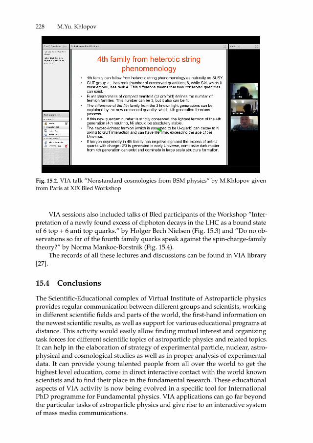
ii

“proc16” — 2016/12/12 — 10:17 — page 228 — #244 ii

ii

ii

228 M.Yu. Khlopov

Fig. 15.2. VIA talk ”Nonstandard cosmologies from BSM physics” by M.Khlopov givenfrom Paris at XIX Bled Workshop

VIA sessions also included talks of Bled participants of the Workshop ”Inter-pretation of a newly found excess of diphoton decays in the LHC as a bound stateof 6 top + 6 anti top quarks.” by Holger Bech Nielsen (Fig. 15.3) and ”Do no ob-servations so far of the fourth family quarks speak against the spin-charge-familytheory?” by Norma Mankoc-Borstnik (Fig. 15.4).

The records of all these lectures and discussions can be found in VIA library[27].

15.4 Conclusions

The Scientific-Educational complex of Virtual Institute of Astroparticle physicsprovides regular communication between different groups and scientists, workingin different scientific fields and parts of the world, the first-hand information onthe newest scientific results, as well as support for various educational programs atdistance. This activity would easily allow finding mutual interest and organizingtask forces for different scientific topics of astroparticle physics and related topics.It can help in the elaboration of strategy of experimental particle, nuclear, astro-physical and cosmological studies as well as in proper analysis of experimentaldata. It can provide young talented people from all over the world to get thehighest level education, come in direct interactive contact with the world knownscientists and to find their place in the fundamental research. These educationalaspects of VIA activity is now being evolved in a specific tool for InternationalPhD programme for Fundamental physics. VIA applications can go far beyondthe particular tasks of astroparticle physics and give rise to an interactive systemof mass media communications.

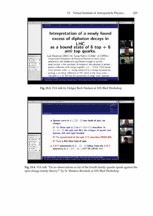
ii

“proc16” — 2016/12/12 — 10:17 — page 229 — #245 ii

ii

ii


Fig. 15.3. VIA talk by Holger Bech Nielsen at XIX Bled Workshop

Fig. 15.4. VIA talk ”Do no observations so far of the fourth family quarks speak against thespin-charge-family theory?” by N. Mankoc-Borstnik at XIX Bled Workshop

ii

“proc16” — 2016/12/12 — 10:17 — page 230 — #246 ii

ii

ii

230 M.Yu. Khlopov

VIA sessions became a natural part of a program of Bled Workshops, main-taining the platform of discussions of physics beyond the Standard Model fordistant participants from all the world. This discussion can continue in posts andpost replies on VIA Forum. The experience of VIA applications at Bled Workshopsplays important role in the development of VIA facility as an effective tool ofe-science and e-learning.

Acknowledgements

The initial step of creation of VIA was supported by ASPERA. I am grateful toP.Binetruy, J.Ellis and S.Katsanevas for permanent stimulating support, to J.C.Hamilton for support in VIA integration in the structure of APC laboratory, toK.Belotsky, A.Kirillov, M.Laletin and K.Shibaev for assistance in educational VIAprogram, to A.Mayorov, A.Romaniouk and E.Soldatov for fruitful collaboration,to M.Pohl, C. Kouvaris, J.-R.Cudell, C. Giunti, G. Cella, G. Fogli and F. DePaolisfor cooperation in the tests of VIA online transmissions in Switzerland, Belgiumand Italy and to D.Rouable for help in technical realization and support of VIAcomplex. I express my gratitude to N.S. Mankoc Borstnik, D. Lukman and allOrganizers of Bled Workshop for cooperation in the organization of VIA Sessionsat XIX Bled Workshop.

References

1. http://www.aspera-eu.org/2. http://www.appec.org/3. M.Yu. Khlopov: Cosmoparticle physics, World Scientific, New York -London-Hong Kong

- Singapore, 1999.4. M.Yu. Khlopov: Fundamentals of Cosmic Particle Physics, CISP-Springer, Cambridge,

2012.5. M. Y. Khlopov, Project of Virtual Institute of Astroparticle Physics, arXiv:0801.0376

[astro-ph].6. http://viavca.in2p3.fr/site.html7. M. Y. Khlopov, Scientific-educational complex - virtual institute of astroparticle physics,

Bled Workshops in Physics 9 (2008) 81–86.8. M. Y. Khlopov, Virtual Institute of Astroparticle Physics at Bled Workshop, Bled Work-

shops in Physics 10 (2009) 177–181.9. M. Y. Khlopov, VIA Presentation, Bled Workshops in Physics 11 (2010) 225–232.

10. M. Y. Khlopov, VIA Discussions at XIV Bled Workshop, Bled Workshops in Physics 12(2011) 233–239.

11. M. Y. .Khlopov, Virtual Institute of astroparticle physics: Science and education online,Bled Workshops in Physics 13 (2012) 183–189.

12. M. Y. .Khlopov, Virtual Institute of Astroparticle physics in online discussion of physicsbeyond the Standard model, Bled Workshops in Physics 14 (2013) 223–231.

13. M. Y. .Khlopov, Virtual Institute of Astroparticle physics and ”What comes beyond theStandard model?” in Bled, Bled Workshops in Physics 15 (2014) 285-293.

14. M. Y. .Khlopov, Virtual Institute of Astroparticle physics and discussions at XVIII BledWorkshop, Bled Workshops in Physics 16 (2015) 177-188.

ii

“proc16” — 2016/12/12 — 10:17 — page 231 — #247 ii

ii

ii


15. In http://viavca.in2p3.fr/ Previous - Conferences - XIII Bled Workshop16. In http://viavca.in2p3.fr/ Previous - Conferences - XIV Bled Workshop17. In http://viavca.in2p3.fr/ Previous - Lectures - Martin Pohl18. In http://viavca.in2p3.fr/ Previous - Events - JDEV 201319. In http://viavca.in2p3.fr/ Previous - Conferences - Subatomic particles, Nucleons,

Atoms, Universe: Processes and Structure International conference in honor of Ya. B.Zeldovich 100th Anniversary

20. In http://viavca.in2p3.fr/ Previous - Conferences - Conference YaB-100, dedicated to100 Anniversary of Yakov Borisovich Zeldovich

21. In http://viavca.in2p3.fr/ Forum - Discussion in Russian - Courses on Cosmoparticlephysics

22. In http://viavca.in2p3.fr/ Forum - Education - From VIA to MOOC23. http://viavca.in2p3.fr/ Previous - Conferences - The International Conference on

Particle Physics and Astrophysics24. http://viavca.in2p3.fr/ Previous - Conferences - Dark Ages and White Nights (Spec-

troscopy of the CMB)25. In http://viavca.in2p3.fr/ Previous - Lectures - John Ellis26. In http://viavca.in2p3.fr/ Forum - CONFERENCES BEYOND THE STANDARD

MODEL - 19 Bled Workshop ”What comes beyond the Standard model?”27. In http://viavca.in2p3.fr/ Previous - Conferences - XIX Bled Workshop ”What comes

beyond the Standard model?”

ii

“proc16” — 2016/12/12 — 10:17 — page 232 — #248 ii

ii

ii

BLEJSKE DELAVNICE IZ FIZIKE, LETNIK 17, ST. 2, ISSN 1580-4992

BLED WORKSHOPS IN PHYSICS, VOL. 17, NO. 2

Zbornik 19. delavnice ‘What Comes Beyond the Standard Models’, Bled, 11. –19. julij 2016

Proceedings to the 19th workshop ’What Comes Beyond the Standard Models’,Bled, July 11.–19., 2016

Uredili Norma Susana Mankoc Borstnik, Holger Bech Nielsen in Dragan Lukman

Izid publikacije je financno podprla Javna agencija za raziskovalno dejavnost RSiz sredstev drzavnega proracuna iz naslova razpisa za sofinanciranje domacihznanstvenih periodicnih publikacij

Brezplacni izvod za udelezence

Tehnicni urednik Matjaz Zaversnik

Zalozilo: DMFA – zaloznistvo, Jadranska 19, 1000 Ljubljana, Slovenija

Natisnila tiskarna Itagraf v nakladi 100 izvodov

Publikacija DMFA stevilka 2007

What Comes Beyond the Standard Models - Inspire HEP

Documents

Transcript of What Comes Beyond the Standard Models - Inspire HEP