Derivation of site-specific relationships between hydraulic parameters and p-

wave velocities based on hydraulic and seismic tomography

Brauchler, R.[1], Doetsch, J. [1,2], Dietrich, P. [3], Sauter, M. [4]

[1] ETH Zurich, Department of Earth Sciences, Sonneggstrasse 5, 8092 Zurich, Switzerland

[2] now at: Earth Sciences Division, Lawrence Berkeley National Laboratory, One Cyclotron Road,

Berkeley, CA 94720

[3] UFZ, Helmholtz Centre for Environmental Research, Department Monitoring and Exploration

Technologies, Permoserstrasse 15, 04318 Leipzig, Germany

[4] Geoscientific Centre, University of Göttingen, Goldschmidtstraße 3, 37077 Göttingen, Germany

1

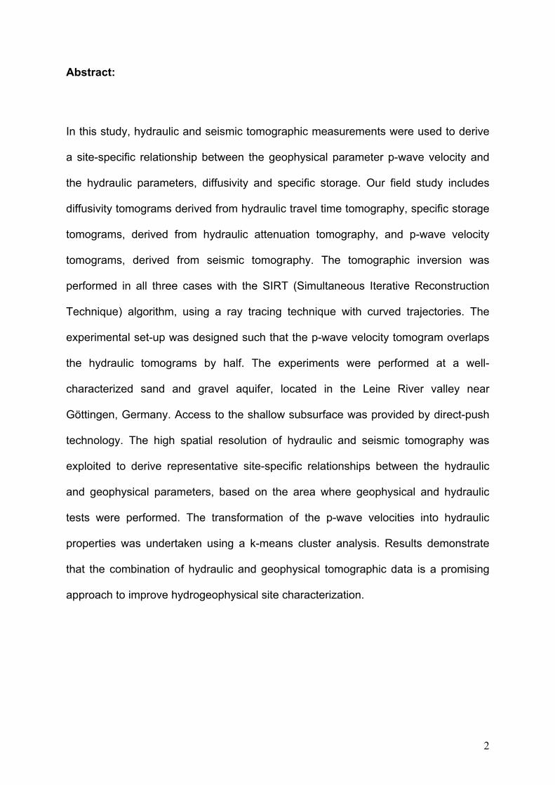
Abstract:

In this study, hydraulic and seismic tomographic measurements were used to derive

a site-specific relationship between the geophysical parameter p-wave velocity and

the hydraulic parameters, diffusivity and specific storage. Our field study includes

diffusivity tomograms derived from hydraulic travel time tomography, specific storage

tomograms, derived from hydraulic attenuation tomography, and p-wave velocity

tomograms, derived from seismic tomography. The tomographic inversion was

performed in all three cases with the SIRT (Simultaneous Iterative Reconstruction

Technique) algorithm, using a ray tracing technique with curved trajectories. The

experimental set-up was designed such that the p-wave velocity tomogram overlaps

the hydraulic tomograms by half. The experiments were performed at a well-

characterized sand and gravel aquifer, located in the Leine River valley near

Göttingen, Germany. Access to the shallow subsurface was provided by direct-push

technology. The high spatial resolution of hydraulic and seismic tomography was

exploited to derive representative site-specific relationships between the hydraulic

and geophysical parameters, based on the area where geophysical and hydraulic

tests were performed. The transformation of the p-wave velocities into hydraulic

properties was undertaken using a k-means cluster analysis. Results demonstrate

that the combination of hydraulic and geophysical tomographic data is a promising

approach to improve hydrogeophysical site characterization.

2

1. Introduction

Tomographic geophysical methods show a great potential in providing information on

the design and parameterization of conceptual and numerical models, allowing the

quantitative prediction of flow and transport processes in the subsurface [Day-Lewis

and Lane, 2004]. From geophysical tomograms, structural information to delineate

zones with constant hydraulic properties in a numerical flow and transport model can

be exploited. [e.g. Hyndman and Harris, 1996]. Several advanced approaches in

delineating zones of constant geophysical properties were developed based on the

joint inversion of multiple geophysical data sets by several researchers [e.g.

Hyndman et al.,1994; Dietrich et al., 1998; Gallardo and Meju, 2003; Tronicke et al.,

2004; Linde et al., 2006a; Cardiff and Kitanidis, 2009; Doetsch et al., 2010]. The

hydraulic properties of the estimated zones can be inferred from core data, hydraulic

tests or tracer test data. However, the key assumption regarding these structural

hydrogeophysical inversion approaches is that the individual zones have

approximately constant hydrogeological and geophysical properties.

Over the last decade and a half, several research groups started to work on

developing coupled hydrogeophysical inversion schemes based on tomographic

geophysical methods. Coupled hydrogeophysical inversion focuses on estimating

hydrogeological parameters and their spatial distribution directly from geophysical

measurements. Usually, petrophysical relationships and models are used to

transform a resulting geophysical parameter distribution into an image of hydraulic

parameters. Often coupled hydrogeophysical inversion schemes can eliminate the

need to construct images of geophysical property distributions [Ferre et al., 2009].

Hinnell et al. [2010] give an excellent overview about the workflow of coupled

3

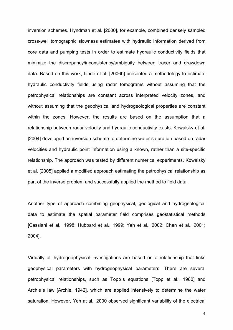
inversion schemes. Hyndman et al. [2000], for example, combined densely sampled

cross-well tomographic slowness estimates with hydraulic information derived from

core data and pumping tests in order to estimate hydraulic conductivity fields that

minimize the discrepancy/inconsistency/ambiguity between tracer and drawdown

data. Based on this work, Linde et al. [2006b] presented a methodology to estimate

hydraulic conductivity fields using radar tomograms without assuming that the

petrophysical relationships are constant across interpreted velocity zones, and

without assuming that the geophysical and hydrogeological properties are constant

within the zones. However, the results are based on the assumption that a

relationship between radar velocity and hydraulic conductivity exists. Kowalsky et al.

[2004] developed an inversion scheme to determine water saturation based on radar

velocities and hydraulic point information using a known, rather than a site-specific

relationship. The approach was tested by different numerical experiments. Kowalsky

et al. [2005] applied a modified approach estimating the petrophysical relationship as

part of the inverse problem and successfully applied the method to field data.

Another type of approach combining geophysical, geological and hydrogeological

data to estimate the spatial parameter field comprises geostatistical methods

[Cassiani et al., 1998; Hubbard et al., 1999; Yeh et al., 2002; Chen et al., 2001;

2004].

Virtually all hydrogeophysical investigations are based on a relationship that links

geophysical parameters with hydrogeophysical parameters. There are several

petrophysical relationships, such as Topp´s equations [Topp et al., 1980] and

Archie´s law [Archie, 1942], which are applied intensively to determine the water

saturation. However, Yeh at al., 2000 observed significant variability of the electrical

4

resistivity-moisture relation in their field samples. Based on theoretical analysis and

numerical experiments they could show that the spatially varying relationship

between electrical resistivity and moisture content can influence the significance of

moisture monitoring results derived from the estimated change in the electrical

resistivity. Liu and Yeh, 2004 supports these findings and concluded that additional

hydrological a priori information next to electrical resistivity measurements are

needed under field conditions in order to yield hydrological realistic inversion results.

Other relationships, e.g. between seismic velocities or radar velocities and hydraulic

conductivity, are likely non-unique. This non-uniqueness leads to the derivation of

site-specific relationships between geophysical and hydraulic parameters. This is in

accordance with Hyndman and Tronicke [2005], who stated: “Estimating the relation

between geophysical and hydrogeologic parameters is a site-specific endeavor, since

no general relation is expected.” The estimation of site-specific relationships can be

very difficult and even erroneous due to the different spatial resolution of available

geophysical and hydraulic data.

Usually, geophysical tomographic reconstructions show a high spatial resolution in

two or even in three dimensions. Classical hydrogeological approaches, however,

appear to have difficulties providing high-resolution parameter estimates [Butler,

2005]. Pumping tests lead to reliable estimates in hydraulic conductivity and storage

but the resulting hydraulic properties represent spatial averages over a large aquifer

volume. Slug tests, however, provide information about the hydraulic parameters in

the immediate vicinity of the well. The resolution of hydraulic testing in a vertical

direction can be even increased by using multi-packer systems [e.g. Melville et al,

1991; Butler 1998; Brauchler et al., 2010]. Lateral changes in hydraulic parameters

5

can be derived from hydraulic cross-well tests. It has to be emphasized that the

estimated hydraulic properties derived from type curve analysis, assuming a

homogeneous parameter distribution, do not reflect a uniformly weighted average,

but the weight depends on the test and observation interval and the heterogeneity of

the subsurface [Wu et al., 2005]. Thus, the spatial assignment of the hydraulic

properties is non-unique [Leven and Dietrich, 2006] and the derivation of site-specific

relationships between hydraulic and geophysical parameter reconstruction could be

biased.

However, several research groups are working on a new hydraulic investigation

technique, termed hydraulic tomography that has the potential to yield information on

spatial variation of hydraulic properties with a resolution comparable to the spatial

resolution of geophysical tomographic investigations [e.g. Gottlieb and Dietrich, 1995;

Yeh and Liu, 2000; Vasco and Karasaki, 2001; Karasaki et al., 2000; Bohling et al.,

2002; Brauchler et al., 2003; Zhu and Yeh; 2005; 2006; Straface et al., 2007; Ni and

Yeh, 2008; Xiang et al., 2009; Yin and Illmann, 2009; Illman et al., 2010]. Hydraulic

tomography consists of a series of short-term pumping or slug tests. Varying the

location of the source stress (pumping or slug interval) and the receivers (pressure

transducers) generates streamline patterns that are comparable to the crossed ray

paths of a seismic tomography experiment [Butler et al., 1999]. One of the first

tomographic measurement arrays in the field were implemented by Hsieh et al.

[1985]. Due to the high spatial resolution of the hydraulic and geophysical

tomographic images, a representative site-specific relationship can be derived over

an area where geophysical and hydraulic tests are performed, if such a relationship

exists.

6

In this study, the potential of hydraulic tomography to derive a site-specific

relationship between hydraulic parameters and p-wave velocity for the well-

characterized Stegemühle site near Göttingen, Germany, will be assessed. The

hydraulic tomographic inversion presented in Brauchler et al. [2011] consists of 196

pressure cross-well interference slug tests performed between five wells, in which the

positions of the sources (injection ports) and the receivers (observation ports),

isolated with double packer systems, were varied between tests. The database for

the seismic tomography experiments comprises four seismic planes overlapping half

the hydraulic tomograms. The derivation of a site specific relationship, based on k-

means clustering [McQueen, 1967], enabled us to identify the spatial position of two

zones and their average hydraulic properties within the reconstructed p-wave velocity

tomograms.

2. Overview of the Stegemühle Site

The Stegemühle site is located in the Leine valley, close to Göttingen, Germany and

has been characterized extensively by geophysical wellbore logging, refraction

seismic and hydraulic testing. The infrastructure of the site consists of a network of

26 wells, comprising 1”, 2”, 6” and multi-chamber wells screened over the whole

aquifer thickness (Figure 1). The 6” wells were drilled with a top drive drilling rig,

whereas all other wells were installed using direct-push (DP) technology. The DP-

technology uses a hydraulic hammer, supplemented with the weight of the direct-

push unit to push drive rods down to the desired depth of the projected well [e.g.

Dietrich and Leven, 2006]. The well casing, consisting of high-density polyethylene

(HDPE) pipes and slotted screens, is then lowered into the drive rods (inner

7

diameter: 0.067 m, outer diameter 0.083 m). By retracting the drive rods, the

formation is allowed to collapse back against the HDPE pipes.

The structural composition of the braided river sediments was characterized by

surface refraction seismic, gamma ray logging and direct-push electrical conductivity

logging. For selected wells, cores are recovered to calibrate the recorded logs. The

aquifer thickness varies between 2-2.5 m and consists of intercalated sand and

gravel layers. A confining unit that consists of silt and clay overlies the aquifer. The

thickness of the confining unit varies between 3-3.5 m [Brauchler et al., 2010]. The

cores displayed, that the aquifer material at the Stegemühle site shows a sharp

transition from one behavior to another [Hu, 2011]. The sharp transition can be

explained by the complexity of depositional and erosional processes in braided river

systems [Huggenberger and Regli, 2006].

The hydraulic characterization is based on pumping and cross-well slug interference

tests. Hydraulic conductivity estimates, derived from multi-level single-well slug tests,

performed at five to seven different depths in each 2” well, vary between 10-4 ms-1

and 5 × 10-3 ms-1. Brauchler et al. [2010] determined vertical changes in hydraulic

conductivity and specific storage with multi-level cross-well interference slug testing

between the five wells (P2.5/M25, P0/M27.5, PM2.5/M25, P0/M22.5 and P0/M25)

arranged in a five-star configuration (Figure 1). The estimated hydraulic conductivity

values decrease from approximately 10-3 ms-1, close to the bottom, to approximately

10-4 ms-1, at the top of the aquifer and the specific storage distribution shows an

opposite behavior. The specific storage values increase from approximately 10-5 m-1

close to the bottom of the aquifer to approximately 10-3 m-1 at the top of the aquifer.

8

Brauchler et al. [2011] inverted the cross-well interference slug tests with a travel

time and attenuation based inversion scheme. They reconstructed the diffusivity and

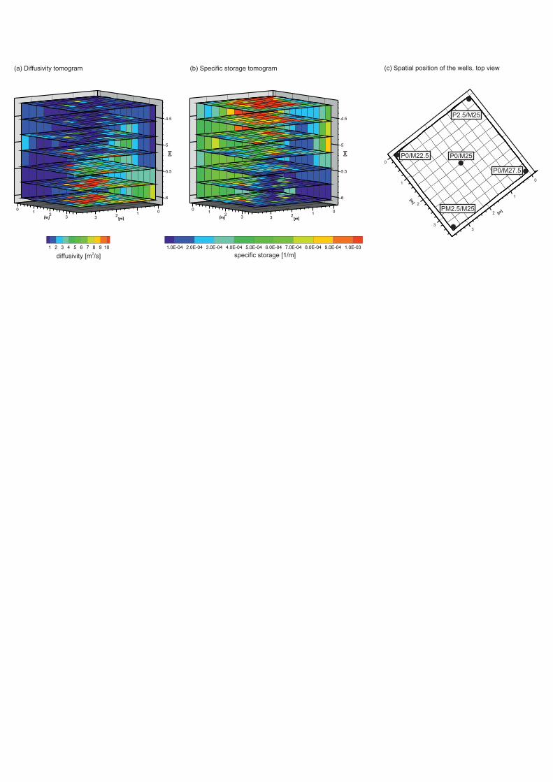
specific storage distribution between the wells in two and three dimensions. In Figure

2, the reconstructed three-dimensional hydraulic diffusivity distribution and specific

storage tomograms are shown. Note that Figure 2 is adapted from the work

performed by Brauchler et al. [2011]. The limited number of injection and observation

intervals prevented us from resolving small-scale (10 cm in size) variability of

hydraulic conductivity. This is in accordance with findings from Hu et al. [2011]. They

performed a numerical case study based on data derived from an aquifer analog

outcrop study and could show that with a reasonable number of source and

receivers, it is not possible to reconstruct small-scale variability (10 cm in size) using

the travel time based inversion approach.

Brauchler et al. [2012] recorded a suite of short-term pumping tests, using a

tomographical measurement array between well P0/M25 and multi-chamber well

PM5/M17.5. The reconstructed hydraulic diffusivity distribution, based on hydraulic

travel time inversion, shows a similar pattern, as the diffusivity tomogram illustrated in

Figure 2, with the highest values close to the bottom of the aquifer. The comparison

of the travel time inversion results with the results based on straight line analysis

(solution of Cooper and Jacob, [1946]) have shown that the hydraulic parameters

estimated with a straight analysis are dominated by the high permeability layer close

to the bottom of the aquifer. The recorded inversion results indicate that the

combination of hydraulic travel time and hydraulic attenuation tomography allows the

reconstruction of the diffusivity and storage distribution in two and three dimensions,

with a resolution and accuracy superior to that possible with type curve/straight line

analysis.

9

The hydraulic characterization of the site showed that the shallow aquifer, with a

thickness of two meters, is ideally suited to develop and perform new investigation

techniques. The thinness of the aquifer allows for the minimization of the logistical

and technical requirements of complex hydraulic testing and simplifies the validation

of new investigation techniques with conventional investigation techniques.

In the following, we exploit the earlier work described above and propose an

approach combining hydraulic and seismic tomography, as well as direct-push (DP)

technology. These three techniques complement one another as described: (1)

Hydraulic tomograms are well suited to derive site-specific relationships between

hydraulic parameters and indirect geophysical measurements because changes in

hydraulic properties can be reconstructed in horizontal, as well as in lateral direction

with high spatial resolution. (2) The integration of hydraulic and seismic tomography

allows for an easy enlargement of the investigation area, since geophysical cross-

well measurements can be performed faster than hydraulic tests, and thus, a larger

area can be covered in one array. (3) The characterization of larger areas with

hydraulic and seismic cross-well tests has been limited by the need for wells that are

arranged and designed in a way that hydraulic multi-level cross-well, as well as

seismic cross-well, experiments can be performed. That limitation, however, can be

readily overcome in unconsolidated formations by exploiting the access to the

shallow subsurface provided by DP technology. DP technology can be used to install

observation points with different types of casing at positions most advantageous for a

particular study and an option to reposition measurement points between tests based

on the former results.

10

3. Seismic tomographic measurements

For the performance of seismic cross-well measurements, four non-permanent direct-

push wells were installed and used as test wells (Figure 1). The installation of the

wells consists of a shielded screen at the lower end of the direct-push tool string. The

used screen, with an inner diameter of 0.016 m, was originally designed for water

sampling or slug testing [Butler et al., 2002]. The temporary wells were chosen as

source wells because conventional wells are likely to be damaged by the action of

the sparker source. For test initiation, a modified p-wave sparker probe, SBS 42,

adapted to small diameter wells in combination with an electric surge generator and a

remote control unit was used.

For the initiation of the seismic experiments, the shielded screen at the lower end of

the direct-push tool string was pushed down to the position of the deepest test

interval. After having reached the selected depth, the shielded screen tool was

exposed and a cross-well seismic test is initiated. Subsequently, the direct-push tool

string was pulled back in order to perform the test at different depths.

The seismic signal was recorded with a hydrophone string, consisting of ten single

hydrophones, placed in the center well P0/M25 of the five-star configuration, with a

spacing of 0.24 m. The individual hydrophones have a diameter of 0.02 m and a

preamplifier of 20 dB. The small distance of 5 m between source and receiver well

and the preamplifier lead to very strong signals with the result that the seismic

waveforms were clipped. However, the first arrivals could be clearly identified (Figure

3). The advantage of using non-permanent direct-push wells as test wells is a low-

11

cost installation in terms of time effort and finances. It has to be mentioned that a

possible vertical deviation of the wells can lead to errors in the inversion results. An

experienced technician team can minimize such deviation but it cannot be fully

excluded.

In total we recorded data on four seismic planes (profiles) between the four non-

permanent direct-push wells and the center well P0/M25 of the five-star configuration.

Therefore, the data set for each plane consists of ten injection and ten observation

positions. The source–receiver configurations are displayed as pink lines in Figure 4.

The black lines, illustrate the measured configurations, as well as the spatial position

of the test and observation intervals of the cross-well slug interference tests. The four

seismic tomograms are half overlapping, with the area investigated by hydraulic

tomography. We used the hydraulic inversion results, based on these measured

configurations, to derive a site-specific relationship for the Stegemühle site between

p-wave velocity and the hydraulic parameters diffusivity and specific storage.

4. Estimation of the site-specific relationship

In this section we provide a short review about the hydraulic travel time inversion,

hydraulic attenuation inversion and seismic travel time inversion, followed by a

description of the derivation of a sites-specific relationship between hydraulic

parameters and p-wave velocity for the Stegemühle site. The inversion results

constitute the basics for the derivation of a representative site-specific relationship.

The hydraulic tomographic inversion results employed in this study are based on

earlier work described by Brauchler et al. [2010, 2011].

12

The work proposed by Vasco et al. [2000] is the starting point of the hydraulic

tomographic inversion. They proposed an inversion scheme that follows the

procedure of seismic ray tomography and is based on the transformation of the

transient ground water flow equation into the eikonal equation using an asymptotic

approach [Virieux et al. 1994]. The eikonal equation can be solved with ray tracing

techniques or particle tracking methods, which allow for the calculation of pressure

propagation along trajectories.

The key element of the hydraulic inversion are two line integrals: (a) A travel time

integral which relates the travel time of transient signal with a Dirac source at the

origin to the diffusivity (D) distribution between source and receiver and (b) an

attenuation integral which relates the attenuation of a pressure signal with a Dirac

source signal at the origin to the specific storage (Ss) distribution.

(a) Travel time integral:

.

)(61 2

1,, ³

x

xdd sD

dsf

tD

D(1)

tD,d is the travel time (arrival time) of a selected point of the signal from the point x1

(source) to the observation point x2 (receiver) and D is the diffusivity as a function of

arc-length along the propagation path (s) and fD,d = tpeak/tD,d the related transformation

factor. tpeak is defined as the peak time of the recorded transient pressure curve and

the subscript d stands for a Dirac source. The transformation factor allows to relate

any recorded travel time tD,d with the diffusivity D and is defined as follows:

� �

� �

¸̧¸¸¸¸¸

¹

·

¨̈¨¨¨¨¨

©

§

¸¸¹

·¨¨©

§

��

32

,

,,

etrhtrh

Wf peakd

d

dD

(2)

13

W stands for Lambert's W function and hd(r,t) describes the hydraulic potential as

function space and time. Brauchler et al. [2003] presents the derivation of the

transformation factor in detail.

b) Attenuation integral:

� �� � dssS

BHxh x

x s³

��

�

¸̧¹

·¨̈©

§ ¸̧

¹

·¨̈©

§ 2

1

31

313

1

0

2 1(3)

The attenuation of the hydraulic signal is expressed by the initial displacement H0

and the hydraulic head h(x2) at the observation interval and Ss is the specific storage

as a function of arc-length along the propagation path (s). The parameter B was

introduced to simplify equation (3) and is defined as follows:

»¼º

«¬ª�

¸¹·

¨©§

23exp

32 3

2

S

S crB

(4)

Here rc is the casing radius. Brauchler et al. [2011] described in detail the derivation

of the attenuation integral.

In seismic tomography a similar relationship exists, which can be expressed as a line

integral. The line integral relates the travel time t of a seismic pulse to the inverse of

the velocity (1/v) as a function of arc-length along the propagation path (s). The

inverse of the velocity is termed slowness.

� �³ 2

1

x

x svdst

(5)

14

The similarity of all three line integrals allows the application of the same inversion

algorithms. The inversion was performed in all three cases with the SIRT

(Simultaneous Iterative Reconstruction Technique) algorithm [Gilbert, 1972]. The

algorithm allows for the application of ray tracing techniques with either straight or

curved ray paths and trajectories, respectively. We used curved ray paths to handle

the large travel time contrasts of several orders of magnitude in hydraulic tomography

[Brauchler et al., 2007]. The curved ray paths are computed based on the ray tracing

algorithm developed by Um and Thurber [1987]. Tests with the LSQR-based

inversion code of Doetsch et al. [2010] recovered the same main features as the

SIRT inversions, when using logarithmic transformations for both data and model

parameters in the hydraulic tomography.

For the seismic travel time inversion, as well as for the hydraulic and attenuation

travel time inversion a homogeneous starting model was used. The starting values

for the velocity/attenuation fields are derived from the mean values of the measured

source-receiver-combinations. The cell size of 0.35 m × 0.4 m is the same for all

three tomograms.

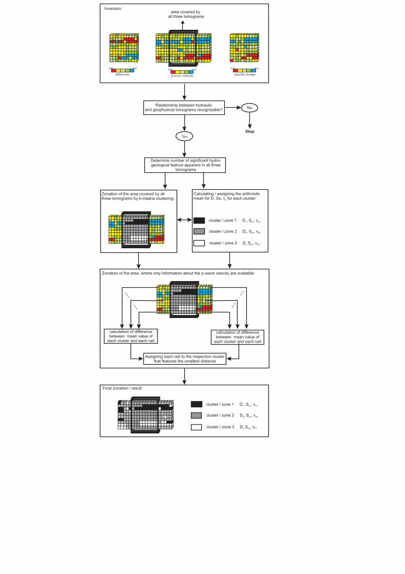
The main steps to derive a site-specific relationship between hydraulic parameters

and p-wave velocity are described in the following and summarized in a flowchart,

which is displayed in Figure 5:

Step 1: Reconstruction of the diffusivity, specific storage and p-wave tomograms

using the inversion scheme described above.

Step 2: Differentiation between hydrogeological units characterized by a significant

diffusivity, specific storage and p-velocity contrast and determination of the number of

15

such significant hydrogeological features apparent in the tomograms. If no

relationship between hydraulic tomograms and geophysical tomograms can be

recognized, the investigation has to be stopped at this step. The approach is limited

to sites where a relationship between hydraulic and geophysical parameters exists.

Step 3: Zonation of the area, which is covered by all three tomograms. In this study,

the area is located between the wells P0/M22.5 and P0/M27.5, as well as the area

between P2.5/M25 and PM2.5/M25. The zonation is performed by k-means cluster

analysis [McQueen, 1969]. The clusters were calculated using normalized Euclidian

distances (root mean squared distances) without using any spatial adjacency. Prior to

the cluster analysis the used parameters, diffusivity, specific storage and p-wave

velocity, were standardized (mean of zero, standard deviation of one) in order to

account for the different units. The number of clusters was chosen equivalent to the

number of the determined hydrogeological features estimated in step 2. Cluster

analysis was applied successfully in several studies to objectively identify major

common trends and groupings in various combinations of hydraulic and geophysical

tomographic data [Eppstein and Dougherty, 1998; Tronicke et al., 2004; Paasche et

al., 2006; 2010; Dietrich and Tronicke, 2009; Doetsch et al., 2010b, Brauchler et al.,

2011].

Step 4: Assignment of an average value for specific storage, diffusivity and p-wave

velocity to each cluster. Therefore, the arithmetic means of the specific storage,

diffusivity and p-wave velocity of the cells, assigned to the respective cluster, are

calculated.

16

Step 5: Zonation of the area, where only information about the p-wave velocities is

available. The zonation is performed by calculating the difference between the p-

wave velocity for each single cell and the p-wave velocity of the clusters estimated in

step 4. The cell is assigned to the cluster, which shows the smallest difference.

Step 6: Verification if the estimated zoned parameter field is consistent with the

original hydraulic and geophysical data. Therefore, a second hydraulic travel time,

hydraulic attenuation and seismic travel time inversion, using the zonation derived

from the k-means cluster analysis as constraints, is performed.

5. Results

The derivation of a site-specific relationship between hydraulic parameters and p-

wave velocity for the Stegemühle site are based on the diffusivity, specific storage

and p-wave velocity tomograms illustrated in Figures 6 and 7. The procedure

described above is performed jointly for the tomograms recorded in (a) North–South

direction and the tomograms in (b) West–East direction.

The comparison of the tomograms illustrated in Figures 6 and 7 indicates that the p-

wave velocity tomogram is positively related to the specific storage and negatively

correlated to the diffusivity distribution. The correlation coefficient for the tomograms

recorded in North–South direction between p-wave velocity and the logarithm of

diffusivity is -0.63 and between p-wave velocity and logarithm of specific storage it is

0.55. For the tomograms recorded in West–East direction the calculated correlation

coefficients are similar. A correlation coefficient of -0.69 between p-wave velocity and

17

the logarithm of diffusivity and a correlation coefficient of 0.68 between p-wave

velocity and logarithm of specific storage were determined.

The respective scatterplots, displayed in Figure 8, indicate, like the calculated

correlation coefficients that the p-wave velocity is negatively correlated to diffusivity

and positively correlated to specific storage.

For hydrogeophysical investigations based on the combination of geophysical and

conventional hydraulic methods, correlation coefficients or scatterplots are often the

only way to evaluate the relationship between geophysical and hydraulic properties.

However, the high spatial resolution of hydraulic and geophysical tomograms allows

for assessing in addition, whether at all and to what extent and detail the most

important features are imaged in both tomograms. Hence, it is possible to determine

the significance of hydrogeophysical investigations in the identification of

hydraulically important features, such as preferential flow paths or barriers influencing

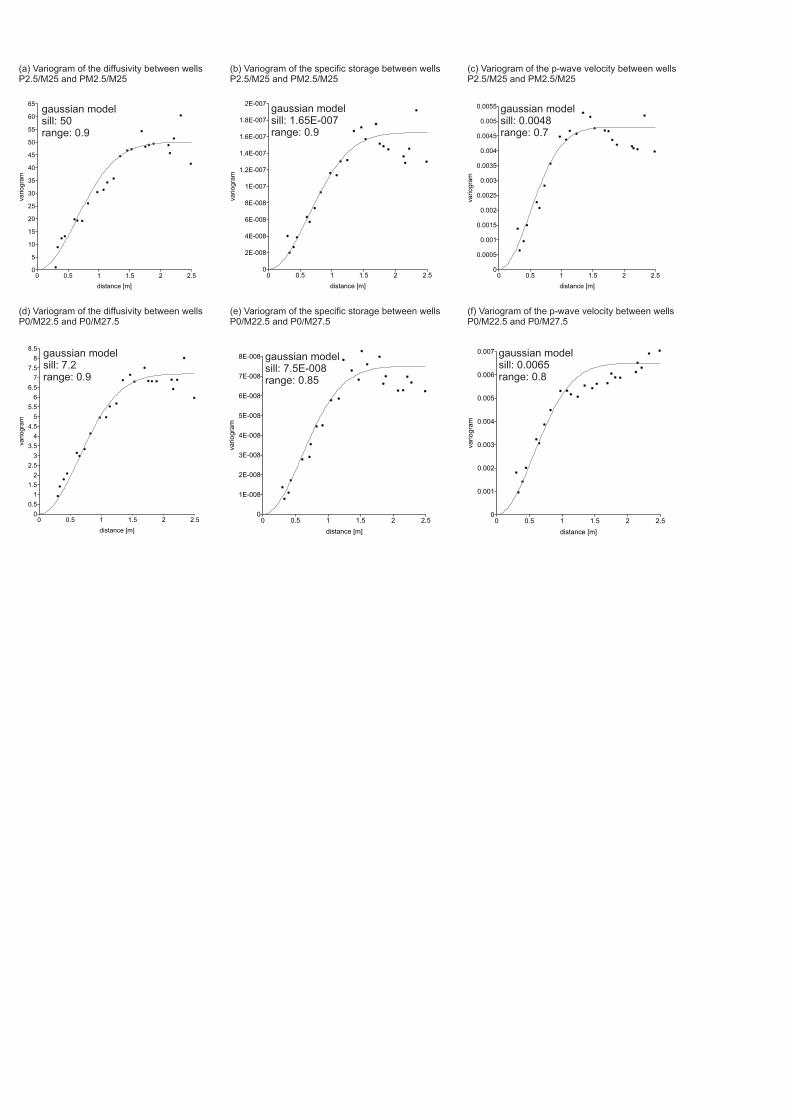
flow and solute transport. We performed a variogram analysis in order to show

objectively the spatial correlation structures of the diffusivity, specific storage and p-

wave velocity tomograms (Figure 9). For all variograms a Gaussian model was

selected. The Gaussian model, with its parabolic behavior at the origin, represents

very smoothly varying properties. The smoothly varying properties can be explained

by the used inversion technique. The SIRT algorithm applied in this study leads to

smoother parameter reconstructions in comparison to other series expansion

inversion methods, because the incremental corrections are applied by averaging the

incremental correction of each single cell after all trajectories have been analyzed

(e.g. Dines and Little, 1979). The range of the variograms displayed in Figure 9 is

between 0.7 and 0.9. The similarity of the variograms and the comparable statistics

18

reveals their spatial correlation structures. Having considered the above statistical

quality criteria, the following results can be summed up:

(a) Tomograms in North–South direction: The lower part of the diffusivity and the

specific storage tomogram is characterized by higher diffusivity values of

approximately 10 m/s2 and lower specific storage values of approximately 10-4 m-1, in

comparison to the upper part. With increasing height, the diffusivity values decrease

to about 1 m/s2 and the specific storage values increase by one order of magnitude,

to a maximum value of 10-3 m-1, respectively. Between the wells P2.5/M25 and

PM2.5./M25, the p-wave velocity tomogram shows a similar pattern. The lower part of

the tomogram is characterized by low p-wave velocities between 2.2 km/s and 2.25

km/s. Closer to the top of the tomogram the velocities increase to 2.35 km/s. The

similar pattern of the three tomograms indicates, along with the estimated correlation

coefficients and the variogram analysis, is evidence of a site-specific relationship

between p-wave velocity and the hydraulic parameters diffusivity and specific

storage. For the interpretation of the hydraulic tomograms in terms of groundwater

flow and solute transport, it is important to question whether or not the higher

diffusivity/low specific storage zone at the bottom extends beyond the area to the left

of well P2.5/M25 and across the area to the right of well PM2.5/M25.

b) Tomograms in West–East direction: Between well P0/M25 and well P0/M27.5 the

hydraulic tomograms, displayed in Figure 7a and b, show a similar pattern as the

hydraulic tomograms recorded in North-South direction. The right section of the

hydraulic tomograms is characterized by diffusivity values ranging between 7 m/s2

and 10 m/s2 and specific storage values between 10-4 m-1 and 3×10-4 m-1 close to the

bottom of the tomograms. At the top of the tomograms the diffusivity values vary

19

between 1 m/s2 and 2 m/s2 and the specific storage values vary between 7×10-4 m-1

and 10-3 m-1. The most significant features in the hydraulic tomograms are the lateral

changes. Between well P0/M22 and well P0/M25 the high diffusivity/low specific

storage zone pinches out. The pinching out of this zone, characterized by low p-wave

velocities between 2.15 km/s and 2.18 km/s, can be also recognized in the p-wave

velocity tomogram. For the interpretation of the hydraulic tomograms it is important to

know whether the high diffusivity/low specific storage zone stretches out over the

area right of well P0/M27.5.

In order to answer these questions we generated two zones based on the

tomograms recorded in North–South and West–East direction to derive a site-specific

relationship using the zonation approach described in section 4. The zonation

approach is introduced jointly for all tomograms. The number of the cluster is chosen

in accordance with the number of significant hydrogeological features that could be

identified reliably from the diffusivity tomograms and specific storage tomograms, as

well as in the p-wave velocity tomogram.

The zoned tomogram recorded in North–South direction displayed in Figure 6d,

shows that the zone at the lower part of the tomogram is pinching out close to the

well P2.5/M25. In the other direction, the thickness of the zone decreases without any

pinching out. The zoned tomogram recorded in West–East direction, illustrated in

Figure 7, displays the pinching out of the high diffusivity/low specific storage between

well P0/M25 and well P0/M22.5. It is difficult to answer whether or not this zone

extends beyond the area to the right of well P0/M27.5. The zoned tomogram

indicates that the high diffusivity/low specific storage zone continues to the right and

ascends towards the aquifer top.

20

The range of the hydraulic conductivity and specific storage displayed by zone 1 and

zone 2 varies between 10-3 m/s and 6×10-4 m/s and 2×10-4 1/m and 8×10-4 1/m,

respectively. These values agree with the hydraulic property estimates derived from

type curve analysis [Brauchler et al. 2010]. The range of the hydraulic properties of

the two zones has to be smaller than the range of the values derived from type curve

analysis, because the two zones display values integrated over half of the model

domain.

For the verification of the zonation approach, we applied the procedure proposed by

Doetsch et al. [2010]. They suggested that for field data with unknown zone

geometries and parameters, the zonation must be judged on the basis of the root

means square residual error (RMSE) and by visual inspection. Hence, we performed

a second hydraulic travel time, hydraulic attenuation and seismic travel time inversion

using the zonation derived from the k-means cluster analysis as constraints. Thereby

the parameters within zone 1, representing the high diffusivity/low specific storage

zone close to the bottom of the aquifer was kept constant. In Table 1, the RMSE of

the hydraulic travel time, hydraulic attenuation, and seismic travel time inversions

with and without constrain are listed for the hydraulic tomograms after five and for the

p-wave velocity tomogram after 10 iteration steps. It is not surprising that the RMSE

of the inversions, without any constraints, is smaller than the RMSE of the inversion

with constraints.

However, the comparison of the RMSE shows that the differences are small with

respect to the arithmetic mean of the measured (a) p-wave travel times of 2.31 µs,

(b) hydraulic travel times of 2.09 s and (c) the attenuation ratio of 0.20. Beyond this,

21

the reconstructed parameter estimates within zone 2 with and without constraints are

comparable. The small difference of the RMSE based on the inversion with and

without constraints, respectively, and the fact that the tomograms with constraints

exhibit no artifact in zone 2 supports the performed zonation approach.

6. Summary and Conclusions

In this study, hydraulic and seismic tomographic measurements were used to derive

a site-specific relationship between the geophysical parameter p-wave velocity and

the hydraulic parameters, diffusivity and specific storage. The database of the

investigation is comprised of diffusivity tomograms derived from hydraulic travel time

inversions, specific storage tomograms derived from hydraulic attenuation

tomography and p-wave velocity tomogram derived from seismic tomography. The

experimental set-up was designed such that the p-wave velocity tomograms overlap

by half with the hydraulic tomograms. The diffusivity and specific storage tomograms

were originally presented in Brauchler et al. [2011].

For the performance of seismic cross-well measurements, four non-permanent direct-

push wells, with an inner diameter of 0.016 m, were installed and used as source

wells. The non-permanent direct-push wells were chosen as source wells because

conventional PVC-wells could possibly be damaged by the sparker source. For test

initiation a modified p-wave sparker probe, SBS 42, adapted to small diameter wells

in combination with an electric surge generator and a remote control unit was used.

For the generation of the needed infrastructure direct-push technology shows a great

deal of flexibility for the performance of high-resolution hydraulic or geophysical

investigations in unconsolidated sediments. Test and observation points could be

22

installed with different types of casing materials and diameters, i.e. very efficient in

terms of time, effort and finances.

The data integration, combining the results of the hydraulic and seismic tomograms,

was realized by applying a procedure, which is based on k-means cluster analysis.

The applied procedure enables us to transform the reconstructed p-wave velocity

distribution of the seismic tomographic measurements into two zones with different

hydraulic properties. In particular, the lateral and vertical changes of a zone,

characterized by higher diffusivity and lower specific storage values, could be

reconstructed.

The investigation showed that geophysical and hydraulic tomography complement

one another because hydraulic tomography overcomes the problems of traditional

hydrogeological measurements that generally do not provide high-resolution

parameter estimates. The comparable spatial resolution of hydraulic and geophysical

tomograms can be exploited to improve the potential of geophysical tomograms in

the analysis of the spatial distribution of hydraulic properties. Hydraulic tomography

can be used, for example, as a criterion in evaluating the individual expressiveness of

the different geophysical methods, with respect to their capability in reconstruction of

hydraulic significant structures from joint hydrogeophysical inversions. Such an

assessment is difficult with conventional hydraulic and laboratory tests due to the low

spatial resolution and uncertainty of the spatial assignment of the estimated hydraulic

properties. Beyond this, the geophysical tomographic measurements allow for an

easy extension of the area investigated with hydraulic tomography, since geophysical

cross-well measurements could be performed more rapidly than hydraulic cross-well

tests and thus, a larger area can be investigated in one array.

23

Acknowledgements

The investigations were partly conducted with the financial support of the German

Research Foundation to the project “High resolution aquifer characterization based

on direct-push technology: An integrated approach coupling hydraulic and seismic

tomography,” under grant no. BR3379/1-2. For the allocation of parts of the seismic

equipment we would like to thank Geotomographie GmbH. Joseph Doetsch was also

partially funded by DOE-LBNL under contract number DE-AC02-05CH11231. Three

anonymous reviews significantly helped to improve the quality of this paper.

24

References:

Archie, G. E. (1942) The electrical resistivity log as an aid in determining some reservoir characterisitics, Trans. Amer. Ins. Mining Metallurgical and Petroleum Engineers, 146, 54-62

Bohling, G. C., X. Zhan, J. J. Butler Jr., and L. Zheng (2002) Steady shape analysis of

tomographic pumping tests for characterization of aquifer heterogeneous, Water Resour. Res., 38(12), 1324, doi: 10.1029/2001WR001176

Brauchler, R., R. Liedl, and P. Dietrich (2003) A travel time based hydraulic tomographic

approach, Water Resour. Res., VOL. 39, NO. 12, 1370, doi:10.1029/2003WR002262. Brauchler, R., J. Cheng, M. Everett, B. Johnson, P. Dietrich, R. Liedl, and M. Sauter (2007)

An inversion strategy for hydraulic tomography: Coupling travel time and amplitude inversion. J. of Hydrol., doi:10.1016/j.jhydrol.2007.08.011.

Brauchler, R., R. Hu, T. Vogt, D. Halbouni, T. Heinrichs, T. Ptak, and M. Sauter (2010)

Cross-well interference slug tests: An efficient tool for high resolution characterization of hydraulic heterogeneity. J. of Hydrol. 384, 33-45, doi:10.1016/j.jhydrol.2010.01.004.

Brauchler, R., R. Hu, P. Dietrich, and M. Sauter (2011) A field assessment of high-resolution

aquifer characterization based on hydraulic travel time and hydraulic attenuation tomography, Water Resour. Res., 47, W03503, doi:10.1029/2010WR009635

Brauchler, R., Hu, R., Hu, L., Ptak, T. (2012) Bestimmung von hydraulischen Parametern in

Lockergesteinen: Ein Vergleich unterschiedlicher Feldmethoden, Grundwasser, doi:10.1007/s00767-011-0185-6

Butler J.J., Jr. (1998) The Design, Performance, and Analysis of Slug Tests, Lewis Pub., 252

pp. Butler Jr., J. J., C. D. McElwee and G. C. Bohling (1999) Pumping tests in networks of

multilevel sampling wells: Motivation and methodology, Water Resources Research, 35(11), 3553-3560

Butler, J.J., Jr. (2005) Hydrogeological methods for estimation of hydraulic conductivity, in

Hydrogeophysics, edited by Y. Rubin and S. Hubbard, Springer, Dordrecht Butler, J.J., Jr. (2002) A simple correction for slug tests in small-diameter wells, Ground

Water, v. 40, no. 3, pp. 303-307 Cardiff, M., Kitanidis, P., K. (2009) Bayesian inversion for facies detection: An extensible

level set framework. Water Resources Research 45, W10416. Cassiani, G., G. Böhm, A. Vesnaver, and R. Nicolich (1998) A geostatistical framework for

incorporating seismic tomography auxiliary data into hydraulic conductivity estimation, J. Hydrol., 206, 58–74, doi:10.1016/S0022694(98)00084-5

Chen, J., S. Hubbard, and Y. Rubin (2001), Estimating the hydraulic conductivity at the South

Oyster Site from geophysical tomographic data using Bayesian techniques based on the normal linear regression model, Water Resour. Res., 37(6), 1603–1613.

25

Chen, J., S. Hubbard, Y. Rubin, C. Murray, and E. Roden (2004), Geochemical characterization using geophysical data and Markov chain Monte Carlo methods: A case study at the South Oyster Bacterial Transport Site in Virginia, Water Resour. Res., 40, W12412, doi:10.1029/2003WR002883.

Cooper H.H., Jacob, C.E. (1946), A Generalized Graphical Method for Evaluation Formation

Constants and Summarizing Well-Field History. Transactions, American Geophysical Union, 27(4), 526- 534.

Day-Lewis, F. D., and J. W. Lane Jr. (2004), Assessing the resolution-dependent utility of

tomograms for geostatistics, Geophys. Res. Lett., 31, L07503, doi:10.1029/2004GL019617

Dietrich P., T. Fechner, J. Whittaker and G. Teutsch, An Integrated Hydrogeophysical

Approach to Subsurface Characterization.- In: Herbert M., Kovar K. (Eds.): Groundwater Quality: Remediation and Protection, IAHS Publication No. 250, ISSN 0144-7815: 513-520, 1998.

Dietrich, P. and C. Leven (2006) Direct push technologies. In Groundwater Geophysics, ed.

R. Kirsch, 321–340. Berlin, Heidelberg, Germany: Springer. Dietrich, P. and Tronicke, J. (2009) Integrated analysis and interpretation of cross-hole P-

and S-wave tomograms: a case study. Near Surface Geophysics, 7, 101-109. doi: 10.3997/1873-0604.2008041.

Doetsch, J., N. Linde, I. Coscia, S. A. Greenhalgh, and A. G. Green (2010), Zonation for 3D

aquifer characterization based on joint inversions of multimethod crosshole geophysical data, Geophysics 75, G53, doi:10.1190/1.3496476

Eppstein, M.J. and D.E. Dougherty (1998) Optimal 3-D Traveltime Tomography, Geophysics,

63, 1053, doi:10.1190/1.1444383 Ferré, T., L. Bentley, A. Binley, N. Linde, A. Kemna, K. Singha, K. Holliger, J. A. Huisman,

and B. Minsley (2009) Critical steps for the continuing advancement of hydrogeophysics. EOS Transactions, American Geophysical Union, 90, 200.

Gallardo, L. A., and M. A. (2003), Characterization of heterogeneous near-surface materials

by joint 2Dinversion of dc resistivity and seismic data, Geophys. Res. Lett. 30, 1658, doi:10.1029/2003GL017370

Gilbert, P. (1972) Iterative methods for three-dimensional reconstruction of an object from

projections. J. Theor. Biol. 36, 105-117. Gottlieb, J. and P. Dietrich (1995) Identification of the permeability distribution in soil by

hydraulic tomography.- Inverse Problems, 11: 353-360. Hsieh, P. A., S. P., Neuman, G. K. Stiles, and E. S. Simpson (1985), Field determination of

the three-dimensional hydraulic conductivity tensor of anisotropic media: 2. Methodology and application to fractured rocks, Water Resources Research, 21, 1667-1676.

Hu, R., Brauchler, R., Herold, M. and P. Bayer. (2011) Hydraulic tomography analogue

study: Coupling travel time and steady shape inversion, Journal of Hydrology, 409, (1-2), 350-362, 10.1016/j.jhydrol.2011.08.031

26

Hu, R. (2011) Hydraulic tomography: a new approach coupling hydraulic travel time, attenuation and steady shape inversions for high-spatial resolution aquifer characterization, Hochschulschrift: Göttingen, Univ., Diss., 116 S.

Huggenberger, P., Regli, C. ( 2006) A sedimentological model to characterize braided river

deposits for hydrogeological applications. In: Sambrook-Smith G, Best J, Bristow C, Petts G (eds) Braided Rivers, Process, Deposits, Ecology and Management. ISA Special Publication 36:51-74.

Hubbard, S. S., Y. Rubin, and E. Majer (1999) Spatial correlation structure estimation using

geophysical and hydrogeological data, Water Resour. Res., 35(6), 1809–1825, doi:10.1029/1999WR900040

Hinnell, A. C., T. Ferré, J. A. Vrugt, J. A. Huisman, S. Moysey, J. Rings, and M. B. Kowalsky

(2010) Improved extraction of hydrologic information from geophysical data through coupled hydrogeophysical inversion, Water Resour. Res., 46, doi:10.1029/2008WR007060, 2010

Hyndman, D. W., Harris, J. M., Gorelick, S. (1994). Coupled seismic and tracer test inversion

for aquifer property characterization. Water Resources Research 30(7): doi: 10.1029/94WR00950

Hyndman, D. W., Harris, J. M. (1996) Traveltime inversion for the geometry of aquifer

lithologies, Geophysics, 61(6), 1728–1737 Hyndman, D. W., J. R. Harris, and S. M. Gorelick (2000), Inferring the relation between

seismic slowness and hydraulic conductivity in heterogeneous aquifers, Water Resour. Res., 36(8), 2121–2132.

Hyndman, D. W., and J. Tronicke (2005) Hydrogeophysical case studies at the local scale:

The saturated zone, in Hydrogeophysics, edited by Y. Rubin and S. Hubbard, Springer, Dordrecht

Illman, W.A., J. Zhu, A.J. Craig, and D. Yin (2010) Comparison of aquifer characterization

approaches through steady state groundwater model validation: A controlled laboratory sandbox study, Water Resour. Res., 46, W04502, doi:10.1029/2009WR007745.

Jackson M.J. and D.R. Tweeton (1996) 3DTOM: Three-dimensional Geophysical

Tomography. United States Department of the Interior, Bureau of Mines, Report of Investigation 9617, 84 pp.

Karasaki, K., B. Friefeld, A. Cohen, K. Grossenbacher, P. Cook, and D. Vasco (2000), A

multi-disciplinary fractured rock characterization study at the Raymond field site, Raymond, California, Journal of Hydrology, 236, 17-34

Kowalsky, M. B., S. Finsterle, and Y. Rubin (2004), Estimating flow parameter distributions

using ground-penetrating radar and hydrological measurements during transient flow in the vadose zone, Adv. Water Resour., 27(6), 583–599

Kowalsky, M., S. Finsterle, J. Peterson, S. Hubbard, Y. Rubin, E. Majer, A. Ward, and G.

Gee (2005), Estimation of field-scale soil hydraulic parameters and dielectric parameters through joint inversion of GPR and hydrological data, Water Resour. Res., 41, W11425, doi:10.1029/2005WR004237

27

Leven, C. and Dietrich, P. (2006) What information can we get from pumping tests?-comparing pumping test configurations using sensitivity coefficients, J. of Hydrol. 319 (1-4), 199-215

Linde, N., A. Binley, A. Tryggvason, L. B. Pedersen, and A. Revil (2006a), Improved

hydrogeophysical characterization using joint inversion of cross-hole electrical resistance and ground-penetrating radar traveltime data, Water Resources Research, 42(12), W12404, doi:10.1029/2006WR005131.

Linde, N., S. Finsterle, and S. Hubbard (2006b), Inversion of tracer test data using

tomographic constraints, Water Resour. Res., 42, W04410, doi:10.1029/2004WR003806 McQueen, J. (1967) Some methods for classification and analysis of multivariate

observations, in Proceedings of the Fifth Berkeley Symposium on Mathematics, Statistics and Probability, 1, pp. 281– 298, Univ. of California, Berkeley.

Melville, J.G., Molz, F.J., Guven, O., and M.A. Widdowson, 1991, Multilevel slug tests with

comparison to tracer data, Ground Water, 29(6), 897-907. Ni, C.F., T.-C. J. Yeh, 2008, Stochastic inversion of pneumatic cross-hole tests and

barometric pressure fluctuations in heterogeneous unsaturated formations, Advances in Water Resources, Volume: 31, Issue: 12 Pages: 1708-1718

Paasche, H., J. Tronicke, K. Holliger, A.G. Green, and H. Maurer (2006) Integration of

diverse physical-property models: Subsurface zonation and petrophysical parameter estimation based on fuzzy c-means cluster analyses. Geophysics, 71

Paasche, H., J. Tronicke, and P. Dietrich, P. (2010) Automated integration of partially

colocated models: subsurface zonation using a modified fuzzy c-means cluster algorithm. Geophysics, 75

Straface, S., T.-C.J Yeh, J. Zhu, S. Troisi, and C.H. Lee (2007) Sequential aquifer tests at a

well field, Montalto Uffugo Scalo, Italy, Water Resources Research, 43, W07432, doi:10.1029/2006WR005287.

Topp, G.C., J.L. Davis, and A.P. Annan (1980) Electromagnetic determination of soil water

content: Measurements in coaxial transmission lines, Waster Resour. Res., 16, 547-582 Tronicke, J., K. Holliger, W. Barrash, and M. D. Knoll (2004), Multivariate analysis of cross-

hole georadar velocity and attenuation tomograms for aquifer zonation, Water Resour. Res., 40, W01519, doi:10.1029/2003WR002031

Vasco, D.W. H. Keers, and K. Karasaki (2000) Estimation of reservoir properties using

transient pressure data: An asymptotic approach, Water Resources Res., 36(9), 3447-3465.

Vasco, D.W., and K. Karasaki (2001), Inversion of pressure observations: an integral

formulation, Journal of Hydrology, 253, 27-40. Virieux, J., C. Flores-Luna, and D. Gibert (1994) Asymptotic theory for diffusive

electromagnetic imaging, Geophys. J. Int., 119, 857–868. Wu, C.-M., T.-C. J. Yeh, J. Zhu, T.H. Lee, N.-S. Hsu, C.-H. Chen, C.-H., and A.F. Sancho

(2005) Traditional analysis of aquifer tests: Comparing apples to oranges?, Water Resour. Res., 41, W09402, doi:10.1029/2004WR003717.

28

Xiang J., T.-C. J. Yeh, C.-H. Lee, K.-C. Hsu, J.-C. Wen (2009), A simultaneous successive linear estimator and a guide for hydraulic tomography analysis, Water Resour. Res., 45, W02432, doi:10.1029/2008WR007180

Yeh, T.-C.J. and S. Liu (2000) Hydraulic tomography: Development of a new aquifer test

method, Water Resources Research 36 (8), 2095-2105 Yeh, T.-C. J., S. Liu, R. J. Glass, K. Baker, J. R. Brainard, D. Alumbaugh, and D. LaBrecque

(2002), A geostatistically based inverse model for electrical resistivity surveys and its applications to vadose zone hydrology, Water Resour. Res., 38(12), 1278, doi:10.1029/2001WR001204

Yin, D. and W. A. Illman (2009) Hydraulic tomography using temporal moments of drawdown

recovery data: A laboratory sandbox study, Water Resour. Res., 45, W01502, doi:10.1029/2007WR006623

Zhu, J., and T.ǦC. J. Yeh (2005), Characterization of aquifer heterogeneity using transient

hydraulic tomography, Water Resour. Res., 41, W07028, doi:10.1029/2004WR003790

Zhu, J., and T.ǦC. J. Yeh (2006), Analysis of hydraulic tomography using temporal moments

of drawdown recovery data, Water Resour. Res., 42, W02403, doi:10.1029/2005WR004309.

29

Table 1: Comparison of the RMSE of the p-wave velocity, diffusivity and specific

storage tomograms with and without constraints.

Tomogram (North – South direction)

Tomogram (West – East direction)

RMSE of p-wave velocity tomogram without constrain [µs]

3.32 × 10-2 4.59 × 10-2

RMSE of p-wave velocity tomogram with constrain [µs] 3.58 × 10-2 5.96 × 10-2

RMSE of diffusivity tomogram without constrain [s] 5.8 × 10-1 5.3 × 10-1

RMSE of diffusivity tomogram with constrain [s] 6.0 × 10-1 6.2 × 10-1

RMSE of specific storage tomogram without constrain [-] 2.17 × 10-2 1.68 × 10-2

RMSE of specific storage tomogram with constrain [-] 2.29 × 10-2 2.09 × 10-2

30

Figure 1: Well network at the Stegemühle site.

Figure 2: a) Reconstructed diffusivity tomogram. b) Reconstructed specific storage

tomogram. The tomograms are taken from Brauchler et al. [2011]. c) Top view of the

spatial position of the wells used for the cross-well slug interference tests.

Figure 3: Typical raw data gathers for a source depth of 5.06 m. Red dots represent

the picked first arrivals. Although the seismic data were clipped, first arrivals could be

picked reliably.

Figure 4: Tomographic measurement of five-star point set-up. Illustration of the

measured source–receiver configurations. The hydraulic tests are displayed in black

and the seismic measurement in pink.

Figure 5: Flowchart of the entire derivation of a site-specific relationship between

hydraulic parameters and p-wave velocity.

Figure 6: Tomograms reconstructed in North-South direction. a) Reconstructed

diffusivity tomogram. b) Reconstructed specific storage tomogram. c) Reconstructed

p-velocity tomogram. d) Interpretation of the tomograms based on a zonation

approach.

Figure 7: Tomograms reconstructed in East-West direction. a) Reconstructed

diffusivity tomogram. b) Reconstructed specific storage tomogram. c) Reconstructed

31

32

p-velocity tomogram. d) Interpretation of the tomograms based on a zonation

approach.

Figure 8: Scatterplots between the hydraulic properties, diffusivity and specific

storage, and the geophysical property p-wave velocity. (a-b) Scatterplots recorded in

North-South direction. (c-d) Scatterplots recorded in East-West direction.

Figure 9: Variograms derived from the diffusivity, specific storage and p-wave velocity

tomograms performed in North-South (a-c) and West-East direction (d-f).

dshawkes

Typewritten Text

Figure 1

[m]

0123[m]

01

23

[m]

-6

-5.5

-5

-4.5

1.0E-04 2.0E-04 3.0E-04 4.0E-04 5.0E-04 6.0E-04 7.0E-04 8.0E-04 9.0E-04 1.0E-03

[m]

0123[m]

01

23

[m]

-6

-5.5

-5

-4.5

1 2 3 4 5 6 7 8 9 10

(a) Diffusivity tomogram (b) Specific storage tomogram

diffusivity [m /s]2 specific storage [1/m]

[m]

0

1

2

3

[m]

0

1

2

3

[m]

-6-5

P0/M22.5

P0/M27.5

P2.5/M25

P0/M25

PM2.5/M25

(c) Spatial position of the wells, top view

4 5 6

1

2

3

4z [m]

Tim

e [m

s]

Direct-Push

P2.5/M25

P0/M22.5

P0/M25

P0/M27.5

PM2.5/M25 PM5/M25

P0/M30P5/M25

P0/M20

Stop

Relationship between hydraulicand geophysical tomograms recognizable?

Determine number of significant hydro-geological feature apparent in all three

tomograms

diffusivity

min max

specific storage

min max

area covered byall three tomograms

p-wave velocity

min max

Inversion:

Yes

No

Zonation of the area covered by allthree tomograms by k-means clustering:

Calculating / assigning the arithmeticmean for D, Ss, v for each cluster:p

cluster / zone 1 D , S , v1 s1 P1

cluster / zone 2 D , S , v2 s2 P2

cluster / zone 3 D S , v3 s3 P3

Zonation of the area, where only information about the p-wave velocity are available:

cluster / zone 1 D , S , v1 s1 P1

cluster / zone 2 D , S , v2 s2 P2

cluster / zone 3 D S , v3 s3 P3

Final zonation / result:

......

......

calculation of differencebetween mean value of

each cluster and each cell

calculation of differencebetween mean value of

each cluster and each cell

Assigning each cell to the respective clusterthat features the smallest distance

[m]-5 -4 -3 -2 -1 0 1 2 3 4 5

[m]

-6

-5.5

-5

-4.5

[m]-5 -4 -3 -2 -1 0 1 2 3 4 5

[m]

-6

-5.5

-5

-4.5

[m]-2 -1 0 1 2

[m]

-6

-5.5

-5

-4.5

P0/M25 PM2.5/M25P2.5/M25

1 2 3 4 5 6 7 8 9 10diffusivity [m /s]

2

[m]-2 -1 0 1 2

[m]

-6

-5.5

-5

-4.5

P0/M25 PM2.5/M25P2.5/M25

1.0E-04 2.0E-04 3.0E-04 4.0E-04 5.0E-04 6.0E-04 7.0E-04 8.0E-04 9.0E-04 1.0E-03

specific storage [1/m]

p-wave velocity [km/s]

P0/M25 PM2.5/M25 PM5/M25P2.5/M25P5/M25

P0/M25 PM2.5/M25P2.5/M25

2.2 2.215 2.23 2.245 2.26 2.275 2.29 2.305 2.32 2.335 2.35

zone 2:- K: 7 10 m/s- S : 7 m

-4

-1

s 10-4

zone 1:- K: 10 m/s- S : 2 10 m

-3

-4 -1

s

(a) Diffusivity tomogram

(c) P-wave velocity tomogram

(d) Interpretation

(b) Specific storage tomogram

P5/M25 PM5/M25

[m]-5 -4 -3 -2 -1 0 1 2 3 4 5

[m]

-6

-5.5

-5

-4.5

[m]-2 -1 0 1 2

[m]

-6

-5.5

-5

-4.5

P0/M25 P0/M27.5P0/M22.5

[m]-2 -1 0 1 2

[m]

-6

-5.5

-5

-4.5

P0/M25 P0/M27.5P0/M22.5

[m]-5 -4 -3 -2 -1 0 1 2 3 4 5

[m]

-6

-5.5

-5

-4.5

P0/M25 P0/M27.5 P0/M30

P0/M30

P0/M22.5P0/M20

P0/M20 P0/M25 P0/M27.5P0/M22.5

p-wave velocity [km/s]2.15 2.165 2.18 2.195 2.21 2.225 2.24 2.255 2.27 2.285 2.3

1 2 3 4 5 6 7 8 9 10diffusivity [m /s]

21.0E-04 2.0E-04 3.0E-04 4.0E-04 5.0E-04 6.0E-04 7.0E-04 8.0E-04 9.0E-04 1.0E-03

specific storage [1/m]

zone 2:- K: 7 10 m/s- S : 7 m

-4

-1

s 10-4

zone 1:- K: 10 m/s- S : 2 10 m

-3

-4 -1

s

(a) Diffusivity tomogram

(c) P-wave velocity tomogram

(d) Interpretation

(b) Specific storage tomogram

2 2.1 2.2 2.3 2.4p-wave velocity [km/s]

-2

-1

0

1

2

3

lnD

[m2/s

]

zone 1

zone 2

Scatterplots (North-South direction):

Scatterplots (East-West direction):

2 2.1 2.2 2.3 2.4p-wave velocity [km/s]

-10

-9

-8

-7

-6

lnS

s[1

/m]

zone 1

zone 2

2.1 2.15 2.2 2.25 2.3 2.35 2.4p-wave velocity [km/s]

-2

-1

0

1

2

3

lnD

[m2/s

]

zone 1

zone 2

2.1 2.15 2.2 2.25 2.3 2.35 2.4p-wave velocity [km/s]

-10

-9

-8

-7

-6

lnS

s[1

/m]

zone 1

zone 2

a) b)

c) d)

(a) Variogram of the diffusivity between wellsP2.5/M25 and PM2.5/M25

(d) Variogram of the diffusivity between wellsP0/M22.5 and P0/M27.5

(b) Variogram of the specific storage between wellsP2.5/M25 and PM2.5/M25

(e) Variogram of the specific storage between wellsP0/M22.5 and P0/M27.5

(c) Variogram of the p-wave velocity between wellsP2.5/M25 and PM2.5/M25

(f) Variogram of the p-wave velocity between wellsP0/M22.5 and P0/M27.5

gaussian modelsill: 7.2range: 0.9

gaussian modelsill: 7.5E-008range: 0.85

gaussian modelsill: 0.0065range: 0.8

gaussian modelsill: 50range: 0.9

gaussian modelsill: 0.0048range: 0.7

gaussian modelsill: 1.65E-007range: 0.9

0 0.5 1 1.5 2 2.5

distance [m]

0

5

10

15

20

25

30

35

40

45

50

55

60

65

vario

gra

m

0 0.5 1 1.5 2 2.5

distance [m]

0

0.5

1

1.5

2

2.5

3

3.5

4

4.5

5

5.5

6

6.5

7

7.5

8

8.5

vari

og

ram

0 0.5 1 1.5 2 2.5

distance [m]

0

2E-008

4E-008

6E-008

8E-008

1E-007

1.2E-007

1.4E-007

1.6E-007

1.8E-007

2E-007

vario

gra

m

0 0.5 1 1.5 2 2.5

distance [m]

0

1E-008

2E-008

3E-008

4E-008

5E-008

6E-008

7E-008

8E-008

vario

gra

m

0 0.5 1 1.5 2 2.5

distance [m]

0

0.0005

0.001

0.0015

0.002

0.0025

0.003

0.0035

0.004

0.0045

0.005

0.0055

vario

gra

m

0 0.5 1 1.5 2 2.5

distance [m]

0

0.001

0.002

0.003

0.004

0.005

0.006

0.007

vari

og

ram

DISCLAIMER This document was prepared as an account of work sponsored by the United States Government. While this document is believed to contain correct information, neither the United States Government nor any agency thereof, nor The Regents of the University of California, nor any of their employees, makes any warranty, express or implied, or assumes any legal responsibility for the accuracy, completeness, or usefulness of any information, apparatus, product, or process disclosed, or represents that its use would not infringe privately owned rights. Reference herein to any specific commercial product, process, or service by its trade name, trademark, manufacturer, or otherwise, does not necessarily constitute or imply its endorsement, recommendation, or favoring by the United States Government or any agency thereof, or The Regents of the University of California. The views and opinions of authors expressed herein do not necessarily state or reflect those of the United States Government or any agency thereof or The Regents of the University of California. Ernest Orlando Lawrence Berkeley National Laboratory is an equal opportunity employer.