1

Wave modeling and extreme value analysis off the northern coast of

the Persian Gulf

M. H. Moeini a*, A. Etemad-Shahidi

a**, V. Chegini

b

a School of Civil Engineering, Iran University of Science and Technology, Tehran, Iran,

P.O. Box 16765-163, Tel.: +9821 77240399, Fax: +9821 77454053.

b Iranian National Center for Oceanography, Tehran, Iran.

*E-mail: mhmoeini@iust.ac.ir

** Corresponding Author, E-mail: etemad@iust.ac.ir

Abstract

This study aims to assess the quality of two sources of surface winds, i.e. the ECMWF

(European Center for Medium Range Weather Forecasts) and measured data, for wave

modeling in the Persian Gulf. The third generation SWAN model was employed for

wave simulation and the results were compared with recorded wave data. It was found

that ECMWF underestimates the wind magnitude and the results of the wave modeling

need to be modified. In addition, it was revealed that adaptation of model parameters

can not lead to comprehensive improvement of model's results. Calibration of the wave

model for high waves led to overestimation of low waves. On the other hand, the

employed measured wind data was found to be a relatively good source for wave

hindcasting at the studied location. Extreme value analysis was conducted based on the

measured and modeled wave data to investigate the influence of wave simulation on the

estimation of design wave height. It was found that the Weibull distribution is better

fitted to the measured and modeled wave data. Modeled wave heights forced by

ECMWF wind showed different behavior compared with measured and modeled wave

heights forced by measured wind from the viewpoint of exceedance probability.

*Manuscript

2

Marginal difference was found between extreme wave heights obtained from measured

and modeled data.

Keywords: Wind waves; Wave modeling; Wind fields; Persian Gulf; SWAN; Extreme

waves

1. Introduction

The economical design of marine structures requires accurate estimation of long term

data about environmental conditions such as waves. The design of coastal and offshore

structures is based on design significant wave height corresponding to a certain return

period. The design wave height is obtained by collecting short-term, e.g. 3-hourly, data

at the given location. Instrumentally measured, visually observed or numerically

simulated wave data can be used for this purpose [1]. Ocean and coastal engineers

generally use these data associated with statistical methods to determine wave climate at

a desired probability.

Due to the lack of measurements and observations in many regions, and development of

numerical wave models, nowadays numerically simulated wave data are widely used as

the data bank for extracting design wave characteristics. Since there are many sources

for wind forcing in numerical wave models, selection of the most appropriate source

and investigation of the effect of different wind sources on both wave modeling and

calculation of extreme waves is very important.

Previous works

Many researchers have studied the quality of modeled surface winds for wave

modeling. Signell et al. [2] assessed the quality of four sources of wind fields including

ECMWF for use in wave modeling at the Adriatic Sea. They used the SWAN model for

3

wave simulation and found that ECMWF global model T511 (with nearly 40 km spatial

resolution) underestimates the wind speed by 36%. They also showed that ECMWF

wind data are very smooth and do not reproduce the spatial structure of strong wind

events. Based on their findings, the modeled wave heights had an average

underestimation of more than 50% compared with recorded wave height in three

stations. Cavaleri and Scalvo [3] evaluated the quality of ECMWF T511 wind fields in

the Mediterranean Sea. They illustrated that ECMWF wind data, in contrast to measured

data, are substantially underestimated. In their study the modeled wave height were also

underestimated mainly due to underestimation of driving wind fields. Brenner at al. [4]

simulated wind waves in the Mediterranean Sea using WAM model forced by several

sources of modeled surface winds including ECMWF ERA-1 (0.50 spatial resolution).

Based on their results, ECMWF wind data had a bias value of 0.3 m against

measurements with a scatter index of 0.43. They showed that WAM model forced by

ECMWF underestimates the significant wave height mostly due to low resolution and

underestimation of ECMWF wind forcing. Caires and Sterl [5], Cavaleri and Bertotti [6]

and Ardhuin et al. [7] also reported the underestimation of ECMWF wind fields in

different cases.

Caires and Sterl [8] estimated global return value for significant wave height based on

the ERA-40 data set. ERA-40 is the name of most recent reanalysis of global

meteorological parameters in ECMWF, including ocean winds and waves, from 1957 to

2002. The wind and wave data used in their study consisted of 6-hourly fields on a 1.5°

× 1.5° latitude/longitude grid covering the whole globe. They found that the ERA-40

data underestimates the high values of Hs. Therefore, they proposed a linear relationship

to correct estimated return values based on the buoys return value estimates.

4

Despite the fact that Caires and Sterl [8] have estimated extreme wave height for the

total oceans of the earth, their results can not provide comprehensive information about

countries surrounding the Persian Gulf mainly due to the lack of field data and

resolution. They validated and corrected their findings based on wave measurements

around the continent of America. Therefore, their results for the Persian Gulf have not

been validated. In addition, they estimated the return values based on information on a

1.5° × 1.5° grid. Since the width of the Persian Gulf is of the order of 1.5° only, their

used grid can not provide detailed information for the countries around the Persian Gulf.

Neelamani et al. [9] estimated design wave characteristics for Kuwaiti territorial waters

based on 12-year simulated data with WAM model on a 0.1° × 0.1° grid and 0.5° × 0.5°

ECMWF wind forcing. They used Peaks over Threshold method to extract storm data

and employed Weibull and Gumbel distribution to estimate extreme wave

characteristics. According to their findings, the Weibull distribution is better fitted to the

storms compared with Gumbel distribution in Kuwaiti territorial waters. They validated

their results against the measurements in Kuwaiti waters and the validity of their

findings along Iranian coasts needs to be proved. In addition, they did not discussed the

effect of modeling results on the extreme value analysis of wave data and the quality of

ECMWF wind source for wave hindcasting in the Persian Gulf.

The main goal of this study is to assess the quality of two sets of wind data for using in

numerical wind wave model and investigate the use of numerically simulated wave data

as a data base for extreme wave analysis at the Northern coast of the Persian Gulf. The

third generation SWAN model [10] is used for wave hindcasting and reproducing time

series of wave data. Both measured and ECMWF wind data are evaluated as the wind

input in the SWAN model. The model results are compared with field measurement

both from the viewpoints of wave hindcasting and extreme value analysis. Some

5

remarks on extreme wave estimation in this region such as the appropriate distribution

and effect of threshold value are also presented.

This paper is organized as follows. Section 2 introduces the study area and the field

data. Section 3 gives a brief description of the SWAN numerical model, and the results

and discussions are described in section 4. Finally, section 5 covers the summary and

conclusions.

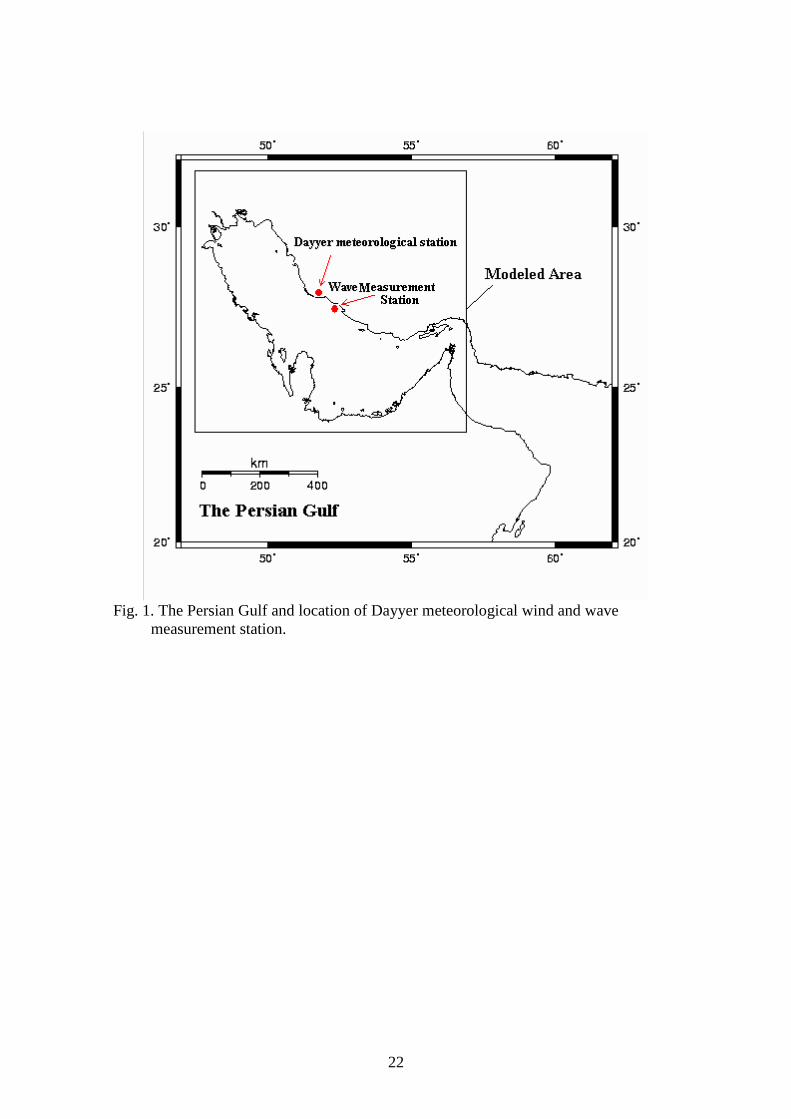
2. Study area and field data

The Persian Gulf is a marginal sea in a typical dry zone and is an extension of the Indian

Ocean. It is located between the longitude of 48-57° E and the latitude of 24–30° N

(Fig. 1). This inland sea is connected to the Gulf of Oman in the East by the Strait of

Hormuz. The gulf includes an area of 226000 km2. It is 990 km long and its width

varies from 56 to 338 km, separating Iran from Arabian Peninsula with the shortest

distance of about 56 km in the Strait of Hormuz. This Gulf has an average depth of

about 35.0 m and the deepest water depth is about 107 m [11, 12].

Assaluyeh area in Iran located at E6352 0 and N0327 0 is the closest land point to

the largest natural gas field in the world, the South Pars/North Dome Gas-Condensate

field. There are many coastal and offshore industrial projects under construction or

planning in this area. Therefore, accurate prediction of wave climate is vital in this area.

The recorded wave data used in this study were collected by an AWAC buoy which was

located in E710352 0 and N935327 0 . The data were recorded hourly from the first

of November, 2002 until 31st October, 2003. Fig. 1 illustrates the location of wave

measurement station.

Since the quality of wind data as the most important input greatly affects the accuracy

of the results, the selection of appropriate wind forcing is an essential prerequisite for

6

obtaining reliable wave hindcasting. Therefore, two sources of wind data, i.e. the

measured and ECMWF wind data, were used and evaluated for wind input in the

SWAN model. The wind measurement station called Dayyer station was located in

E65510 and N0527 0 , which was the nearest station to the wave recording location.

This meteorological station is located on a flat plain with a distance of about 100 m

from the shoreline. The nearest mountain range to this station is about 20 km away. The

wind data in this station have been recorded 3-hourly from the beginning of 1993. The

elevation of the anemometer is 4 m over the ground level. Since the wave model uses

wind velocity at 10-meter elevation, the following equation was used to modify the

velocities [13]:

7

1

10

10

zUU Z (1)

The second source of wind data was the 6-hourly 10 m operational ECMWF wind data

with a resolution of 0.5°. It should be noted that ECMWF operational was selected

because of its higher spatial resolution than ECMWF re-analysis (1.125° spatial

resolution).

3. The SWAN model

The SWAN model [10, 14] is a third generation spectral wind wave model, designed to

obtain reliable estimates of wave parameters in coastal areas. Since in the presence of

currents energy density is not conserved, action density spectrum is considered in the

SWAN model rather than energy density spectrum. The action density is equal to the

energy density divided by the relative frequency:

/),(),( EN (2)

7

The independent variables are the relative frequency (as observed in a frame of

reference moving with current velocity) and the wave direction (the direction normal

to the wave crest of each spectral component). In the SWAN wave model the evolution

of the wave spectrum in the position (x,y) and time (t) is described by the spectral action

balance equation which for Cartesian coordinates is [10]:

S

NCNCNCy

NCx

Nt

yx (3)

The first term in the left-hand side of this equation represents the local rate of change of

action density in time, the second and third terms represent propagation of action in

geographical space with propagation velocities x

C and y

C in x and y space,

respectively. The fourth term represents shifting of the relative frequency due to

variations in depths and currents (with propagation velocity C in space). The fifth

term represents depth-induced and current-induced refraction and propagation in

directional space (with propagation velocity C in space; [10]).

The term ),(SS at the right hand side of the action balance equation is the source

term in terms of energy density representing the effects of generation, dissipation and

nonlinear wave-wave interactions. This term consists of linear and exponential growth

by wind, dissipation due to whitecapping, bottom friction and depth-induced wave

breaking and energy transfer due to quadruplet and triad wave-wave interaction. In this

study SWAN cycle III version 40.41 [15] was used for wave simulation.

4. Results and discussion

4.1. Wave modeling

In the current study the SWAN model was executed in third generation and

nonstationary mode with Cartesian coordinates. Since it has been revealed that using

8

Komen’s formulation [16] for wind input parameterization leads to more accurate

prediction of Hs [17], this expression was used for exponential growths of wind input.

Quadruplet wave interaction was activated for nonlinear interaction as well. Dissipation

due to whitecapping, bottom friction and depth-induced wave breaking were considered

in the simulation.

The geographical domain was discretized into 125×100 cell grid covering the Persian

Gulf with 8800×8000 meter resolution in x and y directions, respectively. The spectral

space was divided into 25 equal directions in the rose (Δθ=3600/25=14.4

0) and 25

logarithmically spaced frequencies, between 0.06 Hz and 1 Hz. This means that the

lowest period of simulated wave was 1 second and the highest was approximately 17

seconds covering typical surface waves in the Persian Gulf. The computational time

step was selected as 10 minutes as well.

The first used wind source was Dayyer measurements which were inputted into the

model as a spatially-constant wind input. As mentioned before, the wind data at the

nearest station to the wave measurement location was taken for this purpose. The

second wind force was the ECMWF wind data varying in time and domain. Both of

these sources had their own advantages and disadvantages. The former data was

measured directly and had a finer temporal resolution (3 hours), but in this wind input

source the spatial variation of wind features over the geographical domain was ignored.

The latter wind source was the results of atmospheric model and had a coarser temporal

resolution (6 hours), but the spatial variation of wind characteristics was considered in

it. The SWAN model was executed with these input sources and the difference and

suitability of these sources from the viewpoint of wave modeling was analyzed based on

the outputs of the SWAN model.

9

The calibration of the model was conducted based on the recorded wave data during

November, 2002. The tunable parameter used for calibration was the rate of

whitecapping dissipation. Sensitivity analysis showed that other physical parameters

such as depth induced wave breaking and bottom friction have no significant effect on

the wave characteristics. Fig. 2 illustrates simulated significant wave height with default

(non-calibrated) and calibrated parameter forced by Dayyer and ECMWF wind data. As

seen in Fig. 2, using non-calibrated model forced by Dayyer wind data has led to slight

overestimation of wave height. In addition, simulation of wind waves with non-

calibrated model forced by ECMWF wind data has resulted in considerable

underestimation of high waves. This can be due to underestimation of wind speed by

ECMWF. To investigate this subject, statistical specifications of Dayyer recorded and

ECMWF modeled wind speed for wave heights greater than 0.5 meter are shown in

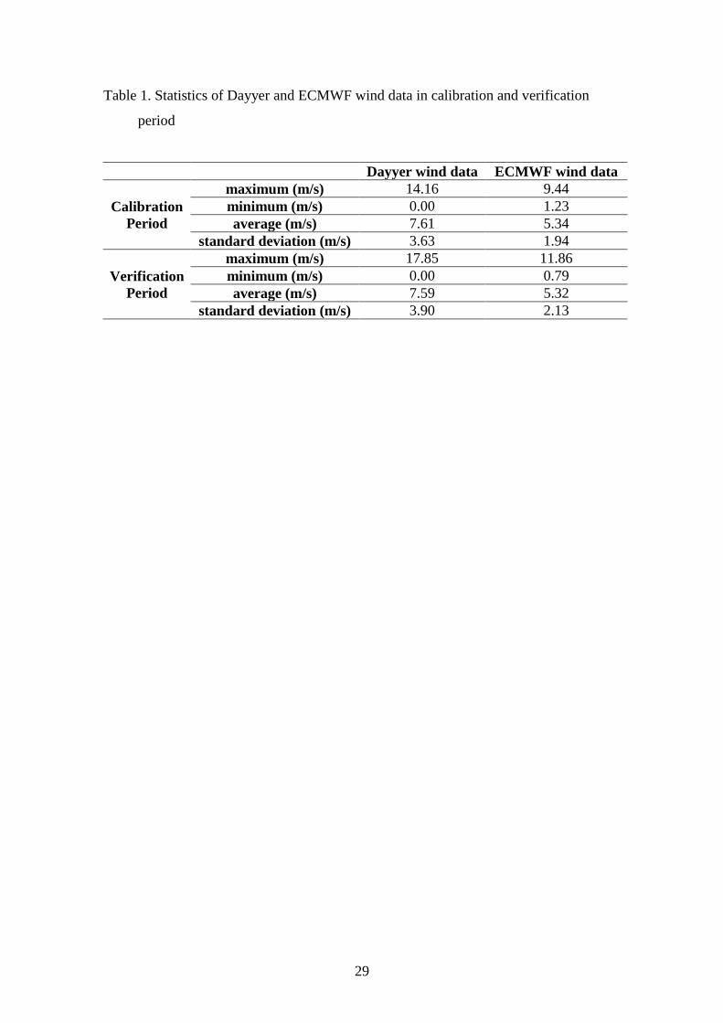
Table 1. As seen, the average of computed ECMWF wind speed in the calibration

period is about 30 percent lower than that of recorded wind speed in Dayyer station. In

addition, the maximum and standard deviation of ECMWF wind speed are considerably

lower than those of measurements indicating underestimation of ECMWF wind data.

Similar results were found for the verification period which will be discussed later.

These results reveal the importance and necessity of calibration process or updating of

wave model's result based on observed data in this condition. Generally these findings

are in agreement with those of Signell et al. [2], Brenner at al. [4], Caires and Sterl [5],

Cavaleri and Bertotti [6], Ardhuin et al. [7] and Janssen et al. [18] showing

underestimation of ECMWF wind data.

After calibration, a two-month recorded wave data during December, 2002 and January,

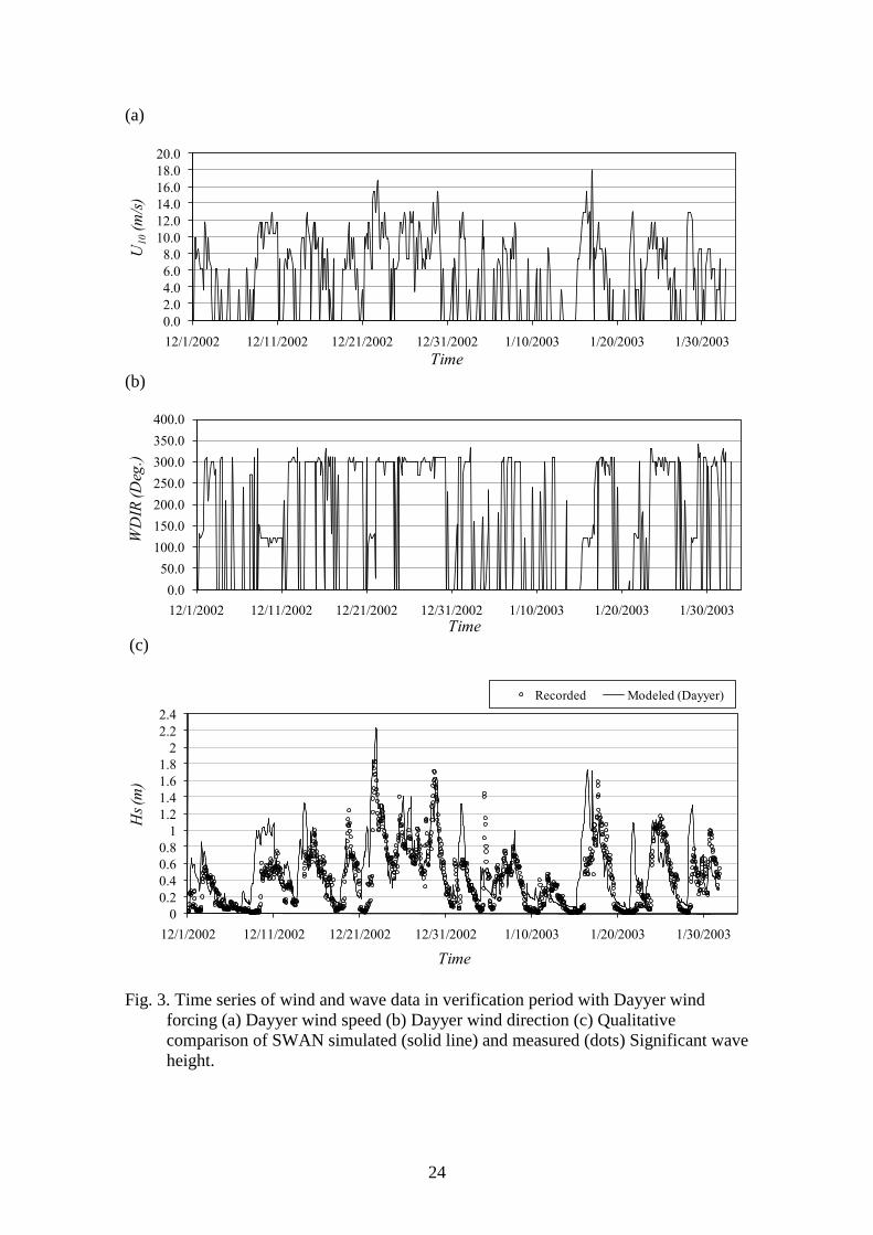
2003, was selected to verify the results of calibration process. Fig. 3 and 4 give

qualitative comparisons of the hourly time series of modeled significant wave height

10

forced by measured and ECMWF winds against the measurements in the verification

period, respectively. As seen, simulations with two source terms follow the

measurements quite well. However, there are a few inconsistencies or delays between

measurement and modeled data in both Dayyer and ECMWF wind forcing. This could

be due to the difference between actual and modeled wind in case of ECMWF, caused

by atmospheric modeling and orography effects. In case of Dayyer forcing, using

spatially-constant wind speed and ignoring the wind speed variability may result in the

observed inconsistencies. In addition, there are more fluctuations in the modeled wave

height forced by measured wind speed as opposed to that forced by ECMWF wind

speed. In other words, the model’s results forced by ECMWF are smoother than those

forced by Dayyer wind data. This could be due to two reasons. Firstly, the Dayyer wind

data had finer temporal resolution (3 hours) compared with ECMWF wind data (6

hours). Thus, it is possible that some peaks with durations less than 6 hours were

ignored in ECMWF data. Secondly, as mentioned before, the ECMWF data are the

outputs of an atmospheric model and sometimes these models can not reproduce the

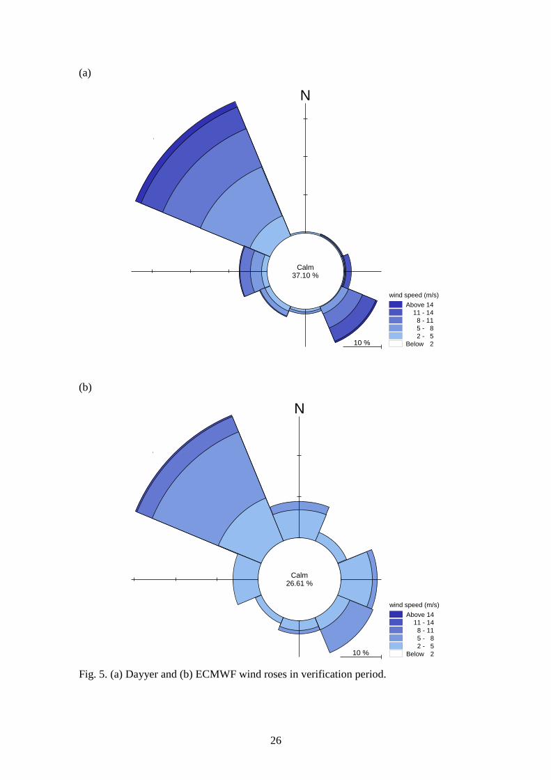
peaks very well and tend to smooth their results [2]. The wind roses of Dayyer and

ECMWF for this period are illustrated in Fig. 5. As seen, ECMWF wind rose is

generally consistent with Dayyer wind rose from the viewpoint of prevailing direction.

High speed winds in ECMWF wind rose are less observed compared with those of

Dayyer wind rose as discussed before.

In addition to above issues, it can be seen in Fig. 4 that in the case of ECMWF forced

results, the simulated wave heights for high values are closer to the measurements

compared with the simulated low wave heights. The modeled wave heights for small

values are higher than the corresponding measurements. To explain this, it should be

noticed that the goal of wave height hindcasting in this study was to investigate the

11

effect of modeling on the extreme wave analysis. Therefore, since the low wave heights

are omitted in extreme wave analysis (by the Peaks over Threshold method) the focus of

calibration was on the simulation of high waves. Thus, since the ECMWF wind data

were underestimated (Table 1), the calibration of high values has led to overestimation

of low wave heights.

After calibration and verification of the SWAN model, one year wave hindcasting was

implemented during the measurement period. For the total hindcast period mentioned

above, distribution of measured significant wave height against those simulated by

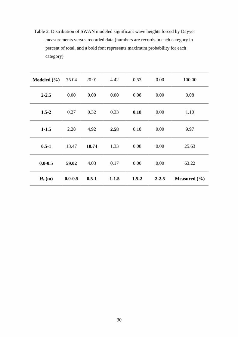
SWAN model with measured and ECMWF winds are represented in Tables 2 and 3,

respectively. In these tables, numbers are records within each category (in percent of

total) and in the case of perfect model performance, only the diagonal elements would

be filled. The results are classified into 0.5 m intervals and the maximum probability for

each category is shown in bold type.

Comparison of these two tables shows that the Dayyer forced simulated data

demonstrate smaller dispersion for low wave heights rather than ECMWF forced data.

In contrast to low wave heights, the dispersion of ECMWF forced hindcasted data is

smaller for high wave heights rather than that of Dayyer forced simulated data. This is

due to underestimation of wind speed by the ECMWF which results in overestimation

of low wave heights in calibration process. These results show that adaptation of model

parameters for improving of outputs does not necessarily lead to comprehensive

improvement of model's results. Therefore, it is recommended that for more accurate

prediction of all ranges of wave data, some other exhaustive methodologies such as

updating of output variables (error prediction) be employed [19]. However, the

maximum probability for each category of the measured wave height is located at its

12

corresponding category from modeled data. This means that calibration process has

been led to relatively correct estimation of significant wave height intervals.

Alari et al. [20] used spatially-uniform wind data for wave simulation. It should be

noted that using spatially-uniform wind input has some limitations for wind wave

simulation. However, in the studied area accurate high-resolution wind fields, which are

generally outputs of local meteorological models, were not available. In the current

study which aimed to wave modeling in one station, using spatially-constant wind input

has led to better results compared with using ECMWF data. In order to evaluate wind

wave simulation over the Persian Gulf, it is planned to use ECMWF wind source

associated with assimilation methods.

4.2. Extreme wave analysis

After hindcasting one year wave data, extreme value analysis was conducted based on

the measured and modeled wave data. The objective of this section was to compare the

results of wave hindcasting in the studied area from the viewpoint of extreme wave

analysis.

Generally, there are three different approaches for preparing the sample of wave data to

be used for extreme value analysis. In the first approach the whole data of wave heights

during a number of years is employed and distribution functions are fitted to cumulative

distribution of these data. This method is called the total sample method, initial

distribution method or the cumulative distribution function method. In the other two

approaches only the peaks of wave heights are employed. The annual maxima method

collects the highest significant wave height in each year, whereas in the Peaks over

Threshold (POT) method the peak heights occurring during each storm over a certain

threshold value are taken. Since the prerequisite of statistical independence is not

13

satisfied in the total sample method, and the annual maxima method provides short

record of extreme data, the POT method is recommended for extraction of the storms

for extreme value analysis [1, 21]. In the present study this method was used with a

primary threshold wave height value of 0.5 m. The number of extreme wave events

were 120, 138 and 87 for measured, Dayyer and ECMWF wind forced simulated waves,

respectively. The probability of exceedance of wave heights was calculated using

grouped data rather than ordered data and plotting position formulas [21]. In this

method, the extreme events are classified into wave height intervals and the exceedance

probability is defined based on the number of events recorded in each interval and the

total number of extreme data. More details can be find in [21].

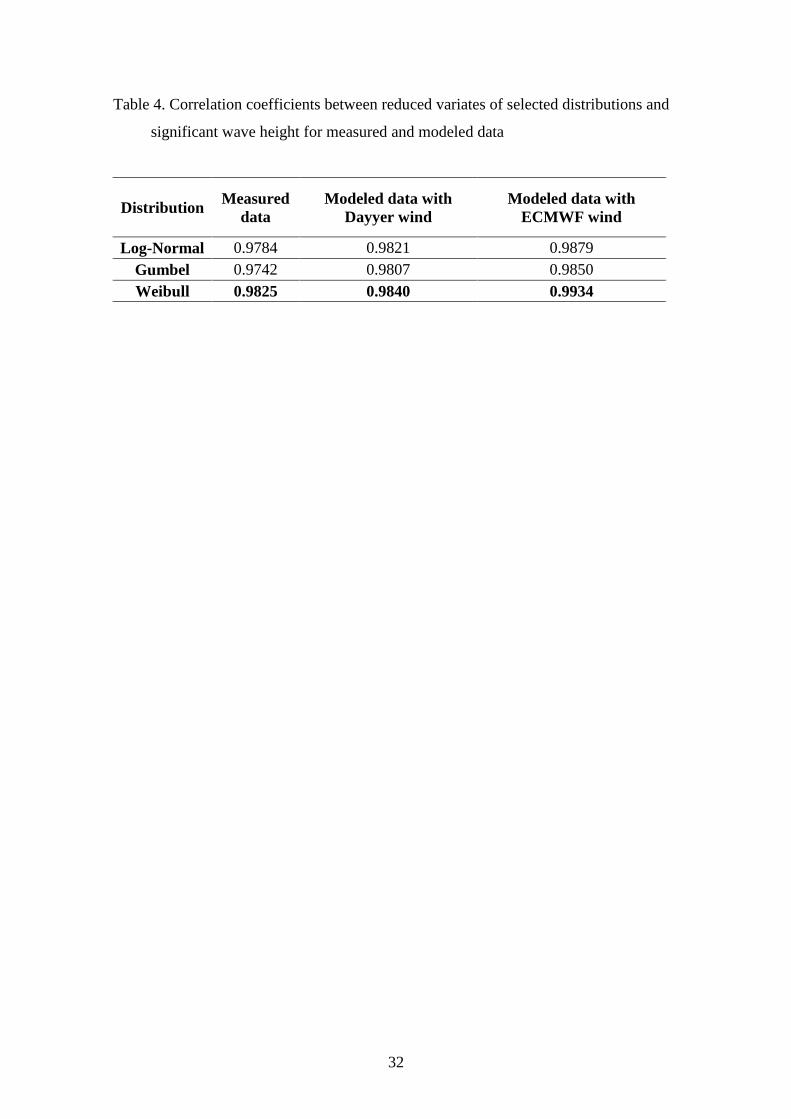
The Log-Normal, Gumbel and Weibull distributions were employed for extreme value

prediction. The correlation coefficients between reduced variates of these distributions

and significant wave height are presented in Table 4 for modeled and measured data. It

can be seen that the Weibull distribution is better fitted to the measured and both

sources of modeled storms compared to the other three distributions. This can be due to

the fact that Weibull distribution is a 3-parameter distribution while the other three

distributions are 2-parameter distributions. Therefore, the fitting of weibull distribution

to the data can be better done. This distribution was used for further investigations in

this study. Neelamani et al. [9] also found that Weibull distribution is better for Kuwaiti

territorial waters in the Persian Gulf.

Fig. 6 illustrates the reduced variates of Log-Normal, Gumbel and Weibull distributions

versus significant wave height (ln(Hs) in the case of Log-Normal distribution) for

measured and modeled data. The linear best fit to this data is also shown on these

figures. As seen, although there are higher wave heights in modeled data using Dayyer

wind compared with measured data, this two sources of data are consistent in reduced

14

variate and their fitted lines are nearly the same. It can be seen that modeled data with

ECMWF wind shows different behavior compared with other two sources from the

viewpoint of probability of exceedance of wave height. In addition, the parameter

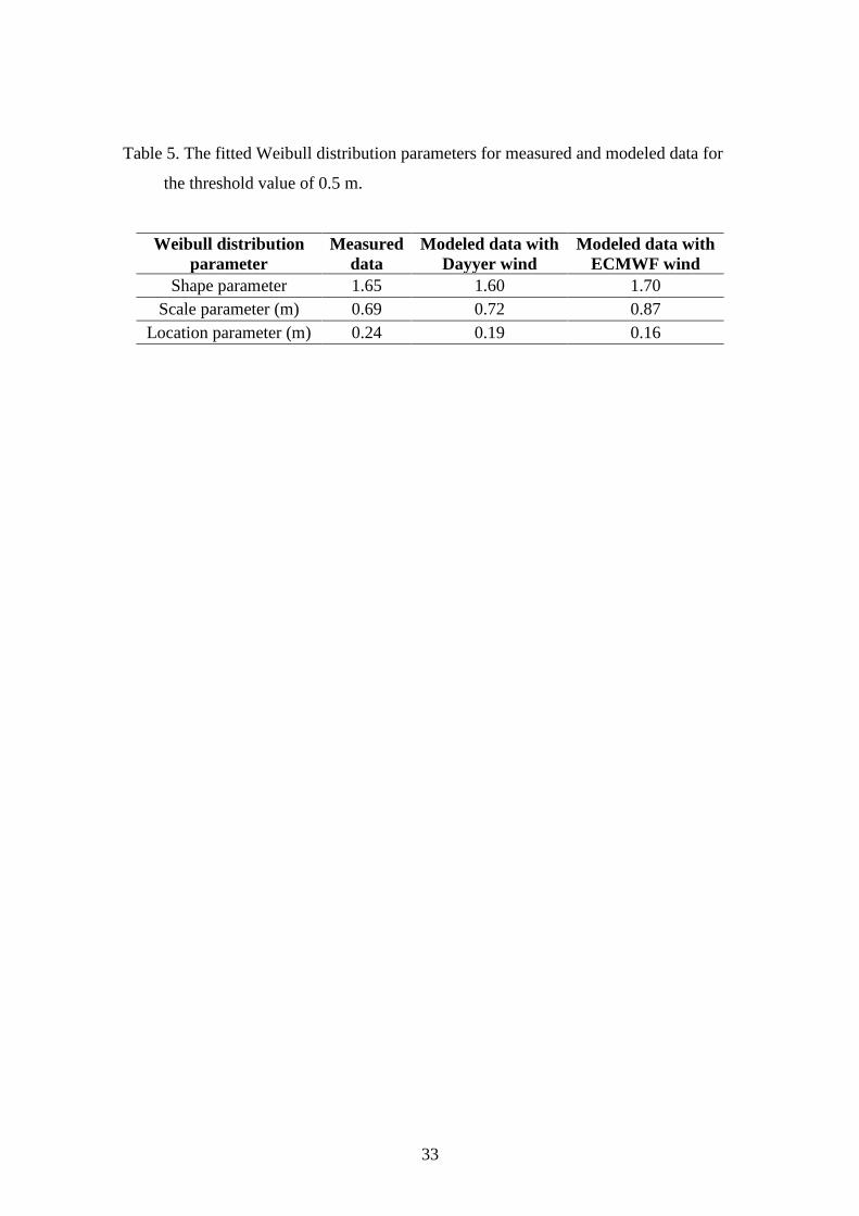
values for the fitted Weibull distribution for the measured and simulated waves forced

by Dayyer and ECMWF wind are presented in Table 5. As seen, the fitted Weibull

distribution parameters for the modeled waves forced by Dayyer wind are closer to

those of measured data rather than modeled data forced by ECMWF wind. This issue

also shows the different behavior of simulated waves forced by ECMWF wind

compared with waves obtained by other two sources of data.

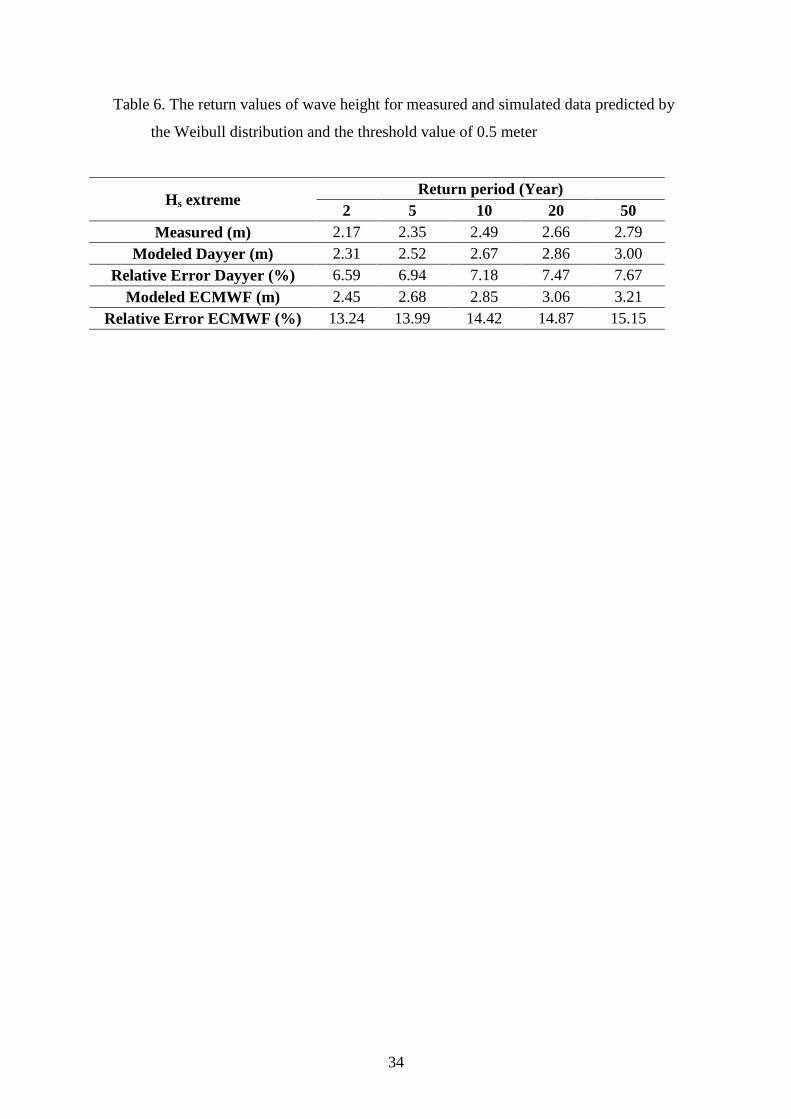
In order to evaluate the results quantitatively, the return values of significant wave

height were estimated based on three sources of wave data. Table 6 shows the extreme

wave heights with different return periods for measured and simulated data predicted by

the Weibull distribution.

As seen in Table 6, the errors of estimation of extreme wave heights are between 6 to 8

percent based on numerically simulated data forced by Dayyer wind for 2 to 50 year

return periods. These errors are between 13 to 16 percent for modeled data forced by

ECMWF wind. Therefore, it can be concluded that the numerically simulated wave data

can be used as a suitable database for estimation of design wave heights with reasonable

accuracy in this area. It should be noted that using modeled data has led to

overestimation of design wave height in both cases. In addition, according to Table 6,

the error of estimation of extreme waves based on simulated data forced by ECMWF

wind is approximately two times larger than that of simulated forced by Dayyer wind.

This is due to more accurate hindcasting of wave heights with Dayyer wind data which

was discussed before. In addition, it can be seen that the errors increase as the return

period increases. This phenomenon shows the increase of confidence intervals for

15

higher return periods. It should be pointed that the aim of this analysis was to evaluate

the effect of wind forcing on the extreme wave prediction. Since the recorded data were

available only for 1 year, extreme value analysis was conducted based on 1 year

measured and modeled data for having a fair comparison. Although extreme wave

heights may contain unreliability because of shortness of data, this issue affects all of

wave data sources in the same way. In other words, the aim of this analysis was not to

compute the value of extreme wave heights, but it was to asses the differences between

extreme values derived from different data sources.

To inspect the influence of threshold value on the estimation of design wave height a

threshold wave height of 1 m was selected and extreme value analysis was conducted

again. In this case the number of extreme events were reduced to 57, 75 and 63 for

measured, Dayyer and ECMWF wind forced modeled waves, respectively. Table 7

presents the extreme wave heights estimated by the Weibull distribution with 1 m

threshold. Comparison with Table 6 shows that increasing of the threshold value has led

to reduction of estimated return values for all cases.

The difference between design wave heights obtained from two threshold values are

higher for measured data compared with two sources of modeled data. This can be due

to smoothing of wave height time series by the numerical model [2]. In addition, the

error of extreme wave height estimation using modeled data increases as the threshold

value increases. This may be due to the increase of confidence intervals as a result of

reduction in the number of storms (associated with increasing of threshold value).

5. Summary and conclusions

In this study two sources of wind data for wind wave simulation at the northern coast of

the Persian Gulf were assessed. The wind sources consisted of recorded data at the

16

nearest meteorological station to the wave measurement location called Dayyer and

ECMWF data. The third generation spectral SWAN model was used for wind wave

simulation and the results were compared with recorded wave data both from the

viewpoint of wave hindcasting and extreme value analysis. The goal of the extreme

analysis was to asses the effect of wind forcing on the extreme wave prediction. It

should be mentioned that the predicted extreme wave heights may contain unreliability

because of the shortness of measured data. However, this issue affects three data

sources in the same way and the results can be compared fairly with each other. The

obtained results are summarized as follows:

Using Dayyer station wind data as the wind input results in slight overestimation of

wave height and there are some inconsistencies mostly due to ignoring of spatial

wind speed variability. Measured data have higher temporal resolution compared

with ECMWF data and more fluctuations are seen in hindcasted data forced by this

source. Generally, Dayyer measured data can be used for wave hindcasting in this

area with reasonable accuracy.

Non-calibrated simulated data forced by ECMWF are considerably underestimated

due to significant underestimation of wind speed by ECMWF. Simulated waves

forced by ECMWF are more smoothed rather than those forced by measured winds

mostly due to lower temporal resolution and atmospheric modeling effects on the

estimation of peaks in wind speed time series.

Since the ECMWF wind speeds are underestimated, the model's result should be

updated based on the observed data. Improving of model's outputs using adaptation

of model parameters leads to overestimation of low wave heights. This shows the

necessity of employing more comprehensive methodologies such as error prediction

for more accurate prediction of all ranges of wave data.

17

For extreme value analysis, the 3-parameter Weibull distribution is better fitted to the

measured and two sets of modeled data. From the viewpoint of probability of

exceedance of wave height, modeled data forced by ECMWF wind shows different

behavior compared with others.

Using numerically simulated data for extreme wave analysis results in overestimation

of design wave height. The error of estimation of extreme wave height based on

ECMWF forced simulated data is higher than that of forced by Dayyer recorded

data. Generally, the amount of errors is negligible and numerically simulated data

can be used as a data base for extreme wave analysis.

It is recommended that for more comprehensive evaluation of ECMWF data several

recorded wind and wave sets be collected. In addition, comparison needs to be made

between ECMWF wind speed and corresponding modeled waves and measured values

in different locations. Discovering the error distribution of ECMWF winds over the

domain is also a matter of interest. Using more comprehensive methodologies for

updating of wave model's results such as error prediction and its distribution over the

spatial domain is recommended. Finally, implementing the wind wave model for longer

periods to reduce unreliability in extreme value analysis is suggested.

6. Acknowledgments

We acknowledge the Iranian National Center for Oceanography and Iranian

Meteorological Office for allowing us to use their Data. Mr. Mostafa Nazarali is

thanked for his constructive comments. We would also like to express our gratefulness

to the SWAN group at Delft University of Technology (Department of Fluid

Mechanics) for providing the model. This study was supported by the Deputy of

Research, Iran University of Science and Technology.

18

7. References

[1] Goda Y. Statistical analysis of extreme waves (Chapter 11). In: Random seas and

design of maritime structures, 15th

volume of advanced series on ocean

engineering, World Scientific Publishing Co., 2000; 377- 425.

[2] Signell R.P., Carniel S., Cavaleri L., Chiggiato J., Doyle J.D., Pullen J., Sclavo M.

Assessment of wind quality for oceanographic modelling in semi-enclosed basins.

Journal of Marine Systems 2005; 53: 217– 233.

[3] Cavaleri L., Sclavo M. The calibration of wind and wave model data in the

Mediterranean Sea. Coastal Engineering 2006; 53: 613–627.

[4] Brenner S., Gertman I., Murashkovsky A. Preoperational ocean forecasting in the

southeastern Mediterranean Sea: Implementation and evaluation of the models

and selection of the atmospheric forcing. Journal of Marine Systems 2007; 65:

268–287.

[5] Caires S., Sterl A. A New Nonparametric Method to Correct Model Data:

Application to Significant Wave Height from the ERA-40 Re-Analysis. Journal of

Atmospheric and Oceanic Technology 2005; 22(4): 443-459.

[6] Cavaleri L., Bertotti L. The improvement of modelled wind and wave fields with

increasing resolution. Ocean Engineering 2006; 33: 553–565.

[7] Ardhuin F., Bertotti L., Bidlot J.R., Cavaleri L., Filipetto V., Lefevre J.M.,

Wittmann P. Comparison of wind and wave measurements and models in the

Western Mediterranean Sea. Ocean Engineering 2007; 34: 526–541.

[8] Caires S., Sterl A. 100-Year return value estimates for ocean wind speed and

significant wave height from the ERA-40 data. Journal of Climate 2005; 18 (7):

1032-1048.

19

[9] Neelamani S., Al-Salem K., Rakha K. Extreme waves for Kuwaiti territorial waters.

Ocean Engineering 2007; 34: 1496-1504.

[10] Booij N., Ris R.C., Holthuijsen L.H. A third generation wave model for coastal

regions. 1. Model description and validation. Journal of Geophysical Research

1999; 104: 7649–7666.

[11] Emery K.O. Sediments and water of the Persian Gulf. Bulletin of the American

Association of Petroleum Geologists 1956; 40 (10): 2354–2383.

[12] Purser B.H., Seibold E. The principal environmental factors influencing Holocene

sedimentation and diagenesis in the Persian Gulf. In: Purser, B.H. (Ed.), Persian

Gulf, Berlin, 1973; 1–9.

[13] U.S. Army. Shore Protection Manual. 4th ed., 2vols. U.S. Army Engineer

Waterways Experiment Station, U.S. Government Printing Office, Washington,

DC., 1984.

[14] Ris R.C., Holthuijsen L.H., Booij N. A third-generation wave model for coastal

regions. 2. Verification. Journal of Geophysical Research 1999; 104: 7667–7681.

[15] Booij N., Haagsma IJ.G., Holthuijsen L.H., Kieftenburg A.T.M.M., Ris R.C., Van

der Westhuysen A.J., Zijlema M. SWAN User Manual (Cycle III version 40.41).

Delft University of Technology, Delft, 2004.

[16] Komen G.J., Hasselmann S., Hasselmann K. On the existence of a fully developed

wind sea spectrum. Journal of Physical Oceanography 1984; 14: 1271-1285.

[17] Moeini M.H., Etemad-Shahidi A. Application of two numerical models for wave

hindcasting in Lake Erie. Applied Ocean Research 2007; 29: 137–145.

20

[18] Janssen P. A. E. M., Hansen B., Bidlot J.R. Verification of the ECMWF wave

forecasting system against buoy and altimeter data. Weather and Forecasting

1997; 12(4): 763-784.

[19] Babovic V., Sannasiraj S.A., Chan E.S. Error correction of a predictive ocean wave

model using local model approximation. Journal of Marine Systems 2005; 53: 1–

17.

[20] Alari V., Raudsepp U., Kõuts T. Wind wave measurements and modelling in

Küdema Bay, Estonian Archipelago Sea. Journal of Marine Systems 2008; 74:

S30– S40.

[21] Kamphuis J.W. Long term wave analysis (Chapter 4). In: Introduction to Coastal

Engineering and Management, 16th

volume of Advanced Series on Ocean

Engineering, World Scientific Publishing Co., 2000; 81-102.

21

Figure’s Caption:

Fig. 1. The Persian Gulf and location of Dayyer meteorological wind and wave

measurement station.

Fig. 2. Comparison of calibrated and non-calibrated modeled data against the

measurements in calibration period (a) Dayyer wind forced data (b) ECMWF wind

forced data.

Fig. 3. Time series of wind and wave data in verification period with Dayyer wind

forcing (a) Dayyer wind speed (b) Dayyer wind direction (c) Qualitative

comparison of SWAN simulated (solid line) and measured (dots) Significant wave

height.

Fig. 4. Time series of wind and wave data in verification period with ECMWF wind

forcing (a) ECMWF wind speed (b) ECMWF wind direction at the wave

measurement location(c) Qualitative comparison of SWAN simulated (solid line)

and measured (dots) Significant wave height.

Fig. 5. Dayyer (a) and ECMWF (b) wind roses in verification period.

Fig. 6. (a) Log-Normal (b) Gumbel and (c) Weibull distribution plots for measured and

modeled data.

22

Fig. 1. The Persian Gulf and location of Dayyer meteorological wind and wave

measurement station.

23

(a)

0

0.2

0.4

0.6

0.8

1

1.2

1.4

1.6

1.8

2

11/1/2002 11/6/2002 11/11/2002 11/16/2002 11/21/2002 11/26/2002 12/1/2002

Hs

(m)

Time

Recorded Modeled (Dayyer Non-calibrated) Modeled (Dayyer Calibrated)

(b)

0

0.2

0.4

0.6

0.8

1

1.2

1.4

1.6

1.8

11/1/2002 11/6/2002 11/11/2002 11/16/2002 11/21/2002 11/26/2002 12/1/2002

Hs

(m)

Time

Recorded Modeled (ECMWF Non-calibrated) Modeled (ECMWF Calibrated)

Fig. 2. Comparison of calibrated and non-calibrated modeled data against the

measurements in calibration period (a) Dayyer wind forced data (b) ECMWF

wind forced data.

24

(a)

0.0

2.0

4.0

6.0

8.0

10.0

12.0

14.0

16.0

18.0

20.0

12/1/2002 12/11/2002 12/21/2002 12/31/2002 1/10/2003 1/20/2003 1/30/2003

U10

(m/s

)

Time (b)

0.0

50.0

100.0

150.0

200.0

250.0

300.0

350.0

400.0

12/1/2002 12/11/2002 12/21/2002 12/31/2002 1/10/2003 1/20/2003 1/30/2003

WD

IR (D

eg.)

Time (c)

0

0.2

0.4

0.6

0.8

1

1.2

1.4

1.6

1.8

2

2.2

2.4

12/1/2002 12/11/2002 12/21/2002 12/31/2002 1/10/2003 1/20/2003 1/30/2003

Hs

(m)

Time

Recorded Modeled (Dayyer)

Fig. 3. Time series of wind and wave data in verification period with Dayyer wind

forcing (a) Dayyer wind speed (b) Dayyer wind direction (c) Qualitative

comparison of SWAN simulated (solid line) and measured (dots) Significant wave

height.

25

(a)

0.0

2.0

4.0

6.0

8.0

10.0

12.0

14.0

12/1/2002 12/11/2002 12/21/2002 12/31/2002 1/10/2003 1/20/2003 1/30/2003

U1

0 (m

/s)

Time

(b)

0.0

50.0

100.0

150.0

200.0

250.0

300.0

350.0

400.0

12/1/2002 12/11/2002 12/21/2002 12/31/2002 1/10/2003 1/20/2003 1/30/2003

WD

IR (D

eg.)

Time

(c)

0

0.2

0.4

0.6

0.8

1

1.2

1.4

1.6

1.8

2

12/1/2002 12/11/2002 12/21/2002 12/31/2002 1/10/2003 1/20/2003 1/30/2003

Hs

(m)

Time

Recorded Modeled (ECMWF)

Fig. 4. Time series of wind and wave data in verification period with ECMWF wind

forcing (a) ECMWF wind speed (b) ECMWF wind direction at the wave measurement

location(c) Qualitative comparison of SWAN simulated (solid line) and measured (dots)

Significant wave height.

26

(a)

wind speed (m/s)

Above 14

11 - 14

8 - 11

5 - 8

2 - 5

Below 2

N

Calm37.10 %

10 %

(b)

wind speed (m/s)

Above 14

11 - 14

8 - 11

5 - 8

2 - 5

Below 2

N

Calm26.61 %

10 %

Fig. 5. (a) Dayyer and (b) ECMWF wind roses in verification period.

27

(a)

-1

-0.6

-0.2

0.2

0.6

1

1.4

1.8

2.2

2.6

-0.6 -0.4 -0.2 0 0.2 0.4 0.6 0.8

Lo

g-N

orm

al red

uce

d v

aria

te

Log(Wave height) (m)

measured Modeled Dayyer Modeled ECMWF

Best fit (Measured) Best fit (Modeled Dayyer) Best fit (Modeled ECMWF)

(b)

-0.6-0.20.20.6

11.41.82.22.6

33.43.84.24.6

5

0.4 0.6 0.8 1 1.2 1.4 1.6 1.8 2 2.2 2.4

Gu

mb

el red

uce

d v

aria

te

Wave height (m)

measured Modeled Dayyer Modeled ECMWF

Best fit (Measured) Best fit (Modeled Dayyer) Best fit (Modeled ECMWF)

(c)

0.2

0.4

0.6

0.8

1

1.2

1.4

1.6

1.8

2

2.2

2.4

2.6

2.8

0.4 0.6 0.8 1 1.2 1.4 1.6 1.8 2 2.2 2.4

Wei

bu

ll red

uce

d v

aria

te

Wave height (m)

measured Modeled Dayyer Modeled ECMWF

Best fit (Measured) Best fit (Modeled Dayyer) Best fit (Modeled ECMWF)

`

Fig. 6. (a) Log-Normal (b) Gumbel and (c) Weibull distribution plots for measured and

modeled data.

28

Table’s Caption:

Table 1. Statistics of Dayyer and ECMWF wind data in calibration and verification

period

Table 2. Distribution of SWAN modeled significant wave heights forced by Dayyer

measurements versus recorded data (numbers are records in each category in

percent of total, and a bold font represents maximum probability for each

category)

Table 3. Distribution of SWAN modeled significant wave heights forced by ECMWF

wind data versus measured data (numbers are records in each category in percent

of total, and a bold font represents maximum probability for each category)

Table 4. Correlation coefficients between reduced variates of selected distributions and

significant wave height for measured and modeled data

Table 5. The fitted Weibull distribution parameters for measured and modeled data for

the threshold value of 0.5 m.

Table 6. The return values of wave height for measured and simulated data predicted by

the Weibull distribution and the threshold value of 0.5 meter

Table 7. Same as Table 6 but for threshold value of 1 meter

29

Table 1. Statistics of Dayyer and ECMWF wind data in calibration and verification

period

Dayyer wind data ECMWF wind data

Calibration

Period

maximum (m/s) 14.16 9.44

minimum (m/s) 0.00 1.23

average (m/s) 7.61 5.34

standard deviation (m/s) 3.63 1.94

Verification

Period

maximum (m/s) 17.85 11.86

minimum (m/s) 0.00 0.79

average (m/s) 7.59 5.32

standard deviation (m/s) 3.90 2.13

30

Table 2. Distribution of SWAN modeled significant wave heights forced by Dayyer

measurements versus recorded data (numbers are records in each category in

percent of total, and a bold font represents maximum probability for each

category)

Modeled (%) 75.04 20.01 4.42 0.53 0.00 100.00

2-2.5 0.00 0.00 0.00 0.08 0.00 0.08

1.5-2 0.27 0.32 0.33 0.18 0.00 1.10

1-1.5 2.28 4.92 2.58 0.18 0.00 9.97

0.5-1 13.47 10.74 1.33 0.08 0.00 25.63

0.0-0.5 59.02 4.03 0.17 0.00 0.00 63.22

Hs (m) 0.0-0.5 0.5-1 1-1.5 1.5-2 2-2.5 Measured (%)

31

Table 3. Distribution of SWAN modeled significant wave heights forced by ECMWF

wind data versus measured data (numbers are records in each category in percent

of total, and a bold font represents maximum probability for each category)

Modeled (%) 75.04 20.01 4.42 0.53 0.00 100.00

2-2.5 0.07 0.07 0.15 0.08 0.00 0.37

1.5-2 0.43 0.93 1.12 0.33 0.00 2.82

1-1.5 3.83 6.74 2.52 0.12 0.00 13.20

0.5-1 27.93 11.87 0.63 0.00 0.00 40.43

0.0-0.5 42.78 0.40 0.00 0.00 0.00 43.18

Hs (m) 0.0-0.5 0.5-1 1-1.5 1.5-2 2-2.5 Measured (%)

32

Table 4. Correlation coefficients between reduced variates of selected distributions and

significant wave height for measured and modeled data

Distribution Measured

data

Modeled data with

Dayyer wind

Modeled data with

ECMWF wind

Log-Normal 0.9784 0.9821 0.9879

Gumbel 0.9742 0.9807 0.9850

Weibull 0.9825 0.9840 0.9934

33

Table 5. The fitted Weibull distribution parameters for measured and modeled data for

the threshold value of 0.5 m.

Weibull distribution

parameter

Measured

data

Modeled data with

Dayyer wind

Modeled data with

ECMWF wind

Shape parameter 1.65 1.60 1.70

Scale parameter (m) 0.69 0.72 0.87

Location parameter (m) 0.24 0.19 0.16

34

Table 6. The return values of wave height for measured and simulated data predicted by

the Weibull distribution and the threshold value of 0.5 meter

Hs extreme Return period (Year)

2 5 10 20 50

Measured (m) 2.17 2.35 2.49 2.66 2.79

Modeled Dayyer (m) 2.31 2.52 2.67 2.86 3.00

Relative Error Dayyer (%) 6.59 6.94 7.18 7.47 7.67

Modeled ECMWF (m) 2.45 2.68 2.85 3.06 3.21

Relative Error ECMWF (%) 13.24 13.99 14.42 14.87 15.15

35

Table 7. Same as Table 6 but for threshold value of 1 meter

Hs extreme Return period (Year)

2 5 10 20 50

Measured (m) 2.04 2.16 2.25 2.36 2.44

Modeled Dayyer (m) 2.31 2.51 2.65 2.85 2.99

Relative Error Dayyer (%) 13.32 15.87 17.87 20.59 22.69

Modeled ECMWF (m) 2.39 2.60 2.75 2.96 3.11

Relative Error ECMWF (%) 17.04 20.09 22.33 25.21 27.32