CAPROCK INTEGRITY STUDY OF THE 2nd WALL

CREEK RESERVOIR: A CASE STUDY FROM TEAPOT

DOME, WYOMING

Supervisors: Ismaila Adetunji Jimoh Authors: Jacquelin Cobos

Wolfgang Weinzierl Jhony Quintal

Erik Gydesen Søgaard

CAPROCK INTEGRI0TY STUDY OF THE 2nd WALL

CREEK RESERVOIR: A CASE STUDY FROM TEAPOT

DOME, WYOMING

Project Period: 01/02/2017 to 08/06/2017

Date of submission: 08/06/2017

Place of study: Aalborg University Esbjerg

Supervisor: Ismaila Adetunji Jimoh, Wolfgang Weinzierl (Schlumberger Oilfield

Services, Denmark) & Erik Gydesen Søgaard

Authors:

Jacquelin Cobos ___________________________________________

Jhony Cesar Quintal Nunes ___________________________________________

I

ABSTRACT

Over the last few years, the study of caprocks for geologic CO2 storage has been

increased due to the significant risk regarding safety and environment if the

containment is not ensured.

In this work, a multi-disciplinary approach that integrates geology, petrophysics,

rockphyics, and geomechanics concepts are used to characterize the caprock of the

2nd Creek Wall reservoir, Teapot Dome, Wyoming regarding its tensile strength. This

field was chosen due to the information availability and the numerous sequestration

pilot projects carried out in the site.

The first part of this study was done in Techlog©, wellbore platform from

Schlumberger and comprises the computation of the petrophysical and mechanical

characteristics of the caprock based on the available wireline logging data for 18 wells.

The integration of that information is then used to calculate the brittleness index

which is related to the tensile strength of the caprock. A neuronal analysis in IPSOM

was considered to classify the caprock regarding its ductility and brittleness.

The final results of this study show that 2nd Wall Creek reservoir can be seen as a good

candidate for a CO2 sequestration project. Finally, those properties are loaded in

Petrel, integrated subsurface platform, to create a 3-D grid map the brittleness and

ductility of the caprock. The map indicates the possible drilling locations for CO2

storage.

II

ACKNOWLEDGEMENT

First and foremost, we wish to thank our project supervisor and Techlog© trainer

Ismaila Adetunji Jimoh. We express our appreciation to Wolfgang Weinzierl who was

our Petrel instructor and also for his help in the 3-D modeling. Last but not least, we

thank Erik Gydesen Søgaard who has been our supervisor in the university.

We would like to extend our gratitude to Schlumberger Software Integrate Solutions

in Denmark for providing the software grant of Techlog© and Petrel and also for the

training received in their office in Copenhagen.

Sincere thanks to Aalborg University-Esbjerg for their support, equipment, and

installations and the IT department.

At last, we would like to acknowledge the US Geological Survey Site (USGS) and Rocky

Mountain Oilfield Testing Center (RMOTC), for the public data source we used for the

present study.

III

CONTENTS CHAPTER I. INTRODUCTION ................................................................................................ 1

1.1. Problem Statement ................................................................................................... 2

1.2. Data and Methods .................................................................................................... 2

1.3. Area of Investigation ................................................................................................. 5

1.4. Carbon Sequestration ............................................................................................... 6

1.5. Project Limitations .................................................................................................... 6

1.6. Project Outline .......................................................................................................... 7

CHAPTER II. LITERATURE REVIEW ........................................................................................ 8

2.1. Caprock in CO2 Sequestration ................................................................................... 8

2.2. Seal Potential ............................................................................................................ 9

2.2.1. Seal Capacity ..................................................................................................... 9

2.2.2. Seal Geometry ................................................................................................. 10

2.2.3. Caprock Integrity ............................................................................................. 10

2.3. Caprock Effectiveness ............................................................................................. 11

2.3.1. Lithology .......................................................................................................... 11

2.3.2. Ductility ........................................................................................................... 11

2.3.3. Thickness ......................................................................................................... 13

2.3.4. Burial Depth .................................................................................................... 13

CHAPTER III. GEOLOGICAL BACKGROUND .......................................................................... 14

3.1. Geology of Teapot Dome ........................................................................................ 14

3.2. Stratigraphy ............................................................................................................. 16

3.3. Lithology .................................................................................................................. 19

CHAPTER IV. . PETROPHYSICAL EVALUATION 21

4.1. Data Analysis ........................................................................................................... 21

4.2. Well Correlation Study ............................................................................................ 23

4.3. Petrophysical Analysis ............................................................................................. 25

4.3.1. Volume of shale .............................................................................................. 26

4.3.2. Porosity calculation ......................................................................................... 30

4.3.3. Fluid Saturation ............................................................................................... 35

IV

4.3.4. Lithology estimation ....................................................................................... 36

CHAPTER V. GEOPHYSICS .................................................................................................... 41

5.1. Overview ................................................................................................................. 41

5.2. Acoustic properties ................................................................................................. 42

5.3. Dynamic Elastic Properties ...................................................................................... 45

CHAPTER V. GEOMECHANICS ............................................................................................. 49

6.1. Overview ................................................................................................................. 49

6.2. In-Situ Stress ........................................................................................................... 51

6.2.1. Overburden Stress .......................................................................................... 51

6.2.2. Pore Pressure .................................................................................................. 53

6.3. Rock Strength .......................................................................................................... 56

6.3.1. Unconfined Compressive Strength ................................................................. 57

6.3.2. Tensile Strength .............................................................................................. 60

CHAPTER VII. CAPROCK INTEGRITY .................................................................................... 62

7.1. Dynamic elastic properties analysis ........................................................................ 62

7.2. IPSOM Classification ............................................................................................... 65

7.3. Brittleness Index ..................................................................................................... 69

7.3.1. Evaluation of Brittleness Index ....................................................................... 72

CHAPTER VIII. CAPROCK MODELING .................................................................................. 75

8.1. Data and Methods .................................................................................................. 75

8.2. Surface Model ......................................................................................................... 77

8.3. Facies Modeling ...................................................................................................... 79

8.4. Petrophysical Modeling .......................................................................................... 82

8.5. Modeling Results ..................................................................................................... 87

8.6. Drilling locations for the CO2 injection wells .......................................................... 89

V

LIST OF FIGURES

Figure 1 – Caprock Integrity Flowchart ..................................................................................... 4

Figure 2 – General location of Wyoming and Teapot Dome Field (4) ...................................... 5

Figure 3 – Upward migration of CO2 due to buoyancy (8). ..................................................... 10

Figure 4 – Relative ductility and compressibility vs strength/sonic velocity .......................... 12

Figure 5 – Map of the Teapot Dome (14) ............................................................................... 14

Figure 6 – Structural map of the reservoir (17) ...................................................................... 15

Figure 7 – Depth-structure map of the 2nd wall creek sandstone (17) ................................... 16

Figure 8 – Teapot Dome stratigraphic column (3) .................................................................. 17

Figure 9 – Frontier formation cross section (18) .................................................................... 18

Figure 10 – Location of the wells in the Teapot Dome field ................................................... 22

Figure 11 – Well correlation in the 2nd Wall Creek formation ................................................ 24

Figure 12 – Determination of GR_Matrix and GR_Shale ........................................................ 27

Figure 13 – Computation of shale volume (Vsh) for the wells: 28-AX-27, 36-MX-10, 67-1-TpX-

10, 11-DX-26, 12-AX-33 ........................................................................................................... 28

Figure 14 – Shale Volume histogram for all the wells ............................................................ 29

Figure 15 – Calculation of porosity by neutron-density logs for the wells: 28-AX-27, 36-MX-

10, 67-1-TpX-10 ....................................................................................................................... 31

Figure 16 – Histogram of total porosity .................................................................................. 33

Figure 17 – Matrix histogram for effective porosity ............................................................... 34

Figure 18 – Distribution of water saturation across the wells in the caprock ........................ 36

Figure 19 -Cross-plot RHomaa vs Umaa for mineralogy identification .................................. 38

Figure 20 -Cross-plot RHomaa vs DTmaa for mineralogy identification ................................. 39

Figure 21 - Mineralogy log for well 67-1-TpX-1 ...................................................................... 40

Figure 22 - Acoustic properties for well 67-1-TpX-10 ............................................................. 43

Figure 23 – Shear velocity for the well 67-1-TpX-10 ............................................................... 44

Figure 24 – Compressional to shear velocity ratio and dynamic Poison’s ratio for the well 67-

1-TpX-10 .................................................................................................................................. 46

Figure 25 – Type of stresses (31) ............................................................................................ 49

Figure 26– Stress-strain curve (32) ......................................................................................... 50

Figure 27 – Stress-strain curve for ductile and brittle rocks ................................................... 50

Figure 28 – Overburden stress ................................................................................................ 52

Figure 29 – Overburden stress histogram............................................................................... 53

Figure 30 – Pore pressure calculation by using the Eton’s method........................................ 55

Figure 31 – Pore pressure histogram ...................................................................................... 56

Figure 32 – Unconfined compressive strength ....................................................................... 58

Figure 33 – Unconfined compressive strength crossplots ...................................................... 59

Figure 34 – Unconfined compressive strength histogram ...................................................... 59

VI

Figure 35 –Tensile strength histogram ................................................................................... 60

Figure 36 –Box plots for UCS and TS ....................................................................................... 61

Figure 37 –Young’s modulus vs Poison’s ratio crossplot colored by gamma ray ................... 63

Figure 38 - Mineral content of the caprock in the well 67-1-TpX-10 ...................................... 64

Figure 39 – Correlation of variables used for IPSOM classification ........................................ 65

Figure 40 – IPSOM classification using an indexation of 2...................................................... 66

Figure 41 - IPSOM classification results using an indexation of 2 ........................................... 67

Figure 42 – a) Young’s modulus vs Poison’s ratio crossplot colored by IPSOM classification

and b) Young’s modulus vs Poison’s ratio crossplot colored by gamma ray .......................... 68

Figure 43 – IPSOM classification pie chart for the well 67-TpX-10 ......................................... 68

Figure 44 – IPSOM classification pie chart for all the wells .................................................... 69

Figure 45 – Brittleness index comparison for the well 67-1-TpX-10 ...................................... 71

Figure 46 – Brittleness index vs volume of shale for all the wells .......................................... 73

Figure 47 – Final result of brittleness index ............................................................................ 74

Figure 48 – Modeling flowchart for the simulation ................................................................ 76

Figure 49 – Conformal gridding example ................................................................................ 77

Figure 50 – Available seismic data for Teapot Dome field...................................................... 77

Figure 51 – Available seismic data for Teapot Dome field...................................................... 78

Figure 52 – Conformal 3D grid ................................................................................................ 79

Figure 53 – Estimated facies proportions percentage ............................................................ 80

Figure 54 – Proportion curves for each facie (ductile and brittle) .......................................... 81

Figure 55 – IPSOM variogram ................................................................................................. 81

Figure 56 – Facies volume height map ................................................................................... 82

Figure 57 – Vertical, Major and minor direction for group 1 .................................................. 84

Figure 58 – Vertical, Major and minor direction for group 2 .................................................. 84

Figure 59 –Distribution of the modeled Brittleness index ...................................................... 85

Figure 60 –Brittleness index volume height maps filtered with IPSOM classification ........... 86

Figure 61 – BI average thickness map ..................................................................................... 86

Figure 62 – Ductility proportional thickness map ................................................................... 87

Figure 63 –Brittleness proportional thickness map ................................................................ 88

Figure 64 –Possible drilling locations for CO2 storage ............................................................ 90

VII

LIST OF TABLES

Table 1 – Ductility of different caprock lithologies (11).......................................................... 12

Table 2 – Well logs summary .................................................................................................. 21

Table 3 – Thickness summary for the 2nd Wall Creek formation ............................................ 25

Table 4 – Mechanical parameters ........................................................................................... 41

Table 5 – Statistical parameters of dynamic properties for the caprock of the 2nd Wall Creek

reservoir and histograms made for Young modulus, shear modulus, bulk modulus and

Poisson’s ratio ......................................................................................................................... 48

Table 6 – Variable correlation and contribution ..................................................................... 66

Table 7 – IPSOM classification statistics ................................................................................. 67

VIII

LIST OF APPENDIX

APPENDIX 1 – WELL LOGGING TOOLS AND PRINCIPLES

Figure 1. 1 – Well logging setup (47) ...................................................................................... 99

Figure 1. 2 – Gamma Ray response (47) ............................................................................... 100

Figure 1. 3 – Bulk Density log (22)......................................................................................... 101

Figure 1. 4 – Photoelectric Factor log (22) ............................................................................ 102

Figure 1. 5 – Neutron log (22) ............................................................................................... 103

Figure 1. 6 – Resistivity logs (22) .......................................................................................... 104

Figure 1. 7 –Compressional Slowness log (22) ..................................................................... 105

APPENDIX 2 – WELL CORRELATION

Figure 2. 1 – Correlation across the 18 wells that penetrates the 2nd Wall Creek Reservoir 107

APPENDIX 3 – SHALE VOLUME

Figure 3. 1 - Shale volume calculation for the wells from left to right: 28-AX-27, 36-MX-10, 67-

1-TPX-10, 11-DX-26, 12-AX-33, 14-LX-28-WD, 28-AX-34, 34-TX-3, 36-11-SX-2 .................... 108

Figure 3. 2 - Shale volume calculation for the wells from left to right: 41-2-X-3, 41-AX-3, 53-

LX-3, 62-TPX-10, 64-JX-15, 71-1-X-4, 75-AX-28, 88-AX-28, 88-DX-3 ..................................... 109

APPENDIX 4 – TOTAL AND EFFECTIVE POROSITY

Figure 4. 1- Total and effective porosity for the wells from left to right: 28-AX-27, 36-MX-10,

67-1-TPX-10, 11-DX-26, 12-AX-33, 14-LX-28-WD, 28-AX-34, 34-TX-3, 36-11-SX- ................. 110

Figure 4. 2 - Total and effective porosity for the wells from left to right: 41-2-X-3, 41-AX-3, 53-

LX-3, 62-TPX-10, 64-JX-15, 71-1-X-4, 75-AX-28, 88-AX-28, 88-DX-3 ..................................... 111

APPENDIX 5 – WATER SATURATION

Figure 5. 1 - Water saturation for the wells from left to right: 28-AX-27, 36-MX-10, 67-1-TPX-

10, 11-DX-26, 12-AX-33, 14-LX-28-WD, 28-AX-34, 34-TX-3, 36-11-SX-2............................... 112

Figure 5. 2 - Water saturation for the wells from left to right: 41-2-X-3, 41-AX-3, 53-LX-3, 62-

TPX-10, 64-JX-15, 71-1-X-4, 75-AX-28, 88-AX-28, 88-DX-3 ................................................... 113

IX

APPENDIX 6 – MINERALOGY

Figure 6. 1- Mineralogy for the wells from left to right: 28-AX-27, 36-MX-10, 67-1-TPX-10, 11-

DX-26, 12-AX-33, 14-LX-28-WD, 28-AX-34, 34-TX-3, 36-11-SX-2 .......................................... 114

Figure 6. 2 - Mineralogy for the wells from left to right: 41-2-X-3, 41-AX-3, 53-LX-3, 62-TPX-10,

64-JX-15, 71-1-X-4, 75-AX-28, 88-AX-28, 88-DX-3 ................................................................ 115

APPENDIX 7 – ACOUSTIC PROPERTIES

Figure 7. 1 - Acoustic Properties for the wells from left to right: 28-AX-27, 36-MX-10, 67-1-

TPX-10, 11-DX-26, 12-AX-33, 14-LX-28-WD, 28-AX-34, 34-TX-3, 36-11-SX-2 ....................... 116

Figure 7. 2 - Acoustic Properties for the wells from left to right: 41-2-X-3, 41-AX-3, 53-LX-3,

62-TPX-10, 64-JX-15, 71-1-X-4, 75-AX-28, 88-AX-28, 88-DX-3 .............................................. 117

APPENDIX 8 – SHEAR VELOCITY

Figure 8. 1 - Shear velocity for the wells from left to right: 28-AX-27, 36-MX-10, 67-1-TPX-10,

11-DX-26, 12-AX-33, 14-LX-28-WD, 28-AX-34, 34-TX-3, 36-11-SX-2 .................................... 118

Figure 8. 2 – Shear velocity for the wells from left to right: 41-2-X-3, 41-AX-3, 53-LX-3, 62-TPX-

10, 64-JX-15, 71-1-X-4, 75-AX-28, 88-AX-28, 88-DX-3 .......................................................... 119

APPENDIX 10 – IPSOM RESULTS AND DYNAMIC ELASTIC PROPERTIES

Figure 9. 1 - Pore pressure for the wells from left to right: 11-DX-26, 12-AX-33,14-LX-28-WD,

28-AX-27,28-AX,34-TX-3 ....................................................................................................... 120

Figure 9. 2 - Pore pressure for the wells from left to right: 36-11-SX-2, 36-MX-10,41-2-X-3,41-

AX-3,53-LX-3,62-TpX-10 ........................................................................................................ 121

Figure 9. 3 - Pore pressure for the wells from left to right: 64-JX-15, 67-1-TpX-10,71-1-X-

4,75,AX-28,88-AX-28,88-DX-3 ............................................................................................... 122

APPENDIX 11 – IPSOM PIE-CHARTS

Figure 10. 1 - IPSOM results and dynamic elastic properties for the wells from left to right: 28-

AX-27, 36-MX-10, 67-1-TPX-10, 11-DX-26, 12-AX-33 ........................................................... 123

Figure 10. 2 - IPSOM results and dynamic elastic properties for the wells from left to right: 14-

LX-28-WD,28-AX-27,28-AX,34-TX-3, 41-2-X-3, 41-AX-3, 53-LX-3 .......................................... 124

Figure 10. 3 - IPSOM results and dynamic elastic properties for the wells from left to right: 62-

TPX-10, 64-JX-15, 71-1-X-4, 75-AX-28, 88-AX-28, 88-DX-3 ................................................... 125

X

APPENDIX 9 – PORE PRESSURE

Figure 11. 1 - Pie-charts for the wells from le - ft to right: 11-DX-26, 12-AX-33, 14-LX-28-WD,

28-AX-27, 28-AX, 34-TX-3 ...................................................................................................... 126

Figure 11. 2 - Pie-charts for the wells from left to right: 36-11-SX-2, 36-MX-10, 41-2-X-3,41-

AX-3,53-LX-3,62-TpX-10 ........................................................................................................ 127

Figure 11. 3 - Pie-charts for the wells from left to right: 64-JX-15, 67-1-TpX-10,71-1-X-4,75-AX-

28,88-AX-28,88-DX-3 ............................................................................................................ 128

APPENDIX 12 – BRITTLE INDEX

Figure 12. 1 – Brittle index for the wells from left to right: 28-AX-27, 28-AX-34, 11-DX-26 129

Figure 12. 2 – Brittle index for the wells from left to right: 36-MX-10, 67-1-TpX-10, 12-AX-33

.............................................................................................................................................. 130

Figure 12. 3 – Brittle index for the wells from left to right: 14-LX-28-WD, 34-TX-3, 36-11-SX-2

.............................................................................................................................................. 131

Figure 12. 4 – Brittle index for the wells from left to right:41-2-X-3,41-AX-3,53-LX-3 ......... 132

Figure 12. 5 – Brittle index for the wells from left to right: 62-TpX-10, 64-JX-15, 71-1-X-4 . 133

Figure 12. 6 – Brittle index for the wells from left to right: 75-AX-28,88-AX-28,88-DX-3 .... 134

XI

NOMENCLATURE

Stress

∅ Porosity 3-D Three dimensional a Tortuosity factor AI Acoustic impedance BI Brittle index BI_H Ingram and Urai brittle index BI_M Wang and Gale’s brittle index BI_R Rickman’s brittle index BIR Brittleness index evaluation CALR Caliper CCS Carbon Capture and Storage Cdyn Dynamic bulk compressibility

CO2 Carbon dioxide

DEN_EXTRAPOLATED Extrapolated bulk density DT Compressional slowness DTmaa Matrix apparent compressional slowness DTnorm Normal Compressional slowness DTo Initial travel time Ductile Caprock ductility percentage

E Young’s modulus

Edyn Dynamic young’s modulus

EOR Enhanced oil recovery

G Shear modulus Gdyn Dynamic shear modulus

GHG Greenhouse emission

GR Gamma ray GRFS Gaussian random function simulation HighThickness_LowBI High Thickness and Low BI IF Integrity factor IPSOM Index and Probability Generating a Self-Organizing Map ITF Interfacial tension K Bulk modulus Kdyn Dynamic bulk modulus L Number of monomineralic lithology constituent m Cementation M Compressional modulus MICP Mercury injection capillary pressure

XII

n Saturation exponent

NPHI Neutron porosity NPR3 Naval petroleum reserve OBMW_EXT Vertical stress gradient equivalent Pc Threshold pressure Pe Photoelectric absorption PE Photoelectric factor PHIE_ND Effective porosity Pp Pore pressure Pp_DT Pore pressure Eaton sonic Pp_R Pore pressure Eaton resistivity Ppnorm Normal pore pressure P-waves Principal compressional waves r Pore radius R Resistivity RDEP Deep resistivity RFOC Shallow resistivity RHOB Bulk density RHomaa Apparent grain density RILM Medium resistivity RMOTC Rocky mountain oilfield testing center Rnorm Normal resistivity Ro Sediment resistivity Rt Formation resistivity Rw Formation water resistivity scf Standard cubic feet SIS Sequential indicator simulation SP Spontaneous potential SPR Slowness time projection SVERTIVAL_EXT Overburden stress Sw Water saturation S-waves Secondary waves T Shear stress TS Tensile strength TVD Truth vertical depth UCS Unconfined compressive strength UCSNC UCS of a consolidated rock Uf Apparent fluid volumetric cross section Umaa Matrix apparent volumetric photoelectric factor v Poisson ratio v/v Volume to volume ratio VANH Volume of anhydrite VCLC Volume of clay VDOL Volume of dolomite Vfi Volume fractions of lithological constituents

XIII

Vo Initial volume VP Compressional velocity VPVS Static Poisson’s ratio VQTZ Volume of quartz VS Shear velocity Vsh Volume of shale Y Shear strain z Depth ΔP Pressure change Δt Wave transit time Δtcomp Bulk formation compressional slowness Δtf Pore fluid transit time Δtshear Bulk formation shear slowness ΔV Volume change ϵ Strain ϵaxial Axial strain ϵtrans Transverse strain θ Contact angle ρ Density ρb Bulk density ρe Electron density ρExtrapolated Extrapolated density Ρfluid Fluid density ρmatrix Matrix density ρmudline Mud density σv Vertical stress, overburden stress ϒ CO2-water interfacial tension

P a g e | 1

CHAPTER I. INTRODUCTION

Carbon Capture and Storage is one of the most efficient alternatives to decrease the

industrial greenhouse emissions (GHG), such as carbon dioxide (CO2), into the

atmosphere. Underground geological formations constitute a suitable storage for

GHG because of its large storage capacity and the presence of an effective trap and

sealing mechanisms. The ideal characteristics of the target reservoir are significant

storage capacity, high leak-proof, effective sealing, and a non-faulted stratum. The

stability of the sealing (caprock) during and after the CO2 storage is associated with

geophysical, geomechanical parameters and caprock-CO2 and pore fluid interactions.

The change in stress, chemical and physical alteration of the reservoir and caprock

caused by carbonic acid (formed when CO2 dissolves in the groundwater) can lead to

strength reduction and failure of the caprock. Besides, the interaction of supercritical

CO2 with the brine in the reservoir and the changes in the stress field due to CO2

injection can have an impact. Consequently, the caprock integrity is becoming more

important in the reservoir characterization and especially for geo-sequestration

projects.

This project covers the theory behind the caprock rock integrity, rock mechanics, and

carbon sequestration. It is emphasized the quality check of conventional logs and

computation of reference/index datasets for each well. The gamma ray and

spontaneous potential logs are examined in the zone of interest for lithologic

information to enable well correlation. The acoustic/rock physics properties are

derived by using a combination of between bulk density, and compressional slowness

log and the values of porosity and saturation are determined by neutron porosity and

deep resistivity logs. Furthermore, the lithology and mineral composition of the rock

is estimated by a four-point mineral model which uses the apparent matrix density

(RHomaa), apparent matrix volumetric photoelectric factor (Umaa), and matrix

apparent compressional slowness (Dtmaa) to interpolate between four end-point

minerals. The 1D outputs from the petrophysical, geophysical and geomechanical

calculations are modeled in 3D to show the variation in the rock properties.

P a g e | 2

1.1. Problem Statement

The success of any CO2 sequestration operation depends on the sealing ability of the

top layer (caprock) in the reservoir. The sealing is influenced by pre-existing

fractures/faults or leakage pathways that are present and the ones that can occur due

to interactions when the CO2 is injected into the reservoir.

The aim of this project is to characterize the caprock of the 2nd Creek Wall reservoir,

Teapot Dome, Wyoming based on the brittle index. This characterization can be done

by integrating geology, petrophysics, rockphyics, and geomechanics concepts.

This project will use a multi-disciplinary approach through Techlog© which takes into

consideration wireline logs including gamma ray (GR), spontaneous potential (SP),

bulk density (RHOB), neutron (NPHI), deep resistivity (RDEP), compressional slowness

(DT), and photoelectric effect (PE) logs and other available information to evaluate

the seal rock. Subsequently, a 3-D grid model of the caprock lithofacies based on

Petrel will be developed to identify the possible drilling locations for the CO2 injection

wells.

1.2. Data and Methods

The evaluation of the caprock in the 2nd Wall Creek reservoir, Teapot Dome field

requires geophysical, geological data. This information was obtained from the US

Geological Survey Site (USGS) and Rocky Mountain Oilfield Testing Center (RMOTC).

The database includes the following well logs: gamma ray (GR), spontaneous potential

(SP), bulk density (RHOB), neutron (NPHI), deep resistivity (RDEP), compressional

slowness (DT), and photoelectric effect (PE) for the 18 wells. The research

methodology of the present study is:

1. Geological background of the Teapot Dome field and 2nd Wall Creek reservoir

2. Well correlation of the caprock across the 18 wells

3. Computation of petrophysical parameters: volume of shale (VSH), porosity

(Ø), water saturation (Sw)

P a g e | 3

4. Identification of the mineral content of the caprock

5. Determination of acoustic properties such as compressional velocity (VP),

shear velocity (VS), acoustic impedance (AI) and compressional modulus (M).

6. Estimation of dynamic elastic properties: Poisson’s ratio, Young’s modulus,

bulk modulus and shear modulus

7. Assessment of the geomechanical properties of the caprock

8. Evaluation of the caprock integrity through dynamic elastic properties, IPSOM

neuronal analysis, and brittleness index

9. 3-D modeling of the caprock integrity

Figure 1 – Caprock Integrity Flowchart

P a g e | 5

1.3. Area of Investigation

The study area of the present project is the 2nd Wall Creek Reservoir in the Teapot

Dome field, Wyoming, located at 48 km north of Casper in the Natrona County near

the southwestern margin of the Powder River Basin (Figure 2). The area of the Teapot

Dome field is approximately 40.5 km2. It has more than 2200 wells around 1200 of

those wells can be accessed, and 400 penetrates 11 formations situated at a depth at

which the CO2 is a supercritical fluid (31.1 °C, 73.9 bar) (1). It is necessary for an

efficient CO2 storage because at pressures higher than the critical point the CO2

density can vary widely; approaching or exceeding the density of the water (2).

Teapot Dome field is considered as a Naval Petroleum Reserve (NPR3) where many

experiments and research projects have been performed to get a scientific and

technical insight into CO2 - enhanced oil recovery (EOR) (3).

Figure 2 – General location of Wyoming and Teapot Dome Field (4)

P a g e | 6

1.4. Carbon Sequestration

Carbon sequestration or also called Carbon Capture and Storage (CCS) is a disposal

option to reduce the greenhouse emissions into the atmosphere. There are two types

of carbon sequestration: direct or indirect. In the direct sequestration, the CO2

produced from industrial processes is captured in the generation place and then

storage in the geological formation. On the contrary, the indirect sequestration

captures the CO2 that has been absorbed in the atmosphere (2).

The principal carbon sequestration techniques include the injection of CO2 into

mature reservoirs for enhanced oil recovery (EOR) purposes, low permeability coal

bed to increase the methane recovery and deep saline formations (onshore or

offshore) (2). Since the depleted oil and gas reservoirs have been already geologically

characterized, the data from seismic and core analysis is available; making those

reservoirs attractive targets for geological sequestration.

Many projects have been conducted worldwide in order to generate new knowledge

that helps to understand the efficiency and risks of the geological carbon storage. One

of the most significant concerns about the CO2 storage is the possible leakage which

can be gradual through undetected faults/fractures or abrupt through damaged

injection wells (2). The presence of CO2 in the subsurface contaminates the

groundwater and has harmful effects on marine plants and animals because of the

associated pH reduction(acidification).

The Teapot Dome oil field is considered as an ideal location for CO2 studies because

of geological, geophysical and geomechanical data availability (3). Some studies have

been conducted in this field to understand fault relationships between deep and

shallow reservoirs and how the seal capacity of the reservoir has been compromised

by the presence of small faults.

1.5. Project Limitations

The lack of core data was one of the project limitations since it was not possible to

confirm some of the results obtained in the study. Moreover, the absence of seismic

data resolution at a depth of interest made impossible the calculation of seismic

inversion properties that could be used to constrain the petrophysical model of the

caprock.

P a g e | 7

1.6. Project Outline

Chapter 1 introduces the problem statement, data, and methods, area of

investigation, overview of the carbon sequestration techniques and the major project

limitations.

Chapter 2 presents a detailed literature review of the caprock characteristics for CO2

geological storage; including the factors that control its integrity and effectiveness.

Chapter 3 gives a geological background of the investigation area. Also, it is described

the geology of the Teapot Dome field, stratigraphy and lithology of the Frontier

formation; being highlight the 2nd Wall Creek reservoir.

Chapter 4 is based on the caprock petrophysical evaluation in which petrophysical

parameters such as the volume of shale, porosity and water saturation are computed

through well logging analysis in Techlog©. The first part of this chapter includes

quality check and data analysis of the available wells that penetrates the 2nd Wall

Creek reservoir.

Chapter 5 involves the calculation of acoustic properties such as shear and

compressional velocity which are determined through logging data in Techlog©.

Those parameters are then used to calculate the dynamic elastic properties: Poisson’s

ratio, Young’s modulus, bulk modulus and shear modulus.

Chapter 6 gives a general overview of the theory behind rock mechanics. The second

part of this chapter comprises the computation of in-situ stress (overburden stress

and pore pressure) and rock strength though unconfined compressive strength and

tensile strength.

Chapter 7 presents the evaluation of the caprock integrity in which is combined the

results from the petrophysical, geophysical and geomechanical analysis.

Chapter 8 address two types of modeling. The first one corresponds to the facies

modeling in which the discrete attribute obtained from the IPSOM classification is

populated into the grid cells. The second simulation corresponds to petrophysical

modeling which is constrained to facies due to the lack of seismic data at the interest

zone.

P a g e | 8

CHAPTER II. LITERATURE REVIEW

A long-term CO2 storage requires a hermetic layer above the reservoir called caprock

or seal which has a low permeability that varies between 10-3 mD to 10-18 mD. The

caprock is the most critical feature of a reservoir because the effectiveness of the

subsurface trapping system is determined by its physical characteristics.

In this chapter is provided an overview of the caprock characteristics and also the

mechanisms that affect the sealing integrity.

2.1. Caprock in CO2 Sequestration

For CO2 storage purposes, the caprock needs to withstand the upward buoyancy-

driven force of the injected supercritical CO2 that is accumulated after a few years of

injection (5). When the excessive pressure overcomes the critical stress and tensile

strength of the rock, the caprock succumbs to hydraulic fracturing; being

compromised its effectiveness. Another factor that needs to be considered for CO2

storage is the migration mechanisms from the reservoir into the caprock. The major

losses of CO2 are: diffusion of the dissolved CO2 in the interstitial water and flow

through existing open fractures (5).

The CO2 diffusion into the caprock occurs due to geochemical reactions between the

CO2 and the rock minerals. Those reactions take place when the CO2 reaches the

caprock bottom and dissolves into the interstitial water. The dissolution of the initial

caprock minerals increases the porosity while the precipitation of the secondary

minerals (reaction products) decreases its value (6). This weakens the rock skeleton

and promotes the mechanical compaction of the rock. Many researchers have shown

that this process has an insignificant relevance in the CO2 leakage. Busch (2010) (7)

shows that even considering the worst scenario (diffusion coefficient of 10-10 m2/s and

a caprock with a thickness of 10 m) the diffusion will take 0.1 million of years.

Therefore, it is considered negligible for CO2 operations.

P a g e | 9

2.2. Seal Potential

The seal potential is described as the capacity, geometry, and integrity of the caprock

to confine CO2. It depends on the size of the interconnected pore throats, relative

densities of CO2/water and petrophysical properties such as wettability and interfacial

tension (8).

2.2.1. Seal Capacity

The seal capacity is the column height of CO2 that can be held back by the caprock

before the capillary forces allow its migration. The CO2 is driven into the pore throats

by the buoyancy (product of the density difference between CO2 and interstitial water

multiplied by the column height and the pressure gradient of pure water). It is control

by the capillary pressure or threshold pressure which is a function of the pore size,

CO2-water interfacial tension (IFT) and wettability of the rock as can be seen in Eq. 1.

In this equation, Pc is the threshold pressure, ϒ is the CO2-water interfacial tension, θ

is the contact angle and r is the radius of the pore which is different from one type of

rock to another (8).

𝑃𝑐 =2 𝛾 𝑐𝑜𝑠𝜃

𝑟 Eq. 1

The CO2-brine interfacial tension (ϒ) is a crucial parameter for the caprock sealing

capacity. It is a function of pressure, temperature, and CO2 density. Under

experimental conditions, the interfacial tension increases slightly as the temperature

increases but decreases with an increase of pressure (8).

Usually to determine the contact angle (θ) is assumed that the wetting phase is water

and CO2 are the non-wetting phase; however, some experimental studies suggest that

the wettability can change depending on the pressure and mineral content of the rock

and can be affected by brine concentrations (8).

Figure 3 shows the migration of CO2 through the pore space. It can be observed that

the force that avoids the upward movement of CO2 is the capillary pressure (8). When

the buoyancy pressure of the CO2 plus the injection pressure exceed the threshold

pressure of the caprock, the CO2 will migrate upwards (8).

P a g e | 10

Figure 3 – Upward migration of CO2 due to buoyancy (8).

2.2.2. Seal Geometry

The seal geometry depends on the thickness, area and structural position of the

caprock. It is determined by an integral core data analysis, well logs, seismic data,

sedimentological analyses, and analogs by making a comparison of the area between

the estimated stratigraphic trap and the seal.

The caprock extension area needs to be sufficient, in other words, equal or greater

than the reservoir area. It is desirable because the capillary of the caprock will be

similar throughout the area.

2.2.3. Caprock Integrity

The caprock integrity is referred to the rock ductility and associated with the presence

or absent of leakage pathways (fractures) and especially with the risk of creating new

fractures or reactivating existing faults while the CO2 is injected into the reservoir (8).

The main effects due to the CO2 injection are (9):

1. Rock fatigue or irreversible deformation because of pressure cycling (injection

and withdrawal of fluids)

2. Increasing of pore pressure that leads to micro shear fractures

3. Possibility of tensile stresses when the effective stresses decrease significantly

4. Failure of the rock when the shear strength is reduced

P a g e | 11

The principal objective of this project is to evaluate the caprock integrity of the 2nd

Wall Creek Reservoir through the brittleness index

2.3. Caprock Effectiveness

The primary factors that control the effectiveness of the caprock are: lithology,

ductility, thickness, lateral seal continuity and burial depth

2.3.1. Lithology

Theoretically, any lithology can be used, the minimum requirement is that the

threshold pressure (displacement pressure) must be greater than the buoyancy

pressure of the fluid inside of the pore spaces (10). Fine-grained siliciclastic (clay,

shales), evaporites (anhydrite, halite) and organic-rich rocks constitute the most

important caprocks. Shale caprocks comprise more than 60% of effective seals for

hydrocarbon bearing reservoirs. This type of caprock seals more than 900 billion oil

barrels and over 500 billion oil equivalent barrels. Evaporites are the next lithology in

order of importance because they are the caprock for the majority of giant oilfields in

the Middle East and North Africa. The organic-rich shale has limited potential due to

substantial diffusive leakage via inherent microporosity (11). Since shale caprocks

dominate over other lithologies in volume terms, they are the principal target for

underground CO2 storage.

2.3.2. Ductility

A caprock needs to be ductile (plastic behavior during the folding and flowage) to

support all effective stresses applied on it. Ductile caprocks are less likely to faulting

and fracturing than brittle lithologies. During periods of structural deformation, the

caprocks are placed under substantial stress. This makes the ductility the most

important requirement for seals in deformed areas like fold-trust belts (11). Table 1

shows the different caprock lithologies in terms of ductility. It can be noticed that

evaporites are the most ductile and chert is the least ductile.

P a g e | 12

Table 1 – Ductility of different caprock lithologies (11)

Caprock Lithology Ductility

Halite Most ductile Anhydrite Organic-rich shales Shales Silty shales Calcareous mudstones Sandy shales Anhydrite plugged dolomite Carbonate cemented sandstones

Chert Least ductile

Ductility and compressibility are inversely proportional to sonic velocity and rock

strength. Some types of lithology are more ductile and compressible than others.

Figure 4 shows the relationship between ductility/compressibility and strength/ sonic

velocity of different lithologies and a relative Integrity Factor (IF) that ranges from 1.0

to 0. It can be appreciated that halite is more ductile and compressible than shales,

but it has lower rock strength. The IF of this type of rock is almost 1 and is less likely

to develop structural permeability (10). The shale, on the other hand, has an integrity

factor between 0.5-0.75. In general, the shale ductility and compressibility are lower

than the evaporites but its strength is higher.

Figure 4 – Relative ductility and compressibility vs. strength/sonic velocity

P a g e | 13

2.3.3. Thickness

The caprock thickness is important because it provides several safety layers capable

of covering the reservoir area. A thick caprock is required because it can prevent the

horizontal leakage of the fluids; providing a lateral seal (10). It does not occur with

thin caprocks since they are laterally no persistent over the entire prospect. Typically,

the thickness of the caprock ranges from tens to hundreds of meters (11).

To determine the thickness of the caprock of the present study, different wells are

correlated to find out the top and base of this unit by using GR.

2.3.4. Burial Depth

The sealing effectiveness of the caprock is influenced by the burial depth. As the burial

depth increases, the pore pressure is increased and consequently the confining

pressure decreases. This drop the effective minimum stresses which can cause failure

along pre-existing fractures and hydraulic fracturing of the caprock (12).

P a g e | 14

CHAPTER III. GEOLOGICAL BACKGROUND

The Teapot Dome Field has plenty research information in the public domain such as

well logs, seismic, production, and core data since it is an experimental facility

designed to conduct carbon storage studies. This data can be used to characterize and

interpret different stratigraphic units.

This chapter describes the geology and stratigraphy of the Teapot Dome and also the

lithology of the Frontier formation; emphasizing the 2nd Wall Creek reservoir and its

caprock.

3.1. Geology of Teapot Dome

The Teapot Dome is a Laramide-age anticline localized above a high angle trust fault.

It is part of the larger Salt Creek complex which is considered as a productive

hydrocarbon structural trap because it provides an excellent four-way closure;

entrapping significant amount of hydrocarbons (13). It can be seen in Figure 5 that

the Teapot Dome is surrounded by Sweetwater, Laramie and Bighorn uplifts and Wind

River, Bighorn and Denver Basins.

Figure 5 – Map of the Teapot Dome (14)

P a g e | 15

The Teapot Dome is a basement-cored anticline which is asymmetrical, doubly

plunging with a north-northwest axis with an approximated azimuth of 3300 (15). It is

characterized by steeper dips on the western flank, and shallow dips on the eastern

flank where normal to oblique strike- slip faults strike almost perpendicular to the fold

hinge (16). In the west side, there is a Laramide-style thrust fault propagating from

north to south.

Figure 6 shows the faults at the Teapot Dome which are separated in two major

blocks, S1 Zone in the south and the S2 Zone in the north in which there are four main

faults, named S1 to S4. The S1 Zone is interpreted as a right lateral NE-SW oblique-slip

fault. The S2 Zone corresponds to NE-SW strike-slip faults which divide the field into

several blocks. Those faults offset the basement and locally have steep dip angles

which make the geometry of the field complex (17).

Figure 6 – Structural map of the reservoir (17)

P a g e | 16

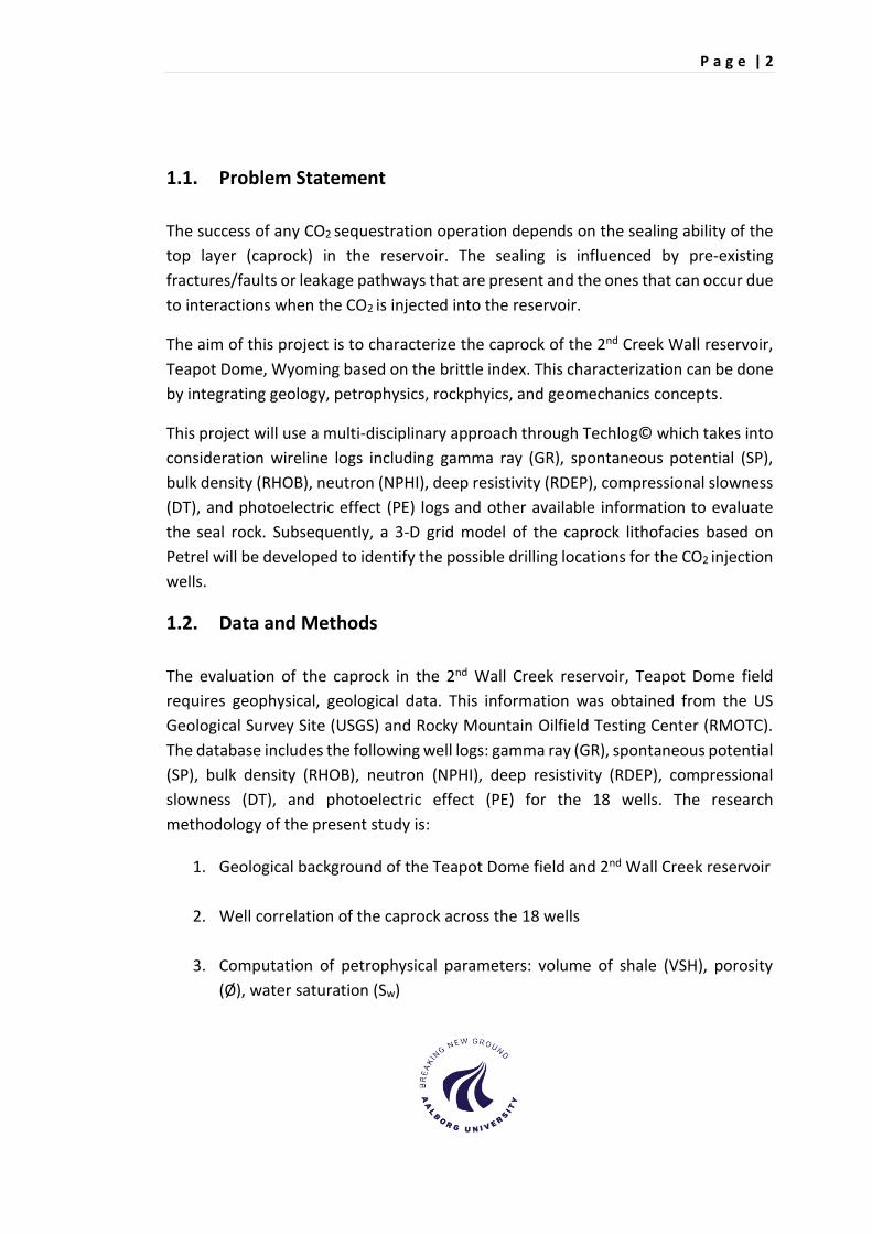
Figure 7 shows the location of the seismic lines in a depth structure map of the 2nd

Wall Creek reservoir for an NW-SE Cross-section of the Teapot Dome. As can be

noticed, the S2 fault network is highly complex both in geometry and azimuths.

Figure 7 – Depth-structure map of the 2nd Wall Creek sandstone (17)

3.2. Stratigraphy

Teapot Dome comprises stratigraphic units from Devonian to Upper Cretaceous

periods where there is an intercalation between permeable and porous formations

with impermeable rocks. It can be seen in the

Figure 8 that the oil producing formations are: Shannon Ss, Niobrara Shale, 2nd Wall

Creek, 3rd Wall Creek, Muddy Sandstone, Dakota, Lakota, and Tensleep. On the other

hand, the water-bearing formations are Sussex Ss, Carlisle Shale, 1st Wall Creek, Upper

Sundance, Crow Mountain, Madison and Undifferentiated. Those formations consist

of marine lacustrine carbonates, sandstones, shallow shelf siliciclastic that overlay a

granitic basement (17). The main productive zones are Shannon Formation, the 2nd

Wall Creek, and the Tensleep Sandstone Formation.

P a g e | 17

Figure 8 – Teapot Dome stratigraphic column (3)

PERIOD FORMATION LITHOLOGY THICKNESS [m] DEPTH [m] PRODUCTIVE

59

Sussex Ss 9

88 69

Shannon Ss 37 157

194

137

73 744

1st Wall Creek 49 817

75 866

2nd Wall Creek 20 940

53 960

3rd Wall Creek 2 1013

81 1015

70 1096

5 1166

41 1170

26 1212

3 1237

82 1241

Upper 29 1323

Lower 46 1352

Crow Mountain 24 1398

Alcova LS 6 1422

Red Peak 158 1428

Permian 98 1586

Pennsylvanian 98 1684

Mississippian 49 1782

Devonian 91 1830

Pre-Cambrian 2160

Steele Shale

Niobrara Shale

Carlisle Shale

Frontier

413

219

Sundance

Chungwater

Group

Goose Egg

Tensleep

Amsden

Madison

Granite

UndifferentiatedCambrian

Upper

Cretaceous

Mowry Shale

Muddy Sandstone

Thermopolis Shale

Dakota

Lakota

Morrison

Lower

Cretaceous

Jurassic

Triassic

OIL BEARING

WATER

POREFLUIDSHALE

SANDSTONE

LIMESTONE

GRANITE

LITHOLOGY

P a g e | 18

The principal objective of this project is to characterize the caprock of the 2nd Wall Creek Reservoir. Therefore, it is important to know the stratigraphy of the frontier formation which is presented as follows.

The Frontier formation is an important oil-bearing zone in Wyoming. It has a series of sandstones, shales, sandy shales and several bentonite beds with a minimum amount of limestone. The total sandstone content varies from one place to another; being maximum (75-120 m) at the Teapot Dome Field (Powder River-Natrona area) (18).

The studies of Towse (1954) (18) divided the Frontier formation into four members: 1st, 2nd, and 3rd Wall Creek, and the Lower shale. Stratigraphic cross-sections were made to determine correlation criteria. For this purpose, rotary cuttings and electric logs of available wells were analyzed.

Figure 9 shows the cross section from Casper to Sage Spring Creek presented by Towse (1954) to exemplify the different units and lithology expected to be found in the Teapot Dome Field.

Figure 9 – Frontier formation cross section (18)

P a g e | 19

3.3. Lithology

Several studies show that the sandstones of the Frontier are relatively quartzose or cherty with minor amounts of other minerals (feldspar, biotite, and muscovite). The sand grains in the rock can be rounded or angular; being clay the cementing material. Concerning texture, the sandstones vary from fine to coarse and conglomeratic (18). Merewether (1917) (19) describes the sandstones in this formation as light-medium to brownish gray with grains that vary from the base to the top. In the base, the grains are very fine grained and horizontally bedded, and in the top, they are fine grained and crossbedded.

Towse (1954), describes the shales presented in the Frontier formation as soft, gray and sandy; being slightly calcareous or bentonitic in some parts of the formation. He also states that in the top of the formation, the sandy shales are thin bedded and better cemented that the ones in the lower shale unit. There are several beds of bentonite that contains siltstone concentrations, where the lowest part of the shale unit is the most bentonitic of the formation (18).

As follows it is described the lithological characteristics of the different units in the Frontier formation found by various authors (18) (19) (20).

The sand of the 1st Wall Creek is fine grained with diameters between 0.10 to 0.13 [mm]. The overall sorting is fair with coefficients between 1.2 to 1.4. There are important amounts of pink and crystalline quartz in the sand unit. The lower part contains limestone concentrations; being bentonite the bottom boundary of the member.

The 2nd Wall Creek in the Frontier Formation is the second largest hydrocarbon

bearing zone at the Teapot Dome Field even though it is relatively thin (20 m). The

sandstones are medium grained with average diameters of 0.09 to 0.22 mm (18). The

sorting is usually poor with coefficients between 1.20 and 1.40. This sandstone unit is

massively bedded, fairly quartzose and its composition is homogeneous (20). Besides,

the sandstones are less shaley than in the 3rd Wall Creek. The overlying cap rock of

this member is 75 m thick. It is considered as the primary regional seal within the

Power River Basin; trapping more than 57 million oil barrels and 45 billion of standard

cubic feet (scf) of natural gas at the Teapot Dome (3). It has similar characteristics to

the Brent Group in the North Sea regarding connectivity, reservoir geometry and

relative permeability (19). Since there is not a clear description for lithology and

P a g e | 20

mineralogy for the caprock of the 2nd Wall Creek due to the lack of information, it will

be determined by using a four-point mineral model in the subsequent chapters.

The 3rd Wall Creek member is separated from the 2nd Wall Creek based on their

sandstone mineralogy, where the top boundary has been placed at a bentonite and

gypsum bed. It comprises a series of sandy shales and sandstones with few

conglomerates.

P a g e | 21

CHAPTER IV. PETROPHYSICAL EVALUATION

The investigation of petrophysical parameters such as the volume of shale, porosity

and water saturation is necessary in order to characterize the caprock of the 2nd Wall

Creek reservoir. In this chapter, a comprehensive petrophysical approach was carried

out over the zone of interest. Well logging analyses of the given wells were used to

determine the petrophysical parameters by using Techlog© (wellbore platform).

4.1. Data Analysis

The available data for the 2nd Wall Creek reservoir consists of 18 wells. Most of the

wells have the traditional well log data, caliper (CALR), gamma ray (GR), bulk density

(RHOB), compressional slowness (DT), deep resistivity (RDEP), shallow resistivity

(RFOC), medium resistivity (RILM), neutron porosity (NPHI) and photoelectric

absorption (PE), which can be used in the petrophysical analysis. Those well logs

passed through a quality check before any calculation in Techlog©. The primary logs

used for the petrophysical analysis in this project are presented in Table 2. Not all the

wells have the basic logs required for the study such as the well 12-AX-33. The

Table 2 – Well logs summary

Index Well DEPT GR RHOB DT RDEP NPHI PE

1 11-DX-26 X X X X X X

2 12-AX-33 X X X X X

3 14-LX-28 X X X X X

4 28-AX-27 X X X X X

5 28-AX-34 X X X X X

6 34-TX-3 X X X X X

7 36-11-SX-2 X X X X

8 36-MX-10 X X X X X X

9 41-2-X-3 X X X X X X

10 41-AX-3 X X X X X X

11 53-LX-3 X X X X X X

12 62-TpX-10 X X X X X

13 64-JX-15 X X X X X

P a g e | 22

Index Well DEPT GR RHOB DT RDEP NPHI PE

14 67-1-TpX-10 X X X X X X X

15 71-1-X-4 X X X X

16 75-AX-28 X X X X X X

17 88-AX-28 X X X X X

18 88-DX-3 X X X X X X

log Count 18 18 15 18 18 8 2

Considering that the Frontier formation properties do not change severely from one

site to another within the Teapot Dome and the wells are relatively close to each

other, the missing logs (bulk density (RHOB), neutron porosity (NPHI), photoelectric

absorption (PE)) can be interpolated from the existed well logs. This procedure was

done through well prediction tool in Techlog©.

Figure 10 shows the position of the wells in a field map. This map is based on the

longitude and latitude of each well. It can be observed that the majority of the wells

are concentrated in the center to the north of the study area while there is only one

well in the southern part of the field.

Figure 10 – Location of the wells in the Teapot Dome field

P a g e | 23

4.2. Well Correlation Study

Well correlation is a process where two or more geological formations spatially

separated are equated. The main correlation methods are marker bed, pattern

matching, and slice techniques. The marker bed is a reliable method where series of

beds can be used as a marker although the lithology or origins are unknown. The

pattern matching involves the recognition of distinctive log patterns that are

correlated based on log shapes. It indicates lateral facies, thickness changes; making

it useful for facies correlations. The slice technique, on the other hand, subdivides the

interval arbitrarily which gives wrong relationship. It is only used when the other

methods do not yield results (21).

The well correlation study in this project is done by using a market bed technique

where gamma ray log indicates different marker beds within the 2nd Wall Creek. This

is because every well without exception have a gamma ray log. The gamma ray log is

used because it gives an indication of lithology. The amount of clay, minerals,

carbonate and organic matter, vary slightly at the same stratigraphic level but changes

abruptly through time which is ideal for well correlation because the gamma ray value

is constant laterally but changes vertically (22).

The well correlation in the 2nd Wall Creek formation was done along with all the wells

which can be found in APPENDIX 2. This correlation provides detailed information on

the lateral extent of the units in the formation which is important both for the

petrophysical analysis and caprock integrity assessment. It can be observed in Figure

11, the correlation of 5 wells from left to right (11-DX-26, 12-AX-33, 14-LX-28, 28-AX-

27, 28-AX-34). In this example, there are two main units in the formation which are

represented in blue (caprock) and yellow (reservoir). The 2nd Wall Creek formation in

the first well (11-DX-26) is located approximately 221 m below the second well (12-

AX-33). The position of the formation in the other wells does not change as it can be

observed in Figure 11.

P a g e | 24

Figure 11 – Well correlation in the 2nd Wall Creek formation

Table 3 gives a summary of the thickness of both caprock and reservoir for each well.

The average thickness of the caprock is 85 m and 19 m for the reservoir. Those values

are similar to the ones showed in the stratigraphic column of the Teapot Dome

obtained from the Rocky Mountain Oilfield Testing Center (RMOTC). The minimum

thickness value for the caprock in the 2nd Wall Creek reservoir is 68.66 m and the

P a g e | 25

maximum 114.01 m. Even though the minimum thickness of the caprock is 67.48 m,

the 2nd Wall Creek reservoir is still acceptable for CO2 geological storage.

Table 3 – Thickness summary for the 2nd Wall Creek formation

Well Caprock Reservoir

[m] [m]

11-DX-26 86.78 16.81

12-AX-33 84.80 16.76

14-LX-28 88.06 13.77

28-AX-27 83.23 17.57

28-AX-34 113.32 18.35

34-TX-3 80.44 19.10

36-11-SX-2 73.20 14.28

36-MX-10 75.06 16.56

41-2-X-3 112.53 19.56

41-AX-3 74.61 22.14

53-LX-3 114.01 18.34

62-TpX-10 67.48 22.16

64-JX-15 70.30 19.35

67-1-TpX-10 68.66 20.99

71-1-X-4 104.73 20.84

75-AX-28 71.45 18.34

88-AX-28 81.23 18.36

88-DX-3 81.23 20.99

Average 85 19

Min value 67.48 13.77

Max value 114.01 22.16

4.3. Petrophysical Analysis

Qualitative and quantitative analyses were carried out over the caprock of the 2nd

Wall Creek formation to describe its petrophysical properties. The interpretation was

made through analyses of the well log data by a probabilistic approach to determine

the volume of shale, porosity, fluid saturation, and lithology. For a better

understanding of those parameters, several histograms are presented for each case.

P a g e | 26

The input data for the petrophysical analysis were obtained from the available logs

for each well described in Table 2.

4.3.1. Volume of shale

The volume of shale expresses the shale percentage contained in the formation. It is

useful to determine if there is a different lithology than shale in caprock. Gamma ray

log is used for the computation of the shale volume because the shale is more

radioactive than the sandstone or carbonates. The calculation is based on the Eq. 2

which is implemented in Techlog©.

𝑉𝑠ℎ =𝐺𝑅 − 𝐺𝑅min

𝐺𝑅max − 𝐺𝑅min Eq. 2

Where GR, is the value read at particular depth; GRmax is the value read in 100% shale,

and GRmin corresponds to 100% matrix rock (22). In Figure 12, GR min represents

GR_Matrix, and GR max is GR_Shale. For the well 11-DX-26, a baseline of 75 API was

chosen for sand, and a baseline of 105 API was chosen for the shale. The same

procedure was repeated for the 18 wells.

P a g e | 27

Figure 12 – Determination of GR_Matrix and GR_Shale

The computation of the volume of shale for 5 wells from left to right (28-AX-27, 36-

MX-10, 67-1-TpX-10, 11-DX-26, 12-AX-33) is presented in Figure 13. This is an

exemplification of the pattern found across the wells in 2nd Wall Creek reservoir. The

shale is represented with the green color, and the yellow color shows other lithology.

It can be noticed that the volume of shale is bigger at the caprock bottom than at the

top. This result is similar to the one presented by Towse (1954). He described the shale

unit in the 2nd Wall Creek reservoir as sandy shale with sandstone streaks (18). The

distribution of volume of shale for the 18 wells can be found in APPENDIX 3

GR_matrix 75

GR_Shale 105

P a g e | 28

Figure 13 – Computation of shale volume (Vsh) for the wells: 28-AX-27, 36-MX-10, 67-1-TpX-10, 11-

DX-26, 12-AX-33

Figure 14 shows a histogram of the volume of shale with an accumulative frequencies

line for the 18 wells that penetrates the 2nd Wall Creek reservoir. It can be observed

that the histogram is not normally distributed. The minimum volume of shale is 0 v/v;

corresponding to sandy streak and the maximum is 1 v/v which represents pure shale.

The average value for the 18 wells in the zone of interest is 0.8388 v/v. This means

that 84% of the caprock is shale and the 16% is another lithology.

P a g e | 29

Figure 14 – Shale Volume histogram for all the wells

P a g e | 30

4.3.2. Porosity Calculation

The porosity represents the fraction of the rock filled with fluids. It can be determined

from laboratory measurements or well logs; being neutron porosity (NPHI), bulk

density (RHOB) and sonic (DT) the logs used for the calculation. There are two types

of porosity: total and effective. The total porosity is the ratio of the total pore volume

to the bulk volume. On the other hand, the effective porosity is the total porosity

minus the fraction of the pore volume occupied by shale or clay. In the present study,

both total and effective porosity are analyzed. Neutron and bulk density log

combination is used for the calculation.

Porosity calculation using neutron-density log combination

The neutron log (NPHI) measures the hydrogen index and therefore responds to the

volume of water that fills the pore space. It gives an indication of porosity which is

display directly in the log. Porosity can also be found by using the bulk density log

(RHOB). The equation that links together porosity and density is:

∅𝑑 =𝜌𝑚𝑎𝑡𝑟𝑖𝑥 − 𝜌𝑏

𝜌𝑚𝑎𝑡𝑟𝑖𝑥 − 𝜌𝑓𝑙𝑢𝑖𝑑 Eq. 3

Where ∅d is the total porosity in the caprock, the ρmatrix, g/cm3, is the matrix density

in the formation and ρ_fluid, g/cm3, is the fluid density in the wellbore and ρb, g/cm3

is the value read in the log. The input parameters in Techlog© are ρmatrix and ρfluid.

The combination of both neutron-density logs is used to determine the porosity

without being affected by lithology. In this method, the values of apparent neutron

and density porosities are averaged. In this way, the effects of dolomite and quartz

tend to cancel out. It is also employed a square root to eliminate the effects of residual

gas in the flushed zone (23). The total porosity is estimated by the Eq. 4 where ∅n and

∅d are the neutron and density porosities, respectively. This equation is implemented

in Techlog©.

∅ = √

∅𝑛2 + ∅𝑑

2

2

Eq. 4

P a g e | 31

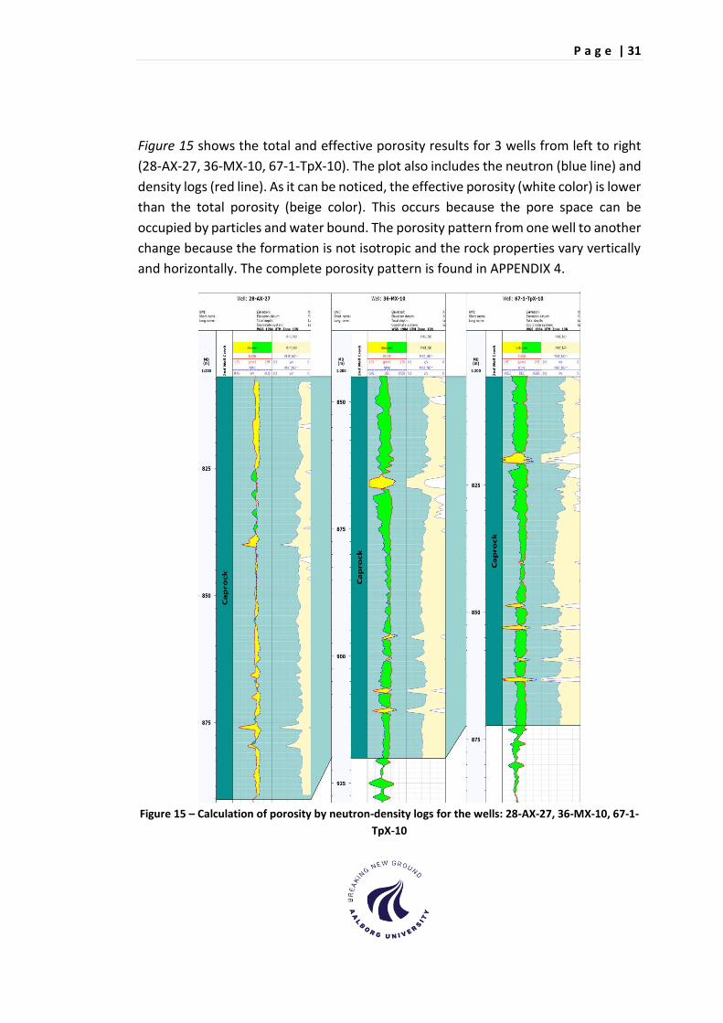
Figure 15 shows the total and effective porosity results for 3 wells from left to right

(28-AX-27, 36-MX-10, 67-1-TpX-10). The plot also includes the neutron (blue line) and

density logs (red line). As it can be noticed, the effective porosity (white color) is lower

than the total porosity (beige color). This occurs because the pore space can be

occupied by particles and water bound. The porosity pattern from one well to another

change because the formation is not isotropic and the rock properties vary vertically

and horizontally. The complete porosity pattern is found in APPENDIX 4.

Figure 15 – Calculation of porosity by neutron-density logs for the wells: 28-AX-27, 36-MX-10, 67-1-

TpX-10

P a g e | 32

The obtained results from the total and effective porosity are presented in the Figure

16 Figure 17. The total porosity histogram is moderately asymmetrical with a kurtosis

of 4.7 and a skewness of 1.51. The peak of the data is between 0.085 and 0.095 v/v;

meaning that the total porosity values are mostly concentrated in this range. Also, it

can be seen that the minimum value for the total porosity is 0.04612 v/v, the

maximum is 0.5207 v/v, and the average is 0.1270 v/v.

The effective porosity histogram (Figure 17) corresponds to a matrix histogram plot

with cumulative frequency. The effective porosity value ranges between 0-0.10 v/v

which is within the range suggested by the literature (22). As it can be noticed, the

histograms in most of the wells are left skew, and the peak of the data is concentrated

in 0 v/v. Consequently, the effective porosity in the caprock is negligible.

P a g e | 33

Figure 16 – Histogram of total porosity

P a g e | 34

Figure 17 – Matrix histogram for effective porosity

P a g e | 35

4.3.3. Fluid Saturation

The water saturation is calculated through Archie’s equation (Eq. 5) which is part of

the typical petrophysical workflow in Techlog©. It is important to highlight that this

calculation was performed since it is an input for the lithology estimation.

𝑆𝑤 = (𝑎 𝑅𝑤

∅𝑚𝑅𝑡)

𝑛

Eq. 5

Where Sw is the water saturation, a is the tortuosity factor in the zone of interest, Rw

is the formation water resistivity, Ø is porosity, m is the cementation factor, Rt is the

formation resistivity, and n is the saturation exponent.

The calculation of Sw requires as an input data, the formation resistivity which

corresponds to deep resistivity log and the porosity that was calculated previously.

The parameters of cementation factor, saturation exponent and tortuosity were set

as default; being the values 2, 2, 1 respectively. In order to get meaningful results, the

value of Rw was set between 0.14 and 0.18 ohm.m.

Figure 18 shows the distribution of the water saturation for 3 wells from left to right

(36-MX-10, 67-1-TpX-10, 11-DX-26,) along with the resistivity and total porosity logs.

The reading values from the resistivity log (blue dashed line) are in the range from 1

to 5 ohm.m, which corresponds to a conductive fluid. As a consequence, the bearing

fluid in the pore space is water. The calculated water saturation log, displayed in blue,

shows that the value of Sw is more than 80 v/v. This result was expected because the

shale in the caprock does not contain any hydrocarbons. APPENDIX 5 shows the

distribution of water saturation across the 18 wells.

P a g e | 36

Figure 18 – Distribution of water saturation across the wells in the caprock

4.3.4. Lithology estimation

The well log data can be used to inferred or determine the lithology, mainly speaking

the mineralogy. Cross-plots, two-dimensional representations of the log response of

different mineralogies, are the primary tool to evaluate the mineralogical

composition. The crossplots: RHomaa (apparent grain density) vs. Umaa (matrix

apparent volumetric photoelectric factor) and RHOmaa vs. DTmaa (matrix apparent

compressional slowness) are used in the present project since they predict complex

lithologies. It was observed in the volume of shale calculation that the caprock is

mainly composed of shale but also includes another type of lithology. Therefore, the

aim of this section is to estimate the mineral content of that percentage of the caprock

that is not shale.

P a g e | 37

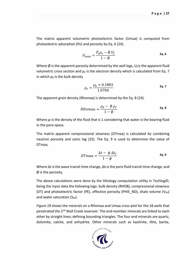
The matrix apparent volumetric photoelectric factor (Umaa) is computed from

photoelectric adsorption (Pe) and porosity by Eq. 6 (24).

𝑈𝑚𝑎𝑎 =𝑃𝑒𝜌𝑒 − ∅ 𝑈𝑓

1 − ∅ Eq. 6

Where Ø is the apparent porosity determined by the well logs, Uf is the apparent fluid

volumetric cross section and ρe is the electron density which is calculated from Eq. 7

in which ρb is the bulk density

𝜌𝑒 =𝜌𝑏 + 0.1883

1.0704 Eq. 7

The apparent grain density (Rhomaa) is determined by the Eq. 8 (24).

𝑅𝐻𝑜𝑚𝑎𝑎 =𝜌𝑏 − ∅ 𝜌𝑓

1 − ∅ Eq. 8

Where ρf is the density of the fluid that is 1 considering that water is the bearing fluid

in the pore space.

The matrix apparent compressional slowness (DTmaa) is calculated by combining

neutron porosity and sonic log (25). The Eq. 9 is used to determine the value of

DTmaa.

𝐷𝑇𝑚𝑎𝑎 =∆𝑡 − 𝜙 ∆𝑡𝑓

1 − 𝜙 Eq. 9

Where Δt is the wave transit time change, Δtf is the pore fluid transit time change, and

Ø is the porosity.

The above calculations were done by the lithology computation utility in Techlog©;

being the input data the following logs: bulk density (RHOB), compressional slowness

(DT) and photoelectric factor (PE), effective porosity (PHIE_ND), shale volume (VSH)

and water saturation (SW).

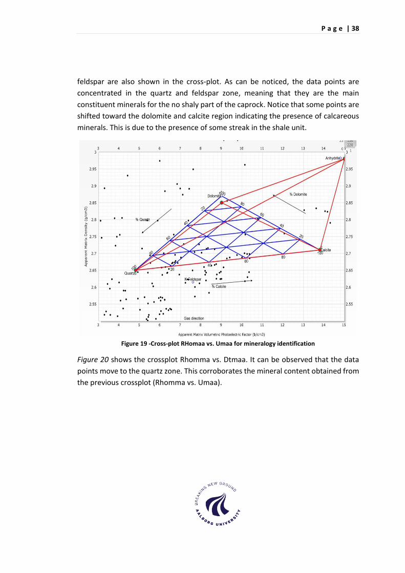
Figure 19 shows the minerals on a RHomaa and Umaa cross-plot for the 18 wells that

penetrated the 2nd Wall Creek reservoir. The end-member minerals are linked to each

other by straight lines; defining bounding triangles. The four end minerals are quartz,

dolomite, calcite, and anhydrite. Other minerals such as kaolinite, illite, barite,

P a g e | 38

feldspar are also shown in the cross-plot. As can be noticed, the data points are

concentrated in the quartz and feldspar zone, meaning that they are the main

constituent minerals for the no shaly part of the caprock. Notice that some points are

shifted toward the dolomite and calcite region indicating the presence of calcareous

minerals. This is due to the presence of some streak in the shale unit.

Figure 19 -Cross-plot RHomaa vs. Umaa for mineralogy identification

Figure 20 shows the crossplot Rhomma vs. Dtmaa. It can be observed that the data

points move to the quartz zone. This corroborates the mineral content obtained from

the previous crossplot (Rhomma vs. Umaa).

P a g e | 39

Figure 20 -Cross-plot RHomaa vs. DTmaa for mineralogy identification

A better illustration of the mineral content of the caprock is found in Figure 21 which

is the lithology log for the well 67-1-TpX-10. In this log is displayed the volume of shale

(VSH), quartz (VQTZ), clay (VCLC), dolomite (VDOL) and anhydrite (VANH). It can be

noticed that the caprock is mainly composed of shale which represents the 84% of the

total mineral content. The remaining 16% is consists of the other minerals. The

volume of dolomite for this well is higher than the other minerals. In order of

importance, the log shows that the unit has quartz, calcite, and anhydrite. The

mineralogy log for the 18 wells is found in APPENDIX 6.

P a g e | 40

Figure 21 - Mineralogy log for well 67-1-TpX-1

P a g e | 41

CHAPTER V. GEOPHYSICS

The geophysics allows linking geologic properties (porosity, volume of shale, water

saturation and lithology) with seismic properties such as acoustic impedance and

elastic modulus. This section covers an overview of the theory behind the main elastic

constants and the basic principles applied to calculated those properties based on the

well log data.

5.1. Overview

Poison’s ratio, Young’s modulus, shear modulus and bulk modulus should be taken

into account in order to characterize the caprock. These parameters can be

determined in static conditions from compressional tests or in dynamic conditions

from well log data. Table 4 shows the basic equations used in the determination of

those parameters.

Table 4 – Mechanical parameters

Stress Strain Poison’s ratio Young’s modulus

Shear modulus

Bulk modulus

𝜎 = 𝐹/A 𝜖 = ∆𝐿/L 𝑣 =ϵ𝑡𝑟𝑎𝑛𝑠

ϵ𝑎𝑥𝑖𝑎𝑙

𝐸 =𝜎

𝜖

𝐺 =𝑇

𝛾

𝐾 =∆𝑃

∆𝑉𝑉𝑜

⁄

σ: Stress F: Force A: Area

ϵ: Strain ΔL:

Longitudinal change

L: Longitude

𝑣: Poison’s ratio ϵtrans: Transverse

strain ϵaxial: Axial strain

E: Young’s modulus σ: Tensile

stress ϵ: Extensional

strain

Τ: Shear stress Υ: Shear strain

ΔP: Pressure change

ΔV: Volume change

Vo: Initial volume

In the present project, those parameters are determined by dynamic conditions

because of available well logs dataset.

P a g e | 42

5.2. Acoustic properties

The Techlog© toolbox function computes the formation acoustic properties:

compressional velocity (VP), acoustic impedance (AI) and compressional modulus (M).

The inputs for this method are compressional slowness (DT) and bulk density (RHOB)

which are part of the primary log data.

The compressional velocity (VP), expressed in m/s, is the propagation of

compressional principal waves (P-waves) in the medium which is longitudinal for

isotropic and homogeneous solids. As a consequence, the particles in the rock vibrate

parallel to the travel direction of the wave (26). It can be calculated by using the

compressional slowness log which is the travel time per feet (µs/ft). The Eq. 10 shows

the conversion between velocity and compressional slowness (27). In the equation,

DT is the compressional slowness in microseconds per foot.

𝑉𝑃 =106

𝐷𝑇 Eq. 10

The acoustic impedance (AI) is defined as the opposition that a rock presents to the

wave propagation. It is computed as the product of the compressional velocity (VP)

and the bulk density (ρb) which is expressed in MPa.s/m (Eq. 11) (27).

𝐴𝐼 = (𝜌𝑏)(𝑉𝑃) Eq. 11

Compressional modulus (M) also called P-wave modulus, or longitudinal modulus is

one of the elastic modules which is expressed in acoustic terms (Eq. 12). The unit of

this modulus is GPa (27).

𝑀 = (𝜌𝑏)(𝑉𝑃2) Eq. 12

Figure 22 shows the elastic properties along with the bulk density and compressional

slowness logs for the well 67-1-TpX-10. The compressional slowness for the shale in

the caprock is proximetely 70 to 120 µs/ft. Consequently, the range of compressional

velocity is low because it takes more time for the wave to travel a certain distance. As

can be observed in the compressional velocity log (magenta color), the velocity varies

between 2620 m/s and 4471 m/s which is in accordance with the values shown in the

literature for this type of lithology (1600 – 5000 m/s) (22). The acoustic impedance

P a g e | 43

and compressional modulus are directly proportional to the bulk density and

compressional velocity. It is noticed in the log that low values for acoustic impedance

and compressional modulus correspond to low bulk density values. If the density is

low, the pore space is higher, and therefore the sonic wave moves faster through the

medium. APPENDIX 7 contains the computed elastic properties for the 18 wells.

Figure 22 - Acoustic properties for well 67-1-TpX-10

The shear velocity (VS), expressed in Km/s, is the propagation of secondary waves (S-

waves) in the medium. In this case, the particles oscillate perpendicular to the travel

direction of the wave (26).

The shear velocity is computed in Techlog© through the lithology dependent

Greenberg- Castagna method. It gives empirical relations to estimate the shear

velocity based on the compressional velocity in multimineral, saturated brine rocks

where the composed minerals are calcite, dolomite, quartz, and shale. The shear

velocity is computed by the following equation which is used in Techlog© (Eq. 13)

𝑉𝑆 =1

2{[∑

𝑉𝑓𝑖

𝑎𝑖𝑉𝑃2 + 𝑏𝑖𝑉𝑃 + 𝑐𝑖

𝐿

𝑖=1

]

−1

+ ∑ 𝑉𝑓𝑖 (𝑎𝑖𝑉𝑃2 + 𝑏𝑖𝑉𝑃 + 𝑐𝑖)

𝐿

𝑖=1

} Eq. 13

P a g e | 44

Where L is the number of monomineralic lithology constituent, the coefficients ai

(quadratic), bi (linear) and ci are provided for each mineral, Vfi is the volume fractions

of lithological constituents.

Figure 23 shows the computed VS log for the well 67-1-TpX-10. The first track is the

mineral composition (calcite, dolomite, shale and quartz) assumed by the model.

Notice that those minerals match with the lithology estimation performed in the

previous section. The compressional velocity and modeled shear velocity are

displayed in the second and third track of the log. The shear velocity is a function of

the compressional velocity. This relationship can be seen in the log since the modeled

shear velocity follows the same trend as the compressional velocity. The complete

description of the shear velocity for all the wells can be found in APPENDIX 8.

Figure 23 – Shear velocity for the well 67-1-TpX-10

P a g e | 45

5.3. Dynamic Elastic Properties

The elastic properties measure the tendency of a rock to deform non-permanently

when the stress is applied. The elastic properties are: Poisson’s ratio (PR), Young’s

modulus (E), bulk modulus (K) and shear modulus (G)

The Poisson’s ratio (PR) is the relationship between the lateral strain to longitudinal

strain related to the elasticity of the material (28). In consequence, the static Poisson’s

ratio (VPVS) can be calculated as the ratio between the compressional and shear

velocities. The dynamic Poisson’s ratio (PR) can be found with the compressional and

shear velocities through the following equation (Eq. 14) in Techlog©.

𝑃𝑅 =1

2

(𝑉𝑃2 − 2 𝑉𝑆2)

(𝑉𝑃2 − 𝑉𝑆2) Eq. 14

In Figure 24 are displayed the output logs from VPVS and PR along with compressional

(VP) and shear velocities (VS) for the well 67-1-TpX-10. It can be seen that the trend

of both static and dinamic Poisson’s ratio logs is similar to the compressional and

shear velocities but with an opposite tendency. This is because the value of the

compressional velocity is higher than the value of the shear velocity; giving as a result

lower values for the Poisson’s ratio. The range of the static Poisson’s ratio has higher

values than the dynamic Poisson’s ratio. Schultz (1995) suggests that this occurs

because in the dynamic properties the effect of the pore fluid is not taking into

account and therefore the intrinsic static/dynamic differences are measured (29).

P a g e | 46

Figure 24 – Compressional to shear velocity ratio and dynamic Poison’s ratio for the well 67-1-TpX-

10

The Young’s modulus is the ratio between the longitudinal stresses to the longitudinal

strain of a material when there is no change in the orthogonal stress. The shear

modulus also called modulus of rigidity is the ratio of shear stress to shear strain (28).

Finally, the bulk modulus is the resistance of the material to isotropic volume change

when there is an isometric compression.

The Dynamic elastic properties (Young’s modulus, shear modulus and bulk modulus)

are calculated in Techlog© based on the Sonic Model in which the relationship

between the sonic logs and the dynamic properties is considered.

The dynamic shear modulus (G_DYN), and bulk modulus (K_DYN) are computed in

Techlog© by the following equations (Eq. 15 and Eq. 16) assuming a homogenous,

isotropic and elastic formation.

P a g e | 47

𝐺𝑑𝑦𝑛 = (13474.45)𝜌𝑏

(∆𝑡𝑠ℎ𝑒𝑎𝑟)2 Eq. 15

𝐾𝑑𝑦𝑛 = (13474.45)𝜌𝑏 [1

(∆𝑡𝑐𝑜𝑚𝑝)2] −

4

3 𝐺𝑑𝑦𝑛 Eq. 16

Where ρb is the bulk density in g/cm3, Δtcomp is the bulk formation compressional

slowness in us/ft, Δtshear is the bulk formation shear slowness in us/ft. Note that

13474.45 is a conversion coefficient.

Once both dynamic shear and bulk modulus are determined, the Dynamic Young’s

Modulus is computed by Eq. 17.

𝐸𝑑𝑦𝑛 =9𝐺𝑑𝑦𝑛 (𝐾𝑑𝑦𝑛)

𝐺𝑑𝑦𝑛 + 3𝐾𝑑𝑦𝑛 Eq. 17

The distribution of the dynamic elastic properties is presented in Table 5. The

histograms for the analyzed elastic properties have a leptokurtic distribution because

the points along the X-axis are cluster; giving, as a result a higher peak (kurtosis). The

distribution of those properties is asymmetric. In the case of Young’s modulus, shear

modulus, and bulk modulus, the distribution is left-skewed because the majority of

data points are concentrated on the right side. It can also be seen that the mean value

for those properties is lower than the median; showing that the distribution is in fact

left skewed. The literature shows that the typical values for shales in the case of

Young’s modulus is 1-70 GPa (30). The Young’s modulus histogram ranges between

the values suggested by the literature; indicating that the rock with low Young’s

modulus has a lower resistance to be deformed and with high values, the rock is

stiffer. The range of bulk modulus according to the literature is between 6.4 to 21.6

GPa

P a g e | 48

Table 5 – Statistical parameters of dynamic properties for the caprock of the 2nd Wall Creek reservoir and histograms made for Young modulus, shear modulus, bulk modulus and Poisson’s

ratio

Elastic Properties

Range of Value

Statistic Parameters

Histogram

Young modulus (E_DYN)

[GPa]

Min: 1.94 Max: 123.67

Mean: 28.198 Median: 28.64 Mode: 29.86

Shear modulus (G_DYN)

[GPa]

Min: 0.67 Max: 49.38

Mean: 11.029 Median: 11.19 Mode: 11.57

Bulk modulus (K_DYN)

[GPa]

Min: 5.84 Max: 90.29

Mean: 21.492 Median: 21.57 Mode: 21.989

P a g e | 49

CHAPTER VI. GEOMECHANICS

The investigation of the rock mechanical properties allows evaluating the forces

acting on the caprock matrix. This is relevant in order to ensure the caprock integrity

during and after the CO2 injection. This chapter analyzes the in-situ stresses and the

caprock strength regarding unconfined compressive strength and tensile strength.

6.1. Overview

The determination of the rock deformation process is based on the relationship

between stress and strain (28)

The Stress () is the force applied to a rock that tries to change its original dimensions;

thus, it is the concentration of a force per unit area. The principal stresses that act on

the rocks are tensile, compression and shear stress. The tensile stress (tension) is the

resistance of the material against being pulling apart by forces. This leads to the

elongation of the rock in the direction where the forces are applied. On the other

hand, the compression stress tries to compact the material by forces directed toward

each other in the same direction; thus, the material is shortening. Finally, the shear

stress is the product of external forces applied in parallel and opposite direction on

different planes. Figure 25 represents those stresses.

Figure 25 – Type of stresses (31)

P a g e | 50

The strain is the change of the rock original dimension as a result of the stresses

applied to it. It is measured by the ratio of change in dimensions to the initial ones.

The stress-strain relationship is usually plotted on the stress vs. strain curve which is

unique for each material (Figure 26). Under low values of stress, elastic region, the

rock dimensions change. However, the dimensions are recovered when the stress is

removed. If the rock matrix is beyond the yield point, plastic region, the original rock

dimensions are deformed permanently from its original characteristics. (28)

Figure 26– Stress-strain curve (32)

Depending on the relative behavior under stress, the rock matrix is classified in two

categories: brittle or ductile. Those two classifications have different stress vs strain

curves as can be seen in Figure 27. The brittle material has low or not plastic

deformation until it reaches the brittle failure (B). On the other hand, the ductile rock

has a clear plastic behavior where it is deformed before the ductile failure (B’).

Consequently, the ductile rocks can absorb large energy amount before failure than

the brittle rocks. (33)

Figure 27 – Stress-strain curve for ductile and brittle rocks

P a g e | 51

6.2. In-Situ Stress

The principal in-situ stresses in the caprock are overburden stress or vertical stress

(σV) and pore pressure (Pp) (34). Different equations and approximations are used to

calculate the principal stresses in the caprock.

6.2.1. Overburden Stress

The overburden stress, also called vertical stress, is the pressure applied by the

overlying sediments weight per unit of area. In order to compute the overburden

stress is important to know the density of the overlying formations (35). Techlog©

extrapolates the density up to the mud line by using the Eq. 18 to have an estimation

of the density of the intervals where the log is not available.

𝜌𝑒𝑥𝑡𝑟𝑎𝑝𝑜𝑙𝑎𝑡𝑒𝑑 = 𝜌𝑚𝑢𝑑𝑙𝑖𝑛𝑒 + 𝐴𝑜(𝑇𝑉𝐷 − 𝐴𝑖𝑟𝐺𝑎𝑝 − 𝑊𝑎𝑡𝑒𝑟𝐷𝑒𝑝𝑡ℎ)𝑎 Eq. 18

Where ρmudline is the mud density at the ground level, Ao and α are fitting parameters,

and TVD is the truth vertical depth. The values used for the calculation are 1.65 g/cm3

of the mud density, 0 m for both AirGap and WaterDepth. Note that those values were

set as defaults in Techlog©.

The overburden stress is calculated with Eq. 19. Where ρextrapolated is density that was

extrapolated previously, σv is the overburden stress, TVD is the true vertical depth,

and z is the depth.

𝜎𝑣 = ∫ 𝜌𝑒𝑥𝑡𝑟𝑎𝑝𝑜𝑙𝑎𝑡𝑒𝑑(𝑧)𝑑𝑧𝑇𝑉𝐷

0

Eq. 19

Figure 28 shows the overburden stress (SVERTIVAL_EXT), vertical stress gradient

equivalent (OBMW_EXT), extrapolated bulk density (DEN_EXTRAPOLATED) and bulk

density (RHOB). The blue line corresponding to DEN_EXTRAPOLATED was interactively

adjusted by changing the position of the points in both density and depth axes in order

to get more accurate results. It can be seen that the overburden stress trend is linear

and is increasing with depth because the geostatic load increased likewise.

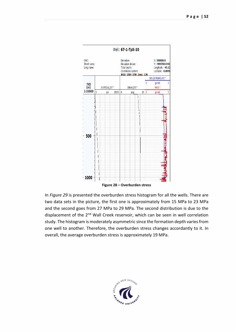
P a g e | 52

Figure 28 – Overburden stress

In Figure 29 is presented the overburden stress histogram for all the wells. There are

two data sets in the picture, the first one is approximately from 15 MPa to 23 MPa

and the second goes from 27 MPa to 29 MPa. The second distribution is due to the

displacement of the 2nd Wall Creek reservoir, which can be seen in well correlation

study. The histogram is moderately asymmetric since the formation depth varies from

one well to another. Therefore, the overburden stress changes accordantly to it. In

overall, the average overburden stress is approximately 19 MPa.

P a g e | 53

Figure 29 – Overburden stress histogram

6.2.2. Pore Pressure

The pore pressure is the fluid’s pressure inside the pore space, and it is given by the

hydrostatic pressure of the overlying formation water (36).

In the case of shales, the prediction of the pore pressure is based on different vertical

effective stress approaches: Eaton, Bowers, and Traugott. Those methods use the

Terzaghi's law which states that pore pressure is a function of the overburden stress

(total stress) and the effective vertical stress (36). The pore pressure method used in

this study is the Eaton since it is widely used for shales.

The Eaton method uses the resistivity and compressional slowness log to estimate the

pore pressure.

The pore pressure computed by resistivity (Pp_R) is based on the following equation

(Eq. 20)

𝑃𝑝_𝑅 = 𝜎𝑣 − (𝜎𝑣 − 𝑃𝑝𝑛𝑜𝑟𝑚) (𝑎) (𝑅

𝑅𝑛𝑜𝑟𝑚)

𝑛

Eq. 20

P a g e | 54

Where σv is the vertical stress, R is a value from the resistivity log, Ro is the initial

sediments resistivity, Rnorm is a measurement value assuming that formation is

frequently pressured, Ppnorm is the normal pore pressure, a and n are fitting

parameters which are set by default as a=1 and n=3

Notice that the Ppnorm and Rnorm are calculated through Eq. 21 and Eq. 22. Where Po is

the pressure at sea floor, k is a constant gradient, and Z is depth measured from the

sea floor

𝑃𝑝𝑛𝑜𝑟𝑚 = 𝑃𝑜 + 𝑘𝑍 Eq. 21

𝑙𝑛𝑅𝑛𝑜𝑟𝑚 = 𝑙𝑛𝑅𝑜 + 𝑘𝑍 Eq. 22

The pore pressure is calculated through Eq. 23 when the compressional slowness log

(DT) is used instead. In this equation DT is value from the compressional slowness log,

DTo is the initial travel time, DTnorm is a measurement value assuming that formation

is normally pressured

𝑃𝑝_𝐷𝑇 = 𝜎𝑣 − (𝜎𝑣 − 𝑃𝑝𝑛𝑜𝑟𝑚) (𝑎) (𝐷𝑇

𝐷𝑇𝑛𝑜𝑟𝑚)

𝑛

Eq. 23

The values for the fitting parameters are a=1 and n=1.2. The Eq. 24 represents DTnorm

in this case.

𝑙𝑛𝐷𝑇𝑛𝑜𝑟𝑚 = 𝑙𝑛𝐷𝑇𝑜 + 𝑘𝑍 Eq. 24

Figure 30 shows the pore pressure calculation for the well 67-1-TpX-10. The second

and third track displays the compressional slowness and the resistivity log for this well.

The magenta color line represents the compaction trend which has been adjusted in

each case to give accurate results. The calculated pore pressure by using

compressional and resistivity logs is shown in the last track. As can be noticed, the

computed logs are close to each other; following a similar trend which is increasing

with depth. Note that the pore pressure is lower than the overburden pressure

because it only takes into account the overlying pore fluids (formation water) but not

the overlying sediments. The normalized value of pore pressure (Pp) is calculated

through the normalization of Pp_R and Pp_DT which in Techlog© the variable is called

P a g e | 55

PPRS_NORM displayed with a sky-blue line. APPENDIX 9 shows the pore pressure for

all the wells.

Figure 30 – Pore pressure calculation by using the Eton’s method

P a g e | 56

The pore pressure (Pp) histogram is similar to the overburden stress histogram since

there are 2 data sets which can be seen in Figure 31. This distribution occurs due to

the displacement of the 2nd Wall Creek reservoir and therefore the pore pressure

increases likewise. The caprock average pore pressure is 9 MPa; being the minimum

value approximately 8 MPa and the maximum around 13 MPa. The Pp gradient is

0.010 MPa/m (0.456 psi/ft); meaning that Pp in SG is 1.05.

Figure 31 – Pore pressure histogram

6.3. Rock Strength

The ability of the rock to resist the deformation induced by external forces is called

strength. It is affected by its mineralogical composition, external pressure and

temperature. Some minerals such as quartz, feldspars are very brittle while clay, mica

and calcite are more ductile. The temperature influences the rock strength because

at high temperatures the molecules can move freely and therefore the rock is more

ductile.

In this section, different equations are applied in order to find the unconfined

compressive strength (UCS) and tensile strength (TS) of the caprock (37).

P a g e | 57

6.3.1. Unconfined Compressive Strength

The unconfined compressive strength (UCS), also called uniaxial compressive

strength, measures the strength of a material (rock) which is stressed axially under

unconfined conditions (38).

The unconfined compressive strength of the caprock can be estimated from the

elastic properties calculated from the log data. It can be calculated through the Coates

and Denoo equation which is the most common for shales (Eq. 25).

𝑈𝐶𝑆 = 0.0866 (𝐸𝑑𝑦𝑛

𝐶𝑑𝑦𝑛) (0.008𝑉𝑠ℎ + 0.0045(1 − 𝑉𝑠ℎ)) Eq. 25

Where UCS is the unconfined compressive stress in MPa, Edyn is the dynamic Young’s

modulus in MPa, Kdyn is the dynamic bulk modulus in MPa and Cdyn is the dynamic bulk

compressibility which is expressed by the Eq. 26.

𝐶𝑑𝑦𝑛 =1

𝐾𝑑𝑦𝑛 Eq. 26

Figure 32 presents the elastic properties and the unconfined strength of the rock. The

first and second track presents Young’s modulus (E_DYN) in GPa and Poisson’s ratio.

The last track shows the caprock unconfined compressive strength in GPa. The

calculation results show that the trend of the UCS is similar to E_DYN but differs from

the Poisson’s ratio. The lithology type plays a major role in the unconfined

compressive stress because both density and porosity change depending on the

mineralogy. Xu, Hao, et al. (2016) show that UCS of a rock increases with the rock

density but decreases with the porosity.

P a g e | 58

Figure 32 – Unconfined compressive strength

Different authors related the unconfined compressive strength with the

compressional transit time (DT), Young’s modulus (E_DYN) and porosity (Ø) in order

to evaluate it (39) (40). UCS vs. DT and UCS vs. E_DYN crossplots are presented in the

Figure 33. Figure 33 a) shows that the UCS is negatively correlated with DT. In other

words, UCS is decreasing with increasing of compressional transit time. On the other

hand, it is observed a positive correlation between UCS and E_DYN because as E_DYN

increases, the UCS is increasing likewise (Figure 33 b).

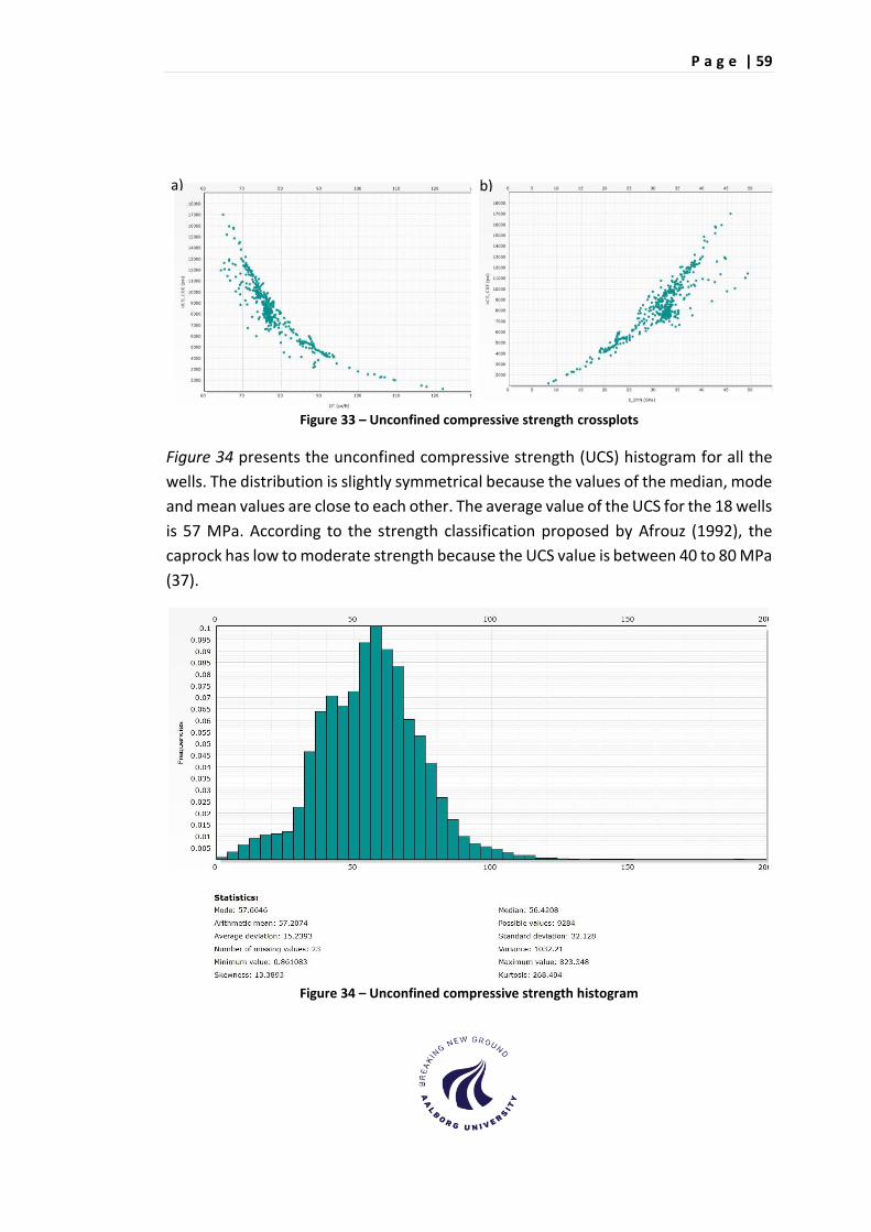
P a g e | 59

Figure 33 – Unconfined compressive strength crossplots

Figure 34 presents the unconfined compressive strength (UCS) histogram for all the

wells. The distribution is slightly symmetrical because the values of the median, mode

and mean values are close to each other. The average value of the UCS for the 18 wells

is 57 MPa. According to the strength classification proposed by Afrouz (1992), the

caprock has low to moderate strength because the UCS value is between 40 to 80 MPa

(37).

Figure 34 – Unconfined compressive strength histogram

a) b)

P a g e | 60

6.3.2. Tensile Strength

The tensile strength is the maximum load that a material can support without being

elongated which is opposed to the compressive strength (37). In order to calculate its

magnitude, it was used in Techlog© the Eq. 27.

𝑇𝑆 = 0.1(𝑈𝐶𝑆) Eq. 27

The tensile strength histogram is presented in Figure 35. The statistics show that the

average tensile strength is 5.7 MPa which is in the range suggested by the literature

(2-10 MPa) for shales. Notice that there are some outliers in the distribution such as

0.086 MPa (minimum value) and 82 MPa (maximum value) and therefore they should

not be considered.

Figure 35 –Tensile strength histogram

P a g e | 61

The presence of outliers for both UCS and TS can be noticed in the box plots shown in

Figure 36.

Figure 36 –Box plots for UCS and TS

According to Nygaard (2010), two modes controls the rock failure. The first one occurs

when the rock reaches the limit for tensile failure and the rock is pulled apart. The

second one is when the shear stress is above the critical level. Note that the tensile

strength is the critical limit for tensile failure, and unconfined compressive strength is

the limit for shear stress (41). Consequently, the caprock will fail in tensile, if the stress

is greater than 5.7 MPa (tensile strength) and will fail in shear if the stress is bigger

than 57 MPa (unconfined compressive strength).

P a g e | 62

CHAPTER VII. CAPROCK INTEGRITY

The caprock integrity is related to ductility and tendency of fracturing. Even though

the ductile rocks have a low strength, they are less likely to develop CO2 migration

pathways through fracturing (8).

In order to determine the caprock integrity of the 2nd Wall Creek reservoir, two

approaches are taken into account. The first one is a detailed understanding of the

ductility and brittleness of the caprock The dynamic elastic properties, Poison’s ratio

and Young’ modulus and the neural network analysis, IPSOM, in Techlog© are used

for this purpose. The second one is the brittleness index calculation using different

methods. This information is then correlated with the IPSOM results to give a final

indication of the caprock integrity.

7.1. Dynamic elastic properties analysis

According to Perez (2013), crossploting Young modulus (E_DYM) vs Poisson’s ratio

(PR) indicates the brittleness or ductility of the rock (33). The brittle rocks have a low

PR and moderate/high E_DYM and the ductile rocks have a high PR and low E_DYM.

A crossplot E_DYM vs PR for the well 67-1-TpX-10 was done in order to determine

qualitatively if the caprock is brittle or ductile. Note that this information was

retrieved from the previous section (Geophysics)

It can be seen in Figure 37 that there is a clear distinction between ductility and

brittleness for the shale unit. Notice that the concentration of points is higher in the

ductile part than in the brittle part. According to the color scale between green and

red, the GR is high which indicates ductility.

P a g e | 63

Figure 37 –Young’s modulus vs Poison’s ratio crossplot colored by gamma ray

Perez (2013) suggests that the zones with the high content of quartz and calcite are

more brittle than the zones with high clay content which are more ductile. Chao, D,

et al (2014) suggests that the quartz content lowers the Poisson’s ratio and increases

the Young’s modulus; representing that the rock is more easily fractured and also can

maintain a fracture. The presence of quartz and dolomite can be seen in the upper

part of the caprock; meaning that this zone is more likely to be brittle (Figure 38)

BRITTLE

DUCTILE

P a g e | 64

Figure 38 - Mineral content of the caprock in the well 67-1-TpX-10

P a g e | 65

7.2. IPSOM Classification

The caprock behavior subjected to stress is classified by using the neural network

analysis module in Techlog© called IPSOM (Index and Probability Generating a Self-

Organizing Map). This module is based on the Kohonen algorithm which learns the

neuronal network in one well and then applies it to the other wells.

IPSOM module uses the following logs in order to identify the characteristics of the

caprock: bulk density (RHOB), gamma ray (GR) and compressional slowness (DT). Also,

the volume of shale was taken into account in order to refine the IPSOM’s results.

Notice that the neutron log (NPHI) was not used because of redundancy with the sonic

log. Figure 39 indicates the variables employed in the neuronal analysis.

Figure 39 – Correlation of variables used for IPSOM classification

The well 67-TpX-10 is selected as a reference well for the neuronal network analysis

because it contains all the log data. The obtained model from this well is then applied

to the other wells. In IPSOM, the user can set the number of indexation depending on

the seeking classification. The crossplot Young Modulus (E_DYN) vs Poisson’s ratio

(PR) (Figure 37) shows that the caprock can be ductile or brittle. Therefore, it was

chosen an indexation of 2.

The IPSOM map classification for the caprock is shown in the Figure 40. In this

classification, there are two main regions, one displayed in sky-blue and the other one

in royal blue. Notice that the meaning of this classification is only known when the

results are compared with the dynamic elastic properties. However, it is assumed that

P a g e | 66

the royal blue region, which occupied the map majority, denotes ductility and the sky-

blue section represents brittleness.

Figure 40 – IPSOM classification using an indexation of 2

Table 6 contains the variables utilized in the IPSOM classification. The volume of shale

is the variable with the highest contribution because it gives more than 53% of the

information employed by the neuronal analysis. Gamma ray is the second variable

with 38% of the information, bulk density and shear slowness have approximately 3%.

Table 6 – Variable correlation and contribution

Variables Classification

1 Variable Correlation Information

2 Shale Volume 0.7774807 0.5381371

3 Gamma Ray 0.5603807 0.3878703

4 Bulk Density 0.05373505 0.03719298

5 Shear Slowness 0.05316667 0.03679957

Table 7 presents the statistics for the group 1 (ductile in royal-blue) and group 2

(brittle in sky-blue); showing the mean and variance for the input parameters (Gamma

ray, shear slowness, bulk density and shale volume). It can be noticed that the

difference of each group is considerable; meaning that IPSOM classification is

accurate.

P a g e | 67

Table 7 – IPSOM classification statistics

Name 1 2

Color

Variables Mean Variance Mean Variance

Gamma Ray 116.69 128.5293 91.5567 32.1725

Shear Slowness 147.5748 506.3431 137.3566 56.8426

Bulk Density 2.4919 0.0195 2.5557 0.0021

Shale Volume 0.9663 0.0042 0.5328 0.0292

Figure 41 shows the IPSOM classification results along with the dynamic elastic

properties and the mineral content of the caprock in the well 67-TpX-10. Comparing

the IPSOM results with the dynamic elastic properties, it can be inferred that the sky-

blue color sections represent brittleness because the Poisson’s ratio is low and the

Young modulus is moderate to high (the curves are deflected to the left side). The

royal blue color sections denote ductility since the Poisson’s ratio is high and the

Young’s modulus is low (the curves are deflected to the right). Also, notice that the

IPSOM classification matches with the mineral content of the rock since the sky-blue

sections are displayed in the regions where there is quartz/dolomite. The IPSOM

classification for the 18 wells is presented in APPENDIX 10.

Figure 41 - IPSOM classification results using an indexation of 2

P a g e | 68

Figure 42 a) presents a crossplot of E_DYN vs PR colored by IPSOM classification for

the well 67-1-TpX-10 and the Figure 42 b) shows a crossplot of E_DYN vs PR colored

by Gamma ray for the well 67-1-TpX-10. It is observed that the ductility group

according to the IPSOM classification matches with moderate to high GR values and

the brittle group corresponds to low GR values.

Figure 42 – a) Young’s modulus vs Poison’s ratio crossplot colored by IPSOM classification and b)

Young’s modulus vs Poison’s ratio crossplot colored by gamma ray

A pie chart for the IPSOM classification for the well 67-TpX-10 can be seen in Figure

43. According to this plot, 74% of the caprock is ductile (group 1) and 26% is brittle

(group 2). The pie charts for all the wells are presented in APPENDIX 11.

Figure 43 – IPSOM classification pie chart for the well 67-TpX-10

BRITTLE

DUCTILE DUCTILE

BRITTLE

P a g e | 69

Figure 44 is a pie chart for brittleness and ductility in the whole caprock. This chart

was done by summing up all the IPSOM classification values for all the wells. In

average the 74% of the caprock can be described as ductile and the remaining 26% as

brittle.

Figure 44 – IPSOM classification pie chart for all the wells

7.3. Brittleness Index

The Brittleness is the lack of ductility in tensile or shear stress which causes the

rupture or failure of a material with a small or no plastic behavior (33). Some of the

characteristics of brittleness are (42)

1. Low elongation/strain when a force is applied.

2. Fracture failure can be observed in the material surface such as cracks and

ruptures

3. Higher ratio of compressive strength to tensile strength

4. Higher v/v concentration of brittle minerals such as quartz, dolomite

compared to the ductile ones (clay).

5. Higher Young’s modulus and lower Poisson’s ratio values compared to their

average values.

The Brittleness index (BI) is used to quantify the brittleness of the rock matrix. It has

diverse expressions depending on the available data such as mineral composition or

in-situs stresses. Different equations can be used for each case (42). The BI calculation

P a g e | 70

for this project was done by various methods like Ingram and Urai (1999), Rickman, et

al. equation (2008), modified Wang and Gale equation (2009).

Ingram and Urai (1999) (BI_H) used the relationship between the estimated in-situ

unconfined compressive strength (UCS) and the unconfined compressive strength of

a consolidated rock (UCSNC) (8). The brittleness index calculated with this method is

presented in the Eq. 28.

𝐵𝐼_𝐻 =

UCS

UCS𝑁𝐶

Eq. 28

The unconfined compressive strength of a consolidated rock is equal to the effective

vertical stress which is calculated by Eq. 29. In this equation, Sv is the vertical stress

and Pp is the pore pressure.

UCS𝑁𝐶 = 𝑆𝑣 − 𝑃𝑃

Eq. 29

The BI computed by the Rickman’s equation (BI_R) (Eq. 30) is based on the dynamic

elastic properties (Young’s modulus and the Poisson’s ratio) which are related to the

stress and strain applied to the rock matrix. Qualitative analysis shows that rocks with

high Young’s modulus and low Poison’s ratio are potentially brittle. In addition, the

effect of both stresses and strains is established by the relationship between those

parameters (43).

𝐵𝐼_𝑅 =

1

2[

𝐸 − 𝐸𝑚𝑖𝑛

𝐸𝑚𝑎𝑥 − 𝐸𝑚𝑖𝑛+

𝑣𝑚𝑎𝑥 − 𝑣

𝑣𝑚𝑎𝑥 − 𝑣𝑚𝑖𝑛]

Eq. 30

The modified Wang and Gale’s method (44) (BI_M) is based on the mineral

composition of the rock. In this approach, the BI is calculated by dividing the

percentage of the most brittle minerals such as quartz and dolomite by the total

mineral composition (Eq. 31).

𝐵I_M =

𝑉𝑄𝑇𝑍 + 𝑉𝐷𝑂𝐿

𝑉𝑄𝑇𝑍 + 𝑉𝐶𝐿𝐶 + 𝑉𝐷𝑂𝐿 + 𝑉𝐴𝑁𝐻 + 𝑉𝑆𝐻

Eq. 31

P a g e | 71

The methods that were used to calculate BI are plotted beside the IPSOM

classification (Figure 45). Notice that each BI method gives different values at the

same point. This is because they are based on different rock properties. The modified

Wang and Gale’s brittleness index (BI_M) in blue line reflects that the zones with a

high concentration of quartz and dolomite are more brittle (high brittleness index)

than the sections in which those minerals are not present. This method is used to give

an indication/suggestion of the possible brittle zones. The Rickman’s brittleness index

log (BI_R) displayed with the red line and Ingram and Urai (BI_H) displayed with the

black line follows a similar trend; however, the values of BI_H are higher than BI_R.

This is because each method is based in different parameters. In APPENDIX 12 is

shown the brittleness index for all the wells

Figure 45 – Brittleness index comparison for the well 67-1-TpX-10

P a g e | 72

According to Perez (2013) (33), the most widely used methods for the brittleness

index calculation in shales are based on the mineral content, Young’s modulus and

Poisson ratio. Zhang, et al. (42) suggests that the Rickman’s method is more precise

in quantifying the rock brittleness index because it evaluates the mutual effect of

stresses and strains. In the (Figure 45) is observed that BI_R shows a positive response

when there is a high concentration of quartz and dolomite, and a moderate/lower

response when there is a high concentration of shale. On the contrary, the Ingram and

Urai index method (Bi_H) shows abnormal high brittleness values in zones where

there is a high concentration of shale (clay); being opposite to the expected behavior;

thus, this method is discarded for future evaluations. Moreover, the IPSOM

classification has a better correlation with BI_R than with the others. For example, the

IPSOM classification indicates that the sky-blue sections denote brittleness which is

confirmed by high values of BI_R (BI>4) and the royal-blue (ductility) has

moderate/lower values of BI_R (BI<4).

In conclusion, the BI_M indicates the brittle zones in the caprock and Rickman’s

brittleness index method (Bi_R) is used for its evaluation because it is more precise in

quantifying the brittleness of the rock. Note that this approach was not calibrated due

to the lack of laboratory results from mechanical tests.

7.3.1. Evaluation of Brittleness Index

Brittleness index and gamma ray crossplot is used to evaluate the brittleness index

(Lou et.al, 2016). For the present study, the brittleness index calculated through

Rickman’s equation is plotted against the volume of shale, VSH, which is shown in

Figure 46. Eq. 32 shows the correlation between those variables and it was obtained

from the regression line (blue line) added to the crossplot.

𝐵IR = −0.1795596(VSH) + 0.5119376

Eq. 32

P a g e | 73

Figure 46 – Brittleness index vs volume of shale for all the wells

The first track of the Figure 47 displays the mineral content of the caprock. The

following tracks shows the IPSOM classification, Rickman’s brittleness index and its

evaluation. It can be noticed that the brittleness index curve and the brittleness

evaluation curve follows a similar trend; fluctuating at the regions where there is a

high concentration of quartz and dolomite and lower shale volume. Therefore, the

BI_R is confirmed. In addition, it can be noticed that both IPSOM classification and

brittleness index evaluation match consistently with the mineral content. Therefore,

the Rickman’s brittleness index and IPSOM classification can be used for the modeling

of the caprock integrity.

P a g e | 74

Figure 47 – Final result of brittleness index

P a g e | 75

CHAPTER VIII. CAPROCK MODELING

When assessing the caprock integrity, the numerical modeling plays a crucial role

since it gives a reasonable understanding of its behavior in the whole area. Two types

of modeling are carried out in Petrel (Schlumberger modeling platform) based on the

obtained results in the previous chapters. The first one corresponds to facies modeling

in which the discrete attributes derived from the IPSOM classification are populated

into the grid cells. Then, this model is used to constrain the petrophysical modeling in

which the continuous property, brittleness index (BI_R), is simulated in the caprock.

The ultimate goal of this section is to develop a robust model to represent the most

suitable areas for CO2 storage and CO2 injection wells in the Teapot Dome Field.

8.1. Data and Methods

The caprock brittleness and ductility of the 2nd Wall Creek reservoir were modeled by

using the Schlumberger modeling platform, Petrel. The information imported to build

the models consists of the data retrieved from Techlog© such as well tops, IPSOM

classification and the Rickman’s brittle index. Besides, it was included the available

seismic and topography information for the Teapot Dome field. The flowchart

presented in Figure 48 shows the methodology carried out in the present section.

Figure 48 – Modeling flowchart for the simulation

P a g e | 77

8.2. Surface Model

The gridded surface and zone layering were done in Petrel. The caprock gridded

surface was done by using the conformal gridding method in which the wanted

surface is confined by 2 horizons (seismic top and seismic base) as can be observed in

Figure 49. Notice that a suitable surface can be created based on the seismic data.

Figure 49 – Conformal gridding example

The Teapot Dome seismic data has a good resolution only at deeper depths; meaning

that there are not good seismic horizons between the wanted surface. Figure 50 a) on

the left side shows that the seismic data between the caprock limits (blue lines) is

insufficient. Figure 50 b) indicates the maximum seismic magnitude that can be

extracted from the top shale and top reservoir. The purple region in this map, which

covers the majority of the area, represents the lack of information and the blue

sections detonate the available seismic data in the zone. As can be seen, the available

seismic data around the 2nd Wall Creek reservoir cannot be used for making the

surface

Figure 50 – Available seismic data for Teapot Dome field

a) b)

P a g e | 78

Since the seismic data at the upper parts of the Teapot Dome field could not be used,

the regional topography was employed as the top horizon and the deeper seismic

(better resolution) as the bottom horizon. Figure 51 represents the conformal grid

obtained between the topography surface and the deep seismic surface.

Figure 51 – Available seismic data for Teapot Dome field

The final conformal grid was built by adding the caprock zone tops and bases for all

the wells. The layering to dive the caprock was 100; meaning that the average

thickness of each layer is 0.8 m which give a good resolution as can be observed in

Figure 52. Notice that the reservoir is displayed in green color with just one layer

because it is no part of the present study.

P a g e | 79

Figure 52 – Conformal 3D grid

8.3. Facies Modeling

The facies modeling is the interpolation of the discrete data in the grid cells (45). This

kind of simulation is usually done to build a superior model.

The facies modeling of the present study is based on the Sequential Indicator

Simulation (SIS) which uses variograms and directional trends to create a stochastic

distribution of the property. The variograms and trends (major range, minor range

and vertical range) are adjusted to refine the data. This method is reasonable when

there is uncertainty in the shape of the subsurface body (caprock) (46), as it was

observed in the conformal gridding

In the facies analysis was used the Techlog© IPSOM classification data (ductile or

brittle) for the 18 wells. The first step in the modeling is upscaling the IPSOM

classification and then analyzing this qualitative property.

Figure 53 indicates the data distribution and the estimated facies proportion in each

layer of the model. The ductility is represented by the blue columns and brittleness

by the purple ones. The distribution of the estimated facies follows a similar trend

P a g e | 80

that was observed before in which the bottom of the caprock is more ductile than the

top which is more brittle.

Figure 53 – Estimated facies proportions percentage

It can be seen in Figure 54 that the estimated facies proportion data has a high

variance in each classification (rough distribution). Therefore, the data was smoothed

by adjusting the proportional curves (blue lines) in order to get a better distribution.

P a g e | 81

Figure 54 – Proportion curves for each facie (ductile and brittle)

After adjusting the proportional curves for each facie (ductile and brittle), the data is

analyzed to specify the variograms (description of a property variation). Major, minor

and vertical ranges were adjusted in order to specify the variograms that will be used

in the simulation. This process is presented in Figure 55. It is important to highlight

that the azimuth in the major direction was set as 330° because the anticlinal of the

Teapot Dome field is oriented NE/ SW approximately at 30°.

Vertical Direction

Major Direction

Minor Direction

Figure 55 – IPSOM variogram

P a g e | 82

Once the proportional curves and variograms were adjusted, the Sequential Indicator

Simulation (SIS) was used to model the facies (IPSOM classification) in the caprock.

The volumetric distribution of ductility (blue) and brittleness (purple) with the

location of some wells can be observed in Figure 56. This 3D grid shows the location

of the ductile and brittle regions. In overall, there are more ductile regions than brittle

regions in the Teapot Dome field.

Figure 56 – Facies volume height map

8.4. Petrophysical Modeling

For the petrophysical modeling, it was used a conditional simulation, series of

methods that simulates spatial and statistical characteristics. In this type of

simulation, a random function of multivariate Gaussian form is assumed to represent

the sample data, histograms and model variograms. In the simulation, each variable

is transformed beforehand into a normal distribution because the technique requires

a multi-Gaussian framework. Afterwards, the simulation results are back-transformed

to the raw distribution. This transformed data is used to represent the sample values

on a multivariate Gaussian function and to determine a probability function at each

unsampled location (47).

P a g e | 83

Gaussian Random Function Simulation (GRFS) was chosen to simulate the mechanical

strength of the caprock because it accurately reproduces the brittleness index

distribution. Moreover, it is faster and efficient because of its parallel algorithm which

is split into the Kriging base algorithm and the unconditional simulation that uses a

fast Fourier transformation which gives an excellent variogram reproduction (47).

Instead of simulating the brittleness index and the IPSOM classification separately,

the model was constrained to facies. This means that the IPSOM classification defines

variograms and data distribution coming from raw logs. In other words, the group 1

(ductility) and group 2 (brittleness) delimit the distribution upfront which will

resemble the final distribution.

The first step of the petrophysical modeling comprises the data analysis in which

variograms and property transformations are defined by constraining the brittleness

index with each IPSOM group.

Figure 57 shows the filtered data for vertical, major and minor direction for the group

1. It is observed that the points were adjusted in each case. Similar to the facies data

analysis, the azimuth of the major direction was set as 330o.

Vertical Direction

Major Direction

P a g e | 84

Minor Direction

Figure 57 – Vertical, Major and minor direction for group 1

The procedure done for the group 1 was repeated for the group 2 of the IPSOM

classification where the vertical, major and minor directions were adjusted and also

the azimuth was set as 30° for the major direction.

Vertical Direction

Major Direction

Minor Direction

Figure 58 – Vertical, Major and minor direction for group 2

The only information available for the simulation are the variograms, and property

transformation acquired previously. Usually, it would be preferred to model the

brittleness using elastic properties obtained from seismic inversion. However, the

P a g e | 85

seismic data of the 2nd Wall Creek reservoir has a weak resolution at a depth of

interest as can be seen in Figure 50.

Figure 59 shows the brittleness index distribution constrained to facies modeling

obtained from petrophysical simulation and also the distribution resulting from facies

modeling (purple color). Notice that the distribution in yellow color represents

ductility because the data was filtered with the IPSOM classification group 1 and the

distribution in pink color denotes the brittle classification. It can be seen that the

results obtained from the simulation are consistent since there is a distinction

between the group 1 (ductility) and group 2 (brittleness). In other words, the ductility

distribution is moved to the left side (low values of BI), and the brittleness distribution

is displaced to the right side (high BI values).

Figure 59 –Distribution of the modeled Brittleness index

Figure 60 presents a 3D volume height maps for the brittleness index filtered with the

IPSOM classification and the location of some of the wells that penetrate the 2nd Wall

Creek reservoir. It is important to highlight that Figure 60 a) was filtered with ductility

P a g e | 86

which has as thicker height column compared to Figure 60 b) which was filtered with

brittleness.

Figure 60 – Brittleness index volume height maps filtered with IPSOM classification

The average brittleness map can be found in Figure 61. In this map is represented the

average values of BI. It can be noticed that there are two patches. The first patch has

a high average BI (0.42); meaning that that region is highly brittle. The second patch,

the purple area, is considered ductile since presents the lowest average BI. Notice that

the zones with a BI< 0.4 have a good integrity.

Figure 61 – BI average thickness map

a) b)

P a g e | 87

8.5. Modeling Results

The results of the facies and petrophysical simulation are presented in the following

proportional maps in which there is a clear distinction between the ductile and brittle

zones in the caprock.

Figure 62 shows the ductility proportional thickness map and two reference wells, in

which the first track corresponds to the brittleness index in the grid and the second

track is related to the IPSOM classification. According to the color scale, the most

ductile regions in the field are the ones highlighted with yellow and orange color.

Those regions have a ductility percentage of 75% or higher. It is observed that those

areas can be found widely distributed in the field.

Figure 62 – Ductility proportional thickness map

P a g e | 88

The brittleness proportional map is found in Figure 63. According to this map, the

most brittle areas within the field are the ones colored with yellow and orange color

(75-90% brittleness). There are only 2 patches highly brittle in the caprock.

Figure 63 –Brittleness proportional thickness map

P a g e | 89

8.6. Drilling locations for the CO2 injection wells

The CO2 injection wells should be drilled in the areas where the caprock is highly

ductile and has sufficient thickness. This will ensure the seal potential and therefore

a long-term CO2 storage.

The possible location of the new injector wells is represented with some stars in

Figure 64. This map is based on the following relationship (Eq. 33), which relates the

facies model to the petrophysical model since the caprock ductility percentage

retrieved from the facies simulation (IPSOM classification group 1) and the average

brittleness index was computed by the petrophysical simulation.

𝐻𝑖𝑔ℎ𝑇ℎ𝑖𝑐𝑘𝑛𝑒𝑠𝑠_𝐿𝑜𝑤𝐵𝐼 =

𝐷𝑢𝑐𝑡𝑖𝑙𝑒

(𝐴𝑣𝑒𝑟𝑎𝑔𝑒 𝐵𝐼_𝑅)(100%)

Eq. 33

According to the color scale, the most suitable drilling locations for CO2 storage are

the areas displayed in green color, high values of the parameter HighThickness_LowBI,

because in those places, the ductility and thickness of the caprock are the highest

(Figure 64). On the other hand, the patches in red/orange color, low values of the

parameter HighThickness_LowBI, have small ductility and thickness and cannot be

considered for CO2 injection wells because the caprock is highly brittle which can

cause an earlier failure. The zones in which the parameter HighThickness_LowBI is

higher than 1.2, can be still considered for CO2 injection. It can also be observed that

the 18 wells are located in places where the caprock effectiveness is not compromised

(green areas), and therefore they can be used for CO2 injection into the 2nd Wall Creek

reservoir.

Figure 64 –Possible drilling locations for CO2 storage

P a g e | 91

CONCLUSIONS

The petrophysical results indicated that the caprock of the 2nd Wall Creek reservoir

could prevent the CO2 horizontal leakage since the average thickness of this unit is

approximately 85 m which is about 4.5 times thicker than the average reservoir height

(approximately 19 m). Therefore, the caprock is reasonable for CO2 storage even

though its minimum thickness is 67.48 m at some places.

The mineralogical evaluation showed that shale mainly composes the 84% of the

caprock and the remaining 16% corresponds to quartz, clay, dolomite and anhydrite.

It can be inferred that clay is the principal mineral in the caprock; being highly

concentrated at the base than at the top of the caprock as was presented in the Vsh

figures.

The geomechanical study indicated that the caprock pore pressure is 1.05 SG;

meaning that the horizontal stresses are lower and therefore faulting is less likely to

occur. It addition, the results showed that caprock strength is relatively low since the

unconfined compressive strength is 57 MPa and the tensile strength is 5.7 MPa

The dynamic elastic properties, Poison’s ratio and Young’s modulus, suggested that

the caprock is more ductile than brittle since the overall tendency of those parameters

is high Poison’s ratio and low Young’s modulus which corresponds to a ductile

behavior.

The IPSOM classification predicted that the group 1 represents the 74% of the caprock

and the group 2 the remaining 16%. By comparison with the dynamic elastic

properties (Poison’s ratio and Young’s modulus) is concluded that group 1 denotes

ductility and the group 2 indicates brittleness.

Different methods were used to calculate the brittleness index. However the most

accurate approach was the Richman’s method (BI_R) since it presented a good

correlation with the IPSOM classification and the mineralogic composition of caprock.

The BI_R showed low to moderate brittleness values in the ductile zones and high

values in the brittle ones.

The caprock integrity was simulated by using facies modeling and petrophysical

modeling. In the first one, the IPSOM classification groups (ductile and brittle) were

P a g e | 92

interpolated in the cells of the grid. The brittleness index was used in the petrophysical

modeling. Due to the lack of properties derived from seismic inversion, this model

was constrained to facies to get better results.

The average thickness map of brittleness index (BI) obtained from the petrophysical

modeling showed that the caprock is mainly ductile since there are only two patches

with a BI bigger than 0.4. in the full extension of the caprock. This result is confirmed

in the ductility proportional map in which can be clearly seen a high percentage of

ductility in the area. There are several zones with high thickness and low brittle index

which are the most appropriated for drilling the new wells for CO2 storage.

After the integrated petrophysical, geophysical and geomechanical analysis, it can be

concluded that the caprock has a satisfactory integrity due to its thickness and

reasonable ductility. Therefore, the 2nd Wall Creek reservoir can potentially be used

for CO2 storage.

P a g e | 93

FUTURE WORK

Future study will provide a better understanding in the caprock integrity of the 2nd

Wall Creek reservoir. Specific investigation efforts can include:

• Obtain geomechanical properties of the caprock based on cores or core plugs

from the Frontier formation and validate the results achieved with Techlog©

• Analyze leak-off tests (LOT) and fracture tests for geomechanical evaluation of

the caprock

• Rerun the caprock simulation using a seismic survey that has a good resolution

at the Frontier formation

• Use stochastic analysis to determine the sensitivity of the parameters,

brittleness index and IPSOM classification

• Assess the geomechanical impact of having a compartmentalized reservoir

• Conduct a critical stress fault analysis and fluid flow simulation to model the

CO2 migration.

• Evaluate the volumes of CO2 than can be injected into the reservoir without

compromising the caprock integrity

P a g e | 94

REFERENCES

1. Okojie, Anita. An Approach to Mapping of Shallow Petroleum Reservoirs Using Integrated

Conventional 3D and Shallow P- and SH-Wave Seismic Reflection Methods at Teapot Dome

Field in Casper, Wyoming. Provo : Bringham Young University, 2007.

2. Metz, Bert, et al. Carbon Dioxide Capture and Storage. New York : Cambridge University

Press, 2005. 13 978-0-521-68551-1.

3. Friedmann, Julio and Stamp, Vicki. Teapot Dome: Site Characterization of a CO2- Enhanced

Oil Recovery Site in Eastern Wyoming. Livermore : Lawrence Livermore National Laboratory,

2005.

4. Chiaramonte, Laura, et al. Fracture Characterization and Fluid Flow Simulation with

Geomechanical Constraints for a CO2- EOR and Sequestration Project Teapot Dome Oil Field,

Wyoming. s.l. : ELSEVIER, 2011.

5. Fleury, M, et al. Evaluating Sealing Efficiency of Caprocks for CO2 Storage: an Overview of

the Geocarbone-Integrity Program and Results. Malmaison : Institut Français du Pétrole,

2010.

6. Chantsalmaa, Dalkhaa. Caprock Integrity in CO2 Storage. Ankara : Middle East Technical

University, 2010.

7. Busch, A, et al. The Significance of Caprock Sealing INtegrity for CO2 Storage. New Orleans :

Society of Petroleum Engineers, 2010.

8. IEAGHG. Caprock Systems for CO2 Geological Storage. Cheltenham : International Energy

Agency, 2011.

9. Khan, S, et al. An Integrated Geomechanics Workflow for Caprock-Integrity Analysis of a

Potential Carbon Storage. New Orleans : Society of Petroleum Emgineers, 2010.

10. Downey, Marlan W. Evaluating seals for hydrocarbon accumulations. s.l. : The american

association of petroleum geologist, 1984. pp. 1752-1763.

11. Allen, Philip and Allen, Jhon. Data Analysis: Principles and Applications. Billiton : WILEY,

1990.

P a g e | 95

12. Niemi, Auili, Bear, Jacob and Bensabat, Jacob. Geological Storage of CO2 in Deep Saline

Formations. Dordrecht : Springer, 2017.

13. Chang, Yang. CO2 Sequestration and EOR Cooptimization in a Mature Field: TEAPOT

DOME, WYOMING. Ann Arbor : ProQuest LLC, 2014.

14. Fox, J., Dolton, G. and Clayton, J. Power River Basin. s.l. : US: Geological Society of

America, 1991.

15. Cooper, Scott, Laurel B, Goodwin and Lorenz, John. Fracture and fault patterns associated

with basement-cored anticlines: The example of Teapot Dome. Wyoming : AAPG, 2006.

16. Cooper, S. Deformation within a basement-cored anticline Teapot Dome. Wyoming : New

Mexico Institute of MIning and Technology, 2000.

17. Zhang, Ye, et al. An Uncertainty Analysis of Modeling Geologic Carbon Sequestration in a

Naturally Fractured Reservoir at Teapot Dome. Wyoming : University of Wyoming, 2014.

18. Towse, Donald. The Frontier Formation in the Southwest Power River Basin, Wyoming.

Massachusetts : Massachusetts Institute of Technology, 1951.

19. Merewether, E.A. Stratigraphy and Tectonic Implications of Upper Cretaceous Rocks in

the Powder River Basin, Northeastern Wyoming and Southeastern Montana. Denver :

U.S.Geological Survey Bulletin, 1917.

20. Lawrence, Anna. Geologic Assessment of Undiscovered Oil and Gas in the Powder River

Basin Province, Wyoming and Montana. Virginia : USGS, 2009.

21. Cant, Douglas. Subsurface Facies Analysis. Calgary : s.n., 2000.

22. Rider, Malcolm. The Geological Interpretation of Well Logs. Scotland : Rider-French

Consulting Ltd, 2000. 0-9541906-0-2.

23. Glover, Paul. Petrophysics Notes. Aberdeen : University of Aberdeen.

24. Rockhold, ML, Sullivan, EC and Murray, CJ. Data Assimilation Tools for CO2 Reservoir

Model DEvelopment- A Review of Key Data Types, Analyses, and Selected Software.

Springfield : Pacific Northwest National Laboratory, 2009.

25. Hallenburg, James. Standard Methods of Geophysical Formation Evaluation. New York :

Lewis Publishers, 1998.

P a g e | 96

26. Bery, Andy and Saad, Rosli. Correlation of Seismic P-Wave Velocities with Engineering

Parameters (N Value and Rock Quality) for Tropical Environmental Study. Penang :

International Journal of Geosciences, 2012.

27. Mavko, Gary, Mukerji, Tapan and Dvorkin, Jack. The Rock Physics Handbook. Edinburgh :

Cambridge University Press, 2009.

28. Dandekar, Abhijit Y. Petroleum Reservoir Rock and Fluid Properties. 2nd edition. s.l. :

Taylor & Francis Group, 2013.

29. Schultz, Richard. Rock Mechanics Proceeding of the 35th U.S. Symposium. Rotterdam :

University of Nevada, 1995.

30. Emujakporue, G and Ekine, A. Determination of Rocks Elastic constants from

Compressional and Shear Waves Velocities for Western Niger Delta, Nigeria. Nigeria : Journal

of Applied Sciences and Environmental Management, 2009.

31. Joo, Tat, Yang, Guilin and Ming, I. Compliant Manipulators. s.l. : Springer, 2014.

32. Perez, Roderick. Brittleness Estimation from Seismic Measurements in Unconventional

Reservoirs: Application to the Barnett Shale. Oklahoma : University of Oklahoma, 2013.

33. Zoback, M, et al. Determination of stress orientation and magnitude in deep wells.

California : PERGAMON, 2003.

34. Peng, Suping and Zhang, Jincai. Engineering Geology for Underground Rocks. Berlin :

Springer, 2007.

35. Zhang, Jincai. Pore Pressure Prediction from Well Logs: Methods, Modifications, and New

Approaches. Houston : ELSEVIER, 2011.

36. Afrouz, Andy. Rock Mass Classification Systems and Mode of Ground Failure. Boca Raton :

CRC Press, 1992.

37. Fox, Amy, et al. Geomechanical Principles for Unconventional Reservoirs. s.l. :

MicroSeismic, 2003.

38. Xu, Hao, et al. Characterization of Rock Mechanical Properties Using Lab Tests and

Numerical Interpretation Model of Well Logs. Chengdu : Hindawi Publishing Corporation,

2016.

P a g e | 97

39. Tove, Linn. Relating Acoustic Wave Velocities to Formation Mechanical Properties.

Trondheim : Norwegian University of Science and Technology, 2012.

40. Nygaard, Runar. Wabamun Area CO2 Sequestration Project. Calgary : Energy&

Environmental Systems, 2010.

41. Zhang, Decheng, Ranjith, P.G. and Perera, M. The Brittleness Indices Used in Rock

Mechanics and Their Application in Shale Hydraulic Fracturing: A Review. Australia : Journal

of Petroleum Science and Engineering, 2016.

42. Rickman, R, et al. A Practical Use of Shale Petrophysics for Stimulation Design

Optimization: All Shale Plays Are Not Clones of the Barnett Shale. s.l. : Society of Petroleum

Engineering, 2008.

43. Wang, F. and Gale, J. Screening criteria for shale-gas systems. s.l. : Gulf Coast As-sociation

of Geological Transactions, 2009.

44. Schlumberger. Glossary Oilfield. [Online] Schlumberger. [Cited: may 24, 2017.]

http://www.glossary.oilfield.slb.com/Terms/f/facies_modeling.aspx.

45. Deutsch, Clayton V. A Sequential Indicator Simulation Program for Categorical Variables

with Point and Block Data: BlockSIS. Alberta : Computer and Geosciences, 2006.

46. Ersoy, Adem, Yusuf, Tayfun and Atici, Umit. Geostatistical Conditional Simulation for the

Assessment of Contaminated Land by Abandoned Heavy Metal Mining. Nigde : Wiley

Periodicals, Inc, 2007.

47. Hyne, Norman J. Nontechnical Guide to petroleum geology, exploration, drilling &

production third edition. 3rd edition. s.l. : Pennwell, 2012.

48. Bassiouni, Zaki. Theory, Measurements, and Interpretation of Well Logs. Richardson :

Society of Petroleum Engineers, 1994.

49. Donnez, Pierre. Essentials of reservoir engineering Volume II. Paris : Technip, 2012. Vol. II.

50. Asquith, George and Krygowski, Daniel. Basic well log anlysis, second edition. 2nd edition.

s.l. : AAPG, 2004.

APPENDIXES

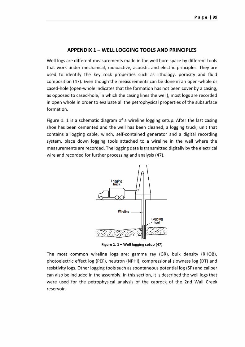
P a g e | 99

APPENDIX 1 – WELL LOGGING TOOLS AND PRINCIPLES

Well logs are different measurements made in the well bore space by different tools

that work under mechanical, radioactive, acoustic and electric principles. They are

used to identify the key rock properties such as lithology, porosity and fluid

composition (47). Even though the measurements can be done in an open-whole or

cased-hole (open-whole indicates that the formation has not been cover by a casing,

as opposed to cased-hole, in which the casing lines the well), most logs are recorded

in open whole in order to evaluate all the petrophysical properties of the subsurface

formation.

Figure 1. 1 is a schematic diagram of a wireline logging setup. After the last casing

shoe has been cemented and the well has been cleaned, a logging truck, unit that

contains a logging cable, winch, self-contained generator and a digital recording

system, place down logging tools attached to a wireline in the well where the

measurements are recorded. The logging data is transmitted digitally by the electrical

wire and recorded for further processing and analysis (47).

Figure 1. 1 – Well logging setup (47)

The most common wireline logs are: gamma ray (GR), bulk density (RHOB),

photoelectric effect log (PEF), neutron (NPHI), compressional slowness log (DT) and

resistivity logs. Other logging tools such as spontaneous potential log (SP) and caliper

can also be included in the assembly. In this section, it is described the well logs that

were used for the petrophysical analysis of the caprock of the 2nd Wall Creek

reservoir.

P a g e | 100

1.1. GAMMA RAY (GR)

The gamma ray tool uses a non-artificial radiation source to measure the natural

radioactivity of the formation since the rocks contain various amounts radioactive

minerals such as potassium, thorium and uranium. Those elements are concentrated

in shales because the surface of clay particles absorb them. On the other hand, the

amount of radioactive minerals in the shale-free sandstones and carbonates is small

because the chemical environment during the deposition of the sediments is not

favorable for the accumulation of radioactive minerals. Figure 1. 2 is an illustration of

the gamma ray log. It can be noticed that the response is higher in shales than

sandstones.

Figure 1. 2 – Gamma Ray response (47)

Principle

The gamma rays are electromagnetic waves emitted by some radioactive elements

such as potassium, potassium, thorium and uranium. The gamma rays scattered and

lose energy due to the following interactions: Compton scattering (energy lose

because of collision with atoms in the formation), photo electric effect (low-energy

gamma photon transfers all its energy to an inner orbital electron and as a

consequence the electron is ejected from the atom) and pair production (the photon

interacts with a nucleus and creates a positron, e+, and negatron, e-) (48).

The gamma ray sonde contains a detector with a scintillation crystal counter. It is used

to measure the natural radioactivity of the formation by a photomultiplier that

P a g e | 101

records the light produced by the gamma rays when they strike the scintillation. The

measurement unit is API and counts the amount of gamma ray striking the detector

in a period of time. (49) (50)

Use

Identify bed boundaries for stratigraphic correlations

Determine the shale content of the formation

Depth control

Identify radioactive deposits

1.2. BULK DENSITY LOG (RHOB)

The density logging tool records the formation’s bulk density which includes both

minerals forming the rock and fluids filling the pore space. It can be run into the well

alone or in combination with another tool such as neutron logging tool (NPHI) and

used as an indicator of primary porosity. This log has a shallow depth of investigation

so the tool is placed against the wellbore in order to record the density of the

formation (49). In Figure 1. 3 is represented that bulk density for different lithologies.

Figure 1. 3 – Bulk Density log (22)

Principle

The density logging tool uses a radioactive source such as Cesium-137 to emit

medium- high energy gamma rays to the formation. It scatters the attenuation of the

gamma rays between the source and detectors. This occurs because of the Compton

effect in which the gamma rays lose energy when they pass through the formation.

P a g e | 102

Therefore, the attenuation is a function of the number of electrons contained by the

formation which is related to its density. When the formation is denser, a few

detectable gamma rays reach the detector because the rock has more atoms per unit

of volume. Conversely, the scattering is higher in porous rocks (49) (50).

Use

Determination of porosity and lithology

Identification of mineral content in evaporites

Gas detection

Evaluation of complex lithologies such as shaly sands

Overpressure identification

Determination of hydrocarbons density

1.3. PHOTOELECTRIC FACTOR LOG (PEF)

This log records the effective photoelectric absorption index (PE) of the formation

which depends on the average atomic number of the elements that constitute the

formation. Figure 1. 4 indicates the response of the photoelectric factor log for

different lithologies, including shale, dolomite, limestone, sandstone (2).

Figure 1. 4 – Photoelectric Factor log (22)

P a g e | 103

Principle

The photoelectric factor logging tool measures the formation photoelectric

absorption index by using a radioactive source that emits gamma ray that collides with

the formation. The absorption depends on the average atomic number of the rock

matrix and it is not affected by the pore space (47).

Use

Evaluation of the lithology and composition of the formation

Matrix indicator

1.4. NEUTRON LOG (NPHI)

The neutron log is used to evaluate the formation’s porosity by measuring the

hydrogen index. In clean formations, the pore space is filled with hydrocarbons or

water; thus, it gives a real value of the pore space filled with fluids (47) (50). Figure 1.

5 shows the neutron porosity values for different lithologies.

Figure 1. 5 – Neutron log (22)

Principle

The neutron logging tool has a radioactive source that uses a mixture of americium

and beryllium to emit continuously high-speed neutrons to the formation. When the

neutrons collide elastically with particles that has the same mass (hydrogen nuclei),

there is significant energy loss. As a consequence, most of the neutrons lose velocity

P a g e | 104

and are captured within short time. On the other hand, if the neutrons collide with

heavy particles, there is not a significant velocity loss (inelastic scattering) and they

can travel further from the source before being captured. In this case, the lecture of

the logging tool is higher (47) (50).

Use

Determination of porosity directly from the log

Interpretation of lithology

Gas identification

Evaluation of clay content, shaliness in the rock

1.5. RESISTIVITY LOGS

The resistivity logging tool measures the formation’s resistivity (resistance of a

compound to the passage of the current) to identify the fluid type in the pore space.

Since the formation water is less resistive than the hydrocarbons, this log is used to

distinguish between zones bearing hydrocarbons and formation water. The resistivity

log for different lithologies is shown in Figure 1. 6. It can be seen that the reading

values in the sandstone unit are high which indicates that the main fluid in the pore

space is hydrocarbons.

Figure 1. 6 – Resistivity logs (22)

P a g e | 105

Principle

A localized electrical current is sent through the formation by some electrodes and is

measured the potential drop between other electrodes. The advantages of using

focused currents are: reduce the borehole effects and can be sent directly to the

required areas (22) (47)

Use

Define oil and water bearing zones

Estimation of the porosity

Calculation of water saturation

Formation correlation

Indication of lithology changes based on a resistivity map

1.6. COMPRESSIONAL SLOWNESS LOG (DT)

The compressional slowness log records the capacity of the formation to transmit

sound waves which is a function of porosity, lithology and rock texture. This is

expressed as interval transit time (Δt) and is measured in ft/sec. Figure 1. 7 indicates

the capacity of different lithologies to transmit the sound waves.

Figure 1. 7 –Compressional Slowness log (22)

Principle

The compressional slowness logging tool uses transducers and receivers to measure

the travel time that the sound wave takes to reach the receivers. The transducer,

P a g e | 106

which is piezoelectric, converts an electrical signal into an ultrasonic vibration that is

sent to the formation. The receivers, on the other hand, provide the logging signal by

converting the pressure waves into electromagnetic signals. The sound speed

depends on the type of rock. It is slow for shale, intermediate for sandstones and fast

for dolomite and limestone (47) (50).

Use

Lithology indicator

Porosity

Well correlation

Indication of fractures

Estimation of mechanical properties

Identify over-pressure

P a g e | 107

APPENDIX 2 – WELL CORRELATION

Figure 2. 1 – Correlation across the 18 wells that penetrates the 2nd Wall Creek Reservoir

P a g e | 108

APPENDIX 3 – SHALE VOLUME

Figure 3. 1 - Shale volume calculation for the wells from left to right: 28-AX-27, 36-MX-10, 67-1-TPX-10, 11-DX-26, 12-AX-33, 14-LX-28-WD, 28-AX-34, 34-TX-3,

36-11-SX-2

P a g e | 109

Figure 3. 2 - Shale volume calculation for the wells from left to right: 41-2-X-3, 41-AX-3, 53-LX-3, 62-TPX-10, 64-JX-15, 71-1-X-4, 75-AX-28, 88-AX-28, 88-DX-3

P a g e | 110

APPENDIX 4 – TOTAL AND EFFECTIVE POROSITY

Figure 4. 1- Total and effective porosity for the wells from left to right: 28-AX-27, 36-MX-10, 67-1-TPX-10, 11-DX-26, 12-AX-33, 14-LX-28-WD, 28-AX-34, 34-TX-3,

36-11-SX-

P a g e | 111

Figure 4. 2 - Total and effective porosity for the wells from left to right: 41-2-X-3, 41-AX-3, 53-LX-3, 62-TPX-10, 64-JX-15, 71-1-X-4, 75-AX-28, 88-AX-28, 88-DX-3

P a g e | 112

APPENDIX 5 – WATER SATURATION

Figure 5. 1 - Water saturation for the wells from left to right: 28-AX-27, 36-MX-10, 67-1-TPX-10, 11-DX-26, 12-AX-33, 14-LX-28-WD, 28-AX-34, 34-TX-3, 36-11-SX-2

P a g e | 113

Figure 5. 2 - Water saturation for the wells from left to right: 41-2-X-3, 41-AX-3, 53-LX-3, 62-TPX-10, 64-JX-15, 71-1-X-4, 75-AX-28, 88-AX-28, 88-DX-3

P a g e | 114

APPENDIX 6 – MINERALOGY

Figure 6. 1- Mineralogy for the wells from left to right: 28-AX-27, 36-MX-10, 67-1-TPX-10, 11-DX-26, 12-AX-33, 14-LX-28-WD, 28-AX-34, 34-TX-3, 36-11-SX-2

P a g e | 115

Figure 6. 2 - Mineralogy for the wells from left to right: 41-2-X-3, 41-AX-3, 53-LX-3, 62-TPX-10, 64-JX-15, 71-1-X-4, 75-AX-28, 88-AX-28, 88-DX-3

P a g e | 116

APPENDIX 7 – ACOUSTIC PROPERTIES

Figure 7. 1 - Acoustic Properties for the wells from left to right: 28-AX-27, 36-MX-10, 67-1-TPX-10, 11-DX-26, 12-AX-33, 14-LX-28-WD, 28-AX-34, 34-TX-3, 36-11-

SX-2

P a g e | 117

Figure 7. 2 - Acoustic Properties for the wells from left to right: 41-2-X-3, 41-AX-3, 53-LX-3, 62-TPX-10, 64-JX-15, 71-1-X-4, 75-AX-28, 88-AX-28, 88-DX-3

P a g e | 118

APPENDIX 8 – SHEAR VELOCITY

Figure 8. 1 - Shear velocity for the wells from left to right: 28-AX-27, 36-MX-10, 67-1-TPX-10, 11-DX-26, 12-AX-33, 14-LX-28-WD, 28-AX-34, 34-TX-3, 36-11-SX-2

P a g e | 119

Figure 8. 2 – Shear velocity for the wells from left to right: 41-2-X-3, 41-AX-3, 53-LX-3, 62-TPX-10, 64-JX-15, 71-1-X-4, 75-AX-28, 88-AX-28, 88-DX-3

P a g e | 120

APPENDIX 9 – PORE PRESSURE

Figure 9. 1 - Pore pressure for the wells from left to right: 11-DX-26, 12-AX-33,14-LX-28-WD, 28-AX-27,28-AX,34-TX-3

P a g e | 121

Figure 9. 2 - Pore pressure for the wells from left to right: 36-11-SX-2, 36-MX-10,41-2-X-3,41-AX-3,53-LX-3,62-TpX-10

P a g e | 122

Figure 9. 3 - Pore pressure for the wells from left to right: 64-JX-15, 67-1-TpX-10,71-1-X-4,75,AX-28,88-AX-28,88-DX-3

P a g e | 123

APPENDIX 10 – IPSOM RESULTS AND DYNAMIC ELASTIC PROPERTIES

Figure 10. 1 - IPSOM results and dynamic elastic properties for the wells from left to right: 28-AX-27, 36-MX-10, 67-1-TPX-10, 11-DX-26, 12-AX-33

P a g e | 124

Figure 10. 2 - IPSOM results and dynamic elastic properties for the wells from left to right: 14-LX-28-WD,28-AX-27,28-AX,34-TX-3, 41-2-X-3, 41-AX-3, 53-LX-3

P a g e | 125

Figure 10. 3 - IPSOM results and dynamic elastic properties for the wells from left to right: 62-TPX-10, 64-JX-15, 71-1-X-4, 75-AX-28, 88-AX-28, 88-DX-3

P a g e | 126

APPENDIX 11 – IPSOM PIE-CHARTS

Figure 11. 1 - Pie-charts for the wells from le - ft to right: 11-DX-26, 12-AX-33, 14-LX-28-WD, 28-AX-27, 28-AX, 34-TX-3

P a g e | 127

Figure 11. 2 - Pie-charts for the wells from left to right: 36-11-SX-2, 36-MX-10, 41-2-X-3,41-AX-3,53-LX-3,62-TpX-10

P a g e | 128

Figure 11. 3 - Pie-charts for the wells from left to right: 64-JX-15, 67-1-TpX-10,71-1-X-4,75-AX-28,88-AX-28,88-DX-3

P a g e | 129

APPENDIX 12 – BRITTLE INDEX

Figure 12. 1 – Brittle index for the wells from left to right: 28-AX-27, 28-AX-34, 11-DX-26

P a g e | 130

Figure 12. 2 – Brittle index for the wells from left to right: 36-MX-10, 67-1-TpX-10, 12-AX-33

P a g e | 131

Figure 12. 3 – Brittle index for the wells from left to right: 14-LX-28-WD, 34-TX-3, 36-11-SX-2

P a g e | 132

Figure 12. 4 – Brittle index for the wells from left to right:41-2-X-3,41-AX-3,53-LX-3

P a g e | 133

Figure 12. 5 – Brittle index for the wells from left to right: 62-TpX-10, 64-JX-15, 71-1-X-4

P a g e | 134

Figure 12. 6 – Brittle index for the wells from left to right: 75-AX-28,88-AX-28,88-DX-3