SEISMIC STUDIES ON THE DERBYSHIRE DOME

SEISMIC STUDIES ON THE

DERBYSHIRE DOME

DAVID EDWARD ROGERS

A Thesis submitted in fulfilment of the

requirements for the degree of

Doctor of Philosophy

Department of Earth Sciences

The University Leeds LS2 9JT

February 1983

PhD Thesis February 1983

SEISMIC STUDIES ON THE DERBYSHIRE DOME D. E. ROGERS Dept Earth Sciences

ABSTRACT

The Derbyshire Dome is thought to have been a stable uplifted area since at least Lower Carboniferous times. This project is principally concerned with four 30km seismic refraction lines which crossed the limestone outcrop of Derbyshire and N. Staffordshire in order to investigate the Dome's upper crustal structure, using quarry blasts as seismic sources.

A time-term analysis of refracted arrival data defined basement structure more complicated than implied by the surface geology. The interpretation of these data was complicated by high (5.6-5.8km/s) velocity refractions from dolomitic horizons within the limestone sequence; the mean overburden velocity was determined to be about 5.2 km/s. The Dome could be divided into two pre-Carboniferous geological units separated approximately by the line of the NNW trending Bonsall Fault. To the north a broadly domal refractor of velocity 5.5-5.55km/s was mapped, and thought to correlate with both the shallow pre- Carboniferous volcanics encountered by the Woo Dale borehole and"the Ordovician shales encountered by the Eyam borehole below 1.8km of limestone. This refractor accordingly deepens beneath the Carboniferous sedimentary basins flanking the Dome.

To the south of the Bonsall Fault zone, the Carbonifer- ous was found to be underlain by a refractor of velocity 5.63-5.7km/s, thought to be of Precambrian material similar to the rocks of Charnwood Forest, Leicestershire, some 40km south. By analysing later arrivals, this refractor has been mapped to the north of the Bonsall Fault at a depth of 2.5-3.5km. The shallower Lower Palaeozoic refractor is thought to be no more than 500m thick, and underlain by lower velocity, possibly Cambrian, material.

This interpretation is consistent with the Bouguer anomaly map of the region, and sheds light on the structural control of Carboniferous sedimentation. The basement fault dividing the two pre-Carboniferous units is thought to have been active during the Dinantian as the northern unit tilted eastwards.

ACKNOWLEDGEMENTS

It would be impossible to mention individually

everyone who helped with this project. I am most indebted

to my two supervisors, Drs. Graham Stuart and David Whitcombe,

for much encouragement and advice. I am particularly grate- ful to my colleague Andrew McDonald, with whom the brunt of the fieldwork was shared.

There are many to thank regarding the fieldwork:

particularly Dennis Flaxington, John Lawes and Ray Dickinson; from the Global Seismology Unit, IGS Edinburgh, Dr. Paul Burton, Bob McGonigle, and Bob Jones for help with the equip-

ment from the NERC Seismic Pool; from the University of Leicester, Drs. Peter Maguire and Aftab Khan for loan of the Geostore boxes and portable recording apparatus, and also the technical staff of the Department of Geology for help with the

controlled shot at Shirley. None of the work would have been

possible without the co-operation of the quarry managers and the farm owners of Derbyshire and Staffordshire, especially Mr. A. Moore of Fivewells Farm who put up with us for three

successive autumns.

For use of the digitising facilities at GSU Edinburgh, I would like to thank Dr. Chris Browitt and Charlie Fyfe. Many thanks are also due to Dave Johnson and staff of the University of Leeds Computing Service.

Miscellaneous thanks are due to: Dr. John Samson for

his hospitality in Edmonton, Canada; Drs. Roger Clark, Neil

Aitkinhead, J. Chisholm, Trevor Ford and Michael Leeder for

discussion on the geology and geophysics of the area; Sue

Nemes for making such a neat job of typing this thesis; and

also Dr. Doyle Watts, Pat Bermingham, Steve Brown, Dr. Jim

Mechie.

This research was supported by a NERC studentship.

To Felicity,

I couldn't have wished for

a more loving wife.

CONTENTS

CHAPTER ONE - Introduction and Geology

1.1 General Introduction . 1

1.2 Regional Geological Setting 3

1.2.1 Geology of the Dinantian Inlier 8

1.2.2 Deep Boreholes 12

1.2.3 Brief Structural History 16

1.3 Previous Geophysical Work 19

1.3.1 Related Seismic Work 19

1.3.2 Gravity Field 21 1.3.3 Magnetic Field 28

1.3.4 Electrical Sounding 31 1.4 Summary - Ideas of the Sub-Carboniferous basement 31

CHAPTER TWO - Theory

2.1 Introduction 35 2.1.1 General 35

2.2 The Time-Term Method - Introduction 38 2.2.1 The Time Term Method 40 2.2.2 Quality of the solution 45 2.2.3 Refractor with a Vertical Velocity

Gradient 47 2.3 The Effect of Structure on the Time-Term

Solution 48 2.3.1 Anticlinal Refractors - Model Studies 50

Raytracing 53

Model Travel Times - Discussion 54

Solving Model Time-Terms 67

Non-Iterated Solutions 68

Iterated Solutions 78

Conclusions 79 2.3.2 Reduced Time Plots 82

2.4 Amplitudes and Frequency Analysis of P waves 84 2.4.1 Amplitudes of P Waves 84 2.4.2 Frequency Analysis of P waves 86

Assessment of Polarisation Filters 87 Box 1 90 Box 2 93 Box 3 95

CHAPTER THREE - Data Collection

3.1 Introduction 97

3.2 The Method 97

3.2.1 Equipment 100

3.2.2 Design of Profiles 103

3.2.3 Deployment of line 106

3.2.4 Maintainance of the Experiment 108

3.2.5 Dismantling the Array - Calibrations 109

3.2.6 Quarry Blasts as Seismic Sources 109

3.3 Seismic Refraction Profiles Across the Derbyshire Dome 110

3.3.1 The North-South Profile 112

3.3.2 Stoney Middleton-Holmfirth Line 114

3.3.3 Northern East-West (NEW) Profile 116

3.3.4 Southern East-West (SEW) Profile 118 3.3.5 DASED1 and DASED2 120

CHAPTER FOUR - Data Processing

4.1 Introduction 122 4.2 The Data Set 122

4.3 Digital Processing 127 i) Time Corrections 129

ii) Reduced Time Sections 132 4.4 Picking Onset Times 133

4.4.1 Method 133 4.4.2 Time Measurement 137 4.4.3 Observational Error 139 4.4.4 Measurement of Relative Amplitudes 141

4.5 Location of Untimed Quarry Blasts 141 4.5.1 Method 142 4.5.2 Other Aids to Location 146

i) The Mansfield Events 147

ii) The Stoke-on-Trent Events 151 iii) The Flamborough Earthquakes 151

4.6 Global Earthquake Data 151

CHAPTER FIVE - Interpretation of the Data

5.1 Introduction 155

5.2 Display of data 155

5.3 Interpretation of the North-South Line 158

5.3.1 Timed and Positioned Shots 158

5.5.2 Discrimination of Basement Refractions 169

5.5.3 First Model and the Interpretation of Refracted Arrivals 179

5.4 Towards a North-South Section of the Derbyshire Dome 191

5.4.1 Testing the Refined Model 197

5.4.2 Later Arrivals from Quarry Blasts 204

5.4.3 Summary - General Observations 211

5.5 The Northern Province 213

5.5.1 Northern East-West (NEW) Line 214

i) Timed Events 214

ii) Northern Quarries 227

iii) Cauldon Events 234

5.5.2 Summary of Interpretation 234

5.5.3 DASED2 236

5.6 The Southern Province - Southern East-West (SEW) Line 241

5.6.1 Velocity Analysis - Shots close to the line 243

5.6.2 Shape of the Basement - Reduced Time Graphs 246

A. Broadside Events from the North 246

B. Quarries close to the line 251

5.6.3 Reduced Time Seismograms 252

5.6.4 Comments on Interpretation 256

5.7 General Notes 258

CHAPTER SIX - Time-Term Analysis


6.2 Application of Method 261

6.2.1 Quality Check of Solutions 264

6.2.2 Display of Data 264

6.3 Profiles Examined Individually 265

6.3.1 North-South Line 265

(a) Single Refractor 266

(b) North of the Bonsall Fault 269

(c) South of the Bonsall Fault 269

(d) Lower Basement Refractor, Whole Profile 272

6.3.2 General Remarks - North-South Line Solutions 274

6.3.2 Northern East-West Profile - Upper Basement Refractor 276

6.3.3 DASED2 - Upper Basement Refractor 280 6.3.4 Southern East-West Line - Lower Basement

Refractor 282 6.4 Multip le Profile Analyses 285

6.4.1 Lower Palaeozoic Refractor 285

6.4.2 Charnoid-Type Basement 291 Lower Basement Time-Terms for the Northern East-West Profile 294

6.5 General Comments on Solutions 297

CHAPTER SEVEN - Teleseismic Work, Gravity Modelling and General Conclusions


7.2 Teleseismic Work 300 7.2.1 Comparison with Midnet Stations 303

Previous Work 303

Analysis 305 General Remarks 308

7.2.2 Comparison of Stations on the Dome 311 7.3 Gravity Modelling 314

7.3.1 North-South Line 316 7.3.2 Northern East-West Line 318 7.3.3 Southern East-West Line 318 7.3.4 General Remarks 321

7.4 General Conclusions - Comments on the Structure of the Derbyshire Dome 321

References 327

Appendix A- Event Data 336

Appendix B- Polarisation Filtering 343

1

CHAPTER ONE

INTRODUCTION AND GEOLOGY

1.1 General Introduction

The Carboniferous limestone outcrop of Derbyshire and North-East Staffordshire, known as the White Peak district,

has been economically important since Roman times (Lewis, 1971),

originally for lead and zinc but more so during the last fifty

years for limestone aggregate and fluorite. Consequently, the

region has been of immense geological interest, at least for

the last two centuries, as Ford's (1967,1972) bibliographies

show.

It is generally agreed that this outcrop, known as the

Derbyshire Dome, represents a feature structurally positive

since at least Lower Carboniferous times, when it had a strong influence on carbonate sedimentation. However, there are differing theories regarding the structure of the Dome itself

and the nature of its sub-Dinantian basement: the Dome is one

of several 'blocks' which hardly subsided during much of the

Carboniferous, and which are thought to be underlain by

Caledonian granites (Kent 1974). Granite beneath the eastern

margin of the Dome is also thought to have caused the mineralisation of the limestone (Ford 1961, Evans and Maroof 1976),

although Ineson and Ford (1982) now doubt this. Basement of different character is suggested by the interpretations of the

LISPB (Bamford et al. 1978) and University of Leicester's

Charnwood-Ballidon line (Whitcombe and Maguire 1981b), which terminated to the north and south of the Dome (see Fig. 1.1)

and which respectively traced Lower Palaeozoic and Precambrian Charnian refractors to its flanks. Alternatively, the Dome is

an integral part of the Pennine Anticline, which George (1963)

considers tobe an entirely Tertiary feature, having had no effect on Carboniferous sedimentation.

2

FIG I-1 ý. I Sketch geological map of region showing

: dQ . .. seismic lines of project, LISPS a Leicester

Coal Measures ® L. Palaeozoic

Millstone Grit Pre-Cambrian Previous surveys "" r® Carboniferous , -'

ILI

S PB Limestone Present survey

ý , M:: .... ......... . Sheffield*. *. --:::: -

Macclesfield :. Buxton

f: ::; ä.. 5'"y^.

Stoke- ,

.... : =: ": :: _-::::. 350

AaE4o, we, 9,4d 400

Ashbourne

Shirley timed shot

\Charnwood- Ballidon profile

7, k i

/ Leicesterm

Birmingham

450

3001

3

The aim of this study is to investigate the upper crustal

structure of the Derbyshire Dome by seismic refraction techni-

ques, in order to differentiate between these various models. Quarry blasts have been used for seismic sources because they

provide a free and abundant source of seismic energy. Despite

the fact they are not ideal (because of irregular distribution

over an area, complex source signals, etc. ), quarry blasts have

been used several times in previous crustal refraction work: the West German Upper Mantle Project (Bamford 1976), in the

East Midlands (Whitcombe and Maguire 1980), and in South Wales (Bayerly and Brooks 1980). Additionally, the repetition of

observations from some quarries has allowed signal processing techniques to be investigated.

Four refraction profiles were established in three years'

successive field seasons to cover the Dome (Fig. 1.1): the first

ran north-south to link the LISPB and Charnwood-Ballidon profiles, the second and third profiles were deployed orthogonally to this first line: one each to the north and south of the

outcrop, and the fourth profile was established by McDonald (1982) at an angle of thirty degrees east of the first line.

1.2 Regional Geological Setting

The Derbyshire Dome is marked by an outcrop of Dinantian limestones at the southern axis of the Pennine Anticline (Fig.

1.1), and surrounded largely by Millstone Grit. The outcrop is characterised by low dips and gentle folding (George 1962)

and mainly comprises massive bedded limestones indicative

of clear, shallow water lagoonal conditions (Ford 1968). The

absence of strata older than Chadian is traditionally thought to signify a late marine transgression during the Carboniferous (Benison and Wright 1969), and the Dome is one of several areas marked by attenuated Dinantian successions (George 1963; Fig. 1.2).

As such, the Dome is thought to have been a stable, high feature since at least the Dinantian, when it formed part of a

4

O

C

N N v

vi

a

0 dý

K- (D c .40 NJ

; ßn9 loodiawp! M

C agy EE Co ýo

m 0

y6noJl puDiMOg

N cY

ýC u cp aý . am

4ßnOJl UO JgwnyIJoN Ch dew

4. -0 0

Ö dý

AaIIDA PUDIP! W

E 0 0

ä CL

C G

" O ` 0) d

Y "1- _ " O O C = O n C

s1C..

*ov * u, .co..

it CL

*** **+ III ' x *xx

xx"x xx xx*x

ýxx**x*xx x*xxx*

x* r

IL

" x* x*

xx *x*

-",., L IL

xxx*IL

x ** x It x

IL 'L ** xe

x x* -, ** x

x

11 1 -0 ý

it x x"

1x**x "

It x **x x x It xx xx x IL x x * x x x* x* x x*

. IL xx x *x*IL xx* *xx x ac 2 ýº

x rx sxx x * x* x* .. j7 ý

n

IL IL IL it L

L " '

IL It ,L lt it

1 "ý

t r

LL.

1 "°0 O 'D

1/

.ý M c0 m IL) a O d c,

I, 0 c

M60 W

N O

V O

d C

v

c v

0

w O c O 0 v

N

lL.

5

'block and basin' system controlling Carboniferous sedimentation (Falcon and Kent 1960; see Fig. 1.3). Leeder (1982) defines

three sedimentary environments: A) the Northern British

Caledonian molasse basins, whose location and subsidence were

controlled by Caledonian tectonics; B) a central region where

the blocks were stable remnants of the Caledonian landmass and

whose basins subsided through crustal stretching caused by the

Hercynian Orogeny; and C) the southerly Rheno-Hercynian back-arc

basin system. The Derbyshire Dome occurs within the type B

system of the 'Central Province' (Fig. 1.3), where blocks are

characterised by reef-flanked carbonate platforms and the basins

by deeper water mud-rich limestones and shales. Differential

subsidence continued into the Namurian, and the Millstone Grit

basins surrounding the Dome are thought to be underlain by

thick Dinantian successions (Kent 1966).

The Askrigg and Alston Blocks-on the northern margin of the Central Province are known to be underlain by pre-Carbonif-

erous granites (Bott 1967, Dunham 1974), and are bounded by

important fault systems which expedited the development of the surrounding basins (George 1958). No such fault system is

obvious on the perimeter of the Dome (Fig. 1.4), but the north-

west apron-reef complex is as well developed as that of the

Craven-Cracoe belt on the southern margin of the Askrigg Block

(Miller and Grayson 1982), and Kent (1974) supposes a similar

granite support to the Dome.

The Dome is also thought to be related to the Midlands

Barrier to the south, from which it forms a north-west facing

promontory (Owen 1976). This trend is the characteristic strike

of the Precambrian rocks of Charnwood Forest (Watts 1947;

Evans (1979) thinks the strike due to Caledonian deformation),

and underlies the structural fabric of the Dome and surrounding

area (Frost and Smart 1979). The north-western continuation

of a Precambrian basement is apparent from both the gravity (first noted by White (1948)) and magnetic maps of the region (see Section 1.3), although Evans and Maroof (1976) also postulate a north-north-western chain of buried Caledonian intrusions

related to the Leicestershire granodiorites.

6

FIG 1-3 Dinantion palaeogeography (from Owen(1976))

Non-depositional areas A- Highland Massif B- Southern Uplands C--Manx-Cumbrian Ridge D- Pennine Block

E- St. Georges Land F- Midlands Barrier

G- Cornubrian Massif H- Derbyshire Dome

Depositional areas I- Scottish Trough 2- Northumbrian Trough 3- Widmerpool Gulf

7

0 0

0 i, ý. `\ .J

4) d Q

LL J

D 0

J

0 0 CL cr w

0

w =s a1-

oc cý '° y'C 1:

m ö Co

LL, Zc

a C (D IC v

c_ *Z; rn Q Q .. ' Z 0d

LL I c x a (D jt 0 0) 4)

a m0

\W

U::

Na 1 to

O

i\ z cr-

C ä °-ö

0 , '- 0ö

o 4) mýý

ýý ýýý ,

JOB Aq,

ii ýzl 11 pJ ö

ýý , '4) d

am

8

1.2.1 Geology of the Dinantian Inlier

Three distinct sedimentary facies can be identified

within the limestone outcrop (Edwards and Trotter 1954; see

Fig. 1.5) :

a) Massif or Shelf: pale, well-bedded massive bioclastic

limestones with a coral-brachioped fauna; rarely argillaceous

and indicative of a clear, shallow water environment. There

are local examples of extremely shallow water conditions: viz

oolites, palaeokarst surfaces (Walkden 1974), (rare) current bedding and occasional non-sequence (Pigott 1965).

b) Basinal or Gulf: thin bedded limestones and shales with

a goniatite-bivalve fauna; representative of a deeper water,

mud rich environment.

c) Marginal or Gulf: well developed apron-reef complex which develops along the margin of the massif; dominantly shallow

water fauna, though goniatites present. There is invariably

a steep basinward dipping talus slope, although the difference

in depth between massif and basin may only be tens of metres (Stevenson and Gaunt, 1971). The classic example at Castleton

is well documented (e. g. Wolfenden 1958).

The main part of the outcrop comprises the massive bedded

limestones of the massif facies, yet south and south-west of the Dovedale Transition (Fig. 1.5) basinal facies of the

Widmerpool Gulf are encountered. These have been subsequently

more deformed than the massif succession, and coupled with rapid lateral facies changes and poor fossil representation are only

correlated with difficulty across the area (Parkinson 1950,

Prentice 1951, Parkinson and Ludford 1964)., The differing

nomenclature between massif and basinal regions is summarised in Table 1-1. Most of the exposed succession is Asbian and Brigantian, with older strata being exposed along the western

axis of the 'Dome'; on the massif these are of Holkerian age, but in Dovedale the Holkerian is largely missing and the

Asbian has been deposited directly on Arundian or Chadian (George

et al. 1976).

FIG 1-5 Sketch geological map 9

Dolomitised limestone (d) Ey=Eyam Limest. UM, LM Upper, Lower Millers Dale Lavas ML= Matlock Lovas -' Dovedale Transition (DT)

Triassic ® Brigantian ; "- Lavas Basinal

R

Coal Measures ®Asbian 7- ® Dolerite intrusions (D)

Q Millstone Grit ® Holkerian a Apron reef er ter Waulsortian reef (Rw) /Fault

400:. 410 1420 ....

1430 . ........ ............

D " ""380

.................... UM

",, UM '-D

. Boreholes0.

'"01 Woo Dale 2 Eyom

"3 Coldon Low " ,ýE"4 Gun Hill

._-., ", ........ 370 ... --II --"I Ev'(L

EY. -

....... Ey

.................

*4 .......... d

". 360 DT

d

............ DT 11

Rw

...... 350

10

4) 0

v

m

0 d ob

w 0 c 0 ob d

w 0 r t v 0 vb .Q

IV)

J-

C)

v H

v\

c w " ov C v M w w M" Nw O " M " JWD in O .+ Nv " c a º- .Ic N w WV L O Oºr v++o

W e z" Nu N ý+ EC -4 M 2 N! OD Ww w W co "E 01 O W+4 I- 2v O 2 " OJ AO 1- Z. 4 N !. O" C o! 3O

{ý N O W. 4 w 1-v o F. 4 000-4 O 1-10 EY O NVY N. 4 14'0 4 J D N" h4UC W" w W P E W'a -J-4 0 E D" EO

W £v L++ r4 E w" J J 2 2 JD O

J

0 N 1- E)-- 014.4 U" JN

N 4114 " . -1 J -4 " QM NN 41 .4w U YC Ja L {a 0O cr ui S. YO 2 W+'1 C WN6- L OZ O Uv C O L to A W OU 1 -0z -4 N0 J 41 2-4 WO 0 F-utL+1

0c . -/ 30 2N YDw Y £ -4 5 . -4 OWO 00 O M " n " E. +ODE

G ""lowM 13 J GM -I

10 4' " 7. O N In .4 SUM WW PY

""M Jz uw "

U2 PO O. OMLVC Ö1

y W JYL M nW D O4+ WY

t M4+ O O£ AV w 2 Id J S" 1O .S º+ O . -1 O" O" 41 J" Da D" 1. - ý W 1 7 -4 -4 Nw

WO" " .4 _ z 4.0 ` 0 .4L f i-s 0

N Fv "+, J CN in .4 w 3 1 W[ wC N WOO E

LL Mvv Z-4 RDM J0 r- C Ö 0 ý tý O " O F-. I

Ä

Z ID C NL 10 C J" o 0550 yý Y 00 Fr Ir "M EvV £P

ºýM Cw ºr 3-vw £M C ý4 4) J D

" C .D i - z -4 -4 6 +i ow O" .4

E M- E .4 tI ý1 W

N O -4 Ili -. 4 E z c 0 0 N ri . 41 .4 O C

N C VrN a= .4 CN Si C U1 C ?. ON G (10 ) O. O -4 in .r -4 2 CL CL Q Ov OOv C CL C O. N C U

y 7C JC Y DC U to S M 7 7 N Uv u V Si D D ä

n ö ö C 3 0 J

2 a 2 2 2 2

N h4 2 Q Q Q Q W I Q M M M U 2 .. ¢ o 0 Q Q m W 2 Q U H U In Y 7 cr In at J S U O

O: 0 Q 0 co x U

-ZQZ F- -QZ

11

The marginal reef complexes ring the massif facies, and

are thought to have protected the lagoonal conditions from

terrigenous sediment (Thach, 1965). Miller and Grayson (1982)

distinguish between these apron-reef complexes and the

Waulsortian-reef complexes which developed only in a basinal

enviroment � and which were well established south-west of the Dovedale Transition. Towards the end of the Brigantian, basinal conditions became established over the massif itself

with the deposition of the Eyam Limestones and shales, during

which patch-reefs developed in scattered areas. This period

preluded the deltaic conditions of the Namurian, which must have originally covered the limestone outcrop, and which followed the Dinantian with only minor local unconformity (Smith et al. 1967).

About the Asbian-Brigantian boundary there are numerous volcanic horizons, including olivine-basalt lavas, tuffs,

agglomerates and dolerite intrusions. These horizons have been

correlated across the area by Walters and Ineson (1981), who postulate a centre of activity to the east of the limestone

outcrop, perhaps near the thick basaltic pile in the Ashover Anticline. The more important horizons are the Lower and Upper

Millers Dale Lavas, the latter of which occur at the base of the Brigantian (see Table 1-1). To the south-east of the area these are represented by the Lower and Upper Matlock Lavas. These lavas and tuffs generally thin to the south and west (the tuffs persevering as clay wayboards (Walkden 1972)), and are largely absent in the Dovedale region.

Two principal post-depositional features are associated with the limestone outcrop: dolomitisation and mineralisation, although syngenetic dolomitisation is evident from deep boreholes. Kent (1957) thinks that most of the dolomitisation was due to the Permian marine trangression, and this is supported by the fact that limestones in the Dovedale region have largely been shielded by overlying shales (Ford 1968). Schoefield (University of Manchester, pers. comm. 1981) believes that dolomitisation was concentrated over basement highs where pore pressure was highest, and that beds such as the Woo Dale Dolomite are not laterally extensive.

12

The mineralisation of Derbyshire has, because of its

economic importance, been discussed by many authors (e. g. Farey 1817, Mueller 1954, Ford and Serjeant 1964, Smith et al. 1967). The type of mineralisation is zoned subparallel to the eastern margin of the limestone outcrop so that minerals

of lower temperature of emplacement are found further west (Fig. 1.6), suggesting a source close to the east of the Dome (Ford 1968), and commonly attributed to a buried granite (Ford

1961, Evans and Maroof 1976). Recently, Ineson and Ford (1982) have suggested that the hot mineralising fluids may have

migrated from further east than supposed, and subsequently 'condensed' on the limestone massif. From isotopic work, Ineson and Al-Kufaishi (1970), and Ineson and Mitchell (1972) have concluded that the mineralisation was episodic from the Upper Carboniferous to the Jurassic.

1.2.2 Deep Boreholes

Three deep boreholes have penetrated the limestone outcrop: two, the Woo Dale (Cope 1973) and Eyam (Dunham 1973)

were sunk within the massif, and the third at Caldon Low (IGS

Report 78/21) in the Widmerpool facies (Fig. 1.7). The first two encountered a marked unconformity at the base of the Carboniferous, on which the Dinantian succession starts at Ramsbottom's (1973) second cycle (about the Courceyan-Chadian boundary). Both basal sequences infer subaerial exposure: Woo Dale with breccia derived the volcanoclastics in which the borehole terminated, and Eyam with a 70 m sequence of anhydrites and dolomites, following an initial 70 cm of green and red sandstones.

The Caldon Low borehole encounted much thicker red- brown and green sandstones, into which Chadian-Courceyan limestones and shales appear to pass conformably. These sandstones are presumed to be Devonian (Aitkinhead, IGS Leeds, pers. comm. 1981); however two other deep boreholes in the region penetrated similar clastic successions, but thought to be Dinantian: the Duke's Wood (Eakring 146) borehole (Lees and

13

FIG 1-6 Mineralisation with major veins (after Mueller (1954) )

® Pyritic fluorite zone 0 Pyritic calcite zone ® Bradwell spar zone "' Ecton type mineralisation

Purple fluorite zone I+++ Baritic zone

increasing "++ : _ýý temperature

1+++++++7º;:

++ ý:

y

:t

ý1ý

............. ................ ..........

I+++++++'; ý

1++++ý

ý`++++++++

. \++ +++

ake -., t +++ eiý

/ Veins

*-"Z; y , t+++++'

%V ++ p+a

1+ + +" 1+ ++

--r. +f /+ ++

1+++ e-+ +++

i 3 i' "'t f

:ý

FIG I-7 DEEP BOREHOLES

WOO DALE

IN ZN WDL Woo Dale Limest

, u, SQ CF WDD Woo Dale Dolomite L" basal breccia Ü- 'i :; ":: ýy altered Pre, volcanics Carb?

CALDON LOW

Z Q cn

z cc

0

ti z

z 0

w 0

Milldale Limest

Rue Hill Dolomite dark mudst

Redhouse Sandst

EYAM

Litton Tuff Cressbrook Dale Lava

pVvv (basalt)

Monsol Dale Limest

0

r N

CM 0

TOURNAISIAN

ORDOVICIAN LLANVIRN?

Z

ltu

>

agglomerate & tuff Bee Low Limest

limest & dolomite

anhydrite & mudst dolomite, basal sandst mudstones

14

15

Taitt 1946), some 10 km east of Mansfield passed through a

550 m Carboniferous succession of red sandstones and

conglomerates before ending in Cambrian quartzites and

shales; and the Gun Hill borehole (Hudson and Cotton 1945;

see Fig. 1.5), which pierced a thick sequence of basinal

Chadian-Courceyan of the North Staffordshire Deep (Fig. 1.4),

the ultimate 505 m of which comprised sandstones and

conglomerates.

Chisholm and Butcher (1981) describe a shallow (100 m)

borehole sunk on the massif near Matlock, which encountered increasing detrital quartz with depth, from which they

presume that the base of the Dinantian to be quite shallow.

The mudstones in which the Eyam borehole terminated

are irrefutably Ordovician, but the age of the pyroclastics in the Woo Dale borehole are uncertain. Originally they were thought to resemble the igneous rocks of Charnwood Forest and

were thus assumed to be Precambrian (e. g. Edwards and Trotter

1954), but petrologically they are more likely to be Carbonif-

erous (La Bas 1972). From isotopic dating, Cope (1979)

observes that the sequence is either Devonian or, he prefers, Ordovician.

The most striking feature about the boreholes on the

massif is the thickening of the pre-Holkerian succession east-

wards: from 400 m in the Woo Dale borehole to about 1400 m

at Eyam. The sequence in the Eyam borehole somewhat invalid-

ates the notion of the Dane being a stable block covered by

attenuated carbonate deposits (Miller and Grayson 1982).

From the presence of numerous thin calcilutites, Cope (1973)

notes that the Woo Dale sequence represents a condensed

version of the Eyam succession rather than loss through over- lap, which suggests that the basement progressively tilted

eastwards between Woo Dale and Eyam during Chadian-Arundian

times.

This idea has prompted Miller and Grayson (1-9'82) to formulate a 'tilt-block' model for the Derbyshire Dome, which they base on the distribution of apron- and Waulsortian-reef

16

complexes. The model (shown in Fig. 1.8), necessarily assumes that the Dome is cut by significant basement faults, largely

defunct by the upper Brigantian.

1.2.3 Brief Structural History

At outcrop, the Derbyshire Dome attests to at least

two major periods of deformation: during the Upper Carboniferous

and during the Tertiary (respectively the Hercynian and Alpine

orogenies; see structural map Fig. 1.9).

Much of the folding and faulting of the Carboniferous

succession was instigated during the Hercynian (Frost and Smart 1979), early movements of which principally affected the marginal areas where local non-sequences and unconformities

suggest at least four episodes during the Briganitan (Stevenson

and Gaunt 1971). Deformation occurred throughout most of the Carboniferous, and reached a climax towards the end of the Westphalian. In the southern Pennines the compression

was near east-west (Owen 1976), but on the Derbyshire Dome Hercynian features strike more north-westerly (Frost and Smart 1979). This implies a certain amount of basement control,

and it is possible that older faults and folds were rejuvinated.

Alpine movements were mainly responsible for the broad

uplift of the north-south trending Pennine Anticline during the Tertiary (George 1963), which accompanied slight accentuat- ion of older faults and folds. Since this uplift, most of the Carboniferous cover has been removed, leaving the present, glacially carved surface.

Clearly the limestone inlier is not a simple dome, but

a broad, north-south striking asymmetric anticline whose axis lies west of centre and whose margins dip steeply beneath the Millstone Grit. Most faulting has occurred along the western margin and south of the Bonsall Fault (Fig. 1.9), and the amplitude of folding increases south and west of the Dovedale Transition, with a marked NNW-SSE strike (Ford 1968).

17

Derbyshire area: Dinantian structure

"

Edaloý /ýýp

Z

n ý

- rn y

., WoodaI"

Gun G N

AstOury

1 Iý ]

Cald

r"- Limits of Dinantion outcrop Anticipated position of

Asbion marginal reef " Astion reeFproved

II Asbion shallow-water Ists. A Late Asb. -Early Brig. reefs * Brigontion patch reefs ýllJ Chadian-Toumoision

buildups inc. Woulsortion 4- Borehole

I

r Tý OR

Duffiold

NFq, ý F'Q'°O

F, 9 pý ýFFP 0 10 20 30 tMrn-1

L

BroWon km cloud

Charnwood

sw F NE N STAFFS H Z, . Q DEEP

o >° ; °s 8

A STAN = SEA LEVEL Z

ALPORT DEEP

CaNß- D AA LOM so

C 4) TI LTA ANHY

AE N

'; A BLOCK IDOL

4

Woulsortion ,ä complex o +ore dicted

ý Km au sortian

Structural model: setting of Waulsortian in Derbyshire and Staffordshire

FIG 1-8 Tilt-Block model for the Derbyshire Dome (from Miller a Grayson(1982))

18

FIG 1-9 Sketch structural map

Key

-4- Anticline --I-- Syncline

-ý-- Fault (tick on downthrow side) --ý Dip + Horizontal bedding

1400J 1410 1420 1430 1ý `ýFy

off s%F

380 ytea� ý\ 01,

pole

1+

370

ttýý FE r

1i I ýy 1\ Stanton S

°v if ---ý, --ý 3

ý1 14ýtý

1ý

4i 50

19

1.3 Previous Geophysical Work

1.3.1 Related Seismic Work

The region falls between two crustal refraction pro-

files: the Lithospheric Profile of Britain, LISPB (Bamford

et al. 1978), which terminated to the north of the Dome at

Buxton, and the University of Leicester's Charnwood-Ballidon

profile (Whitcombe and Maguire 1981b), which ended on the

southern flank of the limestone outcrop. Their respective interpretations are shown in Figs. l. lOa and 1. lOb, and are

plotted against a north-south geological section of the Dome

in Fig.. 1. lOc.

The LISPB section traces a refractor ao, of velocity 5.8 km/s, southwards from the Askrigg Block to a depth of

about 1.0 km at the southern shotpoint, and which was inter-

preted as Lower Palaeozoic. This interpretation contrasts

with the Charnwood-Ballidon profile which followed a continuous

refractor of velocity 5.64-5.8 km/s northwards from outcrop in Charnwood Forest to a depth of approximately 2.0 km beneath

Ballidon, and thought to be Charnian. The velocities of these refractors are similar, and so to assimilate a single

refractor beneath the Dome either

a) The southern end of the LISPB line has defined a

Charnoid refractor, such that Charnian basement exists beneath

the Dome and eventually dips beneath, or is faulted against, Lower Palaeozoic somewhere under the Central Province, or b) the northern end of the Charnwood-Ballidon profile has defined a Lower Palaeozoic refractor, such that the Dome

is underlain by Lower Palaeozoic and the Charnian is faulted

out somewhere within the Widmerpool Gulf.

Another possibility is that both interpretations are

correct and that the Charnian dips below Lower Palaeozoic

underneath the Dome itself. The Eyam borehole (Fig. 1.7),

for example, validates a Lower Palaeozoic refractor at least to the north of the Dome.

20

20

Buxton Askrigg

0 Block

700km ...................... .............. # ý:. Caledonian belt metom orp i cs: 7 h : 1"

Palaeozoic 58-6km/s' Pre-Caledonian Base it t

"6.4km/s ?:

++++'+ý ++++ ý" 6.3kkmý`iS1

++++++++++++++++++++++++++++++++++ ++++++++++++++++

Tkm/s++++-; ý +4 uncertain ýýý ++Lower Crust +++++++..

N Upper M

ntle 8km/s +++++++ \ \ý_ _

110

a'

401\ \\\\\\\\\\\\\\\\\\\I Depth (km)

2

L

(b) Ballidon-Charnwood Ballidon

1 47 15 stations

*5-

1-5- Worthington New Fault Brook Valley

m V= 5.64-0.09z km/s Fault

05 10 15 20 25 30 35 40 45 Distance from Ballidon

Buxton Asbian Si Bailidon younger limest.

'S Volcanics in Holkerion a Woo Dole b/h older 1.0 LISPB

1.5 ao refractor 5.6- 5.8km/s

km

(a) LISPB

(c) North-south section of Dome

Dovedale basinal Transition facies

Charnwood-Bollidon line 5.64-5.8 km/s

FIG 1-10

21

Previous seismic work on the limestone outcrop itself

is scant. Cornwell (in Frost and Smart 1979), on refraction

work south-east of Wirksworth, merely comments that the

observed Dinantian velocities were lower than the 6.18 km/s

determined from laboratory samples. A velocity of 5.95 km/s

was assigned to the Dinantian for a refraction line shot east

of Burton-upon-Trent (Bullerwell, in Stevenson and Mitchell

1955), but it is more likely that the observed refractor was

Lower Palaeozoic or Precambrian.

Table 1-2 summarises velocities recently determined

for strata related to the area. The high Dinantian velocities

observed in South Wales were evident from direct arrivals which

rapidly attenuated with distance and which were thought to

be from dolomitic horizons. The Beckermonds Scar borehole was

sunk about 5 km south-west of the Wensleydale Granite (under

the Askrigg Block) to investigate the magnetic basement, and

encountered at 260m a thick sequence of Ordovician siltstones

and greywacke sandstones with a high magnetite content (Wilson

and Cornwell 1982).

1.3.2 Gravity Field

Several important features are apparent on the Bouguer

anomaly map of the region (IGS 1: 250000 scale, 1977; Fig. 1.11), including two Precaribrian trends: the Charnoid trend which sweeps across from the south-east, and the Malvernian trend

which runs due north from the south-west. The steep gradient to the north-west defines the Red Rock Fault (west of which is the Cheshire Basin), and the Widmerpool Gulf can be distinguished

running WNW-ESE.

The positive anomaly associated with the Dome is

approximately defined by the lOmgal contour and is about 40 km

north-south by 30 km east-west; its total amplitude is thus

about lOmgal, although within the anomaly itself there are two distinct highs: one of about 20mgal to the south-west, and the other of about 16mgal to the north-east (Fig. 1.12).

22

Table 1-2

Recent Velocity Determinations

Velocity means of Strata (km/s) Measurement Reference

South Wales:

Upper Carboniferous 4.3-4.7

Dinantian Limestone 5.1-5.3 Least-squares Bayerley & Brooks

(dolanitised) 5.6-5.7 (T-X plot) (1980)

Old Red Sandstone 4.6-4.8

Ordovician (Beckernonds 5.4-6.1 Wilson & Cornwell

Scar B/H) (Mean 5.85) Velocity Log (1982)

Charnian (Charnwood Forest)

Maplewell Series 5.65 Time-Term hitaiibe & Maguire

Blackbreok Series 5.4 analysis (1980)

Precambrian Chroston & Sola crystalline basement 5.7-6.0 Various (1982) (East Anglia)

23

1400 1450

Contours in mgals

400 -10

0 xp ýS

Sheffield Pik%

1 +10 "Iý" 4`Buxton

. 001.000 +10 Qß2

OZ!, I el . 00,

x Ln -! 030 x1 " Stoke Ashboume

d er

ool Gulf

c +15 0

". 0 Oý

xýOtJ't"1 ""~ý`'1

RAJ

Leicester +5

FIG I- I( Bouguer anomaly map -of region PRI, PR2 Maroof's profiles

FIG 1-12 24

BOUGUER ANOMALY MAP

Contours in mgals seismic station

0

400 1410

0

.. - : ý: ý =1

1,

I

1

380

13

/ \ Q1

E3 i- S'`p 1p ` {1 13

Q

i t ýO

.O

"ý `ý

Cý ,. ýb

Q /

[3)(3

Q 13

Qý i QQ

_Q

7

t, o c1p rr

o` o0 oq

7

Q

19 Q 13 c R-

25

Table 1-3 lists densities for various formations in

the region, determined by Bott (1967), Maroof (1973,1976),

Cornwell (in Frost and Smart 1979), and Wilson and Cornwell

(1982):

The average limestone density in the Eyam borehole is

about 2.72g/cc (Maroof, 1973), and it may be that the anomaly

associated with the Dome is wholly due to a positive contrast between these limestones, and the surrounding Upper Carbonif-

erous all underlain, say, by lower density granites. This

model would suggest the limestones are thickest where the

anomaly is greatest, to the south of the outcrop; however,

the limestone sequence thickens between the Woo Dale and Eyam

boreholes and this accompanies a decrease in anomaly which Dunham (1973) takes to indicate eastward dipping basement.

The total anomaly is more probably due to underlying higher density pre-Carboniferous basement. Maroof (1976)

discusses three Bouguer anomaly sections he derived by digitis-

ing the published contoured map (IGS 1956) at 4 km intervals,

two of which, PR1 and PR2, cross the limestone outcrop (Fig.

1.11). His interpretations of these sections are reproduced in Fig. 1.13, for which the average pre-Carboniferous density

was taken to be 2.80g/cc, a value also assumed for similar work to the north of the area by Barker (University of Birmingham,

pers. comm. 1982); Maroof further assumed a westward increasing

regional of about 0.08mgal/km. These models suggest the base-

ment to be shallower in the south than the north,

where the estimated depths to the base of the

Carboniferous are 130-300 m and 200-530 m respectively.

The two gravity highs within the anomaly are divided

approximately by Charnoid trending belt of contours across which the gradient increases easterly and which roughly

coincides with the Bonsall Fault system (cf. Figs. 1.12 and 1.9). To the north of this belt the overall pattern swings from north-west to more northerly. Note that the Dome's north- south structural axis corresponds to where the two gravity highs merge; this region is marked by the older outcrops of

26

Table 1-3

Representative Densities

Formation Density (9/cc)

Upper Carboniferous

Dinantian Limestone

Carbo. dolerite

Pennine Granites:

Wensleydale

Weaxdale

Ordovician:

Eyam Borehole

Becken nds Scar

Cairbrian: Stockingford shale

Formation

2.45 Precambrian 2.70 tharnian : 2.88 Brand series

Maplewell series 2.63 -- slate agglarerate 2.59 Blackbrook series

Pyroclastic rocks 2.74 Phyllitic shale 2.78 Granodiorite

2.78

Density (g/cc)

2.76

2.70

2.78

2.65

2.83

2.84

2.80

wsw

c ö C

PROFILE 1 PROFILE 2

wsw

1 U) m

27

km

0

i 2

km

0

1

km

Millstone Grit

l

++++

++4+++

Pre-Carboniferous basement 3fi+++++++ km

+

2++++

3rdovician shales

km

Fig 1-13 Maroof's models

0 10 20 30 40 50 km

28

the area, which also supports the notion of a high density

pre-Carboniferous basement.

Bordering the massif, the only fault obvious from the

Bouguer anomaly map is that to the west (discussed by Aitkin-

head in Maroof (1976)). There is no fault apparent along the north-western margin of the massif, nor is there one

marking the Dovedale Transition; this may be due to insuffic-

ient density contrast.

A couple of points may be made regarding the pre- Carboniferous basement:

a) the density contrast between the Dinantian limestones

and the Charnian metasediments may not be sufficient to produce the whole anomaly. The Charnwood Forest inlier itself is

marked by a smaller amplitude anomaly than the Dome (Fig. 1.11),

though it is flanked by lower density tonalite and diorite

intrusions, and El-Nikhely (1980) suggests that the outcrop is underlain by a metamorphosed and crystalline basement of density 2.85-2.9 g/cc at a depth of about 3 km, which agrees with the time-term interpretation of Whitcombe and Maguire (1980). It is therefore possible that such a deeper crystalline

basement is also largely responsible for the broad Bouguer

anomaly that characterises the Dome.

The same might be true if the Carboniferous were underlain by Lower Palaeozoic strata.

b) though the Carboniferous dolerites are more dense than the surrounding rocks, they are not obviously manifest on the Bouguer anomaly map and are therefore probably quite small and shallow.

1.3.3 Magnetic Field

The I. G. S aeromagnetic maps for the area are given in Figs. 1.14 and 1.15 (from Bullerwell 1965). The broad Charnoid trend north-westwards from the Leicestershire granodiorites (Fig. 1.14) led Evans and Maroof (1976) to postulate the north-

29

1400 1450

X\ 400

50

Sheffield

Buxton 0

if .. ý 0

" Ashbourne Stoke Sp

8 100

+50 +50

ý 00 Sp ý f(ýp +l

DO

Leice er

00

FIG 1-14 Aeromagnetic map Contours in gammas

FIG 1-15 30

AEROMAGNETIC MAP

Total field; contours every ten gammas

Local 'lows' shaded

400.410 420 430

+50 380 s. t

13

13 QQ

13 13 [3 370

13

13

13

13

ý_ .. _...,.., 360 ,t5`�

f' Q

tI sC

13

i

ýý _

350 13 13 T

? 13 13

13

13

31

west continuation of Le Bas' (1972) Caledonian igneous

province. If so, then the progressive decrease in amplitude

and broadening of features A, B and C may imply the gradual deepening of this plutonic belt.

It is also possible that these anomalies to the east

of the Dome are due to the Carboniferous volcanism: for

example, anomaly D (Fig. 1.15) corresponds to the dolerite

complex of the Ashover anticline, and the basinal region to

the south-west of the Dome, largely without volcanism, is

featureless. Since the gravity high to the south-west is not

manifest in the aeromagnetic map, then any shallow pre-Carbon- iferous basement must be weakly magnetic, unlike the Pre-

cambrian and Caledonian granodiorites surrounding the Charnian

outcrop (Maroof 1973, El-Nikhely 1980). Cornwell (in Frost

and Smart 1979) notes that the smooth, widely spaced contours

of gradient E are indicative of a Charnoid-trending structure

at considerable depth, and Wills (1978) associates it with the Derby fault line, which he postulates to mark the western

margin of the Precambrian massif (see Fig. 1.16).

1.3.4 Electrical Sounding

A deep resistivity sounding (Habberjam and Thanassoulos 1979) has been conducted on the Namurian at Big Moor, about six kilometres east of Stoney Middleton, by Stevens (1979;

see Fig. 1.5). The favoured interpretation defines a layer

of resistivity 3800 ohm m at between 1300-1500m depth, although Roxis (University of Leeds, pers. comm. 1982) doubts any interpretation of these data deeper than the base of the Namurian at about 600 m.

1.4 Summary - Ideas-of the Sub Carboniferous basement

Structurally and sedimentologically, the Derbyshire limestone outcrop is more complicated than the simple term 'Dome' implies, and it is possible that the gently dipping

32

400

400 FIG 1-16

Palaeogeological map of region, beneath the Devonian (after Wills (1978))

Silurian ® Pre-Cambrian

Ordovician 1+ .+ Charnian

Cambrian Caledoný' &nites

fault ridge of high magnetic

450

Sheff ield

Eyam RN.. Buxton ;

Woo Dale ý- B/h '.,.... , ý, .. ------------... _

Sto - on rent

11

/j //

//

/11

300 1/1

I Birm ham:::::::::

\1 1 "1

/

::. Dukes Wood

9ýoa9P

ßi0

AI "o, 'o

:: ý. ` 4'%s :. , cý`ý I ö/ Co

--lo oz; '747

' ýý ' e, z

I

++

ý` ,ý

ýýý;

33

Asbian and Brigantian strata disguise an even more complex

geology. All three boreholes which pierced the Dinantian,

for example, encountered differing strata, and the thickening

of limestones between Woo Dale and Eyam belies a structurally

stable basement during carbonate sedimentation.

If the Bouguer anomaly high associated with the Dome

is due to a shallow, high density pre-Carboniferous basement,

then this material must be weakly magnetic. The magnetic

contours across the Dome suggest a deep magnetic basement with

a Charnoid trend, which may correlate with the crystalline or

metamorphic basement thought to be at a depth of about 3 km

beneath the Charnwood Forest inlier, which was found to have

aP wave velocity of about 6.4 km/s (Whitcombe and Maguire 1980).

That the Bouguer anomaly of the Dome is some l0mgals

higher than that associated with Charnwood Forest may suggest that lower density Caledonide granodioritic intrusions are largely absent, at least within the upper crust, The

Bouguer anomaly map suggests that the pre-Carboniferous basement

is shallower to the south of the Dome than to the north, and that a north-westerly trending band of contours divides the

Dome into two 'provinces', across which the underlying trend

changes from Charnian (NW-SE) in the south to a more north-

southerly direction to the north.

The sub-Carboniferous outcrop is unquestionably Ordovician in part from borehole evidence, and this may

correspond with the Lower Palaeozoic refractor interpreted from

the LISPB data. Although the Charnoid trend is apparent through-

out the region, it seems to have a more dominant structural pre-

sence in the southern province, under which Whitcombe and Maguire (1981b) believe the basement to be of Charnoid-type

material.

Thus the north-south profile set out to resolve the differences in interpretation between the LISPB and Charnwood- Ballidon lines, and to investigate the nature of the apparent division of the Dome. The northern east-west profile was planned to determine the nature of the basement tilting between

34

Woo Dale and Eyam, and the southern east-west line to

investigate both the nature of the Dovedale Transition and the relationship of the sandstones of the Caldon Low borehole

with the rest of the area.

35

CHAPTER TWO

THEORY

2.1 Introduction

The project is principally concerned with the analysis

of first arrival data from quarry blast sources. Since these

sources are unequally distributed over the area, and relatively few blasts have been accurately located and timed, the refracted data have been analysed using the time-term method of Scheidegger and Willmore (1957), which demands fewer conditions

of the data than other delay-time or intercept-time techniques.

This method is discussed in Section 2.2, along with simulated data studies of an anticlinal refractor, which is the suspected

structure of the sub-Carboniferous surface of the Derbyshire

Dome.

There then follows a brief discussion on amplitudes,

signal analysis, and a short appraisal of the use of polarisation filters to enhance first arrivals.

2.1.1 General

The physical characteristics of different geological formations are expressed as the seismic properties of velocity

of propagation and the attenuation of energy, which are loosely (but not necessarily) inversely related. Few rocks are homo-

geneous and isotropic: P wave velocities within any medium are a function of position, depth, azimuth (anisotropy) and frequency (dispersive effects). Lateral variations occur because of facies changes in sedimentary rocks or because of anomalous zones of mineralisation (e. g. diagenetic dolomitisation of limestones, ore bodies etc. ). Velocity gradients occur in

sedimentary rock where the consolidation increases with depth (Wyrobek 1959), and also within the top five kilometres or so

36

for shallow plutonic bodies (Birch 1959). Azimuthal velocity

anisotropy has received much attention in the literature since Hess (1964) discussed anisotropy in oceanic mantle; in crystalline rocks anisotropy arises through the preferred orientation

of crystals (Meissner and Fakhini 1977), and in sedimentary

rocks through the parallelism of cracks and fractures (Crampin,

McGonigle and Bamford 1980). Vertical velocity anisotropy can

also occur in sedimentary rocks due to facies change with depth.

To some degree all these effects are probably present in

any geological situation although individual media are normally assumed to have a constant seismic velocity unless some other feature (anisotropy, velocity gradient, etc. ) is pronounced

enough to determine from the observed data. This simplification

pervades nearly all seismic refraction interpretation procedures,

which usually start from the notion of a constant velocity stratified earth. Furthermore, the analyses can only easily distinguish those interfaces across which there is a velocity increase, and horizons for which this is not so can only be

investigated through additional observations such as reflections and amplitude information.

The velocity structure of the Dinantian limestones of the Derbyshire Dome, for example, may be similar to the Carbon-

iferous limestones in South Wales investigated by Bayerly and Brooks (1980): viz generally 5.1-5.3km/s with dolomitic bands

of velocity 5.6-5.7km/s. If so, then beneath such high velocity overburden and above the basement, thought to be of velocity 5.6-5.8km/s, there may be

(a) a hidden layer (Fig. 2.1a), which is either too thin to

produce headwaves, or whose velocity contrast is too small for headwaves to precede refractions from a deeper horizon with a larger velocity contrast, or even (b) a velocity inversion (Fig. 2.1b), where the depth of the lower velocity medium is best estimated by plotting T2-X2 curves for the reflected phases.

The sandstones beneath the limestone at Caldon Low (Section 1.2.3) suggest at least one example in the region where a low

37

3WIl

3W I1

w U

to a

W U

0

M

v > V N

>

0

M c O u

U O N

O J

49

CV Cý U-

>- >M

M e

V

i I-

O

CC O U

N

C

x 0

UNIVERSITY. LIBRARY LEEDS

38

velocity layer may be present. Schmöller (1982) has recently

published simple nomographs to interpret cases similar to those

above, given an estimate of the masked layer velocity.

Refractions from high velocity dolomitic layers may

screen a deeper refractor. To investigate the effects of thin

shallow masking layers, Trostle (1967) made the following

studies by considering both scaled models and similar cases in the field:

a) Thin, shallow screening layer (Fig. 2.2a): two sets of

arrivals at the same velocity were observed to succeed the

direct waves, the first which was of lower amplitude and about twice the frequency than the second, and which eventually

attenuated out. The later arrival, which attenuated at a rate

consistent with spherical spreading, was interpreted to be a

true headwave from the lower interface rather than a reflection. b) Thin, high velocity overburden (Fig. 2.2b): two cases

were investigated, with the piezoelectric source above, and

then below the overburden. Each time the effects of the anomaly (Q) were observed at the same detector positions to prove that

the arrivals were refracted from the lower boundary. The case is similar to the screening layer in that direct waves in the

overburden attenuated rapidly, and that the refracted arrivals

were of much lower frequency.

Trostle conducted refraction surveys over similar field

cases to conclude that: a) deep refractions are consistently

observed beneath screening layers, b) the wavelength of the

deep refraction is about equal to the thickness of the screening layer (although the nature of the hidden layer also contributes to the filtering), and c) the deeper refraction can be easily identified as a second arrival.

2.2 The Time-Term Method - Introduction

The time-term method (Scheidegger and Willmore 1957, Willmore and Bancroft 1960) is a least-squares approach to

solving refractor velocities and delay-times (time-terms).

39

PLEXIGLAS, 9360units/s I000units thick

ALUMINIUM 500units

L PLEXIGLAS 12000units

ALUMINIUM, 21000units/s

(a)

source``r I

STEEL

BRASS, 3.85km/s

Q

STEEL, 5.29km/s

(b)

FIG 2-2 Models used by Trostle (1967) to investigate high velocity screening layers

40

Unlike other delay-time methods (e. g. Gardner 1939, Barry 1967),

intercept-time methods (e. g. Wyrobek 1956) or plus-minus methods (Hagedoorn 1959), the time-term technique does not require a

linear configuration of stations and well controlled shots.

The method is well suited to an areally distributed pattern of

shots and stations, and only one observation linking two shot-

points is required to solve the unknowns uniquely.

Extensions to the method have come with application: for

the Lake Superior seismic refraction project, Berry and West

(1966) generalised the depth conversion of time-terms for

several layers, and introduced a weighting function to simplify

the algorithm. For data from the same project, Smith, Steinhart

and Aldrich (1966) included the solution for vertical velocity

gradients. Raitt et al. (1969) extended the method to determine

velocity anisotropy for experiments in the Pacific, and also

used a delay-time-function method to overcome the problems of

unevenly distributed observations by fitting a polynomial surface to the solution rather than solve each time-term uniquely, thus

reducing the number of unknowns. In considering similar poorly distributed data in West Germany, Bamford (1976) assumed groups

of stations to have the same time-term (the MOZAIC method), thus reducing the number of unknowns before, rather than after,

the data were inverted.

2.2.1 The Time Term Method'

Consider the simple refraction example of Fig. 2.3. The

travel time tij between shot i and station j can be written

h. +h. X.. cosý - (h. +h. )tane 1-1 tip ö++

(2.1) + VO öCosec ý 2.1)

for the critical angle ec=sin-1 (Vo/Vr). However, the time can

also be written

41

xi )i 1ý (0c 1 1 the

0c; VO i

11

FIG 2-3

i Xii '1

Ajj

FIG 2-4

42

t1ý _ (2_ w'`) +( -_Su) +V oro

Vr r

hicosec h. cosec xij cos¢

V+VV 0or

= ai + aj + Aij/Vr (2.2)

where ai, aj are known as the delay times associated with shot

and station respectively, and Aij the distance between perpendicular drops from stations to refactor. The time-term technique

employs observation Equation 2.2 as one of a set of simultaneous

equations from which the solution delay times (time-terms) can be estimated by least-squares analysis; this reduces the effect

of azimuth on the observed station delay times and is particul-

arly suited to a patchwork of shots and observations. A more

general approximation to this equation is,

h. cose h cose t1ý =

lV 1+II+ (2.3)

0V0r

where 6i, 0. are the angles of incidence at the refractor boundary, and hi, hj the lengths of perpendicular drops to the

tangents drawn normal to the points of incidence (see Fig. 2.4).

eij is the distance between the perpendicular intercepts.

Obviously the angles of incidence vary from one shot-station connection to another, so the time-terms are usually defined

for critical incidence:

h CVr(h)2 - Vo(z)2] a(h) =

oI Vr h)Vo z (2.4)

(after Berry and West 1966), where a(h) is the time-term of the refractor at depth h, Vr(h) the refractor velocity immedia-

tely below the interface, and V0(z) the velocity structure of the overburden.

43

By using Equation 2.3 it is usually assumed that the

points of refraction below any station lie close to a common

plane such that the effect of offset (wp, qu in Fig. 2.1) is

accounted for (Bamford 1976). In general, however, both overburden and refractor velocities may vary laterally, azimuthally

and with depth and the true station delay times may be highly

azimuthally dependent (Whitcombe and Maguire 1979) so that too

few parameters are known to apply Equation 2.3 literally. The

distance eil is unlikely to be known before the analysis proceed

so that the first assumption made is:

Ail Xi]

so that X..

t.. = a. + aý + 13 + d.. 0

(2.5)

where diJ eij + gi7

for observational error eil and a structurally dependent error variable gib. The solution to Equation 2.5 may be written

Xß- � T1j = asi + ash + V1 + rlý (2.6) s

where the solution residual rid,

ri7 ti7 Tij

for solution time-term asi, ash and solution velocity Vs.

For n shots and m stations there will be L=n xm equations of the form 2.6, and N= n+m+l unknowns, including the refractor velocity. Thus for a least-squares solution to be possible, LZN. Writing Equation 2.6 in vector form (after Whitcombe 1979),

Cti = CA][as1 + CX1/Vs + Cr] (2.7)

44

where the Lx1 vectors [t], [X] and [r] contain the observation times, distances and residuals, [as] an Nxi vector containing the model time-terms, and [A] an LxN matrix which links the

shots and stations for all observations. Now, each solution time-term and residual may be split,

asi = e1 f. h.

Vs r1 gi Vs (2.8)

where ei, gi are elements of [t] and fi, hi elements of IX]. Substituting these in Equation 2.7 and re-arranging,

CA]CfJ [A]Eel -V= [ti - Vý

- [q3 _ vs Vs ss

(2.9)

The least-squares solution is that where the residual terms

are a minimum; thus by setting [g] and [h] to zero and separat- ing elements of time and distance,

[Alle] = It] CA]Cf] = IX]

which may be solved by inverting matrix [A].

To solve for a least-squares velocity, consider the sum of squared residuals, I,

nmnm2 I=EEr.. Y. =EE (ti -V- ai-a ) y.

i=1 j=1 11 i=1 j=1 s>>

(where Yid is unity if tip exists, and zero if not (after Berry

and West 1966))

fi-f. 2 13 e+e+ am) Y i7

E ßt VS -ivSý VS =ij

which on differentiating with respect to 1/Vs and equating the result to zero, reduces to

E dij Y ij ij Vs EcdY (2.10)

ij ij ij ij

ri gi

45

where did = Xis - fi - fý

cif = tip - ei - eý

Thus the solution values ei, fi, Vs, etc. can be substituted into Equations 2.8 to solve the solution time-terms. Note that for Equation 2.6 an arbitrary constant a may be added to

all the station time-terms and subtracted from all the shot time-terms without affecting the observations (Willmore and Bancroft 1960). Thus to prevent the singularity of the

observations matrix [A. ] at least one observation must be a shot- to-shot time, or one time-term be assigned an arbitrary value (Berry and West 1966).

2.2.2 Quality of the solution

A measure of the solution fit to the data is the solution variance, vs where

nm EEr. y

Q2= j=1 j=1 ll iJ

L-N-1

(Berry and West 1966), where L, N are the number of observations and unknowns respectively. For a least-squares solution as2 is a minimum, and obviously the greater as2 the worse the fit

of the solution to the data. The solution residuals are due to both observational error and the differences between the

model and the real earth (due to the assumptions of the method), that is

nm2nm2

2= i=l j=1 e1j Y1J

+1l j=1

g'J Y1]

sL L- N-1

where gib is the structurally related residual due to the

approximations of the model. Thus a good fit to the data is when the solution variance is similar to the observational error variance, ae , estimated from the data. This may be tested by the F ratio

46

2 Q

F=S Q e

(Whitcombe and Maguire 1979), where the nearer the ratio to

unity the more statistically similar the populations for which the variances have been calculated (Davis 1973). Lack of fit

is evident when F exceeds the critical value at the 95 per

cent confidence level (read from the relevant F distribution

chart), or when 1/F exceeds a similar critical value (i. e., the solution is overmodelled and not justified by the data).

Though the F ratio is a good indicator of the quality of a

solution, a decrease of value does not necessarily indicate

that the solution is any more correct, and must not be used as the only criterion to judge a result (Whitcombe and Rogers 1981).

The F ratio can also be used to compare the variances

of two solutions (Whitcombe, pers. comm. ), where if their ratio is insignificantly different from unity at the critical value, then they can be considered indistinguishable on the basis of

variance.

The variance for a time-term may be defined as

2 Er ,j2 __

i=1 i7 ij aj N-1

and the mean deviation by

Q. _J ý7 �N (N-1)

where a. 2 is the variance of all the solution residuals contain-

ing ai ; however, because each observation links two stations, this estimate necessarily contains residuals due to other stations, and thus can only be an approximation. Another

means of estimating the error of individual time-terms is by

considering the diagonals of the inverted matrix [A], which contain the inverse weights of the unknowns; however, this

assumes that all the observations have the same weight which

47

is clearly not the case where the data from some stations

will obviously be better than others.

Assuming that all the solution residuals are due to

uncertainties in the solution velocity, Wilimore and Bancroft (1960) derive

2

v (V) 2= S L 3 di7 Yi7

from which the standard solution velocity variance vv can be estimated.

2.2.3 Refractor with a Vertical Velocity Gradient

Commonly the velocities of refractive media are not constant but vary with depth, z. The simplest function of this kind is the constant velocity gradient, g where

V(z) =V0+gz (2.11)

As shown in BOX 1, a velocity structure of this type results in a suite of circular raypaths the locus for the centres of which is a plane at a height Vo/g above the surface of the

refractor. The distance the ray travels is dependent upon the angle at which the ray enters the medium, io, such that the smaller i0 the larger the radius of curvature of the raypath and the higher the velocity sampled.

A refinement to such a velocity structure can be

considered by which the refractor velocity increases until it

reaches a maximum, ma. The distance at which Vnax is sampled by a raypath, Xmax, is

? ,2_, 2 `max = g max o

So that for Xij `Xmax' the travel time Tij is given by Equation B (v) of BOX 1, while for Xij 2ýXmax'

48

2_2 2 max + (V

max Vo ) (X1j - Xmax

Tip =g In (VV (2.12 ) o max

V constrains the solution velocity structure and may be max

set to a chosen value. Both the constrained and unconstrained (unbounded) vertical velocity gradients may be solved after the inversion of the observations matrix [A] and the best

values for V0 and g found by minimising

L 2z E [t

ij - Ti7 - ei +V1-e+VY ý ij 1j

] 1ý

7

whether Tip is defined by Equation B(v) or 2.12.

The effect of a vertical velocity gradient is to cause the apparent station delay times to decrease with distance from the shot as the mean velocity of the raypath in the

refractor increases. The time-term will also be affected as the angles of incidence steepen with distance from the shot.

2.3 The Effect of Structure on the Time-Term Solution

Several simulated data studies have tested the time-term technique and illustrated how a solution can be affected through its inherent approximations. Willmore and Bancroft (1960) graphically constructed raypaths through a domal

refractor to illustrate the method of time-term analysis; Reiter (1970) considered the relationships between refractor topography and array configurations; Bamford (1971) investigated

model topographies and velocity anisotropy in application to the 1969 south-west Britain Continental Margin experiment. Whitcombe and Maguire (1979) quantitatively studied the effects of dipping, anticlinal and synclinal refractors by ray-tracing 2D models, and more recently Whitcombe and Rogers (1981)

considered the effects of refractor topography in producing velocity anisotropy in the time-term solution, using model studies incorporating 3D ray-tracing.

49

Principally these studies illustrate the dangers of failing to iterate the time-term solution; that is, assuming

Aid equals Xis and proceeding no further. If the refractor

topography has a wavelength greater than the scale of the

survey there may be a systematic difference between Aid and Xis, and the solution time-terms and velocities will not be

exact. Willmore and Bancroft (1960) use their model to show the significance of estimating Aid values from the structure

evident from the first solution; these were employed as a first iteration of the solution, which yielded a much closer fit to the true refractor.

Considering the first-time-term solutions for simple two-dimensional structures, Whitcombe and Maguire (1979)

surmised that:

a) for a re ractor dipping at an angle a, the solution

velocity will be Vr/cosa (i. e., greater than the true refractor

velocity, Vr, by Vr{1/cosy-1}); this is because Aid is equal to Xii cosa. The effect is minimal for a refractor dipping at less than ten degrees, but may induce a solution velocity

error of greater than 6 per cent for dips of twenty degrees

or more. b) the solution velocity for anticlinal refractors is

always greater than the true refractor velocity, and the

solution portrays a radius of curvature larger than the true.

These differences are because Aid is always less than Xis (see

Fig. 2.4). For example, for an anticline of radius of

curvature 30km and overburden, refractor velocities of 3.5,6km/s,

the solution gave a radius of 44km and a velocity of 6.404km/s,

which was in error by 6 per cent.

c) time-term solutions for synclinal refractors yielded

velocities lower than the true refractor velocity, and portrayed radii of curvature less than the true. The reason is the

converse of the anticlinal case: that is, Aid is always greater than Xis. For the same model as above, the solution yielded

a radius of curvature of about 21km and a velocity of 4.86km/s,

which was in error by 19 per cent.

50

These ideas were extended by Whitcombe and Rogers (1981)

to three-dimensional structures and their generation of apparent velocity anisotropy in the non-iterated time-term

solution. For an anticlinal refractor, for example (Fig. 2.5a), the maximum solution velocity will be perpendicular to the

strike, while along strike the refractor is horizontal and the solution velocity will be exact. The model of Fig. 2.5a

was ray-traced by a 3D 'shooting' ray method and the travel times were best fitted by a time-term solution which incorporated

a 4.4 per cent velocity anisotropy, while the isotropic velocity solution yielded a somewhat distorted picture of the basement (Fig. 2.5b). The converse effect will result for synclinal topography, so the most pronounced solution anisotropy will occur for a saddle-shaped refractor (Fig. 2.6). In general, any azimuthally dependent refractor topography will generate false anisotropy.

Distrust of velocities defined by the time-term method dates back to Willmore and Bancroft (1960) who preferred to assume a plausible refractor velocity to solve time-terms. The effect of dipping interfaces on the observed refractor velocity have been discussed by Sjögren (1979) and Palmer (1974), both of whom suggest that the apparent velocity must be corrected once the refractor structure is known; that is, the solution must be iterated.

The effect of iterating a time-term solution was illustrated by Bamford (1973) who re-interpreted the non- iterated solution by Berry and West (1966) of data from the 1963 Lake Superior experiment. Similarly, the apparent aniso- topy of the anticlinal model of Fig. 2.5a almost totally disappears after one iteration, by estimating Aid from the solution model.

2.3.1 Anticlinal Refractors - Model Studies

As it is possible for an anticlinal refractor to induce a velocity higher than the true velocity into the non-iterated

51

ýý

Z O I

GO

a .4U

ýLL

Z O DM JN

Lfý A

VQ N L 0

LL.

J W

a 0 2

2

CL o 0 Z

52

FIG 2-6 Saddle-shaped refractor

shot stations shot station 100 1 II 21 station 200

. -distance of axis

radius of curvature

depth of crest

FIG 2-7 Model anticline

Maximum Solution Velocity

Minimum Solution vetf ýi+.,

53

time-term solution, it may also be possible for a false

velocity gradient to be observed. This is so because not only does the difference between Xis and tip increase with distance,

but d(Xij-Aid)/dx also increases with distance. It is there-

fore important to be able to distinguish between the effect of a structurally induced velocity gradient in the solution,

and the presence of a real velocity gradient in the basement

refractor: for example, the Derbyshire Dome is broadly anti-

clinal, but may be underlain by granodiorites.

To illustrate the effect, four anticlinal refractor

models have been ray-traced and the travel times analysed using the computer programmes TTINV and TTERM described in Section

6.2. All the models use an overburden velocity, ö, of 3.5km/s

and a refractor velocity, r, of 6. Okm/s; these models are illustrated by the schema of Fig. 2.7, and comprise:

Depth of Radius of Distance of Distance of overburden Curvature axis from station 1 spacing

at c_rest(lan) (km) shot (]an) fron shot (km) pan)

MDtEL, 1 .5 15 10 5 .5 MXEL 2 .5 20 15 10 .5 MODEL 3 1 30 15 5 1 NDDEL 4 1 40 20 10 1

All the models are such that station 11 lies at the axis of the anticline, and ten stations lie on each limb. Since part of the exercise was toiterate back to the starting models as accurately as possible, no observational errors were synthesised.

Raytracing

There are two sets of refracted raypaths through an anticlinal structure: those which are refracted into the anticline, and define a chord across the feature (the non-critical raypath), and those which may be critically refracted along the surface of the anticline (the critical raypath). Both are considered here.

54

1) The non-critical ray (see Fig. 2.8a)

The required raypath linking shot EXi, Yi] and station [Xj , Yis SPUG. Since it is difficult to determine this path

analytically, an iterative 'shooting' process has been adopted by minimising the end point error (X'-Xi)2 by varying the

position of point P on the anticline surface, rather than

varying the starting angle as used by most ray-tracers. The

algorithm is given in BOX 2, and the NAG routine E04JAF was

used to minimise the end point error. No travel was given where X' differed from XI by more than im; in fact, successful

rays were traced to an accuracy better than 5mm, which is

negligible. Unsuccessfully traced rays were always for a near

critical angle of incidence, for which the solutions failed

to converge. The travel time is given by

Ti. = (SP + UG) /Vo + D/Vr

2) The Critically Refracted Ray (see Fig. 2.8b)

(2.13)

Again, the required raypath linking shot CXi, yiI and

station [Xj , Xj 3 is SPUG, only the ray segment PU is an arc,

and not a chord. In this case the ray segments linking shot

and station with the refractor surface may be determined independently because the angle of incidence is constant; the

shot ray segment need only be defined once. Again, the raypath

was determined by varying point P on the anticline surface,

using E04JAF to minimise the end point error. The algorithm is given in BOX 3. The total travel time is given by equation 2.13, with arc PU substituted for chord D.

Each ray was generated to an accuracy of ±5mm; if the

solution for X. was such that U>Xj, then no solution time was given.

Model Travel Times - Discussion

The travel times and solution details for all four

models are given in Tables 2-1 to 2-4. One obvious difference between the raypaths considered is that the critically refracted rays always arrive later than those non-critically refracted

rý

£3

WI

a tp .. '>

a: r

X co I OD N

0 LL

. -. v

i3 6.: >

ý -J

y/'f~

. CL

r. ýI

x cn

ý` -_

56

N

0

9

r

Y M Y 9 L

w Y

K

r r V U

4.

I-

v

c 0 t

u

Y b

a

C

V N Y

C s

r O Y

O

C O

y

C A

r

r u

u

p M v

L O

U-

r

Y Y

w

Y C

. r r

O

w

Y

r

I0 1ý

]L Yl N

W

I H t 7 ¢ 7 v

0

N 7 M O t K

1

J W O O i

". OOOOOWU, PaN %a on %a t/' Ph . -" N !V .4 in Y OOOOOOCO Nýy O N09)01A0'0hM)*P O00000M U7 co d cm M in f" 0' -4 4 P.. Ua In $OOo00md 0' 000 rI N tV N Q'

%OOOOOOO 93 dOOOOO ei.... rl rl "y ti

60odorOHd co rFr. 4 nma CO CO a in 000000 N{p m p, Nr in r c* NO M lV'0 U7N

YO OOOýO r. 4 Q'F WD r NOfO Y7 NW r111 4- -4 4' Od OO C3. %D . 4%a In cm U, O In 0' rP I') cm Fa

000OO '0 FF CO CD 0' ON 000 .4 rI NN rf ) N. 4H. 4.4N. 4N. 4N

doooöoIn 0 4,0 0%04.4 Co M) Co nra H pq ppp/7f in Y) WW %o %oýq %o im U71fl«17p ooopopddooodaddadoodoo 00000000000000000C,

co000 42 W %D %D 0 .o %0 .o .o .oo 10 10 .o 13 lu J

10

öooooin mLn -w %o r- .o Mtn aD nmP. in na, H H OQO=ci. Uf {n wI cl vtOnN oN%u tin a, in P- a\OQ OQOO W%o in M N" pO OQO NN 17 in -r A ý+ OQOOO CO h P. PPP 1%. PPP. P. P. P. P Ir V. O

xi 092 000 WWW 44 %D WWV %D W %DA YJ%0%D %4

OPOOO ý0 hW ýO ht Oý rl r/ WMoNNOO cc

OO

OOUO O Y' 4Oý W NO' h U' nU) Yý WO rl pN aOQCC O4hWNY'Y' YI (

Yl 17 W0 O.

1f T. 4flV

' V! Y7 NO 101 hYWYh

1 '0.9 NO0' Y! '

OOO00 000 0 ý. 4.1.4.4.4N N . 4.4.4.4 IN

OOOOO of O up ON U' 0, c4 YI ý0 w Co WW rº N oO 00 oMe c) cm noorNN In f V, On WN

I-- 00000M TW NO W0V M/N. 4. -1 c2 .4 1r4 .4 %D 1oOQOOOoONNM r) -r in %0 r- co 01 O ti N M) t 1- V""""""""""""""""""""""

O0OO0NNNNNN CQ NNNNN Y1 An M1 t

OGO Q OtrºCy +M)%D r1 T 0% f x. 0473p %D ON nA Q g0000CO0 MH C! NG in ID 1. r) m c3 CO

q00 gONn Owm p. Y/q Ul CD eP 01 r" mCY

Qa aao"g" "

o"o" inC, p? S Sýocýol

81) c2 "" """""""""""""""" OOOOOW r- F CO CO O in in OONNNNN ps A"

rl HHNNNN SI SI

O o00ot NO U7 tin Y7 qF dn/70 NOn T .4 OOOO .r MI Nn µw %D SW Cd era W ul u0 nWWN o '- OOOOO %D t r) N ý4". 1 Nnf %D WO V) W Gvl r000 C3 42 C31 C3,0. .- "" 1S 4o" .4f .4 .4NNNnW

a 00000 04000 OO00S0oo00S 00000

OPOOO r/ r ray r p! OWW Y) r/mi tV NN. y OOOOO W cm c3 N r7 to r- co pNt %o co ON N

rr 00CD CD %D%01"I-P FfýP 41 WWW Co OST In l FAc3 400001-1-P r. 1-r n r. h M1fý1ý/ý I- I- P Co 6. v"""""t""""""""""""""""

O00OOoOOO 42 OOOOOQn C+ OOoO

aOaoO4 '0 u r) '0 %0 (v . -1 P) 'O N '0 O 91 OPDN VV 00000 NH Co Co . 10 a' M 00170% Co Co NNN 7i OOOOOM0 min NtiP In pr) Nr100a .4 .1n L '"' OOOOOOOrINMhf'Ifl ýOhIpTOýNnt HH"""""""""""""""""""""

OOOOOfVNNNNNNNNNNN001717O-

OOOOOOOOOOOOgOOOOOOOOO OOOOQOO0OQOOOQOOOOOOOO OOOOOOOgOQOOOOOaOOOOOO

3: OOOOO in O in c: Ul O vi O U) O Y/ O Yl O U7 OO """""""""""""""""""""

O OOOO A Co Co ch 0IOO. . 1N N00 rf VI "

.4 rl . 4.1 r4 -4 '4 ýf. 41-1.4N

r-N M7 t U1 ýa f- co u% 0 eI N in C in %n p. co C% ONO Up

', i ýf -". 4 --4 14 rl. "r/N NO N

57

C P- AN Cl 4 Ul CJ Yl 01 q 10 10 mPdPrONtNO OD A r4 41's41- CD Nq 17"p F pP In M1 MWN T{p O' O

EtmM tº in co -P .4 co 1(1 N0 CO P LO rLn

4- -

4- or) C)

ý H /ý1S

5CO OýPONý-/NI r PYI SOP co U, O rI r"

. ýNr"vl-I .4 cm NNN NNN N4C; r7 41

,0O a' 'O Q) in TW 10 O' PT Ul U) 0' MO 10 0% IO 'D P- 4. co tK%DNNin NM P- M1 NW)Nt c00, NT %O in Oco 'D Q. in N N4 '1 NM1<'0 co O M1%OQ'T

1. - N NN N14.4 NN Nri rl N. ". -1NNN NNN P- 1. -

O CI O 000000000 OOOOOO co co ca

0 c)

N

F-

>+ 1 A1

v1 vs

M1 us I0 1 I -I 4r 1 vs GC 1

>f 1

-J 1 vs

rS

r1

1 U1

ö T V% In T

P. O, T Inn T Ot 0 0, (P W0O, O, In O, T Inn M

.C O) 0% U% 'Ot O)O%TO T?. U' Ot()t0. In U%Vý a. OsGs In a n1ýnAnnnnnnnnnnnnnnnnl+n 1- ..... ""...... "....... F- OOO C2 OOOoOoOQOdooOOoOo

M

Y r -0 CD%a. 4 W nPN C. C* U)f OH to ß-1f co co w)W)co 1ý V Q aI! )Hp' P PH WOtO Ot .4N U' W 91 0. WOH

W Ifl NnN Y 1

nN UI W NU)T NNH W NW In M)NM) W)SD NN UU)O, T V' 000.41iN NM) MI P to %a CO

Y - " """""""". """"""" ax Y

T X

OgOqOOC; OOH "y HHNHHHHHHH

r) to u .1 ,. aic r W ýO n1(1N C Hf W In1t7 V" W mf PW m00 Y1T. W 1 N nHP .rn lp O+ Q u" PNPO Oý NN1! ) WOW ffnO

Y1D C' M T 17 n NN N i0 0 lV pýnf 17 ."O U'U' W GO W GD p' G1 10 J v n ty cu % Yl OOHNN F/ P Y/ WFnN Vl ONN r) I R1Y º- Y """"""""" ""

t"""""""" "" r1Lt H N HHN .yHNNNNNNNNNNN M)M) M)f N

a1 1- rC¢ O

17W NNPU, PnW 61 Og Y) WON, fulW 4m N up P. N 1 r Ot f NM In CO fO in lr Np o On a, W ,4 co C C10U. U N NNn ""I nN 00 fH 1p POP. NN co MN Hr IOn W

q; YO f ONI fl0 PTP CO In nN W HI()Uý /7H a ... . """"""""""""""""""""" "

1 fPh in W ND n nm co wTmO co HHNNN M1 n Y 0 a1 º"1

HHHHH Hý-IH

r1CO I-

10 r .. ' Na'

O C%l P-

P- ig nfWfa, HTP0Pn U) nNTn 17

OPHNW 10 WNHP M) P 1 N

Oq O O" N Q, YI M) qpWf 17 NHHHN M) Pw 69 O P) If) Q' W 1A1 N NNNNHH . 't HHHH "" H r1 H rl HNNN tV N

Y1A ý+ r1

OOOOOOOOOOOOOOOO CO, OOOOO

J2 1n A1MJ

.-IYW on I) on in in m In 171717 In 171) in M M) P) . 171717 /) V T. PfPPPPPPffwW PPP fPPPPPP

V0 1ý ýD %a t0 tC t0 %a %D %a t0 'O %a t0 %a 0W 10 IO ýO WW %a tO uz /"" nnnPnnnnnnnnnnnnnnnnn

oqo cd OopOoodo0oOdooOQo0 a r Y V OPW Ut NN '-1 POW Y) O ma W 1'- rW P1 Y) N tV co

fN in on ;pf %D N r) 1. tp 0 u1 Pn /7 N PCp U) PP L. F- Ot F) rNP. r) 11t W Pl OWW U) P 1') !7 r) 17 "P Y) I7 0 1" N cu [q to V% OOHN P) Y) f Y) ID r' W 0% O r1 N IM) Y1 U. """""""""""""""""""""

H rl H er "y NNNNNNNNNNNN 17 P) M /) P

ý4rn. 4oONrý: F)ýamtiW'rnýoýrn 'ý" W r"tPaN UI W r14r/"o N in W. If "ºO Ni"4r Nh ri Uf Of W NP. -I ino t CO N P'i 1! 1 Qt ei HC U7 frco

.. "s Vi sc.

.. 4 tin h ca. 4 Nh

"""""""""""""""""""""" ý'"--1 ý-I rI NNNNN NNA MH MI )M) r p. N

as a0 aadaaaaa aaa +. doooo Iaoa0a

00 d ooooo0Otocacl o OOOOOOOPOOOOOOOGdOOOOO

xg in o in ca in ono in O in c2 in gnPnonPO """"""""

Q" "

O" """". """"..

P in %o'0 Fh co a) '9 co, , ICI y on )ft inO .i "4 "ý4 Pi rl .4 rS .4 .1NN

.4Nht in %0 h to C% Oof c4 Mt in %O P Q) 0' aNO r r1 rl NNHNH rl 14 NNO

N

58

a 0

M

u 7ý ýV i0 1 -+ CL* V

VIv

V1A A1

Nwiö 1uIV

º- Via uS

MM 1Y

V1E

c, oI w

9

Y

a

1+ 0000 rV)r FT O CO 1d r- in 11) N y'1 in 4N d ++ as aao OF . id 1y0' (, j Ul o FF a0 in Q) in V) 0 00004 w Td rl Nd ylF co Ovi in m. /y)l0 IOOO Odd dr in y) UI U) 97 yl U) ýD lp V! lp Fr r1

X 00 00.4 r1Nr". 4 NNrI N. -1 NH. -1ý-IN N. ý11

doaa ' FO' M1 V) .d of 0' 10 W) In F CO yn in ao 10

O DOD TTNW y1 M1.4 Nd (Y% NNa, In d. 4 r 10 VOOOO y1 M N0 TO F %D a- N .4 pl lp d N04 H OOO d in a Y'10dTrlfldT dta hm MlF NW

O"""""""""""""""""""""" O0O OO#rI NNN V) M)d It VI y)lp lO FF {D W

"4.4.4 l. 4 14 .4 . 4.4. l Nr4Nr4 r4 . -1 HN

dd Odco in e"'D. / y) co TN -1. V TFd x110 Nd

º- 000CD ly 1t CO co P of in Uý a 0o0l OT 0, W coo Mý oooca ocl oooodo. 4.4. rca uco ooca 'r O OOOOOOOOOOOOOO Cl OOO

" > ýn """"""""""""""""""" . " OOOOO 10 *O '. 0 lD .ß ýO ý0 ýp ýp ýO .0 .0 lD ý0 J l0 ý0 ýO

r 1- OQO dF in in y yl d co ON a` d co C2

d 0l'0.. 1 r1 º- 1-- OOOOU 1O in we F LO P) gs ly 0% y) NNP, Y) O M1 %a C ß0 \q 42 CD ap l0 4M)N r100%Q. T Q. 0s 0%OCD CM

co N ++ OOOQ 01 1D mm !a LQ OD t0 py F F F F U) N F P L. >r" """" """" """" " " " . " " "" " a

s a( ooDO to A uo %t lo Ww 1o A ýa %4 %0 AW .o %D %a P.

NY OO CN r dO00N O. 4 N qN d ý/lnd FO` N. -141`0` dr

v OOOON cV O P. f º1 US r .4WdW P) r p, OPO

W 4K

Po Oo l0O rF rl In W .4F . 4%D -$ F r) p, P. d a, 1OOOO U) WWWF 1- ý co W US y' OO .4. lV Pro 0

L F- OOOO .4 .4 .1 .4N .y c" e. 1 .c . -1 "-1 NNNNNN 14 4 C>

X

s¢ D OOOOH P) F .4 in %U U) NNF U) WwN V) WWU.

-. U 00 POF O%0 %0 co M)H OIn 000) 0 yl eiP T U1 O Fý OOOOOF t- in M)"-"T co lp in in rr M/7. r VU

' 1OgOOONNNHhtN lO lD m U) ONN 17 tR

O p. v""""""""""""""""""""" " Q Oo 00 M1PM11f)" inP M)N) 1') N)M'ld d rdd l0 N

C º+ o0 0000TOT co d co oTUw rn r00.. -1 .4 10 '0 Q o00o co TN %D as On 11) co V) %D y 700i NT

M !Y w w lV cli TOOOO 17 up NrN co N c{/ hW O cV NO l0 C1 N aOgOOd 10 WMONFN It rl l/l Od Oý M In r C! ýU Is,

N1 "S 0000OON. /jV NN)PId4 In 01 V) W V! I+F r

ON . -1 r"rl . 411 N If l. 4 r/ . 4rl r1 e1 .4 r1 rM tV

M 4J OOOddh O' N in MO F. * in yl M) y) Pf Y) in N W qOOOOWN 44 Is, all as r. W r! O to ýI y/ h fit /ON

9O :

ý. 5 OOOO lO y71)N N"ti rl rc N 17 d y110 co O Ml0 W 4O 1-O 0000 NNrl rl rl ed rl "-IN ý-1 Nýri eiNN NN CV _; HV""""""""""""""""""""""

N OG OQ 0 aQU OOO QQO OQOO .OQ.

r V

9 OOOO rl WW y) up VI W lV "l /. "q WNV! eV W .y /V O OOOMNa- 'O co ON)7r p. NdF V, Nr1. N L r ý' OOOOOOOOO .4 eil "0 W1 ". l N lV N "1 P) VI W

9 0-0 OOOO Of NNNNNNNNNNN cV NNNNN U. Fv"""""""""""""""""""""" r Q 00014 N. 4N "q If e" i r"11. -1ýHº4 e"ý rl ra

OOOO 14 .i fV 1) f Mf O11N %v r) .r WON fV to %D O, YV Op OO UI ED 4. pn 0 va CD %a v4 %D v 4p %D Oh V7 Ul0 7 00000%0 M10P a7NN0%1- loin a It fntn" l L"' 0000 NN in 17 t U110 %a rr ED u%O rl to) r-

1. - 1- """""""""""""""""""""" OOoohM Mf Mh P) M) MMMM M1 tCdtf %O

do000OOOOOOOQdoodaOOO(2 OQ C2 Qp0ooOooOo0oOow CD Oo0 C3 CM C20 Q0XOOOOOYOOOOOOOOOOQQOOOO

O "o w to 0 in O in 0 In O Ul ca in 0O """"""""""""""""""""""

OOOON N P)I) 4t 1(1 U1'0'. O N P. W Q. 0'ag ri. 4014 -S. i. y. r. i. 1.4.4. y. 4. f""19

M . IN V) 4, %n a P. co 7ý 0-4 NHt 00 I- CO ON 0"0 N .4 .4 . -1 -4 s-1 Nr1 rI r1 M Cl N0 cV

59

V

c

U N N

0 1--

>" 1

C1

"1 M1 U, A1 L1 U Y, 1 OC 1

!. 1

r1 -'1 U' U'

rl M1 T1 'I UI

F

Y Y

M

C

0 A Y

C r

D Y

0

C O

A C N

CL Y

Q Y

A

Y V

L 9

Y L p

Y

u

cc

v

r

00 Y

.d a A r

0 n

W

1-

LL O

N u

oc

J W u 0

c nWý rwWr-W otrmPýf %D .4 ID oI ul nCy% r mo%0ntiao. 4rommnmWin roýr "n Ed in "ONw in c4 o%D r . 4m W %o in 4- in "NNf M- Wm Oý In O Oý 4NN r) 17 in w 1. m O, q ýI N MS

N NNN h 1ý1 ý1 M)M)M N) MN) 4

N) M) e4rt. O

r1np. 0%r. iw Co P. 4- d4rCO anp- a0- nNID MMTnr0Nm Co P- P- .4m Co fdeN UN (n n M in NO ap in M) N N- ýo NNN 1) N3mON in h FNNN ý0 r1 v ý" r1 .4 r" rI NN N- -" .NNNN

.S O00000OOOO0OOOOOOOOOON

M %D %a %D 0 %D %D 10 %D %D %D %a -a O %a 'O O %a %D D %a %D '0 Q 17 M1 V) H Pl M1 17 M7 17 in 17 17 17 17 " V) Fr) M 17 r) M1 17 t in in up in Yf o v) UI In in in Ul in in in in in in in YI in in MNNNNNNNNNNNNNNNNNNNNNN

-""""""""""0"0 """"""" ºý eil rl :

p$. -IN W4 r1 ýq r4 -4 r1 Nr r4 -1 1.414 W4 ý4 ý4 ý4

W. NN d%O R. " ýo 0)o in nOsN V) rr co o"a nvl

V1 M1 QrP. 1. Y) Or aj N P. MN 17 P in P. 17 r. -"N Ul %O N%O O *CO N in co N IA O% M9 P. HW. #PM)ca rVs

1 Mr r If1 in in %O %O Z P. Ph co co ONTOO. -/NNr- . 44 ti """"""""""""""""""", " ý" ýý/'y r"Nr1 "r "1N NNr/HNNNNNNr

1"P PMr/7NOIf1 w17r Won NO, w In O"1 NNr O% W PIA Ilr P on N F) W NOO rn 1-"!

r co MmMP %ON Ol 0/7 l#lyý POf t"N r400 TW N O. U% c. 7 0 "" NNr! r rl V) %U P Q1 1n o r1 N 1'! I) YI

NNNMin nMMin on in in HyhM)r r rr r

w" Co Wr "7 Ol rNr U7 Ft to w Y! WWN rl O /ý us rw W) NNr 0b-I. 41r NCO HAD Nr N%O V10" hr Y 17 CO MT U1-1 P 4p . 11º4p %OCIA ý Y7 co N OO, NO

a }OOOI r0 MIOMh N. 1 01 O'r WN IA N """""""""""""""""""""

W O\ O' T 00,4.4 NN M) /fir r in in V1'O5O P"1. V) . 4.4ß4.4.4M 4 1. "i1 f 414 "-6 e4 .4 r"N

r1 %0 In r1 N rl '0 0, TP 17 FT 91 '0 .4N .4 IA 10 NN I-

%017 l7 '4in

Q r- r- 4 In

ODD Yß ON 1- c: b in M7 MN ri N Al N

c2, Co y4 Ul 17 NN"0 rl .4 rfN N17M WWONN( N FN v1

" ." ."N -4 .4 v1 . .4N.. .ANNN4 N

""""""0""""""""0""""00" OOOOOOOO O" OOOOOOOOOOOO rS.

NNNNNNNNNNNNNNNNNNNNNN

r O" 91 OA Oý P 0.91 Q" V" TT 01 01 D, TPT O% PQ 01 0%

0 ,0 .r ti 411 .4

N in g cu W r. N lp 47 W 77 va 1. Y' W M1 "l ml - .-ý Y) I- I- f co On In .a . -f nN Nino gp IF, NWW %D cy N- Qn01 qr Orf N"DW wc4"u%W Op r- h l- l- {y on

"" I'D Y. O% O .y"N P1 H-r Y/ WHPNA, O .1N P) UW """""

NNN r) n Ii " "n

"7 """

n" w", I/ Mf P) M1 """""""""V! "

I) I) Ue f' UU

. fcd mM%ytn. 40mr- 0er>. QoU, r- 0enr hON Y" Co rIePON Y1 O'1f FOv vlm -0 -r ý4 V Uf c3 tW 44 p- A IA Ot Co N i- ýq in 0 GO N p. .41.

1- GO Oý fNr Yf n. 0O rI Nt 41 1. O. ONf Vf /- IA """""""""""""""""""""

N rf M I1 h 1'7 "r) r) 4art4tr Un" tlI Ul Vl o Ul

aaaaa a0aaaadaaaa a aaa gepppoeacsCh 0CD eaoc3 o9OOOOqo

a c2 O vi OOOOOOoOOOO000000

O IA O Ul O Y/ O Y1 O 22

O Y1 O in O U1 O IPI O Ul OO """""""""""""""""""""" OOA -4 NN Mf m+4 in Y1 %n 'ß F- F- co co T ci c3 O .1 .r ." r1 .M "$ .A .r .1 . -4 .+ rl .r .v .a r4 "f r4 .4 .4 (v r)

-NHt in %0 hm u% OIN 1Mf 4 an %D F. TO . "O ~ .f1H "f . 1. f "0 r-1 ýf NNO 40 N

60

M CD O GOO vi rlf TN %0 /) M7t m M1 p117 N In MO, Y c3 c» OO HNNNU, *0 fV OOO MO e 1-0' O NO O oc0O%DI Ct0N%OO ttD W)' 0 NO42 de 1 Ogool' W WO"p'o 0.0.1 .1 NN pl e pl'a tiln

_r """""""""""""""""""""" X cs OO0O Ci 000 "" ."H N'i .ýNNN rI ti. IN

a

r r v

a. 10

K1Y 17

91 v1V

«1c u1 "O O1 L1w

K) .-1v 1v1v

N oc tc 1 10

dA1 +" r1w

61- V5O

" T1p

1v L1e u1 ý' 11 1- c1 01 I- G1V

Y

a .o º-

d ca dad in T %0.4 f0 rNP. . 0. " º-1n P. a In I--" OdOO a' PA f. A- V. IN Ot T in WT in NOT OD a,

Y OO OO IM t0 a In rI NM 01 Uf -4 W Or NT 1T O' in MO OOONrl NO O Ot Ot O WCO P-tt0LM *MNID

0000 Co 0% 0.4 N NM r In %a N CO 0' O. -" N MN "-1 .4 .4 1"'1 ri "4 .4 r1 1-1 r/ .4NN (V NN

daÖ d r1 Y1m i Mr in in rM 40, %OM 4Cp O r . . F- OOOOO. d"4 rI NNNNNN 04 N'1.4 4 '1 43

41 º- OOOOOOOOd cl OOOdOOOO co C. OO rOOOOOOOOC. OOOOOOOOOOOOO

* _ aOOOO tO tD 0 t0 t0 t0 tD . tD t0 1 0J w tD IO WWIn

M Y º- OOÖÖNO TO NýI Y1 M Ir N 401. co -4 r P. T tO N I- OQOO Ot WO V) NO a' .4 U) P! hl Nr u) WWM t0

Q\ QOO O%D tD 1A rMNO 00ý Ot Ot a, C2 .4Nr %00P Y 1OOOO In in in to in Vl in in rrrr in in in In in t0 Y > +ý """""""""""""""""""" o K S

OOOOt0 t0 Wt0 (0 W t0t0 t01C w t0t0t0 W .0 'D t0 ]C

%A o cM w 0000 CO M {p U% .4 CD 1nN CO r t-Ir %0 W 0- N 1N in r QW

OOOWWO .4 in in N CO ti Oo (p "1 r) 1n t0 Pl WO Q

K¢ OOO ii n t0 M Ot in .4WN os t0 V) NNM in 0% rN

1OOOON W Yt in ON t-1 414 cm P! r YI WNW Ut NN Y . '7 " !ý"""""""""""""""" "" "

tH r aaaaaa00r11.1 .4 rl -I "4 .yN. .r . "1 . yN M "t s

c N. x

"1 > 0OOOO r1 tp WW (V W r! 1N WN 01 V' MrY! N . -1

u o 00 co 01fl U) 000 MW in .4M . 4411)O r. 0 V) O Fr OOOO0, )0. %1) OrwrON in MN ýs#. 4N in if) Y U. 1O 0ca c2 CD St 0INNOn inN co DNr(U)QN r l! 7

F 00 00 NNNMMMM oM rrrdr 'A 1n in t0 O V1

Cw OO OO d ON N Nr10% N in in N'00t t0 r N. 4 MM U7 < r... 000 O1"0tcu rrW. -IN0, O'r1r W'0 MW in a,

.' ;rOOOONM .0OrWMNOMWNNWrO in ,º A b 00 Nr 0 wN1-100 0' U) WI(, rMN r10 Q) a Q C1 " "" " r"""""""""""" " "" AI OO OO co U% 0.4.4 (4M r in WWI- py U' O. -" NNW

HN rl " rl 11 .y It p" 'i 54 (V cm NN lV CL r/ K YJ 0000 rOO NN M 0% O in in 0' t0 0N co f- Nt0 W w4000 r1 /V YI W YI 1w Pn ty vg Wr of V AM -4 W

M0 sr 0 O0 O0 N Q} t0r MMM r t0 T N'0-IN W% OM Y0 117 t0 O F- O 000 OMMNN Cl Cl NNNNNMMrI

Z Nv"""""""""""""""""""""" t

000000000000 d 0000 (7000.4 40

r Y y OOOO (V OO .4w ul vi tV OW OJ W U' O .4 tV 5I W

QOOO 0' O rl (V Mr t0 CD O ri r) V1 Jý O fV r 10 t0 L. 0000 0000000/4 rl ýq a-1 ey cm NN tV M O 1. O Dap 00t O 0000000000000000 4 Nv""""""""""""""""""""""

00000.4 54.4 t- 1.4.4 4 ß-1 rl rl r/ rl l-I Hr1.4 e1

OO0O%. G d .4 pq h4 º- Np Yl %a ul On PT U' NN ow OaO0A U7 CO u' u' AN In iONOMN in Pl an

Op0O"4& W ON or) to 4. OP U1 M N. -ß. 4 N N" Ul L"" OOOO t- Go m tl N 17 Ul f- mONd%a m ON 41 LM I.. F- """"""""""""""""""""""

OOOONNN Mf M1 M M1 M) 17 44444 5) 51 U1 a

OOOOOOOOO co OdOOOOOOOOOO C2, C) O C3, PooOOogoOqo0oaooOn

NOodoOo000oO0Opou t0 O O. OO OOOOOO O" pOOOOOOOOOOO4Op

""""""""""""""""""""" OOOO fA O 'i NMt In aP 47 TO .rN Pl t VI O

"i wd ." .y4.. $. 4 r1 P4 . -1 NNNNNN Pl

M ýNM0 In %D p CD Ul M" N17 t In101" CO to 0.40 O HNHrIH. i . -I rIN. -ANNO

N

61

Y K

V Y

M Y A L

Y «

r r

UY

M r I.

U

v a, c

0 U

M N

d

9

r Y

Y Y N

Cc SI N Y

C SI

r O Y

O

C O

M N C O

Y

Y r

A M Y

L O

V V Y I. O

M V

U- a

C

VA

V V

r 1-

0O

V r a N

1ý

s Y 0 wi

W K 7 I

cc

u

IL P

N

w O

K

"i

J W

0

C OPr%D MF- V tNX "PI Mf AOmm 10 P %0 r pap%D nPMý W P%D N ND %0 a P%D OO P) Mh aD Y1 6 OPiD DW dN U1 Pt PIA NPP 10 In . 01 t. r

I-O tNWPp vM M" ýO NPN 1- PN 17 S

1ý """""""""""""""""""""" NNNNc" W"4 714r)"r7 f ýºt 'A U110

O we mN %0 O P. P. Cl CO .r a) CO ti P. O kO Nm ./ .1d 4J OO%P HU1 o"U I. to N w)P- in 4UU nh O%IºO N ON%D .4 %a N (r. %Q tM 17 M 4' %D T NCO N'D N O'r) P. ca in fo rl in c4 NNNNNN N NM)P) fr I11 U10 P.

od"d"" co, "a

o" o" o" d"" od o" "0""

00 "0""

od """o

o" . +"

.. oeoaoooöoöcooodcooc, oed o OooooovooßcOOOOOOOOOOo t nin in n1-1w, rtin nen nnnnnin nnnin a 0000000000ooooodooooo

.1 .4 .1 .4 .4 .4 It .1 .r .a .r .r1.4 ,4 .4 .+ .a 14 -1 .r

p cam oopPi din aNtttno. ro antun. rn O cr. to on ti cri cu .y N` t ul a Pul OtO, W H) P. n %a Ot 1-{p h Y9 N O-t O in . 11- t NO O, ON UIOM

1 ca It li%DP co 0I of O. 4 1.4n Ir in in F- co 0 .40

XO 100000 O ma/ 4:

rl / 4.4.. 4,1 4.. 1 r1 NM

O 10 P Ut N Oý N co in T/ý -O 14 OD in Go CYin on f 4. In 1O Nip t Yl N In 91 rOt Ul r/ w %a ""P Pý " U% U,

MOt NNN t %U 0%n w in Ol %a n . /O O, alto p%P W U/ O IV Y/ W 1- ry Yl UN P) us w W. cm t us P U% w4 nO Y""""""""""""""""""""""

1- ONNNNNN 1711 M/ nn nt ttttt Yl lýl ýp H

ONfNhOY! W {p WWW P) Q U, r qr r- WN IT r Od 1 %a N ev-0 wO YI OMNUIT UI 0 V) -P N%a V)

0O in c4 -4 Nr ho U70ý d co ciin ho qTP V TAO U1 aeN. O ýA D" aP If1 ,/ M) NNOO ýl`

" W" P"

" Iý %O

""""""""""""""""" " oN Co Q' o .f .fN r'1 too P Co T O-4 NN

--4 .4H r"ýf N _" .4 r1 .4 e4 NN NNN

Owef O- FNO. 00N Co Q` N11OftWt Co O OýOIýNN W MI MO Mt 17 W ýc"0f. O0ýY1A

!- Orl W Co OýoN%D e Mf in V)1 rq4u 5 -f gi g' M" O O<< r) MNNNNNNNNN r1 rl r) 17 * -r Uf v, U1 u O,

"""""""""""""""""""""" OOOO0OOOOOOOOOOOOOOOOO

gW90 mWWqowqmmmmmammqmmw 01" F* ft

V nýnnFnrr ý U%m ONTTnnnrwRnn TmTamm91 m(7% 0% mcrý P. th (y% V% PP T o, 0% Vý o, O, T W. 0,0.0I TT p% o% 0 p1 Tm 0% 0% P """"""""""""""""""""""

oooogooodooooo00000000

o-P. Ill P/ GO U% W U' ww W% wfwo Pl U' P. tv 1- 9NON In -1 %a T N17 no Ui rn to in D co %a"

HO 4r NN M1 v %a o 4r U% up NWw up fr 4r 1 Y/ W 40 in H %1 w in W 1- Yl ON .4Nn Yt r a! ON4Wwq fV f' w

O" N" N" NN ""

(V n"N"" 11 "

P". "

P1n ""

M4 "

4" 40 40 40 In Uf 5. ' """"W

Wndtir. +o, wnCD rr. 0 an0P. 4- q OW W V* OUI -"H C-4 cd 4p O{n rgr- NW 1'O in "hN 14 N-QW fr OfN .1QWP in rN r1 O t0 º+ in P

H rý N in CO ICha NU. CO NV PON in C. -IN """"""""""""""""""""""

N. 1NNNnr )rt in in o w. 0'D. G hCp

OOOOOOÖO cl OaOOOdO C2 OaO C2 O O Co O C. QQgO C2 OOoOOOpOC? OOOQ OOOOOOOOOOOOOQOOpOO

XOogoOOQOooOooOOOooOOo0 """"""""""""""""""""""

in RW 0% O 1INn41. NWP. co a' 0.4 N V) 4. In C3 .4 14 T1 .4 rl ei .4 .4 14 .4NN fV NC cl "')

ti N nt Y9 %01. W Q% C3 r4 Nnt U1 'O h co Ta. fO .4 r". ß. 4 H ý4 r1 . -1 "-1 r1N N co

NN

62

ä r E

x

V d0ý M10' lV %DO f IA O. -I T %a O IF, N /70' N « od. oo%onr. 4 rin . 0PmLa in a 10W)4 V)03 OOr. i co Mf CD NWO q- rite "D. 4tnv, m 4OA 4T 1OP OO4 NNNNAAM t 4In U) WPh mpg

a P- .4 CO rN r%0 in d m. 4 raNmp. 40nW oTn 01 MN CO NrrNor in NNo r) .4N

« oYº 0. r %o .4 . F) pt. rCO to%a. 4in C'Nin a YOdTP /A Co F- F- 11 In n 111 I tMNN 11 0 O""""""""""""""""""""""

t

OOOriN F) t Pý CO 0' O. 4 N F) t n'. p P. 0)º. .i rlr44#4f -0 -4,4.4.1.4 NNNNN NN NN F)

dh O) N V) CD ONt In '. 0 P. HP'. 0 in tNO CO %0 O F- CD dCS N. -110NIN NNNNNNNNcY NNr1.1O rI- doOOododdgddoopodaOoop rý 00000000opo0000000ßo0 19

. a ý. """"""""""""""""""""" o 0o wo oa wo ýo o -o %o .oo ýo %o %a o %a wow w 'o m r O h ci 4, r- rl in .IP N)OM) nt N co p Wt co 041)0

H N N -OO F) . -I in in *t ß-1 0' Cp F- Oo rOr r NNt- u) t e4 I-- \ OP P%a U) tI,. Id P co co h ra'0)p 1" PW0, r.

O Ss O I! ) II 17 in 1N 17 u; t ttt tf ttt tt t%0 It :1Y >r """""""""" """"""""""" O1M

r S X OwO )0 0OOOWWOWWOW ýO )O WWOW

1 M1M Y r1 Ol O ýn Y1C t rdnN1... 1. -1. I'. G P*O P Mm co NO N It In O n. O X1

1 O1T /1a W

OW NW Ps 17(a P w-w q/N. -1 W 1-1f)'4-Dr nw Q Q IL I

. Y1p t

O U) t r/ WtPtPtU. tOWNP Pp in VIP N 1O Y' O "1 NN IV 17 r1 tf Y') WWP. 1- 4) U. ONNO

i 'ir te . ... ... ".. ........ .... a - r O O~~ 4 .4~ . 4.4 ~~ . I~~~~ NNNO .4 Y1 01 < X

M1 C1C > V1 M1 aG O1 17 p O p/ POO Y1 qr w of Al ß) W 1. fr WOPPOO %a F) t1 AlI U wO M) O in %D on 1- P. M) U) N V) M %a th 1r) t OP . +ý

1 V- 1 41O Pte' OPO. 4 F) )0 P F) CO MP U) NP 1- 1f) t M) M) N 11)N NY C1

Y1Y C1

4 0

1O 017n%DP 0)P. IN 4 In Q-dN* 1p mONt W F-. r """"""""""""""""""""""

I O M) M) M in r) Httt ttt in in in us vi p a%aw d ?I "+ 1O N -1 M1 p

pr1 T1 C "+ j- O1 O10 0 d in pp MPPPt rl 4P -4 FN C4 CO O 90 %D U)d U)t

w1 1 'r X ýn "º ONP M)%0 )O x. 10 ýINH 144- W M)p)t CC) In a) T17 r1 wM 0 TFL. * U) go rf in On c) in dnP 17 f- co N V) t N) ell f% M pGOP Cp WP 1ý )D WO In th 1ý) NNNOPWNP T1 Y1C I Qr"""""""""""""""""""""" L1 1 ý7 1 OOON 17 fnW Ir !VPO.. 1 C-4 17 to tl/ WP YI

U/ r1 .4 ß-1N rl r1 NM rI r/rl. 4 vl NN NNNN NNN"/ 11 r1ß t c1 1 "t O1 r1Y J oOwPt Nt so in . 1n %a t Ep 0 in Cp )D CD In in v)

iI vI W O 1'1 PWr. 1 v1 W /ý PI us N us -W Iy q1 1' Y) {V wN u1 off 1a O .'O in O ýI 01) 0Pnt M) 17 in tnPO in P .i )O rI r1

Y1O 0 fpOtt n lýf V) NN U1 r) NNNNNNNn Rl ntt -s +1 S "" F- r""""""""""" " """"""" "

dIT OaO CD OOOOOOOOOOOOOOOOO .1 y0 ,qI I1 r+ v Y Oft rnr. r/ n O0 al t. 44) W as 4 IV Y) PI IY . 1! 1

1. -O'. D 'O f. OD PON P) T %a co P .4 in in P U% -I F) nn

rT OW %a *O W%o F- fH P P. PPPWWW co OD P PP rI V I- OONNNNNN lV NN tV N IV N /V NNNN cV IV r1 1I, 1- """"""""""""""""""""". 1/ O .4 !1 r1 P4 rl . -I rl N .1 .1 .d .4 .4 r1 .4 rl p4 rl 11 P4 r1

Oºi e%o co in In 4 14 NNNOt r) 4 %D O Pf YY Oß'1 cye in NOD %a N pye r4 in Pl in cm 17 co h o%o

! Ou%ord 7%0Tr1 co M) e% Ln Ne r* In tnNN m) c4 LI OM) in w e- co cm iNf in PU Q, ONf %Oco ON e» %o

" "-1- """""""""000""000"00 """ O 17 M1 M 17 17 Meft ir ft IA Yl in vi {A %0 Oj cp

OOOO C3 OOooOoOOOOOOQOOOO OOOOOOOpo0OaOOOOOOQOOO OQOOOOOOOOOOowOO0O0OOu

XOOOOOOOOOOOOOOOOOOOOOO """"""""""""""""""""""

O- NMO Ui OP- 0 0' 0 ei NM4OWAWTOO r4 r r" .yN tV NN t1 (V N fV NNM

N . -" NMt in %o h co u% o .4NMf v) %a P co O% 0 .40 y earl ýl ý4 -q 14" -4"1IN NO

N

63

v

c 0 U

N

a)

0 F-

A1 M

9 Y

Mt u1 N1 L1

wt Y1

rl At u1

r ++ r1 L

u

r

V V

V t

C "

u V

G

C C

M

C A

V

V4

V

4. VV

L

0

a 4 Y G e

M p

c A

M Y

I-

0

0

0

P'

: Y V P

W

r

3- cc Z u

LL O

N Z 1-9 O 4 K

J

crn It ul rrwrfNNhM1r) in CS III .4 N /7 r$ VI in N in 4P U% Cr, in -O N 17 41 mN Yl p in V) PI

irr In %o co er t cc N PM O%%0 in C2 co PU1NIr AP V) r anvN%DOD 0%arfIn %omoaMintiON V) 4t

n in r) r) r) in F) er orr 4p in Un Un in in fir. %o %o ao

o*A (C) P. �0 if) 40' . 40' 4 U, '. 04 ?. n%a aP. Y ."m e" p, MNh fý MrNtMAhNMT eI Op e4 M ain. 4 aMOº- nrMMMrne"oMo . 4in . io F- ntr on MNNNNNNNNNMMrr in M

00 o0 d co od oa 00 od Jo

C1 yd o0o. y

r t- nrý f- tinrP- t- P- P. ý1ý- rP. P. rnP- P- I- ý o on M r1 in M rý W) Mn "ý nMMMMMMMnn FdodoovOdgodooAodoodo0 WMMMMMMMMMMMMMMMMMMM P)

1ý ý-"rl i. I riN Ný. i NrlMNrINN Ned Nrl rl rl rl rl

ci rl Nmr 4- CIA r Ml in N OD U1 Y9 PN 0* U1 P 00h in `VVB 171 017 T co NNO Iº to W F' rW In 0r W {Q 04O

%a in r. 4P 1r1T r 0p 17 co r) co r 01-Y717 NN 17 N OD cr, 1m0.0S "NN 1n 17 It r 67Wl %"

I S" S O. r N.

o ONHH PIHNý-I rl 4

r1 v4 N-14.04 NNNPf X

CD P. r O-o r NO co N1! 7%D 1.1(1 %DO in r. in WH 1N ."W rq NWHOW In NN 41 p% Y7 up OmOW in fV

0.1 Om 0% T rI M in 9% 17 rN co rO 1- U117 N Oca UQ1r

UNP! rw 1- W Yý ýy Nr up It Y. ONrWWOP! 1"

º- nnýnMýnrrrrrrvýýninvýinýoýo. om r

-o U' ýN Y1 WwW' V) UI N I[) (f /) 6l 4 Ul no PI lfl PN T 0000 Nf NIflMt

e UIMNNT

V 1n f 1l1 Qi N 10 ýO CD O Ifl %O rl 0 ýD. 117 TNf ID AID %O N .1O Oý 41 QO PN ýO ýO Ifl hff r) NN Pl c2 On 41 rO Q"""""""""""""""""""""" O, Oo r" Nr in IO P co 0' 0 .4N M) f U11fl IO P iC

.4 -4 Pl. 4N rINr1" -4 4NNNNNNNN NM

MNyN If) )-I N fP Wf %0 f OD -NNU IV .4N V) fWOO U) U)4y MO Mý-" IA Y/O OW PMf f O 9) n0O iO MOP Y) 4 MM r) 4r in OM WO in C2 CD h V) lff in MMNNNNNNNNNMMMftU7N

"""""""""""""""""""""" OOOOOOOOOOOOOOOOOOOOO I-"

1ýNN1ý P. PPP. P. P I. P FH N- P. P PP IMP(. Tffffffffffffffffftfff r ýO WWW ý0 ýO ýO WW W'0 IO %a w IO W %010'S%0%0 "- NNNNNNNNNNNNNNNNNNNNNN

"""""""""""""""""""""" . -1 )-1 _4 .4 .4 r4 r4 .i4 14 .1 "y .i .4 .4 14 .4 .4 rl .4 .4 eil

U% Y) MO WO O' PlO QJ Y) y' W NW ca x-11. W P. W N' NM" W P. �00 NOMM W U%%DPf 1(7 OO f NT

º- U% V, O rI M )O Of p) fOW ""Q% W F. rh1. of M "" NMI(1 W /ý{yONNf %aI-U%ýNf W OONf r

""""""""""""""" MMMMM M" fff f" f" f we U()" U)" U)" U) M %u %o %ry

)-"O1 W MOI") 41-10%%D" )f r10%W not. f )O PNOVO In -g FN CD fapV IFNmf 061-14 Co

V UI d c4 ý4 co r- in fN r1 O 00 P. in fN r" O co r" N "- CD. yf/:

"". N U1" CO.

" ri t" F"

" qN 1W "14. UIf

"""""""""""""" NMM MI fff 1' in in If W'. p'. G WhhP US W co, .4

.1

CA oöooooooooeaDo0odoöDO OOOOOogOOOOOOOOOOO C3 OOo TOOOOOOOOOOOOOOOOOOOOO

7S OOOOO 420 OQOOOOOOOOOOOOO """"""""""""""""""""""

ONNMf d Y1 SOP W 0ý0 ý-I N Mf IA%gR W QNOO 14 .4 .4 1-4 . i. 4 .1 r1 . 4.4 NNNN ['1 Cl N Cl Cl Cl r; or

.4 Cl in 4 IOh co a' 0e" N M1 r U1 %D P. co 0% C3,4a M 'i N rI rI N . 4.1.4 -4 .4 tV Np h Cl

64

(where successfully traced), and that the delay between the two arrivals increases with distance from the shotpoint. This is not surprising as the critically refracted rays have further

to travel around the perimeter of the anticline, while the

non-critically refracted rays take the shortest possible route across it. Since the non-critically refracted rays therefore

constitute the first arrivals, their travel times will be used in the following time-term analysis.

The respective columns contain the following information:

St, Xis Station numbers and horizontal shot-station separation, as shown in Fig. 2.7. The values given for

Xis are those calculated as X'.

True Time, True time (non-critically refracted), Tdir (direct Tdir' TT ray), and TT (critically refracted ray): calculated

travel times through model. Values of zero indicate that no ray was traced for that station.

TT. . (e. ) Time-terms calculated from the perpendicular drops

TTi, j(ec) for each shot (i) and station (j) pair onto the tangent at the point of entry of the ray into the

anticline. Note that for the non-critically refracted rays (e i) the shot time-terms gradually increase as the angle of incidence decreases, and that the station time-terms are larger on the opposing limb of the anticline. Predictably, the time- terms for the shot points (stations 100,200) are equal as the path is symmetrical about the anticline axis. The critically refracted station time-terms

are symmetrical about the anticline axis (at station 11), and are consistantly slightly smaller than the non-critically refracted time-terms, the shot time-term is constant for all raypaths.

eij(ei) The respective distances between the feet of the Acid perpendular drops from shot and station. Aii (0i)

for the non-critically refracted ray is slightly less than that for the critically refracted ray, by that the larger the angle of incidence the closer P to the anticline axis, and the more horizontal the tangent (cf. Figs. 2.8a and 2.8b).

65

T-T(ei) The travel times reconstructed from the time-term

TTc(tt) approximation, for non-critical and critical ray-

paths respectively. Note that for the non-critical

case these values match the first arrivals almost

exactly while the critical angle time-term travel

times progressively under-estimate the true time.

Xis-eid The differences between the perpendicular drop

connections and the horizontal shot-station

distances; those values for the non-critically

refracted case have been plotted against Xis in

Fig. 2.9 for all four models. It is obvious from

these plots that Xis-Aid is not linearly dependent

upon distances from the shot (here plotted at the

origin), but that the gradient of the curve increases

away from the axis of the anticline. Thus if the

shot were on one limb of the anticline, and all

stations on the other, an apparent velocity gradient

would be observed. Similarly a least-squares

straight line could be drawn through the data to

give an overestimated refractor velocity.

Vap, Vit For each connection, an estimate of the refractor

velocity, V, can be made from the calculated travel

time Tip by rearranging Equation 2.2:

X Vr (Ti. - TT. - TTY) (2.14)

where TTi, TTY are the calculated time-terms. Vap

is derived by using Xis for X, and Vit the iterated

version by substituting eil. Vap is predictably higher than the true refractor velocity, but note the apparent velocities decrease towards a mid-line

minimum, offset away from the shot. (The degree of

offset is dependent upon not only the depth of the

refractor and the velocity contrast, but also increases with increasing distance of the shot). For similarly scaled models (1 and 3,2 and 4),

Vap is smaller for larger radii of curvature, and,

as expected, once iterated nearly all structural

effects disappear.

FIG 2-9 X-A vs distance from shot

E

MODEL X3ý

2ý

2468 10 12 14 16 18 X km E

MODEL 2 x_ .

2ý

i

io

4

X 3

2

E ýc 4 t X 3

2

i

20 Xkm

X km

66

to 20 Xkm

5 10 15 20 25 30 35

67

TTshot' The time-term for each station calculated from

ist' the shortest distance between station and surface

TTnin' of the anticline, that is the tangential drops

ST, GW in Fig. 2.8a. These constitute the 'absolute'

time-terms as arcs of radius hi, h3 will only touch

the refractor for stations at the axis. However,

the raypath SPUG cannot be approximated by STWG as

the basic triangulation of the delay-time concept

is violated, and thus it would be difficult to

solve for the 'absolute' time-terms. To illustrate

this, the travel-times TT min are reconstituted from

_ TT _ hicos ec+h. cos ec+Xi

min Vo Vo Vr

where hi, hI are the lengths of the perpendiculars to the refractor surface, and X'ij the distance

between their feet.. The resultant travel times

consistantly underestimate the true travel time,

but are only slightly smaller than TT(t-t). How-

ever, it is doubted whether X'ij could be reliably

used as an iteration upon Xis.

Dtt'Xij Dtt' see below

Solving Model Time-Terms

The non-critically refracted arrival times have been

considered for two time-term solutions: one assuming a constant

velocity refractor, and the other assuming an unconstrained linear vertical velocity gradient. Two computer programmes TTINV and TIMET were used in the analysis, the first of which inverts the observations matrix [A], and the second solves for

the solution velocities and time-terms; the matrix inversion

need only be executed once for both solutions (for a full

description, see Section 6.2).

68

Since the method necessarily requires two shotpoints, the profiles have been 'reversed' by regenerating the travel times and reversing the station numbers. No profile contains

non-critically refracted times at every station, so that some unreversed observations (asterisked) have been included in the

analyses, without contaminating the results. The solutions are summarised in. Tables 2-5 to 2-8.

Non-Iterated Solutions

The first two columns of each table list the mean time- term for each station pair symmetric about the anticline axis, for both the non-critical (9 i) and critical (0 ) cases. Note that the latter portray a minutely shallower and flatter antiform. The shot time-terms for the non-critical cases have been taken from the shot-shot travel time, although the (smaller)

mean shot time-term could equally have been used.

As expected from Whitcombe and Maguire (1979), the least-

squares velocity solutions overestimate the true refractor velocity, an effect which decreases with increasing radius of curvature. The solution time-terms also imply refractors of greater radius of curvature than the starting models (see Fig. 2.10). However, on examination of the solution time-term

residuals (columns 4 and 5 for differences with the non-critical and critical time-terms respectively), it appears that the solution topography is not circular as the model but that the implied radius of curvature increases with increasing distance from the axis. Thus the greatest distortion occurs at the ends of the profile where Xis-tip is greatest: i. e., the shot-to-shot linkage.

As suggested by the non-linearity of the Xis-Aid curves of Fig. 2.9, the geometry of the anticline allows a substantial vertical velocity gradient to occur in the time-term solution where the analysis permits. Both the gradient and initial

velocity, Vo, are greatest for the smaller radii of curvature. In contrast with the constant velocity solutions, the anticline radii here appear to have been accentuated (Fig. 2.10), and this effect increases for the longer wavelength models. The

69

Table 2-5

Tise-Ter Sclutions Facet 1

Time-Terns Time-Terms' frc Time Terms from hsn-Iterated Calculated Non-Iterated Least-squares Linear Vertical Velccity fro m Input Model Velocity Solution 'Grad 'ient Solu tion (* unreversed)

St al ac as (as-al) (as-ac) as (As-ai) (as-sc)

1 . 303* . 293 . 303. 0+ . 01" . 215* -. C8ß+ -. 07E+ 2 . 268* . 26 . 276* . 008 * . 016* . 181+ -. 087* -. 079* 3 "237* . 23 "251* . 014* . 021* . 150* -. 087* -. 0E* 4 . 209* . 204 "229* . 02* . 325* . 122* -. 087* -. 022* 5 . 185* 0181 . 209* . 024* . 028* . 097* -. 088* -. 084* 6 7

. 163 . 161 . 192 . 029 . 031 . 077 -. 086 -. 024 8

. 146

. 133 . 144

132 . 176 . 03 . 032 . 05E -. 088 -. OE6

9 . 124 . . 122 . 164

. 155 . 031 . 031

. 032 033 . 043 -. 09 -. 0E9

10 . 118 . 117 . 149 . 031 . . 032 . 032

. 026 -. Q92 -. 3.92

-. 09 -. 041 11

12 . 117 . 118

. 115 117

. 148 149

. 031 . 033 . 024 -. C93 -. 051 13 "124

.

. 122 . . 155

. 031

. 031 . 032 . 033 . 02E

032 -. 092 -

-. 051 14 . 133 . 132 . 164 . 031 . 032

.

. 043 . 3.2

-. 09 -. 05 - 029 15

16 . 146 . 163

. 144 161

. 176 192

. 03 . 032 . 058 -. 028 .

-. 026 17 . 185*

.

. 181 . . 2D9*

. 029

. 024* . 031 . 028* . 077

. 097. -. 086 -. 088*

-. 024 - 084+ 18

19 . 209* . 237*

"204 . 23 . 229*

251* . 02* . 025* . 122* -. 0.87*

. -. 022*

20 . 268* . 26 " . 276+

. 914*

. 008* . 021* . 016* . 150+

. 181* -. 087* -. 087+

-. OE* - 1179* 21

103 . 303* . 812

. 293

. 764 . 303*

665 0*

- .. 01* . 215* -. 088*

. -. C78.

200 . 812 . 764 . . 665

. 147 -. 147

-. 059 -. 099

. E86 686

-. 126 -

-. 078 . . 126 -. 078

V Lsq = 6.3 84 V 9rad = 5.8124 . 524z

Iterated Time-Term Iterated Time-Term Iterated Time-Term Solut icn (Ty pe 1) Saluticn "CType 2) Solu tion (Type 3) St as (as-ai) (as-ac) as (as-ail

. (as-ac) as (as-ai) (as-ac) 1 2

. 256"

. 230" -. 038. -. 038+

-. 028" -. 030*

. 273"

. 238+ -. 03* - 03*

-. 02A -

. 312" . 1025" Clc. 3 0198" -. 039" -. 032* . 207"

. -. 03" . 022*

-. 0.23. . 280+ . 251+

. 012+

. 014" . 02* . 021* 4 . 170* -. 090 -. 034" . 175+ -. 03* -. 025* . 225* . OlE* . 021" 5 . 145" -. 04* -. 036. . 154" -. 031* -. 021* . 203* 01e* . 022* 6 . 124 -. 39 -. 037 . 134 -. 025 -. 027 . 183 . 02 . 022 7 . 107 -. 039 -. 037 . 117 -. 025 -. 021 . 167 . 021 . 022 8 . 094 -. 039 -. 038 . 103 -. 03 -. 025 . 155 . 022 . 023 9 0084 -. 04 -. 038 . 094 -. 03 -. 022 . 146 . 022 . 024 10

11 . 078 . 076

-. 44 - 041

-. 039 - 039

. 088 -. 03 -. 025 . 140 . 022 . 023 12 . 078

. -. 04

. -0039

. 086

. 088 -. 031 - 03

-. 025 -

. 138 . 021 023 *023 13 . 084 -. 04 -. 038 . 0.94

. -. 03 . 025

-. 02f . 140 . 146 . 022

. 022 . 023 . 024 14 . 094 -. 039 -. 038 . 103 -. 03 -. 025 . 155 . 022 . 023 15 . 107 -. 039 -. 037 . 117 -. 029 -. 027 . 167 . 021 . 023 16 . 124 -. 039 -. 037 . 134 -. 025 -. 021 . 183 . 02 . 022 17

18 . 145

7 -. 04* -. 036* . 154" =. 0314 -. 027" . 203" . 01f" . 022*

19 .1 0 . 198

-. 039" -. 039*

-. 034* -. 032"

. 179*

. 207" -. 03* - 03*

-. 025. -

. 225+ . 016* . 021* 20 . 230 -. 038" -. 03i . 238.

. -. 03"

. 023. -. 022*

. 251" "280"

. 014" "11124

. 02* 02* 21

100 . 265 . 779

-. 03a* -. 033

-. 028* - 015 . 273+ -. 03* -. 02* . 312+ . 005*

" . 01*

200 . 779 -. 033 .

-. 015 . 775 . 775

-. 037 -. 037

-. 011 - 011 . 160 -. 052 -. 004

. . 760 -. 052 -. 004 V Lsq = 5.865 V Lsa = 5. 896 V LsQ = 6. 122 V grad = 5.865.. 0024z V grad = 5.89 6+. OOlz V grad = 6.12 2". 005.

70

Table 2-6

Time-Term : ctutlons PoCet 2

Time-Terms Time-Terms frcm Time Terms from ton-Iterated Calculated Non-Iterated Least-squares Linear Vertical Vetocity

fro m Input Mo aet Velocity Solution bradient Solution (* unreverse4)

St ai ac as (as-ai) (as-ac) as (as-ai) (as-ac) 1 . 26* . 252 . 291* . 031* . 039* . 131* -. 129* -. 121* 2 . 234* 9227 . 270* . 036* . 043* . 106* -. 128* -. 121* 3 . 2129* . 204 . 250* . C41* . 046* . 082* -. 127* -. 122* 4 . 188* . 183 . 233" . 045* . 05* . 061* -. 127* -. 122* 5 . 168 . 165 . 218 . 05 . 053 . 044 -. 124 -. 121 6 . 152 . 15 . 203 . 051 . 053 . 027 -. 125 -. 123 7 . 14 . 138 . 191 .. 051 . 053 . 013 -. 127 -. 125 5 . 13 . 128 . 182 . 052 . 054 . 002 -. 128 -. 126 S . 123 . 121 . 175 . 052 . 054 . 006 -. 129 -. 127 10 . 118 . 117 . 171 . 053 . 1054 . 011 -. 129 -. 122 11 . 117 . 115 . 170 . 053 . 055 . 012 -. 129 -. 127 12 . 118 . 117 . 171 . 053 . 854 . 011 -. 129 -. 128 13 . 123 . 121 . 175 . 052 . 054 . 006 -. 129 -. 127 14 . 13 . 128 . 182 . 052 . 054 . 002 -. 128 -. 12E 15 . 14 . 138 . 191 . 051 . 053 . 013 -. 127 -. 125 16 . 152 . 15 . 203 . 051 . 053 . 027 -. 125 -. 123 17 . 168 . 165 . 218 . 05 . 053 . 044 -. 124 -. 121 18 . 188* . 183 . 2233. . 045* . 05* . 061* -. 127* -. 122* 19 . 209* . 204 . 250* . 041* . 046* . 082* -. 127* -. 122" 20 . 234* . 227 . 270* . 036* . 043* . 106* -. 128* -. 121* 21 . 26* . 252 . 291* . 031* . 039* . 131* -. 129" -. 121* 100 1.28 1.191 . 599 -. 281 -. 192 1.025 -. 251 -. 1E2 200 1.28 1.191 . 599 -. 281 -. 162 1.029 -. 251 -. 1E2

V Lsa = 6.355 V grad = 5.799". 3472

Iterated Time-Term Solution (T e 1)

Iterated lime-Tern S l

Iterated Time-Term y p a uticn -( Type 2) Solution (Type 2)

St as (as-a. 13 (as-ac) as (as-al) (as-ac) as (as-al) (as-ac) 1 2

. 186*

. 159* -. 074 -. 075

-. 066* -. 068*

. 205+ 171+

-. 055. -9047* . 296* . 03E' . 044* 3 . 134. -. 075 -. 07*

.

. 154* -. 05. E+ -. 05: 4

-. 049* - 05. . 271. . 0371d . 044*

4 . 112+ -. 076 -. 071* . 132* -. 056. .

-. 051* . 248+ . 223+

. 035"

. 035* . 044* . 04* 5

6 . 093 -. 075 -. 072 . 113 -. 05! -. 05 . 210 . 042 . 04! 7

. 077 -. 075 -. 073 . 097 -. 05! -. 053 . 196 9044 . 04E 8

. a64 -. 076 -. 074 . 084 -. 05E -. 054 . 183 . 043 . 045 5

. 054 -. 076 -. 074 . 074 -. 05E -. 054 . 174 . 044 . 046 10

. 046

. 042 -. 077 -. 076

-. 075 - Q75

. 017 062

-. 05E -. 054 . 1E7 . 044 . 04E 11 . 040 -. 077

. -. 075

0 . 061

-. 05E -. 056

-. 055 -. 054

. 163 162

. C4_ . 04E 12 13

. 042 -. 076 -. 075 . 0.62 -. 056 -. 05! . . 163

. 04! . D4!

. 047

. 04E 14

. 046

. 054 -. 077 -. 076

-. 075 -. 074

0b7 074

-. 05E -. 054 . 167 . 044 . 04E 15 . 064 -. 076 -. 074

. 0084

-. 05E -. 05E

-. 054 -. 054

. 174 183

. 044 . 04E 16 . 077 -. 075 -. 073 . 097 -. 055 -. 053

.

. 196 . 043 . 044

. 04! 046 17

18 . 093 . 112+

-. 075 -. 07610

-. 072 - 071*

. 113 -. 055 -. 05 . 210 . Q42 . . 04!

19 . 134* -. 075* .

-. 07+ . 132* . 154*

-. 056* -. 055+

-. 051+ - 05*

. 223" . 03519 . 04* 20 0159* -. 075+ -. 068* . 178. -. 05E* .

-. 045* . 248* .2

. 039*

. 03 . 044*

044* 21 100

. 186* 1.222

-. 074* -. 058

-"066" 031

. 205" -. OS°" -. 047* "29966. + . 036E' * . . 044+

200 1.222 -. 058 . . 031

1.213 1.213

-. 067 -. 067

. 022 022

1.184 -. 09E . 007 . 1.184 -. 096 . 007

a s 8 z 5.27 sa Y tsq =6 17 V grad 5.81 . 00372 V gra d 5.07`+. 00.32 . V Srad = 6.17+. 001z

71

Tatle 2-7

Time-Term Solutions Model 3

Time-Terms Time-Terms f nc Time Tarts fro! Non-Iterated Calculated Non-Iterated Least-squares Linear Vertical Velocity fro m Input Madel Velocity Solution brad ient Solution (* unreversed)

St bi dc as (1s-ai) (as-ac) as (as-ai) (as-ac) 1 . 061* . 585 . 584* -. 017* -. 001* . 491* -. 11* -. 054* 2 . 533* . 520 . 529* -. 004* . 009* . 418* -. 115* -. 102" 3 . 471* . 46 . 479* . 008* . 019* . 351* -. 12* -. 109y 4 9416* . 407 9433* . 017* . 026* . 291* -. 125* -. 116* 5 . 365 . 361 . 396 . 031 . 035 . 242 -. 123 -. 119 6 . 324 . 321 . 356 . 032 . 035 . 193 -. 131 -. ldle 2 . 291 . 289 . 324 . 033 .. 035 . 153 -. 138 -. 136 8 . 265 . 263 . 299 . 034 . 036 . 121 -. 144 -. 142 9 . 247 . 245 . 281 . 034 . 036 . 099 -. 148 -. 146 10 . 236 . 234 . 270 . 034 . 036 . 085 -. 151 -. 149 11 . 232 . 23 . 266 . 034 . 036 . 081 -. 151 -. 149 12 . 236 . 234 . 270 . 034 . 036 . 085 -. 151 -. 149 13 . 247 . 245 . 231 . 034 "036 . 099 -. 148 -. 146 14 . 265 . 263 . 299 . 034 . 036 . 121 -. 144 -. 142 15 . 291 . 289 . 324 . 033 . 035 . 153 -. 138 -. 13E 16 . 324 . 321 . 356 . 032 . 035 . 193 -. 131 -. 122 17 . 365 . 361 . 396 . 031 . 035 . 242 -. 123 -. 119 18 . 416* . 407 . 433* . 017* . 026* . 291* -. 125* -. 116* 19 . 471* . 46 . 479* . 008* . 019* . 351* -. 12* -. 109,6 20 . 533+ . 52 . 529* -. 004* . 009* . 41E* -. 115* -. 102" 21 . 601* . 585 0584,0 -. 017* -s001* . 491* -. 91* -. 094* 100 1.037 0998 . 913 -. 093 -. bE5 . 541 -. 096 -. 57 200 1.037 . 998 . 513 -. 093 -d0. e5 . 541 -. 096 -. e1

V Lag = 6. 347 V grad 4 5.7694 . 345z

Iterated Tine-Term Iterated Time-Term Iterated Time-Term Solution (Tripe 1) Solutlcn (Type 2) Sol ution (Type 3) St as (as-aj) (as-ac) as (as-al) '(as-ac) as (as-ai) (as-ac) 1 2

. 571* "502*

-. 03* -. 0314

-. 0144 -. 018*

. 574* 505*

-. 027* -

-. 011* . 596. -. 005. * . 011* 3 . 439* -. 029* -"021*

.

. 444* . 02e*

-. 027* -. C1! * -. Olf* . 532"

474* -. 00.1* . 012*

4 . 384* -. 032* -. 023* . 386. -. 021e -. 015* . . 422*

. 00: + . 006*

. C14* . 01` * S

6 . 335 . 294

-. 03 -. 03

-. 026 -. 027 . 34C

299 -. 02! -

-. 021 . 376 . 011 _ . . 015 7 . 260 -. 031 -. 029

. . 26E

. 02! -. 02!

-. 022 -. 023 . 337

305 . 013

0 . 01E

8 . 234 -. 031 -. 029 . 240 -. 02! -. 023 . . 280

. 14 . 015

. 01E . 017 9

10 9215 . 204

-. 032 -. 032

x. 03 -. 03

"221 205

-. 026 -

-. 024 . 262 . 015 . 017 11 . 200 -. 032 -. 03

.

. 20E . 027

-. 026 -. 42! -. 024

. 251 247

. 01! 01!

. 017 12 . 204 -. 032 -. 03 . 209 -. 027 -. 02!

.

. 251 . . 01`

. 017

. 017 13 14

. 215

. 234 -. 032 - 031

-. 03 - 029

. 221 -. 026 -. 024 . 262 _ . 01° . 017

15 . 260 .

-. 031 .

-. 029 . 240 . 266

-. 02! -. 02!

-. 023 -. 023

. 280 . 305

. 01` 014

. 017 16 . 294 -. 03 -. 027 . 295 -. 02! -. 022 . 337

. . 011

. 01E

. 016 17 . 335 -. 03 -. 026 . 340 -. 02! -. 021 . 376 . 011 . 01! 18 19

. 348*

. 439. -. 032* -. 029+

-. 023* - 021. . 388* -. 02E* -. 015* . 422* . 0060 . 015*

20 . 502. -. 031* .

-. 018. . 444* . 50!.

-. 027* -. 026.

-. 016. -. 01_.

. 4740 532*

. 003. . 014* 21 . 571* -. 030 -. 014* . 5T4* -. 027. -. 01.1.

.

. 596. -. 001* -. 005.

. 012*

. C11" 100 200

1.008 1.008

-. 029 - 029

. 01 01

1.006 -. 031 . 006 . 994 -. 043 -. 004 . . 1.006 -. 031 . 00E . 594 -. 043 -. 004

V V lsa

grad 2 z 5.925 5.925.. 0012

V V 9rad

lsa 2 5. =5 S37

537 " 00 '

V lsp = 6.05E . . 1 Ez V grad = 5. 055+. 002z

72

Table 2-E

Time-Term Solutions Model 4

Time-Terms Time-Terms from Time Terms from Ncn-Iterated C aLcuLated Non-Iterated Least-squares Linear Vertical Velocity

Iro Input MadeL Velocity Solution Gradient Solution (* unreversed)

St al at as (as-al) (as-ac) as (as-ai) (as-at)

1 0516* 0504 . 534* . 018* . 03* . 352* -. 164* -. 152* 2 0458 . 453 . 497 . 039 . 044 . 3002 -. 156 -. 151 3 . 411 . 407 . 451 . 04 . 0.44 . 245 -. 166 -"1E2 4 . 37 . 366 . 411 . 041 . 045 . 194 -. 176 -. 172

. 334 . 331 . 376 . 042 . 045 . 150 -. 184 -. 181 6' . 303 .3 . 346 . 043 . 046 . 113 -. 19 -. 187 7 . 278 . 275 . 322 . 044 0047 . 083 -. 195 -. 152 8 . 258 . 256 . 303 "045 . 047 . 059 -. 199 -. 197 9 . 244 . 242 . 289 . 045 . 047 . 042 -. 202 -. 2 10 . 235 . 233 . 281 . 046 . 048 . 032 -. 203 -. 2C1 11 . 233 . 231 . 278 . 045 1047 . 029 -. 205 -. 203 12 . 235 . 233 . 281 . 046 . 048 . 032 -. 203 -. 201 13 . 244 . 242 . 289 "045 "047 . 042 -. 202 -. 2 14 . 258 . 256 . 303 "045 . 047 . 059 -. 199 -. 197 15 . 278 . 275 . 322 . 044 . 047 . 083 -. 195 -. 152 16 . 303 .3 . 346 . 043 . 046 . 113 -. 19 -. 187 17 . 334 . 331 . 376 . 042 . 045 . 150 -. 124 -. 121 18 . 37 . 366 . 411 . 041 . 045 . 194 -. 176 -. 172 19 . 411 . 407 . 451 . 04 . 044 "245 -. 166 -. 1E2 20 . 458 . 453 . 497 . 035 . 044 . 3.02 -. 156 -. 151 21 . 516* "504 . 534* . D19* . 03* . 352+ -. 164* -. 152* 100 1.315 1.265 1.146 -. 169 -. 119 1.184 -. 131 -. 0E1 200 1.315 1.265 1.146 -. 169 -. 119 1.184 -. 131 -. 0£1

V Lsq = 6.31E V gr ad = 5.73E'. 2E1z

Iterated Time-Term Iterated Time-Term Iterated T1se-Term Solut ion (Type 1) ScLutlan (Type 2) Sol ution (Type 2) St as (as-al) (is-ac) as (as-ail (as-ac) as (as-ail (as-ac) 1 . 475. -. 041. -. 029* . 481* -. 035* -. 023* . 517* . 001" . 013* 2 . 421 -. 037 -. 032 . 427 -. 031 -. 026 . 467 . 009 . 014 3 . 373 -. 038 -. 034 . 375 -. 032 -. 028 . 421 . 01 . 014 4 5

. 331 -. 039 -x. 035 . 337 -. 033 -. 025 . 381 . 011 . 01!

. 294 -. 04 -. 037 . 301 -. 033 -. 03 . 345 . 011 . 014 E . 263 -. 04 -. 037 . 270 -. 033 -. 1)3 . 315 . 012 . 01! 7 . 237 -. 041 -»038 . 244 -. 034 -. 031 . 290 . 012 . 01! 8 . 217 -. 041 -. 039 . 224 -. 034 -. 032 . 271 . 013 . 01! 5 . 203 -. 041 -. 039 . 210 -. 034 -. 032 . 257 . 013 . 015 10 . 194 -. 041 -»039 . 201 -. 034 -. 032 . 249 . 014 . 016 11 . 191 -. 042 -. 04 . 19[ -. 03! -. 033 . 246 . 013 . 01! 12 . 194 -. 041 -. 039 . 201 -. 034 -. 032 . 249 . 014 . 03E 13 . 203 -. 041 -. 039 . 210 -. 0! 4 -. 032 . 257 . 013 . 01! 14 . 217 -. 041 -. 039 . 224 -. 034 -. 032 . 271 . 013 . 01! 15 . 237 -. 04 -. 02 . 244 -. 034 -. 031 . 290 . 012 . 015 16 . 263 -. 04 -»037 . 270 -. 033 -. 43 . 315 . 012 . 01! 17 . 294 -. 04 -. 037 . 301 -. 033 -. 03 . 345 . 011 . 014 18 . 331 -. 039 -. 035 . 337 -. 033 -. 025 . 381 . 011 . 01! 19 . 373 -. 038 -. 034 . 379 -. 032 -. 026 . 421 . 01 . 014 20 . 421 -. 037 -. 032 . 427 -. 031 -. 026 . 467 . 035 . 014 21 . 475* -. 041. -. 0.29* . 481* -. 035d -. 022* . 517* . 0014 . 013* 100 1.279 -. 036 -. 014 1.276 -. 035 . 011 1.260 -. 055 -. 00! 200 1.279 -. 036 -. 014 1.276 -. 035 . 011 1.260 -. 05! -. 00 V lsq = 5.925 Vl sq = 5.5 39 V Lsq z6 . 05E V grad = 5.529+. 00lz V grad = 5.939+ . 00lz V 9rad = E. 0 39+. 04z

FIG 2-10 Solution time-terms for models

v> 0.2 U)

E

1 w 0.4

06

08

0.2

N

Eo"4 0

W 0.6

0-8

0 0

MODEL I stations

QQ0 °°Q° °°

13

QQ°OÖÖ8ooooo0ö

ö QQ

6 OL D Qee e°

MODEL Z stations

ýcl

QQQQ-. AAAAAAAA

QQQo

Q" ocOpoo .

ö° °Ö°°°oö

.. 00

ý. 2 a VELOCITY GRADIENT SOLN. " MODEL TIME TERMS o LEAST-SQUARES SOLN. VELOCITY

0 13

A

73

FIG 2-10 cont.

MODEL 3 stations

°°°°o°°°°

Cl) °'2 °°° °

aeaoosaea° } 04 ýe a66 °

°°

E o. 6 4Q :_

0-8]9

MODEL 4

0.2

E 0.4 aý

0.6 E

0.8

1.2

1.4

stations

o VELOCITY GRADIENT SOLn. MODEL TIME-TERMS

o LEAST-SQUARES VELOCITY SOLn

74

75

most noticeable feature of these solutions is that a constant

seems to have been subtracted from all the solution time-terms,

and that the value of this constant is greatest for the smaller radii of curvature.

To illustrate the relative distortion of the model by

each solution, the time-terms have been superimposed at the

axis of the anticline (Fig. 2.11). Thus while the effect of

structure on the shape of the solution topography is greatest for the cönstant velocity solution at the smaller radii of curvature, the converse is true for solutions allowing a vertical velocity gradient. Both solution velocities depart furthest from the true velocity for the 15km radius model. It is obvious that the refractor structure has greatest influence upon the solution time-terms where Xis-tip is greatest, that is for the end-to-end linkage, which immediately discredits the value of the solution time-terms, which are solved uniquely from the shot-shot travel

time.

Consider the time-term-solutions for a simple flat

refractor for which there will be no structural effects (Fig.

2.12). The travel-times are generated from Equation 2.2, where " is zero. With the correct end-to-end time and distances all the true time-terms are 0.232s. Now,

a) When . 464s are subtracted from the end-to-end times, the error is divided equally between the station and shot time-terms,

such that

tip _ (ai - 0.232) + (ai + 0.232) +V

so that station time-terms increase to 0.464s, the shot time- terms fall to zero, but the solution velocity and refractor structure implied by the stations are the same as the model. For an over-estimated travel time the corrections are applied in the opposite sense.

b) When 2.784km are added to shot-shot distances (i. e. 0.464s at 6km/s, or equivalent to the end-to-end travel time too small by 0.464s), the error is again equally divided between

shot and station time-terms without affecting the solution

FIG 2-11 Solution time-terms normalised to central station (without shotpoints) 76

U)

d 0.1 U) Q"""""""""a

02 o Qý

8Qo

0" o "o

MODEL 2

v

i

CONSTANT VELOCITY SOLN. " MODEL TIME-TERMS Cl VELOCITY GRADIENT SOLN.

77

shot stations shot Ai a;....... as... a; Air

1 km

6 km/s

FIG 2-12 Fiat refractor

Xý Xi

FIG 2-13 Type 3 iteration

Ott

Text cut off in original

78

velocity or shape of the refractor between the stations. Thus

an error in shot-shot distance is equivalent to an error in

shot-shot travel time, which results in half the net error being added to the station time-terms, and half subtracted from the shot time-terms.

Thus the incorrect assumption of Xis for Aid is a double

source of error: firstly on the station time-terms themselves,

and secondly by introducing relative error between shot and

station time-terms, which further exaggerates the broadening

of the delay-time surface (like above, Xis is larger than Aid). The error introduced between shot and station time-terms also occurs for the solution incorporating a velocity gradient, only the anticlinal structure is additionally accentuated for the

station time-terms; thus the two effects result in the apparent d. c. shift of the solution time-terms.

Iterated Solutions

The solutions were iterated by using both Aid (9 i)

(Type 1) and Acid (Type 2) for Xis , for each of which a single iteration was carried out. The results of both are given in

Tables 2.5 to 2.8; the quality of the solution is much improved by either iteration, and any structually induced velocity gradient has almost totally been eliminated, leaving the default

velocity gradient of 0.001 per sec in the solution. However, both solutions have slightly overcorrected the data such that

a) The solution velocities defined by the iterations are too low,

b) The solution time-terms are too low by some constant, and

c) The implied refractor topographies are slightly accentuate (the axial station time-terms are marginally less than

at the profile extremes).

Generally the Type 2 iterations are slightly more accurate than Type-1. These features are indicative of the iterated distances being too small, which is surprising because the theoretical non critical time-term travel times approximated the true travel times so closely.

79

To attempt to improve the solution, a third iteration (Type 3) was executed employing characteristics of both critical and non-critical time-term approximations: at the point of incidence for the non-critically refracted raypath, a line was extended to the surface at the critical angle and a new perpendicular intersection onto the tangent constructed from this

point (see Fig. 2.13). Thus, Dtt is the distance between these

perpendicular drops, and (Xis - Dtt) the correction used for the Type 3 iteration (see tables 2-1 to 2-4). (There is no

geometrical reason for this construction apart from that the

correction is easy to calculate and is proportional to the

position of the station with respect to the axis of the anti-

cline. Within a first approximation, Aid increases by a factor of 2 tanac/tan8i) .

The solutions of the Type 3 iteration are given in the final three columns of Tables 2.5 to 2.8. Although the true

model time-terms have not been obtained, the results are a little closer to the true, but in the opposite sense to either Types 1 or 2 iteration: the refractor velocity is slightly overestimated and the implied refractor topographies have been broadened (Fig. 2.14). Obviously the best values of Aid upon which to iterate are somewhat between this and the Type 2 iteration. This Type 3 iteration has worked best for the longer wavelength models where the time-term residuals are of the order of lOms. Again, no structurally induced velocity gradient occurs.

Conclusions

The models demonstrate how antiform refractors can induce an apparent vertical velocity gradient into the non- iterated time-term solution. As Willmore and Bancroft (1960) conclude, the time-term method is more efficient in defining

refractor structure than velocity character, and for these models the lack of fit caused by the assumptions made about the refractor were absorbed into the velocity gradient term (Whitcombe and Maguire 1979). Whether or not a vertical

velocity gradient exists in the refractor can be tested by

80

Type I iteration Type 2 iteration

Model

uniterated Type 3 iteration solution ýýý"'

"'ýý"' ''"

"y" ''

4"'

FIG 2-14 Scheme of iterated time-term solutions (not to scale)

81

comparing the variances of solutions which assume uniform

or velocity gradient; if the F test is significant then the

inclusion of a gradient term may be justified.

Since a least-squares velocity time-term solution for

a horizontal refractor with a vertical velocity gradient implies

a synclinal refractor (Smith et al. 1966), then presumably a

velocity gradient time-term solution for a synclinal refractor

will yield a horizontal refractor with an apparent velocity

gradient. Strictly speaking, the refractor must have a velocity

gradient for refracted waves to be observed from a synclinal

structure, in which case the two effects may complement each

other: supressing the synclinal shape and accentuating the

solution gradient.

The interchangeable effects of refractor topography and velocity structure present a dilemma with regard to the iterated

solution, for the assumptions of one feature will mitigate the

effects of the other. The difficulty in achieving an accurate

solution by iterating synthetic data must also discredit the

need for numerous iterations upon data which may not justify

the quality of the solution. Generally one or two iterations

are sufficient for the solution to converge to a point that

refractor structure no longer has significant effect upon the

solution velocity (or vice versa).

To constrain the solution time-terms, the velocity is best estimated separately (Willmore and Bancroft 1960, Smith

et al. 1966). Regarding the problems of shot point time-terms

evident from these models, satisfactory time-terms for the

stations would result if they were allowed to 'float' according to, say, geological control, without the need for time-consuming iteration. In their simulated data studies of a domal refractor, for example, Willmore and Bancroft (1960) tethered the solution to an outcrop of the dome at the centre of the array. owing to the approximations of the method, 'absolute' distance from station to refractor surface can only be determined for a horizontal refractor.

Unlike structurally induced velocity anisotropy, the inducement of an apparent velocity gradient will be greatest for an azimuthally independent feature, such as a dome.

82

Conversely, for orthogonal profiles across an azimuthally dependent feature the effect might average out, although a

false velocity gradient may be generated by a saddle-shaped

refractor.

2.3.2 Reduced Time Plots

Equation 2.2 can be re-arranged:

tip -=a. + aý = Triff (2.15) r

for the reduced travel time Triff. Thus by estimating Vr the

observed travel times tip can be easily treated to derive a

quantity related to the sum of delay times at shot and station.

Furthermore, for a suite of observations from the same shot,

the shot time-term ai will be common to each, so that the

relative values of Triff are directly related to aj.

There are two main advantages with this method: firstly

reduced times provide an easy means of qualitatively analysing

the delay-time surface, and secondly the compression of the

travel times enables seismic records to be more easily handled.

When the reduced times are plotted against Xis, arrivals with the reducing velocity will tend to lie parallel to the zero time axis, while those with a velocity less than Vr will have

increasingly positive reduced times. Thus to avoid distortion

of the implied delay-time surface, the reducing velocity must be carefully chosen.

Fig. 2.15 illustrates the reduced times obtained by

plotting the travel times from each of the four anticline models

with three reducing velocities: 5.5km/s, 6.0km/s (the true

refractor velocity) and 6.5km/s. Both forward and reversed times have been considered, and the reduced times have been

plotted positive down to give the effect of depth. The principal differences between the reducing velocities are:

FIG 2-15 Reduced time graphs for anticline models (reduced 83

times in seconds)

MODEL I stations

o"i ý, 2 35 Km's

6.0 Kmts

- : ýý

0.3 63 Km1a

MODEL 2

0-i

0"I

0.2

0.3

04

0"z O. 3

SS Km/s

6.0 Km/s

0.4-{ /I 6"S Km "

MODEL 3

MODEL 4

0. i

0 o

5.5 Km/s

6.0 Km't

6.5 Km/s

5.5 Km/s

6.0 Km/s

6.5 Km/$

84

a) The larger Vr the deeper the implied surface: this is

because Trij is inversely proportional to Vr, such that the

greater Xis the greater the reduced time.

b) The smaller Vr the greater the apparent offset, where 'offset' is here defined as the horizontal distance travelled

by the ray between leaving the refractor and striking the

surface. Thus the reduced time surface is migrated away from

the shot. The degree of offset, o i, is related to the velocity

contrast and the depth of the refractor, h, by

o= htane, =° (2.16) ii (V2 -

hV

Vö )

The smaller the velocity contrast the greater the offset, hence the closing of the reduced time surface for the larger

reducing velocities.

Equation 2.16 can be used to estimate mean overburden

velocities (Smith et al. 1966): if some feature occurs in both

forward and reversed reduced times, then its relative displace-

ment between the two is twice the absolute offset. The mean

overburden velocity V0 may be estimated if h and Vr are known

(or h may be calculated once oi, V0 and Vr are known).

2.4 Amplitudes and Frequency Analysis of P waves

This section discusses two supplementary, but neverthe- less important aids to refraction data interpretation: relative

amplitudes, and the frequency content of P waves.

2.4.1 Amplitudes of P Waves

The factors that influence the observed amplitude at

a station include (O'Brien 1967):

a) the strength of the source, and its geological situation b) attenuation along the travel path

85

c) the angle of approach (for a vertical instrument, the

steeper the angle of incidence the greater the response) d) the seismometer location, including local geology, the thickness and consolidation of the topsoil (which on the lime-

stones in Derbyshire is a metre or less), and the installation

of the instrument (whether buried, housed in a pit, etc)

e) the recording system, in particular the amplitude response

of the individual seismometers (which need to be calibrated in

situ) f) the means of measurement (which phase is considered, whether peak to peak etc., see Section 4.4.4), including

observational errors.

Relative amplitudes between instruments can be readily determined, for which the effects of (a), (e) and (f) are either known or constant for all observations from any one event, and therefore cancel. Similarly, after analysing several events, systematic differences between stations should become apparent,

and thus allowances can be made for (d). It is normally assumed that the variation due to (c) is no more than about 10 per cent, and for refracted arrivals the angle of incidence will be

approximately critical and thus constant over large distances.

Therefore, the differences in relative amplitude between

stations is largely diagnostic of-the attenuation along the

respective raypaths, and sudden changes in relative amplitude with distance may be indicative of different phases being

considered. Heelan (1953) showed that the amplitude of the

refracted wave is normally expected to decay with 1/(XýXr3/2) for

shot-station distance X, and distance travelled in the refractor Xr; note that this cannot hold for stations very close to the

critical distance (O'Brien 1967). For uninterpreted data Xr is difficult to determine, and since over large distances Xr is almost equal to X, the amplitude can be assumed to decay by 1/X2.

In general, attenuation is dependent upon:

86

a) the thickness of the medium: for a refractor only a wavelength or so thick the attenuation may be several decibels

per dominant wavelength, while waves from a much thicker

refractor may only attenuate by fractions of a decibel b) the lithology of the medium: waves through porous or fractured rocks attenuate quicker than those transmitted through

more consolidated media, and

c) the presence of a vertical velocity gradient, which will focus up energy and thus reduce the-rate of attenuation.

Rates of amplitude decay can be a useful discriminant between

refractors of the same velocity, but differing attenuation characteristics. Additionally, direct waves can be distinguished from refractor arrivals because they travel predominantly horizontal raypaths, and thus are observed to attenuate quickly using vertical seismometers, unless there is a vertical velocity gradient in the overburden.

2.4.2 Frequency Analysis of P waves

The frequency content of P waves depend upon factors at source, at detector and during transmission. Greenhalgh (1980) has discussed the effects of quarry blasting on P wave spectra, with the conclusions that:

a) complexities in P and S wave coda are largely due to multiple delay shooting; synthetic seismogram studies attest that this complexity increases with the number of shots and the length of the delays (for example, a blast of 25 holes with 17ms delays lasts for 0.425s). b) the shape of P wave spectra appear remarkably consistent between blasts from the same mine or quarry, despite the differing shot configurations, and c) the amplitude of the 4Hz peak was found to correlate directly with the total size of the blast.

The recorded frequency content of aP wave will mainly depend upon the frequency response of the seismometer (see Section 3.2.1), and the situation of the instrument: for example,

87

if it lies on poorly consolidated material some high frequency

content will be lost (O'Brien 1967).

Since it is difficult to separate individual P wave

phases from noise, instrument response and the source function,

the effects of transmission upon the frequency content are treated easiest by qualitatively comparing arrivals at instru-

ments relative to each other. Generally, the further a ray travels the more attenuated its higher frequencies, which

results in the waveform becoming progressively lower frequency.

The less consolidated the media through which the ray passes, the greater this effect.

Assessment of Polarisation Filters

During the month of March 1982 the author was sponsored by NERC to work with J. Samson at the University of Alberta, Edmonton, Canada on the application of multichannel polarisation filters to seismic data. The trip followed the successful treatment of teleseismic data from the West African Seismic

Project (Briden et al. 1981), discussed in Samson and Olson (1981).

The technique essentially uses the degree of linear

polarisation as an optimising criterion for the design of a filter which operates in the frequency domain on each channel separately. The process is data-adaptive since the filtering

window is slid through the data, at each position of which the degree of polarisation is recalculated and the filter redesigned. The advantage of this technique over most other multichannel filters is that for n channels of input there will be n channels of filtered output, rather than one best filtered channel.

The method is discussed in detail in Appendix B, but

the test example plotted in Fig. 2.16 serves to illustrate the filter's effect. Six identical channels containing the first four seconds of a quarry blast digitised at 50 samples per second were considered (Fig. 2.16a), to which artificial noise was randomly added with a peak-to-peak amplitude about half

that of the signal (Fig. 2.16b). These data were then filtered by sliding a window two wavelengths long through the signal,

88

0 w

w t]

LL. J LL

0 w 0 z U) 3 a

w

w 0 0 Z

a

I w f-

Q O E- U) w f-

In U N

Cl)

N U 0)

Cf)

ü

ý (7 L

s

89

with two samples between adjacent positions; the shorter the

increment between filter positions the less the edge effects

at the extremes of the window.

The filtered data are plotted in Fig. 2.16c. The high

frequency chatter at the start of the filtered output denotes

the window within which the characteristic of the ambient noise

was estimated and an auxilliary filter designed; consequently

within this window nearly all seismic energy (linearly polarised

or not) was filtered out. Since each channel contained the

same signal, the seismic data are extremely well polarised and

consequently recovery is good. However, because the technique

is unbiased and the artificial noise not ideally random, any linearly polarised or correlated (asterisked) component of the

ambient noise remains.

90

BOX 1

Calculation of a Raypath Through a Layer of Constant Vertical

Velocity Gradient.

Consider the case of a ray being refracted downwards through

a sequence of n very thin, constant velocity horizons:

sin in sin i At the nth interface,

V_V0_ siV i

=p constant no

(ray-parameter)

dx =

dt 1 Now, dz tan in and dz v cos i nn

So, consider ray at (x, z) at a time t for infinitesimally thin beds, and

X= Iz pv and t= fz dz

0 (1-p 2V (z)) o V(z)(1-p 2V2 (z))

Now, for linear velocity gradient v(z) = V0 + gz for gradient g. Therefore dz =

ag. Also, let u =pV such that dV = aP

PV V x=

1f udu and t=1f du 9P PV0 (1-u

j/g PV0 u (1-u2)

/

Hence

x=--1 (1-u2 pv

)/I pV and t =-

gj In (u 1+u2} 13V

po PV O

By substituting limits of integration and including V=V0 + gz

and u= PV,

x= gp 111 -p2 V0 }+ {1-p2(Vo + gz)2}/] B(i)

and

91

Y

un-I

In 1.. un zn

---------------- L---- n -----

Fl G BI-I

Vm

FIG BI-2

--------- --i--------------

.r VD

_ %1-

92

N +gz) (1+{1-p2V 2}/)

t= g

In °2 °2 ]B (ii) V° (1+{ 1-p[ V°+gz ]}

The solution for x can be re-arranged to give

(1-p2 vö )/ 2 vo 21 Ex - 9p 9 2 2

9P

which is the equation of a circle of radius (1) and centre

at

C (1-p2 V0 )/- V0I

gp 99

Let the deepest point of the ray be at Exm, zm], at which

_ sin i1 V Vmax B(iii) P=

Vmax - Vo) Z=

mg

Normally we wish to calculate the travel time of a ray between

shot and station Xis apart. By substituting B(iii) into B(i)

and B (ii) ,

Xi. 2g2

Vm=14+ v0 21B (iv)

and V+ (V 2-V 2) /

Tip =g In CmvB (v), 0

(Proof after Slotnick (1959)).

93

BOX 2

Iterative Determination of a Non-critical Ray Through Anti-

clinal Refractor

Consider point P on the surface of the anticline, coordinates

p, q (see Fig. B2.8ä)

q= (r2 - P2) i

ýi = tan-1 (P)

9i = tan 1[R XH q]

i_P

Therefore the angle of incidence Ii, and refraction, Ir

I. = I4. - 8i)

V Ir -r sin V Ii

0

Since the raypath through the anticline is the chord of a

circle, the ray will be incident at both boundaries at the

angle Ir. So, the length of the chord,

PU = 2R cos I r

and the slope of the chord,

CPU = Ir ' IgiI

Thus the co-ordinates of the point U (u, v),

u=p+ PU t cos )I

V=q+ PU. sin (4 PU)

94

So that,

ýý = tan 1 (ü)

And incline of ray segment UG, ej,

for <0 03 = 180 - 14. I - Ii

=0 6ý = infinity (tan 1c used)

>0A=-I jjji

So we may calculate (X', Yi ) on the line y=tanO + C, where

c=v-u. tanO . 7

Thus we may minimise X' w. r. t X.

95

BOX 3

Iterative Determination of Raypath Critically Refracted

Along Surface of Anticline

Consider any point K on surface of anticline, co-ordinates

n, m

m= (R2 - n2) k

Angle of normal to surface at K, = tan-1 (m) n V

Critical angle 9c given by 6c = sin (V ) r

So for the shot, the gradient of the incidence ray, 0i =8c ýi

And for the station where u<O

X. <O J

X. >0 J

and for u>0

ei= k' I +e180

ý ei = 180 - lo

ýL -6

01=ýi-0

.- q) So, gradient of ray segment SP =

(Y)

i (X 1 = tan 6 i-q

(Y. - v) gradient of ray segment UG =X_u -= tan G.

7

(Y, -q+ptan0ý) Therefore Xshot 1

tan e. J

(Yý -v + utane. ) and Xstation

tan 0. J

Whence (X' -X i1i 2

may be minimised to give the correct position of p, q and u, v.

96

Chord length DD= � (p-u) 2+ (q-v) 2

Angle bisected at centre, 6r = 2sin 1( R)

Therefore length of arc PU = 0r(rads)-R

97

CHAPTER THREE

DATA COLLECTION

3.1 Introduction

In all, four seismic refraction lines were deployed

across the Derbyshire Dome (Fig. 3.1). These occupied three

separate field seasons, each of about two months, during

successive autumns from September 1979. This chapter discusses

these experiments from inception to the acquisition of the raw data analysed in Chapter Four, and interpreted in Chapter Five.

It falls into two main sections: firstly the general strategy of the method, and secondly the details of each of the four lines.

The equipment used throughout was largely supplied by

the N. E. R. C. Seismic Pool. Two boxes for housing the Geostore

recorders in the field and the portable recording apparatus were kindly supplied by the Geology Department of the University

of Leicester.

3.2 The Method

Profiles of between 20 and 40 km long with seismic

stations at intervals of 1.5 - 2.0 km were used, with due regard to possible depth and structure of the basement refractor, length and topography of the line, and the amount of equipment available. Obviously it would have been impractical to link

such distances by cable, and extravagant to have recording

apparatus at every station, so a system of central recording sites and telemetred outstations was adopted (see cartoon Fig. 3.2). This method also facilitated maintainance as the trans-

missions from the remote stations could be checked for reception at the recording sites. For the UHF radios used, the outstations had to be in line-of-sight for their signals to be

received, so the recording stations were invariably situated on high ground.

FIG 3-I

SKETCH GEOLOGICAL MAP WITH STATIONS

Key

Q Triassic ® D1 & above Visean

Westphalian ® S2 & earlier Q Namurian -= Line of Widmerpool

Transition

98

wý`"" : 410 ý. ý.. .. 420 430 400j

..........

18i

.. o 18 20 lg , 25.

BUXTON - 26- - ". 700-16 27 "". 30 29

""... " : 21,. ' 31 - ' 3 .fN 15

14m-33 "v =62 37

" 37ý 3ý6 35 13 63 ,

IKI

42 , 4140.12' 64 65

' 39 38'

11 66 "".. ".. 10 67

. .. 68"". """. 80

7' ' 36

565 0 59 58

...:,.... ý .

65 443

40 69 3 47

40

hým 45 51E 36-"--'

'. I"ý

ýý ý! '. ý - ASHBOURNE ý:.

b1 35

..........

99

FIG 3-2 Scheme of experiment

Central Recording Site

box housing Geostore

cQ . moo, Radio y

Outstation y

pit aegis verrtical

seismometer EI amp-mod

ortable, ecording

Apparatus

100

3.2.1 Equipment

Normally each station had a single vertical component Willmore MkIIIa seismometer whose resonant frequency was

calibrated to 1Hz, the amplitude response for which is shown in Fig. 3.3 (Sensonics publ. no. HB 064). For the 1981 experiment, which was primarily a surface wave study designed by A

McDonald (IGS Edinburgh), some three-component sets were used

and the seismometer periods set to 1.5 Hz. Each seismometer had an Amplifier Modulator (amp-mod) which amplifies the signal

according to one of ten possible gain settings (see Table 3-1;

Racal Thermionic publ. no. DS102-1), and frequency modulates it

at 676 Hz. For an outstation this signal was then transmitted

betwee a UHF radio pair preset at one frequency between 458.5

and 458.75 MHz. All the seismometers were placed in covered pits: firstly to protect the instrument from the elements and reduce wind noise, and secondly to minimise waveform differences

between stations due to poor seismometer coupling (O'Brien 1967).

For the 1979 and 1980 seasons, the seismometers merely stood on soil, but in 1981 the base of each pit was concreted, and three-component sets placed on base-plates. To protect the terminal connections from moisture, the transmitter, receiver

and amp-mod were covered with plastic bags and housed in the

pit where possible.

The equipment was powered by 12V heavy duty batteries.

The recording instrument used was the 14-channel Geostore (Racal Thermionic publ. no. D5104-1; Fig. 3.4), which can accommodate ten-channels of data with two channels each for flutter and time. The recorder is designed for low power consumption and slow recording speeds; at a rate of 15/320 ips

an analogue magnetic tape runs for about six days in unidirect- ional mode, which is a convenient interval at which to check the site (twice this recording period is obtained for half the

maximum data channels when recording bimodally). At this speed the recording is made with a high frequency cut-off at about 16 Hz, as shown in Fig. 3.5. For security and protection from weather and livestock, the Geostores were locked in sturdy boxes.

101

Table 3-1

Amplifier Modulator Gains

Input voltages required to give full output-deviation of ±40%

Gain setting

1 2 3 4 5

C 0

t"o Ut) VN O

ý "5 0 E

0.1 0

Volta e (±mV)

250 100 50 25" 10

Gain setting

6 7 8 9

10

i"0

Volta e (iMV3

5 2.5

0.5 0.25

frequency Hi

FIG 3-3 Amplitude response for Willmore Mk Ila, damping factor 07, centre frequency 1Hz (from Sensonics publ no. HB 064)

I

102

battery connections

FIG 3-4 Geostore field recorder (schematic)

tape direction

on/off

channel input connections

0

-5

-10

-15

-20

-25

-30

-35

-40

-45

-50

m v C

0 CL U) d cc m V

CL E

Tape System Response Amplifier Modulator Response

,, / Butterworth 4th. order L. P. Filter

Maximum Sensitivity System Gain Amp/Mod 1'f Input to Reproducer Output - 20.000 (66dß) '"

1A"N"p /ys

tem Lower Band Pass Limit defined °' W1

y Am plifier Modulator AC Coupling 10 1 -ä oN

System Upper Band Pass Limit defined '

by equivalent Real Time Response of Reproducer Output Filters

System Noise Level defined by Compensated Flutter Noise i'

Record Speed 15/640 IPS --------------------

Record Speed 15/320 and 15/160 IPS

-tope speed

"0001 "001 . 01 "1 10 100 Hz

Geostore Frequency Response - overall system excluding seismometer

FIG 3-5 (from Racal-Thermionic publ. 3027-2)

set intend time

103

In addition to seismic data, two time channels were

recorded: the Geostore internal clock, which is standard Vela

encoded, and the MHF time broadcast from Rugby, which is also

encoded (Wireless World, July 1978; see Fig. 3.6) and for

which a small receiver is required. Consequently MSF time was

recorded by all Geostores, and has thus been used as the

standard clock. When each Geostore was started, the internal

clock was set as closely as possible to NSF time so that events

on contemporaneously recorded tapes could be easily found on

playback.

Once deployed, the instruments were maintained for the duration of the experiment, data being recorded continuously. During this period, quarries were visited for timing and locat-

ing blasts. The portable timing apparatus comprised a small tape recorder, an HS1O seismometer, an amp-mod and a good length

of cable to separate the equipment from the shotpoint. For

the 1979 season, a Uher reel-to-reel tape recorder was used,

and in subsequent seasons a cassette-based system. The time

was recorded from an MSF receiver.

3.2.2 Design of Profiles

The profiles were mainly chosen on geological grounds,

although other factors had to be taken into consideration, including

a) Reversal of the line, ideally by shot points at each

end. This study is limited by the distribution of working

quarries on and close to the limestone outcrop, shown in Fig. 3.7. There are about thirty quarries which blast regularly, half of which shoot morethan once weekly. b) Geological control, from deep boreholes (see Fig. 1.7),

etc. c) Geophysical control: for this survey key stations were re-occupied to tie profiles into one another, particularly station 14 (34) which was operative for all the lines. Further-

more, two stations on the 1979 north-south line re-occupied

0 Nw O

N

-O F NW-

W

W-

NZ-

12

z Co IOw

FN IC)

WW1

2-jm us Z

NO

It 0

CD O V

NIN

co 4= co

N

oN

a W

I. - co 0NS

BzN N "D

0Q

O y, aoNO

V 1/!

O ýN

C

Nz

Sm =0

_ N

0F

It - OaNw NQ0

0 N

NO

f CD

co

W4

m N

Cmw

W S.

L O_

0 O v

ld ~ C

N Y

Nw O

(0

C9 U-

104

FIG 3-7

QUARRY DISTRIBUTION

Boreholes

C Caldon Low E Eyam W Woo Dale .

105

400 1410 1420 1430

OELDON ALO HILL 380

BEE LOW

4. :3 DOVEHOLES STONEY

0E WIDDLETON BUXTON GATERSWALLOWS

Ti NSTEAD

TOPLEY PIKER W

' 370 -

HI LOV1ý'ý'ý%BRIER

LOW '

" t4DLOW

' SHINING BANK

' 360 MASSON v

GRANGE BAR

ýý J, LONGCLIFE ýENE

BALLIDON Elm

" MIDOIIDDLEPEAK

ý 350

Sv 1\ yvveynvwvv

ASHBOURNE

106

sites on the University of Leicester's Charnwood-Ballidon

profile (see Section 3.3.1).

d) Geography: urban areas like Buxton and Ashbourne were far too noisy, while the hilly terrain of the Dark Peak

District to the north and west of the limestone outcrop was largely avoided because suitable stations in line-of-sight

would have been difficult to find.

The length and direction of the profiles having been

decided, the positions of central recording sites and out-

stations were chosen in that order from the 1: 50,000 O. S. map, from which topographic sections were drawn to test lines-of-

sight. Potentially noisy sites were avoided: viz close to large farmsteads, main roads, windy copses, etc., and where possible stations were planned where most accessible by road or track: with insufficient manpower, for example, it would have been totally impracticable to carry the artifacts of a Geostore site more than 500m, or an outstation more than 2 km.

For ease of interpretation, the profiles were designed

to be as straight as possible with equi-spaced stations, but

where this was difficult to achieve, it was thought better to tolerate slightly crooked profiles than include substantial gaps between adjacent stations, especially where the lines

were perpendicular to the geological structure.

3.2.3 Deployment of line

The first stage concerned the permissioning of sites' chosen from the map, at the same time as which the pits were prepared and lines-of-sight tested (where questionable) using a spare radio pair. Since the Geostore receiving sites were central to the strategy of each line, and required greater security, they were normally established first.

Station locations changed between map and field for

several reasons: the quantity of equipment required was sometimes not available, some sites were not easily accessible, landowners were not found, and permission was (rarely) refused.

107

More often than not, the station position was determined for

maximum protection from livestock; the mast is the most exposed item of an outstation, for which reason it was commonly placed

against a wall, hedge or even old farm machinery. Dry stone

walls provided excellent ties for mast guys.

Before installation the equipment was checked and radio frequencies were assigned to outstations. In the case of duplicated frequencies, the transmitters were placed as far

apart as possible and beamed in opposite directions; since the

receivers have a phase-lock loop only the stronger signals

received at each Geostore were recorded. For transmission

over long distances, or for poor lines-of-sight, more powerful ten element Yagi antennae were used instead of the usual three

element.

The amp-mods were normally set to a gain as high as the ambient noise would allow. For stations on the Carbonifer-

ous the gains were invariably set to seven, while the noisier

stations on the Permo-Triassic to the west required lower amp-

mod gains (see Section 3.3.2). These gains were sufficient to record quarry blasts, local earthquakes and teleseisms alike

although for some timed shots the gains at stations nearest the quarry were temporarily turned down in order to prevent

overloading.

Every outstation was checked using a field test box as soon as it was installed, whereupon any mis-connections were soon discovered. Battery voltages and power drain were also

checked with an avometer, and the aerial direction noted before

leaving the site, although for a good line-of-sight the system can easily tolerate a ten degree mis-alignment. However, the

ultimate test of operation is made at the Geostore itself,

where the test box can monitor the channels being recorded. This was the easiest means of checking a group of outstations

and was done every time the recording site was visited, saving considerable travel.

108

3.2.4 Maintainance of the Experiment

Maintainance divided between upkeep of the profile

and visiting quarries with the portable shot-time recording

equipment. Most of the upkeep comprised changing batteries

and Geostore tapes; the central recording sites were visited

at least every six days, while, depending upon the state of the batteries, outstations were visited every seven days or

so. Any outstations found not being received, however, were investigated immediately. Most instrumental problems occurred during the initial stages of each profile, while later failures

were often due to bad weather: for example, flooded pits and

masts blown down by the wind. With the experience, diagnostic

ailments were quickly recognised, and it was normally more efficient to replace faulty equipment with spares, where available, than attempt repair in the field.

When possible, the magnetic tapes were monitored as

soon as they were recorded by playing them back on a Racal

Storel4 replay system. Thus station performances and problems could be judged straightaway, and the necessary steps taken

to improve poor sites, essential during the early stages of

each profile.

For timing quarry blasts arrangements were always made beforehand with manager and foreman. Usually the appointments were made days in advance so that a time-table could be

constructed. However, bad weather often brought forward or

postponed shot times, and occasionally arrangements conflicted

with essential on-line maintainance.

The normal shot configuration is a line of equal-spaced holes parallel to, and a couple of metres behind the quarry face (see section 3.2.6 and Fig. 3.2); the HS1O seismometer

was usually placed about ten metres behind the holes, depending upon the size of the blast, and beside the shot nearest the profile. Its amp-mod was set to the lowest gain so that the first ground motion could be recorded without overloading. The location of each blast was determined to within 50m through

taking compass bearings on local landmarks.

109

3.2.5 Dismantling the Array - Calibrations

Obviously stations were not dismantled before their

positions were known; the 1: 25,000 O. S. maps with field

boundaries were sufficiently accurate to locate sites to

within 10 m, which is equivalent to a timing error of about 2ms.

Before each station was dismantled, the seismometer

was first calibrated in situ to normalise the amplitude

response by passing a 4mA step impulse into the amp-mod at

each of the gains used. These calibrations were then recorded

at the Geostore before each site was taken out, leaving those

seismometers at the Geostore site itself to be calibrated last.

Finally, because Geostore recording heads may be

orientated slightly differently from Storel4 playback heads

(see Section 4.3), an impulse was recorded via an amp-mod on

either pairs of channels, or all channels simultaneously for

each Geostore. These signals were later played out on the

Storel4 used for digitising, so that the required corrections

could be determined.

3.2.6 Quarry Blasts as Seismic Sources

Quarry blasts are not ideal seismic sources for a variety of reasons, including,

a) their distribution and times of occurrence cannot be

controlled to suit the experiment, b) most of the energy is used in fragmenting the rock, and c) the source signature is normally quite complicated.

A typical quarry blast in the area comprises 10-20 holes linearly and equi-distantly spaced parallel to the working face (see Fig. 3.2); the shot holes are commonly 10-30m deep, 12-16m apart and lOm behind the face. Only few quarries fire the shots simultaneously, while most 'ripple' shoot by insert-

ing a small (17-34ms) delay between each detonation; this

110

minimises ground vibration (and hence effect on the environ-

ment), and helps to fracture the rock more efficiently. Ripple shooting may result in a blast lasting several tenths

of a second, the effects of which on P waves have been

investigated by Greenhalgh (1980).

The size of blasts varies between tens of kilogrammes

for stump shooting (clearing the remnants of a previous shot), to several tonnes in the larger quarries such as Tunstead and

Dow Low.

3.3 Seismic Refraction Profiles Across the Derbyshire Dome

In total, about seventy stations were established in the area (see Fig. 3.1). These were occupied per profile as follows:

Season Profile

Autumn 1979 North-South

Stoney-Middleton- Holmes Chapel

Autumn 1980 Northern East-West

if Southern East-West

Autumn 1981 DASED 1&2

Station nos.

1- 18

19 - 24

25 - 42,51

43 - 60,34

61,49,69,4,6,8,10 12,14,70

62 - 68

(For the 1980 experiments, station 34 re-occupied the 1979

station 14). The co-ordinates, heights and station names for all these sites are given in Table 3-2.

tit

N

Q

N

C O

:_ 0

Cl)

N M a)

Fý

Z p+-ýonrýrnnrº. r. onWOýa". roo tnorýo rnsO., fo. ýN. rrnr)"rnuin

-4 0) r oN 01 o 01 ul 10N N ND r N. 7N . "r o0 P) 0` [00 10 h' u^ Y) rN . ") "Dr M 1111 hr IN º1 NM ll el r) NN r/ NNNN Pi r) N P) NNN r) rr P) N aV . ti NIV rl

U) CO u' r) u' Ul CN 1- Trw a0 W Co W In Iý %0 Q1 r) NN . "., m. r, 10 191 a.. 4 a0 cr r- 0N C .. ' hW a0 a0Y1o r- 0` W . ON W u, In Nr 1W v' a). ) (. N CP0, º4N a0 P . +O rlf. 1'

." . r"

""""""""""" .C""t" to

" r7" 7 Oa

" !. "

P" CZ "

I+ "

m" p Y, ""

tR ""r

r)" N""NN"""0.0' tD U' P- PPvo r .o ao .u .o .oo tn o in ui l

I' %D u

aD ý

In pn v+ n u, u+ v, in u, rirrerr ln

F)K) rf ri nn F'r) M) Z )nrrr)nr)nrrr)r)r)nnnr)nr)nr)nr)ronr)nr)nnnnnn

In 1n to a1 In in Co ". mN aO N, ONIn as MlNlýaO IN In 01 r- r- WtCYCD In N . lf !ý rl p- hn cm

pr TPN0, e2 N M)In oW Oh Nr1 'fl vmo 0, r1 W r-4 as .1 reN rN n r1ýh u'+A r C""""""""""""""""""""""

Co /- Y/Mh""ON. a ,D 1nhNT Co P in mZ 00" hin r)Ntn 0Tf+r1r r (T T U) OOOOO ci c, M)r)N NN N lV ""1r 1-4 ýti e-1 ý4 Onr, N -. vNN ti N- "l

rrrrrrrrrrrrQrrrrrrarrerrrrrrrrrrr

A 4

Va A-1

!Y =-. JJCLNL LLCO=VCAEV +ý (7 A0 4= CCC+N LL- = L. U 9 IL !mLY". a AOV-- .(OACNO4 .ýC

LCLgJrCrNOJ %a. !O7 -+ A ]QA4 4i L ). L7 qL., =r AqCVL4. + O. +Vw S1CV OAy. Lq Vl OYLAOCC7r4=CY .ýCf. LA rl =+ ACOA

.+UOVtuL7LL ý- OAC tY1 UrO.. + O lý CZSCNOt4 dLCiaW4VrVOOVNäVyVLNIdUw.. LOL r+ ++

V .+MA 4( L 11 .OwNdVLLLOJYNC7OVLQVC -+ N NrrOYULNrVLqAAA7OOMr47A 4[ 9CU2AC

L +ý OY07VýrA4LLO 'r ZLJA

ý` 7A> +` AA O> 7O a+ N7 mi 0] V) < 1- UOm0I2 CG G7 J1 I- m3SCr, fA W3 I- 7mnSI (1) Ih

C 10 P. Co IT O. +NH f UM BOA COT oNN ht0 10 P2% T ýý. 4 ry M7 ýr (n 11) 1ý? f> ra Onnn r) ,<<f4fs4ep to U) v1 to y) in tO vi vi Ill O 42 'O o 'O ý0 ýD fi '0 "O -

N

ýar-wNwlCD auon n4r . +oCU rpwnus nCD go Uno. ucvIn vi - C4 V, C, %Výw Cl lu -Nwwnn-r Nrnnn. +nnrnIn nNnw. r. 4 In n. rnin Fn cm nn-W n

,,. Ut hmP NN U, ýo PT p4 n'p y14* NOT of N ýO V11! ß tO VI Nw. ýp, in in in In n0 ONPPP 1r P ep PP %a V. H 1, wnº. D f

Z in n r) nnr, r) n r) r, -0 nn nº, º, nnnrrnpi nPI nr, r, "r n r, n r, n .n nnr, rir,

21 P e- CO 1- "v 4) TW. I) ýO WmP Co N UN %0 O, t4 r/ r oe 9.4 Co rl pp w (n N. Ifl

"0" Y7

"h0"N" Mº1 ý"ýO aD mm Oý hln NNN. rN VWn1NY, V, WWp

L"' """""""""""""""""""""

Pm 10 %0 nN .4 1º T "i "O N1nO, F. ". - (f1 s It "O m U7 "n jr "a Cý ºý ý. / ý0 t V1 on ot P- PN M1 U1 NNh on Y1 O" hOmn r4 0 "O N r1 ! *" H in dNN

N . -1. -100" mF 1-%0 U1 ff Mf N N. 4 O Co No fT OfM cm ýa vl-4 eb p+ 0d Pl N Ca

Q NNN NHrl NNail ti. y Nß-1 .J ý-1 Hsi N. 1(F, wmPN tV NNN Ný+eýýJ . -ý. + W fff ttffflffflftfdf O MM vi 01)"O etaraarat-rt

en u LCa o i0 CEu OLALc

ýý1 U' LD AA -. - 7VA7 1L JO ýº .CuOOOC SSO CJCa: J7LA

OEVOOJ 0Y C- 4AYCCI. 0

Q Y. 0 WCVLAOCEL NV !r>, a+V Ed QIC O

AAAOO .rLOLACO L lmcit t2< U. K« 2WS

CC OC

! +. º4 E to E L4"L1LE

VEHAVAL

ýL !D-LVU. AY r- iq CdD4AQNLAur. U-

NM O'r -0 N U. 1-, -0 LSArm V -/ U. L. MZ -. 7YL. 4. + A .JL. ./ .+ AOA IL OA2OOOS2NO uý u VVCO C% CS4000OC F- N4 4+

t20 r-5 V OI 'ý L= ur. C4 4+ aC4. VVEO7CUV 4ý 4 0,0 2> JDONMgI. VLnO Ol AL y+ >L OArYrqO02 a- C- T: L.

º-1LUO mNJVZ: l7 -c O7 Y= J13J Q. U. m1i

C Oº4N 17 Ir 00coa, ONN"4.0%aA a ff, cp Nß'71 V1

NN /f fVD no U.. a . .4N .4o .4 .4 -o c4 NNNNNN rI NN F) r) F) F) 17 F)

Q

112

3.3.1 The North-South Profile

The line was principally planned to link the Charnwood-

Ballidon profile with the southern termination of LISPB (see

Fig. 1.1). It was designed to pass the Woo Dale borehole,

and to be reversed between Doveholes and Ballidon quarries (Fig. 3.7). As such, the profile was 31km long and comprised

seventeen single, vertical component stations all on the lime-

stone outcrop.

The geological section of the line is shown in Fig.

3.8. Much of the profile lies within the massif facies;

stations 1 and 2 alone were south of the Dovedale Transition.

The line crossed the Bonsall Fault between stations 6 and 7,

and Woo Dale lay between stations 15 and 16.

Sources along the line of the profile included Dove- holes, Tunstead and Ballidon quarries. Eldon, Dow Low and

Longcliffe were close broadside quarries, while those of

Cauldon, Matlock and Wirksworth formed more distant broadside

sources (see Fig. 3.7). Since no quarries lay immediately

south of stations 1 and 2 (and those of Leicestershire were too far south to record), a controlled shot at Shirley was detonated in collaboration with the Geology Department of the

University of Leicester in order to reverse this section of the line. The shot at [42329 338891 (see Fig. 1.1), comprised three 20m deep drill holes, each containing 40kg of explosive.

Since the topography was fairly gentle along this

section, only two receiving sites were required for the line:

at Fivewells Farm (station 14), which recorded data from

stations 9 to 18, and at Aleck Low (station 6), which was

central to stations 1 to 8, but which was slightly off line. (Station 17 was planned, but was never installed. )

Stations 1 and 2 re-occupied stations 7 and 4 of the

Charnwood-Ballidon profile, for which reason they were established a little off line. Stations 3,15, and 18 were close to Ballidon, Topley Pike and Doveholes quarries respectively,

and were therefore a little noisy at times; for an unknown

i M C9 IL

w z J 2 F- O

I C\1 Sx

o° z Z 0) O cu x

-w U

U

O 0 w 0

0 0 LO 1 1.

N

C`')

U)

ti

co

a)

1

J J 0

0

N

CY)

U,

(D -

<Ö

OLU ýO

m

00

-Lit

ö GGi'

10 co

O NC

O

0

N

E

0 J

JoNi

mE

Ny

0 N 3

JE cJ 3�

ed a

om ö a

ö 0 oiýiº o cu 3E

tz J

113

114

reason, station 18 was atypically sensitive and commonly gave

an anomalous signal. Other noisy stations were 7 and 9; the former of which was near the Freiden Grange brickworks, and the latter beside a windy copse. Station 16 never worked

satisfactorily owing to instrument problems, but all the other

sites proved to yield excellent signal-to-noise ratios.

The area was found seismically quiet enough for the

amp-mods to be normally set at gain seven. Gains of four

were set at the nearest stations for one timed shot each from

Tunstead and Ballidon; there were two other timed shots at Wardlow and Hindlow. The experiment ran from 6th September to the 13th October 1979, during which each Geostore recorded

six tapes.

3.3.2 Stoney Middleton-Holiries"Chapel Line

This profile (see Fig. 3.9) was intended firstly to

provide a cross-arm with the North-South profile for a tele-

seismic T-shaped array, and secondly to test the feasibility

of a sixty kilometre refraction line from the Derbyshire Dome into the Permo-Triassic Cheshire Basin (see Fig. 1.1),

intended to be deployed the following season but which was never followed up.

The line consisted of six stations about seven kilo-

metres apart, with a substantial gap across Buxton. Stations 22 to 24 lay west of the Red Rock Fault, and transmitted east-

wards to a Geostore at station 21, much higher up near the Cat and Fiddle Inn. Stations 19 and 20 both broadcast north to an offline receiving site at Eyam Edge, which had no seismometer.

All stations employed a single, vertical seismometer with amp-mods set at gain seven for stations on the Carbonif- erous, while west of the Red Rock Fault the stations required gains of only four, though they were established in fairly

secluded surroundings. Therefore the ambient noise was approximately ten times greater in the Cheshire Basin.

115

IM

cm `N7

ýM

" WO N

N ý` ý Co

O C

N -Z 12 Q

: : ii ý-

1 7- Hý

04. fýnod M

co CO) 'ý ýN'

v C a) a 0 N CL)

O 2

a)

N C

0'

l9 LL

116

The profile was maintained in full from 25th September

to 13th October. From the 14th to 28th October four single station Geostore sites were retained at stations 1,12,19

and 24 in order to record teleseisms, for which reason a three-component station was further maintained at Moor Lane barn (station 12) from November 1979 to April 1980.

3.3.3 Northern East-West (NEW) Profile

This profile was established to investigate the

structure of the Dome orthogonal to the north-south line, and between the Woo Dale and Eyam boreholes. The section was reversed between Stoney Middleton and Hind Low quarries, and station 34 re-occupied station 14 of the 1979 experiment. This line was the first of two east-west profiles of the Dome deployed during the 1980 season.

Being 33 km long, the profile completely spanned the limestone outcrop (section Fig. 3.10), and of its eighteen stations five were located on the Millstone Grit. The outer stations were deployed over postulated deep Dinantian basins:

the Edale Gulf in the east (stations 25 and 26), and the Goyt Trough to the west (stations 40-42). Like the north-south profile, a basement high was expected in the region of Woo Dale.

Four Geostore recording sites spanned the line: on Big Moor (station 25) which received station 26, on Eyam Edge (without seismometer) which accommodated stations 27 to 30,

at Fivewells Farm (station 34) which recorded stations 32 to 37, and on Axe Edge (station 40) for stations 38 to 42. A further single-site Geostore was at station 51 on the Southern

linki line (see Fig. 3.1), for purposes ofiboth lines, aiding the location of untimed blasts, and to form a wider aperture tele-

seismic array.

The profile was kinked about station 39 because of the difficult topography on the Millstone Grit. Stations 37

and 28 were situated near Hindlow and Stoney Middleton quarrie

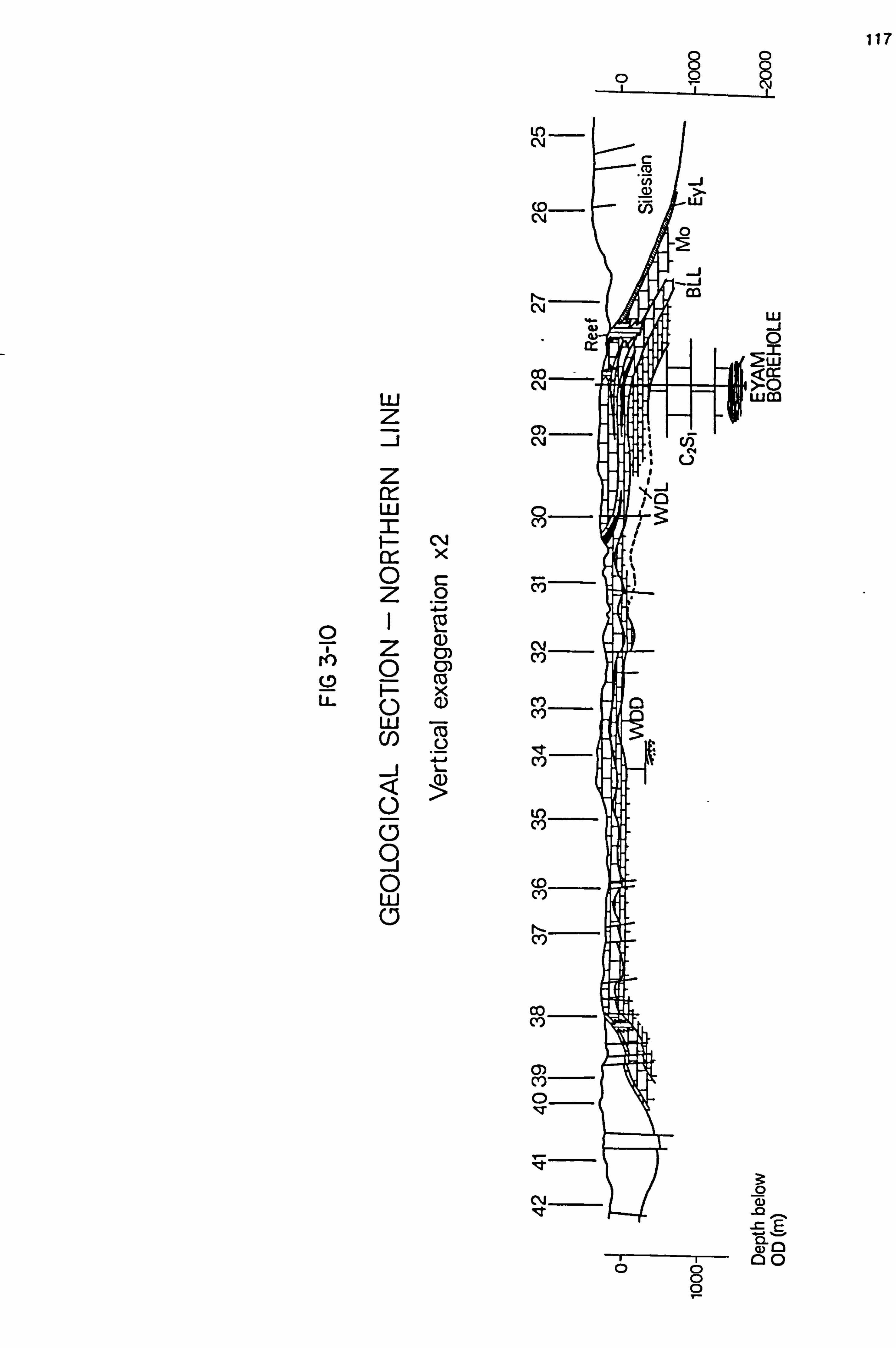
w z J

Z c w I N

X

O c Z o 4-0

O 1 z O

2 CD 0) (D

U`- Ü co

w CD J Q

0 0 O 0 w 0

U') N

(0 - CM

r -- CM

Co N

N

(D (Y)

c`)

N CO

CO M

lKt C, )

to C, )

(D C, )

N (Y)

Co (")

ß)

O

N le

8 00g N

-I

W J 0

2W

>-O Wm

ö

ö. ý

00 co

0

117

118

respectively, although these, in common with all the other

stations, were relatively quiet and yielded excellent signal to noise ratios.

All the sites were occupied by single, vertical

component seismometers; the amp-mod gains were permanently set to seven. The line was maintained from the 7th to the 28th October 1980, during which time three tapes were

recorded at each Geostore, and eight blasts were timed and

positioned: from Cauldon, Stoney Middleton, Dene, Middlepeak,

Ballidon, Tunstead, Longcliffe and Dow Low.

3.3.4 Southern East-West (SEW) Profile

The southern East-West profile was planned to investi-

gate the geology across the Dovedale Transition (Fig. 3.1),

and the nature of the sandstones in which the Caldon Low borehole terminated. As such the line was designed to span the entire limestone outcrop, and to be reversed between the

quarries of Dene (Wirksworth) and Cauldon (Fig. 3.7). As the Bouguer anomaly map suggests (see Section 1.3.2), the

profile was expected to cross shallow basement. The geological section is drawn in Fig. 3.11.

The line was deployed during the same field season and directly after the NEW profile, with one station (34)

maintained in common for the same reasons as station 51 was previously. This profile also comprised eighteen stations, and was 33km long. The topography along line was quite gentle and a straight profile was easily planned. Four Geostore

sites were sufficient: at Bilberry Knoll (station 44) to which station 43 broadcast, the Old Quarry (station 46) which recorded stations 45 to 48, Wibben Hill (station 51) for stations 49 to 53, and Cauldon Low (station 58) which served stations 54 to 60.

The gap between stations 44 and 45 was to avoid Wirksworth, and that between stations 53 and 54 was due to the Manifold Valley. As for the northern line, all amp-mod

M

LL

w z J

z cr- w I

D 0 Cl)

z 0 0 w

J Q U_ a O O Ui 0

N X

a 0

cß a) 0) 0) co

U 41 L

i

0 c0

O 0

OO

0 2

.w

""' ZO Öw

" QÖ

"'" Um

o g 0

L Qv N CO

119

120

gains were permanently set at seven, and each station had

a single vertical seismometer.

Five quarry blasts were timed and recorded during

the three weeks this line was maintained, from 30th October

to 19th November 1980. The northern quarries provided distant

broadside sources, while all the sourthern quarries were

either on-line or closely on-line.

Unfortunately, this line was plagued with bad weather

and instrument problems. Of the stations on the Millstone

Grit, only station 59 ever worked; stations 54 and 55 never

operated satisfactorily, and the old Quarry Geostore only worked during the last week. The only complete records, therefore, are for the Cauldon Low and Wibben Hill Geostores.

Additionally the poor weather also affected quarry blasting, and several quarries reduced their programmes.

3.3.5 DASED1 and DASED2

This experiment was primarily designed by A McDonald

(University of Leeds, and IGS Edinburgh; his acronyms for

these profiles are retained for convenience) for the study

of surface waves; thus the seismometer periods were extended to 1.5s, and the average station interval to about two kilo-

metres. DASED1 and DASED2 radiated south from Tunstead Quarry,

DASED2 being about thirty degrees east of DASED1 (see Fig. 3.1)

DASED1 largely re-occupied the even numbered stations of the

1979 north-south line, but with the southern end straightened

out with three new stations: 69,49 (in common with SEW), and 61. DASED2 was a shorter profile (only 14km long), and was

reversed between Tunstead and Shining Bank quarries.

The lines comprised five Geostore sites: Winn Farm (station 61, for stations 61,49 and 69), Aleck Low (for

stations 4,6 and 8), Fivewells Farm (for stations 10,12,14

and 70), Blore Hill (recording stations 62 to 65), and Stanton- in-the-Peak (for stations 66 to 68). Three component sets were installed at stations 61,6,14 and 64. Station 70

121

comprised an HS1O seismometer situated on the western perimeter

of Tunstead Quarry, to aid location of Tunstead shots and to

record other quarries for shot-shot reciprocal times.

The experiment ran from 20th October to 10th December 1981. The amp-mod gain history was varied to prevent overloading of surface waves recorded from timed and located shots,

of which there were twenty-one from various quarries, including

ten from Tunstead alone.

122

CHAPTER FOUR

DATA PROCESSING

4.1 Introduction

The three years' experiments were recorded on seventy- five analogue magnetic tapes, comprising about 10,800 Geostore

hours' data. In all, about 950 separate, good quality events were detected, of which about 850 were quarry blasts, 29 global earthquakes and the remainder local earthquakes (most of which were from the Mansfield region). Of the total, 800 or so events were digitised, multiplexed and written to digital tape

at IGS Global Seismology Unit (GSU), Edinburgh. This chapter describes the processing of these data into a form suitable for

their interpretation and the discussion of velocity-depth models in Chapter Five.

Essentially, this chapter comprises five sections:

1. The data set 2. Digital processing 3. Picking of onset times 4. Location of untimed events 5. Global earthquake data.

All sections except 4 apply to the teleseismic data recorded during the experiments.

4.2 The Data Set

In basic form the data exists on the analogue magnetic tapes recorded in the field; a listing of these per Geostore per experiment is given in Table 4-1. The first step in

processing these data was the compilation of an events catalogue: a tape by tape listing of events recorded, including times of occurrence, types of signal and quality of recording. After each field season the tapes were monitored on a system originally

123 ED r -I N . O ED 0 tD

2 IM -7 U7 ' . . r-1

U) O N M 0 N LO N - H 0 0 r-4 N N re) Q

13 1 1 1 1 I 1 1 1 E M O N M O N U) N

l0 7 Q) 0 0 r-1 N N M ac N M M M M P) P') F')

. --1 . -1 w

N w

M w

17 w

Ii) w

[D w

N w

U) -

CO M N) M M F') F'M Pr) M Q) 2 2 S 2 = = S Z . --1 m m m co m m m U)

.. f CJ w W. ff) wU) w(0 wN 0 CO . --IM M N MM M U)M (D t' NM mn nEn N) CM MU] MN N)(1) N'') V) N) U) MN

(q Q w Qw Qw C w ¢w gw Qw Cl w p) p) w -1 wN wM w- wýj) wC0 N . U) O-U 1-4 t') NM MM 171') U) N) U)N NM co M (0 0 M2 M2 K)2 PM2 M2 N)2 M2 M2

1- 0 LLB L- 23 LLB I. i: LL- 23 LL3 LL: Li. _

NU wE2 .1O . -i M N H CO 3

2 N M N ... I >% C2H OW0w C) 0 N . -i CD M >C rl E" wU H . -1 . -1 N HW l9 ri

MI HO C) M M N) p) J . r{ H ý Nw= a) L ý. E - . -1 O3H O. EN MO O . -i .1 OOOC X : -0 0C M M M JO a) OCC

.YE: M O B OCD

H +> > W 44 OOJ "r1 C) C C) U) 1-4 N re) N 'p 3 0.03 N N N L, f

E >. ti La.. Cr H7- M3 N -H 43 w w w (0 f0 r-I co H ". 4 . -1 N P'7 MU-4 w cl a) -1 N N r4 -r4 -Y f0 O, c0 N 3 3 a mu2 c0

-P X7 OO w w w N) Q) C) Q O. U "-i N f') N w ". 0) O.

a) N0 N N NY N . -I cy, 1 H C) I- U U U U co CP. -4 'O p) 013 O 1 00m=

+0 3O ßy1 C£ -P N. 1 rn YI OU O M - In N C) C (1) C 4- 2 N M N . -1 X >. E: ", -1 U "1 O ¢HI

U) co U) N U) (4 wC 4- (A H co O O O X C) EO

a) a) O a) N N r) re) I a D -0 -0 1 1 1 1 ,f (a c

>. 0E >. E . -+ co LO N ". i ca 1-1 U (U 7 co m 0) 0 M 4.3 (0 C 0C N N N rl) 3 U) U) EO O ]C '-1 E O. O 3 w J co . ",, 4 U] O (0 L Lil r1 N M O

U) 1- 4J . -1 .ý rl ,Cw3w LL. : U r-4 N >.

w w w CD --I >H . -1 r-1 N M .7 . --1 --1 -1 H I

V-1 . -1 N . -4 M . -1 ¢= LL. UE W W '--1 W V-4 LL O1

U) '. -23 ".: 53 w Q (1) IL QM O C) N . -I N- N) w - . --1 LL.

. -i O. 'O . -i .4 . -i N . -I M . -1 0 -13 D co O X . -4 X . -1 X . -1 X "" M (1) -q C (0 F- 0 Qm cc m Qm cc U) O'O C

O. M W CTS u7 l9

N [D O U) U) N CD M 1- 2 M to (D N Q) (D m . -4

N . -1 U) U) N CO 1-1 to to H U7 U) U) N N co co ! 0)

0 1 1 1 1 1 1 1 1 >- E co N Q) to N co -4 (D R1 7 -7 U) U) to N N co co 0C N N N N N N N N

Q) N O IL

U

L7 ý7 U7 W W N

" w w 0 a1 "-I N M ý7 Ln co N

G) a) LL lL LL LL LL LL LL Q, 13 w w w w w w w R1 0 . -1 N M ý U7 CD N J F-0 ¢ cc Q ¢ Q 4 Q E

124

devised by G. Neilson (GSU Edinburgh), shown in Fig. 4.1.

Normally tapes from the Geostore site with the most complete

recording history and the quietest stations were chosen to

be monitored; this assumed that any event not detected at this site was not worth considering.

Four seismic channels could be monitored during replay: two on the oscilloscope screen, and one to each channel of the stereo headphones (see Fig. 4.1). The ear is far more

sensitive in discriminating between noise and signal than the

eye and demands less concentration: an event is perceived when

a signal is heard simultaneously in both channels, and with experience the listener can distinguish between types of event. For example, a quarry blast is heard as a single gunshot, and

an earthquake as protracted cannon fire. The detection was so sensitive that a good number of events perceived were seen only

with difficulty on the paper playouts, made on the jet pen

recorder.

Most events recorded were quarry blasts which occurred during the normal working week. An overall guide to the frequency of blasting in Derbyshire is presented in Table 4-2,

which is based on the results from a questionnaire sent to

every known working quarry in 1979, primarily to aid the location of untimed blasts.

After each season, the data were digitised on the PDP11/70 facilities at GSU Edinburgh, by which the records

were flutter compensated, digitised at 50 samples per second and multiplexed onto digital magnetic tape. Since the upper frequency cut-off for the analogue recording at 15/320ips and replay is 16Hz (see Fig. 3.5), and the highest frequency

component of P waves from quarry blasts only about 12Hz (observed

from the analogue playbacks), there was little seismic energy above the Nyquist frequency of 25Hz.

All quarry blasts were digitised for a window of one or two minutes (starting on the minute, or the half-minute). Teleseismic and local earthquakes were digitised for up to five

minutes. To save on tape, only those channels with seismic

125

FIG 4-1 Tape monitoring system (schematic)

Storel4' tape replay system

E a

E O.

E a

M

.., E. a N

E CL

. -I

E a

N

E N

r-1

E cu 0

E c0

w U)

0 C 1 0

U') +J >sv Cl) O^ . -I O

. -I ON 'D NM O. Y M 'O C1 O "f 1

. ""i "rr U) CL LO E: E:

n O

n O ,

(! I r-1 CM N1 -01 C

-Ow - >. ^ >. O^ pw^ O^ '. . r0 NO a) . -10 . -i0 CQ . CU') 00 a)r. 40 CUO UO 00 NM. _ >1 0-. -I 1 0-0 1H1 'O 1 EI O-7 0 CU -7 +'"ýi .7 a) -zr "--117 cad

Ov =' - Un E: - : E3 %- W%--, O%-ý

LO O^ (1) Cl) CM N0 C CD O1I . -i 0

. -1 +>P7 CM O1 +3 O^ >- >ý NwOa0M N^

LO 00 N. -40 'O M O- >0 - Cl) O (1) 1OCU0 e--4 O3 a) a1 m >1 11 .-410- 01 71L . --4 C OM 00M'4. ). rfM Co NM U) f0' on O'- = ý> '- U7 E-U-¢O E:

YO C 1. N U') O DN13

(U aN 0 3 >, N^ N^ (u W. r. {^ O^ CL) . -1 17 +) U) . -i O 140 1-4 O CD O U) C3 13 C3 Cl) N7 . 0N) 00 1 CI "O i ", I 1C1

-P .. -1 N 'D N "«-I NHN "1-1 N Cl) av 1--v av my =v

C C 0 O 3 -N

". -1 O -4 0 0) r-1 O Iq0 -00 CDN)

"-h 1 44 10- 01 lo . -f to . -1 -+- "ri . -4 - ' ,

my :v u) a-

O N 0 3 co

1N 0 4- C N (1) "-4 4- 0 C iI r-1 ^ a- "-I a "rj ^. 3^ 4. 14

00 00 1 a) 0- , -f U) 00 >. aD0 00' LO . -t0 H 300 0 -1 JM N. -4PO CU) CD 0) 1 .01; a)1 C 'o 1 N 1- C >N CN -P NI CN 3N O-ON EN O0 r-I ". -1 . -i lU i-i N0 . -1 0 "-1 +a "ri . -h , 1

CO -I

H Il) Y

m I n) r-1 O, ̂ 3w

NO . -i NOO ltl ^ OO v . -I N . -i 177 L r) CI C) I

.. O. 1 LO

t9 rl C -0,4 C . -I 4. . -I co "4 r-1 ". 1 ý4 . -1 c: ) - O E: ='-r-1

Y to (U

C I) N C) O^ (0^ . -1^-, (1 w, `- '

UO cu LO CU) OO-' ri 0 4Ot -4. . -1 M U)

"-+ 1 to I au 1O1 . -t ß-I0 CO >0 DO 1 N "-1 O . -f .0 . --I . ri r-I O m'

N

0 C- +' {a _ yam. Or: >. O LLO a)N (f r-4 CI EI 00) (Urn

CD

v a, U N

01 .aG

4, ) Cl)

r-1 A

H

7.

to u -I CL

N

co F-

126

127

data were digitised, along with the Geostore internal clock

on the first digital channel and MSF always on the last. The

digitiser afforded four gain settings between 2.5mV and 20mV,

with which the output was scaled between +1024 and -1024 digital

units. In order to prevent clipping of the signals, most of

the data were digitised at a low gain, nominally 5mV.

In total, the digitised data comprised 300,165 and 320

events recorded during the 1979,1980 and 1981 seasons respect-

ively. These were written on twelve 3600 foot digital tapes,

for each of which a file by file catalogue was compiled, and a jet pen playout of the complete contents made for future

reference. At this stage, unique catalogue numbers were

assigned to each digital file with the following code: a letter

for the Geostore (e. g. A for Aleck Low, E for Eyam, etc. ), a

single digit each for the experiment number (see below) and the analogue tape number, and three digits for the event number,

counted from zero for each analogue tape. For example

F22034 ---Recorded at Fivewells (F)

Experiment 2 (Southern East-West line)

Tape 2 (which ran for Days 321 to 327)

Event number 034 (34th digitised from Tape 2)

The experiment numbers were: 1979-no number, NEW-l, SEW-2 and 1981-3. Events recorded at several Geostores were assigned the

same event numbers, and differed only by the Geostore prefix. The numbers of events digitised from each tape are included in

Table 4-1.

4.3 Digital Processing

From digital tape to producing records suitable for

picking onset times, a Digital Tape Analysis Package (DTAP) has

been developed on the University of Leeds Amdahl V7 designed

to make the process as easy and efficient as possible. At the

core of this package are the programmes originally written by

D. N. Whitcombe specifically to handle data digitised at G. S. U.

Edinburgh, and further developed by the present author: DECODED,

FSTOR and PLOTTER.

128

The data on tape were written in a specially coded, highly packed format (C. Fyfe, G. S. U. Edinburgh), which DTAP

reads using the subroutine SEIREC, developed by D. K. Johnson

of the Computing Service, the University of Leeds.

The four stages of processing a digital tape were:

1. Checking the Contents of a Tape (programme DECODED)

It was necessary to define the exact start time of

each digitised window before further processing, and also to

check the contents of the tape in case of null files or errors in the documentation. DECODED automatically provides a file

by file log of the tape; by decoding the Geostore internal

clock it lists the precise start and end time of each digitised

window.

2. Creating Event Data Files (programme FSTOR)

The computer at the University of Leeds stores files

on two levels: in the permanent FILESTOR, and on temporary Disk

which is used as work space.

The programme FSTOR reads an event from the tape, demultiplexes it, and writes the data to Disk with headings

specifying details of recording and digitising. This Disk file

is then automatically transferred to FILESTOR, and saved under the same name as its catalogue number. Only a window containing the relevant signal need be copied: typically for a quarry blast about 25secs, and for a teleseism about 40secs. Once a window was written to Disk, a standard plot of its contents

was made on a Calcomp drum plotter.

3. Merging Demultiplexed Files

Most events were recorded on between two and five

Geostores, for each of which there was a separate demultiplexed file created by FILESTOR. To reduce the number of data files

on the computer, and to facilitate processing, these were normally combined into single event files. For consistency, the order by which Geostore records were combined was the same for each experiment. The name of the merged file was usually taken to be that of the first file of the set: for example, the

129

files F35024, A35024, WH35024, BH35024 and S35024 were combined in that order and saved as F35024. Data from 1979 were an

exception in that merged files had the prefix M.

4. Display of Data (programme PLOTTER)

Steps 1 to 3 were repeated with little variation for

all data transferred from the digital tape. By contrast, the

programme PLOTTER used to display the data is a general package

and as such may be employed for a variety of uses; a flow chart

summarising its functions is shown in Fig. 4.2.

For basic processing, PLOTTER was most frequently used for two purposes:

(a) to produce standard plots of the raw data, and (b) to plot the data in a form suitable for picking onset

times: a 'fast replay' with an extended time base.

Case (a) arose where the FSTOR plot was lost or the contents

of a file needed checking. For case (b), the output required large gains, well-spaced channels and a broad time base: the

normal form for quarry blast data comprised channels separated by 4 cm with amplitudes normalised to fit their assigned plotting window, and five seconds of data plotted at 5cm/sec. Both

time channels were plotted. Although it was possible to apply

a bandpass filter to the data (see Fig. 4.2), none of the fast

replays were filtered. This was partly due to the high quality of the events considered, but also because for the picking of first breaks as little distortion of the signal as possible was desired.

i) Time Corrections

Three time corrections were applied to the signals plotted:

A. Clock Corrections

These are the relative differences in start time of the demultiplexed windows between Geostores (see Fig. 4.3). The corrections are determined either by using the output from

DECODED, or by plotting the first five seconds of each time

channel on a fast replay and measuring the differences relative

130

N

(9 LL

2W 44

0 )- g2 WZO

=U' Z&ZDU

K=m W FW� « OX X

JVKm 2Jý{ý WW

WWz

FW gN '' CK 2zz Nj W 3, g d W( a

~~ iO

N

F-p 0Z0 W9- N U2 pl"'W : in

ac w0 f"4F Z V2

Z ?

WL. - : Hý ýOJ. J2> Ö D Wý ý3 WZZK d_ý[ a `ýK 0 vW ciN

GG x$ ,-41 ß"

Z' 2

U1 0ZNZ0 f"

H~ d=W WW

_C IZZ NOVWZO!

NM

LL- >W

= WS

N as rl

WK O

WÜ O z W

w 0 F- Co

LL I

C

0

2Z HO_ Ö

J0 dO

Q. U. -O

W ZN NW W

Wdö a N

131

W J

LL.

0

W

x

w

J

CL

I -- J

W

0

W ih.

0 40 0 0

N

0 1 0 4- 0 m a

fc, a C Y C C

V

FIG 4-3 Clock corrections

EVEN

aI

Geostore recording head ýI

1ý

ODD

difference in skew

j% Store 14

/ replay head

/ U14)

H

difference in separation

Correction (secs)

0

-2.8

+2.2

FIG 4-4 Channel corrections

132

to the first Geostore. Clock corrections accurate to better

than ± lOms were required for the reduced time sections (see

(ii) below).

B. Head Corrections

Head corrections negate the time error due to the

difference in alignment between various Geostore recording heads and Storel4 replay heads, and thus a suite of corrections was required for each Geostore-Storel4 combination used.

There are two components to the correction (see Fig. 4.4):

(a) difference in separation between the heads which

record odd and even channels. This was often the largest

correction to apply, and varied between ± 50 ms. (For this

reason, whenever half the total number of data channels are

used, they should all be recorded on either even or odd channels, rather than mixed between the two).

(b) difference in skew, 0, for each of the heads. This

error was found to be normally smaller, up to ± lOms for

channels at either end of the same head.

The corrections were measured from the calibration

pulses recorded on each Geostore specifically for this purpose (see Section 3.2.5). The signals were replayed by the Storel4

used for digitising and played out with an extended time scale using a jet pen. The time differences were then measured relative to the MSF clock on channel 14, to an accuracy of ± lms.

C. Channel Corrections

During multiplexing, it takes 72 microsecs for the digitiser to sweep from channels 1 to 14 for every sample digitised, and each channel's correction will be a proportion of this value. This correction is negligible compared with the head correction, or picking error.

ii) Reduced Time Sections

PLOTTER was often employed to produce time sections where each seismogram was shifted towards the origin by a reduction time Tr given by

133

Tr = X/Vr

where X is the distance of the station from the source, and

Vr the reducing velocity (cf. Equation 2.15). All phases

travelling at velocity Vr line up parallel to the time axis,

so that if Vr corresponds to the velocity of the arrival of interest, the reduced time section conveniently displays the

data without needing to compress the time scale.

These reduced time seismograms sections were plotted

either against true distance from the source, or against station

distance along each profile. The records were usually plotted

to as large a gain as possible without overlapping adjacent first arrivals.

4.4 Picking Onset Times

At each stage of the digital processing the best quality data were progressively selected: thus of the total 800 events digitised, 400 were copied by FSTOR and saved in FILESTOR, of

which 250 were plotted as fast replays and picked. Timed and

positioned quarry blasts, most of the local tremors and all of

the global earthquakes were processed by default.

These records form the 'raw data' of this section,

although all the teleseismic data from stations outside the

Dome (viz. Charnwood Forest, Haverah Park and Stroke-on-Trent)

have been picked from jet pen records with an extended time

base.

4.4.1 Method

All the data have been picked by eye which is more

accurate, efficient and versatile than any automatic means. A cross-correlation technique was investigated using an Inter-

active Signal Analysis Package (ISAP, see Fig. 4.2), but without

constant user supervision the derived arrival times were found

to be questionable, which rendered the method both time consuming

134

and cumbersome. Furthermore, considering the high quality of

most of the raw data, the development of such a computer-based

system was unjustified.

Rather, traced waveforms were used to correlate P

waves between pairs of stations, whereby a well-defined arrival

was traced and superimposed on a less well recorded signal in

order to judge the onset. Usually this process worked outwards from stations nearest the shot, for as the amplitude of the

wave decreased the signal became more contaminated by noise. However, there was no set approach: normally the stations

nearest the source did not require interstation correlation

since the direct arrivals were extremely well defined; and frequently the refracted phase was best recorded at the more distant stations from the shot, whereupon the correlation

worked inwards.

'Onset' here refers to the earliest point of a signal

correlated from station to station. There are various points

on a wavelet than can be picked, as Fig. 4.5 illustrates. If

this wavelet were incident without change along a profile, then

any of these points may be used without affecting the relative

arrival times. However, because of P wave dispersion, filter-

ing of the signal with distance, interference by later arrivals,

etc, the signal waveform changes between stations and the later

into the signal the point used for correlation the less reliable the picks will be. Therefore, where possible, the first point of displacement, A, in Fig. 4.5 has been used.

Generally, the quality of the 'pick' is dependent upon: (a) the signal to noise ratio, (b) the frequency of the waveform, and (c) the interstation coherency of the signal.

(a) Noise comprises any seismic energy apart from the

signal of interest, and may be either random or correlated between stations. Random noise encompasses both ambient and

system noise; ambient noise (wind, cultural, livestock, etc. )

was observed to differ in amplitude and frequency according to

geology and proximity to habitation, and also to increase in level during the working day for stations near quarries, etc.

135

FIG 4-5

(a) Points for picking

first peak

AV d splacement

C

first trough

(b) Amplitude measurement

a- first peak b- first peak-to-peak c- whole phase

FIG 4-6 Different wavelength arrivals

quarry blast

Teleseism -ý-ý

second marks

136

Correlated noise mainly comprises seismic energy from the

same source as the arrival of interest: for example, precur-

sory ripple to the picked 'direct' wave, or the coda of the

first arrival itself for a later phase.

At various levels noise is always present, and has

greatest effect when prevalent at similar frequencies to the

signal concerned. Where the signal to noise ratio is less

than unity the first break is unlikely to be reliably determined,

unless the frequency of the ambient noise is distinctly different

from the signal. When noise and signal are similar in amplitude

and frequency it is easy to pick on the wrong cycle and. the

trace correlation must be carefully made.

In order to combat the problem of ambient noise of

similar frequency to signal, multichannel polarisation filters

have been assessed to enhance first arrivals (see Section 2.4.1

and Appendix B). The filters essentially discriminate against incoherent energy between the data channels.

(b) The effect of wavelength on the quality of picking is

illustrated in Fig. 4.6, which contrasts quarry blast with teleseism. Obviously the broader the take-off slope, the more difficult it is to estimate its origin. Thus there is a trade-

off between the-frequency of the signal (on the fast replay) and the length of the time scale, for the greater the distance between second marks, the more accurately the pick can be

measured. Thus for quarry blasts, the P waves for which were

commonly between 3 and 6 Hz, a time scale of 5 cms/sec was used,

whereas for teleseismic data, where the first arrival was often 1Hz or less, a scale of 2.5cm/sec was employed.

(c) The more a signal waveform changes down a profile, the

more difficult it becomes to correlate traces, and therefore judge onset times. Noise apart, such changes between stations may be due to: differing station characteristics, differing

angles of incidence (where the steeper the angle of incidence the less the arrival will be affected by near-surface irregular-

ities, and the larger the amplitude response of a vertical seismometer), or through the interference of various arrivals:

137

for example, where headwaves overtake direct waves, where

either phase can be considered as noise. It is unwise to force

a correlation between stations where their first breaks

correspond to differing arrivals.

In cases where, because of noise and changes of waveform, no two stations satisfactorily correlated, picking became

a protracted, iterative process whereby most of the signals were traced and correlated with each other. For emergent teleseismic arrivals the first break was sometimes indefinable,

in which case the first peak or trough was used instead; this

was justifiable as the first arrivals are normally coherent along the profile, and only the relative delay times were required.

Not only was it possible to pick arrivals between

stations for the same event, but it was also possible to

correlate arrivals into the same station for different events from the same source. This could not be done until the sources had been located, but it was one means of improving the quality of the pick, especially for less reliable observations. How-

ever, different shot configurations can yield differing source signatures, and this had to be taken into consideration.

4.4.2 Time Measurement

All arrival times have been measured against the MSF

clock (Fig. 3.6), although absolute MSF time was only used for timed quarry blasts and global earthquakes; for untimed blasts

relative arrival times were merely required, so that the seconds were arbitrarily numbered.

There were two areas where measurement error occurred:

(a) Estimation of the start of the second mark

Fig. 4.7 illustrates the true shape of a received second pulse and three variants after digitisation. None of the NSF receivers seemed to have exactly the same response, so the coded widths varied slightly. The onset of each second mark

138

FIG 4-7 Digitised second marks

analogue digitised variants MSFreceiver (tick marks onset of second) response

0.5sec

FIG 4-8

Quarry X Station

139

was taken to be the sample before deviation from the baseline,

which, as shown, was rarely more than about lOms out.

This error increased for noisy or faulty time channels. MSF

Where thelchannel was unusable the Geostore internal clock

was employed, in which instance it was calibrated against MSF to

time. Since the Geostore clock has been knownLdrift irregular-

ly, particularly in cold weather (when it was observed to

differ from MSF by 0.4s within a week), this calibration was

preferably made using the previous and succeeding records with MSF, whereupon the required correction was interpolated between

the two.

(b) Measurement of arrival

The picks were measured with a ruler from the left hand

margin of the fast replay; since the time scale is known, only

one trace need be measured against the clock per Geostore, as

all the other arrival times can be calculated directly. Thus

the measuring error between signals of the same Geostore was

no more than the accuracy of a ruler, say about ± 0.1 mm,

equivalent to ±2 ms for a5 cms/sec time scale.

Thus the total measurement error is potentially greater between groups of stations due to (a), than between adjacent

stations due to (b).

4.4.3 Observational Error

All the effects upon the quality of pick add uncertainty to the derived arrival time. Whitcombe (1979) suggests blind

repicking to estimate the error variance of the jth observation, 2

cri , so: K (tý-tn)2

o '2 E K-1 } n=1

for k pickings for mean time t7. With trace correlation, how-

ever, it was found more efficient to estimate observational error by moving the trace to either side of the pick, thus

140

actually estimating the limits of correlation. This could be done at the same time as picking, and was a direct reflection on the quality of each individual pick, as opposed to the

above variance method.

Where trace correlation is used to determine an onset time, the observational error of this pick necessarily contains (a) the error in estimating the onset due to noise, etc., (b) the error due to the difference in waveform between the

two traces, and (c) any observational error in defining the

onset of the correlating trace. In the case where the signal waveform, say, progressively broadens with distance from the

shot and the same correlating signal is used throughout, then the error due to (b) will increase away from the shot while that for (c) is constant for each pick. Alternatively, if the event is picked by correlating adjacent pairs of stations and working away from the source, then the error due to (c) may well accumulate with distance, while that for (b) will be

minimal. In most instances, several correlating traces were used to estimate an onset, in which case the estimated observational error was an ensemble average.

The observational error estimates were found to fall into three distinct groups:

1. O-lOms: for strong, high frequency signals with an excellent signal to noise level. Here the observational error is not due to the pick itself, but the errors in time measurement, discussed above. Obviously, it is possible that the true first break occurs between adjacent sample points, so that the observational error is at most lOms.

2.10-50ms: (minor picking error): most observational error estimates for noisy signals fall into this range. The total error also includes the measurement error (above).

3. >50ms (major picking error): errors of this magnitude were normally not obvious during picking (although the picks were known to be questionable), and became apparent when either the data were plotted

141

or the source location was considered unsatisfac- tory. These errors arose where the ambient noise

was similar in amplitude and frequency to the

signal, and the pick was made on the wrong cycle. Such observations were either ignored, or a re-

pick attempted.

Other miscellaneous errors include inaccurate head corrections,

noisy time channels, and a poorly calibrated internal clock (if used). Combined, these additional errors are generally

small, less than 5ms, especially compared to most estimated observational errors.

4.4.4 Measurement of Relative Amplitudes

The first arrival amplitudes were measured from the

fast replay records using a magnifying lens and graticule,

accurate to ± 0.05 mm. For the same reasons as the first break

was picked at point, A, in Fig. 4.5a (see Section 4.5.1), the

amplitudes were measured peak-to-peak between first peak and trough where possible (see Fig. 4.5b). These amplitudes were

expressed relative to the maximum digital range (i. e. 2048 units

= 1.0).

The accuracy of measurement increases with: the signal to noise ratio, the frequency of the first arrival, the accuracy of the pick, the interstation coherence, and the closeness of the first arrival waveform to the ideal wavelet (i. e. Fig. 4.5b).

Note that the correction for Heelan's law gives more weight to observations more distant from the shot whose amplitudes are small and most effected by ambient noise. Normally

such small observations are either ignored, or overestimated.

4.4.5 Location of Untimed Quarry Blasts

Unlike almost all seismic refraction surveys, the vast majority of events recorded by this experiment were untimed and of uncertain origin: of the two hundred or so quarry blasts

142

picked, less than forty were timed or positioned. Thus a

reliable efficient means of estimating a shot location from arrival

relative/times was required.

There is a finite number of shot locations in the area: the working quarry faces on and around the limestone outcrop (see Fig. 3.7). The grid references for these have been

determined by considering points about lOOm apart along each face. The most simple means of locating an untimed quarry blast was therefore to generate travel times from each of these co-ordinates to the observing stations using a suitable velocity-depth model, and select the solution by least-squares

best fit with the observed travel times. The source is assumed to lie on the surface.

4.5.1 Method

Consider Fig. 4.8 where shot

an irregular refractor. The line PQ

refractor slope between the stations

are small compared to the station di

for the approximated raypath SPQG is

Equation 2.2 (terms as given in Fig.

T= (z1 + z2)Cos 0c

V 0

S and station G overly is an average of the

where the depths zl, z2

stance, X. The travel time

then given by using 4.8):

+X coso V

r

Without knowing the detailed structure at depth, a simple two layer model can be assumed whereby the Carboniferous overlies a continuous refractor the length of the Dome (e. g. Whitcombe

and Maguire 1981b). To use Equation 2.2 the depths to a refractor had to be estimated for all stations and quarries. Initially this was done through examining the timed and positioned shots from the 1979 experiment, and subsequently revised after the first time-term solution (see Section 6.3.1). The depths were calculated for overburden and refractor velocities of 5.2km/s and 5.6km/s respectively: those for the

quarries were estimated by interpolation from gravity and borehole information.

143

The travel times using this simple model were

calculated using the computer programme MODFIT (see flow chart, Fig. 4.9). A suite of travel times is calculated from every

co-ordinate specified and the closest set to the observed

arrival times printed along with a printout of the best thirty

locations. A least-squares velocity was also derived for

(arbitrarily) the nearest six stations to the located shot

point, and this value is used as the overburden velocity for

an iterated solution.

Since most picked times are from linear arrays of instruments, the quality of a location may depreciate where the source is collinear with the profile but not within its

ends, EE' (see Fig. 4.10), as the relative arrival times will be least dependent on the distance of the source. A poor location may also arise for a distant source perpendicular to

the line, where the difference in arrival times will be very

small and more dependent upon refractor structure beneath the

line than difference in distance from the source.

To test the routine, timed and positioned events from

the 1979 season were 'located'; the results are summarised in

Table 4-3. Given that the structural and velocity variations

along each raypath were largely unknown, these locations are

quite satisfactory, and predictably the error in position increases for the more distant shots from the line. Clearly it is unnecessary to attempt to define an accurate model for

this purpose, for the object is to discern the refractor

structure once the location is known!

The accuracy of the method was found to be less depend-

ent upon error in the velocity-depth model than picking error in the first arrival time data. Changing the overburden or refractor velocity by 0.2km/s rarely changed a solution. How-

ever, while the system could handle one bad observation, several could steer the location to a nearby quarry and further for

noisy data from a distance broadside source. Occasionally

suspect locations were checked against other diagnostic features (below, Section 4.5.2), but this was only required when the

144

EVENT DATA

PROGRAM

MODFIT

RELATIVE ARRIVAL TIMES

VELOCITY-DEPTH MODEL

QUARRY [-LO' P DATA

LE AST CALCULATE SQUARES

ARRIVAL TIMES BEST FIT NEXT EVENT

NON-ITERATED F---i ITERATED

ESTIMATE OVERBURDEN

VELOCITY

FIG 4-9 Flow chart for MODFIT

145

FIG 4-10

A

B

:E .

S S

S S

EI

*c *o

Table 4-3

Testing location programme using timed events from 1979 expt.

Quarry

Ballidon

Tunstead

Brierlow

Wardlow

Co-ords (km)

419.86 355.58

409.87 373.79

408.97 368.62

408.36 347.28

Location (km) Error

419.71 355.53 0.16

410.1 373.5 0.37

409.21 368.93 0.39

408.64 346.88 0.49

146

data were poor, and it was rare that the true shot point lay outside the thirty best locations (most of which usually

comprised co-ordinates of the same, or closely adjacent quarries).

4.5.2 Other Aids to Location

The blasting schedule of Table 4-2 is a fair check

on the location. P-S times also vindicate or contradict a

solution, and so do amplitudes and signal waveforms, especially for the closest stations to the source. The shape of the

reduced time graph (see Section 2.3.2) was often an effective

quality control check and gross mis-pickings were sometimes

evident from discrepancies between the observed and best-fit

arrival times.

Instead of using a sequence of quarry faces, MODFIT

can be used with a network of points. Thus the location for

a local earthquake may be obtained by considering a regular

grid generated approximately about the source, assuming that a

simple two-layer model can still be applied, and that the focus

is on the surface. For the Mansfield and Stoke-on-Trent

tremors, for example, depths to the basement were first estimated from the Duke's Wood (Lees and Taitt 1946) and Gun Hill (Hudson

and Cotton 1945) boreholes respectively, and a 2km mesh drawn

about the region. Having obtained a coarse solution, smaller

grids of interval 200m were used to estimate the final locations;

within the limits of the model, any finer solution would not be justified.

Similarly, a 50m grid was generated within the perimeter

of Tunstead quarry in order to refine the location of untimed

shots for the 1981 season. This was possible as station 70

was located on the western boundary of the quarry itself (see

Fig. 3.7).

147

4.5.3 Summary of Locations

Table 4-4 summarises the distribution of the timed

and untimed quarry blasts picked. A full listing of the

locations is given in Appendix A. Predictably, most events listed are from quarries nearest to each line, and particularly from the northern quarry groups which are well represented because they fire larger shots more often. Long distance

broadside shots are least represented as their lower amplitude

P arrivals were frequently at noise level.

Of special interest are the local earthquakes recorded from three different regions, during successive experiments: both the Mansfield and Stoke-on-Trent tremors occurred within 45 km of any station to yield strong P waves, and the Flamborough

Head event, about 180km from the Dome, was sufficiently distant

for Pn phases to be recorded.

i) The Mansfield Events

This sequence of shocks was recorded over a period of thirty days from 26th September 1979, with activity concentrated

on Sunday 7th October (Fig. 4.11), when thirty-six events were detected between 04.00 and 10.00 (Fig. 4.12). In all, forty-

three events were identified from P-S times and signal waveform, the largest of which, magnitude about ML 3.7, shook people from

their Sunday morning slumber at 8. lOam. (Fig. 4.12 plots surface wave log(A/T) magnitudes relative to the smallest detectable event, arbitrarily assigned a magnitude of 1.0).

Six tremors have been located using MODFIT using a grid

system, for which data recorded on the Charnwood Forest (CWF)

arrays (Maguire, Whitcombe and Francis 1982) have been kindly

supplied by D. J. Francis. A minimum depth of 2.3km for the

refractor beneath Mansfield has been estimated from the Duke's

Wood borehole, and depths beneath the CWF stations have been

taken from Whitcombe and Maguire (1981a and 1981b).

The solution locations are shown in Fig. 4.13. Although these epicentres do not correspond with a fault at surface, the implied trend is subparallel to the principal strike of faults

148

Table 4-4

Number of untimed quarry blasts lo cated by 100FIT

Quarry 1979 NEW SEW 1981

Eldon Hill 2 1 Hope Valley 1 1 Smalledale 5 Bee Low 2 Doveholes 10 5 6 Waterswallows 5 4 1 Tunstead 10 11 2 16 Topley Pike 2 2 2 1 Stoney riidd. 1 1 1 Hindlow 1 1 1 Brierlow 6 6 3 6 Dow Low 5 3 4 Sterndale 4 2 2 Masson 2 Upperwood 5 1 1 Middlepeakl 6 1 Dene 1 Middleton 1 Ballidon 7 1 4 Longcliffe 1 Grange Bar 4 2 Cauldon 4 1 4 2 Wardlow 4 1 4 Ramshorn2 4

1 For 1979,. may include Middleton shots 2 For 1979, may include Cauldon shots

149

FIG 4-II

DAYS

TIME

FIG 4-12

NUMBER Of EVENTS (EACH 24 HOURS)

HISTOGRAM OF MANSFIELD SHOCKS --------

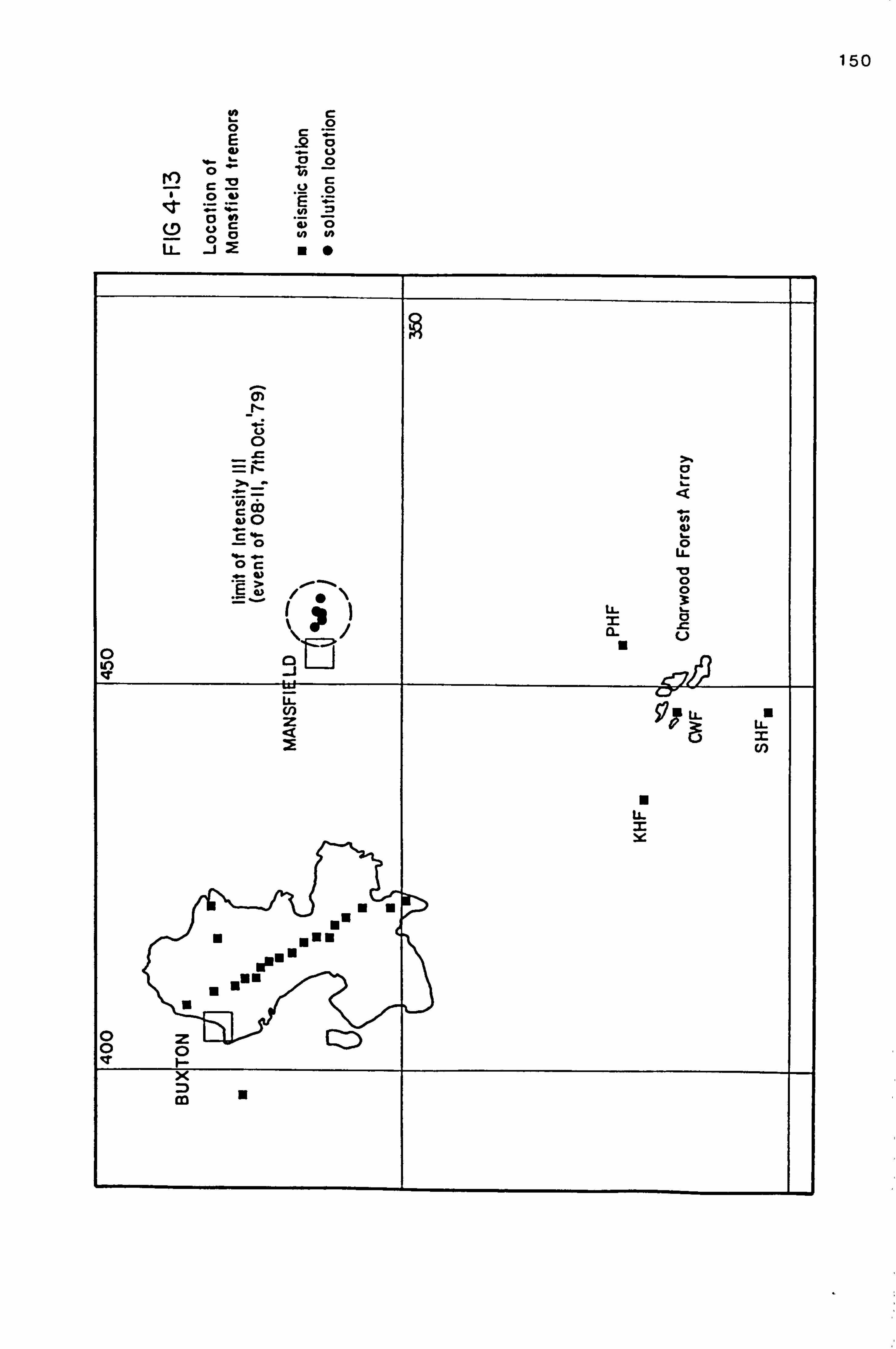
150

` C O E aý

0"

S ü

-° M cv .

Uf

ry 0 VC

V)

C> O

_ 0

0 N Y1

LL "

rn ti U

O

wo (º ö ö

L wý Oc '

10 0 ý

'

\ Ü

O O

li.

Z N a L`

LL

Mann

0 O 0 F-

151

in the underlying Coal Measures. These locations correspond

with the centre of a circle drawn around the limits of Intensity

III, provided by J. Barker (GSU Edinburgh, pers. comm. 1983).

ii) The Stoke-on-Trent Events

Of the twenty-two identified tremors during the period 26th September to 20th November 1980 by the Stoke-on-Trent (STM)

network (specifically deployed to study events in this area;

N. Kusznir, University of Keele), at least seven were recorded by this experiment: one (very weak) event by the northern east-

west profile, and six by the southern east-west line. The largest event of the series was of magnitude ML 3.6, and all but one of the seven were greater than ML 2.3. Mining induced

activity has long been known in the region (e. g. Kusznir et al. 1980), and, like the Mansfield tremors, this sequence was

concentrated within quite a short period, about thirteen hours

(Fig. 4.14; C. Browitt, GSU Edinburgh, pers. comm. 1982).

iii) The Flamborough Earthquakes

These two events of ML 2.4 and ML 4.4 occurred off the

North Yorks coast on the 26th and 27th October 1981, the second

of which was detected by the combined DASED array (event F31055).

These were too distant to use MODFIT, and their location

155012 47854] hasbeen ovided by GSU Edinburgh.

These events were approximately 175km from the Dome, and Pn phases were expected. The picked first arrival times yield

a least-squares apparent velocity of 8.4km/s across the array, but since the azimuth of approach was around 40 degrees, this

value reduces to about 6.2km/s (P* rather than Pn? ).

4.6 Global Earthquake Data

Twenty-nine global earthquakes were recorded during the running of the refraction profiles, of which eleven were recorded in 1979, eight during 1980 (including four successive tremors from Algeria), and ten during 1981. A summary of

,;

152

Magnitude (ML)

4

3

2

bin (Tn o7n tpTn ruin I ITn ILTn

November

FIG 4-14 Magnitudes of the Stoke tremors, November 1980

400 seismic station " epicentre

BU TON

STOKE-

9

ON-TRENT " EN

350 STM

FIG 4-15 Location of Stoke tremors

153

these events is given in Table 4-5, the locations having been

taken from the I. S. C. Monthly Bulletin.

Since the data recorded by the stations from the 1979

season specifically maintained for longer in order to record teleseisms (see Sections 3.3.1 and 3.3.2) could not be used for instrument problems, the data set was enlarged by records of the above events from stations in the Midlands seismic recording network (Midnet): Charnwood Forest (CWF), Haverah

Park (HPK; J. D. Fairhead, University of Leeds), and Stoke-on- Trent (STM). The jet pen fast playouts of these were made available by GSU Edinburgh. In order to aid the picking of the onset times, the digitised data were plotted at the same time scale as these paper records (2.5cm/sec).

Of the twenty-nine earthquakes, eleven were from within teleseismic (30 to 100 degrees) distance, and nine from a distance greater than 100 degrees (most of which were from the

Tonga Trench region).

154

Table 4-5

Global earthquakes recorded by experiment

Event no. Date Region Distance Azimuth degrees degrees

112003 11.9.79 Azores 21 251 112014 11.9.79 Romania 19.7 101 112028 14.9.79 Komandorskyls 73.3 5.3 113021 19.9.79 Cen. Italy 14.3 130 M3044 21.9.79 Tyrrhenian Sea 18 135 114001 23.9.79 Aleutian Is 74.8 2.7 M4002 24.9.79 Noveya Zemlya 30.7 28 114037 27.9.79 New Hebrides 145 16 M5014 1.10.79 Mexico 77.8 280 M5040 2.10.79 Fiji Is 147.3 3.5 M6007 5.10.79 Fiji Is 148.7 2.6

F11011 10.10.80 Algeria 17.2 172 F11015 10.10.80 Algeria 17.2 171 F11017 10.10.80 Algeria 17.2 171 F11018 10.10.80 Algeria 17.3 172 F11019 11.10.80 Noveya Zemlya 30.6 28 F13016 24.10.80 Cen. Mexico 79.4 286 F13017 25.10.80 Loyalty Is 148 15 F13018 25.10.80 Loyalty Is 148.5 14

F31040 25.10.81 Mexico 81.8 289 F33003 3.11.81 Oregon coast 73.1 322 F34024 13.11.81 SW USSR 21.5 99 F34039 16.11.81 Loyalty Is 148.3 15.5 F35036 23.11.81 Kurile Is 80.3 23 F36011 24.11.81 Loyalty Is 148.9 13.8 F36012 24.11.81 Loyalty Is 148.8 13.8 F36020 25.11.81 Fiji Is 147.8 355 F36025 27.11.81 NE China 76 34 F37010 2.12.81 Honshu, Japan 81.4 26.6

155

CHAPTER FIVE

INTERPRETATION OF THE DATA

5.1 Introduction

This chapter concerns the interpretation of the quarry

blast data processed in Chapter Four with the object of

categorising the various recorded phases into direct, refracted

and reflected waves. During this process a number of possible

models will be forwarded in order to explain the data, and the

most satisfactory model used as a basis for the time-term

analysis of the next chapter.

As discussed in Chapter One, the Dome appears to be

divided into two sub-Dinantian geological provinces separated

by the Bonsall Fault zone. The interpretation of the data has

been accordingly divided, starting with the north-south profile

which crossed both provinces and which had the best data.

Once ideas of the structure along this line have been formulated,

the northern province will be investigated by considering the

NEW and DASED2 profiles, and the southern province discussed

by looking at the SEW line.

5.2 Display of data

All the picked events were plotted five ways. The

first arrival times were plotted as 1) time-distance (T-X)

graphs, 2) interstation apparent velocities against station

position along the profile, and 3) reduced times, also against

station position. 4) The log relative amplitudes were plotted

against distance (lnA-X) both corrected and uncorrected for Heelan's (1/X2) Law , but not for refracted raypaths as distances

travelled in the basement refractor were unknown (see Section

2.4.1). Finally 5) the seismograms were plotted as reduced time sections.

156

Much of the interpretation used the reduced time

graphs as they reflect the shape of the refractor so long as the reducing velocity is close to the true refractor velocity (see Section 2.

in 3.2); examples of differing cases are simplisti-

cally sketched/Fig. 5.1. With a few exceptions, a reducing

velocity of 5.6 km/s was used. This accords with both in situ

velocity measurements of the Charnian (5.64 km/s for the

Maplewell series; Whitcombe and Maguire 1980), and the solution

velocity for the a0 refractor interpreted by the LISPB line

(5.6 -5.8 km/s; Bamford et al. 1977).

To facilitate comparison between events, the reduced times were plotted against station positions along the line,

rather than true distance from the source. Since the deeper

the refractor the greater the reduced time, the reduced times

were plotted positive downwards so as to provide a pseudo- depth impression. All the plots were made with the same time

and distance scales for convenience, and for untimed quarry blasts the origin time was arbitrarily calculated by assuming

a direct arrival of 5.2 km/s at the nearest station. Errors

in origin time thus show up as d. c. shifts on the time axis.

The reduced time seismogram section (see Section 4.3

(ii)) aids interpretation as the plot contains information

for all the different phases, but events cannot be as easily compared as using the reduced time graphs. The reduced time

seismograms were normally plotted against true distance from

the source and with the same time scale as the fast replays,

so that picked arrival times could be quickly checked or later

arrivals accurately timed. Like the reduced time graphs, the

seismograms were reduced at 5.6 km/s and the time origin

arbitrarily given for untimed shots. The traces were plotted with as large a gain as possible without overlapping adjacent P waves.

For comparison, plots of first arrival times were also made for groups of blasts from the same quarry or closely grouped quarries, for which the data were usually superimposed i by least-squares best fit. These multiple plots have two uses:

N " 'V

V Ä W > >

L

v

D

LL,

M d n

U

d M

> ýL

NI LI

d

L

v II >

I I I v

ý

v N J Z J > Q n

v

v J . V

7

1

7

d n

v ý

LD

81 7

LL

d

Z

v > of

ni ' d L IIi ii Cý

v

> V

v

> w

v

> A LL-

» >

LL

157

aD N

N

d

I- 0 3

t2 U-

ö U N O

Ö

c

N

vQ

O ný N 7 O

O

O w N L d O Oý

d

E

lf')

U-

158

firstly to provide a convenient comparison between events from similar sources, and secondly to illustrate the margin

of error within which the interpretation is being made.

Once all the data were plotted, observations which

markedly differed from the norm were either repicked or deleted.

On comparison with other reduced time graphs from a similar location, some events were judged to require re-locating,

although only an extremely bad location will seriously corrupt the shape of a reduced time graph. For example, Fig. 5.2

illustrates the first arrival times of an event from Tunstead

quarry, plotted also as if it were from Dow Low, some 10 km

to the south-east.

5.3 Interpretation of the North-South Line

The north-south line passed the Woo Dale borehole,

and linked the LISPB and the University of Leicester's Charn-

wood-Ballidon line, as shown in Fig. 1.1. Both the 1979 and 1981 (DASED1) experiments occupied this line, and jointly the distribution of data is extremely good; at least half a dozen

events have been considered from each quarry group. The data

set also includes local earthquakes from the Mansfield region (see Section 4.5.3), which provides a valuable addition to the quarry blast data.

5.3.1 Timed and-Positioned Shots

The velocities used for the location of untimed quarry blasts were originally taken from the timed shots into the 1979 north-south profile (Section 4.5.1). There were five timed and positioned shots into this line: one each from Tunstead, Ballidon, Wardlow and Hindlow quarries, and the

controlled shot at Shirley (Section 3.3.1). During the 1981

experiment a further nine timed and positioned quarry blasts

were recorded along this profile: five from Tunstead, two from

Iss ;; i:

159

FIG 5-2 Effect of poor location on reduced times

I'll

--O. l

as w

a: 0 10 ui az

0.3 ti

tt Oa

i M5067 -- Tunstead TIMED

13 1

8 12 16 , tö 420=2 F4 '18 32

i -f ý/ t8

--------- 41 sr

0. S' -ý

i

Reduced times using distances / from Dow Low

160

Dove Holes and one each from Ballidon and Shining Bank

quarries. The picked times for the better recorded of these

are plotted in Fig. 5.3.

The immediate striking factor of these picked times

is the linearity of the T-X graphs and the high apparent

velocities, even for the closest stations. There are no clear

examples of classic two- or even three-layer T-X curves, so

an intercept time analysis of these data would be difficult.

Least-squares fits through the T-X points yield velocities

of between 5.2 and 5.6 km/s for Tunstead and Doveholes quarries,

and between 5.3 and 5.8 km/s for Ballidon and Wardlow. Within

10 km of some shotpoints, velocities of 5.6 - 5.7 km/s are

commonly observed (e. g. Ballidon (M4035), and Tunstead (F34026)):

either these velocities represent high velocity overburden,

or basement refractions are observed at every station on the

line.

The reduced time graphs are also difficult to inter-

pret as the distinction between direct and refracted arrivals is not clear. If the first arrivals were all direct, then

the reduced time variation would be expected to be related to

surface geology. For example, stations 3 to 6 lie on Asbian

Bee Low limestones, while station 7 and northwards are on

younger limestones (see Fig. 1.5); this may explain the high

velocity arrivals close to the Ballidon timed shot (M4035),

and the lower velocities north of station 7. Similarly,

stations 10 to 12 lie close to or upon the mud-rich facies of the Eyam Limestones, which can be correlated with increased

reduced times for the Hindlow timed shot (M5064).

However, the reduced times generally decrease towards

the northern end of the line for quarry blasts from south (Ballidon and Wardlow) and north (Tunstead, Doveholes, etc. ).

If the effects were totally due to lateral velocity variation in the overburden, then the reduced times for reversed shots should mirror each other (cf. cases C and D in Fig. 5.1), which is not seen here. Also the nature of the geology does not

greatly change between stations 1 and 18, so it seems more

161

I4"

Mh

S z

V Lsq- 6.16Km/S

M2000 -- Ward1ow timed

"12 -d -4 3d .2 16 20 24

DISTANCE KM (a)

M2000 -- Wardlow timed io 9

8

7

6

5 Ö4

2

048 12 16 20 24 28 32

(b)

M2000 -- Wardlow timed

-a

0. o

0. l

0.2

I 0.3

F

0.4

O. S

DISTANCE ALONG PROFILE (Ktl)

32 48 12 16 20 24 28

. t-- -- ---4 4- 1 -12

(c)

(a) T-X (b)apporent vel. (c)reduced

FIG 5-3

162

I` M E3

S 2

I

M1005 -- Sh tr ley controlled shot

9 1.

C

I

V Lsq= 6.03Km/S

024c9 10 12 14 16 to 20 22

(a) DISTANCE KM

M1005 -- Shirley controlled shot 10 9

e

7 ------- ---- --- --- --- ---

6

S

4

3

2

I

0

3 44 8 i2 16 20 24 28 32

W DISTANCE ALONG PROFILE (KM)

M1005 -- Shirley controlled shot -- I

al

t az

N 0.3

aS

!H v d 12 16 20 24 2a 32

º -s

º

(c)

FIG 5-3 cont

I

3 rý 3 i4

Jý " z 'iD I!

"ß

i7 'ý

,ý ýý "' "ý V Lsq= S. 68Km/SS

M4035 -- Ba Ut don timed

ý6 -# .202i68 to 12 14 1b 18

©iSTANCE KM (0)

M4035 -- Batttdon timed JU

9 8

fi p

ti 4

2

0 iý ý34Sä3t 'zýb ; ri

3

-a )

0.4

ß. Z

ý Tf. 3

0.4

20 24 28 32

UI STAWCE ALONG, PRCPILE (KI I) ä8 i2 i6

(b)

M4035 -- Ba lt dory timed

td i2 26 20 24 28 32

ý_...... ý _n -ice.. r.

r

(c)

FIG 5-3 cunt

164

"r Ia M

"Eg l' S

Z

,ý "19

V lsq= 5.06Km/S 3 ýý'

M5064 -- HINDLOW TIMED

-22 -. 20 -18 -16 . 14 -12 -10 "-0 -6 -4 -2 02468

DISTANCE KM

i0)


10 9

8

7

6

S ti

4

3

2

i

0

04d 12 16 20 24 28 32

-A 1

0.0

0.1

`O 0.2

0.3

0.4

0.5

DISTANCE ALONG PROFILE (KN (b)


" `_ _ 20

. r, ý 24 28 32 48 12

ßr6

J ýY

r

r '1-

(C)

FIG 5.3 cont

165

I0 9

8

7

6

1- S ti Ö4

7

2

O

7--

T 16 E

4-- "' S

2--

V lsq= 5.05Km/S 2 Is ßi! 4 ýý

M5067 -- Tunstead positioned

-26 -24 -22 -20 -18 -16 -14 -12 -10 -8 -6 -4 -2 024

DISTANCE KN

(a)


I L I

__ ____ 3

-3.1

0.3

al

No 0.2

k 0.3

QS

p. 5

cri

At 8 i2 16

(b)


20 24 28 32 DISTANCE ALONG PROFILE (KN)

4d 12 16 2 24

- `ý

128,32

-- --------i-. rýý

FIG 5-3 cont

166

F34026 -- Tunstead positioned

T "ý MI

E 3-

2-

'12 ". c

,

V lsq= S. 14Km/S 1:

-26 -24 -22 -. 20 -18 -16 -14 -12 -10 -8 -6 -4 -2 0

DISTANCE Kt1 (a)


10 9

8

7 ------------ ------------ 6 ---------

----------- ----------

4 W3

2

; 21 1 701

048 12 16 20 24 28 32 DISTANCE ALONG PROFILE (KM)

-a I

o. o

as

L as

0.3

as

(b)


KN

td 12 16,20 2.4-9_. ý 28 32

i

(c)

FIG 5-3 cont

167

10 9

8

7

6

5

4

3

2

1

0

7- T

6

'S Es X59

3

ß12 2

14

V lsq= S. 36Km/S

F35008 -- Doveholes positioned

. 30 -29 -26 -24 -22 -20 -18 -16 -14 -12 -10 -8 -6 -4 -2 0

DISTANCE KN (a)


5,1421 -591 4 -A ISI . 21 14 0

-0.1

C) ao

aý 0 ýo

az

as

QS

0.5

48 12 16 20 24 28 32

DISTANCE ALONG PROFILE (Ktl) (b)


"a 12 16 20 24 28 32

(c)

FIG 5-3 cont

168

likely that much of the variation in reduced times is due to

deeper velocity structure.

Similar velocities for Carboniferous limestones have

been measured in South Wales by Bayerly and Brooks (1980),

who attributed 5.1 -5.3 km/s and 5.6 -5.7 km/s to clean and dolomitised limestones respectively. If one accepts direct

arrival velocities of this magnitude, then at what distance

are refractions from, say, a 5.6 -5.8 km/s layer expected as

first arrivals? For a horizontal two-layer case with an overburden of thickness h and velocity V0,

2 hcos ec 11 -1 XC = v0 VO - Vr)

for cross-over distance Xc, refractor velocity Vr and critical

angle O. Table 5-1 lists the cross-over distances for various

combinations of h, V0 and Vr, and also gives the critical distance, 2 ht an 0c, at which the refracted phase first appears.

Table 5-1

Cross-over Distance Examples

Overburden Refractor Cross-Over Critical Thickness velocity velocity distance distance

km/s h km V km/s V X km km 0 r c

5.3 5.7 5.24 2.52

0.5 5.6 5.7 10.6 5.27

5.6 5.8 7.55 3.71

5.3 5.7 10.5 5.05

1.0 5.6 5.7 21.2 10.54

5.6 5.8 15.1 7.42

5.3 5.7 21.0 10.10

2.0 5.6 5.7 42.4 21.10 5.6 5.8 30.2 14.84

169

The depths used in Table 5-1 approximately correspond

to the refractor depths implied by the Woo Dale borehole,

LISPB and Charnwood-Ballidon profiles respectively. Since

the limestone sequence is not as thick as 2 km everywhere on

the Dome, and that not all limestones are dolomitised, then

basement refractions are expected to be observed as first

arrivals within the limits of a 30 km long profile. However,

if there are laterally extensive dolomitic horizons, then high

velocity 'direct' waves might prelude arrivals from a deeper

refractor over substantial distances, as noted by Bayerly and

Brooks (19 80) .

Taking the model further, a simple plane-layer ray-

tracer has been used to plot T-X curves for the 1.0 km thick

overburden case (above), shown in Fig. 5.4. Obviously, the

smaller the velocity contrast the closer the phases arrive with

respect to each other, and for the lowest velocity contrast there

is a distance of some 20 km over which all the various arrivals fall within 0.1s. This presumably would result in much inter-

ference and loss of definition in the P wave coda.

5.3.2 Discrimination of Basement Refractions

It is apparent from the first arrival times plotted in Fig. 5.3 that T-X and apparent velocity plots alone are

not well suited to distinguish between direct and refracted

arrivals. However, the reduced time graphs suggest that not

all the first arrivals are direct because. the reduced times

decrease towards the north of the line for shots from both

directions. Also, there are consistent sudden increases in

reduced time not clearly due to geological variation: for

example, for the southern evgnts from Shirley (M1005) and Wardlow (M2000), there is a 0.2 -0.3s increase in reduced time between stations 1 and 2, while for the Ballidon timed blast (M4035) there is a O. ls decrease in delay time between these

stations. From northern quarries, examples include the 0.2s

increase in reduced time between stations 9 and 7 for the timed

170

j-o. 1

M E

r 0.0 N

S 4. ß

0.2

0.3

FIG 5-4

MODEL WITH 2 LAYERS (Reducing Vetocity 5.6Km/s) 5.30Km/s 1.00Km -- 5.70Km/s

OVERBURDEN CASE A

direct refracted

reflected

U 5 10 15 20 25 30

DISTANCE (KM)

T -0.2

M E

-o. i I N

0.0 S

0.1

0.2

0.3

MODEL WITH 2 LAYERS (Reducing Velocity 5.6Km/s) 5.60Km/s 1.00Km -- 5.80Km/s

OVERBURDEN CASE B

---------------------------------------- _z --------------------------------------------i

05 10 15 20 25 30 DISTANCE (KM)

171

Hinlow shot (M5064), and the 0.25s increase between stations 8 and 6 for the timed Tunstead shot (F34026).

The effect is illustrated by the good example of the

untimed Tunstead blast M4027, the first arrival times for which

are plotted in Fig. 5.5a. There is an increase in reduced time of about 0.2s between stations 8 and 7, which accompanies

an increase in apparent velocity of about 0.3 km/s south of

station 8. Plotting the relative amplitudes of the first

arrivals (Fig. 5.5b), two rates of amplitude decay are evident:

a residual decay of about 2 db/km between stations 15 and 8,

and one of about 0.3 db/km between stations 7 and 1. The higher rate of amplitude decay may be due to either a thin or

absorptive layer (Section 2.4.1); the Woo Dale borehole implies

that the Dinantian limestones are thin, so the initial high

residual attenuation may correspond to direct waves through them. Thus the delayed first arrivals south of station 8 with the lower attenuation rate may be for refractions from a thick basement refractor.

Two contrasting phases are evident from the reduced time seismograms for this Tunstead event (Fig. 5.5c), where the direct arrivals between stations 11 and 7 (full line)

prelude longer period and proportionally greater amplitude basement refractions (dashed line). By station 7 these

refractions are picked as 'first' arrivals since the amplitude of the high velocity direct waves has decayed to noise level.

As an example of a quarry blast from the south of the line, a similar contrast between direct and refracted wave

residual attenuation is observed for the timed Ballidon event (M4035; Fig. 5.6a). Between stations 7 and 4 the residual

attenuation is about 2db/km, while north of station 8 the rate is only 0.1 db/km. Unlike the untimed shot from Tunstead (above) however, this change in the rate of amplitude decay does not accompany any marked increases in reduced time, or change in apparent velocity (cf. Fig. 5.3). On the reduced time seismogram section (Fig. 5.6b) a basement arrival can be traced northwards from station 7.

172

M4027 -- Tunstead untamed

7 T 16 M5

"ý E "i

"ý

4--

"ý 3

2-- col I

V lsq= S. 02Km/S 3' Z6 -24 -22 -20 -18 -16 -14 -12 -10 -6 -4 -2 024

DISTANCE KM

-3.1

L 0.0

at 0 10

0.2

0.3

it 0.4

0.5

M4027 -- Tunstead untamed 13

A. '` Kn

----- tB 12 16 _y

2(i 24 28

yYý J

t ýS;

M4027 -- Tunstead untamed , li 9

8

6 {ý S ti Ö W3

0

-- --------------

---------------------

.............. --------------------

0w8 12 16 20 24 28 32 DISTANCE ALONG PROFILE (KP1)

FIG 5-5a

FIG 5-5b Relative amplitudes, M4027- Tunstead

Uncor

DISTANCE (KM)

Con 'ow

173

DISTANCE (KM)

-20 -10 0

-20 -10 0

174

M4027 -- TUNSTEAD UNTIMED

FIG 5-5c Seismograms reduced at 566km/s (9-

reyeaýed 7u rsleac( s4ois, see end of'

cýýßends'x 4

05I1.5 Sec

175

FIG 5-6a Relative amplitudes-M4035 Ballidon

-4 -2 02466 10 12 14 16 16

DISTANCE (KM)

-4 -2 02468 10 12 14 16 18

DISTANCE (KM)

176

M4035 -- BALLIDON TIMED

"5 1 1.5 Sec

FIG 5-6b Seismograms reduced at 5.6 km/s direct wave refraction

177

Note that the distance from each shot at which the

basement refractions were picked as first arrivals differs

between 15 km for the untimed Tunstead shot and about 7 km

for the timed Ballidon. This may be because a) the refractor

is much shallower around Ballidon, b) the overburden around

Ballidon is more absorptive, or c) the distance over which

high velocity direct waves mask the refractions is dependent

upon the size of blast (the Tunstead blast was much larger).

To test possibility (c), the relative amplitudes for

a number of blasts from Tunstead quarry are plotted in Fig.

5.7. Without other information, the size of blast has arbit-

rarily been expressed in terms of the number of overloaded

cycles at station 15, which is also dependent on the distance

of the shot from that station. The measured relative amplitudes

vary from shot to shot, but the rate of amplitude decay

generally abates between 4 and 6 km from the source. Therefore

these data indicate that the distance at which basement

refractions are picked as first arrivals is not necessarily

related to charge size, although none of these blasts appear

to be as large as M4027, which overloaded 14 cycles at station 15.

Generally, high velocity direct waves in this region

appear to be characterised by higher attenuation rates than base-

ment refractions and proportionally higher frequency content. The waveforms for direct waves also seem to change more rapidly between stations than basement arrivals. Sudden increases in

reduced time were found to correspond with the picking of base-

ment refractions, where the amplitude of direct waves had

fallen below the ambient noise level. This case seems analogous to the high velocity shallow masking layers discussed by

Trostle (1967) (see Section 2.1.1). The Carboniferous lime-

stones in the Woo Dale borehole are thin (less than 300 m), but since a thicker sequence probably underlies Ballidon it is

equally likely that these direct waves are transmitted along high velocity dolomitic horizons within the limestone succession. The lateral extent of these may determine the distance

over which the basement refractions are preluded.

FIG 5-7 Relative amplitudes, Tunstead events

I

(a) uncor

. rL M--Ml . --M3 ®--M4 f--M4 x--M6 e--MS

(b) correctec

178

-20 -10 0 DISTANCE (KM)

-20 -10 0

DISTANCE (KM)

179

The simple ray-traced examples of Fig. 5.4 suggest

that lags of 0.2 -0.3s should not be expected between direct

and refracted arrivals for uniform high velocity overburden.

These delays therefore suggest a hidden layer: perhaps the

main part of the limestone sequence itself masked by the

shallow dolomitic layers.

5.3.3 First Model and the Interpretation of Refracted

Arrivals

Most reduced time graphs were not easy to interpret

unless different events were compared. Each quarry yielded a

slightly different picture of the refractor topography according to its distance and azimuth to the line. Amplitude information was a useful diagnostic, but the inaccuracy of

measurement (see section 4.4.4) rendered it unreliable. How-

ever, by examining a suite of events from the same or nearby

quarries, a picture of the reduced time surface was gradually

assimilated to facilitate the discrimination between direct

and refracted arrivals, and to enable dubious observations to be identified and rejected.

To further help the interpretation a simple starting

model was assumed which comprised a continuous refractor between

the Leicester and LISPB profiles (as suggested by Whitcombe

and Maguire (1981)), from which all the refracted waves originate. The model (Fig. 5.8) is broadly anticlinal and at

a first approximation accords with the reduced sections of the

timed shots from the 1979 experiment (Rogers 1980).

A selection of reduced time graphs of events from

each quarry group are shown in Fig. 5.9. Like the plots of Fig. 5.3, the implied refractor structure is not simple and the variation between events suggests an azimuthal dependence for the reduced times. In order of distance north from

station 15, the quarries of Tunstead, Waterswallows and Dove holes are approximately collinear with the north-south

profile, such that direct waves from Doveholes were rarely

180

3579 II 13 15 stations 18

Dinantian 5-5.3 km/s

2

I Charnwood- km Ballidon profile

5.6-5.8 km/s

LISPB

FIG 5-8 Simple starting model

181

-411

Q 0.0

1 0. I

O `O 0.2 Eli k

0.3 ti

II 0.4

as

M2007 -- Waterswallows untamed

4e 12 16 20 2 24 -----2b-------g2 19

. ýj 12

3'

---------- 24

M2013 -- Doveholes untamed -0.1

ao

az

0.3

at

as

. 4L i

13

48 12 16 20 I24

. -I-ý 14ý ý- 1011

---------. ý''ýý"

32

M5027 -- Tunstead untamed

0.3

0.1 O `O

0.2

0.3

ll

0.4

0. s

13

-t --Z&62 IS 13

f9 12 16 20, "--

", On

FIG 5-9 Reduced times

182

W

0 ýo Ui k

RE

W

tri

RE

W

0 ýo Ui k

-0.1

0.0

0.1

0.2

0.3

0.4

0. S

M2032 -- Dene untamed

48 12 I6 //

24 -I . 1 311 2O

12

/' `c

am

4

28 32

M2026 -- Brierlow untamed

_-m I

0.0

0.1

0.2

0.3

0.4

0.5

-a %

0.0

0. )

0.2

0.3

0.4

0.5

48 12

. .

.

-ý-'1 -' --

3 `. I

Yý 2

-Eý? 3yß 28 32

1311 14

ýe;

M2034 -- Dow Low untimed

A .c

f ! t7i

ae 12 '`, 16 20 --, 3 la 28 32

r `. r.

r `t ý.

r9

FIG 5-9 cont

183

W N

Q `O U1

k

Fý

Ck

W

0 ýo

k

RE

W

°o

Ui k

RE

M5018 -- Cauldon Low untamed

4e 12 16 20 4,241

% ßi1011

fý3ý. . i'h fi fYýý ýýýý5 9ß 2

28 32

-0.1

Q0

061

0.2

0.3

0. E

0.5

M5003 -- Ball don untamed

48 1ý 16 20 24 4

13 ý'ýý

y5f ýý ti Y

i

r

28 32

-0.1

0. o

0.1

0.2

0.3

0.4

as

M5028 -- Grangemtll untamed

4eu 16 20 ,, 28 32

rýý

-a1

0.3

0.1

0.2

0.3

0.6

0.5

FIG 5-9 cont

1b4

So Ui

It

W

0 ýo Ui k

W

0 ýo lri k

IR- 'i

-0.1

0.0

Al

0.2

0.3

0.4

0.5

F35021 -- Grangemill untimed

Of

48 12 16 20 24 28 32

49 1-4

2

61 Yýg9

F34030 -- Eldon untamed -4L I

0.0

ai

0.2

0.3

0.4

9. S

-0.1

0.0

Q1

0.2

0.3

Q4

0.5

4e 12 16 20 ; 4, j --14

28 32

F35028 -- DovehoLes untimed

32 4e 12 16 70 24 A28

FIG 5-9 cont

185

observed at station 12. If there was a vertical velocity

gradient in the refractor, the reduced times for refracted

arrivals would be expected to decrease with increasing

distance from the shot. Comparing these events, however,

the reduced times at the southern end of the line are much

the same, so therefore any velocity gradient in the basement

is minimal.

Reduced seismogram plots of untimed shots from

Tunstead (M5027) and Waterswallows (M4006) are given in Fig.

5.10, where the full and dashed lines refer to interpreted

direct and refracted arrivals respectively. Waterswallows

quarry is situated on a dolerite intrusion and the source

signal. often contains more high frequency energy than shots from Tunstead or Doveholes. For both events the first break

becomes lower frequency with distance and the attenuation of higher frequencies seems most marked between stations 10 and 8. The arrivals defining a hyperbolic reduced time curve

near the source for M4006 may be reflections off the basement

(cf. Fig. 5.4), although the phase is less easily identified

with distance; the large amplitude later arrival at station 2 may be a wide-angle reflection. If so, the curve suggests that the average overburden velocity is about 5.2 km/s, not 5.6 km/s as those arrivals interpreted as direct for M5027.

If so, then this reiterates the idea that the high velocity 'direct' waves are really transmitted along dolomitic layers

in the limestone sequence.

The quarries of Dow Low, Brierlow, etc., are close broadside to the line (Fig. 3.7), and few basement refractions

are identified as first arrivals except at the ends of the

profile. Dow Low frequently detonates charges of 1 Tonne or

more, such that the reduced times between stations 5 and 15

of M2034 reflect changes in direct wave velocity: note that the relatively lower velocities between stations 8 to 12

correlate with the younger Brigantian limestones. A similar velocity distribution is observed for the Brierlow shot (M2026),

except that refracted arrivals are observed as first arrivals

as close as station 7. The positive feature of station 3 is

186

FIG 5-10 M5027 -- TUNSTEAD UNTIMED

M4006 - WATERSWALLOWS U/T

Sec

Reducing velocity 5.6 km/s `direct wave _--basement refraction

Sec

pt 4r r3oea'cd T? (ns"ac/ -sAo4s, see end of c jopýrc%jý' ý%

187

also seen by Tunstead (M5027), Wardlow (M2000), Dene (M2032),

etc.

Since shots from the south (e. g. Dene (M2032),

Ballidon (M5003), Grangemill (M5028) and Cauldon (M5018))

also imply a refractor dipping south of station 15, it is

less likely that the variation in reduced times is due to lateral velocity variation in the refractor (Fig. 5.1 cases I and J) than true refractor structure (Fig. 5.1 case H).

Refracted arrivals from both directions are only

consistently observed between stations 7 and 14; since there

is no characteristic short-wavelength feature commonly seen in the reduced time graphs for this region, the depth of the

refractor cannot be reliably estimated from offset distances

(see Section 2.3.2). However, the similarity of these data

north of station 10 indicates that the offset may be less

than the interstation separation, and the refractor consequently

shallow in this area: that is, in the region of a few hundred

metres, as expected from the Woo Dale borehole. A shallow basement is also supported by the fact that basement refractions are observed close to northern quarries.

Apparent offset can be estimated from the reduced times to give an idea of the area of basement beneath the line

sampled by refractions from various azimuths. From Equation 2.15, offset of is related to the depth of refractor h by

o. = htane ic

where 0c is the critical angle. Now a station's time-term is also related to h,

a1 = (hcos9c) /o

(from Equation 2.2) for overburden velocity V0. By eliminating h,

of = ai VosinOc

The differences between reduced times for an event are approximately equivalent to the differences in time-terms, the values

188

for which can therefore be estimated by normalising the

reduced times against a known value for one station. For

Fig. 5.11 the reduced times for refracted arrivals have been

normalised against a value of 0.02s for station 15. This

corresponds to a refractor at the depth of the Woo Dale

volcanics. Overburden and refractor velocities of 5.2 and 5.6 km/s respectively have been assumed. Any negative values have been ignored.

Treating only those arrivals thought to be basement

refractions, Fig. 5.12 summarises most of the data for the

north-south profile from (a) Tunstead, Waterswallows, Dove- holes and Topley Pike quarries, (b) Ballidon, Longcliffe,

Grangemill and the quarries of Matlock and Wirksworth, and (c) the quarries of the Cauldon Low group. The reduced time

graphs have been superimposed by eye by shifting the time axes

of the events with respect to each other in order to find a best match (rather than use an automatic technique, which

might be too infuenced by poor observations). Obviously a

certain amount of observational scatter is expected due to

variation in azimuth, picking error, etc., but this does not

explain the difference between stations with the smallest

and largest range of values. For example, Fig. 5.12a considers

quarries approximately collinear with the north-south line,

yet the range of reduced times for station 8 is four times

that of station 4.

Fig. 5.12 generally suggests that the geological

structure beneath the north-south line is more complicated than the starting model of Fig. 5.8 assumes. The variation in reduced times may be due to mispicking of phases, or to

short wavelength structure. Overall, stations 1 to 6 have

the smaller range of reduced times, while the least consistent observations are for stations 9 to 15, particularly for southern quarries. In addition, the larger range of observations for

stations 7 to 9 may be due to the Bonsall Fault which passes between them.

IOM

FIG 5-II Reduced times for north- south line plotted as offsets towards shotpoint

1S0 + southward ray 0 northward ray

0

----------------------------

o

o-t -

o 119

+D 0

Q. Q_-------- ------------------------------ --0+-----

iý0; 4

0 dD O

. F.

t

+

14

---------ý- --- ____----------------------------------

----------

i i

1.410.0

FIG 5-12 190 fired =5.6 km/s

(a) Tunstead, Waterswallows Ek Doveholes

u d N v

.2

"3

"4

1612 49 3694 56789 10 II 12 131415 18

s

(b) Ballidon, Longcliffe, Matlock, Wirksworth

Uv d N v

.1

.2

12 345678 1011 12

(c) Couldon group

0 d N

v

.2

"3

"4

23456789 10 II 12 13 14 15

191

5.4 Towards a North-South Section of the Derbyshire Dome

The data suggests that the starting model of Fig.

5.8 needs to be refined. It is also hard to see how this

model fits in with the Bouguer anomaly map, which suggests

that the basement is deeper to the north of the Dome than it

is to the south (Maroof 1976). However, the gravity model

is not unique, and it is also possible that the anomaly is

due to lateral density variation, or to a high density base-

ment too deep to be resolved by this refraction experiment.

The Mansfield earthquakes (see Section 4.5.3) provide ideal additional sources to the quarry blast data since they

were about 45 km from the north-south line and broadside from

the east. The Mansfield region is within the same block

environ as the Derbyshire Dome (Kent 1966), so it is likely

that a continuous deep refractor connects the two regions. For this reason, and that the raypaths are azimuthally close

to each other, any variation for the Mansfield events is

expected to reflect the basement structure along the profile.

The first arrival times for the biggest of the Mans-

field tremors, M6040, are plotted in the reduced time graph

of Fig. 5.13a. Comparing this plot with the reduced time data

from the quarry blasts (Fig. 5.12), the refractor structures

generally concord. The only difference seems to be the reduced times for station 18, which is about 0.2s smaller for M6040

than the few refracted arrivals observed for the quarry blasts.

However, when the reduced time seismograms are plotted (Fig. 5.14), a contrast is evident between stations 7 and 10

such that to the north the P waves complicate and the first

arrivals become more attenuated (with the exception of station 18, the response of the seismometer at which is known to be

suspect; see Section 3.1.1). This would not be expected of the simple starting model because the effect suggests that

either (a) the first arrivals to north and south originate from

differing refractors, or (b) the rays have passed through overburden of differing characteristics. Since all the stations

192

W Er)

CE o No Ui k ti If

-0.1

0.0

0.1

0.2

0.3

0.4

0. S

M6040 -- Mansfield event

re 12 16 23 24 28- -- i9i2

13 4 15

(a) first arrivals

w

0 1o Ui k

QC

M6040 -- Mansfield event -0.3

0.0

0.1

0.2

0.3

0.4

0. S

(b) with later arrivals

46 12 16 20 24 28 32

12 14

2

FIG 5-13

193

FIG 5-14 M6040 -- MANSFIELD TREMOR 7/10/79 L

Reducing velocity 5.6km/s ., -upper basement refraction ,. lower basement refraction

GAIN

44

108

67

37

57

24

28

15

17

5.6

5.6

Sec

194

are situated on the limestone outcrop, then for case (b)

there must be a deeper lateral change. For case (a), the first arrivals north of station 7 may originate from a thinner

refractor than to the south: the first break is rapidly

attenuated in proportion to the P wave coda, and its frequency

content rises from about 5Hz at station 7 to about 10Hz at

station 13. (Part of the attenuation is undoubtedly due to lower seismometer response to the higher frequencies; see

response curve, Section 3.2.1). The thickness of this refractor

will not be greater than the wavelength of the lowest frequency

that it readily transmits, that is around 570m for a velocity of 5.7 km/s.

Furthermore, the first arrival observed for the

southern stations of the line can be traced towards the north as a later arrival from station 10. Since this phase is delayed by a variable lag, it must be a separate arrival rather than a high amplitude component of the first arrival

phase (which would lag by a constant delay). This later arrival to the north may be (a) a refraction from a deeper horizon (Fig. 5.15a), (b) a wide-angle reflection (Fig. 5.15b), (c) a reverberation (Fig. 5.15c), or (d) the two arrivals may be

respectively diving and critically refracted rays (Fig. 5.15d).

If the later arrivals were due to cases (b), (c) or (d), then

they might also be expected south of station 10, which they are not. Therefore there may be a deeper refractor to the north not similarly present beneath the southern half of the line. The complicated nature of the arrivals to the north may also manifest interference between these refracted phases.

The reduced times for these later arrivals are plotted in Fig. 5.13b. It is tempting to consider that they originate from the same horizon as the first arrivals to the south. If

so, then the sub-Carboniferous refractor in the south deepens

north of the Bonsall Fault and is overlain by another refractor which shallows northwards to Woo Dale. The postulated relationship between this upper basement refractor and the lower base-

ment refractor is depicted in Fig. 5.16. Several comments may be made about this model:

195

FIG 5-155 Possibilities for later arrivals

Ist

------------------------ (a) high velocity 2nd shallow refractor

Ist ý72n (b) wide angle reflection

Ist

�2nd (c)reveberotion

(d) diving ray

196

23456789 10 II 12 13 14 15 16 stations 18

Upper Basement refractor I Dinantian

Hidden Layer

2

'TZ777777-11"7177, Lower Basement refractor

Approx. Depth (km)

FIG 5-16 Refined model

197

a) the surface of the sub-Carboniferous outcrop is

consistent with the starting model, b) the basement deeper northwards implied by the

Bouguer anomaly map is satisfied,

c) the shallow northern refractor may be equated with the volcanics of the Woo Dale borehole (or a similar shallow interface) , and d) the anomalously large range of reduced times observed

at stations 7 to 9 (Fig. 5.12) suggest basement complexity between these stations.

In addition the model may be consistent with the

interpretations of the Leicester and LISPB profiles. The

continuous refractor model of Fig. 5.8 may accord with the

first arrival data because the velocities of the two refract-

ors are very similar. It is also possible that the larger

range of reduced times north of station 6 (see Fig. 5.12) may in part be due to the picking of later arrivals where the

refraction from the upper basement horizon was poorly recorded

or lost in noise.

5.4.1 Testing the Refined Model

We wish to consider whether or not refractions from

a down-faulted lower basement refractor can be observed as later arrivals from quarry blasts on the limestone outcrop. Fig. 5.17a simplistically represents the model for overburden

of velocity V0 and thickness Z0, basement of velocity Vr, and

an intermediate refractor of velocity Vi which occurs to the

right of a dipping interface BC. A line of detectors is con-

sidered along the surface, the first position of which lies

above point B at X=O. The intermediate layer reaches full

thickness Zi at X=D, right of which a horizontal three-layer

case is assumed. For a source far to the left, and ignoring

direct waves, reflections and scattering from point B, P wave

arrivals along the seismic line will comprise refractions from

segments AB, CD and BE. For convenience, time equals zero at the emergence from point A of the first ray to strike X=O.

198

FIG 5-17

seismic line

X =O

Z, v�

(1=

(a) Pinching layer model I

seismic line

X=0

A (t=0)

B zo VO

Ir

1 I I i I

1 0 C Vr

z Vi E

G

ZI vi

1D

(b} Pinching layer model 2

vC

Vr

199

Two such models have been ray-traced for Fig. 5.18.

For each, overburden velocity V0=5 km/s, intermediate layer

velocity Vi =5.5 km/s, refractor velocity V r=

5.65 km/s,

overburden depth Zc =1 km and the three-layer case occurs

after D=5 km. Two values for Zi were used:

1) Zi = 0.5 km Refractions from the lower basement

refractor (segments BC and CD) arrive before those from the

upper basement refractor (segment CE). The same result was

obtained for various combinations of V0 < V. < Vr with the

same depths, and implies that the first arrivals north of

station 7 are really from the lower basement and that the later

arrivals are from the shallower refractor. Clearly this cannot be the case since the lower basement refractions are known to

be the higher amplitude of the two.

2) Zi =1 km Refractions from the lower basement refractor arrive first, but those from segment BC are largely co- incident with refractions from the upper basement refractor.

Refractions from the deepest level of the lower basement (CD)

are offset by some 6 km from the base of the incline and for

about 3 km they occur as later arrivals. Increasing the thick-

ness of the intermediate layer increases the distance over

which these refractions are observed as later arrivals, such

that it is possible to model later arrivals from interface CD

over long distances. However, to achieve this Zi must be

greater than 4 km, which is geologically unreasonable and which

also contradicts the observation that the intermediate refractor is a thin layer.

Thus in order to model later arrivals more easily, the model requires further refinement by introducing a hidden

layer of velocity V1 below the upper basement refractor such that V1<V1 and Vi < Vr. This makes BE the upper surface of a thin, shallow high velocity masking layer (Fig. 5.17b). Two

models were ray-traced in Fig. 5.19, for both of which

200

FIG 5-18

T 0.00

M E 0.05

0.10

S 0. is

0.20

0.25

0.30

0.35

0.43

(1) PINCHING LAYER MODEL 1 (Reducing Velocity 5.6Km/s) Vo 5.00Km/s Carr va l not lotted) , 1.00Km thick Vi 5.50 ------ Full thickness of 0.50Km, 5.00 Km from origin Vr 5.65 Off incline -----

Ifop of ine(ine6ase of inc(? ne

02468 10 12 14 16 18 20 22 24 26 28 SO

DISTANCE (KM) (2)

PINCHING LAYER MODEL 1 (Reducing Velocity 5.6Km/s) Vo S. 00Km/e (arrival not lotted), 1. -00Km thick Vi 5.50 Full thickness of 1.00Km, 5.00 Km from origin Vr 5.65 Off Incline -----

T I 0.00 M E 0.05

0.13

S 0.15

0.20

0.25

0.53

0.35

0.40

Irop of Inc(IneBase of Incline

02468 10 12 14 16 18 20 22 24 26 28 33

DISTANCE (KM)

201

FIG 5-19

T 0.00

M E o. os

N 0.10

S 0.15

0.20

0.25

0.30

0.35

0.40

(1) PINCHING LAYER MODEL 2 (Reducing Velocity 5.6Km/s) Vo 5.00Km/s (arrival not plotted) 1.00Km thick V 5.50 - Thickness 0.501ým VI. 5.40Km/s (no arrival. ), 1.50Km t- ck 3.00Km from origin Vr 5.65 Off Incline -----

Top of incline

Base of incline

02468 10 12 14 16 18 20 22 24 26 28 50

DISTANCE ! KM)

(2) PINCHING LAYER MODEL 2 (Reducing Ve loc ty5.6Km/s) Vo 5.00Km/s (arrival not plotted) 1.00Km thick Vi 5.50 ---- - Thickness 0.50&m Vl 4.80Km/s (no arrival), 1.50Km thick 8.00Km from origin Vr 5.65 Off incline -----

T 0.00

M E 0.05

0.10

S 0.15

0.20

0.25

0.30

0.35

0.40

0 2468 10 12 14 16 18 20 22 24 26 28 SO

DISTANCE ; KMJ

202

overburden velocity V0=5 km/s

thickness Z=1 km 0

upper basement refractor velocity Vi = 5.5 km/s

thickness Z1 = 0.5 km

hidden layer thicknes Z1 = 1.5 km

lower basement refractor velocity Vr = 5.65 km/s

The different values considered were:

1) Vl = 5.4 km/s, D=3 km

2) V1 = 4.8 km/s, D=8 km

With the introduction of V1 it was easy to model a delay

between refractions from upper and lower basement refractors

without necessitating a large vertical displacement across

the incline BC or a very low velocity V1. Obviously there

are many combinations of V11 Z1 which can produce delays of

0.1 -0.2s compatible with those observed for the Mansfield

event M6040.

For this third layer it was difficult to produce

refractions from the segment BC that struck the surface within the length of the seismic line, unless D was very large. Thus

the plotted refractions from the incline are from the segment BF; these are observed at larger X for smaller D. This result is the same whether critical refractions were shot off the incline, or diving waves from a distant source used, as they

were here.

One problem common to both types of model is that

of offset between the base of the incline and the first obser-

vation of the lower basement refraction. This may not affect observations for the Mansfield events whose rays travel subparallel to the strike of the Bonsall Fault line, but may be

significant for quarries on the limestone outcrop whose rays travel perpendicular to the feature and for which lower base-

ment arrivals would not be expected for several kilometres

north of the fault. The effects of two lower velocity zone cases are depicted in Fig. 5.20 which plots the delays between

upper and lower refracted arrivals for five values of Zl. The

203

FIG 5-20

ý-n a) U C Q) L (1) 9-

14-

O

Vo- 5.00 VI = 5.50 Vl= 5.00 Vr= 5.65 Zo= 1.00 Zi= 0.50

2. 2. o_

I.

0.5

32468 10 12 14 16 18 20 22 44

0.33

0.25

0.20

0.15

0.40

0.05

0.30

-0.05

-0. i5

Dist(Km) from basement or, gin

i. -n m U C

L Q)

«-

O

Vo- 5.00 Vt=5.50 V l= S. 40 Vr= 5.65 Zo- 1.00 Zi=0.50

2. 2.0,

1.0 0.5ý_ý

02468 10 12 14 16 18 20 i2 s4

0 . 53

0.25

0.20

0. is

0. to

0.05

0.03

-3. O5

-a Is

Dist(Km) from basement origin

204

difference in arrival time is calculated from the first

emergence of the lower basement refraction, and thus the

first point on each curve occurs at the offset distance.

The same values for Vc, Vi, Vr, Zo and Z. have been used for

both cases, with the result that: for the higher value of Vl

the differences in Z1 are principally manifest in degrees of

offset, while for the lower value of V1 the differences are

mainly shown in the relative delays.

If there are two refractors to the north of the Bonsall

Fault zone such that refractions from the deeper basement are

only observed as later arrivals, then these models suggest that

the delay is best modelled by introducing lower velocity

material beneath the upper basement refractor. Obviously, the

lower the mean velocity of this layer the shallower the lower

basement refractor need be to produce the observed delays

between refractions.

5.4.2 Later Arrivals from Quarry Blasts

A representative sample of quarry blasts from the

area are plotted as reduced time seismograms in Fig. 5.21,

where direct waves are denoted by the full line, arrivals interpreted as refractions from the upper basement refractor by the dotted and dashed line, and basement refractions by

the full dashed line. The seismograms have not been plotted

at the same gain.

Apart from the Mansfield events, the furthest sources

considered to the north-south line are quarry blasts from the

Cauldon Low region. Like the Mansfield event M6040, many of these show contrasts between the P waves recorded to north and

south of the line. South of the Bonsall Fault, and nearer the

quarry, the first arrivals correlate well with each other and

are proportionally larger in amplitude than their P wave coda. To the north the amplitude of the first break decays rapidly, the first arrivals complicate and the first break is less easily

picked. Comparing this event with the northern quarry blasts

205

113008 -- DOVEHOLES UNTIMED M4035 -- BALL IDON TIMED

30

f

I

/Vl 2

4

ct" cti'

15

It I

Sec

FIG 5-21 tont.

-ur r 5oeaiec( -Za1/idon s%oh, sew end

j 4endiX di

.511.5 Sec

206

FIG 5-21

M1010 -- CA UL DON UNTIMED . M4008 -- MIDDLEPEAY, UNTIMED

-plotted ogoinst interstotion separation - plotted against interstation separation

Sec

Reducing velocity 5.6km, direct wave upper basement refraction lower basement refraction

0 "5 I 15 Sec

207

plotted in Fig. 5.10, lower frequency, more coherent basement

refractions south of the Bonsall Fault are also observed.

Thus these waveforms to the south are not only due to increased

filtering of high frequency content with distance, but also

reflect the nature of the basement refractor.

For this Cauldon shot, like the Mansfield event, later arrivals can be identified in the P wave coda for stations

north of the Bonsall Fault that correlate with the first

arrivals to the south, but which are not observed in the P

wave coda for the southern stations. It could be argued that

these later arrivals are not refractions from a deeper inter-

face, but are either wide-angle reflections or direct waves. If they were direct waves this would imply that the first

arrivals for the southern stations are also direct, which is

unlikely.

In order to examine the possibility of wide-angle

reflections, the simple model of Fig. 5.8 was ray-traced using

a programme written by Cassel (1982; Fig. 5.22), but it proved difficult to produce these reflections with such a complicated

refractor structure. As M4006 (Waterswallows) and other events

show, coherent reflections are not often obvious on the reduced

seismograms except for stations close to the source, so it is

thought less likely that these later arrivals are reflections than lower basement refractions.

Fig. 5.21 also considers a re-interpretation of the

timed Ballidon event M4035, where a proportionally larger

amplitude, longer wavelength later arrival can be seen in the

P wave coda north of station 7. Similar later arrivals can be

identified within the first arrival coda for the Middlepeak

event (M4008). For the Doveholes shot (M3008) the larger

amplitude later arrival south of station 12 correlates with the first arrivals to the south and emerges about 13 km from the source. This is consistent with the model of Fig. 5.20a,

where a hidden layer a kilometre thick resulted in an offset of about 6 km, equivalent to a critical distance of 12 km.

Several reduced time graphs with later arrival times

are shown in Fig. 5.23. Although these arrival times are more

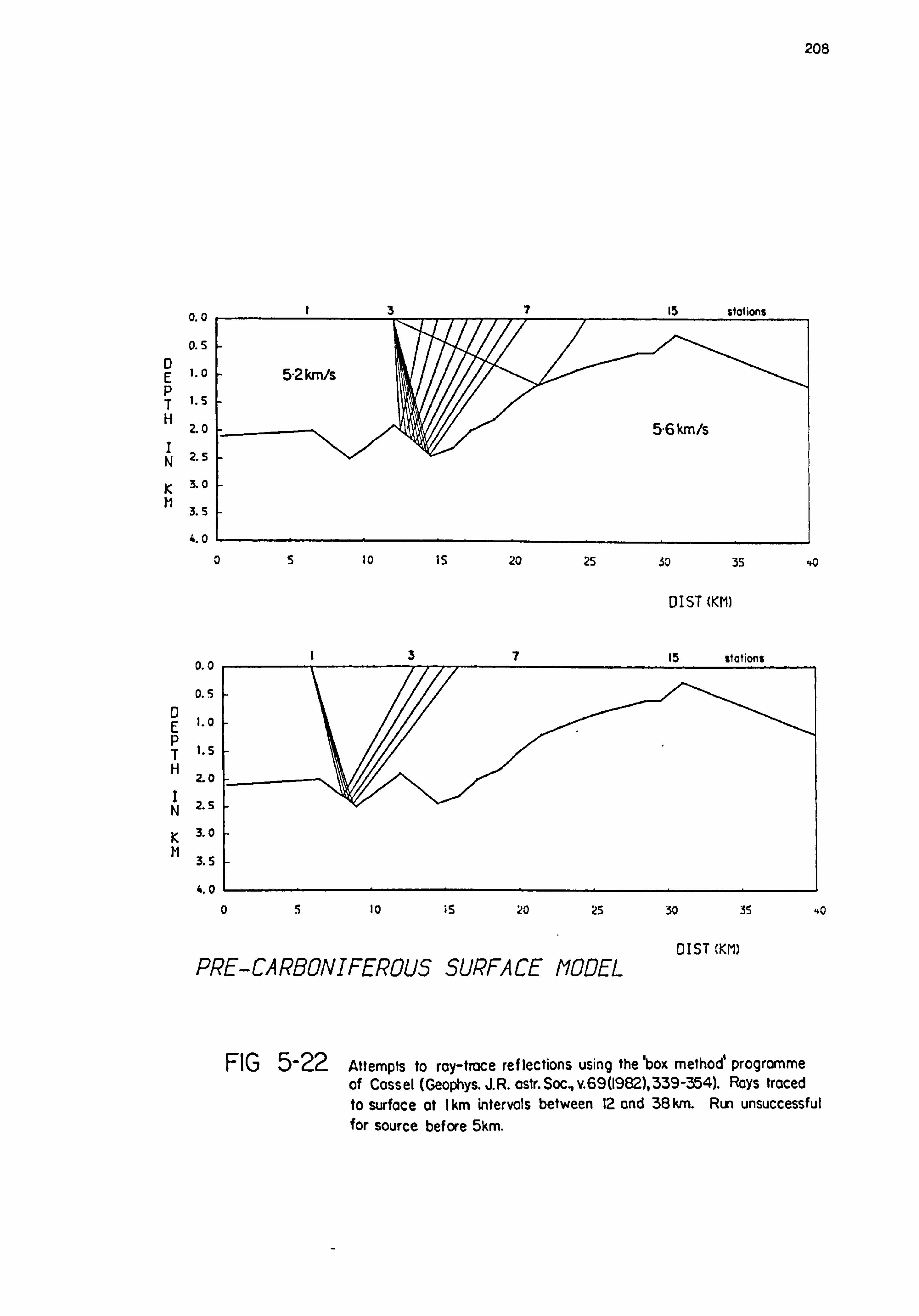
208

0.0

0.5 E

i. o P T 1. s H

2.0

2.5

K 3.0

3.5

4.0

37 15 stotions

5-2km/s

5-6km/s

05 10 iS 20 25

137 0.0

0.5

P t. s

2.0

z. s

K 3.0

M 3. S

t_ 0

30 35

DIST (KM)

15 stations

40

05 10 i5 20 25 30 35

GIST (KM) PRE-CARBONIFEROUS SURFACE MODEL

40

FIG 5-22 Attempts to ray-trace reflections using the'box method' programme of Cassel (Geophys. J. R. astr. Soc, v69(1982), 339-354). Rays traced to surface at I km intervals between 12 and 38 km. Run unsuccessful for source before 5km.

209

W

0 ýo Ui k

Ri

W

0 ýo tri k

ä

W

0 ýo tri k

RE

M3008 -- Ooveholes untamed

f6 12 16 20 a+yJ` 28 32 313

''

I9 ash--ý'' 12

/rte----

2 , Yr

ýj

-0.1

Q0

0.1

0.2

0.3

0.4

0.5

M4035 -- Balldon timed

46 12 16 20 24

23 ýrýi loll fy

28 32

-a1

0.0

0.1

0.2

as

0.4

0.5

M4008 -- Middlepeak untamed

4e 12 16 20 24

13

r5

28 32

-a1

a0

0.2

0.3

0.4

a5

FIG 5-23 Reduced times including later arrival data (---- )

210

W

Ui

ti

RE

W

0 ýo cri k

PC

W

0 ýo tri k

M1010 -- CauLdon Low untlmed

4d 12 16 20 24

. 41

-13ýI.. 11

2-_- _ X12

28 32

-0.1

0.3

0.1

0. z

Q3

0.4

, is

M4023 -- Ramshorn untimed

48 12 16 20 24

11_, 13 11

'12

y 2'c

2

28 32

-0.1

0.0

0.1

0.2

0.3

0.4

Is

M4014 -- Cauldon Low untamed -0.1

0.3

az

0.3

M4

a5

4 tl 12 16 20 T3 ý4 28 32

FIG 5-23 tont

211

subject to picking error than first breaks, some features

are consistent in the data: for example the trough between

stations 9 and 11, and the high between stations 13 and 15.

Since later arrivals have been identified within 5 km north

of the Bonsall Fault (that is within the problematical off-

set distance of Section 5.4.1)., it is possible that they

originated from the northward dipping lower basement inter-

face itself, which may either have an irregular surface or is not too steeply inclined for refractions from it to strike the surface.

5.4.3 Summary - General Observations

The deeper structure along the north-south profile

generally appears to be more complicated and of greater relief than the surface geology implies. The pre-Carboniferous

surface is well-defined by first arrival data, which suggest a general shallowing towards the Woo Dale region (Fig. 5.12).

Refractions from the basement are often observed within 3 km

of quarries around Buxton, although these are frequently preluded for several kilometres by 5.6 -5.8 km/s refractions from

dolomitic horizons within the limestone sequence.

The profile appears to be underlain by two sub- Carboniferous refractors with differing seismic characteristics, but similar velocities. These refractors appear to be divided

by the line of the Bonsall Fault, which may be related to a more important basement fault. To the south of this fault, basement refractions observed from quarry blasts are seen to be coherent and attenuate at a rate less than geometrical spreading. To the north the first arrivals are distinctly higher frequency and lower amplitude, but attenuate at a rate compatible with spherical spreading. These differences are illustrated by the relative amplitudes for several events from

Doveholes quarry (Fig. 5.24). Note that refractions from the

refractor to the north of the Bonsall Fault for quarry blasts do not attenuate as rapidly northwards as those from the

212

FIG 5-24 Relative amplitudes- various Doveholes blasts

stag

Un

Zb

. rL ®--M2011 . --M203C ®--M4011 +--M500S -u--M5032 A--M6004 v--M300E

sc1

Corrected For Heelor, 's low A direct B upper basement refractions C lower -1 of

I/ A

R E L2 A xýo' T

V6 E

A3 M1 P x100

Xw0 1

XI

-30 -20 -10 0

DISTANCE (KM)

-30 -20 -10 0

DISTANCE (KM)

213

Mansfield event (Fig. 5.14). This may be because the latter

signal is three to six times the wavelength of quarry blast

P waves. The better transmission of signal of about 10 Hz

suggests that the upper basement refractor is around 500 m

or so thick.

Refractions observed as first arrivals to the south

can often be traced as later arrivals to the north of the

Bonsall fault. This is thought to indicate that the southern

refractor is downfaulted northwards, and present at depth.

The delay between refractions from upper and lower basement

refractors to the north of the Bonsall Fault may suggest a hidden layer between the two. Similar later arrivals are not

observed at the southern stations.

South of the Bonsall Fault the sub-limestone surface

appears quite irregular and may be cut by faults not evident

at outcrop. Smaller reduced times for stations 1 and 3, for

example, are observed from a variety of azimuths, and the high

at station 3 is similarly shown by station 69 from the DASED1

line. However the reduced times for station 61 seem as large

as those for station 2, so that if there is a basement fault

here it must lie between stations 1 and 61. That station 1

is on the upthrow side of a fault or syncline limb, may be linked with the difference in P wave character with station 2,

the first arrivals at which are generally broader than those

of station 1 even for northern events (e. g. Tunstead M5027

(Fig. 5.10)); thus there may be absorptive material beneath

station 2 but thinned or absent from under station 1, which fills the basement low under station 2 and which filters the

upward travelling P waves. Additionally, first breaks at

station 4 are often similarly broadened.

5.5 The Northern Province

Two profiles lay completely within the northern

province: the northern east-west (NEW) line, and DASED2. Both these profiles had station 14 (re-occupied as station 34 in

214

1980, see Fig. 3.1) in common with the north-south line. The

NEW line additionally had station 51 in common with the

southern east-west profile, and DASED2 was maintained during

a repeat of the 1979 line. Thus the interpretation of these lines is well controlled by the results from the north-south

profile.

This is fortuitous because the data for the NEW profile are not particularly well distributed with azimuth: most

events are from the quarries around Buxton, to the west of the line. Although a few events were detected from Stoney

Middleton, most reversal of the profile comes from shots at Hope Valley quarry (see Fig. 3.7).

5.5.1 Northern East-West (NEW) Line

The NEW profile crossed the north-south profile where the upper basement refractor is shallow and refractions from

the lower basement only seen as later arrivals. The. line

passed both Woo Dale and Eyam boreholes, between which the

sub-Carboniferous surface was expected to dip eastwards. The

ends of the line also lay within the Namurian sedimentary basins

of the Goyt Trough and the Edale Trough, and thus should manifest deeper basement than under the limestone massif.

i) Timed Events

Reduced time graphs for the timed and positioned shots are given in Fig. 5.25. These appear quite varied. Almost

certainly the first arrivals for Ballidon, Longcliffe and Dene

are all refractions, and it is possible that two different

sets of arrivals have been picked: the smaller reduced times

corresponding to the upper basement refractor. If so, then lower basement refractions appear to have been picked for

stations 37 to 41 for all three events. Similarly the reduced times for station 34 are for upper basement refractions. Since the difference in reduced time between stations 34 and 37 is fairly consistent for these events, then a considerable delay

215

-0.1

0.0

0.1

062

0.3

0.4

0.5

-0.1

F13004 -- Oene timed il

48 12, - 16 20 24 28 32

3T ý.

4t


ao

ai

e 0.2 tii

as

0.4

QS

48 t2 ^, f16 20 24 28 32 3

^ý" 'f

. 4-- 37 ff

i3

42 't ff

23

F13015 -- Doveholes timed

-a1

ao

a1

Q2

k as

Qy

015

--` 48 12 aTÖ----- _

40 't

--21* 28 32

ice' ý5

r'

tý


216

FIG 5-25cont

W

0

Ui k

RE

W

0 ýo tri k

It RE

as

a1

0.2

0.3

0.4

QS

--1L I

0.0

0.1

0.2

as

ac

as

F12027 -- Longcliffe timed

34 J-_ ýry

48 12 , 16 -

20-'----2-4_ 28 32 29

27 25

43

r

F13019 -- Ball don timed

49 12 16 20

j. 41

24 28 32

217

between upper and lower refractor arrival times is inferred

for stations 25 and 26 by events F12027 (Longcliffe) and

F13004 (Dene) .

The time shots from Tunstead and Doveholes are a

little harder to interpret. The reduced times for the Dove-

holes event are similar to those from the Longcliffe shot.

This may be credible for the upper basement arrival times,

but not between stations 37 to 41 if it is considered that

Doveholes is too close for lower basement refractions to be

observed (cf. event M3008, Fig. 5.21).

The positioned Tunstead event F12015 is best consid-

ered in comparison with its reduced seismogram section (Fig.

5.26). The arrivals between stations 31 and 25 are interpreted

as refractions from the upper basement refractor, while those

between stations 33 and 38 as direct. The phase travelling at

about 3.5 km/s west of station 38 may be a direct wave through

the Millstone Grit, while the first arrivals at these stations

are probably refractions from the top of the Carboniferous

limestone (as their reduced times are less than those for the

upper basement refractions, and the basement to the Goyt Trough

is not expected to be shallower than that under the limestone

massif).

The same features are evident from the reduced time

seismograms for the larger untimed: Tunstead blast F12010a,

also plotted in Fig. 5.26, except that for this event an early high velocity first arrival is apparent until station 27. If

this arrival is from an inter-limestone dolomitic horizon, it

is strange that it is poorly observed at station 30. This may indicate that such layers are not laterally continuous and that

the arrivals at stations 29 to 27 originate from a similar but

deeper horizon than those for stations 32 and 31 (numerous

dolomitic horizons occurred at depth in the Eyam borehole, see Fig. 1.7). These high velocity arrivals are apparent from the

reduced time graph for this event (Fig. 5.27), and also for

the Sterndale shot F12030 (Figs. 5.26 and 5.27).

The later arrivals for the Tunstead shot F12010a

denoted by the full line are possibly reflections off the upper

218

FIG 5-26

F12010A -- TUNSTEAU UNTIMED

F12015 -- TUNSTEAD POSITIONED

Reducing velocity 5-6km/s / direct wave ý.. upper basement refraction 8i reflection ýi lower basement refraction

051 Sec 0 "5 1 Sec

-a i

Luj 0.0

0.1 14 Q `O

ri 0.2

0.5

-(L I

219

F13001A -- Tunstead untamed

i

3f

:

_----"

8 f16 20 24 28 32

33 60 '

42 41 3i

26


Cj QO

Q1

SO Q2 tri

0.3

RE 0.4

0.5

4a 12 16 20 24 28 32

37 15.5 34tß 27

33 `33

32 3

1- ` %

42 4130 %% %

512,5

F12031 -- Doveholes untamed _-a I

ao

10 az

0 .3

0 .4

O. s

48 12 mid--I----2pß ----- kFzýý-- 32 rti 33

zY

. I'

42

FIG 5-27 (a) Reduced time graphs

Q 0.0

Z 0.1

0.2

0.3

11 0.4

9.5

220

F12030 -- Sterndate untamed

e 12 16 20 ý.

-

ýýt-ý ^3ý

33

3, 51

42 41

29t ` 32

S

S

26 25

F12004 -- Brierlow untimed -11

0.0

0.1

'o ui 0.2

0.3

11 0.4

0.5

--O. i

46; 12 16 20 24 28 32

_" 3T ý

33 'k 35 34 --t'52

42

5!

25

F12026 -- Waterswallows untimed

0.0

o. l

az

k Q3

0.4

0. S

4e 12 "Si%

16 20 24 28 32

42

,5

FIG 5-27(a) cont

221

-a1

Q 0.0

V 0.1

0 10 0.2

0.3

11 0.4

9.5

-0.1

ao

10 a2

tii ( 0.3

Rzf 0.4

0.5

-a. 1

F12028 -- Stoney Middteton untimed

68 12 16 20 24 28 32

27

---33 mai---

26 25, 41

F11009 -- Smalidale untamed

3; KM

4e ý2 1633 `mot 23 24 28 32 32 .

t

3., It

F12011 -- Hope Valley untamed

0.0

aI

Ii 0.2

0.3

ay

as

4e 12 1 , 16 20 24 28 32

-j3 V

33 lti 'f"

Xi 27 ,

{ ýc

r`i' 42

FIG 5-27(a) tont

222

FIG 5-27(a) cont

W

0

Lri

If

W

k 0

Ui

It

F11016 -- Warlow untimed -(L i

0.0

0.1

0.2

0.3

0.4

0.5

48 12 16 20 24 28

37 35

2? ?

23;

32

F12032 -- Cauldon Low untimed

46 12 4 16 20 24 28 32

12 f) '_"i q-ý

25

a0

aI

0.2

0.3

0.4

as

223


T *, i I 15

I's M E3

SZ %2 w

4'S8 t

t, t7

V Lsq= 5.09Km/S

-16 -12 -8 -4 048 12 16 20

DISTANCE KM


T4

M E3--

17

to

°~' V Lsq= 5.3SKm/S

-16 -72 -8 -4 048 12 16 20

DISTANCE KN

F12031 -- Doveholes untamed

T 14 M

"<s E C

4t

J

2 ý3 41

V Lsq= 5.58Km/S

-20 -16 -12 -d .404d 12 16 20 24 28

DISTANCE K/Y

FIG 5-27 (b) T-X graphs

224

F12030 -- Sterndate untamed

ý3 M E g t1

17 023

S ý ý? 2

%l %2

i

V lsq= 5.47Km/S *5 3 ý, ýý ýl

0 -16 -12 -8 -4 0

F12004 -- Brierlow untamed

49 iz 16

DISTANCE KM

T 925

25 M4

St ''7 E

JS 2

"tet 'Z

V lsq= 5.32Km/S 32.3

t' *6 -3

'40

L -20 -16 -12 -a -4 34a 12 16 20

DISTANCE KM

F12026 -- Waterswallows untamed

T I 4--

E 3-- 27

11,. 2 yl

3y3

V Lsq= 5.39Km/S

-20 -16 -12 -8 -4 04d 12 16 20 24

DISTANCE KPf

FIG 5-27(b) cont

F12028 -- Stoney Middleton untamed

225

T

14 -- Z. ý M E3 *5s

"37

S i 031

V Lsq= 5.36Km/S 7 b -4 -2 0246e 10 12 14 16 to 20 22

DISTANCE KIT

F1 1009 -- Sma l lda le unt med

14

M E3

S2 ýý

V Lsq= 7.60Km/S

a -6 ,zoiwe ýo 12 14 16 is DISTANCE KM

F12011 -- Hope Valley untimed

T I4ý.

t 42

M Es

,

Z

i

V Lsq= 5.14Km/S

2 -8 -4 0ie 12 16 20

DISTANCE KN

FIG 5-27(b) cont

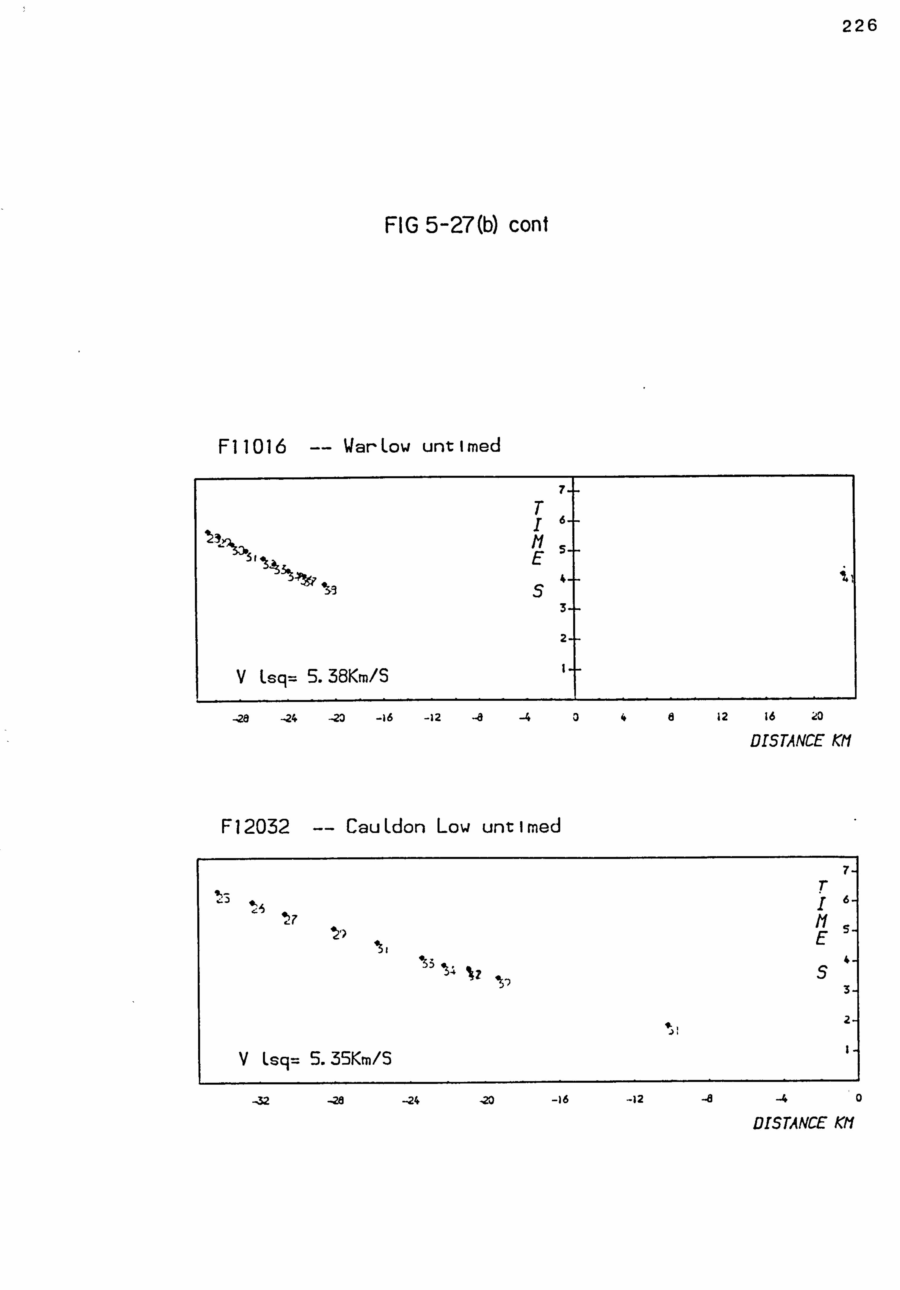
226

FIG 5-27(b) cont

F11016 -- Warlow untamed

7

T I6

E i, 4--

3--

2--

V lsq= 5.38Km/S

-28 --24 -23 -16 -12 -d -4 046 12 16 20

DISTANCE KM

F12032 -- CauLdon Low untamed

7 T

ý5 I 6-

t7 M E

4S 4- 3-

V

ýI

lsq= 5.35Km/S

-32 -29 -24 . 20 -16 -12 -6 -4 0

DISTANCE KN

227

basement. If they can be correlated with the later arrivals

seen in the P wave coda at stations 25 and 26, then the travel

time curve suggests a mean overburden velocity of about 5.2

km/s. These wide-angle reflections must not be confused with

the earlier large amplitude, lower frequency arrivals also

seen in the coda (dashed line), which may be refractions from

the lower basement.

ii) Northern Quarries

A selection of reduced time graphs and T-X plots for

untimed blasts from northern quarries are given in Fig. 5.27.

Except for those observations on the Millstone Grit, the T-X

curves are as linear as those. from the north-south line.

Least-squares velocities for direct waves range from 5.2 to

5.8 km/s (for inter-limestone refractions), and 5.4 to 5.9 km/s

for basement refractions, with no difference between eastward

and westward shots. Direct wave velocities on the Millstone

Grit vary between 4.6 and 4.9 km/s, but mainly these are down-

dip velocities for refractions off the top of the limestone.

These reduced time graphs vary more between events from similar sources than those for the north-south profile,

and consequently it is more difficult to discriminate against high velocity 'direct' waves from these plots alone. However,

the same criteria for the discrimination of basement refractions discussed in Section 5.3.2 still apply, and the inter-limestone

refractions are invariably higher frequency and lower amplitude than those from the sub-Carboniferous horizons. For example Fig. 5.28 illustrates the relative amplitudes for several Tunstead blasts, from which upper basement arrivals are commonly

picked as first breaks east of station 31, and west of 39 (although the lnA-X relationship west of Tunstead is complicated by the anomalously high relative amplitudes between stations 35

and 39).

Interpreted refractions for quarry blasts from (a)

Tunstead and Topley Pike, (b) Doveholes and Waterswallows,

and (c) Dow Low, Brierlow and Sterndale have been plotted in

228

FIG 5-28 Relative amplitudes - various Tunstead blasts

x100,

Uncorrected A sc42

iih,

IP st-25

3

2 ®--F12010ß . --F13020 xio-' o--F11007

1 +--F11013 v--F13001A x--F12002 o--F13023 e--F13005 o--F12033 xio6 v--F13001ß o--F12010A

St

-10 0 10

DISTANCE (KM)

-to 0 10

DISTANCE ; KM)

229

Fig. 5.29 in the same manner as Fig. 5.12. Both Tunstead and

Dow Low accord with a refractor dipping eastwards of station

34, such that the reduced time for station 28 is greater by

about 0.1s. This corresponds to an increase in depth of

1.4 km by inserting the delay, a, into Vo. a/cosec for Vol

Vr of 5.2,5.6 km/s. The deepening sub-Carboniferous surface

off the limestone outcrop is also manifest by these data, yet

for the Doveholes events (Fig. 5.29b) the reduced times are

greater for stations in the Goyt Trough region. However, as

noted for the timed event F13015 (Fig. 5.25), it is possible that the first arrivals to the west of station 36 are from the

lower basement refractor. The larger reduced times to the

east of the profile may also correspond to lower basement

refractions picked where upper basement arrivals were not well

recorded.

Shots collinear with the line from Dow Low, Brierlow and Stoney

Middleton quarries are plotted as reduced time seismograms in

Fig. 5.30, where direct waves are denoted by the full line,

upper basement refractions by the dotted dashed line, and interpreted lower basement refractions by the dashed line.

Like the Tunstead events (Fig. 5.26), broadening of the P

waves for stations 25,26 and 38 to 42 is apparent, and probably indicates an increased attenuation of high frequencies by the

cover of more absorptive Millstone Grit (assuming, that is,

there is no facies change in the limestones off the massif).

Lower basement refractions can only be easily identi-

fied for eastern shots at stations west of about station 33,

that is greater than around 12 km from the shot. This may

correspond to the critical distance for refractions from the

lower basement refractor. These arrivals are typically of lower frequency and higher amplitude than those from

the upper basement refractor, and the delay between these two

arrivals seems to lessen towards stations 37 and 38. For

western quarries, lower basement refractions are observed east from about station 29 (e. g., Tunstead F12010, Fig. 5.26),

although they can only be confidently identified east of station 28.

FIG 5-29 230 Vred = 5.6km/s

(a) Tunstead & Topley Pike

0 N N

.2

"3

"4

42 41 40 39 38 37 36 35 34 33 31 30 2928 27 26 25

(b) Doveholes 8 Waterswallows

"I

.2

"3

"4

42 41 40 39 38 37 36 35 34 3332 31 30 2928 27 26 25

(c) Dow Low group

v CD N

.2

"3

42 41 40 39 38 37 36 35 34 33 32 31 30 29 28 27 26 25

i,

231

F12018 -- DOW LOW UNTIMED F12004 -- BRIERLOW UN TIMED

Sec "5

Sec

FIG 5"30 Key see FIG 5-26(Vr=5-6km/s)

232

F12028 -- STONEY MIDDLETON

UNTIMED

F12011 -- HOPE VALLEY

UNTRIED

Sec

FIG 5-30 cont.

Sec 05I1.5

0 "5 1

233

U d

U)

ti ti j

Ö O j V

i i

M D N

C 0 U

0 F) In

C, LI-

ti ti j

W J Ö J J

i i

Oý O Oy

LLý

U d fV

0

N

L

lp

0

234

Broadside quarry blasts from the north such as Hope

Valley, Smalldale and Eldon Hill (see Fig. 3.7) often manifest eccentric reduced time graphs such as F11009 (Smalldale)

which cannot be resolved through picking error or mislocation

of the source. The nature of the first arrivals at stations 34 to 38 (Fig. 5.30) suggest they may be from the lower base-

ment, and that those at stations 32 and 33 from the upper basement refractor. The event contrasts with F12011 (Hope

Valley), whose reduced time graph (see Fig. 5.27) is similar to those for events closer to the line. The reduced time

seismograms for F12011 (Fig. 5.30) show higher frequency first

arrivals consistent with an upper basement refractor origin,

while west of station 34 broader later arrivals can be identi-

fied, interpreted as from the lower basement refractor.

iii) Cauldon Events

Apart from the timed events, only two shots from the

southern province have been considered, both from Cauldon Low.

All the first arrivals appear to come from the upper basement

refractor, for which the reduced time graphs (Fig. 5.26)

accord with the stb-Carboniferous surface' suggested by the

on-line events. Later arrivals interpreted as lower basement

refractions can be traced along the entire line, although only with difficulty east of station 31 as the signal is close to the ambient noise level (Fig. 12032, Fig. 5.30).

5.5.2 Summary of Interpretation

Fig. 5.31 sketches the interpretation of these data. It is evident that the base of the Carboniferous between Woo Dale and Eyam is not smoothly dipping, but that there is an increase in slope roughly between stations 32 and 30. On the Bouguer anomaly map (Fig. 1.12) this corresponds to a belt of closer spaced contours, but the feature is not obvious from either the geological section (Fig. 3.10), or the surface suggested by the high velocity inter-limestone refractions, which probably originate from a much shallower horizon (e. g.,

236

the Woo Dale Dolomite, the Upper Millers Dale lava, etc. ).

A similar three-layer interpretation of the deep

geology along the NEW profile using gravity data has been

received from R. Barker (University of Birmingham, pers.

comm. ). There is less seismic information on the lower

basement refractor but the evidence suggests a general

shallowing towards stations 37-38, which co-incides with

the hinge region of the massif: marked by scattered Holkerian

inliers and the high on the Bouguer anomaly map (Fig. 1.12).

This region also co-incides with where the Bonsall Fault

splits into several smaller faults, and where the strike of

which turns towards the north (Fig-1.9).

(Note that the northern profile was dog-legged between

stations 39 and 40, such that any continuity of the time

section here may be deceptive. )

5.5.3 DASED2

A representative selection of reduced time graphs for this line are given in Fig. 5.32. As the two 1981

profiles were principally designed to use blasts from

Tunstead quarry (McDonald 1982), most data comprises events from the quarries around Buxton, although sufficient events from Shining Bank, Ballidon, etc. have been considered to

give adequate reversal.

Like the NEW profile, all refractions observed as first arrivals can be interpreted either as from the upper basement, or refractions from layers within the limestone

sequence. Few later arrivals have been identified as lower

basement refractions for this line because a) only stations at the ends are outside the critical distance from shots close to the line, and b) quarry blasts from the southern province were not of good enough quality for later arrivals to be confidently picked.

Least-squares velocities along the profile are typical

of most observations on the limestone massif, although the direct waves are slightly slower (5.1 - 5.5 km/s) as the line

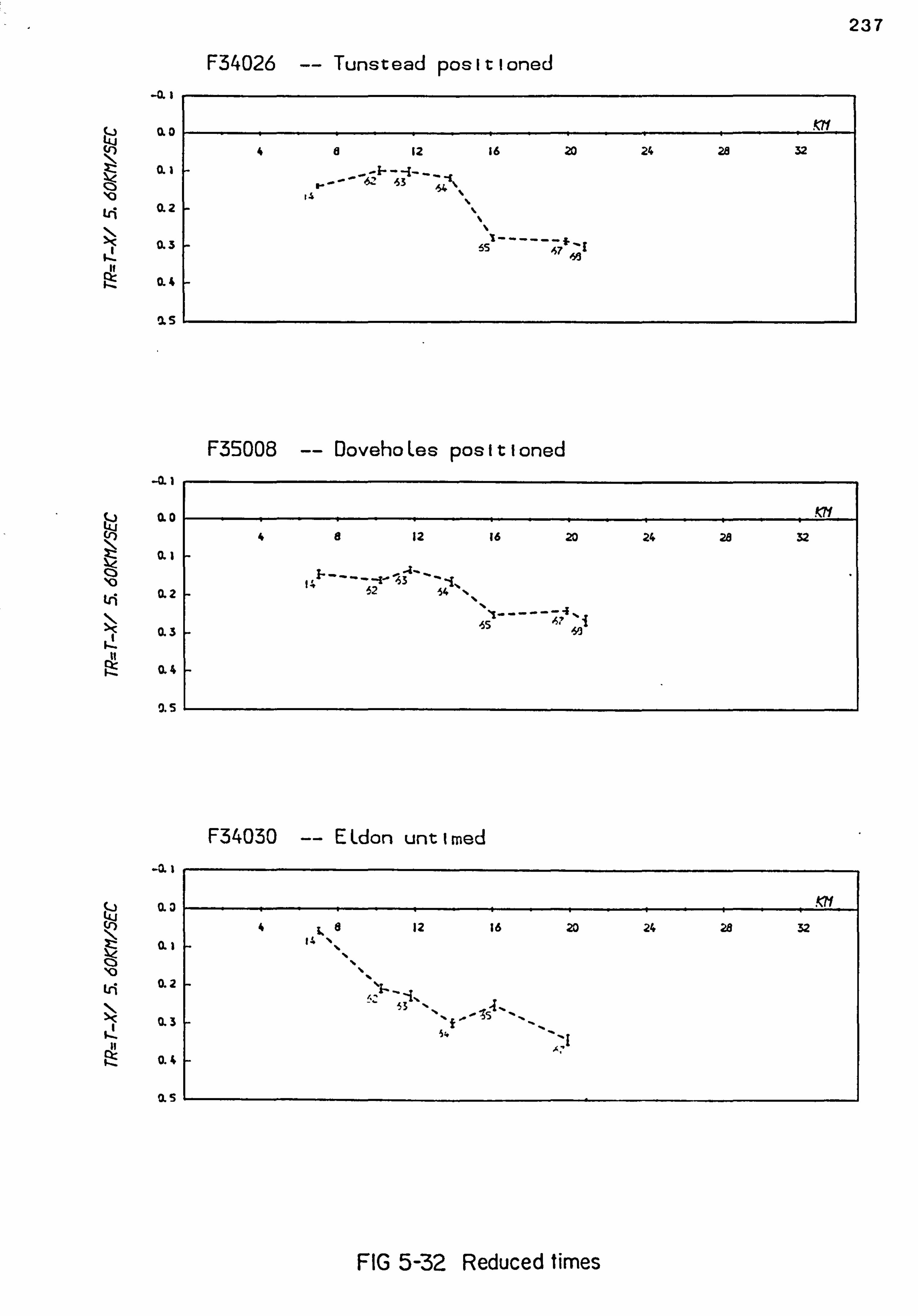
237

-a'

0.0 LIJA

0.2

0.3 ti

0.4

as

--a. i


4B 12 16 20 24 28 32

" 62 43

,s

ßi3


0. o z

ai

0.2

0.3

11 0.4

IS

-3.1

48 12 16 20 24 28 32

S- --ß' 3- Yý 62 S4

35 ,A

F34030 -- Eldon untimed

0.3

Q

`O 0.2

k 0.3

0.4

as

48 12 16 20 24 28 32 1s

sy h, t


238

F33025 -- Dow Low untamed -V. I

0.0 LLJ

ai

0.2

k 0.3

0.4

0.5

B 12 16 20 24

64 s ýc sa 61

28 32

F33030 -- Brierlow untamed -. L% i

8 12 16 20 24

65 -1, 47

3`£'-ý-- 64 . --' s, s9

iz

28 32 Q 0.0 C 11-1

0.1

Lri 0.2

k 0.3

11 0.4

, is

-a l

0.0

V 0.1

0.2

0.3 ti

0.4

, is

F37003 -- Tunstead untamed

f8 12 16 20 24 28 32

S2 t= ý

,9

FIG 5-32 cont

239

-a 1

0.0

V

a2

as

0.4

9.5

-41i

F37006 -- Longcliffe untamed

48 12 16 20 24 28 32

14i ------ 53

65 6a

F33026 -- Shining Bank positioned

M0

ai

Lri 0.2 N k 0.3 ti RE 0.4

as

-a'

0.0 Z

0.1

tri 0.2

N 0.3

11 I 0.4

as

48 12 16 20 24 28 32

a -A ll

__---54 4S i 60

Y

6A

F32020 -- Stoney Middleton positioned

4d 12 16 20 24 28 32

Si f

55 ff

FIG 5-32 cont

240

-0. l

Q ao co

al

Lri 0.2

0.3 ti

0.4

as

-M i

t 0.0

0.1

`O 0.2

0.3

ti 0.4

2S

--I i

0.0

X- 0. i

t 0.2

k 0.3

tt 0.4

0. s

F32021 -- CauLdon Low untamed

46 12 56 20 24 28

14 54 65 66

67 ß`. i

32

F32028 -- Cauldon Low positioned

46 12 16 20 24 28 32

14 - "-'- ------_"_

i 59

F34032 -- Balltdon untamed

i8 12 16 20 24 28 32

FIG 5-32 cont

241

mainly crosses Brigantian Monsol Dale and Eyam limestones

(see Fig. 1.5). Direct wave velocities of 3.5 -4 km/s

are observed between stations 67 and 68, which lie on the

Millstone Grit.

For the identified upper basement arrivals, the

reduced time graphs indicate a gently dipping refractor

between stations 14 and 67, while the reduced time for station

68 is consistently larger as the 'station lies upon the Stanton

syncline (see Fig. 1.9). The most self-consistent reduced

time plots are for shots from the Dow Low Group (e. g. F33025)

the first arrivals from which (Fig. 5.33) are clean, of large

amplitude relative to their P wave coda, and correlate well between stations. These arrivals contrast with the lower

amplitude precursory direct waves of the Tunstead event F37003.

The first arrivals from Cauldon (F35021) are almost

certainly upper basement refractions, and their reduced times

concord with the basement topography implied by northern

quarries. The shallow syncline between stations 14 and 65

agrees with the surface geology, where the line crosses a

central outlier of Eyam limestone.

Even with the paucity of later arrival observations, it does not appear that the line crosses the postulated base-

ment fault evident between stations 7 and 9 on the north-

south line.

5.6 The Southern Province - Southern East-West (SEW) line

Data from south of the Bonsall Fault comprises events

recorded by the southern half of the north-south line, and the whole of the SEW line. The closest stations between

these profiles were 2 and 49 (see Fig. 3.1).

Most of the data recorded by the SEW profile consists

of broadside shots from northern quarries, and shots close to the line from the Cauldon Low group to the west of the

profile (see Fig. 3.7). A few eastern shots from Wirksworth

I O ýö tiw j

3 "ý O

Wý

m

i i

U1 N 0

N-) Ll-

ti j

4 W

t i

M O O ti N-) tlý

ti ti Z

Z

Z

t

`O N O M

i

242

U

0

E

U)

M M

LL

U d

Cl)

LO

0

U N

243

and Ballidon have been considered, as well as the local

earthquakes from Stoke-on-Trent (see Section 4.5.3) which provided seismic sources only about 25 km off the western

end of the profile.

It is postulated that the refractor beneath the Carboniferous in the southern province is equivalent to the lower basement refractor to the north of the Bonsall Fault.

The Caldon Low borehole (Fig. 1.7), to which station 58 was nearest, encountered sandstones under the limestone outcrop, and it is possible that these sub-crop beneath much of the

southern province (Chisholm 1981; see Section 1.2.2). These

sandstones probably thicken westwards into the North Stafford-

shire Deep (Fig. 1.4). The Bouguer anomaly map (Fig. 1.12)

suggests the basement dips steeply west of Caldon Low, which is also inferred from the surface geology (Aitkinhead, IGS Leeds, pers. comm. ).

5.6.1 Velocity Analysis'- Shots close*to the Line

Representative T-X plots are shown in Fig. 5.34.

From the quarry blast data it is apparent that direct waves through the basinal facies are slower than those observed on the massif (i. e., for all stations north of 3). Consequ- ently most T-X curves manifest distinct two-layer cases, and refracted arrivals are more easily identified. Eastwards from Cauldon Low and Wardlow, direct wave velocities are typically 4.6 - 4.8 km/s_; westwards from Longcliffe and Ballidon (though slightly off line) also about 4.8 km/s, and westwards from Dene and Middlepeak, both east of the Dove- dale transition, about 5.1 km/s.

Refracted arrival velocities from quarry blasts

appear no different from those determined along the southern end of the north-south profile, and are interpreted as from the same (i. e., the lower basement) refractor. Eastwards from the Cauldon Low group, refractions arrive at about 5.7 -5.8 km/s; westwards from Ballidon and Matlock the observed

244

C23015 -- Middleton untamed

t9 T I M E3

S 2

tG

ý7 V Lsq= 5.24Km/S

02468 10 12 14 16 18 20 22

DISTANCE KM

C22017 -- Upperwood untamed

J%

ý5

T I4

M E3

S 2

49

V Lsq= S. 14Km/S

32468 10 12 14 16 18 20 22

DISTANCE KM

C23002 -- Dene timed -- ý9 i

ý, I Iý M E3

S 2

-3

V Lsq= 4.60Km/S

02466 10 12 14 16 18 20 22

DISTANCE KM

FIG 5-34 T -X graphs

245

C22009 -- Stoke Event

ä9

T t2

13 M I

16 t7

to E

t9 2

V tsq= 6.49Km/S

-32 -26 -24 -20 -16 -12 -6 -4 0

DISTANCE KH

C21008 -- Cauldon untamed

T I M E3 -- *49

'so s F2

F3 2--

V lsq= 4.96Km/S ,5 ýv

4 -12 -10 -8 -6 -4 -2 024

DISTANCE Kn

C21002 -- Ball don untamed

T I` M E;

S 2

I

ý7 ý

fý

t9 1

V Lsq= 4.81 Km/S fý ý3

S1 , Km

02468 10 12 14 16

DISTANCE K! 1

FIG 5-34 tont

246

velocities are slightly less, about 5.5 -5.6 km/s. These

may correspond to up- and down-dip velocities respectively for a westward dipping refractor.

Unlike the Mansfield events, those from Stoke-on-

Trent were nearly collinear with the SEW line (see Fig. 4.15).

Being about 25 km from the western end of the line, these

first arrivals are almost certainly basement refractions.

The apparent velocity of about 6.5 km/s is much higher than

observed for the quarry blast data, and this may be because

(a) the arrivals originated from where the basement dips

more steeply westward than the region sampled by the quarry blasts (i. e., a higher up-dip velocity). To give an apparent

velocity of 6.5 km/s requires a dip of approximately 14

degrees for overburden and refractor velocities of 5.2 and 5.6 km/s respectively. For overburden of velocity 4.8 km/s,

the dip needs to be about 20 degrees.

(b) the arrivals are from a deeper refractor of higher

velocity.

Unfortunately because stations 54 and 55 never worked, it is difficult to estimate the cross-over distance for shots from Cauldon and Ballidon quarries. Certainly from Cauldon

basement refractions are consistently first arrivals at

station 53, which suggests a cross-over of a least 8 km. Thus

taking the thickness of limestone from the Caldon Low bore-

hole, and assuming the velocity of the Redhouse Sandstones as 4.5 km/s, this means the basement is at most about 1 km deep

around station 53 for a limestone velocity of 4.8 km/s and a basement velocity of 5.65 km/s. Similarly, direct arrivals from Ballidon occur as first arrivals as far as station 53

(Fig. 5.34), 6 km from the shot.

5.6.2 Shape of the Basement - Reduced Time Graphs

A. Broadside Events from the North

The quarries to the north around Buxton are about the same distance from the NEW line as the Stoke tremors.

247

-a1

o. o vn zz- ai 0 10

Q2 N

0.3 I-

0.4

0.5

0.0

ai

0.2

N Q3

0.4

as

--0.1

Cj 0.3

0. I

0.2

Q3

0 .4

0.5

C22009 -- Stoke Event

£n "8 12 4Lbi-gam 23' j 24 28 32

.! S s2 49

r

so

C22005 -- Brierlow untimed

fe 12 a 16 20 24 28 32 34

---I- - SO 57

I- S!.

5?

C21004 -- Topley Pike untimed

4e 12 16 ;

20 24 28 32

I' . 5ý


248

-0.1

0.0

0. I 0 10 a2

0.3

RE 0.4

0.5

C22024 -- Doveholes positioned

e !z"! 53 11,1 20 52

' 5,5ý .. S.

5,49

S r,

24 28 32

ýI

L 0.0

a1

10 a2

0.3

RE M4

Is

L ao uý

aý 0 ýo

a2

k Q3

ý QL

0. S

C23009 -- Htndtow timed

48 12 16 20 24

4Y 47

54

28 52

C22019 -- Tunstead timed

28 32 r9 $2 $6 20 24

FIG 5-35 cont

249

W

0 1o cri k

n

LU 1-1 N 0 1o tri

0ý

W

0

tri

k

it

C23015 -- Middleton untamed

4 12 16 20 24 28 vs

-------- * --

vs Si so

i s: ý--- 59

32

-0.1

0.0

0.1

0.2

0.3

0.4

0.5

C22017 -- Upperwood untamed

48 12 16 20 24 28 32

5 47 If

53 5`Y

-5i

F_ýý_I _ýý!

S5 50 51 57

ao

0.2

0.3

0.4

0.5

C23002 -- Dene timed

49 12 16 20 24 28 32

.

S,

_a I

as

aI

M2

0.3

a4

as

FIG 5-35 tont

250

W

0 ýo Ui k

11

W

0 ýo Ui k ti

19E

0 1o Ui

It

C22025 -- Wardlow untimed

12 16 20 4

57

59

52

ý'I

24 28 32

-a 1

0.3

0.

a2

a3

0.4

0.5

C21008 -- Cauldon untamed -0.1

22

0.1

0.2

0.3

Qi

as

t 1 `. a 12 16 23

5o S! "ýý"

;^ sei

24 28 32

C21002 -- Batt don untamed

12 47ßm - ý- -`^

'r.

24 28 32

-a .i 0.3

a:

az

0.5

Qy

QS

FIG 5-35 tont

251

The reduced times for these events (Fig. 5.35) all show a broadly anticlinal structure. For the northern quarries the

axis appears to be between stations 52 and 53, while for the

Stoke event it seems to be offset eastwards to station 50.

The Cauldon Low anticline (see Fig. 1.9) also commonly

appears on these plots between stations 57 and 58.

Not all events manifest as steep a dip westwards of

station 53 as the Stoke tremor. Events C21004 (Topley Pike),

C22024 (Doveholes) and C23009 (Hindlow) do, for example, but

not C22005 (Brierlow) and C22019 (Tunstead). These differences

are not systematic with distance or azimuth from the line.

An easterly dip between stations 52 and 49 is evident from most reduced time graphs, while events C22005 (Brierlow)

and C23009 (Hindlow) suggest that this is the western limb

of a shallow syncline, perhaps less than 8 km wide. If so

then this feature may correspond with the syncline suggested between stations 1 and 3 on the north-south line (see Fig.

5.16), where stations 1 and 52 lie on the south and western (fault-bounded? ) margin. This basin appears as a Charnoid-

trending low on the Bouguer anomaly map.

B. Quarries close to the line

From Cauldon (e. g. C21008) and Wardlow (e. g. C22025), basement refractions are first observed at station 53. These

data (Fig. 5.35) show the basement to shallow to station

station 51: offset 2 km eastwards from between stations 52

and 53. For the velocity model discussed above in Section 5.6.1, this corresponds to a refractor about 1.3 km deep.

Note that the reduced times for the Stoke event (C22009) this

offset is about 3.5 km. The differing offset is either due

to the different azimuth for the events, or that the first

arrivals for the Stoke event originated from a deeper basement.

This latter possibility is thought unlikely because a similar 3.5 km offset is not observed for the axis of the Cauldon Low

anticline.

252

West of stations 52 and 53, the increase in reduced

times for the Cauldon events (between stations 51 and 50)

appears more pronounced than that for the quarries of Upper-

wood (C22017) and Middleton (C23015) to the east of the line.

These data imply the depression to be a minor feature, and

the Middleton event also shows the basement to shallow further

eastwards to station 47. Generally, the quarries to the east

of the line manifest a basement dipping west of station 53.

The timed Dene shot (C23002) manifests as steep a westward dip

as the Stoke event, but for the untimed Middleton blast

(C23015) the incline appears far more gentle. For the Ballidon

(C21002) and Upperwood (C22017) events, the basement seems to

dip less steeply west of station 56 than it does between

stations 53 and 56.

5.6.3 Reduced Time Seismograms

A selection of reduced time seismograms are plotted in Fig. 5.36. With the exception of station 50, basement

refractions generally appear most coherent between stations 49 and 53. West of station 56 P waves often progressively broaden; this is presumably due to the filtering of the signal by the westwardly thickening sandstones beneath the limestone,

and also by the Millstone Grit for signals recorded at station 59.

. For the Stoke event C22009 the first arrivals between

stations 59 and 56 are of lower amplitude relative to their

coda than those recorded between stations 53 and 49. Their

signal waveforms also appear more complicated and of higher

frequency. These effects may be due to either interference by

later arrivals from a shallower horizon not present beneath

stations 53 to 49, or lateral change in the overburden.

In terms of_freguency content and interstation coherency, the first arrivals at stations 49 to 53 from northern quarries

are very similar to those from the Stoke event (e. g., Tunstead

and Brierlow untimed, Fig. 5.36). It is thus thought likely that

LL -

ti j

J

O

O Vv

(0 r7 lf') C9 U-

I, , Uli

0 1

>lz

U O O

253

C) a En

)

C 0

v v

C

E N O

.a

N

Ü 0

M

LO

>, U 0 >

Cc U 7

0) N

254

Pýj Zz

ti j

3 O J W 1-, Qz

Ln O O

V

z

F. j

O W ti cr)

M N O

V

v

0 M;

O Lh

t7 ý U

v

In

O

LO

9

0

C22017 -- UPPERWOOD UNTIMED 023015 -- IMIDDLETON UNTI MEL

L-

Sec

Sec FIG 5-36 cont.

051

256

they originate from the same refractor. For these northern

events, a lower amplitude, higher frequency precursor to

these basement refractions can be traced west of station 56 (dotted and dashed line). This earlier arrival is inter-

preted as a refraction from a shallower horizon similar to

the upper basement refractor under the northern province. Therefore for events whose reduced times manifest a refractor less steeply dipping west of station 53, this precursory phase was of large enough amplitude to be picked as a first

arrival. The phase can also be observed for the blasts from

Middleton and Upperwood quarries (Fig. 5.36). That it arrives progressively earlier than the deeper basement refractor suggests a westwardly thickening layer.

The refracted arrivals between 49 and 53 are

generally similar in waveform to those observed between

stations 1 and 6 on the north-south line, and suggest the

presence of only one sub-Carboniferous refractor: i. e. no later arrivals interpreted as refractions from a deeper horizon. The signals recorded at station 50 are consistently atypical of the group: they are low amplitude, complicated and not easily correlated with adjacent stations. This may either be because the station lies close to a postulated basement fault (cf. Figs. 5.35) or because the station was situated on a small Millstone Grit outlier (see Fig. 3.1).

Station 49 was sited on the same outlier, and the recorded first breaks Are often (a) of lower frequency than the adjacent stations (e. g. the Stoke event), and (b) 'the P wave coda contains later, high frequency arrivals (e. g. Tunstead C22023),

possibly reverberation.

5.6.4 Comments on Interpretation

The interpretation of the SEW profile is summarised by the cartoon of Fig. 5.37. The (Devonian? ) sandstones encountered by the Caldon Low borehole are labelled as the Redhouse formation, and have been assumed to underly the

257

59 58 57 56 53 52 51 50 49 48 47

M. a Din tian M. G

.! ' R. Hs Sandst

2T?, Lower Basement F?

3 refractor Approx. Depth (km)

FIG 5-37 Sketch of interpretation- SEW line

258

length of the line. As the refractor velocities appear

very similar to those measured for the north-south profile, the basement is taken to be the same. The arrival time

suggests that the shallower refractor to the west also has

a similar velocity.

Despite the lower velocity of the basinal limestone-

shale sequence than its equivalent massif succession, the

shallow Redhouse sandstones have not been considered as a

refractive horizon because refractions are not noted for at least 4 km from Cauldon Low, and 6 km from Ballidon quarry,

even as later arrivals. The distance at which basement

refractions are observed implies a basement about a kilometre

deep around stations 52 and 53. This is comparable with the

depth of the basement under the massif and thus the basinal

region is not necessarily marked by deeper basement.

The surface geology west of the Dovedale Transition

is characterised by increasing high amplitude folding towards

the west (see geological section, Fig. 3.11), which was

possibly syntectonic with the tilt-block mechanism discussed

by Miller and Grayson (1982). The general coherency of the basement refractions implies that the basement itself was not involved in this folding, although the Cauldon Low anticline seems to be a basement feature.

The shallower refractor towards the west of the line

may correspond to the upper basement refractor to the north

of the Bonsall Fault. This horizon either thins through over- lap on the older basement, or was largely eroded at the base

of the Devonian or Carboniferous. It is possible that the

sequence thins completely eastwards, or may subcrop in patches under the southern province: in the. basement depression between

stations 47 and 52 perhaps.

5.7 General Notes

This interpretation of the seismic refraction data tends to vindicate the notion that the Dome can be divided

259

into two sub-Dinantian provinces, separated approximately by the line of the Bonsall Fault. To the north the sub-

Carboniferous refractor appears to shallow towards Woo Dale.

From Woo Dale to Eyam this refractor deepens by some 1.4 km

to about 1.7 -1.9 km, which is consistent with the depth to

the Ordovician shales in the Eyam borehole. Thus this upper

basement refractor is considered to be Ordovician, although

these shales must either overlie the volcanoclastics encountered by the Woo Dale borehole, or vice versa.

In the southern province there is a strong Charnoid

influence on the geology, and it is tempting to consider the

sub-Carboniferous refractor in this region to be of Charnoid-

type material. To the north this lower basement refractor

may be downfaulted across the line of the Bonsall Fault by

some 1-2 km, depending upon the mean velocity of the Lower

Palaeozoic cover. The SEW line seems to be underlain by a

similar refractor, although towards the west the lower base-

ment refractor appears to dip beneath another lower Palaeozoic

refractor.

Neither basement refractor appears to have any sub-

stantial vertical velocity gradient, which might have been

expected were the Dome underlain by granodioritic material similar to the intrusions flanking Charnwood Forest (0.5 per

sec determined by Whitcombe and Maguire (1981b)). Additionally,

the near-surface velocities for the Leicestershire granites

are about 4.7 -4.9 km/s, or 5.2 -5.4 km/s at a depth of 1 km;

these are still lower than the 5.5 -5.8 km/s determined for

the refractors beneath the Dome. However, this does not

completely rule out granitic plutons deeper than these data

sample: that is, deeper than about 3 km, 'supporting' the Dome.

The velocities determined for the upper basement

refractor under the northern province fall within those

measured for the Ordovician in the Beckermonds Scar borehole:

between 5.4 and 5.8 km/s (Wilson and Cornwell 1982). The

velocity of the deeper hidden layer is unknown, though for

the lower basement refractor to be shallower than about 4 km

the mean velocity must be less than around 5.4 km/s. This

260

sequence may comprise Cambrian shales, sandstones and

quartzites as found in the Dukes Wood borehole (Lees and Taitt 1946). Wills (1978) also postulated that the Carbon- iferous is underlain by Cambrian to the north and east of the Derbyshire Dome (see Fig. 1.16).

261

CHAPTER SIX

TIME-TERM ANALYSIS

6.1 Introduction

Having broadly classified and interpreted the

arrival times, and roughly defined a working model, the

data can now be more rigorously treated by the time-term

method described in Section 2.2. The technique is well

suited to spatially distributed data such as these, and the network of profiles can'be treated together, as well

as individually.

This chapter divides into four sections:

1. Application of the method 2. Time-Term solutions for individual profiles 3. Time-Term solutions for grouped profiles 4. General comments on solutions.

6.2 Application of Method

The analysis breaks down into three stages, each

executed interactively on the computer: (1) the creation of

an observations file, (2) the inversion of the observations

matrix, and (3) the solution of the refractor velocity and

station time-terms. These stages were considered separately in order to facilitate processing.

The three stages comprise:

(1) Choice of Data and Creation of the Observations File

Obviously for N unknowns there must be at least N

observations for a least-squares solution (Willmore and Bancroft 1960), and there must be at least one observation for each shot and station otherwise the observations matrix [A] cannot be constructed (see Equation 2.7). For this

262

experiment there were sufficient data and no reduction of

unknowns was required to satisfy these requirements (see

Section 2.2.1).

Quarry blasts were selected from their reduced time

graphs on the basis of the following criteria:

(a) The number of stations that observed refractions

from the horizon of interest. Normally at least three

observations per event were required. (b) The distribution of observations along the profile;

the greater the distribution the better the control on the

solution velocity (see comments on reversal below).

(c) The inclusion of stations (and quarry groups) for

which there were few observations overall, so they would not be omitted from the analysis. (d) The quality of the arrival times; obviously the

smaller the observational errors the better. Events with

anomalous reduced time graphs were avoided.

In order to yield a good estimate of the refractor

velocity, the line must be reversed and the observations file

needs to consist of events from opposing directions along the

profile. Ideally (though not necessarily), the number of

observations from each end should balance, since a large number from one direction may bias the least-squares solution velocity. The observations must also be chosen so that the distance over

which reversal occurs is as large as possible; if the stations

which observed refractions from both directions are close together then the solution velocity might not be reliable.

At least one shot-shot time must be included in the

observations file so that the time-terms can be solved uniquely.

Since there were no quarry-based seismometers that recorded

refracted arrivals (not even station 70 in Tunstead quarry,

see Fig. 3.7), this time was estimated using the nearest

station to a working quarry. For example, for the north-south line, the nearest basement refractions observed to the timed

Ballidon shot (M4035) from the timed Tunstead blast (M5067)

were at station 3, about 1.5 km to the east. By estimating

263

the refractor velocity the required shot-shot time was thus

extrapolated from station 3. These shot-shot times were

averaged using several events.

(2) Inversion of the Observations Matrix (programme TTINV)

The programme TTINV creates the matrix [A] which

links observations with stations (Equation 2.7), and uses the

NAG routine FO1ACF to invert CA]'CA], where [A]' is the

transpose of [A]. The inverted matrix is then written to

Disk.

This stage was executed independently of the calculation of the time-terms because the matrix inversion is common to the analysis whatever model is to be considered, whether

constant velocity or velocity gradient. Thus once this step is completed, the time-terms could be calculated for a variety

of velocity models.

(3) Calculation of the Solution Time-Terms (programme TIMET)

The solution velocities and time-terms were calculated

using the programme TIMET, which employs the Disk files

created by TT. INV. The data may be solved according to various velocity models: a) a least-squares '(uniform) refractor velocity, b) a linear vertical velocity gradient, or c) the

refractor velocity can be constrained to a chosen value (uniform

or-velocity gradient).

If a velocity gradient is required, the user may constrain the gradient by stating a maximum velocity. Con-

strained or otherwise the solution variance v2 is minimised s using the NAG routine E05JAF (see Section 2.2.3). The best

values for the initial velocity and gradient terms are then

used to calculate the solution time-terms.

A further option allows the addition of distance increments to each shot-station linkage as a means of iterat-

ing the solution.

The output from TIMET includes a full listing of each observation and its solution residual. Observations with

264

solution residuals greater than three times the standard

error may be deleted from the observations file (Bamford,

1976), and steps (2) and (3) repeated for the 'cleaned up' data set.

6.2.1 Quality Check of Solutions

The quality of each solution is expressed in terms

of the F ratio between the solution residual variance and the observational error variance, where the nearer this ratio to unity the more statistically similar the solution residuals

and observation error populations (see Section 2.2.2). For

these solutions, the F ratios have been tested against an F

distribution chart, which gives the critical values below

which the solution residuals and observational errors can be

considered insignificantly different. These critical values depend upon the numbers of observations and unknowns, and

upon the level of significance, a, considered, here taken to

be the 0.05 probability point (the 95 per cent confidence limit).

Additionally, the ratio between two solution variances

can be determined by dividing their F ratios (Fx/Fy). By

this means a solution X is significantly different from

solution Y if Fx/Fy is greater than the critical value for

their respective nunbers of unknowns.

6.2.2 Display of Data

The tables of solutions are augmented by plotting the time-terms against station position along each profile,

with time positive downwards to give the effect of depth.

In order to avoid congestion, these values are plotted to

only two decimal places.

The time-terms are converted to depths according to the relationship given by Equation 2.4:

265

h [V (h)2 -V (z)2. ]/ 0 a(h) =

0l

r Vr(h)Vo(z) dz

where a(h) is the time-term to the refractor at depth h,

Vr(h) the refractor velocity immediately below the interface

and V0(z) the velocity structure of the overburden. The most

simple depth conversion is for a constant velocity layer over half space, where the depth to the refractor z0 is given by

vv z= 0 a 0 (V

or 2-V 2ý

r o

(6.1)

for time-term a0. For two layers of thickness zo, zl above a half space, the thickness of the second layer is given by

z (V 2- v 2) /vv

Z1 _ {al o1o}2r12 (6.2) 0V1 (vr - vl

where a1 is the time-term to the half space, and Vl the

velocity of the second layer.

The depths are plotted as 45 degree arcs to which the solution refractor surface is tangential.

6.3 Profiles Examined-Individually

6.3.1 North-South Line

In Chapter Five it was proposed that the sub-Carbon- iferous surface of the Dome comprises two refractors of similar velocity. To the south of the Bonsall Fault zone the basement is thought to be of Charnoid-type material, and to the north the limestones are believed to be underlain by

a Lower Palaeozoic refractor, possibly Ordovician shales and volcanics. North of the Bonsall Fault zone, the Charnoid-type

refractor is thought to be present at depth, and has been traced through looking at later arrivals.

266

This model (see Fig. 5.8) is here tested by time-term

analysis in four stages: (a) the refracted arrivals for the

whole line are considered as a single data set; then obser-

vations from (b) north and (c) south of the Bonsall Fault

are treated separately; and finally (d) later arrivals are incorporated to investigate lower basement refractions along the entire profile.

(a) Single Refractor

From the reduced time graphs discussed in Section 5.3

it was apparent that first arrival refractor velocities of 5.5 -5.7 km/s were observed the length of the north-south line,

and without any significant vertical velocity gradient. This

supported the simple model of Fig. 5.8 where a continuous basement refractor was assumed the length of the line. At a first approximation the reduced time graphs for many events

portray this refractor structure, and which can be used to

give excellent reversal between stations 4 and 15.

A first solution considered 213 observations from 30

events, of which 14 were from northern quarries. The only completely unreversed stations were 1 and 18; basement refractions at station 18 were observed for shots from the Dow Low

group of quarries only. The uniform solution velocity was 5.57 ± 015 km/s with an F ratio of 1.71. At the a =0.05

significance level the critical value is 1.58, so this result is significant. However, when twelve observations with a

solution residual greater than 0.06 s were removed, the F ratio decreased to 1.38, for which the solutions residuals are

statistically insignificantly different from the observational

errors. This Solution A defined a least-squares velocity of 5.59 ± 012 km/s (see Table 6-1). A further solution allowed

an unconstrained vertical velocity gradient, but defined no

gradient term and exactly the same uniform velocity as Solution

A.

The time-terms defined by Solution A are plotted in Fig. 6.1 alongside depths calculated by assuming a mean over-

267

(f)

C 0 U a) N

C

Cl) E N N

41 1

E ", 4

ca

a) . -1

H

Q) co U) . -1 CO CO -7 NN CO Q1 M O) N Q. E -. i NM CO CO . -1 Q) NO CO [O N . -1 M P'7 Q) . -i . -i (1) Y""""""""""""""""""

OO -4 NN'-Ir4 NNNNrINMMM MNMM

C O 6-4 U) (D CD to (D (D (D . -i Ln i ti) NNMM

"ri 0 r-1 0O r-I 00OO0 . -1 r-1 l . -4 . -1 "-I 0-4 r-t tV +3 NOOOOOOOOOOOOOOOOOO

N"""""""""""""""""" 4W000000000000000000

0 N

G) E Q) (D (V P') r-I Q) M CO F') C) (O L() E 54 (0 NMIM M ED NO)In MONN) "7In. -iMM

"e1 C) r-4 NN '--1 r-1 . -4 N r-I . -I . -1 NNNNNNNN

00OOO8OOOOOOOOOO8O

LE 4J -Y a- (D D

a- LE

U +). Y a-

c co ti O C3, -.. o

Ki -H 0

r-1 H OH U7 W

NE E

-lO

17 to -. 1 ED N rnti LnNNr-COOl`-InCO(D

""""""""""

1 NN-- r1ý: NN1 ý-i

CD (D CO Q) U) CDN 0)N Q) Q) ON to Q) N In CD co

"""""""""" . -i NNN . --I '-I NN . -1 . -i

Q) U) Lf co co CO CO CO , -i 000. -100000. -1 0000000000

"""""""" O"

"

OOOOOOOOO

NCONC'J -10 O) M to MM co r in cj 0) in t') . -1 NN '-1 -4 r4N "-1 r-1 r-I

"""""""" 0"

" 000000000

N

E Y_7 -7O [V " ON

OO +1 r4 M +) to ro

"H LO

LL

N

N

E Yr OO M" O . -1

OO +1 . -4 -N N co

"H to

LL

N

r1. -iCD mMQ U)N

ME Ihr-1 (D0to co OY """"""""" E

Y Co co O '-I "-1 . -1 . -i OO Co O . -1 -

C M" 0 N co vi LnLo cD NNu3 N 0. -I

. r4 0 0'-4000000. -1 ; P N 000000000 O C

N """"""""" +1 -4

. -1 W 000000000 4. ) O CO

U] "H ýE (1) of (n m ý7 rn O

EH 0Nco Co LO 0M. -1'-I V-

., { (D . -IOOOOOOOri 4-) """"""""" U)

000000000

+> N CO tf3 r-I ý 0) ' C) 0) (D to C) -7 M N aE ý7 ' Q) MO-; 1 O-: T '-1000Dr-In : L) 0) Y " " " """"""""""""" E

Q O N M ' -i MMNN -I ' . -4 r-1 OOOO -4 -Y co N M

C 1-4 " O i-4 'i LI) N DO U. ) CD M -7 Lf. N . -I id) U) N 0 r4

«-I 0 . -1 O O OO O' -t . -i u-i 000000 r-1 " +) H O O O aoooaaaaaaao0 OO 3 64 " " " """"""""""""" f1 "r4

. -1 W O 0 0 0000000000000 O O

Cr) " fa NE Ql M CO . -INN) ('1 1 r- ED ý7 U) NN N U) E 1-i CD ' r r r-1N-7ONNN- ON. -iO LA-

MI N . -4 N P-4 NN r-I r-1 . -i 0000000 . -t 11 f- -P " " " """"""""""""" U)

O O O O0O00000000O0

C 0

--I . -1 Q) Q) 0 r-1 NN) -ZT t1] co 4) r4 CD N -ýr M (D %I U') ED N 00 m r-1 . -i r-1 .i r-1 r-1

4) U7

V

268

L

Cý I 1

I.

co CD

i

L L co

aj co

C

U

Z

C J O

U')

ö uö

Lr)

Ö

i

0O

C. O -i

co O Ö

OO

Ö

__-4

Ö

Ö

Ö

N

Ö

Ö

1 N Ö

ti

Ö

N M

V

N Lri

N fý +QL

N Lri ti

0 N

y

10 4.4 Q-

cs

U)

.J

N co

L L co

LJ N

m N C

J

Z

d

d

C J

O (n

0 O-NMd U1

OOppp

S ew, 1

N C O

uý ýI

-- jI

V1 ^

u\ '

N 14

__ql

11

ll

10 fl

11

-

1 1

11 11 11

11

11 M 11

11

I

N M

Co N

N

0 N

10

N

02

S

o-NM It vl

w ;j 43 de0

269

burden velocity of 5.2 km/s, estimated from the T-X curves

for the wide-angle reflections discussed in Section 5.3.3.

Between stations 4 and 14, where most of the data are reversed,

the refractor appears to dip southwards at about 10 degrees.

Thus the solution velocity may be 1/cose times the true

refractor velocity, for angle of dip 0, and can be corrected

to 5.5 km/s. Since this interface seems approximately ,

planar, minimal structural influence is expected for the

solution velocity gradient, and none occurs.

(b) North of the Bonsall Fault

The time-terms for Solution A reiterate the picture

of a shallow basement refractor between stations 13 and 15

which can be tentatively correlated with the pre-Carboniferous

volcanics in the Woo Dale borehole, as suggested in Chapter

Five. Since the refractor in this region is so shallow,

refractions from it are observed at short distances, so that

the section of line north of the Bonsall Fault is well

reversed.

Initially, 160 observations from 31 shots (sixteen

from the north) were used, and defined a solution velocity of 5.53 ± 0.37 km/s with an F ratio of 1.84, which exceeds the

critical value of 1.58 at the a=0.05 significance level.

Seven observations with a solution residual greater than three

times: the-mean error were deleted from the data set, for

which Solution B (see Table 6-1) then gave a least-squares

velocity of 5.55 ± . 034 km/s with an F ratio of 1.36. This F ratio is less than the critical value so the solution

residuals are insignificantly different from the observational errors. An unconstrained vertical velocity gradient solution yielded a velocity of 5.37 + . 19z km/s with an F ratio of 1.3.

This solution is insignificantly different from the uniform velocity solution (Fx/Fy=1.05, less than the critical value of 1.35), and the gradient may either be allowed because of

short wavelength refractor structure, or because of the broad

anticlinal crest between stations 8 and 18.

270

The time-terms for Solution B are plotted in Fig. 6.2 and converted to depths assuming an average overburden

velocity of 5.2 km/s, although this velocity may be greater in the vicinity of Woo Dale where the Dinantian sequence is predominantly dolomite. The solution time-terms are very

similar to those of Solution A, and any differences are

probably due to the choice of different events used in the

analysis.

(c) South of the Bonsall Fault

Basement refractions from southern quarries close to the line are only observed north of station 5 because (a) there are no on-line quarries south of Ballidon, and (b) because the pre-Carboniferous surface seems to be deeper

along this section of the line than to the north (see Solution A, Fig. 6.1). Consequently this segment of the north-south line is not as well reversed as the stations north of the Bonsall Fault, although basement refractions from the quarries of Matlock and Cauldon have been observed north of station 1.

-A first solution employed 106 observations from 20

events, ten apiece from north and south, and included five

events from the 1981 experiment. This solution defined a least-squares velocity of 5.75 ± . 041 km/s with an F ratio of 2.98, which is greater than the critical value of 1.68. With the deletion of ten observations with solution residuals greater than 0.06s, and the addition of thirty more, Solution C (Table 6-1) gave a uniform solution velocity of 5.71 ± . 038 km/s

with an F ratio of 1.97. This result is still significant and suggests unresolved short wavelength or azimuthally dependent basement structure.

The data also allow an unconstrained vertical velocity gradient of 5.48 + . 178z km/s (F ratio 1.9), probably because

any structurally related residuals are absorbed by the velocity gradient term. This solution is, however, insignificantly different from the uniform velocity solution (Fx/Fy = 1.04, less than the critical value of 1.35 at the a=0.05 significance level).

271

N (Ö L

L

L 0 C

C

L

0 C?

r

L 0

Z

m

C

O U7

O C

__

ö

N 0 d

ti a

_cn ö

O

N ý/7

ti It

OC

V1

ti

10 4ý

N yý

L 0 C

C

O

L O

Z

Co

C J

0

C) M .t tp ÖÖÖÖÖ

j\ {I

,,

I' "r .'

1ý1

N h

Co y

1 N

C, N

Io

N

no

e

Jn

11 MdV.

w ysdea

272

Plotting the time-terms for Solution C (Fig. 6.3),

the refractor topography appears more irregular than that

north of the Bonsall Fault (cf. Fig. 6.2). The three

stations from the DASED1 line (viz 61,49 and 69) concord

with the structure manifest by the 1979 stations. (Station

69 was about a kilometre from station 3, and not as close

as this plot suggests (see Fig. 3.1)). These time-terms are

converted to depths

(a) by assuming an overburden velocity of 5.2 km/s through-

out, and (b) by using a mean overburden velocity of 4.9 km/s for

stations situated within the basinal facies. This velocity has been estimated from the T-X plots of data from the SEW

profile (see Section 5.2). If sandstones exist beneath the

limestone, it has been assumed that their velocity is less

than 5 km/s.

Obviously the larger the velocity contrast between

overburden and basement, the shallower the calculated depths.

Since most data from this segment of the north-south line are reversed between stations 5 and 7, where the refractor

appears to dip southwards at between 10 and 12 degrees, it

is possible that the least-squares solution velocity is 1/cose

times the true refractor velocity. If so then the solution

velocity can be corrected to about 5.55 -5.62 km/s.

(d) Lower Basement Refractor, Whole Profile

To follow the lower basement refractor north of the

Bonsall Fault requires later arrival times (see Section 5.4.2).

These are generally less reliable than those obtained from

first arrivals, and there are consequently fewer of them,

most of which from southern quarry blasts.

A first solution indiscriminantly used 259 observations from 41 events, of which 23 were from the north. The set included six events from southern quarries with later arrival times. These data gave a least-squares solution velocity of 5.65 ± . 03 km/s with an F ratio of 3.38, which is significantly

273

f9 co

LL- ti

L Y

0 Co

C

0 N

L

L 0

Z

C)

C J

0 Cr)

M

co L

II 11

NN

U1

10 44

.. C N }. )

0 0)

C

-C to 4)

0 N

L

L 0

Z

a u

C J

0

U)

OC

%'Z

NI

a

"O 4

ci-

L

rv +-

O O

C

., C

m O

U

., C

L O

U

C

O tr)

11-0 O-NMt U7 NM4 to ÖÖÖÖÖÖ

9 Bwº1 wy 43dap

S n

ý, cn

ýý

"n -- 11

1

rq ;ý -n Ifll n 11

11

f/l II

ü

N ý/1

Co v

a ti

0 ti

72

N

fo

s

O-NMd !f

wý q dea

274

greater than the critical value of 1.47 at the a=0.05

significance level. Solution D used the better 160 obser-

vations of this set, including two shots from Doveholes

quarry with picked later arrival times. There were 80

observations from each direction. This solution defined

a least-squares velocity of 5.63 ± . 024 km/s with an F

ratio of 2.04 (see Table 6-1). Although this solution is

significantly different from the first solution (Fx/Fy =1.65,

greater than the critical value of 1.35), the F ratio is , still greater than the critical value of 1.68. As well as

unresolved short wavelength structure, lack of fit may also be due to the poorer resolution of the later arrivals.

The data also permit an unconstrained vertical velocity

gradient of 5.46 + . 15z km/s, the F ratio for which was 1.84.

This result is insignificantly different from the uniform

velocity solution (Fx/Fy = 1.1), and is probably induced

through structurally related error.

The time-terms for Solution D are plotted in Fig. 6.4

with depths calculated for two uniform overburden velocities: 4.9 km/s for stations in the Dovedale region and 5.2 km/s

for stations on the massif. The mean velocity of the Lower Palaeozoic intermediate layer to the north of the Bonsall Fault is likely to be greater than 5.2 km/s, in which case the depths to the lower basement refractor north of station 7 are probably underestimated. Note that the basement fault

is smoothed by the averaging of the station delay times; the

effect is best illustrated by the simulated data example of Smith et al. (1966; Fig. 6.5).

General Remarks - North South Line Solutions

The solution velocities for the two sub-Carboniferous refractors to north and south of the Bonsall Fault were 5.55

and 5.7 km/s respectively. The solution velocity for the

southern segment may be too great because of poor reversal, in which case the solution velocity for the lower basement for the entire line, 5.63 km/s, may be closer to its true

275

ey (0

m EL

C 0) m m

.n L m

O

m C

ui

O C

O

C C_ V h V

L7

M

Ö

Ö

t Ö

Ö

tn N

N

C.

n4

ti

Ö

n

Ö

Tý M

Ö

f_ __ý1l1

Ö

ýt ----ý N

Ö

Ö

"r

MD

M Lýý . f5

10

O

N Ö

N

Z- d

co Lri

N \ý +OG

10 44 11

1-ý

N

L

O

C

O U)

-Nw ýf U1 ÖÖc; ÖÖ

S efw l1

c" n

fi

^ r

Ir

11

-

11 11 1

rýý

111! 1111

n .__ .Ir 1

Ir 11

II 111 1 Ir 11 /r

_I 11 1 1

11

/ I I

1, l

11

n

I , 111

- I Ir

:n 1c1 11

_ 11

N Yf

CD N

s ti

O ti

2

N

to

a

4-NMt in

wý yldep

8 9

E 10 8

1 09

10 8 9

10

ASC0123456789 101112131415 FFGH

Double ended "99

Single ended, left " "

" Single ended, tight Model 1063

1.5 Km diiconºiMrily of 10 km depth VI " S. 0 km/sec, V2 = 6.5 km, 4ec

0 100 200 o; iionct from A km

FIG 6-5 Theoretical time-term results across I. 5km fault (from Smith et ol. (1966))

276

velocity. The solution which assumed a continuous refractor

the length of the line yielded a uniform velocity of 5.59 km/s:

approximately the mean of the two basement refractors.

The choice of events for any one solution was found

to have less influence upon the solution velocity than on the

time-terms for individual stations. This was particularly true where fewer than five observations were used from a

station. The stations astride of the Bonsall Fault (viz 7

to 9) were most prone to choice of observations because there

were fewer reliable observations than for other stations (cf. Fig. 5.12).

The quality of solutions for upper basement refractions were consistently better than those for lower basement

refractions. This may be because the structure of the sub- Carboniferous surface is not as irregular to the north of the Bonsall Fault as it appears to the south, and thus there is less short wavelength structure to remain unresolved. The

continuous refractor Solution A produced F ratios lower than

the critical value, possibly because the observations used

were drawn from the events which best defined the refractor

structure.

6.3.2 Northern East-West Profile - Upper Basement Refractor

This profile was difficult to reverse adequately as most observations originated from quarries around Buxton to the west of the line. Eastern sources comprised the quarries of Stoney Middleton and Hope Valley only. Stations 25 to. 27,

and those west of stations 37 were completely unreversed. Nearly all observed refracted arrivals are thought to originate from the Lower Palaeozoic horizon defined by Solution B. Some first arrivals at the western end of the profile have been interpreted as lower basement refractions, and it is possible that some 'upper basement' refractions are actually from the deeper refractor (see Section 5.5.1). Another problem regarding choice of observations for this line concerns the danger

277

of including in the analysis high velocity refractions from

dolomitic horizons within the limestone sequence. These had

to be carefully discriminated against.

The lower basement refractions observed by this profile are discussed in Section 6.4.2.

A first solution employed 126 observations from 13

events, five of which were from the eastern end of the line.

This solution defined a least-squares velocity of 5.46 ±

. 035 km/s with an F ratio of 4.36, which is significantly

greater than the critical value of 1.68 at the a=0.05

significance level. From these data, two events whose solution

residuals increased systematically from west to east by over 0.12s were removed, and a further two events from Cauldon Low

quarries included. Thus, Solution E (see Table 6-2) yielded

a uniform solution velocity of 5.47 ± . 025 km/s with an F

ratio of 2.19. This result is significantly different from the

first solution (Fx/Fy; = 1.99, i. e. greater than the critical

value of 1.35), but the solution residuals are still signifi-

cantly different from the observational errors. The solution

velocity may be lower than that defined by Solution B either because the upper basement refractor is anisotropic, or because the data are biased towards events from the west (predominantly down-dip travel times).

A further solution allowed an unconstrained vertical

velocity gradient, but failed to define one and gave the same

uniform velocity as Solution E. Thus although the F ratio for Solution E was significant, any structurally induced error might not be great enough for it to be included in the velocity

gradient term. Although the solution time-terms suggest a broad anticlinal structure (Fig. 6.6), most data are reversed from stations 34 to 27, between which the refractor is approximately uniformly dipping and expected to induce little structural effect on a velocity gradient solution.

The time-terms for Solution E are converted to depths

in Fig. 6.6 using a mean overburden velocity of 5.2 km/s,

278

r

O. E a) -Y 0

H O

L3 H H

C Li 0

-. 1 -N O) E 7EH

. -1 ". I N O h- +)

N

C 0

"-I

O

U)

(A U C +) O aE U O ,C CD O U)

C ". 1 O

L. H U) H E C W N O al "4

-N +) 0) E I EH E 0 F- -++

"I N F-

N

cD

a, . -4 D

F-

C O

co 4) Cfl

41 O. E (D O -Y O

H 0

WH N

CW 0

". 1 +) OE

EH "1 d

O +) N

C 0

MI 41 (U 4) En

. -i MQ)Q) -, -r Ntor-Nr-100)

LO U rnmýU') N. -4. -40000 0000000 8888888

Ln to Ln %l -e CO O)NCD MN007 O -4 r-1 .i . -I "-1 O

""""""" OOOOOOO

N[D co - (O(D NM

"" " M NN 47 \

E COM toN xr-I O Cl O . -1 U') M 0000 M"

"""" ON 0000 "

O0 i1 "rl

r)r- NN N4- NNX711) " Ri NNM %I U') $4

0000 11 LL.

NCD070. -t NM (D[- CDm -It-; T U'1 Ln lt7 U L) Lf Ln ui

LO MED Nco to Lf)N M-Zr (DLI)

0000000. -1

E CO N . -1 U] 0 (D co CD Y . -I 0 . -i . -1 00000 M <n 00000000 0"

r-i 00000000 C; +1 0 O -ri NI7Nd-4%1N Lt7iJ

MNNtflNPq-70 " (0 0000000. -1 1d] H

00000000 Ills. U1

Nto i ncoL- co . -i CO CO ED ED EDEDCD

U7co ED [OI! )MM. -IN 0)NQ)- r-IED M Mco NONNU]P (0 LO C\lNN0)0)Nt')

"""""""""""""""""" to MM r- NNNr, OOO '-1 "-i . -i . -1 . -1 NN

E Y

(D CO r-CO ED CO U7M-7-, rr-M000CO NM LfO) r-1 iOOOOO . -i OOOO . -1 O . -1 O . -1 . --I N r-i OOOOOOOOOOOOOOOOOO O"

"""""""""""""""""""N OOOOOOOOOOOOOOOOOO0

41 0 N .4

CV lA-7-ZI M. -iC9N Nf' N%7- N, -40 ýj +) MONMMOI- Lnv) , -r -0co . -ir-iEo v) " co

NN . -i . -1 . -1 . -i OOOOOO . '. 4 . -1 r-i r-4 i--I . -1 U) H """""""""""""""""

0" 00000000000000000 II LL. N

U'1to N000O, - Nto -7In(DNCO 0)Or-IN NNN N NMMM M rn M MM MM ýl

d . -1

279

CO ci, CD L

(9 'ý I

ti

c a) E 0) m

m L m a a

c J

W Z

C

0

O N

ý- Ö

M R\N

Cd

O

Ö

ti

N

Ö M

p

M

Ö

O

O

co

Ö

^1 O Q

"r M C.

O

IÖ

O

Ö

K.

O

Ö

C

O

O

rj ... i

ac

N h

NZ Nt,

co Uj ti

NO

Ul

2

o 14

Cz

l-) C Q)

E (D

co

m

L

Iv 0

no a- M

C J

3 W

W

C J

0

U)

0 ]NM3 Ui

cÖÖÖÖ

S ew; 1

1

ri ". 1',

! 11

, II

'1

Ir

11

t

! ý1

ýr /

1 ý

1

1 ry

1 !ý

11 1 1 1

ti "! i

!

11 !1

"1

111 IJ'

1

1r,

_

11 r /

I li I!

ti

N M

y

N

C, V

ý2

N

10

-NMJ Ul

w; j ej de

280

taken from the wide-angle reflection curves discussed in

Section 5.5.1. Since no accurate end-to-end time could be

determined, the time-terms have been baselined to the value defined for station 14(34) by Solutions A and B. For this

model, the depth to the refractor at station 28, about a kilometre from Eyam borehole, is given as 2.08 km. However,

if the Solution B velocity of 5.55 km/s is used instead of

5.47 km/s, this depth becomes 1.84 km, which is close to the

depth at which the Ordovician shales were encountered (1.8 km).

Thus it seems likely that these shales and the upper basement

refractor are equivalent.

Although the increase in time-terms between stations 27 and 26 corresponds with the Edale Trough to the east, the

estimated depths to the refractor are probably exaggerated (a) because of the lower velocity cover of Millstone Grit,

and (b) because there might be a lateral decrease in limestone

velocity into the Trough due to a facies change from massif to basinal. The Goyt Trough is also manifest in the time-

terms west of station 38, and these values suggest the Goyt

Trough is not as deep as the Edale Trough. Similarly, the

cover of Millstone Grit means these depths are probably overestimated.

6.3.3 DASED2 - Upper Basement Refractor

All first arrivals interpreted as refractions for

the DASED2 profile originated from the upper basement refractor. Reversal was between the quarries around Buxton and those

of Shining Bank and Matlock, although far more events detected

were from the north. Accordingly, the data used in the analysis were balanced to unbias the reversal.

The first solution used 71 observations from 14 events (seven in each direction, and about 35 observations apiece),

and defined a uniform velocity of 5.558 ± . 034 km/s with an F

ratio of 2.66, which is greater than the critical value of 1.95. However, by removing three observations whose solution

281

N (0 L

L ti

C. n

C,

a

aO Ö

It, V7

a

i t

rn

O a

-! r

fV

L1

Co Lri

NE

N

'O il

ýUJ

c r.

cr.

Ln {ý. r

(J . 'J

r 1)j

N

Co N

N

R

9-

0 C

a

fV O W

O

LL-

c J

0 rn

N

J

m

0 N C) W

C] a

L. L

(! 7

0 0-NMd Ul ÖÖÖodÖ

S efwI1

2

N

co

*

C5 O-NM Ul

w. 1 q de0

282

residuals were greater than 0.055s, Solution F (see Table 6-2) gave a least-squares velocity of 5.55 ± . 03 km/s with

an F ratio of 1.91, which is insignificant. A solution

which allowed an unconstrained vertical velocity gradient defined exactly the same velocity, without a gradient term.

The time-terms for this solution are plotted in Fig.

6.7 with depths calculated using a mean overburden velocity

of 5.2 km/s. The implied refractor surface is only gently dipping south-eastwards so that the solution velocity must be quite close to the true refractor velocity, from which there is also minimal structural influence. The principal feature of the depth section is the increase in time-terms between stations 67 and 68, where the limestone dips beneath the Millstone Grit in the Stanton Syncline (see Fig. 1.9).

Thus the increase in time-term for station 68 may be partly due to the cover of Millstone Grit, and also any lateral facies

change in the Dinantian.

6.3.4 Southern East-West 'Line '- Lower Basement Refractor

Like the NEW line, most data from sources close to the line are from the west (viz the quarries around Cauldon),

while there are proportionally few quarry blasts that were considered from the east. Part of this problem was due to the largely inoperable eastern stations. However, there are ample broadside events from the quarries around Buxton, and the Stoke-on-Trent tremors provide good seismic sources some 25 km to the west of the line.

The Carboniferous is thought to be underlain by a Charnoid-type refractor for much of the line. There is evidence for a shallower (Lower Palaeozoic? ) refractor thinning from the west to pinch out by station 53, although there are insufficient data to consider it for time-term analysis. The lower basement refractor itself is principally reversed by on-line events between stations 47 and 53, though the Stoke tremors reverse the line between stations 49 and 59.

283

The fewest observations of basement refractions are

for eastern stations: there are none for stations 43 to 46,

and only three observations each for 47 and 48 are recorded.

All these were included in the first solution which employed 96 observations from 17 events, of which five each were from

the east and west, and the remaining seven broadside from the

north. This solution defined a least-squares velocity of

5.71 ± . 04 km/s with an F ratio of 3.25. Taking out four

observations with solution residuals greater than 0.055 s (including one observation at station 47), Solution G (Table

6-2) defined a uniform velocity of 5.7 ± . 035 km/s with an F

ratio of 2.31. This result is significant at the*a=0.05

significance level (critical value 1.68), and implies unresolved

refractor structure. The solution velocities are similar to

those defined by Solution C for the southern half of the north-

south line. Thus the basement velocity does not appear to be

azimuthally dependent.

Structurally related solution residuals also probably influence the unconstrained vertical velocity gradient solution,

which defined a velocity of 5.48 +. 15zkm/s, with an F ratio of 2.09. This solution is insignificantly different from the

uniform velocity solution (Fx/Fy = 1.1, less than the critical

value of 1.35). When the time-terms for solution G are plotted (Fig. 6.8), a broad anticlinal structure is apparent, so it is

possible that the velocity gradient is induced by this feature.

Most data are reversed between stations 49 and 53 where the

refractor appears to dip uniformly eastward, so the least-

squares solution velocity may be similar to the true refractor

velocity.

The time-terms are converted to depths assuming a

mean overburden velocity of 4.9 km/s within the basinal facies

and 5.2 km/s on the massif, although such an abrupt division

is unlikely. The depths given for station 59 might be overestimated due to the cover of lower velocity Millstone Grit.

The Millstone Grit outlier between stations 49 and 50 (see

Fig. 3.1) is probably too thin (less than 150 m) to have a pronounced effect on the time-terms. The values for station

284

CO

LL m

M c

J

W U7

C J

0

c n V

m

ao o ö-ö

0 i-1M1

ti td

m co

ö

Cl

o u ö

0 4l

CJ U

.n if

ti N Ö

Ö

Lin !! 1 M

Ö

L7

N

O

--------------- C t(1

N

II

NO

0 N

h v

10 u

C C, 14 L" if

(r1

\ FI

. I1 -Y \

\1 77

Ij

'I'

Y //

" 1 1 1

1

HI

r., }

1 11

1

1 1

ý1 11

1\ 1 1 1 1

1 w ýI

II 1 1

0

2

N N

Co m c

J 3

C J

0

0 O-NMS U1 ÖÖÖÖÖÖ

9 ewij

N

m rv

a ti

0

a

O-NMd In

LU)j y3dea

285

47 are given for three solutions using different permutations

of its three observations; these time-terms vary between 0.059

and 0.132s.

6.4 Multiple Profile Analyses

The two advantages of solving time-terms for more

than one profile at a time are: firstly that the solution time-terms for each line become tied into each other through

common stations, and secondly that the observations become

more spatially distributed, such that the solution velocities

average between the constituent profiles.

The data have been grouped according to the respective refractors they observe. Thus there are two data sets:

1. Lower Palaeozoic: first arrival refractions from

all stations north of the Bonsall Fault zone: viz North-South

stations 7-18, and all stations from NEW and DASED2.

2. Charnoid-type basement: first arrival refractions from all stations south of the Bonsall Fault zone: viz North-

South line stations 1-7, and all stations from the SEW profile. Mainly later arrivals observed north of the Bonsall Fault zone

except for a few first arrivals from the western end of the

NEW profile.

Owing to limitations of the NAG matrix inversion

routine used, it was not possible to analyse all the data

employed for the single lines solutions. Consequently the best data from each profile were chosen without biasing the

observations in any one direction.

6.4.1 Lower Palaeozoic Refractor

Station 14 (re-occupied as station 34) was common to each of the three profiles grouped for these solutions. As the Lower Palaeozoic is quite, shallow in the region of Woo Dale, upper basement refractions were observed at all the

stations concerned, though stations 18,25,26 and 38 to 42 warF+ nnrcvnrcprl

286

Initially, 32 events (total 65 unknowns) comprising 187 observations were used of which 100 were from the NEW

profile, 40 from DASED2 and 42 from the north-south line.

These gave a uniform solution velocity of 5.46 ± . 03 km/s

(F ratio 3.99), but it was feared that the solution was too

biased towards data from the NEW profile. Instead, a new data

set of 218 observations was constructed with approximately 70

observations from each constituent profile. This solution defined a least-squares velocity of 5.5 ± . 028 km/s with an F ratio of 2.91, which is greater than the critical value of 1.47. By taking out twelve observations whose solution residuals were greater than 0.06s, Solution H (see Table 6-3) defined a velocity of 5.53 ± . 026 km/s with an F ratio of 2.04. This solution is also significant, and the lack of fit may be

mainly due to data from the NEW line, the solutions for which

were also significant, unlike those for data from the north-

south and DASED2 lines (cf. Solution F with Solutions B and E).

The time-terms for Solution H are plotted in Figs. 6.9a-c. There are minor differences with the time-terms defined by the single line solutions, but these are probably more due to the choice of differing observations rather than the act of solving all lines together. These values have been

converted to depths (a) by considering a uniform velocity overburden of 5.2 km/s, and (b) by allowing for any cover of lower velocity Millstone Grit, by which

Vl V

mg o

has been subtracted from each station time-term where d is the thickness of Millstone Grit (taken from borehole information and geological sections), Vmg its velocity, and V0 the

mean overburden velocity. For case (b), V0 has also been taken as 5.4 km/s for stations close to Woo Dale, which are assumed to be mostly underlain by Woo Dale Dolomite: viz stations 13 to 15,33 to 35,62 änd 63. This overburden velocity bring the depth of the refractor for station 15 close to the depth at which the Woo Dale volcanics were encountered. These depths are listed in Table 6-3.

287

Table 6-3

Solution H

Station Time-term Error Depth(a) Depth(b) (s) km km

8 0.11 0.015 1.68 1.68 9 0.091 0.006 1.39 1.39

10 0.086 0.006 1.31 1.31 11 0.083 0.005 1.27 1.27 12 0.057 0.011 0.87 0.87 13 0.016 0.008 0.24 0.4 14 0.033 0.006 0.5 0.86 15 0.01 0.002 0.15 0.25 18 0.097 0.015 1,48 1.48

25 0.218 0.01 3.33 2.8 26 0.23 0.017 3.51 2.98 27 0.117 0.015 1.79 1.7 28 0.124 0.016 1189 1.89 29 0.146 0.016 2.23 2.23 30 0.135 0.019 2.06 2.06 31 0.095 0.013 1.45 1.45 32 0.075 0.025 1.15 1.15 33 0.049 0.014 0.75 1.23 34 0.033 0.006 0.5 0.86 35 0.045 0.006 0.69 1.13 36 0.075 0.009 1.15 1.15 37 0.113 0.015 1.73 1.73 38 0.11 0.018 1.68 1.64 39 0.108 0.01 1.65 1.47 40 0.119 0.004 1.82 1.7 41 0.167 0.008 2.55 2.28 42 0.143 0.013 2.19 2.0

62 0.033 0.006 0.5 0.86 63 0.03 0.007 0.46 0.78 64 0.059 0.006 0.9 0.9 65 0.037 0.007 0.57 0.57 66 0.04 0.005 0.61 0.61 67 0.048 0.007 0.73 0.73' 68 0.103 0.007 1.57 1.27

Vs= 5.5310 . 026km/s F ratio 2.04

a 0) CO L

ri)

LL m

0) m c

J

J

a,

V

C (1) E

a, m

L m Cl- Cl.

Z

C J

p C'

'16 o

'o 0 ö a

O

Ö

c: _1

O Ö

---4 CO

9

N M

V

Co ui

II I

N

II

10 c2

U)

Q)

NJ

J J

0)

C 0)

0)

L G) O.. a

= c J

-Nma yl

C; öddd

S 9w! 1

C _n V

mi tý mi

1

11,

O -- 11

i1

m 11

m

ý+1

Ln

WV1 N

d Z- N

1

O N

ti

i->

NM -t In

my y3detl

288

-'111 h

ff

m ti

11

1N

11 N

_ _11

-

h\

!1

X11 11

'D

J

ý- NMd Ul

wXgdep

289

.n 0) W

iI m E

I

0) m c

1 m

c aý E

cD

L m a a

c J

O (I)

E

N M

v1

Co L

N\.

N Ui

N

C

m

C N --1

J

J

C

E

Co

m

L

Q 0

C

0 C)

C o p-NMs If ÖÖÖÖ co Ö

9 emll

C 'II

N

ý, !r1 l"7

) 1

/

1 1. ý

11

N /+\

Mj

1+) /

lý 1

MI/

1ýJ

1j

\

M --_ I

S ý1 \ 11

-11 t. 1

00 iri

N

V1

O

ti

'o

a) C

"J

J

Y

C a)

E a)

CD

L a) d 2

2

C 0

wýj q dep

- II rý 1

r, l i1

I

11

N! i

Nyr1

_1 Nf

, "1

{1

rl

a/ 1 r In !l

Y !! Ir!

\; {, 1

_\11 4 M !1

11

1 It 11

fr /

ry

11 t1

1

,t_f

N M

CO N

1 ti

C, ti

ý2

N

no

a

O-NM 'S u.

Wx yadea

0 V)

Cfl L

LL

ti

U) a) C

J J

0)

J-)

C a) E

0)

m

L m d Q

C J

0 U)

C+

N UI

N

Ui

0 N

ýO J. f

N -ý

E-

Co

L G) CL

cn

tIIIIoQ .. ý O ý- NM 1f1

ÖCdd C3 d

S ewIl

In

m aS

0'

r

1? i-,

I. i

99

k

Uli 1

It

N Lri

"Q "4i C,

cz,

N^, W

c N

J

CD

4J c a) E 0)

co

m

L a) a a

c J

0

-NM* Ut

wj 4ide0

ü

v:

tý;

290

N ý+1

9

ti

a N

0 y

"0

N

0

*

ONMO in

w. i tide

291

6.4.2 Charnoid-Type Basement

Most lower basement arrivals were observed for the

north-south and SEW profiles; the later arrivals picked along the NEW line and interpreted as lower basement refractions

were considered too speculative to be included in the first

multiple profile anlaysis.

Since there were no common stations between north-

south and SEW lines without incorporating data from DASED1

(when station 49 was re-occupied), the data may be treated

by considering their two closest stations, 2 and 49 (1.2 km

apart), as a single station. This is a very simple application

of the MOZAIC technique (Bamford 1976). Thus there are three

means by which the data can be solved: (a) stations 2 and 49

treated as one station, (b) stations 2 and 49 treated separately,

and (c) including data from DASED1 to establish common stations between the two profiles.

The first solutions considered data from the southern

province only; this was to exclude any untrustworthy later

arrivals. Initially 143 observations from 36 events (twelve

were from the south, and eight broadside from the north into the SEW line) were considered, for which a case (b) solution defined a velocity of 5.6 ± . 038 km/s with an F ratio of 3.41 (i. e. greater than the critical value of 1.47). Taking out five observations with solution residuals greater than 0.06s,

and including two more events from the north to-balance the data set (total 153 observations), two solutions were obtained (also see Table 6-4):

Case(a) Least-squares velocity, 5.66 ± . 036 km/s (F ratio 2.37; Solution 11)

With unconstrained velocity gradient, 5.51 + . 127z] /s (F ratio 2.3)

case(b) Least-squares velocity, 5.65 ± . 035 km/s (F ratio 2'. 22;

Solution 12) With unconstrained velocity gradient, 5.4 + . 16z km/s (F ratio 2.06)

292

N U C 0 U U U)

C MI

co E LI a)

4)

co E

", 4

I

co

a) r-1 D N

H

L +' CO %7-: T NLnMNco ED N NU')(N r-1 -: T O) aE N0) 0)MED f')i-IU7MCV N. -I CD U7 ca N O ,y"""""""""""""""" 0 Lnl! )-4T 11 d-t-7MMM NNNN MM N

"N to In u7 N to [ý u) 03 CO MH ll.

O .1 fV r-1 . -1 . -1 r1 -4 CV NO -4-100 . -1 . -1 4-) EEEE HYYY hN0000000000 0000 00

CW co 000000000OOOOOO0MMMN O . -I 0000

HOODO NEN ý7 O [- co .7N co ,4 . --I r- . -1 CD co NM EHMý cD N .7N . -t CO UD .70 ED O) CO NCO +1 +141 +1

. -1 ". i Co dMMMMMN (V NN '-I "-1 . -i NNC (D CD CD O O F- 4) """"""""""""O

CO OO (O

4. ) """ " w000000000 0" 0" 0" 000 0" +) L7 LC In LC

C 0 p-4

"rl LO CO N CO )O . -1 NM -7 CD DN0 Q) O . -4 NO . -1 NM

-N NNNN NM MMMMMMMMM -7 %7 -' NHHHh

to

CD

t +)LON 11 t17Nco co 0")O) a)Vlncm -IMi ca MMt") aE LO MM[- NQ)LO r' NNLO . -IIt)NC) 4r-i NIt0NMr-1. -iNNM O p), y """"""""""""""""""""""""""""

-7 O .i NN. -INNNN. -q N MMMNNMM iriN1-11-INNM H

C f. . -1 CO P') (D U7 NN to N co r-1 "--I N . -1 - tD O c0 ED to cD co NO O0 . -1 -i O r-1 "-I OOO r--I O '-1 O . -i N . -i r-I . -I N . -1 OOOOOOOO (N

.4 L1 00000000000000000 00000000000

W 00000000000000000 CO OOOOO CO OOO CO

. -1 0N . -t KI r-I CO N . --1 CD O) O) . -1 N Q) Q) ' . -I N0ýi r- M U7 CD NN [O N

U) (D E N' ' F') ONO (0 NO L- M to 0N-: T 'O (V 0) Lo rn 41 cc) NMM E t-1 r-4 NN. -4r-IN Ný 4 . -I N tV C %J NNNNNO . -1 -i r-I . -1 i-I -i NN M'

"ri O"""""""""""""""""""""""""""" IF-+) OOOOOOOOOOOOOOOOO 00000000000

Mk MLO ED OLO NED N. -i H0 9-I0 0000 00r-1

H000000000 CN""""""""" 0W000000000

+) CDM -. 4 O-7tD NN 7NE r- r t) to N0NN -I EN . -1 NN -4 . --I NN . -1 r-I 0 ., 4 a"

cn """ "0"0"0" "

I- -P 0 00000

NpMN Q) H0 . -1 OO

H0OO F4 """

OWOC;

+) NM r-i N E, N .7M

rl E $4 "-I N . -I ol "-f co cn F-+) 0 00

(D rn'i X00-4 0000

0000

r4N m MO r- M NN . -1 . -1 O88O

LO 00000000 00000000 00000000

CU CO l- cD lA '-i

-MM NO or-mn

. -i NNM

00000000

O Ql lf') NNc r- n

. -IOOOOOOON 000000000

1 00 OOOOOOOOO

t! ) 1--1 Lam- O (D ri Nr Co ioco au fl-4 0

OONN K)'

000000000

r -I II M (D 0) LD Q) . -1 CD Q) Q) U') CO N Q) NN H 0 . -1 00 V-400. i OOOOOOOON

H 0 00 0000 OOOOOOOOO C H " "" """" ,""""""""" O W O OO OOOO 000000000

+) C) E (D I! ) N CO U) EN -7 (D CO N CO 03 '

rl E 9-4 N`' P'7 M r) 0NM - P') C) (D ý7 ý7 "-1 0 Co O O . 'i N . -i N . -1 NN , -i r1 N . -1 r-1 r1 . -I M F') M ý7

Cr) ý.. _ " "" """" """"""""" 0 OO OOOO 000000000

C 0

". 1 M Q) d to (D N co C) ONMd Lf7 N CD O) O . -1 NM CO t- m O)

m CD co r-1 . -4 rl .-1 r- q "-1 -7-7-7 117 td) Ln Ln Ul U7 Lnu

U,

293

The velocities defined by these two cases are very

similar and are comparable with the velocity given by Solution

D for the whole north-south line. Setting stations 2 and 49 independent of each other obviously increases the degrees

of freedom of the solution, hence the lower F ratios for

case(b) solutions. However, the time-term for station 2 for

case(b) is about 0.08s greater than that for station 49. If

this is so, then within the accuracy required (about 10 ms), it is an unreasonable assumption to treat them as a single

station.

By including events from DASED2, the data set grew to 171 observations. The case(c) Solution 13 gave a solution

velocity of 5.67 ± . 034 km/s with an F ratio of 2.24. As can be seen from Table 6-4, the solution time-term for station 2

is 50 ms greater than that for station 49. With an uncon-

strained velocity gradient, the best-fit velocity was 5.49 +

. 134z km/s with an F ratio of 1.99.

Those solutions allowing a vertical velocity gradient

are statistically insignificantly different from the uniform.,, -,, velocity solutions. In common with the solutions for the

constituent lines, the F ratios for the uniform velocity

solutions are below the critical value of 1.47 at the a=O. O5

significance level. The lack of fit probably reflects the

generally irregular refractor topography, particularly around the basement depression between stations 1 to 3, and 48 to

50. The station time-terms in this region are also probably

azimuthally dependent.

Including later arrivals from the north of the Bonsall

Fault, 203 observations were considered to yield a least-squareE

solution velocity of 5.59 ± . 026 km/s with an F ratio of 2.35.

This velocity is atypically low for the lower basement refractor

and reflects the inclusion of the less reliable later arrival data. Instead, Solution 14 constrained the refractor velocity to 5.65 km/s, for which the F ratio was 2.44 and the solution is insignificantly different from the unconstrained solution (Fx/Fy = 1.04).

294

The data also allowed an unconstrained vertical

velocity gradient of 5.38 + . 16z (F ratio 2.06), but the

solution is statistically no different from the least-squares

velocity solution.

The time-terms for Solution 14 are plotted in Figs.

6.10a, b. Like Solution H, any differences with the single line solutions probably reflect the choice of observations.

The depths are calculated from mean overburden velocities of 5.2 and 4.9 km/s for massif and basinal facies respectively,

with transitional stations (e. g. 48 and 49), given mean overburden velocities of 5.0 km/s. If the Redhouse sandstones are

widespread under the region and of considerable thickness,

then it is possible that these depths are overestimated. A

mean overburden velocity of 5.2 km/s has been assumed for the

overburden north of the Bonsall Fault; with no velocity information on the hidden Lower Palaeozoic sequence, this

velocity has been estimated to keep the downward throw of the

lower basement geologically feasible (see Section 5.4.1).

Finally, the depth for station 59 has been corrected for a 200 m cover of Millstone Grit.

Lower Basement Time-Terms for the Northern East-West Profile

Since of the total 36 observations of basement arrivals for the NEW line, half are secondary refractions from two

Cauldon events, and the remainder mainly from the unreversed

outer stations of the line, these data were not considered good enough to include in the above solutions. However, once the

time-term for station 14 (34) was well established, data from

the NEW line were combined with the data used for the north-

south line solution D.

A first solution used 166 observations from 28 events, and gave a least-squares velocity of 5.65 ± . 029 km/s with an F ratio of 2.42. Taking out seven observations with solution residual greater than . 06s, and including data from DASED1, Solution J (see Table 6-4) defined a least-squares velocity

295

a O cn (o

ýTll Ü LL

0) a)

J

J

J co

1-ý

C C)

E m

co

co m

J

C J

0 rn

NZ,

L6 10

co Lri

N

Vt, i 1

ItO

10 44 C

N

.. --1C0

Ö

N Ö

------- 4 co

N)ti co

66

1

c; Ö

Ö

... ~

-1 C

O NM U1

ÖÖÖÖÖ

S eU1i1

ý. 1 C n

4 lfl

I,

-ý 1

- aI

' I I I

I / 4

I 1

11 1\

"- Irl

i, 11 1

Iý

I \ I1

m fi

li 11

// 11

:1 II

\1 \

ý Haa M r If r

1

11 \

fl 11 fl

-

I I, /I 1 1 //

OD N

N

R

10

N

43

4

ONM .f Ul

wy y3 dea

296

-0

C r

(n +/1

t r

IJ,

is

1ý

o

E I-

C J J

J-ý

C

E

J

M-.

C J

O (! )

ýo

O ö

O

Ö

J^ O

Ö

N

Ö

0

co Ö

Ö

-----___{ a

Ö

L. 1

M t Ö

--------------- 1ý

co Lri 10

N

QC

44

44

a)

(1) C J

1->

mC a)

E

m

J

O-NMd U1

ÖÖÖÖÖÖ

$ ewl1

ü

N h

co v

N N

N

fo

T

n O-NM1 V1

w, ý y1deG

297

of 5.65 ± . 025 km/s with an F ratio of 1.78. At the a=O. 05

sign ificance'level the critical value is 1.47, so this result is

significant.

The time-terms for solution J are plotted in Fig.

6.11, alongside depths calculated-for a mean overburden velocity

of 5.2 km/s. Comparing these time-terms with those for Solution

H(b), also plotted in Fig. 6.11, it is evident that the Lower

Palaeozoic layer thins towards a basement high between stations 36 and 39. It could be argued that this feature is not real and that the 'basement' arrivals used in this region are

actually poorly picked upper basement refractions. However,

(a) the refracted arrivals between stations 36 and 40 are often of higher amplitude, lower frequency, and less complicated than those towards the east (see Section 5.5.1)

(b) the range of reduced times was generally smaller between

these stations than the rest of the line (see Fig. 5.29), (c) the Bouguer Anomaly map implies a basement high between these stations (see Fig. 1.12), and (d) the region co-incides with the 'hinge region' along the western margin of the Dome which marks the structural axis of the Dome, east of which the limestones thicken towards the Eyam borehole.

6.5 General Comments on Solutions

The method has contrasted the two sub-Carboniferous refractors interpreted in Chapter Five: to the north of' the Bonsall Fault the Carboniferous is underlain by a refractor of velocity 5.5 -5.55 km/s which correlates with both the

volcanics in the Woo Dale borehole and the Ordovician shales in the Eyam borehole. To the south of the Bonsall Fault the Carboniferous is underlain by a refractor of velocity 5.62 - 5.71 km/s, thought to be of Charnoid-type material; this

refractor can be traced at depth beneath the northern province, downthrown by as much as a kilometre or more.

298

C C

N 1 uC V N

1 ý ry Y)

4 (! 1 O l)

r1 N

M

" 0 1

--------i to ui f` ._ __.. _ .... _ __ . _.... -1 I N nl N N N 1

II "\

Ir ! / Ö ll1 1

--_I"--_-""M - ._ . - N O y N 1

cl a N ;l N

M O \ Cl N

-- -----------

\ M II O Q

M h N

NT \11 l

^1

Ö v ly ý

(0 . }-__- Cpl N _j

v I M N rý I' \

O ^ /\1! 2

11 ý M O M

Ij 1 11 11

1N \\

d 1

c c 1 1/ Q) --+-i N

` _ _. 'II E M E Pr) I, ! m ai / co Cl 0) (0 N \

m ° m I

r CD M co a f ) ,

g 0 Z 1ý O --f-a 0

J in 1N J n) il \ \ I \ I

° 3 3 W ----a---D W Z _t

ö Z T I r

11

eC"ý O Erö U'

r +(n

O O

O-NM -t N 0-NId Ul

C. ÖÖ o e

S emit w! 44dep

299

The sub-Dinantian surface in the southern province

generally appears more irregular than that under the northern

province. This is reflected by the lower quality of the

solutions for data from south of the Bonsall Fault, where the

solution residuals are correspondingly greater. Also, data

from the southern province consistently allowed a vertical

velocity gradient term in the solution, while data from the

north usually did not.

It is possible that the quality of the solution could be improved by carrying out an iteration by estimating Aij from

these first solutions. For example, those solutions which define velocity gradient terms may be structurally influenced

by the broad anticlinal structure; this effect may be eliminated by iteration. However, this has not been attempted because

(a) most of the seismic sources are azimuthally distributed

and untimed, for which only poor estimates of their time-terms

could be made and Aijinaccurately calculated, (b) the process would be extremely time consuming, and

only proportionally few events could be considered, and (c) it is unlikely that the solution time-terms would

change by much from these first solutions, especially since the quality was generally high (i. e. F ratios greater than 4

were rarely encountered).

Another problem inherent with these uniterated

solutions is that rays crossing the Bonsall Fault zone

will have necessarily travelled through refractors of differ-

ing mean velocities. Ideally their arrival times should be

accordingly corrected for the distance travelled in both media. However,

(a) The mean velocities differ by only about 0.1 km/s.

This corresponds to a delay of about 15 ms between rays whose

paths in the media differ by 5 km. Since for any quarry on the Dome, this raypath difference cannot exceed 0.5 km between

adjacent stations, so the error is small, and (b) The effect on the least-squares solution velocity for the line segments must be minimal.

300

CHAPTER SEVEN

TELESEISMIC WORK, GRAVITY MODELLING

AND GENERAL CONCLUSIONS

7.1 Introduction

Two peripheral facets of the project are briefly

discussed in this chapter: a look at the teleseismic events

recorded during the fieldwork, and an attempt to model

Bouguer anomaly sections of the three longer profiles based

on the interpretation of the seismic refraction data.

Finally, general conclusions of the whole interpretation

are drawn.

7.2 Teleseismic Work

The epicentres of recorded events within a distance

of 120 degrees are plotted in Fig. 7.1, which excludes ten

events from the Tonga Trench region. Of those shown, eleven

occur within the teleseismic window of 30-100 degrees, all

of which fall within azimuths of 270-40 degrees. This is,

therefore, a limited data set, and the data recorded on the

Dome have been supplemented by records from the Midlands

seismic monitoring network (Midnet) stations of Haverah Park

(HPK) near Leeds, Charnwood Forest (CWF) near Leicester, and

Stoke-on-Trent (STM). These stations are within the presumed

limits of the Precambrian microcontinent known as the Midland

Craton (Thorpe 1974, Phillips et al. 1976), shown in Fig. 7.2.

These data have been considered on two scales: firstly

variation in relative P wave delay between the Dome and the

Midnet stations, and secondly variation among stations on the

Dome itself. Relative delay times (Long and Mitchell 1970)

provide a means of comparing crust and upper mantle structure between stations by eliminating common factors such as source effects, focal position, and much of the variation along the

301

C

C0

No

ICC dO

LL Wý

Pý

CI

ue

"

"",.

"

2i ýýýo ýpÖ

jO

ti A

-0

ýý« cýýg v

FIG 7-2 Principal tectonic units with seismic stations

4. ++ ++,

+{{}tt{++}f

++ 4%

}t ""ý, gis: ' 'ý.:: tir: :.: ý:: ý 'ti'': 1

""': i�t"Ä.

" ý: ý

". '!,: : C:

AA . ýýLýf

Aý'7'l A

: °: : "" AA

A ""AAAAA

AAA

""A "A"

A AA AA 'G'+:: j.

~"sa'' .: SAA AF FAA A

AAA AAA AAA AA AAA f`ý .ýAA FAAFAFAAAA AA A

AA AAA AAAA

i{: }, j'y

ý' : "r'"' "::: ý

""r" AAA FA AAAAAAA AAA AF AAA

AA

". ý3 "" ": ýit .

ý: %:. ýi

""

': . '", '

AAAF A& FA AAA FA AF

AA AAFA ": }. ý ý.

'ý . f:.;:;:

: ':. ": t" AA

AAAAAAAAAA A AA AA AF AA A

AAAAAAA AAA AA

AAAA

:. t" "'s ý""aý .

"'ý "' .A AA

F

AAA AAAAAA

A AA AA FA

A AAAAAA AAa

ý: y: ý: ti:: . ',

ý :: "' AAA FAA FAAA AAA AAA AAAA

.:? ": """"",:: A STM FAFAAA AA , ý.. :: Z , 't:

y'"i

t: "ý: "ý:: " : y. A AAA AA AAF F

AA AAAA FA "' ý: ' ý'. r "'::: "' 1AAAA "A AAFAAAAAAAA A AA "ý:

i .' : ": 5 ; ': ý: ":

i ý':, t": "" AAAAAAAAA ý'ti ý:: :::: : ":.;

"AAAAFFF. CWF AA ýNýrýLý_A AAA ?: ý. ;, :"...,,

""'., "" AA AA AA AA AA AA AA AA AAA .? r AAA :.

':. ý'";:

.. }'. '

""' AAFAAAAAAAAAA "A",

AA

=ýý.. "; ý:: ý ::: t! :. "ý. '^

w"

AAA AA AAA AA AAA

AAA A... .

I..

A ...

'""""AAAA AAA AAF

AAAAAAFA 'ý' ""

", "A AA AA AAAAAAAAAAAAAAA `` "::

A" AAA... . AFAAAF ýAA

F SAA AA

AAA AA AAAAAAA

AA AAA AA

AAAAAAAAAA A AA AAAý.

. .... 4AAAA

Key

Pre- Cambrian, Lewisian FA FFFFF Pre- Cambria n, 'Midlands Cratof

Cole donides, metamorphic 0 Lower Palaeozoic,

, Brabant Massif' Caledonides, non- metamorphic

" UK network stations Derbyshire Dome stations

303

raypaths between source and receivers. The relative delay

time, td, between station i and j is given by

td (ti (obs) tj(obs)) (ti(calc) tj (calc) )

for observed arrival times t(obs) and estimated arrival time

t(calc) calculated from a suitable earth model, such as Herrin (1968). A positive value for td implies either a delay under station i or a 'speeding up' under station j.

7.2.1 Comparison with Midnet Stations

Previous Work

The only published work concerning the region deals

with a relative P wave delay study between Charnwood Forest

and Eskdalemuir (EKA, Fig. 7.2) by Maguire et al. (1981)

and between stations of the Charnwood Forest array (see rig. 4.13; Maguire et al. 1982). Relative to EKA, they determined

a mean delay of about -0.32s at CWF, which they associated with a thick, high velocity lower crust. The relative delay times were observed to increase with increasing epicentral distance (Fig. 7.3a), and also to vary with azimuth (Fig. 7.3b),

particularly between 260 and 350 degrees. This azimuthal variation was thought to be due to structural complexity in the upper mantle to the north-west of EKA. Using data from the CWF array, they have also determined a strong NW-SE trend on the Moho, which was interpreted as dipping south-westwards.

Bermingham (1978) has examined teleseismic data

recorded by the University of Leicester's Charnwood-Ballidon line, and observed a variation in delay relative to CWF of only ±. 05s, which he attributed to differences in thickness of the sediments in the Widmerpool Gulf. A brief examination of relative delay times between HPK and EKA has been made by Peasley (1980), who determined a 0.2s delay under HPK and thought it due to a c. 7km thickness of Palaeozoic sediments (Ramsbottom 1974).

304

o5

"0 S

(a)

N, Istnr, p. 0. « Dstey Isaonds)

10

N4 0S_

pr ro

ýýNo ý111i "nl '1 mo .. Um error °S 11 r tlon0ar0 error ä

(b)

A=. mulh J4 360

.. 1dewOnl

N Nevada K KomcNatka EK EOSl#fn Kazakh NZ Novaya Zemlya

FIG 7-3 Relative P wave delays for CWF relative to EKA (a)vs epicentral distance (dashed line for theoretical delays using models), (b) vs azimuth (from Maguire et al. (1981) )

305

Analysis

The-. P wave delays have been calculated for each Midnet

station relative to the Dome, and have been plotted against (a) epicentral distance, (b) azimuth, and (c) azimuth and

angle of incidence at the station, plotted on a polar

projection. The angle of incidence, I, is given by

I= sin 1 (Vc)

for upper crustal velocity Vc and phase velocity Vp (deter-

mined from the earth model by the computer programme GEDESS),

and is dependent upon the epicentral distance. Since several stations on the Dome recorded each event, the mean relative delay has been plotted, and the root-mean-square deviation

added to the estimated picking error to give the total

estimated observational error.

(a) CWF vs Derbyshire Dome (Fig. 7.4)

For the seven events within the teleseismic window, the mean relative delay is about -0.15 +. ls, which corresponds either to a delay beneath the Dome, or to higher velocity crust beneath CWF. From all the observations it is apparent that the delays increase with epicentral distance (cf. Fig. 7.3a), and that they vary with azimuth. With regards to the

azimuthal variation noted between CWF and EKA (Fig. 7.3b),

an anomalously positive delay is observed at 330 degrees.

(b) HPK vs Derbyshire Dome (Fig. 7.5)

Despite the fact that there are more data, the

variation in delay times with distance and azimuth between

HPK and the Dome appears greater than that observed between

CWF and the Dome. This is either because HPK lies on the

edge of the craton, or because its first arrivals were often difficult to pick through difference in waveform (also

possibly due to deep structural complexity). For events within teleseismic distance all the delay times are positive

d 0

O C7

N

O 3 a

N

E

N t 0 O N

0 0 I-

U

v ti cý L

9 --

o 0

L n n

306

(s) Acjap Q 1 (S) ̂ olaP 1

. W.. CL r-- N

307

0d ma 0

V

0 aý_

0 a

0 v N

T

M

N + -*

1

0 -0- 3:

CL r-r-r-r-T (s) Aojap

d E 0 0 d t

_o

v I- Y a x

ti

L

O

"rN f v

-62

ti N

-M

O TD

ý"-

" N "O

O ýý. rM

'0 jfj

CL

(s) ADap

Y

Y

0 CO

9 tA 0

ö

CL c3 0 Fz

308

with respect to the Dome (delay under HPK), except in the

azimuthal range 280-330 degrees. The mean delay time for

all these events is about 0.18+. 28s, and about 0.36+. 15s

for observations within 0-270 degrees azimuth. The delay

times appear to decrease with increasing epicentral distance,

except for the core phases for which there is much variation.

(c) Derbyshire Dome vs STM (Fig. 7.6)

The-relative delay times between STM and the Dome

vary with distance and azimuth almost identically to those for HPK. All relative delays except one (poor) observation are positive, but in the azimuthal range 270-330 degrees the values are very small. The mean value for events within teleseismic distance is approximately 0.34+. 3s (delayed with respect to the Dome).

General Remarks

The delay times for these Midnet stations appear to be smaller further into the craton: arrivals at CWF are normally early relative to the Dome, while those at stations HPK and STM, close to the presumed perimeter of the Craton, are delayed. The maximum delay between centre and margin is

about 0.3-0.5s, which could be explained by the cover of Palaeozoic sediments under HPK and STM: as much as Tkm beneath HPK (Ramsbottom 1974), and perhaps 3km or more under STM in the North Staffordshire Deep. To test that the observed azimuthal variation was not solely due to the data recorded on the Dome, the delay times for CWF relative to HPK have been

plotted in Fig. 7.7 (negative delay means CWF early). Since this variation is still observed, the effect cannot be local to the Dome (or Charnwood Forest) only.

That the 270-350 degree azimuthal window is anomalous for these data throws doubt on the interpretation that the

effect observed between CWF and EKA is local to EKA (Maguire

et. al. 1981). The Midlands are widely believed to be underlain by a Caledonian igneous province (e. g., Le Bas 1972, Dunham

309

o 0

v 0

-" o

V C

C

"C om

v -f __

v > C

0 S

o CL m 0

. 7: 9= Q.

-

(s)iO9p ° °_ (s)iDIap

d D d

L f- O r O

s 4, I-

CD A cý U.

O CO

U, N IC)

b

FIG 7-7 CWF relative to HPK 310

i"0

a N

J W

-1.0

>

U C

P wave delay vs distance

P wnve delnv We niimtith

I0 NCE

io

311

1974), which may have a pronounced effect on P wave delay

times. Is it therefore coincidence that the anomalous azimuth

window is in the direction of the Charnoid trend (Precambrian

or Caledonian)? Obviously there is scope for a more thorough

investigation of the region than attempted here.

7.2.2 Comparison of Stations on the Dome

The maximum separation of observations on the Dome is

about 30km, and the differences in relative delay between

stations is generally small, less than ± 0.1s. Events with larger relative delays are plotted in Fig. 7.8, where the

delay times have been calculated relative to some base station,

normally station 14. These have been plotted against station

position along the profile. A positive value means the signal

at the station is delayed relative to the base.

For the north-south line (Figs. 7.8a-c), the first

arrivals at stations 1 to 8 are often earlier than stations

9-15 by 0.05-0.2s for events from various azimuths. It is

thought unlikely that these delays are entirely due to the

thickness of lower velocity Lower Palaeozoic to the north of the Bonsall Fault (see Fig. 5.16): for a 2km wedge of velocity 5km/s, the difference in travel time with 2km of velocity 5.65km/s to the south is only about 50ms, for a 20 degrees

angle of incidence. It is possible the rays to the south are

speeded up by an underlying region of high velocity: for

example, shallow crystalline basement. Events M4002 and M2028 are both

approximately from an azimuth of 20 degrees, but were 30 and 73

degrees distant respectively. For M2028 (Komandorsky Is) the

negative relative delay between southern and northern stations is greater than that for the nearer event M4002 (Noveya Zemlya).

Thus the more steeply incident P waves for M2028 have travelled

relatively further in a higher velocity medium for the southern

stations, or lower velocity for the northern stations.

The seismograms for the Noveya Zemlya event M4002 are

plotted in Fig. 7.9, uncorrected for epicentral distance. A later phase is seen to emerge between station 13 and 12, which

312

FIG 7-7 Relative P wave delays between stations on the Dome

M4002 Noveya Zemlyo t'31° Az=28°

2- 1-5 /0 /5 20 25 30 km

10 14 ,5 a

ý2 +3 ,` `S "6 +' f° T ýn +12 Tie

U,

> O

N "0

a)

0

0

a)

v C)

3 M2028 Komondorsky Is A=73° Az=5.3°

e- '# . 30km

>2 41a

45 +2 1

T.

3

M5014 Mexico As 7811 Az-280°

I 30km )F-

3F

C _.,

FI1019 Noveya Zemlya A= 3r Az=28°

Tat Tao

28 . 30km

"3

0

F3016 Mexico 0=79° Az-2860

!. n i &38 . #37

£St 3okm

431

-. 3r I

313

FIG 7-9 114002 -- NOVEYA ZEf7L YA 241911979

sec nd$

314

can be traced southwards as far as STM. M4002 is at the

wrong distance for a triplication, and a deep origin for

the later arrival is thought unlikely because (a) the delay

between first and later arrivals is too small, and (b) the

emergence of the phase does not correlate with any crustal feature deeper than 5km (see LISPB section Fig. 1.10).

Rather, the later arrival is believed to be a free-surface

multiple off the pre-Carboniferous surface, which dips south-

wards from stations 15 to 13. This is because (a) it may have a reversed polarity, and (b) the delay increases from

zero at station 15 to 0.7s at station 2, a distance of 25km;

thus the apparent dip, ý, is given by

d(Dt) _

0.7 _

2tan dx 25 Vo from which ý=8 degrees

for overburden velocity, V0 of 5.2km/s. This value for 4 is consistent with the upper crustal model (Fig. 5.16) at a first approximation.

The two teleseismic events recorded by the NEW

profile are both shown. The delay at stations 38 to 41

relative to stations 28 to 30 for the Noveya Zemlya event A11019 may be due to the kilometre thick Millstone Grit in

the Goyt Trough, although a similar delay is not observed for the Mexican event F13016.

These events serve to illustrate that some deeper

crustal variation is observed by stations on the Dome. Note that were the relative delays between CWF and the Dome

calculated using stations south of the Bonsall Fault zone only, the mean delay time between them would be smaller. Thus their

underlying crustal structures may be more similar than

considered above.

7.3 Gravity Modelling

The object of the exercise was to determine whether or not the interpretations of the seismic refraction profiles

315

could be used to model the Bouguer anomaly sections. For

each of the three longer profiles, a best straight line was

constructed through the station positions (except for the

NEW profile, where this line was kinked to match the dog-

leg between stations 39 and 40). Gravity values were then

extrapolated by hand from the IGS Bouguer anomaly worksheet (kindly supplied by B. Chacksfield, IGS, Keyworth). Where

possible, the gravity sections were drawn longer than the

seismic profiles by about 5-10km at each end: firstly to

accommodate edge effects, and secondly to sample as much

above the 10mgal contour as possible. Smooth curves were then drawn through these points, and the data points read

at kilometre intervals.

The modelling process employed the computer programme G2DPLOT, which calculates the anomaly for two-dimensional

bodies on a flat earth (after Talwani et al. 1959). This

programme was adapted by Smith (1980) at the University of Leeds for interactive use on a graphical VDU. For each

profile a horizontal regional of between 7 and 10mgal was

stripped off, assuming that the remainder of the anomaly was due to more dense crystalline basement deeper than sampled by

the refraction profiles. These residual anomalies were then

modelled until the fit was better than a root-mean-square

error of lmgal, the models being constrained by borehole and

seismic data. For these sampled data it was considered

unjustified to reduce this error further, nor to model gravity

of variations less than about 2km wavelength.

The densities used for these models were:

Millstone Grit -- 2.5g/cc (Maroof 1976)

Carboniferous Limestone -- 2.7g/cc (Maroof 1976)

Upper basement refractor -- 2.74g/cc (consistent with the

density of Ordovician shales in the Eyam borehole (Maroof

1976). Maroof measured the density of the Woo Dale

volcanics as 2.6g/cc, but Schoefield (University of Manchester, pers. comm. ) considers the borehole samples to be too altered to be representative)

c

316

Lower basement refractor -- 2.77g/cc (mean of the Charnian

sediments listed in Table 1-3)

Redhouse Sandstones -- 2.6g/cc (assumed; Devonian? )

Lower Palaeozoic hidden layer -- 2.62g/cc (modelled, see below)

These densities were expressed as contrasts with the normal reduction density of 2.67g/cc.

7.3.1 North-South Line

The known parameters include the depth to the Woo

Dale volcanics and where the Millstone Grit outcrops. A first model employed an undivided Dinantian overburden and a single layer above the lower basement refractor to the

north of the Bonsall Fault zone. However, this could neither generate the northward fall in Bouguer anomaly nor maintain

shallower basement to the south, so two deeper lower density layers were incorporated (Fig. 7.10).

The densities of the Lower Palaeozoic hidden layer to the north, and the Redhouse sandstones to the south were chosen to keep the depths of the lower basement refractor

as consistent as possible with the seismic model. The density

assumed for the Redhouse Sandstones is credible for an Old Red Sandstone formation. This layer has been defined north of the Bonsall Fault, but cannot exist as far north as Woo Dale (cf. borehole, Section 1.2.4). It is equally possible that the upper basement refractor subcrops south of the fault, but this has not been considered here.

The positive anomaly between 33 and 38km has been

modelled without incorporating another body. It is likely that this anomaly is due to a shallow, high density mass: the feature occurs close to a dolerite intrusion north of Woo Dale (see Fig. 1.5).

Of course, this model is not unique, and the inclusion of a deeper, more dense body to the south of the line would

I

C LQ

0 Qr-

, - 0O ZJ Q

r

U-

317

// JJ

/ ý1I

ZR

Z

a u

i

ö

i E

10 n u

C)

0

C?

tl0 n

oý ýr

tf) 14)

c> Wi

U,

ti O

Ul

0

Lr

I-% -- Dl m I` ýO U7 YMO

Ln Q Ln o ul cl u- o to

197VDU) Ii IAvv. 9 (Wy) 141 d30

0 It

Ln

m

0 0

Ill tV

ö N 0

m It G O ü

0

0

In

0

318

require no lower density material to the north. The

sediments of the Charnwood Forest inlier have been estimated

by Watts (1947) to be at least 2.3km thick, beneath which

Whitcombe and Maguire (1980) determined a high (6.4km/s)

velocity upper crustal refractor. Such a refractor may

underly the Dome and be shallower to the south of the Bonsall

Fault, although no refractions at that velocity were observed.

7.3.2 Northern East-West Line

The model of Fig. 7.11 assumes that the volcanics

in the Woo Dale borehole and the Ordovician shales encountered

by the Eyam borehole can be treated as a single horizon. The

Bouguer anomaly high is about 8km west of the Woo Dale

anticline, and this model employs the idea that the lower

basement refractor is shallowest below the structural high

between stations 36 and 39.

The model was mainly based upon the outcrops of Millstone Grit and the depths to the upper basement refractor, for which there is better geological and seismic control than

the deeper horizons. Since the NEW and north-south lines

were modelled at the same time, the thickness and density of the Lower Palaeozoic hidden layer was adjusted to maintain

a consistent picture.

7.3.3 Southern East-West Line

The Bouguer anomaly section suggests a shallow, fairly

flat basement between 8 and 32km. In order to allow a base-

ment refractor to dip steeply west of station 56, a body of Lower Palaeozoic density was introduced to compensate (Fig.

7.12). The shallowing of the basement east of 25km has been

inferred from the time-terms for stations 47 and 48, although there are no seismic data east of about 28km. It is also possible that the gravity high to the east is associated with volcanics around Matlock with which the feature correlates.

319

Cia v 4

. - U, 3W

J U) ti o lý N C NN

0

ti z

LL ýý\

3 3ý

N

ti

m

w

ti

J

Q ö 6 O 3

ci

Cl)

N

I

0 M

K

4

-o a' CDU rmr-i -O -

197v W) A11AY(Y9

H

M

ýd

0 rv

W Ö

0

t

r-.

o vi o in 0 Ur, ca it Cl v+ 0 Ui ÖÖ-- lV N Iri Nl t .i Vi LA

(WX W2 d30

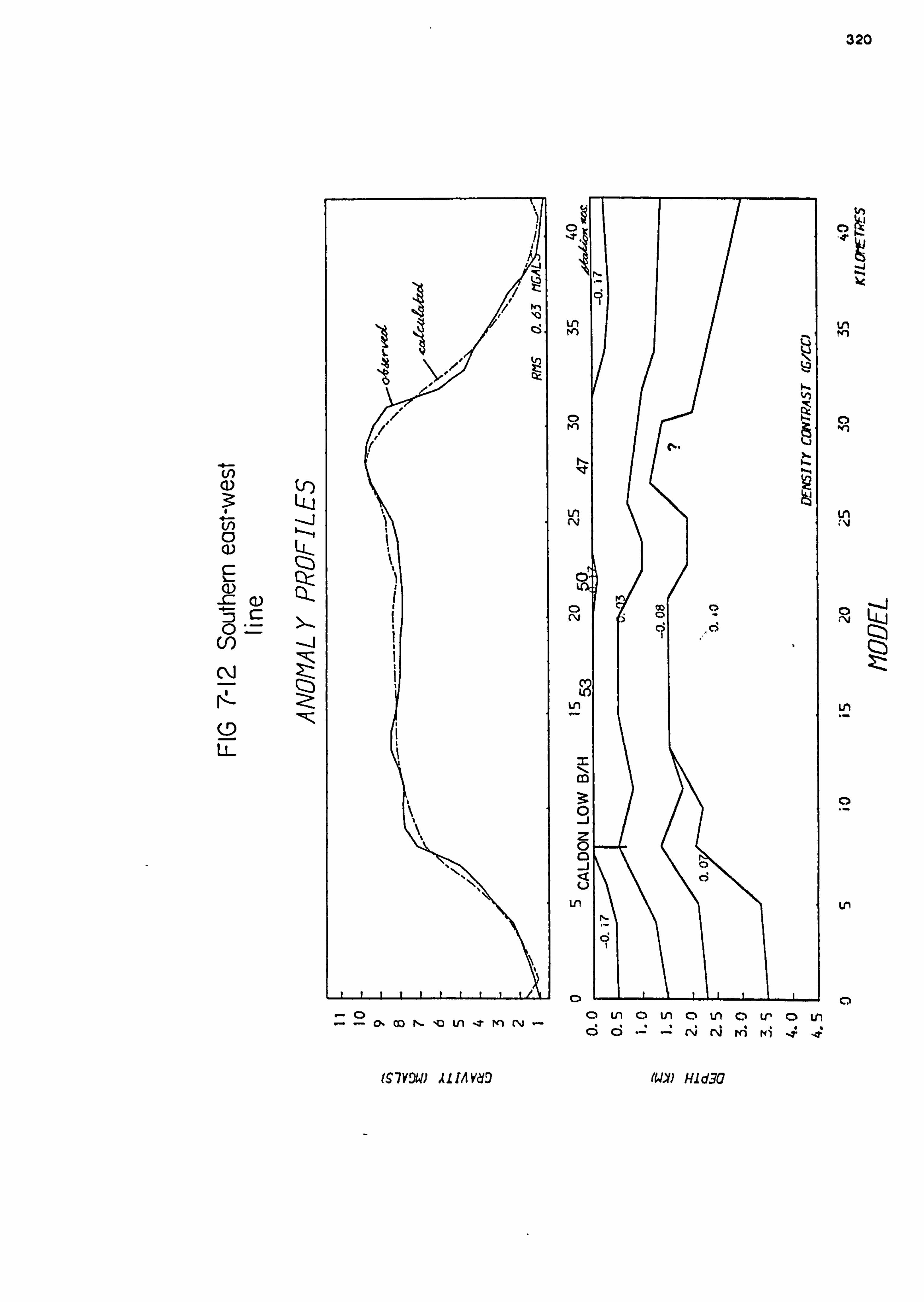
If) W

U) 0 LL-

ýO

Q-

Cý J

N Imo- Z

Cý ý

LL

1

-I

D

l

i

i

h `i

v

J

O

> Q cý v

Z

m Ö

J Ö

D J n Q ci U

n h

Ö

Lt K

C K

u C,

C C,

U

v

r .-oo Ln o in o Ln o Lr o Ln .ý "- O. m h. ýa Ln .YMN00..

.. N rJ M K) 'd

1S7YJW1 ALIAV21J (U) Hi d30

321

This model has not considered any decrease in

density between limestones on the massif and those in the

basinal region (west of about 22km). If the limestones

were generally less dense, then a thinner sequence of

Redhouse Sandstones would be required; the broadening of

the P waves west of station 56 was thought to imply that

these sandstones thickened westwards (see Section 5.6.3).

7.3.4 General Remarks

These models demonstrate that the structure of the

Dome interpreted from the seismic refraction data can be

used as a basis upon which to model the Bouguer anomalies.

Changes in overburden density between massif and basinal

facies, and also because of dolomitisation (which would increase limestone density), have not been taken into account It could be argued that the density chosen for the hidden

layer is too low. If so then the difference in Bouguer

anomaly between southern and northern provinces may be due

to a more dense crystalline basement shallower to the south, but still deeper than the refraction data have sampled.

7.4 General Conclusions - Comments. on the Structure of the Derbyshire Dome

The interpretation of the four refraction profiles is depicted by the isometric projection of Fig. 7.13, which is based upon the time-term solutions of Sections 6.4.1 and 6.4.2. As suspected from previous geological and geophysical

work, the cover of Carboniferous rocks disguises a more

complicated deeper structure. The Dome appears to be divided

into two basement provinces, separated approximately by the line of the NNW trending Bonsall Fault. To the north the Carboniferous appears to be underlain by a refractor of velocity 5.5-5.55km/s, which is believed to correlate with the volcanics in the Woo Dale borehole and the Ordovician

ON

A (0

ti MI

0 N 16.

c)

N

d

N I

N

C

0) t

W. o o> cE 00

oý y '- t 0. N Vo

ot N y,,

M

N

U-

Co Q1

Q Mý

C%j re) IT U')

322

" t++

N

1" :' .f : tit}. }: ": tS '. rf +++ . » ý

N :: :a::; + + ++ +"+

+ N +++

cli

": ti .} ý"'.. " ':: +'? +++

,

g :: "",, ++ : t: :; : fi

: " ý: cli ""ý , ý: ~~ t ý

"' 'i:

ri 3 {' ' "

ý iii :ý

+++ Jt- M 'ý'::; ti: r. ý;., " +++C7

.: ": Jt

t:

t: 1i: ".

1+++++ /

' '", '"rJ, "" 'K::: '? i t: t.: . ";.... `++ ++

.r ++++ co +++++++ti

:,: "j++++++ ýn + qt CD '.

+ +++++

+++ 01 .1 "++ ++++ (D ++

+

0 N +++ ++

N ....

ý,.. ... N"...

" +

O- N '

I- 0 N

, - V 7 O

C C p N N = O O CL. w '- Cl) > . _ O N O 1 d

d v N a : E 0 L- N L O C

L

a o + ö

++ +++ ++++"

N t+++

t+t+ M +++

++t+ ++++

ý4++t +++ +++

++ ++ +++ +++

a +++ ' I nf i ++ +++

) 4++

f /

i' / N++++

/ 0+ +++ ++

+++

" I

t M +++,

J ++

4 +

ON M

1 1,

323

shales encountered at the base of the Eyam borehole, the

relationship between which is uncertain. Characteristically,

refracted P waves observed in the southern province are of lower frequency, less rapidly attenuated and correlate better

between stations than those observed from the Lower

Palaeozoic refractor to the north.

The Bonsall Fault appears to be the surface expression

of a more important basement fault, to the north of which later arrivals are observed in the P wave coda which have

been interpreted as refractions from the downfaulted Charnoid-

type basement. Under the northern province the Lower

Palaeozoic. refractor may be less than 500m thick, deduced

from the increased attenuation of refracted P waves of frequency less than about 10Hz. Refractions are not apparent from any horizon between this Lower Palaeozoic refractor and the Charnoid-type basement, so a hidden or low velocity zone has been inferred. The mean velocity of this hidden layer is

uncertain but probably less than 5.3km/s in order for the

calculated depth to the lower basement refractor to be

geologically feasible (i. e., less than about 4km). Wills (1978) has postulated that beneath the Llanvirnian shales of the Eyam borehole there is a sedimentary sequence comparable

with the quartzites, shales and sandstones at the base of the

Duke's Wood borehole near Mansfield, thought to be Cambrian (Edwards 1967). The Cambrian Stockingford shales near

Nuneaton were found to have aP wave velocity of about 4km/s (Whitcombe and Maguire 1981a), so it is possible that the

Charnoid-type basement is even shallower to the north of the Bonsall Fault than shown by Fig. 7.13.

A speculative pre-Carboniferous palaeogeology of the Dome based upon these seismic data and the Bouguer anomaly map has been sketched in Fig. 7.14. The distribution of the

sandstones encountered by the Caldon Low borehole is unknown, and their widespread occurrence beneath the southern province is inferred from (a) the pronounced high frequency filtering of basement refractions, (b) a shallow borehole near Matlock (Chisholm and Butcher, 1981), and (c) the modelling of the

ýý

324

FIG 7-14 Speculative pre-Dinantian geological outcrop

Charoid-type material ®

Charnion under thin ...... Pre-Corboniferous L. Palaeozoic sandstones

® L. Palaeozoic -ýý limits of Woo Dole F basement fault

. ý` -VIJ volcanics

1420 1400rß` .'f`........,. 430

' ý' ' ý"ý 380

rj "

SL- /ý yy\}

"t,, t- fVVy1

370

` 1L ýý

rt

X

`ý_.

"ý ff fý .... ..... .....

"".... '"....

"y: . f:

} ..

....... ..... f ... ......... ý,; :: ", r:...: ...., . -.......... 350

'"ti

........ L\.

...

... .. t . fol.. ..... .... ... ..

i 4

325

Bouguer anomaly (Section 7.3.1). These sandstones must thin

or be faulted out south of the Woo Dale and Eyam boreholes,

in which they were not found. They do not appear to have

sufficient velocity contrast with the Dinantian limestones

to produce refractions.

The area underlain by the Woo Dale volcanics is also

uncertain. For Fig. 7.14 their subcrop has been constructed from those stations whose time-terms for the upper basement

refractor were markedly smaller (less than . 04s) than adjacent

stations.

The fault drawn marking the western boundary of the

Precambrian block is inferred from a north-south trending

band of closely spaced gravity contours. The basement fault

that divides north and south provinces is characterised by

an eastward increasing gravity gradient, which suggests that its throw also increases eastwards.

At the surface, the maximum northward throw across the Bonsall Fault system is less than 150m. Thus most of the displacement across the basement fault associated with it

must have taken place before the Asbian. It is possible that this fault was active concurrently with the eastward tilting

of the pre-Carboniferous floor between Woo Dale and Eyam. If

so, then the northern province can be considered as an independent tilt-block without necessitating a similar eastward tilting of the basement in the south, say between Ballidon

and Matlock. This mechanism is sketched in Fig. 7.15, which is loosely based on the model of Miller and Grayson (1982;

Fig. 1.8). The western margin of the Dome (Fig. 7.14) is

thus considered to be a relatively stable 'hinge' zone. (Note:

at outcrop the Bonsall Fault appears to be a scissor fault

with a southerly downthrow in the Matlock region. Thus some retrograde displacement has occurred, possible during the Hercynian orogeny).

The pre-Carboniferous surface generally appears to be more irregular underneath the profiles that cross the southern province than those to the north. Surprisingly, the basement does not appear to deepen systematically across the

Z 0

ti

FIG 7-15 Postulated structural control of Dinantian sedimentation

G') O -c -4 -4

O

G7 2

AN -0 \ s 0 F$1

A Positive Axis

5 Carbonate platform

Fault

" Asbion apron reef AL Asbian- Brigantian reef ///ý/ Woulsortion reef complex

I f'

326

Dovedale transition from massif to basinal facies. The

transition is, however, marked by a NW-SE trending, possibly fault-bounded, system of basins, which may represent tectonic

complication between the two regions on the lip of the

Widmerpool Gulf. The pre-Carboniferous basement is seen to deepen appreciably into the Gulf west of Cauldon Low,

which is itself seen as a positive basement feature (Fig.

7.15).

The reason that the southern province may not have

readily subsided like the north may be because it had greater

support from underlying crystalline basement. This is also

suggested by the relative teleseismic P wave delays, which

showed speeding up under the southern province. However, if

there is such a high velocity supporting basement, then it

is too deep to investigate with these refraction data.

327

REFERENCES

BAMFORD, D., 1971, Applications of simulated data studies to crustal refraction studies, Bull. seism. Soc. Am., v61,1013-1031

BAMFORD, D., 1973, An example of the iterative approach to time-term analysis, Geophys. J. R. astr. Soc., v31, 365-372

BAMFORD, D., 1976, MOZAIC time-term analysis, Geophys. J. R. astr. Soc., v44,433-446

BAMFORD, D., FABER, S., JACOB, B., KAMINSKI, W., NUNN, K., PRODEHL, G., FUCHS, K., KING, R. and WILLMORE, P., 1976, A Lithospheric Seismic profile in Britain -I preliminary results, Geophys. J. R. astr. Soc., v44, 145-160

BAMFORD, D., NUNN, K., PRODEHL, C. and JACOB, B., 1977, LISP - III. Upper crustal structure of northern Britain, J1. Geol. Soc. Lond., v133,1977,481-488

BAMFORD, D., NUNN, K., PRODEHL, C. and JACOB, B., 1978, LISB - IV. Crustal structure of Northern Britain Geophys. J. R. astr. Soc., v54,43-60

BAMFORD, D. and PRODEHL, C., 1978, Explosion seismology and the continental crust-mantle boundary, J1. Geol. Soc., v134,139-152

BARRY, K. M., 1967, Delay time and its application to refraction profile interpretation, In Seismic Refraction Prospect- ing, Ed. A. Musgrave, S. E. G. (Tulsa)

BAYERLY, M., 1978, Quarry blast seismic studies in S. Wales, Unpubl. PhD thesis (University College of Wales, Cardiff)

BAYERLY, M. and BROOKS, M., 1980, A seismic study of deep structure in South Wales using quarry blasts, Geophys. J. R. astr. Soc., v60,1-20

BENNISON, G. M. and WRIGHT, A. E., 1969, The Geological History of the British Isles, E. Arnold (London)

BERMINGHAM, P. M., 1978, Determination of teleismic P wave relative delay time between Eskdalemuir and Charnwood Forest, Unpubl. rep. (University of Leicester)

BERRY, M. J. and WEST, G. F., 1966, An interpretation of the first-arrival data of the Lake Superior experiment by the time-term method, Bull. seis. Soc. Am., v56,141- 171

328

BIRCH, A. F., 1958, Interpretation of of the crust in the light of of wave velocities in rocks, Geophysics in Honour of Beno International Series of Mono, vl, 158-170

the seismic structure experimental studies In Contributions in Gutenburg, Ed. Benioff

graphs in Earth Sciences,

BOTT, M. H. P., 1961, Geological interpretation of magnetic anomalies over the Askrigg Blocks, J1. Geol. Soc. Lond., v67,481-495

BOTT, M. H. P., 1967, Geophysical investigations of the Northern Pennine basement rocks, Proc. Geol. Soc. Yorks., v36, 139-168

BRIDEN, J. C., WHITCOMBE, D. N., STUART, G. W., FAIRHEAD, J. D., DORBATH, C. and DORBP. TH, L., 1981, Depth of geological contrast across the West African craton margin, Nature, v292,123-128

BROOKS, M. and AL-SAADI, R. H., 1977, Seismic refraction studies of geological structure in the inner part of the Bristol Chanel, J1. Geol. Soc., v133, '433-446

BULLERWELL, W., 1965, Aeromagnetic map of Great Britain (Sheet 2) 1st Edition, I. G. S. (London)

CHISHOLM, J. I. and BUTCHER, N. J. D., A borehole proving dolomite beneath the Dinantian limestones near Matlock, Derbyshire, Mercian Geologist, v8, ='225-228

CHROSTON, P. N. and SOLA, M. A., 1981, Deep boreholes, seismic refraction lines and the interpretation of gravity anomalies in Norfolk, Jl. Geol. Soc., v. 139,255-264

COPE, F. W., 1973, Woo Dale borehole near Buxton, Derbyshire, Nature, v243,29-30

COPE, F. W., 1979, The age of the volcanic rocks in the Woo Dale borehole, Derbyshire, Geol. Mag., v116,319-320

CRANPIN, S., McGONIGLE, R. and BAMFORD, D., 1980, Estimating crack parameters from observations of P-wave velocity anisotropy, Geophysics, v45,345-360

DONATO, R. J., 1960, Seismic model experiments on the shape and amplitude of the refracted wave, Geophys, J. R. astr. Soc., v3,270-271

DUNHAM, K., 1973, A recent deep borebole near Eyam, Derbyshire, Nature, v214,84-85

DUNHAM, K., 1974, Granite beneath the Pennines in N. Yorks, Proc. Yorks. Geol. Soc., v40,191-194

EDWARDS, W. N., 1967, Geology of the country around Ollerton, Mem. Geol. Surv. U. K.

329

EDWARDS, W. and TROTTER, F. M., 1954, The Pennines and adjacent areas, Brit. Regional Geol., H. M. S. O.

EL-NIKHELY, ADLY, H. D., 1980, Seismic reflection, gravity and magnetic studies of the geology of the East Midlands, Unpubl. PhD. Thesis (University of Leicester)

EVANS, A. M., 1979, The East Midlands Aulacogen of Caledonian Age, Mercian Geologist, v7,31-42

EVANS, A. M. and MAROOF, S. I., 1976, Basement controls on mineralisation in the British Isles, Mining Magazine, v134,401.411

FALCON, N. L. and KENT, P. E., 1960, Geological results of petroleum exploration in Britain 1945-1957, Mem. Geol. Soc. Lond. no. 2

FAREY, J., 1817, A general view of the agriculture and minerals of Derbyshire

FEARNSIDES, W. G., 1933, A correlation of structures in the coalfields of the Midland Province, Rep. Brit. Assoc. (Leicester), 57-80

FORD, T. D., 1961, Recent studies of mineral distribution in Derbyshire and their significance, Bull. Peak Dist. Mines Hist. Soc., v2,3-9

FORD, T. D., 1968, The Carboniferous Limestone, In Geology of the East Midlands, Ed. P. C. Sylvester-Bradley and T. D. Ford, Leicester University Press

FORD, T. D., 1972, Supplement to the bibliography of the -Geology of the Peak District of Derbyshire, Mercian Geologist, v4,109-137

FORD, T. D. and SARJEANT, W. A. S., 1964, The Peak District mineral index, Bull. Peak Dist. Mines Hist. Soc., v2, 122-150

FORD, T. D. and MASON, M. H., 1967, Bibliography of the geology of the Peak District of Derbyshire (to 1965), Mercian Geologist, v2,133-244

FROST, D. V. and SMART, J. G. O., 1979, Geology of the country north of Derby, Mem. Geol. Surv. U. K.

GARDNER, L. W., 1939, An areal plan of mapping subsurface structure by refraction shooting, Geophysics, v4, 247-259

GEORGE, T. N., 1958, Lower Carboniferous palaeogeography of the British Isles, Proc. Yorks. Geol. Soc., v31,227-318

GEORGE, T. N., 1962, Devonian and Carboniferous foundations of the Variscides in N. W. Europe, In Some Aspects of the Variscan Fold Belt, Ed. K. Coe

330

GEORGE, T. N., 1963, Tectonics and palaeography in Northern England, Sci. Progress Lond., v51,32-59

GEORGE, T. N., JOHNSON, G. A. L., MITCHELL, M., PRENTICE, J. E., RAMSBOTTOM, W. H. C., SEVASTOPULO, G. D. and WILSON, R. B., 1976, A correlation of the Dinantian in Britain, Geol. Soc. spec. rep. no. 7

GREEN, G. W. and WELSH, F. B. A., 1965, Geology of the country around Wells and Cheddar, Mem. Geol. Surv. U. K.

GREENHALGH, S. A., 1980, Effects of delay shooting on the nature of P-wave seismograms, Bull. seism. Soc. Am., v70,2037-2050

HABBERJAM, G. M. and THANASSOULAS, D., 1979. A deep resistivity sounding at Rookhope, N. England, Trans. Royal Soc. Edin., v70,171-179

HAGEDOORN, J. G., 1959, The plus-minus method of interpreting seismic refraction sections, Geophys. Prosp., v7, 158-82

HEELAN, P. A., 1953, On the theory of head waves, Geophysics, v18,871-893

HERRIN, E., TUCKER, W., TAGGART, J., GORDON, D. and LOBDELL, J., 1968, Estimation of surface focus P travel times, Bull. seism. Soc. Am., v58,1273-1292

HESS, H., 1964, Seismic anisotropy of the uppermost mantle under oceans, Nature, v203,629-631

HUDSON, R. G. S. and COTTON, G., 1945, The Lower Carboniferous in the boring at Alpont, Derbyshire, Proc. Yorks. Geol. Soc., v25,254-330

INESON, P. R. and AL-KUFAISHI, F. A. M., 1970. The mineralogy and paragenetic sequence of Long Rake Vein at Raper Mine, Derbyshire, Mercian Geologist, v3,337-351

INESON, P. R. and FORD, T. D., 1982, The South Pennine orefield: its genetic theories and eastward extension, Mercian Geologist, v8,285-303

INESON, P. R. and MITCHELL, J. G., 1972, Isotropic age determinations on clay minerals from lavas and tuffs of the Derbyshire orefield, Geol. Mag., v109,501-512

KENNET, B. L. N., 1977, Towards a more detailed seismic picture of oceanic crust and mantle, Marine Geophys. Res. v3(l)

KENT, P. E., 1957, Triassic relics and the 1000ft. surface in the Southern Pennines, East Midlands Geog., vl, 3-10

KENT, P. E., 1966, The structure of the concealed Carboniferous rocks of N. E. England, Proc. Yorks. Geol. Soc., v35, 323-352

331

KENT, P. E., 1974, Structural History, In Geology and Mineral Resources of Yorkshire, Ed. D. H. Rayner and E. M. Hemmingway, Yorks. Geol. Soc. (Leeds)

KUSZNIR, N. J., ASHWIN, D. P. and BRADLEY, A. G., 1979, Mining induced seismicity in the North Staffordshire coal- field, England, Jl. Rock Mech. Min. Sci. and Geomech. Abstr., v17,45-55

KUSZNIR, N. J., FARMER, I. W., ASHWIN, D. P., BRADLEY, L. G. and AL-SAIGH, N. H., 1980, Observations and mechanics of seismicity associated with coal mining in N. Stafford- shire, England (Unpubl. ) 21st U. S. Rock Mech Symp.

LAYAT, C., 1967, Modified 'Gardner' delay time and constant distance correlation, In Seismic Refraction Prospect- ing, Ed. A. Musgrave, S. E. G. (Tulsa)

LE BAS, M. J., 1971, Caledonian igneous rocks beneath Central and Eastern England, Proc. Yorks. Geol. Soc., v39, 71-86

LEES, G. M. and TAITT, A. H., 1946, The geological results of the search for oil fields in G. B., Qt. J1. Geol. Soc. Lond., v10l, 255-317

LEWIS, G. D., 1971, Earliest times to Norman conquest, In Peak District, Ed. P. Monkhouse, H. M. S. O. National Park Guide No. 3

LEEDER, M. R., 1982, Upper Palaeozoic basins of the British Isles Caledonide inheritance versus Hercynian plate margin processes, J1. Geol. Soc. Lond., v139,479-491

LONG, R. E. and MITCHELL, M. G., 1970, Teleseismic P wave delay time in Iceland, Geophys. J. R. astr. Soc., v20, 41-48

MAGUIRE, P. K. H., BERMINGHAM, P. M. and FRANCIS, D. J., 1981, A relative P wave delay study between Eskdalemuir and Charnwood Forest, Geophys. J. R. astr. Soc., v65,229- 235

MAGUIRE, P. K. H., WHITCOMBE, D. N. and FRANCIS, D. J., 1982, Seismic Studies in the Central Midlands of England 1975-1980, Trans. Leic. Lit. and Phil. Soc., v75, 58-66

MAROOF, S. I., 1973, Geophysical investigations of the Carboniferous and pre-Carboniferous formations of the East Midlands of England, Unpubl. PhD thesis (University of Leicester)

MAROOF, S. I., 1976, The structure of the concealed pre- Carboniferous basement of the Derbyshire Dome from gravity data, Proc. Yorks. Geol. Soc., v41,59-69

332

McDONALD, A. J. W., 1982, Surface waves over the Derbyshire Dome, Geophys. J. R. astr. Soc., v69,278 (abstr. )

MEISSNER, R. and FAKHINI, M., 1977, Seismic anisotropy as measured under high-temperature conditions, Geophys. J. R. astr. Soc., v49,133-143

MILLER, J. and GRAYSON, R. F., 1982, The regional context of Waulsortian facies in N. England (in press)

MURDOCK, J., 1980, Seismic velocity structure of the metamorphic belt of central California, Bull. seism. Soc. Am. v70,203-221

O'BRIEN, P. N. S., 1967, The use of amplitudes in seismic refraction survey, In Seismic Refraction Prospecting, Ed. A. Musgrave, S. E. G. (Tulsa)

OWEN, T. R., 1976, The geological evolution of the British Isles, Pergamon Press (London)

PALMER, D., 1974, An application of the time section in shallow seismic refraction studies, Unpubi. MSc thesis (University of Sydney)

PARKINSON, D., 1950, The stratigraphy of the Dovedale area, Derbyshire and Staffordshire, Qt. J1. geol. Soc. Lond., vl05,265-294

PARKINSON, D. and LUDFORD, A., 1964, The Carboniferous limestone of the Blore-with-Swinscoe district N. E. Staffordshire, with revisions to the stratigraphy of the neighbouring areas, Geol. J1., v4,167-76

PEASLEY, G. M., 1980, Travel time analysis between Eskdalemuir and two Leeds stations, Unpubl. MSc. thesis (Univer- sity of Leeds)

PHILLIPS, W. E. A., STILLMAN, C. J. and MURPHY, T., 1976, Caledonide plate tectonic model, Jl. Geol. Soc. Lond., v132,579-609

PIGOTT, C. D., 1965, Structure of limestone surfaces in Derby- shire, Geol. J1., v131,645-652

PRENTICE, J. E., 1951, The Carboniferous limestone of the Manifold Valley region, N. Staffordshire, Qt. Jl. geol. Soc. Lond., vl06,171-209

RAITT, R. W., SHOR, G. G., FRANCIS, T. J. G. and MORRIS, G. B., 1969, Anisotropy of the Pacific upper mantle, J. Geophys. Res., v74,3095-3109

RAMSBOTTOM, W. H. C., 1973, Transgressions and regressions in the Dinantian: a new synthesis of British Dinantian stratigraphy, Proc. Yorks. Geol. Soc., v39,567-607

333

RAMSBOTTOM, W. H. C., 1974, Carboniferous, In the Geology and Mineral Resources of Yorkshire, Ed. D. H. Rayner and J. E. Hemingway, Yorks. Geol. Soc. (Leeds)

REITER, L., 1970, An Investigation into the time-term method in refraction seismology, Bull seism. Soc. Am., v60,1-13

ROGERS, D. E., 1980, Seismic studies on the Derbyshire Dome, Geophys. J. R. astr. Soc., v61,199 (abstr. )

SAMSON, J. C., 1973, Descriptions of the polarisation states of vector processes; applications to ULF magnetic fields, Geophys. J. Royal astr. Soc., v34,403-419

SAMSON; J. C., 1980, Comments on Polarisation and coherence, J. Geophys. Res., v48,195-198

SAMSON, J. C. and OLSON, J. V., 1981, Data-adaptive polarisation filters for multichannel geophysical data, Geophysics, v46,1423-1431

SCHEIDEGGER, A. E. and WILLMORE, P. L., 1957, The use of a least-squares method for the interpretation of data from seismic surveys, Geophysics, v22,9-22

SCHMÖLLER, R., 1982, Some aspects of. -handling velocity inversion I

and hidden layer problems. in seismic refraction work, Geophys.. Prosp., v30,735-751

SJÖGREN, B., 1979, Refractor velocity determination - cause and nature of some errors, Geophysical Prosp., v27, 507-538

SLOTNICK, M. M., 1959, Lessons in seismic computing, S. E. G. (Tulsa)

SMITH, E. G., RHYS, G. H. and EDEN, R. A., 1967, Geology of the country around Chesterfield, Matlock and Mansfield, Mem. Geol. Surv. U. K.

SMITH, P. M., 1980, Gravity program conversion using data from a survey across the Red Rock Fault, Unpubl. MSc thesis (University of Leeds)

SMITH, T. J., STEINHART, J. S. and ALDRICH, L. T., 1966, Lake Superior crustal structure, J. Geophys Res., v7l, 1141-1172

STEPHENS, 1979, A deep electrical sounding on Big and Ramsley Moors, north of Baslow, N. Derbys, Unpubl. MSc thesis (University of Leeds)

334

STEVENSON, I. P. and MITCHELL, M., 1955, Geology of the country around Burton on Trent, Mem. Geol. Surv. U. K.

STEVENSON, I. P. and GAUNT, G. D., 1971, Geology of the country around Chapel-en-la-Frith, Mem. Geol. Surv. U. K.

TALWANI, M., WORZEL, J. L. and LANDISMAN, M., 1959, Rapid

gravity computations for two-dimensional bodies with

application to the Mendocino submarine fracture, J. Geophys. Res., v64,49-59

TELFORD, W. M., GELDART, L. P., SHERIFF, R. E. and KEYS, D. A., 1976, Applied Geophysics, Cambridge University Press

THACH, T. K., 1965, Sedimentology of Lower Carboniferous (Visean) Limestones in North Staffordshire and S. W. Derbyshire, Unpubl. PhD thesis (University of Reading)

THORPE, R. S., 1974, Aspects of magmatism and plate tectonics in the Precambrian of England and Wales, Geol. J1. v9,115-136

WALKDEN, G. M., 1972, Mineralogy and origins of clay wayboards in the Derbyshire Dome, Geol. J1. v8,143-153

WALKDEN, G. M., 1974, Palaeokarst surfaces in Upper Visean limestone of the Derbyshire blocks, il. Sedim. Pet., v44,1232-1247

WALTERS, S. G. and INESON, P. R., 1981, A review of the distribution and correlation of igneous rocks in Derby- shire, England, Mercian Geologist, v8,81-132

WATTS, W. W., 1947, Geology of the ancient rocks of Charnwood Forest, Leicestershire, Leic. Lit. and Phil. Soc. (Leicester)

WHITCOMBE, D. N., 1979, Seismic studies of the upper crust in Central England, Unpubl. PhD thesis (University of Leicester)

WHITCOMBE, D. N. and MAGUIRE, P. K. H., 1979, The response of the time-term method to simulated crustal structures, Bull. seism. Soc. Am., v69,1455-1473

WHITCOMBE, D. N., and MAGUIRE, P. K. H., 1980, An analysis of the velocity structure of the Pre-Cambrian rocks of Charnwood Forest, Geophys. J. R. astr. Soc., v63,405-416

WHITCOMBE, D. N. and MAGUIRE, P. K. H., 1981a, A seismic refraction investigation of the Charnian basement and granitic intrusions flanking Charnwood Forest, Jl. Geol. Soc., v138,643-652

WHITCOMBE, D. M. and MAGUIRE, P. K. H., 1981b, Seismic refraction evidence for a basement ridge between the Derbyshire Dome and the west of Charnwood Forest, il. Geol. Soc., v138,653-659

335

WHITCOMBE, D. N. and ROGERS, D. E., 1981, The effects of refractor topography and overburden anisotropy on time-term solutions of refractor anisotropy, Geophys. J. R. astr. Soc., v67,449-464

WHITE, P. H. N., 1948, Gravity data obtained in Great Britain by the Anglo-American Oil Company Ltd., Qt. J1. Geol. Soc. Lond., vl04,339-364

WILLMORE, P. L. and BANCROFT, A. M., 1960, The time-term approach to refraction seismology, Geophys. J. R. astr. Soc., v3,419-432

WILLS, L. J., 1977, A palaeogeological map of the Lower Palaeozoic floor below the cover of Upper Devonian, Carboniferous and later formations, Mem. Geol. Soc. Lond. no. 8

WILSON, A. A. and CORNWELL, J. D., 1982, The Institute of Geological Sciences borehole at Beckermonds Scar, N. Yorks, Proc. Yorks. Geol. Soc., v44,59-88

WOLFENDEN, E. N., 1958, Palaeoecology of the Carboniferous reef complex and shelf limestones in N. W. Derbyshire, England, Bull. Geol. Soc. Am., v69,871-898

WYROBEK, S. M., 1956, Application of delay and intercept times in the interpretation of multilayer refraction time distance curves, Geophys. Prosp., v4,112-130

WYROBEK, S. M., 1959, Well velocity determinations in the English Trias, Permian and Carboniferous, Geophys. Prosp., v7,218-230.

336

Appendix A Event data

Digitised quarry faces in red, r-. w r7 te

ii ii ii i----i ýLOOn

on 'Lou

n"i0PE V WITHSQUARR I ES

J SMALLDL

- ------------

1L

(lJ cS7Q[VElYgF1 27

+ 29 + 30 BUXTON

TWO + `3

21 ýLSN OAITDP+EYý + 33

+ 25

t 26

i, ;p k+ 7QýQ.

_--------- =37'* -35---ý-ý3---- ----- --- ---. _------- -------- ---------------. +ý 63 iIý@k4zlöv

-N41t40 tt t 42

+ 39+ 38 9T DL + 12 +-64 t+ 65 '.

+ 11 t +66 + 10

s. -. eACK LWSKIN 6BK + 68

t+9t

7 --------- ------------------± -------- +6

c6DlSALL GRANGE B+ 43

t t- pöy+ i4 GRANGEt9 rUPPERYD

44 "ýl? OnGCLFF

LONG CFA ýp ENE 1 + 4DdI. EI

+1669LI DOh

+ 46 r8R0ýý

+ 41 47 chIDPEÄK4

+ 49,,

+ 51+ 50 ºt+2 t+ 52

5S a- 61

--L ý Q------------------------

-ý---- + 55+ ----------------i----*-ý ------------------- i-----------

C"rt + 56 + 97

JZ5 + 60 + 59 +ARDLpy

"Rr äASHBOURNE

00 4 _, i 4 ,. 0 420.0

AM

337

Summary of quarry positions & abbrieviations used by programme MODFIT

TUNSTEAD TUNSTEAD 409.700 373.860 TUNSTO 2 409.810 373.87C TUNSTO 3 410.450 373.88C TUNSTD 4 410.300 373.620

BEE LOW BEE LOW 409.170 '379.140 ASH DALE ASH DALE 407.700 372.300 DOVEHOLES DOVEHOLE 408.210 377.370

DOVEH 2 409.120 377.650 WATERSWALLOWS WATERSW 408.310 374.800 TOPLEY PIKE TOPLEY P 410.050 372.200 HINDLOW HINDLOW 408.120 368.980 BRIERLOW BRIERLOH 408.970 368.800 DOW LOW DOW LOW 409.440 367.760 STERNOALE STERNDL 409.960 367.400 STONEY MIDDLETON STONEY M 421.690 375.620

STONEYM1 421.180 375.600 SHINING BANK SHIN' BK 422.910 365.060 BACK LANE BACK LN 420.720 364.970 BONSALL MOOR BONSALL 426.100 359.100 MASSON MASSON 428.830 360.000 UPPERW00D UPPERIJO 42E. 720 357.410 DENG RENE 428.520 356.360 MIDDLETON MIDDLETN 427.360 355.900 MIDDLEPEAK MIDDPEAK '428.140 354.770

MIDD PK1 428.620 355.320 MIOD PK2 427.950 355.050

BRO BRO 427.020 355.100 GRANGE BAR GRANGE 8 423.320 358.500 LONGCLIFFE (a) LONG CFA 422.310 356.10C GRANGE BAR GRANGEML 424.590 357.450 GRANGE BAR GRA1GEM2 424.190 357.350 LUNGCLIFFE LONGCLFF 423.910 357.020 LONGCLIFFE (b) LONGCL2 423.585 357.200 BALLIDON BALLIDON 420.100 355.580 WARDLOW WARDLOW 408.380 347.350 CAULDON LOW CAULDON 407.800 348.960

CAULD 2 407.720 348.770 CAULDON TARMAC CAULO 3- 407.800 348.620

CAULD 4 408.140 348.560 CAULD 5 409.040 348.830

WREDON HILL WREDOPJ 408.710 346.850 RAMSHORN RATSHORN 408.700 346.090 MONEY STONE MONEYST 404.870 346.240 CROWTREES CR06TREE 404.670 345.960 ELDON HILL ELDCNN 411.440 381.260

ELDCN 1 411.440 3E1.260 SHALLDALE SMALLOL 416.300 381.700

SMALLDLI 416.300 381.700 HOPE VALLEY HOPE V 417.500 382.800

HOPE V1 417.500 382.800

338

V- u C. in CIO NNN /1 N O. C rl . O, a, . -(p r W) VV 1` c1 rl't' a ('l WY 1- U1 r. {I O V1 1O OJ OI aI co .OP in NKC"/ f"i 0Np in 1º T (1 A r- f 10 C'1 0Nt. Ifl 1- r. 3 1! " r. in 'a P- .4 ýD ýi 1O W -P C" C4 1ý C in NW fV in W P. º. N0 al 'n NNP. D , fl (2 Mt

""""""""""""""""""""""""""""""1" "r ."4 .4OOOpNOOo .4o 14 .4O t1 I Cl pOOo .w .r .+ .r.. " ... r .4n ('l F. e"

Ill S avNn0'ow. n. rIll Na, NF OON In lna'. 4nvi in ,.. svlin a. N NFOC. . »ý Of IT Cc tN tD U1 C' M .AN .4 CU H in N in t0 t a0 n if. In O- tV nF0, c+O FT NT N0C9t0)I" In ID CV 4N 10 Ill Nr1rf vt-4 e4In HOOF on in "'ýNN C' vO CJu C2 C' c' C'104. H'iS C..: 3 VNt, tv V Nu C: 4\11t 00 O CU 00 0" 000 C, 1=1 OOQ') 0100 00 C. 5 C. O 01.7 p to C" 110007 ra C C.

"""""""""""""""""""""""" to """""" to OOOOOOOOOOOO Cl n- OO tJ OO{. ) C, OPO CJ O CJ OO ti C, C7 r) O

oo oro cl o cl OO cl OOQ co 00 (, 3 C2 01 CD OCl Cl OO pOO C70 QO OOC O YI rN r/ W C. WW wl Pl NF r1 O 4'1 P. C, %u /'1 tQ CV M) tV r] C) NFOP. 1.1 %a a, Yt "l

Y} C) It Y/ Yl O M1 tW Ut W In W Y! .4 ill V! Pl Cl M1 H r} WO D' W {f1 al {}. tN t", H 5. II t it """""" to """"""""" to """"""" to "

tD t0 t 1. (Cl F" F" "

ar a} 11 r" F In F M1 Y) N r" P. t P. t a) F" LA Ftr F" F F" .01 in W in 111 Y) Yl Vt p- to 4- . /l r. Y] P. in t YI Y1 P. .DP. P. W P. tD F In Ifl 10 r P. U. .DfF Y1 on nnMnn on M ^1 nnM on nnnnnMMMM on nM n" nMnnM on r, n

tJ C. C. C. O CJ CI C. OOVC. VOOO0f" Cl CIO VO r] r-ý Cl CJ t. t r. " C) C. C. t"C. O 1}' n tp O ." 11 co In at .ys .y 1(1 "y 0. HfN YI O CD FOWWOO R} V} q" C) in to, VI - Fn 0` 10 P. HO -" ON 0` .DnF (V 10 T "'a rl Cl n IT t Cl H R" "0 (T .4 on F. 4 F rI P.

""" to """"""""""""" to """" to " to """"""""" w I. P. 40.0 mpmmmt C` O CO t 0" tD TTT a1 0 R" RI tI FTT4.1 O "q tf; 0"

to

uNNNHOOOON C+ .1 ; '. $ N .fJ .d Cl Ca r, nO C' NNNf. 3 C, NH . -1 It ttttV4t4ttV. t0tt t' taeart rf t. t 4. Waatt tf ep

in MN n+ NtN . "r 4r N in PNN0M tJ N P. in Mtt in nN -t Ill .1 CJ V1 41 t

3Z it Z 3NJ Z JZ4 Cl Ot-gOc1J11Jt0 Z N03>": O Jf`}gJ 37N O19ý NNOJ¢ Jt) JW W 3OCI V10 JO W a0 W0 1rO IJO NO Z3 W 700(0(3 CC J 0. -Z cc 2(3 K Ill 192 H .J (01-" 41 y 21-a pt" JZOK a2 SK ZT p'"+ IJO O. JJK W cc JW 0 Z1.1JC) JJCWN C'W IJN WOWWW cc in "j J 6.4 O CO Q. JW 1-W O 1. " Z "r >J tL4J 0. W>Z W 1- 33 (10,. 0 >y(y 1.1! 1-J Cl! lr l""Id41-aell acc Mw nsa 0'40 -oar-40O4&sr0C1CL Ill . .« SZ 27m N3 NU cm 0- V'O m3O CDN 300 aOT. r. )C; JK .J Q"

at T r, on on 0) R" M 0) .4F of N In In n .aF .4tP. - 0' nT .4 Ill n. N ./ 'l t "4 S. H v1 on in a- touOH ."NNN in n It1 .D %ri "0 Fp It C) In P. RI Cl) . r1 0" (! a ra H. 4 (J N O Cl OOOG! OO Cl (Cl OOC, Cl O f! Cl 000 Cl 00 Cl 0 Cl C. UHHH .4 .4 .4H rawa In in in in in In in 4rs in in in in on in in non 10 10 .a .0 .D \A %n D \D D0 5D to =xzrxrzsaZrsIr2: rx a: xxr"x: zrraa: '. xs-7

W 2

4C

0 Q

cr. N

CL 0 (7CF Y'1 HrJPNHN VI YI HN {I" tV U" fý n M1 tW II CI 1}ý FN U1 H4NNCF II r*54,7 tV tt1 ,J1t It''. Z 'y In 0` tR in .41! 1 OO0.0. O e"4 H X31 NN 0" in 50 in N rr" to O it, D r, t0 FF tR l. '1 it, ': 1 N ai . s1 <, 1` to. P" h. }. } NE to u t0 MF .1t al MnT tO n tO 0tY! tp ... 1 OF Vf Ft V1 t .4 v} to u'1 Cl s4I on ar t Cl D0 n .DtHFt """""" to " to """""""""""""""""""" to U. S...... """""" D 4' OHNHNO tJ p IV HOnOHO r"1 OO O"N O C, n r, r7 OO IN . "" {, 1. "r NCr. HIV r^ w/ H N ZCo tD rr in up ". r ') cu tp we NNN a/ P In m co WOHF ttl NC "1. p/ HNa. Y1 tV F

u .1 111 1 Y"

O2 al to ON in tD 1(1.0 HtFQ on in Q10', . 40 fnT t. 4 tNMM .DP. P. Y10, to ('J 10 .Pa NR`

O 11' IT- 4.0 Ili u

. 11 ft

0) .rHT Cl NHNNnoP. n00 .4F .O .VN fV nMHt0, F t) W) H In :" t- n" T J1 H r"l f1

FOOutOa. + VuVu.. 1 OOU rl 0O . "4 .1 c} C. J C} O L. ") N (a t, H r'. H 111,41.1 or, n~ y C.

11 1U 4l "1l

QOOOC. O C. OO Cý OOOOQOpOOOOOOOOUOO fi O f. " '4 to to it "/p.

1 f" r" ""1:

lJ r. to Cl Ut""""""""""""""""""""""""""""""""""""""" to to to Q (ýýj

OOOQOO CI 000000 C] Cý ObOOOOOVOOC, O t} OO Ci pO .ýa r/ .; } tý or0V 13

JOOO Cl O co, OOOOOO co OOQC. OOOOOOOOOOOO Cl C, Ov .4OOhOO Co OOOO Cl

Wd 10 OOF us In CJNO tD tD Pl cm P! W KI FON w/ Ftß1.1 H 1"/ Co. Il a) r, VI "1-" YI In V" IIIn in C, HI N4 .4Z (A OtWF 11 W u" HU a" o: 1. i t U) If) UOOWMN If, ""I 0, {J% . "I Y1 HW 1"I F /. l rl ' 4, .tr1r Yl U1 4" f`I .1 Yl i1

Qt""""""""""""""""""""""""""""""""""" to """""""""

VFr. CO N tD t! 1 to CO 0! aý F to WF0. t0 F In FW ty a' In a) i 0) Pt P1 tt F a) UI ;. "1 FN OD P! VA 1'4 P. M1 C FtF ZUl 1ýFF tit, %av. W 41F1[1 W in el, t. d Wt WFYI to F. FY, Ill 4, it, I[1 FF tin F 1", fFY, F Tj on on e in n .7M in �l n in rl nMMMnn in nnMMnhnn Ml .. 7 Hn r7 Mnnnnnn PI lnnMn J '-

0 Q0 Or: ' C. oOO rv c" orn %ý o <a no tp n r,. C} r, r) O 4. ",, + 1. ) . 1141 1, e, 1. } 1. tr N .1H C1 lQ W 0. ONNTP r'" QN tD ntMT

to M"U1 Nt Ir NQ Ir H, C) nNRn

in f_,

y, t1.,

Y/ M

Ct M"

WH ý1 4 U,

-wl I t5 I"""""""""""""" to """""""""""""""" to to " to to "5 """"

O" m CO t0 01 Ifl" TOO 41 TNT CO OT r0 al T a) tTO R" 0" C1 -. T cc FFnt, Tw .] or :}4 .ýoONNO t"d o .aomnN -4 mnmN r} Nrf ['i c2 O Cl oo . "r .1 "1 O .. Nc. C. ell N. 1 t. u Cl .aN ."11

N"trtttttttttt t' ttfttttatttt 04' t t-W O's rts rf tt4tt4tt QQ

.O Nn. 4tCV. D 4). 4 M. 4 MN IAnN NnN 'a l4 *nHtnn tNn t 4'N Nnr4 t "flN 114 l. 4. I H1^. H m LL

}C1.1 117z Z0Z3 714123 L17n=J t will dCl t ["- ytY Qý N JJt C'03q 3C' -j 1. - U07 JCIJ or031J0 OU3 qJn"- NC 4 34fl. ) Q'E3. Cl OY0 Ow WOOZO V) J3OOOO Cl JO cc JO Cl J (A CI I. ) CJ WWOO1.1 Cl IJ 0>7r, Q "1_ `ZSO .1S. K I- JSOZ º" CCJZ º+ SSKJ F- 111 - 1""I C' C' -aZCJ t9 ."=2 t0 º. 0. -Ill-011 Y ac 61 JZ V) JW in in in K yý 1. } W Lot 1% J 1.1 NW C) 3WNJ Id 41 rot O 1.1 JOZN1.1 NZ (A ( CI J b" "J ä

iJ >> O1Jt-2 VI x to W2 º+ CL 41 Z Id J> S *4 ZO º+ ZJH f- Z C. } aOO at Z> a ."70 0' R C. 2- I QXQ

NOUNK m 3º'- 1. Q31

yi mor

mj C0 N ccoCK mZU ml'-m 0 =1=- Z 000 01- f]W w Ill

7 FO-ý r11 Qw

W O) 211P,

P. T on in P. N a. f1 NtMto, in 4-tif (I% on ; ry. fIll IT-Ir n) r, nt(1 P. MT, 1.. 4 " j- C rs t. ). + . s4 Cl oo s4. l4 NNNNnM Mrap. 4 on nnn ncr r) C. ors H . 4.. 1 .i .r (J NNNNN in nM z a) OOOOqO 000000017 f) 000000 C1 f! O UOQ Ot'! H X70., U 00 rt 4! {., "'1 tJ 1 -, j > .. 1 HHH .1NNNNNNNNNNNNnn on M on n on ntV. ttttttt0tit1ttOft Qv TT=TZZrrr;

.WZ3, X: a'=xrrr S=Z=Ir T_ STT , , _r 57.22 ": T. .. T 7

C 0

a) C

w U) M V

C) N

yHAhHN Or GO YI N 1V Q' .NN

P. N ,o1.. o bn N VI C1d. tO r/ N @0' P-

in ýf ."1 rI P. 4P !V ýD .4 .aN . "1 N "+ P.. 4

...... a,. ... o ..... ZA c o"aoooo. + noono

N U Q

. ". in IY P. N .. -! U1 .-P c+ ý %D i. O

`N of O" %0 . "1 0"

N1 in to -M0~ý CK, c2

(p A Cy r ACT 1NC -4 O. 4 ONo c%#

vVQ6NvOOQ (3 o r, O'O t-, G t--

ca c! oouoooonoc%oovoo """""""". """"""""

oGO L3 (Q QnogO C3 Q9P0np

C> cl cl c> o CD ý C> CM C> 42 Of 00"Dý O .O In' OC) PN

O00 U) U,

Y1 N in c4 f "-t -4 %U U) rt Uli nn tv -i Un av

N Y1 N 1r"o U) U' mF a)H ") U) r" ft 'O PWf Y/ tfNft r) Wt

önnnnnnnnnnnnnnOM nn c r3 cm oooo"ooc)octro"-+ooo p wo. umoormvnr-1oonrýn. cn p . +t .r 0"t. r oo0. O n, +ýDn N. 4

oommmommmP. u caeo"»r-mm N. "O o o. -10 a, H a". '- o'v N oU ýIfr r+ rr 4"" .04. ar0

u -4-@in r 4- --o N. i NN Uf m-ß-/17" r

1.1.

za 30.11 hzs o sro or 0"m ssr-o4

Toto J> JsoouoWJ ý+WJOcc W wo w0 J 6-JJJIr 0 JJOJWJWJIJJQV 000W J JdK7Nyº+Od OQ 2KK OM7 cooM<moof t{Laa: 3 a -C " ce -C cop- sumº-muusº-In msz co m

Nf0 er Pe in p. tim on N+N %D CV

- OOOOPnO o .4 -4 NNN .4 Nýt

Co000oo0000000000 CY N ty NN ty cy r4 N

NN NNNNNNNNN CY CY NN >NN

Li UUUUUUUUUUUUUUUUU

339

U. %a nw cm Iv 19 W. .b 1V "'" U. " "s .. .r o" o" v. t. M P. UN P. 1.! AAý.. "rý o O" ý" r" n" n YI t. n %a V" all w 0. """"""""""""""""

ýi l') N .1 .y I'n r. C7 ry 1ý f1. """ ! '1 Pd ýr /y

YI ýO f º. HI t1 01 /V IrNA ff yB f. U VI A ý1 ff/ if .r "II A O" Pe M p. ý "0 m -4 T in ºý Lm "fl ff1N rl N P. """I fW1JtI/1-tV. "tf. "" r . -# 4 ", ti fSf7F tIL .i l14 t.. 1 ýlt1 r1tC!. t.

""""""""""""""""

ri -: 0

OG7C, O tl C) V) fi Cl Cl ft"" .3 "113 Y/ 0 YI C. p Ul Pt º1 A. V" t7 r a°! "l A O' WWII M1 YI 111 U' f tV - Yf O. U' Of

"""""""""""""""" f I. Vi Q! 0.1 Y" in Www0. N Vt P. O" !1

ýp P. VI 4p YI W F. A y) at Y9 AW" MMMMM +1 rl 01.1 MMMMMM "1

rt tý t" a"1. e. 1"1 O to .. Cl tlt. nqC -4 O. 1.1 Of Vi ." p1 41 CI 1 t1 w" W n" 1ti ýn N N 1"" fV w" w 1º a" N ý. ." " s. """"""""""""""""

r) Lý Nt1 . 'f N .4O. 1. I 41 u1 .ý 17" th fffff ff ff" fff f

H 1'I od %n fN1.11 In CA CA .4ff ý1 ºj

a, r J3 7 Yf t)NJp"yh Nbry

C N O/. Cl WCI.. J I, -J OJ E _ KJY JO< ' ý

J4 J1.1 +. IWt I f- O7 -t J º" !! "I ý) J! to g

Q# , adw r+sw ýä wöümüml.

ýanMu n x W - .n "I "' "" . f*ß4%Cl wrt.. N0. "M fou-N .4 PI M .na. ý. M "n In ""

YO f! f7 b tl f1 %a m Oe to l 09 t.. º. ndNNNNMß'1MM fff"fff

Z M1 MMMM rn MMMMM I'1 hMM IR V IL. IA. W IL U. IL Y. 1L L64. IL Y. V 1ºV V

9

A-. O r+N r- r"Nr W i! -" Yýr-4e lp A"W A`N W lV 1-"r A"y r11 )'! W1A" iV IV ItF ""A "i N *- f-r, -r an r" 0 %0 Y' 1 4- H- A" -Py .d ED r %n rA1 ¢+ 10 en V"

f` P. rNVrN pl

A11.

4OM b7 Y) 1! 1 VI !ON A' r1 A` Pt lA N l-1 in l0 U1 fOr, o t7 tA1WNf0�, !At"h "ý N r/ t" Li 0 . ý1 O O. NOO º1 M t! onnnoOAO "1 r1 wO rJ Ci "-1 NA ! '! el 9. !,. ) ww.! wh)! a ! ý/

0 ft

4)

C r/ NTP Ut r! A .N . "" Q` 0 O, T IA Po-eN--N-A º1 !ºm In wi u, 1. N. . 4) Y" WN A" AM ft PP r1 c0 ' '. r") . p+N in in c4 r1 lA 1P O in nCo Uw 0'i M140. A" CS Pl u AO ti"J N" d% P. 0V J+ 0. t NA N Nr an 00N ^ t. r f! D"/ NP hMf Iý -P. NV2N M1 In f'n "r e-w ry qan u Nryt" Il OUO-O Gx100 N G. " O Ul? 00"" tV 43 GO U"tiul10". " 47 li !" N". r e. 9 l+W N! "i""" OoOOOO CZ OOOOO CD Oo Oo UO Ot1000i OOtl G. ) t"{.! O4N"rU"J t"tl )5ry ",!

C"""""""""""""""""""""""""""""""""""""""" 0. o00ono t7 00 t7 000000000000oO00V f'1 4i l7 1y t) 4") l ! "" tt l. i yVn'

U,

baaaaaaOba0aaa lt aaaabbaaa Ca aaba t+ atlo 11 is 49 "I t" r'" t" el Y1 WY1OOup r1A Cm YIOýaaCC Y/If1 YIa

rl rhh Y1 P

Yl /)Y1W nc1 Ylr1º+"1 of r. r11/a Y1q +HIW 1"" 47 O .rW Mf .iYNP Y1 t+ cJ W .rN -1 d YI T 4+ V' Q+ V m0 Y' ." r11ý y Iw f Iw A Y/ M+ MA 1ý .. " "" yl

"" """""""""""""""""""""""""n" ak- ""N

rf "M""1

1" Iv """f"W""nv. "

N" N Nf YI fI .y .a0WWr r1 PP r) r1 er n P- r Y1 %

1. - P N /r cp l- ply l. ". hr 1+ WWOD 1- Iý a r- ý %W 1ý ti W fý eý I"" W p. p- u. M QI f. tiA WAA Wl. yl Q 1ýlnnnn1717 M9nn MnnMlnM1 M1.71n 1+11+7 r1nnnnn17 M1nnnnlnnl'l /"fnnl'1 n°1 c

OO b'l nOuU, c, oO ry cs e" c. "0000000 fJ Cl U C- htp C1 1) -A r- 1" fl v. h ty r. tý IW 8 .1OWbONNW r7 p r1 17 O 1ý rWW 10199 WNNNA rI W r1 O GI. 1 t: "4 Y1 6 t" NfV HI Y/ hM

cp Q. NTWOrM .p CJ NOr. 4 NHNNc. ""1 .ONW . '"1 NN ti r U1 N v1 Pl f cp "n . r. 1 y1 º" "y rt1 V""""""""""""""""""""""""""""""""""""""""""

a1 Ql on (t aOT 'ö ."b 0' TP Co O 13 W OT m Co f4 ntIO

to o" OTA YI 17 ryý (r V Q. ýy t1 V "*w ID

""4w`""""ä0-h c2 °"ä+i+w*"" .4rw.

f ""4 4p 0 .4 c3 .4'r*f

4e ý..

rrrffrif 0) örr .trnrn Yl . -4 e .r .f Y) NNf1.4 Nr . -1 hHN .1f f4 . -4 N r1 Al 69 M1 M +f "" N ej e1 r" s"

w0 . 4*V .+s 4-: 1 oo. -. 39 -nn+ .1 PN a ptJJN71JO3O7QQJN7OmiJN 1A tNda C% Naj

>. NJWOC. OOO >` oJOOJWWWONJ In >O a- C) JO a- oO 44 Jn ý1 Fh - t- JJN b- xJWZKJO0: J b-h- jxKCK LIZ Mows- K 1- 7J6. CL Oý I.. _ r 41 Y

(4 U WW NJJ1^cm W OZ W NW ONw Jw 41 IJ W2 oC 1.4 jJNW WWW I01.11" 1, /pC w HNZ tQZZ> O H. 7ZH2ZZ t >1-1.11-OW iS º-7> pV ZN6r IF j O 3mHNNI=-"1-.

OZ NN <nOM" In SI-NNO7 m ON NNQUI- b- m

M. n x NM.

711 Cu mI- ^1+f1 V.

O/nu. al .. I

" Y1 A aý Oý N r7 O ýO 6N rf HNhoo ri N. 4 to W Go o .1N 1'f .dN In .OA in 4"N{. NN V1 oo

ºý W w, O co o . -1 4 . -1 .1NN No OQo .d . -1N .4H .1NN" M1 M1 M1 ? .a t) to td. ) J .4 .1Ný .4 14 f4 N P, co 0000000000000000043 IS C2 Oo. 9 u Cl OO tl nn el r/%ý 1V 0% p%V e, /0

_y . 4.4.4 .4 .4 . 4-4 1 r1 .1NNNNNNNNNNN NN N NNr1Mf nr1om., lrýhý

> NN r/A N. 1N.. 1 .d NN. i. .4 -4.4.4 14.4 r4 -4 . '1. -1. H. 1.4-1º4 . 1w/-4.4 MANN W HMºy W tL1LIcIc1a. 1. LL U. 16 LL LL 4.1. U. 4.1L. L6 U. 1a. U. Y. W 4. WLL 1c U. 4. U. W Y. U. Y. U. U. 1L Y. %61ºIt Ibº

340

S ö

r1 t Iff Nw r- a, cu in N U. W O" hTNF. "m r MMhFLn. 4 Ul

E ýoeF. +o. oFwýoýnnwmm """""""""""""" .:. o000o000rOpo0

U

ý. rk" aonouýeýýoon. a N to FO 'O O 0% .4 .4 %D . '0 1n ONO. 4 1M 14 mN (MAO M MO4. raN. 4N q v" O P) C4 OOOOOOOOOOOOO C""""""""" .

C: """

OO cO

OOOOOOOOOOOO

O C. OOOOOOOOOOOO OM 11 NW 0000 . 4-(1N in Ifs a- Fw .4 r1 0, v, NN r" owO

VI """""""""""""" N in W kn FP N' FFPN Wº- O

win W in in O tiFF in r- Wau MMMMMMMM W) MMMM

öOOOOOOOOOOOpOe N rl OMtWWW rl OWp, W N P- NM0 .4 M1 .4 .40tONO """"""""""""""

. 4r" ONN O 000 NNO 00 " r+ 4 4+ 44rtt r+ r

d

0 . 44nF. 4N. 4 4N. "4M4p LL.

Ö J J O O= O NNN777

>. OO .JO WA O J> OOO ` Zr4K"U' CSSSUWJJJ

CJWJ=W W WW IDJ WJ -J -K ->>z 4777

a H <K tK CC O a0 O 00 OO Nmm CO t9 mO 00 J1-- 00 O

V

X10 N. 4 N EO O OD %D 9) PI) %M in OO. 4 N CY -4 NOON ß'l0 C

OOOOOOOOoOOOOo 0! wo Y7 Y'1 U1 in in -O ZOH HP 1-m > HMhHHHHhHHHHhH

W tL U. LL La. u. ýýýU. U. IA. U. u.. 1L.

341

a cc NNONa "-1 to V" a" m a" V. +O r) n' 1-44. " P' M" In Yt f 10 U) In a, 0 ar OD mm It . 4(2 OW0O0O 43 r" 0 CI O

.4 . ýr" . 4o4 rlN I. 4 . ". r . +N cm. N Nr" . 4/v .yNNN .4NN

t> OOOOOOC! OOO C7 pOOOOOOOG fJ Our, ý (3

0

U E

0 0

N H- Z

H O 2

LL- O

F- LU Z

Z U) D

0 W Q

O

}

D O

Q U F- N Z Z) F- 2 O

N F-

J

"4 M) 4r 11' PI "l - P. If) W ul N- in 10 fJ ov0rr u' N III P)

ro .4 r-1 .4 .41.1 " O' rn 1 a' T 0% MM .4" %D m -4 .4uN '0 .4 "- U1N r. OD to p- P. co CO C4 IN P- º+li` %D10 'O It) Mn nN 4P N

C, Ora 00 aca as Co . -1 I14 O' Nn Qnf. a a %l0 nf7 n

C. aaOOGOa l7 ca OaV rr aUOC. a C.? O f! n C'' I., """""" """ to """"""""""""""" to

aas 00 as0a OO 00 OOO f1 00 OO o0 00 O

aoOOC. OOOOOOOOO co, 0: C2 Ooaom co c7 OO

a0oOo0oO Cl C) co O "7 Cl OOOOoDOO C+ O C7 a ýr n u) 1f) 4 U) a' In O rr 1)I U' of ONN Co. ONNNNNr fJ 4?

n It nM r) nnanddo F) drn in on nn on Mn "'1 n in N P. P NP PF ?- P1+ NN N /N P. 1N PH P. N F. F. p- F. It Y) nM P) nnM r') w) n .) It IS P1 n r) I1 nMn on rl It I'll I'l

o4 Od0` O olu aSld c nIn ao If) Or-. p" uO O OM oOlfl O c; co ac In Ocl c "a as ua a' COd O fin OO ID O CJ ra f7 ca O a" -" co O "-1 oONO . 710 a Cl, º) O l? N f7 c1. l o N. " . 4D. 4*O NNO nd rl d'ON%D M"4M Or Innn^r M'A-I IrJiN NnNL9

""""""""""""""""""""""""""""""""""""""" O 44, OO in OOUOn V1 aO 14) OO U) OT It) On a Yl OT in 00 I U) OO in U ý1 IA O C4 Ifl a

.i .r .1 .4 .4 rl . -1 .1 .i. 4 .ý 14 Oo º1 r-1 O 014 .4 .d4 54 .1 .4.. 4 td4frrd4d4ddd*4' d" dCrd d" r* r

11 11 II 11 II 11 11 11 11 it 11 11 II

In . -1 d. n . 1'0 04 rd> >O

. 1CJ NN ^I' ^I CO NM to NNN .4 U1N N. r ya . r> > . r'> >>., T n/ .1? . 4.. a ... r >>.. r a ... r>

wwwww 222222O2C222S22 VaVaaatVQa fJ VVa IV - 4.1 hl 4.4.1 1-1 N IJ N IJ MHNHM 1-ý

It I.. 1() . 1, P- Vd5d IO1- 4' WD. - lu WF-ID1-I-1- In 1- If) InI,, inH in IIIIn 41P 1f11-. . t+ K "t 44 4- 44 Vl 4 V) a444 44

ýc>: T+K7"fr Z-'n 2'- 72,7 +T 00.2 2K 7; o rc 2. TK'""'K+

7 1. ) 70 41 70 4I 77W» IJ O' "I 7 41 77W m> WO UI »WO

:7 Id 73 61 7

1- h- º- F- 1- I- 1- 1- 4. - 1- 1- i- - l- of I- r5 1- S- º. H 1-H H 1ý F1ý H 1ý M Fý IS M- 1ý M ºº-

44 MNMN 1-1 MNMNN º4 "I

r 5- 1- º- F- 1-. F- 1- F- h hIr 54 a' NW 1/) C

rn V1 NNNNNN (A O -1 K .+n n' on Ir d' P In W. ul W. OmT1: ) d' ON IY NaO LM Ifl on p: on N re Nn Ot on u NM P9H -n dN d aM O NM N nM nn. +n onin It Md CID ºa OQ r`1 Co rt" r. 11ri NM

U. "7' a 1. oo Il. o f. U. o ýr 1r_ u-U. a ci I4. noN. 4 OLL ri a Ib oaU. 1"a r3 la. c") '"r it. +

n1HnInn1Md14dledr In 1 In u'1 tMi ºi 0 J) r) 11n1 ý) n1nn1n on 1n ") nnnInnInnInn on n1nH1 LL 1L 1. U. 1L IL k. U. U. LL Y.

I I/. u. U. 11, I6 1t. U. U. N. U. 1o. U. IL LL U.

V, p' hN on rl on in Of. L3 N IV r- N Q co W. a, f NN OO U1 f VI %I u"

ff 10 M %D %v " "" . "1 NNNN

U """" OO """"""

E ". Cl Oo Oa ooaO r7 v

ýc Yl wl L- M ti 1` III r/ N wt ff In Pi

V h Ir 1(1 r" In in NN

OO OV

CA NNN

C aoa, M N NN r" %f1 h P. 00 Eft

Q HH C" a Ctl aO O t' O 0" r'

C, Ca aa li OQ lý r

> o as o ao aa o as ell CA t"

nno0 oa o to to o r� ao tl /-+ na o ao a oas ora o Oo 41 a (Si N cy, V' a YI 111 f U.

N a n M Ml rl I'll r 1r

°a ff

hhP. r" P. h 1r l ri 17 / ri º

P. 1" r" P. P. P.

C rl r) M P) M on r! r) rl M r/ .) rf rl

aas CJ a Gtv f' ý` a Uf t` U? O 1. Hfl t, t-, OIV O Oh t1 O! f1" Of O Cf CA Oa7T O/; 1 fO 0 r1 ýý"ý fN M CaM N1ý NH 0C! N N Hr)

"""""" """ "" " """"" fl o ulomul pý oln o oYl o 1-fNO. +1.1 rD lf+ N .4a tt . "1 H ' H .yN NN r ffff ft Ir f"ff4f

11 11 11 11 11 11 11 M .a nl M 4a, Cl NN NNN {(1N 0 Vl . 10D f Nr- N? N>N N> N > >> N>

J Cl 3 2 r ww z

z

v . i'J o a a VUu 1-. 1. " N

N1-NHº1(1 ý1

Ul on l- Hfl r-10 MN ºV 0- on rr- f" H":

.ca T a a AKT K2 1 . K7 KZ W. Z +K ; º"",

Ir z

JWaD1 7W7 7WD YI :J bl' D 1,1

rf H f"

n Vf d c -C "I on N

a: a C =

NK .a ti a C.: C3 M 4111 HMre W Mh W P",

C r-. 4 r-R1 .aW JC 1I O

own a1 s

N/rN . NNNM PI Mn f H" . LL t. L

H I cl U. O

.. lt rariI. a : i1&. >

=ý :-i Ciw

:" Z H1w lý Ui üü nnnn

wl, n

i LL IS. . rn

It 1.16 W11. IL

342

qro w00 r%0 O ON Co o nP O. I UN nu)NU oe cW ore CU f- oW 44 NU u%U%acu ui 0rß rvP (+

= nruýneoý"nvýmnný+nnruAv+uirnn a. km rrtirýrº-rýýa rlºPý. HNF vi Il1NNH

nnnnnnnnnnynnnnnnnnnn 0 z

p r1. nn Y7 r-4 o rP l" n W. n O, rr oPn. -4 C O> O N%0 OOW P N1" rl M nA ei w m: r4

ý+ ýoý-"oýPPP NPP OaOPP1n 0ý. aoPO' No ENO 000 NpO. d p-. f OOy -1 N1 Gci

rrrrrrrrrrrnrrrrrrrrr W

ZZ ti u F- Y I-

mjZOJ üi U) Z in tu OWOtr. 1 L1 WOONZrdOOO

O. 1 Ot Ot OJW UJUK

WOOO. at H1L OWOW UW GW W OW Wd0001.1 WlJ

LMH º1 º, O= H tu Oi) h =H HUM1.4 oý JH

Nº. NJ Vi ML V) JWNCJNN1.1 NHYJJ7N V) N 7 JZ Z77, iº+7it Z aZ Z? JJ Z 7t OKY Z< OZZ1 Z> O> ZV4Q 1- Z>>

mH WF- UOI- HU I- F- OH F- Om m Wº-F. 1- ZZ

ONO HH Ny

M1 N0P. co V1 t%0 P of %D con tT4. . 4"4f rN fONNNO. dNhONO r1 N .1N r/ MNO º@

COOOOOOOOOOOuOV7 co OOGO0 V HNNN r4 on wi hR 4r in in in a%o waP of a,

M MI r) " Mi V) MI M) r) Ml "011 MI Mf M1 M7 M7 wl in in W)

W LL LLtLLLLLLL LL IL ILLLIa. LL U. LL1a. 1a. LL14.1L U. U.

U, U, 0

W Z O F- N

M c 0

W 2 E-

to p 0'` C1 W Nth C O [a e, t O aý rr ýn ,. / C W t1, D. V Ill W NY)[o1. r fro V" e4 .4 NP + ai W º/N q"

.C r """""

co P. in OD n t «

"""" n U, P. co

Ylh Vl r MI r t. 4)ä L. nrto %ow L. 110In4. In u1l. In II. P. P.. u)v o nn on K) rf 0 nnnnnn in n o nnn w) on 2 y

p O`. D O P. P. 41 17 CY "In 4. C2r 4 61 Oý 0 oul%a C Nn to T Q) C C one (n r Ifln [9 C C fN n1O " " : g 0 r r """"" " " " "º """

++ ntO 0 00 lo J 44 COn10 m ap OT c) J a. ýOp D. QýIJ+ N NONOC, to '4 94 NONN CO N H .4 co U tJ t ý0 fýr'ýd' 4. 15 q 41 ýqf'ýt N 10 rýýrt 41 N W N 1.1

Y "i 31

°S 1 C, 1 4 .+ V)

O .41 W O7Y. NZ 4ý CJ Vf SZO N2UmQ C

IA L

401LZ YWn º U C

7º <JW I. 000 W L I

I WJ WSJC1 1ý J 2 º V

1. WC J41U L. YJ º+ J º- . V . 10

cl WO y 1/17 UJW a= J O

6 '0

1-, OZJ V) VI Z WIi ' W C)JD0 C U X. iq[ W t. 7 i 3 JwJZZ "+ O 70ZQ º"}mot 41 O OL17 O C -9 -C -r O 6 F. UU2Om 4- 4- O 7 mS 4- O JO 0 t0

2 N 1 y

of o Yºr P. h %01Nin 4, r in t O4N rN O, oOnýp W

41 O ý"INOO .4 -1 nl O 41 .4N Nta C OOOOO

C C O CD OO0O0OO O CC O C1 OCOo

V .4NV. cm in Y NNNn on .lnn U NNNMn

=__ __ 30 -4 U. 1 .r ßl. 4.414.4 > NNNNN w W Y. WY. LL 1L IL 1I, IL 41 uUuuU

N O O r-

J'In M

Y0 (") 2

l1) II Z7 G)

U) O

L N m Co U) C

i- N

U)

O N 4- U) cp

.o

co Q'

O

. 4- 03

cc

seismograms plotted vs interstation distance

cat v? Cl)

M 04

N

i i

ýj

,: ,, i

T

to

>ý

CD 3 0 cn n) B

ö

CD Q.

m

ö

a

n) C) m

(b) Ballidon shots

M4035

0 "5 1 1.5 Sec

M5061

14

13

12 II `'

11 ii..

n0, ý/1,, w

10

9

Sec 0 '5 1 1.5

343

APPENDIX B

POLARISATION FILTERING

Polarisation filters were first developed by Samson

and Olson (1981) for the enhancement of three-component,

fluxgate magnetometer data. The technique essentially

calculates the degree of polarisation for all channels in

order to design a filter which operates on each channel

separately in the frequency spectrum. The process is data-

adaptive because the filter is slid through the data, at

each position of which the degree of polarisation is

recalculated and the filter accordingly redesigned.

The principals are given in Samson (1973), Samson

(1980), and Samson and Olson (1981), of which the following

is a brief summary: consider a set of N seismometers, the

information from which can be represented by the time-dependent

vector

[X(t) 7= Exl(t) , x2 (t) ... xN(t) 7 (B1)

which represents N-dimensional data whether xj(t)j=1, N is an

N-component set or N vertical seismometers. The discrete

transform of X(t) is

n-1 1 Z(cý) J= (2 )E Ex(t) ]eikw (O scs 27r) (B2)

k=0

where [Z(w)1 is normally calculated using a fast-Fourier

transform algorithm. n may be the number of points in the time series, or the length of filter chosen. The data may be conveniently written as the spectral matrix [S1, where

w2 [S (w) ]=E [Z (a) ] [Zý (a) ] wl w5 w2 (B3)

a=w1

Where (t) denotes complex conjugate of the transpose. Now, ES] can be expanded

344

N [S (m) 1=

JEl a1 -(w) Cud (w) Cuifi (W) ] (B4)

where A. and Eu3 ] are the eigenvalues and eigenvectors of

ES]. We wish to consider the case where the signal is highly

polarised, that is when ES] has only one non-zero eigenvalue,

or

CS(w)7 = Jý1Eu1]Cu1t] (B5)

In this sense the vector Cut is the complex representation [u] =[r1] + i[r2], where rl, r2 are the major and minor axes

of the polarisation ellipse. Thus a measure of the degree

of polarisation, P, is given by

2 N (Tr S2) - (TS)

(N-1) (Tr S) 2 (B6)

where Tr denotes the sum of the diagonal elements. Having

determined P, CZ(w)] may be operated upon to give the

filted output CY(w)], where

n-1 CY() ]=1E CZ (k) ]Pq (k) e2. ýrik for CZ(k) ], k=1, n (B7)

n k=0

and Y(w) may be transformed to yield the filtered time

dependent matrix [Y(t)]. Variants on the filtering process include the polarisation bias (set by exponent g above), the

smoothing of [S(w)], modification for a sliding filter, and the allowance for lagged arrivals between channels. These

are all discussed in Samson and Olson (1981).

The degree of polarisation is analogous with the

quality of coherence, except that P is not limited to two dimensions nor the orientation of the instruments (Samson 1980). The essence of the technique is to discriminate against that part of the data not observed to be well polarised (i. e. random noise, which should be incoherent between the

345

N-channels), and to enhance that part

well linearly polarised (i. e. seismic

method sets out to represent coherent

linearly polarised state, and differs

channel data-adaptive filters by that

there are N output channels, and not

channel.

of the data which is

signal). Thus the

seismic data as a from other multi- for N input channels

just one best filtered

For a system of vertical seismometers, the signal rarely arrives at more than one instrument at the same time.

While the method can accommodate lagged arrivals by using

a correlation matrix to estimate the lag between each instrument (and accordingly maximise the value of P), if

the lags are greater than the length of the sliding window then problems arise. Few difficulties occur for a teleseimic

event recorded on a small array, where total lag is unlikely to exceed one and a half wavelengths, but for a close high- frequency source (such as a quarry blast), the lag between

adjacent instruments may be several wavelengths or more. A further problem with local-scale data is that the signal changes rapidly between instruments because of velocity filtering, dispersion and the interference of phases.

For these reasons, the part of a seismic refraction signal most suited to polarisation filtering is the first arrival: it is least affected by interfering later phases, and is often of similar amplitude and frequency to the ambient noise. Furthermore, the time of arrival is known within measurement error, so that the seismograms can be easily time shifted so that the arrivals are lined up to within one wavelength or so (the alignment need only be within the length of filter to be used).

For the University of Leeds Amdahl V7, the polarisation filter programme MRCLEAN has been set up to run in conjunction with PLOTTER (see Fig. 4.2). Operative details are expounded in its relevant Manual, which exists as a Disk file.

SEISMIC STUDIES ON THE DERBYSHIRE DOME

Documents

Transcript of SEISMIC STUDIES ON THE DERBYSHIRE DOME