Virtual curve tracer for estimation of static response characteristics of transducers

Measurement 38 (2005) 166–175

www.elsevier.com/locate/measurement

Virtual curve tracer for estimation of staticresponse characteristics of transducers

Amar Partap Singh a,*, Tara Singh Kamal b, Shakti Kumar c

a Department of Electrical and Instrumentation Engineering, S.L.I.E.T., Longowal 148106 (Sangrur) Punjab, Indiab Department of Electronics and Communications Engineering, S.L.I.E.T., Longowal 148106 (Sangrur) Punjab, India

c Centre for Advanced Technologies, Haryana Engineering College, Jagadhri 135003, Haryana, India

Received 17 December 2003; accepted 7 April 2005Available online 20 June 2005

Abstract

The paper proposed a new practical approach for optimal fitting of transducer characteristics to measured datausing artificial neural network (ANN) based virtual curve tracer (VCT). The performance of the implemented systemis examined experimentally for an industrial grade pressure transducer, connected across a data acquisition system(DAS) of a computer based measurement system. The core of applications used ANN architectures, based on multi-layer perceptrons, trained with back-propagation learning algorithm, as solutions to transducer characteristic interpo-lation. However, a number of different variants of the standard basic gradient descent back-propagation learningalgorithm, for training the multilayer perceptrons, are reported in the literature. But there are no specific rules to selectthe best learning algorithm for a given set of input–output pairs, where transducer non-linearity is the main factor to beconsidered. In this context, we present a comparative evaluation of the relative performance of different multilayer per-ceptron based models for optimal fitting of transducer static response characteristics, with particular attention paid tothe speed of computation, accuracy achieved, architectural complexity and computational load for a given set of train-ing data. This type of performance comparison has not been attempted so far.� 2005 Elsevier Ltd. All rights reserved.

Keywords: Static response; Artificial neural network; Back-propagation; Virtual curve tracer

0263-2241/$ - see front matter � 2005 Elsevier Ltd. All rights reservdoi:10.1016/j.measurement.2005.04.005

* Corresponding author. Tel.: +91 1672 280099; fax: +911672 280057.

E-mail address: [email protected] (A.P. Singh).

1. Introduction

There are several software based methods toestimate the non-linear input–output static re-sponse characteristics of transducers from themeasured data [1,2]. These methods may be

ed.

mailto:[email protected]

A.P. Singh et al. / Measurement 38 (2005) 166–175 167

divided into three broad groups [3]. The simplestway is to use numerical interpolation based onNewton [3], Lagrange [2] or spline [4,5] methods.The calculation formulae for the polynomial inter-polation based on Newton or Lagrange methodsare simple and universal but both the methodsare usable with limited order only. Increase inorder often leads to oscillations [2,3]. Similarly,linear and quadratic splines are possible choices[4,5] but their accuracy is limited. However, thecommon choice for interpolation purposes is thecubic splines [3] which are still used universally.Though the cubic splines are comparatively lessprone to oscillations yet the method is not com-pletely immune from this difficulty [2,3]. Anotherway is to use a numerical regression based onChevyshev approximation [2]. In this method,coefficients are required to be solved by Gaussianelimination procedure. But, higher the number ofcoefficients, more severe becomes the numericaldifficulties [2] and hence simpler techniques areadopted such as transforming the non-linear func-tion into linear ones and then using linear regres-sion. This, in fact further complicates the overallcalculation routine and hence, it is not an optimalchoice.

The third category involves the use of leastmean square (LMS) regression approximationusing artificial neural networks (ANNs) [3].ANN based transducer characteristic approxima-tion is a field where a lot of research is beingdone in the recent past, particularly since auto-calibration and self-test of intelligent transducersare topics of major interest [3,6]. In this context,the use of single layer ANN has been suggested intwo separate studies [7–9]. Firstly, the use of afunctional link ANN (FLANN) based on thetopology of a single layer linear ANN, trainedwith l-LMS learning algorithm, is suggested[7,8]. Secondly, a single layer linear ANN, trainedwith a-LMS learning algorithm has been usedsuccessfully to estimate the non-linearity in termsof the coefficients of the power series expan-sion [9]. But from the results of these studies, ithas been found that both these methods sufferfrom the problem of slow convergence. In orderto address this issue, artificial neural networks,based on the topology of multilayer feed-forward

ANNs, have been used successfully with quitesatisfactory results [3,10]. In the domain ofANNs, the main architecture applied for lineariz-ing the transducer elements is the multilayer feed-forward back-propagation (MLFFBP) ANNtrained either with basic gradient descent [10] orgradient descent with momentum [11] or back-propagation combined with random optimization[12,13]. Other frequently used architecture is ra-dial basis function (RBF) ANN. However, theexisting multilayer ANN based techniques donot provide an optimal solution with regard tolower architectural complexity and hence lessercomputational load. The use of multilayer ANNmay accurately match the desired non-linear re-sponse but the main difficulty is to find an opti-mal neural solution with regard to these issues.In order to address this problem, the presentwork used different variants of the basic gradientdescent learning algorithms for network trainingto compare their performance.

A multilayer feed-forward network, trainedwith the back-propagation algorithm, is viewedas a practical vehicle for performing a non-linearinput–output mapping of a general nature [14].In this context, a MLFFBP-ANN manifests itselfas a nested sigmoidal scheme. Therefore, basedon this analogy, for transducer modeling applica-tion, the output function of ANN is proposed tobe computed based on the following expression[15]:

F ðxiÞ ¼ F N ðW N � ðF N�1ð� � � F 2ðW 2 � F 1ðW 1 � x1þ B1Þ þ B2Þ � � �Þ þ BN�1Þ þ BN Þ ð1Þ

where N represents the number of neural networklayers, B, the bias vectors, W the weight vectors,and F the activation transfer function of eachlayer. In general, the neural network is playingthe role of f(Æ) in Y = f(X), where X is the vectorof inputs and Y is the corresponding vector of out-puts. In the feed-forward ANN, a typical ANNelement (node) transfer function is the sigmoidalor linear one [16]. In case of sigmoidal, the outputof the ith node is computed as

oi ¼1

1þ exp½�rðxijwij � biÞ�ð2Þ

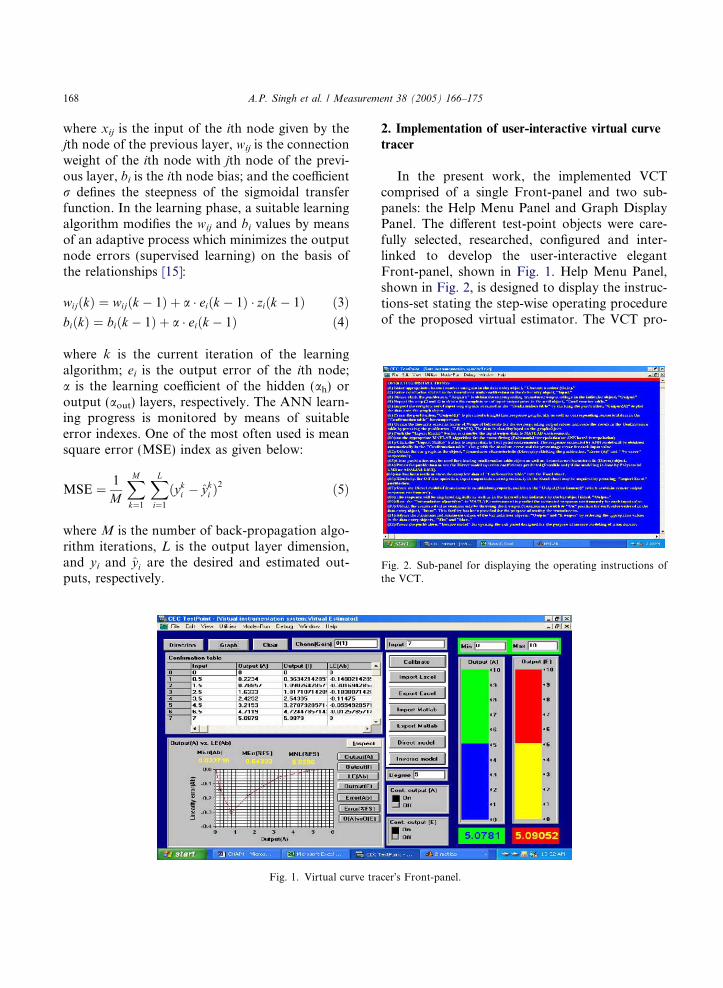
Fig. 2. Sub-panel for displaying the operating instructions ofthe VCT.

168 A.P. Singh et al. / Measurement 38 (2005) 166–175

where xij is the input of the ith node given by thejth node of the previous layer, wij is the connectionweight of the ith node with jth node of the previ-ous layer, bi is the ith node bias; and the coefficientr defines the steepness of the sigmoidal transferfunction. In the learning phase, a suitable learningalgorithm modifies the wij and bi values by meansof an adaptive process which minimizes the outputnode errors (supervised learning) on the basis ofthe relationships [15]:

wijðkÞ ¼ wijðk � 1Þ þ a � eiðk � 1Þ � ziðk � 1Þ ð3ÞbiðkÞ ¼ biðk � 1Þ þ a � eiðk � 1Þ ð4Þ

where k is the current iteration of the learningalgorithm; ei is the output error of the ith node;a is the learning coefficient of the hidden (ah) oroutput (aout) layers, respectively. The ANN learn-ing progress is monitored by means of suitableerror indexes. One of the most often used is meansquare error (MSE) index as given below:

MSE ¼ 1

M

XM

k¼1

XL

i¼1

ðyki � yki Þ2 ð5Þ

where M is the number of back-propagation algo-rithm iterations, L is the output layer dimension,and yi and yi are the desired and estimated out-puts, respectively.

Fig. 1. Virtual curve tra

2. Implementation of user-interactive virtual curve

tracer

In the present work, the implemented VCTcomprised of a single Front-panel and two sub-panels: the Help Menu Panel and Graph DisplayPanel. The different test-point objects were care-fully selected, researched, configured and inter-linked to develop the user-interactive elegantFront-panel, shown in Fig. 1. Help Menu Panel,shown in Fig. 2, is designed to display the instruc-tions-set stating the step-wise operating procedureof the proposed virtual estimator. The VCT pro-

cer�s Front-panel.

Fig. 3. Sub-panel for simultaneous display of the variousgraphs.

Normalized actual input, x

Normalized estimated output, y

Normalized actual output, y

ErrorSignal, e

y

y

Inputlayer

Output layer(linear neuron)

Hidden layer(tansigmoidal neurons)

Transducer(Sensor + Signal

conditioner)

1

12

1

m

Learningalgorithm

Weight adaptation

Σ

Fig. 4. A scheme of a MLFFBP-ANN based direct modeling ofa transducer.


vides the provision for comparing the actual, idealand estimated values of response in the tabular aswell as in graphical form. An inbuilt algorithm wasimplemented as a part of VCT to compute theabsolute value of maximum non-linearity associ-ated with the transducer in terms of percentageof full span. The Signal Processing Software thatperforms the modeling of transducer characteris-tics used MLFFBP-ANN based LMS regressionmethod for accurate fitting of transducer static re-sponse characteristics optimally to measured data.Another sub-panel was designed to display the re-sults of modeling graphically in a single-stroke asshown in Fig. 3. The user-interactive VCT is de-signed in a fourth generation graphical program-ming language using Test-point software [17] andis highly customized for the specific application.The computer selects any one or more of thesechannels under program control of the input datausing Test-point ADC-object configured for thispurpose. The source code for the action of theFront-panel and its various sub-panels was writtenas a complete integrated module to perform vari-ous actions.

3. Implementation of MLFFBP-ANN as a soft

estimator

Here, the neural modeling approach is based onthe use of a MLFFBP-ANN which is capable,

after a proper setup phase, of modeling aninput–output static response characteristics of atransducer. The proposed approach used the con-cept of the well-known system identification tech-nique based on ANN�s [15] as shown in Fig. 4.MLFFBP-ANN with proper biases, a sigmoid hid-den layer, and a linear output layer are capable ofapproximating any function (non-linear regres-sion) with definite number of discontinuities andwith an arbitrary accuracy [18]. An algorithmwas written using MATLAB programming andMATLAB Neural Network Toolbox to synthesizea two layer FFBP-model of transducer. The imple-mented neural model comprised of a hidden layerof sigmoidal neurons that receives measured dataand the broadcasts output values to a layer of lin-ear neurons, which finally compute the networkoutput. Using Eq. (1), the output of the proposedANN model is computed by

y ¼ F ANNðxiÞ¼ purelinðW 2 � tan sigðW 1 � xi þ B1Þ þ B2Þ ð6Þ

where purelin(Æ) is linear and tan sig(Æ) is a hyper-tangent sigmoid activation transfer function(monotonic s-shaped function mapping numbersin the interval j�1 to +1j into a finite intervalsuch as ]�1:1[ or ]0:1[). Generally a more complex

Fig. 5. Training data acquired and displayed by the virtualestimator for simulating the MLFFBP-ANN based directmodel of a pressure transducer.


function, such as transducer static response char-acteristics, particularly in computer based mea-surement system case, that are generally stronglynon-linear, requires more sigmoid neurons in thehidden layer. The best values of [B] and [W] matri-ces, associated with the bias and weights of eachneuron, are computed by minimizing the meansquare error (MSE). Using Eq. (5), the MSE, i.e.,the performance index, for the proposed neuralmodel is given by

MSEðx; yÞ ¼ 1

n

Xn

i¼1

½yi � F ANNðxiÞ�2 ð7Þ

During training, a set of input values corre-sponding to the calibration points help to adjustthe weights and biases of the neurons to minimizethe difference between the ANN output and the ac-tual response. However, the best ANN structure(number of layers, number of neurons in eachlayer, neuron�s activation transfer function, learn-ing algorithm and training parameters) is notknown in advance [14]. Also, several different train-ing algorithms are available for MLFFBP-ANNs[18,19]. It is very difficult to know which trainingalgorithm will provide an optimal learning for agiven problem. It depends upon many factorsincluding the complexity of the problem, the num-ber of data points in the training set, the number ofweights and biases in the network, and the errorgoal [20]. Thus there is an utmost necessity to per-form a comparative evaluation of the various vari-ants of the back-propagation learning algorithmsto obtain an optimal neural solution of curve-fit-ting. With this aim, an experimental evaluationthat consider the number of training epochs, com-putational load and architectural complexity ofANN trained with different variants of the BP algo-rithm for a given input–output data is carried out.From a study available, the different variants of theback-propagation learning algorithm fall into twobroad categories [20]. The first category used heu-ristic techniques, which were developed, from theanalysis of the performance of the standard steep-est descent algorithm. Under this category, fourlearning algorithms—Gradient Descent withMomentum, Adaptive Gradient Descent, AdaptiveGradient Descent with Momentum and Resilient

Back-propagation algorithms, were examined inthe present work. The second category of fast algo-rithms uses standard numerical optimization tech-niques. Under this category, we considered threeimportant variants including Conjugate Gradientalgorithms (Fletcher–Reeves update, Polak–Ribi-ere update, Powell–Beale restarts, and ScaledConjugate Gradient), Quasi-Newton algorithms(BFGS algorithm and One-step-Secant algorithm)and the Levenberg–Marquardt algorithm for train-ing the MLFFBP-ANN. Here, for the sake ofcomparison, we considered two different ANNstructures (1-2-1 and 1-5-1) for all the trainingalgorithms.

4. Experimental study

As a practical application, we used the strain-gauge type of pressure transducer (SenSym:S · 100DN, with bridge excitation of 6.6978 V at25 �C ambient temperature), coupled to a DAS-connected computer based measurement system,to acquire the data for modeling its input–outputstatic response characteristics. A set of nine pairsof input–output data, constituting the trainingset, is acquired by the proposed VCT. The ac-quired data covers the complete range of operation(0–7 bars) of the transducer under calibration andis shown in Fig. 5. The proposed MLFFBP-ANNmodel of transducer is integrated as the SignalProcessing Software of the VCT for three differentneural modeling phases of the transducer, namelylearning, validation and production phases as

0 2 8

Input

0

1

2

3

4

5

6O

utp

ut

(A)

0 2 6Input

0

1

2

3

4

5

Ou

tpu

t (A

)

a b4 6 4 8

Fig. 6. Actual response of a pressure transducer displayed by the VCT with (a) training data and (b) validation data.


usual. After successful training of the proposedMLFFBP-ANN model, for each of the 12 learningalgorithms, the results of direct modeling are vali-dated, by acquiring another set of data constitut-ing the validation set (range: 0.2–6.8 bars)covering all the remaining 34 untrained pairs.The actual (measured) response of the transducerdisplayed by the proposed VCT for training andvalidation data is shown in Fig. 6. The perfor-mance of the proposed neural model is studiedfor 1-2-1 and 1-5-1 structures, trained with differ-ent back-propagation learning algorithms, usingthe default training parameters in the MATLABNeural Network Toolbox.

5. Results and discussion

Table 1 summarizes the results of direct model-ing obtained from MLFFBP-ANN based soft esti-mator, trained with basic gradient descent BPalgorithm and its different variants. Twelve differ-ent training algorithms were considered. A finalcomparison establishes the computational load,speed of learning and accuracy in terms of maxi-mum error obtained for each algorithm in approx-imating the direct model of the transducer. Table 1shows the number of epochs and accuracy in termsof absolute error and error (%FS) obtained for dif-ferent variants of BP algorithms. From the results,it is observed that, the Levenberg–Marquardtalgorithm is the fastest learning algorithm as com-pared with all other algorithms considered. Thereason for its high speed of convergence is due tothe fact that like the Quasi-Newton, the Leven-

berg–Marquardt algorithm [19] was designed toapproach second order training speed withouthaving to compute the Hessian matrix. It providesthe most optimal solution for transducer modelingwith respect to speed of convergence, computa-tional complexity and computational load.

Thus the Levenberg–Marquardt learning algo-rithm, MLFFBP-ANN with 1-2-1 structure (twohidden neurons) has been chosen here to modelthe given pressure transducer. For the presentpractical example, the MLFFBP-ANN is trainedby Levenberg–Marquardt learning algorithm withparameters: performance goal (MSE) = 1e-6,learning rate = 0.3, factor to use for memory/speed tradeoff = 1, and maximum number ofepochs = 1000. The learning characteristics ofANN training are shown in Fig. 7. The estimatedresults displayed by VCT numerically as a resultof proposed neural modeling of pressure trans-ducer are shown in Fig. 8. The estimated static re-sponse of pressure transducer displayed by theVCT graphically is shown in Fig. 9.

From the results, it has been found that withtwo hidden neurons, it is possible to reduce theMSE to 3.06331e-006 in only 91 training epochs.The absolute error between actual and estimatedresponse displayed by the VCT for the trainingand validation data is shown in Fig. 10. Also,the error in terms of percentage of full span be-tween the actual and estimated response, displayedby the VCT, for the training and validation data, isshown in Fig. 11. The absolute value of the maxi-mum absolute error between the measured andpredicted response is found to be only 0.021146for training data and 0.11613 for validation data.

Fig. 7. Learning characteristics of a MLFFBP-ANN withLevenberg–Marquardt learning algorithm.

Fig. 8. Estimated results displayed by VCT numerically as aresult of MLFFBP-ANN based direct modeling of pressuretransducer.

Table 1Comparison of various variants of back-propagation learning algorithm for training MLFFBP-ANN based direct model of pressuretransducer

Training algorithm Number ofhidden neurons

Numberof epochs

Meansquare error

Maximum absolute error Maximum error (%FS)

Trainingdata

Validationdata

Trainingdata

Validationdata

Basic gradient descent 2 81,463 4.86043e-005 0.066795 0.16388 1.3128 3.34235 5221 9.99812e-007 0.0106 0.22872 0.2092 4.6647

Adaptive gradient descent 2 37,863 4.85911e-005 0.07014 0.1688 1.3786 3.44265 4859 9.99742e-007 0.010297 0.22834 0.20238 4.657

Gradient descent withmomentum

2 81,463 4.86043e-005 0.066795 0.16388 1.3128 4.44275 5221 9.99812e-007 0.0106 0.22872 0.2092 4.6647

Adaptive gradientdescent with momentum

2 9794 4.85936e-005 0.066799 0.1639 1.3129 3.34285 1243 9.89317e-007 0.010686 0.22883 0.21003 4.6671

Resilient BP 2 673 4.8584e-005 0.061986 0.14382 1.2183 2.93325 2639 9.99246e-007 0.011931 0.382 0.2345 7.7908

Fletcher–Reeves CG 2 164 2.32338e-005 0.040294 0.13228 0.79196 2.69795 51 8.16989e-007 0.0096375 0.23055 0.18942 4.702

Polak–Ribiere CG 2 82 0.000121744 0.09159 0.19726 1.7993 4.042325 64 8.81283e-007 0.0084558 0.24186 0.1662 4.9327

Powell–Beale CG 2 106 1.85432e-005 0.040815 0.11227 0.80219 2.28985 44 1.90511e-006 0.015097 0.23457 0.29673 4.784

Scaled conjugate gradient 2 131 4.71543e-005 0.065801 0.16348 1.2933 3.33425 59 2.6711e-007 0.0056842 0.23713 0.11172 4.8363

BFGS Quasi-Newton 2 210 3.06331e-006 0.021145 0.11614 0.41558 2.36865 28 1.65527e-008 0.0011958 0.23434 0.023502 4.7793

One-step-Secant 2 361 4.39131e-005 0.054748 0.15111 1.076 3.08195 157 9.29975e-007 0.0083295 0.23888 0.16371 4.872

Levenberg–Marquardt 2 91 3.06331e-006 0.021146 0.11613 0.41561 2.38855 5 1.45678e-028 1.2479e-013 0.2322 2.4527e-012 4.8086


The absolute value of maximum error in terms ofpercentage of full span between the measured

and predicted response is found to only 0.41561for the training data and 2.3885 for validation

0 4 6Input

-2

0

2

4

6O

utp

ut

(E)

0 6

Input

0

1

2

3

4

5

Ou

tpu

t (E

)

a b82 2 4 8

Fig. 9. Static response of pressure transducer estimated by MLFFBP-ANN model trained with Levenberg–Marquardt learningalgorithm using (a) training data and (b) validation data.

0 1 3 5Output (A)

-0.04

-0.02

0.00

0.02

Err

or

(Ab

)

0 5

Output (A)

-0.15

-0.10

-0.05

-0.00

0.05

0.10

0.15E

rro

r (A

b)

a b1 2 3 42 4 6

Fig. 10. Absolute error between actual and estimated response using (a) training data and (b) validation data.

0 1 3 5Output (A)

-0.4

-0.2

-0.0

0.2

0.4

Err

or

(%F

S)

0 4 5

Output (A)

-3

-2

-1

0

1

2

3

Err

or

(%F

S)

a b2 4 6 1 2 3

Fig. 11. Error (%FS) between actual and estimated response using (a) training data and (b) validation data.


data. Achievement of such a low values of theabsolute error and error (%FS) both for the train-ing and validation data indicate the effectiveness ofthe proposed MLFFBP-ANN based modeling ofsensors. Comparison of actual and estimated re-sponse displayed by VCT for training and valida-

tion data is shown in Fig. 12. From theestimated response, it has been found that the ac-tual and estimated values are very close to eachother. The estimated direct response characteris-tics are found to be extremely close to the actualcharacteristics.

0

a b2 5

Output (A)

-2

0

2

4

6

Ou

tpu

t (E

)

0 2 3 4Output (A)

0

1

2

3

4

5

Ou

tpu

t (E

)

1 3 4 6 1 5

Fig. 12. Comparison of actual and estimated response displayed by VCT for (a) training data and (b) validation data.


6. Conclusion

The paper proposes a simple approach for trans-ducer direct modeling using MLFFBP-ANNtrained with Levenberg–Marquardt learning algo-rithm.Multilayer networks are capable of perform-ing just about any linear or non-linear computationand can approximate any reasonable function arbi-trarily well. Such networks overcome the problemsassociated with the conventional numerical as wellas existing ANN based interpolation methods. Inthis context, a study was made to find an efficientandmore accurateMMFFBP-ANN based solutionfor optimal fitting of transducer static responsecharacteristics to measured data. The overall re-sults from the presented study indicate that theLevenberg–Marquardt algorithm based training isa viable and useful alternative to the various othervariants of the BP learning algorithms for optimalfitting of transducer characteristics. This techniquewould be useful for other types of transducers pos-sessing similar non-linear characteristics.

Acknowledgements

The authors wish to thank Prof. (Dr.) R.C.Chauhan, Director, SLIET, Longowal for hisstimulating interest and constant encouragementthroughout the work.

References

[1] D. Patranabis, S. Ghosh, C. Bakshi, Linearizing transducercharacteristics, IEEE Trans. Instrum. Meas. 37 (1) (1988)66–69.

[2] D. Patranabis, Sensors and Transducers, Wheeler Publish-ing Co., Delhi, 1997, pp. 249–254.

[3] J.M. Dias Pereira, P.M.B. Silva Girao, O. Postolache,Fitting transducer characteristics to measured data,IEEE Instrum. Meas. Mag. 4 (December) (2001) 26–39.

[4] S.A. Dyer, J.S. Dyer, Cubic-spline interpolation: Part 1,IEEE Instrum. Meas. Mag. 4 (March) (2001) 44–46.

[5] S.A. Dyer, J.S. Dyer, Cubic-spline interpolation: Part 2,IEEE Instrum. Meas. Mag. 4 (June) (2001) 34–36.

[6] O. Postolache, P. Girao, M. Pereira, Neural networks inautomated measurement systems: state of the art and newresearch trends, in: Proceedings of IEEE InternationalJoint Conference on Neural Networks-IJCNN�01, Wash-ington, DC, USA, 3, July 15–19, 2001, 2310–2315.

[7] J.C. Patra, R.N. Pal, Inverse modeling of pressure sensorsusing artificial neural networks, in: AMSE InternationalConference Signals, Data, and Syst., Banglore, India, 1993,225–236.

[8] J.C. Patra, G. Panda, R. Baliarsingh, Artificial neuralnetwork-based non-linearity estimation of pressure sen-sors, IEEE Trans. Instrum. Meas. 43 (1994) 874–881.

[9] S.A. Khan, A.K. Agarwala, D.T. Shahani, Artificial neuralnetwork (ANN) based non-linearity estimation of therm-istor temperature sensors, in: Proceedings of 24th Nationalsystems Conference, Banglore, India, 2000, 296–302.

[10] A.P. Singh, S. Kumar, T.S. Kamal, Artificial neuralnetwork based modelling of thermocouples, J. Inst. Eng.(E. and T. Div.) 83 (2003) 71–75.

[11] S.K. Rath, J.C. Patra, A.C. Kot, An intelligent pressuresensor with self-calibration capability using artificial neuralnetworks, in: IEEE International Conference on Systems,Man, and Cybernetics Proceedings, 4, October 8–11, 2000,2563–2568.

[12] M. Attari, F. Boudjema, M. Heniche, An artificial neuralnetwork to linearize a G (Tungsten vs. Tungsten 26%Rhenium) thermocouple characteristics in the range of zeroto 2000 �C, in: Proceedings of the International Sympo-sium on Industrial Electronics, ISTE�95, 1, July 10–14,1995, 176–180.

[13] M. Attari, F. Boudjema, M. Heniche, Linearizing athermistor characteristics in the range of zero to 100 �Cwith two layers artificial neural networks, in: IEEE Inst.


Meas. Tech. Conference, IMTC�95, Waltham (USA), 1,April 24–26, 1995, 119–122.

[14] B. Widrow, M.H. Lehr, 30 Years of adaptive neuralnetworks: perceptions, madaline & back-propagation,Proc. IEEE 78 (1990) 1415–1442.

[15] S. Haykin, Neural Networks: A Comprehensive Founda-tion, Pearson Education Asia, 2001, pp. 118–120.

[16] S.V. Kartalopoulos, Understanding Neural Networks andFuzzy Logic, PHI, New Delhi, 2000.

[17] Capital Equipment Test-point Software (Version 3.3)User�s Manual (1997).

[18] B. Kosko, Neural Networks and Fuzzy Systems, PHI, NewDelhi, 2000, pp. 13–14.

[19] M.T. Hagan, M. Menhaj, Training feed-forward networkswith the Marquardt algorithm, IEEE Trans. NeuralNetwor. 5 (6) (1994) 989–993.

[20] M.T. Hagan, H.B. Demuth, M. Beale, Neural NetworkDesign, Thomson Asia Pte Ltd., Singapore, 2002.

Virtual curve tracer for estimation of static response characteristics of transducers

Documents

Transcript of Virtual curve tracer for estimation of static response characteristics of transducers