Vertices of planar curves under the action of linear transformations
28
J. geom. 73 (2002) 148 – 175 0047–2468/02/020148 – 28 $ 1.50 + 0.20/0 © Birkh¨ auser Verlag, Basel, 2002 Vertices of planar curves under the action of linear transformations Douglas S. Shafer and Andr´ e Zegeling Abstract. The number of vertices of a smooth Jordan curve with nowhere vanishing curvature can change under the action of a nonsingular real linear transformation. We examine the bifurcation set in the space of linear trans- formations for the number of vertices on the image curve, showing that generally there is a codimension-one set of linear transformations making an arbitrary point into a vertex, and obtaining conditions that the point be capable of being transformed into a higher vertex. We demonstrate that there is always an open set of linear transformations such that the image curves have at least six vertices. 2000 Mathematics Subject Classification: 53A04, 14H99. Key words: Curvature, linear transformation, vertex. 1. Introduction The classical Four Vertex Theorem, first proved by Mukhopadhaya [6], states that a smooth, convex Jordan curve in the plane has at least four vertices, where by “vertex” is meant a local extreme value of the curvature. For generalizations of this theorem to larger classes of closed curves, see [2], [5], and [7]. In this paper we adopt a slightly different, but more convenient concept of “quasi-vertex of order n,” by which we mean a point on a sufficiently smooth planar curve where the first n derivatives of the curvature vanish, but the (n + 1)st does not. The Four Vertex Theorem then translates into the statement that at least four quasi-vertices of odd order appear on any smooth, convex Jordan curve. Our goal is to investigate the occurrence of quasi-vertices on a planar curve γ with non- vanishing curvature when a nonsingular real linear transformation is applied. The first natural question is the following local problem: given a point P on γ , what order quasi- vertex can P become under the action of a nonsingular linear transformation? In [1] it was proved that generically P is and remains a point at which the derivative of the curvature is non-zero. In Section 1 we study in detail the non-generic transforma- tions changing P into a quasi-vertex. We find that for every point on γ such a non-generic class of transformations exist. Whether or not there exists a transformation creating a mul- tiple quasi-vertex from P depends on a condition on the curve near P (Theorem 2.12, interpreted geometrically in Section 4), but if the curve is closed with nowhere van- ishing curvature (but not necessarily simple) then there must always exist an open arc 148
-
Upload
independent -
Category
Documents
-
view
1 -
download
0
Transcript of Vertices of planar curves under the action of linear transformations

J. geom. 73 (2002) 148 – 1750047–2468/02/020148 – 28 $ 1.50 + 0.20/0© Birkhauser Verlag, Basel, 2002
Vertices of planar curves under the actionof linear transformations
Douglas S. Shafer and Andre Zegeling
Abstract. The number of vertices of a smooth Jordan curve with nowhere vanishing curvature can change underthe action of a nonsingular real linear transformation. We examine the bifurcation set in the space of linear trans-formations for the number of vertices on the image curve, showing that generally there is a codimension-one set oflinear transformations making an arbitrary point into a vertex, and obtaining conditions that the point be capable ofbeing transformed into a higher vertex. We demonstrate that there is always an open set of linear transformationssuch that the image curves have at least six vertices.
2000 Mathematics Subject Classification: 53A04, 14H99.Key words: Curvature, linear transformation, vertex.
1. Introduction
The classical Four Vertex Theorem, first proved by Mukhopadhaya [6], states that a smooth,convex Jordan curve in the plane has at least four vertices, where by “vertex” is meant alocal extreme value of the curvature. For generalizations of this theorem to larger classesof closed curves, see [2], [5], and [7]. In this paper we adopt a slightly different, butmore convenient concept of “quasi-vertex of order n,” by which we mean a point on asufficiently smooth planar curve where the first n derivatives of the curvature vanish, butthe (n + 1)st does not. The Four Vertex Theorem then translates into the statement that atleast four quasi-vertices of odd order appear on any smooth, convex Jordan curve.
Our goal is to investigate the occurrence of quasi-vertices on a planar curve γ with non-vanishing curvature when a nonsingular real linear transformation is applied. The firstnatural question is the following local problem: given a point P on γ , what order quasi-vertex can P become under the action of a nonsingular linear transformation? In [1] itwas proved that generically P is and remains a point at which the derivative ofthe curvature is non-zero. In Section 1 we study in detail the non-generic transforma-tions changing P into a quasi-vertex. We find that for every point on γ such a non-genericclass of transformations exist. Whether or not there exists a transformation creating a mul-tiple quasi-vertex from P depends on a condition on the curve near P (Theorem 2.12,interpreted geometrically in Section 4), but if the curve is closed with nowhere van-ishing curvature (but not necessarily simple) then there must always exist an open arc
148

Vol. 73, 2002 Vertices of planar curves under the action of linear transformations 149
of points satisfying this condition (Theorem 2.13), at least one point of which can betransformed into a quasi-vertex of order n ≥ 3 (Theorem 2.19).
In Section 3 we turn to the global question of the number of vertices that can be created ona closed curve under linear transformation. We find that for any smooth Jordan curve withnon-zero curvature, there always exists a linear transformation yielding a curve with at leastsix. The method of proof is interesting in its own right: to each such curve γ is associated abifurcation curve γ ∗ lying in a two-sphere in the space of linear transformations, every pointof which corresponds to a family of linear transformations which a multiple quasi-vertexfrom a particular point of γ . Moreover, for any real linear transformation µ, the number ofvertices of µ〈γ 〉 is precisely the number of tangent great circles to γ ∗ that pass through thepoint of S2 corresponding to µ. Thus the geometry of γ ∗, notably the number of cusps andloops, reflects the maximum number of quasi-vertices appearing on images of γ , and servesas a tool for classifying convex Jordan curves. In particular, the region in the complementof γ ∗ corresponding to the fewest vertices yields at least four vertices (by the Four VertexTheorem), hence other regions give transformations yielding an image with at least six,giving the result mentioned.
In Section 4, we begin by stating our results in the language of Affine Differential Geometry.The Six Affine Vertex Theorem, also proved by Mukhopadhaya, states that a smooth convexJordan curve γ must have at least six sextactic points (see Section 4 for the definition). Weconclude by showing how our work yields an addendum to the Six Affine Vertex Theorem: ifthe curvature of γ never vanishes, then at least one of the sextactic points must occur at pointsat which γ is elliptically curved, i.e., at a point at which the osculating conic is an ellipse.
The original motivation for this research stems from the investigation of periodic solutionsof planar autonomous ordinary differential equations, which are smooth Jordan curves.Applications of the results of this paper in this context are detailed in a forthcoming paper.
2. Local properties of the curvature function
Let γ denote a Cr curve in the plane, r ≥ 4. It will be convenient to parametrize γ withrespect to a rectangular coordinate system by
x = u(t) y = v(t) (1)
where u and v are at least four times continuously differentiable functions on some openinterval J ⊂ R. (At this point we do not restrict to periodic functions.) With respect to thisparametrization, the curvature κ is expressed as
κ = α(t) = u′v′′ − u′′v′
(u′2 + v′2)3/2,

150 Douglas S. Shafer and Andre Zegeling J. Geom.
where the primes denote differentiation with respect to t . Any change in parametrizationwill have no effect on either κ or on the order of vanishing of its derivative with respect tothe parameter:
PROPOSITION 2.1. Let t = g(τ) be a Ck reparametrization of γ with a Ck inverse.Suppose that with respect to the new parametrization κ = β(τ). Then α(j)(t0) = 0 forj = 1, 2, . . . , k − 1 but α(k)(t0) �= 0 if and only if β(j)(τ0) = 0 for j = 1, 2, . . . , k − 1 butβ(k)(τ0) �= 0.
Proof. This follows from the Chain Rule for higher derivatives. �
On the basis of this result we may unambiguously define:
DEFINITION 2.2. A point P on γ , corresponding to t = t0 in 1, is called a quasi-vertexof order n if α(j)(t0) = 0 for j = 1, 2, . . . , n but α(n+1)(t0) �= 0. In the case n = 1 P istermed a simple quasi-vertex, and otherwise a multiple quasi-vertex.
REMARK 2.3. The case when n is odd corresponds to what is usually called a vertex inthe literature, being a point at which the curvature has a local extreme value. Some authorsreserve the term “vertex” for the case n = 1, and use the term “higher vertex” for theremaining cases, n odd.
Now let µ be a real linear transformation of the plane, carrying γ to a new curve γ := µ〈γ 〉,which receives a naturally induced parametrization. If we take µ to be nonsingular, thenregular points on γ correspond with regular points on γ under the parametrizations, henceso do points at which the curvature is defined. Indeed, if the matrix representative of µ in
(x, y)-coordinates is
(a b
c d
), then the curvature κ along γ is expressed as
κ = ω(t) = det µu′v′′ − u′′v′
((au′ + bv′)2 + (cu′ + dv′)2)3/2. (2)
It is useful to write the denominator as D(t)32 where
D(t) = µ0u′2 + 2µ1u
′v′ + µ2v′2 (3)
forµ0 = a2 + c2 µ1 = ab + cd µ2 = b2 + d2.
Identifying the set of linear transformations of R2 with R
4, we define an analytic mapL : R
4 → R3 by
L : µ =(
a b
c d
)→ (µ0, µ1, µ2).

Vol. 73, 2002 Vertices of planar curves under the action of linear transformations 151
Then L is a submersion except at the zero transformation, and maps R4 onto the set
F := {(µ0, µ1, µ2) | µ0µ2 ≥ µ12}, carrying the set of singular linear transformations
to the boundary ∂F = {(µ0, µ1, µ2) | µ0µ2 = µ12}. Since L is in fact a function of the
columns of the matrix µ,
L([c1 c2]) = (‖c1‖2, c1 · c2, ‖c2‖2),
it follows that L(µ′) = L(µ) iff µ′ = η◦µ, where η is a rigid motion fixing the origin, i.e., arotation, possibly composed with a reflection in, say, the x-axis. (Note that preceding µ witha rotation changes the L-image; see Remark 2.6 below.) Expression 2 shows that vanishingor non-vanishing of the curvature at a point is invariant under linear transformations. Infact, the order of vanishing is also invariant.
PROPOSITION 2.4. If α(j)(t0) = 0 for j = 0, 1, 2, . . . , k − 1 but α(k)(t0) �= 0, thenω(j)(t0) = 0 for j = 0, 1, 2, . . . , k − 1 but ω(k)(t0) �= 0.
This fact is a corollary of the following simple result:
LEMMA 2.5. If f (x) = n(t)/d(t) is a Ck function on an open interval containing t0, thenfor any m ≤ k, f (j)(t0) = 0 for j = 0, 1, . . . , m iff n(j)(t0) = 0 for j = 0, 1, . . . , m.
The essential point of the proposition is that the original curvature vanished at the point inquestion, so that the lemma applied. When the curvature is non-zero, then it is quite possiblethat α′(t0) not vanish, but ω′(t0) be zero for a suitable choice of µ, which is exactly whatmakes the matter interesting and useful. Indeed, our goal is to identify conditions underwhich a point P on γ can be made a quasi-vertex under appropriate choice of µ, and ofwhat order. For example, for any point on an ellipse there is an appropriate choice of µ
making the point into a simple vertex, and another choice of µ making it a quasi-vertex ofinfinite order.
For the general curve (1) with curvature (2), under a linear transformation µ the expressionfor the derivative of the new curvature is, after factoring out the positive term det µ D(t)−5/2,
ω′(t) ∼ ζ1 := µ0f0(t) + µ1f1(t) + µ2f2(t) (4)
where
f0(t) = u′2(u′v′′′ − u′′′v′) − 3u′u′′(u′v′′ − u′′v′)f1(t) = 2u′v′(u′v′′′ − u′′′v′) − 3(u′′v′ + u′v′′)(u′v′′ − u′′v′) (5)
f2(t) = v′2(u′v′′′ − u′′′v′) − 3v′v′′(u′v′′ − u′′v′)
andµ0 = a2 + c2 µ1 = ab + cd µ2 = b2 + d2,
as above.
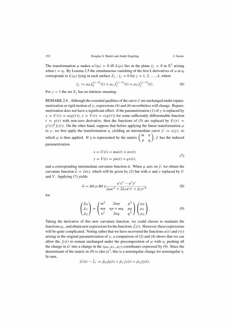
152 Douglas S. Shafer and Andre Zegeling J. Geom.
The transformation µ makes ω′(t0) = 0 iff L(µ) lies in the plane ζ1 = 0 in R3 arising
when t = t0. By Lemma 2.5 the simultaneous vanishing of the first k derivatives of ω at t0
corresponds to L(µ) lying in each surface Zj : ζj = 0 for j = 1, 2, . . . , k, where
ζj := µ0f(j−1)
0 (t) + µ1f(j−1)
1 (t) + µ2f(j−1)
2 (t). (6)
For j > 1 the set Zj has no intrinsic meaning.
REMARK 2.6. Although the essential qualities of the curve γ are unchanged under repara-metrization or rigid motion of γ , expressions (4) and (6) nevertheless will change. Repara-metrization does not have a significant effect: if the parametrization (1) of γ is replaced byx = U(τ) = u(g(τ)), y = V (τ) = v(g(τ)) for some sufficiently differentiable functiont = g(τ) with non-zero derivative, then the functions of (5) are replaced by Fi(τ ) =g′(τ )6fi(τ ). On the other hand, suppose that before applying the linear transformation µ
to γ , we first apply the transformation η, yielding an intermediate curve γ := η〈γ 〉, to
which µ is then applied. If η is represented by the matrix
(m n
p q
), γ has the induced
parametrization
x = U(t) = mu(t) + nv(t)(7)
y = V (t) = pu(t) + qv(t),
and a corresponding intermediate curvature function α. When µ acts on γ , we obtain thecurvature function ¯κ = ω(t), which will be given by (2) but with u and v replaced by U
and V . Applying (7) yields
ω = det µ det ηu′v′′ − u′′v′
µ0u′2 + 2µ1u′v′ + µ2v′2 (8)
for µ0
µ1
µ2
=
m2 2mp p2
mn np + mq pq
n2 2nq q2
µ0
µ1
µ2
. (9)
Taking the derivative of this new curvature function, we could choose to maintain thefunctionsµi , and obtain new expressions for the functions fi (t). However, these expressionswill be quite complicated. Noting rather that we have recovered the functions u(t) and v(t)
arising in the original parametrization of γ , a comparison of (2) and (4) shows that we canallow the fi(t) to remain unchanged under the precomposition of µ with η, pushing allthe change in ω′ into a change in the (µ0, µ1, µ2)-coordinates expressed by (9). Since thedeterminant of the matrix in (9) is (det η)3, this is a nonsingular change for nonsingular η.In sum,
ω′(t) ∼ ζ1 := µ0f0(t) + µ1f1(t) + µ2f2(t),

Vol. 73, 2002 Vertices of planar curves under the action of linear transformations 153
for µi given by (9), and for fi(t) unchanged. We also note that the transformation (9) ofR
3 preserves the set F = im(L).
Fix P corresponding to parameter value t0; the quantities f(j)i (t0), i = 0, 1, 2, j = 0, 1, . . .
appearing in (4) and (6) are given numbers, so that Zj : ζj = 0 are fixed linear subspaces of(µ0, µ1, µ2)-space. Thus for the set of (µ0, µ1, µ2)-values in Z1, the point P is transformedby any element in the corresponding collection of linear transformations into a quasi-vertex of order at least 1. The exact order is determined by how many other of the planesZj pass through (µ0, µ1, µ2). Since we are dealing with linear subspaces we may byhomogeneity restrict ourselves to consideration of the sphere S2 : µ2
0 + µ21 + µ2
2 = 1.Any point (µ0, µ1, µ2) on the sphere now corresponds to a two-parameter family of lineartransformations {L−1(µ0/σ, µ1/σ, µ2/σ) | σ ∈ R\{0}}, all of which yield exactly thesame effect on the image of P insofar as being a quasi-vertex or not (and of what order) isconcerned. The reason for this loss of parameters in the reduction(
a b
c d
)∈ R
4 → (µ0, µ1, µ2) ∈ S2
is easily understood. For a fixed P , neither the one-parameter family of rotations nor theone-parameter family of uniform rescalings has any effect on the shape of the curve (thelatter family changes the curvature at every point, to be sure, but uniformly so, withoutchanging the rate of change of the curvature, hence the shape). Indeed, we will thereforenot distinguish between L and the composition of L with radial projection of R
3 onto S2,and may identify F = Im(L) with its intersection with S2. This is most convenient in thediscussion of the following point. In Section 3 we will be led to a consideration of curveslying in the entire sphere, not just that portion identified with F . The L-preimage of pointsin S2 \F corresponds to certain complex linear transformations. Fixing t0 ∈ J , equatingD(t0) in expression (3) to zero defines a great circle in S2, which lies wholly outside F
except for a point (and antipodal point) of tangency with ∂F . This is a “bad circle” ofcomplex linear transformations (and one singular real transformation) for which the imageof P on the image of γ has no curvature, and in fact the limit of the curvature does not existas the image point P is approached along γ .
In order to establish the behavior of P under arbitrary µ, we must investigate the characterof the subspaces Zj , their relative positions, and their intersection with the set F , since weallow only real transformations.
Let us simplify matters by giving γ a unit speed parametrization, so that u′(t) = cos φ(t)
and v′(t) = sin φ(t), where φ(t) is the angle that the tangent to γ makes with the positivex-axis at parameter value t , and now κ = φ′. Then the expressions (5) become
2
f0
f1
f2
=
3 sin 2φ 1 + cos 2φ
−6 cos 2φ 2 sin 2φ
−3 sin 2φ 1 − cos 2φ
(
φ′2φ′′
). (10)
154 Douglas S. Shafer and Andre Zegeling J. Geom.
LEMMA 2.7. At a regular point of γ (hence of γ ) corresponding to t = t0,
(1) (f0, f1, f2) = (0, 0, 0) iff (κ, κ ′) = (0, 0) (hence (κ, κ ′) = (0, 0)) at t = t0;(2) (f0, f1) = (0, 0) only if κ = 0 (hence κ = 0) at t = t0, and similarly for the pair
(f2, f1);(3) (f ′
0, f′1, f
′2) = (0, 0, 0) iff (κ, κ′′) = (0, 0) at t = t0 when γ is parametrized by and
derivatives of κ are taken with respect to arclength, and only if κ = 0 (hence κ = 0)
in any case.
Proof. Point (1) follows from the fact that the 3 × 2 matrix in (10) has rank 2 for all φ.(Note that by Proposition 2.1 whether or not the derivative of the curvature vanishes isindependent of the parametrization.) For point (2), if the last row of the 3 × 2 matrix in(10) is deleted, the resulting square matrix has rank 2 except when φ is π/2 or 3π/2, inwhich case (f0, f1) = (0, 6φ′2), so that κ = 0. Similarly for the simultaneous vanishingof f1 and f2.
For point (3), differentiate in (10) to obtain
2
f ′
0f ′
1f ′
2
=
4 sin 2φ 6 cos 2φ 1 + cos 2φ
−8 cos 2φ 12 sin 2φ 2 sin 2φ
−4 sin 2φ −6 cos 2φ 1 − cos 2φ
φ′φ′′
φ′3φ′′′
. (11)
The 3 × 3 matrix in (11) is nonsingular for all φ, so when the parameter is arclength theresult is immediate. Because simultaneous vanishing of f ′
0, f ′1, and f ′
2 is independent ofthe vanishing of the derivative of the curvature with respect to arclength, Proposition 2.1no longer applies, and we can conclude only that simultaneous vanishing of the f ′
i forcesκ = 0. �
By Lemma 2.7 and (6) we have:
PROPOSITION 2.8. At a regular point of γ (henceof γ ) corresponding to t = t0,
(1) ζ1 = 0 defines a plane through (0, 0, 0) in R3, hence a great circle in S2, precisely
when (κ, κ ′) �= (0, 0) (hence (κ, κ ′) �= (0, 0)) at t = t0;(2) the plane defined by ζ1 = 0 is one of the two planes µ2 = 0 or µ0 = 0 only if κ = 0
(hence κ = 0) at t = t0;(3) ζ2 = 0 defines a plane through (0, 0, 0) in R
3, hence a great circle in S2, preciselywhen (κ, κ ′′) �= (0, 0) at t = t0 when γ is parametrized by and derivatives of κ aretaken with respect to arclength, and if κ �= 0 (hence κ �= 0) in any case.
Note that by Proposition 2.1 the condition on the first derivative of κ is independent of theparticular parametrization of γ .

Vol. 73, 2002 Vertices of planar curves under the action of linear transformations 155
PROPOSITION 2.9. At a regular point of γ (hence of γ ) corresponding to t = t0, atwhich ζ1 = 0 and ζ2 = 0 both define planes through (0, 0, 0) in R
3, the planes are identicaliff κ = 0 (hence κ = 0) at t = t0.
Proof. Parametrize γ by unit speed, and rotate the plane containing γ so that the tangentline at t = t0 is horizontal. By Remark 2.6, this does not affect whether or not ζ1 = 0 andζ2 = 0 define planes, or whether or not the planes are distinct. Under this parametrization,by (10) and (11)
f0(t0) = κ ′ f1(t0) = −3κ2 f2(t0) = 0
f ′0(t0) = 3κ3 + κ ′′ f ′
1(t0) = −4κκ ′ f ′2(t0) = −3κ3
(12)
Each row gives the entries of the normal vector to the corresponding plane. The third entryimplies that they are collinear only if κ = 0. If κ = 0, then by Proposition 2.8 and thehypothesis that we are dealing with planes in R
3, κ ′κ ′′ �= 0, and the vectors are collinear.�
THEOREM 2.10. Let P be a regular point of γ at which κ �= 0, and let P denote the imageof P under a nonsingular linear transformation µ of the plane.
(1) The set of nonsingular linear transformations of the plane for which P is not a vertexof γ is a dense open set.
(2) The set of nonsingular linear transformations of the plane for which P is a simplevertex of γ is a codimension-one submanifold of R
4.(3) The set of nonsingular linear transformations of the plane for which P is a multiple
quasi-vertex of γ is either empty, or a codimension-two submanifold of R4. More-
over, the multiplicity of the zero of the derivative of the curvature at P is the samefor every linear transformation making P a multiple quasi-vertex.
Proof. Suppose that P corresponds to t = t0 in some parametrization of γ . A necessarycondition that a linear transformation µ make P a vertex of γ is that L(µ) lie in the setZ1 : ζ1 = 0 defined by (4), which by Proposition 2.8 is a plane in R
3. This establishespoint (1).
The set Z2 : ζ2 = 0 is a distinct plane in R3 which intersects Z1 along a line 12. For
µ such that L(µ) ∈ Z1\ 12, the function ω′ has a simple zero at t0. Point (2) will followfrom Remark 2.6, provided Z1 has non-empty intersection with F . To see that this is so, letus take advantage of homogeneity and project F and Z1 radially onto the sphere S2. Theimage of Z1 is a great circle C1. The image of F is a pair of antipodal regions bounded byantipodal ellipses lying in the quadrants {(µ0, µ1, µ2)|µ0µ2 ≥ 0}, and tangent to the greatcircles µ0 = 0 and µ2 = 0 at (±1, 0, 0) and (0, 0, ±1). As noted at the end of Remark 2.6,

156 Douglas S. Shafer and Andre Zegeling J. Geom.
if we parametrize γ by arclength and rotate the plane to make the tangent at P horizontal,F ∩ S2 is unchanged, and from (4) and (12) C1 now passes through (0, 0, ±1) and is notthe great circle µ0 = 0 (since κ �= 0), implying that Z1 ∩ F �= ∅.
The first part of point (3) follows similarly, sinceP is a multiple zero ofω′ only ifL(µ) ∈ 12.The multiplicity of this zero is completely determined by how many of the successiveconditions ζj = 0 of (1.j) are satisfied along 12. Geometrically this corresponds to whetheror not the corresponding plane Zj does or does not contain 12. Of course, 12 need notintersect F . �
DEFINITION 2.11. A regular point P on γ at which κ �= 0 is doubleable if there is a realnonsingular linear transformation µ such that κ ′ = κ ′′ = 0 at P = µ(P ). The point P istripleable if there exists such µ such that κ ′ = κ ′′ = κ ′′′ = 0 at P .
By Proposition 2.1, these terms are well-defined, although somewhat awkward in that“doubleable” for example does not mean the existence of a transformation which makes P
a root of κ ′ of multiplicity exactly two, but of one that makes P a root that is of multiplicitytwo or greater. However, the more precise “at-least-doubleable” is too cumbersome.
When is a point P at which κ �= 0 doubleable? By Propositions 2.8 and 2.9 the two setsζ1 = 0 and ζ2 = 0 are distinct planes in R
3 which intersect along a line 12 through theorigin whose direction vector is �v = (µ∗
0, µ∗1, µ
∗2), where
µ∗0 = det
(f1 f2
f ′1 f ′
2
)µ∗
1 = − det
(f0 f2
f ′0 f ′
2
)µ∗
2 = det
(f0 f1
f ′0 f ′
1
). (13)
The condition that P be doubleable is that 12 lie in the interior of F \{(0, 0, 0)}, that is,that µ∗
0µ∗2 − µ∗
12 > 0. Using (10) and (11), for a unit speed parametrization this condition
reduces to 9φ′6(9φ′4 − 5φ′′2 + 3φ′φ′′′) > 0. Thus we have:
THEOREM 2.12. A regular point P at which κ �= 0 is doubleable iff
D := 3κκ ′′ − 5κ ′2 + 9κ4 > 0
at P , where derivatives are taken with respect to arclength.
With respect to a general parametrization (1), the quantityD is expressed as
D = 3αα′′s′ − 3αα′s′′ − 5α′2s′ + 9α4s′3
s′3 , (14)
where s(t) = ∫ t
0
√u′(ξ)2 + v′(ξ)2 dξ . By Remark 2.6, whether or not D vanishes at P
is independent of the parametrization of γ , and the sign of D at P is unchanged under anonsingular linear transformation of the plane containing γ .
Since both κ andD are everywhere positive along circles and ellipses, hence everywherealong closed curves which are sufficiently C4 close to them, curves composed entirely of

Vol. 73, 2002 Vertices of planar curves under the action of linear transformations 157
doubleable points abound. We now identify a class of curves which contain at least an openarc of doubleable points.
THEOREM 2.13. If γ is a regular closed Cr curve, r ≥ 4, whose curvature is nowherezero, then it contains an open arc of points, every one of which is doubleable.
Proof. Parametrize γ by arclength in such a way that κ > 0 everywhere, and note thatDis a valid indicator of doubleability everywhere on γ . Let P be a point at which κ assumesits minimum. Then κ ′ = 0 and κ ′′ ≥ 0 at P , so that at P D = 3κκ ′′ + 9κ4 is positive at P ,hence is positive on a neighborhood of P . �
Even if the curvature of γ vanishes at just finitely many points, and is of one sign everywhereelse, the conclusion of Theorem 2.13 still need not hold. For example, the curve defined byx4 + y4 = 1 has zero curvature at its four points of intersection with the coordinate axes,but positive curvature everywhere else. Parametrizing the curve by x and using (14) or (16)below, one finds that D is zero at the four relatively flat vertices at which κ = 0, and isnegative everywhere else, so that no point is doubleable.
We note here thatD ≡ 0 along a curve γ iff γ is a line segment or an arc of a parabola (seeProp. 2.20 below).
For the class of curves of Theorem 2.13, it is natural to ask if any of the doubleable pointscan in fact be made into a vertex of even higher order than just the second; i.e., accordingto Definition 2.11, must γ contain a tripleable point? To answer this question, we firstcharacterize tripleable points, then prove a pair of technical results, one of which will proveto be important for the next section.
THEOREM 2.14. A regular point P at which κ �= 0 is tripleable iff
D = 3κκ ′′ − 5κ ′2 + 9κ4 > 0
andT := 40κ ′3 + 9κ2κ ′′′ + 36κ4κ ′ − 45κκ ′κ ′′ = 0
at P , where derivatives are taken with respect to arclength.
Proof. In order that a point P be tripleable, it is necessary that the set Z3 contain the line 12, hence that the normal vector �n = (f ′′
0 , f ′′1 , f ′′
2 ) to Z3 (possibly the zero vector) beorthogonal to the direction vector �v = (µ∗
0, µ∗1, µ
∗2) of 12. Or, what comes to the same
thing, the system of equations ζ0 = 0, ζ1 = 0, ζ2 = 0 must have a non-trivial solution,hence the determinant of the matrix of coefficients be zero:
T ∼ det
f0 f1 f2
f ′0 f ′
1 f ′2
f ′′0 f ′′
1 f ′′2
= 0. (15)
158 Douglas S. Shafer and Andre Zegeling J. Geom.
Using a unit speed parametrization the determinant of the matrix in 15 has value 8φ′3[40φ′′3 + 9φ′2φ(4) + 36φ′4φ′′ − 45φ′φ′′φ′′′] = 0. Since this is of interest only whenκ �= 0, and is sufficient precisely when the non-trivial solution sought lies in F , we havethe theorem. �
REMARK 2.15. The matrix in (15) depends on the parametrization of γ . The quantityT is formed by giving γ a unit speed parametrization and removing a multiplicative factorof 8φ′3 from the determinant. This simplification facilitates the proofs of the next results.When the distinction is important we will write T det for the full determinant of the matrixin (15). Formulas which facilitate computations involvingD and T are (14) above and (16)and (17) below.
REMARK 2.16. The quantity T is a non-zero multiple of the projective length h of thecurve γ (cf. [3]), whose zeros correspond to sextactic points of γ (see Section 4 below.)
The geometric meaning of the vanishing of T and Remark 2.6 again combine to insurethat vanishing of T is independent of parametrization of γ , and of nonsingular lineartransformation of the plane containing P . This is of course in keeping with the meaning oftripleability.
LEMMA 2.17. T = 3κD ′ − 8κ ′D , where derivatives are taken with respect to arclength.
PROPOSITION 2.18. If ta < tb are such thatD (ta) = D (tb) = 0, and if κ is non-zeroon the interval [ta, tb], then there exists τ ∈ (ta, tb) such that T (τ ) = 0.
Proof. Parametrize γ by arclength in such a way that κ > 0 everywhere. Then D :=κ−8/3D and T := κ−11/3T /3 are defined everywhere on γ , and by Lemma 2.17D
′ = T . The result now follows from an application of Rolle’s Theorem to D onthe interval [ta, tb].
�
We can now establish that every curve in the class identified in Theorem 2.13 must containat least one point P for which there exists a real nonsingular linear transformation such thatthe image point P is a quasi-vertex of order at least three.
THEOREM 2.19. If γ is a regular closed Cr curve, r ≥ 4, whose curvature is nowherezero, then it contains a tripleable point.
Proof. Parametrize with respect to arclength in such a way that κ > 0 everywhere, and letD and T be defined as in the proof of Proposition 2.18. If S is the total length of γ ,

Vol. 73, 2002 Vertices of planar curves under the action of linear transformations 159
∫ S
0 T =D (S) −D (0) = 0, hence because T is periodic of period S, it has at least twozeros, hence T has at least two zeros on γ .
Let t be any parameter value at which D > 0, guaranteed to exist by Theorem 2.13. IfT (t) > 0, consider the smallest t1 > t at which T is zero. Then T > 0 on (t , t1), henceD is increasing on (t , t1), soD (t1) >D (t) > 0, henceD (t1) > 0, and by Theorem 2.14the point corresponding to t = t1 is tripleable. If T (t) < 0, then similar considerationsshow that the point corresponding to the largest t1 < t at which T is zero is tripleable.
�
The next result of this section is meant to give information about the genericity of doubleableand tripleable points on an arbitrary curve. The results are as one would expect from theprevious theorems, with the interesting twist that we have to exclude portions of conicsections in curves in order to establish a standard genericity result. This is because of thefollowing fact, showing the intimate connection between conic sections and the quantitiesD and T . The reader is also referred to Exercise I.6 of [4] in this regard. See also Section 4.
PROPOSITION 2.20. (1) D ≡ 0 along a curve γ iff γ is a segment of a straight line oran arc of a parabola.
(2) T ≡ 0 along a curve γ iff γ is a segment of a straight line or an arc of a conicsection.
Proof. Without loss of generality we may perform a rotation of the plane containing γ sothat in a neighborhood of a point P of γ under consideration, γ is given locally as the graphof a function y = f (x). Straightforward computations yield the formulas
D ∼ 3y′′y(4) − 5y′′′2 (16)
T ∼ 9y′′2y(5) + 40y′′′3 − 45y′′y′′′y(4) (17)
where in (16) we have omitted a positive factor, and in (17) a non-zero factor.
The “if” parts of both statements are readily verified. Thus, conversely, suppose D ≡ 0at every point in a neighborhood in γ of a point P ∈ γ . Make a rigid motion of γ ifnecessary so that in a neighborhood of P it becomes the graph of a function y = f (x). Ify′′ vanishes identically near P , then of course γ is a line segment. Otherwise, there areintervals arbitrarily close to P on which y′′ �= 0. On any such interval, the differentialequation (16) satisfied by y may be multiplied by the integrating factor 1
3y′′−8/3 to yield theequivalent equation
d
dx[y′′−5/3y′′′] = 0 or
d
dx[y′′−2/3] = const.,
whence y′′ = (ax + b)−3/2 for some constants a and b. This is readily solved, and yieldsa parabolic arc.

160 Douglas S. Shafer and Andre Zegeling J. Geom.
In the situation that T ≡ 0 on a neighborhood of P in γ , we proceed in precisely thesame manner. On an interval on which y′′ �= 0 we may multiply by 9y′′−11/3 to obtain anequivalent equation
d2
dx2[y′′−5/3y′′′] = 0,
leading to y′′ = (ax2 + bx + c)−3/2 for some constants a, b, and c. If a = 0 we are in theprevious case; otherwise we will obtain some other conic section as the solution. �
Now suppose that the C4 curve γ does not contain an arc of a conic section, nor any point atwhich κ vanishes. Then the set of parameter values in J corresponding to points at whichT vanishes is a closed subset of J , by continuity of the derivatives involved. It is alsonowhere dense in J , for any open set in its closure is an open set yielding points of γ onwhich T vanishes, contradicting Proposition 2.20. Since D is everywhere negative on ahyperbola, and vanishes along parabolas, these observations and Theorem 2.14 combine togive the following result:
THEOREM 2.21. If γ is a Cr curve, r ≥ 4, then the set of tripleable points of γ is a closedset which is a union of line segments, elliptical arcs, and a closed set which is nowheredense in γ .
3. Global properties of the curvature function
Given a regular curve γ as in (1), for each t ∈ J corresponding to a point P of γ at whichκ �= 0, the line 12 exists and intersects the sphere S2 in two points. Thus as t movesthrough J , provided κ remains non-zero, a pair of curves in S2 are traced out. We referto the pair together as the “star curve” associated with γ , and denote it γ ∗. Indeed, for
(µ0, µ1, µ2) ∈ R3, let � =
õ2
0 + µ21 + µ2
2. Then 12 ∩S2 = {±(µ∗0/�, µ∗
1/�, µ∗2/�)}
for (µ∗0, µ
∗1, µ
∗2) given by (13). The star curve picks out those linear transformations which
transform γ to a curve with multiple quasi-vertices, in the following sense. Suppose thatparameter value t = t0, corresponding to point P at which κ �= 0, yields by (13) adirection vector (µ∗
0, µ∗1, µ
∗2), hence the point P ∗ = (µ∗
0/�, µ∗1/�, µ∗
2/�) on γ ∗. Thenfor µ ∈ L−1(P ∗), P = µ(P ) is a multiple quasi-vertex on γ = µ〈γ 〉. Of course, γ is areal curve iff P is a doubleable point, which is true iff P ∗ lies in F . Nevertheless, for everyP in γ the corresponding point P ∗ on the star curve lies somewhere in S2; the portion of γ ∗lying in F corresponds to the doubleable points of γ . Theorem 2.13 implies that for regularclosed curves with non-vanishing curvature, γ ∗ ∩ F �= ∅. Since a linear transformation µ
of the plane containing the original curve γ and its negative −µ have the same effect on γ
except for an immaterial change in the sign of κ , not distinguishing one “half” of the curveγ ∗ from its antipodal image is not serious.
Vol. 73, 2002 Vertices of planar curves under the action of linear transformations 161
The importance of the star curve is the role it plays as the bifurcation set for verticeson images of a closed regular curve γ under linear transformation, as detailed inPropositions 3.14 and 3.16 below. Henceforth restrict to regular curves.
We begin with a study of the properties of γ ∗. It will be convenient to choose as coordinatecharts on S2 the central projections onto the tangent planes �0 at (1, 0, 0) and �2 at (0, 0, 1).Note that both hemispheres of S2 as determined by µ0 = 0, for instance, map onto �0
under the projection, carrying both branches of γ ∗ (points and antipodal points) onto thesame image in �0. Thus the entire star curve, except those points lying in the great circleµ0 = 0, is captured by the one coordinate chart. This chart will be of particular importancewhen we discuss the curve γ ∗ for closed curves near a circle. In these coordinates the starcurve is expressed respectively as
(λ∗1(t), λ
∗2(t)) = (µ∗
1(t)/µ∗0(t), µ
∗2(t)/µ
∗0(t)) ∈ �0 (18)
and(η∗
0(t), η∗1(t)) = (µ∗
0(t)/µ∗2(t), µ
∗1(t)/µ
∗2(t)) ∈ �2. (19)
Applying (13) yields expressions in terms of the functions of (5):
λ∗1 = f ′
0f2 − f0f′2
f1f′2 − f ′
1f2and λ∗
2 = f0f′1 − f ′
0f1
f1f′2 − f ′
1f2(20)
and
η∗0 = f1f
′2 − f ′
1f2
f0f′1 − f ′
0f1and η∗
1 = f ′0f2 − f0f
′2
f0f′1 − f ′
0f1. (21)
Using Remark 2.15, differentiation of formulas (20) yields
λ∗1′ = f2T det
µ∗0
2and λ∗
2′ = −f1T det
µ∗0
2, (22)
hencedλ∗
1
dλ∗2
= −f2
f1and
dλ∗2
dλ∗1
= −f1
f2. (23)
To avoid a plethora of terms referring to what is essentially the same object, we let thename of any object in R
3 also stand for the radial projection of the same object onto or itsintersection with S2, or the corresponding projection into �0 or �2. Thus when the setZ1 : ζ1 = 0 defined by (4) is a plane in space, Z1 will also denote the corresponding greatcircle in S2 and the corresponding line in �0 (or �2), whichever is under consideration.When appropriate, we will write Z1(t) to indicate the dependence of Z1 on the parameter t onγ . Similarly, for a nonsingular linear transformation µ, L(µ) will denote the point in space,the intersection of the radial line in space through L(µ) with S2, and the corresponding

162 Douglas S. Shafer and Andre Zegeling J. Geom.
point in �0 or �2. And again for instance F will also denote the region in �0 lying abovethe parabola λ2 = (λ1)
2.
The following proposition identifies those curves γ for which γ ∗ is a single point. Sincethe conic sections form a closed class under linear transformations, the situation in whichγ ∗ is a point may be removed from consideration.
PROPOSITION 3.1. If γ is a regular curve with nowhere vanishing curvature, then theimage of the star curve is a single point iff γ lies in a conic section.
Proof. If γ lies in a conic section, then by Proposition 2.20(2) T is zero along γ , henceby (22) (λ∗
1, λ∗2) is a single point. Conversely, (λ∗
1, λ∗2) is a single point only if (λ∗
1′, λ∗
2′) ≡
(0, 0). By (22) and their analogues for (η∗1, η∗
2) this implies that either T ≡ 0 or thatf0 = f1 = f2 = 0. The former case yields a conic section, by Proposition 2.20(2). Thelatter case does not hold, by Lemma 2.7. �
For an ellipse, γ ∗ is a point in F , illustrating the fact that the same equivalence class ofnonsingular linear transformations (those having the same projection under L, hence thesame up to a rigid motion fixing the origin) makes P a double point for every point P
in γ , viz., those transformations making γ a circle. For a parabola, γ ∗ is a point of ∂F :wherever P lies on γ , the class of singular transformations carrying γ to a line makes P amultiple quasi-vertex. For a hyperbola, γ ∗ is a point lying outside Cl(F ). Since we wantto consider only curves γ for which the star curve is an actual curve, by Proposition 3.1 wewill henceforth restrict to curves not containing an arc of a conic section.
PROPOSITION 3.2. If γ is a regular simple closed curve with nowhere vanishing curva-ture, then the star curve is contractible to a single point.
Proof. Choose polar coordinates so that the pole lies in the interior of γ . Then there exists asmooth function r(θ) such that γ is the graph of the polar equation r = r(θ), 0 ≤ θ ≤ 2π ,and r(θ) > 0. The condition that κ > 0 along γ is the condition r2 − rr ′′ + 2r ′2 > 0.The corresponding condition holds for every s ∈ [0, 1] for the smooth homotopy R(θ, s) =r(θ)/[(1 − s)r(θ) + s] of γ with the unit circle, which induces the contraction of γ ∗ ontothe point (µ0, µ1, µ2) = (1, 0, 1) ∈ F . �
We wish to understand the geometry of the curve γ ∗ arising from γ . We begin with a localinvestigation. By Lemma 2.7(2), (f1, f2) = (0, 0) only if κ = 0. Thus (22) implies:
PROPOSITION 3.3. If γ is a regular curve with nowhere vanishing curvature, then thecorresponding star curve γ ∗ has a non-regular point at parameter value t iff T (t) = 0.

Vol. 73, 2002 Vertices of planar curves under the action of linear transformations 163
It follows from this proposition that for a closed curve γ with non-vanishing curvature andnot containing arcs of a conic section, the corresponding star curve γ ∗ is a closed sphericalcurve. By Theorem 2.19 such a curve γ ∗ has at least one non-regular point lying in F . Thenext few propositions describe the geometry of these curves.
PROPOSITION 3.4. If γ is a regular curve with nowhere vanishing curvature, then noregular point of the corresponding star curve γ ∗ in �0 or �2 is an inflection point.
Proof. As long as µ∗0 = f1f
′2 − f ′
1f2 �= 0, by (20) the curvature at a regular point of γ ∗works out to be
λ∗1′λ∗
2′′ − λ∗
1′′λ∗
2′
(λ∗1′2 + λ∗
2′2)3/2
= T 2/µ∗0
(λ∗1′2 + λ∗
2′2)3/2
. (24)
The sign is the same everywhere in the (λ1, λ2)-plane �0, since as pointed out above, thatportion of the curve (µ∗
0, µ∗1, µ
∗2) in S2 for which µ0 < 0 has the same image in �0 as the
portion lying in the region µ0 > 0. The result for �2 follows similarly using (21). �
It remains to establish the geometry of γ ∗ near its non-regular points.
PROPOSITION 3.5. Let γ be a regular curve whose curvature is nowhere zero. The starcurve γ ∗ has a cusp at any non-regular point at which T vanishes with odd multiplicity,and has behavior geometrically indistiguishable from that at a regular point at which Tvanishes with even multiplicity.
Proof. Suppose that the non-regular point of γ ∗ occurs for t = t0. Then by Lemma 2.7(2)and Proposition 3.3, (f1(t0), f2(t0)) �= (0, 0) and T (t0) = 0. Thus
limt→t0
λ∗1′(t)
λ∗2′(t)
exists and has value − f1(t0)
f2(t0).
Make a rotation of the plane containing γ so that f1(t0) = 0. Using (22) and examiningeach case geometrically, it follows that if f1 does not change sign as t crosses t0, thenProposition 3.4 is violated, while if it does change sign, there is a geometrical cusp at t = t0
when T changes sign at t0, and a point geometrically identical to a regular point whenT does not change sign at t0. �
PROPOSITION 3.6. Let γ be a regular curve whose curvature is nowhere zero. The starcurve γ ∗ is the envelope of the collection of lines Z1(t), t ∈ J , where Z1(t0) is defined byζ1 = 0 at t = t0 in (4).

164 Douglas S. Shafer and Andre Zegeling J. Geom.
Proof. When it exists, the slope (respectively, reciprocal of the slope) of the tangent line tothe star curve at t = t0 is −f1(t0)/f2(t0) (resp., −f2(t0)/f1(t0)). This is the slope (resp.,reciprocal of the slope) of the line Z1(t0), which passes through the point (λ∗
1(t0), λ∗2(t0)).
�
We wish to find the minimum number of cusps on γ ∗. From Theorem 2.19 it follows thatT has at least one zero of odd multiplicity; periodicity of T therefore implies that thereare at least two zeros of T of odd multiplicity. According to Proposition 3.5 this impliesthat γ ∗ has at least two geometrical cusps. However, the Six Affine Vertex Theorem givesa better lower bound on the number of cusps when γ is simple.
PROPOSITION 3.7. Let γ be a regular closed curve whose curvature is nowhere zero. Thestar curve γ ∗ has at least six geometrical cusps if γ is simple, and at least two geometricalcusps in any case.
Proof. The proof for the general case was outlined just before the statement of the proposition.As for the case that γ is simple, as noted in Remark 2.16, zeros of T correspond to sextacticpoints of γ . The Six Affine Vertex Theorem, also proved by Mukhopadhaya [6], states thata smooth convex Jordan curve γ must have at least six sextactic points. Actually we needthat T not merely vanish but do so with odd multiplicity at six points. The proof of the SixAffine Vertex Theorem given in Section II.3 of [8] shows this. Alternatively, Guieu et al [3]demonstrate that under our hypotheses on γ , the projective length parameter h has at leastsix zeros of odd multiplicity, so the proposition then follows from Remark 2.16 above.
�
The following two examples show that the bounds in Proposition 3.7 cannot be improved.
EXAMPLE 3.8. An example of a simple curve γ with positive curvature for which T hasexactly six simple zeros is provided by any cycle sufficiently close to the circle of radius 1in the period annulus surrounding the center at (0, 0) in the quadratic Hamiltonian vectorfield x′ = −y, y′ = x + εx2. This example is the same as the study of closed curves in thefamily x2 +y2 + 2
3εx3 = c; the use of a differential equation simply makes the perturbationeasier to write down. Differentiating twice and plugging into (5), then into (20), one obtains
λ∗1(t, ε) = −ε
2
3cos3 t (1 + 4 cos2 t) + ε2ρ1(t, ε)
λ∗2(t, ε) = 1 − ε
2
3cos t (8 cos4 t − 10 cos2 t + 5) + ε2ρ2(t, ε).
One can readily verify that for ε sufficiently close to 0, (λ∗1)
′ and (λ∗2)
′ vanish together atprecisely six values of t in [0, 2π). A plot of (λ∗
1/ε, (λ∗2 − 1)/ε)
∣∣ε=0 is shown in Figure 1.

Vol. 73, 2002 Vertices of planar curves under the action of linear transformations 165
Figure 1 Star curve of Example 3.8 Figure 2 Star curve for the limacon r = 32 cos θ + 1
EXAMPLE 3.9. Consider the curve γ expressed in polar coordinates by the equationr = a+b cos θ . For a > b > 0 the curve is a limacon (with everywhere positive curvature),which in the language of [5] is composed of two monotone arcs, an arc of ever-increasingcurvature from θ = 0 to θ = π , and a symmetric arc of ever-decreasing curvature. Thestar-curve has exactly two cusps. A typical example is shown in Figure 2.
We now show that when γ has non-vanishing curvature, the star curve is the bifurcation setfor the number of vertices of γ under nonsingular linear transformation. If γ is allowed tohave points of vanishing curvature, additional bifurcation points can arise. By definition ofZ1(t) in (4) we immediately obtain the following result:
PROPOSITION 3.10. Let γ be a regular curve whose curvature is nowhere zero, and µ anonsingular linear transformation. The number of points on µ〈γ 〉 at which ω′(t) = 0 isthe number of lines Z1(t) passing through L(µ).
COROLLARY 3.11. Let γ be a regular closed curve whose curvature is nowhere zero. Fix(λ1, λ2) in F . There are at least four values of t in J such that (λ1, λ2) ∈ Z1(t).
Proof. By the Four Vertex Theorem, for µ ∈ L−1(λ1, λ2), µ〈γ 〉 has at least four vertices,hence there are four or more values of t at which ω′(t) = 0. �
PROPOSITION 3.12. Let γ be a regular curve, and µ and η nonsingular linear trans-formations. If µ, η ∈ L−1(µ0, µ1, µ2), then µ〈γ 〉 and η〈γ 〉 have the same number ofvertices.
Proof. This follows from the fact that whether or not µ makes a particular point of γ intoa quasi-vertex depends solely on whether or not L(µ) lies in Z1 : ζ1 = 0. �

166 Douglas S. Shafer and Andre Zegeling J. Geom.
LEMMA 3.13. If γ is a regular closed curve with finitely many vertices, all of them simple(κ ′ = 0 implies κ ′′ �= 0), then there is a neighborhood U of Id in L(R2, R
2) such thatµ ∈ U implies that µ〈γ 〉 has the same number of vertices as γ , all of them simple.
Proof. Suppose that γ has vertices at parameter values t1, t2, . . . , tk . Since a simple quasi-vertex is a vertex, the derivative of the curvature does not vanish at any other value. SinceL(Id) = (1, 0, 1), by (4) and (6)
α′(ti) ∼ ζ1(ti) = f0(ti) + f2(ti) = 0
for i = 1, 2, . . . , k.ζ2(ti) = f ′
0(ti) + f ′2(ti) �= 0
Consider µ =(
1 + δ ε
ρ 1 + ν
)for (δ, ε, ρ, ν) near (0, 0, 0, 0). Then
µ0(δ, ε, ρ, ν) = 1 + 2δ + δ2 + ρ2
µ1(δ, ε, ρ, ν) = ε + ρ + δε + ρν
µ2(δ, ε, ρ, ν) = 1 + 2ν + ν2 + ε2
so considering ζ1 and ζ2 as functions of all five variables
ω′ = ζ1(t, δ, ε, ρ, ν) = f0(t) + f2(t) + R1(t, δ, ε, ρ, ν)
∂ζ1
∂t= ζ1(t, δ, ε, ρ, ν) = f ′
0(t) + f ′2(t) + R2(t, δ, ε, ρ, ν)
for functions R1 and R2 such that Ri(t, 0, 0, 0, 0) = 0, i = 1, 2, t ∈ J . Thus fori = 1, 2, . . . , k, ζ1(ti , 0, 0, 0, 0) = f0(ti) + f2(ti) = 0 and ∂ζ1/∂t (ti , 0, 0, 0, 0) =f ′
0(ti) + f ′2(ti) �= 0, hence by the Implicit Function Theorem there exist neighborhoods Ui
of 0 in R4 and Vi of ti in R and functions τi : Ui → Vi such that τi(0, 0, 0, 0) = ti and
ζ1(t, δ, ε, ρ, ν) = 0 in Ui×Vi iff t = τi(δ, ε, ρ, ν). We can choose a compact neighborhoodV0 of the complement of ∪Vi in [0, t], such that |ζ1(t, 0, 0, 0, 0)| assumes a strictly positiveminimum on V0, hence there is a neighborhood U0 of 0 in R
4 such that ζ1(t, δ, ε, ρ, ν) �= 0on U0 × V0. Then for µ ∈ ∩k
i=0Ui , µ〈γ 〉 has k simple vertices. �
PROPOSITION 3.14. Let γ be a regular closed curve with non-vanishing curvature, andhaving finitely many vertices. If (µ0, µ1, µ2) ∈ (S2 ∩ F)\γ ∗, then there exists a neigh-borhood U of (µ0, µ1, µ2) in S2 such that if L(η) ∈ U , then η〈γ 〉 has the same number ofvertices as µ〈γ 〉, for any µ ∈ L−1(µ0, µ1, µ2).
Proof. Fix any µ ∈ L−1(µ0, µ1, µ2). The curve γ := µ〈γ 〉 has only simple vertices:the hypothesis κ �= 0 along γ insures that Z1 and Z2 meet in a line, so transformationsmaking any point of γ at least double lie in γ ∗. Apply Lemma 3.13 to γ to obtain a

Vol. 73, 2002 Vertices of planar curves under the action of linear transformations 167
neighborhood U of Id. Since the map M : L(R2, R2) → L(R2, R
2) : µ → µ ◦ µ is ahomeomorphism, U := M〈U〉 is a neighborhood of µ in L(R2, R
2), hence U := L〈U〉∩S2
is a neighborhood of (µ0, µ1, µ2). By the choice of U it has empty intersection with γ ∗.Now let µ be such that L(µ) lies in U . By Proposition 3.12 we may assume that µ liesin U , hence M−1(µ) = µ ◦ µ−1 ∈ U . Then the curve µ〈µ−1〈γ 〉〉 = µ〈γ 〉 has the samenumber of vertices as γ . �
The previous propositions show that points on S2 not belonging to γ ∗ are not in the bifur-cation set of quasi-vertices of γ under linear transformation. It must next be establishedthat points on γ ∗ do indeed belong to this bifurcation set. This is done by showing that acrossing of γ ∗ along S2 induces a change in the number of quasi-vertices.
LEMMA 3.15. Let c be a smooth curve, P0 a point not on c, and Q0 a regular point of c
such that the tangent line to c at Q0 passes through P0. Then there are neighborhoods U
of P0 and V of Q0 such that for P ∈ U0, there is exactly one point Q in V and on c suchthat the tangent to c at Q passes through P .
PROPOSITION 3.16. Suppose γ has finitely many vertices, and let t0 ∈ J be such that thecorresponding point in γ ∗ is not a point of self-intersection of γ ∗ (i.e., for no other t1 ∈ J
does (λ∗1(t1), λ
∗2(t1)) = (λ∗
1(t0), λ∗2(t0)), unless γ is closed, u(t) and v(t) in (1) are periodic
of least period T , and T divides t1 − t0). Choose ρ > 0 so small that γ ∗ divides the disk D
centered at (λ∗1(t0), λ
∗2(t0)) and of radius ρ into exactly two subsets. Then curves µ〈γ 〉 for
L(µ) in the convex subset of D determined by γ ∗ have two fewer vertices than do curvesµ〈γ 〉 for L(µ) in the complementary subset of D determined by γ ∗.
Proof. By Propositions 2.20 and 3.1 and our restriction to γ having non-trivial γ ∗, the setof points on γ at which T vanishes is nowhere dense in γ ∗, hence by Proposition 3.3 the setof non-regular points on γ ∗ is nowhere dense in γ ∗. By Proposition 3.5 there is a tangentline to γ ∗ at each such point. Let B denote the set of all points of γ ∗ which are eithernon-regular, or on one of the lines tangent to γ ∗ at a non-regular point. Since by (9) noportion of γ ∗ lies in a line, B is nowhere dense in γ ∗.
Suppose first the point P ∗ corresponding to t = t0 is a regular point. If it nevertheless liesin B, choose t0 arbitrarily close to t0 so that the point P ∗ corresponding to t0 does not, andin any case choose ρ > 0 so small that the disk D of radius ρ > 0 and centered at P ∗ hasnon-empty intersection with all the tangent lines at non-regular points. By the hypothesisof finitely many vertices and Proposition 3.10, there are a finite number n of lines throughP ∗ and tangent to γ ∗ at a point Qn other than P ∗, and each point Qj is a regular point ofγ ∗. Thus there exists a positive number ρ ≤ ρ so that the disk D of radius ρ at P ∗ is asubset of the intersection of the n neighborhoods Uj of P ∗ provided by n applications ofLemma 3.15, where we choose each Vj disjoint from D. Choosing t0 sufficiently close to

168 Douglas S. Shafer and Andre Zegeling J. Geom.
t0 originally insures that matters can be arranged so that P ∗ ∈ D. For P ∈ D\γ ∗, thereare exactly n points of γ ∗\D at which the tangent to γ ∗ contains P ∗. For P ∗ in the convexsubset of D, no tangent to γ ∗ ∩ D passes through P ∗, while for P ∗ in the complementarysubset of D, there are two. Thus the conclusion holds for D, hence for a sufficiently smalldisk D about P ∗.
If P ∗ is a non-regular point of γ ∗, then arbitrarily close to it there lies an open intervalof regular points which can be crossed in such a way as to change the number of (simple)vertices by two. Thus P ∗ must lie in the bifurcation set for vertices. �
This geometrical argument could be replaced by an entirely analytical one based on thestudy of the zeros of ω′(t) near regular points of γ ∗. However, we prefer the geometricalargument, because it gives insight into why the result should be true.
The following picture emerges from the previous propositions. Given a regular curve γ
with non-vanishing curvature, for each t ∈ J a line Z1(t) in �0 is specified, picking outthose linear transformations which make the point Pt ∈ γ corresponding to t a quasi-vertex. As t runs through J , Z1(t) moves about �0, determining the envelope γ ∗; γ ∗(t)is simultaneously the unique class of linear transformations, when they exist, making Pt amultiple quasi-vertex. As long as γ ∗(t) lies in F , there is such a real transformation, but forγ ∗(t) outside Cl(F ) a transformation with complex entries is picked out. If γ ∗(t) is a cusp,Pt was an affine vertex of γ and is transformed into a quasi-vertex of order at least three;otherwise Pt is a double quasi-vertex. To each point m in S2\γ ∗ a number is associated:the number of points on γ ∗ (counting Q and −Q only once) whose tangent great circlespass through m. For m ∈ F , this is the same as the number of vertices on µ〈γ 〉 for µ
corresponding to m. As m is brought across γ ∗ at a regular point, the number of vertices onµ〈γ 〉 changes by two. This then is the result we have been seeking: γ ∗ is the bifurcationset of vertices under linear transformation, as long as γ has non-zero curvature. When thecurvature is allowed to vanish, Proposition 3.14 is no longer valid, and the result is a littlemore complicated.
An immediate consequence is the following extension of the Four Vertex Theorem:
THEOREM 3.17. Let γ be a regular simple closed curve with non-vanishing curvature,which is not a circle or ellipse. There exists an open set of nonsingular linear transforma-tions µ such that µ〈γ 〉 has at least six simple vertices.
Proof. By Theorem 2.13 and Proposition 3.1 there is a non-trivial arc of γ ∗ lying in F .Pick any regular point P ∗ on that arc at which γ ∗ does not have a self-intersection. By theFour Vertex Theorem the number mentioned in the previous paragraph which is assigned topoints in the convex subset of the neighborhood of P ∗ of Proposition 3.16 as determined by

Vol. 73, 2002 Vertices of planar curves under the action of linear transformations 169
γ ∗ is at least four, hence by the same proposition the number assigned to points in the othersubset is at least six. Linear transformations corresponding to such points are as required.
�
The results obtained so far in this section show that there are geometrical constraints onthe curve γ ∗, but we expect even more specific, restrictive limitations to be in force. Theremainder of this section is devoted to an investigation of curves γ which are close to acircle.
For the circle itself, the star curve is the single point (µ0, µ1, µ2) = (1, 0, 1) ∈ F , cor-responding to the identity transformation. Regular curves which are close to a circle willnecessarily have star curves close to this point, hence entirely in the single chart describedby (18). We will express such a near-circle curve γ by the parametrization
x = u(t, ε) = r sin t + εu1(t, ε)(25)
y = v(t, ε) = r cos t + εv1(t, ε)
where u1 and v1 are 2π -periodic in t and at least C4. From (5) a computation yields
f0(t, ε) = 3r4 sin t cos t + εh0(t, ε)
f1(t, ε) = 3r4(sin2 t − cos2 t) + εh1(t, ε)
f2(t, ε) = −3r4 sin t cos t + εh2(t, ε)
µ∗0(t, ε) = f1f
′2 − f ′
1f2 = 9r8 + εh(t, ε).
Substitution into (22) gives
λ∗1′(t, ε) =
(− sin 2t
54r12+ εh2(t, ε)
)T det(t, ε)
λ∗2′(t, ε) =
(cos 2t
27r12+ εh1(t, ε)
)T det(t, ε)
so thatdλ∗
2
dλ∗1(t, ε) = −2 cot 2t + εh(t, ε).
Thus we have:
PROPOSITION 3.18. If γ is a simple closed curve sufficiently C1-close to a circle, thenfor every direction θ ∈ [0, 2π), there are exactly four points on γ ∗ at which the tangentvector to γ ∗ has direction θ or direction θ + π .
170 Douglas S. Shafer and Andre Zegeling J. Geom.
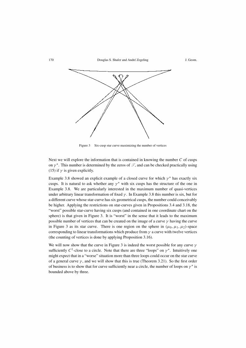
Figure 3 Six-cusp star curve maximizing the number of vertices
Next we will explore the information that is contained in knowing the number C of cuspson γ ∗. This number is determined by the zeros of T , and can be checked practically using(15) if γ is given explicitly.
Example 3.8 showed an explicit example of a closed curve for which γ ∗ has exactly sixcusps. It is natural to ask whether any γ ∗ with six cusps has the structure of the one inExample 3.8. We are particularly interested in the maximum number of quasi-verticesunder arbitrary linear transformation of fixed γ . In Example 3.8 this number is six, but fora different curve whose star-curve has six geometrical cusps, the number could conceivablybe higher. Applying the restrictions on star-curves given in Propositions 3.4 and 3.18, the“worst” possible star-curve having six cusps (and contained in one coordinate chart on thesphere) is that given in Figure 3. It is “worst” in the sense that it leads to the maximumpossible number of vertices that can be created on the image of a curve γ having the curvein Figure 3 as its star curve. There is one region on the sphere in (µ0, µ1, µ2)-spacecorresponding to linear transformations which produce from γ a curve with twelve vertices(the counting of vertices is done by applying Proposition 3.16).
We will now show that the curve in Figure 3 is indeed the worst possible for any curve γ
sufficiently C1-close to a circle. Note that there are three “loops” on γ ∗. Intuitively onemight expect that in a “worse” situation more than three loops could occur on the star curveof a general curve γ , and we will show that this is true (Theorem 3.21). So the first orderof business is to show that for curve sufficiently near a circle, the number of loops on γ ∗ isbounded above by three.

Vol. 73, 2002 Vertices of planar curves under the action of linear transformations 171
DEFINITION 3.19. A loop on a parametrized curve γ ∗(t) is an arc a ≤ t ≤ b of γ ∗ suchthat γ ∗(a) = γ ∗(b) and γ ∗ has no geometrical cusps on the arc.
LEMMA 3.20. The star curve of a closed curve sufficiently C1-close to a circle has at mostthree loops.
Proof. If γ ∗ contains a loop, then there is a direction θ∗ such that there exist two distinctlines with slope tan θ∗ which are tangent to γ ∗ at distinct points lying in an open subarc ofthe arc forming the loop. Any other loop, if one exists, must have at least one tangent linein the direction θ∗. Since by Proposition 3.18 there are exactly four points on γ ∗ whosetangent lines have direction θ∗, there can be at most three loops in all. �
The following general theorem implies the result we set out to establish.
THEOREM 3.21. If γ is a simple closed curve sufficiently C1-close to a circle whosecorresponding star curve has C geometrical cusps, then at most 6 + C (quasi)-verticesappear on the image of γ under nonsingular linear transformation.
Proof. Recalling Proposition 3.1 and the remarks following it, the star curve γ ∗ lies in asmall neighborhood of the point corresponding to the identity, hence lies in its entirety inthe chart �0 of S2 in (µ0, µ1, µ2)-space. In that chart consider a line through the openregion corresponding to those linear transformations which yield the maximum number M
of vertices on the image curve. The line may be chosen so that it is nowhere tangent toγ ∗, and does not pass through any cusps. By a rotation we make horizontal. The part of
lying in the region producing M vertices is bounded by two points which we will label p1
and p2, p1 to the left of p2. There are numbers n1 and S in Z+ ∪ {0} so that at and to the
left of p1 γ ∗ has n1 crossings at which it is locally concave right (i.e., locally like the graphof x = y2), and n1 + S crossings at which it is locally concave left (i.e., locally like thegraph of x = −y2). Proposition 3.16 and the fact that crossing p1 from left to right along leads to a region with the maximum number of vertices on the image of γ imply that thecrossing at p1 is locally concave left, and that S is strictly positive; specifically, the numberof vertices on the image of γ for any linear transformation corresponding to a point of
near p1 and just to its right is 2S more than the number of vertices on the image of γ for anylinear transformation corresponding to a point of to the left of all its intersections withγ ∗. Similarly, there are numbers n2 and T corresponding to crossing of with γ ∗ lying ator to the right of p2, n2 crossings where γ ∗ is locally concave left, and n2 + T where it islocally concave right. Since the number of vertices for transformations for points on theextreme ends of are identical, S = T . The largest possible value of M occurs when S ismaximal, so we seek an upper bound on S.
Beginning at any intersection point p of γ ∗ in (−∞, p1] at which the local character isconcave left, and following γ ∗ downward, if there is no loop or cusp on the curve before the

172 Douglas S. Shafer and Andre Zegeling J. Geom.
Figure 4 Crossing of γ ∗ with
next intersection q of γ ∗, then q must also lie in (−∞, p1), and will be a crossing which islocally concave right. See Figure 4. Since there are only n1 such crossings in (−∞, p1),there must certainly be at least S cusps and loops on γ ∗, and lying in the lower half-planedetermined by . By the same argument, but applied by moving upward along γ ∗ at eachof the n1 + S points at which γ ∗ is locally concave left, there must be at least S arcs of γ ∗in the upper half-plane each of which contains a cusp or a loop. (We may apply a similarargument to the right of p2, but would not necessarily obtain any new arcs containing cuspsand loops.) Since by Lemma 3.20 and the hypothesis there are at most 3 + C loops andcusps altogether, S is bounded above by the greatest integer less than or equal to (3+C)/2.Since C is the number of zeros of the periodic function T of odd multiplicity, it is even,hence
S ≤ 1 + C/2. (26)
Recall that, since γ is close to a circle C, γ ∗ lies in a neighborhood of the identity. Fora linear transformation µ far from the identity, µ〈C〉 is an ellipse, having of course foursimple vertices, every C1-small perturbation of which has four simple vertices. Thus trans-formations corresponding to points on the extreme ends of give an image curve withfour vertices. (One can also see this by combining Propositions 3.6, 3.10, and 3.18.) Weconclude that M = 2S + 4, and from 26 it follows that M ≤ C + 6, as was to be shown.
�
The following theorem strengthens Lemma 3.20, showing that the maximum possiblenumber of loops on a star-curve of a curve close to a circle is actually attained. Notethat the construction does not produce a curve like that shown in Figure 3, whose existenceis still an open question.
THEOREM 3.22. There exists a simple closed curve γ , arbitrarily C1-close to a circle,such that the corresponding star curve has exactly three loops.
Proof. A point on the star curve γ ∗ by definition corresponds to a linear transformationwhich produces a multiple quasi-vertex at some point of γ . At the intersection point of a

Vol. 73, 2002 Vertices of planar curves under the action of linear transformations 173
loop, the corresponding transformation creates two multiple quasi-vertices at two distinctpoints of γ . We shall construct an example in which the three intersection points of the threeloops pass through a single point of S2, which will correspond to the identity transformation.
Consider the function f (t) = t2(t − α)2, 0 < t < α. Choose fixed numbers 0 < α1 <
α2 < α3 < 2π such that α1, α2 − α1, and α3 − α2 all strictly exceed 2. Then the functionψ(t) given by
ψ(t) =
(t − ε)2(t − α1)2 if 0 ≤ t < α1
(t − α1)2(t − α2)
2 if α1 ≤ t < α2
(t − α2)2(t − α3 + ε)2 if α2 ≤ t < α3
has double zeros at t = ε, t = α1, t = α2, and t = α3 − ε, and ψ ′′ + 4ψ > 0 forα1 ≤ t < α3, if ε is sufficiently small. Consider an arc of a curve γ for which the curvatureis given by
κ = g(t) := 1 + ε
∫ t
0ψ(t)dt for 0 ≤ t < α3, 0 < ε � 1.
For ε = 0, the arc becomes a part of a circle of radius 1. Otherwise, by its very constructionthe arc has four points which are multiple quasi-vertices of order 2. Thus the star curvegenerated by the arc passes through the point corresponding to the identity transformationfour times as t runs through the interval [0, α3]. The function T is given by
T = ε[ψ ′′ + 4ψ] + O(ε2).
Since ψ ′′ + 4ψ is strictly positive on 0 ≤ t < α3, T has no zeros on 0 ≤ t < α3
for sufficiently small ε, meaning that the loops we have constructed on γ ∗ are true loopsaccording to Definition 3.19, since cusps occur only at zeros of T .
To draw the conclusion of the theorem we finally choose an arc sufficiently close to a circlefor α3 ≤ t < 2π which closes the arc γ into a simple closed curve. Simple geometricalconsiderations show that this is possible. �
Finally we remark that star curves with more than six cusps have a completely differentstructure, partially due to the dependence of the index of γ ∗ on the number of cusps (seeProposition 3.18). The curve in Figure 5, arising from cycles near the unit circle in theHamiltonian system x = −y, y = x + εx5, appears at first to violate the Four VertexTheorem, since only two tangent lines pass through any point about which γ ∗ winds zerotimes. The fact is, however, that γ ∗ is traced out twice as γ is traced out once, so the curveactually has twelve cusps.
Figure 6 shows the star curve arising from a curve γ close to a circle in the system x = y,y = −x + ε(x2 + 2x3). The star curve has eight cusps, and M is eight.

174 Douglas S. Shafer and Andre Zegeling J. Geom.
Figure 5 Star curve for a cycle of x = −y,y = x + εx5
Figure 6 Star curve for a cycle of x = y,y = −x + ε(x2 + 2x3)
According to Theorems 3.21 and 3.22 we expect there to exist star curves with eight cuspsfor which M is fourteen. The picture is undoubtedly very complicated, so we have notattempted to draw it.
4. Connections to affine differential geometry
Let γ be a smooth regular Jordan curve. Recall that at each point P of γ at which κ �= 0there exists the osculating circle C, which agrees with γ at P through the second derivative,and the osculating conic �, which agrees with γ at P through the fourth derivative. P is avertex precisely when C fits γ at P to one higher order; P is an affine vertex or sextacticpoint when � fits γ at P to one higher order. The linear transformation µ which makesP := µ(P ) into a multiple quasi-vertex (Def. 2.2) is precisely that one linear transformationwhich makes every point of � into a multiple quasi-vertex. The right hand side of (16) isthe negative of the discriminant of �. Thus P is doubleable (the linear transformation µ
making P at least double is real and nonsingular) precisely when the osculating conic �
is an ellipse. Geometrically, the transformation µ takes � to the osculating circle C at P .But the transformation maintains the contact through the fourth derivative, and this is whatmakes P a multiple vertex. We note also that the vanishing of the right hand side of (17) isprecisely the condition that � fit γ at P through the fifth derivative. Thus P is tripleableprecisely when it is an affine vertex and the osculating conic is an ellipse.
Recall that a curve γ is said to be elliptically curved at a point p if the osculating conic toγ at p is an ellipse. Then Theorems 2.13 and 2.19 can be restated in the following way:

Vol. 73, 2002 Vertices of planar curves under the action of linear transformations 175
PROPOSITION 4.1. If γ is a regular closed curve with nowhere vanishing curvature, thenγ must contain an arc of points at each of which it is elliptically curved.
THEOREM 4.2. If γ is a regular closed curve with nowhere vanishing curvature, then atleast one of its sextactic points is a point at which γ is elliptically curved.
We note again that even if the curvature of γ vanishes at just finitely many points, andis of one sign everywhere else, the conclusions of these theorems need not hold. See thediscussion of the curve γ0 defined by x4+y4 = 1 following Theorem 2.13. It is parabolicallycurved at the four flat vertices, which are also affine vertices. It is hyperbolically curvedeverywhere else, including the four sharp vertices, which are also affine vertices.
Acknowledgement
The authors wish to thank the referee for pointing out some of the connections in thiswork to affine differential geometry, particularly the geometric content of doubleability andtripleability noted in the first paragraph of Section 4, and drawing to our attention the SixAffine Vertex Theorem.
References
[1] Bruce, J. W. and Giblin, P. J., Generic curves and surfaces, J. London Math. Soc. (2) 24 (1981), 555–561.[2] Barner, M. and Flohr, F., Der Vierscheitelsatz und seine Verallgemeinerungen, Der Mathematikunterricht 4
(1958) no. 4, 43–73.[3] Guieu, L., Mourre, E. and Yu, V., Ovsienko, Theorem on six vertices of a plane curve via the Sturm theory,
in The Arnold-Gelfand Mathematical Seminars (V. Arnold, I. M. Gelfand, V. S. Retakh, M. Smirnov, eds.),Boston: Birkh’auser Boston, 1997, 257–266.
[4] Ince, E. L., Ordinary Differential Equations, New York: Dover Publications, 1956.[5] Jackson, S. B., Vertices of plane curves, Bull. Amer. Math. Soc. 50 (1944), 564–578.[6] Mukhopadhaya, S., New methods in the geometry of a plane arc, Bull. Calcutta Math. Soc. 1 (1909), 31–37.[7] Osserman, R., The four-or-more vertex theorem, Amer. Math. Monthly 92 (1985), 332–337.[8] Su, B., Affine Differential Geometry, Beijing: Science Press, 1983.
Douglas S. Shafer Andre ZegelingMathematics Department Putsesteenweg 51/4University of North Carolina at Charlotte 2860 Sint Katelijne WaverCharlotte, NC 28223 BelgiumUSA e-mail: [email protected]: [email protected]
Received 23 July 1999; revised 17 March 2000.