Numerical computation of rotation numbers of quasi-periodic planar curves
20
Physica D 238 (2009) 2025–2044 Contents lists available at ScienceDirect Physica D journal homepage: www.elsevier.com/locate/physd Numerical computation of rotation numbers of quasi-periodic planar curves Alejandro Luque, Jordi Villanueva * Departament de Matemàtica Aplicada I, Universitat Politècnica de Catalunya, Diagonal 647, 08028 Barcelona, Spain article info Article history: Received 24 March 2009 Received in revised form 16 July 2009 Accepted 21 July 2009 Available online 30 July 2009 Communicated by V. Rom-Kedar PACS: 02.30.-f 02.60.-x 02.70.-c Keywords: Invariant curves Rotation number Non-twist maps Numerical approximation abstract Recently, a new numerical method has been proposed to compute rotation numbers of analytic circle diffeomorphisms, as well as derivatives with respect to parameters, that takes advantage of the existence of an analytic conjugation to a rigid rotation. This method can be directly applied to the study of invariant curves of planar twist maps by simply projecting the iterates of the curve onto a circle. In this work we extend the methodology to deal with general planar maps. Our approach consists in computing suitable averages of the iterates of the map that allow us to obtain a new curve for which the direct projection onto a circle is well posed. Furthermore, since our construction does not use the invariance of the quasi- periodic curve under the map, it can be applied to more general contexts. We illustrate the method with several examples. © 2009 Elsevier B.V. All rights reserved. 1. Introduction In this paper we present numerical algorithms to deal with quasi-periodic invariant curves of planar maps by adapting a method presented in [1] to compute rotation numbers of analytic circle diffeomorphisms. The developed ideas do not require the curve to be invariant under any map; so they can be applied to more general objects that we refer to as quasi-periodic signals (see Definition 2.2). The method of [1] is built assuming that the circle map is ana- lytically 1 conjugate to a rigid rotation and, basically, it consists in computing suitable averages of the iterates of the map followed by the Richardson extrapolation. Since this construction takes advan- tage of the geometry and the dynamics of the problem, the method turns out to be highly accurate and very efficient in multiple appli- cations. In a few words, if we compute N iterates of the map, then we can approximate the rotation number with an error of order O(1/N p+1 ) where p is the selected order of averaging (compared with O(1/N ) obtained using the definition). This methodology has * Corresponding author. Tel.: +34 934015887; fax: +34 934011713. E-mail addresses: [email protected] (A. Luque), [email protected] (J. Villanueva). 1 The methods of [2,1] also work in the class of C r circle diffeomorphisms, r being sufficiently large, but we restrict the discussion to the analytic case in order to simplify the exposition. been extended in [2] to deal with derivatives of the rotation num- ber with respect to parameters. In this case, it is required to com- pute and average the corresponding derivatives of the iterates of the circle map. We want to point out that this variational informa- tion cannot be obtained in such a direct way by means of other existing methods to compute rotation numbers (we refer to the works [3–8]). As a matter of motivation, let us assume first that F is a map on the real annulus T × I , where I is a real interval and T = R/Z, and let X : T × I → R denote the canonical projection X (x, y) = x. If F is a twist 2 map, the Birkhoff Graph Theorem (see [9]) ensures that every invariant curve Γ is a graph over its projection on the circle by means of X , and its dynamics induces a circle map by projecting the iterates. Hence, it is straightforward to apply the method of [1] in order to approximate the rotation number of Γ , since for any (x 0 , y 0 ) ∈ Γ we can compute the orbit x n = X (F n (x 0 , y 0 )) — this is the only data that the method requires. Furthermore, if F has a differentiable family of invariant curves or a Cantorian family differentiable in the sense of Whitney, we can approximate derivatives of the rotation number with respect to initial conditions and parameters. This allows us to implement a Newton scheme for the computation and continuation of invariant curves of twist maps (as it is discussed in detail in [2]). 2 The map F satisfies the twist condition if ∂(X ◦ F )/∂ y does not vanish. 0167-2789/$ – see front matter © 2009 Elsevier B.V. All rights reserved. doi:10.1016/j.physd.2009.07.014
-
Upload
independent -
Category
Documents
-
view
0 -
download
0
Transcript of Numerical computation of rotation numbers of quasi-periodic planar curves
Physica D 238 (2009) 2025–2044
Contents lists available at ScienceDirect
Physica D
journal homepage: www.elsevier.com/locate/physd
Numerical computation of rotation numbers of quasi-periodic planar curvesAlejandro Luque, Jordi Villanueva ∗Departament de Matemàtica Aplicada I, Universitat Politècnica de Catalunya, Diagonal 647, 08028 Barcelona, Spain
a r t i c l e i n f o
Article history:Received 24 March 2009Received in revised form16 July 2009Accepted 21 July 2009Available online 30 July 2009Communicated by V. Rom-Kedar
PACS:02.30.-f02.60.-x02.70.-c
Keywords:Invariant curvesRotation numberNon-twist mapsNumerical approximation
a b s t r a c t
Recently, a new numerical method has been proposed to compute rotation numbers of analytic circlediffeomorphisms, as well as derivatives with respect to parameters, that takes advantage of the existenceof an analytic conjugation to a rigid rotation. This method can be directly applied to the study of invariantcurves of planar twist maps by simply projecting the iterates of the curve onto a circle. In this work weextend the methodology to deal with general planar maps. Our approach consists in computing suitableaverages of the iterates of the map that allow us to obtain a new curve for which the direct projectiononto a circle is well posed. Furthermore, since our construction does not use the invariance of the quasi-periodic curve under the map, it can be applied to more general contexts. We illustrate the method withseveral examples.
© 2009 Elsevier B.V. All rights reserved.
1. Introduction
In this paper we present numerical algorithms to deal withquasi-periodic invariant curves of planar maps by adapting amethod presented in [1] to compute rotation numbers of analyticcircle diffeomorphisms. The developed ideas do not require thecurve to be invariant under any map; so they can be applied tomore general objects that we refer to as quasi-periodic signals (seeDefinition 2.2).The method of [1] is built assuming that the circle map is ana-
lytically1 conjugate to a rigid rotation and, basically, it consists incomputing suitable averages of the iterates of themap followed bythe Richardson extrapolation. Since this construction takes advan-tage of the geometry and the dynamics of the problem, themethodturns out to be highly accurate and very efficient in multiple appli-cations. In a few words, if we compute N iterates of the map, thenwe can approximate the rotation number with an error of orderO(1/Np+1) where p is the selected order of averaging (comparedwithO(1/N) obtained using the definition). This methodology has
∗ Corresponding author. Tel.: +34 934015887; fax: +34 934011713.E-mail addresses: [email protected] (A. Luque),
[email protected] (J. Villanueva).1 Themethods of [2,1] alsowork in the class ofCr circle diffeomorphisms, r beingsufficiently large, but we restrict the discussion to the analytic case in order tosimplify the exposition.
0167-2789/$ – see front matter© 2009 Elsevier B.V. All rights reserved.doi:10.1016/j.physd.2009.07.014
been extended in [2] to deal with derivatives of the rotation num-ber with respect to parameters. In this case, it is required to com-pute and average the corresponding derivatives of the iterates ofthe circle map. We want to point out that this variational informa-tion cannot be obtained in such a direct way by means of otherexisting methods to compute rotation numbers (we refer to theworks [3–8]).As a matter of motivation, let us assume first that F is a map
on the real annulus T × I , where I is a real interval and T =R/Z, and let X : T × I → R denote the canonical projectionX(x, y) = x. If F is a twist2 map, the Birkhoff Graph Theorem(see [9]) ensures that every invariant curve Γ is a graph over itsprojection on the circle by means of X , and its dynamics induces acircle map by projecting the iterates. Hence, it is straightforwardto apply the method of [1] in order to approximate the rotationnumber of Γ , since for any (x0, y0) ∈ Γ we can compute the orbitxn = X(F n(x0, y0))— this is the only data that themethod requires.Furthermore, if F has a differentiable family of invariant curves ora Cantorian family differentiable in the sense of Whitney, we canapproximate derivatives of the rotation number with respect toinitial conditions and parameters. This allows us to implement aNewton scheme for the computation and continuation of invariantcurves of twist maps (as it is discussed in detail in [2]).
2 The map F satisfies the twist condition if ∂(X ◦ F)/∂y does not vanish.
2026 A. Luque, J. Villanueva / Physica D 238 (2009) 2025–2044
If themap does not satisfy the twist condition or it is notwrittenin suitable coordinates, its invariant curves are not necessarilygraphs over the projection on a circle. In this situation, invariantcurves can fold in a very wild way (see Section 3.3 and referencesgiven therein for examples of such curves). Nevertheless, if we canselect a suitable circle so that the folded curve ‘‘rotates’’ aroundit, then the projection of the iterates of the map does not define acircle map but a ‘‘circle correspondence’’ and we can compute therotation number of the curve from the ‘‘lift’’ of this correspondenceto the real line — see Section 2.1 for details. Moreover, albeit we donot have a justification of this fact,we realize that the extrapolationmethods of [2,1] work quite well when applied to the iterates ofthis ‘‘lift’’.In some cases – for example, if the rotation number is large
compared with the size of the folds – we can compute numericallythis ‘‘lift’’ from the iterates of the map. However, if the curveis extremely folded additional work is required in order to facethe problem in a systematic way. Hence, we propose a numericalmethod to construct a circlemap – preserving the rotation number– from a general invariant curve on the plane. Themethod consistsin averaging the iterates of an orbit of the curve in such a way thatthe new iterates belong to another curve, no longer invariant underthe map, but having the same rotation number. Concretely, if weknow an approximation of the rotation number with error ε, weconstruct a sequence of (averaged) curves that approaches a circleup to terms of orderO(ε).We refer to this construction as unfoldingof the curve since if ε is small enough, then this constructionprovides us with a circle map. Taking into account the discussionin the previous paragraph, in order to apply the methods of [2,1] itis not necessary to unfold completely the curve, but only to ‘‘kill’’its main folds so we can compute the ‘‘lift’’ of the correspondencegenerated by the projection of the iterates of the new (less-folded)curve. In order to justify this unfolding procedure we requirethe curve to be analytic (or at least differentiable enough) andthe rotation number to be Diophantine. Sometimes the requestedapproximation of the rotation number is given by the context ofthe problem – for example, if we look for invariant curves of fixedrotation number – or it can be obtained by means of any methodof frequency analysis (see for example [6,7]). Therefore, we obtaina very efficient toolkit for the study of invariant curves of planarmaps and their numerical continuation.Let us remark that due to the importance, both theoretical and
applied, of invariant curves of maps or two-dimensional tori offlows (for example, they play a fundamental role in the design ofspace missions [10,11] and also in the study of models in CelestialMechanics [12], Molecular Dynamics [13,14] or Plasma-BeamPhysics [15], just to say a few), several approaches to deal withthese objects have been developed in the literature. For example,the methods in [16–18] have been applied efficiently in a wide setof contexts. However, they require to compute a representation– by means of a trigonometric polynomial – of the curve whichsolves the invariance equation of the problem, so it is required tosolve large systems of equations — as large as the used numberof Fourier modes, say M . One possibility to face this difficulty isto solve these full linear systems, with a cost O(M3) in time andO(M2) in memory, by means of efficient parallel algorithms asis proposed in [18]. Another recent approach presented in [17],based on the analytic and geometric ideas developed in [19], allowsus to reduce the computational effort of the problem to a costof order O(M logM) in time and O(M) in memory. On the otherhand, we can compute the invariant curve by looking for a pointso that the corresponding orbit has a prefixed rotation number.Then, rather than approximating explicitly the parameterizationof the curve, we reduce the problem to finding a zero of a function.This approach can be implemented using interpolation methodsas in [20] or also using the extrapolation methods in [2,1]. These
extrapolation methods, that are the cornerstone of the presentedpaper, have a cost of orderO(N logN) in terms of the used numberof iterates N and are free in memory. Once we know a point on thecurve and its rotation number, we can compute a trigonometricapproximation of the curve ‘‘a posteriori’’, using Fourier Transform(FT) on the iterates of the curve. In addition, in Section 2.7 wedevelop a method for performing this FT based also on averaging-extrapolation ideas.Given a numerical method for the continuation of invariant
curves, it is specially interesting to verify if the method is valid upto the breakdown threshold corresponding to the critical invariantcurve (see [21–23]). These critical curves are specially importantobjects that organize the long-term behavior of a given dynamicalsystem, because of their role as ‘‘last barriers’’ or ‘‘bottlenecks’’ tochaos (see [9]). Actually, the critical value for the breakdown ofthe golden curve for the Chirikov standard map was estimated bymeans of extrapolationmethods in [1] obtaining a good agreementwith the value predicted bymeans of the classical Greene criterionin [22]. For the non-twist case, we refer to computations in [24,25]as examples of breakdown studies in non-twist maps. It is worthmentioning that the methods presented in this paper can beapplied also in this context.Since our construction does not use the invariance of the curve
under the map, it can be applied to the study of quasi-periodiccurves that are not necessarily embedded (that we call quasi-periodic signals). This context is very interesting since it allows usto analyze sets of data obtained from real experiments or observednatural phenomena. Actually, in order to check that the methodsare robust when facing experimental data, we consider the effectof Gaussian error in the evaluation of iterates of a known quasi-periodic function.Wewant to point out that our approach can be also understood
as a method for the refinement of the frequency analysis of [7].Actually, an efficient refinement of these methods, based in thesimultaneous improvement of the frequencies and the amplitudesof the signal, is given in [6]. Once again, the main advantage of ourapproach is that we do not have to compute Fourier coefficients ofthe curve. This fact reduces the computational effort of solving biglinear systems of equations required to refine the representationof the signal. In addition, the accuracy in the computation of therotation number is not limited by the truncation error in therepresentation of the signal.Finally, we notice that the methodology of [2,1] also works
for dealing with maps of the d-dimensional torus that admitan analytic conjugation to a rigid rotation having a Diophantinerotation vector. Our aim is to explore the extension of the ideaspresented in this paper to deal with invariant tori and quasi-periodic signals of arbitrary number of frequencies.The paper is organized as follows. In the first part, contained
in Section 2, we develop and justify different results, methodsand algorithms to study quasi-periodic invariant curves (or quasi-periodic signals). In the second part, presented in Section 3, weconsider several examples in order to illustrate different featuresof the presentedmethodology. These examples have been selectedin order to sustain the presentation of themethods and to highlightboth some of the possibilities and limitations of our approach.
2. Exposition of methods
As we said in the introduction, we approach the study of quasi-periodic signals by computing the rotation number of a circlemap (or a circle correspondence) induced by the curve. The maindefinitions and notation, together with a brief overview of theproblem, are given in Section 2.1. After that, we present and justifya method to unfold a quasi-periodic signal. We first assume inSection 2.2 that the rotation number is known exactly in order to
A. Luque, J. Villanueva / Physica D 238 (2009) 2025–2044 2027
-1.5 -1 -0.5 0 0.5 1 1.5-1
-0.5
0
0.5
1
1.5
0
0.5
1
1.5
2
0 0.1 0.2 0.3 0.4 0.5 0.6 0.7 0.8 0.9 1
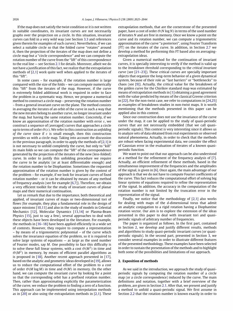
Fig. 1. Left: Folded invariant curve with quasi-periodic dynamics that rotates around the origin in the complex plane (this curve corresponds to an example discussed inSection 3.3). Right: ‘‘Lift’’ of the associated circle correspondence given by (1).
highlight the involved ideas. Basically, we construct a sequenceof curves that converges to a circle whose dynamics correspondsto a rigid rotation. In Section 2.3 we assume that we only havean approximation of the rotation number and we show that theprevious construction allows us to obtain a curve that is C1-closeto be a circle — the proximity being of the same order as the errorin the initial guess of the rotation number.In order to obtain the required approximation, a possibility is
to resort to frequency analysis methods. In Section 2.4 we reviewLaskar’s frequency analysis method in terms of the languagepresented in this paper, just to stress that the same algorithmsderived to unfold the curve can be adapted to obtain the requiredapproximation of the rotationnumber as alternative of the classicalmethods.For the sake of completeness we include in Section 2.5 a brief
survey of the methods of [2,1] to compute the rotation numberand derivatives with respect to parameters of the obtained circlemap or correspondence. This review is necessary to understand thehigher ordermethod that we develop in Section 2.6 to improve theunfolding of curves. During the exposition it will be clear that theideas used in the unfolding are related to FT. This fact is exploitedin Section 2.7 in order to extrapolate Fourier coefficients once therotation number is known.
2.1. Setting of the problem
For convenience, we identify the real plane with the set ofcomplex numbers by defining z = u + iv for any (u, v) ∈ R2.Let Γ ⊂ C be a quasi-periodic invariant curve for a map F : U ⊂C→ C of rotation number θ ∈ R \Q. Let us assume, for example,that the curve ‘‘rotates’’ around the origin and that it is a graph ofthe angular variable. Then, the projection
Γ −→ Tz 7−→ x = arg(z)/2π (1)
generates a circle map induced by the dynamics of F |Γ . On theother hand, if Γ is folded, then the projection (1) does not providea circle map, but defines a correspondence on T that we can‘‘lift’’ to R. For example, in the left plot of Fig. 1 we show a‘‘folded’’ invariant curve on the complex plane for an exampleconsidered in Section 3.3. In the right plot of Fig. 1 we show the‘‘lift’’ of the correspondence on T given by (1). Since the rotationnumber of the curve is no more than the averaged number ofrevolutions per iterate, it is not surprising thatwe can compute it aslimn→∞(xn−x0)/n, where xn are the iterates under the ‘‘lift’’ toR ofthe circle correspondence. In this situation, we have observed thatthemethods of [2,1] can be applied to such a ‘‘lift’’ (see examples inSection 3.3), even thoughwe do not have a justification of this fact.
In some cases, for example if the rotation number is largeenough as to avoid the folds, we can compute numerically the ‘‘lift’’of (1) using the iterates of an orbit. However, if the invariant curvepresents large folds or we cannot identify directly a good pointaround which the curve is rotating, we cannot compute this ‘‘lift’’in a systematic way. Then, our aim is to construct another curve,having the same rotation number, by using suitable averages ofiterates of the original map. If we manage to eliminate (or at leastminimize) the folds in the new curve, then we are able to obtain acircle diffeomorphism (or at least a circle correspondence that wecan ‘‘lift’’ numerically).As Γ is a quasi-periodic invariant curve of rotation number θ ,
there exists an analytic embedding γ : T→ C verifyingΓ = γ (T)and
F(γ (x)) = γ (x+ θ).
In this situation, since the parameterization γ is periodic, wecan use the Fourier series
γ (x) =∑k∈Z
γke2π ikx,
and, moreover, for a given z0 ∈ Γ we can ask for γ (0) = z0. Then,the iterates of z0 under F can be expressed using γ as
zn = F n(z0) = F n(γ (0)) = F n−1(γ (θ))
= γ (nθ) =∑k∈Z
γke2π iknθ . (2)
As we will see, our method does not use the invariance of Γunder F but only the expression (2) for the iterates. Furthermore,even if we start with an invariant curve of a map, the intermediatestages of our construction may produce curves that are notembedded in C. Using this fact as a motivation, we state thefollowing definitions:
Definition 2.1. We say that a complex sequence {zn}n∈Z is a quasi-periodic signal of rotation number θ if there exists a periodicfunction γ : T→ C such that zn = γ (nθ). We also call Γ = γ (T)a quasi-periodic curve.
Definition 2.2. Under the above conditions, let {zn}n∈Z be a quasi-periodic signal. Then, for any θ0 ∈ R and L ∈ N, we define thefollowing iterates
z(L,θ0)n =1L
L+n−1∑m=n
zme2π i(n−m)θ0 . (3)
2028 A. Luque, J. Villanueva / Physica D 238 (2009) 2025–2044
It is clear that {z(L,θ0)n }n∈Z is a quasi-periodic signal on anothercurve Γ (L,θ0) = γ (L,θ0)(T) of the same rotation number, i.e.,
z(L,θ0)n = γ (L,θ0)(nθ) =∑k∈Z
γ(L,θ0)k e2π iknθ , (4)
and the new Fourier coefficients are given by
γ(L,θ0)k =
γk
L
L+n−1∑m=n
e2π i(m−n)(kθ−θ0) =γk
L1− e2π iL(kθ−θ0)
1− e2π i(kθ−θ0). (5)
In Section 2.2 we show that, under conditions on regularity andnon-resonance, if θ0 = θ , then the new curve γ (L,θ) is arbitrarilyC1-close to a circle (see Lemma2.6) for L large enough. On the otherhand, if ε = θ0− θ is small, then we can choose L = L(ε) such thatthe new curve is C1-close to a circle with an error of order O(ε)(this is concluded from Proposition 2.8) so that the projection
Γ (L,θ0) ⊂ C∗ −→ Tz(L,θ0)n 7−→ x(L,θ0)n = arg(z(L,θ0)n )/2π,
(6)
provides an orbit of a circle diffeomorphism f (L,θ0)Γ . Once thiscircle map has been obtained (as we have discussed, in practiceit suffices to obtain a slightly folded curve such that we cancompute the ‘‘lift’’ of the circle correspondence defined by thedirect projection), we can apply the methodology of [2,1] tocompute the rotation number and derivatives with respect toparameters (this is described in Section 2.5). In order to justify thisconstruction, we require the rotation number to be Diophantine.
Definition 2.3. Given θ ∈ R, we say that θ is aDiophantine numberof (C, τ ) type if there exist constants C > 0 and τ ≥ 1 such that
|kθ − l|−1 ≤ C |k|τ , ∀(l, k) ∈ Z× Z∗. (7)
We will denoteD(C, τ ) the set of such numbers andD the set ofDiophantine numbers of any type.
In the aim of KAM theory, we know that the hypothesis ofDiophantine rotation number for the dynamics on the curve isconsistent with its own existence. Although Diophantine setsare Cantorian – i.e., compact, perfect and nowhere dense – aremarkable property is that R \D has zero Lebesgue measure. Forthis reason, this condition fits very well in practical issues and wedo not resort to other weaker conditions on small divisors such asthe Brjuno condition (see [26]). It is worth mentioning that if θ isa ‘‘bad’’ Diophantine rotation number, i.e., having a large constantC in (7), then the methods presented in this paper turn out to beless efficient as we discuss in Section 3.
2.2. Unfolding a curve of known rotation number
Let us consider the previous setting and suppose that theFourier coefficients of γ are γ1 6= 0 and γk = 0 for k ∈ Z \ {1}.In this case, Γ = {z ∈ C | |z| = |γ1|} and the circle map obtainedby the projection (1) is a rigid rotation Rθ (x) = x+ θ .Assume now that γ1 6= 0 and |γk| is small (compared with |γ1|)
for every k ∈ Z\ {1} in such a way that the curve γ is alsoC1-closeto a circle. In this case, the projection x = arg(z)/2π also makessense and defines a circle diffeomorphism.In the general case this projection does not provide a circle
map. However, it turns out that the projection of the iteratesz(L,θ0)n is well posed if we take θ0 = θ and L large enough. Morequantitatively, we assert that the curve γ (L,θ) differs from a circleby an amount of order O(1/L). In Lemma 2.6 bellow we makeprecise the above arguments.
Definition 2.4. Given an analytic function γ : T → C andits Fourier coefficients {γk}k∈Z, we consider the norm ‖γ ‖ =∑k∈Z |γk|.
Definition 2.5. Given k ∈ Z \ {0} and r ∈ C, we define the mapγk[r] : T→ C as
γk[r](x) = r e2π ikx.
Then we state the following result:
Lemma 2.6. Let us consider a quasi-periodic signal zn = γ (nθ) ofrotation number θ ∈ D(C, τ ). Assume that γ : T → C is analyticin the complex strip B∆ = {z ∈ C : |Im(z)| < ∆} and boundedin the closure, with M = supz∈B∆ |γ (z)|. Then, if γ1 6= 0, the curveγ (L,θ) : T→ C given by (4) and (5) satisfies
‖γ (L,θ) − γ1[γ1]‖ ≤AL,
where A is a constant depending on M, C, τ and∆.
Proof. First, let us observe that the Fourier coefficients of the newcurve are given by
γ(L,θ)1 = γ1, γ
(L,θ)k =
γk
L1− e2π i(k−1)θL
1− e2π i(k−1)θ, k ∈ Z \ {1}.
Then, we have to bound the expression
‖γ (L,θ0) − γ1[γ1]‖ ≤1L
∑k∈Z\{1}
∣∣∣∣γk 1− e2π i(k−1)θL1− e2π i(k−1)θ
∣∣∣∣≤1L
∑k∈Z\{1}
2|γk||1− e2π i(k−1)θ |
.
We observe that the Fourier coefficients of γ satisfy |γk| ≤Me−2π∆|k| and we use (7) to control the small divisors. Concretely,standard manipulations show that (see for example [27])
|1− e2π i(k−1)θ |−1 ≤C4|k− 1|τ .
Introducing these expressions in the previous sum we obtainthat
‖γ (L,θ0) − γ1[γ1]‖ ≤CM2L
∑k∈Z\{1}
|k− 1|τe−2π∆|k|
≤CMLsupx≥0{e−π∆x(x+ 1)τ }
∞∑k=0
e−π∆k.
Moreover, we observe that
supx≥0{e−sx(x+ 1)m} =
{1 if s ≥ m,
(m/(se))mes if s < m.
Finally, taking A = MC1−e−π∆ (1 + (
τπ∆)τ ) the stated bound follows
immediately. �
Remark 2.7. Note that in order to guarantee that the projection (6)is well posed we also need to control the derivative (γ (L,θ))′(x). Ofcourse, this can be donemodifying slightly the proof of Lemma 2.6.
A. Luque, J. Villanueva / Physica D 238 (2009) 2025–2044 2029
2.3. Unfolding a curve of unknown rotation number
Since we are concerned with the computation of θ , the con-struction presented in the previous section seems useless. Next weshow that themethod still works –with certain restrictions – if therotation number θ is unknown, but we have an approximation θ0.
Proposition 2.8. Let us consider a quasi-periodic signal zn = γ (nθ)of rotation number θ ∈ D(C, τ ). Assume that γ : T → C isanalytic in the complex strip B∆ and bounded in the closure, withM = supz∈B∆ |γ (z)|. Suppose that θ0 is an approximation of θ andlet us denote ε = θ0 − θ and Kε = b(2C |ε|)−1/τ c. Then, if γ1 6= 0and Kε ≥ 1, for every L ∈ N the following estimate holds
‖γ (L,θ0) − γ1[γ(L,θ0)1 ]‖
|γ(L,θ0)1 |
≤
∣∣∣∣ sin(πε)sin(πεL)
∣∣∣∣×
(A|γ1|+2ML|γ1|
e−2π∆(Kε−1)
1− e−2π∆
), (8)
where A is a constant depending on M, C, τ and∆.
Proof. Let us consider the sets
K(ε) = {k ∈ Z \ {1} : |k− 1| ≤ Kε},K ∗(ε) = Z \ (K(ε) ∪ {1}).
Then, if k ∈ K(ε) the following bound is satisfied ∀l ∈ Z
|kθ − θ0 − l| ≥ |(k− 1)θ − l| − |ε|
≥1
C |k− 1|τ− |ε| ≥
12C |k− 1|τ
allowing us to control the small divisors
|1− e2π i(kθ−θ0)| ≥2
C |k− 1|τ∀k ∈ K(ε). (9)
Then, from formula (5) and recalling that the Fourier coefficientssatisfy |γk| ≤ Me−2π∆|k|, we obtain estimates for γ
(L,θ0)k . If k ∈
K(ε), we use (9) to obtain |γ (L,θ0)k | ≤ MCL−1|k − 1|τe−2π∆|k|. Onthe other hand, for indexes k ∈ K ∗(ε) we use that |γ (L,θ0)k | ≤ |γk|.Therefore, we have to consider the following sums
‖γ (L,θ0) − γ1[γ(L,θ0)1 ]‖ ≤
MCL
∑k∈K(ε)
|k− 1|τe−2π∆|k|
+M∑k∈K∗(ε)
e−2π∆|k|.
Now, the sum for k ∈ K(ε) is controlled by splitting itinto the sets [−Kε + 1, 0] ∩ Z and [2, Kε + 1] ∩ Z. Then, weproceed as in the proof of Lemma 2.6 obtaining the constantA = 2MC
1−e−π∆(1+
(τπ∆
)τ ). Finally, we compute the first Fouriercoefficient
|γ(L,θ0)1 | =
∣∣∣∣ γ1L∣∣∣∣ ∣∣∣∣1− e−2π iεL1− e−2π iε
∣∣∣∣ = ∣∣∣∣ γ1L∣∣∣∣ ∣∣∣∣ sin(πεL)sin(πε)
∣∣∣∣ ,ending up with estimate (8). �
Remark 2.9. If we restrict Proposition 2.8 to those values of θ0such that the Diophantine condition (9) is valid ∀k ∈ Z \ {1}, thenwe obtain the estimate
‖γ (L,θ0) − γ1[γ(L,θ0)1 ]‖
|γ(L,θ0)1 |
≤
∣∣∣∣ sin(πε)sin(πεL)
∣∣∣∣ A|γ1| . (10)
Indeed, if we denote E ⊂ R the set of values of ε such thatθ0 = θ + ε satisfies estimate (9) for every k ∈ Z \ {1}, then for
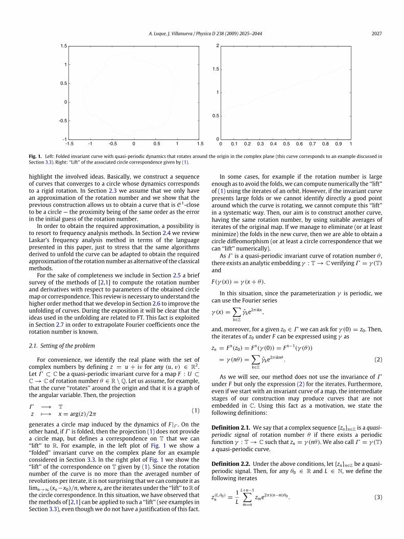
Fig. 2. This diagram summarizes the construction of the analytic circlediffeomorphism f (L,θ0)Γ from a folded invariant curve Γ of F of rotation number θ .
every ε0 sufficiently small the measure of the set [−ε0, ε0] \ E isexponentially small in ε0.3
Observe that for any fixed |ε| > 0, estimate (10) depends | 1ε|-
periodically on L and also does (8) modulo exponentially smallterms in |ε|. Since we are interested in the minimization of (8), wepoint out that if L ' | 12ε |, then
‖γ (L,θ0) − γ1[γ(L,θ0)1 ]‖
|γ(L,θ0)1 |
= O(ε).
Hence, the new parameterization is closer to a circle for |ε|sufficiently small and the projection
Γ (L,θ0) ⊂ C∗ −→ Tz(L,θ0)n 7−→ x(L,θ0)n = arg(z(L,θ0)n )/2π,
induces a well-posed circle diffeomorphism that we denote asf (L,θ0)Γ . Of course, the regularity of the circlemap f (L,θ0)Γ follows fromthe regularity of γ . In Fig. 2 we include a schematic representationof our procedure. Hence, we can compute the rotation numberθ and derivatives with respect to parameters by applying themethods of [2,1] that we recall briefly in Section 2.5. Before that,we discuss how this required guess θ0 can be obtained.
2.4. First approximation of the rotation number
The classical frequency analysis approach introduced by J. Laskar(see [7]) to obtain an approximation of frequencies of a quasi-periodic signal – here we are considering only one independentfrequency – is to look for the frequencies as peaks of the modulusof the Discrete Fourier Transform (DFT) of the studied signal. Inthis section we translate the elementary ideas used in frequencyanalysis into the terminology introduced in Section 2.3.Let us focus on the iterates {z(L,θ0)n }n∈Z of Definition 2.2. We
observe that they look very similar to the DFT of the signal.We alsonotice that they can be defined for any θ0 but the Fourier coefficientγ(L,θ0)1 , given explicitly in (5), has a local maximumwhen θ0 equalsθ , and from Proposition 2.8 we conclude that, for L large enough,the function θ0 7→ |z
(L,θ0)n | has a local maximum for a value of θ0
close to θ . In general, this phenomena occurs for the tth coefficientif we select θ0 close to an integer multiple of the rotation number,i.e., θ0 = tθ + ε, t ∈ Z. The corresponding justification is givenby the following proposition (the proof is analogous to that ofProposition 2.8).
3 These two points of view are analogous to different approaches followed in [28,29] to study reducibility of quasi-periodic linear equations.
2030 A. Luque, J. Villanueva / Physica D 238 (2009) 2025–2044
Proposition 2.10. Let us consider a quasi-periodic signal zn =γ (nθ) of rotation number θ ∈ D(C, τ ). Assume that γ : T → Cis analytic in the complex strip B∆ and bounded in the closure, withM = supz∈B∆ |γ (z)|. Suppose that θ0 is an approximation of tθ andlet us denote ε = θ0 − tθ and Kε = b(2C |ε|)−1/τ c. Then, if γt 6= 0and Kε ≥ |t|, for every L ∈ N the following estimate holds
‖γ (L,θ0) − γt [γ(L,θ0)t ]‖
|γ(L,θ0)t |
≤
∣∣∣∣ sin(πε)sin(πεL)
∣∣∣∣×
(A|γt |+2ML|γt |
e−2π∆(Kε−|t|)
1− e−2π∆
), (11)
where A = 2MC1−e−π∆
(|t|τ +
(τπ∆
)τ ).According with this result and the previous discussion, we
summarize the following observations:• First, we notice that Remark 2.9 also holds in this context, andso we conclude that this estimate behaves periodically in L formost of the values of θ0 close to tθ .• FromEq. (5),we observe that γ (L,θ0)t → γt when ε→ 0 and thatthe modulus |γt | is an upper bound for |γ
(L,θ0)t |. Moreover, for L
sufficiently large, we obtain a local maximum in themodulus ofthe iterates z(L,θ0)n for a value of θ0 close to tθ .• On the other hand, the estimate (11) grows with |t| thusimplying that, for fixed L, only low order harmonics can bedetected.
The previous discussion gives us a heuristic method forcomputing an approximation θ0 of the rotation number θ (and itsmultiples modulo 1). Basically, we fix L and compute the iteratesz(L,θ0)n for different values of θ0 in order to compute local maximaof the modulus. In particular, if we just study the modulus of theinitial iterate z(L,θ0)0 , we recover the method of [7]. This method isenough for our purposes – we recall that we just look for a roughapproximation of the rotation number – but in Remark 2.12 weexplain some refinements that can be performed in this procedure.Thus, from themethod of [7] we find a finite number of candidatesfor the rotation number and we have to decide which one is thegenerator. Details are given in the next four steps.
Step 1: Maxima chasing. First, we fix L ∈ N and define thefunction
T −→ R
θ0 7−→ |z(L,θ0)0 | =
∣∣∣∣∣1LL−1∑m=0
zme−2π imθ0∣∣∣∣∣ . (12)
We want to obtain values of θ0 that correspond tomaxima of the function (12). To this end, let us considera sample of points {θ i0}i=1,...,N , where N ∈ N andθ i0 ∈ [0, 1] (actually, one can reduce the interval if someinformation about the rotation number is available, sayθ ∈ [θmin, θmax]). Then, for every pair {θ
j0, θ
j+10 }, j =
1, . . . ,N − 1, we compute a local maximum for (12) bymeans of golden section search using a tolerance εGSS (werefer to [30] for details). Then, we introduce the followingterminology:
- θ j0: Maximum obtained from the pair {θj0, θ
j+10 }. Let
us observe that this maximum is not necessarilycontained in the interval [θ j0, θ
j+10 ].
- np: Number of maxima obtained at the end of thisstep. In order to avoid redundant information, twomaxima are considered equivalent if dT(θ
j0, θ
k0 ) ≤
10εGSS where dT is the quotient metric induced on thetorus.
Step 2: Maxima selection. Now we sort the obtained points{θ i0}1,...,np according to
|z(L,θ i0)0 | > |z
(L,θ j0)0 | provided i < j.
At this point, we select the first nu points just omittingthose oneswhose correspondingmaxima are small when
compared with |z(L,θ10 )0 |. In particular, we only take those
elements such that
|z(L,θ10 )0 | < ν|z
(L,θ i0)0 |, (13)
where ν > 1 is a ‘‘selecting factor’’ (we typicallytake values of ν between 3 and 6) and we denote by{θ k0 }k=1,...,nu the set of numbers thus obtained.
Step 3: Rotation number selection. This set {θ k0 }k=1,...,nu , withθ k0 ∈ [0, 1], corresponds to approximate multiples ofthe rotation number computed modulo 1. In addition, if|γ1| is not too small, there is an element in this set thatapproximates the rotation number. Notice that for everyθ k0 there exist mk, nk ∈ Z such that θ k0 ≈ mkθ + nk. Thismotivates the following definitions
kij = argmink∈Z {dT(kθ i0, θj0)}, κi =
nu∑j=1
|kij| (14)
dij = mink∈Z {dT(kθ i0, θj0)}, δi =
nu∑j=1
dij. (15)
Let us observe that if we assume that θ i0 ≈ θ , then κicorresponds to the sum of the order of Fourier termsthat allow us to approximate the remaining points θ j0.On the other hand, δi gives an idea of the error whenθ i0 is selected. If the minimum values of {κi}i=1,...,nu and{δi}i=1,...,nu correspond to the same index k ∈ {1, . . . , nu},then we select θ0 = θ k0 as an approximation of θ . If theydo not coincide but δk = mini{δi} is small, then we selectθ0 = θ k0 . Otherwise we start again from Step 1 using alarger value of L.
Step 4: Validation and iteration. Of course, it is recommended toverify that the computations are stable by repeating theprocess (from Step 1) with larger values of N and L.
Remark 2.11. When the frequency of the quasi-periodic signal isnot an integer multiple of the ‘‘basic frequency’’ 1/L associatedto the sample interval of the associated DFT in (12), there appearin the DFT spurious frequencies, that is, the DFT is different fromzero at frequencies not being multiple of the frequency of thefunction. This is a phenomenon known as leakage, that it canbe reduced by means of the so-called filter or window functions(see [6,7]). Nevertheless, these spurious peaks are smaller than thecorresponding harmonic that generates them, sowe get rid of themin Step 2 of the described procedure.
Remark 2.12. Finally, we notice that this procedure can bemodified in several ways taking into account the ideas introducedin this paper. For example, when looking for local maxima offunction (12) we can minimize with respect to θ0 the distance ofthe iterates {z(L,θ0)n }n∈Z to be on a circle – see Proposition 2.10 –that can be measured by means of several criteria discussed inSection 3.1. On the other hand, we can use higher order averagesas discussed in Section 2.6 in order to improve the resolution of themaxima. These refinements may become relevant when dealingwithmore than one frequency as a possible alternative to the filtersmentioned in Remark 2.11.

A. Luque, J. Villanueva / Physica D 238 (2009) 2025–2044 2031
2.5. Computation of rotation numbers and derivatives
Next, we include a brief review of the methods developed in[1,2] to compute numerically the rotation number of circle diffeo-morphisms together with derivatives with respect to parameters.We include this review to set the notation of the rest of the paperand also in order to remark that ideas of Sections 2.6 and 2.7 followfrom those introduced in [1] in a close way.Given an orientation-preserving circle homeomorphism f :
T→ T, we identify f with its lift to R by fixing the normalizationcondition f (0) ∈ [0, 1). Then, we recall that the rotation numberof f is defined as the limit
θ = lim|n|→∞
f n(x0)− x0n
, (16)
that exists for all x0 ∈ R, is independent of x0 and satisfies θ ∈[0, 1). It is well known (we refer to [31]) that if f is an analyticdiffeomorphism and θ ∈ D , then f is analytically conjugate toa rigid rotation Rθ (x) = x + θ , i.e., there exists an orientation-preserving analytic circle diffeomorphism η such that f ◦η = η◦Rθ .Moreover, we can write this conjugacy as η(x) = x+ ξ(x), ξ beinga 1-periodic function normalized in such a way that ξ(0) = x0,for a fixed x0 ∈ [0, 1). Now, by using the fact that η conjugates fto a rigid rotation, we can write the following expression for theiterates under the lift:
f n(x0) = f n(η(0)) = η(nθ) = nθ +∑k∈Z
ξke2π iknθ , ∀n ∈ Z,
where the sequence {ξk}k∈Z denotes the Fourier coefficients of ξ .Then, the above expression gives us the following formula
f n(x0)− x0n
= θ +1n
∑k∈Z∗
ξk(e2π iknθ − 1),
to compute θ modulo terms of order O(1/n). Unfortunately, thisorder of convergence is very slow for practical purposes, since itrequires a huge number of iterates if we want to compute θ withhigh precision. Nevertheless, by averaging the iterates f n(x0) in asuitable way, we can manage to decrease the size of the quasi-periodic remainder.Given p ∈ N∪{0}, that we call the averaging order, we introduce
the following recursive sums of order p
S0N = fN(x0)− x0, SpN =
N∑j=1
Sp−1j ,
and the corresponding averaged sums of order p
SpN =(N + pp+ 1
)−1SpN .
Then, as is shown in [1], these averages satisfy the followingproperty.
Proposition 2.13. If f is the lift of an orientation-preserving analyticcircle diffeomorphism of rotation number θ ∈ D , then the followingexpression holds
SpN = θ +p∑l=1
AplN l+ Ep(N), (17)
where the coefficients Apl depend on f and p but are independent ofN. Furthermore, the remainder Ep(N) is uniformly bounded by anexpression of order O(1/Np+1).
Let us observe that Eq. (17) allows us to extrapolate the rotationnumber just by computing SpN for different values of N , neglectingthe remainder and solving a set of linear equations.
Algorithm 2.14. Once an averaging order p is selected, we takeN = 2q iterates of the map, for some q > p, and compute thesums {SpNj}j=0,...,p with Nj = 2
q−p+j. We approximate the rotationnumber using the formula
θ = Θq,p + O(2−(p+1)q),
Θq,p =
p∑j=0
c(p)j Sp2q−p+j
,(18)
where the coefficients c(p)j are given by
c(p)l = (−1)p−l 2
l(l+1)/2
δ(l)δ(p− l), (19)
with δ(n) = (2n−1)(2n−1−1) · · · (21−1) for n ≥ 1 and δ(0) = 1.The operator Θq,p corresponds to the Richardson extrapolation oforder p of Eq. (17).
As far as the behavior of the error is concerned, if we fix theextrapolation order p and compute Θq,p, from Eq. (18) we knowthat |θ − Θq,p| ≤ c/2q(p+1), for certain (unknown) constant cindependent of q (see [1]). To estimate c , we compute Θq−1,p andconsider the expression |θ − Θq−1,p| ≤ c/2(q−1)(p+1). Then, wereplace in this inequality the exact value of θ byΘq,p, as we expectΘq,p to be closer to θ thanΘq−1,p. After that, we estimate c by
c ' 2(q−1)(p+1)|Θq,p −Θq−1,p|.
From this approximation we obtain the following (heuristic)expression
|θ −Θq,p| ≤ν
2p+1|Θq,p −Θq−1,p|, (20)
where ν is a ‘‘safety parameter’’ whose role is to preventoscillations of c a function of q due to the quasi-periodic part. Inthe computations of Section 3 we take ν = 10 (this value worksquite well as observed in [1]).Furthermore, let us consider a family µ ∈ I ⊂ R 7→ fµ of
orientation-preserving analytic circle diffeomorphisms dependingCd-smoothly with respect toµ. The rotation numbers of the family{fµ}µ∈I induce a function θ : I → [0, 1) given by θ(µ) = ρ(fµ).Let us remark that the function θ is continuous but non-smooth:generically, there exist a family of disjoint open intervals of I , withdense union, such that θ takes distinct constant values on theseintervals (a so-called Devil’s Staircase). However, the derivativesof θ are defined in ‘‘many’’ points (see the discussion in [2] andreferences given therein).In order to computeDdµθ(µ0), the dth derivativewith respect to
µ at µ0, we proceed as before and define recursive sums of orderp (we omit the notation regarding the fact that themap is evaluatedat µ = µ0)
DdµS0N = D
dµ(f
Nµ (x0)− x0), DdµS
pN =
N∑j=0
DdµSp−1j ,
and the corresponding averaged sums
DdµSpN =
(N + pp+ 1
)−1DdµS
pN .
Proposition 2.15. If θ(µ0) ∈ D and Ddµθ(µ0) exists, we obtain(omitting the point µ0)
DdµSpN = D
dµθ +
p−d∑l=1
DdµApl
N l+ DdµE
p(N), (21)
where the remainder DdµEp(N) is of order O(1/Np−d+1).
2032 A. Luque, J. Villanueva / Physica D 238 (2009) 2025–2044
Therefore, according to formula (21), we implement thefollowing algorithm to extrapolate the dth derivative of therotation number.
Algorithm 2.16. Once an averaging order p is selected, we takeN = 2q iterates of the map, for some q > p, and compute thesums {DdµS
pNj}j=0,...,p with Nj = 2q−p+j+d. We approximate the dth
derivative of the rotation number using the formula
Ddµθ = Θdq,p,p−d + O(2−(p−d+1)q), Θdq,p,m =
m∑j=0
c(m)j DdµSp2q−m+j
,
where the coefficients c(m)j are also given by Eq. (19). The operatorΘdq,p,p−d corresponds to the Richardson extrapolation of order p−dof Eq. (21).
In this case, we obtain the following heuristic expression for theextrapolation error
|Ddµθ −Θdq,p,p−d| ≤
ν
2p−d+1|Θdq,p,p−d −Θ
dq−1,p,p−d|. (22)
We remark that if we select an averaging order p, then we arelimited to extrapolate with order p− d instead of p. Moreover, p isthe maximum order of the derivative that can be computed.Let us observe that, in order to approximate derivatives of the
rotation number, we require to compute efficiently the quantitiesDdµ(f
nµ(x)), i.e., the derivatives with respect to the parameter of the
iterates of an orbit. If the familyµ 7→ fµ is known explicitly or it isinduced directly by amap on the annulus, several algorithms basedon recursive and combinatorial formulas are detailed in [2]. In therest of this sectionwedevelop recursive formulas to compute thesederivatives when the family comes from a general planar map.Let us consider an analytic map F : C→ C, with F = F1 + iF2,
having a Cantor family of invariant curves differentiable in thesense of Whitney, i.e., there exists a family of parameterizationsµ ∈ U 7→ γ µ defined in a Cantor set U such that γ µ(T) = Γ µ andF(γ µ(x)) = F(x + θ(µ)), for θ(µ) ∈ D . In the following, we fix avalue of the parameter and we omit the dependence onµ in orderto simplify the notation and we write zn = F n(z0), for z0 ∈ Γ . Asin Section 2, we consider a curve γ of rotation number θ and weassume that we have an approximation θ0. Then, we suppose thatwe can select L ∈ N (depending on µ0 and θ0) in order to unfoldthe curve and obtain an orbit of a circle map f = f (L,θ0) (or circlecorrespondence), that has the same rotation number θ , given by
x(L,θ0)n =12πarctan
Im z(L,θ0)n
Re z(L,θ0)n
where z(L,θ0)n are given in Eq. (3). The computation of the derivativesof x(L,θ0)n = f n(x(L,θ0)0 ), that are required to compute DµS
pN , are
carried out asDµ(x(L,θ0)n )
=12πIm ((Dµzn)(L,θ0))Re z
(L)n − Re ((Dµzn)(L,θ0))Im z
(L,θ0)n
(Re z(L,θ0)n )2 + (Im z(L,θ0)n )2,
where
(Dµzn)(L,θ0) =1L
L+n−1∑m=n
Dµzme2π i(n−m)θ0 .
Then, given an averaging order p, we can compute the sums DµSpN
that allow us to extrapolate Dµθ with an error of order O(1/Np).The only point that we need to clarify is the computation ofthe derivatives Dµzn. They are easily obtained by means of therecursive formula
Re(Dµzn) =∂F1∂u(zn−1)Re(Dµzn−1)+
∂F1∂v(zn−1)Im(Dµzn−1)
and similarly for Im(Dµzn) replacing F1 by F2.
Furthermore, if we consider a family of analytic maps α ∈Λ ⊂ R 7→ Fα such that for any α we have a family of invariantcurves as described before, i.e., there is a parameter µ labelinginvariant curves of Fα in a Cantor set Uα . This setting induces afunction (α, µ) 7→ θ(α, µ). Omitting the dependence on (α, µ),let z(L,θ0)n be the unfolded iterates of an orbit that belongs to one ofthe above curves. Then, we can compute the derivative of θ withrespect toα just by averaging the sums ofDα(x
(L,θ0)n ). These iterates
are evaluated as explained in the text but using now the recursiveformulas
Re(Dαzn) =∂F1∂α(zn−1)+
∂F1∂u(zn−1)Re(Dαzn−1)
+∂F1∂v(zn−1)Im(Dαzn−1),
and similarly for Im(Dαzn) replacing F1 by F2.The generalization of the previous recurrences to compute
high order derivatives of the rotation number is straightforwardfrom Leibniz and product rules (see [2]). We also refer there fordetails about the use of this information to implement a Newtonmethod for the numerical continuation of invariant curves. Inaddition, expression (21) allows us to obtain (pseudo-analytic)asymptotic expansions relating parameters and initial conditionsthat correspond to curves of prefixed rotation number (see anapplication to Hénon’s map in [2]).
2.6. Higher order unfolding of curves
As is discussed in Section 2.3, if we know the rotation numberwith an error ε small enough, then we can select a number L ∈ N(depending on ε) to unfold the curve obtaining a new curve whichis a circle with an error of order O(ε) = O(1/L) — we refer tothe discussion that follows Proposition 2.8. Roughly speaking, inthe same way that the method of [1] accelerates the convergenceof the definition in (16) to the rotation number from O(1/N) toO(1/Np+1), we introduce higher order averages to the iteratesz(L,θ0)n to accelerate the convergence of the new curve to a circle.Concretely, by performing averages of order pwe improve the rateof convergence from O(1/L) to O(1/Lp).Given θ0 ∈ R, a complex sequence {zn}n∈Z and a natural number
Lwe introduce the following recursive sums of order p
S1L,θ0,n =L+n−1∑m=n
zme−2π imθ0 , SpL,θ0,n=
L∑l=1
Sp−1l,θ0,n
,
and the corresponding averaged sums
SpL,θ0,n=
(L+ p− 1p
)−1SpL,θ0,n
.
Definition 2.17. Under the above conditions, given p ∈ N, wedefine the following iterates for any integer q ≥ p
z(2q,θ0,p)
n =
(p−1∑j=0
c(p−1)j SpLj,θ0,n
)e2π inθ0 , (23)
where Lj = 2q−p+j+1 and the coefficients c(p−1)j are given informula (19).
We remark that z(2q,θ,1)
n = z(2q,θ)
n , but that the iterates z(L,θ0,p)nare only defined for L being a power of 2, since they are constructedfollowing the ideas in Algorithms 2.14 and 2.16.We see next that ifcertain non-resonance conditions are fulfilled, these new iteratesbelong to a quasi-periodic signal such that the correspondingcurve approaches a circle improving Proposition 2.8. For thesake of simplicity, we assume non-resonance conditions as thosediscussed in Remark 2.9.
A. Luque, J. Villanueva / Physica D 238 (2009) 2025–2044 2033
Proposition 2.18. Let {zn}n∈Z be a quasi-periodic signal of rotationnumber θ ∈ D and averaging order p. Let us consider that ε = θ0−θis small and that θ0 satisfies
|1− e2π i(kθ−θ0)| ≥2
C |k− 1|τ∀k ∈ Z \ {1}, (24)
for some C, τ > 0. Then, there exists a periodic analytic functionγ (2
q,θ0,p) : T → C such that z(2q,θ0,p)
n = γ (2q,θ0,p)(nθ) and it turns
out that
‖γ (2q,θ0,p) − γ1[γ
(2q,θ0,p)1 ]‖ = O(2−qp), (25)
where the function γ1[·] was introduced in Definition 2.5. Moreover,γ(2q,θ0,p)1 – the first Fourier coefficient of γ (2
q,θ0,p) – has the followingexpression
γ(2q,θ0,p)1 =
p−1∑j=0
c(p−1)j ∆pLj,ε, Lj = 2q−p+j+1, (26)
where ∆pL,ε is defined recursively as follows
∆1L,ε = γ11− e−2π iεL
1− e−2π iε, ∆
pL,ε =
L∑l=1
∆p−1l,ε ,
∆pL,ε =
(L+ p− 1p
)−1∆pL,ε.
In particular, we have that limε→0 γ(2q,θ0,p)1 = γ1.
Proof. This result is obtained by means of the same argumentsused in [1]. First, we claim that the following expression followsby induction
SpL,θ0,n= ∆
pL,εe−2π inε
+
(p−1∑l=1
Apl,θ0(nθ)
(L+ p− l) · · · (L+ p− 1)+ E
pL,θ0(nθ)
)e−2π inθ0 , (27)
where the coefficients {Apl,θ0(nθ)}l=1,...,p−1 are given by
Apl,θ0(nθ) = (−1)l+1(p− l+ 1) · · · p
×
∑k∈Z\{1}
γke2π i(l−1)(kθ−θ0)
(1− e2π i(kθ−θ0))le2π iknθ
and the remainder is
EpL,θ0(nθ) =
(−1)p+1p!L · · · (L+ p− 1)
∑k∈Z\{1}
γk
×e2π i(p−1)(kθ−θ0)(1− e2π iL(kθ−θ0))
(1− e2π i(kθ−θ0))pe2π iknθ .
For example, we consider the sum for p = 2
S2L,θ0,n =L∑l=1
l+m−1∑m=n
zme−2π imθ0 =L∑l=1
l+m−1∑m=n
∑k∈Z
γke2π im(kθ−θ0)
=
L∑l=1
l+m−1∑m=n
γ1e−2π imε
+
∑k∈Z\{1}
γk
L∑l=1
l+m−1∑m=n
e2π im(kθ−θ0) = ∆2L,εe−2π inε
+ L∑k∈Z\{1}
γke2π in(kθ−θ0)
1− e2π i(kθ−θ0)
−
∑k∈Z\{1}
γke2π i(n+1)(kθ−θ0)(1− e2π iL(kθ−θ0))
(1− e2π i(kθ−θ0))2.
Dividing this expression by L(L + 1)/2, we obtain (27) and weproceed inductively to prove the claim. Hence, it is clear that thesequence z(2
q,θ0,p)n in (23) corresponds to a quasi-periodic signal
since it is a linear combination of quasi-periodic functions.Using the analyticity assumptions and estimates in (24) it turns
out that the obtained remainder is of orderEpL,θ0(nθ) = O(1/Lp). Toextrapolate in this expressionusing the coefficients (19)we requirethe denominators (L+ p− l) · · · (L+ p− 1) in (27) not to dependon p. To this end, we write
SpL,θ0,n= ∆
pL,εe−2π inε
+
(p−1∑l=1
Apl,θ0(nθ)
Ll+ E
pL,θ0(nθ)
)e−2π inθ0 ,
by redefining the coefficients {Apl,θ0(nθ)}l=1,...,p−1, also indepen-dent of L, where E
pL,θ0(nθ) differs from E
pL,θ0(nθ) only by terms of
orderO(1/Lp). Hence, we can use the Richardson extrapolation us-ing a maximum number of iterates L = 2q and introduce the cor-responding expression into (23), thus obtaining
z(2q,θ0,p)
n =
(p−1∑j=0
c(p−1)j ∆pLj,ε
)e2π inθ
+
p−1∑j=0
c(p−1)j EpLj,θ0
(nθ) = γ (2q,θ0,p)(nθ).
Therefore, the estimate (25) is obtained after observing that thefirst Fourier coefficient is given by Eq. (26). Finally, using that∑p−1j=0 c
(p−1)j = 1 we get limε→0 γ
(2q,θ0,p)1 = γ1. �
2.7. Extrapolation of Fourier coefficients
Our goal now is to adapt the previous methodology in order toobtain the Fourier coefficients of a quasi-periodic signal of knownrotation number. Let us recall that standard FFT algorithms arebased in equidistant samples of points. Since the iterates of a quasi-periodic signal are not distributed in such a way on T, one hasto implement a non-equidistant FFT or resort to interpolation ofpoints (see for instance [24,5,32]). We avoid this difficulty usingthe fact that the iterates are equidistant ‘‘according with the quasi-periodic dynamics’’.We consider a quasi-periodic signal zn = γ (nθ) of rotation
number θ ∈ D as given by Definition 2.1. Let us observe that wecan compute the tth Fourier coefficient, γt , as the average of thequasi-periodic signal zne−2π intθ . For this purpose, we introduce thefollowing recursive sums of order p
S0N,t = zNe−2π iNtθ , S
pN,t =
N∑n=1
Sp−1n,t , (28)
and their corresponding averages
SpN,t =
(N + p− 1
p
)−1SpN,t .
Proposition 2.19. For any analytic quasi-periodic signal zn = γ (nθ)of rotation number θ ∈ D the following expression is satisfied
SpN,t = γt +
p−1∑l=1
Ap−1t,l
N l+ E
pt (N),
where the coefficients Apt,l are independent of N. Furthermore, the
remainder Ept (N) is uniformly bounded by an expression of order
O(1/Np).

2034 A. Luque, J. Villanueva / Physica D 238 (2009) 2025–2044
This proposition, that can be proved analogously as Proposi-tion 2.13, allows us to obtain the following extrapolation schemeto approximate γt .
Algorithm 2.20. Once an averaging order p is selected, we takeN = 2q iterates of the map, for some q > p, and compute thesums {SpNj,t}j=0,...,p with Nj = 2
q−p+j+1. We approximate the tthFourier coefficient using the formula
γt = Φq,p,t + O(2−pq), Φq,p,t =
p−1∑j=0
c(p−1)j SpNj,t,
using the same formula (19) for the coefficients c(p−1)j .
The extrapolation error of this algorithm can be estimated bymeans of the following (heuristic) expression
|γt − Φq,p,t | ≤ν
2p|Φq,p,t − Φq−1,p,t |. (29)
Remark 2.21. As was mentioned in the introduction, the typicalapproach to compute an invariant curve is to look for it in terms ofits Fourier representation. One of themain features of themethod-ology discussed in this paper is that we can compute these ob-jects looking for an initial condition on the curve (see Section 3.3and also examples in [2,1]) without computing simultaneously anyFourier expansion or similar approximation. Then, themethod dis-cussed above allows us to obtain ‘‘a posteriori’’ Fourier coefficientsof the parameterization from the iterates of the mentioned initialcondition.
Remark 2.22. If wewant to computeM Fourier coefficients, noticethat Algorithm 2.20 involves a computational cost of orderO(NM)that seems to be deceiving when comparing with FFT methods.Nevertheless, it is clear that the sums (28) can be also computed asit is standard in FFT since they also satisfy the Danielson–LanczosLemma (see for example [30]), thus obtaining a cost of orderO(N logN) for computing N coefficients. However, unlike in theother algorithms presented in this paper, this fast implementationrequires to store the iterates of the map.
Remark 2.23. We point out that with Algorithm 2.20 we can com-pute isolated coefficients, meanwhile FFT computes simultane-ously all the coefficients up to a given order. This can be usefulif one is interested only in computing families of coefficients withhigh precision, as for example it is done in [33] – using similar ideas– for coefficients corresponding to Fibonacci numbers.
3. Some numerical illustrations
In this part of the paper we illustrate several features of themethods discussed in Section 2. To this end, we have selected threedifferent contexts that we summarize next.
• First, in Section 3.1, we study invariant curves inside the Siegeldomain of a quadratic polynomial. We use this example, wherethe rotation number is known ‘‘a priori’’, as a test of themethods. In particular, we show how difficult it is to unfold agiven invariant curve as a function of the arithmetic propertiesof the selected rotation numbers. Furthermore, we introducetwo simple criteria to decide if the projection of the iterates ofthe invariant curve induces a circle map.
• Then, in Section 3.2, we dealwith a toymodel obtained by fixingthe Fourier coefficients and the rotation number that define anon-embedded quasi-periodic signal. In this example we studythe behavior of the unfolded curve γ (L,θ0) and we check theestimates in Lemma 2.6 and Proposition 2.8. Furthermore, inorder to simulate uncertainty coming from experimental datawe add to this signal a normally distributed random error andwe show that the method still provides very accurate results tocompute the rotation number of the signal.• In Section 3.3 we consider the study of quasi-periodic invariantcurves for planar non-twist maps. For the standard non-twistmap, we apply Algorithm 2.14 to compute the rotation numberin cases where we can compute easily the ‘‘lift’’ of the circlecorrespondence induced by the direct projection, and also ina very folded curve that we require to unfold. Moreover, weunfold a shearless invariant curve comparing the methods inSections 2.3 and 2.6. For Hénon’s map, we apply Algorithm 2.16to illustrate the computations of derivatives of the rotationnumber from the ‘‘lift’’ of circle correspondences induced by afamily of invariant curves. Finally, we use our methodology tocontinue numerically a folded (labyrinthic) invariant curve in amore degenerate family of maps.
Let us observe that, since all the recursive sums are evaluatedusing lifts rather than maps, they turn out to be very large whenwe increase the order of averaging and the number of iterates.Concretely,
SpN = O(Np+1), DdµSpN = O(Np+1),
SpL,θ0,n= O(Lp), S
pN = O(Np).
A natural way to overcome this problem is to do computationsby using a representation of real numbers using a computerarithmetic having a large number of decimal digits. Moreover, wehave to be very carefulwith themanipulation of this large numbersto prevent the loss of significant digits (for example, by storingseparately integer and decimal parts) and beware not to ‘‘saturate’’them.The presented computations have been performed using a
C++ compiler and multiple arithmetic (when it is required) hasbeen provided by the routines double–double and quad–doublepackage of [34], which include a double–double data type ofapproximately 32 decimal digits and a quadruple–double data typeof approximately 64 digits.
3.1. Siegel domain of a quadratic polynomial
Let F : U → C be an analytic map, where U ⊂ C is an openset, such that F(0) = 0 and F ′(0) = e2π iθ . It is well known that ifθ is a Brjuno number, then there exists a conformal isomorphismthat conjugates F to a rotation around the origin of angle 2πθ(see [26]). The conjugation determines a maximal set (called Siegeldisk) which is foliated by invariant curves of rotation number θ .In particular, we consider the case of the quadratic polynomial
F(z) = λ(z − 12 z2),with λ = e2π iθ , for several rotation numbers θ .
Concretely,we use θ = θ (s) ∈ (0, 1)which is a zero of θ2+sθ−1 =0, with s ∈ N. It is clear that θ (s) is a Diophantine number for any sbutwith a larger constant C (recall Definition 2.3)when s increases.Note that θ (s) = 1/s− 6/s3 + O(1/s5) shows that, for large s, θ (s)is ‘‘close’’ to a rational number.Even in this simple example, the direct projection on the
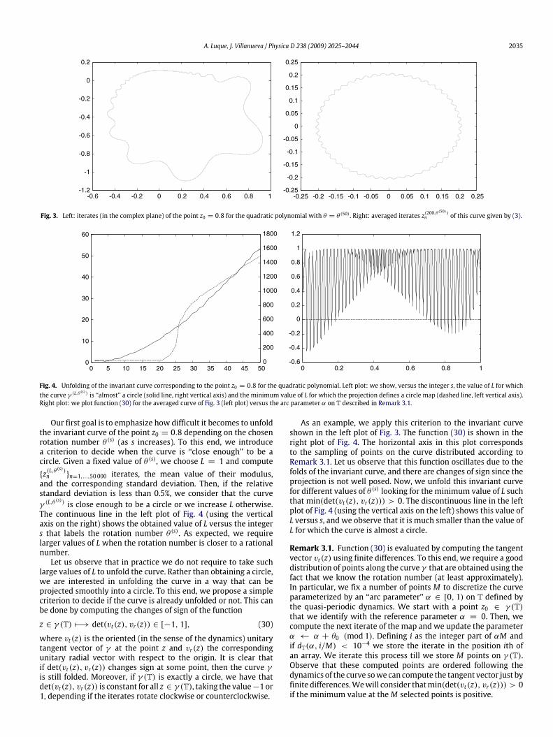
angular variable does not always give a diffeomorphism on T.For example, in the left plot of Fig. 3 we show the curve thatcorresponds to θ = θ (50) for the initial condition z0 = 0.8. Theright plot of Fig. 3 corresponds to the averaged iterates z(200,θ
(50))n
according to (3). As expected, the new curve is closer to a circlecentered at the origin.
A. Luque, J. Villanueva / Physica D 238 (2009) 2025–2044 2035
-1.2
-1
-0.8
-0.6
-0.4
-0.2
0
0.2
-0.6 -0.4 -0.2 0 0.2 0.4 0.6 0.8 1-0.25
-0.2
-0.15
-0.1
-0.05
0
0.05
0.1
0.15
0.2
0.25
-0.25 -0.2 -0.15 -0.1 -0.05 0 0.05 0.1 0.15 0.2 0.25
Fig. 3. Left: iterates (in the complex plane) of the point z0 = 0.8 for the quadratic polynomial with θ = θ (50) . Right: averaged iterates z(200,θ (50))n of this curve given by (3).
0
10
20
30
40
50
60
0 5 10 15 20 25 30 35 40 45 500
200
400
600
800
1000
1200
1400
1600
1800
-0.6
-0.4
-0.2
0
0.2
0.4
0.6
0.8
1
1.2
0 0.2 0.4 0.6 0.8 1
Fig. 4. Unfolding of the invariant curve corresponding to the point z0 = 0.8 for the quadratic polynomial. Left plot: we show, versus the integer s, the value of L for whichthe curve γ (L,θ
(s)) is ‘‘almost’’ a circle (solid line, right vertical axis) and the minimum value of L for which the projection defines a circle map (dashed line, left vertical axis).Right plot: we plot function (30) for the averaged curve of Fig. 3 (left plot) versus the arc parameter α on T described in Remark 3.1.
Our first goal is to emphasize how difficult it becomes to unfoldthe invariant curve of the point z0 = 0.8 depending on the chosenrotation number θ (s) (as s increases). To this end, we introducea criterion to decide when the curve is ‘‘close enough’’ to be acircle. Given a fixed value of θ (s), we choose L = 1 and compute{z(L,θ
(s))n }n=1,...,50 000 iterates, the mean value of their modulus,and the corresponding standard deviation. Then, if the relativestandard deviation is less than 0.5%, we consider that the curveγ (L,θ
(s)) is close enough to be a circle or we increase L otherwise.The continuous line in the left plot of Fig. 4 (using the verticalaxis on the right) shows the obtained value of L versus the integers that labels the rotation number θ (s). As expected, we requirelarger values of L when the rotation number is closer to a rationalnumber.Let us observe that in practice we do not require to take such
large values of L to unfold the curve. Rather than obtaining a circle,we are interested in unfolding the curve in a way that can beprojected smoothly into a circle. To this end, we propose a simplecriterion to decide if the curve is already unfolded or not. This canbe done by computing the changes of sign of the function
z ∈ γ (T) 7−→ det(vt(z), vr(z)) ∈ [−1, 1], (30)
where vt(z) is the oriented (in the sense of the dynamics) unitarytangent vector of γ at the point z and vr(z) the correspondingunitary radial vector with respect to the origin. It is clear thatif det(vt(z), vr(z)) changes sign at some point, then the curve γis still folded. Moreover, if γ (T) is exactly a circle, we have thatdet(vt(z), vr(z)) is constant for all z ∈ γ (T), taking the value−1 or1, depending if the iterates rotate clockwise or counterclockwise.
As an example, we apply this criterion to the invariant curveshown in the left plot of Fig. 3. The function (30) is shown in theright plot of Fig. 4. The horizontal axis in this plot correspondsto the sampling of points on the curve distributed according toRemark 3.1. Let us observe that this function oscillates due to thefolds of the invariant curve, and there are changes of sign since theprojection is not well posed. Now, we unfold this invariant curvefor different values of θ (s) looking for the minimum value of L suchthat min(det(vt(z), vr(z))) > 0. The discontinuous line in the leftplot of Fig. 4 (using the vertical axis on the left) shows this value ofL versus s, and we observe that it is much smaller than the value ofL for which the curve is almost a circle.
Remark 3.1. Function (30) is evaluated by computing the tangentvector vt(z) using finite differences. To this end, we require a gooddistribution of points along the curve γ that are obtained using thefact that we know the rotation number (at least approximately).In particular, we fix a number of points M to discretize the curveparameterized by an ‘‘arc parameter’’ α ∈ [0, 1) on T defined bythe quasi-periodic dynamics. We start with a point z0 ∈ γ (T)that we identify with the reference parameter α = 0. Then, wecompute the next iterate of the map and we update the parameterα ← α + θ0 (mod 1). Defining i as the integer part of αM andif dT(α, i/M) < 10−4 we store the iterate in the position ith ofan array. We iterate this process till we store M points on γ (T).Observe that these computed points are ordered following thedynamics of the curve sowe can compute the tangent vector just byfinite differences.Wewill consider thatmin(det(vt(z), vr(z))) > 0if the minimum value at theM selected points is positive.
2036 A. Luque, J. Villanueva / Physica D 238 (2009) 2025–2044
-2 0 2 4 6 8 10-3
-2
-1
0
1
2
3
4
5
-6 -4 -2 0 2 4 6
L= 2
L= 3
L= 4
-4
-2
0
2
4
6
8
12
Fig. 5. Left: Curve γ (T) in the complex plane corresponding to the parameterization in (31). Right: Unfolded curves γ (L,θ)(T), for L = 2, 3 and 4, using the known value ofthe rotation number θ = (
√5− 1)/2.
0 100 200 300 400 500 600 700 0 100 200 300 400 500 600 700-3
-2.5
-2
-1.5
-1
-0.5
0
0.5
1
-3
-2.5
-2
-1.5
-1
-0.5
0
0.5
1
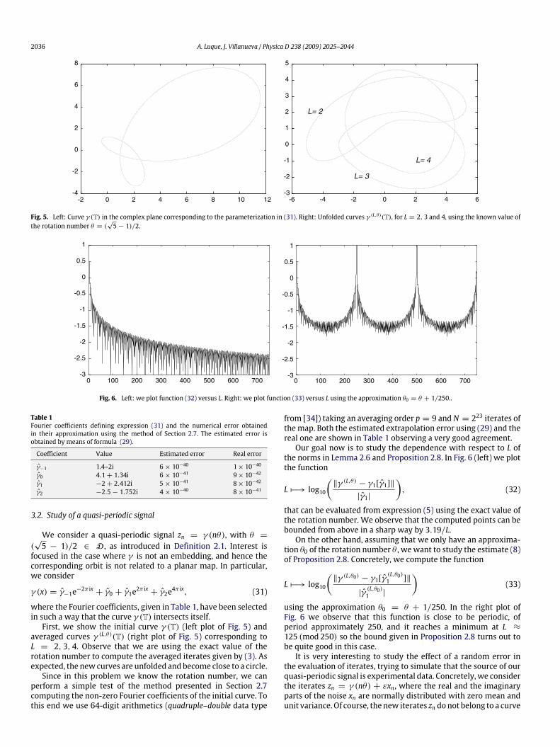
Fig. 6. Left: we plot function (32) versus L. Right: we plot function (33) versus L using the approximation θ0 = θ + 1/250..
Table 1Fourier coefficients defining expression (31) and the numerical error obtainedin their approximation using the method of Section 2.7. The estimated error isobtained by means of formula (29).
Coefficient Value Estimated error Real error
γ−1 1.4–2i 6× 10−40 1× 10−40
γ0 4.1+ 1.34i 6× 10−41 9× 10−42
γ1 −2+ 2.412i 5× 10−41 8× 10−42
γ2 −2.5− 1.752i 4× 10−40 8× 10−41
3.2. Study of a quasi-periodic signal
We consider a quasi-periodic signal zn = γ (nθ), with θ =(√5 − 1)/2 ∈ D , as introduced in Definition 2.1. Interest is
focused in the case where γ is not an embedding, and hence thecorresponding orbit is not related to a planar map. In particular,we consider
γ (x) = γ−1e−2π ix + γ0 + γ1e2π ix + γ2e4π ix, (31)
where the Fourier coefficients, given in Table 1, have been selectedin such a way that the curve γ (T) intersects itself.First, we show the initial curve γ (T) (left plot of Fig. 5) and
averaged curves γ (L,θ)(T) (right plot of Fig. 5) corresponding toL = 2, 3, 4. Observe that we are using the exact value of therotation number to compute the averaged iterates given by (3). Asexpected, the new curves are unfolded and become close to a circle.Since in this problem we know the rotation number, we can
perform a simple test of the method presented in Section 2.7computing the non-zero Fourier coefficients of the initial curve. Tothis end we use 64-digit arithmetics (quadruple–double data type
from [34]) taking an averaging order p = 9 and N = 223 iterates ofthemap. Both the estimated extrapolation error using (29) and thereal one are shown in Table 1 observing a very good agreement.Our goal now is to study the dependence with respect to L of
the norms in Lemma 2.6 and Proposition 2.8. In Fig. 6 (left) we plotthe function
L 7−→ log10
(‖γ (L,θ) − γ1[γ1]‖
|γ1|
), (32)
that can be evaluated from expression (5) using the exact value ofthe rotation number. We observe that the computed points can bebounded from above in a sharp way by 3.19/L.On the other hand, assuming that we only have an approxima-
tion θ0 of the rotation number θ , we want to study the estimate (8)of Proposition 2.8. Concretely, we compute the function
L 7−→ log10
(‖γ (L,θ0) − γ1[γ
(L,θ0)1 ]‖
|γ(L,θ0)1 |
)(33)
using the approximation θ0 = θ + 1/250. In the right plot ofFig. 6 we observe that this function is close to be periodic, ofperiod approximately 250, and it reaches a minimum at L ≈125 (mod 250) so the bound given in Proposition 2.8 turns out tobe quite good in this case.It is very interesting to study the effect of a random error in
the evaluation of iterates, trying to simulate that the source of ourquasi-periodic signal is experimental data. Concretely, we considerthe iterates zn = γ (nθ) + εxn, where the real and the imaginaryparts of the noise xn are normally distributed with zero mean andunit variance. Of course, the new iterates zn donot belong to a curve

A. Luque, J. Villanueva / Physica D 238 (2009) 2025–2044 2037
-8 -6 -4 -2 0 2 4 6 8 10 12 14 16 18 20 22-4
-3
-2
-1
0
1
2
3
4
5
6
-35
-30
-25
-20
-15
-10
-5
Fig. 7. Effect of a random noise in the quasi-periodic signal (31). Left: Unfolded clouds of points (in the complex plane) corresponding to the curves in the right plot of Fig. 5using ε = 0.5 (see text for details). Right: For different noises, taken as ε = 10−δ for δ = 1, . . . , 10,∞, we plot log10 of the real error versus q in the computation of therotation number (using p = 9 and 2q iterates). The data is ‘‘unfolded’’ using L = 10 and θ0 = θ + 1/250.
but they are distributed in a cloud around the curve in Fig. 5 (leftplot). If we compute the iterates z(L,θ0)n , using the approximationθ0 = θ + 1/250, then it turns out that we can ‘‘unfold’’ the cloudof points in a similar way. For example, in the left plot of Fig. 7 weshowunfolded clouds for an error of size ε = 0.5, using L = 2, 3, 4,i.e., the same values that we used in Fig. 5 (right plot).Now we focus on the effect of this external noise when com-
puting the rotation number θ of the ‘‘circle map’’ thus obtained.The size of the considered noise ranges as ε = 10−δ for δ =1, . . . , 10,∞. Although we observe in Fig. 5 (right plot) and Fig. 7(left plot) that the ‘‘projection’’ is well defined for L = 4, in thefollowing computations we take L = 10 since for this value thecorresponding curve is almost a circle. To the constructed ‘‘circlemap’’ we apply Algorithm 2.14 to refine the numerical computa-tion of the rotation number. As implementation parameters wetake an averaging order p = 9 and N = 2q iterates of the map,with q = 9, . . . , 22. The random numbers xn are generated usingthe routine gasdev from [30] for generating normal (Gaussian)deviates. Computations are performed using 32-digit arithmetics(double–double data type from [34]).In the right plot of Fig. 7 we show, in log10 scale, the error
in the computation of the rotation number with respect to q fordifferent values of ε. Let us observe that for ε = 0 (lowest curve)the extrapolation error is saturated around 10−31 for q ≥ 18. Wenotice that this error is of the order of the selected arithmetics. Theother curves in the right Fig. 7 correspond to increasing values ofε (from bottom to top). Let us remark that in all cases the randomerror is averaged in a very efficient way, and it turns out that therotation number is approximated with an error of order ε×10−10.
3.3. Study of invariant curves in non-twist maps
Finally, we apply the developed methodology to the study ofquasi-periodic invariant curves of non-twist maps. It is knownthat the Aubry–Mather variational theory for twist maps does notgeneralize to the non-twist case, but there is an analogue of KAMtheory (see for example the works of [35,36]). However, the loss ofthe twist condition introduces different properties than in the twistcase, for example the fact that the Birkhoff Graph Theorem doesnot generalize. A classical mechanism that creates folded invariantcurves is called reconnection. Reconnection is a global bifurcation ofthe invariantmanifolds of two ormore distinct hyperbolic periodicorbits having the samewinding number (we refer to [25,36,37] andreferences therein for discussion of this bifurcation).Let us start by considering the family of area preserving non-
twist maps given by
Fa,b : (x, y) 7−→ (x, y) =(x+ a(1− y2), y− b sin(2πx)
), (34)
where (x, y) ∈ T × R are phase space coordinates and a, bparameters. This family is usually called standard non-twist mapand it is studied as a paradigmatic example of a non-twist family.Although this family is non-generic (it is degenerate in the sensethat it contains just one harmonic), it describes the essentialfeatures of non-twist systems with a local quadratic extremum inthe rotation number.It is clear that the standard non-twist map violates the twist
condition along the curve y = b sin(2πx) which is called non-monotone curve. Only orbits with points falling on this curve andorbits with points on both sides of it are affected by the non-twist property. Among these orbits, of special interest is the onethat corresponds to an invariant curve having a local extremumin the rotation number, called shearless invariant curve γS . For thestandard non-twistmap this curve is characterized by the fact that,when it exists, it must contain the points
(x(0)± , y(0)± ) =
(±14,±b2
)(x(1)± , y
(1)± ) =
(a2±14, 0),
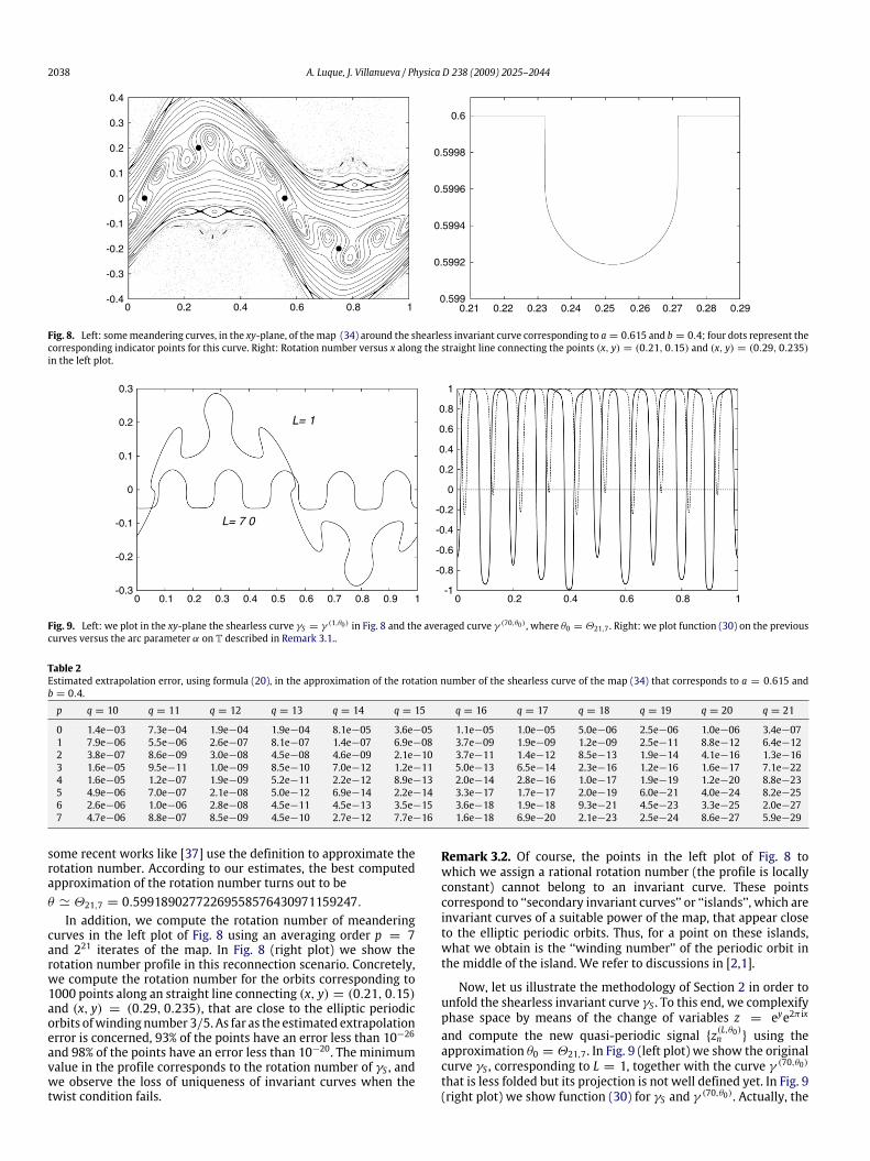
that are called indicator points (see [38]). These points are usedextensively in the literature to study the breakdown of shearlessinvariant curves (we refer for example to [24,37]).In the left plot of Fig. 8 we show some invariant curves close
to a reconnection scenario for a = 0.615 and b = 0.4. We observesomemeandering curves, i.e., curves that are folded around periodicorbits in such a way that they are not graphs over x. In addition,we plot the four indicator points in order to identify the shearlessinvariant curve. Actually, the invariant curve that we used as anillustration in Section 2.1 (see Fig. 1) is precisely this shearlesscurve in the complex variable z = eyeix.First, we focus on this shearless curve computing its rotation
number by applying the extrapolation method of Algorithm 2.14to the circle correspondence obtained by direct projection (seethe discussion in Sections 1 and 2.1) on the angular variable x.Since the folds of this example are relatively small and the rotationnumber is quite big – it is close to 0.6, i.e., the winding numberof the nearby periodic orbits – this direct projection allows us tocompute numerically the lift of this circle correspondence withoutunfolding the curve. In Table 2we give the estimated extrapolationerror, by means of formula (20), in the computation of the rotationnumber of γS , for different values of the extrapolation order pand number of iterates 2q. Computations are performed using32-digit arithmetics (double–double data type from [34]). Let usobserve that the extrapolation method allows us to obtain a verygood approximation of the rotation number with a relative smallnumber of iterates, in contrast with p = 0 which correspondsto the definition of the rotation number — let us mention that
2038 A. Luque, J. Villanueva / Physica D 238 (2009) 2025–2044
0.21 0.22 0.23 0.24 0.25 0.26 0.290.27 0.280.599
0.5992
0.5994
0.5996
0.5998
0.6
-0.4
-0.3
-0.2
-0.1
0.1
0
0.3
0.2
0.4
0 0.2 0.4 0.6 0.8 1
Fig. 8. Left: somemeandering curves, in the xy-plane, of themap (34) around the shearless invariant curve corresponding to a = 0.615 and b = 0.4; four dots represent thecorresponding indicator points for this curve. Right: Rotation number versus x along the straight line connecting the points (x, y) = (0.21, 0.15) and (x, y) = (0.29, 0.235)in the left plot.
0 0.1 0.2 0.3 0.4 0.5 0.6 0.7 0.8 0.9 1
L= 1
L= 7 0
0 0.2 0.4 0.6 0.8 1-0.3
-0.2
-0.1
0
0.1
0.2
0.3
-1
-0.8
-0.6
-0.4
-0.2
0
0.2
0.4
0.6
0.8
1
Fig. 9. Left: we plot in the xy-plane the shearless curve γS = γ (1,θ0) in Fig. 8 and the averaged curve γ (70,θ0) , where θ0 = Θ21,7 . Right: we plot function (30) on the previouscurves versus the arc parameter α on T described in Remark 3.1..
Table 2Estimated extrapolation error, using formula (20), in the approximation of the rotation number of the shearless curve of the map (34) that corresponds to a = 0.615 andb = 0.4.
p q = 10 q = 11 q = 12 q = 13 q = 14 q = 15 q = 16 q = 17 q = 18 q = 19 q = 20 q = 21
0 1.4e−03 7.3e−04 1.9e−04 1.9e−04 8.1e−05 3.6e−05 1.1e−05 1.0e−05 5.0e−06 2.5e−06 1.0e−06 3.4e−071 7.9e−06 5.5e−06 2.6e−07 8.1e−07 1.4e−07 6.9e−08 3.7e−09 1.9e−09 1.2e−09 2.5e−11 8.8e−12 6.4e−122 3.8e−07 8.6e−09 3.0e−08 4.5e−08 4.6e−09 2.1e−10 3.7e−11 1.4e−12 8.5e−13 1.9e−14 4.1e−16 1.3e−163 1.6e−05 9.5e−11 1.0e−09 8.5e−10 7.0e−12 1.2e−11 5.0e−13 6.5e−14 2.3e−16 1.2e−16 1.6e−17 7.1e−224 1.6e−05 1.2e−07 1.9e−09 5.2e−11 2.2e−12 8.9e−13 2.0e−14 2.8e−16 1.0e−17 1.9e−19 1.2e−20 8.8e−235 4.9e−06 7.0e−07 2.1e−08 5.0e−12 6.9e−14 2.2e−14 3.3e−17 1.7e−17 2.0e−19 6.0e−21 4.0e−24 8.2e−256 2.6e−06 1.0e−06 2.8e−08 4.5e−11 4.5e−13 3.5e−15 3.6e−18 1.9e−18 9.3e−21 4.5e−23 3.3e−25 2.0e−277 4.7e−06 8.8e−07 8.5e−09 4.5e−10 2.7e−12 7.7e−16 1.6e−18 6.9e−20 2.1e−23 2.5e−24 8.6e−27 5.9e−29
some recent works like [37] use the definition to approximate therotation number. According to our estimates, the best computedapproximation of the rotation number turns out to beθ ' Θ21,7 = 0.59918902772269558576430971159247.In addition, we compute the rotation number of meandering
curves in the left plot of Fig. 8 using an averaging order p = 7and 221 iterates of the map. In Fig. 8 (right plot) we show therotation number profile in this reconnection scenario. Concretely,we compute the rotation number for the orbits corresponding to1000 points along an straight line connecting (x, y) = (0.21, 0.15)and (x, y) = (0.29, 0.235), that are close to the elliptic periodicorbits ofwindingnumber 3/5. As far as the estimated extrapolationerror is concerned, 93% of the points have an error less than 10−26and 98% of the points have an error less than 10−20. The minimumvalue in the profile corresponds to the rotation number of γS , andwe observe the loss of uniqueness of invariant curves when thetwist condition fails.
Remark 3.2. Of course, the points in the left plot of Fig. 8 towhich we assign a rational rotation number (the profile is locallyconstant) cannot belong to an invariant curve. These pointscorrespond to ‘‘secondary invariant curves’’ or ‘‘islands’’, which areinvariant curves of a suitable power of the map, that appear closeto the elliptic periodic orbits. Thus, for a point on these islands,what we obtain is the ‘‘winding number’’ of the periodic orbit inthe middle of the island. We refer to discussions in [2,1].
Now, let us illustrate the methodology of Section 2 in order tounfold the shearless invariant curve γS . To this end, we complexifyphase space by means of the change of variables z = eye2π ix
and compute the new quasi-periodic signal {z(L,θ0)n } using theapproximation θ0 = Θ21,7. In Fig. 9 (left plot) we show the originalcurve γS , corresponding to L = 1, together with the curve γ (70,θ0)that is less folded but its projection is not well defined yet. In Fig. 9(right plot) we show function (30) for γS and γ (70,θ0). Actually, the
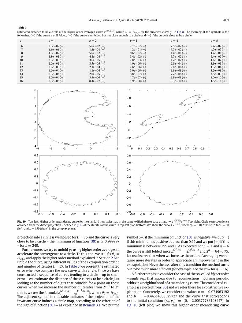
A. Luque, J. Villanueva / Physica D 238 (2009) 2025–2044 2039
Table 3Estimated distance to be a circle of the higher order averaged curve γ (2
q,θ0,p) , where θ0 = Θ21,7 , for the shearless curve γS in Fig. 8. The meaning of the symbols is thefollowing: (−) if the curve is still folded, (=) if the curve is unfolded but not close enough to a circle and (+) if the curve is close to be a circle.
q p = 1 p = 2 p = 3 p = 4 p = 5
6 2.8e−02 (−) 5.6e−02 (−) 7.1e−02 (−) 7.5e−02 (−) 7.4e−02 (−)7 1.1e−01 (+) 1.5e−01 (=) 1.2e−01 (=) 7.7e−02 (−) 4.2e−02 (−)8 4.0e−02 (+) 5.6e−02 (+) 9.6e−02 (=) 1.4e−01 (=) 1.4e−01 (=)9 1.8e−03 (+) 4.4e−03 (+) 3.4e−02 (+) 6.7e−02 (+) 6.4e−02 (=)10 2.8e−03 (+) 3.6e−05 (+) 7.8e−03 (+) 1.2e−02 (+) 1.1e−02 (+)11 2.0e−03 (+) 3.5e−05 (+) 1.0e−06 (+) 2.6e−04 (+) 1.9e−03 (+)12 3.0e−03 (+) 2.1e−04 (+) 7.6e−06 (+) 2.4e−06 (+) 1.3e−04 (+)13 9.6e−04 (+) 1.1e−04 (+) 3.0e−06 (+) 9.8e−08 (+) 1.5e−08 (+)14 8.0e−04 (+) 2.0e−05 (+) 3.8e−07 (+) 7.7e−08 (+) 4.5e−09 (+)15 3.0e−04 (+) 3.5e−06 (+) 1.7e−07 (+) 1.9e−08 (+) 8.0e−10 (+)16 2.0e−05 (+) 8.4e−07 (+) 1.9e−08 (+) 9.3e−10 (+) 1.8e−11 (+)
Fig. 10. Top-left: Higher order meandering curve for the standard non-twist map in the complexified phase space using z = e√2π |a|ye2π ix . Top-right: Circle correspondence
obtained from the direct projection – defined in (1) – of the iterates of the curve in top-left plot. Bottom: We show the curves γ (L,θ0) , where θ0 = 0.0429853252, for L = 50(left) and L = 150 (right) in the complex plane.
projection into a circle iswell posed for L = 75 and the curve is veryclose to be a circle – the minimum of function (30) is' 0.999897– for L = 240.Furthermore, we try to unfold γS using higher order averages to
accelerate the convergence to a circle. To this end, we still fix θ0 =Θ21,7 and apply thehigher ordermethod explained in Section 2.6 tounfold the curve, using different values of the extrapolation order pand number of iterates L = 2q. In Table 3 we present the estimatederror whenwe compare the new curve with a circle. Since we haveconstructed a sequence of curves tending to a circle – up to smallerror – we estimate the distance of these curves to be a circle justlooking at the number of digits that coincide for a point on thesecurves when we increase the number of iterates from 2q−1 to 2q,this is,weuse the formula |z(2
q,θ0,p)0 −z(2
q−1,θ0,p)0 |, where θ0 = Θ21,7.
The adjacent symbol in this table indicates if the projection of theinvariant curve induces a circle map, according to the criterion ofthe sign of function (30) — as explained in Remark 3.1. We put the
symbol (−) if theminimumof function (30) is negative, we put (=)if this minimum is positive but less than 0.99 andwe put (+) if thisminimum is between 0.99 and 1. As expected, for p = 1 and q = 6the curve is still folded since z(2
q,θ0)n = z(2
q,θ0,1)n and 26 = 64 < 75.
Let us observe that whenwe increase the order of averagingwe re-quire more iterates in order to appreciate an improvement in theextrapolation. Nevertheless, after this transition the method turnsout to bemuchmore efficient (for example, see the row for q = 16).A further step is to consider the case of the so-called higher order
meanderings that appear due to reconnections involving periodicorbits in a neighborhood of ameandering curve. The considered ex-ample is selected from [36] andwe refer there for a constructive ex-planation. Concretely, we consider the values a = −0.071963192and b = −0.44614508325727 and the curve that correspondsto the initial condition (x0, y0) = (0,−2.00377736103447). InFig. 10 (left plot) we show this higher order meandering curve
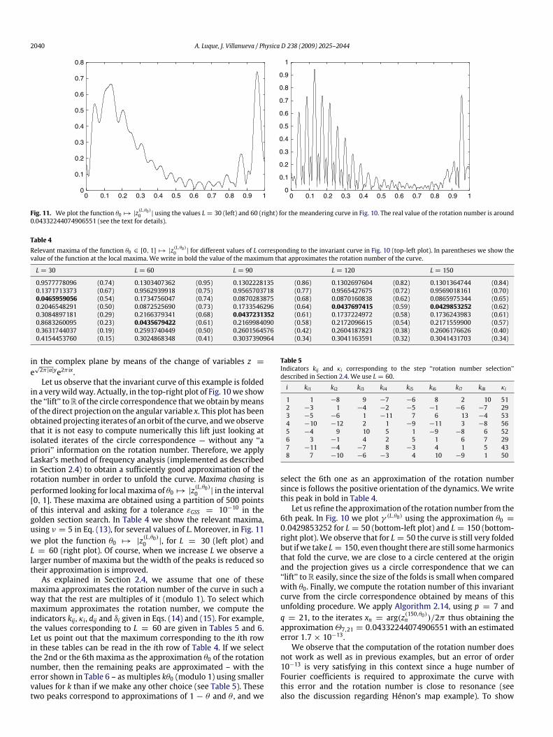
2040 A. Luque, J. Villanueva / Physica D 238 (2009) 2025–2044
0 0.1 0.2 0.3 0.4 0.5 0.6 0.7 0.8 0.9 1 0 0.1 0.2 0.3 0.4 0.5 0.6 0.7 0.8 0.9 1 0
0.1
0.2
0.3
0.4
0.5
0.6
0.7
0.8
0
0.1
0.2
0.3
0.4
0.5
0.6
0.7
0.8
0.9
1
Fig. 11. We plot the function θ0 7→ |z(L,θ0)0 | using the values L = 30 (left) and 60 (right) for the meandering curve in Fig. 10. The real value of the rotation number is around
0.04332244074906551 (see the text for details).
Table 4Relevant maxima of the function θ0 ∈ [0, 1] 7→ |z
(L,θ0)0 | for different values of L corresponding to the invariant curve in Fig. 10 (top-left plot). In parentheses we show the
value of the function at the local maxima. We write in bold the value of the maximum that approximates the rotation number of the curve.
L = 30 L = 60 L = 90 L = 120 L = 150
0.9577778096 (0.74) 0.1303407362 (0.95) 0.1302228135 (0.86) 0.1302697604 (0.82) 0.1301364744 (0.84)0.1371713373 (0.67) 0.9562939918 (0.75) 0.9565703718 (0.77) 0.9565427675 (0.72) 0.9569018161 (0.70)0.0465959056 (0.54) 0.1734756047 (0.74) 0.0870283875 (0.68) 0.0870160838 (0.62) 0.0865975344 (0.65)0.2046548291 (0.50) 0.0872525690 (0.73) 0.1733546296 (0.64) 0.0437697415 (0.59) 0.0429853252 (0.62)0.3084897181 (0.29) 0.2166379341 (0.68) 0.0437231352 (0.61) 0.1737224972 (0.58) 0.1736243983 (0.61)0.8683260095 (0.23) 0.0435679422 (0.61) 0.2169984090 (0.58) 0.2172096615 (0.54) 0.2171559900 (0.57)0.3631744037 (0.19) 0.2593740449 (0.50) 0.2601564576 (0.42) 0.2604187823 (0.38) 0.2606176626 (0.40)0.4154453760 (0.15) 0.3024868348 (0.41) 0.3037390964 (0.34) 0.3041163591 (0.32) 0.3041431703 (0.34)
in the complex plane by means of the change of variables z =e√2π |a|ye2π ix.Let us observe that the invariant curve of this example is folded
in a verywildway. Actually, in the top-right plot of Fig. 10we showthe ‘‘lift’’ toR of the circle correspondence thatwe obtain bymeansof the direct projection on the angular variable x. This plot has beenobtainedprojecting iterates of an orbit of the curve, andweobservethat it is not easy to compute numerically this lift just looking atisolated iterates of the circle correspondence — without any ‘‘apriori’’ information on the rotation number. Therefore, we applyLaskar’s method of frequency analysis (implemented as describedin Section 2.4) to obtain a sufficiently good approximation of therotation number in order to unfold the curve. Maxima chasing isperformed looking for localmaxima of θ0 7→ |z
(L,θ0)0 | in the interval
[0, 1]. These maxima are obtained using a partition of 500 pointsof this interval and asking for a tolerance εGSS = 10−10 in thegolden section search. In Table 4 we show the relevant maxima,using ν = 5 in Eq. (13), for several values of L. Moreover, in Fig. 11we plot the function θ0 7→ |z(L,θ0)0 |, for L = 30 (left plot) andL = 60 (right plot). Of course, when we increase L we observe alarger number of maxima but the width of the peaks is reduced sotheir approximation is improved.As explained in Section 2.4, we assume that one of these
maxima approximates the rotation number of the curve in such away that the rest are multiples of it (modulo 1). To select whichmaximum approximates the rotation number, we compute theindicators kij, κi, dij and δi given in Eqs. (14) and (15). For example,the values corresponding to L = 60 are given in Tables 5 and 6.Let us point out that the maximum corresponding to the ith rowin these tables can be read in the ith row of Table 4. If we selectthe 2nd or the 6th maxima as the approximation θ0 of the rotationnumber, then the remaining peaks are approximated – with theerror shown in Table 6 – as multiples kθ0 (modulo 1) using smallervalues for k than if we make any other choice (see Table 5). Thesetwo peaks correspond to approximations of 1 − θ and θ , and we
Table 5Indicators kij and κi corresponding to the step ‘‘rotation number selection’’described in Section 2.4. We use L = 60.
i ki1 ki2 ki3 ki4 ki5 ki6 ki7 ki8 κi
1 1 −8 9 −7 −6 8 2 10 512 −3 1 −4 −2 −5 −1 −6 −7 293 −5 −6 1 −11 7 6 13 −4 534 −10 −12 2 1 −9 −11 3 −8 565 −4 9 10 5 1 −9 −8 6 526 3 −1 4 2 5 1 6 7 297 −11 −4 −7 8 −3 4 1 5 438 7 −10 −6 −3 4 10 −9 1 50
select the 6th one as an approximation of the rotation numbersince is follows the positive orientation of the dynamics. We writethis peak in bold in Table 4.Let us refine the approximation of the rotation number from the
6th peak. In Fig. 10 we plot γ (L,θ0) using the approximation θ0 =0.0429853252 for L = 50 (bottom-left plot) and L = 150 (bottom-right plot). We observe that for L = 50 the curve is still very foldedbut ifwe take L = 150, even thought there are still someharmonicsthat fold the curve, we are close to a circle centered at the originand the projection gives us a circle correspondence that we can‘‘lift’’ toR easily, since the size of the folds is small when comparedwith θ0. Finally, we compute the rotation number of this invariantcurve from the circle correspondence obtained by means of thisunfolding procedure. We apply Algorithm 2.14, using p = 7 andq = 21, to the iterates xn = arg(z
(150,θ0)n )/2π thus obtaining the
approximationΘ7,21 = 0.04332244074906551 with an estimatederror 1.7× 10⁻¹³.We observe that the computation of the rotation number does
not work as well as in previous examples, but an error of order10−13 is very satisfying in this context since a huge number ofFourier coefficients is required to approximate the curve withthis error and the rotation number is close to resonance (seealso the discussion regarding Hénon’s map example). To show

A. Luque, J. Villanueva / Physica D 238 (2009) 2025–2044 2041
Table 6Indicators dij and δi corresponding to the step ‘‘rotation number selection’’ described in Section 2.4. We use L = 60.
i di1 di2 di3 di4 di5 di6 di7 di8 δi
1 0.00e+00 9.80e−04 4.00e−04 3.60e−04 1.30e−03 8.40e−04 1.30e−03 9.20e−04 6.10e−032 7.70e−04 0.00e+00 1.30e−03 1.50e−04 1.80e−03 1.30e−04 2.80e−03 3.40e−03 1.00e−023 2.20e−03 2.80e−03 0.00e+00 4.50e−03 2.30e−03 2.70e−03 4.10e−03 3.60e−03 2.20e−024 2.80e−03 3.30e−03 1.00e−03 0.00e+00 1.90e−03 3.30e−03 2.30e−03 5.00e−04 1.50e−025 3.10e−03 6.50e−03 7.10e−03 4.00e−03 0.00e+00 6.60e−03 7.50e−03 2.60e−03 3.70e−026 3.60e−04 1.30e−04 7.90e−04 1.10e−04 1.20e−03 0.00e+00 2.00e−03 2.40e−03 7.10e−037 1.60e−02 6.20e−03 1.00e−02 1.20e−02 5.20e−03 6.00e−03 0.00e+00 5.60e−03 6.20e−028 1.20e−02 1.80e−02 1.10e−02 5.20e−03 6.60e−03 1.80e−02 1.80e−02 0.00e+00 9.20e−02
-400 -300 -200 -100 0 100 200 300 400-6
-5
-4
-3
-2
-1
0
-600 -400 -200 0 200 400 600-25
-20
-15
-10
-5
0
5
Fig. 12. We plot log10 |Φ21,7,k| versus k corresponding to the approximated Fourier coefficients of two studied invariant curves. Left: Higher order meandering curve inFig. 10 (top-left plot). Right: Shearless invariant curve in Fig. 8 (left plot).
this, let us compute the Fourier coefficients corresponding to|k| ≤ 750 by means of Algorithm 2.20 using p = 7, q =21 and θ ' Θ21,7. Computations are performed using 32-digitarithmetics (double–double data type from [34]). The modulus ofthe obtained valuesΦ21,7,k are shown in the left plot of Fig. 12. Theextrapolation error, estimated using (29), typically ranges between10−10 and 10−8. As expected, the decay of these coefficients isvery mild and we point out that coefficients for |k| ' 750are still of order 10−5 It is interesting to compare this behaviorto that corresponding to the shearless curve in Fig. 8 since theextrapolation methods can be applied successfully to this case.For this curve the Fourier coefficients – computed using the sameimplementation parameters – decaymuch faster (see the right plotin Fig. 12). In this case, the estimated extrapolation error typicallyranges between 10−16 and 10−24, and Fourier coefficients for |k| ≥400 are so small that we cannot compute any significant digit(we detect this fact because |Φ21,7,k| is of the same order as theextrapolation error). A final remark is that in this plot we observean increase of the size of Fourier coefficients around |k| ' 250 andafter that they decay again at the same rate. The rotation numberof this curve has the convergent 145/242, so the small divisor forthe corresponding Fourier coefficient turns out to be very small.Precisely we observe that |Φ21,7,243| ' 214|Φ21,7,242|.In the next example we want to illustrate the computation of
derivatives of the rotation number by applying Algorithm 2.16 toa circle correspondence that we can ‘‘lift’’ numerically to R. More-over,we alsowant to stress howextrapolationmethods are less ac-curate when the rotation number is a Diophantine number ‘‘closeto a rational’’ — thus having a large constant C in (7). Therefore,we select a problem very close to a resonance. Comparing withprevious examples, we point out that the shearless curve in Fig. 8is not too resonant — actually the continued fraction of the rota-tion number in that case is [0, 1, 1, 2, 48, 1, . . .]. Meanwhile thecase of higher order meandering in Fig. 10 is more resonant butthe curve extremely complicated. Let us consider the well-knownHénon family, which is a paradigmatic example since it appears
generically in the study of a saddle–node bifurcation. This familycan be written as
Hα :(uv
)7−→
(cos(2πα) − sin(2πα)sin(2πα) cos(2πα)
)(u
v − u2
).
It is not difficult to check that we can perform a close to theidentity change of variables to guarantee the twist condition closeto the origin, except for the valuesα = 1/3, 2/3. Then, for values ofα close to 1/3 and 2/3, reconnection takes places and meanderingphenomena arises, i.e., there are folded invariant curves. Next wewant to illustrate the computation of the derivatives of the rotationnumber for α close to 1/3.In the left plot of Fig. 13 we show meandering curves for
α = 0.299544. We use the direct projection and we applyAlgorithm 2.16 to the ‘‘lift’’ of the circle correspondence thusobtained, in order to compute the derivative of the rotationnumber with respect to the initial condition u0, for 6000 pointsof the form (u0, 0.15) along the dotted line in the figure.Computations are performed taking p = 8, q = 23, andusing 32-digit arithmetics (double–double data type from [34]).The corresponding profile is shown in the right plot of Fig. 13,and we observe that the sign of the derivative changes when wepass from one twist zone to another. The isolated points wherethe derivative vanishes correspond to the shearless invariant curvewhile the points where it is locally constant corresponds to thechain of islands (secondary tori) around the elliptic periodic points(see Remark 3.2). We want to stress that since we are very close toa resonance, the convergence of the computations in this exampleis not as good as in the far-from-resonance case. For example, foru0 = 0.28 we obtain the approximationΘ23,8 = 0.299999020519of the rotation numberwith an estimated error, using (20), of order10−12 and the derivativeΘ123,8,7 = −6.027735852× 10
−5 with anestimated error, using (22), of order 10−10. Actually, the continuedfraction expansion of Θ23,8 is given by [0, 3, 2, 1, 10203, 2, . . .]which is close to 3/10 (winding number of the periodic orbit). It isinteresting to compare the error of order 10−12 in the computation
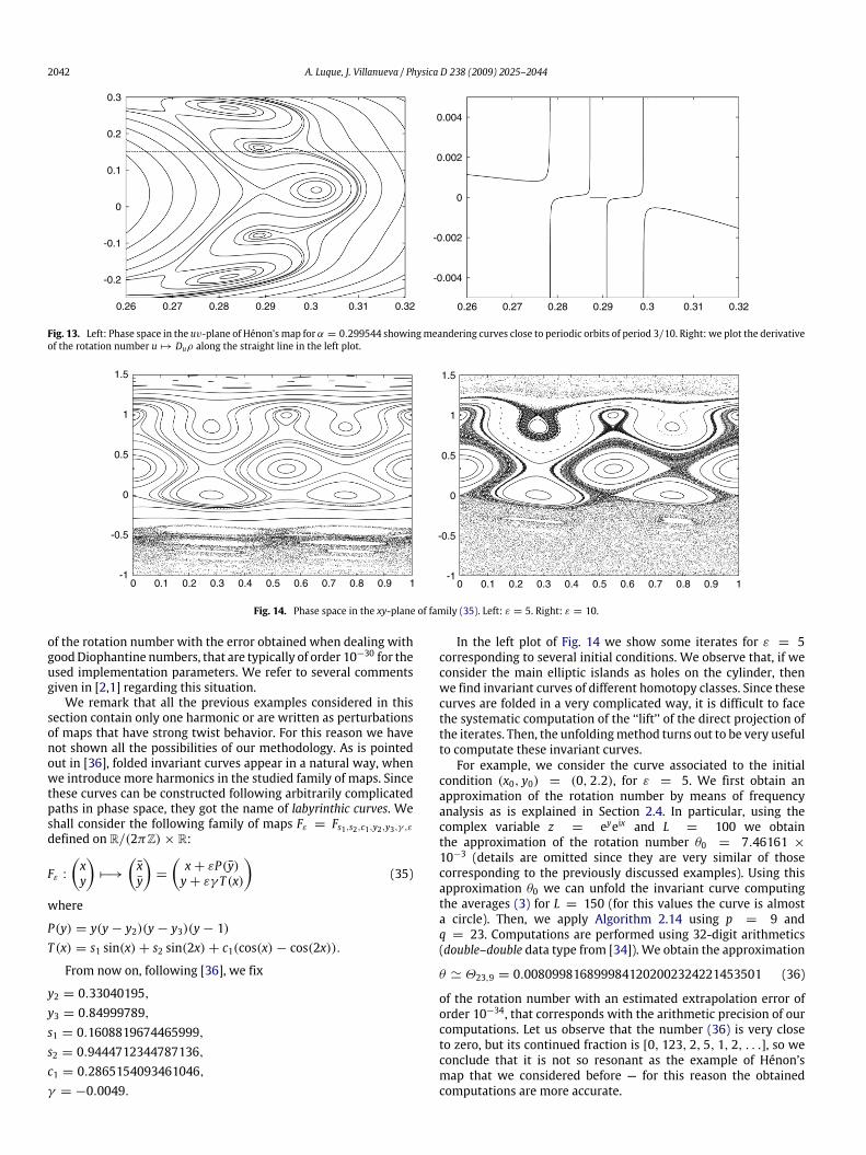
2042 A. Luque, J. Villanueva / Physica D 238 (2009) 2025–2044
0.26 0.27 0.28 0.29 0.3 0.31 0.32 0.26 0.27 0.28 0.29 0.3 0.31 0.32
-0.2
-0.1
0
0.1
0.2
0.3
-0.004
-0.002
0
0.002
0.004
Fig. 13. Left: Phase space in the uv-plane of Hénon’s map for α = 0.299544 showingmeandering curves close to periodic orbits of period 3/10. Right: we plot the derivativeof the rotation number u 7→ Duρ along the straight line in the left plot.
0 0.1 0.2 0.3 0.4 0.5 0.6 0.7 0.8 0.9 1 0 0.1 0.2 0.3 0.4 0.5 0.6 0.7 0.8 0.9 1-1
-0.5
0
0.5
1
1.5
-1
-0.5
0
0.5
1
1.5
Fig. 14. Phase space in the xy-plane of family (35). Left: ε = 5. Right: ε = 10.
of the rotation number with the error obtained when dealing withgoodDiophantine numbers, that are typically of order 10−30 for theused implementation parameters. We refer to several commentsgiven in [2,1] regarding this situation.We remark that all the previous examples considered in this
section contain only one harmonic or are written as perturbationsof maps that have strong twist behavior. For this reason we havenot shown all the possibilities of our methodology. As is pointedout in [36], folded invariant curves appear in a natural way, whenwe introduce more harmonics in the studied family of maps. Sincethese curves can be constructed following arbitrarily complicatedpaths in phase space, they got the name of labyrinthic curves. Weshall consider the following family of maps Fε = Fs1,s2,c1,y2,y3,γ ,εdefined on R/(2πZ)× R:
Fε :(xy
)7−→
(xy
)=
(x+ εP(y)y+ εγ T (x)
)(35)
where
P(y) = y(y− y2)(y− y3)(y− 1)T (x) = s1 sin(x)+ s2 sin(2x)+ c1(cos(x)− cos(2x)).
From now on, following [36], we fix
y2 = 0.33040195,y3 = 0.84999789,s1 = 0.1608819674465999,s2 = 0.9444712344787136,c1 = 0.2865154093461046,γ = −0.0049.
In the left plot of Fig. 14 we show some iterates for ε = 5corresponding to several initial conditions. We observe that, if weconsider the main elliptic islands as holes on the cylinder, thenwe find invariant curves of different homotopy classes. Since thesecurves are folded in a very complicated way, it is difficult to facethe systematic computation of the ‘‘lift’’ of the direct projection ofthe iterates. Then, the unfoldingmethod turns out to be very usefulto computate these invariant curves.For example, we consider the curve associated to the initial
condition (x0, y0) = (0, 2.2), for ε = 5. We first obtain anapproximation of the rotation number by means of frequencyanalysis as is explained in Section 2.4. In particular, using thecomplex variable z = eyeix and L = 100 we obtainthe approximation of the rotation number θ0 = 7.46161 ×10⁻³ (details are omitted since they are very similar of thosecorresponding to the previously discussed examples). Using thisapproximation θ0 we can unfold the invariant curve computingthe averages (3) for L = 150 (for this values the curve is almosta circle). Then, we apply Algorithm 2.14 using p = 9 andq = 23. Computations are performed using 32-digit arithmetics(double–double data type from [34]). We obtain the approximation
θ ' Θ23,9 = 0.0080998168999841202002324221453501 (36)
of the rotation number with an estimated extrapolation error oforder 10−34, that corresponds with the arithmetic precision of ourcomputations. Let us observe that the number (36) is very closeto zero, but its continued fraction is [0, 123, 2, 5, 1, 2, . . .], so weconclude that it is not so resonant as the example of Hénon’smap that we considered before — for this reason the obtainedcomputations are more accurate.
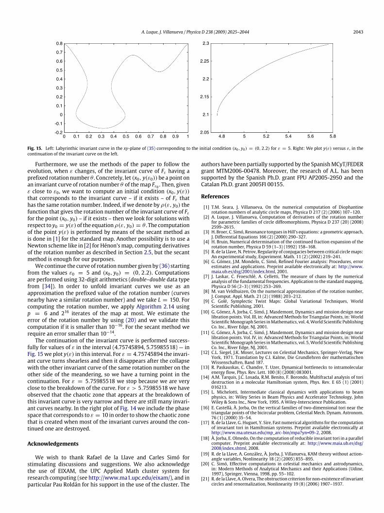
A. Luque, J. Villanueva / Physica D 238 (2009) 2025–2044 2043
0 0.1 0.2 0.3 0.4 0.5 0.6 0.7 0.8 0.9 1 4.8 5 5.2 5.4 5.6 5.8
-0.2
-0.1
0
0.1
0.2
0.3
0.4
0.5
0.6
0.7
0.8
2.05
2.1
2.15
2.2
2.25
2.3
Fig. 15. Left: Labyrinthic invariant curve in the xy-plane of (35) corresponding to the initial condition (x0, y0) = (0, 2.2) for ε = 5. Right: We plot y(ε) versus ε, in thecontinuation of the invariant curve on the left.
Furthermore, we use the methods of the paper to follow theevolution, when ε changes, of the invariant curve of Fε having aprefixed rotation number θ . Concretely, let (x0, y(ε0)) be a point onan invariant curve of rotation number θ of themap Fε0 . Then, givenε close to ε0, we want to compute an initial condition (x0, y(ε))that corresponds to the invariant curve – if it exists – of Fε thathas the same rotation number. Indeed, if we denote by ρ(ε, y0) thefunction that gives the rotation number of the invariant curve of Fεfor the point (x0, y0) – if it exists – then we look for solutions withrespect to y0 = y(ε)of the equationρ(ε, y0) = θ . The computationof the point y(ε) is performed by means of the secant method asis done in [1] for the standard map. Another possibility is to use aNewton scheme like in [2] for Hénon’s map, computing derivativesof the rotation number as described in Section 2.5, but the secantmethod is enough for our purposes.We continue the curve of rotation number given by (36) starting
from the values ε0 = 5 and (x0, y0) = (0, 2.2). Computationsare performed using 32-digit arithmetics (double–double data typefrom [34]). In order to unfold invariant curves we use as anapproximation the prefixed value of the rotation number (curvesnearby have a similar rotation number) and we take L = 150. Forcomputing the rotation number, we apply Algorithm 2.14 usingp = 6 and 216 iterates of the map at most. We estimate theerror of the rotation number by using (20) and we validate thiscomputation if it is smaller than 10−16. For the secant method werequire an error smaller than 10−14.The continuation of the invariant curve is performed success-
fully for values of ε in the interval (4.75745894, 5.75985518) — inFig. 15we plot y(ε) in this interval. For ε = 4.75745894 the invari-ant curve turns shearless and then it disappears after the collapsewith the other invariant curve of the same rotation number on theother side of the meandering, so we have a turning point in thecontinuation. For ε = 5.75985518 we stop because we are veryclose to the breakdown of the curve. For ε > 5.75985518 we haveobserved that the chaotic zone that appears at the breakdown ofthis invariant curve is very narrow and there are still many invari-ant curves nearby. In the right plot of Fig. 14 we include the phasespace that corresponds to ε = 10 in order to show the chaotic zonethat is created when most of the invariant curves around the con-tinued one are destroyed.
Acknowledgements
We wish to thank Rafael de la Llave and Carles Simó forstimulating discussions and suggestions. We also acknowledgethe use of EIXAM, the UPC Applied Math cluster system forresearch computing (see http://www.ma1.upc.edu/eixam/), and inparticular Pau Roldán for his support in the use of the cluster. The
authors have been partially supported by the SpanishMCyT/FEDERgrant MTM2006-00478. Moreover, the research of A.L. has beensupported by the Spanish Ph.D. grant FPU AP2005-2950 and theCatalan Ph.D. grant 2005FI 00155.
References
[1] T.M. Seara, J. Villanueva, On the numerical computation of Diophantinerotation numbers of analytic circle maps, Physica D 217 (2) (2006) 107–120.
[2] A. Luque, J. Villanueva, Computation of derivatives of the rotation numberfor parametric families of circle diffeomorphisms, Physica D 237 (20) (2008)2599–2615.
[3] H. Broer, C. Simó, Resonance tongues inHill’s equations: a geometric approach,J. Differential Equations 166 (2) (2000) 290–327.
[4] H. Bruin, Numerical determination of the continued fraction expansion of therotation number, Physica D 59 (1–3) (1992) 158–168.
[5] R. de la Llave, N. Petrov, Regularity of conjugacies between critical circlemaps:An experimental study, Experiment. Math. 11 (2) (2002) 219–241.
[6] G. Gómez, J.M. Mondelo, C. Simó, Refined Fourier analysis: Procedures, errorestimates and applications. Preprint available electronically at: http://www.maia.ub.es/dsg/2001/index.html, 2001.
[7] J. Laskar, C. Froeschlé, A. Celletti, The measure of chaos by the numericalanalysis of the fundamental frequencies. Application to the standardmapping,Physica D 56 (2–3) (1992) 253–269.
[8] M. van Veldhuizen, On the numerical approximation of the rotation number,J. Comput. Appl. Math. 21 (2) (1988) 203–212.
[9] C. Golé, Symplectic Twist Maps: Global Variational Techniques, WorldScientific Publishing, 2001.
[10] G. Gómez, À. Jorba, C. Simó, J. Masdemont, Dynamics and mission design nearlibration points. Vol. III, in: AdvancedMethods for Triangular Points, in:WorldScientificMonograph Series inMathematics, vol. 4,World Scientific PublishingCo. Inc., River Edge, NJ, 2001.
[11] G. Gómez, À. Jorba, C. Simó, J. Masdemont, Dynamics and mission design nearlibration points. Vol. IV, in: AdvancedMethods for Triangular Points, in:WorldScientificMonograph Series inMathematics, vol. 5,World Scientific PublishingCo. Inc., River Edge, NJ, 2001.
[12] C.L. Siegel, J.K. Moser, Lectures on Celestial Mechanics, Springer-Verlag, NewYork, 1971. Translation by C.I. Kalme, Die Grundlehren der mathematischenWissenschaften, Band 187.
[13] R. Paskauskas, C. Chandre, T. Uzer, Dynamical bottlenecks to intramolecularenergy flow, Phys. Rev. Lett. 100 (8) (2008) 083001.
[14] A.M. Tarquis, J.C. Losada, R.M. Benito, F. Borondo, Multifractal analysis of toridestruction in a molecular Hamiltonian system, Phys. Rev. E 65 (1) (2001)016213.
[15] L. Michelotti, Intermediate classical dynamics with applications to beamphysics, in: Wiley Series in Beam Physics and Accelerator Technology, JohnWiley & Sons Inc., New York, 1995. A Wiley-Interscience Publication.
[16] E. Castellà, À. Jorba, On the vertical families of two-dimensional tori near thetriangular points of the bicircular problem, Celestial Mech. Dynam. Astronom.76 (1) (2000) 35–54.
[17] R. de la Llave, G. Huguet, Y. Sire, Fast numerical algorithms for the computationof invariant tori in Hamiltonian systems. Preprint available electronically athttp://www.ma.utexas.edu/mp_arc-bin/mpa?yn=09-2, 2008.
[18] À. Jorba, E. Olmedo, On the computation of reducible invariant tori in a parallelcomputer. Preprint available electronically at: http://www.maia.ub.es/dsg/2008/index.shtml, 2008.
[19] R. de la Llave, A. González, À. Jorba, J. Villanueva, KAM theory without action-angle variables, Nonlinearity 18 (2) (2005) 855–895.
[20] C. Simó, Effective computations in celestial mechanics and astrodynamics,in: Modern Methods of Analytical Mechanics and their Applications (Udine,1997), Springer, Vienna, 1998, pp. 55–102.
[21] R. de la Llave, A. Olvera, The obstruction criterion for non-existence of invariantcircles and renormalization, Nonlinearity 19 (8) (2006) 1907–1937.
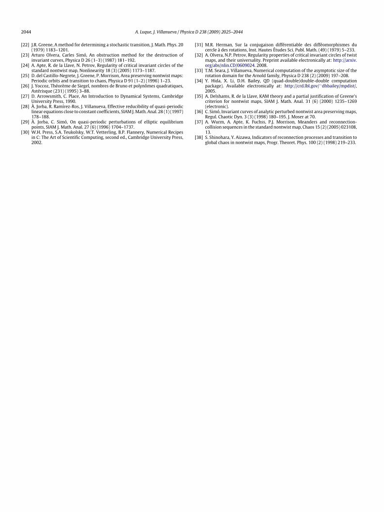
2044 A. Luque, J. Villanueva / Physica D 238 (2009) 2025–2044
[22] J.R. Greene, A method for determining a stochastic transition, J. Math. Phys. 20(1979) 1183–1201.
[23] Arturo Olvera, Carles Simó, An obstruction method for the destruction ofinvariant curves, Physica D 26 (1–3) (1987) 181–192.
[24] A. Apte, R. de la Llave, N. Petrov, Regularity of critical invariant circles of thestandard nontwist map, Nonlinearity 18 (3) (2005) 1173–1187.
[25] D. del Castillo-Negrete, J. Greene, P. Morrison, Area preserving nontwist maps:Periodic orbits and transition to chaos, Physica D 91 (1–2) (1996) 1–23.
[26] J. Yoccoz, Théorème de Siegel, nombres de Bruno et polynômes quadratiques,Astérisque (231) (1995) 3–88.
[27] D. Arrowsmith, C. Place, An Introduction to Dynamical Systems, CambridgeUniversity Press, 1990.
[28] À. Jorba, R. Ramírez-Ros, J. Villanueva, Effective reducibility of quasi-periodiclinear equations close to constant coefficients, SIAM J.Math. Anal. 28 (1) (1997)178–188.
[29] À. Jorba, C. Simó, On quasi-periodic perturbations of elliptic equilibriumpoints, SIAM J. Math. Anal. 27 (6) (1996) 1704–1737.
[30] W.H. Press, S.A. Teukolsky, W.T. Vetterling, B.P. Flannery, Numerical Recipesin C: The Art of Scientific Computing, second ed., Cambridge University Press,2002.
[31] M.R. Herman, Sur la conjugaison différentiable des difféomorphismes ducercle à des rotations, Inst. Hautes Études Sci. Publ. Math. (49) (1979) 5–233.
[32] A. Olvera, N.P. Petrov, Regularity properties of critical invariant circles of twistmaps, and their universality. Preprint available electronically at: http://arxiv.org/abs/nlin.CD/0609024. 2008.
[33] T.M. Seara, J. Villanueva, Numerical computation of the asymptotic size of therotation domain for the Arnold family, Physica D 238 (2) (2009) 197–208.
[34] Y. Hida, X. Li, D.H. Bailey, QD (quad-double/double-double computationpackage). Available electronically at: http://crd.lbl.gov/∼dhbailey/mpdist/,2005.
[35] A. Delshams, R. de la Llave, KAM theory and a partial justification of Greene’scriterion for nontwist maps, SIAM J. Math. Anal. 31 (6) (2000) 1235–1269(electronic).
[36] C. Simó, Invariant curves of analytic perturbed nontwist area preservingmaps,Regul. Chaotic Dyn. 3 (3) (1998) 180–195. J. Moser at 70.
[37] A. Wurm, A. Apte, K. Fuchss, P.J. Morrison, Meanders and reconnection-collision sequences in the standard nontwistmap, Chaos 15 (2) (2005) 023108,13.
[38] S. Shinohara, Y. Aizawa, Indicators of reconnection processes and transition toglobal chaos in nontwist maps, Progr. Theoret. Phys. 100 (2) (1998) 219–233.