The Astronomical Journal, 136:1757–1769, 2008 November doi:10.1088/0004-6256/136/5/1757c© 2008. The American Astronomical Society. All rights reserved. Printed in the U.S.A.

VERTICAL STRUCTURE IN PLUTO’S ATMOSPHERE FROM THE 2006 JUNE 12 STELLAR OCCULTATION

E. F. Young1, R. G. French

2,11, L. A. Young

1, C. R. Ruhland

1, M. W. Buie

3, C. B. Olkin

1, J. Regester

4, K. Shoemaker

5,11,

G. Blow6, J. Broughton

7, G. Christie

8, D. Gault

9, B. Lade

10, and T. Natusch

81 Department of Space Studies, Southwest Research Institute,1050 Walnut St, Suite 300, Boulder, CO 80302, USA

2 Department of Astronomy, Wellesley College, Wellesley, MA 02481, USA3 Lowell Observatory, 1400 W. MarsHill Rd., Flagstaff, AZ 86001, USA

4 Greensboro Day School, 5401 Lawndale Drive, Greensboro, NC 27455, USA5 Shoemaker Labs, Lafayette, CO 80026, USA

6 Occultation Section, Royal Astronomical Society of New Zealand, PO Box 3181, Wellington, New Zealand7 Reedy Creek Observatory, Reedy Creek, Queensland, Australia

8 Auckland Observatory, PO Box 24 180 Royal Oak, Auckland 1345, New Zealand9 Hawkesbury Heights, New South Wales, Australia10 Stockport Observatory, South Australia, Australia

Received 2007 December 27; accepted 2008 June 20; published 2008 September 26

ABSTRACT

Pluto occultations are historically rare events, having been observed in 1988, 2002, 2006, and, as Pluto moves intothe crowded Galactic plane, on several occasions in 2007. Here we present six results from our observations ofthe 2006 June 12 event from several sites in Australia and New Zealand. First, we show that Pluto’s 2006 bulkatmospheric column abundance, as in 2002, is over twice the value measured in 1988, implying that nitrogenfrost on Pluto’s surface is 1.2–1.7 K warmer in 2006 than 1988 despite a 9% drop in incident solar flux.We measure a half-light shadow radius of 1216 ± 8.6 km in 2006, nominally larger than published values of1213 ± 16 km measured in 2002. Given the current error bars, this latest half-light radius cannot discriminatebetween continued atmospheric growth or shrinkage, but it rules out several of the volatile transport scenariosmodeled by Hansen & Paige. Second, we resolve spikes in the occultation light curve that are similar to thoseseen in 2002 and model the vertical temperature fluctuations that cause them. Third, we show that Pluto’supper atmosphere appears to hold a steady temperature of ∼100 K, as predicted from the methane thermostatmodel, even at latitudes where the methane thermostat is inoperative. This implies that energy transport ratesare faster than radiational cooling rates. Fourth, this occultation has provided the first significant detection ofa non-isothermal temperature gradient in Pluto’s upper atmosphere also reported by Elliot et al., possibly theresult of CO gas in Pluto’s upper atmosphere. Fifth, we show that a haze-only explanation for Pluto’s lightcurve is extremely unlikely; a thermal inversion is necessary to explain the observed light curve. And sixth, wederive an upper limit for the haze optical depth of 0.0023 in the zenith direction at average CCD wavelengths.

Key words: occultations – planets and satellites: individual (Pluto)

Online-only material: color figure

1. INTRODUCTION

1.1. Previous Occultations

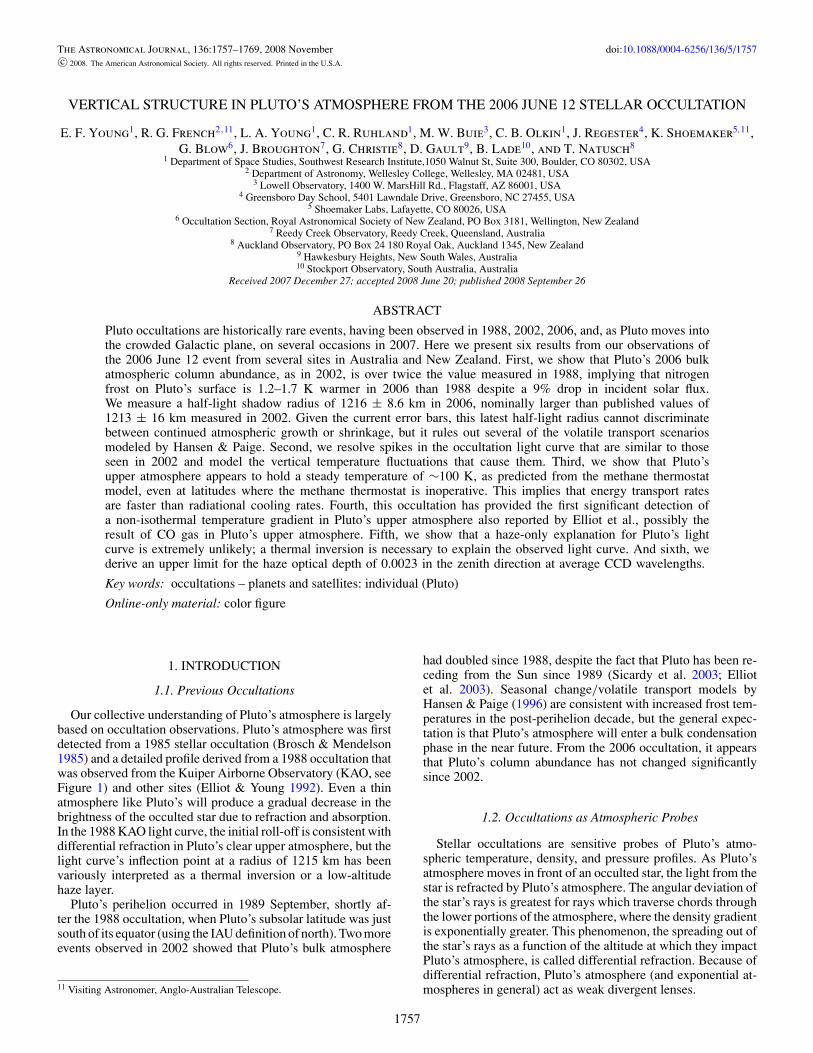
Our collective understanding of Pluto’s atmosphere is largelybased on occultation observations. Pluto’s atmosphere was firstdetected from a 1985 stellar occultation (Brosch & Mendelson1985) and a detailed profile derived from a 1988 occultation thatwas observed from the Kuiper Airborne Observatory (KAO, seeFigure 1) and other sites (Elliot & Young 1992). Even a thinatmosphere like Pluto’s will produce a gradual decrease in thebrightness of the occulted star due to refraction and absorption.In the 1988 KAO light curve, the initial roll-off is consistent withdifferential refraction in Pluto’s clear upper atmosphere, but thelight curve’s inflection point at a radius of 1215 km has beenvariously interpreted as a thermal inversion or a low-altitudehaze layer.

Pluto’s perihelion occurred in 1989 September, shortly af-ter the 1988 occultation, when Pluto’s subsolar latitude was justsouth of its equator (using the IAU definition of north). Two moreevents observed in 2002 showed that Pluto’s bulk atmosphere

11 Visiting Astronomer, Anglo-Australian Telescope.

had doubled since 1988, despite the fact that Pluto has been re-ceding from the Sun since 1989 (Sicardy et al. 2003; Elliotet al. 2003). Seasonal change/volatile transport models byHansen & Paige (1996) are consistent with increased frost tem-peratures in the post-perihelion decade, but the general expec-tation is that Pluto’s atmosphere will enter a bulk condensationphase in the near future. From the 2006 occultation, it appearsthat Pluto’s column abundance has not changed significantlysince 2002.

1.2. Occultations as Atmospheric Probes

Stellar occultations are sensitive probes of Pluto’s atmo-spheric temperature, density, and pressure profiles. As Pluto’satmosphere moves in front of an occulted star, the light from thestar is refracted by Pluto’s atmosphere. The angular deviation ofthe star’s rays is greatest for rays which traverse chords throughthe lower portions of the atmosphere, where the density gradientis exponentially greater. This phenomenon, the spreading out ofthe star’s rays as a function of the altitude at which they impactPluto’s atmosphere, is called differential refraction. Because ofdifferential refraction, Pluto’s atmosphere (and exponential at-mospheres in general) act as weak divergent lenses.

1757

1758 YOUNG ET AL. Vol. 136

Figure 1. A comparison of two stellar occultations by Pluto. A 2006 light curve (top) and a 1988 light curve show several distinctive changes. First, the half-lightradius increased between 1988 and 2002, and continues at the 2002 level in 2006. Second, the 2006 light curve also departs from the isothermal model that fits theupper atmosphere well, but the kink in 2006 is much less abrupt than in 1988. Third, there are resolved spikes observed during ingress and egress in the 2006 lightcurve, including two broad humps seen between 800 and 900 km in the shadow radius. The KAO data set does not show these spikes in the lower parts of the 1988light curve.

Some atmospheres contain fluctuations in their mainly ex-ponential density profiles. In these cases, local density pertur-bations can produce convergent focusing of some of the star’srays. As focused rays pass over ground-based telescopes, theyproduce bright spikes in the occultation light curve. In ourAnglo-Australian Telescope (AAT) light curve, we see multiplespikes that are resolved by at least five to ten data points; theseare the most compelling evidence to date on the size and extentof temperature fluctuations in Pluto’s atmosphere. Sicardy et al.(2003) and Pasachoff et al. (2005) reported spikes in their lightcurves as well, although at lower signal-to-noise ratio (S/N) andtime resolution than in the AAT light curve.

It is possible to construct a simple atmospheric model basedon a few free parameters, such as a temperature gradient or ahaze optical depth over certain ranges of altitudes. Clear, nearly-isothermal models have closely fit the upper atmosphere of Plutowith temperatures near 100 K for both ingress and egress, in alloccultation light curves (in 1988, 2002, and 2006) of whichwe are aware. However, the models which fit Pluto’s upperatmosphere are inconsistent with Pluto’s lower atmosphere. Thecause of the discrepancy has been variously attributed to haze,a thermal inversion, or a combination of the two (e.g., Elliot &Young 1992; Eshelman 1989). We will show that a haze-onlysolution is not tenable.

There are two complementary techniques which we use totransform light curves into density, pressure, and temperatureprofiles. The first is mentioned in the previous paragraph:a forward model, typically based on a few free parameters

(six, in our case). The second is called the inversion method,a bootstrap determination of refractivities from high to lowaltitudes, beginning with an upper boundary condition andprogressing downward on a point-by-point basis in lockstepwith the observed fluxes. Without a boundary condition (e.g., anupper boundary provided by the forward model’s fit to the upperatmosphere), the inversion method could not determine density(or temperature) versus altitude, only density or temperaturegradients versus altitude.

1.3. New Results

The observations and data reduction pipeline are discussedin Section 2, primarily describing how the collected imagesare turned into one-dimensional light curves with propagatederrors and how the light curves determine the geometric solution.The analysis and results section (Section 3) describes how lightcurves map to temperature, density, and pressure profiles, andwhat those profiles are.

We then discuss five significant results from the 2006 June12 occultation in Section 4 as follows. First, we derive ahalf-light radius (a measure of Pluto’s column abundance)which, in the context of previous occultation half-light radii,indicates whether Pluto’s atmosphere is expanding or shrinking.Second, we derive temperature profiles from regions of Pluto’satmosphere sampled at the star’s ingress and egress. These firsttwo results are similar to work presented by other investigatorsfollowing the occultations in 2002 and 2006 (e.g., Elliot et al.2003; Sicardy et al. 2003; Elliot et al. 2007 with respect to

No. 5, 2008 PLUTO’S ATMOSPHERE: 2006 JUNE 12 OCCULTATION RESULTS 1759

Table 1Observing Circumstances for the Five Sites that Contributed to this Paper

Site Location Impact Exp. Time/ S/Nb Weather ObserversParametera (km) Duty Cycle (s)

REEc 28◦06′36′′ S 836.6 (N) 15.0/22.5 5.4 Clear JB153◦23′49′′ E

AATd 31◦16′37′′ S 571.8 (N) 0.1/0.1 333 Clear RGF, KS149◦03′58′′ E

STOe 34◦19′55′′ S 382.2 (N) 1.0/2.0 14 Clear BL138◦43′45′′ E

HHTf 33◦39′52′′ S 302.5 (N) 1.0/2.0 3.6 Clear DG150◦28′38′′ E

CARg 41◦17′03′′ S −857.6 (S) 0.65/0.56 7.7 Cumulus, MWB, CRR174◦45′55′′ E icy cirrus

Notes.a The impact parameter is the minimum distance from a site to the shadow’s center.b S/N is the signal-to-noise ratio in the unocculted signal over an interval during which Pluto’s shadowmoves 60 km, or approximately one scale height.c REE = Reedy Creek Observatory, QLD, AUS (0.5 m aperture).d AAT = Anglo-Australian Observatory, NSW, AUS (4 m).e STO = Stockport Observatory, SA, AUS (0.5 m).f HHT = Hawkesbury Heights, NSW, AUS (0.2 m).g CAR = Carter Observatory, Wellington, NZ (0.6 m). Observations were also attempted at AucklandObservatory (GC, TN); Campbell Farm in Longford, Tasmania (EFY, JR); and Gillespie Farm, Wanaka,NZ (CBO, LAY).

Pluto’s half-light radii, and Sicardy et al. 2003 with respect toPluto’s temperature profile).

Third, we present a new constraint on radiative heatingand cooling rates relative to dynamical timescales in Pluto’supper atmosphere, and fourth, we determine a non-isothermaltemperature gradient in Pluto’s upper atmosphere. Finally, weprovide new evidence against a haze-only solution to explainthe attenuation seen in the lower-atmosphere part of Pluto’soccultation light curve, and present an upper limit to the one-way haze optical depth from the haze-only solution.

2. OBSERVATIONS

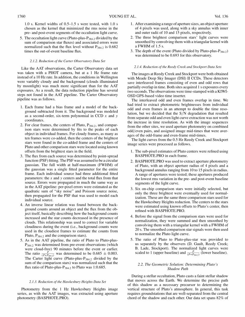
Several research teams deployed observers to southern lati-tudes to observe Pluto move in front of a 15.5 mag star (P384.2from McDonald & Elliot 2000a, 2000b) on 2006 June 12. Ourteam of PHOT observers successfully observed this event fromvarious sites, including the 3.9 m AAT in Siding Spring underclear skies (Table 1). The AAT observations produced a lightcurve with an unprecedentedly high S/N.

Observations were also attempted at Auckland Observatory(GC, TN), Campbell Farm in Longford, Tasmania (EFY, JR),and Gillespie Farm, Wanaka, NZ (CBO, LAY).

2.1. Photometric Reduction

2.1.1. Reduction of the Anglo-Australian Telescope Data Set

The AAT observations were taken unfiltered with one of ourPHOT (portable high-speed occultation telescope) cameras, aPrinceton Instruments MicroMax BFT512 frame-transfer CCDwith low read noise (approximately 3.1 e- per read) and virtuallyno dead time (∼2 ms) between exposures at the 10 Hz framerate used for this event. Conditions were clear with excellentseeing. Despite the fact that Pluto was only 10◦ away from thefull moon, the background was remarkably free of scatteredlight, perhaps because a storm on the previous day may haveremoved suspended particulates. The small field of view of 44′′included Pluto and the occultation star plus two comparison

stars. (In this section, in the context of photometric reduction,we use “Pluto” as a shorthand for the entire Pluto system, i.e.,Pluto, Charon, Nix, and Hydra). The platescale at the AAT’s f /8auxiliary instrument ports is 0.087′′ pixel−1 at full resolution, or0.348′′ pixel−1 with the 4 × 4 binning that was used for theevent. The reduction pipeline consisted of the following steps.

1. Each frame was dark-subtracted using 0.1 s dark frames,the same exposure time as the occultation observations, andnormalized by the flat-field.

2. Photometry of Pluto and two on-chip comparison starswithin the 44′′ field of view was performed with theIDL routine BASPHOTE.PRO′′, part of Marc Buie’s li-brary of IDL routines 200712. This routine performs cir-cular aperture photometry with user-specified aperturesfor the object and the sky annulus. A range of aper-ture radii were tested for the object’s aperture and theinner and outer sky radii. An aperture radius of 4 pix-els (1.4′′) and inner and outer sky radii of 10 and14 pixels were chosen as the aperture sizes that minimizedrms noise in the pre- and post-event segments of the occul-tation light curve. BASPHOTE estimates the noise for eachpixel and propagates that error to the fluxes determined foreach object.

3. Individual photometry of Pluto and the occultation star(P384.2) was obtained from images acquired prior to1.5 h before the event, when the separation between thetwo objects was 5′′ or greater. The ratio of Pluto to Pluto-plus-P384.2 was 0.682 ± 0.003.

4. The flux from Pluto-plus-P384.2 was normalized by the sumof fluxes from the comparison stars. Although sky con-ditions were good, the comparison stars’ fluxes exhibitedslowly changing variability on the few-percent level. Thecomparison stars’ light curves were each smoothed by con-volving them with a triangular kernel with a FWHM of

12 http://www.boulder.swri.edu/∼buie/idl/

1760 YOUNG ET AL. Vol. 136

1.0 s. Kernel widths of 0.5–1.5 s were tested, with 1.0 schosen as the kernel that minimized the rms noise in thepre- and post-event segments of the occultation light curve.

5. The occultation light curve (Pluto-plus-P384.2 divided by thesum of comparison star fluxes) and associated errors werenormalized such that the flux level without P384.2 is 0.682times the out-of-event baseline flux.

2.1.2. Reduction of the Carter Observatory Data Set

Like the AAT observations, the Carter Observatory data setwas taken with a PHOT camera, but at a 1 Hz frame rateinstead of a 10 Hz rate. In addition, the conditions in Wellingtonwere variably cloudy and the background (clouds illuminatedby moonlight) was much more significant than for the AATexposures. As a result, the data reduction pipeline has severalsteps not found in the AAT pipeline. The Carter Observatorypipeline was as follows.

1. Each frame had a bias frame and a model of the back-ground subtracted from it. The background was modeledas a second-order, six-term polynomial in CCD x and ycoordinates.

2. For clear frames, the centers of Pluto, P384.2, and compar-ison stars were determined by fits to the peaks of eachobject in individual frames. For cloudy frames, as many asten frames were co-added, then the centers of the brighteststars were found in the co-added frame and the centers ofPluto and other comparison stars were located using knownoffsets from the brightest stars in the field.

3. The flux from each source was determined by point-spreadfunction (PSF) fitting. The PSF was assumed to be a circulargaussian. The full width at half-maximum (FWHM) ofthe gaussian was a single fitted parameter for the entireframe. Each individual source had three additional fittedparameters: the x and y centers and the total flux from thatsource. Errors were propagated in much the same way asin the AAT pipeline: per-pixel errors were estimated as thequadratic sum of “sky noise” and Poisson source noise,then propagated for the PSF that was used to model eachindividual source.

4. An inverse linear relation was found between the back-ground counts around an object and the flux from the ob-ject itself, basically describing how the background countsincreased and the star counts decreased in the presence ofclouds. This relationship was used to correct for variablecloudiness during the event (i.e., background counts wereused in the cloudiest frames to estimate the counts fromPluto, P384.2 and the comparison stars).

5. As in the AAT pipeline, the ratio of Pluto to Pluto-plus-P384.2 was determined from pre-event observations (whichwere cloud-free) 90 minutes before the event or earlier.The ratio P

(P +P384.2) was determined to be 0.685 ± 0.003.The Carter light curve (Pluto-plus-P384.2 divided by thesum of the comparison stars) was normalized such that theflux ratio of Pluto-plus-P384.2 to Pluto was 1:0.685.

2.1.3. Reduction of the Hawkesbury Heights Data Set

Photometry from the 1 Hz Hawkesbury Heights imageseries, as with the AAT images, was extracted using aperturephotometry (BASPHOTE.PRO).

1. After examining a range of aperture sizes, an object apertureof 4 pixels was used, along with a sky annulus with innerand outer radii of 10 and 15 pixels, respectively.

2. The three brightest comparison stars’ light curves weresmoothed by convolving them with a triangular kernel witha FWHM of 1.5 s.

3. The depth of the event (Pluto divided by Pluto-plus-P384.2)was determined to be 0.693 for this observatory.

2.1.4. Reduction of the Reedy Creek and Stockport Data Sets

The images at Reedy Creek and Stockport were both obtainedwith Meade Deep Sky Imager (DSI) II CCDs. These detectorssave interleaved frames consisting of even and odd rows thatpartially overlap in time. Both sites acquired 1 s exposures everytwo seconds. The observations were time-stamped with a KIWI-OSD GPS-based video time inserter.

The interleaved odd and even frames overlap in time. Wehad tried to extract photometric brightnesses from individualodd and even frames in an attempt to double the time reso-lution, but we decided that the S/N degradation that resultedfrom separate odd and even light curve extraction was not worththe increase in time resolution. As with the image sequencesfrom the other sites, we used aperture photometry on combinedodd/even pairs, and assigned image mid-times that were aver-ages of the odd-frame and even-frame mid-times.

The light curves from the 0.5 Hz Reedy Creek and Stockportimage series were processed as follows.

1. The sub-pixel estimates of Pluto centers were refined usingBASPHOTE.PRO in each frame.

2. BASPHOTE.PRO was used to extract aperture photometryof Pluto, with an object aperture radius of 4 pixels and abackground annulus ranging from 10 to 15 pixels in radius.A range of apertures were tested; these apertures producedthe lowest rms variation in the pre- and post-event baselinesegments of the light curve.

3. Six on-chip comparison stars were initially selected, butonly the three brightest were eventually used for normal-ization. These are the same three comparison stars used forthe Hawkesbury Heights reduction. The centers to the starswere estimated using known offsets to Pluto’s center, thenrefined with BASPHOTE.PRO.

4. Before the signal from the comparison stars were used fornormalization, they were summed and then smoothed byconvolving them with a triangular kernel with a FWHM of20 s. The smoothed comparison star signals were then usedto normalize the Pluto light curve.

5. The ratio of Pluto to Pluto-plus-star was provided tous separately by the observers (D. Gault, Reedy Creek;B. Lade, Stockport). The normalized light curves werescaled to 1 (upper baseline) and P

(P +P384.2) (lower baseline).

2.2. The Geometric Solution: Determining Pluto’sShadow Path

During a stellar occultation, Pluto casts a faint stellar shadowthat moves across the Earth. We determine the precise pathof this shadow as a necessary precursor to determining thevertical structure of Pluto’s atmosphere. In general, this taskrequires groundstations that are well-separated from the centralchord of the shadow and each other. Our data set spans 82% of

No. 5, 2008 PLUTO’S ATMOSPHERE: 2006 JUNE 12 OCCULTATION RESULTS 1761

Figure 2. Light curves from the five sites used in this paper. For each of thefive light curves the AAT-based templates are shown as red overlays; note thatseparate templates were used for ingress and egress. The half-light times aremarked by blue lines.

Pluto’s diameter (Figure 3). It consists of one low-noise lightcurve (AAT) and four noisier light curves obtained from smallertelescopes in Australia and New Zealand (Figure 2).

The precursor to finding the geometric solution is to findthe half-light times of each light curve. Because the S/N ofthe AAT light curve is so much higher than that from ourother sites, we decided to build a template from the AAT lightcurve and fit that template, adjusted in shape to account forthe occultation geometry of each site, to the other four lightcurves. This template is actually a six-parameter model of a

Figure 3. The geometric solution in graphical form. While the AAT light curvewas the only one with a sufficiently high S/N to produce temperature and densityprofiles of Pluto’s atmosphere, the light curves from small telescopes at distantlocations were essential to reconstructing the path of Pluto’s shadow over theEarth.

near-isothermal atmosphere (described in detail in Section 3.2),which we evaluate at the five observing sites to generate site-specific model light curves.

We determine the geometric solution from the half-light times(the times during ingress and egress when the observed flux ishalfway between the full flux the occulted star and zero fluxfrom the occulted star). The geometric solution describes wherePluto’s shadow passed over the Earth. It is equivalent to findingf0 and g0, the offsets to the nominal Pluto-star separation whichwere based on the reference position of the star and the referenceephemeris of Pluto. Alternatively, f0 and g0 are the measuredshadow center offsets in right ascension and declination relativeto the center that was predicted from the reference positions ofthe star and Pluto (i.e., they are the measured corrections to thepredicted shadow center position).

We determine the half-light times with an iterative procedure.The six-parameter fit to the AAT light curve (following Elliot &Young 1992 and described in Section 3.1) depends on assumedvalues for f0 and g0, yet we use the AAT-based template to fit forhalf-light times and improved values for f0 and g0. We iterateto find f0 and g0 as follows.

1. We begin with a graphical exercise to get a ball-parkestimate for g0. Specifically, we plot the chords from eachsite as they would appear on the Earth, but shifted so thattheir approximate mid-times are aligned. We overlay diskscorresponding to Pluto’s projected shadow while varyingg0 (i.e., while moving the shadow’s path north or south)until we find a disk that appears to match the ingress andegress from each site. This exercise produced a rough initialguess for g0 of −1024 km, not too far from our eventualvalue of g0 = −1111 km.

2. We next perform a parameter search in g0 space using50 km increments. For each g0 value, we fit a six-parameteratmospheric model to the AAT light curve.

3. After solving for a six-parameter atmospheric model, wegenerate model light curves for the other four sites. Themodel light curves are shifted in time to match the observed

1762 YOUNG ET AL. Vol. 136

Table 2Half-Light Times

Site Half-light Timea Half-light Timea

(ingress) (egress)

REE 1344.676 ± 2.22 1416.596 ± 3.00AAT 1354.940 ± 0.05 1444.390 ± 0.05STO 1391.968 ± 0.93 1487.278 ± 0.66HHT 1348.360 ± 1.90 1447.050 ± 2.34CAR 1314.080 ± 1.64 1387.570 ± 2.27

Note. a Half-light times in seconds after 16:00:00 UT.

upper and lower baselines from each site. The model lightcurves are intended to be smoothed fits to long sequencesof noisy observations; we can derive more robust half-lighttimes from the fitted model light curves than from the noisyobservations.

4. We now have half-light times for the AAT and the fourother sites for each of the g0 grid-point values. If a g0 valueis too far north or south, then some (but not necessarily all)of the light curves will be too long or too short in duration.We choose the g0 value that minimizes the discrepanciesbetween the model and observed light curves.

5. With a new estimate for g0, we return to step 2 to fit a newsix-parameter model to the AAT light curve and evaluate agrid of possible g0 values using the new model light curves.We stop the procedure when the change in half-light timesis less than a tenth of a second from the previous iteration.

6. After converging on a set of ten half-light times (Table 2),we generate our final values for Pluto’s half-light radius andf0 and g0.

In 1988 Pluto’s half-light shadow radius was 1174 ± 20 km(Elliot & Young 1992). By 2002 Pluto’s half-light radius hadincreased to 1213 ± 16 km (Sicardy et al. 2003; Elliot et al.2003). We now determine a half-light shadow radius of 1216.0 ±8.6 km from the 2006 June 12 event.

3. ANALYSIS AND RESULTS

3.1. Pluto’s Atmosphere by Parametric Fitting

We use two standard techniques for retrieving temperatureand pressure profiles from the AAT light curve: a forwardmodel in which parameters that describe a model atmosphereare adjusted to minimize the sum of weighted, squared residualsbetween the observed light curve and one generated fromthe model atmosphere (Baum & Code 1953; Elliot & Young1992) and the inversion method, a bootstrap determination ofrefractivities from high to low altitudes, beginning with an upperboundary condition and progressing downward on a point-by-point basis in lockstep with the observed fluxes (French et al.1978; Elliot et al. 2003; Roques et al. 1994).

Which haze profile is required to fit the 2006 and 1988light curves under the assumption that the nearly isothermalatmosphere extends down to the minimum altitude that weobserve? In other words, which haze profile explains the lightcurves’ departures from the nearly isothermal profile that wasdetermined from the forward model using points above the0.6 flux level? We use the same forward model as Elliot &Young (1992), which consists of the following equations andassumptions.

1. Gravity varies as 1/r2.2. The atmosphere is in hydrostatic equilibrium.

3. The occultation flux includes the small planet term, con-sisting of refocused starlight perpendicular to the gravitygradient (as opposed to the typical large planet practice ofmodeling the atmosphere as a cylinder).

4. The molecular weight is constant with height.5. The temperature profile has at most a small gradient, which

we have cast into a functional form T (r) = T0(r/r0)b.6. A haze layer characterized by three fitted parameters: an

altitude cap, a scale height (includes a 1/g dependence),and an extinction (κ2) at a reference altitude.

The six parameters are the temperature T0, the pressure P0,and the thermal gradient dT0/dr , all evaluated at a referenceradius r0 = 1275 km, plus three parameters to describe a hazedistribution: a cap (or ceiling) to the haze r1, a haze scale heightHhaze at a reference altitude of r2 = 1200 km, and extinctionfor the haze κ2 evaluated at r2. The model temperature profilehas the form T (r) = T0(r/r0)b, and P (r) is in hydrostaticequilibrium. These parameters are presented in Table 3, alongwith parameters which we have re-fit to the 1988 occultationlight curve obtained from the KAO.

The simplest representation of the temperature gradientwould be a constant. However, an isothermal atmosphere isincompatible with the observations; the residuals between thelight curve observations and the best-fit model (with five freeparameters and b set to zero) are about three times larger thanthe light curve errors. We use the simplest functional form thatwe can to accommodate a constant, non-zero thermal gradient:T (r) = T0(r/r0)b. The use of other functional forms with moredegrees of freedom may yield different solutions for dT /dr , butour S/N does not justify more complicated models for T (r).

The pressure at the reference altitude of r0 = 1275 km is2.26 ± 0.32 times higher in 2006 than in 1988. Since Pluto’satmosphere is supported by the vapor pressure of nitrogen frost,the surface temperature of N2 frost must be 1.2–1.7 K warmerin 2006 than in 1988 (Brown & Ziegler 1980). In addition, thetemperature gradient dT /dr at r0 is −0.086 ± 0.033 K km−1,compared to the dry adiabat at r0 of −0.6 K km−1 (Figure 4D).The thermal profile in the upper atmosphere is slightly negative,but the atmosphere is statically stable over the entire regionthat we have retrieved, approximately 1198–1350 km under theassumption of a clear atmosphere.

3.2. Pluto’s Lower Atmosphere by Light Curve Inversion

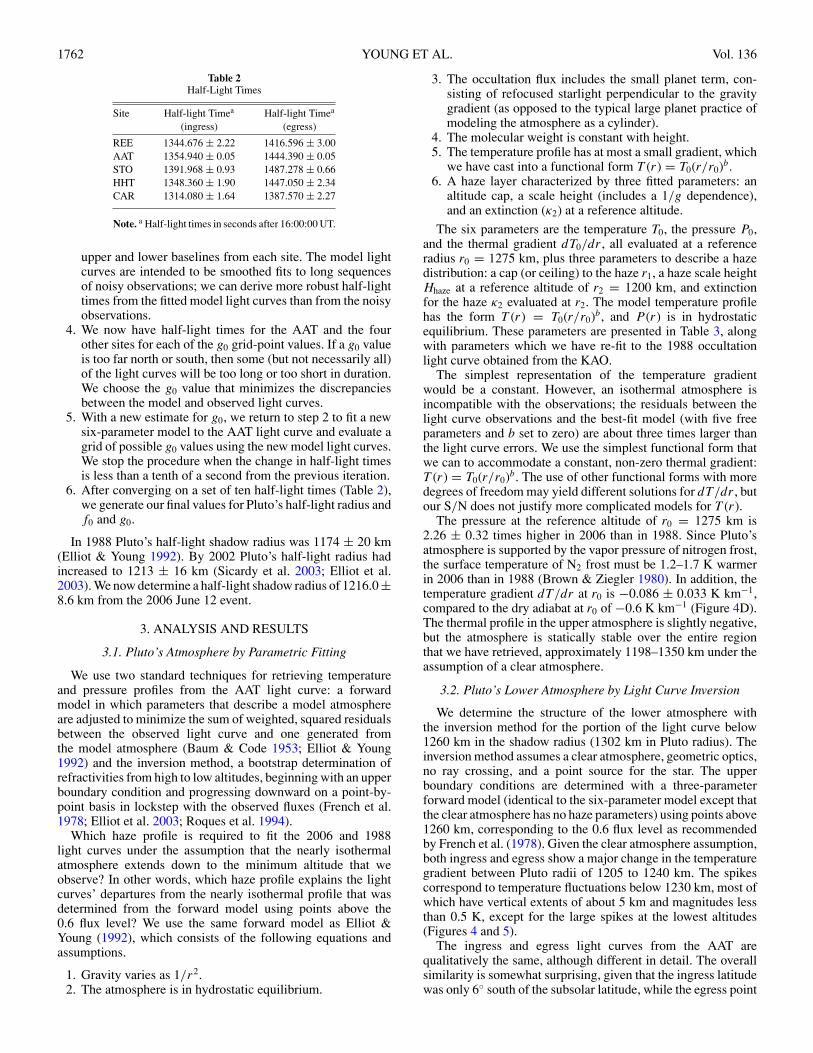
We determine the structure of the lower atmosphere withthe inversion method for the portion of the light curve below1260 km in the shadow radius (1302 km in Pluto radius). Theinversion method assumes a clear atmosphere, geometric optics,no ray crossing, and a point source for the star. The upperboundary conditions are determined with a three-parameterforward model (identical to the six-parameter model except thatthe clear atmosphere has no haze parameters) using points above1260 km, corresponding to the 0.6 flux level as recommendedby French et al. (1978). Given the clear atmosphere assumption,both ingress and egress show a major change in the temperaturegradient between Pluto radii of 1205 to 1240 km. The spikescorrespond to temperature fluctuations below 1230 km, most ofwhich have vertical extents of about 5 km and magnitudes lessthan 0.5 K, except for the large spikes at the lowest altitudes(Figures 4 and 5).

The ingress and egress light curves from the AAT arequalitatively the same, although different in detail. The overallsimilarity is somewhat surprising, given that the ingress latitudewas only 6◦ south of the subsolar latitude, while the egress point

No. 5, 2008 PLUTO’S ATMOSPHERE: 2006 JUNE 12 OCCULTATION RESULTS 1763

(A) (B)

(C)(D)

Figure 4. Ingress and egress light curves are shown in the top two panels. The blue points have been used to fit a three-parameter, nearly isothermal clear atmospheremodel. This model provides upper boundary conditions for the light curve inversion. We have tagged some spikes in red to show that spikes in the light curvescorrespond to small thermal perturbations (or, equivalently, perturbations in the index of refraction). The lower left panel shows yellow and green T (z) profiles (ingressand egress, respectively) with a large temperature inversion taking place around z = 1210 km, below which T decreases with descending altitude. The 1σ envelope isshown as faint yellow lines. The temperature gradients (lower right) show perturbations that are typical of gravity waves seen in occultations by Jupiter or Titan (e.g.,Young et al. 2005).

Table 3Best-fit Parameters for Pluto’s Upper Atmosphere

Parameter 2006 2006 2006 1988 UnitsIngress Egress Average KAO

T0a 100.0 ± 4.2 106.4 ± 4.6 103.9 ± 3.2 104.0 ± 7.3 (K)

P0a 1.76 ± 0.14 1.95 ± 0.15 1.86 ± 0.10 0.83 ± 0.11 (μbar)

dT0/dra −0.113 ± 0.045 −0.082 ± 0.051 −0.086 ± 0.033 −0.040 ± 0.052 (K km−1)r1 1286.8 ± 10.6 1287.1 ± 37. 1273.6 ± 7.1 1215.8 ± 1.3 (km)Hhaze

b 16.6 ± 1.7 15.9 ± 1.8 15.9 ± 1.1 24.6 ± 4.2 (km)κ2

b 2.7 ± 0.5 3.0 ± 0.5 3.0 ± 0.4 4.1 ± 0.3 (1000 × km−1)

Notes.a Value at a reference altitude of r0 = 1275 km.b Value at a reference altitude of r2 = 1260 km.

was less than 0◦.5 south of Pluto’s arctic circle. The surprisingsimilarities between the two light curves are discussed furtherin Section 4.4 in the context of the “methane thermostat.”

As an aside, there are two reasons why Pluto’s stellaroccultations do not (and are not likely to) determine Pluto’ssolid radius. First, the mapping between the shadow radius andthe inferred radius on Pluto is model dependent. In general,more haze in the atmospheric model will reduce the differencesin the shadow radius-to-Pluto radius mapping, because hazecan substitute for a steep refractive gradient as the cause ofattenuation in the lower light curve, and refraction, not haze,causes the shadow radius to be smaller than Pluto’s radius.Second, although we measure events in the shadow radius toaltitudes that are certain to be at or below Pluto’s solid surface,

we cannot use those data to determine Pluto’s physical radius.The light from the occulted star is attenuated to nearly zero bydifferential refraction and haze long before Pluto’s solid surfaceis a factor in the observed light curve. With extraordinarilyhigh S/N, one could discern the differences between the lowerbaseline and zero flux from the star, but even with the AAT lightcurve’s excellent S/N of 333 per 60 km, we can probe to only1198 km (assuming a clear atmosphere). Part of the problemis our great distance from Pluto; differential refraction is apowerful attenuation mechanism when the spread of light takesplace over 30 AU. An alternative would be to observe attenuationfrom much closer distances; the 1984–1990 mutual events(which effectively sampled Pluto’s surface and atmosphere fromCharon’s distance of ∼20,000 km) are a likely data set from

1764 YOUNG ET AL. Vol. 136

which Pluto’s solid radius can be determined before the NewHorizons flyby in 2015.

In other words, the limiting depth of an atmospheric retrievaldepends on small flux differences in the lower baseline. In 1988,flux from the occultation star was detectable down to a shadowradius of 900 km (Elliot et al. 2003; Elliot & Young 1992),limited by the S/N and the determination of the lower baselinefrom pre- and post-event photometry of Pluto relative to thestar. In 2006 we detected the star at shadow radii of 700 km and778 km for immersion and emersion, respectively. For the clear-atmosphere case, the 1988 light curve probes down to 1204 kmon Pluto, and the 2006 light curve probes down to 1198 km(immersion) and 1200 km (emersion).

The temperature gradient below 1205 km is large and positive,with dT /dr approximately equal to 2.5 K km−1 at the lowerlimit of the light curve (near 1200 km in Pluto radius). Ifthis gradient continues, Pluto’s atmosphere reaches 38–42 K,the spectroscopically measured temperature of Pluto’s nitrogenfrost in 1992 (Tryka et al. 1994; Grundy 1995), at a radius near1180 km and a pressure near 13 μbar. Since this pressure is lessthan the vapor pressure at Pluto’s frost temperatures (19 μbarat 38 K to 158 μbar at 42 K), Pluto may have a troposphere(a region in which the temperature gradient is close to theadiabat) of up to a few tens of km.

The source of the discontinuity in the 1988 light curve hasbeen a contested question since its discovery—is it caused bya haze layer, a temperature inversion, or both? We addressthis question by examining the implications of the hypotheticalhaze distribution described in Table 2. The hypothetical 2006haze distribution was determined in exactly the same way asthe haze distribution presented in Elliot & Young (1992) forthe 1988 light curve. We mathematically “remove” the hazeby scaling the 2006 light curve at each timestep by eτ (s),where τ (s) is the haze optical depth along the observer’sinstantaneous line of sight, s, to the star, and then apply theclear-atmosphere inversion method to the scaled light curve.Incidentally, this hypothetical haze distribution would not affectviews of the surface by a spacecraft flyby. The haze optical depthwould be a miniscule 0.0023 in the zenith direction (integratedfrom an assumed surface of 1160 km to the fitted haze capat 1273.6 km).

We discuss the results of the haze layer experiment in moredetail in Section 4.5. Briefly, the resulting temperature profile(after the haze is “removed”) has no thermal inversion—thetemperature stays near 100 K down to the lowest probedradius, which is now 1160 km instead of 1198 km. We thinka haze distribution that is extrapolated to the surface from theupper light curve parametric fit is untenable because extremelylarge temperature gradients would be required to connect theatmospheric temperature of 100 K at 1160 km to the nearbysurface temperature of 38–42 K. There may be smaller amountsof haze present, but there must also be a temperature inversion.Future occultations need to be observed in both visible andinfrared wavelengths to provide stronger constraints on hazeproperties.

3.3. A Qualitative Comparison: The 2006 June 12, CFHT(2002), and KAO (1988) Light Curves

In this section we compare our results to other observationsof the 2006 June 12 occultation (Elliot et al. 2007). We also lookat the time-evolution of Pluto’s atmosphere with comparisonsto the 2002 and 1988 occultations.

3.3.1. Comparison to other 12 June 2006 Observations

Elliot et al. (2007) observed the 2006 June 12 occultationfrom several sites in Australia and New Zealand. Their resultsare based on light curves obtained from Siding Spring, BlackSprings, Stockport, Mt. Stromlo, and Hobart. Their highestS/N (96 per 60 km) is from the 5 Hz observations from the2.3 m telescope at Siding Spring. Both our paper and Elliotet al. (2007) use the Stockport observations provided by B. Lade,but both groups performed separate photometric reductions ofthose data.

With respect to Pluto’s upper atmosphere, there are somedifferences between our results and those of Elliot et al. (2007).Their preferred half-light radius (their fit 2) is 1208 ± 4 kmin the shadow radius (1276.1 ± 3.5 in Pluto radius), comparedto our half-light shadow radius of 1216 ± 8.6 km. Our ingressand egress average temperature at 1275 km is 103.9 ± 3.2 K,compared to 97 ± 5 K for Elliot et al. (2007) at their half-lightradius of 1276.1 km. Their temperature gradient at 1276.1 kmis −0.17 ± 0.05 K km−1, compared to our value of −0.086 ±0.033 K km−1 at 1275 km; both are negative and significantlynon-isothermal.

There is a qualitative difference between the 1988 to 2006trend in our derived upper atmosphere temperatures (T0) andthe trend reported by (Elliot et al. 2007). We find that T0 hasbeen close to 104 K in every occultation observed from 1988through 2006 (with typical errors of ±3.0 K), but Elliot et al.(2007) report a significant cooling trend. They derive T0 valuesat a reference radius of 1276 km of 114 ± 10 K, 108 ± 9 K, and97 ± 5 K in 1988, 2002, and 2006, respectively.

We are at a loss to explain these differences, since bothgroups use nearly identical equations and free parameters in theforward model used to fit the upper atmosphere. It is unlikely thatour separate geometric solutions could explain the discrepancy,since the sensitivity of T0 to ρmin is

dTiso

dρmin= −Tiso

ρmin

ρ2h

(1)

where ρh is the half-light shadow radius, ρmin is the shadowimpact parameter, and Tiso is the temperature determined foran isothermal model of the upper atmosphere. This expressionassumes that the error in ρh is much smaller than the error inρmin.

For values of Tiso around 100 K, ρmin around 571 km (i.e.,Siding Spring) and ρh around 1173 km, the sensitivity ofTiso to errors in ρmin is −0.043 K per km. In other words, a10 km error in the shadow’s central chord location translates toan upper atmosphere error of just −0.43 K. It is unlikely thatour respective geometric solutions differ by more than 10 km,yet our nominal solutions for T0 differ by about 10 K for the1988 event and about 7 K for the 2006 event. Note that bothwe and Elliot et al. (2007) have independently re-analyzed the1988 light curves for these post-2006 occultation papers.

Nor are the discrepancies in T0 solutions likely to lie indifferent photometric calibrations. We derive a ratio of Plutoto Pluto-plus-P384.2 of 0.682 in our AAT observations (at SidingSpring), compared to 0.6727 for the 2.3 m Siding Springlight curve obtained by Elliot et al. (2007). This differencecannot explain the 7 K difference in our respective 2006T0 values. Finally, we note that our assumed value for therefractivity of N2 is higher than that used by Elliot et al.(2007). Using the catalog magnitudes of the star, including theUSNO B1.0 and GSC2.3.2, the quantum efficiency of our

No. 5, 2008 PLUTO’S ATMOSPHERE: 2006 JUNE 12 OCCULTATION RESULTS 1765

cameras, and the known refractivity of N2 (Cox 2000), we usea refractivity at STP of 2.96e-4, similar to the refractivity of2.98e-4 used for the analysis of the 1988 Pluto occultation (Elliotet al. 2003; Elliot & Young 1992). This differs from Elliot et al.(2007), who use a value of 2.82e-4. These differences remain tobe reconciled.

3.3.2. Comparison to 2002 and 1988 Occultations

There are three characteristics of the 2006 light curve worthnoting in comparison to earlier light curves.

1. Like the 2002 light curves, the 2006 light curves imply asurface pressure that is over twice as high as measured in1988.

2. Like the 2002 light curves, the 2006 light curves exhibitspikes that are typical of vertical temperature variations.These spikes are not seen in the 1988 observations belowthe “kink” in the light curve, although the KAO light curvedid resolved three spikes in the upper atmosphere, abovethe kink (Elliot & et al. 1989).

3. The 2006 and 2002 light curves do not show a pronounced“kink” at 1215 km, although their lower altitudes dodeviate from the near-isothermal model that fits the upperatmosphere well in all occultations observed to date.

If the spikes are a manifestation of gravity waves in Pluto’slower atmosphere, then it is curious that the spikes were not seenin 1988; the S/N of the 1988 light curve is sufficient to haveshown the AAT-sized spikes if they were present. In other words,among the other changes that occurred since 1988 (doubling ofthe bulk atmosphere and change in the shape of the tropospherethat produces the “kink”), apparently something occurred thatmay be producing gravity waves.

4. DISCUSSION

4.1. The Evolution of Pluto’s Half-Light Radius

The primary result from this and all previous stellar occul-tations by Pluto is the half-light radius of Pluto, a measureof Pluto’s column abundance and surface frost temperature.Because the vapor pressure of nitrogen frost is an extremelysensitive function of the frost temperature, changes in surfacepressure inferred from occultations will translate to very tightconstraints on the changing temperature of Pluto’s nitrogenfrost. Here we discuss the trend in Pluto’s surface tempera-ture in 1988, 2002, and 2006 in the context of Pluto’s changingsubsolar latitude and heliocentric distance.

Just as the martian atmosphere is supported by the vaporpressure of a surface constituent (carbon dioxide frost), Pluto’satmosphere is supported by the vapor pressure of nitrogen frost.Other volatiles that have been detected in the solid phase onPluto’s surface include CO and CH4. N2 frost is by far themost volatile of these ices, and its latent heat of sublimation/condensation is thought to govern Pluto’s nitrogen-coveredsurfaces to a globally constant temperature of ∼40 K, regardlessof the local diurnally-averaged solar flux (Spencer et al. 1997).The fact that Pluto’s column abundance (or equivalently, itssurface pressure) doubled between 1988 and 2002 implies thatthe global N2 frost temperature increased by about 1.5 K overthat period. This temperature increase occurred as the solar fluxat Pluto decreased by 6% from 1988 to 2002 and by 9% from1988 to 2006.

Hansen & Paige (1996) implemented a model to predictPluto’s surface temperature and pressure throughout a Pluto

– Nominal Case–– 111---sssiiigggmmmaaa eeennnvvveeelllooopppeee

11222666000

11222444000

11222222000

11222000000

1111188800077000 888000 999000 111000000 111111000 111222000

TTeeemmmpppeeerrraaatttuuurrreee (((KKK)))

RRaaa

dddiiiuu

sss((kk

m mm)))

Figure 5. Error bars for the AAT ingress T (z) profile, generated from 1000Monte Carlo simulations. Appropriate noise was generated and added to thelight curve in 1000 separate inversions, including noise propagated from thethree-parameter upper boundary fits.

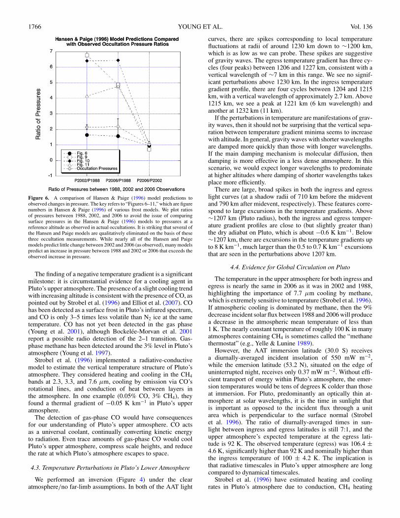
season. Free parameters included global values for the frostalbedo, the substrate albedo, the column of available N2 frost,the emissivity of N2 frost and the thermal inertia of the surface.They considered solar heat input, thermal emission, conductionwith subsurface layers, and the latent heats of the nitrogen α/βcrystalline transition and the sublimation and condensation gas/frost transitions. They point out that small changes in certainparameters result in huge variations in the near-term surfacepressure and temperature variations. There are, however, somecommon themes in all of the Hansen & Paige (1996) modelpredictions. The most striking of these is that Pluto’s seasonalpressure peak will lag its perihelion (in 1989) by tens of years. Asecond result is that the pressure peak is usually (but not always)predicted to be tens of years in duration.

Figure 6 compares the change in pressure between the occul-tation observations in 1988, 2002, and 2006 to the predictionsof four model runs from Hansen & Paige (1996). The best-fitprediction is Hansen & Paige (1996) run #38, with increases onpressure from 1988 to 2002 and 2006 that are just below the ob-served increases of around 2.1. This is a low thermal inertia, highfrost emissivity scenario. It is interesting to note that run #34 isalmost identical to run #38 except that the emissivity is lower(0.6 instead of 0.8) and the column of N2 is half (50 kg m−2

instead of 100). The low emissivity translates to a much largerincrease in Pluto’s post-perihelion frost temperature (becausethe main cooling mechanism, thermal radiation, is inhibited)and much higher pressure increases than we observe from theoccultations. It appears that the Hansen & Paige (1996) modelscould easily match the three occultation pressures observed todate by simply tweaking the frost emissivity to values slightlyless than 0.8. Furthermore, both runs #34 and #38 predict onlyslightly diminishing pressures through 2015, the date of the NewHorizons flyby.

4.2. The Non-Isotropic Temperature Profile of Pluto’s UpperAtmosphere

From the AAT light curve we fit a temperature slope in Pluto’supper atmosphere (above a radius of 1275 km) of −0.086 ±0.033 K km−1, compared to −0.17 ± 0.05 found by Elliotet al. (2007). These are the first inferences of a statistically non-isothermal temperature gradient in Pluto’s upper atmosphere atthe 3σ level. This cooling-with-altitude trend may have beenpresent in earlier occultations, but the S/N of earlier lightcurves was not high enough to infer a significant non-isothermalgradient.

1766 YOUNG ET AL. Vol. 136

Figure 6. A comparison of Hansen & Paige (1996) model predictions toobserved changes in pressure. The key refers to “Figures 6–11,” which are figurenumbers in Hansen & Paige (1996) of various frost models. We plot ratiosof pressures between 1988, 2002, and 2006 to avoid the issue of comparingsurface pressures in the Hansen & Paige (1996) models to pressures at areference altitude as observed in actual occultations. It is striking that several ofthe Hansen and Paige models are qualitatively eliminated on the basis of thesethree occultation measurements. While nearly all of the Hansen and Paigemodels predict little change between 2002 and 2006 (as observed), many modelspredict an increase in pressure between 1988 and 2002 or 2006 that exceeds theobserved increase in pressure.

The finding of a negative temperature gradient is a significantmilestone: it is circumstantial evidence for a cooling agent inPluto’s upper atmosphere. The presence of a slight cooling trendwith increasing altitude is consistent with the presence of CO, aspointed out by Strobel et al. (1996) and Elliot et al. (2007). COhas been detected as a surface frost in Pluto’s infrared spectrum,and CO is only 3–5 times less volatile than N2 ice at the sametemperature. CO has not yet been detected in the gas phase(Young et al. 2001), although Bockelee-Morvan et al. 2001report a possible radio detection of the 2–1 transition. Gas-phase methane has been detected around the 3% level in Pluto’satmosphere (Young et al. 1997).

Strobel et al. (1996) implemented a radiative-conductivemodel to estimate the vertical temperature structure of Pluto’satmosphere. They considered heating and cooling in the CH4bands at 2.3, 3.3, and 7.6 μm, cooling by emission via CO’srotational lines, and conduction of heat between layers inthe atmosphere. In one example (0.05% CO, 3% CH4), theyfound a thermal gradient of −0.05 K km−1 in Pluto’s upperatmosphere.

The detection of gas-phase CO would have consequencesfor our understanding of Pluto’s upper atmosphere. CO actsas a universal coolant, continually converting kinetic energyto radiation. Even trace amounts of gas-phase CO would coolPluto’s upper atmosphere, compress scale heights, and reducethe rate at which Pluto’s atmosphere escapes to space.

4.3. Temperature Perturbations in Pluto’s Lower Atmosphere

We performed an inversion (Figure 4) under the clearatmosphere/no far-limb assumptions. In both of the AAT light

curves, there are spikes corresponding to local temperaturefluctuations at radii of around 1230 km down to ∼1200 km,which is as low as we can probe. These spikes are suggestiveof gravity waves. The egress temperature gradient has three cy-cles (four peaks) between 1206 and 1227 km, consistent with avertical wavelength of ∼7 km in this range. We see no signif-icant perturbations above 1230 km. In the ingress temperaturegradient profile, there are four cycles between 1204 and 1215km, with a vertical wavelength of approximately 2.7 km. Above1215 km, we see a peak at 1221 km (6 km wavelength) andanother at 1232 km (11 km).

If the perturbations in temperature are manifestations of grav-ity waves, then it should not be surprising that the vertical sepa-ration between temperature gradient minima seems to increasewith altitude. In general, gravity waves with shorter wavelengthsare damped more quickly than those with longer wavelengths.If the main damping mechanism is molecular diffusion, thendamping is more effective in a less dense atmosphere. In thisscenario, we would expect longer wavelengths to predominateat higher altitudes where damping of shorter wavelengths takesplace more efficiently.

There are large, broad spikes in both the ingress and egresslight curves (at a shadow radii of 710 km before the mideventand 790 km after midevent, respectively). These features corre-spond to large excursions in the temperature gradients. Above∼1207 km (Pluto radius), both the ingress and egress temper-ature gradient profiles are close to (but slightly greater than)the dry adiabat on Pluto, which is about −0.6 K km−1. Below∼1207 km, there are excursions in the temperature gradients upto 8 K km−1, much larger than the 0.5 to 0.7 K km−1 excursionsthat are seen in the perturbations above 1207 km.

4.4. Evidence for Global Circulation on Pluto

The temperature in the upper atmosphere for both ingress andegress is nearly the same in 2006 as it was in 2002 and 1988,highlighting the importance of 7.7 μm cooling by methane,which is extremely sensitive to temperature (Strobel et al. 1996).If atmospheric cooling is dominated by methane, then the 9%decrease incident solar flux between 1988 and 2006 will producea decrease in the atmospheric mean temperature of less than1 K. The nearly constant temperature of roughly 100 K in manyatmospheres containing CH4 is sometimes called the “methanethermostat” (e.g., Yelle & Lunine 1989).

However, the AAT immersion latitude (30.0 S) receivesa diurnally-averaged incident insolation of 550 mW m−2,while the emersion latitude (53.2 N), situated on the edge ofuninterrupted night, receives only 0.37 mW m−2. Without effi-cient transport of energy within Pluto’s atmosphere, the emer-sion temperatures would be tens of degrees K colder than thoseat immersion. For Pluto, predominantly an optically thin at-mosphere at solar wavelengths, it is the time in sunlight thatis important as opposed to the incident flux through a unitarea which is perpendicular to the surface normal (Strobelet al. 1996). The ratio of diurnally-averaged times in sun-light between ingress and egress latitudes is still 7:1, and theupper atmosphere’s expected temperature at the egress lati-tude is 92 K. The observed temperature (egress) was 106.4 ±4.6 K, significantly higher than 92 K and nominally higher thanthe ingress temperature of 100 ± 4.2 K. The implication isthat radiative timescales in Pluto’s upper atmosphere are longcompared to dynamical timescales.

Strobel et al. (1996) have estimated heating and coolingrates in Pluto’s atmosphere due to conduction, CH4 heating

No. 5, 2008 PLUTO’S ATMOSPHERE: 2006 JUNE 12 OCCULTATION RESULTS 1767

Figure 7. A “what-if” experiment to look at the temperature profile given an assumed haze profile. The left-side panels show (from top to bottom) the observed lightcurves, the temperature profiles as determined by the inversion method, and the temperature gradient profiles. The right column is identical to the left except that thehaze parameters listed in Table 3 have been extrapolated to the lowest chords probed by the occultation. In the top row, the clear atmosphere light curve that remainsafter the assumed haze opacity is divided out (right panel) shows that the lower light curve would be brighter if the assumed haze opacity were not present. In themiddle panels we see that the presence of haze (right) could explain the shape of the lower light curve just as well as a temperature inversion in the no-haze scenario(left), but the assumed-haze T (z) profile reaches a radius of ∼1150 km with temperatures over 100 K, a likely conflict with current estimates of Pluto’s solid radius.Finally, the main effect of an assumed haze distribution on the temperature gradients is to reduce the large dT /dz excursion associated with the temperature inversion.The nearly-vertical lines in the two lower panels are Pluto’s expected dry adiabat.

at 2.3 and 3.3 μm, CH4 cooling at 7.7 μm, and CO cooling at2.3 μm.

The 7.7 μm cooling term has the shortest timescale and isthe primary avenue for cooling Pluto’s upper atmosphere. Wecalculate a time constant of τ7.7 = 0.5 yr, assuming 3% CH4.This long time constant is dramatically different between Plutoand Mars. On Mars, the cooling time constant is on the orderof hours, as evidenced by the dramatic amplitude of the martiandiurnal temperature variation. On Pluto, with CH4 as its primarycooling constituent, the cooling time constant is apparentlymuch longer than the unknown dynamical timescales. We donot know the wind speeds between Pluto’s poles and equator,but if they are in the neighborhood of 10 m s−1, they willproduce dynamical timescales that are on the order of days,about two orders of magnitude faster than the radiative coolingtimescale. In light of these relative rates, it is not surprisingthat the “methane thermostat” seems to be in effect over the

considerable range in latitudes that have been sampled by allprevious occultations, even though some latitudes received verylittle insolation (Table 4).

4.5. Temperature Inversion Versus Haze Opacity

The 1988 occultation light curve showed a pronouncedchange in slope in both ingress and egress at the 1215 km level,prompting a vigorous discussion in the community as to thecause of that change. Could there be a haze layer below 1215 km(in 1988), or is there a thermal inversion in a clear atmospherethat attenuates the starlight by differential refraction? In thissection we explore the temperature profile that would result ifthe exponential distribution of Pluto’s haze were extrapolated tothe surface from the six-parameter fit to the upper atmosphere(Table 3).

Unlike our forward model, our inversion method assumes aclear atmosphere. We are not aware of an inversion code that

1768 YOUNG ET AL. Vol. 136

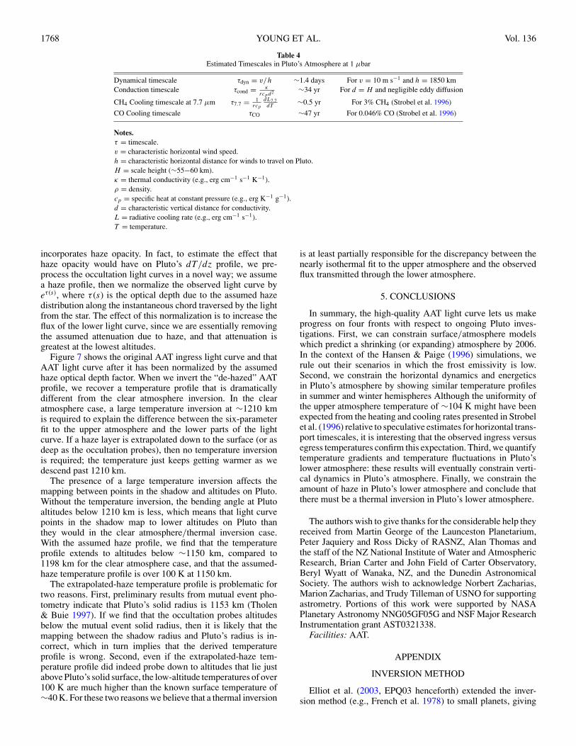
Table 4Estimated Timescales in Pluto’s Atmosphere at 1 μbar

Dynamical timescale τdyn = v/h ∼1.4 days For v = 10 m s−1 and h = 1850 kmConduction timescale τcond = κ

rcpd2 ∼34 yr For d = H and negligible eddy diffusion

CH4 Cooling timescale at 7.7 μm τ7.7 = 1rcp

dL7.7dT

∼0.5 yr For 3% CH4 (Strobel et al. 1996)

CO Cooling timescale τCO ∼47 yr For 0.046% CO (Strobel et al. 1996)

Notes.

τ = timescale.v = characteristic horizontal wind speed.h = characteristic horizontal distance for winds to travel on Pluto.H = scale height (∼55−60 km).κ = thermal conductivity (e.g., erg cm−1 s−1 K−1).ρ = density.cp = specific heat at constant pressure (e.g., erg K−1 g−1).d = characteristic vertical distance for conductivity.L = radiative cooling rate (e.g., erg cm−1 s−1).T = temperature.

incorporates haze opacity. In fact, to estimate the effect thathaze opacity would have on Pluto’s dT /dz profile, we pre-process the occultation light curves in a novel way; we assumea haze profile, then we normalize the observed light curve byeτ (s), where τ (s) is the optical depth due to the assumed hazedistribution along the instantaneous chord traversed by the lightfrom the star. The effect of this normalization is to increase theflux of the lower light curve, since we are essentially removingthe assumed attenuation due to haze, and that attenuation isgreatest at the lowest altitudes.

Figure 7 shows the original AAT ingress light curve and thatAAT light curve after it has been normalized by the assumedhaze optical depth factor. When we invert the “de-hazed” AATprofile, we recover a temperature profile that is dramaticallydifferent from the clear atmosphere inversion. In the clearatmosphere case, a large temperature inversion at ∼1210 kmis required to explain the difference between the six-parameterfit to the upper atmosphere and the lower parts of the lightcurve. If a haze layer is extrapolated down to the surface (or asdeep as the occultation probes), then no temperature inversionis required; the temperature just keeps getting warmer as wedescend past 1210 km.

The presence of a large temperature inversion affects themapping between points in the shadow and altitudes on Pluto.Without the temperature inversion, the bending angle at Plutoaltitudes below 1210 km is less, which means that light curvepoints in the shadow map to lower altitudes on Pluto thanthey would in the clear atmosphere/thermal inversion case.With the assumed haze profile, we find that the temperatureprofile extends to altitudes below ∼1150 km, compared to1198 km for the clear atmosphere case, and that the assumed-haze temperature profile is over 100 K at 1150 km.

The extrapolated-haze temperature profile is problematic fortwo reasons. First, preliminary results from mutual event pho-tometry indicate that Pluto’s solid radius is 1153 km (Tholen& Buie 1997). If we find that the occultation probes altitudesbelow the mutual event solid radius, then it is likely that themapping between the shadow radius and Pluto’s radius is in-correct, which in turn implies that the derived temperatureprofile is wrong. Second, even if the extrapolated-haze tem-perature profile did indeed probe down to altitudes that lie justabove Pluto’s solid surface, the low-altitude temperatures of over100 K are much higher than the known surface temperature of∼40 K. For these two reasons we believe that a thermal inversion

is at least partially responsible for the discrepancy between thenearly isothermal fit to the upper atmosphere and the observedflux transmitted through the lower atmosphere.

5. CONCLUSIONS

In summary, the high-quality AAT light curve lets us makeprogress on four fronts with respect to ongoing Pluto inves-tigations. First, we can constrain surface/atmosphere modelswhich predict a shrinking (or expanding) atmosphere by 2006.In the context of the Hansen & Paige (1996) simulations, werule out their scenarios in which the frost emissivity is low.Second, we constrain the horizontal dynamics and energeticsin Pluto’s atmosphere by showing similar temperature profilesin summer and winter hemispheres Although the uniformity ofthe upper atmosphere temperature of ∼104 K might have beenexpected from the heating and cooling rates presented in Strobelet al. (1996) relative to speculative estimates for horizontal trans-port timescales, it is interesting that the observed ingress versusegress temperatures confirm this expectation. Third, we quantifytemperature gradients and temperature fluctuations in Pluto’slower atmosphere: these results will eventually constrain verti-cal dynamics in Pluto’s atmosphere. Finally, we constrain theamount of haze in Pluto’s lower atmosphere and conclude thatthere must be a thermal inversion in Pluto’s lower atmosphere.

The authors wish to give thanks for the considerable help theyreceived from Martin George of the Launceston Planetarium,Peter Jaquiery and Ross Dicky of RASNZ, Alan Thomas andthe staff of the NZ National Institute of Water and AtmosphericResearch, Brian Carter and John Field of Carter Observatory,Beryl Wyatt of Wanaka, NZ, and the Dunedin AstronomicalSociety. The authors wish to acknowledge Norbert Zacharias,Marion Zacharias, and Trudy Tilleman of USNO for supportingastrometry. Portions of this work were supported by NASAPlanetary Astronomy NNG05GF05G and NSF Major ResearchInstrumentation grant AST0321338.

Facilities: AAT.

APPENDIX

INVERSION METHOD

Elliot et al. (2003, EPQ03 henceforth) extended the inver-sion method (e.g., French et al. 1978) to small planets, giving

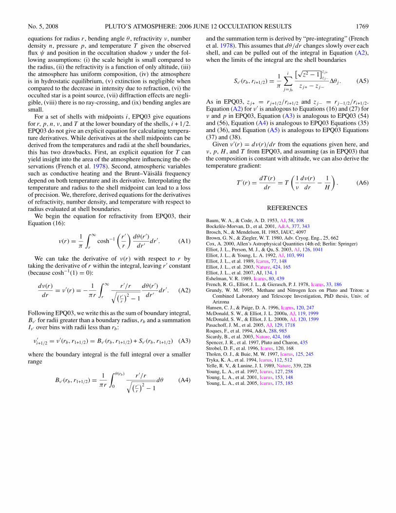
No. 5, 2008 PLUTO’S ATMOSPHERE: 2006 JUNE 12 OCCULTATION RESULTS 1769

equations for radius r , bending angle θ , refractivity ν, numberdensity n, pressure p, and temperature T given the observedflux ψ and position in the occultation shadow y under the fol-lowing assumptions: (i) the scale height is small compared tothe radius, (ii) the refractivity is a function of only altitude, (iii)the atmosphere has uniform composition, (iv) the atmosphereis in hydrostatic equilibrium, (v) extinction is negligible whencompared to the decrease in intensity due to refraction, (vi) theocculted star is a point source, (vii) diffraction effects are negli-gible, (viii) there is no ray-crossing, and (ix) bending angles aresmall.

For a set of shells with midpoints i, EPQ03 give equationsfor r, p, n, ν, and T at the lower boundary of the shells, i + 1/2.EPQ03 do not give an explicit equation for calculating tempera-ture derivatives. While derivatives at the shell midpoints can bederived from the temperatures and radii at the shell boundaries,this has two drawbacks. First, an explicit equation for T canyield insight into the area of the atmosphere influencing the ob-servations (French et al. 1978). Second, atmospheric variablessuch as conductive heating and the Brunt–Vaisala frequencydepend on both temperature and its derivative. Interpolating thetemperature and radius to the shell midpoint can lead to a lossof precision. We, therefore, derived equations for the derivativesof refractivity, number density, and temperature with respect toradius evaluated at shell boundaries.

We begin the equation for refractivity from EPQ03, theirEquation (16):

ν(r) = 1

π

∫ ∞

r

cosh−1

(r ′

r

)dθ (r ′)dr ′ dr ′. (A1)

We can take the derivative of ν(r) with respect to r bytaking the derivative of r within the integral, leaving r ′ constant(because cosh−1(1) = 0):

dν(r)

dr= ν ′(r) = − 1

πr

∫ ∞

r

r ′/r√(r ′r

)2 − 1

dθ (r ′)dr ′ dr ′. (A2)

Following EPQ03, we write this as the sum of boundary integral,Bν ′ for radii greater than a boundary radius, rb and a summationIν ′ over bins with radii less than rb:

ν ′i+1/2 = ν ′(rb, r1+1/2) = Bν ′ (rb, r1+1/2) + Sν ′ (rb, r1+1/2) (A3)

where the boundary integral is the full integral over a smallerrange

Bν ′(rb, r1+1/2) = 1

πr

∫ θ(rb)

0

r ′/r√(r ′r

)2 − 1dθ (A4)

and the summation term is derived by “pre-integrating” (Frenchet al. 1978). This assumes that dθ/dr changes slowly over eachshell, and can be pulled out of the integral in Equation (A2),when the limits of the integral are the shell boundaries

Sν ′ (rb, ri+1/2) = 1

π

i∑j=jb

[√z2 − 1

]zj+

zj−

zj+ − zj−Δθj . (A5)

As in EPQ03, zj+ = rj+1/2/ri+1/2 and zj− = rj−1/2/ri+1/2.Equation (A2) for ν ′ is analogous to Equations (16) and (27) forν and p in EPQ03, Equation (A3) is analogous to EPQ03 (54)and (56), Equation (A4) is analogous to EPQ03 Equations (35)and (36), and Equation (A5) is analogous to EPQ03 Equations(37) and (38).

Given ν ′(r) = dν(r)/dr from the equations given here, andν, p, H , and T from EPQ03, and assuming (as in EPQ03) thatthe composition is constant with altitude, we can also derive thetemperature gradient:

T ′(r) = dT (r)

dr= T

(1

ν

dν(r)

dr− 1

H

). (A6)

REFERENCES

Baum, W. A., & Code, A. D. 1953, AJ, 58, 108Bockelee-Morvan, D., et al. 2001, A&A, 377, 343Brosch, N., & Mendelson, H. 1985, IAUC, 4097Brown, G. N., & Ziegler, W. T. 1980, Adv. Cryog. Eng., 25, 662Cox, A. 2000, Allen’s Astrophysical Quantities (4th ed; Berlin: Springer)Elliot, J. L., Person, M. J., & Qu, S. 2003, AJ, 126, 1041Elliot, J. L., & Young, L. A. 1992, AJ, 103, 991Elliot, J. L., et al. 1989, Icarus, 77, 148Elliot, J. L., et al. 2003, Nature, 424, 165Elliot, J. L., et al. 2007, AJ, 134, 1Eshelman, V. R. 1989, Icarus, 80, 439French, R. G., Elliot, J. L., & Gierasch, P. J. 1978, Icarus, 33, 186Grundy, W. M. 1995, Methane and Nitrogen Ices on Pluto and Triton: a

Combined Laboratory and Telescope Investigation, PhD thesis, Univ. ofArizona

Hansen, C. J., & Paige, D. A. 1996, Icarus, 120, 247McDonald, S. W., & Elliot, J. L. 2000a, AJ, 119, 1999McDonald, S. W., & Elliot, J. L. 2000b, AJ, 120, 1599Pasachoff, J. M., et al. 2005, AJ, 129, 1718Roques, F., et al. 1994, A&A, 288, 985Sicardy, B., et al. 2003, Nature, 424, 168Spencer, J. R., et al. 1997, Pluto and Charon, 435Strobel, D. F., et al. 1996, Icarus, 120, 168Tholen, O. J., & Buie, M. W. 1997, Icarus, 125, 245Tryka, K. A., et al. 1994, Icarus, 112, 512Yelle, R. V., & Lunine, J. I. 1989, Nature, 339, 228Young, L. A., et al. 1997, Icarus, 127, 258Young, L. A., et al. 2001, Icarus, 153, 148Young, L. A., et al. 2005, Icarus, 175, 185