The stellar populations of bright coma cluster galaxies
28
Mon. Not. R. Astron. Soc. 411, 2558–2585 (2011) doi:10.1111/j.1365-2966.2010.17862.x The stellar populations of bright coma cluster galaxies J. Price, 1 S. Phillipps, 1 A. Huxor, 1 R. J. Smith 2 and J. R. Lucey 2 1 Astrophysics Group, H. H. Wills Physics Laboratory, University of Bristol, Tyndall Avenue, Bristol BS8 1TL 2 Department of Physics, University of Durham, Durham DH1 3LE Accepted 2010 October 13. Received 2010 September 21; in original form 2010 June 28 ABSTRACT In this paper we study the stellar populations of 356 bright, M r ≤−19, Coma cluster members located in a 2 ◦ field centred on the cluster core using Sloan Digital Sky Survey (SDSS) Data Release 7 (DR7) spectroscopy. We find ∼31 per cent of the sample have significant emission in Hβ , [O III]5007, Hα or [N II]6585, due to star formation or active galactic nuclei (AGN)/LINER activity. The remaining portion of the sample we describe as passive or quiescent. Using line- ratio diagnostics, we find the fraction of galaxies displaying AGN/LINER type emission increases with increasing galaxy luminosity while the star-forming fraction decreases. For the quiescent galaxies we find strong correlations between absorption-line index strength and velocity dispersion (σ ) for CN2, C4668, Mgb and Hβ . Employing a planar analysis technique that factors out index correlations with σ , we find significant cluster-centric radial gradients in Hβ , Mgb and C4668 for the passive galaxies. We use state-of-the-art stellar population models and the measured absorption-line indices to infer the single-stellar-population-equivalent (SSP- equivalent) age and [Fe/H] for each galaxy, as well as their abundance patterns in terms of [Mg/Fe], [C/Fe], [N/Fe] and [Ca/Fe]. For the passive galaxy subsample we find strong evidence for ‘archaeological downsizing’, with age ∝ σ 0.90±0.06 . This trend is shown to be robust against variations in sample selection criteria (morphologically early-type versus spectroscopically quiescent), emission-line detection thresholds, index velocity broadening corrections and the specific SSP model employed. Weaker positive correlations are obtained between σ and all other measured stellar population parameters. We recover significant cluster-centric radial stellar population gradients for the passive sample in SSP-equivalent age, [Mg/Fe], [C/Fe] and [N/Fe]. These trends are in the sense that, at fixed velocity dispersion, passive galaxies on the outskirts of the cluster are 24 ± 9 per cent younger with lower [Mg/Fe] and [N/Fe] but higher [C/Fe] than those in the cluster core. We find no significant increase in cluster-centric radial stellar population gradients when fitting to a passive galaxy subset selected to cover the cluster core and south-west region, which contains the NGC 4839 subgroup. Thus, we conclude that the NGC 4839 infall region is not unique, at least in terms of the stellar populations of bright galaxies. We speculate that the more pronounced cluster-centric radial gradients seen by other recent studies may be attributed to the luminosity range spanned by their samples, rather than to limited azimuthal coverage of the cluster. Finally, for our passive sample we have found an age–metallicity anti-correlation which cannot be accounted for by correlated errors. Key words: surveys – galaxies: clusters: individual: Coma – galaxies: evolution – galaxies: stellar content. 1 INTRODUCTION Rich galaxy clusters have long been the target of studies attempting to address the fundamental questions of galaxy formation and evo- lution. They are ideal laboratories for this task as they harbour large E-mail: [email protected] numbers of galaxies distributed across a wide range in local density and at a common distance. The most direct route to answer these questions is to observe clusters at a range of redshifts and trace out the assembly history of their galaxy populations. Unfortunately, this method is observationally inefficient, requiring significant amounts of telescope time, and of course often relies on data of lower signal- to-noise ratio (S/N). An alternative approach is to conduct a detailed analysis of the stellar populations of large samples of galaxies in C 2010 The Authors Monthly Notices of the Royal Astronomical Society C 2010 RAS Downloaded from https://academic.oup.com/mnras/article/411/4/2558/982791 by guest on 04 July 2022
-
Upload
khangminh22 -
Category
Documents
-
view
0 -
download
0
Transcript of The stellar populations of bright coma cluster galaxies
Mon. Not. R. Astron. Soc. 411, 2558–2585 (2011) doi:10.1111/j.1365-2966.2010.17862.x
The stellar populations of bright coma cluster galaxies
J. Price,1� S. Phillipps,1 A. Huxor,1 R. J. Smith2 and J. R. Lucey2
1Astrophysics Group, H. H. Wills Physics Laboratory, University of Bristol, Tyndall Avenue, Bristol BS8 1TL2Department of Physics, University of Durham, Durham DH1 3LE
Accepted 2010 October 13. Received 2010 September 21; in original form 2010 June 28
ABSTRACTIn this paper we study the stellar populations of 356 bright, Mr ≤ −19, Coma cluster memberslocated in a 2◦ field centred on the cluster core using Sloan Digital Sky Survey (SDSS) DataRelease 7 (DR7) spectroscopy. We find ∼31 per cent of the sample have significant emission inHβ, [O III]5007, Hα or [N II]6585, due to star formation or active galactic nuclei (AGN)/LINERactivity. The remaining portion of the sample we describe as passive or quiescent. Using line-ratio diagnostics, we find the fraction of galaxies displaying AGN/LINER type emissionincreases with increasing galaxy luminosity while the star-forming fraction decreases. Forthe quiescent galaxies we find strong correlations between absorption-line index strength andvelocity dispersion (σ ) for CN2, C4668, Mgb and Hβ. Employing a planar analysis techniquethat factors out index correlations with σ , we find significant cluster-centric radial gradients inHβ, Mgb and C4668 for the passive galaxies. We use state-of-the-art stellar population modelsand the measured absorption-line indices to infer the single-stellar-population-equivalent (SSP-equivalent) age and [Fe/H] for each galaxy, as well as their abundance patterns in terms of[Mg/Fe], [C/Fe], [N/Fe] and [Ca/Fe]. For the passive galaxy subsample we find strong evidencefor ‘archaeological downsizing’, with age ∝ σ 0.90±0.06. This trend is shown to be robust againstvariations in sample selection criteria (morphologically early-type versus spectroscopicallyquiescent), emission-line detection thresholds, index velocity broadening corrections and thespecific SSP model employed. Weaker positive correlations are obtained between σ and allother measured stellar population parameters. We recover significant cluster-centric radialstellar population gradients for the passive sample in SSP-equivalent age, [Mg/Fe], [C/Fe] and[N/Fe]. These trends are in the sense that, at fixed velocity dispersion, passive galaxies on theoutskirts of the cluster are 24 ± 9 per cent younger with lower [Mg/Fe] and [N/Fe] but higher[C/Fe] than those in the cluster core. We find no significant increase in cluster-centric radialstellar population gradients when fitting to a passive galaxy subset selected to cover the clustercore and south-west region, which contains the NGC 4839 subgroup. Thus, we conclude thatthe NGC 4839 infall region is not unique, at least in terms of the stellar populations of brightgalaxies. We speculate that the more pronounced cluster-centric radial gradients seen by otherrecent studies may be attributed to the luminosity range spanned by their samples, rather thanto limited azimuthal coverage of the cluster. Finally, for our passive sample we have found anage–metallicity anti-correlation which cannot be accounted for by correlated errors.
Key words: surveys – galaxies: clusters: individual: Coma – galaxies: evolution – galaxies:stellar content.
1 IN T RO D U C T I O N
Rich galaxy clusters have long been the target of studies attemptingto address the fundamental questions of galaxy formation and evo-lution. They are ideal laboratories for this task as they harbour large
�E-mail: [email protected]
numbers of galaxies distributed across a wide range in local densityand at a common distance. The most direct route to answer thesequestions is to observe clusters at a range of redshifts and trace outthe assembly history of their galaxy populations. Unfortunately, thismethod is observationally inefficient, requiring significant amountsof telescope time, and of course often relies on data of lower signal-to-noise ratio (S/N). An alternative approach is to conduct a detailedanalysis of the stellar populations of large samples of galaxies in
C© 2010 The AuthorsMonthly Notices of the Royal Astronomical Society C© 2010 RAS
Dow
nloaded from https://academ
ic.oup.com/m
nras/article/411/4/2558/982791 by guest on 04 July 2022
Stellar populations of bright Coma galaxies 2559
nearby clusters and then use these characteristics as a function oftheir mass, environment or other key properties, to try and recon-struct their formation and evolutionary channels.
The latter of the methods described above, which may be termeda type of galaxy archaeology, was pioneered by works which iden-tified the environmental dependence of galaxy morphology in clus-ters (Dressler 1980), confirmed that red galaxies, predominatelyof early-type, follow a well-defined sequence in colour–magnitudespace while later types occupy a blue cloud (Aaronson, Persson& Frogel 1981; Bower, Lucey & Ellis 1992; Strateva et al. 2001)and have analysed the scaling relations seen for early-type galaxies(Kormendy 1977; Dressler et al. 1987; Djorgovski & Davis 1987;Bender, Burstein & Faber 1992).
In a similar vein, the comparison of integrated photometric andspectroscopic observations of unresolved galaxies with stellar pop-ulation models has become an increasingly valuable tool for galaxyarchaeology. While it is possible, at least partially, to break the well-known age–metallicity degeneracy by combining appropriate setsof broad-band optical and near-infrared colours (James et al. 2006;Carter et al. 2009), the standard technique typically relies on usingspectral line indices which target a small number of information-richabsorption features (Burstein et al. 1984; Rose 1985), with Faberet al. (1985) introducing the now de facto standard Lick indices. Inparticular, Worthey (1994) demonstrated how effective pairs of suchindices can be at disentangling the effects of age and metallicity inunresolved optical spectra.
Even prior to this seminal work, evidence had been gatheringthat nearby early-type galaxies had non-solar α-element abundances(Peletier 1989; Worthey, Faber & Gonzalez 1992; Trager 1997), aneffect that manifests itself as different metallic line indices implyingdifferent metallicities and ages for a given galaxy. Typically, thishas been found to be more prevalent in giant early-type galaxies andis considered evidence for shorter star formation episodes in moremassive galaxies (Thomas et al. 2005). This conclusion is drivenby the enrichment history of the interstellar medium out of whichthe current generation of stars formed. On time-scales �1 Gyr,this is dominated by Type II supernova, yielding more α-elements(normally traced via Mg) than Fe relative to the solar neighbour-hood, but on longer time-scales by Type Ia supernova which redressthe balance. With this in mind significant effort has recently beendevoted to including non-solar α-element abundance patterns instellar population models (Trager et al. 2000b; Proctor & Sansom2002; Thomas, Maraston & Bender 2003; Thomas, Maraston &Korn 2004, hereafter TMBK; Dotter et al. 2007; Schiavon 2007).
At ∼100 Mpc, Coma is the nearest rich and dense galaxy clusterand so the stellar populations of its galaxies have been the subjectof extensive study for some time. Below, we review the key findingsof a selection of relevant studies on or involving Coma members.
Using multi-fibre spectroscopic observations of 125 early-typegalaxies with −20.5 � MB � −16 located in two fields, one cen-tred on the cluster core and another ∼40 arcmin to the southwest,Caldwell et al. (1993) identified a number of galaxies with whatthey termed ‘abnormal’ spectra in the latter field. In this case, theydefined abnormal to refer to spectra that show signs of recent starformation and/or nuclear activity. They also note that these galaxiesare closely associated with an area of enhanced X-ray emission, nowgenerally accepted to be indicative of the NGC 4839 group mergingwith the main bulk of the cluster (Briel, Henry & Boehringer 1992).
Jørgensen (1999) analysed the stellar population parameters of115 early-type cluster members with Gunn r � 15, although only71 galaxies in her sample had velocity dispersions and all relevantindices measured. Using the stellar population models of Vazdekis
et al. (1996), she derived a relatively low median age of ∼5 Gyr withsignificant intrinsic scatter (±0.18 dex) and found [Fe/H] ∼ 0.08,again with sizable scatter (±0.19). She also concluded that age and[Fe/H] were not correlated with luminosity or velocity dispersion.However, strong correlations with these descriptors were found for[Mg/Fe].
The spectroscopic survey of Poggianti et al. (2001) observed 278Coma members (257 with no detectable emission by their criteria),across the exceptionally wide magnitude range of −20.5 � MB �−14, located in two 32.5 × 50.8 arcmin2 fields, one targeted on thecluster core and one on the NGC 4839 subgroup. They found thatmetallicity positively correlates with luminosity but with a substan-tial scatter and that, interestingly, the scatter increases for faintergalaxies. In addition, they identify an age–metallicity anticorre-lation in any given luminosity bin, although as they do not takeinto account correlated errors (see e.g. Kuntschner et al. 2001), thestrength of this conclusion is somewhat limited. Further still, usingthe same data set, Carter et al. (2002, hereafer C02) find evidencefor a cluster-centric radial gradient in the stellar populations of theirsample galaxies. They interpret this trend as a variation in metallic-ity in the sense that galaxies in the cluster core are more metal richthan those in the outer regions.
Contemporaneously with the Poggianti et al. study, Moore (2001)obtained spectroscopy for 87 bright early-type galaxies (MB � −17)in the core of the cluster. Using the Worthey (1994) models and amultiple hypothesis testing technique, he found this sample to have asizable metallicity spread, −0.55 ≤ [Fe/H] ≤ +0.92, but a uniform8 Gyr age of formation with an intrinsic scatter of ±0.3 dex (4to 16 Gyr). He identified no correlation between age and velocitydispersion but did find [Fe/H]–σ and [Mg/Fe]–σ relations.
More recently, studies such as those of Thomas et al. (2005) andSanchez-Blazquez et al. (2006) have included Coma members intheir high-density samples when attempting to constrain the envi-ronmental dependence of galaxy stellar populations. The formerreport that all of the stellar population parameters they measure,age, total metallicity and [α/Fe], are correlated with velocity dis-persion regardless of local density and that the ages of galaxies inlow-density environments appear systematically lower than thosein high-density regions. By contrast Sanchez-Blazquez et al. (2006)find a less well defined picture. Only their low-density sample hasa significant metallicity–σ correlation when using Mgb to esti-mate metallicity, as opposed to a positive correlation regardless ofmetallicity indicator for their high-density subset. Even more inter-estingly they observe age–σ , or so-called ‘downsizing’, relationsfor low-density regions and the Virgo cluster but not in their Comagalaxies. Finally, they find no age–metallicity anticorrelation fortheir high-density sample.
Trager, Faber & Dressler (2008, hereafter T08) conducted a de-tailed analysis of 12 early-type Coma cluster members in the mag-nitude range −21.5 � MB � −16.5 based on Keck/LRIS spectra.They concluded that their sample is consistent with having a re-markably young uniform SSP-equivalent age of 5.2 ± 0.2 Gyr andfind no indication of an age–σ relation, a result which they sug-gest is supported by the majority of previous work on the stellarpopulations of Coma early-type galaxies.
In the most recent study, at the time of writing, focusing onthe stellar populations of bright Coma members, Matkovic et al.(2009) observed 74 early-type galaxies with −22 ≤ MR ≤ −17.5(∼ −20.5 ≤ MB ≤ −16) in the cluster core. Their sample spansthe velocity dispersion range 30 ≤ σ ≤ 260 km s−1, 32 galaxieshaving σ ≥ 100 km s−1. Due to large uncertainties in their derivedages they are unable to confirm an age–σ relation but find that on
C© 2010 The Authors, MNRAS 411, 2558–2585Monthly Notices of the Royal Astronomical Society C© 2010 RAS
Dow
nloaded from https://academ
ic.oup.com/m
nras/article/411/4/2558/982791 by guest on 04 July 2022
2560 J. Price et al.
average lower σ galaxies are indeed younger with lower metallicityand [α/Fe] than cluster members with higher velocity dispersions.
Finally, while somewhat fainter in luminosity coverage than thiswork, the most detailed study to date focusing primarily on Comadwarf galaxies is that of Smith et al. (2008) (hereafter S08) andSmith et al. (2009a). They observed 89 red cluster members with−18.5 � MB � −15.75 split across two fields, one targeting thecluster core and one a degree to the south-west of the cluster centre.They found evidence for a strong cluster-centric radial gradient ingalaxy age with galaxies in the core typically having older agesthan systems in the outer region. A similar trend is also reported for[Mg/Fe], with stronger Mg enhancement seen in the cluster corethan the outer region, while no such correlation is observed for[Fe/H].
As such, it is clear that even in this well-studied cluster the stellarpopulation parameters of its host galaxies and how they scale withother galaxy properties are still somewhat in debate. In this currentwork, we aim to resolve many of the issues discussed above and toclarify the effects of velocity dispersion and environment on brightComa cluster members in as homogeneous a fashion as possible.To this end we employ spectroscopy from the Sloan Digital SkySurvey1 (SDSS) Data Release 7 (Abazajian et al. 2009) and theup-to-date stellar population models of Schiavon (2007, hereafterreferred to as the Schiavon models), which allow the determinationof elemental abundance patterns in addition to SSP-equivalent ageand metallicity.
The paper is outlined as follows. In Section 2, we briefly overviewthe SDSS observations and detail our sample selection. In Section3, we perform emission line detection and measure our galaxies’velocity dispersions and absorption-line indices. In Section 4, wederive and analyse their stellar population parameters as a functionof environment and galaxy velocity dispersion. In Section 5, wediscuss our findings and in Section 6 we review our conclusions.
2 TH E SA MPLE
2.1 SDSS data
The SDSS uses a dedicated 2.5 m telescope at Apache Point Ob-servatory with a large format mosaic CCD camera for imaging anda pair of fibre-fed double spectrographs each with 320 fibres. Bothspectrographs have a blue and red channel that when combinedcover ∼3800–9100 Å at a resolution of R = 1850–2200 (for furtherdetails see York et al. 2000). The spectra are flux calibrated by theSDSS spectral reduction pipeline using 16 spectroscopic standardson each plate, colour selected to be F8 subdwarfs. The SDSS fibrediameter of 3 arcsec equates to 1.4 kpc at Coma assuming H0 =71 km s−1 Mpc−1, �M = 0.27 and �� = 0.73 (Hinshaw, Weiland &Hill 2009). We adopt a distance modulus m − M = 35.0 for Coma.
All spectroscopy for this work comes from the SDSS MainGalaxy Sample, the target selection of which is detailed in Strausset al. (2002). Briefly, SDSS imaging is used initially for star–galaxyseparation and then to measure an r-band Petrosian magnitude anddefine a circular aperture containing half a galaxy’s Petrosian flux.The Main Galaxy Sample then consists of galaxies with rpetro ≤17.77 and mean surface-brightness 〈μr〉50 ≤ 24.5 mag arcsec−2 withrfibre < 19, after correcting for Galactic extinction. Objects with rfibre
< 15 are rejected to limit the effects of cross-talk when extractingthe spectra of neighbouring faint objects, as are targets that are
1 http://www.sdss.org
flagged as saturated, bright or blended and not deblended by thephotometric pipeline. For reference, applying the above constraintsto the SDSS photometric data base we estimate ∼96 per cent ofgalaxies in our Coma field (see below) have SDSS spectra. It ismore than likely the remaining fraction result from having a neigh-bour within 55 arcsec, the minimum separation permitted betweenfibres.
2.2 Sample Selection
The rationale behind our sample selection is simple, we aim toinclude as many Coma members as possible and extend the re-cent work of S08 and Smith et al. (2009a) to brighter magnitudes.To this end, we include all galaxies with rpetro ≤ 16 within 2◦
(∼3.3 Mpc) of our designated cluster centre at RA = 12:59:48,Dec. = +27:58:50, which is approximately half way between NGC4889 and NGC 4874, that have spectroscopy in SDSS DR7. Wenote that all SDSS photometric values quoted throughout the rest ofthis paper are Petrosian magnitudes unless otherwise specified andhave been corrected for Galactic extinction and k-correction usingthe provided parameters from the SDSS data base. In addition, weopt for an inclusive redshift cut of 0.01 ≤ z ≤ 0.04 based on ∼4σ
limits of the cluster velocity dispersion from Colless & Dunn (1996)and taking Coma to be at z = 0.0231.2 These criteria result in oursample containing 417 confirmed Coma members. We note that amore conservative 3σ cut only removes six galaxies and does notsignificantly affect our results.
Our magnitude cut is set by a trade off between maximizingsample size, and completeness, and obtaining galaxy spectra thathave sufficient S/N; in this case we opt for a median S/N per Å ≥ 20between 4000 and 6000 Å, to suitably constrain stellar populationparameters (see Section 4.1). Effectively, this amounts to a cut ofrfibre � 18, which results in ∼87 per cent (363) of our sample havingthe desired S/N. Of course, the majority of our incompleteness, dueto our required S/N, occurs in the final 15.75 ≤ r ≤ 16.0 bin wherewe are ∼44 per cent complete.
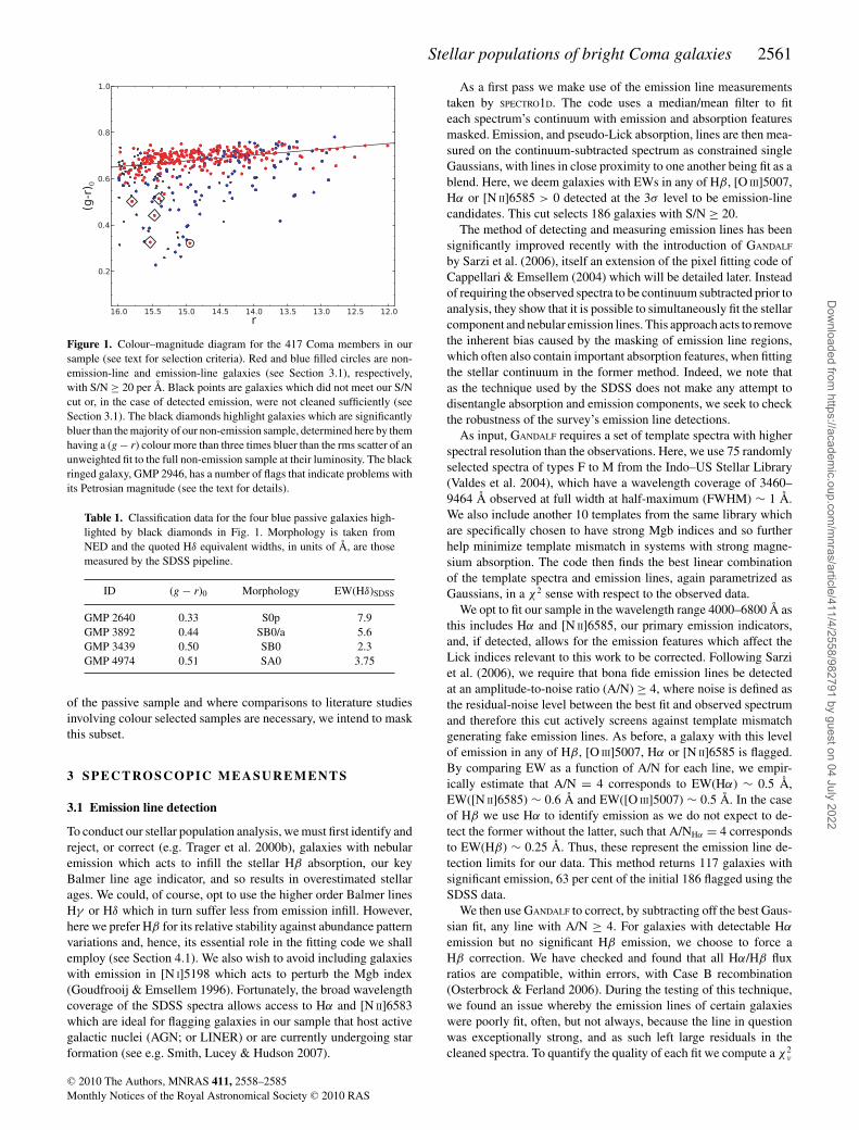
In Fig. 1, we plot the colour–magnitude diagram for our sam-ple. As detailed in Section 3.1, galaxies are, at least initially, onlysubdivided further based on whether they show detectable emis-sion, and as such it is interesting to see from Fig. 1 that almost allspectroscopically quiescent galaxies (98 per cent) that meet our se-lection requirements are compatible with being on the cluster’s redsequence. The remaining five galaxies are worth further comment.
The galaxy highlighted by a black circle in Fig. 1 is GMP 2946(Godwin, Metcalfe & Peach 1983). This object is projected on tothe halo of the giant galaxy NGC 4889, and its SDSS photometry iserroneous. More careful treatment shows that it lies on the cluster’sred sequence. We tabulate the relevant details of the four other bluepassive galaxies, denoted by black diamonds in Fig. 1, in Table 1where the morphological information is taken from NED and theHδ absorption-line equivalent widths (EWs) are those measuredby the SDSS pipeline SPECTRO1D. We note that the Poggianti et al.(2004) classification requirements for post-starburst k+a galaxiesare no emission and EW(Hδ) > 3 Å. Thus, three out of four of thesegalaxies are compatible with being k+a systems. Furthermore, allthree are located towards the faint end of our sample’s magnituderange, a fact which is perhaps not surprising given the lack of brightblue k+a galaxies in Coma as reported by Poggianti et al. (2004).Hereafter, we will refer to these four galaxies as the blue subset
2 http://nedwww.ipac.caltech.edu/
C© 2010 The Authors, MNRAS 411, 2558–2585Monthly Notices of the Royal Astronomical Society C© 2010 RAS
Dow
nloaded from https://academ
ic.oup.com/m
nras/article/411/4/2558/982791 by guest on 04 July 2022
Stellar populations of bright Coma galaxies 2561
Figure 1. Colour–magnitude diagram for the 417 Coma members in oursample (see text for selection criteria). Red and blue filled circles are non-emission-line and emission-line galaxies (see Section 3.1), respectively,with S/N ≥ 20 per Å. Black points are galaxies which did not meet our S/Ncut or, in the case of detected emission, were not cleaned sufficiently (seeSection 3.1). The black diamonds highlight galaxies which are significantlybluer than the majority of our non-emission sample, determined here by themhaving a (g − r) colour more than three times bluer than the rms scatter of anunweighted fit to the full non-emission sample at their luminosity. The blackringed galaxy, GMP 2946, has a number of flags that indicate problems withits Petrosian magnitude (see the text for details).
Table 1. Classification data for the four blue passive galaxies high-lighted by black diamonds in Fig. 1. Morphology is taken fromNED and the quoted Hδ equivalent widths, in units of Å, are thosemeasured by the SDSS pipeline.
ID (g − r)0 Morphology EW(Hδ)SDSS
GMP 2640 0.33 S0p 7.9GMP 3892 0.44 SB0/a 5.6GMP 3439 0.50 SB0 2.3GMP 4974 0.51 SA0 3.75
of the passive sample and where comparisons to literature studiesinvolving colour selected samples are necessary, we intend to maskthis subset.
3 SPECTRO SCOPIC MEASUREMENTS
3.1 Emission line detection
To conduct our stellar population analysis, we must first identify andreject, or correct (e.g. Trager et al. 2000b), galaxies with nebularemission which acts to infill the stellar Hβ absorption, our keyBalmer line age indicator, and so results in overestimated stellarages. We could, of course, opt to use the higher order Balmer linesHγ or Hδ which in turn suffer less from emission infill. However,here we prefer Hβ for its relative stability against abundance patternvariations and, hence, its essential role in the fitting code we shallemploy (see Section 4.1). We also wish to avoid including galaxieswith emission in [N I]5198 which acts to perturb the Mgb index(Goudfrooij & Emsellem 1996). Fortunately, the broad wavelengthcoverage of the SDSS spectra allows access to Hα and [N II]6583which are ideal for flagging galaxies in our sample that host activegalactic nuclei (AGN; or LINER) or are currently undergoing starformation (see e.g. Smith, Lucey & Hudson 2007).
As a first pass we make use of the emission line measurementstaken by SPECTRO1D. The code uses a median/mean filter to fiteach spectrum’s continuum with emission and absorption featuresmasked. Emission, and pseudo-Lick absorption, lines are then mea-sured on the continuum-subtracted spectrum as constrained singleGaussians, with lines in close proximity to one another being fit as ablend. Here, we deem galaxies with EWs in any of Hβ, [O III]5007,Hα or [N II]6585 > 0 detected at the 3σ level to be emission-linecandidates. This cut selects 186 galaxies with S/N ≥ 20.
The method of detecting and measuring emission lines has beensignificantly improved recently with the introduction of GANDALF
by Sarzi et al. (2006), itself an extension of the pixel fitting code ofCappellari & Emsellem (2004) which will be detailed later. Insteadof requiring the observed spectra to be continuum subtracted prior toanalysis, they show that it is possible to simultaneously fit the stellarcomponent and nebular emission lines. This approach acts to removethe inherent bias caused by the masking of emission line regions,which often also contain important absorption features, when fittingthe stellar continuum in the former method. Indeed, we note thatas the technique used by the SDSS does not make any attempt todisentangle absorption and emission components, we seek to checkthe robustness of the survey’s emission line detections.
As input, GANDALF requires a set of template spectra with higherspectral resolution than the observations. Here, we use 75 randomlyselected spectra of types F to M from the Indo–US Stellar Library(Valdes et al. 2004), which have a wavelength coverage of 3460–9464 Å observed at full width at half-maximum (FWHM) ∼ 1 Å.We also include another 10 templates from the same library whichare specifically chosen to have strong Mgb indices and so furtherhelp minimize template mismatch in systems with strong magne-sium absorption. The code then finds the best linear combinationof the template spectra and emission lines, again parametrized asGaussians, in a χ 2 sense with respect to the observed data.
We opt to fit our sample in the wavelength range 4000–6800 Å asthis includes Hα and [N II]6585, our primary emission indicators,and, if detected, allows for the emission features which affect theLick indices relevant to this work to be corrected. Following Sarziet al. (2006), we require that bona fide emission lines be detectedat an amplitude-to-noise ratio (A/N) ≥ 4, where noise is defined asthe residual-noise level between the best fit and observed spectrumand therefore this cut actively screens against template mismatchgenerating fake emission lines. As before, a galaxy with this levelof emission in any of Hβ, [O III]5007, Hα or [N II]6585 is flagged.By comparing EW as a function of A/N for each line, we empir-ically estimate that A/N = 4 corresponds to EW(Hα) ∼ 0.5 Å,EW([N II]6585) ∼ 0.6 Å and EW([O III]5007) ∼ 0.5 Å. In the caseof Hβ we use Hα to identify emission as we do not expect to de-tect the former without the latter, such that A/NHα = 4 correspondsto EW(Hβ) ∼ 0.25 Å. Thus, these represent the emission line de-tection limits for our data. This method returns 117 galaxies withsignificant emission, 63 per cent of the initial 186 flagged using theSDSS data.
We then use GANDALF to correct, by subtracting off the best Gaus-sian fit, any line with A/N ≥ 4. For galaxies with detectable Hα
emission but no significant Hβ emission, we choose to force aHβ correction. We have checked and found that all Hα/Hβ fluxratios are compatible, within errors, with Case B recombination(Osterbrock & Ferland 2006). During the testing of this technique,we found an issue whereby the emission lines of certain galaxieswere poorly fit, often, but not always, because the line in questionwas exceptionally strong, and as such left large residuals in thecleaned spectra. To quantify the quality of each fit we compute a χ 2
ν
C© 2010 The Authors, MNRAS 411, 2558–2585Monthly Notices of the Royal Astronomical Society C© 2010 RAS
Dow
nloaded from https://academ
ic.oup.com/m
nras/article/411/4/2558/982791 by guest on 04 July 2022
2562 J. Price et al.
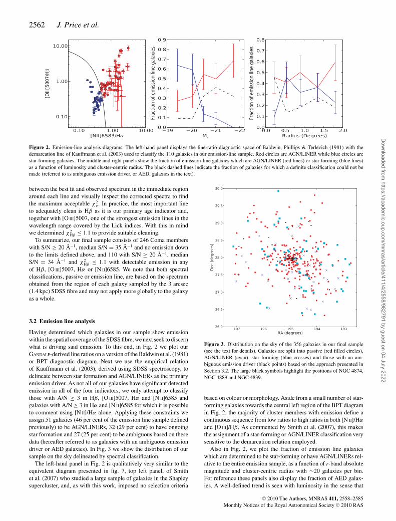
Figure 2. Emission-line analysis diagrams. The left-hand panel displays the line-ratio diagnostic space of Baldwin, Phillips & Terlevich (1981) with thedemarcation line of Kauffmann et al. (2003) used to classify the 110 galaxies in our emission-line sample. Red circles are AGN/LINER while blue circles arestar-forming galaxies. The middle and right panels show the fraction of emission-line galaxies which are AGN/LINER (red lines) or star forming (blue lines)as a function of luminosity and cluster-centric radius. The black dashed lines indicate the fraction of galaxies for which a definite classification could not bemade (referred to as ambiguous emission driver, or AED, galaxies in the text).
between the best fit and observed spectrum in the immediate regionaround each line and visually inspect the corrected spectra to findthe maximum acceptable χ 2
ν . In practice, the most important lineto adequately clean is Hβ as it is our primary age indicator and,together with [O III]5007, one of the strongest emission lines in thewavelength range covered by the Lick indices. With this in mindwe determined χ 2
Hβ ≤ 1.1 to provide suitable cleaning.To summarize, our final sample consists of 246 Coma members
with S/N ≥ 20 Å−1, median S/N = 35 Å−1 and no emission downto the limits defined above, and 110 with S/N ≥ 20 Å−1, medianS/N = 34 Å−1 and χ 2
Hβ ≤ 1.1 with detectable emission in anyof Hβ, [O III]5007, Hα or [N II]6585. We note that both spectralclassifications, passive or emission line, are based on the spectrumobtained from the region of each galaxy sampled by the 3 arcsec(1.4 kpc) SDSS fibre and may not apply more globally to the galaxyas a whole.
3.2 Emission line analysis
Having determined which galaxies in our sample show emissionwithin the spatial coverage of the SDSS fibre, we next seek to discernwhat is driving said emission. To this end, in Fig. 2 we plot ourGANDALF-derived line ratios on a version of the Baldwin et al. (1981)or BPT diagnostic diagram. Next we use the empirical relationof Kauffmann et al. (2003), derived using SDSS spectroscopy, todelineate between star formation and AGN/LINERs as the primaryemission driver. As not all of our galaxies have significant detectedemission in all of the four indicators, we only attempt to classifythose with A/N ≥ 3 in Hβ, [O III]5007, Hα and [N II]6585 andgalaxies with A/N ≥ 3 in Hα and [N II]6585 for which it is possibleto comment using [N II]/Hα alone. Applying these constraints weassign 51 galaxies (46 per cent of the emission line sample definedpreviously) to be AGN/LINERs, 32 (29 per cent) to have ongoingstar formation and 27 (25 per cent) to be ambiguous based on thesedata (hereafter referred to as galaxies with an ambiguous emissiondriver or AED galaxies). In Fig. 3 we show the distribution of oursample on the sky delineated by spectral classification.
The left-hand panel in Fig. 2 is qualitatively very similar to theequivalent diagram presented in fig. 7, top left panel, of Smithet al. (2007) who studied a large sample of galaxies in the Shapleysupercluster, and, as with this work, imposed no selection criteria
Figure 3. Distribution on the sky of the 356 galaxies in our final sample(see the text for details). Galaxies are split into passive (red filled circles),AGN/LINER (cyan), star forming (blue crosses) and those with an am-biguous emission driver (black points) based on the approach presented inSection 3.2. The large black symbols highlight the positions of NGC 4874,NGC 4889 and NGC 4839.
based on colour or morphology. Aside from a small number of star-forming galaxies towards the central left region of the BPT diagramin Fig. 2, the majority of cluster members with emission define acontinuous sequence from low ratios to high ratios in both [N II]/Hα
and [O III]/Hβ. As commented by Smith et al. (2007), this makesthe assignment of a star-forming or AGN/LINER classification verysensitive to the demarcation relation employed.
Also in Fig. 2, we plot the fraction of emission line galaxieswhich are determined to be star-forming or have AGN/LINERs rel-ative to the entire emission sample, as a function of r-band absolutemagnitude and cluster-centric radius with ∼20 galaxies per bin.For reference these panels also display the fraction of AED galax-ies. A well-defined trend is seen with luminosity in the sense that
C© 2010 The Authors, MNRAS 411, 2558–2585Monthly Notices of the Royal Astronomical Society C© 2010 RAS
Dow
nloaded from https://academ
ic.oup.com/m
nras/article/411/4/2558/982791 by guest on 04 July 2022

Stellar populations of bright Coma galaxies 2563
the fraction of AGN/LINERs increases with increasing brightnesswhereas the fraction of star formers decreases, a result in agreementwith Kauffmann et al. (2003) and Smith et al. (2007). Interestingly,no such correlation is observed as a function of radius with thefractional distributions remaining roughly constant, except for theinnermost bin where the star-forming fraction appears to diminish.However, this drop coincides with a rapid increase in those galaxieswhose emission driver is undetermined making firm conclusionsdifficult.
3.3 Velocity dispersions
The SDSS spectroscopic pipeline measures velocity dispersionswithin the survey’s 3 arcsec diameter fibre for the majority of spectrawhich are typical of early-type galaxies, and have redshifts z < 0.4,using a direct fitting method.3 However, 15 (6 per cent) of our non-emission sample and 36 (33 per cent) of our galaxies found to haveemission do not have measured velocity dispersions in DR7. Assuch we opt to use the penalized pixel fitting code (PPXF; Cappellari& Emsellem 2004) to obtain the velocity dispersions for our entiresample in a homogeneous fashion.
Details of the technique used here can be found in Price et al.(2009). Briefly, the routine uses the same 85 stellar templates usedby GANDALF, modulated by multiplicative and additive Legendrepolynomials of the orders of 6 and 2, respectively, and broadenedby a parametric line-of-sight velocity distribution, in this case aGaussian, to construct a model of each galaxy’s spectrum. Priorto fitting, the templates are matched to the variable resolution ofthe SDSS spectra. Fortunately, the SDSS pipeline itself recordsspectral resolution as a function of wavelength for each fibre andso we use this information to smooth the templates with a variablewidth Gaussian, typically with σ inst ∼ 58–70 km s−1 in the 4000–6000 Å fitting range used here, to match our data. Taking advantageof fitting in the pixel space, we mask bad pixels and the NaD lineat 5892 Å which can often be affected by interstellar absorption.
To assess the uncertainty on our velocity dispersion measure-ments ideally one would like to undertake a bootstrap procedure,using the error spectra to generate new pseudo-observations andthen passing them through PPXF, but as our sample size is large thisapproach would be time consuming. As a compromise, we create asubsample of galaxies, 10 per S/N bin with a bin size of 10 betweenS/N = 10 and 50, randomly selected from the full sample. For eachselected galaxy we generate 50 realisations, run them through PPXF
and take the standard deviation of the resulting distribution as theerror on that galaxy’s velocity dispersion. Finally, we interpolatethe σ–S/N–σ error distribution formed by our subsample into a sur-face using a bivariate spline. It is then a simple matter of inputtingthe S/N and σ of each galaxy from the full sample to obtain anestimated σ error.
Comparing our velocity dispersion measurements to those fromthe SDSS pipeline for galaxies with both we find a mean offset〈SDSS-This work〉 = −6 km s−1, likely attributed to our differentfitting range and masking procedures. Once this systematic shiftis accounted for we find an rms scatter of 5 km s−1 with an in-trinsic component of 0. Comparing our measurements with thosefrom (Moore et al. 2002, hereafter M02) we find a mean offset of2.8 km s−1, an rms scatter accounting for the offset of 8 km s−1 withan intrinsic component of 4.7 km s−1. Thus, overall, we find good
3 http://www.sdss.org/dr7/algorithms/veldisp.html
compatibility between our measurements and those made by theSDSS pipeline and M02.
The final step necessary before using the measured velocity dis-persions in our analysis is to aperture correct them to a commonsampling in terms of each galaxy’s half-light radius. Here, we followthe prescription of Jørgensen, Franx & Kjaergaard (1995),
logσSDSS
σRe/2= −0.04 log
1.5 arcsec
Re/2
where Re is the PSF-corrected half-light or effective radius, obtainedby fitting a single Sersic model using GALFIT (Peng et al. 2002) tothe SDSS r-band image of each galaxy. σ SDSS and σRe/2 are thegalaxies’ velocity dispersions through the 1.5 arcsec radius SDSSfibre and the desired Re/2 aperture, respectively. Corrections are inthe range −0.067 to 0.017 dex with a mean of σ cor = −0.004 dexor ∼1 per cent.
3.4 Absorption-line indices
We use the LICK_EW code which is provided as part of the EZ-AGES package4 (Graves & Schiavon 2008) to measure the Lickindices of our sample. The full set of indices defined in table 1of Worthey (1994) and table 1 of Worthey & Ottaviani (1997) aremeasured where possible, although a small fraction of the galaxieshave regions of bad pixels which prevent access to all indices. Theroutine uses the error spectra and the equations of Cardiel et al.(1998) to compute error estimates for the indices.
Having obtained the raw indices for our sample, it is then neces-sary to correct them to the resolution of the Schiavon models, whichare themselves based on stellar spectra smoothed to the wavelength-dependent Lick/IDS resolution. Effectively one wants to know thevalue of each observed index for a given galaxy at the model’sresolution but without any Doppler broadening from that galaxy’sstellar velocity dispersion. One route is to employ multiplicativeand additive corrections derived from artificially broadened starsobserved with the same instrument as the galaxy spectra. Morerecent works have moved towards using stellar population modeltemplates which permit a better match in terms of spectral type toobserved galaxy spectra, while still maintaining the zero velocitydispersion requirement.
Here, we opt to follow a similar method to that of Kelson et al.(2006) and also take advantage of the functionality of PPXF in deriv-ing our velocity broadening corrections. First, PPXF is used to outputthe best-fitting combination of our stellar templates at the resolu-tion of our data for each galaxy with and without smoothing by thevelocity dispersion of that galaxy. Next LICK_EW is executed threetimes; first on the observed spectrum (Iobs), then on the best-fittingspectrum with velocity dispersion broadening (IT ) and finally on thebroadening free spectrum smoothed to the Lick resolution (Ilick) foreach index as defined by table 1 of Schiavon (2007). The correctedindices for each galaxy (Icor) can then be obtained via
Icor = Iobs + (Ilick − IT ). (1)
In Fig. 4, we present the index corrections, that is the value of thebracketed term on the right-hand side of equation (1), for the indiceswhich were used in our stellar population analysis (see Section 4)as a function of galaxy velocity dispersion for both emission andnon-emission line samples. Uncertainties on these corrections areobtained using a similar approach to that used previously for the
4 http://www.ucolick.org/∼graves/EZ_Ages.html
C© 2010 The Authors, MNRAS 411, 2558–2585Monthly Notices of the Royal Astronomical Society C© 2010 RAS
Dow
nloaded from https://academ
ic.oup.com/m
nras/article/411/4/2558/982791 by guest on 04 July 2022
2564 J. Price et al.
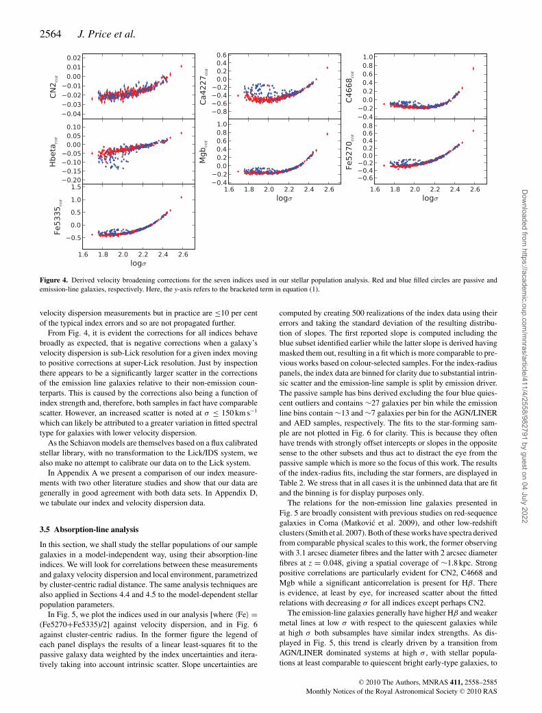
Figure 4. Derived velocity broadening corrections for the seven indices used in our stellar population analysis. Red and blue filled circles are passive andemission-line galaxies, respectively. Here, the y-axis refers to the bracketed term in equation (1).
velocity dispersion measurements but in practice are ≤10 per centof the typical index errors and so are not propagated further.
From Fig. 4, it is evident the corrections for all indices behavebroadly as expected, that is negative corrections when a galaxy’svelocity dispersion is sub-Lick resolution for a given index movingto positive corrections at super-Lick resolution. Just by inspectionthere appears to be a significantly larger scatter in the correctionsof the emission line galaxies relative to their non-emission coun-terparts. This is caused by the corrections also being a function ofindex strength and, therefore, both samples in fact have comparablescatter. However, an increased scatter is noted at σ ≤ 150 km s−1
which can likely be attributed to a greater variation in fitted spectraltype for galaxies with lower velocity dispersion.
As the Schiavon models are themselves based on a flux calibratedstellar library, with no transformation to the Lick/IDS system, wealso make no attempt to calibrate our data on to the Lick system.
In Appendix A we present a comparison of our index measure-ments with two other literature studies and show that our data aregenerally in good agreement with both data sets. In Appendix D,we tabulate our index and velocity dispersion data.
3.5 Absorption-line analysis
In this section, we shall study the stellar populations of our samplegalaxies in a model-independent way, using their absorption-lineindices. We will look for correlations between these measurementsand galaxy velocity dispersion and local environment, parametrizedby cluster-centric radial distance. The same analysis techniques arealso applied in Sections 4.4 and 4.5 to the model-dependent stellarpopulation parameters.
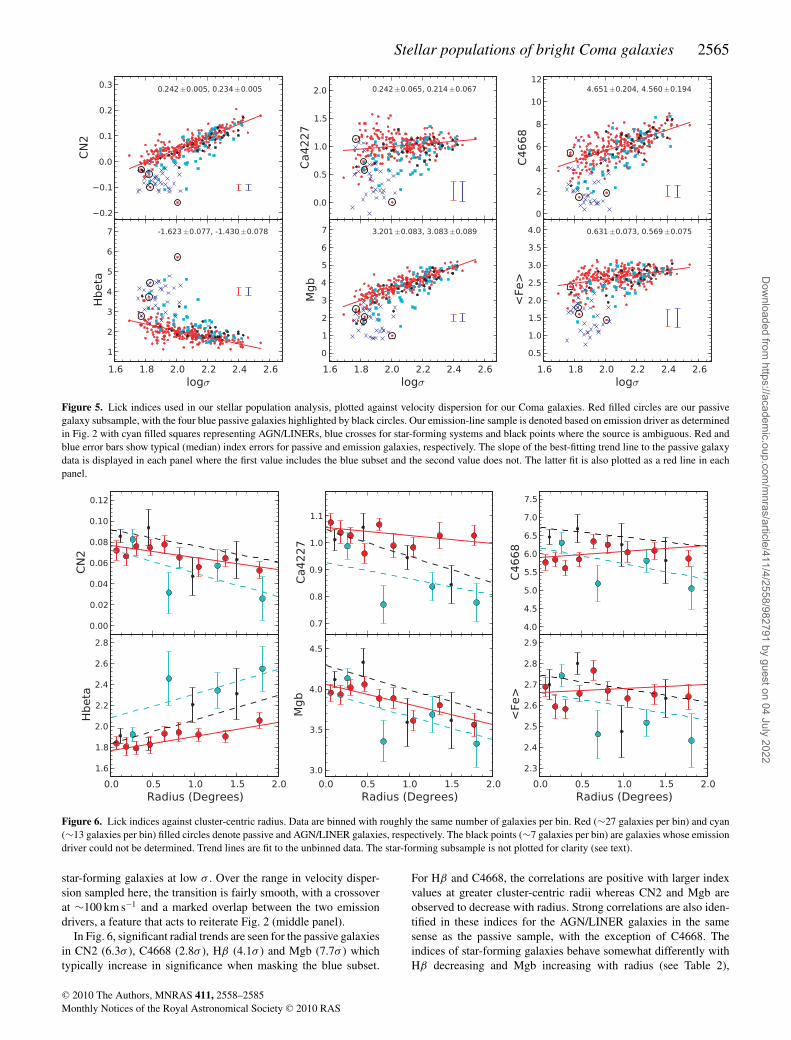
In Fig. 5, we plot the indices used in our analysis [where 〈Fe〉 =(Fe5270+Fe5335)/2] against velocity dispersion, and in Fig. 6against cluster-centric radius. In the former figure the legend ofeach panel displays the results of a linear least-squares fit to thepassive galaxy data weighted by the index uncertainties and itera-tively taking into account intrinsic scatter. Slope uncertainties are
computed by creating 500 realizations of the index data using theirerrors and taking the standard deviation of the resulting distribu-tion of slopes. The first reported slope is computed including theblue subset identified earlier while the latter slope is derived havingmasked them out, resulting in a fit which is more comparable to pre-vious works based on colour-selected samples. For the index-radiuspanels, the index data are binned for clarity due to substantial intrin-sic scatter and the emission-line sample is split by emission driver.The passive sample has bins derived excluding the four blue quies-cent outliers and contains ∼27 galaxies per bin while the emissionline bins contain ∼13 and ∼7 galaxies per bin for the AGN/LINERand AED samples, respectively. The fits to the star-forming sam-ple are not plotted in Fig. 6 for clarity. This is because they oftenhave trends with strongly offset intercepts or slopes in the oppositesense to the other subsets and thus act to distract the eye from thepassive sample which is more so the focus of this work. The resultsof the index-radius fits, including the star formers, are displayed inTable 2. We stress that in all cases it is the unbinned data that are fitand the binning is for display purposes only.
The relations for the non-emission line galaxies presented inFig. 5 are broadly consistent with previous studies on red-sequencegalaxies in Coma (Matkovic et al. 2009), and other low-redshiftclusters (Smith et al. 2007). Both of these works have spectra derivedfrom comparable physical scales to this work, the former observingwith 3.1 arcsec diameter fibres and the latter with 2 arcsec diameterfibres at z = 0.048, giving a spatial coverage of ∼1.8 kpc. Strongpositive correlations are particularly evident for CN2, C4668 andMgb while a significant anticorrelation is present for Hβ. Thereis evidence, at least by eye, for increased scatter about the fittedrelations with decreasing σ for all indices except perhaps CN2.
The emission-line galaxies generally have higher Hβ and weakermetal lines at low σ with respect to the quiescent galaxies whileat high σ both subsamples have similar index strengths. As dis-played in Fig. 5, this trend is clearly driven by a transition fromAGN/LINER dominated systems at high σ , with stellar popula-tions at least comparable to quiescent bright early-type galaxies, to
C© 2010 The Authors, MNRAS 411, 2558–2585Monthly Notices of the Royal Astronomical Society C© 2010 RAS
Dow
nloaded from https://academ
ic.oup.com/m
nras/article/411/4/2558/982791 by guest on 04 July 2022
Stellar populations of bright Coma galaxies 2565
Figure 5. Lick indices used in our stellar population analysis, plotted against velocity dispersion for our Coma galaxies. Red filled circles are our passivegalaxy subsample, with the four blue passive galaxies highlighted by black circles. Our emission-line sample is denoted based on emission driver as determinedin Fig. 2 with cyan filled squares representing AGN/LINERs, blue crosses for star-forming systems and black points where the source is ambiguous. Red andblue error bars show typical (median) index errors for passive and emission galaxies, respectively. The slope of the best-fitting trend line to the passive galaxydata is displayed in each panel where the first value includes the blue subset and the second value does not. The latter fit is also plotted as a red line in eachpanel.
Figure 6. Lick indices against cluster-centric radius. Data are binned with roughly the same number of galaxies per bin. Red (∼27 galaxies per bin) and cyan(∼13 galaxies per bin) filled circles denote passive and AGN/LINER galaxies, respectively. The black points (∼7 galaxies per bin) are galaxies whose emissiondriver could not be determined. Trend lines are fit to the unbinned data. The star-forming subsample is not plotted for clarity (see text).
star-forming galaxies at low σ . Over the range in velocity disper-sion sampled here, the transition is fairly smooth, with a crossoverat ∼100 km s−1 and a marked overlap between the two emissiondrivers, a feature that acts to reiterate Fig. 2 (middle panel).
In Fig. 6, significant radial trends are seen for the passive galaxiesin CN2 (6.3σ ), C4668 (2.8σ ), Hβ (4.1σ ) and Mgb (7.7σ ) whichtypically increase in significance when masking the blue subset.
For Hβ and C4668, the correlations are positive with larger indexvalues at greater cluster-centric radii whereas CN2 and Mgb areobserved to decrease with radius. Strong correlations are also iden-tified in these indices for the AGN/LINER galaxies in the samesense as the passive sample, with the exception of C4668. Theindices of star-forming galaxies behave somewhat differently withHβ decreasing and Mgb increasing with radius (see Table 2),
C© 2010 The Authors, MNRAS 411, 2558–2585Monthly Notices of the Royal Astronomical Society C© 2010 RAS
Dow
nloaded from https://academ
ic.oup.com/m
nras/article/411/4/2558/982791 by guest on 04 July 2022
2566 J. Price et al.
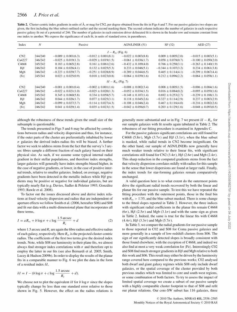
Table 2. Cluster-centric index gradients in units of Å, or mag for CN2, per degree obtained from the fits in Figs 6 and 7. For our passive galaxies two slopes aregiven, the first including the blue subset outlined earlier and the second masking them. The second column indicates the number of galaxies in each respectivepassive galaxy fit out of a potential of 246. The number of galaxies in each emission driver delineated fit is shown in the header row and remains constant fromone index to another. We express the significance of each fit, in units of standard error, in parentheses.
Index N Passive AGN/LINER (51) SF (32) AED (27)
I − Rcc (Fig. 6)CN2 244/240 −0.009 ± 0.001(6.3) −0.012 ± 0.001(8.1) −0.022 ± 0.003(8.8) 0.009 ± 0.005(2.0) −0.015 ± 0.003(5.1)
Ca4227 246/242 −0.025 ± 0.019(1.3) −0.029 ± 0.019(1.5) −0.061 ± 0.036(1.7) 0.058 ± 0.078(0.7) −0.100 ± 0.050(2.0)C4668 245/242 0.183 ± 0.065(2.8) 0.161 ± 0.061(2.6) −0.432 ± 0.109(4.0) 0.766 ± 0.250(3.1) −0.263 ± 0.140(1.9)
Hβ 246/242 0.104 ± 0.026(4.1) 0.132 ± 0.025(5.3) 0.233 ± 0.046(5.1) −0.344 ± 0.107(3.2) 0.234 ± 0.061(3.8)Mgb 246/242 −0.223 ± 0.029(7.7) −0.251 ± 0.028(8.9) −0.289 ± 0.044(6.5) 0.465 ± 0.114(4.1) −0.299 ± 0.067(4.4)〈Fe〉 245/241 0.023 ± 0.025(0.9) 0.018 ± 0.023(0.8) −0.064 ± 0.039(1.6) 0.212 ± 0.096(2.2) −0.064 ± 0.058(1.1)
δI − Rcc (Fig. 7)
CN2 244/240 −0.001 ± 0.001(0.4) −0.002 ± 0.001(1.6) −0.008 ± 0.002(3.4) 0.008 ± 0.005(1.5) −0.006 ± 0.004(1.6)Ca4227 246/242 −0.022 ± 0.021(1.0) −0.025 ± 0.020(1.3) −0.052 ± 0.034(1.5) 0.016 ± 0.084(0.2) −0.095 ± 0.059(1.6)C4668 245/242 0.345 ± 0.060(5.8) 0.334 ± 0.058(5.7) −0.148 ± 0.107(1.4) 0.692 ± 0.253(2.7) −0.239 ± 0.188(1.3)
Hβ 246/242 0.044 ± 0.026(1.7) 0.077 ± 0.025(3.1) 0.118 ± 0.045(2.6) −0.327 ± 0.114(2.9) 0.237 ± 0.083(2.9)Mgb 246/242 −0.099 ± 0.027(3.7) −0.114 ± 0.027(4.3) −0.108 ± 0.046(2.4) 0.467 ± 0.116(4.0) −0.216 ± 0.082(2.6)〈Fe〉 246/242 0.041 ± 0.029(1.4) 0.035 ± 0.023(1.5) −0.042 ± 0.056(0.7) 0.203 ± 0.129(1.6) −0.048 ± 0.093(0.5)
although the robustness of these trends given the small size of thesubsample is questionable.
The trends presented in Figs 5 and 6 may be affected by correla-tions between radius and velocity dispersion and thus, for instance,if the outer parts of the cluster are preferentially inhabited by lowerσ galaxies the derived index-radius fits will be biased. A furtherfactor we seek to address stems from the fact that the survey’s 3 arc-sec fibres sample a different fraction of each galaxy based on theirphysical size. As such, if we assume some typical internal radialgradient in their stellar populations, and therefore index strengths,larger galaxies will generally have index strengths biased higher, inthe case of negative gradients, or lower, in the case of positive inter-nal trends, relative to smaller galaxies. Indeed, on average, negativegradients have been detected in the metallic indices while Hβ gra-dients may be positive or negative for individual galaxies, but aretypically nearly flat (e.g. Davies, Sadler & Peletier 1993; Gonzalez1993; Rawle et al. 2008).
To factor out the issues discussed above and derive index rela-tions at fixed velocity dispersion and radius that are independent ofaperture effects we follow Smith et al. (2006, hereafter S06) and S08and fit our data with a multi-dimensional plane that incorporates allthree terms,
I = aRcc + b log σ + c log1.5 arcsec
Re
+ d (2)
where 1.5 arcsec and Re are again the fibre radius and effective radiusof each galaxy, respectively. Here Rcc is the projected cluster-centricradius. The coefficients of the first two terms give the desired indextrends. Note, while S08 use luminosity in their plane fits, we almostalways find stronger index correlations with σ and therefore opt toemploy the latter in our fits (see also Bernardi et al. 2005; Smith,Lucey & Hudson 2009b). In order to display the results of the planarfits in a comparable manner to Fig. 6 we plot the data in the formof a residual index δI,
δI = I − (b log σ + c log1.5 arcsec
Re
+ d).
We choose not to plot the equivalent δI for b log σ since the slopestypically change by less than one standard error relative to thoseshown in Fig. 5. However, the effect on the radius relations is
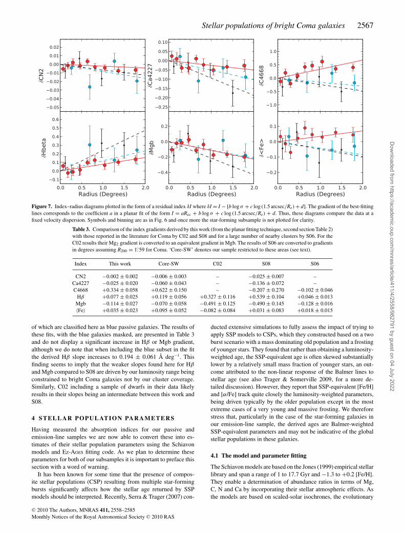
generally more substantial and so in Fig. 7 we present δI − Rcc forour sample galaxies with fit results again tabulated in Table 2. Therobustness of our fitting procedure is examined in Appendix C.
For the passive galaxies significant correlations are still found forC4668 (5.8σ ), Mgb (3.7σ ) and Hβ (3.1σ ), when the blue subsetis masked, while radial trends in CN2 become insignificant. Onthe other hand, our sample of AGN/LINERs now generally havemuch weaker trends relative to their linear fits, with significantcorrelations still found for CN2 (3.4σ ), Hβ (2.6σ ) and Mgb (2.4σ ).This sharp reduction in the computed gradients stems from the factthat velocity dispersion correlates mildly with radius for this samplein the sense that lower dispersions are found at larger radii. Finally,the index trends for star-forming galaxies remain comparativelyunchanged.
A valid question here is to what extent do the outermost pointsdrive the significant radial trends recovered by both the linear andplanar fits for our passive sample. To test this we have repeated thefitting procedure with the outermost points, those in the final binwith Rcc > 1.◦55, and the blue subset masked. There is some changeto the fitted slopes reported in Table 2. However, the three indiceswith significant radial coefficients in the planar fits remain C4668(6σ ), Hβ (2.5σ ) and Mgb (3.1σ ) and with the same sign as givenin Table 2. Indeed, the same is true for the linear fits with C4668(4.4σ ), Hβ (3.3σ ) and Mgb (5.7σ ).
In Table 3, we compare the radial gradients for our passive sampleto those reported in C02 and S08 for Coma passive galaxies andmore generally in a sample of low-redshift clusters from S06. Thesign of our significantly detected slopes is broadly consistent withthose found elsewhere, with the exception of C4668, and indeed wealso find at most a very weak correlation for 〈Fe〉. Interestingly C02and S08 find much stronger gradients in Hβ and Mgb relative to boththis work and S06. This result may either be driven by the luminosityrange covered here compared to the previous works; C02 analysedboth dwarf and giant galaxy regimes while S08 only include dwarfgalaxies, or the spatial coverage of the cluster provided by bothprevious studies which was limited to core and south-west regions,or some combination of both factors. To try to assess the impact oflimited spatial coverage we create a subset of our passive samplewith a highly comparable cluster footprint to that of S08 and refitour planar relations. Our core-SW subset has 116 galaxies, three
C© 2010 The Authors, MNRAS 411, 2558–2585Monthly Notices of the Royal Astronomical Society C© 2010 RAS
Dow
nloaded from https://academ
ic.oup.com/m
nras/article/411/4/2558/982791 by guest on 04 July 2022
Stellar populations of bright Coma galaxies 2567
Figure 7. Index–radius diagrams plotted in the form of a residual index δI where δI = I − [b log σ + c log (1.5 arcsec/Re) + d]. The gradient of the best-fittinglines corresponds to the coefficient a in a planar fit of the form I = aRcc + b log σ + c log (1.5 arcsec/Re) + d. Thus, these diagrams compare the data at afixed velocity dispersion. Symbols and binning are as in Fig. 6 and once more the star-forming subsample is not plotted for clarity.
Table 3. Comparison of the index gradients derived by this work (from the planar fitting technique, second section Table 2)with those reported in the literature for Coma by C02 and S08 and for a large number of nearby clusters by S06. For theC02 results their Mg2 gradient is converted to an equivalent gradient in Mgb. The results of S06 are converted to gradientsin degrees assuming R200 = 1.◦59 for Coma. ‘Core-SW’ denotes our sample restricted to these areas (see text).
Index This work Core-SW C02 S08 S06
CN2 −0.002 ± 0.002 −0.006 ± 0.003 – −0.025 ± 0.007 –Ca4227 −0.025 ± 0.020 −0.060 ± 0.043 – −0.136 ± 0.072 –C4668 +0.334 ± 0.058 +0.622 ± 0.150 – −0.207 ± 0.270 −0.102 ± 0.046
Hβ +0.077 ± 0.025 +0.119 ± 0.056 +0.327 ± 0.116 +0.539 ± 0.104 +0.046 ± 0.013Mgb −0.114 ± 0.027 −0.070 ± 0.058 −0.491 ± 0.125 −0.490 ± 0.145 −0.128 ± 0.016〈Fe〉 +0.035 ± 0.023 +0.095 ± 0.052 −0.082 ± 0.084 +0.031 ± 0.083 +0.018 ± 0.015
of which are classified here as blue passive galaxies. The results ofthese fits, with the blue galaxies masked, are presented in Table 3and do not display a significant increase in Hβ or Mgb gradient,although we do note that when including the blue subset in the fitthe derived Hβ slope increases to 0.194 ± 0.061 Å deg−1. Thisfinding seems to imply that the weaker slopes found here for Hβ
and Mgb compared to S08 are driven by our luminosity range beingconstrained to bright Coma galaxies not by our cluster coverage.Similarly, C02 including a sample of dwarfs in their data likelyresults in their slopes being an intermediate between this work andS08.
4 STELLAR POPULATION PARAMETERS
Having measured the absorption indices for our passive andemission-line samples we are now able to convert these into es-timates of their stellar population parameters using the Schiavonmodels and EZ-AGES fitting code. As we plan to determine theseparameters for both of our subsamples it is important to preface thissection with a word of warning.
It has been known for some time that the presence of compos-ite stellar populations (CSP) resulting from multiple star-formingbursts significantly affects how the stellar age returned by SSPmodels should be interpreted. Recently, Serra & Trager (2007) con-
ducted extensive simulations to fully assess the impact of trying toapply SSP models to CSPs, which they constructed based on a twoburst scenario with a mass dominating old population and a frostingof younger stars. They found that rather than obtaining a luminosity-weighted age, the SSP-equivalent age is often skewed substantiallylower by a relatively small mass fraction of younger stars, an out-come attributed to the non-linear response of the Balmer lines tostellar age (see also Trager & Somerville 2009, for a more de-tailed discussion). However, they report that SSP-equivalent [Fe/H]and [α/Fe] track quite closely the luminosity-weighted parameters,being driven typically by the older population except in the mostextreme cases of a very young and massive frosting. We thereforestress that, particularly in the case of the star-forming galaxies inour emission-line sample, the derived ages are Balmer-weightedSSP-equivalent parameters and may not be indicative of the globalstellar populations in these galaxies.
4.1 The model and parameter fitting
The Schiavon models are based on the Jones (1999) empirical stellarlibrary and span a range of 1 to 17.7 Gyr and −1.3 to +0.2 [Fe/H].They enable a determination of abundance ratios in terms of Mg,C, N and Ca by incorporating their stellar atmospheric effects. Asthe models are based on scaled-solar isochrones, the evolutionary
C© 2010 The Authors, MNRAS 411, 2558–2585Monthly Notices of the Royal Astronomical Society C© 2010 RAS
Dow
nloaded from https://academ
ic.oup.com/m
nras/article/411/4/2558/982791 by guest on 04 July 2022
2568 J. Price et al.
tracks and stellar atmospheres are not treated in a self-consistentmanner in a similar vein to the widely used TMBK models. Here,we employ a Salpeter initial mass function.
We derive the SSP-equivalent parameters for our galaxies usingthe EZ-AGES code of Graves & Schiavon (2008) which, using theSchiavon models, seeks to return consistent stellar population pa-rameters across a number of index–index diagrams. The routinebegins by making an initial estimate of age and [Fe/H] by invertingan Hβ – 〈Fe〉 grid, specifically chosen to strongly break the age–metallicity degeneracy while being largely insensitive to non-solarabundance patterns (Schiavon 2007). Next the code moves on to de-termining [Mg/Fe] from a Hβ – Mgb grid. To do this it first invertsthe new grid, compares the age and [Fe/H] measured from this gridto the fiducial estimates and if they do not agree assumes a non-solar[Mg/Fe] is present and recomputes the model with a new [Mg/Fe].Further iterations occur until the derived age and [Fe/H] converge tothe fiducial values within some tolerance. The code then goes on torepeat this iterative approach replacing Mg by C, N and Ca in turnwith the final abundance pattern used to compute a new model andderive a new fiducial age and [Fe/H], with the entire fitting processrepeating until the fit does not improve. The standard index set usedfor the fitting is Hβ and 〈Fe〉 for the initial age and [Fe/H] estimates,Mgb for [Mg/Fe], C4668 for [C/Fe], CN2 for [N/Fe] and Ca4227for [Ca/Fe].
We could not obtain fits for 11 per cent of our entire sample asthey fell off the fiducial Hβ – 〈Fe〉 grid. This may be because theyeither have SSP parameters, perhaps only marginally, outside themodels coverage or else were carried off the grid by measurementerrors. As a work around we fit these galaxies using Fe5270 orFe5335 only instead of their mean. Typically, the results obtainedfrom the three different approaches are consistent, within errors, forthose galaxies which can be fit by all three.
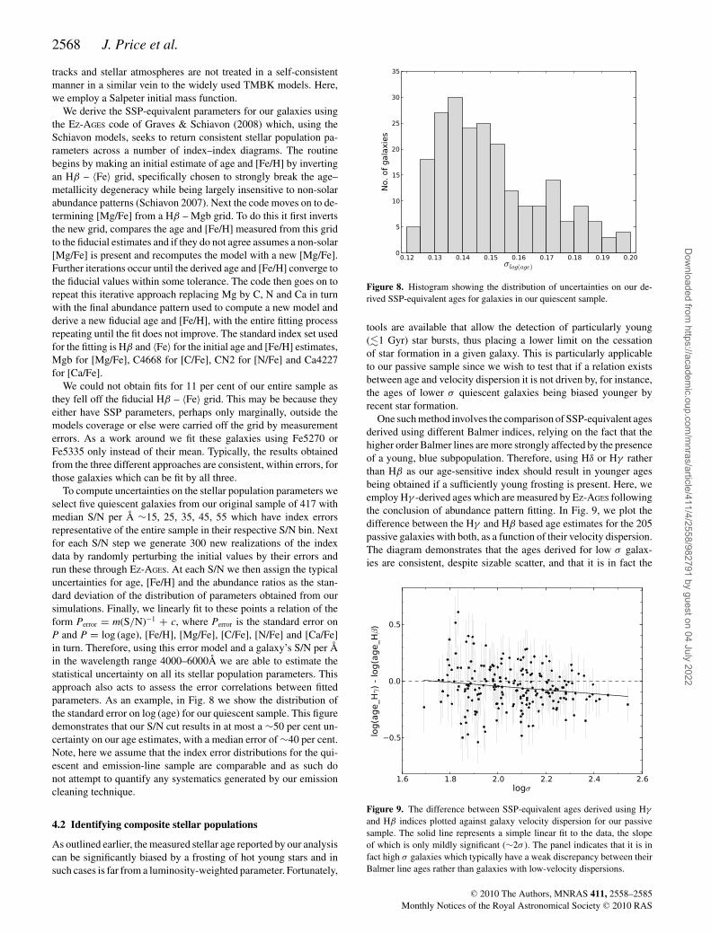
To compute uncertainties on the stellar population parameters weselect five quiescent galaxies from our original sample of 417 withmedian S/N per Å ∼15, 25, 35, 45, 55 which have index errorsrepresentative of the entire sample in their respective S/N bin. Nextfor each S/N step we generate 300 new realizations of the indexdata by randomly perturbing the initial values by their errors andrun these through EZ-AGES. At each S/N we then assign the typicaluncertainties for age, [Fe/H] and the abundance ratios as the stan-dard deviation of the distribution of parameters obtained from oursimulations. Finally, we linearly fit to these points a relation of theform Perror = m(S/N)−1 + c, where Perror is the standard error onP and P = log (age), [Fe/H], [Mg/Fe], [C/Fe], [N/Fe] and [Ca/Fe]in turn. Therefore, using this error model and a galaxy’s S/N per Åin the wavelength range 4000–6000Å we are able to estimate thestatistical uncertainty on all its stellar population parameters. Thisapproach also acts to assess the error correlations between fittedparameters. As an example, in Fig. 8 we show the distribution ofthe standard error on log (age) for our quiescent sample. This figuredemonstrates that our S/N cut results in at most a ∼50 per cent un-certainty on our age estimates, with a median error of ∼40 per cent.Note, here we assume that the index error distributions for the qui-escent and emission-line sample are comparable and as such donot attempt to quantify any systematics generated by our emissioncleaning technique.
4.2 Identifying composite stellar populations
As outlined earlier, the measured stellar age reported by our analysiscan be significantly biased by a frosting of hot young stars and insuch cases is far from a luminosity-weighted parameter. Fortunately,
Figure 8. Histogram showing the distribution of uncertainties on our de-rived SSP-equivalent ages for galaxies in our quiescent sample.
tools are available that allow the detection of particularly young(�1 Gyr) star bursts, thus placing a lower limit on the cessationof star formation in a given galaxy. This is particularly applicableto our passive sample since we wish to test that if a relation existsbetween age and velocity dispersion it is not driven by, for instance,the ages of lower σ quiescent galaxies being biased younger byrecent star formation.
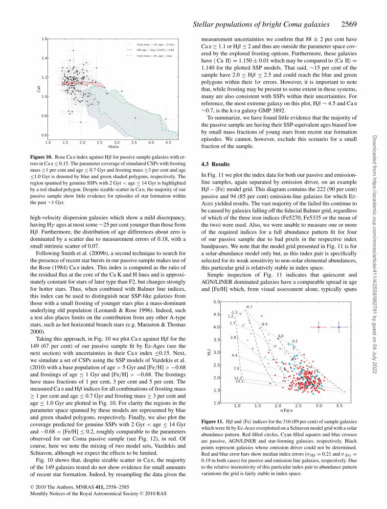
One such method involves the comparison of SSP-equivalent agesderived using different Balmer indices, relying on the fact that thehigher order Balmer lines are more strongly affected by the presenceof a young, blue subpopulation. Therefore, using Hδ or Hγ ratherthan Hβ as our age-sensitive index should result in younger agesbeing obtained if a sufficiently young frosting is present. Here, weemploy Hγ -derived ages which are measured by EZ-AGES followingthe conclusion of abundance pattern fitting. In Fig. 9, we plot thedifference between the Hγ and Hβ based age estimates for the 205passive galaxies with both, as a function of their velocity dispersion.The diagram demonstrates that the ages derived for low σ galax-ies are consistent, despite sizable scatter, and that it is in fact the
Figure 9. The difference between SSP-equivalent ages derived using Hγ
and Hβ indices plotted against galaxy velocity dispersion for our passivesample. The solid line represents a simple linear fit to the data, the slopeof which is only mildly significant (∼2σ ). The panel indicates that it is infact high σ galaxies which typically have a weak discrepancy between theirBalmer line ages rather than galaxies with low-velocity dispersions.
C© 2010 The Authors, MNRAS 411, 2558–2585Monthly Notices of the Royal Astronomical Society C© 2010 RAS
Dow
nloaded from https://academ
ic.oup.com/m
nras/article/411/4/2558/982791 by guest on 04 July 2022
Stellar populations of bright Coma galaxies 2569
Figure 10. Rose Ca II index against Hβ for passive sample galaxies with er-rors in Ca II ≤ 0.15. The parameter coverage of simulated CSPs with frostingmass ≥1 per cent and age ≤ 0.7 Gyr and frosting mass ≥3 per cent and age≤1.0 Gyr is denoted by blue and green shaded polygons, respectively. Theregion spanned by genuine SSPs with 2 Gyr < age ≤ 14 Gyr is highlightedby a red shaded polygon. Despite sizable scatter in Ca II, the majority of ourpassive sample show little evidence for episodes of star formation withinthe past ∼1 Gyr.
high-velocity dispersion galaxies which show a mild discrepancy,having Hγ ages at most some ∼25 per cent younger than those fromHβ. Furthermore, the distribution of age differences about zero isdominated by a scatter due to measurement errors of 0.18, with asmall intrinsic scatter of 0.07.
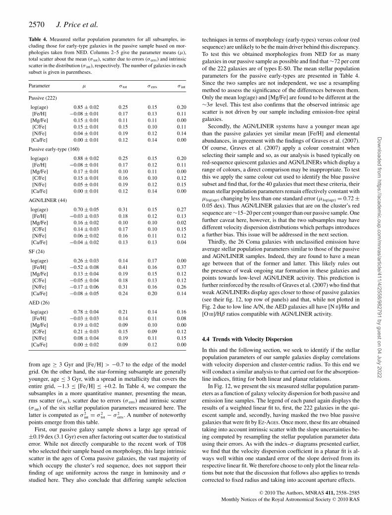
Following Smith et al. (2009b), a second technique to search forthe presence of recent star bursts in our passive sample makes use ofthe Rose (1984) Ca II index. This index is computed as the ratio ofthe residual flux at the core of the Ca K and H lines and is approxi-mately constant for stars of later type than F2, but changes stronglyfor hotter stars. Thus, when combined with Balmer line indices,this index can be used to distinguish near SSP-like galaxies fromthose with a small frosting of younger stars plus a mass-dominantunderlying old population (Leonardi & Rose 1996). Indeed, sucha test also places limits on the contribution from any other A-typestars, such as hot horizontal branch stars (e.g. Maraston & Thomas2000).
Taking this approach, in Fig. 10 we plot Ca II against Hβ for the149 (67 per cent) of our passive sample fit by Ez-Ages (see thenext section) with uncertainties in their Ca II index ≤0.15. Next,we simulate a set of CSPs using the SSP models of Vazdekis et al.(2010) with a base population of age > 5 Gyr and [Fe/H] > −0.68and frostings of age ≤ 1 Gyr and [Fe/H] > −0.68. The frostingshave mass fractions of 1 per cent, 3 per cent and 5 per cent. Themeasured Ca II and Hβ indices for all combinations of frosting mass≥ 1 per cent and age ≤ 0.7 Gyr and frosting mass ≥ 3 per cent andage ≤ 1.0 Gyr are plotted in Fig. 10. For clarity the regions in theparameter space spanned by these models are represented by blueand green shaded polygons, respectively. Finally, we also plot thecoverage predicted for genuine SSPs with 2 Gyr < age ≤ 14 Gyrand −0.68 < [Fe/H] ≤ 0.2, roughly comparable to the parametersobserved for our Coma passive sample (see Fig. 12), in red. Ofcourse, here we note the mixing of two model sets, Vazdekis andSchiavon, although we expect the effects to be limited.
Fig. 10 shows that, despite sizable scatter in Ca II, the majorityof the 149 galaxies tested do not show evidence for small amountsof recent star formation. Indeed, by resampling the data given the
measurement uncertainties we confirm that 88 ± 2 per cent haveCa II ≥ 1.1 or Hβ ≤ 2 and thus are outside the parameter space cov-ered by the explored frosting options. Furthermore, these galaxieshave 〈 Ca II〉 = 1.150 ± 0.01 which may be compared to 〈Ca II〉 =1.140 for the plotted SSP models. That said, ∼15 per cent of thesample have 2.0 ≤ Hβ ≤ 2.5 and could reach the blue and greenpolygons within their 1σ errors. However, it is important to notethat, while frosting may be present to some extent in these systems,many are also consistent with SSPs within their uncertainties. Forreference, the most extreme galaxy on this plot, Hβ ∼ 4.5 and Ca II
∼0.7, is the k+a galaxy GMP 3892.To summarize, we have found little evidence that the majority of
the passive sample are having their SSP-equivalent ages biased lowby small mass fractions of young stars from recent star formationepisodes. We cannot, however, exclude this scenario for a smallfraction of the sample.
4.3 Results
In Fig. 11 we plot the index data for both our passive and emission-line samples, again separated by emission driver, on an exampleHβ – 〈Fe〉 model grid. This diagram contains the 222 (90 per cent)passive and 94 (85 per cent) emission-line galaxies for which EZ-AGES yielded results. The vast majority of the failed fits continue tobe caused by galaxies falling off the fiducial Balmer grid, regardlessof which of the three iron indices (Fe5270, Fe5335 or the mean ofthe two) were used. Also, we were unable to measure one or moreof the required indices for a full abundance pattern fit for fourof our passive sample due to bad pixels in the respective indexbandpasses. We note that the model grid presented in Fig. 11 is fora solar-abundance model only but, as this index pair is specificallyselected for its weak sensitivity to non-solar elemental abundances,this particular grid is relatively stable in index space.
Simple inspection of Fig. 11 indicates that quiescent andAGN/LINER dominated galaxies have a comparable spread in ageand [Fe/H] which, from visual assessment alone, typically spans
Figure 11. Hβ and 〈Fe〉 indices for the 316 (89 per cent) of sample galaxieswhich were fit by EZ-AGES overplotted on a Schiavon model grid with a solarabundance pattern. Red filled circles, Cyan filled squares and blue crossesare passive, AGN/LINER and star-forming galaxies, respectively. Blackpoints represent galaxies whose emission driver could not be determined.Red and blue error bars show median index errors (σHβ = 0.21 and σ 〈Fe〉 =0.19 in both cases) for passive and emission line galaxies, respectively. Dueto the relative insensitivity of this particular index pair to abundance patternvariations the grid is fairly stable in index space.
C© 2010 The Authors, MNRAS 411, 2558–2585Monthly Notices of the Royal Astronomical Society C© 2010 RAS
Dow
nloaded from https://academ
ic.oup.com/m
nras/article/411/4/2558/982791 by guest on 04 July 2022
2570 J. Price et al.
Table 4. Measured stellar population parameters for all subsamples, in-cluding those for early-type galaxies in the passive sample based on mor-phologies taken from NED. Columns 2–5 give the parameter means (μ),total scatter about the mean (σ tot), scatter due to errors (σ errs) and intrinsicscatter in the distribution (σ int), respectively. The number of galaxies in eachsubset is given in parentheses.
Parameter μ σ tot σ errs σ int
Passive (222)
log(age) 0.85 ± 0.02 0.25 0.15 0.20[Fe/H] −0.08 ± 0.01 0.17 0.13 0.11
[Mg/Fe] 0.15 ± 0.01 0.11 0.11 0.00[C/Fe] 0.15 ± 0.01 0.15 0.10 0.11[N/Fe] 0.04 ± 0.01 0.19 0.12 0.14[Ca/Fe] 0.00 ± 0.01 0.12 0.14 0.00
Passive early-type (160)
log(age) 0.88 ± 0.02 0.25 0.15 0.20[Fe/H] −0.08 ± 0.01 0.17 0.12 0.11
[Mg/Fe] 0.17 ± 0.01 0.10 0.11 0.00[C/Fe] 0.15 ± 0.01 0.16 0.10 0.12[N/Fe] 0.05 ± 0.01 0.19 0.12 0.15[Ca/Fe] 0.00 ± 0.01 0.12 0.14 0.00
AGN/LINER (44)
log(age) 0.70 ± 0.05 0.31 0.15 0.27[Fe/H] −0.03 ± 0.03 0.18 0.12 0.13
[Mg/Fe] 0.16 ± 0.02 0.10 0.10 0.02[C/Fe] 0.14 ± 0.03 0.17 0.10 0.15[N/Fe] 0.06 ± 0.02 0.16 0.11 0.12[Ca/Fe] −0.04 ± 0.02 0.13 0.13 0.04
SF (24)
log(age) 0.26 ± 0.03 0.14 0.17 0.00[Fe/H] −0.52 ± 0.08 0.41 0.16 0.37
[Mg/Fe] 0.13 ± 0.04 0.19 0.15 0.12[C/Fe] −0.05 ± 0.04 0.18 0.13 0.12[N/Fe] −0.17 ± 0.06 0.31 0.16 0.26[Ca/Fe] −0.08 ± 0.05 0.24 0.20 0.14
AED (26)
log(age) 0.78 ± 0.04 0.21 0.14 0.16[Fe/H] −0.03 ± 0.03 0.14 0.11 0.08
[Mg/Fe] 0.19 ± 0.02 0.09 0.10 0.00[C/Fe] 0.21 ± 0.03 0.15 0.09 0.12[N/Fe] 0.08 ± 0.04 0.19 0.11 0.15[Ca/Fe] 0.00 ± 0.02 0.09 0.12 0.00
from age ≥ 3 Gyr and [Fe/H] > −0.7 to the edge of the modelgrid. On the other hand, the star-forming subsample are generallyyounger, age ≤ 3 Gyr, with a spread in metallicity that covers theentire grid, −1.3 ≤ [Fe/H] ≤ +0.2. In Table 4, we compare thesubsamples in a more quantitative manner, presenting the mean,rms scatter (σ tot), scatter due to errors (σ errs) and intrinsic scatter(σ int) of the six stellar population parameters measured here. Thelatter is computed as σ 2
int = σ 2tot − σ 2
errs. A number of noteworthypoints emerge from this table.
First, our passive galaxy sample shows a large age spread of±0.19 dex (3.1 Gyr) even after factoring out scatter due to statisticalerror. While not directly comparable to the recent work of T08who selected their sample based on morphology, this large intrinsicscatter in the ages of Coma passive galaxies, the vast majority ofwhich occupy the cluster’s red sequence, does not support theirfinding of age uniformity across the range in luminosity and σ
studied here. They also conclude that differing sample selection
techniques in terms of morphology (early-types) versus colour (redsequence) are unlikely to be the main driver behind this discrepancy.To test this we obtained morphologies from NED for as manygalaxies in our passive sample as possible and find that ∼72 per centof the 222 galaxies are of types E-S0. The mean stellar populationparameters for the passive early-types are presented in Table 4.Since the two samples are not independent, we use a resamplingmethod to assess the significance of the differences between them.Only the mean log(age) and [Mg/Fe] are found to be different at the∼3σ level. This test also confirms that the observed intrinsic agescatter is not driven by our sample including emission-free spiralgalaxies.
Secondly, the AGN/LINER systems have a younger mean agethan the passive galaxies yet similar mean [Fe/H] and elementalabundances, in agreement with the findings of Graves et al. (2007).Of course, Graves et al. (2007) apply a colour constraint whenselecting their sample and so, as our analysis is based typically onred-sequence quiescent galaxies and AGN/LINERs which display arange of colours, a direct comparison may be inappropriate. To testthis we apply the same colour cut used to identify the blue passivesubset and find that, for the 40 galaxies that meet these criteria, theirmean stellar population parameters remain effectively constant withμlog(age) changing by less than one standard error (μlog(age) = 0.72 ±0.05 dex). Thus AGN/LINER galaxies that are on the cluster’s redsequence are ∼15–20 per cent younger than our passive sample. Onefurther caveat here, however, is that the two subsamples may havedifferent velocity dispersion distributions which perhaps introducesa further bias. This issue will be addressed in the next section.
Thirdly, the 26 Coma galaxies with unclassified emission haveaverage stellar population parameters similar to those of the passiveand AGN/LINER samples. Indeed, they are found to have a meanage between that of the former and latter. This likely rules outthe presence of weak ongoing star formation in these galaxies andpoints towards low-level AGN/LINER activity. This prediction isfurther reinforced by the results of Graves et al. (2007) who find thatweak AGN/LINERs display ages closer to those of passive galaxies(see their fig. 12, top row of panels) and that, while not plotted inFig. 2 due to low line A/N, the AED galaxies all have [N II]/Hα and[O III]/Hβ ratios compatible with AGN/LINER activity.
4.4 Trends with Velocity Dispersion
In this and the following section, we seek to identify if the stellarpopulation parameters of our sample galaxies display correlationswith velocity dispersion and cluster-centric radius. To this end wewill conduct a similar analysis to that carried out for the absorption-line indices, fitting for both linear and planar relations.
In Fig. 12, we present the six measured stellar population param-eters as a function of galaxy velocity dispersion for both passive andemission line samples. The legend of each panel again displays theresults of a weighted linear fit to, first, the 222 galaxies in the qui-escent sample and, secondly, having masked the two blue passivegalaxies that were fit by EZ-AGES. Once more, these fits are obtainedtaking into account intrinsic scatter with the slope uncertainties be-ing computed by resampling the stellar population parameter datausing their errors. As with the index–σ diagrams presented earlier,we find that the velocity dispersion coefficient in a planar fit is al-ways well within one standard error of the slope derived from itsrespective linear fit. We therefore choose to only plot the linear rela-tions but note that the discussion that follows also applies to trendscorrected to fixed radius and taking into account aperture effects.
C© 2010 The Authors, MNRAS 411, 2558–2585Monthly Notices of the Royal Astronomical Society C© 2010 RAS
Dow
nloaded from https://academ
ic.oup.com/m
nras/article/411/4/2558/982791 by guest on 04 July 2022
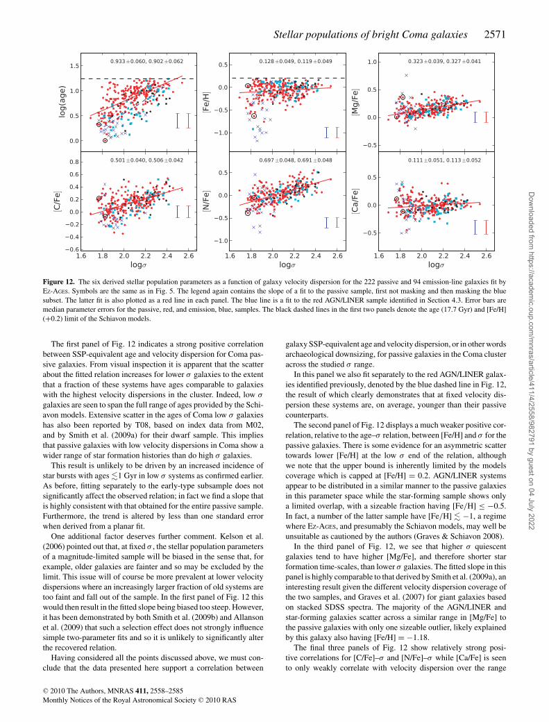
Stellar populations of bright Coma galaxies 2571
Figure 12. The six derived stellar population parameters as a function of galaxy velocity dispersion for the 222 passive and 94 emission-line galaxies fit byEZ-AGES. Symbols are the same as in Fig. 5. The legend again contains the slope of a fit to the passive sample, first not masking and then masking the bluesubset. The latter fit is also plotted as a red line in each panel. The blue line is a fit to the red AGN/LINER sample identified in Section 4.3. Error bars aremedian parameter errors for the passive, red, and emission, blue, samples. The black dashed lines in the first two panels denote the age (17.7 Gyr) and [Fe/H](+0.2) limit of the Schiavon models.
The first panel of Fig. 12 indicates a strong positive correlationbetween SSP-equivalent age and velocity dispersion for Coma pas-sive galaxies. From visual inspection it is apparent that the scatterabout the fitted relation increases for lower σ galaxies to the extentthat a fraction of these systems have ages comparable to galaxieswith the highest velocity dispersions in the cluster. Indeed, low σ
galaxies are seen to span the full range of ages provided by the Schi-avon models. Extensive scatter in the ages of Coma low σ galaxieshas also been reported by T08, based on index data from M02,and by Smith et al. (2009a) for their dwarf sample. This impliesthat passive galaxies with low velocity dispersions in Coma show awider range of star formation histories than do high σ galaxies.
This result is unlikely to be driven by an increased incidence ofstar bursts with ages �1 Gyr in low σ systems as confirmed earlier.As before, fitting separately to the early-type subsample does notsignificantly affect the observed relation; in fact we find a slope thatis highly consistent with that obtained for the entire passive sample.Furthermore, the trend is altered by less than one standard errorwhen derived from a planar fit.
One additional factor deserves further comment. Kelson et al.(2006) pointed out that, at fixed σ , the stellar population parametersof a magnitude-limited sample will be biased in the sense that, forexample, older galaxies are fainter and so may be excluded by thelimit. This issue will of course be more prevalent at lower velocitydispersions where an increasingly larger fraction of old systems aretoo faint and fall out of the sample. In the first panel of Fig. 12 thiswould then result in the fitted slope being biased too steep. However,it has been demonstrated by both Smith et al. (2009b) and Allansonet al. (2009) that such a selection effect does not strongly influencesimple two-parameter fits and so it is unlikely to significantly alterthe recovered relation.
Having considered all the points discussed above, we must con-clude that the data presented here support a correlation between
galaxy SSP-equivalent age and velocity dispersion, or in other wordsarchaeological downsizing, for passive galaxies in the Coma clusteracross the studied σ range.
In this panel we also fit separately to the red AGN/LINER galax-ies identified previously, denoted by the blue dashed line in Fig. 12,the result of which clearly demonstrates that at fixed velocity dis-persion these systems are, on average, younger than their passivecounterparts.
The second panel of Fig. 12 displays a much weaker positive cor-relation, relative to the age–σ relation, between [Fe/H] and σ for thepassive galaxies. There is some evidence for an asymmetric scattertowards lower [Fe/H] at the low σ end of the relation, althoughwe note that the upper bound is inherently limited by the modelscoverage which is capped at [Fe/H] = 0.2. AGN/LINER systemsappear to be distributed in a similar manner to the passive galaxiesin this parameter space while the star-forming sample shows onlya limited overlap, with a sizeable fraction having [Fe/H] ≤ −0.5.In fact, a number of the latter sample have [Fe/H] � −1, a regimewhere EZ-AGES, and presumably the Schiavon models, may well beunsuitable as cautioned by the authors (Graves & Schiavon 2008).
In the third panel of Fig. 12, we see that higher σ quiescentgalaxies tend to have higher [Mg/Fe], and therefore shorter starformation time-scales, than lower σ galaxies. The fitted slope in thispanel is highly comparable to that derived by Smith et al. (2009a), aninteresting result given the different velocity dispersion coverage ofthe two samples, and Graves et al. (2007) for giant galaxies basedon stacked SDSS spectra. The majority of the AGN/LINER andstar-forming galaxies scatter across a similar range in [Mg/Fe] tothe passive galaxies with only one sizeable outlier, likely explainedby this galaxy also having [Fe/H] = −1.18.
The final three panels of Fig. 12 show relatively strong posi-tive correlations for [C/Fe]–σ and [N/Fe]–σ while [Ca/Fe] is seento only weakly correlate with velocity dispersion over the range
C© 2010 The Authors, MNRAS 411, 2558–2585Monthly Notices of the Royal Astronomical Society C© 2010 RAS
Dow
nloaded from https://academ
ic.oup.com/m
nras/article/411/4/2558/982791 by guest on 04 July 2022

2572 J. Price et al.
studied here. Once more, the emission line galaxies occupy similarregions of each respective parameter space to the passive galaxieswith only a few star-forming outliers, typically with [Fe/H] ∼−1.The fitted slopes for [C/Fe], [N/Fe] and [Ca/Fe] are all in agreementwith those found by Graves et al. (2007) within the joint parame-ter uncertainties. They are somewhat larger than those reported bySmith et al. (2009a) for their simple two-parameter fits to Comadwarf galaxies. However, those fits may well be poorly constrainedgiven the narrow σ range covered by their dwarf sample.
4.5 Trends with Radius
In Fig. 13, we plot the measured stellar population parametersagainst cluster-centric radius for three out of four subsamples, only
excluding the star-forming systems again for clarity. The trend linesare linear least-squares fits to the raw data, weighted by their uncer-tainties, which are then binned for clarity. Each bin contains ∼28,∼11 and ∼7 galaxies per bin for the passive, AGN/LINER and AEDsamples, respectively. The results of these fits, including those tothe star-forming galaxies, are presented in Table 5 (first section).
For the quiescent galaxies significant correlations are obtainedfor log(age) (3.8σ ), [Mg/Fe] (3.5σ ) and [N/Fe] (4.4σ ). These trendstypically get marginally stronger when masking the blue subset. Nosignificant trend is seen for [Fe/H]. This implies passive galaxieson the outskirts of the cluster are, on average, 0.15 dex (∼2 Gyr)younger and have more extended star formation histories than thosein the cluster core. Both AGN/LINER galaxies and those with un-classified emission display significant age trends with comparable
Figure 13. Stellar population parameters as a function of projected cluster-centric radius for the passive and emission-line galaxies that were fit by EZ-AGES.Symbols are as in Fig. 6. Trend lines are fit to the raw data which are then binned with ∼27, ∼11 and ∼7 galaxies per bin for red, cyan and black bins,respectively. Star-forming galaxies are not plotted for clarity. The legend contains the slope of the passive galaxy fit, excluding the blue subset, and itssignificance.
Table 5. Stellar population parameter gradients per degree, from the linear fits presented in Fig. 13 and the planar fits displayed in Fig. 14. Thenumber of galaxies in each respective fit is displayed in parentheses in the table header and the significance of each fit in parentheses in the bodyof the table. For the passive sample the results in the first column include the blue subset while second column do not.
Parameter Passive (222/220) AGN/LINER (44) SF (24) AED (26)
Parameter – Rcc (Fig. 13)
log(age) −0.074 ± 0.019(3.8) −0.082 ± 0.018(4.4) −0.154 ± 0.033(4.6) 0.079 ± 0.067(1.2) −0.134 ± 0.046(2.9)[Fe/H] 0.029 ± 0.014(2.1) 0.029 ± 0.014(2.0) −0.004 ± 0.025(0.2) 0.097 ± 0.061(1.6) 0.019 ± 0.034(0.6)
[Mg/Fe] −0.042 ± 0.012(3.5) −0.043 ± 0.011(3.8) 0.006 ± 0.019(0.3) 0.061 ± 0.056(1.1) −0.026 ± 0.028(0.9)[C/Fe] 0.023 ± 0.012(1.9) 0.023 ± 0.012(1.9) −0.025 ± 0.023(1.1) 0.069 ± 0.055(1.3) −0.009 ± 0.030(0.3)[N/Fe] −0.061 ± 0.014(4.4) −0.064 ± 0.015(4.4) −0.025 ± 0.024(1.0) −0.269 ± 0.060(4.5) −0.029 ± 0.034(0.9)[Ca/Fe] −0.014 ± 0.015(1.0) −0.014 ± 0.015(0.9) −0.007 ± 0.026(0.3) −0.116 ± 0.076(1.5) −0.027 ± 0.035(0.8)
δParameter – Rcc (Fig. 14)
log(age) −0.041 ± 0.018(2.3) −0.047 ± 0.018(2.6) −0.081 ± 0.036(2.2) 0.085 ± 0.079(1.1) −0.090 ± 0.053(1.7)[Fe/H] 0.029 ± 0.015(1.9) 0.028 ± 0.016(1.8) −0.011 ± 0.025(0.5) 0.065 ± 0.061(1.1) 0.004 ± 0.042(0.1)
[Mg/Fe] −0.033 ± 0.011(2.9) −0.033 ± 0.010(3.3) 0.022 ± 0.022(1.0) 0.076 ± 0.057(1.3) −0.004 ± 0.034(0.1)[C/Fe] 0.037 ± 0.012(3.1) 0.039 ± 0.012(3.3) 0.014 ± 0.024(0.6) 0.070 ± 0.052(1.3) 0.001 ± 0.033(0.0)[N/Fe] −0.042 ± 0.014(3.0) −0.044 ± 0.014(3.1) −0.004 ± 0.026(0.2) −0.229 ± 0.068(3.4) −0.010 ± 0.041(0.3)[Ca/Fe] −0.012 ± 0.015(0.8) −0.012 ± 0.016(0.7) 0.004 ± 0.027(0.2) −0.130 ± 0.079(1.6) −0.019 ± 0.049(0.4)
C© 2010 The Authors, MNRAS 411, 2558–2585Monthly Notices of the Royal Astronomical Society C© 2010 RAS
Dow
nloaded from https://academ
ic.oup.com/m
nras/article/411/4/2558/982791 by guest on 04 July 2022
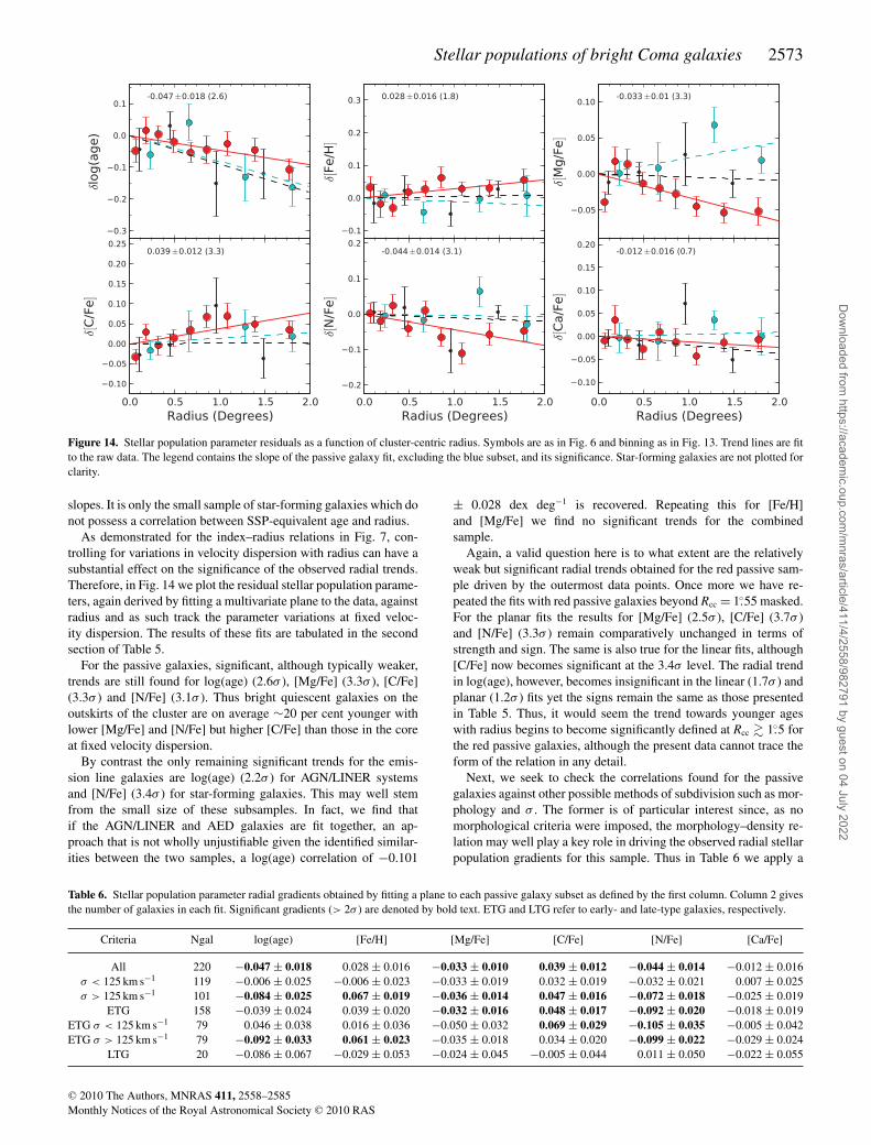
Stellar populations of bright Coma galaxies 2573
Figure 14. Stellar population parameter residuals as a function of cluster-centric radius. Symbols are as in Fig. 6 and binning as in Fig. 13. Trend lines are fitto the raw data. The legend contains the slope of the passive galaxy fit, excluding the blue subset, and its significance. Star-forming galaxies are not plotted forclarity.
slopes. It is only the small sample of star-forming galaxies which donot possess a correlation between SSP-equivalent age and radius.
As demonstrated for the index–radius relations in Fig. 7, con-trolling for variations in velocity dispersion with radius can have asubstantial effect on the significance of the observed radial trends.Therefore, in Fig. 14 we plot the residual stellar population parame-ters, again derived by fitting a multivariate plane to the data, againstradius and as such track the parameter variations at fixed veloc-ity dispersion. The results of these fits are tabulated in the secondsection of Table 5.
For the passive galaxies, significant, although typically weaker,trends are still found for log(age) (2.6σ ), [Mg/Fe] (3.3σ ), [C/Fe](3.3σ ) and [N/Fe] (3.1σ ). Thus bright quiescent galaxies on theoutskirts of the cluster are on average ∼20 per cent younger withlower [Mg/Fe] and [N/Fe] but higher [C/Fe] than those in the coreat fixed velocity dispersion.
By contrast the only remaining significant trends for the emis-sion line galaxies are log(age) (2.2σ ) for AGN/LINER systemsand [N/Fe] (3.4σ ) for star-forming galaxies. This may well stemfrom the small size of these subsamples. In fact, we find thatif the AGN/LINER and AED galaxies are fit together, an ap-proach that is not wholly unjustifiable given the identified similar-ities between the two samples, a log(age) correlation of −0.101
± 0.028 dex deg−1 is recovered. Repeating this for [Fe/H]and [Mg/Fe] we find no significant trends for the combinedsample.
Again, a valid question here is to what extent are the relativelyweak but significant radial trends obtained for the red passive sam-ple driven by the outermost data points. Once more we have re-peated the fits with red passive galaxies beyond Rcc = 1.◦55 masked.For the planar fits the results for [Mg/Fe] (2.5σ ), [C/Fe] (3.7σ )and [N/Fe] (3.3σ ) remain comparatively unchanged in terms ofstrength and sign. The same is also true for the linear fits, although[C/Fe] now becomes significant at the 3.4σ level. The radial trendin log(age), however, becomes insignificant in the linear (1.7σ ) andplanar (1.2σ ) fits yet the signs remain the same as those presentedin Table 5. Thus, it would seem the trend towards younger ageswith radius begins to become significantly defined at Rcc � 1.◦5 forthe red passive galaxies, although the present data cannot trace theform of the relation in any detail.
Next, we seek to check the correlations found for the passivegalaxies against other possible methods of subdivision such as mor-phology and σ . The former is of particular interest since, as nomorphological criteria were imposed, the morphology–density re-lation may well play a key role in driving the observed radial stellarpopulation gradients for this sample. Thus in Table 6 we apply a
Table 6. Stellar population parameter radial gradients obtained by fitting a plane to each passive galaxy subset as defined by the first column. Column 2 givesthe number of galaxies in each fit. Significant gradients (> 2σ ) are denoted by bold text. ETG and LTG refer to early- and late-type galaxies, respectively.
Criteria Ngal log(age) [Fe/H] [Mg/Fe] [C/Fe] [N/Fe] [Ca/Fe]
All 220 −0.047 ± 0.018 0.028 ± 0.016 −0.033 ± 0.010 0.039 ± 0.012 −0.044 ± 0.014 −0.012 ± 0.016σ < 125 km s−1 119 −0.006 ± 0.025 −0.006 ± 0.023 −0.033 ± 0.019 0.032 ± 0.019 −0.032 ± 0.021 0.007 ± 0.025σ > 125 km s−1 101 −0.084 ± 0.025 0.067 ± 0.019 −0.036 ± 0.014 0.047 ± 0.016 −0.072 ± 0.018 −0.025 ± 0.019
ETG 158 −0.039 ± 0.024 0.039 ± 0.020 −0.032 ± 0.016 0.048 ± 0.017 −0.092 ± 0.020 −0.018 ± 0.019ETG σ < 125 km s−1 79 0.046 ± 0.038 0.016 ± 0.036 −0.050 ± 0.032 0.069 ± 0.029 −0.105 ± 0.035 −0.005 ± 0.042ETG σ > 125 km s−1 79 −0.092 ± 0.033 0.061 ± 0.023 −0.035 ± 0.018 0.034 ± 0.020 −0.099 ± 0.022 −0.029 ± 0.024
LTG 20 −0.086 ± 0.067 −0.029 ± 0.053 −0.024 ± 0.045 −0.005 ± 0.044 0.011 ± 0.050 −0.022 ± 0.055
C© 2010 The Authors, MNRAS 411, 2558–2585Monthly Notices of the Royal Astronomical Society C© 2010 RAS
Dow
nloaded from https://academ
ic.oup.com/m
nras/article/411/4/2558/982791 by guest on 04 July 2022

2574 J. Price et al.
Table 7. Comparison between the results obtained for this work’s passivegalaxies, both full sample and core-South-West, and those in the literature.S06 gradients are again converted to per degree assuming R200 = 1.◦59 forComa, and we assume their [α/Fe] gradient is comparable to our [Mg/Fe]gradient.
Source log(age) [Mg/Fe]
This work: all passive −0.047 ± 0.018 −0.033 ± 0.010This work: passive Core-SW −0.041 ± 0.048 −0.047 ± 0.028S08 (Coma dwarfs) −0.369 ± 0.069 −0.128 ± 0.039S06 −0.045 ± 0.011 −0.030 ± 0.006
variety of further cuts to the quiescent galaxies excluding the twoparticularly blue early-type galaxies.
First, the sample is split into subsets based on their velocitydispersion into low (σ < 125 km s−1) and high (σ > 125 km s−1)velocity dispersion bins. Here, we see that, most notably, significanttrends in log(age) (3.2σ ) and [Fe/H] (3.3σ ) are recovered for thehigh σ sample. Next, we separate the sample into early- and late-type galaxies based on their NED morphologies. Here we find thatthe former does not have a significant radial age gradient, though it isconsistent with that found for the passive galaxies as a whole takinginto account the fact that these two samples are not independent.For the latter we find a sizable but insignificant negative trend. Atface value one might now be tempted to conclude that the gradientfound for the entire sample (−0.047 ± 0.018 dex deg−1) may wellbe driven by a combination of a very weak trend in the early-typegalaxies modulated by a larger negative gradient in the late-typegalaxies. To test this, we subdivide the early-type galaxies into lowand high σ bins. Interestingly, we find that the higher σ early-type galaxies possess a strong negative age gradient, comparable inmagnitude to the late-types, while the low σ early-types show nosignificant gradient. This perhaps implies that the radial variation ofthe stellar populations of early-type galaxies in Coma may be morecomplex than the simple planar model applied here. Nevertheless,we confirm that the morphology–density relation does not drive thelog(age)–radius correlation seen for the passive sample.
In Table 7, we present a comparison of the significant results ob-tained in this work for the passive galaxies to those studies featuredpreviously in Table 3, excluding C02 who did not derive log(age) or[Mg/Fe] gradients. Again, we fit separately to the Core-SW region
subsample. We consider the [α/Fe] result of S06 comparable to our[Mg/Fe] gradient. From this table it is immediately apparent thathighly consistent age and abundance ratio gradients are found bythis work and S06, despite each using different SSP models. It alsoindicates that S08 derived much stronger trends for their dwarf sam-ple. We confirm that for bright Coma galaxies a limited azimuthalcoverage does not result in significantly stronger gradients, againtaking into account that the overall and Core-SW samples are notindependent.
4.6 The Z-plane
It was Trager et al. (2000a) who first highlighted an anti-correlationbetween age and metallicity at a fixed velocity dispersion in early-type galaxies, terming it the Z-plane. In physical terms this relationimplies that younger galaxies, in an SSP-equivalent sense, haveplayed host to a larger number of stellar generations allowing forgreater metallic enrichment relative to older galaxies. To test forsuch a trend in our data, we fit our quiescent sample with an Fe-plane of the form
[Fe/H] = a log σ + b log age + c,
where the coefficients a and b give the dependence of [Fe/H] on σ
at a fixed age and on age at fixed σ , respectively. The fit is weightedby errors in [Fe/H] and age but no attempt to account for correlatederrors is made at this stage (but see below). We recover a = 0.93 ±0.10, b = −0.90 ± 0.08 and c = −1.24 ± 0.17 with an rms scatterof 0.17, and in Fig. 15 plot two projections of the fitted plane. Theslope of [Fe/H] with σ is steeper than that found by Trager et al.(2000a), a = 0.48 ± 0.12, and by Smith et al. (2009a) for theirComa dwarf sample, a = 0.51 ± 0.2. However, the age–metallicitycorrelation we derive is comparable within the joint errors to thatobtained by both works, b = −0.74 ± 0.09 from the former andb = −0.74 ± 0.14 from the latter. We estimate an intrinsic scatterof 0.13 in [Fe/H] and in the left-hand panel of Fig. 15, just by eye,note an increased scatter for lower σ galaxies, as also found bySmith et al. (2009a). Quantitatively, the intrinsic scatter increasesfrom 0.04 for log σ > 2.1 to 0.17 for log σ < 2.1.
Correlated errors between age and [Fe/H] can be a seriousproblem when trying to establish whether an age–metallicity anti-correlation exists at a fixed velocity dispersion (e.g. Trager et al.
Figure 15. Two edge on views of our version of the Trager et al. (2000a) Z-plane, plotted here as an Fe-plane, for our quiescent sample. In the right-handpanel we plot a typical 68 per cent confidence error ellipse which, as discussed in the text, is nearly parallel to the observed age–metallicity anti-correlation.The dashed line in this panel shows the best-fitting relation.
C© 2010 The Authors, MNRAS 411, 2558–2585Monthly Notices of the Royal Astronomical Society C© 2010 RAS
Dow
nloaded from https://academ
ic.oup.com/m
nras/article/411/4/2558/982791 by guest on 04 July 2022
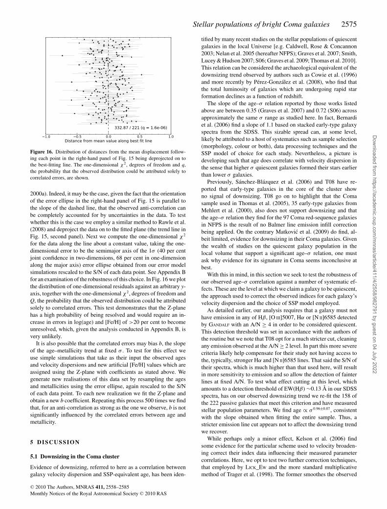
Stellar populations of bright Coma galaxies 2575
Figure 16. Distribution of distances from the mean displacement follow-ing each point in the right-hand panel of Fig. 15 being deprojected on tothe best-fitting line. The one-dimensional χ2, degrees of freedom and q,the probability that the observed distribution could be attributed solely tocorrelated errors, are shown.
2000a). Indeed, it may be the case, given the fact that the orientationof the error ellipse in the right-hand panel of Fig. 15 is parallel tothe slope of the dashed line, that the observed anti-correlation canbe completely accounted for by uncertainties in the data. To testwhether this is the case we employ a similar method to Rawle et al.(2008) and deproject the data on to the fitted plane (the trend line inFig. 15, second panel). Next we compute the one-dimensional χ 2
for the data along the line about a constant value, taking the one-dimensional error to be the semimajor axis of the 1σ (40 per centjoint confidence in two-dimensions, 68 per cent in one-dimensionalong the major axis) error ellipse obtained from our error modelsimulations rescaled to the S/N of each data point. See Appendix Bfor an examination of the robustness of this choice. In Fig. 16 we plotthe distribution of one-dimensional residuals against an arbitrary y-axis, together with the one-dimensional χ 2, degrees of freedom andQ, the probability that the observed distribution could be attributedsolely to correlated errors. This test demonstrates that the Z-planehas a high probability of being resolved and would require an in-crease in errors in log(age) and [Fe/H] of >20 per cent to becomeunresolved, which, given the analysis conducted in Appendix B, isvery unlikely.
It is also possible that the correlated errors may bias b, the slopeof the age–metallicity trend at fixed σ . To test for this effect weuse simple simulations that take as their input the observed agesand velocity dispersions and new artificial [Fe/H] values which areassigned using the Z-plane with coefficients as stated above. Wegenerate new realisations of this data set by resampling the agesand metallicities using the error ellipse, again rescaled to the S/Nof each data point. To each new realization we fit the Z-plane andobtain a new b coefficient. Repeating this process 500 times we findthat, for an anti-correlation as strong as the one we observe, b is notsignificantly influenced by the correlated errors between age andmetallicity.
5 D ISCUSSION
5.1 Downsizing in the Coma cluster
Evidence of downsizing, referred to here as a correlation betweengalaxy velocity dispersion and SSP-equivalent age, has been iden-
tified by many recent studies on the stellar populations of quiescentgalaxies in the local Universe [e.g. Caldwell, Rose & Concannon2003; Nelan et al. 2005 (hereafter NFPS); Graves et al. 2007; Smith,Lucey & Hudson 2007; S06; Graves et al. 2009; Thomas et al. 2010].This relation can be considered the archaeological equivalent of thedownsizing trend observed by authors such as Cowie et al. (1996)and more recently by Perez-Gonzalez et al. (2008), who find thatthe total luminosity of galaxies which are undergoing rapid starformation declines as a function of redshift.
The slope of the age–σ relation reported by those works listedabove are between 0.35 (Graves et al. 2007) and 0.72 (S06) acrossapproximately the same σ range as studied here. In fact, Bernardiet al. (2006) find a slope of 1.1 based on stacked early-type galaxyspectra from the SDSS. This sizable spread can, at some level,likely be attributed to a host of systematics such as sample selection(morphology, colour or both), data processing techniques and theSSP model of choice for each study. Nevertheless, a picture isdeveloping such that age does correlate with velocity dispersion inthe sense that higher σ quiescent galaxies formed their stars earlierthan lower σ galaxies.
Previously, Sanchez-Blazquez et al. (2006) and T08 have re-ported that early-type galaxies in the core of the cluster showno signal of downsizing. T08 go on to highlight that the Comasample used in Thomas et al. (2005), 35 early-type galaxies fromMehlert et al. (2000), also does not support downsizing and thatthe age–σ relation they find for the 97 Coma red-sequence galaxiesin NFPS is the result of no Balmer line emission infill correctionbeing applied. On the contrary Matkovic et al. (2009) do find, al-beit limited, evidence for downsizing in their Coma galaxies. Giventhe wealth of studies on the quiescent galaxy population in thelocal volume that support a significant age–σ relation, one mustask why evidence for its signature in Coma seems inconclusive atbest.
With this in mind, in this section we seek to test the robustness ofour observed age–σ correlation against a number of systematic ef-fects. These are the level at which we claim a galaxy to be quiescent,the approach used to correct the observed indices for each galaxy’svelocity dispersion and the choice of SSP model employed.
As detailed earlier, our analysis requires that a galaxy must nothave emission in any of Hβ, [O III]5007, Hα or [N II]6585 detectedby GANDALF with an A/N ≥ 4 in order to be considered quiescent.This detection threshold was set in accordance with the authors ofthe routine but we note that T08 opt for a much stricter cut, cleaningany emission observed at the A/N ≥ 2 level. In part this more severecriteria likely help compensate for their study not having access tothe, typically, stronger Hα and [N II]6585 lines. That said the S/N oftheir spectra, which is much higher than that used here, will resultin more sensitivity to emission and so allow the detection of fainterlines at fixed A/N. To test what effect cutting at this level, whichamounts to a detection threshold of EW(Hβ) ∼0.13 Å in our SDSSspectra, has on our observed downsizing trend we re-fit the 158 ofthe 222 passive galaxies that meet this criterion and have measuredstellar population parameters. We find age ∝ σ 0.96±0.07, consistentwith the slope obtained when fitting the entire sample. Thus, astricter emission line cut appears not to affect the downsizing trendwe recover.
While perhaps only a minor effect, Kelson et al. (2006) findsome evidence for the particular scheme used to velocity broaden-ing correct their index data influencing their measured parametercorrelations. Here, we opt to test two further correction techniques,that employed by LICK_EW and the more standard multiplicativemethod of Trager et al. (1998). The former smoothes the observed
C© 2010 The Authors, MNRAS 411, 2558–2585Monthly Notices of the Royal Astronomical Society C© 2010 RAS
Dow
nloaded from https://academ
ic.oup.com/m
nras/article/411/4/2558/982791 by guest on 04 July 2022
2576 J. Price et al.
spectra by σsmooth =√
σ 2lick − σ 2
res − σ 2gal where σ lick is the Lick res-
olution of the particular index being measured (taken from table 1 ofSchiavon 2007), σ res is the SDSS instrumental resolution and σ gal isthe galaxy velocity dispersion. Should the sign of the term under thesquare root turn negative the code uses multiplicative correctionsbased on smoothed SSP spectra from Schiavon (2007). We takethe velocity broadening polynomial coefficients for the Trager et al.(1998) multiplicative method from their table 5. The technique usedby LICK_EW yields age ∝ σ 0.83±0.07 while the multiplicative routegives age ∝ σ 0.78±0.06. Thus, while the latter is a shallower trend,our correction scheme and both of those tested produce consistentresults within the joint errors.
To test the model dependence of our observed downsizing trendwe make use of the empirically derived transformations of Smithet al. (2009a) to convert our stellar population parameters to theTMBK model system. Fitting the age–σ relation to the transformeddata we find age ∝ σ 0.83±0.06. Again this is consistent, within thejoint uncertainties, to the result obtained when the Schiavon modelsare employed.
In summary, following the above tests, and those conducted ear-lier, we conclude that our SDSS data do robustly support downsiz-ing in both early-type and passive galaxy populations in the Comacluster. As demonstrated in Appendix A, we have found good con-sistency between this work and NFPS in terms of derived age–σ
relations. We speculate that small sample size may well explain theabsence of downsizing seen by T08 using their Keck/LRIS data,given the sizable scatter in the first panel of Fig. 12. Furthermore,we have identified that, for galaxies which are in both studies, theM02 data set results in a significantly flatter Hβ–σ slope than thiswork. This issue, with as yet unknown origin, may well drive T08to conclude the M02 data display no age–σ correlation.
5.2 Environment
The Coma cluster is an ideal place to study how environment affectsthe stellar populations of galaxies across a wide range of localdensities. Its core represents one of the highest density regions thatis readily observable for line strength studies while the cluster’soutskirts provide excellent insight into galaxies that are, perhaps forthe first time, just starting to feel the effects of a cluster environment.Indeed, evidence has been mounting for some time that galaxies inthe cluster’s core display systematically different line indices, andby inference stellar populations, than those in the outer regions.
The first study to highlight the spatial dependence of the stel-lar populations of Coma members using line indices was that ofGuzman et al. (1992). They observed 51 Coma elliptical galaxieslocated in the cluster’s core and ‘halo’, defined by them having aprojected radius of 1◦ < R < 5◦, with σ > 100 km s−1. As such, theirsample is comparable to the high σ end of this work. They foundthat their Mg2–σ relation displayed a small environmental depen-dence such that, at fixed σ , galaxies in the core have higher indexstrengths than those in the cluster’s halo. Employing early stellarpopulation models, they went on to attribute this trend to variationsin age with younger galaxies at larger cluster-centric radii.
Shortly after the work of Guzman et al., the aforementionedstudy of Caldwell et al. (1993) uncovered a sample of post-starburstearly-type galaxies in the outer south-west region of the cluster.These galaxies were identified based on their strong high-orderBalmer lines, indicative of a subpopulation of A stars with lifetimes∼1 Gyr. Caldwell et al. could not comment further on whether thispost-starburst population were localized to the NGC 4839 subgroup
or spatially a more general phenomenon, as they were only able toobserve one field on the clusters’ outskirts (although see Cald-well & Rose 1997). That said, very recently Mahajan, Haines &Raychaudhury (2010) found that k+a galaxies in Coma are in factuniformly distributed about the cluster, only avoiding regions withsubstantial X-ray emission such as the core.
C02 once more addressed the effect of environment on the stellarpopulations of Coma members, this time spanning a wide rangein total magnitude from dwarf to giants, using Lick indices. Theyfound evidence for a significant radial gradient in Mg2, even afterfactoring out the index’s correlation with luminosity. As previouslymentioned, based on the weaker trends they recovered for Hβ,they interpreted this as a metallicity gradient. More recently, S08have concluded that the radial index trends in a sample of red-sequence Coma dwarf galaxies in fact support a strong gradient intheir SSP-equivalent ages, with older dwarfs preferentially foundin the cluster’s core. Again neither of these studies were able tocomment on the generality of this gradient due to limited azimuthalcoverage.
The results for our quiescent sample, presented in Table 5, providefurther support for an interpretation of the observed radial indextrends in terms of variations in galaxy age rather than metallicity. Wealso find evidence for significant gradients in [Mg/Fe], [C/Fe] and[N/Fe]. These findings indicate that passive galaxies on the outskirtsof the cluster are younger, formed their stars over a longer period oftime and have higher [C/Fe] but lower [N/Fe] than galaxies locatedin the cluster’s core. Furthermore, when considering our core-south-west subsample we find no significant increase in recovered age or[Mg/Fe] gradients, providing the first hint that, at least for brightgalaxies, the south-west field is not unique.
In Tables 3 and 7, we have shown that the samples of S08 andC02 typically display much stronger cluster-centric radial gradientsin terms of line indices and stellar population parameters than de-rived for our sample. We have proposed that this finding can beattributed to the differing luminosity coverage of the three samplesrather than a bias being introduced by S08 and C02 only observ-ing the cluster’s south-west region. Taken together this implies thateither brighter galaxies had finished forming the majority of theirstars before entering the cluster, star formation within these systemswas less affected by the cluster environment, or some mix of thetwo. The former relies on such galaxies having undergone substan-tial pre-processing in groups (e.g. Kodama & Smail 2001; McGeeet al. 2009) prior to being accreted into the cluster while the lattercan likely be put down to their deeper potential wells being bet-ter able to retain gas for star formation. Irrespective of the precisescenario, our results indicate that the stellar populations of brightgalaxies are less influenced by entry into the cluster environmentthan those of dwarf galaxies. Furthermore, this picture fits wellwith that discussed by Gavazzi et al. (2010). They studied galaxiesin the Coma supercluster and report that the colours and luminositydistributions of high-luminosity galaxies display little environmen-tal dependence relative to those of low-luminosity galaxies. Thus,they propose a scenario where the former were in place at earliertimes while the latter are currently, cosmologically speaking, under-going environmentally driven transformations as they enter denserstructures.
We have also compared our findings to those from S06 whostudied quiescent galaxies in a host of nearby clusters across acomparable σ range to this work. Using a similar planar analysistechnique to that used here but employing different SSP models,they found average cluster-centric radial gradients that are highlyconsistent with those reported here.
C© 2010 The Authors, MNRAS 411, 2558–2585Monthly Notices of the Royal Astronomical Society C© 2010 RAS
Dow
nloaded from https://academ
ic.oup.com/m
nras/article/411/4/2558/982791 by guest on 04 July 2022
Stellar populations of bright Coma galaxies 2577
In terms of other recent more general studies, Bernardi et al.(2006) and Clemens et al. (2009) both used large samples of early-type galaxies selected from the SDSS to test the environmentaldependence of their stellar populations. Using differing techniques,they split galaxies into high and low local galaxy density subsam-ples. Here, we note that the outskirts of Coma are unlikely to becomparable to low density or field regions due to the pre-processingof infalling galaxies. Nevertheless, both studies report that early-types in low-density regions are systematically younger than thosein high-density environments, in agreement with our results. Bycontrast, Clemens et al. (2009) find marginal evidence that [Z/H]is lower in dense regions but that [α/Fe] does not depend on envi-ronment, while Bernardi et al. (2006) identify no [Z/H] correlationbut conclude that α-enhancement is greater in high-density regions.Thus, it would appear the latter study fits better with our findings.
Finally, we are able to compare our results with the predictionsfrom the semi-analytic galaxy formation models of De Lucia et al.(2006). Their fig. 8(a) indicates how galaxy median luminosity-weighted age varies, on average, as a function of physical dis-tance out from cluster centres. While direct comparison is compli-cated by deprojection effects, mass segregation and conversion fromluminosity-weighted to SSP-equivalent age (Trager & Somerville2009), this figure predicts a typical change of ∼13 per cent between0.1R200 and R200. This trend is consistent with our finding of 19 ±8 per cent within the same radial range in Coma. In addition, ourresults qualitatively agree with those from the N-body simulationsof Gao et al. (2004). They find that subhaloes located near the centreof cluster-sized parent haloes were accreted earlier. Thus, a com-bination of this correlation with any mechanism that acts to inhibitstar formation in galaxies as they enter the cluster environment willlead to a cluster-centric radial gradient in their stellar populations.
6 C O N C L U S I O N S
In this paper we have studied the stellar populations of bright Comacluster galaxies using SDSS archival spectroscopy and up-to-dateSSP models. The key findings of this work can be summarized asfollows.
(i) Of the 110 galaxies (31 per cent of the entire sample) withdetectable emission we find 46 per cent show AGN/LINER likeemission, 29 per cent have ongoing star formation and 25 per centhave an ambiguous emission driver based on these data. The fractionof AGN/LINER systems is seen to increase with increasing galaxyluminosity while the star-forming fraction decreases.
(ii) For the 246 passive galaxies that meet our selection criteriawe find strong correlations between absorption-line index strengthand velocity dispersion for CN2, C4668, Mgb and Hβ. Particularlyin the case of Hβ, scatter about these relations is seen to increasewith decreasing velocity dispersion. At low σ the emission linegalaxies typically have stronger Hβ and weaker metal lines thanquiescent galaxies, while at high σ both subsets have comparableindex strengths. This trend is driven by the aforementioned tran-sition from star-forming to AGN/LINER galaxies with increasingluminosity, and therefore σ .
(iii) Using a planar analysis technique that factors out index cor-relations with σ , we find significant cluster-centric radial gradientsin Hβ, Mgb and C4668 for passive galaxies. Comparing our re-sults with those of other recent studies that typically show strongerradial index gradients, we have shown that this difference can beattributed to the luminosity range covered by each study and not theuniqueness of the NGC 4839 infall region.
(iv) We have demonstrated that the vast majority of our passivesample do not play host to a frosting of young (�1 Gyr) stars ontop of an underlying, mass-dominant old population.
(v) For 222 passive galaxies in Coma we find a strong positivecorrelation between their SSP-equivalent age and velocity disper-sion. The scatter about this relation increases towards lower σ .This trend is found to be robust against variations in sample selec-tion criteria (early-type versus quiescent), emission line detectionthresholds, index velocity broadening corrections and the particularSSP model employed. Weaker positive correlations are recoveredbetween σ and [Fe/H], [Mg/Fe], [C/Fe] and [N/Fe]. Thus, higherσ quiescent galaxies in Coma are found to have formed their starsearlier, more rapidly and with higher [Fe/H], [C/Fe] and [N/Fe] thancluster members with lower velocity dispersions.
(vi) Galaxies which show AGN/LINER emission are typicallyfound to have younger SSP-equivalent ages than quiescent galaxiesat fixed velocity dispersion.
(vii) Significant cluster-centric radial stellar population gradientsare found for our passive sample in terms of their SSP-equivalentage, [Mg/Fe], [C/Fe] and [N/Fe]. These trends are in the sensethat, at fixed σ , galaxies on the cluster’s outskirts are younger,formed stars over a longer period of time and have higher [C/Fe]but lower [N/Fe]. Again, we attribute fainter luminosity coveragerather than the uniqueness of the NGC 4839 group as the driver forthe stronger radial gradients found by other recent studies. We findthat the morphology–density relation does not drive the recoveredage–radius relation.
(viii) Interpreting galaxies with barely detectable emission asweak AGN/LINER systems, galaxies with this emission driver arefound to have a significant cluster-centric radial gradient in theirSSP-equivalent ages. This trend is more than a factor of 2 strongerthan that seen for quiescent galaxies.
(ix) Finally, for our passive sample we have found an age–metallicity anti-correlation that is consistent with previous works.We have shown that this anti-correlation is resolved, and so is notthe result of correlated errors between age and metallicity, and thatcorrelated errors do not significantly bias the measured slope.
We have demonstrated that the stellar populations of bright qui-escent galaxies in Coma depend strongly on their σ and, relativeto dwarf cluster members in the south-west, less so on their localenvironment. We have also shown that the stellar populations ofsuch galaxies in the NGC 4839 infall region are not unique withrespect to galaxies elsewhere in the outskirts of the cluster. In aforthcoming paper, we will explore these two related issues usingan enlarged sample of faint galaxies. First, to determine whether thestrong environmental trends seen for dwarf galaxies in the south-west are localized there or a more general effect in the outskirts ofthe cluster. Secondly, to identify the transition σ , or range of veloc-ity dispersions, at which the stellar populations of a galaxy start tobecome significantly more affected by its local environment.
AC K N OW L E D G M E N T S
JP acknowledges support from the UK Science and TechnologyFacilities Council. SP and AH acknowledge the support of a grantfrom The Leverhulme Trust to the University of Bristol. RJS wassupported for this work by STFC Rolling Grant PP/C501568/1‘Extragalactic Astronomy and Cosmology at Durham 2008–2013’.
We thank Mark Taylor for writing Tool for Operations on Cat-alogues And Tables (http://www.star.bris.ac.uk/∼mbt/topcat/) andproviding support on its use. Finally, we thank our referee for
C© 2010 The Authors, MNRAS 411, 2558–2585Monthly Notices of the Royal Astronomical Society C© 2010 RAS
Dow
nloaded from https://academ
ic.oup.com/m
nras/article/411/4/2558/982791 by guest on 04 July 2022
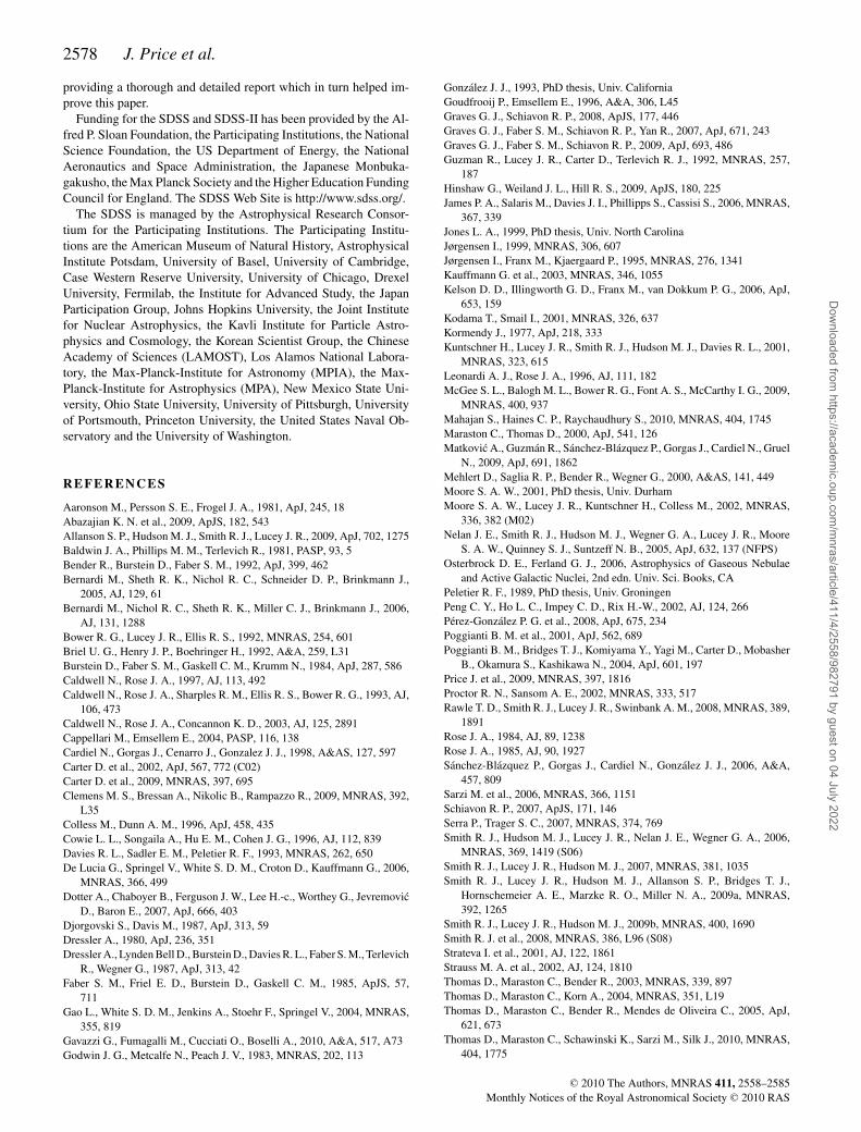
2578 J. Price et al.
providing a thorough and detailed report which in turn helped im-prove this paper.
Funding for the SDSS and SDSS-II has been provided by the Al-fred P. Sloan Foundation, the Participating Institutions, the NationalScience Foundation, the US Department of Energy, the NationalAeronautics and Space Administration, the Japanese Monbuka-gakusho, the Max Planck Society and the Higher Education FundingCouncil for England. The SDSS Web Site is http://www.sdss.org/.
The SDSS is managed by the Astrophysical Research Consor-tium for the Participating Institutions. The Participating Institu-tions are the American Museum of Natural History, AstrophysicalInstitute Potsdam, University of Basel, University of Cambridge,Case Western Reserve University, University of Chicago, DrexelUniversity, Fermilab, the Institute for Advanced Study, the JapanParticipation Group, Johns Hopkins University, the Joint Institutefor Nuclear Astrophysics, the Kavli Institute for Particle Astro-physics and Cosmology, the Korean Scientist Group, the ChineseAcademy of Sciences (LAMOST), Los Alamos National Labora-tory, the Max-Planck-Institute for Astronomy (MPIA), the Max-Planck-Institute for Astrophysics (MPA), New Mexico State Uni-versity, Ohio State University, University of Pittsburgh, Universityof Portsmouth, Princeton University, the United States Naval Ob-servatory and the University of Washington.
REFERENCES
Aaronson M., Persson S. E., Frogel J. A., 1981, ApJ, 245, 18Abazajian K. N. et al., 2009, ApJS, 182, 543Allanson S. P., Hudson M. J., Smith R. J., Lucey J. R., 2009, ApJ, 702, 1275Baldwin J. A., Phillips M. M., Terlevich R., 1981, PASP, 93, 5Bender R., Burstein D., Faber S. M., 1992, ApJ, 399, 462Bernardi M., Sheth R. K., Nichol R. C., Schneider D. P., Brinkmann J.,
2005, AJ, 129, 61Bernardi M., Nichol R. C., Sheth R. K., Miller C. J., Brinkmann J., 2006,
AJ, 131, 1288Bower R. G., Lucey J. R., Ellis R. S., 1992, MNRAS, 254, 601Briel U. G., Henry J. P., Boehringer H., 1992, A&A, 259, L31Burstein D., Faber S. M., Gaskell C. M., Krumm N., 1984, ApJ, 287, 586Caldwell N., Rose J. A., 1997, AJ, 113, 492Caldwell N., Rose J. A., Sharples R. M., Ellis R. S., Bower R. G., 1993, AJ,
106, 473Caldwell N., Rose J. A., Concannon K. D., 2003, AJ, 125, 2891Cappellari M., Emsellem E., 2004, PASP, 116, 138Cardiel N., Gorgas J., Cenarro J., Gonzalez J. J., 1998, A&AS, 127, 597Carter D. et al., 2002, ApJ, 567, 772 (C02)Carter D. et al., 2009, MNRAS, 397, 695Clemens M. S., Bressan A., Nikolic B., Rampazzo R., 2009, MNRAS, 392,
L35Colless M., Dunn A. M., 1996, ApJ, 458, 435Cowie L. L., Songaila A., Hu E. M., Cohen J. G., 1996, AJ, 112, 839Davies R. L., Sadler E. M., Peletier R. F., 1993, MNRAS, 262, 650De Lucia G., Springel V., White S. D. M., Croton D., Kauffmann G., 2006,
MNRAS, 366, 499Dotter A., Chaboyer B., Ferguson J. W., Lee H.-c., Worthey G., Jevremovic
D., Baron E., 2007, ApJ, 666, 403Djorgovski S., Davis M., 1987, ApJ, 313, 59Dressler A., 1980, ApJ, 236, 351Dressler A., Lynden Bell D., Burstein D., Davies R. L., Faber S. M., Terlevich
R., Wegner G., 1987, ApJ, 313, 42Faber S. M., Friel E. D., Burstein D., Gaskell C. M., 1985, ApJS, 57,
711Gao L., White S. D. M., Jenkins A., Stoehr F., Springel V., 2004, MNRAS,
355, 819Gavazzi G., Fumagalli M., Cucciati O., Boselli A., 2010, A&A, 517, A73Godwin J. G., Metcalfe N., Peach J. V., 1983, MNRAS, 202, 113
Gonzalez J. J., 1993, PhD thesis, Univ. CaliforniaGoudfrooij P., Emsellem E., 1996, A&A, 306, L45Graves G. J., Schiavon R. P., 2008, ApJS, 177, 446Graves G. J., Faber S. M., Schiavon R. P., Yan R., 2007, ApJ, 671, 243Graves G. J., Faber S. M., Schiavon R. P., 2009, ApJ, 693, 486Guzman R., Lucey J. R., Carter D., Terlevich R. J., 1992, MNRAS, 257,
187Hinshaw G., Weiland J. L., Hill R. S., 2009, ApJS, 180, 225James P. A., Salaris M., Davies J. I., Phillipps S., Cassisi S., 2006, MNRAS,
367, 339Jones L. A., 1999, PhD thesis, Univ. North CarolinaJørgensen I., 1999, MNRAS, 306, 607Jørgensen I., Franx M., Kjaergaard P., 1995, MNRAS, 276, 1341Kauffmann G. et al., 2003, MNRAS, 346, 1055Kelson D. D., Illingworth G. D., Franx M., van Dokkum P. G., 2006, ApJ,
653, 159Kodama T., Smail I., 2001, MNRAS, 326, 637Kormendy J., 1977, ApJ, 218, 333Kuntschner H., Lucey J. R., Smith R. J., Hudson M. J., Davies R. L., 2001,
MNRAS, 323, 615Leonardi A. J., Rose J. A., 1996, AJ, 111, 182McGee S. L., Balogh M. L., Bower R. G., Font A. S., McCarthy I. G., 2009,
MNRAS, 400, 937Mahajan S., Haines C. P., Raychaudhury S., 2010, MNRAS, 404, 1745Maraston C., Thomas D., 2000, ApJ, 541, 126Matkovic A., Guzman R., Sanchez-Blazquez P., Gorgas J., Cardiel N., Gruel
N., 2009, ApJ, 691, 1862Mehlert D., Saglia R. P., Bender R., Wegner G., 2000, A&AS, 141, 449Moore S. A. W., 2001, PhD thesis, Univ. DurhamMoore S. A. W., Lucey J. R., Kuntschner H., Colless M., 2002, MNRAS,
336, 382 (M02)Nelan J. E., Smith R. J., Hudson M. J., Wegner G. A., Lucey J. R., Moore
S. A. W., Quinney S. J., Suntzeff N. B., 2005, ApJ, 632, 137 (NFPS)Osterbrock D. E., Ferland G. J., 2006, Astrophysics of Gaseous Nebulae
and Active Galactic Nuclei, 2nd edn. Univ. Sci. Books, CAPeletier R. F., 1989, PhD thesis, Univ. GroningenPeng C. Y., Ho L. C., Impey C. D., Rix H.-W., 2002, AJ, 124, 266Perez-Gonzalez P. G. et al., 2008, ApJ, 675, 234Poggianti B. M. et al., 2001, ApJ, 562, 689Poggianti B. M., Bridges T. J., Komiyama Y., Yagi M., Carter D., Mobasher
B., Okamura S., Kashikawa N., 2004, ApJ, 601, 197Price J. et al., 2009, MNRAS, 397, 1816Proctor R. N., Sansom A. E., 2002, MNRAS, 333, 517Rawle T. D., Smith R. J., Lucey J. R., Swinbank A. M., 2008, MNRAS, 389,
1891Rose J. A., 1984, AJ, 89, 1238Rose J. A., 1985, AJ, 90, 1927Sanchez-Blazquez P., Gorgas J., Cardiel N., Gonzalez J. J., 2006, A&A,
457, 809Sarzi M. et al., 2006, MNRAS, 366, 1151Schiavon R. P., 2007, ApJS, 171, 146Serra P., Trager S. C., 2007, MNRAS, 374, 769Smith R. J., Hudson M. J., Lucey J. R., Nelan J. E., Wegner G. A., 2006,
MNRAS, 369, 1419 (S06)Smith R. J., Lucey J. R., Hudson M. J., 2007, MNRAS, 381, 1035Smith R. J., Lucey J. R., Hudson M. J., Allanson S. P., Bridges T. J.,
Hornschemeier A. E., Marzke R. O., Miller N. A., 2009a, MNRAS,392, 1265
Smith R. J., Lucey J. R., Hudson M. J., 2009b, MNRAS, 400, 1690Smith R. J. et al., 2008, MNRAS, 386, L96 (S08)Strateva I. et al., 2001, AJ, 122, 1861Strauss M. A. et al., 2002, AJ, 124, 1810Thomas D., Maraston C., Bender R., 2003, MNRAS, 339, 897Thomas D., Maraston C., Korn A., 2004, MNRAS, 351, L19Thomas D., Maraston C., Bender R., Mendes de Oliveira C., 2005, ApJ,
621, 673Thomas D., Maraston C., Schawinski K., Sarzi M., Silk J., 2010, MNRAS,
404, 1775
C© 2010 The Authors, MNRAS 411, 2558–2585Monthly Notices of the Royal Astronomical Society C© 2010 RAS
Dow
nloaded from https://academ
ic.oup.com/m
nras/article/411/4/2558/982791 by guest on 04 July 2022
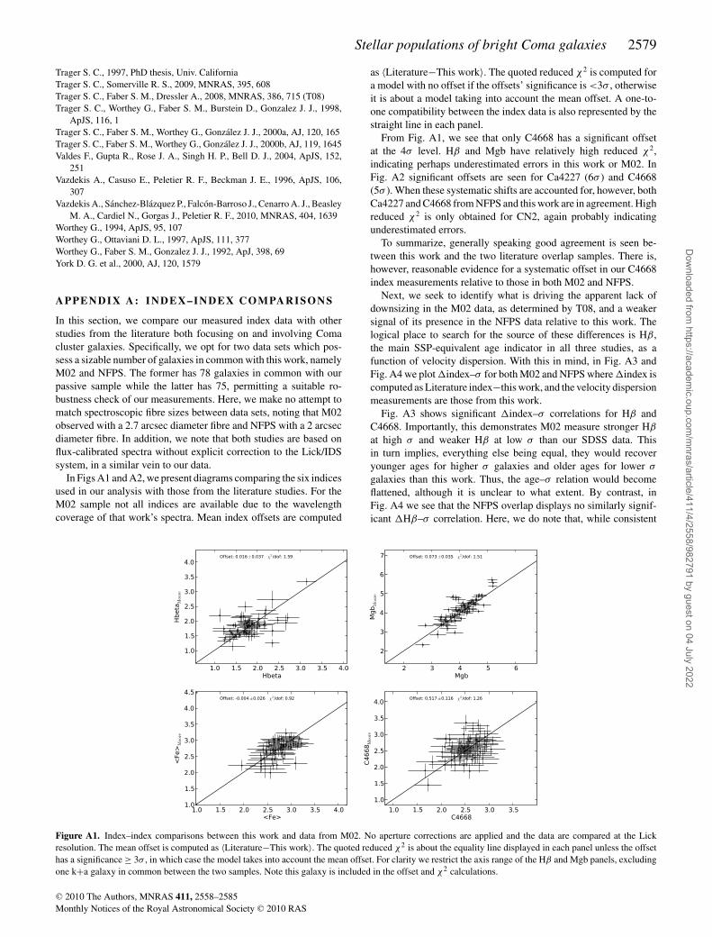
Stellar populations of bright Coma galaxies 2579
Trager S. C., 1997, PhD thesis, Univ. CaliforniaTrager S. C., Somerville R. S., 2009, MNRAS, 395, 608Trager S. C., Faber S. M., Dressler A., 2008, MNRAS, 386, 715 (T08)Trager S. C., Worthey G., Faber S. M., Burstein D., Gonzalez J. J., 1998,
ApJS, 116, 1Trager S. C., Faber S. M., Worthey G., Gonzalez J. J., 2000a, AJ, 120, 165Trager S. C., Faber S. M., Worthey G., Gonzalez J. J., 2000b, AJ, 119, 1645Valdes F., Gupta R., Rose J. A., Singh H. P., Bell D. J., 2004, ApJS, 152,
251Vazdekis A., Casuso E., Peletier R. F., Beckman J. E., 1996, ApJS, 106,
307Vazdekis A., Sanchez-Blazquez P., Falcon-Barroso J., Cenarro A. J., Beasley
M. A., Cardiel N., Gorgas J., Peletier R. F., 2010, MNRAS, 404, 1639Worthey G., 1994, ApJS, 95, 107Worthey G., Ottaviani D. L., 1997, ApJS, 111, 377Worthey G., Faber S. M., Gonzalez J. J., 1992, ApJ, 398, 69York D. G. et al., 2000, AJ, 120, 1579
A P P E N D I X A : IN D E X – I N D E X C O M PA R I S O N S
In this section, we compare our measured index data with otherstudies from the literature both focusing on and involving Comacluster galaxies. Specifically, we opt for two data sets which pos-sess a sizable number of galaxies in common with this work, namelyM02 and NFPS. The former has 78 galaxies in common with ourpassive sample while the latter has 75, permitting a suitable ro-bustness check of our measurements. Here, we make no attempt tomatch spectroscopic fibre sizes between data sets, noting that M02observed with a 2.7 arcsec diameter fibre and NFPS with a 2 arcsecdiameter fibre. In addition, we note that both studies are based onflux-calibrated spectra without explicit correction to the Lick/IDSsystem, in a similar vein to our data.
In Figs A1 and A2, we present diagrams comparing the six indicesused in our analysis with those from the literature studies. For theM02 sample not all indices are available due to the wavelengthcoverage of that work’s spectra. Mean index offsets are computed
as 〈Literature−This work〉. The quoted reduced χ 2 is computed fora model with no offset if the offsets’ significance is <3σ , otherwiseit is about a model taking into account the mean offset. A one-to-one compatibility between the index data is also represented by thestraight line in each panel.
From Fig. A1, we see that only C4668 has a significant offsetat the 4σ level. Hβ and Mgb have relatively high reduced χ 2,indicating perhaps underestimated errors in this work or M02. InFig. A2 significant offsets are seen for Ca4227 (6σ ) and C4668(5σ ). When these systematic shifts are accounted for, however, bothCa4227 and C4668 from NFPS and this work are in agreement. Highreduced χ 2 is only obtained for CN2, again probably indicatingunderestimated errors.
To summarize, generally speaking good agreement is seen be-tween this work and the two literature overlap samples. There is,however, reasonable evidence for a systematic offset in our C4668index measurements relative to those in both M02 and NFPS.
Next, we seek to identify what is driving the apparent lack ofdownsizing in the M02 data, as determined by T08, and a weakersignal of its presence in the NFPS data relative to this work. Thelogical place to search for the source of these differences is Hβ,the main SSP-equivalent age indicator in all three studies, as afunction of velocity dispersion. With this in mind, in Fig. A3 andFig. A4 we plot �index–σ for both M02 and NFPS where �index iscomputed as Literature index−this work, and the velocity dispersionmeasurements are those from this work.
Fig. A3 shows significant �index–σ correlations for Hβ andC4668. Importantly, this demonstrates M02 measure stronger Hβ
at high σ and weaker Hβ at low σ than our SDSS data. Thisin turn implies, everything else being equal, they would recoveryounger ages for higher σ galaxies and older ages for lower σ
galaxies than this work. Thus, the age–σ relation would becomeflattened, although it is unclear to what extent. By contrast, inFig. A4 we see that the NFPS overlap displays no similarly signif-icant �Hβ–σ correlation. Here, we do note that, while consistent
Figure A1. Index–index comparisons between this work and data from M02. No aperture corrections are applied and the data are compared at the Lickresolution. The mean offset is computed as 〈Literature−This work〉. The quoted reduced χ2 is about the equality line displayed in each panel unless the offsethas a significance ≥ 3σ , in which case the model takes into account the mean offset. For clarity we restrict the axis range of the Hβ and Mgb panels, excludingone k+a galaxy in common between the two samples. Note this galaxy is included in the offset and χ2 calculations.
C© 2010 The Authors, MNRAS 411, 2558–2585Monthly Notices of the Royal Astronomical Society C© 2010 RAS
Dow
nloaded from https://academ
ic.oup.com/m
nras/article/411/4/2558/982791 by guest on 04 July 2022

2580 J. Price et al.
Figure A2. Index–index comparisons between this work and data from NFPS. No aperture corrections are applied and the data are compared at the Lickresolution. The mean offset is computed as 〈Literature−This work〉. The quoted reduced χ2 is about the equality line displayed in each panel unless the offsethas a significance ≥3σ , in which case the model takes into account the mean offset.
Figure A3. �index–σ trends for the M02 overlap sample. �index is computed as Literature index−This work and the velocity dispersion measurements arethose from this work.
C© 2010 The Authors, MNRAS 411, 2558–2585Monthly Notices of the Royal Astronomical Society C© 2010 RAS
Dow
nloaded from https://academ
ic.oup.com/m
nras/article/411/4/2558/982791 by guest on 04 July 2022
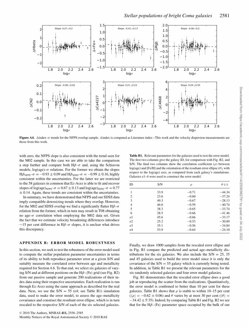
Stellar populations of bright Coma galaxies 2581
Figure A4. �index–σ trends for the NFPS overlap sample. �index is computed as Literature index−This work and the velocity dispersion measurements arethose from this work.
with zero, the NFPS slope is also consistent with the trend seen forthe M02 sample. In this case we are able to take the comparisona step further and compare both Hβ–σ and, using the Schiavonmodels, log(age)–σ relations. For the former we obtain the slopesHβNFPS–σ = −0.93 ± 0.09 and HβSDSS–σ = −0.99 ± 0.16, highlyconsistent within the uncertainties. For the latter we are restrictedto the 58 galaxies in common that EZ-AGES is able to fit and recoverslopes of log(age)NFPS–σ = 0.67 ± 0.13 and log(age)SDSS–σ = 0.77± 0.14. Again, these trends are consistent within the uncertainties.
In summary, we have demonstrated that NFPS and our SDSS dataimply compatible downsizing trends where they overlap. However,for the M02 and SDSS overlap we find a significantly flatter Hβ–σ
relation from the former, which in turn may result in T08 obtainingno age–σ correlation when employing the M02 data set. Giventhe fact that we estimate velocity broadening differences introduce∼15 per cent difference in Hβ–σ slopes, it is unclear what drivesthis discrepancy.
A P P E N D I X B: ER RO R M O D E L RO BU S T N E S S
In this section, we seek to test the robustness of the error model usedto compute the stellar population parameter uncertainties in termsof its ability to both reproduce parameter error at a given S/N andsuitably measure the correlated error between age and metallicityrequired for Section 4.6. To that end, we select six galaxies of vary-ing S/N and at different positions on the Hβ–〈Fe〉 grid (see Fig. B2)from our passive sample and generate 200 realizations of their in-dex data using their respective uncertainties. Each realization is runthrough EZ-AGES using the same approach as described for the realdata. Next, we use the S/N = 55 (e4; see Table B1) simulationdata, used to make the error model, to assess the age–metallicitycovariance and construct the resultant error ellipse, which is in turnrescaled to the respective S/N of each of the six selected galaxies.
Table B1. Relevant parameters for the galaxies used to test the error model.The first two columns give the galaxy ID, for comparison with Fig. B2, andS/N. The final two columns show the correlation coefficient (ρ) betweenlog(age) and [Fe/H] and the orientation of the resultant error ellipse (θ ), withrespect to the log(age) axis, as computed from each galaxy’s simulations.Galaxies e1–4 were used to construct the error model.
ID S/N ρ θ (◦)
1 33.9 −0.71 −44.342 23.6 −0.60 −37.243 49.3 −0.67 −28.134 46.0 −0.59 −40.745 38.3 −0.65 −33.746 28.5 −0.66 −41.46e1 45.6 −0.66 −33.17e2 25.2 −0.53 −30.89e3 35.1 −0.56 −34.84e4 53.9 −0.64 −24.10
Finally, we draw 1000 samples from the rescaled error ellipse andin Fig. B1 compare the predicted and actual age–metallicity dis-tributions for the six galaxies. We also include the S/N = 25, 35and 45 galaxies used to build the error model since it is only thecovariance of the S/N = 55 galaxy which is currently being tested.In addition, in Table B1 we present the relevant parameters for thesix randomly selected galaxies and four error model galaxies.
Fig. B1 demonstrates that the rescaled error ellipse does a goodjob at reproducing the scatter from the realizations. Quantitatively,the error model is confirmed to better than 10 per cent for thesegalaxies. Table B1 shows that ρ is stable to within 10–15 per cent(〈ρ〉 = −0.62 ± 0.06) and θ varies by at most 30 per cent (〈θ〉 =−34.42 ± 5.◦35). Indeed, by comparing Table B1 and Fig. B2 we seethat for the Hβ–〈Fe〉 parameter space occupied by the bulk of our
C© 2010 The Authors, MNRAS 411, 2558–2585Monthly Notices of the Royal Astronomical Society C© 2010 RAS
Dow
nloaded from https://academ
ic.oup.com/m
nras/article/411/4/2558/982791 by guest on 04 July 2022
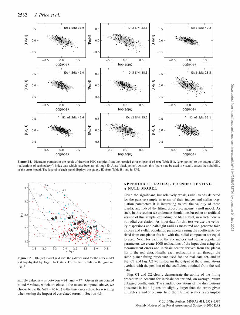
2582 J. Price et al.
Figure B1. Diagrams comparing the result of drawing 1000 samples from the rescaled error ellipse of e4 (see Table B1), (grey points) to the output of 200realizations of each galaxy’s index data which have been ran through EZ-AGES (black points). As such this figure may be used to visually assess the suitabilityof the error model. The legend of each panel displays the galaxy ID from Table B1 and its S/N.
Figure B2. Hβ–〈Fe〉 model grid with the galaxies used for the error modeltest highlighted by large black stars. For further details on the grid seeFig. 11.
sample galaxies θ is between −24◦ and −37◦. Given its associatedρ and θ values, which are close to the means computed above, wechoose to use the S/N = 45 (e1) as the base error ellipse for rescalingwhen testing the impact of correlated errors in Section 4.6.
APPENDI X C : RADI AL TRENDS: TESTI NGA N U L L MO D E L
Given the significant, but relatively weak, radial trends detectedfor the passive sample in terms of their indices and stellar pop-ulation parameters it is interesting to test the validity of theseresults, and indeed the fitting procedure, against a null model. Assuch, in this section we undertake simulations based on an artificialversion of this sample, excluding the blue subset, in which there isno radial correlation. As input data for this test we use the veloc-ity dispersions and half-light radii as measured and generate fakeindices and stellar population parameters using the coefficients de-rived from our planar fits but with the radial component set equalto zero. Next, for each of the six indices and stellar populationparameters we create 1000 realizations of the input data using themeasurement errors and intrinsic scatter derived from the planarfits to the real data. Finally, each realization is run through thesame planar fitting procedure used for the real data set, and inFig. C1 and Fig. C2 we histogram the output of these simulationsoverlaid with the position of the coefficient obtained from the realdata.
Figs C1 and C2 clearly demonstrate the ability of the fittingprocedure to account for intrinsic scatter and, on average, returnunbiased coefficients. The standard deviations of the distributionspresented in both figures are slightly larger than the errors givenin Tables 2 and 5 because here the intrinsic scatter is resampled
C© 2010 The Authors, MNRAS 411, 2558–2585Monthly Notices of the Royal Astronomical Society C© 2010 RAS
Dow
nloaded from https://academ
ic.oup.com/m
nras/article/411/4/2558/982791 by guest on 04 July 2022
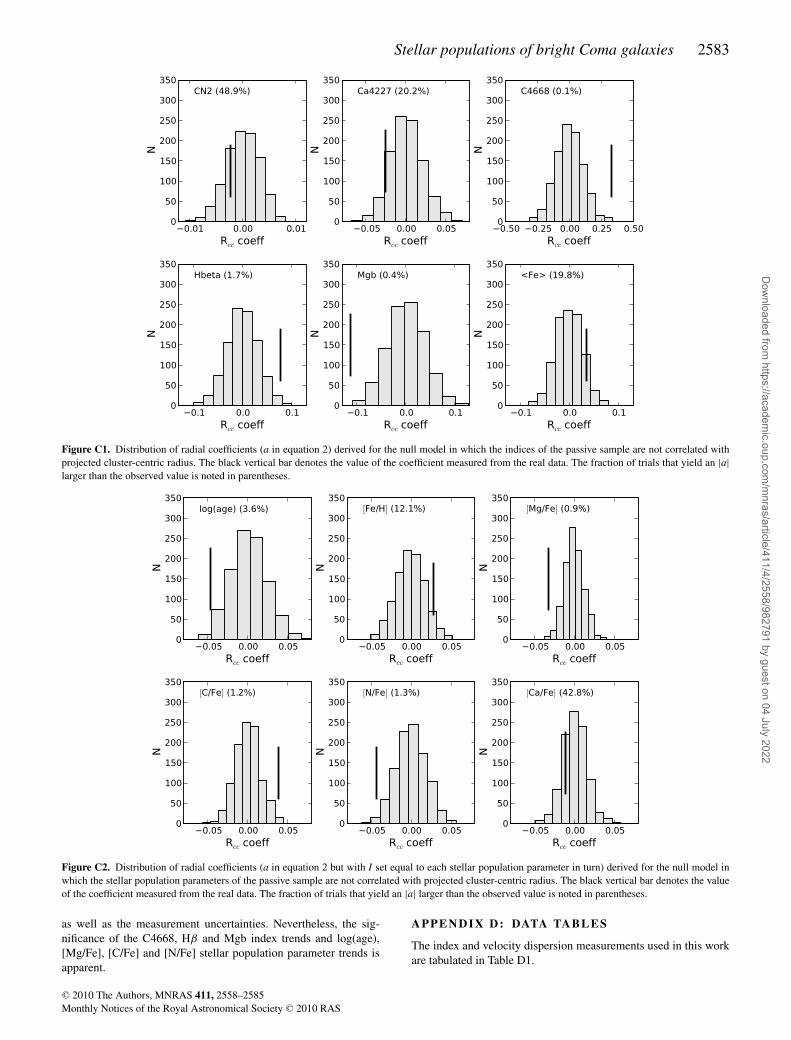
Stellar populations of bright Coma galaxies 2583
Figure C1. Distribution of radial coefficients (a in equation 2) derived for the null model in which the indices of the passive sample are not correlated withprojected cluster-centric radius. The black vertical bar denotes the value of the coefficient measured from the real data. The fraction of trials that yield an |a|larger than the observed value is noted in parentheses.
Figure C2. Distribution of radial coefficients (a in equation 2 but with I set equal to each stellar population parameter in turn) derived for the null model inwhich the stellar population parameters of the passive sample are not correlated with projected cluster-centric radius. The black vertical bar denotes the valueof the coefficient measured from the real data. The fraction of trials that yield an |a| larger than the observed value is noted in parentheses.
as well as the measurement uncertainties. Nevertheless, the sig-nificance of the C4668, Hβ and Mgb index trends and log(age),[Mg/Fe], [C/Fe] and [N/Fe] stellar population parameter trends isapparent.
APPENDI X D : DATA TABLES
The index and velocity dispersion measurements used in this workare tabulated in Table D1.
C© 2010 The Authors, MNRAS 411, 2558–2585Monthly Notices of the Royal Astronomical Society C© 2010 RAS
Dow
nloaded from https://academ
ic.oup.com/m
nras/article/411/4/2558/982791 by guest on 04 July 2022
2584 J. Price et al.
Table D1. Absorption-line index and velocity dispersion measurements used in this work. Galaxies are identified by their position on the sky (J2000) and,where available, their GMP number. The quoted S/N is per Å and the velocity dispersion measurements are not aperture corrected. The indices and their errorsare given in conventional units, i.e. magnitudes for CN1, CN2, Mg1 and Mg2, angstroms for all others. The flag column is binary with 0 indicating no detectedemission with A/N = 4 and 1 denoted galaxies with detected emission. The full version of this table will be provided in the electronic version of the journal(see Supporting Information).
RA Dec. GMP S/N σ σ err HδA HδF CN1 CN2 Ca4227G4300 Hγ A Hγ F Fe4383 Ca4455 Fe4531 C4668 Hβ Fe5015 Mg1 Mg2Mgb Fe5270 Fe5335 Fe5406 Fe5709 Fe5782 HδAerr HδFerr CN1err CN2err Ca4227err
G4300err Hγ Aerr Hγ Ferr Fe4383err Ca4455err Fe4531err C4668err Hβerr Fe5015err Mg1err Mg2err
Mgberr Fe5270err Fe5335err Fe5406err Fe5709err Fe5782err Flag
13:00:08.13 +27:58:37.0 2921 46.7 386.9 6.9 −2.63 −0.04 0.136 0.179 1.145.40 −6.83 −2.04 5.01 1.68 3.84 7.91 1.44 5.30 0.169 0.3255.19 3.06 2.96 1.97 0.96 0.95 0.21 0.14 0.006 0.007 0.110.18 0.22 0.14 0.28 0.16 0.24 0.36 0.16 0.34 0.004 0.0040.16 0.19 0.23 0.18 0.13 0.11 0
13:04:58.38 +29:07:20.1 282 43.1 299.7 6.4 −1.34 0.64 0.087 0.112 1.035.08 −5.85 −1.64 5.00 1.30 3.68 7.90 1.71 4.77 0.144 0.2884.68 2.76 2.74 2.00 1.06 0.76 0.25 0.17 0.007 0.008 0.130.21 0.24 0.15 0.31 0.17 0.26 0.39 0.17 0.37 0.004 0.0050.18 0.21 0.25 0.19 0.15 0.12 0
12:57:24.36 +27:29:52.1 4928 48.3 278.4 4.5 −1.93 0.47 0.103 0.141 1.135.53 −6.27 −1.78 5.16 1.38 3.58 7.86 1.28 5.48 0.147 0.2994.82 2.88 2.70 1.93 0.97 0.76 0.22 0.15 0.006 0.007 0.120.19 0.23 0.14 0.29 0.16 0.23 0.35 0.20 0.34 0.003 0.0040.16 0.19 0.22 0.16 0.12 0.10 0
13:01:53.73 +27:37:28.0 1750 48.6 277.1 4.4 −2.20 0.19 0.124 0.161 1.195.48 −6.80 −2.00 4.93 1.47 3.43 8.01 1.50 5.55 0.158 0.3164.89 3.19 3.07 2.05 0.91 0.94 0.19 0.13 0.005 0.006 0.100.17 0.21 0.13 0.26 0.15 0.22 0.34 0.15 0.33 0.003 0.0040.15 0.19 0.22 0.17 0.12 0.10 0
13:01:57.57 +28:00:21.0 1715 40.9 277.0 6.1 −2.71 −0.23 0.134 0.171 1.035.05 −6.09 −1.92 4.47 1.04 3.44 8.44 1.83 4.80 0.165 0.3164.96 3.13 2.95 1.71 0.77 0.99 0.27 0.18 0.007 0.009 0.140.22 0.26 0.16 0.34 0.18 0.27 0.40 0.18 0.39 0.004 0.0050.19 0.22 0.26 0.20 0.17 0.14 1
12:59:35.71 +27:57:33.3 3329 43.7 273.5 5.1 −2.72 0.14 0.125 0.166 1.235.49 −6.24 −1.86 5.00 1.36 3.65 6.87 1.54 5.44 0.147 0.2924.80 2.99 2.81 1.95 0.84 0.65 0.26 0.18 0.007 0.009 0.130.22 0.26 0.16 0.32 0.17 0.26 0.39 0.17 0.37 0.004 0.0050.17 0.20 0.24 0.18 0.15 0.13 0
12:59:03.90 +28:07:25.3 3792 46.0 273.2 4.8 −2.32 0.14 0.137 0.175 1.135.58 −6.83 −2.19 5.23 1.35 3.39 8.33 1.23 5.83 0.163 0.3275.20 3.06 2.77 1.86 0.86 0.84 0.22 0.15 0.006 0.007 0.110.19 0.23 0.14 0.28 0.16 0.24 0.36 0.16 0.35 0.004 0.0040.16 0.19 0.23 0.18 0.13 0.11 0
13:01:33.60 +29:07:50.1 1990 40.3 269.6 5.9 −2.25 0.19 0.113 0.145 1.065.80 −6.36 −1.84 4.56 1.52 3.57 6.01 1.66 4.56 0.132 0.2794.76 2.75 2.72 1.87 0.82 0.72 0.29 0.19 0.008 0.009 0.150.24 0.28 0.18 0.36 0.19 0.28 0.43 0.18 0.40 0.004 0.0050.19 0.22 0.26 0.20 0.15 0.13 1
12:56:18.60 +26:21:32.0 48.2 263.2 4.2 −2.15 0.16 0.111 0.151 1.155.16 −6.12 −1.70 4.83 1.32 3.58 8.70 1.37 5.33 0.151 0.2984.98 3.09 2.64 2.01 0.89 0.90 0.24 0.16 0.006 0.008 0.120.20 0.23 0.14 0.29 0.16 0.24 0.34 0.15 0.33 0.004 0.0040.16 0.18 0.22 0.16 0.13 0.11 1
12:56:43.52 +27:10:43.7 5279 52.4 259.9 2.7 −2.22 0.24 0.118 0.152 1.005.20 −6.26 −2.01 4.84 1.45 3.73 8.64 1.48 5.53 0.155 0.3064.96 3.13 2.81 1.84 0.85 0.80 0.19 0.13 0.005 0.006 0.100.17 0.20 0.13 0.26 0.14 0.21 0.32 0.14 0.30 0.003 0.0040.14 0.17 0.20 0.15 0.11 0.09 0
12:55:41.30 +27:15:02.7 5886 51.5 258.3 2.7 −2.14 −0.07 0.110 0.150 1.025.30 −6.21 −1.86 5.00 1.27 3.46 8.95 1.49 5.32 0.160 0.3094.91 2.92 2.78 1.93 0.80 0.93 0.20 0.13 0.005 0.007 0.100.17 0.20 0.13 0.26 0.14 0.22 0.32 0.14 0.31 0.003 0.0040.14 0.17 0.21 0.16 0.12 0.10 0
C© 2010 The Authors, MNRAS 411, 2558–2585Monthly Notices of the Royal Astronomical Society C© 2010 RAS
Dow
nloaded from https://academ
ic.oup.com/m
nras/article/411/4/2558/982791 by guest on 04 July 2022
Stellar populations of bright Coma galaxies 2585
SUPPORTING INFORMATION
Additional Supporting Information may be found in the online ver-sion of this article:
Table D1. Absorption-line index and velocity dispersion measure-ments used in this work.
Please note: Wiley-Blackwell are not responsible for the content orfunctionality of any supporting materials supplied by the authors.Any queries (other than missing material) should be directed to thecorresponding author for the article.
This paper has been typeset from a TEX/LATEX file prepared by the author.
C© 2010 The Authors, MNRAS 411, 2558–2585Monthly Notices of the Royal Astronomical Society C© 2010 RAS
Dow
nloaded from https://academ
ic.oup.com/m
nras/article/411/4/2558/982791 by guest on 04 July 2022