Vertical distribution of Saharan dust over Rome (Italy): Comparison between 3-year model predictions...

Vertical distribution of Saharan dust over Rome (Italy):

Comparison between 3-year model predictions

and lidar soundings

P. KishchaDepartment of Geophysics and Planetary Sciences, Tel Aviv University, Tel Aviv, Israel

F. Barnaba and G. P. GobbiIstituto di Scienze dell’Atmosfera e del Clima, CNR, Rome, Italy

P. Alpert, A. Shtivelman, S. O. Krichak, and J. H. JosephDepartment of Geophysics and Planetary Sciences, Tel Aviv University, Tel Aviv, Israel

Received 30 September 2004; accepted 24 November 2004; published 25 March 2005.

[1] Mineral dust particles loaded into the atmosphere from the Sahara desert representone major factor affecting the Earth’s radiative budget. Regular model-based forecasts of3-D dust fields can be used in order to determine the dust radiative effect in climatemodels, in spite of the large gaps in observations of dust vertical profiles. In this study,dust forecasts by the Tel Aviv University (TAU) dust prediction system werecompared to lidar observations to better evaluate the model’s capabilities. The TAU dustmodel was initially developed at the University of Athens and later modified at Tel AvivUniversity. Dust forecasts are initialized with the aid of the Total Ozone MappingSpectrometer aerosol index (TOMS AI) measurements. The lidar soundings employedwere collected at the outskirts of Rome, Italy (41.84�N, 12.64�E) during the high–dustactivity season from March to June of the years 2001, 2002, and 2003. The lidarvertical profiles collected in the presence of dust were used for obtaining statisticallysignificant reference parameters of dust layers over Rome and for model versus lidarcomparison. The Barnaba and Gobbi (2001) approach was used in the current study toderive height-resolved dust volumes from lidar measurements of backscatter. Closeinspection of the juxtaposed vertical profiles, obtained from lidar and model data nearRome, indicates that the majority (67%) of the cases under investigation can be classifiedas good or acceptable forecasts of the dust vertical distribution. A more quantitativecomparison shows that the model predictions are mainly accurate in the middle part ofdust layers. This is supported by high correlation (0.85) between lidar and modeldata for forecast dust volumes greater than the threshold of 1 � 10�12 cm3/cm3. Ingeneral, however, the model tends to underestimate the lidar-derived dust volumeprofiles. The effect of clouds in the TOMS detection of AI is supposed to be the mainfactor responsible for this effect. Moreover, some model assumptions on dust sources andparticle size and the accuracy of model-simulated meteorological parameters are alsolikely to affect the dust forecast quality.

Citation: Kishcha, P., F. Barnaba, G. P. Gobbi, P. Alpert, A. Shtivelman, S. O. Krichak, and J. H. Joseph (2005), Vertical distribution

of Saharan dust over Rome (Italy): Comparison between 3-year model predictions and lidar soundings, J. Geophys. Res., 110,

D06208, doi:10.1029/2004JD005480.

1. Introduction

[2] The problem of climate changes and global warminghas risen in importance during the past decades. In fact, therole of atmospheric aerosols on the climate system is foundto be most significant [Intergovernmental Panel on ClimateChange, 2001]. In this context, mineral dust particles loaded

into the atmosphere from the Sahara desert certainly repre-sent one major factor affecting the Earth’s radiative budget.In particular, Saharan dust is a significant seasonal atmo-spheric phenomenon in the Mediterranean. Every year, fromspring to autumn, mineral dust, produced by wind erosionover arid areas of North Africa, is transported away to theMiddle East, over the Mediterranean to Europe, and acrossthe Atlantic Ocean. These dust intrusions are considered asimportant because of their impact on weather conditions andecosystems [Prospero et al., 2002; Israelevich et al., 2002,

JOURNAL OF GEOPHYSICAL RESEARCH, VOL. 110, D06208, doi:10.1029/2004JD005480, 2005

Copyright 2005 by the American Geophysical Union.0148-0227/05/2004JD005480

D06208 1 of 16

2003]. In particular, dust particles affect the atmosphere intwo ways [e.g., Kaufman et al., 2002; Torres et al., 2002;Ramanathan et al., 2001; Rosenfeld, 2002]: (1) by scatter-ing and absorbing solar and thermal radiation (direct effect),thus reducing the solar irradiance at the Earth’s surface,increasing the solar heating of the atmosphere, and affectingthe atmospheric thermal structure and (2) by altering cloudmicrophysics, often leading to suppression of rainfall, andthus to a less efficient removal of aerosols from theatmosphere (indirect effect). The dust radiative effectstrongly depends on its vertical location. Therefore knowl-edge on dust vertical distribution is of importance indetermining the dust radiative effect in climate models.Besides, knowledge of dust vertical distribution is importantfor the reliable retrieval of aerosol optical depths fromsatellite observations [Torres et al., 2002].[3] Lidars are among the most efficient techniques for

observing the vertical distribution of atmospheric aerosolswith high vertical resolution. However, the Saharan dustlidar observations available in literature mainly refer tolocalized observations and case studies [Hamonou et al.,1999; Gobbi et al., 2000; Di Sarra et al., 2001; De Tomasiet al., 2003; Muller et al., 2003]. To our knowledge, theyearly record of dust lidar profiles over Rome, recentlyanalyzed by Gobbi et al. [2004], is the only long-term studyof the vertical structure of dust layer.[4] To fill the gaps in the observations of dust vertical

profiles (generally spread in time and space), averaged 3-Dfields of dust can be usefully obtained by regular modelforecasts [e.g., Alpert et al., 2004]. Of course, possibleincorrect estimates of these 3-D distributions may add a biasto the model-predicted results. In order to feel confidence inthe model’s correctness, a comprehensive verification ofmodel outputs should be made. In particular, a comparisonof model results against lidar observations is believed to bevery helpful to better understand the model’s capabilities.Moreover, such a comparison could be a useful pilotstudy in using lidar-retrieved data for data assimilationand initialization of numerical short-term dust predictions.Nickovic [2003] has already discussed such a possibility foroperational dust forecasting over the Euro-Mediterraneanregion by using the European Lidar Network (EARLINET)including about 20 stations. Now space missions equippedwith lidar systems are being developed. So one can expectto obtain systematic space-borne lidar measurements soon(e.g., the NASA-CNES CALIPSO experiment, see http://www-calipso.larc.nasa.gov). In this respect, it is worthnoting that the quantitative comparison between dust modeloutputs and lidar soundings is not straightforward. Infact, this comparison requires the conversion of the lidar-measured aerosol backscatter coefficient into the aerosolparameters, which are calculated by the model, typicallydust concentration or dust volume. Recently, a method forestimating desert dust aerosol volume from lidar backscattermeasurements was developed by Barnaba and Gobbi[2001]. A description of that method and discussion onthe accuracy of lidar-derived dust volume estimates aregiven in sections 2.1.2 and 4.1, respectively. The Barnabaand Gobbi [2001] approach was used in the current study toderive height-resolved dust volumes from lidar measure-ments. The measurements over Rome, Italy (41.84�N,12.64�E) collected in the 3-year period 2001–2003 were

considered. With the purpose of verifying model dustforecasts, lidar-derived dust volume profiles were thenquantitatively compared to the corresponding model pre-dicted ones. The dust forecasts were produced by the TelAviv University (TAU) dust prediction system, which wasinitially developed at the University of Athens and latermodified at Tel Aviv University [Alpert et al., 2002]. Thehigh dust activity season from March to June was selectedfor the model versus lidar comparison.

2. Methods

[5] A description of the lidar observations and of themethod used for retrieving dust volume profiles from lidarsoundings is given in this section together with the descrip-tion of the TAU dust prediction system.

2.1. Lidar Observations

[6] Lidar measurements employed in this study werecollected by a single-wavelength, polarization-sensitivelidar system (VELIS), operational since February 2001 inthe ISAC laboratories (41.84�N–12.64�E, 130 m asl) at theoutskirts of Rome. Measurements were carried out daily atnonsynchronous times between 0700 and 2100 (UTC),usually with 2–3 hourly intervals between measurements(observations are mainly performed during working dayssince the system is not automatic). Overall, a total of about1000 profiles/year were collected, although some monthsare missing in the Rome 2002 and 2003 lidar recordsbecause of the system deployment in field campaigns.2.1.1. Lidar System and Lidar Signal Inversion[7] The lidar was designed and assembled at the ISAC-

Rome laboratories with the aim of creating a very compactsystem, capable of operating in both day and night condi-tions. The lidar radiation source is a frequency-doubledNd:YAG laser, emitting plane-polarized pulses at 532 nm.The intensity and repetition rate of laser pulses are generallyset as 30 mJ and 10 Hz, respectively. The system set upallows the collection of the complete tropospheric backscat-ter profile between 300 m and 14 km from the ground [e.g.,Gobbi et al., 2004]. Backscattered light is recorded on boththe parallel and perpendicular polarization planes withrespect to the laser one. Lidar profiles are obtained as 10-minaverages and their vertical resolution is 37.5 m. A thoroughdescription of the lidar signal analysis is given by Gobbi etal. [2002]. Retrieval of the aerosol backscatter is performedby numerically solving the elastic lidar equation [e.g.,Measures, 1984]. A key point in such inversion is repre-sented by the choice of the so-called ‘‘lidar ratio’’ (Lr), i.e.,the ratio between aerosol extinction (sa) and backscatter (ba),both appearing as unknowns in the single-wavelength lidarequation. In the VELIS lidar signal inversion, a verticallyresolved, ba-dependent lidar ratio Lr = sa(z)/ba(z) is chosenaccording to predetermined functional relationships (sa =f(ba)). These were derived from numerical simulations per-formed for different aerosol models (maritime, desert dustcontinental) [Barnaba and Gobbi, 2001, 2004]. In particular,lidar profiles collected during Saharan dust events (as theones discussed in this study) are inverted employing thedesert dust extinction-to-backscatter relationship presentedby Barnaba and Gobbi [2001] and taking into accountparticle nonsphericity following the inversion scheme

D06208 KISHCHA ET AL.: VERTICAL DISTRIBUTION OF SAHARAN DUST OVER ROME

2 of 16

D06208

described by Gobbi et al. [2002]. Overall, this scheme hasbeen proved to provide reliable backscatter and extinctionprofiles in dust load conditions [Gobbi et al., 2002].2.1.2. Dust Detection and Retrieval of Dust Volumeby Lidar[8] The presence of dust is revealed by the lidar depolar-

ization trace (D), which is highly effective at detecting thepresence of nonspherical particles [Gobbi et al., 2000]. Thelidar depolarization D is here defined as the ratiobetween perpendicular and parallel polarized lidar signals(D = S?/Sk / (b?a + b?m)/(bka + bkm), where the subscripts‘‘a’’ and ‘‘m’’ refer to aerosol and molecules, respectively).In fact, spherical particles as liquid aerosols do not generatea depolarized signal, whereas in the presence of nonsphe-rical (solid) particles D levels markedly increase. Inmolecular (aerosol-free) scattering conditions our systemdetects D � 1.4–2.0% and similar low D values are foundin the presence of spherical particles. Conversely, typical Dvalues in the presence of desert dust range between 10and 45%, depending on the relative, optically significant,impact of nonspherical particles on the total (aerosol plusmolecules) backscattered signal (in lidar studies conve-niently expressed in terms of backscatter ratio R = (ba +bm)/bm, being R = 1 in a pure molecular atmosphere).The combination of both the backscatter ratio (R) and thedepolarization information is therefore used to discrimi-nate between dust (typically D > 10%, R > 1.5) andnondust conditions (typically D < 10%).[9] The Barnaba and Gobbi [2001] approach used to

derive the sa = f(ba) relationships (see section 2.1.1) wasalso employed to relate the lidar measured aerosol back-scatter to other aerosol properties such as their surface area(Sa) and volume (Va). These aerosol properties are important(1) to evaluate the aerosol capability to provide a substratumto chemical reactions and (2) to evaluate the aerosol load inthe atmosphere. Functional relationship of the kind Va =f(ba) were therefore derived as a tool to estimate macro-physical aerosol properties from a lidar measurement ofbackscatter. In particular, the desert dust Va = f(ba) relation-ship (only derived for spherical particles) has beenemployed in this study to obtain lidar estimates of desertdust volume profiles to be compared to the TAU modelones. Following this scheme, the minimum dust volumedetectable by the VELIS lidar is 1.0 � 10�12 cm3/cm3,while the maximum dust volume is 1.0 � 10�8 cm3/cm3.Discussion on the error expected to affect such lidar-deriveddesert dust volume estimates is given in section 4.1.

2.2. TAU Dust Prediction System

[10] The dust prediction system was initially developed atthe University of Athens (S. Nickovic et al., Aerosolproduction/transport/deposition processes in the Eta model:Desert cycle simulations, preprint, Proceedings of the Sym-posium on Regional Weather Prediction on Parallel Com-puter Environments, University of Athens, Athens, Greece,1997, hereinafter referred to as Nickovic et al., preprint,1997). After modification the system has been put inoperational use for short-term dust predictions at Tel AvivUniversity since November 2000 [Alpert et al., 2002].Results of the daily model predictions are available athttp://earth.nasa.proj.ac.il/dust/current/. The forecastingmodel with its dust package and initialization procedure

have already been discussed in detail in several publications[Janjic, 1990; Nickovic and Dobricic, 1996; Nickovic et al.,1997; Tsidulko et al., 2002; Alpert et al., 2004; Krichak etal., 2002]. Nevertheless, for the reader’s convenience thefollowing main features are worth outlining.[11] The system is based on the hydrostatic NCEP Eta eta

vertical coordinate model [Mesinger, 1997]. The modeldomain is 0�–50�N, 50�W–50�E including the tropicalNorth Atlantic Ocean, North Africa, the Middle East, andthe Arabian Peninsula. The model is initialized with theNCEP analysis and the lateral boundary data are updatedevery 6h, from the operational forecasts by the NCEP globalmodel. The runs start at 1200 UTC and forecasts areperformed for 3-hour periods up to 48 hours.[12] The model includes packages for dust initialization,

transport, and wet/dry deposition, which had been devel-oped at the University of Athens within the framework ofthe Mediterranean Dust Experiment (MEDUSE) EU project[Nickovic and Dobricic, 1996; Janjic, 1990; Nickovic et al.,preprint, 1997]. The dust mobilization scheme takes intoaccount the values of the friction and threshold frictionvelocity, soil wetness and the distribution of the dust sourceareas, which are specified according to the Olson WorldEcosystem data set [Olson et al., 1985]. The set contains59 classes of vegetation with 100 resolution. Dust forecastsare initialized with the aid of the Total Ozone MappingSpectrometer aerosol index (TOMS AI) measurements[Alpert et al., 2002]. The initial dust vertical distributionover each grid point within the model domain is determinedaccording to the value of TOMS indices among four cate-gories of model-calculated averaged dust profiles over theMediterranean and among four other profiles over NorthAfrica. The four profiles correspond to the average modeloutput profiles at four respective TOMS AI domains of 0.7–1.1, 1.1–1.5, 1.5–1.9, and > 1.9. Some additional commentsabout the TOMS initialization can be seen in section 4.2.2.[13] All the dust (clay) particles were assumed to be of

the same effective radius of 2–2.5 microns. This choiceremained in the model for all period of its operational usewithout changes. Hence all model results used in this studyare homogeneous. We understand, however, that the single-size aerosol is a major shortcoming of the TAU modelversion, and we are currently experimenting with a numberof aerosol sizes (see section 4.2). The dust is considered as apassive substance. No dust feedback effects are included inthe radiation transfer calculations. The feedback, however,could be an important factor in the energy balance, becauseof dust radiative effects, as mentioned in section 1. This isespecially important as, according to lidar measurements(section 3.1), dust layers over Rome are rather thick; theiraveraged thickness exceeds 3 km. Unfortunately, the modeldoes not take the dust feedback into account. The effect ofsuch feedback on the vertical distribution of dust is not wellunderstood and is currently under investigation.[14] The database of model outputs contains a 3-year

daily data set of 48-hour forecasts, obtained for 3-hourperiods, and is available from November 2000 up to thepresent. The data are 2-D and 3-D fields of several atmo-spheric parameters including dust loading, dust concentra-tion, three wind components, temperature, geopotentialheights, sea level pressure and specific humidity. Horizontalresolution of the model is 0.5� and its vertical resolution is


3 of 16

D06208

32 model levels. To compare the dust forecast with lidar-derived volume profiles, modeled mass concentration pro-files over Rome were divided by dust density, assumed as2.5 g/cm3 (in agreement with the majority of other dustmodels [e.g., Kinne et al., 2003, Table 4]).

3. Results

[15] In this section an overview of the dust load overRome is given first, followed by the model-lidar comparisonof dust vertical profiles.

3.1. Statistics of Dusty Day and Dust LayerCharacteristics in Rome

[16] Dust from the Sahara desert is observed irregularlyover Rome. In the beginning, it is therefore important toestimate the mean number of dusty days usually registeredat the Rome site during the year. The TOMS AI was used toproduce these estimates. By definition, AI is positive forabsorbing aerosols, it is �0.2 < AI < 0.2 in the presence ofclouds, while negative AI are found for nonabsorbingparticles [Torres et al., 2002]. The threshold AI > 0.2 wasselected to identify dusty conditions. Owing to sometechnical problems with the Earth Probe TOMS instrument,the TOMS aerosol indices for the 15-year period 1979–1993 are of better quality than the ones retrieved afterNovember 2000 (available at http://toms.gsfc.nasa.gov/aerosols/aerosols_v8.html). Therefore the TOMS data from1979 to 1993 were used in order to get a reliable statistics ofthe mean number of dusty days in Rome.[17] In Table 1 is reported the number of dusty days (N),

averaged on a monthly basis over a small domain (41�N–43�N, 12�E–14�E) around Rome. One can see that themaximum, N � 7 days, is registered in April–May whilethe minimum, N < 2 days, is registered in November. Inaddition, a comparison between TOMS-based statistics andlidar-derived ones is also shown in Table 1. Although somedifferences with the lidar-based statistics are found in thewinter and autumn months, this comparison shows a generalgood agreement between the lidar and TOMS data duringthe season under investigation in the current study (March–June). In fact, both the lidar and TOMS data show a

Table 1. Number of Dusty Days Over Rome Averaged Monthly

as Derived by Both TOMS and Lidar Dataa

Month

Number of Dusty Days Over Rome

TOMS 1979–1993 Lidar 2001–2003

January 3.4 ± 2.4 0.5 ± 0.7February 3.3 ± 2.4 0.3 ± 0.6March 5.6 ± 3.7 7.0 ± 4.6April 6.9 ± 3.2 3.3 ± 2.1May 7.0 ± 3.5 8.3 ± 3.0June 5.6 ± 3.1 6.7 ± 0.6July 5.8 ± 2.7 6.0August 4.2 ± 1.8 -September 2.7 ± 1.7 0.5 ± 0.7October 2.1 ± 1.6 5.0 ± 4.6November 1.9 ± 2.3 4.7 ± 1.5December 2.3 ± 2.4 1.3 ± 2.3

aTotal Ozone Mapping Spectrometer (TOMS) averages were computedfor TOMS aerosol index > 0.2 over the domain (41�N–43�N, 12�E–14�E)around Rome for the 15-year period 1979–1993. The lidar-derived valueswere averaged monthly over the period 2001–2003.

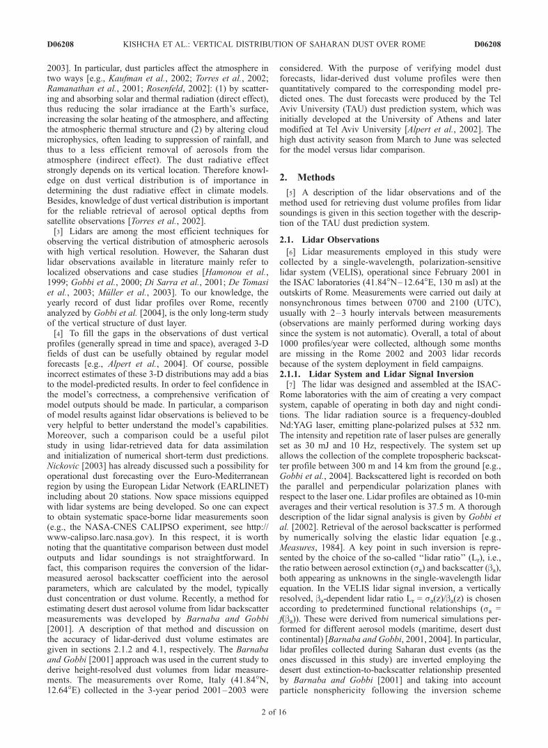
Figure 1. Statistical distributions of lidar-derived param-eters of the dust layer over Rome based on the March-to-June data set of dust-affected lidar profiles (206): (a) bottomand (b) top heights (km), and (c) thickness (km). Fittingcurves of the Gaussian distribution are shown by dottedlines.


4 of 16

D06208

maximum from March to June. Even though the monthlymean numbers of dusty days are not coincident during thisperiod, they are within the associated error bars.[18] Specific atmospheric conditions, accompanied by

dust transport from North Africa to the central Mediterra-nean, lead to the results of Table 1. Saharan dust is generallytransported over the Mediterranean by southerly windsgenerated by cyclones [Alpert and Ziv, 1989; Alpert et al.,1990; Bergametti et al., 1989; Moulin et al., 1998]. Inparticular, Alpert and Ziv [1989] found that spring and earlysummer are the most favorable periods for the developmentof Saharan lows (also called Sharav cyclones) south of theAtlas Mountains. Usually, such cyclones move eastwardand cross Egypt, Israel and the eastern Mediterranean basin.As shown by Bergametti et al. [1989], Moulin et al. [1998],dust outbreaks to the western and central parts of theMediterranean are linked with two depression centers:Saharan lows and a high over Libya. The high over Libya

prevents Saharan lows from following an eastward direc-tion. This synoptic situation, having a peak in spring and inearly summer, induces strong south and southwestern windsbetween the two systems and is characterized by dustintrusions from North Africa to the Mediterranean basin.Moreover, complex wind fields associated with frontalzones under those atmospheric conditions could be one ofthe causal factors for dust over Rome being within a widerange of altitudes, penetrating high into the troposphere.[19] As mentioned in section 1, there is little information

about dust vertical distribution. Therefore the data set ofregular VELIS-lidar soundings is important in obtainingreference values of dust layers over Rome. On the basis ofthe whole data set of dust-affected lidar profiles (206) in theperiod March–June (2001–2003), Figure 1 presents histo-grams of the main parameters of these dust layers. Inparticular, the bottom boundary (BT) was found to rangefrom 0.5 km to 5 km, with the mean value BT = 1.6 ± 0.8 km;

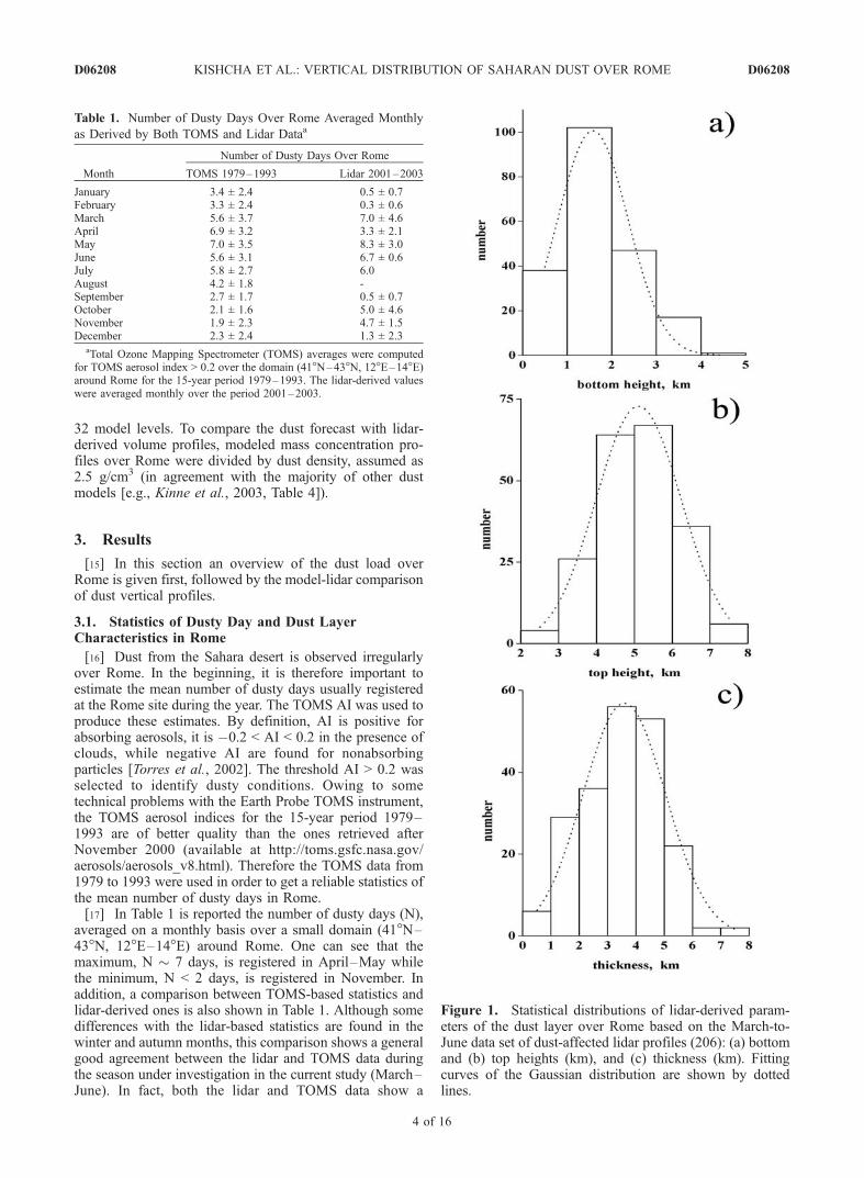
Table 2. Dust Layer Parameters Over Rome Retrieved From Lidar Remote Soundings During March–June 2001–2003, Model-

Calculated Dust Volumes, and the Type of Correspondence Between Lidar and Model Volume Profilesa

DatebTime,UTC

Hbot,km

Htop,km

Thick,km

V1ave,10�12 cm3/cm3

V2ave,10�12 cm3/cm3

V1max,10�12 cm3/cm3

V2max,10�12 cm3/cm3 Type

March1 010316 18.02 1.2 4.2 3 5.28 3.78 7.74 5.00 II2 020304 9.30 1.8 2.7 0.9 6.04 0.04 11.60 0.06 IV3 020305 12.00 0.5 5.5 5.0 5.81 0.51 19.40 0.90 II4 020306 11.21 1.7 4.2 2.5 3.62 7.65 4.90 12.37 II5 020307 11.03 1.2 6.5 5.3 6.69 0.15 14.50 0.40 IV6 020315 11.35 1.2 5 3.8 132.00 0.11 703.00 0.38 IV

April7 020409 7.33 1.4 4.5 3.1 25.80 19.74 38.80 28.08 I8 020412 12.23 0.5 4.5 4.0 87.40 95.00 206.00 133.15 I9 030430 14.30 0.5 5.5 5.0 8.89 5.61 15.10 8.28 I

May10 010502 12.15 3.0 5.4 2.4 9.74 0.17 17.50 0.88 III11 010503 12.16 2 6 4 19.30 0.52 41.80 1.00 II12 010516 12.42 3.0 4.6 1.6 5.23 0.04 9.11 0.09 IV13 010517 11.05 1.2 6 4.8 7.03 0.08 12.00 0.10 II14 010518 15.56 0.5 6 5.5 7.46 0.90 40.30 1.31 II15 010521 16.13 0.5 6.8 6.3 12.80 8.96 31.90 18.83 I16 010523 14.42 0.5 5 4.5 50.01 5.06 409.00 20.67 II17 020507 19.33 1.4 5.5 4.1 9.83 9.18 23.40 14.19 I18 020509 19.05 1.5 5 3.5 4.06 5.80 11.50 15.57 I19 020510 16.30 0.5 6 5.5 17.30 1.23 43.60 1.79 II20 020522 14.51 3 4 1 3.68 1.76 7.98 1.79 III21 020523 12.06 1.5 5.4 3.9 52.20 0.32 135.00 0.89 IV22 030505 10.10 0.5 4 3.5 10.70 11.32 56.20 16.49 III23 030508 12.27 1.2 5.5 4.3 32.50 35.46 212.00 59.94 I24 030512 13.36 1.2 4.8 3.6 7.54 10.03 18.60 14.37 I25 030526 10.45 1 5 4 10.30 6.98 27.90 12.83 I

June26 010611 9.00 1.2 6 4.8 11.40 12.24 37.50 16.70 I27 010612 10.24 1.8 7 5.2 11.80 0.81 80.20 1.10 I28 010613 9.13 0 5.4 3.4 11.30 7.88 29.80 12.40 I29 010628 16.00 0.5 4.6 4.1 14.80 3.10 28.20 6.71 II30 020604 15.20 1.8 6.4 4.6 9.65 11.76 19.80 25.20 I31 020605 10.24 1.4 5.0 3.6 163.00 34.13 1830.00 44.20 IV32 020628 12.23 1.4 5.7 4.3 11.00 4.43 14.80 10.62 III33 030625 14.28 1.8 5.5 3.7 16.80 6.84 32.90 9.86 II34 030627 12.42 1.5 5.6 4.1 10.50 1.53 18.40 5.44 III

aDefinitions are as follows: Hbot, bottom altitude of dust layer; Htop, top altitude; Thick, thickness; V1ave (V1max) and V2ave (V2max), average(maximum) dust volume from lidar and model data, respectively.

bFormat is year, month, and day; read, for example, 010316 as 16 March 2001.


5 of 16

D06208

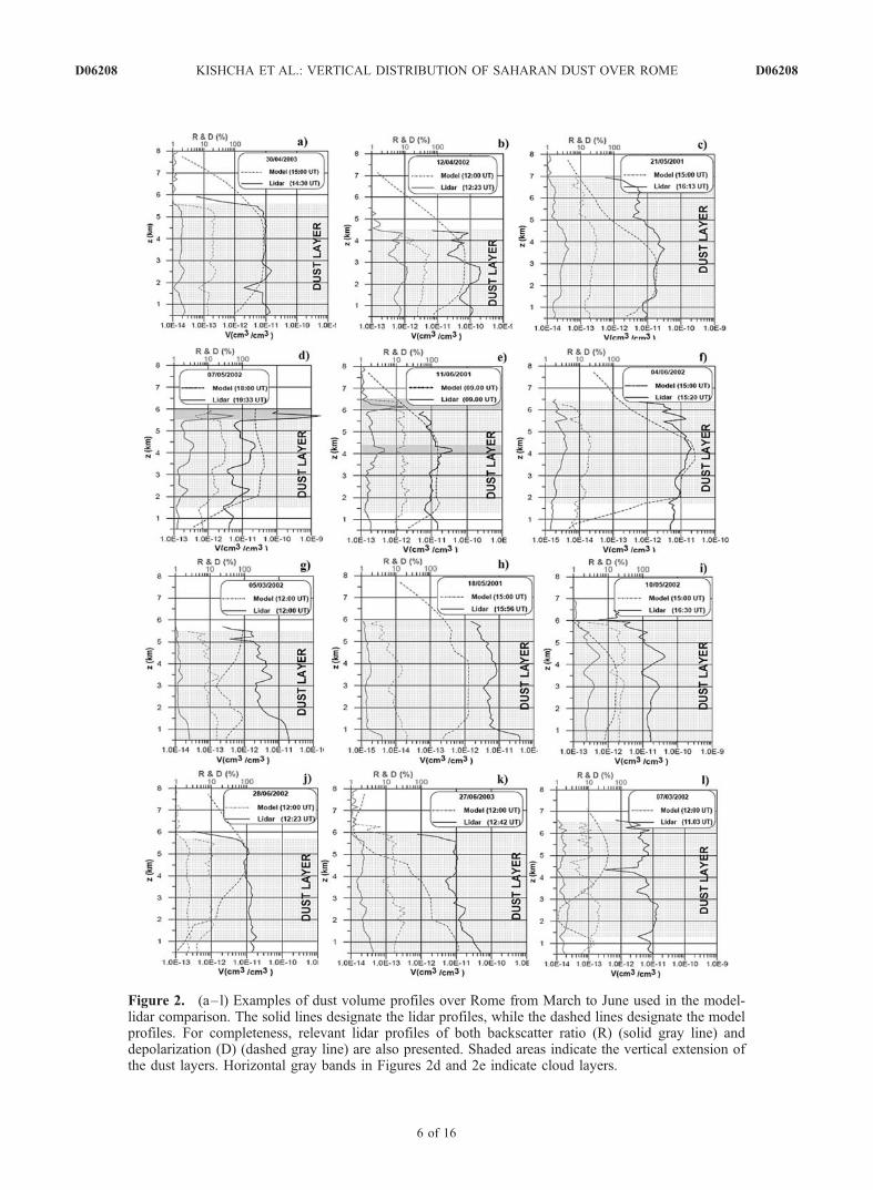
Figure 2. (a–l) Examples of dust volume profiles over Rome from March to June used in the model-lidar comparison. The solid lines designate the lidar profiles, while the dashed lines designate the modelprofiles. For completeness, relevant lidar profiles of both backscatter ratio (R) (solid gray line) anddepolarization (D) (dashed gray line) are also presented. Shaded areas indicate the vertical extension ofthe dust layers. Horizontal gray bands in Figures 2d and 2e indicate cloud layers.


6 of 16

D06208

the top boundary (TP) ranges from 2.4 to 8 km, with meanvalue TP= 5.1 ± 1.1 km, and the thickness of dust layers (TH)ranges from 0.4 km to 7.5 km, with mean value TH = 3.6 ±1.5 km. Hence, on average, dust over Rome is distant fromthe surface. Nonetheless, some mixing of dust with local(typically liquid) aerosols below the dust layer bottomboundary is often highly probable, thus making its detectionmore difficult (see also section 4.1). In Figure 1, Gaussianfitting curves of each variable (dotted lines) are also shown.One can see that these Gaussian distributions suit the histo-grams of lidar-derived data. In seasons other than March–June, some indication of the mean vertical distribution ofdust over Rome are given by Gobbi et al. [2004], based onlidar data collected in the year 2001.

3.2. Model-Lidar Dust Volume Comparison

[20] Saharan dust-affected profiles collected over Romefrom March to June 2001–2003 were considered for theanalysis. Out of the 69 days in which the lidar detected dust,a database of 34 days was selected for the lidar versusmodel comparison. In fact, only days with both the lidarobservations and the model forecast could be taken intoaccount. In particular, there were no model runs for 8 daysbecause of technical problems. Some days (27) with lowdust loading (TOMS AI less than 1) could not be usedbecause of the restriction in model dust forecasts. It is worthmentioning that, in such cases, dust was observed by lidarwithin thin layers (average thickness of TH = 2.7 ± 1.1 km)with respect to the general mean value (TH = 3.6 ± 1.5 km).In these circumstances, the low value of TOMS AI could beexplained by the concurrent presence of nonabsorbinganthropogenic aerosols in the atmospheric column and/orreflecting clouds (see also section 4.2). It should also bementioned that the lidar dust record is partly limited by thepresence of dense clouds. In fact, since Mediterranean dusttransport is often associated with meteorological fronts, dustlayers are frequently associated with water clouds, makingthe lidar soundings inefficient in characterizing the dustvertical distribution.[21] The resulting list of dates employed for the model

versus lidar comparison is given in Table 2, wherecorresponding lidar and model estimates of dust volumeare also reported. Since this study was aimed at checkingthe quality of dust forecasts available daily at 1200 UTC,the lidar dust profiles closest to 1200 UTC were selectedfor the analysis. However, for those few cases when lidarprofiles were available only in the evening or in the morning(e.g., 16 March 2003, 7 May 2002, 9 May 2002), the dustforecast closest to the lidar measurements (either a 21-houror a 30-hour forecast) was selected for the analysis.[22] In order to classify the model-lidar agreement,

four different categories (I– IV) have been defined aslisted below. (For each category, examples are provided inFigure 2): category I, the model profile corresponds well tothe lidar one in the altitude range 1.6–5.1 km (i.e., in thealtitude range within the mean dust bottom and the meandust top) (see Figures 2a–2f ); category II, the model andlidar profiles do not coincide but are similar in shape(Figures 2g–2i); category III, only a part of the modelprofile (e.g., the top or the bottom of dust layers) fits thelidar sounding (Figures 2j and 2k); and category IV, themodel profile does not fit the lidar one at all (Figure 2l).

As also indicated in Table 2, 13 cases (38%) belong tocategory I, even though the model usually underestimatesdust volume derived from the lidar sounding. Category IIis also considered to be tolerable; 10 cases (29%) fall intothis category. Five cases (15%) fall into categories III,while six cases (18%) fall into category IV. It can beobserved that, representing 67% of all cases, categories Iand II (i.e., accurate and acceptable forecasts) are prevalenthere.[23] Note that the discrepancies between lidar and mod-

eled profiles registered at the lower levels (z < 2 km) inFigure 2 are partially due to the presence in this region ofboundary layer aerosols (mainly of local origin) measuredby the lidar but not simulated by the dust model. This pointis further commented on in section 4.1.3.2.1. Case Studies[24] As examples of the above mentioned categories,

three specific cases will be discussed in the following.The purpose is to illustrate how different atmosphericconditions lead to the dust profile observed over Romeand affect the model capability to reproduce it.3.2.1.1. The 12 April 2002 Case[25] Shown in Figure 2b, this case can be classified as

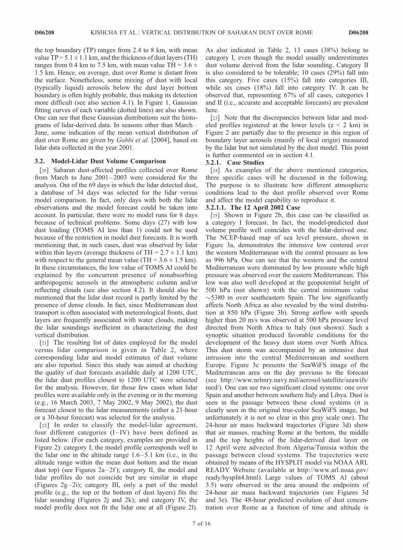
a category I forecast. In fact, the model-predicted dustvolume profile well coincides with the lidar-derived one.The NCEP-based map of sea level pressure, shown inFigure 3a, demonstrates the intensive low centered overthe western Mediterranean with the central pressure as lowas 996 hPa. One can see that the western and the centralMediterranean were dominated by low pressure while highpressure was observed over the eastern Mediterranean. Thislow was also well developed at the geopotential height of500 hPa (not shown) with the central minimum value�5380 m over southeastern Spain. The low significantlyaffects North Africa as also revealed by the wind distribu-tion at 850 hPa (Figure 3b). Strong airflow with speedshigher than 20 m/s was observed at 500 hPa pressure leveldirected from North Africa to Italy (not shown). Such asynoptic situation produced favorable conditions for thedevelopment of the heavy dust storm over North Africa.This dust storm was accompanied by an intensive dustintrusion into the central Mediterranean and southernEurope. Figure 3c presents the SeaWiFS image of theMediterranean area on the day previous to the forecast(see http://www.nrlmry.navy.mil/aerosol/satellite/seawifs/med/). One can see two significant cloud systems: one overSpain and another between southern Italy and Libya. Dust isseen in the passage between these cloud systems (it isclearly seen in the original true-color SeaWiFS image, butunfortunately it is not so clear in this gray scale one). The24-hour air mass backward trajectories (Figure 3d) showthat air masses, reaching Rome at the bottom, the middleand the top heights of the lidar-derived dust layer on12 April were advected from Algeria/Tunisia within thepassage between cloud systems. The trajectories wereobtained by means of the HYSPLIT model via NOAA ARLREADY Website (available at http://www.arl.noaa.gov/ready/hysplit4.html). Large values of TOMS AI (about3.5) were observed in the area around the endpoints of24-hour air mass backward trajectories (see Figures 3dand 3e). The 48-hour predicted evolution of dust concen-tration over Rome as a function of time and altitude is


7 of 16

D06208

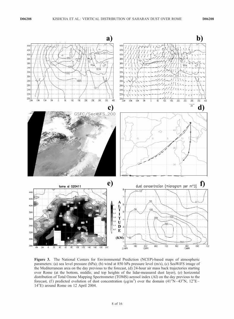
Figure 3. The National Centers for Environmental Prediction (NCEP)-based maps of atmosphericparameters: (a) sea level pressure (hPa); (b) wind at 850 hPa pressure level (m/s), (c) SeaWiFS image ofthe Mediterranean area on the day previous to the forecast, (d) 24-hour air mass back trajectories startingover Rome (at the bottom, middle, and top heights of the lidar-measured dust layer), (e) horizontaldistribution of Total Ozone Mapping Spectrometer (TOMS) aerosol index (AI) on the day previous to theforecast, (f ) predicted evolution of dust concentration (mg/m3) over the domain (41�N–43�N, 12�E–14�E) around Rome on 12 April 2004.


8 of 16

D06208

Figure 4. (left) The 10 May 2002 and (right) 27 June 2003 cases: (a and b) NCEP-based maps of windat 700 hPa pressure level (m/s), (c) SeaWiFS image of the Mediterranean area on the day previous to theforecast (9 May 2002), (d and e) 24-hour air mass back trajectories starting over Rome (at the bottom,middle, and top heights of the lidar-measured dust layer), (f and g) 48-hour Tel Aviv University model-predicted evolution of dust concentration (mg/m3) over the domain (41�N–43�N, 12�E–14�E) aroundRome, and (h) horizontal distribution of TOMS AI on the day previous to the forecast (26 June 2003).


9 of 16

D06208

displayed in Figure 3f. One can see the largest values ofdust concentration are predicted between 1.5 and 4 km on12 April around noon.3.2.1.2. The 10 May 2002 Case[26] This case was classified as an acceptable forecast

(category II, Figure 2i). The synoptic situation on 10 May2002 was characterized by the African cyclone with thecentral pressure dropped to less than 1010 hPa over Algeria/Tunisia. The appropriate distribution of wind at 700 hPashows ordered airflow from North Africa to Italy(Figure 4a). There was only a few clouds on the dayprevious to the forecast (9 May 2002), in accordance withthe SeaWiFS image (Figure 4c). Presented in Figure 4e, the

24-hour backward trajectories show that the air massesreaching Rome at different altitudes follow different trajec-tories from Algeria/Tunisia and from the Mediterraneanarea. Figure 4g shows the 48-hour model-predicted evolu-tion of dust concentration over Rome. One can see that thisdust transport occurred in ‘‘pulses.’’ One can suggest thatthe timing of dust pulses on 10 May 2002 was notsufficiently correct in the model output. As a result, themodel volume profile at 1500 UTC does not coincideexactly with the profile derived from the lidar sounding at1630 UT.3.2.1.3. The 27 June 2003 Case[27] Shown in Figure 2k, this case belongs to category III

because only the bottom part of the model profile fitsapproximately the lidar soundings. The NCEP-based mapof sea level pressure (not shown) demonstrates the lowcentered over the western Sahara. The cyclonic airflow nearthe surface is, however, replaced by the anticyclonic airflowat 850 hPa and higher (see the wind distribution at 700 hPain Figure 4b). Such a synoptic situation produced favorableconditions for the intensive dust intrusion into the AtlanticOcean. Nevertheless, the anticyclonic airflow over north-west Africa at 700–850 hPa could be also responsible fordust intrusion into the western part and subsequently intothe central part of the Mediterranean region. The 24-hourair mass backward trajectories support this assumption(Figure 4d). Presented in Figure 4f, the 48-hour predictedevolution of dust concentration over Rome indicates adescending dust layer having the maximum concentrationclose to the surface and decreasing with time. However, thelidar-derived profiles showed the dust layer between 1.5 and5.6 km with approximately the same dust volume at allaltitudes (see Table 2 and Figure 2k). The discrepancy canbe partly explained by some technical problems with TOMSdetection of aerosol indices on the day previous to theforecast (26 June 2003). According to the horizontal distri-bution of TOMS AI displayed in Figure 4h, data were not

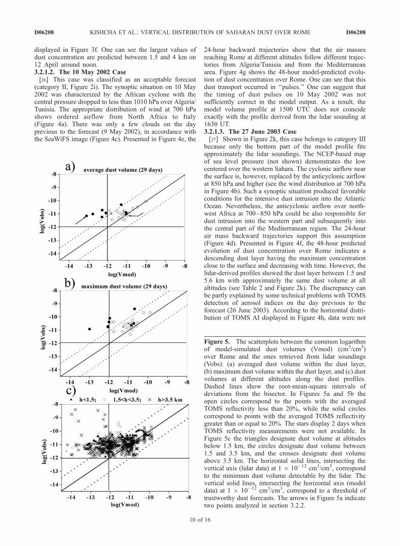
Figure 5. The scatterplots between the common logarithmof model-simulated dust volumes (Vmod) (cm3/cm3)over Rome and the ones retrieved from lidar soundings(Vobs): (a) averaged dust volume within the dust layer,(b) maximum dust volume within the dust layer, and (c) dustvolumes at different altitudes along the dust profiles.Dashed lines show the root-mean-square intervals ofdeviations from the bisector. In Figures 5a and 5b theopen circles correspond to the points with the averagedTOMS reflectivity less than 20%, while the solid circlescorrespond to points with the averaged TOMS reflectivitygreater than or equal to 20%. The stars display 2 days whenTOMS reflectivity measurements were not available. InFigure 5c the triangles designate dust volume at altitudesbelow 1.5 km, the circles designate dust volume between1.5 and 3.5 km, and the crosses designate dust volumeabove 3.5 km. The horizontal solid lines, intersecting thevertical axis (lidar data) at 1 � 10�12 cm3/cm3, correspondto the minimum dust volume detectable by the lidar. Thevertical solid lines, intersecting the horizontal axis (modeldata) at 1 � 10�12 cm3/cm3, correspond to a threshold oftrustworthy dust forecasts. The arrows in Figure 5a indicatetwo points analyzed in section 3.2.2.


10 of 16

D06208

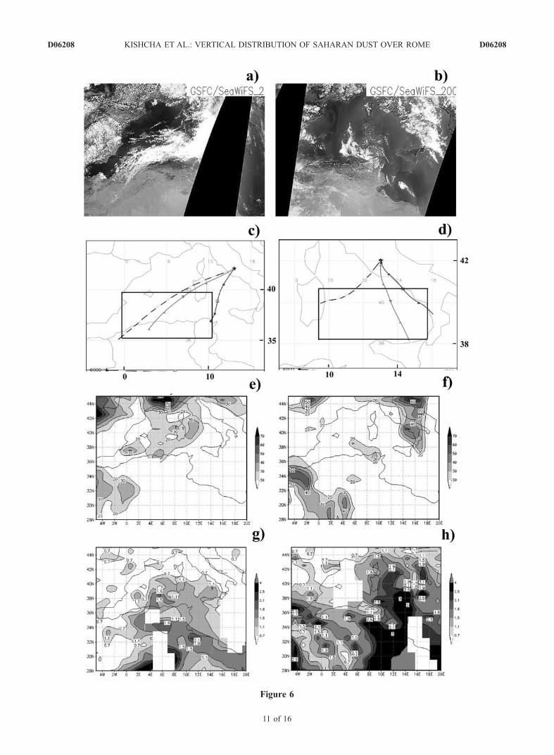
Figure 6


11 of 16

D06208

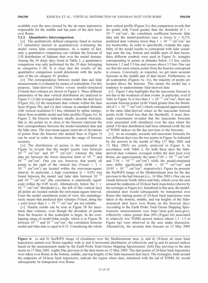
available over the area crossed by the air mass trajectoriesresponsible for the middle and top parts of the dust layerover Rome.3.2.2. Quantitative Intercomparison[28] The qualitatively defined categories listed in section

3.2 stimulated interest in quantitatively evaluating themodel versus lidar correspondence. As a matter of fact,only a quantitative comparison can validate the forecast of3-D distribution of Saharan dust over the model domain.Among the 34 dusty days listed in Table 2, a quantitativecomparison was only performed for the 29 days belongingto categories I– III. It is clear that the results of thequantitative comparison would deteriorate with the inclu-sion of the six category IV profiles.[29] The correspondence between model data and lidar

measurements is evaluated by means of scatterplots. For thispurpose, lidar-derived (Vobs) versus model-simulated(Vmod) dust volumes are shown in Figure 5. Three differentparameters of the dust vertical distribution are analyzed inFigure 5: (1) the averaged dust volume within the dust layer(Figure 5a), (2) the maximum dust volume within the dustlayer (Figure 5b), and (3) dust volume at standard altitudeswith vertical resolution 0.1 km, obtained by spline interpo-lation from available model and lidar profiles (Figure 5c). InFigure 5, the bisector indicates ideally accurate forecasts;that is, the points on or close to the bisector represent thebest correspondence between the model-simulated data andthe lidar ones. The root-mean-square intervals of deviationsof points from the bisector (the dashed lines in Figure 5)can be used in order to characterize the range of forecastaccuracy.[30] The distribution of points in the scatterplot in

Figure 5a reveals that the model results vary between10�14 cm3/cm3 and 10�10 cm3/cm3, whereas the lidardata are between the lower detection limit of 10�12 and10�10 cm3/cm3. One can see, however, that nearly allpoints to the right of the vertical line (Vmod � 1 �10�12 cm3/cm3) are located within the root-mean-squareinterval. In particular, a high correlation (r = 0.85) wasfound between the model and lidar data between 10�12

and 10�10 cm3/cm3 (the correlation is statistically signif-icant within the 0.05 level). Alternatively, below the 1 �10�12 cm3/cm3 threshold (i.e., the left of this vertical line)all points are located outside the root-mean-square interval.From the model simulations point of view, this unambigu-ously means that predicted dust volumes (Vmod, along thex axis) lower than 1 � 10�12 cm3/cm3 are not reliable.[31] Similar results can be seen in Figure 5b for maxi-

mum dust volumes, even though the deviation of pointsfrom the bisector in this scatterplot is larger. In the over-lapping range of model-lidar results, which is in Figure 5bbetween 10�12 and 10�9 cm3/cm3, the correlation betweenmodel and lidar data is equal to 0.51. Considering the whole

dust vertical profile (Figure 5c), this comparison reveals thatfor points with Vmod greater than the threshold of 1 �10�12 cm3/cm3, the correlation coefficient between lidardata and the model-predicted ones is lower (r = 0.37);predicted dust volumes lower than 1 � 10�12 cm3/cm3 arenot trustworthy. In order to specifically evaluate the capa-bility of the model results to correspond with lidar sound-ings near the top, bottom and middle parts of dust layers,three different symbols were used in Figure 5c: trianglescorresponding to points at altitudes below 1.5 km, circlesbetween 1.5 and 3.5 km and crosses above 3.5 km. One cansee that the most remote points from the bisector correspondto crosses. Conversely, as expected, we get more accurateforecasts in the middle part of dust layers. Furthermore, inall scatterplots (Figures 5a–5c), the majority of points arelocated above the bisector. This means the model has atendency to underestimate lidar-derived data.[32] Figure 5 also highlights that the inaccurate forecast is

not due to the weakness of dust events. In particular, even ifVobs in Figure 5a is less than 1 � 10�11 cm3/cm3, there areaccurate forecast points (with Vmod greater than the thresh-old of 1 � 10�12 cm3/cm3) which correspond approximatelyto the same lidar-derived values as the inaccurate forecastpoints (with Vmod less than the threshold). A more thor-ough examination revealed that the inaccurate forecastswere associated with cloudiness over the area where theinitial 3-D dust distribution had been obtained (with the aidof TOMS indices on the day previous to the forecast).[33] As an example, accurate and inaccurate forecasts for

two different days (see the two points in Figure 5a indicatedby the arrows) in the month of May (17 May 2001 and12 May 2003) are jointly analyzed in Figure 6. Inaccordance with Table 2, for both these days the lidar-derived dust volumes, averaged within the dust layer overRome, are approximately the same (7.03 � 10�12 cm3/cm3

and 7.54 � 10�12 cm3/cm3) while the model-simulatedones differ significantly (0.08 � 10�12 cm3/cm3 and10.03 � 10�12 cm3/cm3, respectively). Figure 6a presentsthe SeaWiFS image of the Mediterranean area for the dayprevious to the bad forecast (i.e., 16 May 2001). One can seeclouds between North Africa and Italy, which cover the areaaround the endpoints of 24-hour back trajectories (shown bythe rectangle in Figure 6c). Initialized in this area, the model-simulated dust would subsequently be transported overRome (the starting points of 24-hour back trajectories weretaken at the bottom, middle, and top heights of the lidar-measured dust layer over Rome on the forecast day).According to the Earth Probe Total Ozone Mapping Spec-trometer measurements (see http://daac.gsfc.nasa.gov),reflectivity values greater than 20% (Figure 6e) associatedto relatively low TOMS aerosol indices (about 1.1–1.5 inFigure 6g) were observed in the area under discussion.Alternatively, the accurate dust forecast on 12 May 2003

Figure 6. (a and b) SeaWiFS image of cloudiness over the Mediterranean area, (c and d) 24-hour air mass backtrajectories started over Rome together with (e and f) horizontal distribution of reflectivity and (g and h) aerosol indicesbased on the measurements made by the Earth Probe Total Ozone Mapping Spectrometer. (left) Day previous to the duststorm on 17 May 2001. (right) Day previous to the dust storm on 12 May 2003. The start points of 24-hour back trajectorieswere taken over Rome at the bottom, middle, and top heights of the lidar-measured dust layer. The rectangles, built aroundthe endpoints of 24-hour back trajectories, indicate the region where dust, initialized with the aid of TOMS AI, wouldsubsequently be transported over Rome.


12 of 16

D06208

was accompanied by cloudless conditions (Figure 6b), lowTOMS reflectivity (less than 20% in Figure 6f), and highTOMS aerosol indices (more than 3 in Figure 6h) over therectangular area (Figure 6d), where dust was initialized24 hours before the forecast time.[34] A similar approach of estimating the averaged

TOMS reflectivity was therefore used in order to identifycloudy conditions for all the points in the above-discussedscatterplots of Figures 5a and 5b. In particular, in Figures 5aand 5b the open and solid circles correspond to the pointswith the averaged TOMS reflectivity <20% and 20%,respectively. It is clearly seen that the points with averagedreflectivity less than 20% correspond mainly to acceptableforecast points (within the root-mean-square interval). Con-versely, shown by the solid circles in Figures 5a and 5b,the points with the averaged reflectivity greater than orequal to 20% correspond mainly to inaccurate forecastpoints (outside the root-mean-square interval).

4. Discussion

[35] It should be emphasized that a short-term predictionof 3-D dust distribution is a very complex task. This largelyresults from the lack of operative information on the initial3-D dust distribution. In order to overcome this difficulty,daily available global-scale TOMS aerosol indices wereused for model initialization. The quantitative comparisonbetween the lidar-derived dust volume profiles over Romeand those predicted by the model, initialized with the aid ofTOMS indices, showed that the model is capable of givingmainly accurate forecasts in the middle part of dust layers. Itwas found, however, that the model predictions tend tounderestimate the dust volume values derived by lidar.Furthermore, inaccurate forecasts cannot be explained bythe weakness of dust events. To better understand thisoutcome, discussion on the possible reasons causing suchmodel underestimations is given in section 4.2. Moreover,to correctly interpret the lidar data, evaluation of theexpected accuracy of the lidar dust volume estimates isgiven hereafter.

4.1. Lidar Measurements and Dust Volume EstimatesAccuracy

[36] Uncertainties affecting lidar measurements dependon several factors as the level of background noise, thesignal noise (depending on distance from the system), theaccuracy of the molecular atmosphere employed to calibratethe lidar trace (molecular density error), the accuracy of thelidar ratio assumed in the signal inversion (transmissionerror) [e.g., Russell et al., 1979]. In fact, both signal andbackground noise determines the random error associated tothe lidar signal. For the dust affected profiles discussed inthis study, such random error in daylight conditions is about1% below 4 km, 8% in the range 4–6 km and up to 30% inthe 6–8 km range. For the same altitude ranges, thesepercentages become 1%, 4% and 7%, respectively, formeasurements performed in nighttime conditions.[37] Climatological monthly mean atmospheric p and T

profiles based on 10 years of radiosounding data (recorded30 km west of the measurements site) are employed in thelidar inversion to calibrate the signal. Departures of theresulting climatological molecular density profiles with

respect to the actual ones are typically within 5% (moleculardensity error).[38] Specific investigations were performed to evaluate

the quality of our inversion approach in terms of bothaerosol optical and physical properties in dust load con-ditions. Gobbi et al. [2002] proved that the functionalrelationships adopted to derive the altitude-dependent lidarratio (and thus invert the lidar signal, see section 2.1.1) gavean accuracy on the aerosol extinction retrieval within 22%in Saharan dust conditions (transmission error).[39] An evaluation of the lidar derived aerosol physical

properties in Saharan dust conditions was performed com-paring lidar estimates of desert dust surface area (S) andvolume (V) with simultaneous, colocated in situ measure-ments of S and V [Gobbi et al., 2003]. Outcomes of thatclosure study show a slight lidar tendency to underestimatedesert dust volume, with mean lidar in situ measurementsdiscrepancies within 20%. Since that study was performedin the near range portion of the lidar trace (lidar levels< 500 m), we expect an additional random error to affectthe farther ranges, accordingly with the daytime valuesgiven above (8% at 4–6 km and 30% at 6–8 km).[40] It is also worth noticing that, as opposite to modelled

profiles, in which dust particles are considered on their own,real aerosol profiles also include particles of differentnature. Particularly at lower levels, contribution of theseparticles to the lidar signal is significant. Therefore, whensome increase in depolarisation indicates dust to reach downto the planetary boundary layer (PBL) (z 2 km), somemixing of Saharan dust with PBL aerosol is expected. Inthese conditions it is very difficult to evaluate the relativecontribution of dust with respect to PBL aerosol and thevolume estimate is performed assuming the lidar backscattersignal as fully generated by dust. Dust volume estimate inthe PBL should therefore be considered as the upper limit ofthe real one. Such an effect is observed, for example, in thelidar profiles in Figures 2b, 2g, and 2h.

4.2. Sources of the TAU Model Errors

[41] There could be a few reasons for the model tounderestimate dust volume: (1) accuracy of dynamic atmo-spheric parameter predictions, (2) the model initializationprocedure by the TOMS AI, and (3) assumptions on dustsources and dust particle size.4.2.1. Accuracy of Modeled Meteorological Parameters[42] Dust particles in the model are captured by the wind

at the surface. Subsequently, they are raised to considerablealtitudes in the troposphere by strong convective regimesdeveloped over the desert and are transported by winds tothe Mediterranean Sea and farther. Therefore accuracy ofmodel-predicted atmospheric dynamic parameters is impor-tant in correctly modeling dust generation and transport.One can then suggest that the model underestimation of dustvolume could be due to some significant errors in theforecast of meteorological fields. If this forecast is incorrect,we could find an explicit relationship between the predic-tion errors of dust and the errors of wind, pressure, andtemperature.[43] In order to check this suggestion, a verification of the

24-hour model forecast of several atmospheric parameterswas made. For this purpose, sea level pressure, geopotentialheights at 500 hPa, temperature at 850 hPa, u and v wind


13 of 16

D06208

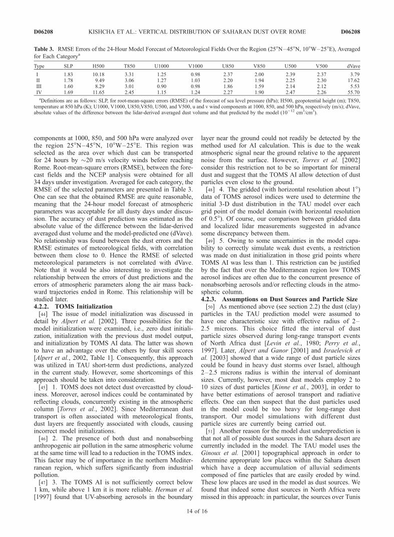
components at 1000, 850, and 500 hPa were analyzed overthe region 25�N–45�N, 10�W–25�E. This region wasselected as the area over which dust can be transportedfor 24 hours by �20 m/s velocity winds before reachingRome. Root-mean-square errors (RMSE), between the fore-cast fields and the NCEP analysis were obtained for all34 days under investigation. Averaged for each category, theRMSE of the selected parameters are presented in Table 3.One can see that the obtained RMSE are quite reasonable,meaning that the 24-hour model forecast of atmosphericparameters was acceptable for all dusty days under discus-sion. The accuracy of dust prediction was estimated as theabsolute value of the difference between the lidar-derivedaveraged dust volume and the model-predicted one (dVave).No relationship was found between the dust errors and theRMSE estimates of meteorological fields, with correlationbetween them close to 0. Hence the RMSE of selectedmeteorological parameters is not correlated with dVave.Note that it would be also interesting to investigate therelationship between the errors of dust predictions and theerrors of atmospheric parameters along the air mass back-ward trajectories ended in Rome. This relationship will bestudied later.4.2.2. TOMS Initialization[44] The issue of model initialization was discussed in

detail by Alpert et al. [2002]. Three possibilities for themodel initialization were examined, i.e., zero dust initiali-zation, initialization with the previous dust model output,and initialization by TOMS AI data. The latter was shownto have an advantage over the others by four skill scores[Alpert et al., 2002, Table 1]. Consequently, this approachwas utilized in TAU short-term dust predictions, analyzedin the current study. However, some shortcomings of thisapproach should be taken into consideration.[45] 1. TOMS does not detect dust overcastted by cloud-

iness. Moreover, aerosol indices could be contaminated byreflecting clouds, concurrently existing in the atmosphericcolumn [Torres et al., 2002]. Since Mediterranean dusttransport is often associated with meteorological fronts,dust layers are frequently associated with clouds, causingincorrect model initializations.[46] 2. The presence of both dust and nonabsorbing

anthropogenic air pollution in the same atmospheric volumeat the same time will lead to a reduction in the TOMS index.This factor may be of importance in the northern Mediter-ranean region, which suffers significantly from industrialpollution.[47] 3. The TOMS AI is not sufficiently correct below

1 km, while above 1 km it is more reliable. Herman et al.[1997] found that UV-absorbing aerosols in the boundary

layer near the ground could not readily be detected by themethod used for AI calculation. This is due to the weakatmospheric signal near the ground relative to the apparentnoise from the surface. However, Torres et al. [2002]consider this restriction not to be so important for mineraldust and suggest that the TOMS AI allow detection of dustparticles even close to the ground.[48] 4. The gridded (with horizontal resolution about 1�)

data of TOMS aerosol indices were used to determine theinitial 3-D dust distribution in the TAU model over eachgrid point of the model domain (with horizontal resolutionof 0.5�). Of course, our comparison between gridded dataand localized lidar measurements suggested in advancesome discrepancy between them.[49] 5. Owing to some uncertainties in the model capa-

bility to correctly simulate weak dust events, a restrictionwas made on dust initialization in those grid points whereTOMS AI was less than 1. This restriction can be justifiedby the fact that over the Mediterranean region low TOMSaerosol indices are often due to the concurrent presence ofnonabsorbing aerosols and/or reflecting clouds in the atmo-spheric column.4.2.3. Assumptions on Dust Sources and Particle Size[50] As mentioned above (see section 2.2) the dust (clay)

particles in the TAU prediction model were assumed tohave one characteristic size with effective radius of 2–2.5 microns. This choice fitted the interval of dustparticle sizes observed during long-range transport eventsof North Africa dust [Levin et al., 1980; Perry et al.,1997]. Later, Alpert and Ganor [2001] and Israelevich etal. [2003] showed that a wide range of dust particle sizescould be found in heavy dust storms over Israel, although2–2.5 microns radius is within the interval of dominantsizes. Currently, however, most dust models employ 2 to10 sizes of dust particles [Kinne et al., 2003], in order tohave better estimations of aerosol transport and radiativeeffects. One can then suspect that the dust particles usedin the model could be too heavy for long-range dusttransport. Our model simulations with different dustparticle sizes are currently being carried out.[51] Another reason for the model dust underprediction is

that not all of possible dust sources in the Sahara desert arecurrently included in the model. The TAU model uses theGinoux et al. [2001] topographical approach in order todetermine appropriate low places within the Sahara desertwhich have a deep accumulation of alluvial sedimentscomposed of fine particles that are easily eroded by wind.These low places are used in the model as dust sources. Wefound that indeed some dust sources in North Africa weremissed in this approach: in particular, the sources over Tunis

Table 3. RMSE Errors of the 24-Hour Model Forecast of Meteorological Fields Over the Region (25�N–45�N, 10�W–25�E), Averagedfor Each Categorya

Type SLP H500 T850 U1000 V1000 U850 V850 U500 V500 dVave

I 1.83 10.18 3.31 1.25 0.98 2.37 2.00 2.39 2.37 3.79II 1.78 9.49 3.06 1.27 1.03 2.20 1.94 2.25 2.30 17.62III 1.60 8.29 3.01 0.90 0.98 1.86 1.59 2.14 2.12 5.53IV 1.69 11.65 2.45 1.15 1.24 2.27 1.90 2.47 2.26 55.70aDefinitions are as follows: SLP, for root-mean-square errors (RMSE) of the forecast of sea level pressure (hPa); H500, geopotential height (m); T850,

temperature at 850 hPa (K); U1000, V1000, U850,V850, U500, and V500, u and v wind components at 1000, 850, and 500 hPa, respectively (m/s); dVave,absolute values of the difference between the lidar-derived averaged dust volume and that predicted by the model (10�12 cm3/cm3).


14 of 16

D06208

and Libya that can be of importance for dust predictionsover Rome.

5. Conclusions

[52] The lidar dust profiles over Rome presented in thisstudy were collected in the 3-year period 2001–2003 duringthe high–dust activity season from March to June. Thesedata were used for obtaining statistically significant refer-ence parameters of dust layers such as the mean top andbottom heights and thickness. It was found that, on average,dust over Rome is distant from the surface and penetrateshigh into the troposphere up to 5–6 km. The lidar data wereused to test the capabilities of the TAU short-term predictionmodel to correctly produce dust vertical distributions. Closeinspection of the juxtaposed vertical profiles, obtained fromlidar and model data near Rome, indicates that the majority(67%) of the cases under investigation can be classified asgood or acceptable model forecasts of dust vertical distri-bution. A quantitative comparison between lidar-derivedand model-predicted dust vertical profiles was alsoperformed. To our knowledge, this is the first time thiskind of long-term quantitative comparison is performed.The quantitative comparison showed that the model pre-dictions are mainly accurate in the middle part of dustlayers. This is supported by high correlation (0.85) betweenlidar and model data for forecasted dust volume greater thanthe threshold of 1 � 10�12 cm3/cm3. The model,however, tends to underestimate the lidar-derived dustvolume profiles. Possible reasons for the model under-estimation have been analyzed. In particular, the TAUmodel initialization appears as one of the major problemof short-term dust forecasting. In those cases when themodel-simulated dust concentrations were much lowerthan the observed ones, the largest role was found to beplayed by effect of clouds in the TOMS detection ofaerosol indices (used to initialize the model). Moreover,some model assumptions on dust sources and particlesize, and the accuracy of model-simulated meteorologicalparameters are also likely to affect the dust forecastquality.

[53] Acknowledgments. This research was supported by IsraeliSpace Agency (ISA) as part of the Mediterranean Israeli Dust Experiment(MEIDEX). The latter is a joint project between ISA and NASA. The studywas also supported by the EU DETECT Project (contract EVK2-CT-1999-00048) and by the grant GLOWA-Jordan River. Lidar measurementsemployed in this study were partly supported by the Italian Space Agency(ASI) in the framework of the GASTRAN project. The authors thankY. Kaufman and O. Torres for helpful discussion. We wish to acknowledgeB. Starobinez, Z. Rosen, and S. Rechave for the encouragement and help.The remarks of anonymous referees improved the clarity of the paper, andwe are grateful to them.

ReferencesAlpert, P., and E. Ganor (2001), Saharan mineral dust measurements fromTOMS: Comparison to surface observations over the Middle East for theextreme dust storm, March 14–17, 1998, J. Geophys. Res., 106(D16),18,275–18,286.

Alpert, P., and B. Ziv (1989), The Sharav cyclone: Observations andsome theoretical considerations, J. Geophys. Res., 94(D15), 18,495–18,514.

Alpert, P., B. U. Neeman, and Y. Shay-El (1990), Intermonthly variabilityof cyclone tracks in the Mediterranean, J. Clim., 3, 1474–1478.

Alpert, P., S. O. Krichak, M. Tsidulko, H. Shafir, and J. H. Joseph (2002), Adust prediction system with TOMS initialization, Mon. Weather Rev.,130, 2335–2345.

Alpert, P., P. Kishcha, A. Shtivelman, S. O. Krichak, and J. H. Joseph(2004), Vertical distribution of Saharan dust based on 2.5-year modelpredictions, Atmos. Res., 70, 109–130.

Barnaba, F., and G. P. Gobbi (2001), Lidar estimation of troposphericaerosol extinction, surface area and volume: Maritime and desert-dustcases, J. Geophys. Res., 106(D13), 3005–3018 (Correction, J. Geophys.Res., 107(D13), 4180, 10.1029/2002 JD002340, 2002.)

Barnaba, F., and G. P. Gobbi (2004), Modeling the aerosol extinction versusbackscatter relationship for lidar applications: Maritime and continentalconditions, J. Atmos. Oceanic Technol., 21(3), 428–442.

Bergametti, G., A. L. Dutot, P. Buat-Menard, R. Losno, and E. Remoudaki(1989), Seasonal variability of the elemental composition of atmosphericaerosol particles over the northwestern Mediterranean, Tellus, Ser. B, 41,353–361.

De Tomasi, F., A. Blanco, and M. R. Perrone (2003), Raman lidar monitor-ing of extinction and backscattering of Africa dust layers and dustcharacterization, Appl. Opt., 42, 1699–1709.

Di Sarra, A., T. Di Iorio, M. Cacciani, G. Fiocco, and D. Fua (2001),Saharan dust profiles measured by lidar at Lampedusa, J. Geophys.Res., 106(D10), 10,335–10,348.

Ginoux, P., M. Chin, I. Tegen, J. M. Prospero, B. Holben, O. Dubovik,and S.-J. Lin (2001), Sources and distributions of dust aerosols simulatedwith the GOCART model, J. Geophys. Res., 106(D17), 20,255–20,274.

Gobbi, G. P., F. Barnaba, R. Giorgi, and A. Santacasa (2000), Altitude-resolved properties of a Saharan-dust event over the Mediterranean,Atmos. Environ., 34, 5119–5127.

Gobbi, G. P., F. Barnaba, M. Blumthaler, G. Labow, and J. Herman(2002), Observed effects of particles non-sphericity on the retrievalof marine and desert-dust aerosol optical depth by lidar, Atmos.Res., 61, 1–14.

Gobbi, G. P., F. Barnaba, R. Van Dingenen, J. P. Putaud, M. Mircea, andM. C. Facchini (2003), Lidar and in situ observations of continentaland Saharan aerosol: Closure analysis of particles optical and physicalproperties, Atmos. Chem. Phys., 3, 2161–2172.

Gobbi, G. P., F. Barnaba, and L. Ammannato (2004), The vertical distribu-tion of aerosols, Saharan dust and cirrus clouds at Rome (Italy) in theyear 2001, Atmos. Chem. Phys., 4, 351–359.

Hamonou, E., P. Chazette, D. Balis, F. Dulac, X. Schneider, E. Galani,G. Ancellet, and A. Papayannis (1999), Characterization of the verticalstructure of Saharan dust export to the Mediterranean basin, J. Geo-phys. Res., 104(D18), 22,257–22,270.

Herman, J. R., P. K. Bhartia, O. Torres, C. Hsu, C. Seftor, and E. Celarier(1997), Global distribution of UV-absorbing aerosol from Nimbus7/TOMS data, J. Geophys. Res., 102, 16,911–16,922.

Intergovernmental Panel on Climate Change (2001), Climate Change2001—Impacts, Adaptation, and Vulnerability, Cambridge Univ. Press,New York.

Israelevich, P. L., Z. Levin, J. H. Joseph, and E. Ganor (2002), Desertaerosol transport in the Mediterranean region as inferred from theTOMS aerosol index, J. Geophys. Res., 107(D21), 4572, doi:10.1029/2001JD002011.

Israelevich, P. L., E. Ganor, Z. Levin, and J. H. Joseph (2003), Annualvariations of physical properties of desert dust over Israel, J. Geophys.Res., 108(D13), 4381, doi:10.1029/2002JD003163.

Janjic, Z. I. (1990), The step-mountain coordinate: Physical package, Mon.Weather Rev., 118, 1429–1443.

Kaufman, Y. J., D. Tanre, and O. Boucher (2002), A satellite view ofaerosols in the climate system, Nature, 419, 215–223.

Kinne, S., et al. (2003), Monthly averages of aerosol properties: A globalcomparison among models, satellite data, and AERONET ground data,J. Geophys. Res., 108(D20), 4634, doi:10.1029/2001JD001253.

Krichak, S. O., M. Tsidulko, and P. Alpert (2002), A study of an INDOEXperiod with aerosol transport to the eastern Mediterranean area, J. Geo-phys. Res., 107(D21), 4582, doi:10.1029/2001JD001169.

Levin, Z., J. H. Joseph, and Y. Mekler (1980), Properties of Sharav(Khamsin) dust—Comparison of optical and direct sampling data,J. Atmos. Sci., 37, 882–891.

Measures, R. M. (1984), Laser Remote Sensing, John Wiley, Hoboken,N. J.

Mesinger, E. (1997), Dynamics of limited area models: Formulation andnumerical methods, Meteorol. Atmos. Phys., 63, 3–14.

Moulin, C., et al. (1998), Satellite climatology of African dust transportin the Mediterranean atmosphere, J. Geophys. Res., 103(D11),13,137–13,144.

Muller, D., I. Mattis, U. Wandinger, A. Ansmann, D. Althausen,O. Dubovik, S. Eckhardt, and A. Sthol (2003), Saharan dust over acentral European EARLINET-AERONET site: Combined observations


15 of 16

D06208

with Raman lidar and Sun photometer, J. Geophys. Res., 108(D12), 4345,doi:10.1029/2002JD002918.

Nickovic, S. (2003), DREAM dust model: Ongoing and future develop-ments, paper presented at 2nd International Workshop on Mineral Dust,Inst. Natl. des Sci. de l’Univ., Paris, 10–12 Sept.

Nickovic, S., and S. Dobricic (1996), A model for long-range transport ofdesert dust, Mon. Weather Rev., 124, 2537–2544.

Olson, J. S., J. A. Watts, and L. J. Alison (1985), Major world ecosys-tem complexes ranked by carbon in live vegetation, Carbon DioxideInf. Cent. Rep. NDP-017, 288 pp., Oak Ridge Natl. Lab., Oak Ridge,Tenn.

Perry, K. D., T. A. Cahill, R. A. Eldred, and D. D. Dutcher (1997), Long-range transport of North African dust to the eastern United States,J. Geophys. Res., 102(D10), 11,225–11,238.

Prospero, J. M., P. Ginoux, O. Torres, S. Nicholson, and E. Gill (2002),Environmental characterization of global sources of atmospheric soil dustidentified with the NIMBUS 7 Total Ozone Mapping Spectrometer(TOMS) absorbing aerosol product, Rev. Geophys., 40(1), 1002,doi:10.1029/2000RG000095.

Ramanathan, V., P. J. Crutzen, J. T. Kiehl, and D. Rosenfeld (2001),Aerosols, climate, and the hydrological cycle, Science, 294, 2119–2124.

Rosenfeld, D. (2002), Suppression of rain and snow by urban and industrialair pollution, Science, 287, 1793–1796.

Russell, P. B., T. J. Swissler, and M. P. McCormick (1979), Methodologyfor error analysis and simulation of lidar aerosol measurements, Appl.Opt., 18, 3783–3797.

Torres, O., P. K. Bhartia, J. R. Herman, A. Sinyuk, P. Ginoux, andB. Holben (2002), A long-term record of aerosol optical depthfrom TOMS observations and comparison to AERONET measure-ments, J. Atmos. Sci., 59, 398–413.

Tsidulko, M., S. O. Krichak, P. Alpert, O. Kakaliagou, G. Kallos, andA. Papadopoulos (2002), Numerical study of a very intensive easternMediterranean dust storm, 13–16 March 1998, J. Geophys. Res.,107(D21), 4581, doi:10.1029/2001JD001168.

��P. Alpert, J. H. Joseph, P. Kishcha, S. O. Krichak, and A. Shtivelman,

Department of Geophysics and Planetary Sciences, Tel Aviv University,Ramat Aviv, 69978 Tel Aviv, Israel. ([email protected])F. Barnaba and G. P. Gobbi, Istituto di Scienze dell’Atmosfera e del

Clima, CNR, Via Fosso del Cavaliere 100, 00133 Rome, Italy.


16 of 16

D06208

Vertical distribution of Saharan dust over Rome (Italy): Comparison between 3-year model predictions...

Documents

Transcript of Vertical distribution of Saharan dust over Rome (Italy): Comparison between 3-year model predictions...