Versión 3.4 QGIS Project - QGIS User Guide
633
QGIS User Guide Versión 3.4 QGIS Project 15 de marzo de 2020
-
Upload
khangminh22 -
Category
Documents
-
view
0 -
download
0
Transcript of Versión 3.4 QGIS Project - QGIS User Guide

QGIS User GuideVersión 3.4
QGIS Project
15 de marzo de 2020


Contents
1 Preámbulo 1
2 Prólogo 3
3 Convenciones 53.1 Convenciones de la Interfaz Gráfica o GUI . . . . . . . . . . . . . . . . . . . . . . . . . . . . . 53.2 Convenciones de Texto o Teclado . . . . . . . . . . . . . . . . . . . . . . . . . . . . . . . . . . 63.3 Instrucciones específicas de cada plataforma . . . . . . . . . . . . . . . . . . . . . . . . . . . . 6
4 Características 74.1 Ver datos . . . . . . . . . . . . . . . . . . . . . . . . . . . . . . . . . . . . . . . . . . . . . . . 74.2 Explorar datos y componer mapas . . . . . . . . . . . . . . . . . . . . . . . . . . . . . . . . . . 74.3 Crear, editar, gestionar y exportar datos . . . . . . . . . . . . . . . . . . . . . . . . . . . . . . . 84.4 Analizar datos . . . . . . . . . . . . . . . . . . . . . . . . . . . . . . . . . . . . . . . . . . . . 84.5 Publicar mapas en Internet . . . . . . . . . . . . . . . . . . . . . . . . . . . . . . . . . . . . . . 84.6 Extender funcionalidades QGIS a través de complementos . . . . . . . . . . . . . . . . . . . . . 94.7 Consola de Python . . . . . . . . . . . . . . . . . . . . . . . . . . . . . . . . . . . . . . . . . . 94.8 Problemas Conocidos . . . . . . . . . . . . . . . . . . . . . . . . . . . . . . . . . . . . . . . . 9
5 Novedades de QGIS 3.4 11
6 Comenzar 136.1 Installing QGIS . . . . . . . . . . . . . . . . . . . . . . . . . . . . . . . . . . . . . . . . . . . . 136.2 Starting and stopping QGIS . . . . . . . . . . . . . . . . . . . . . . . . . . . . . . . . . . . . . 146.3 Sample Session: Loading raster and vector layers . . . . . . . . . . . . . . . . . . . . . . . . . . 15
7 Working with Project Files 217.1 Introducing QGIS projects . . . . . . . . . . . . . . . . . . . . . . . . . . . . . . . . . . . . . . 217.2 Generating output . . . . . . . . . . . . . . . . . . . . . . . . . . . . . . . . . . . . . . . . . . 23
8 IGU QGIS 258.1 Barra de Menú . . . . . . . . . . . . . . . . . . . . . . . . . . . . . . . . . . . . . . . . . . . . 268.2 Paneles y Barras de Herramientas . . . . . . . . . . . . . . . . . . . . . . . . . . . . . . . . . . 358.3 Vista del mapa . . . . . . . . . . . . . . . . . . . . . . . . . . . . . . . . . . . . . . . . . . . . 378.4 3D Map View . . . . . . . . . . . . . . . . . . . . . . . . . . . . . . . . . . . . . . . . . . . . . 388.5 Barra de Estado . . . . . . . . . . . . . . . . . . . . . . . . . . . . . . . . . . . . . . . . . . . . 39
9 Configuración QGIS 419.1 Opciones . . . . . . . . . . . . . . . . . . . . . . . . . . . . . . . . . . . . . . . . . . . . . . . 419.2 Working with User Profiles . . . . . . . . . . . . . . . . . . . . . . . . . . . . . . . . . . . . . 619.3 Propiedades del proyecto . . . . . . . . . . . . . . . . . . . . . . . . . . . . . . . . . . . . . . . 639.4 Personalización . . . . . . . . . . . . . . . . . . . . . . . . . . . . . . . . . . . . . . . . . . . . 69
i

9.5 Atajos de teclado . . . . . . . . . . . . . . . . . . . . . . . . . . . . . . . . . . . . . . . . . . . 709.6 Running QGIS with advanced settings . . . . . . . . . . . . . . . . . . . . . . . . . . . . . . . . 71
10 Trabajar con Proyecciones 7710.1 Vista general de la ayuda de proyección . . . . . . . . . . . . . . . . . . . . . . . . . . . . . . . 7710.2 Layer Coordinate Reference Systems . . . . . . . . . . . . . . . . . . . . . . . . . . . . . . . . 7710.3 Project Coordinate Reference Systems . . . . . . . . . . . . . . . . . . . . . . . . . . . . . . . 7810.4 CRS Settings . . . . . . . . . . . . . . . . . . . . . . . . . . . . . . . . . . . . . . . . . . . . . 7910.5 On The Fly (OTF) CRS Transformation . . . . . . . . . . . . . . . . . . . . . . . . . . . . . . . 8010.6 Coordinate Reference System Selector . . . . . . . . . . . . . . . . . . . . . . . . . . . . . . . 8010.7 Sistema de referencia de coordenadas personalizada . . . . . . . . . . . . . . . . . . . . . . . . 8010.8 Datum Transformations . . . . . . . . . . . . . . . . . . . . . . . . . . . . . . . . . . . . . . . 82
11 Herramientas generales 8511.1 Ayuda de contexto . . . . . . . . . . . . . . . . . . . . . . . . . . . . . . . . . . . . . . . . . . 8511.2 Paneles . . . . . . . . . . . . . . . . . . . . . . . . . . . . . . . . . . . . . . . . . . . . . . . . 8511.3 Anidar proyectos . . . . . . . . . . . . . . . . . . . . . . . . . . . . . . . . . . . . . . . . . . . 9411.4 Working with the map canvas . . . . . . . . . . . . . . . . . . . . . . . . . . . . . . . . . . . . 9611.5 Interacting with features . . . . . . . . . . . . . . . . . . . . . . . . . . . . . . . . . . . . . . . 10711.6 Save and Share Layer Properties . . . . . . . . . . . . . . . . . . . . . . . . . . . . . . . . . . . 11211.7 Storing values in Variables . . . . . . . . . . . . . . . . . . . . . . . . . . . . . . . . . . . . . . 11511.8 Autenticación . . . . . . . . . . . . . . . . . . . . . . . . . . . . . . . . . . . . . . . . . . . . . 11511.9 Common widgets . . . . . . . . . . . . . . . . . . . . . . . . . . . . . . . . . . . . . . . . . . . 117
12 Administrar el origen de datos 12312.1 Opening Data . . . . . . . . . . . . . . . . . . . . . . . . . . . . . . . . . . . . . . . . . . . . . 12312.2 Creando capas . . . . . . . . . . . . . . . . . . . . . . . . . . . . . . . . . . . . . . . . . . . . 14112.3 Exploring Data Formats and Fields . . . . . . . . . . . . . . . . . . . . . . . . . . . . . . . . . 153
13 Trabajar con Datos Vectoriales 16113.1 La librería Símbolo . . . . . . . . . . . . . . . . . . . . . . . . . . . . . . . . . . . . . . . . . . 16113.2 El Dialogo de las Propiedades del Vector . . . . . . . . . . . . . . . . . . . . . . . . . . . . . . 17313.3 Expresiones . . . . . . . . . . . . . . . . . . . . . . . . . . . . . . . . . . . . . . . . . . . . . . 24413.4 Trabajar con la tabla de atributos . . . . . . . . . . . . . . . . . . . . . . . . . . . . . . . . . . . 26413.5 Editar . . . . . . . . . . . . . . . . . . . . . . . . . . . . . . . . . . . . . . . . . . . . . . . . . 284
14 Trabajar con Datos Raster 31114.1 Dialogo de Propiedades Raster . . . . . . . . . . . . . . . . . . . . . . . . . . . . . . . . . . . . 31114.2 Análisis raster . . . . . . . . . . . . . . . . . . . . . . . . . . . . . . . . . . . . . . . . . . . . 323
15 Trabajando con Malla de Datos 32915.1 Trabajando con Malla de Datos . . . . . . . . . . . . . . . . . . . . . . . . . . . . . . . . . . . 329
16 Laying out the maps 33916.1 Overview of the Print Layout . . . . . . . . . . . . . . . . . . . . . . . . . . . . . . . . . . . . 33916.2 Layout Items . . . . . . . . . . . . . . . . . . . . . . . . . . . . . . . . . . . . . . . . . . . . . 35316.3 Crear salida . . . . . . . . . . . . . . . . . . . . . . . . . . . . . . . . . . . . . . . . . . . . . . 38616.4 Creating a Report . . . . . . . . . . . . . . . . . . . . . . . . . . . . . . . . . . . . . . . . . . . 394
17 Trabajar con datos OGC 41117.1 QGIS como Cliente de Datos OGC . . . . . . . . . . . . . . . . . . . . . . . . . . . . . . . . . 41117.2 QGIS como Servidor de Datos OGC . . . . . . . . . . . . . . . . . . . . . . . . . . . . . . . . . 421
18 Trabajar con datos GPS 46318.1 Plugin de GPS . . . . . . . . . . . . . . . . . . . . . . . . . . . . . . . . . . . . . . . . . . . . 46318.2 Seguimiento de GPS en Vivo . . . . . . . . . . . . . . . . . . . . . . . . . . . . . . . . . . . . 467
19 Sistema de autenticación 47319.1 Authentication System Overview . . . . . . . . . . . . . . . . . . . . . . . . . . . . . . . . . . 47319.2 User Authentication Workflows . . . . . . . . . . . . . . . . . . . . . . . . . . . . . . . . . . . 482
ii

19.3 Consideraciones de Seguridad . . . . . . . . . . . . . . . . . . . . . . . . . . . . . . . . . . . . 493
20 Integracion GRASS SIG 49720.1 Conjuntos de datos demostración . . . . . . . . . . . . . . . . . . . . . . . . . . . . . . . . . . 49720.2 Cargar capas ráster y vectorial de GRASS . . . . . . . . . . . . . . . . . . . . . . . . . . . . . . 49720.3 Importar datos dentro de una UBICACIÓN DE GRASS mediante arrastrar y soltar . . . . . . . . 49820.4 Managing GRASS data in QGIS Browser . . . . . . . . . . . . . . . . . . . . . . . . . . . . . . 49820.5 Opciones GRASS . . . . . . . . . . . . . . . . . . . . . . . . . . . . . . . . . . . . . . . . . . 49820.6 Iniciar el complemento GRASS . . . . . . . . . . . . . . . . . . . . . . . . . . . . . . . . . . . 49820.7 Abrir directorio de mapas . . . . . . . . . . . . . . . . . . . . . . . . . . . . . . . . . . . . . . 49920.8 LOCALIZACIÓN y DIRECTORIO DE MAPA GRASS . . . . . . . . . . . . . . . . . . . . . . 49920.9 Importar datos dentro de una LOCALIZACIÓN DE GRASS . . . . . . . . . . . . . . . . . . . . 49920.10 El modelo de datos vectoriales de GRASS . . . . . . . . . . . . . . . . . . . . . . . . . . . . . 50220.11 Crear una nueva capa vectorial GRASS . . . . . . . . . . . . . . . . . . . . . . . . . . . . . . . 50220.12 Digitalizar y editar una capa vectorial GRASS . . . . . . . . . . . . . . . . . . . . . . . . . . . 50320.13 La herramienta de región GRASS . . . . . . . . . . . . . . . . . . . . . . . . . . . . . . . . . . 50520.14 La caja de herramientas GRASS . . . . . . . . . . . . . . . . . . . . . . . . . . . . . . . . . . . 505
21 Entorno de trabajo de procesamiento de QGIS 51521.1 Introducción . . . . . . . . . . . . . . . . . . . . . . . . . . . . . . . . . . . . . . . . . . . . . 51521.2 Configuring the Processing Framework . . . . . . . . . . . . . . . . . . . . . . . . . . . . . . . 51521.3 The Toolbox . . . . . . . . . . . . . . . . . . . . . . . . . . . . . . . . . . . . . . . . . . . . . 51821.4 El administrador del historial . . . . . . . . . . . . . . . . . . . . . . . . . . . . . . . . . . . . 52721.5 Modelador gráfico . . . . . . . . . . . . . . . . . . . . . . . . . . . . . . . . . . . . . . . . . . 52821.6 La interfaz de procesamiento por lotes . . . . . . . . . . . . . . . . . . . . . . . . . . . . . . . . 53821.7 Utilizar algoritmos de procesamiento desde la consola . . . . . . . . . . . . . . . . . . . . . . . 54021.8 Writing new Processing algorithms as Python scripts . . . . . . . . . . . . . . . . . . . . . . . . 54921.9 Configurar aplicaciones externas . . . . . . . . . . . . . . . . . . . . . . . . . . . . . . . . . . . 555
22 Complementos 56522.1 Complementos de QGIS . . . . . . . . . . . . . . . . . . . . . . . . . . . . . . . . . . . . . . . 56522.2 Usar complementos núcleo de QGIS . . . . . . . . . . . . . . . . . . . . . . . . . . . . . . . . 57122.3 Consola Python de QGIS . . . . . . . . . . . . . . . . . . . . . . . . . . . . . . . . . . . . . . . 601
23 Ayuda y apoyo 60523.1 Listas de correos . . . . . . . . . . . . . . . . . . . . . . . . . . . . . . . . . . . . . . . . . . . 60523.2 IRC . . . . . . . . . . . . . . . . . . . . . . . . . . . . . . . . . . . . . . . . . . . . . . . . . . 60623.3 Rastreador de Errores . . . . . . . . . . . . . . . . . . . . . . . . . . . . . . . . . . . . . . . . 60623.4 Blog . . . . . . . . . . . . . . . . . . . . . . . . . . . . . . . . . . . . . . . . . . . . . . . . . 60623.5 Plugins . . . . . . . . . . . . . . . . . . . . . . . . . . . . . . . . . . . . . . . . . . . . . . . . 60723.6 Wiki . . . . . . . . . . . . . . . . . . . . . . . . . . . . . . . . . . . . . . . . . . . . . . . . . 607
24 Colaboradores 60924.1 Autores . . . . . . . . . . . . . . . . . . . . . . . . . . . . . . . . . . . . . . . . . . . . . . . . 60924.2 Traductores . . . . . . . . . . . . . . . . . . . . . . . . . . . . . . . . . . . . . . . . . . . . . . 610
25 Appendices 61325.1 Appendix A: GNU General Public License . . . . . . . . . . . . . . . . . . . . . . . . . . . . . 61325.2 Licencia de Documentación Libre de GNU . . . . . . . . . . . . . . . . . . . . . . . . . . . . . 61625.3 Appendix B: QGIS File Formats . . . . . . . . . . . . . . . . . . . . . . . . . . . . . . . . . . . 622
26 Referencias bibliográficas y web 627
iii

iv

CHAPTER 1
Preámbulo
Este documento es la guía del usuario original del software QGIS. El software y el hardware descrito en estedocumento son, en la mayoría de los casos, marcas registradas y, por lo tanto, están sujetos a requisitos legales.QGIS está sujeto a la Licencia Pública General de GNU. Encuentre más información en la página de QGIS,https://www.qgis.org.
Los detalles, datos y resultados en este documento han sido escritos y verificados con el mejor de los conocimien-tos y responsabilidad de los autores y editores. Sin embargo, son posibles errores en el contenido.
Por lo tanto, los datos no están sujetos a ningún derecho o garantía. Los autores y editores no aceptan ningunaresponsabilidad u obligación por fallos y sus consecuencias. Siempre será bienvenido a informar posibles errores.
Este documento ha sido escrito con reStructuredText. Está disponible su código fuente reST en github y comoHTML y PDF online en https://www.qgis.org/en/docs/. Las versiones traducidas de este documento se puedendescargar también en varios formatos en la sección Documentación del proyecto QGIS. Para mayor informa-ción sobre cómo contribuir a este documento y sobre cómo traducirlo, por favor visite https://qgis.org/en/site/getinvolved/index.html.
Enlaces en este documento
Este documento contiene enlaces internos y externos. Pulsando un enlace interno navega dentro del documento,mientras que pulsando un enlace externo abre una dirección de Internet. En formato PDF, los enlaces internos yexternos son mostrados en azul y son manejados por el navegador del sistema. En formato HTML, el navegadormuestra y maneja ambos de manera idéntica.
Autores y Editores de las Guías de Usuario, Instalación y Programación:
La lista de personas que contribuye escribiendo, revisando y traduciendo la siguiente Documentación estádisponible en Colaboradores.
Copyright (c) 2004 - 2017 QGIS Development Team
Internet: https://www.qgis.org
Licencia de este documento
Se permite la copia, distribución y/o modificación de este documento bajo los términos de la Licencia de Docu-mentación Libre GNU, Versión 1.3 o cualquier versión posterior publicada por la Fundación de Software Libre;sin Secciones Invariante, ni Texto de Portada ni de Contracubierta. Se incluye una copia de la licencia en elApéndice Licencia de Documentación Libre de GNU.
1

QGIS User Guide, Versión 3.4
2 Chapter 1. Preámbulo

CHAPTER 2
Prólogo
¡Bienvenido al maravilloso mundo de los Sistemas de Información Geográfica (SIG)!
QGIS es un Sistema de Información Geográfica de código abierto. El proyecto nació en mayo de 2002 y seestableció como un proyecto en SourceForge en junio del mismo año. Hemos trabajado duro para hacer que elsoftware SIG (tradicionalmente software propietario caro) esté al alcance de cualquiera con acceso básico a unordenador personal. QGIS actualmente funciona en la mayoría de plataformas Unix, Windows y Mac. QGIS sedesarrolla usando el kit de herramientas Qt (https://www.qt.io) y C++. Esto significa que es ligero y tiene unainterfaz gráfica de usuario (GUI) agradable y fácil de usar.
QGIS pretende ser un SIG amigable, proporcionando funciones y características comunes. El objetivo inicialdel proyecto era proporcionar un visor de datos SIG. QGIS ha alcanzado un punto en su evolución en el queestá siendo usado por muchos para sus necesidades diarias de visualización de datos SIG. QGIS admite diversosformatos de datos ráster y vectoriales, con el nuevo formato de ayuda fácilmente agregado usando la arquitecturadel complemento.
QGIS se distribuye bajo la Licencia Pública General GNU (GPL). El desarrollo de QGIS bajo esta licencia sig-nifica que se puede revisar y modificar el código fuente y garantiza que usted, nuestro feliz usuario, siempre tendráacceso a un programa de SIG que es libre de costo y puede ser libremente modificado. Debería haber recibidouna copia completa de la licencia con su copia de QGIS, y también podrá encontrarla en el Apéndice Appendix A:GNU General Public License.
Truco: Documentación al día
The latest version of this document can always be found in the documentation area of the QGIS website at https://www.qgis.org/en/docs/.
3

QGIS User Guide, Versión 3.4
4 Chapter 2. Prólogo

CHAPTER 3
Convenciones
Esta sección describe los estilos homogéneos que se utilizarán a lo largo de este manual.
3.1 Convenciones de la Interfaz Gráfica o GUI
Las convenciones de estilo del GUI están destinadas a imitar la apariencia de la interfaz gráfica de usuario. Engeneral, un estilo reflejará la apariencia simplificada, por lo que un usuario puede escanear visualmente el GUIpara encontrar algo que se parece a lo mostrado en el manual.
• Menú Opciones: Capa → Añadir capa ráster o Preferencias → Barra de Herramientas → Digitalizacion
• Herramienta: Añadir capa ráster
• Button : Save as Default
• Título del Cuadro de Diálogo: Propiedades de capa
• Pestaña: General
• Selección: Renderizar
• Botón de selección: Postgis SRID EPSG ID
• Seleccionar un número:
• Seleccionar una cadena:
• Browse for a file: . . .
• Seleccionar un color:
• Barra de desplazamiento:
• Texto de entrada:
El sombreado muestra un componente de la interfaz que el usuario puede pulsar.
5
QGIS User Guide, Versión 3.4
3.2 Convenciones de Texto o Teclado
Entes manual también inclue estilos relacionados a textos, comandos de teclado y codificacion para indicar difer-entes entidades, como las clases o métodos. Estos estilos no corresponden a la apariencia real de cualquier texto ocodificacion dentro de QGIS.
• Hyperlinks: https://qgis.org
• Combinaciones de Teclas: Pulsar Ctrl+B, significa mantener pulsada la tecla Ctrl y pulsar la letra B.
• Nombre de un Archivo: lakes.shp
• Nombre de una Clase: NewLayer
• Método: classFactory
• Servidor: myhost.de
• Texto para el Usuario: qgis --help
Las líneas de código se muestran con una fuente de ancho fijo:
PROJCS["NAD_1927_Albers",GEOGCS["GCS_North_American_1927",
3.3 Instrucciones específicas de cada plataforma
GUI sequences and small amounts of text may be formatted inline: Click File QGIS → Quit to closeQGIS. This indicates that on Linux, Unix and Windows platforms, you should click the File menu first, then Quit,while on macOS platforms, you should click the QGIS menu first, then Quit.
Las cantidades mayores de texto se pueden formatear como listas:
• Hacer esto
• Hacer aquello
• Or do that
o como párrafos:
Hacer esto y esto y esto. Entonces hacer esto y esto y esto, y esto y esto y esto, y esto y esto y esto.
Do that. Then do that and that and that, and that and that and that, and that and that and that, and that and that.
Las capturas de pantalls que aparecen a lo largo de la guía de usuario han sido creadas en diferentes plataformas;éstas se indicarán por el icono específico para cada una al final del pie de imagen.
6 Chapter 3. Convenciones

CHAPTER 4
Características
QGIS offers many common GIS functions provided by core features and plugins. A short summary of six generalcategories of features and plugins is presented below, followed by first insights into the integrated Python console.
4.1 Ver datos
You can view combinations of vector and raster data (in 2D or 3D) in different formats and projections withoutconversion to an internal or common format. Supported formats include:
• Spatially-enabled tables and views using PostGIS, SpatiaLite and MS SQL Spatial, Oracle Spatial, vectorformats supported by the installed OGR library, including GeoPackage, ESRI Shapefile, MapInfo, SDTS,GML and many more. See section Trabajar con Datos Vectoriales.
• Ráster y formatos de imagenes admitidos por la biblioteda GDAL (Geospatial Data Abstraction Library)instalada, por ejemplo GeoTIFF, ERDAS IMG, ArcInfo ASCII GRID, JPEG, PNG y muchos más. Vea lasección Trabajar con Datos Raster.
• Ráster GRASS y datos vectoriales de base de datos GRASS (location/mapset). Vea sección IntegracionGRASS SIG.
• Datos espaciales en línea servidos como servicios web OGC incluyendo WMS, WMTS, WCS, WFS, yWFS-T. Vea la sección Trabajar con datos OGC.
4.2 Explorar datos y componer mapas
Se puede componer mapas y explorar datos espaciales interactivamente con una GUI amigable. Las muy útilesherramientas disponibles en la GUI incluyen:
• Navegador QGIS
• Reproyección al vuelo
• Gestor de Base de Datos
• Print layout
• Panel de vista general
• Marcadores espaciales
7

QGIS User Guide, Versión 3.4
• Herramientas de anotaciones
• Identificar/seleccionar objetos espaciales
• Editar/ver/buscar atributos
• Data-defined feature labeling
• Vectores definidos por datos y herramientas para simbologia raster.
• Composición del atlas y mapa con capas de cuadricula.
• North arrow, scale bar and copyright label for maps
• Apoyo para guardar y restaurar proyectos
4.3 Crear, editar, gestionar y exportar datos
Puede crear, editar, administrar y exportar capas vectoriales y ráster en varios formatos. QGIS ofrece lo siguiente:
• Herramientas de digitalización para formatos reconocidos OGR y capas vectoriales GRASS
• Ability to create and edit multiple file formats and GRASS vector layers
• Complemento de georeferenciador para geocodificar imágenes
• GPS tools to import and export GPX format, and convert other GPS formats to GPX or down/upload directlyto a GPS unit (on Linux, usb: has been added to list of GPS devices)
• Apoyo para visualizar y editar datos de OpenStreetMap
• Ability to create spatial database tables from files with the DB Manager plugin
• Mejor manejo de tablas de bases de datos espaciales
• Herramientas para la gestión de tablas de atributos vectoriales
• Opción para guardar capturas de pantalla como imágenes georeferenciadas
• Herramienta para exportar DXF con capacidades aumentadas de explorar estilos y plugins que realizanfunciones parecidas a CAD.
4.4 Analizar datos
You can perform spatial data analysis on spatial databases and other OGR-supported formats. QGIS currentlyoffers vector analysis, sampling, geoprocessing, geometry and database management tools. You can also use theintegrated GRASS tools, which include the complete GRASS functionality of more than 400 modules. (See sec-tion Integracion GRASS SIG.) Or, you can work with the Processing Plugin, which provides a powerful geospatialanalysis framework to call native and third-party algorithms from QGIS, such as GDAL, SAGA, GRASS andmore. (See section Introducción.)
4.5 Publicar mapas en Internet
QGIS can be used as a WMS, WMTS, WMS-C or WFS and WFS-T client, and as a WMS, WCS or WFS server(see section Trabajar con datos OGC). Additionally, you can publish your data on the Internet using a webserverwith UMN MapServer or GeoServer installed.
8 Chapter 4. Características

QGIS User Guide, Versión 3.4
4.6 Extender funcionalidades QGIS a través de complementos
QGIS se puede adaptar a sus necesidades especiales con la arquitectura de complemento extensible y bibliotecasque se pueden utilizar para crear complementos. Se puede incluso crear nuevas aplicaciones con C++ o Python.
4.6.1 Complementos del Núcleo
Los complementos del núcleo incluyen:
1. Coordinate Capture (capture mouse coordinates in different CRSs)
2. DB Manager (exchange, edit and view layers and tables from/to databases; execute SQL queries)
3. eVIS (visualize events)
4. Geometry Checker (check geometries for errors)
5. Georeferencer GDAL (add projection information to rasters using GDAL)
6. GPS Tools (load and import GPS data)
7. GRASS 7 (integrate GRASS GIS)
8. MetaSearch Catalogue Client (interacting with metadata catalog services supporting the OGC Catalog Ser-vice for the Web (CSW) standard)
9. Offline Editing (allow offline editing and synchronizing with databases)
10. Processing (the spatial data processing framework for QGIS)
11. Topology Checker (find topological errors in vector layers)
4.6.2 Complementos externos de Python
QGIS ofrece un número creciente de complementos Python externos que son proporcionados por la comunidad.Estos se encuentran en el repositorio oficial de complementos y se pueden instalar fácilmente usando el instaladordel complemento Python. Vea la sección El diálogo de complementos.
4.7 Consola de Python
For scripting, it is possible to take advantage of an integrated Python console, which can be opened with: Plugins→ Python Console. The console opens as a non-modal utility window. For interaction with the QGIS environment,there is the qgis.utils.iface variable, which is an instance of QgisInterface. This interface providesaccess to the map canvas, menus, toolbars and other parts of the QGIS application. You can create a script, thendrag and drop it into the QGIS window and it will be executed automatically.
For further information about working with the Python console and programming QGIS plugins and applications,please refer to Consola Python de QGIS and PyQGIS-Developer-Cookbook.
4.8 Problemas Conocidos
4.8.1 Limitación en el número de archivos abiertos
Si va a abrir un proyecto grande de QGIS y está seguro de que todas las capas son válidas, pero algunas capasse marcan como malas, es probable que se enfrentará a este problema. Linux (y otros sistemas operativos, asímismo) tiene un límite de archivos abiertos por proceso. Los límites de recursos son por proceso y heredados. Elulimit, que es una cáscara integrada, cambia los límites solamente para el proceso actual; el nuevo límite seráheredado por los procesos hijos.
4.6. Extender funcionalidades QGIS a través de complementos 9

QGIS User Guide, Versión 3.4
Puede consultar toda la información actual de ulimit escribiendo:
$ ulimit -aS
Puede ver el número permitido de ficheros abiertos por proceso con el siguiente comando en una consola:
$ ulimit -Sn
Para cambiar los límites de una sesión existente, debería poder usar algo como:
$ ulimit -Sn #number_of_allowed_open_files$ ulimit -Sn$ qgis
Para solucionarlo para siempre
En la mayoría de los sistemas Linux, los límites de recursos se establecen al iniciar sesión por el módulopam_limits de acuerdo con los ajustes contenidos en:file:/etc/security/limits.conf o /etc/security/limits.d/*.conf. Debe ser capaz de editar esos archivos si tiene privilegios de root (también a través desudo), pero tendrá que volver a iniciar sesión para que los cambios surtan efecto.
Más información:
https://www.cyberciti.biz/faq/linux-increase-the-maximum-number-of-open-files/ https://linuxaria.com/article/open-files-in-linux
10 Chapter 4. Características

CHAPTER 5
Novedades de QGIS 3.4
Esta versión contiene nuevas características y se extiende la interfaz de programación con respecto a versionesanteriores. Le recomendamos que utilice esta versión sobre las versiones anteriores.
This release includes hundreds of bug fixes and many new features and enhancements over QGIS 2.18 thatwill be described in this manual. You may also review the visual changelogs at https://qgis.org/en/site/forusers/visualchangelogs.html.
11

QGIS User Guide, Versión 3.4
12 Chapter 5. Novedades de QGIS 3.4

CHAPTER 6
Comenzar
This chapter provides a quick overview of installing QGIS, downloading QGIS sample data, and running a firstsimple session visualizing raster and vector data.
6.1 Installing QGIS
QGIS project provides different ways to install QGIS depending on your platform.
6.1.1 Installing from binaries
Standard installers are available for MS Windows and macOS. Binary packages (rpm and deb) or software
repositories are provided for many flavors of GNU/Linux .
For more information and instructions for your operating system check https://download.qgis.org.
6.1.2 Installing from source
If you need to build QGIS from source, please refer to the installation instructions. They are distributed with theQGIS source code in a file called INSTALL. You can also find them online at https://htmlpreview.github.io/?https://raw.github.com/qgis/QGIS/master/doc/INSTALL.html.
If you want to build a particular release and not the version in development, you should replace master withthe release branch (commonly in the release-X_Y form) in the above-mentioned link (installation instructionsmay differ).
6.1.3 Installing on external media
It is possible to install QGIS (with all plugins and settings) on a flash drive. This is achieved by defining a–profiles-path option that overrides the default user profile path and forces QSettings to use this directory, too.See section System Settings for additional information.
13
QGIS User Guide, Versión 3.4
6.1.4 Downloading sample data
This user guide contains examples based on the QGIS sample dataset (also called the Alaska dataset).
The Windows installer has an option to download the QGIS sample dataset. If checked, the data will bedownloaded to your Documents folder and placed in a folder called GIS Database. You may use WindowsExplorer to move this folder to any convenient location. If you did not select the checkbox to install the sampledataset during the initial QGIS installation, you may do one of the following:
• Usar datos SIG que ya tenga
• Download sample data from https://qgis.org/downloads/data/qgis_sample_data.zip
• Desinstalar QGIS y volver a instalarlo con la opción de descarga de datos marcada (sólo recomendado si lassoluciones anteriores no funcionaron).
For GNU/Linux and macOS, there are no dataset installation packages available as rpm, deb or dmg. To usethe sample dataset, download it from https://qgis.org/downloads/data/qgis_sample_data.zip and unzip the archiveon any convenient location on your system.
The Alaska dataset includes all GIS data that are used for the examples and screenshots in this user guide; it alsoincludes a small GRASS database. The projection for the QGIS sample datasets is Alaska Albers Equal Area withunits feet. The EPSG code is 2964.
PROJCS["Albers Equal Area",GEOGCS["NAD27",DATUM["North_American_Datum_1927",SPHEROID["Clarke 1866",6378206.4,294.978698213898,AUTHORITY["EPSG","7008"]],TOWGS84[-3,142,183,0,0,0,0],AUTHORITY["EPSG","6267"]],PRIMEM["Greenwich",0,AUTHORITY["EPSG","8901"]],UNIT["degree",0.0174532925199433,AUTHORITY["EPSG","9108"]],AUTHORITY["EPSG","4267"]],PROJECTION["Albers_Conic_Equal_Area"],PARAMETER["standard_parallel_1",55],PARAMETER["standard_parallel_2",65],PARAMETER["latitude_of_center",50],PARAMETER["longitude_of_center",-154],PARAMETER["false_easting",0],PARAMETER["false_northing",0],UNIT["us_survey_feet",0.3048006096012192]]
If you intend to use QGIS as a graphical front end for GRASS, you can find a selection of sample locations (e.g.,Spearfish or South Dakota) at the official GRASS GIS website, https://grass.osgeo.org/download/sample-data/.
6.2 Starting and stopping QGIS
QGIS can be started like any other application on your computer. This means that you can launch QGIS by:
• using the Applications menu, the Start menu, or the Dock
• doble clic el ícono en su carpeta de Aplicaciones o atajo de escritorio
• double clicking an existing QGIS project file (with .qgz or .qgs extension). Note that this will also openthe project.
• typing qgis in a command prompt (assuming that QGIS is added to your PATH or you are in its installationfolder)
To stop QGIS, use:
14 Chapter 6. Comenzar

QGIS User Guide, Versión 3.4
• the menu option Project → Exit QGIS or use the shortcut Ctrl+Q
• QGIS → Quit QGIS, or use the shortcut Cmd+Q
• or use the red cross at the top-right corner of the main interface of the application.
6.3 Sample Session: Loading raster and vector layers
Now that you have QGIS installed and a sample dataset available, we will demonstrate a first sample session. Inthis example, we will visualize a raster and a vector layer. We will use:
• the landcover raster layer (qgis_sample_data/raster/landcover.img)
• and the lakes vector layer (qgis_sample_data/gml/lakes.gml)
Where qgis_sample_data represents the path to the unzipped dataset.
1. Start QGIS as seen in Starting and stopping QGIS.
2. To load the files in QGIS:
(a) Click on the Open Data Source Manager icon. The Data Source Manager should open in Browser mode.
(b) Browse to the folder qgis_sample_data/raster/
(c) Select the ERDAS IMG file landcover.img and double-click it. The landcover layer is added inthe background while the Data Source Manager window remains open.
Figure 6.1: Adding data to a new project in QGIS
6.3. Sample Session: Loading raster and vector layers 15

QGIS User Guide, Versión 3.4
(d) To load the lakes data, browse to the folder qgis_sample_data/gml/, and double-click thelakes.gml file to open it.
(e) A Coordinate Reference System Selector dialog opens. In the Filter menu, type 2964, filtering the listof Coordinate Reference Systems below.
Figure 6.2: Select the Coordinate Reference System of data
(f) Select the NAD27 / Alaska Alberts entry
(g) Click OK
(h) Close the Data Source Manager window
You now have the two layers available in your project in some random colours. Let’s do some customization onthe lakes layer.
1. Select the Zoom In tool on the Navigation toolbar
2. Zoom to an area with some lakes
3. Double-click the lakes layer in the map legend to open the Properties dialog
4. To change the lakes color:
(a) Click on the Symbology tab
(b) Select blue as fill color.
(c) Press OK. Lakes are now displayed in blue in the map canvas.
5. To display the name of the lakes:
(a) Reopen the lakes layer Properties dialog
16 Chapter 6. Comenzar

QGIS User Guide, Versión 3.4
Figure 6.3: Selecting Lakes color
6.3. Sample Session: Loading raster and vector layers 17

QGIS User Guide, Versión 3.4
(b) Click on the Labels tab
(c) Select Single labels in the drop-down menu to enable labeling.
(d) From the Label with list, choose the NAMES field.
Figure 6.4: Showing Lakes names
(e) Press Apply. Names will now load over the boundaries.
6. You can improve readability of the labels by adding a white buffer around them:
(a) Click the Buffer tab in the list on the left
(b) Check Draw text buffer
(c) Choose 3 as buffer size
(d) Click Apply
(e) Check if the result looks good, and update the value if needed.
(f) Finally click OK to close the Layer Properties dialog and apply the changes.
Let’s now add some decorations in order to shape the map and export it out of QGIS:
1. Select View → Decorations → Scale Bar menu
2. In the dialog that opens, check Enable Scale Bar option
3. Customize the options of the dialog as you want
4. Press Apply
5. Likewise, from the decorations menu, add more items (north arrow, copyright. . . ) to the map canvas withcustom properties.
18 Chapter 6. Comenzar

QGIS User Guide, Versión 3.4
6. Click Project → Import/Export → Export Map to Image. . .
7. Press Save in the opened dialog
8. Select a file location, a format and confirm by pressing Save again.
9. Press Project → Save. . . to store your changes as a .qgz project file.
That’s it! You can see how easy it is to visualize raster and vector layers in QGIS, configure them and generateyour map in an image format you can use in other softwares. Let’s move on to learn more about the availablefunctionality, features and settings, and how to use them.
Nota: To continue learning QGIS through step-by-step exercises, follow the Training manual.
6.3. Sample Session: Loading raster and vector layers 19

QGIS User Guide, Versión 3.4
20 Chapter 6. Comenzar

CHAPTER 7
Working with Project Files
7.1 Introducing QGIS projects
The state of your QGIS session is called a project. QGIS works on one project at a time. Any settings can beproject-specific or an application-wide default for new projects (see section Opciones). QGIS can save the state
of your workspace into a project file using the menu options Project → Save or Project → Save As. . . .
Nota: If the project you loaded has been modified in the meantime, by default, QGIS will ask you if you want
to overwrite the changes. This behavior is controlled by the Prompt to save project and data source changeswhen required setting under Settings → Options → General menu.
You can load existing projects into QGIS using Project → Open. . . , Project → New from template or Project→ Open Recent →.
At startup, a list of recently opened projects is displayed, including screenshots, names and file paths (for up toten projects). This is a handy quick way to access recently used projects. Double-click an entry in this list to openthe corresponding project. If you instead want to create a new project, just add any layer and the list disappears,giving way to the map canvas.
If you want to clear your session and start fresh, go to Project → New. This will prompt you to save theexisting project if changes have been made since it was opened or last saved.
The information saved in a project file includes:
• Layers added
• Which layers can be queried
• Layer properties, including symbolization and styles
• Projection for the map view
• Last viewed extent
• Print layouts
• Print layout elements with settings
• Print layout atlas settings
21

QGIS User Guide, Versión 3.4
Figure 7.1: Starting a new project in QGIS
• Digitizing settings
• Table Relations
• Project Macros
• Project default styles
• Plugins settings
• QGIS Server settings from the OWS settings tab in the Project properties
• Queries stored in the DB Manager
The project file is saved in XML format. This means that it is possible to edit the file outside of QGIS if you knowwhat you are doing. The file format has been updated several times compared with earlier QGIS versions. Projectfiles from older QGIS versions may not work properly any more.
Nota: By default, QGIS will warn you of version differences. This behavior is controlled in Settings → Options.
On the General tab, you should tick Warn when opening a project file saved with an older version of QGIS.
Whenever you save a .qgs project in QGIS, a backup of the project file is created with the extension .qgs~ andstored in the same directory as the project file.
The extension for QGIS projects is .qgs but when saving from QGIS, the default is to save using a compressedformat with the .qgz extension. The .qgs file is embedded in the .qgz file (a zip archive), together with itsassociated sqlite database (.qgd) for auxiliary data. You can get to these files by unzipping.
Nota: A zipped project may be particularly useful with the Auxiliary Storage Properties mechanism in order toembed the underlying database.
Projects can also be saved/loaded to/from a PostgreSQL database using the following Project menu items:
• Project → Open from
• Project → Save to
22 Chapter 7. Working with Project Files

QGIS User Guide, Versión 3.4
Both menu items have a sub-menu with a list of extra project storage implementations (currently just PostgreSQL).Clicking the action will open a dialog to pick a PostgreSQL connection name, schema name and project.
Projects stored in PostgreSQL can be also loaded from the QGIS browser panel (the entries are located within theschema they are stored in), either by double-clicking them or by dragging them to the map canvas.
7.2 Generating output
There are several ways to generate output from your QGIS session. We have already discussed saving as a projectfile in Introducing QGIS projects. Other ways to produce output files are:
• Creating images: Project → Import/Export → Export Map to Image. . . opens a file dialog where youselect the name, path and type of image (PNG, JPG and many other formats). This will also create a worldfile (with extension PNGW or JPGW) that is saved in the same folder as your image. This world file is usedto georeference the image.
• Exporting to DXF files: Project → Import/Export → Export Project to DXF. . . opens a dialog where youcan define the “Symbology mode”, the “Symbology scale” and vector layers you want to export to DXF.Through the “Symbology mode” symbols from the original QGIS Symbology can be exported with highfidelity (see section Creating new DXF files).
• Exporting to PDF files: Project → Import/Export → Export Map to PDF. . . opens a dialog where you candefine the part (Extent) of the map to be exported, the Scale, Resolution, Output width (pixels) and Outputheight (pixels). You can also choose to Draw active decorations and Draw annotations, as well as Rasterizemap.
• Designing print maps: Project → New Print Layout. . . opens a dialog where you can layout and printthe current map canvas (see section Laying out the maps).
7.2. Generating output 23

QGIS User Guide, Versión 3.4
24 Chapter 7. Working with Project Files

CHAPTER 8
IGU QGIS
When QGIS starts, a GUI displays as shown in the figure below (the numbers 1 through 5 in yellow circles arediscussed below).
Figure 8.1: Interfaz Gráfica de Usuario de QGIS con datos de muestra de Alaska
Nota: Las decoraciones de las ventanas (barra de título, etc.) pueden ser distintas dependiendo de su sistemaoperativo y su gestor de ventanas.
La Interfaz Gráfica de Usuario de QGIS está dividida en cinco componentes:
1. Barra de Menú
25

QGIS User Guide, Versión 3.4
2. Barras de herramientas
3. Paneles
4. Vista del mapa
5. Barra de Estado
Scroll down for detailed explanations of these features.
8.1 Barra de Menú
The Menu bar provides access to various QGIS functions using a standard hierarchical menu. The Menus, theiroptions, associated icons and keyboard shortcuts are outlined below. These keyboard shortcuts are the defaultsettings, but they can be reconfigured using the Keyboard Shortcuts via the Settings → menu.
Most Menu options have a corresponding tool and vice-versa. However, the Menus are not organized exactly likethe toolbars. The locations of menu options in the toolbars are indicated below in the table. Plugins may add newoptions to Menus. For more information about tools and toolbars, see Barras de herramientas.
Nota: QGIS is a cross-platform application - while the same tools are available on all platforms, they maybe placed in different menus on different operating systems. The lists below show the most common locationsincluding known variations.
8.1.1 Proyecto
The Project menu provides access and exit points of the project file. It provides you with tools to:
• Create a New file from scratch or using another project file as a template (see Project files options fortemplate configuration)
• Open. . . a project file from either a file browser or PostgreSQL database
• Close a project or revert it to its last saved state
• Save a project in .qgs or .qgz file format, either as a file or within a PostgreSQL database
• Export the map canvas to different formats or use a print layout for more complex output
• Set the project properties and the snapping options when editing layers.
26 Chapter 8. IGU QGIS

QGIS User Guide, Versión 3.4
Menú Opción Atajos Barra de her-ramietas
Referencia
Nuevo Ctrl+N Proyecto Introducing QGIS projectsNuevo a partir de plan-tilla →
Introducing QGIS projects
Open. . . Ctrl+O Proyecto Introducing QGIS projectsOpen from → Post-greSQL
Introducing QGIS projects
Abrir recientes → Introducing QGIS projectsClose Introducing QGIS projects
Guardar Ctrl+S Proyecto Introducing QGIS projects
Guardar como. . . Ctrl+Shift+SProyecto Introducing QGIS projectsSave to → PostgreSQL Introducing QGIS projectsRevert. . .Propiedades. . . Ctrl+Shift+P Propiedades del proyectoSnapping Options. . . Configurar la tolerancia del autoensamblado y
radio de búsquedaImport/Export →
Export Map to Im-age. . .
Generating output
Export Map toPDF. . .
Generating output
Export Project toDXF. . .
Generating output
Import Layers fromDWG/DXF. . .
Importing a DXF or DWG file
New Print Lay-out. . .
Ctrl+P Proyecto Laying out the maps
New Report. . . Laying out the maps
Layout Manager. . . Proyecto Laying out the mapsLayouts → Laying out the maps
Salir de QGIS Ctrl+Q
Under macOS, the Exit QGIS command corresponds to QGIS → Quit QGIS (Cmd+Q).
8.1.2 Editar
The Edit menu provides most of the native tools needed to edit layer attributes or geometry (see Editar for details).
Menú Opción Atajos Barra de herramietas Referencia
Deshacer Ctrl+Z Digitalización Deshacer y rehacer
Rehacer Ctrl+Shift+Z Digitalización Deshacer y rehacer
Cortar objetos espaciales Ctrl+X Digitalización Cortar, copiar, y pegar objetos espacialesContinued on next page
8.1. Barra de Menú 27

QGIS User Guide, Versión 3.4
Table 8.1 – continued from previous pageMenú Opción Atajos Barra de herramietas Referencia
Copiar objetos espaciales Ctrl+C Digitalización Cortar, copiar, y pegar objetos espaciales
Pegar objetos espaciales Ctrl+V Digitalización Cortar, copiar, y pegar objetos espacialesPaste Features as → Trabajar con la tabla de atributosSeleccionar → Atributos Selecting features
Add Record Ctrl+. Digitalización
Add Point Feature Ctrl+. Digitalización Añadir objetos espaciales
Add Line Feature Ctrl+. Digitalización Añadir objetos espaciales
Add Polygon Feature Ctrl+. Digitalización Añadir objetos espaciales
Añadir cadena circular Shape Digitizing Add Circular string
Añadir cadena circular por radio Shape Digitizing Add Circular stringAdd Circle → Shape DigitizingAdd Rectangle → Shape DigitizingAdd Regular Polygon → Shape DigitizingAdd Ellipse → Shape Digitizing
Mover objeto(s) espacial(es) Digitalización Avanzada Move Feature(s)
Copy and Move Feature(s) Digitalización Avanzada Move Feature(s)
Borrar lo seleccionado Digitalización Borrar objetos espaciales seleccionados
Modificar atributos de los objetos seleccionados Digitalización Editar valores de atributo
Rotar objeto(s) espacial(es) Digitalización Avanzada Rotar objeto(s) espacial(es)
Simplificar objeto espacial Digitalización Avanzada Simplificar objeto espacial
Añadir anillo Digitalización Avanzada Añadir anillo
Añadir parte Digitalización Avanzada Añadir parte
Rellenar anillo Digitalización Avanzada Rellenar anillo
Borrar anillo Digitalización Avanzada Borrar anillo
Borrar parte Digitalización Avanzada Borrar parte
Remodelar objetos espaciales Digitalización Avanzada Remodelar objetos espaciales
Desplazar curva Digitalización Avanzada Desplazar curva
Dividir objetos espaciales Digitalización Avanzada Dividir objetos espaciales
Dividir partes Digitalización Avanzada Dividir partes
Convinar objetos espaciales seleccionados Digitalización Avanzada Combinar objetos espaciales seleccionados
Merge Attributes of Selected Features Digitalización Avanzada Combinar atributos de objetos espaciales
Vertex Tool (All Layers) Digitalización Vertex tool
Vertex Tool (Current Layer) Digitalización Vertex tool
Rotar símbolos de puntos Digitalización Avanzada Rotar símbolos de puntos
Offset Point Symbols Digitalización Avanzada Símbolos de punto de desplazamiento
Reverse Line Digitalización Avanzada
28 Chapter 8. IGU QGIS

QGIS User Guide, Versión 3.4
Tools dependent on the selected layer geometry type i.e. point, polyline or polygon, are activated accordingly:
Menú Opción Point Polilinea Polygon
Move Feature(s)
Copy and Move Feature(s)
8.1.3 Ver
The map is rendered in map views. You can interact with these views using the View tools (see Working with themap canvas for more information). For example, you can:
• Create new 2D or 3D map views next to the main map canvas
• Zoom or pan to any place
• Query displayed features” attributes or geometry
• Enhance the map view with preview modes, annotations or decorations
• Access any panel or toolbar
The menu also allows you to reorganize the QGIS interface itself using actions like:
• Toggle Full Screen Mode: covers the whole screen while hiding the title bar
• Toggle Panel Visibility: shows or hides enabled panels - useful when digitizing features (for maximumcanvas visibility) as well as for (projected/recorded) presentations using QGIS” main canvas
• Toggle Map Only: hides panels, toolbars, menus and status bar and only shows the map canvas. Combinedwith the full screen option, it makes your screen display only the map
Menú Opción Atajos Barra de herramietas Referencia
New Map View Ctrl+M Navegación de mapas
New 3D Map View Ctrl+Shift+M 3D Map View
Pan Map Navegación de mapas Zum y paneo
Pan Map to Selection Navegación de mapas
Acercar zum Ctrl+Alt++ Navegación de mapas Zum y paneo
Alejar zum Ctrl+Alt+- Navegación de mapas Zum y paneo
Identify Features Ctrl+Shift+I Atributos Identifying FeaturesMedir → Atributos Mediciones
Statistical Summary Atributos Panel de resumen estadístico
Zum General Ctrl+Shift+F Navegación de mapas
Zum a la capa Navegación de mapas
Zum a la selección Ctrl+J Navegación de mapas
Zum anterior Navegación de mapas
Zum siguiente Navegación de mapas
Zoom To Native Resolution (100%) Navegación de mapasContinued on next page
8.1. Barra de Menú 29

QGIS User Guide, Versión 3.4
Table 8.2 – continued from previous pageMenú Opción Atajos Barra de herramietas ReferenciaIlustraciones → Elementos decorativosModo Vista previa →
Show Map Tips Atributos Propiedades a mostrar
Nuevo marcador. . . Ctrl+B Navegación de mapas Marcadores espaciales
Mostrar marcadores Ctrl+Shift+B Navegación de mapas Marcadores espaciales
Actualizar F5 Navegación de mapas
Mostrar todas las capas Ctrl+Shift+U Panel de capas
Ocultar todas las capas Ctrl+Shift+H Panel de capas
Show Selected Layers Panel de capas
Hide Selected Layers Panel de capas
Hide Deselected Layers Panel de capasPaneles → Paneles y Barras de HerramientasBarras de herramientas→ Paneles y Barras de HerramientasAlternar el modo de pantalla completa F11Toggle Panel Visibility Ctrl+TabToggle Map Only Ctrl+Shift+Tab
Under Linux KDE, Panels →, Toolbars → and Toggle Full Screen Mode are in the Settings menu.
8.1.4 Capa
The Layer menu provides a large set of tools to create new data sources, add them to a project or save modificationsto them. Using the same data sources, you can also:
• Duplicate a layer, generating a copy you can modify within the same project
• Copy and Paste layers or groups from one project to another as a new instance whose features and propertiesyou can modify independently of the original
• or Embed Layers and Groups. . . from another project, as read-only copies which you cannot modify (seeAnidar proyectos)
The Layer menu also contains tools to configure, copy or paste layer properties (style, scale, CRS. . . ).
30 Chapter 8. IGU QGIS

QGIS User Guide, Versión 3.4
Menú Opción Atajos Barra de her-ramietas
Referencia
Data Source Manager Ctrl+L Data SourceManager
Opening Data
Crear capa → Data SourceManager
Creating new vector layers
Añadir capa → Data SourceManager
Opening Data
Empotrar capas y grupos. . . Anidar proyectosAñadir desde archivo de definiciónde capa. . .
Layer definition file
Copy Style Save and Share Layer Properties
Pegar estilo Save and Share Layer Properties
Copy Layer
Paste Layer/Group
Abrir tabla de atributos F6 Atributos Trabajar con la tabla de atribu-tos
Conmutar edición Digitalización Digitalizando una capa existente
Guardar cambios de la capa Digitalización Guardar capas editadas
Ediciones actuales → Digitalización Guardar capas editadasSave As. . . Creating new layers from an ex-
isting layerSave As Layer Definition File. . . Layer definition file
Eliminar capa/grupo Ctrl+D
Duplicar capa(s)Establecer visibilidad de escala decapa(s)Establecer SRC de la capa(s) Ctrl+Shift+CEstablecer SRC del proyecto a par-tir de capaLayer Properties. . . El Dialogo de las Propiedades
del VectorFilter. . . Ctrl+F Constructor de Consulta
Etiquetado Propiedades de etiquetas
Show in Overview Overview PanelShow All in Overview Overview Panel
Hide All from Overview Overview Panel
8.1. Barra de Menú 31

QGIS User Guide, Versión 3.4
8.1.5 Configuración
Menú Opción ReferenciaUser Profiles → Working with User Profiles
Style Manager. . . El Administrador de estilos
Custom Projections. . . Sistema de referencia de coordenadas personalizada
Keyboard Shortcuts. . . Atajos de teclado
Interface Customization. . . PersonalizaciónOptions. . . Opciones
Under Linux KDE, you’ll find more tools in the Settings menu such as Panels →, Toolbars → and ToggleFull Screen Mode.
8.1.6 Complementos
Menú Opción Atajos Barra de herrami-etas
Referencia
Administrar e Instalar complemen-tos . . .
El diálogo de comple-mentos
Python Console Ctrl+Alt+P Plugins Consola Python de QGIS
Cuando inicie QGIS por primera vez no se cargan todos los complementos principales.
8.1.7 Vectorial
This is what the Vector menu looks like if all core plugins are enabled.
32 Chapter 8. IGU QGIS

QGIS User Guide, Versión 3.4
Menú Opción Atajos Barra de herrami-etas
Referencia
Coordinate Capture Vector Coordinate Capture Plugin
Check Geometries. . . Vector Geometry Checker Plugin
GPS Tools Vector Plugin de GPS
Topology Checker Vector Topology Checker PluginGeoprocessing Tools → Alt+O + G Configuring the Processing Frame-
workGeometry Tools → Alt+O + E Configuring the Processing Frame-
workAnalysis Tools → Alt+O + A Configuring the Processing Frame-
workData Management Tools → Alt+O + D Configuring the Processing Frame-
workResearch Tools → Alt+O + R Configuring the Processing Frame-
work
By default, QGIS adds Processing algorithms to the Vector menu, grouped by sub-menus. This provides shortcutsfor many common vector-based GIS tasks from different providers. If not all these sub-menus are available, enablethe Processing plugin in Plugins → Manage and Install Plugins. . . .
Note that the list of the Vector menu tools can be extended with any Processing algorithms or some externalplugins.
8.1.8 Ráster
This is what the Raster menu looks like if all core plugins are enabled.
Menú Opción Barra de herramietas Referencia
Raster calculator. . . Calculadora RásterAlign Raster. . . Raster AlignmentAnalysis → Configuring the Processing FrameworkProjection → Configuring the Processing FrameworkMiscellaneous → Configuring the Processing FrameworkExtraction → Configuring the Processing FrameworkConversion → Configuring the Processing Framework
Georeferencer Raster Georeferencer Plugin
By default, QGIS adds Processing algorithms to the Raster menu, grouped by sub-menus. This provides a shortcutfor many common raster-based GIS tasks from different providers. If not all these sub-menus are available, enablethe Processing plugin in Plugins → Manage and Install Plugins. . . .
Note that the list of the Raster menu tools can be extended with any Processing algorithms or some externalplugins.
8.1. Barra de Menú 33

QGIS User Guide, Versión 3.4
8.1.9 Base de datos
This is what the Database menu looks like if all the core plugins are enabled. If no database plugins are enabled,there will be no Database menu.
Menú Opción Barra de herramietas Referencia
DB Manager Base de datos DB Manager PlugineVis → Base de datos eVis PluginOffline Editing → Base de datos Offline Editing Plugin
Cuando inicie QGIS por primera vez no se cargan todos los complementos principales.
8.1.10 Web
This is what the Web menu looks like if all the core plugins are enabled. If no web plugins are enabled, there willbe no Web menu.
Menú Opción Barra de herramietas Referencia
MetaSearch Web MetaSearch Catalog Client
Cuando inicie QGIS por primera vez no se cargan todos los complementos principales.
8.1.11 Procesado
Menú Opción Atajos Referencia
Toolbox Ctrl+Alt+T The Toolbox
Graphical Modeler. . . Ctrl+Alt+M Modelador gráfico
History. . . Ctrl+Alt+H El administrador del historial
Results Viewer Ctrl+Alt+R Configurar aplicaciones externas
Edit Features In-Place The Processing in-place layer modifier
Cuando inicie QGIS por primera vez no se cargan todos los complementos principales.
34 Chapter 8. IGU QGIS

QGIS User Guide, Versión 3.4
8.1.12 Ayuda
Menú Opción Atajos Barra de herramietas
Help Contents F1 AyudaAPI DocumentationReportar un problemaNeed commercial support?
QGIS Home Page Ctrl+HCheck QGIS Version
About
Patrocinadores de QGIS
8.1.13 QGIS
This menu is only available under macOS and contains some OS related commands.
Menú Opción Atajos ReferenciaPreferenciasAcerca de QGISHide QGISMostrar todoHide OthersQuit QGIS Cmd+Q
Preferences and About QGIS are the same commands as Settings → Options and Help → About. Quit QGIScorresponds to Project → Exit QGIS under the other platforms.
8.2 Paneles y Barras de Herramientas
From the View menu (or Settings), you can switch QGIS widgets (Panels →) and toolbars (Toolbars →) onand off. To (de)activate any of them, right-click the menu bar or toolbar and choose the item you want. Each panelor toolbar can be moved and placed wherever you feel comfortable within the QGIS interface. The list can alsobe extended with the activation of Core or external plugins.
8.2.1 Barras de herramientas
The toolbar provides access to most of the same functions as the menus, plus additional tools for interacting withthe map. Each toolbar item has pop-up help available. Hover your mouse over the item and a short description ofthe tool’s purpose will be displayed.
Every toolbar can be moved around according to your needs. Additionally, they can be switched off using theright mouse button context menu, or by holding the mouse over the toolbars.
Truco: Restauración de barras de herramientas
8.2. Paneles y Barras de Herramientas 35

QGIS User Guide, Versión 3.4
Figure 8.2: The Toolbars menu
If you have accidentally hidden a toolbar, you can get it back by choosing menu option View → Toolbars →
(or Settings → Toolbars →). If for some reason a toolbar (or any other widget) totally disappears from theinterface, you’ll find tips to get it back at restoring initial GUI.
8.2.2 Paneles
Besides toolbars, QGIS provides many panels to work with by default. Panels are special widgets that you caninteract with (selecting options, checking boxes, filling values. . . ) to perform more complex tasks.
Below are listed default panels provided by QGIS:
• the Panel de capas
• the Browser Panel
• the Advanced Digitizing Panel
• the Spatial Bookmarks Panel
• the GPS Information Panel
• the Tile Scale Panel
• the Identify Panel
• the User Input Panel
• the Layer Order Panel
• el Layer Styling Panel
• el Panel de resumen estadístico
36 Chapter 8. IGU QGIS

QGIS User Guide, Versión 3.4
Figure 8.3: El menú de paneles
• the Overview Panel
• the Panel de mensajes de registro
• the Panel de deshacer/rehacer
• the Processing Toolbox
8.3 Vista del mapa
Also called Map canvas, this is the «business end» of QGIS — maps are displayed in this area. The map displayedin this window will depend on the vector and raster layers you have chosen to load.
When you add a layer (see e.g. Opening Data), QGIS automatically looks for its Coordinate Reference System(CRS) and zooms to its extent if you start with a blank QGIS project. The layer’s CRS is then applied to theproject. If there are already layers in the project, and if the new layer has the same CRS as the project, its featuresfalling in the current map canvas extent will be visualized. If the new layer is in a different CRS from the project’s,you must Enable on-the-fly CRS transformation from the Project → Properties. . . → CRS (see On The Fly (OTF)CRS Transformation). The added layer should now be visible if data are available in the current view extent.
The map view can be panned, shifting the display to another region of the map, and it can be zoomed in and out.Various other operations can be performed on the map as described in the Barras de herramientas section. Themap view and the legend are tightly bound to each other — the maps in the view reflect changes you make in thelegend area.
Truco: Zum al mapa con la rueda del ratón
Puede utilizar la rueda del ratón para acercar y alejar zum en el mapa. Coloque el cursor del ratón dentro del mapay gire la rueda hacia adelante (hacia la derecha) para acercar y hacia atrás (hacia usted) para alejarlo. El zum se
8.3. Vista del mapa 37

QGIS User Guide, Versión 3.4
centra en la posición del cursor del ratón. Puede personalizar el comportamiento del zum de la rueda del ratónusando la pestaña Herramientas del mapa bajo el menú Configuración→ Opciones
Truco: Desplazar el mapa con las teclas de dirección y barra de espaciadora
You can use the arrow keys to pan the map. Place the mouse cursor inside the map area and click on the arrowkeys to pan left, right, up and down. You can also pan the map by moving the mouse while holding down thespace bar or the middle mouse button (or holding down the mouse wheel).
8.4 3D Map View
3D visualization support is offered through the 3D map view.
Nota: 3D visualization in QGIS requires a recent version of the QT library (5.8 or later).
You create and open a 3D map view via View → New 3D Map View. A floating QGIS panel will appear. Thepanel can be docked.
To begin with, the 3D map view has the same extent and view as the 2D canvas. There is no dedicated toolbar fornavigation in the 3D canvas. You zoom in/out and pan in the same way as in the main 2D canvas. You can alsozoom in and out by dragging the mouse down/up with the right mouse button pressed.
Navigation options for exploring the map in 3D:
• Tilt and rotate
– To tilt the terrain (rotating it around a horizontal axis that goes through the center of the window):
* Drag the mouse forward/backward with the middle mouse button pressed
* Press Shift and drag the mouse forward/backward with the left mouse button pressed
* Press Shift and use the up/down keys
– To rotate the terrain (around a vertical axis that goes through the center of the window):
* Drag the mouse right/left with the middle mouse button pressed
* Press Shift and drag the mouse right/left with the left mouse button pressed
* Press Shift and use the left/right keys
• Change the camera angle
– Pressing Ctrl and dragging the mouse with the left mouse button pressed changes the camera anglecorresponding to directions of dragging
– Pressing Ctrl and using the arrow keys turns the camera up, down, left and right
• Move the camera up/down
– Pressing the Page Up/Page Down keys moves the terrain up and down, respectively
• Zoom in and out
– Dragging the mouse with the right mouse button pressed will zoom in (drag down) and out (drag up)
• Move the terrain around
– Dragging the mouse with the left mouse button pressed moves the terrain around
– Using the up/down/left/right keys moves the terrain closer, away, right and left, respectively
To reset the camera view, click the Zoom Full button on the top of the 3D canvas panel.
38 Chapter 8. IGU QGIS

QGIS User Guide, Versión 3.4
8.4.1 Terrain Configuration
A terrain raster provides the elevation. This raster layer must contain a band that represents elevation. To selectthe terrain raster:
1. Click the Configure. . . button at the top of the 3D canvas panel to open the 3D configuration window
2. Choose the terrain raster layer in the Elevation pull-down menu
In the 3D Configuration window there are various other options to fine-tune the 3D scene. Before diving into thedetails, it is worth noting that terrain in a 3D view is represented by a hierarchy of terrain tiles and as the cameramoves closer to the terrain, existing tiles that do not have sufficient detail are replaced by smaller tiles with moredetails. Each tile has mesh geometry derived from the elevation raster layer and texture from 2D map layers.
Configuration options and their meaning:
• Elevation: Raster to be used for generation of terrain.
• Vertical scale: Scale factor for vertical axis. Increasing the scale will exaggerate the terrain.
• Tile resolution: How many samples from the terrain raster layer to use for each tile. A value of 16px meansthat the geometry of each tile will be built from 16x16 elevation samples. Higher numbers create moredetailed terrain tiles at the expense of increased rendering complexity.
• Skirt height: Sometimes it is possible to see small cracks between tiles of the terrain. Raising this value willadd vertical walls («skirts») around terrain tiles to hide the cracks.
• Map tile resolution: Width and height of the 2D map images used as textures for the terrain tiles. 256pxmeans that each tile will be rendered into an image of 256x256 pixels. Higher numbers create more detailedterrain tiles at the expense of increased rendering complexity.
• Max. screen error: Determines the threshold for swapping terrain tiles with more detailed ones (and viceversa) - i.e. how soon the 3D view will use higher quality tiles. Lower numbers mean more details in thescene at the expense of increased rendering complexity.
• Max. ground error: The resolution of the terrain tiles at which dividing tiles into more detailed ones will stop(splitting them would not introduce any extra detail anyway). This value limits the depth of the hierarchy oftiles: lower values make the hierarchy deep, increasing rendering complexity.
• Zoom labels: Shows the number of zoom levels (depends on the map tile resolution and max. ground error).
• Show labels: Toggles map labels on/off
• Show map tile info: Include border and tile numbers for the terrain tiles (useful for troubleshootingterrain issues)
• Show bounding boxes: Show 3D bounding boxes of the terrain tiles (useful for troubleshooting terrainissues)
• Show camera’s view center
8.4.2 3D vector layers
A vector layer with elevation values can be shown in the 3D map view by checking Enable 3D Renderer in the3D View section of the vector layer properties. A number of options are available for controlling the rendering ofthe 3D vector layer.
8.5 Barra de Estado
The status bar provides you with general information about the map view and processed or available actions, andoffers you tools to manage the map view. On the left side of the status bar, the locator bar, a quick search widget,helps you find and run any feature or options in QGIS. Simply type text associated with the item you are looking
8.5. Barra de Estado 39

QGIS User Guide, Versión 3.4
for (name, tag, keyword. . . ) and you get a list that updates as you write. You can also limit the search scope using
locator filters. Click the button to select any of them and press the Configure entry for global settings.
In the area next to the locator bar, a summary of actions you’ve carried out will be shown when needed (such asselecting features in a layer, removing layer) or a long description of the tool you are hovering over (not availablefor all tools).
In case of lengthy operations, such as gathering of statistics in raster layers, executing Processing algorithms orrendering several layers in the map view, a progress bar is displayed in the status bar.
The Coordinate option shows the current position of the mouse, following it while moving across the mapview. You can set the units (and precision) in the Project → Properties. . . → General tab. Click on the small
button at the left of the textbox to toggle between the Coordinate option and the Extents option that displaysthe coordinates of the current bottom-left and top-right corners of the map view in map units.
Next to the coordinate display you will find the Scale display. It shows the scale of the map view. There is a scaleselector, which allows you to choose between predefined and custom scales.
On the right side of the scale display, press the button to lock the scale to use the magnifier to zoom in orout. The magnifier allows you to zoom in to a map without altering the map scale, making it easier to tweak thepositions of labels and symbols accurately. The magnification level is expressed as a percentage. If the Magnifierhas a level of 100%, then the current map is not magnified. Additionally, a default magnification value can bedefined within Settings → Options → Rendering → Rendering behavior, which is very useful for high-resolutionscreens to enlarge small symbols.
To the right of the magnifier tool you can define a current clockwise rotation for your map view in degrees.
On the right side of the status bar, there is a small checkbox which can be used temporarily to prevent layers beingrendered to the map view (see section Renderizado).
To the right of the render functions, you find the EPSG:code button showing the current project CRS. Clickingon this opens the Project Properties dialog and lets you apply another CRS to the map view.
The Messages button next to it opens the Log Messages Panel which has information on underlying processes(QGIS startup, plugins loading, processing tools. . . )
Depending on the Plugin Manager settings, the status bar can sometimes show icons to the right to inform you
about availability of new or upgradeable plugins. Click the icon to open the Plugin Manager dialog.
Truco: Calcular la escala correcta de su lienzo de mapa
When you start QGIS, the default CRS is WGS 84 (EPSG 4326) and units are degrees. This means that QGISwill interpret any coordinate in your layer as specified in degrees. To get correct scale values, you can eithermanually change this setting in the General tab under Project → Properties. . . (e.g. to meters), or you can use
the EPSG:code icon seen above. In the latter case, the units are set to what the project projection specifies (e.g.,+units=us-ft).
Note that CRS choice on startup can be set in Settings → Options → CRS.
40 Chapter 8. IGU QGIS

CHAPTER 9
Configuración QGIS
QGIS is highly configurable. Through the Settings menu, it provides different tools to:
• Options. . . : set global options to apply in different areas of the software. These preferences are savedin the active User profile settings and applied by default whenever you open a new project with this profile.Also, they can be overridden during each QGIS session by the project properties (accessible under Projectmenu).
• Interface Customization. . . : configure the application interface, hiding dialogs or tools you may notneed.
• Keyboard Shortcuts. . . : define your own set of keyboard shortcuts.
• Style Manager. . . : create and manage symbols and color ramps.
• Custom Projections. . . : create your own coordinate reference systems.
9.1 Opciones
Some basic options for QGIS can be selected using the Options dialog. Select the menu option Settings →Options. You can modify the options according to your needs. Some of the changes may require a restart of QGISbefore they will be effective.
The tabs where you can customize your options are described below.
Nota: Plugins can embed their settings within the Options dialog
While only Core settings are presented below, note that this list can be extended by installed plugins implementingtheir own options into the standard Options dialog. This avoids each plugin having their own config dialog withextra menu items just for them. . .
9.1.1 Configuración general
Locale Settings
41
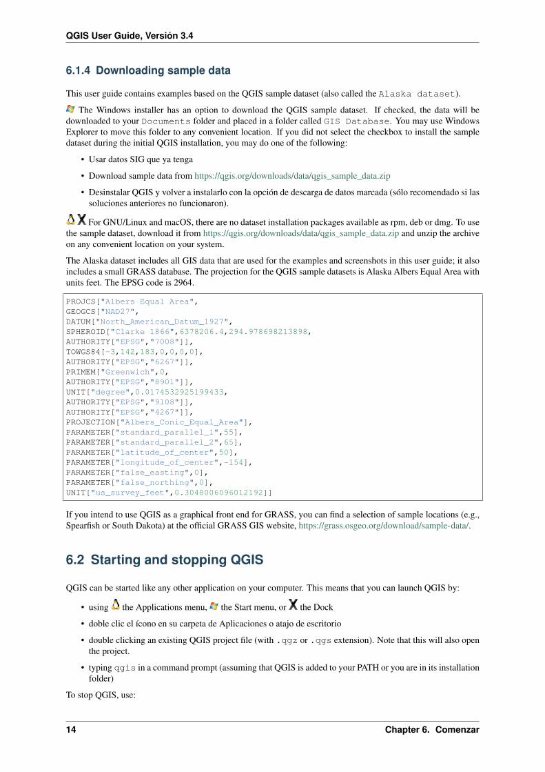
QGIS User Guide, Versión 3.4
• Check Override system locale if you want to use a language different from your system’s and pick thereplacement in Locale to use instead combobox.
• Information about active system locale are provided.
Aplicación
• Select the Style (QGIS restart required) and choose between “Oxygen”, “Windows”, “Motif”,“CDE”, “Plastique” and “Cleanlooks”;
• Define the UI theme . It can be “default” or “Night Mapping”;
• Define the Icon size ;
• Define the Font and its Size. The font can be Qt default or a user-defined one;
• Change the Timeout for timed messages or dialogs ;
• Hide splash screen at startup;
• Check QGIS version at startup to keep you informed if a newer version is released;
• Modeless data source manager dialog to keep the data source manager dialog opened and allow inter-action with QGIS interface while adding layers to project;
• Use native color chooser dialogs (see Selector de color).
Los archivos de proyecto
• Open project on launch (choose between “New”, “Most recent”, “Welcome Page”, and “Specific”).When choosing “Specific” use the . . . button to define the project to use by default. The “Welcome Page”displays a list of recent projects with screenshot.
• Crear nuevo proyecto desde el proyecto predeterminado. Tiene la posibilidad de presionar Establecerel actual proyecto como predeterminado o sobre Restablecer el predeterminado. Puede navegar a través desus archivos y definir un directorio donde se encuentra las plantillas definidas por el usuario. Esto se añadirá
a Proyecto → Nueva plantilla de formulario. Si activa primero Crear nuevo proyecto desde proyectopredeterminado y entonces guarde un proyecto en l la carpeta de las plantillas de proyecto.
• Prompt to save project and data source changes when required to avoid losing changes you made.
• Pedir confirmación cuando se va a eliminar una capa
• Warn when opening a project file saved with an older version of QGIS. You can always open projectscreated with older version of QGIS but once the project is saved, trying to open with older release may failbecause of features not available in that version.
• Enable macros . This option was created to handle macros that are written to perform an actionon project events. You can choose between “Never”, “Ask”, “For this session only” and “Always (notrecommended)”.
9.1.2 System Settings
SVG paths
Add or Remove Path(s) to search for Scalable Vector Graphic (SVG) symbols. These SVG files are then availableto symbolize features or decorate your map composition.
Rutas de complemento
Add or Remove Path(s) to search for additional C++ plugin libraries.
Documentation paths
42 Chapter 9. Configuración QGIS

QGIS User Guide, Versión 3.4
Add or Remove Documentation Path(s) to use for QGIS help. By default, a link to the official online User Manualcorresponding to the version being used is added. You can however add other links and prioritize them from topto bottom: each time you click on a Help button in a dialog, the topmost link is checked and if no correspondingpage is found, the next one is tried, and so on.
Nota: Documentation is versioned and translated only for QGIS Long Term Releases (LTR), meaning that if youare running a regular release (eg, QGIS 3.0), the help button will by default open the next LTR manual page (ie.3.4 LTR), which may contain description of features in newer releases (3.2 and 3.4). If no LTR documentation isavailable then the testing doc, with features from newer and development versions, is used.
QSettings
It helps you Reset user interface to default settings (restart required) if you made any customization.
Entorno
Variables de entorno del sistema ahora se puede ver, y muchos lo configuran en el grupo Entorno (ver fig-ure_environment_variables). Esto es útil para las plataformas, como Mac, donde una aplicación GUI no heredannecesariamente entorno del casco del usuario. También es útil para configurar y visualizar las variables de en-torno para los conjuntos de herramientas externas controladas por la caja de herramientas de procesamiento (porejemplo, SAGA, GRASS), y para activar la salida de depuración para secciones específicas del código fuente.
• Use custom variables (restart required - include separators). You can Add and Remove variables.Already-defined environment variables are displayed in Current environment variables, and it’s possible to
filter them by activating Show only QGIS-specific variables.
Figure 9.1: Variables del ambiente del sistema en QGIS
9.1. Opciones 43
QGIS User Guide, Versión 3.4
9.1.3 Configuraciones SRC
Default CRS for new projects
There is an option to automatically set new project’s CRS:
• Use CRS from first layer added: the CRS of the project is turned to match the CRS of the first layerloaded into it
• Use a default CRS: a preselected CRS is applied by default to any new project and is left unchangedwhen adding layers to the project.
The choice will be saved for use in subsequent QGIS sessions and in any case, the Coordinate Reference Systemof the project can still be overridden from the Project → Project properties → CRS tab.
SRC para nuevas capas
Esta área permite definir la acción a realizar cuando una nueva capa es creada, o cuando una capa sin SRC escargada.
• Prompt for CRS
• Use project CRS
• Use a default CRS
Por defecto transformación de datum
In this group, you can control whether reprojecting layers to another CRS should be:
• automatically processed using QGIS default transformations settings;
• and/or more controlled by you with custom preferences such as:
– Ask for datum transformation if several are available
– a predefined list of datum transformations to apply by default. See Datum Transformations for moredetails.
Nota: For more information on how QGIS handles layers projection, please read the dedicated section at Trabajarcon Proyecciones.
9.1.4 Data Sources Settings
Atributos de entidades espaciales y tabla
• Open attribute table in a dock window
• Copy features as “Plain text, no geometry”, “Plain text, WKT geometry”, or “GeoJSON” when pastingfeatures in other applications.
• Attribute table behavior : set filter on the attribute table at the opening. There are three possibilities:“Show all features”, “Show selected features” and “Show features visible on map”.
• Default view: define the view mode of the attribute table at every opening. It can be “Remember last view”,“Table view” or “Form view”.
• Attribute table row cache . This row cache makes it possible to save the last loaded N attribute rowsso that working with the attribute table will be quicker. The cache will be deleted when closing the attributetable.
• Representación de valores NULOS. Aquí, puede definir un valor para los datos de campos que tienen unvalor NULO.
44 Chapter 9. Configuración QGIS
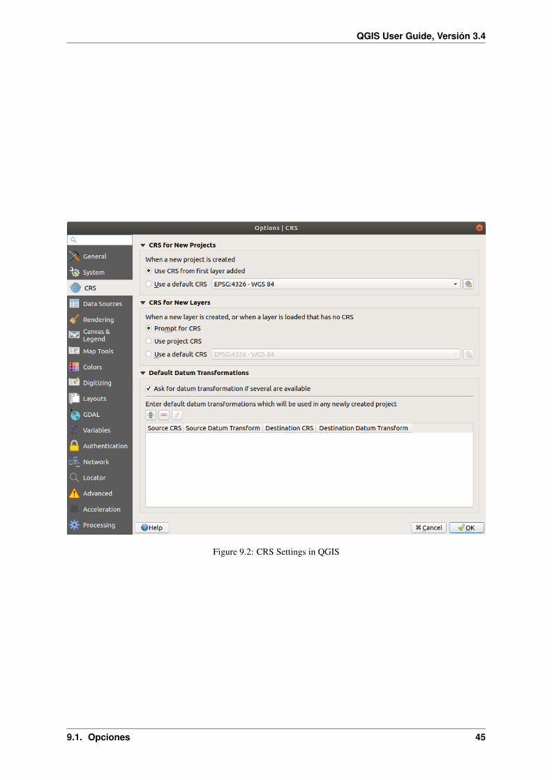
QGIS User Guide, Versión 3.4
Figure 9.2: CRS Settings in QGIS
9.1. Opciones 45
QGIS User Guide, Versión 3.4
Truco: Improve opening of big data attribute table
When working with layers with big amount of records, opening the attribute table may be slow as the dialogrequest all the rows in the layer. Setting the Attribute table behavior to Show features visible on map will makeQGIS request only the features in the current map canvas when opening the table, allowing a quick data loading.
Note that data in this attribute table instance will be always tied to the canvas extent it was opened with, meaningthat selecting Show All Features within such a table will not display new features. You can however update theset of displayed features by changing the canvas extent and selecting Show Features Visible On Map option inthe attribute table.
Manejo de fuente de datos
• Scan for valid items in the browser dock . You can choose between “Check extension” and “Checkfile contents”.
• Scan for contents of compressed files (.zip) in browser dock defines how detailed is the widget infor-mation at the bottom of the Browser panel when querying such files. “No”, “Basic scan” and “Full scan”are possible options.
• Solicitar subcapas raster al abrir. Algunas subcapas raster soportadas — se les llama subdataset en GDAL.Un ejemplo son los archivos netCDF — si hay muchos variables netCDF, GDAL ve cada variable como unsubconjunto de datos. La opción le permite controlar cómo lidiar con subcapas cuando se abre un archivocon subcapas. Dispone de las siguientes opciones:
– ‘Siempre’: Siempre preguntar (Si hay subcapas existentes)
– ‘Si es necesario’: Preguntar si la capa no tiene bandas, pero tiene subcapas
– ‘Nunca’: Nunca preguntar, no se cargará nada
– ‘Cargar todo’: Nunca preguntar, pero cargar todas las subcapas
• Ignore shapefile encoding declaration. If a shapefile has encoding information, this will be ignored byQGIS.
• Añadir capas PostGIS con doble clic y seleccionar en modo extendido
• Añadir capas de Oracle con doble clic y seleccionar en modo extendido
• Ejecutar expresiones en el lado del servidor si es posible
• Evaluate default values defines whether default values from database provider should be calculatedwhen digitizing the new feature (checked status) or when saving the changes.
Hidden Browser Path
This widget lists all the folders you chose to hide from the Browser panel. Removing a folder from the list willmake it available in the Browser panel.
9.1.5 Rendering Settings
Comportamiento de presentación
• By default new layers added to the map should be displayed: unchecking this option can be handy whenloading multiple layers to avoid each new layer being rendered in the canvas and slow down the process
• Utilizar el cacheo de presentación en lo posible a la velocidad de regeneración
• Representación de capas en paralelo utilizando muchos núcleos CPU
• Máximo de núcleos a utilizar
46 Chapter 9. Configuración QGIS

QGIS User Guide, Versión 3.4
Figure 9.3: Data Sources Settings in QGIS
9.1. Opciones 47
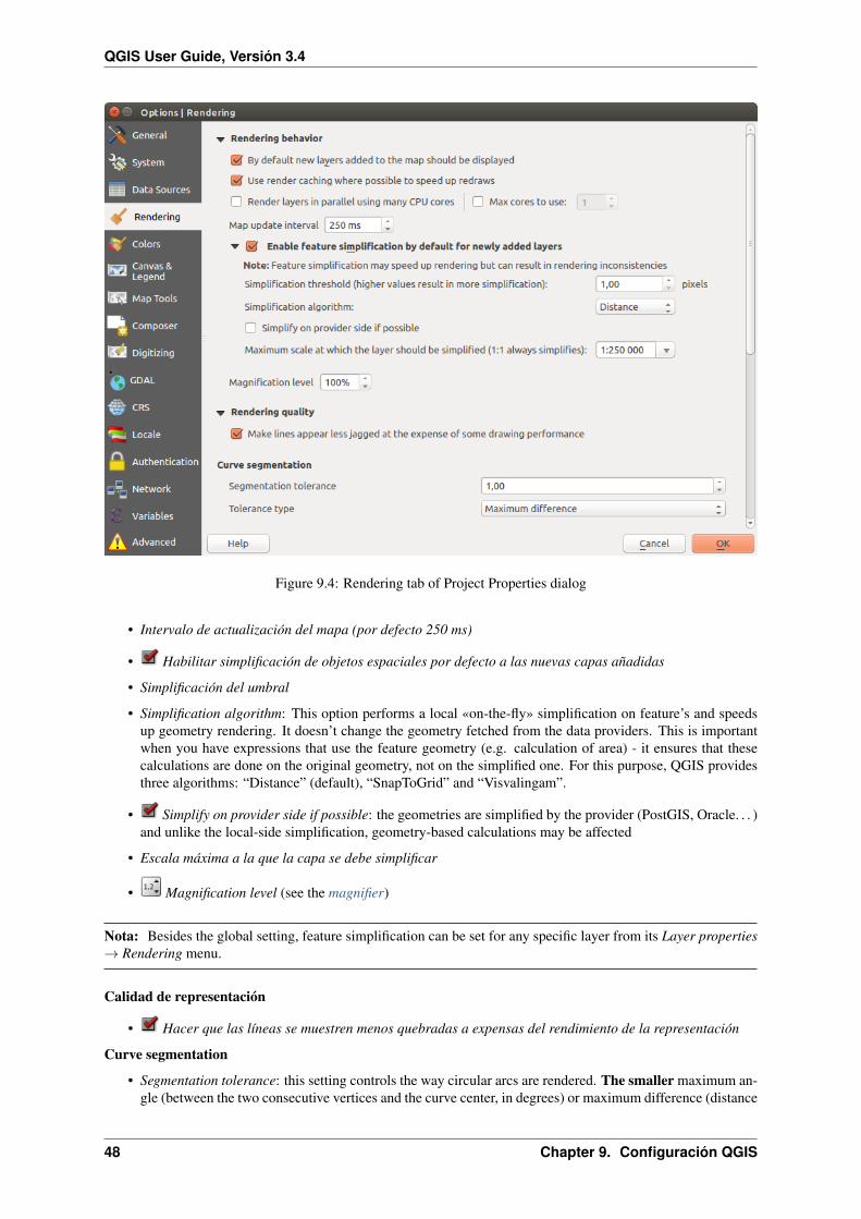
QGIS User Guide, Versión 3.4
Figure 9.4: Rendering tab of Project Properties dialog
• Intervalo de actualización del mapa (por defecto 250 ms)
• Habilitar simplificación de objetos espaciales por defecto a las nuevas capas añadidas
• Simplificación del umbral
• Simplification algorithm: This option performs a local «on-the-fly» simplification on feature’s and speedsup geometry rendering. It doesn’t change the geometry fetched from the data providers. This is importantwhen you have expressions that use the feature geometry (e.g. calculation of area) - it ensures that thesecalculations are done on the original geometry, not on the simplified one. For this purpose, QGIS providesthree algorithms: “Distance” (default), “SnapToGrid” and “Visvalingam”.
• Simplify on provider side if possible: the geometries are simplified by the provider (PostGIS, Oracle. . . )and unlike the local-side simplification, geometry-based calculations may be affected
• Escala máxima a la que la capa se debe simplificar
• Magnification level (see the magnifier)
Nota: Besides the global setting, feature simplification can be set for any specific layer from its Layer properties→ Rendering menu.
Calidad de representación
• Hacer que las líneas se muestren menos quebradas a expensas del rendimiento de la representación
Curve segmentation
• Segmentation tolerance: this setting controls the way circular arcs are rendered. The smaller maximum an-gle (between the two consecutive vertices and the curve center, in degrees) or maximum difference (distance
48 Chapter 9. Configuración QGIS

QGIS User Guide, Versión 3.4
between the segment of the two vertices and the curve line, in map units), the more straight line segmentswill be used during rendering.
• Tolerance type: it can be Maximum angle or Maximum difference between approximation and curve.
Rásters
• Con Selección de la banda RGB, puede definir el numero para la banda Roja, Verde y Azul.
Mejora de contraste
Contrast enhancement options can be applied to Single band gray, Multi band color (byte/band) or Multi bandcolor (>byte/band). For each, you can set:
• the Algorithm to use, whose values can be “No stretch”, “Stretch to MinMax”, “Stretch and Clip to MinMax”or “Clip to MinMax”
• the Limits (minimum/maximum) to apply, with values such as “Cumulative pixel count cut”, “Mini-mum/Maximum”, “Mean +/- standard deviation”.
For rasters rendering, you can also define the following options:
• Límite para corte del conteo acumulativo de píxeles
• Multiplicador de la desviación estándar
Depuración
• Map canvas refresh to debug rendering duration in the Log Messages panel.
9.1.6 Canvas and Legend Settings
Figure 9.5: Canvas and Legend Settings
These properties let you set:
• the Default map appearance (overridden by project properties): the Selection color and Backgroundcolor.
• Layer legend interaction:
– Double click action in legend . You can either “Open layer properties”, “Open attribute table”or “Open layer styling dock” with the double click.
– Display classification attribute names in the Layers panel, e.g. when applying a categorized orrule-based renderer (see Symbology Properties for more information).
– the WMS getLegendGraphic Resolution
9.1. Opciones 49
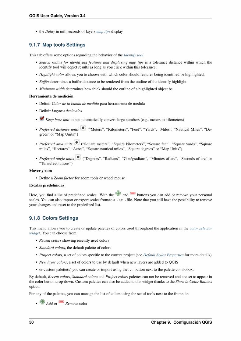
QGIS User Guide, Versión 3.4
• the Delay in milliseconds of layers map tips display
9.1.7 Map tools Settings
This tab offers some options regarding the behavior of the Identify tool.
• Search radius for identifying features and displaying map tips is a tolerance distance within which theidentify tool will depict results as long as you click within this tolerance.
• Highlight color allows you to choose with which color should features being identified be highlighted.
• Buffer determines a buffer distance to be rendered from the outline of the identify highlight.
• Minimum width determines how thick should the outline of a highlighted object be.
Herramienta de medición
• Definir Color de la banda de medida para herramienta de medida
• Definir Lugares decimales
• Keep base unit to not automatically convert large numbers (e.g., meters to kilometers)
• Preferred distance units (“Meters”, “Kilometers”, “Feet”, “Yards”, “Miles”, “Nautical Miles”, “De-grees” or “Map Units” )
• Preferred area units (“Square meters”, “Square kilometers”, “Square feet”, “Square yards”, “Squaremiles”, “Hectares”, “Acres”, “Square nautical miles”, “Square degrees” or “Map Units”)
• Preferred angle units (“Degrees”, “Radians”, “Gon/gradians”, “Minutes of arc”, “Seconds of arc” or“Turns/revolutions”)
Mover y zum
• Define a Zoom factor for zoom tools or wheel mouse
Escalas predefinidas
Here, you find a list of predefined scales. With the and buttons you can add or remove your personalscales. You can also import or export scales from/to a .XML file. Note that you still have the possibility to removeyour changes and reset to the predefined list.
9.1.8 Colors Settings
This menu allows you to create or update palettes of colors used throughout the application in the color selectorwidget. You can choose from:
• Recent colors showing recently used colors
• Standard colors, the default palette of colors
• Project colors, a set of colors specific to the current project (see Default Styles Properties for more details)
• New layer colors, a set of colors to use by default when new layers are added to QGIS
• or custom palette(s) you can create or import using the . . . button next to the palette combobox.
By default, Recent colors, Standard colors and Project colors palettes can not be removed and are set to appear inthe color button drop-down. Custom palettes can also be added to this widget thanks to the Show in Color Buttonsoption.
For any of the palettes, you can manage the list of colors using the set of tools next to the frame, ie:
• Add or Remove color
50 Chapter 9. Configuración QGIS
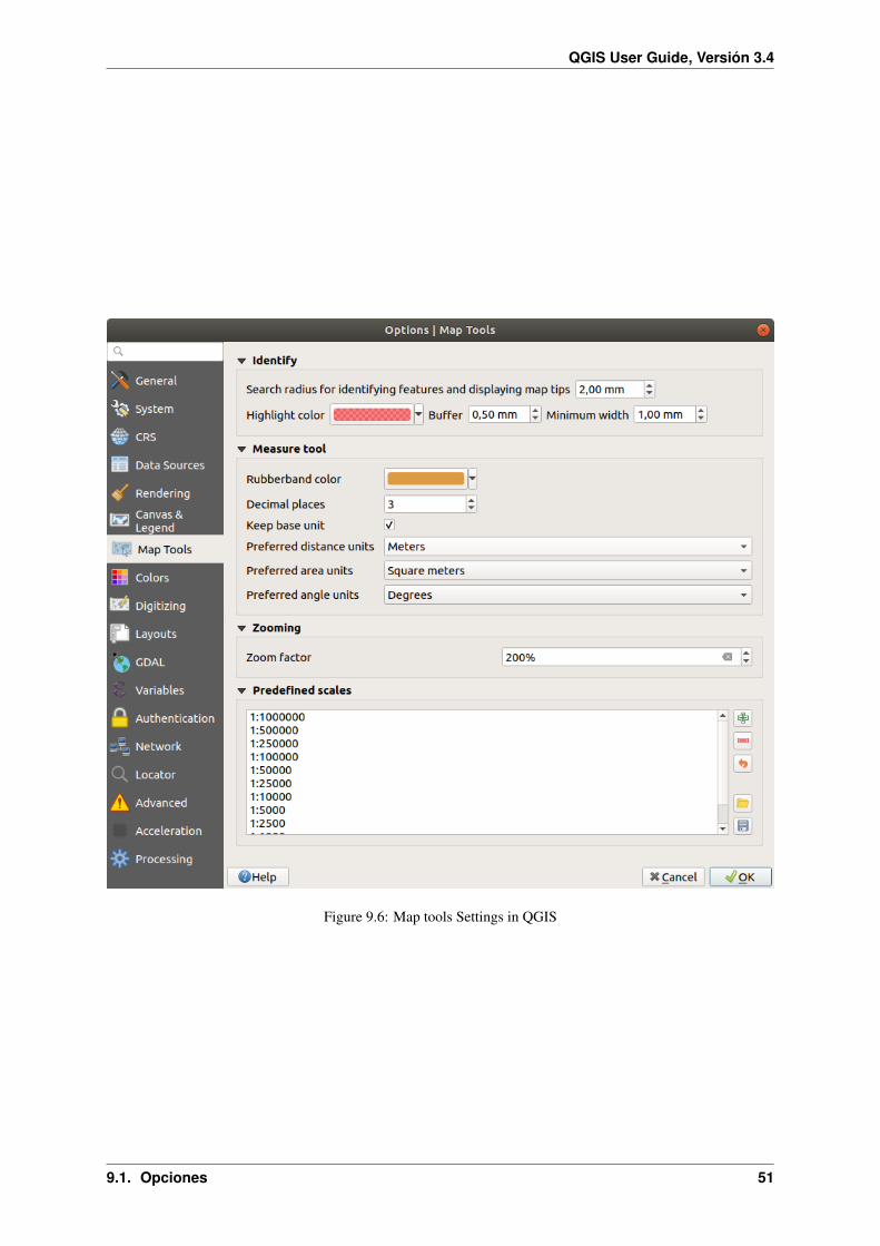
QGIS User Guide, Versión 3.4
Figure 9.6: Map tools Settings in QGIS
9.1. Opciones 51
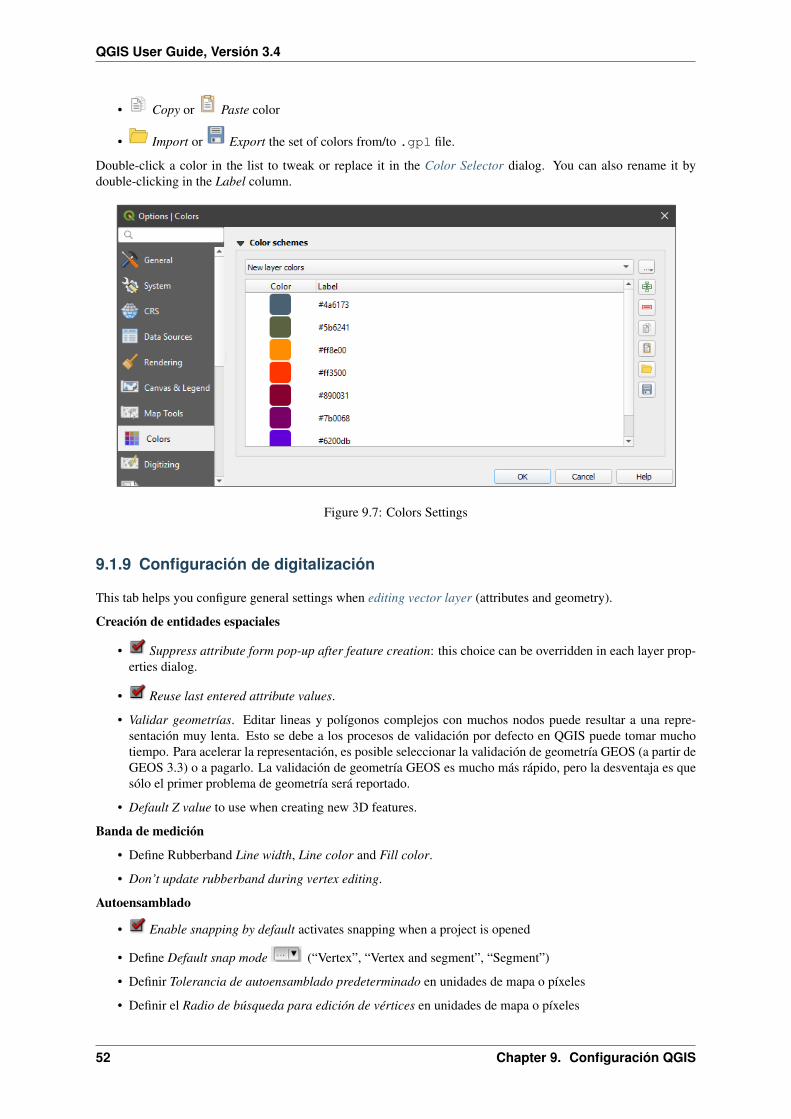
QGIS User Guide, Versión 3.4
• Copy or Paste color
• Import or Export the set of colors from/to .gpl file.
Double-click a color in the list to tweak or replace it in the Color Selector dialog. You can also rename it bydouble-clicking in the Label column.
Figure 9.7: Colors Settings
9.1.9 Configuración de digitalización
This tab helps you configure general settings when editing vector layer (attributes and geometry).
Creación de entidades espaciales
• Suppress attribute form pop-up after feature creation: this choice can be overridden in each layer prop-erties dialog.
• Reuse last entered attribute values.
• Validar geometrías. Editar lineas y polígonos complejos con muchos nodos puede resultar a una repre-sentación muy lenta. Esto se debe a los procesos de validación por defecto en QGIS puede tomar muchotiempo. Para acelerar la representación, es posible seleccionar la validación de geometría GEOS (a partir deGEOS 3.3) o a pagarlo. La validación de geometría GEOS es mucho más rápido, pero la desventaja es quesólo el primer problema de geometría será reportado.
• Default Z value to use when creating new 3D features.
Banda de medición
• Define Rubberband Line width, Line color and Fill color.
• Don’t update rubberband during vertex editing.
Autoensamblado
• Enable snapping by default activates snapping when a project is opened
• Define Default snap mode (“Vertex”, “Vertex and segment”, “Segment”)
• Definir Tolerancia de autoensamblado predeterminado en unidades de mapa o píxeles
• Definir el Radio de búsqueda para edición de vértices en unidades de mapa o píxeles
52 Chapter 9. Configuración QGIS

QGIS User Guide, Versión 3.4
• Display main dialog as (restart required): set whether the Advanced Snapping dialog should be shown as“Dialog” or “Dock”.
• Snapping marker color
• Show snapping tooltips such as name of the layer whose feature you are about to snap. Helpful whenmultiple features overlap.
• Enable snapping on invisible features
Marcar vértices
• Mostrar marcadores sólo para los objetos espaciales seleccionados
• Definir vértice Estilo de marcador (“Cruz” (predeterminado), “Círculo semitransparente” o “Nada”)
• Definir vértice Tamaño de marcador
Herramienta de desplazamiento de curva
The next 3 options refer to the Offset Curve tool in Digitalización avanzada. Through the various settings, it ispossible to influence the shape of the line offset. These options are possible starting from GEOS 3.3.
• Join style: “Round”, “Mitre” or “Bevel”
• Segmentos del cuadrante
• Límite Miter
9.1.10 Layouts Settings
Predeterminados de la composición
You can define the Default font used within the print layout.
Apariencia de la cuadrícula
• Definir el Estilo de cuadrícula (“Sólido, “Puntos”, “Cruces”)
• Definir el Color de la cuadrícula
Valores predeterminados de la cuadrícula y guía
• Define the Grid spacing
• Define the Grid offset for X and Y
• Define the Snap tolerance
Layout Paths
• Define Path(s) to search for extra print templates: a list of folders with custom layout templates to use whilecreating new one.
9.1.11 Configuración de GDAL
GDAL is a data exchange library for vector and raster files. It provides drivers to read and or write data in differentformats. The GDAL tab currently exposes the drivers for raster formats with their capabilities.
GDAL driver options
This frame provides ways to customize the behavior of drivers that support read and write access:
9.1. Opciones 53

QGIS User Guide, Versión 3.4
Figure 9.8: Digitizing Settings in QGIS
54 Chapter 9. Configuración QGIS

QGIS User Guide, Versión 3.4
Figure 9.9: Layouts Settings in QGIS
• Edit create options: allows you to edit or add different profiles of file transformation, i.e. a set of predefinedcombinations of parameters (type and level of compression, blocks size, overview, colorimetry, alpha. . . ) touse when outputting raster files. The parameters depend on the driver.
Figure 9.10: Sample of create options profile (for GeoTiff)
The upper part of the dialog lists the current profile(s) and allows you to add new ones or remove any ofthem. You can also reset the profile to its default parameters if you have changed them. Some drivers (eg,GeoTiff) have some sample of profiles you can work with.
At the bottom of the dialog:
– The button lets you add rows to fill with the parameter name and value
– The button deletes the selected parameter
– Click the Validate button to check that the creation options entered for the given format are valid
– Use the Help button to find the parameters to use, or refer to the GDAL raster drivers documentation.
9.1. Opciones 55

QGIS User Guide, Versión 3.4
• Edit Pyramids Options
Figure 9.11: Sample of Pyramids profile
GDAL drivers
In this frame, you can define which GDAL driver is to use to read and/or write files, as in some cases more thanone GDAL driver is available.
Truco: Double-click a driver that allows read and write access (rw+(v)) opens the Edit Create options dialogfor customization.
9.1.12 Variables Settings
The Variables tab lists all the variables available at the global-level.
It also allows the user to manage global-level variables. Click the button to add a new custom global-level
variable. Likewise, select a custom global-level variable from the list and click the button to remove it.
More information about variables in the Storing values in Variables section.
9.1.13 Authentication Settings
In the Authentication tab you can set authentication configurations and manage PKI certificates. See Sistema deautenticación for more details.
9.1.14 Network Settings
General
• Definir Dirección de búsqueda de WMS, por omisión es http://geopole.org/wms/search?search=\%1\&type=rss
• Definir Expiró el tiempo para solicitudes de red - por omisión 60000
• Define Default expiration period for WMS Capabilities (hours) - default is 24
• Definir Periodo de expiración predeterminada para teselas WMS-C/WMTS (en horas) - por omisión 24
• Define Max retry in case of tile or feature request errors
56 Chapter 9. Configuración QGIS
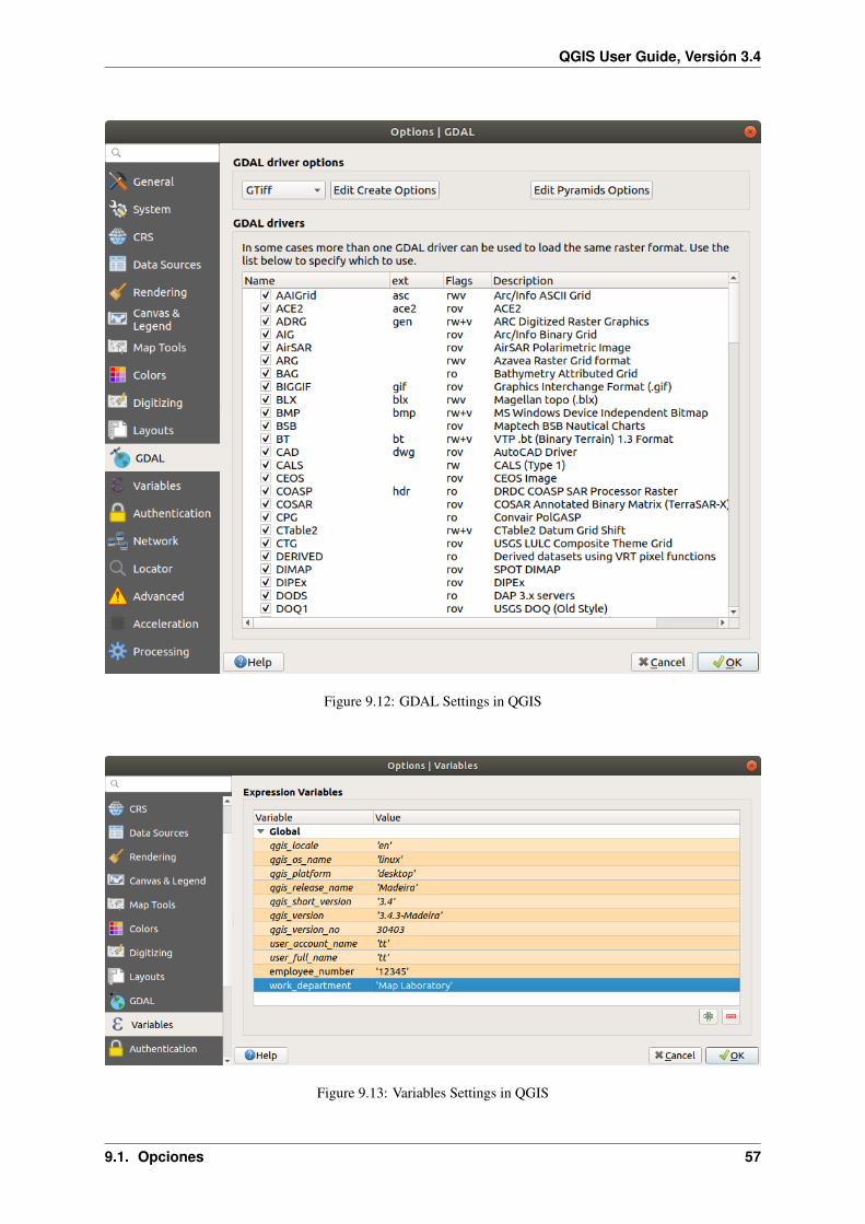
QGIS User Guide, Versión 3.4
Figure 9.12: GDAL Settings in QGIS
Figure 9.13: Variables Settings in QGIS
9.1. Opciones 57

QGIS User Guide, Versión 3.4
Figure 9.14: Authentication Settings in QGIS
• Definir Agente- Usuario
Configuración de caché
Defines the Directory and a Size for the cache. Also offers tools to automatically clear the connection authentica-tion cache on SSL errors (recommended).
Proxy for web access
• Use proxy for web access
• Set the Proxy type according to your needs and define “Host” and “Port”. Available proxy types are:
– Default Proxy: Proxy is determined based on system’s proxy
– Socks5Proxy: Proxy genérico para cualquier tipo de conexión. Soporta TCP, UDP, unión a un puerto(conexiones entrantes) y autenticación.
– HttpProxy: Implementado con el comando «CONNECT», sólo admite conexiones TCP salientes;admite la autenticación.
– HttpCachingProxy: Implementando el uso de comandos HTTP normales, es útil sólo en el contextode peticiones HTTP.
– FtpCachingProxy: Implementar el uso de un proxy FTP, es útil sólo en el contexto de las peticionesFTP.
Credentials of proxy are set using the authentication widget.
Excluir algunas URLs se puede agregar a la caja de texto debajo los valores del proxy (ver Figure_Network_Tab).
If you need more detailed information about the different proxy settings, please refer to the manual of the under-lying QT library documentation at https://doc.qt.io/qt-5.9/qnetworkproxy.html#ProxyType-enum
58 Chapter 9. Configuración QGIS

QGIS User Guide, Versión 3.4
Figure 9.15: Configurar proxy en QGIS
9.1. Opciones 59
QGIS User Guide, Versión 3.4
Truco: Utilizar proxies
Using proxies can sometimes be tricky. It is useful to proceed by “trial and error” with the above proxy types, tocheck if they succeed in your case.
9.1.15 Locator Settings
The Locator tab allows to configure the Locator bar, a quick search widget available on the status bar thathelps you perform searches anywhere in the application. It provides some default filters (with prefix) to use:
• Project layers (l): finds and selects a layer in the Layers panel.
• Project layouts (pl): finds and opens a print layout.
• Actions (.): finds and executes a QGIS action; actions can be any tool or menu in QGIS, opening a panel. . .
• Active layer features (f): searches for matching attributes in any field from the current active layer andzooms to the selected feature.
• Features in all layers (af): searches for matching attributes in the display name of each searchable layersand zooms to the selected feature.
• Calculator (=): allows evaluation of any QGIS expression and, if valid, gives an option to copy the result tothe clipboard.
• Spatial bookmarks (b): finds and zooms to the bookmark extent.
• Settings (set): browses and opens project and application-wide properties dialogs.
• Processing (a): searches and opens a Processing algorithm dialog.
• Edit selected features (ef): gives quick access and runs a compatible modify-in-place Processing algorithmon the active layer.
For each filter, you can customize the filter, set whether it is enabled by default or not. The set of default locatorfilters can be extended by plugins, eg for OSM nominatim searches, direct database searching, layer catalogsearches.
The locator search bar can be activated pressing Ctrl+K. Type your text to perform a search. By default, resultsare returned for all enabled locator filters but you can limit the search to a certain filter by prefixing your text withthe locator filter prefix, ie. typing l cad will return only the layers whose name contains cad. Click on theresult to execute the corresponding action, depending on the type of item.
Searching is handled using threads, so that results always become available as quickly as possible, regardless ofwhether any slow search filters may be installed. They also appear as soon as each result is encountered by eachfilter, which means that e.g. a file search filter will show results one by one as the file tree is scanned. This ensuresthat the UI is always responsive even if a very slow search filter is present (e.g. one which uses an online service).
Truco: Quick access to the locator’s configurations
Click on the icon inside the locator widget on the status bar to display the list of filters you can use and aConfigure entry that opens the Locator tab of the Settings → Options. . . menu.
9.1.16 Configuración avanzada
Depending on your OS, all the settings related to QGIS (UI, tools, data providers, default values, plugins op-tions. . . ) are saved:
• in a text file: $HOME/.config/QGIS/QGIS2.conf
60 Chapter 9. Configuración QGIS

QGIS User Guide, Versión 3.4
Figure 9.16: Locator Settings in QGIS
• in the properties list file: $HOME/Library/Preferences/org.qgis.qgis.plist
• in the registry under: HKEY\CURRENT_USER\Software\QGIS\qgis
The Advanced tab offers you in a single place, regardless your OS, means to manage these settings through theAdvanced Settings Editor. After you promise to be careful, the widget is populated with a tree of all QGIS settings,which you can directly edit.
Advertencia: Avoid using the Advanced tab settings blindly
Be careful while modifying items in this dialog given that changes are automatically applied. Doing changeswithout knowledge can break your QGIS installation in various ways.
9.1.17 Processing Settings
The Processing tab provides you with general settings of tools and data providers that are used in the QGISProcessing framework. More information at Entorno de trabajo de procesamiento de QGIS.
9.2 Working with User Profiles
The Settings → User Profiles menu provides functions to set and access user profiles. A user profile is a unifiedapplication configuration that allows to store in a single folder:
• all the global settings, including locale, projections, authentication settings, color palettes, shortcuts. . .
• GUI configurations and customization
• installed plugins and their configurations
• project templates and history of saved project with their image preview
9.2. Working with User Profiles 61

QGIS User Guide, Versión 3.4
Figure 9.17: Advanced Settings tab in QGIS
Figure 9.18: Pestaña configuración de procesamiento en QGIS
62 Chapter 9. Configuración QGIS

QGIS User Guide, Versión 3.4
• processing settings, logs, scripts, models.
By default, a QGIS installation contains a single user profile named default. But you can create as many userprofiles as you want:
1. Click the New profile. . . entry.
2. You’ll be prompted to provide a profile name, creating a folder of the same name under ~/<UserProfiles>/ where:
• ~ represents the HOME directory, which on Windows is usually something likeC:\Users\(user).
• and <UserProfiles> represents the main profiles folder, i.e.:
– .local/share/QGIS/QGIS3/profiles/
– AppData\Roaming\QGIS\QGIS3\profiles\
– Library/Application Support/QGIS/QGIS3/profiles/
The user profile folder can be opened from within QGIS using the Open Active Profile Folder.
3. A new instance of QGIS is started, using a clean configuration. You can then set your custom configurations.
As each user profile contains isolated settings, plugins and history they can be great for different workflows,demos, users of the same machine, or testing settings, etc. And you can switch from one to the other by selectingthem in the Settings → User Profiles menu. You can also run QGIS with a specific user profile from the commandline.
Unless changed, the profile of the last closed QGIS session will be used in the following QGIS sessions.
Truco: Run QGIS under a new user profile to check for bug persistence
When you encounter weird behavior with some functions in QGIS, create a new user profile and run the commandsagain. Sometimes, bugs are related to some leftovers in the current user profile and creating a new one may fixthem as it restarts QGIS with the new (clean) profile.
9.3 Propiedades del proyecto
In the properties window for the project under Project → Project Properties, you can set project-specific options.The project-specific options overwrite their equivalent in the Options dialog described above.
9.3.1 General Properties
In the General tab, the General settings let you:
• see the location of the project file
• set the folder for the project home (available in the Project Home item in the browser). The path can berelative to the folder of the project file (type it in) or absolute. The project home can be used for storing dataand other content that is useful for the project.
• dé un texto al título del proyecto aparte de la ruta del archivo del proyecto
• escoge el color a usar para objetos espaciales cuando son seleccionados
• escoger el color de fondo: el color a usar para la tela de fondo del mapa
• set whether the path to layers in the project should be saved as absolute (full) or as relative to the project filelocation. You may prefer relative path when both layers and project files can be moved or shared or if theproject is accessed from computers on different platforms.
9.3. Propiedades del proyecto 63
QGIS User Guide, Versión 3.4
• choose to avoid artifacts when project is rendered as map tiles. Note that checking this option can lead toperformance degradation.
Calculating areas and distances is a common need in GIS. However, these values are really tied to the underlyingprojection settings. The Measurements frame lets you control these parameters. You can indeed choose:
• the Ellipsoid, on which distance and area calculations are entirely based; it can be:
– None/Planimetric: returned values are in this case cartesian measurements.
– a Custom one: you’ll need to set values of the semi-major and semi-minor axes.
– or an existing one from a predefined list (Clarke 1866, Clarke 1880 IGN, New International 1967,WGS 84. . . ).
• the units for distance measurements for length and perimeter and the units for area measurements. Thesesettings, which default to the units set in QGIS options but then overrides it for the current project, are usedin:
– Attribute table field update bar
– Cálculos de calculadora de campo
– Identify tool derived length, perimeter and area values
– Default unit shown in measure dialog
The Coordinate display allows you to choose and customize the format of units to use to display the mousecoordinate in the status bar and the derived coordinates shown via the identify tool.
Finally, you can set a Project predefined scales list, which overrides the global predefined scales.
9.3.2 Metadata Properties
The Metadata tab allows detailed metadata to be defined, including (among the others): author, creation date,language, abstracts, categories, keywords, contact details, links, history. There is also a validation functionalitythat checks if specific fields were filled, anyway this is not enforced. See vector layer metadata properties forsome details.
9.3.3 CRS Properties
The CRS tab helps you set the coordinate reference system to use in this project. It can be:
• No projection (or unknown/non-Earth projection): this setting can be used to guess a layer CRS or whenusing QGIS for non earth uses like role-playing game maps, building mapping or microscopic stuff. In thiscase:
– No reprojection is done while rendering the layers: features are just drawn using their raw coordinates.
– The ellipsoid is locked out and forced to None/Planimetric.
– The distance and area units, and the coordinate display are locked out and forced to «unknown units»;all measurements are done in unknown map units, and no conversion is possible.
• or an existing coordinate reference system that can be geographic, projected or user-defined. A preview ofthe CRS extent on earth is displayed to help you select the appropriate one. Layers added to the projectare on-the-fly translated to this CRS in order to overlay them regardless their original CRS. Use of units,ellipsoid setting are available and make sense and you can perform calculations accordingly.
The CRS tab also helps you control the layers reprojection settings by configuring the datum transformationpreferences to apply in the current project. As usual, these override any corresponding global settings. See DatumTransformations for more details.
64 Chapter 9. Configuración QGIS

QGIS User Guide, Versión 3.4
Figure 9.19: General tab of Project Properties dialog
9.3. Propiedades del proyecto 65

QGIS User Guide, Versión 3.4
9.3.4 Default Styles Properties
The Default Styles tab lets you control how new layers will be drawn in the project when they do not have anexisting .qml style defined. You can:
• Set default symbols (Marker, Line, Fill) to apply depending on the layer geometry type as well as a defaultColor Ramp
• Apply a default Opacity to new layers
• Assign random colors to symbols, modifying the symbols fill colors, hence avoiding same rendering forall layers.
Figure 9.20: Default Styles tab
Using the Style Manager button, you can also quickly access the Style Manager dialog and configure symbolsand color ramps.
There is also an additional section where you can define specific colors for the running project. Like the globalcolors, you can:
• Add or Remove color
• Copy or Paste color
• Import or Export the set of colors from/to .gpl file.
Double-click a color in the list to tweak or replace it in the Color Selector dialog. You can also rename it bydouble-clicking in the Label column.
These colors are identified as Project colors and listed as part of color widgets.
Truco: Use project colors to quickly assign and update color widgets
66 Chapter 9. Configuración QGIS

QGIS User Guide, Versión 3.4
Project colors can be refered to using their label and the color widgets they are used in are bound to them. Thismeans that instead of repeatedly setting the same color for many properties and, to avoid a cumbersome updateyou can:
1. Define the color as a project color
2. Apply it using the project_color('color_label') expression in color data defined override wid-get
3. Update the color once in a Project colors list
4. And the change is reflected EVERYWHERE.
9.3.5 Data Sources Properties
In the Data Sources tab, you can:
• Automatically create transaction groups where possible: When this mode is turned on, all (postgres)layers from the same database are synchronised in their edit state, i.e. when one layer is put into edit state,all are, when one layer is committed or one layer is rolled back, so are the others. Also, instead of bufferingedit changes locally, they are directly sent to a transaction in the database which gets committed when theuser clicks save layer. Note that you can (de)activate this option only if no layer is being edited in theproject.
• Evaluate default values on provider side: When adding new features in a PostgreSQL table, fields withdefault value constraint are evaluated and populated at the form opening, and not at the commit moment.This means that instead of an expression like nextval('serial'), the field in the Add Feature formwill display expected value (e.g., 25).
• Trust project when data source has no metadata: To speed up project loading by skipping data checks.Useful in QGIS Server context or in projects with huge database views/materialized views. The extent oflayers will be read from the QGIS project file (instead of data sources) and when using the PostgreSQLprovider the primary key unicity will not be checked for views and materialized views.
• Configure the Layers Capabilities, i.e.:
– Set (or disable) which layers are identifiable, i.e. will respond to the identify tool. By default,layers are set queryable.
– Set whether a layer should appear as read-only, meaning that it can not be edited by the user,regardless of the data provider’s capabilities. Although this is a weak protection, it remains a quickand handy configuration to avoid end-users modifying data when working with file-based layers.
– Define which layers are searchable, i.e. could be queried using the locator widget. By default,layers are set searchable.
– Define which layers are defined as required. Checked layers in this list are protected from inadver-tent removal from the project.
The Layers Capabilities table provides some convenient tools to:
– Select multiple cells and press Toggle Selection to have them change their checkbox state;
– Show spatial layers only, filtering out non-spatial layers from the layers list;
– Filter layers. . . and quickly find a particular layer to configure.
9.3.6 Relations Properties
El panel:guilabel:Relaciones es utilizado para definir relaciones 1:n. Las relaciones están definidas en el diálogode propiedades del proyecto. Una vez que existen las relaciones de una capa, un nuevo elemento de la interfaz deusuario en la vista del formulario (por ejemplo al identificar un elemento espacial y abrir el formulario) mostrará
9.3. Propiedades del proyecto 67

QGIS User Guide, Versión 3.4
una lista de las entidades relacionadas. Este proporciona un poderosa forma para expresar, por ejemplo la inspec-ción de la longitud de una tubería o el segmento de carretera. Se puede encontrar más información acerca derelaciones 1:n y soporte en la sección Creating one or many to many relations.
9.3.7 Variables Properties
The Variables tab lists all the variables available at the project’s level (which includes all global variables). Be-
sides, it also allows the user to manage project-level variables. Click the button to add a new custom project-
level variable. Likewise, select a custom project-level variable from the list and click the button to remove it.More information on variables usage in the General Tools Storing values in Variables section.
9.3.8 Macros Properties
The Macros tab is used to edit Python macros for projects. Currently, only three macros are available:openProject(), saveProject() and closeProject().
Figure 9.21: Definición macro en QGIS
68 Chapter 9. Configuración QGIS

QGIS User Guide, Versión 3.4
9.3.9 QGIS Server Properties
The tab QGIS Server allows you to configure your project in order to publish it online. Here you can defineinformation about the QGIS Server WMS and WFS capabilities, extent and CRS restrictions. More informationavailable in section Configure your project and subsequent.
9.4 Personalización
The customization dialog lets you (de)activate almost every element in the QGIS user interface. This can be veryuseful if you want to provide your end-users with a “light” version of QGIS, containing only the icons, menus orpanels they need.
Nota: Antes de aplicar los cambios, debe reiniciar QGIS.
Figure 9.22: El diálogo de Personalización
Ticking the Enable customization checkbox is the first step on the way to QGIS customization. This enablesthe toolbar and the widget panel from which you can uncheck and thus disable some GUI items.
The configurable item can be:
• a Menu or some of its sub-menus from the Barra de Menú
• a whole Panel (see Paneles y Barras de Herramientas)
• the Status bar described in Barra de Estado or some of its items
• a Toolbar: the whole bar or some of its icons
• or any widget from any dialog in QGIS: label, button, combobox. . .
With Switch to catching widgets in main application, you can click on an item in QGIS interface that you want to be hiddenand QGIS automatically unchecks the corresponding entry in the Customization dialog.
Once you setup your configuration, click Apply or OK to validate your changes. This configuration becomes theone used by default by QGIS at the next startup.
The modifications can also be saved in a .ini file using Save To File button. This is a handy way to share a
common QGIS interface among multiple users. Just click on Load from File from the destination computer inorder to import the .ini file. You can also run command line tools and save various setups for different use casesas well.
Truco: Easily restore predefined QGIS
9.4. Personalización 69

QGIS User Guide, Versión 3.4
The initial QGIS GUI configuration can be restored by one of the methods below:
• unchecking Enable customization option in the Customization dialog or click the Check All button
• pressing the Reset button in the QSettings frame under Settings → Options menu, System tab
• launching QGIS at a command prompt with the following command line qgis --nocustomization
• setting to false the value of UI → Customization → Enabled variable under Settings → Options menu,Advanced tab (see the warning).
In most cases, you need to restart QGIS in order to have the change applied.
9.5 Atajos de teclado
QGIS provides default keyboard shortcuts for many features. You can find them in section Barra de Menú.
Additionally, the menu option Settings → Keyboard Shortcuts. . . allows you to change the default keyboardshortcuts and add new ones to QGIS features.
Figure 9.23: Define shortcut options
Configuration is very simple. Use the search box at the top of the dialog to find a particular action, select it fromthe list and click on :
• Change and press the new combination you want to assign as new shortcut
• Set None to clear any assigned shortcut
• or Set Default to backup the shortcut to its original and default value.
Proceed as above for any other tools you wish to customize. Once you have finished your configuration, simplyClose the dialog to have your changes applied. You can also Save the changes as an .XML file and Load them intoanother QGIS installation.
70 Chapter 9. Configuración QGIS

QGIS User Guide, Versión 3.4
9.6 Running QGIS with advanced settings
9.6.1 Command line and environment variables
We’ve seen that launching QGIS is done as for any application on your OS. QGIS provides command line optionsfor more advanced use cases (in some cases you can use an environment variable instead of the command lineoption). To get a list of the options, enter qgis --help on the command line, which returns:
QGIS is a user friendly Open Source Geographic Information System.Usage: /usr/bin/qgis.bin [OPTION] [FILE]
OPTION:[--version] display version information and exit[--snapshot filename] emit snapshot of loaded datasets to given file[--width width] width of snapshot to emit[--height height] height of snapshot to emit[--lang language] use language for interface text (changes existing
→˓override)[--project projectfile] load the given QGIS project[--extent xmin,ymin,xmax,ymax] set initial map extent[--nologo] hide splash screen[--noversioncheck] don't check for new version of QGIS at startup[--noplugins] don't restore plugins on startup[--nocustomization] don't apply GUI customization[--customizationfile path] use the given ini file as GUI customization[--globalsettingsfile path] use the given ini file as Global Settings
→˓(defaults)[--authdbdirectory path] use the given directory for authentication
→˓database[--code path] run the given python file on load[--defaultui] start by resetting user ui settings to default[--hide-browser] hide the browser widget[--dxf-export filename.dxf] emit dxf output of loaded datasets to
→˓given file[--dxf-extent xmin,ymin,xmax,ymax] set extent to export to dxf[--dxf-symbology-mode none|symbollayer|feature] symbology mode for dxf
→˓output[--dxf-scale-denom scale] scale for dxf output[--dxf-encoding encoding] encoding to use for dxf output[--dxf-map-theme maptheme] map theme to use for dxf output[--take-screenshots output_path] take screen shots for the user
→˓documentation[--screenshots-categories categories] specify the categories of
→˓screenshot to be used (see QgsAppScreenShots::Categories).[--profile name] load a named profile from the user's profiles
→˓folder.[--profiles-path path] path to store user profile folders. Will create
→˓profiles inside a {path}\profiles folder[--version-migration] force the settings migration from older version if
→˓found[--openclprogramfolder] path to the folder containing the sources
→˓for OpenCL programs.[--help] this text[--] treat all following arguments as FILEs
FILE:Files specified on the command line can include rasters,vectors, and QGIS project files (.qgs and .qgz):1. Rasters - supported formats include GeoTiff, DEM
and others supported by GDAL2. Vectors - supported formats include ESRI Shapefiles
and others supported by OGR and PostgreSQL layers usingthe PostGIS extension
9.6. Running QGIS with advanced settings 71

QGIS User Guide, Versión 3.4
Truco: Example Using command line arguments
You can start QGIS by specifying one or more data files on the command line. For example, assuming you arein the qgis_sample_data directory, you could start QGIS with a vector layer and a raster file set to load onstartup using the following command: qgis ./raster/landcover.img ./gml/lakes.gml
--version
This option returns QGIS version information.
--snapshot
This option allows you to create a snapshot in PNG format from the current view. This comes in handy when youhave many projects and want to generate snapshots from your data, or when you need to create snapshots of thesame project with updated data.
Currently, it generates a PNG file with 800x600 pixels. The size can be adjusted using the --width and--height arguments. The filename can be added after --snapshot. For example:
qgis --snapshot my_image.png --width 1000 --height 600 --project my_project.qgs
--width
This option returns the width of the snapshot to be emitted (used with --snapshot).
--height
This option returns the height of the snapshot to be emitted (used with --snapshot).
--lang
Based on your locale, QGIS selects the correct localization. If you would like to change your language, you canspecify a language code. For example, qgis --lang it starts QGIS in Italian localization.
--project
Starting QGIS with an existing project file is also possible. Just add the command line option --projectfollowed by your project name and QGIS will open with all layers in the given file loaded.
--extent
To start with a specific map extent use this option. You need to add the bounding box of your extent in thefollowing order separated by a comma:
--extent xmin,ymin,xmax,ymax
This option probably makes more sense when paired with the --project option to open a specific project at thedesired extent.
72 Chapter 9. Configuración QGIS

QGIS User Guide, Versión 3.4
--nologo
This option hides the splash screen when you start QGIS.
--noversioncheck
Skip searching for a new version of QGIS at startup.
--noplugins
If you have trouble at start-up with plugins, you can avoid loading them at start-up with this option. They will stillbe available from the Plugins Manager afterwards.
--nocustomization
Using this option, any existing GUI customization will not be applied at startup. This means that any hiddenbuttons, menu items, toolbars, and so on, will show up on QGIS start up. This is not a permanent change. Thecustomization will be applied again if QGIS is launched without this option.
This option is useful for temporarily allowing access to tools that have been removed by customization.
--customizationfile
Using this option, you can define a UI customization file, that will be used at startup.
--globalsettingsfile
Using this option, you can specify the path for a Global Settings file (.ini), also known as the Default Set-tings. The settings in the specified file replace the original inline default ones, but the user profiles” settingswill be set on top of those. The default global settings is located in your_QGIS_PKG_path/resources/qgis_global_settings.ini.
Presently, there’s no way to specify a file to write settings to; therefore, you can create a copy of an originalsettings file, rename, and adapt it.
Setting the qgis_global_setting.ini file path to a network shared folder, allows a system administratorto change global settings and defaults in several machines by only editing one file.
The equivalent environment variable is QGIS_GLOBAL_SETTINGS_FILE.
--authdbdirectory
This option is similar to --globalsettingsfile, but defines the path to the directory where the authentica-tion database will be stored and loaded.
--code
This option can be used to run a given python file directly after QGIS has started.
For example, when you have a python file named load_alaska.py with following content:
from qgis.utils import ifaceraster_file = "/home/gisadmin/Documents/qgis_sample_data/raster/landcover.img"layer_name = "Alaska"iface.addRasterLayer(raster_file, layer_name)
9.6. Running QGIS with advanced settings 73

QGIS User Guide, Versión 3.4
Assuming you are in the directory where the file load_alaska.py is located, you can start QGIS, load theraster file landcover.img and give the layer the name “Alaska” using the following command:
qgis --code load_alaska.py
--defaultui
On load, permanently resets the user interface (UI) to the default settings. This option will restore the panelsand toolbars visibility, position, and size. Unless it’s changed again, the default UI settings will be used in thefollowing sessions.
Notice that this option doesn’t have any effect on GUI customization. Items hidden by GUI customization (e.g.the status bar) will remain hidden even using the --defaultui option. See also the --nocustomizationoption.
--hide-browser
On load, hides the Browser panel from the user interface. The panel can be enabled by right-clicking a space in
the toolbars or using the View → Panels (Settings → Panels in Linux KDE).
Unless it’s enabled again, the Browser panel will remain hidden in the following sessions.
--dxf-*
These options can be used to export a QGIS project into a DXF file. Several options are available:
• –dxf-export: the DXF filename into which to export the layers;
• –dxf-extent: the extent of the final DXF file;
• –dxf-symbology-mode: several values can be used here: none (no symbology), symbollayer (Symbollayer symbology), feature (feature symbology);
• –dxf-scale-denom: the scale denominator of the symbology;
• –dxf-encoding: the file encoding;
• –dxf-map-theme: choose a map theme from the layer tree configuration.
--take-screenshots
Takes screenshots for the user documentation. Can be used together with --screenshots-categoriesto filter which categories/sections of the documentation screenshots should be created (see QgsAppScreen-Shots::Categories).
--profile
Loads QGIS using a specific profile from the user’s profile folder. Unless changed, the selected profile will beused in the following QGIS sessions.
--profiles-path
With this option, you can choose a path to load and save the profiles (user settings). It creates profiles inside a{path}\profiles folder, which includes settings, installed plugins, processing models and scripts, and so on.
This option allows you to, for instance, carry all your plugins and settings in a flash drive, or, for example, sharethe settings between different computers using a file sharing service.
The equivalent environment variable is QGIS_CUSTOM_CONFIG_PATH.
74 Chapter 9. Configuración QGIS

QGIS User Guide, Versión 3.4
--version-migration
If settings from an older version are found (e.g., the .qgis2 folder from QGIS 2.18), this option will import theminto the default QGIS profile.
--openclprogramfolder
Using this option, you can specify an alternative path for your OpenCL programs. This is useful for developerswhile testing new versions of the programs without needing to replace the existing ones.
The equivalent environment variable is QGIS_OPENCL_PROGRAM_FOLDER.
9.6.2 Deploying QGIS within an organization
If you need to deploy QGIS within an organization with a custom configuration file, first you needto copy/paste the content of the default settings file located in your_QGIS_PKG_path/resources/qgis_global_settings.ini. This file already contains some default sections identified by a block startingwith []. We recommend that you keep these defaults values and add your own sections at the bottom of the file.If a section is duplicated in the file, QGIS will take the last one from top to bottom.
You can change allowVersionCheck=false to disable the QGIS version check.
If you do not want to display the migration window after a fresh install, you need the following section:
[migration]fileVersion=2settings=true
If you want to add a custom variable in the global scope:
[variables]organisation="Your organization"
To discover all possibilities of the settings INI file, we suggest that you set the config you would like in QGISDesktop and then search for it in your INI file located in your profile using a text editor. A lot of settings can beset using the INI file such as WMS/WMTS, PostGIS connections, proxy settings, maptips. . .
Finally, you need to set the environment variable QGIS_GLOBAL_SETTINGS_FILE to the path of your cus-tomized file.
In addition, you can also deploy files such as Python macros, color palettes, layout templates, project templates. . .either in the QGIS system directory or in the QGIS user profile.
• Layout templates must be deployed in the composer_templates directory.
• Project templates must be deployed in the project_templates directory.
• Custom Python macros must be deployed in the python directory.
9.6. Running QGIS with advanced settings 75

QGIS User Guide, Versión 3.4
76 Chapter 9. Configuración QGIS

CHAPTER 10
Trabajar con Proyecciones
A Coordinate Reference System, or CRS, is a method of associating numerical coordinates with a position on thesurface of the Earth. QGIS has support for approximately 7,000 standard CRSs, each with different use cases,pros and cons! Choosing an appropriate reference system for your QGIS projects and data can be a complex task,but fortunately QGIS helps guide you through this choice, and makes working with different CRSs as transparentand accurate as possible.
10.1 Vista general de la ayuda de proyección
QGIS has support for approximately 7,000 known CRSs. These standard CRSs are based on those defined bythe European Petroleum Search Group (EPSG) and the Institut Geographique National de France (IGNF), and aremade available in QGIS through the underlying «Proj» projection library. Commonly, these standard projectionsare identified through use of an authority:code combination, where the authority is an organisation name such as«EPSG» or «IGNF», and the code is a unique number associated with a specific CRS. For instance, the commonWGS 84 latitude/longitude CRS is known by the identifier EPSG:4326, and the web mapping standard CRS isEPSG:3857.
Custom, user-created CRSs are stored in a user CRS database. See section Sistema de referencia de coordenadaspersonalizada for information on managing your custom coordinate reference systems.
10.2 Layer Coordinate Reference Systems
In order to correctly project data into a specific target CRS, either your data must contain information aboutits coordinate reference system or you will need to manually assign the correct CRS to the layer. For PostGISlayers, QGIS uses the spatial reference identifier that was specified when that PostGIS layer was created. Fordata supported by OGR or GDAL, QGIS relies on the presence of a recognized means of specifying the CRS.For instance, for the Shapefile format this is a file containing the Well-Known Text (WKT) representation of thelayer’s CRS. This projection file has the same base name as the .shp file and a .prj extension. For example,alaska.shp would have a corresponding projection file named alaska.prj.
Whenever a layer is loaded into QGIS, QGIS attempts to automatically determine the correct CRS for that layer. Insome cases this is not possible, e.g. when a layer has been provided without retaining this information. WheneverQGIS cannot automatically determine the correct CRS for a layer, it will prompt you to manually select the CRS.Selecting the correct choice is crucial, as a wrong choice will place your layer in the wrong position on the Earth’s
77

QGIS User Guide, Versión 3.4
surface! Sometimes, accompanying metadata will describe the correct CRS for a layer, in other cases you willneed to contact the original author of the data to determine the correct CRS to use.
10.3 Project Coordinate Reference Systems
Every project in QGIS also has an associated Coordinate Reference System. The project CRS determines howdata is projected from its underlying raw coordinates to the flat map rendered within your QGIS map canvas.Behind the scenes, QGIS transparently reprojects all layers contained within your project into the project’s CRS,so that they will all be rendered in the correct position with respect to each other!
It is important to make an appropriate choice of CRS for your QGIS projects. Choosing an inappropriate CRS cancause your maps to look distorted, and poorly reflect the real-world relative sizes and positions of features. Usually,while working in smaller geographic areas, there will be a number of standard CRSs used within a particularcountry or administrative area. It’s important to research which CRSs are appropriate or standard choices for thearea you are mapping, and ensure that your QGIS project follows these standards.
The project CRS can be set through the CRS tab of the Project properties dialog (Project → Properties. . . ). It willalso be shown in the lower-right of the QGIS status bar.
Figure 10.1: Diálogo de Propiedades del proyecto
The CRS tab also has an optional setting for No projection. Checking this setting will disable ALL projection
78 Chapter 10. Trabajar con Proyecciones

QGIS User Guide, Versión 3.4
handling within the QGIS project, causing all layer and map coordinates to be treated as simple 2D Cartesiancoordinates, with no relation to positions on the Earth’s surface.
Whenever you select a new CRS for your QGIS project, the measurement units will automatically be changedin the General tab of the Project properties dialog (Project → Properties. . . ) to match the selected CRS. Forinstance, some CRSs define their coordinates in feet instead of meters, so setting your QGIS project to one ofthese CRSs will also set your project to measure using feet by default.
10.4 CRS Settings
By default, QGIS starts each new project using a global default projection. This default CRS is EPSG:4326(also known as «WGS 84»), and it is a global latitude/longitude based reference system. This default CRS can bechanged via the CRS for New Projects setting in the CRS tab under Settings → Options. There is an option toautomatically set the project’s CRS to match the CRS of the first layer loaded into a new project, or alternativelyyou can select a different default CRS to use for all newly created projects. This choice will be saved for use insubsequent QGIS sessions.
Figure 10.2: The CRS tab in the QGIS Options Dialog
When you use layers that do not have a CRS, you can define how QGIS responds to these layers. This can be doneglobally in the CRS tab under Settings → Options.
The options shown in figure_projection_options are:
• Prompt for CRS
• Use project CRS
10.4. CRS Settings 79

QGIS User Guide, Versión 3.4
• Use a default CRS
If you want to define the Coordinate Reference System for a certain layer without CRS information, you can alsodo that in the Source tab of the raster and vector properties dialog (see Source Properties for rasters and SourceProperties for vectors). If your layer already has a CRS defined, it will be displayed as shown in Source tab invector Layer Properties dialog. Note that changing the CRS in this setting does not alter the underlying datasource in any way, rather it just changes how QGIS interprets the raw coordinates from the layer in the currentQGIS project only.
Truco: CRS in the Layers Panel
Right-clicking on a layer in the Layers Panel (section Panel de capas) provides two CRS shortcuts. Set layer CRStakes you directly to the Coordinate Reference System Selector dialog (see figure_projection_project). Set projectCRS from Layer redefines the project CRS using the layer’s CRS.
10.5 On The Fly (OTF) CRS Transformation
QGIS supports «on the fly» CRS transformation for both raster and vector data. This means that regardless of theunderlying CRS of particular map layers in your project, they will always be automatically transformed into thecommon CRS defined for your project.
10.6 Coordinate Reference System Selector
This dialog helps you assign a Coordinate Reference System to a project or a layer, provided a set of projectiondatabases. Items in the dialog are:
• Filter: If you know the EPSG code, the identifier, or the name for a Coordinate Reference System, you canuse the search feature to find it. Enter the EPSG code, the identifier or the name.
• Recently used coordinate reference systems: If you have certain CRSs that you frequently use in youreveryday GIS work, these will be displayed in this list. Click on one of these items to select the associatedCRS.
• Coordinate reference systems of the world: This is a list of all CRSs supported by QGIS, includingGeographic, Projected and Custom coordinate reference systems. To define a CRS, select it from the list byexpanding the appropriate node and selecting the CRS. The active CRS is preselected.
• PROJ text: This is the CRS string used by the PROJ projection engine. This text is read-only and providedfor informational purposes.
The CRS selector also shows a rough preview of the geographic area for which a selected CRS is valid for use.Many CRSs are designed only for use in small geographic areas, and you should not use these outside of the areathey were designed for. The preview map shades an approximate area of use whenever a CRS is selected from thelist. In addition, this preview map also shows an indicator of the current main canvas map extent.
10.7 Sistema de referencia de coordenadas personalizada
Si QGIS no provee el sistema de referencia por coordenadas que necesita, puede definir un CRS predeterminado.
Para definir un CRS, elegir Custom CRS. . . del menú Ajustes. CRSs personalizados se almacenan en su basede datos de usuario lqgl. A más del CRS personalizado, esta base de datos también contiene sus separadoresespaciales y otros datos personalizados.
Defining a custom CRS in QGIS requires a good understanding of the PROJ projection library. To begin, refer to«Cartographic Projection Procedures for the UNIX Environment - A User’s Manual» by Gerald I. Evenden, U.S.Geological Survey Open-File Report 90-284, 1990 (available at ftp://ftp.remotesensing.org/proj/OF90-284.pdf).
80 Chapter 10. Trabajar con Proyecciones

QGIS User Guide, Versión 3.4
Figure 10.3: Diálogo SRC Personalizado
10.7. Sistema de referencia de coordenadas personalizada 81
QGIS User Guide, Versión 3.4
This manual describes the use of proj and related command line utilities. The cartographic parameters used withproj are described in the user manual and are the same as those used by QGIS.
El diálogo Definición del Sistema de Referencia de Coordenadas personalizada sólo necesita dos parámetros paradefinir un usuario de SRC:
1. Un nombre descriptivo
2. The cartographic parameters in PROJ format
To create a new CRS, click the Add new CRS button and enter a descriptive name and the CRS parameters.
Note que :guilaber:‘Parámetros‘ debe empezar con un bloque «+proj=», para repersentar el nuevo sistema dereferencia por coordenadas.
You can test your CRS parameters to see if they give sane results. To do this, enter known WGS 84 latitudeand longitude values in North and East fields, respectively. Click on Calculate, and compare the results with theknown values in your coordinate reference system.
10.7.1 Integrate an NTv2-transformation in QGIS
To integrate an NTv2 transformation file in QGIS you need one more step:
1. Place the NTv2 file (.gsb) in the CRS/Proj folder that QGIS uses (e.g. C:\OSGeo4W64\share\projfor windows users)
2. Add nadgrids (+nadgrids=nameofthefile.gsb) to the Proj definition in the Parameters field ofthe Custom Coordinate Reference System Definition (Settings → Custom Projections. . . ).
Figure 10.4: Setting an NTv2 transformation
10.8 Datum Transformations
In QGIS, “on-the-fly” CRS transformation is enabled by default, meaning that whenever you use layers withdifferent coordinate systems QGIS transparently reprojects them to the project CRS. For some CRS, there are anumber of possible transforms available to reproject to the project’s CRS! QGIS optionally allows you to define aparticular transformation to use, otherwise QGIS uses a default one.
This customization is done in the Settings → Options –> CRS tab menu under the Default datum transforma-tions group:
• using Ask for datum transformation if several are available: when more than one appropriate datumtransformation exists for a source/destination CRS combination, a dialog will automatically be openedprompting users to choose which of these datum transformations to use for the project;
• or predefining a list of the appropriate default transformations to use when loading layers to projects orreprojecting a layer.
Use the button to open the Select Datum Transformations dialog. Then:
1. Indicate the Source CRS of the layer, using the drop-down menu or the Select CRS widget.
2. Likewise, provide the Destination CRS.
3. Depending on the transform grid files (based on GDAL and PROJ version installed on your system), alist of available transformations from source to destination is built in the table. Clicking a row showsdetails on the settings applied (epsg code, accuracy of the transform, number of stations involved. . . ).
You can choose to only display current valid transformations by checking the Hide deprecatedoption.
82 Chapter 10. Trabajar con Proyecciones

QGIS User Guide, Versión 3.4
4. Find your preferred transformation, select it and click OK.
A new row is added to the table under CRS → Default datum transformations with information about“Source CRS” and “Destination CRS” as well as “Source datum transform” and “Destination datumtransform”.
From now, QGIS automatically uses the selected datum transformation for further transformation between
these two CRSs until you remove it from the list or replace it with another one.
Figure 10.5: Selecting a preferred default datum transformation
Datum transformations set in the Settings → Options –> CRS tab will be inherited by all new QGIS projectscreated on the system. Additionally, a particular project may have its own specific set of transformations specifiedvia the CRS tab of the Project properties dialog (Project → Properties. . . ). These settings apply to the currentproject only.
10.8. Datum Transformations 83

QGIS User Guide, Versión 3.4
84 Chapter 10. Trabajar con Proyecciones

CHAPTER 11
Herramientas generales
11.1 Ayuda de contexto
Whenever you need help on a specific topic, you can access the corresponding page in the current User Manualvia the Help button available in most dialogs — please note that third-party plugins can point to dedicated webpages.
11.2 Paneles
By default, QGIS provides many panels to work with. Some of these panels are described below while others maybe found in different parts of the document. A complete list of default panels provided by QGIS is available viathe View → Panels → menu and mentioned at Paneles.
11.2.1 Panel de capas
The Layers panel (also called the map legend) lists all the layers in the project and helps you manage theirvisibility. You can show or hide it by pressing Ctrl+1. A layer can be selected and dragged up or down in thelegend to change the Z-ordering. Z-ordering means that layers listed nearer the top of the legend are drawn overlayers listed lower down in the legend.
Nota: The Z-ordering behavior can be overridden by the Layer Order panel.
At the top of the Layers panel, a toolbar allows you to:
• Open the layer styling dock (F7): toggle the layer styling panel on and off.
• Añadir nuevo grupo
• Manage Map Themes: control visibility of layers and arrange them in different map themes.
• Filter Legend by Map Content: only the layers that are set visible and whose features intersect the current mapcanvas have their style rendered in the layers panel. Otherwise, a generic NULL symbol is applied to the
85

QGIS User Guide, Versión 3.4
layer. Based on the layer symbology, this is a convenient way to identify which kind of features from whichlayers cover your area of interest.
• Filter Legend by Expression: apply an expression to remove styles from the selected layer tree that have nofeature satisfying the condition. This can be used to highlight features that are within a given area/featureof another layer. From the drop-down list, you can edit and clear the expression currently applied.
• Expand All or Collapse All layers and groups in the layers panel.
• Remove Layer/Group currently selected.
Figure 11.1: Barra de herramientas de capa en panel de capas
Nota: Tools to manage the layers panel are also available for map and legend items in print layouts
Configuring map themes
The Manage Map Themes drop-down button provides access to convenient shortcuts to manipulate visibility of thelayers in the Layers panel:
• Show All Layers
• Hide All Layers
• Show Selected Layers
• Hide Selected Layers
• Hide Deselected Layers
Beyond the simple control of layer visibility, the Manage Map Themes menu allows you to configure Map Themesin the legend and switch from one map theme to another. A map theme is a snapshot of the current map legendthat records:
• the layers set as visible in the Layers panel
• and for each visible layer:
– the reference to the style applied to the layer
– the visible classes of the style, ie the layer checked node items in the Layers panel. This applies tosymbologies other than the single symbol rendering
– the collapsed/expanded state of the layer node(s) and the group(s) it’s placed inside
To create a map theme:
1. Check a layer you want to show
2. Configure the layer properties (symbology, diagram, labels. . . ) as usual
3. Expand the Style → menu at the bottom and click on Add. . . to store the settings as a new style embeddedin the project
86 Chapter 11. Herramientas generales

QGIS User Guide, Versión 3.4
Nota: A map theme does not remember the current details of the properties: only a reference to the stylename is saved, so whenever you apply modifications to the layer while this style is enabled (eg change thesymbology rendering), the map theme is updated with new information.
4. Repeat the previous steps as necessary for the other layers
5. If applicable, expand or collapse groups or visible layer nodes in the Layers panel
6. Click on the Manage Map Themes button on top of the panel, and Add Theme. . .
7. Enter the map theme’s name and click OK
The new theme is listed in the lower part of the drop-down menu.
You can create as many map themes as you need: whenever the current combination in the map legend (visiblelayers, their active style, the map legend nodes) does not match any existing map theme contents as defined above,click on Add Theme. . . to create a new map theme, or use Replace Theme → to update a map theme. Use theRemove Current Theme button to delete the active theme.
Map themes are helpful to switch quickly between different preconfigured combinations: select a map theme inthe list to restore its combination. All configured themes are also accessible in the print layout, allowing you tocreate different map items based on specific themes and independent of the current main canvas rendering (seeMap item layers).
Overview of the context menu of the Layers panel
At the bottom of the toolbar, the main component of the Layers panel is the frame listing vector or raster layersadded to the project, optionally organized in groups. Depending on the item selected in the panel, a right-clickshows a dedicated set of options presented below.
Opción Capa vectorial Capa Ráster Grupo
Zoom toLayer/Group
Zoom to Selection
Show in Overview
Show Feature Count
Copy Layer/Group
Rename Layer/Group
Zoom to Native Res-olution (100%)
Stretch Using CurrentExtent
Update SQLLayer. . .
Add Group
Duplicate Layer
RemoveLayer/Group. . .
Move Out of Group
Move to TopContinued on next page
11.2. Paneles 87

QGIS User Guide, Versión 3.4
Table 11.1 – continued from previous pageOpción Capa vectorial Capa Ráster Grupo
Check and all its Parents
Group Selected
Open Attribute Table
Toggle Editing
Ediciones actuales→Filter. . .
Set Layer Scale Visibil-ity. . .
Zoom to Visible Scale
Set CRS →
• Set Layer/GroupCRS. . .
• Set Project CRSfrom Layer
Set Group WMS Data. . .
Mutually ExclusiveGroup
Check and all its children(Ctrl-click)
Uncheck and all its chil-dren (Ctrl-click)
Make Permanent
Export →
• Save As. . .
• Save FeaturesAs. . .
• Save Selected Fea-tures As. . .
• Save As Layer Def-inition File. . .
Continued on next page
88 Chapter 11. Herramientas generales

QGIS User Guide, Versión 3.4
Table 11.1 – continued from previous pageOpción Capa vectorial Capa Ráster Grupo
• Save As QGISLayer Style File. . .
Estilos →
• Copy Style
• Paste Style
• Add. . .
• Rename Cur-rent. . .
Properties. . .
Tabla: Menú contextual de los elementos del panel de Capas
For GRASS vector layers, Toggle editing is not available. See section Digitalizar y editar una capa vectorialGRASS for information on editing GRASS vector layers.
Interact with groups and layers
Layers in the legend window can be organized into groups. There are two ways to do this:
1. Press the icon to add a new group. Type in a name for the group and press Enter. Now click on anexisting layer and drag it onto the group.
2. Select some layers, right-click in the legend window and choose Group Selected. The selected layers willautomatically be placed in a new group.
To move a layer out of a group, drag it out, or right-click on it and choose Move Out of Group: the layer is movedfrom the group and placed above it. Groups can also be nested inside other groups. If a layer is placed in a nestedgroup, Move Out of Group will move the layer out of all nested groups.
To move a group or layer to the top of the layer panel, either drag it to the top, or choose Move to Top. If you usethis option on a layer nested in a group, the layer is moved to the top in its current group.
The checkbox for a group will show or hide all the layers in the group with one click.
Enabling the Mutually Exclusive Group option means you can make a group have only one layer visible at thesame time. Whenever a layer within the group is set visible the others will be toggled not visible.
It is possible to select more than one layer or group at the same time by holding down the Ctrl key while clickingadditional layers. You can then move all selected layers to a new group at the same time.
You may also delete more than one layer or group at once by selecting several items with the Ctrl key and thenpressing Ctrl+D: all selected layers or groups will be removed from the layers list.
11.2. Paneles 89

QGIS User Guide, Versión 3.4
More information on layers and groups using indicator icon
In some circumstances, icons appears next to the layer or group in the Layers panel to give more information aboutthe layer/group. These symbols are:
• to indicate that the layer is in edit mode and you can modify the data
• to indicate that the layer being edited has some unsaved changes
• to indicate a filter applied to the layer. Hover over the icon to see the filter expression and double-clickto update the setting
• to identify an embedded group or layer and the path to their original project file
• to remind you that the layer is a temporary scratch layer and its content will be discarded when youclose this project. To avoid data loss and make the layer permanent, click the icon to store the layer in anyof the OGR vector formats supported by QGIS.
Editing vector layer style
From the Layers panel, you have shortcuts to change the layer rendering quickly and easily. Right-click on avector layer and select Styles → in the list in order to:
• see the styles currently applied to the layer. If you defined many styles for the layer, you can switch fromone to another and your layer rendering will automatically be updated on the map canvas.
• copy the current style, and when applicable, paste a copied style from another layer
• rename the current style, add a new style (which is actually a copy of the current one) or delete the currentstyle (when multiple styles are available).
Nota: The previous options are also available for raster layers.
Whether the features in the vector layer all have the same unique symbol or they are classified (in which case thelayer is displayed in a tree structure with each class as a sub-item), the following options are available at layerlevel or class level:
• Edit Symbol. . . to open the El Selector de Símbolo dialog to change any properties of the layer or featuresymbol (symbol, size, color. . . ). Double-clicking on a feature also opens the Symbol Selector dialog.
• Selector de color with a Color Wheel from which you can click a color to update the symbol fill colorautomatically. For convenience, Recent colors are available at the bottom of the color wheel.
• Show All Items and Hide All Items to toggle on or off the visibility of all the classes of features.This avoids (un)checking items one by one.
Truco: Quickly share a layer style
From the context menu, copy the style of a layer and paste it to a group or a selection of layers: the style is appliedto all the layers that are of the same type (vector/raster) as the original layer and, for vector layers, have the samegeometry type (point, line or polygon).
11.2.2 Layer Styling Panel
The Layer Styling panel (also enabled with Ctrl+3) is a shortcut to some of the functionalities of the LayerProperties dialog. It provides a quick and easy way to define the rendering and the behavior of a layer, and tovisualize its effects without having to open the layer properties dialog.
90 Chapter 11. Herramientas generales

QGIS User Guide, Versión 3.4
In addition to avoiding the blocking (or «modal») layer properties dialog, the layer styling panel also avoidscluttering the screen with dialogs, and contains most style functions (color selector, effects properties, rule edit,label substitution. . . ): e.g., clicking color buttons inside the layer style panel causes the color selector dialog to beopened inside the layer style panel itself rather than as a separate dialog.
From a drop-down list of current layers in the layer panel, select an item and:
• Set raster layer Symbology, Transparency, and Histogram properties. These options are thesame as those in the Dialogo de Propiedades Raster.
• Set vector layer Symbology, 3D View and Labels properties. These options are the same asthose in the El Dialogo de las Propiedades del Vector.
• Manage the associated style(s) in the Style Manager (more details at Managing Custom Styles).
• See the History of changes you applied to the layer style in the current project: you can therefore cancelor restore to any state by selecting it in the list and clicking Apply.
Another powerful feature of this panel is the Live update checkbox. Tick it to render your changes immediatelyon the map canvas: you no longer need to click the Apply button.
Truco: Add custom tabs to the Layer Styling panel
Using PyQGIS, you can set new tabs to manage layer properties in the Layer Styling Panel. See https://nathanw.net/2016/06/29/qgis-style-dock-part-2-plugin-panels/ for an example.
11.2.3 Layer Order Panel
By default, layers shown on the QGIS map canvas are drawn following their order in the Layers panel: the highera layer is in the panel, the higher (hence, more visible) it’ll be in the map view.
You can define a drawing order for the layers independent of the order in the layers panel with the Layer Order
panel enabled in View → Panels → menu or with Ctrl+9. Check Control rendering order underneath thelist of layers and reorganize the layers in the panel as you want. This order becomes the one applied to the mapcanvas. For example, in figure_layer_order, you can see that the airports features are displayed over thealaska polygon despite those layers” respective placement in the Layers panel.
Unchecking Control rendering order will revert to default behavior.
11.2.4 Overview Panel
The Overview panel (Ctrl+8) displays a map with a full extent view of some of the layers. The Overview map isfilled with layers using the Show in Overview option from the Layer menu or in the layer contextual menu. Withinthe view, a red rectangle shows the current map canvas extent, helping you quickly to determine which area ofthe whole map you are currently viewing. If you click-and-drag the red rectangle in the overview frame, the mainmap view extent will update accordingly.
Note that labels are not rendered to the map overview even if the layers used in the map overview have been setup for labeling.
11.2.5 Panel de mensajes de registro
When loading or processing some operations, you can track and follow messages that appear in different tabs
using the Log Messages Panel. It can be activated using the most right icon in the bottom status bar.
11.2. Paneles 91

QGIS User Guide, Versión 3.4
Figure 11.2: Defining a layer’s symbology from the layer styling panel
92 Chapter 11. Herramientas generales

QGIS User Guide, Versión 3.4
Figure 11.3: Define a layer order independent of the legend
11.2.6 Panel de deshacer/rehacer
For each layer being edited, the Undo/Redo (Ctrl+5) panel shows the list of actions carried out, allowing youquickly to undo a set of actions by selecting the action listed above. More details at Undo and Redo edits.
11.2.7 Panel de resumen estadístico
The Statistics panel (Ctrl+6) provides summarized information on any vector layer. This panel allows you toselect:
• the vector layer to compute the statistics on
• the column to use, or an expression
• the statistics to return using the drop-down button at the bottom-right of the dialog. Depending on the field’s(or expression’s values) type, available statistics are:
11.2. Paneles 93

QGIS User Guide, Versión 3.4
Estadísticas Cadena Entero Coma flotante Fecha
Contar
Contar valores distintos
Contar valores faltantes
Suma
Media
Desviación estándar
Desviación estándar en ejemplo
Valor mínimo
Valor máximo
Rango
Minoría
Mayoría
Variedad
Primer cuartil
Tercer cuartil
Rango intercuartil
Longitud mínima
Longitud máxima
Tabla: Estadística disponible para cada tipo de campo
The statistical summary can be:
• returned for the whole layer or selected features only
• recalculated using the button when the underlying data source changes (eg, new or removed fea-tures/fields, attribute modification)
• copied to the clipboard and pasted as a table in another application
11.3 Anidar proyectos
Sometimes, you’d like to keep some layers in different projects, but with the same style. You can either create adefault style for these layers or embed them from another project to save time and effort.
Embed layers and groups from an existing project has some advantages over styling:
• All types of layers (vector or raster, local or online. . . ) can be added
• Fetching groups and layers, you can keep the same tree structure of the «background» layers in your differentprojects
• While the embedded layers are editable, you can’t change their properties such as symbology, labels, forms,default values and actions, ensuring consistency across projects
• Modify the items in the original project and changes are propagated to all the other projects
If you want to embed content from other project files into your project, select Layer → Embed Layers and Groups:
1. Click the . . . button to look for a project: you can see the content of the project (see figure_embed_dialog)
94 Chapter 11. Herramientas generales

QGIS User Guide, Versión 3.4
Figure 11.4: Mostrar estadística en un campo
11.3. Anidar proyectos 95

QGIS User Guide, Versión 3.4
2. Hold down Ctrl ( or Cmd) and click on the layers and groups you wish to retrieve
3. Click OK
The selected layers and groups are embedded in the Layers panel and displayed on the map canvas. An iconis added next to their name for recognition and hovering over displays a tooltip with the original project file path.
Figure 11.5: Seleccionar capas y grupos para empotrar
Like any other layer, an embedded layer can be removed from the project by right-clicking on the layer and
clicking Remove.
Truco: Change rendering of an embedded layer
It’s not possible to change the rendering of an embedded layer, unless you make the changes in the original projectfile. However, right-clicking on a layer and selecting Duplicate creates a layer which is fully-featured and notdependent on the original project. You can then safely remove the linked layer.
11.4 Working with the map canvas
11.4.1 Renderizado
By default, QGIS renders all visible layers whenever the map canvas is refreshed. The events that trigger a refreshof the map canvas include:
• adding a layer
• panning or zooming
• resizing the QGIS window
• changing the visibility of a layer or layers
QGIS le permite controlar el proceso de representación de varias maneras.
Renderizado dependiente de la escala
Scale-dependent rendering allows you to specify the minimum and maximum scales at which a layer (raster orvector) will be visible. To set scale-dependent rendering, open the Properties dialog by double-clicking on the
layer in the legend. On the Rendering tab, tick Scale dependent visibility and enter the Minimum (exclusive)and Maximum (inclusive) scale values.
You can also activate scale dependent visibility on a layer from the Layers panel. Right-click on the layer and inthe context menu, select Set Layer Scale Visibility.
The Set to current canvas scale button allow you to use the current map canvas scale as boundary of the range visibil-ity.
96 Chapter 11. Herramientas generales

QGIS User Guide, Versión 3.4
Nota: When a layer is not rendered in the map canvas because the map scale is out of its visibility scale range,the layer is greyed in the Layers panel and a new option Zoom to Visible Scale appears in the layer context menu.Select it and the map is zoomed to the layer’s nearest visibility scale.
Controlar el renderizado del mapa
Map rendering can be controlled in various ways, as described below.
Suspender el renderizado
To suspend rendering, click the Render checkbox in the bottom-right corner of the status bar. WhenRender is not checked, QGIS does not redraw the canvas in response to any of the events described in the sectionRenderizado. Examples of when you might want to suspend rendering include:
• adding many layers and symbolizing them prior to drawing
• adding one or more large layers and setting scale dependency before drawing
• adding one or more large layers and zooming to a specific view before drawing
• any combination of the above
Marcar la casilla Renderizar habilita el renderizado y origina un refresco inmediato del lienzo del mapa.
Configurar la opción de añadir una capa
You can set an option to always load new layers without drawing them. This means the layer will be added to themap, but its visibility checkbox in the legend will be unchecked by default. To set this option, choose menu option
Settings → Options and click on the Rendering tab. Uncheck By default new layers added to the map shouldbe displayed. Any layer subsequently added to the map will be off (invisible) by default.
Detener el renderizado
To stop the map drawing, press the Esc key. This will halt the refresh of the map canvas and leave the mappartially drawn. It may take a bit of time between pressing Esc for the map drawing to halt.
Nota: Actualmente no es posible detener la representación — esto se desactivó en el paso a Qt4 debido aproblemas y cuelgues de la Interfaz de Usuario (IU).
Influir en la calidad del renderizado
QGIS has an option to influence the rendering quality of the map. Choose menu option Settings → Options, click
on the Rendering tab and select or deselect Make lines appear less jagged at the expense of some drawingperformance.
Acelerar renderizado
Hay algunos ajustes que le permiten mejorar la velocidad de presentación. Abrir el diálogo de las opciones deQGIS usando Configuración→ Opciones, ir a la pestaña guilabel:Representación y seleccionar o deseleccionarlas siguientes casillas de verificación:
11.4. Working with the map canvas 97

QGIS User Guide, Versión 3.4
• Use render caching where possible to speed up redraws.
• Render layers in parallel using many CPU cores and then set the Max cores to use.
• The map renders in the background onto a separate image and each Map Update interval, the contentfrom this (off-screen) image will be taken to update the visible screen representation. However, if renderingfinishes faster than this duration, it will be shown instantaneously.
• With Enable Feature simplification by default for newly added layers, you simplify features” geometry(fewer nodes) and as a result, they display more quickly. Be aware that this can cause rendering inconsis-tencies.
11.4.2 Zum y paneo
QGIS provides tools to zoom and pan to your area of interest.
Apart from using the pan and zoom-in/ zoom-out icons on the toolbar with the mouse, you can also navigatewith the mouse wheel, spacebar and arrow keys. A Zoom factor can be set under the Settings → Options →Map tools menu to define the scale behavior while zooming.
With the mouse wheel
You can press the mouse wheel to pan inside of the main window (on macOS, you may need to hold down thecmd key). You can roll the mouse wheel to zoom in and out on the map; the mouse cursor position will be thecenter of the zoomed area of interest. Holding down Ctrl while rolling the mouse wheel results in a finer zoom.
With the arrow keys
Panning the map is possible with the arrow keys. Place the mouse cursor inside the map area, and click on thearrow keys to pan up, down, left and right.
You can also use the space bar to cause mouse movements temporarily to pan the map. The PgUp and PgDownkeys on your keyboard will cause the map display to zoom in or out following the zoom factor set. PressingCtrl++ or Ctrl+- also performs an immediate zoom in/out on the map canvas.
When certain map tools are active (Identify, Measure. . . ), you can perform a zoom by holding down Shift anddragging a rectangle on the map to zoom to that area. This is not enabled for selection tools (since they use Shiftfor adding to selection) or edit tools.
11.4.3 Marcadores espaciales
Spatial Bookmarks allow you to «bookmark» a geographic location and return to it later. By default, bookmarksare saved on the computer, meaning that they are available from any project in the same computer. If you wish tostore the bookmark in the project file (.qgs) then you can do this by selecting the In Project checkbox.
Crear un marcador
Para crear un marcador:
1. Hacer zoom o desplazarse al área de interés.
2. Select the menu option View → New Bookmark or press Ctrl+B. The Spatial Bookmarks panel opens withthe newly created bookmark.
3. Introduzca un nombre descriptivo para el marcador (hasta 255 caracteres).
4. Check the In Project box if you wish to save the bookmark in the project file.
98 Chapter 11. Herramientas generales

QGIS User Guide, Versión 3.4
5. Press Enter to add the bookmark or click elsewhere.
Tenga en cuenta que puede tener múltiples marcadores con el mismo nombre.
Trabajar con marcadores
To use or manage bookmarks, select View → Show Bookmarks or press Ctrl+7. The Spatial Bookmarks panelallows you to:
• Zoom to a Bookmark: select the desired bookmark and then click Zoom To Bookmark. You can also zoomto a bookmark by double-clicking on it.
• Delete a Bookmark: select the bookmark and click Delete Bookmark. Confirm your choice.
• Import or Export a bookmark: To share or transfer your bookmarks between computers you can use theImport/Export Bookmarks drop-down menu to export all bookmarks to an .xml file or import bookmarksfrom such a file.
You can also zoom to saved bookmarks by typing the bookmark name in the locator.
11.4.4 Elementos decorativos
Decorations include Grid, Copyright Label, North Arrow, Scale Bar and Layout Extents. They are used to “deco-rate” the map by adding cartographic elements.
Cuadrícula
Cuadrícula permite agregar una rejilla de coordenadas y anotaciones a la vista del mapa.
1. Select View → Decorations → Grid to open the dialog.
Figure 11.6: El Diálogo Cuadrícula
2. Tick Enable grid and set grid definitions according to the layers loaded in the map canvas.
3. Tick Draw annotations and set annotation definitions according to the layers loaded in the map canvas.
4. Click Apply to verify that it looks as expected or OK if you’re satisfied.
11.4. Working with the map canvas 99

QGIS User Guide, Versión 3.4
Etiqueta de derechos de autor
Copyright label adds a copyright label to the map using your choice of text.
1. Select View → Decorations → Copyright Label to open the dialog
Figure 11.7: El Diálogo de Derechos de Autor
2. Make sure Enable Copyright Label is checked.
3. Enter the text you want to place on the map. You can include expressions (using the Insert an Expressionbutton).
4. Choose the font for the label from the Font combo box. Set the font color and opacity by clicking theblack arrow to the right of the font combo box.
5. Elegir la ubicación de la etiqueta en la lista desplegable Ubicación
6. Refine the placement of the item by setting a horizontal and/or vertical Margin from Edge. These values canbe in Millimeters or Pixels or set as a Percentage of the width or height of the map canvas.
7. You can change the color to apply
8. Click Apply to verify that it looks as expected or OK if you’re satisfied.
In the example above, which is the default, QGIS places a copyright symbol followed by the date in the bottom-right corner of the map canvas.
Flecha del Norte
North Arrow adds a north arrow on the map canvas, with options for style and placement.
To add a north arrow:
1. Select View → Decorations → North Arrow to open the dialog.
2. Make sure Enable north arrow is checked
3. Optionally change the color and size, or choose a custom SVG.
4. Optionally change the angle or choose Automatic to let QGIS determine the direction
5. Optionally choose the placement from the Placement combo box
6. Optionally refine the placement of the arrow by setting a horizontal and/or vertical Margin from (Canvas)Edge. These values can be in Millimeters or Pixels or set as a Percentage of the width or height of the mapcanvas.
7. Click Apply to verify that it looks as expected and OK if you’re satisfied.
100 Chapter 11. Herramientas generales

QGIS User Guide, Versión 3.4
Figure 11.8: El Diálogo Flecha Norte
Barra de escala
Scale Bar adds a simple scale bar to the map canvas. You can control the style and placement, as well as thelabelling of the bar.
QGIS only supports displaying the scale in the same units as your map frame. So, if the units of your project’sCRS are meters, you can’t create a scale bar in feet. Likewise, if you are using decimal degrees, you can’t createa scale bar to display distance in meters.
Para añadir una barra de escala:
1. Select View → Decorations → Scale Bar to open the dialog
Figure 11.9: El Diálogo Barra de Escala
2. Make sure Enable scale bar is checked
3. Choose a style from the Scale bar style combo box
11.4. Working with the map canvas 101

QGIS User Guide, Versión 3.4
4. Select the Color of bar by choosing a fill color (default: black) and an outline color(default: white). The scale bar fill and outline can be made opaque by clicking on the down arrow to theright of the color input.
5. Select the font for the scale bar from the Font of bar combo box
6. Set the Size of bar
7. Optionally check Automatically snap to round number on resize to display easy-to-read values
8. Choose the placement from the Placement combo box
9. You can refine the placement of the item by setting a horizontal and/or vertical Margin from (Canvas) Edge.These values can be in Millimeters or Pixels or set as a Percentage of the width or height of the mapcanvas.
10. Click Apply to verify that it looks as expected or OK if you’re satisfied.
Layout Extents
Layout Extents adds the extents of map item(s) in print layout(s) to the canvas. When enabled, the extents of allmap items within all print layouts are shown using a lightly dotted border labeled with the name of the print layoutand map item. You can control the style and labeling of the displayed layout extents. This decoration is usefulwhen you are tweaking the positioning of map elements such as labels, and need to know the actual visible regionof print layouts.
Figure 11.10: Example of layout extents displayed in a QGIS project with two print layouts. The print layoutnamed “Sights” contains two map items, while the other print layout contains one map item.
102 Chapter 11. Herramientas generales

QGIS User Guide, Versión 3.4
To add layout extent(s):
1. Select View → Decorations → Layout Extents to open the dialog
Figure 11.11: The Layout Extents Dialog
2. Make sure Show layout extents is checked
3. Optionally change the symbol and labeling of the extents
4. Click Apply to verify that it looks as expected and OK if you’re satisfied
Truco: Decorations Settings
When you save a QGIS project file, any changes you have made to Grid, North Arrow, Scale Bar, Copyright andLayout Extents will be saved in the project and restored the next time you load the project.
11.4.5 Herramientas de anotaciones
Annotations are information added to the map canvas and shown within a balloon. This information can be ofdifferent types and annotations are added using the corresponding tools in the Attributes Toolbar:
• Text Annotation for custom formatted text
• HTML Annotation to place the content of an html file
• SVG Annotation to add an SVG symbol
• Form Annotation: useful to display attributes of a vector layer in a customized ui file (see fig-ure_custom_annotation). This is similar to the custom attribute forms, but displayed in an annotation item.Also see this video https://youtu.be/0pDBuSbQ02o?t=2m25s from Tim Sutton for more information.
To add an annotation, select the corresponding tool and click on the map canvas. An empty balloon is added.Double-click on it and a dialog opens with various options. This dialog is almost the same for all the annotationtypes:
• At the top, a file selector to fill with the path to an html, svg or ui file depending on the type of annotation.For text annotation, you can enter your message in a text box and set its rendering with the normal font tools.
• Fixed map position: when unchecked, the balloon placement is based on a screen position (instead ofthe map), meaning that it’s always shown regardless the map canvas extent.
11.4. Working with the map canvas 103

QGIS User Guide, Versión 3.4
Figure 11.12: Customized QT Designer annotation form
• Linked layer: associates the annotation with a map layer, making it visible only when that layer is visible.
• Map marker: using QGIS symbols, sets the symbol to display at the balloon anchor position (shown onlywhen Fixed map position is checked).
• Frame style: sets the frame background color, transparency, stroke color or width of the balloon using QGISsymbols.
• Contents margins: sets interior margins of the annotation frame.
Figure 11.13: Diálogo de texto de anotación
Annotations can be selected when an annotation tool is enabled. They can then be moved by map position (by
dragging the map marker) or by moving only the balloon. The Move Annotation tool also allows you to move theballoon on the map canvas.
To delete an annotation, select it and either press the Del or Backspace button, or double-click it and press theDelete button in the properties dialog.
104 Chapter 11. Herramientas generales

QGIS User Guide, Versión 3.4
Nota: If you press Ctrl+T while an Annotation tool (move annotation, text annotation, form annotation) isactive, the visibility states of the items are inverted.
Truco: Layout the map with annotations
You can print or export annotations with your map to various formats using:
• map canvas export tools available in the Project menu
• print layout, in which case you need to check Draw map canvas items in the corresponding map itemproperties
11.4.6 Mediciones
Información general
QGIS provides four means of measuring geometries:
• interactive measurement tools
• measuring in the Field Calculator
• derived measurements in the Identifying Features tool
• the vector analysis tool: Vector → Geometry Tools → Export/Add Geometry Columns
Measuring works within projected coordinate systems (e.g., UTM) and unprojected data. The first three measuringtools behave equally to global project settings:
• Unlike most other GIS, the default measurement metric is ellipsoidal, using the ellipsoid defined in Project→ Properties. . . → General. This is true both when geographic and projected coordinate systems aredefined for the project.
• If you want to calculate the projected/planimetric area or distance using cartesian maths, the measurementellipsoid has to be set to «None/Planimetric» (Project → Properties. . . → CRS). However, with a ge-ographic (ie unprojected) CRS defined for the data and project, area and distance measurement will beellipsoidal.
However, neither the identify tool nor the field calculator will transform your data to the project CRS beforemeasuring. If you want to achieve this, you have to use the vector analysis tool: Vector → Geometry Tools → AddGeometry Attributes. . . . Here, measurement is planimetric, unless you choose the ellipsoidal measurement.
Measure length, areas and angles interactively
Click the icon in the Attribute toolbar to begin measurements. The down arrow near the icon switches between
length, area or angle. The default unit used in the dialog is the one set in Project → Properties. . . →General menu.
Nota: Configuring the measure tool
While measuring length or area, clicking the Configuration button at the bottom of the widget opens the Settings→ Options → Map Tools menu, where you can select the rubberband color, the precision of the measurementsand the unit behavior. You can also choose your preferred measurement or angle units, but keep in mind that thosevalues are overridden in the current project by the selection made in the Project → Properties. . . → Generalmenu, and by the selection made in the measurement widget.
11.4. Working with the map canvas 105

QGIS User Guide, Versión 3.4
All measuring modules use the snapping settings from the digitizing module (see section Configurar la toleranciadel autoensamblado y radio de búsqueda). So, if you want to measure exactly along a line feature, or around apolygon feature, first set its layer snapping tolerance. Now, when using the measuring tools, each mouse click(within the tolerance setting) will snap to that layer.
By default, Measure Line measures real distances between given points according to a defined ellipsoid. The toolthen allows you to click points on the map. Each segment length, as well as the total, shows up in the measurewindow. To stop measuring, click the right mouse button.
Note that you can use the drop-down list near the total to change the measurement units interactively while work-ing with the measure tool (“Meters”, “Kilometers”, “Feet”, “Yards”, “Miles”, “Nautical miles”, “Centimeters”,“Millimeters”, “Degrees”, “Map units”). This unit is retained for the widget until a new project is created oranother project is opened.
The Info section in the dialog explains how calculations are made according to the CRS settings available.
Figure 11.14: Medir Distancia
Measure Area: Areas can also be measured. In the measure window, the accumulated area size appears. Right-click to stop drawing. The Info section is also available as well as the ability to switch between different areaunits (“Square meters”, “Square kilometers”, “Square feet”, “Square yards”, “Square miles”, “Hectares”, “Acres”,“Square centimeters”, “Square millimeters”, “Square nautical miles”, “Square degrees”, “Map units”).
Figure 11.15: Medir Área
Measure Angle: You can also measure angles. The cursor becomes cross-shaped. Click to draw the first segmentof the angle you wish to measure, then move the cursor to draw the desired angle. The measurement is displayedin a pop-up dialog.
Figure 11.16: Medir Ángulo
106 Chapter 11. Herramientas generales

QGIS User Guide, Versión 3.4
11.5 Interacting with features
11.5.1 Selecting features
QGIS provides several tools to select features on the map canvas. Selection tools are available in the View →Select menu or in the Attributes toolbar.
Nota: Selection tools work with the currently active layer.
Selecting manually on the map canvas
To select one or more features with the mouse, you can use one of the following tools:
• Select Features by area or single click
• Select Features by Polygon
• Select Features by Freehand
• Select Features by Radius
Nota: Other than Select Features by Polygon, these manual selection tools allow you to select feature(s) on the mapcanvas with a single click.
Nota: Use the Select Features by Polygon tool to use an existing polygon to select overlapping features. Right-clickin the polygon and choose it from the context menu that shows a list of all the polygons that contain the clickedpoint. All the overlapping features from the active layer are selected.
While using the Select Feature(s) tool, holding Shift or Ctrl toggles whether a feature is selected (ie eitheradds to the current selection or remove from it).
For the other tools, different behaviors can be performed by holding down:
• Shift: add features to the current selection
• Ctrl: substract features from the current selection
• Ctrl+Shift: intersect with current selection, ie only keep overlapping features from the current selection
• Alt: select features that are totally within the selection shape. Combined with Shift or Ctrl keys, youcan add or substract features to/from the current selection.
Selección automática
The other selection tools, also available from the Attribute table, perform a selection based on a feature’s attributeor its selection state (note that attribute table and map canvas show the same information, so if you select onefeature in the attribute table, it will be selected on the map canvas too):
• Select By Expression. . . select features using expression dialog
• Select Features By Value. . . or press F3
• Deselect Features from All Layers or press Ctrl+Shift+A to deselect all selected features in all layers
11.5. Interacting with features 107

QGIS User Guide, Versión 3.4
• Select All Features or press Ctrl+A to select all features in the current layer
• Invert Feature Selection to invert the selection in the current layer
For example, if you want to find regions that are boroughs from regions.shp of the QGIS sample data, you
can use the Select features using an Expression icon. Then, expand the Fields and Values group and choose the field thatyou want to query. Double-click the field “TYPE_2” and also click All Unique in the panel that shows up. Fromthe list, choose and double-click “Borough”. In the Expression field, write the following query:
"TYPE_2" = 'Borough'
From the expression builder dialog, you can also use Function list → Recent (Selection) to make a selection thatyou have used before. The dialog remembers the last 20 expressions used. See Expresiones for more informationand examples.
Truco: Save your selection into a new file
Users can save selected features into a New Temporary Scratch Layer or a New Vector Layer using Edit →Copy Features and Edit → Paste Features as in the desired format.
Seleccionar objetos por valor
This selection tool opens the layer’s feature form allowing the user to choose which value to look for for eachfield, whether the search should be case-sensitive, and the operation that should be used. The tool has alsoautocompletes, automatically filling the search box with existing values.
Figure 11.17: Filter/Select features using form dialog
Alongside each field, there is a drop-down list with options to control the search behaviour:
108 Chapter 11. Herramientas generales

QGIS User Guide, Versión 3.4
Field search option Cadena Numeric Fecha
Exclude Field from the search
Igual a (=)
Not equal to ()
Mayor que (>)
Menor que (<)
Greater than or equal to ()
Less than or equal to ()
Entre (inclusivo)
Not between (inclusive)
Contiene
No contiene
Falta (nulo)
No Falta (no nulo)
Starts with
Ends with
For string comparisons, it is also possible to use the Case sensitive option.
After setting all search options, click Select features to select the matching features. The drop-down options are:
• Seleccionar objetos espaciales
• Añadir a una selección actual
• Filtrar la selección actual
• Eliminar de la selección actual
You can also clear all search options using the Reset form button.
Once the conditions are set, you can also either:
• Zoom to features on the map canvas without the need of a preselection
• Flash features, highlighting the matching features. This is a handy way to identify a feature without selec-tion or using the Identify tool. Note that the flash does not alter the map canvas extent and would be visibleonly if the feature is within the bounds of the current map canvas.
11.5.2 Identifying Features
The Identify tool allows you to interact with the map canvas and get information on features in a pop-up window.To identify features, use:
• View → Identify Features
• Ctrl+Shift+I (or Cmd+Shift+I),
• Identify Features icon on the Attributes toolbar
11.5. Interacting with features 109

QGIS User Guide, Versión 3.4
Using the Identify Features tool
QGIS offers several ways to identify features with the Identify Features tool:
• left click identifies features according to the selection mode and the selection mask set in the Identify Resultspanel
• right click with Identify Feature(s) as selection mode set in the Identify Results panel fetches all snappedfeatures from all visible layers. This opens a context menu, allowing the user to choose more precisely thefeatures to identify or the action to execute on them.
• right click with Identify Features by Polygon as selection mode in the Identify Results panel identifies thefeatures that overlap with the chosen existing polygon, according to the selection mask set in the IdentifyResults panel
Truco: Filter the layers to query with the Identify Features tool
Under Layer Capabilities in Project → Properties. . . → Data Sources, uncheck the Identifiable column next to a
layer to avoid it being queried when using the Identify Features tool in a mode other than Current Layer. This isa handy way to return features from only layers that are of interest for you.
If you click on feature(s), the Identify Results dialog will list information about the feature(s) clicked. The defaultview is a tree view in which the first item is the name of the layer and its children are its identified feature(s). Eachfeature is described by the name of a field along with its value. This field is the one set in Layer Properties →Display. All the other information about the feature follows.
Feature information
The Identify Results dialog can be customized to display custom fields, but by default it will display the followinginformation:
• The feature display name;
• Actions: Actions can be added to the identify feature windows. The action is run by clicking on the actionlabel. By default, only one action is added, namely View feature form for editing. You can definemore actions in the layer’s properties dialog (see Propiedades de acciones).
• Derived: This information is calculated or derived from other information. It includes:
– general information about the feature’s geometry:
* depending on the geometry type, the cartesian measurements of length, perimeter or area in thelayer’s CRS units
* depending on the geometry type and if an ellipsoid is set in the project properties dialog forMeasurements, the ellipsoidal values of length, perimeter or area using the specified units
* the count of geometry parts in the feature and the number of the part clicked
* the count of vertices in the feature
– coordinate information, using the project properties Coordinates display settings:
* X and Y coordinate values of the point clicked
* the number of the closest vertex to the point clicked
* X and Y coordinate values of the closest vertex (and Z`/`M if applicable)
* if you click on a curved segment, the radius of that section is also displayed.
• Data attributes: This is the list of attribute fields and values for the feature that has been clicked.
110 Chapter 11. Herramientas generales

QGIS User Guide, Versión 3.4
Nota: Links in the feature’s attributes are clickable from the Identify Results panel and will open in your defaultweb browser.
Figure 11.18: Dialogo de resultados de la identificación
The Identify Results dialog
At the top of the window, you have a handful of tools:
• Open Form of the current feature
• Expand tree
• Collapse tree
• Expand New Results by Default to define whether the next identified feature’s information should be collapsedor expanded
• Clear Results
• Copy selected feature to clipboard
• Print selected HTML response
• selection mode to use to fetch features to identify:
– Identify Features by area or single click
– Identify Features by Polygon
– Identify Features by Freehand
– Identify Features by Radius
Nota: When using Identify Features by Polygon, you can right-click any existing polygon and use it to identifyoverlapping features in another layer.
At the bottom of the window are the Mode and View comboboxes. Mode defines from which layers features shouldbe identified:
• Current layer: only features from the selected layer are identified. The layer need not be visible in thecanvas.
11.5. Interacting with features 111

QGIS User Guide, Versión 3.4
• Top down, stop at first: only features from the upper visible layer.
• Top down: all features from the visible layers. The results are shown in the panel.
• Layer selection: opens a context menu where the user selects the layer to identify features from, similar toa right-click. Only the chosen features will be shown in the result panel.
The View can be set as Tree, Table or Graph. “Table” and “Graph” views can only be set for raster layers.
The identify tool allows you to Auto open form. If checked, each time a single feature is identified, a formopens showing its attributes. This is a handy way to quickly edit a feature’s attributes.
Otras funciones se pueden encontrar en el menú contextual del elemento identificado. Por ejemplo, del menúcontextual se puede:
• Ver el formulario del objeto espacial
• Zum a objeto espacial
• Copiar objeto espacial: Copiar toda la geometría y atributos del objeto espacial
• Toggle feature selection: Add identified feature to selection
• Copiar el valor del atributo: copiar solo el valor del atributo sobre el cual se hizo clic
• Copiar atributos del objeto espacial: Copiar atributos del objeto espacial
• Limpiar resultados: quitar resultados de la ventana
• Limpiar resaltados: Deseleccionar los objetos espaciales en el mapa
• Resaltar todo
• Resaltar capa
• Activar capa: Elegir una capa para ser activada
• Propiedades de la capa: Abrir la ventana de propiedades de la capa.
• Expandir todo
• Colapsar todo
11.6 Save and Share Layer Properties
11.6.1 Managing Custom Styles
When a vector layer is added to the map canvas, QGIS by default uses a random symbol/color to render its features.However, you can set a default symbol in Project → Properties. . . → Default styles that will be applied to eachnewly added layer according to its geometry type.
Most of the time, though, you’d rather have a custom and more complex style that can be applied automatically ormanually to the layers (with less effort). You can achieve this by using the Style menu at the bottom of the LayerProperties dialog. This menu provides you with functions to create, load and manage styles.
A style stores any information set in the layer properties dialog to render or interact with the layer (includingsymbology, labeling, fields and form definitions, actions, diagrams. . . ) for vector layers, or the pixels (band orcolor rendering, transparency, pyramids, histogram . . . ) for raster.
By default, the style applied to a loaded layer is named default. Once you have got the ideal and appropriate
rendering for your layer, you can save it by clicking the Style combobox and choosing:
• Rename Current: The active style is renamed and updated with the current options
• Add: A new style is created using the current options. By default, it will be saved in the QGIS project file.See below to save the style in another file or a database
• Remove: Delete unwanted style, in case you have more than one style defined for the layer.
112 Chapter 11. Herramientas generales
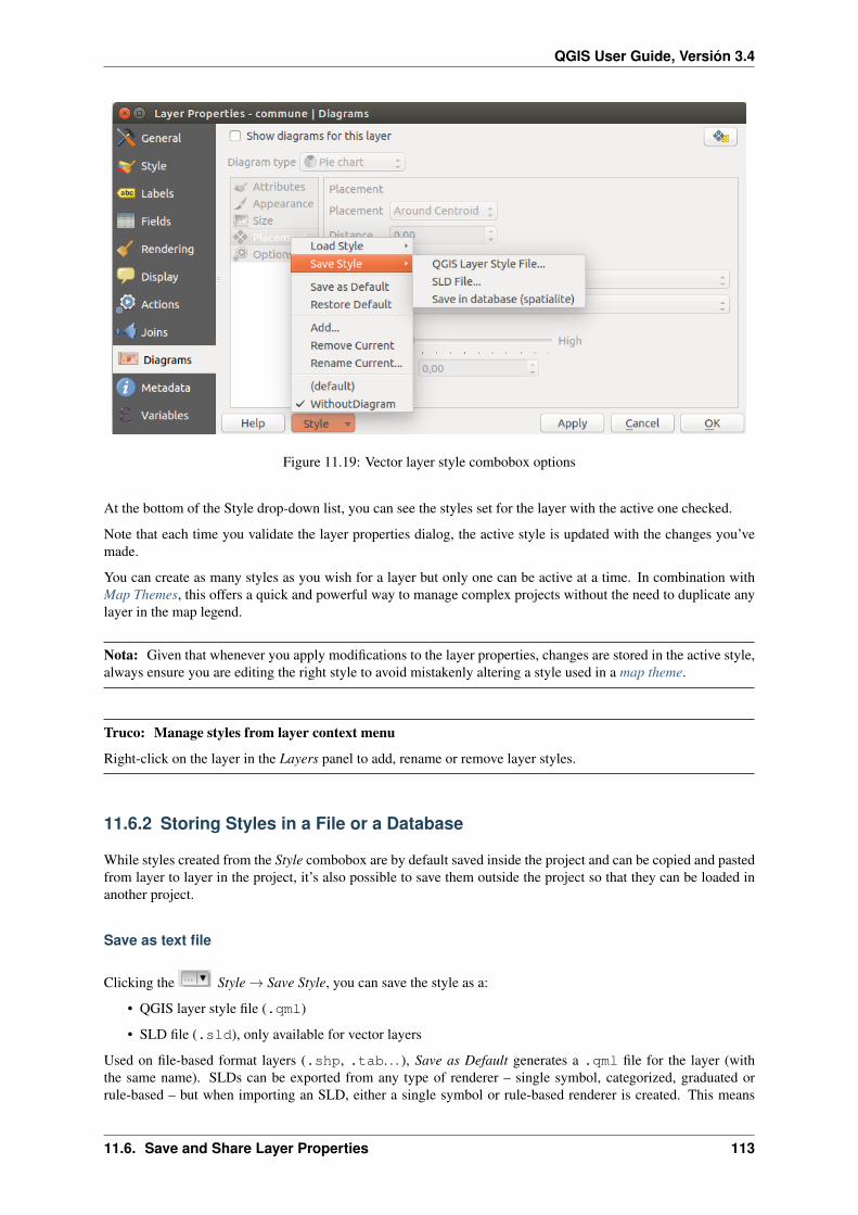
QGIS User Guide, Versión 3.4
Figure 11.19: Vector layer style combobox options
At the bottom of the Style drop-down list, you can see the styles set for the layer with the active one checked.
Note that each time you validate the layer properties dialog, the active style is updated with the changes you’vemade.
You can create as many styles as you wish for a layer but only one can be active at a time. In combination withMap Themes, this offers a quick and powerful way to manage complex projects without the need to duplicate anylayer in the map legend.
Nota: Given that whenever you apply modifications to the layer properties, changes are stored in the active style,always ensure you are editing the right style to avoid mistakenly altering a style used in a map theme.
Truco: Manage styles from layer context menu
Right-click on the layer in the Layers panel to add, rename or remove layer styles.
11.6.2 Storing Styles in a File or a Database
While styles created from the Style combobox are by default saved inside the project and can be copied and pastedfrom layer to layer in the project, it’s also possible to save them outside the project so that they can be loaded inanother project.
Save as text file
Clicking the Style → Save Style, you can save the style as a:
• QGIS layer style file (.qml)
• SLD file (.sld), only available for vector layers
Used on file-based format layers (.shp, .tab. . . ), Save as Default generates a .qml file for the layer (withthe same name). SLDs can be exported from any type of renderer – single symbol, categorized, graduated orrule-based – but when importing an SLD, either a single symbol or rule-based renderer is created. This means
11.6. Save and Share Layer Properties 113
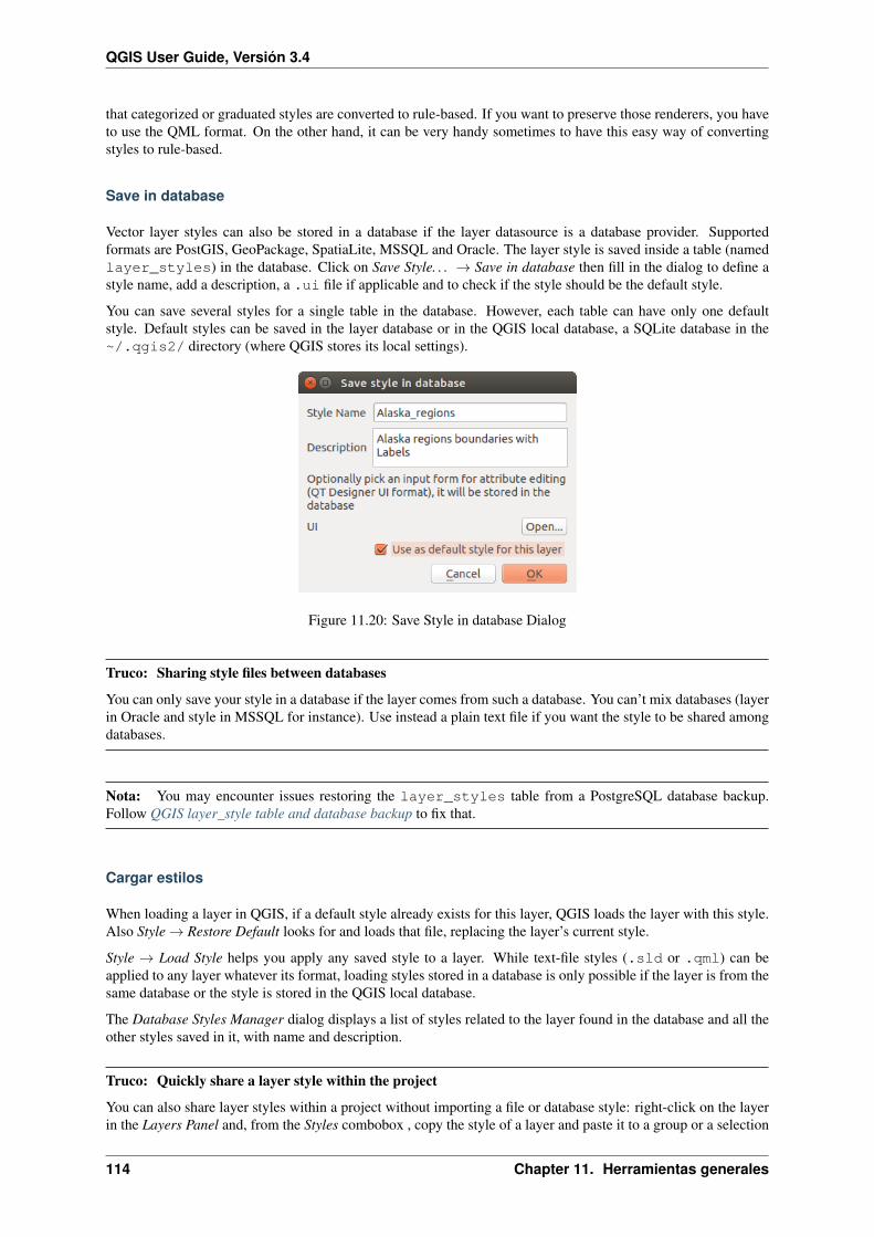
QGIS User Guide, Versión 3.4
that categorized or graduated styles are converted to rule-based. If you want to preserve those renderers, you haveto use the QML format. On the other hand, it can be very handy sometimes to have this easy way of convertingstyles to rule-based.
Save in database
Vector layer styles can also be stored in a database if the layer datasource is a database provider. Supportedformats are PostGIS, GeoPackage, SpatiaLite, MSSQL and Oracle. The layer style is saved inside a table (namedlayer_styles) in the database. Click on Save Style. . . → Save in database then fill in the dialog to define astyle name, add a description, a .ui file if applicable and to check if the style should be the default style.
You can save several styles for a single table in the database. However, each table can have only one defaultstyle. Default styles can be saved in the layer database or in the QGIS local database, a SQLite database in the~/.qgis2/ directory (where QGIS stores its local settings).
Figure 11.20: Save Style in database Dialog
Truco: Sharing style files between databases
You can only save your style in a database if the layer comes from such a database. You can’t mix databases (layerin Oracle and style in MSSQL for instance). Use instead a plain text file if you want the style to be shared amongdatabases.
Nota: You may encounter issues restoring the layer_styles table from a PostgreSQL database backup.Follow QGIS layer_style table and database backup to fix that.
Cargar estilos
When loading a layer in QGIS, if a default style already exists for this layer, QGIS loads the layer with this style.Also Style → Restore Default looks for and loads that file, replacing the layer’s current style.
Style → Load Style helps you apply any saved style to a layer. While text-file styles (.sld or .qml) can beapplied to any layer whatever its format, loading styles stored in a database is only possible if the layer is from thesame database or the style is stored in the QGIS local database.
The Database Styles Manager dialog displays a list of styles related to the layer found in the database and all theother styles saved in it, with name and description.
Truco: Quickly share a layer style within the project
You can also share layer styles within a project without importing a file or database style: right-click on the layerin the Layers Panel and, from the Styles combobox , copy the style of a layer and paste it to a group or a selection
114 Chapter 11. Herramientas generales

QGIS User Guide, Versión 3.4
of layers: the style is applied to all the layers that are of the same type (vector vs raster) as the original layer and,in the case of vector layers, have the same geometry type (point, line or polygon).
11.6.3 Layer definition file
Layer definitions can be saved as a Layer Definition File (.qlr) using Export → Save As Layer Def-inition File. . . in the active layers” context menu. A layer definition file (.qlr) includes references to the datasource of the layers and their styles. .qlr files are shown in the Browser Panel and can be used to add the layers(with the saved style) to the Layers Panel. You can also drag and drop .qlr files from the system file managerinto the map canvas.
11.7 Storing values in Variables
In QGIS, you can use variables to store useful recurrent values (e.g. the project’s title, or the user’s full name) thatcan be used in expressions. Variables can be defined at the application’s global level, project level, layer level,layout level, and layout item’s level. Just like CSS cascading rules, variables can be overwritten - e.g., a projectlevel variable will overwrite any application global level variables set with the same name. You can use thesevariables to build text strings or other custom expressions using the @ character before the variable name. Forexample in print layout creating a label with this content:
This map was made using QGIS [% @qgis_version %]. The project file for thismap is: [% @project_path %]
Representará la etiqueta como ésta:
This map was made using QGIS 3.4.4-Madeira. The project file for this map is:/gis/qgis-user-conference-2019.qgs
Besides the preset read-only variables, you can define your own custom variables for any of the levels mentionedabove. You can manage:
• global variables from the Settings → Options menu
• project variables from the Project Properties dialog (see Propiedades del proyecto)
• vector layer variables from the Layer Properties dialog (see El Dialogo de las Propiedades del Vector);
• layout variables from the Layout panel in the Print layout (see The Layout Panel);
• and layout item variables from the Item Properties panel in the Print layout (see Layout Items CommonOptions).
To differentiate from editable variables, read-only variable names and values are displayed in italic. On the otherhand, higher level variables overwritten by lower level ones are strike through.
Nota: You can read more about variables and find some examples in Nyall Dawson’s Exploring variables inQGIS 2.12, part 1, part 2 and part 3 blog posts.
11.8 Autenticación
QGIS has the facility to store/retrieve authentication credentials in a secure manner. Users can securely savecredentials into authentication configurations, which are stored in a portable database, can be applied to server ordatabase connections, and are safely referenced by their ID tokens in project or settings files. For more informationsee Sistema de autenticación.
A master password needs to be set up when initializing the authentication system and its portable database.
11.7. Storing values in Variables 115

QGIS User Guide, Versión 3.4
Figure 11.21: Variables editor at the project level
116 Chapter 11. Herramientas generales

QGIS User Guide, Versión 3.4
11.9 Common widgets
In QGIS, there are some options you’ll often have to work with. For convenience, QGIS provides you with specialwidgets that are presented below.
11.9.1 Selector de color
The color dialog
The Select Color dialog will appear whenever you click the icon to choose a color. Thefeatures of this dialog depend on the state of the Use native color chooser dialogs parameter checkbox in Settings→ Options. . . → General. When checked, the color dialog used is the native one of the OS on which QGIS isrunning. Otherwise, the QGIS custom color chooser is used.
The custom color chooser dialog has four different tabs which allow you to select colors by Color ramp,Color wheel, Color swatches or Color picker. With the first two tabs, you can browse to all possible color combina-tions and apply your choice to the item.
Figure 11.22: Color selector ramp tab
In the Color swatches tab, you can choose from a list of color palettes (see Colors Settings for details). All but the
Recent colors palette can be modified with the Add current color and Remove selected color buttons at the bottom ofthe frame.
The . . . button next to the palette combobox also offers several options to:
• copy, paste, import or export colors
• create, import or remove color palettes
• add the custom palette to the color selector widget with the Show in Color Buttons item (see fig-ure_color_selector)
Another option is to use the Color picker which allows you to sample a color from under your mouse cursor atany part of the QGIS UI or even from another application: press the space bar while the tab is active, move the
11.9. Common widgets 117

QGIS User Guide, Versión 3.4
Figure 11.23: Color selector swatches tab
mouse over the desired color and click on it or press the space bar again. You can also click the Sample Colorbutton to activate the picker.
Whatever method you use, the selected color is always described through color sliders for HSV (Hue, Saturation,Value) and RGB (Red, Green, Blue) values. The color is also identifiable in HTML notation.
Modifying a color is as simple as clicking on the color wheel or ramp or on any of the color parameters sliders.You can adjust such parameters with the spinbox beside or by scrolling the mouse wheel over the correspondingslider. You can also type the color in HTML notation. Finally, there is an Opacity slider to set transparency level.
The dialog also provides a visual comparison between the Old color (applied to object) and the Current one (being
selected). Using drag-and-drop or pressing the Add color to swatch button, any of these colors can be saved in aslot for easy access.
Truco: Quick color modification
Drag-and-drop a color selector widget onto another one to apply its color.
The color drop-down shortcut
Click the drop-down arrow to the right of the color button to display a widget for quick colorselection. This shortcut provides access to:
• a color wheel to pick a color from
• an alpha slider to change color opacity
• the color palettes previously set to Show in Color Buttons
• copy the current color and paste it into another widget
• pick a color from anywhere on your computer display
• choose a color from the color selector dialog
118 Chapter 11. Herramientas generales

QGIS User Guide, Versión 3.4
Figure 11.24: Menú seleccionador rápido de color
The color ramp drop-down shortcut
Color ramps are a practical way to apply a set of colors to one or many features. Their creation is described in theRampa de color section. As for the colors, pressing the color ramp button opens the correspondingcolor ramp type dialog allowing you to change its properties.
Figure 11.25: Customizing a colorbrewer ramp
The drop-down menu to the right of the button gives quick access to a wider set of color ramps and options:
• Invert Color Ramp
• a preview of the gradient or catalog: cpt-city color ramps flagged as Favorites in the StyleManager dialog
• All Color Ramps to access the compatible color ramps database
• Create New Color Ramp. . . of any supported type that could be used in the current widget (note that thiscolor ramp will not be available elsewhere unless you save it in the library)
• Edit Color Ramp. . . , the same as clicking the whole color ramp button
11.9. Common widgets 119

QGIS User Guide, Versión 3.4
• Save Color Ramp. . . , to save the current color ramp with its customizations in the style library
Figure 11.26: Quick color ramp selection widget
11.9.2 Modos de Mezcla
QGIS offers different options for special rendering effects with these tools that you may previously only knowfrom graphics programs. Blending modes can be applied on layers and features, and also on print layout items:
• Normal: This is the standard blend mode, which uses the alpha channel of the top pixel to blend with thepixel beneath it. The colors aren’t mixed.
• Iluminado: Este selecciona el máximo de cada componente del primer y segundo plano de píxeles. Tengaen cuenta que los resultados tienden a ser irregulares y rigurosos.
• Screen: Light pixels from the source are painted over the destination, while dark pixels are not. This modeis most useful for mixing the texture of one item with another item (such as using a hillshade to textureanother layer).
• Dodge: Brighten and saturate underlying pixels based on the lightness of the top pixel. Brighter top pixelscause the saturation and brightness of the underlying pixels to increase. This works best if the top pixelsaren’t too bright. Otherwise the effect is too extreme.
• Addition: Adds pixel values of one item to the other. In case of values above the maximum value (in thecase of RGB), white is displayed. This mode is suitable for highlighting features.
• Darken: Retains the lowest values of each component of the foreground and background pixels. Likelighten, the results tend to be jagged and harsh.
• Multiply: Pixel values of the top item are multiplied with the corresponding values for the bottom item.The results are darker.
• Burn: Darker colors in the top item cause the underlying items to darken. Burn can be used to tweak andcolorize underlying layers.
• Overlay: Combines multiply and screen blending modes. Light parts become lighter and dark parts becomedarker.
• Soft light: Very similar to overlay, but instead of using multiply/screen it uses color burn/dodge. This issupposed to emulate shining a soft light onto an image.
• Hard light: Hard light is also very similar to the overlay mode. It’s supposed to emulate projecting a veryintense light onto an image.
• Difference: Subtracts the top pixel from the bottom pixel, or the other way around, in order always to get apositive value. Blending with black produces no change, as the difference with all colors is zero.
120 Chapter 11. Herramientas generales

QGIS User Guide, Versión 3.4
• Subtract: Subtracts pixel values of one item from the other. In the case of negative values, black is dis-played.
11.9.3 Configuración de anulación definida por datos
Next to many options in the vector layer properties dialog or settings in the print layout, you will find aData defined override icon. Using expressions based on layer attributes or item settings, prebuilt or custom functionsand variables, this tool allows you to set dynamic values for parameters. When enabled, the value returned by thiswidget is applied to the parameter regardless of its normal value (checkbox, textbox, slider. . . ).
The data defined override widget
Clicking the Data defined override icon shows the following entries:
• Description. . . that indicates if the option is enabled, which input is expected, the valid input type and thecurrent definition. Hovering over the widget also pops up this information.
• Store data in the project: a button allowing the property to be stored using to the Auxiliary Storage Proper-ties mechanism.
• Field type: an entry to select from the layer’s fields that match the valid input type.
• An entry to list the Variable available.
• Edit. . . button to create or edit the expression to apply, using the Expression String Builder dialog. To helpyou correctly fill in the expression, a reminder of the expected output’s format is provided in the dialog.
• Paste and Copy buttons.
• botón de Limpiar para eliminar la configuración.
• For numeric and color properties, Assistant. . . to rescale how the feature data is applied to the property(more details below)
Truco: Use right-click to (de)activate the data override
When the data-defined override option is set up correctly the icon is yellow or . If it is broken, the icon is
red or .
You can enable or disable a configured data-defined override button by simply clicking the widget with the rightmouse button.
Using the data-defined assistant interface
When the Data-defined override button is associated with a numeric or color parameter, it has an Assistant. . . optionthat allows you to change how the data is applied to the parameter for each feature. The assistant allows you to:
• Define the Input data, ie:
– the attribute to represent, using the Field listbox or the Set column expression function (see Expresiones)
– the range of values to represent: you can manually enter the values or use the Fetch value range from layer
button to fill these fields automatically with the minimum and maximum values returned by the chosenattribute or the expression applied to your data
11.9. Common widgets 121

QGIS User Guide, Versión 3.4
• Apply transform curve: by default, output values (see below for setting) are applied to input featuresfollowing a linear scale. You can override this logic: enable the transform option, click on the graphic toadd break point(s) and drag the point(s) to apply a custom distribution.
• Define the Output values: the options vary according to the parameter to define. You can globally set:
– the minimum and maximum values to apply to the selected property (n case of a color setting, you’llneed to provide a color ramp)
– the Scale method of representation which can be Flannery, Exponential, Surface or Radius
– the Exponent to use for data scaling
– the output value or color to represent features with NULL values
When compatible with the property, a live-update preview is displayed in the right-hand side of the dialog to helpyou control the value scaling.
Figure 11.27: The data-defined size assistant
The values presented in the varying size assistant above will set the size “Data-defined override” with:
coalesce(scale_exp(Importance, 1, 20, 2, 10, 0.57), 1)
122 Chapter 11. Herramientas generales

CHAPTER 12
Administrar el origen de datos
12.1 Opening Data
As part of an Open Source Software ecosystem, QGIS is built upon different libraries that, combined with its ownproviders, offer capabilities to read and often write a lot of formats:
• Vector data formats include ESRI formats (Shapefile, Geodatabase. . . ), MapInfo and MicroStation file for-mats, AutoCAD DWG/DXF, GeoPackage, GeoJSON, GRASS, GPX, KML, Comma Separated Values, andmany more. . . Read the complete list of OGR vector supported formats.
• Raster data formats include ArcInfo Binary Grid, ArcInfo ASCII Grid, JPEG, GeoTIFF, ERDAS IMAGINE,MBTiles, R or Idrisi rasters, ASCII Gridded XYZ, GDAL Virtual, SRTM, Sentinel Data, and many more. . .Read the complete list of raster supported formats.
• Database formats include PostgreSQL/PostGIS, SQLite/SpatiaLite, Oracle, DB2 or MSSQL Spatial,MySQL. . .
• Support of web data services (WM(T)S, WFS, WCS, CSW, ArcGIS Servers. . . ) is also handled by QGISproviders (see QGIS como Cliente de Datos OGC).
• You can also read supported files from archived folders and use QGIS native formats such as virtual andmemory layers.
As of the date of this document, more than 80 vector and 140 raster formats are supported by the GDAL/OGR andQGIS native providers.
Nota: Not all of the listed formats may work in QGIS for various reasons. For example, some require externalproprietary libraries, or the GDAL/OGR installation of your OS may not have been built to support the format youwant to use. To have a list of available formats, run the command line ogrinfo --formats (for vector) orcheck settings → Options → GDAL menu (for raster) in QGIS.
In QGIS, depending on the data format, there are different tools to open it, mainly available in the Layer →Add Layer → menu or from the Manage Layers toolbar (enabled through View → Toolbars menu). However, all
these tools point to a unique dialog, the Data Source Manager dialog that you can directly open with theOpen Data Source Manager button available on the Data Source Manager Toolbar or by pressing Ctrl+L. Indeed, theData Source Manager dialog offers a unified interface to open vector or raster file-based data as well as databases
or web services supported by QGIS. It can be set modal or not with the Modeless data source manager dialogin Settings → Options → General menu.
123

QGIS User Guide, Versión 3.4
Figure 12.1: QGIS Data Source Manager dialog
124 Chapter 12. Administrar el origen de datos

QGIS User Guide, Versión 3.4
Beside this main entry point, you also have the DB Manager plugin that offers advanced capabilities to analyzeand manipulate connected databases. More information on DB Manager capabilities are exposed in DB ManagerPlugin.
There are also many other tools, native or third-party plugins, that help you open dedicated data formats.
This chapter will describe only the tools provided by default in QGIS to load data. It will mainly focus on theData Source Manager dialog but more than describing each tab, it will also explore the tools based on the dataprovider or format specificities.
12.1.1 The Browser Panel
The Browser is one of the main ways to quickly and easily add your data to projects. It’s available as:
• a Data Source Manager tab, enabled pressing the Open Data Source Manager button (Ctrl+L);
• as a QGIS panel you can open from the menu View → Panels (or Settings → Panels) or by pressingCtrl+2.
In both cases, the Browser helps you navigate in your file system and manage geodata, regardless the type of layer(raster, vector, table), or the datasource format (plain or compressed files, database, web services).
The context menu for an element in the Browser panel is opened by right-clicking on it.
For file system directory entries, the context menu offers the following:
• Add as a Favorite
• Properties. . .
• Hide from Browser
• Fast Scan this Directory
• New Directory. . .
• Open Directory
Favourites, can also be removed and renamed:
• Rename favourite. . .
• Remove favourite
For leaf entries that can act as layers in the project, the context menu will have a selection of entries. For example,for non-database, non-service-based vector, raster and mesh data sources:
• Add Selected Layer(s) to Canvas
• Properties. . .
• Delete File «<name of file>». . .
In the Layer properties entry, you will find (similar to what you will find in the vector and raster layer propertiesonce the layers have been added to the project):
• Metadata for the layer. Metadata groups: Information from provider (if possible, Path will be a hyperlinkto the source), Identification, Extent, Access, Fields (for vector layers), Bands (for raster layers), Contacts,Links (for vector layers), References (for raster layers), History.
• A Preview panel
• The attribute table for vector sources (in the Attributes panel).
To add a layer to the project using the Browser:
1. Enable the Browser as described above. A browser tree with your file system, databases and web services isdisplayed. You may need to connect databases and web services before they appear (see dedicated sections).
12.1. Opening Data 125

QGIS User Guide, Versión 3.4
2. Find the layer in the list.
3. Use the context menu, double-click its name, or drag-and-drop it into the map canvas. Your layer is nowadded to the Layers panel and can be viewed on the map canvas.
Truco: Open a QGIS project directly from the browser
You can also open a QGIS project directly from the Browser panel by double-clicking its name or by drag-and-drop into the map canvas.
Once a file is loaded, you can zoom around it using the map navigation tools. To change the style of a layer,open the Layer Properties dialog by double clicking on the layer name or by right-clicking on the name in thelegend and choosing Properties from the context menu. See section Symbology Properties for more informationon setting symbology of vector layers.
At the top of the Browser panel, you find some icons that help you to:
• Add Selected Layers: you can also add data into the map canvas by selecting Add selected layer(s) from thelayer’s context menu;
• Refresh the browser tree;
• Filter Browser to search for specific data. Enter a search word or wildcard and the browser will filter the treeto only show paths to matching DB tables, filenames or folders – other data or folders won’t be displayed.See the Browser Panel(2) example on the figure_browser_panels. The comparison can be case-sensitive ornot. It can also be set to:
– normal: return any item containing the search text;
– using wildcard(s): fine tune the search using ? and/or * characters to specify the position of the searchtext;
– empleando una expresión regular.
• Collapse All the whole tree;
• Enable/disable properties widget: when toggled on, a new widget is added at the bottom of the panel showing, ifapplicable, metadatas of the selected item.
Right-click an item in the browser tree helps you to:
• in case of file or table, display its metadata or open it in your project. Tables can even be renamed, deletedor truncated;
• in case of folder, bookmark it into your favourites, hide it from the browser tree. Hidden folders can bemanaged from the Settings → Options → Data Sources tab;
• create connection to databases or web servers;
• refresh, rename or delete schema.
You can also import files into databases or copy tables from one schema/database to another one with a simpledrag-and-drop. There is a second browser panel available to avoid long scrolling while dragging. Just select thefile and drag-and-drop from one panel to the other.
Truco: Add layers to QGIS by simple drag-and-drop from your OS file browser
You can also add file(s) to the project by drag-and-dropping them from your operating system file browser to theLayers Panel or the map canvas.
126 Chapter 12. Administrar el origen de datos

QGIS User Guide, Versión 3.4
Figure 12.2: QGIS Browser panels side-by-side
12.1.2 El gestor de Base de Datos
The DB Manager Plugin is another one of the main and native tools to integrate and manage spatial databaseformats supported by QGIS (PostGIS, SpatiaLite, GeoPackage, Oracle Spatial, MSSQL, DB2, Virtual layers) inone user interface. It can be activated from the Plugins → Manage and Install Plugins. . . menu.
The DB Manager Plugin provides several features:
• connect to databases and display its structure and contents;
• preview tables of databases;
• add layers to map canvas, either by double-click or drag-and-drop;
• add layers to a database from the QGIS Browser or from another database;
• create and add output of SQL queries to the map canvas;
• create virtual layers.
More information on DB Manager capabilities are exposed in DB Manager Plugin.
12.1.3 Provider-based loading tools
Beside Browser Panel and DB Manager, the main tools provided by QGIS to add layers regardless the format,you’ll also find tools that are specific to data providers.
Nota: Some external plugins also propose tools to open specific format files in QGIS.
Cargando una capa desde archivo
To load a layer from a file, you can:
12.1. Opening Data 127
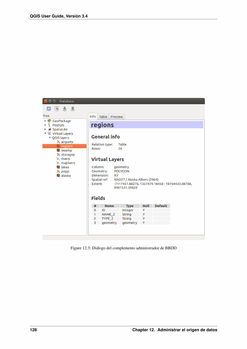
QGIS User Guide, Versión 3.4
Figure 12.3: Diálogo del complemento administrador de BBDD
128 Chapter 12. Administrar el origen de datos

QGIS User Guide, Versión 3.4
• for vector data (like Shapefile, Mapinfo or dxf layer), click on Add Vector Layer toolbar button, select the
Layer → Add Layer → Add Vector Layer menu option or press Ctrl+Shift+V. This will bring up
a new window (see figure_vector_add) from which you can check File and click on Browse. You canalso specify the encoding for the file if desired.
Figure 12.4: Diálogo de Añadir capa vectorial
• for raster layers, click on the Add Raster Layer icon, select the Layer → Add Layer → Add Raster Layermenu option or type Ctrl+Shift+R.
That will bring up a standard open file dialog (see figure_vector_open), which allows you to navigate the file
system and load a shapefile, a geotiff or other supported data source. The selection box Filter allows youto preselect some supported file formats. Only the formats that have been well tested appear in the list. Otheruntested formats can be loaded by selecting All files (*.*).
Figure 12.5: Abre un Diálogo de Capa Vectorial Soportada por OGR
Selecting a file from the list and clicking Open loads it into QGIS. More than one layer can be loaded at the sametime by holding down the Ctrl or Shift key and clicking on multiple items in the dialog. Figure_vector_loadedshows QGIS after loading the alaska.shp file.
Nota: Because some formats like MapInfo (e.g., .tab) or Autocad (.dxf) allow mixing different types ofgeometry in a single file, loading such format in QGIS opens a dialog to select geometries to use in order to have
12.1. Opening Data 129

QGIS User Guide, Versión 3.4
Figure 12.6: QGIS con archivo shape de Alaska cargado
one geometry per layer.
Using the Add Vector Layer tool:
• You can also load specific formats like ArcInfo Binary Coverage, UK. National TransferFormat, as well as the raw TIGER format of the US Census Bureau or OpenfileGDB. To do that,
you’d need to select Directory as Source type. In this case a directory can be selected in the dialog afterpressing Browse.
• With the Database source type you can select an existing database connection or create one tothe selected database type. Available database types are ODBC, OGDI Vectors, Esri PersonalGeodatabase, MySQL as well as PostgreSQL or MSSQL.
Pressing the New button opens the Create a New OGR Database Connection dialog whose parameters areamong the ones you can find in Crear una conexión almacenada. Pressing Open you can select from theavailable tables for example of the PostGIS enabled database.
• The last source type, Protocol, enables to open data from the web using for example GeoJSON orCouchDB format. After selecting the type you have to fill URI of the source.
Truco: Load layers and projects from mounted external drives on macOS
On macOS, portable drives that are mounted beside the primary hard drive do not show up as expected under File→ Open. . . . We are working on a more macOS-native open/save dialog to fix this. As a workaround, you cantype /Volumes in the File name box and press Enter. Then you can navigate to external drives and networkmounts.
130 Chapter 12. Administrar el origen de datos
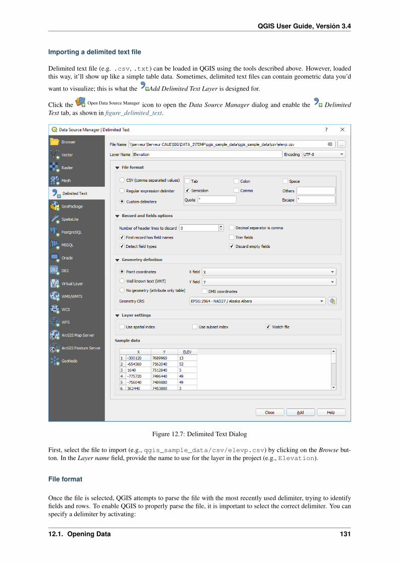
QGIS User Guide, Versión 3.4
Importing a delimited text file
Delimited text file (e.g. .csv, .txt) can be loaded in QGIS using the tools described above. However, loadedthis way, it’ll show up like a simple table data. Sometimes, delimited text files can contain geometric data you’d
want to visualize; this is what the Add Delimited Text Layer is designed for.
Click the Open Data Source Manager icon to open the Data Source Manager dialog and enable the DelimitedText tab, as shown in figure_delimited_text.
Figure 12.7: Delimited Text Dialog
First, select the file to import (e.g., qgis_sample_data/csv/elevp.csv) by clicking on the Browse but-ton. In the Layer name field, provide the name to use for the layer in the project (e.g., Elevation).
File format
Once the file is selected, QGIS attempts to parse the file with the most recently used delimiter, trying to identifyfields and rows. To enable QGIS to properly parse the file, it is important to select the correct delimiter. You canspecify a delimiter by activating:
12.1. Opening Data 131

QGIS User Guide, Versión 3.4
• CSV (comma separated values) to use the comma character;
• Custom delimiters, choosing among some predefined delimiters like comma, space, tab,semicolon. . . ;
• or Regular expression delimiter and entering text into the Expression field. For example, to change thedelimiter to tab, use \t (this is a regular expression for the tab character).
Records and fields
Other than settings to identify rows and fields in the data, some convenient options can be used to tweak the datarecognition:
• Number of header lines to discard: convenient when you want to avoid some lines to show in the import,either because those are blank lines or with another formatting.
• First records has field names: values in the first row of data are used as field names, otherwise QGISadds a fields row of a type field_1, field_2. . .
• Detect field types: automatically recognizes the field type. If unchecked then all attributes are treated astext fields.
• Decimal separator is comma: if necessary, you can force a comma to be the decimal separator.
• Trim fields: allows you to trim leading and trailing spaces from fields.
• Discard empty fields.
As you set the parser properties, a sample data preview updates at the bottom of the dialog.
Geometry definition
Once the file is parsed, set Geometry definition to
• Point coordinates and provide the X field and Y field if the layer is of point geometry type and contain
such coordinate fields. If the coordinates are defined as degrees/minutes/seconds, activate the DMScoordinates checkbox;
• Well known text (WKT) option if the spatial information is represented by WKT: select the Geometryfield containing the WKT definition and choose the approriate Geometry field or let QGIS auto-detect it;
• If the file contains non-spatial data, activate No geometry (attribute only table) and it will be loaded asan ordinary table.
Besides the features geometry information, you can also set the layer’s Geometry CRS using the Select CRS
widget.
Layer settings
Additionally, you can enable:
• Use spatial index to improve the performance of displaying and spatially selecting features;
• Use subset index to improve performance of subset filters (when defined in the layer properties);
• Watch file to watch for changes to the file by other applications while QGIS is running.
132 Chapter 12. Administrar el origen de datos

QGIS User Guide, Versión 3.4
At the end, click OK to add the layer to the map. In our example, a point layer named Elevation is added tothe project and behaves like any other map layer in QGIS. However, this layer is the result of a query on the .csvsource layer (hence, linked to it) and would require to be saved in order to get a spatial layer on disk.
Importing a DXF or DWG file
DXF and DWG files can be added to QGIS by simple drag-and-drop from the common Browser Panel. You’ll beprompted to select the sublayers you’d like to add to the project. Layers are added with random style properties.
Nota: DXF files containing several geometry types (point, line and/or polygon), the name of the layer will bemade from <filename.dxf> entities <geometry type>.
To keep the dxf/dwg file structure and its symbology in QGIS, you may want to use the dedicated Project →Import/Export → Import Layers from DWG/DXF. . . tool which allows you to:
1. import elements from the drawing file into a GeoPackage database.
2. and add to the project any of the imported elements.
In the DWG/DXF Import dialog, to first import the drawing file contents:
1. Input the location of the Target package, i.e. the new GeoPackage file that will store the data. If an existingfile is provided, then it will be overwritten.
2. Specify the coordinate reference system of the data in the drawing file.
3. Check Expand block references to import the blocks in the drawing file as normal elements.
4. Check Use curves to promote the imported layers to a curved geometry type.
5. Use the Import button to select the DWG/DXF file to use (one per geopackage). The GeoPackage databasewill be automatically populated with the drawing file content. Depending on the size of the *CAD file, thiscould take some time.
After the .dwg or .dxf data is imported into the GeoPackage database the frame in the lower half of the dialogis populated with the list of layers from the imported file. There you can select which layers to add to the QGISproject:
1. At the top, set a Group name to group the drawing files in the project.
2. Check layers to show: Each selected layer is added to an ad hoc group which contains vector layers for thepoint, line, label and area features of the drawing layer. The style of each layer is setup so that it resemblesthe look it originally had in *CAD.
3. Check whether layer should be visible at opening.
4. Alternatively using the Merge layers option places all layers in a single group.
5. Press OK to open the layers in QGIS.
Importing OpenStreetMap Vectors
In recent years, the OpenStreetMap project has gained popularity because in many countries no free geodata suchas digital road maps are available. The objective of the OSM project is to create a free editable map of the worldfrom GPS data, aerial photography or local knowledge. To support this objective, QGIS provides support for OSMdata.
Using the Browser Panel, you can load a .osm file to the map canvas, in which case you’ll get a dialog to selectsublayers based on the geometry type. The loaded layers will contain all the data of that geometry type in the fileand keep the osm file data structure.
12.1. Opening Data 133

QGIS User Guide, Versión 3.4
Figure 12.8: Import dialog for DWG/DXF files
134 Chapter 12. Administrar el origen de datos

QGIS User Guide, Versión 3.4
SpatiaLite Layers
The first time you load data from a SpatiaLite database, begin by:
• clicking on the Add SpatiaLite Layer toolbar button;
• selecting the Add SpatiaLite Layer. . . option from the Layer → Add Layer menu;
• or by typing Ctrl+Shift+L.
This will bring up a window that will allow you either to connect to a SpatiaLite database already known to QGIS,which you can choose from the drop-down menu, or to define a new connection to a new database. To define anew connection, click on New and use the file browser to point to your SpatiaLite database, which is a file with a.sqlite extension.
QGIS also supports editable views in SpatiaLite.
GPS
Loading GPS data in QGIS can be done using the core plugin: GPS Tools. Instructions are described in SectionPlugin de GPS.
GRASS
Working with GRASS vector data is described in Section Integracion GRASS SIG.
Database related tools
Crear una conexión almacenada
In order to read and write tables from the many database formats QGIS supports you’ll need to create a connectionto that database. While QGIS Browser Panel is the simplest and recommanded way to connect and use databases,QGIS provides other tools to connect to each of them and load their tables:
• Add PostGIS Layer. . . or by typing Ctrl+Shift+D;
• Add MSSQL Spatial Layer or by typing Ctrl+Shift+M;
• Add Oracle Spatial Layer. . . or by typing Ctrl+Shift+O;
• Add DB2 Spatial Layer. . . or by typing Ctrl+Shift+2.
These tools are accessible either from the Manage Layers Toolbar or the Layer → Add Layer → menu. Connectingto SpatiaLite database is described at SpatiaLite Layers.
Truco: Create connection to database from the QGIS Browser Panel
Select the corresponding database format in the Browser tree, right-click and choose connect will provide youwith the database connection dialog.
Most of the connection dialogs follow a common basis that will be described below using the PostGreSQLdatabase tool as example. For additional settings specific to other providers, you can find corresponding de-scription at:
• Connecting to MSSQL Spatial;
• Connecting to Oracle Spatial;
12.1. Opening Data 135

QGIS User Guide, Versión 3.4
• Connecting to DB2 Spatial.
The first time you use a PostGIS data source, you must create a connection to a database that contains the data.Begin by clicking the appropriate button as exposed above, opening an Add PostGIS Table(s) dialog (see fig-ure_add_postgis_tables). To access the connection manager, click on the New button to display the Create a NewPostGIS Connection dialog.
Figure 12.9: Create a New PostGIS Connection Dialog
The parameters required for a PostGIS connection are exposed below. For the other database types, see theirdifferences at Particular Connection requirements.
• Name: A name for this connection. It can be the same as Database.
• Service: Service parameter to be used alternatively to hostname/port (and potentially database). This can bedefined in pg_service.conf. Check the PostgreSQL Service connection file section for more details.
• Host: Name of the database host. This must be a resolvable host name such as would be used to open aTCP/IP connection or ping the host. If the database is on the same computer as QGIS, simply enter localhosthere.
• Port: Port number the PostgreSQL database server listens on. The default port for PostGIS is 5432.
• Database: Name of the database.
• SSL mode: How the SSL connection will be negotiated with the server. Note that massive speed-ups inPostGIS layer rendering can be achieved by disabling SSL in the connection editor. The following optionsare available:
– Disable: Only try an unencrypted SSL connection;
– Allow: Try a non-SSL connection. If that fails, try an SSL connection;
– Prefer (the default): Try an SSL connection. If that fails, try a non-SSL connection;
– Require: Only try an SSL connection.
136 Chapter 12. Administrar el origen de datos

QGIS User Guide, Versión 3.4
• Username: User name used to log in to the database.
• Password: Password used with Username to connect to the database.
You can save any or both of the username and password parameters, in which case they will be used bydefault each time you need to connect to this database. If not saved, you’ll be prompted to fill the missingcredentials to connect to the database in next QGIS sessions; meanwhile the connection parameters youentered are stored in a temporary internal cache and returned whenever a username/password for the samedatabase is requested, until you close the current QGIS process.
Advertencia: Configuración de usuario QGIS User y seguridad
In the Authentication tab, saving username and password will keep unprotected credentials in theconnection configuration. Those credentials will be visible if, for instance, you shared the projectfile with someone. Therefore, it’s advisable to save your credentials in a Authentication configurationinstead (Configurations tab - See Sistema de autenticación for more details) or in a service connectionfile (see PostgreSQL Service connection file for example).
Optionally, depending on the type of database, you can activate the following checkboxes:
• Only show layers in the layer registries
• Don’t resolve type of unrestricted columns (GEOMETRY)
• Only look in the “public” schema
• Also list tables with no geometry
• Use estimated table metadata
• Allow saving/loading QGIS projects in the database: more details here
Truco: Use estimated table metadata to speed up operations
When initializing layers, various queries may be needed to establish the characteristics of the geometries storedin the database table. When the Use estimated table metadata option is checked, these queries examine only asample of the rows and use the table statistics, rather than the entire table. This can drastically speed up operationson large datasets, but may result in incorrect characterization of layers (eg. the feature count of filtered layerswill not be accurately determined) and may even cause strange behaviour in case columns that are supposed to beunique actually are not.
Once all parameters and options are set, you can test the connection by clicking on the Test Connection button orapply it hitting OK. From the Add PostGIS Table(s), click now on Connect and the dialog is filled with tables fromthe selected database (as shown in figure_add_postgis_tables).
Particular Connection requirements
Because of database type particularities, provided options are all the same for all the databases. Below are exposedthese connection specificities.
PostgreSQL Service connection file
The service connection file allows PostgreSQL connection parameters to be associated with a single service name.That service name can then be specified by a client and the associated settings will be used.
It’s called .pg_service.conf under *nix systems (GNU/Linux, macOS etc.) and pg_service.conf onWindows.
12.1. Opening Data 137

QGIS User Guide, Versión 3.4
The service file looks like:
[water_service]host=192.168.0.45port=5433dbname=gisdbuser=paulpassword=paulspass
[wastewater_service]host=dbserver.comdbname=wateruser=waterpass
Nota: There are two services in the above example: water_service and wastewater_service. You canuse these to connect from QGIS, pgAdmin etc. by specifying only the name of the service you want to connect to(without the enclosing brackets). If you want to use the service with psql you need to do something like exportPGSERVICE=water_service before doing your psql commands.
You can find all the parameters here
Nota: If you don’t want to save the passwords in the service file you can use the .pg_pass option.
On *nix operating systems (GNU/Linux, macOS etc.) you can save the .pg_service.conf file in the user’shome directory and the PostgreSQL clients will automatically be aware of it. For example, if the logged user isweb, .pg_service.conf should be saved in the /home/web/ directory in order to directly work (withoutspecifying any other environment variables).
You can specify the location of the service file by creating a PGSERVICEFILE environment variable (e.g. runthe export PGSERVICEFILE=/home/web/.pg_service.conf command under your *nix OS to tem-porarily set the PGSERVICEFILE variable)
You can also make the service file available system-wide (all users) either by placing the .pg_service.conffile at pg_config --sysconfdir or by adding the PGSYSCONFDIR environment variable to specify thedirectory containing the service file. If service definitions with the same name exist in the user and the system file,the user file takes precedence.
Advertencia: There are some caveats under Windows:
• The service file should be saved as pg_service.conf and not as .pg_service.conf.
• The service file should be saved in Unix format in order to work. One way to do it is to open it withNotepad++ and Edit → EOL Conversion → UNIX Format → File save.
• You can add environmental variables in various ways; a tested one, known to work reliably, is ControlPanel → System and Security → System → Advanced system settings → Environment Variables addingPGSERVICEFILE and the path of the type C:\Users\John\pg_service.conf
• After adding an environment variable you may also need to restart the computer.
Connecting to Oracle Spatial
The spatial features in Oracle Spatial aid users in managing geographic and location data in a native type withinan Oracle database. In addition to some of the options in Crear una conexión almacenada, the connection dialogproposes:
• Database: SID or SERVICE_NAME of the Oracle instance;
138 Chapter 12. Administrar el origen de datos

QGIS User Guide, Versión 3.4
• Port: Port number the Oracle database server listens on. The default port is 1521;
• Workspace: Workspace to switch to.
Optionally, you can activate following checkboxes:
• Only look in metadata table: restricts the displayed tables to those that are in theall_sdo_geom_metadata view. This can speed up the initial display of spatial tables.
• Only look for user’s tables: when searching for spatial tables, restricts the search to tables that are ownedby the user.
• Also list tables with no geometry: indicates that tables without geometry should also be listed by default.
• Use estimated table statistics for the layer metadata: when the layer is set up, various metadata arerequired for the Oracle table. This includes information such as the table row count, geometry type andspatial extents of the data in the geometry column. If the table contains a large number of rows, determiningthis metadata can be time-consuming. By activating this option, the following fast table metadata operationsare done: Row count is determined from all_tables.num_rows. Table extents are always determinedwith the SDO_TUNE.EXTENTS_OF function, even if a layer filter is applied. Table geometry is determinedfrom the first 100 non-null geometry rows in the table.
• Only existing geometry types: only lists the existing geometry types and don’t offer to add others.
• Include additional geometry attributes.
Truco: Capas Oracle Spatial
Normally, an Oracle Spatial layer is defined by an entry in the USER_SDO_METADATA table.
To ensure that selection tools work correctly, it is recommended that your tables have a primary key.
Connecting to DB2 Spatial
In addition to some of the options described in Crear una conexión almacenada, the connection to a DB2 database(see DB2 Spatial Layers for more information) can be specified using either a Service/DSN name defined to ODBCor using the driver, host and port information.
An ODBC Service/DSN connection requires the service name defined to ODBC.
A driver/host/port connection requires:
• Driver: Name of the DB2 driver. Typically this would be IBM DB2 ODBC DRIVER.
• DB2 Host: Name of the database host. This must be a resolvable host name such as would be used toopen a TCP/IP connection or ping the host. If the database is on the same computer as QGIS, simply enterlocalhost here.
• DB2 Port: Port number the DB2 database server listens on. The default DB2 LUW port is 50000. Thedefault DB2 z/OS port is 446.
Truco: DB2 Spatial Layers
A DB2 Spatial layer is defined by a row in the DB2GSE.ST_GEOMETRY_COLUMNS view.
Nota: In order to work effectively with DB2 spatial tables in QGIS, it is important that tables have an INTEGERor BIGINT column defined as PRIMARY KEY and if new features are going to be added, this column should alsohave the GENERATED characteristic.
12.1. Opening Data 139
QGIS User Guide, Versión 3.4
It is also helpful for the spatial column to be registered with a specific spatial reference identifier (most often 4326for WGS84 coordinates). A spatial column can be registered by calling the ST_Register_Spatial_Columnstored procedure.
Connecting to MSSQL Spatial
In addition to some of the options in Crear una conexión almacenada, creating a new MSSQL connection dialogproposes you to fill a Provider/DSN name. You can also display available databases.
Loading a Database Layer
Once you have one or more connections defined to a database (see section Crear una conexión almacenada),you can load layers from it. Of course, this requires having available data. See e.g. section Importing Data intoPostgreSQL for a discussion on importing data into a PostGIS database.
To load a layer from a database, you can perform the following steps:
1. Open the «Add <database> table(s)» dialog (see Crear una conexión almacenada).
2. Choose the connection from the drop-down list and click Connect.
3. Select or unselect Also list tables with no geometry.
4. Optionally, use some Search Options to reduce the list of tables to those matching your search. You canalso set this option before you hit the Connect button, speeding this way the database fetching.
5. Find the layer(s) you wish to add in the list of available layers.
6. Select it by clicking on it. You can select multiple layers by holding down the Shift key while clicking.
7. If applicable, use the Set Filter button (or double-click the layer) to start the Query Builder dialog (Seesection Constructor de Consulta) and define which features to load from the selected layer. The filterexpression appears in the sql column. This restriction can be removed or edited in the Layer Properties →General → Provider Feature Filter frame.
8. The checkbox in the Select at id column that is activated by default gets the features ids without theattributes and speeds in most cases the data loading.
9. Click on the Add button to add the layer to the map.
Truco: Use the Browser Panel to speed up loading of database table(s)
Adding DB tables from their ad hoc tab of the Data Source Manager dialog to QGIS may sometimes be timeconsuming as QGIS fetches statistics and properties (e.g. geometry type and field, CRS, number of features) ofeach table beforehand. To avoid this, once the connection is set, it’s better to use the Browser Panel or the DBManager to drag and drop the database tables in the map canvas.
12.1.4 Formato personalizados QGIS
QGIS proposes two custom formats you can load in the application using their own loading tool:
• Temporary Scratch Layer: a memory layer that is bound to the project it’s opened with (see Crear una nuevacapa temporal for more information)
• Virtual Layers: a layer resulting from a query on other layer(s) (see Creating virtual layers for more infor-mation)
140 Chapter 12. Administrar el origen de datos

QGIS User Guide, Versión 3.4
Figure 12.10: Add PostGIS Table(s) Dialog
12.1.5 QLR - QGIS Layer Definition File
Layer definitions can be saved as a Layer Definition File (QLR - .qlr) using Export → Save As Layer DefinitionFile. . . in the layer context menu.
The QLR format makes it possible to share «complete» QGIS layers with other QGIS users. QLR files containlinks to the data sources and all the QGIS style information necessary to style the layer.
QLR files are shown in the Browser Panel and can be used to add layers (with their saved styles) to the LayersPanel. You can also drag and drop QLR files from the system file manager into the map canvas.
12.1.6 Conectar con el servicios web
With QGIS you can have access to different types of OGC web services (WM(T)S, WFS(-T), CSW . . . ). Thanksto QGIS Server, you can also publish these services. Description of these capabilities and how-to are provided inchapter Trabajar con datos OGC.
12.2 Creando capas
Layers can be created in many ways, including:
• empty layers from scratch;
• layers from existing layers;
• layers from the clipboard;
• layers as a result of an SQL-like query based on one or many layers: the virtual layer.
QGIS also provides tools to import/export different formats.
12.2. Creando capas 141
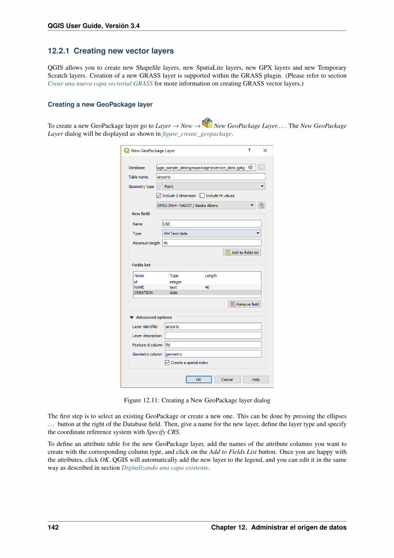
QGIS User Guide, Versión 3.4
12.2.1 Creating new vector layers
QGIS allows you to create new Shapefile layers, new SpatiaLite layers, new GPX layers and new TemporaryScratch layers. Creation of a new GRASS layer is supported within the GRASS plugin. (Please refer to sectionCrear una nueva capa vectorial GRASS for more information on creating GRASS vector layers.)
Creating a new GeoPackage layer
To create a new GeoPackage layer go to Layer → New → New GeoPackage Layer. . . . The New GeoPackageLayer dialog will be displayed as shown in figure_create_geopackage.
Figure 12.11: Creating a New GeoPackage layer dialog
The first step is to select an existing GeoPackage or create a new one. This can be done by pressing the ellipses. . . button at the right of the Database field. Then, give a name for the new layer, define the layer type and specifythe coordinate reference system with Specify CRS.
To define an attribute table for the new GeoPackage layer, add the names of the attribute columns you want tocreate with the corresponding column type, and click on the Add to Fields List button. Once you are happy withthe attributes, click OK. QGIS will automatically add the new layer to the legend, and you can edit it in the sameway as described in section Digitalizando una capa existente.
142 Chapter 12. Administrar el origen de datos

QGIS User Guide, Versión 3.4
Crear una nueva capa de archivo shape
To create a new Shapefile layer, choose Create Layer → New Shapefile Layer. . . from the Layer menu orselect it from the Data Source Manager toolbar. The New Shapefile Layer dialog will be displayed as shown infigure_create_shapefile. The first step is to provide a path and name for the Shapefile. QGIS will automatically addthe .shp extension to the name you specify Next, choose the type of layer (point, line or polygon) and optionalZ or M dimensions, as well as the CRS (coordinate reference system).
Figure 12.12: Creating a new Shapefile layer dialog
To complete the creation of the new Shapefile layer, add the desired attributes by specifying a name and typefor each attribute and clicking on the Add to Fields List button. A first “id” column is added by default but
can be removed, if not wanted. Only Decimal number , Whole number , Text data and Date
attributes are supported. Additionally, depending on the attribute type, you can also define the length andprecision of the new attribute column. Once you are happy with the attributes, click OK. Once the Shapefile hasbeen created, it will be added to the map as a new layer, and you can edit it in the same way as described in sectionDigitalizando una capa existente.
Crear una nueva capa SpatiaLite
To create a new SpatiaLite layer for editing, choose Create Layer → New SpatiaLite Layer. . . from the Layermenu or select it from the Data Source Manager toolbar. The New SpatiaLite Layer dialog will be displayed asshown in Figure_create_spatialite.
The first step is to select an existing SpatiaLite database or to create a new SpatiaLite database. This can bedone with the . . . button at the right of the database field. Then, add a name for the new layer, define the layer
type, and specify the coordinate reference system with Specify CRS. If desired, you can select Create anautoincrementing primary key.
12.2. Creando capas 143

QGIS User Guide, Versión 3.4
Figure 12.13: Creating a New SpatiaLite layer dialog
To define an attribute table for the new SpatiaLite layer, add the names of the attribute columns you want to createwith the corresponding column type, and click on the Add to Fields List button. Once you are happy with theattributes, click OK. QGIS will automatically add the new layer to the legend, and you can edit it in the same wayas described in section Digitalizando una capa existente.
Further management of SpatiaLite layers can be done with the DB Manager. See DB Manager Plugin.
Crear una nueva capa GPX
To create a new GPX file, you need to load the GPS plugin first. Plugins → Plugin Manager. . . opens the
Plugin Manager Dialog. Activate the GPS Tools checkbox.
When this plugin is loaded, choose New → Create new GPX Layer. . . from the Layer menu. In the Save newGPX file as dialog, choose where to save the new file and press Save. Three new layers are added to the LayersPanel: waypoints, routes and tracks with predefined structure.
Crear una nueva capa temporal
Temporary Scratch Layers are in-memory layers, meaning that they are not saved on disk and will be discardedwhen QGIS is closed. They can be handy to store features you temporarily need or as intermediate layers duringgeoprocessing operations.
Empty, editable temporary scratch layers can be defined using Layer → Create Layer → New Temporary
Scratch Layer or New temporary scratch layer button from the Data Source Manager Toolbar. Here you can create a:
• No geometry type layer, served as simple table,
144 Chapter 12. Administrar el origen de datos

QGIS User Guide, Versión 3.4
• Point or MultiPoint layer,
• LineString/CompoundCurve or MultiLineString/MultiCurve layer,
• Polygon/CurvePolygon or MultiPolygon/MultiSurface layer.
Figure 12.14: Creating a new Temporary Scratch layer dialog
By default, a new temporary scratch layer is created without any attribute. But you can also create prepopulatedtemporary scratch layers using e.g. the clipboard (see Creating new layers from the clipboard) or as a result of aProcessing algorithm.
Truco: Permanently store a memory layer on disk
To avoid data loss when closing project with temporary scratch layers, you can save these layers to any vectorformat supported by QGIS:
• clicking the indicator icon next to the layer;
• selecting the Make permanent entry in the layer contextual menu;
• or as of any other vector layer, using the Export → entry from the contextual menu or the Layer → SaveAs. . . menu.
Each of these commands prompts the Save Vector Layer as dialog exposed in Creating new layers from an existinglayer section and the saved file replaces the temporary one in the Layers panel.
12.2.2 Creating new layers from an existing layer
Both raster and vector layers can be saved in a different format and/or reprojected to a different coordinate ref-erence system (CRS) using the Layer → Save As. . . menu or right-clicking on the layer in the Layers panel andselecting:
• Export → Save As. . . for raster layer
• Export → Save Features As. . . or Export → Save Selected Features As. . . for vector layer.
• Drag’n drop layer from the layer tree to the PostGIS entry in the Browser Panel. Note that you should havealready a PostGIS connection in the Browser Panel.
12.2. Creando capas 145

QGIS User Guide, Versión 3.4
Common parameters
The Save Layer as. . . dialog shows several parameters to change the behavior when saving the layer. Among thecommon parameters for raster and vector are:
• File name
• CRS: can be changed to reproject the data
• Add saved file to map: to add the new layer to the canvas
• Extent (possible values are layer, Map view or user-defined extent)
However, some parameters are specific to raster and vector formats:
Raster specific parameters
Depending on the format of export, some of these options may not be available:
• Output mode (it can be raw data or rendered image)
• Format: exports to any raster format GDAL can write to, such as GeoTiff, GeoPackage, MBTiles, GeospatialPDF, SAGA GIS Binary Grid, Intergraph Raster, ESRI .hdr Labelled. . .
• Resolution
• Create Options: use advanced options (file compression, block sizes, colorimetry. . . ) when generating files,either from the predefined create profiles related to the output format or by setting each parameter.
• Pyramids creation
• VRT Tiles in case you opted to Create VRT
• No data values
Figure 12.15: Saving as a new raster layer
146 Chapter 12. Administrar el origen de datos

QGIS User Guide, Versión 3.4
Vector specific parameters
Depending on the format of export, some of these options are available or not:
• Format: exports to any vector format GDAL can write to, such as GeoPackage, ESRI Shapefile, AutoCADDXF, ESRI FileGDB, Mapinfo TAB or MIF, SpatiaLite, CSV, KML, ODS. . .
• Layer name depending on the selected format
• Encoding
• Save only selected features
• Select fields to export and their export options. In case you set your fields behavior with some Edit widgets,
e.g. value map, you can keep the displayed values in the layer by checking Replace all selected rawfields values by displayed values.
• Symbology export: can be used mainly for DXF export and for all file formats who manage OGR featurestyles (see note below) as DXF, KML, tab file formats:
– No symbology: default style of the application that reads the data
– Feature symbology: save style with OGR Feature Styles (see note below)
– Symbol Layer symbology: save with OGR Feature Styles (see note below) but export the samegeometry multiple times if there are multiple symbology symbol layers used
– A Scale value can be applied to the latest options.
Nota: OGR Feature Styles are a way to store style directly in the data as a hidden attribute. Only some formatscan handle this kind of information. KML, DXF and TAB file formats are such formats. For advanced users, youcan read the OGR Feature Styles specification document.
• Geometry: you can configure the geometry capabilities of the output layer
– geometry type: keeps the original geometry of the features when set to Automatic, otherwise removesor overrides it with any type. You can add an empty geometry column to an attribute table, remove thegeometry column of a spatial layer.
– Force multi-type: forces creation of multi-geometry features in the layer.
– Include z-dimension to geometries.
Truco: Overriding layer geometry type makes it possible to do things like save a geometryless table (e.g. .csvfile) into a shapefile WITH any type of geometry (point, line, polygon), so that geometries can then be manually
added to rows with the Add Part tool.
• Datasources Options, Layer Options or Custom Options which allow you to configure some advanced pa-rameters. See the gdal-ogr driver documentation.
When saving a vector layer into an existing file, depending on the capabilities of the output format (Geopackage,SpatiaLite, FileGDB. . . ), the user can decide whether to:
• overwrite the whole file
• overwrite only the target layer (the layer name is configurable)
• append features to the existing target layer
• append features, add new fields if there are any.
For formats like ESRI Shapefile, MapInfo .tab, feature append is also available.
12.2. Creando capas 147

QGIS User Guide, Versión 3.4
Figure 12.16: Saving as a new vector layer
148 Chapter 12. Administrar el origen de datos

QGIS User Guide, Versión 3.4
12.2.3 Creating new DXF files
Besides the Save As. . . dialog which provides options to export a single layer to another format, including *.DXF, QGIS provides another tool to export multiple layers as a single DXF layers. It’s accessible in the Project→ Import/Export → Export Project to DXF. . . menu.
In the DXF Export dialog:
1. Indicate the destination layer file.
2. Choose the symbology mode and scale (see the OGR Feature Styles note) if applicable.
3. Select the data Encoding.
4. Select the CRS to apply: the selected layers will be reprojected to the given CRS.
5. select the layers to include in the DXF files either by checking each in the table widget or automaticallypick them from an existing map theme. The Select All and Deselect All buttons can also help to quickly setthe data to export.
For each layer, you can also choose whether to export all the features in a single DXF layer or rely on a fieldwhose values are used to split the features in generated destination layers in the DXF output.
Optionally, you can also choose to:
• Use the layer title as name if set instead of the layer name itself;
• Export features intersecting the current map extent;
• Force 2d output (eg. to support polyline width);
• Export label as MTEXT elements or TEXT elements.
Figure 12.17: Exporting a project to DXF dialog
12.2. Creando capas 149

QGIS User Guide, Versión 3.4
12.2.4 Creating new layers from the clipboard
Features that are on the clipboard can be pasted into a new layer. To do this, Select some features, copy them tothe clipboard, and then paste them into a new layer using Edit → Paste Features as → and choosing:
• New Vector Layer. . . : you need to select the layer CRS, poping up the Save vector layer as. . . dialogfrom which you can select any supported data format (see Creating new layers from an existing layer forparameters);
• or Temporary Scratch Layer. . . : you need to select the layer CRS and give a name.
A new layer, filled with selected features and their attributes is created and added to map canvas if asked.
Nota: Creating layers from clipboard is possible with features selected and copied within QGIS as well asfeatures from another application, as long as they are defined using well-known text (WKT) string.
12.2.5 Creating virtual layers
Virtual layers are a special kind of vector layer. They allow you to define a layer as the result of an SQL query in-volving any number of other vector layers that QGIS is able to open. Virtual layers do not carry data by themselvesand can be seen as views to other layers.
To create a virtual layer, open the virtual layer creation dialog by:
• clicking Add Virtual Layer option in the Layer → Add Layer → menu;
• enabling the Add Virtual Layer tab in the Data Source Manager dialog;
• or using the DB Manager dialog tree item.
The dialog allows you to specify a Layer name and an SQL Query. The query can use the name (or id) of loadedvector layers as tables, as well as their field names as columns.
For example, if you have a layer called airports, you can create a new virtual layer calledpublic_airports with an SQL query like:
SELECT *FROM airportsWHERE USE = "Civilian/Public"
The SQL query will be executed, regardless of the underlying provider of the airports layer, even if thisprovider does not directly support SQL queries.
Joins and complex queries can also be created, for example, to join airports and country information:
SELECT airports.*, country.populationFROM airportsJOIN countryON airports.country = country.name
Nota: It’s also possible to create virtual layers using the SQL window of DB Manager Plugin.
Embedding layers for use in queries
Besides the vector layers available in the map canvas, the user can add layers to the Embedded layers list, whichhe can use in queries without the need to have them showing in the map canvas or Layers panel.
To embed a layer, click Add and provide the Local name, Provider, Encoding and the path to the Source.
150 Chapter 12. Administrar el origen de datos

QGIS User Guide, Versión 3.4
Figure 12.18: Create virtual layers dialog
The Import button allows adding layers loaded in the map canvas into the Embedded layers list. This allows tolater remove those layers from the Layers panel without breaking any existent query.
Supported query language
The underlying engine uses SQLite and SpatiaLite to operate.
It means you can use all of the SQL your local installation of SQLite understands.
Functions from SQLite and spatial functions from SpatiaLite can also be used in a virtual layer query. For instance,creating a point layer out of an attribute-only layer can be done with a query similar to:
SELECT id, MakePoint(x, y, 4326) as geometryFROM coordinates
Functions of QGIS expressions can also be used in a virtual layer query.
To refer the geometry column of a layer, use the name geometry.
Contrary to a pure SQL query, all the fields of a virtual layer query must be named. Don’t forget to use the askeyword to name your columns if they are the result of a computation or function call.
Problemas de Rendimiento
With default parameters set, the virtual layer engine will try its best to detect the type of the different columns ofthe query, including the type of the geometry column if one is present.
This is done by introspecting the query when possible or by fetching the first row of the query (LIMIT 1) at lastresort. Fetching the first row of the result just to create the layer may be undesirable for performance reasons.
The creation dialog allows to specify different parameters:
12.2. Creando capas 151

QGIS User Guide, Versión 3.4
• Unique identifier column: this option allows specifying which field of the query represents unique integervalues that QGIS can use as row identifiers. By default, an autoincrementing integer value is used. Defininga unique identifier column allows to speed up the selection of rows by id.
• No geometry: this option forces the virtual layer to ignore any geometry field. The resulting layer is anattribute-only layer.
• Geometry Column: this option allows to specify the name of the column that is to be used as the geometryof the layer.
• Geometry Type: this option allows to specify the type of the geometry of the virtual layer.
• Geometry CRS: this option allows to specify the coordinate reference system of the virtual layer.
Special comments
The virtual layer engine tries to determine the type of each column of the query. If it fails, the first row of thequery is fetched to determine column types.
The type of a particular column can be specified directly in the query by using some special comments.
The syntax is the following: /*:type*/. It has to be placed just after the name of a column. type can be eitherint for integers, real for floating point numbers or text.
For instance:
SELECT id+1 as nid /*:int*/FROM table
The type and coordinate reference system of the geometry column can also be set thanks to special commentswith the following syntax /*:gtype:srid*/ where gtype is the geometry type (point, linestring,polygon, multipoint, multilinestring or multipolygon) and srid an integer representing theEPSG code of a coordinate reference system.
Use of indexes
When requesting a layer through a virtual layer, indexes of this source layer will be used in the following ways:
• if an = predicate is used on the primary key column of the layer, the underlying data provider will be askedfor a particular id (FilterFid)
• for any other predicates (>, <=, !=, etc.) or on a column without a primary key, a request built from anexpression will be used to request the underlying vector data provider. It means indexes may be used ondatabase providers if they exist.
A specific syntax exists to handle spatial predicates in requests and triggers the use of a spatial index: a hiddencolumn named _search_frame_ exists for each virtual layer. This column can be compared for equality to abounding box. Example:
SELECT *FROM vtabWHERE _search_frame_=BuildMbr(-2.10,49.38,-1.3,49.99,4326)
Spatial binary predicates like ST_Intersects are significantly sped up when used in conjunction with thisspatial index syntax.
152 Chapter 12. Administrar el origen de datos

QGIS User Guide, Versión 3.4
12.3 Exploring Data Formats and Fields
12.3.1 Datos Raster
Raster data in GIS are matrices of discrete cells that represent features on, above or below the earth’s surface. Eachcell in the raster grid has the same size, and cells are usually rectangular (in QGIS they will always be rectangular).Typical raster datasets include remote sensing data, such as aerial photography, or satellite imagery and modelleddata, such as an elevation matrix.
Unlike vector data, raster data typically do not have an associated database record for each cell. They are geocodedby pixel resolution and the X/Y coordinate of a corner pixel of the raster layer. This allows QGIS to position thedata correctly in the map canvas.
The GeoPackage format is convenient for storing raster data when working with QGIS. The popular and powerfulGeoTiff format is a good alternative.
QGIS makes use of georeference information inside the raster layer (e.g., GeoTiff) or an associated world file toproperly display the data.
12.3.2 Datos Vectoriales
Many of the features available in QGIS work the same, regardless the vector data source. However, because of thedifferences in formats specifications (ESRI Shapefile, MapInfo and MicroStation file formats, AutoCAD DXF,PostGIS, SpatiaLite, DB2, Oracle Spatial and MSSQL Spatial databases, and many more), QGIS may handledifferently some of their properties. This section describes how to work with these specificities.
Nota: QGIS supports (multi)point, (multi)line, (multi)polygon, CircularString, CompoundCurve, CurvePolygon,MultiCurve, MultiSurface feature types, all optionally with Z and/or M values.
You should also note that some drivers don’t support some of these feature types, like CircularString, Compound-Curve, CurvePolygon, MultiCurve, MultiSurface feature type. QGIS will convert them.
GeoPackage
The GeoPackage (GPKG) format is platform-independent, and is implemented as a SQLite database container,and can be used to store both vector and raster data. The format was defined by the Open Geospatial Consortium(OGC), and was published in 2014.
GeoPackage can be used to store the following in a SQLite database:
• vector features
• tile matrix sets of imagery and raster maps
• attributes (non-spatial data)
• extensions
ESRI Shapefile
ESRI Shapefile is still one of the most used vector file format in QGIS. However, this file format has somelimitation that some other file format have not (like GeoPackage, SpatiaLite). Support is provided by the OGRSimple Feature Library.
A Shapefile format dataset consists of several files. The following three are required:
1. .shp file containing the feature geometries
2. .dbf file containing the attributes in dBase format
12.3. Exploring Data Formats and Fields 153

QGIS User Guide, Versión 3.4
3. archivo del índice .shx
A Shapefile format dataset can also include a file with a .prj suffix, which contains the projection information.While it is very useful to have a projection file, it is not mandatory. A Shapefile format dataset can contain addi-tional files. For further details, see the ESRI technical specification at https://www.esri.com/library/whitepapers/pdfs/shapefile.pdf.
Improving Performance for Shapefile format datasets
To improve the performance of drawing a Shapefile format dataset, you can create a spatial index. A spatial indexwill improve the speed of both zooming and panning. Spatial indexes used by QGIS have a .qix extension.
Use these steps to create the index:
1. Load a Shapefile format dataset (see The Browser Panel).
2. Open the Layer Properties dialog by double-clicking on the layer name in the legend or by right-clickingand choosing Properties. . . from the context menu.
3. In the Source tab, click the Create Spatial Index button.
Problem loading a .prj file
If you load a Shapefile format dataset with a .prj file and QGIS is not able to read the coordinate referencesystem from that file, you will need to define the proper projection manually within the Layer Properties →
Source tab of the layer by clicking the Select CRS button. This is due to the fact that .prj files often do notprovide the complete projection parameters as used in QGIS and listed in the CRS dialog.
For the same reason, if you create a new Shapefile format dataset with QGIS, two different projection files are cre-ated: a .prj file with limited projection parameters, compatible with ESRI software, and a .qpj file, providingthe complete parameters of the used CRS. Whenever QGIS finds a .qpj file, it will be used instead of the .prj.
Delimited Text Files
Delimited text file is a very common and widely used format because of its simplicity and readability – data canbe viewed and edited even in a plain text editor. A delimited text file is a tabular data with each column separatedby a defined character and each row separated by a line break. The first row usually contains the column names. Acommon type of delimited text file is a CSV (Comma Separated Values), with each column separated by a comma.Such data files can also contain positional information (see Storing geometry information in delimited text file).
QGIS allows you to load a delimited text file as a layer or ordinal table (see The Browser Panel or Importing adelimited text file). But first check that the file meets the following requirements:
1. The file must have a delimited header row of field names. This must be the first line of the data (ideally thefirst row in the text file).
2. If geometry should be enabled, the header row must contain field(s) with geometry definition. These field(s)can have any name.
3. The X and Y coordinates fields (if geometry is defined by coordinates) must be specified as numbers. Thecoordinate system is not important.
4. If you have any data that is not a string (text) and the file is a CSV file, you must have a CSVT file (seesection Using CSVT file to control field formatting).
As an example of a valid text file, we import the elevation point data file elevp.csv that comes with the QGISsample dataset (see section Downloading sample data):
X;Y;ELEV-300120;7689960;13-654360;7562040;521640;7512840;3[...]
Algunos elementos a tener en cuenta sobre el archivo de texto:
154 Chapter 12. Administrar el origen de datos
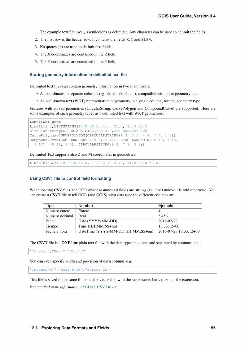
QGIS User Guide, Versión 3.4
1. The example text file uses ; (semicolon) as delimiter. Any character can be used to delimit the fields.
2. The first row is the header row. It contains the fields X, Y and ELEV.
3. No quotes (") are used to delimit text fields.
4. The X coordinates are contained in the X field.
5. The Y coordinates are contained in the Y field.
Storing geometry information in delimited text file
Delimited text files can contain geometry information in two main forms:
• As coordinates in separate columns (eg. Xcol, Ycol. . . ), compatible with point geometry data;
• As well-known text (WKT) representation of geometry in a single column, for any geometry type.
Features with curved geometries (CircularString, CurvePolygon and CompoundCurve) are supported. Here aresome examples of such geometry types as a delimited text with WKT geometries:
Label;WKT_geomLineString;LINESTRING(10.0 20.0, 11.0 21.0, 13.0 25.5)CircularString;CIRCULARSTRING(268 415,227 505,227 406)CurvePolygon;CURVEPOLYGON(CIRCULARSTRING(1 3, 3 5, 4 7, 7 3, 1 3))CompoundCurve;COMPOUNDCURVE((5 3, 5 13), CIRCULARSTRING(5 13, 7 15,
9 13), (9 13, 9 3), CIRCULARSTRING(9 3, 7 1, 5 3))
Delimited Text supports also Z and M coordinates in geometries:
LINESTRINGZ(10.0 20.0 30.0, 11.0 21.0 31.0, 11.0 22.0 30.0)
Using CSVT file to control field formatting
When loading CSV files, the OGR driver assumes all fields are strings (i.e. text) unless it is told otherwise. Youcan create a CSVT file to tell OGR (and QGIS) what data type the different columns are:
Tipo Nombre EjemploNúmero entero Entero 4Número decimal Real 3.456Fecha Date (YYYY-MM-DD) 2016-07-28Tiempo Time (HH:MM:SS+nn) 18:33:12+00Fecha y hora DateTime (YYYY-MM-DD HH:MM:SS+nn) 2016-07-28 18:33:12+00
The CSVT file is a ONE line plain text file with the data types in quotes and separated by commas, e.g.:
"Integer","Real","String"
You can even specify width and precision of each column, e.g.:
"Integer(6)","Real(5.5)","String(22)"
This file is saved in the same folder as the .csv file, with the same name, but .csvt as the extension.
You can find more information at GDAL CSV Driver.
12.3. Exploring Data Formats and Fields 155
QGIS User Guide, Versión 3.4
PostGIS Layers
PostGIS layers are stored in a PostgreSQL database. The advantages of PostGIS are its spatial indexing, filteringand querying capabilities it provides. Using PostGIS, vector functions such as select and identify work moreaccurately than they do with OGR layers in QGIS.
Truco: PostGIS Layers
Normally, a PostGIS layer is defined by an entry in the geometry_columns table. QGIS can load layers that donot have an entry in the geometry_columns table. This includes both tables and views. Defining a spatial viewprovides a powerful means to visualize your data. Refer to your PostgreSQL manual for information on creatingviews.
This section contains some details on how QGIS accesses PostgreSQL layers. Most of the time, QGIS shouldsimply provide you with a list of database tables that can be loaded, and it will load them on request. However,if you have trouble loading a PostgreSQL table into QGIS, the information below may help you understand anyQGIS messages and give you direction on changing the PostgreSQL table or view definition to allow QGIS toload it.
Clave primaria
QGIS requires that PostgreSQL layers contain a column that can be used as a unique key for the layer. For tables,this usually means that the table needs a primary key, or a column with a unique constraint on it. In QGIS, thiscolumn needs to be of type int4 (an integer of size 4 bytes). Alternatively, the ctid column can be used as primarykey. If a table lacks these items, the oid column will be used instead. Performance will be improved if the columnis indexed (note that primary keys are automatically indexed in PostgreSQL).
QGIS offers a checkbox Select at id that is activated by default. This option gets the ids without the attributeswhich is faster in most cases.
View
If the PostgreSQL layer is a view, the same requirement exists, but views do not always have primary keys orcolumns with unique constraints on them. You have to define a primary key field (has to be integer) in the QGISdialog before you can load the view. If a suitable column does not exist in the view, QGIS will not load the layer.If this occurs, the solution is to alter the view so that it does include a suitable column (a type of integer and eithera primary key or with a unique constraint, preferably indexed).
As for table, a checkbox Select at id is activated by default (see above for the meaning of the checkbox). It canmake sense to disable this option when you use expensive views.
QGIS layer_style table and database backup
If you want to make a backup of your PostGIS database using the pg_dump and pg_restore commands, andthe default layer styles as saved by QGIS fail to restore afterwards, you need to set the XML option to DOCUMENTbefore the restore command:
SET XML OPTION DOCUMENT;
Filter database side
QGIS allows to filter features already on server side. Check the Settings → Options → Data Sources →Execute expressions on postgres server-side if possible checkbox to do so. Only supported expressions will be sentto the database. Expressions using unsupported operators or functions will gracefully fallback to local evaluation.
156 Chapter 12. Administrar el origen de datos

QGIS User Guide, Versión 3.4
Support of PostgreSQL data types
Most of common data types are supported by the PostgreSQL provider: integer, float, varchar, geometry, times-tamp, array and hstore.
Importing Data into PostgreSQL
Data can be imported into PostgreSQL/PostGIS using several tools, including the DB Manager plugin and thecommand line tools shp2pgsql and ogr2ogr.
Administrador de BBDD
QGIS comes with a core plugin named DB Manager. It can be used to load data, and it includes support forschemas. See section DB Manager Plugin for more information.
shp2pgsql
PostGIS includes an utility called shp2pgsql that can be used to import Shapefile format datasets into a PostGIS-enabled database. For example, to import a Shapefile format dataset named lakes.shp into a PostgreSQLdatabase named gis_data, use the following command:
shp2pgsql -s 2964 lakes.shp lakes_new | psql gis_data
This creates a new layer named lakes_new in the gis_data database. The new layer will have a spatialreference identifier (SRID) of 2964. See section Trabajar con Proyecciones for more information on spatialreference systems and projections.
Truco: Exporting datasets from PostGIS
Like the import tool shp2pgsql, there is also a tool to export PostGIS datasets in the Shapefile format: pgsql2shp.This is shipped within your PostGIS distribution.
ogr2ogr
Además de shp2pgsql y Administrador de BBDD, hay otra herramienta para alimentar de datos geográficos aPostGIS: ogr2ogr. Esto es parte de su instalación GDAL.
To import a Shapefile format dataset into PostGIS, do the following:
ogr2ogr -f "PostgreSQL" PG:"dbname=postgis host=myhost.de user=postgrespassword=topsecret" alaska.shp
This will import the Shapefile format dataset alaska.shp into the PostGIS database postgis using the userpostgres with the password topsecret on host server myhost.de.
Note that OGR must be built with PostgreSQL to support PostGIS. You can verify this by typing (in )
ogrinfo --formats | grep -i post
If you prefer to use PostgreSQL’s COPY command instead of the default INSERT INTO method, you can export
the following environment variable (at least available on and ):
export PG_USE_COPY=YES
12.3. Exploring Data Formats and Fields 157

QGIS User Guide, Versión 3.4
ogr2ogr does not create spatial indexes like shp2pgsl does. You need to create them manually, using the nor-mal SQL command CREATE INDEX afterwards as an extra step (as described in the next section Mejorar elrendimiento).
Mejorar el rendimiento
Retrieving features from a PostgreSQL database can be time-consuming, especially over a network. You canimprove the drawing performance of PostgreSQL layers by ensuring that a PostGIS spatial index exists on eachlayer in the database. PostGIS supports creation of a GiST (Generalized Search Tree) index to speed up spatialsearches of the data (GiST index information is taken from the PostGIS documentation available at https://postgis.net).
Truco: You can use the DBManager to create an index to your layer. You should first select the layer and clickon Table → Edit table, go to Indexes tab and click on Add Spatial Index.
The syntax for creating a GiST index is:
CREATE INDEX [indexname] ON [tablename]USING GIST ( [geometryfield] GIST_GEOMETRY_OPS );
Tenga en cuenta que para tablas grandes, crear el índice puede tomar un largo tiempo. Una vez que el índicees creado, se debe realizar un VACUUM ANALYZE. Vea la documentación de PostGIS (POSTGIS-PROJECTReferencias bibliográficas y web) para mayor información.
The following is an example of creating a GiST index:
gsherman@madison:~/current$ psql gis_dataWelcome to psql 8.3.0, the PostgreSQL interactive terminal.
Type: \copyright for distribution terms\h for help with SQL commands\? for help with psql commands\g or terminate with semicolon to execute query\q to quit
gis_data=# CREATE INDEX sidx_alaska_lakes ON alaska_lakesgis_data-# USING GIST (the_geom GIST_GEOMETRY_OPS);CREATE INDEXgis_data=# VACUUM ANALYZE alaska_lakes;VACUUMgis_data=# \qgsherman@madison:~/current$
Vector layers crossing 180° longitude
Many GIS packages don’t wrap vector maps with a geographic reference system (lat/lon) crossing the 180 degreeslongitude line (http://postgis.refractions.net/documentation/manual-2.0/ST_Shift_Longitude.html). As result, ifwe open such a map in QGIS, we will see two far, distinct locations, that should appear near each other. InFigure_vector_crossing, the tiny point on the far left of the map canvas (Chatham Islands) should be within thegrid, to the right of the New Zealand main islands.
A work-around is to transform the longitude values using PostGIS and the ST_Shift_Longitude function. Thisfunction reads every point/vertex in every component of every feature in a geometry, and if the longitude coor-dinate is < 0°, it adds 360° to it. The result is a 0° - 360° version of the data to be plotted in a 180°-centricmap.
158 Chapter 12. Administrar el origen de datos

QGIS User Guide, Versión 3.4
Figure 12.19: Map in lat/lon crossing the 180° longitude line
Figure 12.20: Crossing 180° longitude applying the ST_Shift_Longitude function
Uso
• Import data into PostGIS (Importing Data into PostgreSQL) using, for example, the DB Manager plugin.
• Use the PostGIS command line interface to issue the following command (in this example,«TABLE» is the actual name of your PostGIS table): gis_data=# update TABLE setthe_geom=ST_Shift_Longitude(the_geom);
• If everything went well, you should receive a confirmation about the number of features that were updated.Then you’ll be able to load the map and see the difference (Figure_vector_crossing_map).
SpatiaLite Layers
If you want to save a vector layer to SpatiaLite format, you can do this by right clicking the layer in the legend.Then, click on Save as. . . , define the name of the output file, and select “SpatiaLite” as format and the CRS. Also,you can select “SQLite” as format and then add SPATIALITE=YES in the OGR data source creation option field.This tells OGR to create a SpatiaLite database. See also https://www.gdal.org/ogr/drv_sqlite.html.
QGIS also supports editable views in SpatiaLite.
If you want to create a new SpatiaLite layer, please refer to section Crear una nueva capa SpatiaLite.
Truco: SpatiaLite data management Plugins
For SpatiaLite data management, you can also use several Python plugins: QSpatiaLite, SpatiaLite Manager orDB Manager (core plugin, recommended). If necessary, they can be downloaded and installed with the PluginInstaller.
12.3. Exploring Data Formats and Fields 159

QGIS User Guide, Versión 3.4
GeoJSON specific parameters
When exporting layers to GeoJSON, this format has some specific Layer Options available. These options actuallycome from GDAL which is responsible for the writing of the file:
• COORDINATE_PRECISION the maximum number of digits after the decimal separator to write in coor-dinates. Defaults to 15 (note: for Lat Lon coordinates 6 is considered enough). Truncation will occur toremove trailing zeros.
• WRITE_BBOX set to YES to write a bbox property with the bounding box of the geometries at the featureand feature collection level
DB2 Spatial Layers
IBM DB2 for Linux, Unix and Windows (DB2 LUW), IBM DB2 for z/OS (mainframe) and IBM DashDB productsallow users to store and analyse spatial data in relational table columns. The DB2 provider for QGIS supports thefull range of visualization, analysis and manipulation of spatial data in these databases.
User documentation on these capabilities can be found at the DB2 z/OS KnowledgeCenter, DB2 LUW Knowl-edgeCenter and DB2 DashDB KnowledgeCenter.
For more information about working with the DB2 spatial capabilities, check out the DB2 Spatial Tutorial on IBMDeveloperWorks.
The DB2 provider currently only supports the Windows environment through the Windows ODBC driver.
The client running QGIS needs to have one of the following installed:
• DB2 LUW
• IBM Data Server Driver Package
• IBM Data Server Client
To open a DB2 data in QGIS, you can refer to The Browser Panel or Loading a Database Layer section.
If you are accessing a DB2 LUW database on the same machine or using DB2 LUW as a client, the DB2 executa-bles and supporting files need to be included in the Windows path. This can be done by creating a batch file likethe following with the name db2.bat and including it in the directory %OSGEO4W_ROOT%/etc/ini.
@echo offREM Point the following to where DB2 is installedSET db2path=C:\Program Files (x86)\sqllibREM This should usually be ok - modify if necessarySET gskpath=C:\Program Files (x86)\ibm\gsk8SET Path=%db2path%\BIN;%db2path%\FUNCTION;%gskpath%\lib64;%gskpath%\lib;%path%
160 Chapter 12. Administrar el origen de datos

CHAPTER 13
Trabajar con Datos Vectoriales
13.1 La librería Símbolo
13.1.1 El Administrador de estilos
The Style Manager is the place where users can manage and create generic symbols and color ramps to be used inseveral QGIS projects. You can open that modeless dialog:
• with the Style Manager button of the Project toolbar;
• from the Settings → Style Manager. . . menu;
• or from a vector Layer Properties → Symbology tab (using the Style Manager button in a symbol propertydialog).
The dialog allows you to:
• create, edit and remove symbols and color ramps;
• organize symbols and color ramps in custom groups;
• export and import symbols and color ramps.
Organizing symbols and color ramps
The Style Manager dialog displays in its center a frame with previewed items organized into tabs:
• All for a complete collection of point, linear and surface symbols as the following items allow only to displaya single item group;
• Marker for point symbols;
• Line for linear symbols;
• Fill for surface symbols;
• and Color ramp
161

QGIS User Guide, Versión 3.4
Figure 13.1: El Administrador de estilos
For each family of items, you can organize the elements into different categories, listed in the panel on the left:
• Favorites: displayed by default when configuring an item, it shows a set of default symbols and color rampsyou can extend;
• All: listing all the installed symbols and color ramps;
• Tags: shows a list of labels you can use to identify the items. A symbol or color ramp can be tagged morethan once. Select a tag in the list and you’ll see the items that belong to it for each type of item. To create a
new tag you could later attach to symbols or color ramps, use the Add Tag. . . button or select the AddTag. . . from any tag contextual menu;
• Smart Group: a smart group dynamically fetches its symbols according to conditions set (see eg, fig-ure_smart_group). Click the Add Smart Group. . . button to create smart groups. The dialog box allows youto enter an expression to filter the items to select (has a particular tag, have a string in its name, etc.). Anysymbol or color ramp that satisfies the entered condition(s) is automatically added to the smart group.
Figure 13.2: Creating a Smart Group
Tags and smart groups are not mutually exclusive: they are simply two different ways to organize your symbols andcolor ramps. Unlike the smart groups that automatically fetch their belonged items based on the input constraints,tags are filled by the user. To edit any of those categories, you can either:
• select the items, right-click and choose Add to Tag → and then select the tag name or create a new tag;
162 Chapter 13. Trabajar con Datos Vectoriales

QGIS User Guide, Versión 3.4
• select the tag and press Modify group. . . → Attach Selected Tag to Symbols. A checkbox appears neareach item to help you select or deselect it. When selection is finished, press Modify group. . . → FinishTagging.
• select the smart group, press Modify group. . . → Edit smart group. . . and configure a new set of constraintsin the Smart Group Editor dialog. This option is also available in the contextual menu of the smart group.
To remove a tag or a smart group, right-click on it and select the Remove button. Note that this does not deletethe items grouped in the category.
Adding, editing or removing an item
As seen earlier, symbols and color ramps are listed under different tabs whose contents depend on the activecategory (tag, smart group, favorites. . . ). For each type of symbols (Marker , Line or Fill) and color ramp, whenthe tab is enabled, you can:
• Add new items: press the Add item button and configure the item following symbols or color rampsbuilder description.
• Modify an existing item: select an item and press Edit item button and configure as mentioned above.
• Delete existing items: to delete a symbol you no longer need, select it and click Remove item (also availablethrough right-click). The symbol will be deleted from the local symbols database.
Right-clicking over a selection of items also allows you to:
• Add to Favorites;
• Remove from Favorites;
• Add to Tag → and select the appropriate tag or create a new one to use;
• Clear Tags: detaching the symbols from any tag;
• Remove Item(s);
• Edit Item: applies to the item you right-click over;
• Export Selected Symbol(s) as PNG. . . (not available with color ramps);
• Export Selected Symbol(s) as SVG. . . (not available with color ramps);
Sharing symbols and color ramps
The Import/Export tool, at the left bottom of the Style Manager dialog, offers options to easily share symbolsand color ramps with others. These options are also available through right-click over the items.
Exporting items
You can export a set of items to an .XML file:
1. Expand the Import/Export drop-down menu and select Export Item(s). . .
2. Choose the symbols and color ramps you’d like to integrate. Symbol selection can be done with the mouseor using a tag or group previously set.
3. Press Export when ready. You’ll be prompted to indicate the destination of the saved file. The XML formatgenerates a single file containing all the selected symbols. This file can then be imported in another user’sstyle library.
13.1. La librería Símbolo 163

QGIS User Guide, Versión 3.4
Figure 13.3: Exporting symbols and color ramps
When symbols are selected, you can also export them to .PNG or .SVG. Exporting to .PNG or .SVG (both notavailable for color ramp symbols) creates a file for each selected symbol in a given folder. The SVG folder can beadded to the SVG paths in Settings → Options → System menu of another user, allowing him direct access to allthese symbols.
Importing items
You can extend your symbols library by importing new symbols:
1. Expand the Import/Export drop-down menu and select Import Item(s) at the left bottom of thedialog.
2. In the new dialog, indicate the source of the symbols (it can be an .xml file on the disk or a url).
3. Set whether to Add to favorites the items to import.
4. Check Do not import embedded tags to avoid the import of tags associated to the items being imported.
5. Give the name of any Additional tag(s) to apply to the new items.
6. Select from the preview the items you want to add to your library.
7. And press Import.
Rampa de color
The Color ramp tab in the Style Manager dialog helps you preview different color ramps based on the categoryselected in the left panel.
To create a custom color ramp, activate the Color ramp tab and click the Add item button. The button reveals adrop-down list to choose the ramp type:
164 Chapter 13. Trabajar con Datos Vectoriales
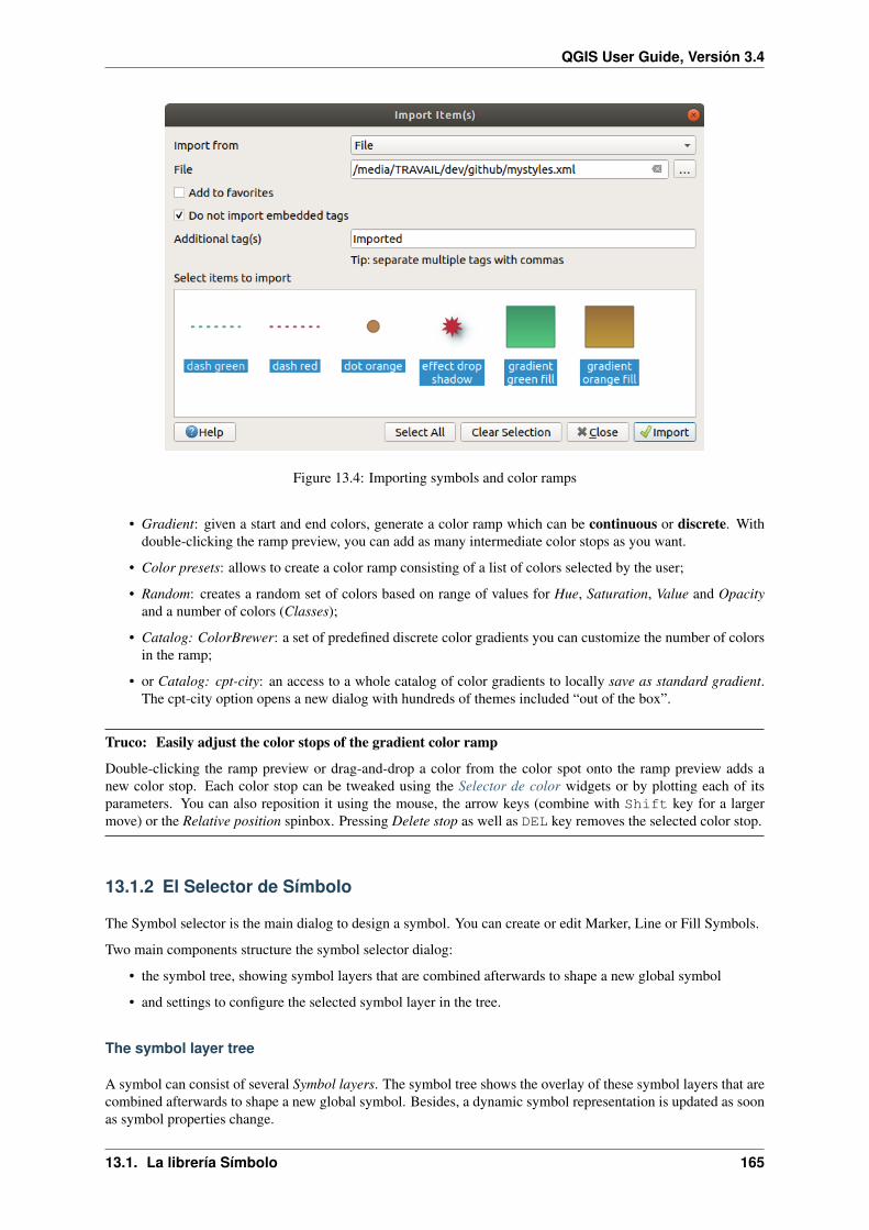
QGIS User Guide, Versión 3.4
Figure 13.4: Importing symbols and color ramps
• Gradient: given a start and end colors, generate a color ramp which can be continuous or discrete. Withdouble-clicking the ramp preview, you can add as many intermediate color stops as you want.
• Color presets: allows to create a color ramp consisting of a list of colors selected by the user;
• Random: creates a random set of colors based on range of values for Hue, Saturation, Value and Opacityand a number of colors (Classes);
• Catalog: ColorBrewer: a set of predefined discrete color gradients you can customize the number of colorsin the ramp;
• or Catalog: cpt-city: an access to a whole catalog of color gradients to locally save as standard gradient.The cpt-city option opens a new dialog with hundreds of themes included “out of the box”.
Truco: Easily adjust the color stops of the gradient color ramp
Double-clicking the ramp preview or drag-and-drop a color from the color spot onto the ramp preview adds anew color stop. Each color stop can be tweaked using the Selector de color widgets or by plotting each of itsparameters. You can also reposition it using the mouse, the arrow keys (combine with Shift key for a largermove) or the Relative position spinbox. Pressing Delete stop as well as DEL key removes the selected color stop.
13.1.2 El Selector de Símbolo
The Symbol selector is the main dialog to design a symbol. You can create or edit Marker, Line or Fill Symbols.
Two main components structure the symbol selector dialog:
• the symbol tree, showing symbol layers that are combined afterwards to shape a new global symbol
• and settings to configure the selected symbol layer in the tree.
The symbol layer tree
A symbol can consist of several Symbol layers. The symbol tree shows the overlay of these symbol layers that arecombined afterwards to shape a new global symbol. Besides, a dynamic symbol representation is updated as soonas symbol properties change.
13.1. La librería Símbolo 165

QGIS User Guide, Versión 3.4
Figure 13.5: Ejemplo de rampa de color gradiente personalizado con pasos múltiples
166 Chapter 13. Trabajar con Datos Vectoriales
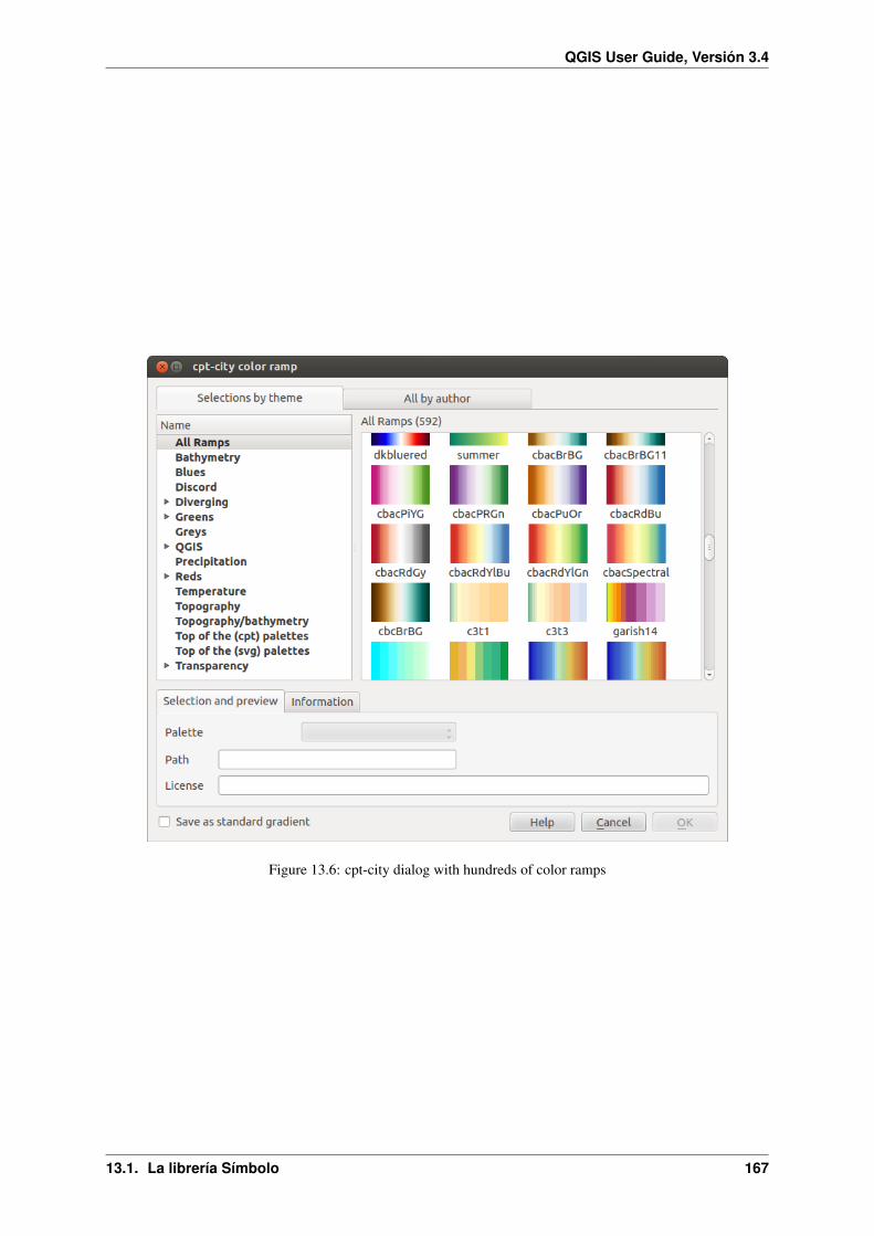
QGIS User Guide, Versión 3.4
Figure 13.6: cpt-city dialog with hundreds of color ramps
13.1. La librería Símbolo 167

QGIS User Guide, Versión 3.4
Figure 13.7: Designing a Line symbol
168 Chapter 13. Trabajar con Datos Vectoriales

QGIS User Guide, Versión 3.4
A set of tools is available to manage the symbol tree items and according to the level selected, you’ll get enableddifferent tools at the bottom of the dialog to:
• add new symbol layer: you can stack as many symbols as you want
• remove the selected symbol layer
• lock colors of symbol layer: a locked color stays unchanged when user changes the color at the global(or upper) symbol level
• duplicate a (group of) symbol layer(s)
• move up or down the symbol layer
When a symbol layer is selected in the tree, you can also:
• control its visibility with the Enable layer option. Disabled symbol layers are not drawn, but are savedand can be enabled at a later stage. This makes it easier to customize parts of the symbol based on thefeature attributes or to tweak symbol appearance without having to totally delete a symbol layer;
• apply rendering effects using the Draw effects button.
Configuring a symbol
In QGIS, configuring a symbol is done in two steps: the symbol and then the symbol layer.
The symbol
At the top level of the tree, it depends on the layer geometry and can be of Marker, Line or Fill type. Eachsymbol can embed one or more symbols (including, of any other type) or symbol layers.
You can setup some parameters that apply to the global symbol:
• Unit: it can be Millimeter, Points, Pixels, Meters at Scale, Map unit or Inches
• Transparencia
• Color: when this parameter is changed by the user, its value is echoed to all unlocked sub-symbols color
• Size and Rotation for marker symbols
• Width for line symbols
Nota: The Data-defined override button beside the last layer-related parameters is inactive when setting thesymbol from the Style manager dialog. When the symbol is connected to a map layer, this button helps you createproportional or multivariate analysis rendering.
The symbols used at this level are items you can pick from the symbols library. Available symbols of the cor-responding type are shown and, through the editable drop-down list just above, can be filtered by free-form text
or by categories. You can also update the list of symbols using the Style Manager button and open the eponymdialog. There, you can use any capabilities as exposed in El Administrador de estilos section.
The symbols are displayed either:
• in an icon list (with thumbnail, name and associated tags) using the List View button below the frame;
• or as icon preview using the Icon View button.
Press the Save Symbol button to add any symbol being edited to the symbols library. With the Advancedoption, you can:
13.1. La librería Símbolo 169

QGIS User Guide, Versión 3.4
• set the symbol levels: defining the way symbol layers are connected to each other in the map canvas (seeSymbol levels for more information)
• and for line and fill symbols, clip features to canvas extent.
Truco: Note that once you have set the size in the lower levels of the Symbol layers dialog, the size of the wholesymbol can be changed with the Size (for marker symbols) or the Width (for line symbols) menu in the first levelagain. The size of the lower levels changes accordingly, while the size ratio is maintained.
The symbol layer
At a lower level of the tree, you can customize the symbol layers. The available symbol layer types depend on the
upper symbol type. You can apply on the symbol layer paint effects to enhance its rendering.
Because describing all the options of all the symbol layer types would not be possible, only particular and signifi-cant ones are mentioned below.
Common parameters
Some common options and widgets are available to build a symbol layer, regardless it’s of marker, line or fillsub-type:
• the color selector widget to ease color manipulation
• Units: it can be Millimeter, Points, Pixels, Meters at Scale, Map unit or Inches
• the data-defined override widget near almost all options, extending capabilities of customizing each symbol(see Configuración de anulación definida por datos for more information)
Nota: While the description below assumes that the symbol layer type is bound to the feature geometry, keepin mind that you can embed symbol layers in each others. In that case, the lower level symbol layer parameter(placement, offset. . . ) might be bound to the upper-level symbol, and not to the feature geometry itself.
Símbolos de marcador
Appropriate for point geometry features, marker symbols have several Symbol layer types:
• Simple marker (default);
• Ellipse marker: a simple marker symbol layer, with customizable width and height;
• Filled marker: similar to the simple marker symbol layer, except that it uses a fill sub symbol to render themarker. This allows use of all the existing QGIS fill (and stroke) styles for rendering markers, e.g. gradientor shapeburst fills;
• Font marker: use installed fonts as marker symbols;
• Geometry generator (see The Geometry Generator);
• Vector Field marker (see The Vector Field Marker);
• SVG marker: provides you with images from your SVG paths (set in Settings → Options. . . → Systemmenu) to render as marker symbol. Width and height of the symbol can be set independently or using the
Lock aspect ratio. Each SVG file colors and stroke can also be adapted.
Nota: SVG version requirements
170 Chapter 13. Trabajar con Datos Vectoriales
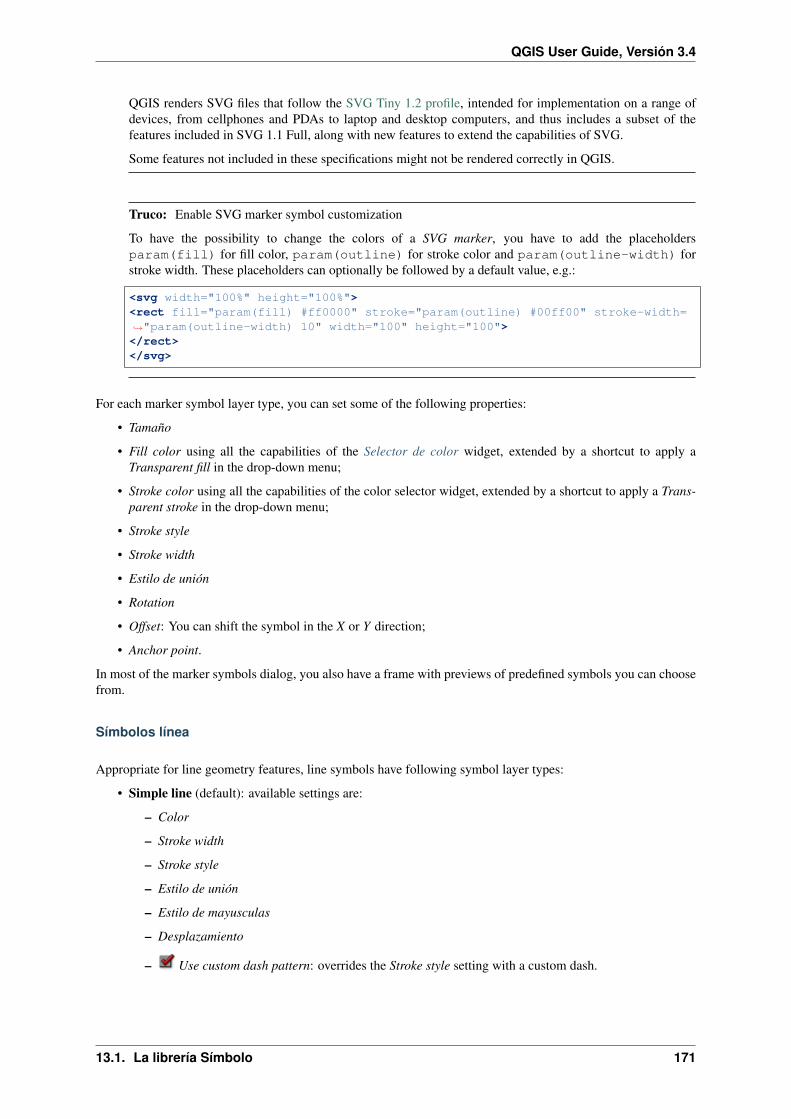
QGIS User Guide, Versión 3.4
QGIS renders SVG files that follow the SVG Tiny 1.2 profile, intended for implementation on a range ofdevices, from cellphones and PDAs to laptop and desktop computers, and thus includes a subset of thefeatures included in SVG 1.1 Full, along with new features to extend the capabilities of SVG.
Some features not included in these specifications might not be rendered correctly in QGIS.
Truco: Enable SVG marker symbol customization
To have the possibility to change the colors of a SVG marker, you have to add the placeholdersparam(fill) for fill color, param(outline) for stroke color and param(outline-width) forstroke width. These placeholders can optionally be followed by a default value, e.g.:
<svg width="100%" height="100%"><rect fill="param(fill) #ff0000" stroke="param(outline) #00ff00" stroke-width=→˓"param(outline-width) 10" width="100" height="100"></rect></svg>
For each marker symbol layer type, you can set some of the following properties:
• Tamaño
• Fill color using all the capabilities of the Selector de color widget, extended by a shortcut to apply aTransparent fill in the drop-down menu;
• Stroke color using all the capabilities of the color selector widget, extended by a shortcut to apply a Trans-parent stroke in the drop-down menu;
• Stroke style
• Stroke width
• Estilo de unión
• Rotation
• Offset: You can shift the symbol in the X or Y direction;
• Anchor point.
In most of the marker symbols dialog, you also have a frame with previews of predefined symbols you can choosefrom.
Símbolos línea
Appropriate for line geometry features, line symbols have following symbol layer types:
• Simple line (default): available settings are:
– Color
– Stroke width
– Stroke style
– Estilo de unión
– Estilo de mayusculas
– Desplazamiento
– Use custom dash pattern: overrides the Stroke style setting with a custom dash.
13.1. La librería Símbolo 171

QGIS User Guide, Versión 3.4
• Arrow: draws lines as curved (or not) arrows with a single or a double head with configurable width, lengthand thickness. To create a curved arrow the line feature must have at least three vertices. It also uses a fillsymbol such as gradients or shapeburst to render the arrow body. Combined with the geometry generator,this type of layer symbol helps you representing flow maps;
• Geometry generator (see The Geometry Generator);
• Marker line: displays a marker symbol along the line. It can be at a regular distance or based on itsgeometry: first, last or each vertex, on central point or on every curve point. You can set an offset along theline for the marker symbol, or offset the line itself. The Rotate marker option allows you to set whether themarker symbol should follow the line orientation or not.
Fill Symbols
Appropriate for polygon geometry features, fill symbols have also several symbol layer types:
• Simple fill (default): the following settings are available:
– Fill color using all the capabilities of the Selector de color widget, extended by a shortcut to apply aTransparent fill
– Estilo de relleno
– Stroke color using all the capabilities of the color selector widget, extended by a shortcut to apply aTransparent stroke
– Stroke width
– Stroke style
– Estilo de unión
– Offset: You can shift the symbol in the X or Y direction;
• Centroid fill: places a marker symbol at the centroid of the visible feature. The position of the marker mayhowever not be the real centroid of the feature because calculation takes into account the polygon(s) clippedto area visible in map canvas for rendering and ignores holes. Use the geometry generator symbol if youwant the exact centroid.
The marker can be placed on every part of a multi-part feature or only on its biggest part, and forced to beinside the polygon;
• Geometry generator (see The Geometry Generator);
• Gradient fill: uses a radial, linear or conical gradient, based on either simple two color gradients or apredefined gradient color ramp to fill polygon layers. Gradient can be rotated and applied on a singlefeature basis or across the whole map extent. Also start and end points can be set via coordinates or usingthe centroid (of feature or map);
• Line pattern fill: fills the polygon with a hatching pattern of line symbol layer. You can set the spacingbetween lines and an offset from the feature boundary;
• Point pattern fill: fills the polygon with a hatching pattern of marker symbol layer. You can set the spacingbetween lines and an offset from the feature boundary;
• Raster image fill: you can fill polygons with a tiled raster image. Options include (data defined) file name,opacity, image size (in pixels, mm or map units), coordinate mode (feature or view) and rotation;
• SVG fill: fills the polygon using SVG markers;
• Shapeburst fill: this option buffered a gradient fill, where a gradient is drawn from the boundary of apolygon towards the polygon’s centre. Configurable parameters include distance from the boundary toshade, use of color ramps or simple two color gradients, optional blurring of the fill and offsets;
• Outline: Arrow: uses a line arrow symbol layer to represent the polygon boundary;
• Outline: Marker line: uses a marker line symbol layer to represent the polygon boundary;
172 Chapter 13. Trabajar con Datos Vectoriales

QGIS User Guide, Versión 3.4
• Outline: simple line: uses a simple line symbol layer to represent the polygon boundary. The Draw lineonly inside polygon option helps polygon borders inside the polygon and can be useful to clearly representadjacent polygon boundaries.
Nota: When geometry type is polygon, you can choose to disable the automatic clipping of lines/polygons to thecanvas extent. In some cases this clipping results in unfavourable symbology (e.g. centroid fills where the centroidmust always be the actual feature’s centroid).
The Geometry Generator
Available with all types of symbols, the geometry generator symbol layer allows to use expression syntax togenerate a geometry on the fly during the rendering process. The resulting geometry does not have to match withthe original geometry type and you can add several differently modified symbol layers on top of each other.
Algún ejemplo:
-- render the centroid of a featurecentroid( $geometry )
-- visually overlap features within a 100 map units distance from a point-- feature, i.e generate a 100m buffer around the pointbuffer( $geometry, 100 )
-- Given polygon layer1( id1, layer2_id, ...) and layer2( id2, fieldn...)-- render layer1 with a line joining centroids of both where layer2_id = id2make_line( centroid( $geometry ),
centroid( geometry( get_feature( 'layer2', 'id2', attribute($currentfeature, 'layer2_id') ) )
)
The Vector Field Marker
The vector field marker is used to display vector field data such as earth deformation, tidal flows, and the like.It displays the vectors as lines (preferably arrows) that are scaled and oriented according to selected attributes ofdata points. It can only be used to render point data; line and polygon layers are not drawn by this symbology.
The vector field is defined by attributes in the data, which can represent the field either by:
• cartesian components (x and y components of the field)
• or polar coordinates: in this case, attributes define Length and Angle. The angle may be measured eitherclockwise from north, or Counterclockwise from east, and may be either in degrees or radians.
• or as height only data, which displays a vertical arrow scaled using an attribute of the data. This is appro-priate for displaying the vertical component of deformation, for example.
The magnitude of field can be scaled up or down to an appropriate size for viewing the field.
13.2 El Dialogo de las Propiedades del Vector
El cuadro de diálogo Propiedades de la capa para una capa vectorial proporciona una configuración general paraadministrar la apariencia de los elementos de la capa en el mapa (simbología, etiquetas, diagramas), interaccióncon el mouse (acciones, textos de aviso del mapa, diseño de formularios). También proporciona información dela capa.
To access the Layer Properties dialog:
• In the Layers panel, double-click the layer or right-click and select Properties. . . from the pop-up menu;
13.2. El Dialogo de las Propiedades del Vector 173

QGIS User Guide, Versión 3.4
• Go to Layer → Properties. . . menu when the layer is selected.
The vector Layer Properties dialog provides the following sections:
• Information
• Source
• Symbology (also available in the Layer styling panel)
• Labels (also available in the Layer styling panel)
• Diagrams
• 3D View (also available in the Layer styling panel)
• Source Fields
• Attributes Form
• Joins
• Auxiliary Storage
• Actions
• Display
• Rendering
• Variables
• Metadata
• Dependencies
• Legend
• QGIS Server
• Digitizing
• and optionally, new tabs added by external plugins you have installed. Those are not presented below.
Truco: Share full or partial properties of the layer styles
The Style menu at the bottom of the dialog allows you to import or export these or part of these properties from/toseveral destination (file, clipboard, database). See Managing Custom Styles.
Nota: Because properties (symbology, label, actions, default values, forms. . . ) of embedded layers (see Anidarproyectos) are pulled from the original project file and to avoid changes that may break this behavior, the layerproperties dialog is made unavailable for these layers.
174 Chapter 13. Trabajar con Datos Vectoriales

QGIS User Guide, Versión 3.4
13.2.1 Information Properties
The Information tab is read-only and represents an interesting place to quickly grab summarized informationand metadata on the current layer. Provided information are:
• based on the provider of the layer (format of storage, path, geometry type, data source encoding, extent. . . );
• picked from the filled metadata (access, links, contacts, history. . . );
• or related to its geometry (spatial extent, CRS. . . ) or its attributes (number of fields, characteristics ofeach. . . ).
13.2.2 Source Properties
Use this tab to define general settings for the vector layer.
Figure 13.8: Source tab in vector Layer Properties dialog
Other than setting the Layer name to display in the Layers Panel, available options include:
Sistema de coordenadas de referencia
• Displays the layer’s Coordinate Reference System (CRS) as a PROJ.4 string. You can change the layer’s
CRS, selecting a recently used one in the drop-down list or clicking on Select CRS button (see CoordinateReference System Selector). Use this process only if the CRS applied to the layer is a wrong one or if nonewas applied. If you wish to reproject your data into another CRS, rather use layer reprojection algorithmsfrom Processing or Save it into another layer.
• Create spatial index (only for OGR-supported formats).
• Update extents information for a layer.
13.2. El Dialogo de las Propiedades del Vector 175

QGIS User Guide, Versión 3.4
Constructor de Consulta
The Query Builder dialog is accessible through the eponym button at the bottom of the Source tab in the LayerProperties dialog, under the Provider feature filter group.
The Query Builder provides an interface that allows you to define a subset of the features in the layer using aSQL-like WHERE clause and to display the result in the main window. As long as the query is active, only thefeatures corresponding to its result are available in the project.
You can use one or more layer attributes to define the filter in the Query Builder. The use of more than oneattribute is shown in Figure_vector_querybuilder. In the example, the filter combines the attributes
• toa (DateTime field: cast("toa" as character) > '2017-05-17' and cast("toa" ascharacter) < '2019-12-24T18:00:00'),
• name (String field: "name" > 'S') and
• FID (Integer field: FID > 10)
using the AND, OR and NOT operators and parenthesis. This syntax (including the DateTime format for the toafield) works for GeoPackage datasets.
The filter is made at the data provider (OGR, PostgreSQL, MSSQL. . . ) level. So the syntax depends on the dataprovider (DateTime is for instance not supported for the ESRI Shapefile format). The complete expression:
cast("toa" as character) > '2017-05-17' ANDcast("toa" as character) < '2019-12-24T18:00:00' ANDNOT ("name" > 'S' OR FID > 10)
Figure 13.9: Constructor de Consulta
176 Chapter 13. Trabajar con Datos Vectoriales

QGIS User Guide, Versión 3.4
You can also open the Query Builder dialog using the Filter. . . option from the Layer menu or the layer contextualmenu. The Fields, Values and Operators sections in the dialog help you to construct the SQL-like query exposedin the Provider specific filter expression box.
The Fields list contains all the fields of the layer. To add an attribute column to the SQL WHERE clause field,double-click its name or just type it into the SQL box.
The Values frame lists the values of the currently selected field. To list all unique values of a field, click the Allbutton. To instead list the first 25 unique values of the column, click the Sample button. To add a value to the SQLWHERE clause field, double click its name in the Values list. You can use the search box at the top of the Valuesframe to easily browse and find attribute values in the list.
The Operators section contains all usable operators. To add an operator to the SQL WHERE clause field, clickthe appropriate button. Relational operators ( = , > , . . . ), string comparison operator (LIKE), and logical operators(AND, OR, . . . ) are available.
The Test button helps you check your query and displays a message box with the number of features satisfying thecurrent query. Use the Clear button to wipe the SQL query and revert the layer to its original state (ie, fully loadall the features).
When a filter is applied, QGIS treats the resulting subset acts as if it were the entire layer. For example if youapplied the filter above for “Borough” ("TYPE_2" = 'Borough'), you can not display, query, save or editAnchorage, because that is a “Municipality” and therefore not part of the subset.
Truco: Filtered layers are indicated in the Layers Panel
In the Layers panel, filtered layer is listed with a Filter icon next to it indicating the query used when the mousehovers over the button. Double-click the icon opens the Query Builder dialog for edit.
13.2.3 Symbology Properties
The Symbology tab provides you with a comprehensive tool for rendering and symbolizing your vector data.You can use tools that are common to all vector data, as well as special symbolizing tools that were designed forthe different kinds of vector data. However all types share the following dialog structure: in the upper part, youhave a widget that helps you prepare the classification and the symbol to use for features and at the bottom theReproducción de capas widget.
Truco: Switch quickly between different layer representations
Using the Styles → Add menu at the bottom of the Layer Properties dialog, you can save as many styles asneeded. A style is the combination of all properties of a layer (such as symbology, labeling, diagram, fields form,actions. . . ) as you want. Then, simply switch between styles from the context menu of the layer in Layers Panelto automatically get different representations of your data.
Truco: Exportar simbología vector
You have the option to export vector symbology from QGIS into Google *.kml, *.dxf and MapInfo *.tab files.Just open the right mouse menu of the layer and click on Save As. . . to specify the name of the output file and itsformat. In the dialog, use the Symbology export menu to save the symbology either as Feature symbology → or asSymbol layer symbology →. If you have used symbol layers, it is recommended to use the second setting.
Representación de elementos
The renderer is responsible for drawing a feature together with the correct symbol. Regardless layer geometrytype, there are four common types of renderers: single symbol, categorized, graduated and rule-based. For point
13.2. El Dialogo de las Propiedades del Vector 177

QGIS User Guide, Versión 3.4
layers, there are a point displacement and a heatmap renderers available while polygon layers can also be renderedwith the inverted polygons and 2.5 D renderers.
There is no continuous color renderer, because it is in fact only a special case of the graduated renderer. Thecategorized and graduated renderers can be created by specifying a symbol and a color ramp - they will set thecolors for symbols appropriately. For each data type (points, lines and polygons), vector symbol layer types areavailable. Depending on the chosen renderer, the dialog provides different additional sections.
Nota: If you change the renderer type when setting the style of a vector layer the settings you made for thesymbol will be maintained. Be aware that this procedure only works for one change. If you repeat changing therenderer type the settings for the symbol will get lost.
Representador de Símbolo Único
The Single Symbol renderer is used to render all features of the layer using a single user-defined symbol. SeeEl Selector de Símbolo for further information about symbol representation.
Figure 13.10: Propiedades de línea con símbolo único
Truco: Edit symbol directly from layer panel
If in your Layers Panel you have layers with categories defined through categorized, graduated or rule-basedsymbology mode, you can quickly change the fill color of the symbol of the categories by right-clicking on a
category and choose the color you prefer from a color wheel menu. Right-clicking on a category will also giveyou access to the options Hide all items, Show all items and Edit symbol.
178 Chapter 13. Trabajar con Datos Vectoriales

QGIS User Guide, Versión 3.4
Sin representación de símbolos
The No Symbols renderer is a special use case of the Single Symbol renderer as it applies the same renderingto all features. Using this renderer, no symbol will be drawn for features, but labeling, diagrams and other non-symbol parts will still be shown.
Selections can still be made on the layer in the canvas and selected features will be rendered with a default symbol.Features being edited will also be shown.
This is intended as a handy shortcut for layers which you only want to show labels or diagrams for, and avoids theneed to render symbols with totally transparent fill/border to achieve this.
Representador Categorizado
The Categorized renderer is used to render the features of a layer, using a user-defined symbol whose aspectreflects the discrete values of a field or an expression. The Categorized menu allows you to
• select an existing field (using the Column listbox) or
• type or build an expression using the Set column expression. The expression used to classify features can beof any type; it can for example:
– be a comparison, e.g. myfield >= 100, $id = @atlas_featureid, myfield % 2 = 0,within( $geometry, @atlas_geometry ). In this case, QGIS returns values 1 (True) and0 (False).
– combine different fields, e.g. concat( field1, ' ', field2 ) particularly useful when youwant to process classification on two or more fields simultaneously.
– be a calculation on fields, e.g. myfield % 2, year( myfield ) field_1 + field_2.
– be used to transform linear values in discrete classes, e.g.:
CASE WHEN x > 1000 THEN 'Big' ELSE 'Small' END
– combine several discrete values in one single category, e.g.:
CASEWHEN building IN ('residence', 'mobile home') THEN 'residential'WHEN building IN ('commercial', 'industrial') THEN 'Commercial and→˓Industrial'END
Nota: While you can use any kind of expression to categorize features, for some complex expressions itmight be simpler to use rule-based rendering.
• the symbol (using the El Selector de Símbolo dialog) which will be used as base symbol for each class;
• the range of colors (using the Color ramp listbox) from which color applied to the symbol is selected.
Then click on Classify button to create classes from the distinct value of the attribute column. Each class can bedisabled unchecking the checkbox at the left of the class name.
To change symbol, value and/or label of the class, just double click on the item you want to change.
Right-click shows a contextual menu to Copy/Paste, Change color, Change transparency, Change output unit,Change symbol width.
The example in figure_categorized_symbology shows the category rendering dialog used for the rivers layer of theQGIS sample dataset.
13.2. El Dialogo de las Propiedades del Vector 179

QGIS User Guide, Versión 3.4
Figure 13.11: Opciones de simbolización categorizadas
Truco: Elegir y cambiar símbolos múltiples
The Symbology allows you to select multiple symbols and right click to change color, transparency, size, or widthof selected entries.
Truco: Hacer coincidir las categorías con el nombre de símbolo
In the [Advanced] menu, under the classes, you can choose one of the two first actions to match symbol name toa category name in your classification. Matched to saved symbols match category name with a symbol name fromyour Style Manager. Match to symbols from file match category name to a symbol name from an external file.
Representador Graduado
The Graduated renderer is used to render all the features from a layer, using an user-defined symbol whosecolor or size reflects the assignment of a selected feature’s attribute to a class.
Like the Categorized Renderer, the Graduated Renderer allows you to define rotation and size scale from specifiedcolumns.
Also, analogous to the Categorized Renderer, it allows you to select:
• The attribute (using the Column listbox or the Set column expression function)
• The symbol (using the Symbol selector dialog)
• El formato de leyenda y la precisión
• The method to use to change the symbol: color or size
• The colors (using the color Ramp list) if the color method is selected
180 Chapter 13. Trabajar con Datos Vectoriales

QGIS User Guide, Versión 3.4
• The size (using the size domain and its unit)
Then you can use the Histogram tab which shows an interactive histogram of the values from the assigned field orexpression. Class breaks can be moved or added using the histogram widget.
Nota: You can use Statistical Summary panel to get more information on your vector layer. See Panel de resumenestadístico.
Back to the Classes tab, you can specify the number of classes and also the mode for classifying features withinthe classes (using the Mode list). The available modes are:
• Equal Interval: each class has the same size (e.g. values from 0 to 16 and 4 classes, each class has a size of4).
• Quantile: each class will have the same number of element inside (the idea of a boxplot).
• Natural Breaks (Jenks): the variance within each class is minimal while the variance between classes ismaximal.
• Standard Deviation: classes are built depending on the standard deviation of the values.
• Pretty Breaks: Computes a sequence of about n+1 equally spaced nice values which cover the range of thevalues in x. The values are chosen so that they are 1, 2 or 5 times a power of 10. (based on pretty from theR statistical environment http://astrostatistics.psu.edu/datasets/R/html/base/html/pretty.html)
The listbox in the center part of the Symbology tab lists the classes together with their ranges, labels and symbolsthat will be rendered.
Click on Classify button to create classes using the chosen mode. Each classes can be disabled unchecking thecheckbox at the left of the class name.
To change symbol, value and/or label of the class, just double click on the item you want to change.
Right-click shows a contextual menu to Copy/Paste, Change color, Change transparency, Change output unit,Change symbol width.
The example in figure_graduated_symbology shows the graduated rendering dialog for the rivers layer of theQGIS sample dataset.
Figure 13.12: Graduated Symbolizing options
13.2. El Dialogo de las Propiedades del Vector 181

QGIS User Guide, Versión 3.4
Truco: Thematic maps using an expression
Categorized and graduated thematic maps can be created using the result of an expression. In the properties dialog
for vector layers, the attribute chooser is extended with a Set column expression function. So you don’t need to writethe classification attribute to a new column in your attribute table if you want the classification attribute to be acomposite of multiple fields, or a formula of some sort.
Proportional Symbol and Multivariate Analysis
Proportional Symbol and Multivariate Analysis are not rendering types available from the Symbology render-ing drop-down list. However with the data-defined override options applied over any of the previous renderingoptions, QGIS allows you to display your point and line data with such representation.
Crear símbolo proporcional
To apply a proportional rendering:
1. First apply to the layer the single symbol renderer.
2. Then set the symbol to apply to the features.
3. Select the item at the upper level of the symbol tree, and use the Data-defined override button next to the Size(for point layer) or Width (for line layer) option.
4. Select a field or enter an expression, and for each feature, QGIS will apply the output value to the propertyand proportionally resize the symbol in the map canvas.
If need be, use the Size assistant. . . option of the menu to apply some transformation (exponential,flannery. . . ) to the symbol size rescaling (see Using the data-defined assistant interface for more details).
You can choose to display the proportional symbols in the Layers panel and the print layout legend item: unfoldthe Advanced drop-down list at the bottom of the main dialog of the Symbology tab and select Data-defined sizelegend. . . to configure the legend items (see Data-defined size legend for details).
Crear análisis multivariable
A multivariate analysis rendering helps you evaluate the relationship between two or more variables e.g., one canbe represented by a color ramp while the other is represented by a size.
The simplest way to create multivariate analysis in QGIS is to:
1. First apply a categorized or graduated rendering on a layer, using the same type of symbol for all the classes.
2. Then, apply a proportional symbology on the classes:
(a) Click on the Change button above the classification frame: you get the El Selector de Símbolo dialog.
(b) Rescale the size or width of the symbol layer using the data defined override widget as seen above.
Like the proportional symbol, the scaled symbology can be added to the layer tree, on top of the categorized orgraduated classes symbols using the data defined size legend feature. And both representation are also availablein the print layout legend item.
Rule-based Renderer
The Rule-based renderer is used to render all the features from a layer, using rule-based symbols whose aspectreflects the assignment of a selected feature’s attribute to a class. The rules are based on SQL statements and canbe nested. The dialog allows rule grouping by filter or scale, and you can decide if you want to enable symbollevels or use only the first-matched rule.
182 Chapter 13. Trabajar con Datos Vectoriales
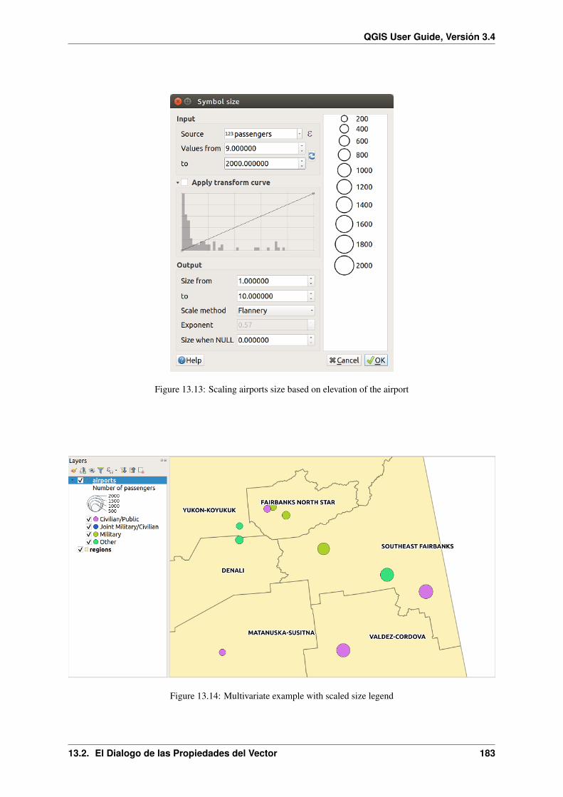
QGIS User Guide, Versión 3.4
Figure 13.13: Scaling airports size based on elevation of the airport
Figure 13.14: Multivariate example with scaled size legend
13.2. El Dialogo de las Propiedades del Vector 183

QGIS User Guide, Versión 3.4
To create a rule:
1. Activate an existing row by double-clicking it (by default, QGIS adds a symbol without a rule when the
rendering mode is enabled) or click the Edit rule or Add rule button.
2. In the Edit Rule dialog that opens, you can define a label to help you identify each rule. This is the label thatwill be displayed in the Layers Panel and also in the print composer legend.
3. Manually enter an expression in the text box next to the Filter option or press the button next to itto open the expression string builder dialog.
4. Use the provided functions and the layer attributes to build an expression to filter the features you’d like toretrieve. Press the Test button to check the result of the query.
5. You can enter a longer label to complete the rule description.
6. You can use the Scale Range option to set scales at which the rule should be applied.
7. Finally, configure the symbol to use for these features.
8. And press OK.
A new row summarizing the rule is added to the Layer Properties dialog. You can create as many rules as necessaryfollowing the steps above or copy pasting an existing rule. Drag-and-drop the rules on top of each other to nestthem and refine the upper rule features in subclasses.
Selecting a rule, you can also organize its features in subclasses using the Refine selected rules drop-down menu.Automated rule refinement can be based on:
• scales;
• categories: applying a categorized renderer;
• or ranges: applying a graduated renderer.
Refined classes appear like sub-items of the rule, in a tree hierarchy and like above, you can set symbology ofeach class.
In the Edit rule dialog, you can avoid writing all the rules and make use of the Else option to catch all thefeatures that do not match any of the other rules, at the same level. This can also be achieved by writing Else inthe Rule column of the Layer Properties → Symbology → Rule-based dialog.
The created rules also appear in a tree hierarchy in the map legend. Double-click the rules in the map legend andthe Symbology tab of the layer properties appears showing the rule that is the background for the symbol in thetree.
The example in figure_rule_based_symbology shows the rule-based rendering dialog for the rivers layer of theQGIS sample dataset.
Point displacement Renderer
The Point Displacement renderer works to visualize all features of a point layer, even if they have the samelocation. To do this, the renderer takes the points falling in a given Distance tolerance from each other and placesthem around their barycenter following different Placement methods:
• Ring: places all the features on a circle whose radius depends on the number of features to display.
• Concentric rings: uses a set of concentric circles to show the features.
• Grid: generates a regular grid with a point symbol at each intersection.
The Center symbol widget helps you customize the symbol and color of the middle point. For the distributed pointssymbols, you can apply any of the No symbols, Single symbol, Categorized, Graduated or Rule-based rendererusing the Renderer drop-down list and customize them using the Renderer Settings. . . button.
184 Chapter 13. Trabajar con Datos Vectoriales

QGIS User Guide, Versión 3.4
Figure 13.15: Opciones de simbología basada en reglas
While the minimal spacing of the Displacement lines depends on the point symbol renderer’s, you can still cus-tomize some of its settings such as the Stroke width, Stroke color and Size adjustment (eg, to add more spacingbetween the rendered points).
Use the Labels group options to perform points labeling: the labels are placed near the displaced position of thesymbol, and not at the feature real position. Other than the Label attribute, Label font and Label color, you canset the Minimum map scale to display the labels.
Nota: Point Displacement renderer does not alter feature geometry, meaning that points are not moved from theirposition. They are still located at their initial place. Changes are only visual, for rendering purpose. Use insteadthe Processing qgispointsdisplacement algorithm if you want to create displaced features.
Point Cluster Renderer
Unlike the Point Displacement renderer which blows up nearest or overlaid point features placement, thePoint Cluster renderer groups nearby points into a single rendered marker symbol. Based on a specified Distance,points that fall within from each others are merged into a single symbol. Points aggregation is made based on theclosest group being formed, rather than just assigning them the first group within the search distance.
From the main dialog, you can:
• set the symbol to represent the point cluster in the Cluster symbol; the default rendering displays the numberof aggregated features thanks to the @cluster_size variable on Font marker symbol layer.
• use the Renderer drop-down list to apply any of the other feature rendering types to the layer (single,categorized, rule-based. . . ). Then, push the Renderer Settings. . . button to configure features” symbologyas usual. Note that this renderer is only visible on features that are not clustered. Also, when the symbolcolor is the same for all the point features inside a cluster, that color sets the @cluster_color variableof the cluster.
Nota: Point Cluster renderer does not alter feature geometry, meaning that points are not moved from their
13.2. El Dialogo de las Propiedades del Vector 185

QGIS User Guide, Versión 3.4
Figure 13.16: Cuadro de diálogo de desplazamiento de punto
Figure 13.17: Point Cluster dialog
186 Chapter 13. Trabajar con Datos Vectoriales

QGIS User Guide, Versión 3.4
position. They are still located at their initial place. Changes are only visual, for rendering purpose. Use instead theProcessing qgiskmeansclustering or qgisdbscanclustering algorithm if you want to create cluster-based features.
Inverted Polygon Renderer
The Inverted Polygon renderer allows user to define a symbol to fill in outside of the layer’s polygons. Asabove you can select subrenderers, namely Single symbol, Graduated, Categorized, Rule-Based or 2.5D renderer.
Figure 13.18: Inverted Polygon dialog
Heatmap Renderer
With the Heatmap renderer you can create live dynamic heatmaps for (multi)point layers. You can specify theheatmap radius in millimeters, points, pixels, map units or inches, choose and edit a color ramp for the heatmapstyle and use a slider for selecting a trade-off between render speed and quality. You can also define a maximumvalue limit and give a weight to points using a field or an expression. When adding or removing a feature theheatmap renderer updates the heatmap style automatically.
2.5D Renderer
Using the 2.5D renderer it’s possible to create a 2.5D effect on your layer’s features. You start by choosing aHeight value (in map units). For that you can use a fixed value, one of your layer’s fields, or an expression. Youalso need to choose an Angle (in degrees) to recreate the viewer position (0° means west, growing in counter clockwise). Use advanced configuration options to set the Roof Color and Wall Color. If you would like to simulate
solar radiation on the features walls, make sure to check the Shade walls based on aspect option. You can alsosimulate a shadow by setting a Color and Size (in map units).
Truco: Using 2.5D effect with other renderers
13.2. El Dialogo de las Propiedades del Vector 187

QGIS User Guide, Versión 3.4
Figure 13.19: Diálogo Mapa de calor
Figure 13.20: Diálogo 2.5D
188 Chapter 13. Trabajar con Datos Vectoriales

QGIS User Guide, Versión 3.4
Once you have finished setting the basic style on the 2.5D renderer, you can convert this to another renderer (single,categorized, graduated). The 2.5D effects will be kept and all other renderer specific options will be available foryou to fine tune them (this way you can have for example categorized symbols with a nice 2.5D representationor add some extra styling to your 2.5D symbols). To make sure that the shadow and the «building» itself do notinterfere with other nearby features, you may need to enable Symbols Levels ( Advanced → Symbol levels. . . ).The 2.5D height and angle values are saved in the layer’s variables, so you can edit it afterwards in the variablestab of the layer’s properties dialog.
Reproducción de capas
From the Symbology tab, you can also set some options that invariably act on all features of the layer:
• Opacity : You can make the underlying layer in the map canvas visible with this tool.Use the slider to adapt the visibility of your vector layer to your needs. You can also make a precisedefinition of the percentage of visibility in the menu beside the slider.
• Blending mode at the Layer and Feature levels: You can achieve special rendering effects with these toolsthat you may previously only know from graphics programs. The pixels of your overlaying and underlayinglayers are mixed through the settings described in Modos de Mezcla.
• Apply paint effects on all the layer features with the Draw Effects button.
• Control feature rendering order allows you, using features attributes, to define the z-order in which they
shall be rendered. Activate the checkbox and click on the button beside. You then get the Define Orderdialog in which you:
1. Choose a field or build an expression to apply to the layer features.
2. Set in which order the fetched features should be sorted, i.e. if you choose Ascending order, thefeatures with lower value are rendered under those with higher value.
3. Define when features returning NULL value should be rendered: first (bottom) or last (top).
4. Repeat the above steps as many times as rules you wish to use.
The first rule is applied to all the features in the layer, z-ordering them according to their returned value.Then, within each group of features with the same value (including those with NULL value) and thus thesame z-level, the next rule is applied to sort them. And so on. . .
Figure 13.21: Layer rendering options
Otras Configuraciones
Symbol levels
For renderers that allow stacked symbol layers (only heatmap doesn’t) there is an option to control the renderingorder of each symbol’s levels.
For most of the renderers, you can access the Symbols levels option by clicking the Advanced button belowthe saved symbols list and choosing Symbol levels. For the Rule-based Renderer the option is directly availablethrough Symbols Levels. . . button, while for Point displacement Renderer renderer the same button is inside theRendering settings dialog.
13.2. El Dialogo de las Propiedades del Vector 189

QGIS User Guide, Versión 3.4
To activate symbols levels, select the Enable symbol levels. Each row will show up a small sample of thecombined symbol, its label and the individual symbols layer divided into columns with a number next to it. Thenumbers represent the rendering order level in which the symbol layer will be drawn. Lower values levels aredrawn first, staying at the bottom, while higher values are drawn last, on top of the others.
Figure 13.22: Symbol levels dialog
Nota: If symbols levels are deactivated, the complete symbols will be drawn according to their respective featuresorder. Overlapping symbols will simply obfuscate to other below. Besides, similar symbols won’t «merge» witheach other.
Figure 13.23: Symbol levels activated (A) and deactivated (B) difference
Data-defined size legend
When a layer is rendered with the proportional symbol or the multivariate rendering or when a scaled size diagramis applied to the layer, you can allow the display of the scaled symbols in both the Layers panel and the print layoutlegend.
To enable the Data-defined Size Legend dialog to render symbology, select the eponym option in the Advanced
190 Chapter 13. Trabajar con Datos Vectoriales

QGIS User Guide, Versión 3.4
button below the saved symbols list. For diagrams, the option is available under the Legend tab. The dialogprovides the following options to:
• select the type of legend: Legend not enabled, Separated legend items and Collapsed legend.For the latter option, you can select whether the legend items are aligned at the Bottom or at the Center;
• set the symbol to use for legend representation;
• insert the title in the legend;
• resize the classes to use: by default, QGIS provides you with a legend of five classes (based on natural pretty
breaks) but you can apply your own classification using the Manual size classes option. Use the
and buttons to set your custom classes values and labels.
A preview of the legend is displayed in the right panel of the dialog and updated as you set the parameters. Forcollapsed legend, a leader line from the horizontal center of the symbol to the corresponding legend text is drawn.
Figure 13.24: Setting size scaled legend
Nota: Currently, data-defined size legend for layer symbology can only be applied to point layer using single,categorized or graduated symbology.
Efectos de dibujo
In order to improve layer rendering and avoid (or at least reduce) the resort to other software for final rendering of
maps, QGIS provides another powerful functionality: the Draw Effects options, which adds paint effects forcustomizing the visualization of vector layers.
The option is available in the Layer Properties → Symbology dialog, under the Layer rendering group (applyingto the whole layer) or in symbol layer properties (applying to corresponding features). You can combine bothusage.
Paint effects can be activated by checking the Draw effects option and clicking the Customize effects button.That will open the Effect Properties Dialog (see figure_effects_source). The following effect types, with custom
13.2. El Dialogo de las Propiedades del Vector 191

QGIS User Guide, Versión 3.4
options are available:
• Source: Draws the feature’s original style according to the configuration of the layer’s properties. TheOpacity of its style can be adjusted as well as the Blend mode and Draw mode. These are common propertiesfor all types of effects.
Figure 13.25: Efectos de dibujo: cuadro de diálogo Fuente
• Blur: Adds a blur effect on the vector layer. The custom options that you can change are the Blur type(Stack blur (fast) or Gaussian blur (quality)) and the Blur strength.
Figure 13.26: Efectos de dibujo: cuadro de diálogo Difuminar
• Colorise: This effect can be used to make a version of the style using one single hue. The base will alwaysbe a grayscale version of the symbol and you can:
– Use the Grayscale to select how to create it: options are “By lightness”, “By luminosity”, “Byaverage” and “Off”.
– If Colorise is selected, it will be possible to mix another color and choose how strong it should be.
– Control the Brightness, Contrast and Saturation levels of the resulting symbol.
• Drop Shadow: Using this effect adds a shadow on the feature, which looks like adding an extra dimension.This effect can be customized by changing the Offset angle and distance, determining where the shadowshifts towards to and the proximity to the source object. Drop Shadow also has the option to change theBlur radius and the Color of the effect.
192 Chapter 13. Trabajar con Datos Vectoriales

QGIS User Guide, Versión 3.4
Figure 13.27: Efectos de dibujo: cuadro de diálogo Dar Color
• Inner Shadow: This effect is similar to the Drop Shadow effect, but it adds the shadow effect on the insideof the edges of the feature. The available options for customization are the same as the Drop Shadow effect.
• Inner Glow: Adds a glow effect inside the feature. This effect can be customized by adjusting the Spread(width) of the glow, or the Blur radius. The latter specifies the proximity from the edge of the feature whereyou want any blurring to happen. Additionally, there are options to customize the color of the glow using aSingle color or a Color ramp.
• Outer Glow: This effect is similar to the Inner Glow effect, but it adds the glow effect on the outside of theedges of the feature. The available options for customization are the same as the Inner Glow effect.
• Transform: Adds the possibility of transforming the shape of the symbol. The first options availablefor customization are the Reflect horizontal and Reflect vertical, which actually create a reflection on thehorizontal and/or vertical axes. The other options are:
– Shear X,Y: Slants the feature along the X and/or Y axis.
– Scale X,Y: Enlarges or minimizes the feature along the X and/or Y axis by the given percentage.
– Rotation: Turns the feature around its center point.
– and Translate X,Y changes the position of the item based on a distance given on the X and/or Y axis.
One or more effect types can be used at the same time. You (de)activate an effect using its checkbox in the
effects list. You can change the selected effect type by using the Effect type option. You can reorder the
effects using Move up and Move down buttons, and also add/remove effects using the Add new effect andRemove effect buttons.
There are some common options available for all draw effect types. Opacity and Blend mode options work similarto the ones described in Reproducción de capas and can be used in all draw effects except for the transform one.
There is also a Draw mode option available for every effect, and you can choose whether to render and/ormodify the symbol, following some rules:
• Effects render from top to bottom.
• Render only mode means that the effect will be visible.
13.2. El Dialogo de las Propiedades del Vector 193

QGIS User Guide, Versión 3.4
Figure 13.28: Efectos de dibujo: cuadro de diálogo Sombra exterior
194 Chapter 13. Trabajar con Datos Vectoriales

QGIS User Guide, Versión 3.4
Figure 13.29: Efectos de dibujo: cuadro de diálogo Sombra interior
• Modifier only mode means that the effect will not be visible but the changes that it applies will be passed tothe next effect (the one immediately below).
• The Render and Modify mode will make the effect visible and pass any changes to the next effect. If theeffect is at the top of the effects list or if the immediately above effect is not in modify mode, then it willuse the original source symbol from the layers properties (similar to source).
13.2.4 Propiedades de etiquetas
The Labels properties provides you with all the needed and appropriate capabilities to configure smart labelingon vector layers. This dialog can also be accessed from the Layer Styling panel, or using the Layer Labeling Options
icon of the Labels toolbar.
The first step is to choose the labeling method from the drop-down list. Available methods are:
• No labels: the default value, showing no labels from the layer
• Single labels, described below
• Rule-based labeling
• and Blocking: allows to set a layer as just an obstacle for other layer’s labels without rendering anylabels of its own.
Configurar una etiqueta
The next steps assume you select the Single labels option, enabling following tabs that help you configure thelabeling:
• Texto
• Formateo
• Buffer
13.2. El Dialogo de las Propiedades del Vector 195

QGIS User Guide, Versión 3.4
Figure 13.30: Efectos de dibujo: cuadro de diálogo Brillo interior
196 Chapter 13. Trabajar con Datos Vectoriales

QGIS User Guide, Versión 3.4
Figure 13.31: Efectos de dibujo: cuadro de diálogo Brillo exterior
13.2. El Dialogo de las Propiedades del Vector 197

QGIS User Guide, Versión 3.4
Figure 13.32: Efectos de dibujo: cuadro de diálogo Transformar
198 Chapter 13. Trabajar con Datos Vectoriales

QGIS User Guide, Versión 3.4
• Fondo
• Sombra
• Ubicación
• Representación
It also enables the Label with drop-down list, from which you can select an attribute column to use. Click ifyou want to define labels based on expressions - See Definir etiquetas basadas en expresiones.
The following steps describe simple labeling without using the Data defined override functions, which are situatednext to the drop-down menus - see Using data-defined override for labeling for a use case.
Figure 13.33: Configuración del etiquetado de capa - Pestaña de Texto
Pestaña de Texto
In the Text tab, you can define the Font, Style, and Size of your labels” text (see Figure_labels). There areoptions available to set the labels” Color and Transparency. Use the Type case option to change the capitalizationstyle of the text. You have the possibility to render the text as “All uppercase”, “All lowercase” or “Capitalizefirst letter”. In Spacing, you can change the space between words and between individual letters. Finally, use theBlend mode option to determine how your labels will mix with the map features below them (see more about it inModos de Mezcla).
The Apply label text substitutes option gives you ability to specify a list of texts to substitute to texts in featurelabels (e.g., abbreviating street types). Replacement texts are thus used to display labels in the map canvas. Users
13.2. El Dialogo de las Propiedades del Vector 199

QGIS User Guide, Versión 3.4
can also export and import lists of substitutes to make reuse and sharing easier.
Pestaña de formato
In the Formatting tab, you can define a character for a line break in the labels with the Wrap on characteroption. You can also format the Line Height and the alignment. For the latter, typical values are available (left,right, and center), plus Follow label placement for point layers. When set to this mode, text alignment for labelswill be dependent on the final placement of the label relative to the point. E.g., if the label is placed to the left ofthe point, then the label will be right aligned, while if it is placed to the right, it will be left aligned.
For line vector layers you can include Line directions symbols to help determine the lines directions. They workparticularly well when used with the curved or Parallel placement options from the Placement tab. There areoptions to set the symbols position, and to reverse direction.
Use the Formatted numbers option to format numeric labels. You can set the number of Decimal places. By
default, 3 decimal places will be used. Use the Show plus sign if you want to show the plus sign in positivenumbers.
Pestaña de buffer
To create a buffer around the labels, activate the Draw text buffer checkbox in the Buffer tab. You can
set the buffer’s Size, color, and Transparency. The buffer expands from the label’s outline , so, if the colorbuffer’s fill checkbox is activated, the buffer interior is filled. This may be relevant when using partially transparent
labels or with non-normal blending modes, which will allow seeing behind the label’s text. Deactivating colorbuffer’s fill checkbox (while using totally transparent labels) will allow you to create outlined text labels.
Pestaña de Fondo
In the Background tab, you can define with Size X and Size Y the shape of your background. Use Size type toinsert an additional “Buffer” into your background. The buffer size is set by default here. The background thenconsists of the buffer plus the background in Size X and Size Y. You can set a Rotation where you can choosebetween “Sync with label”, “Offset of label” and “Fixed”. Using “Offset of label” and “Fixed”, you can rotatethe background. Define an Offset X,Y with X and Y values, and the background will be shifted. When applyingRadius X,Y, the background gets rounded corners. Again, it is possible to mix the background with the underlyinglayers in the map canvas using the Blend mode (see Modos de Mezcla).
Pestaña de Sombra
Use the Shadow tab for a user-defined Draw drop shadow. The drawing of the background is very variable.Choose between “Lowest label component”, “Text”, “Buffer” and “Background”. The Offset angle depends on
the orientation of the label. If you choose the Use global shadow checkbox, then the zero point of the angle isalways oriented to the north and doesn’t depend on the orientation of the label. You can influence the appearanceof the shadow with the Blur radius. The higher the number, the softer the shadows. The appearance of the dropshadow can also be altered by choosing a blend mode.
Pestaña de Colocación
Choose the Placement tab for configuring label placement and labeling priority. Note that the placementoptions differ according to the type of vector layer, namely point, line or polygon, and are affected by the globalPAL setting.
200 Chapter 13. Trabajar con Datos Vectoriales

QGIS User Guide, Versión 3.4
Ubicación para capas punto
With the Cartographic placement mode, point labels are generated with a better visual relationship with thepoint feature, following ideal cartographic placement rules. Labels can be placed at a set Distance either from thepoint feature itself or from the bounds of the symbol used to represent the feature. The latter option is especiallyuseful when the symbol size isn’t fixed, e.g. if it’s set by a data defined size or when using different symbols in acategorized renderer.
By default, placements are prioritised in the following order:
1. arriba derecha
2. arriba izquierda
3. abajo derecha
4. abajo izquierda
5. al medio derecha
6. al medio izquierda
7. arriba, ligeramente derecha
8. abajo, ligeramente izquierda
Placement priority can, however, be customized or set for an individual feature using a data defined list of priori-tised positions. This also allows only certain placements to be used, so e.g. for coastal features you can preventlabels being placed over the land.
The Around point setting places the label in an equal radius (set in Distance) circle around the feature. Theplacement of the label can even be constrained using the Quadrant option.
With the Offset from point, labels are placed at a fixed offset from the point feature. You can select theQuadrant in which to place your label. You are also able to set the Offset X,Y distances between the points andtheir labels and can alter the angle of the label placement with the Rotation setting. Thus, placement in a selectedquadrant with a defined rotation is possible.
Ubicación para capas línea
Label options for line layers include Parallel, Curved or Horizontal. For the Parallel and
Curved options, you can set the position to Above line, On line and Below line. It’s possible to selectseveral options at once. In that case, QGIS will look for the optimal label position. For Parallel and curved place-ment options, you can also use the line orientation for the position of the label. Additionally, you can define a Max-
imum angle between curved characters when selecting the Curved option (see Figure_labels_placement_line).
For all three placement options, in Repeat, you can set up a minimum distance for repeating labels. The distancecan be in mm or in map units.
Ubicación para capas polígono
You can choose one of the following options for placing labels in polygons (see fig-ure_labels_placement_polygon):
• Desplazamiento desde el centroide,
• Horizontal (lento),
• Al rededor del centroide,
13.2. El Dialogo de las Propiedades del Vector 201

QGIS User Guide, Versión 3.4
Figure 13.34: Label placement examples in lines
• Libre (lento),
• Usando perímetro,
• and Usando perímetro (curved).
In the Offset from centroid settings you can specify if the centroid is of the visible polygon or wholepolygon. That means that either the centroid is used for the polygon you can see on the map or the centroid isdetermined for the whole polygon, no matter if you can see the whole feature on the map. You can place yourlabel within a specific quadrant, and define offset and rotation.
The Around centroid setting places the label at a specified distance around the centroid. Again, you can define
visible polygon or whole polygon for the centroid.
With the Horizontal (slow) or Free (slow) options, QGIS places at the best position either a horizontal or a rotatedlabel inside the polygon.
With the Using perimeter option, the label will be drawn next to the polygon boundary. The label will behave like
the parallel option for lines. You can define a position and a distance for the label. For the position, Above
line, On line, Below line and Line orientation dependent position are possible. You can specify thedistance between the label and the polygon outline, as well as the repeat interval for the label.
The Using perimeter (curved) option helps you draw the label along the polygon boundary, using a curved labeling.In addition to the parameters available with Using perimeter setting, you can set the Maximum angle betweencurved characters polygon, either inside or outside.
In the priority section you can define the priority with which labels are rendered for all three vector layer types(point, line, polygon). This placement option interacts with the labels from other vector layers in the map canvas.If there are labels from different layers in the same location, the label with the higher priority will be displayedand the others will be left out.
Pestaña de Renderizado
In the Rendering tab, you can tune when the labels can be rendered and their interaction with other labels andfeatures.
Under Label options, you find the scale-based and the Pixel size-based visibility settings.
The Label z-index determines the order in which labels are rendered, as well in relation with other feature labels inthe layer (using data-defined override expression), as with labels from other layers. Labels with a higher z-indexare rendered on top of labels (from any layer) with lower z-index.
Additionally, the logic has been tweaked so that if 2 labels have matching z-indexes, then:
202 Chapter 13. Trabajar con Datos Vectoriales
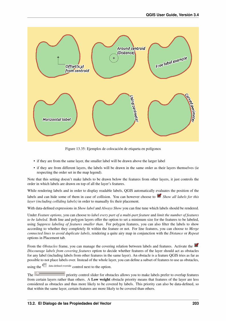
QGIS User Guide, Versión 3.4
Figure 13.35: Ejemplos de colocación de etiqueta en polígonos
• if they are from the same layer, the smaller label will be drawn above the larger label
• if they are from different layers, the labels will be drawn in the same order as their layers themselves (ierespecting the order set in the map legend).
Note that this setting doesn’t make labels to be drawn below the features from other layers, it just controls theorder in which labels are drawn on top of all the layer’s features.
While rendering labels and in order to display readable labels, QGIS automatically evaluates the position of the
labels and can hide some of them in case of collision. You can however choose to Show all labels for thislayer (including colliding labels) in order to manually fix their placement.
With data-defined expressions in Show label and Always Show you can fine tune which labels should be rendered.
Under Feature options, you can choose to label every part of a multi-part feature and limit the number of featuresto be labeled. Both line and polygon layers offer the option to set a minimum size for the features to be labeled,using Suppress labeling of features smaller than. For polygon features, you can also filter the labels to showaccording to whether they completely fit within the feature or not. For line features, you can choose to Mergeconnected lines to avoid duplicate labels, rendering a quite airy map in conjunction with the Distance or Repeatoptions in Placement tab.
From the Obstacles frame, you can manage the covering relation between labels and features. Activate theDiscourage labels from covering features option to decide whether features of the layer should act as obstaclesfor any label (including labels from other features in the same layer). An obstacle is a feature QGIS tries as far aspossible to not place labels over. Instead of the whole layer, you can define a subset of features to use as obstacles,
using the data-defined override control next to the option.
The priority control slider for obstacles allows you to make labels prefer to overlap featuresfrom certain layers rather than others. A Low weight obstacle priority means that features of the layer are lessconsidered as obstacles and thus more likely to be covered by labels. This priority can also be data-defined, sothat within the same layer, certain features are more likely to be covered than others.
13.2. El Dialogo de las Propiedades del Vector 203

QGIS User Guide, Versión 3.4
For polygon layers, you can choose the type of obstacle features could be by minimising the labels placement:
• over the feature’s interior: avoids placing labels over the interior of the polygon (prefers placing labelstotally outside or just slightly inside the polygon)
• or over the feature’s boundary: avoids placing labels over boundary of the polygon (prefers placing labelsoutside or completely inside the polygon). E.g., it can be useful for regional boundary layers, where thefeatures cover an entire area. In this case, it’s impossible to avoid placing labels within these features, andit looks much better to avoid placing them over the boundaries between features.
Setting the automated placement engine
In the top right corner of the Labels tab, you can use the Automated placement settings (applies to all layers) to configure a
global and automated behavior of the labels. Clicking the button provides you with the following options:
Figure 13.36: The labels automated placement engine
• The Search method combobox provides you with different placement methods for finding good placementsolutions for point, line and polygon labeling. More details in this article.
• The Number of candidates controls set how many label placement candidates should be generated for eachfeature type. The more candidates generated, the better the labeling will be - but at a cost of rendering speed.Smaller number of candidates results in less labels placed but faster redraws.
• Draw text as outlines: controls whether text labels are drawn (and exported) as either proper text objectsOR as paths only. If they are exported as text objects then they can be edited in external applications(e.g. Inkscape) as normal text. BUT the side effect is that the rendering quality is decreased, AND there’sissues with rendering when certain text settings like buffers are in place. That’s why drawing as outlines is
204 Chapter 13. Trabajar con Datos Vectoriales

QGIS User Guide, Versión 3.4
recommended. Note that when exporting a layout to svg there’s actually an override for this setting - so youcan leave the project rendering as outlines but for a .svg export export the labels as text.
• Show partial labels: controls whether labels which fall partially outside of the map extent should berendered. If checked, these labels will be shown (when there’s no way to place them fully within the visiblearea). If unchecked then partial visible labels will be skipped.
• show all labels for all layers (i.e. including colliding objects). Note that this option can be also set perlayer (see Pestaña de Renderizado)
• show candidates (for debugging): controls whether boxes should be drawn on the map showing all thecandidates generated for label placement. Like the label says, it’s useful only for debugging and testing theeffect different labeling settings have. This could be handy for a better manual placement with tools fromthe label toolbar.
Etiquetado basado en reglas
With rule-based labeling multiple label configurations can be defined and applied selectively on the base of ex-pression filters and scale range, as in Rule-based rendering.
To create a rule, select the Rule-based labeling option in the main drop-down list from the Labels tab and
click the button at the bottom of the dialog. Then fill the new dialog with a description and an expression tofilter features. You can also set a scale range in which the label rule should be applied. The other options availablein this dialog are the common settings seen beforehand.
A summary of existing rules is shown in the main dialog (see figure_labels_rule_based). You can add multiple
rules, reorder or imbricate them with a drag-and-drop. You can as well remove them with the button or edit
them with button or a double-click.
Definir etiquetas basadas en expresiones
Whether you choose single or rule-based labeling type, QGIS allows using expressions to label features.
Assuming you are using the Single labels method, click the icon near the Label with drop-down list in theLabels tab of the properties dialog.
In figure_labels_expression, you see a sample expression to label the alaska trees layer with tree type andarea, based on the field “VEGDESC”, some descriptive text, and the function $area in combination withformat_number() to make it look nicer.
Expression based labeling is easy to work with. All you have to take care of is that:
• You may need to combine all elements (strings, fields, and functions) with a string concatenation functionsuch as concat, + or ||. Be aware that in some situations (when null or numeric value are involved) notall of these tools will fit your need.
• Strings are written in “single quotes”.
• Fields are written in «double quotes» or without any quote.
Let’s have a look at some examples:
1. Label based on two fields “name” and “place” with a comma as separator:
"name" || ', ' || "place"
Devuelve:
John Smith, Paris
13.2. El Dialogo de las Propiedades del Vector 205
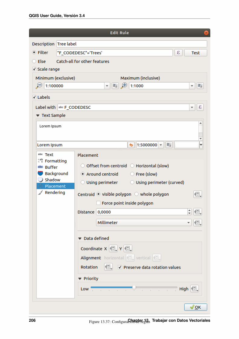
QGIS User Guide, Versión 3.4
Figure 13.37: Configuración de reglas206 Chapter 13. Trabajar con Datos Vectoriales
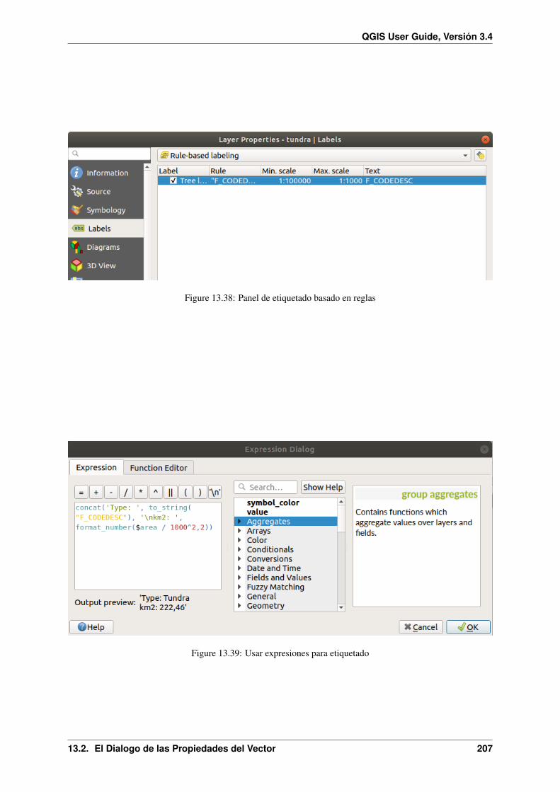
QGIS User Guide, Versión 3.4
Figure 13.38: Panel de etiquetado basado en reglas
Figure 13.39: Usar expresiones para etiquetado
13.2. El Dialogo de las Propiedades del Vector 207

QGIS User Guide, Versión 3.4
2. Label based on two fields “name” and “place” with other texts:
'My name is ' + "name" + 'and I live in ' + "place"'My name is ' || "name" || 'and I live in ' || "place"concat('My name is ', name, ' and I live in ', "place")
Devuelve:
My name is John Smith and I live in Paris
3. Label based on two fields “name” and “place” with other texts combining different concatenation functions:
concat('My name is ', name, ' and I live in ' || place)
Devuelve:
My name is John Smith and I live in Paris
Or, if the field “place” is NULL, returns:
My name is John Smith
4. Multi-line label based on two fields “name” and “place” with a descriptive text:
concat('My name is ', "name", '\n' , 'I live in ' , "place")
Devuelve:
My name is John SmithI live in Paris
5. Label based on a field and the $area function to show the place’s name and its rounded area size in aconverted unit:
'The area of ' || "place" || ' has a size of '|| round($area/10000) || ' ha'
Devuelve:
The area of Paris has a size of 10500 ha
6. Create a CASE ELSE condition. If the population value in field population is <= 50000 it is a town,otherwise it is a city:
concat('This place is a ',CASE WHEN "population" <= 50000 THEN 'town' ELSE 'city' END)
Devuelve:
This place is a town
7. Display name for the cities and no label for the other features (for the «city» context, see example above):
CASE WHEN "population" > 50000 THEN "NAME" END
Devuelve:
Paris
As you can see in the expression builder, you have hundreds of functions available to create simple and verycomplex expressions to label your data in QGIS. See Expresiones chapter for more information and examples onexpressions.
208 Chapter 13. Trabajar con Datos Vectoriales
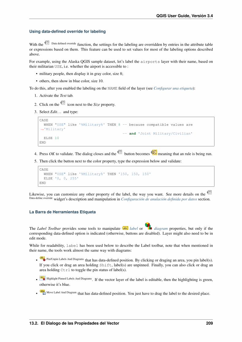
QGIS User Guide, Versión 3.4
Using data-defined override for labeling
With the Data defined override function, the settings for the labeling are overridden by entries in the attribute tableor expressions based on them. This feature can be used to set values for most of the labeling options describedabove.
For example, using the Alaska QGIS sample dataset, let’s label the airports layer with their name, based ontheir militarian USE, i.e. whether the airport is accessible to :
• military people, then display it in gray color, size 8;
• others, then show in blue color, size 10.
To do this, after you enabled the labeling on the NAME field of the layer (see Configurar una etiqueta):
1. Activate the Text tab.
2. Click on the icon next to the Size property.
3. Select Edit. . . and type:
CASEWHEN "USE" like '%Military%' THEN 8 -- because compatible values are
→˓'Military'-- and 'Joint Military/Civilian'
ELSE 10END
4. Press OK to validate. The dialog closes and the button becomes meaning that an rule is being run.
5. Then click the button next to the color property, type the expression below and validate:
CASEWHEN "USE" like '%Military%' THEN '150, 150, 150'ELSE '0, 0, 255'
END
Likewise, you can customize any other property of the label, the way you want. See more details on theData-define override widget’s description and manipulation in Configuración de anulación definida por datos section.
La Barra de Herramientas Etiqueta
The Label Toolbar provides some tools to manipulate label or diagram properties, but only if thecorresponding data-defined option is indicated (otherwise, buttons are disabled). Layer might also need to be inedit mode.
While for readability, label has been used below to describe the Label toolbar, note that when mentioned intheir name, the tools work almost the same way with diagrams:
• Pin/Unpin Labels And Diagrams that has data-defined position. By clicking or draging an area, you pin label(s).If you click or drag an area holding Shift, label(s) are unpinned. Finally, you can also click or drag anarea holding Ctrl to toggle the pin status of label(s).
• Highlight Pinned Labels And Diagrams. If the vector layer of the label is editable, then the highlighting is green,otherwise it’s blue.
• Move Label And Diagram that has data-defined position. You just have to drag the label to the desired place.
13.2. El Dialogo de las Propiedades del Vector 209
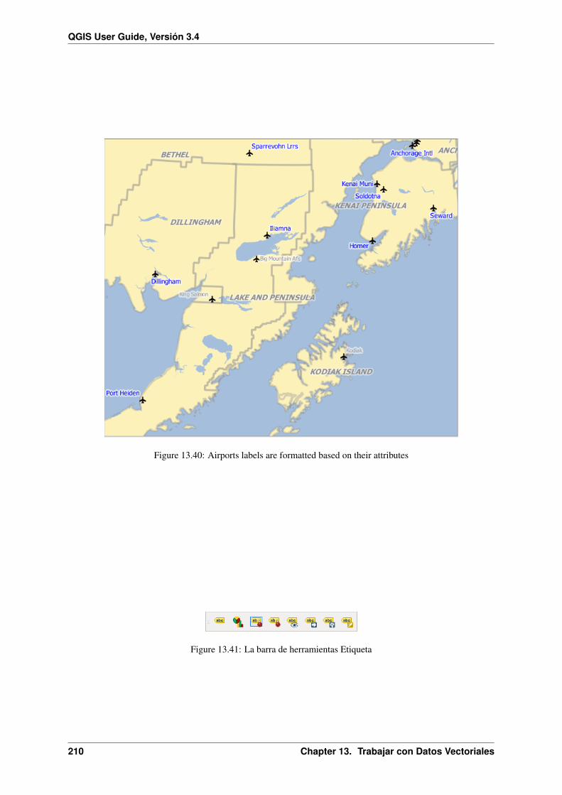
QGIS User Guide, Versión 3.4
Figure 13.40: Airports labels are formatted based on their attributes
Figure 13.41: La barra de herramientas Etiqueta
210 Chapter 13. Trabajar con Datos Vectoriales

QGIS User Guide, Versión 3.4
• Show/Hide Labels And Diagrams that has data-defined visbility. If you click or drag an area holding Shift,then label(s) are hidden. When a label is hidden, you just have to click or drag an area around the feature’spoint to restore its visibility.
• Rotate Label. Click the label and move around and you get the text rotated.
• Change Label. It opens a dialog to change the clicked label properties; it can be the label itself, its coordi-nates, angle, font, size. . . as long as this property has been mapped to a field.
Advertencia: Label tools overwrite current field values
Using the Label toolbar to customize the labeling actually writes the new value of the property in the mappedfield. Hence, be careful to not inadvertently replace data you may need later!
Nota: The Auxiliary Storage Properties mechanism may be used to customize labeling (position, and so on)without modifying the underlying data source.
Customize the labels from the map canvas
Combined with the Label Toolbar, the data defined override setting helps you manipulate labels in the map canvas
(move, edit, rotate). We now describe an example using the data-defined override function for the Move label
function (see figure_labels_coordinate_data_defined).
1. Import lakes.shp from the QGIS sample dataset.
2. Double-click the layer to open the Layer Properties. Click on Labels and Placement. Select Offset fromcentroid.
3. Look for the Data defined entries. Click the icon to define the field type for the Coordinate. Choosexlabel for X and ylabel for Y. The icons are now highlighted in yellow.
Figure 13.42: Labeling of vector polygon layers with data-defined override
4. Acercamiento a un lago
5. Set editable the layer using the Toggle Editing button.
6. Go to the Label toolbar and click the icon. Now you can shift the label manually to another position(see figure_labels_move). The new position of the label is saved in the xlabel and ylabel columns ofthe attribute table.
7. Using The Geometry Generator with the expression below, you can also add a linestring symbol layer toconnect each lake to its moved label:
make_line( centroid( $geometry ), make_point( "xlabel", "ylabel" ) )
13.2. El Dialogo de las Propiedades del Vector 211

QGIS User Guide, Versión 3.4
Figure 13.43: Mover etiquetas
Nota: The Auxiliary Storage Properties mechanism may be used with data-defined properties without having aneditable data source.
13.2.5 Propiedades de diagrama
The Diagrams tab allows you to add a graphic overlay to a vector layer (see figure_diagrams_attributes).
The current core implementation of diagrams provides support for:
• No diagrams: the default value with no diagram displayed over the features;
• Pie charts, a circular statistical graphic divided into slices to illustrate numerical proportion. The arclength of each slice is proportional to the quantity it represents;
• Text diagrams, a horizontaly divided circle showing statistics values inside;
• and Histograms.
In the top right corner of the Diagrams tab, the Automated placement settings (applies to all layers) button provides meansto control diagram labels placement on the map canvas.
Truco: Switch quickly between types of diagrams
Given that the settings are almost common to the different types of diagram, when designing your diagram, youcan easily change the diagram type and check which one is more appropriate to your data without any loss.
212 Chapter 13. Trabajar con Datos Vectoriales
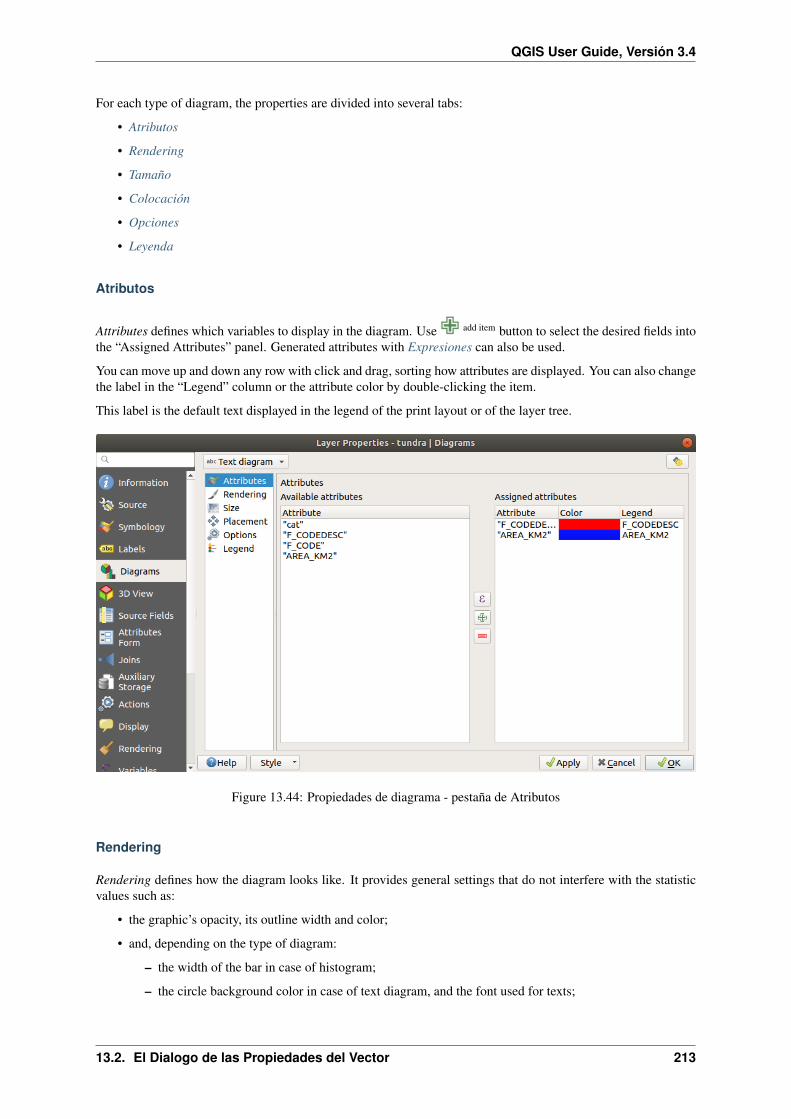
QGIS User Guide, Versión 3.4
For each type of diagram, the properties are divided into several tabs:
• Atributos
• Rendering
• Tamaño
• Colocación
• Opciones
• Leyenda
Atributos
Attributes defines which variables to display in the diagram. Use add item button to select the desired fields intothe “Assigned Attributes” panel. Generated attributes with Expresiones can also be used.
You can move up and down any row with click and drag, sorting how attributes are displayed. You can also changethe label in the “Legend” column or the attribute color by double-clicking the item.
This label is the default text displayed in the legend of the print layout or of the layer tree.
Figure 13.44: Propiedades de diagrama - pestaña de Atributos
Rendering
Rendering defines how the diagram looks like. It provides general settings that do not interfere with the statisticvalues such as:
• the graphic’s opacity, its outline width and color;
• and, depending on the type of diagram:
– the width of the bar in case of histogram;
– the circle background color in case of text diagram, and the font used for texts;
13.2. El Dialogo de las Propiedades del Vector 213

QGIS User Guide, Versión 3.4
– the orientation of the left line of the first slice represented in pie chart. Note that slices are displayedclockwise.
In this tab, you can also manage and fine tune the diagram visibility with different options:
• Diagram z-index: controls how diagrams are drawn on top of each other and on top of labels. A diagramwith a high index is drawn over diagrams and labels;
• Show all diagrams: shows all the diagrams even if they overlap each other;
• Show diagram: allows only specific diagrams to be rendered;
• Always Show: selects specific diagrams to always render, even when they overlap other diagrams or maplabels;
• setting the Scale dependent visibility;
• Discourage diagrams and labels from covering features: defines features to use as obstacles, ie QGIS willtry to not place diagrams nor labels over these features.
Figure 13.45: Diagram properties - Rendering tab
Tamaño
Size is the main tab to set how the selected statistics are represented. The diagram size units can be “Millimeter”,“Points”, Pixels, “Map Units” or “Inches”. You can use :
• Fixed size, an unique size to represent the graphic of all the features, except when displaying histogram
• or Scaled size, based on an expression using layer attributes.
214 Chapter 13. Trabajar con Datos Vectoriales

QGIS User Guide, Versión 3.4
Figure 13.46: Propiedades de diagrama - pestaña de tamaño
Ubicación
Placement helps to define diagram position. According to the layer geometry type, it offers different options forthe placement:
• “Over the point” or “Around the point” for point geometry. The latter variable requires a radius to follow.
• “Over the line” or “Around the line” for line geometry. Like point feature, the last variable requires adistance to respect and user can specify the diagram placement relative to the feature (“above”, “on” and/or“below” the line) It’s possible to select several options at once. In that case, QGIS will look for the optimalposition of the diagram. Remember that here you can also use the line orientation for the position of thediagram.
• “Over the centroid”, “Around the centroid” (with a distance set), “Perimeter” and anywhere “Inside poly-gon” are the options for polygon features.
The diagram can also be placed using feature data to fill the coordinates X and Y fields.
The placement of the diagrams can interact with the labeling, so you can detect and solve position conflictsbetween diagrams and labels by setting the Priority slider value.
Opciones
The Options tab has settings only in case of histogram. You can choose whether the bar orientation should be“Up”, “Down”, “Right” and “Left”.
Leyenda
From the Legend tab, you can choose to display items of the diagram in the Panel de capas, and in the print layoutlegend, next to the layer symbology:
• check Show legend entries for diagram attributes to display in the legends the Color and Legend prop-erties, as previously assigned in the Attributes tab;
13.2. El Dialogo de las Propiedades del Vector 215
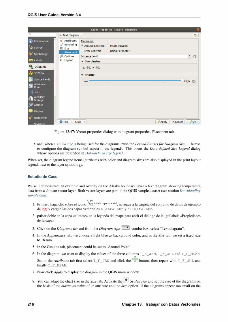
QGIS User Guide, Versión 3.4
Figure 13.47: Vector properties dialog with diagram properties, Placement tab
• and, when a scaled size is being used for the diagrams, push the Legend Entries for Diagram Size. . . buttonto configure the diagram symbol aspect in the legends. This opens the Data-defined Size Legend dialogwhose options are described in Data-defined size legend.
When set, the diagram legend items (attributes with color and diagram size) are also displayed in the print layoutlegend, next to the layer symbology.
Estudio de Caso
We will demonstrate an example and overlay on the Alaska boundary layer a text diagram showing temperaturedata from a climate vector layer. Both vector layers are part of the QGIS sample dataset (see section Downloadingsample data).
1. Primero haga clic sobre el icono Añadir capa vectorial, navegue a la carpeta del conjunto de datos de ejemplode |qg| y cargue las dos capas vectoriales alaska.shp y climate.shp.
2. pulsar doble en la capa «climate» en la leyenda del mapa para abrir el diálogo de la :guilabel: «Propiedadesde la capa»
3. Click on the Diagrams tab and from the Diagram type combo box, select “Text diagram”.
4. In the Appearance tab, we choose a light blue as background color, and in the Size tab, we set a fixed sizeto 18 mm.
5. In the Position tab, placement could be set to “Around Point”.
6. In the diagram, we want to display the values of the three columns T_F_JAN, T_F_JUL and T_F_MEAN.
So, in the Attributes tab first select T_F_JAN and click the button, then repeat with T_F_JUL andfinally T_F_MEAN.
7. Now click Apply to display the diagram in the QGIS main window.
8. You can adapt the chart size in the Size tab. Activate the Scaled size and set the size of the diagrams onthe basis of the maximum value of an attribute and the Size option. If the diagrams appear too small on the
216 Chapter 13. Trabajar con Datos Vectoriales

QGIS User Guide, Versión 3.4
screen, you can activate the Increase size of small diagrams checkbox and define the minimum size ofthe diagrams.
9. Change the attribute colors by double clicking on the color values in the Assigned attributes field. Fig-ure_diagrams_mapped gives an idea of the result.
10. Finally, click OK.
Figure 13.48: Gráfico de temperatura sobrepuesto en un mapa
Remember that in the Position tab, a Data defined position of the diagrams is possible. Here, you can useattributes to define the position of the diagram. You can also set a scale-dependent visibility in the Appearancetab.
The size and the attributes can also be an expression. Use the button to add an expression. See Expresioneschapter for more information and example.
Utilice suplantación definida por datos
As mentioned above, you can use some custom data-defined to tune the diagrams rendering:
• position in Placement tab by filling X and Y fields
• visibility in Appearance tab by filling the Visibility field
Vea Using data-defined override for labeling para más información.
13.2.6 Source Fields Properties
The Source Fields tab provides information on fields related to the layer and helps you organize them.
The layer can be made editable using the Toggle editing mode. At this moment, you can modify its structure using
the New field and Delete field buttons.
You can also rename fields by double-clicking its name. This is only supported for data providers like PostgreSQL,Oracle, Memory layer and some OGR layer depending on the OGR data format and version.
If set in the underlying data source or in the forms properties, the field’s alias is also displayed. An alias is ahuman readable field name you can use in the feature form or the attribute table. Aliases are saved in the projectfile.
13.2. El Dialogo de las Propiedades del Vector 217

QGIS User Guide, Versión 3.4
Depending on the data provider, you can associate a comment with a field, for example at its creation. Thisinformation is retrieved and shown in the Comment column and is later displayed when hovering over the fieldlabel in a feature form.
Other than the fields contained in the dataset, virtual fields and Auxiliary Storage included, the Source Fields tabalso lists fields from any joined layers. Depending on the origin of the field, a different background color is appliedto it.
For each listed field, the dialog also lists read-only characteristics such as its type, type name, length andprecision. When serving the layer as WMS or WFS, you can also check here which fields could be retrieved.
Figure 13.49: Source Field properties tab
13.2.7 Attributes Form Properties
The Attributes Form tab helps you set up the form to display when creating new features or querying existingone. You can define:
• the look and the behavior of each field in the feature form or the attribute table (label, widget, constraints. . . );
• the form’s structure (custom or autogenerated):
• extra logic in Python to handle interaction with the form or field widgets.
At the top right of the dialog, you can set whether the form is opened by default when creating new features. Thiscan be configured per layer or globally with the Suppress attribute form pop-up after feature creation option inthe Settings → Options → Digitizing menu.
Customizing a form for your data
By default, when you click on a feature with the Identify Features tool or switch the attribute table to the formview mode, QGIS displays a basic form with predefined widgets (generally spinboxes and textboxes — each fieldis represented on a dedicated row by its label next to the widget). If relations are set on the layer, fields from thereferencing layers are shown in an embedded frame at the bottom of the form, following the same basic structure.
218 Chapter 13. Trabajar con Datos Vectoriales

QGIS User Guide, Versión 3.4
This rendering is the result of the default Autogenerate value of the Attribute editor layout setting in the Layerproperties → Attributes Form tab. This property holds three different values:
• Autogenerate: keeps the basic structure of «one row - one field» for the form but allows to customizeeach corresponding widget.
• Drag-and-drop designer: other than widget customization, the form structure can be made morecomplex eg, with widgets embedded in groups and tabs.
• Provide ui file: allows to use a Qt designer file, hence a potentially more complex and fully featuredtemplate, as feature form.
The autogenerated form
When the Autogenerate option is on, the Available widgets panel shows lists of fields (from the layer and itsrelations) that would be shown in the form. Select a field and you can configure its appearance and behavior in theright panel:
• adding custom label and automated checks to the field;
• setting a particular widget to use.
El diseñador de arrastrar y soltar
Choose Drag and drop designer from the Attribute editor layout combobox and you enable a Form Lay-out panel next to the Available widgets one. From this panel you can create an editor form with several tabs andnamed groups to present the attribute fields, as shown for example in figure_fields_form.
Figure 13.50: Resulting built-in form with tabs and named groups
To create the form, you can drag and drop fields from the Available Widgets panel to the Form Layout one to havefields added to your custom form and drag and drop fields inside the Form Layout to reorder their position.
13.2. El Dialogo de las Propiedades del Vector 219

QGIS User Guide, Versión 3.4
You can also use categories (tab or group frames) to better structure the form. The first step is to use the iconto create a tab in which fields and groups will be displayed (see figure_fields_layout). You can create as many
categories as you want. Use button to remove any unwanted elements. The next step will be to assign to eachcategory the relevant fields, by simple drag and drop. You can use the same fields many times.
Figure 13.51: El cuadro de diálogo para crear categorías con el Diseño del editor de atributos
You can configure tabs or groups with a double-click. QGIS opens a form in which you can:
• choose to hide or show the item label;
• rename the category;
• set over how many columns the fields under the category should be distributed;
• enter an expression to control the category visibility. The expression will be re-evaluated everytime valuesin the form change and the tab or groupbox shown/hidden accordingly;
• show the category as a group box (only available for tabs).
With a double-click on a field label, you can also specify whether the label of its widget should be visible or notin the form.
In case the layer is involved in one or many to many relations (see Creating one or many to manyrelations), referencing layers are listed in the Relations frame and their form can be embedded in the current layerform by drag-and-drop. Like the other items, double-click the relation label to configure some options:
• choose to hide or show the item label;
• show the link button;
• show the unlink button.
Using custom ui-file
The Provide ui-file option allows you to use complex dialogs made with Qt-Designer. Using a UI-fileallows a great deal of freedom in creating a dialog. Note that, in order to link the graphical objects (textbox,
220 Chapter 13. Trabajar con Datos Vectoriales

QGIS User Guide, Versión 3.4
combobox. . . ) to the layer’s fields, you need to give them the same name.
Use the Edit UI to define the path to the file to use.
You’ll find some example in the Creating a new form lesson of the QGIS-training-manual-index-reference. For more advanced information, see https://nathanw.net/2011/09/05/qgis-tips-custom-feature-forms-with-python-logic/.
Enhance your form with custom functions
QGIS forms can have a Python function that is called when the dialog is opened. Use this function to add extralogic to your dialogs. The form code can be specified in three different ways:
• load from the environment: use a function, for example in startup.py or from an installedplugin
• load from an external file: a file chooser will appear in that case to allow you to select a Pythonfile from your filesystem
• provide code in this dialog: a Python editor will appear where you can directly type the func-tion to use.
In all cases you must enter the name of the function that will be called (open in the example below).
An example is (in module MyForms.py):
def open(dialog,layer,feature):geom = feature.geometry()control = dialog.findChild(QWidged,"My line edit")
Reference in Python Init Function like so: open
Configurar el comportamiento del campo
The main part of the Attributes Form tab helps you set the type of widget used to fill or display values of the field,in the attribute table or the feature form: you can define how user interacts with each field and the values or rangeof values that are allowed to be added to each.
Configuración común
Regardless the type of widget applied to the field, there are some common properties you can set to control whetherand how a field can be edited.
General options
• Alias: a human readable name to use for fields. The alias will be displayed in the feature form, the attributetable, or in the Identify results panel. It can also be used as field name replacement in the expression builder,easing expressions understanding and reviews. Aliases are saved in project file.
• Comment: displays the field’s comment as shown in the Source Fields tab, in a read-only state. Thisinformation is shown as tooltip when hovering over the field label in a feature form.
• Editable: uncheck this option to set the field read-only (not manually modifiable) even when the layeris in edit mode. Note that checking this setting doesn’t override any edit limitation from the provider.
• Label on top: places the field name above or beside the widget in the feature form.
13.2. El Dialogo de las Propiedades del Vector 221
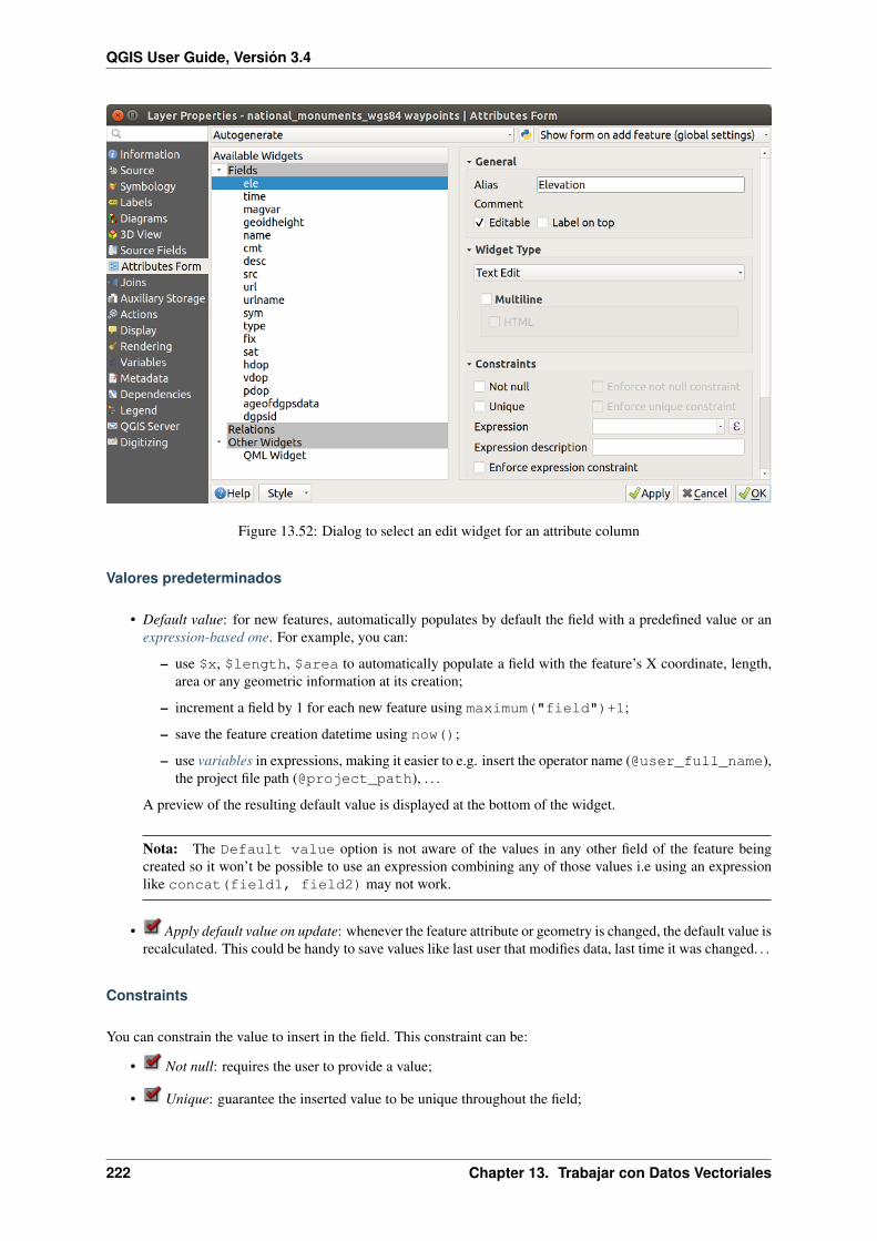
QGIS User Guide, Versión 3.4
Figure 13.52: Dialog to select an edit widget for an attribute column
Valores predeterminados
• Default value: for new features, automatically populates by default the field with a predefined value or anexpression-based one. For example, you can:
– use $x, $length, $area to automatically populate a field with the feature’s X coordinate, length,area or any geometric information at its creation;
– increment a field by 1 for each new feature using maximum("field")+1;
– save the feature creation datetime using now();
– use variables in expressions, making it easier to e.g. insert the operator name (@user_full_name),the project file path (@project_path), . . .
A preview of the resulting default value is displayed at the bottom of the widget.
Nota: The Default value option is not aware of the values in any other field of the feature beingcreated so it won’t be possible to use an expression combining any of those values i.e using an expressionlike concat(field1, field2) may not work.
• Apply default value on update: whenever the feature attribute or geometry is changed, the default value isrecalculated. This could be handy to save values like last user that modifies data, last time it was changed. . .
Constraints
You can constrain the value to insert in the field. This constraint can be:
• Not null: requires the user to provide a value;
• Unique: guarantee the inserted value to be unique throughout the field;
222 Chapter 13. Trabajar con Datos Vectoriales

QGIS User Guide, Versión 3.4
• based on a custom expression: e.g. regexp_match(col0,'A-Za-z') to ensure that the value of thefield col0 has only alphabetical letter. A short description can be added to help you remember the constraint.
Whenever a value is added or edited in a field, it’s submitted to the existing constraints and:
• if it meets all the requirements, a green check is shown beside the field in the form;
• if it does not meet all the requirements, then a yellow or red cross is displayed near the field. You can hoverover the cross to remind which constraints are applied to the field and fix the value:
– A yellow cross appears when the unmet constraint is an unenforced one and it does not prevent you tosave the changes with the «wrong» values;
– A red cross can not be ignored and does not allow you to save your modifications until they meet the
constraints. It appears when the Enforce constraint option is checked.
Modo de edición
Based on the field type, QGIS automatically determines and assigns a default widget type to it. You can thenreplace the widget with any other compatible with the field type. The available widgets are:
• Checkbox: Displays a checkbox whose state defines the value to insert.
• Classification: Only available when a categorized symbology is applied to the layer, displays a combo boxwith the values of the classes.
• Color: Displays a color widget allowing to select a color; the color value is stored as a html notation in theattribute table.
• Date/Time: Displays a line field which can open a calendar widget to enter a date, a time or both. Columntype must be text. You can select a custom format, pop-up a calendar, etc.
• Enumeration: Opens a combo box with predefined values fetched from the database. This is currently onlysupported by the PostgreSQL provider, for fields of enum type.
• Attachment: Uses a «Open file» dialog to store file path in a relative or absolute mode. It can also be usedto display a hyperlink (to document path), a picture or a web page.
• Hidden: A hidden attribute column is invisible. The user is not able to see its contents.
• Key/Value: Displays a two-columns table to store sets of key/value pairs within a single field. This iscurrently supported by the PostgreSQL provider, for fields of hstore type.
• List: Displays a single column table to add different values within a single field. This is currently supportedby the PostgreSQL provider, for fields of array type.
• Range: Allows you to set numeric values from a specific range. The edit widget can be either a slider or aspin box.
• Relation Reference: This widget lets you embed the feature form of the referenced layer on the featureform of the actual layer. See Creating one or many to many relations.
• Text Edit (default): This opens a text edit field that allows simple text or multiple lines to be used. If youchoose multiple lines you can also choose html content.
• Unique Values: You can select one of the values already used in the attribute table. If “Editable” is activated,a line edit is shown with autocompletion support, otherwise a combo box is used.
• Uuid Generator: Generates a read-only UUID (Universally Unique Identifiers) field, if empty.
• Value Map: A combo box with predefined items. The value is stored in the attribute, the description isshown in the combo box. You can define values manually or load them from a layer or a CSV file.
• Value Relation: Offers values from a related table in a combobox. You can select layer, key column andvalue column. Several options are available to change the standard behaviors: allow null value, order byvalue, allow multiple selections and use of auto-completer. The forms will display either a drop-down listor a line edit field when completer checkbox is enabled.
13.2. El Dialogo de las Propiedades del Vector 223

QGIS User Guide, Versión 3.4
Truco: Relative Path in Attachment widget
If the path which is selected with the file browser is located in the same directory as the .qgs project file or below,paths are converted to relative paths. This increases portability of a .qgs project with multimedia informationattached.
13.2.8 Propiedades de unión
The Joins tab allows you to join a loaded attribute table to a loaded vector layer. After clicking , theAdd vector join dialog appears. As key columns, you have to define a join layer you want to connect with thetarget vector layer. Then, you have to specify the join field that is common to both the join layer and the target
layer. Now you can also specify a subset of fields from the joined layer based on the checkbox Choose whichfields are joined. As a result of the join, all information from the join layer and the target layer are displayed inthe attribute table of the target layer as joined information. If you specified a subset of fields only these fields aredisplayed in the attribute table of the target layer.
If the target layer is editable, then some icons will be displayed in the attribute table next to fields, in order toinform their status:
• : the join layer is not configured to be editable. If you want to be able to edit join features from the target
attribute table, then you have to check the option Editable join layer.
• : the join layer is well configured to be editable, but its current status is read only.
• : the join layer is editable but synchronization mechanisms are not activated. If you want to automati-cally add a feature in the join layer when a feature is created in the target layer, then you have to check the
option Upsert on edit. Symmetrically, the option Delete cascade may be activated if you want toautomatically delete join features.
Moreover, the Dynamic form option helps to synchronize join fields on the fly, according to the Target field.This way, constraints for join fields are also correctly updated. Note that it’s deactivated by default because it maybe very time consuming if you have a lot of features or a myriad of joins.
Otherwise, the Cache join layer in virtual memory option allows to cache values in memory (without geome-tries) from the joined layer in order to speed up lookups.
QGIS currently has support for joining non-spatial table formats supported by OGR (e.g., CSV, DBF and Excel),delimited text and the PostgreSQL provider (see figure_joins).
Additionally, the add vector join dialog allows you to:
• Crear índice de atributo en el campo de combinación
• Choose which fields are joined
• Create a Custom field name prefix
13.2.9 Auxiliary Storage Properties
The regular way to customize styling and labeling is to use data-defined properties as described in Configuraciónde anulación definida por datos. However, it may not be possible if the underlying data is read only. Moreover,configuring these data-defined properties may be very time consuming or not desirable! For example, if you wantto fully use map tools coming with La Barra de Herramientas Etiqueta, then you need to add and configure morethan 20 fields in your original data source (X and Y positions, rotation angle, font style, color and so on).
224 Chapter 13. Trabajar con Datos Vectoriales

QGIS User Guide, Versión 3.4
Figure 13.53: Join an attribute table to an existing vector layer
13.2. El Dialogo de las Propiedades del Vector 225

QGIS User Guide, Versión 3.4
The Auxiliary Storage mechanism provides the solution to these limitations and awkward configurations. Auxil-iary fields are a roundabout way to automatically manage and store these data-defined properties (labels, diagram,symbology. . . ) in a SQLite database thanks to editable joins. This allows you to store properties for layers thataren’t editable.
A tab is available in vector layer properties dialog to manage auxiliary storage:
Figure 13.54: Auxiliary Storage tab
Labeling
Considering that the data source may be customized thanks to data-defined properties without being editable,labeling map tools described in La Barra de Herramientas Etiqueta are always available as soon as labeling isactivated.
Actually, the auxiliary storage system needs an auxiliary layer to store these properties in a SQLite database (seeAuxiliary storage database). Its creation process is run the first time you click on the map while a labeling maptool is currently activated. Then, a window is displayed, allowing you to select the primary key to use for joining(to ensure that features are uniquely identified):
Figure 13.55: Auxiliary Layer creation dialog
As soon as an auxiliary layer is configured for the current data source, you can retrieve its information in the tab:
226 Chapter 13. Trabajar con Datos Vectoriales

QGIS User Guide, Versión 3.4
Figure 13.56: Auxiliary Layer key
The auxiliary layer now has these characteristics:
• the primary key is ID,
• there are 0 features using an auxiliary field,
• there are 0 auxiliary fields.
Now that the auxiliary layer is created, you can edit the layer labels. Click on a label while the Change Label
map tool is activated, then you can update styling properties like sizes, colors, and so on. The correspondingdata-defined properties are created and can be retrieved:
As you can see in the figure above, 21 fields are automatically created and configured for labeling. For example,the FontStyle auxiliary field type is a String and is named labeling_fontstyle in the underlyingSQLite database. There is also 1 feature which is currently using these auxiliary fields.
Notice that the icon is displayed in the Labels properties tab indicating that the data-defined override optionsare set correctly:
Otherwise, there’s another way to create an auxiliary field for a specific property thanks to the data-defined override
button. By clicking on Store data in the project, an auxiliary field is automatically created for the Opacity field. Ifyou click on this button whereas the auxiliary layer is not created yet, then the window Auxiliary Layer creationdialog is first displayed to select the primary key to use for joining.
Simbología
Like the method described above for customizing labels, auxiliary fields can also be used to stylize symbols and
diagrams. To do this, click on Data-defined override and select Store data in the project for a specific property. Forexample, the Fill color field:
13.2. El Dialogo de las Propiedades del Vector 227

QGIS User Guide, Versión 3.4
Figure 13.57: Auxiliary Fields
228 Chapter 13. Trabajar con Datos Vectoriales

QGIS User Guide, Versión 3.4
Figure 13.58: Data-defined properties automatically created
Figure 13.59: Data-defined property menu for symbol
13.2. El Dialogo de las Propiedades del Vector 229

QGIS User Guide, Versión 3.4
There are different attributes for each symbol (e.g. fill style, fill color, stroke color, etc. . . ), so each auxiliary fieldrepresenting an attribute requires a unique name to avoid conflicts. After selecting Store data in the project, awindow opens and displays the Type of the field and prompts you to enter a unique name for the auxiliary field.For example, when creating a Fill color auxiliary field the following window opens:
Figure 13.60: Name of the auxiliary field for a symbol
Once created, the auxiliary field can be retrieved in the auxiliary storage tab:
Attribute table and widgets
Auxiliary fields can be edited using the attribute table. However, not all auxiliary fields are initially visible in theattribute table.
Auxiliary fields representing attributes of a layer’s symbology, labeling, appearance, or diagrams will appearautomatically in the attribute table. The exception are attributes that can be modified using the Label Toolbarwhich are hidden by default. Auxiliary fields representing a Color have a widget Color set by default, otherwiseauxiliary fields default to the Text Edit widget.
Auxiliary fields that represent attributes that can be modified using the Label toolbar are Hidden in the at-tribute table by default. To make a field visible, open the Attribute Form properties tab and change the valueof an auxiliary field Widget Type from Hidden to another relevant value. For example, change the auxil-iary_storage_labeling_size to Text Edit or change auxiliary_storage_labeling_color to the Color widget.Those fields will now be visible in the attribute table.
Auxiliary fields in the attribute table will appear like the following image:
Management
The Auxiliary Layer menu allows you to manage the auxiliary fields:
The first item Create is disabled in this case because the auxiliary layer is already created. But in case of a freshwork, you can use this action to create an auxiliary layer. As explained in Labeling, a primary key will be neededthen.
The Clear action allows to keep all auxiliary fields, but remove their contents. This way, the number of featuresusing these fields will fall to 0.
The Delete action completely removes the auxiliary layer. In other words, the corresponding table is deleted fromthe underlying SQLite database and properties customization are lost.
Finally, the Export action allows to save the auxiliary layer as a new vector layer. Note that geometries are notstored in auxiliary storage. However, in this case, geometries are exported from the original data source too.
Auxiliary storage database
When you save your project with the .qgs format, the SQLite database used for auxiliary storage is saved at thesame place but with the extension .qgd.
230 Chapter 13. Trabajar con Datos Vectoriales
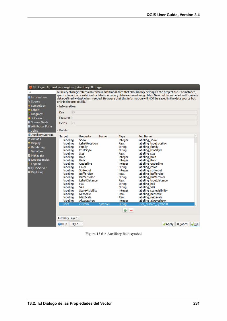
QGIS User Guide, Versión 3.4
Figure 13.61: Auxiliary field symbol
13.2. El Dialogo de las Propiedades del Vector 231

QGIS User Guide, Versión 3.4
Figure 13.62: Form with auxiliary fields
Figure 13.63: Auxiliary layer management
232 Chapter 13. Trabajar con Datos Vectoriales

QGIS User Guide, Versión 3.4
For convenience, an archive may be used instead thanks to the .qgz format. In this case, .qgd and .qgs filesare both embedded in the archive.
13.2.10 Propiedades de acciones
QGIS provides the ability to perform an action based on the attributes of a feature. This can be used toperform any number of actions, for example, running a program with arguments built from the attributes of afeature or passing parameters to a web reporting tool.
Figure 13.64: Overview action dialog with some sample actions
Actions are useful when you frequently want to run an external application or view a web page based on one ormore values in your vector layer. They are divided into six types and can be used like this:
• Las acciones genéricas, Mac, Windows inician un proceso externo.
• Las acciones Python ejecutan una expresión Python.
• Las acciones genéricas y Python son visibles en todos lados.
• Mac, Windows and Unix actions are visible only on the respective platform (i.e., you can define three “Edit”actions to open an editor and the users can only see and execute the one “Edit” action for their platform torun the editor).
There are several examples included in the dialog. You can load them by clicking on Create Default Actions. Toedit any of the examples, double-click its row. One example is performing a search based on an attribute value.This concept is used in the following discussion.
The Show in Attribute Table allows you to display in the attribute table dialog the checked feature-scopedactions, either as Combo Box or as Separate Buttons (see Configuring the columns).
Definir Acciones
To define an attribute action, open the vector Layer Properties dialog and click on the Actions tab. In the Actions
tab, click the Add a new action to open the Edit Action dialog.
Select the action Type and provide a descriptive name for the action. The action itself must contain the name ofthe application that will be executed when the action is invoked. You can add one or more attribute field values as
13.2. El Dialogo de las Propiedades del Vector 233

QGIS User Guide, Versión 3.4
arguments to the application. When the action is invoked, any set of characters that start with a % followed by thename of a field will be replaced by the value of that field. The special characters %% will be replaced by the valueof the field that was selected from the identify results or attribute table (see using_actions below). Double quotemarks can be used to group text into a single argument to the program, script or command. Double quotes will beignored if preceded by a backslash.
The Action Scopes allows you to define where the action should be available. You have 4 different choices:
1. Feature Scope: action is available when right click in the cell within the attribute table.
2. Field Scope: action is available when right click in the cell within the attribute table, in the feature form andin the default action button of the main toolbar.
3. Layer Scope: action is available in the action button in the attribute table toolbar. Be aware that this type ofaction involves the entire layer and not the single features.
4. Canvas: action is available in the main action button in the toolbar.
If you have field names that are substrings of other field names (e.g., col1 and col10), you should indicate thatby surrounding the field name (and the % character) with square brackets (e.g., [%col10]). This will preventthe %col10 field name from being mistaken for the %col1 field name with a 0 on the end. The brackets will beremoved by QGIS when it substitutes in the value of the field. If you want the substituted field to be surroundedby square brackets, use a second set like this: [[%col10]].
Using the Identify Features tool, you can open the Identify Results dialog. It includes a (Derived) item that containsinformation relevant to the layer type. The values in this item can be accessed in a similar way to the other fieldsby proceeding the derived field name with (Derived).. For example, a point layer has an X and Y field, andthe values of these fields can be used in the action with %(Derived).X and %(Derived).Y. The derivedattributes are only available from the Identify Results dialog box, not the Attribute Table dialog box.
Two example actions are shown below:
• konqueror https://www.google.com/search?q=%nam
• konqueror https://www.google.com/search?q=%%
In the first example, the web browser konqueror is invoked and passed a URL to open. The URL performs aGoogle search on the value of the nam field from our vector layer. Note that the application or script called by theaction must be in the path, or you must provide the full path. To be certain, we could rewrite the first example as:/opt/kde3/bin/konqueror https://www.google.com/search?q=%nam. This will ensure thatthe konqueror application will be executed when the action is invoked.
The second example uses the %% notation, which does not rely on a particular field for its value. When the actionis invoked, the %% will be replaced by the value of the selected field in the identify results or attribute table.
Empleando Acciones
QGIS offers many ways to execute actions you enabled on a layer. Depending on their settings, they can beavailable:
• in the drop-down menu of Run Feature Action button from the Attributes toolbar or Attribute table dialog;
• when right-clicking a feature with the Identify Features tool (see Identifying Features for more information);
• from the Identify Results panel, under the Actions section;
• as items of an Actions column in the Attribute Table dialog.
Si se está invocando una acción que utilice la notación ‘‘‘‘ , haga clic derecho en el valor del campo en el cuadrode diálogo Resultados de la Identificación o en Tabla de atributos que desee pasar de la aplicación o script
Here is another example that pulls data out of a vector layer and inserts it into a file using bash and the echo com-
mand (so it will only work on or perhaps ). The layer in question has fields for a species name taxon_name,latitude lat and longitude long. We would like to be able to make a spatial selection of localities and export
234 Chapter 13. Trabajar con Datos Vectoriales
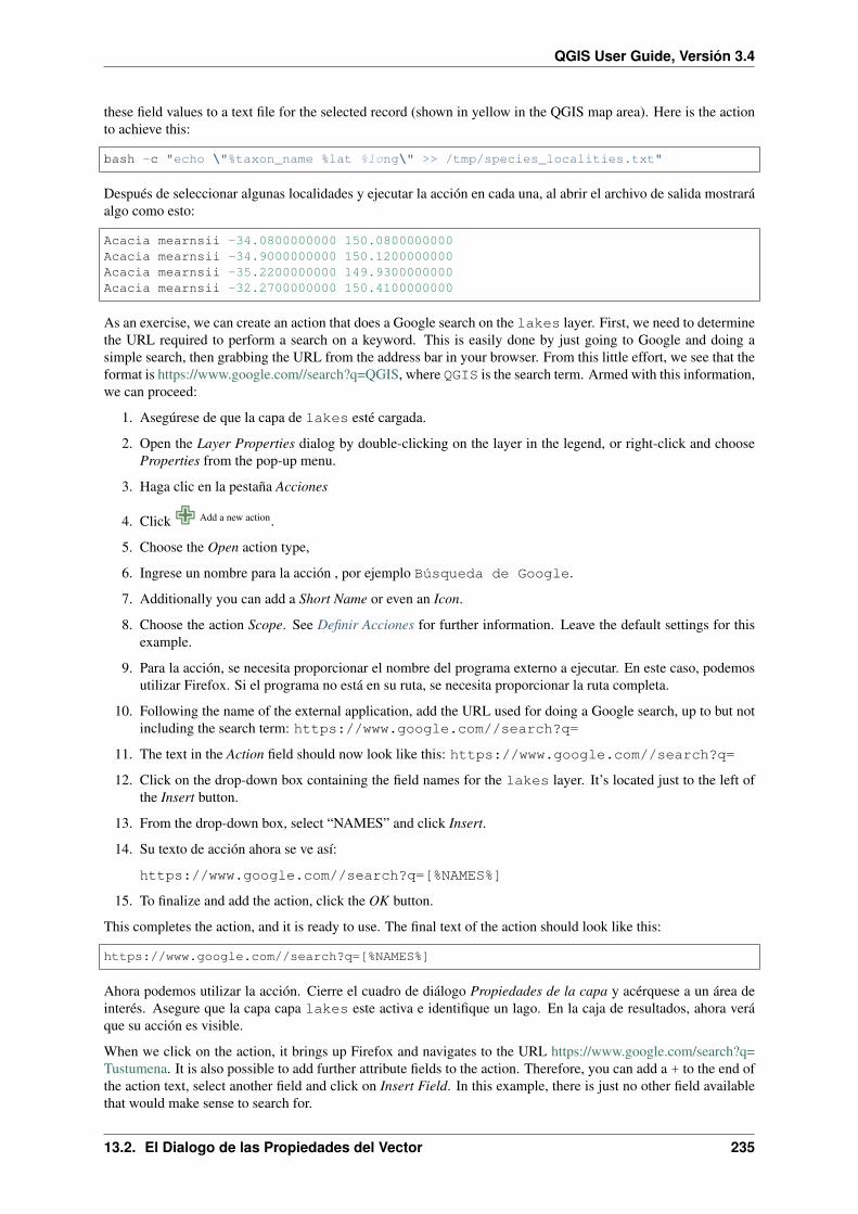
QGIS User Guide, Versión 3.4
these field values to a text file for the selected record (shown in yellow in the QGIS map area). Here is the actionto achieve this:
bash -c "echo \"%taxon_name %lat %long\" >> /tmp/species_localities.txt"
Después de seleccionar algunas localidades y ejecutar la acción en cada una, al abrir el archivo de salida mostraráalgo como esto:
Acacia mearnsii -34.0800000000 150.0800000000Acacia mearnsii -34.9000000000 150.1200000000Acacia mearnsii -35.2200000000 149.9300000000Acacia mearnsii -32.2700000000 150.4100000000
As an exercise, we can create an action that does a Google search on the lakes layer. First, we need to determinethe URL required to perform a search on a keyword. This is easily done by just going to Google and doing asimple search, then grabbing the URL from the address bar in your browser. From this little effort, we see that theformat is https://www.google.com//search?q=QGIS, where QGIS is the search term. Armed with this information,we can proceed:
1. Asegúrese de que la capa de lakes esté cargada.
2. Open the Layer Properties dialog by double-clicking on the layer in the legend, or right-click and chooseProperties from the pop-up menu.
3. Haga clic en la pestaña Acciones
4. Click Add a new action.
5. Choose the Open action type,
6. Ingrese un nombre para la acción , por ejemplo Búsqueda de Google.
7. Additionally you can add a Short Name or even an Icon.
8. Choose the action Scope. See Definir Acciones for further information. Leave the default settings for thisexample.
9. Para la acción, se necesita proporcionar el nombre del programa externo a ejecutar. En este caso, podemosutilizar Firefox. Si el programa no está en su ruta, se necesita proporcionar la ruta completa.
10. Following the name of the external application, add the URL used for doing a Google search, up to but notincluding the search term: https://www.google.com//search?q=
11. The text in the Action field should now look like this: https://www.google.com//search?q=
12. Click on the drop-down box containing the field names for the lakes layer. It’s located just to the left ofthe Insert button.
13. From the drop-down box, select “NAMES” and click Insert.
14. Su texto de acción ahora se ve así:
https://www.google.com//search?q=[%NAMES%]
15. To finalize and add the action, click the OK button.
This completes the action, and it is ready to use. The final text of the action should look like this:
https://www.google.com//search?q=[%NAMES%]
Ahora podemos utilizar la acción. Cierre el cuadro de diálogo Propiedades de la capa y acérquese a un área deinterés. Asegure que la capa capa lakes este activa e identifique un lago. En la caja de resultados, ahora veráque su acción es visible.
When we click on the action, it brings up Firefox and navigates to the URL https://www.google.com/search?q=Tustumena. It is also possible to add further attribute fields to the action. Therefore, you can add a + to the end ofthe action text, select another field and click on Insert Field. In this example, there is just no other field availablethat would make sense to search for.
13.2. El Dialogo de las Propiedades del Vector 235

QGIS User Guide, Versión 3.4
Figure 13.65: Edit action dialog configured with the example
Figure 13.66: Seleccionar objetos espaciales y elegir una acción
236 Chapter 13. Trabajar con Datos Vectoriales

QGIS User Guide, Versión 3.4
You can define multiple actions for a layer, and each will show up in the Identify Results dialog.
You can also invoke actions from the attribute table by selecting a row and right-clicking, then choosing the actionfrom the pop-up menu.
There are all kinds of uses for actions. For example, if you have a point layer containing locations of images orphotos along with a file name, you could create an action to launch a viewer to display the image. You could alsouse actions to launch web-based reports for an attribute field or combination of fields, specifying them in the sameway we did in our Google search example.
We can also make more complex examples, for instance, using Python actions.
Usually, when we create an action to open a file with an external application, we can use absolute paths, oreventually relative paths. In the second case, the path is relative to the location of the external program executablefile. But what about if we need to use relative paths, relative to the selected layer (a file-based one, like Shapefileor SpatiaLite)? The following code will do the trick:
command = "firefox"imagerelpath = "images_test/test_image.jpg"layer = qgis.utils.iface.activeLayer()import os.pathlayerpath = layer.source() if layer.providerType() == 'ogr'
else (qgis.core.QgsDataSourceURI(layer.source()).database()if layer.providerType() == 'spatialite' else None)
path = os.path.dirname(str(layerpath))image = os.path.join(path,imagerelpath)import subprocesssubprocess.Popen( [command, image ] )
We just have to remember that the action is one of type Python and the command and imagerelpath variables mustbe changed to fit our needs.
But what about if the relative path needs to be relative to the (saved) project file? The code of the Python actionwould be:
command = "firefox"imagerelpath = "images/test_image.jpg"projectpath = qgis.core.QgsProject.instance().fileName()import os.pathpath = os.path.dirname(str(projectpath)) if projectpath != '' else Noneimage = os.path.join(path, imagerelpath)import subprocesssubprocess.Popen( [command, image ] )
Another Python action example is the one that allows us to add new layers to the project. For instance, thefollowing examples will add to the project respectively a vector and a raster. The names of the files to be added tothe project and the names to be given to the layers are data driven (filename and layername are column names ofthe table of attributes of the vector where the action was created):
qgis.utils.iface.addVectorLayer('/yourpath/[% "filename" %].shp','[% "layername" %]', 'ogr')
Para añadir un ráster (una imagen TIF en este ejemplo), se vuelve:
qgis.utils.iface.addRasterLayer('/yourpath/[% "filename" %].tif','[% "layername" %]')
13.2.11 Propiedades a mostrar
The Display tab helps you configure fields to use for feature identification:
• The Display name: based on a field or an expression. This is:
13.2. El Dialogo de las Propiedades del Vector 237

QGIS User Guide, Versión 3.4
– the label shown on top of the feature information in the Identify tool results;
– the field used in the locator bar when looking for features in all layers;
– the feature identifier in the attribute table form view;
– the map tip information, i.e. the message displayed in the map canvas when hovering over a feature of
the active layer with the Show Map Tips icon pressed. Applicable when no HTML Map Tip is set.
• The HTML Map Tip is specifically created for the map tips: it’s a more complex and full HTML text mixingfields, expressions and html tags (multiline, fonts, images, hyperlink. . . ).
Figure 13.67: Código HTML para textos de aviso del mapa
To activate map tips, select the menu option View → Show Map Tips or click on the Show Map Tips icon of theAttributes Toolbar. Map tip is a cross-session feature meaning that once activated, it stays on and apply to anylayer in any project, even in future QGIS sessions until it’s toggled off.
Figure 13.68: Textos de aviso del mapa con código HTML
13.2.12 Propiedades de representación
Visibilidad dependiente de escala
You can set the Maximum (inclusive) and Minimum (exclusive) scale, defining a range of scale in which features
will be visible. Out of this range, they are hidden. The Set to current canvas scale button helps you use the current map
238 Chapter 13. Trabajar con Datos Vectoriales

QGIS User Guide, Versión 3.4
canvas scale as boundary of the range visibility. See Renderizado dependiente de la escala for more information.
Simplify geometry
QGIS offers support for on-the-fly feature generalisation. This can improve rendering times when drawing many
complex features at small scales. This feature can be enabled or disabled in the layer settings using the Simplifygeometry option. There is also a global setting that enables generalisation by default for newly added layers (seeglobal simplification for more information).
Figure 13.69: cuadro de diálogo de Simplificación de Geometría de capa
Nota: Feature generalisation may introduce artefacts into your rendered output in some cases. These may includeslivers between polygons and inaccurate rendering when using offset-based symbol layers.
While rendering extremely detailed layers (e.g. polygon layers with a huge number of nodes), this can causelayout exports in PDF/SVG format to be huge as all nodes are included in the exported file. This can also makethe resultant file very slow to work with/open in other programs.
Checking Force layer to render as raster forces these layers to be rasterised so that the exported files won’thave to include all the nodes contained in these layers and the rendering is therefore sped up.
You can also do this by forcing the layout to export as a raster, but that is an all-or-nothing solution, given that therasterisation is applied to all layers.
Refresh layer at interval (seconds): set a timer to automatically refresh individual layers at a matching interval.Canvas updates are deferred in order to avoid refreshing multiple times if more than one layer has an auto updateinterval set.
Depending on the data provider (e.g. PostgreSQL), notifications can be sent to QGIS when changes are applied to
the data source, out of QGIS. Use the Refresh layer on notification option to trigger an update. You can also
limit the layer refresh to a specific message set in the Only if message is text box.
13.2. El Dialogo de las Propiedades del Vector 239

QGIS User Guide, Versión 3.4
13.2.13 Propiedades de variables
The Variables tab lists all the variables available at the layer’s level (which includes all global and project’svariables).
It also allows the user to manage layer-level variables. Click the button to add a new custom layer-level
variable. Likewise, select a custom layer-level variable from the list and click the button to remove it.
Más información sobre el uso de variables en la sección de herramientas Generales Storing values in Variables
13.2.14 Propiedades de metadatos
The Metadata tab provides you with options to create and edit a metadata report on your layer. Information tofill concern:
• the data Identification: basic attribution of the dataset (parent, identifier, title, abstract, language. . . );
• the Categories the data belongs to. Alongside the ISO categories, you can add custom ones;
• the Keywords to retrieve the data and associated concepts following a standard based vocabulary;
• the Access to the dataset (licenses, rights, fees, and constraints);
• the Extent of the dataset, either spatial one (CRS, map extent, altitudes) or temporal;
• the Contact of the owner(s) of the dataset;
• the Links to ancillary resources and related information;
• the History of the dataset.
A summary of the filled information is provided in the Validation tab and helps you identify potential issues relatedto the form. You can then either fix them or ignore them.
Metadata are currently saved in the project file. It can also be saved as an .XML file alongside file based layers orin a local .sqlite database for remote layers (e.g. PostGIS).
13.2.15 Dependencies Properties
The Dependencies tab allows to declare data dependencies between layers. A data dependency occurs when adata modification in a layer, not by direct user manipulation, may modify data of other layers. This is the case forinstance when geometry of a layer is updated by a database trigger or custom PyQGIS scripting after modificationof another layer’s geometry.
In the Dependencies tab, you can select any layers which may externally alter the data in the current layer. Cor-rectly specifying dependent layers allows QGIS to invalidate caches for this layer when the dependent layers arealtered.
13.2.16 Propiedades de la leyenda
The Legend properties tab provides you with advanced settings for the Layers panel and/or the print layoutlegend. These options include:
• Text on symbols: In some cases it can be useful to add extra information to the symbols in the legend.With this frame, you can affect to any of the symbols used in the layer symbology a text that is displayedover the symbol, in both Layers panel and print layout legend. This mapping is done by typing each textnext to the symbol in the table widget or filling the table using the Set Labels from Expression button. Textappearance is handled through the font and color selector widgets of the Text Format button.
240 Chapter 13. Trabajar con Datos Vectoriales

QGIS User Guide, Versión 3.4
Figure 13.70: Setting text on symbols (left) and its rendering in the Layers panel (right)
• a list of widgets you can embed within the layer tree in the Layers panel. The idea is to have a way toquickly access some actions that are often used with the layer (setup transparency, filtering, selection, styleor other stuff. . . ).
By default, QGIS provides transparency widget but this can be extended by plugins registering their ownwidgets and assign custom actions to layers they manage.
13.2.17 QGIS Server Properties
The QGIS Server tab consists of Description, Attribution, MetadataURL, and LegendUrl sections.
You can add or edit a title and abstract for the layer in the Description section. It’s also possible to define aKeyword list here. These keyword lists can be used in a metadata catalog. If you want to use a title from an XMLmetadata file, you have to fill in a link in the DataUrl field.
Use Attribution to get attribute data from an XML metadata catalog.
In MetadataUrl, you can define the general path to the XML metadata catalog. This information will be saved inthe QGIS project file for subsequent sessions and will be used for QGIS server.
In the LegendUrl section, you can provide the url of a legend image in the url field. You can use the Formatdrop-down option to apply the appropriate format of the image. Currently png, jpg and jpeg image formats aresupported.
13.2.18 Digitizing Properties
The Digitizing tab gives access to options that help to ensure the quality of digitized geometries.
Automatic Fixes
Options in the Automatic Fixes section will directly affect the vertices of any geometry which is added or mod-
ified. If the Remove duplicate nodes option is checked, any two subsequent vertices with exactly the samecoordinates will be removed. If the Geometry precision is set, all vertices will be rounded to the closest multipleof the configured geometry precision. The rounding will happen in the layer coordinate reference system. Z andM values are not rounded. With many map tools, a grid is shown on the canvas while digitizing.
13.2. El Dialogo de las Propiedades del Vector 241
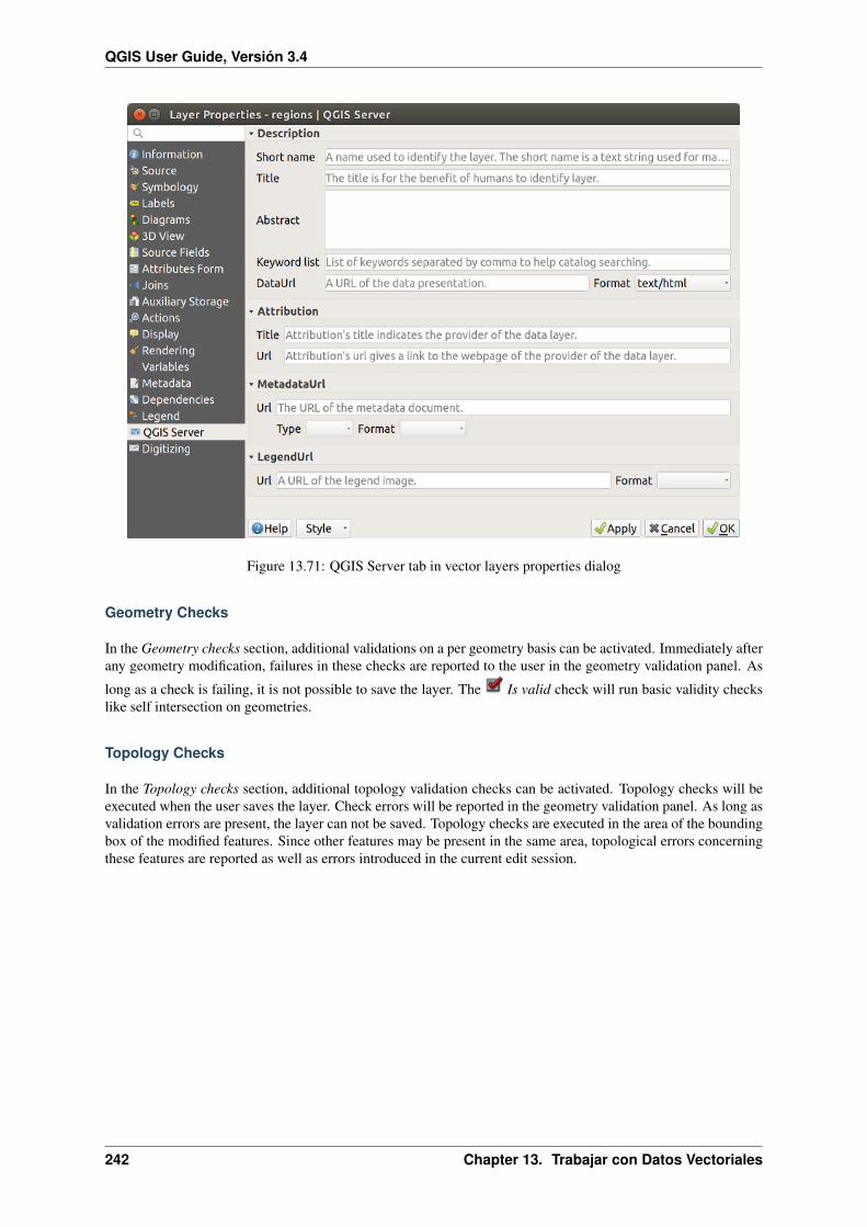
QGIS User Guide, Versión 3.4
Figure 13.71: QGIS Server tab in vector layers properties dialog
Geometry Checks
In the Geometry checks section, additional validations on a per geometry basis can be activated. Immediately afterany geometry modification, failures in these checks are reported to the user in the geometry validation panel. As
long as a check is failing, it is not possible to save the layer. The Is valid check will run basic validity checkslike self intersection on geometries.
Topology Checks
In the Topology checks section, additional topology validation checks can be activated. Topology checks will beexecuted when the user saves the layer. Check errors will be reported in the geometry validation panel. As long asvalidation errors are present, the layer can not be saved. Topology checks are executed in the area of the boundingbox of the modified features. Since other features may be present in the same area, topological errors concerningthese features are reported as well as errors introduced in the current edit session.
242 Chapter 13. Trabajar con Datos Vectoriales
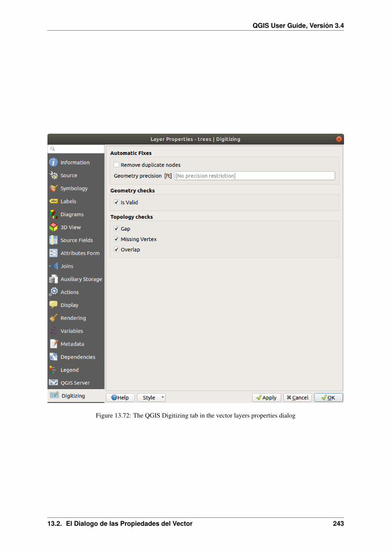
QGIS User Guide, Versión 3.4
Figure 13.72: The QGIS Digitizing tab in the vector layers properties dialog
13.2. El Dialogo de las Propiedades del Vector 243

QGIS User Guide, Versión 3.4
Topology check option Illustration
The Gap check will check for gaps between neighbouring polygons.
The Overlap check will check for overlaps between neighbouring polygons.
The Missing vertex check will check for shared boundaries of neighbouring poly-gons where one border misses a vertex which is present on the other one.
13.3 Expresiones
Based on layer data and prebuilt or user defined functions, Expressions offer a powerful way to manipulateattribute value, geometry and variables in order to dynamically change the geometry style, the content or positionof the label, the value for diagram, the height of a layout item, select some features, create virtual field . . .
13.3.1 The Expression string builder
Main dialog to build expressions, the Expression string builder is available from many parts in QGIS and, canparticularly be accessed when:
• clicking the button;
• selecting features with the Select By Expression. . . tool;
• editing attributes with e.g. the Field calculator tool;
• manipulating symbology, label or layout item parameters with the Data defined override tool (see Configu-ración de anulación definida por datos);
• building a geometry generator symbol layer;
• doing some geoprocessing.
The Expression builder dialog offers access to the:
• Expression tab which, thanks to a list of predefined functions, helps to write and check the expression touse;
• Function Editor tab which helps to extend the list of functions by creating custom ones.
Some use cases of expressions:
• From Field Calculator, calculate a «pop_density» field using existing «total_pop» and «area_km2» fields:
244 Chapter 13. Trabajar con Datos Vectoriales

QGIS User Guide, Versión 3.4
"total_pop" / "area_km2"
• Update the field «density_level» with categories according to the «pop_density» values:
CASE WHEN "pop_density" < 50 THEN 'Low population density'WHEN "pop_density" >= 50 and "pop_density" < 150 THEN 'Medium population
→˓density'WHEN "pop_density" >= 150 THEN 'High population density'
END
• Apply a categorized style to all the features according to whether their average house price is smaller orhigher than 10000C per square metre:
"price_m2" > 10000
• Using the «Select By Expression. . . » tool, select all the features representing areas of “High populationdensity” and whose average house price is higher than 10000C per square metre:
"density_level" = 'High population density' and "price_m2" > 10000
Likewise, the previous expression could also be used to define which features should be labeled or shownin the map.
Using expressions offers you a lot of possibilities.
Truco: Use named parameters to improve the expression reading
Some functions require many parameters to be set. The expression engine supports the use of named parameters.This means that instead of writing the cryptic expression clamp( 1, 2, 9), you can use clamp( min:=1,value:=2, max:=9). This also allows arguments to be switched, e.g. clamp( value:=2, max:=9,min:=1). Using named parameters helps clarify what the arguments for an expression function refer to, whichis helpful when you are trying to interpret an expression at a later date!
13.3.2 Lista de funciones
The Expression tab provides the main interface to write expressions using functions, layer’s fields and values. Itcontains following widgets:
• An expression editor area to type or paste expressions. Autocompletion is available to speed expressionwriting:
– Corresponding variables, function names and field names to the input text are shown below: use theUp and Down arrows to browse the items and press Tab to insert in the expression or simply click onthe wished item.
– Function parameters are shown while filling them.
QGIS also checks the expression rightness and highlights all the errors using:
– Underline: for unknown functions, wrong or invalid arguments;
– Marker: for every other error (eg, missing parenthesis, unexpected character) at a single location.
Truco: Document your expression with comments
When using complex expression, it is good practice to add text either as a multiline comment or inlinecomments to help you remember.
/*Labels each region with its highest (in altitude) airport(s)and altitude, eg 'AMBLER : 264m' for the 'Northwest Artic' region
13.3. Expresiones 245

QGIS User Guide, Versión 3.4
*/with_variable('airport_alti', -- stores the highest altitude of the regionaggregate(
'airports','max',"ELEV", -- the field containing the altitude-- and limit the airports to the region they are withinfilter := within( $geometry, geometry( @parent ) )
),aggregate( -- finds airports at the same altitude in the region
'airports','concatenate',"NAME",filter := within( $geometry, geometry( @parent ) )and "ELEV" = @airport_alti
)|| ' : ' || @airport_alti || 'm'-- using || allows regions without airports to be skipped
)
• Under the expression editor, an Output preview displays the result of the expression evaluated on the firstfeature of the layer. In case of error, it indicates it and you can access details with the provided hyperlink.
• A function selector displays the list of functions, variables, fields. . . organized in groups. A search box isavailable to filter the list and quickly find a particular function or field. Double-clicking an item adds it tothe expression editor.
• A help panel displays help for each selected item in the function selector.
Truco: Press Ctrl+Click when hovering a function name in an expression to automatically display itshelp in the dialog.
• A field’s values widget shown when a field is selected in the function selector helps to fetch features at-tributes. Double-clicking a value adds it to the expression editor.
Truco: The right panel, showing functions help or field values, can be collapsed (invisible) in the dialog. Pressthe Show Values or Show Help button to get it back.
Aggregates Functions
This group contains functions which aggregate values over layers and fields.
246 Chapter 13. Trabajar con Datos Vectoriales

QGIS User Guide, Versión 3.4
Figure 13.73: The Expression tab
Función Descripciónagregar Returns an aggregate value calculated using features from another layerarray_agg Returns an array of aggregated values from a field or expressioncollect Returns the multipart geometry of aggregated geometries from an expressionconcatenar Returns the all aggregated strings from a field or expression joined by a delimiterNúmero Returns the count of matching featurescount_distinct Returns the count of distinct valuescount_missing Returns the count of missing (null) valuesiqr Returns the calculated inter quartile range from a field or expressionmayoría Returns the aggregate majority of values (most commonly occurring value) from a field or
expressionmax_length Returns the maximum length of strings from a field or expressionmáximo Returns the aggregate maximum value from a field or expressionmedia Returns the aggregate mean value from a field or expressionmediana Returns the aggregate median value from a field or expressionmin_length Returns the minimum length of strings from a field or expressionmínimo Returns the aggregate minimum value from a field or expressionminoría Returns the aggregate minority of values (least commonly occurring value) from a field or
expressionq1 Returns the calculated first quartile from a field or expressionq3 Devuelve el tercer cuartil calculado a partir de un campo o expresiónintervalo Returns the aggregate range of values (maximum - minimum) from a field or expressionrela-tion_aggregate
Returns an aggregate value calculated using all matching child features from a layer relation
stdev Returns the aggregate standard deviation value from a field or expressionsum Returns the aggregate summed value from a field or expression
Ejemplos:
• Return the maximum of the «passengers» field from features in the layer grouped by «station_class» field:
13.3. Expresiones 247

QGIS User Guide, Versión 3.4
maximum("passengers", group_by:="station_class")
• Calculate the total number of passengers for the stations inside the current atlas feature:
aggregate('rail_stations','sum',"passengers",intersects(@atlas_geometry, $geometry))
• Return the mean of the «field_from_related_table» field for all matching child features using the“my_relation” relation from the layer:
relation_aggregate('my_relation', 'mean', "field_from_related_table")
o:
relation_aggregate(relation:='my_relation', aggregate := 'mean',expression := "field_from_related_table")
Array Functions
This group contains functions to create and manipulate arrays (also known as list data structures). The order ofvalues within the array matters, unlike the “map” data structure, where the order of key-value pairs is irrelevantand values are identified by their keys.
248 Chapter 13. Trabajar con Datos Vectoriales

QGIS User Guide, Versión 3.4
Función Descripciónarray Returns an array containing all the values passed as parameterar-ray_append
Returns an array with the given value added at the end
array_cat Returns an array containing all the given arrays concatenatedar-ray_contains
Returns true if an array contains the given value
ar-ray_distinct
Returns an array containing distinct values of the given array
ar-ray_filter
Returns an array with only the items for which an expression evaluates to true
array_find Returns the index (0 for the first one) of a value within an array. Returns -1 if the value is notfound.
array_first Returns the first value of an arrayar-ray_foreach
Returns an array with the given expression evaluated on each item
array_get Returns the Nth value (0 for the first one) of an arrayar-ray_insert
Returns an array with the given value added at the given position
ar-ray_intersect
Returns true if any element of array_1 exists in array_2
array_last Returns the last element of an arrayar-ray_length
Returns the number of elements of an array
ar-ray_prepend
Returns an array with the given value added at the beginning
ar-ray_remove_all
Returns an array with all the entries of the given value removed
ar-ray_remove_at
Returns an array with the given index removed
ar-ray_reverse
Returns the given array with array values in reversed order
array_slice Returns the values of the array from the start_pos argument up to and including the end_posargument
ar-ray_to_string
Concatenates array elements into a string separated by a delimiter and using optional string forempty values
gener-ate_series
Creates an array containing a sequence of numbers
reg-exp_matches
Returns an array of all strings captured by capturing groups, in the order the groups themselvesappear in the supplied regular expression against a string
string_to_arraySplits string into an array using supplied delimiter and optional string for empty values
Funciones de Color
This group contains functions for manipulating colors.
13.3. Expresiones 249

QGIS User Guide, Versión 3.4
Función Descripcióncolor_cmyk Devuelve una representación en forma de cadena de un color en base a sus componentes
cian, magenta, amarillo y negrocolor_cmyka Returns a string representation of a color based on its cyan, magenta, yellow, black and alpha
(transparency) componentscolor_grayscale_averageApplies a grayscale filter and returns a string representation from a provided colorcolor_hsl Returns a string representation of a color based on its hue, saturation, and lightness attributescolor_hsla Devuelve una representación en forma de cadena de un color en base a sus atributos de
matiz, saturación, luminosidad y canal alfa (transparencia).color_hsv Returns a string representation of a color based on its hue, saturation, and value attributescolor_hsva Devuelve una representación en forma de cadena de un color en base a sus atributos de
matiz, saturación, valor y canal alfa (transparencia)color_mix_rgb Returns a string representing a color mixing the red, green, blue, and alpha values of two
provided colors based on a given ratiocolor_part Devuelve un componente específico de la cadena de un color, por ejemplo el componente
rojo o el alfacolor_rgb Returns a string representation of a color based on its red, green, and blue componentscolor_rgba Returns a string representation of a color based on its red, green, blue, and alpha (trans-
parency) componentscreate_ramp Returns a gradient ramp from a map of color strings and stepsmás oscuro Devuelve una cadena de color más oscura (o más clara)más claro Devuelve una cadena de color más clara (o más oscura)project_color Devuelve un color del esquema de color del proyectoramp_color Devuelve una cadena que representa un color de una rampa de colorset_color_part Sets a specific color component for a color string, eg the red component or alpha component
Conditional Functions
Este grupo contiene funciones para menejar comprobaciones condicionales en expresiones.
Función DescripciónCASE WHEN . . . THEN . . .END
Evalúa una expresión y devuelve un resultado si es verdadera. Puede probarmúltiples condiciones
CASE WHEN . . . THEN . . .ELSE . . . END
Evalúa una expresión y devuelva un resultado diferente sea verdadero o falso.Puede probar múltiples condiciones
coalesce Devuelve el primer valor no-NULO de la lista de expresiónsi Prueba una condición y devuelve un resultado diferente dependiendo de la
comprobación condicional
Algún ejemplo:
• Send back a value if the first condition is true, else another value:
CASE WHEN "software" LIKE '%QGIS%' THEN 'QGIS' ELSE 'Other' END
Funciones de conversión
This group contains functions to convert one data type to another (e.g., string to integer, integer to string).
250 Chapter 13. Trabajar con Datos Vectoriales

QGIS User Guide, Versión 3.4
Función Descripciónto_date Convierte una cadena de texto en un objeto fechato_datetime Converts a string into a datetime objectto_dm Converts a coordinate to degree, minuteto_dms Converts coordinate to degree, minute, secondto_int Convierte una cadena de texto a número enteroto_interval Converts a string to an interval type (can be used to take days, hours, months, etc. of a date)to_real Convierte una cadena de texto en número realto_string Convierte un número en cadena.to_time Converts a string into a time object
Funciones personalizadas
This group contains functions created by the user. See Editor de Funciones for more details.
Funciones de Fecha y Hora
Este grupo contiene funciones para manipular datos de fecha y hora.
Función Descripciónedad Returns as an interval the difference between two dates or datetimesdía Extracts the day from a date or datetime, or the number of days from an intervalday_of_week Returns a number corresponding to the day of the week for a specified date or datetimeepoch Returns the interval in milliseconds between the unix epoch and a given date valuehora Extracts the hour from a datetime or time, or the number of hours from an intervalminuto Extracts the minute from a datetime or time, or the number of minutes from an intervalmes Extracts the month part from a date or datetime, or the number of months from an intervalnow Returns current date and timesegundo Extracts the second from a datetime or time, or the number of seconds from an intervalsemana Extrae el número de la semana de una fecha o el número de semanas de un intervalo.year Extracts the year part from a date or datetime, or the number of years from an interval
This group also shares several functions with the Funciones de conversión ( to_date, to_time, to_datetime,to_interval) and Funciones de cadena (format_date) groups.
Algún ejemplo:
• Get today’s month and year in the «month_number/year» format:
format_date(now(),'MM/yyyy')-- Returns '03/2017'
Besides these functions, subtracting dates, datetimes or times using the - (minus) operator will return an interval.
Adding or subtracting an interval to dates, datetimes or times, using the + (plus) and - (minus) operators, willreturn a datetime.
• Get the number of days until QGIS 3.0 release:
to_date('2017-09-29') - to_date(now())-- Returns <interval: 203 days>
• The same with time:
13.3. Expresiones 251

QGIS User Guide, Versión 3.4
to_datetime('2017-09-29 12:00:00') - to_datetime(now())-- Returns <interval: 202.49 days>
• Get the datetime of 100 days from now:
now() + to_interval('100 days')-- Returns <datetime: 2017-06-18 01:00:00>
Nota: Storing date and datetime and intervals on fields
The ability to store date, time and datetime values directly on fields may depend on the data source’s provider (e.g.,Shapefile accepts date format, but not datetime or time format). The following are some suggestions to overcomethis limitation:
• date, Datetime and time can be stored in text type fields after using the to_format() function.
• Intervals can be stored in integer or decimal type fields after using one of the date extraction functions (e.g.,day() to get the interval expressed in days)
Campos y Valores
Contains a list of fields from the layer.
Double-click a field name to have it added to your expression. You can also type the field name (preferably insidedouble quotes) or its alias.
To retrieve fields values to use in an expression, select the appropriate field and, in the shown widget, choosebetween 10 Samples and All Unique. Requested values are then displayed and you can use the Search box at thetop of the list to filter the result. Sample values can also be accessed via right-clicking on a field.
To add a value to the expression you are writing, double-click on it in the list. If the value is of a string type, itshould be simple quoted, otherwise no quote is needed.
Funciones Concordancia aproximada
This group contains functions for fuzzy comparisons between values.
Función Descripciónham-ming_distance
Returns the number of characters at corresponding positions within the input strings wherethe characters are different
levensheim Returns the minimum number of character edits (insertions, deletions or substitutions) re-quired to change one string to another. Measure the similarity between two strings
longest_common_substringReturns the longest common substring between two stringssoundex Returns the Soundex representation of a string
Funciones Generales
Este grupo contiene funciones generales variadas.
252 Chapter 13. Trabajar con Datos Vectoriales

QGIS User Guide, Versión 3.4
Fun-ción
Descripción
env Gets an environment variable and returns its content as a string. If the variable is not found, NULLwill be returned.
eval Evaluates an expression which is passed in a string. Useful to expand dynamic parameters passedas context variables or fields
is_layer_visibleReturns true if a specified layer is visiblelayer_propertyReturns a property of a layer or a value of its metadata. It can be layer name, crs, geometry type,
feature count. . .var Returns the value stored within a specified variable. See variable functions belowwith_variableCreates and sets a variable for any expression code that will be provided as a third argument. Useful
to avoid repetition in expressions where the same value needs to be used more than once.
Funciones de Geometría
This group contains functions that operate on geometry objects (e.g., length, area).
Función Descripción$area Returns the area size of the current feature$geometry Returns the geometry of the current feature (can be used for processing with other functions)$length Returns the length of the current line feature$perimeter Returns the perimeter of the current polygon feature$x Returns the X coordinate of the current feature$x_at(n) Returns the X coordinate of the nth node of the current feature’s geometry$y Returns the Y coordinate of the current feature$y_at(n) Returns the Y coordinate of the nth node of the current feature’s geometryangle_at_vertex Returns the bisector angle (average angle) to the geometry for a specified vertex on a linestring geometry. Angles are in degrees clockwise from northarea Devuelve el perímetro de un objeto de geometría poligonal. Los cálculos están en el Sistema de Referencia Espacial de esta geometríaazimut Returns the north-based azimuth as the angle in radians measured clockwise from the vertical on point_a to point_bcontorno Returns the closure of the combinatorial boundary of the geometry (ie the topological boundary of the geometry - see also qgisboundary).límites Returns a geometry which represents the bounding box of an input geometry. Calculations are in the Spatial Reference System of this geometry (see also qgisboundingboxes)bounds_height Returns the height of the bounding box of a geometry. Calculations are in the Spatial Reference System of this geometrybounds_width Devuelve la anchura del recuadro delimitador de una geometría. Los cálculos están en el Sistema de Referencia Espacial de esta geometríabuffer Returns a geometry that represents all points whose distance from this geometry is less than or equal to distance. Calculations are in the Spatial Reference System of this geometry (see also qgisbuffer)buffer_by_m Creates a buffer along a line geometry where the buffer diameter varies according to the M values at the line vertices (see also qgisbufferbym)centroid Returns the geometric center of a geometry (see also qgiscentroids)closest_point Returns the point on a geometry that is closest to a second geometrycombinar Devuelve la combinación de dos geometríascontains(a,b) Returns 1 (true) if and only if no points of b lie in the exterior of a, and at least one point of the interior of b lies in the interior of aconvex_hull Returns the convex hull of a geometry (this represents the minimum convex geometry that encloses all geometries within the set) (see also qgisconvexhull)cruza Returns 1 (true) if the supplied geometries have some, but not all, interior points in commondifference(a,b) Returns a geometry that represents that part of geometry a that does not intersect with geometry b (see also qgisdifference)inconexo Returns 1 (true) if the geometries do not share any space togetherdistance Returns the minimum distance (based on Spatial Reference System) between two geometries in projected unitsdistance_to_vertex Returns the distance along the geometry to a specified vertexend_point Returns the last node from a geometry (see also qgisextractspecificvertices)extend Extends the start and end of a linestring geometry by a specified amount (see also qgisextendlines)exterior_ring Returns a line string representing the exterior ring of a polygon geometry, or null if the geometry is not a polygonextrude(geom,x,y) Returns an extruded version of the input (Multi-) Curve or (Multi-)Linestring geometry with an extension specified by X and Yflip_coordinates Returns a copy of the geometry with the X and Y coordinates swapped (see also qgisswapxy)geom_from_gml Returns a geometry created from a GML representation of geometrygeom_from_wkt Returns a geometry created from a well-known text (WKT) representationgeom_to_wkt Returns the well-known text (WKT) representation of the geometry without SRID metadatageometry Devuelve la geometría de un objeto
Continued on next page
13.3. Expresiones 253

QGIS User Guide, Versión 3.4
Table 13.1 – continued from previous pageFunción Descripcióngeometry_n Returns the nth geometry from a geometry collection, or null if the input geometry is not a collectionhausdorff_distance Returns basically a measure of how similar or dissimilar 2 geometries are, with a lower distance indicating more similar geometriesinclination Returns the inclination measured from the zenith (0) to the nadir (180) on point_a to point_binterior_ring_n Returns the geometry of the nth interior ring from a polygon geometry, or null if the geometry is not a polygonintersección Returns a geometry that represents the shared portion of two geometries (see also qgisintersection)intersecta Tests whether a geometry intersects another. Returns 1 (true) if the geometries spatially intersect (share any portion of space) and 0 if they don’tintersects_bbox Tests whether a geometry’s bounding box overlaps another geometry’s bounding box. Returns 1 (true) if the geometries spatially intersect (share any portion of space) their bounding box, or 0 if they don’tis_closed Returns true if a line string is closed (start and end points are coincident), false if a line string is not closed, or null if the geometry is not a line stringlongitud Returns length of a line geometry feature (or length of a string)line_interpolate_angle Returns the angle parallel to the geometry at a specified distance along a linestring geometry. Angles are in degrees clockwise from north.line_interpolate_point Returns the point interpolated by a specified distance along a linestring geometry. (see also qgisinterpolatepoint)line_locate_point Returns the distance along a linestring corresponding to the closest position the linestring comes to a specified point geometry.line_substring Returns the portion of a line or curve geometry falling betweeen specified start and end distances (measured from the beginning of the line) (see also qgislinesubstring)line_merge Returns a (Multi-)LineString geometry, where any connected LineStrings from the input geometry have been merged into a single linestring.m Returns the M value of a point geometrymake_circle Creates a circular geometry based on center point and radiusmake_ellipse Creates an elliptical geometry based on center point, axes and azimuthmake_line Crea una geometría de línea a partir de una serie de geometrías de puntosmake_point(x,y,z,m) Returns a point geometry from X and Y (and optional Z or M) valuesmake_point_m(x,y,m) Returns a point geometry from X and Y coordinates and M valuesmake_polygon Crea una geometría de polígono a partir de un anillo exterior y series opcionales de geometrías interiores de anillomake_regular_polygon Creates a regular polygonmake_triangle Creates a triangle polygonminimal_circle Returns the minimal enclosing circle of an input geometry (see also qgisminimumenclosingcircle)nodes_to_points Returns a multipoint geometry consisting of every node in the input geometry (see also qgisextractvertices)num_geometries Devuelve el número de geometrías en una colección de geometrías o nulo si la geometría de entrada no es una colecciónnum_interior_rings Devuelve el número de anillos interiores de un polígono o una colección de geometrías o nulo si la geometría de entrada no es un polígono o una colecciónnum_points Devuelve el número de vértices de una geometría.num_rings Devuelve el número de anillos (incluidos los anillos exteriores) de un polígono o una colección de geometrías o nulo si la geometría de entrada no es un polígono o una colecciónoffset_curve Returns a geometry formed by offsetting a linestring geometry to the side. Distances are in the Spatial Reference System of this geometry. (see also qgisoffsetline)order_parts Ordena las partes de una MultiGeometría por los criterios dadosoriented_bbox Returns a geometry representing the minimal oriented bounding box of an input geometry (see also qgisorientedminimumboundingbox)solapa Comprueba si una geometría solapa con otra. Devuelve 1(verdadero) si las geometrías comparten espacio, son de la misma dimensión, pero no están contenidas en la otra.perímetro Devuelve el perímetro de un objeto de geometría poligonal. Los cálculos están en el Sistema de Referencia Espacial de esta geometría.point_n Returns a specific node from a geometry (see also qgisextractspecificvertices)point_on_surface Returns a point guaranteed to lie on the surface of a geometry (see also qgispointonsurface)pole_of_inaccessibility Calculates the approximate pole of inaccessibility for a surface, which is the most distant internal point from the boundary of the surface (see also qgispoleofinaccessibility)proyecto Returns a point projected from a start point using a distance and bearing (azimuth) in radians (see also qgisprojectpointcartesian)relate Prueba o devuelve la representación del Modelo de Intersección 9 Extendido Dimensional (DE-9IM) de la relación entre dos geometrías.invertir Reverses the direction of a line string by reversing the order of its vertices (see also qgisreverselinedirection)segments_to_lines Returns a multi line geometry consisting of a line for every segment in the input geometry (see also qgisexplodelines)shortest_line Returns the shortest line joining two geometries. The resultant line will start at geometry 1 and end at geometry 2simplify Simplifies a geometry by removing nodes using a distance based threshold (see also qgissimplifygeometries)simplify_vw Simplifies a geometry by removing nodes using an area based threshold (see also qgissimplifygeometries)single_sided_buffer Returns a geometry formed by buffering out just one side of a linestring geometry. Distances are in the Spatial Reference System of this geometry (see also qgissinglesidedbuffer)smooth Smooths a geometry by adding extra nodes which round off corners in the geometry (see also qgissmoothgeometry)start_point Returns the first node from a geometry (see also qgisextractspecificvertices)sym_difference Returns a geometry that represents the portions of two geometries that do not intersect (see also qgissymmetricaldifference)tapered_buffer Creates a buffer along a line geometry where the buffer diameter varies evenly over the length of the line (see also qgistaperedbuffer)toca Tests whether a geometry touches another. Returns 1 (true) if the geometries have at least one point in common, but their interiors do not intersectTransformar Returns the geometry transformed from the source CRS to the destination CRS (see also qgisreprojectlayer)Convertir Returns a translated version of a geometry. Calculations are in the Spatial Reference System of the geometry (see also qgistranslategeometry)unión Devuelve una geometría que representa el conjunto unión de los puntos de las geometrías.
Continued on next page
254 Chapter 13. Trabajar con Datos Vectoriales

QGIS User Guide, Versión 3.4
Table 13.1 – continued from previous pageFunción Descripciónwedge_buffer Returns a wedge shaped buffer originating from a point geometry given an angle and radii (see also qgiswedgebuffers)entre(a,b) Tests whether a geometry is within another. Returns 1 (true) if geometry a is completely inside geometry bx Returns the X coordinate of a point geometry, or the X coordinate of the centroid for a non-point geometryx_min Returns the minimum X coordinate of a geometry. Calculations are in the Spatial Reference System of this geometryx_max Returns the maximum X coordinate of a geometry. Calculations are in the Spatial Reference System of this geometryy Returns the Y coordinate of a point geometry, or the Y coordinate of the centroid for a non-point geometryy_min Returns the minimum Y coordinate of a geometry. Calculations are in the Spatial Reference System of this geometryy_max Returns the maximum Y coordinate of a geometry. Calculations are in the Spatial Reference System of this geometryz Returns the Z coordinate of a point geometry
Algún ejemplo:
• You can manipulate the current geometry with the variable $geometry to create a buffer or get the point onsurface:
buffer( $geometry, 10 )point_on_surface( $geometry )
• Return the X coordinate of the current feature’s centroid:
x( $geometry )
• Send back a value according to feature’s area:
CASE WHEN $area > 10 000 THEN 'Larger' ELSE 'Smaller' END
Layout Functions
This group contains functions to manipulate print layout items properties.
Función Descripciónitem_variables Returns a map of variables from a layout item inside this print layout
Algún ejemplo:
• Get the scale of the “Map 0” in the current print layout:
map_get( item_variables('Map 0'), 'map_scale')
Map Layers
This group contains a list of the available layers in the current project. This offers a convenient way to writeexpressions referring to multiple layers, such as when performing aggregates, attribute or spatial queries.
13.3. Expresiones 255

QGIS User Guide, Versión 3.4
Maps Functions
This group contains functions to create or manipulate keys and values of map data structures (also known asdictionary objects, key-value pairs, or associative arrays). Unlike the list data structure where values order matters,the order of the key-value pairs in the map object is not relevant and values are identified by their keys.
Función Descripciónhstore_to_mapCreates a map from a hstore-formatted stringjson_to_map Creates a map from a json-formatted stringmap Returns a map containing all the keys and values passed as pair of parametersmap_akeys Returns all the keys of a map as an arraymap_avals Returns all the values of a map as an arraymap_concat Returns a map containing all the entries of the given maps. If two maps contain the same key,
the value of the second map is taken.map_delete Returns a map with the given key and its corresponding value deletedmap_exist Returns true if the given key exists in the mapmap_get Returns the value of a map, given it’s keymap_insert Returns a map with an added key/valuemap_to_hstoreMerges map elements into a hstore-formatted stringmap_to_json Merges map elements into a json-formatted string
Funciones Matemáticas
Este grupo contiene funciones matemáticas,por ejemplo raíz cuadrada, seno y coseno
256 Chapter 13. Trabajar con Datos Vectoriales

QGIS User Guide, Versión 3.4
Función Descripciónabs Devuelve el valor absoluto de un númeroarcos Devuelve la inversa del coseno de un valor en radianesarcsen Devuelve la inversa del seno de un valor en radianesatan Returns the inverse tangent of a value in radiansatan2(y,x) Returns the inverse tangent of Y/X by using the signs of the two arguments to determine the
quadrant of the resultaz-imuth(a,b)
Returns the north-based azimuth as the angle in radians measured clockwise from the vertical onpoint a to point b
ceil Rounds a number upwardsclamp Restricts an input value to a specified rangecos Devuelve el coseno de un valor en radianesgrados Convierte de radianes a gradosexp Devuelve la exponencial de un valorfloor Rounds a number downwardsinclination Returns the inclination measured from the zenith (0) to the nadir (180) on point_a to point_b.ln Returns the natural logarithm of the passed expressionlog Returns the value of the logarithm of the passed value and baselog10 Returns the value of the base 10 logarithm of the passed expressionmáx Returns the largest not null value in a set of valuesmín Returns the smallest not null value in a set of valuespi Returns the value of pi for calculationsradianes Convierte de grados a radianesrand Returns the random integer within the range specified by the minimum and maximum argument
(inclusive)randf Returns the random float within the range specified by the minimum and maximum argument
(inclusive)round Rounds to number of decimal placesscale_exp Transforma un valor dado de un dominio de entrada a un rango de salida usando una curva
exponencialscale_linear Transforma un valor dado de un dominio de entrada a un rango de salida usando interpolación
linealsen Returns the sine of an angleraízcuadrada
Returns the square root of a value
tan Devuelve la tangente de un ángulo
Operadores
This group contains operators (e.g., +, -, *). Note that for most of the mathematical functions below, if one of theinputs is NULL then the result is NULL.
13.3. Expresiones 257

QGIS User Guide, Versión 3.4
Función Descripcióna + b Addition of two values (a plus b)a - b Subtraction of two values (a minus b).a * b Multiplication of two values (a multiplied by b)a / b División de dos valores (a dividido entre b)a % b Remainder of division of a by b (eg, 7 % 2 = 1, or 2 fits into 7 three times with remainder
1)a ^ b Power of two values (for example, 2^2=4 or 2^3=8)a < b Compares two values and evaluates to 1 if the left value is less than the right value (a is
smaller than b)a <= b Compares two values and evaluates to 1 if the left value isless than or equal to the right
valuea <> b Compara dos valores y evalúa a 1 si no son igualesa = b Compara dos valores y evalúa a 1 si son iguales.a != b a and b are not equala > b Compara dos valores y evalúa como 1 si el valor izquierdo es mayor que el valor derecho
(a es mayor que b)a >= b Compara dos valores y evalúa a 1 si el valor de la izquierda es mayor que o igual que el
valor de la derechaa ~ b a matches the regular expression b|| Joins two values together into a string. If one of the values is NULL the result will be
NULL“\n” Inserta una nueva línea en una cadenaLIKE Devuelve 1 si el primer parámetro coincide con el patrón provistoILIKE Returns 1 if the first parameter matches case-insensitive the supplied pattern (ILIKE can
be used instead of LIKE to make the match case-insensitive)a IS b Tests whether two values are identical. Returns 1 if a is the same as ba OR b Returns 1 when condition a or condition b is truea AND b Returns 1 when conditions a and b are trueNOT Niega una condicióncolumn name«column name»
Value of the field column name, take care to not be confused with simple quote, see below
“cadena” a string value, take care to not be confused with double quote, see aboveNULL valor nuloa IS NULL a no tiene valora IS NOT NULL a tiene valora IN(value[,value])
a esta debajo de los valores listados
a NOT IN(valor[,valor])
a no está debajo de los valores listados
Nota: About fields concatenation
You can concatenate strings using either || or +. The latter also means sum up expression. So if you have aninteger (field or numeric value) this can be error prone. In this case, you should use ||. If you concatenate twostring values, you can use both.
Algún ejemplo:
• Une una cadena de texto y un valor de un nombre de columna:
258 Chapter 13. Trabajar con Datos Vectoriales

QGIS User Guide, Versión 3.4
'My feature''s id is: ' || "gid"'My feature''s id is: ' + "gid" => triggers an error as gid is an integer"country_name" + '(' + "country_code" + ')'"country_name" || '(' || "country_code" || ')'
• Test if the «description» attribute field starts with the “Hello” string in the value (note the position of the %character):
"description" LIKE 'Hello%'
Rasters Functions
This group contains functions to operate on raster layer.
Función Descripciónraster_statistic Returns statistics from a raster layerraster_value Returns the raster band value at the provided point
Record and Attributes Functions
Este grupo contiene funciones que operan sobre identificadores de registros.
Función Descripción$current-feature
Devuelve el objeto espacial que está siendo evaluado. Se puede usar con la función “attribute”para evaluar los valores de atributo del objeto actual.
$id Devuelve el ID del objeto de la fila actualatributo Devuelve el valor del atributo especificado de un objetoget_feature Devuelve el primer objeto de una capa que coincide con un valor de atributo dadoget_feature_by_idReturns the feature of a layer matching the given feature IDis_selected Returns if a feature is selectednum_selected Returns the number of selected features on a given layerrepre-sent_value
Returns the configured representation value for a field value (convenient with some widget types)
uuid Generates a Universally Unique Identifier (UUID) for each row. Each UUID is 38 characterslong.
Algún ejemplo:
• Return the first feature in layer «LayerA» whose field «id» has the same value as the field «name» of thecurrent feature (a kind of jointure):
get_feature( 'layerA', 'id', attribute( $currentfeature, 'name') )
• Calculate the area of the joined feature from the previous example:
area( geometry( get_feature( 'layerA', 'id', attribute( $currentfeature, 'name→˓') ) ) )
Funciones de cadena
Este grupo contiene funciones que operan sobre cadenas, por ejemplo reemplazar, convertir a mayúsculas.
13.3. Expresiones 259

QGIS User Guide, Versión 3.4
Función Descripciónchar Devuelve el carácter asociado con un código unicodeconcat Concatenates several strings to oneformat Da formato a una cadena usando los argumentos proporcionados.for-mat_date
Formats a date type or string into a custom string format
for-mat_number
Devuelve un número formateado con el separador local de miles (también trunca el número alnúmero de decimales indicado)
left(string,n)
Returns a substring that contains the n leftmost characters of the string
longitud Returns length of a string (or length of a line geometry feature)lower Convierte una cadena a letras minúsculas.lpad Returns a string padded on the left to the specified width, using the fill characterreg-exp_match
Returns the first matching position matching a regular expression within a string, or 0 if thesubstring is not found
reg-exp_replace
Devuelve una cadena en la que se ha remplazado la expresión regular proporcionada
reg-exp_substr
Devuelve la parte de una cadena que coincide con una expresión regular proporcionada
remplazar Returns a string with the supplied string, array, or map of strings replaced by a string, an arrayof strings or paired values
right(cadena,n)
Devuelve una subcadena que contiene los n caracteres más a la derecha de la cadena.
rpad Returns a string padded on the right to the specified width, using the fill characterstrpos Returns the first matching position of a substring within another string, or 0 if the substring is
not foundsubstr Devuelve una parte de una cadena.Título Convierte todas las palabras de una cadena a formato de título (todas las palabras en minúscula
con la primera letra en mayúscula)trim Elimina todos los espacios en blanco (espacios, tabuladores, etc.) de comienzo y final de una
cadena.upper Convierte una cadena a letras mayúsculas.wordwrap Devuelve una cadena ajustada un número de caracteres máximo/mínimo
Variables Functions
This group contains dynamic variables related to the application, the project file and other settings. It means thatsome functions may not be available according to the context:
• from the Select by expression dialog
• desde Calculadora de campos dialog
• desde el diálogo de propiedades de la capa
• from the print layout
To use these functions in an expression, they should be preceded by @ character (e.g, @row_number). Areconcerned:
Función Descripciónalgorithm_id Returns the unique ID of an algorithmatlas_feature Devuelve el objeto del atlas actual (como objeto espacial)atlas_featureid Devuelve el ID de objeto del atlas actual.atlas_featurenumber Returns the current atlas feature number in the layoutatlas_filename Devuelve el nombre de archivo del atlas actual.
Continued on next page
260 Chapter 13. Trabajar con Datos Vectoriales

QGIS User Guide, Versión 3.4
Table 13.2 – continued from previous pageFunción Descripciónatlas_geometry Devuelve la geometría de objeto del atlas actualatlas_layerid Returns the current atlas coverage layer IDatlas_layername Returns the current atlas coverage layer nameatlas_pagename Devuelve el nombre de la página del atlas actualatlas_totalfeatures Devuelve el número total de objetos en el atlas.canvas_cursor_point Returns the last cursor position on the canvas in the project’s geographical coordinatescluster_color Returns the color of symbols within a cluster, or NULL if symbols have mixed colorscluster_size Returns the number of symbols contained within a clustercurrent_feature Returns the feature currently being edited in the attribute form or table rowcurrent_geometry Returns the geometry of the feature currently being edited in the form or the table rowgeometry_part_count Returns the number of parts in rendered feature’s geometrygeometry_part_num Returns the current geometry part number for feature being renderedgeometry_point_count Returns the number of points in the rendered geometry’s partgeometry_point_num Returns the current point number in the rendered geometry’s partgrid_axis Devuelve el eje de la anotación de la cuadrícula actual (ej.: “x” para longitud, “y” para latitud).grid_number Devuelve el valor de anotación de la cuadrícula actual.item_id Returns the layout item user ID (not necessarily unique)item_uuid Returns the layout item unique IDlayer Returns the current layerlayer_id Devuelve el ID de la capa actuallayer_name Devuelve el nombre de la capa actuallayout_dpi Devulve la resolución de la composición (DPI).layout_name Returns the layout namelayout_numpages Returns the number of pages in the layoutlayout_page Returns the page number of the current item in the layoutlayout_pageheight Returns the active page height in the layout (in mm)layout_pagewidth Returns the active page width in the layout (in mm)map_crs Returns the Coordinate reference system of the current mapmap_crs_definition Returns the full definition of the Coordinate reference system of the current mapmap_extent Returns the geometry representing the current extent of the mapmap_extent_center Returns the point feature at the center of the mapmap_extent_height Devuelve la altura actual del mapamap_extent_width Devuelve el ancho actual del mapamap_id Returns the ID of current map destination. This will be “canvas” for canvas renders, and the item ID for layout map rendersmap_layer_ids Returns the list of map layer IDs visible in the mapmap_layers Returns the list of map layers visible in the mapmap_rotation Devuelve la rotación actual del mapamap_scale Devuelve la escala actual del mapamap_units Returns the units of map measurementsnotification_message Content of the notification message sent by the provider (available only for actions triggered by provider notifications).parent Refers to the current feature in the parent layer, providing access to its attributes and geometry when filtering an aggregate functionproject_abstract Returns the project abstract, taken from project metadataproject_author Returns the project author, taken from project metadataproject_basename Returns the basename of current project’s filename (without path and extension)project_creation_date Returns the project creation date, taken from project metadataproject_crs Returns the Coordinate reference system of the projectproject_crs_definition Returns the full definition of the Coordinate reference system of the projectproject_filename Returns the filename of the current projectproject_folder Returns the folder of the current projectproject_home Returns the home path of the current projectproject_identifier Returns the project identifier, taken from the project’s metadataproject_keywords Returns the project keywords, taken from the project’s metadataproject_path Returns the full path (including file name) of the current project
Continued on next page
13.3. Expresiones 261

QGIS User Guide, Versión 3.4
Table 13.2 – continued from previous pageFunción Descripciónproject_title Devuelve el Título del proyecto actual.qgis_locale Returns the current language of QGISqgis_os_name Devuelve el nombre del sistema operativo, ej. “Windows”, “Linux” o “OSX”.qgis_platform Devuelve la plataforma de QGIS, ej. “Escritorio” o “Servidor”.qgis_release_name Devuelve el nombre de la versión actual de QGISqgis_short_version Returns current QGIS version short stringqgis_version Devuelve la versión actual de QGIS como cadenaqgis_version_no Devuelve la versión actual de QGIS como númerosnapping_results Gives access to snapping results while digitizing a feature (only available in add feature)symbol_angle Devuelve el ángulo del símbolo usado para representar el objeto (solo válido para símbolos de marcador).symbol_color Returns the color of the symbol used to render the featureuser_account_name Devuelve el nombre de la cuenta del sistema operativo del usuario actual.user_full_name Devuelve el nombre de usuario del sistema operativo del usuario actual.row_number Guarda el número de la fila actual.Valor Devuelve el valor actualwith_variable Allows setting a variable for usage within an expression and avoid recalculating the same value repeatedly
Algún ejemplo:
• Return the X coordinate of a map item center to insert into a label in layout:
x( map_get( item_variables( 'map1'), 'map_extent_center' ) )
• Return for each feature in the current layer the number of overlapping airports features:
aggregate( layer:='airport', aggregate:='count', expression:="code",filter:=intersects( $geometry, geometry( @parent ) ) )
• Get the object_id of the first snapped point of a line:
with_variable('first_snapped_point',array_first( @snapping_results ),attribute(
get_feature_by_id(map_get( @first_snapped_point, 'layer' ),map_get( @first_snapped_point, 'feature_id' )
),'object_id'
))
Funciones recientes
This group contains recently used functions. Depending on the context of its usage (feature selection, field calcu-lator, generic), any applied expression is added to the corresponding list (up to ten expressions), sorted from themore recent to the less one. This helps to quickly retrieve and reapply any previously used expression.
13.3.3 Editor de Funciones
With the Function Editor tab, you are able to write your own functions in Python language. This provides a handyand comfortable way to address particular needs that would not be covered by the predefined functions.
262 Chapter 13. Trabajar con Datos Vectoriales

QGIS User Guide, Versión 3.4
Figure 13.74: La pestaña Editor de funciones
13.3. Expresiones 263

QGIS User Guide, Versión 3.4
To create a new function:
1. Press the New File button.
2. Enter a name to use in the form that pops up and press OK.
A new item of the name you provide is added in the left panel of the Function Editor tab; this is a Python.py file based on QGIS template file and stored in the /python/expressions folder under the activeuser profile directory.
3. The right panel displays the content of the file: a python script template. Update the code and its helpaccording to your needs.
4. Press the Save and Load Functions button. The function you wrote is added to the functions tree in theExpression tab, by default under the Custom group.
5. Enjoy your new function.
6. If the function requires improvements, enable the Function Editor tab, do the changes and press again the
Save and Load Functions button to make them available in the file, hence in any expression tab.
Custom Python functions are stored under the user profile directory, meaning that at each QGIS startup, it willauto load all the functions defined with the current user profile. Be aware that new functions are only saved in the/python/expressions folder and not in the project file. If you share a project that uses one of your customfunctions you will need to also share the .py file in the /python/expressions folder.
Here’s a short example on how to create your own functions:
from qgis.core import *from qgis.gui import *
@qgsfunction(args='auto', group='Custom')def my_sum(value1, value2, feature, parent):
"""Calculates the sum of the two parameters value1 and value2.<h2>Example usage:</h2><ul>
<li>my_sum(5, 8) -> 13</li><li>my_sum("field1", "field2") -> 42</li>
</ul>"""return value1 + value2
The short example creates a function my_sum that will give you a function with two values. When using theargs='auto' function argument the number of function arguments required will be calculated by the numberof arguments the function has been defined with in Python (minus 2 - feature, and parent).
This function can then be used in expressions:
Se puede encontrar más información sobre cómo crear código Python en:ref:PyQGIS-Developer-Cookbook.
13.4 Trabajar con la tabla de atributos
La tabla de atributos muestra información sobre los elementos de una capa seleccionada. Cada fila en la tablarepresenta un elemento (con o sin geometría), y cada columna contiene una pieza de información particular acercade ese elemento. Puede buscar, seleccionar, mover o incluso editar elementos en la tabla.
13.4.1 Prefacio: Tablas espaciales y no espaciales
QGIS permite cargar capas espaciales y no espaciales. Esto actualmente incluye tablas soportadas por OGR ytexto delimitado, así como las de los proveedores PostgreSQL, MSSQL, SpatiaLite, DB2 and Oracle. Todas las
264 Chapter 13. Trabajar con Datos Vectoriales

QGIS User Guide, Versión 3.4
Figure 13.75: Custom Function added to the Expression tab
capas cargadas son listadas en el panel Panel Capas. La interacción con una capa en el mapa es posible si la capaesta habilitada espacialmente.
Non-spatial tables can be browsed and edited using the attribute table view. Furthermore, they can be used forfield lookups. For example, you can use columns of a non-spatial table to define attribute values, or a range ofvalues that are allowed, to be added to a specific vector layer during digitizing. Have a closer look at the editwidget in section Attributes Form Properties to find out more.
13.4.2 Introducing the attribute table interface
To open the attribute table for a vector layer, activate the layer by clicking on it in the Panel de capas. Then, from
the main Layer menu, choose Open Attribute Table. It is also possible to right-click on the layer and choose
Open Attribute Table from the drop-down menu, or to click on the Open Attribute Table button in theAttributes toolbar. If you prefer shortcuts, F6 will open the attribute table. Shift+F6 will open the attributetable filtered to selected features and Ctrl+F6 will open the attribute table filtered to visible features.
This will open a new window that displays the feature attributes for the layer (figure_attributes_table). Accordingto the setting in Settings → Options → Data sources menu, the attribute table will open in a docked window ora regular window. The total number of features in the layer and the number of currently selected/filtered featuresare shown in the attribute table title, as well as if the layer is spatially limited.
Los botones de la parte superior de la ventana de la tabla de atributos proporcionan la siguiente funcionalidad:
13.4. Trabajar con la tabla de atributos 265

QGIS User Guide, Versión 3.4
Figure 13.76: Tabla de atributos de la capa regiones
Icono Etiqueta Propósito Atajo de teclado prede-terminado
Conmutar el modo de edición Habilitar funciones de edición Ctrl+E
Conmutar el modo multiedición Actualizar múltiples campos demuchos objetos
Guardar ediciones Guardar las modificaciones ac-tuales
Ctrl+S
Recargar la tabla
Añadir objeto espacial Añadir nuevo objeto sin geometría
Borrar objetos seleccionados Eliminar los objetos seleccionadosde la capa
Cortar elementos seleccionados alportapapeles
Ctrl+X
Copiar elementos seleccionados alportapapeles
Ctrl+C
Paste features from clipboard Insert new features from copiedones
Ctrl+V
Seleccionar objetos usando unaexpresión
Seleccionar todo Seleccionar todos los objetos de lacapa
Ctrl+A
Invertir selección Invertir la selección actual de lacapa
Ctrl+R
Deseleccionar todo Deseleccionar todos los objetos dela capa actual
Ctrl+Shift+A
Filter/Select features using form Ctrl+F
Mover la selección arriba del todo Move selected rows to the top of thetable
Desplazar el mapa a las filas selec-cionadas
Ctrl+P
Zoom map to the selected rows Ctrl+J
New field Add a new field to the data source Ctrl+W
Borrar campo Remove a field from the data source Ctrl+L
Open field calculator Update field for many features in arow
Ctrl+I
Formato condicional Habilitar formato de tabla
Dock attribute table Allows to dock/undock the attributetable
Actions Lists the actions related to the layer
266 Chapter 13. Trabajar con Datos Vectoriales

QGIS User Guide, Versión 3.4
Table Attribute 1: Available Tools
Nota: Depending on the format of the data and the OGR library built with your QGIS version, some tools maynot be available.
Below these buttons is the Quick Field Calculation bar (enabled only in edit mode), which allows to quickly apply
calculations to all or part of the features in the layer. This bar uses the same expressions as the Field Calculator
(see Editar valores de atributo).
Vista tabla vs Vista forma
QGIS ofrece dos modos de vista para manipular fácilmente los datos en la tabla de atributos:
• The Table view, displays values of multiple features in a tabular mode, each row representing a feature andeach column a field.
• And the Form view shows feature identifiers in a first panel and displays only the attributes of the clickedidentifier in the second one. Form view uses the layer fields configuration (see Attributes Form Properties).
You can switch from one mode to the other by clicking the corresponding icon at the bottom right of the dialog.
You can also specify the Default view mode at the opening of the attribute table in Settings → Options → DataSources menu. It can be “Remember last view”, “Table view” or “Form view”.
Configuring the columns
Right-click in a column header when in table view to have access to tools that help you configure what can bedisplayed in the attribute table and how.
Hiding and organizing columns and enabling actions
By right-clicking in a column header, you can choose to hide it from the attribute table. To change several columnsbehavior at once, unhide a column or change the order of the columns, choose Organize columns . . . . In the newdialog, you can:
• check/uncheck columns you want to show or hide
• drag-and-drop items to reorder the columns in the attribute table. Note that this change is for the tablerendering and does not alter the fields order in the layer datasource
• enable a new virtual Actions column that displays in each row a drop-down box or button list of actions foreach row, see Propiedades de acciones for more information about actions.
Redimensionar el ancho de columnas
El ancho de las columnas puede especificarse via un clic derecho en la cabecera de la columna y seleccionar:
• Set width. . . to enter the desired value. By default, the current value is displayed in the widget
• Autosize to resize at the best fit the column.
It can also be changed by dragging the boundary on the right of the column heading. The new size of the columnis maintained for the layer, and restored at the next opening of the attribute table.
13.4. Trabajar con la tabla de atributos 267

QGIS User Guide, Versión 3.4
Figure 13.77: Attribute table in form view (top) vs table view (bottom)
268 Chapter 13. Trabajar con Datos Vectoriales

QGIS User Guide, Versión 3.4
Sorting columns
The table can be sorted by any column, by clicking on the column header. A small arrow indicates the sortorder (downward pointing means descending values from the top row down, upward pointing means ascendingvalues from the top row down). You can also choose to sort the rows with the sort option of the column headercontext menu and write an expression, e.g. to sort the row using multiple columns you can write concat(col0,col1).
In form view, features identifier can be sorted using the Sort by preview expression option.
Truco: Sorting based on columns of different types
Trying to sort an attribute table based on columns of string and numeric types may lead to unexpected re-sult because of the concat("USE", "ID") expression returning string values (ie, 'Borough105' <'Borough6'). You can workaround this by using eg concat("USE", lpad("ID", 3, 0)) which re-turns 'Borough105' > 'Borough006'.
Formatting of table cells using conditions
Conditional formatting settings can be used to highlight in the attribute table features you may want to put aparticular focus on, using custom conditions on feature’s:
• geometry (e.g., identifying multi-parts features, small area ones or in a defined map extent. . . );
• or field value (e.g., comparing values to a threshold, identifying empty cells. . . ).
You can enable the conditional formatting panel clicking on at the top right of the attributes window in tableview (not available in form view).
The new panel allows user to add new rules to format rendering of Field or Full row. Adding new ruleopens a form to define:
• el nombre de la regla;
• a condition using any of the expression builder functions;
• the formatting: it can be choosen from a list of predefined formats or created based on properties like:
– background and text colors;
– use of icon;
– bold, italic, underline, or strikeout;
– tipo de letra.
13.4.3 Interacting with features in an attribute table
Selecting features
In table view, each row in the attribute table displays the attributes of a unique feature in the layer. Selecting a rowselects the feature and likewise, selecting a feature in the map canvas (in case of geometry enabled layer) selectsthe row in the attribute table. If the set of features selected in the map canvas (or attribute table) is changed, thenthe selection is also updated in the attribute table (or map canvas) accordingly.
Los registros se pueden seleccionar haciendo clic en el número de registros del lado izquierdo del registro. Múlti-ples registros se pueden marcar al mantener la tecla Ctrl. Una selección continua se puede hacer al mantener latecla Shift y haciendo clic en varios encabezados de registros del lado izquierdo del registro. Todos los registrosentre la posición actual del cursos y el registro donde se hace clic son seleccionados. Mover la posición del cursos
13.4. Trabajar con la tabla de atributos 269

QGIS User Guide, Versión 3.4
Figure 13.78: Formateo Condicional de una tabla de atributos
en la tabla de atributos, al hacer clic en una celda de la tabla, no cambia el registro seleccionado. Cambiar laselección en el lienzo principal no mueve la posición del cursos en la tabla de atributos.
In form view of the attribute table, features are by default identified in the left panel by the value of their displayedfield (see Propiedades a mostrar). This identifier can be replaced using the drop-down list at the top of the panel,either by selecting an existing field or using a custom expression. You can also choose to sort the list of featuresfrom the drop-down menu.
Click a value in the left panel to display the feature’s attributes in the right one. To select a feature, you need toclick inside the square symbol at the left of the identifier. By default, the symbol turns into yellow. Like in thetable view, you can perform multiple feature selection using the keyboard combinations previously exposed.
Beyond selecting features with the mouse, you can perform automatic selection based on feature’s attribute usingtools available in the attribute table toolbar, such as (see section Selección automática and following one for moreinformation and use case):
• Select By Expression. . .
• Select Features By Value. . .
• Deselect Features from All Layers
• Select All Features
• Invert Feature Selection.
It is also possible to select features using the Filtering and selecting features using forms.
270 Chapter 13. Trabajar con Datos Vectoriales

QGIS User Guide, Versión 3.4
Filtering features
Once you have selected features in the attribute table, you may want to display only these records in the table.This can be easily done using the Show Selected Features item from the drop-down list at the bottom left of theattribute table dialog. This list offers the following filters:
• Show All Features
• Show Selected Features
• Show Features visible on map
• Show Edited and New Features
• Field Filter - allows the user to filter based on value of a field: choose a column from a list, type a value andpress Enter to filter. Then, only the matching features are shown in the attribute table.
• Advanced filter (Expression) - Opens the expression builder dialog. Within it, you can create complexexpressions to match table rows. For example, you can filter the table using more than one field. Whenapplied, the filter expression will show up at the bottom of the form.
It is also possible to filter features using forms.
Nota: Filtering records out of the attribute table does not filter features out of the layer; they are simply momen-taneously hidden from the table and can be accessed from the map canvas or by removing the filter. For filters thatdo hide features from the layer, use the Query Builder.
Truco: Update datasource filtering with Show Features Visible on Map
When for performance reasons, features shown in attribute table are spatially limited to the canvas extent at itsopening (see Data Source Options for a how-to), selecting Show Features Visible on Map on a new canvas extentupdates the spatial restriction.
Filtering and selecting features using forms
Clicking the Filter/Select features using form or pressing Ctrl+F will make the attribute table dialog switch to formview and replace each widget with its search variant.
From this point onwards, this tool functionality is similar to the one described in Seleccionar objetos por valor,where you can find descriptions of all operators and selecting modes.
Figure 13.79: Attribute table filtered by the filter form
13.4. Trabajar con la tabla de atributos 271

QGIS User Guide, Versión 3.4
When selecting / filtering features from the attribute table, there is a Filter features button that allows definingand refining filters. Its use triggers the Advanced filter (Expression) option and displays the corresponding filterexpression in an editable text widget at the bottom of the form.
If there are already filtered features, you can refine the filter using the drop-down list next to the Filter featuresbutton. The options are:
• Filter within («AND»)
• Extend filter («OR»)
To clear the filter, either select the Show all features option from the bottom left pull-down menu, or clear theexpression and click Apply or press Enter.
13.4.4 Using action on features
Users have several possibilities to manipulate feature with the contextual menu like:
• Select all (Ctrl+A) the features;
• Copy the content of a cell in the clipboard with Copy cell content;
• Zoom to feature without having to select it beforehand;
• Pan to feature without having to select it beforehand;
• Flash feature, to highlight it in the map canvas;
• Open form: it toggles attribute table into form view with a focus on the clicked feature.
Figure 13.80: Copy cell content button
If you want to use attribute data in external programs (such as Excel, LibreOffice, QGIS or a custom web applica-
tion), select one or more row(s) and use the Copy selected rows to clipboard button or press Ctrl+C. In Settings →Options → Data Sources menu you can define the format to paste to with Copy features as dropdown list:
• Plain text, no geometry,
272 Chapter 13. Trabajar con Datos Vectoriales

QGIS User Guide, Versión 3.4
• Plain text, WKT geometry,
• GeoJSON
You can also display a list of actions in this contextual menu. This is enabled in the Layer properties → Actionstab. See Propiedades de acciones for more information on actions.
Saving selected features as new layer
The selected features can be saved as any OGR-supported vector format and also transformed into another coordi-nate reference system (CRS). In the contextual menu of the layer, from the Layers panel, click on Export → Saveselected features as. . . to define the name of the output dataset, its format and CRS (see section Creating new
layers from an existing layer). You’ll notice that Save only selected features is checked. It is also possible tospecify OGR creation options within the dialog.
13.4.5 Editar valores de atributo
Editing attribute values can be done by:
• typing the new value directly in the cell, whether the attribute table is in table or form view. Changes arehence done cell by cell, feature by feature;
• using the field calculator: update in a row a field that may already exist or to be created but for multiplefeatures. It can be used to create virtual fields;
• using the quick field calculation bar: same as above but for only existing field;
• or using the multi edit mode: update in a row multiple fields for multiple features.
Using the Field Calculator
The Field Calculator button in the attribute table allows you to perform calculations on the basis of existing attributevalues or defined functions, for instance, to calculate length or area of geometry features. The results can be usedto update an existing field, or written to a new field (that can be a virtual one).
The field calculator is available on any layer that supports edit. When you click on the field calculator icon thedialog opens (see figure_field_calculator). If the layer is not in edit mode, a warning is displayed and using thefield calculator will cause the layer to be put in edit mode before the calculation is made.
Based on the Expression Builder dialog, the field calculator dialog offers a complete interface to define an expres-sion and apply it to an existing or a newly created field. To use the field calculator dialog, you must select whetheryou want to:
1. apply calculation on the whole layer or on selected features only
2. create a new field for the calculation or update an existing one.
If you choose to add a new field, you need to enter a field name, a field type (integer, real, date or string) and ifneeded, the total field length and the field precision. For example, if you choose a field length of 10 and a fieldprecision of 3, it means you have 7 digits before the dot, and 3 digits for the decimal part.
A short example illustrates how field calculator works when using the Expression tab. We want to calculate thelength in km of the railroads layer from the QGIS sample dataset:
1. Load the shapefile railroads.shp in QGIS and press Open Attribute Table.
2. Click on Toggle editing mode and open the Field Calculator dialog.
3. Select the Create a new field checkbox to save the calculations into a new field.
4. Set Output field name to length_km
13.4. Trabajar con la tabla de atributos 273

QGIS User Guide, Versión 3.4
Figure 13.81: Calculadora de Campos
5. Select Decimal number (real) as Output field type
6. Set the Output field length to 10 and the Precision to 3
7. Double click on $length in the Geometry group to add the length of the geometry into the Field calculatorexpression box.
8. Complete the expression by typing / 1000 in the Field calculator expression box and click OK.
9. You can now find a new length_km field in the attribute table.
Creating a Virtual Field
A virtual field is a field based on an expression calculated on the fly, meaning that its value is automatically updatedas soon as an underlying parameter changes. The expression is set once; you no longer need to recalculate thefield each time underlying values change. For example, you may want to use a virtual field if you need area tobe evaluated as you digitize features or to automatically calculate a duration between dates that may change (e.g.,using now() function).
Nota: Uso de Campos Virtuales
• Virtual fields are not permanent in the layer attributes, meaning that they’re only saved and available in theproject file they’ve been created.
• Un campo puede definirse como virtual sólo al momento de su creación y la expresión usado no puedecambiarse luego: necesitará borrar y recrear el campo.
274 Chapter 13. Trabajar con Datos Vectoriales

QGIS User Guide, Versión 3.4
Using the Quick Field Calculation Bar
While Field calculator is always available, the quick field calculation bar on top of the attribute table is only visibleif the layer is in edit mode. Thanks to the expression engine, it offers a quicker access to edit an already existingfield:
1. Select the field to update in the drop-down list.
2. Fill the textbox with a value, an expression you directly write or build using the expression button.
3. Click on Update All, Update Selected or Update Filtered button according to your need.
Figure 13.82: Quick Field Calculation Bar
Editing multiple fields
Unlike the previous tools, multi edit mode allows multiple attributes of different features to be edited simultane-ously. When the layer is toggled to edit, multi edit capabilities are accessible:
• using the Toggle multi edit mode button from the toolbar inside the attribute table dialog;
• or selecting Edit → Modify attributes of selected features menu.
Nota: Unlike the tool from the attribute table, hitting the Edit → Modify Attributes of Selected Features optionprovides you with a modal dialog to fill attributes changes. Hence, features selection is required before execution.
In order to edit multiple fields in a row:
1. Select the features you want to edit.
2. From the attribute table toolbar, click the button. This will toggle the dialog to its form view. Featureselection could also be made at this step.
3. At the right side of the attribute table, fields (and values) of selected features are shown. New widgetsappear next to each field allowing for display of the current multi edit state:
• The field contains different values for selected features. It’s shown empty and each feature willkeep its original value. You can reset the value of the field from the drop-down list of the widget.
• All selected features have the same value for this field and the value displayed in the form will bekept.
13.4. Trabajar con la tabla de atributos 275

QGIS User Guide, Versión 3.4
• The field has been edited and the entered value will be applied to all the selected features. Amessage appears at the top of the dialog, inviting you to either apply or reset your modification.
Clicking any of these widgets allows you to either set the current value for the field or reset to original value,meaning that you can roll back changes on a field-by-field basis.
Figure 13.83: Editing fields of multiple features
4. Make the changes to the fields you want.
5. Click on Apply changes in the upper message text or any other feature in the left panel.
Changes will apply to all selected features. If no feature is selected, the whole table is updated with your changes.
Modifications are made as a single edit command. So pressing Undo will rollback the attribute changes for allselected features at once.
Nota: Multi edit mode is only available for auto generated and drag and drop forms (see Customizing a form foryour data); it is not supported by custom ui forms.
13.4.6 Creating one or many to many relations
Relations are a technique often used in databases. The concept is that features (rows) of different layers (tables)can belong to each other.
Introducing 1-N relations
As an example you have a layer with all regions of alaska (polygon) which provides some attributes about its nameand region type and a unique id (which acts as primary key).
Then you get another point layer or table with information about airports that are located in the regions and youalso want to keep track of these. If you want to add them to the regions layer, you need to create a one to manyrelation using foreign keys, because there are several airports in most regions.
276 Chapter 13. Trabajar con Datos Vectoriales

QGIS User Guide, Versión 3.4
Figure 13.84: Región de Alaska con aeropuertos
Layers in 1-N relations
QGIS makes no difference between a table and a vector layer. Basically, a vector layer is a table with a geometry.So you can add your table as a vector layer. To demonstrate the 1-n relation, you can load the regions shapefileand the airports shapefile which has a foreign key field (fk_region) to the layer regions. This means, thateach airport belongs to exactly one region while each region can have any number of airports (a typical one tomany relation).
Foreign keys in 1-N relations
In addition to the already existing attributes in the airports attribute table, you’ll need another field fk_regionwhich acts as a foreign key (if you have a database, you will probably want to define a constraint on it).
This field fk_region will always contain an id of a region. It can be seen like a pointer to the region it belongsto. And you can design a custom edit form for editing and QGIS takes care of the setup. It works with differentproviders (so you can also use it with shape and csv files) and all you have to do is to tell QGIS the relationsbetween your tables.
Defining 1-N relations (Relation Manager)
The first thing we are going to do is to let QGIS know about the relations between the layers. This is done inProject → Project Properties. . . . Open the Relations tab and click on Add Relation.
• Name is going to be used as a title. It should be a human readable string, describing, what the relation isused for. We will just call say Airports in this case.
• Referenced Layer (Parent) also considered as parent layer, is the one with the primary key, pointed to, sohere it is the regions layer
• Referenced Field is the primary key of the referenced layer so it is ID
• Referencing Layer (Child) also considered as child layer, is the one with the foreign key field on it. In ourcase, this is the airports layer
• Referencing Field will say, which field points to the other layer so this is fk_region in this case
• Id will be used for internal purposes and has to be unique. You may need it to build custom forms. If youleave it empty, one will be generated for you but you can assign one yourself to get one that is easier tohandle
13.4. Trabajar con la tabla de atributos 277

QGIS User Guide, Versión 3.4
• Relationship strength sets the strength of the relation between the parent and the child layer. The defaultAssociation type means that the parent layer is simply linked to the child one while the Composition typeallows you to duplicate also the child features when duplicating the parent ones.
Figure 13.85: Administrador de relaciones
Forms for 1-N relations
Ahora que QGIS conoce la relación, se utilizará para mejorar el formulario generado. Como no hemos cambiadoel método de formulario predeterminado (autogenerado) simplemente se añadirá un nuevo control a nuestro for-mulario. Así que vamos a seleccionar la capa Regiones en la leyenda y a utilizar la herramienta de identificación.Dependiendo de la configuración, el formulario se puede abrir directamente o se tendrá que abrir desde el diálogode identificación, dentro de las acciones.
As you can see, the airports assigned to this particular region are all shown in a table. And there are also somebuttons available. Let’s review them shortly:
• The button is for toggling the edit mode. Be aware that it toggles the edit mode of the airport layer,although we are in the feature form of a feature from the region layer. But the table is representing featuresof the airport layer.
• The button is for saving all the edits.
• The button will add a new record to the airport layer attribute table. And it will assign the new airportto the current region by default.
• The button allows you to copy one or more child features.
278 Chapter 13. Trabajar con Datos Vectoriales

QGIS User Guide, Versión 3.4
Figure 13.86: Identification dialog regions with relation to airports
• The button will delete the selected airport permanently.
• El símbolo abrirá un nuevo diálogo en el que se puede seleccionar cualquier aeropuerto existente queluego serán asignados a la región actual. Esto puede ser útil si ha creado el aeropuerto en la región equivo-cada por accidente.
• The symbol will unlink the selected airport from the current region, leaving them unassigned (theforeign key is set to NULL) effectively.
• With the button you can zoom the map to the selected child features.
• The two buttons and to the right switch between table view and form view where the later let’s youview all the airports in their respective form.
In the above example the referencing layer has geometries (so it isn’t just an alphanumeric table) so the above stepswill create an entry in the layer attribute table that has no corresponding geometric feature. To add the geometry:
1. Choose Open Attribute Table for the referencing layer.
2. Select the record that has been added previously within the feature form of the referenced layer.
3. Use the Add Part digitizing tool to attach a geometry to the selected attributes table record.
If you work on the airport table, the widget Relation Reference is automatically set up for the fk_region field(the one used to create the relation), see Relation Reference widget.
In the airport form you will see the button at the right side of the fk_region field: if you click on the buttonthe form of the region layer will be opened. This widget allows you to easily and quickly open the forms of thelinked parent features.
The Relation Reference widget has also an option to embed the form of the parent layer within the child one. It isavailable in the Properties → Attributes Form menu of the airport layer: select the fk_region field and checkthe Show embedded form option.
13.4. Trabajar con la tabla de atributos 279

QGIS User Guide, Versión 3.4
Figure 13.87: Identification dialog airport with relation to regions
If you look at the feature dialog now, you will see, that the form of the region is embedded inside the airports formand will even have a combobox, which allows you to assign the current airport to another region.
Moreover if you toggle the editing mode of the airport layer, the fk_region field has also an autocompleterfunction: while typing you will see all the values of the id field of the region layer.
Introducing many-to-many (N-M) relations
N-M relations are many-to-many relations between two tables. For instance, the airports and airlineslayers: an airport receives several airline companies and an airline company flies to several airports.
This SQL code creates the three tables we need for an N-M relationship in a PostgreSQL/PostGIS schema namedlocations. You can run the code using the Database → DB Manager. . . for PostGIS or external tools such aspgAdmin. The airports table stores the airports layer and the airlines table stores the airlines layer. Inboth tables few fields are used for clarity. The tricky part is the airports_airlines table. We need it to listall airlines for all airports (or vice versa). This kind of table is known as a pivot table. The constraints in this tableforce that an airport can be associated with an airline only if both already exist in their layers.
CREATE SCHEMA locations;
CREATE TABLE locations.airports(
id serial NOT NULL,geom geometry(Point, 4326) NOT NULL,airport_name text NOT NULL,CONSTRAINT airports_pkey PRIMARY KEY (id)
);
CREATE INDEX airports_geom_idx ON locations.airports USING gist (geom);
CREATE TABLE locations.airlines(
id serial NOT NULL,geom geometry(Point, 4326) NOT NULL,airline_name text NOT NULL,CONSTRAINT airlines_pkey PRIMARY KEY (id)
);
280 Chapter 13. Trabajar con Datos Vectoriales

QGIS User Guide, Versión 3.4
CREATE INDEX airlines_geom_idx ON locations.airlines USING gist (geom);
CREATE TABLE locations.airports_airlines(
id serial NOT NULL,airport_fk integer NOT NULL,airline_fk integer NOT NULL,CONSTRAINT airports_airlines_pkey PRIMARY KEY (id),CONSTRAINT airports_airlines_airport_fk_fkey FOREIGN KEY (airport_fk)
REFERENCES locations.airports (id)ON DELETE CASCADEON UPDATE CASCADEDEFERRABLE INITIALLY DEFERRED,
CONSTRAINT airports_airlines_airline_fk_fkey FOREIGN KEY (airline_fk)REFERENCES locations.airlines (id)ON DELETE CASCADEON UPDATE CASCADEDEFERRABLE INITIALLY DEFERRED
);
Instead of PostgreSQL you can also use GeoPackage. In this case, the three tables can be created manually usingthe Database → DB Manager. . . . In GeoPackage there are no schemas so the locations prefix is not needed.
Foreign key constraints in airports_airlines table can´t be created using Table → Create Table. . . or Table→ Edit Table. . . so they should be created using Database → SQL Window. . . . GeoPackage doesn’t support ADDCONSTRAINT statements so the airports_airlines table should be created in two steps:
1. Set up the table only with the id field using Table → Create Table. . .
2. Using Database → SQL Window. . . , type and execute this SQL code:
ALTER TABLE airports_airlinesADD COLUMN airport_fk INTEGER
13.4. Trabajar con la tabla de atributos 281

QGIS User Guide, Versión 3.4
REFERENCES airports (id)ON DELETE CASCADEON UPDATE CASCADEDEFERRABLE INITIALLY DEFERRED;
ALTER TABLE airports_airlinesADD COLUMN airline_fk INTEGERREFERENCES airlines (id)ON DELETE CASCADEON UPDATE CASCADEDEFERRABLE INITIALLY DEFERRED;
Then in QGIS, you should set up two one-to-many relations as explained above:
• a relation between airlines table and the pivot table;
• and a second one between airports table and the pivot table.
An easier way to do it (only for PostgreSQL) is using the Discover Relations in Project → Properties → Rela-tions. QGIS will automatically read all relations in your database and you only have to select the two you need.Remember to load the three tables in the QGIS project first.
Figure 13.88: Relations and autodiscover
In case you want to remove an airport or an airline, QGIS won’t remove the associated record(s) inairports_airlines table. This task will be made by the database if we specify the right constraints inthe pivot table creation as in the current example.
Nota: Combining N-M relation with automatic transaction group
You should enable the transaction mode in Project Properties → Data Sources → when working on such context.QGIS should be able to add or update row(s) in all tables (airlines, airports and the pivot tables).
Finally we have to select the right cardinalilty in the Layer Properties → Attributes Form for the airports andairlines layers. For the first one we should choose the airlines (id) option and for the second one the airports(id) option.
Now you can associate an airport with an airline (or an airline with an airport) using Add child feature or Linkexisting child feature in the subforms. A record will automatically be inserted in the airports_airlinestable.
282 Chapter 13. Trabajar con Datos Vectoriales

QGIS User Guide, Versión 3.4
Figure 13.89: Set relationship cardinality
Figure 13.90: N-M relationship between airports and airlines
13.4. Trabajar con la tabla de atributos 283

QGIS User Guide, Versión 3.4
Nota: Using Many to one relation cardinality
Sometimes hiding the pivot table in an N-M relationship is not desirable. Mainly because there are attributes in therelationship that can only have values when a relationship is established. If your tables are layers (have a geometryfield) it could be interesting to activate the On map identification option (Layer Properties → Attributes Form →Available widgets → Fields) for the foreign key fields in the pivot table.
Nota: Pivot table primary key
Avoid using multiple fields in the primary key in a pivot table. QGIS assumes a single primarykey so a constraint like constraint airports_airlines_pkey primary key (airport_fk,airline_fk) will not work.
13.5 Editar
QGIS supports various capabilities for editing OGR, SpatiaLite, PostGIS, MSSQL Spatial and Oracle Spatialvector layers and tables.
Nota: El procedimiento para edición de capas GRASS es diferente - vea la sección Digitalizar y editar una capavectorial GRASS para más detalles.
Truco: Las ediciones simultáneas
This version of QGIS does not track if somebody else is editing the same feature at the same time as you are. Thelast person to save its edits wins.
13.5.1 Configurar la tolerancia del autoensamblado y radio de búsqueda
For an optimal and accurate edit of the vector layer geometries, we need to set an appropriate value of snappingtolerance and search radius for features vertices.
Tolerancia de autoensamblado
When you add a new vertex or move an existing one, snapping tolerance is the distance QGIS uses to search forthe closest vertex or segment you are trying to connect to. If you aren’t within the snapping tolerance, QGIS willleave the vertex where you release the mouse button, instead of snapping it to an existing vertex or segment.
The snapping tolerance setting affects all tools that work with tolerance.
You can enable or disable snapping by using the Enable snapping button on the Snapping Toolbar or pressing Sat any time while you’re on the map view. This toolbar is also very convenient to quickly configure the snappingmode, tolerance value, and units. The snapping configuration can also be set in Project → Snapping Options. . . .
There are three options to select the layer(s) to snap to:
• All layers: quick setting for all visible layers in the project so that the pointer snaps to all vertices and/orsegments. In most cases, it is sufficient to use this snapping mode, but beware when using it on projectswith many vector layers, as it may cause slowness.
• Current layer: only the active layer is used, a convenient way to ensure topology within the layer beingedited.
284 Chapter 13. Trabajar con Datos Vectoriales

QGIS User Guide, Versión 3.4
• Advanced Configuration: allows you to enable and adjust snapping mode and tolerance on a layer basis (seefigure_edit_snapping). If you need to edit a layer and snap its vertices to another, ensure the target layer ischecked and increase the snapping tolerance to a higher value. Snapping will not occur to a layer that is notchecked in the snapping options dialog.
As for snapping mode, you can select between To vertex, To segment, and To vertex and segment.
The tolerance values can be set either in the project’s map units or in pixels. The advantage of choosingpixels is that it keeps the snapping constant at different map scales. 10 to 12 pixels is normally a good value, butit depends on the DPI of your screen. Using map units allows the tolerance to be related to real ground distances.For example, if you have a minimum distance between elements, this option can be useful to ensure that you don’tadd vertexes too close to each other.
Figure 13.91: Snapping options (Advanced Configuration mode)
Nota: By default, only visible features (the features whose style is displayed, except for layers where the symbol-
ogy is «No symbols») can be snapped. You can enable the snapping on invisible features by checking Enablesnapping on invisible features under the Settings → Options → Digitizing tab.
Truco: Enable snapping by default
You can set snapping to be enabled by default on all new projects in the Settings → Options → Digitizing tab.You can also set the default snapping mode, tolerance value, and units, which will populate the Snapping Optionsdialog.
Habilitar autoensamblado en intersecciones
Another available option is to use snapping on intersection, which allows you to snap to geometry intersec-tions of snapping enabled layers, even if there are no vertices at the intersections.
Radio de búsqueda
Search radius is the distance QGIS uses to search for the closest vertex you are trying to select when you clickon the map. If you aren’t within the search radius, QGIS won’t find and select any vertex for editing. The searchradius for vertex edits can be defined under the Settings → Options → Digitizing tab. This is the same placewhere you define the snapping default values.
Snap tolerance and search radius are set in map units or pixels, so you may find you need to experiment toget them set right. If you specify too big of a tolerance, QGIS may snap to the wrong vertex, especially if you
13.5. Editar 285
QGIS User Guide, Versión 3.4
are dealing with a large number of vertices in close proximity. Set the search radius too small, and it won’t findanything to move.
13.5.2 Edición topológica
Apart from snapping options, the Snapping options. . . ‘ dialog (Project → Snapping options) and the Snappingtoolbar allow you to enable and disable some topological functionalities.
Habilitar edición topológica
The Topological editing button helps when editing and maintaining features with common boundaries. Withthis option enabled, QGIS “detects” boundaries that are shared by the features; When you move common ver-tices/segments, QGIS will also move them in the geometries of the neighboring features.
Topological editing works with features from different layers, as long as the layers are visible and in editing mode.
Evitar intersecciones de nuevos polígonos
When the snapping mode is set to Advanced configuration, for polygon layers, there’s an option called
Avoid intersections. This option prevents you from drawing new features that overlap existing ones in theselected layer, speeding up digitizing of adjacent polygons.
With avoid intersections enabled, if you already have one polygon, you can digitize a second one such that bothintersect. QGIS will cut the second polygon to the boundary of the existing one. The advantage is that you don’thave to digitize all vertices of the common boundary.
Nota: If the new geometry is totally covered by existing ones, it gets cleared, and QGIS will show an errormessage.
Advertencia: Use cautiously the Avoid overlap option
Since this option will cut new overlapping geometries of any polygon layer, you can get unexpected geometriesif you forget to uncheck it when no longer needed.
Comprobador de Geometría
A core plugin can help the user to find the geometry invalidity. You can find more information on this plugin atGeometry Checker Plugin.
Rastreo Automático
Usually, when using capturing map tools (add feature, add part, add ring, reshape and split), you need to clickeach vertex of the feature. With the automatic tracing mode, you can speed up the digitization process as you nolonger need to manually place all the vertices during digitization:
1. Enable the Tracing tool by pushing the icon or pressing T key.
2. Snap to a vertex or segment of a feature you want to trace along.
3. Move the mouse over another vertex or segment you’d like to snap and, instead of the usual straight line,the digitizing rubber band represents a path from the last point you snapped to the current position.
QGIS actually uses the underlying features topology to build the shortest path between the two points.Tracing requires snapping to be activated in traceable layers to build the path. You should also snap to
286 Chapter 13. Trabajar con Datos Vectoriales

QGIS User Guide, Versión 3.4
an existing vertex or segment while digitizing and ensure that the two nodes are topologically connectablethrough existing features edges, otherwise QGIS is unable to connect them and thus traces a single straightline.
4. Click and QGIS places the intermediate vertices following the displayed path.
Unfold the Enable Tracing icon and set the Offset option to digitize a path parallel to the features instead of tracingalong them; a positive value shifts the new drawing to the left side of the tracing direction and a negative valuedoes the opposite.
Nota: Adjust map scale or snapping settings for an optimal tracing
If there are too many features in map display, tracing is disabled to avoid potentially long tracing structure prepa-ration and large memory overhead. After zooming in or disabling some layers the tracing is enabled again.
Nota: Does not add topological points
This tool does not add points to existing polygon geometries even if Topological editing is enabled. If geometryprecision is activated on the edited layer, the resulting geometry might not exactly follow an existing geometry.
Truco: Quickly enable or disable automatic tracing by pressing the T key
By pressing the T key, tracing can be enabled/disabled anytime even while digitizing one feature, so it is possibleto digitize some parts of the feature with tracing enabled and other parts with tracing disabled. Tools behave asusual when tracing is disabled.
13.5.3 Digitalizando una capa existente
By default, QGIS loads layers read-only. This is a safeguard to avoid accidentally editing a layer if there is a slipof the mouse. However, you can choose to edit any layer as long as the data provider supports it (see ExploringData Formats and Fields), and the underlying data source is writable (i.e., its files are not read-only).
Truco: Restrict edit permission on layers within a project
From the Project → Properties. . . → Data Sources → Layers Capabilities table, You can choose to set any layerread-only regardless the provider permission. This can be a handy way, in a multi-users environment to avoidunauthorized users to mistakenly edit layers (e.g., Shapefile), hence potentially corrupt data. Note that this settingonly applies inside the current project.
In general, tools for editing vector layers are divided into a digitizing and an advanced digitizing toolbar, describedin section Digitalización avanzada. You can select and unselect both under View → Toolbars →. Using the basicdigitizing tools, you can perform the following functions:
13.5. Editar 287

QGIS User Guide, Versión 3.4
Icono Propósito Icono Propósito
Ediciones actuales Conmutar edición
Guardar cambios de la capa
Add new record Adicionar Característica: CapturarPunto
Añadir objeto espacial: Capturar línea Add Feature: Capture Polygon
Vertex Tool (All Layers) Vertex Tool (Current Layer)
Modify the attributes of all selected features simulta-neously
Borrar lo seleccionado Cortar objetos espaciales
Copiar objetos espaciales Pegar objetos espaciales
Deshacer Rehacer
Edición de tabla: Barra de herramientas de edición básica de capa vectorial
Note that while using any of the digitizing tools, you can still zoom or pan in the map canvas without losing thefocus on the tool.
All editing sessions start by choosing the Toggle editing option found in the context menu of a given layer, fromthe attribute table dialog, the digitizing toolbar or the Edit menu.
Once the layer is in edit mode, additional tool buttons on the editing toolbar will become available and markerswill appear at the vertices of all features unless Show markers only for selected features option under Settings →Options. . . → Digitizing menu is checked.
Truco: Guardar regularmente
Remember to Save Layer Edits regularly. This will also check that your data source can accept all the changes.
Añadir objetos espaciales
Depending on the layer type, you can use the Add Record, Add Point Feature, Add Line Feature orAdd Polygon Feature icons on the toolbar to add new features into the current layer.
To add a geometryless feature, click on the Add Record button and you can enter attributes in the feature form thatopens. To create features with the spatially enabled tools, you first digitize the geometry then enter its attributes.To digitize the geometry:
1. Left-click on the map area to create the first point of your new feature. For point features, this should beenough and trigger, if required, the feature form to fill in their attributes. Having set the geometry precisionin the layer properties you can use snap to grid here to create features based on a regular distance.
2. For line or polygon geometries, keep on left-clicking for each additional point you wish to capture oruse automatic tracing capability to accelerate the digitization. This will create consecutive straight linesbetween the vertices you place.
Nota: Pressing Delete or Backspace key reverts the last node you add.
3. When you have finished adding points, right-click anywhere on the map area to confirm you have finishedentering the geometry of that feature.
288 Chapter 13. Trabajar con Datos Vectoriales

QGIS User Guide, Versión 3.4
Nota: While digitizing line or polygon geometries, you can switch back and forth between the linear Addfeature tools and circular string tools to create compound curved geometries.
Truco: Customize the digitizing rubber band
While capturing polygon, the by-default red rubber band can hide underlying features or places you’d liketo capture a point. This can be fixed by setting a lower opacity (or alpha channel) to the rubber band’s FillColor in Settings → Options → Digitizing menu. You can also avoid the use of the rubber band by checkingDon’t update rubber band during node editing.
4. The attribute window will appear, allowing you to enter the information for the new feature. Fig-ure_edit_values shows setting attributes for a fictitious new river in Alaska. However, in the Digitizingmenu under the Settings → Options menu, you can also activate:
• Suppress attributes pop-up windows after each created feature to avoid the form opening;
• or Reuse last entered attribute values to have fields automatically filled at the opening of the formand just have to type changing values.
Figure 13.92: Enter Attribute Values Dialog after digitizing a new vector feature
Vertex tool
Nota: QGIS 3 major changes
In QGIS 3, the node tool has been fully redesigned and renamed to Vertex Tool. It was previously working with«click and drag» ergonomy, and now uses a «click - click» workflow. This allows major improvements like takingprofit of the advanced digitizing panel with the vertex tool while digitizing or editing objects of multiple layers atthe same time.
For any editable vector layer, the Vertex tool (Current Layer) provides manipulation capabilities of feature verticessimilar to CAD programs. It is possible to simply select multiple vertices at once and to move, add or delete themaltogether. The vertex tool also works with “on the fly” projection turned on and supports the topological editingfeature. This tool is selection persistent, so when some operation is done, selection stays active for this featureand tool.
It is important to set the property Settings → Options → Digitizing → Search Radius: to a numbergreater than zero. Otherwise, QGIS will not be able to tell which vertex is being edited and will display a warning.
Truco: Marcadores vértices
13.5. Editar 289

QGIS User Guide, Versión 3.4
La actual versión de QGIS reconoce tres tipos de marcadores de vértices: “Círculo semitransparente”, “Cruz” y“Nada”. Para cambiar el estilo del marcador, seleccione Opciones del menú Configuración, haga clic en lapestaña Digitalización y seleccione la entrada apropiada.
Operaciones básicas
Start by activating the Vertex Tool (Current Layer). Red circles will appear when hovering vertices.
• Selecting vertices: You can select vertices by clicking on them one at a time holding Shift key pressed,or by clicking and dragging a rectangle around some vertices. When a vertex is selected, its color changesto blue. To add more vertices to the current selection, hold down the Shift key while clicking. To removevertices from the selection, hold down Ctrl.
• Batch vertex selection mode: The batch selection mode can be activated by pressing Shift+R. Selecta first node with one single click, and then hover without clicking another vertex. This will dynamicallyselect all the nodes in between using the shortest path (for polygons).
Figure 13.93: Batch vertex selection using Shift+R
Press Ctrl will invert the selection, selecting the longest path along the feature boundary. Ending yournode selection with a second click, or pressing Esc will escape the batch mode.
• Adding vertices: To add a vertex, a virtual new node appears on the segment center. Simply grab it to add anew vertex. Double click on any location of the boundary also creates a new node. For lines, a virtual nodeis also proposed at both extremities of a line to extend it.
• Deleting vertices: Select the vertices and click the Delete key. Deleting all the vertices of a featuregenerates, if compatible with the datasource, a geometryless feature. Note that this doesn’t delete the
complete feature, just the geometry part; To delete a complete feature use the Delete Selected tool.
• Moving vertices: Select all the vertices you want to move, click on a selected vertex or edge, and clickagain on the desired new location. All the selected vertices will move together. If snapping is enabled, thewhole selection can jump to the nearest vertex or line. You can use Advanced Digitizing Panel constraintsfor distance, angles, exact X Y location before the second click. Here you can use the snap-to-grid
290 Chapter 13. Trabajar con Datos Vectoriales

QGIS User Guide, Versión 3.4
Figure 13.94: Virtual nodes for adding vertices
feature. Having set a value for the geometry precision in the layer properties, a grid appears on a zoom levelaccording to the Geometry precision.
Figure 13.95: Selecting a vertex and moving the vertices to grid
Each change made with the vertex is stored as a separate entry in the Undo dialog. Remember that all operationssupport topological editing when this is turned on. On-the-fly projection is also supported, and the node toolprovides tooltips to identify a vertex by hovering the pointer over it.
The Vertex Editor Panel
When using the Vertex tool on a feature, it is possible to right click to open the Vertex Editor panel listing allthe vertices of the feature with their x, y (z, m if applicable) coordinates and r (for the radius, in case of circulargeometry). Simply select a row in the table does select the corresponding vertex in the map canvas, and vice versa.Simply change a coordinate in the table and your vertex position is updated. You can also select multiple rowsand delete them altogether.
Nota: Changed behavior in QGIS 3.4
13.5. Editar 291

QGIS User Guide, Versión 3.4
Right click on a feature will immediately show the vertex editor and lock this feature, thus disabling the editingof any other features. While being locked, a feature is exclusive for editing: Selecting and moving of verticesand segments by clicking or dragging is only possible for this feature. New vertices can only be added to thelocked feature. Also, the vertex editor panel now opens itself automatically upon activating the vertex tool, and itsposition/docked state remembered across uses.
Figure 13.96: Vertex editor panel showing selected nodes
Cortar, copiar, y pegar objetos espaciales
Selected features can be cut, copied and pasted between layers in the same QGIS project, as long as destination
layers are set to Toggle editing beforehand.
Truco: Transform polygon into line and vice-versa using copy/paste
Copy a line feature and paste it in a polygon layer: QGIS pastes in the target layer a polygon whose boundarycorresponds to the closed geometry of the line feature. This is a quick way to generate different geometries of thesame data.
Features can also be pasted to external applications as text. That is, the features are represented in CSV format,with the geometry data appearing in the OGC Well-Known Text (WKT) format. WKT and GeoJSON featuresfrom outside QGIS can also be pasted to a layer within QGIS.
When would the copy and paste function come in handy? Well, it turns out that you can edit more than one layerat a time and copy/paste features between layers. Why would we want to do this? Say we need to do some workon a new layer but only need one or two lakes, not the 5,000 on our big_lakes layer. We can create a new layerand use copy/paste to plop the needed lakes into it.
Como un ejemplo, copiaremos algunos lagos a una nueva capa:
1. Cargar la capa desde donde desee copiar (capa fuente)
2. Cargar o crear la capa a la que desee copiar (capa destino)
3. Comenzar a editar la capa destino
4. Hacer la capa de fuente activa haciendo clic sobre ella en la leyenda
5. Use the Select Features by area or single click tool to select the feature(s) on the source layer
292 Chapter 13. Trabajar con Datos Vectoriales

QGIS User Guide, Versión 3.4
6. Click on the Copy Features tool
7. Hacer la capa de destino activa haciendo clic en la leyenda.
8. Click on the Paste Features tool
9. Detener edición y guardar los cambios
¿Qué pasa si la capa de origen y destino tienen diferentes esquemas (los nombres de campo y tipo no son losmismos)? QGIS poblará los que coinciden e ignorará el resto. Si no son importantes los atributos que se copian ala capa de destino, no importa la forma de diseñar los campos y tipos de datos. Si desea asegurarse de que todo -el objeto espacial y sus atributos - se copia, asegúrese de que los esquemas coincidan.
Nota: Congruencia del pegado de objetos espaciales
Si su capa de origen y destino utilizan la misma proyección, entonces el pegado de objetos espaciales tendrá lageometría idéntica a la capa origen. Sin embargo, si el destino tiene una proyección diferente, entonces QGIS nopuede garantizar que la geometría sea idéntica. Esto es simplemente porque hay pequeños errores de redondeoinvolucrados en la conversión entre las proyecciones.
Truco: Copiar atributos de texto en otro
If you have created a new column in your attribute table with type “string” and want to paste values from anotherattribute column that has a greater length the length of the column size will be extended to the same amount. Thisis because the GDAL Shapefile driver starting with GDAL/OGR 1.10 knows to auto-extend string and integerfields to dynamically accommodate for the length of the data to be inserted.
Borrar objetos espaciales seleccionados
If we want to delete an entire feature (attribute and geometry), we can do that by first selecting the geometry using
the regular Select Features by area or single click tool. Selection can also be done from the attribute table. Once you
have the selection set, press Delete or Backspace key or use the Delete Selected tool to delete the features.Multiple selected features can be deleted at once.
La herramienta Cortar objetos espaciales en la barra de herramientas de digitalización también se puede utilizar paraborrar objetos espaciales. Este efectivamente borra el objeto espacial pero también lo coloca en un «portapapeles
espacial». Por lo tanto, cortamos el objeto espacial para borrar. Entonces podríamos utilizar la herramientaPegar objetos espaciales para colocarlo de nuevo, nos da una capacidad de deshacer de un nivel. Cortar, copiar y pegarfuncionan sobre los objetos espaciales seleccionados, lo que significa que podemos operar más de una a la vez.
Deshacer y rehacer
The Undo and Redo tools allows you to undo or redo vector editing operations. There is also a dockablewidget, which shows all operations in the undo/redo history (see Figure_edit_undo). This widget is not displayedby default; it can be displayed by right-clicking on the toolbar and activating the Undo/Redo Panel checkbox. TheUndo/Redo capability is however active, even if the widget is not displayed.
When Undo is hit or Ctrl+Z (or Cmd+Z) pressed, the state of all features and attributes are reverted to thestate before the reverted operation happened. Changes other than normal vector editing operations (for example,changes done by a plugin) may or may not be reverted, depending on how the changes were performed.
Utilizar el widget de historial de deshacer/rehacer, sólo haga clic para seleccionar la operación en la lista delhistórico. Todos los objetos espaciales se revertirán al estado que tenían después de la operación de seleccionada.
13.5. Editar 293

QGIS User Guide, Versión 3.4
Figure 13.97: Rehacer y deshacer pasos digitalizados
Guardar capas editadas
When a layer is in editing mode, any changes remain in the memory of QGIS. Therefore, they are not commit-ted/saved immediately to the data source or disk. If you want to save edits to the current layer but want to continue
editing without leaving the editing mode, you can click the Save Layer Edits button. When you turn editing mode
off with Toggle editing (or quit QGIS for that matter), you are also asked if you want to save your changes ordiscard them.
Si los cambios no se pueden guardar (por ejemplo, disco lleno, o los atributos tienen valores que están fuera derango), el estado de memoria de QGIS es preservado. Esto le permite ajustar sus ediciones e intentar de nuevo.
Truco: Integridad de datos
Siempre es buena idea respaldar sus datos fuente antes de iniciar la edición. Mientras los autores de QGIS hanhecho todo el esfuerzo para preservar la integridad de sus datos, nosotros no ofrecemos garantía en este sentido.
Saving multiple layers at once
Este objeto espacial permite la digitalización de múltiples capas. Elegir Guardar las capas seleccionadas para
guardar todos los cambios que se hicieron en múltiples capas. Se tiene la oportunidad para Revertir las capasseleccionadas, así que la digitalización puede ser retirada de todas las capas seleccionadas. Si se desea detener la
edición de las capas seleccionadas, Cancelar para la capa(s) seleccionada(s) es una forma fácil.
Las mismas funciones están disponibles para editar todas las capas del proyecto.
Truco: Use transaction group to edit, save or rollback multiple layers changes at once
When working with layers from the same PostGreSQL database, activate the Automatically create transactiongroups where possible option in Project → Properties. . . → Data Sources to sync their behavior (enter or exit theedit mode, save or rollback changes at the same time).
294 Chapter 13. Trabajar con Datos Vectoriales

QGIS User Guide, Versión 3.4
13.5.4 Digitalización avanzada
Icono Propósito Icono Propósito
Habilitar herramientas de digitalización avan-zada
Habilitar Trazado
Move Feature(s) Copy and Move Feature(s)
Rotar objeto(s) espacial(es) Simplificar objeto espacial
Añadir anillo Añadir parte
Rellenar anillo
Borrar anillo Borrar parte
Desplazar curva Remodelar objetos espaciales
Dividir partes Dividir objetos espaciales
Combinar atributos de objetos espaciales se-leccionados
Combinar objetos espaciales selec-cionados
Rotar símbolos de puntos Símbolos de punto de desplaza-miento
Edición avanzada de tabla: la barra de herramientas de edición avanzada de capa vectorial
Move Feature(s)
The Move Feature(s) tool allows you to move existing features:
1. Select the feature(s) to move.
2. Click on the map canvas to indicate the origin point of the displacement; you can rely on snapping capabil-ities to select an accurate point.
You can also take advantages of the advanced digitizing constraints to accurately set the origin point coor-dinates. In that case:
(a) First click on the button to enable the panel.
(b) Type x and enter the corresponding value for the origin point you’d like to use. Then press thebutton next to the option to lock the value.
(c) Do the same for the y coordinate.
(d) Click on the map canvas and your origin point is placed at the indicated coordinates.
3. Move over the map canvas to indicate the destination point of the displacement, still using snapping mode or,as above, use the advanced digitizing panel which would provide complementary distance and angleplacement constraints to place the end point of the translation.
4. Click on the map canvas: the whole features are moved to new location.
Likewise, you can create a translated copy of the feature(s) using the Copy and Move Feature(s) tool.
Nota: If no feature is selected when you first click on the map canvas with any of the Move Feature(s) or Copyand Move Feature(s) tools, then only the feature under the mouse is affected by the action. So, if you want to
13.5. Editar 295

QGIS User Guide, Versión 3.4
move several features, they should be selected first.
Rotar objeto(s) espacial(es)
Use the Rotate Feature(s) tool to rotate one or multiple features in the map canvas:
1. Press the Rotate Feature(s) icon
2. Then click on the feature to rotate. The feature’s centroid is referenced as rotation center, a preview of therotated feature is displayed and a widget opens showing the current Rotation angle.
3. Click on the map canvas when you are satisfied with the new placement or manually enter the rotation anglein the text box. You can also use the Snap to ° box to constrain the rotation values.
4. If you want to rotate several features at once, they shall be selected first, and the rotation is by default aroundthe centroid of their combined geometries.
You can also use an anchor point different from the default feature centroid: press the Ctrl button, click on themap canvas and that point will be used as the new rotation center.
Si se mantiene Shift antes de hacer clic en el mapa, la rotación se hará en pasos de 45 grados, que pueden sermodificados después en el widget de entrada del usuario.
To abort feature rotation, press the ESC button or click on the Rotate Feature(s) icon.
Simplificar objeto espacial
The Simplify Feature tool allows you to interactively reshape a line or polygon geometry by reducing or densifyingthe number of vertices, as long as the geometry remains valid:
1. Select the Simplify Feature tool.
2. Click on the feature or drag a rectangle over the features.
3. A dialog pops up allowing you to define the Method to apply, ie whether you would like to:
• simplify the geometry, meaning less vertices than the original. Available methods areSimplify by distance, Simplify by snapping to grid or simplify by area(Visvalingam). You’d then need to indicate the value of Tolerance in Layer units, Pixelsor map units to use for simplification. The higher the tolerance is the more vertices can be deleted.
• or densify the geometries with new vertices thanks to the Smooth option: for each existing vertex,two vertices are placed on each of the segments originated from it, at an Offset distance representingthe percentage of the segment length. You can also set the number of Iterations the placement wouldbe processed: the more iterations, the more vertices and smoother is the feature.
Settings that you used will be saved when leaving a project or an edit session. So you can go back to thesame parameters the next time you simplify a feature.
4. A summary of the modifications that would apply is shown at the bottom of the dialog, listing number offeatures and number of vertices (before and after the operation and the ratio the change represents). Also,in the map canvas, the expected geometry is displayed over the existing one, using the rubberband color.
5. When the expected geometry fits your needs, click OK to apply the modification. Otherwise, to abort theoperation, you can either press Cancel or right-click in the map canvas.
Nota: Unlike the feature simplification option in Settings → Options → Rendering menu which simplifies the
geometry just for rendering, the Simplify Feature tool permanently modifies feature’s geometry in data source.
296 Chapter 13. Trabajar con Datos Vectoriales

QGIS User Guide, Versión 3.4
Añadir parte
You can Add Part to a selected feature generating a multipoint, multiline or multipolygon feature. The new partmust be digitized outside the existing one which should be selected beforehand.
The Add Part can also be used to add a geometry to a geometryless feature. First, select the feature in the
attribute table and digitize the new geometry with the Add Part tool.
Borrar parte
The Delete Part tool allows you to delete parts from multifeatures (e.g., to delete polygons from a multi-polygonfeature). This tool works with all multi-part geometries: point, line and polygon. Furthermore, it can be used tototally remove the geometric component of a feature. To delete a part, simply click within the target part.
Añadir anillo
You can create ring polygons using the Add Ring icon in the toolbar. This means that inside an existing area, itis possible to digitize further polygons that will occur as a “hole”, so only the area between the boundaries of theouter and inner polygons remains as a ring polygon.
Rellenar anillo
The Fill Ring tool helps you create polygon feature that totally falls within another one without any overlappingarea; that is the new feature covers a hole within the existing one. To create such a feature:
1. Select the Fill Ring tool.
2. Draw a new polygon over the existing feature: QGIS adds a ring to its geometry (like if you used theAdd Ring tool) and creates a new feature whose geometry matches the ring (like if you traced over the interior
boundaries with the Add polygon feature tool).
3. Or alternatively, if the ring already exists on the feature, place the mouse over the ring and left-click whilepressing Shift: a new feature filling the hole is drawn at that place.
The Feature Attributes form of the new feature opens, pre-filled with values of the «parent» feature and/orfields constraints.
Borrar anillo
The Delete Ring tool allows you to delete rings within an existing polygon, by clicking inside the hole. Thistool only works with polygon and multi-polygon features. It doesn’t change anything when it is used on the outerring of the polygon.
Remodelar objetos espaciales
You can reshape line and polygon features using the Reshape Features tool on the toolbar. For lines, it replaces theline part from the first to the last intersection with the original line.
Truco: Extend linestring geometries with reshape tool
13.5. Editar 297

QGIS User Guide, Versión 3.4
Figure 13.98: Remodelar linea
Use the Reshape Features tool to extend existing linestring geometries: snap to the first or last vertex of the lineand draw a new one. Validate and the feature’s geometry becomes the combination of the two lines.
For polygons, it will reshape the polygon’s boundary. For it to work, the reshape tool’s line must cross thepolygon’s boundary at least twice. To draw the line, click on the map canvas to add vertexes. To finish it, justright-click. Like with the lines, only the segment between the first and the last intersections is considered. Thereshape line’s segments that are inside the polygon will result in cropping it, where the ones outside the polygonwill extend it.
Figure 13.99: Remodelar polígono
With polygons, reshaping can sometimes lead to unintended results. It is mainly useful to replace smaller partsof a polygon, not for major overhauls, and the reshape line is not allowed to cross several polygon rings, as thiswould generate an invalid polygon.
Nota: La herramienta de remodelar podría alterar la posición inicial de un anillo de polígono o una linea cerrada.Por lo tanto, el punto que está representado “dos veces” no será más el mismo. Esto puede no ser un problemapara la mayoría de las aplicaciones, pero es algo a considerar.
298 Chapter 13. Trabajar con Datos Vectoriales

QGIS User Guide, Versión 3.4
Desplazar curva
The Offset Curve tool creates parallel shifts of line layers. The tool can be applied to the edited layer (thegeometries are modified) or also to background layers (in which case it creates copies of the lines / rings and addsthem to the edited layer). It is thus ideally suited for the creation of distance line layers. The User Input dialogpops-up, showing the displacement distance.
Crear un desplazamiento de una capa de línea, primero se debe entrar en el modo de edición y activar la her-
ramienta Desplazar curva. A continuación, haga clic en un objeto espacial para desplazarlo. Mueva el ratón y hagaclic donde desee o introducir la distancia deseada en el widget de entrada del usuario. Los cambios pueden ser
guardados con la herramienta Guardar edición de capa.
QGIS options dialog (Digitizing tab then Curve offset tools section) allows you to configure some parameterslike Join style, Quadrant segments, Miter limit.
Dividir objetos espaciales
Use the Split Features tool to split a feature into two or more new and independent features, ie. each geometrycorresponding to a new row in the attribute table.
To split line or polygon features:
1. Select the Split Features tool.
2. Draw a line across the feature(s) you want to split. If a selection is active, only selected features are split.When set, default values or clauses are applied to corresponding fields and other attributes of the parentfeature are by default copied to the new features.
3. You can then as usually modify any of the attributes of any resulting feature.
Truco: Split a polyline into new features in one-click
Using the Split Features tool, snap and click on an existing vertex of a polyline feature to split that feature intotwo new features.
Dividir partes
En QGIS ahora es posible dividir las partes de un objeto espacial múlti-parte, de modo que se incrementa el
número de partes. Sólo se tiene que dibujar una línea en la parte que se desea dividir utilizando el iconoDividir partes
Truco: Split a polyline into new parts in one-click
Using the Split Parts tool, snap and click on an existing vertex of a polyline feature to split the feature into twonew polylines belonging to the same feature.
Combinar objetos espaciales seleccionados
The Merge Selected Features tool allows you to create a new feature by merging existing ones: their ge-ometries are merged to generate a new one. If features don’t have common boundaries, a multipoly-gon/multipolyline/multipoint feature is created.
13.5. Editar 299

QGIS User Guide, Versión 3.4
1. First, select the features you’d like to combine.
2. Then press the Merge Selected Features button.
3. In the new dialog, the Merge line at the bottom of the table shows the attributes of the resulting feature. Youcan alter any of these values either by:
• manually replacing the value in the corresponding cell;
• selecting a row in the table and pressing Take attributes from selected feature to use the values of thisinitial feature;
• pressing Skip all fields to use empty attributes;
• or, expanding the drop down menu at the top of the table, select any of the above options to applyto the corresponding field only. There, you can also choose to aggregate the initial features attributes(Minimum, Maximum, Median, Sum, Count, Concatenation. . . depending on the type of the field. seePanel de resumen estadístico for the full list of functions).
Nota: If the layer has default values or clauses present on fields, these are used as the initial value for themerged feature.
4. Press OK to apply the modifications. A single (multi)feature is created in the layer, replacing the previouslyselected ones.
Combinar atributos de objetos espaciales
The Merge Attributes of Selected Features tool allows you to apply same attributes to features without merging theirboundaries. The dialog is the same as the Merge Selected Features tool’s except that unlike that tool,selected objects are kept with their geometry while some of their attributes are made identical.
Rotar símbolos de puntos
The Rotate Point Symbols allows you to change the rotation of point symbols in the map canvas.
1. First of all, apply to the symbol a data-defined rotation:
(a) In the Layer Properties → Symbology dialog, browse to the symbol editor dialog.
(b) Click the Data-defined override widget near the Rotation option of the top Marker level (prefer-ably) of the symbol layers.
(c) Choose a field in the Field Type combobox. Values of this field are hence used to rotate each feature’ssymbol accordingly.
Nota: Make sure that the same field is assigned to all the symbol layers
Setting the data-defined rotation field at the topmost level of the symbol tree automatically propagates itto all the symbol layers, a prerequisite to perform graphical symbol rotation with the Rotate Point Symbolstool. Indeed, if a symbol layer does not have the same field attached to its rotation property, the tool willnot work.
2. Then click on a point feature in the map canvas with the Rotate Point Symbols and move the mousearound, holding the left button pressed. A red arrow with the rotation value will be visualized (see Fig-ure_rotate_point).
3. Release the left mouse button again, the symbol is defined with this new rotation and the rotation field isupdated in the layer’s attribute table.
300 Chapter 13. Trabajar con Datos Vectoriales
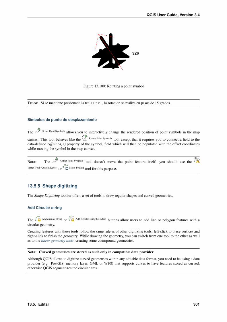
QGIS User Guide, Versión 3.4
Figure 13.100: Rotating a point symbol
Truco: Si se mantiene presionada la tecla Ctrl, la rotación se realiza en pasos de 15 grados.
Símbolos de punto de desplazamiento
The Offset Point Symbols allows you to interactively change the rendered position of point symbols in the map
canvas. This tool behaves like the Rotate Point Symbols tool except that it requires you to connect a field to thedata-defined Offset (X,Y) property of the symbol, field which will then be populated with the offset coordinateswhile moving the symbol in the map canvas.
Nota: The Offset Point Symbols tool doesn’t move the point feature itself; you should use theVertex Tool (Current Layer) or Move Feature tool for this purpose.
13.5.5 Shape digitizing
The Shape Digitizing toolbar offers a set of tools to draw regular shapes and curved geometries.
Add Circular string
The Add circular string or Add circular string by radius buttons allow users to add line or polygon features with acircular geometry.
Creating features with these tools follow the same rule as of other digitizing tools: left-click to place vertices andright-click to finish the geometry. While drawing the geometry, you can switch from one tool to the other as wellas to the linear geometry tools, creating some coumpound geometries.
Nota: Curved geometries are stored as such only in compatible data provider
Although QGIS allows to digitize curved geometries within any editable data format, you need to be using a dataprovider (e.g. PostGIS, memory layer, GML or WFS) that supports curves to have features stored as curved,otherwise QGIS segmentizes the circular arcs.
13.5. Editar 301
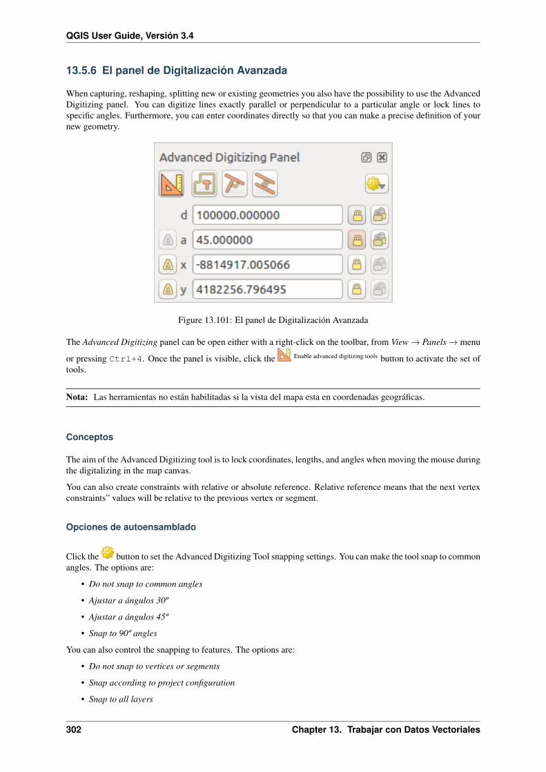
QGIS User Guide, Versión 3.4
13.5.6 El panel de Digitalización Avanzada
When capturing, reshaping, splitting new or existing geometries you also have the possibility to use the AdvancedDigitizing panel. You can digitize lines exactly parallel or perpendicular to a particular angle or lock lines tospecific angles. Furthermore, you can enter coordinates directly so that you can make a precise definition of yournew geometry.
Figure 13.101: El panel de Digitalización Avanzada
The Advanced Digitizing panel can be open either with a right-click on the toolbar, from View → Panels → menu
or pressing Ctrl+4. Once the panel is visible, click the Enable advanced digitizing tools button to activate the set oftools.
Nota: Las herramientas no están habilitadas si la vista del mapa esta en coordenadas geográficas.
Conceptos
The aim of the Advanced Digitizing tool is to lock coordinates, lengths, and angles when moving the mouse duringthe digitalizing in the map canvas.
You can also create constraints with relative or absolute reference. Relative reference means that the next vertexconstraints” values will be relative to the previous vertex or segment.
Opciones de autoensamblado
Click the button to set the Advanced Digitizing Tool snapping settings. You can make the tool snap to commonangles. The options are:
• Do not snap to common angles
• Ajustar a ángulos 30º
• Ajustar a ángulos 45º
• Snap to 90º angles
You can also control the snapping to features. The options are:
• Do not snap to vertices or segments
• Snap according to project configuration
• Snap to all layers
302 Chapter 13. Trabajar con Datos Vectoriales

QGIS User Guide, Versión 3.4
Atajos de teclado
To speed up the use of Advanced Digitizing Panel, there are a couple of keyboard shortcuts available:
Key Simple Ctrl+ or Alt+ Shift+D Establecer distancia Bloquear distanciaA Establecer ángulo Bloquear ángulo Toggle relative angle to last segmentX Set X coordinate Lock X coordinate Toggle relative X to last vertexY Set Y coordinate Lock Y coordinate Toggle relative Y to last vertexC Toggle construction modeP Toggle perpendicular and parallel modes
Absolute reference digitizing
When drawing a new geometry from scratch, it is very useful to have the possibility to start digitizing vertexes atgiven coordinates.
For example, to add a new feature to a polygonal layer, click the button. You can choose the X and Ycoordinates where you want to start editing the feature, then:
• Click the x text box (or use the X keyboard shortcut).
• Type the X coordinate value you want and press Enter or click the button to their right to lock themouse to the X axis on the map canvas.
• Click the y text box (or use the Y keyboard shortcut).
• Type the Y coordinate value you want and press Enter or click the button to their right to lock themouse to the Y axis on the map canvas.
Two blue dotted lines and a green cross identify the exact coordinates you entered. Start digitizing by clicking onthe map canvas; the mouse position is locked at the green cross.
Figure 13.102: Start drawing at given coordinates
You can continue digitizing by free hand, adding a new pair of coordinates, or you can type the segment’s length(distance) and angle.
If you want to draw a segment of a given length, click the d (distance) text box (keyboard shortcut D), type the
distance value (in map units) and press Enter or click the button on the right to lock the mouse in the mapcanvas to the length of the segment. In the map canvas, the clicked point is surrounded by a circle whose radius isthe value entered in the distance text box.
13.5. Editar 303

QGIS User Guide, Versión 3.4
Figure 13.103: Fixed length segment
Finally, you can also choose the angle of the segment. As described before , click the a (angle) text box (keyboard
shortcut A), type the angle value (in degrees), and press Enter or click the buttons on the right to lock it. Inthis way the segment will follow the desired angle:
Figure 13.104: Fixed angle segment
Relative reference digitizing
Instead of using absolute values of angles or coordinates, you can also use values relative to the last digitizedvertex or segment.
For angles, you can click the button on the left of the a text box (or press Shift+A) to toggle relative anglesto the previous segment. With that option on, angles are measured between the last segment and the mouse pointer.
For coordinates, click the buttons to the left of the x or y text boxes (or press Shift+X or Shift+Y) totoggle relative coordinates to the previous vertex. With these options on, coordinates measurement will considerthe last vertex to be the X and Y axes origin.
304 Chapter 13. Trabajar con Datos Vectoriales

QGIS User Guide, Versión 3.4
Continuous lock
Both in absolute or relative reference digitizing, angle, distance, X and Y constraints can be locked continuously
by clicking the Continuous lock buttons. Using continuous lock allows you to digitize several points orvertexes using the same constraints.
Parallel and perpendicular lines
All the tools described above can be combined with the Perpendicular and Parallel tools. These two tools allowdrawing segments perfectly perpendicular or parallel to another segment.
To draw a perpendicular segment, during the editing click the Perpendicular icon (keyboard shortcut P) to ac-tivate it. Before drawing the perpendicular line, click on the segment of an existing feature that you want to beperpendicular to (the line of the existing feature will be colored in light orange); you should see a blue dotted linewhere your feature will be snapped:
Figure 13.105: Perpendicular digitizing
To draw a parallel feature, the steps are the same: click on the Parallel icon (keyboard shortcut P twice), clickon the segment you want to use as reference and start drawing your feature:
These two tools just find the right angle of the perpendicular and parallel angle and lock this parameter duringyour editing.
Modo de construcción
You can enable and disable construction mode by clicking on the Construction icon or with the C keyboardshortcut. While in construction mode, clicking the map canvas won’t add new vertexes, but will capture theclicks” positions so that you can use them as reference points to then lock distance, angle or X and Y relativevalues.
As an example, the construction mode can be used to draw some point at an exact distance from an existing point.
With an existing point in the map canvas and the snapping mode correctly activated, you can easily draw other
points at given distances and angles from it. In addition to the button, you have to activate also the construction
mode by clicking the Construction icon or with the C keyboard shortcut.
13.5. Editar 305

QGIS User Guide, Versión 3.4
Figure 13.106: Parallel digitizing
Click next to the point from which you want to calculate the distance and click on the d box (D shortcut) type thedesired distance and press Enter to lock the mouse position in the map canvas:
Figure 13.107: Distance from point
Before adding the new point, press C to exit the construction mode. Now, you can click on the map canvas, andthe point will be placed at the distance entered.
You can also use the angle constraint to, for example, create another point at the same distance of the original one,
but at a particular angle from the newly added point. Click the Construction icon or with the C keyboard shortcutto enter construction mode. Click the recently added point, and then the other one to set a direction segment. Then,click on the d text box (D shortcut) type the desired distance and press Enter. Click the a text box (A shortcut)type the angle you want and press Enter. The mouse position will be locked both in distance and angle.
Before adding the new point, press C to exit the construction mode. Now, you can click on the map canvas, andthe point will be placed at the distance and angle entered. Repeating the process, several points can be added.
306 Chapter 13. Trabajar con Datos Vectoriales

QGIS User Guide, Versión 3.4
Figure 13.108: Distance and angle from points
Figure 13.109: Points at given distance and angle
13.5. Editar 307

QGIS User Guide, Versión 3.4
13.5.7 The Processing in-place layer modifier
The Processing menu provides access to a large set of tools to analyze and create new features based on theproperties of the input features or their relations with other features (within the same layer or not). While thecommon behavior is to create new layers as outputs, some algorithms also allow modifications to the input layer.This is a handy way to automate multiple features modification using advanced and complex operations.
To edit features in-place:
1. Select the layer to edit in the Layers panel.
2. Select the concerned features. You can skip this step, in which case the modification will apply to the wholelayer.
3. Press the Edit Features In-Place button at the top of the Processing toolbox. The list of algorithms is filtered,showing only those compatible with in-place modifications, i.e.:
• They work at the feature source and not at the layer level.
• They do not change the layer structure, e.g. adding or removing fields.
• They do not change the geometry type, e.g. from line to point layer.
Figure 13.110: Processing algorithms: all (left) vs polygon in-place editors (right)
4. Find the algorithm you’d like to run and double-click it.
308 Chapter 13. Trabajar con Datos Vectoriales

QGIS User Guide, Versión 3.4
Nota: If the algorithm does not need any additional user-set parameters (excluding the usual input andoutput layer parameters), then the algorithm is run immediately without any dialog popup.
(a) If parameters other than the usual input or output layers are needed, the algorithm dialog pops up. Fillin the required information.
(b) Click Modify Selected Features or Modify All Features depending on whether there’s an active selec-tion.
Changes are applied to the layer and placed in the edit buffer: the layer is indeed toggled to editing mode
with unsaved modification as indicated by the icon next to the layer name.
5. As usual, press Save layer edits to commit the changes in the layer. You can also press Undo to rollbackthe whole modification.
13.5. Editar 309

QGIS User Guide, Versión 3.4
310 Chapter 13. Trabajar con Datos Vectoriales

CHAPTER 14
Trabajar con Datos Raster
14.1 Dialogo de Propiedades Raster
To view and set the properties for a raster layer, double click on the layer name in the map legend, or right click onthe layer name and choose Properties from the context menu. This will open the Raster Layer Properties dialog.
There are several tabs in the dialog:
• Information
• Source
• Symbology
• Transparency
• Histogram
• Rendering
• Pyramids
• Metadata
• Legend
• QGIS Server
Truco: Live update rendering
The Layer Styling Panel provides you with some of the common features of the Layer properties dialog and is agood modeless widget that you can use to speed up the configuration of the layer styles and automatically viewyour changes in the map canvas.
Nota: Because properties (symbology, label, actions, default values, forms. . . ) of embedded layers (see Anidarproyectos) are pulled from the original project file and to avoid changes that may break this behavior, the layer
311
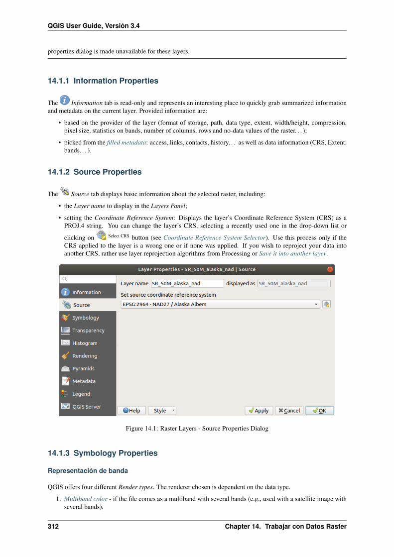
QGIS User Guide, Versión 3.4
properties dialog is made unavailable for these layers.
14.1.1 Information Properties
The Information tab is read-only and represents an interesting place to quickly grab summarized informationand metadata on the current layer. Provided information are:
• based on the provider of the layer (format of storage, path, data type, extent, width/height, compression,pixel size, statistics on bands, number of columns, rows and no-data values of the raster. . . );
• picked from the filled metadata: access, links, contacts, history. . . as well as data information (CRS, Extent,bands. . . ).
14.1.2 Source Properties
The Source tab displays basic information about the selected raster, including:
• the Layer name to display in the Layers Panel;
• setting the Coordinate Reference System: Displays the layer’s Coordinate Reference System (CRS) as aPROJ.4 string. You can change the layer’s CRS, selecting a recently used one in the drop-down list or
clicking on Select CRS button (see Coordinate Reference System Selector). Use this process only if theCRS applied to the layer is a wrong one or if none was applied. If you wish to reproject your data intoanother CRS, rather use layer reprojection algorithms from Processing or Save it into another layer.
Figure 14.1: Raster Layers - Source Properties Dialog
14.1.3 Symbology Properties
Representación de banda
QGIS offers four different Render types. The renderer chosen is dependent on the data type.
1. Multiband color - if the file comes as a multiband with several bands (e.g., used with a satellite image withseveral bands).
312 Chapter 14. Trabajar con Datos Raster

QGIS User Guide, Versión 3.4
2. Paletted/Unique values - for single band files that come with an indexed palette (e.g., used with a digitaltopographic map) or for general use of palettes for rendering raster layers.
3. Singleband gray - (one band of) the image will be rendered as gray; QGIS will choose this renderer if thefile has neither multibands nor an indexed palette nor a continuous palette (e.g., used with a shaded reliefmap).
4. Singleband pseudocolor - this renderer is possible for files with a continuous palette, or color map (e.g.,used with an elevation map).
5. Hillshade - Creates hillshade from a band.
Multiband color
With the multiband color renderer, three selected bands from the image will be rendered, each band representingthe red, green or blue component that will be used to create a color image. QGIS automatically fetches Min andMax values for each band of the raster and scales the coloring accordingly. You can control the value ranges withthe help of the Min/Max Value Settings section.
A Contrast enhancement method can also be applied to the values: “No enhancement”, “Stretch to MinMax”,“Stretch and clip to MinMax” and “Clip to min max”.
Nota: Mejorar contraste
When adding GRASS rasters, the option Contrast enhancement will always be set automatically to stretch to minmax, regardless of if this is set to another value in the QGIS general options.
Figure 14.2: Raster Symbology - Multiband color rendering
Truco: Viewing a Single Band of a Multiband Raster
14.1. Dialogo de Propiedades Raster 313

QGIS User Guide, Versión 3.4
If you want to view a single band of a multiband image (for example, Red), you might think you would set theGreen and Blue bands to Not Set. But this is not the correct way. To display the Red band, set the image type toSingleband gray, then select Red as the Gray band to use.
Paletted/Unique values
This is the standard render option for singleband files that include a color table, where a certain color is assignedto each pixel value. In that case, the palette is rendered automatically.
It can be used for all kinds of raster bands, assigning a color to each unique raster value.
If you want to change a color, just double-click on the color and the Select color dialog appears.
It is also possible to assign labels to the colors. The label will then appear in the legend of the raster layer.
Right-clicking over selected rows in the color table shows a contextual menu to:
• Change Color. . . for the selection
• Change Opacity. . . for the selection
• Change Label. . . for the selection
Figure 14.3: Raster Symbology - Paletted unique value rendering
The pulldown menu, that opens when clicking the . . . (Advanced options) button below the color map to the right,offers color map loading (Load Color Map from File. . . ) and exporting (Export Color Map to File. . . ), and loadingof classes (Load Classes from Layer).
314 Chapter 14. Trabajar con Datos Raster

QGIS User Guide, Versión 3.4
Singleband gray
This renderer allows you to render a single band layer with a Color gradient: “Black to white” or “White to black”.You can define a range of values to color other than the default Min and Max values of the whole raster, thanks tothe Min/Max Value Settings option.
Again, a Contrast enhancement method can be applied to the values: “No enhancement”, “Stretch to MinMax”,“Stretch and clip to MinMax” and “Clip to min max”.
Figure 14.4: Raster Symbology - Singleband gray rendering
Singleband pseudocolor
This is a render option for single-band files that include a continuous palette. You can also create color maps fora bands of a multiband raster.
Using a Band of the layer and a values range, three types of color Interpolation are available:
• Discrete (a <= symbol appears in the value column)
• Lineal
• Exact (an equal symbol appears in the Value column)
The Color ramp drop down list lists the color ramp in your QGIS. You can add a new one, edit or save the oneyou changed. The name of the color ramp will be saved in the configuration and in the QML files.
The Label unit suffix is a label added after the value in the legend.
For the classification Mode “Equal interval”, you only need to select the number of classes and press
the button Classify. In the case of the Mode “Continuous”, QGIS creates classes automatically dependingon the Min and Max.
The button Add values manually adds a value to the individual color table. The button Remove selected row deletes avalue from the individual color table. Double clicking on the value column lets you insert a specific value. Doubleclicking on the color column opens the dialog Change color, where you can select a color to apply on that value.Further, you can also add labels for each color, but this value won’t be displayed when you use the identify featuretool.
Right-clicking over selected rows in the color table shows a contextual menu to:
• Change Color. . . for the selection
• Change Opacity. . . for the selection
You can use the buttons Load color map from file or Export color map to file to load an existing color table or to savethe color table for later use.
The Clip out of range values allows QGIS to not render pixel greater than the Max value.
14.1. Dialogo de Propiedades Raster 315

QGIS User Guide, Versión 3.4
Figure 14.5: Raster Symbology - Singleband pseudocolor rendering
316 Chapter 14. Trabajar con Datos Raster

QGIS User Guide, Versión 3.4
Hillshade
Render a band of the raster layer using hillshading.
Figure 14.6: Raster Symbology - Hillshade rendering
Options:
• Band: The raster band to use.
• Altitude: The elevation angle of the light source (default is 45°).
• Azimuth: The azimuth of the light source (default is 315°).
• Z Factor: Scaling factor for the values of the raster band (default is 1).
• Multidirectional: Specify if multidirectional hillshading is to be used (default is off).
Setting the min and max values
By default, QGIS reports the Min and Max values of the band(s) of the raster. A few very low and/or high valuescan have a negative impact on the rendering of the raster. The Min/Max Value Settings menu helps you control thevalues to render.
Figure 14.7: Raster Symbology - Min and Max Value Settings
Available options are:
14.1. Dialogo de Propiedades Raster 317

QGIS User Guide, Versión 3.4
• User defined: The default Min and Max values of the band(s) can be overridden
• Cumulative count cut: Removes outliers. The standard range of values is 2% to 98%, but can be adaptedmanually.
• Min/max: Uses the whole range of values in the image band.
• Mean +/- standard deviation x: Creates a color table that only considers values within the standard devi-ation or within multiple standard deviations. This is useful when you have one or two cells with abnormallyhigh values in a raster grid that are having a negative impact on the rendering of the raster.
Calculations of the min and max values of the bands are made based on the:
• Statistics extent: it can be Whole raster, Current canvas or Updated canvas. Updated canvas means thatmin/max values used for the rendering will change with the canvas extent (dynamic stretching).
• Accuracy, which can be either Estimate (faster) or Actual (slower).
Nota: For some settings, you may need to press the Apply button of the layer properties dialog in order to displaythe actual min and max values in the widgets.
Color de renderizado
For every Band rendering, a Color rendering is possible.
You can also achieve special rendering effects for your raster file(s) using one of the blending modes (see Modosde Mezcla).
Further settings can be made in modifying the Brightness, the Saturation and the Contrast. You can also use aGrayscale option, where you can choose between “By lightness”, “By luminosity” and “By average”. For one huein the color table, you can modify the “Strength”.
Remuestreo
The Resampling option makes its appearance when you zoom in and out of an image. Resampling modes canoptimize the appearance of the map. They calculate a new gray value matrix through a geometric transformation.
Figure 14.8: Raster Symbology - Color rendering and Resampling settings
When applying the “Nearest neighbour” method, the map can have a pixelated structure when zooming in. Thisappearance can be improved by using the “Bilinear” or “Cubic” method, which cause sharp features to be blurred.The effect is a smoother image. This method can be applied, for instance, to digital topographic raster maps.
At the bottom of the Symbology tab, you can see a thumbnail of the layer, its legend symbol, and the palette.
318 Chapter 14. Trabajar con Datos Raster

QGIS User Guide, Versión 3.4
14.1.4 Transparency Properties
QGIS has the ability to display each raster layer at a different transparency level. Use the transparency slider
to indicate to what extent the underlying layers (if any) should be visible through the currentraster layer. This is very useful if you like to overlay more than one raster layer (e.g., a shaded relief map overlayedby a classified raster map). This will make the look of the map more three dimensional.
Figure 14.9: Raster Transparency
Additionally, you can enter a raster value that should be treated as NODATA in the Additional no data value option.
An even more flexible way to customize the transparency can be done in the Custom transparency options section:
• Use Transparency band to apply transparency on an entire band.
• Provide a list of pixels to make transparent with the corresponding level of transparency:
1. Click the Add values manually button. A new row will appear in the pixel list.
2. Enter the Red, Green and Blue values of the pixel and adjust the Percent Transparent to apply.
3. Alternatively, you can directly fetch the pixel values directly from the raster using theAdd values from display button. Then enter the transparency value.
4. Repeat the steps to adjust more values with custom transparency.
5. Press the Apply button and have a look at the map.
As you can see, it is quite easy to set custom transparency, but it can be quite a lot of work. Therefore, you
can use the button Export to file to save your transparency list to a file. The button Import from file loadsyour transparency settings and applies them to the current raster layer.
14.1. Dialogo de Propiedades Raster 319

QGIS User Guide, Versión 3.4
14.1.5 Histogram Properties
The Histogram tab allows you to view the distribution of the bands or colors in your raster. The histogram isgenerated when you press the Compute Histogram button. All existing bands will be displayed together. You can
save the histogram as an image with the button.
At the bottom of the histogram, you can select a raster band in the drop-down menu and Set min/max style for it.
The Prefs/Actions drop-down menu gives you advanced options to customize the histogram:
• With the Visibility option, you can display histograms of the individual bands. You will need to select the
option Show selected band.
• The Min/max options allow you to “Always show min/max markers”, to “Zoom to min/max” and to “Updatestyle to min/max”.
• The Actions option allows you to “Reset” or “Recompute histogram” after you changed the min or maxvalues of the band(s).
Figure 14.10: Histograma de Ráster
14.1.6 Rendering Properties
In the Rendering tab, it’s possible to:
• apply a Scale dependent visibility to the layer: You can set the Maximum (inclusive) and Minimum (exclu-sive) scale, defining a range of scale in which the layer will be visible. Out of this range, it’s hidden. The
320 Chapter 14. Trabajar con Datos Raster

QGIS User Guide, Versión 3.4
Set to current canvas scale button helps you use the current map canvas scale as boundary of the range visibility.See Renderizado dependiente de la escala for more information.
• Refresh layer at interval (seconds): set a timer to automatically refresh individual layers at a matchinginterval. Canvas updates are deferred in order to avoid refreshing multiple times if more than one layer hasan auto update interval set.
You can set the Maximum (inclusive) and Minimum (exclusive) scale, defining a range of scale in which the layer
will be visible. Out of this range, it’s hidden. The Set to current canvas scale button helps you use the current mapcanvas scale as boundary of the range visibility. See Renderizado dependiente de la escala for more information.
Figure 14.11: Raster Rendering
14.1.7 Pyramids Properties
Large resolution raster layers can slow navigation in QGIS. By creating lower resolution copies of the data (pyra-mids), performance can be considerably improved, as QGIS selects the most suitable resolution to use dependingon the level of zoom.
You must have write access in the directory where the original data is stored to build pyramids.
From the Resolutions list, select resolutions for which you want to create pyramid by clicking on them.
If you choose Internal (if possible) from the Overview format drop-down menu, QGIS tries to build pyramidsinternally.
Nota: Please note that building pyramids may alter the original data file, and once created they cannot beremoved. If you wish to preserve a “non-pyramided” version of your raster, make a backup copy prior to buildingpyramids.
If you choose External and External (Erdas Imagine) the pyramids will be created in a file next to the originalraster with the same name and a .ovr extension.
Several Resampling methods can be used to calculate the pyramids:
• Vecino más próximo
• Promedio
• Gauss
14.1. Dialogo de Propiedades Raster 321

QGIS User Guide, Versión 3.4
• Cúbico
• Cubic Spline
• Laczos
• Modo
• Ninguno
Finally, click Build Pyramids to start the process.
Figure 14.12: Raster Pyramids
14.1.8 Metadata Properties
The Metadata tab provides you with options to create and edit a metadata report on your layer. See vectorlayer metadata properties for more information.
14.1.9 Propiedades de la leyenda
The Legend tab provides you with a list of widgets you can embed within the layer tree in the Layers panel.The idea is to have a way to quickly access some actions that are often used with the layer (setup transparency,filtering, selection, style or other stuff. . . ).
By default, QGIS provides transparency widget but this can be extended by plugins registering their own widgetsand assign custom actions to layers they manage.
14.1.10 QGIS Server Properties
The QGIS Server tab displays a wealth of information about the raster layer, including statistics about eachband in the current raster layer. From this tab, entries may be made for the Description, Attribution, MetadataUrland Properties. In Properties, statistics are gathered on a “need to know” basis, so it may well be that a givenlayer’s statistics have not yet been collected.
322 Chapter 14. Trabajar con Datos Raster

QGIS User Guide, Versión 3.4
Figure 14.13: QGIS Server in Raster Properties
14.2 Análisis raster
14.2.1 Calculadora Ráster
La Calculadora Ráster en el menú Ráster permite realizar cálculos sobre la base de valores de píxeles de unráster existente (vea figure_raster). Los resultados están escritos en una nueva capa ráster con un formato GDAL-reconocido.
The Raster bands list contains all loaded raster layers that can be used. To add a raster to the raster calculatorexpression field, double click its name in the Fields list. You can then use the operators to construct calculationexpressions, or you can just type them into the box.
In the Result layer section, you will need to define an output layer. You can then define the extent of the calculationarea based on an input raster layer, or based on X,Y coordinates and on columns and rows, to set the resolution ofthe output layer. If the input layer has a different resolution, the values will be resampled with the nearest neighboralgorithm.
The Operators section contains all available operators. To add an operator to the raster calculator expression box,click the appropriate button. Mathematical calculations (+, -, *, . . . ) and trigonometric functions (sin, cos,tan, . . . ) are available. Conditional expressions (=, !=, <, >=, . . . ) return either 0 for false or 1 for true, andtherefore can be used with other operators and functions. Stay tuned for more operators to come!
With the Add result to project checkbox, the result layer will automatically be added to the legend area andcan be visualized.
Ejemplos
Convert elevation values from meters to feet
Creating an elevation raster in feet from a raster in meters, you need to use the conversion factor for meters to feet:3.28. The expression is:
"elevation@1" * 3.28
Using a mask
If you want to mask out parts of a raster – say, for instance, because you are only interested in elevations above 0meters – you can use the following expression to create a mask and apply the result to a raster in one step.
14.2. Análisis raster 323

QGIS User Guide, Versión 3.4
Figure 14.14: Calculadora Ráster
324 Chapter 14. Trabajar con Datos Raster

QGIS User Guide, Versión 3.4
("elevation@1" >= 0) * "elevation@1"
In other words, for every cell greater than or equal to 0 the conditional expression evaluates to 1, which keeps theoriginal value by multiplying it by 1. Otherwise the conditional expression evaluates to 0, which sets the rastervalue to 0. This creates the mask on the fly.
Si desea clasificar un ráster –digamos, por ejemplo en dos clases de elevación, puede utilizar la siguiente expresiónpara crear un ráster con dos valores 1 y 2 en un solo paso.
("elevation@1" < 50) * 1 + ("elevation@1" >= 50) * 2
In other words, for every cell less than 50 set its value to 1. For every cell greater than or equal 50 set its value to2.
14.2.2 Raster Alignment
This tool is able to take several rasters as input and to align them perfectly, that means:
• reproyectar al mismo SRC,
• remuestrea al mismo tamaño de celda y desplazamiento en la cuadrícula (grid),
• clip to a region of interest,
• reescale valores cuando sea necesario.
All rasters will be saved in another files.
First, open the tools from Raster → Align Raster. . . and click on the Add new raster button to choose one existingraster in QGIS. Select an output file to save the raster after the alignment, the resampling method and if the toolsneed to Rescale values according to the cell size. The resampling method can be (see figure_raster_align_edit):
• Vecino más próximo
• Bilineal (núcleo 2x2)
• Cubic (4x4 kernel): Cubic Convolution Approximation
• Cubic B-Spline (4x4 kernel): Cubic B-Spline Approximation
• Lanczos (6x6 kernel): Lanczos windowed sinc interpolation
• Average: computes the average of all non-NODATA contributing pixels
• Mode: selects the value which appears most often of all the sampled points
• Maximum, Minimum, Mediane, First Quartile (Q1) or Third Quartile (Q3) of all non-NODATA con-tributing pixels
Nota: Methods like maximum, minimum, mediane, first and third quartiles are available only if QGIS is builtwith GDAL >= 2.0.
In the main Align raster dialog, you can still Edit file settings or Remove an existing file from the list of raster layers.You can also choose one or more other options (see figure_raster_align):
• Select the Reference Layer,
• Transform into a new CRS,
• Setup a different Cell size,
• Setup a different Grid Offset,
• Clip to Extent: it can be user-defined or based on a layer or the map view
• Output Size,
14.2. Análisis raster 325
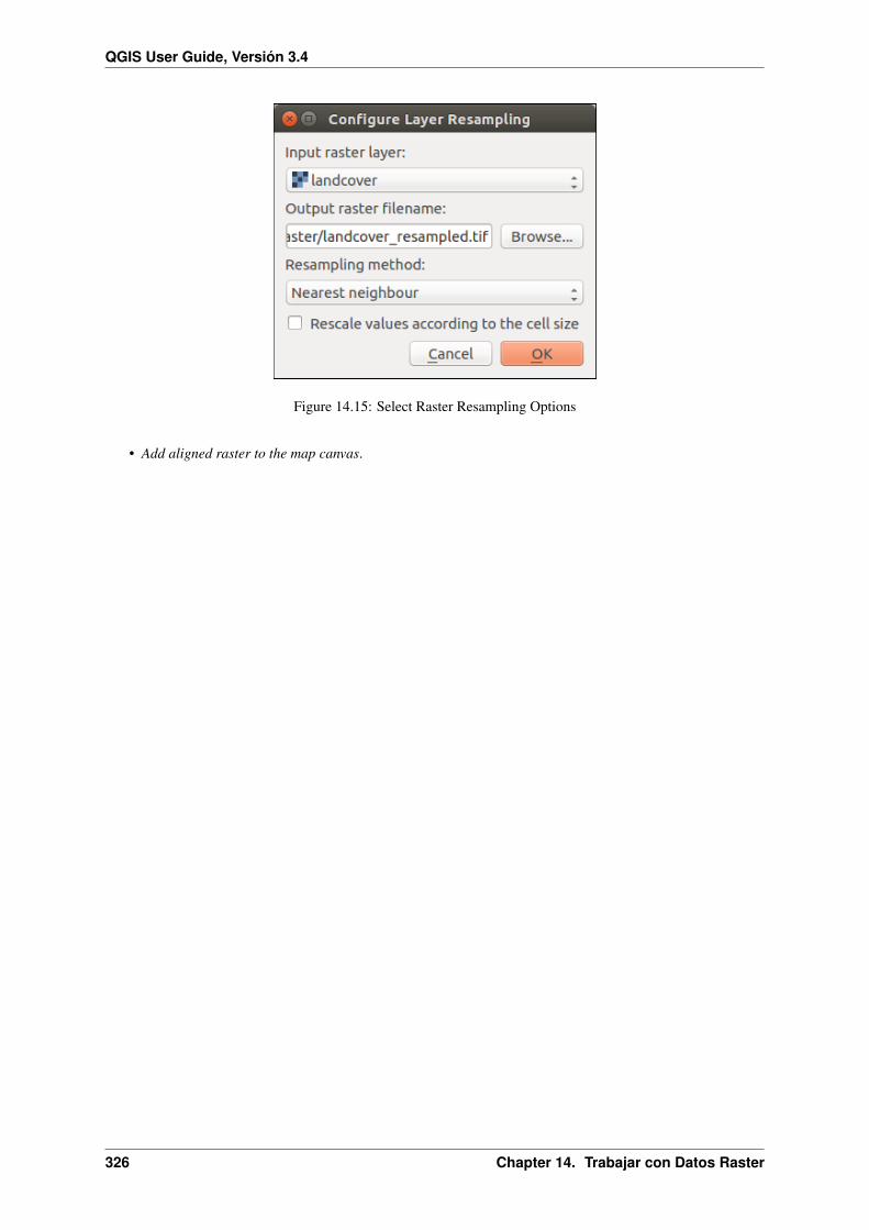
QGIS User Guide, Versión 3.4
Figure 14.15: Select Raster Resampling Options
• Add aligned raster to the map canvas.
326 Chapter 14. Trabajar con Datos Raster

QGIS User Guide, Versión 3.4
Figure 14.16: Raster Alignment
14.2. Análisis raster 327

QGIS User Guide, Versión 3.4
328 Chapter 14. Trabajar con Datos Raster

CHAPTER 15
Trabajando con Malla de Datos
15.1 Trabajando con Malla de Datos
15.1.1 Qué es una malla?
Una malla es una cuadricula no estructurada que usualmente incluye componente temporales y otros. El compo-nente espacial contiene una colección de vértices, bordes y facetas en un espacio 2D o 3D.
• vértices - puntos XY(Z) (en el sistema de referencia de coordenadas de la capa)
• segmento- formado por un par de vértices conectados
• faceta - una faceta es un conjunto de segmentos que producen una forma cerrada - tipicamente un triánguloo un cuadrilátero (cuadros), raramente polígonos con mas vértices
Figure 15.1: Diferentes tipos de Malla
QGIS puede representar actualmente datos de malla usando triángulos o cuadrados regulares.
329

QGIS User Guide, Versión 3.4
Una malla provee información acerca de su estructura espacial. Además, la malla puede tener conjuntos de datos(grupos) asociados que asignan un valor a cada vértice. Por ejemplo, se puede tener una malla triangular convértices numerados como se muestra en la imagen abajo:
Figure 15.2: Malla triangular con vértices numerados
Cada vértice puede tener asociado differentes conjuntos de datos (típicamente múltiples cantidades), y esos con-juntos de datos pueden tener tambien una dimension temporal. Así, un solo achivo puede contener múltiplesconjuntos de datos.
La siguiente tabla brinda una idea acerca de la información que puede ser almacenada en un conjunto de datos demalla. Las columnas de la tabla representan índices de los vértices de la malla, cada fila representa un conjuntode datos. Cada conjunto de datos puede ser de un tipo de datos diferente. En este caso, se almacena velocidad delviento a 10 metros en momentos determinados (t1,t2,t3).
De manera similar, el conjunto de datos de malla puede almacenar valores de vectores para cada vértice. Porejemplo, vectores de dirección del viento en tiempos dados:
Viento a 10 metros 1 2 3 . . .Velocidad a 10 metros en tiempo t=t1 17251 24918 32858 . . .Velocidad a 10 metros en tiempo t=t2 19168 23001 36418 . . .Velocidad a 10 metros en tiempo t=t3 21085 30668 17251 . . .. . . . . . . . . . . . . . .Dirección de viento a 10 metros en tiempo t=t1 [20,2] [20,3] [20,4.5] . . .dirección del viento a 10m en tiempo=t2 [21,3] [21,4] [21,5.5] . . .dirección del viento a 10 metros en tiempo=t3 [22,4] [22,5] [22,6.5] . . .. . . . . . . . . . . . . . .
330 Chapter 15. Trabajando con Malla de Datos

QGIS User Guide, Versión 3.4
Se puede visualizar datos al asignar colores a los valores (de manera similar a como se renderiza un raster Sin-gleband pseudocolor raster rendering) e interpolar datos entre vértices de acuerdo con la topología de la malla.Es común que algunas cantidades sean vectores 2D en lugar de un solo valor escalar (por ejemplo, dirección delviento). Para tales cantidades es deseable desplegar flechas indicando las direcciones.
Figure 15.3: Posible visualización de Datos de Malla
15.1.2 Formatos soportados
QGIS accede a los datos de malla utilizando los controladored de MDAL. Por tanto, los formatos soportados deforma nativa son:
• NetCDF: Formato genérico para datos científicos
• GRIB: Formato comúnmente usado en metereología
• XMDF: Formato de resultado de ciertos paquetes de modelado hidráulico, por ejemplo, TUFLOW
• DAT: Formato de resultado de varios paquetes de modelado hidrodinámico (por ejemplo, BASEMENT,HYDRO_AS-2D, TUFLOW)
• 3Di: Formato convencional en modelado del clima y pronóstico (http://cfconventions.org/)
• Algunos ejemplos de conjunto de datos tipo malla pueden encontrarse en https://apps.ecmwf.int/datasets/data/interim-full-daily/levtype=sfc/
15.1.3 Cargando una capa de malla
Para añadir una capa de malla en QGIS:
1. Abra el cuadro de diálogo Administrador de fuentes de datos, seleccionandolo desde el menú Capa → o
haciendo click en el botón Abrir Administrador de fuentes de datos
2. Luego, active la pestaña Malla en el panel izquierdo
3. Presione el botón . . . para seleccionar el archivo y presione Open. La capa será agregada usando la repre-sentación predeterminada para malla de datos
15.1. Trabajando con Malla de Datos 331

QGIS User Guide, Versión 3.4
Figure 15.4: Pestaña Malla en el Administrador de fuentes de datos
332 Chapter 15. Trabajando con Malla de Datos

QGIS User Guide, Versión 3.4
15.1.4 Propiedades del Conjunto de Datos tipo Malla
Información
Figure 15.5: Propiedades de la Capa Malla
La pestaña Información es de solo lectura y representa un lugar interesante para obtener rápidamente los metadatose información resumida sobre la capa actual. La información proporcionada es (basada en el proveedor de la capa)uri, número de vértices, número de facetas o caras y el número de grupos de conjunto de datos.
Fuente
La pestaña Fuente muestra información básica sobre la capa malla seleccionada, incluyendo:
• el nombre de la Capa para mostrar en el panel Capas
• Establecer el Sistema de Referencia de Coordenadas del origen: Muestra el Sistema de Referencia de Co-ordenadas (CRS) de la capa como una cadena de texto PROJ.4. Se puede cambiar el CRS de la capa al
seleccionar uno usado recientemente en la lista desplegable o haciendo click en el botón Select CRS(vea Coordinate Reference System Selector). Use este proceso solo si el CRS aplicado a la capa es incorrectoo no tiene ninguno asignado.
Use el botón Assign Extra Dataset to Mesh para agregar mas grupos a la capa de malla actual.
Estilo
Haga click en el botón Estilo para activar el cuadro diálogo como se muestra en la siguiente imagen:
Las propiedades de estilo están divididas en diferentes pestañas:
• General
• Contours Symbology
• Vectors Symbology
• Rendering
15.1. Trabajando con Malla de Datos 333
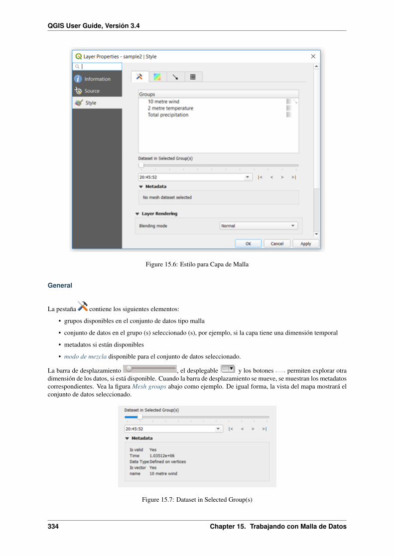
QGIS User Guide, Versión 3.4
Figure 15.6: Estilo para Capa de Malla
General
La pestaña contiene los siguientes elementos:
• grupos disponibles en el conjunto de datos tipo malla
• conjunto de datos en el grupo (s) seleccionado (s), por ejemplo, si la capa tiene una dimensión temporal
• metadatos si están disponibles
• modo de mezcla disponible para el conjunto de datos seleccionado.
La barra de desplazamiento , el desplegable y los botones permiten explorar otradimensión de los datos, si está disponible. Cuando la barra de desplazamiento se mueve, se muestran los metadatoscorrespondientes. Vea la figura Mesh groups abajo como ejemplo. De igual forma, la vista del mapa mostrará elconjunto de datos seleccionado.
Figure 15.7: Dataset in Selected Group(s)
334 Chapter 15. Trabajando con Malla de Datos

QGIS User Guide, Versión 3.4
Se puede aplicar simbología a cada grupo usando las pestañas.
Simbología de Contornos
En Grupos, haga click en para mostrar contornos con los parámetros de visualización predeterminados.
En la pestaña se puede ver y cambiar las opciones actuales de visualización de contornos para el gruposeleccionado, como se muestra en la imagen siguiente Styling contours in a mesh:
Figure 15.8: Aplicando Estilo a Contornos en una Capa de Malla de Datos
Use la barra de desplazamiento o el desplegable para especificar la opacidad del grupo actual.
Use Load para ajustar los valores mínimo y máximo del grupo actual.
La lista Interpolación contiene tres opciones para renderizar contornos: Lineal, Discreto and Exacto.
The Color ramp widget opens the color ramp drop-down shortcut.
La Label unit suffix es una etiqueta agregada despues del valor en la leyenda.
Al seleccionar Continuo en el modo de clasificación Modo, QGIS crea clases de manera automatica considerandolos valores Mín and Máx. Con la opción ‘Intervalo igual’, solo se necesita seleccionar el número de clases usando
15.1. Trabajando con Malla de Datos 335

QGIS User Guide, Versión 3.4
el desplegable Clases y presionar el botón Clasificar.
El botón Añadir valores manualmente agrega un valor a la tabla de colores individuales. El botónEliminar fila(s) seleccionada(s) borra un valor de la tabla de colores individuales. Haciendo doble click sobre un valoren una columna se puede insertar en ella un valor de color específico. El doble clik sobre la columna color abre elcuadro de diálogo Change color, donde se puede seleccionar un color para aplicar en dicho valor.
Simbología de vectores
En la pestaña , haga click sobre para desplegar vectores si están disponibles. La vista del mapa desplegará
los vectores en el grupo seleccionado con los parámetros predeterminados. Haga click en la pestaña paracambiar los parámetros de visualización para vectores como se muestra en la imagen debajo:
Figure 15.9: Aplicando Estilo a Vectores en Capa de Malla de Datos
El ancho de la línea puede especificarse usando el desplegable o escribiendo el valor. El control Change colorabre el cuadro de diálogo de color, donde se puede seleccionar un color para aplicar a los vectores.
Introduzca valores para Min and Max para filtrar los vectores considerando su magnitud.
336 Chapter 15. Trabajando con Malla de Datos

QGIS User Guide, Versión 3.4
Marque en la casilla de verificación Display Vectors on User Grid y especifique el X spacing y el Y spacing,QGIS renderizará los vectores considerando el espaciamiento dado.
Con las opciones de cabeza Head Options, QGIS permite configurar la forma de la flecha al especificar el anchoy longitud (en porcentaje).
La Arrow length de los vectores puede ser renderizada en QGIS en tres formas diferentes:
• Definido por Mínimo and Máximo: se especifica la longitud mínima y máxima para los vectores, QGISajustará su visualización con estos parámetros.
• Escala a magnitud: se especifica el factor multiplicativo a usar
• Fijo: todos los vectores se muestran con la misma longitud
Representación
In the tab , QGIS offers two possibilities to display the grid, as shown in the image Mesh rendering:
• Representación de malla nativa que muestra una grid regular
• Representación de malla triangular que muestra una cuadrícula triángular
Figure 15.10: Representación de Malla
15.1. Trabajando con Malla de Datos 337

QGIS User Guide, Versión 3.4
El ancho y el color de la línea pueden cambiarse en este cuadro de diálogo, y ambas representaciones de cuadrícualpueden desactivarse.
338 Chapter 15. Trabajando con Malla de Datos

CHAPTER 16
Laying out the maps
With Print Layouts and Reports you can create maps and atlases, and print them or save them as image, PDF orSVG files.
16.1 Overview of the Print Layout
The print layout provides growing layout and printing capabilities. It allows you to add elements such as the QGISmap canvas, text labels, images, legends, scale bars, basic shapes, arrows, attribute tables and HTML frames. Youcan size, group, align, position and rotate each element and adjust their properties to create your layout. The layoutcan be printed or exported to image formats, PostScript, PDF or to SVG (export to SVG is not working properlywith some recent Qt4 versions; you should try and check individually on your system). You can save the layout asa template and load it again in another session. Finally, generating several maps based on a template can be donethrough the atlas generator.
16.1.1 Ejemplo de sesión
Before you start to work with the print layout, you need to load some raster or vector layers in the QGIS mapcanvas and adapt their properties to suit your own convenience. After everything is rendered and symbolized
to your liking, click the New Print Layout icon in the toolbar or choose File → New Print Layout. You will beprompted to choose a title for the new layout.
To demonstrate how to create a map please follow the next instructions.
1. On the left side, select the Add new map toolbar button and draw a rectangle on the canvas holding downthe left mouse button. Inside the drawn rectangle the QGIS map view to the canvas.
2. Select the Add new scalebar toolbar button and click with the left mouse button on the print layout canvas.A scalebar will be added to the canvas.
3. Select the Add new legend toolbar button and draw a rectangle on the canvas holding down the left mousebutton. Inside the drawn rectangle the legend will be drawn.
4. Select the Select/Move item icon to select the map on the canvas and move it a bit.
339

QGIS User Guide, Versión 3.4
5. While the map item is still selected you can also change the size of the map item. Click while holding downthe left mouse button, in a white little rectangle in one of the corners of the map item and drag it to a newlocation to change its size.
6. Click the Item Properties panel on the left down side and find the setting for the orientation. Change thevalue of the setting Map orientation to “15.00° “. You should see the orientation of the map item change.
7. Now, you can print or export your print layout to image formats, PDF or to SVG with the export tools inLayout menu.
8. Finally, you can save your print layout within the project file with the Save Project button.
You can add multiple elements to the print layout. It is also possible to have more than one map view or legend orscale bar in the print layout canvas, on one or several pages. Each element has its own properties and, in the caseof the map, its own extent. If you want to remove any elements from the layout canvas you can do that with theDelete or the Backspace key.
16.1.2 The Layout Manager
The Layout Manager is the main window to manage print layouts in the project. It gives you an overview ofexisting print layouts and reports in the project and offers tools to:
• add new print layout or new report from scratch, template or duplicating an existing one;
• rename or delete any of them;
• open them in the project.
To open the layout manager dialog:
• from the main QGIS dialog, select Project → Layout Manager. . . menu or click on the Layout Manager
button in the Project Toolbar;
• from a print layout or report dialog, select Layout → Layout Manager. . . menu or click on theLayout Manager button in the Layout Toolbar.
Figure 16.1: The Print Layout Manager
The layout manager lists in its upper part all the available print layouts or reports in the project with tools to:
• show the selection: you can select multiple reports and/or print layout(s) and open them in one-click.Double-click a name also opens it;
• duplicate the selected print layout or report (available only if one item is selected): it creates a new dialogusing the selected one as template. You’ll be prompted to choose a new title for the new layout;
340 Chapter 16. Laying out the maps

QGIS User Guide, Versión 3.4
• rename the report or layout (available only if one item is selected): you’ll be prompted to choose a new titlefor the layout;
• remove the layout: the selected print layout(s) will be deleted from the project.
In the lower part, it’s possible to create new print layouts or reports from scratch or a template. By default, QGISwill look for templates in the user profile and the application template directories (accessible with the two buttonsat the bottom of the frame) but also in any folder declared as Path(s) to search for extra print templates in Settings→ Options → Layouts. Found templates are listed in the combobox. Select an item and press the Create buttonto generate a new report or print layout.
You can also use layout templates from a custom folder; in that case, select specific in the templates drop-downlist, browse to the template and press Create.
Truco: Creating template-based print layouts from Browser panel
Drag-and-drop a print layout template .qpt file from any file browser onto the map canvas or double-click it inthe Browser panel generates a new print layout from the template.
16.1.3 Menus, tools and panels of the print layout
Opening the print layout provides you with a blank canvas that represents the paper surface when using the printoption. Initially you find buttons on the left beside the canvas to add print layout items: the current QGIS mapcanvas, text labels, images, legends, scale bars, basic shapes, arrows, attribute tables and HTML frames. In thistoolbar you also find buttons to navigate, zoom in on an area and pan the view on the layout a well as buttons toselect any layout item and to move the contents of the map item.
figure_layout_overview shows the initial view of the print layout before any elements are added.
Figure 16.2: Print Layout
On the right beside the canvas you find two set of panels. The upper one holds the panels Items and Undo Historyand the lower holds the panels Layout, Item properties and Atlas generation.
16.1. Overview of the Print Layout 341

QGIS User Guide, Versión 3.4
• The Items panel provides a list of all the print layout items added to the canvas and ways to globally interactwith them (see The Items Panel for more information).
• The Undo History panel displays a history of all changes applied to the layout. With a mouse click, it ispossible to undo and redo layout steps back and forth to a certain status.
• The Layout panel allows you to set general parameters to apply to the layout when exporting or workingwithin (see The Layout Panel for more details);
• The Item Properties panel displays the properties for the selected item. Click the Select/Move item iconto select an item (e.g., legend, scale bar or label) on the canvas. Then click the Item Properties panel andcustomize the settings for the selected item (see Layout Items for detailed information on each item settings).
• The Atlas panel allows you to enable the generation of an atlas for the current layout and gives access to itsparameters (see Generar un Atlas for detailed information on atlas generation usage).
In the bottom part of the print layout window, you can find a status bar with mouse position, current page number,a combo box to set the zoom level, the number of selected items if applicable and, in the case of atlas generation,the number of features.
In the upper part of the print layout window, you can find menus and other toolbars. All print layout tools areavailable in menus and as icons in a toolbar.
The toolbars and the panels can be switched off and on using the right mouse button over any toolbar or throughView → Toolbars → or View → Panels →.
Menus and Tools
Layout menu
The Layout provides action to manage the layout:
• Save the project file directly from the print layout window.
• Create a new and blank print layout with New Layout. . . .
• Duplicate Layout. . . : Create a new print layout by duplicating the current one.
• Remove the current layout with Delete Layout. . . .
• Open the Layout Manager. . . .
• Layouts → : Open an existing print layout.
Once the layout is designed, with Save as Template and Add Items from Template icons, you can savethe current state of a print layout session as a .qpt template file and load its items again in another session/printlayout.
In the Layout menu, there are also powerful ways to share geographical information produced with QGIS that can
be included in reports or published. These tools are Export as Image. . . , Export as PDF. . . , Export
as SVG. . . and Print. . . .
Below is a list of all the available tools in this menu with some convenient information.
342 Chapter 16. Laying out the maps

QGIS User Guide, Versión 3.4
Tool Shortcut Toolbar Reference
Save Project Ctrl+S Layout Introducing QGIS projects
New Layout Ctrl+N Layout The Layout Manager
Duplicate Layout Layout The Layout Manager
Delete Layout
Layout Manager. . . Layout The Layout ManagerLayouts →Layout Properties. . . The Layout PanelRename Layout. . .
Add Pages. . . Layout Working with the page properties
Add Items from Template Layout Creating a layout item
Save as Template. . . Layout The Layout Manager
Export as Image. . . Layout Export as Image
Export as SVG. . . Layout Exportar como SVG
Export as PDF. . . Layout Exportar como PDFPage Setup. . . Ctrl+Shift+P
Print. . . Ctrl+P Layout Crear salidaClose Ctrl+Q
Edit menu
The Edit menu offers tools to manipulate print layout items. It includes common actions like selection tools,Copy/Cut/Paste and undo/redo (see The Undo History Panel: Revert and Restore actions) functionality for theitems in the layout.
When using the Paste action, the elements will be pasted according to the current mouse position. Using theEdit → Paste in Place action or pressing Ctrl+Shift+V will paste the items into the current page, at the sameposition they were in their initial page. It ensures to copy/paste items at the same place, from page to page.
Below is a list of all the available tools in this menu with some convenient information.
16.1. Overview of the Print Layout 343

QGIS User Guide, Versión 3.4
Tool Shortcut Tool-bar
Reference
Undo (last change) Ctrl+Z Layout The Undo History Panel: Revert and Restore ac-tions
Redo (last revertedchange)
Ctrl+Y Layout The Undo History Panel: Revert and Restore ac-tions
Delete Del
Cut Ctrl+X
Copy Ctrl+C
Paste Ctrl+VPaste in place Ctrl+Shift+V
Select All Ctrl+A
Deselect all Ctrl+Shift+A
Invert SelectionSelect Next Item Below Ctrl+Alt+[Select Next Item above Ctrl+Alt+]
Pan Layout P Tool-box
Zoom Z Tool-box
Select/Move Item V Tool-box
Interacting with layout items
Move Content C Tool-box
El elemento del mapa
Edit Nodes Item Tool-box
The Node-Based Shape Items
View menu
The View menu gives access to navigation tools and helps to configure general behavior of the print layout. Besidethe common zoom tools, you have means to:
• Refresh view (if you find the view in an inconsistent state);
• enable a grid you could snap items to when moving or creating them. Grids setting is done in Settings →Layout Options. . . or in the Layout Panel;
• enable guides you could snap items to when moving or creating them. Guides are red lines that you cancreate by clicking in the ruler (above or at the left side of the layout) and drag and drop to the desiredlocation;
• Smart Guides: uses other layout items as guides to dynamically snap to as you move or reshape an item;
• Clear Guides to remove all current guides;
• Show Bounding box around the items to better identify your selection;
• Show Rules around the layout;
• Show Pages or set up pages to transparent. Often layout is used to create non-print layouts, e.g. for inclusionin presentations or other documents, and it’s desirable to export the composition using a totally transparent
344 Chapter 16. Laying out the maps

QGIS User Guide, Versión 3.4
background. It’s sometimes referred to as «infinite canvas» in other editing packages.
In the print layout, you can change the zoom level using the mouse wheel or the slider and combo boxin the status bar. If you need to switch to pan mode while working in the layout area, you can hold theSpacebar or the mouse wheel. With Ctrl+Spacebar, you can temporarily switch to Zoom In mode, andwith Ctrl+Alt+Spacebar, to Zoom Out mode.
Panels and toolbars can be enabled from the View → menu. To maximise the space available to interact with a
composition you can check the View → Toggle Panel Visibility option or press Ctrl+Tab; all panels arehidden and only previously visible panels are restored when unchecked.
It’s also possible to switch to a full screen mode to have more space to interact with by pressing F11 or using
View → Toggle Full Screen.
Tool Shortcut Toolbar Reference
Refresh F5 NavigationPreview →
Zoom In Ctrl++ Navigation
Zoom Out Ctrl+- Navigation
Zoom to 100% Ctrl+1 Navigation
Zoom Full Ctrl+0 NavigationZoom to Width
Show Grid Ctrl+' Guides and Grid
Snap to Grid Ctrl+Shift+' Guides and Grid
Show Guides Ctrl+; Guides and Grid
Snap to Guides Ctrl+Shift+; Guides and Grid
Smart Guides Ctrl+Alt+;Manage Guides. . . The Guides PanelClear Guides The Guides Panel
Show Rulers Ctrl+R
Show Bounding Boxes Ctrl+Shift+B
Show PagesToolbars → Paneles y Barras de HerramientasPanels → Paneles y Barras de Herramientas
Toggle Full Screen F11 Ver
Toggle Panel Visibility Ctrl+Tab Ver
Items menu
The Items helps you configure items” position in the layout and the relations between them (see Interacting withlayout items).
16.1. Overview of the Print Layout 345

QGIS User Guide, Versión 3.4
Tool Shortcut Toolbar Reference
Group Ctrl+G Actions Grouping items
Ungroup Ctrl+Shift+G Actions Grouping items
Raise Ctrl+] Actions Alineación
Lower Ctrl+[ Actions Alineación
Bring to Front Ctrl+Shift+] Actions Alineación
Send to Back Ctrl+Shift+[ Actions Alineación
Lock Selected Items Ctrl+L Actions Locking items
Unlock All Ctrl+Shift+L Actions Locking itemsAlign Items → Actions AlineaciónDistribute Items → Actions Moving and resizing itemsResize → Actions Moving and resizing items
Add Item menu
These are tools to create layout items. Each of them is deeply described in Layout Items chapter.
Tool Toolbar Reference
Add Map Toolbox El elemento del mapa
Add Picture Toolbox The Picture Item
Add Label Toolbox El elemento etiqueta
Add Legend Toolbox El elemento leyenda
Add Scale Bar Toolbox El elemento de barra de escala
Add Shape → Toolbox The Regular Shape Item
Add Arrow Toolbox El elemento flecha
Add Node Item → Toolbox The Node-Based Shape Items
Add HTML Toolbox El elemento del marco HTML
Add Attribute Table Toolbox El elemento de Tabla de Atributos
346 Chapter 16. Laying out the maps

QGIS User Guide, Versión 3.4
Atlas menu
Tool Shortcut Toolbar Reference
Preview Atlas Ctrl+ALt+/ Atlas Preview and generate an atlas
First Feature Ctrl+< Atlas Preview and generate an atlas
Previous Feature Ctrl+, Atlas Preview and generate an atlas
Next Feature Ctrl+. Atlas Preview and generate an atlas
Last feature Ctrl+> Atlas Preview and generate an atlas
Print Atlas. . . Atlas Preview and generate an atlas
Export Atlas as Images. . . Atlas Preview and generate an atlas
Export Atlas as SVG. . . Atlas Preview and generate an atlas
Export Atlas as PDF. . . Atlas Preview and generate an atlas
Atlas Settings Atlas Generar un Atlas
Menú Configuración
The Settings → Layout Options. . . menu is a shortcut to Settings → Options → Layouts menu of QGIS maincanvas. Here, you can set some options that will be used as default on any new print layout:
• Layout defaults let you specify the default font to use;
• With Grid appearance, you can set the grid style and its color. There are three types of grid: Dots, Solidlines and Crosses;
• Grid and guide defaults defines spacing, offset and tolerance of the grid (see Guides and Grid for moredetails);
• Layout Paths: to manage list of custom paths to search print templates.
Contextual menus
Depending on where you right-click in the print layout dialog, you open a contextual menu with various features:
• Right-click on the menu bar or any toolbar and you get the list of layout panels and toolbars you can enableor disable in one-click.
• Right-click over a ruler and you can Show Guides, Snap to Guides, Manage Guides. . . opening theGuides panel or Clear Guides. It’s also possible to hide the rulers.
• Right-click in the print layout canvas and:
– You’ll be able to Undo and Redo recent changes, or Paste any copied item (only available if no item isselected).
– If you click over a page, you can additionally access the current Page Properties panel or RemovePage.
– If you click on a selected item then you can cut or copy it as well as open the Item Properties panel.
– If more than one item are selected, then you can either group them and/or ungroup if at least one groupis already in the selection.
• Right-click inside a text box or spinbox widget of any layout panel provides edit options to manipulate itscontent.
16.1. Overview of the Print Layout 347

QGIS User Guide, Versión 3.4
The Layout Panel
In the Layout panel, you can define the global settings of your print layout.
Figure 16.3: Layout Settings in the Print Layout
General settings
In a print layout, you can use more than one map item. The Reference map selects the map item to be used as thelayout’s master map. The layout will use this map in any properties and variable calculating units or scale. Thisincludes exporting the print layout to georeferenced formats.
Guides and Grid
You can put some reference marks on your paper sheet to help you accurately place some items. These marks canbe:
• simple horizontal or vertical lines (called Guides) put at the position you want (see The Guides Panel forguides creation).
• or regular Grid: a network of horizontal and vertical lines superimposed over the layout.
348 Chapter 16. Laying out the maps
QGIS User Guide, Versión 3.4
Settings like Grid spacing or Grid offset can be adjusted in this group as well as the Snap tolerance to use foritems. The tolerance is the maximum distance below which the mouse cursor is snapped to a grid or a guide, whilemoving, resizing or creating an item.
Whether grid or guides should be shown is set in View menu. There, you can also decide if they might be used tosnap layout items. When both a grid line and a guide line are within tolerance of a point, guides will always takeprecedence - since they have been manually set (hence, assumption that they have been explicitly placed at highlydesirable snapping locations, and should be selected over the general grid).
Nota: In the Settings → Layout Options menu, you can also set the grid and guides parameters exposed above.However, these options will only apply as defaults to new print layouts.
Configuración de exportación
You can define a resolution to use for all exported maps in Export resolution. This setting can then be overriddeneach time you export a map.
Because of some advanced rendering options (blending mode, effects. . . ), a layout item may need rasterizationin order to be exported correctly. QGIS will individually rasterize it without forcing every other item to also berasterized. This allows printing or saving as PostScript or PDF to keep items as much as possible as vectors, e.g.a map item with layer opacity won’t force labels, scale bars, etc to be rasterized too. You can however:
• force all the items to be rasterized checking the Print as raster box;
• or use the opposite option, i.e. Always export as vectors, to force the export to keep items as vectors whenexported to a compatible format. Note that in some cases, this could cause the output to look different tolayout.
Where the format makes it possible (e.g., .TIF, .PDF) exporting a print layout results by default in a georef-erenced file (based on the Reference map item in the General settings group). For other formats, georeferenced
output requires you to generate a world file by checking Save world file. The world file is created besidethe exported map(s), has the name of the page output with the reference map item and contains information togeoreference it easily.
Resize layout to content
Using the Resize page tool in this group, you create a unique page composition whose extent covers the currentcontents of the print layout (with some optional margins around the cropped bounds).
Note that this behavior is different from the crop to content option in that all the items are placed on a real andunique page in replacement of all the existing pages.
Variables
The Variables lists all the variables available at the layout’s level (which includes all global and project’s variables).
It also allows the user to manage layout-level variables. Click the button to add a new custom layout-level
variable. Likewise, select a custom layout-level variable from the list and click the button to remove it.
More information on variables usage in the General Tools section.
Working with the page properties
A layout can be composed of several pages. For instance, a first page can show a map canvas, and a second pagecan show the attribute table associated with a layer, while a third one shows an HTML frame linking to your
16.1. Overview of the Print Layout 349

QGIS User Guide, Versión 3.4
Figure 16.4: Variables Editor in the Print Layout
organization website. Or you can add many types of items on each page.
Adding a new page
Futhermore, a layout can be made using different size and/or orientation of pages. To add a page, select theAdd Pages. . . tool from the Layout menu or Layout Toolbar. The Insert Pages dialog opens and you are asked tofill:
• the number of pages to insert;
• the position of the page(s): before or after a given page or at the end of the print layout;
• The Page size: it could be of a preset format page (A4, B0, Legal, Letter, ANSI A, Arch A and theirderivatives as well as a resolution type, such as 1920x1080 or 1024x768) with associated Orientation(Portrait or Landscape).
The page size can also be of a custom format; In that case, you’d need to enter its Width and Height (withlocked size ratio if needed) and select the unit to use among mm, cm, px, pt, in, ft. . . Conversion ofentered values is automatically applied when switching from one unit to another.
Figure 16.5: Creating a new page in the Print Layout
350 Chapter 16. Laying out the maps

QGIS User Guide, Versión 3.4
Updating page properties
Any page can be later customized through the Page Item Properties panel. Right-click on a page and select PageProperties. . . . The Item Properties panel opens with settings such as:
• the Page size frame described above. You can modify each property using the data defined override options(see Explore Data-defined override buttons with atlas for a use case);
• the Exclude page from exports to control whether the current page with its content should be includedin the layout output;
• the Background using the color or symbol you want.
Figure 16.6: Page properties dialog
The Guides Panel
Guides are vertical or horizontal line references you can place on a layout page to assist you on items placement,when creating, moving or resizing them. To be active, guides require the View → Show Guides and View → Snapto Guides options to be checked. To create a guide, two ways:
• assuming View → Show Rulers option is set, drag out a ruler and release the mouse button within the pagearea, at the desired position.
• more accurate and always available, use the Guides panel.
The Guides panel allows creation of snap lines at specific locations: click the Add new guide button and entercoordinates of the horizontal or vertical line. Different units are available for setting. The panel also allowsadjusting position of existing guides to exact coordinates: double-click a guide coordinate and replace the value.
To delete a guide, select it and press Remove selected guide button. Use Clear All Guides to remove all the guidesin the panel.
Guides are single page only meaning that the Guides panel lists guides of the current page (whose number isshown at the top of the dialog). Likewise, it allows creation or removal of guides only in the current page. TheApply to All Pages button allows you to setup the guide configuration on a single page and easily transfer it to allother pages in the layout.
Truco: Snapping to existing layout items
Other than guides and grids, you can use existing items as snapping references when moving, resizing or creatingnew items; these are called smart guides and require View → Smart Guides option to be checked. Anytime themouse pointer is close to an item’s bound, a snapping cross appears.
16.1. Overview of the Print Layout 351

QGIS User Guide, Versión 3.4
Figure 16.7: The Guides panel
The Items Panel
The Items panel offers some options to manage selection and visibility of items. All the items added to the printlayout canvas (including items group) are shown in a list and selecting an item makes the corresponding rowselected in the list as well as selecting a row does select the corresponding item in the print layout canvas. This isthus a handy way to select an item placed behind another one. Note that a selected row is shown as bold.
For any selected item, you can :
• set it visible or not;
• lock or unlock its position;
• sort its Z position. You can move up and down each item in the list with a click and drag. The upper itemin the list will be brought to the foreground in the print layout canvas. By default, a newly created item isplaced in the foreground.
• change the item ID by double-clicking the text;
• right-click an item and copy or delete it or open its properties panel.
Once you have found the correct position for an item, you can lock it by ticking the box in column. Lockeditems are not selectable on the canvas. Locked items can be unlocked by selecting the item in the Items panel andunchecking the tickbox or you can use the icons on the toolbar.
The Undo History Panel: Revert and Restore actions
During the layout process, it is possible to revert and restore changes. This can be done with the revert and restoretools available in the Edit menu, the Layout toolbar or the contextual menu any time you right-click in the printlayout area:
• Revert last change
352 Chapter 16. Laying out the maps

QGIS User Guide, Versión 3.4
• Restore last change
This can also be done by mouse click within the Undo history panel (see figure_layout). The History panel liststhe last actions done within the print layout. Just select the point you want to revert to and once you do new actionall the actions done after the selected one will be removed.
Figure 16.8: Undo History in the Print Layout
16.2 Layout Items
16.2.1 Layout Items Common Options
QGIS provides a large set of items to layout a map. They can be of map, legend, scale bar, picture, table, northarrow, image type. . . They however share some common options and behavior that are exposed below.
Creating a layout item
Items can be created using different tools, either from scratch or based on existing items.
To create a layout item from scratch:
1. Select the corresponding tool either from the Add Item menu or the Toolbox bar.
2. Then:
• Click on the page and fill the size and placement information requested in the New Item Propertiesdialog that pops up (for details, see Position and Size);
Figure 16.9: New Item properties dialog
• Or click-and-drag to define the initial size and placement of the item. You can rely on grids and guidessnapping for a better position.
16.2. Layout Items 353

QGIS User Guide, Versión 3.4
Nota: Because they can have particular shapes, drawing node or arrow items does not work with one-click norclick-and-drag methods; you need to click and place each node of the item. See The Node-Based Shape Items formore details.
You can also:
1. Select an existing item with the Select/Move item button from the Toolbox toolbar
2. Use the contextual menu or the Edit menu tools to copy/cut the item and paste it at the mouse position as anew item.
You can also use the Paste in Place (Ctrl+Shift+V) command to duplicate an item from one page toanother and place it in the new page at the same coordinates as the original.
Moreover, you can create items using a print layout template (for details, see The Layout Manager) through theLayout → Add Items from Template. . . command.
Truco: Add layout items using the file browser
From your file browser or using the Browser panel, drag-and-drop a print layout template (.qpt file) onto a printlayout dialog and QGIS automatically adds all items from that template to the layout.
Interacting with layout items
Each item inside the print layout can be moved and resized to create a perfect layout. For both operations the first
step is to activate the Select/Move item tool and click on the item.
You can select multiple items with the Select/Move item button: click and drag over the items or hold the Shiftbutton and click on each of the items you want. To deselect an item, click on it holding the Shift button.
Each time there’s a selection, count of selected items is displayed on the status bar. Inside the Edit menu, you canfind actions to select all the items, clear all selections, invert the current selection and more. . .
Moving and resizing items
Unless View → Show Bounding Boxes option is unchecked, a selected item will show squares on its boundaries ;moving one of them with the mouse will resize the item in the corresponding direction. While resizing, holdingShift will maintain the aspect ratio. Holding Alt will resize from the item center.
To move a layout item, select it with the mouse and move while holding the left button. If you need to constrainthe movements to the horizontal or vertical axis, just hold the Shift button on the keyboard while moving themouse. You can also move a selected item using the Arrow keys on the keyboard; if the movement is tooslow, you can speed it up by holding Shift. If you need better precision, use the Position and size properties, orgrid/guides snapping as explained above for item’s creation.
Resizing or moving several items at once is made the same way as for a single item. QGIS however provides someadvanced tools to automatically resize a selection of items following different rules:
• each item height matches the tallest or the shortest selected item;
• each item width matches the widest or the narrowest selected item;
• resizes items to squares: each item is enlarged to form a square.
Likewise, automated tools are available to organize multiple items position by distributing equidistantly:
• edges (left, right, top or bottom) of items;
354 Chapter 16. Laying out the maps

QGIS User Guide, Versión 3.4
• centers of items either horizontally or vertically.
Grouping items
Grouping items allows you to manipulate a set of items like a single one: you can easily resize, move, delete, copythe items as a whole.
To create a group of items, select more than one and press the Group button on the View menu or the Actionstoolbar or from the right-click menu. A row named Group is added to the Items panel and can be locked or hiddenlike any other Items panel’s object. Grouped items are not individually selectable on the canvas; use the Itemspanel for direct selection and access the item’s properties panel.
Locking items
Once you have found the correct position for an item, you can lock it by using the Lock selected items buttonin the View menu or the Actions toolbar or ticking the box next to the item in the Items panel. Locked items arenot selectable on the canvas.
Locked items can be unlocked by selecting the item in the Items panel and unchecking the tickbox or you can usethe icons on the toolbar.
Alineación
Raising or lowering the visual hierarchy for elements are inside the Raise selected items pull-down menu. Choosean element on the print layout canvas and select the matching functionality to raise or lower the selected elementcompared to the other elements. This order is shown in the Items panel. You can also raise or lower objects in theItems panel by clicking and dragging an object’s label in this list.
Figure 16.10: Alignment helper lines in the print layout
16.2. Layout Items 355

QGIS User Guide, Versión 3.4
There are several alignment options available within the Align selected items pull-down menu (see fig-ure_layout_common_align). To use an alignment function, you first select the elements and then click on oneof the alignment icons:
• Align Left or Align Right;
• Align Top or Align Bottom;
• Align Center horizontally or Align Center Vertical.
All selected elements will then be aligned to their common bounding box. When moving items on the layoutcanvas, alignment helper lines appear when borders, centers or corners are aligned.
Items Common Properties
Layout items have a set of common properties you will find at the bottom of the Item Properties panel: Positionand size, Rotation, Frame, Background, Item ID, Variables and Rendering (See figure_layout_common).
Figure 16.11: Common Item Properties groups
Nota: The Data defined override icon next to most of the options means that you can associate that property witha layer, features attributes, geometry or with any other layout item’s property, using expressions or variables. For
356 Chapter 16. Laying out the maps

QGIS User Guide, Versión 3.4
more information see Configuración de anulación definida por datos.
• The Position and size group lets you define the size and position of the frame which contains the item (seePosition and Size for more information).
• The Rotation sets the rotation of the element (in degrees).
• The Frame shows or hides the frame around the item. Click on the Color and Thickness and Join stylewidgets to adjust those properties.
• Use the Background color menu for setting a background color. Click on the [Color. . . ] button to display adialog where you can pick a color or choose from a custom setting. Transparency can be adjusted throughaltering the alpha field settings.
• Use the Item ID to create a relationship to other print layout items. This is used with QGIS server and otherpotential web clients. You can set an ID on an item (for example, a map or a label), and then the web clientcan send data to set a property (e.g., label text) for that specific item. The GetProjectSettings command willlist the items and IDs which are available in a layout.
• Rendering mode helps you set whether and how the item can be displayed: you can, for instance, applyblending mode, adjust the opacity of the item or Exclude item from exports.
Position and Size
Extending the features of the New Item Properties dialog with data-defined capabilities, this group allows you toplace the items accurately.
Figure 16.12: New Item properties dialog
• the actual number of the page to place the item on;
• the reference point of the item;
• the X and Y coordinates of the Reference point of the item on the chosen page. The ratio between these
values can be locked by clicking on the button. Changes made to a value using the widget or theSelect/Move item tool will be reflected in both of them;
• the Width and Height of the item bounding box. As for coordinates, the ratio between width and height canbe locked.
Modo de representación
QGIS allows advanced rendering for layout items just like vector and raster layers.
16.2. Layout Items 357

QGIS User Guide, Versión 3.4
Figure 16.13: Modo de representación
• Blending mode: With this tool you can achieve effects which would otherwise only be achieved usinggraphic rendering software. The pixels of your overlaying and underlaying items can be mixed accordingto the mode set (see Modos de Mezcla for description of each effect).
• Transparency : You can make the underlying item in the layout visible with this tool.Use the slider to adapt the visibility of your item to your needs. You can also make a precise definition ofthe percentage of visibility in the menu beside the slider.
• Exclude item from exports: You can decide to make an item invisible in all exports. After activating thischeckbox, the item will not be included in export to PDF, print etc..
Variables
The Variables lists all the variables available at the layout item’s level (which includes all global, project andcomposition’s variables). Map items also include Map settings variables that provide easy access to values likethe map’s scale, extent, and so on.
In Variables, it’s also possible to manage item-level variables. Click the button to add a new custom variable.
Likewise, select any custom item-level variable from the list and click the button to remove it.
More information on variables usage in the Storing values in Variables section.
16.2.2 El elemento del mapa
The map item is the main frame that displays the map you’ve designed in the map canvas. Use the Add Maptool following items creation instructions to add a new map item that you can later manipulate the same way asexposed in Interacting with layout items.
By default, a new map item shows the current status of the map canvas with its extent and visible layers. Youcan customize it thanks to the Item Properties panel. Other than the items common properties, this feature has thefollowing functionalities:
Propiedades principales
In the Main properties group (see figure_layout_map) of the map Item Properties panel, available options are:
• The Update Preview button to refresh the map item rendering if the view in map canvas has been modified.Note that most of the time, the map item refresh is automatically triggered by the changes;
• The Scale to manually set the map item scale;
• The Map rotation allows you to rotate the map item content clockwise in degrees. The rotation of the mapcanvas can be imitated here;
• The CRS allows you to display the map item content in any CRS. It defaults to Use project CRS;
• Draw map canvas items lets you show in the print layout annotations that are placed on the main mapcanvas.
358 Chapter 16. Laying out the maps

QGIS User Guide, Versión 3.4
Figure 16.14: Map Item Properties Panel
Layers
By default, map item appearance is synced with the map canvas rendering meaning that toggling visibility of thelayers or modifying their style in the Layers Panel is automatically applied to the map item. Because, like anyother item, you may want to add multiple map items to a print layout, there’s a need to break this synchronizationin order to allow showing different areas, layer combinations, at different scales. . . The Layers properties group(see figure_layout_map_layers) helps you do that.
Figure 16.15: Map Layers group
If you want to keep the map item consistent with an existing map theme, check Follow map theme and selectthe desired theme in the drop-down list. Any changes applied to the theme in QGIS” main window (using thereplace theme function) will automatically affect the map item. If a map theme is selected, the Lock styles forlayers option is disabled because Follow map theme also updates the style (symbology, labels, diagrams) of thelayers.
16.2. Layout Items 359

QGIS User Guide, Versión 3.4
To lock the layers shown in a map item to the current map canvas visibility, check Lock layers. When thisoption is enabled, any changes on the layers” visibility in QGIS” main window will not affect the layout’s mapitem. Nevertheless, style and labels of locked layers are still refreshed according to QGIS” main window. You canprevent this by using Lock styles for layers.
Instead of using the current map canvas, you can also lock the layers of the map item to those of an existing
map theme: select a map theme from the Set layer list from a map theme drop-down button, and the Lock layers isactivated. The set of visible layers in the map theme is from now on used for the map item until you select another
map theme or uncheck the Lock layers option. You then may need to refresh the view using the Refresh view
button of the Navigation toolbar or the Update Preview button seen above.
Note that, unlike the Follow map theme option, if the Lock layers option is enabled and set to a map theme, thelayers in the map item will not be refreshed even if the map theme is updated (using the replace theme function)in QGIS” main window.
Locked layers in the map item can also be data-defined, using the icon beside the option. When used, thisoverrides the selection set in the drop-down list. You need to pass a list of layers separated by | character. Thefollowing example locks the map item to use only layers layer 1 and layer 2:
concat ('layer 1', '|', 'layer 2')
Extensión
The Extents group of the map item properties panel provides the following functionalities (see fig-ure_layout_map_extents):
Figure 16.16: Map Extents group
The Extents area displays X and Y coordinates of the area shown in the map item. Each of these values canbe manually replaced, modifying the map canvas area displayed and/or map item size. Clicking the Set to MapCanvas Extent button sets the extent of the layout map item to the extent of the main map canvas. The button ViewExtent in Map Canvas does exactly the opposite; it updates the extent of the main map canvas to the extent of thelayout map item.
You can also alter a map item extent using the Move item content tool: click-and-drag within the map item to
modify its current view, keeping the same scale. With the tool enabled, use the mouse wheel to zoom in orout, modifying the scale of the shown map. Combine the movement with Ctrl key pressed to have a smallerzoom.
Controlled by atlas
The Controlled by atlas group properties is available only if an atlas is active in the print layout. Check thisoption if you want the map item being ruled by the atlas; when iterating over the coverage layer, the map itemextent is panned/zoomed to the atlas feature following:
360 Chapter 16. Laying out the maps

QGIS User Guide, Versión 3.4
• Margin around features: zooms to the feature at the best scale, keeping around each a margin repre-senting a percentage of the map item width or height. The margin can be the same for all features or setvariable, e.g., depending on map scale;
• Predefined scale (best fit): zooms to the feature at the project predefined scale where the atlas featurebest fits;
• Fixed scale: atlas features are panned from one to another, keeping the same scale of the map item.Ideal when working with features of same size (e.g., a grid) or willing to highlight size differences amongatlas features.
Cuadrículas
With grids, you can add, over your map, information relative to its extent or coordinates, either in the map itemprojection or a different one. The Grids group provides the possibility to add several grids to a map item.
• With the and buttons you can add or remove a selected grid;
• With the and buttons you can move up and down a grid in the list, hence move it on top or bottomof another one, over the map item.
Double-click the added grid to rename it.
Figure 16.17: Diálogo de cuadrículas del mapa
After you add a grid, you can activate the checkbox Draw grid to allow overlaying the grid onto the map item.Press the Modify Grid. . . button to access configuration options.
Grid Appearance
As grid type, you can specify to use a:
• Solid: shows a line across the grid frame. The Line style can be customized using color and symbol selectorwidget;
• Cross: displays segment at the grid lines intersection for which you can set the Line style and the Crosswidth;
• Markers: only displays customizable markers symbol at grid lines intersection;
• or Frame and annotations only.
Other than the grid type, you can define:
• the CRS which could not be the same as the map item’s;
• the Interval between two consecutive grid references in X and Y directions;
• the Interval Units to use for the grid references, in Map units, Millimeters or Centimeters;
• an Offset from the map item edges, in X and Y directions;
16.2. Layout Items 361
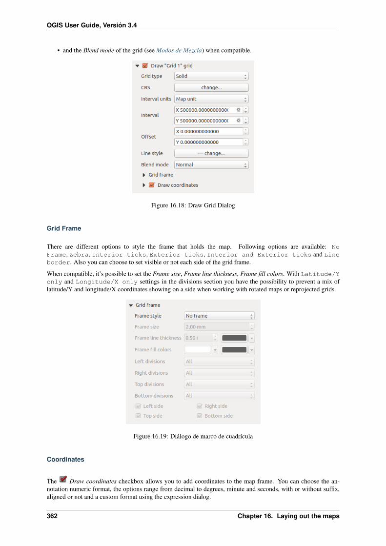
QGIS User Guide, Versión 3.4
• and the Blend mode of the grid (see Modos de Mezcla) when compatible.
Figure 16.18: Draw Grid Dialog
Grid Frame
There are different options to style the frame that holds the map. Following options are available: NoFrame, Zebra, Interior ticks, Exterior ticks, Interior and Exterior ticks and Lineborder. Also you can choose to set visible or not each side of the grid frame.
When compatible, it’s possible to set the Frame size, Frame line thickness, Frame fill colors. With Latitude/Yonly and Longitude/X only settings in the divisions section you have the possibility to prevent a mix oflatitude/Y and longitude/X coordinates showing on a side when working with rotated maps or reprojected grids.
Figure 16.19: Diálogo de marco de cuadrícula
Coordinates
The Draw coordinates checkbox allows you to add coordinates to the map frame. You can choose the an-notation numeric format, the options range from decimal to degrees, minute and seconds, with or without suffix,aligned or not and a custom format using the expression dialog.
362 Chapter 16. Laying out the maps

QGIS User Guide, Versión 3.4
You can choose which annotation to show. The options are: show all, latitude only, longitude only, or dis-able(none). This is useful when the map is rotated. The annotation can be drawn inside or outside the map frame.The annotation direction can be defined as horizontal, vertical ascending or vertical descending.
Finally, you can define the annotation font, font color, distance from the map frame and the precision of the drawncoordinates.
Figure 16.20: Diálogo Coordenadas para dibujo de rejilla
Vistas generales
Sometimes you may have more than one map in the print layout and would like to locate the study area of one mapitem on another one. This could be for example to help map readers identify the area in relation with its largergeographic context shown in the second map.
The Overviews group of the map panel helps you create the link between two different maps extent and providesthe following functionalities:
To create an overview, select the map item on which you want to show the other map item’s extent and expand the
Overviews option in the Item Properties panel. Then press the button to add an overview.
Initially this overview is named “Overview 1” (see Figure_layout_map_overview). You can:
• Rename it with a double-click;
• With the and buttons, add or remove overviews;
• With the and buttons, move up and down an overview in the list, hence move it on top or bottom ofanother one, over the map item.
16.2. Layout Items 363
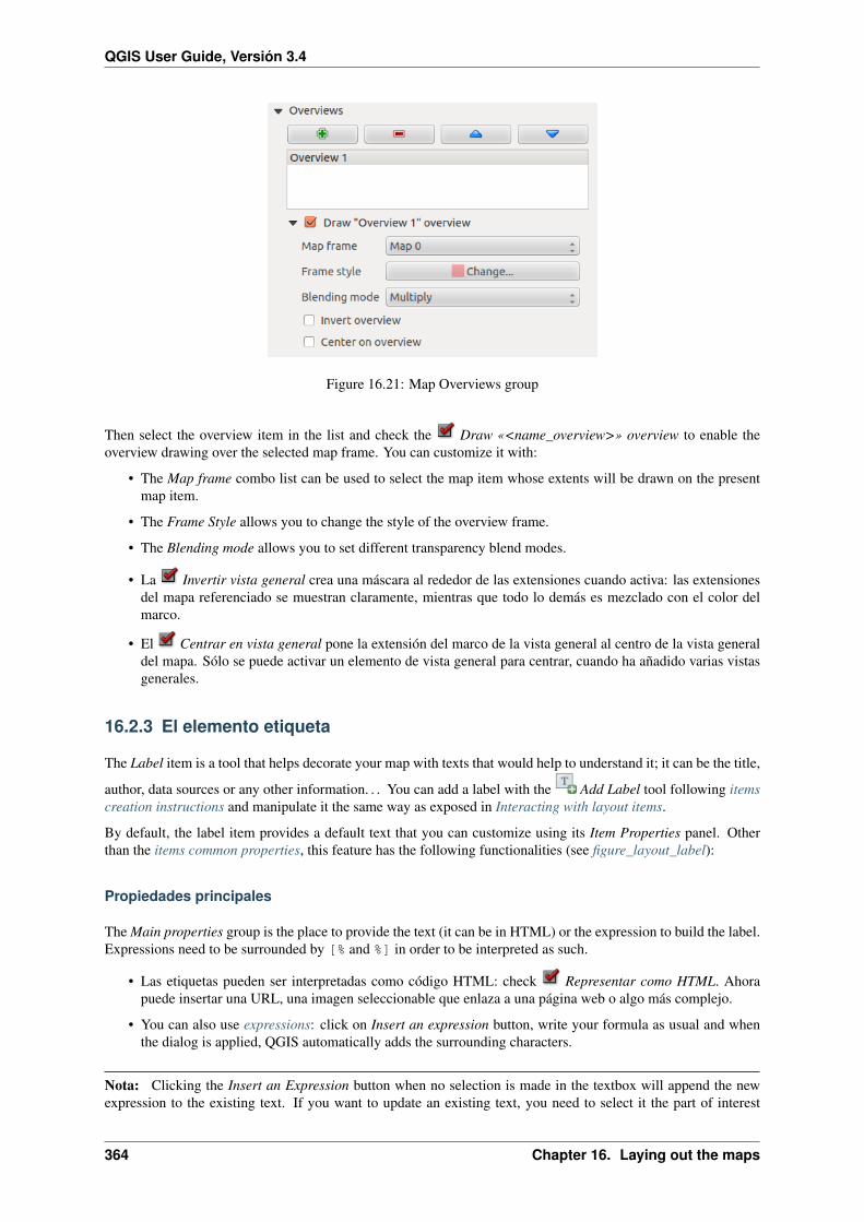
QGIS User Guide, Versión 3.4
Figure 16.21: Map Overviews group
Then select the overview item in the list and check the Draw «<name_overview>» overview to enable theoverview drawing over the selected map frame. You can customize it with:
• The Map frame combo list can be used to select the map item whose extents will be drawn on the presentmap item.
• The Frame Style allows you to change the style of the overview frame.
• The Blending mode allows you to set different transparency blend modes.
• La Invertir vista general crea una máscara al rededor de las extensiones cuando activa: las extensionesdel mapa referenciado se muestran claramente, mientras que todo lo demás es mezclado con el color delmarco.
• El Centrar en vista general pone la extensión del marco de la vista general al centro de la vista generaldel mapa. Sólo se puede activar un elemento de vista general para centrar, cuando ha añadido varias vistasgenerales.
16.2.3 El elemento etiqueta
The Label item is a tool that helps decorate your map with texts that would help to understand it; it can be the title,
author, data sources or any other information. . . You can add a label with the Add Label tool following itemscreation instructions and manipulate it the same way as exposed in Interacting with layout items.
By default, the label item provides a default text that you can customize using its Item Properties panel. Otherthan the items common properties, this feature has the following functionalities (see figure_layout_label):
Propiedades principales
The Main properties group is the place to provide the text (it can be in HTML) or the expression to build the label.Expressions need to be surrounded by [% and %] in order to be interpreted as such.
• Las etiquetas pueden ser interpretadas como código HTML: check Representar como HTML. Ahorapuede insertar una URL, una imagen seleccionable que enlaza a una página web o algo más complejo.
• You can also use expressions: click on Insert an expression button, write your formula as usual and whenthe dialog is applied, QGIS automatically adds the surrounding characters.
Nota: Clicking the Insert an Expression button when no selection is made in the textbox will append the newexpression to the existing text. If you want to update an existing text, you need to select it the part of interest
364 Chapter 16. Laying out the maps

QGIS User Guide, Versión 3.4
Figure 16.22: Label Item Properties Panel
beforehand.
You can combine HTML rendering and expressions, leading to e.g. a text like:
[% '<b>Check out the new logo for ' || '<a href="https://www.qgis.org" title="Nice→˓logo" target="_blank">QGIS ' ||@qgis_short_version || '</a>' || ' : <img src=→˓"https://qgis.org/en/_downloads/qgis-icon128.png" alt="QGIS icon"/>' %]
which will render: Check out the new logo for QGIS 3.0 :
Apariencia
• Define Font by clicking on the Font. . . button or a Font color by pushing the color widget.
• You can specify different horizontal and vertical margins in mm. This is the margin from the edge of thelayout item. The label can be positioned outside the bounds of the label e.g. to align label items with otheritems. In this case you have to use negative values for the margin.
• Using the text alignment is another way to position your label. It can be:
– Left, Center, Right or Justify for Horizontal alignment
– and Top, Middle, Bottom for Vertical alignment.
Exploring expressions in a label item
Below some examples of expressions you can use to populate the label item with interesting information - re-member that the code, or at least the calculated part, should be surrounded by [% and %] in the Main propertiesframe:
• Display a title with the current atlas feature value in «field1»:
'This is the map for ' || "field1"
or, written in the Main properties section:
16.2. Layout Items 365

QGIS User Guide, Versión 3.4
This is the map for [% "field1" %]
• Add a pagination for processed atlas features (eg, Page 1/10):
concat( 'Page ', @atlas_featurenumber, '/', @atlas_totalfeatures )
• Return the X coordinate of the bottom left corner of a map canvas:
x_min( map_get( item_variables( 'Map 1' ), 'map_extent' ) )
• Retrieve the name of the layers in the current layout “Map 1” item, and formats in one name by line:
array_to_string(array_foreach(
map_get( item_variables( 'Map 1' ), 'map_layers' ), -- retrieve the layers→˓list
layer_property( @element, 'name' ) -- retrieve each layer name),'\n' -- converts the list to string separated by breaklines
)
16.2.4 El elemento leyenda
The Legend item is a box or a table that explains the meanings of the symbols used on the map. A legend is
then bound to a map item. You can add a legend item with the Add Legend tool following items creationinstructions and manipulate it the same way as exposed in Interacting with layout items.
By default, the legend item displays all available layers and can be refined using its Item Properties panel. Otherthan the items common properties, this feature has the following functionalities (see figure_layout_legend):
Figure 16.23: Legend Item Properties Panel
Propiedades principales
The Main properties group of the legend Item Properties panel provides the following functionalities (see fig-ure_layout_legend_ppt):
366 Chapter 16. Laying out the maps

QGIS User Guide, Versión 3.4
Figure 16.24: Legend Main properties group
En propiedades principales se puede:
• change the title of the legend. It can be made dynamic using the data-defined override setting, useful forexample when generating atlas;
• set the Title alignment to Left, Center or Right;
• choose which Map item the current legend will refer to;
• wrap the text of the legend on a given character: each time the character appears, it’s replaced by a linebreak;
• use Resize to fit contents to control whether or not a legend should be automatically resized to fit itscontents. If unchecked, then the legend will never resize and instead just stick to whatever size the user hasset. Any content which doesn’t fit the size is cropped out.
Elementos de la leyenda
The Legend items group of the legend Item Properties panel provides the following functionalities (see fig-ure_layout_legend_items):
Figure 16.25: Legend Items group
• La leyenda se actualizará automáticamente si Auto actualizar es activado. Cuando guilabel:Auto actu-alizar es desactivado este le dará más control sobre los elementos de la leyenda. Los iconos debajo de loselementos de la leyenda se activarán.
• La ventana de los elementos de la leyenda lista todos los elementos y le permite cambiar el orden, capas degrupos, eliminar y restaurar elementos en la lista, editar nombres de capas y añadir un filtro.
16.2. Layout Items 367
QGIS User Guide, Versión 3.4
– The item order can be changed using the and buttons or with “drag-and-drop” functionality.The order can not be changed for WMS legend graphics.
– Use the button to add a legend group.
– Use the button to add layers and button to remove groups, layers or symbol classes.
– The button is used to edit the layer, group name or title. First you need to select the legend item.Double-clicking the item also opens the text box to rename it.
– The button adds a feature count for each class of vector layer.
– With the Filter legend by map content button, only the legend items visible in the map will be listed in the
legend. This tool remains available when Auto-update is active.
– The Filter legend by expression helps you filter which of the legend items of a layer will be displayed, i.e.using a layer that has different legend items (e.g., from a rule-based or categorized symbology), youcan specify a boolean expression to remove from the legend tree, styles that have no feature satisfyinga condition. Note that the features are nevertheless kept and shown in the layout map item.
While the default behavior of the legend item is to mimic the Layers panel tree, displaying the same groups,layers and classes of symbology, right-click any item offers you options to hide layer’s name or raise it as agroup or subgroup. In case you have made some changes to a layer, you can revert them by choosing Resetto defaults from the contextual menu.
After changing the symbology in the QGIS main window, you can click on Update All to adapt the changesin the legend element of the print layout.
• While generating an atlas with polygon features, you can filter out legend items that lie outside the current
atlas feature. To do that, check the Only show items inside current atlas feature option.
Fuentes, Columnas, Símbolo
The Fonts, Columns and Symbol groups of the legend Item Properties panel provide the following functionalities(see figure_layout_legend_fonts):
• You can change the font of the legend title, group, subgroup and item (feature) in the legend item using thefont selector widget;
• You provide the labels with a Color using the color selector widget. The selected color will apply to allfont items in the legend;
• Legend items can be arranged over several columns. Set the number of columns in the Count field.This value can be made dynamic e.g., following atlas features, legend contents, the frame size. . .
– Anchura de columnas igual controla cómo deberían ser ajustadas las columnas de la leyenda.
– La opción Dividir capas permite a una capa categorizada o graduada de la leyenda repartirse encolumnas.
• You can also change the width and height of the legend symbol, set a color and a thickness in case of rasterlayer symbol.
WMS LegendGraphic y espaciamiento
The WMS LegendGraphic and Spacing groups of the legend Item Properties panel provide the following function-alities (see figure_layout_legend_wms):
368 Chapter 16. Laying out the maps

QGIS User Guide, Versión 3.4
Figure 16.26: Legend Fonts, Columns and Symbol groups
Figure 16.27: WMS LegendGraphic and Spacing groups
16.2. Layout Items 369

QGIS User Guide, Versión 3.4
When you have added a WMS layer and you insert a legend item, a request will be sent to the WMS server toprovide a WMS legend. This Legend will only be shown if the WMS server provides the GetLegendGraphiccapability. The WMS legend content will be provided as a raster image.
GráficoDeLeyenda WMS se utiliza para poder ajustar el Anchura de la leyenda y la Altura de la leyenda de laimagen ráster de la leyenda WMS.
Spacing around title, group, subgroup, symbol, icon label, box, column or line can be customized through thisdialog.
16.2.5 El elemento de barra de escala
Scale bars provide a visual indication of the size of features, and distance between features, on the map item. A
scale bar item requires a map item. Use the Add Scale Bar tool following items creation instructions to add anew scale bar item that you can later manipulate the same way as exposed in Interacting with layout items.
By default, a new scale bar item shows the scale of the most recently added map item. You can customize it thanksto the Item Properties panel. Other than the items common properties, this feature has the following functionalities(see figure_layout_scalebar):
Figure 16.28: Scale Bar Item Properties Panel
Propiedades principales
The Main properties group of the scale bar Item Properties panel provides the following functionalities (seefigure_layout_scalebar_ppt):
Figure 16.29: Scale Bar Main properties group
• First, choose the map the scale bar will be attached to.
• Then, choose the style of the scale bar. Six styles are available:
– Single box and Double box styles, which contain one or two lines of boxes alternating colors;
370 Chapter 16. Laying out the maps

QGIS User Guide, Versión 3.4
– Middle, Up or Down line ticks;
– Numérico, donde se imprime la relación de escala (por ejemplo, 1:50000).
Unidades y Segmentos
The Units and Segments groups of the scale bar Item Properties panel provide the following functionalities (seefigure_layout_scalebar_units):
Figure 16.30: Scale Bar Units and Segments groups
In these two groups, you can set how the scale bar will be represented.
• Select the units you want to use with Scalebar units. There are many possible choices: Map Units (thedefault one), Meters, Feet, Miles or Nautical Miles. . . which may force unit conversions.
• The Label unit multiplier specifies how many scale bar units per labeled unit. Eg, if your scale bar units areset to «meters», a multiplier of 1000 will result in the scale bar labels in «kilometers».
• The Label for units field defines the text used to describe the units of the scale bar, eg m or km. This shouldbe matched to reflect the multiplier above.
• You can define how many Segments will be drawn on the left and on the right side of the scale bar.
• You can set how long each segment will be (Fixed width), or limit the scale bar size in mm with Fit segmentwidth option. In the latter case, each time the map scale changes, the scale bar is resized (and its labelupdated) to fit the range set.
• Height is used to define the height of the bar.
Mostrar
The Display group of the scale bar Item Properties panel provides the following functionalities (see fig-ure_layout_scalebar_display):
Se puede definir como la barra de escala se mostrará en un marco.
• Margen de caja : espacio entre texto y bordes del marco
• Labels margin : space between text and scale bar drawing
• Line width : line width of the scale bar drawing
• Join style : Corners at the end of scale bar in Bevel, Miter or Round style (only available for Scale bar styleSingle Box & Double Box)
16.2. Layout Items 371
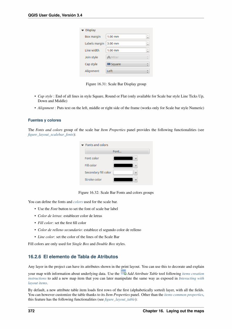
QGIS User Guide, Versión 3.4
Figure 16.31: Scale Bar Display group
• Cap style : End of all lines in style Square, Round or Flat (only available for Scale bar style Line Ticks Up,Down and Middle)
• Alignment : Puts text on the left, middle or right side of the frame (works only for Scale bar style Numeric)
Fuentes y colores
The Fonts and colors group of the scale bar Item Properties panel provides the following functionalities (seefigure_layout_scalebar_fonts):
Figure 16.32: Scale Bar Fonts and colors groups
You can define the fonts and colors used for the scale bar.
• Use the Font button to set the font of scale bar label
• Color de letras: establecer color de letras
• Fill color: set the first fill color
• Color de relleno secundario: establece el segundo color de relleno
• Line color: set the color of the lines of the Scale Bar
Fill colors are only used for Single Box and Double Box styles.
16.2.6 El elemento de Tabla de Atributos
Any layer in the project can have its attributes shown in the print layout. You can use this to decorate and explain
your map with information about underlying data. Use the Add Attribute Table tool following items creationinstructions to add a new map item that you can later manipulate the same way as exposed in Interacting withlayout items.
By default, a new attribute table item loads first rows of the first (alphabetically sorted) layer, with all the fields.You can however customize the table thanks to its Item Properties panel. Other than the items common properties,this feature has the following functionalities (see figure_layout_table):
372 Chapter 16. Laying out the maps

QGIS User Guide, Versión 3.4
Figure 16.33: Attribute table Item Properties Panel
Propiedades principales
The Main properties group of the attribute table provides the following functionalities (see fig-ure_layout_table_ppt):
Figure 16.34: Attribute table Main properties Group
• For Source you can by default only select Layer features allowing you to select a Layer from the vectorlayers loaded in the project.
The data-defined override button near the layer list allows you to dynamically change the layer which is usedto populate the table, e.g. you could fill the attribute table with different layer attributes per atlas page. Notethat the table structure used (column settings) is the one of the layer shown in the Layer drop-down list andit is left intact, meaning that setting a data defined table to a layer with different field(s) will result in emptycolumn(s) in the table.
In case you activate the Generate an atlas option in the Atlas panel (see Generar un Atlas), there are twoadditional Source possible:
– Current atlas feature (see figure_layout_table_atlas): you won’t see any option to choose the layer,and the table item will only show a row with the attributes from the current feature of the atlas coveragelayer.
– and Relation children (see figure_layout_table_relation): an option with the relation names will showup. This feature can only be used if you have defined a relation using your atlas coverage layer asparent, and the table will show the children rows of the atlas coverage layer’s current feature.
• The button Refresh Table Data can be used to refresh the table when the actual contents of the table haschanged.
16.2. Layout Items 373

QGIS User Guide, Versión 3.4
Figure 16.35: Attribute table Main properties for “Current atlas feature”
Figure 16.36: Attribute table Main properties for “Relation children”
• The button Attributes. . . starts the Select Attributes dialog, (see figure_layout_table_select) that can be usedto change the visible contents of the table. The upper part of the window shows the list of the attributes todisplay and the lower part helps you sort the data.
En la sección Columnas se puede:
– Move attributes up or down the list by selecting the rows and then using the and buttons toshift the rows. Multiple rows can be selected and moved at any one time.
– Add an attribute with the button. This will add an empty row at the bottom of the table where youcan select a field to be the attribute value or create an attribute via a regular expression.
– Remove an attribute with the button. Multiple rows can be selected and removed at any one time.
– Reset the attribute table back to its default state with the Reset button.
– Clear the table using the Clear button. This is useful when you have a large table but only want toshow a small number of attributes. Instead of manually removing each row, it may be quicker to clearthe table and add the rows needed.
– Cell headings can be altered by adding the custom text in the Heading column.
– Cell alignment can be managed with the Alignment column which will dictate the texts position withinthe table cell.
– Cell width can be manually managed by adding custom values to the width column.
En la sección Ordenar se puede:
– Add an attribute to sort the table with. Select an attribute and set the sorting order to Ascending or
Descending and press the button. A new line is added to the sort order list.
– select a row in the list and use the and buttons to change the sort priority on attribute level.Selecting a cell in the Sort Order column helps you change the sorting order of the attribute field.
– use the button to remove an attribute from the sort order list.
Filtrado de objetos espaciales
The Feature filtering group of the attribute table provides the following functionalities (see fig-ure_layout_table_filter):
374 Chapter 16. Laying out the maps

QGIS User Guide, Versión 3.4
Figure 16.37: Attribute table Select attributes Dialog
Figure 16.38: Attribute table Feature filtering Group
16.2. Layout Items 375

QGIS User Guide, Versión 3.4
Puede:
• Define the Maximum rows to be displayed.
• Activar Eliminar filas duplicadas de la tabla para mostrar sólo registros únicos.
• Activate Show only visible features within a map and select the corresponding Linked map whose visiblefeatures attributes will be displayed.
• Activate Show only features intersecting Atlas feature is only available when Generate an atlas isactivated. When activated it will show a table with only the features which intersect the current atlas feature.
• Activar Filtrar con y proporciona un filtro al escribir en la línea de entrada o insertar una expresión
regular utilizando el botón de expresión dado. Unos pocos ejemplos de declaraciones de filtrado quepuede utilizar cuando se han cargado la capa de aeropuertos a partir del conjunto de datos de la muestra:
– ELEV > 500
– NAME = 'ANIAK'
– NAME NOT LIKE 'AN%'
– regexp_match( attribute( $currentfeature, 'USE' ) , '[i]')
La ultima expresión regular incluirá sólo los aeropuertos que tienen una letra “i” en el campo de atributos“USE”.
Apariencia
The Appearance group of the attribute table provides the following functionalities (see fig-ure_layout_table_appearance):
Figure 16.39: Attribute table appearance Group
• Click Show empty rows to fill the attribute table with empty cells. This option can also be used to provideadditional empty cells when you have a result to show!
• With Cell margins you can define the margin around text in each cell of the table.
• With Display header you can select from a list one of “On first frame”, “On all frames” default option, or“No header”.
• The option Empty table controls what will be displayed when the result selection is empty.
– Dibujar cabeceras solamente, sólo dibuja la cabecera excepto si se tiene elegido “Sin encabezado”por Mostrar encabezado.
376 Chapter 16. Laying out the maps

QGIS User Guide, Versión 3.4
– Ocultar tabla entera, sólo dibujará el fondo de la tabla. Se puede activar No dibujar el fondo siel marco esta vacío en Marcos para ocultar la tabla completamente.
– Mostrar mensaje establecido dibujará el encabezado y añadirá un espaciado a la celda a todas lascolumnas y mostrará un mensaje como “Sin resultados” que puede ser proveído en la opción Mensajea mostrar
• La opción Mensaje a mostrar sólo se activa cuando se ha seleccionado Mostrar mensaje establecido paraTabla Vacía. El mensaje proporcionado se mostrará en la tabla en la primer fila, cuando el resultado es unatabla vacía.
• With Background color you can set the background color of the table using the color selector widget.The Advanced customization option helps you define different background colors for each cell (see fig-ure_layout_table_background)
Figure 16.40: Attribute table Advanced Background Dialog
• With the Wrap text on option, you can define a character on which the cell content will be wraped each timeit is met
• With Oversized text you define the behavior when the width set for a column is smaller than its content’slength. It can be Wrap text or Truncate text.
Mostrar cuadrícula
The Show grid group of the attribute table provides the following functionalities (see figure_layout_table_grid):
Figure 16.41: Attribute table Show grid Group
• Activate Show grid when you want to display the grid, the outlines of the table cells. You can also selectto either Draw horizontal lines or Draw vertical lines or both.
16.2. Layout Items 377
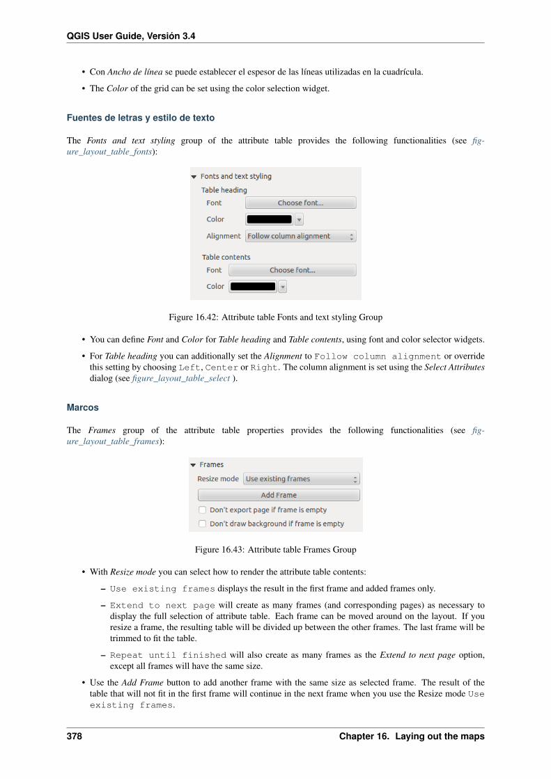
QGIS User Guide, Versión 3.4
• Con Ancho de línea se puede establecer el espesor de las líneas utilizadas en la cuadrícula.
• The Color of the grid can be set using the color selection widget.
Fuentes de letras y estilo de texto
The Fonts and text styling group of the attribute table provides the following functionalities (see fig-ure_layout_table_fonts):
Figure 16.42: Attribute table Fonts and text styling Group
• You can define Font and Color for Table heading and Table contents, using font and color selector widgets.
• For Table heading you can additionally set the Alignment to Follow column alignment or overridethis setting by choosing Left, Center or Right. The column alignment is set using the Select Attributesdialog (see figure_layout_table_select ).
Marcos
The Frames group of the attribute table properties provides the following functionalities (see fig-ure_layout_table_frames):
Figure 16.43: Attribute table Frames Group
• With Resize mode you can select how to render the attribute table contents:
– Use existing frames displays the result in the first frame and added frames only.
– Extend to next page will create as many frames (and corresponding pages) as necessary todisplay the full selection of attribute table. Each frame can be moved around on the layout. If youresize a frame, the resulting table will be divided up between the other frames. The last frame will betrimmed to fit the table.
– Repeat until finished will also create as many frames as the Extend to next page option,except all frames will have the same size.
• Use the Add Frame button to add another frame with the same size as selected frame. The result of thetable that will not fit in the first frame will continue in the next frame when you use the Resize mode Useexisting frames.
378 Chapter 16. Laying out the maps

QGIS User Guide, Versión 3.4
• Activate Don’t export page if frame is empty prevents the page to be exported when the table frame hasno contents. This means all other layout items, maps, scalebars, legends etc. will not be visible in the result.
• Activar No dibujar fondo si el marco está vacío impide que el fondo que se puede extraer cuando elmarco de la tabla no tiene contenido.
16.2.7 The Picture Item
The Picture item is a tool that helps decorate your map with pictures, logos. . . It’s also the one that provides
the in-built north arrows. You can add a picture with the Add Picture following items creation instructions andmanipulate it the same way as exposed in Interacting with layout items.
By default, the picture item is a blank frame that you can customize using its Item Properties panel. Other thanthe items common properties, this feature has the following functionalities (see figure_layout_image):
Figure 16.44: Picture Item Properties panel
You first have to select the image you want to display. There are several ways to set the Image source:
1. In the Main properties group, use the . . . Browse button of image source to select a file on your computer. Thebrowser will start in the SVG-libraries provided with QGIS. Besides SVG, you can also select other imageformats like .png or .jpg.
2. You can enter the source directly in the Image source text field. You can even provide a remote URL-addressto a picture.
3. From the Search directories area you can also select an image from the loaded previews to set the imagesource. These images are by default provided by folders set in Settings → Options → System → SVG Paths.
4. Use the data defined override button to set the image source from a feature attribute or using a regular expres-sion.
16.2. Layout Items 379

QGIS User Guide, Versión 3.4
Nota: In the Search directories group, you can use the Add and Remove buttons in the group to customize the listof folders to fetch and preview images from.
With the Resize mode option, you can set how the image is displayed when the frame is resized:
• Zoom: enlarges/reduces the image to the frame while maintaining aspect ratio of picture;
• Stretch: stretches image to fit inside the frame, ignores aspect ratio;
• Clip: use this mode for raster images only, it sets the size of the image to original image size withoutscaling and the frame is used to clip the image, so only the part of the image inside the frame is visible;
• Zoom and resize frame: enlarges image to fit frame, then resizes frame to fit resultant image;
• Resize frame to image size: sets size of frame to match original size of image without scaling.
Depending on the selected Resize mode, the Placement and Image rotation options are disabled or not. WithPlacement you can select the position of the image inside its frame. QGIS default provided .SVG files arecustomizable, meaning that you can easily apply different Fill color, Stroke color (including opacity) and Strokewidth than the original, using their corresponding feature in the SVG Parameters group. These properties can aswell be data-defined.
If you add a .SVG file that does not enable these properties, you may need to add the following tags to the file inorder to add support e.g. for transparency:
• fill-opacity=»param(fill-opacity)»
• stroke-opacity=»param(outline-opacity)»
You can read this blog post to see an example.
Images can be rotated with the Image rotation field. Activating the Sync with map checkbox synchronizes therotation of the image with the rotation applied to a selected map item; this is a convenient feature for north arrowsthat you can align with either:
• the Grid north: direction of a grid line which is parallel to the central meridian on the national/local grid;
• or the True north: direction of a meridian of longitude which converges on the North Pole.
You can also apply a declination Offset to the picture rotation.
Nota: Muchas de las flechas del norte no tienen una “N” añadida, esto se hace a propósito para los idiomas queno utilizan una “N” para Norte, para que pueda utilizar otra letra.
16.2.8 El elemento del marco HTML
It is possible to add a frame that displays the contents of a website or even create and style your own HTML
page and display it! You can add a picture with the Add HTML following items creation instructions andmanipulate it the same way as exposed in Interacting with layout items.
The HTML item can be customized using its Item Properties panel. Other than the items common properties, thisfeature has the following functionalities (see figure_layout_html):
Fuente HTML
The HTML Source group of the HTML frame Item Properties panel provides the following functionalities (seefigure_layout_html_ppt):
380 Chapter 16. Laying out the maps

QGIS User Guide, Versión 3.4
Figure 16.45: Las flechas de norte disponibles para la selección en la biblioteca SVG proporcionada.
Figure 16.46: HTML Frame, the Item Properties Panel
16.2. Layout Items 381
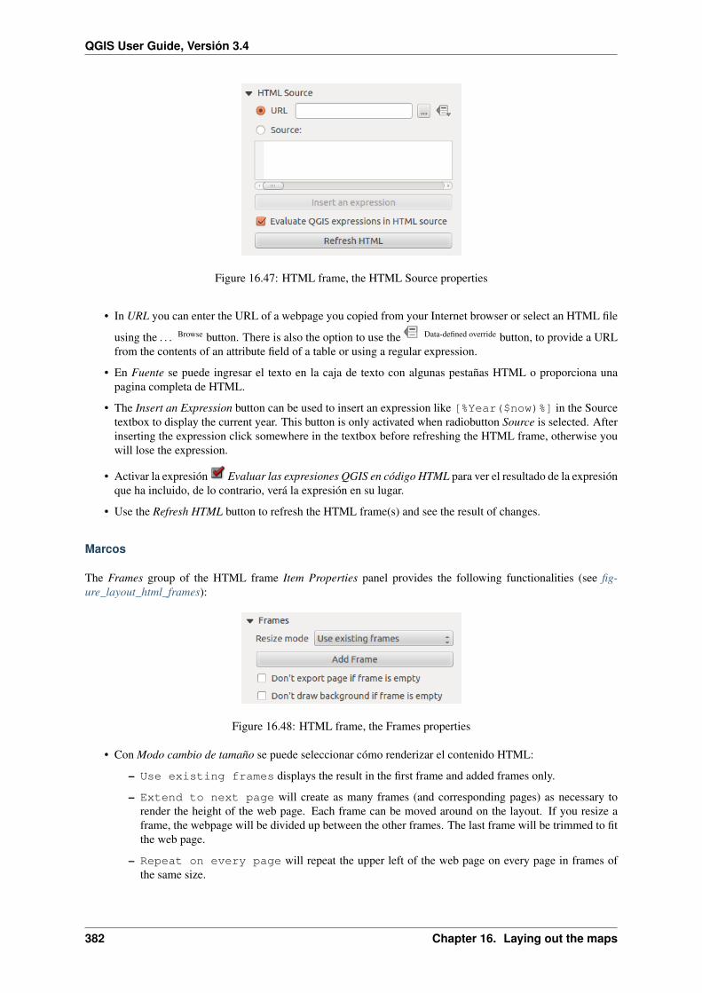
QGIS User Guide, Versión 3.4
Figure 16.47: HTML frame, the HTML Source properties
• In URL you can enter the URL of a webpage you copied from your Internet browser or select an HTML file
using the . . . Browse button. There is also the option to use the Data-defined override button, to provide a URLfrom the contents of an attribute field of a table or using a regular expression.
• En Fuente se puede ingresar el texto en la caja de texto con algunas pestañas HTML o proporciona unapagina completa de HTML.
• The Insert an Expression button can be used to insert an expression like [%Year($now)%] in the Sourcetextbox to display the current year. This button is only activated when radiobutton Source is selected. Afterinserting the expression click somewhere in the textbox before refreshing the HTML frame, otherwise youwill lose the expression.
• Activar la expresión Evaluar las expresiones QGIS en código HTML para ver el resultado de la expresiónque ha incluido, de lo contrario, verá la expresión en su lugar.
• Use the Refresh HTML button to refresh the HTML frame(s) and see the result of changes.
Marcos
The Frames group of the HTML frame Item Properties panel provides the following functionalities (see fig-ure_layout_html_frames):
Figure 16.48: HTML frame, the Frames properties
• Con Modo cambio de tamaño se puede seleccionar cómo renderizar el contenido HTML:
– Use existing frames displays the result in the first frame and added frames only.
– Extend to next page will create as many frames (and corresponding pages) as necessary torender the height of the web page. Each frame can be moved around on the layout. If you resize aframe, the webpage will be divided up between the other frames. The last frame will be trimmed to fitthe web page.
– Repeat on every page will repeat the upper left of the web page on every page in frames ofthe same size.
382 Chapter 16. Laying out the maps

QGIS User Guide, Versión 3.4
– Repeat until finished will also create as many frames as the Extend to next pageoption, except all frames will have the same size.
• Use the Add Frame button to add another frame with the same size as selected frame. If the HTML pagedoes not fit in the first frame it will continue in the next frame when you use Resize mode or Use existingframes.
• Activate Don’t export page if frame is empty prevents the page from being exported when the frame hasno HTML contents. This means all other layout items, maps, scale bars, legends etc. will not be visible inthe result.
• Activar No saque el fondo si el marco es empty impide que el marco HTML está elaborando si la tramaestá vacía.
Usar saltos de página inteligentes y hoja de estilos de usuario
The Use smart page breaks dialog and User style sheet dialog of the HTML frame Item Properties panel providesthe following functionalities (see figure_layout_html_breaks):
Figure 16.49: HTML frame, Use smart page breaks and User style sheet properties
• Activar Usar saltos de página inteligentes para impedir para evitar que el contenido del marco html deromper a mitad de camino una línea de texto por lo que continúa agradable y sencillo en el cuadro siguiente.
• Establecer la Máxima distancia permite en el cálculo de dónde colocar los saltos de página en el html. Estadistancia es la cantidad máxima de espacio vacío permitido en la parte inferior de un marco después decalcular la ubicación óptima de descanso. Ajustar un valor más grande resultará en una mejor elección dela ubicación de salto de página, pero más espacio perdido en la parte inferior de los marcos. Esto sólo seutiliza cuando Usar saltos de página inteligentes está activado.
• Activate User style sheet to apply HTML styles that often is provided in cascading style sheets. Anexample of style code is provided below to set the color of <h1> header tag to green and set the font andfont size of text included in paragraph tags <p>.
h1 {color: #00ff00;}p {font-family: "Times New Roman", Times, serif;
font-size: 20px;}
• Use the Update HTML button to see the result of the style sheet settings.
16.2.9 The Shape Items
QGIS provides a couple of tools to draw regular or more complex shapes over the print layout.
16.2. Layout Items 383
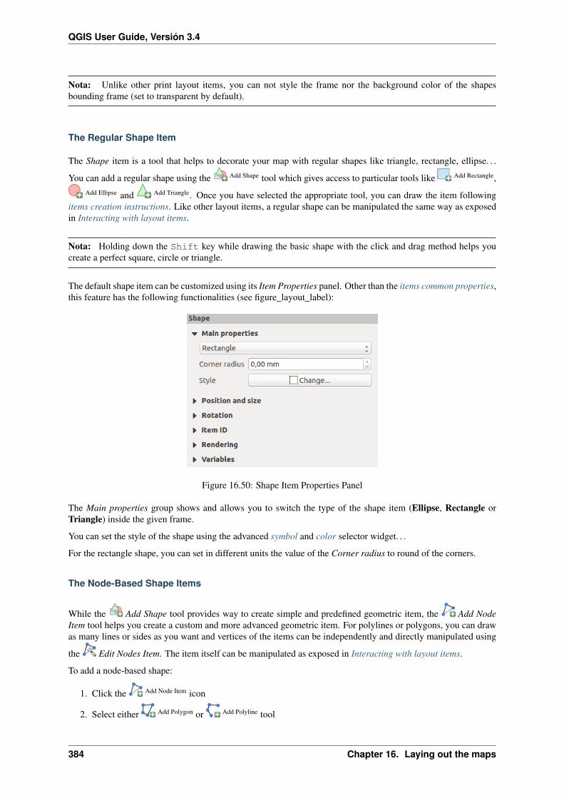
QGIS User Guide, Versión 3.4
Nota: Unlike other print layout items, you can not style the frame nor the background color of the shapesbounding frame (set to transparent by default).
The Regular Shape Item
The Shape item is a tool that helps to decorate your map with regular shapes like triangle, rectangle, ellipse. . .
You can add a regular shape using the Add Shape tool which gives access to particular tools like Add Rectangle,Add Ellipse and Add Triangle. Once you have selected the appropriate tool, you can draw the item following
items creation instructions. Like other layout items, a regular shape can be manipulated the same way as exposedin Interacting with layout items.
Nota: Holding down the Shift key while drawing the basic shape with the click and drag method helps youcreate a perfect square, circle or triangle.
The default shape item can be customized using its Item Properties panel. Other than the items common properties,this feature has the following functionalities (see figure_layout_label):
Figure 16.50: Shape Item Properties Panel
The Main properties group shows and allows you to switch the type of the shape item (Ellipse, Rectangle orTriangle) inside the given frame.
You can set the style of the shape using the advanced symbol and color selector widget. . .
For the rectangle shape, you can set in different units the value of the Corner radius to round of the corners.
The Node-Based Shape Items
While the Add Shape tool provides way to create simple and predefined geometric item, the Add NodeItem tool helps you create a custom and more advanced geometric item. For polylines or polygons, you can drawas many lines or sides as you want and vertices of the items can be independently and directly manipulated using
the Edit Nodes Item. The item itself can be manipulated as exposed in Interacting with layout items.
To add a node-based shape:
1. Click the Add Node Item icon
2. Select either Add Polygon or Add Polyline tool
384 Chapter 16. Laying out the maps

QGIS User Guide, Versión 3.4
3. Perform consecutive left clicks to add nodes of your item. If you hold down the Shift key while drawinga segment, it is constrained to follow an orientation multiple of 45°.
4. When you’re done, right-click to terminate the shape.
You can customize the appearance of the shape in the Item Properties panel.
Figure 16.51: Polygon Node Shape Item Properties Panel
In the Main properties, you can set the style of the shape using the advanced symbol and color selector widget. . .
For polyline node items, you can also parameterize the Line markers i.e. add:
• start and/or end markers with options:
– None: draws a simple polyline.
– Arrow: adds a regular triangular arrow head that you can customize.
– SVG marker: uses an SVG file as arrow head of the item.
• customize the arrow head:
– Arrow stroke color: sets the stroke color of the arrow head.
– Arrow fill color: sets the fill color of the arrow head.
– Arrow stroke width: sets the stroke width of the arrow head.
– Arrow head width: sets the size of the arrow head.
SVG images are automatically rotated with the line. Stroke and fill colors of QGIS predefined SVG images canbe changed using the corresponding options. Custom SVG may require some tags following this instruction.
El elemento flecha
The Add Arrow tool is a shortcut to create an arrow-enabled polyline by default and thus has the same propertiesand behavior as a polyline node item.
Actually, the arrow item can be used to add a simple arrow, for example, to show the relation between two differentprint layout items. However, to create a north arrow, the image item should be considered first as it gives access toa set of north arrows in .SVG format that you can sync with a map item so that it rotates automatically with it.
Editing a node item geometry
A specific tool is provided to edit node-based shapes through Edit Nodes Item. Within this mode, you can selecta node by clicking on it (a marker is displayed on the selected node). A selected node can be moved either bydragging it or by using the arrow keys. Moreover, in this mode, you are able to add nodes to an existing shape:double-click on a segment and a node is added at the place you click. Finally, you can remove the currentlyselected node by hitting the Del key.
16.2. Layout Items 385
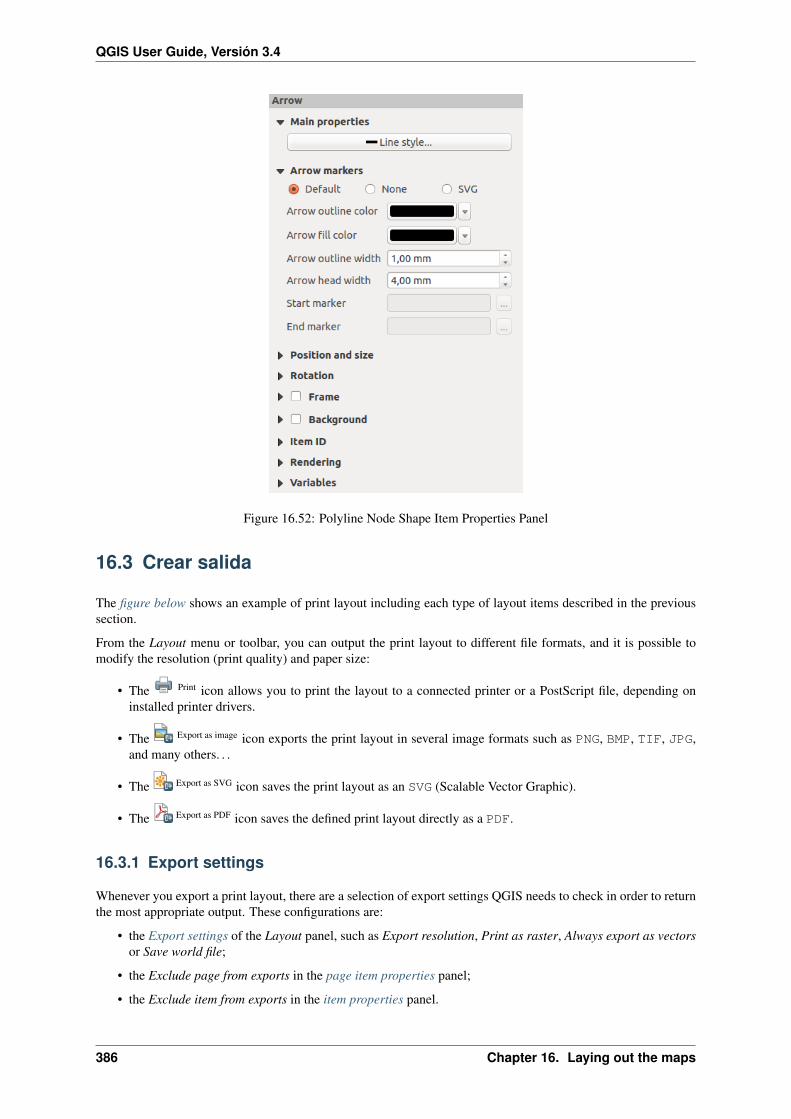
QGIS User Guide, Versión 3.4
Figure 16.52: Polyline Node Shape Item Properties Panel
16.3 Crear salida
The figure below shows an example of print layout including each type of layout items described in the previoussection.
From the Layout menu or toolbar, you can output the print layout to different file formats, and it is possible tomodify the resolution (print quality) and paper size:
• The Print icon allows you to print the layout to a connected printer or a PostScript file, depending oninstalled printer drivers.
• The Export as image icon exports the print layout in several image formats such as PNG, BMP, TIF, JPG,and many others. . .
• The Export as SVG icon saves the print layout as an SVG (Scalable Vector Graphic).
• The Export as PDF icon saves the defined print layout directly as a PDF.
16.3.1 Export settings
Whenever you export a print layout, there are a selection of export settings QGIS needs to check in order to returnthe most appropriate output. These configurations are:
• the Export settings of the Layout panel, such as Export resolution, Print as raster, Always export as vectorsor Save world file;
• the Exclude page from exports in the page item properties panel;
• the Exclude item from exports in the item properties panel.
386 Chapter 16. Laying out the maps

QGIS User Guide, Versión 3.4
Figure 16.53: Print Layout with map view, legend, image, scale bar, coordinates, text and HTML frame added
16.3.2 Export as Image
Clicking the Export as image icon will ask you to select the image format and enter the filename to use to exportthe print layout: in the case of multi-page composition, each page will be exported to a file with the given nameappended with the page number.
In the next Image Export Options dialog, you can optionally override the print layout resolution and the exportedpage dimensions (set in Layout panel).
By checking Crop to content option, the image output by the layout will include the minimal area enclosingall the items (map, legend, scale bar, shapes, label, image. . . ) of each page of the composition:
• If the composition includes a single page, then the output is resized to include EVERYTHING on thecomposition. The page can then be reduced or extended to all items depending on their position (on, above,below, left or right of the page).
• In case of a multi-page layout, each page will be resized to include items in its area (left and right sidesfor all pages, plus top for the first page and bottom for the last page). Each resized page is exported to aseparate file.
The Crop to content dialog also allows to add some margins around the cropped bounds.
Truco: Use image formats that support transparency when items extend beyond the paper extent
Since layout items may be placed outside the paper extent, using the Crop to content option while exporting canresult in an image that extends beyond the paper extent. Since the background outside of the paper extent will betransparent, for image formats that do not support transparency (eg, .BMP, .JPG) it will be rendered as full black,«corrupting» the image.
Use transparency-compatible formats like .TIFF or .PNG in such a case.
If you need to export your layout as a georeferenced image (e.g., to share with other projects), check theGenerate world file option and a world file named like the page on which the map reference set in Layout panel is
16.3. Crear salida 387
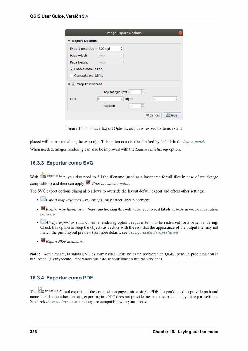
QGIS User Guide, Versión 3.4
Figure 16.54: Image Export Options, output is resized to items extent
placed will be created along the export(s). This option can also be checked by default in the layout panel.
When needed, images rendering can also be improved with the Enable antialiasing option.
16.3.3 Exportar como SVG
With Export as SVG, you also need to fill the filename (used as a basename for all files in case of multi-page
composition) and then can apply Crop to content option.
The SVG export options dialog also allows to override the layout default export and offers other settings:
• Export map layers as SVG groups: may affect label placement.
• Render map labels as outlines: unchecking this will allow you to edit labels as texts in vector illustrationsoftware.
• Always export as vectors: some rendering options require items to be rasterized for a better rendering.Check this option to keep the objects as vectors with the risk that the appearance of the output file may notmatch the print layout preview (for more details, see Configuración de exportación).
• Export RDF metadata.
Nota: Actualmente, la salida SVG es muy básica. Este no es un problema en QGIS, pero un problema con labiblioteca Qt subyacente. Esperamos que esto se solucione en futuras versiones.
16.3.4 Exportar como PDF
The Export as PDF tool exports all the composition pages into a single PDF file you’d need to provide path andname. Unlike the other formats, exporting to .PDF does not provide means to override the layout export settings.So check these settings to ensure they are compatible with your needs.
388 Chapter 16. Laying out the maps

QGIS User Guide, Versión 3.4
Figure 16.55: Opciones de Exportación de SVG
Figure 16.56: PDF Export Options
16.3. Crear salida 389

QGIS User Guide, Versión 3.4
Nota: Exporting a print layout to formats like .PDF or .TIFF creates a georeferenced output (no world fileneeded) by default.
16.3.5 Generar un Atlas
Atlas functions allow you to create map books in an automated way. Atlas uses the features of a vector or tablelayer called coverage layer and creates an output for each atlas feature. The most common usage is to zoom amap item to the current atlas feature. Further use cases include:
• a map item showing, for another layer, only features that share the same attribute as the atlas feature or arewithin its geometry;
• a label or html item whose text is replaced as features are iterated over;
• a table item showing attributes of associated parent or children features of the current atlas feature. . .
For each feature, an output is processed for all pages and items according to their exports settings.
Truco: Use variables for more flexibility
QGIS provides a large panel of functions and variables, including atlas related ones, that you can use to manipulatethe layout items but also the layers symbology according to atlas status. Combining these features gives you a lotof flexibility and helps you easily produce advanced mappings.
To enable the generation of an atlas and access atlas parameters, refer to the Atlas panel. This panel contains thefollowing functionalities (see figure_layout_atlas):
Figure 16.57: Atlas Panel
• Generate an atlas, which enables or disables the atlas generation;
• A Coverage layer combo box that allows you to choose the table or vector layer containing thefeatures to iterate over;
• An optional Hidden coverage layer that, if checked, will hide the coverage layer (but not the otherlayers) during the generation;
• An optional Page name combo box to give a more explicit name to each feature page(s) when previewingatlas. You can select a field of the coverage layer or set an expression. If this option is empty, QGIS willuse an internal ID, according to the filter and/or the sort order applied to the layer;
390 Chapter 16. Laying out the maps
QGIS User Guide, Versión 3.4
• An optional Filter with text area that allows you to specify an expression for filtering features from thecoverage layer. If the expression is not empty, only features that evaluate to True will be processed;
• An optional Sort by that allows you to sort features of the coverage layer, using a field of the coveragelayer or an expression. The sort order (either ascending or descending) is set by the two-state Sort directionbutton that displays an up or a down arrow.
You also have options to set the output of the atlas:
• An Output filename expression textbox that is used to generate a filename for each geometry if needed. It isbased on expressions. This field is meaningful only for rendering to multiple files;
• A Single file export when possible that allows you to force the generation of a single file if this is possiblewith the chosen output format (PDF, for instance). If this field is checked, the value of the Output filenameexpression field is meaningless;
• An Image export format drop-down list to select the output format when using the Export atlas as Images. . .
button.
Control map by atlas
The most common usage of atlas is with the map item, zooming to the current atlas feature, as iteration goes overthe coverage layer. This behavior is set in the Controlled by atlas group properties of the map item. See Controlledby atlas for different settings you can apply on map item.
Customize labels with expression
In order to adapt labels to the feature the atlas iterates over, you can include expressions. What you should takecare of is to place expression part (including functions, fields or variables) between [% and %] (see El elementoetiqueta for more details).
For example, for a city layer with fields CITY_NAME and ZIPCODE, you could insert this:
The area of [% concat( upper(CITY_NAME), ',', ZIPCODE, ' is ',format_number($area/1000000, 2) ) %] km2
or, another combination:
The area of [% upper(CITY_NAME)%],[%ZIPCODE%] is[%format_number($area/1000000,2) %] km2
The information [% concat( upper(CITY_NAME), ',', ZIPCODE, ' is ',format_number($area/1000000, 2) ) %] is an expression used inside the label. Both expres-sions would result in the generated atlas as:
The area of PARIS,75001 is 1.94 km2
Explore Data-defined override buttons with atlas
There are several places where you can use a Data defined override button to override the selected setting. Theseoptions are particularly useful with atlas generation. See Configuración de anulación definida por datos for moredetails on this widget.
For the following examples the Regions layer of the QGIS sample dataset is used and selected as coverage layerfor the atlas generation. We also assume it’s a single page layout containing a map and a label items.
16.3. Crear salida 391

QGIS User Guide, Versión 3.4
When the height (north-south) of the extents of a region is greater than its width (east-west), you rather want to
use Portrait instead of Landscape orientation to optimize the use of paper. With a Data Defined Override button youcan dynamically set the paper orientation.
Right-click on the page and select Page Properties to open the panel. We want to set the orientation dynamically,
using an expression depending on the region geometry so press the button of field Orientation, select Edit. . .to open the Expression string builder dialog and enter the following expression:
CASE WHEN bounds_width(@atlas_geometry) > bounds_height(@atlas_geometry)THEN 'Landscape' ELSE 'Portrait' END
Now if you preview the atlas, the paper orients itself automatically but items placement may not be ideal. For
each Region you need to reposition the location of the layout items as well. For the map item you can use thebutton of its Width property to set it dynamic using following expression:
@layout_pagewidth - 20
Likewise, use the button of the Height property to provide following expression and constrain map item size:
@layout_pageheight - 20
To ensure the map item is centered in the page, set its Reference point to the upper left radio button and enter 10for its X and Y positions.
Let’s add a title above the map in the center of the page. Select the label item and set the horizontal alignment to
Center. Next move the label to the right position, activate from Reference point any of the middle buttons,and provide the following expression for field X:
@layout_pagewidth / 2
For all other layout items you can set the position in a similar way so they are correctly positioned when the pageis automatically rotated in portrait or landscape. You can also do more tweaks such as customizing the title withfeature attributes (see Customize labels with expression example), updating images with atlas feature, resizing thelegend columns number according to page orientation. . .
Information provided is an update of the excellent blog (in English and Portuguese) on the Data Defined Overrideoptions Multiple_format_map_series_using_QGIS_2.6 .
This is just one example of how you can use some advanced settings with atlas.
Preview and generate an atlas
Figure 16.58: Barra de herramienta Vista Previa del Atlas
Once the atlas settings have been configured and layout items (map, table, image. . . ) linked to it, you can create a
preview of all the pages by clicking Atlas → Preview Atlas or Preview Atlas icon. You can then use the arrows inthe same toolbar to navigate through all the features:
• First feature
• Previous feature
• Next feature
• Last feature
392 Chapter 16. Laying out the maps
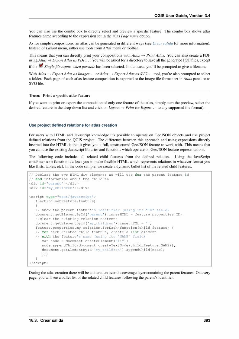
QGIS User Guide, Versión 3.4
You can also use the combo box to directly select and preview a specific feature. The combo box shows atlasfeatures name according to the expression set in the atlas Page name option.
As for simple compositions, an atlas can be generated in different ways (see Crear salida for more information).Instead of Layout menu, rather use tools from Atlas menu or toolbar.
This means that you can directly print your compositions with Atlas → Print Atlas. You can also create a PDFusing Atlas → Export Atlas as PDF. . . : You will be asked for a directory to save all the generated PDF files, except
if the Single file export when possible has been selected. In that case, you’ll be prompted to give a filename.
With Atlas → Export Atlas as Images. . . or Atlas → Export Atlas as SVG. . . tool, you’re also prompted to selecta folder. Each page of each atlas feature composition is exported to the image file format set in Atlas panel or toSVG file.
Truco: Print a specific atlas feature
If you want to print or export the composition of only one feature of the atlas, simply start the preview, select thedesired feature in the drop-down list and click on Layout → Print (or Export. . . to any supported file format).
Use project defined relations for atlas creation
For users with HTML and Javascript knowledge it’s possible to operate on GeoJSON objects and use projectdefined relations from the QGIS project. The difference between this approach and using expressions directlyinserted into the HTML is that it gives you a full, unstructured GeoJSON feature to work with. This means thatyou can use the existing Javascript libraries and functions which operate on GeoJSON feature representations.
The following code includes all related child features from the defined relation. Using the JavaScriptsetFeature function it allows you to make flexible HTML which represents relations in whatever format youlike (lists, tables, etc). In the code sample, we create a dynamic bullet list of the related child features.
// Declare the two HTML div elements we will use for the parent feature id// and information about the children<div id="parent"></div><div id="my_children"></div>
<script type="text/javascript">function setFeature(feature){// Show the parent feature's identifier (using its "ID" field)document.getElementById('parent').innerHTML = feature.properties.ID;//clear the existing relation contentsdocument.getElementById('my_children').innerHTML = '';feature.properties.my_relation.forEach(function(child_feature) {// for each related child feature, create a list element// with the feature's name (using its "NAME" field)
var node = document.createElement("li");node.appendChild(document.createTextNode(child_feature.NAME));document.getElementById('my_children').appendChild(node);});
}</script>
During the atlas creation there will be an iteration over the coverage layer containing the parent features. On everypage, you will see a bullet list of the related child features following the parent’s identifier.
16.3. Crear salida 393
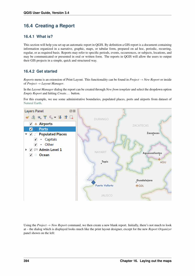
QGIS User Guide, Versión 3.4
16.4 Creating a Report
16.4.1 What is?
This section will help you set up an automatic report in QGIS. By definition a GIS report is a document containinginformation organized in a narrative, graphic, maps, or tabular form, prepared on ad hoc, periodic, recurring,regular, or as required basis. Reports may refer to specific periods, events, occurrences, or subjects, locations, andmay be communicated or presented in oral or written form. The reports in QGIS will allow the users to outputtheir GIS projects in a simple, quick and structured way.
16.4.2 Get started
Reports menu is an extension of Print Layout. This functionality can be found in Project → New Report or insideof Project → Layout Manager.
In the Layout Manager dialog the report can be created through New from template and select the dropdown optionEmpty Report and hitting Create. . . button.
For this example, we use some administrative boundaries, populated places, ports and airports from dataset ofNatural Earth.
Using the Project → New Report command, we then create a new blank report. Initially, there’s not much to lookat – the dialog which is displayed looks much like the print layout designer, except for the new Report Organizerpanel shown on the left:
394 Chapter 16. Laying out the maps

QGIS User Guide, Versión 3.4
16.4. Creating a Report 395

QGIS User Guide, Versión 3.4
16.4.3 Layout Report Workspace
QGIS reports can consist of multiple, nested sections. In our new blank report we initially have only the mainreport section. The only options present for this report section is Include report header or Include report footer.If we enable these options, the header will be included as the very first page (or pages. . . — individual parts ofreports can be multi-page if desired) in the report, and the footer would be the last page. Let’s go ahead and enablethe header, and hit the Edit button next to it:
A few things happen as a result. Firstly, an edit pencil is now shown next to the Report section in the ReportOrganizer, indicating that the report section is currently being edited in the designer. We also see a new blankpage shown in the designer itself, with the small Report Header title. In QGIS reports, every component of thereport is made up of individual layouts. They can be created and modified using the exact same tools as areavailable for standard print layouts – so you can use any desired combination of labels, pictures, maps, tables, etc.Let’s add some items to our report header to demonstrate:
We’ll also create a simple footer for the report, by checking the Include report footer option and hitting Edit.
Before proceeding further, let’s export this report and see what we get. Exporting is done from the Report menu– in this case we select Export Report as PDF to render the whole report to a PDF file. Here’s the not-very-impressive result – a two page PDF consisting of our header and footer:
396 Chapter 16. Laying out the maps

QGIS User Guide, Versión 3.4
16.4. Creating a Report 397

QGIS User Guide, Versión 3.4
398 Chapter 16. Laying out the maps
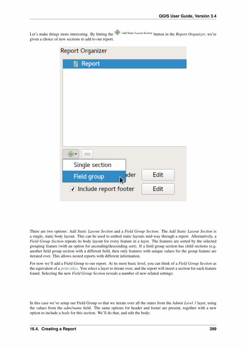
QGIS User Guide, Versión 3.4
Let’s make things more interesting. By hitting the Add Static Layout Section button in the Report Organizer, we’regiven a choice of new sections to add to our report.
There are two options: Add Static Layout Section and a Field Group Section. The Add Static Layout Section isa single, static body layout. This can be used to embed static layouts mid-way through a report. Alternatively, aField Group Section repeats its body layout for every feature in a layer. The features are sorted by the selectedgrouping feature (with an option for ascending/descending sort). If a field group section has child sections (e.g.another field group section with a different field, then only features with unique values for the group feature areiterated over. This allows nested reports with different information.
For now we’ll add a Field Group to our report. At its most basic level, you can think of a Field Group Section asthe equivalent of a print atlas. You select a layer to iterate over, and the report will insert a section for each featurefound. Selecting the new Field Group Section reveals a number of new related settings:
In this case we’ve setup our Field Group so that we iterate over all the states from the Admin Level 1 layer, usingthe values from the adm1name field. The same options for header and footer are present, together with a newoption to include a body for this section. We’ll do that, and edit the body:
16.4. Creating a Report 399

QGIS User Guide, Versión 3.4
400 Chapter 16. Laying out the maps

QGIS User Guide, Versión 3.4
We’ve setup this body with a map (set to follow the current report feature – just like how a map item in an atlascan follow the current atlas feature), and a label showing the state’s name. If we went ahead and exported ourreport now, we’d get something like this:
First, the report header, then a page for each state, and finally the report footer. So more or less an atlas, but with aheader and footer page. Let’s make things more interesting by adding a subsection to our state group. We do this
by first selecting the state field group in the organizer, then hitting the Field Group Section button and adding a newField Group Section:
When a Field Group Section is iterating over its features, it will automatically filter these features to match thefeature attributes from its parent groups. In this case, the subsection we added will iterate over a Populated Placeslayer, including a body section for each place encountered. The magic here is that the Populated Places layer hasan attribute named adm1name, tagging each place with the state it’s contained within (if you’re lucky your datawill already be structured like this – if not, run the Processing Join Attributes by Location algorithm and createyour own field). When we export this report, QGIS will grab the first state from the Admin Level 1 layer, and theniterate over all the Populated Places with a matching adm1name value. Here’s what we get:
Here we created a basic body for the Populated Places group, including a map of the place and a table of someplace attributes. So our report is now a report header, a page for each state followed by a page for every populated
16.4. Creating a Report 401

QGIS User Guide, Versión 3.4
402 Chapter 16. Laying out the maps

QGIS User Guide, Versión 3.4
16.4. Creating a Report 403

QGIS User Guide, Versión 3.4
place within that state, and finally the report footer. If we were to add a header for the Populated Places group, itwould be included just before listing the populated places for each state:
Similarly, a footer for the Populated Places group would be inserted after the final place for each state is included.
In addition to nested subsections, subsections in a report can also be included consecutively. If we add a secondsubsection to the Admin Level 1 group for Airports, then our report will first list ALL the populated places foreach state, followed by all the airports within that state, before proceeding to the next state. In this case our reportwould be structured like this:
16.4.4 Report Output
The key point here is that our Airports group is a subsection of the Admin Level 1 group – not the Populated Placesgroup. Here’s what our report could look like now:
Combining nested and consecutive sections, together with section headers and footers allows for tons of flexibility.For instance, in the below report we add another field group as a child of the main report for the :guilabel‘Ports‘layer. Now, after listing the states together with their populated places and airports, we’ll get a summary list of allthe ports in the region:
This results in the last part of our report exporting as:
404 Chapter 16. Laying out the maps

QGIS User Guide, Versión 3.4
16.4. Creating a Report 405

QGIS User Guide, Versión 3.4
406 Chapter 16. Laying out the maps

QGIS User Guide, Versión 3.4
16.4. Creating a Report 407

QGIS User Guide, Versión 3.4
408 Chapter 16. Laying out the maps

QGIS User Guide, Versión 3.4
16.4. Creating a Report 409
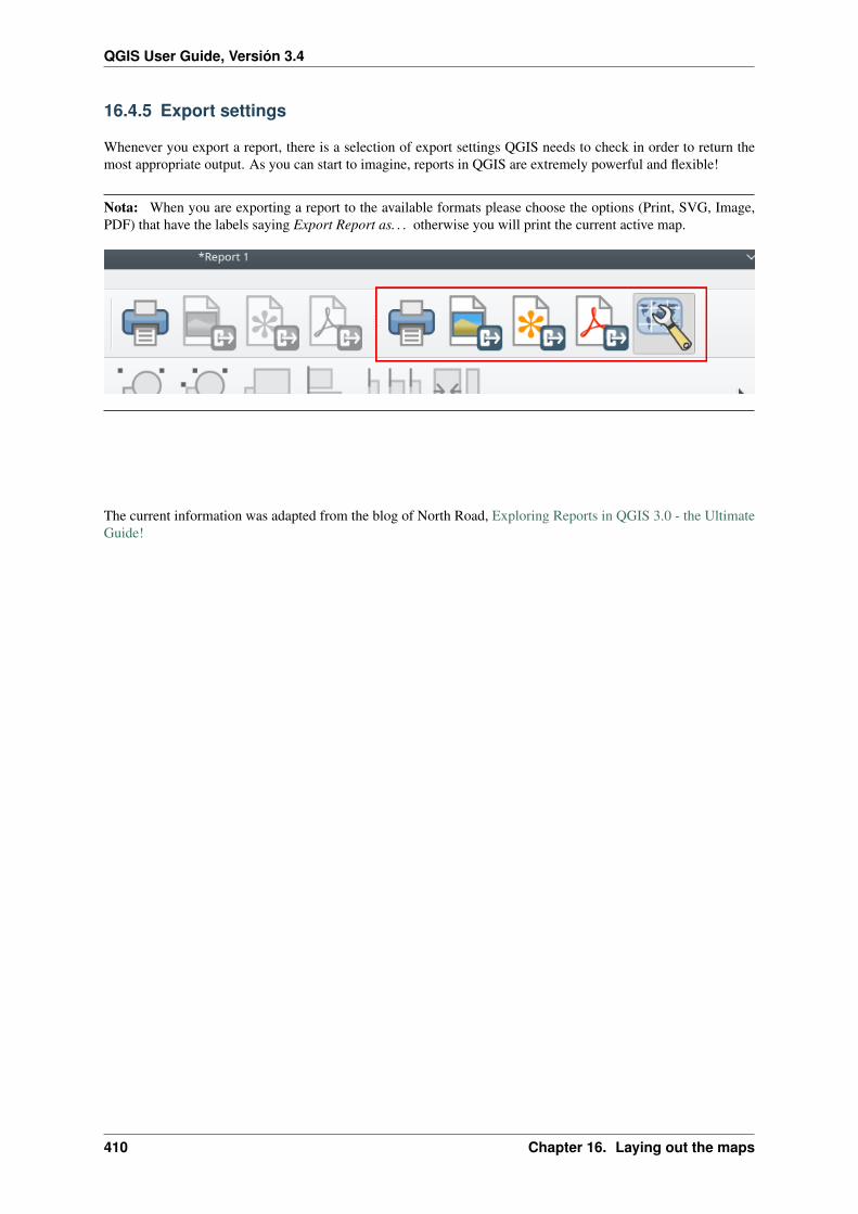
QGIS User Guide, Versión 3.4
16.4.5 Export settings
Whenever you export a report, there is a selection of export settings QGIS needs to check in order to return themost appropriate output. As you can start to imagine, reports in QGIS are extremely powerful and flexible!
Nota: When you are exporting a report to the available formats please choose the options (Print, SVG, Image,PDF) that have the labels saying Export Report as. . . otherwise you will print the current active map.
The current information was adapted from the blog of North Road, Exploring Reports in QGIS 3.0 - the UltimateGuide!
410 Chapter 16. Laying out the maps

CHAPTER 17
Trabajar con datos OGC
17.1 QGIS como Cliente de Datos OGC
El Open Geospatial Consortium (OGC) es una organización internacional con miembros de más de 300 organi-zaciones comerciales, gubernamentales, sin fines de lucro y de investigación de todo el mundo. Sus miembrosdesarrollan e implementan estándares para contenido geoespacial y servicios, procesamiento de datos SIG y elintercambio.
Describing a basic data model for geographic features, an increasing number of specifications are developedby OGC to serve specific needs for interoperable location and geospatial technology, including GIS. Furtherinformation can be found at https://www.opengeospatial.org/.
Importar especificaciones OGC implementadas por QGIS:
• WMS — Web Map Service (Cliente WMS/WMTS)
• WMTS — Web Map Tile Service (Cliente WMS/WMTS)
• WFS — Web Feature Service (Cliente WFS y WFS-T)
• WFS-T — Web Feature Service - Transactional (Cliente WFS y WFS-T)
• WCS — Web Coverage Service (WCT Cliente)
• WPS — Web Processing Service
• CSW — Catalog Service for the Web
• SFS — Simple Features for SQL (PostGIS Layers)
• GML — Lenguaje de Marcado Generalizado
Los servicios de QGIS esta incrementando el uso para intercambiar datos geoespaciales entre diferentes imple-mentaciones GIS y almacenes de datos. QGIS puede hacer frente a las especificaciones anteriores como un cliente,siendo SFS (a través del apoyo del proveedor PostgreSQL / PostGIS, vea la sección PostGIS Layers).
17.1.1 Cliente WMS/WMTS
411

QGIS User Guide, Versión 3.4
Información general de la implementación WMS
Actualmente QGIS puede actual como un cliente WMS que entiende servidores WMS 1.1, 1.1.1 y 1.3. En partic-ular, se ha probado contra los servidores de acceso público como DEMIS.
Un servidor WMS actúa sobre las peticiones por parte del cliente (por ejemplo, QGIS) para un mapa ráster conuna extensión dada, el conjunto de capas, el estilo de simbolización y la transparencia. El servidor WMS despuésconsulta sus fuentes de datos locales, rásteriza el mapa y lo envía de vuelta al cliente en formato ráster. Para QGIS,este formato sería típicamente JPEG o PNG.
WMS es genéricamente un servicio REST (Representational State Transfer) en lugar de un servicio Web en todaregla. Como tal, puede tomar las URLs generadas por QGIS y utilizarlos en el navegador web para recuperar lasmismas imágenes que QGIS utiliza internamente. Esto puede ser útil para la solución de problemas, ya que hayvarias marcas de servidores WMS en el mercado y ellos tienen su propia interpretación de la estándar WMS.
Las capas WMS se pueden añadir sencillamente, siempre que conozca la URL para acceder al servidor WMS, sitiene una conexión útil a ese servidor, y el servidor entiende HTTP como mecanismo de transporte de datos.
Additionally, QGIS will cache your WMS responses (i.e. images) for 24h as long as the GetCapabilities requestis not triggered. The GetCapabilities request is triggered everytime the Connect button in the Add Layer(s) fromWMS(T) Server dialog is used to retrieve the WMS server capabilities. This is an automatic feature meant tooptimize project loading time. If a project is saved with a WMS layer, the corresponding WMS tiles will beloaded from the cache the next time the project is opened as long as they are no older than 24H.
Información general de la implementación WMTS
QGIS también puede actuar como un cliente WMTS. WMTS es un estándar OGC para distribuir tiles de conjuntode datos geoespaciales. Este es una manera más rápida y más eficiente de distribuir datos que WMS porque conWMTS, el conjunto de tile es pregenerado y el cliente sólo solicita la transmisión de los tiles, no su producción.Una petición WMS implica típicamente ambos la generación y la transmisión de los datos. Un ejemplo bienconocido de un estándar no OGC para la visualización de datos geoespaciales de tiles es Google Maps.
Para mostrar los datos en una variedad de escalas cercanas a lo que el usuario podría querer, los conjuntos deteselas WMTS se producen en varios niveles de escala diferentes y están disponibles para el cliente SIG parapedirlos.
Este diagrama ejemplifica el concepto de conjunto de teselas:
Figure 17.1: Concepto de conjunto de teselas WMTS
Los dos tipos de interfaz WMTS que QGIS reconoce son a través de Key-Value-Pairs (KVP) y RESTful. Estasdos interfaces son diferentes y es necesario especificarlos a QGIS diferente.
1. Con el fin de acceder a un servicio WMTS KVP, un usuario QGIS debe abrir la interfaz WMS/WMTS yañadir la siguiente cadena a la URL del servicio tile WMTS:
412 Chapter 17. Trabajar con datos OGC

QGIS User Guide, Versión 3.4
"?SERVICE=WMTS&REQUEST=GetCapabilities"
Un ejemplo de este tipo de dirección es
https://opencache.statkart.no/gatekeeper/gk/gk.open_wmts?\service=WMTS&request=GetCapabilities
Para probar la capa topo2 en este WMTS funciona muy bien. Añadir esta cadena indica que un servicioweb WMTS se va a utilizar en lugar de un servicio WMS.
2. EL servicio RESTful WMTS toma una forma diferente, una URL sencilla. EL formato recomendado porOGC es:
{WMTSBaseURL}/1.0.0/WMTSCapabilities.xml
This format helps you to recognize that it is a RESTful address. A RESTful WMTS is accessed in QGIS bysimply adding its address in the WMS setup in the URL field of the form. An example of this type of addressfor the case of an Austrian basemap is https://maps.wien.gv.at/basemap/1.0.0/WMTSCapabilities.xml.
Nota: You can still find some old services called WMS-C. These services are quite similar to WMTS (i.e., samepurpose but working a little bit differently). You can manage them the same as you do WMTS services. Just add?tiled=true at the end of the url. See https://wiki.osgeo.org/wiki/Tile_Map_Service_Specification for moreinformation about this specification.
Cuando se lee WMTS, a menudo se puede pensar en WMS-C también.
Seleccionar servidor WMS/WMTS
La primera ves que utiliza la característica WMS en QGIS, no hay servidores definidos.
Comience haciendo clic en el botón Añadir capa WMS en la barra de herramientas, o seleccionando Capa →Añadir capa WMS. . . .
The dialog Add Layer(s) from a Server for adding layers from the WMS server appears. You can add some serversto play with by clicking the Add Default Servers button. This will add two WMS demo servers for you to use: theWMS servers of the DM Solutions Group and Lizardtech. To define a new WMS server in the Layers tab, selectthe New button. Then enter the parameters to connect to your desired WMS server, as listed in table_OGC_wms:
Nombre Un nombre para esta conexión. Este nombre se utilizará en la lista desplegable de conex-iones a servidor así que se puede distinguir de otros servidores WMS.
URL La URL del servidor provee los datos. Este debe ser un nombre de host soluble – el mismoformato que usaría para abrir una conexión telnet o ping a un host.
Nombre deusuario
Nombre de usuario para acceder a un servidor asegurado de WMS. Este parámetro esopcional.
Contraseña Contraseña para una autentificación básica al servidor WMS. Este parámetro es opcional
Ignorar URIGetMap
Ignorar URI GetMap reportada en las capacidades. Utilice un URI dado del campoURL anterior.
Ignorar la URIGetFeatureInfo
Ignorar la URI GetFeatureInfo reportada en las capacidades. Utilice un URI dado delcampo URL anterior.
Tabla OGC 1: Parámetros de conexión WMS
Si necesita configurar un servidor proxy para poder recibir servicios WMS de internet, puede añadir su servidorproxy en las opciones. Elija Configuración → Opciones y haga clic en la pestaña Red. Ahí, puede añadir su
configuración de proxy y habilitarlos al ajustar Usar proxy para acceso web. Compruebe que selecciono el
tipo de proxy correcto del menú desplegable Tipo de proxy .
17.1. QGIS como Cliente de Datos OGC 413

QGIS User Guide, Versión 3.4
Una vez que la nueva conexión al servidor WMS ha sido creada, será preservado para futuras sesiones.
Truco: En las direcciones URL del servidor WMS
Asegúrese, al introducir la URL del servidor WMS, que tiene solo la base URL. Por ejemplo, no debe tenerfragmentos como request=GetCapabilities o version=1.0.0 en su URL.
Advertencia: Entering username and password in the Authentication tab will keep unprotected credentialsin the connection configuration. Those credentials will be visible if, for instance, you shared the projectfile with someone. Therefore, it’s advisable to save your credentials in a Authentication configuration instead(configurations tab). See Sistema de autenticación for more details.
Cargando capas WMS/WMTS
Once you have successfully filled in your parameters, you can use the Connect button to retrieve the capabilities ofthe selected server. This includes the image encoding, layers, layer styles and projections. Since this is a networkoperation, the speed of the response depends on the quality of your network connection to the WMS server. Whiledownloading data from the WMS server, the download progress is visualized in the lower left of the WMS dialog.
Your screen should now look a bit like figure_OGC_add_wms, which shows the response provided by the Euro-pean Soil Portal WMS server.
Figure 17.2: El diálogo para añadir un servidor WMS, muestra las capas disponibles
Codificación de la Imagen
414 Chapter 17. Trabajar con datos OGC

QGIS User Guide, Versión 3.4
La sección Codificación de la imagen lista los formatos que reconoce por ambos el cliente y el servidor. Elija unodependiendo de sus requerimientos de precisión de imagen.
Truco: Codificación de la Imagen
Normalmente, encontrará que un servidor WMS le ofrece la opción de codificación de la imagen en JPEG o PNG.JPEG es un formato de compresión con pérdida, mientras que PNG reproduce fielmente los datos crudos raster.
Utilizar JPEG si se espera que los datos WMS sean de naturaleza fotográfica y/o no le importa cierta perdida decalidad de la imagen. Esta disyuntiva típicamente reduce en cinco veces la necesidad de transferencia de datos encomparación con PNG.
Utilice PNG si desea representaciones precisas de los datos originales y no le importa el incremento de los requi-sitos de transferencia de datos.
Opciones
La zona Opciones del diálogo provee un campo de texto donde se puede añadir un Nombre de capa para la capaWMS. Este nombre aparecerá en la leyenda después de cargar la capa.
Debajo del nombre de la capa, se puede definir Tamaño de la tesela, si desea establecer tamaños de tesela (porejemplo, 256x256) para dividir la petición WMS en múltiples peticiones.
El Límite del objeto espacial para GetFeatureInfo define los objetos espaciales del servidor a consultar.
If you select a WMS from the list, a field with the default projection provided by the mapserver appears. If theChange. . . button is active, you can click on it and change the default projection of the WMS to another CRSprovided by the WMS server.
Finalmente puede activar Utiliza leyenda-WMS contextual si el servidor WMS admite este objeto. Entoncessólo la leyenda relevante para su actual extensión de vista de mapa se mostrará y así no incluirá los elementos dela leyenda por cosas que no puede ver en el mapa actual.
Orden de la capa
La pestaña Orden de Capas lista las capas seleccionadas disponibles de la conexión actual al servidor WMS.Puede notar que algunas capas son ampliables; esto significa que la capa se puede visualizar en una selección deestilos de imagen.
Se puede seleccionar varias capas a la vez, pero solo una imagen de estilo por capa. Cuando varias capas sonseleccionadas, estas se combinarán en el servidor WMS y se transmitirán a QGIS una sola vez.
Truco: Ordenar capas WMS
Las capas WMS representadas por un servidor son sobrepuestas en el orden listado en la sección de Capas, desdela parte superior a la parte inferior de la lista. Si se desea cambiar el orden de la superposición, se puede usar lapestaña Orden de capas.
Transparencia
En esta versión de QGIS, la configuración Transferencia global de Propiedades de la capa esta codificado paraestar siempre en donde este disponible.
Truco: Transparencia de capa WMS
La disponibilidad de imagen WMS transparente depende de la codificación de la imagen utilizada: PNG y GIFreconoce la transparencia, mientras JPEG deja sin reconocerlo.
Sistema de referencia de coordenadas
Un sistema de referencia de coordenadas (SRC) es la terminología para una proyección QGIS.
Cada capa WMS se puede representar en múltiples SRC’s, dependiendo de la capacidad del servidor WMS.
17.1. QGIS como Cliente de Datos OGC 415

QGIS User Guide, Versión 3.4
To choose a CRS, select Change. . . and a dialog similar to Diálogo SRC Personalizado will appear. The maindifference with the WMS version of the dialog is that only those CRSs supported by the WMS server will beshown.
Busqueda del servidor
Within QGIS, you can search for WMS servers. Figure_OGC_search shows the Server Search tab with the AddLayer(s) from a Server dialog.
Figure 17.3: Diálogo de búsqueda de servidores WMS después de algunas palabras clave
As you can see, it is possible to enter a search string in the text field and hit the Search button. After a shortwhile, the search result will be populated into the list below the text field. Browse the result list and inspect yoursearch results within the table. To visualize the results, select a table entry, press the Add Selected Row to WMSList button and change back to the Layers tab. QGIS has automatically updated your server list, and the selectedsearch result is already enabled in the list of saved WMS servers in the Layers tab. You only need to request thelist of layers by clicking the Connect button. This option is quite handy when you want to search maps by specifickeywords.
Básicamente, esta opción es una interfaz del API de http://geopole.org.
Conjunto de teselas
Al utilizar servicios WMTS (Cached WMS) como
https://opencache.statkart.no/gatekeeper/gk/gk.open_wmts?\service=WMTS&request=GetCapabilities
you are able to browse through the Tilesets tab given by the server. Additional information like tile size, formatsand supported CRS are listed in this table. In combination with this feature, you can use the tile scale slider by
selecting View → Panels ( or Settings → Panels), then choosing Tile Scale Panel. This gives you the availablescales from the tile server with a nice slider docked in.
416 Chapter 17. Trabajar con datos OGC

QGIS User Guide, Versión 3.4
Utilizar la herramienta de Identificar objetos espaciales
Una vez que haya añadido un servidor WMS, y si alguna capa de un servidor WMS es consultable, puede entonces
utilizar la herramienta Identificar objetos espaciales para seleccionar un píxel del lienzo del mapa. Una consulta sehace al servidor WMS por cada selección realizada. El resultado de la consulta es regresada en texto plano. Elformato de este texto es dependiente del servidor WMS particular utilizado. Selección de Formato
Si múltiples formatos de salida son reconocidos por el servidor, una lista desplegable con formatos admitidos seañade automáticamente al diálogo de resultados identificados y el formato seleccionada puede ser almacenado enel proyecto para la capa. Usar formato GML
La herramienta Identificar reconoce la respuesta del servidor WMS (GetFeatureInfo) en formato GML (se llamaObjeto espacial en la GUI de QGIS en este contexto). Si el formato «Objeto espacial» es admitido por el servidor yseleccionado, los resultados de la herramienta de identificador son objetos vectoriales, como de una capa vectorialregular. Cuando un objeto espacial es seleccionado en el árbol, este resalta en el mapa y se puede copiar a lapapelera y pegar a otra capa vectorial. Vea el ejemplo de configuración de UMN Mapserver abajo que admiteGetFeatureInfo en formato GML.
# in layer METADATA add which fields should be included and define geometry→˓(example):
"gml_include_items" "all""ows_geometries" "mygeom""ows_mygeom_type" "polygon"
# Then there are two possibilities/formats available, see a) and b):
# a) basic (output is generated by Mapserver and does not contain XSD)# in WEB METADATA define formats (example):"wms_getfeatureinfo_formatlist" "application/vnd.ogc.gml,text/html"
# b) using OGR (output is generated by OGR, it is send as multipart and contains→˓XSD)# in MAP define OUTPUTFORMAT (example):OUTPUTFORMAT
NAME "OGRGML"MIMETYPE "ogr/gml"DRIVER "OGR/GML"FORMATOPTION "FORM=multipart"
END
# in WEB METADATA define formats (example):"wms_getfeatureinfo_formatlist" "OGRGML,text/html"
Ver propiedades
Una vez que haya añadido un servidor WMS, puede ver sus propiedades haciendo clic derecho sobre el mismo enla leyenda y la seleccionar Propiedades. Pestaña de Metadatos
La pestaña Metadatos muestra una gran cantidad de información acerca del servidor WMS, generalmente obtenidade la declaración de capacidades de ese servidor. Muchas definiciones pueden ser extraídas mediante la lecturadel estándar WMS (vea OPEN-GEOSPATIAL-CONSORTIUM en Referencias bibliográficas y web), pero aquíhay algunas definiciones útiles:
• Propiedades del servidor
– Versión WMS — La versión WMS implementada por el servidor.
– Formatos de Imagen — La lista de MIME-types que el servidor puede responder con la elaboracióndel mapa. QGIS reconoce cualquier formato las bibliotecas Qt subyacentes con que fueron constru-idas, que es típicamente por lo menos image/png y image/jpeg.
17.1. QGIS como Cliente de Datos OGC 417

QGIS User Guide, Versión 3.4
– Formato de Identificación — La lista de tipos MIME, el servidor puede responder, cuando utilice laherramienta de Identificación. Actualmente, QGIS reconoce el tipo texto plano.
• Propiedades de la capa
– Seleccionar — Sea o no esta capa seleccionada cuando su servidor fue añadido a este proyecto.
– Visible — Si la capa seleccionada es o no visible en la leyenda (aun no utilizada en esta versión deQGIS).
– Poder Identificar — Sea o no esta capa regresará algunos resultados cuando la herramienta de iden-tificar se utilice en él.
– Puede ser transparente — Si esta capa puede ser representada o no con transparencia. Esta versión deQGIS siempre usará transparencia si este es Si y la codificación de la imagen admite la transparencia.
– ** Puede Acercar zum ** — Si en esta capa se puede o no hacer zum en el servidor. Esta versiónde QGIS asume que todas las capas WMS tienen este conjunto de Si. Capas deficientes pueden serpresentadas de manera extraña.
– Conteo en Cascada — Los servidores WMS pueden actuar como proxy para otros servidores WMSpara obtener datos ráster de una capa. Esta entrada muestra el número de veces que se remitió lasolicitud de esta capa para ver a los servidores WMS para obtener un resultado.
– Ancho fijo, altura fija — Si esta capa o no tiene fijas las dimensiones en píxeles de origen. Estaversión de QGIS asume que todas las capas WMS tienen este conjunto a nada. Capas deficientespueden ser presentadas de forma extraña.
– Recuadro delimitador WGS 84 — El recuadro delimitador de la capa, en coordenadas WGS 84.Algunos servidores WMS no establecen esto correctamente (por ejemplo, utilizan coordenadas UTMen su lugar). Si éste es el caso, entonces la vista inicial de la capa puede aparecer muy “lejana”en QGIS. El webmaster de WMS debería ser informado de este error, que probablemente conocencomo los elementos XML de WMS LatLonBoundingBox, EX_GeographicBoundingBox oel BoundingBox‘ de CRS:84.
– Disponible en SRC — Las proyecciones que esta capa puede representar por el servidor WMS. Éstosse enumeran en el formato nativo de WMS.
– Disponible en estilo — Los estilos de imagen que esta capa puede representar por el servidor WMS.
Show WMS legend graphic in table of contents and layout
The QGIS WMS data provider is able to display a legend graphic in the table of contents” layer list and in theprint layout. The WMS legend will be shown only if the WMS server has GetLegendGraphic capability and thelayer has getCapability url specified, so you additionally have to select a styling for the layer.
Si hay definida una legendGraphic, ésta se mostrará debajo de la capa. Es pequeña y hay que hacer clic sobre ellapara abrirla en tamaño real (debido a una limitación de la arquitectura de QgsLegendInterface). Al hacer clic enla leyenda de la capa se abrirá un cuadro con la leyenda a la máxima resolución.
In the print layout, the legend will be integrated at it’s original (downloaded) dimension. Resolution of the legendgraphic can be set in the item properties under Legend → WMS LegendGraphic to match your printing require-ments.
La leyenda mostrará información contextual basada en su escala actual. La leyenda WMS se muestra sólo si elservidor WMS tiene capacidad GetLegendGraphic y la capa tiene definida una url getCapability, para lo que sedebe seleccionar un estilo.
Limitaciones del cliente WMS
No es posible la funcionalidad de cliente WMS que se ha incluido en esta versión de QGIS. Algunas de lasexcepciones más notables siguen.
Editar la configuración de la capa WMS
418 Chapter 17. Trabajar con datos OGC

QGIS User Guide, Versión 3.4
Una vez que haya completado el procedimiento de Añadir capa WMS, no se podrá cambiar la configuración. Unasolución alternativa es eliminar la capa por completo y empezar de nuevo.
**Autentificación necesaria en servidores WMS **
Actualmente, se admiten servicios WMS públicamente accesibles y garantizados. Los servidores WMS garantiza-dos se puede acceder mediante autenticación pública. El usuario puede agregar las credenciales (opcional) cuandoagregue un servidor WMS. Vea la sección :ref: ogc-wms-servers para más detalles.
Truco: Acceso garantizado a capas OGC
If you need to access secured layers with secured methods other than basic authentication, you can use InteProxyas a transparent proxy, which does support several authentication methods. More information can be found in theInteProxy manual at https://inteproxy.wald.intevation.org.
Truco: QGIS WMS Mapserver
Desde la versión 1.7.0, QGIS tiene su propia implementación de un servidor de mapas WMS 1.3.0. Lea más sobreesto en el capítulo QGIS como Servidor de Datos OGC.
17.1.2 WCT Cliente
Un Web Coverage Service (WCS) proporciona acceso a los datos ráster en formas que son útiles para larepresentación del lado cliente, como datos de entrada en los modelos científicos, y para otros clientes. El WCSse puede comparar con la WFS y el WMS. Como WMS y WFS instancias de servicios, un WCS permite a losclientes elegir partes de las explotaciones de información de un servidor basado en restricciones espaciales y otroscriterios de consulta.
QGIS tiene un proveedor WCS nativo y reconoce ambas versiones 1.0 y 1,1 (que son significativamente difer-entes), pero actualmente se prefiere 1.0, porque 1.1 tiene muchos problemas (por ejemplo, cada servidor lo imple-menta de diferente forma con varias particularidades).
El proveedor de WCS nativo se encarga de todas las solicitudes de red y utiliza las configuraciones de red estándarde QGIS (especialmente de proxy). También es posible seleccionar el modo de caché ( “siempre caché”, “prefer-entemente caché”, “preferentemente red”, “siempre red” ). El proveedor también es compatible con la selecciónde tiempo de la posición, si el servidor ofrece el dominio temporal.
Advertencia: Entering username and password in the Authentication tab will keep unprotected credentialsin the connection configuration. Those credentials will be visible if, for instance, you shared the projectfile with someone. Therefore, it’s advisable to save your credentials in a Authentication configuration instead(configurations tab). See Sistema de autenticación for more details.
17.1.3 Cliente WFS y WFS-T
En QGIS, una capa WFS funciona prácticamente como cualquier otra capa vectorial. Puede identificar y se-leccionar objetos espaciales, y ver la tabla de atributos. Desde QGIS 1.6, la edición WFS-T está también dereconocida.
En general, añadir una capa WFS es muy similar al procedimiento utilizado con WMS. La diferencia es que nohay servidores por defecto definidos, así que tenemos que añadir la nuestra.
Cargar una capa WFS
As an example, we use the Gateway Geomatics WFS server and display a layer. https://demo.gatewaygeomatics.com/cgi-bin/wfs_gateway?REQUEST=GetCapabilities&VERSION=1.0.0&SERVICE=WFS
17.1. QGIS como Cliente de Datos OGC 419

QGIS User Guide, Versión 3.4
To be able to load a WFS Layer we create a connection to the WFS server first.
1. Open the Data Source Manager dialog by pressing the Open Data Source Manager button
2. Enable the WFS tab
3. Click on New. . . to open the Create a New WFS Connection dialog
4. Enter Gateway Geomatics as name
5. Enter the URL (see above)
Figure 17.4: Creating a connection to a WFS server
6. In the WFS settings dialog, you can:
• Indicate the WFS version of the server. If unknown, press the Detect button to automatically retrieveit.
• Define the maximum number of features retrieved in a single GetFetFeature request. If empty, no limitis set.
• Invert axis orientation.
• And depending on the WFS version:
– Force to Ignore axis orientation (WFS 1.1/WFS 2.0)
– Enable feature paging and specify the maximum number of features to retrieve with Page size. Ifno limit is defined, then the server default is applied.
420 Chapter 17. Trabajar con datos OGC

QGIS User Guide, Versión 3.4
Advertencia: Entering username and password in the Authentication tab will keep unprotected cre-dentials in the connection configuration. Those credentials will be visible if, for instance, you sharedthe project file with someone. Therefore, it’s advisable to save your credentials in an Authenticationconfiguration instead (Configurations tab). See Sistema de autenticación for more details.
7. Press OK to create the connection.
Tenga en cuenta que cualquier configuración de proxy que pueda haber establecido en sus preferencias tambiénson reconocidos.
Now we are ready to load WFS layers from the above connection.
1. Choose “Gateway Geomatics” from the Server Connections drop-down list.
2. Click Connect
3. Select the Parks layer in the list
4. You can also choose whether to:
• Use title for layer name, showing the layer’s title as defined on the server in the Layers panelinstead of its Name
• Only request features overlapping the view extent
• Change the layer’s CRS
• or Build query to specify particular features to retrieve, by either using the corresponding button ordouble-clicking the target layer.
5. Click Add to add the layer to the map.
You’ll notice the download progress is visualized in the lower left of the QGIS main window. Once the layer isloaded, you can identify and select a couple of features and view the attribute table.
Nota: QGIS supports different versions of the WFS protocol, with background download and progressive ren-dering, on-disk caching of downloaded features and version autodetection.
Truco: Encontrar servidores WFS
Puede encontrar servidores WFS adicionales al utilizar Google o su buscador favorito. Hay un número de listascon URLs publicas, algunos son mantenidos y otros no.
17.2 QGIS como Servidor de Datos OGC
QGIS Server is an open source WMS 1.3, WFS 1.0.0, WFS 1.1.0 and WCS 1.1.1 implementation that, in addition,implements advanced cartographic features for thematic mapping. QGIS Server is a FastCGI/CGI (CommonGateway Interface) application written in C++ that works together with a web server (e.g., Apache, Lighttpd).It has Python plugin support allowing for fast and efficient development and deployment of new features. Theoriginal development of QGIS Server was funded by the EU projects Orchestra, Sany and the city of Uster inSwitzerland.
El servidor QGIS utiliza QGIS como back-end para la lógica de los SIG y de mapa de representación. Además, labiblioteca Qt se utiliza para gráficos y para la plataforma independiente la programación en C++. En contraste conotro software de WMS, el servidor de |qg| utiliza reglas cartográficos como un lenguaje de configuración, tantopara la configuración del servidor y de las reglas cartográficas definidas por el usuario.
As QGIS desktop and QGIS Server use the same visualization libraries, the maps that are published on the weblook the same as in desktop GIS.
17.2. QGIS como Servidor de Datos OGC 421

QGIS User Guide, Versión 3.4
Figure 17.5: Añadir una capa WFS
422 Chapter 17. Trabajar con datos OGC

QGIS User Guide, Versión 3.4
In the following sections, we will provide a sample configuration to set up a QGIS Server on Debian/UbuntuLinux. For more detailed installation instructions on other platforms or distributions and more information onworking with QGIS Server, we recommend reading the QGIS Server Training Manual or server_plugins.
17.2.1 Empezando
Installation on Debian-based systems
At this point, we will give a short and simple installation how-to for a minimal working configuration on Debianbased systems. However, many other distributions and OSs provide packages for QGIS Server.
Requirements and steps to install QGIS Server on a Debian based system are provided in QGIS installers page.Please refer to that section.
HTTP Server configuration
Apache
Apache and its mod_fcgid module may be used for executing QGIS Server.
Install Apache and mod_fcgid:
sudo apt install apache2 libapache2-mod-fcgid
Here we assume that an Apache VirtualHost is already set up. For example this is what a basicVirtualHost configuration may look like:
<VirtualHost *:80>
ServerAdmin webmaster@localhostDocumentRoot /var/www/html
ErrorLog ${APACHE_LOG_DIR}/error.logCustomLog ${APACHE_LOG_DIR}/access.log combined
</VirtualHost>
Nota: On Debian systems, a default VirtualHost is available in /etc/apache2/sites-available/000-default.conf.
Let’s now add mod_fcgid configuration directives for QGIS Server:
<VirtualHost *:80>
ServerAdmin webmaster@localhostDocumentRoot /var/www/html
ErrorLog ${APACHE_LOG_DIR}/error.logCustomLog ${APACHE_LOG_DIR}/access.log combined
FcgidInitialEnv DISPLAY ":99"FcgidInitialEnv QGIS_SERVER_LOG_LEVEL "0"FcgidInitialEnv QGIS_SERVER_LOG_STDERR "1"
<Location /qgisserver>SetHandler fcgid-scriptFcgidWrapper /usr/lib/cgi-bin/qgis_mapserv.fcgi virtualOptions +ExecCGI -MultiViews +FollowSymLinks
17.2. QGIS como Servidor de Datos OGC 423

QGIS User Guide, Versión 3.4
Require all granted</Location>
</VirtualHost>
See the mod_fcgid documentation for more information on the Fcgid parameters used. And see below tounderstand when and why the DISPLAY environment variable needs to be set.
Now restart Apache for the new configuration to be taken into account:
sudo service apache2 restart
QGIS Server is now available at http://localhost/qgisserver.
NGINX
You can also use QGIS Server with NGINX. Unlike Apache, NGINX does not automatically spawn FastCGIprocesses. The FastCGI processes are to be started by something else.
On Debian-based systems, you may use fcgiwrap or spawn-fcgi to start and manage the QGIS Server processes.Official Debian packages exist for both.
Nota: fcgiwrap is easier to set up than spawn-fcgi, because it’s already wrapped in a Systemd service. But italso leads to a solution that is much slower than using spawn-fcgi. With fcgiwrap a new QGIS Server process iscreated on each request, meaning that the QGIS Server initialization process, which includes reading and parsingthe QGIS project file, is done on each request. With spawn-fcgi, the QGIS Server process remains alive betweenrequests, resulting in much better performance. For that reason, spawn-fcgi is recommended for production use.
Install NGINX:
sudo apt install nginx
fcgiwrap
If you want to use fcgiwrap to run QGIS Server, you first have to install the corresponding package:
sudo apt install fcgiwrap
Then, introduce the following block in your NGINX server configuration:
1 location /qgisserver {2 gzip off;3 include fastcgi_params;4 fastcgi_pass unix:/var/run/fcgiwrap.socket;5 fastcgi_param SCRIPT_FILENAME /usr/lib/cgi-bin/qgis_mapserv.fcgi;6 }
Finally, restart NGINX and fcgiwrap to take into account the new configuration:
sudo service nginx restartsudo service fcgiwrap restart
QGIS Server is now available at http://localhost/qgisserver.
424 Chapter 17. Trabajar con datos OGC
QGIS User Guide, Versión 3.4
spawn-fcgi
If you prefer to use spawn-fcgi instead of fcgiwrap, the first step is to install the package:
sudo apt install spawn-fcgi
Then, introduce the following block in your NGINX server configuration:
location /qgisserver {gzip off;include fastcgi_params;fastcgi_pass unix:/var/run/qgisserver.socket;
}
And restart NGINX to take into account the new configuration:
sudo service nginx restart
Finally, considering that there is no default service file for spawn-fcgi, you have to manually start QGIS Server inyour terminal:
sudo spawn-fcgi -s /var/run/qgisserver.socket \-U www-data -G www-data -n \/usr/lib/bin/cgi-bin/qgis_mapserv.fcgi
Of course, you may write an init script (like a qgisserver.service file with Systemd) to start QGIS Serverat boot time or whenever you want.
QGIS Server is now available at http://localhost/qgisserver.
Nota: With the above command spawn-fcgi spawns only one QGIS Server process. To use more than one QGISServer process you can combine spawn-fcgi with the multiwatch tool, which is also packaged in Debian.
Configuration
The include fastcgi_params; used in previous configuration is important as it adds the parameters from /etc/nginx/fastcgi_params:
fastcgi_param QUERY_STRING $query_string;fastcgi_param REQUEST_METHOD $request_method;fastcgi_param CONTENT_TYPE $content_type;fastcgi_param CONTENT_LENGTH $content_length;
fastcgi_param SCRIPT_NAME $fastcgi_script_name;fastcgi_param REQUEST_URI $request_uri;fastcgi_param DOCUMENT_URI $document_uri;fastcgi_param DOCUMENT_ROOT $document_root;fastcgi_param SERVER_PROTOCOL $server_protocol;fastcgi_param REQUEST_SCHEME $scheme;fastcgi_param HTTPS $https if_not_empty;
fastcgi_param GATEWAY_INTERFACE CGI/1.1;fastcgi_param SERVER_SOFTWARE nginx/$nginx_version;
fastcgi_param REMOTE_ADDR $remote_addr;fastcgi_param REMOTE_PORT $remote_port;fastcgi_param SERVER_ADDR $server_addr;fastcgi_param SERVER_PORT $server_port;fastcgi_param SERVER_NAME $server_name;
17.2. QGIS como Servidor de Datos OGC 425

QGIS User Guide, Versión 3.4
# PHP only, required if PHP was built with --enable-force-cgi-redirectfastcgi_param REDIRECT_STATUS 200;
Of course, you may override these variables in your own configuration. For example:
include fastcgi_params;fastcgi_param SERVER_NAME domain.name.eu;
Moreover, you can use some Variables de entorno to configure QGIS Server. With NGINX as HTTP Server, youhave to use fastcgi_param to define these variables as shown below:
fastcgi_param QGIS_DEBUG 1;fastcgi_param QGIS_SERVER_LOG_FILE /tmp/qgis-000.log;fastcgi_param QGIS_SERVER_LOG_LEVEL 0;
Nota: When using spawn-fcgi, you may directly define environment variables before running the server. Forexample: export QGIS_SERVER_LOG_FILE=/home/user/qgis.log
Xvfb
QGIS Server needs a running X Server to be fully usable. But if you don’t have one, you may use xvfb to have avirtual X environment.
To install the package:
sudo apt install xvfb
Then, according to your HTTP server, you should configure the DISPLAY parameter or directly use xvfb-run.
For example with NGINX and spawn-fcgi using xvfb-run:
xvfb-run /usr/bin/spawn-fcgi -f /usr/lib/bin/cgi-bin/qgis_mapserv.fcgi \-s /tmp/qgisserver.socket \-G www-data -U www-data -n
The other option is to start a virtual X server environment with a specific display number thanks to Xvfb:
/usr/bin/Xvfb :99 -screen 0 1024x768x24 -ac +extension GLX +render -noreset
Then we just have to set the DISPLAY environment variable in the HTTP server configuration. For example withNGINX:
fastcgi_param DISPLAY ":99";
Or with Apache:
FcgidInitialEnv DISPLAY ":99"
Installation on Windows
QGIS Server can also be installed on Windows systems. While the QGIS Server package is available in the 64 bitversion of the OSGeo4W network installer (https://qgis.org/en/site/forusers/download.html) there is no Apache(or other web server) package available, so this must be installed by other means.
A simple procedure is the following:
426 Chapter 17. Trabajar con datos OGC

QGIS User Guide, Versión 3.4
• Download the XAMPP installer (https://www.apachefriends.org/download.html) for Windows and installApache
• Download the OSGeo4W installer, follow the «Advanced Install» and install both the QGIS Desktop andQGIS Server packages
• Edit the httpd.conf file (C:\xampp\apache\httpd.conf if the default installation paths have beenused) and make the following changes:
From:
ScriptAlias /cgi-bin/ "C:/xampp/cgi-bin/"
To:
ScriptAlias /cgi-bin/ "c:/OSGeo4W64/apps/qgis/bin/"
From:
<Directory "C:/xampp/cgi-bin">AllowOverride NoneOptions NoneRequire all granted</Directory>
To:
<Directory "c:/OSGeo4W64/apps/qgis/bin">SetHandler cgi-scriptAllowOverride NoneOptions ExecCGIOrder allow,denyAllow from all
17.2. QGIS como Servidor de Datos OGC 427

QGIS User Guide, Versión 3.4
Require all granted</Directory>
From:
AddHandler cgi-script .cgi .pl .asp
To:
AddHandler cgi-script .cgi .pl .asp .exe
Then at the bottom of httpd.conf add:
SetEnv GDAL_DATA "C:\OSGeo4W64\share\gdal"SetEnv QGIS_AUTH_DB_DIR_PATH "C:\OSGeo4W64\apps\qgis\resources"SetEnv PYTHONHOME "C:\OSGeo4W64\apps\Python36"SetEnv PATH "C:\OSGeo4W64\bin;C:\OSGeo4W64\apps\qgis\bin;C:\OSGeo4W64\apps\Qt5\bin;→˓C:\WINDOWS\system32;C:\WINDOWS;C:\WINDOWS\System32\Wbem"SetEnv QGIS_PREFIX_PATH "C:\OSGeo4W64\apps\qgis"SetEnv QT_PLUGIN_PATH "C:\OSGeo4W64\apps\qgis\qtplugins;→˓C:\OSGeo4W64\apps\Qt5\plugins"
Restart the Apache web server from the XAMPP Control Panel and open browser window to testing a GetCapa-bilities request to QGIS Server
http://localhost/cgi-bin/qgis_mapserv.fcgi.exe?SERVICE=WMS&VERSION=1.3.0&REQUEST=GetCapabilities
Serve a project
Now that QGIS Server is installed and running, we just have to use it.
Obviously, we need a QGIS project to work on. Of course, you can fully customize your project by definingcontact information, precise some restrictions on CRS or even exclude some layers. Everything you need to knowabout that is described later in Configure your project.
But for now, we are going to use a simple project already configured. To retrieve the project:
428 Chapter 17. Trabajar con datos OGC
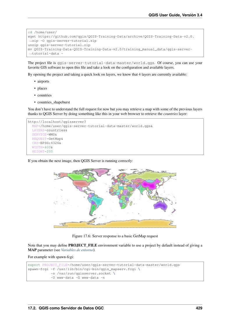
QGIS User Guide, Versión 3.4
cd /home/user/wget https://github.com/qgis/QGIS-Training-Data/archive/QGIS-Training-Data-v2.0.→˓zip -O qgis-server-tutorial.zipunzip qgis-server-tutorial.zipmv QGIS-Training-Data-QGIS-Training-Data-v2.0/training_manual_data/qgis-server-→˓tutorial-data ~
The project file is qgis-server-tutorial-data-master/world.qgs. Of course, you can use yourfavorite GIS software to open this file and take a look on the configuration and available layers.
By opening the project and taking a quick look on layers, we know that 4 layers are currently available:
• airports
• places
• countries
• countries_shapeburst
You don’t have to understand the full request for now but you may retrieve a map with some of the previous layersthanks to QGIS Server by doing something like this in your web browser to retrieve the countries layer:
http://localhost/qgisserver?MAP=/home/user/qgis-server-tutorial-data-master/world.qgs&LAYERS=countries&SERVICE=WMS&REQUEST=GetMap&CRS=EPSG:4326&WIDTH=400&HEIGHT=200
If you obtain the next image, then QGIS Server is running correctly:
Figure 17.6: Server response to a basic GetMap request
Note that you may define PROJECT_FILE environment variable to use a project by default instead of giving aMAP parameter (see Variables de entorno).
For example with spawn-fcgi:
export PROJECT_FILE=/home/user/qgis-server-tutorial-data-master/world.qgsspawn-fcgi -f /usr/lib/bin/cgi-bin/qgis_mapserv.fcgi \
-s /var/run/qgisserver.socket \-U www-data -G www-data -n
17.2. QGIS como Servidor de Datos OGC 429

QGIS User Guide, Versión 3.4
Configure your project
To provide a new QGIS Server WMS, WFS or WCS, you have to create a QGIS project file with some data or useone of your current project. Define the colors and styles of the layers in QGIS and the project CRS, if not alreadydefined.
Figure 17.7: Definitions for a QGIS Server WMS/WFS/WCS project
Then, go to the QGIS Server menu of the Project → Properties. . . dialog and provide some information aboutthe OWS in the fields under Service Capabilities. This will appear in the GetCapabilities response of the WMS,
WFS or WCS. If you don’t check Service capabilities, QGIS Server will use the information given in thewms_metadata.xml file located in the cgi-bin folder.
Capacidades WMS
In the WMS capabilities section, you can define the extent advertised in the WMS GetCapabilities response byentering the minimum and maximum X and Y values in the fields under Advertised extent. Clicking Use Current
Canvas Extent sets these values to the extent currently displayed in the QGIS map canvas. By checking CRSrestrictions, you can restrict in which coordinate reference systems (CRS) QGIS Server will offer to render maps.
430 Chapter 17. Trabajar con datos OGC
QGIS User Guide, Versión 3.4
It is recommended that you restrict the offered CRS as this reduces the size of the WMS GetCapabilities response.
Use the button below to select those CRSs from the Coordinate Reference System Selector, or click Used toadd the CRSs used in the QGIS project to the list.
If you have print layouts defined in your project, they will be listed in the GetProjectSettings response, and theycan be used by the GetPrint request to create prints, using one of the print layout layouts as a template. This isa QGIS-specific extension to the WMS 1.3.0 specification. If you want to exclude any print layout from being
published by the WMS, check Exclude layouts and click the button below. Then, select a print layoutfrom the Select print layout dialog in order to add it to the excluded layouts list.
If you want to exclude any layer or layer group from being published by the WMS, check Exclude Layers
and click the button below. This opens the Select restricted layers and groups dialog, which allows you tochoose the layers and groups that you don’t want to be published. Use the Shift or Ctrl key if you want toselect multiple entries. It is recommended that you exclude from publishing the layers that you don’t need as thisreduces the size of the WMS GetCapabilities response which leads to faster loading times on the client side.
You can receive requested GetFeatureInfo as plain text, XML and GML. Default is XML, text or GML formatdepends the output format chosen for the GetFeatureInfo request.
If you wish, you can check Add geometry to feature response. This will include in the GetFeatureInfo responsethe geometries of the features in a text format.
As many web clients can’t display circular arcs in geometries you have the option to segmentize the geometrybefore sending it to the client in a GetFeatureInfo response. This allows such clients to still display a feature’s
geometry (e.g. for highlighting the feature). You need to check the Segmentize feature info geometry to activatethe option.
You can also use the GetFeatureInfo geometry precision option to set the precision of the GetFeatureInfo geometry.This enables you to save bandwidth when you don’t need the full precision.
If you want QGIS Server to advertise specific request URLs in the WMS GetCapabilities response, enter thecorresponding URL in the Advertised URL field.
Furthermore, you can restrict the maximum size of the maps returned by the GetMap request by entering themaximum width and height into the respective fields under Maximums for GetMap request.
If one of your layers uses the Map Tip display (i.e. to show text using expressions) this will be listed inside theGetFeatureInfo output. If the layer uses a Value Map for one of its attributes, this information will also be shownin the GetFeatureInfo output.
WFS capabilities
In the WFS capabilities area you can select the layers you want to publish as WFS, and specify if they will allowupdate, insert and delete operations. If you enter a URL in the Advertised URL field of the WFS capabilitiessection, QGIS Server will advertise this specific URL in the WFS GetCapabilities response.
WCS capabilities
In the WCS capabilities area, you can select the layers that you want to publish as WCS. If you enter a URL in theAdvertised URL field of the WCS capabilities section, QGIS Server will advertise this specific URL in the WCSGetCapabilities response.
Ajuste fino de OWS
For vector layers, the Fields menu of the Layer → Properties dialog allows you to define for each attribute if itwill be published or not. By default, all the attributes are published by your WMS and WFS. If you don’t want aspecific attribute to be published, uncheck the corresponding checkbox in the WMS or WFS column.
17.2. QGIS como Servidor de Datos OGC 431
QGIS User Guide, Versión 3.4
You can overlay watermarks over the maps produced by your WMS by adding text annotations or SVG annotationsto the project file. See the Herramientas de anotaciones section for instructions on creating annotations. Forannotations to be displayed as watermarks on the WMS output, the Fixed map position checkbox in the Annotationtext dialog must be unchecked. This can be accessed by double clicking the annotation while one of the annotationtools is active. For SVG annotations, you will need either to set the project to save absolute paths (in the Generalmenu of the Project → Properties. . . dialog) or to manually modify the path to the SVG image so that it representsa valid relative path.
17.2.2 Servicios
QGIS Server is able to serve data according to standard protocols as described by the Open Geospatial Consor-tium (OGC):
• WMS 1.1.0 and 1.3.0
• WFS 1.0.0 and 1.1.0
• WCS 1.1.1
• WMTS 1.0.0
Extra vendor parameters and requests are supported in addition to the original standard that greatly enhance thepossibilities of customizing its behavior thanks to the QGIS rendering engine.
Web Map Service (WMS)
The 1.1.0 and 1.3.0 WMS standards implemented in QGIS Server provide a HTTP interface to request map orlegend images generated from a QGIS project. A typical WMS request defines the QGIS project to use, the layersto render as well as the image format to generate. Basic support is also available for the Styled Layer Descriptor(SLD) standard.
Specifications document according to the version number of the service:
• WMS 1.1.0
• WMS 1.3.0
Standard requests provided by QGIS Server:
Request DescriptionGetCapabilities Return XML metadata with information about the serverGetMap Return a mapGetFeatureInfo Retrieves data (geometry and values) for a pixel locationGetLegendGraphics Returns legend symbols
Vendor requests provided by QGIS Server:
Request DescriptionGetPrint Returns a QGIS compositionGetProjectSettings Returns specific information about QGIS Server
GetMap
Standard parameters for the GetMap request according to the OGC WMS 1.1.0 and 1.3.0 specifications:
432 Chapter 17. Trabajar con datos OGC

QGIS User Guide, Versión 3.4
Parameter Required DescriptionSERVICE Yes Name of the service (WMS)VERSION No Version of the serviceREQUEST Yes Name of the request (GetMap)LAYERS No Layers to displaySTYLES No Layers” styleSRS / CRS Yes Coordinate reference systemBBOX No Map extentWIDTH Yes Width of the image in pixelsHEIGHT Yes Height of the image in pixelsFORMAT No Image formatTRANSPARENT No Transparent background
In addition to the standard ones, QGIS Server supports the following extra parameters:
Parameter Required DescriptionMAP Yes Specify the QGIS project fileBGCOLOR No Specify the background colorDPI No Specify the output resolutionIMAGE_QUALITY No JPEG compressionOPACITIES No Opacity for layer or groupFILTER No Subset of featuresSELECTION No Highlight featuresFILE_NAME No Only for
FORMAT=application/dxfFile name of the downloaded file
FORMAT_OPTIONS No Only forFORMAT=application/dxfkey:value pairs separated by semi-colon.
• SCALE: to be used forsymbology rules, filters andstyles (not actual scaling ofthe data - data remains in theoriginal scale).
•MODE:NOSYMBOLOGY|FEATURESYMBOLOGY|SYMBOLLAYERSYMBOLOGY:corresponds to the three ex-port options offered in theQGIS Desktop DXF exportdialog.
•LAYERSATTRIBUTES:yourcolumn_with_values_to_be_used_for_dxf_layernamesif not specified, the originalQGIS layer names are used.
•USE_TITLE_AS_LAYERNAME:if enabled, the title of thelayer will be used as layername.
17.2. QGIS como Servidor de Datos OGC 433

QGIS User Guide, Versión 3.4
URL example:
http://localhost/qgis_server?SERVICE=WMS&VERSION=1.3.0&REQUEST=GetMap&MAP=/home/user/project.qgs&LAYERS=mylayer1,mylayer2,mylayer3&STYLES=style1,default,style3&OPACITIES=125,200,125&CRS=EPSG:4326&WIDTH=400&HEIGHT=400&FORMAT=image/png&TRANSPARENT=TRUE&DPI=300
SERVICE
This parameter has to be WMS in case of the GetMap request.
VERSION
This parameter allows to specify the version of the service to use. Available values for the VERSION parameterare:
• 1.1.0
• 1.3.0
If no version is indicated in the request, then 1.3.0 is used by default.
According to the version number, slight differences have to be expected as explained later for the next parameters:
• CRS / SRS
• BBOX
REQUEST
This parameter is GetMap in case of the GetMap request.
LAYERS
This parameter allows to specify the layers to display on the map. Names have to be separated by a comma.
In addition, QGIS Server introduced some options to select layers by:
• a short name
• the layer id
The short name of a layer may be configured through Properties → Metadata in layer menu. If the short name isdefined, then it’s used by default instead of the layer’s name:
434 Chapter 17. Trabajar con datos OGC
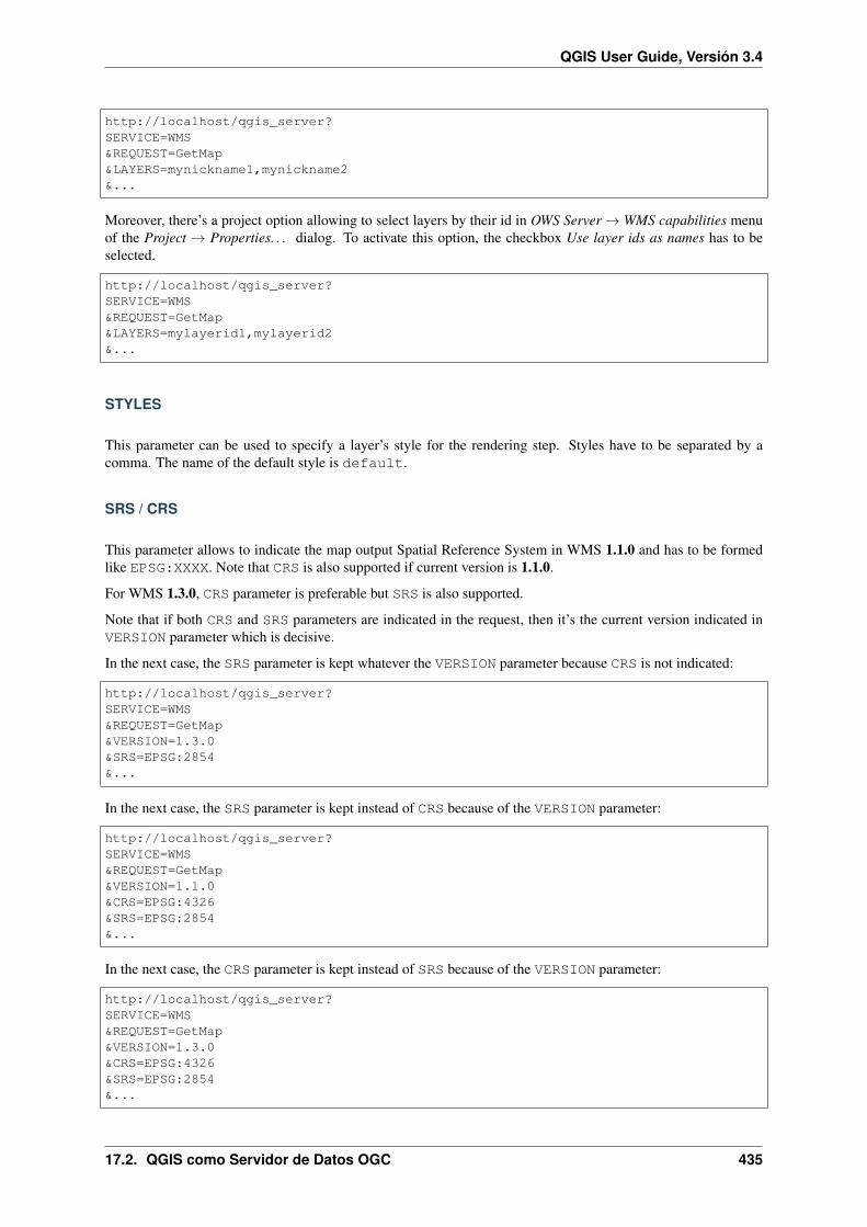
QGIS User Guide, Versión 3.4
http://localhost/qgis_server?SERVICE=WMS&REQUEST=GetMap&LAYERS=mynickname1,mynickname2&...
Moreover, there’s a project option allowing to select layers by their id in OWS Server → WMS capabilities menuof the Project → Properties. . . dialog. To activate this option, the checkbox Use layer ids as names has to beselected.
http://localhost/qgis_server?SERVICE=WMS&REQUEST=GetMap&LAYERS=mylayerid1,mylayerid2&...
STYLES
This parameter can be used to specify a layer’s style for the rendering step. Styles have to be separated by acomma. The name of the default style is default.
SRS / CRS
This parameter allows to indicate the map output Spatial Reference System in WMS 1.1.0 and has to be formedlike EPSG:XXXX. Note that CRS is also supported if current version is 1.1.0.
For WMS 1.3.0, CRS parameter is preferable but SRS is also supported.
Note that if both CRS and SRS parameters are indicated in the request, then it’s the current version indicated inVERSION parameter which is decisive.
In the next case, the SRS parameter is kept whatever the VERSION parameter because CRS is not indicated:
http://localhost/qgis_server?SERVICE=WMS&REQUEST=GetMap&VERSION=1.3.0&SRS=EPSG:2854&...
In the next case, the SRS parameter is kept instead of CRS because of the VERSION parameter:
http://localhost/qgis_server?SERVICE=WMS&REQUEST=GetMap&VERSION=1.1.0&CRS=EPSG:4326&SRS=EPSG:2854&...
In the next case, the CRS parameter is kept instead of SRS because of the VERSION parameter:
http://localhost/qgis_server?SERVICE=WMS&REQUEST=GetMap&VERSION=1.3.0&CRS=EPSG:4326&SRS=EPSG:2854&...
17.2. QGIS como Servidor de Datos OGC 435
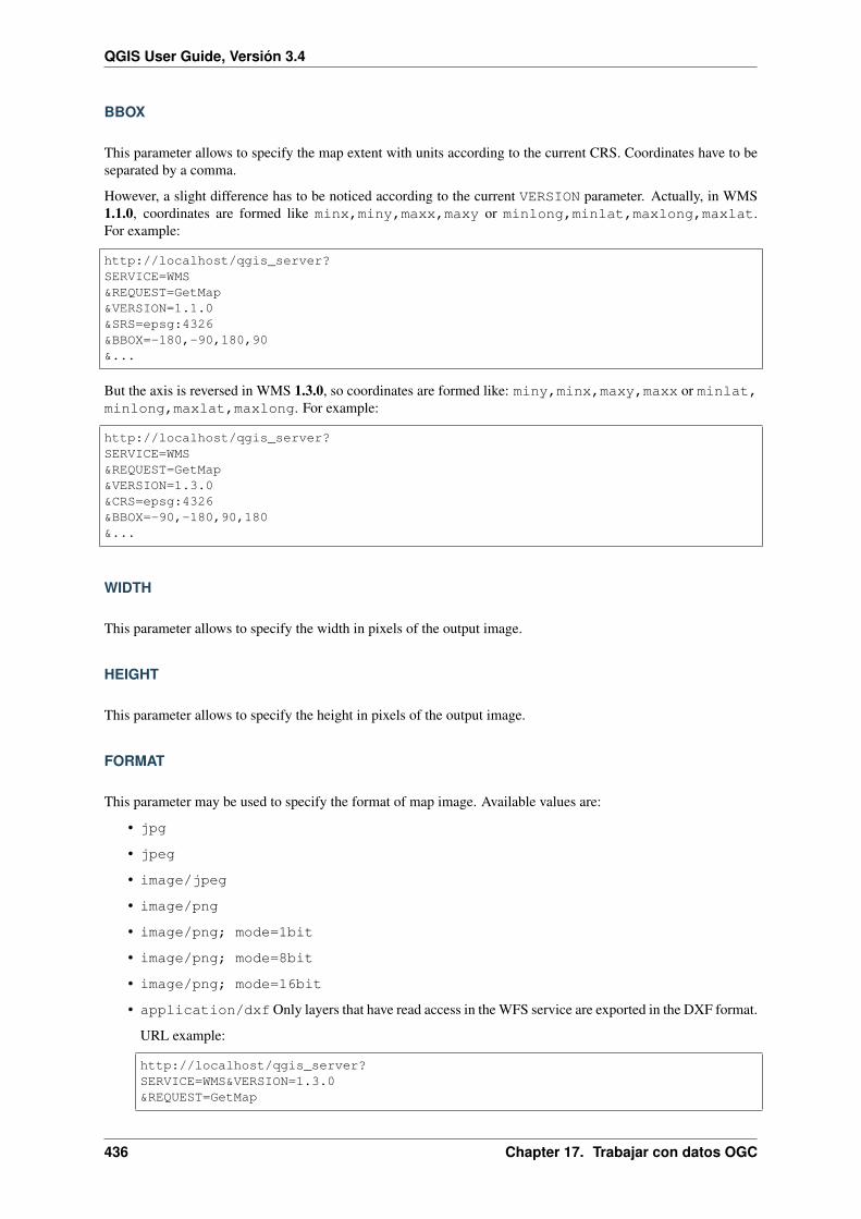
QGIS User Guide, Versión 3.4
BBOX
This parameter allows to specify the map extent with units according to the current CRS. Coordinates have to beseparated by a comma.
However, a slight difference has to be noticed according to the current VERSION parameter. Actually, in WMS1.1.0, coordinates are formed like minx,miny,maxx,maxy or minlong,minlat,maxlong,maxlat.For example:
http://localhost/qgis_server?SERVICE=WMS&REQUEST=GetMap&VERSION=1.1.0&SRS=epsg:4326&BBOX=-180,-90,180,90&...
But the axis is reversed in WMS 1.3.0, so coordinates are formed like: miny,minx,maxy,maxx or minlat,minlong,maxlat,maxlong. For example:
http://localhost/qgis_server?SERVICE=WMS&REQUEST=GetMap&VERSION=1.3.0&CRS=epsg:4326&BBOX=-90,-180,90,180&...
WIDTH
This parameter allows to specify the width in pixels of the output image.
HEIGHT
This parameter allows to specify the height in pixels of the output image.
FORMAT
This parameter may be used to specify the format of map image. Available values are:
• jpg
• jpeg
• image/jpeg
• image/png
• image/png; mode=1bit
• image/png; mode=8bit
• image/png; mode=16bit
• application/dxfOnly layers that have read access in the WFS service are exported in the DXF format.
URL example:
http://localhost/qgis_server?SERVICE=WMS&VERSION=1.3.0&REQUEST=GetMap
436 Chapter 17. Trabajar con datos OGC
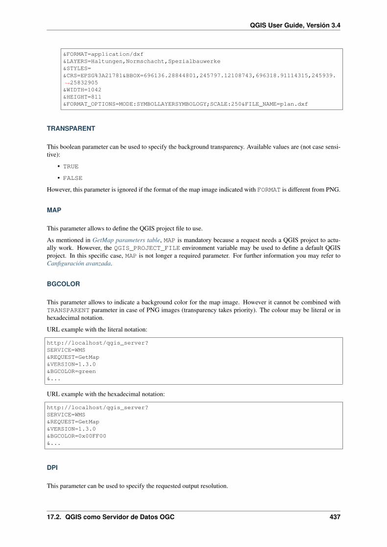
QGIS User Guide, Versión 3.4
&FORMAT=application/dxf&LAYERS=Haltungen,Normschacht,Spezialbauwerke&STYLES=&CRS=EPSG%3A21781&BBOX=696136.28844801,245797.12108743,696318.91114315,245939.→˓25832905&WIDTH=1042&HEIGHT=811&FORMAT_OPTIONS=MODE:SYMBOLLAYERSYMBOLOGY;SCALE:250&FILE_NAME=plan.dxf
TRANSPARENT
This boolean parameter can be used to specify the background transparency. Available values are (not case sensi-tive):
• TRUE
• FALSE
However, this parameter is ignored if the format of the map image indicated with FORMAT is different from PNG.
MAP
This parameter allows to define the QGIS project file to use.
As mentioned in GetMap parameters table, MAP is mandatory because a request needs a QGIS project to actu-ally work. However, the QGIS_PROJECT_FILE environment variable may be used to define a default QGISproject. In this specific case, MAP is not longer a required parameter. For further information you may refer toCanfiguración avanzada.
BGCOLOR
This parameter allows to indicate a background color for the map image. However it cannot be combined withTRANSPARENT parameter in case of PNG images (transparency takes priority). The colour may be literal or inhexadecimal notation.
URL example with the literal notation:
http://localhost/qgis_server?SERVICE=WMS&REQUEST=GetMap&VERSION=1.3.0&BGCOLOR=green&...
URL example with the hexadecimal notation:
http://localhost/qgis_server?SERVICE=WMS&REQUEST=GetMap&VERSION=1.3.0&BGCOLOR=0x00FF00&...
DPI
This parameter can be used to specify the requested output resolution.
17.2. QGIS como Servidor de Datos OGC 437

QGIS User Guide, Versión 3.4
IMAGE_QUALITY
This parameter is only used for JPEG images. By default, the JPEG compression is -1.
You can change the default per QGIS project in the OWS Server → WMS capabilities menu of the Project →Properties. . . dialog. If you want to override it in a GetMap request you can do it using the IMAGE_QUALITYparameter.
OPACITIES
Opacity can be set on layer or group level. Allowed values range from 0 (fully transparent) to 255 (fully opaque).
FILTER
A subset of layers can be selected with the FILTER parameter. Syntax is basically the same as for the QGISsubset string. However, there are some restrictions to avoid SQL injections into databases via QGIS Server. If adangerous string is found in the parameter, QGIS Server will return the next error:
Indeed, text strings need to be enclosed with quotes (single quotes for strings,→˓double quotes for attributes). A space between each word / special character is→˓mandatory. Allowed Keywords and special characters are 'AND','OR','IN','=','<','>→˓=','>','>=','!=*,'(',')'. Semicolons in string expressions are not allowed
URL example:
http://localhost/qgis_server?SERVICE=WMS&REQUEST=GetMap&LAYERS=mylayer1,mylayer2&FILTER=mylayer1:"OBJECTID" = 3;mylayer2:'text' = 'blabla'&...
Nota: It is possible to make attribute searches via GetFeatureInfo and omit the X/Y parameter if a FILTER isthere. QGIS Server then returns info about the matching features and generates a combined bounding box in thexml output.
SELECTION
The SELECTION parameter can highlight features from one or more layers. Vector features can be selected bypassing comma separated lists with feature ids.
http://localhost/qgis_server?SERVICE=WMS&REQUEST=GetMap&LAYERS=mylayer1,mylayer2&SELECTION=mylayer1:3,6,9;mylayer2:1,5,6&...
The following image presents the response from a GetMap request using the SELECTION option e.g. http://myserver.com/...&SELECTION=countries:171,65.
As those features id’s correspond in the source dataset to France and Romania they’re highlighted in yellow.
438 Chapter 17. Trabajar con datos OGC

QGIS User Guide, Versión 3.4
Figure 17.8: Server response to a GetMap request with SELECTION parameter
17.2. QGIS como Servidor de Datos OGC 439

QGIS User Guide, Versión 3.4
GetFeatureInfo
Standard parameters for the GetFeatureInfo request according to the OGC WMS 1.1.0 and 1.3.0 specifications:
Parameter Required DescriptionSERVICE Yes Name of the service (WMS)VERSION No See GetMapREQUEST Yes See GetMapLAYERS No See GetMapSTYLES No See GetMapSRS / CRS Yes See GetMapBBOX No See GetMapWIDTH Yes See GetMapHEIGHT Yes See GetMapTRANSPARENT No See GetMapINFO_FORMAT No Output formatQUERY_LAYERS Yes Layers to queryFEATURE_COUNT No Maximum number of features to returnI No Pixel column of the point to queryX No Same as I parameter, but in WMS 1.1.0J No Pixel row of the point to queryY No Same as J parameter, but in WMS 1.1.0
In addition to the standard ones, QGIS Server supports the following extra parameters:
Parameter Required DescriptionMAP Yes See GetMapFILTER No See GetMapFI_POINT_TOLERANCE No Tolerance in pixels for point layersFI_LINE_TOLERANCE No Tolerance in pixels for line layersFI_POLYGON_TOLERANCE No Tolerance in pixels for polygon layersFILTER_GEOM No Geometry filteringWITH_MAPTIP No Add map tips to the outputWITH_GEOMETRY No Add geometry to the output
URL example:
http://localhost/qgis_server?SERVICE=WMS&VERSION=1.3.0&REQUEST=GetMap&MAP=/home/user/project.qgs&LAYERS=mylayer1,mylayer2,mylayer3&CRS=EPSG:4326&WIDTH=400&HEIGHT=400&INFO_FORMAT=text/xml&TRANSPARENT=TRUE&QUERY_LAYERS=mylayer1
440 Chapter 17. Trabajar con datos OGC
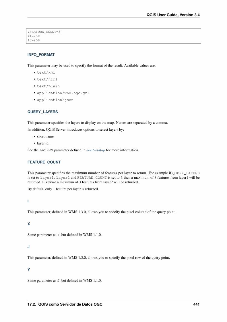
QGIS User Guide, Versión 3.4
&FEATURE_COUNT=3&I=250&J=250
INFO_FORMAT
This parameter may be used to specify the format of the result. Available values are:
• text/xml
• text/html
• text/plain
• application/vnd.ogc.gml
• application/json
QUERY_LAYERS
This parameter specifies the layers to display on the map. Names are separated by a comma.
In addition, QGIS Server introduces options to select layers by:
• short name
• layer id
See the LAYERS parameter defined in See GetMap for more information.
FEATURE_COUNT
This parameter specifies the maximum number of features per layer to return. For example if QUERY_LAYERSis set to layer1,layer2 and FEATURE_COUNT is set to 3 then a maximum of 3 features from layer1 will bereturned. Likewise a maximun of 3 features from layer2 will be returned.
By default, only 1 feature per layer is returned.
I
This parameter, defined in WMS 1.3.0, allows you to specify the pixel column of the query point.
X
Same parameter as I, but defined in WMS 1.1.0.
J
This parameter, defined in WMS 1.3.0, allows you to specify the pixel row of the query point.
Y
Same parameter as J, but defined in WMS 1.1.0.
17.2. QGIS como Servidor de Datos OGC 441

QGIS User Guide, Versión 3.4
FI_POINT_TOLERANCE
This parameter specifies the tolerance in pixels for point layers.
FI_LINE_TOLERANCE
This parameter specifies the tolerance in pixels for line layers.
FI_POLYGON_TOLERANCE
This parameter specifies the tolerance in pixels for polygon layers.
FILTER_GEOM
This parameter specifies a WKT geometry with which features have to intersect.
WITH_MAPTIP
This parameter specifies whether to add map tips to the output.
Available values are (not case sensitive):
• TRUE
• FALSE
WITH_GEOMETRY
This parameter specifies whether to add geometries to the output.
Available values are (not case sensitive):
• TRUE
• FALSE
GetPrint
QGIS Server has the capability to create print layout output in pdf or pixel format. Print layout windows in thepublished project are used as templates. In the GetPrint request, the client has the possibility to specify parametersof the contained layout maps and labels.
Parameters for the GetPrint request:
442 Chapter 17. Trabajar con datos OGC

QGIS User Guide, Versión 3.4
Parameter Required DescriptionMAP Yes Specify the QGIS project fileSERVICE Yes Name of the service (WMS)VERSION No See GetMapREQUEST Yes Name of the request (GetPrint)LAYERS No See GetMapTEMPLATE Yes Layout template to useSRS / CRS Yes See GetMapFORMAT Yes Output formatSTYLES No See GetMapTRANSPARENT No See GetMapOPACITIES No See GetMapSELECTION No See GetMapmapX:EXTENT No Extent of the map “X”mapX:LAYERS No Layers of the map “X”mapX:STYLES No Layers” style of the map “X”mapX:SCALE No Layers” scale of the map “X”mapX:ROTATION No Rotation of the map “X”mapX:GRID_INTERVAL_X No Grid interval on x axis of the map “X”mapX:GRID_INTERVAL_Y No Grid interval on y axis of the map “X”
URL example:
http://localhost/qgis_server?SERVICE=WMS&VERSION=1.3.0&REQUEST=GetPrint&MAP=/home/user/project.qgs&CRS=EPSG:4326&FORMAT=png&map0:EXTENT=-180,-90,180,90&map0:LAYERS=mylayer1,mylayer2,mylayer3&map0:OPACITIES=125,200,125&map0:ROTATION=45
Note that the layout template may contain more than one map. In this way, if you want to configure a specificmap, you have to use mapX: parameters where X is a positive number that you can retrieve thanks to the GetPro-jectSettings request.
For example:
<WMS_Capabilities>...<ComposerTemplates xsi:type="wms:_ExtendedCapabilities"><ComposerTemplate width="297" height="210" name="Druckzusammenstellung 1"><ComposerMap width="171" height="133" name="map0"/><ComposerMap width="49" height="46" name="map1"/></ComposerTemplate></ComposerTemplates>...</WMS_Capabilities>
SERVICE
This parameter has to be WMS.
17.2. QGIS como Servidor de Datos OGC 443

QGIS User Guide, Versión 3.4
REQUEST
This parameter has to be GetPrint for the GetPrint request.
TEMPLATE
This parameter can be used to specify the name of a layout template to use for printing.
FORMAT
This parameter specifies the format of map image. Available values are:
• jpg
• jpeg
• image/jpeg
• png
• image/png
• svg
• image/svg
• image/svg+xml
• application/pdf
If the FORMAT parameter is different from one of these values, then an exception is returned.
mapX:EXTENT
This parameter specifies the extent for a layout map item as xmin,ymin,xmax,ymax.
mapX:ROTATION
This parameter specifies the map rotation in degrees.
mapX:GRID_INTERVAL_X
This parameter specifies the grid line density in the X direction.
mapX:GRID_INTERVAL_Y
This parameter specifies the grid line density in the Y direction.
mapX:SCALE
This parameter specifies the map scale for a layout map item. This is useful to ensure scale based visibility oflayers and labels even if client and server may have different algorithms to calculate the scale denominator.
444 Chapter 17. Trabajar con datos OGC

QGIS User Guide, Versión 3.4
mapX:LAYERS
This parameter specifies the layers for a layout map item. See See GetMap for more information on this parameter.
mapX:STYLES
This parameter specifies the layers” styles defined in a specific layout map item. See See GetMap for moreinformation on this parameter.
GetLegendGraphics
Several additional parameters are available to change the size of the legend elements:
• BOXSPACE space between legend frame and content (mm)
• LAYERSPACE vertical space between layers (mm)
• LAYERTITLESPACE vertical space between layer title and items following (mm)
• SYMBOLSPACE vertical space between symbol and item following (mm)
• ICONLABELSPACE horizontal space between symbol and label text (mm)
• SYMBOLWIDTH width of the symbol preview (mm)
• SYMBOLHEIGHT height of the symbol preview (mm)
These parameters change the font properties for layer titles and item labels:
• LAYERFONTFAMILY / ITEMFONTFAMILY font family for layer title / item text
• LAYERFONTBOLD / ITEMFONTBOLD TRUE to use a bold font
• LAYERFONTSIZE / ITEMFONTSIZE Font size in point
• LAYERFONTITALIC / ITEMFONTITALIC TRUE to use italic font
• LAYERFONTCOLOR / ITEMFONTCOLOR Hex color code (e.g. #FF0000 for red)
• LAYERTITLE / RULELABEL set them to FALSE to get only the legend graphics without labels
Content based legend. These parameters let the client request a legend showing only the symbols for the featuresfalling into the requested area:
• BBOX the geographical area for which the legend should be built
• CRS / SRS the coordinate reference system adopted to define the BBOX coordinates
• WIDTH / HEIGHT if set these should match those defined for the GetMap request, to let QGIS Serverscale symbols according to the map view image size.
Content based legend features are based on the UMN MapServer implementation:
• SHOWFEATURECOUNT if set to TRUE adds in the legend the feature count of the features like in thefollowing image:
17.2. QGIS como Servidor de Datos OGC 445

QGIS User Guide, Versión 3.4
GetProjectSettings
This request type works similar to GetCapabilities, but it is more specific to QGIS Server and allows a client toread additional information which is not available in the GetCapabilities output:
• initial visibility of layers
• information about vector attributes and their edit types
• information about layer order and drawing order
• list of layers published in WFS
Web Feature Service (WFS)
The 1.0.0 and 1.1.0 WFS standards implemented in QGIS Server provide a HTTP interface to query geographicfeatures from a QGIS project. A typical WFS request defines the QGIS project to use and the layer to query.
Specifications document according to the version number of the service:
• WFS 1.0.0
• WFS 1.1.0
Standard requests provided by QGIS Server:
Request DescriptionGetCapabilities Returns XML metadata with information about the serverGetFeature Returns a selection of featuresDescribeFeatureType Returns a description of feature types and propertiesTransaction Allows features to be inserted, updated or deleted
GetFeature
Standard parameters for the GetFeature request according to the OGC WFS 1.0.0 and 1.1.0 specifications:
Parameter Required DescriptionSERVICE Yes Name of the serviceVERSION No Version of the serviceREQUEST Yes Name of the requestTYPENAME No Name of layersOUTPUTFORMAT No Output FormatRESULTTYPE No Type of the resultPROPERTYNAME No Name of properties to returnMAXFEATURES No Maximum number of features to returnSRSNAME No Coordinate reference systemFEATUREID No Filter the features by idsFILTER No OGC Filter EncodingBBOX No Map ExtentSORTBY No Sort the results
In addition to the standard ones, QGIS Server supports the following extra parameters:
446 Chapter 17. Trabajar con datos OGC

QGIS User Guide, Versión 3.4
Parameter Required DescriptionMAP Yes Specify the QGIS project fileSTARTINDEX No PagingGEOMETRYNAME No Type of geometry to returnEXP_FILTER No Expression filtering
SERVICE
This parameter has to be WFS in case of the GetFeature request.
For example:
http://localhost/qgis_server?SERVICE=WFS&...
VERSION
This parameter allows to specify the version of the service to use. Available values for the VERSION parameterare:
• 1.0.0
• 1.1.0
If no version is indicated in the request, then 1.1.0 is used by default.
URL example:
http://localhost/qgis_server?SERVICE=WFS&VERSION=1.1.0&...
REQUEST
This parameter is GetFeature in case of the GetFeature request.
URL example:
http://localhost/qgis_server?SERVICE=WFS&VERSION=1.1.0&REQUEST=GetFeature&...
RESULTTYPE
This parameter may be used to specify the kind of result to return. Available values are:
• results: the default behavior
• hits: returns only a feature count
URL example:
17.2. QGIS como Servidor de Datos OGC 447

QGIS User Guide, Versión 3.4
http://localhost/qgis_server?SERVICE=WFS&VERSION=1.1.0&REQUEST=GetFeature&RESULTTYPE=hits&...
GEOMETRYNAME
This parameter can be used to specify the kind of geometry to return for features. Available values are:
• extent
• centroid
• none
URL example:
http://localhost/qgis_server?SERVICE=WFS&VERSION=1.1.0&REQUEST=GetFeature&GEOMETRYNAME=centroid&...
STARTINDEX
This parameter is standard in WFS 2.0, but it’s an extension for WFS 1.0.0. Actually, it can be used to skip somefeatures in the result set and in combination with MAXFEATURES, it provides the ability to page through results.
URL example:
http://localhost/qgis_server?SERVICE=WFS&VERSION=1.1.0&REQUEST=GetFeature&STARTINDEX=2&...
Web Map Tile Service (WMTS)
The 1.0.0 WMTS standard implemented in QGIS Server provides a HTTP interface to request tiled map imagesgenerated from a QGIS project. A typical WMTS request defined the QGIS project to use, some WMS parameterslike layers to render, as well as tile parameters.
Specifications document of the service:
• WMTS 1.0.0
Standard requests provided by QGIS Server:
Request DescriptionGetCapabilities Returns XML metadata with information about the serverGetTile Returns a tileGetFeatureInfo Retrieves data (geometry and values) for a pixel location
448 Chapter 17. Trabajar con datos OGC

QGIS User Guide, Versión 3.4
GetCapabilities
Standard parameters for the GetCapabilities request according to the OGC WMTS 1.0.0 specifications:
Parameter Required DescriptionSERVICE Yes Name of the service (WMTS)REQUEST Yes Name of the request (GetCapabilities)
In addition to the standard ones, QGIS Server supports the following extra parameters:
Parameter Required DescriptionMAP Yes Specify the QGIS project file
URL example:
http://localhost/qgis_server?SERVICE=WMTS&REQUEST=GetCapabilities&MAP=/home/user/project.qgs
SERVICE
This parameter has to be WMTS in case of the GetCapabilities request.
REQUEST
This parameter is GetCapabilities in case of the GetCapabilities request.
MAP
This parameter allows to define the QGIS project file to use.
GetTile
Standard parameters for the GetTile request according to the OGC WMTS 1.0.0 specifications:
Parameter Required DescriptionSERVICE Yes Name of the service (WMTS)REQUEST Yes Name of the request (GetTile)LAYER Yes Layer identifierFORMAT Yes Output format of the tileTILEMATRIXSET Yes Name of the pyramidTILEMATRIX Yes MeshingTILEROW Yes Row coordinate in the meshTILECOL Yes Column coordinate in the mesh
17.2. QGIS como Servidor de Datos OGC 449

QGIS User Guide, Versión 3.4
In addition to the standard ones, QGIS Server supports the following extra parameters:
Parameter Required DescriptionMAP Yes Specify the QGIS project file
URL example:
http://localhost/qgis_server?SERVICE=WMTS&REQUEST=GetTile&MAP=/home/user/project.qgs&LAYER=mylayer&FORMAT=image/png&TILEMATRIXSET=EPSG:4326&TILEROW=0&TILECOL=0
SERVICE
This parameter has to be WMTS in case of the GetTile request.
REQUEST
This parameter is GetTile in case of the GetTile request.
LAYER
This parameter allows to specify the layer to display on the tile.
In addition, QGIS Server introduced some options to select a layer by:
• a short name
• the layer id
The short name of a layer may be configured through Properties → Metadata in layer menu. If the short name isdefined, then it’s used by default instead of the layer’s name:
http://localhost/qgis_server?SERVICE=WMTS&REQUEST=GetTile&LAYER=mynickname&...
Moreover, there’s a project option allowing to select layers by their id in OWS Server → WMS capabilities menuof the Project → Project Properties dialog. To activate this option, the checkbox Use layer ids as names has to beselected.
450 Chapter 17. Trabajar con datos OGC

QGIS User Guide, Versión 3.4
http://localhost/qgis_server?SERVICE=WMTS&REQUEST=GetTile&LAYER=mylayerid1&...
FORMAT
This parameter may be used to specify the format of tile image. Available values are:
• jpg
• jpeg
• image/jpeg
• image/png
If the FORMAT parameter is different from one of these values, then the default format PNG is used instead.
TILEMATRIXSET
This parameter allows to define the CRS to use to compute the underlying pyramid and has to be formed likeEPSG:XXXX.
TILEMATRIX
This parameter allows to define the matrix to use for the output tile.
TILEROW
This parameter allows to select the row of the tile to get within the matrix.
TILECOL
This parameter allows to select the column of the tile to get within the matrix.
MAP
This parameter allows to define the QGIS project file to use.
As mentioned in GetMap parameters table, MAP is mandatory because a request needs a QGIS project to actu-ally work. However, the QGIS_PROJECT_FILE environment variable may be used to define a default QGISproject. In this specific case, MAP is not longer a required parameter. For further information you may refer toCanfiguración avanzada.
GetFeatureInfo
Standard parameters for the GetFeatureInfo request according to the OGC WMTS 1.0.0 specifications:
• WMS 1.1.0
17.2. QGIS como Servidor de Datos OGC 451
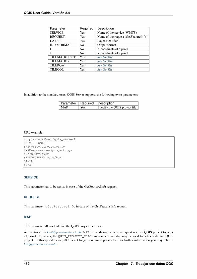
QGIS User Guide, Versión 3.4
Parameter Required DescriptionSERVICE Yes Name of the service (WMTS)REQUEST Yes Name of the request (GetFeatureInfo)LAYER Yes Layer identifierINFOFORMAT No Output formatI No X coordinate of a pixelJ No Y coordinate of a pixelTILEMATRIXSET Yes See GetTileTILEMATRIX Yes See GetTileTILEROW Yes See GetTileTILECOL Yes See GetTile
In addition to the standard ones, QGIS Server supports the following extra parameters:
Parameter Required DescriptionMAP Yes Specify the QGIS project file
URL example:
http://localhost/qgis_server?SERVICE=WMTS&REQUEST=GetFeatureInfo&MAP=/home/user/project.qgs&LAYER=mylayer&INFOFORMAT=image/html&I=10&J=5
SERVICE
This parameter has to be WMTS in case of the GetFeatureInfo request.
REQUEST
This parameter is GetFeatureInfo in case of the GetFeatureInfo request.
MAP
This parameter allows to define the QGIS project file to use.
As mentioned in GetMap parameters table, MAP is mandatory because a request needs a QGIS project to actu-ally work. However, the QGIS_PROJECT_FILE environment variable may be used to define a default QGISproject. In this specific case, MAP is not longer a required parameter. For further information you may refer toCanfiguración avanzada.
452 Chapter 17. Trabajar con datos OGC

QGIS User Guide, Versión 3.4
LAYER
This parameter allows to specify the layer to display on the tile.
In addition, QGIS Server introduced some options to select a layer by:
• a short name
• the layer id
The short name of a layer may be configured through Properties → Metadata in layer menu. If the short name isdefined, then it’s used by default instead of the layer’s name:
http://localhost/qgis_server?SERVICE=WMTS&REQUEST=GetFeatureInfo&LAYER=mynickname&...
Moreover, there’s a project option allowing to select layers by their id in OWS Server → WMS capabilities menuof the Project → Project Properties dialog. To activate this option, the checkbox Use layer ids as names has to beselected.
http://localhost/qgis_server?SERVICE=WMTS&REQUEST=GetFeatureInfo&LAYER=mylayerid1&...
INFOFORMAT
This parameter allows to define the output format of the result. Available values are:
• text/xml
• text/html
• text/plain
• application/vnd.ogc.gml
The default value is text/plain.
I
This parameter allows to define the X coordinate of the pixel for which we want to retrieve underlying information.
J
This parameter allows to define the Y coordinate of the pixel for which we want to retrieve underlying information.
Extra parameters supported by all request types
• FILE_NAME parameter: if set, the server response will be sent to the client as a file attachment with thespecified file name.
• MAP parameter: Similar to MapServer, the MAP parameter can be used to specify the path to the QGISproject file. You can specify an absolute path or a path relative to the location of the server executable(qgis_mapserv.fcgi). If not specified, QGIS Server searches for .qgs files in the directory where theserver executable is located.
17.2. QGIS como Servidor de Datos OGC 453

QGIS User Guide, Versión 3.4
Ejemplo:
http://localhost/cgi-bin/qgis_mapserv.fcgi?\REQUEST=GetMap&MAP=/home/qgis/mymap.qgs&...
Nota: You can define a QGIS_PROJECT_FILE as an environment variable to tell the server executable whereto find the QGIS project file. This variable will be the location where QGIS will look for the project file. If notdefined it will use the MAP parameter in the request and finally look at the server executable directory.
REDLINING
This feature is available and can be used with GetMap and GetPrint requests.
The redlining feature can be used to pass geometries and labels in the request which are overlapped by the serverover the standard returned image (map). This permits the user to put emphasis or maybe add some comments(labels) to some areas, locations etc. that are not in the standard map.
The request is in the format:
http://qgisplatform.demo/cgi-bin/qgis_mapserv.fcgi?map=/world.qgs&SERVICE=WMS&→˓VERSION=1.3.0&REQUEST=GetMap...&HIGHLIGHT_GEOM=POLYGON((590000 5647000, 590000 6110620, 2500000 6110620, 2500000→˓5647000, 590000 5647000))&HIGHLIGHT_SYMBOL=<StyledLayerDescriptor><UserStyle><Name>Highlight</Name>→˓<FeatureTypeStyle><Rule><Name>Symbol</Name><LineSymbolizer><Stroke><SvgParameter→˓name="stroke">%23ea1173</SvgParameter><SvgParameter name="stroke-opacity">1</→˓SvgParameter><SvgParameter name="stroke-width">1.6</SvgParameter></Stroke></→˓LineSymbolizer></Rule></FeatureTypeStyle></UserStyle></StyledLayerDescriptor>&HIGHLIGHT_LABELSTRING=Write label here&HIGHLIGHT_LABELSIZE=16&HIGHLIGHT_LABELCOLOR=%23000000&HIGHLIGHT_LABELBUFFERCOLOR=%23FFFFFF&HIGHLIGHT_LABELBUFFERSIZE=1.5
Here is the image outputed by the above request in which a polygon and a label are drawn on top of the normalmap:
You can see there are several parameters in this request:
• HIGHLIGHT_GEOM: You can add POINT, MULTILINESTRING, POLYGON etc. It supports multipartgeometries. Here is an example: HIGHLIGHT_GEOM=MULTILINESTRING((0 0, 0 1, 1 1)).The coordinates should be in the CRS of the GetMap/GetPrint request.
• HIGHLIGHT_SYMBOL: This controls how the geometry is outlined and you can change the stroke width,color and opacity.
• HIGHLIGHT_LABELSTRING: You can pass your labeling text to this parameter.
• HIGHLIGHT_LABELSIZE: This parameter controls the size of the label.
• HIGHLIGHT_LABELCOLOR: This parameter controls the label color.
• HIGHLIGHT_LABELBUFFERCOLOR: This parameter controls the label buffer color.
• HIGHLIGHT_LABELBUFFERSIZE: This parameter controls the label buffer size.
External WMS layers
QGIS Server allows including layers from external WMS servers in WMS GetMap and WMS GetPrint requests.This is especially useful if a web client uses an external background layer in the web map. For performance
454 Chapter 17. Trabajar con datos OGC

QGIS User Guide, Versión 3.4
Figure 17.9: Server response to a GetMap request with redlining parameters
17.2. QGIS como Servidor de Datos OGC 455

QGIS User Guide, Versión 3.4
reasons, such layers should be directly requested by the web client (not cascaded via QGIS server). For printinghowever, these layers should be cascaded via QGIS server in order to appear in the printed map.
External layers can be added to the LAYERS parameter as EXTERNAL_WMS:<layername>. The parameters forthe external WMS layers (e.g. url, format, dpiMode, crs, layers, styles) can later be given as service parameters<layername>:<parameter>. In a GetMap request, this might look like this:
http://localhost/qgis_server?SERVICE=WMS&REQUEST=GetMap...&LAYERS=EXTERNAL_WMS:basemap,layer1,layer2&STYLES=,,&basemap:url=http://externalserver.com/wms.fcgi&basemap:format=image/jpeg&basemap:dpiMode=7&basemap:crs=EPSG:2056&basemap:layers=orthofoto&basemap:styles=default
Similarly, external layers can be used in GetPrint requests:
http://localhost/qgis_server?SERVICE=WMS...&REQUEST=GetPrint&TEMPLATE=A4&map0:layers=EXTERNAL_WMS:basemap,layer1,layer2&map0:EXTENT=<minx,miny,maxx,maxy>&basemap:url=http://externalserver.com/wms.fcgi&basemap:format=image/jpeg&basemap:dpiMode=7&basemap:crs=EPSG:2056&basemap:layers=orthofoto&basemap:styles=default
17.2.3 Plugins
Instalación
La instalación de un complemento de ejemplo HelloWorld para probar los servidores. Se puede crear un direc-torio para mantener los complementos del servidor. Esto se especificará en la configuración del host virtual ytransmitirlo al servidor a través de una variable de entorno.
sudo mkdir -p /opt/qgis-server/pluginscd /opt/qgis-server/pluginssudo wget https://github.com/elpaso/qgis-helloserver/archive/master.zipIn case unzip was not installed before:sudo apt install unzipsudo unzip master.zipsudo mv qgis-helloserver-master HelloServer
HTTP Server configuration
Apache
To be able to use server plugins, FastCGI needs to know where to look. So, we have to modify the Apacheconfiguration file to indicate the QGIS_PLUGINPATH environment variable to FastCGI:
456 Chapter 17. Trabajar con datos OGC

QGIS User Guide, Versión 3.4
FcgidInitialEnv QGIS_SERVER_LOG_FILE /tmp/qgis-000.logFcgidInitialEnv QGIS_SERVER_LOG_LEVEL 0FcgidInitialEnv QGIS_PLUGINPATH "/opt/qgis-server/plugins"
Moreover, a basic HTTP authorization is necessary to play with the HelloWorld plugin previously introduced. Sowe have to update the Apache configuration file a last time:
# Needed for QGIS HelloServer plugin HTTP BASIC auth<IfModule mod_fcgid.c>
RewriteEngine onRewriteCond %{HTTP:Authorization} .RewriteRule .* - [E=HTTP_AUTHORIZATION:%{HTTP:Authorization}]
</IfModule>
A continuación, reinicie Apache:
sudo a2ensite 001-qgis-serversudo service apache2 restart
Truco: If you work with a feature that has many nodes then modifying and adding a new feature will fail. In thiscase it is possible to insert the following code into the 001-qgis-server.conf file:
<IfModule mod_fcgid.c>FcgidMaxRequestLen 26214400FcgidConnectTimeout 60</IfModule>
How to use a plugin
Test the server with the HelloWorld plugin:
wget -q -O - "http://localhost/cgi-bin/qgis_mapserv.fcgi?SERVICE=HELLO"HelloServer!
Se puede echar un vistazo al GetCapabilities predeterminado del servidor QGIS en : http://localhost/cgi-bin/qgis_mapserv.fcgi?SERVICE=WMS&VERSION=1.3.0&REQUEST=GetCapabilities
17.2.4 Canfiguración avanzada
Registro
To log requests sent to the server, you have to set the following environment variables:
• QGIS_SERVER_LOG_LEVEL
• QGIS_SERVER_LOG_FILE
• QGIS_SERVER_LOG_STDERR
Take a look on Variables de entorno to understand their meanings.
Variables de entorno
You can configure some aspects of QGIS Server by setting environment variables.
According to the HTTP server and how you run QGIS Server, there are several ways to define these variables.This is fully described in HTTP Server configuration.
17.2. QGIS como Servidor de Datos OGC 457

QGIS User Guide, Versión 3.4
QGIS_OPTIONS_PATH
Specifies the path to the directory with settings. It works the same way as QGIS application --optionspathoption. It is looking for settings file in <QGIS_OPTIONS_PATH>/QGIS/QGIS3.ini.
QUERY_STRING
The query string, normally passed by the web server. This variable can be useful while testing QGIS server binaryfrom the command line.
For example for testing a GetCapabilities request on the command line to a project that also requires a PostgreSQLconnection defined in a pg_service.conf file:
PGSERVICEFILE=/etc/pg_service.conf QUERY_STRING="MAP=/path/to/test.qgs&SERVICE=WMS&→˓REQUEST=GetCapabilities" /path/to/qgis_mapserv.fcgi
The result should be either the content of the GetCapabilities response or, if something is wrong, an error message.
QGIS_PROJECT_FILE
The .qgs or .qgz project file, normally passed as a parameter in the query string (with MAP), you can also setit as an environment variable (for example by using mod_rewrite Apache module).
Note that you may also indicate a project stored in PostgreSQL, e.g. postgresql://localhost:5432?sslmode=disable&dbname=mydb&schema=myschema&project=myproject.
QGIS_SERVER_LOG_FILE
Specify path and filename. Make sure that server has proper permissions for writing to file. File should be createdautomatically, just send some requests to server. If it’s not there, check permissions.
QGIS_SERVER_LOG_FILE is deprecated since QGIS 3.4. File logging support will be removed in QGIS 4.0.
QGIS_SERVER_LOG_STDERR
Activate logging to stderr. It’s disabled by default. This variable has no effect when QGIS_SERVER_LOG_FILEis set.
• 0 or false (case insensitive)
• 1 or true (case insensitive)
MAX_CACHE_LAYERS
Specify the maximum number of cached layers (default: 100).
DISPLAY
This is used to pass (fake) X server display number (needed on Unix-like systems).
QGIS_PLUGINPATH
Useful if you are using Python plugins for the server, this sets the folder that is searched for Python plugins.
458 Chapter 17. Trabajar con datos OGC

QGIS User Guide, Versión 3.4
QGIS_SERVER_LOG_LEVEL
Specify desired log level. Available values are:
• 0 or INFO (log all requests)
• 1 or WARNING
• 2 or CRITICAL (log just critical errors, suitable for production purposes)
QGIS_SERVER_PARALLEL_RENDERING
Activates parallel rendering for WMS GetMap requests. It’s disabled (false) by default. Available values are:
• 0 or false (case insensitive)
• 1 or true (case insensitive)
QGIS_SERVER_MAX_THREADS
Number of threads to use when parallel rendering is activated. Default value is -1 to use the number of processorcores.
QGIS_SERVER_CACHE_DIRECTORY
Specifies the network cache directory on the filesystem. The default directory is named cache and located in theprofile directory.
QGIS_SERVER_CACHE_SIZE
Sets the network cache size in MB. The default value is 50 MB.
Settings summary
When QGIS Server is starting, you have a summary of all configurable parameters thanks to environment variables.Moreover, the value currently used and the origin is also displayed.
For example with spawn-fcgi:
export QGIS_OPTIONS_PATH=/home/user/.local/share/QGIS/QGIS3/profiles/default/export QGIS_SERVER_LOG_FILE=/home/user/qserv.logexport QGIS_SERVER_LOG_LEVEL=2spawn-fcgi -f /usr/lib/cgi-bin/qgis_mapserv.fcgi -s /tmp/qgisserver.sock -U www-→˓data -G www-data -n
QGIS Server Settings:
- QGIS_OPTIONS_PATH / '' (Override the default path for user configuration): '/→˓home/user/.local/share/QGIS/QGIS3/profiles/default/' (read from ENVIRONMENT_→˓VARIABLE)
- QGIS_SERVER_PARALLEL_RENDERING / '/qgis/parallel_rendering' (Activate/→˓Deactivate parallel rendering for WMS getMap request): 'true' (read from INI_→˓FILE)
- QGIS_SERVER_MAX_THREADS / '/qgis/max_threads' (Number of threads to use when→˓parallel rendering is activated): '4' (read from INI_FILE)
17.2. QGIS como Servidor de Datos OGC 459

QGIS User Guide, Versión 3.4
- QGIS_SERVER_LOG_LEVEL / '' (Log level): '2' (read from ENVIRONMENT_VARIABLE)
- QGIS_SERVER_LOG_FILE / '' (Log file): '/tmp/qserv.log' (read from ENVIRONMENT_→˓VARIABLE)
- QGIS_PROJECT_FILE / '' (QGIS project file): '' (read from DEFAULT_VALUE)
- MAX_CACHE_LAYERS / '' (Specify the maximum number of cached layers): '100'→˓(read from DEFAULT_VALUE)
- QGIS_SERVER_CACHE_DIRECTORY / '/cache/directory' (Specify the cache→˓directory): '/root/.local/share/QGIS/QGIS3/profiles/default/cache' (read from→˓DEFAULT_VALUE)
- QGIS_SERVER_CACHE_SIZE / '/cache/size' (Specify the cache size): '52428800'→˓(read from INI_FILE)
Ini file used to initialize settings: /home/user/.local/share/QGIS/QGIS3/profiles/→˓default/QGIS/QGIS3.ini
In this particular case, we know that QGIS_SERVER_MAX_THREADS andQGIS_SERVER_PARALLEL_RENDERING values are read from the ini file found inQGIS_OPTIONS_PATH directory (which is defined through an environment variable). The correspond-ing entries in the ini file are /qgis/max_threads and /qgis/parallel_rendering and their values are true and 4threads.
Short name for layers, groups and project
A number of elements have both a <Name> and a <Title>. The Name is a text string used for machine-to-machine communication while the Title is for the benefit of humans.
For example, a dataset might have the descriptive Title “Maximum Atmospheric Temperature” and be requestedusing the abbreviated Name “ATMAX”. User can already set title for layers, groups and project.
OWS name is based on the name used in layer tree. This name is more a label for humans than a name formachine-to-machine communication.
Servidor QGIS soporta:
• short name line edits to layers properties You can change this by right clicking on a layer, choose Properties→ Metadata tab → Description → Short name.
• WMS data dialog to layer tree group (short name, title, abstract)
By right clicking on a layer group and selecting the Set Group WMS data option you will get:
Figure 17.10: Set group WMS data dialog
• short name line edits to project properties - add a regexp validator "^[A-Za-z][A-Za-z0-9\._-]*"to short name line edit accessible through a static method
460 Chapter 17. Trabajar con datos OGC
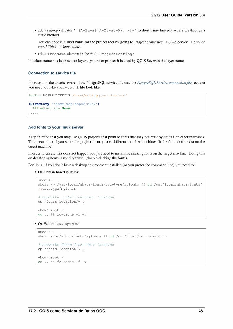
QGIS User Guide, Versión 3.4
• add a regexp validator "^[A-Za-z][A-Za-z0-9\._-]*" to short name line edit accessible through astatic method
You can choose a short name for the project root by going to Project properties → OWS Server → Servicecapabilities → Short name.
• add a TreeName element in the fullProjectSettings
If a short name has been set for layers, groups or project it is used by QGIS Sever as the layer name.
Connection to service file
In order to make apache aware of the PostgreSQL service file (see the PostgreSQL Service connection file section)you need to make your *.conf file look like:
SetEnv PGSERVICEFILE /home/web/.pg_service.conf
<Directory "/home/web/apps2/bin/">AllowOverride None
.....
Add fonts to your linux server
Keep in mind that you may use QGIS projects that point to fonts that may not exist by default on other machines.This means that if you share the project, it may look different on other machines (if the fonts don’t exist on thetarget machine).
In order to ensure this does not happen you just need to install the missing fonts on the target machine. Doing thison desktop systems is usually trivial (double clicking the fonts).
For linux, if you don’t have a desktop environment installed (or you prefer the command line) you need to:
• On Debian based systems:
sudo sumkdir -p /usr/local/share/fonts/truetype/myfonts && cd /usr/local/share/fonts/→˓truetype/myfonts
# copy the fonts from their locationcp /fonts_location/* .
chown root *cd .. && fc-cache -f -v
• On Fedora based systems:
sudo sumkdir /usr/share/fonts/myfonts && cd /usr/share/fonts/myfonts
# copy the fonts from their locationcp /fonts_location/* .
chown root *cd .. && fc-cache -f -v
17.2. QGIS como Servidor de Datos OGC 461

QGIS User Guide, Versión 3.4
462 Chapter 17. Trabajar con datos OGC

CHAPTER 18
Trabajar con datos GPS
18.1 Plugin de GPS
18.1.1 ¿Qué es GPS?
GPS, the Global Positioning System, is a satellite-based system that allows anyone with a GPS receiver to find theirexact position anywhere in the world. GPS is used as an aid in navigation, for example in airplanes, in boats andby hikers. The GPS receiver uses the signals from the satellites to calculate its latitude, longitude and (sometimes)elevation. Most receivers also have the capability to store locations (known as waypoints), sequences of locationsthat make up a planned route and a tracklog or track of the receiver’s movement over time. Waypoints, routesand tracks are the three basic feature types in GPS data. QGIS displays waypoints in point layers, while routesand tracks are displayed in linestring layers.
Nota: QGIS supports also GNSS receivers. But we keep using the term GPS in this documentation.
18.1.2 Cargando datos GPS desde archivo
There are dozens of different file formats for storing GPS data. The format that QGIS uses is called GPX (GPSeXchange format), which is a standard interchange format that can contain any number of waypoints, routes andtracks in the same file.
To load a GPX file, you first need to load the plugin. Plugins → Plugin Manager. . . opens the Plugin Manager
Dialog. Activate the GPS Tools checkbox. When this plugin is loaded, a button with a small handheld GPSdevice will show up in the toolbar and in Layer → Create Layer → :
• Herramientas GPS
• Create new GPX Layer
For working with GPS data, we provide an example GPX file available in the QGIS sample dataset:qgis_sample_data/gps/national_monuments.gpx. See section Downloading sample data for moreinformation about the sample data.
463

QGIS User Guide, Versión 3.4
1. Select Vector → GPS Tools or click the GPS Tools icon in the toolbar and open the Load GPX file tab (seefigure_GPS).
2. Browse to the folder qgis_sample_data/gps/, select the GPX file national_monuments.gpxand click Open.
Figure 18.1: La ventana de diálogo Herramientas GPS
Use the Browse. . . button to select the GPX file, then use the checkboxes to select the feature types you wantto load from that GPX file. Each feature type will be loaded in a separate layer when you click OK. The filenational_monuments.gpx only includes waypoints.
Nota: GPS units allow you to store data in different coordinate systems. When downloading a GPX file (fromyour GPS unit or a web site) and then loading it in QGIS, be sure that the data stored in the GPX file uses WGS 84(latitude/longitude). QGIS expects this, and it is the official GPX specification. See https://www.topografix.com/GPX/1/1/.
18.1.3 GPSBabel
Since QGIS uses GPX files, you need a way to convert other GPS file formats to GPX. This can be done for manyformats using the free program GPSBabel, which is available at https://www.gpsbabel.org. This program can alsotransfer GPS data between your computer and a GPS device. QGIS uses GPSBabel to do these things, so it isrecommended that you install it. However, if you just want to load GPS data from GPX files you will not need it.Version 1.2.3 of GPSBabel is known to work with QGIS, but you should be able to use later versions without anyproblems.
18.1.4 Importando datos GPS
To import GPS data from a file that is not a GPX file, you use the tool Import other file in the GPS Tools dialog.Here, you select the file that you want to import (and the file type), which feature type you want to import from it,where you want to store the converted GPX file and what the name of the new layer should be. Note that not allGPS data formats will support all three feature types, so for many formats you will only be able to choose betweenone or two types.
18.1.5 Downloading GPS data from a device
QGIS can use GPSBabel to download data from a GPS device directly as new vector layers. For this we usethe Download from GPS tab of the GPS Tools dialog (see Figure_GPS_download). Here, we select the type ofGPS device, the port that it is connected to (or USB if your GPS supports this), the feature type that you want todownload, the GPX file where the data should be stored, and the name of the new layer.
464 Chapter 18. Trabajar con datos GPS

QGIS User Guide, Versión 3.4
Figure 18.2: La herramienta de descarga
The device type you select in the GPS device menu determines how GPSBabel tries to communicate with yourGPS device. If none of the available types work with your GPS device, you can create a new type (see sectionDefining new device types).
The port may be a file name or some other name that your operating system uses as a reference to the physical portin your computer that the GPS device is connected to. It may also be simply USB, for USB-enabled GPS units.
• On Linux, this is something like /dev/ttyS0 or /dev/ttyS1.
• On Windows, it is COM1 or COM2.
When you click OK, the data will be downloaded from the device and appear as a layer in QGIS.
18.1.6 Uploading GPS data to a device
You can also upload data directly from a vector layer in QGIS to a GPS device using the Upload to GPS tab ofthe GPS Tools dialog. To do this, you simply select the layer that you want to upload (which must be a GPXlayer), your GPS device type, and the port (or USB) that it is connected to. Just as with the download tool, youcan specify new device types if your device isn’t in the list.
This tool is very useful in combination with the vector-editing capabilities of QGIS. It allows you to load a map,create waypoints and routes, and then upload them and use them on your GPS device.
18.1.7 Defining new device types
There are lots of different types of GPS devices. The QGIS developers can’t test all of them, so if you have onethat does not work with any of the device types listed in the Download from GPS and Upload to GPS tools, youcan define your own device type for it. You do this by using the GPS device editor, which you start by clickingthe Edit Devices button in the download or the upload tab.
To define a new device, you simply click the New Device button, enter a name, enter download and uploadcommands for your device, and click the Update Device button. The name will be listed in the device menus inthe upload and download windows – it can be any string. The download command is the command that is used todownload data from the device to a GPX file. This will probably be a GPSBabel command, but you can use anyother command line program that can create a GPX file. QGIS will replace the keywords %type, %in, and %outwhen it runs the command.
%type will be replaced by -w if you are downloading waypoints, -r if you are downloading routes and -t ifyou are downloading tracks. These are command-line options that tell GPSBabel which feature type to download.
%in will be replaced by the port name that you choose in the download window and %out will be replaced bythe name you choose for the GPX file that the downloaded data should be stored in. So, if you create a devicetype with the download command gpsbabel %type -i garmin -o gpx %in %out (this is actually the
18.1. Plugin de GPS 465

QGIS User Guide, Versión 3.4
download command for the predefined device type “Garmin serial”) and then use it to download waypoints fromport /dev/ttyS0 to the file output.gpx, QGIS will replace the keywords and run the command gpsbabel-w -i garmin -o gpx /dev/ttyS0 output.gpx.
The upload command is the command that is used to upload data to the device. The same keywords are used, but%in is now replaced by the name of the GPX file for the layer that is being uploaded, and %out is replaced bythe port name.
You can learn more about GPSBabel and its available command line options at https://www.gpsbabel.org.
Once you have created a new device type, it will appear in the device lists for the download and upload tools.
18.1.8 Download of points/tracks from GPS units
As described in previous sections QGIS uses GPSBabel to download points/tracks directly in the project. QGIScomes out of the box with a pre-defined profile to download from Garmin devices. Unfortunately there is a bug#6318 that does not allow create other profiles, so downloading directly in QGIS using the GPS Tools is at themoment limited to Garmin USB units.
Garmin GPSMAP 60cs
MS Windows
Install the Garmin USB drivers from https://www8.garmin.com/support/download_details.jsp?id=591
Connect the unit. Open GPS Tools and use type=garmin serial and port=usb: Fill the fields Layername and Output file. Sometimes it seems to have problems saving in a certain folder, using something likec:\temp usually works.
Ubuntu/Mint GNU/Linux
It is first needed an issue about the permissions of the device, as described at https://wiki.openstreetmap.org/wiki/USB_Garmin_on_GNU/Linux. You can try to create a file /etc/udev/rules.d/51-garmin.rulescontaining this rule
ATTRS{idVendor}=="091e", ATTRS{idProduct}=="0003", MODE="666"
After that is necessary to be sure that the garmin_gps kernel module is not loaded
rmmod garmin_gps
and then you can use the GPS Tools. Unfortunately there seems to be a bug #7182 and usually QGIS freezesseveral times before the operation work fine.
BTGP-38KM datalogger (only Bluetooth)
MS Windows
The already referred bug does not allow to download the data from within QGIS, so it is needed to use GPSBabelfrom the command line or using its interface. The working command is
gpsbabel -t -i skytraq,baud=9600,initbaud=9600 -f COM9 -o gpx -F C:/GPX/aaa.gpx
Ubuntu/Mint GNU/Linux
Use same command (or settings if you use GPSBabel GUI) as in Windows. On Linux it maybe somehow commonto get a message like
skytraq: Too many read errors on serial port
it is just a matter to turn off and on the datalogger and try again.
466 Chapter 18. Trabajar con datos GPS

QGIS User Guide, Versión 3.4
BlueMax GPS-4044 datalogger (both BT and USB)
MS Windows
Nota: Se necesita instalar los controladores antes de usarlo en Windows 7. Vea el sitio del fabricante para ladescarga apropiada.
Downloading with GPSBabel, both with USB and BT returns always an error like
gpsbabel -t -i mtk -f COM12 -o gpx -F C:/temp/test.gpxmtk_logger: Can't create temporary file data.binError running gpsbabel: Process exited unsuccessfully with code 1
Ubuntu/Mint GNU/Linux
Con USB
After having connected the cable use the dmesg command to understand what port is being used, for example/dev/ttyACM3. Then as usual use GPSBabel from the CLI or GUI
gpsbabel -t -i mtk -f /dev/ttyACM3 -o gpx -F /home/user/bluemax.gpx
Con Bluetooth
Use Blueman Device Manager to pair the device and make it available through a system port, then run GPSBabel
gpsbabel -t -i mtk -f /dev/rfcomm0 -o gpx -F /home/user/bluemax_bt.gpx
18.2 Seguimiento de GPS en Vivo
To activate live GPS tracking in QGIS, you need to select View → Panels GPS Information Panel or pressCtrl+0. You will get a new docked window on the left side of the canvas.
There are four possible screens in this GPS tracking window:
• GPS position coordinates and an interface for manually entering vertices and features
• GPS signal strength of satellite connections
• GPS options screen (see figure_gps_options)
With a plugged-in GPS receiver (has to be supported by your operating system), a simple click on Connect con-nects the GPS to QGIS. A second click (now on Disconnect) disconnects the GPS receiver from your computer.For GNU/Linux, gpsd support is integrated to support connection to most GPS receivers. Therefore, you first haveto configure gpsd properly to connect QGIS to it.
Advertencia: If you want to record your position to the canvas, you have to create a new vector layer firstand switch it to editable status to be able to record your track.
18.2.1 Posición y atributos adicionales
If the GPS is receiving signals from satellites, you will see your position in latitude, longitude and altitudetogether with additional attributes.
18.2. Seguimiento de GPS en Vivo 467

QGIS User Guide, Versión 3.4
Figure 18.3: GPS tracking position and additional attributes
468 Chapter 18. Trabajar con datos GPS

QGIS User Guide, Versión 3.4
18.2.2 Fuerza de la señal GPS
Here, you can see the signal strength of the satellites you are receiving signals from.
Figure 18.4: GPS tracking signal strength
18.2.3 Opciones GPS
In case of connection problems, you can switch between:
• Autodetect
• Internal
• Serial device
• gpsd (selecting the Host, Port and Device your GPS is connected to)
A click on Connect again initiates the connection to the GPS receiver.
You can activate Automatically save added features when you are in editing mode. Or you can activateAutomatically add points to the map canvas with a certain width and color.
Activating Cursor, you can use a slider to shrink and grow the position cursor on thecanvas.
You can also set an Acquisition interval (seconds) and a Distance threshold (meters) parameters to keep the cursorstill active when the receiver is in static conditions.
Activating Map centering allows you to decide in which way the canvas will be updated. This includes“always”, “when leaving”, if your recorded coordinates start to move out of the canvas, or “never”, to keep mapextent.
Finally, you can activate Log file and define a path and a file where log messages about the GPS tracking arelogged.
If you want to set a feature manually, you have to go back to Position and click on Add Point or Add Track Point.
18.2.4 Connect to a Bluetooth GPS for live tracking
With QGIS you can connect a Bluetooth GPS for field data collection. To perform this task you need a GPSBluetooth device and a Bluetooth receiver on your computer.
At first you must let your GPS device be recognized and paired to the computer. Turn on the GPS, go to theBluetooth icon on your notification area and search for a New Device.
18.2. Seguimiento de GPS en Vivo 469

QGIS User Guide, Versión 3.4
Figure 18.5: GPS tracking options window
470 Chapter 18. Trabajar con datos GPS
QGIS User Guide, Versión 3.4
On the right side of the Device selection mask make sure that all devices are selected so your GPS unit willprobably appear among those available. In the next step a serial connection service should be available, select itand click on Configure button.
Remember the number of the COM port assigned to the GPS connection as resulting by the Bluetooth properties.
After the GPS has been recognized, make the pairing for the connection. Usually the authorization code is 0000.
Now open GPS information panel and switch to GPS options screen. Select the COM port assigned to the GPSconnection and click the Connect. After a while a cursor indicating your position should appear.
If QGIS can’t receive GPS data, then you should restart your GPS device, wait 5-10 seconds then try to connectagain. Usually this solution work. If you receive again a connection error make sure you don’t have anotherBluetooth receiver near you, paired with the same GPS unit.
18.2.5 Utilizando GPSMAP 60cs
MS Windows
Easiest way to make it work is to use a middleware (freeware, not open) called GPSGate.
Launch the program, make it scan for GPS devices (works for both USB and BT ones) and then in QGIS just click
Connect in the Live tracking panel using the Autodetect mode.
Ubuntu/Mint GNU/Linux
Para Windows la formas más fácil es usar un servidor en medio, en este caso GPSD, de manera
sudo apt install gpsd
Then load the garmin_gps kernel module
sudo modprobe garmin_gps
And then connect the unit. Then check with dmesg the actual device being used bu the unit, for example /dev/ttyUSB0. Now you can launch gpsd
gpsd /dev/ttyUSB0
Y finalmente conectar con la herramienta de rastreo en vivo QGIS.
18.2.6 Using BTGP-38KM datalogger (only Bluetooth)
Using GPSD (under Linux) or GPSGate (under Windows) is effortless.
18.2.7 Using BlueMax GPS-4044 datalogger (both BT and USB)
MS Windows
The live tracking works for both USB and BT modes, by using GPSGate or even without it, just use theAutodetect mode, or point the tool the right port.
18.2. Seguimiento de GPS en Vivo 471

QGIS User Guide, Versión 3.4
Ubuntu/Mint GNU/Linux
Para USB
The live tracking works both with GPSD
gpsd /dev/ttyACM3
or without it, by connecting the QGIS live tracking tool directly to the device (for example /dev/ttyACM3).
Para Bluetooth
The live tracking works both with GPSD
gpsd /dev/rfcomm0
or without it, by connecting the QGIS live tracking tool directly to the device (for example /dev/rfcomm0).
472 Chapter 18. Trabajar con datos GPS

CHAPTER 19
Sistema de autenticación
19.1 Authentication System Overview
Figure 19.1: Anatomy of authentication system
19.1.1 Base de datos de autenticación
The new authentication system stores authentication configurations in an SQLite database file located, by default,at <user home>/.qgis3/qgis-auth.db.
473

QGIS User Guide, Versión 3.4
This authentication database can be moved between QGIS installations without affecting other current QGIS userpreferences, as it is completely separate from normal QGIS settings. A configuration ID (a random 7-characteralphanumeric string) is generated when initially storing a configuration to the database. This represents the con-figuration, thereby allowing the ID to be stored in plain text application components, (such as project, plugin, orsettings files) without disclosure of its associated credentials.
Nota: The parent directory of the qgis-auth.db can be set using the following environment variable,QGIS_AUTH_DB_DIR_PATH, or set on the command line during launch with the --authdbdirectoryoption.
19.1.2 Contraseña maestra
To store or access sensitive information within the database, a user must define a master password. A new masterpassword is requested and verified when initially storing any encrypted data to the database. Only when sensitiveinformation is accessed is the user prompted for the master password, which is then cached for the remainder ofthe session (until application is quit), unless the user manually chooses an action to clear its cached value. Someinstances of using the authentication system do not require input of the master password, such as when selecting anexisting authentication configuration, or applying a configuration to a server configuration (such as when addinga WMS layer).
Figure 19.2: Input new master password
Nota: A path to a file containing the master password can be set using the following environment variable,QGIS_AUTH_PASSWORD_FILE.
Managing the master password
Once set, the master password can be reset; the current master password will be needed prior to resetting. Duringthis process, there is an option to generate a complete backup of the current database.
Figure 19.3: Restablecer contraseña maestra
474 Chapter 19. Sistema de autenticación

QGIS User Guide, Versión 3.4
If the user forgets the master password, there is no way to retrieve or override it. There is also no means ofretrieving encrypted information without knowing the master password.
If a user inputs their existing password incorrectly three times, the dialog will offer to erase the database.
Figure 19.4: Password prompt after three invalid attempts
19.1.3 Configuraciones de autenticación
You can manage authentication configurations from Configurations in the Authentication tab of the QGIS Optionsdialog (Settings → Options).
Figure 19.5: Configurations editor
Use the button to add a new configuration, the button to remove configurations, and the button tomodify existing ones.
The same type of operations for authentication configuration management (Add, Edit and Remove) can be donewhen configuring a given service connection, such as configuring an OWS service connection. For that, there areaction buttons within the configuration selector for fully managing configurations found within the authentication
19.1. Authentication System Overview 475

QGIS User Guide, Versión 3.4
Figure 19.6: Adding config from within Configuration editor
database. In this case, there is no need to go to the configurations in Authentication tab of QGIS options unlessyou need to do more comprehensive configuration management.
When creating or editing an authentication configuration, the info required is a name, an authentication methodand any other info that the authentication method requires (see more about the available authentication types inMétodos de autenticación).
19.1.4 Métodos de autenticación
Available authentications are provided by C++ plugins much in the same way data provider plugins are sup-ported by QGIS. The method of authentication that can be selected is relative to the access needed for the re-source/provider, e.g. HTTP(S) or database, and whether there is support in both QGIS code and a plugin. As such,some authentication method plugins may not be applicable everywhere an authentication configuration selector isshown. A list of available authentication method plugins and their compatible resource/providers can be accessedgoing to Settings → Options and, in the Authentication tab, click the Installed Plugins button.
Plugins can be created for new authentication methods that do not require QGIS to be recompiled. Since thesupport for plugins is currently (since QGIS 2.12) C++-only, QGIS will need to be restarted for the new dropped-in plugin to become available to the user. Ensure your plugin is compiled against the same target version of QGISif you intend to add it to an existing target install.
Nota: The Resource URL is currently an unimplemented feature that will eventually allow a particular configu-ration to be auto-chosen when connecting to resources at a given URL.
19.1.5 Master Password and Auth Config Utilities
Under the Options menu (Settings → Options) in the Authentication tab, there are several utility actions to managethe authentication database and configurations:
• Input master password:
– Opens the master password input dialog, independent of performing any authentication database com-mand.
476 Chapter 19. Sistema de autenticación

QGIS User Guide, Versión 3.4
Figure 19.7: WMS connection dialog showing Add, Edit, and Remove authentication configuration buttons
Figure 19.8: Available method plugins list
Figure 19.9: Basic HTTP authentication configs
19.1. Authentication System Overview 477

QGIS User Guide, Versión 3.4
Figure 19.10: ESRI Token authentication configs
478 Chapter 19. Sistema de autenticación

QGIS User Guide, Versión 3.4
Figure 19.11: OAuth2 authentication configs
19.1. Authentication System Overview 479

QGIS User Guide, Versión 3.4
Figure 19.12: PKI paths authentication configs
Figure 19.13: PKI PKCS#12 file paths authentication configs
Figure 19.14: Stored Identity authentication configs
480 Chapter 19. Sistema de autenticación

QGIS User Guide, Versión 3.4
Figure 19.15: Menú utilidades
• Clear cached master password:
– Unsets the master password if it has been set via input dialog.
• Reset master password:
– Opens a dialog to change the master password (the current password must be known) and optionallyback up the current database.
• Clear cached authentication configurations: Clears the internal lookup cache for configurations used tospeed up network connections. This does not clear QGIS’s core network access manager’s cache, whichrequires a relaunch of QGIS.
• Reset master password: Replaces the current master password for a new one. The current master passwordwill be needed prior to resetting and a backup of database can be done.
• Remove all authentication configurations: Clears the database of all configuration records, without re-moving other stored records.
• Erase authentication database: Schedules a backup of the current database and complete rebuild of thedatabase table structure. These actions are scheduled for a later time, so as to ensure other operations likeproject loading do not interrupt the operation or cause errors due to a temporarily missing database.
Figure 19.16: DB erase verification menu
19.1.6 Using authentication configurations
Typically, an authentication configuration is selected in a configuration dialog for a network services (such asWMS). However, the selector widget can be embedded anywhere authentication is needed or in non-core func-tionality, like in third-party PyQGIS or C++ plugins.
When using the selector, No authentication is displayed in the pop-up menu control when nothing is selected,when there are no configurations to choose from, or when a previously assigned configuration can no longer befound in the database. The Type and Id fields are read-only and provide a description of the authentication methodand the config’s ID respectively.
19.1. Authentication System Overview 481

QGIS User Guide, Versión 3.4
Figure 19.17: Authentication configuration selector with no authentication
Figure 19.18: Authentication configuration selector with selected config
19.1.7 Python bindings
All classes and public functions have sip bindings, except QgsAuthCrypto, since management of the masterpassword hashing and auth database encryption should be handled by the main app, and not via Python. SeeConsideraciones de Seguridad concerning Python access.
19.2 User Authentication Workflows
Figure 19.19: Generic user workflow
482 Chapter 19. Sistema de autenticación

QGIS User Guide, Versión 3.4
19.2.1 Autenticación HTTP(S)
One of the most common resource connections is via HTTP(S), e.g. web mapping servers, and authenticationmethod plugins often work for these types of connections. Method plugins have access to the HTTP requestobject and can manipulate both the request as well as its headers. This allows for many forms of internet-basedauthentication. When connecting via HTTP(S) using the standard username/password authentication method willattempt HTTP BASIC authentication upon connection.
Figure 19.20: Configuring a WMS connection for HTTP BASIC
19.2.2 Base de datos de autenticación
Connections to database resources are generally stored as key=value pairs, which will expose usernames and(optionally) passwords, if not using an authentication configuration. When configuring with the new auth system,the key=value will be an abstracted representation of the credentials, e.g. authfg=81t21b9.
19.2.3 PKI authentication
When configuring PKI components within the authentication system, you have the option of importing compo-nents into the database or referencing component files stored on your filesystem. The latter may be useful if suchcomponents change frequently, or where the components will be replaced by a system administrator. In eitherinstance you will need to store any passphrase needed to access private keys within the database.
All PKI components can be managed in separate editors within the Certificate Manager, which can be accessedin the Authentication tab in QGIS Options dialog (Settings → Options) by clicking the Manage Certificates button.
In the Certificate Manager, there are editors for Identities, Servers and Authorities. Each of these are containedin their own tabs, and are described below in the order they are encountered in the workflow chart above. The taborder is relative to frequently accessed editors once you are accustomed to the workflow.
Nota: Because all authentication system edits write immediately to the authentication database, there is no needto click the Options dialog OK button for any changes to be saved. This is unlike other settings in the Options
19.2. User Authentication Workflows 483

QGIS User Guide, Versión 3.4
Figure 19.21: Configuring a Postgres SSL-with-PKI connection
dialog.
Autoridades
You can manage available Certificate Authorities (CAs) from the Authorities tab in the Certificate manager fromthe Authentication tab of the QGIS Options dialog.
As referenced in the workflow chart above, the first step is to import or reference a file of CAs. This step isoptional, and may be unnecessary if your PKI trust chain originates from root CAs already installed in youroperating system (OS), such as a certificate from a commercial certificate vendor. If your authenticating root CAis not in the OS’s trusted root CAs, it will need to be imported or have its file system path referenced. (Contactyour system administrator if unsure.)
By default, the root CAs from your OS are available; however, their trust settings are not inherited. You shouldreview the certificate trust policy settings, especially if your OS root CAs have had their policies adjusted. Anycertificate that is expired will be set to untrusted and will not be used in secure server connections, unless youspecifically override its trust policy. To see the QGIS-discoverable trust chain for any certificate, select it and click
the Show information for certificate.
You can edit the trust policy for any selected certificate within the chain. Any change in trust policy to
a selected certificate will not be saved to the database unless the Save certificate trust policy change to database button isclicked per selected certification. Closing the dialog will not apply the policy changes.
You can review the filtered CAs, both intermediate and root certificates, that will be trusted for secure connections
or change the default trust policy by clicking the Options button.
484 Chapter 19. Sistema de autenticación

QGIS User Guide, Versión 3.4
Figure 19.22: PKI configuration workflow
19.2. User Authentication Workflows 485

QGIS User Guide, Versión 3.4
Figure 19.23: Opening the Certificate Manager
Figure 19.24: Editor de autoridades
486 Chapter 19. Sistema de autenticación

QGIS User Guide, Versión 3.4
Figure 19.25: Dialogo de Información del certificado
Figure 19.26: Saving the trust policy changes
19.2. User Authentication Workflows 487
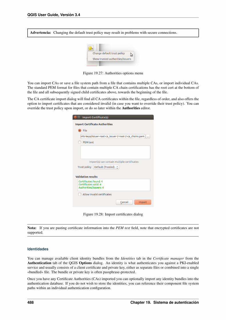
QGIS User Guide, Versión 3.4
Advertencia: Changing the default trust policy may result in problems with secure connections.
Figure 19.27: Authorities options menu
You can import CAs or save a file system path from a file that contains multiple CAs, or import individual CAs.The standard PEM format for files that contain multiple CA chain certifications has the root cert at the bottom ofthe file and all subsequently signed child certificates above, towards the beginning of the file.
The CA certificate import dialog will find all CA certificates within the file, regardless of order, and also offers theoption to import certificates that are considered invalid (in case you want to override their trust policy). You canoverride the trust policy upon import, or do so later within the Authorities editor.
Figure 19.28: Import certificates dialog
Nota: If you are pasting certificate information into the PEM text field, note that encrypted certificates are notsupported.
Identidades
You can manage available client identity bundles from the Identities tab in the Certificate manager from theAuthentication tab of the QGIS Options dialog. An identity is what authenticates you against a PKI-enabledservice and usually consists of a client certificate and private key, either as separate files or combined into a single«bundled» file. The bundle or private key is often passphrase-protected.
Once you have any Certificate Authorities (CAs) imported you can optionally import any identity bundles into theauthentication database. If you do not wish to store the identities, you can reference their component file systempaths within an individual authentication configuration.
488 Chapter 19. Sistema de autenticación

QGIS User Guide, Versión 3.4
Figure 19.29: Identities editor
When importing an identity bundle, it can be passphrase-protected or unprotected, and can contain CA certificatesforming a trust chain. Trust chain certifications will not be imported here; they can be added separately under theAuthorities tab.
Upon import the bundle’s certificate and private key will be stored in the database, with the key’s storage encryptedusing the QGIS master password. Subsequent usage of the stored bundle from the database will only require inputof the master password.
Personal identity bundles consisting of PEM/DER (.pem/.der) and PKCS#12 (.p12/.pfx) components are sup-ported. If a key or bundle is passphrase-protected, the password will be required to validate the component priorto import. Likewise, if the client certificate in the bundle is invalid (for example, its effective date has not yetstarted or has elapsed) the bundle can not be imported.
Figure 19.30: PEM/DER identity import
19.2. User Authentication Workflows 489

QGIS User Guide, Versión 3.4
Figure 19.31: PKCS#12 identity import
19.2.4 Handling bad layers
Occasionally, the authentication configuration ID that is saved with a project file is no longer valid, possiblybecause the current authentication database is different than when the project was last saved, or due to a credentialsmismatch. In such cases the Handle bad layers dialog will be presented upon QGIS launch.
Figure 19.32: Handle bad layers with authentication
If a data source is found to have an authentication configuration ID associated with it, you will be able to edit it.Doing so will automatically edit the data source string, much in the same way as opening the project file in a texteditor and editing the string.
19.2.5 Changing authentication config ID
Occasionally, you will need to change the authentication configuration ID that is associated with accessing aresource. There are instances where this is useful:
• Resource auth config ID is no longer valid: This can occur when you have switched auth databases addneed to align a new configuration to the ID already associated with a resource.
• Shared project files: If you intended to share projects between users, e.g. via a shared file server, you canpredefine a 7-character (containing a-z and/or 0-9) that is associated with the resource. Then, individualusers change the ID of an authentication configuration that is specific to their credentials of the resource.When the project is opened, the ID is found in the authentication database, but the credentials are differentper user.
490 Chapter 19. Sistema de autenticación

QGIS User Guide, Versión 3.4
Figure 19.33: Editar ID de configuración de la autenticación
Figure 19.34: Changing a layer’s authentication config ID (unlocked yellow text field)
19.2. User Authentication Workflows 491

QGIS User Guide, Versión 3.4
Advertencia: Changing the auth config ID is considered an advanced operation and should only be done withfull knowledge as to why it is necessary. This is why there is a lock button that needs clicked, to unlock theID’s text field prior to editing the ID.
19.2.6 Soporte de Servidor QGIS
When using a project file, with layers that have authentication configurations, as a basis for a map in QGIS Server,there are a couple of additional setup steps necessary for QGIS to load the resources:
• La base de datos de autenticación necesita estar disponible
• Authentication database’s master password needs to be available
When instantiating the authentication system, Server will create or use qgis-auth.db in ~/.qgis2/ or thedirectory defined by the QGIS_AUTH_DB_DIR_PATH environment variable. It may be that the Server’s user hasno HOME directory, in which case, use the environment variable to define a directory that the Server’s user hasread/write permissions and is not located within the web-accessible directories.
To pass the master password to Server, write it to the first line of file at a path on the file system readable by theServer processes user and defined using the QGIS_AUTH_PASSWORD_FILE environment variable. Ensure tolimit the file as only readable by the Server’s process user and to not store the file within web-accessible directories.
Nota: QGIS_AUTH_PASSWORD_FILE variable will be removed from the Server environment immediatelyafter accessing.
19.2.7 excepciones de servidor SSL
Figure 19.35: excepción de servidor SSL
You can manage SSL server configurations and exceptions from the Servers tab in the Authentication section ofthe QGIS Options dialog.
Sometimes, when connecting to an SSL server, there are errors with the SSL «handshake» or the server’s certifi-cate. You can ignore those errors or create an SSL server configuration as an exception. This is similar to howweb browsers allow you to override SSL errors, but with more granular control.
Advertencia: You should not create an SSL server configuration unless you have complete knowledge of theentire SSL setup between the server and client. Instead, report the issue to the server administrator.
Nota: Some PKI setups use a completely different CA trust chain to validate client identities than the chain usedto validate the SSL server certificate. In such circumstances, any configuration created for the connecting server
492 Chapter 19. Sistema de autenticación

QGIS User Guide, Versión 3.4
will not necessarily fix an issue with the validation of your client identity, and only your client identity’s issuer orserver administrator can fix the issue.
You can pre-configure an SSL server configuration by clicking the button. Alternatively, you can add aconfiguration when an SSL error occurs during a connection and you are presented with an SSL Error dialog(where the error can be ignored temporarily or saved to the database and ignored):
Figure 19.36: Adición manual de configuración
Once an SSL configuration is saved to the database, it can be edited or deleted.
If you want to pre-configure an SSL configuration and the import dialog is not working for your server’s con-nection, you can manually trigger a connection via the Python Console by running the following code (replacehttps://bugreports.qt-project.org with the URL of your server):
from PyQt4.QtNetwork import *req = QNetworkRequest(QUrl('https://bugreports.qt-project.org'))reply = QgsNetworkAccessManager.instance().get(req)
This will open an SSL error dialog if any errors occur, where you can choose to save the configuration to thedatabase.
19.3 Consideraciones de Seguridad
Once the master password is entered, the API is open to access authentication configs in the authenticationdatabase, similar to how Firefox works. However, in the initial implementation, no wall against PyQGIS ac-cess has been defined. This may lead to issues where a user downloads/installs a malicious PyQGIS plugin orstandalone app that gains access to authentication credentials.
19.3. Consideraciones de Seguridad 493

QGIS User Guide, Versión 3.4
Figure 19.37: Adicionar configuración durante un error SSL
Figure 19.38: Configuración SSL existente
494 Chapter 19. Sistema de autenticación

QGIS User Guide, Versión 3.4
Figure 19.39: Editar una configuración SSL existente
The quick solution for initial release of feature is to just not include most PyQGIS bindings for the authenticationsystem.
Another simple, though not robust, fix is to add a combobox in Settings → Options → Authentication (defaults to«never»):
"Allow Python access to authentication system"Choices: [ confirm once per session | always confirm | always allow | never]
Such an option’s setting would need to be saved in a location non-accessible to Python, e.g. the authenticationdatabase, and encrypted with the master password.
• Another option may be to track which plugins the user has specifically
• allowed to access the authentication system, though it may be tricky to deduce which plugin is actuallymaking the call.
• Sandboxing plugins, possibly in their own virtual environments, would reduce “cross-plugin” hacking ofauthentication configs from another plugin that is authorized. This might mean limiting cross-plugin com-munication as well, but maybe only between third-party plugins.
• Another good solution is to issue code-signing certificates to vetted plugin authors. Then validate the plu-gin’s certificate upon loading. If need be the user can also directly set an untrusted policy for the certificateassociated with the plugin using existing certificate management dialogs.
• Alternatively, access to sensitive authentication system data from Python
• could never be allowed, and only the use of QGIS core widgets, or duplicating authentication system in-tegrations, would allow the plugin to work with resources that have an authentication configuration, whilekeeping master password and authentication config loading in the realm of the main app.
The same security concerns apply to C++ plugins, though it will be harder to restrict access, since there is nofunction binding to simply be removed as with Python.
19.3.1 Limitaciones
The confusing licensing and exporting issues associated with OpenSSL apply. In order for Qt to work with SSLcertificates, it needs access to the OpenSSL libraries. Depending upon how Qt was compiled, the default is to
19.3. Consideraciones de Seguridad 495

QGIS User Guide, Versión 3.4
dynamically link to the OpenSSL libs at run-time (to avoid the export limitations).
QCA follows a similar tactic, whereby linking to QCA incurs no restrictions, because the qca-ossl (OpenSSL)plugin is loaded at run-time. The qca-ossl plugin is directly linked to the OpenSSL libs. Packagers would be theones needing to ensure any OpenSSL-linking restrictions are met, if they ship the plugin. Maybe. I don’t reallyknow. I’m not a lawyer.
The authentication system safely disables itself when qca-ossl is not found at run-time.
496 Chapter 19. Sistema de autenticación

CHAPTER 20
Integracion GRASS SIG
GRASS integration provides access to GRASS GIS databases and functionalities (see GRASS-PROJECT in Ref-erencias bibliográficas y web). The integration consists of two parts: provider and plugin. The provider allowsto browse, manage and visualize GRASS raster and vector layers. The plugin can be used to create new GRASSlocations and mapsets, change GRASS region, create and edit vector layers and analyze GRASS 2-D and 3-D datawith more than 400 GRASS modules. In this section, we’ll introduce the provider and plugin functionalities andgive some examples of managing and working with GRASS data.
The provider supports GRASS version 6 and 7, the plugin supports GRASS 6 and 7 (starting from QGIS 2.12).QGIS distribution may contain provider/plugin for either GRASS 6 or GRASS 7 or for both versions at the sametime (binaries have different file names). Only one version of the provider/plugin may be loaded on runtimehowever.
20.1 Conjuntos de datos demostración
As an example, we will use the QGIS Alaska dataset (see section Downloading sample data). It includes asmall sample GRASS LOCATION with three vector layers and one raster elevation map. Create a new foldercalled grassdata, download the QGIS “Alaska” dataset qgis_sample_data.zip from https://qgis.org/downloads/data/ and unzip the file into grassdata.
More sample GRASS LOCATIONs are available at the GRASS website at https://grass.osgeo.org/download/sample-data/.
20.2 Cargar capas ráster y vectorial de GRASS
If the provider is loaded in QGIS, the location item with GRASS icon is added in the browser tree under eachfolder item which contains GRASS location. Go to the folder grassdata and expand location alaska andmapset demo.
You can load GRASS raster and vector layers like any other layer from the browser either by double click on layeritem or by dragging and dropping to map canvas or legend.
Truco: Cargando datos GRASS
497

QGIS User Guide, Versión 3.4
If you don’t see GRASS location item, verify in Help → About → Providers if GRASS vector provider is loaded.
20.3 Importar datos dentro de una UBICACIÓN DE GRASS medi-ante arrastrar y soltar
This section gives an example of how to import raster and vector data into a GRASS mapset.
1. In QGIS browser navigate to the mapset you want to import data into.
2. In QGIS browser find a layer you want to import to GRASS, note that you can open another instance of thebrowser (Browser Panel (2)) if source data are too far from the mapset in the tree.
3. Drag a layer and drop it on the target mapset. The import may take some time for larger layers, you will seeanimated icon in front of new layer item until the import finishes.
When raster data are in different CRS, they can be reprojected using an Approximate (fast) or Exact (precise)transformation. If a link to the source raster is created (using r.external), the source data are in the same CRSand the format is known to GDAL, the source data CRS will be used. You can set these options in the Browser tabin Opciones GRASS.
If a source raster has more bands, a new GRASS map is created for each layer with .<band number> suffix and
group of all maps with icon is created. External rasters have a different icon .
20.4 Managing GRASS data in QGIS Browser
• Copying maps: GRASS maps may be copied between mapsets within the same location using drag anddrop.
• Deleting maps: Right click on a GRASS map and select Delete from context menu.
• Renaming maps: Right click on a GRASS map and select Rename from context menu.
20.5 Opciones GRASS
GRASS options may be set in GRASS Options dialog, which can be opened by right clicking on the location ormapset item in the browser and then choosing GRASS Options.
20.6 Iniciar el complemento GRASS
To use GRASS functionalities in QGIS, you must select and load the GRASS plugin using the Plugin Manager.
To do this, go to the menu Plugins → Manage and Install Plugins. . . , select GRASS and click OK.
The following main features are provided with the GRASS menu (Plugins → GRASS) when you start the GRASSplugin:
• Abrir directorio de mapas
• Nuevo directorio de mapas
• Cerrar directorio de mapas
• Abrir herramientas de GRASS
498 Chapter 20. Integracion GRASS SIG

QGIS User Guide, Versión 3.4
• Mostrar región actual de GRASS
• GRASS Options
20.7 Abrir directorio de mapas
A GRASS mapset must be opened to get access to GRASS Tools in the plugin (the tools are disabled if no mapsetis open). You can open a mapset from the browser: right click on mapset item and then choose Open mapset fromcontext menu.
20.8 LOCALIZACIÓN y DIRECTORIO DE MAPA GRASS
GRASS data are stored in a directory referred to as GISDBASE. This directory, often called grassdata, mustbe created before you start working with the GRASS plugin in QGIS. Within this directory, the GRASS GISdata are organized by projects stored in subdirectories called LOCATIONs. Each LOCATION is defined by itscoordinate system, map projection and geographical boundaries. Each LOCATION can have several MAPSETs(subdirectories of the LOCATION) that are used to subdivide the project into different topics or subregions, or asworkspaces for individual team members (see Neteler & Mitasova 2008 in Referencias bibliográficas y web). Inorder to analyse vector and raster layers with GRASS modules, you generally have to import them into a GRASSLOCATION. (This is not strictly true – with the GRASS modules r.external and v.external you cancreate read-only links to external GDAL/OGR-supported datasets without importing them. This is not the usualway for beginners to work with GRASS, therefore this functionality will not be described here.)
Figure 20.1: Datos GRASS en la LOCALIZACIÓN alaska
20.9 Importar datos dentro de una LOCALIZACIÓN DE GRASS
See section Importar datos dentro de una UBICACIÓN DE GRASS mediante arrastrar y soltar to find how datacan be easily imported by dragging and dropping in the browser.
This section gives an example of how to import raster and vector data into the “alaska” GRASS LOCATIONprovided by the QGIS “Alaska” dataset in traditional way, using standard GRASS modules. Therefore, we use thelandcover raster map landcover.img and the vector GML file lakes.gml from the QGIS “Alaska” dataset(see Downloading sample data).
1. Inicie QGIS y asegúrese que el complemento GRASS está cargado.
20.7. Abrir directorio de mapas 499

QGIS User Guide, Versión 3.4
2. En la barra de herramientas de GRASS, haga clic en el icono Abrir directorio de mapas para que aparezca elasistente DIRECTORIO DE MAPA.
3. Select as GRASS database the folder grassdata in the QGIS Alaska dataset, as LOCATION “alaska”, asMAPSET “demo” and click OK.
4. Ahora haga clic en el icono Abrir herramientas de GRASS. El diálogo de la caja de herramientas de GRASS(vea la sección La caja de herramientas GRASS) aparece.
5. Para importar el mapa ráster landcover.img, haga clic en el modulo r.in.gdal en la pestañaÁrbol de módulos. Este modulo GRASS le permite importar archivos ráster GDAL-admitidos en unLOCALIZACIÓN de GRASS. El diálogo del módulo para que r.in.gdal aparezca.
6. Browse to the folder raster in the QGIS “Alaska” dataset and select the file landcover.img.
7. As raster output name, define landcover_grass and click Run. In the Output tab, you seethe currently running GRASS command r.in.gdal -o input=/path/to/landcover.imgoutput=landcover_grass.
8. When it says Successfully finished, click View Output. The landcover_grass raster layer is nowimported into GRASS and will be visualized in the QGIS canvas.
9. Para importar el archivo vector GML lakes.gml, haga clic en el modulo v.in.ogr en la pestaña Ár-bol de módulos. Este modulo GRASS le permite importar archivos vectoriales OGR-admitidos en unaLOCAZACIÓN de GRASS. El diálogo del modulo para que v.in.ogr aparezca.
10. Browse to the folder gml in the QGIS “Alaska” dataset and select the file lakes.gml as OGR file.
11. As vector output name, define lakes_grass and click Run. You don’t have to care about the otheroptions in this example. In the Output tab you see the currently running GRASS command v.in.ogr -odsn=/path/to/lakes.gml output=lakes\_grass.
12. When it says Succesfully finished, click View Output. The lakes_grass vector layer is now importedinto GRASS and will be visualized in the QGIS canvas.
20.9.1 Crear una nueva LOCALIZACIÓN GRASS
As an example, here is the sample GRASS LOCATION alaska, which is projected in the Albers Equal Areaprojection using feet as units. This sample GRASS LOCATION alaska will be used for all examples and exer-cises in the following GRASS-related sections. It is useful to download and install the dataset on your computer(see Downloading sample data).
1. Inicie QGIS y asegúrese que el complemento GRASS está cargado.
2. Visualize the alaska.shp shapefile (see section Cargando una capa desde archivo) from the QGISAlaska dataset (see Downloading sample data).
3. In the GRASS toolbar, click on the New mapset icon to bring up the MAPSET wizard.
4. Select an existing GRASS database (GISDBASE) folder grassdata, or create one for the newLOCATION using a file manager on your computer. Then click Next.
5. We can use this wizard to create a new MAPSET within an existing LOCATION (see section Añadir un
nuevo DIRECTORIO DE MAPA) or to create a new LOCATION altogether. Select Create new location(see figure_grass_new_location).
6. Enter a name for the LOCATION – we used “alaska” – and click Next.
7. Define the projection by clicking on the radio button Projection to enable the projection list.
8. Estamos usando la proyección Albers Equal Area Alaska (pies). Puesto que nos ha tocado saber que estárepresentado por el EPSG ID 2964, ingresamos en el cuadro de búsqueda. (Nota: Si desea repetir esteproceso para otra LOCALIZACIÓN y proyección y no ha memorizado el EPSG ID, haga clic en el icono
SRC actual en la esquina inferior derecha de la barra de estado (vea sección Trabajar con Proyecciones)).
500 Chapter 20. Integracion GRASS SIG

QGIS User Guide, Versión 3.4
9. En Filtrar, inserte 2964 para seleccionar la proyección.
10. Click Next.
11. To define the default region, we have to enter the LOCATION bounds in the north, south, east, and westdirections. Here, we simply click on the button Set Current QGIS Extent, to apply the extent of the loadedlayer alaska.shp as the GRASS default region extent.
12. Click Next.
13. We also need to define a MAPSET within our new LOCATION (this is necessary when creating a newLOCATION). You can name it whatever you like - we used “demo”. GRASS automatically creates a specialMAPSET called PERMANENT, designed to store the core data for the project, its default spatial extent andcoordinate system definitions (see Neteler & Mitasova 2008 in Referencias bibliográficas y web).
14. Check out the summary to make sure it’s correct and click Finish.
15. La nueva LOCALIZACIÓN, “alaska”, y los dos DIRECTORIO DE MAPAS, “demo” y “PERMANENT”,son creados. El conjunto de trabajo abierto actualmente es “demo”, como se ha definido.
16. Tenga en cuenta que algunas de las herramientas en la barra de herramientas de GRASS que estaban inhab-ilitadas ahora están habilitadas.
Figure 20.2: Cree una nueva LOCALIZACIÓN GRASS o un nuevo DIRECTORIO DE MAPA en QGIS
Si eso parecía como una gran cantidad de pasos, en realidad no es tan malo y una forma muy rápida de crearuna LOCALIZACIÓN. La LOCALIZACIÓN “alaska” ahora está listo para la importación de datos (vea la secciónImportar datos dentro de una LOCALIZACIÓN DE GRASS). También puede utilizar los datos ya existentes vec-toriales y ráster en el ejemplo LOCALIZACIÓN “alaska” de GRASS, incluido en el conjunto de datos “Alaska”de QGIS Downloading sample data, ya pasar a la sección El modelo de datos vectoriales de GRASS.
20.9.2 Añadir un nuevo DIRECTORIO DE MAPA
Un usuario sólo tiene acceso de escritura a un DIRECTORIO DE MAPA GRASS que él o ella crearon. Estosignifica que además de acceder a su propio DIRECTORIO DE MAPA, se pueden leer mapas de otros usuar-ios” DIRECTORIO DE MAPAS (y ellos pueden leer los tuyos), pero sólo puede modificar o eliminar su propioDIRECTORIO DE MAPA.
Todos los DIRECTORIO DE MAPAS incluyen un archivo WIND que almacena los valores de las coordenadas delos límites actuales y la resolución ráster actualmente seleccionado (vea Neteler & Mitasova 2008 en Referenciasbibliográficas y web, y la sección La herramienta de región GRASS).
1. Inicie QGIS y asegúrese que el complemento GRASS está cargado.
2. In the GRASS toolbar, click on the New mapset icon to bring up the MAPSET wizard.
3. Seleccione la base de datos GRASS (GISDBASE) la carpeta grassdata con la LOCALIZACIÓN“alaska”, donde queremos añadir otro DIRECTORIO DE MAPA llamado “test”.
4. Click Next.
20.9. Importar datos dentro de una LOCALIZACIÓN DE GRASS 501

QGIS User Guide, Versión 3.4
5. We can use this wizard to create a new MAPSET within an existing LOCATION or to create a new
LOCATION altogether. Click on the radio button Select location (see figure_grass_new_location) andclick Next.
6. Introduzca el nombre text para el nuevo DIRECTORIO DE MAPA. A continuación en el asistente, se veuna lista de un existente DIRECTORIO DE MAPAS y titulares correspondientes.
7. Click Next, check out the summary to make sure it’s all correct and click Finish.
20.10 El modelo de datos vectoriales de GRASS
It is important to understand the GRASS vector data model prior to digitizing. In general, GRASS uses a topolog-ical vector model. This means that areas are not represented as closed polygons, but by one or more boundaries.A boundary between two adjacent areas is digitized only once, and it is shared by both areas. Boundaries must beconnected and closed without gaps. An area is identified (and labelled) by the centroid of the area.
Además de los límites y centroides, un mapa vectorial también puede contener puntos y líneas. Todos estoselementos geométricos se pueden mezclar en una vector y serán representados en diferentes denominadas “capas”dentro de un mapa vectorial GRASS. Por lo que en GRASS, una capa no es un mapa vectorial o ráster pero unnivel dentro de una capa vectorial. Esto es importante para distinguir cuidadosamente. (aunque es imposiblemezclar elementos, es inusual e incluso en GRASS, sólo se utiliza en casos especiales como análisis de redesvectoriales. Usualmente, se debe preferir almacenar diferentes elementos geométricos en diferentes capas.)
Es posible almacenar varias “capas” en un conjunto de datos vectoriales. Por ejemplo, campos, bosques y lagos sepueden almacenar en un vector. Un bosque y lago adyacente pueden compartir el mismo límite, pero tienen tablasde atributos separados. También es posible adjuntar atributos a límites. Un ejemplo podría ser el caso donde loslímites entre un lago y un bosque es una carretera, por lo que puede tener una tabla de atributos diferente.
La “capa” del objeto espacial es definido por la “capa” dentro de GRASS. “Capa” es el número que define sihay más de una capa dentro del conjunto de datos (por ejemplo, si la geometría es bosque o lago). Por ahora,sólo puede ser un número. En el futuro, GRASS también implementara nombres como campos en la interfaz deusuario.
Los atributos se pueden almacenar dentro de la LOCALIZACIÓN en GRASS como dBase o SQLite3 o en tablasde base de datos externa, por ejemplo, PostgreSQL, MySQL, Oracle, etc.
Los atributos en la tabla de base de datos están enlazadas a los elementos geométricos utilizando un valor “cate-goría”.
“Categoría” (llave, ID) es un entero adjunto a la geometría primitiva, y se utiliza como el enlace a una columnallave en la tabla de base de datos.
Truco: Aprendizaje del modelo vectorial GRASS
The best way to learn the GRASS vector model and its capabilities is to download one of the many GRASStutorials where the vector model is described more deeply. See https://grass.osgeo.org/documentation/manuals/for more information, books and tutorials in several languages.
20.11 Crear una nueva capa vectorial GRASS
To create a new GRASS vector layer, select one of following items from mapset context menu in the browser:
• Nueva Capa de Puntos
• Nueva Capa de Líneas
• Nueva capa de polígonos
502 Chapter 20. Integracion GRASS SIG

QGIS User Guide, Versión 3.4
and enter a name in the dialog. A new vector map will be created and layer will be added to canvas and editingstarted. Selecting type of the layer does not restrict geometry types which can be digitized in the vector map. InGRASS, it is possible to organize all sorts of geometry types (point, line and polygon) in one vector map. Thetype is only used to add the layer to the canvas, because QGIS requires a layer to have a specific type.
It is also possible to add layers to existing vector maps selecting one of the items described above from contextmenu of existing vector map.
In GRASS, it is possible to organize all sorts of geometry types (point, line and area) in one layer, because GRASSuses a topological vector model, so you don’t need to select the geometry type when creating a new GRASS vector.This is different from shapefile creation with QGIS, because shapefiles use the Simple Feature vector model (seesection Creating new vector layers).
20.12 Digitalizar y editar una capa vectorial GRASS
GRASS vector layers can be digitized using the standard QGIS digitizing tools. There are however some particu-larities, which you should know about, due to
• GRASS topological model versus QGIS simple feature
• complejidad del modelo GRASS
– multiple layers in single maps
– multiple geometry types in single map
– geometry sharing by multiple features from multiple layers
The particularities are discussed in the following sections.
Save, discard changes, undo, redo
Advertencia: All the changes done during editing are immediately written to vector map and related attributetables.
Changes are written after each operation, it is however, possible to do undo/redo or discard all changes whenclosing editing. If undo or discard changes is used, original state is rewritten in vector map and attribute tables.
There are two main reasons for this behaviour:
• It is the nature of GRASS vectors coming from conviction that user wants to do what he is doing and it isbetter to have data saved when the work is suddenly interrupted (for example, blackout)
• Necessity for effective editing of topological data is visualized information about topological correctness,such information can only be acquired from GRASS vector map if changes are written to the map.
Barra de herramientas
The “Digitizing Toolbar” has some specific tools when a GRASS layer is edited:
Icono Herramienta Propósito
Nuevo punto Digitalizar un nuevo punto
Nueva línea Digitalizar nueva línea
Nuevo límite Digitalizar nuevo borde
Nuevo centroide Digitalizar nuevo centroide (etiqueta de área existente)
Nuevo Contorno Cerrado Digitalizar nuevo borde cerrado
Table GRASS Digitizing: GRASS Digitizing Tools
20.12. Digitalizar y editar una capa vectorial GRASS 503

QGIS User Guide, Versión 3.4
Truco: Digitalizando polígonos en GRASS
If you want to create a polygon in GRASS, you first digitize the boundary of the polygon. Then you add a centroid(label point) into the closed boundary. The reason for this is that a topological vector model links the attributeinformation of a polygon always to the centroid and not to the boundary.
Categoría
Category, often called cat, is sort of ID. The name comes from times when GRASS vectors had only singlyattribute «category». Category is used as a link between geometry and attributes. A single geometry may havemultiple categories and thus represent multiple features in different layers. Currently it is possible to assign onlyone category per layer using QGIS editing tools. New features have automatically assigned new unique category,except boundaries. Boundaries usually only form areas and do not represent linear features, it is however possibleto define attributes for a boundary later, for example in different layer.
New categories are always created only in currently being edited layer.
It is not possible to assign more categories to geometry using QGIS editing, such data are properly represented asmultiple features, and individual features, even from different layers, may be deleted.
Atributos
Attributes of currently edited layer can only be modified. If the vector map contains more layers, features of otherlayers will have all attributes set to “<not editable (layer #)>” to warn you that such attribute is not editable. Thereason is, that other layers may have and usually have different set of fields while QGIS only supports one fixedset of fields per layer.
If a geometry primitive does not have a category assigned, a new unique category is automatically assigned andnew record in attribute table is created when an attribute of that geometry is changed.
Truco: If you want to do bulk update of attributes in table, for example using “Field Calculator” (Using the FieldCalculator), and there are features without category which you don’t want to update (typically boundaries), youcan filter them out by setting “Advanced Filter” to cat is not null.
Editing style
The topological symbology is essential for effective editing of topological data. When editing starts, a specialized“GRASS Edit” renderer is set on the layer automatically and original renderer is restored when editing is closed.The style may be customized in layer properties “Style” tab. The style can also be stored in project file or inseparate file as any other style. If you customize the style, do not change its name, because it is used to reset thestyle when editing is started again.
Truco: Do not save project file when the layer is edited, the layer would be stored with “Edit Style” which hasno meaning if layer is not edited.
The style is based on topological information which is temporarily added to attribute table as field “topo_symbol”.The field is automatically removed when editing is closed.
Truco: Do not remove “topo_symbol” field from attribute table, that would make features invisible because therenderer is based on that column.
Autoensamblado
To form an area, vertices of connected boundaries must have exactly the same coordinates. This can be achievedusing snapping tool only if canvas and vector map have the same CRS. Otherwise, due conversion from mapcoordinates to canvas and back, the coordinate may become slightly different due to representation error and CRStransformations.
504 Chapter 20. Integracion GRASS SIG
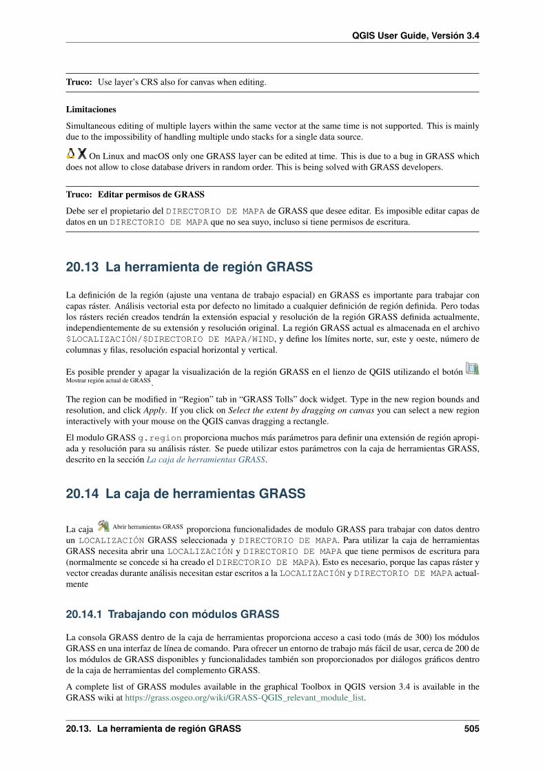
QGIS User Guide, Versión 3.4
Truco: Use layer’s CRS also for canvas when editing.
Limitaciones
Simultaneous editing of multiple layers within the same vector at the same time is not supported. This is mainlydue to the impossibility of handling multiple undo stacks for a single data source.
On Linux and macOS only one GRASS layer can be edited at time. This is due to a bug in GRASS whichdoes not allow to close database drivers in random order. This is being solved with GRASS developers.
Truco: Editar permisos de GRASS
Debe ser el propietario del DIRECTORIO DE MAPA de GRASS que desee editar. Es imposible editar capas dedatos en un DIRECTORIO DE MAPA que no sea suyo, incluso si tiene permisos de escritura.
20.13 La herramienta de región GRASS
La definición de la región (ajuste una ventana de trabajo espacial) en GRASS es importante para trabajar concapas ráster. Análisis vectorial esta por defecto no limitado a cualquier definición de región definida. Pero todaslos rásters recién creados tendrán la extensión espacial y resolución de la región GRASS definida actualmente,independientemente de su extensión y resolución original. La región GRASS actual es almacenada en el archivo$LOCALIZACIÓN/$DIRECTORIO DE MAPA/WIND, y define los límites norte, sur, este y oeste, número decolumnas y filas, resolución espacial horizontal y vertical.
Es posible prender y apagar la visualización de la región GRASS en el lienzo de QGIS utilizando el botónMostrar región actual de GRASS.
The region can be modified in “Region” tab in “GRASS Tolls” dock widget. Type in the new region bounds andresolution, and click Apply. If you click on Select the extent by dragging on canvas you can select a new regioninteractively with your mouse on the QGIS canvas dragging a rectangle.
El modulo GRASS g.region proporciona muchos más parámetros para definir una extensión de región apropi-ada y resolución para su análisis ráster. Se puede utilizar estos parámetros con la caja de herramientas GRASS,descrito en la sección La caja de herramientas GRASS.
20.14 La caja de herramientas GRASS
La caja Abrir herramientas GRASS proporciona funcionalidades de modulo GRASS para trabajar con datos dentroun LOCALIZACIÓN GRASS seleccionada y DIRECTORIO DE MAPA. Para utilizar la caja de herramientasGRASS necesita abrir una LOCALIZACIÓN y DIRECTORIO DE MAPA que tiene permisos de escritura para(normalmente se concede si ha creado el DIRECTORIO DE MAPA). Esto es necesario, porque las capas ráster yvector creadas durante análisis necesitan estar escritos a la LOCALIZACIÓN y DIRECTORIO DE MAPA actual-mente
20.14.1 Trabajando con módulos GRASS
La consola GRASS dentro de la caja de herramientas proporciona acceso a casi todo (más de 300) los módulosGRASS en una interfaz de línea de comando. Para ofrecer un entorno de trabajo más fácil de usar, cerca de 200 delos módulos de GRASS disponibles y funcionalidades también son proporcionados por diálogos gráficos dentrode la caja de herramientas del complemento GRASS.
A complete list of GRASS modules available in the graphical Toolbox in QGIS version 3.4 is available in theGRASS wiki at https://grass.osgeo.org/wiki/GRASS-QGIS_relevant_module_list.
20.13. La herramienta de región GRASS 505

QGIS User Guide, Versión 3.4
Figure 20.3: Caja de herramienta GRASS y módulo
También es posible personalizar el contenido de la caja de herramientas GRASS. Este procedimiento se describeen la sección Personalizar la caja de herramientas GRASS.
As shown in figure_grass_toolbox, you can look for the appropriate GRASS module using the thematicallygrouped Modules Tree or the searchable Modules List tab.
Al hacer clic en un icono de modulo gráfico, una nueva pestaña se añadirá al diálogo de Caja de herramientas,proporciona tres nuevas sub-pestañas Opciones, Salida y Manual.
Opciones
The Options tab provides a simplified module dialog where you can usually select a raster or vector layer visualizedin the QGIS canvas and enter further module-specific parameters to run the module.
The provided module parameters are often not complete to keep the dialog simple. If you want to use furthermodule parameters and flags, you need to start the GRASS shell and run the module in the command line.
Una nueva característica desde QGIS 1.8 es la implementación de un botón Mostrar opciones avanzadas abajo deldiálogo del modulo simplificado en la pestaña Opciones. Por el momento, sólo se añade al modulo v.in.asciicomo ejemplo de uso, pero probablemente es parte de más o todos los módulos en la caja de herramientas GRASSen futuras versiones de QGIS. Esto le permite usar las opciones del modulo de GRASS completo sin la necesidadde cambiar la consola de GRASS.
Salida
The Output tab provides information about the output status of the module. When you click the Run button, themodule switches to the Output tab and you see information about the analysis process. If all works well, you willfinally see a Successfully finished message.
Manual
La pestaña Manual muestra la página de ayuda HTML del modulo GRASS. Se puede utilizar para comprobarotros parámetros de los módulos y las banderas o para obtener un conocimiento más profundo acerca de la final-idad del módulo. Al final de cada página del manual del módulo, se ven otros enlaces al Índice de ayudaprincipal, al Índice temático y al Índice completo. Estos enlaces proporcionar información deejemplo como el modulo g.manual.
Truco: Mostrar resultados inmediatamente
506 Chapter 20. Integracion GRASS SIG

QGIS User Guide, Versión 3.4
Figure 20.4: Opciones del módulo de la caja de herramientas GRASS
Figure 20.5: Salida del módulo de la caja de herramientas GRASS
20.14. La caja de herramientas GRASS 507

QGIS User Guide, Versión 3.4
Figure 20.6: Módulo Manual de la caja de herramientas GRASS
508 Chapter 20. Integracion GRASS SIG

QGIS User Guide, Versión 3.4
Si desea mostrar sus resultados de cálculo inmediatamente en su lienzo de mapa, se puede utilizar el botón “VerSalida” en la parte inferior de la pestaña de módulo.
20.14.2 Ejemplos del módulo GRASS
Los siguientes ejemplos demostrarán el poder de algunos módulos GRASS.
Crear curvas de nivel
El primer ejemplo crea un mapa de curvas de nivel vectoriales de un ráster de elevación (DEM). Aquí, se asumeque se tiene LOCALIZACIÓN Alaska configurado como se explica en la sección Importar datos dentro de unaLOCALIZACIÓN DE GRASS.
• First, open the location by clicking the Open mapset button and choosing the Alaska location.
• Ahora abra la caja de herramientas con el botón Abrir herramientas de GRASS.
• En la lista de categorías de herramientas, haga doble clic Ráster → Administración de superficie→ Generarcurvas de nivel vectoriales.
• Now a single click on the tool r.contour will open the tool dialog as explained above (see Trabajando conmódulos GRASS).
• In the Name of input raster map enter gtopo30.
• Type into the Increment between Contour levels the value 100. (This will create contour lines atintervals of 100 meters.)
• Escriba en Nombre de salida del mapa vectorial el nombre ctour_100.
• Click Run to start the process. Wait for several moments until the message Successfully finishedappears in the output window. Then click View Output and Close.
Dado que esta es una región grande, tomará un tiempo para mostrarla. Después de que termine la presentación,puede abrir la ventana de propiedades de la capa para cambiar el color de línea así el contorno aparece claramentesobre el ráster de elevación, como en El Dialogo de las Propiedades del Vector.
El siguiente acercamiento a una pequeña y montañosa área en el centro de Alaska. Al acercarse, se puede observarque las curvas de nivel tienen esquinas afiladas. GRASS ofrece la herramienta v.generalize para alterar ligera-mente mapas vectoriales, manteniendo su forma general. La herramienta utiliza varios algoritmos diferentes conpropósitos diferentes. Algunos de los algoritmos (es decir, Douglas Peucker y Vertex Reduction) simplificar lalínea mediante la eliminación de algunos de los vértices. El vector resultante se carga más rápido. Este proceso esútil cuando se tiene un vector muy detallado, pero va a crear un mapa de escala muy pequeña, por lo que el detallees innecesario.
Truco: La herramienta de simplificar
Note that QGIS has a Vector → Geometry Tools → Simplify geometries tool that works just like the GRASSv.generalize Douglas-Peuker algorithm.
Sin embargo, el proposito de este ejemplo es diferente. Las líneas de curvas de nivel creadas por r.contourtiene ángulos agudos que deben ser suavizados. Entre el algoritmo v.generalize hay Chaiken’s, lo que haceprecisamente eso (también astillas de Hermite). Tenga en cuenta que estos algoritmos se pueden añadir vérticesadicionales al vector, haciendo que se cargue más lentamente
• Abra la caja de herramientas GRASS y haga doble clic en las categorías Vectorial → Desarrollar mapa →Generalización,
• Compruebe que el vector “ctour_100” aparece como el Nombre del vector de entrada.
20.14. La caja de herramientas GRASS 509

QGIS User Guide, Versión 3.4
• From the list of algorithms, choose Chaiken’s. Leave all other options at their default, and scroll down tothe last row to enter in the field Name for output vector map “ctour_100_smooth”, and click Run.
• The process takes several moments. Once Successfully finished appears in the output windows,click View Output and then Close.
• Se puede cambiar el color del vector para que se muestre claramente sobre el fondo del ráster y para con-trastar con las curvas de nivel originales. Se dará cuenta de que las nuevas curvas de nivel tienen esquinasmás suaves que el original durante su estancia fiel a la original de forma general.
Figure 20.7: Módulo GRASS v.generalize para suavizar un mapa vectorial
Truco: Otros usos de r.contour
El proceso descrito anteriormente se puede utilizar en otras situaciones equivalentes. Si tiene un mapa ráster dedatos de precipitación, por ejemplo, entonces el mismo método se utilizará para crear un mapa vectorial de líneasisoyetas (lluvia constante).
Crear un efecto sombreado de relieve 3-D
Varios métodos se utilizan para mostrar capas de elevación y da un efecto #-D a mapas. El uso de líneas decurvas de nivel, como se mostro anteriormente, es un método popular regularmente elejido para producir mapastopológicos. El efecto de sombreado se crea de un ráster (elevación) DEM calculando primero la pendiente y elaspecto de cada celda, entonces simula la posición del sol en el cielo y da un valor de reflectancia a cada celda. Deeste modo se obtienen pendientes frente al sol iluminadas; las pendientes orientadas lejos del sol(en la sombra) seoscurecen.
• Comience este ejemplo cargando el ráster de elevación gtopo30. Inicie la caja de herramientas GRASS ybajo la categoría ráster, haga doble clic para abrir Análisis espacial → Análisis del terreno.
• A continuación haga clic en r.shaded.relief para abrir el módulo.
• Cambie el ángulo del azimut 270 a 315
• Enter gtopo30_shade for the new hillshade raster, and click Run.
• Cuando el proceso finalice, añada el ráster de mapa de sombras al mapa. Debe verlo desplegado en escalade grises.
• Para ver ambos sombreados y los colores de la gtopo30‘ juntos, mueva el mapa de sombreado abajo del mapagtopo30 en la tabla de contenido, a continuación abra la ventana Propiedades de gtopo30, cambie a lapestaña de Transparencia y establezca su nivel de transparencia a cerca de 25%.
510 Chapter 20. Integracion GRASS SIG

QGIS User Guide, Versión 3.4
Ahora debe tener la elevación gtopo30 con su mapa de color y ajuste de transparencia mostrado arriba el mapade sombras en escala de grises. Con el fin de ver los efectos visuales en el mapa de sombras, apague el mapagtopo30_shade, a continuación, vuelva a encenderla.
Utilizar la consola de GRASS
The GRASS plugin in QGIS is designed for users who are new to GRASS and not familiar with all the modulesand options. As such, some modules in the Toolbox do not show all the options available, and some modules donot appear at all. The GRASS shell (or console) gives the user access to those additional GRASS modules thatdo not appear in the Toolbox tree, and also to some additional options to the modules that are in the Toolbox withthe simplest default parameters. This example demonstrates the use of an additional option in the r.shaded.reliefmodule that was shown above.
Figure 20.8: La consola de GRASS, módulo r.shaded.relief
El modulo r.shaded.relief puede tomar un parámetro zmult, que multiplica los valores de elevación relativas alas unidades de las coordenadas X-Y por lo que el efecto de sombreado es incluso más pronunciado.
• Load the gtopo30 elevation raster as above, then start the GRASS Toolbox and click on theGRASS shell. In the shell window, type the command r.shaded.relief map=gtopo30shade=gtopo30_shade2 azimuth=315 zmult=3 and press Enter.
• After the process finishes, shift to the Browse tab and double-click on the new gtopo30_shade2 rasterto display it in QGIS.
• Como se explicó anteriormente, mueva ráster del relieve sombreado a bajo del ráster gtopo30 en la tabla
20.14. La caja de herramientas GRASS 511

QGIS User Guide, Versión 3.4
de contenido, entonces valide la transparecia de la capa coloreada gtopo30. Debe ver que el efecto 3-Ddestaca más fuertemente comparada con el primer mapa de relieve sombreado.
Figure 20.9: Mostrar relieve sombreado creado con el módulo de GRASS r.shaded.relief
Estadísticas de ráster en un mapa vectorial
El siguiente ejemplo muestra como un módulo GRASS puede agregar datos ráster y añadir columnas de unaestadística para cada polígono en un mapa vectorial.
• Again using the Alaska data, refer to Importar datos dentro de una LOCALIZACIÓN DE GRASS to importthe shapefiles/trees.shp file into GRASS.
• Ahora un paso intermedio es necesario: los centroides se deben añadir al mapa de árboles importado paraque sea una zona de GRASS completa del vector (incluyendo ambos límites y centroides).
• De la caja de herramientas, elija Vectorial → Desarrollar mapa -> Administrar objetos espaciales, y abrael modulo v.centroids.
• Introduzca como el Mapa vectorial de salida “forest_areas” y ejecute el módulo.
• Ahora cargue el vector forest_areas y muestre los tipos de bosque - caducifolio, árbol de hoja perenne,mixto - en diferentes colores: En la ventana Propiedades de la capa, la pestaña Simbología, elija de Tipo
de leyenda “Valor único” y establezca el Campo de clasificación a “VEGDESC”. (Consulte la expli-cación de la pestaña de simbología en Symbology Properties de la sección vectorial.)
• A continuación vuelva a abrir la caja de herramientas de GRASS y abra Vectorial → Actualizacion vectorialpor otros mapas.
• Haga clic en el modulo v.rast.stats. Ingrese gtopo30 y forest_areas.
• Only one additional parameter is needed: Enter column prefix elev, and click Run. This is a computation-ally heavy operation, which will run for a long time (probably up to two hours).
• Finalmente, abra la tabla de atributos forest_areas, y verifique que varias de las nuevas columnas sehan añadido, incluyendo elev_min, elev_max, elev_mean, etc., para cada polígono de bosque.
20.14.3 Personalizar la caja de herramientas GRASS
Casi todos los módulos de GRASS se pueden añadir a la caja de herramientas de GRASS. Una interfaz XML seproporciona para analizar los archivos XML muy sencillos que configuran la apariencia y los parámetros de losmódulos dentro de la caja de herramientas.
Un ejemplo del archivo XML para generar el módulo v.buffer (v.buffer.qgm) luce como esto:
512 Chapter 20. Integracion GRASS SIG

QGIS User Guide, Versión 3.4
<?xml version="1.0" encoding="UTF-8"?><!DOCTYPE qgisgrassmodule SYSTEM "http://mrcc.com/qgisgrassmodule.dtd">
<qgisgrassmodule label="Vector buffer" module="v.buffer"><option key="input" typeoption="type" layeroption="layer" /><option key="buffer"/><option key="output" />
</qgisgrassmodule>
The parser reads this definition and creates a new tab inside the Toolbox when you select the module. A moredetailed description for adding new modules, changing a module’s group, etc., can be found at https://qgis.org/en/site/getinvolved/development/addinggrasstools.html.
20.14. La caja de herramientas GRASS 513

QGIS User Guide, Versión 3.4
514 Chapter 20. Integracion GRASS SIG

CHAPTER 21
Entorno de trabajo de procesamiento de QGIS
21.1 Introducción
Este capítulo introduce al marco de procesamiento de QGIS, un entorno de geoprosesamiento que se puede utilizarpara llamar algoritmos nativos o de terceros de QGIS, haciendo su tarea de análisis espacial más productivo y fácilde lograr.
En las siguientes secciones, revisaremos cómo usar los elementos gráficos de este sistema y sacar el máximoprovecho de cada uno de ellos.
There are four basic elements in the framework GUI, which are used to run algorithms for different purposes.Choosing one tool or another will depend on the kind of analysis that is to be performed and the particularcharacteristics of each user and project. All of them (except for the batch processing interface, which is calledfrom the toolbox or the algorithm execution dialog, as we will see) can be accessed from the Processing menuitem (you will see more entries; the remaining ones are not used to execute algorithms and will be explained laterin this chapter).
• The Toolbox: The main element of the GUI, it is used to execute a single algorithm or run a batch processbased on that algorithm.
• The Graphical Modeler: Several algorithms can be combined graphically using the modeler to define aworkflow, creating a single process that involves several subprocesses.
• The History manager: All actions performed using any of the aforementioned elements are stored in ahistory file and can be later easily reproduced using the history manager.
• The Batch Processing interface: This interface allows you to execute batch processes and automate theexecution of a single algorithm on multiple datasets.
En las siguientes secciones, revisaremos cada uno de los elementos a detalle.
21.2 Configuring the Processing Framework
As has been mentioned, the configuration menu gives access to a new dialog where you can configure how algo-rithms work. Configuration parameters are structured in separate blocks that you can select on the left-hand sideof the dialog.
Along with the aforementioned Output folder entry, the General block contains parameters for setting the defaultrendering style for output layers (that is, layers generated by using algorithms from any of the framework GUI
515

QGIS User Guide, Versión 3.4
Figure 21.1: Caja de Herramientas de Procesamiento
Figure 21.2: Procesamiento del modelador
516 Chapter 21. Entorno de trabajo de procesamiento de QGIS

QGIS User Guide, Versión 3.4
Figure 21.3: El historial del procesamiento
Figure 21.4: Interfaz de procesamiento por lote
21.2. Configuring the Processing Framework 517

QGIS User Guide, Versión 3.4
components). Just create the style you want using QGIS, save it to a file, and then enter the path to that file in thesettings so the algorithms can use it. Whenever a layer is loaded by Processing and added to the QGIS canvas, itwill be rendered with that style.
Rendering styles can be configured individually for each algorithm and each one of its outputs. Just right-click onthe name of the algorithm in the toolbox and select Edit rendering styles for outputs. You will see a dialog like theone shown next.
Figure 21.5: Rendering Styles
Select the style file (.qml) that you want for each output and press OK.
Other configuration parameters in the General group are listed below:
• Use filename as layer name. The name of each resulting layer created by an algorithm is defined by thealgorithm itself. In some cases, a fixed name might be used, meaning that the same output name will beused, no matter which input layer is used. In other cases, the name might depend on the name of the inputlayer or some of the parameters used to run the algorithm. If this checkbox is checked, the name will betaken from the output filename instead. Notice that, if the output is saved to a temporary file, the filenameof this temporary file is usually a long and meaningless one intended to avoid collision with other alreadyexisting filenames.
• Keep dialog open after running algorithm. Once an algorithm has finished execution and its output layersare loaded into the QGIS project, the algorithm dialog is closed. If you want to keep it open (to run thealgorithm again with different parameters, or to better check the output that is written to the log tab), checkthis option
• Use only selected features. If this option is selected, whenever a vector layer is used as input for an al-gorithm, only its selected features will be used. If the layer has no selected features, all features will beused.
• Pre-execution script file and Post-execution script file. These parameters refer to scripts written using theprocessing scripting functionality, and are explained in the section covering scripting and the console.
Apart from the General block in the settings dialog, you will also find a block for algorithm providers. Eachentry in this block contains an Activate item that you can use to make algorithms appear or not in the toolbox.Also, some algorithm providers have their own configuration items, which we will explain later when coveringparticular algorithm providers.
21.3 The Toolbox
The Processing Toolbox is the main element of the processing GUI, and the one that you are more likely to usein your daily work. It shows the list of all available algorithms grouped in different blocks called Providers, andcustom models and scripts you can add to extend the set of tools. Hence the toolbox is the access point to runthem, whether as a single process or as a batch process involving several executions of the same algorithm ondifferent sets of inputs.
Providers can be (de)activated in the Processing settings dialog. By default, only providers that do not rely onthird-party applications (that is, those that only require QGIS elements to be run) are active. Algorithms requiring
518 Chapter 21. Entorno de trabajo de procesamiento de QGIS

QGIS User Guide, Versión 3.4
Figure 21.6: Caja de Herramientas de Procesamiento
21.3. The Toolbox 519
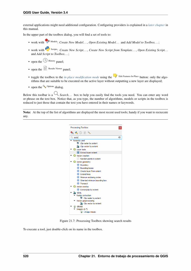
QGIS User Guide, Versión 3.4
external applications might need additional configuration. Configuring providers is explained in a later chapter inthis manual.
In the upper part of the toolbox dialog, you will find a set of tools to:
• work with Models: Create New Model. . . , Open Existing Model. . . and Add Model to Toolbox. . . ;
• work with Scripts: Create New Script. . . , Create New Script from Template. . . , Open Existing Script. . .and Add Script to Toolbox. . . ;
• open the History panel;
• open the Results Viewer panel;
• toggle the toolbox to the in-place modification mode using the Edit Features In-Place button: only the algo-rithms that are suitable to be executed on the active layer without outputting a new layer are displayed;
• open the Options dialog.
Below this toolbar is a Search. . . box to help you easily find the tools you need. You can enter any wordor phrase on the text box. Notice that, as you type, the number of algorithms, models or scripts in the toolbox isreduced to just those that contain the text you have entered in their names or keywords.
Nota: At the top of the list of algorithms are displayed the most recent used tools; handy if you want to reexecuteany.
Figure 21.7: Processing Toolbox showing search results
To execute a tool, just double-click on its name in the toolbox.
520 Chapter 21. Entorno de trabajo de procesamiento de QGIS

QGIS User Guide, Versión 3.4
21.3.1 El cuadro de diálogo de algoritmo
Once you double-click on the name of the algorithm that you want to execute, a dialog similar to that in the figurebelow is shown (in this case, the dialog corresponds to the Centroids algorithm).
Figure 21.8: Algorithm Dialog - Parameters
This dialog is used to set the input values that the algorithm needs to be executed. It shows a list of input valuesand configuration parameters to be set. It of course has a different content, depending on the requirements of thealgorithm to be executed, and is created automatically based on those requirements.
Aunque el número y el tipo de parámetro dependen de las características del algoritmo, la estructura es similarpara todos ellos. Los parámetros encontrados en la tabla pueden ser de uno de los siguientes tipos.
• A raster layer, to select from a list of all such layers available (currently opened) in QGIS. The selectorcontains as well a button on its right-hand side, to let you select filenames that represent layers currently notloaded in QGIS.
• A vector layer, to select from a list of all vector layers available in QGIS. Layers not loaded in QGIS canbe selected as well, as in the case of raster layers, but only if the algorithm does not require a table fieldselected from the attributes table of the layer. In that case, only opened layers can be selected, since theyneed to be open so as to retrieve the list of field names available.
You will see an iterator button by each vector layer selector, as shown in the figure below.
Si el algoritmo contiene varios de ellos, será capaz de cambiar cada uno de ellos. Si el botón correspondientea una entrada vectorial se cambia, el algoritmo será ejecutado iterativamente en cada uno de sus elementos,en lugar de sólo una vez para toda la capa, produciendo mayor cantidad de salidas como veces que se ejecuta
21.3. The Toolbox 521
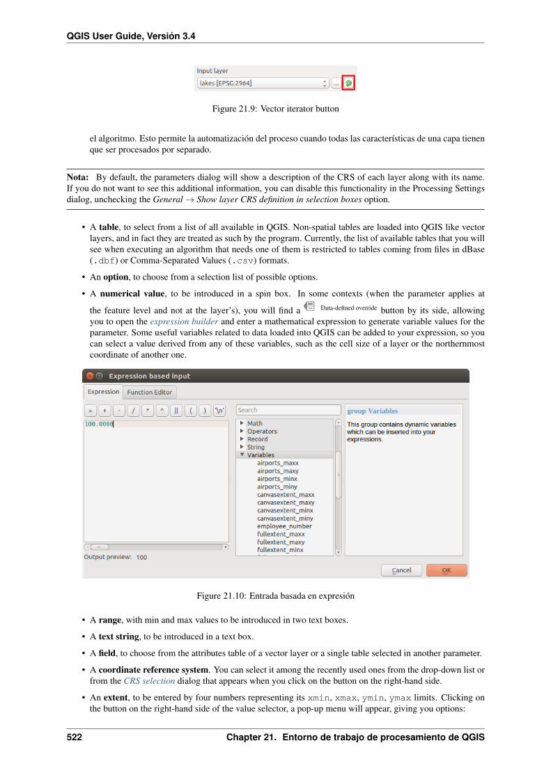
QGIS User Guide, Versión 3.4
Figure 21.9: Vector iterator button
el algoritmo. Esto permite la automatización del proceso cuando todas las características de una capa tienenque ser procesados por separado.
Nota: By default, the parameters dialog will show a description of the CRS of each layer along with its name.If you do not want to see this additional information, you can disable this functionality in the Processing Settingsdialog, unchecking the General → Show layer CRS definition in selection boxes option.
• A table, to select from a list of all available in QGIS. Non-spatial tables are loaded into QGIS like vectorlayers, and in fact they are treated as such by the program. Currently, the list of available tables that you willsee when executing an algorithm that needs one of them is restricted to tables coming from files in dBase(.dbf) or Comma-Separated Values (.csv) formats.
• An option, to choose from a selection list of possible options.
• A numerical value, to be introduced in a spin box. In some contexts (when the parameter applies at
the feature level and not at the layer’s), you will find a Data-defined override button by its side, allowingyou to open the expression builder and enter a mathematical expression to generate variable values for theparameter. Some useful variables related to data loaded into QGIS can be added to your expression, so youcan select a value derived from any of these variables, such as the cell size of a layer or the northernmostcoordinate of another one.
Figure 21.10: Entrada basada en expresión
• A range, with min and max values to be introduced in two text boxes.
• A text string, to be introduced in a text box.
• A field, to choose from the attributes table of a vector layer or a single table selected in another parameter.
• A coordinate reference system. You can select it among the recently used ones from the drop-down list orfrom the CRS selection dialog that appears when you click on the button on the right-hand side.
• An extent, to be entered by four numbers representing its xmin, xmax, ymin, ymax limits. Clicking onthe button on the right-hand side of the value selector, a pop-up menu will appear, giving you options:
522 Chapter 21. Entorno de trabajo de procesamiento de QGIS

QGIS User Guide, Versión 3.4
– to select the value from a layer or the current canvas extent;
– or to define it by dragging directly onto the map canvas.
Figure 21.11: Selector de extensión
Si se selecciona la primera opción, se verá una ventana como la siguiente.
Figure 21.12: Lista de Extensión
Si se selecciona la segunda opción, la ventana de parámetros se ocultará, para que se pueda definir el rectán-gulo haciendo click y arrastrando dentro del lienzo. Una vez hecho esto, el cuadro de diálogo reaparecerá,con los valores correspondientes ya rellenos en en cuadro de texto.
Figure 21.13: Arrastrar Extensión
• A list of elements (whether raster or vector layers, tables, fields) to select from. Click on the . . . buttonat the left of the option to see a dialog like the following one. Multiple selection is allowed and when thedialog is closed, number of selected items is displayed in the parameter text box widget.
• A small table to be edited by the user. These are used to define parameters like lookup tables or convolutionkernels, among others.
Click en el botón del lado derecho para ver la tabla y editar sus valores.
Dependiendo del algoritmo, el número de filas que pueden ser modificadas o no al utilizar los botones dellado derecho de la ventana.
Nota: Some algorithms require many parameter to run, e.g. in the qgisrastercalculator you have to specifymanually the cell size, the extent and the CRS. You can avoid to choose all the parameters manually when thealgorithm has the Reference layers parameter. With this parameter you can choose the reference layer andall its properties (cell size, extent, CRS) will be used.
21.3. The Toolbox 523

QGIS User Guide, Versión 3.4
Figure 21.14: Selección Múltiple
Figure 21.15: Tabla Fija
524 Chapter 21. Entorno de trabajo de procesamiento de QGIS
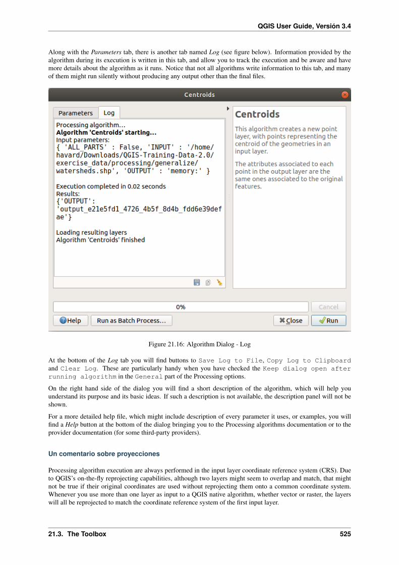
QGIS User Guide, Versión 3.4
Along with the Parameters tab, there is another tab named Log (see figure below). Information provided by thealgorithm during its execution is written in this tab, and allow you to track the execution and be aware and havemore details about the algorithm as it runs. Notice that not all algorithms write information to this tab, and manyof them might run silently without producing any output other than the final files.
Figure 21.16: Algorithm Dialog - Log
At the bottom of the Log tab you will find buttons to Save Log to File, Copy Log to Clipboardand Clear Log. These are particularly handy when you have checked the Keep dialog open afterrunning algorithm in the General part of the Processing options.
On the right hand side of the dialog you will find a short description of the algorithm, which will help youunderstand its purpose and its basic ideas. If such a description is not available, the description panel will not beshown.
For a more detailed help file, which might include description of every parameter it uses, or examples, you willfind a Help button at the bottom of the dialog bringing you to the Processing algorithms documentation or to theprovider documentation (for some third-party providers).
Un comentario sobre proyecciones
Processing algorithm execution are always performed in the input layer coordinate reference system (CRS). Dueto QGIS’s on-the-fly reprojecting capabilities, although two layers might seem to overlap and match, that mightnot be true if their original coordinates are used without reprojecting them onto a common coordinate system.Whenever you use more than one layer as input to a QGIS native algorithm, whether vector or raster, the layerswill all be reprojected to match the coordinate reference system of the first input layer.
21.3. The Toolbox 525

QGIS User Guide, Versión 3.4
This is however less true for most of the external applications whose algorithms are exposed through the processingframework as they assume that all of the layers are already in a common coordinate system and ready to beanalyzed.
By default, the parameters dialog will show a description of the CRS of each layer along with its name, making iteasy to select layers that share the same CRS to be used as input layers. If you do not want to see this additionalinformation, you can disable this functionality in the Processing settings dialog, unchecking the Show layer CRSdefinition in selection boxes option.
If you try to execute an algorithm using as input two or more layers with unmatching CRSs, a warning dialog willbe shown. This occurs thanks to the Warn before executing if layer CRS’s do not match option.
Aún se puede ejecutar el algoritmo, pero en la mayoría de los casos se producirán resultados incorrectos, comocapas vacias debido a que las capas de entrada no se solapan.
Truco: Use Processing algorithms to do intermediate reprojection
When an algorithm can not successfully perform on multiple input layers due to unmatching CRSs, use QGISinternal algorithm such as qgisreprojectlayer to perform layers” reprojection to the same CRS before executingthe algorithm using these outputs.
21.3.2 Resultados generados por algoritmos
Los tipos de resultados que se pueden generar cor un algoritmo son los siguientes:
• Una capa ráster.
• Una capa vectorial.
• Una tabla
• Un archivo HTML (usado para salidas de texto y salidas gráficas).
These are all saved to disk, and the parameters table will contain a text box corresponding to each one of theseoutputs, where you can type the output channel to use for saving it. An output channel contains the informationneeded to save the resulting object somewhere. In the most usual case, you will save it to a file, but in the case ofvector layers, and when they are generated by native algorithms (algorithms not using external applications) youcan also save to a PostGIS, GeoPackage or SpatiaLite database, or a memory layer.
To select an output channel, just click on the button on the right side of the text box, and you will see a smallcontext menu with the available options.
In the most usual case, you will select saving to a file. If you select that option, you will be prompted with asave file dialog, where you can select the desired file path. Supported file extensions are shown in the file formatselector of the dialog, depending on the kind of output and the algorithm.
The format of the output is defined by the filename extension. The supported formats depend on what is supportedby the algorithm itself. To select a format, just select the corresponding file extension (or add it, if you are directlytyping the file path instead). If the extension of the file path you entered does not match any of the supportedformats, a default extension will be appended to the file path, and the file format corresponding to that extensionwill be used to save the layer or table. Default extensions are .dbf for tables, .tif for raster layers and .gpkgfor vector layers. These can be modified in the setting dialog, selecting any other of the formats supported byQGIS.
If you do not enter any filename in the output text box (or select the corresponding option in the context menu),the result will be saved as a temporary file in the corresponding default file format, and it will be deleted once youexit QGIS (take care with that, in case you save your project and it contains temporary layers).
You can set a default folder for output data objects. Go to the settings dialog (you can open it from the Settings→ Options → Processing menu), and in the General group, you will find a parameter named Output folder. Thisoutput folder is used as the default path in case you type just a filename with no path (i.e., myfile.shp) whenexecuting an algorithm.
526 Chapter 21. Entorno de trabajo de procesamiento de QGIS

QGIS User Guide, Versión 3.4
Al ejecutar un algoritmo que utiliza una capa vectorial en modo iterativo, la ruta del archivo introducido se utilizacomo la ruta de la base para todos los archivos generados, los cuales se denominan utilizando el nombre base yañadiendo un número que representa el índice de la iteración. La extensión del archivo (y el formato) se utilizapara todos los archivos generados.
Apart from raster layers and tables, algorithms also generate graphics and text as HTML files. These results areshown at the end of the algorithm execution in a new dialog. This dialog will keep the results produced by anyalgorithm during the current session, and can be shown at any time by selecting Processing → Results Viewerfrom the QGIS main menu.
Algunas aplicaciones externas pueden tener archivos (sin restricciones de extensión particulares) como de salida,pero no pertenece a ninguna de las categorías anteriores. Esos archivos de salida no serán procesadas por QGIS(abierto o incluido en el proyecto actual de QGIS), ya que la mayor parte del tiempo que corresponden a formatosde archivo o elementos no compatibles con QGIS. Esto es, por ejemplo, en el caso de archivos LAS utilizadospara datos LiDAR. Los archivos se crean, pero no se ve nada nuevo en su sesión de trabajo en QGIS.
Para todos los otros tipos de salida, encontrará una casilla de verificación que se puede utilizar para decirle alalgoritmo si se debe cargar el archivo una vez que se genera por el algoritmo o no. Por defecto, se abren todos losarchivos.
Optional outputs are not supported. That is, all outputs are created. However, you can uncheck the correspondingcheckbox if you are not interested in a given output, which essentially makes it behave like an optional output (inother words, the layer is created anyway, but if you leave the text box empty, it will be saved to a temporary fileand deleted once you exit QGIS).
21.4 El administrador del historial
21.4.1 El historial del procesamiento
Cada vez que ejecutas un algoritmo, la información acerca del proceso es almacenado en el administrador de lahistoria. Junto con los parámetros usados, la fecha y hora de la ejecución también se guardan.
De esta manera, es fácil rastrear y controlar todo el trabajo que se ha desarrollado usando la caja de herramientasde procesado, y fácil reproducirlo.
El administrador del historial es un conjunto de entradas de registros agrupados de acuerdo a su fecha de ejecución,por lo que es más fácil encontrar información sobre un algoritmo ejecutado en cualquier momento en particular.
Figure 21.17: Historial
Información del proceso se mantiene como una expresión de línea de comandos, incluso si el algoritmo fue lanzadodesde la caja de herramientas. Esto hace que sea también útil para aquellos que están aprendiendo cómo utilizar lainterfaz de línea de comandos, ya que se pueden llamar un algoritmo usando la caja de herramientas y compruebeel administrados del historial para ver cómo ese mismo algoritmo podría ser llamado desde la línea de comandos.
21.4. El administrador del historial 527

QGIS User Guide, Versión 3.4
Apart from browsing the entries in the registry, you can also re-execute processes by simply double-clicking onthe corresponding entry: the algorithm dialog opens with parameters already filled; you can then change any ofthem to fit your needs and re-run the algorithm.
The History dialog also provides a convenient way to contribute to the consolidation of the testing infrastructure ofQGIS Processing algorithms and scripts. Right-click on a command you previously executed and you can CreateTest. . . for the concerned algorithm, following instructions at https://github.com/qgis/QGIS/blob/release-3_4/python/plugins/processing/tests/README.md.
21.4.2 El registro de procesamiento
The history dialog only contains the execution calls, but not the information produced by the algorithm whenexecuted. That information is written to the QGIS log (View → Panels → Log Messages Panel), in a Processingtab.
Third-party algorithms are usually executed by calling their command-line interfaces, which communicate withthe user via the console. Although that console is not shown, usually a full dump of it is written to the log eachtime you run one of those algorithms. To avoid cluttering the log with that information, you can disable it for eachprovider, looking for the corresponding option in the provider entry of the settings dialog.
Algunos algoritmos, incluso si pueden producir un resultado con los datos de entrada dados , puede añadir comen-tarios o información adicional al registro, si detectan problemas potenciales con los datos, con el fin de advertirle.Asegúrese de revisar esos mensajes en el registro si se esta teniendo resultados inesperados.
21.5 Modelador gráfico
The graphical modeler allows you to create complex models using a simple and easy-to-use interface. Whenworking with a GIS, most analysis operations are not isolated, rather part of a chain of operations. Using thegraphical modeler, that chain of operations can be wrapped into a single process, making it convenient to executelater with a different set of inputs. No matter how many steps and different algorithms it involves, a model isexecuted as a single algorithm, saving time and effort.
The graphical modeler can be opened from the Processing menu (Processing → Graphical Modeler).
The modeler has a working canvas where the structure of the model and the workflow it represents are shown. Theleft part of the window is a panel with two tabs that can be used to add new elements to the model.
Crear un modelo requiere dos pasos:
1. «Definición de entradas no necesarias». Estas entradas se agregaran a la ventana de parámetros, asi elusuario puede poner sus valores cuando se ejecutan los modelos. El modelo en si es un algoritmo, asi laventana de parámetros de genera automáticamente como pasa con todos los algoritmos disponibles en elmarco de referencia del procesador.
2. Definition of the workflow. Using the input data of the model, the workflow is defined by adding algorithmsand selecting how they use the defined inputs or the outputs generated by other algorithms in the model.
21.5.1 Definir entradas
The first step is to define the inputs for the model. The following elements are found in the Inputs tab on the leftside of the modeler window:
• Boolean
• CRS
• Distance
• Enum
• Expression
528 Chapter 21. Entorno de trabajo de procesamiento de QGIS

QGIS User Guide, Versión 3.4
Figure 21.18: Modelador
21.5. Modelador gráfico 529

QGIS User Guide, Versión 3.4
• Extensión
• Fields Mapper
• File/Folder
• Map Layer
• Matrix
• Multiple Input
• NUmero
• Point
• Range
• Raster Band
• Raster Layer
• Cadena
• Vector Features
• Vector Field
• Vector Layer
When double-clicking on an element, a dialog is shown that lets you define its characteristics. Depending onthe parameter, the dialog will contain at least one basic element (the description, which is what the user will seewhen executing the model). When adding a numerical value, as can be seen in the next figure, in addition to thedescription of the parameter, you have to set a default value and the range of valid values.
Para cada entrada adicional, un nuevo elemento se agrega al canvas modelador.
You can also add inputs by dragging the input type from the list and dropping it in the position where you want itin the modeler canvas.
21.5.2 Definicion del flujo de trabajo.
Once the inputs have been defined, it is time to define the algorithms of the model. Algorithms can be found inthe Algorithms tab, grouped much in the same way as they are in the Processing toolbox.
To add an algorithm to a model, double-click on its name or drag and drop it, just like for inputs. An executiondialog will appear, with a content similar to the one found in the execution panel that is shown when executingthe algorithm from the toolbox. The ones shown next correspond to the QGIS “Drape (set Z value from raster)”algorithm and the QGIS “Climb along line” algorithm.
Como se puede ver, existen algunas diferencias. En lugar de la caja de salida de archivo que se utiliza paraestablecer la ruta del archivo para capas y tablas de salida, una caja de texto simple se utiliza aquí. Si la capagenerada por el algoritmo es sólo un resultado temporal que será utilizado como la entrada de otro algoritmo yno debe ser mantenida como resultado final, simplemente no modificar ese cuadro de texto. No escribir nada enél significa que el resultado es definitivo y el texto que se proporciona es la descripción de la salida, que será lasalida que el usuario verá cuando se ejecute el modelo.
Seleccionar el valor de cada parámetro también es un poco diferente, ya que hay diferencias importantes entrecontexto del modelador y de la caja de herramientas. Vamos a ver cómo introducir los valores para cada tipo deparámetro
• Las capas (ráster o vectorial) y tablas. Estos se seleccionan de una lista, pero en este caso, los posiblesvalores no son las capas o tablas actualmente cargadas en QGIS, sino la lista de modelos de entrada del tipocorrespondiente, u otras capas o tablas generadas por algoritmos ya añadidos al modelo.
• Numerical values. Literal values can be introduced directly in the text box. Clicking on the button besidethe text box, expressions can be entered. Available variables for expressions include numerical inputs of themodel, outputs from model algorithms and also statistical values from available layers within the model.
530 Chapter 21. Entorno de trabajo de procesamiento de QGIS

QGIS User Guide, Versión 3.4
Figure 21.19: Model Parameters Definition
Figure 21.20: Model Parameters
21.5. Modelador gráfico 531

QGIS User Guide, Versión 3.4
Figure 21.21: Model Inputs
532 Chapter 21. Entorno de trabajo de procesamiento de QGIS

QGIS User Guide, Versión 3.4
Figure 21.22: Model Algorithm parameters
• String. Literal strings can be typed in the corresponding text box. Clicking on the button beside the textbox, expressions can be entered, as for numerical values.
• Vector Field. The fields of a vector layer cannot be known at design time, since they depend on the selectionof the user each time the model is executed. To set the value for this parameter, type the name of a fielddirectly in the text box, or use the list to select a table field. The validity of the selected field will be checkedat run time.
En todos los casos, se encontrará un parámetro adicional llamado Algoritmos padres que no esta disponible cuandollama al algoritmo de la caja de herramientas. Este parámetro permite definir el orden en que se ejecuten losalgoritmos definiendo explícitamente un algoritmo como padre de la actual, lo que obligará al padre a ser ejecutadoantes del actual.
When you use the output of a previous algorithm as the input of your algorithm, that implicitly sets the previousalgorithm as parent of the current one (and places the corresponding arrow in the modeler canvas). However,in some cases an algorithm might depend on another one even if it does not use any output object from it (forinstance, an algorithm that executes a SQL sentence on a PostGIS database and another one that imports a layerinto that same database). In that case, just select the previous algorithm in the Parent algorithms parameter andthey will be executed in the correct order.
Once all the parameters have been assigned valid values, click on OK and the algorithm will be added to thecanvas. It will be linked to the elements in the canvas (algorithms or inputs) that provide objects that are used asinputs for the algorithm.
Elements can be dragged to a different position on the canvas. This is useful to make the structure of the modelmore clear and intuitive. Links between elements are updated automatically. You can zoom in and out by usingthe mouse wheel.
You can run your algorithm any time by clicking on the Run button. In order to use the algorithm from the toolbox,it has to be saved and the modeler dialog closed, to allow the toolbox to refresh its contents.
21.5. Modelador gráfico 533

QGIS User Guide, Versión 3.4
Figure 21.23: A complete model
534 Chapter 21. Entorno de trabajo de procesamiento de QGIS

QGIS User Guide, Versión 3.4
21.5.3 Guardar y cargar modelos.
Use the Save button to save the current model and the Open button to open any previously saved model. Modelsare saved with the .model3 extension. If the model has been already been saved from the modeler window, youwill not be prompted for a filename. Since there is already a file associated with the model, that file will be usedfor subsequent saves.
Before saving a model, you have to enter a name and a group for it in the text boxes in the upper part of thewindow.
Models saved in the models folder (the default folder when you are prompted for a filename to save the model)will appear in the toolbox in the corresponding branch. When the toolbox is invoked, it searches the modelsfolder for files with the .model3 extension and loads the models they contain. Since a model is itself an algo-rithm, it can be added to the toolbox just like any other algorithm.
Models can also be saved within the project file using the Save model in project button. Models saved using thismethod won’t be written as .model3 files on the disk but will be embedded in the project file.
Project models are available in the Project models menu of the toolbox.
La carpeta de los modelos se puede configurar desde el diálogo Procesos, bajo el grupo Modelador.
Models loaded from the models folder appear not only in the toolbox, but also in the algorithms tree in theAlgorithms tab of the modeler window. That means that you can incorporate a model as a part of a bigger model,just like other algorithms.
Models will show up in the Browser panel , and can be run from there.
Exporting a model as an image, PDF or SVG
A model can also be exported as an image, SVG or PDF (for illustration purposes).
21.5.4 Editar un modelo.
You can edit the model you are currently creating, redefining the workflow and the relationships between thealgorithms and inputs that define the model.
If you right-click on an algorithm in the canvas, you will see a context menu like the one shown next:
Figure 21.24: Click derecho en el modelador
Seleccionando la opción Remove va a causar que el algoritmo seleccionado se elimine. Un algoritmo se puedeeliminar solo si no hay otros algoritmas dependiendo de este. Eso es, si ninguna salida del algoritmo se utiliza en
21.5. Modelador gráfico 535

QGIS User Guide, Versión 3.4
uno diferente de salida. Si intentar elimiar el algoritmo donde hay dependencia, un mensaje de advertencia comoel que se ve abajo va a salir.
Figure 21.25: No se puede borrar el algoritmo
Selecting the Edit option will show the parameter dialog of the algorithm, so you can change the inputs andparameter values. Not all input elements available in the model will appear as available inputs. Layers or valuesgenerated at a more advanced step in the workflow defined by the model will not be available if they cause circulardependencies.
Select the new values and click on the OK button as usual. The connections between the model elements willchange in the modeler canvas accordingly.
Un modelo se puede ejecutar parcialmente, desactivando algunos de sus algoritmos. Para hacer eso, seleccionela opción Desactivar en el menú contextual que aparece cuando hace clic derecho en un elemento del algoritmo.El algoritmo seleccionado, y todos los que están en ella se mostrarán en gris y no se ejecutarán como parte delmodelo.
Figure 21.26: Modelo con algoritmos desactivados
When right-clicking on an algorithm that is not active, you will see a Activate menu option that you can use toreactivate it.
21.5.5 Editando archivos de ayuda y meta informacion de modelos
You can document your models from the modeler itself. Just click on the Edit Model Help button, and a dialoglike the one shown next will appear.
En el lado derecho, verá una página HTML simple, creado mediante la descripción de los parámetros de entraday salidas del algoritmo, junto con algunos elementos adicionales como una descripción general del modelo o suautor. La primera vez que se abre el editor de ayuda, todas estas descripciones están vacíos, pero se pueden editarutilizando los elementos en la parte izquierda del cuadro de diálogo. Seleccione un elemento en la parte superiory luego escriba su descripción en el cuadro de texto de abajo.
Modelo de ayuda se guarda como parte de un modelo en si.
536 Chapter 21. Entorno de trabajo de procesamiento de QGIS

QGIS User Guide, Versión 3.4
Figure 21.27: Editing Help
21.5. Modelador gráfico 537

QGIS User Guide, Versión 3.4
21.5.6 Exporting a model as a Python script
As we will see in a later chapter, Processing algorithms can be called from the QGIS Python console, and newProcessing algorithms can be created using Python. A quick way of creating such a Python script is to create amodel and then to export is as a Python file.
To do so, right click on the name of the model in the Processing Toolbox and choose Export Model as PythonAlgorithm. . . .
21.5.7 Acerca de algoritmos disponibles
You might notice that some algorithms that can be executed from the toolbox do not appear in the list of availablealgorithms when you are designing a model. To be included in a model, an algorithm must have the correctsemantic. If an algorithm does not have such a well-defined semantic (for instance, if the number of output layerscannot be known in advance), then it is not possible to use it within a model, and it will not appear in the list ofalgorithms that you can find in the modeler dialog.
21.6 La interfaz de procesamiento por lotes
21.6.1 Introducción
All algorithms (including models) can be executed as a batch process. That is, they can be executed using not justa single set of inputs, but several of them, executing the algorithm as many times as needed. This is useful whenprocessing large amounts of data, since it is not necessary to launch the algorithm many times from the toolbox.
Para ejecutar un algoritmo como un proceso por lotes, haga clic en su nombre en la caja de herramientas yseleccionar la opción Ejecutar como proceso por lotes en el menú emergente que aparecerá.
Figure 21.28: Batch Processing from right-click
Si tiene que ejecutar el diálogo del algoritmo abierto, también puede iniciar la interfaz de procesamiento por lotesdesde allí, haga clic en el botón Ejecutar como proceso por lotes. . . .
21.6.2 La tabla de parámetros
La ejecución de un proceso por lotes es similar a la realización de una sola ejecución de un algoritmo. Los valoresde los parámetros tienen que ser definidos, pero en este caso no sólo necesitan un valor único para cada parámetro,sino un conjunto de ellos en su lugar, una por cada vez que el algoritmo tiene que ser ejecutado. Los valores seintroducen mediante una tabla como la que se muestra a continuación.
Cada línea de esta tabla representa una sola ejecución del algoritmo, y cada celda contiene el valor de uno delos parámetros. Es similar al diálogo de los parámetros que se ve cuando se ejecuta un algoritmo de la caja deherramientas, pero con una disposición diferente.
Por defecto, la tabla contiene sólo dos filas. Puede agregar o quitar filas utilizando los botones de la parte inferiorde la ventana.
Una vez que el tamaño de la tabla se ha establecido, este tiene que ser llenado con los valores deseados.
538 Chapter 21. Entorno de trabajo de procesamiento de QGIS

QGIS User Guide, Versión 3.4
Figure 21.29: diálogo de procesamiento por lotes de algoritmo
Figure 21.30: Procesamiento por Lotes
21.6. La interfaz de procesamiento por lotes 539

QGIS User Guide, Versión 3.4
21.6.3 Llenado de la tabla de parámetros
Para la mayoría de los parámetros, establecen el valor es trivial. Sólo tienes que escribir el valor o seleccionarlode la lista de opciones disponibles, dependiendo del tipo de parámetro.
Filenames for input data objects are introduced directly typing or, more conveniently, clicking on the . . . buttonon the right hand of the cell, which will show a context menu with two option: one for selecting from the layerscurrently opened and another to select from the filesystem. This second option, when selected, shows a typicalfile chooser dialog. Multiple files can be selected at once. If the input parameter represents a single data objectand several files are selected, each one of them will be put in a separate row, adding new ones if needed. If theparameter represents a multiple input, all the selected files will be added to a single cell, separated by semicolons(;).
Identificadores de capa se pueden introducir directamente en el cuadro de texto del parámetro. Puede introducir laruta completa a un archivo o el nombre de una capa que está cargado actualmente en el proyecto de QGIS actual.El nombre de la capa se resolverá de forma automática a su ruta de origen. Tenga en cuenta que, si varias capastienen el mismo nombre, esto podría causar resultados inesperados debido a la ambigüedad.
Los objetos de datos de salida siempre se guardan en un archivo y, a diferencia de cuando se ejecuta un algoritmode la caja de herramientas, guardar en un archivo temporal o base de datos no está permitido. Puede escribir elnombre directamente o utilizar el diálogo de selector de archivos que aparece al hacer clic en el botón que loacompaña.
Una ves que seleccione el archivo, un nuevo diálogo se mostrará para permitir la terminación automática de otrasceldas en la misma columna (mismo parámetro).
Figure 21.31: Guardar Procesamiento por lotes
Si se selecciona el valor por defecto (“No autocompletar”), se acaba de poner el nombre del archivo seleccionadoen la celda seleccionada de la tabla de parámetros. Si se selecciona cualquiera de las otras opciones, todas lasceldas debajo de la seleccionada será automáticamente llenado basado en un criterio definido. De esta manera, esmucho más fácil llenar la tabla, y el proceso por lotes se puede definir con menos esfuerzo.
El llenado automático puede hacerse por simple adición de los números correlativos a la ruta del archivo selec-cionado, o al añadir el valor de otro campo en la misma fila. Esto es particularmente útil para nombrar a los objetosde datos de salida de acuerdo con los de entrada.
21.6.4 Ejecutar el proceso por lotes
To execute the batch process once you have introduced all the necessary values, just click on OK. Progress of theglobal batch task will be shown in the progress bar in the lower part of the dialog.
21.7 Utilizar algoritmos de procesamiento desde la consola
La consola permite a los usuarios avanzados incrementar su productividad y realizar operaciones complejas queno se pueden realizar utilizando cualquiera de los otros elementos de la GUI del marco de procesamiento. Mod-elos que involucran varios algoritmos se pueden definir mediante la interfaz de línea de comandos y operacionesadicionales tales como bucles y sentencias condicionales que se pueden añadir para crear flujos de trabajo másflexibles y potentes.
540 Chapter 21. Entorno de trabajo de procesamiento de QGIS

QGIS User Guide, Versión 3.4
Figure 21.32: Ruta de archivo de procesamiento por lotes
There is not a processing console in QGIS, but all processing commands are available instead from the QGISbuilt-in Python console. That means that you can incorporate those commands into your console work and connectprocessing algorithms to all the other features (including methods from the QGIS API) available from there.
El código se puede ejecutar desde la consola de Python, incluso si no especifica ningún método de procesamiento,se puede convertir en un nuevo algoritmo que más tarde puede llamar desde la caja de herramientas, el mode-lador gráfico o algún otro componente, tal como lo hace con cualquier otro algoritmo. De hecho, algunos de losalgoritmos que se pueden encontrar en la caja de herramientas son sencillas secuencias de comandos.
En esta sección, veremos como utilizar algoritmos de procesado desde la consola de Python de QGIS, y tambiéncómo escribir algoritmos utilizando Python.
21.7.1 Invocando algoritmos desde la consola de Python
Lo primero que tiene que hacer es importar las funciones de procesamiento con la siguiente línea:
>>> import processing
Now, there is basically just one (interesting) thing you can do with that from the console: execute an algorithm.That is done using the run method, which takes the name of the algorithm to execute as its first parameter,and then a variable number of additional parameters depending on the requirements of the algorithm. So thefirst thing you need to know is the name of the algorithm to execute. That is not the name you see in thetoolbox, but rather a unique command–line name. To find the right name for your algorithm, you can use theprocessingRegistry. Type the following line in your console:
>>> for alg in QgsApplication.processingRegistry().algorithms():print(alg.id(), "->", alg.displayName())
You will see something like this (with some extra dashes added to improve readability).
3d:tessellate --------------> Tessellategdal:aspect ----------------> Aspectgdal:assignprojection ------> Assign projectiongdal:buffervectors ---------> Buffer vectorsgdal:buildvirtualraster ----> Build Virtual Rastergdal:cliprasterbyextent ----> Clip raster by extentgdal:cliprasterbymasklayer -> Clip raster by mask layergdal:clipvectorbyextent ----> Clip vector by extentgdal:clipvectorbypolygon ---> Clip vector by mask layergdal:colorrelief -----------> Color reliefgdal:contour ---------------> Contour
21.7. Utilizar algoritmos de procesamiento desde la consola 541

QGIS User Guide, Versión 3.4
gdal:convertformat ---------> Convert formatgdal:dissolve --------------> Dissolve...
That’s a list of all the available algorithm IDs, sorted by provider name and algorithm name, along with theircorresponding names.
Once you know the command-line name of the algorithm, the next thing to do is to determine the right syntax toexecute it. That means knowing which parameters are needed when calling the run() method.
There is a method to describe an algorithm in detail, which can be used to get a list of the parametersthat an algorithm requires and the outputs that it will generate. To get this information, you can use thealgorithmHelp(id_of_the_algorithm) method. Use the ID of the algorithm, not the full descriptivename.
Calling the method with native:buffer as parameter (qgis:buffer is an alias for native:buffer andwill also work), you get the following description:
>>> processing.algorithmHelp("native:buffer")Buffer (native:buffer)
This algorithm computes a buffer area for all the features in aninput layer, using a fixed or dynamic distance.
The segments parameter controls the number of line segments touse to approximate a quarter circle when creating roundedoffsets.
The end cap style parameter controls how line endings are handledin the buffer.
The join style parameter specifies whether round, miter orbeveled joins should be used when offsetting corners in a line.
The miter limit parameter is only applicable for miter joinstyles, and controls the maximum distance from the offset curveto use when creating a mitered join.
----------------Input parameters----------------
INPUT: Input layer
Parameter type: QgsProcessingParameterFeatureSource
Accepted data types:- str: layer ID- str: layer name- str: layer source- QgsProcessingFeatureSourceDefinition- QgsProperty- QgsVectorLayer
DISTANCE: Distance
Parameter type: QgsProcessingParameterDistance
Accepted data types:- int- float- QgsProperty
542 Chapter 21. Entorno de trabajo de procesamiento de QGIS

QGIS User Guide, Versión 3.4
SEGMENTS: Segments
Parameter type: QgsProcessingParameterNumber
Accepted data types:- int- float- QgsProperty
END_CAP_STYLE: End cap style
Parameter type: QgsProcessingParameterEnum
Available values:- 0: Round- 1: Flat- 2: Square
Accepted data types:- int- str: as string representation of int, e.g. '1'- QgsProperty
JOIN_STYLE: Join style
Parameter type: QgsProcessingParameterEnum
Available values:- 0: Round- 1: Miter- 2: Bevel
Accepted data types:- int- str: as string representation of int, e.g. '1'- QgsProperty
MITER_LIMIT: Miter limit
Parameter type: QgsProcessingParameterNumber
Accepted data types:- int- float- QgsProperty
DISSOLVE: Dissolve result
Parameter type: QgsProcessingParameterBoolean
Accepted data types:- bool- int- str- QgsProperty
OUTPUT: Buffered
Parameter type: QgsProcessingParameterFeatureSink
Accepted data types:- str: destination vector file, e.g. 'd:/test.shp'
21.7. Utilizar algoritmos de procesamiento desde la consola 543
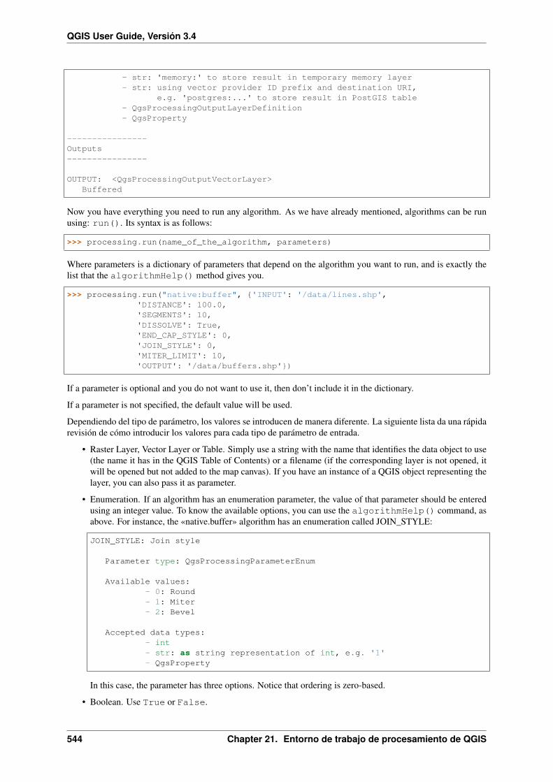
QGIS User Guide, Versión 3.4
- str: 'memory:' to store result in temporary memory layer- str: using vector provider ID prefix and destination URI,
e.g. 'postgres:...' to store result in PostGIS table- QgsProcessingOutputLayerDefinition- QgsProperty
----------------Outputs----------------
OUTPUT: <QgsProcessingOutputVectorLayer>Buffered
Now you have everything you need to run any algorithm. As we have already mentioned, algorithms can be runusing: run(). Its syntax is as follows:
>>> processing.run(name_of_the_algorithm, parameters)
Where parameters is a dictionary of parameters that depend on the algorithm you want to run, and is exactly thelist that the algorithmHelp() method gives you.
>>> processing.run("native:buffer", {'INPUT': '/data/lines.shp','DISTANCE': 100.0,'SEGMENTS': 10,'DISSOLVE': True,'END_CAP_STYLE': 0,'JOIN_STYLE': 0,'MITER_LIMIT': 10,'OUTPUT': '/data/buffers.shp'})
If a parameter is optional and you do not want to use it, then don’t include it in the dictionary.
If a parameter is not specified, the default value will be used.
Dependiendo del tipo de parámetro, los valores se introducen de manera diferente. La siguiente lista da una rápidarevisión de cómo introducir los valores para cada tipo de parámetro de entrada.
• Raster Layer, Vector Layer or Table. Simply use a string with the name that identifies the data object to use(the name it has in the QGIS Table of Contents) or a filename (if the corresponding layer is not opened, itwill be opened but not added to the map canvas). If you have an instance of a QGIS object representing thelayer, you can also pass it as parameter.
• Enumeration. If an algorithm has an enumeration parameter, the value of that parameter should be enteredusing an integer value. To know the available options, you can use the algorithmHelp() command, asabove. For instance, the «native.buffer» algorithm has an enumeration called JOIN_STYLE:
JOIN_STYLE: Join style
Parameter type: QgsProcessingParameterEnum
Available values:- 0: Round- 1: Miter- 2: Bevel
Accepted data types:- int- str: as string representation of int, e.g. '1'- QgsProperty
In this case, the parameter has three options. Notice that ordering is zero-based.
• Boolean. Use True or False.
544 Chapter 21. Entorno de trabajo de procesamiento de QGIS

QGIS User Guide, Versión 3.4
• La entrada múltiple. El valor es una cadena con descriptores de entrada separadas por punto y coma (;).Como en el caso de capas individuales o tablas, cada descriptor de entrada se puede el nombre del objeto dedatos, o su ruta de archivo.
• El campo de la tabla de XXX. Utilice una cadena con el nombre del campo a usar. Este parámetro essensible a mayúsculas y minúsculas.
• Tabla fija. Escribir la lista de todas las tablas de valores separadas por comas (,) y cerrar entre comillas("). Los valores que empiezan en la fila superior y van de izquierda a derecha. También se puede utilizarun arreglo 2-D de valores que representen la tabla.
• SRC. Introduzca el número del código EPSG del SRC deseado.
• Extensión. Se debe utilizar una cadena con valores de xmin, xmax, ymin y ymax` separados porcomas (,‘‘).
Los parámetros boolean, archivo, cadena y numéricos no necesitan alguna explicación adicional.
Input parameters such as strings, booleans, or numerical values have default values. The default value is used ifthe corresponding parameter entry is missing.
For output data objects, type the file path to be used to save it, just as it is done from the toolbox. If the outputobject is not specified, the result is saved to a temporary file (or skipped if it is an optional output). The extensionof the file determines the file format. If you enter a file extension not supported by the algorithm, the default fileformat for that output type will be used, and its corresponding extension appended to the given file path.
Unlike when an algorithm is executed from the toolbox, outputs are not added to the map canvas if you executethat same algorithm from the Python console using run(), but runAndLoadResults() will do that.
The runmethod returns a dictionary with one or more output names (the ones shown in the algorithm description)as keys and the file paths of those outputs as values:
>>> myresult = processing.run("native:buffer", {'INPUT': '/data/lines.shp','DISTANCE': 100.0,'SEGMENTS': 10,'DISSOLVE': True,'END_CAP_STYLE': 0,'JOIN_STYLE': 0,'MITER_LIMIT': 10,'OUTPUT': '/data/buffers.shp'})
>>> myresult['OUTPUT']/data/buffers.shp
You can load feature output by passing the corresponding file paths to the load() method. Or you could userunAndLoadResults() instead of run() to load them immediately.
21.7.2 Crear scripts y ejecurarlos desde le Caja de Herramientas
You can create your own algorithms by writing Python code. Processing scripts extendQgsProcessingAlgorithm, so you need to add some extra lines of code to implement mandatoryfunctions. You can find Create new script (clean sheet) and Create New Script from Template (template thatincludes code for mandatory functions of QgsProcessingAlgorithm) under the Scripts dropdown menu onthe top of the Processing toolbox. The Processing Script Editor will open, and that’s where you should type yourcode. Saving the script from there in the scripts folder (the default folder when you open the save file dialog)with a .py extension should create the corresponding algorithm.
The name of the algorithm (the one you will see in the toolbox) is defined within the code.
Let’s have a look at the following code, which defines a Processing algorithm that performs a buffer operationwith a user defined buffer distance on a vector layer that is specified by the user, after first smoothing the layer.
from qgis.core import (QgsProcessingAlgorithm,QgsProcessingParameterNumber,QgsProcessingParameterFeatureSource,
21.7. Utilizar algoritmos de procesamiento desde la consola 545

QGIS User Guide, Versión 3.4
QgsProcessingParameterFeatureSink)
import processing
class algTest(QgsProcessingAlgorithm):INPUT_BUFFERDIST = 'BUFFERDIST'OUTPUT_BUFFER = 'OUTPUT_BUFFER'INPUT_VECTOR = 'INPUT_VECTOR'
def __init__(self):super().__init__()
def name(self):return "algTest"
def displayName(self):return "algTest script"
def createInstance(self):return type(self)()
def initAlgorithm(self, config=None):self.addParameter(QgsProcessingParameterFeatureSource(
self.INPUT_VECTOR, "Input vector"))self.addParameter(QgsProcessingParameterNumber(
self.INPUT_BUFFERDIST, "Buffer distance",QgsProcessingParameterNumber.Double,100.0))
self.addParameter(QgsProcessingParameterFeatureSink(self.OUTPUT_BUFFER, "Output buffer"))
def processAlgorithm(self, parameters, context, feedback):#DO SOMETHINGalgresult = processing.run("native:smoothgeometry",
{'INPUT': parameters[self.INPUT_VECTOR],'ITERATIONS':2,'OFFSET':0.25,'MAX_ANGLE':180,'OUTPUT': 'memory:'},
context=context, feedback=feedback, is_child_algorithm=True)smoothed = algresult['OUTPUT']algresult = processing.run('native:buffer',
{'INPUT': smoothed,'DISTANCE': parameters[self.INPUT_BUFFERDIST],'SEGMENTS': 5,'END_CAP_STYLE': 0,'JOIN_STYLE': 0,'MITER_LIMIT': 10,'DISSOLVE': True,'OUTPUT': parameters[self.OUTPUT_BUFFER]},context=context, feedback=feedback, is_child_algorithm=True)
buffered = algresult['OUTPUT']return {self.OUTPUT_BUFFER: buffered}
After doing the necessary imports, the following QgsProcessingAlgorithm functions are specified:
• name: The id of the algorithm (lowercase).
• displayName: A human readable name for the algorithm.
• createInstance: Create a new instance of the algorithm class.
• initAlgorithm: Configure the parameterDefinitions and outputDefinitions.
546 Chapter 21. Entorno de trabajo de procesamiento de QGIS

QGIS User Guide, Versión 3.4
Here you describe the parameters and output of the algorithm. In this case, a feature source for the input, afeature sink for the result and a number for the buffer distance.
• processAlgorithm: Do the work.
Here we first run the smoothgeometry algorithm to smooth the geometry, and then we run the bufferalgorithm on the smoothed output. To be able to run algorithms from within another algorithm we haveto define a dummy function for the onFinish parameter for run. This is the no_post_processfunction. You can see how input and output parameters are used as parameters to the smoothgeometryand buffer algorithms.
There are a number of different parameter types available for input and output. Below is an alphabetically sortedlist:
• QgsProcessingParameterBand
• QgsProcessingParameterBoolean
• QgsProcessingParameterCrs
• QgsProcessingParameterDistance
• QgsProcessingParameterEnum
• QgsProcessingParameterExpression
• QgsProcessingParameterExtent
• QgsProcessingParameterFeatureSink
• QgsProcessingParameterFeatureSource
• QgsProcessingParameterField - A field in the attributes table of a vector layer. The name of thelayer has to be specified.
• QgsProcessingParameterFile
• QgsProcessingParameterFileDestination
• QgsProcessingParameterFolderDestination
• QgsProcessingParameterMapLayer
• QgsProcessingParameterMatrix
• QgsProcessingParameterMultipleLayers
• QgsProcessingParameterNumber
• QgsProcessingParameterPoint
• QgsProcessingParameterRange
• QgsProcessingParameterRasterDestination
• QgsProcessingParameterRasterLayer
• QgsProcessingParameterString
• QgsProcessingParameterVectorDestination
• QgsProcessingParameterVectorLayer
The first parameter to the constructors is the name of the parameter, and the second is the description of theparameter (for the user interface). The rest of the constructor parameters are parameter type specific.
The input can be turned into QGIS classes using the parameterAs functions ofQgsProcessingAlgorithm. For instance to get the number provided for the buffer distance as adouble:
self.parameterAsDouble(parameters, self.INPUT_BUFFERDIST, context)).
21.7. Utilizar algoritmos de procesamiento desde la consola 547

QGIS User Guide, Versión 3.4
The processAlgorithm function should return a dictionary containing values for every output defined by thealgorithm. This allows access to these outputs from other algorithms, including other algorithms contained withinthe same model.
Well behaved algorithms should define and return as many outputs as makes sense. Non-feature outputs, such asnumbers and strings, are very useful when running your algorithm as part of a larger model, as these values can beused as input parameters for subsequent algorithms within the model. Consider adding numeric outputs for thingslike the number of features processed, the number of invalid features encountered, the number of features output,etc. The more outputs you return, the more useful your algorithm becomes!
Feedback
The feedback object passed to processAlgorithm should be used for user feedback / interaction. You canuse the setProgress function of the feedback object to update the progress bar (0 to 100) to inform the userabout the progress of the algorithm. This is very useful if your algorithm takes a long time to complete.
The feedback object provides an isCanceled method that should be monitored to enable cancelation of thealgorithm by the user. The pushInfo method of feedback can be used to send information to the user, andreportError is handy for pushing non-fatal errors to users.
Algorithms should avoid using other forms of providing feedback to users, such as print statements or loggingto QgsMessageLog, and should always use the feedback object instead. This allows verbose logging for thealgorithm, and is also thread-safe (which is important, given that algorithms are typically run in a backgroundthread).
Handling errors
If your algorithm encounters an error which prevents it from executing, such as invalid input values or some othercondition from which it cannot or should not recover, then you should raise a QgsProcessingException.E.g.:
if feature['value'] < 20:raise QgsProcessingException('Invalid input value {}, must be >= 20'.
→˓format(feature['value']))
Try to avoid raising QgsProcessingException for non-fatal errors (e.g. when a feature has a null geometry),and instead just report these errors via feedback.reportError() and skip the feature. This helps makeyour algorithm «model-friendly», as it avoids halting the execution of an entire algorithm when a non-fatal erroris encountered.
Documentación de las secuencias de comandos
As in the case of models, you can create additional documentation for your scripts, to explain what they do andhow to use them.
QgsProcessingAlgorithm provides the helpString, shortHelpString and helpUrl functions forthat purpose. Specify / override these to provide more help to the user.
shortDescription is used in the tooltip when hovering over the algorithm in the toolbox.
21.7.3 Pre y post-ejecución de la secuencia de comandos hooks
Scripts can also be used as pre- and post-execution hooks that are run before and after an algorithm is run, respec-tively. This can be used to automate tasks that should be performed whenever an algorithm is executed.
La sintaxis es idéntica a la que se ha explicado anteriormente, pero una variable global adicional llamada alg estádisponible, lo que representa el algoritmo que acaba de ser (o está a punto de ser) ejecutado.
548 Chapter 21. Entorno de trabajo de procesamiento de QGIS

QGIS User Guide, Versión 3.4
In the General group of the processing options dialog, you will find two entries named Pre-execution script andPost-execution script where the filenames of the scripts to be run in each case can be entered.
21.8 Writing new Processing algorithms as Python scripts
In QGIS 3.4, the only way to write Processing algorithms using Python is to extend theQgsProcessingAlgorithm class.
Within QGIS, you can use Create new script in the Scripts menu at the top of the Processing Toolbox to openthe Processing Script Editor where you can write your code. To simplify the task, you can start with a scripttemplate by using Create new script from template from the same menu. This opens a template that extendsQgsProcessingAlgorithm.
If you save the script in the scripts folder (the default location) with a .py extension, the algorithm willbecome available in the Processing Toolbox.
21.8.1 Extending QgsProcessingAlgorithm
The following code
1. takes a vector layer as input
2. counts the number of features
3. does a buffer operation
4. creates a raster layer from the result of the buffer operation
5. returns the buffer layer, raster layer and number of features
from qgis.PyQt.QtCore import QCoreApplicationfrom qgis.core import (QgsProcessing,
QgsProcessingAlgorithm,QgsProcessingException,QgsProcessingOutputNumber,QgsProcessingParameterDistance,QgsProcessingParameterFeatureSource,QgsProcessingParameterVectorDestination,QgsProcessingParameterRasterDestination)
import processing
class ExampleProcessingAlgorithm(QgsProcessingAlgorithm):"""This is an example algorithm that takes a vector layer,creates some new layers and returns some results."""
def tr(self, string):"""Returns a translatable string with the self.tr() function."""return QCoreApplication.translate('Processing', string)
def createInstance(self):# Must return a new copy of your algorithm.return ExampleProcessingAlgorithm()
def name(self):"""Returns the unique algorithm name."""
21.8. Writing new Processing algorithms as Python scripts 549

QGIS User Guide, Versión 3.4
return 'bufferrasterextend'
def displayName(self):"""Returns the translated algorithm name."""return self.tr('Buffer and export to raster (extend)')
def group(self):"""Returns the name of the group this algorithm belongs to."""return self.tr('Example scripts')
def groupId(self):"""Returns the unique ID of the group this algorithm belongsto."""return 'examplescripts'
def shortHelpString(self):"""Returns a localised short help string for the algorithm."""return self.tr('Example algorithm short description')
def initAlgorithm(self, config=None):"""Here we define the inputs and outputs of the algorithm."""# 'INPUT' is the recommended name for the main input# parameter.self.addParameter(
QgsProcessingParameterFeatureSource('INPUT',self.tr('Input vector layer'),types=[QgsProcessing.TypeVectorAnyGeometry]
))self.addParameter(
QgsProcessingParameterVectorDestination('BUFFER_OUTPUT',self.tr('Buffer output'),
))# 'OUTPUT' is the recommended name for the main output# parameter.self.addParameter(
QgsProcessingParameterRasterDestination('OUTPUT',self.tr('Raster output')
))self.addParameter(
QgsProcessingParameterDistance('BUFFERDIST',self.tr('BUFFERDIST'),defaultValue = 1.0,# Make distance units match the INPUT layer units:parentParameterName='INPUT'
))
550 Chapter 21. Entorno de trabajo de procesamiento de QGIS

QGIS User Guide, Versión 3.4
self.addParameter(QgsProcessingParameterDistance(
'CELLSIZE',self.tr('CELLSIZE'),defaultValue = 10.0,parentParameterName='INPUT'
))self.addOutput(
QgsProcessingOutputNumber('NUMBEROFFEATURES',self.tr('Number of features processed')
))
def processAlgorithm(self, parameters, context, feedback):"""Here is where the processing itself takes place."""# First, we get the count of features from the INPUT layer.# This layer is defined as a QgsProcessingParameterFeatureSource# parameter, so it is retrieved by calling# self.parameterAsSource.input_featuresource = self.parameterAsSource(parameters,
'INPUT',context)
numfeatures = input_featuresource.featureCount()
# Retrieve the buffer distance and raster cell size numeric# values. Since these are numeric values, they are retrieved# using self.parameterAsDouble.bufferdist = self.parameterAsDouble(parameters, 'BUFFERDIST',
context)rastercellsize = self.parameterAsDouble(parameters, 'CELLSIZE',
context)if feedback.isCanceled():
return {}buffer_result = processing.run(
'native:buffer',{
# Here we pass on the original parameter values of INPUT# and BUFFER_OUTPUT to the buffer algorithm.'INPUT': parameters['INPUT'],'OUTPUT': parameters['BUFFER_OUTPUT'],'DISTANCE': bufferdist,'SEGMENTS': 10,'DISSOLVE': True,'END_CAP_STYLE': 0,'JOIN_STYLE': 0,'MITER_LIMIT': 10
},# Because the buffer algorithm is being run as a step in# another larger algorithm, the is_child_algorithm option# should be set to Trueis_child_algorithm=True,## It's important to pass on the context and feedback objects to# child algorithms, so that they can properly give feedback to# users and handle cancelation requests.context=context,feedback=feedback)
# Check for cancelation
21.8. Writing new Processing algorithms as Python scripts 551

QGIS User Guide, Versión 3.4
if feedback.isCanceled():return {}
# Run the separate rasterization algorithm using the buffer result# as an input.rasterized_result = processing.run(
'qgis:rasterize',{
# Here we pass the 'OUTPUT' value from the buffer's result# dictionary off to the rasterize child algorithm.'LAYER': buffer_result['OUTPUT'],'EXTENT': buffer_result['OUTPUT'],'MAP_UNITS_PER_PIXEL': rastercellsize,# Use the original parameter value.'OUTPUT': parameters['OUTPUT']
},is_child_algorithm=True,context=context,feedback=feedback)
if feedback.isCanceled():return {}
# Return the resultsreturn {'OUTPUT': rasterized_result['OUTPUT'],
'BUFFER_OUTPUT': buffer_result['OUTPUT'],'NUMBEROFFEATURES': numfeatures}
Processing algorithm standard functions:
• createInstance (mandatory) Must return a new copy of your algorithm. If you change the name of theclass, make sure you also update the value returned here to match!
• name (mandatory) Returns the unique algorithm name, used for identifying the algorithm.
• displayName (mandatory) Returns the translated algorithm name.
• group Returns the name of the group this algorithm belongs to.
• groupId Returns the unique ID of the group this algorithm belongs to.
• shortHelpString Returns a localised short help string for the algorithm.
• initAlgorithm (mandatory) Here we define the inputs and outputs of the algorithm.
INPUT and OUTPUT are recommended names for the main input and main output parameters, respec-tively.
If a parameter depends on another parameter, parentParameterName is used to specify this rela-tionship (could be the field / band of a layer or the distance units of a layer).
• processAlgorithm (mandatory) This is where the processing takes place.
Parameters are retrieved using special purpose functions, for instance parameterAsSource andparameterAsDouble.
processing.run can be used to run other processing algorithms from a processing algorithm. Thefirst parameter is the name of the algorithm, the second is a dictionary of the parameters to the algo-rithm. is_child_algorithm is normally set to True when running an algorithm from withinanother algorithm. context and feedback inform the algorithm about the environment to run inand the channel for communicating with the user (catching cancel request, reporting progress, pro-viding textual feedback). When using the (parent) algorithm’s parameters as parameters to «child»algorithms, the original parameter values should be used (e.g. parameters['OUTPUT']).
It is good practice to check the feedback object for cancelation as much as is sensibly possible! Doingso allows for responsive cancelation, instead of forcing users to wait for unwanted processing to occur.
552 Chapter 21. Entorno de trabajo de procesamiento de QGIS

QGIS User Guide, Versión 3.4
The algorithm should return values for all the output parameters it has defined as a dictionary. In thiscase, that’s the buffer and rasterized output layers, and the count of features processed. The dictionarykeys must match the original parameter/output names.
21.8.2 Input and output types for Processing Algorithms
Here is the list of input and output types that are supported in Processing with their corresponding alg decoratorconstants (algfactory.py contains the complete list of alg constants). Sorted on class name.
Table 21.1: Input typesClass DescriptionQgsProcessingParameterBand A band of a raster layerQgsProcessingParameterBoolean A boolean valueQgsProcessingParameterCrs A Coordinate Reference
SystemQgsProcessingParameterDistance A double numeric parame-
ter for distance valuesQgsProcessingParameterEnum An enumeration, allowing
for selection from a set ofpredefined values
QgsProcessingParameterExpression An expressionQgsProcessingParameterExtent A spatial extent defined by
xmin, xmax, ymin, ymaxQgsProcessingParameterFeatureSink A feature sinkQgsProcessingParameterFeatureSource A feature sourceQgsProcessingParameterField A field in the attribute table
of a vector layerQgsProcessingParameterFile A filename of an existing
fileQgsProcessingParameterFileDestination A filename for a newly cre-
ated output fileQgsProcessingParameterFolderDestination A folderQgsProcessingParameterMapLayer A map layerQgsProcessingParameterMatrix A matrixQgsProcessingParameterMultipleLayers A set of layersQgsProcessingParameterNumber A numerical valueQgsProcessingParameterPoint A pointQgsProcessingParameterRange A number rangeQgsProcessingParameterRasterLayer A raster layerQgsProcessingParameterRasterDestination A raster layerQgsProcessingParameterString A text stringQgsProcessingParameterVectorLayer A vector layerQgsProcessingParameterVectorDestination A vector layer
21.8. Writing new Processing algorithms as Python scripts 553

QGIS User Guide, Versión 3.4
Table 21.2: Output typesClass DescriptionQgsProcessingOutputFile A filename of an existing fileQgsProcessingOutputFolder A folderQgsProcessingOutputHtml HTMLQgsProcessingOutputLayerDefinition A layer definitionQgsProcessingOutputMapLayer A map layerQgsProcessingOutputMultipleLayers A set of layersQgsProcessingOutputNumber A numerical valueQgsProcessingOutputRasterLayer A raster layerQgsProcessingOutputString A text stringQgsProcessingOutputVectorLayer A vector layer
21.8.3 Handing algorithm output
When you declare an output representing a layer (raster or vector), the algorithm will try to add it to QGIS once itis finished.
• Raster layer output: QgsProcessingParameterRasterDestination.
• Vector layer output: QgsProcessingParameterVectorDestination.
So even if the processing.run() method does not add the layers it creates into the user’s current project, thetwo output layers (buffer and raster buffer) will be loaded, since they are saved to the destinations entered by theuser (or to temporary destinations if the user does not specify a destination).
If a layer is created as output of an algorithm, it should be declared as such. Otherwise, you will not be able toproperly use the algorithm in the modeler, since what is declared will not match what the algorithm really creates.
You can return strings, numbers and more by specifying them in the result dictionary (as demonstrated for «NUM-BEROFFEATURES»), but they should always be explicitly defined as outputs from your algorithm. We encouragealgorithms to output as many useful values as possible, since these can be valuable for use in later algorithms whenyour algorithm is used as part of a model.
21.8.4 La comunicación con el usuario
If your algorithm takes a long time to process, it is a good idea to inform the user about the progress. You can usefeedback (QgsProcessingFeedback) for this.
The progress text and progressbar can be updated using two methods: setProgressText(text) andsetProgress(percent).
You can provide more information to the user using pushCommandInfo(text), pushDebugInfo(text),pushInfo(text) and reportError(text).
If your script has a problem, the correct way of handling it is to raise a QgsProcessingException. Youcan pass a message as an argument to the constructor of the exception. Processing will take care of handling itand communicating with the user, depending on where the algorithm is being executed from (toolbox, modeler,Python console, . . . )
21.8.5 Documentando sus scripts
You can document your scripts by overloading the helpString() and helpUrl() methods ofQgsProcessingAlgorithm.
554 Chapter 21. Entorno de trabajo de procesamiento de QGIS

QGIS User Guide, Versión 3.4
21.8.6 Flags
You can override the flags method of QgsProcessingAlgorithm to tell QGIS more about your algorithm.You can for instance tell QGIS that the script shall be hidden from the modeler, that it can be canceled, that it isnot thread safe, and more.
Truco: By default, Processing runs algorithms in a separate thread in order to keep QGIS responsive while theprocessing task runs. If your algorithm is regularly crashing, you are probably using API calls which are notsafe to do in a background thread. Try returning the QgsProcessingAlgorithm.FlagNoThreading flag from youralgorithm’s flags() method to force Processing to run your algorithm in the main thread instead.
21.8.7 Las mejores practivas al escribir scripts de algoritmos
Here’s a quick summary of ideas to consider when creating your script algorithms and, especially, if you wantto share them with other QGIS users. Following these simple rules will ensure consistency across the differentProcessing elements such as the toolbox, the modeler or the batch processing interface.
• No cargar la capa resultante. Deje al Procesamiento manejar sus resultados y cargue sus capas si es nece-sario.
• Always declare the outputs your algorithm creates.
• Do not show message boxes or use any GUI element from the script. If you want to communi-cate with the user, use the methods of the feedback object (QgsProcessingFeedback) or throw aQgsProcessingException.
There are already many processing algorithms available in QGIS. You can find code on https://github.com/qgis/QGIS/blob/release-3_4/python/plugins/processing/algs/qgis.
21.9 Configurar aplicaciones externas
The processing framework can be extended using additional applications. Currently, SAGA, GRASS, R, TauDEMand LAStools are supported (and GDAL is shipped with QGIS). Algorithms that rely on external applications aremanaged by their own algorithm providers. Additional providers can be found as separate plugins, and installedusing the QGIS Plugin Manager.
This section will show you how to configure the Processing framework to include these additional applications,and it will explain some particular features of the algorithms based on them. Once you have correctly configuredthe system, you will be able to execute external algorithms from any component like the toolbox or the graphicalmodeler, just like you do with any other algorithm.
By default, algorithms that rely on an external application not shipped with QGIS are not enabled. You can enablethem in the Processing settings dialog if they are installed on your system.
21.9.1 Aclaración para los usuarios de Windows
If you are not an advanced user and you are running QGIS on Windows, you might not be interested in readingthe rest of this chapter. Make sure you install QGIS in your system using the standalone installer. That willautomatically install SAGA and GRASS in your system and configure them so they can be run from QGIS. Allthe algorithms from these providers will be ready to be run without needing any further configuration. If installingwith the OSGeo4W application, make sure that you also select SAGA and GRASS for installation.
21.9. Configurar aplicaciones externas 555

QGIS User Guide, Versión 3.4
21.9.2 Aclaración respecto a los formatos de archivos
When using external software, opening a file in QGIS does not mean that it can be opened and processed in thatother software. In most cases, other software can read what you have opened in QGIS, but in some cases, thatmight not be true. When using databases or uncommon file formats, whether for raster or vector layers, problemsmight arise. If that happens, try to use well-known file formats that you are sure are understood by both programs,and check the console output (in the log panel) to find out what is going wrong.
You might for instance get trouble and not be able to complete your work if you call an external algorithm with aGRASS raster layers as input. For this reason, such layers will not appear as available to algorithms.
You should, however, not have problems with vector layers, since QGIS automatically converts from the originalfile format to one accepted by the external application before passing the layer to it. This adds extra processingtime, which might be significant for large layers, so do not be surprised if it takes more time to process a layerfrom a DB connection than a layer from a Shapefile format dataset of similar size.
Providers not using external applications can process any layer that you can open in QGIS, since they open it foranalysis through QGIS.
All raster and vector output formats produced by QGIS can be used as input layers. Some providers do not supportcertain formats, but all can export to common formats that can later be transformed by QGIS automatically. Asfor input layers, if a conversion is needed, that might increase the processing time.
21.9.3 Nota referente a las seleccion de capas vectoriales
Las aplicaciones externas pueden también ser conscientes de las selecciones que existen en capas vectoriales den-tro |qg|. Sin embargo, eso requiere reescribir todas las capas vectoriales de entrada, al igual que si originalmenteestuvieran en un formato no compatible con la aplicación externa. Sólo cuando no existe ninguna selección o laopción *Utilizar sólo objetos espaciales seleccionados * no está activada en la configuración general de proce-samiento, puede una capa ser directamente pasada a una aplicación externa.
In other cases, exporting only selected features is needed, which causes longer execution times.
21.9.4 SAGA
SAGA algorithms can be run from QGIS if you have SAGA installed and you configure the processing frameworkto find SAGA executables. In particular, the SAGA command-line executable is needed to run SAGA algorithms.
If you are running Windows, both the stand-alone installer and the OSGeo4W installer include SAGA along withQGIS, and the path is automatically configured, so there is no need to do anything else.
If you have installed SAGA yourself and your QGIS installer did not include it, the path to the SAGA executablemust be configured. To do this, open the configuration dialog. In the SAGA block, you will find a setting namedSAGA Folder. Enter the path to the folder where SAGA is installed. Close the configuration dialog, and now youare ready to run SAGA algorithms from QGIS.
If you are running Linux, SAGA binaries are not included with Processing, so you have to download and installthe software yourself. Please check the SAGA website for more information.
En este caso, no hay necesidad de configurar la ruta al ejecutable de SAGA, y no se verán esas carpetas. En sulugar, debe asegurarse de que SAGA está correctamente instalado y se añade su carpeta a la variable de entornoPATH. Sólo tiene que abrir una consola y escribir saga_cmd para comprobar que el sistema puede encontrardonde se encuentran los archivos binarios de SAGA.
Sobre las limitaciones del sistema de cuadrícula de SAGA
Most SAGA algorithms that require several input raster layers require them to have the same grid system. That is,they must cover the same geographic area and have the same cell size, so their corresponding grids match. Whencalling SAGA algorithms from QGIS, you can use any layer, regardless of its cell size and extent. When multiple
556 Chapter 21. Entorno de trabajo de procesamiento de QGIS
QGIS User Guide, Versión 3.4
raster layers are used as input for a SAGA algorithm, QGIS resamples them to a common grid system and thenpasses them to SAGA (unless the SAGA algorithm can operate with layers from different grid systems).
La definición de este sistema de cuadrícula común es controlado por el usuario, y se encontrará varios parámetrosen el grupo SAGA de la ventana de configuración para hacerlo. Hay dos formas de establecer el sistema decuadrícula de destino.
• Establecerlo manualmente. se define la extensión estableciendo los valores de los siguientes parámetros:
– Resampling min X
– Resampling max X
– Resampling min Y
– Resampling max Y
– Resampling cellsize
Notice that QGIS will resample input layers to that extent, even if they do not overlap with it.
• Ajuste de forma automática a partir de capas de entrada. Para seleccionar esta opción, simplemente marquela opción Utilizar el sistema de cuadrícula mínima para remuestreo. Todos los demás ajustes se ignoran yla medida mínima que cubre todas las capas de entrada que se utilizarán. El tamaño de celda de la capa dedestino es el máximo de todos los tamaños celulares de las capas de entrada.
Para los algoritmos que no utilizan múltiples capas raster, o para aquellos que no necesitan un único sistema decuadrícula de entrada, no se realizará un remuestreo antes de invocar SAG y dichos parámetros no son utilizados.
Limitaciones para las capas multibanda
A diferencia de QGIS, SAGA no tiene soporte para capas multibanda. Si desea utilizar una capa multibanda (comoun RGB o imagen multiespectral), primero hay que dividirlo en imágenes de un sola banda. Para ello, se puedeutilizar el algoritmo “imagen SAGA/Grid - Herramientas/Dividir” (que crea tres imágenes de una imagen RGB)o el algoritmo “banda SAGA/Grid - Herramientas / Extracto” (para extraer una sola banda).
Limitaciones en el tamaño de celda
SAGA asume que las capas ráster tienen el mismo tamaño de celda en el eje X y Y. Si se está trabajando conuna capa con diferentes valores para el tamaño de celda horizontal y vertical, es posible que obtenga resultadosinesperados. En este caso, se añadirá una advertencia al registro de procesamiento, lo que indica que una capa deentrada podría no ser adecuada para ser procesada por SAGA.
Registro
Cuando QGIS llama a SAGA, lo hace utilizando su interfaz de linea de comandos, pasando así de un conjunto decomandos para realizar todas las operaciones necesarias. SAGA muestra su progreso al escribir información a laconsola, que incluye el porcentaje de procesamiento ya realizado junto con el contenido adicional. Esta salida sefiltra y utiliza para actualizar la barra de proceso mientras el algoritmo se ejecuta.
Both the commands sent by QGIS and the additional information printed by SAGA can be logged along withother processing log messages, and you might find them useful to track what is going on when QGIS runs aSAGA algorithm. You will find two settings, namely Log console output and Log execution commands, to activatethat logging mechanism.
Most other providers that use external applications and call them through the command-line have similar options,so you will find them as well in other places in the processing settings list.
21.9. Configurar aplicaciones externas 557
QGIS User Guide, Versión 3.4
21.9.5 R scripts
To enable R in Processing you need to install the Processing R Provider plugin and configure R for QGIS.
Configuration is done in Provider-> R in the Processing tab of Settings-> Options.
Depending on your operating system, you may have to use R folder to specify where your R binaries are located.
Nota: On Windows the R executable file is normally in a folder (R-<version>) under C:\ProgramFiles\R\. Specify the folder and NOT the binary!
On Linux you just have to make sure that the R folder is in the PATH environment variable. If R in a terminalwindow starts R, then you are ready to go.
After installing the Processing R Provider plugin, you will find some example scripts in the Processing Toolbox:
• Scatterplot runs an R function that produces a scatter plot from two numerical fields of the provided vectorlayer.
• test_sf does some operations that depend on the sf package and can be used to check if the R packagesf is installed. If the package is not installed, R will try to install it (and all the packages it depends on)for you, using the Package repository specified in Provider-> R in the Processing options. The default ishttp://cran.at.r-project.org/. Installing may take some time. . .
• test_sp can be used to check if the R package sp is installed. If the package is not installed, R will try toinstall it for you.
If you have R configured correctly for QGIS, you should be able to run these scripts.
Adding R scripts from the QGIS collection
R integration in QGIS is different from that of SAGA in that there is not a predefined set of algorithms you canrun (except for some example script that come with the Processing R Provider plugin).
A set of example R scripts is available in the QGIS Repository. Perform the following steps to load and enablethem using the QGIS Resource Sharing plugin.
1. Add the QGIS Resource Sharing plugin (you may have to enable Show also experimental plugins in thePlugin Manager Settings)
2. Open it (Plugins-> Resource Sharing-> Resource Sharing)
3. Choose the Settings tab
4. Click Reload repositories
5. Choose the All tab
6. Select QGIS R script collection in the list and click on the Install button
7. The collection should now be listed in the Installed tab
8. Close the plugin
9. Open the Processing Toolbox, and if everything is OK, the example scripts will be present under R, invarious groups (only some of the groups are expanded in the screenshot below).
The scripts at the top are the example scripts from the Processing R Provider plugin.
10. If, for some reason, the scripts are not available in the Processing Toolbox, you can try to:
(a) Open the Processing settings (Settings-> Options-> Processing tab)
(b) Go to Providers-> R-> R scripts folder
• On Ubuntu, set the path to (or, better, include in the path):
558 Chapter 21. Entorno de trabajo de procesamiento de QGIS

QGIS User Guide, Versión 3.4
21.9. Configurar aplicaciones externas 559

QGIS User Guide, Versión 3.4
Figure 21.33: The Processing Toolbox with some R scripts shown
560 Chapter 21. Entorno de trabajo de procesamiento de QGIS

QGIS User Guide, Versión 3.4
/home/<user>/.local/share/QGIS/QGIS3/profiles/default/resource_sharing/repositories/github.com/qgis/QGIS-Resources/collections/rscripts
• On Windows, set the path to (or, better, include in the path):
C:Users<user>AppDataRoamingQGISQGIS3profilesdefaultresource_sharingrepositoriesgithub.comqgisQGIS-Resourcescollectionsrscripts
To edit, double-click. You can then choose to just paste / type the path, or you can navigate to thedirectory by using the . . . button and press the Add button in the dialog that opens. It is possible toprovide several directories here. They will be separated by a semicolon («;»).
If you would like to get all the R scrips from the QGIS 2 on-line collection, you can select QGIS R script collection(from QGIS 2) instead of QGIS R script collection. You will find probably find that scripts that depend on vectordata input or output will not work.
Creating R scripts
You can write scripts and call R commands, as you would do from R. This section shows you the syntax for usingR commands in QGIS, and how to use QGIS objects (layers, tables) in them.
To add an algorithm that calls an R function (or a more complex R script that you have developed and you wouldlike to have available from QGIS), you have to create a script file that performs the R commands.
R script files have the extension .rsx, and creating them is pretty easy if you just have a basic knowledge of Rsyntax and R scripting. They should be stored in the R scripts folder. You can specify the folder (R scripts folder)in the R settings group in Processing settings dialog).
Let’s have a look at a very simple script file, which calls the R method spsample to create a random grid withinthe boundary of the polygons in a given polygon layer. This method belongs to the maptools package. Sincealmost all the algorithms that you might like to incorporate into QGIS will use or generate spatial data, knowledgeof spatial packages like maptools and sp/sf, is necessary.
##polyg=vector##numpoints=number 10##output=output vector##sp=grouppts=spsample(polyg,numpoints,type="random")output=SpatialPointsDataFrame(pts, as.data.frame(pts))
21.9. Configurar aplicaciones externas 561

QGIS User Guide, Versión 3.4
The first lines, which start with a double Python comment sign (##), tell QGIS about the inputs of the algorithmin the file and the outputs that it will generate.
Nota: To find out more about how to write your own R scripts, have a look at the R Intro and the R SyntaxTraining Manual Chapters.
When you declare an input parameter, QGIS uses that information for two things: creating the user interface toask the user for the value of that parameter, and creating a corresponding R variable that can later be used as Rfunction input.
In the above example, we have declared an input of type vector, named polyg. When executing the algorithm,QGIS will open the layer selected by the user and store it in a variable named polyg. So, the name of a parameteris the name of the variable that we can use in R for accessing the value of that parameter (you should thereforeavoid using reserved R words as parameter names).
Spatial parameters such as vector and raster layers are read using the readOGR() and brick() commands (youdo not have to worry about adding those commands to your description file – QGIS will do it), and they are storedas Spatial*DataFrame objects. Table fields are stored as strings containing the name of the selected field.
Las tablas se abren con el comando read.csv(). Sin una tabla introducida por el usuario no esta en formatoCSV, será convertirá antes de importarlo en R.
Raster files can be read using the readGDAL() command instead of brick() by specifying##usereadgdal.
If you are an advanced user and do not want QGIS to create the object representing the layer, you can use##passfilenames to indicate that you prefer a string with the filename instead. In this case, it is up toyou to open the file before performing any operation on the data it contains.
With the above information, we can now understand the first line of this script (the first line not starting with aPython comment).
pts=spsample(polyg,numpoints,type="random")
The variable polyg already contains a SpatialPolygonsDataFrame object, so it can be used when callingthe spsample method, just like the numpoints one, which specifies the number of points to add to the createdsample grid.
Since we have declared a vector output named out, we have to create a variable named out and store aSpatial*DataFrame object in it (in this case, a SpatialPointsDataFrame). You can use any namefor your intermediate variables. Just make sure that the variable storing your final result has the same name thatyou used to declare it, and that it contains a suitable value.
In this case, the result obtained from the spsample method has to be converted explicitly into aSpatialPointsDataFrame object, since it is itself an object of class ppp, which can not be returned toQGIS.
If your algorithm generates raster layers, the way they are saved will depend on whether or not you have used the##dontuserasterpackage option. If you have used it, layers are saved using the writeGDAL() method.If not, the writeRaster() method from the raster package will be used.
If you have used the ##passfilenames option, outputs are generated using the raster package (withwriteRaster()).
If your algorithm does not generate a layer, but a text result in the console instead, you have to indicate that youwant the console to be shown once the execution is finished. To do so, just start the command lines that producethe results you want to print with the > (“greater”) sign. The output of all other lines will not be shown. Forinstance, here is the description file of an algorithm that performs a normality test on a given field (column) of theattributes of a vector layer:
##layer=vector##field=field layer##nortest=group
562 Chapter 21. Entorno de trabajo de procesamiento de QGIS

QGIS User Guide, Versión 3.4
library(nortest)>lillie.test(layer[[field]])
La salida de la última línea se imprime, pero la salida de la primera no (y tampoco están las salida de otras líneasde comando agregadas automáticamente por QGIS).
Si su algoritmo crea algún tipo de gráficos (utilizando el método plot()), añada la siguiente línea:
##showplots
Esto provocará que QGIS redireccione todas las salidas de gráficas R a un archivo temporal, que se abrirá una vezque terminé la ejecución de R.
Tanto los resultados gráficos como de consola, se mostrará en el gesto de resultados de procesamiento.
For more information, please check the script files provided with Processing. Most of them are rather simple andwill greatly help you understand how to create your own scripts.
Nota: The rgdal and raster libraries are loaded by default, so you do not have to add the correspond-ing library() commands (you just have to make sure that those two packages are installed in your R dis-tribution). However, other additional libraries that you might need have to be explicitly loaded by typing:library(ggplot2) (to load the ggplot2 library). If the package is not already installed on your machine,Processing will download and install it. In this way the package will be also available in R Standalone. Be awarethat if the package has to be downloaded, the first time you run the script it might take a long time.
21.9.6 R libraries
The R script sp_test tries to load the R packages sp and raster.
R libraries installed when running sf_test
The R script sf_test tries to load sf and raster. If these two packages are not installed, R may try to load andinstall them.
The following R libraries end up in ~/.local/share/QGIS/QGIS3/profiles/default/processing/rscripts after sf_test has been run from the Processing Toolbox on Ubuntu withversion 2.0 of the Processing R Provider plugin and R 3.4.4 (apt package r-base-core only):
abind, askpass, assertthat, backports, base64enc, BH, bit, bit64, blob,brew, callr, classInt, cli, colorspace, covr, crayon, crosstalk, curl,DBI, deldir, desc, dichromat, digest, dplyr, e1071, ellipsis, evaluate,fansi, farver, fastmap, gdtools, ggplot2, glue, goftest, gridExtra,gtable, highr, hms, htmltools, htmlwidgets, httpuv, httr, jsonlite, knitr,labeling, later, lazyeval, leafem, leaflet, leaflet.providers, leafpop,leafsync, lifecycle, lwgeom, magrittr, maps, mapview, markdown, memoise,microbenchmark, mime, munsell, odbc, openssl, pillar, pkgbuild, pkgconfig,pkgload, plogr, plyr, png, polyclip, praise, prettyunits, processx,promises, ps, purrr, R6, raster, RColorBrewer, Rcpp, reshape2, rex, rgeos,rlang, rmarkdown, RPostgres, RPostgreSQL, rprojroot, RSQLite, rstudioapi,satellite, scales, sf, shiny, sourcetools, sp, spatstat, spatstat.data,spatstat.utils, stars, stringi, stringr, svglite, sys, systemfonts, tensor,testthat, tibble, tidyselect, tinytex, units, utf8, uuid, vctrs, viridis,viridisLite, webshot, withr, xfun, XML, xtable
21.9. Configurar aplicaciones externas 563

QGIS User Guide, Versión 3.4
21.9.7 GRASS
Configuring GRASS is not much different from configuring SAGA. First, the path to the GRASS folder has to bedefined, but only if you are running Windows.
By default, the Processing framework tries to configure its GRASS connector to use the GRASS distribution thatships along with QGIS. This should work without problems for most systems, but if you experience problems, youmight have to configure the GRASS connector manually. Also, if you want to use a different GRASS installation,you can change the setting to point to the folder where the other version is installed. GRASS 7 is needed foralgorithms to work correctly.
If you are running Linux, you just have to make sure that GRASS is correctly installed, and that it can be runwithout problem from a terminal window.
Los algoritmos de GRASS utilizan una región para cálculos. Esta región se puede definir manualmente utilizandovalores similares a los encontrados en la configuración de SAGA, o automáticamente tomara la extensión mínimaque cubre todas las capas de entrada utilizadas para ejecutar el algoritmo cada vez. Si el último enfoque esel comportamiento que prefiere, simplemente marque la opción Utilizar la región de cobertura mínima en losparámetros de configuración de GRASS.
21.9.8 LAStools
To use LAStools in QGIS, you need to download and install LAStools on your computer and install the LAStoolsplugin (available from the official repository) in QGIS.
On Linux platforms, you will need Wine to be able to run some of the tools.
LAStools is activated and configured in the Processing options (Settings → Options, Processing tab, Providers→LAStools), where you can specify the location of LAStools (LAStools folder) and Wine (Wine folder). On Ubuntu,the default Wine folder is /usr/bin.
564 Chapter 21. Entorno de trabajo de procesamiento de QGIS

CHAPTER 22
Complementos
22.1 Complementos de QGIS
QGIS ha sido diseñado con una arquitectura de complementos. Esto permite que sea fácil añadir muchas carac-terísticas y funciones nuevas a la aplicación. Muchas de las características de QGIS están en realidad implemen-tadas como complementos.
22.1.1 Complementos base y externos
QGIS plugins are implemented either as Core Plugins or External Plugins.
Core Plugins are maintained by the QGIS Development Team and are automatically part of every QGIS distribu-tion. They are written in one of two languages: C++ or Python.
Most of External Plugins are currently written in Python. They are stored either in the “Official” QGIS Repos-itory at https://plugins.qgis.org/plugins/ or in external repositories and are maintained by the individual authors.Detailed documentation about the usage, minimum QGIS version, home page, authors,and other important infor-mation are provided for the plugins in the Official repository. For other external repositories, documentation mightbe available with the external plugins themselves. External plugins documentation is not included in this manual.
To install or activate a plugin, go to Plugins menu and select Manage and install plugins. . . . Installed externalpython plugins are placed under the python/plugins folder of the active user profile path.
Paths to Custom C++ plugins libraries can also be added under Settings → Options → System.
Nota: According to the plugin manager settings, QGIS main interface can display an icon on the right of thestatus bar to inform you that there are updates for your installed plugins or new plugins available.
22.1.2 El diálogo de complementos
The tabs in the Plugins dialog allow the user to install, uninstall and upgrade plugins in different ways. Eachplugin has some metadata displayed in the right panel:
• information on whether the plugin is experimental
• descripción
565

QGIS User Guide, Versión 3.4
• rating vote(s) (you can vote for your preferred plugin!)
• etiquetas
• some useful links to the home page, tracker and code repository
• autor(es)
• versión disponible
At the top of the dialog, a Search function helps you find any plugin using metadata information (author, name,
description. . . ). It is available in nearly every tab (except Settings).
The Settings tab
The Settings tab is the main place you can configure which plugins can be displayed in your application. Youcan use the following options:
• Comprobar actualizaciones al inicio. Siempre que un nuevo complemento o actualización de comple-mento esta disponible, QGIS informará “cada vez que se inicia QGIS”, “una vez al día”, “cada 3 días”,“cada semana”, “cada 2 semanas” o “cada mes”.
• Mostrar también los complementos experimentales. QGIS mostrará complementos en etapas tempranasde desarrollo, que son generalmente inadecuados para su uso en producción.
• Show also deprecated plugins. Because they use functions that are no longer available in QGIS, theseplugins are set deprecated and generally unsuitable for production use. They appear among invalid pluginslist.
By default, QGIS provides you with its official plugin repository with the URL https://plugins.qgis.org/plugins/plugins.xml?qgis=3.0 (in case of QGIS 3.0) in the Plugin repositories section. To add external author repositories,click Add. . . and fill in the Repository Details form with a name and the URL. The URL can be of http:// orfile:// protocol type.
The default QGIS repository is an open repository and you don’t need any authentication to access it. You canhowever deploy your own plugin repository and require an authentication (basic authentication, PKI). You can getmore information on QGIS authentication support in Autenticación chapter.
If you do not want one or more of the added repositories, they can be disabled from the Settings tab via the Edit. . .button, or completely removed with the Delete button.
The All tab
In the All tab, all the available plugins are listed, including both core and external plugins. Use UpgradeAll to look for new versions of the plugins. Furthermore, you can use Install Plugin if a plugin is listed butnot installed, Uninstall Plugin as well as Reinstall Plugin if a plugin is installed. An installed plugin can betemporarily de/activated using the checkbox.
The Installed tab
In the Installed tab, you’ll find listed the Core plugins, that you can not uninstall. You can extend this list withexternal plugins that can be uninstalled and reinstalled any time, using the Uninstall Plugin and Reinstall Pluginbuttons. You can Upgrade All the plugins here as well.
566 Chapter 22. Complementos

QGIS User Guide, Versión 3.4
Figure 22.1: The Settings tab
Figure 22.2: The All tab
22.1. Complementos de QGIS 567

QGIS User Guide, Versión 3.4
Figure 22.3: The Installed tab
The Not installed tab
The Not installed tab lists all plugins available that are not installed. You can use the Install Plugin button toimplement a plugin into QGIS.
The Upgradeable and New tabs
The Upgradeable and New tabs are enabled when new plugins are added to the repository or a new version
of an installed plugin is released. If you activated Show also experimental plugins in the Settings menu,those also appear in the list giving you opportunity to early test upcoming tools.
Installation can be done with the Install Plugin, Upgrade Plugin or Upgrade All buttons.
The Invalid tab
The Invalid tab lists all installed plugins that are currently broken for any reason (missing dependency, errorswhile loading, incompatible functions with QGIS version. . . ). You can try the Reinstall Plugin button to fixan invalidated plugin but most of the times the fix will be elsewhere (install some libraries, look for anothercompatible plugin or help to upgrade the broken one).
The Install from ZIP tab
The Install from ZIP tab provides a file selector widget to import plugins in a zipped format, e.g. pluginsdownloaded directly from their repository.
568 Chapter 22. Complementos

QGIS User Guide, Versión 3.4
Figure 22.4: The Not installed tab
Figure 22.5: The Upgradeable tab
22.1. Complementos de QGIS 569

QGIS User Guide, Versión 3.4
Figure 22.6: The Invalid tab
Figure 22.7: The Install from zip tab
570 Chapter 22. Complementos

QGIS User Guide, Versión 3.4
22.2 Usar complementos núcleo de QGIS
22.2.1 Coordinate Capture Plugin
The coordinate capture plugin is easy to use and provides the ability to display coordinates on the map canvas fortwo selected coordinate reference systems (CRS).
Figure 22.8: Coordinate Capture Plugin
1. Start QGIS, select Properties. . . from the Project menu and click on the CRS tab. As an alternative, you
can also click on the CRS icon in the lower right-hand corner of the status bar.
2. Click on the Enable on the fly projection checkbox and select a projected coordinate system of yourchoice (see also Trabajar con Proyecciones).
3. Activate the coordinate capture plugin in the Plugin Manager (see El diálogo de complementos) and ensure
that the dialog is visible by going to View → Panels and ensuring that Coordinate Capture is enabled.The coordinate capture dialog appears as shown in Figure figure_coordinate_capture. Alternatively, youcan also look for Vector → Coordinate Capture.
4. Click on the Click to the select the CRS to use for coordinate display icon and select a different CRS from the one youselected above.
5. To start capturing coordinates, click on Start Capture. You can now click anywhere on the map canvas andthe plugin will show the coordinates for both of your selected CRS.
6. To enable mouse coordinate tracking, click the mouse tracking icon.
7. You can also copy selected coordinates to the clipboard.
22.2.2 DB Manager Plugin
The DB Manager Plugin is intended to be the main tool to integrate and manage spatial database formats sup-
ported by QGIS (PostGIS, SpatiaLite, GeoPackage, Oracle Spatial, Virtual layers) in one user interface. TheDB Manager Plugin provides several features. You can drag layers from the QGIS Browser into the DB Manager, andit will import your layer into your spatial database. You can drag and drop tables between spatial databases andthey will get imported.
The Database menu allows you to connect to an existing database, to start the SQL window and to exit the DBManager Plugin. Once you are connected to an existing database, the menus Schema (relevant for DBMSs, suchas PostGIS / PostgreSQL) and Table will appear.
The Schema menu includes tools to create and delete (only if empty) schemas and, if topology is available (e.g.with PostGIS topology), to start a TopoViewer.
The Table menu allows you to create and edit tables and to delete tables and views. It is also possible to emptytables and to move tables between schemas. You can Run Vacuum Analyze for the selected table. Vacuum reclaimsspace and makes it available for reuse, and analyze updates statistics that is used to determine the most efficient
22.2. Usar complementos núcleo de QGIS 571

QGIS User Guide, Versión 3.4
Figure 22.9: DB Manager dialog
572 Chapter 22. Complementos

QGIS User Guide, Versión 3.4
way to execute a query. Change Logging. . . allows you to add change logging support to a table. Finally, you canImport Layer/File. . . and Export to File. . . .
The Providers window lists all existing databases supported by QGIS. With a double-click, you can connect to thedatabase. With the right mouse button, you can rename and delete existing schemas and tables. Tables can also beadded to the QGIS canvas with the context menu.
If connected to a database, the main window of the DB Manager offers four tabs. The Info tab provides infor-mation about the table and its geometry, as well as about existing fields, constraints and indexes. It allows youto create a spatial index on a the selected table. The Table tab shows the table, and the Preview tab renders thegeometries as preview. When you open an SQL Window, it will be placed in a new tab.
Working with the SQL Window
You can use the DB Manager to execute SQL queries against your spatial database. Queries can be saved andloaded, and there the SQL Query Builder will help you formulate your queries. You can even view spatial outputby checking Load as new layer and specifying Column(s) with unique values (IDs), Geometry column and Layername (prefix). It is possible to highlight a portion of the SQL to only execute that portion when pressing Ctrl+Ror clicking the Execute button.
Figure 22.10: Executing SQL queries in the DB Manager SQL window
Nota: The SQL Window can also be used to create Virtual Layers. In that case, instead of selecting a database,select QGIS Layers under Virtual Layers before opening the SQL Window. See Creating virtual layers forinstructions on the SQL syntax to use.
22.2. Usar complementos núcleo de QGIS 573

QGIS User Guide, Versión 3.4
22.2.3 eVis Plugin
(This section is derived from Horning, N., K. Koy, P. Ersts. 2009. eVis (v1.1.0) User’s Guide. American Museumof Natural History, Center for Biodiversity and Conservation. Available from https://biodiversityinformatics.amnh.org/, and released under the GNU FDL.)
The Biodiversity Informatics Facility at the American Museum of Natural History’s (AMNH) Center for Biodi-versity and Conservation (CBC) has developed the Event Visualization Tool (eVis), another software tool to addto the suite of conservation monitoring and decision support tools for guiding protected area and landscape plan-ning. This plugin enables users to easily link geocoded (i.e., referenced with latitude and longitude or X and Ycoordinates) photographs, and other supporting documents, to vector data in QGIS.
eVis is now automatically installed and enabled in new versions of QGIS, and as with all plugins, it can be disabledand enabled using the Plugin Manager (see El diálogo de complementos).
The eVis plugin is made up of three modules: the “Database Connection tool”, “Event ID tool”, and the “EventBrowser”. These work together to allow viewing of geocoded photographs and other documents that are linked tofeatures stored in vector files, databases, or spreadsheets.
Event Browser
The Event Browser module provides the functionality to display geocoded photographs that are linked to vectorfeatures displayed in the QGIS map window. Point data, for example, can be from a vector file that can be inputusing QGIS or it can be from the result of a database query. The vector feature must have attribute informationassociated with it to describe the location and name of the file containing the photograph and, optionally, thecompass direction the camera was pointed when the image was acquired. Your vector layer must be loaded intoQGIS before running the Event Browser.
Launch the Event Browser module
To launch the Event Browser module, click on Database → eVis → eVis Event Browser. This will open theGeneric Event Browser window.
The Event Browser window has three tabs displayed at the top of the window. The Display tab is used to view thephotograph and its associated attribute data. The Options tab provides a number of settings that can be adjusted tocontrol the behavior of the eVis plugin. Lastly, the Configure External Applications tab is used to maintain a tableof file extensions and their associated application to allow eVis to display documents other than images.
Understanding the Display window
To see the Display window, click on the Display tab in the Event Browser window. The Display window is usedto view geocoded photographs and their associated attribute data.
1. Display window: A window where the photograph will appear.
2. Zoom in button: Zoom in to see more detail. If the entire image cannot be displayed in the display window,scroll bars will appear on the left and bottom sides of the window to allow you to pan around the image.
3. Zoom out button: Zoom out to see more area.
4. Zoom to full extent button: Displays the full extent of the photograph.
5. Attribute information window: All of the attribute information for the point associated with the photo-graph being viewed is displayed here. If the file type being referenced in the displayed record is not animage but is of a file type defined in the Configure External Applications tab, then when you double-clickon the value of the field containing the path to the file, the application to open the file will be launched toview or hear the contents of the file. If the file extension is recognized, the attribute data will be displayedin green.
574 Chapter 22. Complementos

QGIS User Guide, Versión 3.4
Figure 22.11: The eVis display window
22.2. Usar complementos núcleo de QGIS 575

QGIS User Guide, Versión 3.4
6. Navigation buttons: Use the Previous and Next buttons to load the previous or next feature when morethan one feature is selected.
Understanding the Options window
Figure 22.12: The eVis Options window
1. File path: A drop-down list to specify the attribute field that contains the directory path or URL for thephotographs or other documents being displayed. If the location is a relative path, then the checkbox mustbe clicked. The base path for a relative path can be entered in the Base Path text box below. Informationabout the different options for specifying the file location are noted in the section Specifying the locationand name of a photograph below.
2. Compass bearing: A drop-down list to specify the attribute field that contains the compass bearing asso-ciated with the photograph being displayed. If compass bearing information is available, it is necessary toclick the checkbox below the drop-down menu title.
3. Compass offset: Compass offsets can be used to compensate for declination (to adjust bearings collected
using magnetic bearings to true north bearings). Click the Manual radio button to enter the offset in
the text box or click the From Attribute radio button to select the attribute field containing the offsets.For both of these options, east declinations should be entered using positive values, and west declinationsshould use negative values.
4. Directory base path: The base path onto which the relative path defined in Figure_eVis_options (A) willbe appended.
5. Replace path: If this checkbox is checked, only the file name from A will be appended to the base path.
576 Chapter 22. Complementos

QGIS User Guide, Versión 3.4
6. Apply rule to all documents: If checked, the same path rules that are defined for photographs will be usedfor non-image documents such as movies, text documents, and sound files. If not checked, the path ruleswill only apply to photographs, and other documents will ignore the base path parameter.
7. Remember settings: If the checkbox is checked, the values for the associated parameters will be saved forthe next session when the window is closed or when the Save button below is pressed.
8. Reset values: Resets the values on this line to the default setting.
9. Restore defaults: This will reset all of the fields to their default settings. It has the same effect as clickingall of the Reset buttons.
10. Save: This will save the settings without closing the Options pane.
Understanding the Configure External Applications window
Figure 22.13: The eVis External Applications window
1. File reference table: A table containing file types that can be opened using eVis. Each file type needs afile extension and the path to an application that can open that type of file. This provides the capability ofopening a broad range of files such as movies, sound recordings, and text documents instead of only images.
2. Add new file type: Add a new file type with a unique extension and the path for the application that canopen the file.
3. Delete current row: Delete the file type highlighted in the table and defined by a file extension and a pathto an associated application.
Specifying the location and name of a photograph
The location and name of the photograph can be stored using an absolute or relative path, or a URL if the pho-tograph is available on a web server. Examples of the different approaches are listed in Table evis_examples.
X Y FILE BEARING780596 1784017 C:\Workshop\eVis_Data\groundphotos\DSC_0168.JPG 275780596 1784017 /groundphotos/DSC_0169.JPG 80780819 1784015 https://biodiversityinformatics.amnh.org/\
evis_testdata/DSC_0170.JPG 10780596 1784017 pdf:https://www.testsite.com/attachments.php?\
attachment_id-12 76
Specifying the location and name of other supporting documents
Supporting documents such as text documents, videos, and sound clips can also be displayed or played by eVis. Todo this, it is necessary to add an entry in the file reference table that can be accessed from the Configure External
22.2. Usar complementos núcleo de QGIS 577

QGIS User Guide, Versión 3.4
Applications window in the Generic Event Browser that matches the file extension to an application that can beused to open the file. It is also necessary to have the path or URL to the file in the attribute table for the vectorlayer. One additional rule that can be used for URLs that don’t contain a file extension for the document you wantto open is to specify the file extension before the URL. The format is — file extension:URL. The URLis preceded by the file extension and a colon; this is particularly useful for accessing documents from wikis andother web sites that use a database to manage the web pages (see Table evis_examples).
Using the Event Browser
When the Event Browser window opens, a photograph will appear in the display window if the document refer-enced in the vector file attribute table is an image and if the file location information in the Options window isproperly set. If a photograph is expected and it does not appear, it will be necessary to adjust the parameters in theOptions window.
If a supporting document (or an image that does not have a file extension recognized by eVis) is referenced in theattribute table, the field containing the file path will be highlighted in green in the attribute information window ifthat file extension is defined in the file reference table located in the Configure External Applications window. Toopen the document, double-click on the green-highlighted line in the attribute information window. If a supportingdocument is referenced in the attribute information window and the file path is not highlighted in green, then itwill be necessary to add an entry for the file’s filename extension in the Configure External Applications window.If the file path is highlighted in green but does not open when double-clicked, it will be necessary to adjust theparameters in the Options window so the file can be located by eVis.
If no compass bearing is provided in the Options window, a red asterisk will be displayed on top of the vectorfeature that is associated with the photograph being displayed. If a compass bearing is provided, then an arrow willappear pointing in the direction indicated by the value in the compass bearing display field in the Event Browserwindow. The arrow will be centered over the point that is associated with the photograph or other document.
To close the Event Browser window, click on the Close button from the Display window.
Event ID Tool
The “Event ID” module allows you to display a photograph by clicking on a feature displayed in the QGIS mapwindow. The vector feature must have attribute information associated with it to describe the location and name ofthe file containing the photograph and, optionally, the compass direction the camera was pointed when the imagewas acquired. This layer must be loaded into QGIS before running the “Event ID” tool.
Launch the Event ID module
To launch the “Event ID” module, either click on the Event ID icon or click on Database → eVis → Event IDTool. This will cause the cursor to change to an arrow with an “i” on top of it signifying that the ID tool is active.
To view the photographs linked to vector features in the active vector layer displayed in the QGIS map window,move the Event ID cursor over the feature and then click the mouse. After clicking on the feature, the EventBrowser window is opened and the photographs on or near the clicked locality are available for display in thebrowser. If more than one photograph is available, you can cycle through the different features using the Previousand Next buttons. The other controls are described in the Event Browser section of this guide.
Database connection
The “Database Connection” module provides tools to connect to and query a database or other ODBC resource,such as a spreadsheet.
eVis can directly connect to the following types of databases: PostgreSQL, MySQL, and SQLite; it can alsoread from ODBC connections (e.g., MS Access). When reading from an ODBC database (such as an Excelspreadsheet), it is necessary to configure your ODBC driver for the operating system you are using.
578 Chapter 22. Complementos

QGIS User Guide, Versión 3.4
Launch the Database Connection module
To launch the “Database Connection” module, either click on the appropriate icon eVis Database Connection or clickon Database → eVis → Database Connection. This will launch the Database Connection window. The windowhas three tabs: Predefined Queries, Database Connection, and SQL Query. The Output Console window at thebottom of the window displays the status of actions initiated by the different sections of this module.
Connect to a database
Click on the Database Connection tab to open the database connection interface. Next, use the Database Type
combo box to select the type of database that you want to connect to. If a password or username is required,that information can be entered in the Username and Password textboxes.
Enter the database host in the Database Host textbox. This option is not available if you selected “MS Access” asthe database type. If the database resides on your desktop, you should enter «localhost».
Enter the name of the database in the Database Name textbox. If you selected “ODBC” as the database type, youneed to enter the data source name.
When all of the parameters are filled in, click on the Connect button. If the connection is successful, a messagewill be written in the Output Console window stating that the connection was established. If a connection was notestablished, you will need to check that the correct parameters were entered above.
Figure 22.14: The eVis Database connection window
1. Database Type: A drop-down list to specify the type of database that will be used.
2. Database Host: The name of the database host.
3. Port: The port number if a MySQL or PostgreSQL database type is selected.
4. Database Name: The name of the database.
22.2. Usar complementos núcleo de QGIS 579

QGIS User Guide, Versión 3.4
5. Connect: A button to connect to the database using the parameters defined above.
6. Output Console: The console window where messages related to processing are displayed.
7. Username: Username for use when a database is password protected.
8. Password: Password for use when a database is password protected.
9. Predefined Queries: Tab to open the «Predefined Queries» window.
10. Database Connection: Tab to open the «Database Connection» window.
11. SQL Query: Tab to open the «SQL Query» window.
12. Help: Displays the online help.
13. OK: Closes the main «Database Connection» window.
Running SQL queries
SQL queries are used to extract information from a database or ODBC resource. In eVis, the output from thesequeries is a vector layer added to the QGIS map window. Click on the SQL Query tab to display the SQL queryinterface. SQL commands can be entered in this text window. A helpful tutorial on SQL commands is available athttps://www.w3schools.com/sql. For example, to extract all of the data from a worksheet in an Excel file, select* from [sheet1$] where sheet1 is the name of the worksheet.
Click on the Run Query button to execute the command. If the query is successful, a Database File Selectionwindow will be displayed. If the query is not successful, an error message will appear in the Output Consolewindow.
In the Database File Selection window, enter the name of the layer that will be created from the results of thequery in the Name of New Layer textbox.
Figure 22.15: The eVis SQL query tab
580 Chapter 22. Complementos

QGIS User Guide, Versión 3.4
1. SQL Query Text Window: A screen to type SQL queries.
2. Run Query: Button to execute the query entered in the SQL Query Window.
3. Console Window: The console window where messages related to processing are displayed.
4. Help: Displays the online help.
5. OK: Closes the main Database Connection window.
Use the X Coordinate and Y Coordinate combo boxes to select the fields from the database that storesthe X (or longitude) and Y (or latitude) coordinates. Clicking on the OK button causes the vector layer createdfrom the SQL query to be displayed in the QGIS map window.
To save this vector file for future use, you can use the QGIS “Save as. . . ” command that is accessed by right-clicking on the layer name in the QGIS map legend and then selecting “Save as. . . ”
Truco: Creating a vector layer from a Microsoft Excel Worksheet
When creating a vector layer from a Microsoft Excel Worksheet, you might see that unwanted zeros («0») havebeen inserted in the attribute table rows beneath valid data. This can be caused by deleting the values for thesecells in Excel using the Backspace key. To correct this problem, you need to open the Excel file (you’ll need toclose QGIS if you are connected to the file, to allow you to edit the file) and then use Edit → Delete to remove theblank rows from the file. To avoid this problem, you can simply delete several rows in the Excel Worksheet usingEdit → Delete before saving the file.
Running predefined queries
With predefined queries, you can select previously written queries stored in XML format in a file. This is par-ticularly helpful if you are not familiar with SQL commands. Click on the Predefined Queries tab to display thepredefined query interface.
To load a set of predefined queries, click on the Open File icon. This opens the Open File window, which is usedto locate the file containing the SQL queries. When the queries are loaded, their titles as defined in the XML filewill appear in the drop-down menu located just below the Open File icon. The full description of the query isdisplayed in the text window under the drop-down menu.
Select the query you want to run from the drop-down menu and then click on the SQL Query tab to see that thequery has been loaded into the query window. If it is the first time you are running a predefined query or areswitching databases, you need to be sure to connect to the database.
Click on the Run Query button in the SQL Query tab to execute the command. If the query is successful, aDatabase File Selection window will be displayed. If the query is not successful, an error message will appear inthe Output Console window.
1. Open File: Launches the «Open File» file browser to search for the XML file holding the predefined queries.
2. Predefined Queries: A drop-down list with all of the queries defined by the predefined queries XML file.
3. Query description: A short description of the query. This description is from the predefined queries XMLfile.
4. Console Window: The console window where messages related to processing are displayed.
5. Help: Displays the online help.
6. OK: Closes the main «Database Connection» window.
XML format for eVis predefined queries
The XML tags read by eVis
22.2. Usar complementos núcleo de QGIS 581

QGIS User Guide, Versión 3.4
Figure 22.16: The eVis Predefined Queries tab
Tag Descriptionquery Defines the beginning and end of a query statement.shortde-scription
A short description of the query that appears in the eVis drop-down menu.
descrip-tion
A more detailed description of the query displayed in the Predefined Query text window.
database-type
The database type, defined in the Database Type drop-down menu in the Database Connection tab.
database-port
The port as defined in the Port text box in the Database Connection tab.
database-name
The database name as defined in the Database Name text box in the Database Connection tab.
databaseuser-name
The database username as defined in the Username text box in the Database Connection tab.
databasep-assword
The database password as defined in the Password text box in the Database Connection tab.
sqlstate-ment
The SQL command.
autocon-nect
A flag («true»» or «false») to specify if the above tags should be used to automatically connect tothe database without running the database connection routine in the Database Connection tab.
A complete sample XML file with three queries is displayed below:
<?xml version="1.0"?><doc><query><shortdescription>Import all photograph points</shortdescription><description>This command will import all of the data in the SQLite database to
→˓QGIS
582 Chapter 22. Complementos

QGIS User Guide, Versión 3.4
</description><databasetype>SQLITE</databasetype><databasehost /><databaseport /><databasename>C:\textbackslash Workshop/textbackslash
eVis\_Data\textbackslash PhotoPoints.db</databasename><databaseusername /><databasepassword /><sqlstatement>SELECT Attributes.*, Points.x, Points.y FROM Attributes LEFT JOIN
Points ON Points.rec_id=Attributes.point_ID</sqlstatement><autoconnect>false</autoconnect>
</query><query><shortdescription>Import photograph points "looking across Valley"</
→˓shortdescription><description>This command will import only points that have photographs
→˓"looking acrossa valley" to QGIS</description>
<databasetype>SQLITE</databasetype><databasehost /><databaseport /><databasename>C:\Workshop\eVis_Data\PhotoPoints.db</databasename><databaseusername /><databasepassword /><sqlstatement>SELECT Attributes.*, Points.x, Points.y FROM Attributes LEFT JOIN
Points ON Points.rec_id=Attributes.point_ID where COMMENTS='Looking acrossvalley'</sqlstatement>
<autoconnect>false</autoconnect></query><query>
<shortdescription>Import photograph points that mention "limestone"</→˓shortdescription>
<description>This command will import only points that have photographs that→˓mention
"limestone" to QGIS</description><databasetype>SQLITE</databasetype><databasehost /><databaseport /><databasename>C:\Workshop\eVis_Data\PhotoPoints.db</databasename><databaseusername /><databasepassword /><sqlstatement>SELECT Attributes.*, Points.x, Points.y FROM Attributes LEFT JOIN
Points ON Points.rec_id=Attributes.point_ID where COMMENTS like '%limestone%'</sqlstatement>
<autoconnect>false</autoconnect></query>
</doc>
22.2.4 Geometry Checker Plugin
Geometry Checker is a powerful core plugin to check and fix the geometry validity of a layer. It is available from
the Vector menu ( Check Geometries. . . ).
Configuring the checks
The Check Geometries dialog shows different grouped settings in the first tab (Setup):
• Input vector layers: to select the layers to check. A Only selected features checkbox can be used torestrict the checking to the geometries of the selected features.
22.2. Usar complementos núcleo de QGIS 583

QGIS User Guide, Versión 3.4
• Allowed geometry types: to allow only some geometry types like point, multipoint, line, multiline, polygonand multipolygon.
• Geometry validity: depending on geometry types, the user can choose Self intersections, Duplicate
nodes, Self contacts and Polygon with less than 3 nodes.
• Geometry properties: depending on geometry types, the user can choose Polygons and multipolygons
may not contain any holes, Multipart objects must consist of more than one part and Lines must nothave dangles.
• Geometry conditions: user can add some condition to validate the geometries with a minimal segmentlength, a minimum angle between segment, a minimal polygon area and sliver polygons detection.
• Topology checks: depending on geometry types, the user can choose Checks for duplicates, Checks
for features within other features, Checks for overlaps smaller than , Checks for gaps smaller
than , Points must be covered by lines, Points must properly lie inside a polygon, Lines
must not intersect any other lines, Lines must not intersect with features of layer , Polygons
must follow boundaries of layer .
• Tolerance: you can define the tolerance of the check in map layer units.
• Output vector layer gives the choice to the user how get the result between modify the current layer andcreate a new layer.
When you are happy with the configuration, you can click on the Run button.
The Geometry Checker Plugin can find the following errors:
• Self intersections: a polygon with a self intersection;
• Duplicate nodes: two duplicates nodes in a segment;
• Holes: hole in a polygon;
• Segment length: a segment length lower than a threshold;
• Minimum angle: two segments with an angle lower than a threshold;
• Minimum area: polygon area lower than a threshold;
• Silver polygon: this error come from very small polygon (with small area) with a large perimeter;
• Duplicar objetos:
• Feature within feature;
• Overlaps: polygon overlapping;
• Gaps: gaps between polygons.
The following figure shows the different checks made by the plugin.
Analysing the results
The results appear in the second tab (Result) and as an overview layer of the errors in the canvas (its name has thedefault prefix checked_). A table lists the Geometry check result with one error per row and columns containing:the layer name, an ID, the error type, then the coordinates of the error, a value (depending on the type of the error)and finally the resolution column which indicates the resolution of the error. At the bottom of this table, you canExport the error into different file formats. You also have a counter with the number of total errors and fixed ones.
You can select a row to see the location of the error. You can change this behavior by selecting another action
between Error (default), Feature, Don’t move, and Highlight contour of selected features.
Below the zoom action when clicking on the table row, you can:
584 Chapter 22. Complementos

QGIS User Guide, Versión 3.4
Figure 22.17: The Geometry Checker Plugin
22.2. Usar complementos núcleo de QGIS 585

QGIS User Guide, Versión 3.4
Figure 22.18: Some checks supported by the plugin
586 Chapter 22. Complementos
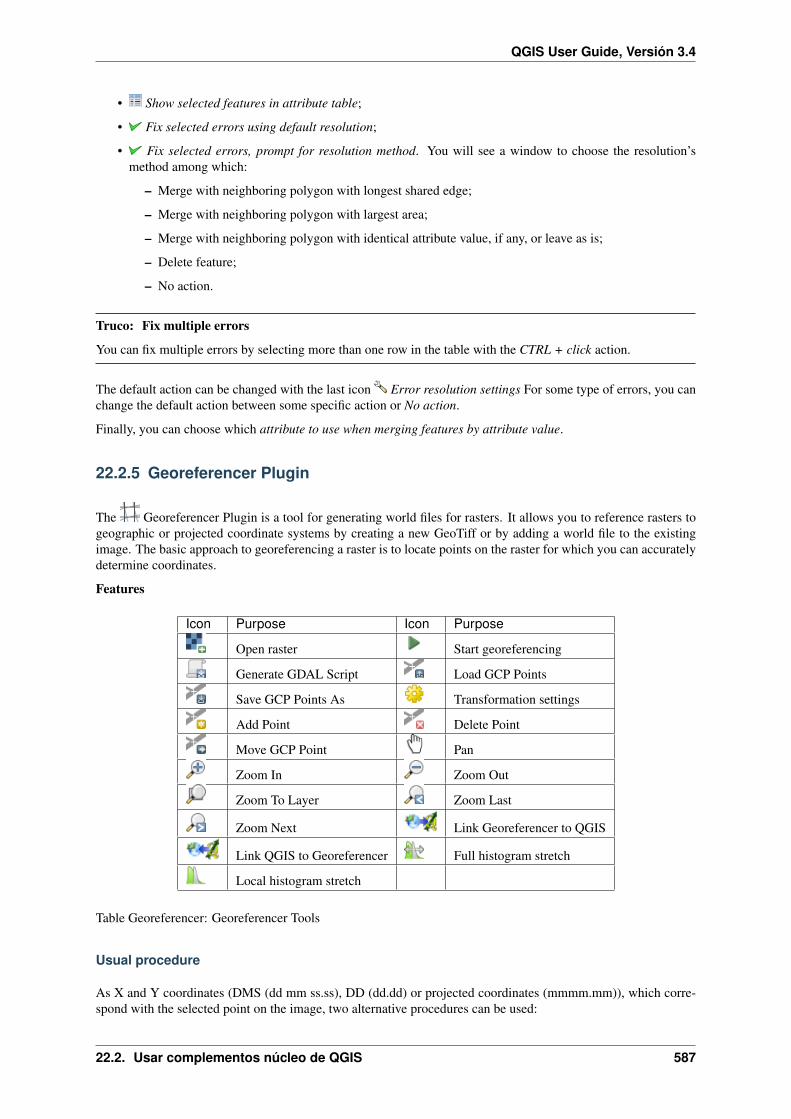
QGIS User Guide, Versión 3.4
• Show selected features in attribute table;
• Fix selected errors using default resolution;
• Fix selected errors, prompt for resolution method. You will see a window to choose the resolution’smethod among which:
– Merge with neighboring polygon with longest shared edge;
– Merge with neighboring polygon with largest area;
– Merge with neighboring polygon with identical attribute value, if any, or leave as is;
– Delete feature;
– No action.
Truco: Fix multiple errors
You can fix multiple errors by selecting more than one row in the table with the CTRL + click action.
The default action can be changed with the last icon Error resolution settings For some type of errors, you canchange the default action between some specific action or No action.
Finally, you can choose which attribute to use when merging features by attribute value.
22.2.5 Georeferencer Plugin
The Georeferencer Plugin is a tool for generating world files for rasters. It allows you to reference rasters togeographic or projected coordinate systems by creating a new GeoTiff or by adding a world file to the existingimage. The basic approach to georeferencing a raster is to locate points on the raster for which you can accuratelydetermine coordinates.
Features
Icon Purpose Icon Purpose
Open raster Start georeferencing
Generate GDAL Script Load GCP Points
Save GCP Points As Transformation settings
Add Point Delete Point
Move GCP Point Pan
Zoom In Zoom Out
Zoom To Layer Zoom Last
Zoom Next Link Georeferencer to QGIS
Link QGIS to Georeferencer Full histogram stretch
Local histogram stretch
Table Georeferencer: Georeferencer Tools
Usual procedure
As X and Y coordinates (DMS (dd mm ss.ss), DD (dd.dd) or projected coordinates (mmmm.mm)), which corre-spond with the selected point on the image, two alternative procedures can be used:
22.2. Usar complementos núcleo de QGIS 587

QGIS User Guide, Versión 3.4
• The raster itself sometimes provides crosses with coordinates «written» on the image. In this case, you canenter the coordinates manually.
• Using already georeferenced layers. This can be either vector or raster data that contain the same ob-jects/features that you have on the image that you want to georeference and with the projection that youwant for your image. In this case, you can enter the coordinates by clicking on the reference dataset loadedin the QGIS map canvas.
The usual procedure for georeferencing an image involves selecting multiple points on the raster, specifying theircoordinates, and choosing a relevant transformation type. Based on the input parameters and data, the plugin willcompute the world file parameters. The more coordinates you provide, the better the result will be.
The first step is to start QGIS, load the Georeferencer Plugin (see El diálogo de complementos) and click on Raster
→ Georeferencer, which appears in the QGIS menu bar. The Georeferencer Plugin dialog appears as shownin figure_georeferencer_dialog.
For this example, we are using a topo sheet of South Dakota from SDGS. It can later be visualized together withthe data from the GRASS spearfish60 location. You can download the topo sheet here: https://grass.osgeo.org/sampledata/spearfish_toposheet.tar.gz.
Figure 22.19: Georeferencer Plugin Dialog
Entering ground control points (GCPs)
1. To start georeferencing an unreferenced raster, we must load it using the button. The raster will showup in the main working area of the dialog. Once the raster is loaded, we can start to enter reference points.
2. Using the Add Point button, add points to the main working area and enter their coordinates (see Figurefigure_georeferencer_add_points). For this procedure you have three options:
• Click on a point in the raster image and enter the X and Y coordinates manually.
588 Chapter 22. Complementos

QGIS User Guide, Versión 3.4
• Click on a point in the raster image and choose the From map canvas button to add the X and Ycoordinates with the help of a georeferenced map already loaded in the QGIS map canvas.
• With the button, you can move the GCPs in both windows, if they are at the wrong place.
3. Continue entering points. You should have at least four points, and the more coordinates you can provide,the better the result will be. There are additional tools on the plugin dialog to zoom and pan the workingarea in order to locate a relevant set of GCP points.
Figure 22.20: Add points to the raster image
The points that are added to the map will be stored in a separate text file ([filename].points) usuallytogether with the raster image. This allows us to reopen the Georeferencer plugin at a later date and add newpoints or delete existing ones to optimize the result. The points file contains values of the form: mapX, mapY,
pixelX, pixelY. You can use the Load GCP points and Save GCP points as buttons to manage the files.
Defining the transformation settings
After you have added your GCPs to the raster image, you need to define the transformation settings for thegeoreferencing process.
Available Transformation algorithms
Depending on how many ground control points you have captured, you may want to use different transformationalgorithms. Choice of transformation algorithm is also dependent on the type and quality of input data and theamount of geometric distortion that you are willing to introduce to the final result.
Currently, the following Transformation types are available:
• The Linear algorithm is used to create a world file and is different from the other algorithms, as it doesnot actually transform the raster. This algorithm likely won’t be sufficient if you are dealing with scannedmaterial.
• The Helmert transformation performs simple scaling and rotation transformations.
• The Polynomial algorithms 1-3 are among the most widely used algorithms introduced to match sourceand destination ground control points. The most widely used polynomial algorithm is the second-orderpolynomial transformation, which allows some curvature. First-order polynomial transformation (affine)preserves collinearity and allows scaling, translation and rotation only.
• The Thin Plate Spline (TPS) algorithm is a more modern georeferencing method, which is able to intro-duce local deformations in the data. This algorithm is useful when very low quality originals are beinggeoreferenced.
• The Projective transformation is a linear rotation and translation of coordinates.
22.2. Usar complementos núcleo de QGIS 589

QGIS User Guide, Versión 3.4
Figure 22.21: Defining the georeferencer transformation settings
Define the Resampling method
The type of resampling you choose will likely depending on your input data and the ultimate objective of theexercise. If you don’t want to change statistics of the image, you might want to choose “Nearest neighbour”,whereas a “Cubic resampling” will likely provide a more smoothed result.
It is possible to choose between five different resampling methods:
1. Nearest neighbour
2. Linear
3. Cubic
4. Cubic Spline
5. Lanczos
Define the transformation settings
There are several options that need to be defined for the georeferenced output raster.
• The Create world file checkbox is only available if you decide to use the linear transformation type,because this means that the raster image actually won’t be transformed. In this case, the Output raster fieldis not activated, because only a new world file will be created.
• For all other transformation types, you have to define an Output raster. As default, a new file ([file-name]_modified) will be created in the same folder together with the original raster image.
• As a next step, you have to define the Target SRS (Spatial Reference System) for the georeferenced raster(see Trabajar con Proyecciones).
590 Chapter 22. Complementos
QGIS User Guide, Versión 3.4
• If you like, you can generate a pdf map and also a pdf report. The report includes information about theused transformation parameters, an image of the residuals and a list with all GCPs and their RMS errors.
• Furthermore, you can activate the Set Target Resolution checkbox and define the pixel resolution of theoutput raster. Default horizontal and vertical resolution is 1.
• The Use 0 for transparency when needed can be activated, if pixels with the value 0 shall be visualizedtransparent. In our example toposheet, all white areas would be transparent.
• Finally, Load in QGIS when done loads the output raster automatically into the QGIS map canvas whenthe transformation is done.
Show and adapt raster properties
Clicking on the Raster properties option in the Settings menu opens the Layer properties dialog of the raster filethat you want to georeference.
Configure the georeferencer
• You can define whether you want to show GCP coordinates and/or IDs.
• As residual units, pixels and map units can be chosen.
• For the PDF report, a left and right margin can be defined and you can also set the paper size for the PDFmap.
• Finally, you can activate to Show Georeferencer window docked.
Running the transformation
After all GCPs have been collected and all transformation settings are defined, just press the Start georeferencing
button to create the new georeferenced raster.
22.2.6 MetaSearch Catalog Client
Introduction
MetaSearch is a QGIS plugin to interact with metadata catalog services, supporting the OGC Catalog Service forthe Web (CSW) standard.
MetaSearch provides an easy and intuitive approach and user-friendly interface to searching metadata catalogswithin QGIS.
Installation
MetaSearch is included by default with QGIS 2.0 and higher. All dependencies are included within MetaSearch.
Install MetaSearch from the QGIS plugin manager, or manually from https://plugins.qgis.org/plugins/MetaSearch.
Working with Metadata Catalogs in QGIS
CSW (Catalog Service for the Web)
CSW (Catalog Service for the Web) is an OGC (Open Geospatial Consortium) specification that defines commoninterfaces to discover, browse and query metadata about data, services, and other potential resources.
22.2. Usar complementos núcleo de QGIS 591

QGIS User Guide, Versión 3.4
Figure 22.22: Search and results of Services in MetaSearch
inicio
To start MetaSearch, click the icon or select Web → MetaSearch → MetaSearch via the QGIS main menu.The MetaSearch dialog will appear. The main GUI consists of three tabs: Services, Search and Settings.
Managing Catalog Services
The Services tab allows the user to manage all available catalog services. MetaSearch provides a default list ofCatalog Services, which can be added by pressing Add Default Services button.
To all listed Catalog Service entries, click the dropdown select box.
To add a Catalog Service entry, click the New button, and enter a Name for the service, as well as the URL(endpoint). Note that only the base URL is required (not a full GetCapabilities URL). If the CSW requiresauthentication, enter the appropriate User name and Password credentials. Clicking OK will add the service tothe list of entries.
To edit an existing Catalog Service entry, select the entry you would like to edit and click the Edit button, andmodify the Name or URL values, then click OK.
To delete a Catalog Service entry, select the entry you would like to delete and click the Delete button. You willbe asked to confirm deleting the entry.
MetaSearch allows for loading and saving connections to an XML file. This is useful when you need to sharesettings between applications. Below is an example of the XML file format.
<?xml version="1.0" encoding="UTF-8"?><qgsCSWConnections version="1.0">
<csw name="Data.gov CSW" url="https://catalog.data.gov/csw-all"/><csw name="Geonorge - National CSW service for Norway" url="https://www.
→˓geonorge.no/geonetwork/srv/eng/csw"/>
592 Chapter 22. Complementos

QGIS User Guide, Versión 3.4
Figure 22.23: Managing Catalog Services
22.2. Usar complementos núcleo de QGIS 593

QGIS User Guide, Versión 3.4
<csw name="Geoportale Nazionale - Servizio di ricerca Italiano" url="http://→˓www.pcn.minambiente.it/geoportal/csw"/>
<csw name="LINZ Data Service" url="http://data.linz.govt.nz/feeds/csw"/><csw name="Nationaal Georegister (Nederland)" url="http://www.
→˓nationaalgeoregister.nl/geonetwork/srv/eng/csw"/><csw name="RNDT - Repertorio Nazionale dei Dati Territoriali - Servizio di
→˓ricerca" url="http://www.rndt.gov.it/RNDT/CSW"/><csw name="UK Location Catalogue Publishing Service" url="http://csw.data.gov.
→˓uk/geonetwork/srv/en/csw"/><csw name="UNEP/GRID-Geneva Metadata Catalog" url="http://metadata.grid.unep.
→˓ch:8080/geonetwork/srv/eng/csw"/></qgsCSWConnections>
To load a list of entries, click the Load button. A new window will appear; click the Browse button and navigateto the XML file of entries you wish to load and click Open. The list of entries will be displayed. Select the entriesyou wish to add from the list and click Load.
Click the Service Info button to displays information about the selected Catalog Service such as service identi-fication, service provider and contact information. If you would like to view the raw XML response, click theGetCapabilities Response button. A separate window will open displaying Capabilities XML.
Searching Catalog Services
The Search tab allows the user to query Catalog Services for data and services, set various search parameters andview results.
The following search parameters are available:
• Keywords: free text search keywords;
• From: the Catalog Service to perform the query against;
• Bounding box: the spatial area of interest to filter on defined by Xmax, Xmin, Ymax, and Ymin. Click SetGlobal to do a global search, click Map Extent to do a search on the visible area only or manually entercustom values as desired.
Clicking the Search button will search the selected Metadata Catalog. Search results are displayed in a list and aresortable by clicking on the column title. You can navigate through search results with the directional buttons belowthe search results. Clicking the View Search Results as XML button opens a window with the service response inraw XML format.
Clicking a result will provide the following options:
• if the metadata record has an associated bounding box, a footprint of the bounding box will be displayed onthe map;
• double-clicking the record displays the record metadata with any associated access links. Clicking the linksopens the link in the user’s web browser;
• if the record is a supported web service (WMS/WMTS, WFS, WCS, ArcGIS MapServer, ArcGIS Feature-Server, etc.), the Add Data button will be enabled for the user to add to QGIS. When clicking this button,MetaSearch will verify if this is a valid OWS. The service will then be added to the appropriate QGISconnection list, and the appropriate connection dialog will then appear.
Settings
You can fine tune MetaSearch with the following settings:
• Results paging: when searching metadata catalogs, the number of results to show per page. Default value is10;
• Timeout: when searching metadata catalogs, the number of seconds for blocking connection attempt. De-fault value is 10.
594 Chapter 22. Complementos

QGIS User Guide, Versión 3.4
Figure 22.24: Searching catalog services
22.2. Usar complementos núcleo de QGIS 595

QGIS User Guide, Versión 3.4
Figure 22.25: Metadata record display
596 Chapter 22. Complementos

QGIS User Guide, Versión 3.4
Figure 22.26: MetaSearch settings
22.2. Usar complementos núcleo de QGIS 597

QGIS User Guide, Versión 3.4
22.2.7 Offline Editing Plugin
For data collection, it is a common situation to work with a laptop or a cell phone offline in the field. Upon return-ing to the network, the changes need to be synchronized with the master datasource (e.g., a PostGIS database). Ifseveral persons are working simultaneously on the same datasets, it is difficult to merge the edits by hand, even ifpeople don’t change the same features.
The Offline Editing Plugin automates the synchronisation by copying the content of a datasource (usually PostGISor WFS-T) to a SpatiaLite or GeoPackage database and storing the offline edits to dedicated tables. After beingconnected to the network again, it is possible to apply the offline edits to the master dataset.
To use the plugin:
1. Open a project with some vector layers (e.g., from a PostGIS or WFS-T datasource).
2. Assuming you have already enabled the plugin (see Complementos base y externos) go to Database →
Offline Editing → Convert to offline project. The eponym dialog opens.
3. Select the Storage type. It can be of GeoPackage or SpatiaLite database type.
4. Use the Browse button to indicate the location of the database in which to store the Offline data. It can bean existing file or one to create.
5. In the Select remote layers section, check the layers you’d like to save. The content of the layers is saved todatabase tables.
6. You can check Only synchronize selected features if a selection is present allowing to only save andwork on a subset. It can be invaluable in case of large layers.
This is all!
7. Save your project and bring it on the field.
8. Edit the layers offline.
9. After being connected again, upload the changes using Database → Offline Editing → Synchronize.
22.2.8 Topology Checker Plugin
Topology describes the relationships between points, lines and polygons that represent the features of a geographicregion. With the Topology Checker plugin, you can look over your vector files and check the topology with severaltopology rules. These rules check with spatial relations whether your features “Equal”, “Contain”, “Cover”, are“CoveredBy”, “Cross”, are “Disjoint”, “Intersect”, “Overlap”, “Touch” or are “Within” each other. It depends onyour individual questions which topology rules you apply to your vector data (e.g., normally you won’t acceptovershoots in line layers, but if they depict dead-end streets you won’t remove them from your vector layer).
QGIS has a built-in topological editing feature, which is great for creating new features without errors. But existingdata errors and user-induced errors are hard to find. This plugin helps you find such errors through a list of rules.
It is very simple to create topology rules with the Topology Checker plugin.
On point layers the following rules are available:
• Must be covered by: Here you can choose a vector layer from your project. Points that aren’t covered bythe given vector layer occur in the “Error” field.
• Must be covered by endpoints of: Here you can choose a line layer from your project.
• Must be inside: Here you can choose a polygon layer from your project. The points must be inside apolygon. Otherwise, QGIS writes an “Error” for the point.
• Must not have duplicates: Whenever a point is represented twice or more, it will occur in the “Error” field.
• Must not have invalid geometries: Checks whether the geometries are valid.
• Must not have multi-part-geometries: All multi-part points are written into the “Error” field.
598 Chapter 22. Complementos

QGIS User Guide, Versión 3.4
Figure 22.27: Create an offline project
Figure 22.28: The Topology Checker Plugin
22.2. Usar complementos núcleo de QGIS 599

QGIS User Guide, Versión 3.4
On line layers, the following rules are available:
• End points must be covered by: Here you can select a point layer from your project.
• Must not have dangles: This will show the overshoots in the line layer.
• Must not have duplicates: Whenever a line feature is represented twice or more, it will occur in the “Error”field.
• Must not have invalid geometries: Checks whether the geometries are valid.
• Must not have multi-part geometries: Sometimes, a geometry is actually a collection of simple (single-part) geometries. Such a geometry is called multi-part geometry. If it contains just one type of simplegeometry, we call it multi-point, multi-linestring or multi-polygon. All multi-part lines are written into the“Error” field.
• Must not have pseudos: A line geometry’s endpoint should be connected to the endpoints of two othergeometries. If the endpoint is connected to only one other geometry’s endpoint, the endpoint is called apseudo node.
On polygon layers, the following rules are available:
• Must contain: Polygon layer must contain at least one point geometry from the second layer.
• Must not have duplicates: Polygons from the same layer must not have identical geometries. Whenever apolygon feature is represented twice or more it will occur in the “Error” field.
• Must not have gaps: Adjacent polygons should not form gaps between them. Administrative boundariescould be mentioned as an example (US state polygons do not have any gaps between them. . . ).
• Must not have invalid geometries: Checks whether the geometries are valid. Some of the rules that definea valid geometry are:
– Polygon rings must close.
– Rings that define holes should be inside rings that define exterior boundaries.
– Rings may not self-intersect (they may neither touch nor cross one another).
– Rings may not touch other rings, except at a point.
• Must not have multi-part geometries: Sometimes, a geometry is actually a collection of simple (single-part) geometries. Such a geometry is called multi-part geometry. If it contains just one type of simplegeometry, we call it multi-point, multi-linestring or multi-polygon. For example, a country consisting ofmultiple islands can be represented as a multi-polygon.
• Must not overlap: Adjacent polygons should not share common area.
• Must not overlap with: Adjacent polygons from one layer should not share common area with polygonsfrom another layer.
Below is the list of Core plugins provided with QGIS. They are not necessarily enabled by default.
600 Chapter 22. Complementos

QGIS User Guide, Versión 3.4
Icono Complemento Descripción Manual Reference
Coordinate Capture Capture mouse coordinate in differ-ent CRS
Coordinate Capture Plugin
DB Manager Manage your databases withinQGIS
DB Manager Plugin
eVis Event Visualization Tool eVis Plugin
Geometry Checker Check and repair errors in vectorgeometries
Geometry Checker Plugin
Georeferencer GDAL Georeference rasters with GDAL Georeferencer Plugin
GPS Tools Tools for loading and importingGPS data
Plugin de GPS
GRASS GRASS functionality Integracion GRASS SIG
Cliente de Catálogo demetasearch
Interact with metadata catalog ser-vices (CSW)
MetaSearch Catalog Client
Edición fuera de línea Offline editing and synchronizingwith database
Offline Editing Plugin
Processing Spatial data processing framework Entorno de trabajo de proce-samiento de QGIS
Topology Checker Find topological errors in vectorlayers
Topology Checker Plugin
22.3 Consola Python de QGIS
As you will see later in this chapter, QGIS has been designed with a plugin architecture. Plugins can be written inPython, a very famous language in the geospatial world.
QGIS brings a Python API (see PyQGIS Developer Cookbook for some code sample) to let the user interact withits objects (layers, feature or interface). QGIS also has a Python console.
The QGIS Python Console is an interactive shell for the python command executions. It also has a python fileeditor that allows you to edit and save your python scripts. Both console and editor are based on PyQScintilla2package. To open the console go to Plugins → Python Console (Ctrl+Alt+P).
22.3.1 The Interactive Console
The interactive console is composed of a toolbar, an input area and an output one.
Barra de herramietas
The toolbar proposes the following tools:
• Clear Console to wipe the output area;
• Run Command available in the input area: same as pressing Enter;
• Show Editor: toggles El Editor de código visibility;
• Options. . . : opens a dialog to configure console properties (see Opciones);
22.3. Consola Python de QGIS 601

QGIS User Guide, Versión 3.4
• Help. . . : browses the current documentation.
Consola
The console main features are:
• Code completion, highlighting syntax and calltips for the following APIs:
– Python
– PyQGIS
– PyQt5
– QScintilla2
– osgeo-gdal-ogr
• Ctrl+Alt+Space to view the auto-completion list if enabled in the Opciones;
• Execute code snippets from the input area by typing and pressing Enter or Run Command;
• Execute code snippets from the output area using the Enter Selected from the contextual menu or pressingCtrl+E;
• Browse the command history from the input area using the Up and Down arrow keys and execute thecommand you want;
• Ctrl+Shift+Space to view the command history: double-clicking a row will execute the command.The Command History dialog can also be accessed from context menu of input area;
• Save and clear the command history. The history will be saved into the file ~/.qgis2/console_history.txt;
• Open QGIS C++ API documentation by typing _api;
• Open QGIS Python API documentation by typing _pyqgis.
• Open PyQGIS Cookbook by typing _cookbook.
Truco: Reuse executed commands from the output panel
You can execute code snippets from the output panel by selecting some text and pressing Ctrl+E. No matter ifselected text contains the interpreter prompt (>>>, ...).
Figure 22.29: Consola de Python
602 Chapter 22. Complementos

QGIS User Guide, Versión 3.4
22.3.2 El Editor de código
Use the Show Editor button to enable the editor widget. It allows editing and saving Python files and offersadvanced functionalities to manage your code (comment and uncomment code, check syntax, share the code viacodepad.org and much more). Main features are:
• Code completion, highlighting syntax and calltips for the following APIs:
– Python
– PyQGIS
– PyQt5
– QScintilla2
– osgeo-gdal-ogr
• Ctrl+Space to view the auto-completion list.
• Sharing code snippets via codepad.org.
• Ctrl+4 Syntax check.
• Search bar (open it with the default Desktop Environment shortcut, usually Ctrl+F):
– Use the default Desktop Environment shortcut to find next/previous (Ctrl+G and Shift+Ctrl+G);
– Automatically find first match when typing in find box;
– Set initial find string to selection when opening find;
– Pressing Esc closes the find bar.
• Object inspector: a class and function browser;
• Go to an object definition with a mouse click (from Object inspector);
• Execute code snippets with the Run Selected command in contextual menu;
• Execute the whole script with the Run Script command (this creates a byte-compiled file with theextension .pyc).
Nota: Running partially or totally a script from the Code Editor outputs the result in the Console output area.
22.3.3 Opciones
Accessible from the Console toolbar and the contextual menus of the Console output panel and the Code Editor,the Python Console Settings help manage and control the Python console behavior.
For both Console and Editor you can specify:
• Autocompletion: Enables code completion. You can get autocompletion from the current document, theinstalled API files or both.
– Autocompletion threshold: Sets the threshold for displaying the autocompletion list (in characters)
• Typing
– Automatic parentheses insertion: Enables autoclosing for parentheses
– Automatic insertion of the “import” string on “from xxx”: Enables insertion of “import” when speci-fying imports
For Editor you can also specify:
• Run and Debug
22.3. Consola Python de QGIS 603

QGIS User Guide, Versión 3.4
Figure 22.30: The Python Console editor
– Enable Object Inspector (switching between tabs may be slow): Enable the object inspector.
– Auto-save script before running: Saves the script automatically when executed. This action will storea temporary file (in the temporary system directory) that will be deleted automatically after running.
• Font and Colors: Here you can specify the font to use in the editor and the colors to use for highlighting
For APIs you can specify:
• Using preloaded APIs file: You can choose if you would like to use the preloaded API files. If this is notchecked you can add API files and you can also choose if you would like to use prepared API files (see nextoption).
• Using prepared APIs file: If checked, the chosen *.pap file will be used for code completion. To generatea prepared API file you have to load at least one *.api file and then compile it by clicking the CompileAPIs. . . button.
Truco: Save the options
To save the state of console’s widgets you have to close the Python Console from the close button. This allowsyou to save the geometry to be restored to the next start.
604 Chapter 22. Complementos

CHAPTER 23
Ayuda y apoyo
23.1 Listas de correos
QGIS está en desarrollo activo y como tal, no siempre funciona como se espera. La forma preferida de obtenerayuda es uniéndose a la lista de correo qgis-users. Sus preguntas llegarán a un público más amplio y las respuestasbeneficiarán a otros.
23.1.1 Usuarios de QGIS
This mailing list is used for discussion of QGIS in general, as well as specific questions regarding its installationand use. You can subscribe to the qgis-users mailing list by visiting the following URL: https://lists.osgeo.org/mailman/listinfo/qgis-user
23.1.2 Desarrolladores QGIS
If you are a developer facing problems of a more technical nature, you may want to join the qgis-developer mailinglist. This list is also a place where people can chime in and collect and discuss QGIS related UX (User Experience)/ usability issues. It’s here: https://lists.osgeo.org/mailman/listinfo/qgis-developer
23.1.3 QGIS Community Team
This list deals with topics like documentation, context help, user guide, web sites, blog, mailing lists, forums, andtranslation efforts. If you would like to work on the user guide as well, this list is a good starting point to ask yourquestions. You can subscribe to this list at: https://lists.osgeo.org/mailman/listinfo/qgis-community-team
23.1.4 QGIS Translations
This list deals with the translation efforts. If you like to work on the translation of the website, manuals or thegraphical user interface (GUI), this list is a good starting point to ask your questions. You can subscribe to this listat: https://lists.osgeo.org/mailman/listinfo/qgis-tr
605

QGIS User Guide, Versión 3.4
23.1.5 QGIS Project Steering Committee (PSC)
This list is used to discuss Steering Committee issues related to overall management and direction of QGIS. Youcan subscribe to this list at: https://lists.osgeo.org/mailman/listinfo/qgis-psc
23.1.6 QGIS User groups
In order to locally promote QGIS and contribute to its development, some QGIS communities are organized intoQGIS User Groups. These groups are places to discuss local topics, organize regional or national user meetings,organize sponsoring of features. . . The list of current user groups is available at https://qgis.org/en/site/forusers/usergroups.html
You are welcome to subscribe to any of the lists. Please remember to contribute to the list by answering questionsand sharing your experiences.
23.2 IRC
We also maintain a presence on IRC - visit us by joining the #qgis channel on irc.freenode.net. Please wait for aresponse to your question, as many folks on the channel are doing other things and it may take a while for them tonotice your question. If you missed a discussion on IRC, not a problem! We log all discussion, so you can easilycatch up. Just go to https://qgis.org/irclogs and read the IRC-logs.
Commercial support for QGIS is also available. Check the website https://qgis.org/en/commercial-support.htmlfor more information.
23.3 Rastreador de Errores
While the qgis-users mailing list is useful for general “How do I do XYZ in QGIS?”-type questions, you may wishto notify us about bugs in QGIS. You can submit bug reports using the QGIS bug tracker at https://issues.qgis.org/projects/qgis/issues. When creating a new ticket for a bug, please provide an email address where we can contactyou for additional information.
Por favor, tenga en cuenta que su error no siempre puede disfrutar de la prioridad que podría esperar (depende desu gravedad). Algunos errores pueden requerir de significativo esfuerzo por parte del desarrollador para remediar,y la mano de obra no siempre está disponible para esto.
Se pueden presentar las solicitudes de funciones utilizando el mismo sistema de ticket de errores. Asegúrate deseleccionar el tipo «Función».
If you have found a bug and fixed it yourself, you can submit either a Pull Request on the Github QGIS Project(prefered) or a patch also. The lovely redmine ticketsystem at https://issues.qgis.org/projects/qgis/issues has thistype as well. Check the Patch supplied checkbox and attach your patch before submitting your bug. Oneof the developers will review it and apply it to QGIS. Please don’t be alarmed if your patch is not applied straightaway – developers may be tied up with other commitments.
Tenga en cuenta que si proporciona una solicitud de extracción, su cambio sería más probable que se fusione enel código fuente!
23.4 Blog
The QGIS community also runs a weblog at https://planet.qgis.org/planet/, which has some interesting articles forusers and developers as well provided by other blogs in the community. You are invited to contribute your ownQGIS blog!
606 Chapter 23. Ayuda y apoyo
QGIS User Guide, Versión 3.4
23.5 Plugins
The website https://plugins.qgis.org provides the official QGIS plugins web portal. Here, you find a list of allstable and experimental QGIS plugins available via the “Official QGIS Plugin Repository”.
23.6 Wiki
Lastly, we maintain a WIKI web site at https://github.com/qgis/QGIS/wiki where you can find a variety of usefulinformation relating to QGIS development, release plans, links to download sites, message-translation hints andmore. Check it out, there are some goodies inside!
23.5. Plugins 607

QGIS User Guide, Versión 3.4
608 Chapter 23. Ayuda y apoyo

CHAPTER 24
Colaboradores
QGIS es un proyecto de Código Libre desarrollado por un equipo de voluntarios dedicados y organizaciones.Nosotros nos esforzamos por ser una comunidad acogedora para todas las personas de todas las carreras, credos,géneros y profesiones. En cualquier momento, puedes involucrarte.
24.1 Autores
Debajo están listadas las personas que dedican su tiempo y esfuerzo para escribir, revisar y actualizar toda laDocumentación de QGIS.
609

QGIS User Guide, Versión 3.4
Tara Athan Radim Blazek K. Koy Godofredo Contr-eras
Martin Dobias
Peter Ersts Anne Ghisla Stephan Holl14. Horning
Magnus Homann
Werner Macho Denis Rouzaud Tyler Mitchell Claudia A. Engel Lars LuthmanOtto Dassau Brendan Morely David Willis Jürgen E. Fischer Yoichi KayamaAlexander Bruy Anita Graser Victor Olaya Marco Hugentobler Gary E. ShermanTim Sutton Larissa Junek Raymond Nijssen Richard Duivenvo-
ordeAndreas Neumann
Astrid Emde Yves Jacolin Alexandre Neto Alessandro Pasotti Hien Tran-QuangAndy Schmid Arnaud Morvan Akgar Gumbira Giovanni Allegri Diethard JansenAndy Allan Matthias Kuhn Chris Berkhout Carson J.Q. Farmer Steven CordwellEric Goddard Frank Sokolic Luca Casagrande Harrissou Sant-
annaSaber Razmjooei
Ilkka Rinne Jacob Lanstorp Ujaval Gandhi Jean-Roc Morreale Salvatore LarosaJoão Gaspar Joshua Arnott Thomas Gratier Marco Bernasocchi Marie SilvestreKo Nagase Larry Shaffer Luigi Pirelli Konstantinos Niko-
laouManing Sambale
Manel Clos Mattheo Ghetta Bernhard Ströbl Luca Manganelli Nathan WoodrowNick Bearman Paul Blottière Vincent Picavet Maximilian Kram-
bachRené-Luc D’Hont
Tom Chadwin Patrick Sunter Nyall Dawson Milo Van der Lin-den
Paolo Cavallini
Paolo Corti Hugo Mercier Gavin Macaulay Stefan Blumentrath Nicholas DugganDavid Adler Vincent Mora Tudor Barascu QGIS Koran Trans-
latorStéphane Brunner
Jaka Kranjc Tom Kralidis Zoltan Siki Sebastian Dietrich Uros PreloznikDick Groskamp Mezene Worku Alexandre Bus-
quetsDominic Keller Andre Mano
Chris Mayo Håvard Tveite Mie Winstrup Jonathan Willitts Giovanni ManghiMartina Savarese icephale Andrei GiordanoPezzola zstadlerRamon embelding ajazepk
24.2 Traductores
QGIS es una aplicación multilingüe y, como tal, también publica una Documentación traducida a varios id-iomas. Se están traduciendo muchos otros idiomas y se publicarán tan pronto como alcancen un porcentajerazonable de traducción. Si desea ayudar a mejorar un idioma o solicitar uno nuevo, consulte https://qgis.org/es/site/getinvolved/index.html.
Las traducciones actuales son posibles gracias a:
610 Chapter 24. Colaboradores
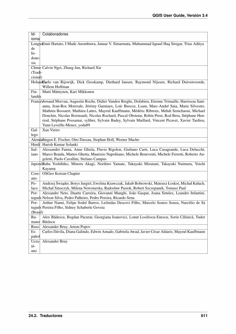
QGIS User Guide, Versión 3.4
Id-ioma
Colaboradores
LenguadeIn-done-sia
Emir Hartato, I Made Anombawa, Januar V. Simarmata, Muhammad Iqnaul Haq Siregar, Trias Aditya
Chino(Tradi-cional)
Calvin Ngei, Zhang Jun, Richard Xie
HolandésCarlo van Rijswijk, Dick Groskamp, Diethard Jansen, Raymond Nijssen, Richard Duivenvoorde,Willem Hoffman
Fin-landés
Matti Mäntynen, Kari Mikkonen
FrancésArnaud Morvan, Augustin Roche, Didier Vanden Berghe, Dofabien, Etienne Trimaille, Harrissou Sant-anna, Jean-Roc Morreale, Jérémy Garniaux, Loïc Buscoz, Lsam, Marc-André Saia, Marie Silvestre,Mathieu Bossaert, Mathieu Lattes, Mayeul Kauffmann, Médéric Ribreux, Mehdi Semchaoui, MichaelDouchin, Nicolas Boisteault, Nicolas Rochard, Pascal Obstetar, Robin Prest, Rod Bera, Stéphane Hen-riod, Stéphane Possamai, sylther, Sylvain Badey, Sylvain Maillard, Vincent Picavet, Xavier Tardieu,Yann Leveille-Menez, yoda89
Gal-lego
Xan Vieiro
AlemánJürgen E. Fischer, Otto Dassau, Stephan Holl, Werner MachoHindi Harish Kumar SolankiItal-iano
Alessandro Fanna, Anne Ghisla, Flavio Rigolon, Giuliano Curti, Luca Casagrande, Luca Delucchi,Marco Braida, Matteo Ghetta, Maurizio Napolitano, Michele Beneventi, Michele Ferretti, Roberto An-geletti, Paolo Cavallini, Stefano Campus
JaponésBaba Yoshihiko, Minoru Akagi, Norihiro Yamate, Takayuki Mizutani, Takayuki Nuimura, YoichiKayama
Core-ano
OSGeo Korean Chapter
Po-laco
Andrzej Swiader, Borys Jurgiel, Ewelina Krawczak, Jakub Bobrowski, Mateusz Łoskot, Michał Kułach,Michał Smoczyk, Milena Nowotarska, Radosław Pasiok, Robert Szczepanek, Tomasz Paul
Por-tugués
Alexandre Neto, Duarte Carreira, Giovanni Manghi, João Gaspar, Joana Simões, Leandro Infantini,Nelson Silva, Pedro Palheiro, Pedro Pereira, Ricardo Sena
Por-tugués(Brasil)
Arthur Nanni, Felipe Sodré Barros, Leônidas Descovi Filho, Marcelo Soares Souza, Narcélio de SáPereira Filho, Sidney Schaberle Goveia
Ru-mano
Alex Badescu, Bogdan Pacurar, Georgiana Ioanovici, Lonut Losifescu-Enescu, Sorin Calinica, TudorBarascu
Ruso Alexander Bruy, Artem PopovEs-pañol
Carlos Dávila, Diana Galindo, Edwin Amado, Gabriela Awad, Javier César Aldariz, Mayeul Kauffmann
Ucra-ni-ano
Alexander Bruy
24.2. Traductores 611

QGIS User Guide, Versión 3.4
612 Chapter 24. Colaboradores

CHAPTER 25
Appendices
25.1 Appendix A: GNU General Public License
Versión 2, Junio de 1991
Copyright (C) 1989, 1991 Free Software Foundation, Inc. 59 Temple Place - Suite 330, Boston, MA 02111-1307,USA
Se permite a todos copiar y distribuir copias exactas de este documento de licencia, aunque no se permite sucambio.
Preámbulo
The licenses for most software are designed to take away your freedom to share and change it. By contrast,the GNU General Public License is intended to guarantee your freedom to share and change free software–tomake sure the software is free for all its users. This General Public License applies to most of the Free SoftwareFoundation’s software and to any other program whose authors commit to using it. (Some other Free SoftwareFoundation software is covered by the GNU Library General Public License instead.) You can apply it to yourprograms, too.
When we speak of free software, we are referring to freedom, not price. Our General Public Licenses are designedto make sure that you have the freedom to distribute copies of free software (and charge for this service if youwish), that you receive source code or can get it if you want it, that you can change the software or use pieces ofit in new free programs; and that you know you can do these things.
To protect your rights, we need to make restrictions that forbid anyone to deny you these rights or to ask you tosurrender the rights. These restrictions translate to certain responsibilities for you if you distribute copies of thesoftware, or if you modify it.
For example, if you distribute copies of such a program, whether gratis or for a fee, you must give the recipientsall the rights that you have. You must make sure that they, too, receive or can get the source code. And you mustshow them these terms so they know their rights.
We protect your rights with two steps: (1) copyright the software, and (2) offer you this license which gives youlegal permission to copy, distribute and/or modify the software.
Also, for each author’s protection and ours, we want to make certain that everyone understands that there is nowarranty for this free software. If the software is modified by someone else and passed on, we want its recipientsto know that what they have is not the original, so that any problems introduced by others will not reflect on theoriginal authors” reputations.
613

QGIS User Guide, Versión 3.4
Finally, any free program is threatened constantly by software patents. We wish to avoid the danger that redis-tributors of a free program will individually obtain patent licenses, in effect making the program proprietary. Toprevent this, we have made it clear that any patent must be licensed for everyone’s free use or not licensed at all.
The precise terms and conditions for copying, distribution and modification follow. TERMS AND CONDITIONSFOR COPYING, DISTRIBUTION AND MODIFICATION
0. This License applies to any program or other work which contains a notice placed by the copyright holdersaying it may be distributed under the terms of this General Public License. The «Program», below, refers toany such program or work, and a «work based on the Program» means either the Program or any derivativework under copyright law: that is to say, a work containing the Program or a portion of it, either verbatimor with modifications and/or translated into another language. (Hereinafter, translation is included withoutlimitation in the term «modification».) Each licensee is addressed as «you».
Activities other than copying, distribution and modification are not covered by this License; they are outsideits scope. The act of running the Program is not restricted, and the output from the Program is covered onlyif its contents constitute a work based on the Program (independent of having been made by running theProgram). Whether that is true depends on what the Program does.
1. You may copy and distribute verbatim copies of the Program’s source code as you receive it, in any medium,provided that you conspicuously and appropriately publish on each copy an appropriate copyright noticeand disclaimer of warranty; keep intact all the notices that refer to this License and to the absence of anywarranty; and give any other recipients of the Program a copy of this License along with the Program.
You may charge a fee for the physical act of transferring a copy, and you may at your option offer warrantyprotection in exchange for a fee.
2. You may modify your copy or copies of the Program or any portion of it, thus forming a work based on theProgram, and copy and distribute such modifications or work under the terms of Section 1 above, providedthat you also meet all of these conditions:
(a) You must cause the modified files to carry prominent notices stating that you changed the files and thedate of any change.
(b) You must cause any work that you distribute or publish, that in whole or in part contains or is derivedfrom the Program or any part thereof, to be licensed as a whole at no charge to all third parties underthe terms of this License.
(c) If the modified program normally reads commands interactively when run, you must cause it, whenstarted running for such interactive use in the most ordinary way, to print or display an announcementincluding an appropriate copyright notice and a notice that there is no warranty (or else, saying thatyou provide a warranty) and that users may redistribute the program under these conditions, and tellingthe user how to view a copy of this License. (Exception: if the Program itself is interactive but doesnot normally print such an announcement, your work based on the Program is not required to print anannouncement.)
These requirements apply to the modified work as a whole. If identifiable sections of that work are notderived from the Program, and can be reasonably considered independent and separate works in themselves,then this License, and its terms, do not apply to those sections when you distribute them as separate works.But when you distribute the same sections as part of a whole which is a work based on the Program, thedistribution of the whole must be on the terms of this License, whose permissions for other licensees extendto the entire whole, and thus to each and every part regardless of who wrote it.
Thus, it is not the intent of this section to claim rights or contest your rights to work written entirely by you;rather, the intent is to exercise the right to control the distribution of derivative or collective works based onthe Program.
In addition, mere aggregation of another work not based on the Program with the Program (or with a workbased on the Program) on a volume of a storage or distribution medium does not bring the other work underthe scope of this License.
3. You may copy and distribute the Program (or a work based on it, under Section 2) in object code or exe-cutable form under the terms of Sections 1 and 2 above provided that you also do one of the following:
614 Chapter 25. Appendices

QGIS User Guide, Versión 3.4
(a) Accompany it with the complete corresponding machine-readable source code, which must be dis-tributed under the terms of Sections 1 and 2 above on a medium customarily used for software inter-change; or,
(b) Accompany it with a written offer, valid for at least three years, to give any third party, for a charge nomore than your cost of physically performing source distribution, a complete machine-readable copyof the corresponding source code, to be distributed under the terms of Sections 1 and 2 above on amedium customarily used for software interchange; or,
(c) Accompany it with the information you received as to the offer to distribute corresponding sourcecode. (This alternative is allowed only for noncommercial distribution and only if you received theprogram in object code or executable form with such an offer, in accord with Subsection b above.)
The source code for a work means the preferred form of the work for making modifications to it. For anexecutable work, complete source code means all the source code for all modules it contains, plus anyassociated interface definition files, plus the scripts used to control compilation and installation of the ex-ecutable. However, as a special exception, the source code distributed need not include anything that isnormally distributed (in either source or binary form) with the major components (compiler, kernel, andso on) of the operating system on which the executable runs, unless that component itself accompanies theexecutable.
If distribution of executable or object code is made by offering access to copy from a designated place, thenoffering equivalent access to copy the source code from the same place counts as distribution of the sourcecode, even though third parties are not compelled to copy the source along with the object code.
4. You may not copy, modify, sublicense, or distribute the Program except as expressly provided under thisLicense. Any attempt otherwise to copy, modify, sublicense or distribute the Program is void, and willautomatically terminate your rights under this License. However, parties who have received copies, orrights, from you under this License will not have their licenses terminated so long as such parties remain infull compliance.
5. You are not required to accept this License, since you have not signed it. However, nothing else grants youpermission to modify or distribute the Program or its derivative works. These actions are prohibited by lawif you do not accept this License. Therefore, by modifying or distributing the Program (or any work basedon the Program), you indicate your acceptance of this License to do so, and all its terms and conditions forcopying, distributing or modifying the Program or works based on it.
6. Each time you redistribute the Program (or any work based on the Program), the recipient automaticallyreceives a license from the original licensor to copy, distribute or modify the Program subject to these termsand conditions. You may not impose any further restrictions on the recipients” exercise of the rights grantedherein. You are not responsible for enforcing compliance by third parties to this License.
7. If, as a consequence of a court judgment or allegation of patent infringement or for any other reason (notlimited to patent issues), conditions are imposed on you (whether by court order, agreement or otherwise)that contradict the conditions of this License, they do not excuse you from the conditions of this License.If you cannot distribute so as to satisfy simultaneously your obligations under this License and any otherpertinent obligations, then as a consequence you may not distribute the Program at all. For example, if apatent license would not permit royalty-free redistribution of the Program by all those who receive copiesdirectly or indirectly through you, then the only way you could satisfy both it and this License would be torefrain entirely from distribution of the Program.
If any portion of this section is held invalid or unenforceable under any particular circumstance, the balanceof the section is intended to apply and the section as a whole is intended to apply in other circumstances.
It is not the purpose of this section to induce you to infringe any patents or other property right claims orto contest validity of any such claims; this section has the sole purpose of protecting the integrity of thefree software distribution system, which is implemented by public license practices. Many people havemade generous contributions to the wide range of software distributed through that system in reliance onconsistent application of that system; it is up to the author/donor to decide if he or she is willing to distributesoftware through any other system and a licensee cannot impose that choice.
This section is intended to make thoroughly clear what is believed to be a consequence of the rest of thisLicense.
25.1. Appendix A: GNU General Public License 615

QGIS User Guide, Versión 3.4
8. If the distribution and/or use of the Program is restricted in certain countries either by patents or by copy-righted interfaces, the original copyright holder who places the Program under this License may add anexplicit geographical distribution limitation excluding those countries, so that distribution is permitted onlyin or among countries not thus excluded. In such case, this License incorporates the limitation as if writtenin the body of this License.
9. The Free Software Foundation may publish revised and/or new versions of the General Public License fromtime to time. Such new versions will be similar in spirit to the present version, but may differ in detail toaddress new problems or concerns.
Each version is given a distinguishing version number. If the Program specifies a version number of this Li-cense which applies to it and «any later version», you have the option of following the terms and conditionseither of that version or of any later version published by the Free Software Foundation. If the Programdoes not specify a version number of this License, you may choose any version ever published by the FreeSoftware Foundation.
10. If you wish to incorporate parts of the Program into other free programs whose distribution conditions aredifferent, write to the author to ask for permission. For software which is copyrighted by the Free SoftwareFoundation, write to the Free Software Foundation; we sometimes make exceptions for this. Our decisionwill be guided by the two goals of preserving the free status of all derivatives of our free software and ofpromoting the sharing and reuse of software generally.
NO WARRANTY
11. BECAUSE THE PROGRAM IS LICENSED FREE OF CHARGE, THERE IS NO WARRANTY FORTHE PROGRAM, TO THE EXTENT PERMITTED BY APPLICABLE LAW. EXCEPT WHEN OTH-ERWISE STATED IN WRITING THE COPYRIGHT HOLDERS AND/OR OTHER PARTIES PROVIDETHE PROGRAM «AS IS» WITHOUT WARRANTY OF ANY KIND, EITHER EXPRESSED OR IM-PLIED, INCLUDING, BUT NOT LIMITED TO, THE IMPLIED WARRANTIES OF MERCHANTABIL-ITY AND FITNESS FOR A PARTICULAR PURPOSE. THE ENTIRE RISK AS TO THE QUALITY ANDPERFORMANCE OF THE PROGRAM IS WITH YOU. SHOULD THE PROGRAM PROVE DEFEC-TIVE, YOU ASSUME THE COST OF ALL NECESSARY SERVICING, REPAIR OR CORRECTION.
12. IN NO EVENT UNLESS REQUIRED BY APPLICABLE LAW OR AGREED TO IN WRITING WILLANY COPYRIGHT HOLDER, OR ANY OTHER PARTY WHO MAY MODIFY AND/OR REDIS-TRIBUTE THE PROGRAM AS PERMITTED ABOVE, BE LIABLE TO YOU FOR DAMAGES, IN-CLUDING ANY GENERAL, SPECIAL, INCIDENTAL OR CONSEQUENTIAL DAMAGES ARISINGOUT OF THE USE OR INABILITY TO USE THE PROGRAM (INCLUDING BUT NOT LIMITED TOLOSS OF DATA OR DATA BEING RENDERED INACCURATE OR LOSSES SUSTAINED BY YOUOR THIRD PARTIES OR A FAILURE OF THE PROGRAM TO OPERATE WITH ANY OTHER PRO-GRAMS), EVEN IF SUCH HOLDER OR OTHER PARTY HAS BEEN ADVISED OF THE POSSIBIL-ITY OF SUCH DAMAGES.
QGIS Qt excepciones para GPL
In addition, as a special exception, the QGIS Development Team gives permission to link the code of this programwith the Qt library, including but not limited to the following versions (both free and commercial): Qt/Non-commercial Windows, Qt/Windows, Qt/X11, Qt/Mac, and Qt/Embedded (or with modified versions of Qt that usethe same license as Qt), and distribute linked combinations including the two. You must obey the GNU GeneralPublic License in all respects for all of the code used other than Qt. If you modify this file, you may extend thisexception to your version of the file, but you are not obligated to do so. If you do not wish to do so, delete thisexception statement from your version.
25.2 Licencia de Documentación Libre de GNU
Versión 1.3, 3 de Noviembre de 2008
Derechos Reservados 2000, 2001, 2002, 2007, 2008 Free Software Foundation, Inc
https://fsf.org/
616 Chapter 25. Appendices

QGIS User Guide, Versión 3.4
Se permite a todos copiar y distribuir copias exactas de este documento de licencia, aunque no se permite sucambio.
Preámbulo
El propósito de esta Licencia es permitir que un manual, libro de texto, u otro documento escrito sea «libre»en el sentido de libertad: asegurar a todo el mundo la libertad efectiva de copiarlo y redistribuirlo, con o sinodificaciones, de manera comercial o no. En segundo término, esta Licencia proporciona al autor y al editoruna manera de obtener reconocimiento por su trabajo, sin que se le considere responsable de las modificacionesrealizadas por otros.
Esta Licencia es de tipo «copyleft», lo que significa que los trabajos derivados del documento deben a su vez serlibres en el mismo sentido. Complementa la Licencia Pública General de GNU, que es una licencia tipo copyleftdiseñada para el software libre.
We have designed this License in order to use it for manuals for free software, because free software needs freedocumentation: a free program should come with manuals providing the same freedoms that the software does.But this License is not limited to software manuals; it can be used for any textual work, regardless of subjectmatter or whether it is published as a printed book. We recommend this License principally for works whosepurpose is instruction or reference.
1. DEFINICIONES Y APLICABILIDAD
Esta Licencia se aplica a cualquier manual u otro trabajo, en cualquier soporte, que contenga una nota del propi-etario de los derechos de autor que indique que puede ser distribuido bajo los términos de esta Licencia. Tal notagarantiza en cualquier lugar del mundo, sin pago de derechos y sin límite de tiempo, el uso de dicho trabajo segúnlas condiciones aquí estipuladas. En adelante la palabra Documento se referirá a cualquiera de dichos manualeso trabajos. Cualquier persona es un licenciatario y será referido como «Usted». Usted acepta la licencia si copia.modifica o distribuye el trabajo de cualquier modo que requiera permiso según la ley de propiedad intelectual.
A «Modified Version» of the Document means any work containing the Document or a portion of it, either copiedverbatim, or with modifications and/or translated into another language.
Una «Sección Secundaria» es un apéndice con título o una sección preliminar del Documento que trata exclusi-vamente de la relación entre los autores o editores y el tema general del Documento (o temas relacionados) peroque no contiene nada que entre directamente en dicho tema general (por ejemplo, si el Documento es en parte untexto de matemáticas, una Sección Secundaria puede no explicar nada de matemáticas). La relación puede ser unaconexión histórica con el tema o temas relacionados, o una opinión legal, comercial, filosófica, ética o políticaacerca de ellos.
The «Invariant Sections» are certain Secondary Sections whose titles are designated, as being those of InvariantSections, in the notice that says that the Document is released under this License. If a section does not fit theabove definition of Secondary then it is not allowed to be designated as Invariant. The Document may containzero Invariant Sections. If the Document does not identify any Invariant Sections then there are none.
Los «Textos de Cubierta» son ciertos pasajes cortos de texto que se listan como Textos de Cubierta Delantera oTextos de Cubierta Trasera en la nota que indica que el documento es liberado bajo esta Licencia. Un Texto deCubierta delantera puede tener como mucho 5 palabras, y uno de Cubierta Trasera puede tener hasta 25 palabras.
A «Transparent» copy of the Document means a machine-readable copy, represented in a format whose specifi-cation is available to the general public, that is suitable for revising the document straightforwardly with generictext editors or (for images composed of pixels) generic paint programs or (for drawings) some widely availabledrawing editor, and that is suitable for input to text formatters or for automatic translation to a variety of formatssuitable for input to text formatters. A copy made in an otherwise Transparent file format whose markup, or ab-sence of markup, has been arranged to thwart or discourage subsequent modification by readers is not Transparent.An image format is not Transparent if used for any substantial amount of text. A copy that is not «Transparent» iscalled Opaque.
Como ejemplos de formatos adecuados para copias Transparentes están ASCII puro sin marcaje, formato deentrada de Texinfo, formato de entrada de LaTeX, SGML o XML usando una DTD disponible públicamente,y HTML, PostScript o PDF simples, que sigan los estándares y diseñados para que los modifiquen personas.Ejemplos de formatos de imagen transparentes son PNG, XCF y JPG. Los formatos Opacos incluyen formatospropietarios que pueden ser leídos y editados únicamente en procesadores de palabras propietarios, SGML o
25.2. Licencia de Documentación Libre de GNU 617

QGIS User Guide, Versión 3.4
XML para los cuáles las DTD y/o herramientas de procesamiento no estén ampliamente disponibles, y HTML,PostScript o PDF generados por algunos procesadores de palabras sólo como salida.
La «Portada» significa, en un libro impreso, la página de título, más las páginas siguientes que sean necesariaspara mantener legiblemente el material que esta Licencia requiere en la portada. Para trabajos en formatos que notienen página de portada como tal, Portada significa el texto cercano a la aparición más prominente del título deltrabajo, precediendo el comienzo del cuerpo del texto.
El «Editor» se refiere a cualquier persona o entidad que distribuya copias del Documento a el público.
Una sección «Titulada XYZ» significa una parte del Documento cuyo título es precisamente XYZ o contieneXYZ entre paréntesis, a continuación de texto que traduce XYZ a otro idioma (aquí XYZ se refiere a nombresde sección específicos mencionados más abajo, como «Agradecimientos», «Dedicatorias», «Aprobaciones» o«Historia»). «Conservar el Título» de tal sección cuando se modifica el Documento significa que permaneceuna sección «Titulada XYZ» según esta definición.
The Document may include Warranty Disclaimers next to the notice which states that this License applies to theDocument. These Warranty Disclaimers are considered to be included by reference in this License, but only asregards disclaiming warranties: any other implication that these Warranty Disclaimers may have is void and hasno effect on the meaning of this License.
2. COPIA LITERAL
You may copy and distribute the Document in any medium, either commercially or noncommercially, providedthat this License, the copyright notices, and the license notice saying this License applies to the Document arereproduced in all copies, and that you add no other conditions whatsoever to those of this License. You may notuse technical measures to obstruct or control the reading or further copying of the copies you make or distribute.However, you may accept compensation in exchange for copies. If you distribute a large enough number of copiesyou must also follow the conditions in section 3.
Usted también puede prestar copias, bajo las mismas condiciones establecidas anteriormente, y puede exhibircopias públicamente.
3. COPIADO EN CANTIDAD
If you publish printed copies (or copies in media that commonly have printed covers) of the Document, numberingmore than 100, and the Document’s license notice requires Cover Texts, you must enclose the copies in coversthat carry, clearly and legibly, all these Cover Texts: Front-Cover Texts on the front cover, and Back-Cover Textson the back cover. Both covers must also clearly and legibly identify you as the publisher of these copies. Thefront cover must present the full title with all words of the title equally prominent and visible. You may add othermaterial on the covers in addition. Copying with changes limited to the covers, as long as they preserve the titleof the Document and satisfy these conditions, can be treated as verbatim copying in other respects.
Si los textos requeridos para la cubierta son muy voluminosos para que ajusten legiblemente, debe colocar losprimeros (tantos como sea razonable colocar) en la verdadera cubierta y situar el resto en páginas adyacentes.
If you publish or distribute Opaque copies of the Document numbering more than 100, you must either includea machine-readable Transparent copy along with each Opaque copy, or state in or with each Opaque copy acomputer-network location from which the general network-using public has access to download using public-standard network protocols a complete Transparent copy of the Document, free of added material. If you use thelatter option, you must take reasonably prudent steps, when you begin distribution of Opaque copies in quantity, toensure that this Transparent copy will remain thus accessible at the stated location until at least one year after thelast time you distribute an Opaque copy (directly or through your agents or retailers) of that edition to the public.
It is requested, but not required, that you contact the authors of the Document well before redistributing any largenumber of copies, to give them a chance to provide you with an updated version of the Document.
4. MODIFICACIONES
Puede copiar y distribuir una Versión Modificada del Documento bajo las condiciones de las secciones 2 y 3anteriores, siempre que usted libere la Versión Modificada bajo esta misma Licencia, con la Versión Modificadahaciendo el rol del Documento, por lo tanto dando licencia de distribución y modificación de la Versión Modificadaa quienquiera posea una copia de la misma. Además, debe hacer lo siguiente en la Versión Modificada:
1. Usar en la Portada (y en las cubiertas, si hay alguna) un título distinto al del Documento y de sus versionesanteriores (que deberían, si hay alguna, estar listadas en la sección de Historia del Documento). Puede usar
618 Chapter 25. Appendices

QGIS User Guide, Versión 3.4
el mismo título de versiones anteriores al original siempre y cuando quien las publicó originalmente otorguepermiso.
2. List on the Title Page, as authors, one or more persons or entities responsible for authorship of the modifi-cations in the Modified Version, together with at least five of the principal authors of the Document (all ofits principal authors, if it has fewer than five), unless they release you from this requirement.
3. Mostrar en la Portada como editor el nombre del editor de la Versión Modificada.
4. Preservar todas las notas de derechos de autor del Documento.
5. Agregue una nota de derechos reservados apropiada para sus modificaciones adyacente a las otras notas dederechos reservados.
6. Include, immediately after the copyright notices, a license notice giving the public permission to use theModified Version under the terms of this License, in the form shown in the Addendum below.
7. Preserve in that license notice the full lists of Invariant Sections and required Cover Texts given in theDocument’s license notice.
8. Incluir una copia sin modificación de esta Licencia.
9. Preserve the section Entitled «History», Preserve its Title, and add to it an item stating at least the title, year,new authors, and publisher of the Modified Version as given on the Title Page. If there is no section Entitled«History» in the Document, create one stating the title, year, authors, and publisher of the Document asgiven on its Title Page, then add an item describing the Modified Version as stated in the previous sentence.
10. Conservar la dirección en red, si la hay, dada en el Documento para el acceso público a una copia transpar-ente del mismo, así como las otras direcciones de red dadas en el Documento para versiones anteriores enlas que estuviese basado. Pueden ubicarse en la sección «Historia». Se puede omitir la ubicación en red deun trabajo que haya sido publicado por lo menos cuatro años antes que el Documento mismo, o si el editororiginal de dicha versión da permiso.
11. For any section Entitled «Acknowledgements» or «Dedications», Preserve the Title of the section, andpreserve in the section all the substance and tone of each of the contributor acknowledgements and/ordedications given therein.
12. Conservar todas las Secciones Invariantes del Documento, sin alterar su texto ni sus títulos. Números desección o el equivalente no son considerados parte de los títulos de la sección.
13. Borrar cualquier sección titulada Aprobaciones. Tales secciones no pueden estar incluidas en las VersionesModificadas.
14. Do not retitle any existing section to be Entitled «Endorsements» or to conflict in title with any InvariantSection.
15. Conservar todas las Limitaciones de Garantía.
Si la Versión Modificada incluye secciones o apéndices nuevos que califiquen como Secciones Secundarias ycontienen material no copiado del Documento, puede opcionalmente designar algunas o todas esas seccionescomo invariantes. Para hacerlo, añada sus títulos a la lista de Secciones Invariantes en la nota de licencia de laVersión Modificada. Tales títulos deben ser distintos de cualquier otro título de sección.
You may add a section Entitled «Endorsements», provided it contains nothing but endorsements of your ModifiedVersion by various parties—for example, statements of peer review or that the text has been approved by anorganization as the authoritative definition of a standard.
Puede añadir un pasaje de hasta cinco palabras como Texto de Cubierta Delantera y un pasaje de hasta 25 palabrascomo Texto de Cubierta Trasera en la Versión Modificada. Una entidad solo puede añadir (o hacer que se añada)un pasaje al Texto de Cubierta Delantera y uno al de Cubierta Trasera. Si el Documento ya incluye un textos decubiertas añadidos previamente por usted o por la misma entidad que usted representa, usted no puede añadir otro;pero puede reemplazar el anterior, con permiso explícito del editor que agregó el texto anterior.
Con esta Licencia ni el/los autor(es) ni el/los editor(es) del Documento dan permiso para usar sus nombres parapublicidad ni para asegurar o implicar aprobación de cualquier Versión Modificada.
5. COMBINACIÓN DE DOCUMENTOS
25.2. Licencia de Documentación Libre de GNU 619

QGIS User Guide, Versión 3.4
Usted puede combinar el Documento con otros documentos liberados bajo esta Licencia, bajo los términosdefinidos en la sección 4 anterior para versiones modificadas, siempre que incluya en la combinación todas lasSecciones Invariantes de todos los documentos originales, sin modificar, listadas todas como Secciones Invariantesdel trabajo combinado en su nota de licencia. Así mismo debe incluir la Limitación de Garantía.
El trabajo combinado necesita contener solamente una copia de esta Licencia, y puede reemplazar varias SeccionesInvariantes idénticas por una sola copia. Si hay varias Secciones Invariantes con el mismo nombre pero concontenidos diferentes, haga el título de cada una de estas secciones único añadiéndole al final del mismo, entreparéntesis, el nombre del autor o editor original de esa sección, si es conocido, o si no, un número único. Hagael mismo ajuste a los títulos de sección en la lista de Secciones Invariantes de la nota de licencia del trabajocombinado.
En la combinación, debe combinar cualquier sección Titulada «Historia» de los documentos originales, formandouna sección Titulada «Historia»; de la misma forma combine cualquier sección Titulada «Agradecimientos», ycualquier sección Titulada «Dedicatorias». Debe borrar todas las secciones tituladas «Aprobaciones».
6. COLECCIONES DE DOCUMENTOS
You may make a collection consisting of the Document and other documents released under this License, andreplace the individual copies of this License in the various documents with a single copy that is included in thecollection, provided that you follow the rules of this License for verbatim copying of each of the documents in allother respects.
Puede extraer un solo documento de una de tales colecciones y distribuirlo individualmente bajo esta Licencia,siempre que inserte una copia de esta Licencia en el documento extraído, y siga esta Licencia en todos los demásaspectos relativos a la copia literal de dicho documento.
7. AGREGACIÓN CON TRABAJOS INDEPENDIENTES
Una recopilación que conste del Documento o sus derivados y de otros documentos o trabajos separados e inde-pendientes, en cualquier soporte de almacenamiento o distribución, se denomina un «agregado» si el copyrightresultante de la compilación no se usa para limitar los derechos de los usuarios de la misma más allá de lo que losde los trabajos individuales permiten. Cuando el Documento se incluye en un agregado, esta Licencia no se aplicaa otros trabajos del agregado que no sean en sí mismos derivados del Documento.
Si el requisito de la sección 3 sobre el Texto de Cubierta es aplicable a estas copias del Documento y el Documentoes menor que la mitad del agregado entero, los Textos de Cubierta del Documento pueden colocarse en cubiertasque enmarquen solamente el Documento dentro del agregado, o el equivalente electrónico de las cubiertas si eldocumento está en forma electrónica. En caso contrario deben aparecer en cubiertas impresas enmarcando todo elagregado.
8. TRADUCCIÓN
La Traducción es considerada como un tipo de modificación, por lo que usted puede distribuir traducciones delDocumento bajo los términos de la sección 4. El reemplazo las Secciones Invariantes con traducciones requierepermiso especial de los dueños de derecho de autor, pero usted puede añadir traducciones de algunas o todas lasSecciones Invariantes a las versiones originales de las mismas. Puede incluir una traducción de esta Licencia, detodas las notas de licencia del documento, así como de las Limitaciones de Garantía, siempre que incluya tambiénla versión en Inglés de esta Licencia y las versiones originales de las notas de licencia y Limitaciones de Garantía.En caso de desacuerdo entre la traducción y la versión original en Inglés de esta Licencia, la nota de licencia o lalimitación de garantía, la versión original en Inglés prevalecerá.
Si una sección del Documento está Titulada «Agradecimientos», «Dedicatorias» o «Historia» el requisito (sección4) de Conservar su Título (Sección 1) requerirá, típicamente, cambiar su título.
9. TERMINACIÓN
Usted no puede copiar, modificar, sublicenciar o distribuir el Documento salvo por lo permitido expresamentebajo esta Licencia. Cualquier intento en otra manera de copia, modificación, sublicenciamiento, o distribución deél es nulo, y dará por terminados automáticamente sus derechos bajo esa Licencia.
Sin embargo, si usted cesa toda violación a esta Licencia, entonces su licenca proveniente de un titular de copyrightqueda restaurada (a) provisionalmente, a menos y hasta que el titular del copyright explicita y finalmente terminesu licencia, y (b) permanentemente, si el titual del copyright falla en notificarle de la violación por algún mediorazonable en un tiempo menor a 60 días después del cese.
620 Chapter 25. Appendices

QGIS User Guide, Versión 3.4
Además, su licencia proveniente de un titular del copyright particular queda restaurada permanentemente si eltitular del copyright lo notifica de la violación por algún método razonable, es la primera vez que usted ha recibidoaviso de la violación de esta Licencia (para cualquier trabajo) de ese titular del copyright, y usted remedia laviolación en un tiempo menor a 30 días después de recibir dicho aviso.
La terminación de sus derechos bajo ésta sección no termina la licenica de terceros que hayan recibido copias oderechos de usted bajo ésta Licencia. Si sus derechos han sido terminados y no restaurados permanentemente,recibir una copia de alguna parte o el total del mismo material no le da ningún derecho de usarlo.
10. REVISIONES FUTURAS DE ESTA LICENCIA
The Free Software Foundation may publish new, revised versions of the GNU Free Documentation License fromtime to time. Such new versions will be similar in spirit to the present version, but may differ in detail to addressnew problems or concerns. See https://www.gnu.org/copyleft/.
Cada versión de la Licencia tiene un número de versión que la distingue. Si el Documento especifica que se aplicauna versión numerada en particular de esta licencia «o cualquier versión posterior», usted tiene la opción de seguirlos términos y condiciones de la versión especificada o cualquiera posterior que haya sido publicada (no comoborrador) por la Free Software Foundation. Si el Documento no especifica un número de versión de esta Licencia,puede escoger cualquier versión que haya sido publicada (no como borrador) por la Free Software Foundation. Siel Documento especifica que un apoderado puede decidir qué versión futura de esta Licencia puede ser utilizada,esa frase de aceptación del apoderado de una versión le autoriza permanentemente a escoger esa versión para elDocumento.
11. RENOVACIÓN DE LICENCIAS
«Massive Multiauthor Collaboration Site» (or «MMC Site») means any World Wide Web server that publishescopyrightable works and also provides prominent facilities for anybody to edit those works. A public wiki thatanybody can edit is an example of such a server. A «Massive Multiauthor Collaboration» (or «MMC») containedin the site means any set of copyrightable works thus published on the MMC site.
«CC-BY-SA» significa la licencia Creative Commons Attribution-Share Alike 3.0 (Reconocimiento-Compartirbajo la misma licencia 3.0 de Creative Commons) publicada por Creative Commons Corporation, una corporaciónsin fines de lucro con base en San Francisco, California, así como versiones futuras copyleft de esa licenciapublicada por esa misma organización.
«Incorporate» means to publish or republish a Document, in whole or in part, as part of another Document.
Un sitio CMM es «elegible para re-licenciamiento» si es licenciado bajo esta Licencia, y si todos los trabajos quefueron publicados originalmente bajo esta Licencia en algún otro lugar diferente a esta CMM, y subsecuentementeincorporado como un todo o parcialmente a la CMM, (1)no tenía textos de cubierta o secciones invariantes, y (2)fueron incorporados previo a Noviembre 1, 2008.
The operator of an MMC Site may republish an MMC contained in the site under CC-BY-SA on the same site atany time before August 1, 2009, provided the MMC is eligible for relicensing.
APÉNDICE: Cómo usar esta Licencia para sus documentos
To use this License in a document you have written, include a copy of the License in the document and put thefollowing copyright and license notices just after the title page:
Copyright © YEAR YOUR NAME.Permission is granted to copy, distribute and/or modify this documentunder the terms of the GNU Free Documentation License, Version 1.3or any later version published by the Free Software Foundation;with no Invariant Sections, no Front-Cover Texts, and no Back-Cover Texts.A copy of the license is included in the section entitled "GNUFree Documentation License".
Si tiene Secciones Invariantes, Textos de Cubierta Delantera y Textos de Cubierta Trasera, reemplace la frase «sin. . . Trasera» por esto:
with the Invariant Sections being LIST THEIR TITLES, with theFront-Cover Texts being LIST, and with the Back-Cover Texts being LIST.
25.2. Licencia de Documentación Libre de GNU 621

QGIS User Guide, Versión 3.4
If you have Invariant Sections without Cover Texts, or some other combination of the three, merge those twoalternatives to suit the situation.
If your document contains nontrivial examples of program code, we recommend releasing these examples inparallel under your choice of free software license, such as the GNU General Public License, to permit their usein free software.
25.3 Appendix B: QGIS File Formats
25.3.1 QGS/QGZ - The QGIS Project File Format
The QGS format is an XML format for storing QGIS projects. The QGZ format is a compressed (zip) archivecontaining a QGS file and a QGD file. The QGD file is the associated sqlite database of the qgis project thatcontain auxiliary data for the project. If there are no auxiliary data, the QGD file will be empty.
A QGIS file contains everything that is needed for storing a QGIS project, including:
• project title
• project CRS
• the layer tree
• snapping settings
• relations
• the map canvas extent
• project models
• legend
• mapview docks (2D and 3D)
• the layers with links to the underlying datasets (data sources) and other layer properties including extent,SRS, joins, styles, renderer, blend mode, opacity and more.
• project properties
The figures below show the top level tags in a QGS file and the expanded ProjectLayers tag.
25.3.2 QLR - The QGIS Layer Definition file
A Layer Definition file (QLR) is an XML file that contains a pointer to the layer data source in addition to QGISstyle information for the layer.
The use case for this file is simple: To have a single file for opening a data source and bringing in all the relatedstyle information. QLR files also allow you to mask the underlying datasource in an easy to open file.
An example of QLR usage is for opening MS SQL layers. Rather than having to go to the MS SQL connectiondialog, connect, select, load and finally style, you can simply add a .qlr file that points to the correct MS SQLlayer with all the necessary style included.
In the future a .qlr file may hold a reference to more than one layer.
25.3.3 QML - The QGIS Style File Format
QML is an XML format for storing layer styling.
A QML file contains all the information QGIS can handle for the rendering of feature geometries including symboldefinitions, sizes and rotations, labelling, opacity and blend mode and more.
The figure below shows the top level tags of a QML file (with only renderer_v2 and its symbol tag expanded).
622 Chapter 25. Appendices

QGIS User Guide, Versión 3.4
Figure 25.1: The top level tags in a QGS file
25.3. Appendix B: QGIS File Formats 623

QGIS User Guide, Versión 3.4
Figure 25.2: The expanded top level ProjectLayers tag of a QGS file
624 Chapter 25. Appendices

QGIS User Guide, Versión 3.4
Figure 25.3: The top level tags of a QLR file
25.3. Appendix B: QGIS File Formats 625

QGIS User Guide, Versión 3.4
Figure 25.4: The top level tags of a QML file (only the renderer_v2 tag with its symbol tag is expanded)
626 Chapter 25. Appendices

CHAPTER 26
Referencias bibliográficas y web
GDAL-SOFTWARE-SUITE. Geospatial data abstraction library. https://www.gdal.org, 2013.
GRASS-PROJECT. Geographic resource analysis support system. https://grass.osgeo.org, 2013.
NETELER, M., AND MITASOVA, H. Open source gis: A grass gis approach, 2008.
OGR-SOFTWARE-SUITE. Geospatial data abstraction library. https://www.gdal.org/ogr, 2013.
OPEN-GEOSPATIAL-CONSORTIUM. Web map service (1.1.1) implementation specification. https://portal.opengeospatial.org, 2002.
OPEN-GEOSPATIAL-CONSORTIUM. Web map service (1.3.0) implementation specification. https://portal.opengeospatial.org, 2004.
POSTGIS-PROJECT. Spatial support for postgresql. http://postgis.refractions.net/, 2013.
627