Verifying Stochastic Well-formed Nets with CSL Model-Checking Tools�D. Cerotti, D. D’Aprile, S. Donatelli, and J. Sproston

Dipartimento di Informatica, Universita di Torino, Torino, Italyfcerotti,daprile,susi,sprostong@di.unito.it

Abstract

Model-checking algorithms for Continuous StochasticLogic (CSL) properties have been introduced to facilitatethe verification of stochastic systems against a variety offormally-defined performance indices.

In this paper, we consider the application ofCSL model-checking methods and tools to Stochastic Well-formedNets (SWN), a colored extension of Stochastic Petri Nets(SPN). Our approach is to connect an existing tool forthe description and performance analysis ofSWN, calledGREATSPN, to two model-checking tools forCSL prop-erties, namelyPRISM and MRMC. We illustrate our ap-proach using a simple example of resource usage. As aby-product of the implementation of the model translationfrom GREATSPN to PRISM, a method for unfoldingSWNmodels intoSPNmodels has been implemented, as a stand-alone, re-usable component.

1. Introduction

Model checking [8] is a verification method which es-tablishes automatically whether a formal description of asystem satisfies a property. Examples of properties whichcan be verified by model checking are absence of deadlockor reachability of error states. Typically, the system is de-scribed in terms of high-level languages such as Petri netsor process algebras, whereas the property to be verified isspecified in terms of a temporal logic.

Systems which exhibit non-trivial probabilistic orstochastic behavior are modelled more appropriately usingformalisms such as stochastic Petri nets [21] or stochas-tic process algebra [17, 15], the underlying semantics ofwhich take the form of Markov chains. Model-checkingalgorithms for continuous-time Markov chains (CTMCs)have been developed, where the property to be verified isdescribed in terms of Continuous Stochastic Logic (CSL)�Supported in part by the FIRB-Perf project of the Italian Ministry ofResearch.

[2, 3]. The logic CSL provides a formal way to describe po-tentially complex properties reasoning about both the func-tional behavior and the performance of a stochastic system.It includes a steady-state operator, which can refer to theprobabilities of the system being in certain states in equi-librium, and a probabilistic operator, which can refer to theprobability with which a certain (possibly timed) propertyis satisfied, such as “does the system reach an error statewithin 5 minutes with probability greater than 0.01?” Themodel-checking tools ETMCC [16], its successor MRMC[19], and PRISM [20, 24], have been used to analyze CSL

properties of stochastic systems in application areas suchasfault-tolerant systems, manufacturing systems and biologi-cal processes.

In this paper, we focus on the use of CSL model-checking tools for the verification of systems described us-ing Stochastic Well-formed Nets[7] (SWN). SWN are acolored extension of Generalized Stochastic Petri Nets [1](GSPN), and have two main advantages over GSPN.Firstly, SWN allow us to define models that are paramet-ric in the “structure” of the system: for example, a GSPNmodel of a system in which a pool of servers visit a setof stations in a given order is parametric in the number ofservers, in the number of clients at each station, but not inthe number of stations, whereas in an SWN model a colorcan be used to distinguish the stations, without the need ofreplicating station subnets. The second advantage of SWNis related to the solution process: if the color is used to rep-resent a symmetric behavior of the system, this symmetricbehavior can be exploited to build a “compact” state space,thus enlarging the size of systems that can be solved. De-spite the appealing characteristics of SWN, and the avail-ability of an associated tool (GREATSPN [4, 23] of the Uni-versity of Torino and the University of Paris 6), SWN mod-elling is not widespread. One reason for this is the limitedsupport available to validate an SWN model (for example,structural analysis, such as P- and T- invariant computation,is not available for SWN models).

In order to (partially) address this problem, model-checking techniques have been used previously to pro-vide support for the validation of SWN models: in [13],

an extension of GREATSPN that allows the use of thePROD tool [25] (a reachability graph analyzer definedfor predicate-transition nets) to model check an SWN netagainst a number of temporal logic properties is presented.However, this approach considers only functional proper-ties of the system, such as “can the system reach an errorstate”, rather than performance indices, and hence is onlypartially adequate when considering analysis of stochasticformalisms such as SWN. In this paper, we extend the workof [13], and our work on CSL model checking of stochas-tic Petri nets [12], by considering CSL model checking ofSWN. Following our work in [12], we have not built a newCSL model checker, but we have provided a CSL model-checking facility for SWN models in GREATSPN by link-ing GREATSPN to MRMC and PRISM. These links takethe form of programs which translate SWN from the for-mat used in GREATSPN to the (different) input languagesof PRISM and MRMC.

We have preferred to consider two “stand-alone” modelcheckers because they have been built and are maintainedby researchers in the specific field of stochastic modellingand verification, and are constantly updated to reflect recentresearch results. Moreover, although neither tool is basedon Petri nets, we considered that they would not be diffi-cult to connect with the GREATSPN modules for SWN,given that there is already some reported experience in in-terfacing these tools with other tools (ETMCC, the precur-sor of MRMC, has been interfaced with the Petri net toolDaNAMiCS [11] and the process algebra tool TIPP [14],while PRISM has been interfaced with the PEPA process al-gebra [17]). We observe that this choice is based on re-use,and it has the significant advantage of being able to profit ofall future developments of MRMC and PRISM. However,on the other hand, there is the drawback of not being ableto exploit all the peculiarities and properties of nets in themodel checking algorithm, as it would have been the case ifan ad-hoc solution had been devised.

Note that, as a by-product of the translation fromGREATSPN models to PRISM models, we have imple-mented a method for unfolding SWN nets to GSPN netswithin GREATSPN, which can be used in other contextsaside from CSL model checking.

Another contribution of this paper is the considerationof the way in which meaningful CSL properties of SWNmay be specified. In particular, we concentrate on the wayin which “atomic propositions”, which are used in modelchecking to identify portions of the state space of interest(for example, error states or goal states), can be described.Note that, for SWN, this task is not always straightforward,as the model-checking tool user may need to refer to com-plex expressions including net places, transitions, and col-ored tokens, to identify the required part of the state space.

In this paper we concentrate on SWN and on the

GREATSPN tool, but there are other colored extensions ofstochastic Petri nets with associated tools. The tool APNNhas a built-in CSL model checker [5] which works on thecolored GSPN class defined in APNN; however, we wereunfortunately not able to use APNN extensively due to lackof documentation. A notion of colors based on replicationis present in SAN nets in UltraSAN [10] and Mobius [9].There are plans to add a CSL model checker to the latter.

The paper is organized as follows: Section 2 recalls thedefinitions of CSL, GSPN, and SWN, and presents our run-ning example. Section 3 discusses CSL model-checkingof SWN, in particular with respect to the choice of theset of atomic propositions. Section 4 describes linkingGREATSPN to PRISM and to MRMC with the help of therunning example. Section 5 concludes the paper.

2. Background

In this section, we summarize the temporal logic CSL

and the formalisms GSPN and SWN, together with an as-sociated running example of a central server system.

CSL model checking. Let AP be a set of atomic proposi-tions, and letR�0 be the set of non-negative real numbers.The syntax of CSL [2, 3] is defined as follows:

Φ ::= a jΦ^Φ j :Φ j P./λ(XI Φ) j P./λ(ΦU I Φ) j S./λ(Φ)where a 2 AP is an atomic proposition,I � R�0 is anonempty interval, interpreted as a time interval,./2 f<;�;�;>g is a comparison operator, andλ 2 [0;1℄ is inter-preted as a probability. Formulae of CSL are evaluatedover continuous-time Markov chains (CTMCs), each stateof which is labelled with the subset of atomic propositionsAP that hold true in that state.

The logic CSL can be divided intostate formulae, whichare true or false in a state, andpath formulae, which areinterpreted as being true or false for a path of the system(where a path is a sequence of transitions which representsa computation of the CTMC). The interpretation of the stateformulae is as follows: a states satisfies the atomic propo-sition a if s is labelled witha, the operators and: havethe usual interpretation, whileS./λ(Φ) is true ins if, assum-ing s as initial state, the sum of the steady state probabili-ties of the states that satisfyΦ is ./ λ. For a path formulaϕ 2 fXI Φ;Φ1U I Φ2g, the state formulaP./λ(ϕ) is true ins if the probability of the paths leavings which satisfyϕ is./λ. We say thatP./λ(ϕ) is aprobabilistic formula, whereasS./λ(Φ) is asteady-state formula.

The interpretation of the path formulaeXI Φ andΦ1U I Φ2 is as follows. The Next formulaXI Φ is true fora path if the state reached after the first transition along thepath satisfiesΦ, and the duration of this transition lies in the

2

interval I . The Until formulaΦ1U I Φ2 is true along a pathif Φ2 is true at some state along the path, possibly also theinitial state of the path under consideration, the time elapsedbefore reaching this state lies inI , andΦ1 is true along thepath until that state. The formal semantics of CSL canbe found in [3]. The usual abbreviations for propositionaland temporal logic will be used throughout the paper; forexample,F I Φ� trueU I Φ, P�λ(GI Φ)� P<1�λ(F I:Φ).

Model checkinga CTMC against a CSL formulaΦ con-sists of computing the set of statesSat(Φ) such thats2Sat(Φ) if and only if Φ is true ins. The setSat(Φ) is con-structed by computing recursively the sets of states satis-fying the sub-formulas ofΦ. When probability boundsare present in the CSL formula (P./λ or S./λ), the model-checking algorithm requires the computation of transient orsteady-state probabilities of the original CTMC as well as,depending on the formula, a number of additional CTMCsbuilt through manipulation of the original one: see [3] formore details.

GSPNand SWN. A Stochastic Petri Net [21] (SPN) is atupleS= (P;T; I ;O;W;m0), whereP is the set of places,Tis the set of transitions,I ;O : P! T ! 2N define the inputand output arcs with associated multiplicity,W : T ! R�0

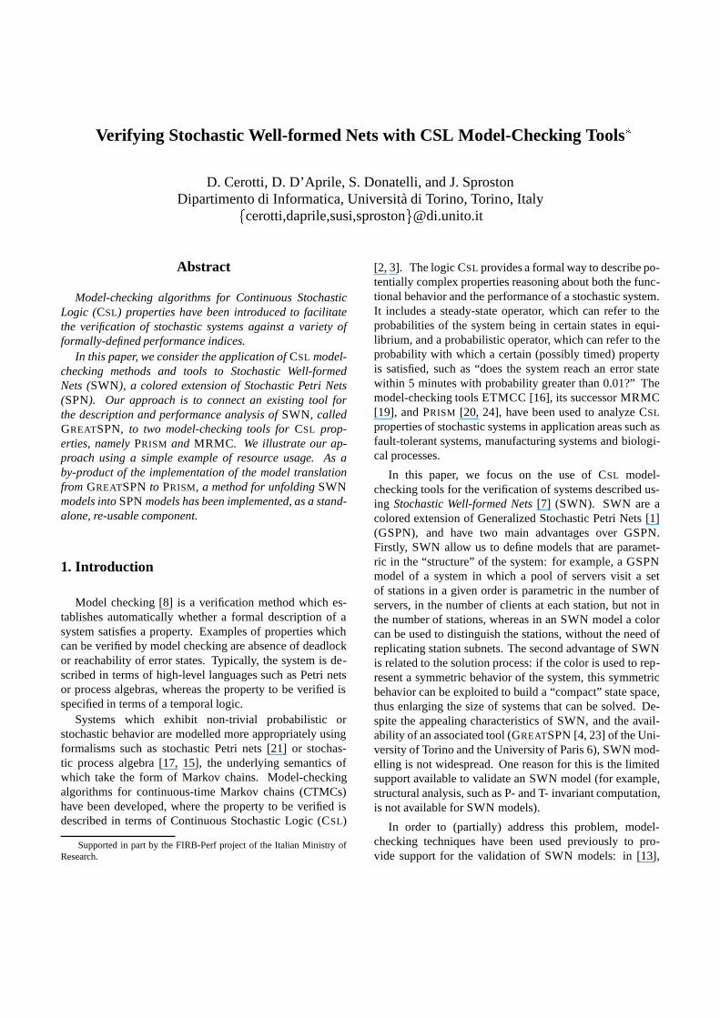
defines the rate of the exponential distributions associatedto transitions, andm0 : P! N describes the initial mark-ing. It is well-known that the stochastic process underlyingan SPN is a CTMC which is isomorphic to the reachabil-ity graph (RG) of the SPN built disregarding the timing as-pects. Generalized SPN (GSPN) [1] are an extension ofSPN in which the setT is split into immediate and stochas-tic transitions. Immediate transitions fire in zero time, withpriority over timed ones, and conflicts are resolved proba-bilistically. As a consequence the RG includes also somevanishingstates in which zero time elapses. We distinguishthe RG from the Tangible RG (TRG) in which only tangible(non-vanishing) states are preserved. The stochastic pro-cess associated to a GSPN is a semi-Markov process fromwhich a CTMC can be produced considering only the tan-gible states. Figure 1, in its right-most path, describes thesolution process of a GSPN, in particular that followed byGREATSPN: the Reachability Graph is built first, and eacharc is labelled with the name of the transition that causesthat change of state; then the vanishing states are elim-inated, thus creating the Tangible Reachability Graph, inwhich each arc is labelled with either the name of a timedtransition or of a timed followed by a sequence of immedi-ates. The CTMC is then built using the TRG and the ratesand probabilities associated to the transitions of the net.

Stochastic Well-formed Nets [7] are a colored extensionof GSPN. The peculiarity of SWN is that thecolor domainof places is built as the Cartesian product of a limited num-ber of basic color classes, and that functions on arcs are

SWN

RG

CTMC

UnfoldingGSPN

ColoredRG

Symbolic RG

Lumped CTMC

Colored RGconstruction

Symbolic RGconstruction

Ordinary RGconstruction

CTMCconstruction

CTMCconstruction

CTMCconstruction

lumpability

bisimulation isomorphism

TRGColoredTRG

Symbolic TRG bisimulation isomorphism

vanishingelimination

vanishingelimination

vanishingelimination

Figure 1. Solution approaches for SWN

un_av

D

av

D

ND

loc

N

wait

D

srv

D

back

s_srv e_srvtloc<x>

<x> <x>

<x>

<x><x>

<x>

<x>

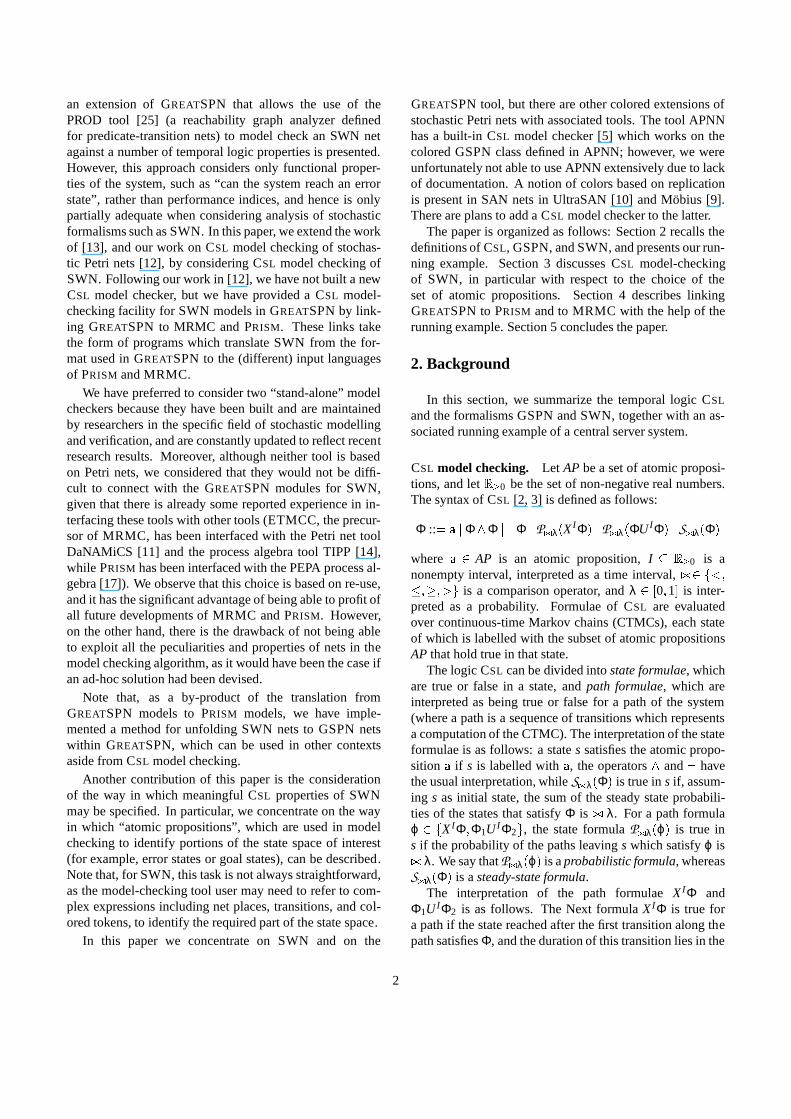
Figure 2. The SWN model of the running ex-ample

expressed as linear combination of a few basic functions(projection to select an element, sum function to select thewhole color class). We do not provide a formal definitionof SWN in this context, due to space reasons, but we recallthe main points by using an example.

The net of Figure 2 shows an SWN model of a simplecomputing system: there is a central server, modelled byplaceloc and transitiontloc, at which there are initiallyNjobs.

Once the computation local to the central server termi-nates, a job chooses one of the peripherical devices, and arequest for that device is put in placewait. Different devicesare modelled as different colors of the color classD. HenceD = fd1;d2; : : : ;dKg indicates that there areK different de-vices. A deviced can be in one of the following states:available (one token of colord in placeav), being used by ajob (one token of colord in placesrv), and unavailable (onetoken of colord in placeun av). The choice of a device by ajob is modelled by the single server transitiontloc that, dueto the free variablex associated to the arc out oftloc, puts inplacewait a token of colord, randomly chosen with equal

3

probability amongst allK colors of the color classD.A function hxi, such as the one on the arc fromwait to

s srv, is called a projection function and evaluates to one ofthe elements ofD: if in a marking there is a token in placeloc then there areK instancesof transitiontloc enabled, oneper each possible color assignment tox.

Transitions srv can fire for an assignment to variablexof color d only if there is at least one token of colord inplacewait and at least one token of colord in placeav. Thefiring of s srv for x = d puts a token of the same color insrv.Observe that, once the device has provided the required ser-vice, transitione srv fires, and puts an uncolored token (thejob) back to the server placeloc, and a coloredd token (thedevice) into placeun av. Placeun av models some resettime of the device (a period in which the device is unavail-able). We assume that all devices have the same speed andthat each device can work on a single job at a time (the ser-vice policy of transitions srv ande srv is “single server percolor”).

The other basic function of SWN is the constant functionS: if we change the function on the arc out oftloc to hSi, theneach firing oftloc addsK tokens to placewait, one token percolor in D, thus representing a fork of a job intoK threads,one per device. If the functionhSi is associated also to thearc fromsrv to e srv then the transition can fire only if thereis in srv at least one token per color: therefore it expressesa synchronization in the elaboration at then periphericaldevices.

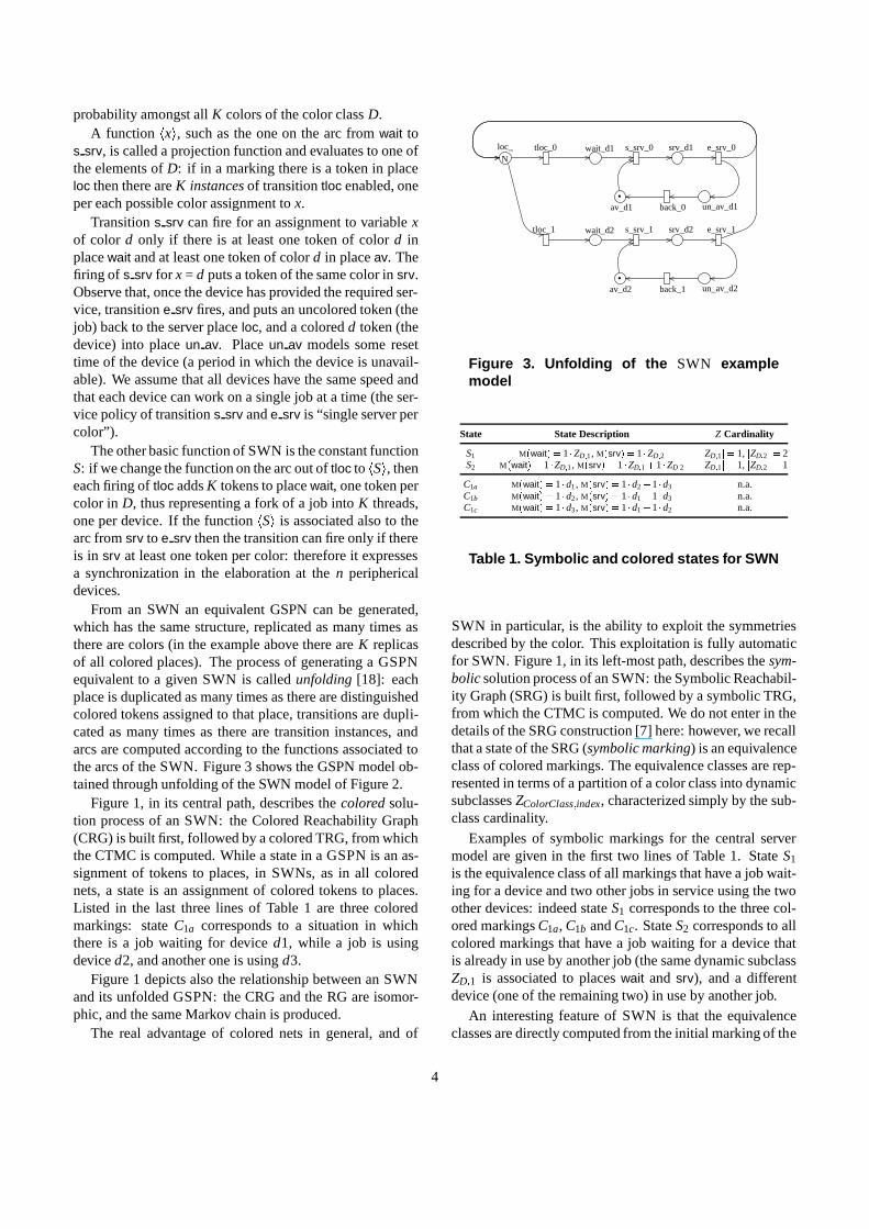
From an SWN an equivalent GSPN can be generated,which has the same structure, replicated as many times asthere are colors (in the example above there areK replicasof all colored places). The process of generating a GSPNequivalent to a given SWN is calledunfolding[18]: eachplace is duplicated as many times as there are distinguishedcolored tokens assigned to that place, transitions are dupli-cated as many times as there are transition instances, andarcs are computed according to the functions associated tothe arcs of the SWN. Figure 3 shows the GSPN model ob-tained through unfolding of the SWN model of Figure 2.

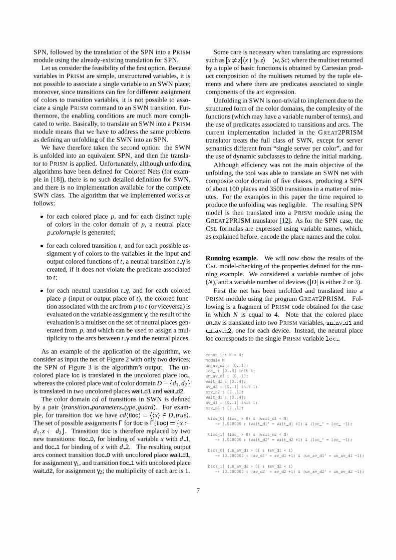
Figure 1, in its central path, describes thecoloredsolu-tion process of an SWN: the Colored Reachability Graph(CRG) is built first, followed by a colored TRG, from whichthe CTMC is computed. While a state in a GSPN is an as-signment of tokens to places, in SWNs, as in all colorednets, a state is an assignment of colored tokens to places.Listed in the last three lines of Table 1 are three coloredmarkings: stateC1a corresponds to a situation in whichthere is a job waiting for deviced1, while a job is usingdeviced2, and another one is usingd3.

Figure 1 depicts also the relationship between an SWNand its unfolded GSPN: the CRG and the RG are isomor-phic, and the same Markov chain is produced.

The real advantage of colored nets in general, and of

av_d1 un_av_d1

av_d2 un_av_d2

wait_d1loc_N

wait_d2

srv_d1

srv_d2

back_1

back_0

tloc_1

tloc_0

s_srv_1

s_srv_0

e_srv_1

e_srv_0

Figure 3. Unfolding of the SWN examplemodel

State State Description Z Cardinality

S1 M(wait) = 1�ZD;1, M(srv) = 1�ZD;2 jZD;1j = 1, jZD;2j = 2S2 M(wait) = 1�ZD;1, M(srv) = 1�ZD;1 +1�ZD;2 jZD;1j = 1, jZD;2j = 1

C1a M(wait) = 1�d1, M(srv) = 1�d2 +1�d3 n.a.C1b M(wait) = 1�d2, M(srv) = 1�d1 +1�d3 n.a.C1c M(wait) = 1�d3, M(srv) = 1�d1 +1�d2 n.a.

Table 1. Symbolic and colored states for SWN

SWN in particular, is the ability to exploit the symmetriesdescribed by the color. This exploitation is fully automaticfor SWN. Figure 1, in its left-most path, describes thesym-bolicsolution process of an SWN: the Symbolic Reachabil-ity Graph (SRG) is built first, followed by a symbolic TRG,from which the CTMC is computed. We do not enter in thedetails of the SRG construction [7] here: however, we recallthat a state of the SRG (symbolic marking) is an equivalenceclass of colored markings. The equivalence classes are rep-resented in terms of a partition of a color class into dynamicsubclassesZColorClass;index, characterized simply by the sub-class cardinality.

Examples of symbolic markings for the central servermodel are given in the first two lines of Table 1. StateS1

is the equivalence class of all markings that have a job wait-ing for a device and two other jobs in service using the twoother devices: indeed stateS1 corresponds to the three col-ored markingsC1a, C1b andC1c. StateS2 corresponds to allcolored markings that have a job waiting for a device thatis already in use by another job (the same dynamic subclassZD;1 is associated to placeswait and srv), and a differentdevice (one of the remaining two) in use by another job.

An interesting feature of SWN is that the equivalenceclasses are directly computed from the initial marking of the

4

SWN, thanks to a definition ofsymbolic transition firing: afiring in which dynamic subclasses, instead of specific col-ors, are assigned to variables. Therefore in the SRG, outof stateS1 there is an arc in whichx is associated toZD;1:the single arc represents the three arcs corresponding to thepossible assignment tox of a color inD.

The SRG is a bisimulation of the CRG (although thebisimulation relation is never computed), while the CTMCbuilt from the SRG is a lumped CTMC with respect to theCTMC generated from the CRG, as summarized by Fig-ure 1. Observe that, for each symbolic marking, it is possi-ble to build the list of corresponding colored markings.

Note that both of the CSL model-checking tools whichwe consider in this paper, PRISM and MRMC, do not al-low actions to happen in zero-time and with priority overexponential activities: therefore we limit our scope to netswithout immediate transitions only.

3. CSL model checking ofGSPNand SWN

CSL model checking of GSPN/SWN requires the fol-lowing set of ingredients: a GSPN/SWN model, a set ofatomic propositions expressed in terms of net elements, aCSL model checker, and a way to interpret the results ofmodel checking.

Let us consider the set of atomic propositionsAP.With regard to place-related atomic propositions, which wehenceforth callplace propositions, the expressions of inter-est are of the form:

(Type M): ∑p2Pwp �M(p)� K

(Type Mcol): ∑p2P;c2CD(p) wp;c �M(p)[c℄� K

where wp and wp;c are integers,CD(p) is the color do-main of placep (set of possible colors of tokens inp), and�2 f�;=;�g: observe that, sincewp andwp;c can be zero,the atomic propositions can refer also to an arbitrary set ofplaces or to an arbitrary set of colors and places.

Examples of place propositions, using the net of Fig-ure 2, are:M(loc) = 1 (there is one job at the central server),M(wait)[d2℄� 2 (there are at least two jobs waiting for theservices of deviced2).

With regard to transition-related atomic propositions,which we henceforth calltransition propositions, the ex-pressions of interest are of the form(Type T) the transitiont is enabled, or(Type Tcol) the transitiont is enabled for agiven assignment to the variables oft. Examples of transi-tion propositions, using the net of Figure 2, are: transitions srv is enabled (a device has been assigned to a job), tran-sitions srv is enabled for variablex instantiated to colord1(deviced1 has been assigned to a job).

For what concerns the evaluation of atomic propositionswe can again distinguish marking propositions from tran-sition propositions. Propositions of typeM can be defined

for GSPN and SWN, and can be computed trivially usingthe RG for GSPN, and with some effort using the CRGor SRG for SWN (indeed a sum over all colors is neces-sary for the CRG case, while the cardinality of the dynamicsubclasses is used for the SRG case). Propositions of typeMcol are defined instead only for SWN, and can be com-puted only for the CRG, since this is a type of propositionthat may hold in some of the states corresponding to a sym-bolic marking, but not in all of them. In the running exam-ple, the propositionM(srv)[d1℄ � 1, which is of typeMcol,is valid only for two of the three states represented by thesymbolic markingS1 (more precisely, statesC1b andC1c).In this case, the proposition distinguishes more than the net,and requires a modified SRG construction, as in [6]. We donot consider this possibility in this paper.

Propositions of typeT can be defined for GSPN andSWN, and can be computed trivially on the three typesof reachability graphs, by simply checking the name of thetransitions associated to the arcs out of a state. Propositionsof typeTcol are defined instead only for SWN, and can becomputed easily from the CRG, where this information isexplicitly present, while for the SRG the considerations aresimilar to theMcol case; again using the example, if weconsider theTcol proposition “s srv enabled for an assign-ment tox of d1,” then not all colored states represented bya symbolic marking enable transitions srv for the requiredvariable assignment.

There is another type of proposition of interest whendealing with SWN, which we callsymbolic: these areproposition that consider the color, but not the specific valueof the color. Examples of such proposition on the SWN ofFig. 2 are: there are at least two tokens of the same color inplacewait; transitions srv is enabled for a value of variablex equal to the value of variabley (assuming a modified ex-ample in which the function on the arc fromav to s srv isy). Observe that the first (second) atomic proposition can becomputed as the logical disjunction of atomic propositionsof typeMcol (Tcol respectively).

Instead of defining two new types of properties that maybe cumbersome to compute, we prefer to consider the use of“observation transitions”: the SWN is modified so as to in-clude a new transition for each such property, and the prop-erty is associated to a colored or symbolic marking only ifthe transition is enabled in that marking. In the first case wecan add to the net a transition having an arc to and fromwait,with the function 2hxi, and in the second case we have tosplit transitions srv in two transitions with the same inputand output function, but with a guard to distinguish whetherx= y or not. Observe thatTcol can be rephrased in termsof enabling of an observation transition.

Observation transitions have been introduced by the au-thors of SPOT, a model checker for colored (non-stochastic)nets [26], and are described in detail in [27]: “observation”

5

transitions are there defined as transitions with a modifiedsemantics (they are enabled but they never fire), a change inthe semantics that is not necessary in our case, if we excludethe use of the Next operator of CSL, because an exponentialtransition which does not change the marking does not alterthe (infinitesimal generator of the) CTMC.

Running example: properties of interest. The verifica-tion of our running example can range from classical Petrinet properties like liveness of transitions and marking in-variants, to probabilistic properties that ensure that theser-vice is provided according to certain quality criteria. Theliveness of a transitiont can be restated as the CSL formula:(Ψ1) : S�1:0(P�1:0(F [0;∞)t( is enabled)� 1))Less trivial is the check of marking invariants. The factthat, in any state, there is only one device per type, can bechecked as the logical conjunction over alld 2D of follow-ing property:(Ψ2) : S�1:0(M(av)[d℄+M(srv)[d℄+M(un av)[d℄ = 1)Note that M(av)[d℄ + M(srv)[d℄ + M(un av)[d℄ = 1 is anatomic proposition ofMcol type and it is not simple to de-fine the property in a symbolic manner using an observationtransition.

If we are interested instead in proving that each deviced will be available upon request, we can verify that the fol-lowing formula is satisfied in all states:(Ψ3) : M(wait)[d℄� 1) P�1:0(F [0;∞)M(srv)[d℄� 1)

For what concerns probabilistic aspects, assume we areinterested in identifying states that are “hot spots”, in whichthe number of jobs waiting for a device exceeds a certainamount. Given a constanths, the atomic propositionHSis valid in states in which the number of tokens in placewait exceedshs, HS[d℄ is valid in those states in which thenumber of tokens of colord in placewait exceedshs, whileHSx is valid in those states in which there are at leasthsjobs waiting for the same device (independently of the de-vice identity). The first two propositions belong to theMandMcol types, while the third requires the introduction ofan observation transitiont HS having an arc to and fromwait, with the functionhs� hxi. In the following properties,hot spot can be eitherHS, HS[d℄, orHSx.(Φ1) : S>0:7(hot spot): in steady state the sum of the prob-abilities of states that are hot spots is greater than 0:7. Therunning example has a CTMC with a single strongly con-nected component, henceΦ1 is either true in all states orfalse in all states.(Φ2) : S�0:2(P�0:9(F [0;5℄hot spot)): this property is true forthose states in which the probability of being, in equilib-rium, in “bad” states which can reach a hot spot within 5time units with probability 0.9 or greater, is at most 0.2.(Φ3) : P�0:9(F [0;5℄(hot spot^P�0:7(F [0;3℄:hot spot)): thisproperty is true for those states in which the probability ofreaching “good hot spot” states within 5 time units is at

least 0.9, where “good hot spot” states are hot spot statesin which, with probability 0.7 or greater, the system exitsfrom hot spot states within 3 time units.

In the following sections, we illustrate two different ap-proaches to SWN model checking using existing tools: thefirst is the interface with PRISM, and is realized at the netlevel. The second is the interface with MRMC, and is real-ized at the CTMC level. The two approaches will be illus-trated on our central server example.

4. Linking GREATSPN to PRISM and MRMC

4.1 From GREATSPNto PRISM

PRISM [24] is a probabilistic model-checking tool of theUniversity of Birmingham. The PRISM input language isa state-based language in which a state of a system is de-scribed in terms of a valuation of a number of boundedvariables declared by the user. The variables may be or-ganized into a series of interacting modules. The dynamicsof the system is represented by a set of guarded commandswhich define sets of state-to-state transitions of the CTMCmodel. Each command is of the formGUARD �! RATE

: UPDATE, whereGUARD specifies a logical condition onthe system variables describing the states in which the com-mand is enabled,RATE is the rate of the command, andUPDATE is a set of assignments that specify the new valuesof the variables in terms of old ones (where a prime is usedto distinguish the new value from the old one), and thus de-scribes the target states of the CTMC transitions defined bythe command.

The generation of a PRISM model corresponding to anSPN has been presented in [12]: a single PRISM moduleis created with as many variables as there are places, andas many commands as there are transitions, whereGUARD

encodes the transition enabling conditions, andUPDATE en-codes the state modification caused by the firing. The setAP of atomic propositions is implicitly defined in PRISM

models, as the user is allowed to include in a CSL formulaany logical condition on the values of the variables. In theimplemented translation place names are mapped one-to-one to variable names, and therefore any logical expressionon place markings is allowed and is realized trivially (thereis no need to translate typeM andMcol atomic propositions,whereasT andTcol propositions have to be restated in termsof markings).

Based on our experience with the translation of SPNmodels we examined two possible ways of connectingGREATSPN to PRISM for SWN: producing directly aPRISM module that is equivalent to the SWN, meaning thatthe CRG of the SWN and the state space of the PRISM

module are isomorphic, and that the same CTMC (up tostate numbering) is produced; orunfoldingthe SWN into an

6

SPN, followed by the translation of the SPN into a PRISM

module using the already-existing translation for SPN.Let us consider the feasibility of the first option. Because

variables in PRISM are simple, unstructured variables, it isnot possible to associate a single variable to an SWN place;moreover, since transitions can fire for different assignmentof colors to transition variables, it is not possible to asso-ciate a single PRISM command to an SWN transition. Fur-thermore, the enabling conditions are much more compli-cated to write. Basically, to translate an SWN into a PRISM

module means that we have to address the same problemsas defining an unfolding of the SWN into an SPN.

We have therefore taken the second option: the SWNis unfolded into an equivalent SPN, and then the transla-tor to PRISM is applied. Unfortunately, although unfoldingalgorithms have been defined for Colored Nets (for exam-ple in [18]), there is no such detailed definition for SWN,and there is no implementation available for the completeSWN class. The algorithm that we implemented works asfollows:� for each colored placep, and for each distinct tuple

of colors in the color domain ofp, a neutral placep colortupleis generated;� for each colored transitiont, and for each possible as-signmentγ of colors to the variables in the input andoutput colored functions oft, a neutral transitiont γ iscreated, if it does not violate the predicate associatedto t;� for each neutral transitiont γ, and for each coloredplacep (input or output place oft), the colored func-tion associated with the arc fromp to t (or viceversa) isevaluated on the variable assignmentγ; the result of theevaluation is a multiset on the set of neutral places gen-erated fromp, and which can be used to assign a mul-tiplicity to the arcs betweent γ and the neutral places.

As an example of the application of the algorithm, weconsider as input the net of Figure 2 with only two devices:the SPN of Figure 3 is the algorithm’s output. The un-colored placeloc is translated in the uncolored placeloc ,whereas the colored placewait of color domainD= fd1;d2gis translated in two uncolored placeswait d1 andwait d2.

The color domaincd of transitions in SWN is definedby a pairhtransition parameterstype;guardi. For exam-ple, for transitiontloc we havecd(tloc) = hhxi 2 D; truei.The set of possible assignmentsΓ for tloc is Γ(tloc) = fx d1;x d2g. Transition tloc is therefore replaced by twonew transitions:tloc 0, for binding of variablex with d 1,andtloc 1 for binding ofx with d 2. The resulting outputarcs connect transitiontloc 0 with uncolored placewait d1,for assignmentγ1, and transitiontloc 1 with uncolored placewait d2, for assignmentγ2; the multiplicity of each arc is 1.

Some care is necessary when translating arc expressionssuch as[x 6= z℄hx+!y;zi+hw;Sciwhere the multiset returnedby a tuple of basic functions is obtained by Cartesian prod-uct composition of the multisets returned by the tuple ele-ments and where there are predicates associated to singlecomponents of the arc expression.

Unfolding in SWN is non-trivial to implement due to thestructured form of the color domains, the complexity of thefunctions (which may have a variable number of terms), andthe use of predicates associated to transitions and arcs. Thecurrent implementation included in the GREAT2PRISMtranslator treats the full class of SWN, except for serversemantics different from “single server per color”, and forthe use of dynamic subclasses to define the initial marking.

Although efficiency was not the main objective of theunfolding, the tool was able to translate an SWN net withcomposite color domain of five classes, producing a SPNof about 100 places and 3500 transitions in a matter of min-utes. For the examples in this paper the time required toproduce the unfolding was negligible. The resulting SPNmodel is then translated into a PRISM module using theGREAT2PRISM translator [12]. As for the SPN case, theCSL formulas are expressed using variable names, which,as explained before, encode the place names and the color.

Running example. We will now show the results of theCSL model-checking of the properties defined for the run-ning example. We considered a variable number of jobs(N), and a variable number of devices (jDj is either 2 or 3).

First the net has been unfolded and translated into aPRISM module using the program GREAT2PRISM. Fol-lowing is a fragment of PRISM code obtained for the casein which N is equal to 4. Note that the colored placeun av is translated into two PRISM variables,un av d1 andun av d2, one for each device. Instead, the neutral placeloc corresponds to the single PRISM variablelo .

const int N = 4;module Mun_av_d2 : [0..1];loc_ : [0..4] init 4;un_av_d1 : [0..1];wait_d2 : [0..4];av_d2 : [0..1] init 1;srv_d2 : [0..1];wait_d1 : [0..4];av_d1 : [0..1] init 1;srv_d1 : [0..1];

[tloc_0] (loc_ > 0) & (wait_d1 < N)-> 1.000000 : (wait_d1’ = wait_d1 +1) & (loc_’ = loc_ -1);

[tloc_1] (loc_ > 0) & (wait_d2 < N)-> 1.000000 : (wait_d2’ = wait_d2 +1) & (loc_’ = loc_ -1);

[back_0] (un_av_d1 > 0) & (av_d1 < 1)-> 10.000000 : (av_d1’ = av_d1 +1) & (un_av_d1’ = un_av_d1 -1);

[back_1] (un_av_d2 > 0) & (av_d2 < 1)-> 10.000000 : (av_d2’ = av_d2 +1) & (un_av_d2’ = un_av_d2 -1);

7

Observe that anMcol atomic proposition, such asM(p)[d℄ > k, is translated asp d > k, wherep d is thePRISM variable representing the placep with colord. Givenan appropriate choice for the constanths (we chosehs=bN

2 ), the atomic propositionsHS, HS[d℄ andHSx can thenbe defined in terms of PRISM variables and used as input tothe tool.

Table 2 shows the results for the various instances ofthe model (with different values ofN, different numbers ofdevices in the setD, and different choices for the atomicpropositionhot spot) for the CSL formulaeΦ1, Φ2 andΦ3.The probabilities illustrated in the table correspond to thosecomputed for the outermost probabilistic or steady-state op-erators in the formulae, and were computed for the initialstate of the system, as in Figure 2. The cases ofΦ1 andΦ2

for HS[d1℄ are combined, as they result in the same prob-ability for all values ofjDj and N. The results were ob-tained using the backwards Gauss-Seidel method, with amaximum number of iterations equal to 100000, and withan error of 10�9 (these are the default options of MRMC,and were adopted in order to compare our results with thetwo tools). We note that all of the other properties listed inSection 3 (Ψ1, Ψ2 andΨ3) are satisfied in all states of thesystem.

4.2 From GREATSPNto MRMC

MRMC [19] is a probabilistic model-checking tool forMarkov chains of the Universities of Twente and Aachen.When interfacing GREATSPN to MRMC, we consider ver-ification of the CTMCs corresponding to the CRG or theSRG. To link GREATSPN to MRMC it is necessary toprovide the two MRMC input files: a .tra file that containsan ASCII description of the CTMC rate matrix, and a .labfile that lists all possible atomic propositions and associatesto each state the atomic propositions valid in that state. Thelink for SWN model checking has been realized as an up-graded version of our previous tool GREATSPN2ETMCC[12], which linked GREATSPN to ETMCC, and which hadthe limitation of working only for SPN and of being ableto express only atomic propositions of typeM. The result-ing tool, named GREATSPN2MRMC, consists of two mainmodules,GMC2MRMC and APGENERATOR.

The operational flow to model check an SWN withGREATSPN2MRMC is the following.Firstly, GREATSPNis used to define a SWN.Secondly,the user creates a .aptext file that contains the atomic propositions of interest ofthe M, Mcol, T, Tcol types. Thirdly, the description of thenet (.net and .def-file) is passed to theGMC2MRMC module,which uses offline solvers1 for the generation of the net’s

1These are stand-alone SWN solvers that are not yet part of thecurrentGREATSPN distribution, and for which we would like to thank MarcoBeccuti from the University of Piemonte Orientale.

CRG or SRG and associated CTMC. Two output files aregenerated: the .tra-file, in the MRMC syntax, and a .xlab-file, which is the base for the production of the .lab file re-quired by MRMC. The .xlab-file contains triples of theform (CTMC�state� id, corresponding�net�marking,enabled� transitions) if the CRG is considered, or pairs(CTMC� state� id, enabled� transitions) if the SRG isused. Finally, the .xlab-file and the .ap-file are processedby the APGENERATORmodule; if the SRG is used, onlyMandT propositions present in the .ap-file are evaluated andthe labelled CTMC is produced; if CRG is used, alsoMcolandTcol propositions are considered.

Running example. We now discuss the approaches tothe specification of atomic propositions in term of SWNelements for the cases of CRG and SRG. To do this, wedescribe some of the steps involved in the verification ofthe running example (withN = 8 and jDj = 2) againstpropertyΦ1, using either the CRG or the SRG option.

CRG approach. If we pass the .net and .def-file tothe GMC2MRMC module, then we obtain the followingMRMC-ready-to-use .tra-file, consisting of a list of transi-tions, each described in terms of a source state, target stateand rate, respectively:

STATES 352TRANSITIONS 12061 2 1.0000001 3 1.0000002 4 10.000000...

GMC2MRMC also produces an .xlab file, which encodes themarking of each state and the transition enabled in the state:

1 av(1<d2>1<d1>) loc(8) tloc2 av(1<d2>1<d1>)loc(7)wait(1<d1>) s_srv_1 ......

With the latter file, we are able to derive thehot spotdefinitions. To achieve this, we create an .ap-file (thecontent of which is shown in Table 3) and call theAPGENERATORmodule, which scans the .xlab-file and the.ap file, and produces the final .lab file for MRMC. The.lab file, which associates atomic propositions to each state,takes the following form:

#DECLARATIONt_HS#END...25 wait>=4 wait_d1>=4...34 wait>=4 wait_d2>=4...

SRG approach.For the SRG case, onlyHS andHSx willbe considered ashot spot (sinceHS[d℄ cannot be checkedagainst the SRG, as explained in Section 3). If we pass the

8

Dimension HS HS[d1℄ HSxjDj N jStatesj Φ1 Φ2 Φ3 Φ1;Φ2 Φ3 Φ1 Φ2 Φ3

2 4 106 0.6207 1.0 0.9461 0.2559 0.5121 0.5115 0.8336 0.858016 1276 0.9064 0.9289 0.0695 0.3583 0.0053 0.7166 0.7494 0.010732 4852 0.9826 0.9858 2.0745e-4 0.4175 4.4289e-7 0.8351 0.8495 8.8578e-748 10732 0.9968 0.9973 6.5822e-8 0.4447 1.8819e-12 0.8894 0.8987 3.7638e-1264 18916 0.9994 0.9995 3.2673e-12 0.4590 8.4724e-19 0.9180 0.9248 1.6944e-18

3 4 584 0.5756 1.0 0.9929 0.1411 0.3800 0.2821 0.2821 0.671216 22184 0.9298 0.9663 0.2231 0.1728 0.0057 0.3456 0.3456 0.011632 16184 0.9885 0.9920 0.0035 0.1964 4.4399e-7 0.3928 0.3928 8.8798e-748 529640 0.9980 0.9984 0.0053 0.2098 1.8819e-12 0.6294 0.6294 5.6458e-1264 123614 0.9996 0.9997 8.9402e-5 0.2177 8.4724e-19 0.6531 0.6531 2.5417e-18

Table 2. Model checking results

Atomic proposition Content of .ap-filehot spot CRG approach SRGapproachHS wait >= 4 t HSHS[d℄ wait d1>= 4 N/AHSx (wait d1>= 4)jj(wait d2>= 4) t HSxTable 3. Atomic proposition specifications

.net and .def-file to theGMC2MRMC module (after havingmodified the net by the addition of observation transitionscalledt HS andt HSx, the meaning of which will be clearin the following), then we obtain the MRMC-ready-to-use.tra-file and the .xlab-file. The latter file containsonly theenabled transitions for each state, and not the encoding ofthe markings (which is lost because we are working withthe SRG). We consider the twohot spot definitionsHSandHSx as enabling conditions of two observation transi-tions calledt HS (self-loop transition on placewait, labelledas< x1>+< x2>+< x3>+< x4>) andt HSx (self-loop transition on placewait, labelled as 4�< x>). There-fore, the .ap file contains two lines, fort HS andt HSx, andwill be passed, with the .xlab-file, to the APGENERATOR

module, in order to produce the .lab file for MRMC.

We performed a set of model-checking tests for the CSL

formulae described in Section 3, obtaining identical resultsas those obtained for PRISM for propertiesΨ1, Ψ2, Ψ3 andΦ3, and results which differ with an error of approximately10�6 for the steady-state computations in propertiesΦ1 andΦ2. We note that the size of the CRG for each instanceof the model was the same as the unfolded PRISM model,as shown in Table 2, and as expected. Instead, the num-ber of states of the SRGs were approximately a half of theCRG/unfolded state spaces in the case of two devices (forexample, whenN= 64 the SRG contained 9507 states), andapproximately one fifth of the CRG/unfolded state spacesin the case of three devices (for example, whenN = 48 theSRG contained 90992 states).

5. Conclusions and future work

This paper discusses how we have exploited two CSL

model checkers, PRISM and MRMC, to add CSL modelchecking facilities for SWN in the GREATSPN tool. Weallow checking of the unfolding of an SWN via PRISM per-mitting us to take advantage of the efficient MTBDD datastructures used in PRISM. We can alternatively check theCRG or SRG of an SWN, in the case of SRG taking advan-tage of the symmetries of the SWN, using MRMC. We arecurrently testing the implementation against a set of bench-marking SPN and SWN nets from the literature. The cur-rent paper extends the work of [12] along two directions.The first direction permits us to treat SWN models, whereasthe second allows us to define atomic propositions also ontransition enabling.

We note that model-checking methods for variants ofCSL which refer to rewards have also been implementedin MRMC and PRISM, and can be used to verify an evenwider variety of performance properties than those consid-ered by CSL. The presence of rewards is orthogonal to ourtranslation methods, and therefore our programs can be ex-tended easily to accommodate rewards.

We intend to improve the links between GREATSPN andthe two model-checking tools by reducing the level of ex-pertise that a GREATSPN user requires to have of the tools.In particular, we aim to automate as much as possible thedescription of CSL properties, so that the user can expresssuch properties at the net level. For example, in the con-text of the translation to PRISM models, the mapping ofplaces to variables is partially lost due to unfolding, andtherefore it may be advantageous to have a translator fromCSL formulae ofMcol andTcol type to formulae given interms of PRISM variables. Another problem that we willaddress is the presentation of the model checking results tothe GREATSPN user.

With regard to the translation to PRISM, the MTBDDrepresentation of the transition matrix depends heavily onthe ordering of the PRISM variables in the module descrip-

9

tion. A good ordering for the variables of the example is ob-tained by declaring together the variables which are closelyrelated (as suggested by the developers of PRISM [22]). Forexample, in general, places which are connected to eachother by transitions are listed together in the variable order-ing. The translator does not have any associated heuristic:for the purposes of this paper we chose to manually changethe variable ordering in the PRISM models obtained by ourtranslator. To avoid such manual intervention, we intend toexploit the structure of the Petri net model to define an ef-ficient ordering of the variables used in the PRISM model’sdescription.

Other future work includes extension of CSL and associ-ated tools to allow the use of immediate transitions. Recallthat the reachability graph of a GSPN/SWN correspondsto a semi-Markov process, from which a CTMC can beobtained by eliminating vanishing states (in which no timeelapses). As noted in [5], the elimination of vanishing statesremoves information about the dynamic behavior of the sys-tem which may be relevant for the evaluation of a CSL prop-erty.

Acknowledgements

We would like to thank Dave Parker and Ivan Zapreevfor help with PRISM and MRMC.

References

[1] M. Ajmone Marsan, G. Balbo, G. Conte, S. Donatelli, andG. Franceschinis.Modelling with Generalized StochasticPetri Nets. J. Wiley, 1995.

[2] A. Aziz, K. Sanwal, V. Singhal, and R. Brayton. Model-checking continuous time Markov chains.ACM Transac-tions on Computational Logic, 1(1):162–170, 2000.

[3] C. Baier, B. Haverkort, H. Hermanns, and J.-P. Katoen.Model-checking algorithms for continuous-time Markovchains. IEEE Transactions on Software Engineering,29(6):524–541, 2003.

[4] S. Bernardi, C. Bertoncello, S. Donatelli, G. Franceschi-nis, R. Gaeta, M. Gribaudo, and A. Horvath. GreatSPNin the new millenium. InIn Tools of Aachen 2001, Inter-national MultiConference on Measurement, Modelling andEvaluation of Computer-Communication System, 2001. Re-search Report no. 760/2001, Universitat Dortmund (Ger-many), pages 17–23.

[5] P. Buchholz, J.-P. Katoen, P. Kemper, and C. Tepper. Model-checking large structured Markov chains.Journal of Logicand Algebraic Programming, 56:69–96, 2003.

[6] L. Capra, C. Dutheillet, G. Franceschinis, and J.-M. Ilie. Ex-ploiting partial symmetries for Markov chain aggregation.InMTCS’00, volume 39 ofENTCS. Elsevier, 2000.

[7] G. Chiola, C. Dutheillet, G. Franceschinis, and S. Had-dad. Stochastic well-formed coloured nets for symmetricmodelling applications.IEEE Transaction on Computers,42(11):1343–1360, 1993.

[8] E. M. Clarke, O. Grumberg, and D. A. Peled.Model Check-ing. MIT Press, 1999.

[9] T. Courtney, D. Daly, S. Derisavi, S. Gaonkar, M. Griffith,V. Lam, and W. H. Sanders. The Mobius modeling environ-ment: Recent developments. InQEST’04, pages 328–329.IEEE Computer Society, 2002.

[10] J. A. Couvillion, R. Freire, R. Johnson, W. Douglas ObalII, M. A. Qureshi, M. Rai, W. H. Sanders, and J. E. Tvedt.Performability modeling with UltraSAN. IEEE Software,8(5):69–80, 1991.

[11] DANAMiCS web page.http://www.cs.uct.ac.za/Research/DNA/DaNAMiCS/.

[12] D. D’Aprile, S. Donatelli, and J. Sproston. CSL modelchecking for the GreatSPN tool. InISCIS’04, volume 3280of LNCS, pages 543–552. Springer, 2004.

[13] S. Donatelli and L. Ferro. Validation of GSPN and SWNmodels through the PROD tool. InTOOLS’02, volume 2324of LNCS, pages 131–140. Springer, 2002.

[14] H. Hermanns, U. Herzog, U. Klehmet, V. Mertsiotakis, andM. Siegle. Compositional performance modelling with theTIPPtool.Performance Evaluation, 39(1–4):5–35, 2000.

[15] H. Hermanns, U. Herzog, and V. Mertsiotakis. Stochas-tic process algebras: Between LOTOS and Markov chains.Computer Networks and ISDN Systems, 30(9–10):901–924,1997.

[16] H. Hermanns, J.-P. Katoen, J. Meyer-Kayser, and M. Siegle.A tool for model-checking Markov chains.Software Toolsfor Technology Transfer, 4(2):153–172, 2003.

[17] J. Hillston. A Compositional Approach to PerformanceModelling. Cambridge University Press, 1996.

[18] K. Jensen. Coloured Petri Nets. Basic Concepts, Analy-sis Methods and Practical Use. Monographs in TheoreticalComputer Science. Springer-Verlag, 1997.

[19] J.-P. Katoen, M. Khattri, and I. S. Zapreev. A Markov re-ward model checker. InQEST’05, pages 243–244. IEEEComputer Society Press, 2005.

[20] M. Kwiatkowska, G. Norman, and D. Parker. PRISM 2.0:A tool for probabilistic model checking. InQEST’04, pages322–323. IEEE Computer Society Press, 2004.

[21] M. Molloy. Performance analysis using Stochastic PetriNets. IEEE Transactions on Computers, 31(9):913–917,1982.

[22] D. Parker. Personal communication, 2005.[23] Performance Evaluation group of University of Torino.The

GreatSPN tool. http://www.di.unito.it/ greatspn.[24] PRISM web site. http://www.cs.bham.ac.uk/ dxp/prism.[25] PROD web site. http://www.tcs.hut.fi/Software/prod/.[26] SPOT web site. http://spot.lip6.fr/.[27] Y. Thierry-Mieg. Techniques pour le Model-Checking de

specifications de Haut Niveau. PhD thesis, Laboratoired’Informatique de Paris 6, 2004.

10