Venture capital valuation of small life science companies

Venture capital valuation of small life science companies

Robert Harju-Jeanty, Salim Gabro

Stockholm Business School

Master’s Degree Thesis (one year) 15 HE credits

Subject: Business Administration

Spring semester 2014

Supervisor: Lars Vigerland

2

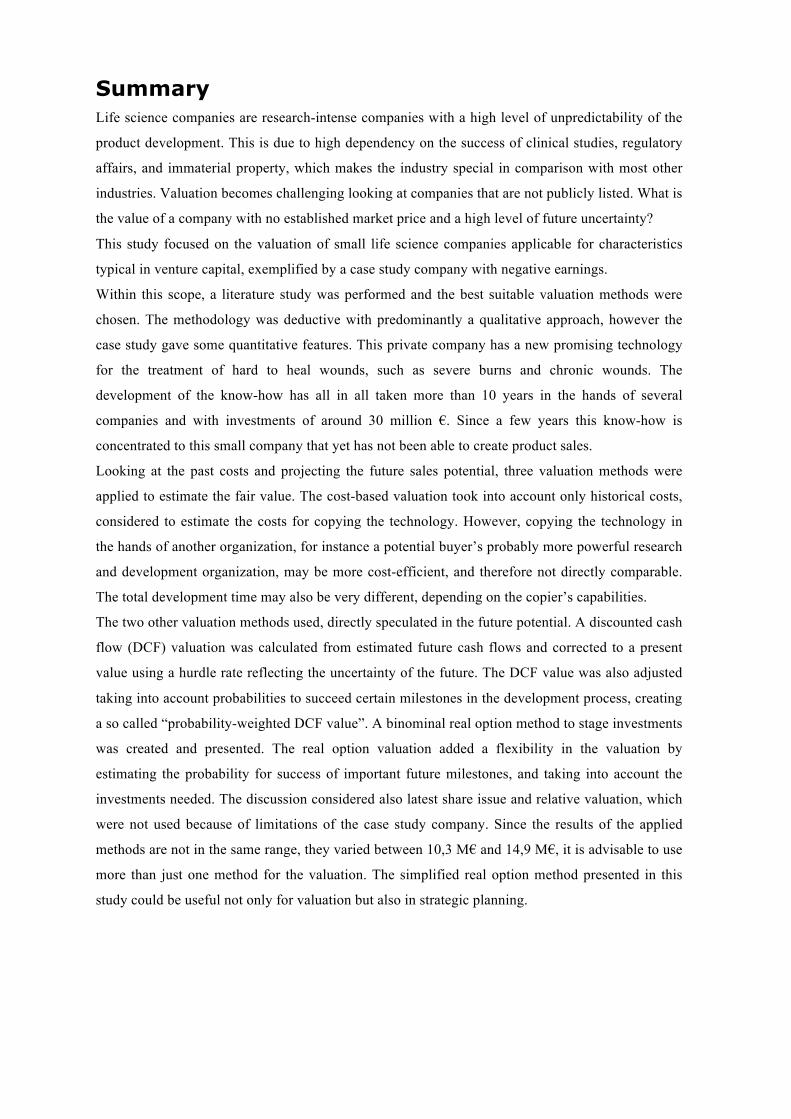
Summary Life science companies are research-intense companies with a high level of unpredictability of the

product development. This is due to high dependency on the success of clinical studies, regulatory

affairs, and immaterial property, which makes the industry special in comparison with most other

industries. Valuation becomes challenging looking at companies that are not publicly listed. What is

the value of a company with no established market price and a high level of future uncertainty?

This study focused on the valuation of small life science companies applicable for characteristics

typical in venture capital, exemplified by a case study company with negative earnings.

Within this scope, a literature study was performed and the best suitable valuation methods were

chosen. The methodology was deductive with predominantly a qualitative approach, however the

case study gave some quantitative features. This private company has a new promising technology

for the treatment of hard to heal wounds, such as severe burns and chronic wounds. The

development of the know-how has all in all taken more than 10 years in the hands of several

companies and with investments of around 30 million €. Since a few years this know-how is

concentrated to this small company that yet has not been able to create product sales.

Looking at the past costs and projecting the future sales potential, three valuation methods were

applied to estimate the fair value. The cost-based valuation took into account only historical costs,

considered to estimate the costs for copying the technology. However, copying the technology in

the hands of another organization, for instance a potential buyer’s probably more powerful research

and development organization, may be more cost-efficient, and therefore not directly comparable.

The total development time may also be very different, depending on the copier’s capabilities.

The two other valuation methods used, directly speculated in the future potential. A discounted cash

flow (DCF) valuation was calculated from estimated future cash flows and corrected to a present

value using a hurdle rate reflecting the uncertainty of the future. The DCF value was also adjusted

taking into account probabilities to succeed certain milestones in the development process, creating

a so called “probability-weighted DCF value”. A binominal real option method to stage investments

was created and presented. The real option valuation added a flexibility in the valuation by

estimating the probability for success of important future milestones, and taking into account the

investments needed. The discussion considered also latest share issue and relative valuation, which

were not used because of limitations of the case study company. Since the results of the applied

methods are not in the same range, they varied between 10,3 M€ and 14,9 M€, it is advisable to use

more than just one method for the valuation. The simplified real option method presented in this

study could be useful not only for valuation but also in strategic planning.

3

Contents 1. Background and problem statement ...................................................... 4

1.1. Objectives and research question ................................................... 6

1.2. Limitations .................................................................................. 6

2. Theory .............................................................................................. 7

2.1. Net assets valuation ..................................................................... 8

2.2. Latest share issue valuation ........................................................... 8

2.3. Cost-based valuation .................................................................... 9

2.4. DCF valuation .............................................................................. 9

2.5. Relative valuation ....................................................................... 11

2.6. Real option valuation ................................................................... 12

2.6.1. Theoretical case ....................................................................... 13

2.6.2. Binomial option pricing model .................................................... 14

3. Methods ........................................................................................... 17

3.1. Positivism, quantitative and qualitative .......................................... 17

3.2. Case study and sample ................................................................ 17

3.3. Deductivism versus inductivism ..................................................... 17

3.4. Ethics and intrinsic value .............................................................. 18

3.5. Reliability and validity .................................................................. 18

4. Empirical case: Analysis and results ..................................................... 20

4.1. Wound care technology company .................................................. 20

4.2. Net assets valuation .................................................................... 20

4.3. Latest share issue valuation .......................................................... 21

4.4. Cost-based valuation ................................................................... 21

4.5. Relative valuation ....................................................................... 22

4.6. Discounted cash flow valuation ..................................................... 22

4.6.1. Probability-weighted DCF value .................................................. 23

4.7. Real option valuation ................................................................... 24

5. Discussion and conclusions ................................................................. 29

6. Suggested further research ................................................................. 33

References .............................................................................................. 34

Appendix 1: Wound care technology company .............................................. 36

Appendix 2: The wound care market ........................................................... 37

Appendix 3: DCF prognosis ........................................................................ 38

Appendix 4: Gross value ........................................................................... 39

Appendix 5: 10 year governmental bond average ......................................... 40

Appendix 6: Real option ............................................................................ 41

4

1. Background and problem statement

Valuation of smaller, such as early stage, private companies, not yet generating profit, is a

challenge in private equity. For the venture capitalist the main objective is to make a successful

exit, in the best case, making a ”home run” giving returns of more than 25 times its capital (Fraser-

Sampson, 2011).

During the last three decades, there have been more than a handful global financial crises, mainly

due to short-term loans given by banks and companies to finance illiquid assets (Koller et al.,

2010). This means the valuation of the assets have failed, and the borrower’s assets and liabilities

were mismatched. To have an effect on global scale, the fiascos have been done with major

corporations on going-concern policy. If the world has repeatedly failed in valuation of major

going-concern companies, what about companies with negative cash flow and no profit, to be

classified as high risk investments? This segment should be especially demanding to valuate.

Moreover, common financial ratios or multiples used for stock market listed companies, like the

capital asset pricing model (CAPM) are not applicable to small companies in an early life cycle

stage (Bogdan & Villiger, 2008).

Fundaments to keep the society in continuous high economic development and sustain

competitiveness are to facilitate innovation and maintain an efficient financial market. In Europe,

the countries having the highest competitiveness scores, are firstly developed in institutional

excellence, such as giving financial support to research and development projects, secondly they

have a strong skill base through good high education and training, and thirdly, they maintain an

increased innovation capacity (Schwab, 2013). To create radical innovations firms needs to

generate ground-breaking ideas and be able to convert them into commercially competitive

advantage (Zhou & Li, 2012). In financial theory, value is created particularly if the growth strategy

is based on product innovation (Koller et al., 2010). High-tech technology companies in an early

stage usually represent a high level of innovation. One of the high-tech industries highly

represented within venture capital investments is the life science sector (Fraser-Sampson, 2011).

Fund raising, licensing, mergers & acquisitions, and portfolio management are examples of

situations were valuation is needed (Bogdan & Villiger, 2008). The high barriers in form of long

and costly R&D processes make it difficult for venture capitalist to valuate high tech companies.

There are a lot of investment opportunities currently uncharted. There is a need for valuation

methods that are suitable to these circumstances (Schneider, 2009). When it comes to healthcare

companies there is even a higher level of risk, mainly due to regulatory requirements. For

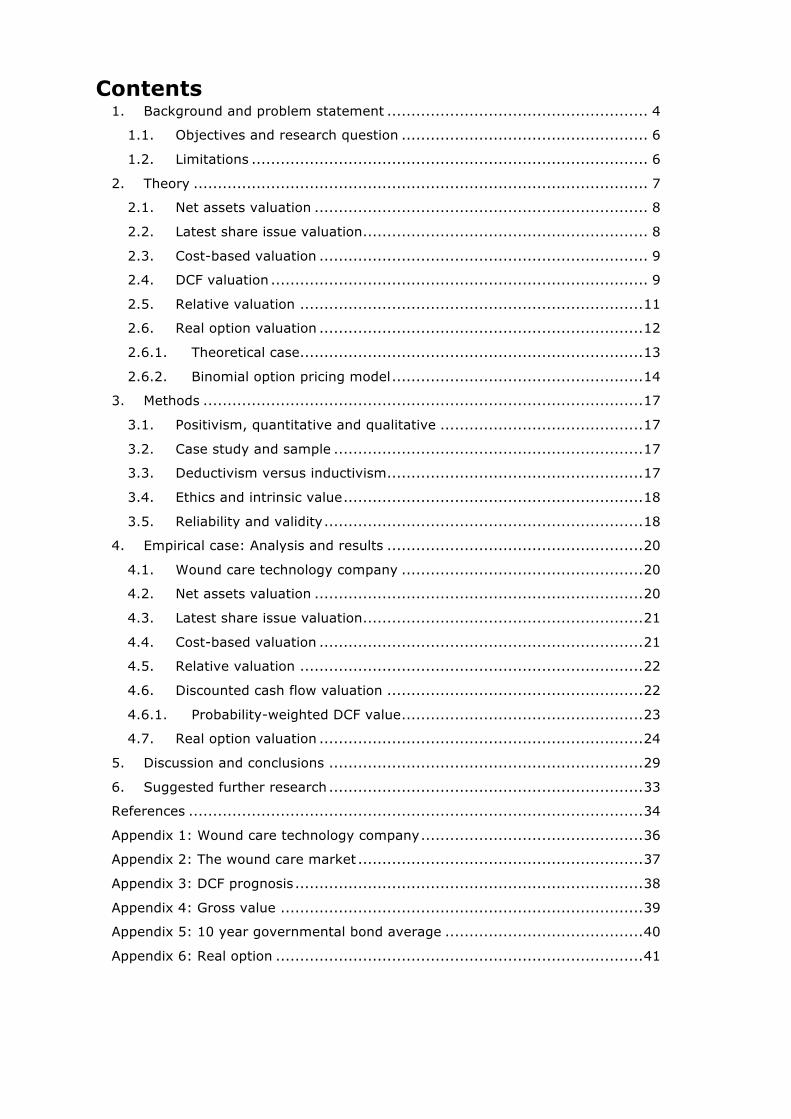
pharmaceutical products only one out of 10 000 drug candidates make it to the market, which

5

shows the high level of investment and risk that comes to hand in the industry (PhRMA, 2014;

DiMasi & Grabowski, 2007).

Figure 1: The Pharmaceutical Research and Manufacturers of America, shows in the figure above the 10 to 15 years long process of developing a drug until launch on the US market (PhRMA, 2014).

In the pharmaceutical industry, increase in shareholder wealth does not only happen when new

drugs are approved by regulatory authorities, but this is also true for just an application for an

improvement of an existing drug (Hamill et al., 2013). Simpler life science products within medical

technology, also have to be approved by regulatory bodies, and even though the approval process

might by shorter and faster, this also affects the value of the company. The approvals will often

require complicated empirical clinical studies that are very costly to perform. Lately, the economic

aspects in health care have increased importance, and therefore health economic studies is required

to show, not only the clinical benefits of a new treatment or diagnostic procedure, but also cost-

savings for society. Health care products do not only have one regulatory process to go through,

most markets have their own regulatory authorities, such as USA, European Union, Japan and

China. Since the regulatory affairs often represent a high cost for any life science company, in

practice, this means that small companies have to focus on certain markets due to limitations in

financial capability and expertise. These are special features in the healthcare industry that makes

valuation different in comparison to other research intense technology sectors.

Traditional valuation methods are considered limited in the life science field, due to long and

uncertain product development cycles with high failure rates, and undefined product and market

profiles of assets (Mayhew, 2010). There is no current established consensus of valuation methods

in life science (Bogdan & Villiger, 2008; Mayhew, 2010). In Sweden, during the last few years,

both the number of life science companies, as well as the employees working in this industry have

decreased (Sandström, 2014). This reflects the ongoing global recession in which estimating the fair

value of an investment becomes even more important.

6

This study will focus on the valuation of life science companies, exemplified by a case study

company with a new medical technology based on biomaterials. This subsector of life sciences is

sometimes called “white” biotechnology, and considered a new investment opportunity, with the

big challenge of adequate valuation of the investment (Schneider, 2009).

1.1. Objectives and research question

The aim of the study is to find suitable valuation models for small, private life science companies

with negative earnings.

The study aims to answer following questions:

• Which valuation models are relevant for small life science companies with negative

earnings?

• Which ones should be used in the valuation of the case study company?

• What challenges will the different valuation methods bring in the case study company, such

as, which input parameters should be used?

1.2. Limitations

The focus is on the life science industry, which is defined in the scope of this study as small,

research and development intensive companies focused on healthcare.

The study is within venture capital, which means private firms, often early in the life cycle, and if

the firm itself already has many years of age, it will have a new technology or significant new

products in an early development phase with a potentially high economic impact considering the

size of the company.

A wound care technology company is used as a case study to test different valuation methods,

because it is a small life science company with a new medical technology in development. The

company came into current ownership in 2009, and has had an accumulative positive cash flow, but

recently the earnings are negative. The company has a distribution-business as a way to survive, but

in other ways it is representative to a small research-intense company with a new product in

development. The case study company is giving all its hopes to a new in-licensed wound care

technology that combines with the know-how the company already has from before. The current

earnings are negative and the company is looking for financing to be able to continue with the

product development. These are reasons why the chosen case company can serve as an example

within the scope of this study. The company is located in the European Union, and all the data are

real, as given by the President, however, the name of the company is kept confidential.

7

2. Theory

What is value? Value may be very subjective. Oscar Wilde said (Wilde, 1892):

”A cynic is a man who knows the price of everything but the value of nothing.”

This could be the description of an investor meaning the value is irrelevant, as long as a bigger fool

is willing to pay more for the asset. The value of something could be a lot for one person and

nothing for another. In finance, it is crucial not to pay more for an asset than it is worth

(Damodaran, 2002). Value and valuation is an important part of today’s market economy. With

valuation we can measure and manage a company’s performance, and thereby see if value is

created. It also gives a long term view in contrast to only looking at accounting revenues (Copeland

et al., 2005).

The International Private Equity and Venture Capital Valuation Guidelines, IPEV defines the

process of valuation in the following way (IPEV, 2012):

“In estimating Fair Value for an Investment,

the Valuer should apply a technique or techniques

that is/are appropriate in light of the nature, facts

and circumstances of the Investment in the context

of the total Investment portfolio and should

use reasonable current market data and inputs

combined with Market Participant assumptions.”

In this chapter, different valuation methods are presented that may be of interest in valuation of not

listed, small life science companies. IPEV lists these valuation methods: price of recent investment

(compare to “latest share issue” in table below), multiples, net assets, discounted cash flows (DCF),

industry valuation benchmarks (compare to “relative” in table below), and available market prices

(also comparable to “latest share issue” in table below). In a literature search, the following

valuation methods have been mentioned in relevant references:

Valuation method (Mayhew, 2010)

(Bogdan & Villiger, 2008)

(Ixora, 2013)

(Damodaran, 2006)

(Sammut, 2012)

(Brantic et al., 2014)

Net Assets

X

X Latest Share Issue

X

Cost-‐Based X

DCF X X X X X X Relative X

X X X

Real Option X X

X

8

2.1. Net assets valuation

When valuing a firm, all assets will be listed, the value is estimated and also the degree of

uncertainty should be determined. Fixed assets, are long-term assets, such as plant, equipment

subject to depreciation, and buildings, and short-term assets, such as inventory, receivables and

cash. Additionally, in the balance sheet there may be assets in other firms, called financial

investments. These assets are in accounting basically valued according to historical costs or book

values. Finally, intangible assets, such as patents and trademarks, and goodwill arouse from

acquisitions, are valued. These, also called growth assets, are more difficult to value since they are

valued according to potential future earnings and cash flows created. (Damodaran, 2001)

To get the net assets value, all liabilities or debts will be subtracted from the total assets. An

adjusted net assets method values the assets and liabilities to current market values, thereby valuing

historical costs to current values.

2.2. Latest share issue valuation

Also called “price of recent investment”, the valuation of a company based on the latest share issue

in which external investors have invested new capital of a significant amount, or recent share

transactions of significant amount are commonly used in private equity and venture capital. During

the limited time following the date of the relevant transaction, the new valuation must be adjusted

according to changes or events that may influence the fair value. (IPEV, 2012)

Latest share issue valuation is frequent in valuation of life science companies (Ixora, 2013). For not

listed companies this is the only way to get a real historical price of the company, and therefore it

can be used as the base line for the current fair value of the company. However, it has to be adjusted

to significant events in time. The longer the time period since last share issue, the higher the

uncertainty of the valuation. For research intensive companies, the difficulty comes in valuing the

impact of the research and development on future cash flows since last share issue. An important

accounting effect is if the R&D has been capitalized, which means the costs have been placed in the

balance sheet as an asset. Here are different practices used within the life science industry,

pharmaceutical companies do rarely capitalize the R&D, because of the great uncertainty before

market launch, while medical technology companies may apply capitalization of R&D costs. For

small companies, not yet making profit, this may be a problem, since the assets may grow to

become very high in comparison to equity.

For a company with negative earnings, the current financial status may influence the valuation. The

more urgent the cash situation is for the company, the bigger the risk is it will be undervalued. In

venture capital the dilution of old shareholders is a typical part of the valuation game for smaller

companies in crisis.

9

2.3. Cost-based valuation

The crucial question in cost-based valuation is how much would the buyer have to invest to

reproduce the asset it is buying? What are the accumulated costs incurred? These should include all

research costs, but also licensing costs, regulatory, legal and intellectual property costs, as well as

non-recoverable taxes. In accounting terms these are book values. How long development time is

needed for copying the asset? Therefore these values may be adjusted for inflation, depreciation or

exchange-rate fluctuation (Mayhew, 2010). To conclude, this valuation is looking at the history, not

taking into account the future potential.

This study is focused on research-intense values with a high innovation level. It is probable that

these innovations should give a premium price, and therefore the future income is an important

factor. Even the time itself may have significant importance, for instance, considering time to

market in comparison to competitors, and then also potential revenue loss might be calculated as a

value. Taking these considerations into account, the cost-based valuation, or the sum of book

values, serve more as a base line, the lowest value of the asset in question. Any other values, such

as, human, market, reputation or innovation values should be added to the book values (Mayhew,

2010). From the potential buyer’s side, precaution has to be taken to count in all investments a

small life science company has invested in a certain project. Many times small companies have

inefficient organisations and the valuation should be done from the buyer’s, normally a bigger

company’s more cost-efficient organization.

2.4. DCF valuation

Discounted cash flow valuation methods value an asset by the present value of its expected cash

flows, with a discount rate that estimates the risk or these cash flows.

The enterprise DCF model uses four steps (Koller et al., 2010):

1) Discounting of free cash flow with the cost of capital.

2) Identifying and valuing non-operating assets.

3) Identifying and valuing debt and non-equity claims.

4) Subtracting the value of non-equity financial claims.

In venture capital the discount rates are of a complete different magnitude compared listed public

companies, and therefore the choice of discount rate has a fundamental influence on the valuation.

The future cash flows (CF) are estimated and discounted (kc) year by year (t), ending with an

eternal value, the so called terminal value (TV). Usually, the discounted cash flow is estimated

during the following ten years, and then adding the terminal value.

10

Formula for valuing the firm with annual cash flows plus terminal value (Damodaran, 2006):

There are several ways of calculating the terminal value, assuming a stable growth, the multiple

approach, or the liquidation value. The last one assumes the company will end the operations and it

is sold to the highest bidder. The first and second alternatives, calculate the terminal value assuming

the company will grow at a certain perpetual stable rate (g) with a certain cost of capital (r).

Formula for calculation of terminal value (Damodaran, 2006):

𝑇𝑒𝑟𝑚𝑖𝑛𝑎𝑙 𝑉𝑎𝑙𝑢𝑒 = 𝐶𝑎𝑠ℎ 𝐹𝑙𝑜𝑤!!!𝑟 − 𝑔!"#$%&

When a company’s life-cycle goes from high to stable growth, the features of the company changes.

A mature firm with a stable growth will have other expectations. It will be assumed to reinvest less,

be less risky, increase debts, etc. Concerning listed companies, Damodaran recommends using betas

closer to one when calculating required return for the terminal value (Damodaran, 2006).

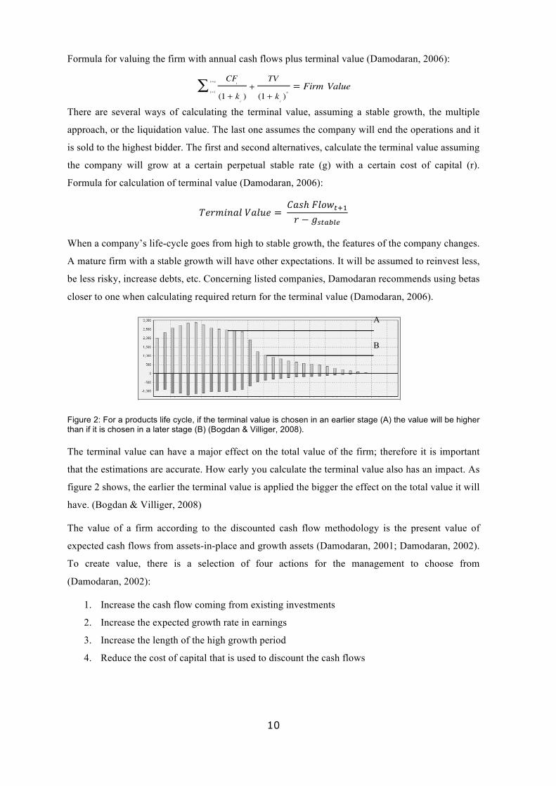
Figure 2: For a products life cycle, if the terminal value is chosen in an earlier stage (A) the value will be higher than if it is chosen in a later stage (B) (Bogdan & Villiger, 2008).

The terminal value can have a major effect on the total value of the firm; therefore it is important

that the estimations are accurate. How early you calculate the terminal value also has an impact. As

figure 2 shows, the earlier the terminal value is applied the bigger the effect on the total value it will

have. (Bogdan & Villiger, 2008)

The value of a firm according to the discounted cash flow methodology is the present value of

expected cash flows from assets-in-place and growth assets (Damodaran, 2001; Damodaran, 2002).

To create value, there is a selection of four actions for the management to choose from

(Damodaran, 2002):

1. Increase the cash flow coming from existing investments

2. Increase the expected growth rate in earnings

3. Increase the length of the high growth period

4. Reduce the cost of capital that is used to discount the cash flows

Company and Stock Valuation 197

Feed Rate and Terminal Value

The feed rate represents the ability of the company to generate or to license projects. The feed rates correspond in a way to the terminal value in standard valuation. Like terminal value, the feed rate is a very sensitive variable that can have a major impact on the value. A feed rate is however a more imag-inable parameter than a constant cash flow in 20 years from now. Imagine a company that has one extraordinary product responsible for most of its reve-nues like in the figure below. If we apply the terminal value principle at a moment when this project still strongly contributes to the company’s reve-nues (A), this implies that we assume that the company can replace this product by another of the same economic power. We can only use this as-sumption when there is an indicator that the company can indeed replace the product with a similar one. If on the other hand we apply the terminal value only once the project is off-market (B), then most other projects’ life cycles might have ended as well and the terminal value becomes too low. The ter-minal value this way might misguide and give a much too high or low value. We therefore propose to use the feed rate approach.

Fig. 4.46. Where to start assuming constant cash flows for the terminal value?

Taxes

The calculation of taxes first requires annual net cash flows. Second, we have to keep track of the accumulated losses; only once these are offset by earnings, the company starts to pay taxes. Applying the tax rate to project valuation is not a clean solution, because taxes are assessed on a company level. Earnings from one project can be used up by investments in another project. Calculating the tax value on a risk-adjusted basis is also not cor-rect as displayed in the following example: Assume a one-project com-pany. If one day it has to pay taxes, i.e. if its product reaches market, it can

A

B

CFt

(1 + kc)

t =1

t = n∑ +TV

(1 + kc)n= Firm Value

11

Revenue Growth Target Operating Margin

Applying the DCF on research intensive, small life science companies, it is easy to understand that

the value growth potential will normally be in the growth assets, that is, the new innovation coming

from research and development. Damodaran (Damodaran, 2002) concludes: “As long as the

projects, no matter how risky they are, have a marginal return on capital that exceeds their cost of

capital, they will create value.”

Damodaran (Damodaran, 2002) makes also some remarks for negative earnings firms. He says the

cash flow is dependent on three variables:

- the expected growth rate in revenues,

- the target operating margin, and

- the sales to capital ratio.

Free Cash Flow to Firm (FCFF) = EBIT (t - tax rate) – Reinvestment Needs

Figure 3: The parameters affecting the future value of a company with negative earnings (Damodaran, 2002).

The major concern with the discounted cash flow method in life science is the uncertainty, the first

being the accuracy of the estimates, for instance the unknown impact of competitor actions, and the

second is the technical uncertainty, which in worst case means the product will never be launched

on the market, for instance, due to failing of regulatory requirements (Bogdan & Villiger, 2008).

The numerous assumptions of key valuation parameters for which actual information is as yet

unknown, make DCF valuations especially controversial in the valuation of early-stage life science

companies (Mayhew, 2010). One method to give a more justified estimation is to correct the value

with probabilities to succeed in different milestones (Shockley et al., 2003).

2.5. Relative valuation

In relative valuation, like the name says, the value of an asset is estimated as relative to the market

prices of similar assets. One of the simplest examples would be to value a car, for instance a Volvo

V70, year model 2008. In this case it would be quite easy to find the current average selling price of

all cars of this year model on a specific market. This would be a good estimation of this particular

car’s value.

When talking about valuation of companies, relative valuation would mean comparing similar or

comparable companies in the same industry, and more specifically with the same type of products,

similar cash flows, company size, risks, growth, and so forth.

Sales to Capital Ratio

12

According to Damodaran (Damodaran, 2006), there are three types of relative valuation:

1. Direct comparison: Find a company (or several) that are very much alike the company to be

valued, and comparing the market value of this (these) to the analysed one.

2. Peer group average: Compare a multiple of the analysed company to a peer group of same type

of companies. The average of a sector, for instance life science, is assumed to be representative of a

typical company of that same sector.

3. Peer group average adjusted for differences: While there can be big differences between

companies of the same sector, the comparative peer group average value can be narrowed, for

instance a company with higher expected growth than the industry will be valued higher than the

industry average. For instance, by using PEG ratios, dividing PE ratios by expected growth rates,

the companies can be compared also when they have different growth rates.

Mayhew (Mayhew, 2010) calls relative valuation marked-based valuation, which he defines as the

determination of the value of an asset in comparison to a similar asset.

In publicly listed companies, relative valuation is much easier because different multiples are easily

available and they can be used to calculate averages and make comparisons.

In private equity, it is much more difficult to collect data, and therefore the comparisons may be

used with a statistically insignificant number of similar firms, therefore increasing the insecurity of

the valuation. Since the private companies are not publically traded, the valuation of them will be a

challenge.

With small research-intense companies, the relative valuation will most often be very subjective,

since finding other innovative comparable companies will be difficult. Earlier mentioned “direct

comparison” might be difficult to make. To find a recently sold, same sized, innovative life science

company within the same research field may many times be impossible. Intellectual property and

portfolios of assets represent more challenges in market-based comparisons within life sciences

(Mayhew, 2010).

Market-based comparisons or industry benchmarks are more likely to be useful as a sanity check of

other valuation methods (IPEV, 2012).

2.6. Real option valuation

A financial option is a tool that gives the holder a future right to buy or sell an asset for a certain

price. Real option is an analogy of financial options, defined as the right, but no obligation to

purchase an underlying asset during a certain period (Verdu et al., 2012). The biggest difference

13

between real options and financial options are the underlying asset. In real options, the underlying

asset doesn’t have to be financial, but could for instance be intellectual property (Cotropia, 2009).

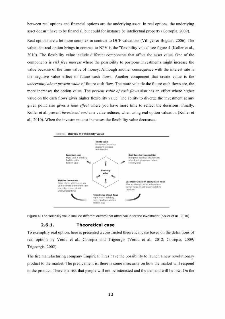
Real options are a lot more complex in contrast to DCF valuations (Villiger & Bogdan, 2006). The

value that real option brings in contrast to NPV is the ”flexibility value” see figure 4 (Koller et al.,

2010). The flexibility value include different components that affect the asset value. One of the

components is risk free interest where the possibility to postpone investments might increase the

value because of the time value of money. Although another consequence with the interest rate is

the negative value effect of future cash flows. Another component that create value is the

uncertainty about present value of future cash flow. The more volatile the future cash flows are, the

more increases the option value. The present value of cash flows also has an effect where higher

value on the cash flows gives higher flexibility value. The ability to diverge the investment at any

given point also gives a time effect where you have more time to reflect the decisions. Finally,

Koller et al. present investment cost as a value reducer, when using real option valuation (Koller et

al., 2010). When the investment cost increases the flexibility value decreases.

Figure 4: The flexibility value include different drivers that affect value for the investment (Koller et al., 2010).

2.6.1. Theoretical case

To exemplify real option, here is presented a constructed theoretical case based on the definitions of

real options by Verdu et al., Cotropia and Trigeorgis (Verdu et al., 2012; Cotropia, 2009;

Trigeorgis, 2002).

The tire manufacturing company Empirical Tires have the possibility to launch a new revolutionary

product to the market. The predicament is, there is some insecurity on how the market will respond

to the product. There is a risk that people will not be interested and the demand will be low. On the

P1: OTA/XYZ P2: ABCc32 JWBT347/Mckinsey June 9, 2010 11:45 Printer Name: Hamilton

UNCERTAINTY, FLEXIBILITY, AND VALUE 685

Flexibilityvalue

Time to expireMore time to learn about uncertainty increases flexibility value

Present value of cash flowsHigher value of underlying project cash flows increases flexibility value

Cash flows lost to competitionLosing more cash flows to competitors when deferring investment reduces flexibility value

Investment costsHigher costs of exercising flexibility reduce flexibility value

Risk-free interest rateHigher interest rate increases time value of deferral of investment—but may reduce present value of underlying cash flows

Uncertainty (volatility) about present valueMore uncertainty increases option value—but may reduce present value of underlying cash flows

EXHIBIT 32.3 –Drivers of Flexibility Value

$400 across outcomes.5 As with financial options, the value of a real optiondepends on six parameters, summarized in Exhibit 32.3.

These drivers of value show how allowing for flexibility affects the valua-tion of a particular investment project. Holding other drivers constant, optionvalue decreases with higher investment costs and more cash flows lost whileholding the option. Option value increases with higher value of the underly-ing asset’s cash flows, greater uncertainty, higher interest rates, and a longerlifetime of the option. With higher option values, a standard NPV calculationthat ignores flexibility will more seriously underestimate the true NPV.

Be careful how you interpret the impact of value drivers when designinginvestment strategies to exploit flexibility. The impact of any individual driverdescribed in Exhibit 32.3 holds only when all other value drivers remain con-stant. In practice, changes in uncertainty and interest rates not only affect thevalue of the option but usually change the value of the underlying asset aswell. When you assess the impact of these drivers, you need to assess all theireffects on the option’s value, both direct and indirect. Take the case of higheruncertainty. In our example, we increased the uncertainty of future cash flowwithout changing its expectation or present value. But if greater uncertaintylowers the expected level of cash flows or raises the cost of capital, the impacton the value of the option could be negative, because the value of the underly-ing assets declines. The same holds for the impact of an interest rate increase.

5 The current value of the underlying risky asset is the present value of expected annual cash flows of$300 into perpetuity, discounted at a 5 percent cost of capital.

14

other hand there is likelihood that people will adopt the product and that will generate a high

demand.

One option Empirical Tires has, to reduce the risk, is to patent the product for a year. During the

year they can do a market analysis on how the market will respond. Later a decision, depending on

what the feasibility report shows, can be made. In this case the cost of the option is the cost of the

patent and market analysis.

As the theoretical case above exemplifies, real options give the project manager the possibility and

flexibility to adapt to different factors in the environment that affects the project. This gives the

possibility to limit loss and expenses. In other words real options give you different decision

options (Trigeorgis, 2002).

2.6.2. Binomial option pricing model

There are several option pricing models with different complexities. Here is presented a basic,

fundamental option-pricing model. The implementation of other more complex option pricing

models are unnecessary and will not bring significance to our study. The objective is to study if real

option valuation is applicable to the case study.

The option-pricing model looks at the market as binominal. The outcomes are like a coin toss game,

where it can wither go one way or another, success of failure. The price of the coupon can either go

up or down. There are a lot of assumptions for the model to be valid. The capital market has to be

frictionless, competitive, and no risk-free arbitrage opportunities can exist. There have to be

continuous trading opportunities. Stock price, needs to obey a multiplicative binomial generating

process, this implies that the stock prices can’t be below zero, no matter how many periods there

are. The pay-off for a one period call option is described as:

𝑓 = 𝑒!!∆!(𝑝𝑓! + 1 − 𝑝 𝑓! Where 𝑝 = !!∆!!!!!!

(Hull, 2012)

When adapting Hull’s formula to real options, f is the same as the expected net present value

(ENPV). To calculate the value needed to know how to estimate the inputs d and u. Hull gives the

definition𝑠 𝑢 = 𝑒ℴ ∆! and 𝑑 = 𝑒!ℴ ∆! where the standard deviation is of the price in the underlying

asset during the period (Hull, 2012).

S = The current value of the underlying asset, usually the current stock price.

K = Strike price of the option is the price that the buyer needs to pay to exercise the option.

rf = The risk free rate of return, usually a 10-year government bond.

σ = The volatility of the underlying asset, which means the fluctuations of its price.

ENPV fu =Max[0,uS−k]

fd =Max[0,dS−k]

15

T = The time to maturity. The time until the option can be exercised.

𝑓 = The option value of the company in the period.

p = The probability for an upward movement, where 1-p is the probability for an downward

movement.

Another model for estimating the value of an option is the Black & Scholes model. The

assumptions are similar of the binominal option-pricing model based on a portfolio consistent of the

underlying asset and a risk free asset with the same cash flows. Black & Scholes use a couple of

assumptions that limit the model. For instance stock price follows a Geometric Brownian Motion

with the population mean and standard deviation being constant. Another assumption is that the

risk-free interest rate is constant and the same for all maturities. The model also assumes that there

are no transaction costs or taxes. Finally the model is designed to measure the value of an option

that can only be exercised on the time of expiration and where the underlying asset do not pay any

dividends. (Damodaran, 2006)

When valuing the flexibility value in a real option, there are different alternative approaches

depending on each situation and the options of the company. Bogdan & Villiger (Bogdan &

Villiger, 2008) present a summary:

Option to defer – The option to postpone an investment. If an investment is uncertain, waiting for

indications that the investment will succeed on the market could bring an added value.

Option to expand or contract – The company’s ability to adapt to the market expectations adds a

value. If the production exceeds the expected demand, the ability to meet the expectations by e.g.

having larger plants adds a value.

Option to abandon or license – If a project is not succeeded, the company may have the option to

abandon the project. “The more reversible the investments, the higher the salvation.”

Option to switch – The flexibility to switch location or switch production have an effect on the

production cost or revenue.

Option to stage investments – In each time step the investment is evaluated and a decision is made

to either continue or abandon the investment, depending on the new learned facts at each stage. This

is a common method used in R&D projects and start-ups (Bogdan & Villiger, 2008).

Option to grow – A company who has the possibility to expand into new markets or geographical

areas. The structure is similar to stage investments, where the option is evaluated from the facts

given from previous stage. While staged investments is considered as a multi-stage, growth options

are usually based on a single-stage option.

16

A company can have several options and each option adds a value to the net present value of the

company. The value of the company with the option is called the expected net present value, ENPV

(Damodaran, 2006).

17

3. Methods 3.1. Positivism, quantitative and qualitative

The human’s learning capacity and ability to reason has given rise to science. Modern science was

developed through scientists like Galileo Galilei (1564-1642) and Isaac Newton (1642-1727), and

from the natural sciences evolved social sciences. Starting with Voltaire’s claim that the tiny human

being has to follow the universal laws also in his thoughts, August Compte developed the

philosophy that is called positivism. In a simplified form it means that social science studies use

natural scientific methods, like quantification, to measure results and use logical reasoning to

establish conclusions. This study is using mathematics for creating values, these are compared with

each other, and logical conclusions are made, making the methodology positivistic. (Williams,

1999)

This study is principally quantitative, but since the research contains a case study, where data is

collected through interviews, a part of the study may also be considered qualitative.

3.2. Case study and sample

According to Robert Yin, the case study is a suitable research strategy when:

“a `how´ or `why´ question is being asked about a contemporary set of events over which the investigator has little or no control.” (Yin, 1994)

In chapter 1.1 a few research questions have been asked. If we try to rephrase them to fit Yin’s

definition they would be:

- How can a small life science company be valuated?

- Why should we choose a certain venture capital valuation technique?

It seems these questions fits very well to the objectives of this study, and while the investigators are

only observing, not influencing on-going events, hence, it is possible to use a case study approach.

However, using more than one case study would increase the validity of the conclusions.

A common concern about case studies is how you may make generalizations, especially in this case

where only one “experiment” is used? According to Yin (Yin, 1994), the case study, like the

experiment, does not represent a “sample”, and the reserachers’ purpose is to make an analytic

generalization, to expand and generalize theories, and not to make a statistical generalization, such

as enumerate frequencies.

3.3. Deductivism versus inductivism

Deductivism means that a certain theory is used as a basis, an analysis is done and the results give

logical conclusions of the theory. A theoretical hypothesis can be confirmed or abandoned through

adapted experiments, calculations or observations. The opposite methodology is called inductivism,

where a lot of observations or measurements are collected and based on the results and an analysis,

18

a theory will be developed. This study uses a deductive approach. Based on the knowledge and

experience of the researchers and literature studies, a number of theoretical models are chosen that

will be tested on a real case, and the results will be discussed leading to conclusions of the validity

of the theory.

3.4. Ethics and intrinsic value

G. E. Moore was one of the greater philosophers in Anglo-American moral philosophy in the first

half of the 20th century. In his works about ethics, Moore rebutted egoism and claimed that it is

always our duty to perform that action, of the various ones open to us, the total consequences of

which will have the greatest intrinsic value (Moore & Shaw, 2005). In the world of finance,

intrinsic value means the extra value of a company or an asset taking into account both tangible and

intangible factors, and comparing them to current market value. Taking a call option as an example,

the intrinsic value is the difference between the price of the option and the current stock’s price. If

the call options strike price is 100 and the stock’s price is 150, then the intrinsic value of the call

option is 50. A correct valuation will reveal if this is true or not. Going back to Moore, it can be

claimed that the company’s duty is to perform all those actions that lead to the highest possible

intrinsic value.

Research ethics is not a clearly defined area, but an obvious part deals with following current laws.

In any research, special consideration is put into not harming any individual, physically,

psychologically or legally. In this research a case study company is used, and on the request of the

company’s owner, the company and the owner are anonymous. This is ethical. However, a problem

rises if anyone wants to check the data, because this will not be possible (Gustafsson et al., 2011).

Anyhow, the company is registered within the European Union, and the accounting follows national

laws. Yet, some of the data comes from companies not existing any more, and therefore not

checked by the researchers, and here the resource, the owner of the case study company is trusted.

3.5. Reliability and validity

When using a qualitative approach it is important that the study is reliable and valid. This affect the

study´s generalizability and to avoid being biased (Hammersly, 1992). With reliability means how

reliable the data is and how it has been collected and processed (Holme & Solvang, 1997). By

having direct contact with the President of the company, this primary source increases the reliability

of the study. However, it has to be taken into account that by using the company itself as a source,

the collected data on the estimated earnings could be subjectively biased.

Is this study really studying what it says it is, that is, different relevant valuation methods? The

reliability is increased by referring to earlier peer-reviewed studies. The more research has been

done on the subject, the more reliable should the use of the same methods be. By creating a new

19

model that has the properties it can be repeated by other researchers, the reliability can be

confirmed in the future.

Validity means a stable logical consequence, in its absolute form, a universal truth. Internal validity

means how stable a causal relation is between two variables, in this study how truthful the different

valuations are. This becomes a problem, since we do not know the truth, which in this case would

be the price someone would pay for the case study company. There is no stock market price for the

shares of the company, so in these terms the results of the valuations can not be compared to a

“truth”. External validity means how general the internal validity can be in other similar situations.

The internal validity in the scope of this study could mean how valid the valuation models are in

small life science companies in venture capital. The external validity could mean how valid the

valuation models are for similar small research-intense companies, still in a venture capital setting,

but in another industry, for instance other technology sectors. In this study the validity lies in the

discussion and its comparison to theory.

The study contains a lot of data based on subjective assumptions, and should these be changed, the

results would be different. However, the theoretical study in combination with an analysis of a real

case, and the following discussion should give conclusions ethically defendable, as long as,

wherever uncertainty can be suspected, it is spelled out. The conclusions of the case study are

generalizable to theoretical propositions and not to populations (Yin, 1994). The final validity is in

the eyes and the judgement of the reader, in relation to what the reader is investigating. The authors

hope this study will give valuable insight in the chosen subject.

20

4. Empirical case: Analysis and results The case study company will be valued using the most appropriate valuation methods identified in

the theory chapter (IPEV, 2012).

4.1. Wound care technology company

As a case study, a small life science company is used. See also appendixes 1 and 2. The name of the

company is confidential. The history of the company goes back to a larger international corporation

focused on a biodegradable polymer technology with a large number of patents. The case study

company was originally a subsidiary of the mother company, however, after the owners decided to

close down the mother company, the President of the daughter company was offered to make a

management buy-out of the daughter company. This happened in 2009, and this company is now in

many ways comparable to a start-up company within the life science field. It has a new technology

that is not yet launched on the market, and the current earnings are negative.

The company has two principal competence and know-how areas:

- Biodegradable polymers, originally the mother company’s know-how.

- Medical cellulose, a new technology fitting into the field of polymers, licenced in 2012

from the owners of a bankrupt company that was developing this technology during many

years.

Additionally, the company has a distribution activity, which is merely for financing the

development of the new technologies. However, this is not enough, and the company is looking for

external financing to be able to speed up the development process. The first product is based on a

material the company calls medical cellulose that is shown through clinical studies to be very good

for the treatment of severe wounds. The first indication would be for the treatment of 3rd degree

burns. The second product would be for the treatment of chronic wounds. The projected sales of

both these products are included in the prognosis presented in appendix 3. In the prognosis, no

financial figures concerning the distribution business is taken into consideration, the calculations

only include figures related to revenues and costs for the new technologies in development, as

presented in appendix 1.

4.2. Net assets valuation

For any small company with negative earnings the net assets will probably be low. The value in the

company will not be in current assets, but in the future earnings. This will be especially true for a

research-intense life science company, where future milestones, like regulatory approvals and

clinical studies will give a high future value. An adjusted net assets method that values the assets

21

and liabilities to current market values is doubtfully more appropriate, since still the impact of

future research and development results will not be taken into account. The particular case study

company does not have any current intellectual property with book values, nor are there any

goodwill. Therefore, other valuation methods will give a more accurate result and net assets

valuation will not be used for the valuation of the case study.

4.3. Latest share issue valuation

Latest share issue valuation is not used for the valuation of the particular case study in the scope of

this study, because the case study company is privately owned and it has been owned by the same

owner during its whole history, and therefore there are no share issues done.

4.4. Cost-based valuation

The President of the Wound care technology company says:

“It will be difficult and very time consuming to try to copy the present technology. For a competitor to copy our material, both time consuming development work, as well as even more time consuming clinical testing, will be required for approval of a new product. It would be much more efficient to acquire a license to the production recipes from us.”

A valuation based on historical costs is one way of valuing the company. The challenge is to find

information of the actual costs incurred for the development of the technology that has been done in

several companies not existing anymore. Best estimates have been done in collaboration with the

President of the case study company. The estimates are considered as quite accurate.

The R&D costs for the polymer part, 2004-2013: 3,18 M€.

EU and governmental support, 2002-2011: 0,9 M€. However, these are already included in the

R&D costs and should not be included once more.

The least exact estimate in the cost-based valuation is the R&D costs for the development of the

medical cellulose technology before licensing of the product: 3,0 M€.

Earlier in the history, the case study company had a mother company, in which approximately

30 M€ was invested. Of this sum 12 M€ was invested in a pilot factory and its equipment, leaving

18 M€ for the development of the biodegradable polymer technology.

In the analysis, it seems reasonable to take into account all direct R&D costs of the Wound Care

Company itself, both for the polymer technology and the cellulose technology, since the company

claims there is a combined value, despite the fact that the first product will be based only on the

medical cellulose. The mother company´s pilot factory and the production process know-how

derived from there, certainly has also a value, but 18 M€ seems too high. Because this mother

company is no longer registered, there are no figures available for analyse the total costs in more

detail. An estimate is to value the know-how to 20% of the total value, which gives 3,6 M€.

22

The patents are all expired, and there is certainly immaterial value in the company’s know-how.

However, since there are no immaterial values in the balance sheet, the value of the know-how is

estimated to be included in the R&D costs. This becomes a weakness of the valuation.

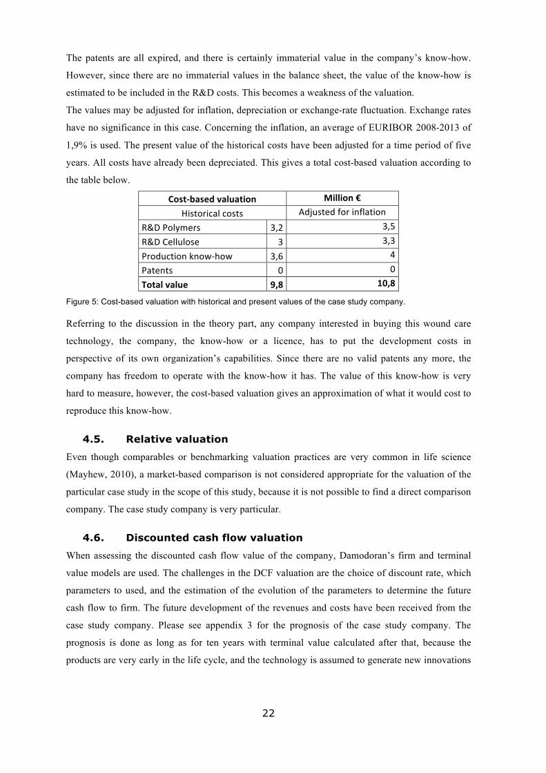
The values may be adjusted for inflation, depreciation or exchange-rate fluctuation. Exchange rates

have no significance in this case. Concerning the inflation, an average of EURIBOR 2008-2013 of

1,9% is used. The present value of the historical costs have been adjusted for a time period of five

years. All costs have already been depreciated. This gives a total cost-based valuation according to

the table below.

Cost-‐based valuation Million € Historical costs Adjusted for inflation

R&D Polymers 3,2 3,5 R&D Cellulose 3 3,3 Production know-‐how 3,6 4 Patents 0 0 Total value 9,8 10,8

Figure 5: Cost-based valuation with historical and present values of the case study company.

Referring to the discussion in the theory part, any company interested in buying this wound care

technology, the company, the know-how or a licence, has to put the development costs in

perspective of its own organization’s capabilities. Since there are no valid patents any more, the

company has freedom to operate with the know-how it has. The value of this know-how is very

hard to measure, however, the cost-based valuation gives an approximation of what it would cost to

reproduce this know-how.

4.5. Relative valuation

Even though comparables or benchmarking valuation practices are very common in life science

(Mayhew, 2010), a market-based comparison is not considered appropriate for the valuation of the

particular case study in the scope of this study, because it is not possible to find a direct comparison

company. The case study company is very particular.

4.6. Discounted cash flow valuation

When assessing the discounted cash flow value of the company, Damodoran’s firm and terminal

value models are used. The challenges in the DCF valuation are the choice of discount rate, which

parameters to used, and the estimation of the evolution of the parameters to determine the future

cash flow to firm. The future development of the revenues and costs have been received from the

case study company. Please see appendix 3 for the prognosis of the case study company. The

prognosis is done as long as for ten years with terminal value calculated after that, because the

products are very early in the life cycle, and the technology is assumed to generate new innovations

23

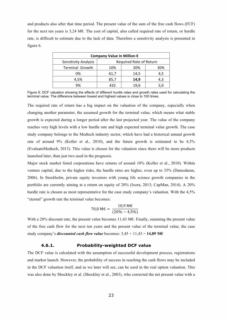
and products also after that time period. The present value of the sum of the free cash flows (FCF)

for the next ten years is 3,24 M€. The cost of capital, also called required rate of return, or hurdle

rate, is difficult to estimate due to the lack of data. Therefore a sensitivity analysis is presented in

figure 6.

Company Value in Million € Sensitivity Analysis Required Rate of Return Terminal Growth 10% 20% 30%

0% 61,7 14,5 4,5 4,5% 85,7 14,9 4,3 9% 432 19,6 5,0

Figure 6: DCF valuation showing the effects of different hurdle rates and growth rates used for calculating the terminal value. The difference between lowest and highest values is close to 100 times.

The required rate of return has a big impact on the valuation of the company, especially when

changing another parameter, the assumed growth for the terminal value, which means what stable

growth is expected during a longer period after the last projected year. The value of the company

reaches very high levels with a low hurdle rate and high expected terminal value growth. The case

study company belongs to the Medtech industry sector, which have had a historical annual growth

rate of around 9% (Koller et al., 2010), and the future growth is estimated to be 4,5%

(EvaluateMedtech, 2013). This value is chosen for the valuation since there will be more products

launched later, than just two used in the prognosis.

Major stock market listed corporations have returns of around 10% (Koller et al., 2010). Within

venture capital, due to the higher risks, the hurdle rates are higher, even up to 35% (Damodaran,

2006). In Stockholm, private equity investors with young life science growth companies in the

portfolio are currently aiming at a return on equity of 20% (Ixora, 2013; CapMan, 2014). A 20%

hurdle rate is chosen as most representative for the case study company’s valuation. With the 4,5%

“eternal” growth rate the terminal value becomes:

70,8 M€ = 10,9 M€

(20% − 4,5%)

With a 20% discount rate, the present value becomes 11,43 M€. Finally, summing the present value

of the free cash flow for the next ten years and the present value of the terminal value, the case

study company’s discounted cash flow value becomes: 3,45 + 11,43 = 14,89 M€

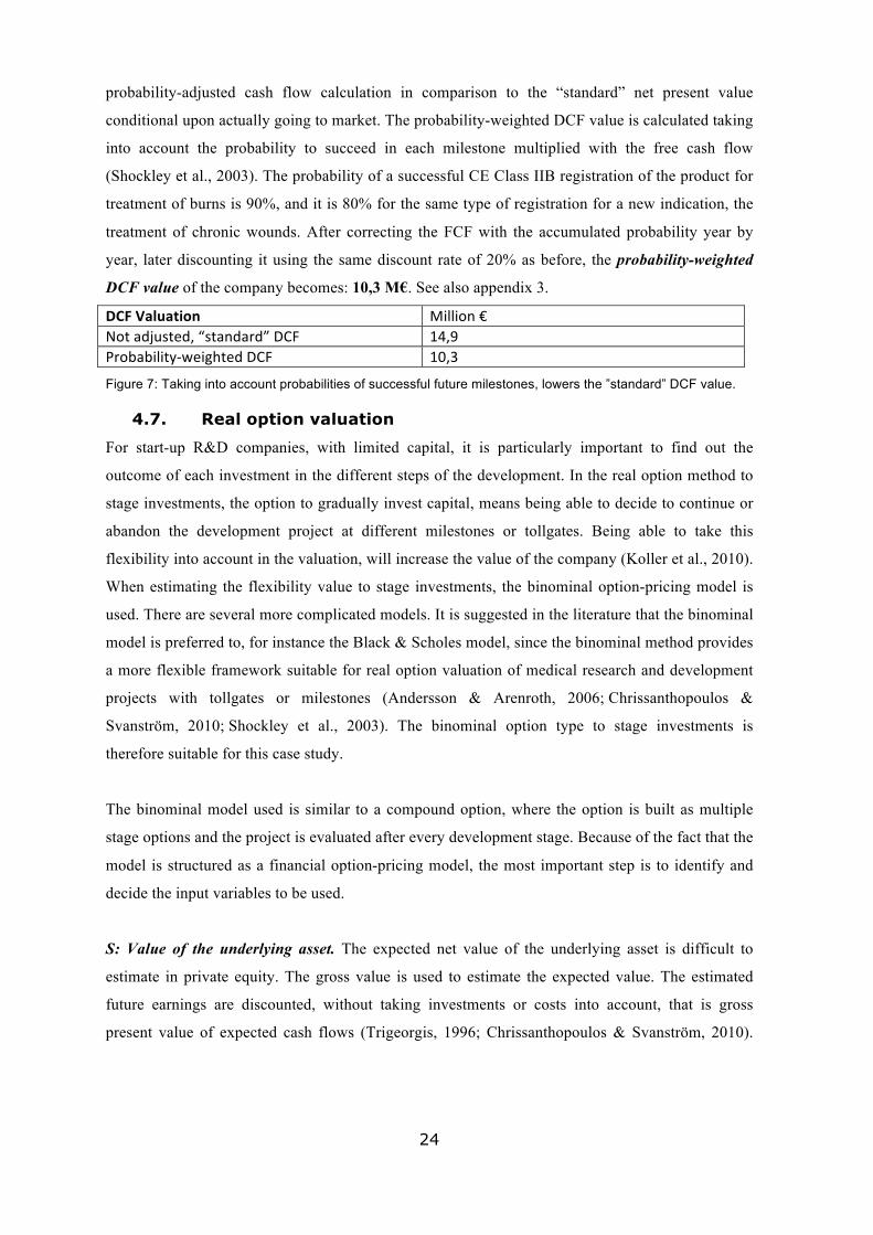
4.6.1. Probability-weighted DCF value

The DCF value is calculated with the assumption of successful development process, registrations

and market launch. However, the probability of success in reaching the cash flows may be included

in the DCF valuation itself, and as we later will see, can be used in the real option valuation. This

was also done by Shockley et al. (Shockley et al., 2003), who corrected the net present value with a

24

probability-adjusted cash flow calculation in comparison to the “standard” net present value

conditional upon actually going to market. The probability-weighted DCF value is calculated taking

into account the probability to succeed in each milestone multiplied with the free cash flow

(Shockley et al., 2003). The probability of a successful CE Class IIB registration of the product for

treatment of burns is 90%, and it is 80% for the same type of registration for a new indication, the

treatment of chronic wounds. After correcting the FCF with the accumulated probability year by

year, later discounting it using the same discount rate of 20% as before, the probability-weighted

DCF value of the company becomes: 10,3 M€. See also appendix 3.

DCF Valuation Million € Not adjusted, “standard” DCF 14,9 Probability-‐weighted DCF 10,3

Figure 7: Taking into account probabilities of successful future milestones, lowers the ”standard” DCF value.

4.7. Real option valuation

For start-up R&D companies, with limited capital, it is particularly important to find out the

outcome of each investment in the different steps of the development. In the real option method to

stage investments, the option to gradually invest capital, means being able to decide to continue or

abandon the development project at different milestones or tollgates. Being able to take this

flexibility into account in the valuation, will increase the value of the company (Koller et al., 2010).

When estimating the flexibility value to stage investments, the binominal option-pricing model is

used. There are several more complicated models. It is suggested in the literature that the binominal

model is preferred to, for instance the Black & Scholes model, since the binominal method provides

a more flexible framework suitable for real option valuation of medical research and development

projects with tollgates or milestones (Andersson & Arenroth, 2006; Chrissanthopoulos &

Svanström, 2010; Shockley et al., 2003). The binominal option type to stage investments is

therefore suitable for this case study.

The binominal model used is similar to a compound option, where the option is built as multiple

stage options and the project is evaluated after every development stage. Because of the fact that the

model is structured as a financial option-pricing model, the most important step is to identify and

decide the input variables to be used.

S: Value of the underlying asset. The expected net value of the underlying asset is difficult to

estimate in private equity. The gross value is used to estimate the expected value. The estimated

future earnings are discounted, without taking investments or costs into account, that is gross

present value of expected cash flows (Trigeorgis, 1996; Chrissanthopoulos & Svanström, 2010).

25

The same discount factor as in the DCF-model of 20% is used to make comparison easier. The

gross value is estimated to 20 M€. See appendix 4.

σ: Volatility: The volatility of the asset, in this case based on the future earnings, is another variable

that is difficult to estimate. This has been criticized against using real options in valuation (Amram

& Kulatilaka, 2000). Villiger & Bogdan (Villiger & Bogdan, 2006) suggest that the volatility

should be between 30-40% for biomedical companies. In this study, 30% is chosen. Nonetheless,

the final result is not sensitive to changes in volatility (Shockley et al., 2003).

K: Strike price: The strike price in real option is the total new capital investments to reach the

milestones successfully (Damodaran, 2002). In this case, 2,7 M€ is needed to invest in the CE

registrations, including clinical trials needed and the automation of the production. This total

investment is divided in three parts and invested at different stages in time.

Time to maturity: The time for expiration is the period until the final milestone. In this case the

product hits the market at a very early stage as a bandage for burn wounds. To achieve the total

estimated earnings, the product needs to be approved for chronic wounds in year five. This is

important for the whole prognosis, since the new indication, treatment of chronic wounds, will

reach at least double the sales compared to the first indication, treatment of severe burns. Time to

maturity in this calculation is until the 5:th year when both CE Class IIB approvals are made for

both indications, which coincides with automation of the small-scale production and a positive cash

flow. After this point in time, the risk for failure of the whole project, and in worst case bankruptcy

of the company, is much smaller.

∆𝑡: Time step: The time is divided in steps according to when the value may go up or down. For a

listed company, this may be every day the stock can be bought or sold. However, in private equity

the period may follow events in the scenario, such as milestones, investments and/or sales. One

time step is the time between two nodes in the binominal tree (Bogdan & Villiger, 2008). In this

study, one time step equals to one year. However, the number of periods or the length of the time

steps do not affect much the final option value (Shockley et al., 2003).

r: Risk free rate: 10 year governmental bond average of the EU countries: 3,25% is used as the risk

free rate, since the case study company is registered within the EU and inside the Euro monetary

system. See appendix 5.

26

EPNV: Expected present net value is the value of the probability weighted net present value plus

the option value.

After deciding the variables, the probability and the structure of the binominal option tree is

calculated. The up and down movements of the binominal tree with the chosen volatility and time

to expiration is: 𝑢 = 𝑒!"% ! ≈ 1,35 and 𝑑 = !!= !

!,!"≈ 0,74

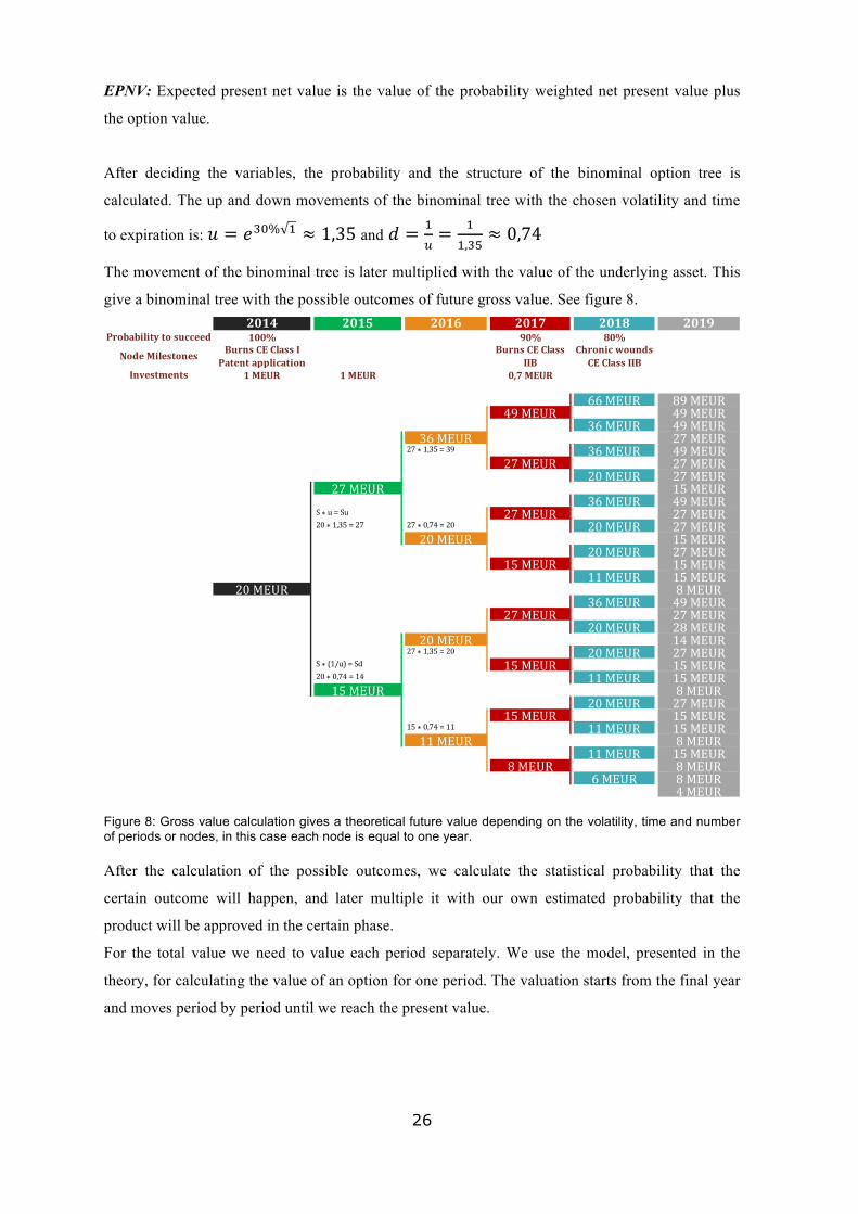
The movement of the binominal tree is later multiplied with the value of the underlying asset. This

give a binominal tree with the possible outcomes of future gross value. See figure 8.

Figure 8: Gross value calculation gives a theoretical future value depending on the volatility, time and number of periods or nodes, in this case each node is equal to one year.

After the calculation of the possible outcomes, we calculate the statistical probability that the

certain outcome will happen, and later multiple it with our own estimated probability that the

product will be approved in the certain phase.

For the total value we need to value each period separately. We use the model, presented in the

theory, for calculating the value of an option for one period. The valuation starts from the final year

and moves period by period until we reach the present value.

2014 2015 2016 2017 2018 2019Probability to succeed 100% 90% 80%

Investments 1 MEUR 1 MEUR 0,7 MEUR

66 MEUR 89 MEUR49 MEUR 49 MEUR


27 * 1,35 = 39 36 MEUR 49 MEUR27 MEUR 27 MEUR


36 MEUR 49 MEURS * u = Su 27 MEUR 27 MEUR20 * 1,35 = 27 27 * 0,74 = 20 20 MEUR 27 MEUR





20 MEUR 14 MEUR27 * 1,35 = 20 20 MEUR 27 MEUR

S * (1/u) = Sd 15 MEUR 15 MEUR20 * 0,74 = 14 11 MEUR 15 MEUR15 MEUR 8 MEUR


15 * 0,74 = 11 11 MEUR 15 MEUR11 MEUR 8 MEUR


6 MEUR 8 MEUR4 MEUR

Node Milestones Burns CE Class I Patent application

Burns CE Class IIB

Chronic wounds CE Class IIB

27

𝑝 = (!!∆! –!)(!!!)

𝑝! = (!!,!"%∗!!!,!")(!,!"!!,!")

≈ 0,48 𝑝! = 1 − (!!,!"%∗!!!,!")(!,!"!!,!")

=0,52

When the probability of each outcome is calculated we subtract the investment needed for the

project to take place. Later we add our estimated probability that the clinical testing and registration

will be successful. For instance, for 2018 we have no investment to subtract but we need to take

account for the CE Class IIB for Chronic wounds which is estimated to have 80% chance of

success. For 2017 on the other hand we also have 0,7 M€ to subtract from the total value,

additionally taking into account the 90% probability to succeed with the node milestone. The

expected net present value is calculated (Chrissanthopoulos & Svanström, 2010):

𝐸𝑁𝑃𝑉 = 𝑒!!∆![(𝑝𝑢 + 1 − 𝑝 𝑑] ∗ 𝑝𝑟𝑜𝑏𝑎𝑏𝑖𝑙𝑖𝑡𝑦 𝑡𝑜 𝑠𝑢𝑐𝑐𝑒𝑒𝑑 − 𝐾

The highest value in 2018 will be:

53 = 𝑒!!,!"%∗! ∗ 0,48 ∗ 89 + 0,52 ∗ 49 ∗ 80% − 0

In the same way the value for each outcome in 2017 is calculated. Consequently, the value for each

period is then calculated for all the years with the basis from the previous year. See also appendix 6.

Figure 9: Starting from the future gross value of 89 M€, the final expected net present value is received after all milestones taking into account the probabilities of up and down going time steps, as well as the probability of success in each milestone.

2014 2015 2016 2017 2018 2019Probability to succeed 100% 90% 80%

Investments 1 MEUR 1 MEUR 0,7MEUR 53 EUR

0,968*((0,48*89)+(0,52*49))*80%-‐0= 53 MEUR0,968*((0,48*53)+(0,52*29))*90%-‐0,7= 34 MEUR 53 MEUR 89 MEUR








11,5 MEUR 8 MEUR29 MEUR 49 MEUR








0,968*((0,48*8)+(0,52*4))*80%-‐0= 5 MEUR 4 MEUR

Chronic wounds CE Class IIBNode Milestones Burns CE Class I

Patent applicationBurns CE Class

IIB

28

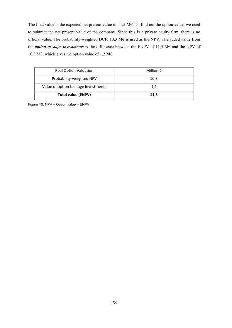
The final value is the expected net present value of 11,5 M€. To find out the option value, we need

to subtract the net present value of the company. Since this is a private equity firm, there is no

official value. The probability-weighted DCF, 10,3 M€ is used as the NPV. The added value from

the option to stage investments is the difference between the ENPV of 11,5 M€ and the NPV of

10,3 M€, which gives the option value of 1,2 M€.

Real Option Valuation Million €

Probability-‐weighted NPV 10,3 Value of option to stage investments 1,2

Total value (ENPV) 11,5

Figure 10: NPV + Option value = ENPV

29

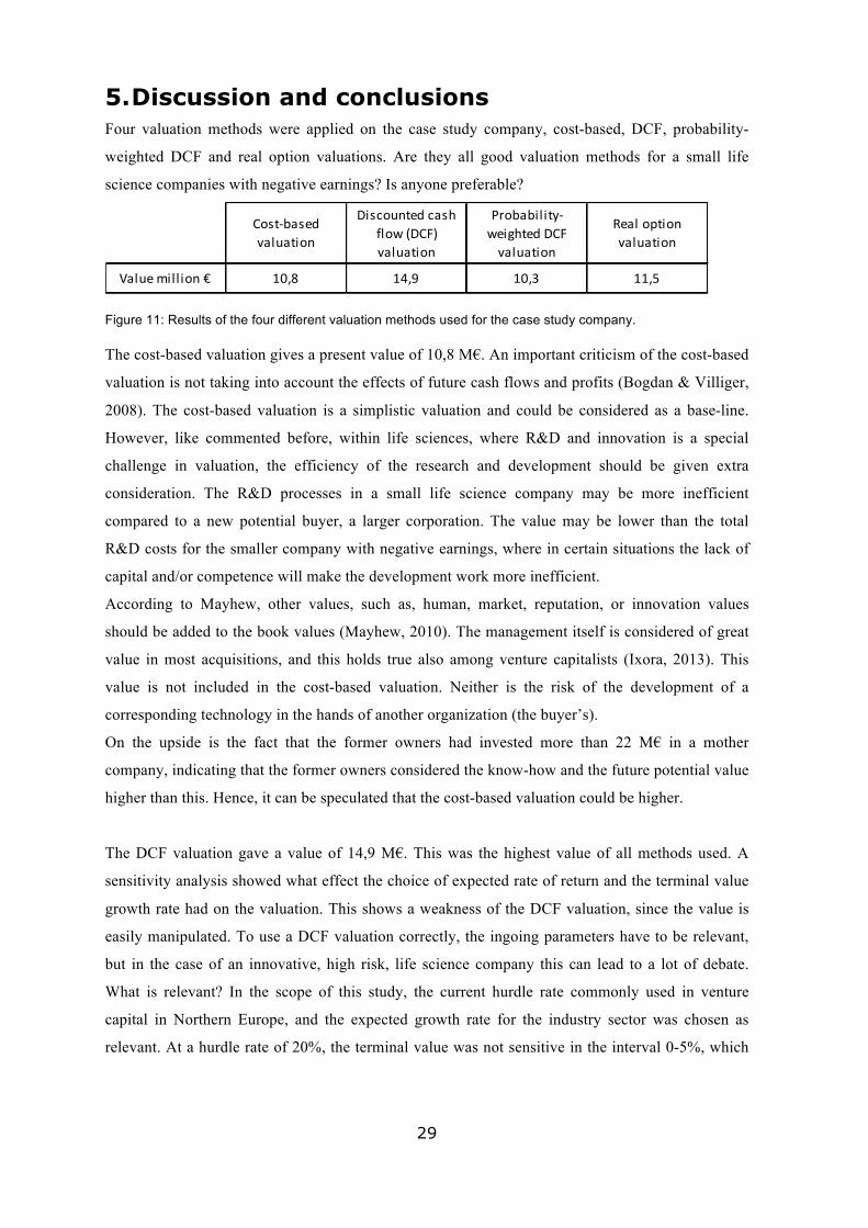
5. Discussion and conclusions Four valuation methods were applied on the case study company, cost-based, DCF, probability-

weighted DCF and real option valuations. Are they all good valuation methods for a small life

science companies with negative earnings? Is anyone preferable?

Figure 11: Results of the four different valuation methods used for the case study company.

The cost-based valuation gives a present value of 10,8 M€. An important criticism of the cost-based

valuation is not taking into account the effects of future cash flows and profits (Bogdan & Villiger,

2008). The cost-based valuation is a simplistic valuation and could be considered as a base-line.

However, like commented before, within life sciences, where R&D and innovation is a special

challenge in valuation, the efficiency of the research and development should be given extra

consideration. The R&D processes in a small life science company may be more inefficient

compared to a new potential buyer, a larger corporation. The value may be lower than the total

R&D costs for the smaller company with negative earnings, where in certain situations the lack of

capital and/or competence will make the development work more inefficient.

According to Mayhew, other values, such as, human, market, reputation, or innovation values

should be added to the book values (Mayhew, 2010). The management itself is considered of great

value in most acquisitions, and this holds true also among venture capitalists (Ixora, 2013). This

value is not included in the cost-based valuation. Neither is the risk of the development of a

corresponding technology in the hands of another organization (the buyer’s).

On the upside is the fact that the former owners had invested more than 22 M€ in a mother

company, indicating that the former owners considered the know-how and the future potential value

higher than this. Hence, it can be speculated that the cost-based valuation could be higher.

The DCF valuation gave a value of 14,9 M€. This was the highest value of all methods used. A

sensitivity analysis showed what effect the choice of expected rate of return and the terminal value

growth rate had on the valuation. This shows a weakness of the DCF valuation, since the value is

easily manipulated. To use a DCF valuation correctly, the ingoing parameters have to be relevant,

but in the case of an innovative, high risk, life science company this can lead to a lot of debate.

What is relevant? In the scope of this study, the current hurdle rate commonly used in venture

capital in Northern Europe, and the expected growth rate for the industry sector was chosen as

relevant. At a hurdle rate of 20%, the terminal value was not sensitive in the interval 0-5%, which

Value million € 10,8 14,9 11,5

Cost-‐based valuation

Discounted cash flow (DCF) valuation

Real option valuation

Probability-‐weighted DCF valuation

10,3

30

gives confidence to the final valuation of 14,9 M€. However, it must be emphasized that if the

expected rate of return is 30%, the value of the company drops to 4-5 M€. If the case study

company is for sale, a large corporation within the industry that has a lot of competence and capital,

will probably require a lower hurdle rate, since the share size and capabilities of the buyer will

lower the risks for the acquisition. In this case a 20% hurdle is reasonable, some might even

consider it high.

Another issue with the DCF valuation is the estimation of the future cash flows and revenues. In

this case study there was no historical data to be beneficial for the prognosis. Usually the historical

sales development is the starting point of the estimation. The new technology is yet not in a life

cycle stage to create revenues. The uncertainty of DCF valuation is particularly questioned within

an industry where unsuccessful clinical trials can suddenly lead to abandonment of the project

(Villiger & Bogdan, 2006). In discussion with the President, the future revenue and earnings margin

were estimated. As the future earnings have a big effect on the value of the company, the

estimations need to be accurate and could also be influenced by biased and subjective assumptions.

For a bigger company with a long history of different product life-cycles, the future projections will

be more trustworthy. On the other hand, the increased risk of the correctness of the prognosis is

reflected in the hurdle rate.

It may seem starling that the DCF value is higher than the real option value. However, the two

should not be directly compared, due to the fact that the DCF valuation is conditional upon going to

market. Since the “standard” DCF model is composed of revenues generated with the assumption of

successfully getting through the development and regulatory obstacles, an additional risk factor was

added to create a probability-weighted DCF value (Shockley et al., 2003). Two milestones in the

development process where the before mentioned uncertainty of registration as a consequence of

clinical trials were mathematically taken into account. This calculation lowered the “standard” DCF

value with over 30%. The results are similar to Shockley, who used the same method and also got a

“standard” DCF value higher than the real option value (Shockley et al., 2003). The probability-

weighted DCF value of 10,3 M€ is very close to the cost-based value of 10,8 M€.

The real option valuation gave a value of 11,5 M€. This value is 1,2 M€ higher than the value of

the probability-weighted DCF method. Note that if the future development of the company would

include more types of options, such as the value to delay, the value to expand, the value to product

patents, and the value to financial flexibility, these real options would add more value. The DCF

method, a simple straight-forward method has a major flaw, especially important for the life science

industry. Because of the high level of uncertainty, the DCF model does not take into account

possible changes in market conditions (Bogdan & Villiger, 2008). The DCF model makes some

31

assumptions as the whole truth, and the risk is estimated in the discount factor. If this is done for a

certain project, and this fails, the value becomes zero (or negative). Real option valuation, on the

other hand, includes one important additional factor, the probability that something happens in the

future. This gives a welcome flexibility, and includes future uncertainty into the valuation.

As biotech companies usually have a higher market value than a DCF valuation shows, the real

option approach may help discover the extra value (Kellog & Charnes, 2000). However, not all

agree that it is appropriate to implement real option valuation to health care industries, as the risk

and uncertainty of the volatility in the underlying products is hard to estimate (Amram &

Kulatilaka, 2000).

Real option valuation is the most complicated valuation method that was used for the case study,

but the use of probabilities in predicting future value depending on future milestones seems to be

very relevant for estimation of fair value of the case study’s most important asset, the new medical

technology. Andersson & Arenroth (Andersson & Arenroth, 2006), chose the option to stage

investments, and the option to expand for the valuation of a life science company, in this case a

publicly listed company. It is reassuring that three research groups selected the same method used

in this study, real option to stage investments, as suitable for valuation of life science companies

(Andersson & Arenroth, 2006; Chrissanthopoulos & Svanström, 2010; Shockley et al., 2003). If the

real option valuation is performed with a lot of insight and expertise, it may give good extra

perspectives to a valuation, especially significant for the life science industry, where important

milestones certainly contribute significantly to the value of a company or a technology. However,

the option-based methods for life science companies are still not established, and can make the

valuation a time consuming ad hoc process (Shockley et al., 2003). Even the International Private

Equity and Venture Capital Valuation Guidelines, as presented in chapter 2, do not consider real

option as an established method, and this valuation is not listed in the guidelines (IPEV, 2012).

The conclusions are that for the case study company, all three methods used, cost-based, discounted

cash flow and real option valuations gave results that are defendable, even though some of the

results are far from each other. The probability-weighted DCF valuation gives a welcome extra risk

adjustment to correct one of the features criticized in the normal DCF method. Looking at all

valuation methods presented in the theory, three were not applicable for the case study company,

net assets, latest share issue and relative valuations. Latest share issue valuation method is the only

one actually giving a company’s true price, but it is historical. The latest share issue valuation is

more accurate the closer in time, and the fewer significant events have occurred since latest share

issue. It is also commonly used in venture capital (Ixora, 2013). Concerning the relative valuation,

this method may be useful, only if there is a very similar company found for comparison. Finally,

32

net assets are not considered reflecting a fair value in small research-intense life science companies,

especially with negative earnings, since creation of immaterial property and future earnings are

crucial and not valued in the net assets.

The simplified real option approach presented in this study could not only be very useful in

valuation, but also convenient in strategic planning and estimating the effects of different

investments, the probabilities of the milestones to succeed and the influence these parameters have

on the real option value. This can easily be illustrated by referring to the chart in appendix 6. For

example, assuming an extra investment of 100 000 € in clinical studies year 3, will increase the

probability from 80% to 90% of CE Class IIB approval of the chronic wounds treatment indication

in year 5. When these new values, and not forgetting that the probability-weighted DCF also

increases to 11,8 M€, the real option value increases from 1,2 to 1,4 M€. The conclusion is that

with an extra investment of 0,1 M€, the value of the company increases with 0,2 M€. This shows

the utility of the real option method also in planning investments and understanding the influence of

future probabilities to succeed with milestones on the value of the company.

Venture capital valuation of small life science companies, especially for those with negative

earnings, which means in practice that there is probably no reliable historical sales data available, is

a big challenge due to the uncertainty of the future development. To use more than one valuation

model will decrease the risks of wrong estimation of the fair value. Therefore, the recommendation

is to use at least two of the most suitable valuation methods, latest share issue, relative, cost-based,

DCF, probability-weighted DCF and real option, depending on the characteristics of the small life

science company. A simplified real option method, based on the binominal option to stage

investments, was created, and this can be used or further developed in the valuation of projects or

companies involving the staging of capital expenditures around milestones in life science.

33

6. Suggested further research Future research could include an alternative approach to improve the cost-based valuation by taking

into account the risk of development of the know-how. By calculating the future value of the cost-

based valuation, using a certain hurdle rate, the future value gives a possibility to compare

alternative investments (Damodaran, 2001).

Future Value = Current Value (1+discount rate)t

The same discount rate as used in the DCF-valuation can be chosen, 20%. The years of

development is depending on the capability of the other organization, so below is presented the

value of the cost-based valuation, adjusted with value of the risk of developing the know-how over

3, 5 and 10 years (t).

Discount rate: 20% Value today Value 3 years Value 5 years Value 10 years M€ 10,8 18,7 26,9 66,9

Figure 12: Future value calculation of the cost-based valuation to estimate risk.

So, if a potential buyer would like to compare what another investment with the same value as the

cost-based valuation would be worth after a certain number of years with a discount rate of 20%,

the future value can give an estimation of this. Say the potential buyer estimates the development

time to five years to copy the technology, this gives a future value of 26,9 M€ for the case study

company. However, the development’s total cost might be lower than 10,8 M€ because of the

increased efficiency of the buyer’s organisation, so the future value might not be directly

comparable using the historical costs for a less efficient organisation. For instance, if the buyer

considers the new technology’s development cost to be just the half, 5,4 M€, this gives a five year

future value of 13,4 M€. When a potential buyer is able to give quite an accurate estimate of its own

capability, thereby estimating the total costs and the time of development, this alternative approach

might be very useful.

The simplified real option valuation method developed in this study to use probabilities and

investments in relation to milestones could be an excellent tool in strategic planning. Complicated

models giving seemingly exact results may give a false image that the results are trustworthy. The

simplified method with just six nodes seems completely sufficient in valuation of assets with high

uncertainty. This should be studied further, not only for the life science industry but also for other

sectors with uncertain, critical milestones in the product development.

This study has used only one case study company. To increase the validity of the conclusions, it is

suggested that a larger number of small life science companies should be studied and valuated.

34

References Amram, M. & Kulatilaka, N., 2000. Strategy and shareholder value creation: The real options frontier. Journal of Applied Corporate Finance, 13(2), pp. 8-21. Andersson, D. & Arenroth, N., 2006. Valuation of biotechnology firms with real options. Magisteruppsats i Internationella Ekonomprogrammet LIU-EKI/IEP-D--06/012—SE. Bogdan, B. & Villiger, R., 2008. Valuation in Life Sciences: A Practical Guide. Berlin, Germany: Springer Verlag. Bratic, W., Blok, J. & Gostola, M., 2014. Valuation of early-stage companies in the biotechnology industry. Journal of Commercial Biotechnology, 20(2), pp. 51-58. CapMan, 2014. www.capman.com. [Online, Accessed 11 April 2014]. Carver, L., 2011. Venture Capital Valuation: Case Studies and Methodology. Hoboken, USA: John Wiley & Sons. Chrissanthopoulos, N. & Svanström, R., 2010. Utvärdering av värderingsmodell som hanterar osäkerhet och tid. Stockholm, Sweden: Stockholm University. Copeland, T., Weston, F. & Shastri, K., 2005. Financial Theory and Corporate Policy. 4 ed. Boston, USA: Pearson Addison-Wesley. Cotropia, C., 2009. Describing Patents as Real Options. The Journal of Coproration Law, 34(4), pp. 1127-1149. Damodaran, A., 2001. Coprorate Finance - Theory and Practice. 2 ed. Hoboken, USA: John Wiley & Sons. Damodaran, A., 2002. Investment valuation. 2 ed. Hoboken, USA: John Wiley & Sons. Damodaran, A., 2006. Damodaran on Valuation - Security Analysis for Investment and Corporate Finance. 2 ed. Hoboken, USA: John Wiley & Sons. DiMasi, J. & Grabowski, H., 2007. The Cost of Biopharmaceutical R&D: Is Biotech Different? Managerial and Decision Economics, Volume 28, pp. 469-479. EvaluateMedtech, 2013. www.evaluategroup.com. [Online, Accessed 10 April 2014]. Fraser-Sampson, G., 2011. Private Equity as an Asset Class. 2 ed. Hoboken, USA: John Wiley & Sons. Gustafsson, B., Göran, H. & Petterson, B., 2011. God forskningssed. Vetenskapsrådet. Hamill, P., McIlkenny, P. & Opong, K., 2013. Valuation implications of pharmaceutical companies’ R&D regulatory approval notifications. The British Accounting Review, 45(Elsevier), pp. 99-111. Hull, J. C., 2012. Options, futures and other derivatives. 8 ed. Upper Saddle River, USA: Prentice Hall. IPEV, 2012. www.privateequityvaluation.com. [Online, Accessed 19 March 2014]. Ixora, S., 2013. Investment Summary - Portfolio of leading innovative growth companies. Stockholm: Serendipity. Kellog, D. & Charnes, J., 2000. Real-Options Valuation for a Biotechnology Company. Association for investment management and research. Koller, T., Goedhart, M. & Wessel, D., 2010. Valuation. 5 ed. Hoboken, USA: (McKinsey & Company) John Wiley & Sons. Mayhew, S., 2010. Practical approaches to early stage life sciences technology valuations. Journal of commercial biotechnology. 16(2) pp. 120-134. Moore, E. G. & Shaw, W. H., 2005. Ethics: and "The Nature of Moral Philosophy". Oxford Scholarship Online. Penman, S. H., 2013. Financial Statement Analysis and Security Valuation. 5 ed. Singapore: McGraw-Hill. PhRMA, 2014. www.phrma.org. [Online, Accessed 19 March 2014]. Sammut, S., 2012. Valuation methods in early-stage biotechnology enterprises: The "Venture Capital Method" at work. Journal of Commercial Biotechnology, 18(2), pp. 78-82. Sandström, A., 2014. Global trends with local effects - The Swedish Life Science Industry 1998-2012, Sweden: Vinnova Analysis, VA 2014:03.

35

Schneider, B., 2009. A capital market's view on Industrial Biotechnology - proper valuation is the key for picking the right investment opportunities in stormy times. Journal of Business Chemistry, 6(3), pp. 108-110. Schwab, K., 2013. www3.weforum.org. [Online, Accessed 11 February 2014]. Shockley, R. L., Curtis, J. S., Jafari, J. & Tibbs, K., 2003. The Option Value of an Early-Stage Biotechnology Investment. Journal of Applied Corporate Finance, Volume 15.2, pp. 44-55. Trigeorgis, L., 1996. Real Options: Managerial Flexibility and Strategy in Resource Allocation. Cambridge, USA: MIT Press. Trigeorgis, L., 2002. Real options and uncertainty - What do we know?, Working paper No. 22, May 2002: National Bank of Belgium. Verdu, A., Tamayo, I. & Ruiz-Moreno, A., 2012. The moderating effect of environmental uncertainty on the relationship between real options and technological innovation in high-tech firms. Technovation, Volume 32, pp. 579-590. Wilde, O., 1892. Lady Windermere's Fan - A Play About a Good Woman. [Art]. Williams, M., 1999. Science and Social Science : An Introduction. London: Routledge. Villiger, R. & Bogdan, B., 2006. Pitfalls of valuation in biotech. journal of Commercial Biotechnology, 12(3), pp. 175-181. Yin, R., 1994. Case study research - Design and methods. 2 ed. Thousand Oaks, USA: SAGE Publications. Zhou, K. Z. & Li, C. B., 2012. How knowledge affects radical innovation: Knowledge base, market knowledge acquisition, and internal knowledge sharing. Strategic Management Journal, Volume 33, pp. 1090-1102.

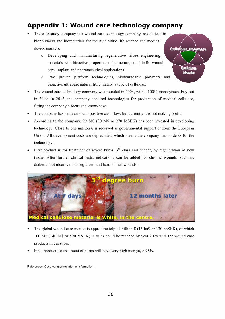
36

Cellulose

Building blocks

Polymers

Appendix 1: Wound care technology company • The case study company is a wound care technology company, specialized in

biopolymers and biomaterials for the high value life science and medical

device markets.

o Developing and manufacturing regenerative tissue engineering

materials with bioactive properties and structure, suitable for wound

care, implant and pharmaceutical applications.

o Two proven platform technologies, biodegradable polymers and

bioactive ultrapure natural fibre matrix, a type of cellulose.

• The wound care technology company was founded in 2004, with a 100% management buy-out

in 2009. In 2012, the company acquired technologies for production of medical cellulose,

fitting the company’s focus and know-how.

• The company has had years with positive cash flow, but currently it is not making profit.

• According to the company, 22 M€ (30 M$ or 270 MSEK) has been invested in developing

technology. Close to one million € is received as governmental support or from the European

Union. All development costs are depreciated, which means the company has no debts for the

technology.

• First product is for treatment of severe burns, 3rd class and deeper, by regeneration of new

tissue. After further clinical tests, indications can be added for chronic wounds, such as,

diabetic foot ulcer, venous leg ulcer, and hard to heal wounds.

3rd degree burn

At 7 days 12 months later Medical cellulose material is white, in the centre. • The global wound care market is approximately 11 billion € (15 bn$ or 130 bnSEK), of which

100 M€ (140 M$ or 890 MSEK) in sales could be reached by year 2026 with the wound care

products in question.

• Final product for treatment of burns will have very high margin, > 95%.

References: Case company’s internal information.

37

Appendix 2: The wound care market • A wound is an injury or break in the skin, generally a dissection of tissue or rupture of a

membrane. Traditional wound care products are dry dressings, bandages, etc. Advanced wound

care product constitutes of alginates, hydrogels, hydrocolloids and collagen, skin substitutes

and biological growth factors. The most sophisticated treatments are regenerative medicine.

• The global wound care market reached revenues of 11 billion € (15 bn$ or 130 bnSEK), in

2010, with a growth of 6%. One third is so called Advanced Wound Care. Of this share 3

billion $ is wet products, and to this segment belong artificial skin products.

• Major general wound care companies are Smith and Nephew, Kinetic Concepts, Convatec,

Systagenix, and Mölnlycke Healthcare.

• Major players in regenerative medicine and extremity reconstruction are Johnson & Johnson,

Pfizer, Sanofi, Roche, GlaxoSmithKline, Wright Medical Group and Integra Lifesciences.

• A few examples of product specific sales, and product prices:

o Dermagraft (treatment of diabetic foot ulcer); 147 M$, 2010.

o Apligraf (treatment of diabetic foot ulcer and venous leg ulcer); >100 M$, 2010.

o The artificial skin’s (treatment of burns) product price is around 10 € per cm2.

o For chronic wounds are both expensive artificial skin products, as well as cheaper

dressings used. A cheaper bandage is sold for around 0,05 € per cm2.

• The wound care market is driven by rise in chronic diseases, such as diabetes and hypertension,

increase in the ageing population, and technological advancements. The demand for mobile,

user-friendly devices is expected to grow the wound care market in the coming years. In a more

long term perspective, biological growth factors, and tissue-engineered products like skin

substitutes will become market-drivers.

• 15% of diabetes patients develop one or more diabetic foot ulcer (DFU) during their lifetime. In

USA, 26 million people have diabetes. 2% of diabetes patients develop DFU annually.

• In USA, 500 000 patients annually seek medical treatment for venous leg ulcer.

• In USA, 15% of elderly patients develop pressure ulcers during hospitalisation.

• Rapid breakthrough in wound-healing technologies to develop cost effective treatment is

expected to drive the growth of the market. Companies are now focusing on the introduction of

advanced materials, methods, and active substances for the treatment of wounds.

• Regenerative medicine has become increasingly popular in recent years, with the number of

deals announced growing steadily. In years 2009-2012, there have been 570 regenerative

medicine / stem cell deals.

References: Case company’s internal information, originally collected from market research companies, such as Kalorama information, MarketsandMarkets 2012, and GlobalData 2010, and Duodecim 2009; 125:457-65.

38

Appendix 3: DCF prognosis

€ 2014 2015 2016 2017 2018 2019 2020 2021 2022 2023Revenue -‐ 20 000 140 000 450 000 1 100 000 2 200 000 3 900 000 6 800 000 10 500 000 15 800 000 Annual Growth % 600% 221% 144% 100% 77% 74% 54% 50%ExpensesCOGS (cost of gods), production and lab 65 000 46 000 50 000 75 000 113 000 195 000 302 000 515 000 780 000 1 149 000 Personnel costs 527 144 591 440 609 224 671 624 671 624 734 024 734 024 734 024 734 024 734 024 Other costs (IPR, marketing, royalties, QA, clinical studies, etc.) 160 000 120 800 145 600 148 000 174 000 218 000 286 000 402 000 550 000 130 000 Depreciation 10 000 14 000 18 000 22 000 26 000 70 000 70 000 70 000 70 000 70 000

Net operating Income -‐752 144 -‐738 240 -‐664 824 -‐444 624 141 376 1 052 976 2 577 976 5 148 976 8 435 976 13 786 976Taxable Income -‐762 144 -‐752 240 -‐682 824 -‐466 624 115 376 982 976 2 507 976 5 078 976 8 365 976 13 716 976EBITA -‐margin -‐3761% -‐488% -‐104% 10% 45% 64% 75% 80% 87%Tax -‐152 429 -‐150 448 -‐136 565 -‐93 325 23 075 196 595 501 595 1 015 795 1 673 195 2 743 395FCF -‐609 715 -‐601 792 -‐546 259 -‐373 299 92 301 786 381 2 006 381 4 063 181 6 692 781 10 973 581Probability for succesful milestone 100% 100% 100% 90% 80% 100% 100% 100% 100% 100%Cumulative probability 100% 100% 100% 90% 72% 72% 72% 72% 72% 72%Probability weighted FCF -‐609 715 -‐601 792 -‐546 259 -‐335 969 66 457 566 194 1 444 594 2 925 490 4 818 802 7 900 978

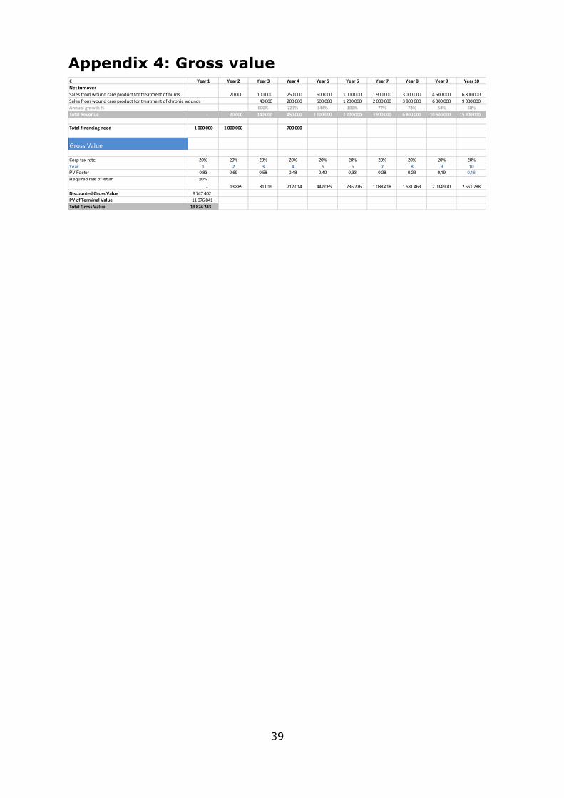
39

Appendix 4: Gross value

€ Year 1 Year 2 Year 3 Year 4 Year 5 Year 6 Year 7 Year 8 Year 9 Year 10Net turnoverSales from wound care product for treatment of burns 20 000 100 000 250 000 600 000 1 000 000 1 900 000 3 000 000 4 500 000 6 800 000 Sales from wound care product for treatment of chronic wounds 40 000 200 000 500 000 1 200 000 2 000 000 3 800 000 6 000 000 9 000 000 Annual growth % 600% 221% 144% 100% 77% 74% 54% 50%Total Revenue -‐ 20 000 140 000 450 000 1 100 000 2 200 000 3 900 000 6 800 000 10 500 000 15 800 000

Total financing need 1 000 000 1 000 000 700 000

Gross Value

Corp tax rate 20% 20% 20% 20% 20% 20% 20% 20% 20% 20%Year 1 2 3 4 5 6 7 8 9 10PV Factor 0,83 0,69 0,58 0,48 0,40 0,33 0,28 0,23 0,19 0,16Required rate of return 20% 20% 0,2 0,2 0,2 0,2 0,2 0,2 0,2 0,2

-‐ 13 889 81 019 217 014 442 065 736 776 1 088 418 1 581 463 2 034 970 2 551 788 Discounted Gross Value 8 747 402 PV of Terminal Value 11 076 841 Total Gross Value 19 824 243

40

Appendix 5: 10 year governmental bond average

Belgium 2,25 2,04 2,06 2,44 2,54 2,65 2,75 2,57 2,42 2,43 2,45 2,4 2,26Germany 1,35 1,2 1,29 1,53 1,56 1,73 1,89 1,76 1,68 1,8 1,76 1,56 1,51Ireland 3,83 3,78 3,48 4,02 3,88 3,92 3,95 3,65 3,53 3,48 3,39 3,24 3,05Greece 11,38 11,58 9,07 10,07 10,53 10,01 10,15 8,74 8,41 8,66 8,18 7,7 6,9Spain 4,92 4,59 4,25 4,67 4,67 4,5 4,42 4,22 4,1 4,13 3,79 3,56 3,31France 2,07 1,8 1,87 2,21 2,25 2,36 2,49 2,39 2,27 2,33 2,38 2,25 2,15Italy 4,64 4,28 3,96 4,38 4,42 4,42 4,54 4,25 4,1 4,11 3,87 3,65 3,4Cyprus 7 7 7 7 6 6 6 6 6 6 6 6 6Latvia 3,17 3,15 3,1 3,17 3,25 3,25 3,45 3,78 3,71 3,62 3,48 3,07 2,87Luxembourg ( 3 ) 1,55 1,41 1,47 1,76 2,02 2,2 2,27 2,14 2,01 2,1 2,06 1,87 1,8Malta 3,56 3,37 3,31 3,35 3,21 3,23 3,28 3,25 3,18 3,19 3,05 2,96 3,02Netherlands 1,67 1,66 1,69 2 2,03 2,2 2,32 2,18 2,06 2,16 2,09 1,89 1,81Austria 1,75 1,64 1,75 2,04 2,06 2,22 2,34 2,19 2,08 2,17 2,13 1,95 1,87Portugal 6,1 6,15 5,46 6,3 6,87 6,6 7,06 6,33 5,98 6,04 5,21 4,94 4,43Slovenia 5,09 5,93 5,35 6,38 6,58 6,51 6,56 6,47 5,91 5,27 4,73 4,43 3,85Slovakia 3,95 3,01 2,52 2,45 3,15 3,15 3,15 3,15 3,15 2,69 2,53 2,48 2,47Finland 1,61 1,51 1,6 1,88 1,91 2,07 2,19 2,04 1,94 2,03 1,99 1,92 1,91Bulgaria 3,54 3,47 3,36 3,4 3,46 3,51 3,64 3,71 3,64 3,43 3,56 3,58 3,54Czech Republic 1,98 1,82 1,67 2,14 2,23 2,4 2,42 2,33 2,18 2,2 2,43 2,28 2,2Denmark 1,59 1,42 1,45 1,72 1,77 1,94 2,1 1,93 1,8 1,89 1,86 1,67 1,61Croatia 4,32 4,34 4,38 4,63 4,91 5,04 4,92 4,99 4,97 5,1 5,11 4,78 4,51Lithuania 4,15 3,95 3,54 3,54 3,54 3,65 3,89 4,01 3,99 3,69 3,42 3,33 3,33Hungary 6,38 5,65 5,08 6,02 5,78 6,31 6,16 5,58 5,82 5,78 5,6 6,03 5,83Poland 3,93 3,5 3,28 3,95 3,97 4,3 4,49 4,28 4,38 4,42 4,42 4,47 4,25Romania 5,86 5,46 5,23 5,43 5,26 5,04 5,27 5,22 5,29 5,29 5,22 5,35 5,31Sweden 1,92 1,66 1,79 2,05 2,16 2,34 2,6 2,44 2,3 2,39 2,37 2,23 2,16United Kingdom 1,65 1,46 1,62 1,96 2,09 2,29 2,44 2,26 2,31 2,5 2,48 2,37 2,34

87,69Average 3,25

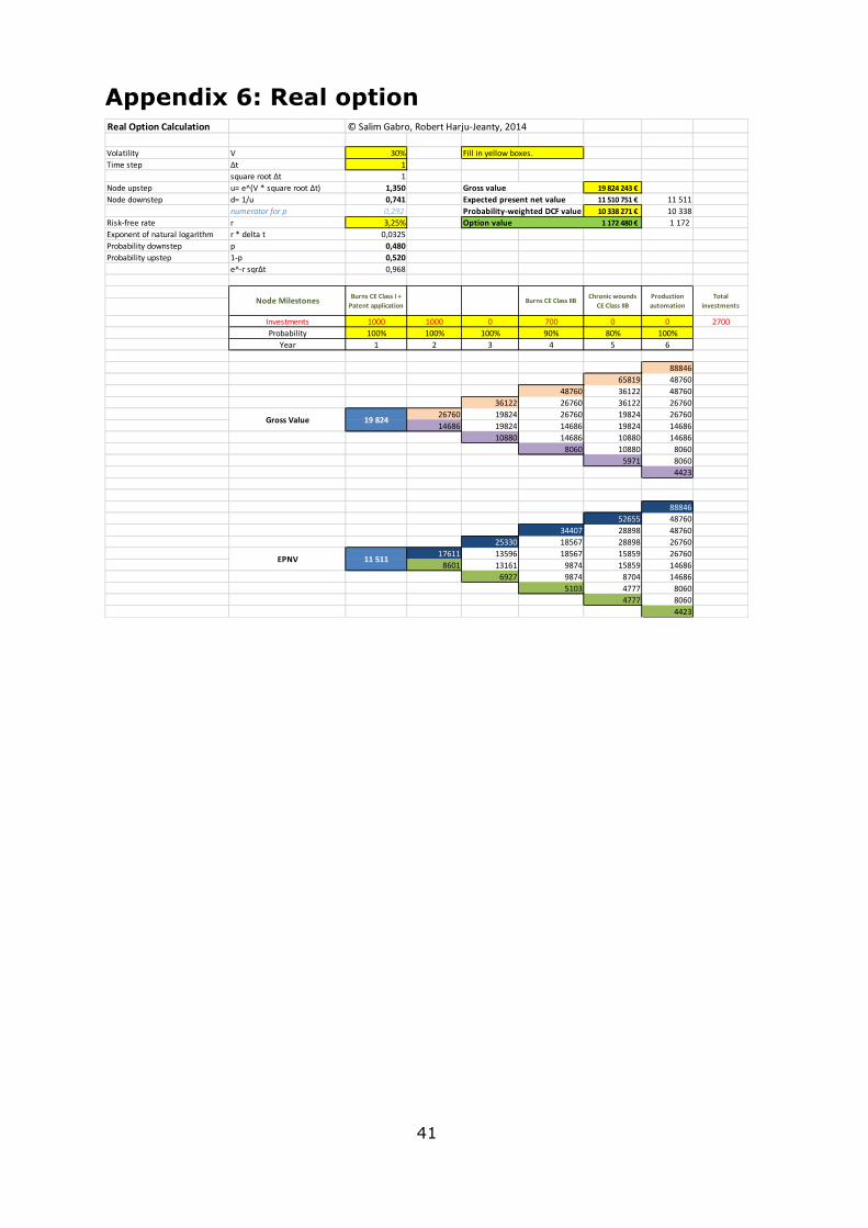
41

Appendix 6: Real option

Real Option Calculation © Salim Gabro, Robert Harju-‐Jeanty, 2014

Volatility V 30% Fill in yellow boxes.Time step Δt 1

square root Δt 1Node upstep u= e^(V * square root Δt) 1,350 19 824 243 € Node downstep d= 1/u 0,741 11 510 751 € 11 511

numerator for p 0,292 10 338 271 € 10 338Risk-‐free rate r 3,25% 1 172 480 € 1 172Exponent of natural logarithm r * delta t 0,0325Probability downstep p 0,480Probability upstep 1-‐p 0,520

e^-‐r sqrΔt 0,968

Investments 1000 1000 0 700 0 0 2700Probability 100% 100% 100% 90% 80% 100%

Year 1 2 3 4 5 6

8884665819 48760

48760 36122 4876036122 26760 36122 26760

26760 19824 26760 19824 2676014686 19824 14686 19824 14686

10880 14686 10880 146868060 10880 8060

5971 80604423

8884652655 48760

34407 28898 4876025330 18567 28898 26760

17611 13596 18567 15859 267608601 13161 9874 15859 14686

6927 9874 8704 146865103 4777 8060

4777 80604423

EPNV

Total investments

Production automation

19 824

11 511

Burns CE Class I + Patent application

Burns CE Class IIB Chronic wounds CE Class IIB

Expected present net valueProbability-‐weighted DCF valueOption value

Gross Value

Gross value

Node Milestones

42

Stockholm University

SE-106 91 Stockholm

Tel: 08 – 16 20 00

www.sbs.su.se

Venture capital valuation of small life science companies

Documents

Transcript of Venture capital valuation of small life science companies