VENTURE CAPITAL AND UNDERPRICING:

CAPACITY CONSTRAINTS AND EARLY SALES�

ROBERTO PINHEIROy

November 2008

Abstract

I present a new theory that addresses an apparent puzzle of empirical �nance literature: why

do venture capital (VC) �rms take young and poorly developed companies public? The key feature

presented to solve this puzzle is human capital capacity constraints. Venture capital �rms can take

only a limited number of new projects at once, and they must go public with current projects in

order to take advantage of new opportunities. The more constrained a VC �rm, the earlier it needs

to take companies public. This framework also predicts that technological waves and cost-reducing

�nancial innovations reduce time to an IPO and increase expected �rst-day return, the discrete jump

from o¤er price to �rst-day market price. Finally, the model endogeneizes the relation between �rst-

day return and time to an IPO by explicitly modeling the process of building competition between

potential buyers through time.

Keywords: IPO,Venture Capital, Underpricing, Capacity Constraints.

JEL Codes: G24, G11.

�I would like to thank Jan Eeckhout Ken Burdett and Guido Menzio for several discussions and encouragement

during this project. I am also indebted with Andrew Postlewaite, Boyan Jovanovic, Randall Wright, Philipp

Kircher, Manju Puri, Ludo Visschers, Chao Fu, Teddy Kim and the participants of Penn Search and Matching

workshop and Micro theory club for helpful comments and discussions. I�m also deeply in debt with Cezar Santos

for his help with MATLAB. Finally, I�d like to thank Rafael Silveira for lengthy discussions at the beginning of

this project. All remaining errors are mine.yDepartment of Economics, University of Pennsylvania, rpinheir@econ.upenn.edu

1

1 Introduction

There is an apparent puzzle in the recent empirical literature on venture capital: Even though initial

public o¤ers (IPOs) of young companies are deeply underpriced, venture capital (VC) �rms1 insist on

taking these infant companies public. Underprice, the o¤er price being lower than the price in the

�rst day of public trade, represents a loss for original shareholders. VC-backed companies are usually

younger, have lower revenues, and are less likely to be pro�table than non-VC-backed companies at

their IPOs. This pattern is even clearer if we look at young VC �rms: these intermediaries take public

companies on average two years younger and raise much less money on the IPO than their more mature

counterparts.

In this paper, I present a model that proposes a new explanation for this puzzle. The main trade-o¤

behind the IPO timing decision by a venture capital �rm is the opportunity cost of turning down new

projects against the bene�t of holding on to existing projects. The key to this trade-o¤ is that VC

�rms are capacity constrained, that is, they are able to handle only a limited number of companies.

This means that a VC �rm needs to go public with its current project to accept a new partnership.

The bene�ts of taking a project public would then include not only the sale�s proceeds but also the

opportunity of engaging in new projects. The bene�ts of waiting to go public come from the increase

in the expected return on a given project. This is obtained by improving the project�s quality and

by increasing the number of potential buyers, thereby increasing the competition for shares o¤ered at

the IPO. In this framework, I show that VCs have a higher incentive to take their companies public

than entrepreneurs do. VC-backed companies therefore end up going public earlier than non-VC-backed

companies in equilibrium. The distinction between young and mature VC �rms comes from how binding

the capacity constraints are; young �rms usually have fewer and less experienced managers and are able

to handle less projects at the same time. As a result, they need to go public with younger projects than

mature VC �rms.

As opposed to previous models, this model also delivers many predictions about market reactions to

di¤erent technological and �nancial shocks. According to my model, technological waves reduce the time

to an IPO, increase VC-backed companies�underpricing, and increase the average quality of projects

looking for a VC. These waves also change VC�s relative patience towards better projects. During a

technological wave, the minimum quality a VC �rm would demand from a new project before going

public with a good current project goes up. At the same time, the minimum quality demanded before

going public with a low-quality current project goes down. Reductions in new project�s starting costs

also generate faster IPOs, higher underpricing, and better projects in the VC market. However, in this

1 I use the abbreviation "VC �rms" throughout the paper to stand for venture capital �rms. However, I will also use

the term "VC" to refer to an individual venture capitalist.

2

case there is no change in relative patience between good and bad current projects. These predictions

are in line with the empirical evidence on hot issues markets, periods where many companies go public

in a short interval, su¤ering large underprices. The model also leads me to conjecture that underpricing

signals the arrival of new good projects. Therefore, forward-looking investors invest in VC funds after

large underpriced IPOs, establishing a positive relationship between underpricing and fund-raising.

Finally, the model addresses the existence of underpricing itself by endogenizing the expected return

obtained through an initial public o¤er. Following previous empirical and theoretical literature, I

assume collusion between underwriter and institutional investors, where investors receive underpriced

shares in exchange for future deals with the underwriter. Di¤erently from previous models, I pin down

the underpricing�s size by looking at the time to an IPO as a process in which competition between

institutional investors is built. In a more crowded IPO, less money left on the table is necessary

to guarantee future deals for the underwriter. The IPO process creates an S-shaped expected return

function. Additional bidders raise expected revenue from competition less and less, hence the concavity.

However, there is no competition if one or fewer potential buyers appear. Therefore, the initial convexity

derives from the discrete increase in expected revenue from the arrival of the second potential buyer.

I also obtain testable results for the impact of �rm age and the time between registration and the

IPO on underpricing. This is an important �rst attempt to evaluate the impact of the road shows on

underpricing. My preliminary empirical results seem to agree with the predictions of the model.

The next section will discuss the main features of the VC market. In the third section, I present

the setup of the model. The fourth section presents the equilibrium and main results, while the �fth

section discusses the possible ways to endogenize the expected return function. The sixth section shows

empirical evidence about the correlation between measures of time to IPO and underpricing to support

my results from the �fth section. The seventh section concludes the paper. All proofs are presented in

the appendix.

2 The Venture Capital Market

A Venture capital �rm is a �nancial intermediary that takes investors�capital and invests it directly in

portfolio companies. Its primary goal is to maximize its �nancial return by exiting investments through

a sale or an Initial Public O¤ering (IPO). Its payment is based on a pro�t-sharing arrangement, the

usual being an 80-20 split: after returning all of the original investment to the external investors, the

general partner (VC) keeps 20% of everything else. VC �rms are usually small (on average they have 10

senior partners) and handle a restricted amount of resources and few portfolio companies. According

to Metrick (2006):

3

"VCs recognize that most of what they do is not scalable and there are limits on the total number of

investments that they can make (...) �rms are reluctant to increase fund sizes by very much".

The estimated total committed capital in the industry is US$ 261 billion, which is managed by an

estimated 9,239 VC professionals, meaning that the industry is managing about US$ 28 million per

investment professional. Even the most famous VC funds usually only manage about US$ 50 million to

US$ 100 million per professional. A typical VC fund will invest in portfolio companies and draw down

capital over its �rst �ve years, which are known as the investment period or commitment period. After

the investment period is over, the VC can only continue to invest in its current portfolio companies.

However, VC �rms usually raise news fund every few years, so that there is always at least one fund in

the investment period at all times. Venture capitalists retain extensive control rights, in particular rights

to claim control on a contingent basis and the right to �re the founding management team; they keep

hard claims in the form of convertible debt or preferred stock, underpinning the right to claim/control

and abandon the project; staged �nancing and the inclusion of explicit performance benchmarks make

it possible to �ne-tune the abandonment decision. In summary, venture capital �rms are �nancial

intermediaries that su¤er from capacity constraints (they have limited human capital to manage their

portfolio companies), share the pro�ts realized through competitive sale or IPO, have strong control

over exit decisions, and keep looking for new opportunities.

In early studies, as Barry at al. (1990), Megginson and Weiss (1991), and Lin and Smith (1998),

VC backed IPOs were found to be less underpriced than non VC-backed IPOs. However, more recent

papers found clear evidences that VC-backed IPOs are more underpriced than their non VC-backed

counterparts, after controlling for selection bias. Looking at a sample of 6; 413 IPOs between 1980 and

2000, of which over 37% (2,383) are VC-backed, Lee and Wahal (2004) found out that venture capitalists

took smaller, younger �rms public. VC-backed companies are on average 7 years old at IPO, compared

to 14:7 years old average non VC-backed �rms. They also have lower book value (0:76 compared to

6:63) and lower total assets ($104:4 million compared to $543:3). These features imply that VC-backed

IPOs are generally smaller (average net proceeds are $40:5 million compared to $58:3), even though

they have higher quality underwriters. Controlling for selection bias through matching estimators2, Lee

and Wahal (2004) show that the average di¤erence in �rst day return between VC-backed �rms and

comparable non VC-backed ranges from 6.20 to 9.51 percent. Since the average �rst day return in the

full sample is about 18%; a �rst-day return di¤erential about 9% represents a signi�cant portion of

2The instrument variables used in the �rst stage were: logarithm of net proceeds, 2-digit SIC code dummies, calendar

year dummies, headquarter-state dummies, underwriter rank and book value of equity per share. Robustness checks

were realized both including other instrumental variables, as logarithm of total assets and �rms�age and changing the

methodology to endogenous switching regressions. No qualitative change were found from the robustness exercise

4

average underpricing. Using di¤erent econometric approaches and data sets, similar results were found

by Francis and Hasan (2001), Loughram and Ritter (2004), Frankze (2004) and Smart and Zutter

(2003).

SEE TABLE 1

Some papers proposed theories to answer this apparent puzzle, as Loughran and Ritter (2002),

Michelacci and Suarez (2002), Rossetto (2004), and Gompers (1996). Loughran and Ritter (2002)

assumes collusion between VCs and underwriters, which empirically just seems to be true from 1999

on, not explaining the long lasting pattern. Both Michellacci and Suarez (2002) and Rossetto (2004)

explanations assume scarcity of �nancial resources and the arrival of new pro�table investment oppor-

tunities. However, the leading explanation is the grandstanding hypothesis, �rst proposed by Gompers

(1996). According to this theory, since VC �rms must periodically raise funds, they need to establish

a reputation of being capable of taking portfolio companies public. Therefore, whenever a VC raises a

new fund, she has incentives to rush to IPO to signal her high skills. This relation between bringing

companies public and fund-raising ability should be stronger for young venture capital �rms, since they

have less reputation. As a result, they are more willing to bear the cost of greater underpricing.

SEE TABLE 2

Table 2 summarizes some of this empirical evidence: Analyzing a sample of 433 venture-backed

initial public o¤erings (IPOs) from January 1, 1978, through December 31, 1987, Gompers (1996)

found that IPO companies �nanced by young VCs are nearly two years younger and more underpriced

when they go public than companies backed by older ones. He also found that young VCs spend on

average 14 months less on the IPO company�s board of directors and hold smaller percentage equity

stakes at the time of IPO than the stakes held by established venture �rms. The o¤erings also di¤er

in magnitude. The equity stake retained by managers and employees after the o¤ering is much larger

for �rms backed by the less experienced VCs. In addition the dollars raised in the IPOs by �rms with

seasoned VCs is larger. These results are consistent with Leland and Pyle (1977), who argue that lower

quality managers must retain larger equity stakes and raise less money to obtain any external �nancing.

Testing the grandstanding hypothesis, Lee and Wahal (2004) found that the �ow of capital into

the lead VC �rm is positively related to VC age, the number of previous IPOs done by the VC, and

underpricing, implying a bene�t to bearing the cost of underpricing. They also found that interaction

e¤ects between reputation (proxied by VC age and number of previous IPOs done by the VC �rm) and

underpricing are negative, supporting grandstanding. The real loss in underpricing for the VC �rm is

5

that it transfers wealth from existing shareholders to new share holders. Since venture capitalists owns

on average 36% of the �rm prior to the IPO and 26.3% immediately after, they also embody a huge

loss through underpricing.

However, there are many features in the market that are not answered by the traditional grandstand-

ing model presented by Gompers (1993). The model is silent about what determines and the impact of

hot issue markets on VC markets. It also has nothing to say about changes in the VC�s cost of entering

in a new partnership, which can be reduced by �nancial innovations or more money available in the

market. As argued by many authors including Jovanovic and Rousseau (2001), technological shocks

increase the speed at which �rms come to an IPO, being considered a main driving forces behind hot

IPO markets. Such shocks also seem to increase the fund-raising by VC �rms, as empirically con�rmed

by Gompers and Lerner (1998) and Bouis (2004). Behind the impact of technological shocks in VC

fund-raising and faster IPOs lies an important feature missed by grandstanding models: demand-side

factors in the VC industry. The demand of capital from entrepreneurs in innovative industries is a

major determinant of the amount and allocation of funds. According to Gompers and Lerner(1998)

and Poterba (1989), demand-factors actually have a determinant e¤ect on VC fund-raising. As Hellman

(1998) says:

�At a theoretical level, it is hard to argue that demand considerations are of no importance. And

casual observation suggests that in many countries the obstacles to investing in venture capital are

relatively minor, yet there is no active venture capital market, suggesting that supply alone cannot be

the problem. Instead, it is frequently argued that the lack of venture capital is due �rst and foremost to

the lack of entrepreneurs.�

My goal in this paper is to introduce an alternative explanation that can preserve the results derived

from the grandstanding hypothesis while still addressing additional features observed in the market. I

will introduce here a model that posits capacity constraints (represented by human capital constraints)

associated with the random arrival of new opportunities as the driving forces in this market. In this

framework, Gompers�s empirical results arise from di¤erences in the strength of these constraints.

Younger VC �rms have a smaller number of senior partners with less experience and are thus more

human-capital-constrained than well established �rms. Therefore, they can take part in fewer projects.

As a result, when taking on a new project, these companies have to exit younger projects on average

than older VC companies. As I show in the �fth section, exiting a young project means lower expected

return and higher underpricing.

This model is related to Michelacci and Suarez (2002) and Rossetto (2004) in terms of having

capacity constraints as a driving force. However, di¤erently from these models, I consider human capital

6

constraints, which seem more empirically relevant. I am also able to deliver qualitatively di¤erent results

on the impact of technological waves and cost reducing shocks on VCs�behavior, as well as pin down the

quality of projects that look for a VC. These features cannot be incorporated in their models. Finally,

I endogenize the expected return of going public and the expected underpricing by modelling the IPO

process. This microfoundation establishes a relation between time to an IPO and underpricing which

is not present in the current literature.

This model leads me to conjecture that underpricing leads to higher fundraising by signalling a good

project has been found. In contrast to the reputational story presented by the literature, my conjecture

is that investors are forward-looking. They see the underpricing as a signal of higher expected returns

in the future. Since the young VC �rms are more capacity-constrained, the e¤ect of underpricing must

be higher to them. Finally, the relation between technological shocks, higher fund-raising, and lower

average time until the IPO is associated with demand-side explanations. Technological shocks, proxied

in the empirical literature by number of patents registered and investment in R&D, can change the

in�ow, distribution, cost, and return of new projects in the market. These changes induce the VCs to

exit earlier from current projects to realize pro�ts and engage in new ventures.

3 Setup

Time is continuous and the horizon is in�nite. The economy is populated by four types of agents: VCs,

entrepreneurs, underwriters and investors, being all risk neutral and in�nitely lived, although I will

consider the case in which entrepreneurs leave the market after their project is terminated. All agents

discount future utility at rate r > 0. These agents are divided between two markets: A decentralized

private equity/VC market and a public market. In the VC market, entrepreneurs with new projects and

VCs look for partners. The public market is where investors negotiate projects previously took public

by VCs with the help of underwriters. I assume that there are two types of investors: institutional

investors, that collude with the underwriter and are allowed to participate in initial public o¤ers (IPOs)

and regular investors, which are only allowed to buy seasoned shares.

At each instant, a measure n of entrepreneur receive a new project. The project�s initial quality S

is a draw from a distribution H with support�0; T �;

�3. This quality improves as time is spent running

it. A project with initial quality S developed during an interval of time �T has quality T = S+�T at

the end of the interval. All projects will be considered identical except for the initial quality, i.e., any

project can become as good as any other if enough time and e¤ort is spent improving it. I also assume

3The use of T �; is only a simpli�cation that does not generate qualitative changes in the model that could possibly

change my explanations on the main features presented by the model.

7

that the expected return from selling a project depends only on the project�s current quality and VC�s

partnership.

Once he draws his project, an entrepreneur must decide if he tries to �nd a VC or run the project

by himself. If he runs by himself, he decides when to take the company public and therefore, its quality

at the IPO. The expected proceeds follow the deterministic rule g (T ), where T is the project�s quality

at the time of the sale. I assume g0 (�) > 0 and g00(T )g0(T ) < r, for reasons that will be clear later. Since

an entrepreneur is less skillful marketing his project, he obtains g (T ), where is the discount factor

that determines the reduction on the proceeds. If he chooses to look for a VC, the project�s quality

is constant until he �nds a VC . If he �nds a VC, which happens with probability � > 0 and the VC

accepts his project, they start running it together. Once the project is sold, the entrepreneur will receive

(1� �) g (T ), where (1� �) > is the fraction of the sales revenue that belongs to the entrepreneur andT is the project�s quality at the IPO. In this case, however, I assume that the VC determines when the

project will be sold4. Her decision depends on the outside options that she faces, i.e., the new projects

that are randomly o¤ered to her. Once a entrepreneur is in a partnership, he cannot �nd another VC

and change partners. I summarize this structure in the picture below.

Given these features, the only choice made by the entrepreneur is to enter or not to enter in the

VC market. Once he entered, he would accept any VC, since all VCs are homogeneous conditional

4We could consider here that both parts need to agree to keep the partnership, otherwise the project is sold and the

partnership dissolved. However, it would make no di¤erence since we show that the VC always have a higher incentive to

walk away.

8

on accepting the project. Therefore, entrepreneurs�decisions are summarized by VC market projects�

distribution F , with support possibly on�0; T �;

�:

There is a measure v of VCs in the private equity/ VC market. Each VC has capacity constraints,

being able to handle one or two projects at the same time. I assume that VCs can hold only one project,

unless mentioned di¤erently. A VC receives new o¤ers with probability �, which will be endogenized

in equilibrium: If the VC is currently in a partnership and decides to enter in a new one, she needs to

take her current project public. A project switch generates the bene�t of realizing current project�s

pro�ts, represented by (1� �) g (T ) : It also embodies two costs. One is a sunk cost c of entering ina new project. The second cost is losing the opportunity of keeping improving the current project,

represented by the value V (T ) : The decision rule obtained from the VC�s problem, T �c (T ), gives the

new project�s minimum quality that would induce the VC to go public with a current project of quality

T: The decisions about which would be the minimum acceptable quality for an unmatched VC, R and

the quality at which a VC would take the project public and open a vacancy, T �; complete the VC�s

decision set. The de�nition of private equity market equilibrium is given below:

De�nition 1 An Equilibrium is this economy is a vector�T �c (�) ; R; T �; ; T

F (�) ; F (T )such that:

� Given F (T ); Venture Capitalists are choosing optimally their termination rule T �c (�) ;

� Give F (T ) ; unmatched Venture Capitalist accept projects with initial quality equal or higherthan R;

� Given F (T ) ; a Venture Capitalist matched with a project with current quality equal orhigher than T �; goes public even without a new project;

� Given F (T ) and T �c (�), entrepreneurs choose optimally their entrance rule TF (c) ;

� Given T �c (�) and TF (c), the distribution of initial projects�quality in the market is given byF (T ) :

Notice that this is a partial equilibrium, since the expected return of an IPO, given by g (�) is taken asgiven and it needs to be determined in the public market, which I describe in the next paragraph. I also

endogenize the probabilities of �nding a VC and �nding a new project, given by � and �; respectively,

by introducing a matching function with constant returns to scale, m (u; v), where u is the measure of

unmatched entrepreneurs in the VC market. Therefore, � = m(u;v)u and � = m(u;v)

v :

The public market is populated by investors. As mentioned before, I consider that only institutional

investors are able to participate in IPOs. Following previous papers in the literature, as Jovanovic and

Szentes (2007), I assume that there is a collusion between underwriter and institutional investors. Once

9

receiving underpriced shares today, investors oblige themselves to a future contract with the underwriter.

However, the more institutional investors interested in the current project, the lower the underpriced

necessary to commit investors to future business with the underwriter. Assuming that the longer a

project is marketed the higher the number of institutional investors interested in it, underpricing is

decreasing on marketing time. The �rst day return occurs because regular investors are able to extract

a signal of the quality of the �rm through the IPO price and adjust their reserve price accordingly.

The more crowded an IPO, the better is the signal quality, the lower the underprice. A more detailed

description of the IPO process is given in section 5.

4 Benchmark model

I present the model following these steps: First, I will address the VC problem, taken as given the

decisions by entrepreneurs and investors, embodied in the distribution F (�) and the expected returnfunction g (�), respectively. Then, taking as given the VC�s optimal choices

�R; T �c (�) ; T �;

and investors�

decisions, I address the entrepreneur�s choice between entering the VC/private equity market and

autarky. Finally, I address the investors�problem and give a microfoundation to the expected return

function g (�) :

4.1 Venture Capitalist�s Problem

The VC needs to take 3 decisions: First, which projects to accept if she currently has an open spot;

Second, once she is in a partnership with project�s quality T and a new opportunity is o¤ered, which

new projects would generate an IPO and partnership change; Finally, which current project�s quality

would generate an IPO even though no new partnership is at sight. These decisions will be represented

by�R; T �c (�) ; T �;

; respectively, where T �c (�) is a function of the current project�s quality T .

Since T �c (�) and T �; have similar reasonings, I will consider both at �rst. Therefore, let�s considera VC in a partnership with a project with current quality T: The value of being in this partnership is

given by:

(1 + rdT )V (T ) = �dTEeS maxnV�eS�� c+ �g (T + dT ) ; V (T + dT )o+

(1� �dT )max��g (T + dT ) + V 0; V (T + dT )

:

10

The value function above presents choices and features of the VC�s problem: there is no �ow bene�t

of keeping the project, since all pro�ts are realized through exit. Once a new partnership is o¤ered,

which happens with probability �, the VC needs to decide if she accepts the new partnership or she

turns down the new o¤er to keep marketing the current project. If she takes the current project public,

she realizes her pro�ts �g (T + dT ) ; and pays the sunk cost of starting a new venture c. Since partner

are found at random and there are projects with di¤erent initial qualities looking for VC to start a new

venture, I assume the quality of the project o¤ered is a draw from the market distribution of initial

qualities F�eS�. Finally, even if no new project is o¤ered, A VC has to decide if she goes public with

the current project, obtaining �g (T + dT ) and opening a vacancy, or she stays in the partnership.

Notice that this value function clearly presents the interaction between timing and capacity con-

straints, with the costs and bene�ts of waiting to go public: The cost of waiting is postponing pro�ts

and turning down partnerships o¤ered in the meanwhile. The bene�t is improving the project�s quality

and marketing it better, which generates a higher expected return when it goes public. Starting with

the decision of keeping the current project or going public if no new venture is o¤ered. As I show in

the appendix, this decision is represented by a threshold T �; , which is given by:

g0�T �;�

g�T �;� = r

Notice that T �; only depends on g and r. Since the probability a VC receives a new o¤er is indepen-

dent of being in a current project or not, there is no additional bene�t of going public than realizing the

payo¤ �g (T ). If no new project appears, the VC will hold the project until the cost of postponing con-

sumption is equal to the bene�t of holding it. For any T < T �; , I have V (T + dT ) > �g (T + dT )+ V0.

Then, taking T 2�0; T �;

�and dT ! 0, I obtain:

rV (T ) = �EeS maxnV�eS�� c+ �g (T )� V (T ) ; 0o+ @V (T )

@T(1)

Given the nature of this problem, there is a threshold T �c (T ) in which the VC is indi¤erent between

keeping the current project of size T or ending it to engage in a new project of size T �c (T ) : This

threshold is de�ned by:

V (T �c (T )) + �g (T )� c = V (T ) (2)

According to this equation, a VC would �nish the current project of quality T to enter in a new

project with starting quality T �c (T ) if the gain from the termination of the current project, �g (T ) plus

the value of the new project minus the initial sunk cost, V (T �c (T )) � c compensates the loss of thevalue of the current project V (T ) : Comparing this to the investment literature, this is simply telling

11

us that the VC will compare Net Present Values. After several manipulations, I obtain the following

implicit expression for T �c (T ) :

�g (T �c (T ))� c+Z T �c (T )

T

Z T �;

Se�

R zS r+�[1�F (T

�c (!))]d!�

�g00 (z)� rg0 (z)

�dzdS = 0 (3)

Using this expression, I can evaluate the impact of changes in the parameters of the model - c; �,

and r - on T �c (T ). This exercise gives us an intuition of how changes in interest rates, sunk costs and

bargaining power a¤ect VC�s decision rules. Since F (�) depends on the entrepreneurs�decision and theseare also a¤ected by the parameters, this is just a preliminary study which takes the market distribution

of projects�qualities as exogenously given. This would be the case if VCs are cash constrained and

unable to obtain loans from banks. Next section endogenizes F (�) and the probabilities � and � bystudying entrepreneurs�decision problem and introducing a matching function.

Example 1 Let�s consider the case in which R = 0:3; c = 0:4; r = 0:1; � = 0:15, g =pT , � = 0:5 and

F (�) is a uniform distribution with support�R; 12r

�: Then, numerically computing T �c (�) using

the above expression, I have:

0 0.5 1 1.5 2 2.5 3 3.5 4 4.5 50

0.1

0.2

0.3

0.4

0.5

0.6

0.7

0.8

0.9

T

T c* (T)

where the dashed line represents the 45o line.�

First of all, let�s consider the case in which there is no sunk cost to enter in a new project. In this

case, from eq. (2), I can easily show that T �c (T ) = 0; 8T 2�R; T �;

�. Graphically:

12

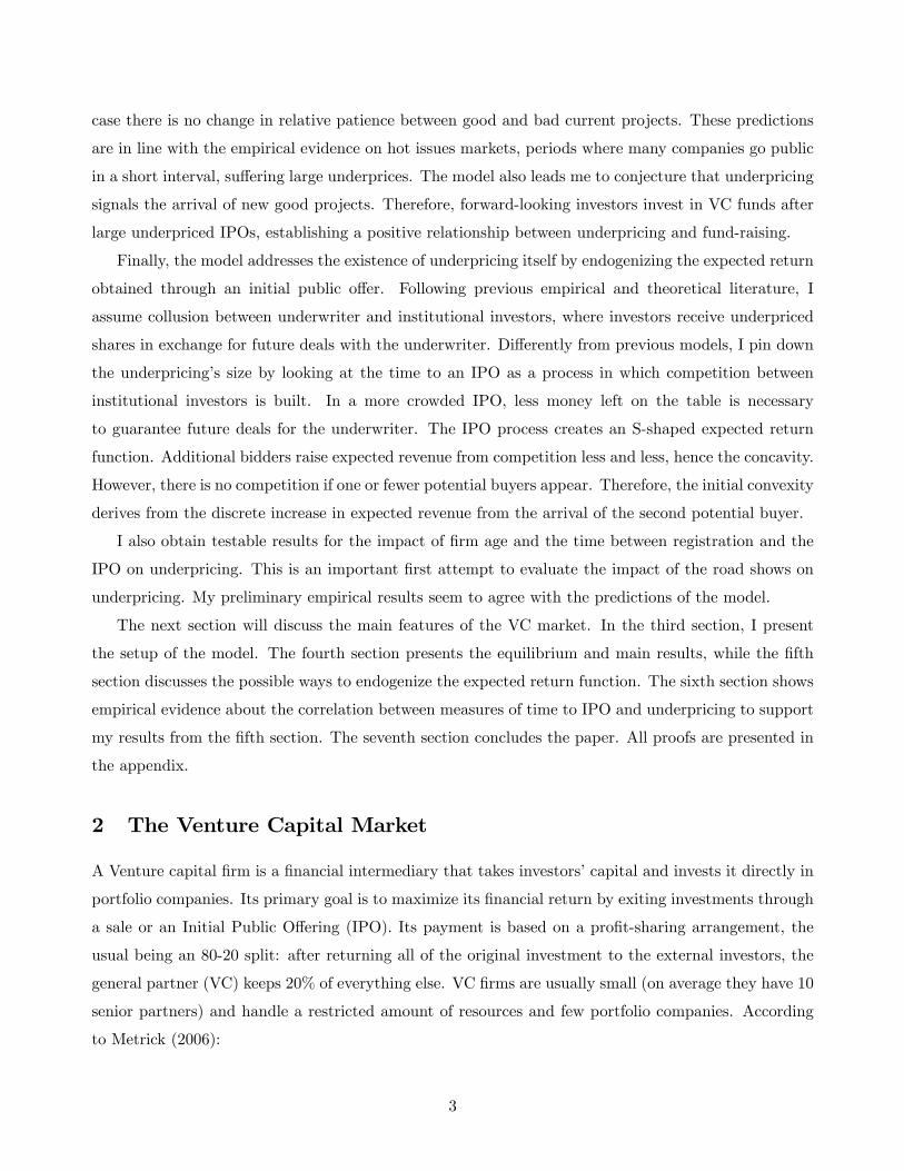
Therefore, regardless the quality of the current project, a venture capitalist has an incentive to enter

in a new partnership whenever this is o¤ered to her, taking the current project public. The intuition is

simple, since entering in a new partnership is always costless, the VC has an incentive to realize pro�ts

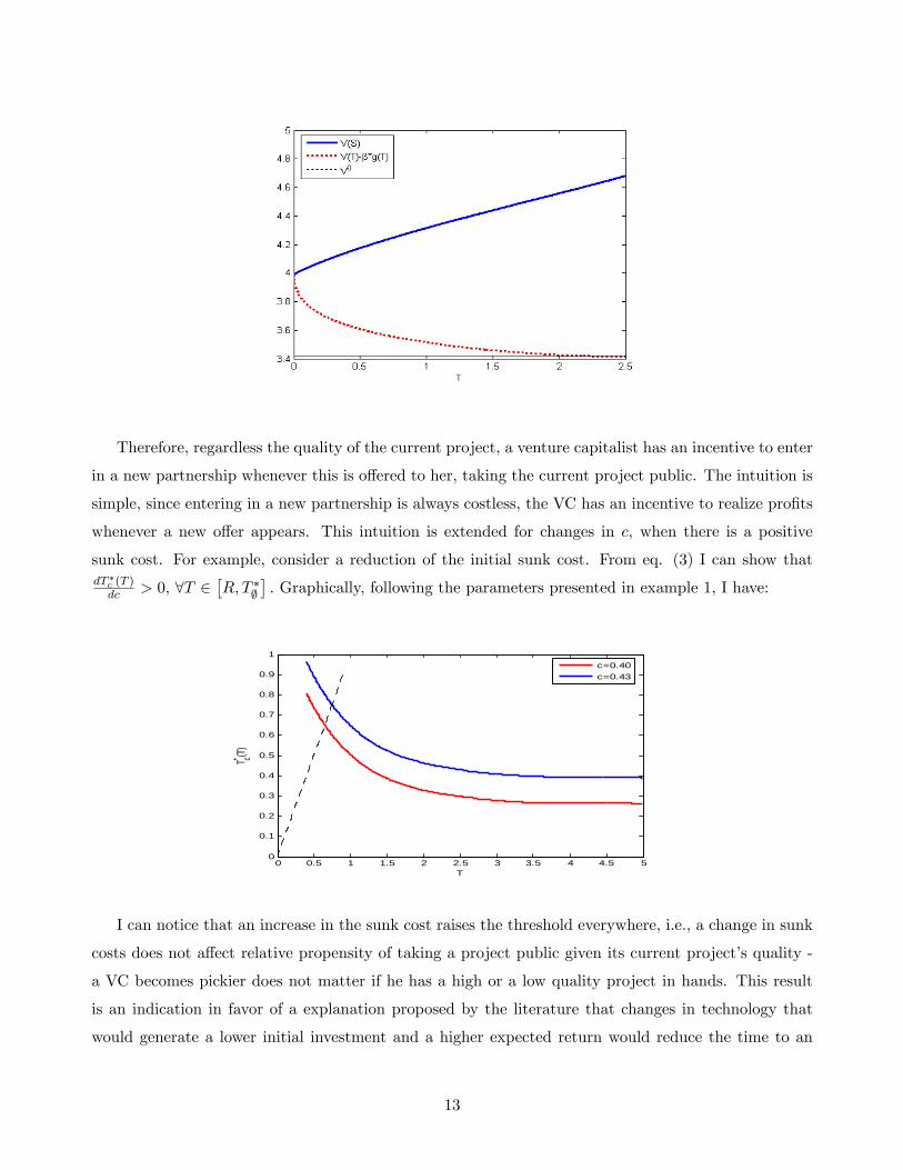
whenever a new o¤er appears. This intuition is extended for changes in c, when there is a positive

sunk cost. For example, consider a reduction of the initial sunk cost. From eq. (3) I can show thatdT �c (T )dc > 0, 8T 2

�R; T �;

�: Graphically, following the parameters presented in example 1, I have:

0 0.5 1 1.5 2 2.5 3 3.5 4 4.5 50

0.1

0.2

0.3

0.4

0.5

0.6

0.7

0.8

0.9

1

T

T c* (T)

c=0.40c=0.43

I can notice that an increase in the sunk cost raises the threshold everywhere, i.e., a change in sunk

costs does not a¤ect relative propensity of taking a project public given its current project�s quality -

a VC becomes pickier does not matter if he has a high or a low quality project in hands. This result

is an indication in favor of a explanation proposed by the literature that changes in technology that

would generate a lower initial investment and a higher expected return would reduce the time to an

13

IPO. A leading example of this theory is the work by Jovanovic and Rousseau (2001) on the impact of

Information Technology in reducing the time until IPO in the last 30 years.

Considering a change in market tightness, the ratio between the industry�s total capacity of mar-

keting projects and the number of projects, we have strikingly di¤erent results. A decrease in market

tightness implies that the probability a VC �nds a new project goes up. Through eq. (3), I show that

this generates a change in relative propensity to take a given project public, i.e.:

@T �c (T )

@�< 0 if T < T �c (T )

and@T �c (T )

@�> 0 if T > T �c (T )

where T = T �c (T )) �g (T ) = c: Graphically:

0 0.5 1 1.5 2 2.5 3 3.5 4 4.5 50

0.1

0.2

0.3

0.4

0.5

0.6

0.7

0.8

0.9

T

T c* (T)

λ=0.15

λ=0.40

This means that an increase in market tightness in the VC/private equity market makes the VC

relatively more prone to spend time with high quality projects. The reason is a shift in the costs and

bene�ts of holding a project. In particular, the reduction in the risk of staying to long with a high

quality project and staying unmatched for a long while. Since the probability of receiving an o¤er of

a new partnership is high, the risk of staying unmatched for a long period is low. Therefore, the VC

does not need to accept a partnership with initial quality very low for insurance purposes.

It�s easy to show that changes in interest rate have the inverse e¤ect. A increase in interest rates

make the VC more impatient, being relatively more prone to take public high quality projects. In this

sense, the decision rule T �c (�) would turn in favor of less developed projects.The proposition below summarizes the results from comparative statics. I would like to reinforce that

these are just preliminary results, since they take entrepreneurs�decisions as given. A full development

14

of these results will be considered in the next subsection, once I take into account the entrepreneur�s

problem. As mentioned before, all proofs are in the appendix.

Proposition 1 From the VC�s problem, taking entrepreneurs�decisions as given, I obtain the following:

� If there are no sunk cost to enter in a new project, VCs will take a project public whenevera new opportunity appears.

� If sunk costs are positive, VC�s acceptance rule of a new partnership is given by a threshold,which decreases the higher is the current project�s quality;

� As the sunk cost of entering in a new project increases, VC demands higher quality to enterin a new project and bring the current public .

� If the market tightness of the market increases, VCs become relatively more prone to keeplonger better developed projects. If interest rate goes up, less developed projects are relatively

more probable to be kept.

Finally, the VC needs to decide, once she has a vacancy and needs to pay the sunk cost to start a

new partnership. Therefore, a VC would accept a new project of initial quality eT if and only if:V�eT�� c � V 0

where V 0 is the value of being unmatched. I can easily show that there is a initial quality R such that:

V (R)� c = V 0

again, by manipulating these expressions, I obtain:

�g (R) = c+

Z T �c (R)

R

Z T �;

Se�

R zS r+�[1�F (T

�c (!))]d!�

�g00 (z)� rg0 (z)

�dzdS

with together with the expressions for T �c (�) and T �; pins down the optimal choices for the VC.The next step I need to consider is endogenizing the distribution of projects looking for VCs, F (�),

by looking at the entrepreneurs�decision problem.

15

4.2 The entrepreneurs�Entry Decision

An entrepreneur has two potential decisions: First, if he looks for a VC or runs the project by himself;

Second, if he decides to run the project in autarky, he needs to choose to optimal time to take it public

Let�s start with the second choice. If he decides to go to autarky (undertaking the project by

himself), he faces the following optimal stopping problem:

maxTe�r(T�S) [ g (T )]

with solution:

g0�TA�

g (TA)= r (4)

Notice that T �; = TA. Therefore, if no new project is o¤ered to the VC running a current project,

both VC and entrepreneur agree when the project should be �nished. As mentioned before, this result

comes from the fact of "on-the-project" search and search while unmatched are equally e¢ cient, such

that there is no bene�t in opening a vacancy.

Now, let�s consider the decision of entering or not the VC market. Since this decision is way more

involving, I start presenting the simplest case in which c = 0, i.e., the VC has no sunk cost in entering

a new partnership. As I showed before, in this case the VC �nishes the current partnership whenever

a new project is found. Later, I generalize my results to the case in which c > 0:

4.2.1 Case 1: c = 0

In this case, the entrepreneur knows that the VC will terminate the partnership whenever a new project

with quality T �c (T ) or higher is o¤ered to her. Therefore, his expected value of the partnership is:

rP (T ) = � f(1� �) g (T )� P (T )g+ dP (T )dT

Then, let�s consider the value function of a entrepreneur in the VC�s market searching for a partner

with a project with initial quality S. Since the entrepreneur would accept any VC and would also be

accepted by any of them, I would have:

S (S) =�

(r + �)P (S) (5)

where � is the meeting rate for an entrepreneur. Then, an entrepreneur would enter VC�s market after

getting a project of initial quality S, if and only if:

16

S (S) � A (S)

Lemma 1 There exists a TF in which any project larger than TF enters the VC market.

Therefore, I have that the better projects will enter the market, being terminated earlier than

the worse projects that chose autarky, even though those ones give a higher expected value for their

entrepreneurs. Finally, notice that a measure n�1�H

�TF��of entrepreneurs will enter the market

every instant.

To close the equilibrium in the VC/private equity market, I need obtain F (�) and u�; which arethe distribution of initial qualities in the VC market and the measure of entrepreneurs looking for a

VC in steady state. In order to obtain these values, let�s introduce a matching function m (u; v), where

u is the measure of entrepreneurs looking for a VC and v is the measure of VCs in the VC/private

equity market. I assume that the matching function has constant returns to scale and satisfy Inada

Conditions5. Then, � and � will be de�ned as m(u;v)u and m(u;v)v , respectively. All my analysis here will

be in steady state. Let�s start with u�. In steady state, since � = m(u�;v)u� ; I must have:

nh1�H

�TF�i= m (u�; v)

Since I am assuming that v is a constant, I can de�ne q (u) � m (u; v). Doing this, I can express

u� = q�1�n�1�H

�TF���: Before I analyze the consequences of this result, let�s pin down F (�) : In

steady state, de�ning F 0 (T ) � f (T ), I obtain:

f (T ) =n

�h (T ) k

where k is a constant term that allows f (�) to integrate 1. In this case one can clearly see thatk = �

n

�1�H

�TF��: Therefore, the pdf of project qualities in the market looking for a VC is given by:

f (T ) =h (T )

[1�H (TF)] :

Now, let�s study the impact of changes in the number of entrepreneurs that obtain a new project, n.

This can be seen as a technological boom, in which many new ideas are appearing and start-ups need

money and expertise. I show in the appendix that @TF

dn > 0; @u�

@n > 0 and consequently that@�@n < 0 and

@�@n > 0. The next proposition summarizes and interpret these results.

Proposition 2 In a technological boom (increase in n):

5 limu!0@m(u;v)

@u=1; limu!1

@m(u;v)@u

= 0; limv!0@m(u;v)

@v=1; limv!1

@m(u;v)@u

= 0

17

� The average quality of the pool of projects that look for a VC increase;

� The expected time a VC stays in a given partnership decreases;

� It takes longer for a given project to �nd a VC.

Now, let�s introduce a positive sunk cost. As expected, this will make calculations more involving

and the I will need to pin down the distribution of quality of current projects to analyze the market.

4.2.2 Case 2: c > 0:

In this case, VC�s decision of going public with her current project and starting a new partnership is

given by the downward sloping function T �c (T ). Therefore, the value for an entrepreneur of now being

in a partnership with project with current quality T is:

rP (T ) = � [1� F (T �c (T ))] f(1� �) g (T )� P (T )g+dP (T )

dT

Then, let�s consider the value function of a entrepreneur in the VC market searching for a partner

with a project with initial quality S. In this case, the value of looking for a VC is given by:

S (S) =���1� J

�T ��1c (S)

�� �1� vv

v

�+ vv

v

r + �

��1� J

�T ��1c (S)

�� �1� vv

v

�+ vv

v

P (S)where J (�) is the distribution of projects in current partnerships and vv the measure of unmatchedVCs.. A entrepreneur decides to enter the VC/Private Equity market if:

S (S) > A (S)

From this decision problem, I obtain the following lemma:

Lemma 2 There exists a TF (c) in which any project larger than TF (c) enters the VC market.

Therefore, the existence of a threshold of quality in projects entering the VC market is robust to

the introduction of an initial sunk cost. However now the acceptance/termination rule depends on the

size/quality of the project ( better developed projects have a higher probability of being accepted and

terminated than less developed ones) which would induce a steady state distribution of projects in the

market that has a higher weight on smaller projects than the one observed in the in�ow of projects. To

be able to address these questions, I need to pin down, F (�) ; u� and this time I also need to determinevv and J (�) :

18

Let�s start taking a look at vv. In steady state:

vvv=

j�T �;�

�+ j�T �;� :

Now, let�s look at F (�) ; the distribution of projects looking for a partnership. In steady state, Iobtain:

F 0 (T ) � f (T ) = knh (T )

��vvv +

�1� vv

v

� �1� J

�T ��1c (T )

���where k is a constant that guarantees that the density integrates 1. Let�s now obtain a formula to J (�).In steady state, taking J 0 (T ) = j (T ):

j0 (T ) = � [1� F (T �c (T ))] j (T ) +u�

vnh (T ) k

Finally, let�s obtain an expression for u�: In steady state:

nh1�H

�TF (c)

�i= �u�

Z T �;

TF(c)

nvvv+�1� vv

v

� �1� J

�T ��1c (S)

��of (S) dS

substituting f (S) and manipulating it:

u� =1

k:

which can be substituted in the de�nitions of f (T ) and j0 (T ) : These equations pin down the

distribution of projects in partnerships and looking for VCs, up to a constant. However, given that the

system is quite involving, and T �c (�) is only determined implicitly, which impossibilities full theoreticalanalysis. However, a numerical analysis is still possible and will be done in future work.

In the next subsection, I analyze two extensions of this benchmark model. The �rst one addresses

the case in which VCs are only allowed to search whenever they have a vacancy. This constraint will

generate as a result a smaller total time a VC would spend with a given project and a knife edge result on

the VC market, in which or all entrepreneurs look for VCs or none of them does. The second extension

considers the possibility of a VC holding two projects at the same time. This extension addresses

the distinction between young and old VCs as a di¤erence in capacity constraints: it shows that the

expected quality that a project goes public increases as capacity constraints are ease. Therefore, the

results on grandstanding are addressed by this simple extension.

19

4.2.3 Extensions

No �on-the-project� search This section considers the case in which only unmatched VCs will

be able to enter in a new partnership. This case shows why it is important that, di¤erently from

Michelacci and Suarez (2002), I consider a better structured set up to understand some of the stylized

facts obtained in the empirical literature.

Consider that each unmatched VC �nds a new project with probability �. Then, the optimal

termination time is the solution for the following problem:

maxTe�r(T�S)

��g (T ) + V 0

�Notice that V 0 now embodies the bene�t of being to look for new opportunities. At the optimal

selling time6 :

g0 (T �)� rg (T �) = rV 0

�(6)

Because the constraint on g (T ), the LHS is decreasing on T . Since the RHS is a constant on T , it

guarantees that there is a unique T � that satis�es the above equation. It can seen that, as expected,

the higher the value of a vacancy V 0, the lower the waiting time to �nish the project. Notice that V 0

is given by:

(1 + rdT )V 0 = �dT

Zmax

nV�eS� ; V 0o dF �eS�+ (1� �dT )V 0

Therefore, the value of being able to look for a new project�V 0�is given by the expected return of

the arrival of a new opportunity with initial quality eS, given by a draw from the distribution of initial

qualities in the market F .

But note that since you can always get the project and �nish it immediately, receiving �g (T ) ;

where T � 0, the VC will always accept it. Then, manipulating and taking dT ! 0:

V 0 =�

r + �

Z T

0V�eS� dF �eS� (7)

Substituting these expressions in my previous results:

g0 (T �)

g (T �)=

(r + �) r

r + ��1� e�rT �

R T0 e

reSdF �eS�� (8)

6We could have corner solutions in which the VC immediately sells the project without compromising the model.

However, given our assumptions, no VC would keep a project forever.

20

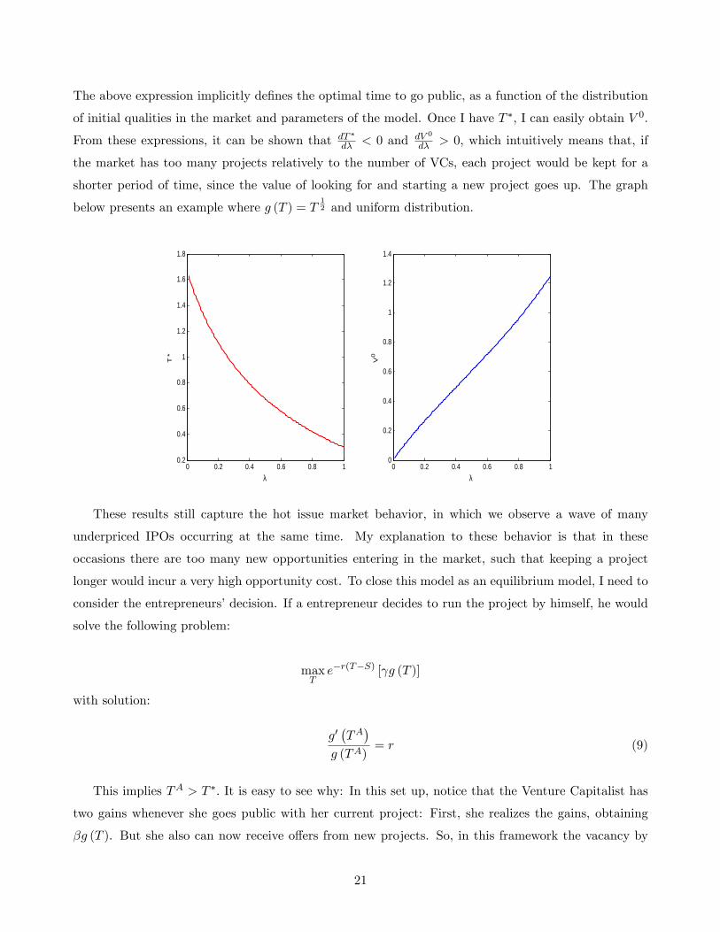
The above expression implicitly de�nes the optimal time to go public, as a function of the distribution

of initial qualities in the market and parameters of the model. Once I have T �, I can easily obtain V 0:

From these expressions, it can be shown that dT �

d� < 0 and dV 0

d� > 0, which intuitively means that, if

the market has too many projects relatively to the number of VCs, each project would be kept for a

shorter period of time, since the value of looking for and starting a new project goes up. The graph

below presents an example where g (T ) = T12 and uniform distribution.

0 0.2 0.4 0.6 0.8 10.2

0.4

0.6

0.8

1

1.2

1.4

1.6

1.8

λ

T*

0 0.2 0.4 0.6 0.8 10

0.2

0.4

0.6

0.8

1

1.2

1.4

λ

V0

These results still capture the hot issue market behavior, in which we observe a wave of many

underpriced IPOs occurring at the same time. My explanation to these behavior is that in these

occasions there are too many new opportunities entering in the market, such that keeping a project

longer would incur a very high opportunity cost. To close this model as an equilibrium model, I need to

consider the entrepreneurs�decision. If a entrepreneur decides to run the project by himself, he would

solve the following problem:

maxTe�r(T�S) [ g (T )]

with solution:

g0�TA�

g (TA)= r (9)

This implies TA > T �: It is easy to see why: In this set up, notice that the Venture Capitalist has

two gains whenever she goes public with her current project: First, she realizes the gains, obtaining

�g (T ). But she also can now receive o¤ers from new projects. So, in this framework the vacancy by

21

itself is valuable for a VC. However, this di¤erence in potential sources of earnings would create a clear

distinction for the entrepreneur: He knows that if he looks for a Venture Capitalist, the company will

necessarily be sold before its optimal time, while, if he decides to run the company by himself, he would

choose the optimal time to sell it, however he would not be able to usufruct all the expertise that a VC

has (therefore, obtains << 1� �). If a entrepreneur with a project with initial quality S enters theVC market, he has a expected value of:

�

� + re�r(T

��S) (1� �) g (T �)

Therefore, he would choose to look for a VC if and only if:

�

� + re�rT

�(1� �) g (T �) > e�rTA g

�TA�

Therefore, the initial quality S does not a¤ect the decision of looking for a VC or not. This implies

that all qualities would join the market or it would simply shut down, with all entrepreneurs going to

autarky. Finally, this framework cannot address the question why young VCs would go public earlier

than tenured ones: Once VCs are only allowed to search for new opportunities if they have an opening,

capacity constraints are not binding in this framework. Another point we should emphasize for future

references is that the introduction of an initial sunk cost generates an increase in T � and a decrease in

the value of a vacancy.

The proposition below summarizes my �ndings on this section.

Proposition 3 In an economy with no "on-the-project search":

� All qualities of projects enter the VC market or not;

� All projects would go public at same age/quality;

� Hot issue markets would be occur whenever the market is tight (� is close to 1);

� There would have no di¤erentiation between the behavior of young and old VC �rms.

� If there is a initial sunk cost (c > 0), T � will be increasing in c, while V 0 will be decreasingon it.

Two project VCs As mentioned before, I consider that young and mature VC �rms are distinct in

terms of how binding capacity constraints are. To address this point, I extend the model presented

here to the case in which a VC can hold two projects at the same time. In this case, it can be shown

that whenever a VC has to go public with a given project to enter in a new venture, she chooses

22

the older/better quality one. Then, in the case in which the entrepreneur still accepts any VC7, the

expected time until an IPO is larger for a mature (two spots) VC �rm. Therefore, my model can obtain

the same result obtained by the grandstanding hypothesis literature.

Therefore, the expected value for a VC of holding projects of quality T1 and T2 is given by:

rV (T1; T2) = �E eT max

8>>>>>>>>><>>>>>>>>>:

24 V �eT ; T2�+ �g (T1)�c� V (T1; T2)

35 ;24 V �T1; eT�+ �g (T2)�c� V (T1; T2)

35 ;0

9>>>>>>>>>=>>>>>>>>>;+

�@V

@T1(T1; T2) +

@V

@T2(T1; T2)

�Then, looking at the cut o¤ rule, let�s analyze the conditions in which:

V�eT ; T2�+ �g (T1)� c� V (T1; T2) � V �T1; eT�+ �g (T2)� c� V (T1; T2)

Simplifying, and assuming symmetry:

V�eT ; T2�+ �g (T1) � V �T1; eT�+ �g (T2)

First of all, consider a symmetry condition:

[�g (T1)� �g (T2)]�hV�T1; eT�� V �T2; eT�i � 0

Manipulating this expression, I show in Appendix B the following result:

Lemma 3 Whenever a VC has two current projects and decides to go public to join a new venture,

she goes public with the better developed one.

As a corollary of this result:

Corollary 1 The Expected time of a partnership increases the easier is the capacity constraint faced

by a VC.7The presence of young and mature VCs can also change the distribution of projects in the market. However, whenever

both VCs are accepted by the same projects, they face the same distribution.

23

5 A Microfoundations for the IPO procedure: Endogenizing g (T )

In this section, I present one way in which the return from the exit in a venture investment can be

endogenized. Since the most successful exits are through initial public o¤ers (IPOs), endogenizing g (T )

necessarily involves a discussion about IPOs and their main players and features.

The main feature that we observe in IPOs is the presence of underpricing: According to Jenkinson

and Ljungqvist (2001), the �rst day returns are positive in virtually all country. They typically average

more than 15% in industrialized countries and around 60% in emerging markets. Such returns are

viewed as anomalies: In e¢ cient markets, competition between investors would necessarily exhaust all

possible gains from private information, as presented by Grossman (1976), and no money would be "left

on the table".

Many theories were developed to address this issue, all with limited success. The traditional explana-

tions are based on asymmetric information. According to Rock (1986), there is asymmetric information

between potential buyers, which generates a lemon�s problem for the uninformed buyer. In Benveniste

and Spindt (1989), the seller that is actually trying to extract information from institutional investors

about the value of the company being sold. The main problem with these theories is that they take the

sale�s procedure as given. Rock (1986) takes as given �rm commitment o¤ers, avoiding the transmis-

sion of information from informed to uninformed buyers through price changes. Benveniste and Spindt

(1989) assume the existence of a pre-market in which only regular investors participate. They assume

that �cost of conducting an all-inclusive pre-market is prohibitive�. Another theoretical explanation

for underpricing presented by the literature is signaling. In this case, the seller knows the quality of the

�rm being sold, while underpricing would be a way to signal better quality. This explanation, although

theoretically elegant su¤ers from empirical �aws (some assumptions used in these models are wrong

and the data don�t corroborate their results) and it also seems susceptible of collusion between the

seller and some buyers or even the seller can "create" false investors, as discussed lately in the auction

literature.

The explanation I am going to present here is related to the one defended by Jovanovic and Szentes

(2007) and empirically discussed by Loughram and Ritter (2004). Jovanovic and Szentes (2007) claim

that underprice is created by an agreement between institutional investors and underwriters. Invest-

ment bankers allocate underpriced stocks to institutional investors in the hope of winning their future

investment banking business. This practice, called �spinning�, is well-documented. The most famous

case the $100 million �ne that Credit Suisse First Boston received because of these activities. Firm�s

original owners accept this practice because IPOs disclosure information to the market.

I introduce a step further, considering the competition between institutional investor for underpriced

24

shares and how this impacts the amount of information released and therefore, the size of the �rst day

return. Given this e¤ect of competition, I consider how the increase in competition is related with time.

I claim that one important role performed by Venture Capitalists and underwriters is to publicize the

�rm to be marketed. The more institutional investors that get information about the �rm, higher the

expected competition for its shares and therefore, lower underprice. One simple way that I can see this

e¤ort on publicizing an IPO �rm and its impact on competition is looking at the length of the road

show, that I will proxy looking at the number of days in registration. The Road Shows are tours taken

by IPO �rms�top managers and investment bankers to visit groups of invited institutional investors,

publicizing the �rm and also to elicit bids from investors. Although these bids don�t have legal tender,

there is a strong presumption that investors should be prepared to honour their bids. Looking at

the data for more than 1500 IPOs in the period between 1984 and 2004 (I used data from the SDC

Platinum), I can show a negative correlation between the number of days in registration and the �rst

day return. This result is robust to di¤erent speci�cations of my multivariate linear regressions or even

multivariate fractional polynomial models. Although the lack of data with respect to the number of

bidders doesn�t allow me look for deeper empirical relations, I imagine that this is a clear indication

that timing and its impact on building up competition is an important factor to understand the size of

the underpricing. In the next section, I give details on my empirical results.

I agree that this is one of many ways in which I could endogenize the expected return. However, I

believe that my explanation not only adds in matching some empirical evidence that was not considered

before, but it also gives a clear theoretical foundation for some hypothesis presented by the empirical

literature on �rm managers behavior. In addition, my speci�cations are not in disagreement with other

conjectures, as the idea that Venture Capitalists not only publicize the project but also increase its

quality (as it can be seen below, all results are kept if I imagine that the real value of the venture ! is

an increasing function of time spent in the partnership).

5.1 Basic Framework

In this basic framework, I model IPOs as �rst price auctions in which only institutional investors

participate. Even though the bookbuilding process is not an auction, the road show has a structure

that can be approximated to one. I initially consider that there are N potential buyers participating

in this auction. Later, I show ways to endogenize N and therefore evaluate the expected return on

exiting as time passes. I assume that the value of the company ! is known by institutional investors

and/or it can be credible communicated by the underwriter. I also assume that the underwriter and

the venture capitalist knows ! but other players in the market don�t . However, from my claim about

the agreement between underwriter and investors, the investor that wins the auction obliges himself

25

to a future contract with the underwriter. Consider that this future contract between investor and

investment banker generates a private cost to the investor. This cost is i.i.d. draw " from a distribution

Z with support on [0; !] 8: Therefore, investor i�s gain in winning the auction is given by ! � "i � pwhen he bids p and this is the highest bid. Therefore, I have the following payo¤ function:

�i =

8<: ! � "i � pi if pi > maxj 6=i pj

0 if pi < maxj 6=i pj

Then, the problem of investor i is:

maxp�0

(! � "i � p)�1� Z

�! � P�1 (p)

��N�1Then, solving the symmetric equilibrium case:

P (! � "i) = ! � "i �Z !

"i

�1� Z (y)1� Z ("i)

�N�1dy (10)

Then, the expected revenue is:

R (!;N) = ! �NZ !

0[1� Z (")]N�1 F (") d"�

Z !

0[1� Z (")]N d" (11)

Claim 1 Expected Return is increasing in N .

Claim 2 Expected payment converges to ! as N !1:

Now consider that the winner paid a price p. How much would the market pay for this company in

the next day? Remember that p is given by:

p = ! � "w �Z !

"w

�1� Z (y)1� Z ("w)

�N�1dy:

where "w is the winner�s private cost of sealing the agreement with the underwriter. Considering the

market agents are risk neutral, we are looking for E [! jp is the winner ] : Then, from the expression

above:

! = p+ "w +

Z !

"w

�1� Z (y)1� Z ("w)

�N�1dy

Since the agent won the auction, "w is the minimum between N . Therefore, taking the expected

value of the last two terms on RHS:8The support being between 0 and ! is just a simplifying assumption that can be dropped without qualitative changes

in the results.

26

b! = p+N Z b!0[1� Z (y)]N�1 dy � (N � 1)

Z b!0[1� Z (y)]N dy

It is easy to show that the RHS of the above expression is constant in b!. Since the LHS is increasing,I can show that it crosses once. Let�s show an example with a Uniform distribution

Example 2 "i � U [0; !] : Then: b! = p+ b! � N � 1N + 1

b!Therefore: b! = N + 1

N � 1p:

Notice that as N increases b! converges to p. Therefore, as N increases, p becomes a better signal

of !.

In this example, the expected �rst day return is given by:

b! � p =N + 1

N � 1p� p

fdr =2

N � 1p

substituting p:

dfdr =

�2

N � 1

���N � 1N + 1

�!

=2

N + 1!:

Therefore, the higher !, the higher the expected �rst day return. This result is in agreement with

the intuition presented by Ritter (1998) to why pre-IPO shareholders don�t get upset when they see a

large underprice:

"Bad news that a lot of money was left on the table arrived at the same time that the good news of

high market price"

Since more valuable companies (High !) usually have a higher �rst day return, a large underprice

in a crowded IPO implies a high value to the shares kept by the pre-IPO shareholders. It also gives us

an indication about the relationship between hot issue markets and technological shocks. Considering a

technological shock as a jump in !, this would imply an increase in the expected underprice, as advocate

by some authors.

27

Finishing this example, it�s easy to show that R (!;N) =�N�1N+1

�! is concave in (!;N). In this way,

even if I consider that ! increases through time given VC�s activity (changing managers, restructuring

production, etc...), I still obtain the same results and the concave shape necessary for my previous

results about optimal selling time. Graphically:

0 1 2 3 4 50

1

2

3

N

R(w,N)

Where ! = 2,3 and 4 in the black (solid), red (dot-dash) and green (dash) lines, respectively.�

Concavity in general is not necessarily granted, especially given that there is a jump in revenue

from the entrance of the second bidder in the auction9. However, it is easy to show that there is a

cuto¤ number of bidders N� such that for any N � N�; R (!;N) is concave in N :

N� =

R !0 [1� Z (")]

N��2 Z (")2 d"R !0 [1� Z (")]

N��2 Z (")3 d":

Up to now, I considered the number of bidders in a given IPO as constant. However, my intuition

from the length of the road show and importance of good marketing skills by underwriters and VCs are

related with an in�ow of institutional investors. These players get to know the IPO �rm and then decide

to participate or not in the IPO. I will model this considering the arrival of potential buyers as a Poisson

Process with average �: Therefore, the number of investors that observed their valuations in an interval

of length T is a random variable with Poisson distribution with parameter �T: The probability that an

auction realized after a waiting time of length T has N bidders is pN (T ) =e��T (�T )N

N ! . I consider that

all investors that where contacted and draw their " will wait for the auction. This assumption does

not a¤ect qualitatively the results. A simple generalization would consider that investors could sample

other opportunities and leave. It generates similar results since the investors that are more probable

to stay waiting for the auction are the ones with low costs, and these are the agents important to my

results. Therefore, the expected return of an auction realized after waiting T is given by:

9The introduction of reserve prices and some additional assumptions can mitigate this problem.

28

1XN=2

pN (T )R (!;N) :

Manipulating it:

g (T ) = ! �Z !

0[1 + �TZ (")] e��TZ(")d"

It is easy to see that g0 (�) > 0 and g00 (T ) < 0 ; 8T � TC given by:

TC =

R !0 �Z (") e

��TCZ(")d"R !0 (�Z ("))

2 e��TCZ(")d"

Plotting g (T ):

0 5 10 15 20 25 30 35 40 45 500

0.1

0.2

0.3

0.4

0.5

0.6

0.7

0.8

0.9

1

T

g(T)

The initial convexity comes from the large impact on auction�s expected revenue generated by the

entry of a second potential buyer, since it introduces competition and raises the price from zero to a

positive value. The introduction of reserve prices and assuming log concavity of the distribution Z (�)would help us to avoid the initial non-concavity in g (T ). Finally, I can see that my previous discussions

on technological shocks in g (T ) could be modeled as jumps in !:

6 Empirical Evidence

I will present now some evidence about the impact of days in registration and the age of the �rm on

�rst day return and therefore, underpricing. The number of days in registration is considered here as

29

a proxy for the length of the road show, indicating the e¤ort of sale and/or the expected number of

potential bidders.

The source of my data is SDC Platinum, from which I look at US data on IPOs from 1984-2004,

focusing on Common Stocks. I include as control variables the number of days in registration, the

age at which the �rst investment was made (di¤erence between year of foundation and year at the

�rst investment), number of investment rounds, book value per share, book value before o¤er, market

indexes at the IPO date and �rm�s age at the IPO. I also include in my analysis dummy variables that

control for: sector in which the �rm is, year in which the IPO was realized, market in which the IPO

was realized.

Results from regression analysis with robust errors are presented in the table below. It show that

Days in Registration have an impact on First Day Return that is always signi�cative (consider � � 5%).The size varies between [�0:11;�0:04] ; while age at the IPO has a negative and signi�cant impact on�rst day return (size varies but it is usually big: around �0:4). These results are in agreement with mytheory on IPOs: The higher the time until the IPO, the lower the amount of money left on the table

for investors that buy at the initial public o¤er1011.

.

SEE TABLE 3

Another empirical analysis that I present here comes from a nonlinear analysis using a Multivariable

fractional polynomial model. The obtained results are presented below:

SEE TABLE 4

The adjustments in the variables are obtained after 3 iterations in the fractional polynomial �tting

algorithm. Dummy variables are included in the estimation, although their results are omitted here.

As I can see, again there is a negative impact of days in registration and age at the IPO in the �rst

day return, showing that my intuition that the longer the venture capitalist keeps the �rm/project, the

lower is the amount of money left on the table for institutional investors.

As we mentioned before, these results are only indications in favor of my theory, showing that the

correlations obtained in the data are in agreement to my results. Unfortunately, a deeper empirical

10As additional results we have that: Dummy for 1999 is the only year dummy consistently signi�cant. It has a positive

impact on �rst day return. Sector dummies have the expected signals from a asymmetric information claim (positive for

high tech, negative for manufacture and health) but they are not signi�cant in many cases. All other variables are usually

not statistically signi�cant at 5%11 I also included dummies to take into account the impact of price revisions on underpricing, as presented by Hanley

(1993). Results are robust to this exercie.

30

analysis, with the estimation of more structured models is not possible since most data on the IPO

process is not public, not being disclosed by investment banks for further analysis.

7 Conclusion

In this paper, I present a new theory about underpricing and VC-backed companies where the key

feature is VC�s capacity constraints, i.e., Venture Capital �rms can only handle a limited number of

projects.

I show that this theory can match not only the empirical evidence that VC �rms take younger

companies public and that younger VC �rms take even younger �rms public than their more mature

counterparts, but it also presents as a nice framework to address additional features in the market, as

the impact of technological waves, �nancial shocks on time to IPO, underpricing and average time spent

by a VC in a given project. These predictions seem to be aligned to what was found by the empirical

literature while studying hot market issues and the grandstanding hypothesis.

Finally, this model addresses the underpricing paradox by assuming a collusion between institutional

investors and underwriter. However, di¤erently from previous models, it looks at competition between

institutional investor for underpriced shares as a way to pin down underpricing�s magnitude and the

expected return to an IPO given the time spent marketing it. My initial empirical evidence between

time to IPO -measure by �rm�s age at the IPO and days in registration - and underpricing corroborates

the predictions of the model.

31

References

[1] Aghion, P., P. Bolton and J. Tirole (2004): "Exit Options in Corporate Finance: Liquidity versus

Incentives", Review of Finance 8: 327-353.

[2] Barry, C., C. Muscarella, and J. Peavy (1990): "The role of venture capital in the creation of

public companies: evidence from the going public process", Journal of Financial Economics 27,

447-471.

[3] Benveniste, L. M. and P. A. Spindt (1989): "How Investment Bankers Determine the O¤er Price

and Allocation of New Issues", Journal of Financial Economics, 24, 343-361.

[4] Black, B. and R. J. Gilson (1998): "Venture Capital and the Structure of Capital Markets: Banks

versus Stock Markets", Journal of Financial Economics 47, 243-278.

[5] Booth, J. and L. Booth (2003): "Technology Shocks, Regulation and the IPO Market", mimeo.

[6] Bouis, R. (2004): "Does VC Fund-raising Respond to Hot IPO Markets?", mimeo.

[7] Brock, W. A., M. Rothschild and J. Stiglitz (1989): "Stochastic Capital Theory" in: Feiwel, G. R.

(ed.), Joan Robinson and Modern Economic Theory, New York University Press, 591-622.

[8] Faustmann, M., "On the determination of the value which forest land and inmature stands pose

for forestry" in: Gane, M. (ed), Martin Faustmann and the evolution of discounted cash, Oxford,

England, 1968.

[9] Francis, B. and I. Hasan (2001): "The underpricing of venture and non venture capital IPOs: an

empirical investigation", Journal of Financial Services Research 19, 99-113.

[10] Franzke, S. (2004): "Underpricing of venture-backed and non venture-backed IPOs: Germany�s

neuer markt" in: Giudici, B. and P. Roosenboom (ed.), The rise and fall of Europe�s new stock

markets, Oxford, Elsevier, 2004.

[11] Gompers, P. (1993): "The Theory, Structure and Performance of Venture Capital", unpublished

Phd. Dissertation, Harvard University.

[12] Gompers, P. (1996): "Grandstanding in the venture capital industry", Journal of Financial Eco-

nomics, 42, 133-156.

[13] Gompers, P. and J. Lerner (1998): "What Drives Venture Capital Fund-raising", Brookings Papers

on Economic Activity - Microeconomics, 149-192.

32

[14] Gompers, P. and J. Lerner, The Venture Capital Cycle, second ed., Cambridge, Massachusetts:

MIT Press, 2004.

[15] Hanley, K. (1993): "The underpricing of initial public o¤erings and the partial adjustment phe-

nomenon", Journal of Financial Economics 34, 231-250.

[16] Hellman, T. (1998): Commentary on "What Drives Venture Capital Fund-raising", Brookings

Papers on Economic Activity - Microeconomics, 197-204.

[17] Jenkinson, T. and A. Ljungqvist (2001), Going Public, second ed., Oxford University Press.

[18] Jovanovic, B. and Szentes, B. (2006): "On the return to venture capital", mimeo.

[19] Jovanovic, B. and Szentes, B. (2007): "IPO Underpricing: Auctions vs. Book Building", mimeo.

[20] Jovanovic, B. and P. L. Rousseau (2001): "Why wait? A Century of Life Before IPO", AEA Papers

and Proceedings 91, 2, 336-341.

[21] Lee, P. M. and S. Wahal (2004): "Grandstanding, certi�cation and the underpricing of venture

capital backed IPOs", Journal of Financial Economics, 73, 375-407.

[22] Levitt, S. and C. Syverson (2005): "Market Distortions when agents are better informed: the value

of information in Real Estate", NBER Working Paper 11053, 2005

[23] Lin, T. and R. Smith (1998): "Insider reputation and selling decisions: the unwinding of venture

capital investments during equity IPOs", Journal of Corporate Finance 4, 241-263.

[24] Lippman, S. and S. Ross (1971): "The Streetwalker�s Dilemma: A Job Shop Model", SIAM Journal

of Applied Math, 20, no. 3, 338-342.

[25] Ljungqvist, A. P. and J.R. William (2003): "IPO Pricing in the Dot-Com Bubble", Journal of

Finance 58, 723-752.

[26] Megginson, W. and K. Weiss (1991): "Venture capitalist certi�cation in initial public o¤erings",

Journal of Finance 46, 879-903.

[27] Metrick, A., Venture Capital and the Finance of Innovation, Wiley Publications, 2006.

[28] Michelacci, C. and J. Suarez (2004): "Business Creation and the Stock Market", Review of Eco-

nomic Studies 71, 459-481.

[29] Newman, D. A., "The Optimal Forest Rotation: A Discussion and Annotated Bibliography", US

Department of Agriculture General Technical Report SE-48, 1987.

33

[30] Pindick, R. S. (1991): "Irreversibility, Uncertainty and Investment", Journal of Economic Litera-

ture, XXIX, 1110-1148.

[31] Poterba, J. (1989): "Venture Capital and Capital Gains Taxation" in: Summers, L. H., Tax Policy

and the Economy, MIT Press.

[32] Rock, K. (1986): "Why New Issues are Underpriced", Journal of Financial Economics 15, 187-212.

[33] Ross, S., Applied Probability Models with Optimization Applications, Dover Publications, 1970.

[34] Rossetto, S. (2008): "The price of rapid exit in venture capital-backed IPOs", Annals of Finance

4, 29-53.

[35] Sahlman, W. A. (1990): "The Structure and Governance of Venture-Capital Organizations", Jour-

nal of Financial Economics 27, 473-521.

[36] Smart, S. and C. Zutter (2003): "Control as a motivation for underpricing: a comparison of dual

and single class IPOs", Journal of Financial Economics 15, 85-110.

[37] Stokey, N. and Lucas, R., Recursive Methods in Economic Dynamics, Harvard University Press,

1989.

34

8 Appendix A

Claim A.1 T �; is given by:

g0�T �;�

g�T �;� = r:

Proof: Notice that the VC must be indi¤erent between keeping the project or �nishing it and

opening a vacancy, i.e.:

�g�T �;�+

1

1 + rdT

n�dTE ~TV

�eT�+ (1� �dT )V 0o = 1

1 + rdT

8<: �dTh�g�T �; + dT

�+ E ~TV

�eT�i+(1� �dT )

��g�T �; + dT

�+ V 0

�9=;

Simplifying:

g�T �;�=

1

1 + rdTg�T �; + dT

�(1 + rdT ) g

�T �;�= g

�T �; + dT

�rdTg

�T �;�= g

�T �; + dT

�� g

�T �;�

Dividing by dT and taking dT ! 0:

g0�T �;�

g�T �;� = r

�

Proof of Proposition 1

To obtain the proof of this proposition, we need to show a few intermediary steps:

Claim A.2 V (T ) is strictly increasing.

Proof: By now, assume that V is increasing in T: Then, I know that any project with starting age

T � T � (T ) will induce the termination of the current project. Therefore, I have that for T < T � (T ) :

rV (T ) = �

Z T �;

T �c (T )

hV�eS�+ �g (T )� c� V (T )i dF �eS�+ dV (T )

dT(12)

Rearranging and using (2):

35

rV (T ) =dV (T )

dT+ �

Z T �;

T �(T )

h1� F

�eS�i dV�eT�d eT deS (13)

If we solve this ODE:

V (T ) = e�r(T�;�T)

��g�T �;�+ V 0

�+ �

Z T �;

Te�r(s�T )

Z T �;

T �c (s)

dV�eS�d eT

h1� F

�eS�i deSdsTaking the derivative with respect to T and manipulating:

d2V (T )

dT 2= fr + � [1� F (T �c (T ))]g

dV (T )

dT� � [1� F (T �c (T ))]�g0 (T )

Note that this is a �rst order ODE in dV (T )dT :

For notational reasons, let�s de�ne:

(S) = r + � [1� F (T �c (S))]

Then, solving the ODE:

dV (T )

dT= e

R TT0(s)ds

x0 � �Z T

T0

eR Ts (z)dz�g0 (s) [1� F (T �c (s))] ds

where T0 is an initial condition. Using T �; as a terminal condition and manipulating:

dV (T )

dT= e�

R T�;T (s)ds�

(g0�T �;�+ �

Z T �;

TeR T�;s (z)dzg0 (s) [1� F (T �c (s))] ds

)> 0

�

Claim A.3 dV (T )dT � �g0 (T ) :

Proof:From previous calculations:

dV (T )

dT= e�

R T�;T r+�[1�F (T �c (s))]ds�g0

�T �;�+

Z T �;

T� [1� F (T �c (s))] e�

R sT r+�[1�F (T

�c (z))]dz�g0 (s) ds

Using integration by parts:

dV (T )

dT= �g0 (T ) +

Z T �;

Te�

R sT r+�[1�F (T

�(z))]dz��g00 (s)� rg0 (s)

�ds

Since g00 (T )� rg0 (T ) < 0, 8T 2�0; T �;

�; I must have dV (T )

dT < �g0 (T )

�

Now, let�s derive equation (3)

36

Claim A.4 T �c (T ) is implicitly de�ned by:

�g (T �c (T ))� c+Z T �c (T )

T

Z T �;

Se�

R zS r+�[1�F (T

�c (!))]d!�

�g00 (z)� rg0 (z)

�dzdS = 0

Proof:

dV (S)

dS= e�

R T�;S r+�[1�F(T �; (z))]dz�g0

�T �;�

+�e�R T�;S r+�[1�F(T �; (z))]dz

Z T �;

SeR T�;z r+�[1�F(T �; (!))]d!g0 (z) [1� F (T � (z))] dz

Integrating both sides:

Z T �;

T

dV (S)

dSdS =

Z T �;

Te�

R T�;S r+�[1�F(T �; (z))]dz�g0

�T �;�

+�e�R T�;S r+�[1�F(T �; (z))]dz

Z T �;

SeR T�;z r+�[1�F(T �; (!))]d!g0 (z) [1� F (T � (z))] dzdS

Rearranging:

V�T �;�� V (T ) =

8<: �g0�T �;� R T �;

T e�R T�;S r+�[1�F (T �(z))]dzdS

+�R T �;T

R T �;S e

R Sz r+�[1�F (T

�(!))]d!�g0 (z) [1� F (T � (z))] dzdS

9=;Now, looking at the second term on RHS:

Z T �;

T

Z T �;

SeR Sz r+�[1�F (T

�(!))]d!�g0 (z)� [1� F (T � (z))] dzdS =8<: ��g�T �;� R T �;

T e�R T�;S r+�[1�F (T �(!))]d!dS + �g

�T �;�� �g (T )

+R T �;T

R T �;S e

R Sz r+�[1�F (T

�(!))]d!� [g00 (z)� rg0 (z)] dzdS

9=;Substituting it back:

V�T �;�� V (T ) =

8<: �g�T �;�� �g (T )

+R T �;T

R T �;S e

R Sz r+�[1�F (T

�(!))]d!� [g00 (z)� rg0 (z)] dzdS

9=;Substituting V

�T �;�= �g

�T �;�+ V 0 and manipulating it:

V 0 � V (T ) = ��g (T ) +Z T �;

T

Z T �;

SeR Sz r+�[1�F (T

�(!))]d!��g00 (z)� rg0 (z)

�dzdS

37

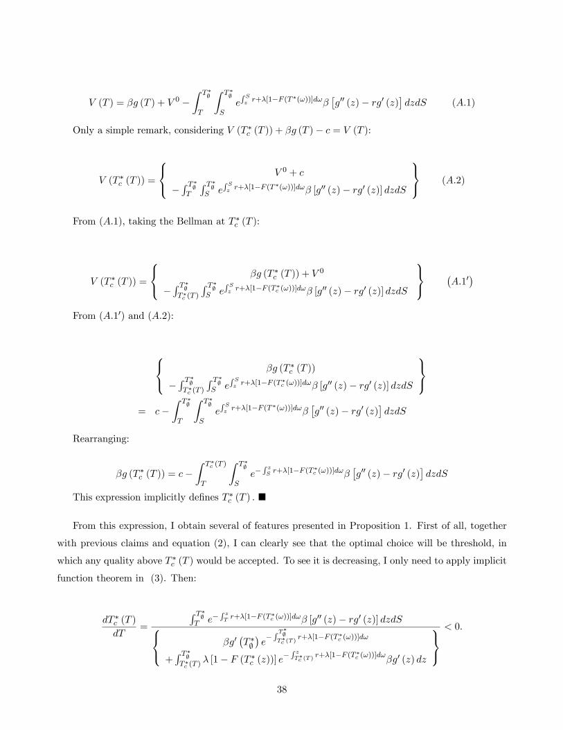
V (T ) = �g (T ) + V 0 �Z T �;

T

Z T �;

SeR Sz r+�[1�F (T

�(!))]d!��g00 (z)� rg0 (z)

�dzdS (A:1)

Only a simple remark, considering V (T �c (T )) + �g (T )� c = V (T ):

V (T �c (T )) =

8<: V 0 + c

�R T �;T

R T �;S e

R Sz r+�[1�F (T

�(!))]d!� [g00 (z)� rg0 (z)] dzdS

9=; (A:2)

From (A:1), taking the Bellman at T �c (T ):

V (T �c (T )) =

8<: �g (T �c (T )) + V0

�R T �;T �c (T )

R T �;S e

R Sz r+�[1�F (T

�c (!))]d!� [g00 (z)� rg0 (z)] dzdS

9=; �A:10

�From (A:10) and (A:2):

8<: �g (T �c (T ))

�R T �;T �c (T )

R T �;S e

R Sz r+�[1�F (T

�c (!))]d!� [g00 (z)� rg0 (z)] dzdS

9=;= c�

Z T �;

T

Z T �;

SeR Sz r+�[1�F (T

�(!))]d!��g00 (z)� rg0 (z)

�dzdS

Rearranging:

�g (T �c (T )) = c�Z T �c (T )

T

Z T �;

Se�

R zS r+�[1�F (T

�c (!))]d!�

�g00 (z)� rg0 (z)

�dzdS

This expression implicitly de�nes T �c (T ) : �

From this expression, I obtain several of features presented in Proposition 1. First of all, together

with previous claims and equation (2), I can clearly see that the optimal choice will be threshold, in

which any quality above T �c (T ) would be accepted. To see it is decreasing, I only need to apply implicit

function theorem in (3). Then:

dT �c (T )

dT=

R T �;T e�

R zT r+�[1�F (T

�c (!))]d!� [g00 (z)� rg0 (z)] dzdS8<: �g0

�T �;�e�R T�;T�c (T )

r+�[1�F (T �c (!))]d!

+R T �;T �c (T )

� [1� F (T �c (z))] e�R zT�c (T )

r+�[1�F (T �c (!))]d!�g0 (z) dz

9=;< 0:

38

in similar ways, I obtain results on changes in cost and market tightness:

dT �c (T )

dc=

18<: �g0�T �;�e�R T�;T�c (T )

r+�[1�F (T �c (!))]d!

+R T �;T �c (T )

� [1� F (T �c (z))] e�R zT�c (T )

r+�[1�F (T �c (!))]d!�g0 (z) dz

9=;> 0; 8T

and

dT �c (T )

d�= �

R T �c (T )T

R T �;S e

R Sz r+�[1�F (T

�c (!))]d!

R Sz [1� F (T

�c (!))] d!� [g

00 (z)� rg0 (z)] dzdS

�g0�T �;�e�R T�;T�c (T )

r+�[1�F (T �c (!))]d! +R T �;�c(T )

� [1� F (T �c (z))]�g0 (z) dz

=

R T �c (T )T

R T �;S e�

R zS r+�[1�F (T

�c (!))]d!

R zS [1� F (T

�c (!))] d!� [g

00 (z)� rg0 (z)] dzdS

�g0�T �;�e�R T�;T�c (T )

r+�[1�F (T �c (!))]d! +R T �;�c(T )

� [1� F (T �c (z))]�g0 (z) dz

Notice that, if T < T �c (T ), we have thatdT �c (T )d� < 0, while if T > T �c (T ), I have that

dT �c (T )d� > 0:

Finally, looking at interest rates:

�g (T �c (T ))� c+Z T �c (T )

T

Z T �;

Se�

R zS r+�[1�F (T

�c (!))]d!�

�g00 (z)� rg0 (z)

�dzdS = 0

dr : �Z T �c (T )

T

Z T �;

Se�

R zS fr+�[1�F (T

�c (!))]gd!�g0 (z) dzdS

�Z T �c (T )

T

Z T �;

S(z � S) e�

R zS �[1�F (T

�c (!))]d!e�r(z�S)�

�g00 (z)� rg0 (z)

�dzdS

+

Z T �c (T )

Te�

R T�;S fr+�[1�F (T �c (!))]gd!�g0

�T �;� dT �;drdS

wheredT �;dr =

g(T �; )2

g00(T �; )g(T�; )�g0(T

�; )

2 < 0:

Let�s take the second integral and work it out:

39

�Z T �c (T )

T

Z T �;

Sze�

R zS �[1�F (T

�c (!))]d!| {z } e�r(z�S)� �g00 (z)� rg0 (z)�| {z }

dv

dzdS =I:P:

= �T �; �g0 �T �; � Z T �c (T )

Te�

R T�;S r+�[1�F (T �c (!))]d!dS +

Z T �c (T )

TS�g0 (S) dS

+

Z T �c (T )

T

Z T �;

Se�

R zS r+�[1�F (T

�c (!))]d!�g0 (z) dzdS

�Z T �c (T )

T

Z T �;

S� [1� F (T �c (z))] ze�

R zS r+�[1�F (T

�c (!))]d!�g0 (z) dzdS

while

Z T �c (T )

TS

Z T �;

Se�

R zS �[1�F (T

�c (!))]d!e�r(z�S)

��g00 (z)� r�g0 (z)

�dzdS =

= �g0�T �;� Z T �c (T )

TSe�

R T�;S r+�[1�F (T �c (!))]d!dS �

Z T �c (T )

TSg0 (S) dS

+

Z T �c (T )

TS

Z T �;

S� [1� F (T �c (z))] e�

R zS r+�[1�F (T

�c (!))]d!�g0 (z) dzdS

Putting things together:

�Z T �c (T )

T

Z T �;

S(z � S) e�

R zS �[1�F (T

�c (!))]d!e�r(z�S)�

�g00 (z)� rg0 (z)

�dzdS

= ��g0�T �;� Z T �c (T )

T

�T �; � S

�e�

R T�;S r+�[1�F (T �c (!))]d!dS

+

Z T �c (T )

T

Z T �;

Se�

R zS r+�[1�F (T

�c (!))]d!�g0 (z) dzdS

�Z T �c (T )

T

Z T �;

S� [1� F (T �c (z))] (z � S) e�

R zS r+�[1�F (T

�c (!))]d!�g0 (z) dzdS

Now, substituting it back into dr:

dr : ��g0�T �;� Z T �c (T )

T

�T �; � S

�e�

R T�;S r+�[1�F (T �c (!))]d!dS

�Z T �c (T )

T

Z T �;

S� [1� F (T �c (z))] (z � S) e�

R zS r+�[1�F (T

�c (!))]d!�g0 (z) dzdS

+

Z T �c (T )

Te�

R T�;S fr+�[1�F (T �c (!))]gd!�g0

�T �;� dT �;drdS

40

Notice that dr < 0 if T �c (T ) > T and dr > 0 if T > T�c (T ). Since dT

�c (T ) > 0 :

@T �c (T )

@r> 0 if T < T �c (T )

and

@T �c (T )

@r< 0 if T > T �c (T )

To obtain the result on c = 0; I just need to use the fact that T �c (T ) is decreasing, Claims A.2 and

A.3 and the fact that T �c (T ) crosses the 45 degree line. Then, I can see that if c = 0 T�c (T ) crosses the

45 degree line at zero. Since it is decreasing, it must be zero everywhere. �

Proof of Lemma 1:

Proof: First of all, I must have in mind that this is the optimal decision of entering or not which

is taken by the entrepreneur. Therefore, he takes � and � as given. Then, remember that the value of

a partnership for the entrepreneur with a project of size T is given by

rP (T ) = � f(1� �) g (T )� P (T )g+ dP (T )dT

(14)

solving the ODE and remembering that:

P�T �;�= (1� �) g

�T �;�

I have:

P (T ) = (1� �) g�T �;�e�(r+�)(T

�;�T) + �

Z T �;

T(1� �) g (s) e�(r+�)(s�T )ds

solving the integral and rearranging,

P (T ) =(1� �)r + �

(�

"g (T ) +

Z T �;

Tg0 (s) e�(r+�)(s�T )ds

#+ rg

�T �;�e�(r+�)(T

�;�T)

)Finally, let�s consider the value function of a entrepreneur that is in the VC�s market searching for

a partner. Since the entrepreneur would accept any VC and would also be accepted by any of them, I

would have:

S (S) =�

(r + �)P (S) (15)

Then, substituting P (S):

41

S (S) =� (1� �)

(r + �) (r + �)

(�

"g (S) +

Z T �;

Sg0 (x) e�(r+�)(x�S)dx

#+ rg

�T �;�e�(r+�)(T

�;�S)

)(16)

Then, an seller would enter the broker�s market after getting a project of initial quality S, if and

only if:

S (S) � A (S)

i.e.,

� (1� �)(r + �) (r + �)

(g�T �;�e�(r+�)(T

�;�S) + �

Z T �;

Sg (x) e�(r+�)(x�S)dx

)� e�r(T �;�S) g

�T �;�

Then, rearranging the above expression:

e�S

(g�T �;�e�(r+�)T

�; + �

Z T �;

Sg (x) e�(r+�)xdx

)� (r + �)

� (1� �)g�T �;�e�rT

�; (F)

Take the derivative of each term:

d

dS

ne�Sg

�T �;�e�(r+�)T

�;

o= �e�Sg

�T �;�e�(r+�)T

�; > 0:

d

dS

(�e�S

Z T �;

Sg (x) e�(r+�)xdx

)= �2e�S

Z T �;

Sg (x) e�(r+�)xdx� �e�rSg (S)

= �

(�e�rSg (S) + �e�T

Z T �;

Sg (x) e�(r+�)xdx

)Note:

�e�SZ T �;

Sg (x) e�(r+�)xdx =I:P:

�e�S

r + �

8<: �g�T �;�e�(r+�)T

�;+

g (S) e�(r+�)S +R T �;S g0 (x) e�(r+�)xdx

9=;Now, assume that T �; > 012, this implies that g0 (S) � rg (S) � 0 (being = 0 i¤ S = T �; ). Then,

g0 (S) � rg (S) : Using this:

�e�SZ T �;

Sg (x) e�(r+�)xdx � �e�S

r + �

8<: �g�T �;�e�(r+�)T

�;+

g (S) e�(r+�)S + rR T �;S g (x) e�(r+�)xdx

9=;12Note that we already assumed this when we wrote P (S)

42

rearranging:

�

Z T �;

Sg (x) e�(r+�)xdx � �g

�T �;�e�(r+�)T

�; + g (S) e�(r+�)S

Substituting this back:

d

dS

(�eS

Z T �;

Sg (x) e�(r+�)xdx

)� �

n�e�rSg (S) + g (S) e�rS � g

�T �;�e�(r+�)T

�; e�S

orearranging:

d

dS

(�e�T

Z T �;

Tg (s) e�(r+�)sds

)� ��e�T g (T ) e�(r+�)T

Then, putting everything together:

dLHS

dS� �e�Sg

�T �;�e�(r+�)T

�; � �e�Sg (S) e�(r+�)S = 0:

�

Proof of Proposition 2:

To prove this proposition, I will present a sequence of claims:

Claim A.5 @TF@n > 0, i.e., the more the number of new projects in the hands of entrepreneurs, better

the minimum quality project that decides to look for a VC;

Proof: From a steady state perspective:

nh1�H

�TF�i= �u�

since � = m(u�;v)u� :

nh1�H

�TF�i= m (u�; v)

Since I am assuming that v is a constant, I can de�ne q (u) � m (u; v). Then:

u� = q�1�nh1�H

�TF�i�

I will now derive the pieces to apply implicit function theorem. From the above expression:

43

du�

dTF=

�h�TF�n

q0 (q�1 (n (1�H (TF)))) < 0:

anddu�

dn=

�1�H

�TF��

q0 (q�1 (n (1�H (TF)))) > 0

Then:

@�

@TF=

du�

dTF

�mu (u

�; v)u� �m (u�; v)u�2

�=

du�

dTF

��mv (u

�; v) v

u�2

�> 0

where I used the Euler Theorem from the �rst to the second line.

@�

@TF= �

nh�SF�

v< 0

Also applying the Euler Theorem, we obtain:

@�

dn= �du

�

dn� mv (u

�; v)

u�v

u�< 0

@�

@n=

�1�H

�TF��

v> 0

Then, let�s obtain the sign of dTF

dn by IFT. Then:

�dn :

8<: e�TF @�@n

R T �;TF [g

0 (x)� rg (x)] e�(r+�)x�x� TF

�dx

� @�@n

r�2

1�� g

�T �;�e�rT

�;

9=; > 0

dTF :

8<: e�TF R T �;

TF [g0 (x)� rg (x)] e�(r+�)x

��� @�

@TF�x� TF

��dx

+ @�@TF

r�2

1�� g

�T �;�e�rT

�;

9=; > 0

Then:

@TF

@n=�dndTF

> 0

�

Claim A.6 d�dn > 0, therefore the expected time a VC spends with a project

�1�

�decreases as n increases

44

Proof: Remember that:

� = n [1�H (S)]

Then, let�s look at the total di¤erentiation of � with respect to n. Then:

d� =�1�H

�TF��� nh

�TF� dTFdn

putting�1�H

�TF��in evidence and manipulating it:

d�

dn=�1�H

�TF�� �e�T

F R T �;TF [g

0 (x)� rg (x)] e�(r+�)xdx8<: e�TF R T �;

TF [g0 (x)� rg (x)] e�(r+�)x

��� @�

@TF�x� TF

��dx

+ @�@TF

r�2

1�� g

�T �;�e�rT

�;

9=;> 0:

�Similar calculations show that d�dn < 0, which concludes my proof.�Proof of Lemma 2:

Proof: Solving the ODE and using the terminal condition:

P (T ) = (1� �) g (T ) +Z T �;

T(1� �)

�g0 (s)� rg (s)

�e�

R sT (z)dz:ds

Then:

dP (T )

dT=

(r (1� �) g (T ) + (T )

Z T �;

T(1� �)

�g0 (s)� rg (s)

�e�

R sT (z)dz:ds

)> 0

Since g0 (s)� rg (s) ; 8s 2�0; T �;

�: Then:

S (T ) =��1� F

�T ��1 (T )

��r + � [1� F (T ��1 (T ))]P (T )

As we know, a entrepreneur enters the VC market if:

S (T ) � A (T )

which means:

��1� F

�T ��1 (T )

��r + � [1� F (T ��1 (T ))]e

�rTP (T ) � e�rT �; g�T �;�

45

Then:

dLHS

dT=

8><>: � r�f(T ��1(T )) dT��1(T )dT

fr+�[1�F (T ��1(T ))]g2 e�rTP (T )

+�[1�F(T ��1(T ))]r+�[1�F (T ��1(T ))]e

�rTh�rP (T ) + dP (T )

dT

i9>=>;

notice that:

dP (T )

dT� rP (T ) = [� (1� F (T � (T )))]

Z T �;

T(1� �)

�g0 (s)� rg (s)

�e�

R sT (z)dz:ds > 0

Since dT ��1(T )dT < 0, we have that dLHSdT � 0: Therefore, there exists a threshold TF (c) such that if

T � TF (c) the entrepreneur enters the VC market. �

Proof of Claim 1:

Proof: Using induction. We can easily show that it increases from N = 1 to N = 2. Now consider

a given N � 2. For N + 1:

! � (N + 1)

Z !

0[1� Z (")]N Z (") d"�

Z !

0[1� Z (")]N+1 d"

while for N it was already seen:

! �NZ !

0[1� Z (")]N�1 Z (") d"�

Z !

0[1� Z (")]N d"

Therefore, the change in expected return as we increased the number of bidders in 1 is:

N

Z !

0[1� Z (")]N�1 Z (")2 d"+

Z !

0[1� Z (")]N+1 d"�

Z !

0[1� Z (")]N+1 d"

= N

Z !

0[1� Z (")]N�1 Z (")2 d" > 0

�Proof of Claim 2:

Proof:

limN!1

! �NZ !

0[1� Z (")]N�1 Z (") d"�

Z !

0[1� Z (")]N d"

notice that:

limN!1

Z !

0[1� Z (")]N d" = 0

Consider that there exists z0 (") and z (�) > 0, then:

46

�NZ !

0[1� Z (")]N�1 Z (") d" =

Z !

0N [1� Z (")]N�1 (�z (")) Z (")

z (")d"

= �Z !

0[1� Z (")]N

�1� Z (") z

0 (")

z (")2

�d"

But then, it is easy to see that this expression goes to zero as N ! 1: Therefore, expected valueconverges to !:�

47

9 Appendix B

In this appendix, I will consider the case in which the Venture Capital can handle two projects at the

same time. In this case, her Bellman function is given by:

(1 + rdT )V (T1; T2) = �dTEeT max8>>><>>>:V�eT ; T2 + dT�+ �g (T1 + dT )� c;

V�T1 + dT; eT�+ �g (T2 + dT )� c;

V (T1 + dT; T2 + dT )

9>>>=>>>;

+(1� �dT )max

8>>>>><>>>>>:V (;; T2 + dT ) + �g (T1 + dT ) ;V (T1 + dT; ;) + �g (T2 + dT ) ;

V (;; ;) + �g (T1 + dT ) + �g (T2 + dT ) ;V (T1 + dT; T2 + dT )

9>>>>>=>>>>>;Then, considering max fT1; T2g < T �; :

(1 + rdT )V (T1; T2) = �dTEeT max8>>><>>>:V�eT ; T2 + dT�+ �g (T1 + dT )� c;

V�T1 + dT; eT�+ �g (T2 + dT )� c;

V (T1 + dT; T2 + dT )

9>>>=>>>;+(1� �dT )V (T1 + dT; T2 + dT )

Rearranging:

rdTV (T1; T2) = �dTEeT max

8>>>>>>>>><>>>>>>>>>:

24 V �eT ; T2 + dT�+ �g (T1 + dT )�c� V (T1 + dT; T2 + dT )

35 ;24 V �T1 + dT; eT�+ �g (T2 + dT )�c� V (T1 + dT; T2 + dT )

35 ;0

9>>>>>>>>>=>>>>>>>>>;+V (T1 + dT; T2 + dT )� V (T1; T2)

Then, dividing by dT and taking dT ! 0:

48

rV (T1; T2) = �E eT max

8>>>>>>>>><>>>>>>>>>:

24 V �eT ; T2�+ �g (T1)�c� V (T1; T2)

35 ;24 V �T1; eT�+ �g (T2)�c� V (T1; T2)

35 ;0

9>>>>>>>>>=>>>>>>>>>;+

�@V

@T1(T1; T2) +

@V

@T2(T1; T2)

�Then, looking at the cut o¤ rule, let�s analyze the conditions in which I have:

V�eT ; T2�+ �g (T1)� c� V (T1; T2) � V �T1; eT�+ �g (T2)� c� V (T1; T2)

Simplifying:

V�eT ; T2�+ �g (T1) � V �T1; eT�+ �g (T2)

First of all, consider a symmetry condition:

V�eT ; T2� = V �T2; eT�

Then, rearranging:

[�g (T1)� �g (T2)]�hV�T1; eT�� V �T2; eT�i � 0

Therefore, since both functions are increasing (as we showed before), I must have the increase in

�g (�) higher than the increase in V��; eT� as T increases. Taking T1 = T2 + dT , dividing by dT and

taking dT ! 0:

�g0 (T2)�@V

@T1

�T2; eT� � 0

which is exactly what I showed previously. Therefore, if the VC �nishes one project to undertake a new

one, she chooses the bigger one. Then, there is a decision about cutting a project or not: Imagining

again that T1 is the bigger one,

49

V�eT ; T2�+ �g (T1)� c � V (T1; T2)

I will again have a T �c (T1), in which the only contribution of T2 is that T2 � T1:

Let�s consider now calculations related to the expected time until an IPO. First of all, notice that

in the usual case in which a Venture Capital �rm can only handle one project, the survival rate of a

project of size/quality T is given by:

S (t jT ) = e��R t0 [1�F (T

�(T+s))]ds

1� e��R T�; �T0 [1�F (T �(T+s))]ds

; for t 2�0; T �; � T

�then the hazard rate conditional on T is:

~ (t jT ) = �S0 (t jT )S (t jT ) = � [1� F (T

� (T + t))] :

and the lifetime distribution, conditional on T is:

K (t jT ) = 1� S (t jT ) = 1� e��R t0 [1�F (T

�(T+s))]ds

1� e��R T�; �T0 [1�F (T �(T+s))]ds

which implies:

k (t jT ) = � [1� F (T � (T + t))] e��R t0 [1�F (T

�(T+s))]ds

1� e��R T�; �T0 [1�F (T �(T+s))]ds

Then the expected lifetime of a partnership given a starting size/quality T is:

R T �;�T0 e��

R t0 [1�F (T

�(T+s))]dsdt��T �; � T

�e��

R T�; �T0 [1�F (T �(T+s))]ds

1� e��R T�; �T0 [1�F (T �(T+s))]ds

Then the expected lifetime of a partnership is given by:

Z T �;

0

R T �;�T0 e��

R t0 [1�F (T

�(T+s))]dsdt��T �; � T

�e��

R T�; �T0 [1�F (T �(T+s))]ds

1� e��R T�; �T0 [1�F (T �(T+s))]ds

dF (T ) :

Now consider the case in which a VC can handle two projects. Whenever she has a free spot, she

will prefer ful�lling that spot instead of going public with the current project to accommodate the new

project than cutting a current project. So she will cut projects when they are mature or if she �nds a

50

new one and have both vacancies ful�lled. Considering this second case, the Survival rate for a project

with size quality T is given by:

S (t jT ) = e��R t0 G(T+s)[1�F (T

�(T+s))]ds

1� e��R T�; �T0 G(T+s)[1�F (T �(T+s))]ds

; for t 2�0; T �; � T

�which is bigger than the previous one, since G (�) � 1. It�s routine to show that in this case the

expected lifetime of a partnership is given by:

Z T �;

0

R T �;�T0 e��

R t0 G(T+s)[1�F (T

�(T+s))]dsdt��T �; � T

�e��

R T�; �T0 G(T+s)[1�F (T �(T+s))]ds

1� e��R T�; �T0 G(T+s)[1�F (T �(T+s))]ds

dF (T ) :

which is bigger than the previous one.

51

TABLE 1: Characteristics of VC backed and non VC-backed IPOs

VC- backed IPOs Non VC-backed IPOs

Mean N Mean N T-stat Age 7.0 1159 14.7 1446 12.13Book Value 0.76 1961 6.63 3253 11.28Revenue 19.9 1732 52.1 2759 3.16EPS (% pos.) 49.7 806 76.5 1358 12.71Total Assets 104.4 1719 543.2 2628 3.97Net proceeds 40.5 2286 58.3 3782 5.44First-day Return (%) 26.82 2208 19.36 4030 5.99Underwriter Rank 7.80 2383 6.79 4030 21.02Gross spread 7.09 2285 7.36 3781 1.76Source: Lee and Wahal (2004)

TABLE 2: Comparison of characteristics for IPOs backed by young and old VC firms

VC firms <6 yr. at IPO VC firms ≥6 yr. at IPO p-value test of no difference

Avg. time from IPO date to next follow-on fund in months 16.0[12.0] 24.2

[24.0] 0.001[0.002]

Avg. size of next follow-on fund (1997 $mil) 87.9[68.0] 136.6

[113.4] 0.018[0.024]

Avg. age of VC-backed company at IPO date in months 55.1[42.0] 79.6

[64.0] 0.000[0.000]

Avg. duration of board representation for lead VC in months 24.5[20.0] 38.8

[28.0] 0.001[0.000]

Avg. underpricing at the IPO date 0.136[0.067] 0.073

[0.027] 0.001[0.036]

Avg. offer size (1997 $mil) 18.3[13.0] 24.7

[19.1] 0.013[0.000]

Avg. Carter and Manaster underwriter rank 6.26[6.50] 7.43

[8.00] 0.000[0.000]

Avg. number of previous IPOs 1[0] 6

[4] 0.000[0.000]

Avg. fraction of equity held by all VCs prior to IPO 0.321[0.287] 0.377

[0.371] 0.025[0.024]

Avg. fraction of equity held by lead VC after IPO 0.122[0.100] 0.139

[0.120] 0.098[0.031]

Avg. market value of lead VC’s equity after IPO (1997 $mil) 9.5[4.3] 14.7

[8.7] 0.033[0.000]

Avg. aftermarket std. deviation 0.034[0.030] 0.030

[0.028] 0.080[0.324]

Number of Observations 99 240 Note: Sample is 433 VC-backed companies that went public between January 1, 1978 and December 31, 1987. Medians are in brackets. Significance tests in the third column are p-values of t-tests for differences in averages and p-values of two-sample Wilconson rank-sum tests for differences in medians in brackets. Source: Gompers and Lerner (2001)

TABLE 3: Multivariate Regression with Robust Errors No. obs.: 1550 F(26, 1523) = 9.64 Prob > F = 0.000 R2 = 0.239 Root MSE = 60.18

fdr Coef. Std. Error t P>⏐t⏐ [95% Conf. Interval] Reg -0.09982 0.02185 -4.57 0.000 -0.142670 -0.056962 Age -0.48988 0.11376 -4.31 0.000 -0.713018 -0.266745 AMEXdummy -7.01536 9.55909 -0.73 0.463 -25.76573 11.73501 NASDQdummy 0.56059 2.79067 0.20 0.841 -4.913374 6.034551 NYSEdummy -7.36085 4.33795 -1.70 0.090 -15.86984 1.148125 Djod -0.02486 0.01441 -1.73 0.085 -0.053122 0.003401 Dummy1999 57.81929 20.6124 2.81 0.005 17.38751 98.25106 Health -11.10043 3.07635 -3.61 0.000 -17.13477 -5.066087 High tech 3.380294 2.82414 1.20 0.232 -2.159312 8.919901 Spod 0.196895 0.11041 1.54 0.125 -0.046873 0.386251 _cons 90.97264 44.9188 2.03 0.043 2.863437 179.0818

Where: reg ≡ days in registration; age ≡ firm age at IPO; djod ≡ dow jones index at offer date; health ≡ dummy for firm in health sector; high tech ≡ dummy for firm in tech sector; spod ≡ S & P 500 at offer date.

TABLE 4: Multivariable Fractional Polynomial Model Source SS df MS No. obs.: 1550

Model 1830577.8 28 65377.8 F(28,1521) =18.35 Residual 5419252.1 1521 3562.95 Prob > F = 0.000 Total 7249829.9 1549 4680.33 R2 = 0.2525

Root MSE = 59.69 fdr Coef. Std. Error t P>⏐t⏐ [95% Conf. Interval]

lreg -10.6595 2.183401 -4.88 0.000 -14.9423 -6.3767 Lage1 -0.50835 0.187997 -2.70 0.007 -0.87711 -0.1396 Ldjod_1 -3.47512 0.844651 -4.11 0.000 -5.13193 -1.8183 Ldjod_2 1.26426 0.313333 4.03 0.000 0.64965 1.8789 High tech 2.71745 3.927244 0.69 0.489 -4.98594 10.421 Health -10.5799 8.051582 -1.31 0.189 -26.3733 5.2135 lspod_1 435.539 92.85873 4.69 0.000 253.394 617.68 lspod_2 -657.809 141.3594 -4.65 0.000 -935.089 -380.53 NASDQdummy -0.15150 5.607602 -0.03 0.978 -11.1509 10.8479 NYSEdummy -7.50743 9.710198 -0.77 0.440 -26.5542 11.5393 _cons 107.522 29.09031 3.70 0.000 50.4606 164.583

Where: lreg_1 = ln(reg/100) + 0.3457942617, lnage_1 = age – 7.612903226, Ldjod_1 = (djod/100)3 – 218.8132734, Ldjod_2 = (djod/100)3ln(djod/100) – 393.004593; lspod_1 = (spod/100)3 – 0.4248286209; lspod_2 = (spod/100)3 ln(spod/100) – 0.1212275993.