Pedosphere 23(1): 48–58, 2013

ISSN 1002-0160/CN 32-1315/P

c© 2013 Soil Science Society of China

Published by Elsevier B.V. and Science Press

Vegetation and Topographic Control on Spatial Variability

of Soil Organic Carbon∗1

I. OUESLATI1, P. ALLAMANO1,∗2, E. BONIFACIO2 and P. CLAPS1

1DITIC, Politecnico di Torino, 10129 Torino (Italy)2DIVAPRA, Universita di Torino, 10095 Grugliasco (Italy)

(Received May 19, 2012; revised November 23, 2012)

ABSTRACTSoil organic carbon (SOC) is one of the most important parameters affecting the hydraulic characteristics of natural soils. Despite

being rather easy to measure, SOC is known to be highly variable in space. In this study, vegetation, climate, and morphology factors

were used to reproduce the spatial distribution of SOC in the mineral horizons of forest and grassland areas in north-western Italy

and the feasibility of the approach was evaluated. When the overall sample (114 samples) was analyzed, average annual rainfall

and elevation were significant descriptors of the SOC variability. However, a large part of the variability remains unexplained. Two

stratification criteria were then adopted, based on vegetation and topographic properties. We obtained an improvement of the quality

of the estimates, particularly for grasslands and forests in the absence of local curvatures. These results indicate that the spatial

variability of soil organic matter is scarcely reproducible at the regional scale, unless an a-priori reduction of the heterogeneity is

applied. A discussion on the feasibility of applying stratification criteria to deal with heterogeneous samples closes the paper.

Key Words: climate factor, natural soils, regression analysis, SOC

Citation: Oueslati, I., Allamano, P., Bonifacio, E. and Claps, P. 2013. Vegetation and topographic control on spatial variability of

soil organic carbon. Pedosphere. 23(1): 48–58.

INTRODUCTION

Soils are among the most important global carboncycle reservoirs. They represent 75% of the total ter-restrial organic carbon pool, and twice the atmosphericcarbon content (Farquhar et al., 2001). Most soil car-bon is stored as soil organic matter; inorganic carbo-nates are largely restricted to dry lands (Lal, 2008). Fo-rest and grassland soils are therefore of utmost impor-tance as their organic matter content is much higherthan that of agricultural soils.

In addition to its well-known effect on soil fertility,soil organic carbon (SOC) is also one of the most im-portant parameters affecting soil hydraulic properties:by enhancing soil aggregation and increasing pores con-tinuity and stability (Tisdall and Oades, 1982), it ame-liorates water holding capacity and saturated hydraulicconductivity (Nemes et al., 2005). As a consequence,it is used as an independent variable in several pedo-transfer functions to estimate soil hydraulic properties(e.g., Guber et al., 2006).

Despite being rather easy to measure, SOC ishighly variable in space. Evaluating its concentration

in areas greater than an agricultural plot can be there-fore rather difficult. A large effort has been made topredict its areal distribution through digital soil map-ping approaches (Arrouays et al., 1998; Bell et al.,2000; Chaplot et al., 2001; Abnee et al., 2004a, b; Terraet al., 2004; Thompson and Kolka, 2005; Lagacherieand McBratney, 2006). Typically, the approach is im-plicitly based on Jenny (1941)’s factors of soil forma-tion: it produces empirical quantitative relations be-tween soil characteristics and spatially referenced fac-tors, with the aim of using these relations as soil spatialprediction functions (McBratney et al., 2003).

The most relevant pedogenic factors controllingSOC are climate, vegetation, and topography (Baldockand Nelson, 2000). Climate impacts directly on SOCcontent and rate of mineralization primarily throughthe effects of temperature and moisture. Temperatureis a key factor controlling the rate of decomposition ofplant residues. For example, reaction rates double foreach increase of 8–9 ◦C in the mean annual air tem-perature (Bot and Benites, 2005). As a consequence,soils in cooler climates commonly contain more organicmatter because of slower mineralization rates. In addi-

∗1Supported by the Italian Ministry of Education (No. 2007HBTS85).∗2Corresponding author. E-mail: paola.allamano@polito.it.

VEGETATION AND TOPOGRAPHIC EFFECTS ON SOC 49

tion, SOC content increases as average annual rainfallincreases (Meier and Leutschner, 2010).

Changes in SOC concentration also correlate withchanges in vegetation. For instance, herbaceous vege-tation produces a big root mass compared with theabove-ground component whereas, in forests, most or-ganic matter is produced above ground and residuesare more resistant to decomposition (Melillo et al.,1993).

The latter pedogenic factor controlling SOC is to-pography. Topography affects soil properties mainlythrough its effects on water movements. In terrain de-pressions, in fact, soils are moister because they receiverunoff, sediments (including organic matter), and see-page from the surroundings, leading to a higher SOCconcentration than that in drier uphill soils (Yoo et al.,2006). On the contrary, soils on steep slopes tend tolose organic matter because the topsoil is constantlyeroded. Therefore, the spatial distribution of topo-graphic attributes that characterize the flow paths canhelp in capturing the soil variability and in predictingsoil properties (Moore et al., 1991, 1993; Florinsky andKuryakova, 1996).

Landscape characteristics can be expressed bymeans of geomorphic and hydrological indexes ge-nerated with digital terrain analysis (Speight, 1968;MacMillan and Pettapiece, 1997; Wilson and Gallant,2000). These indexes are widely used in hydrologicmodelling, e.g., to characterize the spatial distributionand the extent of zones of saturation for runoff gene-ration (Beven and Kirkby, 1979). Climatic data are of-ten available through gridded datasets, and vegetationcharacteristics can be derived qualitatively from landcover maps such as CORINE (European EnvironmentAgency, 2005), or quantitatively by making use of re-

mote sensing. Quantitative environmental variablescan be then associated to SOC, resulting in long setsof potential descriptors of SOC variability.

In this study we evaluated the spatial variabilityof SOC and the feasibility of prediction of organic car-bon concentration by means of quantitative descrip-tors of vegetation, climate and topography in forestand grassland soils of alpine and sub-alpine areas ofnorth-western Italy. No specific survey was performedfor this study and the data were all derived (and ho-mogenised) from existing databases.

MATERIALS AND METHODS

Study area

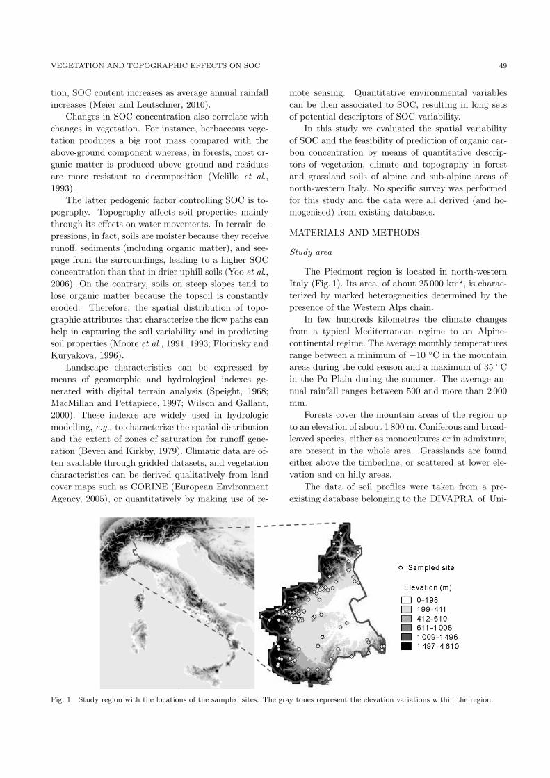
The Piedmont region is located in north-westernItaly (Fig. 1). Its area, of about 25 000 km2, is charac-terized by marked heterogeneities determined by thepresence of the Western Alps chain.

In few hundreds kilometres the climate changesfrom a typical Mediterranean regime to an Alpine-continental regime. The average monthly temperaturesrange between a minimum of −10 ◦C in the mountainareas during the cold season and a maximum of 35 ◦Cin the Po Plain during the summer. The average an-nual rainfall ranges between 500 and more than 2 000mm.

Forests cover the mountain areas of the region upto an elevation of about 1 800 m. Coniferous and broad-leaved species, either as monocultures or in admixture,are present in the whole area. Grasslands are foundeither above the timberline, or scattered at lower ele-vation and on hilly areas.

The data of soil profiles were taken from a pre-existing database belonging to the DIVAPRA of Uni-

Fig. 1 Study region with the locations of the sampled sites. The gray tones represent the elevation variations within the region.

50 I. OUESLATI et al.

versity of Torino (67 samples) and to Regional SoilSurvey Service (IPLA, 55 samples). The chemical char-acteristics considered were soil organic carbon (SOC)and total nitrogen (N) concentrations in the mineralhorizons. The data were available for all genetic hori-zons (A, B, or C types) and also aggregated on the0–30 cm depth (SOC30). The chemical characteristicsof the dataset are reported in Table I.

No significant differences were found in SOC andN concentrations between forests and grasslands, whilethe C to N ratio clearly reflected the differences in or-ganic matter decomposition, with the lowest values ingrasslands and the highest in conifers, both in the Ahorizon and in the 0–30 cm layer. The concentrationsof SOC and N were generally more variable in the ge-netic soil horizons than in the 0–30 cm layer, reflectingthe different thicknesses of the SOC enriched A hori-zons. The same behaviour was observed for the C toN ratio, with lower standard deviations in the 0–30 cmlayer, particularly in grassland samples.

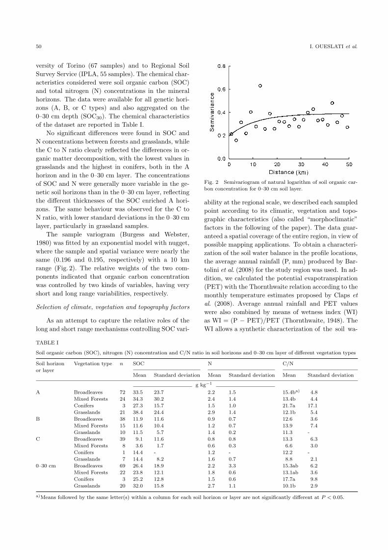
The sample variogram (Burgess and Webster,1980) was fitted by an exponential model with nugget,where the sample and spatial variance were nearly thesame (0.196 and 0.195, respectively) with a 10 kmrange (Fig. 2). The relative weights of the two com-ponents indicated that organic carbon concentrationwas controlled by two kinds of variables, having veryshort and long range variabilities, respectively.

Selection of climate, vegetation and topography factors

As an attempt to capture the relative roles of thelong and short range mechanisms controlling SOC vari-

Fig. 2 Semivariogram of natural logarithm of soil organic car-

bon concentration for 0–30 cm soil layer.

ability at the regional scale, we described each sampledpoint according to its climatic, vegetation and topo-graphic characteristics (also called “morphoclimatic”factors in the following of the paper). The data guar-anteed a spatial coverage of the entire region, in view ofpossible mapping applications. To obtain a characteri-zation of the soil water balance in the profile locations,the average annual rainfall (P, mm) produced by Bar-tolini et al. (2008) for the study region was used. In ad-dition, we calculated the potential evapotranspiration(PET) with the Thornthwaite relation according to themonthly temperature estimates proposed by Claps etal. (2008). Average annual rainfall and PET valueswere also combined by means of wetness index (WI)as WI = (P − PET)/PET (Thornthwaite, 1948). TheWI allows a synthetic characterization of the soil wa-

TABLE I

Soil organic carbon (SOC), nitrogen (N) concentration and C/N ratio in soil horizons and 0–30 cm layer of different vegetation types

Soil horizon Vegetation type n SOC N C/N

or layerMean Standard deviation Mean Standard deviation Mean Standard deviation

g kg−1

A Broadleaves 72 33.5 23.7 2.2 1.5 15.4ba) 4.8

Mixed Forests 24 34.3 30.2 2.4 1.4 13.4b 4.4

Conifers 3 27.3 15.7 1.5 1.0 21.7a 17.1

Grasslands 21 38.4 24.4 2.9 1.4 12.1b 5.4

B Broadleaves 38 11.9 11.6 0.9 0.7 12.6 3.6

Mixed Forests 15 11.6 10.4 1.2 0.7 13.9 7.4

Grasslands 10 11.5 5.7 1.4 0.2 11.3 -

C Broadleaves 39 9.1 11.6 0.8 0.8 13.3 6.3

Mixed Forests 8 3.6 1.7 0.6 0.3 6.6 3.0

Conifers 1 14.4 - 1.2 - 12.2 -

Grasslands 7 14.4 8.2 1.6 0.7 8.8 2.1

0–30 cm Broadleaves 69 26.4 18.9 2.2 3.3 15.3ab 6.2

Mixed Forests 22 23.8 12.1 1.8 0.6 13.1ab 3.6

Conifers 3 25.2 12.8 1.5 0.6 17.7a 9.8

Grasslands 20 32.0 15.8 2.7 1.1 10.1b 2.9

a)Means followed by the same letter(s) within a column for each soil horizon or layer are not significantly different at P < 0.05.

VEGETATION AND TOPOGRAPHIC EFFECTS ON SOC 51

ter balance in a certain location and provides a relativemeasure of potential biological productivity of the site.

The normalized difference vegetation index (NDVI)maps, derived from SPOT-VEGETATION data (http://free.vgt.vito.be/) for the years 1998–2005, were usedto characterize vegetation. For each month the com-posite NDVI values were averaged over 1 km2 cells. Foreach cell containing at least one soil sampling we con-sidered the minimum NDVI (NDVImin), the maximumNDVI (NDVImax), the difference between maximumand minimum NDVI (NDVIdiff) and the mean NDVI(NDVImean). The CORINE land cover map (EuropeanEnvironment Agency, 2005) and the forests map ofthe Piedmont Regional Administration were also takeninto account for further evaluations of vegetation typesin correspondence of the sampling points.

The selection of the terrain descriptors was basedon the prior experience by Chai et al. (2008), who con-sidered elevation, slope and CTI (see Table II) as ex-ternal drift variables for predicting soil organic matter,and Mueller and Pierce (2003) and Simbahan et al.(2006), who used terrain attributes as secondary spa-tial variables to increase the accuracy of predictionsat different scales. To determine the primary and se-condary terrain attributes (Table II), we used a digitalelevation model (derived from contour line interpola-tion) with a spatial resolution of 50 m. The primary at-tributes in Table II include elevation (EL), slope (SL),profile (kv) and plan curvature (kh). In kv and kh, thesign ensures that positive curvatures refer to convexforms and negative curvatures refer to concave forms.The expected values for a hilly area (moderate relief)can vary from −0.5 to 0.5, while for steep and rugged

mountains (extreme relief), they can vary between −4and 4. A value of zero indicates that the surface isflat. As secondary terrain attributes in Table II, weconsidered compound topographic index (CTI), alsoknown as topographic wetness index (Wilson and Gal-lant, 2000), and stream power index (SPI). The CTI,expressed as reported in Table II, is related to zones ofsurface saturation (Moore et al., 1993) and quantifies apoint in the landscape in terms of water and sedimentaccumulation: the higher the value of this index in acell, the higher the soil moisture that can be found init. SPI instead, expressed as reported in Table II, isrelated to erosion processes, being an indicator of thecapability of a flow to generate net erosion.

Establishment and verification of SOC models

Linear multiple regression is the most widely usedmethod to capture soil carbon patterns, as demon-strated by numerous applications (Walker et al., 1968;Pennock et al., 1987; Moore et al., 1993; Gessler et al.,1995, 2000; Chaplot et al., 2000). This preference stemsfrom its ease of use, computational efficiency, andstraightforward interpretation (Hastie et al., 2005).

In order to select the possible relationships betweensoil carbon concentration and environmental factors,we implemented simple correlation and multiple regres-sion schemes. The simple correlations between SOCand environmental variables were evaluated on all ge-netic horizons and on the fixed 0–30 depth. The mul-tiple regressions were calculated only on the values re-lated to 30 cm depth, to avoid considering horizons ofvariable thickness.

The models were tested against the assumptions of

TABLE II

Definitions, formulas and physical interpretations for the topographic variables considered in the study

Variable Definitions and formula Interpretation

Slope gradient (SL, ◦) Angle between a tangent plane and a horizontal one at a

given point of the land surface

Velocity of substance flows

Profile curvature (kv, m−1) Profile curvature is parallel to the direction of the maxi-

mum slope. A negative value indicates that the surface is

upwardly convex at that cell. A positive profile curvature

indicates that the surface is upwardly concave at that cell.

A value of zero indicates that the surface is flat.

Relative acceleration/deceleration of

flows across the surface

Plan curvature (kh, m−1) Planform curvature (commonly called plan curvature) is

perpendicular to the direction of the maximum slope. A

positive value indicates the surface is sidewardly convex

at that cell. A negative value indicates the surface is side-

wardly concave at that cell. A value of zero indicates the

surface is flat.

Convergence/divergence of flows acro-

ss a surface

Compound topographic in-

dex (CTI)

CTI = lnCA

SLa) Extent of potential flow accumulation

Stream power index (SPI) SPI = CA·SL Extent of potential flow erosion

a)CA is specific catchment area (m2 m−1), i.e., upslope area per unit width of contour (Wilson and Gallant, 2000).

52 I. OUESLATI et al.

the linear regression analysis (Kottegoda and Rosso,1997), namely lack of multicollinearity, equal errorvariance (homoscedasticity), and normal and ran-dom residuals. In some cases we used the logarithmictransformation of the variable for complying to theseassumptions, particularly as regards normality. Thegoodness of relationships was verified using standarderror of the estimate and adjusted determination coef-ficient (R2

adj). The variogram analysis was also appliedto the residuals of regressions in order to assess theirresidual spatial variability.

RESULTS AND DISCUSSION

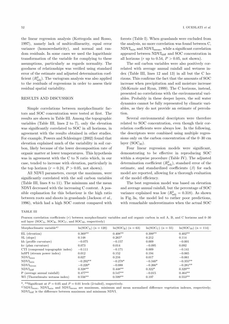
Simple correlations between morphoclimatic fac-tors and SOC concentration were tested at first. Theresults are shown in Table III. Among the topographicvariables (Table III, lines 2 to 7), only the elevationwas significantly correlated to SOC in all horizons, inagreement with the results obtained in other studies.For example, Powers and Schlesinger (2002) found thatelevation explained much of the variability in soil car-bon, likely because of the lower decomposition rate oforganic matter at lower temperatures. This hypothesiswas in agreement with the C to N ratio which, in ourcase, tended to increase with elevation, particularly inthe top horizon (r = 0.24, P > 0.05, not shown).

All NDVI parameters, except the maximum, weresignificantly correlated with the soil carbon variables(Table III, lines 8 to 11). The minimum and the meanNDVI decreased with the increasing C content. A pos-sible explanation for this behaviour is the high ratiobetween roots and shoots in grasslands (Jackson et al.,1996), which had a high SOC content compared with

forests (Table I). When grasslands were excluded fromthe analysis, no more correlation was found between C,NDVImin and NDVImean, while a significant correlationappeared between NDVIdiff and SOC concentration inall horizons (r up to 0.54, P > 0.05, not shown).

The soil carbon variables were also positively cor-related with average annual rainfall and wetness in-dex (Table III, lines 12 and 13) in all but the C ho-rizons. This confirms the fact that the amounts of SOCincrease when precipitation and soil moisture increase(McKenzie and Ryan, 1999). The C horizons, instead,presented no correlations with the environmental vari-ables. Probably in these deeper layers, the soil waterdynamics cannot be fully represented by climatic vari-ables, as they do not provide an estimate of percola-tion.

Several environmental descriptors were thereforerelated to SOC concentration, even though their cor-relation coefficients were always low. In the following,the descriptors were combined using multiple regres-sions only on the carbon concentration of the 0–30 cmlayer (SOC30).

Four linear regression models were significant,demonstrating to be effective in reproducing SOCwithin a stepwise procedure (Table IV). The adjusteddetermination coefficient (R2

adj), standard error of theestimate, and standardized coefficients (β) for eachmodel are reported, allowing for a thorough evaluationof the model efficiency.

The best regression model was based on elevationand average annual rainfall, but the percentage of SOCvariance explained was low (R2

adj = 0.318). As shownin Fig. 3a, the model led to rather poor predictions,with remarkable underestimates when the actual SOC

TABLE III

Pearson correlation coefficients (r) between morphoclimatic variables and soil organic carbon in soil A, B, and C horizons and 0–30

soil layer (SOCA, SOCB, SOCC, and SOC30, respectively)

Morphoclimatic variablea) ln(SOCA) (n = 120) ln(SOCB) (n = 63) ln(SOCC) (n = 55) ln(SOC30) (n = 114)

EL (elevation) 0.369** 0.408** 0.399** 0.402**

SL (slope) 0.148 0.265* 0.212 0.114

kh (profile curvature) −0.075 −0.157 0.009 −0.001

kv (plan curvature) 0.073 0.014 −0.095 0.092

CTI (compound topographic index) −0.111 −0.171 0.009 −0.141

lnSPI (stream power index) 0.012 0.152 0.194 −0.065

NDVImax 0.027 0.216 0.017 −0.061

NDVImin −0.292** −0.278* −0.340* −0.355**

NDVImean −0.220* −0.088 −0.266* −0.281**

NDVIdiff 0.328** 0.448** 0.322* 0.329**

P (average annual rainfall) 0.477** 0.547** −0.015 0.464**

WI (Thornthwaite wetness index) 0.556** 0.599** 0.197 0.553**

*, **Significant at P = 0.05 and P = 0.01 levels (2-tailed), respectively.a)NDVImax, NDVImin and NDVImean are maximum, minimum and mean normalized difference vegetation indexes, respectively;

NDVIdiff is the difference between maximum and minimum NDVI.

VEGETATION AND TOPOGRAPHIC EFFECTS ON SOC 53

TABLE IV

Significant multiple regression models for evaluation of soil or-

ganic carbon concentration in 0–30 cm layer (SOC30) based on

the whole dataset

Dependent Independent Radj2b) SEEc) βd) P

variable variablesa)

ln(SOC30) EL, P 0.318 0.530 0.34, 0.41 < 0.001

NDVImin, P 0.310 0.533 −0.33, 0.44 < 0.001

NDVImean, P 0.301 0.536 −0.31, 0.49 < 0.001

NDVIdiff , P 0.250 0.555 0.23, 0.41 < 0.01

a)See Table III for the descriptions of independent variables.b)Adjusted determination coefficient.c)Standard error of estimate.d)Standardized coefficient.

concentration was above 50–60 g kg−1 and visible over-estimates in correspondence of low values of observedSOC. NDVI parameters contributed to SOC variabilityin the three other regression models, where the stan-dardized coefficients for NDVI parameters assumedalso negative values. This outcome could be related tothe large heterogeneity of broadleaved forests which,in the study area, included both relatively highly pro-ductive beech stands, with poor understory vegetation,and degraded woodlands, where pioneer tree speciessuch as birch, shrubs and grasses were rather abundantand could influence the NDVI parameters. Both the

amount of carbon added annually to the soil and therecalcitrance to decomposition of organic residues arein fact tree-species dependent (Augusto et al., 2002).

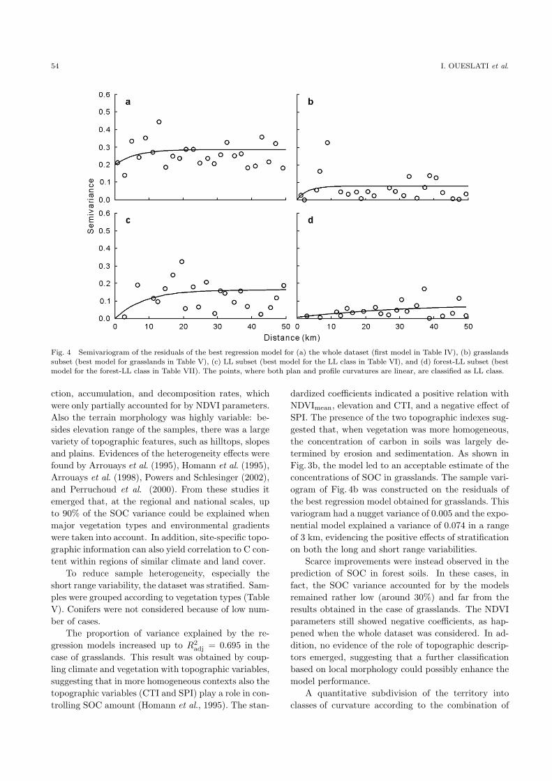
Fig. 4a shows the sample variogram of the residu-als of the best regression model in Table IV (i.e., EL,P). The variance related to the nugget was 0.197, theone for the exponential model was 0.089, and the rangewas 6 km. The regression model therefore reduced thespatial variability but had no effect on the very shortrange variability represented by the nugget. This wasconfirmed by analyzing separately the variograms ofthe two environmental factors (data not shown). Wefound that these variograms had rather large ranges(i.e., 35 and 88 km, respectively, as calculated by fit-ting an exponential model to the observed variograms).This is due to the fact that these variables are stronglyrelated to large scale phenomena, such as general to-pography and climate.

Although climate and vegetation appeared to bethe main drivers of SOC variability, the relationshipswere still unsuitable to be used for estimation. Thiscould be explained by the heterogeneity of vegeta-tion and topographic characteristics of the samples. Infact, four land cover classes were present, namelybroadleaved trees, coniferous, mixed forests, and grass-lands, each of them giving rise to different SOC produ-

Fig. 3 Comparison between the measured and estimated values of soil organic carbon in 0–30 cm layer (SOC30) for (a) the whole

dataset (first model in Table IV), (b) grasslands subset (best model for grasslands in Table V), (c) LL subset (best model for the LL

class in Table VI), and (d) forest-LL subset (best model for the forest-LL class in Table VII). The points, where both plan and profile

curvatures are linear, are classified as LL class.

54 I. OUESLATI et al.

Fig. 4 Semivariogram of the residuals of the best regression model for (a) the whole dataset (first model in Table IV), (b) grasslands

subset (best model for grasslands in Table V), (c) LL subset (best model for the LL class in Table VI), and (d) forest-LL subset (best

model for the forest-LL class in Table VII). The points, where both plan and profile curvatures are linear, are classified as LL class.

ction, accumulation, and decomposition rates, whichwere only partially accounted for by NDVI parameters.Also the terrain morphology was highly variable: be-sides elevation range of the samples, there was a largevariety of topographic features, such as hilltops, slopesand plains. Evidences of the heterogeneity effects werefound by Arrouays et al. (1995), Homann et al. (1995),Arrouays et al. (1998), Powers and Schlesinger (2002),and Perruchoud et al. (2000). From these studies itemerged that, at the regional and national scales, upto 90% of the SOC variance could be explained whenmajor vegetation types and environmental gradientswere taken into account. In addition, site-specific topo-graphic information can also yield correlation to C con-tent within regions of similar climate and land cover.

To reduce sample heterogeneity, especially theshort range variability, the dataset was stratified. Sam-ples were grouped according to vegetation types (TableV). Conifers were not considered because of low num-ber of cases.

The proportion of variance explained by the re-gression models increased up to R2

adj = 0.695 in thecase of grasslands. This result was obtained by coup-ling climate and vegetation with topographic variables,suggesting that in more homogeneous contexts also thetopographic variables (CTI and SPI) play a role in con-trolling SOC amount (Homann et al., 1995). The stan-

dardized coefficients indicated a positive relation withNDVImean, elevation and CTI, and a negative effect ofSPI. The presence of the two topographic indexes sug-gested that, when vegetation was more homogeneous,the concentration of carbon in soils was largely de-termined by erosion and sedimentation. As shown inFig. 3b, the model led to an acceptable estimate of theconcentrations of SOC in grasslands. The sample vari-ogram of Fig. 4b was constructed on the residuals ofthe best regression model obtained for grasslands. Thisvariogram had a nugget variance of 0.005 and the expo-nential model explained a variance of 0.074 in a rangeof 3 km, evidencing the positive effects of stratificationon both the long and short range variabilities.

Scarce improvements were instead observed in theprediction of SOC in forest soils. In these cases, infact, the SOC variance accounted for by the modelsremained rather low (around 30%) and far from theresults obtained in the case of grasslands. The NDVIparameters still showed negative coefficients, as hap-pened when the whole dataset was considered. In ad-dition, no evidence of the role of topographic descrip-tors emerged, suggesting that a further classificationbased on local morphology could possibly enhance themodel performance.

A quantitative subdivision of the territory intoclasses of curvature according to the combination of

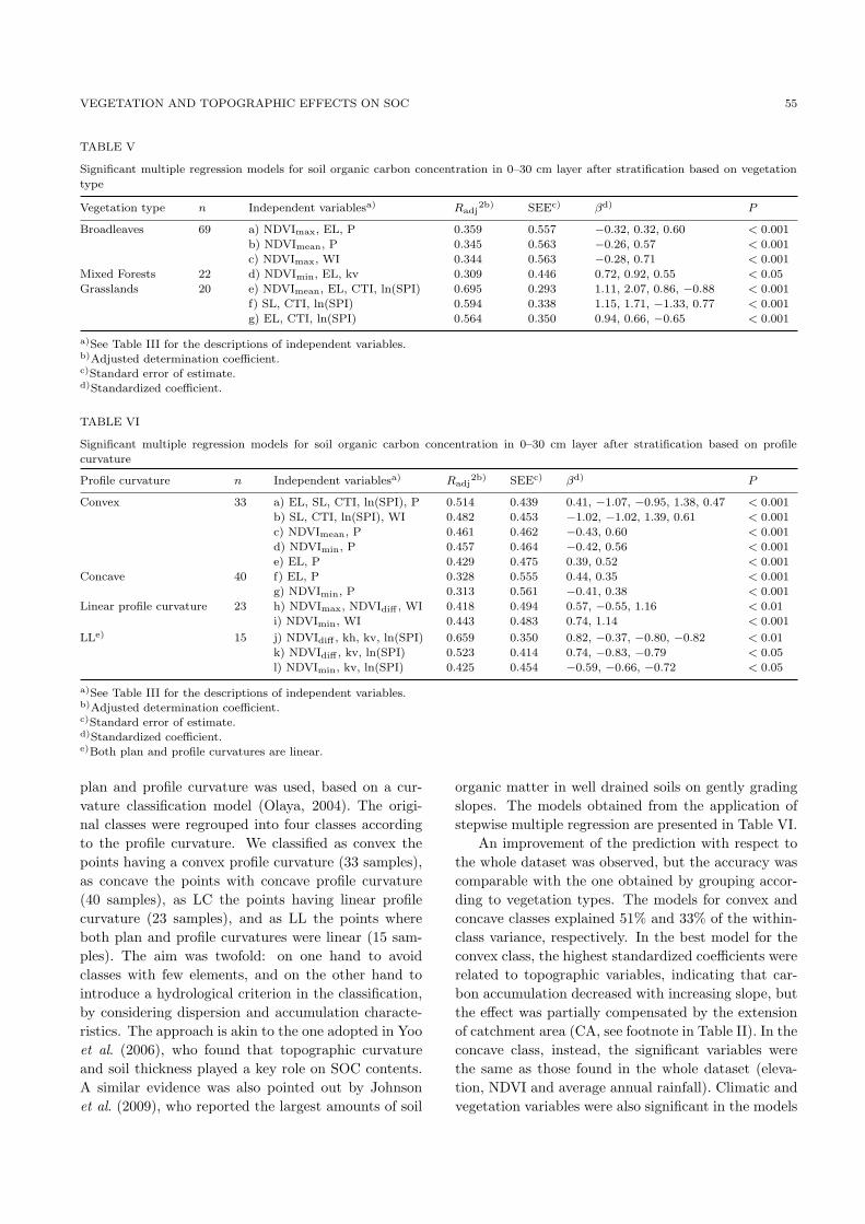
VEGETATION AND TOPOGRAPHIC EFFECTS ON SOC 55

TABLE V

Significant multiple regression models for soil organic carbon concentration in 0–30 cm layer after stratification based on vegetation

type

Vegetation type n Independent variablesa) Radj2b) SEEc) βd) P

Broadleaves 69 a) NDVImax, EL, P 0.359 0.557 −0.32, 0.32, 0.60 < 0.001

b) NDVImean, P 0.345 0.563 −0.26, 0.57 < 0.001

c) NDVImax, WI 0.344 0.563 −0.28, 0.71 < 0.001

Mixed Forests 22 d) NDVImin, EL, kv 0.309 0.446 0.72, 0.92, 0.55 < 0.05

Grasslands 20 e) NDVImean, EL, CTI, ln(SPI) 0.695 0.293 1.11, 2.07, 0.86, −0.88 < 0.001

f) SL, CTI, ln(SPI) 0.594 0.338 1.15, 1.71, −1.33, 0.77 < 0.001

g) EL, CTI, ln(SPI) 0.564 0.350 0.94, 0.66, −0.65 < 0.001

a)See Table III for the descriptions of independent variables.b)Adjusted determination coefficient.c)Standard error of estimate.d)Standardized coefficient.

TABLE VI

Significant multiple regression models for soil organic carbon concentration in 0–30 cm layer after stratification based on profile

curvature

Profile curvature n Independent variablesa) Radj2b) SEEc) βd) P

Convex 33 a) EL, SL, CTI, ln(SPI), P 0.514 0.439 0.41, −1.07, −0.95, 1.38, 0.47 < 0.001

b) SL, CTI, ln(SPI), WI 0.482 0.453 −1.02, −1.02, 1.39, 0.61 < 0.001

c) NDVImean, P 0.461 0.462 −0.43, 0.60 < 0.001

d) NDVImin, P 0.457 0.464 −0.42, 0.56 < 0.001

e) EL, P 0.429 0.475 0.39, 0.52 < 0.001

Concave 40 f) EL, P 0.328 0.555 0.44, 0.35 < 0.001

g) NDVImin, P 0.313 0.561 −0.41, 0.38 < 0.001

Linear profile curvature 23 h) NDVImax, NDVIdiff , WI 0.418 0.494 0.57, −0.55, 1.16 < 0.01

i) NDVImin, WI 0.443 0.483 0.74, 1.14 < 0.001

LLe) 15 j) NDVIdiff , kh, kv, ln(SPI) 0.659 0.350 0.82, −0.37, −0.80, −0.82 < 0.01

k) NDVIdiff , kv, ln(SPI) 0.523 0.414 0.74, −0.83, −0.79 < 0.05

l) NDVImin, kv, ln(SPI) 0.425 0.454 −0.59, −0.66, −0.72 < 0.05

a)See Table III for the descriptions of independent variables.b)Adjusted determination coefficient.c)Standard error of estimate.d)Standardized coefficient.e)Both plan and profile curvatures are linear.

plan and profile curvature was used, based on a cur-vature classification model (Olaya, 2004). The origi-nal classes were regrouped into four classes accordingto the profile curvature. We classified as convex thepoints having a convex profile curvature (33 samples),as concave the points with concave profile curvature(40 samples), as LC the points having linear profilecurvature (23 samples), and as LL the points whereboth plan and profile curvatures were linear (15 sam-ples). The aim was twofold: on one hand to avoidclasses with few elements, and on the other hand tointroduce a hydrological criterion in the classification,by considering dispersion and accumulation characte-ristics. The approach is akin to the one adopted in Yooet al. (2006), who found that topographic curvatureand soil thickness played a key role on SOC contents.A similar evidence was also pointed out by Johnsonet al. (2009), who reported the largest amounts of soil

organic matter in well drained soils on gently gradingslopes. The models obtained from the application ofstepwise multiple regression are presented in Table VI.

An improvement of the prediction with respect tothe whole dataset was observed, but the accuracy wascomparable with the one obtained by grouping accor-ding to vegetation types. The models for convex andconcave classes explained 51% and 33% of the within-class variance, respectively. In the best model for theconvex class, the highest standardized coefficients wererelated to topographic variables, indicating that car-bon accumulation decreased with increasing slope, butthe effect was partially compensated by the extensionof catchment area (CA, see footnote in Table II). In theconcave class, instead, the significant variables werethe same as those found in the whole dataset (eleva-tion, NDVI and average annual rainfall). Climatic andvegetation variables were also significant in the models

56 I. OUESLATI et al.

of the LC class, with an explained variance up to 42%.A better regression model was obtained in the LL case(R2

adj = 0.659). When both the profile and plan cur-vature were linear (i.e., less than 0.1 in module), evensmall variations in concavity/convexity affected carbonconcentration, with higher amounts of SOC in relativeconcavities. The quality of the estimate (Fig. 3c) wascomparable with that obtained for the grasslands whenthe dataset was stratified by vegetation type, sugges-ting that a further improvement of the estimation qua-lity might be obtained by combining topography andvegetation classes.

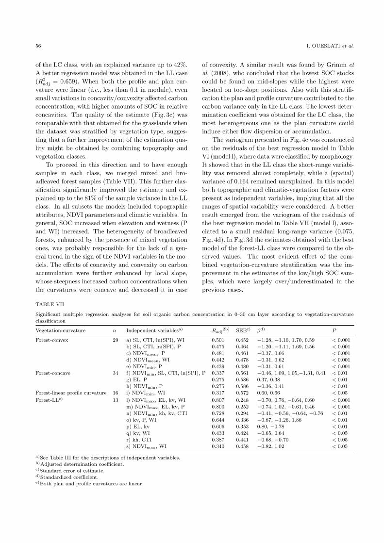
To proceed in this direction and to have enoughsamples in each class, we merged mixed and bro-adleaved forest samples (Table VII). This further clas-sification significantly improved the estimate and ex-plained up to the 81% of the sample variance in the LLclass. In all subsets the models included topographicattributes, NDVI parameters and climatic variables. Ingeneral, SOC increased when elevation and wetness (Pand WI) increased. The heterogeneity of broadleavedforests, enhanced by the presence of mixed vegetationones, was probably responsible for the lack of a gen-eral trend in the sign of the NDVI variables in the mo-dels. The effects of concavity and convexity on carbonaccumulation were further enhanced by local slope,whose steepness increased carbon concentrations whenthe curvatures were concave and decreased it in case

of convexity. A similar result was found by Grimm etal. (2008), who concluded that the lowest SOC stockscould be found on mid-slopes while the highest werelocated on toe-slope positions. Also with this stratifi-cation the plan and profile curvature contributed to thecarbon variance only in the LL class. The lowest deter-mination coefficient was obtained for the LC class, themost heterogeneous one as the plan curvature couldinduce either flow dispersion or accumulation.

The variogram presented in Fig. 4c was constructedon the residuals of the best regression model in TableVI (model l), where data were classified by morphology.It showed that in the LL class the short-range variabi-lity was removed almost completely, while a (spatial)variance of 0.164 remained unexplained. In this modelboth topographic and climatic-vegetation factors werepresent as independent variables, implying that all theranges of spatial variability were considered. A betterresult emerged from the variogram of the residuals ofthe best regression model in Table VII (model l), asso-ciated to a small residual long-range variance (0.075,Fig. 4d). In Fig. 3d the estimates obtained with the bestmodel of the forest-LL class were compared to the ob-served values. The most evident effect of the com-bined vegetation-curvature stratification was the im-provement in the estimates of the low/high SOC sam-ples, which were largely over/underestimated in theprevious cases.

TABLE VII

Significant multiple regression analyses for soil organic carbon concentration in 0–30 cm layer according to vegetation-curvature

classification

Vegetation-curvature n Independent variablesa) Radj2b) SEEc) βd) P

Forest-convex 29 a) SL, CTI, ln(SPI), WI 0.501 0.452 −1.28, −1.16, 1.70, 0.59 < 0.001

b) SL, CTI, ln(SPI), P 0.475 0.464 −1.20, −1.11, 1.69, 0.56 < 0.001

c) NDVImean, P 0.481 0.461 −0.37, 0.66 < 0.001

d) NDVImean, WI 0.442 0.478 −0.31, 0.62 < 0.001

e) NDVImin, P 0.439 0.480 −0.31, 0.61 < 0.001

Forest-concave 34 f) NDVImin, SL, CTI, ln(SPI), P 0.337 0.561 −0.46, 1.09, 1.05,−1.31, 0.41 < 0.01

g) EL, P 0.275 0.586 0.37, 0.38 < 0.01

h) NDVImin, P 0.275 0.586 −0.36, 0.41 < 0.01

Forest-linear profile curvature 16 i) NDVImin, WI 0.317 0.572 0.60, 0.66 < 0.05

Forest-LLe) 13 l) NDVImax, EL, kv, WI 0.807 0.248 −0.70, 0.76, −0.64, 0.60 < 0.001

m) NDVImax, EL, kv, P 0.800 0.252 −0.74, 1.02, −0.61, 0.46 < 0.001

n) NDVImin, kh, kv, CTI 0.728 0.294 −0.41, −0.56, −0.64, −0.76 < 0.01

o) kv, P, WI 0.644 0.336 −0.87, −1.26, 1.88 < 0.01

p) EL, kv 0.606 0.353 0.80, −0.78 < 0.01

q) kv, WI 0.433 0.424 −0.65, 0.64 < 0.05

r) kh, CTI 0.387 0.441 −0.68, −0.70 < 0.05

s) NDVImax, WI 0.340 0.458 −0.82, 1.02 < 0.05

a)See Table III for the descriptions of independent variables.b)Adjusted determination coefficient.c)Standard error of estimate.d)Standardized coefficient.e)Both plan and profile curvatures are linear.

VEGETATION AND TOPOGRAPHIC EFFECTS ON SOC 57

CONCLUSIONS

In this work we exploited the information derivedfrom vegetation, climate, and morphology for studyingthe spatial distribution of soil organic carbon concen-tration in forest and grassland areas. The case studywas formed by 114 samples belonging to a vast hete-rogeneous region of north-western Italy. The first at-tempts to statistically reproduce SOC concentrationby means of vegetation and climatic predictors wereunsatisfactory. In fact, these explanatory variables al-lowed us to reduce the long-range spatial variability,but had no effect on the short-range dependence andwere therefore unable to take into account all factorsinfluencing organic matter concentration in a highlyheterogeneous region. Better results were obtained af-ter stratification of the samples, and by introducing inthe regression models topographic variables, by gover-ning water fluxes, had a large influence on SOC inputs,losses and turnover. When classes of homogeneous ve-getation and topography were considered, the qualityof the estimates improved, particularly for grasslandsand forests in the absence of local curvatures. The re-sults of this work indicate that the spatial variabilityof soil organic matter can be overcome only when ana-priori reduction of the heterogeneity is applied. Theonly limitation to the feasibility of the approach is inthe availability of the predictors, included the avai-lability of finer scale digital elevation models. Furtherefforts in this field of investigation will be devoted to in-troduce more causative factors in the prediction mod-els, provided that additional and more focused datawill become available.

ACKNOWLEDGEMENTS

The IPLA Institute (Turin, Italy) is acknowledgedfor providing part of the soil data used in this study.Dr. G. LAGUARDIA from Politecnico di Torino, Italyis gratefully acknowledged for assistance in data prepa-ration and some computations.

REFERENCES

Abnee, A. C., Thompson, J. A. and Kolka, R. K. 2004a. Land-

scape modeling of in situ soil respiration in a forested wa-

tershed of southeastern Kentucky. Environ. Manage. 33:

S168–S175.

Abnee, A. C., Thompson, J. A., Kolka, R. K., D’Angelo, E. M.

and Coyne, M. S. 2004b. Landscape influences on poten-

tial soil respiration in a forested watershed of southeastern

Kentucky. Environ. Manage. 33: S160–S167.

Arrouays, D., Daroussin, J., Kicin, J. L. and Hassika, P. 1998.

Improving topsoil carbon storage prediction using a digital

elevation model in temperate forest soils of France. Soil Sci.

163: 103–108.

Arrouays, D., Vion, I. and Kicin, J. L. 1995. Spatial analysis

and modeling of topsoil carbon storage in temperate forest

humic loamy soils of France. Soil Sci. 159: 191–198.

Augusto, L., Ranger, J., Binkley, D. and Rothe, A. 2002. Im-

pact of several common tree species of European temperate

forests on soil fertility. Ann. For. Sci. 59: 233–253.

Baldock, J. A. and Nelson, P. N. 2000. Soil organic matter. In

Sumner, M. E. (ed.) Handbook of Soil Science. CRC Press,

Boca Raton. pp. B25–B84.

Bartolini, E., Claps, P. and Laio, F. 2008. Analysis of the

spatial variability of precipitation characteristics in Pie-

monte (in Italian). Available online at http://www.idrolo-

gia.polito.it/∼bartolini/WP2008 01.pdf (verified on Nove-

mber 22, 2012).

Bell, J. C., Grigal, D. F. and Bates, P. C. 2000. A soil-terrain

model for estimating spatial patterns of soil organic carbon.

In Wilson, J. P. and Gallant, J. C. (eds.) Terrain Analysis—

Principles and Applications. John Wiley & Sons, New York.

pp. 295–310.

Beven, K. J. and Kirkby, M. J. 1979. A physicallybased, variable

contributing area model of basin hydrology. Hydrol. Sci.

Bull. 24: 43–69.

Bot, A. and Benites, J. 2005. The Importance of Soil Organic

Matter: Key to Drought-Resistant Soil and Sustained Food

and Production. FAO Soils Bulletin 80. FAO of the United

Nations, Rome.

Burgess, T. M. and Webster, R. 1980. Optimal interpolation and

isarithmic mapping of soil properties. I. The semi-variogram

and punctual kriging. Eur. J. Soil Sci. 31: 315–331.

Chai, X., Shen, C., Yuan, X. and Huang, Y. 2008. Spatial pre-

diction of soil organic matter in the presence of different

external trends with REML-EBLUP. Geoderma. 148: 159–

166.

Chaplot, V., Bernoux, M., Walter, C., Curmi, P. and Herpin, U.

2001. Soil carbon storage prediction in temperate hydro-

morphic soils using a morphologic index and digital eleva-

tion model. Soil Sci. 166: 48–60.

Chaplot, V., Walter, C. and Curmi, P. 2000. Improving soil

hydromorphy prediction according to DEM resolution and

available pedological data. Geoderma. 97: 405–422.

Claps, P., Giordano, P. and Laguardia, G. 2008. Spatial distribu-

tion of the average air temperatures in Italy: quantitative

analysis. J. Hydrol. Eng. 13: 242–249.

European Environment Agency. 2005. CORINE land cover 2000.

Available online at http://dataservice.eea.europa.eu/data-

service/available2.asp?type=findkeyword&theme=clc2000

(verified on November 22, 2012).

Farquhar, G. D., Fasham, M. J. R., Goulden, M. L., Heimann,

M., Jaramillo, V. J., Kheshgi, H. S., Le Quere, C., Scholes,

R. J. and Wallace, D. W. R. 2001. Climate Change 2001:

The Scientific Basis IPCC. Chapter 3. The Carbon Cycle

and Atmospheric Carbon Dioxide. Cambridge University

Press, Cambridge. pp. 183–237.

Florinsky, I. V. and Kuryakova, G. A. 1996. Influence of topog-

raphy on some vegetation cover properties. Catena. 27:

123–141.

Gessler, P. E., Chadwick, O. A., Chamran, F., Althouse, L. and

Holmes, K. 2000. Modeling soil-landscape and ecosystem

properties using terrain attributes. Soil Sci. Soc. Am. J.

64: 2046–2056.

Gessler, P. E., Moore, I. D., McKenzie, N. J. and Ryan, P. J.

1995. Soil-landscape modelling and spatial prediction of soil

attributes. Int. J. Geogr. Inf. Syst. 9: 421–432.

58 I. OUESLATI et al.

Grimm, R., Behrens, T., Marker, M. and Elsenbeer, H. 2008. Soil

organic carbon concentrations and stocks on Barro Colorado

Island—Digital soil mapping using Random Forests analy-

sis. Geoderma. 146: 102–113.

Guber, A. K., Pachepsky, Y. A., van Genuchten, M. T., Rawls,

W. J., Simunek, J., Jacques, D., Nicholson, T. J. and Cady,

R. E. 2006. Field-scale water flow simulations using en-

sembles of pedotransfer functions for soil water retention.

Vadose Zone J. 5: 234–247.

Hastie, T., Tibshirani, R., Friedman, J. and Franklin, J. 2005.

The elements of statistical learning: data mining, inference

and prediction. Math. Intell. 27: 83–85.

Homann, P. S., Sollins, P., Chappell, H. N. and Stangenberger,

A. G. 1995. Soil organic carbon in a mountainous, forested

region: relation to site characteristics. Soil Sci. Soc. Am.

J. 59: 1468–1475.

Jackson, R. B., Canadell, J., Ehleringer, J. R., Mooney, H. A.,

Sala, O. E. and Schulze, E. D. 1996. A global analysis of root

distributions for terrestrial biomes. Oecologia. 108: 389–

411.

Jenny, H. 1941. Factors of Soil Formation: A System of Quanti-

tative Pedology. McGraw-Hill, New York.

Johnson, K. D., Scatena, F. N., Johnson, A. H. and Pan, Y. 2009.

Controls on soil organic matter content within a northern

hardwood forest. Geoderma. 148: 346–356.

Kottegoda, N. T. and Rosso, R. 1997. Statistics, Probabili-

ty, and Reliability for Civil and Environmental Engineers.

McGraw-Hill, New York.

Lagacherie, P. and McBratney, A. B. 2006. Spatial soil informa-

tion systems and spatial soil inference systems: perspectives

for digital soil mapping. Dev. Soil Sci. 31: 3–22.

Lal, R. 2008. Sequestration of atmospheric CO2 in global carbon

pools. Energ. Environ. Sci. 1: 86–100.

MacMillan, R. A. and Pettapiece, W. W. 1997. Soil Landsca-

pe Models: Automated Landscape Characterization and

Generation of Soil-Landscape models. Technical Bulletin

No. 1997-1E. Research Branch, Agriculture and Agri-Food

Canada, Lethbridge.

McBratney, A. B., Mendonca Santo, M. L. and Minasny, B. 2003.

On digital soil mapping. Geoderma. 117: 3–52.

McKenzie, N. J. and Ryan, P. J. 1999. Spatial prediction of soil

properties using environmental correlation. Geoderma. 89:

67–94.

Meier, I. C. and Leuschner, C. 2010. Variation of soil and biomass

carbon pools in beech forests across a precipitation gradient.

Glob. Change Biol. 16: 1035–1045.

Melillo, J. M., McGuire, A. D., Kicklighter, D. W., Moore, B.,

Vorosmarty, C. J. and Schloss, A. L. 1993. Global climate

chage and terrestrial net primary production. Nature. 363:

234–240.

Moore, I. D., Gessler, P. E., Nielsen, G. A. and Peterson, G. A.

1993. Soil attribute prediction using terrain analysis. Soil

Sci. Soc. Am. J. 57: 443–452.

Moore, I. D., Grayson, R. B. and Ladson, A. R. 1991. Digital ter-

rain modelling: a review of hydrological, geomorphological

and biological applications. Hydrol. Process. 5: 3–30.

Mueller, T. G. and Pierce, F. J. 2003. Soil carbon maps: En-

hancing spatial estimates with simple terrain attributes at

multiple scales. Soil Sci. Soc. Am. J. 67: 258–267.

Nemes, A., Rawls, W. J. and Pachepsky, Y. A. 2005. Influence

of organic matter on the estimation of saturated hydraulic

conductivity. Soil Sci. Soc. Am. J. 69: 1330–1337.

Olaya, V. 2004. A gentle introduction to SAGA GIS. Edition 1.1.

The SAGA User Group e.V., Gottingen, Germany.

Pennock, D. J., Zebarth, B. J. and De Jong, E. 1987. Land-

form classification and soil distribution in hummocky ter-

rain, Saskatchewan, Canada. Geoderma. 40: 297–315.

Perruchoud, D., Walthert, L., Zimmermann, S. and Luscher, P.

2000. Contemporary carbon stocks of mineral forest soils in

the Swiss Alps. Biogeochemistry. 50: 111–136.

Powers, J. S. and Schlesinger, W. H. 2002. Relationships among

soil carbon distributions and biophysical factors at nested

spatial scales in rain forests of northeastern Costa Rica.

Geoderma. 109: 165–190.

Simbahan, G. C., Dobermann, A., Goovaerts, P., Ping, J. and

Haddix, M. L. 2006. Fine-resolution mapping of soil organic

carbon based on multivariate secondary data. Geoderma.

132: 471–489.

Speight, J. G. 1968. Parametric description of landform. In Ste-

wart, G. A. (ed.) Land Evaluation. Macmillan, Melbourne.

Terra, J. A., Shaw, J. N., Reeves, D. W., Raper, R. L., van San-

ten, E. and Mask, P. L. 2004. Soil carbon relationships with

terrain attributes, electrical conductivity, and a soil survey

in a coastal plain landscape. Soil Sci. 169: 819–831.

Thompson, J. A. and Kolka, R. K. 2005. Soil carbon storage esti-

mation in a central hardwood forest watershed using quan-

titative soil-landscape modeling. Soil Sci. Soc. Am. J. 69:

1086–1093.

Thornthwaite, C. W. 1948. An approach toward a rational clas-

sification of climate. Geogr. Rev. 38: 55–94.

Tisdall, J. M. and Oades, J. M. 1982. Organic matter and water

stable aggregates in soils. Eur. J. Soil Sci. 33: 141–163.

Walker, P. H., Hall, G. F. and Protz, R. 1968. Relation between

landform parameters and soil properties. Soil Sci. Soc. Am.

J. 32: 101–104.

Wilson, J. P. and Gallant, J. C. 2000. Terrain Analysis: Princi-

ples and Applications. Wiley, New York. pp. 295–310.

Yoo, K., Amudson, R., Heimsath, A. M. and Dietrich, D. E.

2006. Spatial patterns of soil organic carbon on hillslopes:

Integrating geomorphic processes and the biological C cycle.

Geoderma. 130: 47–65.